Embed Size (px)
Citation preview
Clemson UniversityTigerPrints
All Dissertations Dissertations
5-2007
Analytical and Intelligent Techniques forDynamically Secure DispatchesAftab AlamClemson University, [email protected]
Follow this and additional works at: https://tigerprints.clemson.edu/all_dissertations
Part of the Electrical and Computer Engineering Commons
This Dissertation is brought to you for free and open access by the Dissertations at TigerPrints. It has been accepted for inclusion in All Dissertations byan authorized administrator of TigerPrints. For more information, please contact [email protected].
Recommended CitationAlam, Aftab, "Analytical and Intelligent Techniques for Dynamically Secure Dispatches" (2007). All Dissertations. 60.https://tigerprints.clemson.edu/all_dissertations/60
ii
ANALYTICAL AND INTELLIGENT TECHNIQUES FOR DYNAMCALLY SECURE DISPATCHES
A DissertationPresented to
the Graduate School ofClemson University
In Partial Fulfillmentof the Requirements for the Degree
Doctor of PhilosophyElectrical Engineering.
byAftab AlamMay 2007
Accepted by:Dr. Elham B. Makram, Committee Chair
Dr. Adly. A. GirgisDr. Ian WalkerDr. Hyesuk Lee

iii
ABSTRACT
The NERC August 14th Blackout report brought out by the task force cited
‘failure to ensure operation within secure limits’ as one of the main reasons.
Many of the numerous recommendations focused on the need for better real-time
tools for operators and reliability coordinators. In the absence of such tools the
operators are limited to operating in conservative secure operating regions
established using offline studies. At the same time, with the fast inception of
deregulation, the need to ensure a reliable and secure power system has become
all the more vital. The success of a competitive market is dependent upon a
reliable and secure transmission system at all times. This dissertation investigates
ideas for analytical and intelligent techniques to obtain generation dispatches that
would be first-swing stable for a certain set of credible contingencies (three-phase
faults) with their respective fault clearing times.
In a deregulated environment, fair operation is dependent upon maximum
utilization of available resources. Conventionally the maximum utilization has
been made possible by use of the optimal power flow where certain objective(s)
are maximized/minimized subject to certain constraints through various
mathematical programming techniques. Due to the extremely large computation
times required to carry out dynamic security assessment of large disturbances,
constraints to ensure dynamic stability, more specifically transient stability have
been ignored from state of the art optimal power flow routines today. Rather, such
limits are established using offline studies. Since, these limits are established from

iv
forecasted data, they are kept on the conservative side to ensure that the power
system would be transiently stable for a certain set of credible contingencies. One
of the major obstacles of including dynamic security assessment subroutines
within the optimal power flow method for real-time operations is the heavy
computational burden since it requires solution of differential equations. Another
is the extremely high analytical and programming complexity involved with
inclusion of constraints to ensure that the ‘solution of the differential equations is
within certain bounds’.
The presented research proposes to explore analytical and intelligent
techniques of dynamic security assessment which would aid in the development
of software based subroutines to be included in the optimal power flow. This
would enhance the already existing state of the art dispatch routines within energy
managements systems by allowing operation closer to stability limits. It would
also aid in the successful and fair operation of a competitive market. On a more
general note, the research work carried out would help in improving power
system reliability and operation. It would also allow maximum utilization of
available resources, Transmission and Distribution assets by having operating
closer to ‘real-time’ steady-state and dynamic stability limits. On the whole, it
would aid in the move towards a deregulated environment leading to long term
economic benefits for both generating companies and consumers.

iii
DEDICATION
This dissertation is dedicated to My Parents, Shadab & Sadaf for their loving
support and encouragement, Chinar, my partner for life and friends without
whom this would not have been possible.

iv

v
ACKNOWLEDGMENTS
I would like to express my sincere appreciation to my advisor Dr. Elham
B. Makram for her guidance throughout this research. I am grateful for her
support and patience during the entire period of this research. I would like to
thank Dr. Adly. A. Girgis, Dr. Ian D. Walker and Dr. Hyesuk Lee for serving as
my graduate committee members.
The financial support of Clemson University Electric Power Research
Association (CUEPRA), and the Electrical and Computer Engineering (ECE)
Department at Clemson University are greatly appreciated.
I would like to thank all my colleagues in the power group for their
professional and friendly relationship.
Finally I would like to thank my parents for their patience and their
emotional and financial support throughout my life.

vi

vii
TABLE OF CONTENTS
Page
TITLE PAGE.............................................................................................. i
ABSTRACT................................................................................................ iii
DEDICATION............................................................................................ v
ACKNOWLEDGEMENTS........................................................................ vii
LIST OF TABLES...................................................................................... xi
LIST OF FIGURES .................................................................................... xii
CHAPTER
1. INTRODUCTION ....................................................................... 1
1.1 Motivation…………....................................................... 11.2 Transient Stability Assessment. ...................................... 51.3 Research Objectives/Contributions................................. 10
2. TRANSIENT STABILITY CONSTRAINEDOPTIMAL POWER FLOW .................................................. 13
2.1 Background..................................................................... 132.2 A Computationally Efficient Method to
Obtain Rotor Angles ...................................................... 172.2.1 Review of Equations for Classical Transient Stability Analysis.................................. 182.2.2 Solution Using Taylor Series
Expansion.............................................................. 222.2.3 Results with the IEEE 9-Bus and 39-Bus Systems..................................................... 242.2.4 Discussion ............................................................. 27
2.3 The Transient Stability Constraint .................................. 272.4 Optimal Power Flow with Transient
Stability Constraints Formulation .................................. 292.4.2 Objective Function................................................ 292.4.3 Equality Constraints.............................................. 302.4.4 Inequality Constraints ........................................... 30

viii
Table of Contents (Continued)
Page
2.5 Results with the IEEE 9-Bus System.............................. 34 2.5.1 75% Loading, BOPF............................................. 342.5.2 75% Loading, TSCOPF ........................................ 372.5.3 100% Loading, BOPF........................................... 382.5.4 100% Loading, TSCOPF ...................................... 402.5.5 125% Loading, BOPF........................................... 422.5.6 125% Loading, TSCOPF ...................................... 44
2.6 Results with the IEEE 39-Bus System............................ 462.6.1 75% Loading, BOPF............................................. 472.6.2 75% Loading, TSCOPF ........................................ 492.6.3 100% Loading, BOPF........................................... 502.6.4 100% Loading, TSCOPF ...................................... 532.6.5 125% Loading, BOPF........................................... 542.6.6 125% Loading, TSCOPF ...................................... 57
2.7 Discussion ....................................................................... 592.8 Conclusions..................................................................... 70
3. APPLICATION OF SINGLE MACHINE EQUIVALENT METHOD AND NEURAL NETWORKS FOR ESTIMATION OF CRITICAL CLEARING TIME ............................................. 73
3.1 Single Machine Equivalent Method ............................... 733.1.1 Methodology......................................................... 75
3.2 Results with the IEEE 9-Bus System.............................. 813.2.1 Fault near Bus 5 on Line 5-7 for 0.28s ................. 823.2.2 Fault near Bus 5 on Line 5-7 for 0.33s ................. 843.2.3 Fault near Bus 7 on Line 7-5 for 0.083s ............... 863.2.4 Fault near Bus 7 on Line 5-7 for 0.17s ................. 883.2.5 Fault near Bus 6 on Line 6-9 for 0.17s ................. 903.2.6 Fault near Bus 6 on Line 6-9 for 0.14s ................. 92
3.3 Results with the IEEE 39-Bus Systems .......................... 943.3.1 Fault near Bus 3 on Line 3-4 for 0.28s ................. 943.3.2 Fault near Bus 3 on Line 3-4 for 0.33s ................. 96
3.4 Discussion ....................................................................... 983.5 Fast Determination of Critical Clearing Time
Using SIME Method....................................................... 983.5.1 Background........................................................... 98 3.5.2 Methodology......................................................... 100 3.5.4 Discussion ............................................................. 103
3.6 Application of Feedforward Networks for Critical Clearing Time Estimation .................................. 103

ix
Table of Contents (Continued)
Page
3.6.1 Background........................................................... 103 3.6.1 Methodology......................................................... 1033.6.3 Result with the IEEE 9-Bus System ..................... 1063.6.4 Discussion ............................................................. 108
3.7 Conclusions..................................................................... 111
4. A HYBRID NEURAL NETWORK-OPTIMIZATIONAPPROACH FOR DYNAMIC SECURITYCONSTRAINED OPTIMAL POWER FLOW ..................... 115
4.1 Transient Stability Constraint ......................................... 1154.2 Results with the IEEE 9-Bus System (
single contingency) ......................................................... 1174.3 Discussion ....................................................................... 1204.4 Results with the IEEE 9-Bus System (
multiple contingencies)................................................... 1234.5 Discussion ....................................................................... 1344.5 Conclusions..................................................................... 135
5. SUMMARY AND CONCLUSIONS .......................................... 137
APPENDICES ............................................................................................ 145
A: System Data for the 3-Machine 9-Bus IEEE Test System (Base Case) [46]................................................ 147
B: System Data for the 10-Machine 39-Bus IEEE Test System (Base Case) [46]................................................ 149
REFERENCES ........................................................................................... 153

x

xi
LIST OF TABLES
Table Page
2.1 List of faults considered in the IEEE 9-Bus System ...................... 35
2.2 List of faults considered in the IEEE 9-Bus System ...................... 38
2.3 List of faults considered in the IEEE 9-Bus System ...................... 42
2.4 List of faults considered in the IEEE 39-Bus System .................... 47
2.5 List of faults considered in the IEEE 39-Bus System .................... 51
2.6 List of faults considered in the IEEE 39-Bus System .................... 55
3.1 List of faults considered in the IEEE 9-Bus System ...................... 102
4.1 TSCOPF results for fault near Bus 7 on Line 5-7........................... 118
4.2 TSCOPF results for fault near Bus 6 on Line 6-9........................... 119
4.3 TSCOPF results for fault near Bus 5 on Line 5-4........................... 119
4.4 TSCOPF results for fault near Bus 5 on Line 5-7........................... 120
4.5 TSCOPF results for fault near Bus 7 on Line 5-7and near Bus 6 on Line 6-9 ....................................................... 124
4.6 TSCOPF results for fault near Bus 7 on Line 5-7 and near Bus 5 on Line 5-4 ....................................................... 126
4.7 TSCOPF results for fault near Bus 5 on Line 5-7 and near Bus 6 on Line 6-9 ....................................................... 128
4.8 TSCOPF results for fault near Bus 5 on Line 5-7 and near Bus 6 on Line 6-4 ....................................................... 130
4.9 TSCOPF results for fault near Bus 7 on Line 5-7, near Bus 6 on Line 6-9 and near Bus 6 on Line 6-9..................................................................................... 132

xii
List of Tables (Continued)
Table Page
A.1 Generator Data ............................................................................... 147
A.2 Bus Data ......................................................................................... 147
A.3 Branch Data ................................................................................... 148
B.1 Generator Data ............................................................................... 149
B.2 Bus Data ......................................................................................... 150
B.3 Branch Data ................................................................................... 151
B.4 Branch Data (continued) ................................................................ 152
xiii
LIST OF FIGURES
Figure Page
2.1 Sample Power System..................................................................... 21
2.2 Comparison of Taylor series expansion method and 4/5th order Runge-Kutta method for fault nearBus 7 on Line 5-7 for 0.15s ...................................................... 25
2.3 Comparison of Taylor series expansion method and4/5th order Runge-Kutta method for fault nearBus 7on Line 5-7 for 0.17s ....................................................... 25
2.4 Comparison of Taylor series expansion method and 4/5th order Runge-Kutta method for fault nearBus 3 on Line 3-4 for 0.2s ........................................................ 26
2.5 Comparison of Taylor series expansion method and4/5th order Runge-Kutta method for fault nearBus 3 on Line 3-4 for 0.3s ........................................................ 26
2.6 General representation of the transient stabilityconstrained optimal power flow problem ................................. 33
2.6 Rotor angles for fault near Bus 7 on Line 7-5 for afault duration of 0.26s following a dispatch given by the BOPF.............................................................................. 35
2.7 Rotor angles for fault near Bus 9 on Line 9-8 for afault duration of 0.28s following a dispatch givenby the BOPF.............................................................................. 36
2.8 Rotor angles for fault near Bus 8 on Line 7-8 for afault duration of 0.35s following a dispatch givenby the BOPF.............................................................................. 36
2.9 Rotor angles for fault near Bus 9 on Line 9-8 for a fault duration of 0.28s following a dispatch givenby the TSCOPF......................................................................... 37

xiv
List of Figures (Continued)
Figure Page
2.10 Rotor angles for fault near Bus 7 on Line 7-5 for afault duration of 0.26s following a dispatch givenby the BOPF.............................................................................. 39
2.11 Rotor angles for fault near Bus 9 on Line 9-8 for afault duration of 0.28s following a dispatch givenby the BOPF.............................................................................. 39
2.12 Rotor angles for fault near Bus 8 on Line 7-8 for a fault duration of 0.35s following a dispatch givenby the BOPF.............................................................................. 40
2.13 Rotor angles for fault near Bus 7 on Line 7-5 for a fault duration of 0.26s following a dispatch given by the TSCOPF......................................................................... 41
2.14 Rotor angles for fault near Bus 9 on Line 9-8 for a fault duration of 0.28s following a dispatch given by the TSCOPF......................................................................... 41
2.15 Rotor angles for fault near Bus 7 on Line 7-5 for a fault duration of 0.26s following a dispatch given by the BOPF.............................................................................. 43
2.16 Rotor angles for fault near Bus 9 on Line 9-8 for a fault duration of 0.28s following a dispatch given by the BOPF.............................................................................. 43
2.17 Rotor angles for fault near Bus 8 on Line 7-8 for a fault duration of 0.35s following a dispatch given by the BOPF.............................................................................. 44
2.18 Rotor angles for fault near Bus 7 on Line 7-5 for a fault duration of 0.26s following a dispatch given by the BOPF.............................................................................. 45
2.19 Rotor angles for fault near Bus 9 on Line 9-8 for a fault duration of 0.28s following a dispatch given by the BOPF.............................................................................. 45

xv
List of Figures (Continued)
Figure Page
2.20 Rotor angles for fault near Bus 8 on Line 7-8 for a fault duration of 0.35s following a dispatch given by the BOPF.............................................................................. 46
2.21 Rotor angles for fault near Bus 3 on Line 3-4 for a fault duration of 0.2s following a dispatch given by the BOPF.............................................................................. 48
2.22 Rotor angles for fault near Bus 10 on Line 10-13 fora fault duration of 0.35s following a dispatchgiven by the BOPF.................................................................... 48
2.23 Rotor angles for fault near Bus 25 on Line 25-2 for a fault duration of 0.24s following a dispatchgiven by the BOPF.................................................................... 49
2.24 Rotor angles for fault near Bus 25 on Line 25-2 for a fault duration of 0.24s following a dispatch givenby the TSOPF............................................................................ 50
2.25 Rotor angles for fault near Bus 3 on Line 3-4 for a fault duration of 0.2s following a dispatch givenby the BOPF.............................................................................. 51
2.27 Rotor angles for fault near Bus 10 on Line 10-13 for a fault duration of 0.35s following a dispatchgiven by the BOPF.................................................................... 52
2.28 Rotor angles for fault near Bus 25 on Line 25-4 for a fault duration of 0.24s following a dispatchgiven by the BOPF.................................................................... 52
2.29 Rotor angles for fault near Bus 10 on Line 10-13 for a fault duration of 0.35s following a dispatchgiven by the TSCOPF ............................................................... 53
2.30 Rotor angles for fault near Bus 25 on Line 25-2 for afault duration of 0.24s following a dispatch givenby the TSCOPF......................................................................... 54

xvi
List of Figures (Continued)
Figure Page
2.31 Rotor angles for fault near Bus 3 on Line 3-4 for a fault duration of 0.2s following a dispatch given by the BOPF.............................................................................. 55
2.32 Rotor angles for fault near Bus 10 on Line 10-13 fora fault duration of 0.35s following a dispatch given by the BOPF.................................................................... 56
2.33 Rotor angles for fault near Bus 25 on Line 25-2 fora fault duration of 0.24s following a dispatch given by the BOPF.................................................................... 56
2.34 Rotor angles for fault near Bus 3 on Line 3-4 for a fault duration of 0.2s following a dispatch given by the TSCOPF......................................................................... 57
2.35 Rotor angles for fault near Bus 10 on Line 10-13 fora fault duration of 0.35s following a dispatch given by the TSCOPF ............................................................... 58
2.36 Rotor angles for fault near Bus 25 on Line 25-2 fora fault duration of 0.24s following a dispatch given by the TSCOPF ............................................................... 59
2.37 Comparison of generator active power outputs obtained by BOPF and TSCOPF with constraints for fault near Bus 7 on Line 7-5................................................ 60
2.38 Comparison of generator active power outputs obtained by BOPF and TSCOPF with constraints for fault near Bus 9 on Line 8-9................................................ 61
2.39 Comparison of generator active power outputs obtained by BOPF and TSCOPF with constraintsfor fault near Bus 8 on Line 7-8................................................ 62
2.40 Comparison of generator reactive power outputsobtained by BOPF and TSCOPF with constraintsfor fault near Bus 7 on Line 7-5................................................ 63

xvii
List of Figures (Continued)
Figure Page
2.41 Comparison of generator reactive power outputs obtained by BOPF and TSCOPF with constraintsfor fault near Bus 9 on Line 8-9................................................ 63
2.42 Comparison of generator reactive power outputsobtained by BOPF and TSCOPF with constraintsfor fault near Bus 8 on Line 7-8................................................ 64
2.43 Comparison of Bus voltage magnitudes obtained by BOPF and TSCOPF with constraints for fault near Bus 7 on Line 7-5...................................................................... 64
2.44 Comparison of Bus voltage magnitudes obtained by BOPF and TSCOPF with constraints for fault near Bus 9 on Line 8-9...................................................................... 65
2.45 Comparison of Bus voltage magnitudes obtained by BOPF and TSCOPF with constraints for fault near Bus 8 on Line 7-8...................................................................... 65
2.46 Comparison of generator active power outputs obtained by BOPF and TSCOPF with constraints for fault near Bus 3 on Line 3-4................................................ 66
2.47 Comparison of generator active power outputs obtained by BOPF and TSCOPF with constraintsfor fault near Bus 10 on Line 10-13.......................................... 66
2.48 Comparison of generator active power outputs obtained by BOPF and TSCOPF with constraints for fault near Bus 25 on Line 25-2............................................ 67
2.49 Comparison of generator reactive power outputsobtained by BOPF and TSCOPF with constraints for fault near Bus 3 on Line 3-4................................................ 68
2.50 Comparison of generator reactive power outputs obtained by BOPF and TSCOPF with constraints for fault near Bus 10 on Line 10-13.......................................... 68

xviii
List of Figures (Continued)
Figure Page
2.51 Comparison of generator reactive power outputs obtained by BOPF and TSCOPF with constraints for fault near Bus 25 on Line 25-2............................................ 69
3.1 An example of a stable OMIB trajectory........................................ 79
3.2 An example of an unstable OMIB trajectory.................................. 80
3.3 Phase plane plot of OMIB speed vs. the OMIB angle.................... 81
3.4 Plot of OMIB mechanical input, electrical power output, accelerating power and angle and speed trajectory for Case 1.................................................................. 82
3.5 OMIB speed vs. the OMIB angle for Case 1 .................................. 83
3.6 Plot of generator angles for Case 1 ................................................. 83
3.7 Plot of OMIB mechanical input, electrical power output, accelerating power and angle and speed trajectory for Case 2.................................................................. 84
3.8 OMIB speed vs. the OMIB angle for Case 2 .................................. 85
3.9 Plot of generator angles for Case 2 ................................................. 85
3.10 Plot of OMIB mechanical input, electrical power output, accelerating power and angle and speedtrajectory for Case 3.................................................................. 86
3.11 OMIB speed vs. the OMIB angle for Case 3 .................................. 87
3.12 Plot of generator angles for Case 3 ................................................. 87
3.13 Plot of OMIB mechanical input, electrical power output, accelerating power and angle and speedtrajectory for Case 4.................................................................. 88
3.14 OMIB speed vs. the OMIB angle for Case 4 .................................. 89
3.15 Plot of generator angles for Case 4 ................................................. 89

xix
List of Figures (Continued)
Figure Page
3.16 Plot of OMIB mechanical input, electrical power output, accelerating power and angle and speed trajectory for Case 5.................................................................. 90
3.17 OMIB speed vs. the OMIB angle for Case 5 .................................. 91
3.18 Plot of generator angles for Case 5 ................................................. 91
3.19 Plot of OMIB mechanical input, electrical poweroutput, accelerating power and angle and speed trajectory for Case 6.................................................................. 92
3.20 OMIB speed vs. the OMIB angle for Case 6 .................................. 93
3.21 Plot of generator angles for Case 6 ................................................. 93
3.22 Plot of OMIB mechanical input, electrical poweroutput, accelerating power and angle and speedtrajectory for Case 7.................................................................. 94
3.23 OMIB speed vs. the OMIB angle for Case 7 .................................. 95
3.24 Plot of generator angles for Case 7 ................................................. 95
3.25 Plot of OMIB mechanical input, electrical power output, accelerating power and angle and speed trajectory for Case 8.................................................................. 96
3.26 OMIB speed vs. the OMIB angle for Case 8 .................................. 97
3.27 Plot of generator angles for Case 8 ................................................. 97
3.28 Plot of stable/unstable margins for a fault near Bus 7 on Line 7-8.............................................................. 101
3.29 Plot of stable/unstable margins for a fault near Bus 7 on Line 7-5.............................................................. 102
3.30 Proposed Feedforward Neural Network for CriticalClearing Time Estimation ......................................................... 107

xx
List of Figures (Continued)
Figure Page
3.31 Comparison of Critical Clearing Time for a fault nearBus 7 on Line 7-5...................................................................... 109
3.32 Comparison of Critical Clearing Time for a fault nearBus 5 on Line 7-5...................................................................... 109
3.33 Comparison of Critical Clearing Time for a fault nearBus 5 on Line 5-4...................................................................... 110
3.34 Comparison of Critical Clearing Time for a fault nearBus 6 on Line 6-9...................................................................... 110
4.1 Conceptual illustration of the transient stabilityconstrained optimal power flow formulation............................ 117
4.2 Comparison of the critical clearing time with the faultclearing time and the neural network estimate ......................... 122
4.3 Comparison of generator active power outputs .............................. 122
4.4 Comparison of the critical clearing time with the faultclearing time and the neural network estimate forfault near Bus 7 on Line 5-7 .................................................... 125
4.5 Comparison of the critical clearing time with the faultclearing time and the neural network estimate forfault near Bus 6 on Line 6-4 .................................................... 125
4.6 Comparison of the critical clearing time with the faultclearing time and the neural network estimate forfault near Bus 7 on Line 7-8 .................................................... 127
4.7 Comparison of the critical clearing time with the faultclearing time and the neural network estimate forfault near Bus 5 on Line 5-4 .................................................... 127
4.8 Comparison of the critical clearing time with the faultclearing time and the neural network estimate forfault near Bus 5 on Line 5-7 .................................................... 129

xxi
List of Figures (Continued)
Figure Page
4.9 Comparison of the critical clearing time with thefault clearing time and the neural networkestimate for fault near Bus 6 on Line 6-9 ................................ 129
4.10 Comparison of the critical clearing time with thefault clearing time and the neural networkestimate for fault near Bus 5 on Line 5-7 ................................ 131
4.11 Comparison of the critical clearing time with thefault clearing time and the neural networkestimate for fault near Bus 6 on Line 6-4 ................................ 131
4.12 Comparison of the critical clearing time with thefault clearing time and the neural networkfault Bus 7 on Line 7-8 ............................................................ 133
4.13 Comparison of the critical clearing time with thefault clearing time and the neural networkestimate for fault near Bus 5 on Line 5-4 ................................ 133
4.14 Comparison of the critical clearing time with thefault clearing time and the neural networkestimate for fault near Bus 6 on Line 6-9 ................................ 134

xxii

1
CHAPTER ONE
INTRODUCTION
1.1 Motivation
The August 14th Blackout affected an area of 50 million people and 61,800
MWs of load in the states of Ohio, Michigan, Pennsylvania, New York, Vermont,
Massachusetts, Connecticut, New Jersey and the Canadian state of Ontario[1].
The total estimated losses were between 4 to 10 billion dollars. One of the main
reasons cited by the task force that led to the blackout was ‘failure to ensure
operation within secure limits’. It has been reiterated in the blackout report that it
could have been prevented. The task force provided an exhaustive list of
recommendations many of which focused on the need for better tools for dynamic
security assessment. Recommendation no. 22 asserts to ‘evaluate and adopt better
real-time tools for operators and reliability coordinators’. In the absence of such
tools the operators are limited to operating in regions of secure operating limits
established using offline studies, since they require a considerable engineering
and computational effort. Also these studies consider every possible credible
contingency which would deem them unusable for real-time applications due to
the large computation time.
The Federal Energy Regulatory Commission (FERC) issued a final rule,
Order No. 888 [2] in response to provisions of the Energy Policy Act (EPACT) of
1992. Order No. 888 opens wholesale electric power sales to competition. It

2
requires utilities that own, control, or operate transmission lines to file non-
discriminatory open access tariffs that offer others the same electricity
transmission service they provide themselves. The second final rule, Order No.
889 [3] issued on the same date, requires a real-time information system to assure
that transmission owners and their affiliates do not have an unfair competitive
advantage in using transmission to sell power. It is expected that Orders No. 888
and No. 889 and other actions taken by State Public Service Commissions to
promote competition in the electric power industry will result in increased
demands for transmission services. With the fast inception of deregulation into the
market the need for a reliable and secure power system has become all the more
vital. The successful operation of a competitive market is based on the
transmission system being reliable and secure at all times [4]. Failure can lead to
huge financial losses and ensuring that the power system is reliable and secure
both in a static and dynamic sense is very important. Utilities in almost every
country over the last century have been regulated utilities which are a natural
monopoly. In such vertically integrated systems, it is easier to ensure security for
various reasons. One of the main reasons is that these are monopolies operating
and managing their own generation, transmission and distribution systems and are
well aware of the load growth in their systems. This allows the regulated utility to
avoid overloading lines and equipment whose failure could lead to severe static
and dynamic system disturbances.
In a deregulated environment large inter-area transactions can occur over the
transmission system provided that the transaction does not violate system

3
operating security limits such as transmission line-flow limits and bus voltage
limits. In the presence of such large transactions, large disturbances such as faults,
loss or acquisition of generation, loss or acquisition of loads etc can lead to power
system instability due to loss of synchronism. So it is very vital that the entity
managing the operation of the transmission system, the Independent System
Operator (ISO), ensure that the execution of the transaction occurs within the
bounds of not only static-security criterion, but also within a similar region which
ensures dynamic or transient stability for the power system.
According to [5], ‘if the oscillatory response of the power system during the
transient period following such disturbances is damped and the system settles in a
finite time to a new steady operating condition, the system is stable’. One of the
biggest problems of building real time online dynamic security assessment
software applications is the heavy computation involved since any dynamic
security assessment involves solution of power system differential equations. This
has caused the system operators considering only static-security criterion for real-
time applications and using corrective procedures established by offline methods
to ensure power system dynamic security [6]. In some markets, offline studies are
used to develop operating limits (e.g. maximum output of a generator,
transmission line flow limits, bus voltage limits) to avoid dynamic stability
problems. These are often conservative and contradictory to the concept of a
competitive deregulated environment. In a deregulated system, the efficient
utilization of the transmission system and maximum utilization of revenue would
require the operation of the power system close to limits of stability. But the lack

4
of fast assessment methods has avoided the incorporation of dynamic security
assessment into online applications. Dynamic security assessment software is
used to carry out transient stability analysis for each condition of a large set of
possible outage conditions that could occur. A transient stability simulation time
frame of usually up to 10 seconds is required [6]. These studies are usually done
offline and take hours to complete. This makes them impossible to use in a real-
time environment, wherein an operator would need to perform real world control
actions within ten minutes after a real-world outage has occurred. The operator
would need to do this to ensure that the outage does not cause the grid to go
unstable due to a voltage instability situation or a cascading outage situation
leading to blackouts.
Dynamic security assessment methods can be broadly divided into corrective
and preventive methods. A "corrective" approach requires immediate action, such
as switching circuits or other actions, after a contingency occurs, so the system
performance will be adequate. Corrective operation is less reliable than preventive
operation, but allows greater power transfers during normal operations. Corrective
measures between systems sometimes become so complex that when a certain
contingency occurs, the system fails. Some corrective methods are used to
reschedule generator dispatches based on limits established by offline studies.
Power transfers between areas are limited to levels determined by offline system
contingency studies. However as mentioned earlier these limits are conservative.
“Preventive” operating procedures mean operating the system in such a way
as to avoid service interruptions as a result of certain component outages. So, the

5
preventive methods eliminate the need for a re-dispatch or corrective actions
following an outage as the dispatch itself would be transiently stable for the set of
faults considered while obtaining the dispatch. It is recognized as good utility
practice and regarded by the North American Electric Reliability Council (NERC)
as the primary means of preventing disturbances in one area from causing service
failures in another. The NERC guidelines recommend making it an operational
requirement that systems be able to handle any single contingency. The ability to
handle multiple contingencies should be an operational requirement when
practical, according to NERC. Hence, the "preventive" operating procedures,
ensures that no action is required in the event of a system contingency other than
clearing the fault. When contingencies arise, the system is capable of responding
without lines overheating, voltage problems, and instability.
1.2 Transient Stability Assessment
Transient stability studies have been part of electric utility guideline for more
than two decades now. Whether a corrective or preventive method is employed,
its effectiveness in a real-time environment is based on upon the method being
extremely fast and reasonable accurate. The early methods used to detect the
transient stability swings were based on the out-of-step relays using the apparent
impedance concept [8, 9]. In the early years of transient stability assessment
studies, time domain simulation methods were used. These basically relied on
using classical integration methods such as the Euler method, the trapezoidal
method, Runge-Kutta methods etc of converting the differential equations into

6
algebraic form. These methods were did not include load modeling and used
classical power system models of constant impedance models. This eliminated the
need to consider the non-generator bus voltages and the prefault, faulted and
postfault admittance matrices used for the transient stability analysis were reduced
to the generator nodes. Inclusion of load models was deemed necessary and this
required the power flow solution at each step of the time domain simulation to
obtain the new bus voltages and angles. This led to the development of explicit
and implicit methods to solve the differential-algebraic set of equations to include
load models [10]. Each of these methods has its own advantages and
disadvantages. [11] proposed semi-implicit numerical integration methods for
solving differential equations which had the advantages of both the explicit and
implicit methods and also allowed a large time step without encountering
numerical instability problems. Pai et al in [12] presented a new trajectory
approximation technique for transient stability analysis where a number of
contingencies can be simulated in a very short period of time. The proposed
method uses piecewise linearization of the nonlinearities combined with
trapezoidal integration of the differential equation to approximate the trajectory of
a multimachine system. But the method is limited to the use of classical power
system models.
In parallel with the development of the time domain simulation methods has
been the development of a class of direct methods derived from Lyapunov’s
stability criterion. These classes of methods are based on calculating the transient
energy margin by using transient energy functions which are free from time

7
domain simulations and then provide an index known as the transient energy
margin that provides both qualitative and quantitative information about the
transient stability of the system [13]. These methods have been explored in great
depth in [14-15] and have been very popular for use in on-line dynamic security
assessment. One of the major problems associated with these methods is the use
of detailed power system models. Another major disadvantage is the accurate
determination of the unstable equilibrium point required to calculate the transient
energy margin. The transient energy function methods were later coupled with
time domain simulation methods to form hybrid methods to further improve the
accuracy of the method and also provided the provision to include transfer
conductances and detailed load models. One such method is provided in [16].
Some of the newer corrective methods are based on employing sensitivity
analysis. Laufenberg et. al in [17] suggested an approach dynamic security
analysis based on sensitivity theory. The trajectory sensitivity is computed with
respect to a pre-selected set of parameters such as generator output using different
contingencies and clearing times. From this the critical machines were found out
for a given clearing time. The biggest disadvantage of this method is the
additional burden on integrating the additional differential equations required
which was hoped to be overcome with faster computers and newer parallel
algorithms. The method is also limited to simple power system models. Another
disadvantage of this method is that it would be helpful in corrective schemes only
and preventive methods cannot employ this method due to the extremely large
computation time.

8
Another class of methods employs the development of equivalent one
machine infinite bus equivalents for multimachine systems and using the well
known equal area criterion for transient stability assessment. In [18] Da-zhong et
al developed a dynamic single machine equivalent system model for on-line first
swing critical clearing time estimation. Assessment of the transient energy
margin, identification of a group of machines called the ‘dominant critical
machines and an interpolation formula for CCT evaluation were proposed to
achieve high speed and accuracy in transient stability assessment. These classes of
methods have provided consistent results to utilities and are not limited to
classical power system models and also provide early termination criterion to
improve computation time for carrying out the transient energy assessment of a
large number of contingencies.
Transient instability is a major concern of system operators because it is the
most common source of instability and because changes in operating conditions
produce the greatest variation in stability constraints. If system limitations can be
calculated for actual conditions rather than off line, the system can be operated
closer to actually needed limitations. These calculations require on-line data that
provide immediate measurements of actual loading, generation, and transmission
system status. Some utilities perform their off-line dynamic security studies every
day based on the operating conditions forecast for the next day. The results of
these studies, which are usually performed overnight, are provided to the control
center for operating the power system the next day. On-line dynamic security
assessment eliminates all conservative assumptions about future operating

9
conditions because actual data on system operating conditions are used. This on-
line assessment can increase the actual transfer capability of a power system. Also
as the restructuring of the electric power industry for increased competition
continues, along with increases of wholesale trade, it is expected that the future
operators of the transmission system, whether they are independent system
operators (ISOs), regional transmission groups (RTOs), power pools, or utilities,
will be interested in increasing the utilization rates of the existing transmission
lines. This increased utilization and also taking into account system security at the
same time can only be provided by preventive methods. Preventive methods
limits the amount of inter-area transfers as compared to considering only static-
security constraints. But there is an increasing interest among utilities to increase
transmission capacity by upgrading the existing lines since it can be done at a
considerably less cost than constructing a new transmission line and with a shorter
lead time. Hence preventive methods definitely have the potential for use in real-
time operations and finally finding their way into energy management systems.
The advent of open access and the competitive market has given the optimal
power flow a new lease on life and respectability as the indispensable tool for
nodal pricing. One of the greatest provisions provided by the optimal power flow
is the inclusion of the security constraints. The state-of-the-art optimal power flow
software today includes static security constraints to ensure precontingency
transmission line flows, thermal limits, bus voltages, generator power outputs etc.
Many of the preventive schemes also include post-contingency transmission line

10
flows and bus voltage limits to ensure that the power system would be stable in a
static sense following credible contingencies.
1.3 Research Objectives / Contributions
Thus, this research aims at developing techniques for assessment of dynamic
security of the power system which can be applicable to both regulated and
deregulated power systems. The primary motives have been to
1. Development of a preventive method that provides generation dispatches
using the optimal power flow that would be ‘transiently stable’ for a set of
credible contingencies
This involves:
a. Investigation of methods to efficiently integrate the differential equations
by converting them to algebraic form
b. Assessing the transient stability assessment using the values of the rotor
angles obtain by the efficient method investigated above leading to the
development of the dynamic security constraint that needs to be included
in the optimal power flow to ensure transient stability for a given fault.
c. Developing a transient stability constrained optimal power flow method
by including the algebraic equations obtained by converting the
differential equations by the above method in the optimal power flow
without drastically increasing both the state-variable set and the constraint
set for a given fault location and fault clearing time.

11
2. Development of an artificial intelligence based method to assess the transient
stability of the power system for a given fault and fault clearing time:
This involves:
a. Investigation of methods to quickly generate the training set required to
train the weights of the artificial neural network.
b. Use of feedforward neural networks trained for each fault location for fast
estimation of critical clearing time with a very high accuracy.
3. Development of a computationally efficient way to implement transient
stability constrained optimal power flow with the consideration of multiple
contingencies:
This involves:
a. Use of the developed neural net in the optimal power flow to further
decrease the computation time required to carry out the transient stability
constrained optimal power flow.
b. Extension of the above method for an efficient implementation of
multiple-contingency transient stability constrained optimal power flow.
c. Study of the impact of unbalanced faults in systems with dispatches
obtained by the transient stability constrained optimal power flow with
constraints for three-phase faults in the same location as the unbalanced
fault to assess the need of inclusion of constraints for unbalanced faults.

12

13
CHAPTER TWO
TRANSIENT STABILITY CONSTRAINED OPTIMAL POWER FLOW
The initial thrust has been on identifying and developing means for quick
assessment of the impact of various contingencies on the power system from the
point of view of transient stability. In this chapter, efforts have been specifically
made to obtain the rotor angles of the generators in the system very quickly which
are the best indicators of power system stability or instability. The value of the
rotor angles with respect to a center of inertia frame of reference are an
industrially accepted indicator of transient stability/instability. This concept is
used to form the transient stability related constraint. The method is then utilized
to develop a transient stability constrained optimal power flow formulation that
enables us to obtain a dispatch that would be transient stable for a given set of
credible contingencies.
2.1. Background
The optimal power flow has been an important tool in power system
operations for the past 4 decades. The development of various efficient techniques
of nonlinear mathematical programming have allowed the implementation of
complex algorithms for the optimal power flow where a certain objective is
optimized while respecting certain physical and operating constraints also. The
state of the art optimal power flow is able to handle static-security considerations

14
also where physical and operating constraints would not be violated following a
credible contingency. Prior to the move of the vertically integrated power system
industry towards a deregulated type, the power systems have been operated in a
conservative manner. With the advent of competition into the power system
industry, the transmission systems would be pushed to near their operating limits
for fair usage. The optimal power flow is set to become a fundamental tool for use
in such deregulated power systems to decide the final dispatch and hence the
operating point. As mentioned earlier, although conventional optimal power flows
are able to take into account static-security considerations, the operating point
decided by the optimal power flow does not guarantee that the power system
would be transiently stable following a fault. With the power systems being
operated near their stability limits transient stability is the main concern in real-
time operations and is the biggest challenges to the optimal power flow [19].
Conventionally this problem has been approached by trial and error methods
where a re-dispatch is carried out after analyzing the transient stability for various
faults. This is a part of the standard online Dynamic Security Assessment
procedures [20] where the transient stability analysis is carried out by: i) A direct
step-by-step integration (SBSI) method which is computationally intensive ii) An
indirect energy function approach which is computationally cheaper. There has
been some recent research in direct incorporation of transient stability based
constraints into the conventional OPF. Deb et al presented a theoretically straight-
forward method in [21-22] where both voltage stability and transient stability
constraints were integrated, at least in theory, into the dispatch/pricing

15
optimization model. The dynamic equations were converted into numerically
equivalent pure algebraic equations so that they can be easily incorporated into
the dispatch optimization as additional equality constraints. This increased the
state variable and constraint set significantly and is the major source of the
computational burden of the method. Singh and David have proposed a transient
energy function based re-dispatch method in [23] where the generators are re-
dispatched if the stability margin of power system, calculated is inadequate. The
re-dispatch was also made sensitive to price signals so that the competing
generators had an input to the re-dispatch. But the method can provide a
transiently stable dispatch for only a single fault at a time and cannot provide a
dispatch that would be transiently stable for any fault among a set of faults at
different locations. This is in general a major drawback of any such re-dispatch
method. Vittal and Gleason have proposed an application of linearized techniques
for the transient energy function method to determine transient stability
constrained line flow limits [24]. A parallel computation method was presented in
[25] where the large computation was distributed among a cluster of workstations
to ensure transient stability for a set of contingencies collectively. Chen et al
attacked the OPF with transient stability constraints (OTS) problem using
functional transformation techniques by converting the infinite dimensional OTS
into a finite dimensional optimization problem [26]. A primal-dual Newton
interior point method was presented by Yuan et al in [27] to solve a multi-
contingency OTS formulation. Another primal-dual interior point method was
used to implement a concept of “the most effective section of the transient-

16
stability constraints” in [28]. Li et al exploited the quadratic convergence of the
inexact Newton method in [29]. Sun et al have proposed a penalty based approach
in [30] where the adjoint equation method is applied to evaluate the gradient of
the penalty term associated with the stability constraints. A functional estimation
technique was used in [31] to form a dynamic security constraint by evaluating
the critical clearing time as a function of the bus voltages and restricting the actual
clearing time. A preventive and an emergency control technique for real-time
transient stability control based on shifting active power generation were
proposed in [32-33]. A trajectory sensitivities based method was suggested by T.
Nguyen et al in [34]. A rescheduling method to improve small-signal stability was
presented by C. Y. Chung et al in [35]. D. Gan et al showed the openness of the
feasible set for a transient stability constrained optimal power flow problem and
hence the uncertainty of an optimal solution in [36]. [37] presented a transient
stability constrained optimal power flow formulation based on expansion of
differential equations using the trapezoidal rule. A nonlinear transformation
technique was used in [38] to transform the power system variables into a higher
dimensional feature space to determine the transient stability boundary. A
lagrangian based method to incorporate voltage stability constraints and allowed
for ‘reserve’ generation to be used to move from the current loading point to the
maximum loading point in [39]. An Eigenvalue and Eigenvector sensitivity based
optimal power flow formulation was used in [40] to find an operating point that is
both economically optimal and stable in the small-signal sense. M. La. Scala et al

17
described a methodology for an online dynamic preventive control scheme using
discretization of the differential algebraic equations of the power system in [41].
This chapter presents the results of a formulation of an OTS where the
solution of the differential equations is obtained using the Taylor series expansion
(TSE) of differential equations method. The TSE method does not require a small
time step as compared to the discretization of the differential equations to
algebraic form using the Trapezoidal rule or the Euler method. This considerably
reduces the number of integration steps needed for the solution of the machine
dynamic equations. The value of the rotor angles in the center of inertia frame of
reference have been used to model the transient stability constraint as described in
[22]. The MATLAB optimization toolbox [42] has been used to implement the
method.
2.2. A Computationally Efficient Method to Obtain Rotor Angles
This section presents a method to obtain the generator rotor angles to evaluate
first swing stability following the occurrence of a fault on the system. A single
switching action is considered here i.e., it is assumed that the fault is cleared by
opening of the line that the fault occurs on. It is also assumed that the fault occurs
close to a bus so that the fault can be simulated by assuming occurrence of the
fault on the bus which makes it to form the faulted and post-fault admittance
matrices. These are for convenience only and do not affect the results in any way.
The classical model representation of power system is used here, where generator
mechanical power is assumed constant, loads are represented by constant

18
impedances, and generators are represented by voltages behind transient
reactances. The traditional methods of solving differential equations like the
Trapezoidal method or the Euler method are avoided here which results in
considerable saving in computation time required for the solution of the
differential equations.
2.2.1 Review of Equations for Classical Transient Stability Analysis
The main equations involved in the carrying out transient stability with the
classical model representation of the power system are repeated here for a quick
review [47]. The passive electrical network is represented by the admittance
matrix Y . The diagonal elements iiY are the driving point admittances for the
respective nodes and are given by Equation (2.1).
iiiiiiiiii jBGYY (2.1)
The off-diagonal elements ijY are the negative of the transfer admittance
between nodes i and j.
ijijijijij jBGYY (2.2)
Let iV represent the complex voltage at Bus i in the network with magnitude
imV and angle i . We assume there are p buses in the network.

19
p1,2,...,ifor VV imi i (2.3)
The system consists of gn generators that output active and reactive powers
given by gP and gQ respectively. These are supplied to loads that demand
active and reactive powers given by dP and dQ respectively. A steady state
solution of the system requires the solution of the following set of equations. This
solution is known as the loadflow solution.
p1,2,....,i ,PPPp
ijjijLDg ii
0,1
(2.4)
p1,2,.....,i ,0QQQp
ij1,jijLDg ii
(2.5)
ggiggi n1,2,....,i ,PPPmaximin
(2.6)
ggiggi n1,2,....,i ,QQQmaximin
(2.7)
Here ijP and ijQ represent the real and reactive power flow between nodes
and are given by Equations (2.8)-(2.9).
jiijijmmij YVVPji
cos (2.8)
jiijijmmij YVVQji
sin (2.9)

20
Any transient stability analysis requires some preliminary calculations which
are summarized below. The internal emf of each generator is calculated by first
calculating the current output of each generator for the instant before the
occurrence of the fault.
*i
gggen
V
jQPI ii
i
(2.4)
The output current is then used along with the corresponding terminal bus
voltage and direct axis reactance 'dx to find the internal emf of each generator.
ii gendii IjxVE ' (2.5)
Fig.2.1 illustrates a simple power system showing the main variables and
constants involved in the various calculations described above.
The equations of motion for the generators are given by:
ii emiii
i P PDdt
dM
(2.6)
grii n1,2,.....,ifor
dt
d
(2.7)

21
Fig.2.1 Sample Power System
Here eiP represents the electrical power output and is given by Equation
(2.8). iM is the inertial constant of generator i . i is the rotor speed and iD is
the damping constant. r is a constant equal to the synchronous speed which is
377 rad/s.
n
ijj
jiijijjiiiiei YEEGEP1
'2 cos (2.8)
G1 G3
G2 G4
'd1
x
'd2
x
'd3
x
'd4
x
1V 3V
2V 4V
5V
6V
7V
1E 2E
3E4E
11, gg QP
22, gg QP
33, gg QP
44, gg QP
55, dd QP
66, dd QP
77, dd QP
G1G1 G3G3
G2G2 G4G4
'd1
x
'd2
x
'd3
x
'd4
x
1V 3V
2V 4V
5V
6V
7V
1E 2E
3E4E
11, gg QP
22, gg QP
33, gg QP
44, gg QP
55, dd QP
66, dd QP
77, dd QP

22
Here 'ijY refers to the admittance matrix of the network that has been reduced
to the internal nodes of the generators obtained by Kron reduction. The
mechanical power output of each generator i is given by its electrical power
output just before the instant the fault occurs, i.e.,
n
ijj
jiijijjiiii0(t
eimi YEEGEPP-
1
00'2) cos (2.9)
Equations (2.6) and (2.7) are solved for two different time periods. One is
from the instant of the fault to the time the fault is cleared. The second is from the
time, the fault is cleared to the time, the simulation is to be carried out. During
these two time periods what differs is the admittance matrix of the network, 'Y .
2.2.2 Solution using Taylor Series Expansion
The idea is based on converting the differential equations to algebraic form by
expanding them using the Taylor series expansion method. The Taylor series
expansion method was used by Haque et al to efficiently identify coherent
generators in [43], determine first swing stability in [44] and for rapid
computation of critical clearing time by utilizing energy functions in [45]. The
rotor angle and speed of the generator can be predicted rapidly by using Equations
(2.10) and (2.11) as shown below:

23
..)!4
()!3
(
)!2
()()()(
4)4(
3)3(
2)2()1(
1
tt
tttt
ii
iinini
(2.10)
...)!3
()!2
()()(3
)4(2
)3()2()1(1
tttt iiiini (2.11)
Here )t( ni is the prefault angle for generator i at time nt .
,..3,2,1m,)m(i is the mth derivative of rotor angle evaluated at the beginning of
each time interval nn ttt 1 and N is the number of integration steps. Here
)t( ni is the rotor speed for generator i at time nt . Detailed expressions for
higher derivatives are available in [43]. After carrying out several runs of
transient stability analysis by the Taylor series expansion method, it was observed
that a time step of 0.05 seconds and calculations of derivatives upto 4th were
enough to approximately simulate the trajectory as given by the time-domain
simulation method. The MATLAB differential equation solver ‘ode45’ which
uses the 4/5th order Runge-Kutta method, was used to solve for the solution of the
differential equations to compare the accuracy of the solution obtained with the
Taylor series expansion method.

24
2.2.3 Results with IEEE 9-Bus and 39-Bus Systems
Fig.2.2 shows a comparison of the rotor angles of the three generators in the
9-Bus system [46] as obtained by the Taylor series method and the 4/5th order
Runge-Kutta method. The comparison is shown for a fault near Bus 7 on Line 5-7
for 0.15s which does not cause transient instability. The generator rotor angles
have been plotted for 2s. The same fault is simulated for 0.17s which causes the
generators to lose synchronism as evident from the rotor angles plot. The
comparison is carried out again for the two methods. The rotor angles obtained by
the two methods are plotted in Fig.2.3. A similar pair of results is shown for two
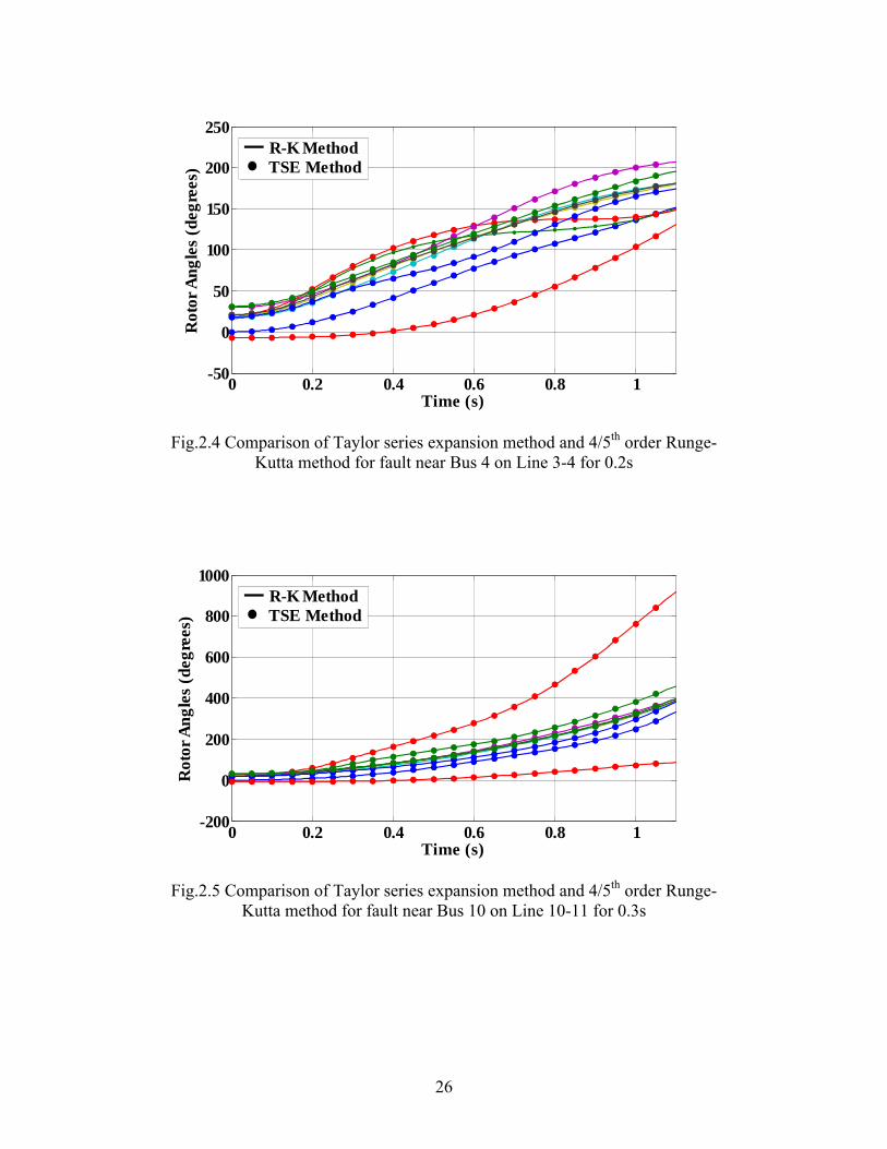
faults on the 39-Bus system, one stable and one unstable. Fig.2.4 shows a
comparison of the rotor angles obtained by the two methods for a fault near Bus 4
on Line 3-4 for 0.2s. Fig.2.5 shows the comparison for another fault near Bus 10
on Line 10-11 for 0.3s which renders the system unstable.

25
0 0.2 0.4 0.6 0.8 10
50
100
150
200
250
Time (s)
Rot
or A
ngle
s (d
egre
es)
R-K MethodTSE Method
Fig.2.2 Comparison of Taylor series expansion method and 4/5th order Runge-Kutta method for fault near Bus 7 on Line 5-7 for 0.15s
0 0.2 0.4 0.6 0.8 10
100
200
300
400
500
Time (s)
Rot
or A
ngle
s (d
egre
es)
R-K MethodTSE Method
Fig.2.3 Comparison of Taylor series expansion method and 4/5th order Runge-Kutta method for fault near Bus 7 on Line 5-7 for 0.17s
26
0 0.2 0.4 0.6 0.8 1-50
0
50
100
150
200
250
Time (s)
Rot
or A
ngle
s (d
egre
es)
R-K MethodTSE Method
Fig.2.4 Comparison of Taylor series expansion method and 4/5th order Runge-Kutta method for fault near Bus 4 on Line 3-4 for 0.2s
0 0.2 0.4 0.6 0.8 1-200
0
200
400
600
800
1000
Time (s)
Rot
or A
ngle
s (d
egre
es)
R-K MethodTSE Method
Fig.2.5 Comparison of Taylor series expansion method and 4/5th order Runge-Kutta method for fault near Bus 10 on Line 10-11 for 0.3s
27
2.2.4 Discussion
As seen from the comparisons above the Taylor series method provides an
efficient and accurate method to provide the rotor angles of the generators. One of
the main advantages of converting the differential equations to algebraic form by
using the Taylor series expansion method is the use of the large time step. The
large step of 0.05s considerably reduces the number of iterations required to find
out accurately the state of the rotor angles at 1s. In comparison to the trapezoidal
rule method or the Euler method or other conventional differential equation
solving methods which require a very small time-step, the Taylor series method
reduces the total number of iterations. Also it is seen that expansion upto the 4th
derivative provides highly accurate values of the rotor angles. So the rotor angles
to evaluate first-swing stability can be obtained quickly and accurately using the
Taylor series expansion method.
2.3 The Transient Stability Constraint
This section present the formulation of the transient stability related inequality
constraints to be incorporated into the conventional optimal power flow. The
above section described how the rotor angles at 1s would be obtained efficiently
and accurately by using the Taylor series expansion method. The transient
stability or instability state of a power system at any time can be indicated by the
distance of the rotor angles from the center of inertia angle at that time [22] as
shown in Equation (2.12).

28
gicoi n1,2,...,i (2.12)
where
gg n
ii
n
iiicoi MM
11/ (2.13)
Here coi is the center of inertia angle of the generator i . The value of in
Equation (2.12) above varies from system to system and an appropriate value for
a particular system would be learnt from operator experience after intensive
offline transient stability analysis of the system for various credible contingencies
under various loading conditions.
Consider a function ),,( gPV that is a function of the bus voltages and
the power output of each generator. The function calculates the rotor angles using
the TSE method and the center of inertia at 1s and evaluates a vector with the
absolute value of the difference between each rotor angle and the center of inertia.
Hence the transient stability can be enforced for a particular fault by limiting the
value of the rotor angle at time nt using the inequality constraint shown below
0),,(_ gPV (2.14)
Here _ is an gn x1 vector with all components equal to

29
2.4 Optimal Power Flow with Transient Stability Constraints Formulation
This section highlights the details of the formulation of the optimal power
flow with transient stability constraints.
2.4.1 Objective Function
The objective function in a centrally dispatched market is the sum of the cost
functions of the generators and the objective is to minimize the total cost. When
demand bids are also considered the objective is the difference between the sum
of the cost functions and the sum of the demand bids and the objective is to
maximize social welfare. Demand bids have not been considered in this study. So
the objective here is:
g
i
n
igi Pf Min
1 (2.15)
Here igi Pf represents the cost function of each generator and is given by a
quadratic expression as shown in Equation (2.6).
cbPaPPfiii g
2ggi (2.16)

30
2.4.2 Equality constraints
The basic equality constraints consist of the load flow equations which are
required to be satisfied for any optimal power flow and are shown in Equations
(2.17) and (2.18)
p1,2,....,i ,PPPp
ijjijLDg ii
0,1
(2.17)
p1,2,.....,i ,0QQQp
ij1,jijLDg ii
(2.18)
2.4.3 Inequality constraints
The basic inequality constraints arise from limitations on the active and
reactive power output of the generators and also on the voltages at each bus as
shown below in Equations (2.8)-(2.10).
ggiggi n1,2,....,i ,PPPmaximin
(2.19)
ggiggi n1,2,....,i ,QQQmaximin
(2.20)
p1,2,....,i ,VVV maxiimini (2.21)
Additional inequality constraints are needed to limit the rotor angles of the
generators in the case of faults. Hence inequality constraints of the form shown in
Equation (2.14) have to be included for each generator for each fault. We are

31
considered with only first-swing stability here and the classical model is
appropriate for dynamic simulation during that period. Hence, the classical model
of the generator has been considered for the dynamic equations in ).,,( gPV
Additional inequality constraints can be included for thermal limits of the lines,
power flow over the lines etc. But these are quite straightforward and are not
included in this study. The bus voltage angles are also included in the state-
variable set.
The above formulation was implemented in MATLAB using the ‘fmincon’
function [42] available in the optimization toolbox. An advantage of using the
‘fmincon’ is that the constraints can be directly evaluated as functions of the state
variables which can be separate modules reducing programming complexity. In
this case for example, the transient stability constraint was formed by having
another function that evaluates and returns a gn x1 matrix with the absolute value
of the difference of the rotor angles from the center of inertia at 1s. The [C]
matrix required by the ‘nonlcon’ [42] is evaluated as shown below.
1
2
1
),,(
xnncoi
coi
coi
g
gg
PVA
(2.22)

32
11
1
1
xng
xB
(2.23)
BAC (2.24)
Hence, the transient stability constraint is given by equation (2.14).
10
0
0
][
gn
C (2.25)
The number of transient stability related constraints and the related state-
variables i.e., the rotor angle for each generator and for each fault would increase
considerably. Obviously this would have a direct effect on the computation time
and also lead to convergence issues. Instead of restricting rotor angles in the
center of inertia frame of reference for each step of the integration, the rotor
angles at 1s have only been considered to control first swing stability. This
reduces the number of additional constraints and state variables needed. Fig.2.6
summarizes the dynamic stability constrained optimization process required to
ensure transient stability along with static-security.

33
Fig.2.6 General representation of the transient stability constrained optimal power flow problem
p
p
g
g
g
g
V
V
Q
Q
P
P
ng
ng
1
1
1
1
p1,2,....,i ,PPPp
ijjijLDg ii
0,1
p1,2,.....,i ,0QQQp
ij1,jijLDg ii
ggiggi n1,2,....,i ,PPPmaximin
ggiggi n1,2,....,i ,QQQmaximin
p1,2,....,i ,VVV maxiimini
0
0
0
ε
ε
ε
δδ
δδ
δδ
gncoi
2coi
1coi
),,( gPV
Stea
dy S
tate
Con
stra
ints
Dyn
amic
Con
stra
ints
tosubject
Pf Ming
i
n
igi
1
Set
Variable
tateS
p
p
g
g
g
g
V
V
Q
Q
P
P
ng
ng
1
1
1
1
p1,2,....,i ,PPPp
ijjijLDg ii
0,1
p1,2,.....,i ,0QQQp
ij1,jijLDg ii
ggiggi n1,2,....,i ,PPPmaximin
ggiggi n1,2,....,i ,QQQmaximin
p1,2,....,i ,VVV maxiimini
0
0
0
ε
ε
ε
δδ
δδ
δδ
gncoi
2coi
1coi
),,( gPV
Stea
dy S
tate
Con
stra
ints
Dyn
amic
Con
stra
ints
p
p
g
g
g
g
V
V
Q
Q
P
P
ng
ng
1
1
1
1
p1,2,....,i ,PPPp
ijjijLDg ii
0,1
p1,2,.....,i ,0QQQp
ij1,jijLDg ii
ggiggi n1,2,....,i ,PPPmaximin
ggiggi n1,2,....,i ,QQQmaximin
p1,2,....,i ,VVV maxiimini
0
0
0
ε
ε
ε
δδ
δδ
δδ
gncoi
2coi
1coi
),,( gPV
Stea
dy S
tate
Con
stra
ints
Dyn
amic
Con
stra
ints
tosubject
Pf Ming
i
n
igi
1
Set
Variable
tateS

34
2.5 Results with the IEEE 9-Bus System
This section presents the results of the application of the above OTS
formulation on the 9-Bus system. Three different loading situations of 75%, 100%
and 125% have been considered. For each loading scenario, three faults have been
considered. The fault locations have been selected so that represent locations near
a generator, to a load bus and buses where neither a generator nor a load is
connected. Initially a base optimal power flow is carried out to obtain a basic
dispatch that includes steady-state operating constraints on the generator active
and reactive power outputs and the voltages at all buses. The results of the fault
simulations following these dispatches is shown first. The transient stability
constraint for the unstable faults are then included separately and a new dispatch
is obtained. The fault simulations are then carried out again to show the effect of
inclusion of the transient stability constraint. Note that each fault is considered
separately. So the dispatch obtained to restrain the rotor angles for one particular
fault is not the same as the dispatch obtained to restrain the rotor angles for
another fault.
2.5.1 75% Loading, BOPF
A base optimal power flow is first carried out with no transient stability
related constraints. Table 2.1 lists the faults that have been considered and shows
the status of the transient stability of the system for each of the faults taking into
the consideration the base optimal power flow for a 75% loading situation. All

35
plots have been obtained using the Taylor series expansion method with a time-
step of 0.05s. Fig. 2.7-2.9 show the rotor plots obtained for simulating the faults.
Table 2.1 List of faults considered in the IEEE 9-Bus System
Case Fault Near Bus Faulted Line Fault Clearing Time Stable/Unstable
1 7 7-5 0.26 Stable
2 9 9-8 0.28 Unstable
3 8 7-8 0.35 Stable
0 0.5 1 1.5 20
100
200
300
400
Time (s)
Rot
or A
ngle
s (d
egre
es)
Fig.2.7 Rotor angles for fault near bus 7 on Line 7-5 for a fault duration of 0.26s following a dispatch given by the BOPF

36
0 0.5 1 1.5 20
500
1000
1500
Time (s)
Rot
or A
ngle
s (d
egre
es)
Fig.2.8 Rotor angles for fault near Bus 9 on Line 9-8 for a fault duration of 0.28s following a dispatch given by the BOPF
0 0.5 1 1.5 20
100
200
300
400
500
Time (s)
Rot
or A
ngle
s (d
egre
es)
Fig.2.9 Rotor angles for fault near Bus 8 on Line 7-8 for a fault duration of 0.35s following a dispatch given by the base optimal power flow
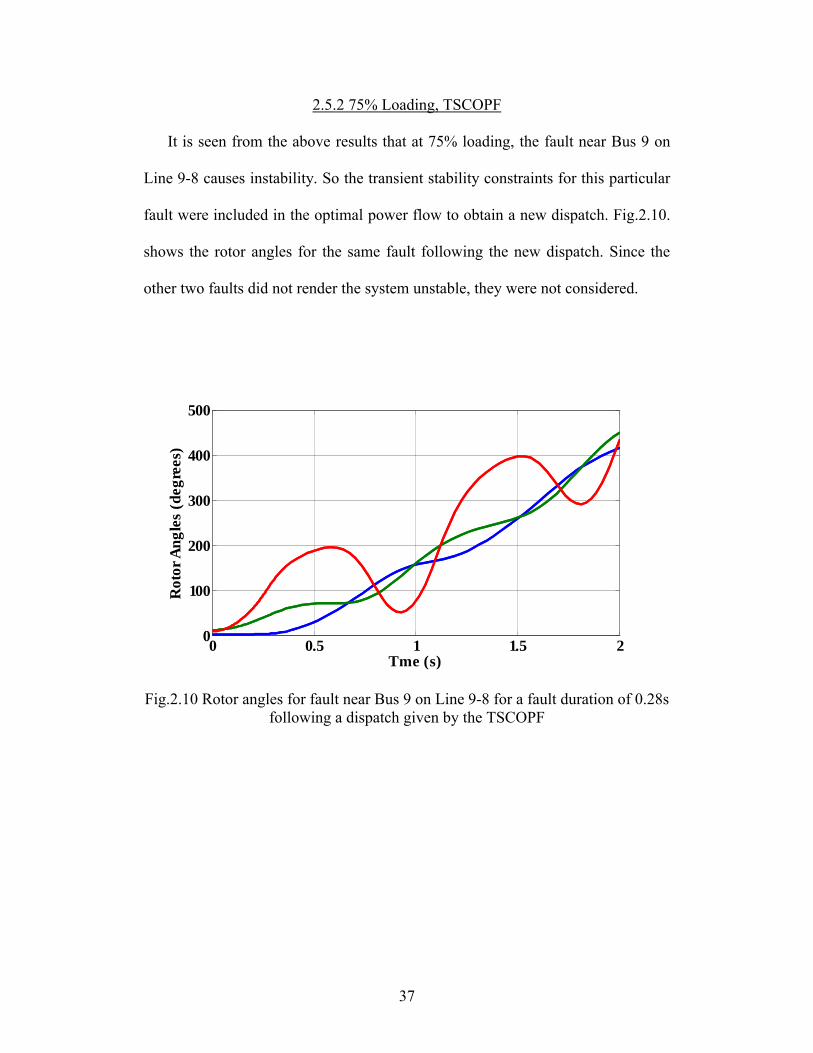
37
2.5.2 75% Loading, TSCOPF
It is seen from the above results that at 75% loading, the fault near Bus 9 on
Line 9-8 causes instability. So the transient stability constraints for this particular
fault were included in the optimal power flow to obtain a new dispatch. Fig.2.10.
shows the rotor angles for the same fault following the new dispatch. Since the
other two faults did not render the system unstable, they were not considered.
0 0.5 1 1.5 20
100
200
300
400
500
Tme (s)
Rot
or A
ngle
s (d
egre
es)
Fig.2.10 Rotor angles for fault near Bus 9 on Line 9-8 for a fault duration of 0.28s following a dispatch given by the TSCOPF

38
2.5.2 100% Loading, BOPF
A base optimal power flow is first carried out with no transient stability
related constraints. Table 2.2 lists the faults that have been considered and shows
the status of the transient stability of the system for each of the faults taking into
the consideration the base optimal power flow for a 100% loading situation. All
plots have been obtained using the Taylor series expansion method with a time-
step of 0.05s.
Table 2.2 List of faults considered in the IEEE 9-Bus System
Case Fault Near Bus Faulted Line Fault Clearing Time Stable/Unstable
1 7 7-5 0.26 Unstable
2 9 9-8 0.28 Unstable
3 8 7-8 0.35 Stable
Figs.2.11-2.13 show the rotor plots obtained for simulating the above faults
following a dispatch obtained by running the base optimal power flow as
described earlier.

39
0 0.5 1 1.5 20
500
1000
1500
2000
Time (s)
Rot
or A
ngle
s (d
egre
es)
Fig.2.11 Rotor angles for fault near Bus 7 on Line 7-5 for a fault duration of 0.26s following a dispatch given by the BOPF
0 0.5 1 1.5 20
500
1000
1500
2000
2500
Time (s)
Rot
or A
ngle
s (d
egre
es)
Fig.2.12 Rotor angles for fault near Bus 9 on Line 9-8 for a fault duration of 0.28s following a dispatch given by the BOPF

40
0 0.5 1 1.5 20
200
400
600
800
Time (s)
Rot
or A
ngle
s (d
egre
es)
Fig.2.13 Rotor angles for fault near Bus 8 on Line 7-8 for a fault duration of 0.35s following a dispatch given by the BOPF
2.5.3 100% Loading, TSCOPF
It is seen from the above results that at 100% loading, the faults near Bus 7 on
Line 7-5 and near Bus 9 on Line 9-8 cause instability. Hence, two different
dispatches were obtained. The first includes the transient stability constraints for
the fault near Bus 7. Fig.2.14 shows the rotor angles for the same fault following
the new dispatch. The second dispatch includes the transient stability constraints
for the fault near Bus 9. Fig.13 shows the rotor angles obtained for the fault near
Bus 9 on Line 9-8 for 0.28s following the new dispatch.

41
0 0.5 1 1.5 20
200
400
600
800
1000
Time (s)
Rot
or A
ngle
s (d
egre
es)
Fig.2.14 Rotor angles for fault near Bus 7 on Line 7-5 for a fault duration of 0.26s following a dispatch given by the TSCOPF
0 0.5 1 1.5 20
200
400
600
800
Time (s)
Rot
or A
ngle
s (d
egre
es)
Fig.2.15 Rotor angles for fault near Bus 9 on Line 9-8 for a fault duration of 0.28s following a dispatch given by the TSCOPF

42
2.5.4. 125% Loading, BOPF
A base optimal power flow is first carried out with no transient stability related
constraints. Table 2.3 lists the faults that have been considered and shows the
status of the transient stability of the system for each of the faults taking into the
consideration the base optimal power flow for a 125% loading situation. All plots
have been obtained using the Taylor series expansion method with a time-step of
0.05s.
Table 2.3 List of faults considered in the IEEE 9-Bus System
Case Fault Near Bus Faulted Line Fault Clearing Time Stable/Unstable
1 7 7-5 0.26 Unstable
2 9 9-8 0.28 Unstable
3 8 7-8 0.35 Unstable
Figs.2.16-2.18 show the rotor plots obtained for simulating the above faults
following a dispatch obtained by running the base optimal power flow as
described earlier.

43
0 0.5 1 1.5 20
500
1000
1500
Time (s)
Rot
or A
ngle
s (d
egre
es)
Fig.2.16 Rotor angles for fault near Bus 7 on Line 7-5 for a fault duration of 0.26s following a dispatch given by the base optimal power flow
0 0.5 1 1.5 20
500
1000
1500
2000
2500
3000
Time (s)
Rot
or A
ngle
s (d
egre
es)
Fig.2.17 Rotor angles for fault near Bus 9 on Line 9-8 for a fault duration of 0.28s following a dispatch given by the base optimal power flow

44
0 0.5 1 1.5 20
1000
2000
3000
4000
Time (s)
Rot
or A
ngle
s (d
egre
es)
Fig.2.18 Rotor angles for fault near Bus 8 on Line 7-8 for a fault duration of 0.35s following a dispatch given by the BOPF
2.5.5 125% Loading, Transient Stability Constrained Optimal Power Flow
It is seen from the above results that at 125% loading, all the three faults
considered cause instability. Hence, three different dispatches were obtained. The
first includes the transient stability constraints for the fault near Bus 7. Fig. 2.19
shows the rotor angles for the same fault following the new dispatch. The second
dispatch includes the transient stability constraints for the fault near Bus 9.
Fig.2.20 shows the rotor angles obtained for the fault near Bus 9 on Line 9-8 for
0.27s following the new dispatch. The third dispatch includes the transient
stability constraints for the fault near Bus 8. Fig. 2.21 shows the rotor angles
obtained for the fault near Bus 8 on Line 7-8 for 0.35s following the new
dispatch.

45
0 0.5 1 1.5 20
200
400
600
800
1000
1200
Time (s)
Rot
or A
ngle
s (d
egre
es)
Fig.2.19 Rotor angles for fault near Bus 7 on Line 5-7 for a fault duration of 0.26s following a dispatch given by the TSCOPF
0 0.5 1 1.5 20
200
400
600
800
1000
Time (s)
Rot
or A
ngle
s (d
egre
es)
Fig.2.20 Rotor angles for fault near Bus 9 on Line 9-8 for a fault duration of 0.28s following a dispatch given by the TSCOPF

46
0 0.5 1 1.5 20
200
400
600
800
1000
1200
Time (s)
Rot
or A
ngle
s (d
egre
es)
Fig.2.21 Rotor angles for fault near Bus 8 on Line 7-8 for a fault duration of 0.35s following a dispatch given by the TSCOPF
2.6 Results with the IEEE 39-Bus system
This section presents the results of the application of the above OTS
formulation on the 39-Bus system. Three different loading situations of 75%,
100% and 125% have been considered. For each loading scenario, three faults
have been considered. As with the 9-Bus system, initially a base optimal power
flow is carried out to obtain a basis dispatch that includes steady-state operating
constraints on the generator active and reactive power outputs and the voltages at
all buses. The results of the fault simulations following these dispatches is shown
first. The transient stability constraint for the unstable faults are then included
separately and a new dispatch is obtained, one for each of the unstable faults. The
fault simulations are then carried out again to show the effect of inclusion of the
transient stability constraint. Note that each fault is considered separately. So the

47
dispatch obtained to restrain the rotor angles for one particular fault is not the
same as the dispatch obtained to restrain the rotor angles for another fault.
2.6.1 75% Loading, BOPF
A base optimal power flow is first carried out with no transient stability
related constraints. Table 2.4 lists the faults that have been considered and shows
the status of the transient stability of the system for each of the faults taking into
the consideration the base optimal power flow for a 75% loading situation. All
plots have been obtained using the Taylor series expansion method with a time-
step of 0.05s.
Table 2.4 List of faults considered in the IEEE 39-Bus System
Case Fault Near Bus Faulted Line Fault Clearing Time Stable/Unstable
1 3 3-4 0.2 Stable
2 10 10-13 0.35 Stable
3 25 25-2 0.24 Unstable
Figs. 2.22-2.24 show the rotor plots obtained for simulating the above faults
following a dispatch obtained by running the base optimal power flow as
described earlier.

48
0 0.5 1 1.5 2
0
50
100
150
200
250
Time (s)
Rot
or A
ngle
s (d
egre
es)
Fig.2.22 Rotor angles for fault near Bus 3 on Line 3-4 for a fault duration of 0.2s following a dispatch given by the BOPF
0 0.5 1 1.5 2
0
100
200
300
400
Time (s)
Rot
or A
ngle
s (d
egre
es)
Fig.2.23 Rotor angles for fault near Bus 10 on Line 10-13 for a fault duration of 0.35s following a dispatch given by the BOPF

49
0 0.5 1 1.5 20
200
400
600
800
1000
Time (s)
Rot
or A
ngle
s (d
egre
es)
Fig.2.24 Rotor angles for fault near Bus 25 on Line 25-2 for a fault duration of 0.24s following a dispatch given by the BOPF
2.6.2 75% Loading, TSCOPF
It is seen from the above results that at 75% loading, the fault near Bus 25 on
Line 25-2 causes instability. So the transient stability constraints for this particular
fault were included in the optimal power flow to obtain a new dispatch. Fig.2.25
shows the rotor angles for the same fault following the new dispatch. Since the
other two faults did not render the system unstable, they were not considered.
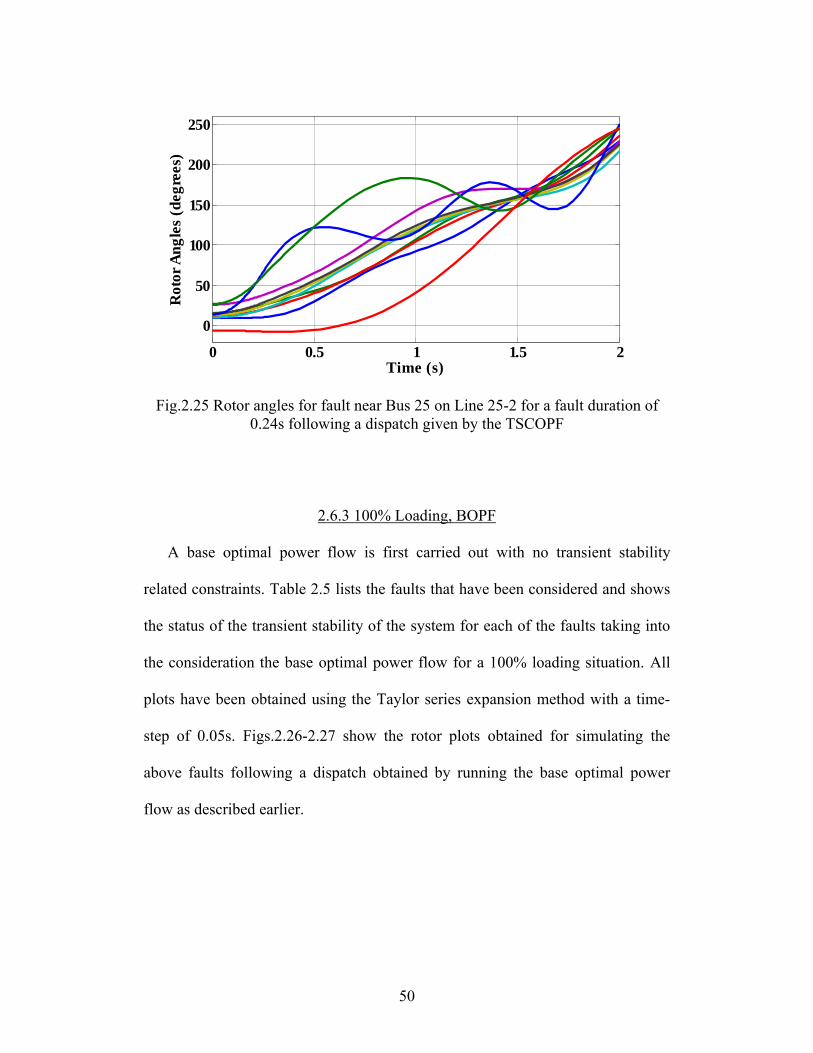
50
0 0.5 1 1.5 2
0
50
100
150
200
250
Time (s)
Rot
or A
ngle
s (d
egre
es)
Fig.2.25 Rotor angles for fault near Bus 25 on Line 25-2 for a fault duration of 0.24s following a dispatch given by the TSCOPF
2.6.3 100% Loading, BOPF
A base optimal power flow is first carried out with no transient stability
related constraints. Table 2.5 lists the faults that have been considered and shows
the status of the transient stability of the system for each of the faults taking into
the consideration the base optimal power flow for a 100% loading situation. All
plots have been obtained using the Taylor series expansion method with a time-
step of 0.05s. Figs.2.26-2.27 show the rotor plots obtained for simulating the
above faults following a dispatch obtained by running the base optimal power
flow as described earlier.

51
Table 2.5 List of faults considered in the IEEE 39-Bus System
Case Fault Near Bus Faulted Line Fault Clearing Time Stable/Unstable
1 3 3-4 0.2 Stable
2 10 10-13 0.35 Unstable
3 25 25-2 0.24 Unstable
0 0.5 1 1.5 20
100
200
300
400
Time (s)
Rot
or A
ngle
s (d
egre
es)
Fig.2.26 Rotor angles for fault near Bus 3 on Line 3-4 for a fault duration of 0.2s following a dispatch given by the BOPF

52
0 0.5 1 1.5 20
500
1000
1500
2000
2500
3000
Time (s)
Rot
or A
ngle
s (d
egre
es)
Fig.2.27 Rotor angles for fault near Bus 10 on Line 10-13 for a fault duration of 0.35s following a dispatch given by the BOPF
0 0.5 1 1.5 20
500
1000
1500
2000
2500
3000
Time (s)
Rot
or A
ngle
s (d
egre
es)
Fig.2.28 Rotor angles for fault near Bus 25 on Line 25-4 for a fault duration of 0.24s following a dispatch given by the BOPF
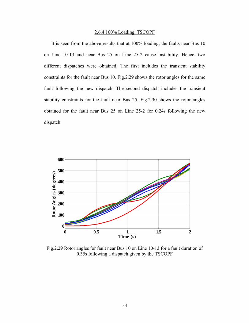
53
2.6.4 100% Loading, TSCOPF
It is seen from the above results that at 100% loading, the faults near Bus 10
on Line 10-13 and near Bus 25 on Line 25-2 cause instability. Hence, two
different dispatches were obtained. The first includes the transient stability
constraints for the fault near Bus 10. Fig.2.29 shows the rotor angles for the same
fault following the new dispatch. The second dispatch includes the transient
stability constraints for the fault near Bus 25. Fig.2.30 shows the rotor angles
obtained for the fault near Bus 25 on Line 25-2 for 0.24s following the new
dispatch.
0 0.5 1 1.5 20
100
200
300
400
500
600
Time (s)
Rot
or A
ngle
s (d
egre
es)
Fig.2.29 Rotor angles for fault near Bus 10 on Line 10-13 for a fault duration of 0.35s following a dispatch given by the TSCOPF

54
0 0.5 1 1.5 20
100
200
300
400
Time (s)
Rot
or A
ngle
s (d
egre
es)
Fig.2.30 Rotor angles for fault near Bus 25 on Line 25-2 for a fault duration of 0.24s following a dispatch given by the TSCOF
2.6.5 125% Loading, BOPF
A base optimal power flow is first carried out with no transient stability
related constraints. Table 2.6 lists the faults that have been considered and shows
the status of the transient stability of the system for each of the faults taking into
the consideration the base optimal power flow for a 125% loading situation.
Figs.2.31-2.33 show the rotor plots obtained for simulating the above faults
following a dispatch obtained by running the base optimal power flow as
described earlier.

55
Table 2.6 List of faults considered in the IEEE 39-Bus System
Case Fault Near Bus Faulted Line Fault Clearing Time Stable/Unstable
1 3 3-4 0.2 Unstable
2 10 10-13 0.35 Unstable
3 25 25-2 0.24 Unstable
0 0.5 1 1.5 20
200
400
600
800
1000
1200
1400
Time (s)
Rot
or A
ngle
s (d
egre
es)
Fig.2.31 Rotor angles for fault near Bus 3 on Line 3-4 for a fault duration of 0.2s following a dispatch given by the BOPF

56
0 0.5 1 1.5 20
500
1000
1500
2000
2500
3000
3500
Time (s)
Rot
or A
ngle
s (d
egre
es)
Fig.2.32 Rotor angles for fault near Bus 10 on Line 10-13 for a fault duration of 0.35s following a dispatch given by the BOPF
0 0.5 1 1.5 20
1000
2000
3000
4000
Time (s)
Rot
or A
ngle
s (d
egre
es)
Fig.2.33 Rotor angles for fault near Bus 25 on Line 25-2 for a fault duration of 0.24s following a dispatch given by the BOPF

57
2.6.6 125% Loading, TSCOPF
It is seen from the above results that at 125% loading, all the three faults
considered cause instability. Hence, three different dispatches were obtained. The
first includes the transient stability constraints for the fault near Bus 3. Fig.2.34
shows the rotor angles for the same fault following the new dispatch. The second
dispatch includes the transient stability constraints for the fault near Bus 10.
Fig.2.35 shows the rotor angles obtained for the fault near Bus 10 on Line 10-13
for 0.35s following the new dispatch. The third dispatch includes the transient
stability constraints for the fault near Bus 25. Fig.2.36 shows the rotor angles
obtained for the fault near Bus 25 on Line 25-2 for 0.24s following the new
dispatch.
0 0.5 1 1.5 2
0
100
200
300
400
500
600
Time (s)
Rot
or A
ngle
s (d
egre
es)
Fig.2.34 Rotor angles for fault near Bus 3 on Line 3-4 for a fault duration of 0.2s following a dispatch given by the TSCOPF

58
0 0.5 1 1.5 20
200
400
600
800
Time (s)
Rot
or A
ngle
s (d
egre
es)
Fig.2.35 Rotor angles for fault near Bus 10 on Line 10-13 for a fault duration of 0.35s following a dispatch given by the TSCOPF
0 0.5 1 1.5 20
100
200
300
400
500
600
Time (s)
Rot
or A
ngle
s (d
egre
es)
Fig.2.36 Rotor angles for fault near Bus 25 on Line 25-2 for a fault duration of 0.24s following a dispatch given by the TSCOPF

59
2.7 Discussion
It is seen from the results that although the base optimal power flow provides
a dispatch that respects the physical and operational limitations, it does not
guarantee the transient stability of the system after a fault has been cleared.
Incorporating the transient stability constraints into the optimal power flow to
limit the value of the rotor angles allows us to ensure that the system would be
transiently stable following the occurrence and clearing of the fault. By using an
appropriate value of , a dispatch can be obtained that would be transiently stable
for the set of faults in consideration. Fig.2.37 shows the comparison of the
generator active power outputs obtained by both the base optimal power flow
(BOPF) and the transient stability constrained optimal power flow (TSCOPF)
with constraints for the fault near Bus 7 on Line 7-5. It is seen that the active
power outputs of generators 1 and 3 is slightly increased and generator 2 is
slightly decreased. At 125% loading, the increase in power output of generator 1
is greater than before and a similar decrease in the power output of generator 2.
The power output of generator 3 does not change appreciably from the base case
value. The variation in the power outputs of the generators depends on a lot of
factors like proximity to the fault, active power output etc. From Fig.2.37 it can be
concluded that the active power output of generator 2 needs to be decreased

60
1 2 30
50
100
150100% Loading
Generator
Pg
(MW
)
1 2 30
50
100
150
200125% Loading
Generator
Pg
(MW
)
BOPFTSCOPF
Fig.2.37 Comparison of generator active power outputs obtained by BOPF and TSCOPF with constraints for fault near Bus 7 on Line 7-5
Fig.2.38 shows the comparison of the generator active power outputs obtained
by BOPF and the TSCOPF with constraints for the fault near Bus 9 on Line 8-9. It
is seen that to prevent the fault at near Bus 8 on Line 8-9, the active power outputs
of generators 2 needs to be increased in contrary to the case above to prevent a
fault near Bus 7 on Line 7-5. Also the active power output of generator 3 is
decreased for all loading conditions. The decrease in power output increases with
loading. Hence system loading also has an effect on the ‘redispatch’ required to
prevent a fault from causing instability for a given fault clearing time. Fig.2.39
shows the comparison of the generator active power outputs obtained by BOPF
and TSCOPF with constraints for the fault near Bus 8 on Line 7-8.

61
1 2 30
50
100
75% Loading
Generator
Pg
(M
W)
1 2 30
50
100
150100% Loading
Generator
Pg
(M
W)
1 2 30
100
200125% Loading
Generator
Pg
(MW
) BOPFTSCOPF
Fig.2.38 Comparison of generator active power outputs obtained by BOPF and TSCOPF with constraints for fault near Bus 9 on Line 8-9
1 2 30
50
100
150
200125% Loading
Generator
Pg
(MW
)
BOPFTSCOPF
Fig.2.39 Comparison of generator active power outputs obtained by the TSCOPF with constraints for fault near Bus 8 on Line 7-8
Fig.2.40 shows the comparison of the generator reactive power outputs
obtained BOPF and TSCOPF with constraints for the fault near Bus 7 on Line 7-

62
5. Fig.2.41 shows the comparison of the generator reactive power outputs
obtained by BOPF and TSCOPF with constraints for the fault near Bus 9 on Line
8-9. Fig.2.42 shows the comparison of the generator reactive power outputs
obtained by BOPF and TSCOPF with constraints for the fault near Bus 8 on Line
7-8. Fig.2.43 shows the comparison of the bus voltages obtained by BOPF and
TSCOPF with constraints for the fault near Bus 7 on Line 5-7. Fig.2.44 shows the
comparison of the bus voltages obtained by BOPF and TSCOPF with constraints
for the fault near Bus 9 on Line 8-9. Fig.2.45 shows the comparison of the
generator reactive power outputs obtained BOPF and TSCOPF with constraints
for the fault near Bus 8 on Line 7-8.
1 2 3-10
-5
0
5
10100% Loading
Generator
Qg
(MV
AR
)
1 2 3-20
0
20
40
60125% Loading
Generator
Qg
(MV
AR
)
BOPFTSCOPF
Fig.2.40 Comparison of generator reactive power outputs obtained by BOPF and TSCOPF with constraints for fault near Bus 7 on Line 7-5

63
1 2 3-30
-20
-10
0
75% Loading
Generator
Qg
(MV
AR
)
1 2 3
-10
0
10
20100% Loading
Generator
Qg
(MV
AR
)
1 2 3
0
20
40
125% Loading
Generator
Qg
(MV
AR
)
BOPFTSCOPF
Fig.2.41 Comparison of generator reactive power outputs obtained by BOPF and TSCOPF with constraints for fault near Bus 9 on Line 8-9
1 2 3-10
0
10
20
30
40
50125% Loading
Generator
Qg
(MV
AR
)
BOPFTSCOPF
Fig.2.42 Comparison of generator reactive power outputs obtained by BOPF and TSCOPF with constraints for fault near Bus 8 on Line 7-8

64
1 2 3 4 5 6 7 8 90
0.2
0.4
0.6
0.8
1
100% Loading
Buses
Vm
(pu
)
1 2 3 4 5 6 7 8 90
0.2
0.4
0.6
0.8
1
125% Loading
Buses
Vm
(pu
)
BOPFTSCOPF
Fig.2.43 Comparison of bus voltage magnitudes obtained by BOPF and TSCOPF with constraints for fault near Bus 7 on Line 5-7
1 2 3 4 5 6 7 8 90
0.5
1
75% Loading
Buses
Vm
(pu
)
1 2 3 4 5 6 7 8 90
0.5
1
100% Loading
Buses
Vm
(pu
)
1 2 3 4 5 6 7 8 90
0.5
1
125% Loading
Buses
Vm
(pu
) BOPFTSCOPF
Fig.2.44 Comparison of bus voltage magnitudes obtained by BOPF and TSCOPF with constraints for fault near Bus 9 on Line 8-9

65
1 2 3 4 5 6 7 8 90
0.2
0.4
0.6
0.8
1
1.2
125% Loading
Buses
Vm
(pu
)
BOPFTSCOPF
Fig.2.45 Comparison of bus voltage magnitudes obtained by BOPF and TSCOPF with constraints for fault near Bus 8 on Line 7-8
Fig.2.46 shows the comparison of the generator active power outputs obtained
by BOPF and TSCOPF with constraints for the fault near Bus 3 on Line 3-4.
Fig.2.47 shows the comparison of the generator active power outputs obtained by
BOPF and TSCOPF with constraints for the fault near Bus 10 on Line 10-13.
Fig.2.48 shows the comparison of the generator active power outputs obtained by
BOPF and TSCOPF with constraints for the fault near Bus 25 on Line 25-2.

66
1 2 3 4 5 6 7 8 9 100
500
1000
1500
125% Loading
Generator
Pg
(MW
)
BOPFTSCOPF
Fig.2.46 Comparison of generator active power outputs obtained by BOPF and TSCOPF with constraints for fault near Bus 3 on Line 3-4
1 2 3 4 5 6 7 8 9 100
200
400
600
800
1000
1200100% Loading
Generator
Pg (M
W)
1 2 3 4 5 6 7 8 9 100
500
1000
1500
125% Loading
Generator
Pg (M
W)
BOPFTSCOPF
Fig.2.47 Comparison of generator active power outputs obtained by BOPF and TSCOPF with constraints for fault near Bus 10 on Line 10-13

67
1 2 3 4 5 6 7 8 9 100
500
75% Loading
Generator
Pg
(MW
)
1 2 3 4 5 6 7 8 9 100
500
1000100% Loading
Generator
Pg
(MW
)
1 2 3 4 5 6 7 8 9 100
500
1000
1500125% Loading
Generator
Pg
(MW
) BOPFTSCOPF
Fig.2.48 Comparison of bus generator active power outputs obtained by BOPF and TSCOPF with constraints for fault near Bus 25 on Line 25-2
Fig.2.49 shows the comparison of the generator reactive power outputs
obtained by BOPF and TSCOPF with constraints for the fault near Bus 3 on Line
3-4. Fig.2.50 shows the comparison of the generator reactive power outputs
obtained by BOPF and TSCOPF with constraints for the fault near Bus 10 on Line
10-13. Fig.2.51 shows the comparison of the generator active power outputs
obtained by BOPF and TSCOPF with constraints for the fault near Bus 25 on Line
25-2.

68
1 2 3 4 5 6 7 8 9 100
100
200
300
400
100% Loading
Generator
Qg
(MV
AR
)
BOPFTSCOPF
Fig.2.49 Comparison of bus generator reactive power outputs obtained by BOPF and TSCOPF with constraints for fault near Bus 3 on Line 3-4
1 2 3 4 5 6 7 8 9 10-50
150
350
500100% Loading
Generator
Qg
(MV
AR
)
1 2 3 4 5 6 7 8 9 100
200
400
550125% Loading
Generator
Qg
(MV
AR
)
BOPF
TSCOPF
Fig.2.50 Comparison of generator reactive power outputs obtained by BOPF and TSCOPF with constraints for fault near Bus 10 on Line 10-13

69
1 2 3 4 5 6 7 8 9 10
0
100
200
Generator
Qg
(MV
AR
)
75% Loading
1 2 3 4 5 6 7 8 9 10-200
0
200
400
Generator
Qg
(MV
AR
)
100% Loading
1 2 3 4 5 6 7 8 9 10-200
0
200
400
Generator
Qg
(MV
AR
)
125% Loading
BOPFTSCOPF
Fig.2.51 Comparison of generator reactive power outputs obtained by BOPF and TSCOPF with constraints for fault near Bus 25 on Line 25-2
In each of the above cases it is seen that the variation of active generator
power outputs obtained from the transient stability constrained optimal power
flow is not very much different than those obtained from the base optimal power
flow. The variation in bus voltages on the other hand was very large. Hence, the
reactive power variation was also very large to maintain the voltages within the
prescribed limits. The large sensitivity of the reactive power to transient stability
constrained optimal power flows also concurs with the results in [18] where it was
concluded that the generator reactive power was an important input for estimating
the critical clearing time and the output was very sensitive to variations in the
reactive power output of each generator.

70
2.6 Conclusions
From the above results we can conclude that
1. With small adjustments of the state-variables in the original optimal power
flow it is possible to ensure the transient stability of the system for a particular
fault. Although the locational marginal prices would increase considering the
increased constraint set, since the variation in active power outputs is not very
large, the increase in cost would not be very large.
2. The functional evaluation of the transient stability of the system for the
particular fault under consideration and its use as inequality constraints in the
OPF allows us to ensure transient stability for faults at a particular fault
location.
3. Incorporating such equations for a set of faults at different locations can
ensure transient stability of the power system for faults occurring at those
locations. Hence a set of faults can be treated simultaneously.
4. It is a well known fact that the numerical integration of the differential
equations by methods such as the trapezoidal rule requires a very small time-
step to be accurate. Using the Taylor series expansion method to form a
functional constraint that allows us to use a much larger time step of
integration can prove to be more efficient.

71
5. Also instead of actually integrating the solution of the differential equations
into the optimal power flow by forming a functional constraint that restricts
the rotor angles at 1s considerably reduces the number of additional
constraints and state variables needed.
6. It has also been observed that using previous converged states as starting
points for obtaining new dispatches with additional constraints such as
transient stability constraints considerably reduces the total computation time
required.

72

73
CHAPTER THREE
APPLICATION OF SINGLE MACHINE EQUIVALENT METHOD AND
NEURAL NETWORKS FOR ESTIMATION OF CRITICAL CLEARING TIME
The analysis of system security from a dynamic point of view by running time
domain simulations seems useful only for offline studies and almost impossible to
use in a real-time operations environment where solutions are needed fast and
within reasonable tolerance as far as accuracy is concerned. This chapter aims at
analyzing a class of One Machine Infinite Bus (OMIB)-based methods, the Single
Machine Equivalent Method which offers a solution towards the goal mentioned
above. The method is employed to quickly generate a large training set of data
which is then utilized to estimate the critical clearing time for a fault with a single
switching action (i.e the faulted line is opened to clear the fault) using
feedforward neural networks which seem to offer promising intelligent system
solutions for real-time operations if trained well i.e. provide accurate estimates for
cases unknown during training, that are suitable for use in real-time operations.
3.1 Single Machine Equivalent Method
The single machine equivalent method belongs to those class of methods that
rely on building a OMIB equivalent of the system. Such OMIB methods are based
on the simple idea of replacing the machines in a system with two sets of
machines, one consisting of the critical machines and the other consisting of the

74
non-critical machines. These two sets of machines are then further reduced to a
OMIB system as is done to analyze the transient stability of a system for a two-
machine system using the Equal Area Criterion. Thus, the OMIB method provides
a way of transforming the large number of multidimensional multimachine
dynamical equations into a single dynamic equation. The OMIB-based methods
to carry out transient stability analysis are divided into “time-invariant”, “time-
varying” and “generalized ones”. A common feature of all OMIB-based methods
is that they rely on the classical and well-known equal area criterion method
which offers a ‘one-shot’ way to assess the transient stability of a system
following a fault without time domain simulations. Simplified power system
modeling and coherency of the machines within each one of the critical and non-
critical sets, so as to ‘freeze’ their relative motion in the fault-on and post-fault
periods, is one of the main properties of time-invariant OMIB-based methods.
[48-52] present a brief history of these methods. Time-varying methods relax
the coherency assumption, but stick to a simplified power system model. In
contrast to the time-varying methods, the generalized OMIB-based methods
consider detailed power system models. Here variation between the accelerating
power and the rotor angle of the OMIB system is no longer sinusoidal as is with
both the time-invariant and time-varying OMIB-based methods. Detailed theory
and derivations of expressions for these methods can be found in [53-54].
The single machine equivalent method is a method to assess the transient
stability and is based on a generalized OMIB method. It is a hybrid method
created by coupling time domain simulation with the direct analysis offered by the

75
equal-area criterion for the time-varying OMIB system developed at each step of
the time domain simulation for the respective decomposition of the machines into
the critical and non-critical sets. Obviously, the good performance of the single
machine equivalent method is based on the right decomposition of the machines
into the critical and non-critical sets. A number of ways are available to sort
machines so as to form the critical and non-critical sets. Rotor angles at fault
initiation, initial accelerations, proximity to fault etc can be used to form the
critical and non-critical sets.
3.1.2 Methodology
A time domain simulation program is run. As soon as the system enters the
post-fault state, the SIME method subroutine starts considering at each time step,
candidate decomposition patterns (i.e., splitting of the machines into the critical
clusters and non-critical clusters). For each of these decompositions, the One
Machine Infinite Bus (OMIB) parameters are computed according to the
expressions shown below. The above procedure is repeated till a particular
“candidate” OMIB reaches the unstable condition as defined later. This candidate
OMIB is declared to be the critical OMIB. For a given set of critical and non-
critical machines, the procedure of forming the OMIB is repeated here for a quick
review.
At each time step of the time domain simulation we have:
1. A set ‘S’ representing the cluster of critical machines [53].
2. A set ‘A’ represent the cluster of non-critical machines [53].

76
3. The OMIB parameters to be calculated are aem PPP M,, ,,, . Here
aP is the accelerating power given by Equation (3.1).
ema PPP (3.1)
Let the inertia constant for set ‘S be given by
Sk
kS MM
(3.2)
The inertia constant for the set ‘A’ is given by
Al
lA MM
(3.3)
Let S , and A denote the Center-Of-Inertia-Angle (COA) for the sets S and
A respectively. They are calculated as shown below
)(1 tMMSk
kksS
(3.4)
)(1 tMMAl
llAA
(3.5)

77
Let the corresponding rotor speeds for each set be given by:
)(1 tMMSk
kkss
(3.6)
)(1 tMMAl
llAA
(3.7)
The rotor angle and speed for the OMIB are then given by:
)()()( ttt AS (3.8)
)()()( ttt AS (3.9)
The OMIB mechanical power is given by
Sk AlmAmSm tPMtPMMtP
lk
)()()( 11 (3.10)
In Equation (3.10) the inertial constant M of the OMIB system is given by:
AS
AS
MM
MMM
* (3.11)

78
The OMIB electrical power is given by
Sk AleAeSm tPMtPMMtP
lk
)()()( 11 (3.12)
The time domain simulation is carried out until we reach the termination
situation as described below:
i) The unstable angle u is found at the crossing of eP and mP curves
during the post-fault stage for an unstable scenario
ii) The stable (or return) angle r , (r for return) represents the maximum
angular excursion of eP during the post-fault stage for a stable
scenario
iii) ru when a maximum angular excursion is reached at the
crossing of eP and mP during the post-fault stage
A trajectory would be classified as stable if eP returns back before
crossing mP . If r is the return angle ( )ur at time rt with
0rt and 0ra tP (3.13)

79
Then, these conditions classify the trajectory to be stable and the time domain
simulation can be terminated. Fig.3.1 illustrates a stable scenario.
10 20 30 40 50 60 70 80 90 1000
50
100
150
200
250
OMIB Angle (degrees)
OM
IB P
m &
Pe
(MW
)
Pm
Pe
r(Point of Return)
Fig.3.1 An example of a stable OMIB trajectory
The conditions of an unstable trajectory are that it reaches the unstable angle
u at a time ut when the accelerating power aP becomes zero and the rate of
change of the accelerating power is positive, i.e.,
0dt
dPtP ,0)(tP
utt
auaua
with 0 for ott (3.14)

80
The above conditions determine the early conditions to terminate the time
domain simulation. These conditions are also used to identify the critical OMIB.
Fig.3.2 illustrates an unstable scenario.
0 20 40 60 80 100 120 140 160 180
100
150
200
250
OMIB Angle (degrees)
OM
IB P
m &
Pe
Pm
Pe
u
Fig.3.2 An example of an unstable OMIB trajectory
Another property of a stable OMIB trajectory is the phase-plane plot of the
OMIB speed vs. the OMIB angle. A stable OMIB trajectory always has a
continuously revolving phase-plane plot while an unstable OMIB trajectory
would have a divergent phase-plane plot that showing no decrease in the OMIB
speed as shown below in Fig.3.3

81
0 50 100
-50
0
50
OMIB Angle (degrees)
OM
IB S
peed
(0.
1 ra
d/s)
Stable Case
0 10000
100
200
300
400
OMIB Angle (degrees)
OM
IB S
peed
(0.
1 ra
d/s)
Unstable Case
Fig.3.3 Phase plane plot of OMIB speed vs. the OMIB angle
3.2 Results with the IEEE 9-Bus system
This section presents illustrations of the above methodology on various fault
cases in the 9-Bus system. For each case, the set ‘S’ consisting of the critical
machines and the set ‘A’ consisting of the non-critical machines at the terminating
time step are also listed. It has been assumed that no reclosing takes place and the
fault is a permanent one that is cleared by opening the faulted line.

82
3.2.1 Case 1: Fault near Bus 5 on Line 5-7 for 0.28s (S: [2, 3], A: [1])
In this case, a fault near Bus 5 on Line 8 is considered. It is assumed to be
cleared in 0.28s by opening the line. Fig.3.4 shows the OMIB mechanical input,
electrical power output, accelerating power and angle and speed trajectory. From
the conditions in Equation (3.13) we can conclude that the system is stable. The
phase plane plot is shown in Fig.3.5. The generator rotor plots in Fig.3.6 confirm
it as a stable scenario.
-100 -50 0 50 100
100
150
200
OMIB Angle (degrees)
OM
IB P
m &
Pe
(MW
)
-100 -50 0 50 100-0.8
-0.6
-0.4
-0.2
0
OMIB Angle (degrees), OMIB Speed (0.1 rad/s), OMIB Pa(MW)
Tim
e (s
)
SpeedPaAngle
PePm
Fig.3.4 Plot of OMIB mechanical input, electrical power output, accelerating power and angle and speed trajectory for Case 1

83
-20 0 20 40 60 80 100
-60
-40
-20
0
20
40
60
OMIB Angle (degrees)
OM
IB S
peed
(0.
1 ra
d/s)
Fig.3.5 OMIB speed vs. the OMIB angle for Case 1
0 0.2 0.4 0.6 0.8 1 1.2 1.4 1.6 1.8 20
100
200
300
400
500
600
700
Time (s)
Rot
or A
ngle
s (d
egre
es)
Fig.3.6 Plot of generator rotor angles for Case 1

84
3.2.2 Case 2: Fault near Bus 5 on Line 5-7 for 0.33s (S: [2, 3], A: [1])
In this case the same fault is considered as in case 1 but with an increased
fault clearing time of 0.33s. Fig.3.7 shows the OMIB mechanical input, electrical
power output, accelerating power and angle and speed trajectory. From the
conditions in Equation (3.14) we can conclude that the system is unstable. The
phase plane plot is shown in Fig.3.8. The generator rotor plots in Fig.3.9 confirm
it as an unstable scenario.
-50 0 50 100 150
100
150
200
OMIB Angle (degrees)
OM
IB P
m &
Pe
(MW
)
-50 0 50 100 150-1
-0.5
0
OMIB Angle (degrees), OMIB Speed (0.1 rad/s), OMIB Pa(MW)
Tim
e (s
)
PePm
SpeedPaAngle
Fig.3.7 Plot of OMIB mechanical input, electrical power output, accelerating power and angle and speed trajectory for Case 2

85
0 200 400 600 800 1000 1200 1400 16000
100
200
300
400
500
OMIB Angle (degrees)
OM
IB S
peed
(0.
1 ra
d/s)
Fig.3.8 OMIB speed vs. the OMIB angle for Case 2
0 0.2 0.4 0.6 0.8 1 1.2 1.4 1.6 1.8 20
500
1000
1500
2000
Time (s)
Rot
or A
ngle
s (d
egre
es)
Fig.3.9 Plot of generator rotor angles for Case 2

86
3.2.3 Case 3: Fault near Bus 7 on Line 7-5 for 0.083s (S: [2, 3], A: [1])
This case illustrates another stable case with the fault on the same line, but
near Bus 7 this time. Fig.3.10 shows the OMIB mechanical input, electrical power
output, accelerating power and angle and speed trajectory. The phase plane plot is
shown in Fig.3.11. The generator rotor plots in Fig.3.12 confirm it as a stable
scenario.
-40 -20 0 20 40 60 800
50
100
150
200
OMIB Angle (degrees)
OM
IB P
m &
Pe
(MW
)
-40 -20 0 20 40 60 80
0.4
0.2
0
OMIB Angle (degrees), OMIB Speed (0.1 rad/s), OMIB Pa(MW)
Tim
e (s
)
PePm
SpeedPaAngle
Fig.3.10 Plot of OMIB mechanical input, electrical power output, accelerating power and angle and speed trajectory for Case 3

87
0 10 20 30 40 50 60 70 80-40
-30
-20
-10
0
10
20
30
40
OMIB Angle (degrees)
OM
IB S
peed
(0.
1 ra
d/s)
Fig.3.11 OMIB speed vs. the OMIB angle for Case 3
0 0.2 0.4 0.6 0.8 1 1.2 1.4 1.6 1.8 20
50
100
150
200
250
300
Time (s)
Rot
or A
ngle
s (d
egre
es)
Fig.3.12 Plot of generator rotor angles for Case 3

88
3.2.4 Case 4: Fault near Bus 7 on Line 7-5 for 0.17s (S: [2, 3], A: [1])
This case illustrates the same fault as above with an increased fault clearing
time of 0.17s which renders the system unstable. Fig.3.13 shows the OMIB
mechanical input, electrical power output, accelerating power and angle and speed
trajectory. The phase plane plot is shown in Fig.3.14. The generator rotor plots in
Fig.3.15 confirm it as an unstable scenario.
-50 0 50 100 1500
50
100
150
200
OMIB Angle (degrees)
OM
IB P
m &
Pe
(MW
)
-50 0 50 100 150
0.6
0.4
0.2
OMIB Angle (degrees), OMIB Speed (0.1 rad/s), OMIB Pa(MW)
Tim
e (s
)
PePm
SpeedPaAngle
Fig.3.13 Plot of OMIB mechanical input, electrical power output, accelerating power and angle and speed trajectory for Case 4

89
0 200 400 600 800 1000 1200 1400 1600 18000
100
200
300
400
500
OMIB Angle (degrees)
OM
IB S
peed
(0.
1 ra
d/s)
Fig.3.14 OMIB speed vs. the OMIB angle for Case 4
0 0.2 0.4 0.6 0.8 1 1.2 1.4 1.6 1.8 20
500
1000
1500
2000
Time (s)
Rot
or A
ngle
s (d
egre
es)
Fig.3.15 Plot of generator rotor angles for Case 4

90
3.2.5 Case 5: Fault near Bus 6 on Line 6-9 for 0.17s (S: [2, 3], A: [1])
This case illustrates the methodology for a fault near Bus 6 on Line 6-9 for
0.17s. Fig.3.16 shows the OMIB mechanical input, electrical power output,
accelerating power and angle and speed trajectory. The phase plane plot is shown
in Fig.3.17. The generator rotor plots in Fig.3.18 confirm it as a stable scenario.
-40 -20 0 20 40 60
100
150
200
OMIB Angle (degrees)
OM
IB P
m &
Pe
(MW
)
-40 -20 0 20 40 60
-0.6
-0.4
-0.2
0
OMIB Angle (degrees), OMIB Speed (0.1 rad/s), OMIB Pa(MW)
Tim
e (s
)
PePm
SpeedPaAngle
Fig.3.16 Plot of OMIB mechanical input, electrical power output, accelerating power and angle and speed trajectory for Case 5

91
0 10 20 30 40 50-40
-30
-20
-10
0
10
20
30
40
OMIB Angle (degrees)
OM
IB S
peed
(0.
1 ra
d/s)
Fig.3.17 OMIB speed vs. the OMIB angle for Case 5
0 0.2 0.4 0.6 0.8 1 1.2 1.4 1.6 1.8 20
50
100
150
200
250
300
Time (s)
Rot
or A
ngle
s (d
egre
es)
Fig.3.18 Plot of generator rotor angles for the Case 5

92
3.2.6 Case 6: Fault near Bus 6 on Line 6-9 for 0.4s (S: [2, 3], A: [1])
This case illustrates the same fault as above with an increased fault clearing
time of 0.4s which renders the system unstable. Fig.3.19 shows the OMIB
mechanical input, electrical power output, accelerating power and angle and speed
trajectory. The phase plane plot is shown in Fig.3.20. The generator rotor plots in
Fig.3.21 confirm it as an unstable scenario.
-50 0 50 100 150
100
150
200
250
OMIB Angle (degrees)
OM
IB P
m &
Pe
(MW
)
-50 0 50 100 150-1
-0.5
0
OMIB Angle (degrees), OMIB Speed (0.1 rad/s), OMIB Pa(MW)
Tim
e (s
)
PePm
SpeedPaAngle
Fig.3.19 Plot of OMIB mechanical input, electrical power output, accelerating power and angle and speed trajectory for Case 6

93
0 500 1000 15000
50
100
150
200
250
300
350
400
OMIB Angle (degrees)
OM
IB S
peed
(0.
1 ra
d/s)
Fig.3.20 OMIB speed vs. the OMIB angle for Case 6
0 0.2 0.4 0.6 0.8 1 1.2 1.4 1.6 1.8 20
500
1000
1500
2000
Time (s)
Rot
or A
ngle
s (d
egre
es)
Fig.3.21 Plot of generator rotor angles for Case 6

94
3.3 Results with the IEEE 39-Bus system
3.3.1 Case 7: Fault near Bus 3 on Line 3-4 for 0.18s (S: [3, 5, 6, 7, 8, 9], A: [1, 2,
4, 10])
This case illustrates the methodology for a fault near Bus 3 on Line 3-4 for
0.18s. Fig.3.22 shows the OMIB mechanical input, electrical power output,
accelerating power and angle and speed trajectory. The phase plane plot is shown
in Fig.3.23. The generator rotor plots in Fig.3.24 confirm it as a stable scenario.
-20 0 20 40 60 801000
2000
3000
4000
OMIB Angle (degrees)
OM
IB P
m &
Pe
(MW
)
-20 0 20 40 60 80-0.8
-0.6
-0.4
-0.2
0
OMIB Angle (degrees), OMIB Speed (0.1 rad/s), OMIB Pa(MW)
Tim
e (s
)
PePm
SpeedPaAngle
Fig.3.22 Plot of OMIB mechanical input, electrical power output, accelerating power and angle and speed trajectory for Case 7

95
-10 0 10 20 30 40 50 60 70 80-30
-20
-10
0
10
20
30
OMIB Angle (degrees)
OM
IB S
peed
(0.
1 ra
d/s)
Fig.3.23 OMIB speed vs. the OMIB angle for Case 7
0 0.2 0.4 0.6 0.8 1 1.2 1.4 1.6 1.8 2
0
50
100
150
200
250
300
350
Time (s)
Rot
or A
ngle
s (d
egre
es)
Fig.3.24 Plot of generator rotor angles for Case 7

96
3.3.2 Case 8: Fault near Bus 3 on Line 3-5 for 0.23s (S: [3, 5, 6, 7, 8, 9], A: [1, 2,
4, 10])
This case illustrates the same fault as above with an increased fault clearing
time of 0.23s which renders the system unstable. Fig.3.25 shows the OMIB
mechanical input, electrical power output, accelerating power and angle and speed
trajectory. The phase plane plot is shown in Fig.3.26. The generator rotor plots in
Fig.3.27 confirm it as an unstable scenario.
-20 0 20 40 60 80 100 120 140 1601000
2000
3000
4000
OMIB Angle (degrees)
OM
IB P
m &
Pe
(MW
)
-20 0 20 40 60 80 100 120 140 160-1
-0.5
0
OMIB Angle (degrees), OMIB Speed (0.1 rad/s), OMIB Pa(MW)
Tim
e (s
)
PePm
SpeedPaAngle
Fig.3.25 Plot of OMIB mechanical input, electrical power output, accelerating power and angle and speed trajectory for Case 8
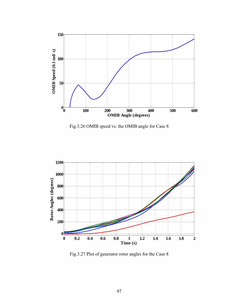
97
0 100 200 300 400 500 6000
50
100
150
OMIB Angle (degrees)
OM
IB S
peed
(0.
1 ra
d/s)
Fig.3.26 OMIB speed vs. the OMIB angle for Case 8
0 0.2 0.4 0.6 0.8 1 1.2 1.4 1.6 1.8 20
200
400
600
800
1000
1200
Time (s)
Rot
or A
ngle
s (d
egre
es)
Fig.3.27 Plot of generator rotor angles for the Case 8

98
3.4 Discussion
It can be seen from the above results that the single machine equivalent
method provides a faithful picture of the multimachine stability phenomenon. The
consistent results for the 9-Bus and 39-Bus system show that the method is
applicable to both small-scale and large-scale systems and is also independent of
the number of the machines in the system. One of the major advantages of
performing the SIME analysis at each step of the time domain simulation is that
the time domain simulation can be stopped once the OMIB trajectory exhibits the
termination criterion for a stable or unstable scenario.
3.5 Fast Determination of Critical Clearing Time Using SIME Method
3.5.1 Background
The SIME Method can be used for fast determination of critical clearing time
by plotting the stable/unstable margins for a set of clearing times. These points are
then fitted by a polynomial. The roots of the polynomial are found to obtain the
critical clearing time (The margin at critical clearing time is 0). As described
earlier by Equation (3.14), the conditions of an unstable trajectory are that it
reaches the unstable angle u at a time ut when the accelerating power aP
becomes zero and the rate of change of the accelerating power is positive. These
conditions determine the early conditions to terminate the time domain
simulation. These conditions are also used to identify the critical OMIB. Now
aPM (3.15)

99
Multiplying both sides of Equation (3.15) by we obtain
aPM (3.16)
Also 00 . Integrating Equation (3.16) we obtain,
u
dPM au
0
2
2
1 (3.17)
The general stability margin is obtained as
ch u
ch
dPdPAA aaaccdec
0
(3.18)
In Equation (3.15) ch is the angle at which aP changes sign from positive
to negative. Using the Equations (3.14) and (3.15), we obtain the unstable margin
as:
2
2
1uu M (3.19)

100
As described earlier, a trajectory would be classified as stable if eP returns
back before crossing mP . If r is the return angle ( )ur at time rt with
0rt and 0tP ra , then these conditions determine classify the trajectory
to be stable and the time domain simulation can be terminated. Observing that
0 at 0t and rt , we get the stable margin as,
ruaraast PdPdPu
r
u
r
2
1 (3.20)
u is obtained by extrapolating the aP curve as a function of by using
values of aP taken at three successive time steps near the ‘point of return’.
3.5.2 Methodology
The above described procedure is used to calculate the stable/unstable margins
for four different clearing times. These are then fitted using polynomial
interpolation functions. The roots of the polynomial are then found one of which
would be the critical clearing time as the margin at the critical clearing time is 0.
3.5.3 Results with the IEEE 9-Bus System
This section shows some results of the above methodology to quickly obtain
the critical clearing time using a limited number of Single Machine Equivalent
Method simulations which are terminated as soon as a stable or unstable condition

101
is detected. In each of the results shown below, the value of the margin is
calculated for four different fault clearing times. These are then fitted by a
polynomial using MATLAB’s polynomial fitting function. A cubic polynomial
was found to give the best polynomial to obtain the critical clearing time. Fig.3.28
shows the results for a fault near Bus 7 on Line 7-8. In a similar manner SIME
simulations carried out for other fault locations for various fault clearing times
and the critical clearing times were estimated as above. The cases studied have
been listed in Table 3.1. The critical clearing times from time-domain simulations
for the respective cases obtained using time domain simulations have also been
listed
0.2 0.22 0.24 0.26 0.28 0.3-200
-150
-100
-50
0
50
100
Clearing Time
Stab
ility
Mar
gin
CCT
Fig.3.28 Plot of stable/unstable margins for a fault near Bus 7 on Line 7-8

102
0.23 0.24 0.25 0.26 0.27 0.28-100
-80
-60
-40
-20
0
20
40
60
Clearing Time (s)
Stab
ility
Mar
gin
CCT
Fig.3.29 Plot of stable/unstable margins for a fault near Bus 7 on Line 7-5
Table 3.1 List of faults considered in the IEEE 9-Bus System
Case Fault Near
Bus
Fault on
Line
Actual critical
clearing time
Critical clearing time
from TD
1 7 7-8 0.252 0.253
2 7 5-7 0.248 0.249
3 9 6-9 0.242 0.242
4 5 5-7 0.288 0.289
5 6 4-6 0.306 0.306

103
3.5.4 Discussion
From the above results we can see that the error between the estimated critical
clearing time and the actual critical clearing time obtained by time domain
simulations is of the order of 0.001 and negligible as far as real-time operations
are concerned. Thus the single machine equivalent method provides a
computationally efficient technique to obtain the critical clearing time for a fault.
This technique is not only fast as compared to running numerous time domain
simulations to narrow down on the critical clearing time but is also very accurate.
The single machine equivalent method allows further saving in time as it is not
required to run the entire time domain simulation. The simulations are terminated
as soon as a stable or an unstable condition is reached. In this manner the critical
clearing time for a set of cases at various loading levels and for various topology
situations can be found using the SIME method to train a neural network.
3.6 Application of Feedforward Neural Networks for critical clearing time
estimation
3.6.1 Background
Artificial neural networks have been used for dynamic security assessment.
One method used several indices as input to the artificial neural network to
predict system instability (stable/unstable) [55]. Other methods use several key
features as input to the ANN to estimate maximum generator swing angles [56],
and the Transient Energy Margin that are used for contingencies screening and
ranking [57]. Other methods utilize the artificial neural network in transient

104
stability assessment to estimate the critical clearing time, or the stability index
(stable/unstable) for a given clearing time, of a multimachine power system [58].
A. D. Angel et al focused on the development of a technique for the estimation of
generator rotor angle and speed, based on phasor measurement units for transient
stability assessment and control in real-time in [59]. M. Moghavvemi examined
the performance of two nonlinear multilayered ANN models for the estimation of
a stability index to gauge the stability of a power system network in [60].
Dynamic security margin assessment for a both voltage and dynamic stability
using artificial neural networks were explored by A. Sittithumwat in [61].
Eigenvalue prediction of critical stability modes of power systems based on
neural networks was dealth with in [62] to predict the stability condition of the
power system with high accuracy. Pattern recognition techniques using artificial
neural networks and linear classification were used in [63] for the classification of
swing curves generated in a power system transient stability study. Artificial
neural networks have been used for a wide variety of other applications in power
systems. [64] presents a method for topological observability based on multilayer
perceptrons using the back-propogation algorithm for training. Y. Y. Hsu et al
evaluated the dynamic performance of power system by computation of the
dominant eigenvalues for the worst damped electromechanical mode using neural
networks in [65]. A load forecasting technique has been suggested in [66] that
utilizes a swarm optimization algorithm. B. Thukaram et al have dealt with
providing solutions for monitoring and control of voltage stability in the day-to-
day operations of power systems in [67]. An intelligent load shedding scheme

105
using artificial neural networks was developed by D. Nosovel et al in [68]. Some
other applications have been explored in [69-70].
3.6.2 Methodology
A feed-forward artificial neural network was developed using the MATLAB
Neural Network toolbox to predict the critical clearing time for various other
loading conditions and topology situations. The inputs to the neural network were:
1. Mechanical input of each generator:imP
2. Initial rotor angle for each generator with respect to the center of inertia:
n
ii
n
iii
icoiM
M
i
1
1
(3.21)
Here iM is the inertial constant and i is the rotor angle of the generator
3. Initial acceleration of each generator:
i
tem
i M
PPii
0
(3.22)

106
4. Initial acceleration energies of each generator:
i
tem
M
PPii
i
2
2
0
(3.23)
5. Post-fault driving point susceptance of each generator i.e., iiB
6. Reactive power output of each generator i.e., igQ
The output of the ANN is a single quantity i.e., the critical clearing time. Two
layers of hidden neurons were used. The thumb rule of having 2n+1 hidden
neurons was followed here. Since, the 9-Bus, 3-machine system is being used
here, there were a total of 5*3=15 inputs and 31 neurons in each hidden layer.
The log sigmoid transfer function was used and the TRAINLM learning method
was used for training the weights of the neural method. Although the TRAINLM
method requires large memory, it is the fastest weight training method as
compared to the other training algorithms in the MATLAB Neural Network
Toolbox. Fig.3.30 gives a diagrammatic representation of the neural network. The
maximum number of epochs to train was set to 50,000 while the minimum
performance gradient was set to 10-6. Also the learning rate was set to 0.02 while
the performance goal was set to 10-6. A large training set is to be generated to
consider varying generator active power outputs and loads. The initial estimations
of the critical clearing time for various faults showed significant errors even

107
though a large training set covering the entire range of possible loading conditions
and generator active power outputs was considered. Instead of having a single
neural network for the whole system, it was observed that having ‘localized’
neural networks for each fault location i.e., a neural network trained for a
particular fault location worked much better in estimating the critical clearing
time. This is expected because the training set for the ‘localized’ neural networks
would be concentrated on the particular fault location and not be generalized due
to inputs for other fault locations.
Fig.3.30 Proposed Feedforward Neural Network for Critical Clearing Time Estimation
Input Layer
Hidden Layer
CCT
OutputLayer
.
.
.
.
.
.
.
.
.
.
1g
11
21
1
1
m
Q
B
γ
γ
δ
P1
g
gg
g
g
g
gn
n
nn
2n
n
n
m
Q
B
γ
γ
δ
P
Input Layer
Hidden Layer
CCT
OutputLayer
.
.
.
.
.
.
.
.
.
.
1g
11
21
1
1
m
Q
B
γ
γ
δ
P1
g
gg
g
g
g
gn
n
nn
2n
n
n
m
Q
B
γ
γ
δ
P

108
3.6.3 Results with the IEEE 9-Bus system
Four different fault locations have been considered. For each fault, a wide
variety of loading conditions was used. To test the robustness and applicability of
the trained neural networks, different type of fault locations considered i.e. close
to a generator or a load bus etc. The optimal power flow varies the output of each
generator to minimize the net operating cost and also respect the security
constraints. Hence, the training inputs were also varied by having a wide range of
generator active power outputs for each loading condition. As expected a large
training set is generated for each fault location. This is to ensure the best possible
mapping from any given operating state to the critical clearing time, given the
fault location. A performance goal of 10-6 for the testing set was used to
terminate the training. This made sure that the maximum error for testing cases
would be less than 1 cycle time. Training was carried out for four different fault
locations in the 9-Bus system. Hence, four different neural networks were
developed and stored for use later in the optimization process. A comparison of
the critical clearing time estimates obtained using the trained neural networks
(ANN) and the actual critical clearing times obtained by time domain simulations
(TD) for various testing cases are shown in Figs.3.31-3.34. The testing cases were
not known to the neural networks at the time of training.
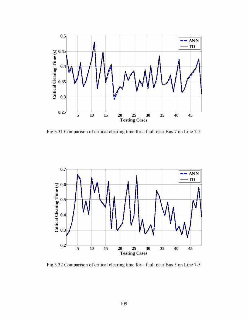
109
5 10 15 20 25 30 35 40 450.25
0.3
0.35
0.4
0.45
0.5
Testing Cases
Cri
tica
l Cle
arin
g T
ime
(s)
ANNTD
Fig.3.31 Comparison of critical clearing time for a fault near Bus 7 on Line 7-5
5 10 15 20 25 30 35 40 450.2
0.3
0.4
0.5
0.6
0.7
Testing Cases
Cri
tica
l Cle
arin
g T
ime
(s)
ANNTD
Fig.3.32 Comparison of critical clearing time for a fault near Bus 5 on Line 7-5

110
5 10 15 20 25 30 35 40 450.2
0.3
0.4
0.5
0.6
0.7
Testing Cases
Cri
tica
l Cle
arin
g T
ime
(s)
ANNTD
Fig.3.33 Comparison of critical clearing time for a fault near Bus 5 on Line 5-4
5 10 15 20 25 30 35 40 450.2
0.3
0.4
0.5
0.6
0.7
Testing Cases
Cri
tica
l Cle
arin
g T
ime
(s)
ANNTD
Fig.3.34 Comparison of critical clearing time for a fault near Bus 6 on Line 6-9

111
3.6.4 Discussion
It is observed that the critical clearing estimated by using neural networks is
very close and in many cases almost exactly equal to the critical clearing times
obtained by time domain simulations. Also, the time taken by the neural network
to estimate the critical clearing time is negligible. It is extremely fast and very
accurate if trained properly. In each of the above testing cases, the maximum error
was less than one cycle time (0.0167s).
From the above results we can conclude that the artificial neural network
provides a promising computationally efficient and reasonably accurate method to
estimate the critical clearing time for a given input to the neural net.
3.7 Conclusions
1. The idea of converting the multidimensional dynamic equations into a single
machine dynamic equation by decomposition of the machines into critical and
non-critical sets and then further reducing the two sets to a OMIB system is
supportive to elimination of the vast number of calculations required to solve
the dynamic equations in a multimachine system.
2. In a real-time operations scenario, qualitative information would be more
important rather than quantitative information i.e., it would be more vital to
know if the system is stable or not rather than knowing the values of the rotor
angles or other state variables. Provided the critical and non-critical clusters
are formed correctly, the SIME method is not only accurate and fast, but the

112
consistency shown as evident in the results makes it suitable for real-time
dynamic security assessment. The rotor angle plots obtained from running the
entire time domain simulation showed that the results of the single machine
equivalent method were consistent in all cases and we could accurately know
if a particular fault would cause system transient instability or not.
3. Another great qualitative advantage of the single machine equivalent method
is that it provides knowledge of ‘how far’ the system is from instability or
‘how unstable’ is the system. This was shown in the second part of this
chapter. These margins can be utilized to quickly estimate the critical clearing
time. Conventionally this has been done by running various time domain
simulations, till we ‘lock down’ on the critical clearing time. The single
machine equivalent method avoids this need by providing stable/unstable
margins which are then used along with polynomial interpolation to obtain the
critical clearing time with very high accuracy provided the sample fault
clearing times used to estimate the critical clearing time are in close proximity
to the actual critical clearing time. Operator experience would be a big factor
in determining what these sample fault clearing times are. Hence, the single
machine equivalent method can be used to quickly estimate the critical
clearing time.
4. The above was the main incentive for using the SIME method to generate the
training set data to be fed to the feedforward neural networks that would allow

113
a further saving in computation time as far as estimation of critical clearing
time is concerned. With proper training the feedforward neural networks can
be used for estimation of the critical clearing time. It was seen that with
proper training, the neural network can be used to approximately estimate the
critical clearing time.
5. The application of artificial intelligence to establish the complex mapping
between an operating condition to the critical clearing time for a particular
fault leads to a vast saving in computation time and completely eliminates the
need for any time domain simulations needed to assess the transient stability.
6. The accuracy of the artificial neural network output can be improved by
having different neural nets for different fault locations and it is expected that
the estimate can be made even more accurate by further considering different
sets of loading conditions. This would avoid the need for extrapolation by the
neural network and provide better results.

114

115
CHAPTER FOUR
A HYBRID NEURAL NETWORK-OPTIMIZATION APPROACH FOR
DYNAMIC SECURITY CONSTRAINED OPTIMAL POWER FLOW
The chapter presents the formulation of a hybrid neural network-optimization
scheme to carry out transient stability constrained optimal power flow. The
transient stability constraint ensures that the critical clearing time for the
particular three-phase fault under consideration will be more than the fault
clearing time for the respective fault. The neural network developed in chapter 3
has been used here for the estimation of the critical clearing time, in each iteration
of the optimization process. The results show that accurate estimation of the
critical clearing time using intelligent techniques and their incorporation into
conventional optimization schemes can allow the inclusion of dynamic security
constraints for real-time operations.
4.1 Transient Stability Constraint
In addition to the conventional constraints listed out in Chapter 2, an
additional inequality constraint is needed to ensure the transient stability of the
power system with regards to the respective fault under consideration and its fault
clearing time. The estimated critical clearing time given by the neural networks
can be greater than or less than the actual clearing time. Also in practice, the fault
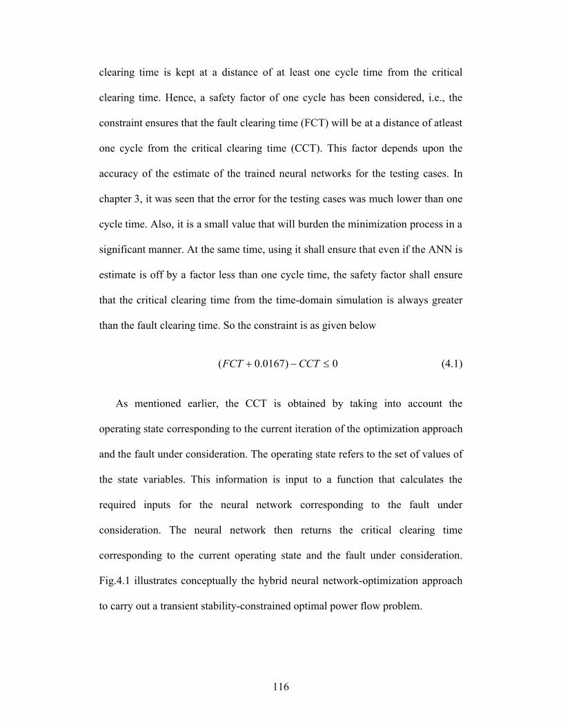
116
clearing time is kept at a distance of at least one cycle time from the critical
clearing time. Hence, a safety factor of one cycle has been considered, i.e., the
constraint ensures that the fault clearing time (FCT) will be at a distance of atleast
one cycle from the critical clearing time (CCT). This factor depends upon the
accuracy of the estimate of the trained neural networks for the testing cases. In
chapter 3, it was seen that the error for the testing cases was much lower than one
cycle time. Also, it is a small value that will burden the minimization process in a
significant manner. At the same time, using it shall ensure that even if the ANN is
estimate is off by a factor less than one cycle time, the safety factor shall ensure
that the critical clearing time from the time-domain simulation is always greater
than the fault clearing time. So the constraint is as given below
0)0167.0( CCTFCT (4.1)
As mentioned earlier, the CCT is obtained by taking into account the
operating state corresponding to the current iteration of the optimization approach
and the fault under consideration. The operating state refers to the set of values of
the state variables. This information is input to a function that calculates the
required inputs for the neural network corresponding to the fault under
consideration. The neural network then returns the critical clearing time
corresponding to the current operating state and the fault under consideration.
Fig.4.1 illustrates conceptually the hybrid neural network-optimization approach
to carry out a transient stability-constrained optimal power flow problem.

117
Fig.4.1 Conceptual illustration of the transient stability constrained optimal power flow formulation
4.2 Results with the IEEE 9-Bus System (Single-Contingency)
This section presents results for the optimization process with the dynamic
constraint included for a single contingency using the 9-Bus system. Five
different fault locations have been considered and the optimization is carried out
with the transient stability constraint for each location taking one at a time. For
each fault location, the optimization is carried out for various loading conditions.
To study the performance of the optimization process under stressed and non-
stressed conditions, the fault clearing time is varied for each loading condition.
For each case the critical clearing time that was estimated by the neural network
for the last iteration of the optimization process has been noted. Also the critical
Evaluation of physical/operating
constraints
Evaluation of Static-security
constraints
NeuralNetwork
FCT – CCT 0
CCT
Current Operating
State
Transient stability constrained optimal power flow
Evaluation of physical/operating
constraints
Evaluation of Static-security
constraints
NeuralNetwork
FCT – CCT 0FCT – CCT 0
CCT
Current Operating
State
Transient stability constrained optimal power flow

118
clearing times from time domain simulations for the corresponding operating
states, obtained after the optimization has converged, have also been listed. Table
5.1 lists the results obtained for including the constraint for a fault near Bus 7 on
Line 5-7. Table 4.2 lists the results obtained for including the constraint for a fault
near Bus 6 on Line 6-9. Table 4.3 lists the results obtained for including the
constraint for a fault near Bus 5 on Line 5-4. Table 4.4 lists the results obtained
for including the constraint for a fault near Bus 5 on Line 5-7. Table 4.5 lists the
results obtained for including the transient stability constraint for a fault near Bus
6 on Line 6-4.
Table.4.1 TSCOPF results with constraint for fault near Bus 7 on Line 5-7
Case Loading FCT ANN TD% CCT CCT
1 120 0.3 0.3167 0.32532 110 0.3 0.3167 0.31743 100 0.3 0.3167 0.31594 90 0.3 0.3167 0.31885 80 0.3 0.3167 0.32556 70 0.3 0.3314 0.34297 120 0.2 0.2167 0.21588 100 0.2 0.2167 0.21479 90 0.2 0.261 0.2688
10 80 0.2 0.2938 0.303811 70 0.2 0.3314 0.343
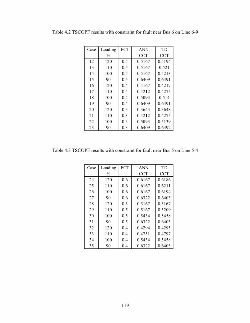
119
Table.4.2 TSCOPF results with constraint for fault near Bus 6 on Line 6-9
Case Loading FCT ANN TD% CCT CCT
12 120 0.5 0.5167 0.519413 110 0.5 0.5167 0.52114 100 0.5 0.5167 0.521315 90 0.5 0.6409 0.649116 120 0.4 0.4167 0.421717 110 0.4 0.4212 0.427518 100 0.4 0.5094 0.51419 90 0.4 0.6409 0.649120 120 0.3 0.3643 0.364821 110 0.3 0.4212 0.427522 100 0.3 0.5093 0.513923 90 0.3 0.6409 0.6492
Table.4.3 TSCOPF results with constraint for fault near Bus 5 on Line 5-4
Case Loading FCT ANN TD% CCT CCT
24 120 0.6 0.6167 0.618625 110 0.6 0.6167 0.621126 100 0.6 0.6167 0.619427 90 0.6 0.6322 0.640328 120 0.5 0.5167 0.516729 110 0.5 0.5167 0.520930 100 0.5 0.5434 0.545831 90 0.5 0.6322 0.640332 120 0.4 0.4294 0.429533 110 0.4 0.4751 0.479734 100 0.4 0.5434 0.545835 90 0.4 0.6322 0.6403

120
Table.4.4 TSCOPF results with constraint for fault near Bus 5 on Line 5-7
Case Loading FCT ANN TD% CCT CCT
36 120 0.6 0.6167 0.613837 110 0.6 0.6167 0.615938 90 0.6 0.6167 0.615639 120 0.5 0.5167 0.513240 110 0.5 0.5167 0.520241 100 0.5 0.5167 0.518842 90 0.5 0.5754 0.574843 120 0.4 0.4725 0.475744 110 0.4 0.5754 0.574945 120 0.3 0.4756 0.472446 90 0.3 0.5755 0.575
4.3 Discussion
It was seen in chapter 3 earlier that the critical clearing estimated by using
neural networks is very close and in many cases almost exactly equal to the
critical clearing times obtained by time domain simulations. Also, the time taken
by the neural network to estimate the critical clearing time is negligible. It is
extremely fast and was therefore, the main incentive in the hybrid neural network-
optimization approach proposed in this chapter. When used along with the
optimization process to carry out the optimal power flow, it is seen in all cases
that the reformulated transient stability constrained optimal power flow was able
to converge to find a solution even under highly stressed conditions
corresponding to very large loading or long fault clearing times. The estimated
critical clearing time can be more than or less than the actual critical clearing
time. Hence it is possible that in the final iteration of optimization, the estimated
critical clearing time is equal to the fault clearing time thereby respecting the

121
constraint, but the critical clearing time from time domain simulations actually
being less than the estimated value. The use of the safety factor of one cycle time
eliminates any such situation. The value of the safety factor is obviously
dependent on the accuracy of the neural network also. As mentioned earlier, the
neural networks were trained well enough to keep the errors for the testing sets to
much below one cycle time. Fig. 4.2 shows the difference between the critical
clearing time from time domain simulations and the fault clearing time (TD CCT
– FCT, blue solid line) and the difference between the critical clearing time from
time domain simulations and the neural network estimate (TD CCT – ANN CCT,
black dotted line) for the various cases listed in Section 4.2. Two key observations
are to be noted. Firstly, the transient stability constrained optimal power flow was
able to converge even under stressed conditions keeping the critical clearing time
from time domain simulations at a distance of atleast once cycle time from the
fault clearing time (SF limit). In some cases this difference was a little less than
one cycle. These are the cases where the neural network estimate is more than the
actual critical clearing time. But the error, as seen in Fig. 4.2 is negligible. So the
neural network was able to accurately estimate the critical clearing time even for
cases that could not have been generated otherwise i.e., without the optimization
process. Fig. 4.3 shows a comparison of the generator active power outputs
obtained by carrying out the optimization without the transient stability constraint
at 120% loading (Base OPF) and those obtained for case 24. It is seen that with
little variation in the active power outputs of the generators, it is also possible to
ensure transient stability for a given fault.

122
5 10 15 20 25 30 35 40
0.0167
0.05
0.1
0.15
0.2
0.25
0.3
0.35
Cases
Tim
e (s
)
TD CCT - FCTTD CCT - ANN CCT
SFLimit
Fig.4.2 Comparison of the critical clearing time with the fault clearing time and the neural network estimate
1 2 30
20
40
60
80
100
120
140
160
Generators
Pg
(MW
)
BOPFTSCOPF
Fig.4.3. Comparison of generator active power outputs

123
4.4 Results with the IEEE 9-Bus System (Multiple-Contingencies)
In a practical system it would be necessary to consider not one but multiple
contingencies with varying fault clearing times. The proposed method makes this
possible in a very simple manner without any additional comparable
computational burden on the already existing optimization process. This is made
possible by including constraints of the type shown in Equation 4.1 for each
contingency to be considered. The appropriate neural network is used for each
fault location. The application of the method is first shown considering two
contingencies at a time. The first of these scenarios considers a fault near Bus 7
on Line 7-5 and near Bus 6 on Line 6-9. Table 4.6 lists the results for various
stressed conditions, either due to loading or high FCTs. The second scenario
considers a fault near Bus 5 on Line 5-7 and near Bus 6 on Line 6-9. A third one
considers a fault near Bus 5 on Line 5-7 and Bus 6 on Line 6-4. Constraints for
three different fault locations with varying fault clearing times and loading
conditions were studied in the final scenario.
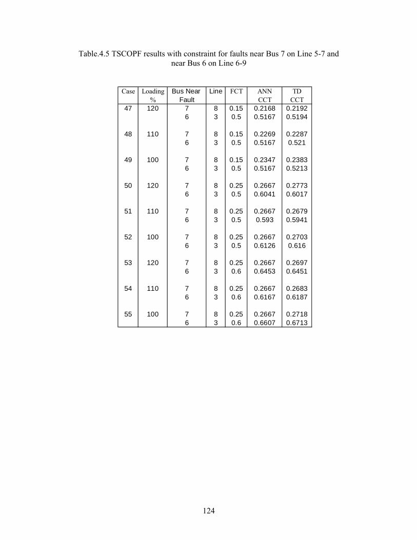
124
Table.4.5 TSCOPF results with constraint for faults near Bus 7 on Line 5-7 and near Bus 6 on Line 6-9
Case Loading Bus Near Line FCT ANN TD% Fault CCT CCT
47 120 7 8 0.15 0.2168 0.21926 3 0.5 0.5167 0.5194
48 110 7 8 0.15 0.2269 0.22876 3 0.5 0.5167 0.521
49 100 7 8 0.15 0.2347 0.23836 3 0.5 0.5167 0.5213
50 120 7 8 0.25 0.2667 0.27736 3 0.5 0.6041 0.6017
51 110 7 8 0.25 0.2667 0.26796 3 0.5 0.593 0.5941
52 100 7 8 0.25 0.2667 0.27036 3 0.5 0.6126 0.616
53 120 7 8 0.25 0.2667 0.26976 3 0.6 0.6453 0.6451
54 110 7 8 0.25 0.2667 0.26836 3 0.6 0.6167 0.6187
55 100 7 8 0.25 0.2667 0.27186 3 0.6 0.6607 0.6713

125
47 48 49 50 51 52 53 54 550
0.0167
0.04
0.06
0.08
0.1
Tim
e (s
)
Cases
TD CCT - FCTTD CCT - ANN CCT
SFLimit
Fig.4.4 Comparison of the critical clearing time with the fault clearing time and the neural network estimate for fault near Bus 7 on Line 5-7
47 48 49 50 51 52 53 54 550
0.0167
0.05
0.1
Tim
e (s
)
Cases
TD CCT - FCTTD CCT - ANN CCT
SFLimit
Fig.4.5 Comparison of the critical clearing time with the fault clearing time and the neural network estimate for fault near Bus 6 on Line 6-4

126
Table.4.6 TSCOPF results with constraint for faults near Bus 7 on Line 5-7 and near Bus 5 on Line 5-4
Case Loading Bus Near Line FCT ANN TD% Fault CCT CCT
56 120 7 8 0.2 0.2167 0.21565 9 0.5 0.5167 0.5172
57 110 7 8 0.2 0.224 0.22285 9 0.5 0.5167 0.5209
58 100 7 8 0.2 0.2167 0.2285 9 0.5 0.5252 0.5257
59 120 7 8 0.2 0.2454 0.24555 9 0.6 0.6167 0.6186
60 110 7 8 0.2 0.2516 0.25275 9 0.6 0.6167 0.6211
61 100 7 8 0.2 0.2532 0.25815 9 0.6 0.6167 0.6194
62 120 7 8 0.25 0.2667 0.26975 9 0.6 0.7127 0.7159
63 110 7 8 0.25 0.2667 0.26795 9 0.6 0.6617 0.6648
64 100 7 8 0.25 0.2667 0.27035 9 0.6 0.6509 0.654

127
56 57 58 59 60 61 62 63 64
0
0.010.0167
0.03
0.04
0.05
0.06T
ime
(s)
Cases
TD CCT - FCTTD CCT - ANN CCT
SFLimit
Fig.4.6 Comparison of the critical clearing time with the fault clearing time and the neural network estimate for fault near Bus 7 on Line 7-8
56 57 58 59 60 61 62 63 640
0.0167
0.04
0.06
0.08
0.1
0.12
Tim
e (s
)
Cases
TD CCT - FCTTD CCT - ANN CCT
SFLimit
Fig.4.7 Comparison of the critical clearing time with the fault clearing time and the neural network estimate for fault near Bus 5 on Line 5-4
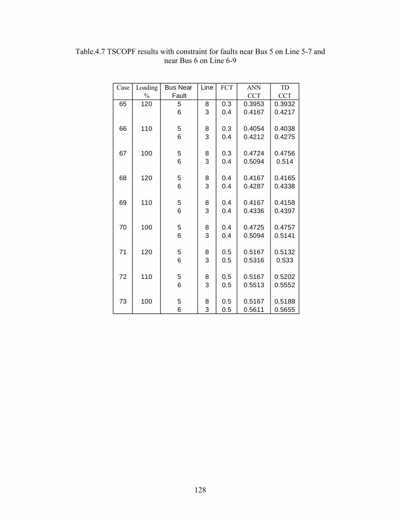
128
Table.4.7 TSCOPF results with constraint for faults near Bus 5 on Line 5-7 and near Bus 6 on Line 6-9
Case Loading Bus Near Line FCT ANN TD% Fault CCT CCT
65 120 5 8 0.3 0.3953 0.39326 3 0.4 0.4167 0.4217
66 110 5 8 0.3 0.4054 0.40386 3 0.4 0.4212 0.4275
67 100 5 8 0.3 0.4724 0.47566 3 0.4 0.5094 0.514
68 120 5 8 0.4 0.4167 0.41656 3 0.4 0.4287 0.4338
69 110 5 8 0.4 0.4167 0.41586 3 0.4 0.4336 0.4397
70 100 5 8 0.4 0.4725 0.47576 3 0.4 0.5094 0.5141
71 120 5 8 0.5 0.5167 0.51326 3 0.5 0.5316 0.533
72 110 5 8 0.5 0.5167 0.52026 3 0.5 0.5513 0.5552
73 100 5 8 0.5 0.5167 0.51886 3 0.5 0.5611 0.5655

129
65 66 67 68 69 70 71 72 730
0.0167
0.05
0.1
0.15T
ime
(s)
Cases
TD CCT - FCTTD CCT - ANN CCT
SFLimit
Fig.4.8 Comparison of the critical clearing time with the fault clearing time and the neural network estimate for fault near Bus 5 on Line 5-7
65 66 67 68 69 70 71 72 730
0.0167
0.04
0.06
0.08
0.1
0.12
Tim
e (s
)
Cases
TD CCT - FCTTD CCT - ANN CCT
SFLimit
Fig.4.9 Comparison of the critical clearing time with the fault clearing time and the neural network estimate for fault near Bus 6 on Line 6-9

130
Table.4.8 TSCOPF results with constraint for faults near Bus 5 on Line 5-7 and near Bus 6 on Line 6-4
Case Loading Bus Near Line FCT ANN TD% Fault CCT CCT
74 120 5 8 0.3 0.3481 0.34666 2 0.4 0.4257 0.4274
75 110 5 8 0.3 0.4054 0.40386 2 0.4 0.4839 0.4856
76 100 5 8 0.3 0.4724 0.47566 2 0.4 0.5646 0.5664
77 120 5 8 0.5 0.5167 0.51326 2 0.5 0.5943 0.5919
78 110 5 8 0.5 0.5167 0.52026 2 0.5 0.609 0.6094
79 100 5 8 0.5 0.5167 0.51886 2 0.5 0.6136 0.6161
80 120 5 8 0.5 0.5167 0.51386 2 0.6 0.6167 0.6153
81 110 5 8 0.5 0.5188 0.52196 2 0.6 0.6167 0.6175
82 100 5 8 0.5 0.5167 0.51856 2 0.6 0.6167 0.6193

131
1 2 3 4 5 6 7 8 90
0.0167
0.05
0.1
0.15
Tim
e (s
)
Cases
TD CCT - FCTTD CCT - ANN CCT
SFLimit
Fig.4.10 Comparison of the critical clearing time with the fault clearing time and the neural network estimate for fault near Bus 5 on Line 5-7
75 76 77 78 79 80 81 82 830
0.0167
0.05
0.1
0.15
Tim
e (s
)
Cases
TD CCT - FCTTD CCT - ANN CCT
SFLimit
Fig.4.11 Comparison of the critical clearing time with the fault clearing time and the neural network estimate for fault near Bus 6 on Line 6-4

132
Table.4.9 TSCOPF results with constraint for faults near Bus 7 on Line 5-7, near Bus 5 on Line 5-9 and near Bus 6 on Line 6-9
Case Loading Bus Near Line FCT ANN TD% Fault CCT CCT
83 120 7 8 0.2 0.2167 0.21585 9 0.3 0.5128 0.51526 3 0.4 0.4383 0.4428
84 110 7 8 0.2 0.2167 0.21475 9 0.3 0.4918 0.49686 3 0.4 0.4353 0.4413
85 100 7 8 0.2 0.2336 0.23695 9 0.3 0.5434 0.54586 3 0.4 0.5094 0.514
86 120 7 8 0.25 0.2667 0.27655 9 0.5 0.7178 0.72186 3 0.5 0.5814 0.5808
87 110 7 8 0.25 0.2667 0.26795 9 0.5 0.6617 0.66486 3 0.5 0.5928 0.5939
88 100 7 8 0.25 0.2667 0.27055 9 0.5 0.6545 0.65766 3 0.5 0.6209 0.625
89 120 7 8 0.25 0.2667 0.26915 9 0.6 0.7181 0.72236 3 0.65 0.6667 0.6714
90 110 7 8 0.25 0.2667 0.26935 9 0.6 0.6898 0.69596 3 0.65 0.6667 0.677
91 100 7 8 0.25 0.2822 0.28685 9 0.6 0.7099 0.71996 3 0.65 0.6667 0.6775

133
83 84 85 86 87 88 89 90 91
0
0.01
0.0167
0.03
0.04
Tim
e (s
)
Cases
TD CCT - FCTTD CCT - ANN CCT
SFLimit
Fig.4.12 Comparison of the critical clearing time with the fault clearing time and the neural network estimate for fault near Bus 7 on Line 7-8
83 84 85 86 87 88 89 90 91 920
0.0167
0.04
0.06
0.08
0.1
0.12
Tim
e (s
)
Cases
TD CCT - FCTTD CCT - ANN CCT
SFLimit
Fig.4.13 Comparison of the critical clearing time with the fault clearing time and the neural network estimate for fault near Bus 5 on Line 5-4

134
83 84 85 86 87 88 89 90 910
0.0167
0.05
0.1
0.15
Tim
e (s
)
Cases
TD CCT - FCTTD CCT - ANN CCT
SFLimit
Fig.4.14 Comparison of the critical clearing time with the fault clearing time and the neural network estimate for fault near Bus 6 on Line 6-9
4.5 Discussion
With multiple contingency constraints, the optimization process was able to
converge, where possible. It is evident from the results from that dynamic limits
cannot be established by offline studies, because the ‘distance from instability’ is
always a function of current operating state which seldom matches conditions
used for offline studies. In Case 47, it is seen that at 120% loading, with the fault
clearing time for the fault near Bus 7 on Line 8 at 0.15s, both the constraints are
binding at the time of convergence. In Case 50 however, with the fault clearing
time for the fault near Bus 7 on Line 8 increased to 0.25s, the second constraints
was not binding for the optimal solution. It would be extremely difficult to arrive
at such solutions manually using offline studies and also very time consuming.
Instead we see the advantage of rapid and accurate mapping of an operating state
not known during training to the dynamic stability index i.e. the critical clearing

135
time and how it can be used to ensure dynamic stability the operating state in
question.
4.6 Conclusions
1. It is seen from the results that the trained neural networks were able to predict
the critical clearing times for the various operating conditions established by
the optimal power flow with very high accuracy.
2. The application of artificial intelligence to establish the complex mapping
between an operating condition to the critical clearing time for a particular
fault leads to a vast saving in computation time and completely eliminates the
need for any time domain simulations needed to assess the transient stability.
3. Coupling the neural networks with the already existing optimization
techniques provides a computationally efficient approach to carry out transient
stability constrained optimal power flow. Only one more state variable i.e., the
critical clearing time and constraint are added for each contingency to be
considered in addition to the already existing state variables and constraints.
So no additional burden is posed on the optimization process. Hence with
small adjustments in the active power output of the generators it is not only
possible to respect the conventional static-security constraints, but also
transient stability constraints that are going to be more vital for deregulated
power system operations.

136
4. The use of a safety factor as small as one cycle time ensures that the actual
critical clearing time is always greater than the fault clearing time provided
the neural networks are well trained. Hence, it is possible to carry out real-
time dispatches for generators respecting both the conventional static-security
constraints and also the more important transient stability constraints.
5. Ensuring dynamic security is very vital for a successful competitive market
that depends upon the reliable and secure operation of the power system. The
method also provides a computationally efficient way to carry out the optimal
power flow with transient stability constraints for multiple contingencies.

137
CHAPTER FIVE
SUMMARY AND CONCLUSIONS
An attempt has been made in this dissertation to enhance the usage of the
optimal power flow tool with security constraints as a means to operate in regions
that would not only be secure with respect to pre-contingency and post-
contingency static security constraints, but also be secure with respect to dynamic
stability of the power system. Ideas have been proposed and implemented for both
analytical and intelligent techniques to obtain generation dispatches that would be
first-swing stable for a certain set of credible contingencies (three-phase faults)
with their respective fault clearing times. In the absence of such tools the
operators are limited to operating in conservative secure operating regions
established using offline studies. With the fast inception of deregulation, the need
to ensure a reliable and secure power system and allocate fair generation
dispatches has become very vital. Large computation times have avoided the use
of dynamic security constraints to ensure dynamic stability, more specifically
transient stability in state-of-the-art optimal power flow methods today, an
indispensable tool for nodal pricing in a competitive market. The major
disadvantages of the conservative solutions and the corrective methods are that
although they may be able to withstand the effect of major disturbances on the
transient stability of the system, they may not be the optimal solution required for
a fair operation of a competitive electricity market. The work in this dissertation is

138
an attempt to enhance the already existing state-of-the-art dispatch methods
within energy managements systems by development of computationally efficient
formulations for the evaluation and inclusion of ‘transient stability’ constraints.
This would allow the transient stability constrained optimal power flow
techniques to be adopted for real-time dispatch methods. It would thus aid in
maintaining a reliable and secure power system by prevention of blackouts and
also in the successful and fair operation of a competitive market.
The analytical technique developed initially is focused on ‘bounding the
solution of the differential equations’ to implement a practical preventive
methodology for transient stability constrained optimal power flow. The
industrially accepted stability/instability indicator was formed using the value of
the rotor angles with respect to a center of inertia frame of reference. Putting a
bound on this value would mean that the generator rotor angles are within close
proximity of each other and not diverging indicating an unstable scenario. This
idea is used to form the transient stability related constraint. The other part of
implementing the transient stability constrained optimal power flow formulation
involved including the solution of the differential equations corresponding to the
values of the state variables for the current iteration of the optimization process.
The current values of the state variables decide the initial conditions for the
differential equations. This was implemented by an external function that actually
calculates the solution of the differential equations using the Taylor series
expansion of differential equations. This external function solves the differential
equations and returns a vector containing the distance of the rotor angle of each

139
generator from the center of inertia angle at 1s. This distance is constrained to be
less than a particular value that is learnt from offline stability studies on the power
system. It was seen that with small adjustments of the state-variables in the
original optimal power flow it is possible to ensure the transient stability of the
system for a particular fault. Although the net cost of supplying this power would
increase considering the increased constraint set, but the dynamic stability of the
system with respect to a certain fault that has been considered in the transient
stability constrained optimal power flow would not be uncertain. This was
confirmed by solving the differential equations with the new generator active
power outputs and looking at the generator rotor plots. Incorporating such
constraints for a set of faults at different locations can ensure transient stability of
the power system for faults occurring at those locations. Hence a set of faults can
be treated simultaneously. Also instead of actually integrating the solution of the
differential equations into the optimal power flow, a functional constraint
externally calculates the distance of the rotor angles from their center of inertia at
1s. This distance is restricted by including the respective constraints in the
optimization process. Some of the issues dealing with computation are reviewed
here. It has also been observed that using previous converged states as starting
points for obtaining new dispatches with additional constraints such as transient
stability constraints considerably reduces the total computation time required.
Also, for further improving the performance of this method, the process for the
solution of the differential equations can be carried out on a machine with a much
powerful processor for a faster and practical application.

140
Following this, a methodology has been proposed for the development of an
intelligent technique that would completely eliminate the need for any time
domain simulations. The main thrust of the idea is to establish an excellent
nonlinear mapping of an operating state to the critical clearing time for a
particular fault. A well established mapping would require a large training set
covering the entire range of the possible values for each state variable. Using
time-domain simulations for each possible operating state to manually obtain the
critical clearing time and form the training set does not seem viable. So the initial
work in this direction focused on a method for quick training of neural networks
for the estimation of critical clearing time for a particular fault corresponding to a
given operating state (i.e. the state variable set of the optimization process). The
SIME method was employed for the quick training of the neural networks.
Provided the critical and non-critical clusters are formed correctly, the SIME
method provides for the early termination of the time domain simulations on
detection of a stable or unstable situation. The consistency evident in the results
makes it suitable for real-time dynamic security assessment also in regulated
systems. The qualitative advantage of the SIME method providing margins to
indicate stable/unstable situations can be utilized to quickly estimate the critical
clearing time. These two advantages makes the SIME were the main reasons of its
selection to train the neural networks. It was seen that with proper training, the
neural network can be used to estimate the critical clearing time with very high
accuracy. The accuracy of the artificial neural network output can be improved by
having different neural nets for different fault locations and it is expected that the
141
estimate can be made even more accurate by further considering different sets of
loading conditions. Also, this completely eliminated the need for any time domain
simulations needed to assess the transient stability.
The neural networks trained above are used further in the next section for the
formulation of a hybrid neural network-optimization scheme to carry out transient
stability constrained optimal power flow. Since, the trained neural networks
estimate the critical clearing time, the transient stability constraint in this
formulation ensures that the critical clearing time for the particular three-phase
fault under consideration will be more than the fault clearing time for the
respective fault. It was seen that with small adjustments in the active power output
of the generators it is not only possible to respect the conventional static-security
constraints, but also transient stability constraints that are going to be more vital
for deregulated power system operations. Also, coupling the neural networks with
the already existing optimization techniques provides a highly computationally
efficient approach to carry out transient stability constrained optimal power flow
of multiple contingencies. Only one more state variable i.e., the critical clearing
time and constraint are added for each contingency to be considered in addition to
the already existing state variables and constraints. So no additional burden is
posed on the already existing state-of-the-art optimization processes that provide
static-security constrained optimal power flows.
Ensuring dynamic security is very vital for a successful competitive market
that depends upon the reliable and secure operation of the power system. An
introductory treatise is presented for an efficient implementation of the transient

142
stability constrained optimal power flow problem. The practical application of
such a real-time scheme based on preventive methodology can enable power
system operators to prevent potential stability problems before they occur and
lead to cascading outages.
The faults studied have been assumed to be 3-phase faults although it is well
known that 3-phase faults are the rarest of the faults and 85% of the faults are
single-line-to-ground faults. The dynamic constrained dispatches obtained were
tested for single-line-to-ground faults in the same locations for which the dynamic
constraint for the three-phase was included. None of the cases studied produced
an unstable scenario. But, it is always possible that the fault could be unstable and
practical scenarios would want to consider including constraints for unbalanced
faults also to make sure it is not a binding constraint for the fault location under
question. Also the faults have been assumed to occur near the bus so that the
analysis for bus faults can be used for reasons of simplicity. But faults are a
random phenomenon and may occur anywhere in the line. So a realistic
application should be able to consider any fault location. Also, since the classical
model was used for the transient stability analysis, this does not represent a
realistic model beyond the first swing time period and the effect of excitation
systems, regulators and governors would need to be included if the second and
subsequent stability scenarios need to be considered while obtaining an optimal
dispatch. All the dispatches obtained in this work, assumed that the fault has been
cleared by opening the line. Inadvertently, that assumes a permanent fault. From a
practical power system operations viewpoint, the effect of reclosing should be

143
taken into account and optimal dispatches should be obtained considering a
permanent fault or temporary fault. Future work can also involve further use of
neural networks to remove other nonlinear constraints from the optimization
process and further decrease the computation time for the optimization process.
The transmission system is the heart of a successful competitive market in a
deregulated environment. Keeping it secure and reliable is the most important task
of the entity handling the transmission operations.

144

145
APPENDICES

146
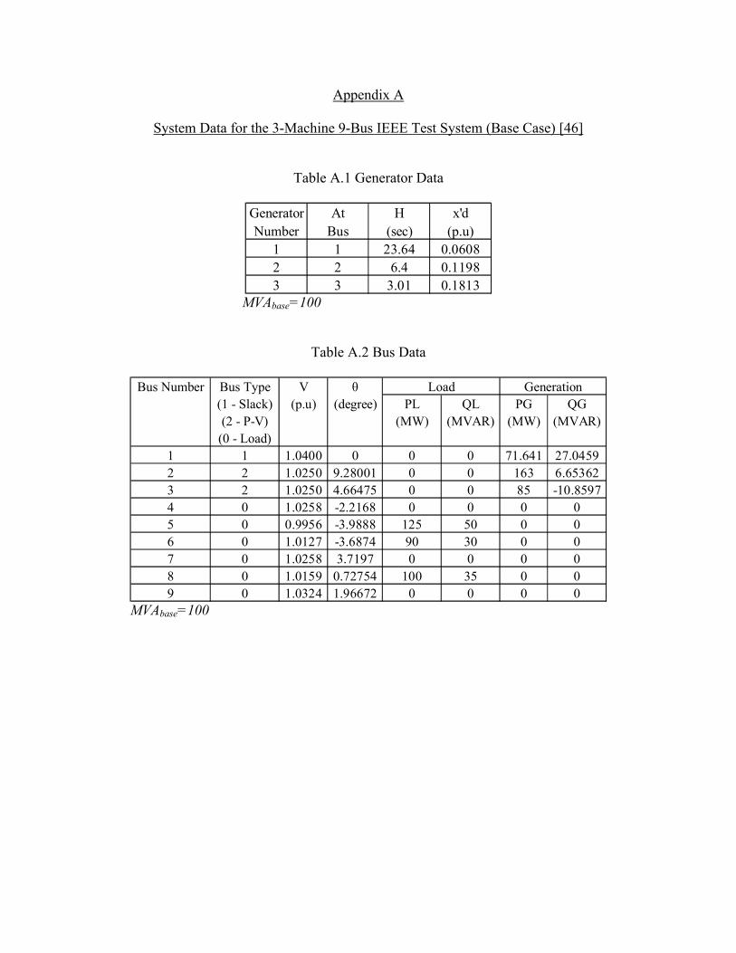
147
Appendix A
System Data for the 3-Machine 9-Bus IEEE Test System (Base Case) [46]
Table A.1 Generator Data
Generator At H x'dNumber Bus (sec) (p.u)
1 1 23.64 0.06082 2 6.4 0.11983 3 3.01 0.1813
MVAbase=100
Table A.2 Bus Data
Bus Number Bus Type V θ(1 - Slack) (p.u) (degree) PL QL PG QG(2 - P-V) (MW) (MVAR) (MW) (MVAR)
(0 - Load)1 1 1.0400 0 0 0 71.641 27.04592 2 1.0250 9.28001 0 0 163 6.653623 2 1.0250 4.66475 0 0 85 -10.85974 0 1.0258 -2.2168 0 0 0 05 0 0.9956 -3.9888 125 50 0 06 0 1.0127 -3.6874 90 30 0 07 0 1.0258 3.7197 0 0 0 08 0 1.0159 0.72754 100 35 0 09 0 1.0324 1.96672 0 0 0 0
Load Generation
MVAbase=100

148
Table A.3 Branch Data
Shunt Branch typeSusceptance (0 - T.L)
From To R X (B/2) (1 - Transf.) Mag Angle(p.u) (p.u) (p.u) (p.u) (degree)
1 4 0 0.0576 0 1 1 04 6 0.017 0.092 0.079 0 0 06 9 0.039 0.17 0.179 0 0 03 9 0 0.0586 0 1 1 08 9 0.0119 0.1008 0.1045 0 0 07 8 0.0085 0.072 0.0745 0 0 07 2 0 0.0625 0 1 1 05 7 0.032 0.161 0.153 0 0 05 4 0.01 0.085 0.088 0 0 0
Impedance TapTransformerBus Series
MVAbase=100

149
Appendix B
System Data for the 10-Machine 39-Bus IEEE Test System (Base Case) [46]
Table B.1 Generator Data
Generator At H x'dNumber Bus (sec) (p.u)
1 30 42 0.0312 31 30.3 0.06973 32 35.8 0.05314 33 38.6 0.04365 34 26 0.1326 35 34.8 0.057 36 26.4 0.0498 37 24.3 0.0579 38 34.5 0.05710 39 500 0.006
MVAbase=100

150
Table B.2 Bus Data
Bus Bus Type V θNumber (1 - Slack) (p.u) (degree) PL QL PG QG
(2 - P-V) (MW) (MVAR) (MW) (MVAR)(0 - Load)
1 0 1.0475 -9.582818 0 0 0 02 0 1.04883 -7.023205 0 0 0 03 0 1.03016 -9.870743 322 2.4 0 04 0 1.00355 -10.66587 500 184 0 05 0 1.0048 -9.477869 0 0 0 06 0 1.00716 -8.775401 0 0 0 07 0 0.99648 -10.9799 233.8 84 0 08 0 0.9955 -11.48621 522 176.6 0 09 0 1.028 -11.31081 0 0 0 0
10 0 1.01683 -6.390371 0 0 0 011 0 1.01233 -7.203946 0 0 0 012 0 0.99978 -7.219655 8.5 88 0 013 0 1.01397 -7.105162 0 0 0 014 0 1.01143 -8.775415 0 0 0 015 0 1.01526 -9.193591 320 153 0 016 0 1.03165 -7.78864 329.4 32.3 0 017 0 1.03349 -8.787632 0 0 0 018 0 1.03091 -9.628719 158 30 0 019 0 1.04979 -3.162591 0 0 0 020 0 0.99084 -4.574777 680 103 0 021 0 1.03128 -5.378162 274 115 0 022 0 1.04898 -0.921697 0 0 0 023 0 1.04322 -1.117214 247.5 84.6 0 024 0 1.03697 -7.668835 308.6 -92.2 0 025 0 1.05741 -5.661638 224 47.2 0 026 0 1.05193 -6.918366 139 17 0 027 0 1.03761 -8.930536 281 75.5 0 028 0 1.05005 -3.406101 206 27.6 0 029 0 1.04989 -0.646634 283.5 26.9 0 030 2 1.0475 -4.603657 0 0 250 103.331 1 0.982 0 9.2 4.6 572.9 170.332 2 0.9831 1.608247 0 0 650 175.933 2 0.9972 2.05504 0 0 632 103.334 2 1.0123 0.615694 0 0 508 164.435 2 1.0493 4.043931 0 0 650 204.836 2 1.059 6.784177 0 0 560 96.937 2 1.0278 1.123671 0 0 540 -4.438 2 1.0265 6.41694 0 0 830 19.439 2 1.03 -11.12007 1104 250 1000 68.5
Load Generation
MVAbase=100

151
Table B.3 Branch Data
Shunt Branch typeSusceptance (0 - T.L)
From To R X (B/2) (1 - Transf.) Mag Angle(p.u) (p.u) (p.u) (p.u) (degree)
1 2 0.0035 0.0411 0.34935 0 0 01 39 0.001 0.025 0.375 0 0 02 3 0.0013 0.0151 0.1286 0 0 02 25 0.007 0.0086 0.073 0 0 03 4 0.0013 0.0213 0.1107 0 0 03 18 0.0011 0.0133 0.1069 0 0 04 5 0.0008 0.0128 0.0671 0 0 04 14 0.0008 0.0129 0.0691 0 0 05 6 0.0002 0.0026 0.0217 0 0 05 8 0.0008 0.0112 0.0738 0 0 06 7 0.0006 0.0092 0.0565 0 0 06 11 0.0007 0.0082 0.06945 0 0 07 8 0.0004 0.0046 0.039 0 0 08 9 0.0023 0.0363 0.1902 0 0 09 39 0.001 0.025 0.6 0 0 0
10 11 0.0004 0.0043 0.03645 0 0 010 13 0.0004 0.0043 0.03645 0 0 013 14 0.0009 0.0101 0.08615 0 0 014 15 0.0018 0.0217 0.183 0 0 015 16 0.0009 0.0094 0.0855 0 0 016 17 0.0007 0.0089 0.0671 0 0 016 19 0.0016 0.0195 0.152 0 0 016 21 0.0008 0.0135 0.1274 0 0 016 24 0.0003 0.0059 0.034 0 0 017 18 0.0007 0.0082 0.06595 0 0 017 27 0.0013 0.0173 0.1608 0 0 021 22 0.0008 0.014 0.12825 0 0 022 23 0.0006 0.0096 0.0923 0 0 023 24 0.0022 0.035 0.1805 0 0 025 26 0.0032 0.0323 0.2565 0 0 026 27 0.0014 0.0147 0.1198 0 0 026 28 0.0043 0.0474 0.3901 0 0 026 29 0.0057 0.0625 0.5145 0 0 0
Bus Series TransformerImpedance Tap
MVAbase=100

152
Table B.4 Branch Data (continued.)
Shunt Branch typeSusceptance (0 - T.L)
From To R X (B/2) (1 - Transf.) Mag Angle(p.u) (p.u) (p.u) (p.u) (degree)
28 29 0.0014 0.0151 0.1245 0 0 012 11 0.0016 0.0435 0 1 1.006 012 13 0.0016 0.0435 0 1 1.006 06 31 0 0.025 0 1 1.07 0
10 32 0 0.02 0 1 1.07 019 33 0.0007 0.0142 0 1 1.07 020 34 0.0009 0.018 0 1 1.009 022 35 0 0.0143 0 1 1.025 023 36 0.0005 0.0272 0 1 1 025 37 0.0006 0.0232 0 1 1.025 02 30 0 0.0181 0 1 1.025 0
29 38 0.0008 0.0156 0 1 1.025 019 20 0.0007 0.0138 0 1 1.06 0
Bus Series TransformerImpedance Tap
MVAbase=100

153
REFERENCES
[1] August 14, 2003 Blackout Investigation [Online]. Available: http://www.nerc.com/~f ilez/blackout.html.
[2] “Promoting Wholesale Competition Through Open Access Non-Discriminatory Transmission Services by Public Utilities; Recovery of Stranded Costs by Public Utilites and Transmitting Utilities,” Docket Nos. RM95-8-000 and RM-7-001, Order No. 888, April 24, 1996
[3] "Open Access Same-Time Information System (formerly Real-time Information Networks) and Standards of Conduct," Docket No. RM95-9-000, Order No. 889, April 24, 1996.
[4] L. L. Lai, “Power System Restructuring and Deregulation,” 1st ed., John Wiley & Sons, 2001.
[5] P.M Anderson, A. A. Fouad, “Power System Control and Stability,” 2nd ed., Wiley-IEEE Press, 2002.
[6] R. Schainker, P. Miller, W. Dubbelday, P. Hirsh, G. Zhang, “Real time dynamic security assessment: fast simulation and modeling applied to emergency outage security of the electric grid,” in IEEE Power and Energy magazine, vol. 4, pp.51-58, March-April 2006.
[8] J. A. Imhof, et al, “Out of step relaying for generators working group report,” IEEE Trans. on Power Apparatus and Systems, vol. 96(5), pp. 1556-1564, Sept 1977.
[9] C. W. Taylor, R. L. Cresap, J. M. Haner, L. A. Hill, W. A. Mittelstadt, “A new out-of-step relay with rate of change of apparent resistance augmentation,” IEEE Trans. on Power Apparatus and Systems, vol. 102(3), pp. 631-639, Mar. 1983.
[10] P. Kundur, “Power system stability and control,” 1st. ed., McGraw-Hill Professional, Jan. 1994.
[11] S. C. Tripathy, R. Balasubramaniam, S. Balasubramaniam, “Semi-implicity Runge-kutta methods for power system transient stability studies,” Electric Power System Research, vol. 10(4), pp. 253-259, Oct. 1988.
[12] M. A. Pai, P. W. Sauer, F. Dobraca, “A new trajectory approximation technique for transient stability studies,” International Journal of Electrical Power and Energy Systems, vol. 13(5), pp. 249-254, Feb. 1991

154
[13] A. A. Fouad, V. Vittal, “The transient energy function method,” International Journal of Electric Power and Energy Systems, vol. 10(4), pp. 233-246, May 1988.
[14] A. A. Fouad, V. Vittal, “Power system transient stability analysis using the transient energy function method,” 1st ed., Prentice Hall PTR, Dec. 1996.
[15] M. A. Pai, “Energy function analysis for power system stability,” 1st ed., Springer, Aug. 1989.
[16] S. Iwamoto, S. Furuya, H. Suzuki, “Fast transient stability solution approach combining taylor series expansion and transient energy function,” in Proc. 1987 International Federation of Automatic Control. World Congress, vol. 2, pp. 13-18, July 1987.
[17] M. J. Laufenberg, M. A. Pai, “Sensitivity theory in power systems: application in dynamic security analysis,” in Proc. 1996 IEEE InternationalConference on Control Applications, pp. 738-743, Sept 1996.
[18] F. Da-zhong, T. S. Chung, “Dynamic single machine equivalent techniques for on-line transient stabilty assessment,” Electric Power Systems Research, vol. 39, pp. 179-186, Dec. 1996.
[19] J. A. Momoh, R. J. Koessler, M. S. Bond, B. Stott, D. Sun, A. Papalexopoulos, P. Ristanovic, “Challenges to optimal power flow,” IEEE Trans. Power Systems, vol. 12, pp. 444-455, Feb. 1997.
[20] G. C. Ejebe, C. Jing, J. G. Waight, V. Vittal, G. Pieper, F. Jamshidian, P. Hirsh, D. Sobajic, “Online dynamic security assessment in an EMS,” in IEEE Computer Applications in Power, vol. 11, pp. 43-47, Jan. 1998.
[21] D. Chattopadhyay, D. Gan , “Dispatch optimization incorporating transient and voltage stability constraints,” in Proc. 2000 IEEE Power Engineering Society Summer Meeting, pp. 516-521.
[22] D. Gan, D. Chattopadhyay, X. Luo, “Stability constrained OPF: new results,” in Proc. 2003 Southeastern Symposium on System Theory, pp.273-277.
[23] S. N. Singh, A. K. David, “Dynamic security in open power market dispatch,” Electrical Power Components and Systems, vol. 30, pp. 315-330, Mar. 2002.
[24] V. Vittal, J. L. Gleason, “Determination of transient stability constrained line flow limits: an application of linearized techniques for the transient energy function method,” in Proc. 1989 Twenty-First Annual North American Power Symposium, pp.142-150.

155
[25] S. Bruno, E. D. Tuglie, M. L. Scala, “Transient security dispatch for the concurrent optimization of plural postulated contingencies,” IEEE Trans. Power Systems, vol. 17, pp. 707-713, Aug. 2002.
[26] L. Chen, A. Ono, Y. Tada, H. Okamoto, R. Tanabe, “Optimal power flow constrained by transient stability,” in Proc. 2000 International Conference on Power System Technology, pp. 1-6.
[27] Y. Yuan, J. Kubokawa, H. Sasaki, “A solution of optimal power flow with multicontingency transient stability constraints,” IEEE Trans. Power Systems, vol. 18, pp. 1094-1102, Aug. 2003.
[28] Y. Xia, K. W. Chan, M. Liu, “Direct nonlinear primal-dual interior-point method for transient stability constrained optimal power flow,” IEE Proc. Generation, Transmission and Distribution, vol. 152, pp. 11-16, Jan. 2005.
[29] R. Li, L. Chen, R. Yokoyama, “Stability constrained optimal power flow by inexact Newton method,” in Proc. 2001 IEEE Porto Power Tech Conference, vol. 2, pp. 549-557.
[30] Y. Sun, Y. Xinlin, H. F. Wang, “Approach for optimal power flow with transient stability constraints,” IEE Proc. Generation, Transmission and Distribution, vol. 151, pp. 8-18, Jan. 2004.
[31] L. Y. C. Amarasinghe, B. Jayasekara, U. D. Annakkage , “The effect of dynamic security constraints on the locational marginal price,” in Proc. 2005 IEEE Power Engineering Society General Meeting, pp. 1556-1561
[32] D. Ruiz-Vega, M. Pavella , “A comprehensive approach to transient stability control: Part I-Near Optimal Preventive Control,” IEEE Trans. Power Systems, vol. 18(4), pp. 1446-1453, Nov. 2003.
[33] D. Ruiz-Vega, M. Pavella , “A comprehensive approach to transient stability control: Part II-Open Loop Emergency Control,” IEEE Trans. Power Systems, vol. 18(4), pp. 1454-1460, Nov. 2003.
[34] C. Y. Chung, L. Wang, F. Howell, P. Kundur, “Generation rescheduling methods to improve power transfer capability constrained by small-signal stability,” IEEE Trans. Power Systems, vol. 19(4), pp. 524-530, Feb. 2004.
[35] T. Nguyen, M. A. Pai, “Dynamic security-constrained rescheduling of power Systems using trajectory sensitivities,” IEEE Trans. Power Systems, vol. 18(2), pp. 848-854, May 2003.

156
[36] D. Gan, D. Chattopadhyay, X. Luo, “An improved method for optimal operation under stability constraints,” in Proc. 2003 IEEE Transmission and Distribution Conference and Exposition, vol. 2, pp. 683-688, Sept. 2003.
[37] D. Layden, B. Jeyasurya, “Integrating security constraints in optimal power flow studies,” in Proc. 2004 IEEE Power Engineering Society General Meeting, vol. 1, pp. 125-129, June. 2004.
[38] B. Jayasekara, U. D. Annakkage, “Determination of the transient stability boundary,” in Proc. 2004 IEEE Power Engineering Society General Meeting, vol. 2, pp. 1590-1594, June. 2004.
[39] W. Rosehart, “Optimal power flows incorporating network stability,” in Proc. 2002 IEEE Power Engineering Society Winter Meeting, vol. 2, pp. 1100-1104, Jan. 2002.
[40] J. E. Condren, T. W. Gedra, “Eigenvalue and Eigenvector sensitivities applied to power system steady-state operating point,” in Proc. 2002 45th Midwest Symposium on Circuits and Systems, vol. 1, pp. 683-686, Aug. 2002.
[41] M. L. Scala, M. Trovato, C. Antonelli, “On-line dynamic preventive control: An algorithm for transient security dispatch,” IEEE Trans. Power Systems, vol. 13(2), pp. 601-610, May 1998.
[42] The Mathworks Optimization Toolbox [Online]. Available: http://www.mathworks.com/products/optimization
[43] M. H. Haque, A. H. M. A. Rahim, “An efficient method of identifying coherent generators using taylor series expansion,” IEEE Trans. Power Systems, vol. 3, pp. 1112-1118, Aug. 1988.
[44] M. H. Haque, A. H. M. A. Rahim, “Determination of first swing stability limit of multimachine power systems through Taylor series expansions,” IEE Proc. Part. C, vol. 136, pp. 373-379, Nov. 1989.
[45] M. H. Haque, A. H. M. A. Rahim, A. M. Al-Shehri, “Rapid computation of critical clearing time through energy function and taylor series expansion,” in Proc. 1989 Middle East Power System Conference, pp. 267-271.
[46] R.D. Zimmerman, Carlos E. Murillo-Sanchez, D. Gan, MATPOWER- A MATLAB based Power System Simulation Package [Online]. Available: http://www.pserc.cornell.edu/matpower/
[47] P. M. Anderson, A. A. Fouad, “Power system control and stability,” 2nd
edition, Wiley-IEEE Press, 2002.

157
[48] Y. Xue, V. Custern, T. Ribbens, M. Pavella, “A simple direct method for fast transient stability assessment of large power systems,” IEEE Trans. on Power Systems, vol. 3(2), pp. 400-412, May 1988.
[49] Y. Xue, V. Custern, T. Ribbens, M. Pavella, “Extended equal area criterion justificiations, generalizations and applications,” IEEE Trans. on Power Systems, vol. 4(1), pp. 44-52, Feb. 1989.
[50] Y. Xue, M. Pavella, “Extended equal-area criterion: An analytical ultra-fast method for transient stability assessment and preventive control of power systems,” International Journal of Electric Power and Energy Systems, vol. 11(2), pp. 131, 1989.
[51] Y. Xue, L. Wehenkel, R. Belhomme, P. Rousseaux, M. Pavella, E. Euxibie, B. Heilbronn, J. F. Lesigne, “Extended equal area criterion revisited [EHV power systems],” IEEE Trans. on Power Systems, vol. 7(3), pp. 1012-1022, Aug. 1992.
[52] Y. Xue, P. Rousseaux, Z. Gao, R. Belhomme, E. Euxible, B. Heilbronn, “Dynamic extended equal area criterion,” in Proc. 1993 Athens Power Tech-Joint International Power Conference, vol. (2), pp.889-895, Sept. 1993
[53] M. Pavella, D. Ernst, D. Ruiz-Vega, “Transient stability of power systems: A Unified approach to assessment and control,” 1st ed., Springer, Oct. 2000.
[54] M. Pavella, P. G. Murthy, “Transient stability of power systems: Theory and Practice,” John Wiley and Sons, Aug. 1994.
[55]. V. Brandwajin, A.B. R. Kumar, A. Ipakchi, A. Bose, S. D. Kuo, “Severity indices for contingency screening in dynamic security assessment,” IEEE Trans. on Power Systems, vol. 12(3), pp. 1136-1142, Aug. 1997.
[56] A. R. Edwards, K. W. Chan, R. W. Dunn, A. R. Daniels, “Transient stability screening using artificial neural networks within a dynamic security assessment system,” IEE Proc. Generation, Transmission and Distribution, vol. 143(2), pp. 129-134, Mar. 1996.
[57] Y. Mansour, E. Vaahedi, M. A. El-Sharkawi, “Large scale dynamic security screening and ranking using artificial neural networks,” IEEE Trans. on Power Systems, vol. 4(1), pp. 220-228, Feb. 1989
[58] K. Omata, K. Tanomura, “Transient stability evaluation using an artificial neural network,” in Proc. 1993 Second International Forum on Applications of Neural Networks on Power Systems, pp. 130-135, April 1993.

158
[59] A. D. Angel, M. Gavic, L. Wehenkel, “Using artificial neural networks to estimate rotor angles and speeds from phasor measurements,” in Proc. 2003 Intelligent Systems Applications to Power Systems, 2003.
[60] M. Moghavvemi, S. S. Yang, “ANN Application Techniques for Power System Stability Estimation,” Electric Machines and Power Systems, vol. 28(2), pp. 167-178, Feb. 2000.
[61] A. Sittithumwat, K. Tomsovic, “Dynamic security margin estimation using artificial neural networks,” in Proc. 2002 IEEE Power Engineering Society Summer Meeting, vol. 3, pp. 1322-1327, 2002.
[62] S. P. Teeuwsen, I. Erlich, M. A. El-Sharkawi, “Small-signal stability assessment based on advanced neural network methods,” in Proc. 2003 IEEE Power Engineering Society General Meeting, vol. 4, pp. 2534-2537, July 2003.
[63 P. Yan, A. Sekar, P. K. Rajan, “Pattern recognition techniques applied to the classification of swing curves generated in a power system transient stability study,” in Proc. 2000 IEEE Southeastcon, pp. 493-496, April 2000.
[64] A. Jain, R. Balasubramaniam, S. C. Tripathy, B. N. Singh, Y. Kawazoe, “Power system topological observability analysis using artificial neural networks,” in Proc. 2005 IEEE Power Engineering Society General Meeting, vol. 1, pp. 497-502, June 2005.
[65] Y. Y. Hsu, C. R Chen, C. C. Su, “Analysis of electromechanical modes using an artificial neural network,” IEE Proc. Generation, Transmission and Distribution, vol. 141, pp. 198-204, May 1994.
[66] W. Liu, K. Wang, M. Tang, “Study on power system load forecasting based on MPSO artificial neural networks,” in Proc. 2006 The Sixth World Congress on Intelligent Control and Automation, vol. 1, pp. 2728-2732, June 2006.
[67] D. B. Thukaram, K. H. Kashyap, “Artificial neural network application to power system voltage stability improvement,” in Proc. TENCON 2003 Conference on Convergent Technologies, vol. 1, pp. 53-57, Oct. 2003.
[68] D. Nosovel, R. L. King, “Using artificial neural networks for load shedding to alleviate overloaded lines,” IEEE Trans. Power Delivery, vol. 9(1), p. 425-433, Jan. 1994.
[69] H. Mori, Y. Tamaru, S. Tsuzuki, “An artificial neural-net based technique for power system dynamic stability with the Kohonen model,” in Proc. 1991 Power Industry Computer Application Conference, pp. 293-301, May 1991.

159
[70] K. P. Wong, “Computational intelligence applications in unit commitment, economic dispatch and load flow,” in Proc. 1997 Fourth International Conference on Advances in Power System Control, Operation and Management, vol. 1, pp. 54-59, Nov. 1997.