Thinking Dynamically About Biological Mechanisms: Networks of Coupled Oscillators

William Bechtel

Department of Philosophy and Center for Chronobiology University of California, San Diego

Adele A. Abrahamsen

Center for Research in Language University of California, San Diego

Abstract

Explaining the complex dynamics exhibited in many biological mechanisms requires extending the recent philosophical treatment of mechanisms that emphasizes sequences of operations. To understand how nonsequentially organized mechanisms will behave, scientists often advance what we call dynamic mechanistic explanations. These begin with a decomposition of the mechanism into component parts and operations, using a variety of laboratory-based strategies. Crucially, the mechanism is then recomposed by means of computational models in which variables or terms in differential equations correspond to properties of its parts and operations. We provide two illustrations drawn from research on circadian rhythms. Once biologists identified some of the components of the molecular mechanism thought to be responsible for circadian rhythms, computational models were used to determine whether the proposed mechanisms could generate sustained oscillations. Modeling has become even more important as researchers have recognized that the oscillations generated in individual neurons are synchronized within networks; we describe models being employed to assess how different possible network architectures could produce the observed synchronized activity.

Although the construction of mechanistic accounts to explain phenomena has been the dominant research strategy in biology since the 19th century, philosophy of science has only recently started to catch up by examining the character of mechanistic explanation (Bechtel & Richardson, 1993/2010; Bechtel & Abrahamsen, 2005; Machamer, Darden, & Craver, 2000; Thagard, 2003; Wimsatt, 1976). This new mechanistic philosophy of science has emphasized the same explanatory endeavor that most biologists themselves emphasize: the decomposition of the system responsible for a given phenomenon into component parts and operations. Identifying components – treating the responsible system as a mechanism to be taken apart – is quintessentially reductionistic. In both biology and philosophy of science there has been much less attention to the converse endeavor: the recomposition of the mechanism. The components will not produce the phenomenon unless they are put back together properly; that is, they must be organized so as to produce the phenomenon of interest. Even as staunch a reductionist as E. O. Wilson has urged attention to recomposition:

The greatest challenge today, not just in cell biology and ecology but in all of science, is the accurate and complete description of complex systems. Scientists have broken down many kinds of systems. They think they know most of the elements and forces. The next task is to reassemble them, at least in mathematical models that capture the key properties of the entire ensembles (Wilson, 1998, p. 85).

Recomposition – reassembly of the components – means figuring out the spatial organization of the parts and the temporal organization of the operations in the system producing the phenomenon targeted for explanation. This is more difficult, and tends to begin later, than decomposition of the system, but is essential for achieving a complete mechanistic explanation. Through most of the history of biology, such work has been guided by rather limited, though tractable, conceptions of organization: spatial adjacency and connectedness (for parts) and stepwise temporal sequencing (for operations). Those developing the new mechanistic philosophy of science have incorporated this preference for the simplicity of sequential thinking. One influential account (Machamer, Darden, & Craver, 2000) portrayed mechanisms as “productive of regular changes from start or set-up conditions to finish or termination conditions.”1 As they point out, the simplest sequential accounts guided by this conceptualization in science often have been useful, at least as idealizations, but not uncommonly more complex organizational schemes are required. A classic example is the Krebs cycle in oxidative metabolism: after years of struggle to compose an adequate sequential account, closing the sequence into a loop was the key innovation leading to success. Even these accounts, though, lack attention to dynamics in real time. In recent years biologists have increasingly incorporated a concern with dynamics into their mechanistic accounts of various living systems. The simplest possible assumption regarding the dynamics of a mechanism is that it will operate at a constant or steady rate once the start or set-up conditions are met and continue at that rate until the finish or termination conditions are achieved. But many biological mechanisms exhibit oscillations or more complex dynamical behavior, and this can be crucial for orchestrating operations within the mechanism. Such complex dynamical behavior is possible when the organization is non-sequential, at least some of the interactions in the mechanism are nonlinear, and the system is open to energy. When complex dynamics are not present, or are present but not addressed, simple stepwise sequences of operations can be specified on paper or even in the researcher’s head. Achieving an account of complex dynamics such as oscillations, though, requires the tools of computational (mathematical) modeling. A typical dynamical model consists of a set of differential equations that indicate how the values of certain variables change over time relative to parameters (constants for which appropriate values must be estimated) and other variables. Of particular interest here are those dynamical models for which key variables, and terms in the equations

1 One of the first philosophical characterizations of a mechanism was due to Bechtel and Richardson (1993/2010): “A machine is a composite of interrelated parts, each performing its own functions, that are combined in such a way that each contributes to producing a behavior of the system. A mechanistic explanation identifies these parts and their organization, showing how the behavior of the machine is a consequence of the parts and their organization.” This account did not impose sequential organization and indeed one of the objectives of the analysis was to trace the process by which scientists moved from early accounts which focused on only one component (we called such accounts simple or direct localizations) or a sequence of operations performed by different parts (complex localizations) to accounts that identified cycles and other complex arrangements of parts that we termed integrated systems. But we did not address the complex temporal behavior of such systems in that book.

correspond to selected properties of the parts and operations of the target mechanism. The tools of dynamical systems theory can elucidate such models, and often are explicitly called upon. Bechtel and Abrahamsen (2010, 2011) have characterized the endeavor of integrating mechanistic decomposition of a system into its parts and operations and computational modeling of its real-time dynamics as dynamic mechanistic explanation. We illustrate the project of dynamic mechanistic explanation by discussing how computational models have been used to explore the dynamics of the mechanisms responsible for circadian rhythms. Research aimed at decomposition has, over the past two decades, elucidated many of the parts and operations in the molecular mechanisms that are responsible for circadian oscillations in organisms ranging from bacteria to mammals. Recomposition has kept pace, because these molecular mechanisms utilize an already well-known cyclic organizational scheme (gene expressed as a protein with negative feedback inhibiting further expression). This scheme enables, but does not guarantee, oscillatory behavior. Assessing the dynamics of networks requires that computational modeling be carried out alongside mechanistic modeling. In particular, the finding in mammals that individual neurons vary significantly in periodicity when dispersed in culture has made it important to address the question of how biological oscillators such as neurons synchronize their behavior and how this is affected by the their organization. 1. From Reactive to Endogenously Active Mechanisms The initial metaphor giving rise to mechanistic accounts of living systems is that they bear some resemblance to machines designed by humans. Many machines are set up to begin working when appropriate conditions are met, carry out a fixed sequence of steps, and then stop. Such machines are reactive: they react to the onset of their start or set-up conditions and continue until they reach the finish or termination condition. Scientists using the machine metaphor have therefore tended to conceptualize biological systems in this way. Thus, gene expression is characterized as beginning when a specialized molecule “unzips” the helical structure of the relevant segment of DNA and continuing through transcription and then translation until synthesis of the relevant protein has been achieved. Glycolysis is described as a sequence of reactions that begins when glucose is present and terminates in the production of pyruvic acid. Visual processing in the brain is conceived as beginning with the presentation of a visual stimulus and continuing through numerous steps until an object is recognized and localized in space. We will argue that this reactive conception is inadequate to account for the behavior of numerous biological mechanisms. The first step away from a reactive conception of mechanisms is to advance beyond purely sequential organization. The first non-sequential design principle to be discovered was negative feedback. Tellingly, two thousand years intervened between its first introduction by Ktesbios in his design for a water clock and the cyberneticists’ recognition in the 1940s that negative feedback is a general organizational principle for living and social systems (see Mayr, 1970). Humans, even scientists, find it difficult or inconvenient to stretch their thinking beyond sequential organization. Even the cyberneticists, moreover, treated negative feedback primarily as a way of maintaining a system in a steady state—a means of achieving what Claude Bernard (1865) referred to as the constancy of the organism’s “internal environment.” Walter Cannon (1929) coined the term homeostasis for this phenomenon and explored ways in which the

autonomic nervous system served to maintain homeostasis. A common, but misleading, way of characterizing homeostasis is that it involves maintaining a state in which the organism is in equilibrium with its environment. This is misleading in that the most fundamental type of equilibrium with an environment – thermodynamic equilibrium – entails the death of the organism. As highly organized systems, organisms are far from thermodynamic equilibrium with their environments, and to perpetuate their identity as organisms they must maintain the non-equilibrium relation. This in turn necessitates that they recruit matter and energy from their environment and deploy these resources to build and repair themselves. Energy and matter can be procured either from non-biological sources (sunlight in the case of photosynthesis) or from foodstuffs provided by other organisms and then utilized in energy demanding activities such as synthesizing and repairing the organism’s own body, locomotion, and transporting substances through physiological systems. Recognizing that maintaining a relation of non-equilibrium with the environment rather than one of equilibrium has fostered an alternative perspective in which organisms are understood as autonomous systems. Ruiz-Mirazo and Moreno characterize an autonomous system as:

a far-from-equilibrium system that constitutes and maintains itself establishing an organizational identity of its own, a functionally integrated (homeostatic and active) unit based on a set of endergonic-exergonic couplings between internal self-constructing processes, as well as with other processes of interaction with its environment (Ruiz-Mirazo, Peretó, & Moreno, 2004).

Since the processes that would serve to bring an organism back into thermodynamic equilibrium with its environment are relentless, every organism needs to be endogenously active – regularly performing the activities that keep it in the appropriate non-equilibrium relation with its environment. The result is that mechanisms in living systems, rather than needing to have their actions initiated, tend to be designed so that by default they are performing operations. One of the simplest forms of dynamical behavior that exhibits sustained activity is oscillation: the values of variables characterizing the behavior of the system repeatedly rise and fall rather than remain constant. Delayed negative feedback in a system driven by an energy source can readily produce such oscillations. For example, adding a thermostat to a heating system turns the furnace off whenever the target temperature is achieved and back on when it drops below the target. Given the inevitable time delay between the thermostat and furnace, room temperature oscillates rather than being maintained at exactly the target value: the temperature gradually rises while the furnace is on and then declines while the furnace is off. Often, as in this example, oscillations are viewed as nuisances and the goal for engineers is to minimize or dampen them as much as possible. When data collected from biological systems reveal oscillations, the oscillations are frequently regarded by investigators as noise to be removed by statistical techniques; what remains is regarded as the signal to be analyzed. But such oscillations are a resource that can be used by the system in generating important biological phenomena. It is then a mistake to treat them as noise; oscillations that are exploited by the system are, rather, an important part of the signal.

Circadian rhythms are one important class of biological oscillations; by definition, they include any biological rhythm for which the period (one rise and fall) is approximately 24 hours.2 These endogenously maintained oscillations affect a wide range of physiological and behavioral processes in virtually all life forms on our planet in which they have been sought. They have been identified and investigated, for example, in cyanobacteria (Synechococcus elongatus), fungi (Neurospora), plants (Mimosa, Arabidopsis), and animals (Drosophila, Mus). The rhythms, in processes ranging from gene expression to sleep, are shown to be endogenous by removing all cues to time of day (Zeitgebers) and determining that the rhythms nonetheless are maintained with only a small discrepancy from 24 hours. Beyond endogenous maintenance of rhythms, two further features that are considered fundamental are the ability to be entrained by Zeitgebers (e.g., light or temperature) and temperature compensation (so that circadian oscillators, unlike most biological processes, do not speed up as temperature rises). In industrialized human society these rhythms tend to be either ignored or regarded as a nuisance; for example, they make life more difficult for shift workers and travelers who cross multiple time zones. Even biological researchers tend not to take into account regular, well-described variations with time of day in a host of basic physiological and behavioral processes. For example, body temperature oscillates over a range of 1°C. daily and reaction times are measurably faster in the afternoon, but time of day at which a measurement was made usually is ignored and these periodic variations therefore treated as part of the error variance (noise) in data analysis. Yet many of these rhythms play crucial roles. One is to coordinate essential behaviors with daily and annual changes in the environment (e.g., fruit flies must eclose from their pupae in the morning when temperatures are lower and humidity is higher, and many rodent species move about mainly at night while their predators sleep). Certain activities require several hours of preparation, necessitating some means of anticipating the time at which they must be performed. Another essential role is to segregate in time activities that are incompatible with each other (e.g., nitrogen fixation and photosynthesis in cyanobacteria, since the critical enzyme for nitrogen fixation is destroyed by the oxygen generated by photosynthesis). In this section we have argued that in living organisms researchers confront active, not reactive, systems that maintain themselves in a non-equilibrium condition. These systems exhibit non-sequential organization, such as negative and positive feedback loops, and non-linear interactions between components, all of which contribute to oscillatory behavior and other complex dynamics. Accordingly, the focus on mechanistic explanation in philosophy of biology must be extended to include a conception of dynamical mechanistic explanation. In inquiring into this type of explanation, we will take advantage of the fact that it has been well-developed in biological research on circadian rhythms. . 2. Complex Dynamics: Oscillatory Mechanisms

2Although we will focus on circadian rhythms, oscillatory processes with both shorter and longer periods are ubiquitous in the biological world. Oscillations with periods of less than 20 hours are termed ultradian, and include oscillations in basic metabolic processes (e.g., glycolytic oscillations), cardiac rhythms, neuronal spiking, the cell division cycle, and sleep cycle. Oscillations with periods longer than 28 hours are termed infradian and include menstrual cycles and hibernation cycles. Whether and how oscillations of different periods either share a common mechanism or affect each other is a topic of significant ongoing investigation.

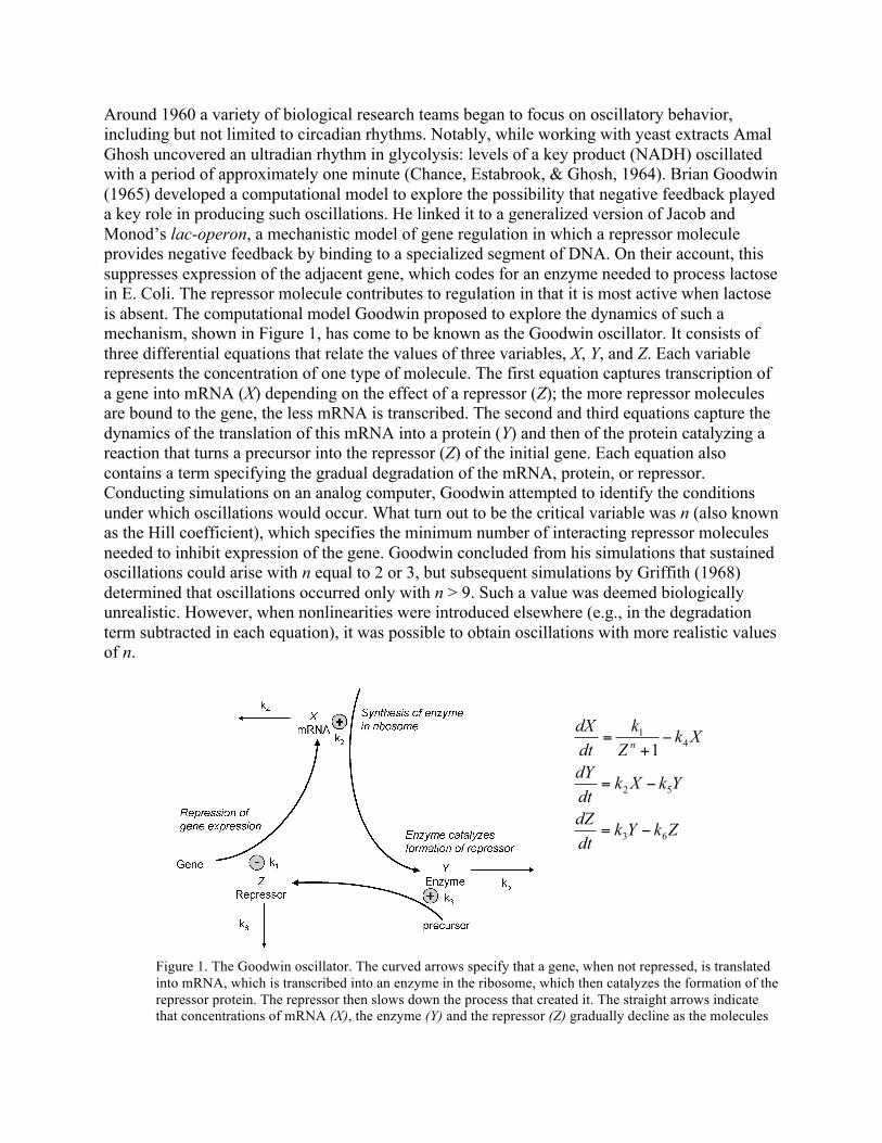
Around 1960 a variety of biological research teams began to focus on oscillatory behavior, including but not limited to circadian rhythms. Notably, while working with yeast extracts Amal Ghosh uncovered an ultradian rhythm in glycolysis: levels of a key product (NADH) oscillated with a period of approximately one minute (Chance, Estabrook, & Ghosh, 1964). Brian Goodwin (1965) developed a computational model to explore the possibility that negative feedback played a key role in producing such oscillations. He linked it to a generalized version of Jacob and Monod’s lac-operon, a mechanistic model of gene regulation in which a repressor molecule provides negative feedback by binding to a specialized segment of DNA. On their account, this suppresses expression of the adjacent gene, which codes for an enzyme needed to process lactose in E. Coli. The repressor molecule contributes to regulation in that it is most active when lactose is absent. The computational model Goodwin proposed to explore the dynamics of such a mechanism, shown in Figure 1, has come to be known as the Goodwin oscillator. It consists of three differential equations that relate the values of three variables, X, Y, and Z. Each variable represents the concentration of one type of molecule. The first equation captures transcription of a gene into mRNA (X) depending on the effect of a repressor (Z); the more repressor molecules are bound to the gene, the less mRNA is transcribed. The second and third equations capture the dynamics of the translation of this mRNA into a protein (Y) and then of the protein catalyzing a reaction that turns a precursor into the repressor (Z) of the initial gene. Each equation also contains a term specifying the gradual degradation of the mRNA, protein, or repressor. Conducting simulations on an analog computer, Goodwin attempted to identify the conditions under which oscillations would occur. What turn out to be the critical variable was n (also known as the Hill coefficient), which specifies the minimum number of interacting repressor molecules needed to inhibit expression of the gene. Goodwin concluded from his simulations that sustained oscillations could arise with n equal to 2 or 3, but subsequent simulations by Griffith (1968) determined that oscillations occurred only with n > 9. Such a value was deemed biologically unrealistic. However, when nonlinearities were introduced elsewhere (e.g., in the degradation term subtracted in each equation), it was possible to obtain oscillations with more realistic values of n.

Figure 1. The Goodwin oscillator. The curved arrows specify that a gene, when not repressed, is translated into mRNA, which is transcribed into an enzyme in the ribosome, which then catalyzes the formation of the repressor protein. The repressor then slows down the process that created it. The straight arrows indicate that concentrations of mRNA (X), the enzyme (Y) and the repressor (Z) gradually decline as the molecules

ZkYkdtdZ

YkXkdtdY

XkZk

dtdX

n

63

52

41

1

!=

!=

!+

=

degrade. The rate of each operation is specified by a parameter (k1, k2, . . . k6). The differential equations on the right give the rates over time (t) at which concentrations of X, Y, and Z are changing..

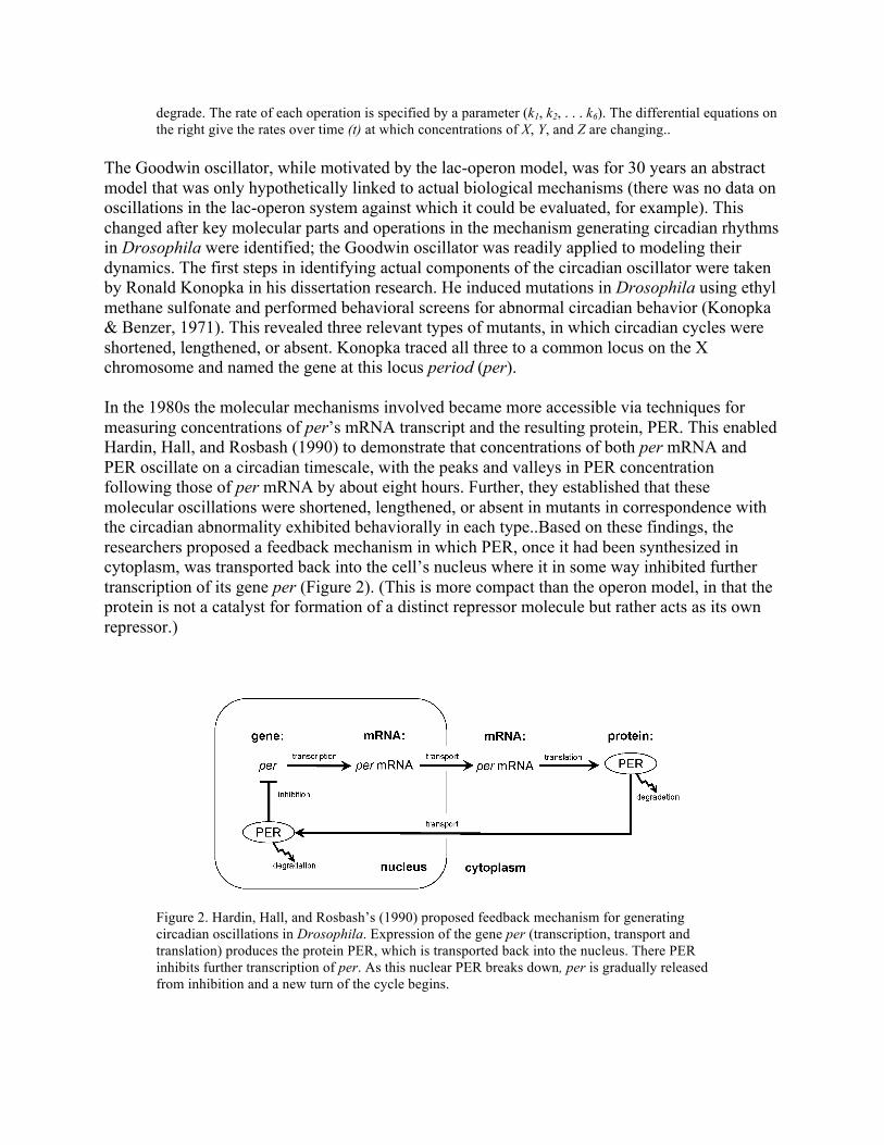
The Goodwin oscillator, while motivated by the lac-operon model, was for 30 years an abstract model that was only hypothetically linked to actual biological mechanisms (there was no data on oscillations in the lac-operon system against which it could be evaluated, for example). This changed after key molecular parts and operations in the mechanism generating circadian rhythms in Drosophila were identified; the Goodwin oscillator was readily applied to modeling their dynamics. The first steps in identifying actual components of the circadian oscillator were taken by Ronald Konopka in his dissertation research. He induced mutations in Drosophila using ethyl methane sulfonate and performed behavioral screens for abnormal circadian behavior (Konopka & Benzer, 1971). This revealed three relevant types of mutants, in which circadian cycles were shortened, lengthened, or absent. Konopka traced all three to a common locus on the X chromosome and named the gene at this locus period (per). In the 1980s the molecular mechanisms involved became more accessible via techniques for measuring concentrations of per’s mRNA transcript and the resulting protein, PER. This enabled Hardin, Hall, and Rosbash (1990) to demonstrate that concentrations of both per mRNA and PER oscillate on a circadian timescale, with the peaks and valleys in PER concentration following those of per mRNA by about eight hours. Further, they established that these molecular oscillations were shortened, lengthened, or absent in mutants in correspondence with the circadian abnormality exhibited behaviorally in each type..Based on these findings, the researchers proposed a feedback mechanism in which PER, once it had been synthesized in cytoplasm, was transported back into the cell’s nucleus where it in some way inhibited further transcription of its gene per (Figure 2). (This is more compact than the operon model, in that the protein is not a catalyst for formation of a distinct repressor molecule but rather acts as its own repressor.)

Figure 2. Hardin, Hall, and Rosbash’s (1990) proposed feedback mechanism for generating circadian oscillations in Drosophila. Expression of the gene per (transcription, transport and translation) produces the protein PER, which is transported back into the nucleus. There PER inhibits further transcription of per. As this nuclear PER breaks down, per is gradually released from inhibition and a new turn of the cycle begins.

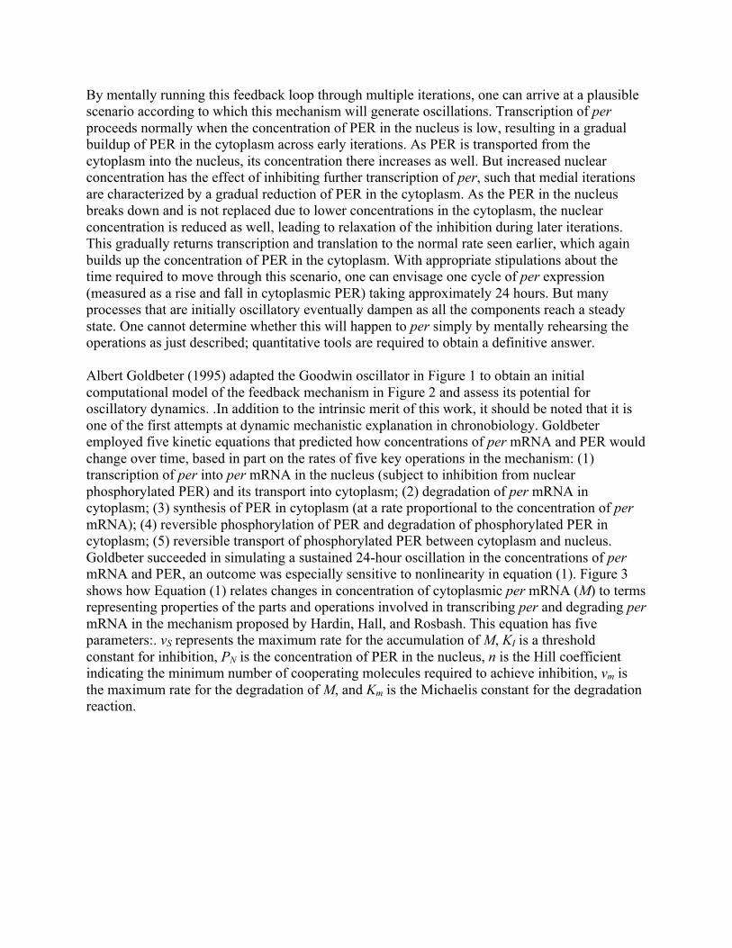
By mentally running this feedback loop through multiple iterations, one can arrive at a plausible scenario according to which this mechanism will generate oscillations. Transcription of per proceeds normally when the concentration of PER in the nucleus is low, resulting in a gradual buildup of PER in the cytoplasm across early iterations. As PER is transported from the cytoplasm into the nucleus, its concentration there increases as well. But increased nuclear concentration has the effect of inhibiting further transcription of per, such that medial iterations are characterized by a gradual reduction of PER in the cytoplasm. As the PER in the nucleus breaks down and is not replaced due to lower concentrations in the cytoplasm, the nuclear concentration is reduced as well, leading to relaxation of the inhibition during later iterations. This gradually returns transcription and translation to the normal rate seen earlier, which again builds up the concentration of PER in the cytoplasm. With appropriate stipulations about the time required to move through this scenario, one can envisage one cycle of per expression (measured as a rise and fall in cytoplasmic PER) taking approximately 24 hours. But many processes that are initially oscillatory eventually dampen as all the components reach a steady state. One cannot determine whether this will happen to per simply by mentally rehearsing the operations as just described; quantitative tools are required to obtain a definitive answer. Albert Goldbeter (1995) adapted the Goodwin oscillator in Figure 1 to obtain an initial computational model of the feedback mechanism in Figure 2 and assess its potential for oscillatory dynamics. .In addition to the intrinsic merit of this work, it should be noted that it is one of the first attempts at dynamic mechanistic explanation in chronobiology. Goldbeter employed five kinetic equations that predicted how concentrations of per mRNA and PER would change over time, based in part on the rates of five key operations in the mechanism: (1) transcription of per into per mRNA in the nucleus (subject to inhibition from nuclear phosphorylated PER) and its transport into cytoplasm; (2) degradation of per mRNA in cytoplasm; (3) synthesis of PER in cytoplasm (at a rate proportional to the concentration of per mRNA); (4) reversible phosphorylation of PER and degradation of phosphorylated PER in cytoplasm; (5) reversible transport of phosphorylated PER between cytoplasm and nucleus. Goldbeter succeeded in simulating a sustained 24-hour oscillation in the concentrations of per mRNA and PER, an outcome was especially sensitive to nonlinearity in equation (1). Figure 3 shows how Equation (1) relates changes in concentration of cytoplasmic per mRNA (M) to terms representing properties of the parts and operations involved in transcribing per and degrading per mRNA in the mechanism proposed by Hardin, Hall, and Rosbash. This equation has five parameters:. vS represents the maximum rate for the accumulation of M, KI is a threshold constant for inhibition, PN is the concentration of PER in the nucleus, n is the Hill coefficient indicating the minimum number of cooperating molecules required to achieve inhibition, vm is the maximum rate for the degradation of M, and Km is the Michaelis constant for the degradation reaction.

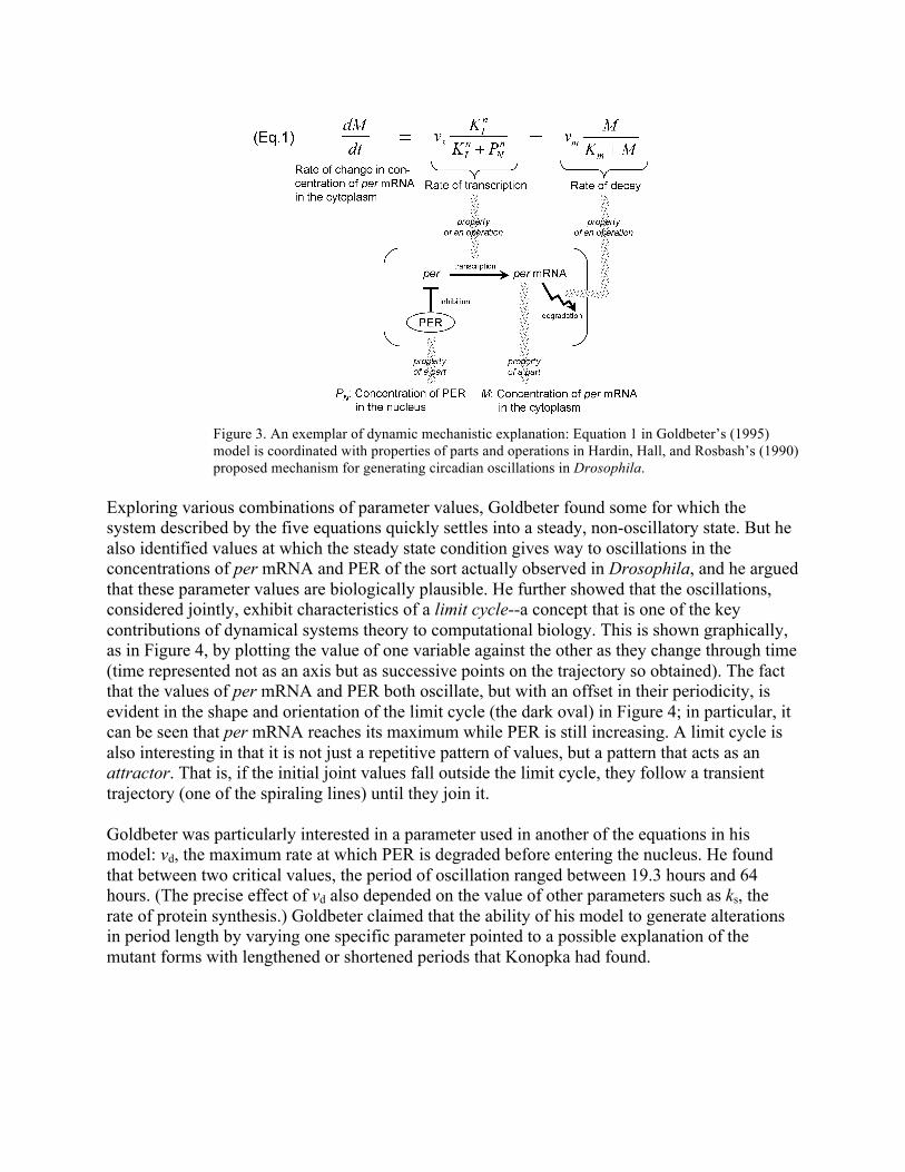
Figure 3. An exemplar of dynamic mechanistic explanation: Equation 1 in Goldbeter’s (1995) model is coordinated with properties of parts and operations in Hardin, Hall, and Rosbash’s (1990) proposed mechanism for generating circadian oscillations in Drosophila.

Exploring various combinations of parameter values, Goldbeter found some for which the system described by the five equations quickly settles into a steady, non-oscillatory state. But he also identified values at which the steady state condition gives way to oscillations in the concentrations of per mRNA and PER of the sort actually observed in Drosophila, and he argued that these parameter values are biologically plausible. He further showed that the oscillations, considered jointly, exhibit characteristics of a limit cycle--a concept that is one of the key contributions of dynamical systems theory to computational biology. This is shown graphically, as in Figure 4, by plotting the value of one variable against the other as they change through time (time represented not as an axis but as successive points on the trajectory so obtained). The fact that the values of per mRNA and PER both oscillate, but with an offset in their periodicity, is evident in the shape and orientation of the limit cycle (the dark oval) in Figure 4; in particular, it can be seen that per mRNA reaches its maximum while PER is still increasing. A limit cycle is also interesting in that it is not just a repetitive pattern of values, but a pattern that acts as an attractor. That is, if the initial joint values fall outside the limit cycle, they follow a transient trajectory (one of the spiraling lines) until they join it. Goldbeter was particularly interested in a parameter used in another of the equations in his model: vd, the maximum rate at which PER is degraded before entering the nucleus. He found that between two critical values, the period of oscillation ranged between 19.3 hours and 64 hours. (The precise effect of vd also depended on the value of other parameters such as ks, the rate of protein synthesis.) Goldbeter claimed that the ability of his model to generate alterations in period length by varying one specific parameter pointed to a possible explanation of the mutant forms with lengthened or shortened periods that Konopka had found.

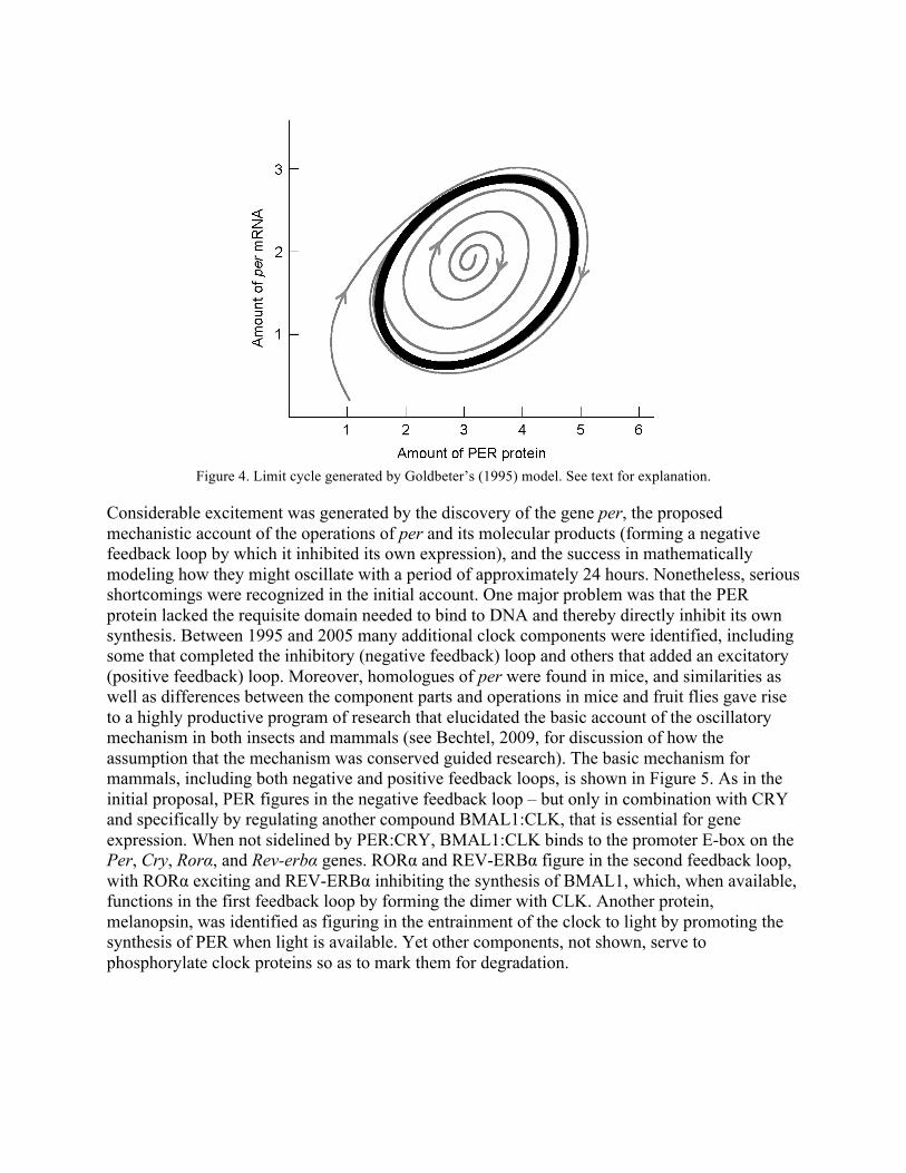
Figure 4. Limit cycle generated by Goldbeter’s (1995) model. See text for explanation.

Considerable excitement was generated by the discovery of the gene per, the proposed mechanistic account of the operations of per and its molecular products (forming a negative feedback loop by which it inhibited its own expression), and the success in mathematically modeling how they might oscillate with a period of approximately 24 hours. Nonetheless, serious shortcomings were recognized in the initial account. One major problem was that the PER protein lacked the requisite domain needed to bind to DNA and thereby directly inhibit its own synthesis. Between 1995 and 2005 many additional clock components were identified, including some that completed the inhibitory (negative feedback) loop and others that added an excitatory (positive feedback) loop. Moreover, homologues of per were found in mice, and similarities as well as differences between the component parts and operations in mice and fruit flies gave rise to a highly productive program of research that elucidated the basic account of the oscillatory mechanism in both insects and mammals (see Bechtel, 2009, for discussion of how the assumption that the mechanism was conserved guided research). The basic mechanism for mammals, including both negative and positive feedback loops, is shown in Figure 5. As in the initial proposal, PER figures in the negative feedback loop – but only in combination with CRY and specifically by regulating another compound BMAL1:CLK, that is essential for gene expression. When not sidelined by PER:CRY, BMAL1:CLK binds to the promoter E-box on the Per, Cry, Rorα, and Rev-erbα genes. RORα and REV-ERBα figure in the second feedback loop, with RORα exciting and REV-ERBα inhibiting the synthesis of BMAL1, which, when available, functions in the first feedback loop by forming the dimer with CLK. Another protein, melanopsin, was identified as figuring in the entrainment of the clock to light by promoting the synthesis of PER when light is available. Yet other components, not shown, serve to phosphorylate clock proteins so as to mark them for degradation.

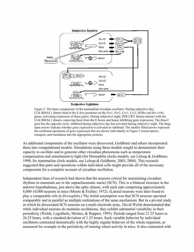
Figure 5. The basic components of the mammalian circadian oscillator. During subjective day, CLK:BMAL1 dimers bind to the E-box promoter on the Per1, Per2, Cry1, Cry2, RORα and Rev-erbα genes, activating expression of these genes. During subjective night, PER:CRY dimers interact with the CLK:BMAL1 dimers, removing them from the E-boxes and hence inhibiting gene expression. The Bmal1 gene has the opposite cycle, inhibited during subjective day but activated during subjective night. The large open arrows indicate whether gene expression is activated or inhibited. The smaller filled arrows represent the combined operations of gene expression that are shown individually in Figure 2 (transcription, transport, and translation into the appropriate protein).

As additional components of the oscillator were discovered, Goldbeter and others incorporated them into computational models. Simulations using these models sought to demonstrate their capacity to oscillate and to generate other circadian phenomena such as temperature compensation and entrainment to light (for Drosophila clocks models, see Leloup & Goldbeter, 1998; for mammalian clock models, see Leloup & Goldbeter, 2003; 2004). This research suggested that parts and operations within individual cells might provide all of the necessary components for a complete account of circadian oscillation. Independent lines of research had shown that the neurons critical for maintaining circadian rhythms in mammals are in the suprachiasmatic nuclei (SCN). This is a bilateral structure in the anterior hypothalamus, just above the optic chiasm, with each side comprising approximately 8,000-10,000 neurons in mice (Moore & Eichler, 1972). (Lateral neurons were later found to play a comparable role in Drosophila.) The initial assumption was that SCN neurons operated comparably and in parallel as multiple realizations of the same mechanism. But in a pivotal study in which he dissociated SCN neurons on a multi-electrode array, David Welsh demonstrated that while individual neurons do maintain oscillations, they exhibit substantial variability in their periodicity (Welsh, Logothetis, Meister, & Reppert, 1995). Periods ranged from 21.25 hours to 26.25 hours, with a standard deviation of 1.25 hours. Such variable behavior by individual oscillators contrasted dramatically with the highly regular behavior of the whole organism, as measured for example in the periodicity of running wheel activity in mice. It also contrasted with

the results of multi-electrode recording in slices in which neural connections between neurons were preserved (Herzog, Aton, Numano, Sakaki, & Tei, 2004). This indicated that in some manner the variable behavior of the individual oscillating neurons was coordinated into a highly regular common pattern, and that the dispersal of neurons disrupted this coordination. To understand circadian rhythms, therefore, researchers must understand not only the mechanism of oscillation within neurons but also how they interact in networks (as discussed by Bechtel & Abrahamsen, 2009). 3. Networks of Coupled Oscillators The research trajectory we just described in circadian research, whereby what were initially thought to be mechanisms producing the phenomenon of interest on their own are later recognized to be submechanisms in a larger system, is common in science. Once researchers determine that the mechanism they were investigating is linked into a larger, cohesively functioning mechanism, two questions arise. First, what is the nature of the connection or signal between local components? Second, what kind of network is involved? In the case of circadian rhythms, the first question has already been successfully addressed. Aton, Colwell, Harmar, Waschek and Herzog (2005) fingered vasoactive intestinal polypeptide (VIP), a peptide hormone, as the likely synchronizing agent. VIP is produced by about 15% of SCN neurons, all in its core. A VIP receptor, VPAC2, is found in about 60% of SCN neurons. While there may be other modes of connection between SCN neurons (e.g., gap junctions), the evidence that VIP plays a central role is highly compelling. That answers the first question regarding the nature of local connections. The second question – how they are organized into an overall network – has proven more challenging. Mathematicians in the subfield of graph theory initially focused on two types of network for which analytical tools could most easily be developed: (1) regular lattices in which nodes can be connected only to their neighbors (e.g., in the simplest one-dimensional lattice with a neighborhood of 1, each node has two neighbors, one on each side, and hence a maximum of two connections); and (2) random networks in which there is an equal probability that any two nodes will be connected. Ermentrout and his collaborators found that one-dimensional lattice models could replicate rhythmic waves such as those found in the human intestine (Ermentrout & Kopell, 1984) or the central pattern generator of the lamprey eel (Kopell & Ermentrout, 1986). Erdös and Rényi (1960) focused instead on random networks and developed mathematical tools to explore their structure. They demonstrated, for example, that when the number of connections (m) is small relative to the number of nodes (n), the graph consists of a number of clusters of connected units (components). In a phase transition occurring at m = n/2, though, a giant component emerges that is much larger than any other. In the limit, each node is connected to every other node. Winfree (1967) examined synchronization among oscillators with different natural frequencies by treating them as nodes in a fully connected network of this kind..Analyzing the coupling strength, he found a threshold, below which each oscillator runs at its natural frequency, but above which clusters of synchronized oscillators form. At a sufficiently high coupling strength, he showed, the entire network is synchronized.. Regular lattices and random networks exhibit contrasting properties as reflected in two measures. First, the clustering coefficient for a given node j (Cj) measures the percentage of permissible

connections that are actually realized. A high clustering coefficient for the whole network (C) indicates it is highly interconnected. Second, the characteristic path length (L) is the number of connections that must be traversed to get from one node to another, on average. Regular lattices have larger values of both C and L than random networks. A regular lattice therefore allows for efficient, specialized processing within each cluster of nodes but less efficient integration of results across clusters, whereas a random network favors more homogeneous, integrated processing. While regular lattices and random networks are the easiest to analyze, Watts and Strogratz (1998) found that many real-world networks fall into a class that lies between them, which they designated small worlds. In these networks most connections are between near neighbors, thus generating a high clustering coefficient close to that of a regular lattice. A few connections are long-distance, though; adding just a few of these radically reduces the characteristic path length so that it approximates that of a random network. Thus, small worlds exhibit both local clusters of nodes that can perform distinct tasks and high levels of integration across the whole network. Small-world architectures are interesting not just as modes of structural organization but because of their functional potential. Watts and Strogatz, in their pioneering paper, speculated that small-world networks would “display enhanced signal propagation speed, computational power, and synchronizability.” As Strogatz (2001) elaborated: “The intuition is that the short paths could provide high-speed communication channels between distant parts of the system, thereby facilitating any dynamical process (like synchronization or computation) that requires global coordination and information flow.” The high clustering, on the other hand, enables the development of local clusters with different functional capacities without sacrificing the ability of individual clusters to adapt rapidly to activity elsewhere in the network. Small-world organization has been identified in numerous neural networks. For example, Watts and Strogratz demonstrated that the 302-neuron network in the nematode worm Caenorhabditis elegans, with approximately 5000 chemical synapses, 2000 neuromuscular junctions, and 600 gap junctions, has the structure of a small world. Small-world structure also has been found in brains at a variety of scales, including the vertebrate reticular system (Humphries, Gurney, & Prescott, 2006) and the mammalian neocortex (Song, Sjöström, Reigl, Nelson, & Chklovskii, 2005). In the macaque visual system, Felleman and van Essen (1991) identified 30 different cortical areas involved in visual processing and showed that 311 of the nearly 900 possible pairwise connections were realized. Sporns and Zwi (2004) demonstrated that this network exhibited small-world properties: a high clustering coefficient and short characteristic path length. They also found that these characteristics of small worlds were found in the interconnections within brain areas as well and commented:

Our analysis provides preliminary indications that the network topology of cortex incorporates aspects of heterogeneity (“randomness”) and homogeneity (“regularity”) at several spatial scales, including large-scale cortical systems and local intra-areal networks. Nested and embedded modules of densely coupled and thus functionally interrelated elements are combined and recombined across multiple levels. Modular and hierarchical organization appears to be a robust feature of other biological systems such as metabolic and protein networks (p. 159).

In light of these results, it is of interest to determine what sort of network exists in the SCN. This project has been pursued mainly by modeling – building specific design features into an abstract mechanistic model and using computational modeling to determine whether it behaves in the manner of the actual SCN. In one of the first such projects, Gonze, Bernard, Waltermann, Kramer, and Herzel (2005) specified a network of 1000 fully interconnected oscillators, each a Goodwin oscillator. That is, the three equations in Figure 1 provided an initial characterization of the behavior of each of the 1000 component oscillators. However, they added equations characterizing the synthesis and breakdown of VIP – the synchronizing agent – by each oscillator individually and computed from those the mean concentration of VIP across the whole system. They then added a term to the equation for computing the change in concentration of a circadian clock protein (e.g., PER), which increased the protein’s concentration proportional to the mean concentration of VIP. When the parameter associated with this term was set to 0 (i.e., no effect of VIP), Gonze et al. obtained results much like those of Welsh et al. (periods that were highly variable across oscillators), but when it was set to 0.5, the oscillators synchronized. By making the response of individual oscillators dependent on the mean concentration of VIP, Gonze et al. treated the SCN network as fully interconnected. In subsequent research, these researchers explored other options including,nearest neighbor (regular lattice) and random connectivity, as well as a design intended to capture the relation between core and shell regions of the SCN (S. Bernard, Gonze, Čajavec, Herzel, & Kramer, 2007). With the latter design, for example, they were able to replicate the phenomenon that shell neurons tend to oscillate in advance of core neurons, and that when a 12 hour phase shift is introduced, core neurons resynchronize with the day-night cycle within two days but shell neurons require more than ten days. In an separate modeling project, To, Henson, Herzog, and Doyle (2007) addressed the fact that VIP diffusion varies with distance between oscillators. They also randomly perturbed a parameter specifying basal transcription of Per mRNA such that only about 40% of the model SCN cells sustained oscillation in the absence of VIP. (Aton et al. had found that in the mouse SCN only 30% of cells appear capable of sustaining oscillations on their own.) They succeeded in replicating Aton et al.’s empirical findings – when VIP was present the cells synchronized, but when VIP was removed approximately 60% became arrhythmic and the rest desynchronized. They also replicated a finding that in constant light, individual SCN cells continue to oscillate but are desynchronized (Ohta, Yamazaki, & McMahon, 2005). None of these initial simulations employed a small-world design, so an intriguing question is how a small-world structure would affect SCN behavior. To et al.’s model included the equation

∑=

=N

jjiji tat

1)(1)( ρ

εγ

to compute the VIP concentration (γi) that each neuron (i) would receive, given the total VIP released by the neurons to which it is connected (ρj). Vasalou, Herzog, and Henzon (2009) replaced this with

∑=

=N

jjij

ii ta

kt

1)(1)( ργ

in which ki is the number of inputs received by neuron i, and aij is set to 1 if there is a connection between i and j and 0 otherwise. This enabled the investigators to specify a small-world architecture in which there was a high probability of short range connections, a much smaller

(but important) probability of long range connections, and only some of the neurons generate VIP. They employed two measures for the performance of the resulting network: (1) a synchronization index, which compares the instantaneous phase angle of each oscillator relative to a reference cycle (this quantifies the ability of the network to produce a coherent signal), and (2) an order parameter that measures overall degree of synchrony. On these measures, small-world networks scored comparably with fully interconnected networks and significantly outperformed regular lattice networks. If they perform equally in terms of synchronizing behavior, what would be the advantages of a small-world design over fully connected networks? One obvious advantage is the energetic cost associated with maintaining each connection – there is a clear advantage to achieving the same benefits at a lower cost. But a further factor is that small-world designs allow for specialized subpopulations that differ from the overall population. There is compelling evidence that core and shell neurons form distinct subpopulations, and that the shell neurons oscillate in advance of the core neurons (with a phase offset of approximately one hour). .These regions also have different patterns of projection to peripheral oscillators elsewhere in the organism, which use those projections for purposes of synchronization. .Conceivably the core and shell each contain smaller subpopulations with different phase relations that could be useful in setting the timing for a variety of peripheral oscillators. Yet another advantage is that variability across different subpopulations of SCN neurons could be useful for representing photoperiod length. Individual oscillators exhibit peak PER concentrations for only part of the subjective day, and there is evidence that on longer days these peaks are more widely dispersed (vanderLeest et al., 2007). By allowing such specialization of subpopulations of neurons within the SCN – at a finer grain than simply core versus shell – a small-world design may provide a much richer representation of time for the rest of the organism. These possibilities are the focus of ongoing active investigation, as the details of how the SCN regulates circadian behavior in the rest of the organism remains poorly understood.3 4. Conclusions We have emphasized the importance of thinking dynamically about mechanisms – of not limiting inquiry to sequential analysis of component operations, but seeking to understand the often complex temporal orchestration of these operations. Oscillations and other complex dynamical behavior can emerge when operations in mechanisms are organized non-sequentially, the interactions are non-linear, and the system is partially open to energy; moreover, such dynamic behavior may play an important role in regulating other operations in the mechanism. Understanding such dynamic behavior of mechanisms typically requires the tools of computational modeling or dynamical systems theory. Sometimes this modeling is done in isolation from mechanistic decomposition of the system into parts and operations. When these two kinds of analysis are coordinated, though, some or all of the variables and terms in the mathematical model correspond to properties of identified parts and operations (e.g., the rate of

3A procedure for forcing desynchronization of core and peripheral oscillators in rats was developed by (de la Iglesia, Cambras, Schwartz, & Díez-Noguera, 2004). They entrain rats to a 22-hour day (to which only the core neurons can entrain; the shell neurons continue to free-run with a period greater than 24 hours) and have recently explored how different signals affecting melatonin concentrations are generated (Schwartz et al., 2009).

an operation). Bechtel and Abrahamsen call the accounts that result from analyzing the orchestration of operations in this manner dynamic mechanistic explanations. It is still common to view endogenous biological oscillations as noise, but we have discussed how these can provide a valuable resource for organizing and orchestrating operations within an organism. For example, oscillations can be used to ensure that operations occur at appropriate times with respect to each other and to environmental conditions; notably, they can segregate incompatible operations. Circadian oscillations – endogenous oscillations that approximate the 24 hour day-night cycle found on this planet – are an exemplar. Humans often ignore these oscillations, which affect many aspects of their physiological and behavioral functioning, but they figure crucially not just in humans but in most other life forms. We described the model of a biological oscillator proposed by Goodwin in the 1960s, which in recent years has been widely employed in dynamic mechanistic modeling of circadian oscillators at the molecular level. The opening to this very productive research program was an initial success in decomposing the mechanism: identification of the first clock protein, PER, which was proposed to feed back negatively on its own transcription such that its concentrations in cytoplasm and in the nucleus oscillated on an approximately 24 hour cycle. Computational models of this proposed feedback mechanism demonstrated that with appropriate and biologically plausible parameters it would generate circadian oscillations. Subsequently numerous other clock proteins were identified, and their organization in negative and positive feedback loops has been increasingly well-specified. Demonstrating that these feedback loops would generate sustained oscillations, rather than a steady state, required further development of mathematical accounts and especially the exploration of parameter values. Often mechanisms are organized into larger mechanisms of which they are components. The system may then modulate the behavior of its component mechanisms. In the case of circadian rhythms in mammals, isolated SCN neurons can serve as circadian mechanisms, but exhibit significant variability in their periodicity. When coupled into a network – the SCN – they function cohesively. Understanding this involves determining the organization in the network, which again requires mathematical modeling. In this case, the modeling has suggested how individual oscillators could be organized in a small-world architecture, which enables local subpopulations to specialize but still be responsive to behavior elsewhere in the network. There is not, as yet, detailed understanding of the organization in the SCN itself and the functional significance, but it is clear that the organization does modulate the behavior of components and that understanding it requires adopting a dynamical mechanistic perspective. And as the science goes, so goes the philosophy of science: while once we advocated replacing a concern with laws with a focus on mechanistic accounts, we are here advocating that philosophers concern themselves with the dynamic mechanistic explanation that is at the leading edge of many fields of investigation. References Aton, S. J., Colwell, C. S., Harmar, A. J., Waschek, J., & Herzog, E. D. (2005). Vasoactive

intestinal polypeptide mediates circadian rhythmicity and synchrony in mammalian clock neurons. Nature Neuroscience, 8, 476-483.

Bechtel, W. (2009). Generalization and discovery by assuming conserved mechanisms: Cross species research on circadian oscillators. Philosophy of Science, 76, 762-773.

Bechtel, W., & Abrahamsen, A. (2005). Explanation: A mechanist alternative. Studies in History and Philosophy of Biological and Biomedical Sciences, 36, 421-441.

Bechtel, W., & Abrahamsen, A. (2009). Decomposing, recomposing, and situating circadian mechanisms: Three tasks in developing mechanistic explanations. In H. Leitgeb & A. Hieke (Eds.), Reduction and elimination in philosophy of mind and philosophy of neuroscience (pp. 173-186). Frankfurt: Ontos Verlag.

Bechtel, W., & Abrahamsen, A. (2010). Dynamic mechanistic explanation: Computational modeling of circadian rhythms as an exemplar for cognitive science. Studies in History and Philosophy of Science Part A.

Bechtel, W., & Abrahamsen, A. (2011). Complex biological mechanisms: Cyclic, oscillatory, and autonomous. In C. A. Hooker (Ed.), Philosophy of complex systems. Handbook of the philosophy of science, Volume 10. New York: Elsevier.

Bechtel, W., & Richardson, R. C. (1993/2010). Discovering complexity: Decomposition and localization as strategies in scientific research. Cambridge, MA: MIT Press. 1993 edition published by Princeton University Press.

Bernard, C. (1865). An introduction to the study of experimental medicine. New York: Dover. Bernard, S., Gonze, D., Čajavec, B., Herzel, H., & Kramer, A. (2007). Synchronization-induced

rhythmicity of circadian oscillators in the suprachiasmatic nucleus. PLoS Computational Biology, 3 (4), e68.

Cannon, W. B. (1929). Organization of physiological homeostasis. Physiological Reviews, 9, 399-431.

Chance, B., Estabrook, R. W., & Ghosh, A. (1964). Damped sinusoidal oscillations of cytoplasmic reduced pyridine nucleotide in yeast cells. Proceedings of the National Academy of Sciences, 51 (6), 1244-1251.

de la Iglesia, H. O., Cambras, T., Schwartz, W. J., & Díez-Noguera, A. (2004). Forced desynchronization of dual circadian oscillators within the rat suprachiasmatic nucleus. Current Biology, 14 (9), 796-800.

Erdös, P., & Rényi, A. (1960). On the evolution of random graphs. Proceedings of the Mathematical Institute of the Hungarian Academy of Sciences, 5, 17-61.

Ermentrout, G. B., & Kopell, N. (1984). Frequency plateaus in a chain of weakly coupled oscillators. 1. Siam Journal on Mathematical Analysis, 15 (2), 215-237.

Felleman, D. J., & van Essen, D. C. (1991). Distributed hierarchical processing in the primate cerebral cortex. Cerebral Cortex, 1, 1-47.

Goldbeter, A. (1995). A model for circadian oscillations in the Drosophila Period protein (PER). Proceedings of the Royal Society of London. B: Biological Sciences, 261 (1362), 319-324.

Gonze, D., Bernard, S., Waltermann, C., Kramer, A., & Herzel, H. (2005). Spontaneous synchronization of coupled circadian oscillators. Biophysical Journal, 89 (1), 120-129.

Goodwin, B. C. (1965). Oscillatory behavior in enzymatic control processes. Advances in Enzyme Regulation, 3, 425-428.

Griffith, J. S. (1968). Mathematics of cellular control processes I. Negative feedback to one gene. Journal of Theoretical Biology, 20 (2), 202-208.

Hardin, P. E., Hall, J. C., & Rosbash, M. (1990). Feedback of the Drosophila period gene product on circadian cycling of its messenger RNA levels. Nature, 343 (6258), 536-540.

Herzog, E. D., Aton, S. J., Numano, R., Sakaki, Y., & Tei, H. (2004). Temporal precision in the mammalian circadian system: A reliable clock from less reliable neurons. Journal of Biological Rhythms, 19 (1), 35-46.

Humphries, M. D., Gurney, K., & Prescott, T. J. (2006). The brainstem reticular formation is a small-world, not scale-free, network. Proceedings of the Royal Society B: Biological Sciences, 273 (1585), 503-511.

Konopka, R. J., & Benzer, S. (1971). Clock mutants of Drosophila melanogaster. Proceedings of the National Academy of Sciences (USA), 89, 2112-2116.

Kopell, N., & Ermentrout, G. B. (1986). Symmetry and phaselocking in chains of weakly coupled oscillators. Communications on Pure and Applied Mathematics, 39 (5), 623-660.

Leloup, J.-C., & Goldbeter, A. (1998). A model for circadian rhythms in Drosophila incorporating the formation of a complex between the PER and TIM proteins. Journal of Biological Rhythms, 13 (1), 70-87.

Leloup, J.-C., & Goldbeter, A. (2003). Toward a detailed computational model for the mammalian circadian clock. Proceedings of the National Academy of Sciences, 100 (12), 7051-7056.

Leloup, J.-C., & Goldbeter, A. (2004). Modeling the mammalian circadian clock: Sensitivity analysis and multiplicity of oscillatory mechanisms. Journal of Theoretical Biology, 230 (4), 541-562.

Machamer, P., Darden, L., & Craver, C. F. (2000). Thinking about mechanisms. Philosophy of Science, 67, 1-25.

Mayr, O. (1970). The origins of feedback control. Cambridge, MA: MIT Press. Moore, R. Y., & Eichler, V. B. (1972). Loss of a circadian adrenal corticosterone rhythm

following suprachiasmatic lesions in the rat. Brain Research, 42, 201-206. Ohta, H., Yamazaki, S., & McMahon, D. G. (2005). Constant light desynchronizes mammalian

clock neurons. Nature Neuroscience, 8, 267-269. Ruiz-Mirazo, K., Peretó, J., & Moreno, A. (2004). A universal definition of life: Autonomy and

open-ended evolution. Origins of Life and Evolution of the Biosphere, 34, 323-346. Schwartz, M. D., Wotus, C., Liu, T., Friesen, W. O., Borjigin, J., Oda, G. A., et al. (2009).

Dissociation of circadian and light inhibition of melatonin release through forced desynchronization in the rat. Proceedings of the National Academy of Sciences, 106 (41), 17540-17545.

Song, S., Sjöström, P. J., Reigl, M., Nelson, S., & Chklovskii, D. B. (2005). Highly nonrandom features of synaptic connectivity in local cortical circuits. PLoS Biology, 3 (3), e68.

Sporns, O., & Zwi, J. D. (2004). The small world of the cerebral cortex. Neuroinformatics, 2 (2), 145-162.

Strogatz, S. H. (2001). Exploring complex networks. Nature, 410 (6825), 268-276. Thagard, P. (2003). Pathways to biomedical discovery. Philosophy of Science, 70, 235-254. To, T.-L., Henson, M. A., Herzog, E. D., & Doyle, F. J., III. (2007). A molecular model for

intercellular synchronization in the mammalian circadian clock. Biophysical Journal, 92 (11), 3792-3803.

vanderLeest, H. T., Houben, T., Michel, S., Deboer, T., Albus, H., Vansteensel, M. J., et al. (2007). Seasonal encoding by the circadian pacemaker of the SCN. Current Biology, 17 (5), 468-473.

Vasalou, C., Herzog, E. D., & Henson, M. A. (2009). Small-world network models of intercellular coupling predict enhanced synchronization in the suprachiasmatic nucleus. Journal of Biological Rhythms, 24 (3), 243-254.

Watts, D., & Strogratz, S. (1998). Collective dynamics of small worlds. Nature, 393 (440-442). Welsh, D. K., Logothetis, D. E., Meister, M., & Reppert, S. M. (1995). Individual neurons

dissociated from rat suprachiasmatic nucleus express independently phased circadian firing rhythms. Neuron, 14 (4), 697-706.

Wilson, E. O. (1998). Consilience: The unity of knowledge. New York: Knopf. Wimsatt, W. C. (1976). Reductionism, levels of organization, and the mind-body problem. In G.

Globus, G. Maxwell & I. Savodnik (Eds.), Consciousness and the brain: A scientific and philosophical inquiry (pp. 202-267). New York: Plenum Press.

Winfree, A. T. (1967). Biological rhythms and the behavior of populations of coupled oscillators. Journal of Theoretical Biology, 16 (1), 15-42.