Embed Size (px)
Citation preview
Master Thesis
Analysis on Solar Retrofit in Combined CyclePower Plants
ausgefuhrt zum Zwecke der Erlangung des akademischen Grades eines Master of Scienceunter Anleitung von
Univ.Ass. Dipl.-Ing. Armin STEINERUniv.Prof. Dipl.-Ing. Dr.tech. Markus HAIDER
E 302 - Institut fur Energietechnik und Thermodynamik
erstellt an der
Technische Universitat WienFakultat fur Maschinenwesen und Betriebswissenschaften von
Andrea MIGUEZ DA ROCHA
Wien, am 23.04.2010
Contents
Contents
1 Introduction 1
2 Combined Cycle Power Plants 22.1 Gas Turbine . . . . . . . . . . . . . . . . . . . . . . . . . . . . . . . . . . . . 2
2.1.1 Improvements for increasing the work output . . . . . . . . . . . . . . 32.1.2 Part-load performance . . . . . . . . . . . . . . . . . . . . . . . . . . 6
2.2 Steam Cycle . . . . . . . . . . . . . . . . . . . . . . . . . . . . . . . . . . . . 92.2.1 Types of Condensers . . . . . . . . . . . . . . . . . . . . . . . . . . . 11
2.3 Heat Recovery Steam Generator . . . . . . . . . . . . . . . . . . . . . . . . . 132.3.1 Types of HRSGs . . . . . . . . . . . . . . . . . . . . . . . . . . . . . 142.3.2 Design considerations . . . . . . . . . . . . . . . . . . . . . . . . . . . 15
2.4 Combined Cycle Power Plants . . . . . . . . . . . . . . . . . . . . . . . . . . 17
3 Concentrating Solar Power Plants 203.1 Solar Thermal Concentrating Collectors . . . . . . . . . . . . . . . . . . . . . 20
3.1.1 Parabolic-Trough Power Plants . . . . . . . . . . . . . . . . . . . . . 203.1.2 Dish Stirling Systems . . . . . . . . . . . . . . . . . . . . . . . . . . . 223.1.3 Central Receiver System . . . . . . . . . . . . . . . . . . . . . . . . . 23
3.2 Parabolic Trough Power Plant Configurations . . . . . . . . . . . . . . . . . 253.2.1 Solar Mode . . . . . . . . . . . . . . . . . . . . . . . . . . . . . . . . 253.2.2 Direct Steam Generation . . . . . . . . . . . . . . . . . . . . . . . . . 253.2.3 Integrated Solar Combined Cycle (ISCC) . . . . . . . . . . . . . . . . 26
4 Modeling and Simulation with EBSILONr Professional 274.1 Basics of the Ebsilon Software . . . . . . . . . . . . . . . . . . . . . . . . . . 27
4.1.1 Data introduction . . . . . . . . . . . . . . . . . . . . . . . . . . . . . 284.1.2 Calculation Modes . . . . . . . . . . . . . . . . . . . . . . . . . . . . 29
5 Model of the Gas Turbine GE 9FA 305.1 Gas Turbine GE 9FA in Design Conditions . . . . . . . . . . . . . . . . . . . 305.2 Gas Turbine GE 9FA in Off-design . . . . . . . . . . . . . . . . . . . . . . . 32
5.2.1 Variation of Ambient Temperature . . . . . . . . . . . . . . . . . . . 325.2.2 Variation of fuel and air flows . . . . . . . . . . . . . . . . . . . . . . 355.2.3 Variation of Efficiency in Components . . . . . . . . . . . . . . . . . 38
5.3 Off-load Model of HRSG, Steam Turbine and Condenser . . . . . . . . . . . 40
6 Modeling a Single Pressure CCPP 42
7 Modeling a Two Pressure CCPP 46
8 Modeling a Three Pressure CCPP 488.1 Performance of Three Pressure CCPP in ISO Conditions . . . . . . . . . . . 498.2 Performance of Three Pressure CCPP with Changing Ambient Temperature 49
ii

Contents
9 Standard Three Pressure CCPP with Solar Boosting 559.1 Standard Three Pressure CCPP with Solar Boosting and Saturated High Pres-
sure Steam (SHP) . . . . . . . . . . . . . . . . . . . . . . . . . . . . . . . . . 569.2 Standard Three Pressure CCPP with Solar Boosting and Cold Reheated
Steam (CRH) . . . . . . . . . . . . . . . . . . . . . . . . . . . . . . . . . . . 59
10 Conversion Efficiency of Solar Boosting 6810.1 Conversion Efficiency of Saturated High Pressure Steam . . . . . . . . . . . 6810.2 Conversion Efficiency of Cold Reheated Steam . . . . . . . . . . . . . . . . . 68
11 Impact of Solar Steam Injection on Temperatures and Pressures 6811.1 Impact of Saturated High Pressure Steam Injection . . . . . . . . . . . . . . 6811.2 Impact of Solar Heat Injection as Cold Reheated Steam . . . . . . . . . . . . 69
12 Thermal Efficiency of the CCPP 7012.1 Thermal Efficiency of the CCPP with Solar Boosting . . . . . . . . . . . . . 70
13 Standard Three Pressure CCPP with Increased Solar Boosting 70
14 Economic Analysis of the Three Pressure CCPP with Solar Boosting 7214.1 Pneumatic Pre-Stressed Concentrators (PPC) . . . . . . . . . . . . . . . . . 7514.2 Parabolic Trough Concentrators (PTC) . . . . . . . . . . . . . . . . . . . . . 77
15 Economic Analysis of the Three Pressure CCPP with Increased Solar Boosting 7815.1 Pneumatic Pre-Stressed Concentrators (PPC) . . . . . . . . . . . . . . . . . 7915.2 Parabolic Trough Concentrators (PTC) . . . . . . . . . . . . . . . . . . . . . 80
16 Conclusion and Summary 80
Bibliography 82
iii
1 Introduction
1 Introduction
The objective of the thermodynamics studies of thermal power plants is the determina-tion and maximization of the efficiency of combined cycle power plants. With other words,we wish to study and apply the methods for increasing the plant effectiveness by saving costs.
In the production of electricity the combined cycle power plants are largely known anddeveloped. A combined cycle power plant is the combination of two cycles associated withthe power production, Rankine and Brayton.
The Rankine cycle consists in a close steam cycle where the steam at high pressure is ex-panded in a turbine to produce power. The Brayton cycle is an open cycle in which air entersin a compressor for being mixed with fuel in a combustor chamber. The mixture of fuel andair, at high pressure and temperature, is expanded through a turbine which produces power.Both cycles are combined in a way that the energy in the exhaust gases of the gas turbinesupports the steam cycle.
Gas Turbines are volumetric machines. At high ambient temperature the air and gas flowthrough the gas turbine decreases due to the lower air density. The gas turbine produces lesspower. The steam cycle is also over dimensioned due to the fact it is receiving less exhaustenergy than in its design.
In this study we propose a solar retrofit for making up for the lack of input energy inthe steam cycle from the gas turbine. Linear concentrating thermal technology is applied.The solar retrofit can deliver additional steam for the steam cycle without spending theinvestment costs of power island. Therefore the concept can be economically advantageous.
In the following process models of a single, two and three pressure combined cycle powerplants will be developed and simulated with the software EBSILONr Professional 8.0. Thedifferent modes of operation will be analyzed. The performance of the three pressure com-bined cycle will be modeled under different load conditions.
Two different modes of boosting the combined cycle power plant will be studied and com-pared: boosting the steam cycle with saturated steam at high pressure (SHP) or with coldreheated steam (CRH). The chosen solution will be analyzed both technically and econom-ically comparing two concentrating thermal technologies, Parabolic Trough Concentrators(PTC) and Pneumatic Pre-Stressed Concentrators (PPC).
1
2 Combined Cycle Power Plants
2 Combined Cycle Power Plants
The combined cycle is one of the most efficient cycles in operation for power generation. Itsthermal efficiency can reach 66%. In design conditions, the gas turbine supplies the 60% ofthe power, while the steam turbine delivers only the 34% of the energy.
The combined cycle exists in different configurations: single-shaft or multi-shaft. The differ-ence is the number of gas turbines and heat recovery steam generators (HRSGs) deliveringpower to the steam turbine.
2.1 Gas Turbine
A gas turbine is an engine which allows the conversion of the energy of fuel in some form ofuseful power, such as mechanical power. The simplest cycle of a gas turbine is formed bya compressor, where the air is compressed until the required pressure; a combustion cham-ber, where the fuel and air at high pressure are mixed, and a turbine, where the mixtureof gases are expanded after the combustion. In the turbine, the gases are expanded adia-batically generating a big amount of work. Part of the work obtained, between the 50% to60%, is used to drive the compressor an the rest is delivered to the surroundings, Bathie [2].
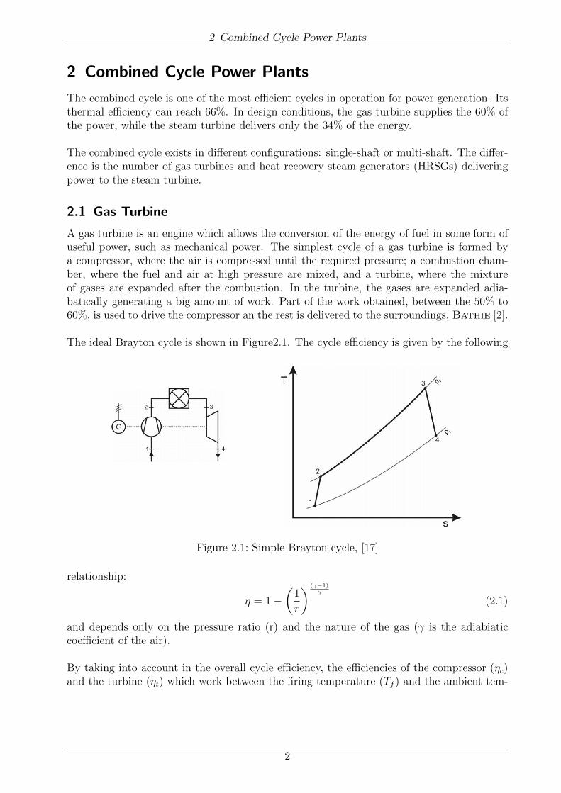
The ideal Brayton cycle is shown in Figure2.1. The cycle efficiency is given by the following
Figure 2.1: Simple Brayton cycle, [17]
relationship:
η = 1−(
1
r
) (γ−1)γ
(2.1)
and depends only on the pressure ratio (r) and the nature of the gas (γ is the adiabiaticcoefficient of the air).
By taking into account in the overall cycle efficiency, the efficiencies of the compressor (ηc)and the turbine (ηt) which work between the firing temperature (Tf ) and the ambient tem-
2

2 Combined Cycle Power Plants
perature (Tamb), we can obtain the following equation:
ηcycle =
ηtTf − Tambr( γ−1
γ )ηc
Tf − Tamb − Tamb(r(
γ−1γ )−1ηc
)(1− 1
r(γ−1γ )
)(2.2)
The Figure 2.2 shows how increases the cycle efficiency when the pressure ratio and the fir-
Figure 2.2: Overall Cycle Efficiency of the Pressure Ratio [3]
ing temperature increase. At a given firing temperature, the efficiency increases with higherpressure ratios; however, increasing the pressure ratio too much over a specific value canresult in the opposite effect, lowering the overall efficiency.
The optimum pressure ratio for getting the maximum power output of the turbine canbe expressed by the following relationship:
ropt =
[(TambTf
)(1
ηcηt
)] γ2−2γ
(2.3)
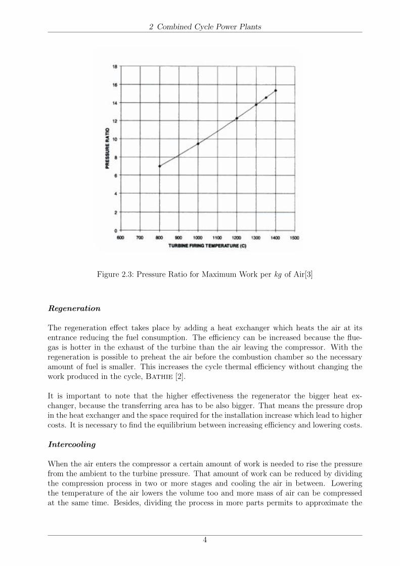
Comparing Figure 2.2 and Figure 2.3, we can come to the conclusion that the pressureratio for reaching the maximum efficiency is much higher than for reaching the maximumwork per kg of air.
It is necessary to be noted, that having a look at the efficiency equation we can conclude thatthe overall efficiency of the cycle can be improved by increasing the pressure ratio, decreasingthe compressor inlet temperature or increasing the turbine inlet temperature.
2.1.1 Improvements for increasing the work output
There are many ways of improving the performance of the basic gas turbine and raising thecycle efficiency. We will discuss in the following three of the most common possibilities:
3
2 Combined Cycle Power Plants
Figure 2.3: Pressure Ratio for Maximum Work per kg of Air[3]
Regeneration
The regeneration effect takes place by adding a heat exchanger which heats the air at itsentrance reducing the fuel consumption. The efficiency can be increased because the flue-gas is hotter in the exhaust of the turbine than the air leaving the compressor. With theregeneration is possible to preheat the air before the combustion chamber so the necessaryamount of fuel is smaller. This increases the cycle thermal efficiency without changing thework produced in the cycle, Bathie [2].
It is important to note that the higher effectiveness the regenerator the bigger heat ex-changer, because the transferring area has to be also bigger. That means the pressure dropin the heat exchanger and the space required for the installation increase which lead to highercosts. It is necessary to find the equilibrium between increasing efficiency and lowering costs.
Intercooling
When the air enters the compressor a certain amount of work is needed to rise the pressurefrom the ambient to the turbine pressure. That amount of work can be reduced by dividingthe compression process in two or more stages and cooling the air in between. Loweringthe temperature of the air lowers the volume too and more mass of air can be compressedat the same time. Besides, dividing the process in more parts permits to approximate the
4
2 Combined Cycle Power Plants
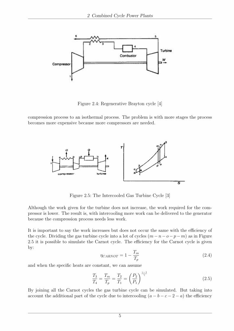
Figure 2.4: Regenerative Brayton cycle [4]
compression process to an isothermal process. The problem is with more stages the processbecomes more expensive because more compressors are needed.
Figure 2.5: The Intercooled Gas Turbine Cycle [3]
Although the work given for the turbine does not increase, the work required for the com-pressor is lower. The result is, with intercooling more work can be delivered to the generatorbecause the compression process needs less work.
It is important to say the work increases but does not occur the same with the efficiency ofthe cycle. Dividing the gas turbine cycle into a lot of cycles (m−n− o− p−m) as in Figure2.5 it is possible to simulate the Carnot cycle. The efficiency for the Carnot cycle is givenby:
ηCARNOT = 1− TmTp
(2.4)
and when the specific heats are constant, we can assume
T3T4
=TmTp
=T2T1
=
(P2
P1
) γ−1γ
(2.5)
By joining all the Carnot cycles the gas turbine cycle can be simulated. But taking intoaccount the additional part of the cycle due to intercooling (a− b− c− 2− a) the efficiency
5
2 Combined Cycle Power Plants
will decrease because in that part the efficiencies of the Carnot cycles are smaller.
An intercooling regenerative cycle can increase the power output and the thermal efficiency.This combination provides an increase in efficiency of 12% and an increase in power outputof about 30%, Boyce [3].
Reheat
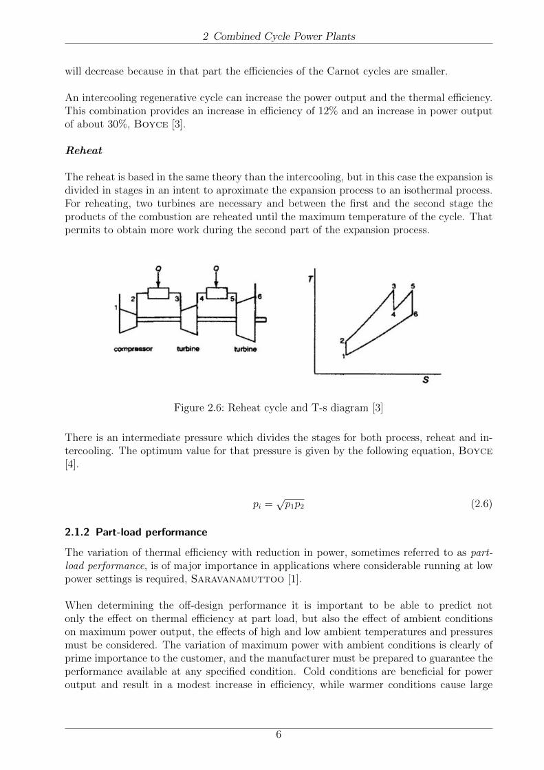
The reheat is based in the same theory than the intercooling, but in this case the expansion isdivided in stages in an intent to aproximate the expansion process to an isothermal process.For reheating, two turbines are necessary and between the first and the second stage theproducts of the combustion are reheated until the maximum temperature of the cycle. Thatpermits to obtain more work during the second part of the expansion process.
Figure 2.6: Reheat cycle and T-s diagram [3]
There is an intermediate pressure which divides the stages for both process, reheat and in-tercooling. The optimum value for that pressure is given by the following equation, Boyce[4].
pi =√p1p2 (2.6)
2.1.2 Part-load performance
The variation of thermal efficiency with reduction in power, sometimes referred to as part-load performance, is of major importance in applications where considerable running at lowpower settings is required, Saravanamuttoo [1].
When determining the off-design performance it is important to be able to predict notonly the effect on thermal efficiency at part load, but also the effect of ambient conditionson maximum power output, the effects of high and low ambient temperatures and pressuresmust be considered. The variation of maximum power with ambient conditions is clearly ofprime importance to the customer, and the manufacturer must be prepared to guarantee theperformance available at any specified condition. Cold conditions are beneficial for poweroutput and result in a modest increase in efficiency, while warmer conditions cause large
6
2 Combined Cycle Power Plants
decrease in both power output and efficiency.
The start point for studying the flow rate behaviour of a multistage turbine is the inves-tigation of the behaviour of a single stage. If we apply the continuity equation to a crosssection in a nozzle, every unit of section is being crossed for an amount of flow:
m
Amin= ρc = µρscs (2.7)
where µ is the flow rate, ρ and c the medium magnitudes, and ρs and cs, the isentropicmedium values of density and velocity in the cross section. The flow rate depends of theefficiency and because of that depends also of Reynolds and Mach. In most of the practicalcases the variation of µ is very small because Reynolds values are high enough.
The velocity in the outlet of the stage is calculated with the total pressure at the inlet,pA, and the static pressure at the outlet, pB:
c =
√√√√ 2κ
κ− 1pAvA
[1−
(pBpA
)κ−1κ
](2.8)
For the density ρ = 1/v
ρs =1
vA
(pBpA
) 1κ
(2.9)
Combining equations 2.8 and 2.9, we obtain:
m = µApA√pAvA
√2κ
κ− 1
√(pBpA
) 2κ
−(pBpA
)κ+1κ
= µA
√pAvAξ (2.10)
The capacity is described by the next function
ξ =
√√√√ 2κ
κ− 1
[(pBpA
) 2κ
−(pBpA
)κ+1κ
](2.11)
For the sound pressure ratio
pBκpA
=
(2
κ+ 1
) κκ−1
(2.12)
it is possible to obtain the maximum value
ξmax =
(2
κ+ 1
) 1κ−1√
2κ
κ+ 1(2.13)
If the pressure ratio decreases below the critical value compare to the equation (2.12), the
7

2 Combined Cycle Power Plants
capacity does not change, that means that the capacity function ξ remains at the maximumlevel. By leaving κ = constant, the relative capacity function:
φ =ξ
ξmax(2.14)
which looks like in Figure (2.7).
Figure 2.7: Relative flow rate function, [15]
The behaviour presented is associated with an ideal single nozzle. When we connect morenozzles in series, we can make an approximate statement for a complete turbine. The flow isin critical conditions in such a configuration, equation (2.12) has to be filled for at least onenozzle. The product of the pressure ratio of all nozzles has to be smaller than in equation(2.12), due to the fact that the pressure ratio, pB/pA, for the rest of nozzles have to be belowthe unity.
The point K in the Figure 2.8 slices to the left until finally, for a multi-stage turbine, weobtain an ellipse as the curve which describes the turbine behaviour.
For this case the function can be approximated for a circle,
φ =
√1−
(pBpA
)2
(2.15)
Furthermore, the flow rate is influenced by the rotation of the turbine. Therefore the functionµ is formed. Now it is possible to describe the ratio of two flow rates by using equation (2.10),where the index ”0” marks the design case.
m
m0
=µ
µ0
pApA0
√pA0pA
vA0vA
φ
φ0
(2.16)
8

2 Combined Cycle Power Plants
Figure 2.8: Relative flow rate function, [15]
Taking into account the caloric equation of state pAva = κ−1κhA, we get:
m
m0
=µ
µ0
pApA0
√hA0
hA
φ
φ0
(2.17)
For a multi-stage turbine the influence of the revolution speed is small, so we can stateµ/µ0 = 1. Finally, we write the simplified equation as:
m
m0
=
√hA0hA
√p2A − p2Bp2A0 − p2B0
(2.18)
In steam turbines the conditions at the entrance can be changed by the throttling, so it ispossible to say that hA = hA0. If hA = hA0 = constant the equation (2.18) describes a conecylindrical surface.
In steam turbines and stationary gas turbines the case of constant power output have apractical meaning. With pB = pB0 = constant and a fixed ratio hA/hA0 the equation (2.18)describes a hyperbola. That is described in the Figure 2.9, with m as abscissas and pAas ordinates. hA/hA0 appears as parameter. For ratios pA/pB > 4 the hyperbola can bequite exactly replaced with its asymptote in the way that the flow ratio will be directlyproportional to the initial pressure.
m
m0
=
√hA0hA
pApA0
(2.19)
In the turbine condenser the final pressure has only a hundredth bar, that means that prac-tically pB = pB0 = 0 can be applied in the (2.19) for all the pressure range.
2.2 Steam Cycle
The steam turbine is an engine in which a steam flow, at high pressure and temperature, isexpanded transforming its energy into kinetic energy, which is as well converted into workby moving the rotational parts of the turbine, Boyce [3]. The performance of the steamturbine is described by the Rankine cycle.
9

2 Combined Cycle Power Plants
Figure 2.9: Ratio between mass flow and inlet pressure by leaving the outlet pressure con-stant, [15]
The Rankine cycle is the most common thermodynamic cycle utilized in the productionof electrical power with water-steam as the working fluid and consists in two isobaric andtwo adiabatic processes. Pumped water from low to high pressure enters a boiler where itis heated at constant pressure by an external heat source to become a dry saturated steam.The saturated steam expands through a turbine, generating power and decreasing its tem-perature. The wet steam enters a condenser to become a saturated liquid.
Figure 2.10: Rankine cycle
10
2 Combined Cycle Power Plants
The thermal efficiency of the Rankine cycle is given by the following expression:
η =(Wturb − Wpump)
Qin
≈ Wturb
Qin
(2.20)
The work required for pumping the water is very small compared with the work that theturbine produces, so is not taken into account at the time to estimate the efficiency.
In a real Rankine cycle, the compression in the pump and the expansion in the turbine arenot isentropic. In other words, these processes are non-reversible and entropy is increasedduring the two processes. This increases the power required by the pump and decreases thepower generated by the turbine.
In particular the efficiency of the steam turbine will be limited by water droplet forma-tion. As the water condenses, water droplets hit the turbine blades at high speed causingpitting and erosion, gradually decreasing the life of turbine blades and efficiency of the tur-bine. The way used to avoid this problem is superheating the steam.
As for the gas turbine, there are improvements for increasing the efficiency of the cycle:
In the reheated cycle two turbines work in series and after the first expansion in the highpressure turbine the steam re-enters the boiler and is reheated almost until the maximumtemperature of the cycle. Then pass through the second, lower pressure turbine. Amongother advantages, this prevents the vapor from condensing during its expansion which canseriously damage the turbine blades, and improves the efficiency of the cycle.
In the regenerative Rankine cycle the water after emerging from the condenser (possiblyas a subcooled liquid) is heated by steam tapped from the hot side of the cycle.
2.2.1 Types of Condensers
In the condenser the steam leaving the turbine in the steam turbine is condensate to water.The steam quality before entering the turbine is usually between 90% to 96% which means10% to 4% of liquid in the mixture, Boyce [3].
The amount of heat removed (Qc)by the condenser is given by the next equation:
Qc = ms(hs − hc) (2.21)
where ms is the mass flow of steam through the condenser, hs is the enthalpy of the steamleaving the steam turbine and hc is the enthalpy of the liquid leaving the condenser.
In condensers, working with water or with air, the amount of heat extracted from the steamhas to be the same that the cooling fluid receives.
ms(hs − hc) = mair(ho − hi) = mwCpw(To − Ti) (2.22)
11
2 Combined Cycle Power Plants
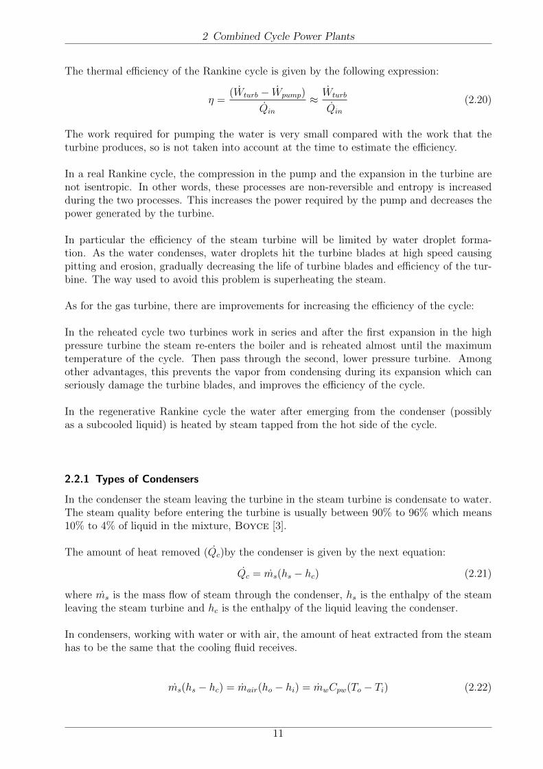
Figure 2.11: Regenerative and reheated Rankine cycle, [22]
where ˙mair and mw are respectively the mass of air and water and the the subscripts ”o” and”i” refers to the values at the condenser output and inlet.
The overall thermal transmittance (U) in a condenser is the amount of heat transmittedper unit of time, unit of surface and degree of temperature difference being the propertywhich defines the behavior of the condenser. The thermal transmittance is written as in theequation (2.23):
U =mwCpwA
Ln
(θ1θ2
)(2.23)
where θ1 is the temperature difference between the steam and the cooling water entering thecondenser, and θ2 is the temperature difference between the the steam and the cooling waterafter passing through the condenser.
The most common types of condensers used in combined cycle power plants are the water-cooled condenser and the air-cooled condenser.
Water-cooled Condenser
In this type of condensers, the cooling water is the refrigerant fluid and it removes theheat from the steam flow condensing the steam to water. That condenser consists of abunch of pipes through which the cooling water flows while the steam flows out of the pipes.The cooling water can be provided from a river or the sea, from where it is pumped to thecondenser. Before returning to the river or sea the water is put in a holding pond. Thewater-cooled condenser can be either classified in shell-and-tube or in tube-and-tube type,Petchers [6].
Air-cooled Condenser
12

2 Combined Cycle Power Plants
The Air-cooled condenser is used in places where it is difficult to find a source of coolingwater. This is generally the most expensive type of condenser. When the ambient tempera-ture is high the resulting operation temperature in the condenser can reduce significantly theefficiency of the refrigerator system. Air-cooled condensers do not need water treatment andhave less problems of freezing up with cold temperatures. Air-cooled condenser require lessmaintenance than other types but the service life is shorter than water-cooled condensersdue to the coil degradation.
In air-cooled condensers the steam flow is condensed into finned tubes by ambient air. Thecooling air is moved by axial fans, which are moved by electric motors.
Cooling Tower
A cooling tower is a heat exchanger in which two fluids, water and cooling air, are putin direct contact to transfer heat. The process consists of a water flow which is sprayed intoa rain-like pattern, through which the ambient air is induced by fans.
2.3 Heat Recovery Steam Generator
The heat recovery steam generator (HRSG) is an important subsystem of a combined powerplant which uses the energy from the exhaust gases of the turbine for transferring heat towater and generating steam at high temperature and pressure.
The exhaust gases leave the gas turbine at approximately ambient pressure and at veryhigh temperature (500◦C to 600◦C). This energy is used for the HRSG to produce steam.Although there are many configurations of HRSG, most of them are divided in the samenumber of sections as the steam turbine. There is one section for high pressure (HP), lowpressure (LP) and sometimes for an intermediate pressure (IP). Each section of the HRSGhas a evaporator or steam generator and depending on the section is possible to find aneconomizer or a superheater, Boyce [4].
A HRSG is composed basically of individual heat exchangers which exchange the energyfrom the exhaust gases of the turbine with the water/steam of the Rankine cycle.
The water enters first in the economizer for being pre-heated and then goes through theevaporator where the steam is generated at constant pressure and temperature. Finally thesteam is superheated in the superheater. After that, the superheated steam enters the tur-bine where it is expanded and the power is generated.
The majority of the heat is transferred by convection and for increasing the heat surfacefinned tubes are used. As the heat transfer on the waterside is much higher than on theexhaust gas side, due to the bigger temperature difference between gas and water than be-tween gas and steam, the fins are used on the gas side to rise the heat transfer.
13
2 Combined Cycle Power Plants
2.3.1 Types of HRSGs
The selection of the HRSG depends of many factors but the most determinant are the initialcost and the global efficiency of the plant. A 1% of increase in efficiency leads to a 3-4% ofincrease in the costs, Boyce [3].
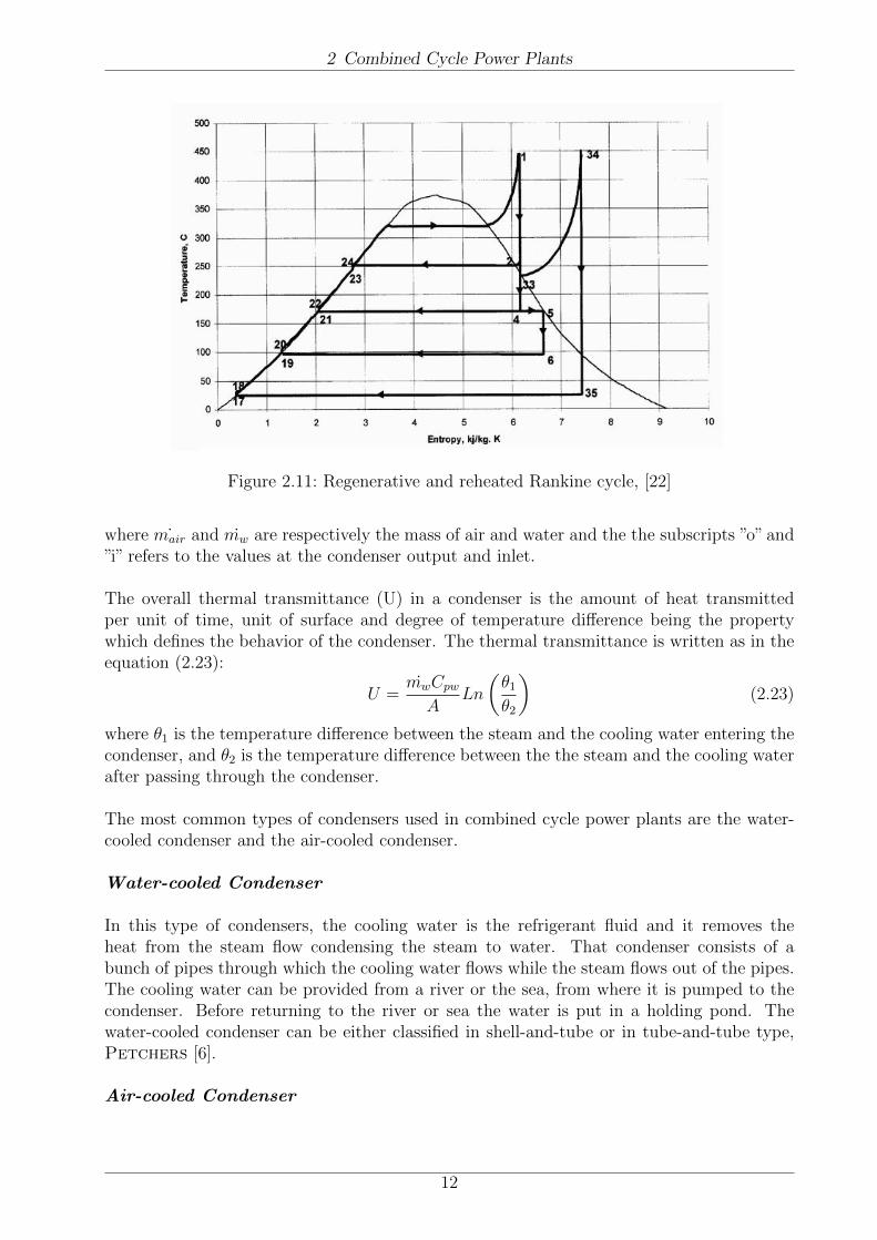
The most common units used in combined cycle power plants are the the drum type HRSGwith natural circulation. The type shown in Figure 2.12 is formed by separate components:drums, economizers, superheaters, generating tubes and blowdown systems. The tubes aredisposed vertically and the exhaust gas flow is horizontal. In HRSGs with forced circulation,the mixture of steam and water is pumped through the evaporator tubes. But the use ofpumps brings to the cycle a parasitic load lowering the efficiency of the cycle. There aresome vertical HRSGs with natural circulation or the other possibility are the Once ThroughSteam Generators, which do not have the defined sections as we can find in the drum HRSG.The OTSG is a pipe in which the water enters at one side and the steam leaves the pipe atthe other side. There are no evaporators and no drums so there is no defined point wherethe evaporation takes place and the interface between water and steam changes its positiondepending on the heat supplied.
Figure 2.12: Section of an horizontal HRSG, [20]
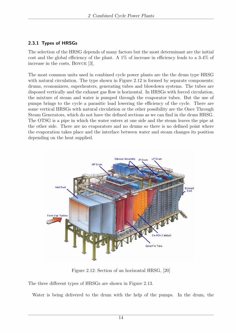
The three different types of HRSGs are shown in Figure 2.13.
Water is being delivered to the drum with the help of the pumps. In the drum, the
14
2 Combined Cycle Power Plants
Figure 2.13: Types of HRSGs, [20]
feed water is mixed with the mixture of water/steam being the steam separated due to thehigher density of the water.
The circulation ratio can be described as the ratio between the mass flow of water circulatinginto the evaporator and the mass flow of steam leaving the evaporator, Effenberger [21] .
U =mcirc
ms
(2.24)
The circulation ratio depends on the pressure and normal values for natural circulation arefrom 5 to 50 and pressures around 160 bar, while for forced circulation normal values arebetween 3 to 10 and pressures around 180 bar.
Other possible classification for HRSG can be made depending on supplementary firing.There are unfired, supplementary fired and exhaust fired HRSGs. In unfired HRSGs, theenergy supplied for the turbine is used without changes, while in the others the mass of gasfrom the turbine is mixed with additional fuel to increase the steam production, Boyce [3].
One of the advantages of the supplementary firing is that the system is able to follow thedemand, providing more power at peak loads. In these systems the gas turbine is sizedaccording to base load demand, but it has to deliver enough power for higher peaks loads.
2.3.2 Design considerations
Some other features should be taken into account in the design of HRSGs.
Pinch Point
15
2 Combined Cycle Power Plants
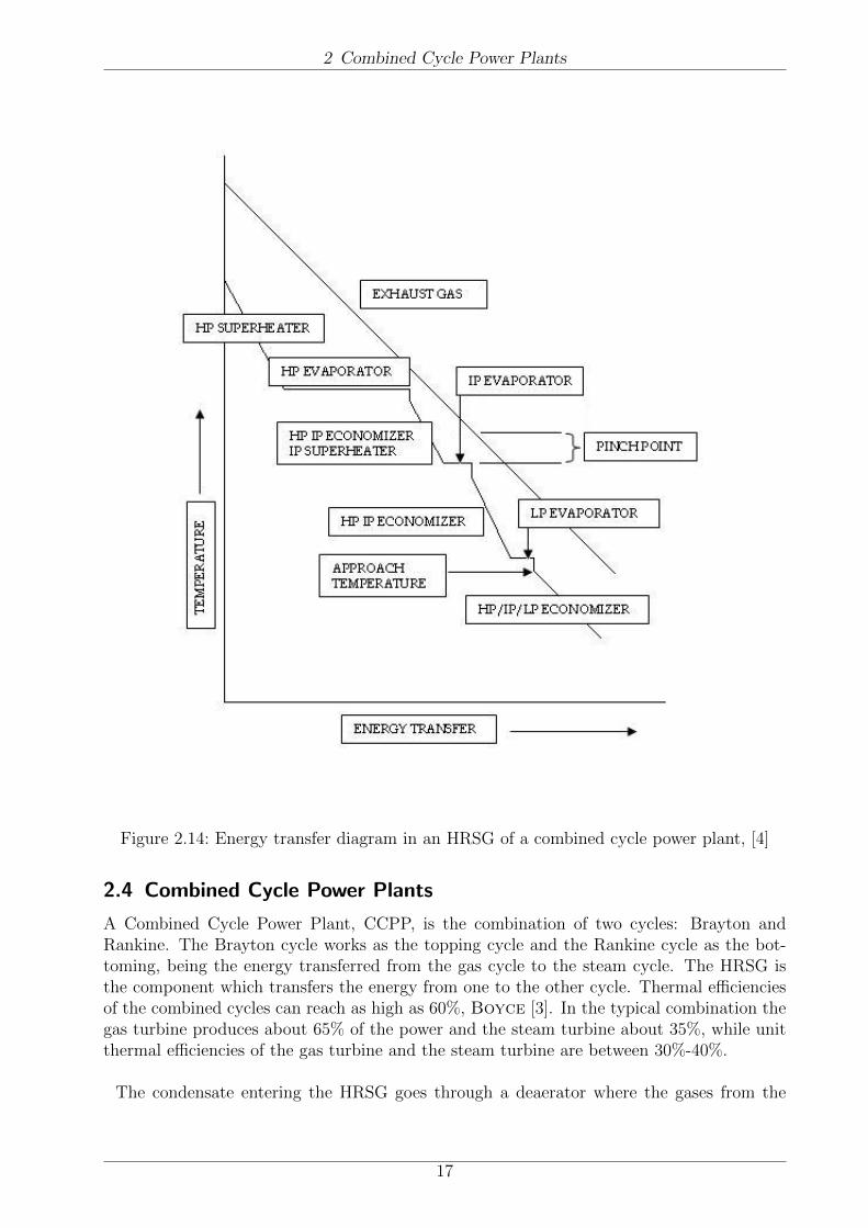
The pinch point is the temperature difference between the gas at the evaporators exit andthe steam saturation temperature. For lowers pinch points the transferred heat is higher.But the heating surfaces have to be bigger with the consequent increase of pressure drop andcosts. Higher pinch points could mean a lower production of steam. The range for normalvalues of pinch points is between 8-22◦ C.
Approach Temperature
The approach temperature is defined as the temperature difference between water at theevaporator inlet and the steam saturation temperature. The production of steam is higherat small approach temperatures. Typically, approach temperatures are in the 5.5-11◦ Crange.
The Figure 2.14 represents the q,T diagram for one section of the HRSG where we cansee the evolution of the water and steam going through the HRSG:
Off-design performance
The gas turbine performance and in particular the exhaust energy determines the opera-tion of the HRSG. The variation in the ambient conditions, the load or the own health of gasturbine change the output conditions of the gas flow, changing the behavior of the HRSG too.
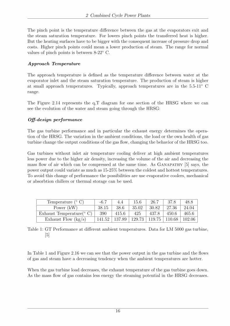
Gas turbines without inlet air temperature cooling deliver at high ambient temperaturesless power due to the higher air density, increasing the volume of the air and decreasing themass flow of air which can be compressed at the same time. As Ganapathy [5] says, thepower output could variate as much as 15-25% between the coldest and hottest temperatures.To avoid this change of performance the possibilities are use evaporative coolers, mechanicalor absorbtion chillers or thermal storage can be used.
Temperature (◦ C) -6.7 4.4 15.6 26.7 37.8 48.8Power (kW) 38.15 38.6 35.02 30.82 27.36 24.04
Exhaust Temperature(◦ C) 390 415.6 425 437.8 450.6 465.6Exhaust Flow (kg/s) 141.52 137.89 129.73 119.75 110.68 102.06
Table 1: GT Performance at different ambient temperatures. Data for LM 5000 gas turbine,[5]
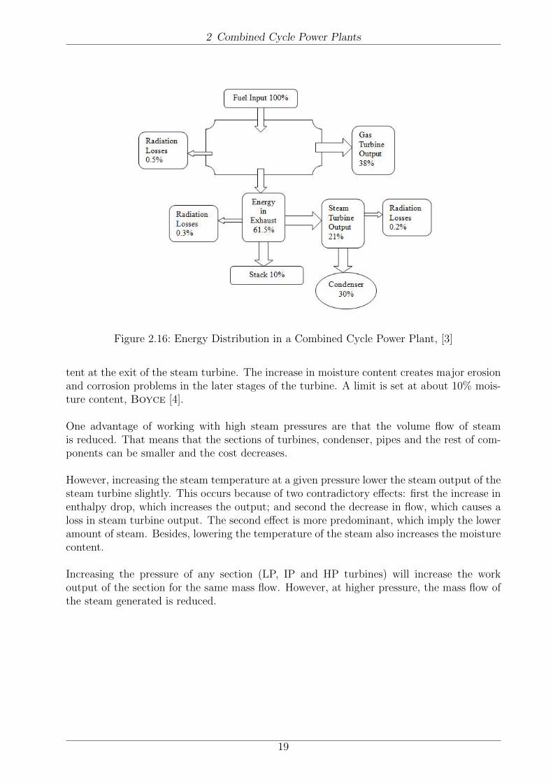
In Table 1 and Figure 2.16 we can see that the power output in the gas turbine and the flowsof gas and steam have a decreasing tendency when the ambient temperatures are hotter.
When the gas turbine load decreases, the exhaust temperature of the gas turbine goes down.As the mass flow of gas contains less energy the steaming potential in the HRSG decreases.
16
2 Combined Cycle Power Plants
Figure 2.14: Energy transfer diagram in an HRSG of a combined cycle power plant, [4]
2.4 Combined Cycle Power Plants
A Combined Cycle Power Plant, CCPP, is the combination of two cycles: Brayton andRankine. The Brayton cycle works as the topping cycle and the Rankine cycle as the bot-toming, being the energy transferred from the gas cycle to the steam cycle. The HRSG isthe component which transfers the energy from one to the other cycle. Thermal efficienciesof the combined cycles can reach as high as 60%, Boyce [3]. In the typical combination thegas turbine produces about 65% of the power and the steam turbine about 35%, while unitthermal efficiencies of the gas turbine and the steam turbine are between 30%-40%.
The condensate entering the HRSG goes through a deaerator where the gases from the
17

2 Combined Cycle Power Plants
Figure 2.15: HRSG performance versus ambient temperature. Gas flow shown has a multi-plication factor of 0.1, [5]
water or steam are removed. This is important because a high oxygen content can causecorrosion in the pipes and the rest of components in contact with the water/steam. Thedeaerator is normally placed on top of the feedwater tank and the process occurs when thewater is sprayed and then heated, thus releasing the gases.
Deaeration also takes place in the condenser and sometimes this could lead to not utiliz-ing a separate deaerator/feedwater tank, and the condensate being fed directly into theHRSG from the condenser.
The economizer is used to heat the water under its saturation temperature. The risk ofgenerating steam in the economizer has to be taken into account because that can block theflow. To prevent the appearance of steam in the economizer a feedwater control valve canbe installed for keeping the pressure high and avoiding the steaming.
The steam turbines in most of the large power plants are at minimum divided in two sec-tions: the High Pressure Section (HP) and the Low Pressure Section (LP). In some plants,the HP section is as well divided into a High Pressure Section and an Intermediate PressureSection (IP). The HRSG is divided in the same sections as the steam turbine. The LP steamturbine’s performance is further dictated by the condenser backpressure, which is a functionof the cooling and the fouling.
The efficiency of the steam section in many of these plants varies from 30%-40%. To ensurethat the steam turbine is operating in an efficient mode, the gas turbine exhaust temperatureis maintained over a wide range of operating conditions. This enables the HRSG to maintaina high degree of effectiveness over this wide range of operation.
In a combined cycle plant, high steam pressures do not necessarily imply a high thermalefficiency. Expanding the steam at higher pressure causes an increase in the moisture con-
18
2 Combined Cycle Power Plants
Figure 2.16: Energy Distribution in a Combined Cycle Power Plant, [3]
tent at the exit of the steam turbine. The increase in moisture content creates major erosionand corrosion problems in the later stages of the turbine. A limit is set at about 10% mois-ture content, Boyce [4].
One advantage of working with high steam pressures are that the volume flow of steamis reduced. That means that the sections of turbines, condenser, pipes and the rest of com-ponents can be smaller and the cost decreases.
However, increasing the steam temperature at a given pressure lower the steam output of thesteam turbine slightly. This occurs because of two contradictory effects: first the increase inenthalpy drop, which increases the output; and second the decrease in flow, which causes aloss in steam turbine output. The second effect is more predominant, which imply the loweramount of steam. Besides, lowering the temperature of the steam also increases the moisturecontent.
Increasing the pressure of any section (LP, IP and HP turbines) will increase the workoutput of the section for the same mass flow. However, at higher pressure, the mass flow ofthe steam generated is reduced.
19

3 Concentrating Solar Power Plants
3 Concentrating Solar Power Plants
Solar energy is the energy generated by the sun which is converted in useful energy by thehuman being for heating or electricity generation. Every year the sun supplies 4 times moreenergy than we consume, so its potential is almost unlimited.
The technology used in thermal power plants is the same used in conventional power plants,except that the heating source is the Sun. The heat energy is used to drive a steam turbineand to produce electricity with generators coupled to the turbines. In the conventional powergeneration, the heat energy comes from combustion of fossil fuels or from nuclear fission. Un-like traditional power plants, concentrating solar power systems produce a source of energywithout emissions and the only impact is the land use. Other benefits of concentrating solarpower plants include low operating costs and an increase in energy independence from foreignoil imports.
Solar energy, in contrast with fossil fuels, is not available around the clock and the intensityof the available energy in a defined point of the Earth depends on the day of the year, thehour and the latitude. Besides, the quantity of energy that can be obtained depends onthe orientation of the receiver mechanism. The gaps can be filled in two ways: switchingto fossil fuel combustion or storing the colected heat energy for when the Sun is not available.
Concentrating solar power plants produce electric power by converting the energy of thesun into high-temperature heat using various mirror configurations which concentrate therays of the Sun for obtaining a high temperature. At least 300◦C are necessary in order togenerate power effectively and economically. For reaching this is essential to have a highpercentage of direct solar radiation. This is more the case in the Sun Belt between the 35th
northern and 35th southern latitudes.
Concentrating solar power (CSP) plants consist of two parts: one that collects solar en-ergy and converts it to heat (solar field), and another that converts heat energy to electricity(power island). The power gained from sunlight can be increased if the light is gatheredand concentrated on a single point and the heat is then channeled through a conventionalgenerator. For concentrating the Sun’s rays there are two possibilities: concentrating theradiation in a fixed point (here the concentrators have to follow the Sun by moving alongtwo axes) or using linear concentrators and only need to move along one axis in order tofollow the Sun.
3.1 Solar Thermal Concentrating Collectors
In practice the most used concentrators are linear concentrators because they are more suit-able for assembly on a large scale and less costly to construct. The different types of linearconcentrators are explained in the following.
3.1.1 Parabolic-Trough Power Plants
The first commercial CSP were parabolic trough systems installed in the United States inthe 1980’s and are the most proven, developed and commercially-ready CSP technologies.
20
3 Concentrating Solar Power Plants
Parabolic trough technology is a clean and mature solar power solution with years of success-ful power generation behind it. The technology has been improving steadily for the last 30years, and modern troughs operate more efficiently and at lower cost. Today, there is morethan 700 MW of CSP trough power in operation around the world, with 400 MW underconstruction and around 20 GW in development.
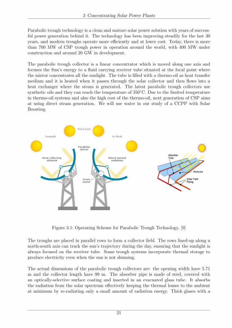
The parabolic trough collector is a linear concentrator which is moved along one axis andfocuses the Sun’s energy to a fluid carrying receiver tube situated at the focal point wherethe mirror concentrates all the sunlight. The tube is filled with a thermo-oil as heat transfermedium and it is heated when it passes through the solar collector and then flows into aheat exchanger where the steam is generated. The latest parabolic trough collectors usesynthetic oils and they can reach the temperature of 350◦C. Due to the limited temperaturein thermo-oil systems and also the high cost of the thermo-oil, next generation of CSP aimsat using direct steam generation. We will use water in our study of a CCPP with SolarBoosting.
Figure 3.1: Operating Scheme for Parabolic Trough Technology, [9]
The troughs are placed in parallel rows to form a collector field. The rows lined-up along anorth-south axis can track the sun’s trajectory during the day, ensuring that the sunlight isalways focused on the receiver tube. Some trough systems incorporate thermal storage toproduce electricity even when the sun is not shinning.
The actual dimensions of the parabolic trough collectors are: the opening width have 5.71m and the collector length have 99 m. The absorber pipe is made of steel, covered withan optically-selective surface coating and inserted in an evacuated glass tube. It absorbsthe radiation from the solar spectrum effectively keeping the thermal losses to the ambientat minimum by re-radiating only a small amount of radiation energy. Thick glases with a
21
3 Concentrating Solar Power Plants
low content of iron are used to built the mirrors. German organizations have developed theEurotrough collector, which is lighter and stiffer, and is less cost to produce, to assembleand to maintain.
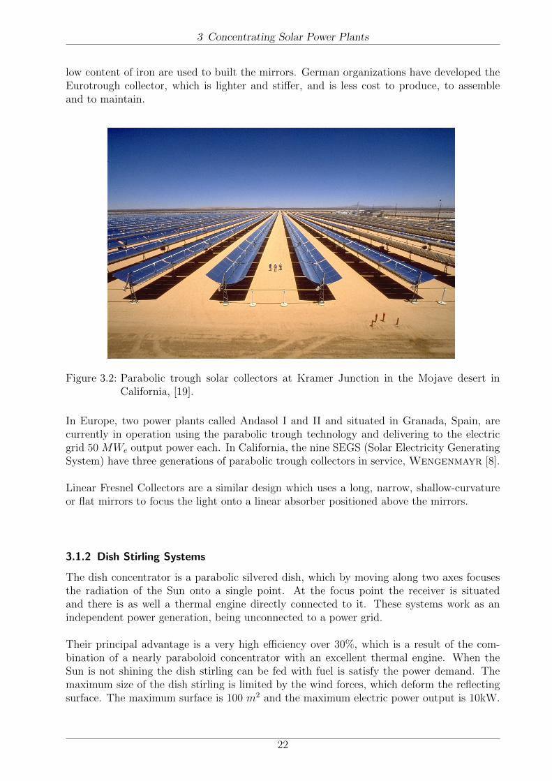
Figure 3.2: Parabolic trough solar collectors at Kramer Junction in the Mojave desert inCalifornia, [19].
In Europe, two power plants called Andasol I and II and situated in Granada, Spain, arecurrently in operation using the parabolic trough technology and delivering to the electricgrid 50 MWe output power each. In California, the nine SEGS (Solar Electricity GeneratingSystem) have three generations of parabolic trough collectors in service, Wengenmayr [8].
Linear Fresnel Collectors are a similar design which uses a long, narrow, shallow-curvatureor flat mirrors to focus the light onto a linear absorber positioned above the mirrors.
3.1.2 Dish Stirling Systems
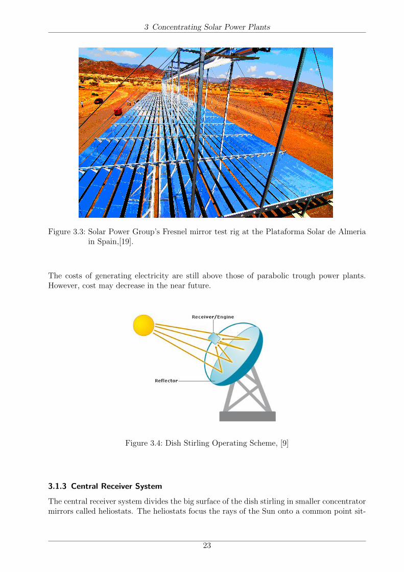
The dish concentrator is a parabolic silvered dish, which by moving along two axes focusesthe radiation of the Sun onto a single point. At the focus point the receiver is situatedand there is as well a thermal engine directly connected to it. These systems work as anindependent power generation, being unconnected to a power grid.
Their principal advantage is a very high efficiency over 30%, which is a result of the com-bination of a nearly paraboloid concentrator with an excellent thermal engine. When theSun is not shining the dish stirling can be fed with fuel is satisfy the power demand. Themaximum size of the dish stirling is limited by the wind forces, which deform the reflectingsurface. The maximum surface is 100 m2 and the maximum electric power output is 10kW.
22
3 Concentrating Solar Power Plants
Figure 3.3: Solar Power Group’s Fresnel mirror test rig at the Plataforma Solar de Almeriain Spain,[19].
The costs of generating electricity are still above those of parabolic trough power plants.However, cost may decrease in the near future.
Figure 3.4: Dish Stirling Operating Scheme, [9]
3.1.3 Central Receiver System
The central receiver system divides the big surface of the dish stirling in smaller concentratormirrors called heliostats. The heliostats focus the rays of the Sun onto a common point sit-
23
3 Concentrating Solar Power Plants
uated on a central tower, where the receiver collects the heat. The heliostats are flat mirrorsand they can not concentrate as much as the ideal paraboloid does.
Large central receiver systems with thousands of heliostats, each with 100 m2 of reflect-ing surface, require towers of 100-200 m high and they can collect several hundred MW ofsolar radiation power.
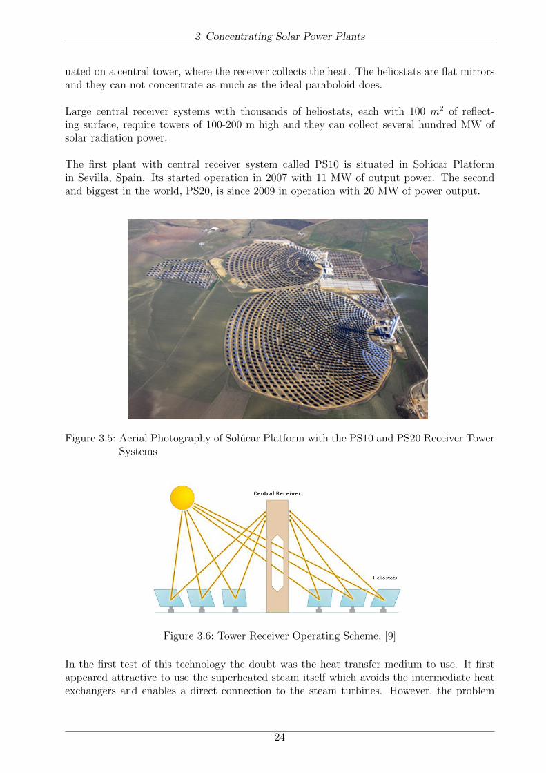
The first plant with central receiver system called PS10 is situated in Solucar Platformin Sevilla, Spain. Its started operation in 2007 with 11 MW of output power. The secondand biggest in the world, PS20, is since 2009 in operation with 20 MW of power output.
Figure 3.5: Aerial Photography of Solucar Platform with the PS10 and PS20 Receiver TowerSystems
Figure 3.6: Tower Receiver Operating Scheme, [9]
In the first test of this technology the doubt was the heat transfer medium to use. It firstappeared attractive to use the superheated steam itself which avoids the intermediate heatexchangers and enables a direct connection to the steam turbines. However, the problem
24

3 Concentrating Solar Power Plants
was how to control the generation of superheated steam with changing radiation conditions.Besides, storing the heat energy was almost impossible without having a big amount of heatlosses. Therefore, the PS10 Solar Power Plant is based on saturated steam at moderatetemperature and pressures to avoid these problems.
Other possibility is the use of alkali-metal salts as heat medium transfer. They have twoadvantages: the good heat transfer properties and the possibility of storage at low pressuresin tanks. However, the high melting point makes necessary electrical heating the pipes toavoid freezing out of the salts with the pipe blockage as result.
3.2 Parabolic Trough Power Plant Configurations
3.2.1 Solar Mode
In these systems the only heat source which moves the steam turbine is the Sun. As the Sundoes not radiate continuously the heat source is not stable and systems for thermal storageare necessary. In summer, the average operating hours are 10-12 hours, which means theremaining time the plant can only be operated using the stored energy.
Since the Sun rises in the morning the solar field starts delivering heat to the thermal cycle.During the radiation peak, the excess heat is stored in the thermal storage system which willbe in charge of delivering the necessary heat during the period when the Sun’s radiation isnot enough.
The differences between the available thermal storage systems are basically the storagemedium used. In the following we will describe the most common storage mediums:
• Salt: Sodium-nitrate salts and Potasium-nitrate salts are cheap materials for storagesystems. They have a high transmission coefficient and can be stored in big salt tanks.The problem is their high melting point which needs electrical heating of the pipingfor avoiding the blockage for example during system start up.
3.2.2 Direct Steam Generation
In a parabolic trough collector, the oil as a heat transfer fluid is heated by concentrated solarradiation. The thermal energy contained in the oil is transferred to the Rankine cycle wherethe power is generated. One of the limitations is the chemical stability of the syntheticoil when it is heated at high temperatures, being the limit about 395◦C. That limits themaximum temperature of the steam in the Rankine cycle being not possible to reach higherefficiencies.
One of the possible alternatives is Direct Steam Generation (DSG)in the collector field.This configuration consists of evaporating and superheating the water directly in the solarfield which makes the oil-water heat exchangers unnecessary. With the DSG the steam canreach temperatures from 400◦C to 550◦C increasing the thermal efficiency of the Rankinecycle. The optimization and demonstration of these technology components has been donein the a 700 m collector loop in the Plataforma Solar de Almerıa, [10].
Three different regimes of operation are possible:
25

3 Concentrating Solar Power Plants
• Once Trough System: preheates, evaporates and superheates the feed water. Thissystem is the simplest and cheapest but the control of the temperature in the receivertube is complex due to the inhomogeneous distribution of temperature on the tubecircumference.
• Injection System: the water is injected in several points of the receiver tube. Thissystem presents the problem of a complex measurement and control operation.
• Recirculation System: in this system the collector tube is divided in two sections.In the first section the water is preheated and evaporated, while in the second the wateris superheated. In between the two sections there is a water-steam separator, wherethe water content in the mixture is separated and sent back to the solar collector inlet.
3.2.3 Integrated Solar Combined Cycle (ISCC)
The Integrated Solar Combined Cycle (ISCC) consists of a conventional Combined CyclePower Plant (CCPP) which is combined with a parabolic trough solar field. The solar fieldproduces superheated steam which is fed into the heat recovery steam generator (HRSG) ofthe combined cycle allowing the increase of the themal efficiency of the steam cycle in theCCPP.
The benefits of employing this technology are to overcome some problems related with
Figure 3.7: ISCC Operating Scheme
the start up and shut down in solar power plants, reduce the capital costs and improve thesolar-to-electricity efficiency.
26

4 Modeling and Simulation with EBSILONr Professional
4 Modeling and Simulation with EBSILONr Professional
In this chapter several modeling processes of a Combined Cycle Power Plant will be de-scribed. The software used for modeling is EBSILONr Professional 8.0, which we will callEbsilon. Ebsilon is a mass and energy balance calculation program for thermodynamicalcycles. With Ebsilon we will be able to simulate the performance of a combined cycle powerplant in design and partload conditions, which is adequate for analyzing its performanceunder several loading conditions.
In the following, we will shortly describe the features and tools available in Ebsilon.
4.1 Basics of the Ebsilon Software
EBSILON is the abbreviation for ”Energy balance and simulation of the load response ofpower generating or process controlling network structures” and is suitable for nearly allstationary thermodynamic model request coming out of energy cycles or plant schemes.
Ebsilon permits the balancing of components, individually or in groups, as well as sub-systems integrated in bigger systems, without taking into account whether these componentsor systems form a closed or an open cycle. The model structure of Ebsilon is based on:
• standard components, which are used for modeling common power plants,
• programmable components for modeling complex power plants processes with user-defined behaviour.
The data basis of Ebsilon is made up of:
• IAPWS-IF97 or the IFC67 steam table,
• cp-polinomial for air/fuel gas.
Ebsilon is a variable program system, by means of which you can balance all occurring powerplant circuits using a closed solution based on a sequential solution method.
The cycles are constructed from objects. The object types can be:
• Components
• Pipes
• Macros (such as the gas turbines from the library)
• Value Crosses
• Text Fields
• Graphical elements
27

4 Modeling and Simulation with EBSILONr Professional
• OLE Objects
Components and pipes form cycles, while value crosses, text fields, graphical elements andOLE objects are used for displaying the results, such as comments and explanations.
In a short description, the basic control elements and tool bars are:
• Standard toolbar,
• Component bar, for selecting a component from a category,
• Component wizard bar, for accessing components classified by numbers,
• Ebsilon bar, for starting simulations,
• Zoom bar, for zooming in the model and finding objects.
4.1.1 Data introduction
After defining the topology of the cycle, it is time to define the values that characterize it.There are two ways of doing that:
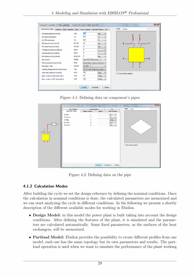
1. Some components can define or calculate values in affiliated pipes, like e.g. the steamgenerator, as shown in Figure 4.1.
2. The other possibility is to set the value directly on the pipe using the ”Measured/Gen-eral value input”, as shown in Figure 4.2.
28
4 Modeling and Simulation with EBSILONr Professional
Figure 4.1: Defining data on component’s pipes
Figure 4.2: Defining data on the pipe
4.1.2 Calculation Modes
After building the cycle we set the design reference by defining the nominal conditions. Oncethe calculation in nominal conditions is done, the calculated parameters are memorized andwe can start analyzing the cycle in different conditions. In the following we present a shortlydescription of the different available modes for working in Ebsilon.
• Design Model: in this model the power plant is built taking into account the designconditions. After defining the features of the plant, it is simulated and the parame-ters are calculated automatically. Some fixed parameters, as the surfaces of the heatexchangers, will be memorized.
• Partload Model: Ebsilon provides the possibility to create different profiles from onemodel, each one has the same topology but its own parameters and results. The part-load operation is used when we want to simulate the performance of the plant working
29
5 Model of the Gas Turbine GE 9FA
under different load situations. The new profile Partload has the same parameters asthe root profile (Design) but calculates in off-Design mode. All the input values areinherited from the parent profile.
• Validation Model: that model is used for controlling the performance of existingplants. Weak points can be detected and from that derives that quality statementsabout power plants can be derived.
• Optimization Model: the optimization model is used for the variation of power plantparameter and what-if calculations. Different strategies of optimization can be appliedas well as a combination with the validation model.
In our analysis of Solar Retrofit in Combined Cycle Power Plants. We will use the Designand Partload models in studying the impact caused for feeding the plant with energy comingfrom a solar field.
5 Model of the Gas Turbine GE 9FA
5.1 Gas Turbine GE 9FA in Design Conditions
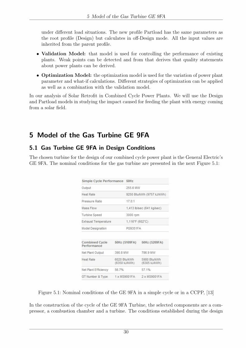
The chosen turbine for the design of our combined cycle power plant is the General Electric’sGE 9FA. The nominal conditions for the gas turbine are presented in the next Figure 5.1:
Figure 5.1: Nominal conditions of the GE 9FA in a simple cycle or in a CCPP, [13]
In the construction of the cycle of the GE 9FA Turbine, the selected components are a com-pressor, a combustion chamber and a turbine. The conditions established during the design
30

5 Model of the Gas Turbine GE 9FA
process are the ISO conditions: 1.013 bar and 15◦C for ambient air.
In nominal conditions, the turbine has a pressure ratio of 17 and is crossed by a mass flow of641 kg/s. The temperature of the gas flow after the expansion is 602◦C at the outlet. Usinga ”general input value” we set the nominal exhaust temperature and the mass flow, whilethe pressure is sett in the turbine component. The general input value has to be situatedafter the turbine, because we only know the exhaust temperature. After writing all data andsimulating the performance of the turbine, we obtain that 627.04 kg/s of air are necessaryfor reaching the nominal conditions in the gas turbine.
G
GE Turbine 9FA 50Hz
ISO Conditions
17.000 1278.077
1514.160 641.000 P bar
T °C
H kJ/kg
M kg/s
17.002 420.710
436.334 627.074
17.002 15.000
32.681 13.926
1.013 15.000
15.155 627.074
1.013 602.000
666.952 641.000
260017.690 kW
270851.761 kW
Figure 5.2: Model of GE 9FA in Design Conditions
Once we know that information we are able to set the air conditions at the entrance of thegas turbine. Using a ”boundary value input” we set the conditions of the air (1.013 bar,15◦C and 627.04 kg/s) and simulate the performance again. The results are the same thatin the step before, we are reaching again the nominal conditions for the gas turbine. Thereason of doing this last step is because we will control the turbine performance in partloadby means of the amount of air which enters the compressor and the mass of fuel burnt in thecombustion chamber. Now, it is possible to set the new parameters of the air in partload byintroducing the values in the ”boundary value input” at the entrance of the gas turbine.
Comparing the data of the Figure 5.2 and Figure 5.1 we can conclude that the perfor-mance of model of the GE 9FA Turbine represents approximately the performance of theturbine in reality. Both the exhaust temperature and the gas flow coincide with the datagiven for General Electric and the only difference is the power output, which is higher in ourmodel. That could be a consequence of a different air ratio which could result as a differentturbine inlet temperature, different isentropic efficiencies in turbine and compressor or theelectrical efficiency of the generator.
The previous results show the gas turbine behaviour in nominal conditions. In the following
31

5 Model of the Gas Turbine GE 9FA
we will discuss the behaviour of the same turbine when the conditions of the surroundingschange and when the net needs less power than the delivered power in nominal conditions.
5.2 Gas Turbine GE 9FA in Off-design
The gas turbine working in nominal conditions means that the turbine works in the sameconditions for which it was designed. Partload conditions are the conditions in which theturbine works under different specifications. Partload can be reached when the ambientconditions changes, the temperature, or when the turbine is delivering less power than thenominal power. The objective of this study is to establish the performance of the gas turbinein the first case, when the air temperature differs from the ISO temperature, although wewill also briefly describe the performance when less than nominal power is enough.
5.2.1 Variation of Ambient Temperature
The variation of ambient temperature produces a change in the turbine behaviour becausethe air entering the turbine changes its properties, such as temperature and humidity.
For our study we will suppose a variation of 5% in humidity (φ) when the temperaturechanges 15◦C. Besides, the density (ρ) changes when the temperature does in a way that,the density is inversely proportional to the temperature.
This has to be taken into account because in the different seasons of the year, the ambi-ent temperature raises, being higher than 15◦C, or decreases and the air density is differentas well. That means that the same turbine working at a fixed place will deliver more or lesspower depending on the season of the year.
In Europe, in summer normally the ambient temperature is higher than 15◦C and thatmeans the air density is lower. As we know, the air density is inversely proportional to itsvolume, so the volume occupied for the same amount of air will be bigger. Thus, the amountof air entering the compressor will be lower, due to the fact that compressor has a fixedvolume capacity, and the gas flow passing through the turbine is lower too. That meansthat the same turbine working in summer has lower power output, because the expandedmass flow is smaller. If we think that in summer the demand of electricity is not lower thanin winter, although no energy for heating is required, the same turbine working in summerconditions will not be enough for satisfying the energy demanded. For this reason, it isnecessary to analyze how much can vary the turbine efficiency depending on the ambienttemperature.
In winter, for colder temperatures than 15◦C, the opposite occurs. The density will de-crease and the compressed mass of air will be bigger. That changes the performance of theturbine in a way that in winter delivers more power, if there is no limit for the turbine inlettemperature.
In the following we will analyze three representative cases for the partload behaviour, 30◦C,45◦C and 0◦C.
First of all, we have to calculate the variation of density and air flow for each case. Knowing
32
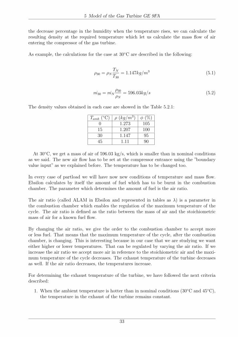
5 Model of the Gas Turbine GE 9FA
the decrease percentage in the humidity when the temperature rises, we can calculate theresulting density at the required temperature which let us calculate the mass flow of airentering the compressor of the gas turbine.
As example, the calculations for the case at 30◦C are described in the following:
ρ30 = ρNTNT30
= 1.147kg/m3 (5.1)
m30 = mNρ30ρN
= 596.03kg/s (5.2)
The density values obtained in each case are showed in the Table 5.2.1:
Tamb (◦C) ρ (kg/m3) φ (%)0 1.273 10515 1.207 10030 1.147 9545 1.11 90
At 30◦C, we get a mass of air of 596.03 kg/s, which is smaller than in nominal conditionsas we said. The new air flow has to be set at the compressor entrance using the ”boundaryvalue input” as we explained before. The temperature has to be changed too.
In every case of partload we will have now new conditions of temperature and mass flow.Ebsilon calculates by itself the amount of fuel which has to be burnt in the combustionchamber. The parameter which determines the amount of fuel is the air ratio.
The air ratio (called ALAM in Ebsilon and represented in tables as λ) is a parameter inthe combustion chamber which enables the regulation of the maximum temperature of thecycle. The air ratio is defined as the ratio between the mass of air and the stoichiometricmass of air for a known fuel flow.
By changing the air ratio, we give the order to the combustion chamber to accept moreor less fuel. That means that the maximum temperature of the cycle, after the combustionchamber, is changing. This is interesting because in our case that we are studying we wanteither higher or lower temperatures. That can be regulated by varying the air ratio. If weincrease the air ratio we accept more air in reference to the stoichiometric air and the maxi-mum temperature of the cycle decreases. The exhaust temperature of the turbine decreasesas well. If the air ratio decreases, the temperatures increase.
For determining the exhaust temperature of the turbine, we have followed the next criteriadescribed:
1. When the ambient temperature is hotter than in nominal conditions (30◦C and 45◦C),the temperature in the exhaust of the turbine remains constant.
33

5 Model of the Gas Turbine GE 9FA
2. At colder temperatures than in nominal conditions (0◦C) that the maximum tempera-ture in the cycle remains constant. The temperature before entering the turbine doesnot vary.
Figure 5.3 shows the evolution of the exhaust and inlet temperature of the gas turbineaccording to the criteria followed for establishing the temperatures in partload.
1210
1220
1230
1240
1250
1260
1270
1280
1290
0 15 30 45
Atmospheric Temperature
555
560
565
570
575
580
585
590
595
600
605
Tin (ºC) Texh (ºC)
TIT (ºC) TOT (ºC)
Figure 5.3: Temperature Evolution in Off-design
We already know that in a combined cycle power plant, the energy in the exhaust gases of thegas turbine is transferred to the steam cycle by using a HRSG. The exhaust gases of the gasturbine have a big amount of energy when they are leaving the turbine with a temperatureover 600◦C. The parameters which define the HRSG are set for the design case, that meansthat the surfaces of the heat exchangers are designed according to these conditions. At otherconditions they are of course constant. For adequate performance of the combined cyclepower plant the conditions of the steam cycle should remain constant. In consequence theoutlet temperature (TOT) of the gas turbine should be as constant as possible independentfrom the ambient temperature.
In the Table 2 and the Table 3 the different values of mass flows, temperatures and air ratiosobtained in each case are shown:
34

5 Model of the Gas Turbine GE 9FA
Figure 5.4: Variation of gas turbine performance in T-s diagram depending on the ambienttemperature, [7]
Tamb (◦C) mair (kg/s) mfuel (kg/s) mgas (kg/s)0 661.5 15.9 677.0
ISO 627.1 13.9 641.030 596.0 12.4 608.545 576.0 11.4 588.4
Table 2: Mass flows in Off-design
As we can see, the power of the gas turbine is higher when the ambient conditions are colderdue to the fact that a bigger amount of gas is expanded in the turbine and the pressure ratiois higher than in nominal conditions. That makes the gas turbine power output higher inwinter, while in summer it decreases.
5.2.2 Variation of fuel and air flows
When an amount of power smaller than in nominal conditions is enough for satisfying thedemand, the gas turbine can works in partload as well.
In first place, the pursued objective is to determine how much power we need. As wesaid, we want to obtain the variation in power but always taking into account that after thegas turbine there is a heat recovery steam generator and the exhaust temperature in the gasturbine has to remain constant. For adjusting the exhaust temperature we will vary againthe air ratio.
In this case the criteria followed establishes a constant exhaust temperature while the rangeof power is between the 50% of the load and nominal conditions. For obtaining a constantexhaust temperature, the air ratio has to be changed in the same way that we have alreadyexplained when the gas turbine works in an ambient with changing temperatures. For ob-taining the required power, the mass of air has to be changed as well, taking into account
35

5 Model of the Gas Turbine GE 9FA
Tamb (◦C) pin (bar) λ Power (MWe) TIT (◦C) TOT (◦C)0 18.0 2.462 318.63 1278.0 573.0
ISO 17.0 2.595 260.02 1278.1 602.030 16.0 2.762 213.53 1253.4 602.045 15.4 2.916 183.85 1238.6 602.0
Table 3: Parameters in Off-design
that the smaller amount of air the less power is delivered. Depending on the required power,Ebsilon calculates by itself the amount of fuel necessary for doing that the gas turbine de-livers exactly that amount.
The Figure 5.5 shows the evolution of the gas flow and exhaust temperature when theperformance of the gas turbine varies from 30% to 110% of the nominal power.
• The ratio Mgas/Mgas0 represents the decrease of the gas flow with regard to the nominalgas flow.
• The ratio Texh/Texh0 represents the variation of temperature with regard to the exhausttemperature in design conditions.
60%
65%
70%
75%
80%
85%
90%
95%
100%
105%
110%
110%100%90%80%70%60%50%40%30%
Paprox/P0
Mgas/Mgas0 Texh/Texh0
Figure 5.5: Temperature and Mass flow Behaviours in Off-desing for a specific power
As we can see in the Figure 5.5 less mass goes through the turbine when we move intopartload operation. That means that the air flow and the fuel flow decrease.
36
5 Model of the Gas Turbine GE 9FA
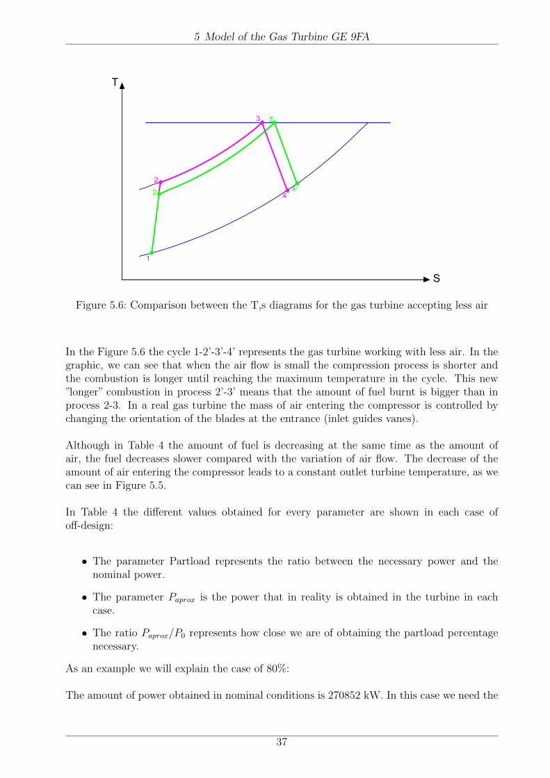
Figure 5.6: Comparison between the T,s diagrams for the gas turbine accepting less air
In the Figure 5.6 the cycle 1-2’-3’-4’ represents the gas turbine working with less air. In thegraphic, we can see that when the air flow is small the compression process is shorter andthe combustion is longer until reaching the maximum temperature in the cycle. This new”longer” combustion in process 2’-3’ means that the amount of fuel burnt is bigger than inprocess 2-3. In a real gas turbine the mass of air entering the compressor is controlled bychanging the orientation of the blades at the entrance (inlet guides vanes).
Although in Table 4 the amount of fuel is decreasing at the same time as the amount ofair, the fuel decreases slower compared with the variation of air flow. The decrease of theamount of air entering the compressor leads to a constant outlet turbine temperature, as wecan see in Figure 5.5.
In Table 4 the different values obtained for every parameter are shown in each case ofoff-design:
• The parameter Partload represents the ratio between the necessary power and thenominal power.
• The parameter Paprox is the power that in reality is obtained in the turbine in eachcase.
• The ratio Paprox/P0 represents how close we are of obtaining the partload percentagenecessary.
As an example we will explain the case of 80%:
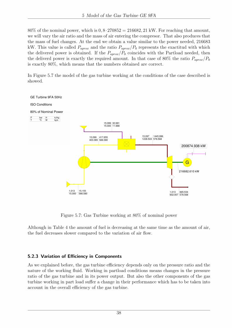
The amount of power obtained in nominal conditions is 270852 kW. In this case we need the
37
5 Model of the Gas Turbine GE 9FA
80% of the nominal power, which is 0, 8 ·270852 = 216682, 21 kW. For reaching that amount,we will vary the air ratio and the mass of air entering the compresor. That also produces thatthe mass of fuel changes. At the end we obtain a value similar to the power needed, 216683kW. This value is called Paprox and the ratio Paprox/P0 represents the exactitud with whichthe delivered power is obtained. If the Paprox/P0 coincides with the Partload needed, thenthe deliverd power is exactly the required amount. In that case of 80% the ratio Paprox/P0
is exactly 80%, which means that the numbers obtained are correct.
In Figure 5.7 the model of the gas turbine working at the conditions of the case described isshowed.
G
GE Turbine 9FA 50Hz
ISO Conditions
80% of Nominal Power 15.097 1228.503
1445.996 578.568 P bar
T °C
H kJ/kg
M kg/s
15.099 403.385
417.655 566.580
15.099 15.000
32.681 11.988
1.013 15.000
15.155 566.580
1.013 602.007
665.534 578.568
200874.938 kW
216682.610 kW
G
GE Turbine 9FA 50Hz
ISO Conditions
80% of Nominal Power 15.097 1228.503
1445.996 578.568 P bar
T °C
H kJ/kg
M kg/s
15.099 403.385
417.655 566.580
15.099 15.000
32.681 11.988
1.013 15.000
15.155 566.580
1.013 602.007
665.534 578.568
200874.938 kW
216682.610 kW
Figure 5.7: Gas Turbine working at 80% of nominal power
Although in Table 4 the amount of fuel is decreasing at the same time as the amount of air,the fuel decreases slower compared to the variation of air flow.
5.2.3 Variation of Efficiency in Components
As we explained before, the gas turbine efficiency depends only on the pressure ratio and thenature of the working fluid. Working in partload conditions means changes in the pressureratio of the gas turbine and in its power output. But also the other components of the gasturbine working in part load suffer a change in their performance which has to be taken intoaccount in the overall efficiency of the gas turbine.
38

5 Model of the Gas Turbine GE 9FA
Partload P0 (kW) Paprox (kW) mair (kg/s) mfuel (kg/s) mgas (kg/s) λ Texh (◦C)110.00% 297937 297932 625.0 15.1 640.1 2.380 643.1100.00% 270852 270852 627.1 13.9 641.0 2.595 602.090.00% 243767 243768 597.9 13.0 610.9 2.657 602.080.00% 216682 216683 566.6 12.0 578.6 2.724 602.070.00% 189597 189597 532.6 11.0 543.6 2.798 602.060.00% 162512 162512 495.3 9.9 505.2 2.881 602.050.00% 135426 135426 453.9 8.8 462.7 2.976 602.040.00% 108341 108342 447.0 7.4 454.4 3.459 540.130.00% 81256 81304 444.5 6.1 450.6 4.220 466.6
Table 4: Variation of Parameters in Off-design when the power is specified
Paprox/P0 Mgas/Mgas0 Texh/Texh0110.0% 99.7% 106.8%100.0% 100.0% 100.0%90.0% 95.4% 100.0%80.0% 90.4% 100.0%70.0% 84.9% 100.0%60.0% 79.0% 100.0%50.0% 72.4% 100.0%40.0% 71.3% 89.7%30.0% 70.9% 77.5%
Table 5: Relative Parameters in Off-design
In Ebsilon compressors and turbines have an established default value of isentropic effi-ciency. The isentropic efficiency in a compressor or a turbine is a comparison between thereal power obtained or consumed and the isentropic case. The default isentropic efficiencyfor turbines is 0.9 and for compressors is 0.85 and in partload that value is defined by somecorrection curves. The variation of isentropic efficiency is directly proportional to the changeof mass flow which is going through the compressor or turbine.
The Tables 6 and 7 show the respective correction curves:
m/mN ETAI/ETAIN0 0.85
0.4 0.90.7 0.951 1
1.2 1.1
Table 6: Variation of Efficiency in the Turbine with the mass flow
The value of the isentropic efficiency is represented in Tables 6 and 7 by the name of ETAI.
39

5 Model of the Gas Turbine GE 9FA
m1/m1N ETAI/ETAIN0 0
0.4 0,91 1
1.2 1.1
Table 7: Variation of Efficiency in the Compresor with the mass flow
5.3 Off-load Model of HRSG, Steam Turbine and Condenser
In this chapter we pretend to analyze how the parameters in every component variate whenthe operation of the steam cycle is not in design conditions.
Heat Exchangers
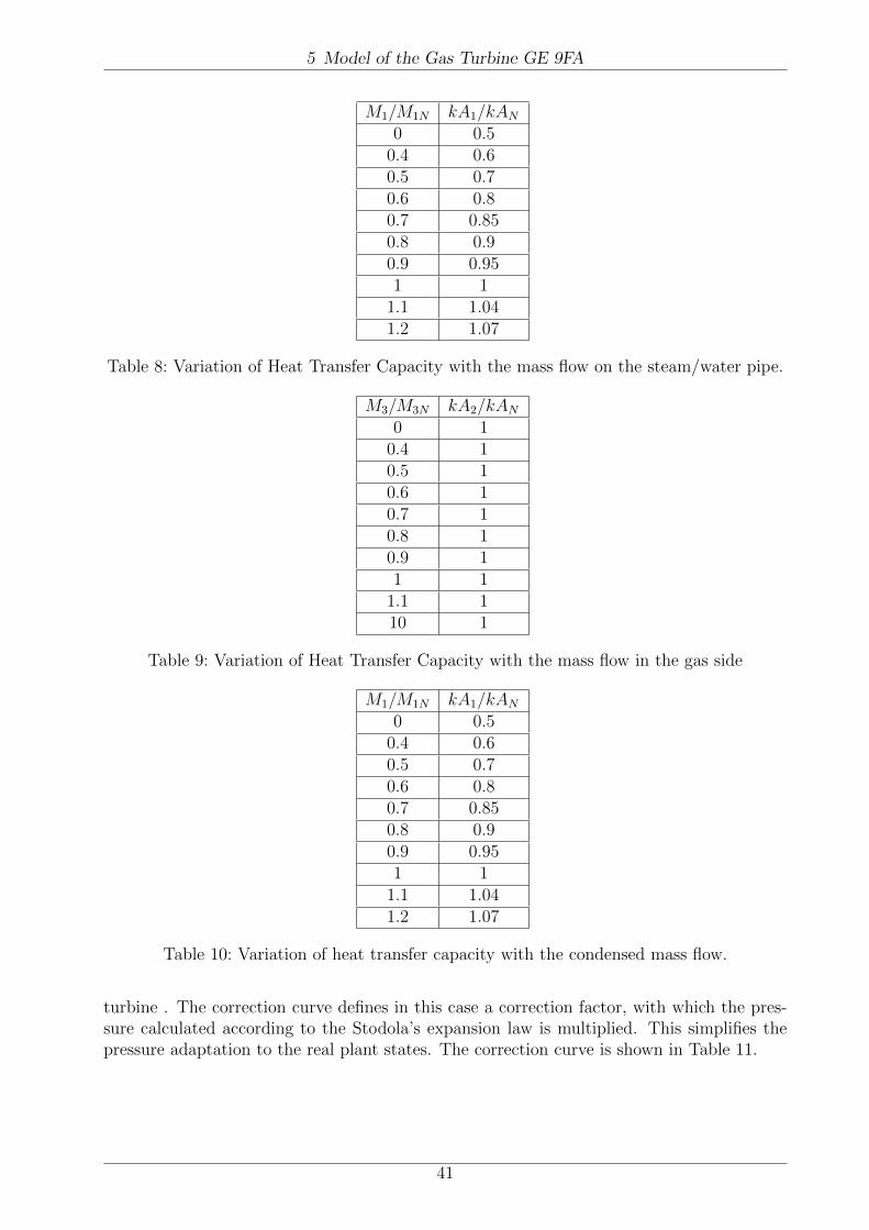
The heat transfer capacity of a heat exchanger variates with the change in mass flow troughthe heat exchanger. The transfer surfaces in the heat exchanger are defined in design condi-tions and remain constant in every mode of operation. The variation of the product of theheat transfer capacity and the transfer surface is defined by some default correction curvesimplemented in Ebsilon.
A heat exchanger is a component where two fluids transfer heat between them. The Figure5.8 shows a section of a heat exchanger in Ebsilon software. Independent of water or steam(1-2) the variation of the heat transfer capacity of the heat exchanger for each fluid is repre-sented in Table 8. In Table 9 the gas side (3-4) is represented. As we can see, it is assumedthat the heat transfer capacity remains constant in the gas pipe of the heat exchanger whenthe mode of operation is off-load.
Figure 5.8: Section of a heat exchanger in Ebsilon
Condenser
The heat transferred in the condenser also variates with the mode of operation. Although thecondenser is also a heat exchanger we only study the pipe in which the steam is condensedto water, the other pipe is not interesting because it is suppose that the condenser can use asmuch as it needs for condesing the steam. The Table 10 shows the variation of heat transfercapacity with the mass of steam condensed in off-load.
Steam Turbine
In steam turbine, the pressure variates in accordance with the Stodola’s law which defines avariation in pressure proportional to the variation of mass flow expanded through the steam
40
5 Model of the Gas Turbine GE 9FA
M1/M1N kA1/kAN0 0.5
0.4 0.60.5 0.70.6 0.80.7 0.850.8 0.90.9 0.951 1
1.1 1.041.2 1.07
Table 8: Variation of Heat Transfer Capacity with the mass flow on the steam/water pipe.
M3/M3N kA2/kAN0 1
0.4 10.5 10.6 10.7 10.8 10.9 11 1
1.1 110 1
Table 9: Variation of Heat Transfer Capacity with the mass flow in the gas side
M1/M1N kA1/kAN0 0.5
0.4 0.60.5 0.70.6 0.80.7 0.850.8 0.90.9 0.951 1
1.1 1.041.2 1.07
Table 10: Variation of heat transfer capacity with the condensed mass flow.
turbine . The correction curve defines in this case a correction factor, with which the pres-sure calculated according to the Stodola’s expansion law is multiplied. This simplifies thepressure adaptation to the real plant states. The correction curve is shown in Table 11.
41

6 Modeling a Single Pressure CCPP
M1/M1N P1/P1St0 1
0.2 10.4 10.5 10.6 10.7 10.8 10.9 11 1
1.1 11.2 1
Table 11: Stodola Correction for the Steam Turbine
6 Modeling a Single Pressure CCPP
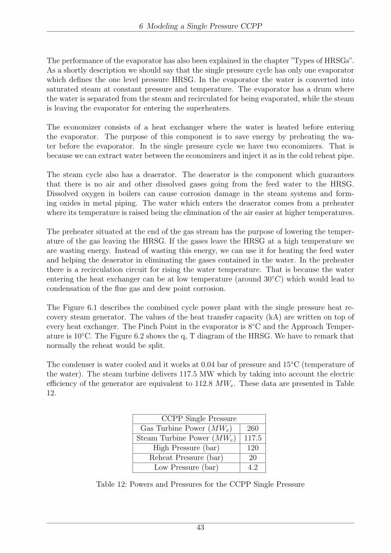
The simplest steam cycle consists of a steam turbine, a condenser, the heat exchangers ofthe one level pressure heat recovery steam generator and the pumps. This is the singlepressure cycle (1P) and the heat recovery steam generator consists of two economizers, theevaporator, two superheaters and one reheater.
The performances of the steam turbine and the condenser have been explained in the chap-ters ”Steam Cycle” and ”Types of Condensers”, but it is important to notice that in ourCCPP the steam turbine will have always three stages of expansion although the HRSG hasonly a single pressure level. The reason of three stages in the steam turbine is because wehave reheat and a deaerator and we need some opening point for taking the steam. In thereheat the steam goes again through a heat exchanger where it is heated and recovers itsenergy and the deaerator needs to extract some steam from the steam turbine at low pressure.
By superheating the steam leaving the evaporator we ensure that the saturated steam con-verts into dry steam and there is no water droplets in the steam flow. The superheater alsorises the steam temperature at the inlet of the steam turbine which allow us to obtain morepower output.
The reason of having two superheaters in the HRGS is because we need to control the tem-perature. Feed water is injected for controlling the superheat temperature. Although thepipe connection is made in the cycle, we will not use the feed water injection for controllingthe superheater temperature in the modeling of the one pressure CCPP. This temperaturewill be controlled in our model by using the settings in the components.
The reheat process has been explained in the chapter ”Improvements for increasing thework output” of the gas turbine. The pipe which enters the reheater is called the cold reheatpipe. In this pipe there is another connection for injecting feed water in case we want tocontrol the reheat temperature. As in the case of superheaters we will not use it, being themass flow through the pipe 0 kg/s. The reheat temperature will be controlled by using thesetting in the reheater pipes.
42
6 Modeling a Single Pressure CCPP
The performance of the evaporator has also been explained in the chapter ”Types of HRSGs”.As a shortly description we should say that the single pressure cycle has only one evaporatorwhich defines the one level pressure HRSG. In the evaporator the water is converted intosaturated steam at constant pressure and temperature. The evaporator has a drum wherethe water is separated from the steam and recirculated for being evaporated, while the steamis leaving the evaporator for entering the superheaters.
The economizer consists of a heat exchanger where the water is heated before enteringthe evaporator. The purpose of this component is to save energy by preheating the wa-ter before the evaporator. In the single pressure cycle we have two economizers. That isbecause we can extract water between the economizers and inject it as in the cold reheat pipe.
The steam cycle also has a deaerator. The deaerator is the component which guaranteesthat there is no air and other dissolved gases going from the feed water to the HRSG.Dissolved oxygen in boilers can cause corrosion damage in the steam systems and form-ing oxides in metal piping. The water which enters the deaerator comes from a preheaterwhere its temperature is raised being the elimination of the air easier at higher temperatures.
The preheater situated at the end of the gas stream has the purpose of lowering the temper-ature of the gas leaving the HRSG. If the gases leave the HRSG at a high temperature weare wasting energy. Instead of wasting this energy, we can use it for heating the feed waterand helping the deaerator in eliminating the gases contained in the water. In the preheaterthere is a recirculation circuit for rising the water temperature. That is because the waterentering the heat exchanger can be at low temperature (around 30◦C) which would lead tocondensation of the flue gas and dew point corrosion.
The Figure 6.1 describes the combined cycle power plant with the single pressure heat re-covery steam generator. The values of the heat transfer capacity (kA) are written on top ofevery heat exchanger. The Pinch Point in the evaporator is 8◦C and the Approach Temper-ature is 10◦C. The Figure 6.2 shows the q, T diagram of the HRSG. We have to remark thatnormally the reheat would be split.
The condenser is water cooled and it works at 0.04 bar of pressure and 15◦C (temperature ofthe water). The steam turbine delivers 117.5 MW which by taking into account the electricefficiency of the generator are equivalent to 112.8 MWe. These data are presented in Table12.
CCPP Single PressureGas Turbine Power (MWe) 260
Steam Turbine Power (MWe) 117.5High Pressure (bar) 120
Reheat Pressure (bar) 20Low Pressure (bar) 4.2
Table 12: Powers and Pressures for the CCPP Single Pressure
43

6 Modeling a Single Pressure CCPP
GM
M
G
GE
Turb
ine 9
FA
50H
z
1P
HR
SG
ISO
Conditio
ns
1.2
MW
/K0
.8M
W/K
0.2
MW
/K0
.2M
W/K
0.2
MW
/K0
.4M
W/K
2.1
MW
/K
17
.00
0
12
78
.07
7 1
51
4.1
60
6
41
.00
0
Pb
ar
T°C
H
kJ/k
g
Mkg/s
260017.6
90 k
W
270851.7
61 k
W
1.0
10 b
ar
468
.79
3 °
C
1.0
11 b
ar
519
.79
6 °
C
1.0
10
ba
r 3
36.4
32
°C
1.0
09
bar
26
7.7
87 °
C
1.0
08 b
ar
245
.347
°C
1.0
07 b
ar
190
.024
°C
1.0
12 b
ar
572
.04
0 °
C
4.2
00 b
ar
14
5.3
54 °
C
120.000
542.000
3460.975
78.441
21.0
00
bar
298
.93
8 °
C
0.0
40
2
8.9
62
2
37
8.6
13
7
8.4
37
1.0
53
ba
r 2
3.9
62 °
C
1.1
03
ba
r 1
5.0
00 °
C
6.7
00
ba
r 2
9.0
16 °
C
20.000
514.796
3500.782
78.441
4.200
308.656
3084.401
0.004
117555.0
33 k
W
122453.1
59 k
W
123
.00
0 b
ar
439
.04
0 °
C
6.700
77.345
324.311
133.437
4.700
145.347
612.219
133.437
4.2
00 b
ar
14
5.3
80 °
C
13
0.0
00 b
ar
14
7.4
87 °
C
12
8.0
00
1
93.7
87
82
9.6
80
7
8.4
41
126
.00
0
318
.43
2
14
48
.95
8
0.0
00
1
28
.00
0
19
3.7
87
82
9.6
80
0
.00
0
12
6.0
00
3
28
.43
2
26
72
.207
7
8.4
41
17
.00
2
15
.00
0 3
2.6
81
1
3.9
26
17
.00
2
42
0.7
10
43
6.3
34
6
27
.07
4
1.0
13
1
5.0
00
1
5.1
55
6
27
.07
4
Fig
ure
6.1:
CC
PP
wit
ha
Sin
gle
Pre
ssure
HR
SG
44
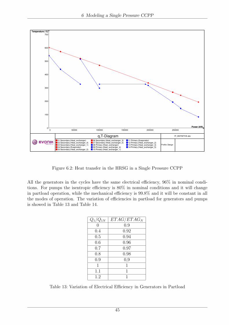
6 Modeling a Single Pressure CCPP
q,T-Diagram 1P_DEFINITIVE.ebs
Profile: Design
01 Secondary (Heat_exchanger) 02 Secondary (Heat_exchanger_4) 03 Secondary (Heat_exchanger_1) 04 Secondary (Evaporator) 05 Secondary (Heat_exchanger_2)
06 Secondary (Heat_exchanger_3) 07 Secondary (Heat_exchanger_5) 08 Primary (Heat_exchanger) 09 Primary (Heat_exchanger_4) 10 Primary (Heat_exchanger_1)
11 Primary (Evaporator) 12 Primary (Heat_exchanger_2) 13 Primary (Heat_exchanger_3) 14 Primary (Heat_exchanger_5)
Temperature (°C)
0
100
200
300
400
500
600
700
Power (kW)
0 50000 100000 150000 200000 250000
Figure 6.2: Heat transfer in the HRSG in a Single Pressure CCPP
All the generators in the cycles have the same electrical efficiency, 96% in nominal condi-tions. For pumps the isentropic efficiency is 80% in nominal conditions and it will changein partload operation, while the mechanical efficiency is 99.8% and it will be constant in allthe modes of operation. The variation of efficiencies in partload for generators and pumpsis showed in Table 13 and Table 14.
Q1/Q1N ETAG/ETAGN
0 0.90.4 0.920.5 0.940.6 0.960.7 0.970.8 0.980.9 0,91 1
1.1 11.2 1
Table 13: Variation of Electrical Efficiency in Generators in Partload
45

7 Modeling a Two Pressure CCPP
M1/M1N ETAI/ETAIN0 0.92
0.6 0.940.7 0.960.8 0.981 1
1.1 0.98
Table 14: Variation of Isentropic Efficiency in Pumps in Partload
7 Modeling a Two Pressure CCPP
By dividing the heat transfer process in the heat recovery steam generator in two stages,we have now two evaporators, one for high pressure and other for the low pressure. Thenew HRSG is composed of two superheaters at high pressure and one superheater at lowpressure, two reheaters at the reheat pressure and two evaporators. The low pressure evap-orator has one economizer, while the high pressure evaporator has two. We also have in thiscycle the preheater at the end of the gas flow and the steam turbine is divided in three stages.
The feed water, after being preheated and leaving the deaerator, is divided in two pipesand pumped to the different pressure levels. Approximately, the 13% of the water goes toone economizer and then to the low pressure evaporator. After being evaporated and con-verted in saturated steam is injected in the cold reheat pipe acting as cooling steam in thereheat process. The 87% of the water goes first through two economizers and then is evap-orated in the high pressure evaporator. This process needs two economizers before reachingan adequate temperature for entering the evaporator.
In the new HRSG we have the two superheaters with the water injection between them,as in the case of a single pressure CCPP. The reheat process is divided in two stages withthe water injection in between. In the cold reheat pipe saturated steam at low pressure isadded for cooling and between the two reheaters water is injected. As in the single pressureprocess we are not injecting spray water.
CCPP Two PressuresGas Turbine Power (MWe) 260
Steam Turbine Power (MWe) 124.4High Pressure (bar) 120
Reheat Pressure (bar) 32Low Pressure (bar) 5.1
Table 15: Power and Pressures for the CCPP Two Pressures
46
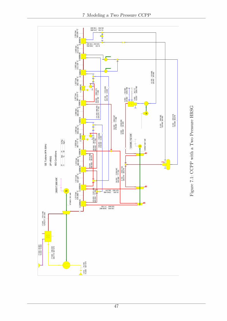
7 Modeling a Two Pressure CCPP
G
G
M
GE
Tu
rbin
e 9
FA
50
Hz
2P
HR
SG
ISO
Co
nd
itio
ns
0.2
MW
/K0.4
MW
/K0.3
MW
/K0.1
MW
/K1.1
MW
/K0.1
MW
/K0.1
MW
/K0.6
MW
/K0.3
MW
/K2.1
MW
/K1.1
MW
/K
34
.000
3
50.3
88
310
8.0
45
77.7
93
0.0
40
28
.962
2
336
.836
8
4.4
65
5
.10
0
29
4.5
74
30
53
.12
6
89
.27
9
120.000
533.900
3439.887
77.793
12
9.2
00
31
8.5
39
144
8.9
58
0.0
00
47
.100
2
34.1
49
101
0.0
06
0.0
00
12
6.0
00
32
8.4
32
26
72
.207
7
7.7
93
33.0
00
3
92
.98
3
32
10
.282
8
9.2
79
1
23.0
00
44
5.5
50
319
1.4
89
77.7
93
1.0
11 b
ar
537.2
87 °
C
1.0
12 b
ar
576.4
89 °
C
1.0
10 b
ar
482.9
83 °
C
1.0
09 b
ar
467.7
17 °
C
1.0
09 b
ar
336.4
32 °
C
1.0
08
bar
283.4
69 °
C
1.0
07 b
ar
281.5
18 °
C
1.0
07 b
ar
252.1
86 °
C
1.0
05 b
ar
212.1
29 °
C
1.0
05 b
ar
212.1
29 °
C
1.0
04 b
ar
165.2
36 °
C 10.100
65.259
273.980
139.465
8.100
120.442
506.092
139.465
10
.10
0
29
.04
3
12
2.6
66
84
.46
5
5.1
00
12
0.4
92 5
06.0
92
84
.465
5.1
00
15
2.5
84 6
43.4
18
89
.279
13
1.2
00
2
24.2
75
96
6.3
00
7
7.7
93
36
.000
2
44.1
86
280
2.4
70
11.4
86
32.000
537.955
3540.486
89.279
0.9
50
2
3.9
62
1
00
.580
3
20
0.7
88
1.0
00
1
0.0
00
42
.117
3
200
.788
17
.00
0
12
78
.077
151
4.1
60
641
.000
17
.002
1
5.0
00
32.6
81
13.9
26
17
.002
4
20.7
10 4
36.3
34
62
7.0
74
1.0
13
15
.000
1
5.1
55
6
27
.07
4
34.0
00
278
.265
2
922
.087
1
1.4
86
Pbar
T°C
H
kJ/k
g
Mkg/s
260017.6
90 k
W
124385.1
52 k
W
27
08
51
.76
1 k
W
12
95
67
.86
7 k
W
Fig
ure
7.1:
CC
PP
wit
ha
Tw
oP
ress
ure
HR
SG
47
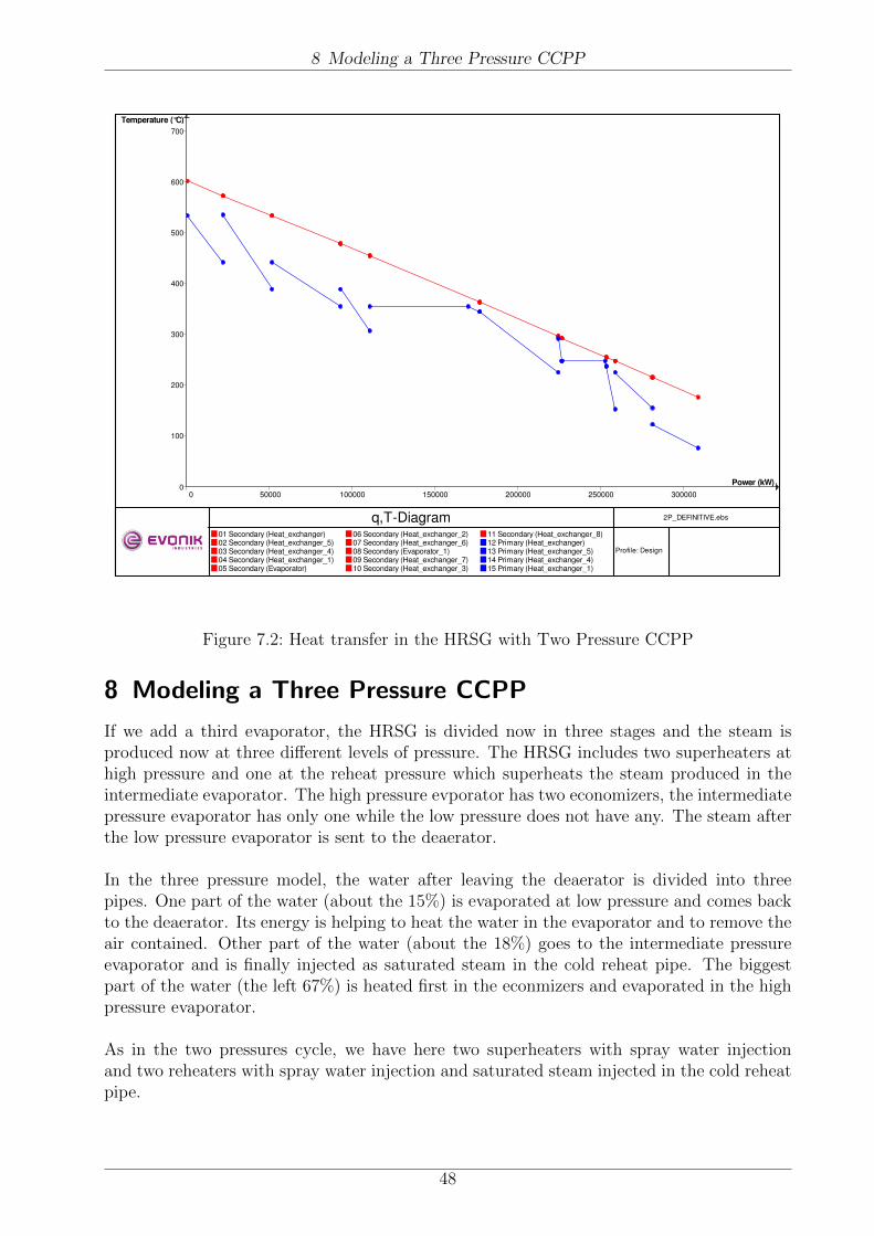
8 Modeling a Three Pressure CCPP
q,T-Diagram 2P_DEFINITIVE.ebs
Profile: Design
01 Secondary (Heat_exchanger) 02 Secondary (Heat_exchanger_5) 03 Secondary (Heat_exchanger_4) 04 Secondary (Heat_exchanger_1) 05 Secondary (Evaporator)
06 Secondary (Heat_exchanger_2) 07 Secondary (Heat_exchanger_6) 08 Secondary (Evaporator_1) 09 Secondary (Heat_exchanger_7) 10 Secondary (Heat_exchanger_3)
11 Secondary (Heat_exchanger_8) 12 Primary (Heat_exchanger) 13 Primary (Heat_exchanger_5) 14 Primary (Heat_exchanger_4) 15 Primary (Heat_exchanger_1)
Temperature (°C)
0
100
200
300
400
500
600
700
Power (kW)
0 50000 100000 150000 200000 250000 300000
Figure 7.2: Heat transfer in the HRSG with Two Pressure CCPP
8 Modeling a Three Pressure CCPP
If we add a third evaporator, the HRSG is divided now in three stages and the steam isproduced now at three different levels of pressure. The HRSG includes two superheaters athigh pressure and one at the reheat pressure which superheats the steam produced in theintermediate evaporator. The high pressure evporator has two economizers, the intermediatepressure evaporator has only one while the low pressure does not have any. The steam afterthe low pressure evaporator is sent to the deaerator.
In the three pressure model, the water after leaving the deaerator is divided into threepipes. One part of the water (about the 15%) is evaporated at low pressure and comes backto the deaerator. Its energy is helping to heat the water in the evaporator and to remove theair contained. Other part of the water (about the 18%) goes to the intermediate pressureevaporator and is finally injected as saturated steam in the cold reheat pipe. The biggestpart of the water (the left 67%) is heated first in the econmizers and evaporated in the highpressure evaporator.
As in the two pressures cycle, we have here two superheaters with spray water injectionand two reheaters with spray water injection and saturated steam injected in the cold reheatpipe.
48

8 Modeling a Three Pressure CCPP
In our three pressures model appears as well an extra circuit designed for injecting solarboosting in the CCPP. This circuit is not in operation in this model and its performancewill be explained later.
8.1 Performance of Three Pressure CCPP in ISO Conditions
Table 16 presents the results obtained for the Three Pressure CCPP working at the condi-tions for which it was designed.
CCPP Three PressuresGas Turbine Power (MWe) 260
Steam Turbine Power (MWe) 138.5High Pressure (bar) 155
Reheat Pressure (bar) 32Low Pressure (bar) 4.7
Table 16: Power and Pressures for the CCPP Three Pressures
Comparing the results for the final electric power delivered to the net, the three pressurecycle produces more power than the other two cycles. This is a consequence of having abigger HRSG which transfers more power to the steam cycle generating more steam andincreasing the efficiency of the cycle.
8.2 Performance of Three Pressure CCPP with Changing AmbientTemperature
As we have explained for the gas turbine, its offload performance changes when the ambienttemperature changes. The steam-water cycle depends on the exhaust gases of the gas turbineso its performance will change as well.
We will study the same cases studied for the gas turbine, at three different temperatures:0◦C, 30◦C and 45◦C.
Working in an ambient temperature lower than the design temperature causes an incrementof efficiency of the gas turbine due to the higher density of the air which enables acceptingmore air into the compressor. However, the exhaust temperature of the gases is lower andwith it the energy available in the gas stream for heating the water/steam in the HRSG.That means that although the gas turbine power output increases, the steam turbine poweroutput decreases.
All the settings of the components in the steam/water cycle remain constant except in
49
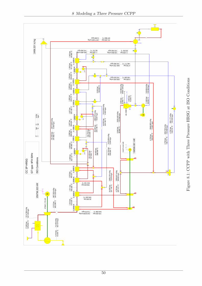
8 Modeling a Three Pressure CCPP
G
G
M
-
CC
3P
-HR
SG
GT
typ
e:
9F
A 5
0H
z
IS
O C
onditio
ns
0.2
MW
/K0.3
MW
/K0.3
MW
/K0.3
MW
/K1.1
MW
/K0.1
MW
/K0.1
MW
/K1.0
MW
/K0.1
MW
/K3.1
MW
/K
26
.1M
W/K
1.3
MW
/K1
.9M
W/K
1.3
MW
/K
24
56
.22
1 k
J/k
g
25
97
96
.32
3 k
W
1.0
13
bar
60
2.2
96 °
C
667.3
03 k
J/k
g
641.0
00 k
g/s
17.0
00 b
ar
127
8.5
54 °
C
15
14.7
84 k
J/k
g
64
1.0
00 k
g/s
1.0
10 b
ar
15
.000
°C
1
5.1
55
kJ/k
g
62
7.0
74 k
g/s
1.0
12
bar
573.5
35 °
C
1.0
11 b
ar
546
.428
°C
1.0
10 b
ar
49
3.3
37 °
C
155.000 bar
540.296 °C
3418.506 kJ/kg
72.975 kg/s
1.0
09
bar
457.1
37 °
C
1.0
09 b
ar
355
.862
°C
1.0
08
bar
29
8.0
99 °
C
1.0
07 b
ar
29
4.6
34 °
C
1.0
07 b
ar
252
.186
°C
1.0
06 b
ar
243
.273
°C
1
.005 b
ar
20
6.0
45 °
C
1.0
04 b
ar
20
4.0
55 °
C
1.0
04
bar
16
1.3
20 °
C
1.0
03
bar
84
.98
5 °
C
34.0
00 b
ar
321.1
45 °
C
303
6.1
53 k
J/k
g
72.9
75 k
g/s
4.7
00
bar
287.4
10 °
C
303
9.4
01 k
J/k
g
89.6
22 k
g/s
0
.04
0 b
ar
28.9
62 °
C
23
23.4
40
kJ/k
g
10
3.3
62 k
g/s
4.700 bar
148.717 °C
626.722 kJ/kg
103.362 kg/s
36.0
00 b
ar
244
.186
°C
2
802.4
70 k
J/k
g
16
.647
kg/s
5.200 bar
149.528 °C
630.245 kJ/kg
103.523 kg/s
11.200 bar
62.727 °C
263.480 kJ/kg
143.362 kg/s
11.2
00 b
ar
29.0
52 °
C
122.8
04 k
J/k
g
103.3
62 k
g/s
4.7
00 b
ar
14
8.7
17 °
C
62
6.7
22 k
J/k
g
10
3.3
62 k
g/s
4.7
00
bar
149.5
19 °
C
630
.177
kJ/k
g
103
.523
kg/s
161.000 bar
347.862 °C
2577.625 kJ/kg
0.000 kg/s
161
.000
bar
347
.862
°C
2
577.6
25 k
J/k
g
0.0
00 k
g/s
44.0
00 b
ar
234.1
60 °
C
101
0.0
06 k
J/k
g
0.0
00 k
g/s
4.7
00 b
ar
19
6.0
45 °
C
2848
.99
5 k
J/k
g
13.9
01 k
g/s
13
85
99
.08
1 k
W
Pbar
T°C
H
kJ/k
g
Mkg/s
1.0
00
bar
15
.00
0 °
C
0.9
50 b
ar
23.9
62 °
C
10
0.5
80 k
J/k
g
60
69.1
28 k
g/s
158.000 bar
443.194 °C
32.000 bar
540.255 °C
34.0
00 b
ar
288.0
99 °
C
161.0
00 b
ar
347.8
62 °
C
16
6.7
00 b
ar
23
3.0
09 °
C
16
4.7
00 b
ar
33
8.0
66 °
C
157
0.6
24 k
J/k
g
0.0
00 k
g/s
5.2
00
bar
14
9.5
28 °
C
11.200 bar
29.052 °C
122.804 kJ/kg
103.362 kg/s
27
06
21
.17
0 k
W
14
43
74
.04
2 k
W
Fig
ure
8.1:
CC
PP
wit
hT
hre
eP
ress
ure
HR
SG
atIS
OC
ondit
ions
50

8 Modeling a Three Pressure CCPP
q,T-Diagram 3P_SOLAR_v2_difftemp.ebs
Profile: Design
01 Secondary (Heat_exchanger) 02 Secondary (Heat_exchanger_5) 03 Secondary (Heat_exchanger_4) 04 Secondary (Heat_exchanger_1) 05 Secondary (Evaporator)
06 Secondary (Heat_exchanger_2) 07 Secondary (Heat_exchanger_6) 08 Secondary (Evaporator_1) 09 Secondary (Heat_exchanger_7) 10 Secondary (Heat_exchanger_3)
11 Secondary (Heat_exchanger_9) 12 Secondary (Evaporator_2) 13 Secondary (Heat_exchanger_8) 14 Primary (Heat_exchanger) 15 Primary (Heat_exchanger_5)
Temperature (°C)
0
100
200
300
400
500
600
700
Power (kW)
0 50000 100000 150000 200000 250000 300000 350000
Figure 8.2: Heat transfer in the HRSG with Three Pressure CCPP at ISO Conditions
the condenser, where the cooling water suffers a variation in temperature at the same timethat the ambient temperature changes. In this case, when the ambient temperature is 0◦C,we suppose the sea water has a temperature of 10◦C.
Cases Gas Turbine Power Steam Turbine Power msteam (kg/s) mgas (kg/s)ISO 260 MWe 138.5 MWe 72.9 6410 ◦C 318.6 MWe 134.6 MWe 70.4 67730 ◦C 213.3 MWe 122.5 MWe 69.2 608.545 ◦C 183.6 MWe 115.4 MWe 66.9 588.4
Table 17: Comparison between the Partload Performance and Design Performance
The Table 17 shows the power and mass fluctuation when the ambient temperature changes.As we can see, although the gas turbine delivers more power when the ambient temperatureis lower, the steam turbine always has its maximum power at design conditions. The closerto ISO conditions the higher power delivered.
51

8 Modeling a Three Pressure CCPP
G
G
M
-
CC
3P
-HR
SG
GT
type:
9F
A 5
0H
z
Atm
ospheric T
em
pera
ture
: 0 º
C
0.2
MW
/K0.3
MW
/K0.3
MW
/K0.3
MW
/K1.1
MW
/K0.1
MW
/K0.1
MW
/K1.0
MW
/K0.1
MW
/K3.3
MW
/K
26
.1M
W/K
1.3
MW
/K2
.0M
W/K
1.3
MW
/K
25
02
.47
6 k
J/k
g
31
86
34
.20
9 k
W
1.0
13
bar
57
3.0
43 °
C
634.2
89 k
J/k
g
677.0
18 k
g/s
17.9
55 b
ar
127
8.0
77 °
C
15
18.4
09 k
J/k
g
67
7.0
18 k
g/s
1.0
13 b
ar
0.0
00 °
C
-7.2
44 k
J/k
g
66
1.5
28 k
g/s
1.0
12
bar
549.7
47 °
C
1.0
11 b
ar
526
.588
°C
1.0
10 b
ar
48
1.3
21 °
C
147.597 bar
520.046 °C
3370.819 kJ/kg
70.436 kg/s
1.0
09
bar
447.4
25 °
C
1.0
09 b
ar
351
.959
°C
1.0
07
bar
30
0.4
70 °
C
1.0
06 b
ar
29
6.7
54 °
C
1.0
06 b
ar
252
.440
°C
1.0
05 b
ar
243
.279
°C
1.0
04 b
ar
20
8.4
85 °
C
1.0
03 b
ar
20
6.3
64 °
C
1.0
03
bar
16
1.9
42 °
C
1.0
02
bar
94
.43
6 °
C
33.2
56 b
ar
309.0
18 °
C
300
7.4
47 k
J/k
g
70.4
36 k
g/s
4.5
81
bar
272.1
65 °
C
300
8.3
21 k
J/k
g
88.7
59 k
g/s
0
.02
9 b
ar
23.6
29 °
C
22
78.8
66
kJ/k
g
10
1.9
34 k
g/s
4.581 bar
137.894 °C
580.241 kJ/kg
101.934 kg/s
35.6
74 b
ar
243
.661
°C
2
802.5
65 k
J/k
g
18
.323
kg/s
5.184 bar
148.577 °C
626.147 kJ/kg
104.033 kg/s
13.753 bar
86.052 °C
361.395 kJ/kg
222.934 kg/s
13.7
53 b
ar
23.7
36 °
C
100.8
27 k
J/k
g
101.9
34 k
g/s
4.5
81 b
ar
13
7.8
94 °
C
58
0.2
41 k
J/k
g
10
1.9
34 k
g/s
4.5
81
bar
148.5
67 °
C
626
.065
kJ/k
g
104
.033
kg/s
153.198 bar
343.850 °C
2601.582 kJ/kg
0.000 kg/s
153
.198
bar
343
.850
°C
2
601.5
82 k
J/k
g
0.0
00 k
g/s
45.3
16 b
ar
232.4
58 °
C
100
2.0
37 k
J/k
g
0.0
00 k
g/s
4.5
81 b
ar
19
6.9
70 °
C
2851
.59
9 k
J/k
g
15.2
74 k
g/s
13
46
19
.16
7 k
W
Pbar
T°C
H
kJ/k
g
Mkg/s
1.0
00
bar
10
.00
0 °
C
0.9
50 b
ar
18.7
43 °
C
78
.745
kJ/k
g
60
66.2
11 k
g/s
150.397 bar
435.130 °C
31.292 bar
520.139 °C
33.2
56 b
ar
288.8
88 °
C
153.1
98 b
ar
343.8
50 °
C
15
8.5
07 b
ar
23
3.8
91 °
C
15
6.6
40 b
ar
33
6.4
42 °
C
156
1.9
04 k
J/k
g
0.0
00 k
g/s
5.1
84
bar
14
8.5
77 °
C
13.753 bar
23.736 °C
100.827 kJ/kg
101.934 kg/s
33
19
10
.63
4 k
W
14
13
30
.76
5 k
W
Fig
ure
8.3:
Thre
eP
ress
ure
CC
PP
at0◦
C
52

8 Modeling a Three Pressure CCPP
G
G
M
-
CC
3P
-HR
SG
GT
typ
e: 9F
A 5
0H
z
Atm
ospheri
c T
em
pera
ture
: 30 º
C
0.2
MW
/K0.3
MW
/K0.3
MW
/K0.3
MW
/K1.1
MW
/K0.1
MW
/K0.1
MW
/K1.0
MW
/K0.1
MW
/K3.3
MW
/K
26
.1M
W/K
1.3
MW
/K1
.8M
W/K
1.2
MW
/K
24
39
.87
6 k
J/k
g
21
32
91
.93
4 k
W
1.0
13
bar
60
2.3
02 °
C
665.4
91 k
J/k
g
608.4
69 k
g/s
16.0
11 b
ar
125
3.9
64 °
C
14
78.0
70 k
J/k
g
60
8.4
69 k
g/s
1.0
10 b
ar
30
.000
°C
3
0.3
17
kJ/k
g
59
6.0
30 k
g/s
1.0
12
bar
574.4
56 °
C
1.0
11 b
ar
547
.592
°C
1.0
10 b
ar
49
3.4
10 °
C
148.281 bar
545.693 °C
3440.620 kJ/kg
69.240 kg/s
1.0
09
bar
457.5
44 °
C
1.0
09 b
ar
351
.937
°C
1.0
08
bar
29
4.3
40 °
C
1.0
08 b
ar
29
0.9
31 °
C
1.0
08 b
ar
248
.449
°C
1.0
07 b
ar
239
.615
°C
1.0
06 b
ar
20
2.5
76 °
C
1.0
05 b
ar
20
0.6
23 °
C
1.0
05
bar
15
8.2
02 °
C
1.0
04
bar
94
.52
7 °
C
32.1
94 b
ar
325.6
29 °
C
305
2.1
75 k
J/k
g
69.2
40 k
g/s
4.4
06
bar
289.5
68 °
C
304
4.6
36 k
J/k
g
84.8
91 k
g/s
0
.06
7 b
ar
38.2
54 °
C
23
96.1
67
kJ/k
g
96
.538
kg/s
4.406 bar
139.794 °C
588.368 kJ/kg
96.538 kg/s
33.9
58 b
ar
240
.830
°C
2
802.9
73 k
J/k
g
15
.652
kg/s
4.843 bar
147.137 °C
619.927 kJ/kg
97.904 kg/s
11.544 bar
86.458 °C
362.927 kJ/kg
182.538 kg/s
11.5
44 b
ar
38.3
57 °
C
161.6
96 k
J/k
g
96.5
38 k
g/s
4.4
06 b
ar
13
9.7
94 °
C
58
8.3
68 k
J/k
g
96
.538
kg/s
4.4
06
bar
147.1
30 °
C
619
.868
kJ/k
g
97.9
04 k
g/s
153.693 bar
344.110 °C
2600.118 kJ/kg
0.000 kg/s
153
.693
bar
344
.110
°C
2
600.1
18 k
J/k
g
0.0
00 k
g/s
40.9
88 b
ar
231
.672
°C
9
98
.279
kJ/k
g
0.0
00 k
g/s
4.4
06 b
ar
19
3.4
38 °
C
2845
.00
5 k
J/k
g
13.0
13 k
g/s
12
24
94
.15
7 k
W
Pbar
T°C
H
kJ/k
g
Mkg/s
1.0
00
bar
25
.00
0 °
C
0.9
50 b
ar
33.5
13 °
C
14
0.5
11 k
J/k
g
60
66.2
11 k
g/s
150.987 bar
448.883 °C
30.397 bar
543.041 °C
32.1
94 b
ar
285.3
34 °
C
153.6
93 b
ar
344.1
10 °
C
15
8.8
00 b
ar
22
9.9
63 °
C
15
6.9
96 b
ar
33
5.2
41 °
C
155
3.0
26 k
J/k
g
0.0
00 k
g/s
4.8
43
bar
14
7.1
37 °
C
11.544 bar
38.357 °C
161.696 kJ/kg
96.538 kg/s
22
85
53
.20
4 k
W
13
01
11
.26
5 k
W
Fig
ure
8.4:
Thre
eP
ress
ure
CC
PP
at30
◦ C
53
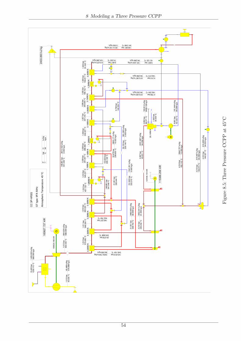
8 Modeling a Three Pressure CCPP
G
G
M
-
CC
3P
-HR
SG
GT
typ
e: 9F
A 5
0H
z
Atm
ospheri
c T
em
pera
ture
: 45 º
C
0.2
MW
/K0.3
MW
/K0.3
MW
/K0.3
MW
/K1.1
MW
/K0.1
MW
/K0.1
MW
/K0.9
MW
/K0.1
MW
/K3.0
MW
/K
26
.1M
W/K
1.2
MW
/K1
.8M
W/K
1.2
MW
/K
24
33
.89
3 k
J/k
g
18
36
27
.72
7 k
W
1.0
13
bar
60
2.3
30 °
C
664.0
24 k
J/k
g
588.3
95 k
g/s
15.4
05 b
ar
123
9.1
15 °
C
14
55.0
53 k
J/k
g
58
8.3
95 k
g/s
1.0
10 b
ar
45
.000
°C
4
5.4
88
kJ/k
g
57
6.9
88 k
g/s
1.0
12
bar
575.0
83 °
C
1.0
11 b
ar
548
.304
°C
1.0
10 b
ar
49
3.3
22 °
C
143.812 bar
549.164 °C
3454.749 kJ/kg
66.938 kg/s
1.0
10
bar
457.7
25 °
C
1.0
10 b
ar
349
.237
°C
1.0
09
bar
29
1.8
47 °
C
1.0
08 b
ar
28
8.4
82 °
C
1.0
08 b
ar
246
.027
°C
1.0
07 b
ar
237
.316
°C
1.0
06 b
ar
20
0.6
50 °
C
1.0
05 b
ar
19
8.7
42 °
C
1.0
05
bar
15
6.8
17 °
C
1.0
05
bar
91
.24
5 °
C
31.0
51 b
ar
328.7
02 °
C
306
2.6
55 k
J/k
g
66.9
38 k
g/s
4.3
10
bar
293.2
42 °
C
305
2.4
41 k
J/k
g
81.9
59 k
g/s
0
.08
7 b
ar
43.0
31 °
C
24
31.6
87
kJ/k
g
94
.296
kg/s
4.310 bar
146.015 °C
615.067 kJ/kg
94.296 kg/s
32.6
79 b
ar
238
.650
°C
2
803.1
71 k
J/k
g
15
.022
kg/s
4.708 bar
146.334 °C
616.463 kJ/kg
94.353 kg/s
9.801 bar
74.030 °C
310.670 kJ/kg
134.296 kg/s
9.8
01
bar
43.1
23 °
C
181.4
44 k
J/k
g
94.2
96 k
g/s
4.3
10 b
ar
14
6.0
15 °
C
61
5.0
67 k
J/k
g
94
.296
kg/s
4.3
10
bar
146.3
27 °
C
616
.409
kJ/k
g
94.3
53 k
g/s
148.861 bar
341.548 °C
2614.102 kJ/kg
0.000 kg/s
148
.861
bar
341
.548
°C
2
614.1
02 k
J/k
g
0.0
00 k
g/s
39.1
53 b
ar
230
.144
°C
9
91
.095
kJ/k
g
0.0
00 k
g/s
4.3
10 b
ar
19
2.1
15 °
C
2842
.70
7 k
J/k
g
12.3
93 k
g/s
11
53
88
.20
6 k
W
Pbar
T°C
H
kJ/k
g
Mkg/s
1.0
00
bar
30
.00
0 °
C
0.9
50 b
ar
38.3
71 °
C
16
0.8
14 k
J/k
g
60
69.1
28 k
g/s
146.337 bar
452.784 °C
29.378 bar
544.898 °C
31.0
51 b
ar
283.4
44 °
C
148.8
61 b
ar
341.5
48 °
C
15
3.6
03 b
ar
22
8.1
38 °
C
15
1.9
20 b
ar
33
3.3
10 °
C
154
1.0
51 k
J/k
g
0.0
00 k
g/s
4.7
08
bar
14
6.3
34 °
C
9.801 bar
43.123 °C
181.444 kJ/kg
94.296 kg/s
19
99
29
.19
8 k
W
12
34
36
.15
0 k
W
Fig
ure
8.5:
Thre
eP
ress
ure
CC
PP
at45
◦ C
54

9 Standard Three Pressure CCPP with Solar Boosting
9 Standard Three Pressure CCPP with Solar Boosting
The efficiency of the Rankine cycle increases with the steam pressure and the amount ofsteam expanding through the turbine. When the ambient temperature rises the mass flowexpanded through the gas turbine decreases and the energy available in the gas stream de-creases as well. For this reason the heat transferred in the HRSG is smaller. That generatesa smaller amount of steam in the HRSG and the power output of the steam turbine decreasesdue to the less mass of steam expanded.
At hot temperature conditions the overall efficiency of the CCPP decreases. Usually hottemperatures and sunny sky come together so if the location of our CCPP is in a placewhere the incident radiation of the Sun is enough for running a solar field, the energy whichthat field provides can help the electricity production in the CCPP. With a parabolic troughsystem installed next to the combined cycle plant, the incident radiation can be used as heatenergy into the Rankine cycle of the CCPP. With this energy the lack of input energy in theRankine cycle is compensated and the power output of the steam cycle increases.
That configuration, called Solar Boosting, is only possible when the Sun is shining andthe mass flow of steam going through the steam turbine is smaller than in design conditions.We consider a parabolic trough solar field next to the CCPP in which the steam is generateddirectly using a once through system. In the solar field the water is converted into saturatedsteam and injected in the Rankine cycle. In state of art technology the solar field wouldbe cooled by synthetic oil and the steam would be generated in an additional evaporator,see Figure 3.7. In this work we analyze an advanced system based on direct steam generation.
For modeling the solar boosting we have designed an extra circuit, shown in Figure 9.1.The water, after leaving the condenser, is pumped to the drum of the forced circulation solarsteam generator. The water evaporates into saturated steam and goes through the steamdrum. There, water in the mixture it is separated from the steam and recirculated in thesolar boosting cycle. The concentrator heat exchangers of the solar field are not simulatedin Ebsilon. Instead we use a ”boundary value component” for setting the solar heat added ineach case. We set a recirculation mass flow in the solar boosting circuit always higher thanten times the mass of saturated steam generated.
The amount of heat added is calculated as the heat necessary to heat the water from theconditions after leaving the condenser until saturated steam at high pressure. This specificheat is the difference between the enthalpy of the condensed water at high pressure andthe enthalpy of the steam generated in the high pressure evaporator. The specific heat ismultiplied by the mass flow added in each case getting the final value of heat added to thecycle.
There are four different possibilities for injecting the steam into the Rankine cycle dependingon the point of injection and the properties of the injected steam:
• Cold Reheated Steam: the steam is injected after the first expansion in the turbinebefore the reheat exchanger.
• Hot Reheated Steam: the steam is injected after the reheat, just before entering inthe second stage of the turbine.
55
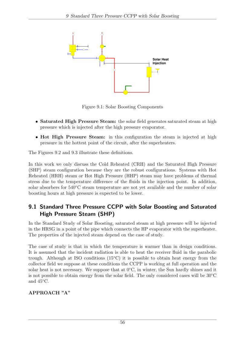
9 Standard Three Pressure CCPP with Solar Boosting
Solar Heat Injection
Figure 9.1: Solar Boosting Components
• Saturated High Pressure Steam: the solar field generates saturated steam at highpressure which is injected after the high pressure evaporator.
• Hot High Pressure Steam: in this configuration the steam is injected at highpressure in the hottest point of the circuit, after the superheaters.
The Figures 9.2 and 9.3 illustrate these definitions.
In this work we only discuss the Cold Reheated (CRH) and the Saturated High Pressure(SHP) steam configuration because they are the robust configurations. Systems with HotReheated (HRH) steam or Hot High Pressure (HHP) steam may have problems of thermalstress due to the temperature difference of the fluids in the injection point. In addition,solar absorbers for 540◦C steam temperature are not yet available and the number of solarboosting hours at high pressure is expected to be lower.
9.1 Standard Three Pressure CCPP with Solar Boosting and SaturatedHigh Pressure Steam (SHP)
In the Standard Study of Solar Boosting, saturated steam at high pressure will be injectedin the HRSG in a point of the pipe which connects the HP evaporator with the superheater.The properties of the injected steam depend on the case of study.
The case of study is that in which the temperature is warmer than in design conditions.It is assumed that the incident radiation is able to heat the receiver fluid in the parabolictrough. Although at ISO conditions (15◦C) it is possible to obtain heat energy from thecollector field we suppose at these conditions the CCPP is working at full operation and thesolar heat is not necessary. We suppose that at 0◦C, in winter, the Sun hardly shines and itis not possible to obtain energy from the solar field. The only considered cases will be 30◦Cand 45◦C.
APPROACH ”A”
56
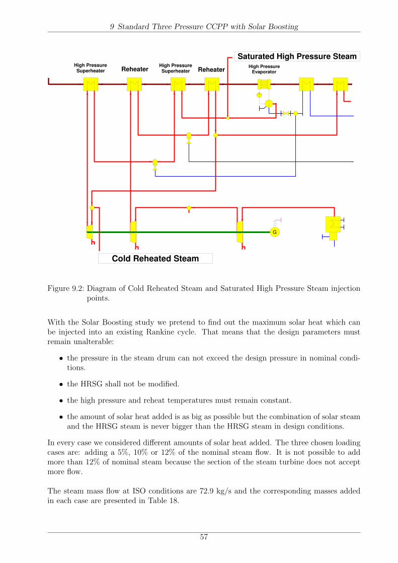
9 Standard Three Pressure CCPP with Solar Boosting
G
Saturated High Pressure SteamHigh PressureSuperheater
High PressureSuperheaterReheater Reheater
High PressureEvaporator
Cold Reheated Steam
Figure 9.2: Diagram of Cold Reheated Steam and Saturated High Pressure Steam injectionpoints.
With the Solar Boosting study we pretend to find out the maximum solar heat which canbe injected into an existing Rankine cycle. That means that the design parameters mustremain unalterable:
• the pressure in the steam drum can not exceed the design pressure in nominal condi-tions.
• the HRSG shall not be modified.
• the high pressure and reheat temperatures must remain constant.
• the amount of solar heat added is as big as possible but the combination of solar steamand the HRSG steam is never bigger than the HRSG steam in design conditions.
In every case we considered different amounts of solar heat added. The three chosen loadingcases are: adding a 5%, 10% or 12% of the nominal steam flow. It is not possible to addmore than 12% of nominal steam because the section of the steam turbine does not acceptmore flow.
The steam mass flow at ISO conditions are 72.9 kg/s and the corresponding masses addedin each case are presented in Table 18.
57
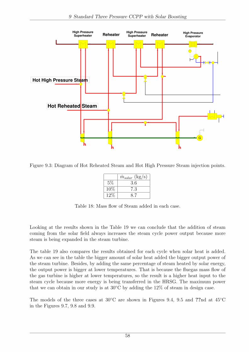
9 Standard Three Pressure CCPP with Solar Boosting
G
High PressureSuperheater
High PressureSuperheaterReheater Reheater
High PressureEvaporator
Hot Reheated Steam
Hot High Pressure Steam
Figure 9.3: Diagram of Hot Reheated Steam and Hot High Pressure Steam injection points.
msolar (kg/s)5% 3.610% 7.312% 8.7
Table 18: Mass flow of Steam added in each case.
Looking at the results shown in the Table 19 we can conclude that the addition of steamcoming from the solar field always increases the steam cycle power output because moresteam is being expanded in the steam turbine.
The table 19 also compares the results obtained for each cycle when solar heat is added.As we can see in the table the bigger amount of solar heat added the bigger output power ofthe steam turbine. Besides, by adding the same percentage of steam heated by solar energy,the output power is bigger at lower temperatures. That is because the fluegas mass flow ofthe gas turbine is higher at lower temperatures, so the result is a higher heat input to thesteam cycle because more energy is being transferred in the HRSG. The maximum powerthat we can obtain in our study is at 30◦C by adding the 12% of steam in design case.
The models of the three cases at 30◦C are shown in Figures 9.4, 9.5 and ??nd at 45◦Cin the Figures 9.7, 9.8 and 9.9.
58
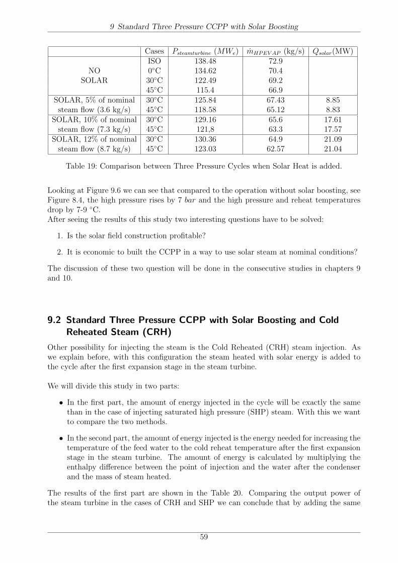
9 Standard Three Pressure CCPP with Solar Boosting
Cases Psteamturbine (MWe) mHPEV AP (kg/s) Qsolar(MW)ISO 138.48 72.9
NO 0◦C 134.62 70.4SOLAR 30◦C 122.49 69.2
45◦C 115.4 66.9SOLAR, 5% of nominal 30◦C 125.84 67.43 8.85steam flow (3.6 kg/s) 45◦C 118.58 65.12 8.83
SOLAR, 10% of nominal 30◦C 129.16 65.6 17.61steam flow (7.3 kg/s) 45◦C 121,8 63.3 17.57
SOLAR, 12% of nominal 30◦C 130.36 64.9 21.09steam flow (8.7 kg/s) 45◦C 123.03 62.57 21.04
Table 19: Comparison between Three Pressure Cycles when Solar Heat is added.
Looking at Figure 9.6 we can see that compared to the operation without solar boosting, seeFigure 8.4, the high pressure rises by 7 bar and the high pressure and reheat temperaturesdrop by 7-9 ◦C.After seeing the results of this study two interesting questions have to be solved:
1. Is the solar field construction profitable?
2. It is economic to built the CCPP in a way to use solar steam at nominal conditions?
The discussion of these two question will be done in the consecutive studies in chapters 9and 10.
9.2 Standard Three Pressure CCPP with Solar Boosting and ColdReheated Steam (CRH)
Other possibility for injecting the steam is the Cold Reheated (CRH) steam injection. Aswe explain before, with this configuration the steam heated with solar energy is added tothe cycle after the first expansion stage in the steam turbine.
We will divide this study in two parts:
• In the first part, the amount of energy injected in the cycle will be exactly the samethan in the case of injecting saturated high pressure (SHP) steam. With this we wantto compare the two methods.
• In the second part, the amount of energy injected is the energy needed for increasing thetemperature of the feed water to the cold reheat temperature after the first expansionstage in the steam turbine. The amount of energy is calculated by multiplying theenthalpy difference between the point of injection and the water after the condenserand the mass of steam heated.
The results of the first part are shown in the Table 20. Comparing the output power ofthe steam turbine in the cases of CRH and SHP we can conclude that by adding the same
59

9 Standard Three Pressure CCPP with Solar Boosting
G
G
M
-
CC
3P
-HR
SG
GT
type:
9F
A 5
0H
z
Atm
ospheric T
em
pera
ture
: 30 º
C 5
% S
ola
r H
eat
Inje
ction
0.2
MW
/K0.3
MW
/K0.3
MW
/K0.3
MW
/K1.1
MW
/K0.1
MW
/K0.1
MW
/K0.9
MW
/K0.1
MW
/K3.3
MW
/K
26
.1M
W/K
1.3
MW
/K1
.8M
W/K
1.2
MW
/K
24
28
.40
2 k
J/k
g
21
33
07
.15
9 k
W
1.0
13
bar
60
2.3
13 °
C
665.5
05 k
J/k
g
608.4
69 k
g/s
16.0
09 b
ar
125
3.9
36 °
C
14
78.0
34 k
J/k
g
60
8.4
69 k
g/s
1.0
10 b
ar
30
.000
°C
3
0.3
17
kJ/k
g
59
6.0
30 k
g/s
1.0
12
bar
572.9
20 °
C
1.0
11 b
ar
544
.958
°C
1.0
10 b
ar
49
0.4
09 °
C
151.391 bar
542.099 °C
3427.445 kJ/kg
71.083 kg/s
1.0
09
bar
453.9
52 °
C
1.0
09 b
ar
353
.325
°C
1.0
08
bar
29
6.7
82 °
C
1.0
08 b
ar
29
3.2
39 °
C
1.0
08 b
ar
250
.009
°C
1.0
07 b
ar
240
.964
°C
1.0
06 b
ar
20
4.4
94 °
C
1.0
05 b
ar
20
2.4
70 °
C
1.0
05
bar
15
9.2
62 °
C
1.0
04
bar
95
.70
7 °
C
32.9
72 b
ar
322.4
37 °
C
304
2.1
90 k
J/k
g
71.0
83 k
g/s
4.5
08
bar
286.7
66 °
C
303
8.5
96 k
J/k
g
87.0
62 k
g/s
0
.06
8 b
ar
38.5
52 °
C
23
90.4
46
kJ/k
g
99
.065
kg/s
4.508 bar
141.075 °C
593.868 kJ/kg
95.421 kg/s
34.8
15 b
ar
242
.257
°C
2
802.7
89 k
J/k
g
15
.979
kg/s
4.964 bar
147.981 °C
623.568 kJ/kg
96.692 kg/s
11.517 bar
87.529 °C
367.425 kJ/kg
181.421 kg/s
11.5
17 b
ar
38.6
55 °
C
162.9
40 k
J/k
g
95.4
21 k
g/s
4.5
08 b
ar
14
1.0
75 °
C
59
3.8
68 k
J/k
g
95
.421
kg/s
4.5
08
bar
147.9
73 °
C
623
.505
kJ/k
g
96.6
92 k
g/s
157.084 bar
345.869 °C
2589.890 kJ/kg
3.644 kg/s
157
.084
bar
345
.869
°C
2
589.8
90 k
J/k
g
3.6
44 k
g/s
42.1
70 b
ar
232.7
21 °
C
100
3.2
17 k
J/k
g
0.0
00 k
g/s
4.5
08 b
ar
19
4.9
62 °
C
2847
.70
6 k
J/k
g
13.2
74 k
g/s
12
58
33
.44
0 k
W
Pbar
T°C
H
kJ/k
g
Mkg/s
1.0
00
bar
25
.00
0 °
C
0.9
50 b
ar
33.7
04 °
C
14
1.3
11 k
J/k
g
60
69.1
28 k
g/s
154.237 bar
444.326 °C
31.084 bar
540.144 °C
32.9
72 b
ar
287.2
95 °
C
157.0
84 b
ar
345.8
69 °
C
16
1.9
46 b
ar
23
1.7
12 °
C
16
0.2
38 b
ar
33
7.1
69 °
C
156
5.8
14 k
J/k
g
0.0
00 k
g/s
4.9
64
bar
14
7.9
81 °
C
11.517 bar
38.655 °C
162.940 kJ/kg
95.421 kg/s
22
85
45
.62
2 k
W
13
32
39
.16
7 k
W
Fig
ure
9.4:
Thre
eP
ress
ure
CC
PP
at30
◦ Cw
ith
a5%
ofhig
hpre
ssure
stea
mad
ded
asSol
arH
eat
60

9 Standard Three Pressure CCPP with Solar Boosting
G
G
M
-
CC
3P
-HR
SG
GT
type:
9F
A 5
0H
z
Atm
ospheric T
em
pera
ture
: 30 º
C 1
0%
Sola
r H
eat
Inje
ction
0.2
MW
/K0.3
MW
/K0.3
MW
/K0.3
MW
/K1.1
MW
/K0.1
MW
/K0.1
MW
/K0.9
MW
/K0.1
MW
/K3.3
MW
/K
26
.1M
W/K
1.3
MW
/K1
.8M
W/K
1.2
MW
/K
24
16
.33
7 k
J/k
g
21
33
07
.15
9 k
W
1.0
13
bar
60
2.3
13 °
C
665.5
05 k
J/k
g
608.4
69 k
g/s
16.0
09 b
ar
125
3.9
36 °
C
14
78.0
34 k
J/k
g
60
8.4
69 k
g/s
1.0
10 b
ar
30
.000
°C
3
0.3
17
kJ/k
g
59
6.0
30 k
g/s
1.0
12
bar
571.3
31 °
C
1.0
11 b
ar
542
.288
°C
1.0
10 b
ar
48
7.4
82 °
C
154.554 bar
538.278 °C
3413.423 kJ/kg
72.903 kg/s
1.0
09
bar
450.3
86 °
C
1.0
09 b
ar
354
.725
°C
1.0
08
bar
29
9.2
60 °
C
1.0
08 b
ar
29
5.5
75 °
C
1.0
08 b
ar
251
.568
°C
1.0
07 b
ar
242
.304
°C
1.0
06 b
ar
20
6.4
42 °
C
1.0
05 b
ar
20
4.3
43 °
C
1.0
05
bar
16
0.3
18 °
C
1.0
04
bar
96
.89
5 °
C
33.7
68 b
ar
319.0
76 °
C
303
1.5
77 k
J/k
g
72.9
03 k
g/s
4.6
12
bar
283.8
62 °
C
303
2.3
32 k
J/k
g
89.2
24 k
g/s
0
.06
9 b
ar
38.8
53 °
C
23
84.6
11
kJ/k
g
10
1.5
93 k
g/s
4.612 bar
142.364 °C
599.401 kJ/kg
94.304 kg/s
35.6
90 b
ar
243
.686
°C
2
802.5
60 k
J/k
g
16
.321
kg/s
5.086 bar
148.822 °C
627.195 kJ/kg
95.480 kg/s
11.497 bar
88.616 °C
371.987 kJ/kg
180.304 kg/s
11.4
97 b
ar
38.9
57 °
C
164.2
00 k
J/k
g
94.3
04 k
g/s
4.6
12 b
ar
14
2.3
64 °
C
59
9.4
01 k
J/k
g
94
.304
kg/s
4.6
12
bar
148.8
14 °
C
627
.130
kJ/k
g
95.4
80 k
g/s
160.542 bar
347.631 °C
2579.085 kJ/kg
7.289 kg/s
160
.542
bar
347
.631
°C
2
579.0
85 k
J/k
g
7.2
89 k
g/s
43.3
75 b
ar
233.7
74 °
C
100
8.1
81 k
J/k
g
0.0
00 k
g/s
4.6
12 b
ar
19
6.5
10 °
C
2850
.45
9 k
J/k
g
13.5
45 k
g/s
12
91
48
.08
2 k
W
Pbar
T°C
H
kJ/k
g
Mkg/s
1.0
00
bar
25
.00
0 °
C
0.9
50 b
ar
33.8
98 °
C
14
2.1
20 k
J/k
g
60
69.1
28 k
g/s
157.548 bar
439.743 °C
31.785 bar
537.139 °C
33.7
68 b
ar
289.2
86 °
C
160.5
42 b
ar
347.6
31 °
C
16
5.1
71 b
ar
23
3.4
45 °
C
16
3.5
54 b
ar
33
9.0
92 °
C
157
8.7
41 k
J/k
g
0.0
00 k
g/s
5.0
86
bar
14
8.8
22 °
C
11.497 bar
38.957 °C
164.200 kJ/kg
94.304 kg/s
22
85
45
.62
2 k
W
13
63
12
.43
2 k
W
Fig
ure
9.5:
Thre
eP
ress
ure
CC
PP
at30
◦ Cw
ith
a10
%of
hig
hpre
ssure
stea
mad
ded
asSol
arH
eat
61

9 Standard Three Pressure CCPP with Solar Boosting
G
G
M
-
CC
3P
-HR
SG
GT
type:
9F
A 5
0H
z
Atm
ospheric T
em
pera
ture
: 30 º
C 1
2%
Sola
r H
eat
Inje
ction
0.2
MW
/K0.3
MW
/K0.3
MW
/K0.3
MW
/K1.1
MW
/K0.1
MW
/K0.1
MW
/K0.9
MW
/K0.1
MW
/K3.3
MW
/K
26
.1M
W/K
1.3
MW
/K1
.8M
W/K
1.2
MW
/K
24
11
.27
4 k
J/k
g
21
33
07
.15
9 k
W
1.0
13
bar
60
2.3
13 °
C
665.5
05 k
J/k
g
608.4
69 k
g/s
16.0
09 b
ar
125
3.9
36 °
C
14
78.0
34 k
J/k
g
60
8.4
69 k
g/s
1.0
10 b
ar
30
.000
°C
3
0.3
17
kJ/k
g
59
6.0
30 k
g/s
1.0
12
bar
570.6
68 °
C
1.0
11 b
ar
541
.203
°C
1.0
10 b
ar
48
6.3
26 °
C
155.844 bar
536.577 °C
3407.256 kJ/kg
73.662 kg/s
1.0
09
bar
449.0
27 °
C
1.0
09 b
ar
355
.296
°C
1.0
08
bar
30
0.2
41 °
C
1.0
08 b
ar
29
6.4
99 °
C
1.0
08 b
ar
252
.197
°C
1.0
07 b
ar
242
.847
°C
1.0
06 b
ar
20
7.2
22 °
C
1.0
05 b
ar
20
5.0
94 °
C
1.0
05
bar
16
0.7
51 °
C
1.0
04
bar
97
.37
1 °
C
34.0
96 b
ar
318.0
24 °
C
302
7.9
97 k
J/k
g
73.6
62 k
g/s
4.6
55
bar
283.0
93 °
C
303
0.6
26 k
J/k
g
90.1
16 k
g/s
0
.07
0 b
ar
38.9
79 °
C
23
82.6
89
kJ/k
g
10
2.6
26 k
g/s
4.655 bar
142.883 °C
601.632 kJ/kg
93.879 kg/s
36.0
49 b
ar
244
.265
°C
2
802.4
55 k
J/k
g
16
.453
kg/s
5.138 bar
149.173 °C
628.711 kJ/kg
95.020 kg/s
11.495 bar
89.051 °C
373.817 kJ/kg
179.879 kg/s
11.4
95 b
ar
39.0
83 °
C
164.7
25 k
J/k
g
93.8
79 k
g/s
4.6
55 b
ar
14
2.8
83 °
C
60
1.6
32 k
J/k
g
93
.879
kg/s
4.6
55
bar
149.1
65 °
C
628
.645
kJ/k
g
95.0
20 k
g/s
161.958 bar
348.343 °C
2574.547 kJ/kg
8.747 kg/s
161
.958
bar
348
.343
°C
2
574.5
47 k
J/k
g
8.7
47 k
g/s
43.8
65 b
ar
234.2
05 °
C
101
0.2
18 k
J/k
g
0.0
00 k
g/s
4.6
55 b
ar
19
7.1
33 °
C
2851
.55
6 k
J/k
g
13.6
51 k
g/s
13
03
64
.42
0 k
W
Pbar
T°C
H
kJ/k
g
Mkg/s
1.0
00
bar
25
.00
0 °
C
0.9
50 b
ar
33.9
79 °
C
14
2.4
57 k
J/k
g
60
69.1
28 k
g/s
158.901 bar
437.826 °C
32.073 bar
535.889 °C
34.0
96 b
ar
290.0
73 °
C
161.9
58 b
ar
348.3
43 °
C
16
6.5
00 b
ar
23
4.1
40 °
C
16
4.9
17 b
ar
33
9.8
60 °
C
158
3.9
45 k
J/k
g
0.0
00 k
g/s
5.1
38
bar
14
9.1
73 °
C
11.495 bar
39.083 °C
164.725 kJ/kg
93.879 kg/s
22
85
45
.62
2 k
W
13
74
35
.75
8 k
W
Fig
ure
9.6:
Thre
eP
ress
ure
CC
PP
at30
◦ Cw
ith
a12
%of
hig
hpre
ssure
stea
mad
ded
asSol
arH
eat
62
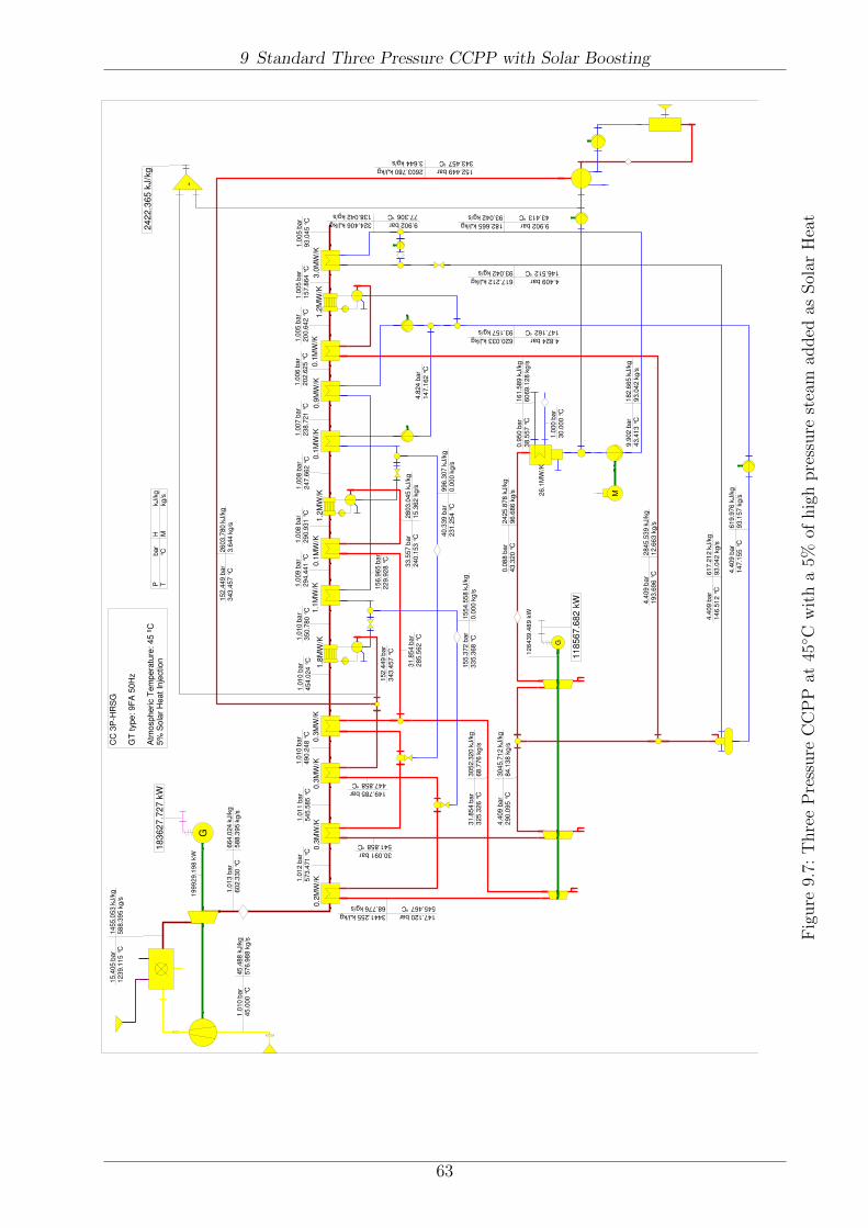
9 Standard Three Pressure CCPP with Solar Boosting
G
G
M
-
CC
3P
-HR
SG
GT
type:
9F
A 5
0H
z
Atm
ospheric T
em
pera
ture
: 45 º
C 5
% S
ola
r H
eat
Inje
ction
0.2
MW
/K0.3
MW
/K0.3
MW
/K0.3
MW
/K1.1
MW
/K0.1
MW
/K0.1
MW
/K0.9
MW
/K0.1
MW
/K3.0
MW
/K
26
.1M
W/K
1.2
MW
/K1
.8M
W/K
1.2
MW
/K
24
22
.36
5 k
J/k
g
18
36
27
.72
7 k
W
1.0
13
bar
60
2.3
30 °
C
664.0
24 k
J/k
g
588.3
95 k
g/s
15.4
05 b
ar
123
9.1
15 °
C
14
55.0
53 k
J/k
g
58
8.3
95 k
g/s
1.0
10 b
ar
45
.000
°C
4
5.4
88
kJ/k
g
57
6.9
88 k
g/s
1.0
12
bar
573.4
71 °
C
1.0
11 b
ar
545
.585
°C
1.0
10 b
ar
49
0.2
48 °
C
147.120 bar
545.467 °C
3441.255 kJ/kg
68.776 kg/s
1.0
10
bar
454.0
24 °
C
1.0
10 b
ar
350
.780
°C
1.0
09
bar
29
4.4
41 °
C
1.0
08 b
ar
29
0.9
31 °
C
1.0
08 b
ar
247
.662
°C
1.0
07 b
ar
238
.721
°C
1.0
06 b
ar
20
2.6
25 °
C
1.0
05 b
ar
20
0.6
42 °
C
1.0
05
bar
15
7.8
64 °
C
1.0
05
bar
93
.04
5 °
C
31.8
54 b
ar
325.3
26 °
C
305
2.3
20 k
J/k
g
68.7
76 k
g/s
4.4
09
bar
290.0
95 °
C
304
5.7
12 k
J/k
g
84.1
38 k
g/s
0
.08
8 b
ar
43.3
20 °
C
24
25.8
78
kJ/k
g
96
.686
kg/s
4.409 bar
146.512 °C
617.212 kJ/kg
93.042 kg/s
33.5
57 b
ar
240
.153
°C
2
803.0
45 k
J/k
g
15
.362
kg/s
4.824 bar
147.162 °C
620.033 kJ/kg
93.157 kg/s
9.902 bar
77.306 °C
324.406 kJ/kg
138.042 kg/s
9.9
02
bar
43.4
13 °
C
182.6
65 k
J/k
g
93.0
42 k
g/s
4.4
09 b
ar
14
6.5
12 °
C
61
7.2
12 k
J/k
g
93
.042
kg/s
4.4
09
bar
147.1
55 °
C
619
.976
kJ/k
g
93.1
57 k
g/s
152.449 bar
343.457 °C
2603.780 kJ/kg
3.644 kg/s
152
.449
bar
343
.457
°C
2
603.7
80 k
J/k
g
3.6
44 k
g/s
40.3
39 b
ar
231
.254
°C
9
96
.307
kJ/k
g
0.0
00 k
g/s
4.4
09 b
ar
19
3.6
96 °
C
2845
.53
9 k
J/k
g
12.6
63 k
g/s
11
85
67
.68
2 k
W
Pbar
T°C
H
kJ/k
g
Mkg/s
1.0
00
bar
30
.00
0 °
C
0.9
50 b
ar
38.5
57 °
C
16
1.5
89 k
J/k
g
60
69.1
28 k
g/s
149.785 bar
447.858 °C
30.091 bar
541.858 °C
31.8
54 b
ar
285.5
62 °
C
152.4
49 b
ar
343.4
57 °
C
15
6.9
65 b
ar
22
9.9
28 °
C
15
5.3
72 b
ar
33
5.3
68 °
C
155
4.5
58 k
J/k
g
0.0
00 k
g/s
4.8
24
bar
14
7.1
62 °
C
9.902 bar
43.413 °C
182.665 kJ/kg
93.042 kg/s
19
99
29
.19
8 k
W
12
64
39
.48
9 k
W
Fig
ure
9.7:
Thre
eP
ress
ure
CC
PP
at45
◦ Cw
ith
a5%
ofhig
hpre
ssure
stea
mad
ded
asSol
arH
eat
63
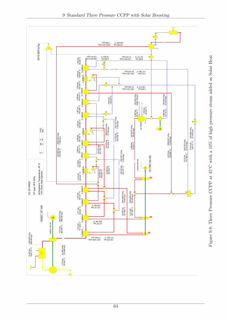
9 Standard Three Pressure CCPP with Solar Boosting
G
G
M
-
CC
3P
-HR
SG
GT
type:
9F
A 5
0H
z
Atm
ospheric T
em
pera
ture
: 45 º
C 1
0%
Sola
r H
eat
Inje
ction
0.2
MW
/K0.3
MW
/K0.3
MW
/K0.3
MW
/K1.1
MW
/K0.1
MW
/K0.1
MW
/K0.9
MW
/K0.1
MW
/K3.0
MW
/K
26
.1M
W/K
1.2
MW
/K1
.8M
W/K
1.2
MW
/K
24
10
.62
0 k
J/k
g
18
36
27
.72
7 k
W
1.0
13
bar
60
2.3
30 °
C
664.0
24 k
J/k
g
588.3
95 k
g/s
15.4
05 b
ar
123
9.1
15 °
C
14
55.0
53 k
J/k
g
58
8.3
95 k
g/s
1.0
10 b
ar
45
.000
°C
4
5.4
88
kJ/k
g
57
6.9
88 k
g/s
1.0
12
bar
571.8
39 °
C
1.0
11 b
ar
542
.841
°C
1.0
10 b
ar
48
7.2
17 °
C
150.349 bar
541.684 °C
3427.449 kJ/kg
70.602 kg/s
1.0
10
bar
450.3
61 °
C
1.0
10 b
ar
352
.256
°C
1.0
09
bar
29
7.0
11 °
C
1.0
08 b
ar
29
3.3
53 °
C
1.0
08 b
ar
249
.265
°C
1.0
07 b
ar
240
.096
°C
1.0
06 b
ar
20
4.6
19 °
C
1.0
05 b
ar
20
2.5
59 °
C
1.0
05
bar
15
8.9
35 °
C
1.0
05
bar
94
.28
3 °
C
32.6
52 b
ar
321.9
44 °
C
304
1.8
26 k
J/k
g
70.6
02 k
g/s
4.5
12
bar
287.0
96 °
C
303
9.2
63 k
J/k
g
86.3
08 k
g/s
0
.08
9 b
ar
43.6
23 °
C
24
19.9
73
kJ/k
g
99
.204
kg/s
4.512 bar
147.799 °C
622.755 kJ/kg
91.915 kg/s
34.4
32 b
ar
241
.624
°C
2
802.8
76 k
J/k
g
15
.706
kg/s
4.945 bar
148.018 °C
623.725 kJ/kg
91.952 kg/s
9.892 bar
78.222 °C
328.245 kJ/kg
136.915 kg/s
9.8
92
bar
43.7
16 °
C
183.9
32 k
J/k
g
91.9
15 k
g/s
4.5
12 b
ar
14
7.7
99 °
C
62
2.7
55 k
J/k
g
91
.915
kg/s
4.5
12
bar
148.0
10 °
C
623
.666
kJ/k
g
91.9
52 k
g/s
155.965 bar
345.292 °C
2593.302 kJ/kg
7.289 kg/s
155
.965
bar
345
.292
°C
2
593.3
02 k
J/k
g
7.2
89 k
g/s
41.5
33 b
ar
232.3
38 °
C
100
1.4
07 k
J/k
g
0.0
00 k
g/s
4.5
12 b
ar
19
5.2
90 °
C
2848
.38
1 k
J/k
g
12.9
33 k
g/s
12
17
89
.10
3 k
W
Pbar
T°C
H
kJ/k
g
Mkg/s
1.0
00
bar
30
.00
0 °
C
0.9
50 b
ar
38.7
52 °
C
16
2.4
02 k
J/k
g
60
69.1
28 k
g/s
153.157 bar
443.084 °C
30.797 bar
538.796 °C
32.6
52 b
ar
287.6
45 °
C
155.9
65 b
ar
345.2
92 °
C
16
0.2
57 b
ar
23
1.7
02 °
C
15
8.7
52 b
ar
33
7.3
77 °
C
156
7.9
51 k
J/k
g
0.0
00 k
g/s
4.9
45
bar
14
8.0
18 °
C
9.892 bar
43.716 °C
183.932 kJ/kg
91.915 kg/s
19
99
29
.19
8 k
W
12
94
65
.06
8 k
W
Fig
ure
9.8:
Thre
eP
ress
ure
CC
PP
at45
◦ Cw
ith
a10
%of
hig
hpre
ssure
stea
mad
ded
asSol
arH
eat
64

9 Standard Three Pressure CCPP with Solar Boosting
G
G
M
-
CC
3P
-HR
SG
GT
type:
9F
A 5
0H
z
Atm
ospheric T
em
pera
ture
: 45 º
C 1
2%
Sola
r H
eat
Inje
ction
0.2
MW
/K0.3
MW
/K0.3
MW
/K0.3
MW
/K1.0
MW
/K0.1
MW
/K0.1
MW
/K0.9
MW
/K0.1
MW
/K3.0
MW
/K
26
.1M
W/K
1.2
MW
/K1
.8M
W/K
1.2
MW
/K
24
05
.92
8 k
J/k
g
18
36
27
.72
7 k
W
1.0
13
bar
60
2.3
30 °
C
664.0
24 k
J/k
g
588.3
95 k
g/s
15.4
05 b
ar
123
9.1
15 °
C
14
55.0
53 k
J/k
g
58
8.3
95 k
g/s
1.0
10 b
ar
45
.000
°C
4
5.4
88
kJ/k
g
57
6.9
88 k
g/s
1.0
12
bar
571.1
82 °
C
1.0
11 b
ar
541
.738
°C
1.0
10 b
ar
48
6.0
18 °
C
151.618 bar
540.148 °C
3421.844 kJ/kg
71.329 kg/s
1.0
10
bar
448.9
06 °
C
1.0
10 b
ar
352
.828
°C
1.0
09
bar
29
8.0
29 °
C
1.0
08 b
ar
29
4.3
11 °
C
1.0
08 b
ar
249
.895
°C
1.0
07 b
ar
240
.632
°C
1
.006 b
ar
20
5.4
02 °
C
1.0
05 b
ar
20
3.3
09 °
C
1.0
05
bar
15
9.3
34 °
C
1.0
05
bar
95
.11
0 °
C
32.9
69 b
ar
320.5
88 °
C
303
7.5
81 k
J/k
g
71.3
29 k
g/s
4.5
50
bar
285.8
17 °
C
303
6.5
27 k
J/k
g
87.1
72 k
g/s
0
.09
0 b
ar
43.7
34 °
C
24
17.7
04
kJ/k
g
10
0.1
31 k
g/s
4.550 bar
147.834 °C
622.909 kJ/kg
91.384 kg/s
34.7
81 b
ar
242
.201
°C
2
802.7
97 k
J/k
g
15
.843
kg/s
4.990 bar
148.325 °C
625.050 kJ/kg
91.470 kg/s
9.955 bar
79.952 °C
335.503 kJ/kg
139.384 kg/s
9.9
55
bar
43.8
28 °
C
184.4
03 k
J/k
g
91.3
84 k
g/s
4.5
50 b
ar
14
7.8
34 °
C
62
2.9
09 k
J/k
g
91
.384
kg/s
4.5
50
bar
148.3
17 °
C
624
.989
kJ/k
g
91.4
70 k
g/s
157.350 bar
346.005 °C
2589.072 kJ/kg
8.747 kg/s
157
.350
bar
346
.005
°C
2
589.0
72 k
J/k
g
8.7
47 k
g/s
42.0
11 b
ar
232.7
57 °
C
100
3.3
82 k
J/k
g
0.0
00 k
g/s
4.5
50 b
ar
19
5.9
07 °
C
2849
.49
7 k
J/k
g
13.0
44 k
g/s
12
30
24
.06
2 k
W
Pbar
T°C
H
kJ/k
g
Mkg/s
1.0
00
bar
30
.00
0 °
C
0.9
50 b
ar
38.8
23 °
C
16
2.6
99 k
J/k
g
60
69.1
28 k
g/s
154.484 bar
441.220 °C
31.077 bar
537.567 °C
32.9
69 b
ar
288.4
65 °
C
157.3
50 b
ar
346.0
05 °
C
16
1.5
53 b
ar
23
2.3
98 °
C
16
0.0
82 b
ar
33
8.1
65 °
C
157
3.2
74 k
J/k
g
0.0
00 k
g/s
4.9
90
bar
14
8.3
25 °
C
9.955 bar
43.828 °C
184.403 kJ/kg
91.384 kg/s
19
99
29
.19
8 k
W
13
06
20
.36
6 k
W
Fig
ure
9.9:
Thre
eP
ress
ure
CC
PP
at45
◦ Cw
ith
a12
%of
hig
hpre
ssure
stea
mad
ded
asSol
arH
eat
65
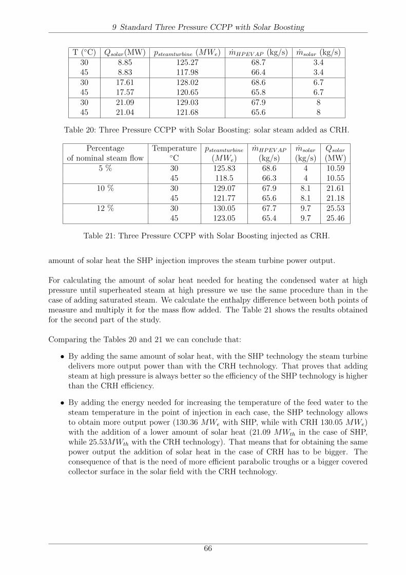
9 Standard Three Pressure CCPP with Solar Boosting
T (◦C) Qsolar(MW) psteamturbine (MWe) mHPEV AP (kg/s) msolar (kg/s)30 8.85 125.27 68.7 3.445 8.83 117.98 66.4 3.430 17.61 128.02 68.6 6.745 17.57 120.65 65.8 6.730 21.09 129.03 67.9 845 21.04 121.68 65.6 8
Table 20: Three Pressure CCPP with Solar Boosting: solar steam added as CRH.
Percentage Temperature psteamturbine mHPEV AP msolar Qsolar
of nominal steam flow ◦C (MWe) (kg/s) (kg/s) (MW)5 % 30 125.83 68.6 4 10.59
45 118.5 66.3 4 10.5510 % 30 129.07 67.9 8.1 21.61
45 121.77 65.6 8.1 21.1812 % 30 130.05 67.7 9.7 25.53
45 123.05 65.4 9.7 25.46
Table 21: Three Pressure CCPP with Solar Boosting injected as CRH.
amount of solar heat the SHP injection improves the steam turbine power output.
For calculating the amount of solar heat needed for heating the condensed water at highpressure until superheated steam at high pressure we use the same procedure than in thecase of adding saturated steam. We calculate the enthalpy difference between both points ofmeasure and multiply it for the mass flow added. The Table 21 shows the results obtainedfor the second part of the study.
Comparing the Tables 20 and 21 we can conclude that:
• By adding the same amount of solar heat, with the SHP technology the steam turbinedelivers more output power than with the CRH technology. That proves that addingsteam at high pressure is always better so the efficiency of the SHP technology is higherthan the CRH efficiency.
• By adding the energy needed for increasing the temperature of the feed water to thesteam temperature in the point of injection in each case, the SHP technology allowsto obtain more output power (130.36 MWe with SHP, while with CRH 130.05 MWe)with the addition of a lower amount of solar heat (21.09 MWth in the case of SHP,while 25.53MWth with the CRH technology). That means that for obtaining the samepower output the addition of solar heat in the case of CRH has to be bigger. Theconsequence of that is the need of more efficient parabolic troughs or a bigger coveredcollector surface in the solar field with the CRH technology.
66
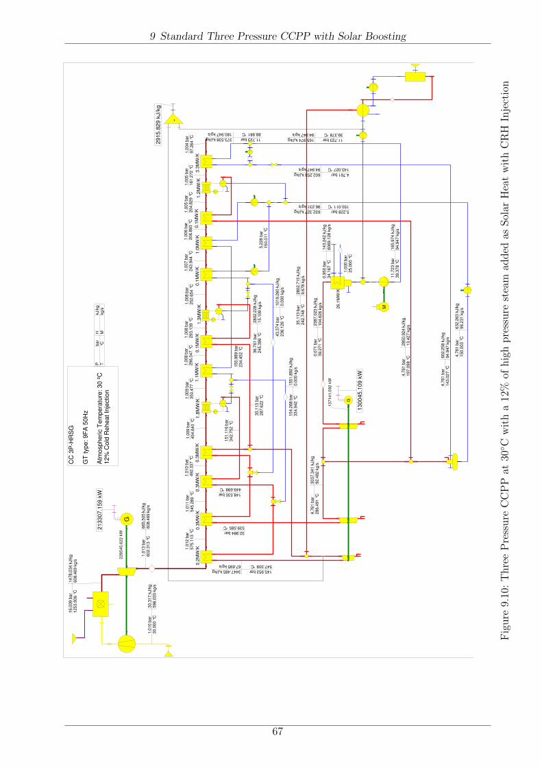
9 Standard Three Pressure CCPP with Solar Boosting
G
G
M
-
CC
3P
-HR
SG
GT
type: 9F
A 5
0H
z
Atm
ospheric T
em
pera
ture
: 30 º
C 1
2%
Cold
Reheat In
jection
0.2
MW
/K0.3
MW
/K0.3
MW
/K0.3
MW
/K1.1
MW
/K0.1
MW
/K0.1
MW
/K1.0
MW
/K0.1
MW
/K3.3
MW
/K
26
.1M
W/K
1.3
MW
/K1
.2M
W/K
1.8
MW
/K
291
5.8
29
kJ/k
g
21
33
07
.15
9 k
W
1.0
13
bar
60
2.3
13 °
C
665.5
05 k
J/k
g
608.4
69 k
g/s
16.0
09 b
ar
125
3.9
36 °
C
14
78.0
34 k
J/k
g
60
8.4
69 k
g/s
1.0
10 b
ar
30
.000
°C
3
0.3
17
kJ/k
g
59
6.0
30 k
g/s
1.0
12
bar
575.1
13 °
C
1.0
11 b
ar
545
.289
°C
1.0
10 b
ar
49
2.3
37 °
C
145.953 bar
547.309 °C
3447.485 kJ/kg
67.695 kg/s
1.0
09 b
ar
350
.477
°C
1.0
08
bar
29
6.3
47 °
C
1.0
08 b
ar
29
3.1
39 °
C
1.0
08 b
ar
252
.654
°C
1.0
07 b
ar
243
.944
°C
1.0
06 b
ar
20
6.8
93 °
C
1.0
05 b
ar
20
4.8
29 °
C
1.0
05
bar
16
1.2
72 °
C
1.0
04
bar
97
.26
4 °
C
4.7
61
bar
286.4
91 °
C
303
7.3
41 k
J/k
g
92.4
82 k
g/s
0
.07
1 b
ar
39.2
71 °
C
23
87.0
23
kJ/k
g
10
4.6
26 k
g/s
4.761 bar
143.027 °C
602.258 kJ/kg
94.947 kg/s
36.7
61 b
ar
245
.399
°C
2
802.2
28 k
J/k
g
15
.109
kg/s
5.228 bar
150.011 °C
632.327 kJ/kg
96.231 kg/s
11.723 bar
88.981 °C
373.538 kJ/kg
180.947 kg/s
11.7
23 b
ar
39.3
78 °
C
165.9
74 k
J/k
g
94.9
47 k
g/s
4.7
61 b
ar
14
3.0
27 °
C
60
2.2
58 k
J/k
g
94
.947
kg/s
4.7
61
bar
150.0
03 °
C
632
.263
kJ/k
g
96.2
31 k
g/s
43.3
74 b
ar
236.1
26 °
C
101
9.2
60 k
J/k
g
0.0
00 k
g/s
4.7
61 b
ar
19
7.0
98 °
C
2850
.92
4 k
J/k
g
13.4
27 k
g/s
13
00
45
.10
9 k
W
Pbar
T°C
H
kJ/k
g
Mkg/s
1.0
00
bar
25
.00
0 °
C
0.9
50 b
ar
34.1
67 °
C
14
3.2
42 k
J/k
g
60
69.1
28 k
g/s
148.535 bar
449.698 °C
32.984 bar
539.585 °C
35.1
13 b
ar
287.6
22 °
C
15
5.9
89 b
ar
23
4.4
52 °
C
15
4.2
68 b
ar
33
4.9
42 °
C
155
1.8
92 k
J/k
g
0.0
00 k
g/s
5.2
28
bar
15
0.0
11 °
C
11.723 bar
39.378 °C
165.974 kJ/kg
94.947 kg/s
22
85
45
.62
2 k
W
13
71
41
.09
2 k
W
1.0
09 b
ar
45
4.6
40 °
C
151.1
16 b
ar
342.7
52 °
C
35
.113
ba
r 2
42.7
48 °
C
280
2.7
15 k
J/k
g
9.6
78 k
g/s
Fig
ure
9.10
:T
hre
eP
ress
ure
CC
PP
at30
◦ Cw
ith
a12
%of
hig
hpre
ssure
stea
mad
ded
asSol
arH
eat
wit
hC
RH
Inje
ctio
n
67
10 Conversion Efficiency of Solar Boosting
10 Conversion Efficiency of Solar Boosting
The energy conversion efficiency is an useful ratio for comparing the impact of introducingsolar heat. We will define it as the ratio between the additional electric power when we injectthe CCPP with solar steam and the amount of solar heat that we are injecting.
ηsolar =Pel,solar − PelQth,solar
(10.1)
We will compare the conversion efficiencies for both SHP and CRH technologies at 30◦C.
10.1 Conversion Efficiency of Saturated High Pressure Steam
For the case of injection with saturated high pressure steam, the conversion efficiency iscalculated as:
ηsolar,30◦C =Pel,30◦C,solar − Pel,30◦C
Qth,30◦C,solar=
130.36MWe − 122.49MWe
21.09MWe
= 0.373 (10.2)
The SHP technology has a nominal gross efficiency which is only 1% lower than the efficienciespublished in literature for PTC systems (38.5% gross efficiency in [14]).
10.2 Conversion Efficiency of Cold Reheated Steam
When the injection of solar heat is made in the cold reheat pipe:
ηsolar,30◦C =Pel,30◦C,solar − Pel,30◦C
Qth,30◦C,solar=
130.05MWe − 122.49MWe
25.53MWe
= 0.296 (10.3)
Comparing the results for SHP and CRH we can conclude that the SHP is a more efficienttechnology. With SHP we obtain 130.36 MWe by injecting only 21.09 MWth of solar heat,while with CRH we need more thermal heat for reaching lower power output. Although theSHP technology is more expensive than CRH in terms of installation in the CCPP, becausethe injection is done around 155 bar, due to its high efficiency we need a smaller solar fieldthan with the CRH technology being cheaper in terms of construction of the solar field.
11 Impact of Solar Steam Injection on Temperatures andPressures
11.1 Impact of Saturated High Pressure Steam Injection
In this chapter we will discuss briefly the impact of injecting saturated steam at high pressureas solar heat on the temperature of the superheated steam and its pressure. The Table 22shows the values of pressures and temperatures in each case:
In the Table 22 the pHP,SH,INLET represents the high pressure value of the saturated steamin the point of injection. The THP,ST represents the temperature of the superheated steambefore entering the steam turbine.
68
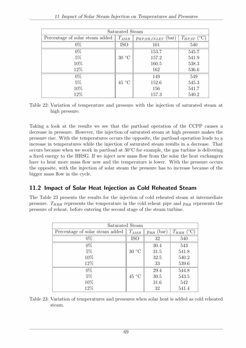
11 Impact of Solar Steam Injection on Temperatures and Pressures
Saturated SteamPercentage of solar steam added TAMB pHP,SH,INLET (bar) THP,ST (◦C)
0% ISO 161 540
0% 153.7 545.75% 30 ◦C 157.2 541.910% 160.5 538.312% 162 536.6
0% 149 5495% 45 ◦C 152.6 545.310% 156 541.712% 157.3 540.2
Table 22: Variation of temperature and pressure with the injection of saturated steam athigh pressure.
Taking a look at the results we see that the partload operation of the CCPP causes adecrease in pressure. However, the injection of saturated steam at high pressure makes thepressure rise. With the temperatures occurs the opposite, the partload operation leads to aincrease in temperatures while the injection of saturated steam results in a decrease. Thatoccurs because when we work in partload at 30◦C for example, the gas turbine is deliveringa fixed energy to the HRSG. If we inject new mass flow from the solar the heat exchangershave to heat more mass flow now and the temperature is lower. With the pressure occursthe opposite, with the injection of solar steam the pressure has to increase because of thebigger mass flow in the cycle.
11.2 Impact of Solar Heat Injection as Cold Reheated Steam
The Table 23 presents the results for the injection of cold reheated steam at intermediatepressure. THRH represents the temperature in the cold reheat pipe and pRH represents thepressure of reheat, before entering the second stage of the steam turbine.
Saturated SteamPercentage of solar steam added TAMB pRH (bar) THRH (◦C)
0% ISO 32 540
0% 30.4 5435% 30 ◦C 31.5 541.810% 32.5 540.212% 33 539.6
0% 29.4 544.85% 45 ◦C 30.5 543.510% 31.6 54212% 32 541.4
Table 23: Variation of temperatures and pressures when solar heat is added as cold reheatedsteam.
69

12 Thermal Efficiency of the CCPP
With the injection of cold reheated steam the variation of pressures and temperatures isexactly in the same way than with saturated high pressure steam. But with CRH thevariation in both pressure and temperature is smaller compared with SHP as we can see inthe Table 24.
Technology ∆P (bar) ∆T (◦C)SHP 8.3 9CRH 2.6 3.4
Table 24: Variation of temperatures and pressures with solar steam injection
It is worthwhile to mention that the limit of HP value is not attained. The pressure is lowerthan in the ISO case (155 bar), see Figure 9.10.
12 Thermal Efficiency of the CCPP
The thermal efficiency of the CCPP is defined as the ratio between the output power obtainedfrom the whole power plant and the energy given to the gas turbine. The energy given to thegas turbine is the amount of fuel burnt in the combustion chamber multiplied by its lowerheating value. For the case of an ambient temperature of 30◦C:
η30◦C =PGT + PSTmfuel ·Hu
=213.3MW + 122.5MW
12.4kg/s · 50.015MJ/kg= 0.541 (12.1)
12.1 Thermal Efficiency of the CCPP with Solar Boosting
If we assume that the solar energy is for free, we can calculate the thermal efficiency of theCCPP when solar heat is injected:
η30◦C,SHP =PGT + PSTmfuel ·Hu
=213.3MW + 130.4MW
12.4kg/s · 50.015MJ/kg= 0.554 (12.2)
η30◦C,CRH =PGT + PSTmfuel ·Hu
=213.3MW + 130.1MW
12.4kg/s · 50.015MJ/kg= 0.553 (12.3)
The thermal efficiency of the CCPP increases with the addition of solar heat and is higherin the case of the SHP technology.
13 Standard Three Pressure CCPP with Increased SolarBoosting
Until now we have studied the introduction of solar energy in a CCPP for improving theoverall efficiency. We only considered the cases with warmer temperatures and partloadperformance in the gas turbine.
The steam turbine is designed for given conditions (ISO Conditions) and the design cal-culations correspond to these conditions. That means that, for example the cross section
70

13 Standard Three Pressure CCPP with Increased Solar Boosting
of the steam turbine is fixed in design conditions and it defines the limit of the steam flowthrough the turbine. If we want to inject more steam in the cycle the total mass never canbe bigger than in the design conditions.
Even in ISO conditions (15◦C) it is possible to obtain solar energy with the parabolic troughtechnology. That means, that at ISO conditions we are wasting the energy obtained in thesolar field because the limited cross section does not allow to inject more steam in the Rank-ine cycle. Wasting this solar energy makes the solar field less economic.
We can consider the injection of solar energy in design conditions by making the crosssection of the steam turbine bigger. How big? We have to design a new steam turbine whosemass flow in design conditions is the sum of the solar steam and the steam flow that we hadin the previous steam turbine in ISO conditions.
APPROACH ”B”
For modeling this concept in Ebsilon we will use the three pressure cycle with solar boosting.But the difference now is that we will also introduce steam heated with solar energy in designconditions.
The Table 26 shows the results obtained for the three pressures CCPP when in designconditions we add a 12% of solar heat. We have to notice that the HRSGs in both cycles(with solar or no solar in design conditions) are not exactly the same. In the cycle withsolar injection in design conditions, the gas temperature in the economizer at the end of thegas stream is not so low as in the cycle without solar injection. This is because the mass ofwater through it is bigger and the temperature of the water is higher as well. That makesimpossible to reach the temperature of 85◦C at the end of the gas steam. Instead we reach atemperature of 86.7◦C and despite of this small difference we can consider that both HRSGswork in a similar way.
By comparing the results for ISO conditions, with or without solar heat injection, we canconclude that the addition of solar heat to the CCPP in design conditions allows reachinghigher output power. If the hours of operation of the solar field are bigger we will obtainmore energy for a defined investment costs and the energy will be cheaper in a long-term.
Conditions mHPEV AP (kg/s) msolar (kg/s) psteamturbine (MWe) Qsolar(MW)ISO 72.9 138.5
ISO with Solar Inject. 67.7 8.7 145.96 21.48
Table 25: Comparison between the CCPP working in ISO conditions with and without solarinjection.
For all the cases in a range between 10◦C and 45◦C the mass of solar heat injected is the same.When the temperature rises and the gas turbine starts working in off-design conditions, theproduction of steam in the high pressure evaporator decreases. The solar heat needed forheating the mass flow decreases with higher temperatures and the result is a lower outputpower in the steam turbine.
71
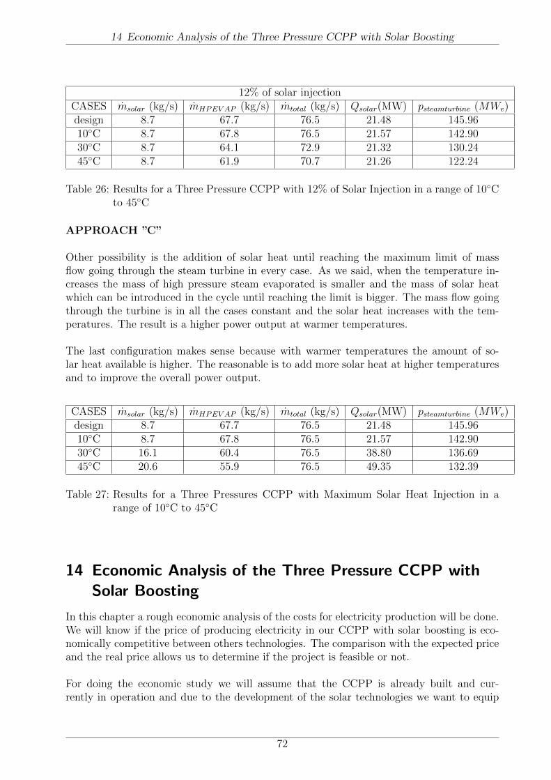
14 Economic Analysis of the Three Pressure CCPP with Solar Boosting
12% of solar injectionCASES msolar (kg/s) mHPEV AP (kg/s) mtotal (kg/s) Qsolar(MW) psteamturbine (MWe)design 8.7 67.7 76.5 21.48 145.9610◦C 8.7 67.8 76.5 21.57 142.9030◦C 8.7 64.1 72.9 21.32 130.2445◦C 8.7 61.9 70.7 21.26 122.24
Table 26: Results for a Three Pressure CCPP with 12% of Solar Injection in a range of 10◦Cto 45◦C
APPROACH ”C”
Other possibility is the addition of solar heat until reaching the maximum limit of massflow going through the steam turbine in every case. As we said, when the temperature in-creases the mass of high pressure steam evaporated is smaller and the mass of solar heatwhich can be introduced in the cycle until reaching the limit is bigger. The mass flow goingthrough the turbine is in all the cases constant and the solar heat increases with the tem-peratures. The result is a higher power output at warmer temperatures.
The last configuration makes sense because with warmer temperatures the amount of so-lar heat available is higher. The reasonable is to add more solar heat at higher temperaturesand to improve the overall power output.
CASES msolar (kg/s) mHPEV AP (kg/s) mtotal (kg/s) Qsolar(MW) psteamturbine (MWe)design 8.7 67.7 76.5 21.48 145.9610◦C 8.7 67.8 76.5 21.57 142.9030◦C 16.1 60.4 76.5 38.80 136.6945◦C 20.6 55.9 76.5 49.35 132.39
Table 27: Results for a Three Pressures CCPP with Maximum Solar Heat Injection in arange of 10◦C to 45◦C
14 Economic Analysis of the Three Pressure CCPP withSolar Boosting
In this chapter a rough economic analysis of the costs for electricity production will be done.We will know if the price of producing electricity in our CCPP with solar boosting is eco-nomically competitive between others technologies. The comparison with the expected priceand the real price allows us to determine if the project is feasible or not.
For doing the economic study we will assume that the CCPP is already built and cur-rently in operation and due to the development of the solar technologies we want to equip
72
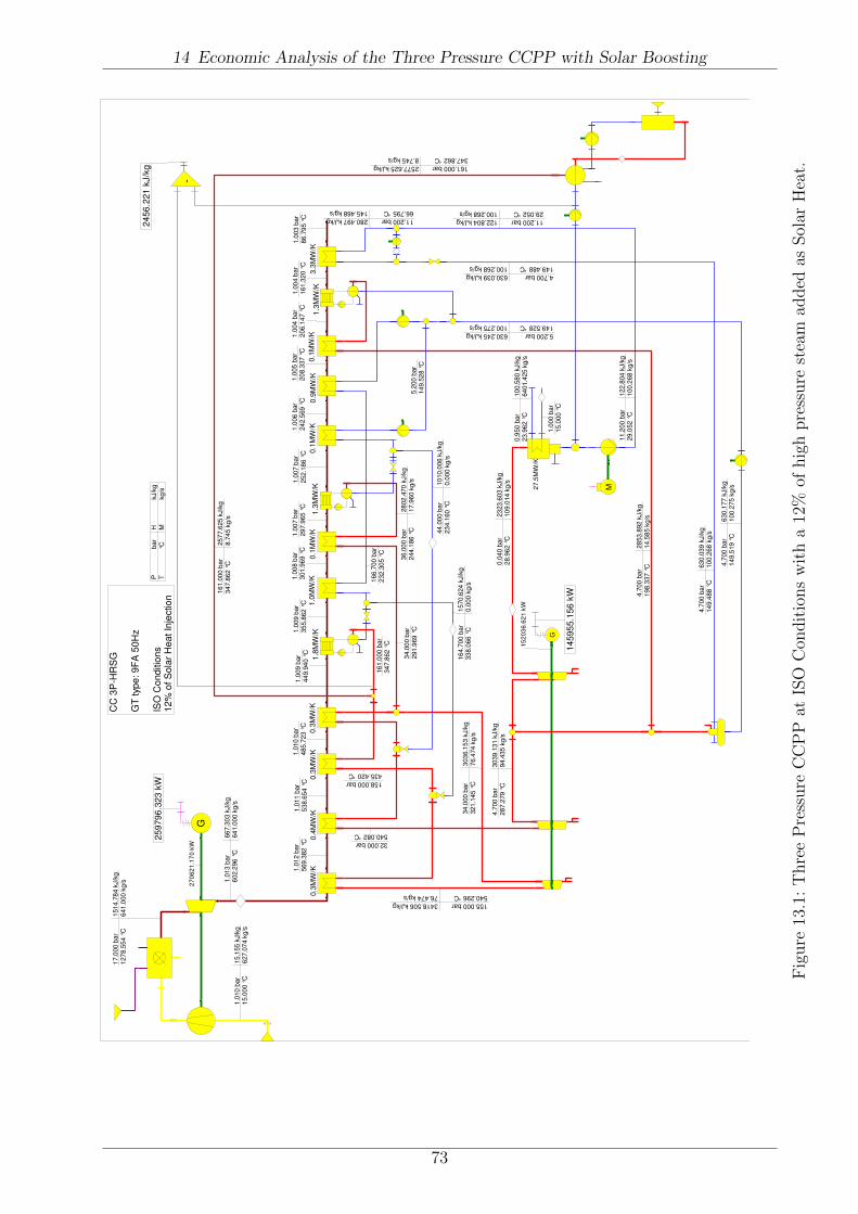
14 Economic Analysis of the Three Pressure CCPP with Solar Boosting
G
G
M
-
CC
3P
-HR
SG
GT
typ
e: 9
FA
50
Hz
IS
O C
on
ditio
ns
12
% o
f S
ola
r H
ea
t In
jectio
n
0.3
MW
/K0.4
MW
/K0.3
MW
/K0.3
MW
/K1.0
MW
/K0.1
MW
/K0.1
MW
/K0.9
MW
/K0.1
MW
/K3.3
MW
/K
27
.5M
W/K
1.8
MW
/K1
.3M
W/K
1.3
MW
/K
2456.2
21 k
J/k
g
259796.3
23 k
W
1.0
13
ba
r 6
02
.296
°C
6
67.3
03 k
J/k
g
64
1.0
00 k
g/s
17.0
00 b
ar
127
8.5
54 °
C
1514
.78
4 k
J/k
g
641.0
00
kg/s
1.0
10
bar
15.0
00 °
C
15.1
55
kJ/k
g
627
.07
4 k
g/s
1.0
12 b
ar
569
.382
°C
1
.011
ba
r 5
38
.654
°C
1.0
10
bar
485.7
23 °
C
1.0
09 b
ar
44
9.9
40 °
C
1.0
09 b
ar
35
5.8
62 °
C
1.0
08 b
ar
301
.96
9 °
C
1.0
07 b
ar
29
7.9
65 °
C
1.0
07 b
ar
252
.18
6 °
C
1.0
06
bar
24
2.5
69 °
C
1.0
05
bar
20
8.3
37 °
C
1.0
04
ba
r 2
06.1
47
°C
1
.00
4 b
ar
161
.32
0 °
C
1.0
03
bar
86
.79
5 °
C
34.0
00 b
ar
321
.145
°C
3
03
6.1
53 k
J/k
g
76.4
74 k
g/s
4.7
00
bar
28
7.2
79 °
C
30
39.1
31 k
J/k
g
94
.435
kg/s
0
.040
bar
28.9
62 °
C
23
23
.603
kJ/k
g
10
9.0
14 k
g/s
4.700 bar
149.488 °C
630.039 kJ/kg
100.268 kg/s
36.0
00 b
ar
244.1
86 °
C
28
02
.470
kJ/k
g
17
.96
0 k
g/s
5.200 bar
149.528 °C
630.245 kJ/kg
100.275 kg/s
11.200 bar
66.795 °C
280.497 kJ/kg
145.468 kg/s
11.2
00
bar
29.0
52
°C
1
22.8
04
kJ/k
g
100.2
68
kg/s
4.7
00
bar
14
9.4
88 °
C
630
.039
kJ/k
g
100
.268
kg/s
4.7
00
bar
14
9.5
19 °
C
630
.177
kJ/k
g
100
.275
kg/s
161.000 bar
347.862 °C
2577.625 kJ/kg
8.745 kg/s
16
1.0
00 b
ar
34
7.8
62 °
C
257
7.6
25 k
J/k
g
8.7
45 k
g/s
44
.00
0 b
ar
23
4.1
60 °
C
10
10.0
06
kJ/k
g
0.0
00 k
g/s
4.7
00
ba
r 1
98.3
37
°C
2
853
.892
kJ/k
g
14
.58
5 k
g/s
145955.1
56 k
W
Pb
ar
T°C
H
kJ/k
g
Mkg/s
1.0
00 b
ar
15.0
00
°C
0.9
50
bar
23
.96
2 °
C
10
0.5
80 k
J/k
g
64
01.4
25 k
g/s
158.000 bar
435.420 °C
32.000 bar
540.082 °C
34.0
00 b
ar
291.9
69
°C
16
1.0
00 b
ar
34
7.8
62 °
C
166
.700
bar
232
.305
°C
16
4.7
00 b
ar
33
8.0
66 °
C
15
70.6
24
kJ/k
g
0.0
00 k
g/s
5.2
00
bar
14
9.5
28 °
C
11.200 bar
29.052 °C
122.804 kJ/kg
100.268 kg/s
27
06
21
.17
0 k
W
15
20
36
.62
1 k
W
155.000 bar
540.296 °C
3418.506 kJ/kg
76.474 kg/s
Fig
ure
13.1
:T
hre
eP
ress
ure
CC
PP
atIS
OC
ondit
ions
wit
ha
12%
ofhig
hpre
ssure
stea
mad
ded
asSol
arH
eat.
73

14 Economic Analysis of the Three Pressure CCPP with Solar Boosting
G
G
M
-
CC
3P
-HR
SG
GT
typ
e: 9F
A 5
0H
z
Atm
ospheric T
em
pera
ture
: 30 º
C L
imit o
f S
ola
r In
jection
0.3
MW
/K0.4
MW
/K0.3
MW
/K0.3
MW
/K1.0
MW
/K0.1
MW
/K0.1
MW
/K0.8
MW
/K0.1
MW
/K3.3
MW
/K
27
.5M
W/K
1.8
MW
/K1
.3M
W/K
1.3
MW
/K
2415.2
99 k
J/k
g
213307.1
59 k
W
1.0
13
ba
r 6
02
.313
°C
6
65.5
05 k
J/k
g
60
8.4
69 k
g/s
16.0
09 b
ar
125
3.9
36 °
C
1478
.03
4 k
J/k
g
608.4
69
kg/s
1.0
10
bar
30.0
00 °
C
30.3
17
kJ/k
g
596
.03
0 k
g/s
1.0
12 b
ar
566
.742
°C
1
.011
ba
r 5
33
.816
°C
1.0
10
bar
479.3
71 °
C
1.0
09 b
ar
44
2.7
80 °
C
1.0
09 b
ar
35
4.7
48 °
C
1.0
08 b
ar
303
.34
9 °
C
1.0
08 b
ar
29
9.0
87 °
C
1.0
08 b
ar
251
.61
9 °
C
1.0
07
bar
24
1.6
51 °
C
1.0
06
bar
20
8.9
97 °
C
1.0
05
ba
r 2
06.6
95
°C
1
.00
5 b
ar
160
.62
2 °
C
1.0
04
bar
94
.68
7 °
C
33.8
03 b
ar
318
.766
°C
3
03
0.6
97 k
J/k
g
76.5
00 k
g/s
4.6
58
bar
28
4.3
51 °
C
30
33.2
12 k
J/k
g
94
.116
kg/s
0
.070
bar
38.9
82 °
C
23
83
.435
kJ/k
g
10
8.2
38 k
g/s
4.658 bar
148.824 °C
627.178 kJ/kg
92.174 kg/s
35.7
27 b
ar
243.7
46 °
C
28
02
.550
kJ/k
g
17
.61
6 k
g/s
5.131 bar
149.191 °C
628.787 kJ/kg
92.238 kg/s
10.505 bar
80.438 °C
337.583 kJ/kg
147.174 kg/s
10.5
05
bar
39.0
78
°C
1
64.6
13
kJ/k
g
92.1
74 k
g/s
4.6
58
bar
14
8.8
24 °
C
627
.178
kJ/k
g
92.1
74 k
g/s
4.6
58
bar
14
9.1
82 °
C
628
.722
kJ/k
g
92.2
38 k
g/s
160.698 bar
347.710 °C
2578.587 kJ/kg
16.064 kg/s
16
0.6
98 b
ar
34
7.7
10 °
C
257
8.5
87 k
J/k
g
16.0
64
kg/s
43
.41
9 b
ar
23
3.8
60 °
C
10
08.5
88
kJ/k
g
0.0
00 k
g/s
4.6
58
ba
r 1
99.0
91
°C
2
855
.721
kJ/k
g
14
.18
7 k
g/s
136688.1
90 k
W
Pb
ar
T°C
H
kJ/k
g
Mkg/s
1.0
00 b
ar
25.0
00
°C
0.9
50
bar
33
.98
1 °
C
14
2.4
67 k
J/k
g
64
01.4
25 k
g/s
157.696 bar
431.495 °C
31.816 bar
536.546 °C
33.8
03 b
ar
293.3
64
°C
16
0.6
98 b
ar
34
7.7
10 °
C
165
.260
bar
232
.914
°C
16
3.6
68 b
ar
33
9.2
73 °
C
15
80.0
56
kJ/k
g
0.0
00 k
g/s
5.1
31
bar
14
9.1
91 °
C
10.505 bar
39.078 °C
164.613 kJ/kg
92.174 kg/s
22
85
45
.62
2 k
W
14
41
80
.66
3 k
W
154.694 bar
537.897 °C
3412.212 kJ/kg
76.500 kg/s
Fig
ure
13.2
:T
hre
eP
ress
ure
CC
PP
at30
◦ Cw
ith
hig
hpre
ssure
stea
mad
ded
asSol
arH
eat
unti
lre
achin
gth
em
ass
flow
lim
itin
the
stea
mtu
rbin
e.
74
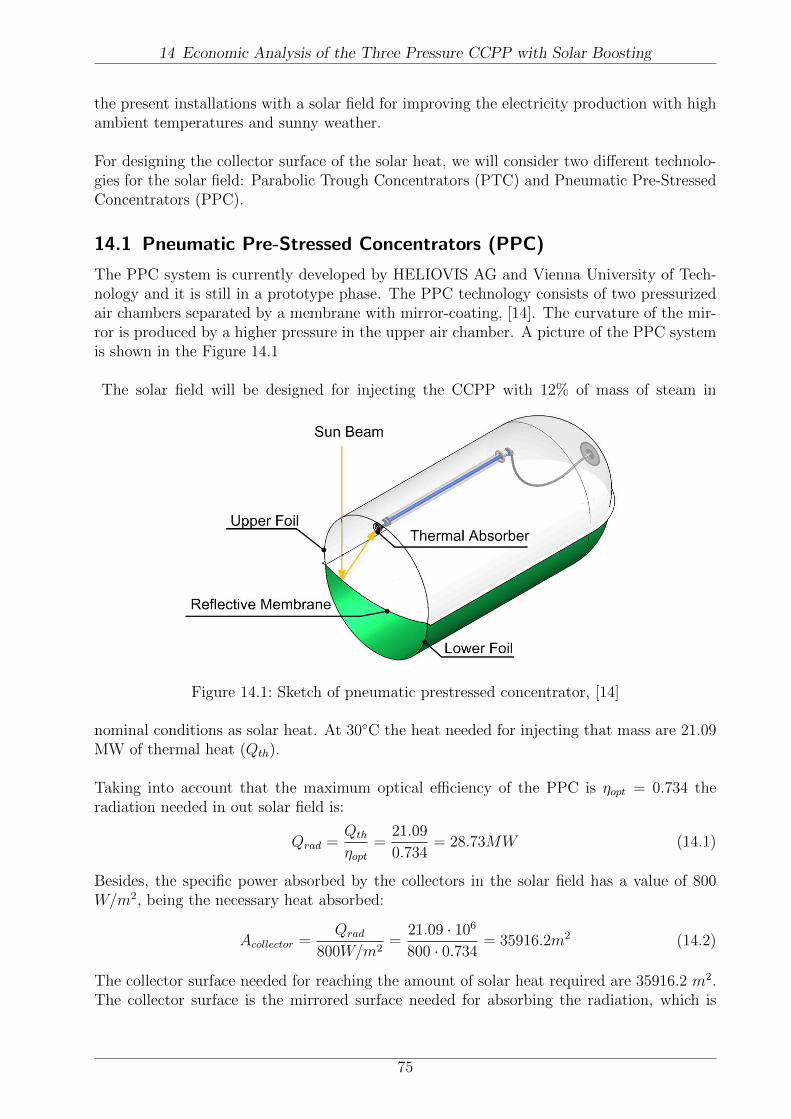
14 Economic Analysis of the Three Pressure CCPP with Solar Boosting
the present installations with a solar field for improving the electricity production with highambient temperatures and sunny weather.
For designing the collector surface of the solar heat, we will consider two different technolo-gies for the solar field: Parabolic Trough Concentrators (PTC) and Pneumatic Pre-StressedConcentrators (PPC).
14.1 Pneumatic Pre-Stressed Concentrators (PPC)
The PPC system is currently developed by HELIOVIS AG and Vienna University of Tech-nology and it is still in a prototype phase. The PPC technology consists of two pressurizedair chambers separated by a membrane with mirror-coating, [14]. The curvature of the mir-ror is produced by a higher pressure in the upper air chamber. A picture of the PPC systemis shown in the Figure 14.1
The solar field will be designed for injecting the CCPP with 12% of mass of steam in
Figure 14.1: Sketch of pneumatic prestressed concentrator, [14]
nominal conditions as solar heat. At 30◦C the heat needed for injecting that mass are 21.09MW of thermal heat (Qth).
Taking into account that the maximum optical efficiency of the PPC is ηopt = 0.734 theradiation needed in out solar field is:
Qrad =Qth
ηopt=
21.09
0.734= 28.73MW (14.1)
Besides, the specific power absorbed by the collectors in the solar field has a value of 800W/m2, being the necessary heat absorbed:
Acollector =Qrad
800W/m2=
21.09 · 106
800 · 0.734= 35916.2m2 (14.2)
The collector surface needed for reaching the amount of solar heat required are 35916.2 m2.The collector surface is the mirrored surface needed for absorbing the radiation, which is
75
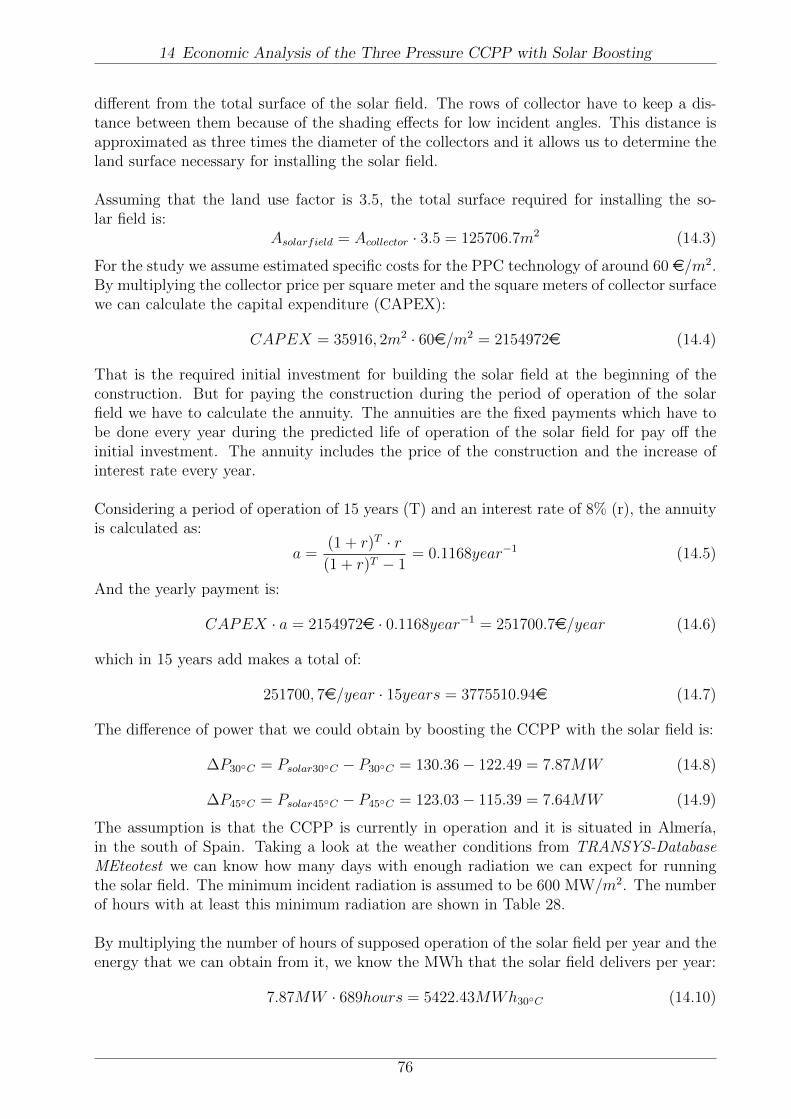
14 Economic Analysis of the Three Pressure CCPP with Solar Boosting
different from the total surface of the solar field. The rows of collector have to keep a dis-tance between them because of the shading effects for low incident angles. This distance isapproximated as three times the diameter of the collectors and it allows us to determine theland surface necessary for installing the solar field.
Assuming that the land use factor is 3.5, the total surface required for installing the so-lar field is:
Asolarfield = Acollector · 3.5 = 125706.7m2 (14.3)
For the study we assume estimated specific costs for the PPC technology of around 60 e/m2.By multiplying the collector price per square meter and the square meters of collector surfacewe can calculate the capital expenditure (CAPEX):
CAPEX = 35916, 2m2 · 60e/m2 = 2154972e (14.4)
That is the required initial investment for building the solar field at the beginning of theconstruction. But for paying the construction during the period of operation of the solarfield we have to calculate the annuity. The annuities are the fixed payments which have tobe done every year during the predicted life of operation of the solar field for pay off theinitial investment. The annuity includes the price of the construction and the increase ofinterest rate every year.
Considering a period of operation of 15 years (T) and an interest rate of 8% (r), the annuityis calculated as:
a =(1 + r)T · r(1 + r)T − 1
= 0.1168year−1 (14.5)
And the yearly payment is:
CAPEX · a = 2154972e · 0.1168year−1 = 251700.7e/year (14.6)
which in 15 years add makes a total of:
251700, 7e/year · 15years = 3775510.94e (14.7)
The difference of power that we could obtain by boosting the CCPP with the solar field is:
∆P30◦C = Psolar30◦C − P30◦C = 130.36− 122.49 = 7.87MW (14.8)
∆P45◦C = Psolar45◦C − P45◦C = 123.03− 115.39 = 7.64MW (14.9)
The assumption is that the CCPP is currently in operation and it is situated in Almerıa,in the south of Spain. Taking a look at the weather conditions from TRANSYS-DatabaseMEteotest we can know how many days with enough radiation we can expect for runningthe solar field. The minimum incident radiation is assumed to be 600 MW/m2. The numberof hours with at least this minimum radiation are shown in Table 28.
By multiplying the number of hours of supposed operation of the solar field per year and theenergy that we can obtain from it, we know the MWh that the solar field delivers per year:
7.87MW · 689hours = 5422.43MWh30◦C (14.10)
76
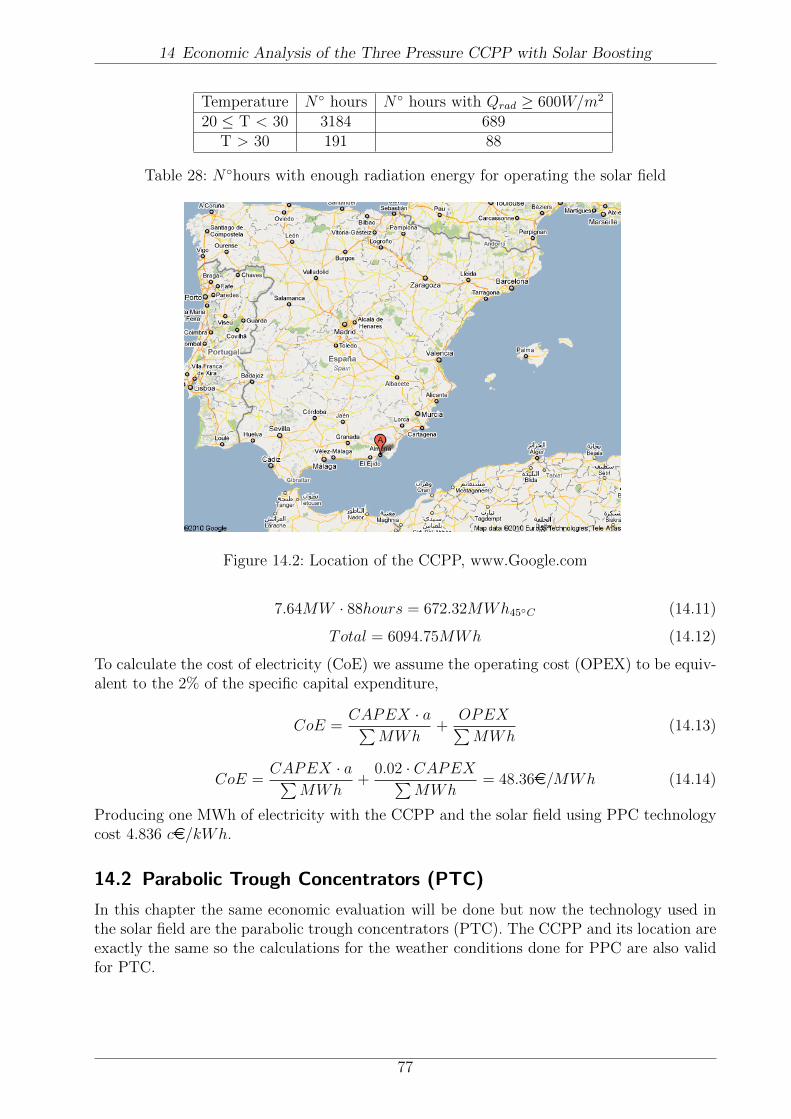
14 Economic Analysis of the Three Pressure CCPP with Solar Boosting
Temperature N◦ hours N◦ hours with Qrad ≥ 600W/m2
20 ≤ T < 30 3184 689T > 30 191 88
Table 28: N◦hours with enough radiation energy for operating the solar field
Dirección Almería
España
Almería España - Google Maps http://maps.google.com/maps?f=q&source=s_q&hl=es&geocode=...
1 de 1 11/04/2010 20:08
Figure 14.2: Location of the CCPP, www.Google.com
7.64MW · 88hours = 672.32MWh45◦C (14.11)
Total = 6094.75MWh (14.12)
To calculate the cost of electricity (CoE) we assume the operating cost (OPEX) to be equiv-alent to the 2% of the specific capital expenditure,
CoE =CAPEX · a∑
MWh+
OPEX∑MWh
(14.13)
CoE =CAPEX · a∑
MWh+
0.02 · CAPEX∑MWh
= 48.36e/MWh (14.14)
Producing one MWh of electricity with the CCPP and the solar field using PPC technologycost 4.836 ce/kWh.
14.2 Parabolic Trough Concentrators (PTC)
In this chapter the same economic evaluation will be done but now the technology used inthe solar field are the parabolic trough concentrators (PTC). The CCPP and its location areexactly the same so the calculations for the weather conditions done for PPC are also validfor PTC.
77
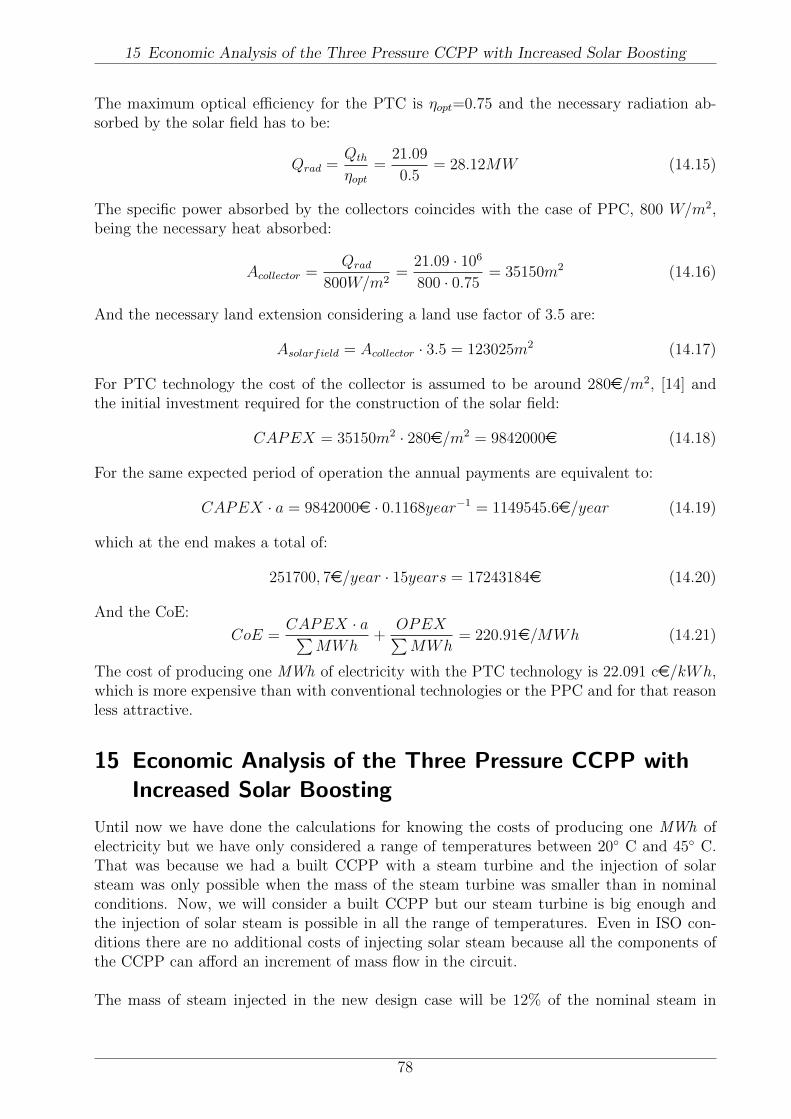
15 Economic Analysis of the Three Pressure CCPP with Increased Solar Boosting
The maximum optical efficiency for the PTC is ηopt=0.75 and the necessary radiation ab-sorbed by the solar field has to be:
Qrad =Qth
ηopt=
21.09
0.5= 28.12MW (14.15)
The specific power absorbed by the collectors coincides with the case of PPC, 800 W/m2,being the necessary heat absorbed:
Acollector =Qrad
800W/m2=
21.09 · 106
800 · 0.75= 35150m2 (14.16)
And the necessary land extension considering a land use factor of 3.5 are:
Asolarfield = Acollector · 3.5 = 123025m2 (14.17)
For PTC technology the cost of the collector is assumed to be around 280e/m2, [14] andthe initial investment required for the construction of the solar field:
CAPEX = 35150m2 · 280e/m2 = 9842000e (14.18)
For the same expected period of operation the annual payments are equivalent to:
CAPEX · a = 9842000e · 0.1168year−1 = 1149545.6e/year (14.19)
which at the end makes a total of:
251700, 7e/year · 15years = 17243184e (14.20)
And the CoE:
CoE =CAPEX · a∑
MWh+
OPEX∑MWh
= 220.91e/MWh (14.21)
The cost of producing one MWh of electricity with the PTC technology is 22.091 ce/kWh,which is more expensive than with conventional technologies or the PPC and for that reasonless attractive.
15 Economic Analysis of the Three Pressure CCPP withIncreased Solar Boosting
Until now we have done the calculations for knowing the costs of producing one MWh ofelectricity but we have only considered a range of temperatures between 20◦ C and 45◦ C.That was because we had a built CCPP with a steam turbine and the injection of solarsteam was only possible when the mass of the steam turbine was smaller than in nominalconditions. Now, we will consider a built CCPP but our steam turbine is big enough andthe injection of solar steam is possible in all the range of temperatures. Even in ISO con-ditions there are no additional costs of injecting solar steam because all the components ofthe CCPP can afford an increment of mass flow in the circuit.
The mass of steam injected in the new design case will be 12% of the nominal steam in
78

15 Economic Analysis of the Three Pressure CCPP with Increased Solar Boosting
ISO conditions for the case without solar boosting, which are 8.75 kg/s. The total heatneeded for injecting that mass in ISO conditions are 21.48 MW of thermal heat.
The difference of power that we could obtain in ISO conditions:
∆PISO = PsolarISO − PISO = 145.96− 138.5 = 7.46MW (15.1)
and taking into account that the number of hours with enough radiation for running thesolar system are shown in Table 29:
Temperature N◦ hours N◦ hours with Qrad ≥ 600W/m2
0 ≤ T < 20 5386 52620 ≤ T < 30 3184 689
T > 30 191 88
Table 29: N◦hours with enough radiation energy for operating the solar field
By multiplying the new number of hours of operation of the solar field and the power thatwe could obtain by using it, we know the MWh that the solar field produces:
7.87MW · 689hours = 5422.43MWh30◦C (15.2)
7.64MW · 88hours = 672.32MWh45◦C (15.3)
7.46MW · 526hours = 3923.96MWhISO (15.4)
Total = 10018.71MWh (15.5)
By taking advantage of the radiation even in ISO conditions we can produce about 3900MWh more that in the case before by not increasing too much the costs. As we said, theCCPP will be the same and the only thing which increases the investment in the installationis a bigger solar field because now it has to absorb more radiation.
15.1 Pneumatic Pre-Stressed Concentrators (PPC)
The calculations for the new solar field with PPC technology are presented in the following.The values of optical efficiencies and land use factors are the same that in the chapter before.
The collector surface needed for absorbing 21.48 MW of thermal heat are:
Acollector =Qrad
800W/m2=
21.48 · 106
800 · 0.734= 36580.4m2 (15.6)
and taking into account the land use factor:
Asolarfield = Acollector · 3.5 = 128031.33m2 (15.7)
The necessary initial investment for performing the construction of the solar field:
CAPEX = 36580.4m2 · 60e/m2 = 2194822.89e (15.8)
79
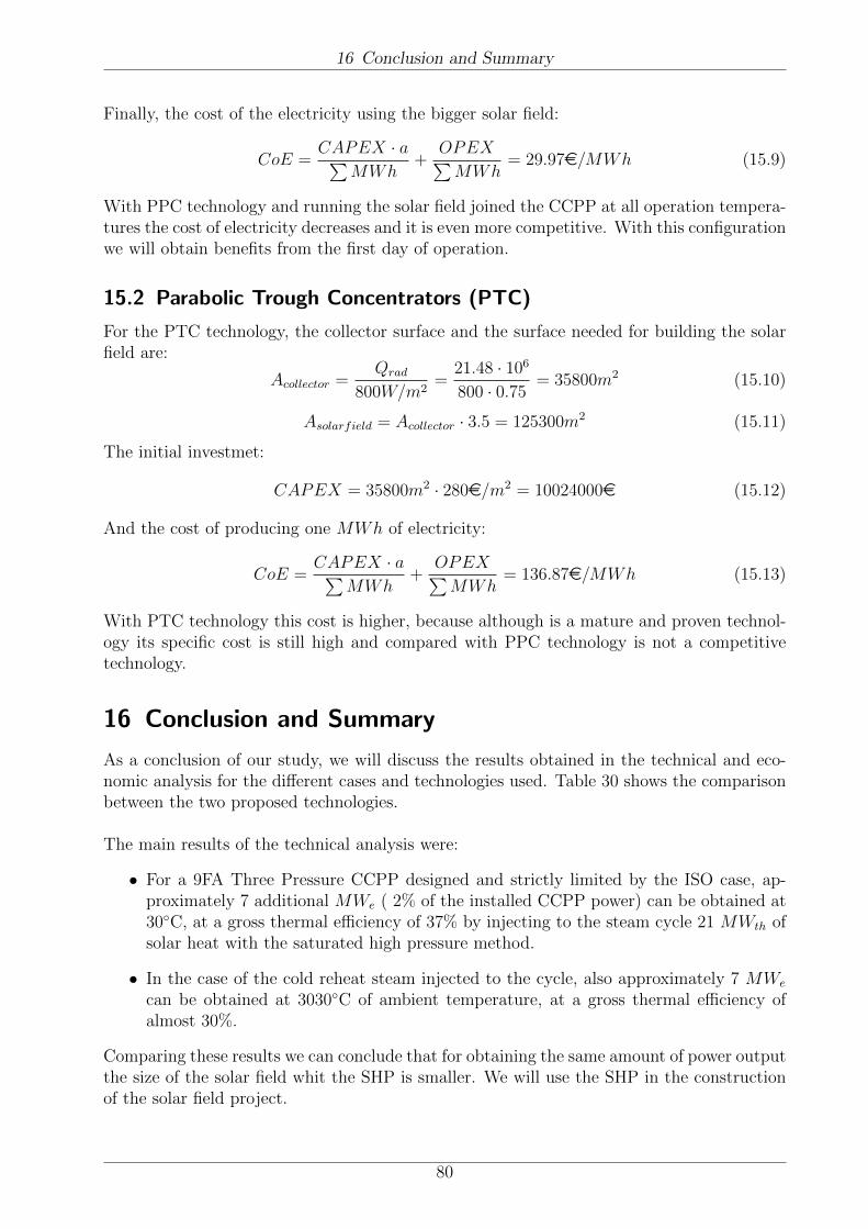
16 Conclusion and Summary
Finally, the cost of the electricity using the bigger solar field:
CoE =CAPEX · a∑
MWh+
OPEX∑MWh
= 29.97e/MWh (15.9)
With PPC technology and running the solar field joined the CCPP at all operation tempera-tures the cost of electricity decreases and it is even more competitive. With this configurationwe will obtain benefits from the first day of operation.
15.2 Parabolic Trough Concentrators (PTC)
For the PTC technology, the collector surface and the surface needed for building the solarfield are:
Acollector =Qrad
800W/m2=
21.48 · 106
800 · 0.75= 35800m2 (15.10)
Asolarfield = Acollector · 3.5 = 125300m2 (15.11)
The initial investmet:
CAPEX = 35800m2 · 280e/m2 = 10024000e (15.12)
And the cost of producing one MWh of electricity:
CoE =CAPEX · a∑
MWh+
OPEX∑MWh
= 136.87e/MWh (15.13)
With PTC technology this cost is higher, because although is a mature and proven technol-ogy its specific cost is still high and compared with PPC technology is not a competitivetechnology.
16 Conclusion and Summary
As a conclusion of our study, we will discuss the results obtained in the technical and eco-nomic analysis for the different cases and technologies used. Table 30 shows the comparisonbetween the two proposed technologies.
The main results of the technical analysis were:
• For a 9FA Three Pressure CCPP designed and strictly limited by the ISO case, ap-proximately 7 additional MWe ( 2% of the installed CCPP power) can be obtained at30◦C, at a gross thermal efficiency of 37% by injecting to the steam cycle 21 MWth ofsolar heat with the saturated high pressure method.
• In the case of the cold reheat steam injected to the cycle, also approximately 7 MWe
can be obtained at 3030◦C of ambient temperature, at a gross thermal efficiency ofalmost 30%.
Comparing these results we can conclude that for obtaining the same amount of power outputthe size of the solar field whit the SHP is smaller. We will use the SHP in the constructionof the solar field project.
80
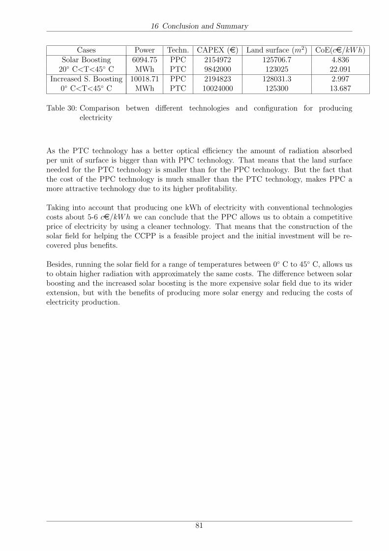
16 Conclusion and Summary
Cases Power Techn. CAPEX (e) Land surface (m2) CoE(ce/kWh)Solar Boosting 6094.75 PPC 2154972 125706.7 4.836
20◦ C<T<45◦ C MWh PTC 9842000 123025 22.091Increased S. Boosting 10018.71 PPC 2194823 128031.3 2.997
0◦ C<T<45◦ C MWh PTC 10024000 125300 13.687
Table 30: Comparison betwen different technologies and configuration for producingelectricity
As the PTC technology has a better optical efficiency the amount of radiation absorbedper unit of surface is bigger than with PPC technology. That means that the land surfaceneeded for the PTC technology is smaller than for the PPC technology. But the fact thatthe cost of the PPC technology is much smaller than the PTC technology, makes PPC amore attractive technology due to its higher profitability.
Taking into account that producing one kWh of electricity with conventional technologiescosts about 5-6 ce/kWh we can conclude that the PPC allows us to obtain a competitiveprice of electricity by using a cleaner technology. That means that the construction of thesolar field for helping the CCPP is a feasible project and the initial investment will be re-covered plus benefits.
Besides, running the solar field for a range of temperatures between 0◦ C to 45◦ C, allows usto obtain higher radiation with approximately the same costs. The difference between solarboosting and the increased solar boosting is the more expensive solar field due to its widerextension, but with the benefits of producing more solar energy and reducing the costs ofelectricity production.
81

References
References
[1] Saravanamuttoo,H.I.H., Rogers, G.F.C., Cohen H., Gas Turbine Theory, Pearson Edu-cation, Cornwall, 2001.
[2] Fundamentals of Gas Turbines, William B., John Wiley and Sons, Inc., United Statesof America, 1996.
[3] Boyce, M., Handbook for Cogeneration and Combined Cycle Power Plants, Asme Press,New York, 2002.
[4] Boyce, M., Ph.D and P.E., Gas Turbine Engineering Handbook, Butterworth-Heinemann, Oxford, 2006.
[5] Ganapathy, V., Industrial Boilers and Heat Recovery Steam Generators, MarcelDekker,Inc., New York, 2003.
[6] Petchers, N., Combined Heating, Cooling and Power Handbook, Marcel Dekker, Inc.,New York, 2003.
[7] Lechner, C., Seume, J., Stationare Gasturbinen, Springer, Berlin, 2003.
[8] Wengenmayr,R., Buhrke, T., Renewable Energy, Wiley-VCH, Weinheaim, 2008 .
[9] Abengoa Solar, www.abengoasolar.com, 2010.
[10] Birnbaum, J., Eck M., Fichtner, M., Hirsch, T., Lehman, D., Zimmermann, G., A DirectSteam Generation Solar Power Plant with Integrated Thermal Storage, 2008.
[11] Herrmann, U., Nava, P., Performance of the Skal-et Collectors of the Andasol PowerPlants
[12] Zarza, E., Lopez, C., Camara, A., Martınez, A., Burgaleta, J. I., Martın, J. C., Fresneda,A., Almerıa GDV The first Solar Power Plant with Direct Steam Generation.
[13] General Electric Energy, www.gepower.com, 2010
[14] Hartl, M., Ponweiser, K., Haider, M., Tiefenbacher, F., Comparison of a PrestressedPneumatic Concentrator CSP System with Conventional Systems.
[15] Willinger, R., Thermische Turbomaschinen, Lecture notes, TU Wien, 2008.
[16] Dolezal, R., Kombinierte Gas und Dampfkraftwerte, Springer Verlag, Berlin, 2001
[17] Steiner, A., Numerische Prozesssimulation von Thermischen Energieanlagen, LectureNotes, 2009.
[18] Elsaket G., Simulating the Integrated Solar Combined Cycle for Power Plants Applica-tion in Libia, Cranfield University, 2007.
[19] Desertec-UK, www.trec-uk.org.uk, 2010
[20] Kreuzer D., Dynamic Simulation of a Combined Cycle Power Plant, ITE Departmentof Thermodynamics and Thermal Engineering, TU Vienna, 2008.
82

References
[21] Effenberger, H., Dampferzeugung, Springer Verlag, Berlin, Heidelberg, New York, 2000.
[22] Wikipatents, www.wikipatents.com, 2010.
83