Embed Size (px)
Citation preview

Analysis of Pilot Contamination inVery Large Scale MIMO Systems
By
Zaka ul Mulk
NUST201260894MSEECS61212F
Supervisor
Dr. Syed Ali Hassan
Department of Electrical Engineering
A thesis submitted in partial fulfillment of the requirements for the degree
of Masters in Electrical Engineering (MS EE-TCN)
In
School of Electrical Engineering and Computer Science,
National University of Sciences and Technology (NUST),
Islamabad, Pakistan.
(April 2015)

Approval
It is certified that the contents and form of the thesis entitled “Analysis of
Pilot Contamination in Very Large Scale MIMO Systems” submitted
by Zaka ul Mulk have been found satisfactory for the requirement of the
degree.
Advisor: Dr. Syed Ali Hassan
Signature:
Date:
i

ii
Committee Member 1: Dr. Adnan Kiani
Signature:
Date:
Committee Member 2: Dr. Khawar Khurshid
Signature:
Date:
Committee Member 3: Dr. Hassaan Khaliq
Signature:
Date:

Dedication
I dedicate this thesis to my parents.
iii

Certificate of Originality
I hereby declare that this submission is my own work and to the best of my
knowledge it contains no materials previously published or written by another
person, nor material which to a substantial extent has been accepted for the
award of any degree or diploma at NUST SEECS or at any other educational
institute, except where due acknowledgement has been made in the thesis.
Any contribution made to the research by others, with whom I have worked
at NUST SEECS or elsewhere, is explicitly acknowledged in the thesis.
I also declare that the intellectual content of this thesis is the product
of my own work, except for the assistance from others in the project’s de-
sign and conception or in style, presentation and linguistics which has been
acknowledged.
Author Name: Zaka ul Mulk
Signature:
iv

Acknowledgment
All praises to Allah Almighty who gave me strength to complete this work.
I would like to thank my adviser who made this research work possible. I
have achieved this goal only because of his guidance and motivation.
Zaka ul Mulk
v
Table of Contents
1 Introduction 1
1.1 Background . . . . . . . . . . . . . . . . . . . . . . . . . . . . 3
1.2 Going Large: Massive MIMO . . . . . . . . . . . . . . . . . . 6
1.3 The potential of Massive MIMO . . . . . . . . . . . . . . . . . 8
1.4 Limiting factors of massive MIMO . . . . . . . . . . . . . . . . 9
1.4.1 Channel Reciprocity . . . . . . . . . . . . . . . . . . . 9
1.4.2 Pilot Contamination . . . . . . . . . . . . . . . . . . . 10
1.4.3 Orthogonality of Channel Responses and Radio Prop-
agation . . . . . . . . . . . . . . . . . . . . . . . . . . . 13
1.5 Thesis Contribution . . . . . . . . . . . . . . . . . . . . . . . . 14
1.6 Thesis Organization . . . . . . . . . . . . . . . . . . . . . . . . 15
2 Literature Review 16
2.1 Pilot Open-Loop Power Control . . . . . . . . . . . . . . . . . 18
2.2 Less Aggressive pilot Reuse . . . . . . . . . . . . . . . . . . . 21
2.3 Effect of pilot Contamination in massive MIMO cellular uplink
systems with pilot reuse . . . . . . . . . . . . . . . . . . . . . 24
3 System Model 27
vi

TABLE OF CONTENTS vii
3.1 Multi-cell Uplink Communication . . . . . . . . . . . . . . . . 29
3.1.1 Uplink Training with Pilot Reuse . . . . . . . . . . . 29
3.1.2 Actual Transmission of Data . . . . . . . . . . . . . . . 31
3.1.3 Achievable Cell Throughput . . . . . . . . . . . . . . . 31
4 Numerical Results 36
5 Conclusion 43

List of Figures
1.1 Deployment and configuration of massive MIMO antenna arrays. 7
1.2 Pilot Contamination for uplink transmission. . . . . . . . . . . 12
1.3 Array of Massive MIMO antennas used for the measurements. 14
2.1 Uplink transmission with all users transmitting at max power 20
2.2 Time-frequency resources consumed by pilots for K = 12, reuse
factor 1 and 1/3 respectively . . . . . . . . . . . . . . . . . . . 22
2.3 Pilot distribution scheme for Soft pilot Reuse . . . . . . . . . . 24
2.4 Network topology for pilot reuse in uplink cellular system. . . 26
3.1 System model . . . . . . . . . . . . . . . . . . . . . . . . . . . 28
4.1 Average throughput with different number of users and reuse
factor . . . . . . . . . . . . . . . . . . . . . . . . . . . . . . . 37
4.2 Average throughput with different number of antennas . . . . 38
4.3 Average throughput with coherence period and different num-
ber of users . . . . . . . . . . . . . . . . . . . . . . . . . . . . 39
4.4 Interference types with reuse factor and different number of
users . . . . . . . . . . . . . . . . . . . . . . . . . . . . . . . . 40
4.5 Comparison between throughputs of MMSE and MRC receivers 42
viii

List of Abbreviations
Abbreveation Description
BS Base Station
MIMO Multiple Input Multiple Output
MU-MIMO Multi User-Multiple Input Multiple Output
TDD Time Division Duplex
FDD Frequency Division Duplex
SINR Signal-to-Interference Plus Noise Ratio
SDMA Space Division Multiple Access
CSI Channel State Information
MRC Maximum Ratio Combining
ix

Abstract
In this thesis, a regular hexagonal geometry with random deployment of
users is considered in order to study the impact of pilot contamination for a
more general scenario. Specifically, we study a conventional frequency reuse
hexagonal geometry and derive the throughput of the network when multiple
users are reusing the same pilots leading to pilot contamination problem. We
restrict ourselves to only first tier of co-channel interferers. Finally, with the
help of numerical simulations, relations among cell throughput, numbers of
antennas, number of users per cell, pilot reuse factor and coherence period
have been studied. It is shown that the reuse pattern has strong impact on
the system achievable throughput.
x

Chapter 1
Introduction
From the past ten years, the wireless technology has been made the con-
stitutional supporter of universal and flexible network access. There is a re-
quirement of easy connectivity and data rates due to which the developments
in cellular technology are being made very fast. A host of data demanding
applications is needed to be fulfilled, which are lead by video streaming,
navigation and graphics heavy social media boundaries on portable gadgets.
For attaining high rates and ethereal effectiveness in wireless communication
systems, MIMO i.e. Multi-input multiple-output has come out as the part of
major technologies from about past ten years. MIMO air interface is being
counted on, by the newest wireless transmission principles, through which
cost-effective consumption of gigabit links in wireless local area network in
addition to commercial cellular networks are gained. Attainments through
MIMO, on the other hand, are acquired at the rate of amplified processing
density and hardware costs. In the previous ten years, by assisting large-scale
creation of low-cost chips with small form features, hardware technology have
acted as facilitator for MIMO due to their fast progresses. 8 antenna ports
1

CHAPTER 1. INTRODUCTION 2
at base station and equivalent amount of ports at terminal are acceptable in
the recent state of art in cellular technology. Development of massive MIMO
is a result of the struggles being made through research, to form a technology
which will raise spectral efficiency while the mass of processing complexity
is controlled at the BS.
There are many advantages of Multi-user MIMO over general point-to-
point MIMO for example the antenna terminals needed are often cheap, the
environment required is not supposed to be rich in scattering and the allo-
cation of resources is simplified as the time-frequency bins are utilized by
every active terminal. However, using almost equal terminals and number
of antennas multi-user MIMO is not a scalable technology. Massive MIMO
which is also known as Very Large MIMO, Large-Scale Antenna Systems
and Hyper MIMO has a clear edge over the technology that is currently in
practice by using a large number TDD operations and service antennas on
terminals [1][2][3]. With the help of extra antennas throughput and radiated
energy efficiency can be improved at a large scale. A lot of other benefits of
massive MIMO include the reduced latency, robustness, simplified MAC layer
and utilization of cheap low power components. The throughput is mainly
dependent upon the propagation environment when the channels assigned to
the terminals are orthogonal. However, no limitations have been disclosed in
this regard with the help of experiments. Therefore massive MIMO invokes
many research problems which need to be addressed yet including internal
power consumption, increasing energy efficiency, making of low cost compo-
nents and their synchronization issues.

CHAPTER 1. INTRODUCTION 3
1.1 Background
Interference initiated by other appliances broadcasting at the same time over
the same bandwidth and fading or the difference of signal power over time,
are the two foremost troubles confronted by the wireless communication of
given bandwidth. Signals are disturbed to SINR i.e. signal-to-interference-
and-noise ratio at the receiver by these sources and a crucial edge is located
on the attainable rate with a randomly low error rate.
To enhance linearly with the bandwidth and logarithmically with SINR,
R is demonstrated, if Gaussian allocation of thermal noise and interference
power occurs. The spectral efficiency of a link is referred to as the information
rate which is diffused in one unit bandwidth. While positioning a cellular
system, the most important metric to bear in mind is spectral efficiency,
because spectrum is a restricted and costly supply. Only adequate achieve-
ments in the spectral efficiency of the link may be achieved as an outcome of
a huge growth in signal power because spectral efficiency only develops loga-
rithmically with SINR. Additionally, the interference initiated on other links
rise comparably as the signal power rises, and the enhancement of spectral
efficiency of the overall system is restricted. Alternate ways to advance the
spectral efficiency are obviously required, either by interference reduction or
by formation of extra orthogonal channels within the given spectrum.
To upgrade spectral efficiency, MIMO uses the basic method; (i) to en-
hance the collected signal power, signals are administered comprehensibly at
multiple transmitter ports, (ii) Termination of interference, or (iii) individual
data streams diffused over spatially separate links. These are corresponding
methods, and there are several factors responsible for the optimal attempt

CHAPTER 1. INTRODUCTION 4
with regard to maximizing R. To convey/ accept data to/from each terminal
spatially detached streams can be used in such a situation where the mass of
UEs over the same time-frequency resources, is assisted by BS. Above men-
tioned method is called MIMO (MU-MIMO), similarly referred to as space
division multiple access (SDMA). With the number of terminals provided
under the standard channel circumstances, spectral efficiency of MU-MIMO
can multiply linearly, with surplus degrees of independence at the BS array.
Honestly exact data of the forward and reverse-link channels for each
terminal is needed by the BS to attain profits in R with MU-MIMO. Diffus-
ing an identified arrangement of symbols (pilot sequence) and observing the
outcome which marks effect on the channel arrangement at the receiver is a
general method used for assessing channel. The channel assessment is only
beneficial for a restricted phase of time and coherence interval; the chan-
nel can be supposed persistent over the coherence frequency interval. The
amount of supplies accessible for collecting or diffusing data within the co-
herence interval is restricted due to the amount of supplies used to acquire
the channel state information (CSI), therefore, attaining CSI comprises an
operating cost. The arrangement to conclude the optimal considerations
among pilot and data revenues for amplifying the cell amount is a significant
research dilemma.
The signal is concentrated into smaller sections of space at the preferred
terminal due to the accumulation of more antennas at BS, as a result, the
collected signal power and vindicating interference is enhanced. The inquiry
of asymptotically immeasurable amount of antennas at the BS in a multi-
cell structure, and its influence on the R is assessed by this inspiration. It

CHAPTER 1. INTRODUCTION 5
has been discovered that the system material and energy productivity is
being improved intensely in case of noticeably many antennas. Simple lined
administering evaporates the result of disturbing sound and interference, and
as an outcome of pilots being reprocessed across cells, impurity of channel
assessment limits the operating supposedly.
In wireless communication systems multiple antennas are used to trans-
mit multiple streams of data simultaneously in MIMO technology. Multi
user MIMO is a term used when MIMO communicates with more than one
terminal at a single time. Following are the main advantages provided by
the MU-MIMO:
• Improved energy efficiency, energy is only transmitted in a direction
where the terminal is located hence emitted energy can be focused into
the spatial directions
• Increased data rate, with the help of multi antennas more data streams
can be sent hence more terminals can be served.
• Enhanced reliability, more antennas more paths hence the probability
of a signal to reach its destination is increased.
• Reduced interference, the direction for the transmission of a signal is
controlled at the base station hence interference can be avoided. MU-
MIMO is evolving the broadband standards of wireless i.e. 4G LTE
and LTE-Advance (LTE-A). In recent years this technology is getting
matured very rapidly. If we consider the above four points than we
know the fact that with the increase in number of antennas we can
achieve better results in all of them, but the number of antennas used
CHAPTER 1. INTRODUCTION 6
today is modest. Maximum number of antennas allowed by LTE-A is
8 and equipments being built dont even have this amount of ports in
the base station.
1.2 Going Large: Massive MIMO
Massive MIMO is the evolution of MU-MIMO that massively scales up the
magnitude of MIMO. In the same time frequency resource tens of terminals
are considered to be served with hundreds of base station antennas [4]. Basi-
cally massive MIMO will provide all the benefits of conventional MU-MIMO
but at a very large scale. Massive MIMO is a technology of future that will
provide broadband networks more security, robustness, energy efficiency and
efficient use of spectrum. Different kinds of deployment and configuration
for massive MIMO can be envisioned in the Fig 1.
Massive MIMO requires good knowledge about the channel for both up-
link and downlink channels for the fact that it uses spatial multiplexing.
This can be easily achieved in uplink when terminals send pilots to the base
station that can be used to estimate the channel. In the downlink it is more
complex. First base station sends pilots to the terminals where they estimate
the channel and quantize the so-obtained estimation; this estimation is then
sent back to the base station. This is not possible in massive MIMO because
of two reasons. First, the downlink pilots should be orthogonal which means
that as the number of antennas increase more frequency and time resources
are utilized than conventional MIMO [5]. Secondly, each terminal accepts
multiple numbers of pilots so the number of channel estimation at the termi-

CHAPTER 1. INTRODUCTION 7
Figure 1.1: Deployment and configuration of massive MIMO antenna arrays.
.
CHAPTER 1. INTRODUCTION 8
nal also increase with the increase in number of antennas. The solution for
this problem is to operate in TDD mode and depend upon the uplink and
downlink channel reciprocity [6].
1.3 The potential of Massive MIMO
Some of the major benefits of massive MIMO are:
• Increase in capacity and energy efficiency, with the help of spatial mul-
tiplexing we can increase the capacity up to 10 times than the conven-
tional MIMO [7]. The reason is that many tens of terminals are served
in the same frequency and time resource hence increasing the spectral
efficiency as well. By focusing our energy with extreme sharpness we
can into small areas we can increase energy up to 100 times.
• Massive MIMO can be built with cheap components; the ultra linear
50 Watt amplifiers are replaced by the cheap hundreds of amplifiers
that has the output power in milli-Watt range. Massive MIMO rely on
the law of large numbers which concludes that the fading, noise and
hardware imperfections cancel out when signals are transmitted from
many antennas. This will help a lot in the near future as the energy
issues faced by the base stations are getting severe day by day. Massive
MIMO decreases the energy consumption by the order of 2 as compared
to the conventional MIMO.
• Massive MIMO offers significantly less latency, as discussed earlier mas-
sive MIMMO depends upon the weak law of large numbers which can-
cels out the fading and noise effects.
CHAPTER 1. INTRODUCTION 9
• Simplification in the multiple access layer, when using OFDM almost
same channel gain is provided to each subcarrier so whole bandwidth
can be given to all the subcarriers.
• Massive MIMO has robustness against jamming, in massive MIMO this
is achieved by spreading the data in frequency domain that it makes it
difficult to decode.
1.4 Limiting factors of massive MIMO
A lot of research is being carried out in this domain still there are many open
research problems that are to be solved yet. Mainly these problems include:
1. Channel Reciprocity.
2. Pilot Contamination.
3. Orthogonality of Channel Responses and Radio Propagation.
1.4.1 Channel Reciprocity
Channel reciprocity is what TDD operation depends upon [8]. Propagation
channel is believed to be essentially reciprocal, only if the propagation is not
affected by materials having unusual magnetic properties. Yet, it is possible
that the hardware chain in the base station and terminal transceivers are not
reciprocal between the uplink and the downlink. Adjustment of the hardware
chains does not apparently create any serious problem and there are such
calibration-based solutions which have been tested to a certain degree [9, 10].
Specially, [9] handles reciprocity calibration for 64-antenna system with more

CHAPTER 1. INTRODUCTION 10
specifications and affirm a successful experimental application. It is to be
noted that, in order to acquire a full beamforming benefits of massive MIMO,
calibration of the terminal uplink and downlink chains is not compulsory; a
coherent beam will surely be passed to the terminal by the arrays, only if
the base station equipment is accurately calibrated (some imbalance will
still be possible in terminals receiver chain but by transmitting pilots to
the terminal through the beams, it is possible to handle this imbalance).
Complete calibration in array is not necessary. One of the antennas can
rather be handled as a reference and hence the signals can be exchanged
from the reference antenna to the other antennas to derive a settlement factor
between the antennas, which is suggested in [9]. It can also be possible to
abandon the reciprocity calibration in the array, for instance, supposing that
the maximum phase difference between the uplinks and the downlinks were
less than 60 degrees, coherent beam forming would still exist (at least with
MRT beamforming) even with a possible 3db reduction in gain.
1.4.2 Pilot Contamination
The uplink pilot sequence that is ideally assigned to any terminal in massive
MIMO systems is orthogonal [11 ]. Therefore, number of pilots required in
a system is upper bounded and are defined as the division of channel co-
herence time by channel delay spread. In a general scenario the number of
maximum orthogonal pilots for 1 millisecond coherence time is estimated to
be 200 [12]. In a multi cellular system these pilots are used very quickly that
demands the need of reuse of pilots [13][14]. Pilot contamination is the term
associated with the negative effects of reusing pilots in more than one cells
CHAPTER 1. INTRODUCTION 11
[15]. Correlation of pilot sequence assigned to a particular terminal with the
received pilot signal gives the estimation of channel that is contaminated by
channels that use the same pilot sequence. Therefore considering downlink
beamforming interference occurs in those terminals that have the same pi-
lot sequence similar is the case for uplink transmissions. This interference
increases directly with the increase in service antennas [16]. Pilot contami-
nation is not only restricted to massive MIMO it is a general phenomenon
but it is appears at a high rate in massive MIMOs than ordinary MIMOs
[17]. Marzetta et al. [18] has discussed in their work that the occurrence of
pilot contamination degrades the performance. There are several ways that
can be used in order to avoid this contamination as the channel estimation
is dependent upon it in many cases.
• One way is to use less number of reuse factor for pilots which sets the
cells with same pilot sequence far apart. Or the allocation of pilots can
be done adaptively but so far optimal scheme is not known.
• Blind techniques and channel estimation algorithms are also used to
eliminate the effect of interference.
• Using precoding techniques that involve the network topology like pilot
contamination techniques [19]. This utilizes the cooperative communi-
cation over multiple cells that are outside the beamforming region in
order to at least remove the effect of partially overlapping interference
caused by pilot contamination. This kind of precoding does not require

CHAPTER 1. INTRODUCTION 12
the actual estimate of channel instead it only requires the slow fading
coefficients. In practical these precoding techniques need to be devel-
oped yet.
Figure 1.2: Pilot Contamination for uplink transmission.
.

CHAPTER 1. INTRODUCTION 13
1.4.3 Orthogonality of Channel Responses and Radio
Propagation
Massive MIMO (Specifically MRC/MRT processing) depends to a great de-
gree on Favorable Propagation which is a quality of the radio environment
[20]. In simple words, favorable propagation means that the propagation
channel feedbacks from the base station given to several terminals are differ-
ent enough. Channel assessments should be done with the help of realistic
antenna arrays, in order to study the nature of massive MIMO systems. It is
done this way because if using large arrays, channel behavior changes from
what is mostly seen with the use of conventional smaller arrays. These are
the most crucial differences; (I) a large scale fading is possible over the ar-
ray and (II) perhaps the small-scale signal statistics change as well over the
array [21]. It is also appropriate for arrays which are smaller in size with
directional antenna elements pointing in different paths [22].
Two massive MIMO arrays which are used for the measurement reported
in the paper are shown in Figure.5. A closely packed round massive MIMO
array with 128 antenna ports is at the left side. This array constitutes 16
dual-polarized patch antenna elements in spheres, and 4 of these spheres are
stacked on one and other. This array gives the possibility to settle down the
scatters at various elevations along with the benefit of being closely packed.
But because of its defined aperture, it deals with worse settlements in az-
imuth. At the right side there is a larger in size straight horizontal array,
where, to imitate a genuine array with same proportions, a single omnidi-
rectional antenna element is moved to 128 various locations in an otherwise
constant environment [23].

CHAPTER 1. INTRODUCTION 14
Figure 1.3: Array of Massive MIMO antennas used for the measurements.
1.5 Thesis Contribution
In this thesis, a regular hexagonal geometry with random deployment of
users is considered in order to study the impact of pilot contamination for a
more general scenario. Specifically, we study a conventional frequency reuse
hex geometry and derive the throughput of the network when multiple users
are reusing the same pilots leading to pilot contamination problem. We
restrict ourselves to only first tier of co-channel interferers. Finally, with the
help of numerical simulations, relations among cell throughput, numbers of
antennas, number of users per cell, pilot reuse factor and coherence period
have been studied. It is shown that the reuse pattern has strong impact on
the system achievable throughput.
The concept of massive MIMO includes a large array of transmit antennas
i.e. up to hundreds of antennas at the base station. It has been concluded in
this thesis that massive MIMOs can be a lot helpful in improving the data
rates and link reliability. Moreover powers saving issues are also solved with
the help of this concept. Massive MIMO which is also known as Very Large
MIMO, Large-Scale Antenna Systems and Hyper MIMO has a clear edge

CHAPTER 1. INTRODUCTION 15
over the technology that is currently in practice by using a large number of
TDD operations and service antennas on terminals . With the help of extra
antennas throughput and radiated energy efficiency can be improved at a
large scale
1.6 Thesis Organization
In Chapter 2 we describe the literature review related to the massive MIMO
systems and pilot contamination. Different techniques have been studied to
analyze the effect of pilot contamination and techniques related to mitigate
the effect of pilot contamination have also been studied. In Chapter 3 System
Model for the throughput of the hexagonal geometry and random deployment
of users has been described. All the mathematical equations have been thor-
oughly explained with derivations in this chapter. In Chapter 4 Numerical
Results have been discussed. All the figures have been plotted on Matlab
with respect to different parameters like throughput, reuse factor, number of
users per cell and coherence time. Chapter 5 contains the Conclusion of the
thesis and the future work. References have been given at the end.
Chapter 2
Literature Review
In wireless cellular systems, multiple antennas are used at the base station
(BS), which provide high throughput as well as improved quality of service
to its users. Considering a multiple cell geometry, where each cell is equipped
with tens of antenna making a massive MIMO system, it is obvious that the
knowledge of channel state information (CSI) at the base station plays an
important role to achieve high system performance. The most efficient way
of obtaining CSI is through reciprocity that uses uplink training of pilots [24],
[25]. The major constraint while considering a multiple cell scenario is the
allocation of pilot signals to the users. This affects the system performance in
a great way as the CSI is further dependent upon the pilot allocation scheme.
The frequent mobility of users shortens the channel coherence period and as
a result the length of pilot sequence gets limited. Therefore, considering the
scarcity of bandwidth it is not feasible to allocate distinct orthogonal pilot
signals to users in each cell. The major issue of reusing non-orthogonal pilot
signals in different cells is commonly known as pilot contamination that limits
the achievable throughput [26]. It is caused when the CSI at BS is corrupted
16

CHAPTER 2. LITERATURE REVIEW 17
because of pilot signals from neighboring cells using the same frequency.
Marzetta [18] has shown in his work that as the number of antennas in-
creases to infinity, the throughput eventually saturates. Gopalakrishnan et
al. [27] and Ngo et al. [28] derived the asymptotic throughput bound, which
shows that the throughput is limited by pilot contamination. Different tech-
niques have been studied in order to reduce the effect of pilot contamination.
Tadilo et al. [29] proposed a novel pilot optimization and channel estimation
algorithm to reduce the weighted sum mean square error (WSMSE). Pa-
padopoulos et al. [30] and Huh et al. [31] improved the throughput with the
help of cooperative communication in which they divided the mobile termi-
nals in different groups. Appaiah et al. [32] used asynchronous transmission
of pilots to reduce the correlation error for channel estimation and Jose et al.
[26] worked on regularized zero force precoding. Peng Xu et al. [33] studied
that the pilot contamination problem is not relieved by increasing number
of pilot sub-carriers while using the channel estimators like least square (LS)
and minimum mean square error (MMSE) but it can be mitigated if proper
pilot reuse or allocation scheme is proposed [34][35]. Yang et al. [36] derived
the throughput for a line geometry of cells where users are co-located in each
cell.
In massive MIMO system, the pilot resources are constructed in a way
that theyd be orthogonal in the cell, but are used again by terminals in other
cells. Pilot contamination is the reuse of pilots in neighboring cells causes
intrusion during channel estimation phase. Different techniques have been
studied to mitigate the effect of pilot contamination. Some of them have
been explained below in detail
CHAPTER 2. LITERATURE REVIEW 18
2.1 Pilot Open-Loop Power Control
Mobile terminals pathloss and transmit power are what the average obtained
power of a pilot signal at the BS relies on. Moreover, a terminal has normally
a lower pathloss, if its placed near the BS, and therefore, if located at the
BS it would have higher signal power. If terminals are at cell-edge they
normally have greater pathloss, and hence, even during transmitting at their
maximum power, they have a low signal power. This is why they are prone to
disturbance from non-orthogonal pilot transmissions from the cells nearby.
On the contrary, when the terminals are near BS, they enjoy a reduced
pathloss, which in return gives a better SINR.
Uplink power control or disseminating the power control in the reverse
link is very essential in controlling the shared radio resources. Pilot open
loop power control (pilot OLPC) scheme approves the terminal to adapt the
transmit power of its pilot signal based on its approximate of the pathloss to
its serving BS. The pathloss is estimated from forward-link reference signal
by the terminals which try to duplicate network-wide desired pilot signal
strength at the BS. The received pilot SNR is balanced by this technique at
the serving BS of a terminal with the interruption produced at the nearby
BSs [37]. SNR fairness of pilot signals is maximized by the attempts of Pilot
OLPC, through compensating for their further added pathloss. Pathloss
compensation has the planned effect of shortening overall pilot intrusions in
the network at the price of SNR deterioration for terminals positioned near
BS.
While using closed-loop power control technique the BS transmits peri-
odic signals for power increment or decrement based on the estimates from

CHAPTER 2. LITERATURE REVIEW 19
SINR due to which tighter range of operating point is created. We can imple-
ment power control with an ease because it only dependents upon large-scale
fading [38]. The compensation factor and operating levels depend upon the
existing standard measurements. Here, only open loop closed systems trans-
mit power will be considered. The transmit power will depend upon two
things (i) an open-loop path loss compensation factor and (ii) a base level
of power P0 that is same across the system. The pathloss βjk for the k th
terminal of j th cell is given as
Pjk = min(P0 + α · βjk, Pmax) + 10log10M (2.1)
Where α is the path loss compensation component, Pmax is the max-
imum terminal power in a single RB and M is the total number of RBs
allocated. Maximum fairness for the edge users is achieved when α =
1i.e.fullpathlosscompensation.
In the presence of OLPC the users that have strong channel estimates
control their transmit power in order to reduce the SNR to achieve the desired
level of SNR. By doing so, the interference created on other BS is also reduced
by the same amount. The users at the cell edge continue to transmit at the
higher power that improves their SINR as described in Fig 2.1a. Whereas,
the SINR of the user closer the base station is decreased because of OLPC.
The SINR of a received signal depends upon the estimate of channel at the
BS. Per-cell throughput is increased if estimated channel is good enough with
the help spatial multiplexing [39][40]. The achievable throughput in a multi-
cell scenario depends upon the operating point and the amount of users and
their location in a cell [41].
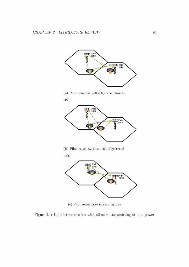
CHAPTER 2. LITERATURE REVIEW 20
(a) Pilot reuse at cell edge and close to
BS
(b) Pilot reuse by close cell-edge termi-
nals
(c) Pilot reuse close to serving BSs
Figure 2.1: Uplink transmission with all users transmitting at max power

CHAPTER 2. LITERATURE REVIEW 21
2.2 Less Aggressive pilot Reuse
Full pilot reuse prompts most extreme inter-cell interference amid channel
estimation, which can be relieved utilizing a less forceful pilot reuse factor.
Pilot reuse is closely resembling to the conventional frequency reuse as the
terminals inside the pilot reuse region can use just a small amount of the
time-frequency resources, within the channel estimation stage. Whereas, in
the case of pilot reuse, every terminal is allowed to utilize all the accessible
resources for communication for the remaining coherence time. The pilots
are reused in the system by the rate of 1/U, where U is the quantity of
cells that are allotted orthogonal pilots. While using reuse factor of U ¿ 1
dependably limits the effect of pilot contamination by allocating orthogonal
pilots to the neighboring cells. The aggregate number of novel time-frequency
components held for pilot transmission are KU, where K is the quantity of
terminals in each cell.
The trifling instance of pilot reuse is full pilot reuse with U = 1. For
this situation, we hold K time-frequency indices for pilot sequences. The
indices may be found anyplace inside the resource block without loss of sim-
plification. We create K orthogonal pilot sequences including these indices,
that are circulated at arbitrary or algorithmically among the mobile user in-
side each one cell. Since the cells are thought to be synchronized, the pilot
transmissions are synchronized crosswise over cells also.
Moderate value of Reuse factor in this scenario will be used and the
orthogonal pilots are used by the terminals of the nearby cells that cause
much interference. If we use a hexagonal geometry for cellular layout then
the minimum reuse factor that can help in assigning the orthogonal pilots to
CHAPTER 2. LITERATURE REVIEW 22
(a) Pilot reuse 1
(b) Pilot reuse 1/3
(c) Pilot reuse 1/3 pattern
Figure 2.2: Time-frequency resources consumed by pilots for K = 12, reuse
factor 1 and 1/3 respectively

CHAPTER 2. LITERATURE REVIEW 23
the adjacent cells will 1/3. The resources used to implement this reuse factor
will be three time the number of users i.e. 3K. A group of pilots is assigned
to each cell and the terminals are assigned with the pilots as in the case of
full pilot reuse scheme. In a similar way we can define schemes for the reuse
factors 4, 7 and 9 which can reduce the pilot contamination even more as the
terminals using the same pilots are now placed at a farther distance.
Using higher values of pilot reuse we can eliminate the pilot contamination
but at the cost of the overheads added by using the pilot resources. This
overhead will limit the amount of data that is to be sent in the next phase.
Anyhow this better estimate of channel will result in better beamforming for
the uplink and downlink transmissions using spatial multiplexing to serve
the terminals. Hence there is a tradeoff between the exact beamforming and
data transmission afterwards.
There is another technique that is also known as Soft Pilot Reuse, in
which the terminals at the cell edge of each cell are assigned the orthogonal
pilot sequences. Hence the terminals will not affect the transmission of the
adjacent cell terminals with this implementation. As we know that cell-edge
terminals have the poor SNR therefore with the help of this technique higher
rates can also be achieved.

CHAPTER 2. LITERATURE REVIEW 24
Figure 2.3: Pilot distribution scheme for Soft pilot Reuse
2.3 Effect of pilot Contamination in massive
MIMO cellular uplink systems with pilot
reuse
A pilot reuse scheme has been employed in an uplink massive MIMO sys-
tem. Lower bound for non asymptotic throughput is shown to be precise
with the help of simulations. Three types of interferences affect the lower
bound namely: inter-cell interference, intra-cell interference and pilot con-
tamination. Certain conditions are examined on which the behavior of each
interference dominates. These conditions include the pilot reuse number, M
(number of mobile stations) and network topology. For example when M=100
then throughput is maximum when we use pilot reuse number 2. Pilot con-
tamination in this case is eliminated and inter-cell interference dominates.
In this paper a pilot reuse scheme is considered for an uplink massive

CHAPTER 2. LITERATURE REVIEW 25
MIMO network. Pilot reuse number can be more than one in this case.
Lower bound for throughput that is non-asymptotic is derived for the cellular
network. The lower bound is characterized with three interference terms:
inter-cell, intra-cell interference and pilot contamination. Studies on the
conditions for which certain interference dominates are discussed with the
help of numerical simulations which gives insight about the relation among
number of base station antennas optimal throughput, network topology and
pilot reuse number.
A 2L+1 cells ranging from L to L are considered to be deployed in a
line, shown in the following figure. M numbers of base station antennas are
located in each cell and the distance between two closest neighboring base
stations is d. k number mobiles are served in each cell. The K mobiles are
considered to be single antenna and co-located for the sake of simplicity i.e.
the distance between mobile and its respective base station is do.
In this paper lower bound for throughput in a massive MIMO uplink
cellular network with a pilot reuse scheme has been found. Three types of
interference were identified and discussed. It has been shown that the pilot
contamination does not limit the throughput when (1) pilot reuse number
is greater than 1 or (2) the mobiles are located at the cell center with pilot
reuse 1.

CHAPTER 2. LITERATURE REVIEW 26
Figure 2.4: Network topology for pilot reuse in uplink cellular system.

Chapter 3
System Model
Consider a tier-1 hexagonal geometry of a cellular system, where each cell
has a radius R. By tier-1 we refer to the area of interfering cells that causes
co-channel interference (CCI) and is considered the main source of pilot con-
tamination. The reuse factor of the hexagonal geometry is given by Q , where
Q = 1, 3, 4, 7, .... For instance, in Fig. 1, six interfering cells for the center
cell constitute tier-1 geometry with Q=1. Each cell contains an M -antenna
base station (BS) that serves K randomly deployed single antenna mobiles.
Let di,j,k be the distance between user k of cell j and the BS antennas of cell
i , then the path loss factor is given by
ϕi,j,k =1
dαi,j,k(3.1)
Where α is the path loss exponent. Although the distance to all BS antennas
potentially remains the same for one user, however, we will use this notation
for consistency with fading gains.
A Rayleigh block fading channel is assumed where all the channel co-
27

CHAPTER 3. SYSTEM MODEL 28
Figure 3.1: System model

CHAPTER 3. SYSTEM MODEL 29
efficients remain constant for a block of T symbols; T being the channel
coherence period. Considering the geometry, the channel matrix between
the antenna i and mobiles in cell j is Ci ,j ∈ CM×K where all the entries of
Ci ,j are independent and identically distributed (i.i.d.) complex Gaussian
with zero mean and unit variance.
3.1 Multi-cell Uplink Communication
All the mobiles in this uplink scenario communicate with their respective base
station in two stages: uplink training with pilot reuse and actual transmission
of the data.
3.1.1 Uplink Training with Pilot Reuse
In each cell, orthogonal pilots are assigned to the users, which are reused by
other cells by the factor Q. Assume a pre-designed pilot sequence matrix
Ψ = [Ψ0, · · ·,ΨQ−1] ∈ CQK×QK (3.2)
Where Ψ is divided among all cells. Assume that Ψ0 is assigned to the Cell
0 which is considered to be the serving cell (center cell from Fig. 1) and the
pilot sequence is further reused by Cell lQ where 1 ≤ |l | ≤ b LQc where L is
the total number of cells in geometry. The pilot Ψq,k is assigned to a single
user k of a cell in order to remove intra-cell interference with the help of
orthogonality of pilot signals.
We only analyze Cell 0 here for brevity. In a single time-frequency block,
all the mobiles send their pilot signals to the base station. The signals re-
ceived at base station 0 are

CHAPTER 3. SYSTEM MODEL 30
P0 =√φτQK
L−1∑j=0
C0,j Ψ∗(j ) + W0, ∈ CM×K (3.3)
where C0,j = [ϕ0,j ,1c0,j ,1 , · · ·, ϕ0,j ,Kc0,j ,K ] is the channel matrix between the
mobiles of cell j and base station 0, c0,j ,k is the channel vector between base
station 0 and cell j ′s k -th mobile user and (j) = (j mod Q). The variable
W0 is i.i.d. CN (0, 1) and φτ is the average transmission power per mobile.
The factor√
QK guarantees that average power is φτ .
The received signal P0 is projected onto Ψ0,k in order to estimate c0,0,k
at the base station 0. After normalization, the resulting signals are
p0,k = c0,0,k +∑l 6=0
√ϕ0,lQ ,k
ϕ0,0,k
c0,lQ ,k +w0,k√
ϕ0,0,kφτKQ∈ CM×1. (3.4)
A minimum mean squared error (MMSE) estimator [42] is applied to the
received vector of pilots to get
c0,0,k = YcpY−1pp P0,k ; (3.5)
where Ypp and Ycp are the correlation and cross-correlation matrices, re-
spectively. As all the channel vectors are independent therefore, the cross-
correlation matrix becomes Ycp = IM . The correlation matrix Ypp is given
as
Ypp = IM +∑l 6=0
ϕ0,lQ ,k
ϕ0,0,k︸ ︷︷ ︸a1
IM +1
ϕ0,0,k φτKQ︸ ︷︷ ︸a2
IM . (3.6)
From the above equation, we can define σ2τ = (1+a1+a2)−1 and now applying
the MMSE decomposition
c0,0,k = c0,0,k + c0,0,k , (3.7)
where c0,0,k is the independent uncorrelated estimation error. Both the en-
tries are i.i.d. where c0,0,k is CN (0, σ2τ ) and c0,0,k is CN (0, 1− σ2
τ ).

CHAPTER 3. SYSTEM MODEL 31
3.1.2 Actual Transmission of Data
In the next T − KQ slots, all the mobiles transmit their data. This takes
place in all cells after the uplink training of pilots. The received signal at
base station 0 is
r0 =∑j ,k
√φϕ0,j ,k c0,j ,k rj ,k + n0, (3.8)
where φ is the average power consumed by a mobile to transmit the data rj ,k
by a user k in cell j and no is the noise, which is CN (0, 1). At base station
0, maximum ratio combining (MRC) is applied to receive the k -th mobile’s
signal. The unit norm vector is denoted as
uk =c0,0,k
‖c0,0,k‖∈ CM×1. (3.9)
After applying maximum ratio combining and normalization, we get
u∗kr0 = u∗k c0,0,k r0,k +
√1
φτϕ0,0,k
wk (3.10)
+ u∗k c0,0,k r0,k + u∗k∑i 6=k
√ϕ0,0,i
ϕ0,0,k
c0,0,ir0,i (10a)
+ u∗k∑j 6=0
K∑i=1
√ϕ0,j,i
ϕ0,0,k
c0,j,irj,i. (10b)
In (3.10), the two terms are desired signal and the noise respectively. In
(3.10a) the terms refer to intra-cell interference and in (3.10b) the term de-
notes inter-cell interference.
3.1.3 Achievable Cell Throughput
The average throughput of cell 0 using the above mentioned scheme is achieved
by the following derivation. Tier-1 base stations of hexagonal geometry with

CHAPTER 3. SYSTEM MODEL 32
M -antenna are deployed. Each base station serves K randomly located sin-
gle antenna mobiles of its own cell with path loss factor ϕ0,0,k. The inter cell
interference in equation (3.10b) can be re-written as
u∗k∑j 6=0
K∑i=1
√ϕ0,j,i
ϕ0,0,k
c0,j,irj,i − u∗k∑l 6=0
√ϕ0,lQ,k
ϕ0,0,k
c0,lQ,krlQ,k (3.11)
+u∗k∑l 6=0
√ϕ0,lQ,k
ϕ0,0,k
c0,lQ,krlQ,k, (11a)
where (3.11a) represents the pilot contamination. For a single user k , we can
calculate the throughput as
R ≥ log
(1 +
|u∗k c0,0,k |21
φϕ0,0,k+ I1 + I2 + I3
), (3.12)
where I1, I2, I3 are intra-cell, inter-cell and interference due to pilot contam-
ination, respectively and given as
I1 = |u∗k c0,0,k |2 +∑i 6=k
∣∣∣∣u∗k√ϕ0,0,i
ϕ0,0,k
c0,0,i
∣∣∣∣2, (3.13)
I2 =∑j 6=0
K∑i=1
ϕ0,j,i
ϕ0,0,k
|u∗kc0,j,i |2 −∑l 6=0
ϕ0,lQ,k
ϕ0,0,k
|u∗kc0,lQ,k |2, (3.14)
I3 =∑l 6=0
ϕ0,lQ,k
ϕ0,0,k
|u∗kc0,lQ,k |2. (3.15)
Both the terms I1 and I2 are independent of |u∗k c0,0,k |2, whereas I3 is de-
pendent upon c0,0,k which also shows dependence upon |u∗k c0,0,k |2. In order
to analyze I3, MMSE decomposition is applied on c0,lQ,k. Hence we can
write c0,lQ,k as c0,0,k because the MMSE decomposition for both the terms is
proportional. Thus,

CHAPTER 3. SYSTEM MODEL 33
c0,lQ,k =
√ϕ0,lQ,k
ϕ0,0,k
c0,0,k + c0,lQ,k , (3.16)
where c0,lQ,k is i.i.d. CN (0, 1 − ϕ0,lQ,k
ϕ0,0,kσ2τ ) and denotes the estimation error
and is not dependent upon c0,lQ,k . Re-write I3 as
I3 =∑l 6=0
ϕ20,lQ,k
ϕ20,0,k
|u∗k c0,0,k |2 +∑l 6=0
ϕ0,lQ,k
ϕ0,0,k
|u∗k c0,lQ,k |2
+∑l 6=0
((ϕ0,lQ,k
ϕ0,0,k
)32 (u∗k c0,0,k c∗0,lQ,kuk + u∗k c0,lQ,k c∗0,0,kuk)
),
(3.17)
and denote the rate conditioned on c∗0,0,k by R. To achieve the lower bound
of R, convexity of log(1 + 1x) is used, therefore,
R ≥ log
(1 +
|u∗k c0,0,k |21
φϕ0,0,k+ E [I1] + E [I2] + E [I3]
)(3.18)
where E [I1] ,E [I2] and E [I3] are given as
E [I1] = (1− σ2τ ) +
∑i 6=k
ϕ0,0,i
ϕ0,0,k
(3.19)
E [I2] =∑j 6=0
K∑i=1
ϕ0,j,i
ϕ0,0,k
−∑l 6=0
ϕ0,lQ,k
ϕ0,0,k
(3.20)
E [I3] =∑l 6=0
ϕ20,lQ,k
ϕ20,0,k
|u∗k c0,0,k |2 +∑l 6=0
ϕ0,lQ,k
ϕ0,0,k
(1− ϕ0,lQ,k
ϕ0,0,k
σ2τ ). (3.21)
The last two terms in (20) have zero mean hence neglected in (24). Note
that
|u∗k c0,0,k |2 =M∑q=1
c2k,q, (3.22)
where the term ck,q is i.i.d. CN (0, σ2τ ). Hence, |u∗k c0,0,k |2 has Gamma dis-
tribution with parameters (M,σ2τ ). The right hand side of (21) is written
as

CHAPTER 3. SYSTEM MODEL 34
log
1 +Γk
1φϕ0,0,k
+ Ω1 + Ω2 +∑
l 6=0
ϕ20,lQ,k
ϕ20,0,k
Γk
, (3.23)
where Γk = |u∗k c0,0,k |2, Ω1 is the intra-cell interference and Ω2 is the inter-cell
interference given as
Ω1 = (1− σ2τ ) +
∑i 6=k
ϕ0,0,i
ϕ0,0,k
, (3.24)
Ω2 =∑j 6=0
K∑i=1
ϕ0,j,i
ϕ0,0,k
−∑l 6=0
ϕ20,lQ,k
ϕ20,0,k
σ2τ . (3.25)
The inverse Gamma distribution (1/Γk) has a mean value of 1/(M − 1)σ2τ
[43]. Therefore,
Rk ≥ log
1 +1
( 1φϕ0,0,k
+ Ω1 + Ω2)/Γk +∑
l 6=0
ϕ20,lQ,k
ϕ20,0,k
(3.26)
≥ log
1 +1
( 1φϕ0,0,k
+ Ω1 + Ω2)/E[
1Γk
]+∑
l 6=0
ϕ20,lQ,k
ϕ20,0,k
(3.27)
≥ log
(1 +
(M − 1)σ2τ
( 1φϕ0,0,k
+ Ω1 + Ω2 + Ω3
)(3.28)
where Ω3 = (M − 1)∑
l 6=0
ϕ20,lQ,k
ϕ20,0,k
σ2τ is the pilot contamination.
The average achievable throughput for cell 0 is given by
R ≥ K (1− QK
T) log
(1 +
(M − 1)σ2τ
1φϕ0,0,k
+ Ω1 + Ω2 + Ω3
), (3.29)
where φ is the average data power, T is the channel coherence period and
σ2τ is the normalized estimation power

CHAPTER 3. SYSTEM MODEL 35
σ2τ =
(1 +
∑l 6=0
ϕ0,lQ,k
ϕ0,0,k
+1√
φτKQ
)−1
. (3.30)
In (29) the constants Ω1, Ω2 and Ω3 are defined as
Ω1 = (1− σ2τ ) +
∑i 6=k
ϕ0,0,i
ϕ0,0,k
,
Ω2 =∑j 6=0
K∑i=1
ϕ0,j,i
ϕ0,0,k
−∑l 6=0
ϕ20,lQ,k
ϕ20,0,k
σ2τ ,
Ω3 = (M − 1)σ2τ
∑l 6=0
ϕ20,lQ,k
ϕ20,0,k
.
(3.31)
The derived equation for cell throughput R is valid for even small values
of M and the achievable rate is non-asymptotic which is valid for any M .
Three types of interference terms are characterized in this derivation, Ω1
is the intra-cell interference, Ω2 is the inter-cell interference and Ω3 is the
interference caused due to pilot contamination. Ω2 is referred as non-coherent
interference whereas Ω3 is the coherently added inter-cell interference referred
as coherent interference. Both Ω1 and Ω2 have direct dependence upon K but
are independent of M . Both these interferences also depend upon the network
topology, if the cell size is large then less inter and intra-cell interference will
occur keeping other parameters constant. Whereas, Ω3 increases linearly
with M and is independent of K as there is only single mobile per cell that
is using the pilot with same frequency.

Chapter 4
Numerical Results
In this section, we evaluate the effect of different interferences, pilot reuse
factor and network topology on the average cell throughput. Different simu-
lations have been carried out to study the parameters upon which maximum
throughput is achieved. For all simulations, we assume coherence period T
= 100ms, radius R = 1.4km, path loss exponent α = 3.8 and φτ = φ =
100mW, unless noted otherwise. All the mobiles operate at 3GHz frequency
and 10MHz bandwidth. In order to get ergodic cell throughput, Monte-
Carlo method is applied with 1e6 simulations for a single user having random
location in every trial.
Fig. 2 shows the average throughput of the system versus the number
of users. We can observe the dependence of throughput on the reuse factor
and the number of users per cell. Average throughput of a cell increases
when the number of users increases. Similarly R increases as the reuse fac-
tor goes from 1 to 7 because the coherent interference decreases when the
interfering mobiles get far away from the serving cell 0’s base station. On
the contrary, Non-coherent and intra-cell interference have no effect with the
36

CHAPTER 4. NUMERICAL RESULTS 37
2 4 6 8 10 12 14 16 18 200
5
10
15
20
25
Number of users; M=100
Q=1Q=7Q=3
Figure 4.1: Average throughput with different number of users and reuse
factor
.

CHAPTER 4. NUMERICAL RESULTS 38
change in Q but both interferences tend to increase with increasing K . The
gain overcomes the loss due to both interferences hence the final net result is
the increase in average throughput of a cell. Fig. 2 also shows the achievable
throughput to a specific number of users for different reuse factors. For ex-
ample, a throughput of more than 20 bits/sec/Hz is provided when serving
20 users for Q=3.
10 20 30 40 50 60 70 80 90 1000
2
4
6
8
10
12
14
16
18
Number of antennas
Ave
rage
sum
rat
e B
its/S
ec/H
z
K=5,Q=1K=10,Q=3K=5,Q=3
Figure 4.2: Average throughput with different number of antennas
.
Fig. 3 depicts the relation between number of antennas and the average
throughput for different reuse factor. The average sum-rate increases as the
number of antennas increase. The saturation in throughput is not obvious

CHAPTER 4. NUMERICAL RESULTS 39
for 100 antennas for reuse factor 3 as the interference power caused by pilot
contamination using Q=3 is very small, whereas, the throughput saturates
for higher number of antennas at reuse factor 1. Hence we can say that pilot
contamination almost vanishes for higher reuse factors.
10 20 30 40 50 60 70 80 1008
10
12
14
16
18
20
22
24
Coherence Period T (ms); M=100; Q=3
Ave
rage
Sum
−R
ate
Bits
/Sec
/Hz
K=20K=5K=10
Figure 4.3: Average throughput with coherence period and different number
of users
.
Fig. 4 shows the relation between coherence period T and the average
throughput with different number of mobiles K . When we consider only 5
users in a cell, the throughput doesn’t change much with the increase in T
but when K goes to 20, the throughput starts increasing gradually as T
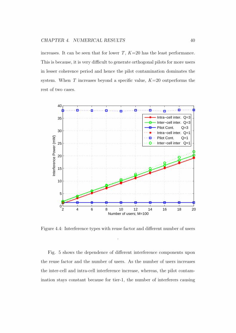
CHAPTER 4. NUMERICAL RESULTS 40
increases. It can be seen that for lower T , K =20 has the least performance.
This is because, it is very difficult to generate orthogonal pilots for more users
in lesser coherence period and hence the pilot contamination dominates the
system. When T increases beyond a specific value, K =20 outperforms the
rest of two cases.
2 4 6 8 10 12 14 16 18 200
5
10
15
20
25
30
35
40
Number of users; M=100
Inte
rfer
ence
Pow
er (
mW
)
Intra−cell inter. Q=3Inter−cell inter. Q=3Pilot Cont. Q=3Intra−cell inter. Q=1Pilot Cont. Q=1Inter−cell inter Q=1
Figure 4.4: Interference types with reuse factor and different number of users
.
Fig. 5 shows the dependence of different interference components upon
the reuse factor and the number of users. As the number of users increases
the inter-cell and intra-cell interference increase, whereas, the pilot contam-
ination stays constant because for tier-1, the number of interferers causing

CHAPTER 4. NUMERICAL RESULTS 41
pilot contamination will always be six for any reuse factor. On the aver-
age, the inter-cell and intra-cell interferences have the same impact on the
throughput because the location of user is random; for distances closer to the
base station, the intra-cell interference dominates and for distances far away,
the inter-cell interference dominates. Hence, on the average, both contribute
the same to the cell throughput. It can also be observed from Fig. 5 that
the reuse factor only affects the pilot contamination, whereas, the inter-cell
and intra-cell interferences remain almost constant because the interferers
that cause pilot contamination move away from the serving cell as the reuse
factor increases. Hence, the throughput is increased while using higher reuse
factors.
Fig. 4.5 shows the average throughput rates for two receivers i.e. MMSE
and MRC. We can see that MMSE receiver performs better than the MRC for
all number of antennas. This is because of the reason that MMSE minimizes
the interference terms only, whereas, MRC amplifies the whole signal and
then multiplies the data that has higher amplitude with some weights of
higher value and leaves the low amplitude signals as it is that does not
ensure the minimization of interference. In MMSE receivers the interference
terms are minimized to zero and the original data is amplified. Hence, we
get higher rates in case of MMSE receiver.

CHAPTER 4. NUMERICAL RESULTS 42
2 4 6 8 10 12 14 16 18 204
6
8
10
12
14
16
18
20
22
Number of users; Q=3
Ave
rage
sum
rat
e B
its/s
ec/H
z
MMSE, M=100MRC, M=100
Figure 4.5: Comparison between throughputs of MMSE and MRC receivers
.

Chapter 5
Conclusion
In this paper, we evaluated the lower bound for non-asymptotic throughput
of an uplink massive MIMO system with hexagonal geometry and random
deployment of users. It was observed that the effect of pilot contamination
diminishes when we have reuse factor greater than 1. Moreover, relation-
ship between the number of users in a cell, number of base station antennas,
duration of coherence period and average cell throughput has been stud-
ied through simulations. Through these studies, we can calculate the lower
bound of average throughput for a cell that can be achieved for the different
values of parameters like K ,T ,Q and M . We quantified the cell throughput
for various reuse factors and showed that by moving to higher reuse factors,
pilot contamination is reduced, however, there is very little or no effect on
the inter-cell and intra-cell interference. We considered only MRC receivers,
however in future we intend to also look into the MMSE receivers.
43
Bibliography
[1] F. Rusek, D. Persson, B. K. Lau, E. G. Larsson, T. L. Marzetta, O. Ed-
fors, and F. Tufvesson, “Scaling up MIMO: Opportunities and challenges
with very large arrays,” IEEE Signal Process. Mag., vol. 30, pp. 4060,
Jan. 2013.
[2] H. Q. Ngo, E. G. Larsson, and T. L.Marzetta, “Energy and spectral effi-
ciency of very large multiuser MIMO systems,” IEEE Trans. Commun.,
vol. 61, pp. 14361449, Apr. 2013.
[3] B. Hochwald and T. Maretta, “Adapting a downlink array from uplink
measurements,” IEEE Trans. Signal Process., vol. 49, no. 3, pp. 642653,
Mar 2001.
[4] E. Larsson, O.Edfors, F.Tufvesson, and T. Marzetta, “Massive MIMO for
next generation wireless systems” IEEE Commun. Mag., vol. 52, no. 2,
pp. 186195, Feb. 2014
[5] T. Marzetta, “Noncooperative cellular wireless with unlimited numbers
of base station antennas,” IEEE Trans. Wireless Commun., vol. 9, no.
11, pp. 35903600, Sep. 2010.
44

BIBLIOGRAPHY 45
[6] M. Jain, J. Choi, T. Kim, D. Bharadia, S. Seth, K. Srinivasan, P. Levis, S.
Katti, and P. Sinha, “Practical, real-time, full duplex wireless,” in Proc.
Int. Conf. on Mobile Computing and Networking (ACM), New York, NY,
USA, 2011, pp. 301312.
[7] D. Chizhik, F. Rashid-Farrokhi, J. Ling, and A. Lozano, “Effect of an-
tenna separation on the capacity of BLAST in correlated channels,”
IEEE Commun. Lett., vol. 4, no. 11, pp. 337339, Nov. 2000.
[8] J. Duplicy, B. Badic, R. Balraj, R. Ghaffar, P. Horvath, F. Kaltenberger,
R. Knopp, I. Kovacs, H. Nguyen, D. Tandur, and G. Vivier, “MU-MIMO
in LTE systems,” EURASIP J. on Wireless Comm. and Netw., Mar.
2011.
[9] C. Shepard, H. Yu, N. Anand, L. E. Li, T. L. Marzetta, R. Yang, and
L. Zhong “Argos: Practical many-antenna base stations,” ACM Int.
Conf.Mobile Computing and Networking (MobiCom), 2002.
[10] F. Kaltenberger, J. Haiyong, M. Guillaud, and R. Knopp, “Relative
channel reciprocity calibration in MIMO/TDD systems,” Proc. of Future
Network and Mobile Summit, 2010, 2002.
[11] B. Gopalakrishnan and N. Jindal, “How much training is required for
multiuser MIMO?” in Proc. IEEE Workshop on Signal Processing Adv.
in Wire-less Commun. (SPAWC), Jun 2011, pp. 381385.
[12] F. Rusek, D. Persson, B. K. Lau, E. G. Larsson, T. L. Marzetta, O. Ed-
fors, and F. Tufves-son, “Scaling up MIMO: Opportunities and challenges
BIBLIOGRAPHY 46
with very large arrays,” IEEE Com-mun. Mag., Jan. 2013.., vol.54, pp.
1268-1278,
[13] N. Krishnan, R. Yates, , and N. Mandayam, “Uplink linear receivers
for multicell multiuser MIMO with pilot contamination: Large system
analysis,” IEEE Trans. Wireless Commun., vol. 13, no. 8, pp. 43604373,
Aug. 2014.
[14] E. Dahlman, S. Parkvall, and J. Skld, “4G: LTE/LTE-Advanced for
Mobile Broadband”.Elsvier, 2014.
[15] M. Biguesh and A. Gershman, “Training-based mimo channel estima-
tion: a study of estimator tradeoffs and optimal training signals,” IEEE
Trans. Signal Process., vol. 54, no. 3, pp. 884893, Mar 2006.
[16] J. Jose, A. Ashikhmin, T. Marzetta, and S. Vishwanath, “Pilot contam-
ination problem in multi-cell TDD systems,” in Proc. IEEE Int. Symp.
on Inf. Theory (ISIT), Jun 2009, pp. 21842188.
[17] H. Yin, D. Gesbert, M. Filippou, and Y. Liu, “A coordinated approach
to channel estimation in large-scale multiple-antenna systems,” IEEE J.
Sel. Areas Commun., vol. 31, no. 2, pp. 264273, Feb 2013.
[18] T. L. Marzetta “Noncooperative cellular wireless with unlimited number
of base station antenna,” IEEE Trans. Wireless Commun., vol. 9, no. 11,
pp. 3590-3600, Nov. 2010.
[19] A. Ashikhmin and T. L. Marzetta “Pilot contamination precoding in
multi-cell large scale antenna systems,” IEEE International Symposium
on Information Theory (ISIT),,Cam-bridge, MA, Jul. 2012
BIBLIOGRAPHY 47
[20] A. Paulraj, R. Nabar, and D. Gore, “Introduction to Space-Time Wire-
less Communications”’. Cambridge University Press, 2008
[21] G. Xiang, F. Tufvesson, O. Edfors, and F. Rusek, “Measured propa-
gation characteristics for very-large MIMO at 2.6 GHz,” in Proc. IEEE
Asilomar Conf. Signals, Systems, and Computers, Nov. 2012, pp. 295299.
[22] M. Steinbauer, A. Molisch, and E. Bonek, “The double-directional radio
channel,” IEEE Anten. and Prop. Mag., vol. 43, no. 4, pp. 5163, Aug.
2001.
[23] ITU-R, “Guidelines for evaluation of radio interface technologies for IM-
TAdvanced,” International Telecommunication Union, Tech. Rep. ITU-
R, M.2135-1, Dec. 2009.
[24] T. L. Marzetta and B. M. Hochwald, “Fast transfer of channel state
information in wireless systems,” IEEE Trans. Signal Process., vol.54,
pp. 1268-1278, 2006.
[25] L. Lu, G. Y. Li, A. L. Swindlehurst, A. Ashikhmin, and R. Zhang, “An
overview of massive MIMO: Benets and challenges,” IEEE J. Sel Topics
Signal Process., April 2014.
[26] J. Jose, A. Ashikhmin, T. L. Marzetta and S. Vishwanath. “Pilot con-
tamination problem in multi-cell TDD systems,” IEEE International
Symposium on Information Theory, pp 2184-2188, July, 2009.
[27] B. Gopalkrishnan and N. Jindal, “An analysis of pilot contamination on
Multi-user MIMO cellular systems with many antennas,” IEEE SPAWC,
pp. 381-385, June 2011.

BIBLIOGRAPHY 48
[28] H. Q. Ngo, T.L.Marzetta and E.G.Larsson “Analysis of pilot contami-
nation effect in very large multicell multiuser MIMO systems for physical
channel models”, IEEE ICASSP, pp. 3464-3467, May 2011.
[29] T. E. Bogale and L. B. Le “Pilot optimization and channel estimation
for multiuser massive MIMO systems”, IEEE CISS, Mar. 2014.
[30] Papadopoulos, G. Caire and S. Ramprashad, “Achieving large spectral
efficiencies from MU-MIMO with tens of antennas: location adaptive
TDD MU-MIMO design and user scheduling”, IEEE ASILOMAR, pp.
636-643, Nov. 2010.
[31] H. Huh, G. Caire, Papadopoulos, Ramprashad “Achieving ”Massive
MIMO” Spectral Efficiency with a Not-so-Large Number of Antennas,”
IEEE Trans. on Wireless Communications, vol.11, no.9, pp.3226-3239,
September 2012
[32] K. Appaiah, A. Ahsikhmin and T. Marzetta, “Pilot contamination re-
duction in multi-user TDD systems,” IEEE ICC, May 2010.
[33] P. Xu, J. Wang and J. Wang “Effect of pilot contamination on channel
estimation in massive MIMO systems,” IEEE WCSP, 2013.
[34] S. M. Kay, “Fundamentals of statistical signal processing: estimation
theory”. Prentice-Hall, 1993.
[35] H. Yin, D. Gesbert, M. Filippou, and Y. Liu, “A coordinated approach
to channel estimation in large-scale multiple-antenna systems,” IEEE J.
Sel. Areas Commun., vol. 31, no. 2, pp. 264273, Feb 2013.

BIBLIOGRAPHY 49
[36] Y. Li, Y.-H. Nam, B. l. Ng and J. Zhang “A non-asymptotic throughput
for massive MIMO cellular uplink with pilot reuse,” Wireless Communi-
cation Symposium - Globecom, pp. 4500-4504, 2012.
[37] P. Xu, J. Wang, and J. Wang, “Effect of pilot contamination on channel
estimation in massive MIMO systems,” in Proc. Int. Conf. on Wireless
Commun. Signal Proces. (ICWCSP), Oct 2013, pp. 16.
[38] A. Simonsson and A. Furuskar, “Uplink power control in LTE - overview
and performance,” in Proc. IEEE Veh. Tech. Conf. (VTC), Sep 2008, pp.
15.
[39] A. Scherb and K. Kammeyer, “Bayesian channel estimation for doubly
correlated mimo systems,” in Proc. ITG Workshop on Smart Antennas
(WSA), Vienna, Austria, Feb 2007.
[40] M. Frenne, “On RSRP determination for UE to node association,”
3rd Generation Partnership Project, Tech. Rep. 3GPP, TSG-RAN WG1
Meeting 75, Aug. 2001.
[41] S. Jrmyr, “MIMO transceiver design for multi-antenna communications
over fading channels,” Ph.D. dissertation, Royal Institute of Technology
(KTH), Sweden, 2013.
[42] G. L. Stuber, Principles of Mobile Communication, 2nd ed. NYC, NY,
USA: Springer, 2011.
[43] David G. T. Denison, Christopher C. Holmes, Bani K. Mallick, Adrian F.
M. Smith Bayesian Methods for Nonlinear Classification and Regression,
2002.


![Performance of Massive MIMO Uplink with Zero-Forcing ... · cell systems with perfect channel state information (CSI) [10] and with the arising pilot contamination [11]. Despite that](https://img.dokumen.tips/doc/110x75/603e04f5cb85744bc72d424b/performance-of-massive-mimo-uplink-with-zero-forcing-cell-systems-with-perfect.jpg)