J Stat Phys (2007) 128: 1391–1414DOI 10.1007/s10955-007-9346-5

Analysis of Path Integrals at Low Temperature:Box Formula, Occupation Timeand Ergodic Approximation

Sébastien Paulin · Angel Alastuey · Thierry Dauxois

Received: 27 July 2006 / Accepted: 9 May 2007 / Published online: 3July 2007© Springer Science+Business Media, LLC 2007

Abstract We study the low temperature behavior of path integrals for a simple one-dimensional model. Starting from the Feynman–Kac formula, we derive a new functionalrepresentation of the density matrix at finite temperature, in terms of the occupation timesfor Brownian motions constrained to stay within boxes with finite sizes. From that repre-sentation, we infer a kind of ergodic approximation, which only involves double ordinaryintegrals. As shown by its applications to different potentials, the ergodic approximationturns out to be quite efficient, especially in the low-temperature regime where other usualapproximations fail.

1 Introduction

The knowledge of the density matrix at finite temperature T for few interacting particles, isimportant for studying equilibrium properties of quantum many-body systems. In this con-text, the Feynman–Kac (FK) representation of the density matrix in terms of path integrals[1–4] is particularly useful. On the one hand, it has been used for deriving exact analyticalexpressions for simple models (see e.g. [5]). On the other hand, beyond the well-knownWigner-Kirkwood expansion [6–9] around the classical limit, various approximations, non-perturbative in �, have been introduced within that framework: for instance, the celebratedsemi-classical approximation [1, 11] or the variational approach of Feynman and Klein-ert [10].

The FK representation is described in Sect. 2. For the sake of pedagogy, we considera single particle in one dimension submitted to a stationary potential. Furthermore, the in-fimum of the corresponding spectrum is assumed to be a bound state. The mean spatialextension of the Brownian paths, which intervene in the FK representation, is controlled bythe thermal de Broglie wavelength of the quantum particle. At high temperatures, Wigner–

S. Paulin · A. Alastuey · T. Dauxois (�)Laboratoire de Physique, CNRS, ENS Lyon, 46 allée d’Italie, 69364 Lyon cédex 07, Francee-mail: Thierry.Dauxois@ens-lyon.fr

1392 J Stat Phys (2007) 128: 1391–1414

Kirkwood �2-expansions around the classical limit, which have been derived long ago in

other frameworks, are easily recovered since path extension vanishes. At finite temperatures,non-perturbative effects in � can be accounted for through various approximations [10, 11],which are briefly described. When temperature goes to zero, the asymptotic structure of thedensity matrix, provided by the groundstate contribution in its spectral expression, does notclearly emerge from its FK representation. In fact, in that temperature regime, the averageextension of paths diverge, whereas the main contribution to the functional integral arisesfrom paths with a finite extension, of the order of the localization length of the ground state:contributions of such minority paths are significantly different from the average contribu-tion. Most of our knowledge is negative, i.e. tells us which trajectories are not important [12],so, in some sense, we will try to have a positive attitude [13].

In this paper, we derive a new functional representation of the density matrix, which ismore suitable than the genuine FK formula for tackling the low-temperature regime (seeSect. 3). The starting central observations are described in Sect. 3.1. First, in the FK func-tional integral, only marginal paths with finite extensions, i.e. large deviations with respectto the average, contribute when T goes to zero. Second, many of such paths with quite differ-ent jagged shapes, provide similar contributions, mainly determined by the correspondinglocal occupation times. Thus, it is quite natural to collect paths into sets defined by theirspatial extension and their local occupation times. That procedure allows us to transformexactly FK representation (2) into the so-called box formula (13). That formula is definedvia the introduction of paths constrained to stay in a box with size � and characterized by anintermediate flight time s (in β� units with β = 1/kBT ). It involves a double ordinary in-tegral over � and s, combined to functional integrals over local occupation times associatedwith the constrained paths. As required, box formula (13) provides a better understandingof the low-temperature behavior of the density matrix than FK representation (2). WhenT vanishes, leading contributions obviously arise from typical sizes � much smaller thande Broglie wavelength. In a forthcoming paper, we will argue how groundstate quantitiesemerge from box formula (13), by using scaling properties of the probability distributionfunction (PDF) of occupation times at low temperatures.

Beyond its conceptual interest for understanding low-temperature behaviors of path in-tegrals, box formula (13) also allows us to derive new approximations. This is illustratedin Sect. 4, where we present the so-called ergodic approximation. That approximation re-sults from the truncation to first order of cumulant expansions of the functional averages.It amounts to replace each local occupation time associated with a given constrained path,by its average over the corresponding PDF. This can be viewed as some kind of ergodichypothesis, because the imaginary-time average of the potential experienced by the particlealong that path, is then replaced by a spatial average with a measure defined by the meanoccupation-time. Ergodic expression (16) involves only an ordinary double integral over �

and s, so the tremendous difficulty of computing a functional integral is circumvented. Thekey ingredient, namely the mean occupation-time (in units of 1/�), depends on three dimen-sionless variables. Using its low and high temperature behaviors derived analytically, wepropose simple tractable expressions for that quantity, which turn out to be quite accurate atany temperature.

Section 5 is devoted to the applications of the ergodic approximation to various sim-ple forms of the potential. First, we determine the asymptotic analytical forms of the ap-proximate density matrices at both low and high temperatures. When T diverges, Wigner–Kirkwood expansion is partially recovered. When T vanishes, the main features of the exactbehaviors are well reproduced. The approximate density matrices then do factorize as a

J Stat Phys (2007) 128: 1391–1414 1393

product of a Boltzmann factor associated with a given energy, times a function of posi-tion only: this provides satisfactory approximate expressions for the groundstate energy andwavefunction. Second, numerical calculations are performed at finite intermediate temper-atures. As expected from the previous analytical results, the ergodic approximation turnsout to be quite reasonably accurate over the whole range of considered temperatures, anddiscrepancies with numerically exact results1 do not exceed a few percent in most cases.Moreover, it significantly improves over the well-known semi-classical approximation, inparticular at low temperatures (except for the harmonic potential of course). Also, furtherapplications and extensions of the ergodic approximation to other potentials and two- orthree-dimensional systems with one or two particles, are briefly discussed.

Let us mention that various computationally exact methods have been derived for cal-culating path integrals with an arbitrary high accuracy. A first type of such methods startswith Trotter formula, and rely on the use of simple thermal propagators (see e.g. [14]), com-bined to Monte Carlo sampling of multi-dimensional integrals and other algorithmic tricks[15, 16]. Quantum Monte Carlo methods extend those approaches to many-body systems,for which they have provided remarkable results (see e.g. [16–18]). Another type of compu-tationally exact methods follows from Ito–Nisio theorem [19] and involve decompositionsof Brownian paths on suitable basis.

Eventually, we emphasize that our approach is not intended to provide numerically exactresults. The ergodic formula (16) enters in the class of simple approximation schemes, likethose described above [10, 11], which account for non-perturbative quantum effects. Its mainadvantages rely on both an analytical control of low-temperature behaviors, and an accuratedescription over a wide temperature-range via numerical calculations easily performed bya pocket calculator. In the framework of the many-body problem, this should be useful forvarious purposes, like fast and reliable estimates of first quantum virial coefficients in low-fugacity expansions, or tractable modelizations of two-body effective interactions. Also,use of the ergodic approximation for few-body density matrices in quantum Monte Carlomethods, might improve the accuracy and convergence of the corresponding calculations.

2 Path Integral Framework

In this Section, we first define the model and then introduce the FK representation of thecorresponding density matrix. Next, we briefly recall the efficiency of FK formula for de-scribing the high-temperature regime, and we argue about its drawbacks for analyzing low-temperature behaviors.

We consider a quantum non-relativistic particle of mass m in one dimension z withHamiltonian H = −�

2/(2m)Δ + V (z). The matrix elements of Gibbs operator ρ =exp[−βH ] with β = 1/(kBT ), define the so-called density matrix ρ(x, y,β) = 〈x|ρ|y〉.The partition function Z(β) = Trace[ρ] is well behaved for a confining potential such thatV (z) → ∞ when |z| → ∞. The normalized probability density to find the particle at posi-tion x then reduces to Ψ (x,β) = ρ(x, x,β)/Z(β). For a potential which vanishes at infinityin an integrable way, we introduce the virial coefficient B(β) = Trace[ρ − ρ0] where ρ0

is the free density matrix, as well as the normalized deviation to the uniform free density

1Such results are inferred from the spectral representation on the one hand, and from a transfer-matrix diag-onalization method specific to one-dimensional systems on the other hand.

1394 J Stat Phys (2007) 128: 1391–1414

Φ(x,β) = [ρ(x, x,β) − ρ0(x, x,β)]/B(β).2 For further purposes, it is also convenient tointroduce the spectral representation of the density matrix

ρ(x, y,β) =+∞∑

k=0

φk(x)φ∗k (y) exp(−βEk), (1)

where φk is the k-th eigenstate of H with energy Ek . It is understood that, for the continuouspart of the spectrum, the discrete sum in the r.h.s. of (1) is replaced by an integral over theenergies of diffusion states.

Path integrals were first introduced for representing the matrix elements of the evolu-tion operator exp(−iH t/�) associated with Schrödinger equation [1]. It was soon real-ized that a similar path integral representation for matrix elements of Gibbs operator atinverse temperature β can be inferred via the formal substitution t → −iβ�. In that gen-uine representation of ρ(x, y,β), paths can be rewritten within the parametrization ω(u) =(1 − s)x + sy +λDξ(s), where s = u/(β�) is the dimensionless time in β� units, while ξ(s)

is a Brownian bridge satisfying boundary conditions ξ(0) = ξ(1) = 0 and λD = (β�2/m)1/2

is the de Broglie wavelength. This provides the so-called Feynman–Kac formula [2–4]

ρ(x, y,β) = exp[−(x − y)2/(2λ2D)]√

2πλD

×∫

Ω

DW(ξ) exp

(−β

∫ 1

0dsV ((1 − s)x + sy + λDξ(s))

)(2)

where Ω = {ξ(·)} is the infinite set of realizations of the Brownian bridge process, whileDW(ξ) is the normalized Gaussian Wiener measure defined by its first two moments,〈ξ(s)〉Ω = 0 and 〈ξ(s1)ξ(s2)〉Ω = min(s1, s2)(1 − max(s1, s2)). Wiener measure is intrinsicto Brownian motion and does not depend on any physical parameter. Mass m of the parti-cle, as well as Planck’s constant � only intervene in the de Broglie wavelength λD , whichcontrols the size of quantum fluctuations, as shown by specifying (2) to diagonal elements,i.e.

ρ(x, x,β) = 1√2πλD

∫

Ω

DW(ξ) exp

(−β

∫ 1

0dsV (x + λDξ(s))

). (3)

In time-average∫ 1

0 dsV (x + λDξ(s)), particle experiences the potential around position x

on a length scale obviously determined by λD , as illustrated in Fig. 1. Notice that, besides itsinterest for analytical or numerical calculations (see below), Feynman–Kac representationis also quite useful for mapping a quantum system into a classical one [20–23].

At high temperatures, de Broglie wavelength is small, so only paths which remainclose to reference position x contribute significantly to ρ(x, x,β) in (3). Therefore, thetime-average of V along path x + λDξ(s) can be performed by replacing V (x + λDξ(s))

by its Taylor series around V (x). This generates quantum corrections to classical formexp[−βV (x)]/(√2πλD) because λD is proportional to �. Thanks to Wick’s theorem, we

2Virial coefficient B occurs in low-fugacity expansions of thermodynamical quantities for a many-body sys-tem made with two-body interactions V (xi − xj ). Deviation Φ then determines leading particle correlationsat low densities.

J Stat Phys (2007) 128: 1391–1414 1395

Fig. 1 (Color online) Typical path which starts and ends at position x, along which particle experiencespotential V . Dashed lines indicate the two edges of a fictitious box determined by the extremal deviations ξ1and ξ2 of the path. Typical sizes of ξ1 and ξ2 are of order one

easily retrieve the well-known Wigner–Kirkwood expansion in powers of �2

ρ(x, x,β) = e−βV (x)

√2πλD

[1 − β2

�2

12m

d2V

dx2+ β3

�2

24m

(dV

dx

)2

+ · · ·], (4)

which was derived long ago by using the Wigner-distribution formalism (see e.g. Ref. [9]).Previous method might be used for calculating higher-order terms beyond �

2-correction(terms up to order �

6 have been already determined in the literature [24]). Moreover, itclearly emphasizes that expansion (4) is appropriate when the de Broglie wavelength ismuch smaller than the typical length of variation of the potential.

When the temperature decreases, the de Broglie wavelength increases, so Wigner–Kirkwood expansion is no longer applicable. At the analytical level, exact evaluations ofthe corresponding path integrals are not accessible in general, except for some simple mod-els [5]. Non-perturbative effects in � can be partially accounted for through various meth-ods. The celebrated semi-classical approximation is based on an expansion with respect tothe deviation of an arbitrary path with respect to the classical trajectory. The truncation ofthat expansion up to second order leads to a Gaussian functional integral, which is exactlycomputed in terms of the classical action and its derivatives [11]. A second method relieson the introduction of auxiliary harmonic potentials with adjustable frequencies [10]. Suchfrequencies are then determined by a variational criterion which follows from Jensen in-equality. The reliability of those methods remains questionable since they do not involveany small control-parameter like (4). Nonetheless, for numerical purposes, their accuracymay be satisfactory, at least at not too low temperatures.

When temperature goes to zero, λD diverges, so most paths explore a rather large regionnot restricted to the neighborhood of reference position x. A direct analysis of FK expres-sion (3) then becomes quite cumbersome. In particular, ρ(x, x,β) must behave as

ρ(x, x,β)β→+∞∼ |φ0(x)|2 exp[−βE0], (5)

which immediately follows from spectral representation of density matrix (1). The factor-ization of position and temperature dependencies in (5) does not come out easily from FK

1396 J Stat Phys (2007) 128: 1391–1414

formula (3), where both position and temperature are coupled in an absolutely non-trivialway.

3 Box Formula

3.1 The Central Observations

For fixing ideas, let us consider a symmetric potential V (z) with a minimum located atz = 0. On the one hand, low-temperature behavior (5) of the corresponding density matrixis mainly determined by the local shape of V (z) over finite length scale a0, which charac-terizes the spatial extension of the groundstate wave function φ0(x). On the other hand, fortypical paths with size of order λD , time-average potential

∫ 10 dsV (x + λDξ(s)) becomes,

roughly speaking, of order∫ λD

0 dzV (z)/λD when λD is sufficiently large. At low temper-

atures, β∫ 1

0 dsV (x + λDξ(s)) does not behave as a constant times β in general. Thus,low-temperature behavior (5) is not provided by typical paths. That argument can be im-plemented through semi-quantitative estimations in some specific cases. For a confiningpotential which diverges as |z|n (n > 0), contributions of typical paths to (3) then behave(discarding multiplicative powers of β) as exp(−cβ1+n/2) with some positive constant c.For integrable potentials, such contributions become of order exp(−c/β1/2). In both cases,typical contributions are exponentially smaller than leading Boltzmann factor exp[−βE0].

The previous analysis suggests that, at low temperatures, leading contributions to ther.h.s. of (3) arise from paths with a spatial extension of order a0, i.e. from quite smallBrownian bridges with size |ξ(s)| of order a0/λD . For such paths, time-average potential∫ 1

0 dsV (x + λDξ(s)) is of order V (a0), so the corresponding Boltzmann factor indeed is oforder exp[−βE0]. Notice that, paths with very different shapes give raise to similar contribu-tions, since the Wiener weights of the associated Brownian bridges remain of order (roughlyspeaking) exp(− ∫ 1

0 ds(ξ̇ (s))2/2) ∼ exp(−a20/λ

2D) ∼ 1. Consequently, when the temperature

decreases, only a very tiny subset of paths gives a relevant contribution to the r.h.s. of (3).In other words, important paths are not any more typical but, on the contrary, they can beviewed as large deviations. This explains why direct numerical evaluations of (3) becomerather difficult: the subset of important paths remains, in some sense, hidden in the entireconfigurational space.

In order to extract from (3) the relevant contributions at low temperatures, it is temptingto collect all paths with the same finite spatial extension, and then to sum over all possibleextensions. That procedure is not easy to carry out directly in the r.h.s. of (3), within asuitable partition of functional integration space over Brownian bridges. As described below,it is more convenient to transform first the density matrix within the operator representation,by introducing an auxiliary Hamiltonian which confines the particle inside a box with size �.

3.2 The Auxiliary Hamiltonian Approach

Let us introduce the auxiliary Hamiltonian H� = H 0 +V +V�, where H 0 denotes the kineticHamiltonian. The additional potential V� is defined by

V�(z) = V0[1 − Θ(z + �) + Θ(z − l)], (6)

where Θ is the Heavyside function, while V0 denotes barrier height (V0 > 0). That poten-tial tends to confine the particle inside a box with extension �. The auxiliary Hamiltonian

J Stat Phys (2007) 128: 1391–1414 1397

reduces to the genuine one when � goes to infinity. In that limit, for x kept fixed, diagonalpart 〈x|ρ�|x〉 of density matrix ρ� = exp[−βH�] goes to 〈x|ρ|x〉.

The identity,

〈x|ρ|x〉 = 〈x|ρL|x〉 +∫ ∞

L

d�〈x|∂�[ρ�]|x〉 (7)

which is valid for any reference extension L and for any height V0 of the confining potentialis quite useful for our purpose. We set L = |x|, and we consider an infinitely high potentialbarrier V0. Under that limit, 〈x|ρL|x〉 goes to zero because the probability for the particle tostay on the boundary vanishes for infinitely high walls. By using Dyson formula for ∂�[ρ�],we then obtain

ρ(x, x,β) = limV0→∞

βV0

∫ ∞

|x|d�

∫ 1

0ds[ρ�(x, �,β[1 − s])ρ�(�, x,βs)

+ ρ�(x,−�,β[1 − s])ρ�(−�, x,βs)]. (8)

Expression (8) must be considered with some caution because when V0 diverges the differentintegrands vanishes. In order to control limit V0 → ∞, we rewrite the integrands in terms ofconstrained density matrix ρ0

� of the free particle submitted to confining potential V�. Afterdefining

g±(x, �, s, β) = limV0→∞

(2π)1/2λD(βV0)ρ0� (x,±�,βs)ρ0

� (±�, x,β(1 − s)), (9)

we transform (8) into

ρ(x, x,β) =∫ +∞

|x|d�

∫ 1

0ds

g−(x, �, s, β)√2πλD

⟨exp

[−βs

∫ 1

0duV (z(u))

]⟩

Ω−s

×⟨exp

[−β(1 − s)

∫ 1

0duV (z(u))

]⟩

Ω−1−s

+∫ +∞

|x|d�

∫ 1

0ds

g+(x, �, s, β)√2πλD

⟨exp

[−βs

∫ 1

0duV (z(u))

]⟩

Ω+s

×⟨exp

[−β(1 − s)

∫ 1

0duV (z(u))

]⟩

Ω+1−s

. (10)

Notation 〈.〉ω denotes an average over a constrained Brownian process which belongs to aset ω. Paths z(u) are expressed in terms of Brownian bridges according to z(u) = x(1 −u) ± u� + √

sλDξ(u) for Ω±s . Moreover those paths must stay inside the box [−�,+�], so

that constraint defines the corresponding sets Ω±s . The statistical weight of a path in such

a constrained average is its associated Wiener measure DW(ξ). For the sake of notationalconvenience, we do not explicitly write the dependencies on both x and � of Ω±

s .The physical interpretation of functions g± clearly emerges from (10), if we specify that

general formula to the particular case V (z) = 0. Such functions are the (normalized) statisti-cal weights of the constrained sets Ω± = Ω±

s ∪Ω±1−s , i.e. the sum of statistical weights of all

paths touching the boundaries of the box at time s (see Fig. 2). Therefore, in the following,we set g±(x, �, s, β) = g(Ω±). Analytical calculations of those weights are performed inAppendix, by using the spectral representation of ρ0

� .

1398 J Stat Phys (2007) 128: 1391–1414

Fig. 2 (Color online) Typicalpaths which start and end atposition x. Solid and dashed linesrepresent paths which belong toΩ+ and to Ω− respectively

The first step of our rewriting of Feynman–Kac representation, is achieved through for-mula (10). Paths are indeed collected together according to their extension ±�. Notice thatthe touching time, s, is also crucial for defining the corresponding proper partition of thegenuine integration space over all unconstrained paths.

3.3 Introduction of Averages Over Occupation Times

In a second step, we introduce the so-called occupation time, defined for each given pathz(u) in Ω±

s by

θz(x′) =

∫ 1

0duδ(x ′ − z(u)). (11)

The quantity θz(x′)dx ′ is the total time passed in a neighborhood dx ′ of position x ′ by the

particle when it follows Brownian path z(u). Of course, the total time passed in the wholebox is always equal to 1, i.e.

∫ +�

−�dx ′θz(x

′) = 1. Time-averaged potential along path z(u) isthen expressed in terms of occupation time via the obvious identity

∫ 1

0duV (z(u)) =

∫ +�

−�

dx ′θz(x′)V (x ′), (12)

valid for any path z(u).According to identity (12), Boltzmann factors involved in averages 〈· · ·〉Ω±

sin the r.h.s.

of (10), only depend on the occupation time θz(x′). As illustrated in Fig. 3, various differ-

ent paths may provide the same occupation time. As quoted in Sect. 3.1, their statisticalweights are close together, so their contributions to 〈· · ·〉Ω±

sare almost identical. Thus, it

is now tempting to collect all paths which provide the same occupation time θ(x ′), via theintroduction of the corresponding density measure DΩ±

s[θ ]. After expressing averages over

constrained paths, as averages over occupation times with (normalized) measure DΩ±s[θ ],

we eventually obtain the box formula

J Stat Phys (2007) 128: 1391–1414 1399

Fig. 3 (Color online) Threedifferent paths which start at x

and end at +�, while thecorresponding occupation timesare identical

ρ(x, x,β) =∫ +∞

|x|d�

∫ 1

0ds

g(Ω−)√2πλD

∫DΩ−

s[θ ] exp

[−βs

∫ +�

−�

dx ′θ(x ′)V (x ′)]

×∫

DΩ−1−s

[θ ] exp

[−β(1 − s)

∫ +�

−�

dx ′θ(x ′)V (x ′)]

+∫ +∞

|x|d�

∫ 1

0ds

g(Ω+)√2πλD

∫DΩ+

s[θ ] exp

[−βs

∫ +�

−�

dx ′θ(x ′)V (x ′)]

×∫

DΩ+1−s

[θ ] exp

[−β(1 − s)

∫ +�

−�

dx ′θ(x ′)V (x ′)]. (13)

If statistical weights g(Ω±) are analytically known (see Appendix), explicit expressionsfor density measures DΩ±

s[θ ] are not available. Such probability densities result from the

summation of Wiener measures over all Brownian paths inside Ω±s which provide the same

occupation time. That procedure is quite difficult to handle in closed analytical forms, andonly the moments of DΩ±

s[θ ] can be computed explicitly. Nevertheless, box formula (13)

turns out to be quite useful for various purposes, as suggested by the following simple com-ments and arguments.

Contrary to the case of the genuine Feynman–Kac representation, leading contributionsat low temperature merely emerge from box formula (13). Indeed, for x of order a0, boxeswith size � of order a few a0 do provide contributions of order exp(−βE0), because weightfactors g(Ω±) are of order exp(−π2λ2

D/(8�2)) for � � λD (see Appendix), while productsof averages of Boltzmann factors over occupation times are of order exp(−β

∫ �

0 dx ′V (x ′)/�).That rough analysis will be implemented in a forthcoming paper, where we show moreprecisely how low temperature behavior (5) arises from scaling properties of distributionsDΩ±

s[θ ] in the regime � � λD .

If Brownian paths are quite noisy, the corresponding occupation times may have ratherregular shapes. This is illustrated in Fig. 4(a), which shows a regular path on the one hand, ana very jagged one on the other hand: both paths provide occupation times with regular shapes

1400 J Stat Phys (2007) 128: 1391–1414

Fig. 4 (Color online) Panel (a) presents two different paths which start at position x at time u = 0 and endat � for time u = 1. Panel (b) shows their corresponding occupation times θz(x

′)

displayed in Fig. 4(b) (notice that the corresponding contributions to Boltzmann factors areof course different). That observation leads to a first type of approximations based on simplemodelizations of distributions DΩ±

s[θ ] within restricted sets of elementary functions which

represent the various occupation times (they will be described elsewhere). A second type ofapproximations is based on the truncation of cumulant expansions, where key ingredients doexhibit regular behaviors with respect to spatial positions. One of them is presented furtherin Sect. 4.

4 Ergodic Approximation

4.1 Truncation of the Cumulant Expansion

Formally, averages over distributions DΩ±s[θ ] involved in the r.h.s. of box formula (13) can

be represented by their infinite cumulant expansions. A natural approximation consists intruncating that expansion up to its first term, i.e. we replace the averages

∫DΩ±

s[θ ] exp

[−βs

∫ +�

−�

dx ′θ(x ′)V (x ′)]

(14)

by

exp

(−βs

∫ +�

−�

dx ′〈θ(x ′)〉Ω±sV (x ′)

). (15)

We call that lowest order approximation ergodic, since it would be exact if paths were ex-periencing all parts of the potential with a probability independent of time. It amounts toreplace (imaginary) time averages of the potential by spatial averages with a measure de-fined by mean occupation-time 〈θ(x ′)〉Ω±

s. Inserting (15) into (13), we obtain the subsequent

J Stat Phys (2007) 128: 1391–1414 1401

ergodic approximation for density matrix,

ρerg(x, x,β) =∫ +∞

|x|d�

∫ 1

0ds

g(Ω−)√2πλD

× exp

[−β

∫ +�

−�

dx ′(s〈θ(x ′)〉Ω−s

+ [1 − s]〈θ(x ′)〉Ω−1−s

)V (x ′)]

+∫ +∞

|x|d�

∫ 1

0ds

g(Ω+)√2πλD

× exp

[−β

∫ +�

−�

dx ′(s〈θ(x ′)〉Ω+s

+ [1 − s]〈θ(x ′)〉Ω+1−s

)V (x ′)]. (16)

Notice that Jensen inequality ensures ρerg(x, x,β) ≤ ρ(x, x,β).

4.2 Mean Occupation Time in Terms of Brownian Green Functions

The average occupation time can be obtained within two different methods: either by usingoperator algebra or, in a more physical way, by using Brownian motion properties, as shownbelow. First we compute the mean occupation time around position x ′, over Brownian pathsat inverse temperature β ′ which start from xi at time u = 0 and end at xf for time u = 1.Those Brownian paths are constrained within the interval [−�,+�], and they define a setω = {z(u) = xi(1 − u) + xf u + λξ(u)} with λ2 = β ′

�2/m.

Introducing the constrained probability density fω(z,u) to find the Brownian particle atthe position z for time u, the mean occupation time reads

〈θ(x ′)〉ω =∫ 1

0dufω(x ′, u). (17)

The probability density fω(x ′, u) can be generated by using the Green function Gω(z,

t |z0, t0) of the diffusion equation, solved with Dirichlet boundary conditions Gω(±�,

t |z0, t0) = 0 and initial condition Gω(z, t0|z0, t0) = δ(z − z0). That Green function reducesto

Gω(z, t |z0, t0) = 1

�

∞∑

n=1

ψn(z0/�)ψn(z/�) exp

[−(t − t0)

λ2

�2

π2

8n2

], (18)

with ψn(z/�) = sin [nπ(z + �)/(2�)]. Since Brownian motion is a Markov process, the con-strained probability density fω(x ′, u) is then

fω(x ′, u) = Gω(x ′, u|xi,0)Gω(xf ,1 − u|x ′,0)

Gω(xf ,1|xi,0). (19)

Using scaling and symmetry properties of the Green function, we obtain

〈θ(x ′)〉Ω∓s

= 1

�Φ

(±x

�,±x ′

�,λD

√s

�

), (20)

where Φ is a dimensionless function derived by using expressions (17), (18) and (19) (seebelow). Inserting those expressions of mean occupation times for various sets Ω±

s into (16),

1402 J Stat Phys (2007) 128: 1391–1414

the ergodic form of the density matrix is rewritten as

ρerg(x, x,β)

=∫ +∞

|x|d�

∫ 1

0ds

g(Ω−s )√

2πλD

exp

(−βs

∫ +1

−1dα′Φ

(x

�,α′,

πλD

√s

2�

)V (α′�)

)

× exp

(−β[1 − s]

∫ +1

−1dα′Φ

(x

�,α′,

πλD

√1 − s

2�

)V (α′�)

)

+∫ +∞

|x|d�

∫ 1

0ds

g(Ω+s )√

2πλD

exp

(−βs

∫ +1

−1dα′Φ

(−x

�,α′,

πλD

√s

2�

)V (−α′�)

)

× exp

(−β[1 − s]

∫ +1

−1dα′Φ

(−x

�,α′,

πλD

√1 − s

2�

)V (−α′�)

)(21)

with g(Ω∓s ) = g(±x, �, s, β). In (21), all quantities are explicitly known in terms of sim-

ple series involving Gaussian and trigonometric functions. Box weight g(x, �, s, β) is com-puted in Appendix, while a similar expression is derived for Φ in the next subsection (seeformula (22)). Within the ergodic approximation, we are left with the evaluation of twoordinary integrals, which is of course much easier than a direct evaluation of the genuinefunctional integrals.

4.3 Analytical Estimations for Φ at Low and High Temperatures

Use of simple summation formulas [25] provides the general form

Φ(α,α′, y) =∑∞

n=1 exp[− y2

2 n2]ψn(α′)[nψn(α)ψn(α

′) + 2y2 An(α,α′)]

∑∞n=1 ψn(α)n exp[− y2

2 n2], (22)

with

An(α,α′) = π

8

[(1 − α − 2α′) sin

[n

π

2(α + α′ + 2)

]

+(

1 + α − 2α′ − 2α − α′

|α − α′|)

sin

[n

π

2(α − α′)

]]. (23)

In formula (21), third variable y of the function Φ is proportional to λD/�. Thus the low andhigh temperature regimes correspond to the limits y → ∞ and y → 0 respectively. In thefollowing, we derive asymptotic formulas for Φ in those two limits.

The asymptotic form of Φ when y → ∞ is obtained by keeping only terms n = 1 informula (22). This leads to

Φ(α,α′, y) = cos2

(πα′

2

)[1 + π

4y2(α′ − 1) tan

(π

2α′

)]

+ cos2

(πα′

2

)[(Mα,α′ − 1) tan

(π

2Mα,α′

)

+ (1 + mα,α′) tan

(π

2mα,α′

)]π

4y2

+ O(exp[−y2/2]), (24)

J Stat Phys (2007) 128: 1391–1414 1403

Fig. 5 (Color online)Dimensionless functionΦ(α,α′,2) for α = −0.99(circles), α = 0 (plus signs) andα = 0.99 (squares). Solid linesfollow from the numericalcalculation of expression (22),while points correspond toasymptotic formula (24)

where mα,α′ = min(α,α′) and Mα,α′ = max(α,α′). Notice that the leading the term is nor-malized to unity (in other words, the leading term satisfies the normalization condition of Φ).Figure 5 shows the comparison between asymptotic expression (24) and the exact formula(22) evaluated numerically. Asymptotic formula is really accurate for any α, even for y closeto unity.

In order to obtain the small-y behavior of Φ , the Poisson transform (46) is applied to (22).We find

Φ(α,α′, y) = 1

2+ 1

2

(1 − α) + (1 − α)∑

n�=0 exp[− π2

y2 n(2n − α − 1)](1 + α) + ∑

n�=0(1 + α + 4n) exp[− π2

y2 n(1 + α + 2n)]

+∑

n�=0 n exp[− π2

2y2 (α′ + α − 2n)(α′ − 1 − 2n)](1 + α) + ∑

n�=0(1 + α + 4n) exp[− π2

y2 n(1 + α + 2n)]

−∑

n�=0 n exp[− π2

2y2 (α′ − α − 2n)(1 + α′ − 2n)](1 + α) + ∑

n�=0(1 + α + 4n) exp[− π2

y2 n(1 + α + 2n)] (25)

for α′ < α, while

Φ(α,α′, y) = 1

2− 1

2

{(1 + α) − 2 exp

[− π2

2y2(α′ − α)(1 + α′)

]

+ (1 + α)∑

n�=0

exp

[−π2

y2n(2n − α − 1)

]}

×{(1 + α) +

∑

n�=0

(1 + α + 4n) exp

[−π2

y2n(1 + α + 2n)

]}−1

1404 J Stat Phys (2007) 128: 1391–1414

Fig. 6 (Color online) Dimensionless function Φ(α,α′,1.5) (left panel) and Φ(α,α′,0.5) (right panel) forα = −0.99 (square), α = 0 (cross) and α = 0.5 (circle). The solid lines follow from numerical calculationsof formulas (25–26), while symbols correspond to small-y asymptotic formula

+∑

n�=0 n exp[− π2

2y2 (α′ + α − 2n)(α′ − 1 − 2n)](1 + α) + ∑

n�=0(1 + α + 4n) exp[− π2

y2 n(1 + α + 2n)]

+∑

n�=0(1 − n) exp[− π2

2y2 (α′ − α − 2n)(1 + α′ − 2n)](1 + α) + ∑

n�=0(1 + α + 4n) exp[− π2

y2 n(1 + α + 2n)] (26)

for α′ > α. For y small, numerical estimates of those expressions are obtained by truncatingall sums to terms n = ±1. They are compared with exact formulas (25–26) in Fig. 6 and arequite accurate for any α, and even for y close to unity. In the very high temperature regimeand for almost all values of α, Φ is close to Θ(α − α′)/(1 + α).

5 Applications of the Ergodic Approximation to Symmetric and Monotonic Potentials

In the remainder of the paper, we will restrict ourselves to a potential such that V (−x) =V (x), V ′(x) ≥ 0 for x ≥ 0, and either V (x) → ∞ or V (x) → 0− when x → ∞. Let us focusat first on the following question: does the ergodic approximation lead to reliable estimatesin the low temperature regime?

5.1 Low Temperature Regime

Inserting the asymptotic expressions (24) and (45) for Φ and g respectively into for-mula (21), we find the low-temperature behavior of the ergodic density matrix,

ρerg(x, x,β)β→∞∼

∫ +∞

|x|d�

π2λ2D

8�4sin2

[π(x + �)

2�

]exp[−βE(�)]

× (exp[−ϕ+(�, x/�)] + exp[−ϕ−(�,−x/�)]), (27)

J Stat Phys (2007) 128: 1391–1414 1405

with

E(�) = π2�

2

8m�2+

∫ +1

−1dα′ cos2

(πα′

2

)V (α′�), (28)

ϕ±(�,α) = 2m�2

π�2

[2∫ 1

0dα′V (α′�) sin(πα′)α′ −

∫ 1

α

dα′V (α′�) sin(πα′)]

+ 2m�2

π�2α tan

(πα

2

)

×[∫ 1

0dα′V (α′�) cos2

(πα′

2

)− 1

α

∫ α

0dzV (α′�) cos2

(πα′

2

)].

(29)

Positivity of ϕ± enforces the convergence of the integral in the r.h.s. of (27) (contributionsfrom boxes with large sizes � do vanish in an integrable way). Expression (27) can stillbe simplified in the low temperature regime (β → ∞), by using the saddle point method.Either the divergence of potential V (z) for z large, or

∫ ∞−∞ dzV (z) < 0, ensure the existence

of a value �0 which minimizes the function E(�). We emphasize that �0 depends, of course,on the potential, and is attained in integral (27) only for values of x such that |x| < �0.Assuming that the second derivative of E is well defined at �0, we can apply the saddlepoint method for |x| < �0. This provides the general result

ρerg(x, x,β)β→∞∼ n(x)Γ (β) (30)

for |x| < �0. In (30), n(x) is the unnormalized density

n(x) = 1

�0sin2

[π(x + �0)

2�0

](exp[−ϕ+(�0, x/�0)] + exp[−ϕ−(�0,−x/�0)]), (31)

while the temperature dependence is entirely embedded into

Γ (β) = π2λD

8�0

√2π�2

m�40E

′′(�0)exp[−βE(�0)]. (32)

We stress that temperature and position dependencies are factorized in formula (30), likein the exact low-temperature behavior (5). Although the temperature dependence of the er-godic density matrix is not entirely correct (because of the presence of factor λD in Γ (β)),the quantity E(�0) can be identified as the ergodic groundstate energy: indeed, it controlsthe exponential decay of ρerg(x, x,β) when β → ∞. Below, we show, through several ex-amples, that E(�0) is a good approximation for the real groundstate energy.

For |x| > �0, the saddle point �0 is outside the integration range of (27). In that case,ρerg(x, x,β) could be evaluated by expanding the involved integrand for � close to |x|. Ofcourse, for a given β , if x becomes sufficiently large, ρerg(x, x,β) tends to the classicalBoltzmann factor which, by the way, vanishes exponentially fast.

Now, we turn to specific forms of V (x). First, let us consider confining potentialsV (z) = anz

n/n, where n is an even integer and an > 0. The associated Schrödinger equa-tion depends only on the two parameters �

2/m and an. Only one typical energy εp =(�2/m)n/(n+2)a

2/(n+2)n and one typical length �p = [�2/(man)]1/(n+2) can be built in terms

1406 J Stat Phys (2007) 128: 1391–1414

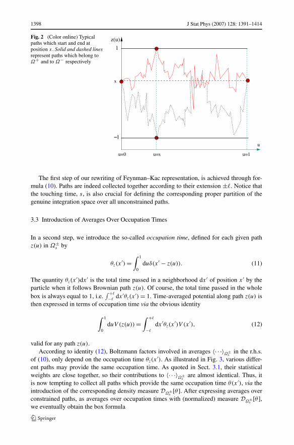
of those parameters. Therefore, the energy and the spatial extension of the ground state areproportional to those typical energy and length respectively. Formula (30) can be used tocompute the ergodic density matrix elements in the low temperature regime for |x| < �0.Function E(�) reads

E(�) = π2�

2

8m�2+ an�

n

nRn, (33)

where Rn = ∫ 1−1 dz cos2(πz/2)zn is a pure numerical coefficient. The minimum of above

expression, reached for �0 = �p(π2/4Rn)1/(n+2), is

E(�0) = an�n

0 Rn

[1

2+ 1

n

]. (34)

We also find

ϕ±(�0, x/�0) = π

2nRn

[2∫ 1

0dz sin(πz)zn+1 −

∫ 1

x/�0

dz sin(πz)zn

]

+ π

2nRn

(x

�0

)tan

(πx

2�0

)

×[∫ 1

0dz cos2

(πz

2

)zn − �0

x

∫ x/�0

0dz cos2

(πz

2

)zn

](35)

which provides n(x). Two important comments are in order. The scaling properties of thegroundstate energy and extension are indeed recovered within the ergodic approximation.Table 1 presents a comparison with the numerical resolution of Schrödinger equation. Theagreement, already good for low values of the exponent n, becomes better when n increases.This could be expected a priori, because the ergodic approximation becomes exact for aninfinite square well potential. Comparisons for the groundstate pdf are presented in Fig. 7:the agreement is impressive.

Second, we consider a modified Pöschl–Teller potential namely V (x) = −V0/

[√2 cosh(x/ lp)]2 with V0 > 0. The spectrum of the corresponding Hamiltonian is exactlyknown. In particular, the groundstate energy is given by E0 = −(V0/2)(

√1 + 2γ /π2 −√

2γ /π)2 with γ = π2�

2/(8ml2pV0). Parameter γ −1 controls the strength of the confine-

ment: for γ −1 sufficiently small, the groundstate is the sole bound state, while the numberof bound states increases when γ −1 increases. Now, the ergodic energy reads

E(�0) = V0

(γ

(lp

�0

)2

−∫ 1

0dz

cos2(πz/2)

cosh2(z�0/lp)

), (36)

Table 1 Comparison of the ergodic groundstate energy E(�0) derived by using formula (34), to the exact re-sult E0 (obtained by numerically solving Schrödinger equation). Integer n is the exponent of the anharmonicpotential

n 2 4 6 8 10

E(�0)−E0E0

13% 12% 10% 7.5% 6%

J Stat Phys (2007) 128: 1391–1414 1407

Fig

.7(C

olor

onlin

e)Pr

obab

ility

dens

ityfu

nctio

nof

the

grou

ndst

ate

for

confi

ning

pote

ntia

ls.T

heso

lidlin

eis

obta

ined

thro

ugh

anu

mer

ical

reso

lutio

nof

Schr

ödin

ger

equa

tion,

whi

lepo

ints

corr

espo

ndto

the

ergo

dic

appr

oxim

atio

nob

tain

edfr

om(3

5)

1408 J Stat Phys (2007) 128: 1391–1414

Table 2 Comparison of the ergodic groundstate energy E(�0) derived by using formula (36), to the exactresult E0

γ 0.01 0.1 1 5 10

E(�0)−E0E0

1.33% 4.8% 20% 43% 50%

where �0 is the unique solution of

γ

(lp

�0

)3

=∫ 1

0dz

cos2(πz/2) tanh(z�0/lp)

cosh2(z�0/lp). (37)

In Table 2 we compare E(�0) to E0 for different values of γ . Figure 8 shows the correspond-ing comparisons for the groundstate pdf’s. For values of γ smaller than 1, ergodic energiesstay close to the exact values and ergodic groundstate pdf’s are quite good. Even for val-ues of γ of order 1, the main shape of the groundstate pdf remains well approximated. Ifwe set γ → ∞ by taking the double limit lp → 0 and V0 → ∞ with V0lp = C fixed, thenV (x) reduces to the singular potential −Cδ(x). In that rather unfavorable case, the discrep-ancy between E(�0) and E0 becomes of order 60 percent. However, notice that the ergodicapproximation does predict the existence of a bound state, contrarily to semi-classical esti-mations.

From the low-temperature behavior of the semi-classical density matrix [11], we extractthe semi-classical groundstate energy Esc = V (0) + �ω0/2 with ω0 = [d2V/dx2(0)/m]1/2.That simple formula can be interpreted by noticing that the semi-classical approximationthen amounts to replace the genuine potential by its harmonic local form near its minimumat x = 0. For considered anharmonic potentials, Esc vanishes because ω0 = 0, so the semi-classical approximation completely fails at low temperatures. For the modified Pöschl–Tellerpotential, Esc becomes exact when the confinement is strong, i.e. when γ → 0, in agreementwith the fact that the semi-classical approximation turns to be exact for a harmonic poten-tial. Above a given value of γ , Esc becomes positive so the semi-classical approximationerroneously predicts that all bound states disappear.

5.2 Intermediate and High Temperature Regimes

At intermediate temperatures, formula (21) is implemented through simple numerical eval-uations of ordinary integrals. As shown below, the ergodic approximation is particularlyefficient in that regime or, in other words, it provides a good interpolation between the exactbehaviors at high and low temperatures. Here, we consider both global and local quanti-ties, namely internal energy U = −∂β(log(Z(β)) and probability density function (PDF)Ψ (x,β) = ρ(x, x,β)/Z(β) for confining potentials (V (x) → ∞) on the one hand, virialcoefficient B(β) and deviation Φ(x,β) = [ρ(x, x,β) − (

√2πλD)−1]/B(β) for hole poten-

tials (V (x) → 0−) on the other hand. Comparisons are made with either numerically exactresults or other familiar approximations.

The ergodic approximation appears to be rather accurate for estimating the consideredthermodynamic quantities. There always exists a large-temperature domain where the er-godic approximation is significantly better than other considered approximations. Abovetemperature domain becomes larger when the anharmonicity of the potential increases. Fig-ures 9 and 10 show results for respectively, the anharmonic potential V (x) = a4x

4, and themodified Pöschl–Teller potential with γ = 1 .

J Stat Phys (2007) 128: 1391–1414 1409

Fig

.8(C

olor

onlin

e)Pr

obab

ility

dens

ityfu

nctio

nof

the

grou

ndst

ate

for

mod

ified

Pösc

hl–T

elle

rpo

tent

ial.

The

solid

lines

repr

esen

tth

eex

act

grou

ndst

ates

pdf,

whi

lepo

ints

corr

espo

ndto

thei

rer

godi

cap

prox

imat

ion

1410 J Stat Phys (2007) 128: 1391–1414

Fig

.9(C

olor

onlin

e)R

elat

ive

erro

rfo

rin

tern

alen

ergy

(lef

tpa

nel)

and

mea

n-sq

uare

erro

rfo

rth

epr

obab

ility

dens

ityfu

nctio

nΨ

(rig

htpa

nel)

,as

func

tions

ofth

ete

mpe

ratu

refo

rth

epo

tent

ialV

(x)=

a4x

4.

Cir

cles

corr

espo

ndto

the

ergo

dic

appr

oxim

atio

n,sq

uare

sre

fer

toW

igne

r–K

irkw

ood

expa

nsio

ntr

unca

ted

upto

orde

r�

2,

cros

ses

desc

ribe

the

sem

i-cl

assi

cala

ppro

xim

atio

nan

ddi

amon

dsar

eth

ecl

assi

calv

alue

s.Q

uant

ityΔ

0,1

isth

een

ergy

gap

betw

een

the

grou

ndst

ate

and

the

first

exci

ted

one

J Stat Phys (2007) 128: 1391–1414 1411

Fig

.10

(Col

oron

line)

Rel

ativ

eer

ror

for

viri

alco

effic

ient

(lef

tpan

el)

and

mea

n-sq

uare

erro

rfo

rth

epr

obab

ility

dens

ityfu

nctio

nΦ

(rig

htpa

nel)

,as

func

tions

ofth

ete

mpe

ratu

refo

rth

eγ

=1

mod

ified

Pösc

hl–T

elle

rpo

tent

ial.

Cir

cles

corr

espo

ndto

the

ergo

dic

appr

oxim

atio

n,sq

uare

sre

fer

toW

igne

r–K

irkw

ood

expa

nsio

ntr

unca

ted

upto

orde

r�

2an

ddi

amon

dsar

eth

ecl

assi

calv

alue

s.Q

uant

ityΔ

0,1

isth

een

ergy

gap

betw

een

the

grou

ndst

ate

and

the

first

exci

ted

one

1412 J Stat Phys (2007) 128: 1391–1414

Either the Wigner–Kirkwood expansion or the semi-classical approximation becomewell-suited when the temperature increases. Does the ergodic approximation provides sat-isfactory results in the high temperature regime? More precisely, what part of the Wigner–Kirkwood expansion is accounted for within that approximation? We obtain, in that regime,

ρerg(x, x,β)β→0∼ e−βV (x)

√2πλD

[1 − β

d2V

dx2

λ2D

12+

(β

dV

dx

)2λ2

D

24A0 + o(λ2

D)

], (38)

with the pure numerical coefficient

A0 = −1

2+ 3

√2π

∫ 1

0ds

(s

1 − s

)3/2

×∫ ∞

0dzz2 erfc2

(z√2s

)exp

(−z2(2s − 1)

2s(1 − s)

)

+ 3√

2π

∫ 1

0ds

∫ ∞

0dzz2 erfc

(z√2s

)erfc

(z√

2(1 − s)

)� 0.8. (39)

Thus, the ergodic approximation does provide the leading classical term, while part of the�

2-correction is also correctly reproduced. At that order �2, the discrepancy of (38) with

exact expansion (4), arises from correlations between occupation times which are not takeninto account in the ergodic approximation. Moreover, A0 is indeed smaller than 1 in agree-ment with inequality ρerg(x, x,β) ≤ ρ(x, x,β). Eventually, the ergodic approximation turnsout to be also quite reasonable at high temperatures.

5.3 Further Applications and Extensions

For a single particle, the ergodic approximation can been also applied to other one-dimensional potentials of interest (Morse, double well, periodic, . . .), with possible simplemodifications of box formula (13). For instance, for asymmetric Morse potential defined forx > 0 (V (x) = ∞ for x < 0), the confining box is chosen as [0, �] of course. Accordingto preliminary calculations, accuracy of the ergodic approximation is comparable to thatobserved above.

The extension of the ergodic approximation to two- or three-dimensional potentials re-quires the derivation of suitable box formulas similar to (13). A first possible route startswith an auxiliary Hamiltonian which tends to confine the particle inside a disk or a spherewith radius �. This provides an exact formula identical to (13), except for an additional or-dinary integral over the angle(s) of the boundary touching point. The corresponding ergodicapproximation involves an occupation-time average, which is easily expressed in terms ofthe known free Green functions with Dirichlet boundary conditions on a disk or on a sphere.

For two particles with an interaction potential V (r1, r2) = V (r1 − r2) which dependsonly on their relative position r1 − r2, thanks to the trivial motion of their mass center weare left with the previous case of a single particle in an external potential V (r). For othercases, like two interacting particles in an external potential or three interacting particles, boxformulas could also be derived in the same spirit as (13). Nevertheless, the correspondingergodic approximation should become rather difficult to numerically handle because of theincreasing number of intricated ordinary integrals.

J Stat Phys (2007) 128: 1391–1414 1413

Appendix Statistical weights of boxes

Eigenstates and eigenvalues of the auxiliary Hamiltonian H 0� are obtained by solving the

Schrödinger equation

d2φ0�

dz2= 2mV0

�2

[1 − Θ(z + �) + Θ(z − �) − E

V0

]φ0

� (z). (40)

After introducing dimensionless function ψ(z) = √�φ0

� (z) and setting En = π2�

2n2/

(8m�2) = E1n2 for the n-th eigenvalue in the large-V0-limit, a straightforward calculation

leads to

ψn(z�)

V0→∞∼

⎧⎪⎪⎪⎨

⎪⎪⎪⎩

√E1V0

n, if z = −�,

sin[

nπ2�

(z + �)], ∀z ∈]−�,+�[ ,

(−1)(n−1)√

E1V0

n, if z = �.

(41)

By using spectral decomposition (1), we eventually obtain the following expression for thestatistical weight functions

g ± (x, �, s, β) = √2π

π2λ3D

8�4S±

g

(x

�,πλD

√s

2�

)S±

g

(x

�,πλD

√1 − s

2�

), (42)

where

S±g (α, y) =

∞∑

n=1

n(∓1)n−1 sin

[n

π

2(α + 1)

]exp

[−y2

2n2

]. (43)

Those two functions satisfy the equality g+(x, �, s, β) = g−(−x, �, s, β), the normalizationcondition

∫ ∞

|x|d�

∫ 1

0ds[g−(x, �, s, β) + g+(x, �, s, β)] = 1, (44)

and their asymptotic form merely is

g ± (x, �, s, β)λD��∼ √

2ππ2λ3

D

8�4sin2

[π(x + �)

2�

]exp

[−π2λ2

D

8�2

](45)

in the low temperature regime. The asymptotic expression of g± in the high-temperatureregime is derived from the Poisson transform of expression (43). According to Poisson for-mula, if the Fourier transform of a function f exists, then, for all values of Δy

Δy

∞∑

n=−∞f (nΔy) =

+∞∑

m=−∞

∫ +∞

−∞dzf (z) e−im2πz/Δy. (46)

Application of that transformation to expression (43) provides

g−(x, �, s, β) = g+(−x, �, s, β)

λD��∼√

2

π

�2

λ3D

1√s(1 − s)

(1 + x/�)2

s(1 − s)exp

[− �2

2λ2D

(1 + x/�)2

s(1 − s)

](47)

in the high temperature regime.

1414 J Stat Phys (2007) 128: 1391–1414

References

1. Feynman, R.P., Hibbs, A.R.: Quantum Mechanics and Path Integrals. McGraw–Hill, New York (1965)2. Simon, B.: Functional Integration and Quantum Physics. Academic, New York (1979)3. Schulman, L.S.: Techniques and Applications of Path Integrals. Wiley, New York (1981)4. Roepstorff, G.: Path Integral Approach to Quantum Physics. Springer, Berlin (1994)5. Kleinert, H.: Path Integrals in Quantum Mechanics, Statistics, and Polymer Physics, and Financial Mar-

kets. World Scientific, Singapore (2004)6. Wigner, E.P.: Phys. Rev. 40, 749 (1932)7. Kirkwood, J.G.: Phys. Rev. 44, 31 (1933).8. Kirkwood, J.G.: Phys. Rev. 45, 116 (1934)9. Landau, L., Lifschitz, E.: Statistical Physics. Pergamon, Elmsford (1980)

10. Feynman, R., Kleinert, H.: Phys. Rev. A 34, 5080 (1986)11. Dashen, R., Hasslacher, B., Neveu, A.: Phys. Rev. D 10, 4114 (1974)12. Bogojevic̀, A., Balaz̀, A., Belic̀, A.: Phys. Lett. A 345, 258 (2005)13. Raffarin, J.P.: General communication (2004)14. Bogojevic̀, A., Balaz̀, A., Belic̀, A.: Phys. Lett. A 344, 84 (2005)15. Krauth, W.: Introduction to Monte Carlo algorithms. In: Kertesz, J., Kondor, I. (eds.) Advances in Com-

puter Simulation. Lecture Notes in Physics. Springer, Berlin (1998)16. Krauth, W.: Statistical Mechanics: Algorithms and Computations. Oxford University Press, Oxford

(2006)17. Ceperley, D.M.: Rev. Mod. Phys. 67, 279 (1995)18. Militzer, B., Ceperley, D.M.: Phys. Rev. E 63, 066404 (2001)19. Predescu, C., Sabo, D., Doll, J.D.: J. Chem. Phys. 119, 4641 (2003)20. Ginibre, J.: Some applications of functional integration in statistical mechanics. In: DeWitt, C., Stora, R.

(eds.) Statistical Mechanics and Quantum Field Theory. Gordon and Breach, Les Houches (1971)21. Cornu, F.: Phys. Rev. E 53, 4562 (1996)22. Brydges, D.C., Martin, Ph.A.: J. Stat. Phys. 96, 1163 (1999)23. Martin, Ph.A.: Acta Phys. Pol. B 34, 3629 (2003)24. Kihara, T., Midzuno, Y., Shizume, T.: J. Phys. Soc. Jpn. 10, 249 (1955)25. Gradshteyn, I.S., Ryzhik, I.M.: Tables of Integrals Series and Products, 5th edn. Academic Press, New

York (2000)