Path Integrals in Polar and Spherical Coordinates

H. Kleinert, PATH INTEGRALSJanuary 6, 2016 (/home/kleinert/kleinert/books/pathis/pthic8.tex)

Every path hath a puddleGeorge Herbert, Outlandish Proverbs, 1640

8

Path Integrals in Polar and Spherical Coordinates

Many physical systems possess rotational symmetry. In operator quantum mechan-ics, this property is of great help in finding wave functions and energies of a system.If a rotationally symmetric Schrodinger equation is transformed to spherical coordi-nates, it separates into a radial and several angular differential equations. The latterare universal and have well-known solutions. Only the radial equation contains spe-cific information on the dynamics of the system. Being an ordinary one-dimensionalSchrodinger equation, it can be solved with the usual techniques.

In the path integral approach, a similar coordinate transformation is possible,although it makes things initially more complicated rather than simpler. First, theuse of non-Cartesian coordinates causes nontrivial problems of the kind observedin Chapter 6, where the configuration space was topologically constrained. Suchproblems can be solved as in Chapter 6 using the knowledge of the correct procedurein Cartesian coordinates. A second complication is more severe: When studying asystem at a given angular momentum, the presence of a centrifugal barrier destroysthe possibility of setting up a time-sliced path integral of the Feynman type as inChapter 2. The recent solution of the latter problem has paved the way for twomajor advances in path integration which will be presented in Chapters 10, 11,and 12.

8.1 Angular Decomposition in Two Dimensions

Consider a two-dimensional quantum-mechanical system with rotational invariance.In Schrodinger quantum mechanics, it is convenient to introduce polar coordinates

x = r(cosϕ, sinϕ), (8.1)

and to split the differential equation into a radial and an azimuthal one which aresolved separately. Let us try to follow the same approach in path integrals. Toavoid the complications associated with path integrals in the canonical formulation[1],all calculations will be done in the Lagrange formulation. It will, moreover,be advantageous to work with the imaginary-time amplitude (the thermal density

706

8.1 Angular Decomposition in Two Dimensions 707

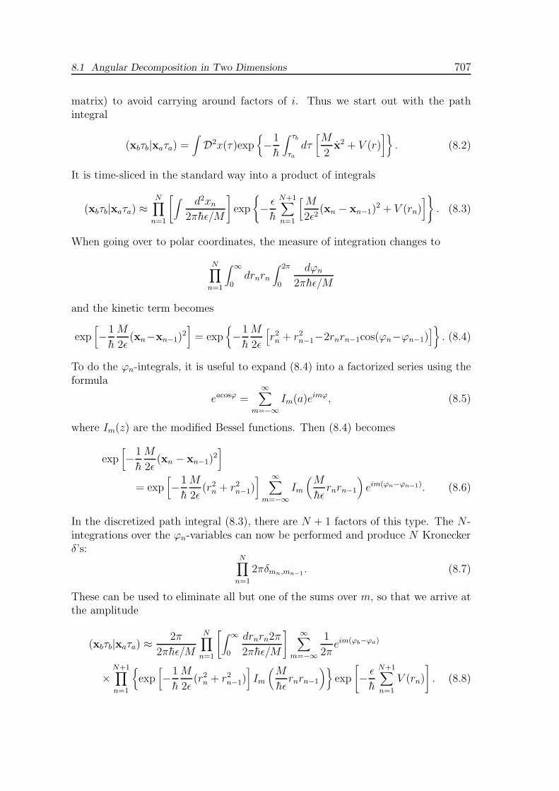
matrix) to avoid carrying around factors of i. Thus we start out with the pathintegral

(xbτb|xaτa) =∫

D2x(τ)exp{

−1

h

∫ τb

τadτ[

M

2x2 + V (r)

]}

. (8.2)

It is time-sliced in the standard way into a product of integrals

(xbτb|xaτa) ≈N∏

n=1

[

∫

d2xn2πhǫ/M

]

exp

{

− ǫ

h

N+1∑

n=1

[

M

2ǫ2(xn − xn−1)

2 + V (rn)]

}

. (8.3)

When going over to polar coordinates, the measure of integration changes to

N∏

n=1

∫ ∞

0drnrn

∫ 2π

0

dϕn

2πhǫ/M

and the kinetic term becomes

exp[

−1

h

M

2ǫ(xn−xn−1)

2]

= exp{

−1

h

M

2ǫ

[

r2n + r2n−1−2rnrn−1cos(ϕn−ϕn−1)]

}

. (8.4)

To do the ϕn-integrals, it is useful to expand (8.4) into a factorized series using theformula

eacosϕ =∞∑

m=−∞

Im(a)eimϕ, (8.5)

where Im(z) are the modified Bessel functions. Then (8.4) becomes

exp[

−1

h

M

2ǫ(xn − xn−1)

2]

= exp[

−1

h

M

2ǫ(r2n + r2n−1)

] ∞∑

m=−∞

Im

(

M

hǫrnrn−1

)

eim(ϕn−ϕn−1). (8.6)

In the discretized path integral (8.3), there are N + 1 factors of this type. The N -integrations over the ϕn-variables can now be performed and produce N Kroneckerδ’s:

N∏

n=1

2πδmn,mn−1. (8.7)

These can be used to eliminate all but one of the sums over m, so that we arrive atthe amplitude

(xbτb|xaτa) ≈2π

2πhǫ/M

N∏

n=1

[

∫ ∞

0

drnrn2π

2πhǫ/M

]

∞∑

m=−∞

1

2πeim(ϕb−ϕa)

×N+1∏

n=1

{

exp[

−1

h

M

2ǫ(r2n + r2n−1)

]

Im

(

M

hǫrnrn−1

)}

exp

[

− ǫ

h

N+1∑

n=1

V (rn)

]

. (8.8)

708 8 Path Integrals in Polar and Spherical Coordinates

We now define the radial time evolution amplitudes by the following expansion withrespect to the azimuthal quantum numbers m:

(xbτb|xaτa) =∞∑

m=−∞

1√rbra

(rbτb|raτa)m1

2πeim(ϕb−ϕa). (8.9)

The amplitudes (rbτb|raτa)m are obviously given by the radial path integral

(rbτb|raτa)m ≈ 1√

2πhǫ/M

N∏

n=1

∫ ∞

0

drn√

2πhǫ/M

×N+1∏

n=1

[

exp{

− M

2ǫh(rn − rn−1)

2}

Im

(

Mrnrn−1

hǫ

)]

exp

{

− ǫ

h

N+1∑

n=1

V (rn)

}

. (8.10)

Here we have introduced slightly different modified Bessel functions

Im(z) ≡√2πze−zIm(z). (8.11)

They will also be called “Bessel functions”, for short. They have the asymptoticbehavior

Im(z)z→∞−−−→ 1− m2 − 1/4

2z+ . . . = e−

m2−1/42z + . . . , (8.12)

Im(z)z→0−−−→ 2

√π(z/2)m+1/2 + . . . . (8.13)

In the case of a free particle with V (r) = 0, it is easy to perform all the inter-mediate integrals over rn in (8.10). Two neighboring figures in the product requirethe integral

∫ ∞

0dr′ exp

(

−r′′2

2ǫ2− r2

2ǫ1

)

exp[

−r′2(

1

2ǫ2+

1

2ǫ1

)]

√r′′r′

ǫ2Im

(

r′′r′

ǫ2

)√r′r

ǫ1Im

(

r′r

ǫ1

)

= exp

[

− r′′2 + r2

2 (ǫ1 + ǫ2)

]√r′′r

ǫ1 + ǫ2Im

(

r′′r

ǫ1 + ǫ2

)

. (8.14)

For simplicity, the units in this formula are M = 1, h = 1. The right-hand side of(8.14) follows directly from the formula

∫ ∞

0drre−r2/ǫIν (βr) Iν (αr) =

ǫ

2e(α

2+β2)ǫ/4Iν (ǫαβ/2) , (8.15)

after identifying ǫ, α, β as

ǫ = 2ǫ1ǫ2/ (ǫ1 + ǫ2) ,

α = r/ǫ1, (8.16)

β = r′′/ǫ2.

H. Kleinert, PATH INTEGRALS

8.2 Trouble with Feynman’s Path Integral Formula in Radial Coordinates 709

Thus, the integrals in (8.10) with V (r) = 0 can successively be performed yieldingthe thermal amplitude for τb > τa:

(rbτb|raτa)m =M

h

√rbra

τb − τaexp

[

−M2h

r2b + r2a(τb − τa)

]

Im

(

M

h

rbraτb − τa

)

. (8.17)

Note that the same result could have been obtained more directly from theimaginary-time amplitude of a free particle in two dimensions,

(xbτb|xaτa) =M

2πh(τb − τa)exp

[

−M2h

(xb − xa)2

τb − τa

]

, (8.18)

by rewriting the right-hand side as

M

2πh (τb − τa)exp

(

−M2h

r2b + r2aτb − τa

)

exp[

M

2h

rbraτb − τa

cos (ϕb − ϕa)]

,

and expanding the second exponential according to (8.5) into the series

∞∑

m=−∞

Im

(

M

h

rbraτb − τa

)

eim(ϕb−ϕa). (8.19)

A comparison of the coefficients with those in (8.9) gives the radial amplitudes(8.17).

Due to (8.14), the radial amplitude satisfies a fundamental composition lawcorresponding to (2.4), which reads for τb > τ > τa

∫ ∞

0drr (rbτb|r τ)m (r τ |raτa)m = (rbτb|raτa)m . (8.20)

8.2 Trouble with Feynman’s Path Integral Formula inRadial Coordinates

In the above calculation we have shown that the expression (8.10) is certainly thecorrect radial path integral. It is, however, not of the Feynman type. In operatorquantum mechanics we learn that the action of a particle moving in a potentialV (r) at a fixed angular momentum L3 = mh contains a centrifugal barrier h2(m2 −1/4)/2Mr2 and reads

Am =∫ τb

τadτ

(

M

2r2 +

h2

2M

m2 − 1/4

r2+ V (r)

)

. (8.21)

This is shown by separating the Hamiltonian operator into radial and azimuthalcoordinates, over fixing the azimuthal angular momentum L3, and choosing for it thequantum-mechanical value hm. According to Feynman’s rules, the radial amplitudetherefore should simply be given by the path integral

(rbτb|raτa)m =∫ ∞

0Dr exp

(

−1

hAm

)

. (8.22)


The reader may object to using the word “classical” in the presence of a termproportional to h2 in the action. In this section, however, hm is merely meantto be a parameter specifying the azimuthal momentum pϕ ≡ hm in the classicalcentrifugal barrier p2ϕ/2Mr2. It is parametrized in terms of a dimensionless numberm which does not necessarily have the integer values required by the quantizationof the azimuthal motion.

By naively time-slicing (8.22) according to Feynman’s rules of Section 2.1 wewould have defined it by the finite-N expression


2πhǫ/M

N∏

n=1

∫ ∞

0

drn√

2πhǫ/M

× exp

{

−1

h

N+1∑

n=1

[

M

2ǫ(rn − rn−1)

2 + ǫh2

2M

m2 − 1/4

rnrn−1

+ ǫV (rn)

]}

. (8.23)

Actually, the denominators in the centrifugal barrier could have been chosen to ber2n. This would make a negligible difference for small ǫ. Note that in contrast to astandard Feynman path integral in one dimension, the integrations over r cover onlythe semi-axis r ≥ 0 rather than the complete r-axis. This represents no problemsince we have learned in Chapter 6 how to treat such half-spaces.

The expression (8.23) is now a place for an unpleasant surprise: For m = 0, atime-sliced Feynman path integral formula cannot possibly exist since the potentialhas an abyss at small r. This leads to a phenomenon which will be referred to as thepath collapse, to be understood physically and resolved later in Chapter 12. At thisplace we merely point out the mathematical origin of the problem, by comparingthe naively time-sliced expression (8.23) with the certainly correct one (8.10). Thesingularity would be of no consequence if the two expressions were to convergetowards each other in the continuum limit ǫ → 0. At first sight, this seems to bethe case. After all, ǫ is assumed to be infinitesimally small so that we may replacethe “Bessel function” Im (Mrnrn−1/hǫ) by its asymptotic form (8.12),

Im

(

Mrnrn−1

hǫ

)

ǫ→0−−−→ exp

(

−ǫ h

2M

m2 − 1/4

rnrn−1

)

. (8.24)

For a fixed set of rn, i.e., for a given path, the continuum limit ǫ → 0 makes theintegrands (8.10) and (8.23) coincide, the difference being of the order ǫ2. Unfortu-nately, the path integral requires the limit to be taken after the integrations overthe drn. The integrals, however, do not exist at m = 0. For paths moving veryclose to the singularity at r = 0, the approximation (8.24) breaks down. In fact, thelarge-z expansion

Im(z) = 1− m2 − 1/4

2z+

(m2 − 1/4)(m2 − 1/9)

2!(2z)2− . . . (8.25)

with z =Mrnrn−1/hǫ is never convergent even for a very small ǫ. The series showsonly an asymptotic convergence (more on this subject in Section 17.9). If we want


8.2 Trouble with Feynman’s Path Integral Formula in Radial Coordinates 711

to evaluate Im(z) =√2πze−zIm(z) for all z we have to use the convergent power

series expansion of Im(z) around z = 0:

Im(z) =(

z

2

)m[

1

0!m!+

1

1!(m+ 1)!

(

z

2

)2

+1

2!(m+ 2)!

(

z

2

)4

+ . . .

]

.

It is known from the Schrodinger theory that the leading power zm determinesthe threshold behavior of the quantum-mechanical particle distribution near theorigin. This is qualitatively different from the exponentially small distributionexp [−ǫh(m2 − 1/4)/2Mr2] contained in each time slice of the Feynman formula(8.23) for |m| > 1/2.

The root of these troubles is an anomalous behavior in the high-temperature limitof the partition function. In this limit, the imaginary time difference τb−τa = h/kBTis very small and it is usually sufficient to keep only a single slice in a time-slicedpath integral (see Sections 2.9, 2.13). If this were true also here, the formula (8.23)would lead, in the absence of a potential V (r), to the classical particle distribution[compare (2.349)]

(ra τa + ǫ|raτa) =1

√

2πhǫ/Mexp

(

−ǫ h

2M

m2 − 1/4

r2a

)

. (8.26)

If we subtract the barrier-free distribution, this amounts to the classical partitionfunction1

Zcl =∫ ∞

0

dr√2πa

[

exp

(

−am2 − 1/4

2r2

)

− 1

]

= −1

2

√

m2 − 1

4, (8.27)

where we have abbreviated the factor ǫh/M by a. The integral is temperature-independent and converges only for |m| > 1/2.

Compare this result with the proper high-temperature limit of the exact partitionfunction calculated with the use of (8.17) and with the same subtraction as before.It reads for all T

Z =1

2

∫ ∞

0dze−z [Im(z)− I1/2(z)]. (8.28)

As in the classical expression, there is no temperature dependence. The integral

∫ ∞

0dze−αzIµ(z) = (α2 − 1)

−1/2(α+

√α2 − 1)

−µ(8.29)

[see formula (2.475)] converges for arbitrary real ν and α > 1, and gives in the limitα→ 1

Z = −1

2(m− 1/2). (8.30)

1This follows by expanding the formula∫∞

0 dxe−a/x2−bx2

=√

π/4be−2√ab in powers of

√b,

subtracting the a = 0 -term, and taking the limit b → 0.


This is different from the classical result (8.27) and agrees with it only in the limitof large m.2

Thus we conclude that a time-sliced path integral containing a centrifugal barriercan only give the correct amplitude when using the Euclidean action

ANm =

N+1∑

n=1

[

M

2ǫ(rn − rn−1)

2 − hlogIm

(

M

hǫrnrn−1

)]

, (8.31)

in which the neighborhood of the singularity is treated quantum-mechanically. Thenaively time-sliced classical action in (8.23) is of no use. The centrifugal barrierrenders therefore a counterexample to Feynman rules of path integration accordingto which quantum-mechanical amplitudes should be obtainable from a sum over allhistories of exponentials which involve only the classical expression for the short-timeactions.

It is easy to see where the derivation of the time-sliced path integral in Section 2.1breaks down. There, the basic ingredient was the Trotter product formula (2.26),which for imaginary time reads

e−β(T+V ) = limN→∞

(

e−ǫTe−ǫV)N+1

, ǫ ≡ β/(N + 1). (8.32)

An exact identity is e−β(T+V ) ≡(

e−ǫT e−ǫV eiǫ2X)N+1

with X given in Eq. (2.10) con-

sisting of a sum of higher and higher commutators between V and T . The Trotterformula neglects these commutators. In the presence of a centrifugal barrier, how-ever, this is not permitted. Although the neglected commutators carry increasingpowers of the small quantity ǫ, they are more and more divergent at r = 0, likeǫn/r2π. The same terms occur in the asymptotic expansion (8.25) of the “Besselfunction”. In the proper action (8.31), these terms are present.

It should be noted that for a Hamiltonian possessing a centrifugal barrier Vcb inaddition to an arbitrary smooth potential V , i.e., for a Hamiltonian operator of theform H = T + Vcf + V , the Trotter formula is applicable in the form

e−βH = limN→∞

(

e−ǫ(T+Vcb)e−ǫV)N+1

, ǫ ≡ β/(N + 1). (8.33)

It leads to a valid time-sliced path integral formula

(rbτb|raτa)m ≈N∏

n=1

[∫ ∞

0drn

] N+1∏

n=1

[

∫

dpn2πh

]

exp{

−1

hAN

m[p, r]}

, (8.34)

with the sliced action

ANm[p, r] =

N+1∑

n=1

[

−ipn(rn − rn−1) + ǫp2n2M

− hlogIm

(

M

hǫrnrn−1

)

+ ǫV (rn)

]

. (8.35)

2If m were not merely a dimensionless number parametrizing an arbitrary centrifugal barrierwith fixed p2ϕ/2Mr2, as it is in this section, the classical limit at a fixed pϕ would eliminate theproblem since for h → 0, the number m would become infinitely large, leading to the correcthigh-temperature limit of the partition function. For a fixed finite m, however, the discrepancy isunavoidable.


8.3 Cautionary Remarks 713

After integrating out the momenta, this becomes


2πhǫ/M

N∏

n=1

∫ ∞

0

drn√

2πhǫ/M

exp{

−1

hAN

m[r]}

, (8.36)

with the action

ANm[r, r] =

N+1∑

n=1

[

M

2ǫ(rn − rn−1)

2 − hlogIm

(

Mrnrn−1

hǫ

)

+ ǫV (rn)]

. (8.37)

The path integral formula (8.36) can in principle be used to find the amplitude fora fixed angular momentum of some solvable systems.

An example is the radial harmonic oscillator at an angular momentum m, al-though it should be noted that this particularly simple example does not reallyrequire calculating the integrals in (8.36). The result can be found much more sim-ply from a direct angular momentum decomposition of the amplitude (2.177). Aftera continuation to imaginary times t = −iτ and an expansion of part of the exponentwith the help of (8.5), it reads for D = 2

(xbτb|xaτa) =1

2π

Mω

h sinh[ω(τb − τa)]e−

Mω2h

coth[ω(τb−τa)](r2b+r2a)

×∞∑

m=−∞

Im

(

Mωrbrah sinh[ω(τb − τa)]

)

eim(ϕb−ϕa). (8.38)

By comparison with (8.9), we extract the radial amplitude

(rbτb|raτa)m =M

h

ω√rbra

coth[ω(τb − τa)]Im

(


)

. (8.39)

The limit ω → 0 gives the free-particle result

(rbτb|raτa)m =M

h

√rbra

τb − τaIm

(

M

h

rbraτb − τa

)

. (8.40)

8.3 Cautionary Remarks

It is important to emphasize that we obtained the correct amplitudes by performingthe time slicing in Cartesian coordinates followed by the transformation to the polarcoordinates in the time-sliced expression. Otherwise we would have easily missedthe factor −1/4 in the centrifugal barrier. To see what can go wrong let us proceedillegally and do the change of variables in the initial continuous action. Thus we tryto calculate the path integral

(xbτb|xaτa) =∑

l=−∞,∞

∫ ∞

0Dr r

∫ ∞

−∞Dϕ

× exp{

1

h

∫ τb

τadτ[

M

2(r2 + r2ϕ2) + V (r)

]}∣

∣

∣

∣

ϕ(τb)=ϕb+2πl

. (8.41)


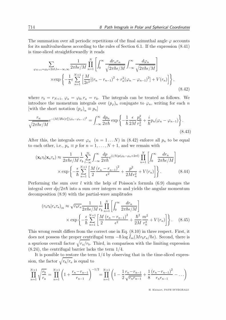
The summation over all periodic repetitions of the final azimuthal angle ϕ accountsfor its multivaluedness according to the rules of Section 6.1. If the expression (8.41)is time-sliced straightforwardly it reads

∑

ϕN+1=ϕb+2πl,l=−∞,∞

1

2πhǫ/M

N∏

n=1

∫ ∞

0

drnrn√

2πhǫ/M

∫ ∞

−∞

dϕn√

2πhǫ/M

×exp

{

−1

hǫN+1∑

n=1

[

M

2ǫ2[(rn − rn−1)

2 + r2n(ϕn − ϕn−1)2] + V (rn)

]

}

,

(8.42)

where rb = rN+1, ϕa = ϕ0, ra = r0. The integrals can be treated as follows. Weintroduce the momentum integrals over (pϕ)n conjugate to ϕn, writing for each n[with the short notation (pϕ)n ≡ pn]

rn√

2πhǫ/Me−(M/2hǫ)r2n(ϕn−ϕn−1)

2

=∫ ∞

−∞

dpn2πh

exp

{

−1

h

ǫ

2M

p2nr2n

+i

hpn(ϕn − ϕn−1)

}

.

(8.43)

After this, the integrals over ϕn (n = 1 . . .N) in (8.42) enforce all pn to be equalto each other, i.e., pn ≡ p for n = 1, . . . , N + 1, and we remain with

(xbτb|xaτa) ≈1

2πhǫ/M

1

rb

∞∑

l−∞

∫ ∞

−∞

dp

2πhe(i/h)p(ϕb−ϕa+2πl)

N∏

n=1

[

∫ ∞

0

drn2πhǫ/M

]

× exp

{

− ǫ

h

N+1∑

n=1

[

M

2

(rn − rn−1)2

ǫ2+

p2

2Mr2n+ V (rn)

]}

. (8.44)

Performing the sum over l with the help of Poisson’s formula (6.9) changes theintegral over dp/2πh into a sum over integers m and yields the angular momentumdecomposition (8.9) with the partial-wave amplitudes

(rbτb|raτa)m ≈ √rbra

1

2πhǫ/M

1

rb

N∏

n=1

[

∫ ∞

0

drn2πhǫ/M

]

× exp

{

− ǫ

h

N+1∑

n=1

[

M

2

(rn − rn−1)2

ǫ2+

h2

2M

m2

r2n+ V (rn)

]}

. (8.45)

This wrong result differs from the correct one in Eq. (8.10) in three respect. First, itdoes not possess the proper centrifugal term −h log Im(Mrbra/hǫ). Second, there is

a spurious overall factor√

ra/rb. Third, in comparison with the limiting expression

(8.24), the centrifugal barrier lacks the term 1/4.It is possible to restore the term 1/4 by observing that in the time-sliced expres-

sion, the factor√

rb/ra is equal to

N+1∏

n=1

√

rbra

=N+1∏

n=1

(

1 +rn−rn−1

rn−1

)−1/2

=N+1∏

n=1

(

1− 1

2

rn−rn−1√rnrn−1

+1

8

(rn−rn−1)2

rnrn−1

− . . .

)


8.3 Cautionary Remarks 715

= exp

(

−1

2

N+1∑

n=1

rn − rn−1√rnrn−1

+ . . .

)

. (8.46)

This, in turn, can be incorporated into the kinetic term of (8.45) via a quadraticcompletion leading to

exp

− ǫ

h

N+1∑

n=1

M

2

(

rn − rn−1

ǫ+ i

h

2M√rnrn−1

)2

+h2

2M

m2 − 1/4

r2n

. (8.47)

The centrifugal barrier is now correct, but the kinetic term is wrong. In fact, itdoes not even correspond to a Hermitian Hamiltonian operator, as can be seen byintroducing momentum integrations and completing the square to

exp

{

−ipn(rn − rn−1) +ǫ

h

[

p2n2M

− ihpn

2Mrn

]}

. (8.48)

The last term is an imaginary energy. Only by dropping it artificially would thetime-sliced action acquire the Feynman form (8.23), while still being beset with theproblem of nonexistence for m = 0 (path collapse) and the nonuniform convergenceof the path integrations to be solved in Chapter 12.

The lesson of this is the following: A naive time slicing cannot be performed incurvilinear coordinates. It can safely be done in the Cartesian formulation.

Fortunately, a systematic modification of the naive slicing rules has recently beenfound which makes them applicable to non-Cartesian systems. This will be shownin Chapters 10 and 11.

In the sequel it is useful to maintain, as far as possible, the naive notation forthe radial path integral (8.23) and the continuum limit of the action (8.21). Theplaces where care has to be taken in the time-slicing process will be emphasized bysetting the centrifugal barrier in quotation marks and defining

“ǫh2

2M

m2 − 1/4

rnrn−1

” ≡ −h log Im(

Mrnrn−1

hǫ

)

. (8.49)

Thus we shall write the properly sliced action (8.37) as

ANm[r, r] =

N+1∑

n=1

[

M

2ǫ(rn − rn−1)

2 +“ǫh2

2µ

m2 − 1/4

rnrn−1

”+ ǫV (rn)

]

, (8.50)

and emphasize the need for the non-naive time slicing of the continuum actioncorrespondingly:

Am =∫ τb

τadτ

[

M

2r2 +

“ h2

2M

m2 − 1/4

r2”+ V (r)

]

. (8.51)


8.4 Time Slicing Corrections

It is interesting to find the origin of the above difficulties. For this purpose, we takethe Cartesian kinetic terms expressed in terms of polar coordinates

(xn − xn−1)2 = (rn − rn−1)

2 + 2rnrn−1[1− cos(ϕn − ϕn−1)], (8.52)

and treat it perturbatively in the coordinate differences [2]. Expanding the cosineinto a power series we obtain the time-sliced action

AN =M

2ǫ

N+1∑

n=1

(xn − xn−1)2 =

M

2ǫ

N+1∑

n=1

{

(rn − rn−1)2

+ 2rnrn−1

[

1

2!(ϕn − ϕn−1)

2 − 1

4!(ϕn − ϕn−1)

4 + . . .] }

.(8.53)

In contrast to the naively time-sliced expression (8.42), we now keep the quarticterm (ϕn−ϕn−1)

4. To see how it contributes, consider a single intermediate integral

∫

dϕn−1√

2πǫ/ae−(a/2ǫ)[(ϕn−ϕn−1)2+a4(ϕn−ϕn−1)

4+...]. (8.54)

The first term in the exponent restricts the width of the fluctuations of the differenceϕn − ϕn−1 to

〈(ϕn − ϕn−1)2〉0 =

ǫ

a. (8.55)

If we rescale the arguments, ϕn → √ǫun, the integral takes the form

∫

dun−1√

2π/ae−(a/2)[(un−un−1)

2+ǫa4(un−un−1)4+...]. (8.56)

This shows that each higher power in the difference un − un−1 is suppressed by anadditional factor

√ǫ. We now expand the integrand in powers of

√ǫ and use the

integrals

∫ du√

2π/ae−(a/2)u2

u2

u4

...u2n

=

a−1

3a−2

...(2n− 1)!!a−n

, (8.57)

with odd powers of u giving trivially 0, to find an expansion of the integral (8.56).It begins as follows:

1− ǫa

2a4 3a−2 +O(ǫ2). (8.58)

This can be thought of as coming from the equivalent integral

∫

dϕn−1√

2πǫ/ae−(a/2ǫ)(ϕn−ϕn−1)

2−3a4ǫ/2a+... . (8.59)


8.4 Time Slicing Corrections 717

The quartic term in (8.54),

∆A =a

2ǫa4(ϕn − ϕn−1)

4, (8.60)

has generated an effective action-like term in the exponent:

Aeff = ǫ3a42a

. (8.61)

This is obviously due to the expectation value 〈∆A〉0 of the quartic term and wecan record, for later use, the perturbative formula

Aeff = 〈∆A〉0. (8.62)

If u is a vector in D dimensions to be denoted by u, with the quadratic termbeing (a/2ǫ)(un − un−1)

2, the integrals (8.57) are replaced by

∫

dDu√

2π/aD e

−(a/2)u2

uiujuiujukul

...ui1 · . . . · ui2n

=

a−1δija−2(δijδkl + δikδjl + δilδjk)...a−nδi1...i2n

, (8.63)

where δi1...i2n will be referred to as contraction tensors , defined recursively by therelation

δi1...i2n = δi1i2δi3i4...i2n + δi1i3δi2i4...i2n + . . .+ δi1i2nδi2i3...i2n−1. (8.64)

A comparison with the Wick expansion (3.306) shows that this recursion relationamounts to δi1...i2n possessing a Wick-like expansion into the sum of products ofKronecker δ’s, each representing a pair contraction. Indeed, the integral formulas(8.63) can be derived by adding a source term j ·u to the exponent in the integrand,completing the square, and differentiating the resulting e(1/2a)j

2

with respect to the“current” components ji. For vectors ϕi, a possible quartic term in the exponent of(8.54) may have the form

∆A =a

2ǫ(a4)ijkl(ϕn − ϕn−1)i(ϕn − ϕn−1)j(ϕn − ϕn−1)k(ϕn − ϕn−1)l. (8.65)

Then the factor 3a4 in Aeff of Eq. (8.61) is replaced by the three contractions

(a4)ijkl(δijδkl + 2 more pair terms).

Applying the simple result (8.61) to the action (8.53), where a = (M/h)2rnrn−1

and a4 = −1/4!, we find that the naively time-sliced kinetic term of the ϕ field

M

2ǫrnrn−1(ϕn − ϕn−1)

2

is extended to


M

2ǫrnrn−1(ϕn − ϕn−1)

2 − ǫh21/4

2Mrnrn−1

+ . . . .

Thus, the lowest perturbative correction due to the fourth-order expansion term ofcos(ϕn − ϕn−1) supplies precisely the 1/4-term in the centrifugal barrier which wasmissing in (8.45). Proceeding in this fashion, the higher powers in the expansion ofcos(ϕn − ϕn−1) give higher and higher contributions (ǫ/rnrn−1)

n. Eventually, theywould of course produce the entire asymptotic expansion of the “Bessel function”in the correct time-sliced action (8.37).

Note that the failure of this series to converge destroys the justification for trun-cating the perturbation series after any finite number of terms. In particular, theknowledge of the large-order behavior (the “tail end” of the series) [3] is needed torecover the correct threshold behavior ∝ rm in the amplitudes observed in (8.26).

The reader may rightfully object that the integral (8.56) should really containan exponential factor exp [−(a/2)(un−1 − un−2)

2] from the adjacent time slice whichalso contains the variable un−1 and which has been ignored in the integral (8.56) overun−1. In fact, with the abbreviations un−1 ≡ (un + un−2)/2, δ ≡ un−1 − un−1, ∆ ≡un − un−2, the complete integrand containing the variable un−1 can be written as

∫

dδ√

2π/ae−aδ2e−a∆2/4

{

1− a

2ǫa4[(−δ +∆/2)4 + (δ +∆/2)4] + . . .

}

. (8.66)

When doing the integral over δ, each even power δ2n gives a factor (1/2a)(2n −1)!! and we observe that the mean value of the fluctuating un−1 is different fromwhat it was above, when we singled out the expression (8.56) and ignored the un−1

dependence of the adjacent integral. Instead of un in (8.56), the mean value ofun−1 is now the average position of the neighbors, un−1 = (un + un−2)/2. Moreover,instead of the width of the un−1 fluctuations being 〈(un − un−1)

2〉0 ∼ 1/a, as in(8.55), it is now given by half this value:

〈(un−1 − un−1)2〉0 =

1

2a. (8.67)

At first, these observations seem to invalidate the above perturbative evaluationof (8.56). Fortunately, this objection ignores an important fact which cancels theapparent mistake, and the result (8.62) of the sloppy derivation is correct after all.The argument goes as follows: The integrand of a single time slice is a sharplypeaked function of the coordinate difference whose width is of the order ǫ and goesto zero in the continuum limit. If such a function is integrated together with somesmooth amplitude, it is sensitive only to a small neighborhood of a point in the am-plitude. The sharply peaked function is a would-be δ-function that can be effectivelyreplaced by a δ-function plus correction terms which contain increasing derivativesof δ-functions multiplied by corresponding powers of

√ǫ. Indeed, let us take the

integrand of the model integral (8.54),

1√


4+...], (8.68)


8.4 Time Slicing Corrections 719

and integrate it over ϕn−1 together with a smooth amplitude ψ(ϕn−1) which playsthe same role of a test function in mathematics [recall Eq. (1.162)]:

∫ ∞

−∞

dϕn−1√


4+...]ψ(ϕn−1). (8.69)

For small ǫ, we expand ψ(ϕn−1) around ϕn,

ψ(ϕn−1) = ψ(ϕn)− (ϕn − ϕn−1)ψ′(ϕn) +

1

2(ϕn − ϕn−1)

2ψ′′(ϕn) + . . . ,

(8.70)

and (8.69) becomes

(1− Aeff)ψ(ϕn) +ǫ

2aψ′′(ϕn) + . . . . (8.71)

This shows that the amplitude for a single time slice, when integrated together witha smooth amplitude, can be expanded into a series consisting of a δ-function and itsderivatives:

1√


4+...]

= (1− Aeff)δ(ϕn − ϕn−1) +ǫ

2aδ′′(ϕn − ϕn−1) + . . . . (8.72)

The right-hand side may be viewed as the result of a simpler would-be δ-function

1√

2πǫ/ae−(a/2ǫ)(ϕn−ϕn−1)2e−Aeff , (8.73)

correct up to terms of order ǫ. This is precisely what we found in (8.59).The problems observed above arise only if the would-be δ-function in (8.72) is

integrated together with another sharply peaked neighbor function which is itselfa would-be δ-function. Indeed, in the theory of distributions, it is strictly forbid-den to form integrals over products of two proper distributions. For the would-bedistributions at hand the rule is not quite as strict and integrals over products canbe formed. The crucial expansion (8.72), however, is no longer applicable if theaccompanying function is a would-be δ-function, and a more careful treatment isrequired.

The correctness of formula (8.62) derives from the fact that each time slice has,for sufficiently small ǫ, a large number of neighbors at earlier and later times. If theintegrals are done for all these neighbors, they render a smooth amplitude beforeand a smooth amplitude after the slice under consideration. Thus, each intermediateintegral in the time-sliced product contains a would-be δ-function multiplied onthe right- and left-hand side with a smooth amplitude. In each such integral, thereplacement (8.59) and thus formula (8.62) is correct. The only exceptions are time


slices near the endpoints. Their integrals possess the above subtleties. The relativenumber of these, however, goes to zero in the continuum limit ǫ → 0. Hence theydo not change the final result (8.62).

For completeness, let us state that the presence of a cubic term in the single-slicedaction (8.68) has the following δ-function expansion

1√


3+a4(ϕn−ϕn−1)4+...] (8.74)

= (1− Aeff)δ(ϕn − ϕn−1) + 3a3ǫ

2aδ′(ϕn − ϕn−1) +

ǫ

2aδ′′(ϕn − ϕn−1) + . . .

corresponding to an “effective action”

Aeff =ǫ

2a

[

3a4 −15

4a23

]

. (8.75)

Using (8.75), the left-hand side of (8.74) can also be replaced by the would-be δ-function

1√

2πǫ/ae−(a/2ǫ)(ϕn−ϕn−1)2e−Aeff [1− 3a3

2(ϕn − ϕn−1) + . . .], (8.76)

which has the same leading terms in the δ-function expansion.In D dimensions, the term 3a3(ϕn − ϕn−1) has the general form

[(a3)ijj + (a3)jij + (a3)jji](ϕn − ϕn−1)i,

and the term 15a23 in Aeff becomes

(a3)ijk(a3)i′j′k′(δii′δjj′δkk′ + 14 more pair terms).

8.5 Angular Decomposition in Three and More Dimensions

Let us now extend the two-dimensional development of Section 8.2 and study theradial path integrals of particles moving in three and more dimensions. Considerthe amplitude for a rotationally invariant action in D dimensions

(xbτb|xaτa) =∫

DDx(τ) exp{

−1

h

∫ τb

τa

[

M

2x2 + V (r)

]}

. (8.77)

By time-slicing this in Cartesian coordinates, the kinetic term gives an integrand

exp

[

−1

h

M

2ǫ

N+1∑

n=1

(r2n + r2n−1 − 2rnrn−1 cos∆ϑn)

]

, (8.78)

where ∆ϑn is the relative angle between the vectors xn and xn−1.


8.5 Angular Decomposition in Three and More Dimensions 721

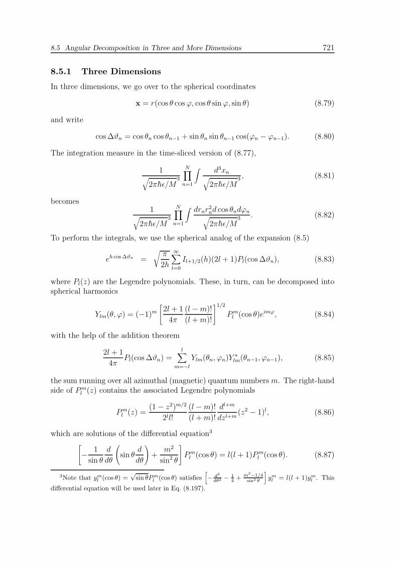
8.5.1 Three Dimensions

In three dimensions, we go over to the spherical coordinates

x = r(cos θ cosϕ, cos θ sinϕ, sin θ) (8.79)

and write

cos∆ϑn = cos θn cos θn−1 + sin θn sin θn−1 cos(ϕn − ϕn−1). (8.80)

The integration measure in the time-sliced version of (8.77),

1√

2πhǫ/M3

N∏

n=1

∫

d3xn√

2πhǫ/M3 , (8.81)

becomes1

√

2πhǫ/M3

N∏

n=1

∫

drnr2nd cos θndϕn

√

2πhǫ/M3 . (8.82)

To perform the integrals, we use the spherical analog of the expansion (8.5)

eh cos∆ϑn =

√

π

2h

∞∑

l=0

Il+1/2(h)(2l + 1)Pl(cos∆ϑn), (8.83)

where Pl(z) are the Legendre polynomials. These, in turn, can be decomposed intospherical harmonics

Ylm(θ, ϕ) = (−1)m[

2l + 1

4π

(l −m)!

(l +m)!

]1/2

Pml (cos θ)eimϕ, (8.84)

with the help of the addition theorem

2l + 1

4πPl(cos∆ϑn) =

l∑

m=−l

Ylm(θn, ϕn)Y∗lm(θn−1, ϕn−1), (8.85)

the sum running over all azimuthal (magnetic) quantum numbersm. The right-handside of Pm

l (z) contains the associated Legendre polynomials

Pml (z) =

(1− z2)m/2

2ll!

(l −m)!

(l +m)!

dl+m

dzl+m(z2 − 1)l, (8.86)

which are solutions of the differential equation3

[

− 1

sin θ

d

dθ

(

sin θd

dθ

)

+m2

sin2 θ

]

Pml (cos θ) = l(l + 1)Pm

l (cos θ). (8.87)

3Note that yml (cos θ) =√

sin θPml (cos θ) satisfies

[

− d2

dθ2 − 14 + m2−1/4

sin2 θ

]

yml = l(l + 1)yml . This

differential equation will be used later in Eq. (8.197).


Thus, the expansion (8.83) becomes

eh cos∆ϑn =

√

π

2h4π

∞∑

l=0

Il+1/2(h)l∑

m=−l

Ylm(θn, ϕn)Y∗lm(θn−1, ϕn−1). (8.88)

Inserted into (8.78), it leads to the time-sliced path integral

(xbτb|xaτa) ≈ 4π√

2πhǫ/M3

N∏

n=1

∫ ∞

0

drnr2nd cos θndϕn4π√

2πhǫ/M3

×N+1∏

n=1

[(

hǫπ

2Mrnrn−1

)1/2 ∞∑

ln=0

ln∑

mn=−ln

Iln+1/2

(

M

hǫrnrn−1

)

× Ylnmn(θn, ϕn)Y∗lnmn

(θn−1, ϕn−1)

]

exp

{

− ǫ

h

N+1∑

n=1

[

M

2

r2n + r2n−1

ǫ2+V (rn)

]}

. (8.89)

The intermediate ϕn- and cos θn-integrals can now all be done using the orthogonal-ity relation

∫ 1

−1d cos θ

∫ π

−πdϕ Y ∗

lm(θ, ϕ)Yl′m′(θ, ϕ) = δll′δmm′ . (8.90)

Each ϕn-integral yields a product of Kronecker symbols δlnln−1δmnmn−1

. Only theinitial and the final spherical harmonics survive, YlN+1mN+1

and Y ∗l0m0

, since they arenot subject to integration. Thus we arrive at the angular momentum decomposition

(xbτb|xaτa) =∞∑

l=0

l∑

m=−l

1

rbra(rbτb|raτa)lYlm(θb, ϕb)Y

∗lm(θa, ϕa), (8.91)

with the radial amplitude

(rbτb|raτa)l ≈4πrbra

√

2πhǫ/M3

N∏

n=1

∫ drnr2n4π

√

2πhǫ/M3

N+1∏

n=1

[

hǫ

2Mrnrn−1

]

(8.92)

×N+1∏

n=1

[

Il+1/2

(

M

hǫrnrn−1

)]

exp

{

− ǫ

h

N+1∑

n=1

[

M

2ǫ2(rn − rn−1)

2 + V (rn)]

}

.

The factors∏N

a r2n/∏N+1

a rnrn−1 pile up to 1/rbra and cancel the prefactor rbra.Together with the remaining product, the integration measure takes the usual one-dimensional form

1√

2πhǫ/M

N∏

n=1

∫ ∞

0

drn√

2πhǫ/M

. (8.93)

If we were to use here the large-argument limit (8.24) of the Bessel function, theintegrand would become exp(−AN

l /h), with the time-sliced radial action

ANl = ǫ

N+1∑

n=1

[

M

2ǫ2(rn − rn−1)

2 +h2

2M

l(l + 1)

rnrn−1

+ V (rn)

]

. (8.94)



The associated radial path integral

(rbτb|raτa)l ≈1

√

2πǫh/M

N∏

n=1

∫ ∞

0

drn√

2πhǫ/M

exp(

−1

hAN

l

)

(8.95)

agrees precisely with what would have been obtained by naively time-slicing thecontinuum path integral

(rbτb|raτa)l =∫ ∞

0Dr(τ)e− 1

hAl[r], (8.96)

with the radial action

Al[r] =∫ τb

τadτ

[

M

2r2 +

h2

2M

l(l + 1)

r2+ V (r)

]

. (8.97)

In particular, this would contain the correct centrifugal barrier

Vcf =h2

2M

l(l + 1)

r2. (8.98)

However, as we know from the discussion in Section 8.2, Eq. (8.95) is incorrect andmust be replaced by (8.92), due to the non uniformity of the continuum limit ǫ→ 0in the integrand of (8.92).

8.5.2 D Dimensions

The generalization to D dimensions is straightforward. The main place where thedimension enters is the expansion of

eh cos∆ϑn = e−Mhǫ

rnrn−1 cos∆ϑn, (8.99)

in which ∆ϑn is the relative angle between D-dimensional vectors xn and xn−1. Theexpansion reads [compare with (8.5) and (8.83)]

eh cos∆ϑn =∞∑

l=0

al(h)l +D/2− 1

D/2− 1

1

SDC

(D/2−1)l (cos∆ϑn), (8.100)

where SD is the surface of a unit sphere in D dimensions (1.558), and

al(h) ≡ (2π)D/2h1−D/2Il+D/2−1(h)

≡ ehal(h) = eh(

2π

h

)(D−1)/2

Il+D/2−1(h). (8.101)

The functions C(α)l (cosϑ) are the ultra-spherical Gegenbauer polynomials, defined

by the expansion

1

(1− 2tα + α2)λ=

∞∑

n=0

C(λ)n αn. (8.102)


The expansion (8.100) follows from the completeness of the polynomials C(ν)l (cos ϑ)

at fixed ν, using the integration formulas4

∫ π

0dϑ sinν ϑeh cos ϑC

(ν)l (cosϑ) = π

21−νΓ(2ν + l)

l!Γ(ν)h−νIν+l(h), (8.103)

∫ π

0dϑ sinν ϑC

(ν)l (cosϑ)C

(ν)l′ (cosϑ) = π

21−2νΓ(2ν + l)

l!(l + ν)Γ(ν)2δll′ . (8.104)

The Gegenbauer polynomials are related to Jacobi polynomials, which are definedin terms of hypergeometric functions (1.453) by5

P(α,β)l (z) ≡ 1

l!

Γ(l + 1 + β)

Γ(1 + β)F (−l, l + 1 + α + β; 1 + β; (1− z)/2). (8.105)

The relation is

C(ν)l (z) =

Γ(2ν + l)Γ(ν + 1/2)

Γ(2ν)Γ(ν + l + 1/2)P

(ν−1/2,ν−1/2)l (z). (8.106)

This follows from the relation6

C(ν)l (z) =

1

l!

Γ(l + 2ν)

Γ(2ν)F (−l, l + 2ν; 1/2 + ν; (1− z)/2). (8.107)

For D = 2 and 3, one has7

limν→0

1

νC

(ν)l (cosϑ) =

1

2lcos lϑ, (8.108)

C(1/2)l (cos ϑ) = P

(0,0)l (cosϑ) = Pl(cosϑ), (8.109)

and the expansion (8.100) reduces to (8.5) and (8.7), respectively.For D = 4

C(1)l (cos ϑ) =

sin(l + 1)β

sin β. (8.110)

According to an addition theorem, the Gegenbauer polynomials can be decom-posed into a sum of pairs of D-dimensional ultra-spherical harmonics Ylm(x).8

The label m stands collectively for the set of magnetic quantum numbers

4I. S. Gradshteyn and I. M. Ryzhik, op. cit., Formulas 7.321 and 7.313.5M. Abramowitz and I. Stegun, op. cit., Formula 15.4.6.6ibid., Formula 15.4.5.7I.S. Gradshteyn and I.M. Ryzhik, op. cit.,ibid., Formula 8.934.4.8See H. Bateman, Higher Transcendental Functions , McGraw-Hill, New York, 1953, Vol. II,

Ch. XI; N.H. Vilenkin, Special Functions and the Theory of Group Representations , Am. Math.Soc., Providence, RI, 1968.



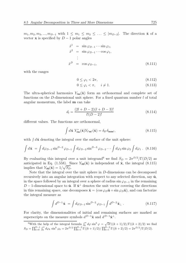
m1, m2, m3, ..., mD−1 with 1 ≤ m1 ≤ m2 ≤ . . . ≤ |mD−2|. The direction x of avector x is specified by D − 1 polar angles

x1 = sinϕD−1 · · · sinϕ1,

x2 = sinϕD−1 · · · cosϕ1,...

xD = cosϕD−1, (8.111)

with the ranges

0 ≤ ϕ1 < 2π, (8.112)

0 ≤ ϕi < π, i 6= 1. (8.113)

The ultra-spherical harmonics Ylm(x) form an orthonormal and complete set offunctions on the D-dimensional unit sphere. For a fixed quantum number l of totalangular momentum, the label m can take

dl =(2l +D − 2)(l +D − 3)!

l!(D − 2)!(8.114)

different values. The functions are orthonormal,∫

dx Y ∗lm(x)Yl′m′(x) = δll′δmm′ , (8.115)

with∫

dx denoting the integral over the surface of the unit sphere:∫

dx =∫

dϕD−1 sinD−2 ϕD−1

∫

dϕD−2 sinD−3 ϕD−2 · · ·

∫

dϕ2 sinϕ2

∫

dϕ1 . (8.116)

By evaluating this integral over a unit integrand9 we find SD = 2πD/2/Γ(D/2) asanticipated in Eq. (1.558). Since Y00(x) is independent of x, the integral (8.115)implies that Y00(x) = 1/

√SD.

Note that the integral over the unit sphere in D-dimensions can be decomposedrecursively into an angular integration with respect to any selected direction, say u,in the space followed by an integral over a sphere of radius sinϕD−1 in the remainingD− 1-dimensional space to u. If x⊥ denotes the unit vector covering the directionsin this remaining space, one decomposes x = (cosϕDu+sinϕDx), and can factorizethe integral measure as

∫

dD−1 x =∫

dϕD−1 sinD−2 ϕD−1

∫

dD−2 x⊥ . (8.117)

For clarity, the dimensionalities of initial and remaining surfaces are marked assuperscripts on the measure symbols dD−1x and dD−1x⊥.

9With the help of the integral formula∫ π

0dϕ sink ϕ =

√πΓ((k + 1)/2)/Γ((k + 2)/2) we find

SD =∏D−1

k=0

∫ π

0 dϕk sink ϕk = 2πD/2∏D−2

k=1 Γ((k + 1)/2)/∏D−2

k=1 Γ((k + 2)/2) = 2πD/2/Γ(D/2).


For the surface of the sphere, this corresponds to the recursion relation

SD =

√πΓ((D − 1)/2)

Γ(D/2)× SD−1, (8.118)

which is solved by SD = 2πD/2/Γ(D).In four dimensions, the unit vectors x have a parametrization in terms of polar

angles

x = (cos θ, sin θ cosψ, sin θ sinψ cosϕ, sin θ sinψ sinϕ), (8.119)

with the integration measure

dx = dθ sin2 θdψ sinψ dϕ. (8.120)

It is, however, more convenient to go over to another parametrization in terms ofthe three Euler angles which are normally used in the kinematic description of thespinning top. In terms of these, the unit vectors have the components

x1 = cos(θ/2) cos[(ϕ+ γ)/2],

x2 = − cos(θ/2) sin[(ϕ+ γ)/2],

x3 = sin(θ/2) cos[(ϕ− γ)/2],

x4 = sin(θ/2) sin[(ϕ− γ)/2], (8.121)

with the angles covering the intervals

θ ∈ [0, π), ϕ ∈ [0, 2π), γ ∈ [−2π, 2π). (8.122)

We have renamed the usual Euler angles α, β, γ introduced in Section 1.15 callingthem ϕ, θ, γ, since the formulas to be derived for them will be used in a later ap-plication in Chapter 13 [see Eq. (13.102)]. There the first two Euler angles coincidewith the polar angles ϕ, θ of a position vector in a three-dimensional space. It isimportant to note that for a description of the entire surface of the sphere, the rangeof the angle γ must be twice as large as for the classical spinning top. The associatedgroup space belongs to the covering group, of the rotation group which is equivalentto the group of unimodular matrices in two dimensions called SU(2). It is definedby the matrices

g(ϕ, θ, γ) = exp(iϕσ3/2) exp(iθσ2/2) exp(iγσ3/2), (8.123)

where σi are the Pauli spin matrices (1.448). In this parametrization, the integrationmeasure reads

dx =1

8dθ sin θ dϕ dγ. (8.124)

When integrated over the surface, the two measures give the same result S4 = 2π2.The Euler parametrization has the advantage of allowing the spherical harmonics in



four dimensions to be expressed in terms of the well-known representation functionsof the rotation group introduced in (1.445), (1.446):

Yl,m1,m2(x) =

√

l + 1

2π2Dl/2

m1m2(ϕ, θ, γ) =

√

l + 1

2π2dl/2m1m2

(θ)ei(m1ϕ+m2γ). (8.125)

For even and odd l, the numbersm1, m2 are both integer or half-integer, respectively.In arbitrary dimensions D > 2, the ultra-spherical Gegenbauer polynomials sat-

isfy the following addition theorem

2l +D − 2

D − 2

1

SD

C(D/2−1)l (cos∆ϑn) =

∑

m

Ylm(xn)Y∗lm(xn−1). (8.126)

For D = 3, this reduces properly to the well-known addition theorem for the spher-ical harmonics

1

4π(2l + 1)Pl(cos∆ϑn) =

l∑

m=−l

Ylm(xn)Y∗lm(xn−1). (8.127)

For D = 4, it becomes10

l + 1

2π2C

(1)l (cos∆ϑn) =

l + 1

2π2

l/2∑

m1,m2=−l/2

Dl/2m1m2

(ϕn, θn, γn)Dl/2 ∗m1m2

(ϕn−1, θn−1, γn−1),

(8.128)

where the angle ∆ϑn is related to the Euler angles of the vectors xn, xn−1 by

cos∆ϑn = cos(θn/2) cos(θn−1/2) cos[(ϕn − ϕn−1 + γn − γn−1)/2]

+ sin(θn/2) sin(θn−1/2) cos[(ϕn − ϕn−1 − γn + γn−1)/2]. (8.129)

Using (8.126), we can rewrite the expansion (8.100) in the form

eh(cos∆ϑn−1) =∞∑

l=0

al(h)∑

m

Ylm(xn)Y∗lm(xn−1). (8.130)

This is now valid for any dimension D, including the case D = 2 where the left-handside of (8.126) involves the limiting procedure (8.108). We shall see in Chapter 9in connection with Eq. (9.61) that it also makes sense to apply this expansion tothe case D = 1 where the “partial-wave expansion” degenerates into a separationof even and odd wave functions. In four dimensions, we shall mostly prefer theexpansion

eh(cos∆ϑn−1) =∞∑

l=0

al(h)l + 1

2π2

l/2∑

m1,m2=−l/2

Dl/2m1m2


(ϕn−1, θn−1, γn−1),

(8.131)

10Note that C(1)l (cos∆ϑn) coincides with the trace over the representation functions (1.446) of

the rotation group, i.e., it is equal to∑l/2

m=−l/2 dl/2m,m(∆ϑn).


where the sum over m1, m2 runs for even and odd l over integer and half-integernumbers, respectively.

The reduction of the time evolution amplitude in D dimensions to a radial pathintegral proceeds from here on in the same way as in two and three dimensions. Thegeneralization of (8.89) reads

(xbτb|xaτa) ≈1

√

2πhǫ/MD

N∏

n=1

∫ ∞

0

drnrD−1n dxn

√

2πhǫ/MD

×N+1∏

n=1

(

2πhǫ

Mrnrn−1

)(D−1)/2 ∞∑

ln=0

ID/2−1+ln

(

M

hǫrnrn−1

)

(8.132)

×∑

mn

Ylnmn(xn)Y∗lnmn

(xn−1)

]

exp

{

− ǫ

h

N+1∑

n=1

[

M

2ǫ2(rn − rn−1)

2 + V (rn)]

}

.

By performing the angular integrals and using the orthogonality relations (8.115),the product of sums over ln,mn reduces to a single sum over l,m, just as in thethree-dimensional amplitude (8.91). The result is the spherical decomposition

(xbτb|xaτa) =1

(rbra)(D−1)/2

∞∑

l=0

(rbτb|raτa)l∑

m

Ylm(xb)Y∗lm(xa), (8.133)

where (rbτb|raτa)l is the purely radial amplitude

(rbτb|raτa)l ≈1

√

2πhǫ/M

N∏

n=1

∫ ∞

0

drn√

2πhǫ/M

exp{

−1

hAN

l [r]}

, (8.134)

with the time-sliced action

ANl [r] = ǫ

N+1∑

n=1

[

M

2ǫ2(rn − rn−1)

2 − hǫlogIl+D/2−1

(

M

hǫrnrn−1

)

+ V (rn)

]

. (8.135)

As before, the product∏N+1

n=1 1/(rnrn−1)(D−1)/2 has removed the product

∏Nn=1 r

D−1n

in the measure as well as the factor (rbra)(D−1)/2 in front of it, leaving only the

standard one-dimensional measure of integration.In the continuum limit ǫ → 0, the asymptotic expression (8.24) for the Bessel

function brings the action to the form

ANl [r, r] ≈ ǫ

N+1∑

n=1

[

M

2ǫ2(rn − rn−1)

2 +h2

2M

(l +D/2− 1)2 − 1/4

rnrn−1+ V (rn)

]

. (8.136)

This looks again like the time-sliced version of the radial path integral in D dimen-sions

(rbτb|raτa)l =∫

Dr(τ) exp{

−1

hAl[r]

}

, (8.137)


8.6 Radial Path Integral for Harmonic Oscillator and Free Particle . . . 729

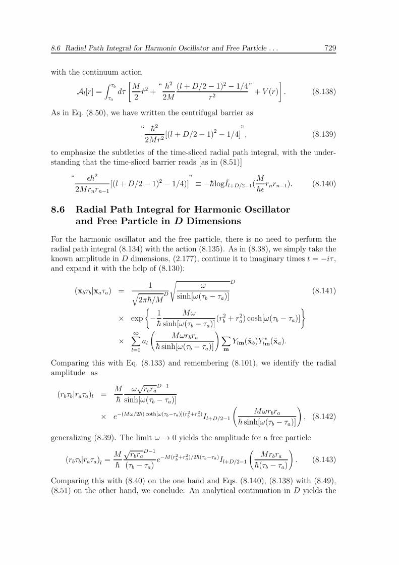
with the continuum action

Al[r] =∫ τb

τadτ

[

M

2r2 +

“ h2

2M

(l +D/2− 1)2 − 1/4

r2”+ V (r)

]

. (8.138)

As in Eq. (8.50), we have written the centrifugal barrier as

“ h2

2Mr2[(l +D/2− 1)2 − 1/4]

”, (8.139)

to emphasize the subtleties of the time-sliced radial path integral, with the under-standing that the time-sliced barrier reads [as in (8.51)]

“ ǫh2

2Mrnrn−1[(l +D/2− 1)2 − 1/4)]

” ≡ −hlogIl+D/2−1(M

hǫrnrn−1). (8.140)

8.6 Radial Path Integral for Harmonic Oscillator

and Free Particle in D Dimensions

For the harmonic oscillator and the free particle, there is no need to perform theradial path integral (8.134) with the action (8.135). As in (8.38), we simply take theknown amplitude in D dimensions, (2.177), continue it to imaginary times t = −iτ ,and expand it with the help of (8.130):

(xbτb|xaτa) =1

√

2πh/MD

√

ω

sinh[ω(τb − τa)]

D

(8.141)

× exp

{

−1

h

Mω

sinh[ω(τb − τa)](r2b + r2a) cosh[ω(τb − τa)]

}

×∞∑

l=0

al

(


)

∑

m

Ylm(xb)Y∗lm(xa).

Comparing this with Eq. (8.133) and remembering (8.101), we identify the radialamplitude as

(rbτb|raτa)l =M

h

ω√rbra

D−1

sinh[ω(τb − τa)]

× e−(Mω/2h) coth[ω(τb−τa)](r2b+r2a)Il+D/2−1

(


)

, (8.142)

generalizing (8.39). The limit ω → 0 yields the amplitude for a free particle

(rbτb|raτa)l =M

h

√rbra

D−1

(τb − τa)e−M(r2

b+r2a)/2h(τb−τa)Il+D/2−1

(

Mrbrah(τb − τa)

)

. (8.143)

Comparing this with (8.40) on the one hand and Eqs. (8.140), (8.138) with (8.49),(8.51) on the other hand, we conclude: An analytical continuation in D yields the


path integral for a linear oscillator in the presence of an arbitrary 1/r2-potential asfollows:

(rbτb|raτa)l =∫ ∞

0Dr(τ) exp

[

−1

h

∫ τb

τadτ

(

M

2r2 +

“ h2

2M

µ2 − 1/4

r2”+M

2ω2r2

)]

=M

h

ω√rbra

D−1

sinh[ω(τb − τa)]e−(Mω/2h) coth[ω(τb−τa)](r

2b+r2a)Iµ

(


)

.

(8.144)

Here µ is some strength parameter which initially takes the values µ = l +D/2− 1with integer l and D. By analytic continuation, the range of validity is extendedto all real µ > 0. The justification for the continuation procedure follows fromthe fact that the integral formula (8.14) holds for arbitrary m = µ ≥ 0. Theamplitude (8.144) satisfies therefore the fundamental composition law (8.20) for allreal m = µ ≥ 0. The harmonic oscillator with an arbitrary extra centrifugal barrierpotential

Vextra(r) = h2l2extra2Mr2

(8.145)

has therefore the radial amplitude (8.144) with

µ =√

(l +D/2− 1)2 + l2extra . (8.146)

For a finite number N +1 of time slices, the radial amplitude is known from theangular momentum expansion of the finite-N oscillator amplitude (2.199) in its obvi-ous extension to D dimensions. It can also be calculated directly as in Appendix 2Bby a successive integration of (8.132), using formula (8.14). The iteration formulasare the Euclidean analogs of those derived in Appendix 2B, with the prefactor of theamplitude being 2πN 2

1N 2N+1

√rbra, with the exponent −aN+1(r

2b + r2a)/h, and with

the argument of the Bessel function 2bN+1rbra/h. In this way we obtain precisely theexpression (8.144), except that sinh[ω(τb−τa)] is replaced by sinh[ω(N+1)ǫ]ǫ/ sinh ωǫand cosh[ω(τb − τa)] by cosh[ω(N + 1)ǫ].

8.7 Particle near the Surface of a Sphere

in D Dimensions

With the insight gained in the previous sections, it is straightforward to calculateexactly a certain class of auxiliary path integrals. They involve only angular variablesand will be called path integrals of a point particle moving near the surface of asphere in D dimensions. The resulting amplitudes lead eventually to the physicallymore relevant amplitudes describing the behavior of a particle on the surface of asphere.

On the surface of a sphere of radius r, the position of the particle as a functionof time is specified by a unit vector u(t). The Euclidean action is

A =M

2r2∫ τb

τadτ u2(τ). (8.147)


8.7 Particle near the Surface of a Sphere in D Dimensions 731

The precise way of time-slicing this action is not known from previous discussions.It cannot be deduced from the time-sliced action in Cartesian coordinates, nor fromits angular momentum decomposition. A new geometric feature makes the previousprocedures inapplicable: The surface of a sphere is a Riemannian space with nonzerointrinsic curvature. Sections 1.13 to 1.15 have shown that the motion in a curvedspace does not follow the canonical quantization rules of operator quantum mechan-ics. The same problem is encountered here in another form: Right in the beginning,we are not allowed to time-slice the action (8.147) in a straightforward way. Thecorrect slicing is found in two steps. First we use the experience gained with theangular momentum decomposition of time-sliced amplitudes in a Euclidean spaceto introduce and solve the earlier mentioned auxiliary time-sliced path integral nearthe surface of the sphere. In a second step we shall implement certain correctionsto properly describe the action on the sphere. At the end, we have to construct thecorrect measure of path integration which will not be what one naively expects. Toset up the auxiliary path integral near the surface of a sphere we observe that thekinetic term of a time slice in D dimensions

M

2ǫ

N+1∑

n=1

(r2n + r2n−1 − 2rnrn−1 cos∆ϑn) (8.148)

decomposes into radial and angular parts as

−M2ǫ

N+1∑

n=1

(r2n + r2n−1 − 2rnrn−1) +M

2ǫ

N+1∑

n=1

2rnrn−1(1− cos∆ϑn). (8.149)

The angular factor can be written as

−M2ǫ

N+1∑

n=1

rnrn−1(xn − xn−1)2, (8.150)

where xn, xn−1 are the unit vectors pointing in the directions of xn, xn−1 [recall(8.111)]. Restricting all radial variables rn to the surface of a sphere of a fixed radiusr and identifying x with u leads us directly to the time-sliced path integral near thesurface of the sphere in D dimensions:

(ubτb|uaτa) ≈1

√

2πhǫ/Mr2D−1

N∏

n=1

∫

dun√

2πhǫ/Mr2D−1

exp(

−1

hAN

)

, (8.151)

with the sliced action

AN =M

2ǫr2

N+1∑

n=1

(un − un−1)2. (8.152)

The measure dun denotes infinitesimal surface elements on the sphere in D dimen-sions [recall (8.116)]. Note that although the endpoints un lie all on the sphere, thepaths remain only near the sphere since the path sections between the points leave


the surface and traverse the embedding space along a straight line. This will bestudied further in Section 8.8.

As mentioned above, this amplitude can be solved exactly. In fact, for each timeinterval ǫ, the exponential

exp

[

−Mr2

2hǫ(un − un−1)

2

]

= exp

[

−Mr2

hǫ(1− cos∆ϑn)

]

(8.153)

can be expanded into spherical harmonics according to formulas (8.100)–(8.101),

exp

[

−Mr2

2hǫ(un − un−1)

2

]

=∞∑

l=0

al(h)l +D/2− 1

D/2− 1

1

SDC

(D/2−1)l (cos∆ϑn)

=∞∑

l=0

al(h)∑

m

Ylm(un)Y∗lm(un−1), (8.154)

where

al(h) =(

2π

h

)(D−1)/2

Il+D/2−1(h), h =Mr2

hǫ. (8.155)

For each adjacent pair (n+1, n), (n, n−1) of such factors in the sliced path integral,the integration over the intermediate un variable can be done using the orthogonalityrelation (8.115). In this way, (8.151) produces the time-sliced amplitude

(ubτb|uaτa) =

(

h

2π

)(N+1)(D−1)/2 ∞∑

l=0

al(h)N+1

∑

m

Ylm(ub)Y∗lm(ua). (8.156)

We now go to the continuum limit N → ∞, ǫ = (τb−τa)/(N+1) → 0, where [recall(8.11)]

(

h

2π

)(N+1)(D−1)/2

al(h)N+1 =

[

Il+D/2−1

(

Mr

hǫ

2)]N+1

ǫ→0−−−→ exp

{

−(τb − τa)h(l +D/2− 1)2 − 1/4

2Mr2

}

. (8.157)

Thus, the final time evolution amplitude for the motion near the surface of thesphere is

(ubτb|uaτa) =∞∑

l=0

exp

[

− hL2

2Mr2(τb − τa)

]

∑

m

Ylm(ub)Y∗lm(ua), (8.158)

withL2 ≡ (l +D/2− 1)2 − 1/4. (8.159)

For D = 3, this amounts to an expansion in terms of associated Legendre polyno-mials


l=0

2l + 1

4πexp

{

− hL2

2Mr2(τb − τa)

}

×l∑

m=−l

(l −m)!

(l +m)!Pml (cos θb)P

ml (cos θa)e

im(ϕb−ϕa). (8.160)


8.8 Angular Barriers near the Surface of a Sphere 733

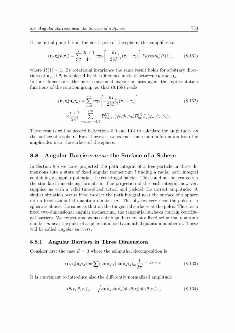
If the initial point lies at the north pole of the sphere, this simplifies to

(ubτb|zaτa) =∞∑

l=0

2l + 1

4πexp

[

− hL2

2Mr2(τb − τa)

]

Pl(cos θb)Pl(1), (8.161)

where Pl(1) = 1. By rotational invariance the same result holds for arbitrary direc-tions of ua, if θb is replaced by the difference angle ϑ between ub and ua.In four dimensions, the most convenient expansion uses again the representationfunctions of the rotation group, so that (8.158) reads


l=0

exp

[

− hL2

2Mr2(τb − τa)

]

(8.162)

× l + 1

2π2

l/2∑

m1,m2=−l/2

Dl/2m1m2

(ϕb, θb, γb)Dl/2 ∗m1m2

(ϕa, θa, γa).

These results will be needed in Sections 8.9 and 10.4 to calculate the amplitudes onthe surface of a sphere. First, however, we extract some more information from theamplitudes near the surface of the sphere.

8.8 Angular Barriers near the Surface of a Sphere

In Section 8.5 we have projected the path integral of a free particle in three di-mensions into a state of fixed angular momentum l finding a radial path integralcontaining a singular potential, the centrifugal barrier. This could not be treated viathe standard time-slicing formalism. The projection of the path integral, however,supplied us with a valid time-sliced action and yielded the correct amplitude. Asimilar situation occurs if we project the path integral near the surface of a sphereinto a fixed azimuthal quantum number m. The physics very near the poles of asphere is almost the same as that on the tangential surfaces at the poles. Thus, at afixed two-dimensional angular momentum, the tangential surfaces contain centrifu-gal barriers. We expect analogous centrifugal barriers at a fixed azimuthal quantumnumber m near the poles of a sphere at a fixed azimuthal quantum numberm. Thesewill be called angular barriers .

8.8.1 Angular Barriers in Three Dimensions

Consider first the case D = 3 where the azimuthal decomposition is

(ubτb|uaτa) =∑

m

(sin θbτb| sin θaτa)m1

2πeim(ϕb−ϕa). (8.163)

It is convenient to introduce also the differently normalized amplitude

(θbτb|θaτa)m ≡√

sin θb sin θa(sin θbτb| sin θaτa)m, (8.164)


in terms of which the expansion reads

(ubτb|uaτa) =∑

m

1√sin θb sin θa

(θbτb|θaτa)m1

2πeim(ϕb−ϕa). (8.165)

While the amplitude (sin θbτb| sin θaτa)m has the equal-time limit

(sin θbτ | sin θaτ)m =1

sin θaδ(θb − θa) (8.166)

corresponding to the invariant measure of the θ-integration on the surface of thesphere

∫

dθ sin θ, the new amplitude (θbτb|θaτ)m has the limit

(θbτ |θaτ)m = δ(θb − θa) (8.167)

with a simple δ-function, just as for a particle moving on the coordinate intervalθ ∈ (0, 2π) with an integration measure

∫

dθ. The renormalization is analogous tothat of the radial amplitudes in (8.9).

The projected amplitude can immediately be read off from Eq. (8.158):

(θbτb|θaτa)m =√

sin θb sin θa

×∞∑

l=m

exp

[

− hl(l + 1)

2Mr2(τb − τa)

]

2πYlm(θb, 0)Y∗lm(θa, 0). (8.168)

In terms of associated Legendre polynomials [recall (8.84)], this reads


sin θb sin θa∞∑

l=m

exp

{

− hl(l + 1)

2Mr2(τb − τa)

}

(8.169)

× (2l + 1)

2

(l −m)!


ml (cos θa).

Let us look at the time-sliced path integral associated with this amplitude. We startfrom Eq. (8.151) for D = 3,

(ubτb|uaτa) ≈1

2πhǫ/Mr2

N∏

n=1

[

∫

d cos θndϕn

2πhǫ/Mr2

]

exp(

−1

hAN

)

, (8.170)

and use the addition theorem

cos∆ϑn = cos θn cos θn−1 + sin θn sin θn−1 cos(ϕn − ϕn−1) (8.171)

to expand the exponent as

exp

[

−Mr2

2hǫ(un − un−1)

2

]

= exp

[

−Mr2

hǫ(1− cos∆ϑn)

]

= exp

[

−Mr2

hǫ(1− cos θn cos θn−1 − sin θn sin θn−1)

]

× 1√2πhn

∞∑

m=−∞

Im(hn)eim(ϕn−ϕn−1), (8.172)



where hn is defined as

hn ≡ Mr2

hǫsin θn sin θn−1. (8.173)

By doing successively the ϕn-integrations, we wind up with the path integral for theprojected amplitude

(θbτb|θaτa)m ≈ 1√

2πǫh/Mr2

N∏

n=1

∫ π

0

dθn√

2πǫh/Mr2

exp(

−1

hAN

m

)

, (8.174)

where ANm is the sliced action

ANm =

N+1∑

n=1

{

Mr2

ǫ[1− cos(θn − θn−1)]− h log Im(hn)

}

. (8.175)

For small ǫ, this can be approximated (setting ∆θn ≡ θn − θn−1) by

ANm ≈ ǫ

N+1∑

n=1

{

Mr2

2ǫ2

[

(∆θn)2 − 1

12(∆θn)

4 + . . .]

+h2

2Mr2m2 − 1/4

sin θn sin θn−1

}

, (8.176)

with the continuum limit

Am =∫ τb

τadτ

(

Mr2

2θ2 − h2

8Mr2+

h2

2Mr2m2 − 1/4

sin2 θ

)

. (8.177)

This action has a 1/ sin2 θ -singularity at θ = 0 and θ = π, i.e., at the north andsouth poles of the sphere, whose similarity with the 1/r2-singularity of the centrifugalbarrier justifies the name “angular barriers”.

By analogy with the problems discussed in Section 8.2, the amplitude (8.174)with the naively time-sliced action (8.176) does not exist for m = 0, this being thepath collapse problem to be solved in Chapter 12. With the full time-sliced action(8.175), however, the path integral is stable for all m. In this stable expression,the successive integration of the intermediate variables using formula (8.14) givescertainly the correct result (8.169).

To do such a calculation, we start out from the product of integrals (8.174) andexpand in each factor Im(hn) with the help of the addition theorem

√

2ζ

πeζ cos θn cos θn−1Im(ζ sin θn sin θn−1)

=∞∑

l=m

Il+1/2(ζ)(2l + 1)(l −m)!

(l +m)!Pml (cos θn)P

ml (cos θn−1), (8.178)

where ζ ≡ Mr2/hǫ. This theorem follows immediately from a comparison of twoexpansions

e−ζ(1−cos∆θn) = e−ζ[1−cos θn cos θn−1−sin θn sin θn−1 cos(ϕn−ϕn−1)] (8.179)

× 1√2πζ sin θn sin θn−1

∞∑

m=−∞

Im(ζ sin θn sin θn−1)eim(ϕn−ϕn−1),

e−ζ(1−cos∆θn) = e−ζ

√

π

2ζ

∞∑

l=0

(2l + 1)Il+1/2(ζ)Pl(cos∆θn). (8.180)


The former is obtained with the help (8.5), the second is taken from (8.83). After thecomparison, the Legendre polynomialis expanded via the addition theorem (8.85),which we rewrite with (8.84) as

Pl(cos∆θn) =l∑

m=−l

(l −m)!

(l +m)!Pml (θn)P

ml (θn−1)e

im(ϕn−ϕn−1). (8.181)

We now recall the orthogonality relation (8.50), rewritten as

∫ 1

−1

d cos θ

sin2 θPml (cos θ)Pm

l′ (cos θ) =(l +m)!

(l −m)!

2

2l + 1δll′. (8.182)

This allows us to do all angular integrations in (8.175). The result



l=m

[Im+l+1/2(ζ)]N+1

×(2l + 1)

2

(l −m)!


ml (cos θa) (8.183)

is the solution of the time-sliced path integral (8.174).In the continuum limit, [Im+l+1/2(ζ)]

N+1 is dominated by the leading asymptoticterm of (8.12) so that

[Im+l+1/2(ζ)]N+1 ≈ exp

[

− h

2Mr2L2(τb − τa)

]

, (8.184)

leading to the previously found expression (8.169).We have gone through this calculation in detail for the following purpose. Later

applications will require an analytic continuation of the path integral from integervalues of m to arbitrary real values µ ≥ 0. With the present calculation, sucha continuation is immediately possible by rewriting (8.183) with the help of therelation

Pml (z) = (−)mP−m

l

(l +m)!

(l −m)!(8.185)

as

(θbτb|θaτa)µ =√


n=0

[In+µ+1/2(ζ)]N+1

× (2n+ 2µ+ 1)

2

(n+ 2µ)!

n!P−µn+µ(cos θb)P

−µn+µ(cos θa). (8.186)

Here, µ can be an arbitrary real number if the factorials (n+2µ)! and n! are definedas Γ(n + 2µ+ 1) and Γ(n + 1). In the continuum limit, (8.186) becomes

(θbτb|θaτa)µ =√


n=0

exp

[

− h(n+ µ)(n+ µ+ 1)

2Mr2(τb − τa)

]

× (2n+ 2µ+ 1)

2

(n+ 2µ)!

n!P−µn+µ(cos θb)P

−µn+µ(cos θa). (8.187)



We prove this to solve the time-sliced path integral (8.174) for arbitrary realvalues of m = µ [4] by using the addition theorem11

(sinα sin β)−µJµ(z sinα sin β)eiz cosα cos β =22µ+1Γ2(µ+ 1/2)√

2πz

×∞∑

n=0

inn!(n+ µ+ 1/2)

Γ(n+ 2µ+ 1)Jn+µ+1/2(z)C

(µ+1/2)n (cosα)C(µ+1/2)

n (cos β). (8.188)

After substituting z by ζe−iπ/2 this turns into

(sinα sin β)−µIµ(ζ sinα sin β) exp(ζ cosα cos β) =22µ+1Γ2(µ+ 1/2)√

2πζ

×∞∑

n=0

n!(n+ µ+ 1/2)

Γ(n + 2µ+ 1)In+µ+1/2(ζ)C

(µ+1/2)n (cosα)C(µ+1/2)

n (cos β). (8.189)

The Gegenbauer polynomials C(µ+1/2)n (z) can be expressed, for arbitrary µ, by means

of Eq. (8.106) in terms of Jacobi polynomials P (µ,µ)n , and these further in terms of

Legendre functions P−µn+µ, using the formula

P (µ,µ)n (z) = (−2)µ

(n+ µ)!

n!(1− z2)−µ/2P−µ

n+µ(z). (8.190)

Thus12

C(µ+1/2)n (z) =

Γ(n+ 2µ+ 1)Γ(µ+ 1)

Γ(2µ+ 1)n!

[

1− z2

4

]−µ/2

P−µn+µ(z). (8.191)

We can now perform the integrations in the time-sliced path integral by means ofthe known continuation of the orthogonality relation (8.182) to arbitrary real valuesof µ:

∫ 1

−1

d cos θ

sin2 θP−µn+µ(cos θ)P

−µn′+µ(cos θ) =

n!

(n + 2µ)!

2

2n+ 1µ+ 1δnn′ . (8.192)

Note that for noninteger µ, the Legendre functions P−mn+m(cos θ) are no longer poly-

nomials as in (1.421). Instead, they are defined in terms of the hypergeometricfunction as follows:

P µν (z) =

1

Γ(1− µ)

(

1 + z

1− z

)µ/2

F (−ν, ν + 1; 1− µ; (1− z)/2). (8.193)

The integral formula (8.192) is a consequence of the orthogonality of the Gegenbauerpolynomials (8.104), which is applied here in the form

∫ 1

−1dz (1− z2)µC(µ+1/2)

n (z)C(µ+1/2)n′ (z) = δnn′

π2−2µΓ(2µ+ 2 + n)

n!(n + µ)[Γ(µ+ 1/2)]2. (8.194)

11G.N. Watson, Theory of Bessel Functions , Cambridge University Press, 1952, Ch. 11.6,Eq. (11.9).

12I.S. Gradshteyn and I.M. Ryzhik, op. cit., Formula 8.936.


Using (8.189), (8.191) and (8.192), the integrals in the product (8.207) can all beperformed as before, resulting in the amplitude (8.186) with the continuum limit(8.187), both valid for arbitrary real values of m = µ ≥ 0.

The continuation to arbitrary real values of µ has an important application:The action (8.177) of the projected motion of a particle near the surface of thesphere coincides with the action of a particle moving in the so-called Poschl-Tellerpotential [5]:

V (θ) =h2

2Mr2s(s+ 1)

sin2 θ(8.195)

with the strength parameter s = m − 1/2. After the continuation of arbitrary realm = µ ≥ 0, the amplitude (8.187) describes this system for any potential strength.This fact will be discussed further in Chapter 14 where we develop a general methodfor solving a variety of nontrivial path integrals.

Note that the amplitude (sin θbτb| sin θaτa)m satisfies the Schrodinger equation

[

h2

Mr2

(

−1

2

1

sin θ

d

dθsin θ

d

dθ+

m2

2 sin2 θ

)

+ h∂τ

]

(sin θ τ | sin θaτa)m= hδ(τ − τa)δ(cos θ − cos θa). (8.196)

This follows from the differential equation obeyed by the Legendre polynomialsPml (cos θ) in (8.87). The new amplitude (θ τ |θaτa)m, on the other hand, satisfies the

equation [corresponding to that of√sin θPm

l (cos θ) in the footnote to Eq. (8.87)]

[

h2

Mr2

(

−1

2

d

dθ2− 1

8+m2 − 1/4

2 sin2 θ

)

+ h∂τ

]

(θ τ |θaτa)m = hδ(τ − τa)δ(θ − θa). (8.197)

8.8.2 Angular Barriers in Four Dimensions

In four dimensions, the angular momentum decomposition reads in terms of Eulerangles [see (8.162)]


l=0

exp

{

− hL2

2Mr2(τb − τa)

}

× l + 1

2π2

l/2∑

m1m2=−l/2

dl/2m1m2(θb)d

l/2m1m2

(θa)eim1(ϕb−ϕa)+im2(γb−γa), (8.198)

with

L2 ≡ (l + 1)2 − 1/4 = 4(l/2)(l/2 + 1) + 3/4 (8.199)

and m1, m2 running over integers or half-integers depending on l/2. We now definethe projected amplitudes by the expansion

(ubτb|uaτa) = 8∑

m1m2

(sin θbτb| sin θaτa)m1m2

1

2πeim1(ϕb−ϕa)

1

4πeim2(γb−γa). (8.200)



As in (8.164), it is again convenient to introduce the differently normalized amplitude(θbτb|θaτa)m defined by

(θbτb|θaτa)m1m2≡√

sin θb sin θa(sin θbτb| sin θaτa)m1m2, (8.201)

in terms of which the expansion becomes [compare (8.163)]

(ubτb|uaτa) =∑

m

8√sin θb sin θa

(θbτb|θaτa)m1m2

1

2πeim(ϕb−ϕa)

1

4πeim(γb−γa). (8.202)

A comparison with (8.198) gives immediately the projected amplitude

(θbτb|θaτa)m1m2=√

sin θb sin θa (8.203)

×∞∑

l

exp

{

− h[(l + 1)2 − 1/4]

2Mr2(τb − τa)

}

l + 1

2dl/2m1m2

(θb)dl/2m1m2

(θa),

in which l is summed in even steps from the larger value of |2m1|, |2m2| to infinity.Let us write down the time-sliced path integral leading to this amplitude. Ac-

cording to (8.151)–(8.153), it is given by

(ubτb|uaτa) ≈ 1√

2πhǫ/Mr23

N∏

n=1

∫ π

0

∫ 2π

0

∫ 4π

0

dθn sin θndϕndγn

8√

2πhǫ/Mr23

exp(

−1

hAN

)

.

(8.204)

In each time slice we make use of the addition theorem (8.129) and expand theexponent with (8.6) as

exp

[

−Mr2

2hǫ(un − un−1)

2

]

= exp

[

−Mr2

hǫ(1− cos∆ϑn)

]

= exp

{

−Mr2

2hǫ[1− cos(θn/2) cos(θn−1/2)− sin(θn/2) sin(θn−1/2)]

}

× 1√

2πhcn

1√

4πhsn

∞∑

m1,m2=−∞

I|m1+m2|(hcn)I|m1−m2|(h

sn) (8.205)

× exp{im1(ϕn − ϕn−1) + im2(γn − γn−1)},

where hcn and hsn are given by

hcn =Mr2

hǫcos(θn/2) cos(θn−1/2), hsn =

Mr2

hǫsin(θn/2) sin(θn−1/2). (8.206)

By doing successively the ϕn- and γn-integrations, we wind up with the path integralfor the projected amplitude

(θbτb|θaτa)m1m2≈ 1√

2πǫh/4Mr2

N∏

n=1

∫ π

0

dθn√

2πǫh/4Mr2

exp{

−1

hAN

m1m2

}

, (8.207)


where ANm1m2

is the sliced action

ANm1m2

=N+1∑

n=1

{

Mr2

ǫ[1− cos[(θn − θn−1)/2]

− h log I|m1+m2|(hcn)− h log I|m1−m2|(h

sn)

}

. (8.208)

For small ǫ, this can be approximated (setting ∆θn ≡ θn − θn−1) by

ANm1m2

→ ǫN+1∑

n=1

{

Mr2

2ǫ2[(∆θn/2)

2 − 1

12(∆θn/2)

4 + . . .]

+h2

2Mr2(m1 +m2)

2 − 1/4

cos(θn/2) cos(θn−1/2)+

h2

2Mr2(m1 −m2)

2 − 1/4

sin(θn/2) sin(θn−1/2)

}

, (8.209)

with the continuum limit

Am1m2=∫ τb

τadτ

(

Mr2

8θ2 − h2

8Mr2+

h2

2Mr2|m1 +m2|2 − 1/4

cos2(θ/2)

+h2

2Mr2|m1 −m2|2 − 1/4

sin2(θ/2)

)

. (8.210)

After introducing the auxiliary mass

µ =M/4 (8.211)

and rearranging the potential terms, we can write the action equivalently as

Am1m2=∫ τb

τadτ

(

µr2

2θ2 − h2

32µr2+

h2

2µr2m2

1 +m22 − 1/4− 2m1m2 cos θ

sin2 θ

)

. (8.212)

Just as in the previous system, this action contains an angular barrier 1/ sin2 θ atθ = 0, and θ = π, so that the amplitude (8.207) with the naively time-sliced action(8.176) does not exist for m1 = m2 or m1 = −m2, due to path collapse. Only withthe properly time-sliced action (8.208) is the path integral stable and solvable bysuccessive integrations with the result (8.203).

As before, the path integral (8.207) is initially only defined and solved by (8.203)if both m1 and m2 have integer or half-integer values. The path integral and itssolution can, however, be continued to arbitrary real values of m1 = µ1 ≥ 0 and itsm2 = µ2 ≥ 0. For this we rewrite (8.203) in the form [4]

(θbτb|θaτa)µ1µ2=√

sin θb sin θa (8.213)

×∞∑

n=0

exp

{

−h[(n+ µ1 + 1)2 − 1/4]

2Mr2(τb − τa)

}

n+ µ1 + 1

2dn+µ1

µ1µ2(θb)d

n+µ1

µ1µ2(θa),



assuming that µ1 ≥ µ2. The products of the rotation functions dλµ1µ2(θ) have a

well-defined analytic continuation to arbitrary real values of the indices µ1, µ2, λ, ascan be seen by expressing them in terms of Jacobi polynomials via formula (1.446).

To perform the path integral in the analytically continued case, we use the ex-pansion valid for all µ+, µ−,

13

z

2Jµ+

(z cosα cos β)Jµ−(z sinα sin β) = cosµ+ α cosµ+ β sinµ− α sinµ− β

×∞∑

n=0

(−1)n(µ+ + µ− + 2n+ 1)Jµ++µ−+2n+1(z)

× Γ(n+ µ+ + µ− + 1)Γ(n+ µ− + 1)

n!Γ(n+ µ+ + 1)[Γ(µ− + 1)]2

× F (−n, n + µ+ + µ− + 1;µ− + 1; sin2 α)

× F (−n, n + µ+ + µ− + 1;µ− + 1; sin2 β) (8.214)

with ζ ≡ Mr2/hǫ. The hypergeometric functions appearing on the right-hand sidehave a first argument with a negative integer value. They are therefore proportionalto the Jacobi polynomials P (µ−,µ+)

n :

P (µ−,µ+)n (x) =

1

n!

Γ(n+ µ− + 1)

Γ(µ− + 1)F (−n, n + µ+ + µ− + 1; 1 + µ−; (1− x)/2) (8.215)

[recall (1.446) and the identity P (µ−,µ+)n (x) = (−)nP (µ−,µ+)

n (−x)]. Inserting z = iζ ,α = θn/2, β = θn−1/2, and expressing the Jacobi polynomials in terms of rotationfunctions continued to real-valued µ1, µ2, we obtain from (8.214) for µ1 ≥ µ2

Iµ+

(

ζ cosθn2cos

θn−1

2

)

Iµ−

(

ζ sinθn2sin

θn−1

2

)

=4

ζ

∞∑

n=0

I2n+µ++µ−+1(ζ)(n+ µ1 + µ2)!(n+ µ1 − µ2)!

(n+ 2µ1)!n!dn+µ1

µ1µ2(θn)d

n+µ1

µ1µ2(θn−1). (8.216)

Now we make use of the orthogonality relation [compare (1.455)]

∫ 1

−1d cos θ dn+µ1

µ1µ2(θ)dn

′+µ1µ1µ2

(θ) = δnn′

2

2n+ 1, (8.217)

which for real µ1, µ2 follows from the corresponding relation for Jacobi polynomials14

∫ 1

−1dx (1− x)µ−(1 + x)µ+P (µ−,µ+)

n (x)P(µ−,µ+)n′ (x)

= δnn′

2µ++µ−+1Γ(µ+ + n + 1)Γ(µ− + n + 1)

n!(µ+ + µ− + 1 + 2n)Γ(µ+ + µ− + n+ 1), (8.218)

13G.N. Watson, op. cit., Chapter 11.6, Gl. (11.6), (1).14I.S. Gradshteyn and I.M. Ryzhik, op. cit., Formula 7.391.


valid for Reµ+ > −1 , Reµ− > −1. Performing all θn-integrations in (8.207) yieldsthe time-sliced amplitude

(θb τb|θa τa)µ1µ2=√


n=0

[

I2n+µ++µ−+1(ζ)]N+1

dn+µ1

µ1µ2(θb)d

n+µ1

µ1µ2(θa), (8.219)

valid for all real µ1 ≥ µ2 ≥ 0. In the continuum limit, this becomes

(θb τb|θa τa)µ1µ2=√


n=0

e−En(τb−τa)/hdn+µ1µ1µ2

(θb)dn+µ1µ1µ2

(θa), (8.220)

with

En =h

2Mr2[(2n+ µ+ + µ− + 1)2 − 1/4], (8.221)

which proves (8.213).Apart from the projected motion of a particle near the surface of the sphere,

the amplitude (8.213) describes also a particle moving in the general Poschl-Tellerpotential [5]

VPT ′(θ) =h2

2Mr2

[

s1(s1 + 1)

sin2(θ/2)+s2(s2 + 1)

cos2(θ/2)

]

. (8.222)

Due to the analytic continuation to arbitrary real m1, m2 the parameters s1 ands2 are arbitrary with the potential strength parameters s1 = m1 + m2 − 1/2 ands2 = m1 −m2 − 1/2. This will be discussed further in Chapter 14.

Recalling the differential equation (1.454) satisfied by the rotation functionsdl/2m1m2

(θ), we see that the original projected amplitude (8.207) obeys the Schrodingerequation

[

h2

2µr2

(

− 1

sin θ

d

dθsin θ

d

dθ+

3

16+m2

1 +m22 − 2m1m2 cos θ

sin2 θ

)

+ h∂τ

]

× (sin θ τ | sin θaτa)m1m2= hδ(τ − τa)δ(cos θ − cos θa). (8.223)

The extra term 3/16 is necessary to account for the energy difference betweenthe motion near the surface of a sphere in four dimensions, whose energy is(h2/2µr2)[(l/2)(l/2 + 1) + 3/16] [see (8.158)], and that of a symmetric spinningtop with angular momentum L = l/2 in three dimensions, whose energy is(h2/2µr2)(l/2)(l/2 + 1), as shown in the next section in detail.

The amplitude (θbτb|θaτa)m1m2defined in (8.201) satisfies the differential equation

[

h2

2µr2

(

− d2

dθ2− 1

16+m2

1 +m22 − 1/4− 2m1m2 cos θ

sin2 θ

)

+ h∂τ

]

× (θ τ |θaτa)m1m2= hδ(τ − τa)δ(θ − θa). (8.224)

This is, of course, precisely the Schrodinger equation associated with the action(8.212).


8.9 Motion on a Sphere in D Dimensions 743

8.9 Motion on a Sphere in D Dimensions

The wave functions in the time evolution amplitude near the surface of a sphere arealso correct for the motion on a sphere. This is not true for the energies, for whichthe amplitude (8.158) gives

El =h2

2Mr2(L2

2)l, (8.225)

with(L2

2)l = (l +D/2− 1)2 − 1/4, l = 0, 1, 2, . . . . (8.226)

As we know from Section 1.14, the energies should be equal to

El =h2

2Mr2(L2)l, (8.227)

where (L2)l denotes the eigenvalues of the square of the angular momentum operator.In D dimensions, the eigenvalues are known from the Schrodinger theory to be

(L2)l = l(l +D − 2), l = 0, 1, 2, . . . . (8.228)

Apart from the trivial case D = 1, the two energies are equal only for D = 3, where(L2

2)l ≡ (L2)l = l(l + 1). For all other dimensions, we shall have to remove thedifference

∆(L22)l ≡ L2 − L2

2 =1

4−(

D

2− 1

)2

= −(D − 1)(D − 3)

4. (8.229)

The simplest nontrivial case where the difference appears is for D = 2 where the roleof l is played by the magnetic quantum number m and (L2

2)m = m2 − 1/4, whereasthe correct energies should be proportional to (L2)m = m2.

Two changes are necessary in the time-sliced path integral to find the correct en-ergies. First, the time-sliced action (8.152) must be modified to measure the properdistance on the surface rather than the Euclidean distance in the embedding space.Second, we will have to correct the measure of path integration. The modificationof the action is simply

ANon sphere =

M

ǫr2

N+1∑

n=1

(∆ϑn)2

2, (8.230)

in addition to

AN =M

ǫr2

N+1∑

n=1

(1− cos∆ϑn). (8.231)

Since the time-sliced path integral was solved exactly with the latter action, it isconvenient to expand the true action around the solvable one as follows:

ANon sphere =

M

ǫr2

N+1∑

n=1

[

(1− cos∆ϑn) +1

24(∆ϑn)

4 − . . .]

. (8.232)


There is no need to go to higher than the fourth order in ∆ϑn , since these do notcontribute to the relevant order ǫ. ForD = 2, the correction of the action is sufficientto transform the path integral near the surface of the sphere into one on the sphere,which in this reduced dimension is merely a circle. On a circle, ∆ϑn = ϕn − ϕn−1

and the measure of path integration becomes

1√

2πhǫ/Mr2

N+1∏

n=1

∫ π/2

−π/2

dϕn√

2πhǫ/Mr2. (8.233)

The quartic term (∆ϑn)4 = (ϕn − ϕn−1)

4 can be replaced according to the rules ofperturbation theory by its expectation [see (8.62)]

〈(∆ϑn)4〉0 = 3ǫh

Mr2. (8.234)

The correction term in the action

∆quAN =M

ǫr2

N+1∑

n=1

1

24(∆ϑn)

4 (8.235)

has, therefore, the expectation

〈∆quAN〉0 = (N + 1)ǫh2/4

2Mr2. (8.236)

This supplies precisely the missing term which raises the energy from the near -the-surface value Em = h2(m2 − 1/4)/2Mr2 to the proper on-the-sphere value Em =h2m2/2Mr2.

In higher dimensions, the path integral near the surface of a sphere requires asecond correction. The difference (8.229) between L2 and L2

2 is negative. Since theexpectation of the quartic correction term alone is always positive, it can certainlynot explain the difference.15 Let us calculate first its contribution at arbitrary D.For very small ǫ, the fluctuations near the surface of the sphere lie close to theD − 1 -dimensional tangent space. Let ∆xn be the coordinates in this space. Thenwe can write the quartic correction term as

∆quAN ≈ M

ǫ

N+1∑

n=1

1

24r2(∆xn)

4, (8.237)

where the components (∆xn)i have the correlations

〈(∆xn)i(∆xn)j〉0 =hǫ

Mδij . (8.238)

15This was claimed by G. Junker and A. Inomata, in Path Integrals from meV to MeV, editedby M.C. Gutzwiller, A. Inomata, J.R. Klauder, and L. Streit (World Scientific, Singapore, 1986),p.333.


8.9 Motion on a Sphere in D Dimensions 745

Thus, according to the rule (8.62), ∆quAN has the expectation

〈∆AN〉0 = (N + 1)ǫh2

2Mr2∆quL

22, (8.239)

where ∆quL22 is the contribution of the quartic term to the value L2

2:

∆quL22 =

D2 − 1

12. (8.240)

This result is obtained using the contraction rules for the tensor

〈∆xi∆xj∆xk∆xl〉0 =(

ǫh

M

)2

(δijδkl + δikδjl + δilδjk), (8.241)

which follow from the integrals (8.63).Incidentally, the same result can also be derived in a more pedestrian way:

The term (∆xn)4 can be decomposed into D − 1 quartic terms of the individ-

ual components ∆xni, and (D − 1)(D − 2) mixed quadratic terms (∆xni)2(∆xnj)

2

with i 6= j. The former have an expectation (D − 1) · 3(ǫh/Mr)2, the latter(D − 1)(D − 2) · (ǫh/Mr)2. When inserted into (8.237), they lead to (8.239).

Thus we remain with a final difference in D dimensions:

∆fL22 = ∆L2

2 −∆quL22 = −1

3(D − 1)(D − 2). (8.242)

This difference can be removed only by the measure of the path integral. Near thesphere we have used the measure

N∏

n=1

∫ dD−1un√

2πhǫ/Mr2D−1

. (8.243)

In Chapter 10 we shall argue that this measure is incorrect. We shall find that themeasure (8.243) receives a correction factor

N∏

n=1

[

1 +D − 2

6(∆ϑn)

2]

(8.244)

[see the factor (1 + i∆AǫJ) of Eq. (10.151)]. Setting (∆ϑn)

2 = (∆xn/r)2, the expec-

tation of this factor becomes

N∏

n=1

[

1 +(D − 2)(D − 1)

6r2ǫh

M

]

(8.245)

corresponding to a correction term in the action

〈∆ANf 〉0 = (N + 1)ǫ

h2

2Mr2∆fL

22, (8.246)


with ∆fL22 given by (8.242). This explains the remaining difference between the

eigenvalues (L2)l and (L)2l .In summary, the time evolution amplitude on the D-dimensional sphere reads

[6]


l=0

exp

[

− hL2

2Mr2(τb − τa)

]

∑

m

Ylm(ub)Y∗lm(ua), (8.247)

withL2 = l(l +D − 2), (8.248)

which are precisely the eigenvalues of the squared angular momentum operator ofSchrodinger quantum mechanics. For D = 3 and D = 4, the amplitude (8.247)coincides with the more specific representations (8.161) and (8.162), if L2

2 is replacedby L2.

Finally, let us emphasize that in contrast to the amplitude (8.158) near thesurface of the sphere, the normalization of the amplitude (8.247) on the sphere is

∫

dD−1ub (ubτb|uaτa) = 1. (8.249)

This follows from the integral∫

dD−1ub

∑

m

Ylm(ub)Y∗lm(ua) = δl0

∫

dD−1ub Y00(ub)Y∗00(ua)

= δl0

∫

dD−1ub 1/SD = δl0. (8.250)

This is in contrast to the amplitude near the surface which satisfies

∫

dD−1ub (ubτb|uaτa) = exp

[

−(D/2− 1)2 − 1/4

2µr2(τb − τa)

]

. (8.251)

We end this section with the following observation. In the continuum, the Eu-clidean path integral on the surface of a sphere can be rewritten as a path integralin flat space with an auxiliary path integral over a Lagrange multiplier λ(τ) in theform16

(xbτb|xaτa) =∫ i∞

−i∞

∫

D2x(τ)Dλ(τ)2πih

exp

(

−1

h

∫ τb

τadτ

{

M

2x2 +

λ(τ)

2r[x2(τ)− r2]

})

.

(8.252)

A naive time slicing of this expression would not yield the correct energy spectrumon the sphere. The slicing would lead to the product of integrals

(ubtb|uata) ≈N∏

n=1

[∫

dDxn

] N∏

n=1

[

∫

dλn2πih/ǫ

]

exp(

i

hAN

)

, (8.253)

16The field-theoretic generalization of this path integral, in which τ is replaced by a d-dimensionalspatial vector x, is known as the O(D)-symmetric nonlinear σ-model in d dimensions. In statisticalmechanics it corresponds to the well-studied classical O(D) Heisenberg model in d dimensions.


8.10 Path Integrals on Group Spaces 747

with u ≡ x/|x| and the time-sliced action

AN =N+1∑

n=1

[

M

2ǫ(xn − xn−1)

2 + ǫλn2r

(x2n − r2)

]

. (8.254)

Integrating out the λn’s would produce precisely the expression (8.151) with theaction (8.152) near the surface of the sphere. The δ-functions arising from the λn-integrations would force only the intermediate positions xn to lie on the sphere; thesliced kinetic terms, however, would not correspond to the geodesic distance. Also,the measure of path integration would be wrong.

8.10 Path Integrals on Group Spaces

In Section 8.3, we have observed that the surface of a sphere in four dimensionsis equivalent to the covering group of rotations in three dimensions, i.e., with thegroup SU(2). Since we have learned how to write down an exactly solvable time-sliced path integral near and on the surface of the sphere, the equivalence opens upthe possibility of performing path integrals for the motion of a mechanical systemnear and on the group space of SU(2). The most important system to which thepath integral on the group space of SU(2) can be applied is the spinning top, whoseSchrodinger quantum mechanics was discussed in Section 1.15. Exploiting the aboveequivalence we are able to describe the same quantum mechanics in terms of pathintegrals. The theory to be developed for this particular system will, after a suitablegeneralization, be applicable to systems whose dynamics evolves on any group space.

First, we discuss the path integral near the group space using the exact resultof the path integral near the surface of the sphere in four dimensions. The crucialobservation is the following: The time-sliced action near the surface

AN =M

2ǫr2

N+1∑

n=1

(un − un−1)2 =

Mr2

ǫ

N+1∑

n=1

(1− cos∆ϑn) (8.255)

can be rewritten in terms of the group elements g(ϕ, θ, γ) defined in Eq. (8.123) as

AN =M

ǫr2

N+1∑

n=1

[

1− 1

2tr(gng

−1n−1)

]

, (8.256)

with the obvious notationgn = g(ϕn, θn, γn). (8.257)

This follows after using the explicit matrix form for g, which reads

g(ϕ, θ, γ) = exp(iϕσ3/2) exp(iθσ2/2) exp(iγσ3/2) (8.258)

=

(

eiϕ/2 00 e−iϕ/2

)(

cos(θ/2) sin(θ/2)− sin(θ/2) cos(θ/2)

)(

eiγ/2 00 e−iγ/2

)

.


After a little algebra we find

1

2tr(gng

−1n−1) = cos(θn/2) cos(θn−1/2) cos[(ϕn − ϕn−1 + γn − γn−1)/2]

+ sin(θn/2) sin(θn−1/2) cos[(ϕn − ϕn−1 − γn + γn−1)/2],

(8.259)

just as in (8.129). The invariant group integration measure is usually defined to benormalized to unity, i.e.,

∫

dg ≡ 1

16π2

∫ π

0

∫ 2π

0

∫ 4π

0dθ sin θdϕdγ =

1

2π2

∫

d3u = 1. (8.260)

We shall renormalize the time evolution amplitude (ubτb|uaτa) near the surface ofthe four-dimensional sphere accordingly, making it a properly normalized amplitudefor the corresponding group elements (gbτb|gaτa). Thus we define

(ubτb|uaτa) ≡1

2π2(gbτb|gaτa). (8.261)

The path integral (8.151) then turns into the following path integral for the motionnear the group space [compare also (8.204)]:

(gbτb|gaτa) ≈2π2

√

2πhǫ/Mr23

N∏

n=1

∫

2π2dgn√

2πhǫ/Mr23

exp

(

−1

hAN

)

. (8.262)

Let us integrate this expression within the group space language. For this we expandthe exponential as in (8.131):

exp

{

−Mr2

hǫ

[

1− 1

2tr(gng

−1n−1)

]

}

=∞∑

l=0

al(h)l + 1

2π2C

(1)l (cos∆ϑn) (8.263)

=∞∑

l=0

al(h)l + 1

2π2

l/2∑

m1,m2=−l/2

Dl/2m1m2


(ϕn−1, θn−1, γn−1).

In general terms, the right-hand side corresponds to the well-known character ex-

pansion for the group SU(2):

exp

[

h

2tr(gng

−1n−1)

]

=1

h

∞∑

l=0

(l + 1)Il+1(h)χ(l/2)(gng

−1n−1). (8.264)

Here χl/2(g) are the so-called characters , the traces of the representation matricesof the group element g, i.e.,

χ(l/2)(g) = Dl/2mm(g). (8.265)


8.10 Path Integrals on Group Spaces 749

The relation between the two expansions is obvious if we use the representationproperties of the Dl/2

m1m2functions and their unitarity to write

χ(l/2)(gng−1n−1) = Dl/2

mm′(gn)Dl/2∗mm′(gn−1). (8.266)

This leads directly to (8.263) [see also the footnote to (8.128)]. Having done thecharacter expansion in each time slice, the intermediate group integrations can allbe performed using the orthogonality relations of group characters

∫

dgχ(L)(g1g−1)χ(L′)(gg−1

2 ) = δLL′

1

dLχ(L)(g1g

−12 ). (8.267)

The result of the integrations is, of course, the same amplitude as before in (8.162):

(gbτb|gaτa) =∞∑

l=0

exp

[

− hL2

2Mr2(τb − τa)

]

(8.268)

× (l + 1)l/2∑

m1,m2=−l/2

Dl/2m1m2


(ϕn−1, θn−1, γn−1).

Given this amplitude near the group space we can find the amplitude for themotion on the group space, by adding to the energy near the sphere E = h2[(l/2 +1)2−1/4]/2Mr2 the correction ∆E = h2∆L2

2/2Mr2 associated with Eq. (8.229). ForD = 4, L2

2 = (l/2)(l/2+1)+3/4 has to be replaced by L2 = L22+∆L2

2 = (l/2)(l/2+1),and the energy changes by

∆E = −3h2

8M. (8.269)

Otherwise the amplitude is the same as in (8.268) [6].Character expansions of the exponential of the type (8.264) and the orthogonality

relation (8.267) are general properties of group representations. The above time-sliced path integral can therefore serve as a prototype for the quantum mechanicsof other systems moving near or on more general group spaces than SU(2).

Note that there is no problem in proceeding similarly with noncompact groups[7]. In this case we would start out with a treatment of the path integral near and on

the surface of a hyperboloid rather than a sphere in four dimensions. The solutionwould correspond to the path integral near and on the group space of the coveringgroup SU(1,1) of the Lorentz group O(2,1). The main difference with respect tothe above treatment would be the appearance of hyperbolic functions of the secondEuler angle θ rather than trigonometric functions.

An important family of noncompact groups whose path integral can be obtainedin this way are the Euclidean groups [8] consisting of rotations and translations.Their Lie algebra comprises the momentum operators p, whose representation onthe spatial wave functions has the Schrodinger form p = −ih∇. Thus, the canonicalcommutation rules in a Euclidean space form part of the representation algebraof these groups. Within a Euclidean group, the separation of the path integralinto a radial and an azimuthal part is an important tool in obtaining all grouprepresentations.


8.11 Path Integral of Spinning Top

We are now also in a position to solve the time-sliced path integral of a spinning topby reducing it to the previous case of a particle moving on the group space SU(2).Only in one respect is the spinning top different: the equivalent “particle” does notmove on the covering space SU(2) of the rotation group, but on the rotation groupO(3) itself. The angular configurations with Euler angles γ and γ+2π are physicallyindistinguishable. The physical states form a representation space of O(3) and thetime evolution amplitude must reflect this. The simplest possibility to incorporatethe O(3) topology is to add the two amplitudes leading from the initial configurationϕa, θa, γa to the two identical final ones ϕb, θb, γb and ϕb, θb, γb + 2π. This yields theamplitude of the spinning top:

(ϕb, θb, γb τb|ϕb, θb, γb τa)top (8.270)

= (ϕb, θb, γb τb|ϕb, θb, γb τa) + (ϕb, θb, γb + 2π τb|ϕb, θb, γb τa).

The sum eliminates all half-integer representation functions Dl/2mm′(θ) in the expan-

sion (8.268) of the amplitude.Instead of the sum we could have also formed another representation of the

operation γ → γ + 2π, the antisymmetric combination

(ϕb, θb, γb τb|ϕb, θb, γb τa)fermionic (8.271)

= (ϕb, θb, γb τb|ϕb, θb, γb τa)− (ϕb, θb, γb + 2π τb|ϕb, θb, γb τa).

Here the expansion (8.268) retains only the half-integer angular momenta l/2. Asdiscussed in Chapter 7, half-integer angular momenta are associated with fermionssuch as electrons, protons, muons, and neutrinos. This is indicated by the subscript“fermionic”. In spite of this, the above amplitude cannot be used to describe a singlefermion since this has only one fixed spin l/2, while (8.271) contains all possiblefermionic spins at the same time.

In principle, there is no problem in also treating the non-spherical top. In theformulation near the group space, the gradient term in the action,

1

ǫ2

[

1− 1

2tr(gng

−1n−1)

]

, (8.272)

has to be separated into time-sliced versions of the different angular velocities. Inthe continuum these are defined by

ωa = −itr (σag−1), a = ξ, η, ζ. (8.273)

The gradient term (8.272) has the symmetric continuum limit ω2a. With the different

moments of inertia Iξ, Iη, Iζ , the asymmetric sliced gradient term reads

1

ǫ2

{

Iξ

[

1− 1

2tr(gnσξg

−1n−1)

]

+ Iη

[

1− 1

2tr(gnσηg

−1n−1)

]

+ Iζ

[

1− 1

2tr(gnσζg

−1n−1)

]}

, (8.274)


8.12 Path Integral of Spinning Particle 751

rather than (8.272). The amplitude near the top is an appropriate generalization of(8.268). The calculation of the correction term ∆E, however, is more complicatedthan before and remains to be done, following the rules explained above.

8.12 Path Integral of Spinning Particle

The path integral of a particle on the surface of a sphere contains states of allinteger angular momenta l = 1, 2, 3, . . . . The path integral on the group spaceSU(2) contains also all half-integer spins s = 1

2 ,32 ,

52 , . . . .

The question arises whether it is possible to set up a path integral which containsonly a single spinning particle, for instance of spin s = 1/2. Thus we need a pathintegral which for each time slice spans precisely one irreducible representation spaceof the rotation group, consisting of the 2s + 1 states |s s3〉 for s3 = −s, . . . , s. Inorder to sum over paths, we must parametrize this space in terms of a continuousvariable. This is possible by selecting a particular spin state, for example the state|ss〉 pointing in the z-direction, and rotating it into an arbitrary direction u =(sin θ cosϕ, sin θ sinϕ, cos θ) with the help of some rotation, for instance

|θ ϕ〉 ≡ Rs(θ, ϕ)|ss〉 ≡ e−iS3ϕe−iS2θ|ss〉, (8.275)

where Si are matrix generators of the rotation group of spin s, which satisfy thecommutation rules of the generators Li in (1.414). The states (8.275) are nonabelianversions of the coherent states (7.343). They can be expanded into the 2s + 1 spinstates |s s3〉 as follows:

|θ ϕ〉 =s∑

s3=−s

|s s3〉〈s s3|R(θ, ϕ)|ss〉 =s∑

s3=−s

|s s3〉e−is3ϕdss3 s(θ), (8.276)

where djmm′(θ) are the representation matrices of e−iS2θ with angular momentum jgiven in Eq. (1.446). For s = 1/2, where the matrix djmm′ has the form (1.447), thestates (8.276) are

|θϕ〉 = eiϕ/2 cos θ/2| 12 12〉 − e−iϕ/2 sin θ/2| 12 − 1

2〉. (8.277)

At this point it is useful to introduce the so-called monopole spherical harmonics

defined by

Y jmq(θ, ϕ) ≡

√

2j + 1

4πeimϕdjm q(θ). (8.278)

Comparison with Eq. (8.125) shows that these are simply the ultra-spherical har-monics Yj m q(x) with vanishing third Euler angle γ. They satisfy the orthogonalityrelation

∫ 1

−1d cos θ

∫ 2π

0dϕ Y j ∗

mq(θ, ϕ)Yj′

m′q(θ, ϕ) = δjj′δmm′ , (8.279)


and the completeness relation

∑

j,m

Y jmq(θ, ϕ)Y

j ∗mq(θ

′, ϕ′) = δ(cos θ − cos θ′)δ(ϕ− ϕ′). (8.280)

We define now the covariant looking states

|u〉 ≡√

2j + 1

4π|θ ϕ〉 =

s∑

s3=−s

|s s3〉 Y s ∗s3 s

(θ, ϕ), (8.281)

and write the angular integral as an integral over the surface of the unit sphere:

∫ 1

−1d cos θ

∫ 2π

0dϕ =

∫

d3u δ(u2 − 1) ≡∫

du. (8.282)

From (8.279) we deduce that the states |u〉 are complete in the space of spin-s states:

∫

du |u〉〈u| =s∑

s3=−s

s∑

s′3=−s

|s s3〉∫ 1

−1d cos θ

∫ 2π

0dϕY s ∗

s3 s(θ, ϕ)Y s

s′3s(θ, ϕ)〈ss′3|

=s∑

s3=−s

|s s3〉〈s s3| = 1s. (8.283)

The states are not orthogonal, however. Writing Y ss3 s(θ, ϕ) as Y

ss3 s(u), we see that

〈u|u′〉=s∑

s3=−s

s∑

s′3=−s

Y ss3 s(u)〈s s3|ss′3〉Y s

s′3s(u

′) =s∑

s3=−s

Y ss3 s(u)Y

s ∗s3 s(u

′). (8.284)

The right-hand side can be calculated as follows:

2j + 1

4π〈ss|eiθS2eiϕS3e−iϕ′S3e−iθ′S2 |ss〉 = 2j + 1

4π〈ss|e−isAS3e−iβS2 |ss〉

=2j + 1

4πe−isAS3dsss(β) =

2j + 1

4πe−isAS3

(

1 + u · u′

2

)s

, (8.285)

where β is the angle between u and u′, and A(u,u′, z) is the area of the sphericaltriangle on the unit sphere formed by the three points in the argument. For a radiusR, the area is equal to R2 time the angular excess E of the triangle, defined as theamount by which the sum of the angles in the triangle is larger that π. An explicitformula for E is the spherical generalization of Heron’s formula for the area A of atriangle [9]:

A =√

s(s− a)(s− b)(s− c), s = (a+ b+ c)/2 = semiperimeter. (8.286)

The angular excess on a sphere is

tanE

4=

√

tanφs

2tan

φs − φa

2tan

φs − φb

2tan

φs − φc

2, (8.287)



where φa, φb, φc are the angular lengths of the sides of the triangle and

φs = (φa + φb + φc)/2 (8.288)

is the angular semiperimeter on the sphere.We can now set up a path integral for the scalar product (8.285):

〈ub|ua〉=[

N∏

n=1

∫

dun

]

〈ub|uN 〉〈uN |uN−1〉〈uN−1| · · · |u1〉〈u1|ua〉. (8.289)

For large N , the intermediate un-vectors will all lie close to their neighbors and wecan write approximately

〈un|un−1〉≈2s+ 1

4πei∆An [1 + 1

2un(un − un−1)]s≈ 2s+ 1

4πei∆An+

s2un(un−un−1). (8.290)

Let us take this expression to the continuum limit. We introduce a time parameterlabeling the chain of un-vectors by tn = nǫ, and find the small-ǫ approximation

2s+ 1

4πexp

[

iǫ s cos θ ϕ− s

4ǫ2(

θ2 + sin2 θ ϕ2)

+ . . .]

. (8.291)

The first term is obtained from the scalar product

〈θ ϕ|i∂t|θ ϕ〉 = 〈ss|eiS2θeiS3ϕi∂te−iS3ϕe−iS2θ|ss〉

= 〈ss|eiS2θeiS3ϕ(

ϕS3e−iS3ϕe−iS2θ + e−iS3ϕθS2e

−iS2θ)

|ss〉= 〈ss| (cos θS3 − sin θS1) ϕ+ θS2|ss〉 = s cos θ ϕ. (8.292)

This result is actually not completely correct. The reason is that the angular vari-ables in the states (8.275) are cyclic variables. For integer spins, θ and ϕ are cyclicin 2π, for half-integer spins in 4π. Thus there can be jumps by 2π or 4π in theseangles which do not change the states (8.275). In writing down the approximation(8.291) we must assume that we are at a safe distances from such singularities. Ifwe get close to them, we must change the direction of the quantization axis.

Keeping this in mind we can express the scalar product in the limit ǫ → 0 bythe path integral

〈ub|ua〉=∫

Du eih

∫ tbta

dt hs cos θϕ, (8.293)

where∫ Du is defined by the limit N → ∞ of the product of integrals

∫

Du ≡ limN→∞

[

2s+ 1

4π

N∏

n=1

∫

dun

]

. (8.294)

The path integral fixes the Hilbert space of the spin theory. It is the analog of thezero-Hamiltonian path integral in Eqs. (2.17) and (2.18). Comparing (8.293) with(2.18), we see that sh cos θ plays the role of a canonically conjugate momentum ofthe variable ϕ.


For a specific spin dynamics we must add, as in (2.15), a HamiltonianH(cos θ, ϕ),and arrive at the general path integral representation for the time evolution ampli-tude of a spinning particle [10]

(ubtb|uata)=∫

Du ei∫ tbta

dt [hs cos θϕ−H(θ,ϕ)]/h. (8.295)

The above path integral has a remarkable property which is worth emphasizing.For half-integer spins s = 1

2 ,32 ,

52 , . . . it is able to describe the physics of a fermion in

terms of a field theory involving a unit vector field u which describes the directionof the spin state:

〈u|S|u〉 = 〈ss|R−1(θ, ϕ)SR(θ, ϕ)|ss〉 = Ri j(θ, ϕ)〈ss|Sj|ss〉 = su. (8.296)

This follows from the vector property of the spin matrices S. The matrices Ri j(θ, ϕ)are the defining 3× 3 matrices of the rotation group (the so-called adjoint represen-

tation). Thus we describe a fermion in terms of a Bose field.The above path integral is only the simplest illustration for a more general phe-

nomenon. In 1961, Skyrme pointed out that a certain field configuration of pions iscapable of behaving in many respects like a nucleon [11], in particular its fermionicproperties.

In two dimensions, Bose field theories are even more powerful and can describeparticles with any commutation rule, called anyons in Section 7.5. This will beshown in Chapter 16.

In Chapter 10 we shall see that the action in (8.293) can be interpreted asthe action of a particle of charge e on the surface of the unit sphere whose centercontains a fictitious magnetic monopole of charge g = −4πhcs/e. The associatedvector potential A(g)(u) will be given in Eq. (10A.59). Coupling this minimally toa particle of charge e as in Eq. (2.635) on the surface of the sphere yields the action

A0 =e

c

∫ tb

taA(g)(u) · u = h s

∫ tb

tadt cos θ ϕ , (8.297)

where the magnetic flux is supplied to the monopole by two infinitesimally thin fluxtubes, the famous Dirac strings , one from below and one from above. The fieldA(−s) in (8.297) is the average of the two expressions in (10A.61) for g = −4πhcs/e.We can easily change the supply line to a single string from above, by choosing thestates

|θ ϕ〉′ ≡ R(θ, ϕ)|ss〉 = e−iS3ϕe−iS2θeiS3ϕ|ss〉 = |θ ϕ〉eisϕ, (8.298)

rather than |θ ϕ〉 of Eq. (8.275) for the construction of the path integral. The physicsis the same since the string is an artifact of the choice of the quantization axis.

In terms of Cartesian coordinates, the action (8.297) with a flux supplied fromthe north pole can also be expressed in terms of the vector u(t) as [compare (10A.59)]

A0 = hs∫

dtz× u(t)

1− uz(t)· u(t). (8.299)



This expression is singular on the north pole of the unit sphere. The singularity canbe rotated into an arbitrary direction n, leading to

A0 = hs∫

dtn× u(t)

1− n · u(t) · u(t). (8.300)

If u gets close to n we must change the direction of n. The action (8.300) is referredto as Wess-Zumino action.

In Chapter 10 we shall also calculate the curl of the vector potential A(g) of amonopole of magnetic charge g and find the radial magnetic field accompanied by asingular string contribution along the direction n of flux supply [compare (10A.54)]:

B(g) = ∇×A(g) = gu

|u| − 4πg∫ ∞

0ds n δ(3)(u− s n), (8.301)

The singular contribution is an artifact of the description of the magnetic field. Theline from zero to infinity is called a Dirac string . Since the magnetic field has nodivergence, the magnetic flux emerging at the origin of the sphere must be importedfrom somewhere at infinity. In the field (8.302) the field is imported along thestraight line in the direction u. Indeed, we can easily check that the divergence of(8.302) is zero.

For a closed orbit, the interaction (8.297) can be rewritten by Stokes’ theoremas

A0 =e

c

∫

dtA(g)(t) · u(t) = e

c

∫

dS ·[

∇×A(g)]

=e

c

∫

dS ·B(g), (8.302)

where∫

dS runs over the surface enclosed by the orbit. This surface may or maynot contain the Dirac string of the monopole, in which case A0 differ by 4πge/c. Apath integral over closed orbits of the spinning particle

ZQM =∮

du ei(A0+A)/h, (8.303)

is therefore invariant under changes of the position of the Dirac string if the monopolecharge g satisfies the Dirac charge quantization condition

ge

hc= s, (8.304)

with s =half-integer or integer.Dirac was the first to realize that as a consequence of quantum mechanics, an

electrically charged particle whose charge satisfies the quantization condition (8.304)sees only the radial monopole field in (8.302), not the field in the string. The stringcan run along any line L without being detectable. This led him to conjecture thatthere could exist magnetic monopoles of a specific g, which would explain that allcharges in nature are integer multiples of the electron charge [16]. More on thissubject will be discussed in Section 16.2.

In Chapter 10 we shall learn how to define a monopole field A(g) which is freeof the artificial string singularity [see Eq. (10A.58)]. With the new definition, thedivergence of B is a δ-function at the origin:

∇×B(u) = 4πg δ(3)(u). (8.305)


8.13 Berry Phase

This phenomenon has a simple physical basis which can be explained most clearly bymeans of the following gedanken experiment. Consider a thin rod whose dynamicsis described by a unit vector field u(t) with an action

A =M

2

∫

dt[

u2(t)− V (u2(t))]

, u2(t) ≡ 1, (8.306)

where u(t) is a unit vector along the rod. This is the same Lagrangian as for aparticle on a sphere as in (8.147) (recall p. 746).

Let us suppose that the thin rod is a solenoid carrying a strong magnetic field,and containing at its center a particle of spin s = 1/2. Then (8.306) is extended bythe action [13]

A0 =∫

dt ψ∗(t) [ih∂t + γu(t) · �]ψ(t), (8.307)

where σi are the Pauli spin matrices (1.448). For large coupling strength γ andsufficiently slow rotations of the solenoid, the direction of the fermion spin willalways be in the ground state of the magnetic field, i.e., its direction will follow thedirection of the solenoid adiabatically, pointing always along u(t). If we parametrizeu(t) in terms of spherical angles θ(t), φ(t) as n = (sin θ cosφ, sin θ sin φ, cos θ), theassociated wave function satisfies u(t) · �ψ(u(t)) = (1/2)ψ(u(t)), and reads

ψ(u(t)) =

(

e−iφ(t)/2 cos θ(t)/2eiφ(t)/2 sin θ(t)/2

)

. (8.308)

Inserting this into (8.307) we obtain [compare (8.292)]

A0 =∫

dt ψ(u(t)) ih∂t ψ(u(t)) = h1

2cos θ(t) φ(t) ≡ hβ(t). (8.309)

The action coincides with the previous expression (8.297). The angle β(t) is calledBerry phase [14].

In this simple model it is obvious why the bosonic theory of the solenoid behaveslike a spin-1/2 particle: It simply inherits the physical properties of the enslavedspinor.

The reason why it is a monopole field that causes the spin-1/2 behavior willbecome clear in another way in Section 14.6. There we shall solve the path integralof a charged particle in a monopole field and show that it behaves like a fermion ifits charge e and the monopole charge g have half-integer products q ≡ eg/hc.

8.14 Spin Precession

The Wess-Zumino action A0 adds an interesting kinetic term to the equation ofmotion of a solenoid. Extremizing A0 +A yields

M(

u+ u2 u)

= −∂uV (u)− δ

δu(t)A0. (8.310)


8.14 Spin Precession 757

The functional derivative of A0 is most easily calculated starting from the generalexpression in (8.297)

δ

δui(t)h∫ tb

tadtA(g) · u = h

(

∂uiA

(g)j uj − ∂tA

(g)i

)

= h[(

∂uiA

(g)j − ∂uj

A(g)i

)

uj]

= h[(

∇×A(g))

× u]

i. (8.311)

Inserting here the curl of Eq. (8.302), while staying safely away from the singularity,the last term in (8.310) becomes hgu× u, and the equation of motion (8.310) turnsinto

M(

u+ u2 u)

= −∂uV (u)− hg u× u. (8.312)

Multiplying this vectorially by u(t) we find [15, 16]

Mu× u = −u× ∂uV (u)− hg[

u (u · u)− u u2]

. (8.313)

Since u2 = 1, this reduces to

Mu× u− hgu = −u× ∂uV (u(t)). (8.314)

If M is small we obtain for a particle of spin s, where g = −s, the so-called Landau-

Lifshitz equation [17, 18]hs u = −u× ∂uV (u). (8.315)

This is a useful equation for studying magnetization fields in ferromagnetic materials.The interaction energy of a spinning particle with an external magnetic field has

the general formHint = −� ·B, � = −γS, (8.316)

where � is the magnetic moment, S the vector of spin matrices, and γ the gyromag-

netic ratio.Since u is the direction vector of the spin, we may identify the magnetic moment

of the spin s as� = γshu, (8.317)

so that the interaction energy becomes

Hint = −γshu ·B. (8.318)

Inserting this for V (u) in (8.315) yields the equation of motion

u = −γB× u, (8.319)

showing a rate of precession = −γB.For comparison we recall the derivation of this result in the conventional way

from the Heisenberg equation of motion (1.272):

h S = i[H,S]. (8.320)


Inserting for H the interaction energy (8.316) and using the commutation relations(1.414) of the rotation group for the spin matrices S, this yields the Heisenbergequation for spin precession

S = −γB× S, (8.321)

in agreement with the Landau-Lifshitz equation (8.315). This shows that the Wess-Zumino term in the action A0 + A has the ability to render quantum equations ofmotion from a classical action. This allows us, in particular, to mimic systems of half-integer spins, which are fermions, with a theory containing only a bosonic directionalvector field u(t). This has important applications in statistical mechanics wheremodels of interacting quantum spins for ferro- and antiferromagnets a la Heisenbergcan be studied by applying field theoretic methods to vector field theories.

Notes and References

The path integral in radial coordinates was advanced byS.F. Edwards and Y.V. Gulyaev, Proc. Roy. Soc. London, A 279, 229 (1964);D. Peak and A. Inomata, J. Math. Phys. 19, 1422 (1968);A. Inomata and V.A. Singh, J. Math. Phys. 19, 2318 (1978);C.C. Gerry and V.A. Singh, Phys. Rev. D 20, 2550 (1979); Nuovo Cimento 73B, 161 (1983).The path integral with a Bessel function in the measure has a predecessor in the theory of stochas-tic differential equations:J. Pitman and M. Yor, Bessel Processes and Infinitely Divisible Laws , in Stochastic Integrals ,Springer Lecture Notes in Mathematics 851, ed. by D. Williams, 1981, p. 285.Difficulties with radial path integrals have been noted before byW. Langguth and A. Inomata, J. Math. Phys. 20, 499 (1979);F. Steiner, in Path Integrals from meV to MeV, edited by M. C. Gutzwiller, A. Inomata,J.R. Klauder, and L. Streit (World Scientific, Singapore, 1986), p. 335.The solution to the problem was given byH. Kleinert, Phys. Lett. B 224, 313 (1989) (http://www.physik.fu-berlin.de/~kleinert/195).It will be presented in Chapters 12 and 14.

The path integral on a sphere and on group spaces was found byH. Kleinert, Phys. Lett. B 236, 315 (1990) (ibid.http/202).Compare also with earlier attempts byL.S. Schulman, Phys. Rev. 174, 1558 (1968),who specified the correct short-time amplitude but did not solve the path integral.

The individual citations refer to

[1] C.C. Gerry, J. Math. Phys. 24, 874 (1983);C. Garrod, Rev. Mod. Phys. 38, 483 (1966).

[2] These observations are due toS.F. Edwards and Y.V. Gulyaev, Proc. Roy. Soc. London, A 279, 229 (1964).See alsoD.W. McLaughlin and L.S. Schulman, J. Math. Phys. 12, 2520 (1971).

[3] H. Kleinert and V. Schulte-Frohlinde, Critical Properties of Φ4-Theories , World Scientific,Singapore 2001, pp. 1–487 (http://www.physik.fu-berlin.de/~kleinert/b8).

[4] H. Kleinert and I. Mustapic, J. Math. Phys. 33, 643 (1992) (http://www.physik.fu-berlin.de/~kleinert/207).


Notes and References 759

[5] G. Poschl and E. Teller, Z. Phys. 83, 143 (1933).See alsoS. Flugge, Practical Quantum Mechanics , Springer, Berlin, 1974, p. 89.

[6] H. Kleinert, Phys. Lett. B 236, 315 (1990) (ibid.http/202).

[7] M. Bohm and G. Junker, J. Math. Phys. 28, 1978 (1987).Note, however, that these authors do not really solve the path integral on the group spaceas they claim but only near the group space. Also, many expressions are meaningless dueto path collapse.

[8] M. Bohm and G. Junker, J. Math. Phys. 30, 1195 (1989). See also remarks in [7].

[9] D.D. Ballow and F.H. Steen, Plane and Spherical Trigonometry with Tables , Ginn, NewYork , 1943.

[10] J.R. Klauder, Phys. Rev. D 19, 2349 (1979);A. Jevicki and N. Papanicolaou, Nucl. Phys. B 171, 382 (1980).

[11] T.H.R. Skyrme, Proc. R. Soc. London A 260, 127 (1961).

[12] P.A.M. Dirac, Proc. Roy. Soc. A 133, 60 (1931); Phys. Rev. 74, 817 (1948), Phys. Rev. 74,817 (1948).

[13] M. Stone, Phys. Rev. D 33, 1191 (1986).

[14] For the Berry phase and quantum spin systems see the reprint collectionA. Shapere and F. Wilczek, Geometric Phases in Physics , World Scientific, Singapore, 1989,and the textbookE. Fradkin, Field Theories of Condensed Matter Systems, Addison-Wesley, Reading, MA,1991.

[15] H. Poincare, Remarques sur une experience de Birkeland , Rendues, 123, 530 (1896).

[16] E. Witten, Nucl. Phys. B 223, 422 (1983).

[17] L.D. Landau and E.M. Lifshitz, Statistical Physics , Pergamon, London, 1975, Chapter 7.

[18] The ability of the monopole action to generate the Landau-Lifshitz equation in a classicalequation of motion was apparently first recognized byC.F. Valenti and M. Lax, Phys. Rev. B 16, 4936-4944 (1977).

Documents

Path Integrals in Polar and Spherical Coordinates