Analysis of Mixed Finite Element Methods for the Stokes ... · mathematics of computation volume 42, number 165 january 1984, pages 9-23 Analysis of Mixed Finite Element Methods for

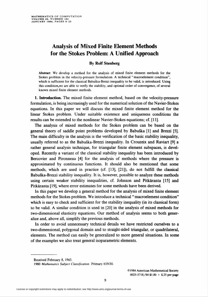
mathematics of computationvolume 42, number 165january 1984, pages 9-23

Analysis of Mixed Finite Element Methods

for the Stokes Problem: A Unified Approach

By Rolf Stenberg

Abstract. We develop a method for the analysis of mixed finite element methods for the

Stokes problem in the velocity-pressure formulation. A technical "macroelement condition",

which is sufficient for the classical Babuska-Brezzi inequality to be valid, is introduced. Using

this condition,we are able to verify the stability, and optimal order of convergence, of several

known mixed finite element methods.

1. Introduction. The mixed finite element method, based on the velocity-pressure

formulation, is being increasingly used for the numerical solution of the Navier-Stokes

equations. In this paper we will discuss the mixed finite element method for the

linear Stokes problem. Under suitable existence and uniqueness conditions the

results can be extended to the nonlinear Navier-Stokes equations; cf. [11].

The analysis of mixed methods for the Stokes problem can be based on the

general theory of saddle point problems developed by BabuSka [1] and Brezzi [5].

The main difficulty in the analysis is the verification of the basic stability inequality,

usually referred to as the BabuSka-Brezzi inequality. In Crouzeix and Raviart [9] a

rather general analysis technique, for triangular finite element subspaces, is devel-

oped. Recently a variant of the classical stability inequality has been introduced by

Bercovier and Pironneau [4] for the analysis of methods where the pressure is

approximated by continuous functions. It should also be mentioned that some

methods, which are used in practice (cf. [13], [21]), do not fulfill the classical

BabuSka-Brezzi stability inequality. It is, however, possible to analyze these methods

using certain weaker stability inequalities, cf. Johnson and Pitkäranta [15] and

Pitkäranta [19], where error estimates for some methods have been derived.

In this paper we develop a general method for the analysis of mixed finite element

methods for the Stokes problem. We introduce a technical "macroelement condition"

which is easy to check and sufficient for the stability inequality (in its classical form)

to be valid. A similar condition is used in [20] in the analysis of mixed methods for

two-dimensional elasticity equations. Our method of analysis seems to both gener-

alize and, above all, simplify the previous methods.

In order to avoid unnecessary technical details we have restricted ourselves to a

two-dimensional, polygonal domain and to straight-sided triangular, or quadrilateral,

elements. The method can easily be generalized to more general situations. In some

of the examples we also treat general isoparametric elements.

Received February 8, 1983.

1980 Mathematics Subject Classification. Primary 65N30.

©1984 American Mathematical Society

0025-5718/84 $1.00 + $.25 per page

9

License or copyright restrictions may apply to redistribution; see http://www.ams.org/journal-terms-of-use

10 ROLF STENBERG

The plan of the paper is as follows: In Section 2 we state the problem and its finite

element discretization and give some preliminary results. The next section is devoted

to the stability inequality. We introduce the macroelement condition and show how

it implies the stability inequality. In Section 4 we apply our method of analysis to

four mixed methods.

2. Preliminaries. Let ß be a polygonal domain in R2 with boundary T. We

consider the stationary Stokes problem: Find functions u = (ux,u2) and p defined

on ß such that

-¡>Au + vp = f in ß,

(2.1) divu = 0 inß,u = 0 on r,

where u is the fluid velocity, p is the pressure, / is the body force and v > 0 is the

kinematic viscosity.

We denote by | • \sT and || • \\sT, respectively, the seminorm and norm of the

Sobolev space [Hs(T)]a, where s and a are integers. For noninteger s, s ^ 0,

[Hs(T)]a and || • \\sT are defined as usual by interpolation. H(\(T) denotes the

subspace of HX(T) of functions vanishing on 37". We will also use the space

L2(T)=l{p<=L2(T)\JTpdx = 0J.

By (•. )t we denote the inner product in [L2(T)]a, where a is an integer. The

subscript T is omitted if T = ß.

Throughout the paper, C and C will stand for a positive constant, possibly

different at different occurrences, which is independent of the mesh parameter h, but

may depend on ß, v and some other parameters introduced in the text.

Using the above notations, (2.1) allows the following weak formulation: Find

u e [//0'(ß)]2 and/? e L„(ß) such that

(2.2) v(vu,vv)- (di\v,p) = (/, t>) Vt> e [//¿(Ö)]2,

(divu,/i) = 0 V<xeLu(ß).

In the finite element discretization of (2.2) we introduce the finite-dimensional

subspaces Vh c [//0'(ß)]2 and Ph c Ll(2) and formulate the approximate problem

as: Find uh e Vh and ph e Ph such that

(2.3) v(vuh,vv)-(dxyv,ph) = (f,v) Vu e Vh,

(divu„,M) = 0 VMe/V

In order to define the finite element spaces we introduce a partitioning l2h of ß

into subdomains which are assumed to be either triangles or convex quadrilaterals

whose diameters are bounded by h. Given an element K g (iA, we denote by hK the

diameter of K, by pK the maximum diameter of all circles contained in K and by 6lK,

1 < i < 4, the angles of AT if A" is a quadrilateral. We suppose that the family Qh is

regular in the sense that there exist two constants a > 1 and 0 < y < 1 independent

of h such that

(2.4) hK^apK Vtfeß,,

(2.5) |cos 0lK\ < y, 1 < < < 4, for all quadrilaterals K e Qh.


MIXED FINITE ELEMENT METHODS FOR THE STOKES PROBLEM 11

Now, for each integer m>Owe denote by Pm(K) the space of polynomials of

degree < m on A and by Qm(A ) the space

(2.6) Qm(K) = {p=poFKx\p^Qm(k)),

where Â is the unit sphere, Qm(K) is the space of polynomials of the form

p(x)= £ a¡jx\x{, fl,7eR,0<i',y<m

and FK is a bilinear transformation which maps A onto A. Setting

Pm{K) if Ais a triangle,(2 71 R ( K ) =

' mK ' \Qm(K) if A" is a quadrilateral,

the space Vh is defined as

(2.8) Vh = {v = {vx,v2)e [Hx(íl)]2\v¡lK<BRk(K),i=\,2,VKeeh}.

Since the pressure does not need to be continuous, we have various possibilities of

choosing Ph. A continuous pressure is obtained by defining

(2.9a) Ph = {p e L0(ß) n C(ß)|/>,* e Ä,(A) VA g ß„}.

We will also consider the following alternatives for a discontinuous pressure

(2.9b) P„ = {p s L2(ß)|P^ g Ä,( A) VA g ß,},

(2.9c) Pt-{pe lg(Q)||>|JC E />,(*) VA E S,}.

Remark. (2.9c) defines/?^ g P¡(K) also for quadrilaterals. This can occasionally

be a good choice; cf. Example 4 in Section 4.

The spaces KA and Ph have the following well-known (cf. [6], [7]) approximation

properties.

Lemma 2.1. If u e [Hr(Q) n H¿(ti)]2, r > I, then there exist ù g Vh such that

\\u - Mj|, < CAí,"1||m||(7i, where qx = min{/\ k + 1}.

Lemma 2.2. If p ^ HS(Q) n Ll(Q), s > 0, then there exist p G Ph such that

\\P - ño < CA*MI/»II,2, wAere <72 = min{i, / + 1}.

The BabuSka-Brezzi stabihty condition [5], [ 11 ] for the approximate problem (2.3)

is satisfied if there is a constant C > 0 such that

(2.10) sup {dlWZ'P) > Q\p\\0 Vp G Ph.vev, \v\\

v»Q

This condition is fundamental for the analysis of the mixed method since it,

together with Lemmas 2.1 and 2.2, implies the following error estimates (cf. [11]).

Theorem 2.1. Suppose that the solution of (2.1) satisfies u g [//r(ß)]2, r > 1, and

p G HS(Q), s > 0, and let (uh, ph) be the solution of (2.3). Then if the condition (2.10)

is satisfied, we have the error estimate

I« - u»li + \\p - Ph\\0 < cfA"-1!!«!!,, + A"||/>||J,


12 ROLF STENBERG

where qx = min{r, k + 1} and q2 — min{i, / + 1}. Moreover, if the region ß is convex,

we have the additional estimate

\\u - uh\\0 ̂ c(h«\\u\\q¡ + h<> + VlU-

In the next section we will show how the stability condition (2.10) can be verified

in practice.

3. The Stability Inequality. Let us start by introducing some additional notation.

By a macroelement we mean the union of one or more neighboring triangles or

quadrilaterals satisfying the regularity assumptions (2.4) and (2.5). A macroelement

M is said to be equivalent to a reference macroelement M if there is a mapping

FM: M -» M satisfying the conditions:

(i) FM is continuous and one-to-one.

(Ü) FM(M) = M.(iii) If M = xj"kj, where Ây, j= 1,2.m, are the triangles or

quadrilaterals in M, then Kj = FM(kj), j = 1,2,..., m, are the tri-

angles or quadrilaterals in M.

(iv) FM- = FK ° F % , j = 1,2,..., m, where FK and FK are the affine or

bilinear mappings from the reference triangle (with vertices (0,0), (0,1) and

(1,0)) or unit square onto Ay and Ay, respectively.

The family of macroelements equivalent with M will be denoted by &^.

For a macroelement M we define the space V0 M as

(3.1) V0M={v& [Hx(M)]2\v,iK<ERk(K),,= 1,2, VA CM}.

Depending on which of the alternatives (2.9abc) is chosen to define Ph, we define the

space PM respectively as

(3.2a) PM = {p g L2(M) n C(M)\piK g R,(K)VK c M),

(3.2b) PM = {pe L2(M)\p^ g Ä,(A)VAc M)

or

(3.2c) PM = {pe L2(M)\plK G P,(K)VK c A/}.

We will further define

(3.3) P0M = P„nL2(M)

and

(3-4) ^ = (pe ^|(div», /7)w = 0 Vt; g ^0 M}.

Let us now prove the following



Lemma 3.1. Let &A be a class of equivalent macroelements. Suppose that for every

M g &M, the space NM is one-dimensional, consisting of functions that are constant on

M. Then there is a positive constant ß^ = ß(M,a,y) such that the condition

(3.5) sup {dl™'P)">ßu\\p\\o.M V/>GP0v<£Vnu \V".M

Mirn.M

t)*0

holds for every M G S^.

Proof. Consider a fixed M G &A. Define the constant ßM as

ßM= inf sup (di\v,p)M.Pg>o.m v<=V0M

IIPllo.M-' \V\ÍM=\

Since NM consists of functions that are constant on M, and P0 M and V0M are finite

dimensional, it follows that ßM > 0.

Let us now prove that there is a constant ßA such that ßM > ßA > 0 for every

M G &A.

Let xx, x2,..., Xa be the vertices of the triangles or quadrilaterals in M. Every

M G &ú is now uniquely defined by its vertices x' = FM(x'), i = 1,2,..., d, and so

we may write ßM = ß(xx, x2,..., xd). We will now consider the vertices as a point

X = (xx,x2,..., xu) in R2J, and ßM = ß(X) as a function of X. Let hM =

maxKlzM(hK). We may assume that hM = 1 and that xx coincides with the origin in

R2, since the general case can be handled by a scaling argument using the mapping

G(x) = h~u(x - xx). Sincexx is chosen as the origin, every vertex xx, x2,..., xd lies

within a given distance from the origin. Further, every A c M has a diameter less

than or equal to unity and satisfies the regularity assumptions (2.4) and (2.5). This

means that the point X belongs to a compact set, denoted by D, in R2d. It can now

easily be proved that the function ß is continuous, and since ß(X) > 0 for every

X g D, we conclude that there is a constant ßM > 0 such that ß( X) > ßM for every

X g D. We have thus proved the condition

inf sup (divü, p)M > ßu > 0 VA/g Sj¿,

IIPllo.M=l M,M=1

which is equivalent to (3.5). D

We are now ready to introduce a " macroelement condition" which is sufficient for

the stability inequality (2.10) to be valid. Let us assume that there is a fixed set of

classes $A, i = 1,..., n, n > 1, such that

,_ ,s For each M G Ê^, / = I,..., n, the space NM is one-dimen-

sional, consisting of functions that are constant on M.

Let us further assume that for each A the triangles or quadrilaterals in Qh can be

grouped together to form macroelements such that the so obtained macroelement

partitioning 'DIL^ of ß satisfies the following condition:

Each M g 91t belongs to some of the classes Sc ,(3.7) * & M>

i = 1,2.n.


14 Rolf stenberc;

In the case when linear and bilinear elements are used for the velocities we will need

one additional condition:

If k = 1 in (2.8) and T is the common part of the boundaries

of two macroelements in k^Lh, then T is connected and

contains at least two edges of the triangles or quadrilaterals in

We can now state the main result of this section.

Theorem 3.1. If the above conditions are satisfied, then (2.10) holds.

Let us postpone the proof of the theorem and first prove two lemmas.

Below we will denote by I1h the L2-projection from Ph onto the space

(3.9) Qh = {p. g L2(ß)|ii|M is constant VA/ g ^Slh).

Lemma 3.2. Suppose that the conditions (3.6) and (3.7) are valid. Then there is a

constant C, > 0 such that for every p G Ph there is a v G Vh satisfying

(divo, p) = (d¡vt>,(/ - nh)p) > c,||(/ - nj^lo

and

\v\x <n(/- njp||0.

Proof. For every p G Ph we have

(/-nA)/>e/>0JW va/e9ka.

Since every M G fltA belongs to some of the classes &A , i = 1,2.n. Lemma 3.1

implies that for every M there exists vM g V0 m such that

(3.10) (divt^.u - nh)p)„ > cx\\(i- nh)p\\lM

and

(3.11) It-M|,.M<||(/- nh)p\\i)Xi.

where Cx = min{/}A}. i = 1.n) and the positive constants ß^ are as in Lemma

3.1. Let us now define v through

Vo* VA/G^lt,.

Since ü = 0 on 3A/ for every A/ G 9R. A we conclude that u g Vh and

(3.12) (divü,nA/7) = 0 V/»EPA,

and the assertion of the lemma now follows from (3.10) through (3.12). D

Lemma 3.3. Suppose that the condition (3.8) is valid. Then there is a constant C2 > 0

such that for every p G Ph there ¡sage Vh satisfying

(divg,Tlhp)=\\nhp\\l and |g|, < c2||n^||0-

Proof. Let p G Ph be arbitrary. Since II»; e L¿(U), there exists (cf. [11])

z g [//(j(ß)]2 such that

(3.13) divz = nA/»



and

(3.14) |z|, < qin^iio.

We will now combine some ideas from [8] and [9] in order to construct an operator

Ih:[H0x(Q))2 -» Vh such that

(3.15) (divlhz,p) = (divz,p) V^Ö,

and

(3.16) |/Az|, < C|z|,.

The assertion then follows from (3.13) through (3.16).

In order to define Ih we introduce some additional notation. As the degrees of

freedom ofaoE Vh we choose the values v¡ = v(x'), / = 1,2,..., q, at the Lagrange

nodes x', i = 1,2,..., q (cf. [6], [7]). Let w¡, i = 1,2,..., q, be the corresponding

basis functions defined by w¡(xJ) — 8¡¡. The support of the basis function wt will be

denoted by S¡, and \S,\ will stand for the area of 5,. The inter-element boundaries of

the macroelements in <DltA will be denoted by T¡, i = 1,..., k (i.e. each 7] is the

common part of the boundaries of two neighboring macroelements). We will assume

that "DltA consists of at least two macroelements so that 1 < k < q.

Due to the assumption (3.8) we may assume that for / = 1,_k the node x' g T,

and that supp wt c A/, U A/, , where A/, and A/, are the macroelements in GJ\Lh such

that 7] = A/, n M^ (when k > 2 in (2.8) x', i = 1,..., k, is taken as one of the

interior nodes on an edge, of a triangle or quadrilateral, common to A/, and A/, ).

Since fT w¡ ds * 0, we can uniquely define Ih z by requiring

I z dx

(i) (Ihz)(x') = ^y- (ori = K+\,...,m,

and

(ii) / Ihz ds = I z ds for / = 1_, k.T JT,

Since Qh consists of functions that are constant on each A/ G 9ltA, an integration by

parts shows that condition (ii) implies (3.15). The estimate (3.16) is easily proved

using a scaling argument.

The lemma is thus proved. D

We close this section by giving the

Proof of Theorem 3.1. Let/? g Ph be arbitrary, and let v g Vh, g g Vh, Cx and C2

be as in Lemma 3.2 and Lemma 3.3. Set z = d + 8g, where S = 2(7,(1 + C2)'x.

Then we have

(3.17) (divz, p) - (divu, p) + ô(divg, p)

> cx\\(i - uh)p\\2 + s(divg, nhP) + ô{divg,(i - uh)p)

> cx\\(i - nh)p\\2 + 8\\nhP\\2 - fi|g|,n(/ - uh)phJPWO

I 8C2\ ñ>[C>--2L)ll(/-n*)^lo+2llI1*^lo

= C,(l + C22)"'|^||S


16 ROI.FSTENBERC;

and

(3.18) ¡--i, < n(/- nh)p\\{) + «c2nnA/J||0 < c\\p\\0.

The inequalities (3.17) and (3.18) are just an alternative way of stating the condition

(2.10),and the theorem is thus proved. D

4. Applications. In this section we apply the theory developed in Section 3 to some

mixed methods. Let us first note that all the conforming methods discussed in [4], [9]

and [18] can also be analyzed using the technique of Section 3. In fact, the essence of

the analysis of [9], [18] consists of verifying the condition (3.6) for macroelements

consisting of only one element. Using the present technique, we obtain optimal

convergence rates for both the velocity and the pressure in the examples studied in

[4], [9] and [18]. Thus, our analysis shows that the assumption of [4], [9] and [18] that

the mesh is quasiuniform (i.e. hK ^ Ch for every K E (iA) can be dropped and that

the suboptimal estimates for the pressure proved in [4] can be improved to optimal

ones. Improvements of some of the results of [4] are also obtained in [23], but still

under the quasiuniformity assumption.

The simplest method of approximation would be a piecewise linear or bilinear

approximation for the velocities and a piecewise constant approximation for the

pressure. It is, however, well known (cf. [15], [21]) that the corresponding mixed

method in general does not satisfy (2.10). In particular, when the region ß is

rectangular and lrA consists of rectangular elements it is well known (cf. [15].

[21]... ) that there is a nonconstant, "checkerboard" function ju g Ph such that

(div v. p.) = 0 for every v G Vh. In our first example below we propose an alternative

of this method, using bilinear quadrilateral approximations for the velocities and a

piecewise constant approximation for the pressure, which satisfies the stability

inequality (2.10).

9

Figure 1

Example 1. Consider the reference macroelement M and an arbitrary A/ g &m as

shown in Figure 1. Define the spaces V0 M and PM as

K.m= {»e [Hr$M)]2\v,lK^Qx(K),i= 1,2, VAC A/},



and

PM = (pe L2( M)\p\K is constant VA c A/}.

Let us now check the condition (3.6). Choose v g Vn M such that ü(jc') = 0,

i = 1,2.10, ; * 5, and vt(x5) = 1, ü2(x5) = 0, respectively, vx(x5) = 0, u2(x5)

= 1. The condition (divu, p)M = 0 then gives the equations

lpx(x2 - *?)+/>,(*? - x2)+p,(xt - xl) = 0,

\px(x¡ - x¡) +p3{x92- x$ + pA(x4- x\) = 0,

where we have written x' = (x\, x2), i = 1,2,..., 10, and pi = p,K, i = 1,2,..., 5.

The equations are easily seen to be linearly independent with the only solution

P\ = Ps = Pi- ln tne same way we conclude that the condition (divu, p)M = 0,

where v is chosen such that v(x') = 0, i= 1,2,..., 10, / *= 6, and vx(x6) = 1,

v2(xb) = 0, respectively, vx(xb) = 0, v2(xb) = 1, implies that p2 = p¿ = p5. The

condition (3.6) is thus satisfied. Let us now define

Vh = {v g [^(ß)]2]^ G ß,(A) VA G eA}

and

Ph = {/> g L^ß)!^ is constant VA g 6a).

Suppose that for every A there is a macroelement partitioning G31tA such that every

M g 91tA belongs to &¿, where M is as in Figure 1. Since the conditions (3.6) and

(3.8) are satisfied, Theorem 3.1 shows that the stability inequality (2.10) is valid.

Suppose ß is convex. We then have u g [//2(ß)]2 and p g //'(ß) if/g [L2(ß)]2

(cf. [11]), and Theorem 2.1 implies the estimates

(4.1) l|«-«*lli+ll/»-/»*llo<Cfc(lMl2 + IIPlli)and

(4.2) ||M-Ua||0<CA2(||M||2 + ||/>||,).

Remark. The method proposed by Le Tallec [16] can also be analyzed with the

present technique, and the estimates (4.1) and (4.2) hold also for this method.

In the following examples we consider three mixed methods for which we have not

found detailed error analysis in the literature.

Example 2. The Hood-Taylor method [12]. In this method the elements A g Qh

are quadrilaterals and the approximating spaces are defined as

(4.3) Vh = {v G [//¿(ß)]2^ G Q2(K), i = 1,2, VA G ßh)

and

(4.4) Ph = {p G L2(ß) n C(Ü)\pÍK g QX(K) VA G eh).

The method has previously been analyzed in [4] in the case of rectangular elements.

We will now derive error estimates for the general quadrilateral case.


18 ROLF- STENBERG

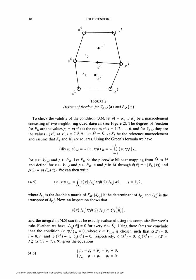
Figure 2

Degrees of freedom for V0 M (•) and PM (o)

To check the validity of the condition (3.6). let M = A, U A2 be a macroelement

consisting of two neighboring quadrilaterals (see Figure 2). The degrees of freedom

for PSI are the values/», = p(x') at the nodes x'. i' = 1,2.6, and for V0 M they are

the values v(x') at x', i = 7.8,9. Let A/ = Â, U A2 be the reference macroelement

and assume that A, and A2 are squares. Using the Green's formula we have

(divu. p)M = ~(v.Vp)M = - £ (v,Vp)k,,

/-i

for v g V0 M and p g Pm. Let FM be the piecewise bilinear mapping from A/ to M

and define, for v g Vom and /? g Pm. v and ^ in M through v(x) = v(FM(x)) and

p(x) = p( Fm(.x)). We can then write

(4.5 ) ( v. Vp ) k, = /. t3( x)JfJ Vp( x)\JFJ dx, j = 1,2,

where 7F is the Jacobian matrix of FM, \JF I is the determinant of J. and Je T is the

transpose of JF]. Now, an inspection shows that

ô(x)JF-JvP(x)\JFjBQ,(kj),

and the integral in (4.5) can thus be exactly evaluated using the composite Simpson's

rule. Further, we have \JF^ (x)\ =*= 0 for every x g k. Using these facts we conclude

that the condition (v, Vp)M = 0, where v G V0 M is chosen such that i5(jc') = 0,

; = 8,9, and t5,(i7) = 1, t52(i7) = 0, respectively, t3,(x7) = 0, t52(x7) = 1 (x' =

FMx(x'),i = 7,8,9), gives the equations

(46) /ft-A+A-P.-O.

I ft - P\ + ft * ft = °-



In the same way we get (taking v(x') = 0, i = 7,8, and vx(x9) = 1, t32(x9) = 0,

respectively, vx(x9) = 0, v2(x9) = 1)

'ft "ft +ft "ft = °.(4.7)

\ft "ft +ft-ft = 0-

The equations in (4.6) and (4.7) are linearly independent with the solution

(4.8) <P>-P,-H-a.

V \ ft = ft = ft = D'

where a and b are arbitrary real constants. Now, choose v g K0 w such that

t3(x') = 0, / = 7,9, and u,(i8) = 1, v2(x%) = 0, respectively, t5,(j£8) = 0, t52(x8) = 1.

If p G PM satisfies (4.8), then the condition (v, Vp)M = 0 gives the equations

i(a-b){x\ + x4-x\-x2) = 0,

\{a - b){x52 + x42 - x2 - x2) = 0.

Now, we cannot simultaneously have xx + x4 - x\ - x2 = 0 and x\ + x2 - x\ -

x\ = 0, since it would imply that the midpoint of the side x4 - x5 coincides with the

midpoint of the side xx - x2. Therefore we conclude that a = b and (3.6) is thus

valid for A/. In the same way one can show that (3.6) is also satisfied for a

macroelement consisting of more than two quadrilaterals. The quadrilaterals in (?A

can always be grouped together to macroelements consisting of two or three

quadrilaterals. There is only a finite number of different classes of such macroele-

ments and (3.7) is thus satisfied. Theorem 3.1 and Theorem 2.1 then imply the

estimates

(4.10) |« - 11,1, + \\p- Ph\\0 < CA2(||M||3 + \\p\\2)

and

(4.11) II« " Mû < CA3(||«||3 + ||/>||2),

provided that u G [//3(ß)]2,/> G //2(ß) and ß is convex.

Remark. If the boundary of ß is curved, then the velocities are usually (cf. [12])

approximated with isoparametric biquadratic elements whereas the pressure is

approximated with "superparametric" bilinear elements, i.e., (3,(A), ; = 1,2, in

(4.3), (4.4) are defined as

e,(A)= {a-j^'Ia *&(*)},where Q,(k) is defined in (2.6) and FK: A -» A is a regular biquadratic mapping as

defined in [7]. For each A g Qh let a¡ K, i = 1,2,..., 9, be the usual Lagrange nodes

such that aiK, i = 1,2,3,4, are the vertices of A. Let â, ¿, / = 1,2,..., 9, be the

nodes for the corresponding straightsided quadrilateral Â with a¡ j¿ = a, K for

i = 1,2,3,4. One can now easily show that the stability inequality (2.10) still holds if

we have

(4.12) ||fl/fjr - äik || < ChK, / = 5,6,...,9,VAGeA,

where C stands for a sufficiently small positive constant. In the definition of the

regular mapping FK one has the condition \\a¡ K - äi ¿|| = 0(h\), / = 5,6,..., 9,


20 ROI 1 STENBERG

and (4.12) thus holds provided that the mesh parameter A is sufficiently small. Since

the approximation properties of Vh and Ph are as in Lemmas 2.1 and 2.2, Theorem

2.1 holds. The estimates (4.10) and (4.11) are thus also valid for the general

isoparametric Hood-Taylor method.

Example 3. In this example we treat a modifaction of the previous Hood-Taylor

method (cf. [14]). We assume that ß is a rectangle (or the union of rectangles) and

that the elements A g c\ are rectangles. The space Ph is defined as in (4.4) and Vh as

Vh = {ve [//(!(ß)]2|iVG(22(A),,= 1,2,VAgca}.

where Q'-,(K) is the reduced space of biquadratic polynomials defined in [6, p. 63].

Q-

G-

Ô-

Q-

&

■0

&

&

&

12€>

V,

114)

K,

10é

Figure 3

Degrees of freedom for K0 M (•) and for ft, (o)

Let us now check the validity of the crucial condition (3.6). Consider a macroele-

ment M consisting of six rectangles arranged as in Figure 3. Consider first the

macroelement A/, = U ,4=l A,. The condition (divt;, p)M¡ = 0, for every v G Vnu¡,

gives a system of ten equations for the nine pressures p¡ = p(x'). i = 1,2.9. The

system (which we omit to write out explicitly) is easily seen to have a rank of seven

and the nontrivial solution

(4.13)

•P\ =ft = ft = Pi = a-

Pi = ft = ft = Pu = b>

yPs = \{a + b).

where a and b are arbitrary real constants. Repeating this argument for the

macroelement A/2 = U *_3 K,, we conclude similarly that

(Pa =ft = fto =ft2 = c<

^ft = Pi =ft =^11 = ¿.

,-i(c + i/).

Now, if /» satisfies (divo, /))M = 0 for every v g V0m, then it has to satisfy both

(4.13) and (4.14), which is possible only if a — b — c = d, i.e. p is a constant in M.

The condition (3.6) is thus satisfied. In the same way we conclude that if a

macroelement contains another macroelement which is equivalent to the macroele-

ment in Figure 3, then (3.6) is satisfied. There is now a finite number of classes of

macroelements, consisting of less than or equal to 24 rectangles, which satisfies (3.6).



Since for each A there is an 91tA where each A/ G 91tA belongs to one of the above

classes, Theorem 3.1 holds and the error estimates (4.10) and (4.11) are valid.

Example 4. In this method, which is being increasingly used in practice (cf. [10]),

the space Vh is defined as in (4.3), whereas one uses a discontinuous approximation

for the pressure,

(4.15) Ph = (p g L2(ß)|^ G />,( A) VA G eh) .

Let us now show that the condition (3.6) is valid for macroelements consisting of

only one quadrilateral. On an arbitrary quadrilateral A g Qh, p g Ph can be written

as

P\K ~ a0,K + a\,Kx\ + a2,KX2-

Let x° be the interior node in A, and let w0 be the corresponding basis function of

Vh. Choose t> g V0 K such that vx(x°) = 1 and v2(x°) = 0. We then obtain

(divv,p)K= _(o,v/>)jf = -aXKfw0dx.JK

Since fKw0dx > 0, the condition (divu, p)K = 0 implies that ax K = 0. In the same

way, choosing v G V0 K such that vx(x°) = 0 and v2(x°) = 1, we conclude that the

condition (divu, p)K = 0 gives a2K = 0. The condition (3.6) is thus satisfied for an

arbitrary A/ = A g Qh. We may then choose 91tA = 6A in (3.7) and (3.8), and so we,

once again, obtain the estimates (4.10) and (4.11).

Remarks. (1) As in the remark following Example 2 we can conclude that the

stated error estimates remain valid for the general isoparametric method.

(2) Of the methods treated in Examples 2, 3 and 4 the last one seems superior, due

to the fact that the discrete system can in this case be solved effectively using the

penalty method, cf. [2], [10], [17].

(3) A method which is also often used in practice (cf. [3], [13], [17]) consists of the

following choices for Vh and ft:

KA = {üG[//(J(ß)]2|ü,|i,G02(A),i=l,2,VAGeA},

ft = {p G L2(Sl)\p}K G Ô,(A) VAG ßh).

The method has originally been introduced in the engineering literature as a penalty

method with "reduced selective integration", cf. [3], [13], [17].

The method does not satisfy the condition (3.6), so we cannot apply the theory

developed in this paper. For rectangular elements it is, however, possible to analyze

the method using the technique developed in [15]. The error estimates one obtains in

this way are [22]

\u-uh\x <Ch2(\u\3 + \u\Aq + \p\2),

\\u-uh\\0<Ch'{\u\3 + \u\^ + \p\2)

and

H/»-/»Jlo<Cfc(|«l3 + M4..+ l/»l2).


22 ROLFSTENBERG

where q > 1 and | • |4 stands for the usual seminorm in the Sobolev space W/4</(ß).

From the estimates one sees that the pressure does not converge with the optimal

rate, a fact also observed in practical computations [21]. In [21] it is also noted that

one can get a good approximation for the pressure by simply omitting the jci*^com-

ponent in each element in the computed ph, and this can also be proved theoretically

[22]. The resulting smoothed pressure then converges with the optimal 0(A2)-rate. In

view of this analysis, the role of the X|X2-component is mainly disturbing and it is

therefore natural to drop it from Ph¡K. This leads back to (4.10).

Acknowledgement. The author is grateful to Professor Juhani Pitkäranta for

suggesting this study and for numerous fruitful discussions during the course of the

work.

Institute of Mathematics

Helsinki University of Technology

SF-02150Espoo 15. Finland

1. I. Babuska. "The finite element method with Lagrangian multipliers," Numer. Math., v. 20, 1973,

pp. 179-192.2. M. Bercovier. "Perturbation of mixed variational problems. Application to mixed finite element

methods", RAlROAnal. Numer.. v. 12, 1978. pp 211-236.

3. M. Bercovier & M. Engelman. "A finite element method for the numerical solution of viscous

incompressible flows"../. Comput. Phys.. v. 30, 1979, pp. 181-201.

4. M. Bercovier & O. Pironneau. "Error estimates for finite element solution of the Stokes problem

in the primitive variables," Numer. Math., v. 33. 1979, pp. 211-224.

5. F. Brezzi, "On the existence, uniqueness and approximation of saddle-point problems arising from

Lagrangian multipliers." RAIRO Ser. Rouge, v. 8. 1974, pp. 129-151.

6. P. G. ClARLET, The Finite Element Method for Elliptic Problems. North-Holland, Amsterdam. 1978.

7. P. G. Ciarlet & P. A. Raviart. "Interpolation theory over curved elements, with applications to

finite element methods," Comput. Methods Appl. Mech. Engrg.. v. 1, 1972, pp. 217-249.

8. P. Clement. "Approximation by finite elements using local regularization." RAIRO Ser Rouge, v.

9. 1975. pp. 77-84.

9. M. Crouzeix & P. A. Ravi art. "Conforming and nonconforming finite element methods for

solving the stationary Stokes equations," RAIRO Ser Rouge, v. 7. 1973. pp. 33-76.

10. M. Engelman, R. Sani, P. Gresho & M Bercovier, "Consistent vs. reduced integration penalty

methods for incompressible media using several old and new elements," Internat. J. Numer. Methods

Fluids, v. 2. 1982. pp. 25-42.

11. V. GlRAULT & P. A. Raviart. Finite Element Approximation of the Navier-Stokes Equations,

Lecture Notes in Math.. Vol. 749. Springer, Berlin, 1979.

12. P. Hood & C. Taylor, "Navier-Stokes equations using mixed interpolation." Finite Element

Methods in Flow Problems (J. T. Oden. ed.). UAH Press, Huntsville, Alabama, 1974, pp. 121-131.

13. T. J. Hughes, W. K. Liu & A. Brooks, "Finite element analysis of incompressible viscous flows by

the penalty function formulation," J. Comput. Phys., v. 30, 1979, pp. 1-60.

14. P. Huyakorn. C. Taylor. R. Lee & P. Gresho, "A comparison of various mixed-interpolation

finite elements for the Navier-Stokes equations," Comput. & Fluids, v. 6, 1978, pp. 25-35.

15. C. Johnson & J. Pitkäranta, "Analysis of some mixed finite element methods related to reduced

integration," Math. Comp., v. 38. 1982. pp. 375-400.

16. P. Le Tallec, "Compatibility condition and existence results in discrete finite incompressible

elasticity." Comput. Methods Appl. Mech. Engrg., v. 27, 1981, pp. 239-259.

17. D. Malkus & T. J. Hughes, "Mixed finite element methods—reduced and selective integration

techniques: a unification of concepts," Comput. Mehtods Appl. Mech. Engrg., v. 15, 1978, pp. 63-81.

18. L. Mansfield, "Finite element subspaces with optimal rates of convergence for the stationary

Stokes problem." RAlROAnal. Numer.. v. 16. 1982, pp. 49-66.

19. J. Pitkäranta, "On a mixed finite element method for the Stokes problem in Rs, RAIRO Anal

Numer., v. 16, 1982, pp. 275-291.



20. J. Pitkäranta & R. Stenberg, "Analysis of some mixed finite element methods for plane elasticity

equations," Math. Comp., v. 41, 1983, pp. 399-423.

21. R. Sani, P. Gresho, R. Lee & D. Griffiths, "The cause and cure (?) of the spurious pressures

generated by certain GFEM solutions of the incompressible Navier-Stokes equations," Internat. J. Numer.

Methods Fluids, v. 1, 1981, Part 1, pp. 17-44; Part 2, pp. 171-204.

22. R. Stenberg, Mixed Finite Element Methods for Two Problems in Elasticity Theory and Fluid

Mechanics, Licentiate thesis, Helsinki University of Technology, 1981.

23. R. Verfürt, Error Estimates for a Mixed Finite Element Approximation of the Stokes Equations,

Ruhr-Universität Bochum, 1982. (Preprint.)


Documents

Analysis of Mixed Finite Element Methods for the Stokes ... · mathematics of computation volume 42, number 165 january 1984, pages 9-23 Analysis of Mixed Finite Element Methods for