Embed Size (px)
Citation preview
Noname manuscript No.(will be inserted by the editor)
Multigrid Methods for A Mixed Finite Element
Method of The Darcy-Forchheimer Model
Jian Huang · Long Chen · Hongxing Rui
Received: date / Accepted: date
Abstract An e�cient multigrid method for a mixed finite element method of theDarcy-Forchheimer model is constructed in this paper. A Peaceman-Rachford typeiteration is used as a smoother to decouple the nonlinearity from the divergenceconstraint. The nonlinear equation can be solved element wise with a closed for-mulae. The linear saddle point system for the constraint is further reduced intoa symmetric positive definite system of Poisson type. Furthermore an empiricalchoice of the parameter used in the splitting is found. By comparing the numberof iterations and CPU time of di↵erent solvers in several numerical experiments,our method is shown to convergent with a rate independent of the mesh size andthe nonlinearity parameter and the computational cost is nearly linear.
Keywords Darcy-Forchheimer model · Multigrid method · Peaceman-Rachforditeration
1 Introduction
Darcy’s law
u = �K
µrp,
The work of the authors Jian Huang and Hongxing Rui was supported by the National NaturalScience Foundation of China Grant No. 91330106, 11171190. Long Chen was supported by NSFGrant DMS-1418934 and in part by NIH Grant P50GM76516. The work of the author JianHuang was supported by 2014 China Scholarship Council (CSC).
J. Huang · H. RuiSchool of Mathematic, Shandong University, Jinan, Shandong 250100, ChinaE-mail: [email protected]
L.ChenDepartment of Mathematics, University of California at Irvine, Irvine, CA 92697, USAE-mail: [email protected]
H. RuiE-mail: [email protected]
2 Jian Huang et al.
describes the linear relationship between the velocity of the creep flow and thegradient of the pressure, which is valid when the Darcy velocity is extremely small[2]. Forchheimer in [8] carried out flow experiments and pointed out that whenthe velocity of the flow is relatively high, Darcy’s law should be replaced by theso-called Darcy-Forchheimer (DF) equation by adding a quadratic nonlinear termto the velocity, shown as follows:
µ⇢K
�1u+
�⇢|u|u+rp = 0.
A theoretical derivation of the Darcy-Forchheimer equation can be found in [17].In recent years, many numerical methods of the Darcy-Forchheimer equation
have been developed. A mixed finite element method with a semi-discrete schemefor the time dependent problem was considered by Park in [12]. Pan and Ruiin [11] gave a mixed element method for the Darcy-Forchheimer problem basedon the Raviart-Thomas (RT) element or the Brezzi-Douglas-Marini (BDM) ele-ment. Rui and Pan in [15] proposed the block-centered finite di↵erence method forthe Darcy-Forchheimer model, which was thought of as the lowest-order Raviart-Thomas mixed element with proper quadrature formula. Rui, Zhao and Pan in [16]presented a block-centered finite di↵erence method for Darcy-Forchheimer modelwith variable Forchheimer number. Wang and Rui in [19] constructed a stabilizedCrouzeix-Raviart (CR) element for the Darcy-Forchheimer equation. Rui and Liuin [14] introduced a two-grid block-centered finite di↵erence method for the Darcy-Forchheimer model.
Girault and Wheeler in [9] proved the existence and uniqueness of the solutionof the Darcy-Forchheimer model. They approximated the velocity and the pressureby piecewise constant and nonconforming CR elements, respectively. They alsosuggested an alternating directions iterative method to solve the nonlinear system.The convergences of both the iterative algorithm and the mixed finite elementscheme are also proved. Lopez, Molina and Salas in [10] carried out numericaltests of the methods studied in [9], and compared with the Newton’s method forsolving this problem.
Since it is a nonlinear system, an iterative method should be used, whichcould be very computationally expensive if the convergence of nonlinear iterationis slow. Multigrid method is one of the most e�cient methods on solving thenonlinear elliptic systems. It should be clarified that we no longer have a simplelinear residual equation, which is the most significant di↵erence between linear andnonlinear systems. The multigrid scheme we used here is the most commonly usednonlinear version of multigrid. It is called the full approximation scheme (FAS) [3]because the problem in the coarse grid is solved for the full approximation ratherthan the correction; see Section 5 for details.
We use piecewise constant and piecewise linear polynomial to discretize thevelocity and the pressure, respectively. We shall apply FAS to construct an ef-ficient V-cycle multigrid method for the nonlinear Darcy-Forchheimer equationand demonstrate the e�ciency of our multigrid method. We use the Peaceman-Rachford (PR) type iteration developed in [9] as a smoother. The most relevantwork is [10] and our improvement are: 1. We choose a smaller value of the stop-ping criterion by achieving a better approximation of the pressure accuracy. 2. Wereport a better choice of the parameter ↵ for decoupling the nonliearity from theconstraint rather than the suggested value ↵ = 1 for di↵erent values of �, and
Multigrid Method of The Darcy-Forchheimer Model 3
show the advantage of our choice by comparing the number of iterations and CPUtime. 3. We carry out some experiments to show the e�ciency of our multigridsolver by comparing with the PR iterative solvers. 4. We reduce the saddle pointsystem into a Poisson system and demonstrate the e�ciency of our approach.
The remainder of this article is organized as follows: The model problem isdemonstrated in Section 2. The mixed weak formulation and the discrete weakformulation are presented in Section 3. The PR iteration and an e�cient solverfor the linear saddle point systems are posted in Section 4. We construct a V-cyclemultigrid scheme by applying FAS for the nonlinear problem in Section 5. Somenumerical experiments using our multigrid method are carried out in Section 6 toverify that the e�ciency of our method in comparison with solving this nonliearproblem using the other iterative methods. Finally, conclusions, and further ideasare presented in Section 7.
2 The Problem and Some Notations
We consider the steady Darcy-Forchheimer flow of a single phase fluid in a porousmedium in a two-dimensional bounded domain⌦, with Lipschitz continuous bound-ary @⌦:
µ⇢K
�1u+
�⇢|u|u+rp = f in ⌦, (2.1)
with the divergence constraint
divu = g in ⌦, (2.2)
and Neumann boundary conditions,
u · n = gN on @⌦, (2.3)
where u and p are the velocity vector and the pressure, respectively; µ, ⇢ and � aregiven positive constants that represent the viscosity of the fluid, its density and itsdynamic viscosity, respectively; |·| denotes the Euclidean vector norm |u|2 = u ·u,n is the unit exterior normal vector to the boundary of the given domain ⌦; K isthe permeability tensor, assumed to be uniformly positive definite and bounded.According to the divergence theorem, g and gN are given given functions satisfyingthe compatibility condition
Z
⌦
g (x)dx =
Z
@⌦
gN (�)d�. (2.4)
We use the standard notations of the Sobolev spaces and the associated norms,see e.g.[1]. We also use the space
L20 (⌦) =
⇢
v 2 L2 (⌦) :
Z
⌦
v (x) dx = 0
�
.
4 Jian Huang et al.
3 Weak Formulation
In this section, we define the function spaces as follows:
X = L3(⌦)2,
M = W 1, 32 (⌦) \ L2
0 (⌦) .
where the zero mean value condition is added because p is only defined by the (2.1)-
(2.3) up to an additive constant. Given f 2 L3(⌦), g 2 L32 (@⌦), the variational
formulation is: find a pair (u, p) in X ⇥M such that
µ⇢
Z
⌦
⇣
K
�1u
⌘
· ' dx+�⇢
Z
⌦
|u| (u · ') dx
+
Z
⌦
rp · ' dx =
Z
⌦
f · ' dx, 8' 2 X,(3.1)
Z
⌦
rq · u dx = �Z
⌦
gq dx+
Z
@⌦
gNq dx, 8q 2M. (3.2)
The variational formulation (3.1), (3.2) and the original problem (2.1)-(2.3)are equivalent by using the Green’s formula:
Z
⌦
v ·rq dx = �Z
⌦
q div v dx+ hq, v · ni@⌦ , 8q 2M, 8v 2 H, (3.3)
whereH =
n
v 2 L3(⌦)2 : div v 2 L65 (⌦)
o
.
If the given functions g and gN satisfy the compatibility condition (2.4), thenthe problem has a unique solution (u, p) in X ⇥M [9].
Let ⌦ be a polygon in two dimensions which can be completely triangulated bytriangles. Let T1 be a triangulation of ⌦, and the triangulations Tk (k = 2, 3, . . .) beobtained form T1 via regular subdivision, i.e. edge midpoints in Tk�1 are connectedby new edges to form Tk. Therefore, Tk is a family of conforming triangulations of⌦,
⌦ =[
T2Tk
T for k = 1, 2, 3, . . . ,
The family Tk is regular (also called non-degenerate) in the sense of Ciarlet [6].We discretize u and p in di↵erent finite element spaces. The velocity u is
approximated in the following space:
Xk =n
v 2 L2(⌦)2 : 8T 2 Tk, v|T 2 P20
o
, (3.4)
and the pressure p is approximated in the following space:
Mk = Qk \ L20 (⌦) , (3.5)
where Pm denotes the space of polynomials of degree m, and Qk is the linear finiteelement space.
Qk =n
q 2 C0�⌦�
: 8T 2 Tk, q|T 2 P1
o
.

Multigrid Method of The Darcy-Forchheimer Model 5
With these spaces, we can have the k-th level discrete formulation of the prob-lem (3.1),(3.2):
µ⇢
Z
⌦
⇣
K
�1uk
⌘
· 'k dx+�⇢
Z
⌦
|uk| (uk · 'k) dx
+X
T2Tk
Z
T
rpk · 'k dx =
Z
⌦
f · 'k dx, 8'k 2 Xk,
(3.6)
X
T2Tk
Z
T
rqk · uk dx = �Z
⌦
gqk dx+
Z
@⌦
gNqk dx, 8qk 2Mk. (3.7)
In universal practice,
hk�1 = 2hk, for k = 2, 3, . . . .
Note that Tk are nested meshes, and thus
Xk�1 ⇢ Xk,Mk�1 ⇢Mk.
In [18], the authors demonstrated that the discrete problem has a unique solution.Moreover, if Tk is shape regular with mesh size h and the solution u belongsto W 1,4(⌦) and p belongs to W 2, 3
2 (⌦), then the following error estimations areobtained in [18](Theorem 4.10):
ku� uhkL2(⌦) Ch|u|W 1,4(⌦), (3.8)
kr (p� ph)kL
32 (T )
Ch⇣
|p|W 2, 3
2 (⌦)+ kukW 1,4(⌦)
⌘
. (3.9)
4 Nonlinear Iteration
In this section, we present the Peaceman-Rachford (PR) type method developedin [9] to decouple the nonlinearity and the constraint.
First, choose an initial guess�
u
0k, p
0k
�
by solving a linear Darcy equation:
µ⇢
Z
⌦
⇣
K
�1u
0k
⌘
· 'k dx+X
T2Tk
Z
T
rp0k · 'k dx =
Z
⌦
f · 'k dx, 8'k 2 Xk, (4.1)
X
T2Tk
Z
T
rqk · u0k dx = �
Z
⌦
gqk dx+
Z
@⌦
gNqk dx, 8qk 2Mk. (4.2)
The linear Darcy system (4.1) and (4.2) can be rewritten in the matrix formas
A BBT 0
�
u
p
�
=
fd
w
�
, (4.3)
where A is the symmetric and positive definite matrix associated to the term
µ⇢
Z
⌦
⇣
K
�1uk
⌘
· 'k dx,

6 Jian Huang et al.
B is the matrix corresponding to
X
T2Tk
Z
T
rpk · 'k dx,
and fd and w represent the right hand side of (4.1) and (4.2), respectively.Then, knowing
�
u
0k, p
0k
�
, construct a sequence�
u
n+1k , pn+1
k
�
for n � 0 in twosteps: Let ↵ be a positive parameter chosen to enhance the convergence.
1. A nonlinear step without constraint: knowing (unk , p
nk ) compute the inter-
mediate velocity u
n+ 12
k by solving the following equation:
1↵
Z
⌦
⇣
u
n+ 12
k � u
nk
⌘
· 'kdx+�⇢
Z
⌦
�
�
�
u
n+ 12
k
�
�
�
⇣
u
n+ 12
k · 'k
⌘
dx =
Z
⌦
f · 'k dx
�µ⇢
Z
⌦
⇣
K
�1u
nk
⌘
· 'kdx�X
T2Tk
Z
T
rpnk · 'k dx, 8'k 2 Xk.(4.4)
2. A linear step with constraint: compute�
u
n+1k , pn+1
k
�
with the known u
n+ 12
k
1↵
Z
⌦
⇣
u
n+1k � u
n+ 12
k
⌘
· 'kdx+µ⇢
Z
⌦
⇣
K
�1u
n+1k
⌘
· 'kdx+X
T2Tk
Z
T
rpn+1k · 'k dx
=
Z
⌦
f · 'k dx��⇢
Z
⌦
�
�
�
u
n+ 12
k
�
�
�
⇣
u
n+ 12
k · 'k
⌘
dx, 8'k 2 Xk,
(4.5)
X
T2Tk
Z
T
rqk · un+1k dx = �
Z
⌦
gqk dx+
Z
@⌦
gNqk dx, 8qk 2Mk. (4.6)
A key observation in [9] is that because the test functions 'k, the solution
u
n+ 12
k , and rpnk are constant in each element T , the nonlinear step (4.4) can besolved as follows:
u
n+ 12
T =1�F
n+ 12
T (4.7)
where
F
n+ 12
T =1↵u
nT �
µ⇢K
�1T u
nT �rT p
nk + fT ,
K
�1T =
1|T |
Z
T
K
�1 (x) dx,
� =12↵
+12
s
1↵2
+ 4�⇢
�
�
�
F
n+ 12
T
�
�
�
.
In the second step, the linear system (4.5) and (4.6) can be rewritten in thefollowing matrix form:
A↵ BBT 0
�
u
p
�
=
fn+ 12
w
�
, (4.8)
Multigrid Method of The Darcy-Forchheimer Model 7
where A↵ is the matrix corresponding to
1↵
Z
⌦
⇣
u
n+1k
⌘
· 'kdx+µ⇢
Z
⌦
⇣
K
�1u
n+1k
⌘
· 'kdx,
and fn+ 12is the vector corresponding to
Z
⌦
f · 'k dx+1↵
Z
⌦
⇣
u
n+ 12
k
⌘
· 'kdx��⇢
Z
⌦
�
�
�
u
n+ 12
k
�
�
�
⇣
u
n+ 12
k · 'k
⌘
dx.
In [9], the authors proved that (4.1), (4.2) and (4.5), (4.6) have a unique so-lution. The iterative method is convergent for an arbitrary choice of the initialguess
�
u
0k, p
0k
�
and an arbitrary positive ↵. Numerically, choice of ↵ will a↵ectthe convergence of the nonlinear iteration. We shall report a good choice of thisparameter.
We can reduce the linear saddle point system into a SPD system. Because ofA and A↵ are symmetric positive definite operators, without loss of generality, wetake (4.8) as an example to expound an idea as follows:
Eliminate u from the first equation of (4.8), i.e.
u = A�1↵
⇣
fn+ 12�Bp
⌘
, (4.9)
and then, substituting to the second equation of (4.8), we get
Mp = b, (4.10)
where M = BTA�1↵ B, b = BTA�1
↵ fn+ 12� w. After solving (4.10), we can get u
by solving (4.9).Since A↵ is block-diagonal, A�1
↵ can be formed easily. Equation (4.10) is thelinear finite element dscretization of an elliptic equation in primary formulation.Solving the SPD system (4.10) is much easier than the saddle point system (4.8)and many fast solvers are available. The equivalence between (4.9),(4.10) and (4.8)is obvious.
5 Multigrid Algorithm
In this section, we consider a generic system of nonlinear equations,
L (z) = s
where z, s 2 R
n. Suppose that v is an approximation to the exact solution z.Define the error e and the residual r:
e = z � v,
r = s� L (v) .
We can solve this nonlinear system by using some iterative solver,
Lk (z) = s,
here k means the discrete problem on the k-th level mesh Tk.

8 Jian Huang et al.
Because of the iterative nature, multigird ideas should be e↵ective on the non-linear problem. The multigrid scheme here we used for this nonlinear problem isthe most commonly used nonlinear version of multigrid. It is called the full approx-imation scheme (FAS) [3] because the problem in the coarse grid is solved for thefull approximation zk�1 = Ik�1
k vk + ek�1 rather than the error ek�1. A V-cyclemultigrid scheme is described as follows:
Full Approximation Scheme (FAS).
• Pre-smoothing: For 1 j m, relax m times with an initial guess v0 byvj = Rkvj�1. The current approximation vk = vm.
• Restrict the current approximation and its fine grid residual to the coarse grid:rk�1 = Ik�1
k (sk � Lk (vk)) and vk�1 = Ik�1k vk.
• Solve the coarse grid problem: Lk�1 (zk�1) = Lk�1 (vk�1) + rk�1.
• Compute the coarse grid approximation to the error: ek�1 = zk�1 � vk�1.
• Interpolate the error approximation up to the fine grid and correct the currentfine grid approximation: vm+1 vk + Ikk�1ek�1.
• Post-smoothing: For m+ 2 j 2m+ 1, relax m times by vj = Rk0vj�1.
then we get the approximate solution v2m+1. Here m denotes the number of pre-smoothing and post-smoothing steps, Rk denotes the chosen relaxation method,and Ik�1
k is an intergrid transfer operator from the fine grid to the coarse grid.We apply the PR iteration as the smoother Rk. We need to switch the ordering
of the linear and nonlinear steps in the post-smoothing step in order to keep thesymmetry of the V-cycle. It is worth pointing out that although the chosen finiteelement spaces are nested, the constrained subspaces are non-nested when weinterpolated the correction of the velocity, which was obtained in the coarser space,to the finer space. Namely, if we directly interpolated the correction obtained onthe coarser grid to the finer grid, the approximation we got do not satisfy thedivergence equation in this Darcy-Forchheimer model. We need to construct a L2
projection to map the correction obtained before into the constrained space in thefine grid. This can be realized by solving a saddle point system:
A� BBT 0
�
�
✓
�
=
0
BTeu
�
, (5.1)
where A� is the matrix corresponding to
µ⇢
Z
⌦
⇣
K
�1�
⌘
· 'k dx+�⇢
Z
⌦
|v| (� · 'k) dx,
�, ✓ represent the error between the restriction of the approximation of velocityand pressure on the finer grid and their approximation obtained on the coarsergrid, respectively, and eu is the prolonged correction to the fine space.
Again, (5.1) can be reduced to a SPD system. We can get � = A�1� B✓ through
the idea demonstrated in Section 4. Then we obtain a corrected approximation ofvelocity v = v � �, which satisfied the divergence equation.
Multigrid Method of The Darcy-Forchheimer Model 9
6 Numerical Experiments
In this section, we present some numerical results to illustrate the e�ciency of ourmultigrid method for the Darcy-Forchheimer equation (2.1)-(2.3). The followingtest problems were taken from [10]. All of our experiments are implemented basedon the MATLAB c� software package iFEM [4].
We choose µ = 1, ⇢ = 1, K = I. ⌦ ⇢ R2 is a square,
⌦ =n
(x, y) 2 R2 : �1 < x < 1, �1 < y < 1o
.
Problem 1:
u (x, y) = [x+ y, x� y]T ,
p (x, y) = x3 + y3,
f (x, y) =
2
4
⇣
1 + �p
2x2 + 2y2⌘
(x+ y) + 3x2
⇣
1 + �p
2x2 + 2y2⌘
(x� y) + 3y2
3
5 ,
gN (x, y) =
8
>
>
>
<
>
>
>
:
1 + y, x = 1,
1� y, x = �1,x� 1, y = 1,
�x� 1, y = �1.
Problem 2:
u (x, y) =
(x+ 1)2
4,� (x+ 1) (y + 1)
2
�T
,
p (x, y) = x3 + y3,
f (x, y) =
2
6
6
4
(x+1)2
4
✓
1 + � (x+1)4
q
(x+ 1)2 + 4(y + 1)2◆
+ 3x2
� (x+1)(y+1)2
✓
1 + � (x+1)4
q
(x+ 1)2 + 4(y + 1)2◆
+ 3y2
3
7
7
5
,
gN (x, y) =
8
>
>
>
<
>
>
>
:
1, x = 1,
0, x = �1,�x� 1, y = 1,
0, y = �1.
For all above test problems, g = 0. The chosen termination criterion is
r = ru + rp tol,

10 Jian Huang et al.
105
106
10−4
10−3
10−2
Number of unknowns
Err
or
Rate of convergence is CN−0.50228
||u−u
h||
L2
C1N−0.50274
||p−ph||
L2
C2N−0.77647
||p−ph||
H1
C3N−0.50228
(a) Convergence Rate of Problem 1 with tol =10�5
105
106
10−5
10−4
10−3
10−2
Number of unknowns
Err
or
Rate of convergence is CN−0.50267
||u−uh||
L2
C1N−0.50274
||p−ph||
L2
C2N−0.97991
||p−ph||
H1
C3N−0.50267
(b) Convergence Rate of Problem 1 with tol =10�6
105
106
10−5
10−4
10−3
10−2
Number of unknowns
Err
or
Rate of convergence is CN−0.50151
||u−uh||
L2
C1N−0.49463
||p−ph||
L2
C2N−0.85863
||p−ph||
H1
C3N−0.50151
(c) Convergence Rate of Problem 2 with tol =10�5
105
106
10−5
10−4
10−3
10−2
Number of unknowns
Err
or
Rate of convergence is CN−0.50168
||u−uh||
L2
C1N−0.49463
||p−ph||
L2
C2N−0.96944
||p−ph||
H1
C3N−0.50168
(d) Convergence Rate of Problem 2 with tol =10�6
Fig. 1 Comparison of the convergence rate for Problem 1 and 2 with di↵erent tols.
where
ru =
8
<
:
�
�
�
f � µ⇢K
�1u
nh + �
⇢ |unh|un
h +rpnh�
�
�
/ kfk , when kfk 6= 0,�
�
�
f � µ⇢K
�1u
nh + �
⇢ |unh|un
h +rpnh�
�
�
, when kfk = 0.
rp =
(
kg � divunhk / kgk , when kgk 6= 0,
kg � divunhk , when kgk = 0.
In the first test, we study that whether the accuracy will change according todi↵erent choices of tol. Numerical tests were performed for all these problems, andthe behaviour of these experiments was similar for all these problems. Therefore,here we only posed the results when ↵ = 1,� = 10.
The letter N stands for ‘Number of unknowns of p’, which is the same as‘Numbers of vertices’, so h = 2p
N�1, which represents the discretization mesh
size in one direction. The results confirmed the convergence order for ku� uhkL2
and kp� phkH1 are O (h). However, the accuracy of the pressure approximationsin L2-norm depends on tol. From Figure 1, it is clear that the L2-norm of thepressure approximations when tol = 10�6 is better than the one when tol = 10�5
for Problem 1 and Problem 2. Meanwhile, in consideration of the computation

Multigrid Method of The Darcy-Forchheimer Model 11
Table 1 Comparison of di↵erent values of ↵ with h = 164 for � = 10, 20, 30.
Problem� = 10 � = 20 � = 30
↵ = 1 ↵ = 1/10 ↵ = 1 ↵ = 1/20 ↵ = 1 ↵ = 1/30
Problem 1iter 229 73 457 105 686 120CPU time 14 s 4 s 26 s 6 s 38 s 7 s
Problem 2iter 230 171 459 183 688 191CPU time 13 s 10 s 26 s 11 s 38 s 11 s
Table 2 Comparison of di↵erent values of ↵ with h = 164 for � = 40, 50, 60.
Problem� = 40 � = 50 � = 60
↵ = 1 ↵ = 1/40 ↵ = 1 ↵ = 1/50 ↵ = 1 ↵ = 1/60
Problem 1iter 914 126 1143 129 1371 131CPU time 53 s 7 s 66 s 7 s 79 s 8 s
Problem 2iter 917 198 1146 205 1376 213CPU time 52 s 11 s 65 s 11 s 79 s 12 s
cost, the su�ciently accurate results were achieved when tol = 10�6 for Problem1 and 2. Therefore, the value of tol = 10�6 is used in the remaining numericalexperiments. Instead, in [10] the authors use tol = 1.95h, which only consideredthe L2-norm approximation for velocity.
In the second test, we give an empirical choice of parameter ↵ = 1/�. Asit is mentioned in [9], the PR nonlinear iteration converges for any ↵ > 0. Itsconvergence rate, however, is very sensitive to the choice of this parameter. Fromthe convergence proof of the PR algorithm in [9], we inferred that the choices of↵ depends on �. Here we tested ↵ = 1/�, then compared with the choice ↵ = 1in two aspects: the number of iterations (abbreviated as iter) and CPU time. Asshown in Table 1 and 2, this choice of the parameter ↵ is much better than thefixed selection for di↵erent values of �. Therefore, this choice of ↵ will be used inthe remaining numerical experiments.
In the following experiments, we compare the multigrid method with the PR it-erative method for solving this nonlinear systems. Here we choose m = 3 for all thefollowing tests. It means that we apply three PR iterations in the pre-smoothingstep and post-smoothing step, respectively. In order to keep the symmetry of theV-cycle, we switch the ordering of the linear and nonlinear steps in the post-smoothing step. We set h = 1/16 as the initial mesh. In the tables, we use thefollowing symbols: Eu,0 = ku� uhkL2 , Ep,0 = kp� phkL2 , Ep,1 = kp� phkH1 .
The PR solver is denoted by s, whereas the multigrid solver is denoted bym. I - number of iterations, and CPU - CPU time. ‘s1’ represents that we solvethose linear saddle point systems directly in each step while we use the PR itera-tive method to solve this nonlinear system, ‘s2’ is that we solve the SPD systemmentioned in Section 4 rather than solving the saddle point system directly. Ourmultigrid solver is constructed based on ‘s2’. In all examples we achieve optimalorder convergence of ku� uhkL2 and kp� phkH1 . Since our focus is on the e�-ciency of solvers, we mainly report the comparison of the number of iterations andCPU time by using di↵erent solvers.
12 Jian Huang et al.
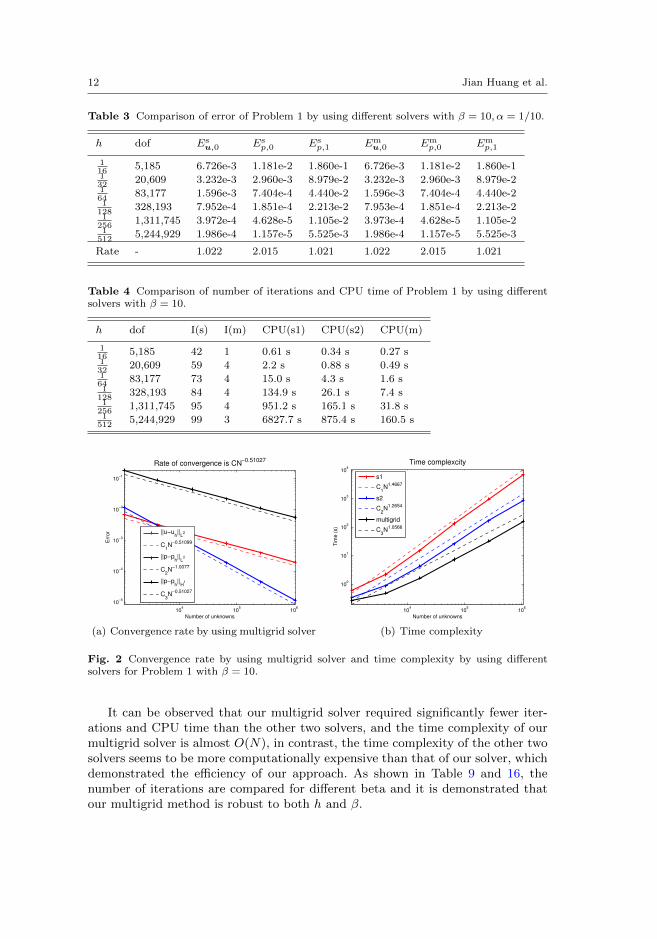
Table 3 Comparison of error of Problem 1 by using di↵erent solvers with � = 10,↵ = 1/10.
h dof E
su,0 E
sp,0 E
sp,1 E
mu,0 E
mp,0 E
mp,1
116 5,185 6.726e-3 1.181e-2 1.860e-1 6.726e-3 1.181e-2 1.860e-1132 20,609 3.232e-3 2.960e-3 8.979e-2 3.232e-3 2.960e-3 8.979e-2164 83,177 1.596e-3 7.404e-4 4.440e-2 1.596e-3 7.404e-4 4.440e-21
128 328,193 7.952e-4 1.851e-4 2.213e-2 7.953e-4 1.851e-4 2.213e-21
256 1,311,745 3.972e-4 4.628e-5 1.105e-2 3.973e-4 4.628e-5 1.105e-21
512 5,244,929 1.986e-4 1.157e-5 5.525e-3 1.986e-4 1.157e-5 5.525e-3
Rate - 1.022 2.015 1.021 1.022 2.015 1.021
Table 4 Comparison of number of iterations and CPU time of Problem 1 by using di↵erentsolvers with � = 10.
h dof I(s) I(m) CPU(s1) CPU(s2) CPU(m)
116 5,185 42 1 0.61 s 0.34 s 0.27 s132 20,609 59 4 2.2 s 0.88 s 0.49 s164 83,177 73 4 15.0 s 4.3 s 1.6 s1
128 328,193 84 4 134.9 s 26.1 s 7.4 s1
256 1,311,745 95 4 951.2 s 165.1 s 31.8 s1
512 5,244,929 99 3 6827.7 s 875.4 s 160.5 s
104
105
106
10−5
10−4
10−3
10−2
10−1
Number of unknowns
Err
or
Rate of convergence is CN−0.51027
||u−uh||
L2
C1N−0.51099
||p−ph||
L2
C2N−1.0077
||p−ph||
H1
C3N−0.51027
(a) Convergence rate by using multigrid solver
104
105
106
100
101
102
103
104
Number of unknowns
Tim
e (
s)
Time complexcity
s1
C1N1.4667
s2
C2N1.2654
multigrid
C3N1.0566
(b) Time complexity
Fig. 2 Convergence rate by using multigrid solver and time complexity by using di↵erentsolvers for Problem 1 with � = 10.
It can be observed that our multigrid solver required significantly fewer iter-ations and CPU time than the other two solvers, and the time complexity of ourmultigrid solver is almost O(N), in contrast, the time complexity of the other twosolvers seems to be more computationally expensive than that of our solver, whichdemonstrated the e�ciency of our approach. As shown in Table 9 and 16, thenumber of iterations are compared for di↵erent beta and it is demonstrated thatour multigrid method is robust to both h and �.

Multigrid Method of The Darcy-Forchheimer Model 13
Table 5 Comparison of number of iterations and CPU time of Problem 1 by using di↵erentsolvers with � = 20.
h dof I(s) I(m) CPU(s1) CPU(s2) CPU(m)
116 5,185 49 1 0.68 s 0.43 s 0.34 s132 20,609 75 6 2.7 s 1.1 s 0.62 s164 83,177 105 6 24.6 s 5.1 s 2.0 s1
128 328,193 126 5 195.1 s 32.5 s 9.5 s1
256 1,311,745 139 5 1312.2 s 209.5 s 52.0 s1
512 5,244,929 153 5 10354.2 s 1380.2 s 219.2 s
104
105
106
10−4
10−3
10−2
10−1
Number of unknowns
Err
or
Rate of convergence is CN−0.52587
||u−u
h||
L2
C1N−0.52589
||p−ph||
L2
C2N−1.0077
||p−ph||
H1
C3N−0.52587
(a) Convergence rate by using multigrid solver
104
105
106
100
101
102
103
104
Number of unknowns
Tim
e (
s)
Time complexcity
s1
C1N1.4848
s2
C2N1.304
multigrid
C3N1.0872
(b) Time complexity
Fig. 3 Convergence rate by using multigrid solver and time complexity by using di↵erentsolvers for Problem 1 with � = 20.
Table 6 Comparison of number of iterations and CPU time of Problem 1 by using di↵erentsolvers with � = 30.
h dof I(s) I(m) CPU(s1) CPU(s2) CPU(m)
116 5,185 50 1 0.70 s 0.43 s 0.34 s132 20,609 81 6 3.0 s 1.1 s 0.65 s164 83,177 120 6 28.6 s 6.6 s 2.3 s1
128 328,193 154 6 242.3 s 48.8 s 12.1 s1
256 1,311,745 168 6 1554.7 s 308.3 s 56.5 s1
512 5,244,929 185 5 11857.3 s 1667.7 s 254.6 s
Table 7 Comparison of number of iterations and CPU time of Problem 1 by using di↵erentsolvers with � = 40.
h dof I(s) I(m) CPU(s1) CPU(s2) CPU(m)
116 5,185 50 1 0.80 s 0.43 s 0.35 s132 20,609 82 7 3.1 s 1.1 s 0.70 s164 83,177 126 7 30.5 s 7.7 s 2.4 s1
128 328,193 171 6 269.9 s 59.5 s 13.1 s1
256 1,311,745 192 6 1786.3 s 329.6 s 63.9 s1
512 5,244,929 207 6 13504.1 s 1819.4 s 270.4 s

14 Jian Huang et al.
104
105
106
10−4
10−3
10−2
10−1
Number of unknowns
Err
or
Rate of convergence is CN−0.54598
||u−u
h||
L2
C1N−0.54323
||p−ph||
L2
C2N−1.0077
||p−ph||
H1
C3N−0.54598
(a) Convergence rate by using multigrid solver
104
105
106
100
101
102
103
104
Number of unknowns
Tim
e (
s)
Time complexcity
s1
C1N1.4905
s2
C2N1.3406
multigrid
C3N1.0979
(b) Time complexity
Fig. 4 Convergence rate by using multigrid solver and time complexity by using di↵erentsolvers for Problem 1 with � = 30.
104
105
106
10−4
10−3
10−2
10−1
Number of unknowns
Err
or
Rate of convergence is CN−0.5673
||u−u
h||
L2
C1N−0.56075
||p−ph||
L2
C2N−1.0077
||p−ph||
H1
C3N−0.5673
(a) Convergence rate by using multigrid solver
104
105
106
100
101
102
103
104
Number of unknowns
Tim
e (
s)
Time complexcity
s1
C1N1.51
s2
C2N1.3468
multigrid
C3N1.1017
(b) Time complexity
Fig. 5 Convergence rate by using multigrid solver and time complexity by using di↵erentsolvers for Problem 1 with � = 40.
Table 8 Comparison of number of iterations and CPU time of Problem 1 by using di↵erentsolvers with � = 50.
h dof I(s) I(m) CPU(s1) CPU(s2) CPU(m)
116 5,185 50 1 0.91 s 0.45 s 0.35 s132 20,609 82 7 3.1 s 1.1 s 0.72 s164 83,177 129 7 31.4 s 7.9 s 2.6 s1
128 328,193 181 7 312.6 s 61.9 s 13.5 s1
256 1,311,745 210 6 1955.6 s 371.1 s 64.8 s1
512 5,244,929 222 6 14733.5 s 2009.4 s 306.8 s

Multigrid Method of The Darcy-Forchheimer Model 15
104
105
106
10−4
10−3
10−2
10−1
Number of unknowns
Err
or
Rate of convergence is CN−0.58817
||u−u
h||
L2
C1N−0.57923
||p−ph||
L2
C2N−1.0077
||p−ph||
H1
C3N−0.58817
(a) Convergence rate by using multigrid solver
104
105
106
100
101
102
103
104
Number of unknowns
Tim
e (
s)
Time complexcity
s1
C1N1.527
s2
C2N1.368
multigrid
C3N1.1111
(b) Time complexity
Fig. 6 Convergence rate by using multigrid solver and time complexity by using di↵erentsolvers for Problem 1 with � = 50.
Table 9 Comparison of iteration steps of multigrid solver according to di↵erent h and � forProblem 1 with ↵ = 1/�.
h � = 10 � = 20 � = 30 � = 40 � = 50
132 4 6 6 7 7164 4 6 6 7 71
128 4 5 6 6 71
256 4 5 6 6 61
512 3 5 5 6 6
Table 10 Comparison of error of Problem 2 by using di↵erent solvers with � = 10,↵ = 1/10.
h dof E
su,0 E
sp,0 E
sp,1 E
mu,0 E
mp,0 E
mp,1
116 5,185 3.244e-2 5.863e-3 1.772e-1 3.244e-2 5.863e-3 1.772e-1132 20,609 1.740e-2 1.680e-3 8.846e-2 1.740e-2 1.680e-3 8.846e-2164 83,177 9.048e-3 4.676e-4 4.421e-2 9.042e-3 4.676e-4 4.421e-21
128 328,193 4.610e-3 1.258e-4 2.210e-2 4.601e-3 1.250e-4 2.210e-21
256 1,311,745 2.323e-3 3.285e-5 1.105e-2 2.314e-3 3.250e-5 1.105e-21
512 5,244,929 1.165e-3 8.448e-6 5.524e-3 1.159e-3 8.288e-6 5.524e-3Rate - 0.970 1.904 1.009 0.972 1.910 1.009
Table 11 Comparison of number of iterations and CPU time of Problem 2 by using di↵erentsolvers with � = 10.
h dof I(s) I(m) CPU(s1) CPU(s2) CPU(m)
116 5,185 75 1 0.87 s 0.51 s 0.29 s132 20,609 111 5 4.0 s 1.4 s 0.95 s164 83,177 171 5 42.6 s 10.7 s 2.4 s1
128 328,193 269 5 437.3 s 91.8 s 8.7 s1
256 1,311,745 428 4 3983.2 s 733.5 s 43.2 s1
512 5,244,929 686 4 > 13 hours 6331.6 s 203.3 s
16 Jian Huang et al.
104
105
106
10−5
10−4
10−3
10−2
10−1
Number of unknowns
Err
or
Rate of convergence is CN−0.50432
||u−uh||
L2
C1N−0.48592
||p−ph||
L2
C2N−0.95487
||p−ph||
H1
C3N−0.50432
(a) Convergence rate by using multigrid solver
104
105
106
100
101
102
103
104
Number of unknowns
Tim
e (
s)
Time complexcity
s1
C1N1.6892
s2
C2N1.5269
multigrid
C3N0.9878
(b) Time complexity
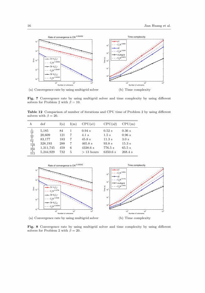
Fig. 7 Convergence rate by using multigrid solver and time complexity by using di↵erentsolvers for Problem 2 with � = 10.
Table 12 Comparison of number of iterations and CPU time of Problem 2 by using di↵erentsolvers with � = 20.
h dof I(s) I(m) CPU(s1) CPU(s2) CPU(m)
116 5,185 84 1 0.94 s 0.52 s 0.36 s132 20,609 121 7 4.1 s 1.5 s 0.96 s164 83,177 183 7 45.8 s 11.3 s 3.0 s1
128 328,193 288 7 465.8 s 93.8 s 15.3 s1
256 1,311,745 459 6 4338.6 s 776.5 s 65.5 s1
512 5,244,929 732 5 > 13 hours 6350.6 s 268.4 s
104
105
106
10−5
10−4
10−3
10−2
10−1
Number of unknowns
Err
or
Rate of convergence is CN−0.50542
||u−uh||
L2
C1N−0.4759
||p−ph||
L2
C2N−0.9428
||p−ph||
H1
C3N−0.50542
(a) Convergence rate by using multigrid solver
104
105
106
100
101
102
103
104
Number of unknowns
Tim
e (
s)
Time complexcity
s1
C1N1.6954
s2
C2N1.5176
multigrid
C3N1.0404
(b) Time complexity
Fig. 8 Convergence rate by using multigrid solver and time complexity by using di↵erentsolvers for Problem 2 with � = 20.

Multigrid Method of The Darcy-Forchheimer Model 17
Table 13 Comparison of number of iterations and CPU time of Problem 2 by using di↵erentsolvers with � = 30.
h dof I(s) I(m) CPU(s1) CPU(s2) CPU(m)
116 5,185 92 1 0.96 s 0.54 s 0.39 s132 20,609 128 9 4.6 s 1.6 s 1.0 s164 83,177 191 9 46.5 s 11.8 s 3.8 s1
128 328,193 296 9 462.9 s 98.3 s 18.2 s1
256 1,311,745 468 8 4412.9 s 792.6 s 83.6 s1
512 5,244,929 746 7 > 14 hours 6440.3 s 357.2 s
104
105
106
10−4
10−3
10−2
10−1
Number of unknowns
Err
or
Rate of convergence is CN−0.50713
||u−uh||
L2
C1N−0.46878
||p−ph||
L2
C2N−0.94006
||p−ph||
H1
C3N−0.50713
(a) Convergence rate by using multigrid solver
104
105
106
100
101
102
103
104
Number of unknowns
Tim
e (
s)
Time complexcity
s1
C1N1.6846
s2
C2N1.5086
multigrid
C3N1.0765
(b) Time complexity
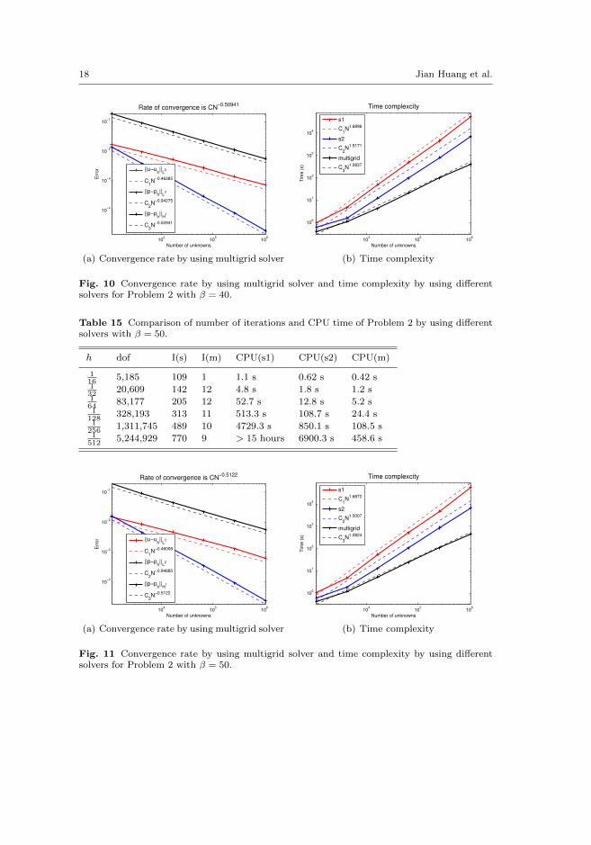
Fig. 9 Convergence rate by using multigrid solver and time complexity by using di↵erentsolvers for Problem 2 with � = 30.
Table 14 Comparison of number of iterations and CPU time of Problem 2 by using di↵erentsolvers with � = 40.
h dof I(s) I(m) CPU(s1) CPU(s2) CPU(m)
116 5,185 100 1 1.0 s 0.63 s 0.39 s132 20,609 134 11 4.6 s 1.6 s 1.1 s164 83,177 198 11 49.9 s 12.1 s 4.2 s1
128 328,193 306 10 500.4 s 98.8 s 21.6 s1
256 1,311,745 481 9 4532.5 s 802.5 s 96.1 s1
512 5,244,929 759 8 > 15 hours 6875.1 s 405.1 s
7 Conclusions
In this paper, we constructed a nonlinear multigrid method for a mixed finiteelement method of the two-dimensional Darcy-Forchheimer model. We presenteda comparative study between the multigrid solver and the PR iterative solver,at the same time compared CPU time of the e�cient solver of solving the SPDsystems with that obtained by solving the linear saddle point systems directly. Wetook into account the pressure accuracy when we set the termination criterion, andchose a better value of the stopping criterion tol. In comparison with the authorsin [10] always chose ↵ = 1 for di↵erent values of �, we reported a better choice and
18 Jian Huang et al.
104
105
106
10−4
10−3
10−2
10−1
Number of unknowns
Err
or
Rate of convergence is CN−0.50941
||u−uh||
L2
C1N−0.46385
||p−ph||
L2
C2N−0.94275
||p−ph||
H1
C3N−0.50941
(a) Convergence rate by using multigrid solver
104
105
106
100
101
102
103
104
Number of unknowns
Tim
e (
s)
Time complexcity
s1
C1N1.6896
s2
C2N1.5171
multigrid
C3N1.0837
(b) Time complexity
Fig. 10 Convergence rate by using multigrid solver and time complexity by using di↵erentsolvers for Problem 2 with � = 40.
Table 15 Comparison of number of iterations and CPU time of Problem 2 by using di↵erentsolvers with � = 50.
h dof I(s) I(m) CPU(s1) CPU(s2) CPU(m)
116 5,185 109 1 1.1 s 0.62 s 0.42 s132 20,609 142 12 4.8 s 1.8 s 1.2 s164 83,177 205 12 52.7 s 12.8 s 5.2 s1
128 328,193 313 11 513.3 s 108.7 s 24.4 s1
256 1,311,745 489 10 4729.3 s 850.1 s 108.5 s1
512 5,244,929 770 9 > 15 hours 6900.3 s 458.6 s
104
105
106
10−4
10−3
10−2
10−1
Number of unknowns
Err
or
Rate of convergence is CN−0.5122
||u−uh||
L2
C1N−0.46008
||p−ph||
L2
C2N−0.94685
||p−ph||
H1
C3N−0.5122
(a) Convergence rate by using multigrid solver
104
105
106
100
101
102
103
104
Number of unknowns
Tim
e (
s)
Time complexcity
s1
C1N1.6872
s2
C2N1.5007
multigrid
C3N1.0824
(b) Time complexity
Fig. 11 Convergence rate by using multigrid solver and time complexity by using di↵erentsolvers for Problem 2 with � = 50.

Multigrid Method of The Darcy-Forchheimer Model 19
Table 16 Comparison of iteration steps of multigrid solver according to di↵erent h and � forProblem 2 with ↵ = 1/�.
h � = 10 � = 20 � = 30 � = 40 � = 50
132 5 7 9 11 12164 5 7 9 11 121
128 5 7 9 10 111
256 4 6 8 9 101
512 4 5 7 8 9
compared with the previous choice through comparing the number of iterationsand CPU time. The results obtained from our tests indicate that the multigridsolver is very e�cient for numerically solving this nonlinear elliptic equation. Thenumber of iterations and CPU time for using multigrid solver are shown to besignificantly less than that obtained by using the other solvers.
In the future work, we shall extend our results to two directions. One is that wewould like to find a better smoother, which is used in the pre-smoothing and post-smoothing step, to reduce CPU time and make the multigrid solver more e�cient.Another is that we intend to carry out some studies on the three-dimensionalDarcy-Forchheimer problem and the real application in a porous medium.
References
1. Adams, R. A., Sobolev Spaces, Academic Press, New York (1975)2. Aziz, K., Settari, A., Petroleum Reservoir Simulation, Applied Science Publishers LTD,London (1979)
3. Briggs, W. L., Henson, V. E., McCormick, S. F., A Multigrid tutorial, 2ndEdition, SIAM,Philadelphia (2000)
4. Chen, L., iFEM: an integrated finite element methods package in MATLAB, TechnicalReport, Technical Report, University of California at Irvine (2009)
5. Chen, L., Multigrid methods for saddle point systems using constrained smoothers, Com-puters and Mathematics with Applications, 70(12), 2854-2866 (2015)
6. Ciarlet, P. G., The Finite Element Method for Elliptic Problems, North-Holland, Amster-dam, New York, Oxford (1978)
7. Crouzeix, M., Raviart, P. A., Conforming and non-conforming finite element methods forsolving the stationary Stokes problem, RAIRO Anal. Numer, 8, 33-76 (1973)
8. Forchheimer, P., Wasserbewegung durch Boden, Z. Ver. Deutsch. Ing., 45, 17821788 (1901)9. Girault, V., Wheeler, M. F., Numerical discretization of a Darcy-Forchheimer model, Nu-mer. Math., 110, 161-198 (2008)
10. Lopez, H., Molina, B., Salas, Jose J., Comparison between di↵erent numerical discretiza-tions for a DarcyForchheimer model, ETNA 34, 187-203 (2009)
11. Pan H., Rui, H., Mixed element method for two-dimensional Darcy-Forchheimer model,J.Sci. Comput., 52, 563587 (2012)
12. Park, E. J., Mixed finite element method for generalized Forchheimer flow in porous media,Numer. Methods Partial Di↵erential Equations, 21, 213228 (2005)
13. Peaceman, D. W., Rachford, H. H., The numerical solution of parabolic and elliptic dif-ferential equations, J. Soc. Indust. Appl. Math., 3, 28-41 (1955)
14. Rui, H., Liu, W., A two-grid block-centered finite di↵erence method for Darcy-Forchheimerflow in porous media, SIAM J. Numer. Anal., 53(4), 1941-1962 (2015)
15. Rui, H., Pan H., A block-centered finite di↵erence method for the Darcy-Forchheimermodel, SIAM J. Numer. Anal., 50(5), 26122631 (2012)
16. Rui, H., Zhao, D., Pan H., A block-centered finite di↵erence method for Darcy-Forchheimermodel with variable Forchheimer number, Numer. Methods Partial Di↵erential Equations,31,1603-1622 (2015)

20 Jian Huang et al.
17. Ruth, D., Ma, H., On the derivation of the Forchheimer equation by means of the averagingtheorem, Transport in Porous Media, 7, 255264 (1992)
18. Salas, Jose J., Lopez, H., Molina, B., An analysis of a mixed finite element method for aDarcyForchheimer model, Mathematical and Computer Modelling 57, 2325-2338 (2013)
19. Wang, Y., Rui, H., Stabilized CrouzeixRaviart element for DarcyForchheimer model, Nu-mer. Methods Partial Di↵erential Equations,31, 1568-1588.(2015)