Embed Size (px)
Citation preview
PROYECTO FIN DE CARRERA
Analysis and adaptation of Methods of Assessment of Sensor Concepts for
Collision Avoidance Systems
AUTOR: MACÍAS JAREÑO, RAÚL
MADRID, Septiembre 2008
UNIVERSIDAD PONTIFICIA COMILLAS
ESCUELA TÉCNICA SUPERIOR DE INGENIERÍA (ICAI) INGENIERO INDUSTRIAL

List of Contents II
List of Contents
List of Contents ............................................................................................................II Formulas and Indices .................................................................................................. IV List of Abbreviations ....................................................................................................V List of Figures............................................................................................................ VII List of Tables............................................................................................................VIII 1 Introduction........................................................................................................... 1 2 Sensor Concepts Fundamentals ............................................................................. 3
2.1. RADAR ......................................................................................................... 3 2.2. LIDAR ........................................................................................................... 4 2.3. Ultrasound...................................................................................................... 6 2.4. Video and image processing ........................................................................... 7 2.5. Photonic Mixer Device ................................................................................... 8 2.6. Combinations of sensors................................................................................10
3 Assessment methods ............................................................................................11 3.1. Assessment methods’ fields of use.................................................................11
3.1.1 Product development ................................................................................11 3.1.2 Quality management .................................................................................12 3.1.3 Hazard assessment ....................................................................................13
3.2. Types of assessment methods ........................................................................14 3.2.1 Design assessment methods ......................................................................14 3.2.2 Inspection Assessment Methods ...............................................................18
3.3. Main ideas and tools from Assessment Methods............................................23 3.3.1 Collecting Data.........................................................................................24 3.3.2 Presenting Data.........................................................................................26 3.3.3 Analyzing Data.........................................................................................27
4 Description of the system .....................................................................................30 4.1. Collecting Data..............................................................................................30
4.1.1 Description and interaction of sensor properties ........................................31 4.1.2 Definition of the first set of inputs: General Properties ..............................34 4.1.3 Definition of the second set of inputs: Benefit of the CA System ..............35
4.2. Presenting Data .............................................................................................48 4.2.1 Requirements to the Assessment Method ..................................................48 4.2.2 Application of the Review ........................................................................49
4.3. Analyzing Data..............................................................................................55 4.3.1 Ranking Tool............................................................................................55
5 Application of the Assessment Method.................................................................58 5.1. Collecting Data..............................................................................................58
5.1.1 Selection of sensors considered along the study ........................................58

List of Contents III
5.1.2 Definition of the first set of inputs: General Properties ..............................59 5.1.3 Definition of the second set of inputs: Benefit of the CA System ..............61
5.2. Presenting Data .............................................................................................65 5.2.1 Application of the Review to the General Properties .................................65 5.2.2 Application of the Review to the benefit of the system..............................74
5.3. Analyzing Data..............................................................................................80 5.3.1 Graphical representation of the results ......................................................81 5.3.2 Analysis of the results...............................................................................82 5.3.3 Ranking of sensors concepts .....................................................................84 5.3.4 Ranking of single sensors .........................................................................86
6 Verification and Validation ..................................................................................89 6.1. Verification of the assessment method...........................................................89
6.1.1 Requirements on the method is respect to the inputs .................................90 6.1.2 Requirements on the method is respect to the assessment..........................91 6.1.3 Requirements on the method is respect to the output .................................92
6.2. Validation of the assessment method .............................................................92 7 Conclusion ...........................................................................................................93 Bibliography................................................................................................................94 Appendix A: Sets of Inputs ................................................................................. XCVIII Appendix B: Reviews ..................................................................................................CI
Formulas and Indices IV
Formulas and Indices
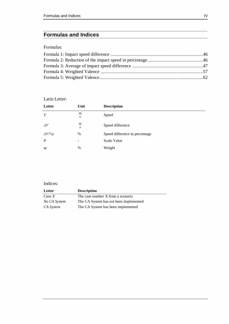
Formulas: Formula 1: Impact speed difference .............................................................................46 Formula 2: Reduction of the impact speed in percentage ..............................................46 Formula 3: Average of impact speed difference ...........................................................47 Formula 4: Weighted Valence .....................................................................................57 Formula 5: Weighted Valence......................................................................................62
Latin Letter: Letter Unit Description
V ms Speed
ΔV ms Speed difference
ΔV/%) % Speed difference in percentage
P - Scale Value
w % Weight
Indices: Letter Description Case X The case number X from a scenario No CA System The CA System has not been implemented CA System The CA System has been implemented
List of Abbreviations V
List of Abbreviations
ACC Adaptive Cruise Control ANOVA Analysis Of Variance BAST Bundesanstalt für Straßenwesen CA Collision Avoidance DESTATIS Statistisches Bundesamt DOE Design Of Experiments DRBFM Design Review Based on Failure Mode EU European Union FAT Forschungsvereinigung Automobiltechnik e.V FMEA Failure Mode and Effect Analysis FTA Fault Tree Analysis FZD Fahrzeugtechnik Darmstadt GIDAS German In-Depth Accident Study GHz Giga Herz GUI Graphical User Interface HL Hardware-in-the-Loop HOQ House Of Quality IR Infrared LIDAR Light Detection And Ranging MAIS Maximum Abbreviated Injury Scale ML Model-in-the-Loop PMD Photonic Mixer Device NWV Not Weighted Value PW Proportional Weight QFD Quality Function Deployment RADAR Radio Detection And Ranging SAE Society of Automotive Engineers SBI Suppression of Background Illumination SL Software-in-the-Loop SPC Statistical Process Control SQC Statistical Quality Control SUV Sport Utility Vehicle SV Scale Value TQM Total Quality Management TU Technische Universität Darmstadt TRIZ Theory of inventive problem solving

List of Abbreviations VI
V Value VITES Virtual Testing for Extended Vehicle Passive Safety WV Weighted Value

List of Figures VII
List of Figures
Figure 1: The Doppler Effect [PUSI06]......................................................................... 4 Figure 2: Several beams in sequence [WAGN07].......................................................... 6 Figure 3: Ultrasound is medium dependent ................................................................... 7 Figure 4: Image obtained and processed by a video system [MOBI08] .......................... 8 Figure 5: Diagram from a Photonic Mixer Device System [RIED02] ............................ 9 Figure 6: System Design Review Process [SHIM03]................................................... 15 Figure 7: House of quality [HALE01] ......................................................................... 16 Figure 8: The general model for TRIZ problem solving [STOL07] ............................. 17 Figure 9: Principal facets of the Six Sigma initiative [TRUS03] .................................. 18 Figure 10: Failure Ranking Modes [MACD04] ........................................................... 20 Figure 11: Pareto analysis by frequency [OAKL03] .................................................... 22 Figure 12: Common Timeline of Main Ideas ............................................................... 23 Figure 13: Collecting Data .......................................................................................... 24 Figure 14: Presenting Data .......................................................................................... 26 Figure 15: Analyzing Data .......................................................................................... 27 Figure 16: Block diagram of the system including the main tools ................................ 34 Figure 17: Block diagram of the system focusing in the General Properties................. 34 Figure 18: Block diagram of the system ...................................................................... 35 Figure 19: Scenarios from CarMaker [IPG_08] ........................................................... 37 Figure 20: Diagram representing the implementation of sensors.................................. 40 Figure 21: Distribution of impact speeds ..................................................................... 41 Figure 22: Block diagram of the system ...................................................................... 42 Figure 23: Categories of Crash Costs [VTPI07] .......................................................... 44 Figure 24: Estimated costs per fatality or injury, 2002 Euros [ICFC03 ........................ 45 Figure 25: Block diagram of the system focusing on the assessment method ............... 48 Figure 26: Block diagram of the system ...................................................................... 50 Figure 27: Block Diagram of the System..................................................................... 55 Figure 28: Comparison from possible graphic situations ............................................. 56 Figure 29: Block diagram of the system ...................................................................... 59 Figure 30: Block Diagram of the system ..................................................................... 61 Figure 31: All collisions (belted, front-seat occupants), [GIDAS]................................ 62 Figure 32: Frontal collisions (belted, front-seat occupants), [GIDAS]. ........................ 62 Figure 33: Side collisions (belted, front-seat occupants), [GIDAS].............................. 63 Figure 34: Block Diagram of the system ..................................................................... 66 Figure 35: Block Diagram of the system ..................................................................... 74 Figure 36: Block Diagram of the System..................................................................... 80 Figure 37: Graph with the results from the review methods......................................... 82 Figure 38: Comparison between the four Sensor Concepts .......................................... 84 Figure 39: Comparison between Long Range RADAR and LIDAR ............................ 86

List of Tables VIII
List of Tables
Table 1: Comparison of advantages and disadvantages for RADAR sensors...................... 3 Table 2: Comparison between qualitative and quantitative risk assessments [TAYL06]. .. 14 Table 3: List of External Factors [STROB04].................................................................. 31 Table 4: List of Performance Properties for RADAR, LIDAR and Ultrasound................. 32 Table 5: List of Performance Properties for video and PMD [STROB04] ........................ 32 Table 6: List of External Factors...................................................................................... 33 Table 7: KABC Scale [VTPI07] ...................................................................................... 43 Table 8: AIS Scale [VTPI07]........................................................................................... 43 Table 9: Calculation from the difference between impact speeds ..................................... 47 Table 10: Inputs matrix [BIRK06] ................................................................................... 50 Table 11: Definition of the scale ...................................................................................... 51 Table 12: Special values scale [BIRK06] ......................................................................... 51 Table 13: Assignment of scale values [BIRK06].............................................................. 52 Table 14: Classification of values to the selection of inputs [BIRK06]............................. 53 Table 15: Selection of inputs values [BIRK06] ................................................................ 53 Table 16: Assessment matrix [BIRK06] .......................................................................... 54 Table 17: Formulas used in the Assessment matrix [BIRK06] ........................................ 54 Table 18: Selection of the sensors for the study ............................................................... 59 Table 19: Collection of General Properties for RADAR .................................................. 60 Table 20: Collection of General Properties’ data for LIDAR and Video........................... 60 Table 21: Selection of the accident types ......................................................................... 64 Table 22: Accidents Matrix ............................................................................................. 65 Table 23: Definition of minimum and maximum values .................................................. 67 Table 24: Definition of the scale...................................................................................... 68 Table 25: Special Value Scale ......................................................................................... 69 Table 26: Assign scale values .......................................................................................... 69 Table 27: Selection of General Properties and assignment if weights ............................... 71 Table 28: Results from the Assessment Matrix ................................................................ 72 Table 29: Results from the General Properties assessment ............................................... 73 Table 30: Accidents Matrix ............................................................................................. 75 Table 31: Special Values Scale ........................................................................................ 76 Table 32: Assign Scale Values Table............................................................................... 76 Table 33: Level of occurrence from the different accidents.............................................. 77 Table 34: Selection of inputs values ................................................................................ 77 Table 35: Assessment Matrix........................................................................................... 79 Table 36: Results from the benefit assessment ................................................................. 79 Table 37: Results of the review methods.......................................................................... 81 Table 38: Quality levels from the different Sensor Concepts............................................ 83 Table 39: Ranking of Sensor Concepts ............................................................................ 85 Table 40: Ranking among single sensors ......................................................................... 87

1. Introduction 1
1 Introduction
There are over 600 million motor vehicles in the world today, a fact showing the impor-
tance that transport vehicles, especially the automobile, have taken into our daily lives.
Due to its popularity and extensive use, vehicle accidents take occur often than desired.
In 2000, 1.7 million people were injured and more than 40.000 people died in Europe
during car accidents. The EU has issued the goal of reducing these fatalities by half in
the year 2010 [ETP_01].
Collision Avoidance Systems are safety systems with a high potential to reduce the se-
verity of accidents. The development of these systems is motivated by their capability to
react to situations that humans are not able. Collision Avoidance Systems process data
from the environment through the use of sensors to activate a response system when an
action is required. Therefore, it is possible to differentiate two different sub-systems
among Collision Avoidance Systems: the detection system and the response system.
The detection system is responsible of processing information from the surroundings
through the use of sensors. The response system warns the driver from the imminent
danger or activates the appropriate braking or steering measures to avoid the collision or
at least mitigate the accident to the largest degree possible. The contribution from both
systems is extremely important to Collision Avoidance Systems [SEIL98].
Vehicle accidents present similarities making it possible to define precisely the condi-
tions and causes of the accidents. The characteristics of accidents can be reproduced in a
simulation where different CA Systems can be implemented allowing to test the capa-
bility of the systems to reduce the severity of vehicle crashes. In a CA System, the de-
tection sub-system is responsible of processing the information that could lead to an
accident. The study focuses on the contribution of sensors to prevent or mitigate colli-
sions since the choice of the right sensor is crucial to the performance, to the cost and to
benefit of Collision Avoidance Systems.
In the automobile industry, a wide range of sensors can be used depending on the char-
acteristics of the application. The physical principle of each sensor determines its char-
acteristics and allows for the classification of sensors into Sensor Concepts. Each Sen-
sor Concept presents particular properties leading to a specific performance.

1. Introduction 2
Several Sensor Concepts are often suitable to collision avoidance, but it is necessary to
determine which one is able to provide the best performance at the minimum cost. The
development of an assessment method capable of evaluating sensor performance leads
to the design optimization of new Collision Avoidance Systems and facilitates decision
making.
This Thesis focuses at first in the most relevant sensor technologies for CA Systems;
RADAR, LIDAR, Ultrasound, Video, and PMD. Each sensor technology is analyzed
focusing on the physical principles and the main properties. Then an in depth research
has been undertaken to identify the main Assessment Methods used in the industry fo-
cusing, above all areas, in Product Development and Quality Management. The differ-
ent methods are summarized and explained focusing on their working mechanisms, ad-
vantages, and disadvantages. The last step consists of a more in depth analysis on exist-
ing assessment methods, allowing the adaptation of Assessment Methods to sensors.
The goal is the development of an overall assessment concept, as well as a procedure
where sensors can be integrated.

2. Sensor Concepts Fundamentals 3
2 Sensor Concepts Fundamentals
Collision Avoidance Systems process data from the environment through the use of
sensors. In the automobile industry, a wide range of different sensors can be used de-
pending on the characteristics of the application. The physical principle of each sensor
determines its properties and allows to classify them in Sensor Concepts.
During this study, five Sensor Concepts have been considered to be the best fitted sen-
sors to collision avoidance: RADAR, LIDAR, Ultrasound, Video and Photonic Mixer
Device. Different aspects from Sensor Concepts as working mechanism, components,
advantages, disadvantages, etc. are presented in following sub-sections.
2.1. RADAR
RADAR which stands for Radio Detection and Ranging is a system that uses long
wavelength electromagnetic waves (microwave and radio range) for detecting, locating,
tracking and identifying moving and fixed objects at considerable distances. [WINN05]
The frequency range for RADAR ranges between 500MHz – 50 GHz. In the automobile
industry there are two kinds of RADAR: short range and long range RADAR. Short
range RADAR (24 GHz) reaches approximately a range of 0.2-20 m, while long range
RADAR (76-77 GHz) reaches a distance between 1-200 m. The characteristics from
RADAR change a lot depending on short range or long range. In Table 1, the main ad-
vantages and disadvantages from the two kinds of RADAR are illustrated.
RADAR
Short Range RADAR Long Range RADAR
Adv
anta
ges - Good integration capability
- Efficiency under all weather conditions
- High precision
- Small measure cycles
- Large Range
- Efficiency under all weather conditions
- High precision
- Small measure cycles
Dis
adva
ntag
es
- Limited European radio licences
- High costs (expensive technology)
- Integration
Table 1: Comparison of advantages and disadvantages for RADAR sensors

2. Sensor Concepts Fundamentals 4
A RADAR system installed in a vehicle is composed of a transmitter, an antenna and a
receiver. In RADAR technology the distance from the object is calculated through the
echoes that are sent back from the object. A common problem is that not all objects re-
flect electromagnetic waves in the same way. For example, we know that reflection by
metals is 100 %, by glass and stone is 50%, by plastic is 20% while persons barely re-
flect any rays [WINN05].
The determination of the position of an object is done through the Time-of-flight and
angle measurement. In Time-of-flight measurements, electromagnetic energy is sent
toward objects and the returning echoes are observed. The measured time difference and
the speed of the signal allow to calculate the distance to the object. For large distances,
large pulse energies are required [WINN05].
The Speed measurement is made through the “Doppler Effect”. The Doppler Effect is
based on the change of wavelength due to the changing gap between waves. For exam-
ple, in a situation where an object is moving faster as the transmitter each wave
has to travel a larger distance to reach the object, increasing the distance between
waves. The difference between the original gap and the final gap, once the waves have
been reflected permits the accurate calculation of the velocity of the vehicle. Figure 1
depicts the Doppler Effect.
Figure 1: The Doppler Effect [PUSI06]
2.2. LIDAR
LIDAR meaning Light Detection And Ranging, better known as Laser-RADAR is a
system that uses light (Ultraviolet, Infrared or rays in the visible range) for positioning
and measuring distances. In the same way as RADAR, LIDAR measures the distance
between the transmitted pulse and the reflected pulse. [WINN05].

2. Sensor Concepts Fundamentals 5
LIDAR determines position using the Time-of-flight and the angle measurement. A
difference with RADAR is that the angle measurement can be done through different
procedures: One-/more rays, scanner and sweep.
The major difference between LIDAR and RADAR lies on the calculation of speed.
LIDAR does not use the Doppler’s effect due to limits of the technology. The velocity
is calculated through the derivation from the position signal. The noise introduced at the
position measurement is extremely amplified when the speed is calculated, but it is pos-
sible to soften the noise effect through filters. In the case of acceleration, the velocity
signal cannot be derived because the noise is extremely high and filters have no effect.
The use of LIDAR to detect objects at large distances requires large pulse energies. LI-
DAR presents a strict energy limit fixed by the authorities due to safety issues. Outside
the limits, it exists a high risk of damaging people’s visibility. It is necessary to make
sure that the laser wavelength is in the eye safe region. The amount of energy is a strong
limiting factor to the technology.
LIDAR presents other disadvantages, such as a strong susceptibility to noise. LIDAR
signals are very sensible to interferences, which lead to damaged data in the presence of
noise. Another inconvenient is the reflexion of signals because the object to detect does
not present always the best conditions to reflect the signals. For example, a dirty car
compared to a clean car barely reflects the incident rays, a thin water film difficults re-
flexion as well as shiny cars. [WINN05]
Among the main advantages presented by LIDAR, the small costs (price can be as-
sumed to be half of the cost from RADAR), high resolutions (in respect to ranging, ob-
ject detection, speed measurements, etc.), and the possibility to send several beams in
sequence stand out the most. Figure 2 illustrates how LIDAR can send several beams in
sequence, and different echoes are reflected when coming in contact with a dirty sensor
surface, precipitation and an object.

2. Sensor Concepts Fundamentals 6
Figure 2: Several beams in sequence [WAGN07]
2.3. Ultrasound
Ultrasound systems use high-frequency sound waves (above the range of audible sound
to humans) to measure the position of objects. The electrical stimulation of a piezoelec-
tric crystal produces ultrasonic waves that reach the object, reflecting back at any point
where there is a change of density (Puls-echo principle). The intensity of the reflected
echoes determines the position of the object [WINN05].
Ultrasound systems used the same piezoceramic as sender and receiver. All the emitters
of the system send sound waves in all directions, and the triangle method allows calcu-
lating the exact distance between the vehicle and the object [WINN05].
Ultrasound presents different advantages compared to other sensor concepts. The sen-
sors are robust, small and cheap because of their multiple uses in daily life. They do not
require mechanical mechanisms and it is easy to assembly. The main disadvantage of
ultrasound sensors are the limitations caused by the transport medium. The air medium
confines the application to small intervals lying between 2 and 3 meters and small driv-
ing speeds less than 20 km/h.
Ultrasound presents three important restrictions: limited range, limited signal processing
and limited static behaviour. In ultrasound systems the range is limited to 2-3 m reduc-
ing its application to short range. The signal processing is not immediate, meaning that
the system requires a minimum time to process the signals, which could be too long to
prevent a collision. The limited static behaviour refers to the loss of information due to
the motion from emitter, reflector and medium. For example, two vehicles driving par-
allel at the same speed (relative speed of 0); if the cars are driving at 20 km/h there will
not be any problems, but if the speed is 120 km/h the wind causes the waves to be
drawn away. Figure 3 depicts the effect of wind in ultrasound waves.

2. Sensor Concepts Fundamentals 7
Figure 3: Ultrasound is medium dependent
2.4. Video and image processing
Image processing describes a technique of digital image analysis using programmable
algorithms to understand images. Video cameras are used to record the scenes, while the
algorithms detect the main characteristics from the surroundings: size of objects, dis-
tance to objects and speeds.
A video system for the automobile industry is composed of two main components: cam-
eras and a processor. Cameras are usually CMOS cameras with a low accuracy and me-
dium resolution, but relatively cheap. The second main component is the processor and
the corresponding software capable of dealing with complicated algorithms. Image
processing techniques required special processors and on board computers used in vehi-
cles should not be very expensive. On board computers and the development of the al-
gorithms rises the cost of the system. [MOBI08]
Figure 4 illustrates how the algorithms identify different objects on the image (green
and red squares), calculates the distance to the objects and locates at all times the object
presenting the higher risk of collision (red square).
win
d
sensor
object
win
d
sensor
object

2. Sensor Concepts Fundamentals 8
Figure 4: Image obtained and processed by a video system [MOBI08]
The main advantage from video systems in respect to other systems is object classifica-
tion. There are different methods to identify the characteristics of an image; Edge De-
tection, Optical flow, Cross correlation and Image Processing. All these methods have
the capacity of classification except for optical flow [PUSI07]. The systems can identify
different kinds of objects, but nowadays they are used to detect lane marking and road
boundaries, providing very useful information to the human eye. Another relevant ad-
vantage is the capability to detect objects under any kind of environmental conditions,
including inclement weather.
2.5. Photonic Mixer Device
Photonic Mixer Devices (PMD) are a new generation of active pixel sensors able to
capture an entire 3D scene in real time and calculate the distance to objects. A transmit-
ter sends a modulated optical signal (infrared light) to a specific scene. The light is re-
flected by the object and enters the PMD sensor. The electrons converted into photons
are separated inside the optically sensitive area of the semiconductor in relation to the
reference signal. A comparison between the optical and electrical reference signals pro-
vides an output signal with the 3D data. [PMDT08]
Figure 5 depicts the different components from a Photonic Mixer Device (IR Transmit-
ter, 3D-scene, Receiver, Signal Processing) as well as the interaction between the device
and the environment.

2. Sensor Concepts Fundamentals 9
Figure 5: Diagram from a Photonic Mixer Device System [RIED02]
Due to its versatility, PMD sensors are used in many and different fields such as: trans-
port application (automotive and navigation), industrial applications, virtual reality and
man-machine interface applications. Depending on the field of use, the sensor presents
different characteristics. In the specific case of the automotive industry, a 64 x 16 pixels
sensor is used due to necessity of measuring wide angles in horizontal and vertical. In
the automotive industry the PMD system is mainly used for short range applications in
active and passive safety. [RIED02]
The main advantage presented by Photonic Mixer Device Systems is the robustness and
efficiency presented under difficult environmental conditions. The signals can be fil-
tered from external sources of light such as incidental solar radiation through a process
called “Suppression of Background Illumination (SBI)” [PMDT08]
Photonic Mixer Device technology is a new born technology, presenting the typical
inconveniences in these kinds of cases; lack of research and high prices. In order to be-
come a competitive technology, it requires research and the high prices are needed to
decrease. One of the characteristics of the sensor is that price increases when more light
is needed in higher resolutions of 3-D Cameras [RIED02].

2. Sensor Concepts Fundamentals 10
2.6. Combinations of sensors
Nowadays the tendency of safety systems is the combination of different Sensor Con-
cepts in the same system. The resulting systems offer a much higher quality since it pre-
sents the positive aspects from two different Sensor Concepts.
In order to combine different Sensor Concepts, the first step is to identify the benefits
and limits of each separate system. Not every combination of sensors is interesting; it
would be necessary to see how the different Sensor Concepts match together. The most
typical combinations are the following: Video/LIDAR, Video/RADAR, Ultrasound
(Short range)/RADAR (long range) and RADAR (Short range)/LIDAR (long range).
The most interesting combinations among the different possibilities are the systems in-
cluding video as one of the sensors. This is because video provides direct information
for the human eye and a real picture is always more reliable than a measurement. Video
matches perfectly with RADAR and LIDAR, since it is capable of object recognition
which is a task that other systems can not provide. Due to this fact, the combinations of
video/RADAR and video/LIDAR present nowadays the best technological answer.
The combination of Sensor Concepts is the best existing possible choice, but it also pre-
sents inconveniences: high costs and difficulties on the integration of two different sys-
tems. Safety Systems are expensive, and the price rises when two systems are used in-
stead of one. The interaction of the two systems requires the development of additional
software, which difficults the interaction and raises costs even more.

3. Assessment methods 11
3 Assessment methods
Improvement is a common objective in the human being, which manifests in many dif-
ferent ways (self development, better job, new car, etc.). Organizations such as compa-
nies seek improvements as well, for instance: to reduce costs, to increase benefits, to
expand, etc. In order to achieve progress it is required to identify specific points of im-
provement. “Assessment Methods” are tools which help reach goals through the analy-
sis and evaluation of a situation. The information collected provides important knowl-
edge in making consequent decisions.
3.1. Assessment methods’ fields of use
Assessment methods can document knowledge, skills, attitudes and beliefs. Due to its
variety and the goal of assessing Sensor Concepts, it is considered to focus on methods
used in the industry. The decision is based on the fact that industrial companies use very
precise methods to collect and analyze data. Industrial companies use assessment meth-
ods mainly to:
Create new products based on client needs (Product development techniques)
[BIRK06].
Reduce costs or improve benefits through quality studies (Quality Management)
[GALE01].
Reduce risk or danger in complicated situations (Hazard Assessments) [MANN05].
The three areas present different characteristics and objectives which leads to the next
step; the study and analysis from each one of these fields.
3.1.1 Product development
Product development is the name used to describe the process of creating a new physi-
cal product or service. It follows different steps: creation from ideas, construction, test-
ing from prototypes and manufacturing.
Idea Generation and Brainstorming are the normal sources of new ideas for new prod-
ucts, but it also has to be taken into account research on already existing products. New
products can be very well created from already existing ideas or combination of differ-
ent products. After the new idea has been created, the design of the product will be

3. Assessment methods 12
made. In this phase of the process it would be also advisable and convenient to make
studies and plans on how the product would work in the real plane. [BIRK06]
After the design phase of the process comes the design and production of prototypes.
These will be tested as if they were the final product, in order to get knowledge about
the viability of the wanted product.
A market research and test should also be made, as it is very important to see how the
product will be sold in the future. Testing prototypes determine if the product fulfils the
requirements, and check if it really works as it is intended. It is also possible that a pro-
totype has excellent results which are not reflected on the final product since the hoped
results are not obtained; but most of the time prototypes are a very valuable and reliable
source of information [PILL03].
Once the idea has been defined, it is necessary to make the designs. Then different tests
are carried out in order to approve the prototypes. The final step is to decide the place,
the process and the amount of final product which will be produced, and then comes the
manufacture of the final product. [PILL03]
3.1.2 Quality management
There are many studies, interpretations and definitions about quality but they all agree
on “meeting the requirements of the customer” [OAKL03]. A practical and managerial
definition was introduced by F. Galetto (1985) who proposed the following one: “Qual-
ity is the set of characteristics of a system that makes it able to satisfy the NEEDS of the
Customer, of the User and of the Society” [GALE01].
Quality Management techniques ensure all the necessary activities to the creation of a
product or service (design, development and implementation) are effective and efficient.
In order to fulfil the mentioned requirements different aspects from the quality concept
need to be identified.
The overall quality concept integrates three areas: quality development, quality mainte-
nance and quality improvement [GREE04]. Quality development ensures the consis-
tency of the process, quality maintenance satisfies the specified requirements and qual-
ity improvement intends to improve the process to achieve the results.

3. Assessment methods 13
All Quality Management methods used to evaluate a process/system require the gather-
ing of data in order to determine the state of the process/system and be able to improve
this state [GREE04].
Quality Management offers many benefits like [GREE04]: better product design and
quality; reduction in consumer complaints; efficient use of people, machines and mate-
rials, resulting in higher productivity. The goal of a “Total Quality Management” is the
capacity of applying these ideas in all areas of a business: marketing, engineering,
manufacture, maintenance, and so on. One aspect that helps reaching the best equilib-
rium is the balance between the costs (the most economical levels) and customer satis-
faction.
3.1.3 Hazard assessment
Hazard assessments are undertaken to assist in making engineering decisions in the
‘grey’ areas, where further investigation is needed in order to decide on the most cost-
effective measures, and to prevent threats to the public [MANN05].
The aim of the Hazard Analysis is to select a measure to deal with a hazard. An estima-
tion is made from the frequency of realization of the hazard, based on a simple calcula-
tion using field data. The estimation made should be somehow conservative
[MANN05].
Hazard assessments are comprehensive and rational reviews that offer a logical and de-
fensible method for security professionals to make decisions about security expendi-
tures and to select cost-effective security measures that will protect critical assets and
reduce risk to an acceptable level [VELL07].
Hazard assessments can be either quantitative or qualitative, or a hybrid. Qualitative
assessments are based on the data available and on the skills of the assessment team,
while quantitative assessments use numeric data to evaluate risks. Table 2 shows the
main characteristics from these two assessments. Hybrid risk assessments use quantita-
tive data where available and qualitative data where metrics are not readily available or
insufficient [TAYL06].

3. Assessment methods 14
Hazard Assessment
Qualitative Assessment Quantitative Assessment
A faster process Emphasizes descriptions Findings are simple and expressed in rela-tive terms Values are perceived values, not actual values Requires less training
Very time intensive Yields results that are financial in nature Used for cost benefit analysis Good for justifying the procurement of safeguards Requires tracking the financial value of assets
Table 2: Comparison between qualitative and quantitative risk assessments [TAYL06].
Once the data is gathered and organized, each of the hazards should be reviewed. It will
be necessary to determine the hazard type, the risk level, the risk probability and poten-
tial impact from each of the hazards previously defined [TAYL06].
Assessment methods are used in areas where little information is available and an
evaluation is necessary. Hazard assessments increases awareness of hazards, provides
opportunity to identify and control hazards and can lead to increased productivity.
3.2. Types of assessment methods
Product development, quality management and hazard assessment are extremely exten-
sive fields. An in-depth research which focused on the three areas has been undertaken
to find all existing assessment methods used these days in the industry.
Assessment methods can be divided in two main groups: Design and inspection assess-
ment methods. Design methods are measures lent to the creation of new products, proc-
esses, systems, and so on, according to specified requirements. Inspection procedures
are focused on the examination from existing situations to identify problems that could
occur due to changes in the system.
3.2.1 Design assessment methods
Design assessment methods are procedures which gather and analyze different data and
requirements, in order to create and design different products and/or services. There are
several types of design methods according to the targets and workings mechanisms.

3. Assessment methods 15
3.2.1.1 Design Review Based on Failure Mode (DRBFM)
Design Review Based on Failure Mode (DRBFM) is a tool first developed by the Toy-
ota Company. It was created on the basis that problems in designs appear when changes
are done to an engineering design already proved to be successful, and it used to ad-
vance discussions among designers and engineers. “DRBFM is a method of discovering
problems and developing countermeasures by taking notice and discussing intentional
changes (design modifications) and incidental changes (changes in part environment)”
[SHIM03].
This method is widely applicable, since it can be applied to new development parts, to
parts concerned in a partial engineering change, and/or to subcomponents. It is a practi-
cal tool based on FMEA (Failure Mode and Effect Analysis) and FTA (Fault Tree
Analysis) [SHIM03]; as a matter of fact, a good FMEA is indeed necessary if we want
to apply DRBFM.
Figure 6: System Design Review Process [SHIM03]
There three steps which form the structure of DRBFM: Good Design, Good Discussion
and Good Design Review. Good Design means that a design should be reliable from the
very beginning, needing no changes at all. If changes should be made to a design, they
should be few and not at the same time; a successful change must be a visible and clear
change. As far as Good Discussion is concerned, they should be focused on the changes

3. Assessment methods 16
proposed in respect to the design. Good Design Review involves testing all the results
of validation, trying to make all mistakes visible [SHIM03].
3.2.1.2 Quality Function Deployment (QFD)
Quality function deployment is a development methodology for products and services
aiming to increase customer attention throughout the whole process. “Quality function
deployment is a market-driven design and development methodology to meet or exceed
customer’s needs and expectations” [HALE01]. It is a system designed to identify cus-
tomer needs and requirements and to introduce them in product design. It also uses total
quality management (TQM) principles to introduce a high quality product in a short
development lead time [HALE01].
The modus operandi of this method first identifies costumers’ needs and wants, then
identifies engineering characteristics of products and services which agree with cos-
tumers’ needs and wants, and, afterwards, sets development goals and tests methods for
products and services.
The areas of application are quite a lot and different: wide variety of services, consumer
products, military needs and new technology products. It is also used in the areas of
marketing and tactics.
The entire quality function deployment process is mainly driven by the House of Qual-
ity (HOQ), similar to a conceptual map that provides the means for inter-functional
planning and communication [HALE01]. The HOQ takes the same of a house and util-
izes a matrix to relate customer’s needs to the characteristics of a product as it can be
seen in Figure 7.
Figure 7: House of quality [HALE01]
3. Assessment methods 17
3.2.1.3 Design of experiments (DoE)
DoE consists of the design of all information-gathering exercises where variation is pre-
sent, whether under the full control of the experimenter or not. It is widely considered
that Design of experiments (DOE) or Experimental Design forms is an essential part of
the quest for effective improvement in process performance or product quality [JIJU03].
DoE is an approach commonly used to optimize complicated multi response systems by
varying controlling parameters one at a time [ARRO06].
Ronald A. Fisher was the first person who gave a mathematical methodology for Design
of Experiments. This methodology consist of comparison, randomization, replication
(repeat measurements), blocking (arrangement of experimental units into groups that are
similar), orthogonality (contrasts that can be legitimately and efficiently carried out),
and use of factorial experiments.
The main tasks of DoE are assessing ‘Voice of the Customer’ systems, assessing factors
to isolate the ‘vital’ root cause of problems, testing combinations of possible solutions
to find optimal improvement strategies, and evaluating product or service designs to
identify potential problems and reduce defects [OAKL03].
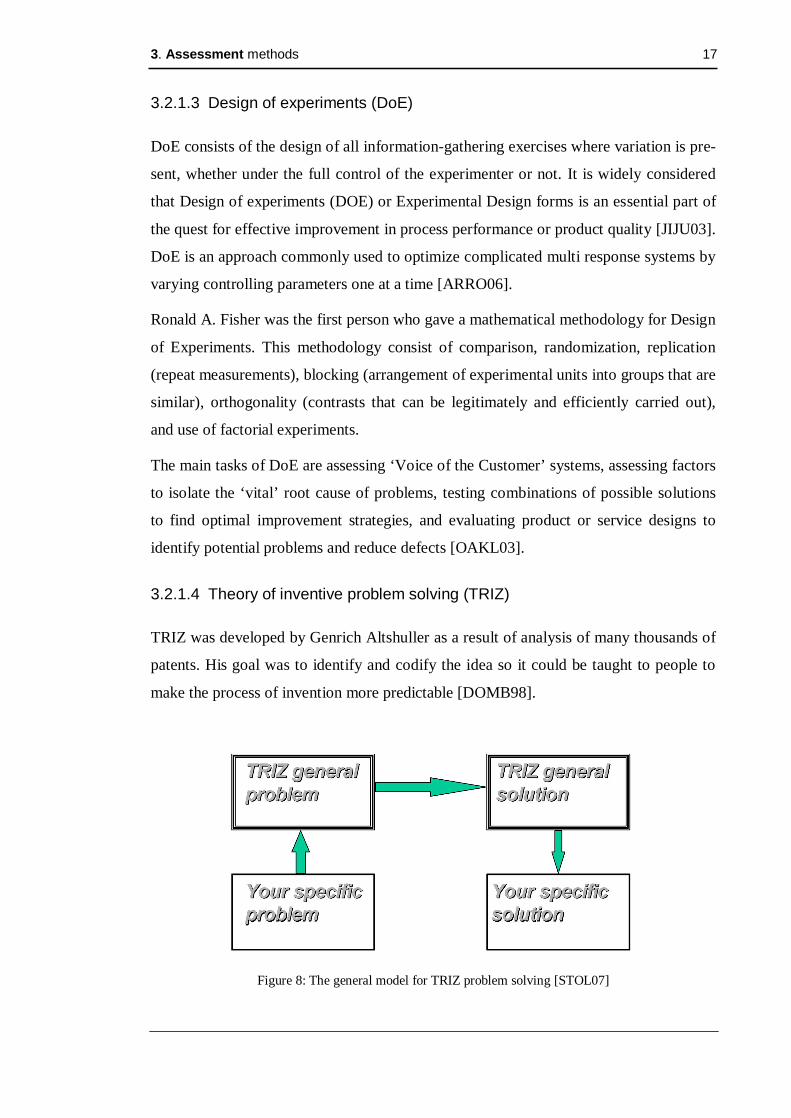
3.2.1.4 Theory of inventive problem solving (TRIZ)
TRIZ was developed by Genrich Altshuller as a result of analysis of many thousands of
patents. His goal was to identify and codify the idea so it could be taught to people to
make the process of invention more predictable [DOMB98].
Figure 8: The general model for TRIZ problem solving [STOL07]

3. Assessment methods 18
“TRIZ systematic approach to the concept development offers advantages of productiv-
ity, robustness and repeatability of the innovation process.” [STOL07].
Overall, the TRIZ body of knowledge contains 40 inventive principles, the laws of sys-
tems evolution, the algorithm of inventive problem solving, substance–field analysis,
and 76 standard solutions [STOL07]. It provides with tools and methods for use in prob-
lem formulation, system analysis, failure analysis and patterns of system evolution. Alt-
shuller discovered that system characteristics tend to evolve along “S” shaped curves
over the life time of the system. TRIZ has been used successfully in more than 500
companies.
3.2.2 Inspection Assessment Methods
Inspection Assessment Methods are procedures which, in opposite to design methods,
are focused on finding the roots and causes of problems present in products and ser-
vices, and they also try to give a solution to these problems and/or defects.
3.2.2.1 Six Sigma (6S)
Six Sigma is a business management strategy which “analyses the root causes of manu-
facturing and business problems/processes by eliminating defects” [OAKL03]. Six
Sigma is not just process-improvement techniques but methodology to make the pro-
jects become financial goals. [OAKL03] Each Six Sigma project developed in an or-
ganization follows a defined sequence of steps and has quantified financial targets.
It is possible to identify two main branches in the application of Six Sigma: the statisti-
cal model and the improvement process [TRUS03].
Figure 9: Principal facets of the Six Sigma initiative [TRUS03]

3. Assessment methods 19
Its main aim is to discover and remove the causes of defects and mistakes in manufac-
turing and business processes.
The methodology of Six Sigma uses the statistical theory and thus assumes that every
process factor can be characterized by a statistical distribution curve [TAGH06]. Six
Sigma improves the product driving toward six standard deviations between the mean
and the nearest specification limit [OAKL03]. Six Sigma also uses quality management
methods, such as analysis of variance, Failure Mode and Effect Analysis (FMEA),
Pareto Charts, histograms, and so on. It also creates a special infrastructure of people,
experts in these methods.
Six Sigma is widely used in companies all over the world, nevertheless there are several
criticisms of it. This criticisms base their arguments in such reasons as the lack of origi-
nality of the system, negative effects which some studies affirm were caused by Six
Sigma, its arbitrary standards.
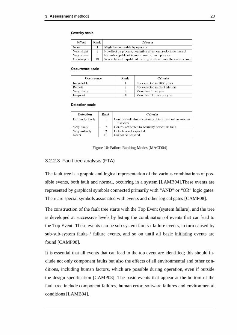
3.2.2.2 Failure Mode and Effect Analysis (FMEA)
Failure mode and effects analysis (FMEA) is used to identify equipment or system fail-
ures arising from component faults, in order to evaluate and prioritize the effects of fail-
ures according to the severity of the damage [MACD04].
FMEA techniques work by listing all possible failure modes of devices or components
followed by the cause of the failure mode, failure effect, criticality and failure rate. In
other words, failures are classified according to seriousness, frequency and how easily
they are detected.
FMEA must be updated whenever a new process/product is started, changes are made to
the operating conditions or in the design, when new regulations are made or when prob-
lems are detected be costumer feedback.
FMEA has several advantages, such as improving the quality, reliability and safety of a
product/process; improvement of company image and competitiveness; it increases the
user satisfaction; it reduces the time of system development and cost, etc.
In the other hand, one disadvantage of FMEA would be that if used as a top down tool,
FMEA may only identify major failure modes in a system; in this case Fault Tree
Analysis would be more appropriated.
3. Assessment methods 20
Figure 10: Failure Ranking Modes [MACD04]
3.2.2.3 Fault tree analysis (FTA)
The fault tree is a graphic and logical representation of the various combinations of pos-
sible events, both fault and normal, occurring in a system [LAMB04].These events are
represented by graphical symbols connected primarily with “AND” or “OR” logic gates.
There are special symbols associated with events and other logical gates [CAMP08].
The construction of the fault tree starts with the Top Event (system failure), and the tree
is developed at successive levels by listing the combination of events that can lead to
the Top Event. These events can be sub-system faults / failure events, in turn caused by
sub-sub-system faults / failure events, and so on until all basic initiating events are
found [CAMP08].
It is essential that all events that can lead to the top event are identified; this should in-
clude not only component faults but also the effects of all environmental and other con-
ditions, including human factors, which are possible during operation, even if outside
the design specification [CAMP08]. The basic events that appear at the bottom of the
fault tree include component failures, human error, software failures and environmental
conditions [LAMB04].
3. Assessment methods 21
Then, we have five steps involved by a FTA: definition of the undesired event to study,
understanding of the system, construction of the fault tree, evaluation of the fault tree,
and control of the hazards identified.
3.2.2.4 Statistical Process and Quality Control (SPC and SPQ)
Statistic Quality Control (SQC) is the application of statistical techniques to measure
and improve the quality of processes. SQC provides support analysis and decision-
making tools to help determine if a process is stable and predictable from shift to shift,
day in and day out, and from supplier to supplier [GREE04]. Statistic Quality Control
includes Statistical Process Control (SPC, effective method of monitoring a process
through the use of control charts), diagnostic tools, sampling plans and other statistical
techniques. It has enormous potential in terms of cost savings, improvements in quality,
productivity and market share [OAKL03].
3.2.2.5 Taguchi Methods
Genichi Taguchi has defined a number of methods to improve the quality of manufac-
tured goods, and lately they have been also applied to biotechnology. These methods
reduce costs and improve quality of manufactured goods simultaneously. Taguchi con-
siders that “the quality of a product is measured in terms of the total loss to society due
to functional variation and harmful side effects” [PILL03].
Taguchi's principal contributions to statistics are: the Taguchi loss-function, the phi-
losophy of off-line quality control, and innovations in the design of experiments.
The Taguchi loss-function is based on the assumption that when a functional character-
istic deviates from the specified target value, an economical loss is experienced due to
poorer product quality. This economic loss is expressed as a loss function. [PILL03].
Taguchi identified as the best opportunity to eliminate variation to be the product design
phase and its manufacturing process. Taguchi’s experiment designs are most exten-
sively used to determine the parameter values or settings required to achieve the desired
function [TRUS03].
The philosophy of off-line quality control affirms that the best opportunity to eliminate
variation is during design of a product and its manufacturing process. This leads to a
process of three steps: system design, parameter design, and tolerance design.

3. Assessment methods 22
Taguchi also created many methods for analysing experimental result, which included
new applications of the analysis of variance
3.2.2.6 Pareto Analysis
Pareto analysis is based on the Pareto Principle, which says that states that, for many
events, 80% of the effects come from 20% of the causes. It a statistical tool in decision
making that is used for selection of a limited number of tasks that produce significant
overall effect. It is used extensively by improvement teams all over the world. The tech-
nique is used to identify the most important problems and to establish priorities for ac-
tion [OAKL03].
Pareto analysis is a powerful ‘narrowing down’ tool but it is based on empirical rules
which have no mathematical foundation [OAKL03]. The problem-solver estimates the
benefit of each action, and then selects some of the most effective actions that give a
total benefit reasonably close to the maximal possible one.
The Pareto plot allows the detection of the factor and interaction effects which are most
important to the process or design optimization study. It displays the absolute values of
the effects, and draws a reference line on the chart. Any effect that extends past this
reference line is potentially important [OAKL03].
Figure 11: Pareto analysis by frequency [OAKL03]

3. Assessment methods 23
The steps to follow using Pareto Analysis are: a table listing the causes and their fre-
quency as a percentage, arranging the rows in the decreasing order of importance of the
causes, adding a cumulative percentage column to the table, plot with causes on x- and
cumulative percentage on y-axis, join the above points to form a curve, Plot (on the
same graph) a bar graph with causes on x- and percent frequency on y-axis, draw line at
80% on y-axis parallel to x-axis (then drop the line at the point of intersection with the
curve on x-axis. This point on the x-axis separates the important causes (on the left) and
trivial causes (on the right)).
3.3. Main ideas and tools from Assessment Methods
Assessment methods describe a procedure to evaluate a situation or process in order to
identify the weak points [TAYL06]. The goal of this section is to discretize the ideas
behind the main assessments methods used in the industry to understand the assessment
principles. The gathered knowledge would be used to evaluate a situation in a com-
pletely different field; the suitability of Sensor Concepts to reduce the severity of vehi-
cle accidents.
The previous chapter has provided an overview of the different methods used in the
industry. The following step is to expand our knowledge about assessment methods
through the definition of a common timeline of main ideas.
All the methods previously presented describe three main steps; the first step is to col-
lect data from meaningful sources, then it is necessary to present the data in some visi-
ble form and finally this data has to be analyzed in order to take decisions according to
the results. Each one of the three steps is presented along the chapter together with dif-
ferent tools. Figure 12 depicts the timeline described by Assessment Methods.
Figure 12: Common Timeline of Main Ideas

3. Assessment methods 24
3.3.1 Collecting Data
Collected data is the basis for analysis, decision and action since it’s the information
used to discover the actual situation. It’s a very important step because the whole study
depends on the collected information [OAKL03].
The methods of Collecting Data and the amount collected must be taking into account
before any measure is taken. It is necessary to be 100% sure that the data collected is
representative of what we want to measure, meaning that the reasons for collecting data
and the correct sampling techniques are crucial to obtain meaningful results [OAKL03].
There are three aspects that contribute to the gathering of relevant data as it can be seen
in Figure 13: description of the process, timeline and analysis of the problem’s causes
Figure 13: Collecting Data
3.3.1.1 Description of the process
The first step to analyze a system is to understand how it really works. This is a very
important step because the rest of the study depends on its quality. We have to identify
and link all the components of the system in order to describe the process as good as
possible. There are mainly two ways: Process Mapping and Process flowcharting. Proc-
ess mapping is a communication tool where different steps from the process are repre-
sented in blocks connected by arrows that represent specific actions. While Process
flowcharting is a schematic representation of a process divided into different lanes de-
scribing defined areas, usually control areas; the different actions will be link showing
the order of the process.

3. Assessment methods 25
3.3.1.2 Timeline
The timeline tools provided an overview of the process along a fix period of time. The
objective is to find the progression of the process and measure the time requirements for
every step of the whole process. The analysis of the timeline allows detecting irregulari-
ties and opportunities for improvement.
The record of data through time can be done with check sheets; documents designed for
the quick, easy and efficient collection of information. The main characteristic relies on
the use of check marks to evaluate situations and on the capability to collect data in real-
time. Other possibility is to use a functional time-line flowchart which is basically a
process flowchart considering the time factor. Each step of the process will have a cor-
responding time that has to be measured and documented.
3.3.1.3 Analysis of the problem’s causes
The analysis of problems’ causes studies in depth the origins when there is a sign that
something is not working properly. The identification of the causes is not always obvi-
ous and different tools can help recognize them. Among the possible tools to identify
the problems’ causes stand out the following tools: cause and effect diagram, the fault
tree diagram and brainstorming.
The cause and effect diagram, also known as the Ishikawa diagram (after its inventor),
or the fishbone diagram (after its appearance) is a graphic tool. It shows the effect at the
head of a central ‘spine’ with the causes at the ends of the ‘ribs’ which branch from it
[OAKL03].
The fault tree diagram (FTA) is a graphic tool starting with a Top Event (system fail-
ure); followed by successive sub-levels representing the possible combination of events
leading to the system failure [CAMP08].
Brainstorming is a group technique oriented to the conception of new creative ideas and
it can be used to identify the causes of a problem. This tool combines the creativity of
each participant in order to reach the desired outcome.

3. Assessment methods 26
3.3.2 Presenting Data
After data is collected, data should be presented in a form that will simplify the subse-
quent analysis. Charts, tables, graphs are tools capable of providing a visual representa-
tion of thousands of measurements. It’s necessary to decide how the data will be repre-
sented because it would help us to extract information. Figure 14 illustrates how Pre-
senting Data is divided in two different proceudres: the normal representation of the
variation and the representation of the variation in time series.
Figure 14: Presenting Data
3.3.2.1 Representation of the variation
Variation is the degree to which the data is spread out. The representation of the varia-
tion provides a visual view of the distribution of data and allows having a first impres-
sion of data.
Among the graphic tools bar charts and histograms (column graphs) are the most com-
mon formats for illustrating comparative data. They are easy to construct and to under-
stand. Column graphs are usually constructed with the measured values on the horizon-
tal axis and the frequency or number of observations on the vertical axis, while in a bar
chart the bars extend horizontally. When there are a large number of observations, the
graphic tools are often more useful to present data in the condensed form of a grouped
frequency distribution [OAKL03].
3.3.2.2 Representation of the variation in time series
The representation of the variation in a time series allows controlling the evolution from
data along a fix period of time. The typical tools to represent the variation along a pe-

3. Assessment methods 27
riod of time are graphs where different variables would be introduced. A graph allows
the comparison from samples taken at different times and provides a visual view of how
the variables change [OAKL03].
3.3.3 Analyzing Data
Analyzing data presents many challenges to professionals because gaining understand-
ing of a system or process is a complex procedure. The most common used tool are sta-
tistical methods because they will help us meet the requirements to reach a specified
purpose and draw conclusions from the resulting information.
There are three questions that we have to ask ourselves: which are the most relevant
factors? What are the relationships between factors? Which variations to control and
how? [OAKL03]. These questions lead to the differentiation between factors, analysis
of dependency relationships and the evaluation from the variation. Figure 15 depicts
different procedures to Analyzing Data.
Figure 15: Analyzing Data
3.3.3.1 Differentiate between factors
Processes and systems are usually composed from several factors. It is necessary to
make a distinction between important factors and trivial factors. Trivial factors require
our attention because they are crucial to the development of the process.
There are different methods that can help identify the most important factors such as
Pareto analysis (identify the crucial factors), Main effects plot (compare the relative

3. Assessment methods 28
strength of the effects of various factors) and Cube plots (determine the best and the
worst combinations of factor levels) [JIJU03].
Other methods such as House of quality and FMEA accomplish the same goal of classi-
fication through a different procedure. The house of quality (HOQ) correlates customer
needs and product characteristics to assess the relationship (or impact) of the measures
on the needs [DORF01]. FMEA techniques allow the ranking of the different failure
modes through the severity (consequences) and occurrence (probability of happening)
of the different failure modes.
3.3.3.2 Analyze the dependency relationships among components
Processes and systems subject to be analyzed usually present a large number of compo-
nents. Variables usually present dependencies not easy to detect at first sight and re-
quires an analysis to identify the relationships.
The conventional procedure to locate relationships among components is the collection
of data from different variables and the execution of tools to identify dependencies. Two
of these tools are interaction plots and scatter diagrams. Interaction plot is a graphical
tool plotting the mean response of two factors at all possible combinations of their set-
tings and if the lines are parallel, then it connotes that there is an interaction [JIJU03].
Another tool is the scatter diagram, where all the values from two variables for a set of
data are plotted on a graph and the location of the values suggests different kinds of
correlations: positive (rising), negative (falling), or null (uncorrelated) [OAKL03].
3.3.3.3 Evaluate the variation of the process
The evaluation of the variation is crucial to maintain the ideal performance of a process
or system. The variation is the degree to which the different parameters can change
overtime. The monitoring of the process and the identification of process changes en-
sures the right development of the process or system [GALE01].
The main tools used to control the variation of the process are Control Charts and analy-
sis of variance (ANOVA). Control Charts provide visual representations of how a proc-
ess varies over time or from unit to unit. On the charts control limits separate natural
variations from unusual variations allowing to identify unusual sources of variation.
[GALE01] Another tool typically used is the analysis of variance (ANOVA); a statisti-

3. Assessment methods 29
cally based decision tool for detecting differences in average performance of groups of
items tested. It is usually carried out to interpret experimental data and factor effects.
[PILL03].
4. Description of the system 30
4 Description of the system
Vehicle accidents usually lead to unfortunate and terrible consequences; severe injuries
and death, as well as a high economic cost. The prevention from vehicle accidents pre-
sents many challenges to the automobile industry; however, Collision Avoidance Sys-
tems are means to improve safety. These systems process information from the envi-
ronment to activate braking and steering systems.
CA Systems process information from the environment through the use of sensors. Dif-
ferent sensors are often suitable to be used in a CA System, therefore the necessity of a
procedure to evaluate sensors. The choice of the right sensor is crucial to the cost, to
the performance and to the benefit of the Collision Avoidance System.
Assessment methods describe a procedure to evaluate a situation or process for decision
making [TAYL06]. Different Assessment Methods have been presented and a common
timeline of main ideas has been developed.
During this chapter Sensor Concepts and the outline of main ideas come together into
the development of an Assessment Method to evaluate the suitability of sensors for CA
Systems. The goal from the timeline of main ideas is to apply the ideas used in other
fields to evaluate Sensor Concepts. The three steps (Collecting Data, Presenting Data
and Analyzing Data) are developed and adapted to sensor concepts. While collecting
data, different sets of inputs are defined. Presenting data describes the procedure to ob-
tain final ponderated values for each set of inputs. Analyzing data represents graphically
the results obtained and allows one to draw conclusions.
4.1. Collecting Data
One of the main factors leading to selecting the right sensor is the performance of the
sensor. The performance depends on the reliability of the sensor properties and on the
effect that External Factors can cause. Other relevant factors to be taken into considera-
tion are the general characteristics of sensors such as price, size, weight, and power con-
sumption. It is possible for these factors to have considerable influences on the decision
making.
While collecting data sensor properties are analyzed to identify two sets of inputs which
are representative of CA Systems; the general properties of sensors and the benefit of

4. Description of the system 31
the CA System. Different procedures are presented to collect data for each one of these
sets of inputs.
4.1.1 Description and interaction of sensor properties
The main Sensor Concepts used in Collision Avoidance Systems have been presented in
chapter 2. The following objective is to describe a set of characteristics common to the
Sensor Concepts previously presented. The different features can be classified in three
classes: General Properties, performance properties and External Factors. The next step
is to define the manner in which these properties come together in a system to proceed
with an assessment between different sensors.
4.1.1.1 Sensor properties
4.1.1.1.1 General Properties
The General Properties refer to those features having no direct connection with the per-
formance of the sensor. This set of properties defines those characteristics of the sensor
not participating in any kind of the measurement mechanisms. Table 3 depicts the most
important General Properties. This group of features contains a relevant role in the sys-
tem because they represent critical factors on decision making.
General Properties Units Price Euros
Size (Height, Width, Depth) m
Weight Kg
Power Consumption W
Voltage V
Temperature for storage °C
Table 3: List of External Factors [STROB04]
4.1.1.1.2 Performance Properties
The Performance Properties are directly linked to the performance of the sensor. These
features are responsible for object detection and the calculation from position, speed,

4. Description of the system 32
etc. Each Sensor Concept has different features but it is possible to divide them in two
main groups: the sensors using some kind of wave (RADAR, LIDAR and Ultrasound)
and the sensors using camera systems (Video and PMD). Table 4 and table 5 demon-
strate the main Performance Properties for wave systems and video systems respec-
tively.
Performance Properties (RADAR, LIDAR and Ultrasound) - Wavelength
- Resolution Number of beams
- Horizontal Performance Field of view, Beam width, Accuracy, Separation, Resolution
- Vertical Performance Field of view, Beam width, Accuracy, Separation, Resolution
- Ranging and detection Coverage, Accuracy, Separation, Resolution
- Measuring of relative speed Coverage, Accuracy, Separation, Resolution
- Measuring of relative accelera-tion
Coverage, Accuracy, Separation
- Acquisition delay Position, Speed, Acceleration
- Update rate
- Maximum number of targets tracked
Table 4: List of Performance Properties for RADAR, LIDAR and Ultrasound
Performance Properties (Video and PMD) - Spectral Sensitivity
- Resolution (Video) Pixels, Number of lines
- Optics Horizontal field of view, Vertical field of view, Zoom, Focal Length
- Sensitivity
- Dynamic range Intra-scene, Inter-scene, Accuracy, Resolution
- Acquisition delay
- Update Rate
Table 5: List of Performance Properties for video and PMD [STROB04]
4.1.1.1.3 External Factors
The External Factors are influences capable of altering the performance of the sensor to
some degree. The physical principles explaining the working mechanism of sensors is
directly linked to the limits of each technology. For example, poor light decreases the
capability of video to characterize objects and dirty objects are not detected by LIDAR.

4. Description of the system 33
The influence of the External Factor and the degree of this effect changes from one Sen-
sor Concept to the other. Table 6 outlines the most relevant External Factors.
Table 6: List of External Factors
4.1.1.2 Interactions of the properties
As it has been presented, the Performance Properties and the External Factors are con-
nected to the performance of the sensor while the General Properties are completely
independent. This statement helps identify two separate directions over the course of the
study: the first consists of the evaluation of the General Properties while the second
consists of the analysis from sensor performance.
The evaluation of sensor performance can only be completed through driving tests or
simulations. Due to the difficulty to reproduce External Factors, a computer simulation
has been considered to be the best solution. The simulation is used to represent the most
typical vehicle accidents and the analysis from the results provides the benefit presented
by the system for different types of accidents.
After the completion from the simulation, two different sources of information are
available: the General Properties and the benefit of the collision. The two data sources
for different sensors come together in an assessment method. The technique evaluates
the data and identifies the most suitable Sensor Concept to Collision Avoidance. Figure
16 details the different components of the system, focusing on the inputs (sensor proper-
ties), the output (the suitability of the system) and the steps in between (simulation tool
and assessment method).
External Factors - Weather Influences Rain, Snow, Wind, Fog, Floods, High humidity, etc.
- Temperature
- Light Poor light (Dusk, Dawn,..), Night (Night Drive)
- Medium dependency Air (Ultrasound)
- Reflexion problems Dirty Cars, Angle surface who does not allow reflexion, No reflecting surfaces
- Interferences Noise
- Power Limitation Security factors (Eyes)

4. Description of the system 34
Figure 16: Block diagram of the system including the main tools
4.1.2 Definition of the first set of inputs: General Properties
The General Properties of sensors refer to all the features not participating directly on
the performance of the sensor. However, they have an important relevance in the selec-
tion of sensors for Collision Avoidance Systems.
The evaluation of General Properties is done through the application of the Assessment
Method, as it can be seen in Figure 17. Before the application, it is necessary to deter-
mine the most relevant General Properties and their values for the different sensors.
Figure 17: Block diagram of the system focusing in the General Properties
There are a large number of features that can be considered General Properties. Among
all General Properties, it is necessary to decide which properties are relevant to the
study and which properties are not. The selection should be carried out through the
comparison of each general property among a large number of sensors. The information
required to carry out the comparison is obtained from sensor data sheets. The properties

4. Description of the system 35
presenting different values for the different sensor concepts would be considered, while
the properties with similar values would be excluded.
4.1.3 Definition of the second set of inputs: Benefit of the CA System
As it has been explained previously, the performance of a CA System is directly linked
to the Performance Properties of sensors and the External Factors. The goal is to evalu-
ate the performance of sensors, therefore the benefit presented by CA Systems.
The means to evaluate the performance of Sensor Concepts is a computer simulation
due to the difficulty to replicate External Factors in real driving tests. Figure 18 depicts
the block diagram of the whole system, where it can be seen that the Performance Prop-
erties and the External Factors come together into the simulation. The simulation pre-
sents other advantages such as time, calculation speed, price, etc.
Figure 18: Block diagram of the system
One of the tasks from this Thesis is to develop an assessment capable of evaluating the
results of the simulation. This information is extremely valuable to automobile manu-
facturers because it illustrates which sensor could deliver the best benefit in a CA Sys-
tem.
Automobile companies are interested in the benefit presented by Collision Avoidance
Systems which is linked to the performance of Sensor Concepts under typical vehicle
accidents. The focus from this study is directed to typical traffic accidents, since they
are responsible for a large number of injuries, deaths and costs. The possibility to simu-
late different car accidents under the functionality of different Sensor Concepts can pro-

4. Description of the system 36
vide information pertaining to which sensor is able to perform better under typical vehi-
cle accidents.
4.1.3.1 Simulation Tool
4.1.3.1.1 CarMaker
The simulation tool CarMaker assist companies in the automobile industry to the devel-
opment of vehicle systems in cars. CarMaker is a professional simulation tool suited for
the modelling and simulation of vehicles. It has been available since 2001 and it is
commercialized by IPG Automotive [IPG_08].
CarMaker contains a wide range of ready-to-use vehicle models ranging from compact
cars to vans. The IPG CarMaker graphical user interface (GUI) allows to remodel and
change specific parameters to be able to simulate accurate models. The tool offers the
classical vehicle dynamics simulation as well as a large range of applications using
Model, Software and Hardware-in-the-Loop simulations. The tool is mainly used for the
development and testing of chassis control systems, driver assistance systems, fuel con-
sumption analysis and emerging hybrid technologies [IPG_08].
CarMaker is easy to use and does not require additional programming. The existing in-
terface uses Matlab/Simulink allowing a fast implementation. Another advantage is that
IPG Automotive brings out new updates with new functionalities for CarMaker
[PUSI07].
4.1.3.1.2 Suitability of CarMaker to simulate Collision Avoidance Systems
At the conference “Active Safety through Driver Assistance 2008” IPG Automotive
first presented the latest development stage of the traffic simulation module, IPGTraffic.
The module is suited for the model based development of advanced driver assistance
systems, such as adaptive cruise control (ACC), lane change assistance, brake assis-
tance, assisted parking, intersection assistant, congestion assistant or pre-crash systems
[IPG_08].

4. Description of the system 37
Figure 19: Scenarios from CarMaker [IPG_08]
The object simulation capability IPGTraffic within CarMaker enables the interactive
generation of arbitrary traffic scenarios and is well suited for the testing of different
advanced driver assistance systems with object detection. The control systems and the
dedicated sensors can be integrated easily and quickly into the virtual test vehicle. De-
pending on the development stage and the test objective they are tested by model-,
software- or hardware-in-the-loop in different driving situations and traffic scenarios
[IPG_08]. The traffic scenarios contain an arbitrary number of moving objects (e.g. traf-
fic, pedestrians) and stationary obstacles (e.g. parking cars, crash-barriers, traffic signs
and buildings) [IPG_08].
4.1.3.2 Selection of typical vehicle accidents
At this point, the attention is focused on the most typical vehicle accidents. The simula-
tion tool is used as a reliable tool to represent real life vehicle crashes. The results of the
simulation provide numerical data on the performance of sensors for several accidents.
The present goal is to simulate the most typical vehicle accidents under different sensors
to evaluate the degree to which they are capable of mitigating the accident. The analysis
of vehicle accidents presents many difficulties due to the lack of data. Nevertheless,
accident statistics exist and the data required to design the different accident scenarios is
obtained from two German studies; DESTATIS and GIDAS. These data sources allow
to identify the main characteristics of the accidents needed for the design of the scenar-

4. Description of the system 38
ios. Once a complete accident study has been carried out, it is necessary to define the
requirements for the design of the scenarios. The next step is the execution from the
different simulations and the gathering of results. An analysis of the results identifies
the benefit presented by each sensor.
4.1.3.2.1 Accident Statistics
Since the aspiration is to discover which sensor performs better under typical accidents,
accident data is an excellent information source for the design of the scenarios. As pre-
viously noted accident data comes mainly from two sources: DESTATIS (Accident sta-
tistics of German federal agency for statistics) and GIDAS (German In-Depth Accident
Study).
DESTATIS are accident statistics from the German Federal Statistical Office containing
all the accidents with personal damage in Germany. The accidents are subdivided by
accident type and accident kind. Accident type refers to the conflict or situation leading
to accident while accident kind is the position or accident constellation. The study also
contains records of time, locality of accident, data of involved persons and environment
conditions [PUSI07].
German In-Depth Accident Study (GIDAS) is a project of BAST (Bundesanstalt für
Straßenwesen) and FAT (Forschungsvereinigung Automobiltechnik e.V.). The study is
focused in accidents occurring around the areas of Hannover and Dresden. It contains
very detailed recordings allowing the reconstruction of every single accident. The data
sets include environment conditions, traffic regulation, crash information, kinematic
data, injuries, accident sequence and causes [PUSI07].
4.1.3.3 Design of the scenarios
The design of the scenarios determines the outcome of the entire analysis. An in depth
study on accident data (DESTATIS and GIDAS) is required to collect as much data as
possible on accident types.
All the characteristics from the accidents have to be clearly specified: Participants of the
accident (vehicle-vehicle, vehicle-pedestrians, vehicle-pole, etc.), road characteristics
(straight road, curve, inclination, etc.), weather conditions (rain, snow, wind, fog, etc.),
etc. All this information is used to define a specific scenario for each accident.

4. Description of the system 39
During this section, the requirements of the scenarios on the simulation are explained in
detail as well as the need of different cases to represent an accident accurately.
4.1.3.3.1 Requirements of the scenario on the simulation
In order to have the simulation done properly, some deliverables of the environment
model are required. For instance, in roads and intersections the deliverables required
would be lane markings, the road edge, construction areas (with multiple markings and
narrow lanes).
As far as traffic participants are concerned, we should count on several types of partici-
pants, such as pedestrians, motorcycles, cars, trucks, etc. All the information on these
participants must be specified such us dimensions (length, width and height), positions
(where all of them are placed), speeds and directions.
We also have to be aware about side objects to make the scenario the most realistic pos-
sible, meaning that the simulation must have traffic lights, houses, trees, guardrails, and
all the things we normally find on the roads.
4.1.3.3.2 Design of the different cases for every scenario
Once the different scenarios have been designed, it is required to prepare a set of simu-
lations for each scenario, which from here on will be referred to as the cases of a sce-
nario. Real life accidents might be grouped in types of accidents, but we should never
forget that each accident is unique. For example there are a lot of rear-end crashes in
road traffic between two mid-size cars during heavy rain, but they all differ on the speed
of the cars, intensity of road traffic, characteristics from the mid-size cars, intensity of
rain, etc.
In order to replicate an accident accurately, it is necessary to identify a set of decisive
properties where the variation of the accident remains such as speed of the vehicles,
distance between vehicles, etc. Without altering the characteristics of the accident, dif-
ferent values are assigned to these properties allowing to represent the largest amount of
possible cases for a specific accident.
When a single simulation is executed, the result obtained from the simulation tool is the
impact speed from the vehicle into an object. The execution from the set of cases for a
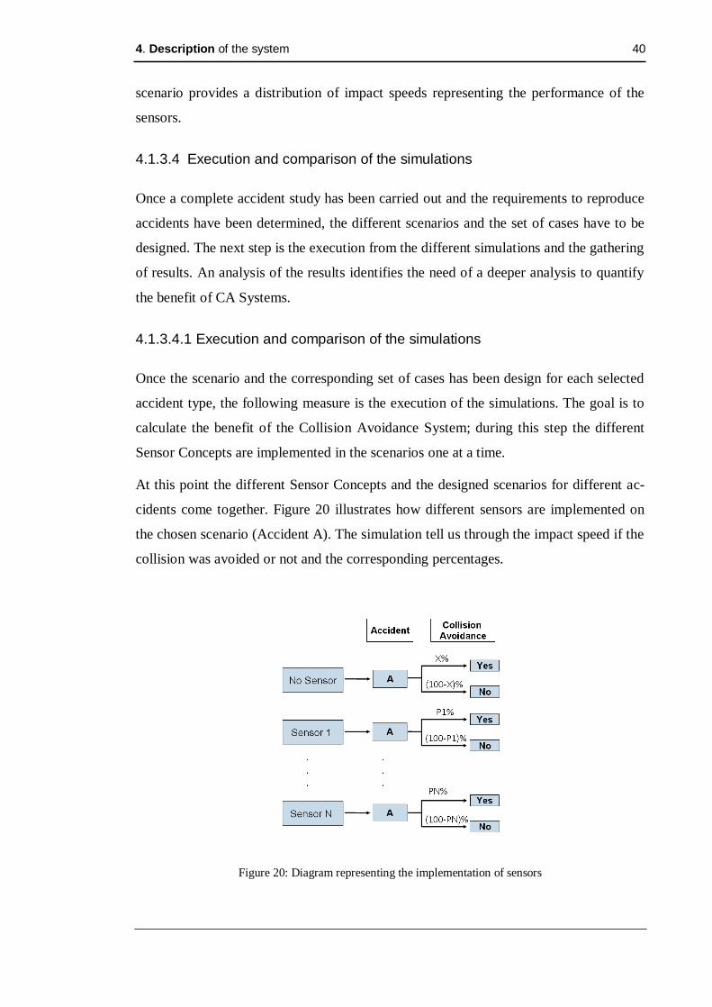
4. Description of the system 40
scenario provides a distribution of impact speeds representing the performance of the
sensors.
4.1.3.4 Execution and comparison of the simulations
Once a complete accident study has been carried out and the requirements to reproduce
accidents have been determined, the different scenarios and the set of cases have to be
designed. The next step is the execution from the different simulations and the gathering
of results. An analysis of the results identifies the need of a deeper analysis to quantify
the benefit of CA Systems.
4.1.3.4.1 Execution and comparison of the simulations
Once the scenario and the corresponding set of cases has been design for each selected
accident type, the following measure is the execution of the simulations. The goal is to
calculate the benefit of the Collision Avoidance System; during this step the different
Sensor Concepts are implemented in the scenarios one at a time.
At this point the different Sensor Concepts and the designed scenarios for different ac-
cidents come together. Figure 20 illustrates how different sensors are implemented on
the chosen scenario (Accident A). The simulation tell us through the impact speed if the
collision was avoided or not and the corresponding percentages.
Figure 20: Diagram representing the implementation of sensors

4. Description of the system 41
The distribution of impact speeds obtained from the simulation of one scenario repre-
sents the performance of the Sensor Concept. The performance by itself does not illus-
trate the benefit of the system. The comparison of the distributions from different sen-
sors in respect to the distribution when no sensor used, allows to evaluate the quality of
the sensor. It is the contrast in respect to a case where no sensor is used which shows the
difference and therefore the benefit of the tested Collision Avoidance System. Figure 21
shows how the previously mentioned situations provide respectively different distribu-
tion of impact speeds.
Figure 21: Distribution of impact speeds
A direct comparison between distributions corresponding to different sensors is also
possible. The obtained values, relative to one of the Sensor Concepts, represent the dif-
ferences on the capability to mitigate accidents between the two sensors. If the results
from the simulation from different sensors are referred to the same sensor, the benefit
from the different sensor can be compared. In this case, it is necessary to become aware
of the limitations since the obtained values remain relative to one sensor.
The graphical representation of the distributions and their comparison allow to visualize
the benefit of the system but it does not present an easy procedure to quantify the bene-
fit of the CA System. Each distribution represents the overall performance of the CA
System for a large number of cases and the graphical comparison in respect to another

4. Description of the system 42
distribution shows the differences between the two situations. The study requires to
quantify the benefit, and the graphical comparison of two curves does not present any
possibilities to quantify the benefit. The difficulties lead to the need of a deeper analysis
to quantify the benefit of the CA System.
4.1.3.4.2 Simulation Analysis
As it has been explained previously, the direct impact speeds represent the performance
of the sensor but they are not able to quantify the benefit of the system. The review
method requires an index which is capable to quantify the benefit of the Collision
Avoidance System. This situation leads to the need of a new step between the simula-
tion and the review method called the Simulation Analysis.
During this section, different possibilities to calculate the benefit of the system are iden-
tified. Then every possible index is explained and analysed to select the most represen-
tative index. Once the right index has been chosen, the procedure which transforms the
impact speeds on the benefit of the system is presented.
Figure 22: Block diagram of the system
4.1.3.5 Research on the right index for the benefit
The right index is a measure capable of quantifying the benefit of the system. Three
possible indices have been identified: reduction of injury levels, accident costs savings
and decrease of the impact speed. The three possibilities are analysed focusing on the

4. Description of the system 43
correlation between the indices and the results of the simulations, as well as the capacity
to quantify the benefit of the system.
4.1.3.5.1 Reduction of injury levels
The accident severity informs on the injuries’ degree from the different participants af-
ter a vehicle crash. The are mainly two scales to characterize the severity of an accident:
KABC Scale and the Abbreviated Injury Scale (AIS), as it can be seen in tables 7 and 8
respectively.
SEVERITY DESCRIPTOR
K Fatal
A Incapacitating
B Evident
C Possible
PDO Property Damage Only
SEVERITY DESCRIPTOR AIS 6 Fatal
AIS 5 Critical
AIS 4 Severe
AIS 3 Serious
AIS 2 Moderate
AIS 1 Minor
Table 7: KABC Scale [VTPI07] Table 8: AIS Scale [VTPI07]
There are many factors which determine the severity of an accident and the impact
speed is one of the most important. At first sight it makes sense to say that a correlation
could be found between impact speeds and injury levels, and then the benefit of the sys-
tem could be quantified as the reduction of the accident severity.
The VITES Project (Virtual Testing for Extended Vehicle Passive Safety) has studied
the differences between predicted injuries and real measured values [VITE04]. They
have come to the conclusion that it is not possible to correlate the impact speeds to in-
jury levels. The same impact speed can lead to different kinds of injuries depending on
factors such as size, age and gender of the driver.
Injury scales intend to evaluate the severity of an accident in respect to the injuries en-
dured by the occupants after the accident has taken place. Unfortunately, this type of
data is not provided by the simulation when an accident is simulated, instead we have
all the parameters characterizing the accident and the impact speed of the car. The im-
pact speed is a valuable source of information but it does not give any kind of informa-

4. Description of the system 44
tion on the consequences of the accident. Therefore, the reduction of injury levels can-
not be used to represent the benefit of the system.
4.1.3.5.2 Reduction of the accident cost
Every time an accident occurs, the results can be divided in direct and indirect conse-
quences. Direct consequences from the crash of one or more vehicles are the injuries
endured by the occupants. Also there are indirect consequences consisting of all the
measures which need to be taken such as the need of ambulances, police, fireman, etc.
including the alterations caused by the accident. There is only one value capable of
quantifying direct and indirect consequences of the accident; the cost of the accident.
Crash costs can be divided into internal (damages borne by the individual who uses a
particular vehicle), external (damages and risks borne by other road users), and insur-
ance compensation (damages compensated by insurance). Figure 23 indicates how vari-
ous crash costs are categorized in market and non-market. [VTPI07]
Figure 23: Categories of Crash Costs [VTPI07]
The cost and the classification upon their different categories is the best indicator of the
consequences of an accident, since it considers all the factors resulting from the crash.
In 2002 the “Cost-Benefit Analysis of Road Safety Improvements” report for the Euro-
pean Union estimated the costs per fatality which results can be seen in Figure 24
[ICFC03].

4. Description of the system 45
Figure 24: Estimated costs per fatality or injury, 2002 Euros [ICFC03
In our specific case, the simulation tool does not provide any kind of information on the
consequences from the accident, in fact it only provides an impact speed. As it has been
explained prior the same impact speed can lead to different injury levels and conse-
quently to different cost levels. Even if cost would be the best index to quantify the
benefit of the system, since there is no correlation possible between the impact speed
and the cost, this option has to be rejected.
4.1.3.5.3 Difference of impact speed
As previously explained, the difference between distributions of impact speeds shows
visually the benefit of the system, but it does not present an easy way to quantify the
benefit. The idea is to compare single cases from a scenario, instead the whole distribu-
tions of impact speeds.
It has been explained previously the necessity to simulate a set of different cases for
every scenario in order to replicate all possible variations during a vehicle crash. The
impact speed for one single case represents the performance of the system for that spe-
cific case, but the mitigation capacity of the CA System cannot be calculated. The same
problem occurs when the whole set of cases is simulated to obtain a distribution of im-
pact speeds. It is the comparison with the cases where no sensor is used which allows to
quantify the benefit of the system.
It is possible to compare the distributions of impact speeds corresponding to the simula-
tions where a CA System was implemented and another where it was not. Actually if
the two distributions are represented graphically, the mitigation capacity of system dur-
ing the accident is represented by the differences between the distributions. The prob-
lem is the difficulty to quantify the benefit since we are talking about two distributions
representing each one of them a set of cases.

4. Description of the system 46
Instead of comparing distributions of impact speeds, it is considered appropriate to
compare the impact speeds for single cases. The same case is simulated two times; the
first time implementing a CA System and the second time without it. The subtraction
between the impacts speeds tells us how much was the impact speed reduced with the
use of the CA System. The same process is repeated for the other cases of the scenario.
At the end it is possible to calculate the average which represents the mitigation capac-
ity of the CA System for a specific accident.
4.1.3.6 Calculation and application of the benefit index
Different possible indices to represent the benefit of the study have been presented but
not all of them adjust to the available data. The reduction of injury levels and accident
costs savings could represent the benefit of the system but they have been rejected due
to the impossibility to be correlated with impact speeds. The difference between impact
speeds has been considered the most representative index for the benefit of the system
and in following sections it would be presented in depth.
The goal from this section is to obtain a final value which represents the benefit of CA
Systems in respect to no system at all. As it has been explained earlier, the difference of
single impact speeds and the calculation of the average for the whole set of cases has the
ability to assign a numerical value to what is considered to be the benefit of a CA Sys-
tem.
The first step consists in the simulation of an aleatory case of a specific scenario. This
case is simulated twice; the first time with no sensor and the second time with one sen-
sor. The difference between the resulting impact speeds is calculated as in Formula 1.
The impact speed difference provides the mitigation capacity of the system in m/s.
Case X No CA System- X CA System- XCase CaseV V V
Formula 1: Impact speed difference
It is also possible to obtain the impact speed reduction in percentage which is a more
representative value of the mitigation capacity of the system. Formula 2 depicts the re-
quired terms.

4. Description of the system 47
No CA System- X CA System- X X
No CA System- X
(%) 100%Case CaseCase
Case
V VV
V
Formula 2: Mitigation capacity in percentage
The same procedure would be carried out with the rest of the cases from the scenario.
Table 9 illustrates for each case the corresponding impact speeds and how the mitiga-
tion capacity is calculated.
Cases from the scenario
Impact Speed using
sensor Impact Speed
not using sensor Reduction of impact speed in percent-
age
Case 1 VCA System-1 VNo CA System-1 No CA System-1 CA System-11
No CA System-1
(%) 100%V V
VV
Case 2 VCA System-2 VNo CA System-2 No CA System-2 CA System-2
2No CA System-2
(%) 100%V V
VV
... .... .... ....
Case N VCA System-N VNo CA System-N No CA System-N CA System-N
No CA System-N
(%) 100%N
V VV
V
Table 9: Calculation from the difference between impact speeds
Once the collision capacity of the system has been obtained for each case of the sce-
nario, an average for the scenario is calculated. Formula 3 depicts how to calculate the
mitigation capacity of the sensor for a specific scenario. The same procedure would be
carried out for each scenario and for each sensor.
0
N
iT
ViV
N
Formula 4: Average of impact speed differences

4. Description of the system 48
4.2. Presenting Data
Presenting Data defines in first place the requirements imposed by the set of inputs
(General Properties and Benefit) on the Assessment Method. The main requirement is
the need of a procedure to evaluate each set of inputs.
The selected procedure is a review method based in product development techniques. It
assigns scale values and weights to the different inputs. At the end, the review provides
a final weighted value representing the whole set of inputs for each sensor. This value
can be used to compare a set of inputs for different sensors.
4.2.1 Requirements to the Assessment Method
The assessment method has two sets of inputs for each sensor: the General Properties
and the benefit of the system for several accidents. The characteristics from the two sets
of data establish several requirements on the choice and/or development of the appro-
priate assessment method.
The first requirement consists of the distinction between the two sets of inputs of the
assessment method. The General Properties and the benefit of the system for several
accidents present different characteristics and they cannot be assessed together. As
shown in figure 25 the assessment method is divided into two review methods.
Figure 25: Block diagram of the system focusing on the assessment method

4. Description of the system 49
The following two requirements focus on the single review method:
- The review method should allow the comparison among inputs. There is considerable
amount of General Properties, as well as a large number of typical vehicle accidents and
not all of them have the same relevance. The review applied to each one of these sets of
data should allow comparing different inputs, General Properties and accident types
respectively.
- Another requirement of the review consists on the capacity to combine different inputs
in one output. Every set of inputs contains a considerable number of variables resulting
in difficulty when comparing the sensors. Grouping different values in one overall value
will make things easier. At the end, there will be a final value for each sensor which
represents all the General Properties, while other final value represents the benefit of the
sensor.
The last requirement is the need of a last step, able to combine the results from each of
the review methods; this technique is referred to as a ranking method. The ranking
method compares and ranks the different sensors upon their suitability to collision
avoidance.
4.2.2 Application of the Review
An assessment method is a procedure considering different aspects of a process or sys-
tem to carry a consequent evaluation with collected coherent data. The development of
an assessment method to evaluate the cost, the performance and the benefit of Collision
Avoidance Systems is the pillar for this Thesis. The proposed assessment method is
based on product development techniques used to make a selection upon different new
product possibilities. [BIRK06].
The adapted assessment method to evaluate Sensor Concepts is divided into two review
methods (directed to the General Properties and the benefit of the system) and a ranking
tool. Each review method provides a final value for each sensor representing the Gen-
eral Properties and another value standing for the benefit of the system. All the sensors
and its weighted values are plotted on a 2-D graph for comparison purposes and for
ranking of the different sensors.

4. Description of the system 50
Figure 26: Block diagram of the system
The Review Method is a five step process that assigns scale values and weights to the
different inputs. The result is a ponderation of values from the different inputs to obtain
a final and unique value representing each sensor.
4.2.2.1 Inputs Matrix
The Inputs Matrix assigns values to several inputs according to the available data
sources [BIRK06]: In the case of the General Properties data sheets, the results from the
simulations would be used for the benefit of the system.
In Table 10 the different inputs should be defined (general sensor properties and types
of accidents in each one of the two reviews), as well as the different sensors. It is possi-
ble to consider as many sensors as necessary belonging to any Sensor Concept and/or
manufacturer. The cells are filled with the information sources previously mentioned.
Table 10: Inputs matrix [BIRK06]
Sensors Sensor 1 Sensor 2 Sensor 3 … Sensor N
Inputs
A Input 1 VA1 VA2 VA3 … VAN
B Input 2 VB1 VB2 VB3 … VBN
C Input 3 VC1 VC2 VC3 … VCN D Input 4 VD1 VD2 VD3 … VDN

4. Description of the system 51
4.2.2.2 Special Values Scale
The Special Values Scale contains a quantitative scale corresponding to each input
[BIRK06]. The available data (from data sheets or simulations) and experience in the
field helps design the scale. The goal of the scale is to characterize all the values that
could present a particular input going from unacceptable to ideal values; this is demon-
strated in Table 11.
Quality Levels Scale Values
Unacceptable 0
Very Bad 1
Bad 2
Below acceptable 3
Acceptable 4
Satisfactory 5
Above satisfactory 6
Good 7
Very Good 8
Ideal 9
Table 11: Definition of the scale
Each input has different units and a different range of possible values, thus making the
scale unique for each input. Table 12 depicts how the scale table looks like.
Scale 9 8 7 6 5 4 3 2 1 0
Inputs
A Input 1 [A10,A9] (A9;A8] (A8;A7] (A7;A6] (A6;A5] (A5;A4] (A4;A3] (A3;A2] (A2;A1] (A1;A0]
B Input 2 [B10,B9] (B9;B8] (B8;B7] (B7;B6] (B6;B5] (B5;B4] (B4;B3] (B3;B2] (B2;B1] (B1;B0]
C Input 3 [C10,C9] (C9;C8] (C8;A7] (C7;C6] (C6;C5] (C5;C4] (C4;C3] (C3;C2] (C2;C1] (C1;C0]
D Input 4 [D10,D9] (D9;D8] (D8;D7] (D7;D6] (D6;D5] (D5;D4] (D4;D3] (D3;D2] (D2;D1] (D1;D0]
Table 12: Special values scale [BIRK06]

4. Description of the system 52
4.2.2.3 Assignment of scale values
According to the values assigned to the inputs in the Inputs Matrix and the scale defined
in the Special Values Scale, we are able to assign scale values to the different inputs
[BIRK06].
The idea behind this step is the homogenization of the data. To this point each input had
a specific range of values and units. The use of the scale allows to assign common scale
values to the different inputs. The only values that are considered from here on range
between 0-9 as they describe the quality of the input. Table 13 demonstrates how scale
values are assigned to each input for the different sensors.
Table 13: Assignment of scale values [BIRK06]
4.2.2.4 Selection of properties and assignment of weights
The goal from the Selection of Inputs is to classify the different inputs and obtain
weights of importance [BIRK06]. This is noted upon defining a criterion which allows
for the classification of the different inputs. Once the classification is made, propor-
tional weights are calculated in relation to the most relevant property.
The method takes the form of a matrix with the same set of inputs on both axes. The
different inputs would then be compared one to one, and the values ranging from 0 to 2
would then be awarded according to the criteria described in Table 14.
Sensors Sensor 1 Sensor 2 Sensor 3 … Sensor N
Inputs
A Input 1 SVA1 SVA2 SVA3 … SVAN
B Input 2 SVB1 SVB2 SVB3 … SVBN C Input 3 SVC1 SVC2 SVC3 … SVCN
D Input 4 SVD1 SVD2 SVD3 … SVDN

4. Description of the system 53
2 When an input is more important than other input
1 When both inputs are equally important
0 When a input is less important than other input
Table 14: Classification of values to the selection of inputs [BIRK06]
The criterion of selection depends on the particular study carried; it focuses on impor-
tance in the case of the General Properties and level of occurrence in the case of the
benefit study of accidents. Table 15 depicts the one to one comparison from the differ-
ent inputs. Where the same inputs meet, the value assigned is one; Vij = 1 when i=j.
*SMAX = MAX (SA, SB , SC, SD)
Table 15: Selection of inputs values [BIRK06]
Once the root matrix has been completed, the values from each column are summed into
the Absolute Sum row. The weights will be obtained through the division between the
values from the Absolute Sum Row and the largest number from the Absolute Sum
Row. The weights are values providing a level of comparison among the different in-
puts [BIRK06].
4.2.2.5 Assessment matrix
The Assessment Matrix assigns a final value to each Sensor Concept which allows for a
comparison. The matrix collects the results from the previous steps of the process; the
scale values assigned from step 3 and the weights obtained from step 4 [BIRK06]. The
final result for each Sensor Concept is a balanced value of the scale values and the
weights.
Inputs A B C D
Input 1 A VAA VAB VAC VAD
Input 2 B VBA VBB VBC VBD
Input 3 C VCA VCB VCC VCD
Input 4 D VDA VDB VDC VDD
Absolute Sum
, , ,
0
A B C D
A iAi
S V
, , ,
0
A B C D
B iBi
S V
, , ,
0
A B C D
C iCi
S V
, , ,
0
A B C D
D iDi
S V
Normalize Sum
(Weight)
AA
MAX
SWS
BB
MAX
SWS
CC
MAX
SWS
DD
MAX
SWS

4. Description of the system 54
In Table 16 three different kinds of columns are identified; Proportional Weight (PW),
Not Weighted Value (NWV) and Weighted Value (WV). In the PW Column, the differ-
ent obtained weights are recorded. Then for each sensor the NWV column is filled in
with the obtained scale values. The values in the WV column for each sensor are the
multiplication from the values in the PW and NWV columns.
Table 16: Assessment matrix [BIRK06]
The values from the row Sum and Valence will be calculated with the formulas de-
scribed in Table 17. The Sum, as the name implies, is the sum from the values above.
While the values from the Valence row are a ponderation considering the sum of the
weighted values, the largest not weighted value and the sum of weights [BIRK06].
Sum (WOV) Valence (Quality Rating) Legend
( )j i i ji
WOV w P
( )
max
i i ji
ji
i
w PV
P w
WOV = Weighted Overall Value
V = Valence
Pij= Not Weighted Values
wi=Weighted factor
(i,j) = (Sensor Nr. ; Input Nr.)
Table 17: Formulas used in the Assessment matrix [BIRK06]
The final values obtained in the Valence row are a ponderation of the different inputs
and leads to a final quantitative value between 0 and 1. The position of the obtained
value between 0 and 1 describes the quality presented by the sensor; a number nearing 0
Sensors Sensor 1 Sensor 2 … Sensor N
Inputs
Proportional Weight
Not Weighted
Value
Weighted Value
Not Weighted
Value
Weighted Value
Not Weighted
Value
Weighted Value
A Input 1 wA PA1 wA*PA1 PA2 wA*PA2 ... ... PAN wA*PAN
B Input 2 wB PB1 wB*PB1 PB2 wB*PB2 ... ... PBN wB*PBN
C Input 3 wC PC1 wC*PC1 PC2 wC*PC2 ... ... PCN wC*PCN
D Input 4 wD PD1 wD*PD1 PD2 wD*PD2 ... ... PDN wD*PDN
Sum - - WOV1 - WOV2 - ... - WOVN
Valence - - WV1 - WV2 - ... - WVN

4. Description of the system 55
represents an unacceptable area while a number nearing 1 represents an ideal area
[BIRK06].
4.3. Analyzing Data
During this Thesis different sensors have been evaluated at different levels, analyzing
data is the last step of the whole procedure. The analysis of data allows comparing the
results from previous steps to obtain a ranking of sensors according to their suitability to
avoid or mitigate collisions.
A review technique has been adapted to assess the main characteristics of Collision
Avoidance Systems providing a final value for each sensor representing the General
Properties and the benefit of the system respectively. During this last step from the
whole assessment method both aspects of sensors come together. A graphic tool collects
the different values obtained for the General Properties and for the benefit of the sys-
tem. The position of the sensors on the graph determines the classification of single sen-
sors as well as the classification of Sensor Concepts.
Figure 27: Block Diagram of the System
4.3.1 Ranking Tool
The ranking tool compares different aspects from Sensor Concepts and evaluates which
one presents the best suitability to collision avoidance. From previous steps, we have

4. Description of the system 56
obtained for all Sensor Concepts two final values: a General Properties weighted value
and an overall benefit value. The graphical illustration from the two values takes the
form of a 2-Dimensional graph. The graph will be scaled with values ranging from 0 to
1. On the X-axis, the overall benefit will be plotted, while the General Properties will be
represented on the Y-axis.
The point (1,1) represents the ideal situation, meaning a perfect combination of General
Properties and an excellent benefit of the system according to the criteria used along the
assessment method. The distance between (1,1) and the different sensors represents the
degree to which each sensor fits the fixed requirements. Each sensor has a wide range of
possible values for each one of the two axes whose values range between 0 and 1. The
distances between sensors and the ideal point range between 0 and √2. Once the points
are plotted on the graph, circles containing the points and with centre the ideal point are
drawn. The circles provide a visual view from the final results at the same time that it
allows to create a ranking among the sensors [BIRK06].
Figure 28 shows an example where three possible situations are represented for Sensors
A, B and C. The distance from the circles to the point (1,1) determines the quality of
the sensor, and in this particular case sensor A presents better characteristics in respect
to sensor B, and sensor B in respect to sensor C.
Figure 28: Comparison from possible graphic situations

4. Description of the system 57
The dots situated where the y-axis (General Properties) takes a value of 0.9 means that
all three dots present a very interesting combination of General Properties but they dif-
fer on the benefit to reduce accidents. The dots situated where the x-axis (Benefit) takes
a value of 0.9 means that all three dots present are very good benefit but they differ on
the General Properties. The dots along the imaginary line between (0,0) and (1,1) pre-
sent the same value for the General Properties and for the benefit of the system. From
the comparison of the different possibilities, it is possible to draw the following conclu-
sion. Along the circle, the closer is the point to the diagonal that lays the point (0,0)
with the point (1,1), the better is the balance between General Properties and the benefit
of the system.

5. Application of the Assessment Method 58
5 Application of the Assessment Method
Once the Assessment Method has been developed and adapted to sensors, the next step
would be to obtain results. During this chapter the three steps from the common time-
line of main ideas are applied to a set of general properties and a set of accidents.
The chapter takes the same structure than chapter 4 but this time the procedure is ap-
plied to 16 sensors. Firstable each of the two set of inputs is defined in detail to assign
values to every input. Then the data is analyzed through the assessment method which
enables the final values for each sensor to be presented. Last but not least, a ranking of
sensor concepts and single sensor concepts is completed.
5.1. Collecting Data
The application of the collection of data consists on the definition of the inputs for each
one of the two sets (the general properties and the benefit of the system), as well as the
assignment of values to the different inputs for each sensor. The data would be obtained
from data sheets in the case of the general properties and the simulation in the case of
the benefit of the system.
In the case of the general properties, five features are considered for the study; Price,
Weight, Size (Height, Width and Depth) and Power consumption. The data for these
inputs is obtained from Data Sheets.
In order to calculate the benefit of the system, frontal collisions have been considered
the most important vehicle crashes. Different scenarios and a set of cases for each sce-
nario are designed and simulated with CarMaker. The results and corresponding analy-
sis provides the benefit of the CA System for each accident type and for each sensor.
5.1.1 Selection of sensors considered along the study
Before the definition of the different sets of inputs, it is necessary to define the parame-
ters of the study concerning sensors. The relevant and available Sensor Concepts to be
analyzed need to be determined as well, the number of sensors to consider for each Sen-
sor Concept.
In chapter 2 five Sensor Concepts have been presented and explained but only three
(RADAR, LIDAR and Video) are considered during the assessment. Ultrasound and

5. Application of the Assessment Method 59
PMD are excluded from the study for different reasons. In the case of ultrasound the
limits of the technology in respect to detecting distances and speeds is too high to be
applied in Collision Avoidance Systems. PMD is a new technology and there is a lack
of available information, therefore it is not included in the study.
Every sensor manufacturer has different types and several categories of sensors. It is not
relevant to analyze all existing sensors in the market, so it is assumed that the evaluation
of 4 random sensors for each Sensor Concept including the two types of RADAR is
representative. Table 18 depicts the four Sensor Concepts and the sensors for each cate-
gory which are considered within the analysis.
Table 18: Selection of the sensors for the study
5.1.2 Definition of the first set of inputs: General Properties
During this section the general properties that are going to be considered in the Assess-
ment Method are defined. This step is very important because the quality of the final
results depend upon it. Figure 29 depicts the set of general properties as a set of inputs
to one of the Reviews.
Figure 29: Block diagram of the system
Sensor Concept Short Range RADAR Long Range RADAR LIDAR Video
Sensors S1 S2 S3 S4 S5 S6 S7 S8 S9 S10 S11 S12 S13 S14 S15 S16

5. Application of the Assessment Method 60
At first, it is necessary to make the distinction between relevant properties and irrelevant
properties. The distinction is made through the comparison of the values for each prop-
erty for a large number of sensors. It has been identified that sensor concepts present a
wide range of possible values for Price, Size (Height, Width and Depth), Weight, and
Power consumption, making it meaningful to consider all of them. The values for stor-
age temperature and voltage remain constant therefore they do not bring any value to
the study. Table 19 depicts the most relevant General Properties and the values for the
16 sensors.
Short Range RADAR Long Range RADAR
General Properties Unit S1 S2 S3 S4 S5 S6 S7 S8
Price € 90 100 140 120 450 300 400 375
- Height m 0,071 0,091 0,085 0,095 0,072 0,129 0,076 0.098
- Width m 0,115 0,105 0,072 0,091 0,069 0,130 0,103 0,101
Size
- Depth m 0,054 0,025 0,036 0,028 0,062 0,053 0,056 0,058
Weight g 412 243 331 280 320 515 395 402
Power Cons. W 3,0 3,5 6 4,5 10 7.5 6 8
Table 19: Collection of General Properties for RADAR
LIDAR Video
General Properties Unit S9 S10 S11 S12 S13 S14 S15 S16
Price € 180 200 250 230 350 400 450 405
- Height m 0,087 0,060 0,066 0,072 0,063 0,039 0,027 0,045
- Width m 0,072 0,126 0,114 0,097 0,084 0,035 0,036 0,062
Size
- Depth m 0,057 0,066 0,129 0,075 0,029 0,033 0,023 0,025
Weight g 405 360 450 400 150 115 100 125
Power Cons. W 5 5 3 3 3,2 1,8 2,5 3,2
Table 20: Collection of General Properties’ data for LIDAR and Video
Appendix A.1 outlines the input data for the review method in respect to the general
properties.
5. Application of the Assessment Method 61
5.1.3 Definition of the second set of inputs: Benefit of the CA System
The benefit of the CA System represents the capability of the system to reduce the se-
verity during vehicle crashes. The mitigation level is obtained from the simulation of
different accidents and is quantified during the simulation analysis. Figure 30 depicts
how the results from the simulation analysis are the inputs to the review method.
Figure 30: Block Diagram of the system
During this section, different types of accidents are explained and categorized upon
their level of occurrence. From all the vehicle accidents a selection is made to carry out
the assessment method.
5.1.3.1 Types of accidents
Accident statistics are a valuable source of information to characterise the most com-
mon accidents. Among accident features, the types of accidents and their corresponding
level of occurrence are crucial to the study.
As previously mentioned the most current accidents are divided into three main classes:
Frontal collisions, side collisions and other collisions with less relevance. Figure 31
shows the distributions of types of accidents for two different injury levels (MAIS 0+
and MAIS 3+). Maximum Abbreviated Injury Scale (MAIS) is an injury scale of 7 lev-
els to characterize the severity of an accident. MAIS 0+ includes all possible injuries
from an accident while MAIS 3+ includes serious, severe, critical and fatal injuries.

5. Application of the Assessment Method 62
Figure 31: All collisions (belted, front-seat occupants), [GIDAS].
5.1.3.1.1 Frontal collisions
As the name implies, frontal collisions are crashes from the vehicle’s front with another
object. In the majority of frontal collisions the occupants are aware of the collision right
before it happens and this allows them to brace themselves. Two factors play an impor-
tant role in these types of accidents: the speed and the weight of the vehicle. The values
of the two factors play a major role in the outcome of the crash. In front collisions there
are air bags, bumpers, engines, etc. absorbing energy and reducing the impact
[PAGE08]. Figure 32 depicts the percentages of frontal collisions for MAIS 0+ and
MAIS 3+.
Figure 32: Frontal collisions (belted, front-seat occupants), [GIDAS].
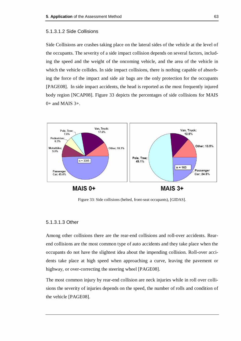
5. Application of the Assessment Method 63
5.1.3.1.2 Side Collisions
Side Collisions are crashes taking place on the lateral sides of the vehicle at the level of
the occupants. The severity of a side impact collision depends on several factors, includ-
ing the speed and the weight of the oncoming vehicle, and the area of the vehicle in
which the vehicle collides. In side impact collisions, there is nothing capable of absorb-
ing the force of the impact and side air bags are the only protection for the occupants
[PAGE08]. In side impact accidents, the head is reported as the most frequently injured
body region [NCAP08]. Figure 33 depicts the percentages of side collisions for MAIS
0+ and MAIS 3+.
Figure 33: Side collisions (belted, front-seat occupants), [GIDAS].
5.1.3.1.3 Other
Among other collisions there are the rear-end collisions and roll-over accidents. Rear-
end collisions are the most common type of auto accidents and they take place when the
occupants do not have the slightest idea about the impending collision. Roll-over acci-
dents take place at high speed when approaching a curve, leaving the pavement or
highway, or over-correcting the steering wheel [PAGE08].
The most common injury by rear-end collision are neck injuries while in roll over colli-
sions the severity of injuries depends on the speed, the number of rolls and condition of
the vehicle [PAGE08].

5. Application of the Assessment Method 64
5.1.3.2 Selection of accidents
As it has been explained earlier the most typical accidents can be divided into three
classes: frontal impacts, side impacts and other (rear-end and roll-over accidents). Fron-
tal impact collisions represent the largest percentage of accidents. Figure 31 obtained
from GIDAS, shows that for MAIS 0+ and MAIS 3+, frontal impacts represent respec-
tively 43% and 49% of all the cases. Due to this fact, it has been considered appropriate
to include in the study the different types of frontal collisions. Front impacts are classi-
fied into four categories: Passenger Car, Pole/Tree, Van/Truck and other (Pedestrian).
Table 21 depicts the types of front impact accidents for MAIS3+ and their percentages
of occurrence. Our study considers the four sub categories and from this point, they will
be referred to as accidents: A (Passenger Car), B (Pole/Tree), C (Van/Truck) and C
(Other such as pedestrians)
MAIS 3+ (GIDAS) Types of accidents (Simulation)
Passenger Car 15,533% Accident A 31,7%
Pole/Tree 17,591% Accident B 35,9%
Van/Truck 8,183% Accident C 16,7%
Front Impact
Other 7,693% Accident D 15,7%
Total 49% 100% Table 21: Selection of the accident types
5.1.3.3 Results of the simulations
Different scenarios are designed according to the characteristics of the different types of
frontal collisions. The simulation of the frontal collisions have been done at speeds
ranging between 30 and 70 km/h. The mitigation levels take a wide range of values de-
pending on the sensor and the accident type. Accidents A and C present mitigation lev-
els that reach reductions of 27 % while the maximum impact speed reduction for acci-
dents B and D are 16,2. Table 22 depicts the impact speed reductions obtained from the
simulation for the 16 sensors.

5. Application of the Assessment Method 65
Short Range Ra-dar
Long Range Ra-dar
Lidar Video
Accidents S1 S2 S3 S4 S5 S6 S7 S8 S9 S10 S11 S12 S13 S14 S15 S16
Accident A 8,2 7,4 5,0 7,6 28,2 26,5 27,0 24,2 23,6 24,5 26,5 22,2 17,8 18,2 14,8 15,6
Accident B 7,8 6,9 4,5 6,5 15,2 15,7 16,0 16,1 11,9 11,6 10,6 9,3 9,8 7,8 8,6 6,8
Accident C 7,9 6,7 4,7 7,1 26,4 27,3 23,0 15,4 20,4 23 18,3 18,2 16,3 17,6 16,7 14,8
Accident D 6,5 7,2 9,8 5,9 16,1 15,9 16,2 14,2 10,8 13,2 11,0 12,6 11,4 7,9 11.4 10,3
Table 22: Accidents Matrix
Appendix A.2 outlines the input data for the review method in respect to the benefit of
CA Systems.
5.2. Presenting Data
In Presenting Data the review procedure is applied to each one of the sets of inputs
(General Properties and Benefit of the System).
In the case of the general properties, the review uses the data obtained from the data
sheets, defines a specific scale for each general property and assigns weights according
the importance of the property.
In respect to the benefit of the system, the review uses the results from the simulation
analysis, defines a specific scale for each accident types and assigns weights according
the level of occurrence.
The final results are two weighted values: a weighted value representing the general
properties and another weighted value representing the benefit of the CA System for
frontal collisions.
5.2.1 Application of the Review to the General Properties
The general properties of sensors refer to all the features not participating directly on the
performance of the sensor. However they have an important relevance in the selection
of sensors for Collision Avoidance Systems.
The assessment of general properties is done through the application of the review
method, as it can be seen on Figure 34. The review method applied to the general prop-

5. Application of the Assessment Method 66
erties assigns a numerical value and a specific weight to every property. A ponderation
will generate a final value that represents the general properties for each sensor.
Figure 34: Block Diagram of the system
As it has been presented in previous chapters, there are many features that can be con-
sidered as general properties. It has been considered appropriate to consider only the
most relevant features. The information required to carry out the assessment is obtained
from sensor data sheets.
5.2.1.1 General Properties Matrix
As it has been defined previously, the General Properties are those features which do
not participate directly in the measurement but are relevant to the final evaluation of the
sensor. There are relatively many features among this class and not all of them have the
same relevance. The first requirement is to define which General Properties are going to
be taken into consideration. The selection of process is done through the comparison of
the same property among the different sensors. In the case of price, size, weight and
power consumption the values vary extremely and need to be considered. While in the
case of temperature storage and voltage the values remain relatively constant and their
inclusion in the study does not bring any benefit.
The goal from the properties matrix is to define the most important General Properties
for each sensor and assign to each of them a numerical value. Among the General Prop-

5. Application of the Assessment Method 67
erties we would have price, size (Height, Width, and Depth), weight and power con-
sumption. The values will be assigned to each property according to data sheets from
the sensors and information provided from the sensor’s manufacturers. In Appendix
B.1, the General Properties Matrix is represented for 16 sensors.
5.2.1.2 Special Values scale
The General Properties Matrix has assigned values to the most relevant features for all
the sensors. As it can be seen in Appendix 1, the values among each property hold a
wide range of values. At first glance it is difficult to recognize the quality of the values
for most properties but the need of a procedure is identified. The procedure is based on
the definition of a scale of values where all the possible values for every General Prop-
erty are represented. The goal is to identify later on the quality of the values assigned on
the General Properties matrix.
Several requirements should be imposed on the design of the values scale. In order to
have an effective scale it needs to represent a wide range of possible values. The proce-
dure is based on the analysis from the chosen General Properties for a large number of
sensors. The minimum and maximum values, as well as the difference between them for
each property are identified. Table 23 outlines the values obtained from a research for
more than 25 sensors.
General Properties Units Minimum Value Maximum Value Difference
Price Euros 90 450 360
Height m 0.040 0.150 0,11
Width m 0.035 0.155 0,12
Size
Depth m 0.023 0.104 0,081
Weight Kg 0.100 1300 1200
Power Consumption W 1.8 10 8,2
Table 23: Definition of minimum and maximum values
Another requirement to the scale is the need to represent values that can be linked to a
certain level of quality. The number of quality levels should be enough to consider a
wide range going from unacceptable to ideal levels. It has been considered appropriate

5. Application of the Assessment Method 68
to use a scale from 0 to 9 since it offers enough levels to represent different quality lev-
els as it can be see on Table 24.
Quality Levels Scale Values
Unacceptable 0
Very Bad 1
Bad 2
Below acceptable 3
Acceptable 4
Satisfactory 5
Above satisfactory 6
Good 7
Very Good 8
Ideal 9
Table 24: Definition of the scale
Now we are in the position with the two data sources previously presented to build up
the Special Values Scale for each relevant General Property. The unacceptable and ideal
quality levels correspond to the minimum and maximum value from each property re-
spectively, meaning that values smaller or equal than the minimum are assigned a value
of 1, while values larger than the maximum are assigned a value of 9. The difference
between the two extreme values (minimum and maximum values) is divided among
eight intervals corresponding to the eight quality levels between 0 and 9. Table 25 de-
picts the scale defined for the General Properties.

5. Application of the Assessment Method 69
Scale 9 8 7 6 5 4 3 2 1 0 Gen. Prop. U.
Price € [0; 90] (90; 135] (135;180] (180;225] (225;270]
(270;
315]
(315;
360]
(360;
405]
(405;
450] (450; ∞]
Height m [0; 0.04]
(0,04;
0,054]
(0,054;
0,068]
(0,068;
0,081]
(0,081;
0,095]
(0,095;
0,109]
(0,109;
0,122]
(0,122;
0,136]
(0,136;
0,15]
(0.150;
∞]
Width m [0; 0.035]
(0,035;
0,05]
(0,05;
0,065]
(0,065;
0,08]
(0,08;
0,095]
(0,095;
0,11]
(0,11;
0,125]
(0,125;
0,14]
(0,14;
0,155]
(0.155;
∞]
Length m [0; 0.023]
(0,023;
0,033]
(0,033;
0,043]
(0,043;
0,053]
(0,053;
0,063]
(0,063;
0,073]
(0,073;
0,084]
(0,084;
0,094]
(0,094;
0,104]
(0.104;
∞]
Weight Kg [0; 100]
(100;
250]
(250;
400]
(400;
550]
(550;
700]
(700;
850]
(850;
1000]
(1000;
1150]
(1150;
1300] (1300; ∞]
Power Cons.
W [0; 1.8]
(1,8;
3,075]
(3,075;
4,35]
(4,35;
5,625]
(5,625;
6,9]
(6,9;
8,175]
(8,175;
9,45]
(9,45;
10,725]
(10,725;
12] (12; ∞]
Table 25: Special Value Scale
5.2.1.3 Assign scale values
During this step, scale values are assigned to each property from the General Properties
Matrix according to the previously defined Special values scale. The goal from this step
is to eliminate the possible differences between the different inputs. Each property has
its own units and takes values along a specific range of values. The assignment of scale
values allows to homogenize the process because the units disappear and only values
between 0 and 9 are considered. Table 26 demonstrates the results from the assignment
of scale values.
Table 26: Assign scale values
Sensors Short Range RADAR Long Range RADAR LIDAR Video
General Prop. S1 S2 S3 S4 S5 S6 S7 S8 S9 S10 S11 S12 S13 S14 S15 S16
A Price 9 8 7 8 1 4 2 2 6 6 5 4 3 2 1 2
B Height 6 5 5 5 6 2 6 4 5 7 7 6 7 8 9 8
C Width 3 4 6 5 6 2 2 4 6 2 3 4 5 9 8 7
D Length 5 8 7 8 5 6 5 7 5 4 1 3 8 8 9 9
E Weight 6 8 7 7 7 6 7 6 6 7 6 8 8 8 8 8
F Power Cons. 8 7 5 6 2 4 5 4 6 6 8 8 7 8 8 7
5. Application of the Assessment Method 70
5.2.1.4 Selection of properties and assignment of weights
The goal from the Selection of properties is to identify the most important properties
and assign weights according to a criterion. All the properties are compared together
and different values can be assigned; 0, 1 and 2. In the case of 0, a property is less im-
portant than the other, 1 means that both properties have the same importance and 2 is
assigned when a property is more important than the other.
The assignment of the values is based on the requirements of the study. For example, if
the study focuses on the installation of Collision Avoidance Systems for small cars, the
size of the sensor would be crucial, whereas in the case of SUV the size would not be
relevant. The characteristics from each particular case determine the criteria used for the
comparison.
The chosen criterion is the application of a general case giving to all the General Prop-
erties equal importance except for prize. The results can be seen on Table 26 where the
cells from column A, corresponding to prize, has values of 2 while the cells from the
other comparisons have 1. Once the table is completed, the sum of the values for each
column is written on the “Absolute Sum” row. The values from this row outline the
overall result of the comparison and identify the relevance of each property.
The next step is the calculation of the weights according to the results from the absolute
sum. The property with the highest value is identified and the remainders of the values
are normalized in respect to this value. In this case the row with the total sums is di-
vided by 11, the value corresponding to the price. The obtain weights represent the rele-
vance that has been awarded to each property according to the requirements from the
study.
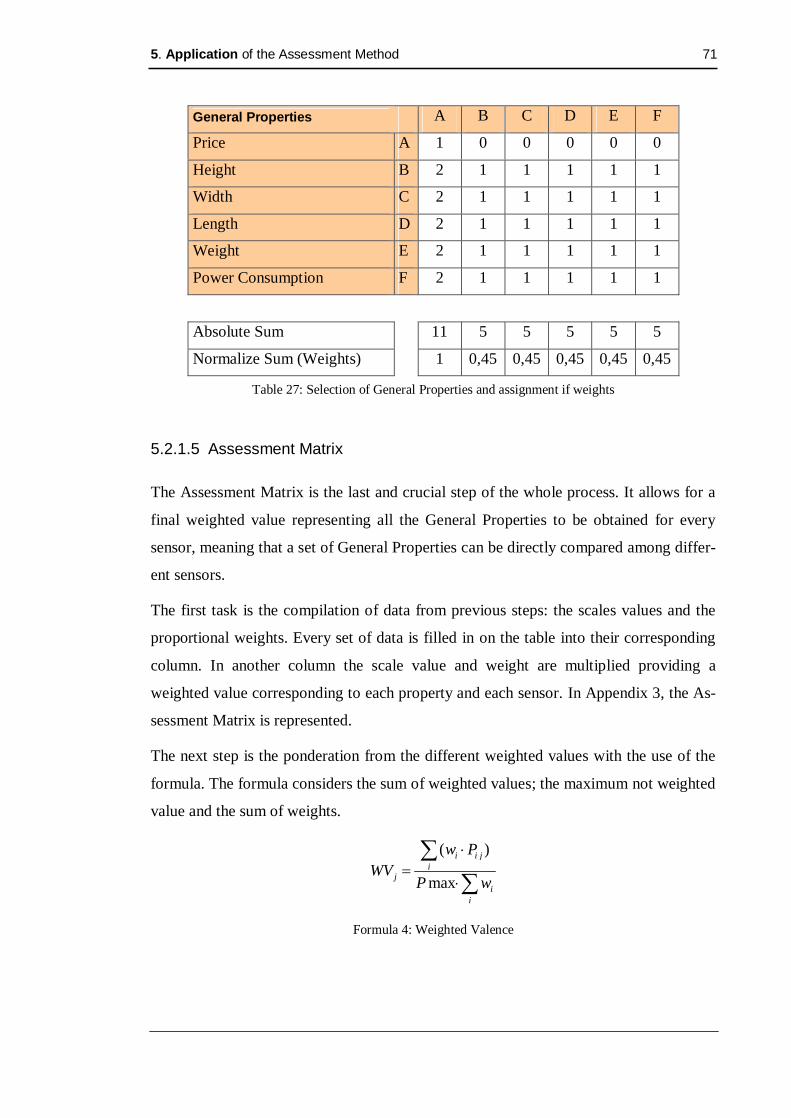
5. Application of the Assessment Method 71
Table 27: Selection of General Properties and assignment if weights
5.2.1.5 Assessment Matrix
The Assessment Matrix is the last and crucial step of the whole process. It allows for a
final weighted value representing all the General Properties to be obtained for every
sensor, meaning that a set of General Properties can be directly compared among differ-
ent sensors.
The first task is the compilation of data from previous steps: the scales values and the
proportional weights. Every set of data is filled in on the table into their corresponding
column. In another column the scale value and weight are multiplied providing a
weighted value corresponding to each property and each sensor. In Appendix 3, the As-
sessment Matrix is represented.
The next step is the ponderation from the different weighted values with the use of the
formula. The formula considers the sum of weighted values; the maximum not weighted
value and the sum of weights.
( )
max
i i ji
ji
i
w PWV
P w
Formula 4: Weighted Valence
General Properties A B C D E F
Price A 1 0 0 0 0 0
Height B 2 1 1 1 1 1
Width C 2 1 1 1 1 1
Length D 2 1 1 1 1 1
Weight E 2 1 1 1 1 1
Power Consumption F 2 1 1 1 1 1
Absolute Sum 11 5 5 5 5 5
Normalize Sum (Weights) 1 0,45 0,45 0,45 0,45 0,45

5. Application of the Assessment Method 72
Where ( )i i ji
w P Sum of weighted values
maxP Maximum not weighted value
ii
w Sum of weights
The final weighted value for each Sensor Concept is a value between 0 and 1, which is
able to quantify the quality of the sensor in respect to the requirements imposed previ-
ously. Table 28 depicts the results obtained from the assessment matrix where the val-
ues ranged between 0,434 and 0,766. The entire Assessment Matrix can be seen in Ap-
pendix B.1.
Table 28: Results from the Assessment Matrix
5.2.1.6 Analysis of the results
The final result from the assessment matrix and at the same time from the review is a
final value representing the General Properties for each sensor. The results obtained
from the review are presented in Table 29 in the form of a ranking. The ranking is only
based on the General Properties from the different sensors.
Sensor Concepts Short Range RADAR Long Range RADAR
Sensors S1 S2 S3 S4 S5 S6 S7 S8
General Properties 0,738 0,766 0,702 0,750 0,434 0,444 0,453 0,453
Sensor Concepts LIDAR Video
Sensors S9 S10 S11 S12 S13 S14 S15 S16
General Properties 0,636 0,605 0,555 0,583 0,641 0,699 0,68 0,668

5. Application of the Assessment Method 73
Table 29: Results from the General Properties assessment
As it can be seen, the sensor in the first position is a short range RADAR sensor pre-
senting a value of 0,766, meaning that this sensor meets 77% of the fixed requirements.
On the last position of the ranking stands a long range RADAR which is only capable to
satisfy the requirements in a 43,4%.
Another valuable observation is the ranking among Sensor Concepts. The table shows
that sensors belonging to the same Sensor Concept present similar values. The ranking
among Sensor Concepts identifies short range RADAR as the Sensor Concept present-
ing the best overall General Properties followed by Video systems, LIDAR, and in the
last position long range RADAR.
An explanation of the results relies on the price of sensors. We have considered price to
be the most important General Property through the assignment of the largest weight
value and it turns out that short range RADAR is a cheaper technology than long range
RADAR, LIDAR and Video. But price is not the only factor since video sensors are
very expensive and still they present an excellent combination of General Properties. It
Ranking of sensors Values Sensor Sensor Concept Ranking of Sensor
Concepts
1 0,766 S2 Short range RADAR
2 0,75 S4 Short range RADAR
3 0,738 S1 Short range RADAR
4 0,701 S3 Short range RADAR
1
5 0,699 S14 Video
6 0,68 S15 Video
7 0,67 S16 Video
8 0,64 S13 Video
2
9 0,636 S9 LIDAR
10 0,605 S10 LIDAR
11 0,583 S12 LIDAR
12 0,555 S11 LIDAR
3
13 0,453 S7 Long range RADAR
14 0,453 S8 Long range RADAR
15 0,444 S6 Long range RADAR
16 0,434 S5 Long range RADAR
4

5. Application of the Assessment Method 74
turns out that video systems are lighter and smaller in size than other systems leading to
present better General Properties than long range RADAR and LIDAR.
5.2.2 Application of the Review to the benefit of the system
Collision Avoidance Systems activate braking or steering systems through the process-
ing of data from the environment. The data is collected with sensors under different
forms corresponding to the physical principle from each of them. The role of sensors is
crucial to reduce the high accident statistics.
During this section a procedure to evaluate the sensor performance is developed. The
goal is to find which sensor among the different Sensor Concepts is the more suitable to
Collision Avoidance during typical vehicle accidents. The main aspect to be taken into
consideration is the benefit offer by the sensors in such complicated situations.
The most typical vehicle accidents would be presented, followed by the comparison
between the simulations and an analysis providing an index of the benefit from the sys-
tem. The next step is to apply the review method previously described to the benefit of
the system.
Figure 35: Block Diagram of the system
The next step is the application of the review method to the benefit of the system. The
review method assigns scales values and weights to every type of vehicle accident. A
ponderation will generate a final value that represents the benefit of each Sensor Con-
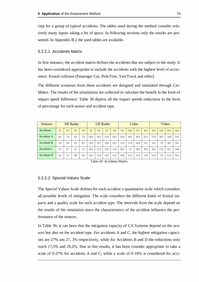
5. Application of the Assessment Method 75
cept for a group of typical accidents. The tables used during the method consider rela-
tively many inputs taking a lot of space. In following sections only the results are pre-
sented. In Appendix B.2 the used tables are available.
5.2.2.1 Accidents Matrix
In first instance, the accident matrix defines the accidents that are subject to the study. It
has been considered appropriate to include the accidents with the highest level of occur-
rence: frontal collision (Passenger Car, Pole/Tree, Van/Truck and other).
The different scenarios from these accidents are designed and simulated through Car-
Maker. The results of the simulations are collected to calculate the benefit in the form of
impact speed difference. Table 30 depicts all the impact speeds reductions in the form
of percentage for each sensor and accident type.
Sensors SR Radar LR Radar Lidar Video
Accidents S1 S2 S3 S4 S5 S6 S7 S8 S9 S10 S11 S12 S13 S14 S15 S16
Accident A 8,2 7,4 5,0 7,6 28,2 26,5 27,0 24,2 23,6 24,5 26,5 22,2 17,8 18,2 14,8 15,6
Accident B 7,8 6,9 4,5 6,5 15,2 15,7 16,0 16,1 11,9 11,6 10,6 9,3 9,,8 7,8 8,6 6,8
Accident C 7,9 6,7 4,7 7,1 26,4 27,3 23,0 15,4 20,4 23 18,3 18,2 16,3 17,6 16,7 14,8
Accident D 6,5 7,2 9,8 5,9 16,1 15,9 16,2 14,2 10,8 13,2 11,0 12,6 11,4 7,9 11.4 10,3
Table 30: Accidents Matrix
5.2.2.2 Special Values Scale
The Special Values Scale defines for each accident a quantitative scale which considers
all possible levels of mitigation. The scale considers the different kinds of frontal im-
pacts and a quality scale for each accident type. The intervals from the scale depend on
the results of the simulation since the characteristics of the accident influence the per-
formance of the sensors.
In Table 30, it can been that the mitigation capacity of CA Systems depend on the sen-
sors but also on the accident type. For accidents A and C, the highest mitigation capaci-
ties are 27% ans 27, 3% respectively, while for Accidents B and D the reductions only
reach 17,5% and 18,2%. Due to this results, it has been consider appropriate to take a
scale of 0-27% for accidents A and C, while a scale of 0-18% is considered for acci-

5. Application of the Assessment Method 76
dents B and D. The difference could rely on the fact that the vehicles (cars, vans and
trucks) are usually easier to detect as other objects, leading to a higher possible mitiga-
tion of the accident; Accidents A and C correspond to vehicles’ crashes while accidents
B and D are due to crashes against poles, trees or pedestrians In Table 31 a scale from 0
to 9 is used to characterize the capacity mitigation of the sensors during frontal colli-
sions.
Scale 9 8 7 6 5 4 3 2 1 0 Accidents Max. Min. Accident A [∞; 27] (27; 24] (24; 21] (21; 18] (18; 15] (15; 12] (12; 9] (9; 6] (6; 3] (3; 0]
Accident B [∞; 18] (18; 16] (16; 14] (14; 12] (12; 10] (10; 8] (8; 6] (6; 4] (4; 2] (2; 0]
Accident C [∞; 27] (27; 24] (24; 21] (21; 18] (18; 15] (15; 12] (12; 9] (9; 6] (6; 3] (3; 0]
Accident D [∞; 18] (18; 16] (16; 14] (14; 12] (12; 10] (10; 8] (8; 6] (6; 4] (4; 2] (2; 0]
Table 31: Special Values Scale
5.2.2.3 Assign scale values
According to the values that have been assigned to the inputs in the Accidents Matrix
and the Special Values Scale that has been defined, it is possible to assign scale values
to each accident and sensor. The goal is to eliminate the possible differences between
the accident types through the assignment of quality values. The quality scale is com-
mon to all accidents and sensors allowing direct comparisons. The combination from
previous steps is represented in Table 32.
Table 32: Assign Scale Values Table
Sensors Short Range Ra-
dar Long Range Ra-
dar Lidar Video
Accidents S1 S2 S3 S4 S5 S6 S7 S8 S9 S10 S11 S12 S13 S14 S15 S16
Accident A 2 2 1 2 9 8 9 8 7 8 8 7 5 6 4 5
Accident B 3 3 2 2 7 7 8 8 5 5 5 4 4 3 4 3
Accident C 3 2 2 1 8 8 7 8 6 7 6 6 5 5 5 3
Accident D 3 3 4 2 8 7 8 7 5 6 5 6 5 3 5 5

5. Application of the Assessment Method 77
5.2.2.4 Selection of accidents and assignment of weights
The goal from the selection of accidents is to decide which accidents are the most rele-
vant and assign corresponding weights. The decision about the relevance of accidents is
done according to the percentage of occurrence based on existing statistics. An accident
that occurs more often takes precedence. Table 33 depicts the levels of occurrence for
the different types of frontal collisions.
Table 33: Level of occurrence from the different accidents
In Table 34 the different types of frontal collision are compared. Since Accident B takes
a percentage of 35,9%, higher than the others accidents, the column corresponding to
Accident B takes values of 2. Accident C takes a percentage of 31,7% meaning that it is
more important than Accidents C and D. Then Accidents C and D present similar per-
centages and a value of 1 is assigned to the comparison.
Table 34: Selection of inputs values
The Absolute Sum row illustrates that Accident B is the most relevant accident, fol-
lowed very closely by Accident A and in the far distance Accidents C and D. The next
step is the calculation from the different weights which determine the importance of
each accident type. Since Accident B obtains the highest value, the normalization uses
this value to calculate the weights. Accidents A, B, C and D obtain weights of 1; 0,71;
Accidents Level of occurrence* Accident A 31,7% Accident B 35,9% Accident C 16,7% Accident D 15,7%
* According to GIDAS
Accidents A B C D Accident A A 1 2 0 0 Accident B B 0 1 0 0 Accident C C 2 2 1 1 Accident D D 2 2 1 1
Absolute Sum 5 7 2 2 Normalize Sum (Weights) 0,71 1 0,29 0,29

5. Application of the Assessment Method 78
0,29 and 0,29 respectively. The weights represent the relevance that has been awarded
to each accident type.
5.2.2.5 Assessment matrix
The Assessment Matrix is the last and crucial step of the whole process. It allows for a
final weighted value representing the benefit from CA Systems, meaning that the bene-
fit can be directly compared among different sensors.
The first task is the compilation of data from previous steps: the scales values and the
proportional weights. Every set of data is filled in on the table into their corresponding
column. In another column the scale value and weight are multiplied providing a
weighted value corresponding to each property and each sensor. In Appendix 4, the As-
sessment Matrix is represented.
The next step is the ponderation from the different weighted values with the use of the
formula 5. The formula considers the sum of weighted values, the maximum not
weighted value and the sum of weights.
( )
max
i i ji
ji
i
w PWV
P w
Formula 5: Weighted Valence
Where ( )i i ji
w P Sum of weighted values
maxP Maximum not weighted value
ii
w Sum of weights
The final weighted value for each Sensor Concept is a value between 0 and 1, which is
able to quantify the quality of the sensor in respect to the requirements imposed previ-
ously. Table 35 depicts the results obtained from the assessment matrix where the val-
ues range between 0,147 and 0,64. The entire Assessment Matrix can be seen in Appen-
dix 4.

5. Application of the Assessment Method 79
Table 35: Assessment Matrix
5.2.2.6 Analysis of the results
The final result from the assessment matrix and at the same time from the review is a
final value representing the benefit of the CA System for each sensor. The results ob-
tained from the review are presented in table 36 in the form of a ranking. The ranking is
only based on the benefit presented by the different CA Systems.
Table 36: Results from the benefit assessment
Sensor Concepts Short Range RADAR Long Range RADAR
Sensors S1 S2 S3 S4 S5 S6 S7 S8 Benefit 0,21 0,201 0,152 0,147 0,616 0,582 0,64 0,616
Sensor Concepts LIDAR Video
Sensors S9 S10 S11 S12 S13 S14 S15 S16 General Properties 0,636 0,605 0,555 0,583 0,641 0,699 0,68 0,668
Ranking of sensors Values Sensor Sensor Concept Ranking of Sensor
Concepts
1 0,64 S7 Long range RADAR
2 0,616 S5 Long range RADAR
3 0,616 S8 Long range RADAR
4 0,582 S6 Long range RADAR
1
5 0,45 S9 LIDAR
6 0,445 S11 LIDAR
7 0,42 S12 LIDAR
8 0,396 S10 LIDAR
2
9 0,357 S13 Video
10 0,333 S15 Video
11 0,328 S14 Video
12 0,303 S16 Video
3
13 0,21 S1 Short range RADAR
14 0,201 S2 Short range RADAR
15 0,152 S3 Short range RADAR
16 0,147 S4 Short range RADAR
4

5. Application of the Assessment Method 80
As it can be seen, the sensor in the first position is a long range RADAR sensor present-
ing a value of 0,64, meaning that this sensor meets 64% of the fixed requirements. In
the last position of the ranking stands a short range RADAR which is only capable to
satisfy the requirements 14,7%.
The ranking illustrates that the most suited sensor to avoid or mitigate collisions is Long
range RADAR, followed by LIDAR, Video Systems and Short Range RADAR. The
values obtained for Short range RADAR are extremely low and it would be reasonable
to discard it from the study.
5.3. Analyzing Data
Analyzing Data is the last step from the outline of main ideas and consists on the
graphical representation from previous results. Each sensor is characterised by two val-
ues, which on the graph became two coordinates. The general properties are represented
on the Y-axes, while the benefit of the system is represented on the X-axes.
The position of the coordinates for each sensor determines the quality of the combina-
tion between general properties and benefit. The point (1,1) is the ideal point since it
presents a perfect set of general properties and a perfect benefit to prevent accidents.
The distance between the sensors and the point (1,1) determines the ranking of sensors
upon their suitability.
Figure 36: Block Diagram of the System

5. Application of the Assessment Method 81
5.3.1 Graphical representation of the results
Along the study sixteen different sensors have been analyzed at different levels. At this
point the applied assessment method has provided for each sensor two final values rang-
ing between 0 and 1. The two final values are quality indices corresponding to the Gen-
eral Properties and to the benefit offered by Collision Avoidance Systems. In Table 37
the results from previous sections are collected.
Table 37: Results of the review methods
A graphic tool is used to compare the different sensors. Every sensor is characterised by
two values (the General Properties and the benefit of the system) which from this in-
stant are considered to be the coordinates of each sensor. The graph has two axes; the
X-axis represents the benefit of the system, while the Y-axis corresponds to the General
Properties. Since the values obtained from the review methods theoretically range be-
tween 0 and 1, the same scale is used for both axes.
In figure 37 the coordinates from each sensor have been drawn in the same graph. As it
can be seen, the sensors belonging to the same Sensor Concept are close to each other.
Red circles have been used to locate the areas from the different Sensor Concepts. The
graph shows how sensors with the same physical principle present similar characteris-
tics. If more sensors would be tested, they would likely be included inside the circle or
not very far from it.
Sensor Concepts Short Range RADAR Long Range RADAR
Sensors S1 S2 S3 S4 S5 S6 S7 S8
General Properties 0,738 0,766 0,701 0,75 0,434 0,444 0,453 0,453 Benefit 0,21 0,201 0,152 0,147 0,616 0,582 0,64 0,616 Sensor Concepts LIDAR Video
Sensors S9 S10 S11 S12 S13 S14 S15 S16
General Properties 0,636 0,605 0,555 0,583 0,64 0,699 0,68 0,67 Benefit 0,45 0,396 0,445 0,42 0,357 0,328 0,333 0,303

5. Application of the Assessment Method 82
Figure 37: Graph with the results from the review methods
5.3.2 Analysis of the results
The graph shows that sensors belonging to the same Sensor Concept present similar
values, since sensors from the same class present similar advantages and inconven-
iences. The differences may rely on different categories for the same sensor and/or the
manufacturer. During this section the results obtained for each Sensor Concept are ex-
plained and discussed.
5.3.2.1 Short range RADAR
The four short range RADAR sensors present the best combination of General Proper-
ties among the tested sensors, mainly due to a low cost, appropriate dimensions and
light weight. During the tests the short range RADAR was only able to reduce the im-
pact speed in a 5-9%, below the performance provided by other sensors.
5.3.2.2 Long range RADAR
The General Properties for long range RADAR sensors present the worst value among
the four classes, mainly due to the high price of these sensors ranging between 300-450

5. Application of the Assessment Method 83
€ and large dimensions. In respect to the benefit, long range RADARS are in the best
position to avoid or mitigate an accident since the reduction of impact speed ranges be-
tween 14,2-28,2%.
5.3.2.3 LIDAR
LIDAR falls behind short range RADAR and Video in respect to the General Properties
but it does present satisfactory levels, mainly due to the affordable price of these sen-
sors. In the case of the benefit, LIDAR is the second best performing sensor after Long
Range RADAR presenting reductions between 9,3-26,5%.
5.3.2.4 Video
Among the four sensor types, video is the second best Sensor Concept in respect to the
General Properties with values ranging between 0,64-0,69 mainly due to the dimensions
and weights of these sensors. The capacity to detect objects is worse than LIDAR and
RADAR, since it can only reduce the impact speed by 10-18 %.
5.3.2.5 Summary
Table 38 shows an overview of the results obtained from the graph. Each Sensor Con-
cept is awarded two ranges of quality level, corresponding to the General Properties and
the benefit. The quality levels are assigned with the use of Table 11 (Definition of the
scale) which assigns quality levels to a range of values from 0 to 9.
General Properties Benefit
Sensor Results Quality level Results Quality level
Short Range 0,7-0,766 Good 0,15-0,21 Very bad- bad
Long Range 0,43-0,45 Acceptable 0,58-0,64 Satisfactory-Above satisfac-tory
LIDAR 0,55-0,63 Satisfactory-Above satisfac-tory
0,40-0,45 Acceptable
Video 0,64-0,69 Above satisfactory 0,3-0,35 Below acceptable
Table 38: Quality levels from the different Sensor Concepts
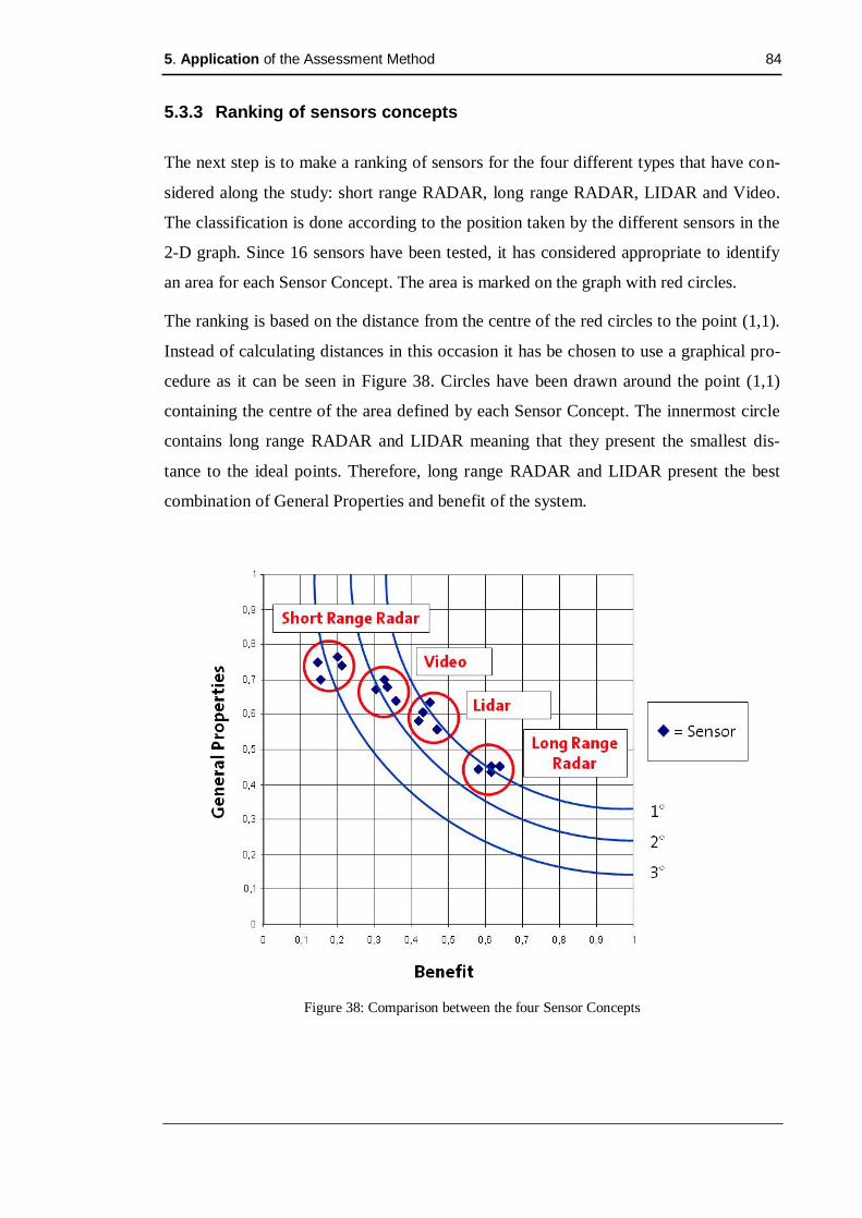
5. Application of the Assessment Method 84
5.3.3 Ranking of sensors concepts
The next step is to make a ranking of sensors for the four different types that have con-
sidered along the study: short range RADAR, long range RADAR, LIDAR and Video.
The classification is done according to the position taken by the different sensors in the
2-D graph. Since 16 sensors have been tested, it has considered appropriate to identify
an area for each Sensor Concept. The area is marked on the graph with red circles.
The ranking is based on the distance from the centre of the red circles to the point (1,1).
Instead of calculating distances in this occasion it has be chosen to use a graphical pro-
cedure as it can be seen in Figure 38. Circles have been drawn around the point (1,1)
containing the centre of the area defined by each Sensor Concept. The innermost circle
contains long range RADAR and LIDAR meaning that they present the smallest dis-
tance to the ideal points. Therefore, long range RADAR and LIDAR present the best
combination of General Properties and benefit of the system.
Figure 38: Comparison between the four Sensor Concepts

5. Application of the Assessment Method 85
Table 39 illustrates the ranking of Sensor Concepts. The first place is shared by two
sensor concepts since long range RADAR and LIDAR present both of them the best
combination, followed by Video systems and short range RADAR.
Ranking Sensor Concepts
1º Long Range RADAR /LIDAR
2º Video Systems
3º Short Range RADAR
Table 39: Ranking of Sensor Concepts
5.3.3.1 Long range RADAR vs. LIDAR
The position of long range RADAR and LIDAR in the graph are different but the dis-
tance from them to the point (1,1) is the same. It means that both sensors concepts pre-
sent the same combination of General Properties and benefit, but for different reasons.
Long range RADAR presents an acceptable combination of General Properties and a
good benefit of the system, while LIDAR is the opposite. LIDAR presents a good com-
bination of General Properties but only an acceptable benefit of the system.
The question to be asked is which sensor is better? Since there is no sensor standing out,
the selection criterion depends on certain priorities. If we are looking for the best per-
forming sensor and the cost is less relevant, Long Range RADAR would be the best
choice. Instead we might be looking for an affordable sensor with an acceptable per-
formance and in this case LIDAR would be more suitable.
In previous sections, it has been explained that sensors on the imaginary line between
(0,0) and (1,1) present the perfect balance between General Properties and the benefit of
the system. Figure 39 illustrates the long range RADAR and LIDAR sensors, as well as
the line with the perfect balance. Both Sensor Concepts are not far from the perfect bal-
ance but some aspects should be improved. In the case of LIDAR, the system should be
capable of higher benefits, while for RADAR the prices and the dimensions should de-
crease.

5. Application of the Assessment Method 86
Figure 39: Comparison between Long Range RADAR and LIDAR
5.3.4 Ranking of single sensors
The objective of this section is to classify the different sensors upon their suitability to
be used in Collision Avoidance Systems. The ranking considers the overall profit pre-
sented by two different aspects of Sensor Concepts; the General Properties and the
benefit of the system.
The results obtained from the review methods range between 0 and 1. The ponderation
during the review method assigns values to the different Sensor Concepts according to
their quality. The quality is quantified with a value between 0 and 1, where 1 represents
the ideal situation. This means the closer to value 1, the higher the quality of the sensor.
The sensors are ranked upon the distance between the values to 1.
When both aspects of sensors come together on the graph, the quality is not determined
any more by the distance to 1. Now the evaluation considers both aspects of Sensor
Concepts meaning that a new criterion is required. Since the value 1 keeps referring to
the ideal situation, the point (1,1) represented on the graph means the perfect combina-

5. Application of the Assessment Method 87
tion of General Properties and benefit of the system. The distance from the points repre-
senting the sensors to (1,1), determines the ranking among single sensors.
The distance to the point (1,1) is a measure of the degree to which each sensor fulfils the
quality requirements fixed at the beginning of the process. These requirements are re-
lated to an excellent combination of General Properties and an extraordinary benefit of
the system. Table 40 presents the results for the ranking of single sensors. The table has
been constructed through the calculation of the distance between the different points
(Sensors) and the ideal point (1,1). Another possibility is to draw circles around (1,1),
since what matters is the distance to the point (1,1). If two sensors are located on the
same circle, it will mean that they present a proportional combination of General Prop-
erties and benefit.
Table 40: Ranking among single sensors
The ranking of single sensors depicts that even if long range RADAR takes three from
the top four positions, the values for LIDAR and long range RADAR are very similar.
Some video sensors follow closely but many aspects should be improved to be able to
Ranking of single sensors Distance to (1,1) Sensor Sensor Concept
1 0,654835 S7 Long range RADAR
2 0,659542 S9 LIDAR
3 0,66833 S8 Long range RADAR
4 0,683968 S5 Long range RADAR
5 0,692044 S11 LIDAR
6 0,693488 S10 LIDAR
7 0,6956 S6 Long range RADAR
8 0,714345 S12 LIDAR
9 0,736332 S14 Video
10 0,736919 S13 Video
11 0,73979 S15 Video
12 0,771174 S16 Video
13 0,832312 S1 Short range RADAR
14 0,832561 S2 Short range RADAR
15 0,888881 S4 Short range RADAR
16 0,899169 S3 Short range RADAR

5. Application of the Assessment Method 88
compete with the sensors in the top. Short range RADAR sensors are positioned in the
last places; therefore they do not present good conditions to be used in Collision Avoid-
ance Systems.
6. Verification and Validation 89
6 Verification and Validation
The development of processes and/or products requires testing procedures to verify and
ensure the appropriate performance. During the development, different kinds of assump-
tions and concepts might be considered which could lead to inaccurate results. The test-
ing procedures focus on the quality and reliability.
There are two aspects that need to be tested when a model is designed; Verification and
Validation. The terms Verification and Validation are often used improperly leading to
considerable confusions. Verification expresses that the model or product has all charac-
teristics and properties needed to accomplish the aim it was created for, while Validity
presents the effective solution to a problem or work. [WINN05]
Verification refers to the fulfilment of the requirements while validation refers to the
integrity of the procedure. This means that verification should be used in contexts of
process/product description and technical documents; validation in contexts of proc-
ess/product functions and user requirements. [WINN05]
Concerning the assessment of Sensor Concepts, it is necessary to distinguish between
local and global systems. The global system is the whole system which considers the
properties of sensors and provides the suitability of Sensor Concepts to prevent vehicle
accidents. Inside the global system, there are two local systems: the Simulation and the
Assessment Method.
The verification and validation have to be applied to each one of the local systems, as
well as to the global system. Since the goal from this Thesis is the development of an
Assessment Method to evaluate Sensor Concepts, it is necessary to focus on this local
system. In following sections different procedures are described to verify and validate
the Assessment Method.
6.1. Verification of the assessment method
In order to verify a model, the simplest solution is to compare the model to a reference.
Nevertheless, it is possible that the needed model of reference is not available. In this
case, it is necessary to develop references for the whole system that can be compared to
the model. The differences between the model and the developed references determine
the verification of the system.

6. Verification and Validation 90
The characteristics from the global system impose specific characteristics to the As-
sessment Method. During this section, the different requirements are described to ex-
plain how does the developed Assessment Method fulfils the requests. The requirements
of the global system are divided into requirements in respect to the inputs, to the as-
sessment and to the output.
6.1.1 Requirements on the method is respect to the inputs
6.1.1.1 Sets of inputs
Sensor Concepts have a considerable large number of properties. The main properties
are classified in General Properties, Performance Properties and External Factors. Per-
formance Properties and External Factors are directly linked to the performance of sen-
sors while the General Properties are completely independent. The ideal method should
be able to deal with different sets of inputs.
The Assessment Method considers two sets of inputs; a set of General Properties and
a set of accident types (the simulation of accident types is used to evaluate the perform-
ance of sensors)
6.1.1.2 Number of inputs
Two different sets of inputs are identified; the General Properties and the benefit pre-
sented by Sensor Concepts. Each set could have a large number of inputs and the
method should not restrict this amount.
The Assessment Method considers an unlimited number of inputs.
6.1.1.3 Range of values
Each input is different and it can present a specific range of values. For example, each
General Property such as price, size and weight has a different range of possible values.
The method should not limit the range of values from the inputs.
The Assessment Method considers a wide range of realistic values.

6. Verification and Validation 91
6.1.1.4 Difference between values
As it has been explained earlier, each input has a specific range of values which compli-
cates the comparison. The method should be capable of comparing the quality presented
by the different values.
The Assessment Method uses a quality scale to assign scale values to the different
inputs and eliminate the differences between inputs.
6.1.2 Requirements on the method is respect to the assessment
6.1.2.1 Distinction between inputs
Every set considers a wide range of inputs but not all of them have the same signifi-
cance to the study. The method should distinguish for each set the relevance of the in-
puts
The Assessment Method takes into consideration the differences between inputs:
General Properties (according to importance) and between types of accidents (according
to level of occurrence).
6.1.2.2 Consideration from the differences between inputs
Once the distinction has been made, it is appropriate that the method considers the rele-
vance of the different inputs.
The Assessment Method calculates weights for each input according to their signifi-
cance.
6.1.2.3 Combination from the sets of inputs
The two aspects of Sensor Concepts (General Properties and benefit) are equally impor-
tant. The method should combine both aspects to allow comparisons between sensors.
The Assessment Method uses a graphic tool to present the results.

6. Verification and Validation 92
6.1.3 Requirements on the method is respect to the output
6.1.3.1 Classification
The final goal is to evaluate suitability of sensors concepts to be used in Collision
Avoidance System. A criterion is required to classify Sensor Concepts.
The Assessment Method describes a procedure to rank sensors upon the analysis
from the graphic results.
6.2. Validation of the assessment method
The validation of the Assessment Method is the confirmation that the method fulfils its
intended purpose, which is the determination of the suitability of Sensor Concepts to
Collision Avoidance
The assessment method is composed of two review methods being applied to two dif-
ferent concepts and a ranking tool assessing the results from the reviews. The goal from
the assessment is to rank the sensors upon the quality of the General Properties and the
benefit offered by Collision Avoidance Systems.
In our case, the assessment method has been applied to 16 sensors corresponding
equally to four Sensor Concepts; RADAR (Short Range and Long Range), LIDAR and
Video. The assessment has identified that sensors with the same physical principle pre-
sent similar characteristics. In Figure 26, a graph illustrates with red circles the different
Sensor Concepts.
The assessment method would be validated if the method is capable of providing similar
results with different sensors. The validation procedure consists on the application of
the Assessment Method to other group of sensors. The sensors can be from different
manufacturers or from different categories, but they have to correspond to the four Sen-
sor Concepts that are subject to the study. It is necessary to keep the same General
Properties, the same types of accidents and the scales that have been defined. The only
variables that change are the sensors and their values.
If the results from the assessment locate the sensors in the same areas than the first time
that the method was applied, the Assessment Method would be validated.

7. Conclusion 93
7 Conclusion
The reduction of vehicle accidents statistics presents a serious challenge to governments
and vehicle manufacturers. Collision Avoidance Systems based on the processing of
data from the environment to activate an automated braking or steering systems present
good conditions to mitigate accidents. Consequently, there is a need to develop an as-
sessment method capable of evaluating the performance, as well as the characteristics
from different Collision Avoidance Systems.
In depth research has been carried out to identify different aspects of assessment meth-
ods. At first place it has been identified the fields of the industry where assessment
methods are used; product development, quality management and hazard assessment.
Then the most important methods in each one of the areas have been studied to be able
to develop a common timeline of main ideas for assessment methods. The timeline is
divided in three steps: collecting data, representing data and analyzing data.
This Thesis tries to achieve as a main goal the development of an assessment in order to
find the most suitable sensor concept to collision avoidance during typical vehicle acci-
dents. The suitability concept contains two different aspects: the general properties of
the system and the benefit of the system. Therefore, an analysis is conducted to both
concepts. In first place the assessment of the general properties through the application
of a review method. In second place the simulation of the most typical vehicle accidents
followed by the application of a review method to the results of the simulation. At the
end each review provides a final value for each sensor. The different values are plotted
on the same graph and the position analysis of the points allows the comparison and
ranking among sensors.
The main goal of the Assessment Method is to provide the necessary information to
implement the best possible sensor into a Collision Avoidance System. The choice of
the right sensor is crucial to the performance, to the cost and to benefit of the system.
Automobile manufacturers could use the described Assessment Method to the develop-
ment of new CA Systems. The new CA System can be tested in the simulation and dif-
ferent existing sensors can be implemented. The Assessment Method would consider
the General Properties from the sensors, together with the benefit of the system to inves-
tigate the best possible choice.
Bibliography 94
Bibliography
[ARRO06] Arrowsmith, Duncan, “Development of a Compact Urea-
SCR+CRT(Trademark) System for Heavy-Duty Diesel Using a Design of Experiments Approach”, Society of Automotive Engineers Inc., SAE Technical Paper Series, SAE-2006-01-0636, Warrendale, Pennsylvania, USA, 2006.
[BIRK06] Birkhofer, H., Kloberdanz, H., “Produktentwicklung I”, Fachgebiet
Produkentwiclung und Maschinenelemente, Technische Universität Darmstadt, Germany, 2006.
[BRIT00] “Encyclopedia Britannica”, 2002. [CAMP08] Campean, Felician, “A Function Failure Approach to Fault Tree Analysis
for Automotive Systems”, SAE International, SAE Technical Paper Se-ries, SAE-2008-01-0846, Warrendale, Pennsylvania, USA, 2008.
[DOMB98] Domb, Ellen, “Applying TRIZ to develop new designs for the future of
the airbag”, , USA Society of Automotive Engineers Inc., SAE Technical Paper Series, SAE-980647, Warrendale, Pennsylvania, USA, 1998.
[DORF01] Dorf, Richard C., “Technology, Humans, and Society: Toward a Sus-
tainable World”, Academic Press, 2001. [ETP_01] European Commission, WHITE PAPER: “European transport policy for
2010: time to decide“, http://ec.europa.eu/transport/white_paper/documents/doc/lb_texte_complet_en.pdf, 2001.
[GALE01] Galetto, F., “Quality, QFD and control charts: A managerial assessment
during the product development and production process”. Society of Automotive Engineers Inc., SAE Technical Paper Series, SAE-2001-01-3365, Warrendale, Pennsylvania, USA, 2001.
[GREE04] Greeff, Gerhard, “Ghoshal, Ranjan, Practical E-Manufacturing and Sup-
ply Chain Management”. Newnes, 2004. [HALE01] Halevi, Gideon, “Handbook of Production Management Methods”, El-
sevier Butterworth-Heinemann, 2001. [ICFC03] ICF Consulting, Ltd., “Costs-Benefit Analysis of Road Safety Improve-
ments”, Imperial College Centre for Transport Studies London, United Kindom, 2003.

Bibliography 95
[IPG_08] IPG Automotive, “CarMaker: The professional simulation platform for virtual test driving”, http://www.ipg.de, 2008.
[JIJU03] Jiju Antony, “Design of Experiments for Engineers and Scientists”. But-
terworth-Heinemann, 2003. [LAMB04] Lambert, Howard E., “Use of fault tree analysis for automotive reliability
and safety analysis”, Society of Automotive Engineers Inc., SAE Tech-nical Paper Series, SAE-2004-01-1537, Warrendale, Pennsylvania, USA, 2004.
[LORE04] Lorenz, Bernd, “Adaptive Insassenschutzsysteme aus der Sicht des
Gesetzgebers und der Verbraucherschutzorganisaionen”, Referat Passive Fahrzeugsicherheit, Biomechanik, Bergisch Gladbach, 2007.
[MACD04] Macdonald, David, “Practical Hazops, Trips and Alarms”, Elsevier
Newnes, 2004. [MANN05] Mannan, Sam, “Lees' Loss Prevention in the Process Industries (Third
Edition): Hazard Identification, Assessment and Control”, Butterworth-Heinemann, 2005.
[MOBI08] Mobileye-vision, “Consumer Products”, http://www.mobileye-
vision.com, 2008. [NCAP08] Euro NCAP, “Test Procedure: Frontal Impacts”,
http://www.euroncap.com/, 2008. [OAKL03] Oakland, John S., “Statistical Process Control”, Elsevier Butterworth-Heinemann, 2003. [PAGE08] PAGE || CAGLE, “Missouri Car Crashes & Motorcycle Crashes” (http://www.missouritractortrailercrash.com/missouri_car_crash.html), 2008. [PILL03] Pillaz, Anand, Wang, Jin, “Technology and Safety of Marine Systems”,
Elsevier Ocean Engineering Series, 2003. [PTAK99] Ptak, T. J. “SPC in filtration for non-normal distribution”, USA Society
of Automotive Engineers, Inc., SAE Technical Paper Series, SAE-1999-01-0009, Warrendale, Pennsylvania, 1999.
[PMDT08] PMD Technologies, “ PMD Principle”, http://www. pmdtec.com, 2008. [PUSI06] Pusic, Danijel, Wagner, Nikolas, “Assessment of Collision Avoidance
Sensors for vehicles using sensor modeling and variation of properties”, Summary, Adam Opel GmbH, Rüsselsheim, Germany, 2006.

Bibliography 96
[PUSI07] Pusic, Danijel, “Assessment of Sensor Concepts for CA/CM-Systems”,
Collision Avoidance Powerpoint presentation, Adam Opel GmbH, Rüsselsheim, Germany, 2007.
[RIED02] Riedel, H. “3D Vision Systems for Active Safety”, USA Society of
Automotive Engineers Inc., SAE Technical Paper Series, SAE-2002-01-1306m Warrendale, Pennsylvania, 2002.
[SEIL98] Seiler, Peter, Song, Bongsob, Hedrick, J. Karl: “Development of a Colli-
sion Avoidance System”, University of California-Berkeley, Society of Automotive Engineers Inc., SAE Technical Paper Series, 1998.
[SHIM03] Shimizu, Hirokazu “Reliability problem prevention method for automo-
tive components ̃ Development of GD(sup 3) activity and DRBFM (de-sign review based on failure mode)”. Society of Automotive Engineers Inc., SAE Technical Paper Series, SAE-2003-01-2877, Warrendale, Pennsylvania, USA, 2003.
[SNED07] Snedaker, Susan, “Business Continuity and Disaster Recovery Planning
for IT Professionals”, Syngress, 2007. [STROB04] Strobel, Tobias, Servel, Alain “Sensor Data Sheets - State-of the-art of
Sensors and Sensor Data Fusion for Automotive Preventive Safety Ap-plications”, Preventive and Active Safety Applications Integrated Project Contract number FP6-507075 eSafety for road and air transport. Sixth Framework Program, Information Society Technologies, 2004.
[STOL07] Stoletova, Maria V., “Leveraging Success of Six Sigma Initiatives With
TRIZ”. SAE International, SAE Technical Paper Series, SAE-2007-01-0529, Warrendale, Pennsylvania, USA, 2007.
[TAGH06] Taghizadegan, Salman, “Essentials of Lean Six Sigma”. Butterworth-
Heinemann, 2006. [TAYL06] Taylor, Laura, Shepherd, Matthew, “FISMA Certification and Accredita-
tion Handbook”, Syngress, 2006. [TRUS03] Truscott, William, “Six Sigma”, Elsevier Butterworth-Heinemann, 2003. [VELL07] Vellani, Karim H., “Strategic Security Management: A Risk Assessment
Guide for Decision Makers”, Butterworth-Heinemann, 2007. [VITE04] VITES Project, “Virtual Testing for Extended Vehicle Passive Sadety”,
In Depth Analysis of the UK CCIS Database, 2004.
Bibliography 97
[VTPI07] Safety and Health Costs Victoria Transport Policy Institute, “Transporta-tion Cost and Benefit Analysis”, www.vtpi.org, Victoria, British Colum-bia, Canada, 2007.
[WAGN07] Wagner, Nikolas, “Mechatronik im Automobil- Fahrassistenzsysteme
längs I: Ultraschall, Radar, Lidar“, Vorausentwicklung Elektronik, General Motors Europe Engineering, Adam Opel GmbH, Rüsselsheim, Germany, 2007.
[WINN05] Winner, Hermann, “Verifikation und Validierung von Modellen und
Produktentwicklungen 1.0. ”, Fachgebiet Fahrzeugtechnik, Technische Universität Darmstadt, 2005.
[WINN06] Winner, Hermann, “Fahrassistenz-Systeme”, Fachgebiet
Fahrzeugtechnik, Technische Universität Darmstadt, 2006.

Appendix A: Sets of Inputs XCVIII
Appendix A: Sets of Inputs
A.1 General Properties A.1.1 Overview of the General Properties
Short Range Radar Long Range Radar Lidar Video
General Properties Unit S1 S2 S3 S4 S5 S6 S7 S8 S9 S10 S11 S12 S13 S14 S15 S16
Price € 90 100 140 120 450 300 400 375 180 200 250 230 350 400 450 405
Height m 0,071 0,091 0,085 0,095 0,072 0,129 0,076 0.098 0,087 0,060 0,066 0,072 0,063 0,039 0,027 0,045
Width m 0,115 0,105 0,072 0,091 0,069 0,130 0,103 0,101 0,072 0,126 0,114 0,097 0,084 0,035 0,036 0,062
Size
Depth 0,054 0,025 0,036 0,028 0,062 0,053 0,056 0,058 0,057 0,066 0,129 0,075 0,029 0,033 0,023 0,025
Weight g 412 243 331 280 320 515 395 402 405 360 450 400 150 115 100 125
Power Cons. W 3,0 3,5 6 4,5 10 7.5 6 8 5 5 3 3 3,2 1,8 2,5 3,2
Voltage V 12 9-15 12 12 12 12 12 10 12 12 9-16 12 12 14 10 12

Appendix A: Sets of Inputs XCIX
A.1.2 Selection and summary of General Properties
General Properties Units Minimun Value Maximun Value Difference Intervals (8) Price € 90 450 360 45
Height m 0.040 0.150 0,11 0,01375
Width m 0.035 0.155 0,12 0,015
Size
Depth m 0.023 0.104 0,081 0,010125
Weight g 0.100 1300 1200 150
Power Consumption W 1.8 10 8,2 1,025

Appendix A: Sets of Inputs C
A.2 Overview of the mitigation capacity from different CA Systems
A.2.1 Overview of the mitigation capacity from different CA Systems during frontal collisions
Short Range Radar Long Range Radar Lidar Video Accidents S1 S2 S3 S4 S5 S6 S7 S8 S9 S10 S11 S12 S13 S14 S15 S16 Accident A 8,2 7,4 5,0 7,6 28,2 26,5 27,0 24,2 23,6 24,5 26,5 22,2 17,8 18,2 14,8 15,6 Accident B 7,8 6,9 4,5 6,5 15,2 15,7 16,0 16,1 11,9 11,6 10,6 9,3 9,,8 7,8 8,6 6,8 Accident C 7,9 6,7 4,7 7,1 26,4 27,3 23,0 15,4 20,4 23 18,3 18,2 16,3 17,6 16,7 14,8 Accident D 6,5 7,2 9,8 5,9 16,1 15,9 16,2 14,2 10,8 13,2 11,0 12,6 11,4 7,9 11.4 10,3
A.2.2 Selection and summary of the benefit presented by CA Systems
Accidents Minimun Value Maximun Value Difference Intervals (8) Accident A 3 27 24 3
Accident B 2 18 16 2
Accident C 3 27 24 3
Accident D 2 18 16 2
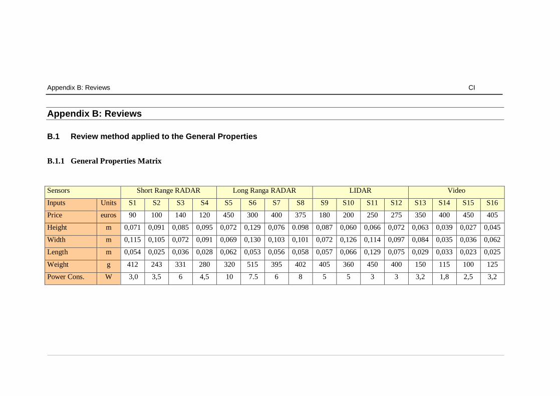
Appendix B: Reviews CI
Appendix B: Reviews
B.1 Review method applied to the General Properties B.1.1 General Properties Matrix
Sensors Short Range RADAR Long Ranga RADAR LIDAR Video
Inputs Units S1 S2 S3 S4 S5 S6 S7 S8 S9 S10 S11 S12 S13 S14 S15 S16
Price euros 90 100 140 120 450 300 400 375 180 200 250 275 350 400 450 405
Height m 0,071 0,091 0,085 0,095 0,072 0,129 0,076 0.098 0,087 0,060 0,066 0,072 0,063 0,039 0,027 0,045
Width m 0,115 0,105 0,072 0,091 0,069 0,130 0,103 0,101 0,072 0,126 0,114 0,097 0,084 0,035 0,036 0,062
Length m 0,054 0,025 0,036 0,028 0,062 0,053 0,056 0,058 0,057 0,066 0,129 0,075 0,029 0,033 0,023 0,025
Weight g 412 243 331 280 320 515 395 402 405 360 450 400 150 115 100 125
Power Cons. W 3,0 3,5 6 4,5 10 7.5 6 8 5 5 3 3 3,2 1,8 2,5 3,2
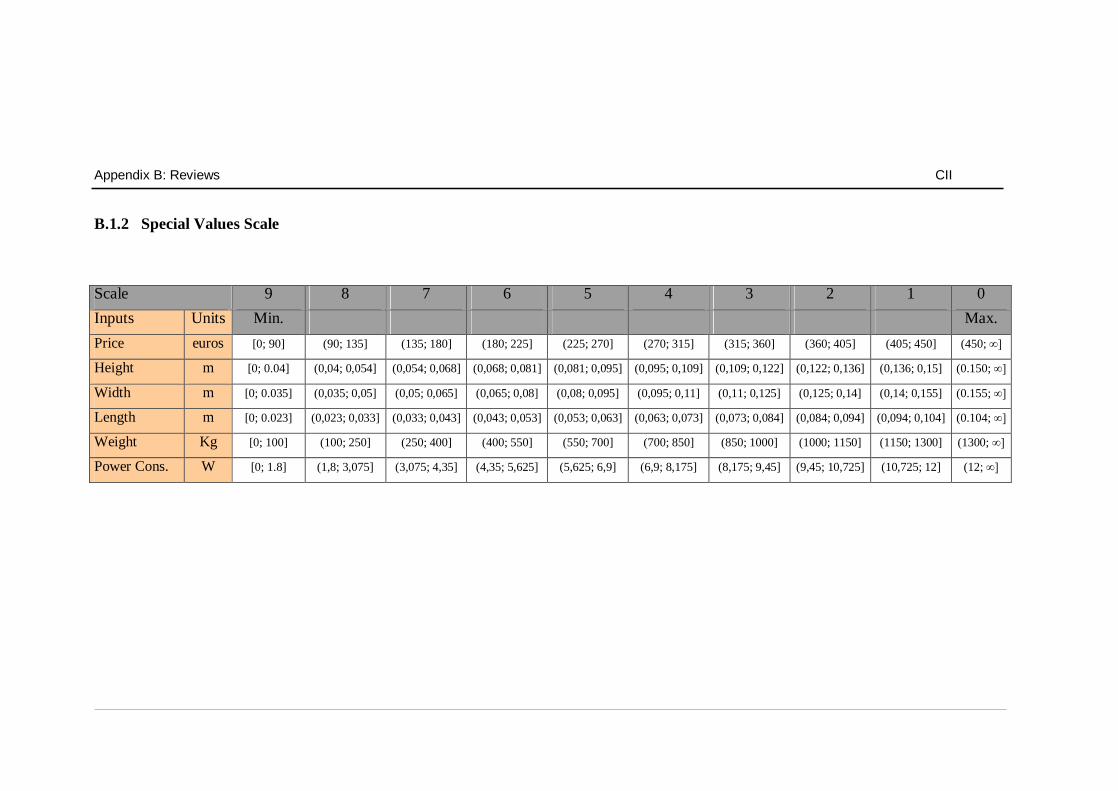
Appendix B: Reviews CII
B.1.2 Special Values Scale
Scale 9 8 7 6 5 4 3 2 1 0 Inputs Units Min. Max. Price euros [0; 90] (90; 135] (135; 180] (180; 225] (225; 270] (270; 315] (315; 360] (360; 405] (405; 450] (450; ∞]
Height m [0; 0.04] (0,04; 0,054] (0,054; 0,068] (0,068; 0,081] (0,081; 0,095] (0,095; 0,109] (0,109; 0,122] (0,122; 0,136] (0,136; 0,15] (0.150; ∞]
Width m [0; 0.035] (0,035; 0,05] (0,05; 0,065] (0,065; 0,08] (0,08; 0,095] (0,095; 0,11] (0,11; 0,125] (0,125; 0,14] (0,14; 0,155] (0.155; ∞]
Length m [0; 0.023] (0,023; 0,033] (0,033; 0,043] (0,043; 0,053] (0,053; 0,063] (0,063; 0,073] (0,073; 0,084] (0,084; 0,094] (0,094; 0,104] (0.104; ∞]
Weight Kg [0; 100] (100; 250] (250; 400] (400; 550] (550; 700] (700; 850] (850; 1000] (1000; 1150] (1150; 1300] (1300; ∞]
Power Cons. W [0; 1.8] (1,8; 3,075] (3,075; 4,35] (4,35; 5,625] (5,625; 6,9] (6,9; 8,175] (8,175; 9,45] (9,45; 10,725] (10,725; 12] (12; ∞]

Appendix B: Reviews CIII
B.1.3 Assignment of scale values
Sensors Short Range RADAR Long Range RADAR LIDAR Video
Inputs S1 S2 S3 S4 S5 S6 S7 S8 S9 S10 S11 S12 S13 S14 S15 S16
Price 9 8 7 8 1 4 2 2 6 6 5 4 3 2 1 2 Height 6 5 5 5 6 2 6 4 5 7 7 6 7 8 9 8 Width 3 4 6 5 6 2 2 4 6 2 3 4 5 9 8 7 Length 5 8 7 8 5 6 5 7 5 4 1 3 8 8 9 9 Weight 6 8 7 7 7 6 7 6 6 7 6 8 8 8 8 8 Power Cons. 8 7 5 6 2 4 5 4 6 6 8 8 7 8 8 7
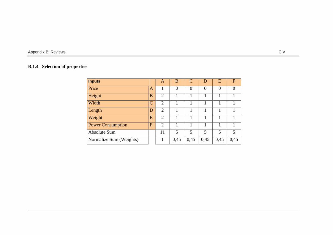
Appendix B: Reviews CIV
B.1.4 Selection of properties
Inputs A B C D E F Price A 1 0 0 0 0 0 Height B 2 1 1 1 1 1 Width C 2 1 1 1 1 1 Length D 2 1 1 1 1 1 Weight E 2 1 1 1 1 1 Power Consumption F 2 1 1 1 1 1 Absolute Sum 11 5 5 5 5 5 Normalize Sum (Weights) 1 0,45 0,45 0,45 0,45 0,45

Appendix B: Reviews CV
B.1.5 Assessment Matrix Assessment Matrix for Short Range RADAR and Long Range RADAR Sensor concepts Short Range RADAR Long Range RADAR
Sensors S1 S2 S3 S4 S5 S6 S7 S8
Inputs PW NWV WV NWV WV NWV WV NWV WV NWV WV NWV WV WV NWV WV NWV
Price 1 9 9 8 8 7 7 8 8 1 1 4 4 2 2 2 2
Height 0,45 6 2,7 5 2,25 5 2,25 5 2,25 6 2,7 2 0,9 6 2,7 4 1,8
Width 0,45 3 1,35 4 1,8 6 2,7 5 2,25 6 2,7 2 0,9 2 0,9 4 1,8
Length 0,45 5 2,25 8 3,6 7 3,15 8 3,6 5 2,25 6 2,7 5 2,25 7 3,15
Weight 0,45 6 2,7 8 3,6 7 3,15 7 3,15 7 3,15 6 2,7 7 3,15 6 2,7
Pow.Cons. 0,45 8 3,6 7 3,15 5 2,25 6 2,7 2 0,9 4 1,8 5 2,25 4 1,8
Sum 3,25 - 21,6 - 22,4 - 20,5 - 21,95 - 12,7 - 13 - 13,25 - 13,25
Valency - 0,738 - 0,766 - 0,702 - 0,750 - 0,434 - 0,444 - 0,453 - 0,453
Ranking 3 1 4 2 16 15 13 14

Appendix B: Reviews CVI
Assessment Matrix for LIDAR and Video
Sensor concepts LIDAR Video
Sensors S9 S10 S11 S12 S13 S14 S15 S15
Inputs PW NWV WV NWV WV NWV WV NWV WV NWV WV NWV WV WV NWV WV NWV
Price 1 6 6 6 6 5 5 4 4 3 3 2 2 1 1 2 2
Height 0,45 5 2,25 7 3,15 7 3,15 6 2,7 7 3,15 8 3,6 9 4,05 8 3,6
Width 0,45 6 2,7 2 0,9 3 1,35 4 1,8 5 2,25 9 4,05 8 3,6 7 3,15
Length 0,45 5 2,25 4 1,8 1 0,45 3 1,35 8 3,6 8 3,6 9 4,05 9 4,05
Weight 0,45 6 2,7 7 3,15 6 2,7 8 3,6 8 3,6 8 3,6 8 3,6 8 3,6
Pow. Cons. 0,45 6 2,7 6 2,7 8 3,6 8 3,6 7 3,15 8 3,6 8 3,6 7 3,15
Sum 3,25 - 18,6 - 17,7 - 16,25 - 17,05 - 18,75 - 20,45 - 19,9 - 19,55
Valency - 0,636 - 0,605 - 0,555 - 0,583 - 0,641 - 0,699 - 0,680 - 0,668
Ranking 9 10 12 11 8 5 6 7

Appendix B: Reviews CVII
B.2 Review method applied to the benefit presented by different CA Systems during frontal collisions B.2.1 Accidents Matrix
B.2.2 Special Values Scale Scale 9 8 7 6 5 4 3 2 1 0 Accidents Max. Min. Accident A [∞; 27] (27; 24] (24; 21] (21; 18] (18; 15] (15; 12] (12; 9] (9; 6] (6; 3] (3; 0] Accident B [∞; 18] (18; 16] (16; 14] (14; 12] (12; 10] (10; 8] (8; 6] (6; 4] (4; 2] (2; 0] Accident C [∞; 27] (27; 24] (24; 21] (21; 18] (18; 15] (15; 12] (12; 9] (9; 6] (6; 3] (3; 0] Accident D [∞; 18] (18; 16] (16; 14] (14; 12] (12; 10] (10; 8] (8; 6] (6; 4] (4; 2] (2; 0]
Sensors Short Range RADAR Long Range RADAR LIDAR Video
Accidents S1 S2 S3 S4 S5 S6 S7 S8 S9 S10 S11 S12 S13 S14 S15 S16
Accident A 8,2 7,4 5,0 7,6 28,2 26,5 27,0 24,2 23,6 24,5 26,5 22,2 17,8 18,2 14,8 15,6 Accident B 7,8 6,9 4,5 6,5 15,2 15,7 16,0 16,1 11,9 11,6 10,6 9,3 9,,8 7,8 8,6 6,8 Accident C 7,9 6,7 4,7 7,1 26,4 27,3 23,0 15,4 20,4 23 18,3 18,2 16,3 17,6 16,7 14,8 Accident D 6,5 7,2 9,8 5,9 16,1 15,9 16,2 14,2 10,8 13,2 11,0 12,6 11,4 7,9 11.4 10,3

Appendix B: Reviews CVIII
B.2.3 Assignment of scale values
B.2.4 Selection of properties
Sensors Short Range RADAR Long Range RADAR LIDAR Video
Accidents S1 S2 S3 S4 S5 S6 S7 S8 S9 S10 S11 S12 S13 S14 S15 S16
Accident A 2 2 1 2 9 8 9 8 7 8 8 7 5 6 4 5 Accident B 3 3 2 2 7 7 8 8 5 5 5 4 4 3 4 3 Accident C 3 2 2 1 8 8 7 8 6 7 6 6 5 5 5 3 Accident D 3 3 4 2 8 7 8 7 5 6 5 6 5 3 5 5
Inputs A B C D Accident A A 1 2 0 0 Accident B B 0 1 0 0 Accident C C 2 2 1 1 Accident D D 2 2 1 1 Absolute Sum 5 7 2 2 Normalize Sum (Weights) 0,71 1 0,29 0,29
Accidents Level of ocurrence* Accident A 31,7 Accident B 35,9 Accident C 16,7 Accident D 15,7 * According to GIDAS

Appendix B: Reviews CIX
B.2.5 Assessment Matrix Assessment Matrix for Short Range RADAR and Long Range RADAR Sensor concepts Short Range RADAR Long Range RADAR
Sensors S1 S2 S3 S4 S5 S6 S7 S8
Accidents PW NWV WV NWV WV NWV WV NWV WV NWV WV NWV WV WV NWV WV NWV
Accident A 0,71 2 1,42 2 1,42 1 0,71 2 1,42 9 6,39 8 5,68 9 6,39 8 5,68
Accident B 1 3 3 3 3 2 2 2 2 7 7 7 7 8 8 8 8
Accident C 0,29 3 0,87 2 0,58 2 0,58 1 0,29 8 2,32 8 2,32 7 2,03 8 2,32
Accident D 0,29 3 0,87 3 0,87 4 1,16 2 0,58 8 2,32 7 2,03 8 2,32 7 2,03
Sum - 6,16 - 5,87 - 4,45 - 4,29 - 18,03 - 17,03 - 18,74 - 18,03
Valency - 0,210 - 0,201 - 0,152 - 0,147 - 0,616 - 0,582 - 0,641 - 0,616
Ranking 14 13 15 16 2 4 1 3

Appendix B: Reviews CX
Assessment Matrix for LIDAR and Video
Sensor concepts LIDAR Video
Sensors S1 S2 S3 S4 S5 S6 S7 S8
Accidents PW NWV WV NWV WV NWV WV NWV WV NWV WV NWV WV WV NWV WV NWV
Accident A 0,71 7 4,97 6 4,26 8 5,68 7 4,97 5 3,55 6 4,26 4 2,84 5 3,55
Accident B 1 4 4 5 5 5 5 4 4 4 4 3 3 4 4 3 3
Accident C 0,29 4 1,16 7 2,03 6 1,74 6 1,74 5 1,45 5 1,45 5 1,45 3 0,87
Accident D 0,29 5 1,45 6 1,74 5 1,45 6 1,74 5 1,45 3 0,87 5 1,45 5 1,45
Sum - 11,58 - 13,03 - 13,87 - 12,45 - 10,45 - 9,58 - 9,74 - 8,87
Valency - 0,396 - 0,445 - 0,474 - 0,426 - 0,357 - 0,327 - 0,333 - 0,303
Ranking 8 6 5 7 10 11 9 12