Embed Size (px)
Citation preview

An Entangled Bayesian Gestalt:Mean-field, Monte-Carlo and
Quantum Inferencein Hierarchical Perception
�Charles Fox
Christ Church
University of Oxford
A thesis submitted for the degree of
Doctor of Philosophy
Trinity 2008

2

Jenny,
this one’s for you

Acknowledgements
With thanks to:
My adviser Prof. Stephen Roberts for allowing me the freedom to pursue
my own ideas unhindered, to make mistakes and learn to fix them.
Examiners Prof. Sir Mike Brady and Prof. Kathryn Laskey for their time
and help with corrections.
My family for their unfailing support during what I hope is the hardest
thing I will ever write.
Anuj Dawar for spending many hours teaching me Quantum Computing
in Borders coffee shop. David Deutsch for his valuable time listening to
and helping with the quantum Gibbs sampler. John Quinn for help with
particle filters and the meaning of Bayes. Amos Storkey for wondering if
quantum Gibbs does work after all. Matthew Dovey for help with black-
boards and introducing me to the London computer music scene. Penny
Probert Smith for help with low-level methods. Neil Girdhar for talking
too much. Chris Raphael for access to and in-depth voyages through his
Music++ code. Iead Rezek and John Winn for help understanding varia-
tional methods. Stuart Hameroff and Roger Penrose for discussions about
their quantum ideas. Stephen N.P. Smith for inspiring me to become an
Engineer. Josh Tenenbaum, Nick Chater and Alan Yuille for ideas about
the ‘Bayesian Brain’. Douglas Hofstadter, Eric Nichols, Chris Honey and
FARG for detailed discussions about Copycat, music, philosophy and ev-
erything.
Housemen Chris Aycock, Akshay Mangla, Jason Lotay, Dan Koch and
Raphael Espinoza and local tabs Andy Bower, Rob Fellows and Chris
Ramshaw; for collectively keeping it real.

Abstract
Scene perception is the general task of constructing an interpretation of
low-level sense data in terms of high-level objects, whose number is not
known in advance. This task is examined from a Bayesian perspective.
Simple examples from musical Machine Listening are provided, but this
thesis is intended as a general view of scene perception.
After reviewing relevant mathematics and low-level pre-processing meth-
ods, the psychologically inspired concepts of priming and pruning are
introduced, first in a novel extension to low-level particle filters, then in
a mid-level segmentation step, and finally in the high-level hierarchical
perception setting. Inference in the mid- and high-level networks is in-
tractable so two approximate methods – mean-field and Monte Carlo – are
examined. A novel mean-field Machine Listening application is presented,
and is extended to handle multiple objects using priming and pruning
ideas from classical Artificial Intelligence. A novel priming and prun-
ing Monte Carlo sampler is developed, which is specialised for high-level
perception, and provides new Bayesian semantics for classical blackboard
systems. Extensions to learning and action selection are discussed. The
previously unexplored field of Bayesian inference with quantum computing
is examined in the scene perception context, showing how a new algorithm
on quantum hardware can generalise both mean-field and Monte-Carlo
approaches to obtain a free quadratic speedup using only local operators.

Contents
1 Introduction 1
1.1 Scene perception . . . . . . . . . . . . . . . . . . . . . . . . . . . . . 1
1.1.1 Simplified scene perception . . . . . . . . . . . . . . . . . . . . 3
1.1.2 Minidomain approach . . . . . . . . . . . . . . . . . . . . . . . 5
1.1.3 Engineering vs. biology . . . . . . . . . . . . . . . . . . . . . . 6
1.1.4 Speeding up scene perception . . . . . . . . . . . . . . . . . . 7
1.2 Minidomain subtasks: a slice of iguana . . . . . . . . . . . . . . . . . 8
1.3 Positions-in-time and attention . . . . . . . . . . . . . . . . . . . . . 9
1.4 Contributions to knowledge . . . . . . . . . . . . . . . . . . . . . . . 11
2 Inference 12
2.1 Bayesian theory . . . . . . . . . . . . . . . . . . . . . . . . . . . . . . 12
2.1.1 Conjugacy and the exponential family . . . . . . . . . . . . . 13
2.2 Bayesian networks . . . . . . . . . . . . . . . . . . . . . . . . . . . . 14
2.2.1 Dynamic Bayesian networks . . . . . . . . . . . . . . . . . . . 17
2.2.1.1 Dynamic time warping . . . . . . . . . . . . . . . . . 17
2.2.2 Loopy graphs and approximate inference . . . . . . . . . . . . 18
2.2.2.1 Brute force inference . . . . . . . . . . . . . . . . . . 18
2.2.2.2 Clustering and junction trees . . . . . . . . . . . . . 18
2.2.2.3 Loopy belief propagation . . . . . . . . . . . . . . . . 19
2.2.2.4 Monte Carlo sampling . . . . . . . . . . . . . . . . . 19
2.2.2.5 Variational Bayesian inference . . . . . . . . . . . . . 22
2.3 Towards a quantum generalisation . . . . . . . . . . . . . . . . . . . . 23
2.4 Temporal hierarchies . . . . . . . . . . . . . . . . . . . . . . . . . . . 24
2.4.0.6 Hidden semi-Markov models (HSMMs) . . . . . . . . 25
2.4.1 Inside-outside algorithm . . . . . . . . . . . . . . . . . . . . . 25
2.5 Statistics and hash-classifiers . . . . . . . . . . . . . . . . . . . . . . . 27
i

3 Low-level audio inference
in the music minidomain 30
3.1 The music minidomain . . . . . . . . . . . . . . . . . . . . . . . . . . 31
3.1.1 Practical applications . . . . . . . . . . . . . . . . . . . . . . . 32
3.2 Review of musical audio structures . . . . . . . . . . . . . . . . . . . 33
3.2.1 Musical audio signals . . . . . . . . . . . . . . . . . . . . . . . 35
3.2.2 Pitch . . . . . . . . . . . . . . . . . . . . . . . . . . . . . . . . 38
3.2.3 Chords . . . . . . . . . . . . . . . . . . . . . . . . . . . . . . . 38
3.2.4 Keys . . . . . . . . . . . . . . . . . . . . . . . . . . . . . . . . 40
3.2.5 Rhythm . . . . . . . . . . . . . . . . . . . . . . . . . . . . . . 40
3.2.6 High-level structures . . . . . . . . . . . . . . . . . . . . . . . 41
3.3 A menagerie of musical hash-classifiers . . . . . . . . . . . . . . . . . 42
3.3.1 Normalised power DFT (NPDFT) . . . . . . . . . . . . . . . . 43
3.3.2 Radial basis functions (RBF) . . . . . . . . . . . . . . . . . . 43
3.3.3 Normalised dot product (NDP) . . . . . . . . . . . . . . . . . 43
3.3.4 Chroma vectors (CHV) . . . . . . . . . . . . . . . . . . . . . . 44
3.3.5 Chordality vectors (CDV) . . . . . . . . . . . . . . . . . . . . 44
3.3.6 Energy feature (E1) . . . . . . . . . . . . . . . . . . . . . . . . 45
3.3.7 Novelty (NOV) . . . . . . . . . . . . . . . . . . . . . . . . . . 45
3.3.8 Raphael burstiness (RB) . . . . . . . . . . . . . . . . . . . . . 45
3.3.9 Raphael generative spectra (RGS) . . . . . . . . . . . . . . . . 46
3.4 Overview of existing research areas . . . . . . . . . . . . . . . . . . . 46
3.5 Score following: review and preliminary tests . . . . . . . . . . . . . . 47
3.5.1 Dynamic time warping . . . . . . . . . . . . . . . . . . . . . . 47
3.5.1.1 DTW experiments . . . . . . . . . . . . . . . . . . . 48
3.5.1.2 DTW limitations . . . . . . . . . . . . . . . . . . . . 50
3.5.2 Hidden Markov models . . . . . . . . . . . . . . . . . . . . . . 51
3.5.2.1 HMM experiments . . . . . . . . . . . . . . . . . . . 51
3.5.2.2 HMM limitations . . . . . . . . . . . . . . . . . . . . 57
3.6 A novel priming particle filter score-follower . . . . . . . . . . . . . . 59
3.6.1 Tempo model . . . . . . . . . . . . . . . . . . . . . . . . . . . 60
3.6.2 Likelihoods . . . . . . . . . . . . . . . . . . . . . . . . . . . . 60
3.6.3 Injecting primed particles . . . . . . . . . . . . . . . . . . . . 61
3.6.4 Results . . . . . . . . . . . . . . . . . . . . . . . . . . . . . . . 63
3.6.5 Discussion . . . . . . . . . . . . . . . . . . . . . . . . . . . . . 64
3.7 Higher-level models in Music++ . . . . . . . . . . . . . . . . . . . . . 65
3.7.1 Architecture . . . . . . . . . . . . . . . . . . . . . . . . . . . . 66
ii

3.7.2 Hidden Markov model . . . . . . . . . . . . . . . . . . . . . . 67
3.7.3 Gaussian Bayesian network . . . . . . . . . . . . . . . . . . . 70
3.8 Onset detection and classification . . . . . . . . . . . . . . . . . . . . 72
3.9 Beat Tracking Research . . . . . . . . . . . . . . . . . . . . . . . . . 73
3.10 Towards semi-improvised score following . . . . . . . . . . . . . . . . 74
4 Application of variational Bayes
to segmentation of rhythmic scenes 76
4.1 Single models . . . . . . . . . . . . . . . . . . . . . . . . . . . . . . . 78
4.1.1 Switchboard . . . . . . . . . . . . . . . . . . . . . . . . . . . . 80
4.1.1.1 Sibling rivalry . . . . . . . . . . . . . . . . . . . . . . 81
4.1.1.2 Sinks . . . . . . . . . . . . . . . . . . . . . . . . . . 83
4.1.2 Precisions . . . . . . . . . . . . . . . . . . . . . . . . . . . . . 84
4.1.3 Visual display . . . . . . . . . . . . . . . . . . . . . . . . . . . 84
4.2 Example of a single model inference . . . . . . . . . . . . . . . . . . . 85
4.2.1 Cyclic and divergent behaviour . . . . . . . . . . . . . . . . . 85
4.2.2 Annealed variational message passing . . . . . . . . . . . . . . 89
4.3 Hypothesis management . . . . . . . . . . . . . . . . . . . . . . . . . 91
4.3.1 Priming . . . . . . . . . . . . . . . . . . . . . . . . . . . . . . 94
4.4 Evaluation . . . . . . . . . . . . . . . . . . . . . . . . . . . . . . . . . 95
4.4.1 Comparison with naive tracking . . . . . . . . . . . . . . . . . 95
4.4.2 Issues and extensions arising from the evaluation . . . . . . . 96
4.4.2.1 Need for missing children penalties . . . . . . . . . . 96
4.4.2.2 Tempo changes in bars, and tempo priors . . . . . . 102
4.4.2.3 Learning new models . . . . . . . . . . . . . . . . . . 102
4.4.2.4 Data-model mis-assignments . . . . . . . . . . . . . . 103
4.4.2.5 Non-Markovian priming . . . . . . . . . . . . . . . . 104
4.5 Discussion . . . . . . . . . . . . . . . . . . . . . . . . . . . . . . . . . 105
5 Blackboard systems review 107
5.1 From sets to sequences to hierarchies . . . . . . . . . . . . . . . . . . 107
5.1.1 Music-related issues . . . . . . . . . . . . . . . . . . . . . . . . 108
5.2 Blackboard systems . . . . . . . . . . . . . . . . . . . . . . . . . . . . 109
5.2.1 The Copycat approach to scene perception . . . . . . . . . . . 112
5.2.2 Numbo: an example of the Copycat family . . . . . . . . . . . 113
5.3 Blackboards in musical scene perception . . . . . . . . . . . . . . . . 114
5.3.1 Pre-Bayesian blackboard music models . . . . . . . . . . . . . 114
iii

5.3.2 Dynamic Bayesian network music models . . . . . . . . . . . . 116
5.4 Inference algorithms on Bayesian logics . . . . . . . . . . . . . . . . . 117
5.5 Summary . . . . . . . . . . . . . . . . . . . . . . . . . . . . . . . . . 118
6 Perceptual construction and inference in Bayesian blackboards 121
6.1 The matchstickmen microdomain . . . . . . . . . . . . . . . . . . . . 124
6.1.1 Hypothesis generation by priming . . . . . . . . . . . . . . . . 125
6.1.2 Parameters . . . . . . . . . . . . . . . . . . . . . . . . . . . . 126
6.1.3 Noisy-OR vs. feedforward neural networks . . . . . . . . . . . 127
6.1.4 Inference with Gibbs sampling, or ‘spiking nodes’ . . . . . . . 128
6.1.5 Matchstickmen results . . . . . . . . . . . . . . . . . . . . . . 129
6.2 The music minidomain . . . . . . . . . . . . . . . . . . . . . . . . . . 130
6.2.1 Formal task specification . . . . . . . . . . . . . . . . . . . . . 131
6.2.1.1 Example song . . . . . . . . . . . . . . . . . . . . . . 133
6.2.1.2 Freefloat priors . . . . . . . . . . . . . . . . . . . . . 133
6.2.1.3 Key factors . . . . . . . . . . . . . . . . . . . . . . . 134
6.2.1.4 Simplifications . . . . . . . . . . . . . . . . . . . . . 134
6.2.2 ThomCat architecture: static structures . . . . . . . . . . . . 134
6.2.2.1 Internal and external hypothesis parameters . . . . . 135
6.2.2.2 Lengthened grammars . . . . . . . . . . . . . . . . . 138
6.2.2.3 Discussion of the static structure . . . . . . . . . . . 140
6.2.3 ThomCat architecture: structural dynamics . . . . . . . . . . 140
6.2.4 Inference . . . . . . . . . . . . . . . . . . . . . . . . . . . . . . 143
6.2.5 Attention . . . . . . . . . . . . . . . . . . . . . . . . . . . . . 144
6.2.6 ‘Thalamus’ and ‘hippocampus’ as structural speedups . . . . . 145
6.2.7 Software architecture . . . . . . . . . . . . . . . . . . . . . . . 146
6.2.8 Results . . . . . . . . . . . . . . . . . . . . . . . . . . . . . . . 147
6.2.8.1 Gibbs walkthrough . . . . . . . . . . . . . . . . . . . 148
6.2.8.2 Gibbs bar-end collapsed percepts . . . . . . . . . . . 148
6.2.8.3 VB walkthrough . . . . . . . . . . . . . . . . . . . . 157
6.2.8.4 VB bar-end collapsed percepts . . . . . . . . . . . . 159
6.2.8.5 Effects of annealing schedule on Gibbs performance . 159
6.2.8.6 Performance with freefloaters . . . . . . . . . . . . . 166
6.3 Future extensions . . . . . . . . . . . . . . . . . . . . . . . . . . . . . 168
6.3.1 Action and utility . . . . . . . . . . . . . . . . . . . . . . . . . 168
6.3.1.1 Tree searching and hashing in AI . . . . . . . . . . . 169
6.3.1.2 Unitary coherent scenes vs. optimal actions . . . . . 171
iv

6.3.1.3 Network extension . . . . . . . . . . . . . . . . . . . 173
6.3.2 Learning . . . . . . . . . . . . . . . . . . . . . . . . . . . . . . 175
6.3.2.1 Tuning parameters . . . . . . . . . . . . . . . . . . . 176
6.3.2.2 Learning new models . . . . . . . . . . . . . . . . . . 177
6.3.3 Extended musical structures . . . . . . . . . . . . . . . . . . . 178
6.3.4 (Re)constructing the past and future . . . . . . . . . . . . . . 180
6.3.5 Modelling human cognition . . . . . . . . . . . . . . . . . . . 180
6.4 Discussion . . . . . . . . . . . . . . . . . . . . . . . . . . . . . . . . . 181
7 A quantum generalisation
speeds up scene perception 183
7.1 Quantum computing theory . . . . . . . . . . . . . . . . . . . . . . . 186
7.1.1 Summary of quantum computing theory . . . . . . . . . . . . 191
7.1.2 Comparison to existing work . . . . . . . . . . . . . . . . . . . 191
7.1.2.1 Grover’s algorithm . . . . . . . . . . . . . . . . . . . 192
7.1.2.2 Adiabatic optimisation . . . . . . . . . . . . . . . . . 195
7.1.2.3 Physical annealing . . . . . . . . . . . . . . . . . . . 195
7.1.2.4 Bayesian models of quantum systems . . . . . . . . . 195
7.2 Quantum hierarchical scene perception . . . . . . . . . . . . . . . . . 195
7.3 Representing joints by superpositions . . . . . . . . . . . . . . . . . . 197
7.4 Side-stepping the unitary requirement by extending the state space . 198
7.5 Intuitive explanation . . . . . . . . . . . . . . . . . . . . . . . . . . . 200
7.6 Formal algorithm description . . . . . . . . . . . . . . . . . . . . . . . 202
7.6.1 Algorithm . . . . . . . . . . . . . . . . . . . . . . . . . . . . . 203
7.6.2 Constructing the local operators . . . . . . . . . . . . . . . . . 203
7.7 Results . . . . . . . . . . . . . . . . . . . . . . . . . . . . . . . . . . . 205
7.8 Discussion . . . . . . . . . . . . . . . . . . . . . . . . . . . . . . . . . 206
7.8.1 Comparison to classical Gibbs sampling . . . . . . . . . . . . . 206
7.8.2 Comparison to variational inference . . . . . . . . . . . . . . . 207
8 Conclusion 208
Bibliography 213
v

Chapter 1
Introduction
1.1 Scene perception
This thesis is about scene perception. Scene perception is the general task of con-
structing a unitary, coherent and useful interpretation of low-level sense data, in
terms of almost-known high-level objects whose numerosity is not known in advance.
Unitary means there is a single unambiguous interpretation, in contrast to a fuzzy
or probabilistic set of possible interpretations. Coherent means that the parts of the
scene are mutually non-contradictory. Useful means as close to optimal as compu-
tationally possible, with respect to some task. Almost-known means that we have
approximate a priori models of the high-level objects, but some of their details may
be inaccurate and occasionally whole models may be missing and need to be learned.
Fig. 1.1 shows some examples of particular domains of scene perception. Visual
scene perception (a) is perhaps the best-known example. In vision, the low-level
data consists of coloured pixels, and the known high-level objects are physical three-
dimensional structures such as HOUSE, PERSON and SKY. Vision tasks are typically
characterised as atemporal: the task is to interpret a static image offline1. A simpler
scene perception domain is tactile scene perception. (b) shows a simulation of a
whiskered robot, whose task is to construct a high-level interpretation of its three-
dimensional environment from the low-level bending data from its whiskers as they
make contact with objects of different shapes and textures. Unlike the typical visual
task, the scene here is a map of the whole spatial environment around the robot,
rather than a sub-region of this space defined by the view of some camera. Another
difference is that with whiskers, the sense data arrive over time, even though the scene
itself may not be changing over time. This temporal element leads to the notion of
‘attention’: the robot can choose where to place its whiskers to gather data and
1though recent work has begun to consider video scene perception
1

Figure 1.1: Examples of scene perception domains. (a) Visual scene perception fromimages. (b) Tactile scene perception by a simulated whiskered robot. (c) Finan-cial time series perceived as large-scale patterns. (d) Semi-improved musical sceneperception.
perform computations on that data. Attention can be used in vision but its presence
is less obvious in static image interpretation tasks than in the whisker task where
the robot must physically move over time to gather information. Both the visual
and tactile tasks considered above aim to construct static models of spatial three-
dimensional scenes. Other particular types of scene perception may seek to construct
interpretations of temporal structures. ‘Chartist’ financial traders attempt to interpret
the low-level time series data of asset prices in terms of high-level objects such as
the ‘head-and-shoulders’ pattern and ‘trend lines’ shown in (c). As in tactile scene
perception, attention is important but is now less controllable than in the tactile case.
The trader may focus his computations on any point of the time series seen so far, but
the arrival of new data is now beyond his control – unlike the tactile robot which can
choose where in the world to collect data. The finance example especially emphasises
the role of utility in perception. Traders do not passively construct interpretations
of price series for fun: they do it for profit. This means they will try to perceive
the scene in terms of structures that are not just a good fit to the data, but also
have some (supposed) power to make money via their ‘filling in’ of the unobserved
parts of the scene – in the temporal case, their predictions of the future.2 Speech
scene perception has similar attributes to this type of financial scene perception.
Again, low-level data – this time audio samples – arrives over time, and the perceiver
2Similarly, fortune-tellers look for structures in tea-leaves which allow them to make a profitrather than structures which merely fit the low-level tea-leaf data.
2
may focus computational but not data-collection attention. Speech perception has
perhaps the best-developed theory of hierarchies of percepts. In vision, a HOUSE
may be made of subcomponents, WINDOW, DOOR, WALL and ROOF, and the
WINDOW may be made of several glass PANEs. In speech, intricate theories of
grammar describe how similarly, a SENTENCE may be made of NOUN-PHRASEs
and VERB-PHRASEs which in turn are made of various other parts of speech in
highly specific orderings. Musical scene perception (d) will be used as the running
particular example in this thesis. Musical scenes are auditory performances by one
or more musicians, and like language, include detailed structure at many levels. As
in language and finance, data arrive over time, and the scene exists over time rather
than space. The structures are simpler than natural language and vision – both of
which have grown huge research areas around their minutiae – but are just complex
enough to capture most of the general features of the general scene perception task.
Unlike finance, they are predictable enough to allow realistic building and testing of
simple models. Like speech, low-level data arrives as audio samples. A hierarchy of
musical percepts can be constructed, beginning with events such as onsets of drum
hits, progressing through musical bars and chords, and up to large-scale structures
such as verses and choruses.
1.1.1 Simplified scene perception
Artificial Intelligence (AI) research has commonly used two simplifications of general
scene perception: microdomains and deterministic scenes. Microdomains [81] are arti-
ficial scenes constructed specifically to illustrate particular aspects of scene perception
whilst keeping the tasks as computationally simple as possible. Deterministic scenes
drop the requirement that the scene content is unknown in advance. For example, in
musical scenes, we may often assume that we possess a known musical score of what
notes will be played; or in certain constrained vision problems such as production
line automation or medical image analysis [109] we may assume that the scene will
contain exactly one object of a known type. In these cases, the overall structure is
known, though the parameters of the models (such as musical tempo or visual object
position and configuration) are unknown.
Classical AI (i.e. pre-1990s, non-probabilistic and predominantly symbol-based;
e.g. [144]) often took microdomain approaches in order to demonstrate general con-
cepts using very limited computational resources. Whilst this laid the conceptual
foundation for much present work, three particular problems were later found to
have recurred in this approach. First, the microdomain approach by definition limits
3

testing to computationally feasible data sets. This meant that computationally in-
tractable tasks (in the sense of NP-hardness, discussed in chapter 2) could be scaled
down and appeared to be easily solvable. But of course such methods do not scale up
to real world problems on account of their intractability. The classical microdomain
approach ignored computational complexity. Second, classical AI’s use of symbols
often lead to a problem of modularity, in which the really hard parts of tasks were
performed (sometimes unknowingly) by humans in their pre-processing of the raw
data into symbols for use by the program. The SME and BACON projects were clas-
sical examples of this problem, as discussed in [23]. Third, the brittleness of classical
logic is of little use in real-world noisy data. To its credit however, non-microdomain
classical AI researched scalable heuristics for tractable model construction, such as
those of the ‘blackboard systems’ reviewed in chapter 5.
In contrast, the more recent Machine Learning approach to AI (e.g. [11]) has
preferred the deterministic scene simplification. Where classical AI drew on math-
ematical logic as its basis, Machine Learning begins with Statistics – in particular
subjective Bayesian probability theory as reviewed in chapter 2. Statistical thought
throughout the twentieth century has had much in common with the aims of AI,
seeking to infer explanations of low-level data in terms of models, and to make op-
timal actions based on those explanations. However much of its focus has been on
finding analytical solution and efficient approximation algorithms for particular mod-
els, rather than on automating the initial selection of models. R.A. Fisher held the
opinion that ‘initial choice of candidate models is more an art than a science’ [25],
and most modern Statistics texts focus on inference methods within models and on
model comparison rather than on the selection of initial hypotheses. For example,
in most branches of science, complex hypotheses are constructed by scientists using
their creativity and knowledge of their field. Data are then collected, and the meth-
ods of Statistics are used to test hypotheses. In scene perception however, hypothesis
selection is key, as we do not in advance what objects are in the scene and thus what
models to use. We cannot usually evaluate all known models (such as models of
pink elephants at every possible location in the room) at every moment in time. But
neither can we ask a human domain expert to use her knowledge and creativity to
conjecture an appropriate hypothesis set at every moment, if we wish to construct
autonomous agents. Scene perception systems need to automate this task as well as
making inferences and comparing models.
4

1.1.2 Minidomain approach
This thesis examines the general task of scene perception, using a musical minidomain
as a recurring example. Like a microdomain, a minidomain is chosen specifically to
illustrate general concepts, but in a simplified task chosen to fit computational and
research restrictions (in this case, a desktop PC and a three year doctoral thesis).
Unlike a microdomain, a minidomain has some practical use in the real world rather
than being the simplest possible ‘toy’ exemplar. In the case of music, microdomains
could for example include the perception of three-note melodies chosen to illustrate
perception of rising and falling melodies [122]. In contrast, the minidomain described
in chapter 3 – semi-improvised musical perception – while being ‘mini’ enough to
be feasible under our constraints, is a real-world practical problem with immediate
useful applications such as in components of automated musical accompaniment sys-
tems. The requirement for real-world activity also removes the classic temptations
to move the hard problems into human pre-processing. If the algorithms are to run
online, there will be no time to repeatedly ask human experts to suggest models –
the algorithms must be responsible for this part of perception too. This leads to
the idea of implementing a ‘whole iguana’ [18], that is, a complete vertical stack of
perception components which begin by processing the raw lowest level data (in this
case, audio samples) and increase in abstraction up to the highest level of objects in
the world (in this case, large musical structures such as verses and choruses). The
minidomain approach aims to implement a whole though small iguana: emphasis
is given to a complete vertical stack in a small domain. In contrast, much of the
Machine Learning approach focuses on detailed implementation of some single layer
in a rich domain (for example it is not uncommon for vision theses to spend three
years researching a slight improvement to some low-level feature detector); and classic
microdomain-based AI built a limited number of layers for a limited domain.
The musical minidomain is described fully in chapter 3, but briefly it is that
of perceiving simple semi-improvised, almost-known musical performances. Semi-
improvised is the type of compositional and improvisational structure found in forms
of Western jazz and popular music as well as non-Western art musics such as Indian
raga, in which a ‘composition’ is fluid and open to interpretation by the perform-
ers at the level of notes, rhythm, chords and large-scale structures, though bound
together by a set of strong prior conventions. Conventions may be written, such as
the suggested chords and melodies found in jazz and pop arrangements, or may be
the product of aural tradition, such as the motifs that are associated with particular
ragas or particular jazz pieces; and ‘standard’ chord substitutions, rhythmic devices,
5

and structural changes (such as inserting extra choruses on the fly if the audience is
enjoying the piece and wants more). Relative semi-improvised perception also arises
when a performance is deterministic but the listener only has a vague prior upon
it, as occurs when an unfamiliar listener perceives a performance of a notated, de-
terministic symphony. We restrict the minidomain to a series of sub-tasks, chosen
specifically to represent general scene perception tasks across all vertical layers of
perception. In particular, the concepts of feature-based priming, ‘almost-known’-ness
and the presence of global probability factors are characteristic of the general prob-
lem and we ensure they are retained in the minidomain. The minidomain and the
sub-tasks within it are slightly artificial, being restricted to feasible complexities on
a modern desktop PC, and restricted in development time by the requirements of a
doctoral thesis. We emphasise that the software implementations discussed here are
used to illustrate and demonstrate the ideas about scene perception of the thesis:
they are not yet intended to be practical tools (although we hope that development
of the research presented here could later produce such tools).
1.1.3 Engineering vs. biology
The purpose of the thesis is to present a unified view of what the perceptual process
for scenes could be, all the way up from raw data to high-level concepts, but presented
in a minidomain to allow it to be feasible. ‘The perceptual process’ is left as a delib-
erately ambiguous phrase, which can refer to both the human (or animal) biological
perception system, or to a constructed, engineered method for performing perception
by machine. There is a continuum of research approaches between hard engineering
AI (which only cares about producing solutions to tasks) and computational neuro-
science (which only cares about explaining what biological neurons do). The present
work is close to the engineering side of this continuum, but with some weight given
to biological ideas. In particular we intend the architectures to inform computational
neuroscientists’ high-levels models of what perception is, and perhaps provide inspi-
ration for future biological theories that implement the engineering ideas. A point
of strong agreement between the engineering and neuroscience views is the need for
parallel distributed processing (PDP) architectures, developed for completely differ-
ent reasons. Neuroscience studies the distributed system that is the brain, which –
as far as is known – appears to lack any central executive unit (except possibly dur-
ing very high-level conscious decision making), instead using a multitude of parallel
structures to process information. Machine Learning, on the other hand, has inde-
pendently discovered the utility of parallel distributed message-passing algorithms as
6

a means of making efficient inferences, and all the algorithms used in this thesis have
this character. Such algorithms will become especially useful as processor technol-
ogy moves towards multi-cores. We have chosen to use such algorithms mostly for
engineering efficiency reasons, but also as a weak biological constraint, to prevent
the architectures from being neurally implausible on the grounds of central planning
requirements.
1.1.4 Speeding up scene perception
A fundamental difficultly with general scene perception is that it is computation-
ally intractable, because inference – even approximate inference – is known to be
NP-hard [32]. This would appear to invalidate the whole project of scaling up to
real-world systems, if not for the fact that an existing computational device – the
brain – is known to be capable of performing it very well indeed. The brain’s general
mechanism for scene perception is not currently known (though research such as the
present work aims to provide candidate mechanisms to model and test). Scaling up
from microdomains to minidomains can quickly reach the threshold of intractability
for exact inference. Several methods have been proposed to speed up inference to
get closer to real time execution. An essential view, taken here as in all non-trivial
Machine Learning, is the need for approximations. Rather than compute exact prob-
ability distributions and functions of those distributions, we work with related but
simplified versions of those distributions. The variational and sampling approaches
are reviewed and used throughout this thesis. However it is known [148] that even
approximate inference is still NP-hard in the sense of reaching an arbitrary degree of
accuracy, and the approximate inference algorithms used in the minidomain tasks still
require greater than real time to run on a desktop PC to produce reasonable results.
A key point is the introduction of heuristics in the sense of classical AI: algorithms
which make ad-hoc but empirically-useful simplifications to the task to improve its
performance. We will draw on the classical AI ideas of blackboards, priming and
pruning, but use them as heuristics in Bayesian networks. However even with good
heuristics, inference can be very slow (slower than real-time).
More radical solutions to the slowness of perception have been suggested. One
possibility is that the real brain is an extremely large parallel processor, using brute
force parallel computation to solve NP-hard problems up to some size. However, such
parallelism can only achieve a constant factor speedup, given by the number of parallel
units, which is not even counted by standard computational complexity theory. So it
appears that we are left with a desperate problem: how can any computing device,
7

including the brain, possibly solve real-world sized scene perception problems when
we know them to be NP-hard?
One radical suggestion based on cutting-edge computer science is that quantum
computing – the new underlying theory of all computation, which generalises classical
Turing machines [42] – may be able to give a greater speedup than brute-force paral-
lelism. While quantum computing has not yet entered the commercial mainstream,
its theory [119] has been well-developed since the mid 1980s, and proof-of-concept
hardware has been constructed and successfully demonstrated standard algorithms
in practice by IBM, MIT and others [157]. Outside the peer-reviewed literature,
commercial enterprises claim to have successfully implemented non-general forms of
quantum computing, adiabatic [113] and secure cryptography [92], the latter in the
context of a real financial transfer between investment banks. Both theory and prac-
tice have showed greater than constant factor speedups in a variety of tasks, including
a quadratic speedup for unstructured database search [71]. Though extremely uncon-
ventional, this is of interest with regard to the scene perception task, as it provides
a speedup far greater than the constant factor gain from brute force parallelism.
Quantum methods have also been gaining currency in biology over the last 30 years
[102], [41] as increased computation power allows more accurate Schrodinger-equation
modelling of biological and pharmaceutical molecules. Given the large computational
speedups of theoretical quantum computing, it seems unlikely that biology should
not use such computations if physically convenient. This thesis has nothing to say
about the biological plausibility of quantum computing except to note that the cur-
rent quadratic speedup for database search relies on the use of large coherent global
operators, which would seem to be especially difficult to implement biologically. Out
of sheer desperation at the slowness of all known Bayesian approximation methods –
even with good heuristics – the final part of this thesis considers how future quantum
hardware could speed up general scene perception. Unlike the previous unstructured
database search method, we continue to respect the weak biological constraint that
algorithms should be comprised of parallel, local messages only, rather than large
global operators, and derive a novel quantum computational form of the Gibbs sam-
pler which achieves a quadratic speedup using only local operators.
1.2 Minidomain subtasks: a slice of iguana
The minidomain under consideration is semi-improvised musical scene perception.
Fig. 3.1 (in chapter 3) shows an example application of this domain in automated
accompaniment. The laptop attached to the drum kit runs a perception system
8

which listens to the musicians (and perhaps also received direct control signals from
the drummer) and schedules MIDI accompaniment notes to play along with them.
For example, this could be used if the bass player is absent from the rehearsal, to fill
in the bass part automatically – even if the players make semi-improvised structural,
rhythmic and tonal changes on the fly.
As our use of the minidomain is to illustrate a general view of scene perception
across all vertical layers, we will focus only on particular subtasks of such an accom-
paniment system which are relevant to achieving this goal. We will not consider the
generation of accompaniment, or perception of individual notes or melodies. These
are all fascinating areas within the accompaniment problem, but are not required
for our more theoretical goal. Rather, we pick a minimum set of subtasks from the
architecture shown in fig. 3.26 to use as illustrations of all vertical layers. The archi-
tecture shown in the figure begins with human performers generating sound waves.
Some form of pre-processing is performed (which we refer to as ‘hash-classifiers’ for
reasons that will become apparent in chapter 2), which occupies a similar architec-
tural position to the pre-thalamic nuclei of the biological system. In chapter 4 we use
information from the drummer’s signals in a program, RhythmKitten, to infer a single
segmentation of time into musical bars, which form the basic ‘grid’ of the high-level
blackboard system on which larger structures will be extended in chapter 6. We will
use only chord information from a single instrument to illustrate these structures,
which will include riffs, verses, choruses and songs. The blackboard – implemented in
a program called ThomCat – will handle rivalry, priming and pruning of hypotheses.
We do not aim to implement a complete computer music system, but to give
enough illustrations of all levels of perception to demonstrate a ‘whole iguana’ view
of scene perception. We have trimmed the minidomain into a series of implemented
subtasks: pre-processing, rhythm recognition, blackboard construction and black-
board inference, which together form a whole ‘vertical slice of iguana’.
While it is not currently possible to obtain desktop quantum computing to illus-
trate high-level quantum scene perception speedups, chapter 7 will give theory and
proof-of-concepts simulations showing how inference in ThomCat-like domains may
be improved using quantum hardware, and gesture towards a hypothetical ErwinCat
program at the highest level of the vertical slice.
1.3 Positions-in-time and attention
Music is inherently temporal, unlike other forms of scene perception such as vision,
and provides a useful minidomain to emphasise this often overlooked aspect of scene
9

perception. Two broad classes of temporal representation have been used in Machine
Learning and classic AI. Dynamic-state models maintain beliefs over the state at a
point or points in time. Position-in-time models maintain beliefs over the time at
which an event or events occur. The latter are a better fit with subjective notions of
perception, and are a good fit with blackboard concepts and heuristics. Though both
approaches have similar computational powers we work mostly with position-in-time
architectures. Classically, blackboard systems were often discussed using the language
of logic, for example statements of the form isAtLocation(object,location), giv-
ing rise to apparently mathematical-looking descriptions. We take the view that mod-
ern object oriented languages have largely removed the need for such representation,
as the languages themselves are rich enough to express such information. For example,
the instruction object.setLocation(location) expresses exactly the same state of
the world as the classical logical form (though as a constructive command rather than
a descriptive statement). Such constructive statements appear throughout our code
implementations but are mostly described in simple English in the dissertation text.
(In contrast, the Bayesian inference methods that run on these constructions are best
described using continuous mathematics notation.)
A key distinction is between represented and representing time. The former is
the domain of the blackboard in which the scene is constructed, and which behaves
much like space in visual scenes. The latter is the real processor time in which
computation about these structures is performed. Confusion between the two has
led to great philosophical debates [40], and we hope that our implemented models
show concretely how to resolve them. Again this issue is not as apparent in other
scene perception domains such as vision. The notion of attention involves these two
concepts of time, as we may focus our inferences onto distant past represented times
(i.e. when thinking about the past) but these computations are always performed at
the present representing time.
All the algorithms here – from low-level particle filters through variational rhythm
trackers to hierarchical Gibbs blackboards and quantum Gibbs sampler – are built
on the same concept of the annealing cycle in representing time. They maintain a
set of beliefs about the content of represented time, but during representing time the
attended beliefs are ‘heated’, ‘cooled’ and ‘collapsed’ regularly to update them. We
postulate this ‘blowtorch of attention’ as a basic mechanism for scene perception.
10

1.4 Contributions to knowledge
• A novel ‘priming’ particle filter algorithm for musical score following (published
in Proceedings of the International Computer Music Conference 2007, [60]).
• A novel application of variational message passing to simultaneous beat track-
ing and rhythm recognition (published in Proceedings of the International Com-
puter Music Conference 2007, [62]).
• A re-appraisal and re-construction of classical blackboard system ideas – in
particular the Copycat architecture – in a modern Machine Learning framework.
• Practical Bayesian blackboard methods for high-level musical scene perception,
illustrating the above ideas. (Published in Proceedings of the AAAI Interna-
tional Florida Artificial Intelligence Research Society Conference 2008, [58]).
• An open-source quantum computing simulation library for Matlab, called QCF
(published as Oxford University Technical Report PARG-03-02, [55]; and as
SourceForge code downloaded by more than 70 users from June 2007 to June
2008).
• A new local-only quantum computing algorithm which generalises the Gibbs
sampler and achieves a quadratic speedup (Published in the Second AAAI Sym-
posium on Quantum Interaction, 2008, [63]).
• Clarification of the role of heuristic ‘hash-classifiers’ in inference and action
selection (published in part in Proceedings of the AAAI International Florida
Artificial Intelligence Research Society Conference 2008, [59]).
• An illustration of the ‘vertical iguana slice’ minidomain methodology for AI.
• Steps towards computational definitions of psychological concepts such as prim-
ing, attention, and rivalry, which may help to clarify discussion.
11

Chapter 2
Inference
2.1 Bayesian theory
In Statistics, we are generally given a parametric model for data, but are uncertain
about its parameters and wish to make inferences about them from data. Given
a model M with parameters θ generating data D with P (D|M, θ), we use Bayes’
theorem to invert the model:
P (θ|D,M) =P (D|θ,M)P (θ|M)
P (D|M)
The term on the left is called the posterior. The three terms on the right are called
the likelihood, the prior, and the evidence. The evidence can be obtained using the
integrating out theorem over θ.
The posterior can be utilised in various ways: ideally, the whole distribution is
preserved and future inferences involving θ are made by integrating over it. If we seek
a single statistic to describe the value of θ, we may quote the value with the maximum
probability, the maximum a posteriori (MAP) value: θMAP = arg maxθ P (θ|D,M),
or we may choose to quote the mean or the median of the posterior. The choice here
depends on what we want to do with the result: if we are interested in the average
height of a population, the mean or median is appropriate; however if we want to
know the best place in a piece of music to provide accompaniment, the MAP may
be more appropriate. The standard deviation of the posterior can be used as an
indication of uncertainty in these statistics. Sometimes we will be interested in the
joint distribution of particular subsets of variables, and in these cases we can choose
to quote values such as the MAP solution for the subset’s joint.
The evidence term P (D|M) is independent of θ so does not need to be computed
for the parameter-fitting task. However it becomes useful if we are given two or
more competing models to fit the data. Then the P (D|Mi) give us likelihoods that
12

each model generated the data. These may be combined with prior beliefs about the
presence of the models to give posteriors for the models, to compare them:
P (Mi|D) =1
ZP (D|Mi)P (Mi)
where evidence Z is a normalising coefficient, in this case summing over all candidate
models Mj ,
Z = P (D) =∑
j
P (D|Mj)P (Mj)
Models with large numbers of parameters are automatically penalised for over-fitting
the data by this system – giving a mathematical clarification of ‘Occam’s razor’.
When a prediction of a random variable f is required, we can choose to work with
only the most probable model M and predict using P (f |M); or if resources allow, we
may go ‘fully-Bayesian’ by keeping all the models and integrating over them:
P (f |D) =∑
j
P (f |Mj)P (Mj|D)
The latter is the optimal strategy for a rational agent with infinitely large and fast
computational resources. But for real-world agents it is often considerably time-
consuming to compute. Time consumption often carries its own utility penalties so
the strategy may not be optimal for such agents.
2.1.1 Conjugacy and the exponential family
When making inferences using Bayes theorem, a prior distribution P (θ) is updated
on observation of a variable x to become the posterior P (θ|x) by
P (θ|x) ∝ P (θ)P (x|θ)
It is computationally convenient if the posterior has the same parametric form as the
prior, in which case the result of the inference may be represented simply by updating
these parameters. For a given parametric likelihood form, a prior/posterior form is
said to be conjugate to the likelihood form if it has this property.
A large class of likelihood-prior conjugates is the exponential family of distribu-
tions, which are defined by
P (x|θ) = exp {〈u(x)|φ(θ)〉+ f(x) + g(φ)}
where u(x) is a vector of sufficient statistics, φ(θ) is a vector of multi-linear natural
parameters, 〈|〉 is the inner product operation, and g is a multi-linear function and f is
13

a normalising function. We will make heavy use of conjugate-exponential distributions
in variational inference due to their simplified computational properties. A problem
with their use is that they assume our subjective priors to have particular parametric
forms, which may not exactly match our actual beliefs. However in practice many
beliefs are unimodal and approximately exponential – generally with Gaussian or
Gaussian-like shapes defined on various domains.
2.2 Bayesian networks
The configuration space of a model grows exponentially in its number of variables.
So in general, representing and computing with the full posterior requires exponential
space and time respectively. However many models exhibit conditional independence
relationships between variables which may be exploited to reduce space and time
requirements. Variables X and Y are conditionally independent on variable Z if
P (X, Y |Z) = P (X|Z)P (Y |Z). The minimal set of variables Z separating X from all
other variables Y in the model is called the Markov blanket of X, or mb(X).
Bayesian networks (BNs) [124] are directed acyclic graphs (DAGs) which represent
conditional independence relationships intuitively for models of the form
P (X1, X2, ...XN) =
N∏
i=1
P (Xi|par(Xi))
with the parent function par satisfying, par(Xi) ⊂ {Xj|j < i}. The DAG represents
each variable Xi by a node, and contains a directed edge from each parent of Xi to
Xi. Each node is associated with a function P (Xi|par(Xi)). The DAG structure is
utilised by many algorithms for performing efficient inference.
Pearl [124] showed that for DAGs which are also polytrees, with discrete-valued
variables, there is a polynomial-time algorithm for making inferences about variable
marginals. The following update equations are computed repeatedly for each possible
value xi of each node Xi until they converge:
14

Bel(xi) ← αλ(xi)π(xi)
λ(xi) ←∏
j
λYj(xi)
π(xi) ←∑
u1...un
P (x : u1, ..., un)∏
i
πX(ui)
λX(ui) ←∑
xi
λ(xi)∑
uk:k 6=iP (xi : u1, ...un)
∏
k 6=iπX(uk)
πYj(xi) ← α(
∏
k 6=jλYk
(xi))∑
u1,...un
P (xi : u1, ...un)∏
i
πX(ui)
where Ui are the parents of X and Yi are the children of X. Bel becomes the posterior
marginal belief in a node’s state; π the prior; and λ the likelihood. λX(ui) are
likelihood messages sent by X to its parents and πYj(xi) are prior messages sent to
its children.
If we wish to make a decision based on the value of a single node, then we should
use its marginal Bel distribution. However for some tasks we are instead interested
in the configuration of a collection of nodes. In scene perception we want to know
the single most likely interpretation of the whole musical environment so that we can
make accompaniment actions based on it. [30] gives an alternative message-passing
algorithm called max-propagation which enables this form of inference on polytrees.
Bayesian networks are intended [124] to model causality rather than merely passive
correlation. For causal modelling, the network is provided with a set of operators
do(Xi = xi) which when applied to nodes Xi, set pa(Xi) = ∅ and P (Xi) = δ(Xi; xi).
δ is a Kronecker or Dirac Delta function for discrete or continuous nodes respectively.
The do operators correspond [125] to the effects of performing an intervention on the
system being modelled.
Fig. 2.1 shows a visualisation of a Bayesian Network structure being used by
Pearl’s algorithm. The task, described in full in [124], is to compute the posterior
probability of a burglary, given an observation of the alarm sounding and evidence of
a radio report that there has been an earthquake (which may also explain the alarm
activation). Similar visualisations will be used in the next chapter.
Similar networks and update equations can be constructed for certain classes of
continuous state networks, namely those which nodes have conjugate priors as neigh-
bours [124]. For such variables, there exist simple equations to update the posterior
parameters as a function of the prior and likelihood parameters. A particularly sim-
ple case occurs with collections of Gaussian-valued nodes, parametrised by (µ, σ).
Such nodes are self-conjugate as the sum of any number of Gaussian variables is also
15
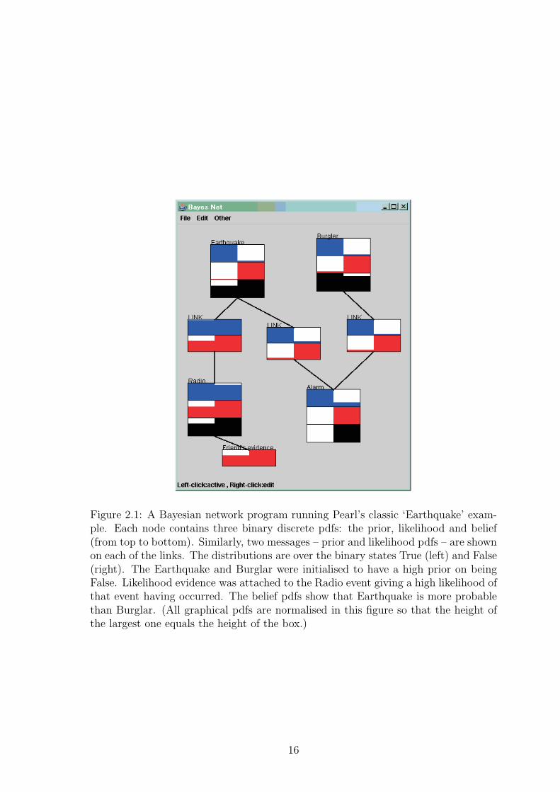
Figure 2.1: A Bayesian network program running Pearl’s classic ‘Earthquake’ exam-ple. Each node contains three binary discrete pdfs: the prior, likelihood and belief(from top to bottom). Similarly, two messages – prior and likelihood pdfs – are shownon each of the links. The distributions are over the binary states True (left) and False(right). The Earthquake and Burglar were initialised to have a high prior on beingFalse. Likelihood evidence was attached to the Radio event giving a high likelihood ofthat event having occurred. The belief pdfs show that Earthquake is more probablethan Burglar. (All graphical pdfs are normalised in this figure so that the height ofthe largest one equals the height of the box.)
16

Gaussian. In the general case, we may create Bayesian networks with arbitrary mix-
tures of parameter types. However in such cases are unlikely to yield tractable exact
message passing algorithms. Various methods for approximate inference are reviewed
in section 2.2.2.
Graphical models (GMs) generalise BNs by dropping the BN requirements that
the network be directed and causal. Models used in physics such as Ising models [19]
and Boltzmann machines [1] are examples of GMs that are not Bayesian networks.
In GMs, undirected pairwise specify pairwise probability factors, which are functions
of the connected nodes’ values and multiply into the joint posterior. Models having
only pairwise undirected links are called Markov random fields (MRFs) and generalise
the Ising Model (which is restricted to having identical factors on all links). MRFs
are also known as ‘structural equation models’ in some fields. Any graphical model
can be converted into an equivalent MRF form [117], though this discards causal
semantics and usually adds nodes.
2.2.1 Dynamic Bayesian networks
A Hidden Markov Model (HMM) [129] is a special case of a Bayesian network, having
all discrete-valued nodes, a particular structure, and particular set of observations.
A set of hidden variables Xt are conditioned in a sequence such P (Xt) = f(Xt−1)
(this is the Markov property) where f is the transition function. A set of observation
nodes Yt are conditioned on the hidden variables, P (Yt) = g(Xt). t is often (though
not necessarily) used to represent time. When the nodes are continuous and f and g
are Gaussians, the resulting model is called a Kalman filter.
2.2.1.1 Dynamic time warping
Dynamic time warping (DTW) [130] is a pre-Bayesian approach to sequence align-
ment, using standard dynamic programming to perform a similar task to HMMs.
Given two sequences of symbols – the template and the observation – we wish to
map each member of the observation to a member of the template. DTW assumes
that there exists a distance measure on pairs of sequence elements. DTW creates a
local distance matrix L with elements Lit which are the distances between the ith
member of the input sequence and the tth member of a template sequence. Dynamic
programming is then used to find the shortest path through the matrix subject to
specified constraints on the form of paths. A second ‘total distance’ matrix keeps
track of the shortest distance from the start to each column t of row i. The algorithm
is independent of path histories, so is of order O(T ) at each point in time, where T
17

is the length of the template sequence. For path constraints which allow only steps
from row i to row i + 1, DTW is equivalent to a HMM with a flat transition prior
over the allowable future states.
2.2.2 Loopy graphs and approximate inference
The Pearl update equations are valid only for polytrees, which is a severe limita-
tion. We will often have some data D which can be accounted for by two different
models M1 and M2. To allow these models to compete, we need a parent node N
which controls the joint probabilities of M1 and/or M2. So we have probabilities
P (M1,M2|N), P (D|M1), P (D|M2) which form an acyclic loop as shown in fig. 2.2.
(A cycle, in contrast, is a directed loop, such as a→ b→ a.) With the Pearl equations
invalid, we must use alternative algorithms.
2.2.2.1 Brute force inference
For small BNs, it is possible to compute the complete posterior by tracing all possible
paths through the network and keeping track of their probabilities. General inference
may then be done by cropping and re-normalising this posterior to condition on
evidence. Such brute-force computation would be intractable O(∏i=N
i=1 di) where there
are N nodes having discrete state sizes di, and would be uncomputable for general
continuous nodes.
2.2.2.2 Clustering and junction trees
If the cycles are ‘small’ it may be possible to manually group nodes together that are
involved in loops, into larger nodes with more complex states (i.e. tensor products of
the loopy nodes).
The junction tree or J-tree algorithm automates the manual clustering process.
The DAG is converted algorithmically into an undirected graph, some extra edges
added (via a process known as moralisation, or ‘marrying parents’), and cliques found
(which is itself an NP-hard problem). Then a new undirected graph is constructed
where each of these cliques becomes a node. Joint PDFs are computed for each clique,
and messages are sent between cliques to normalise them [86]. This requires ‘compil-
ing’ the network into the ‘junction tree’ form every time an inference is required, so
is unlikely to be useful for realtime systems when the network structure is changing.
18

N
D
M2M1
Figure 2.2: Loops arise when rival models are considered to explain data D.
2.2.2.3 Loopy belief propagation
Simply applying the polytree Pearl equations to loopy graphs without modification
achieves reasonable approximations to the node marginals in useful cases [116, 65].
[162] explains this by showing that the computed marginals do not correspond to
marginals of any actual joint, but are obtained by replacing the true entropy of the
joint with a ‘Bethe entropy’ simplification which assumes the joint is factorisable
as in a polytree. Approximation accuracy may be improved at the expense of extra
computation by performing Bethe-like message passing on clusters rather than nodes,
as in the J-tree algorithm: this approach is known as the Kikuchi approximation due
to its connection to a statistical mechanics method of the same name [162].
As the Pearl equations compute individual node marginals, the Bethe approxi-
mation computes approximate node marginals. For many applications, such as scene
perception, we prefer a single estimate of the MAP of the joint, as found by the max-
propagation equations in the polytree case. The loopy message passing scheme can
be converted into an MAP-joint estimator by introducing a temperature parameter
T [164], and replacing P (x|par(x)) by P (x|par(x))1/T . As T → 0, the joint tends to a
Delta spike1 at the MAP. As a Delta spike is equal to the product of its marginals, the
Bethe node marginals may be interpreted as factors in the approximate joint MAP.
Temperature must be reduced slowly to avoid becoming trapped in local minima; and
even the global MAP estimate if found is still a Bethe approximation, not the true
MAP. This scheme is called deterministic annealing.
2.2.2.4 Monte Carlo sampling
The previous methods (with the exception of deterministic annealing) are all to com-
pute or estimate the individual node marginals. However in scene perception tasks
we want to approximate the MAP of the joint P (xi=1:N), not the individual nodes
1i.e. the product∏
i δ(xi; Xi) of Kronecker and/or Delta distributions on node variables Xi,according to their discreteness or continuousness.
19

{Pi(xi)}i=1:N . We will discuss two classes of methods that do this, and one spec-
ulative method. The fundamental problem with joint distributions is that they are
exponential in size: even just writing them down would require exponential space and
hence exponential computing time (to visit each location and write its value). The
first approximate method – Monte Carlo sampling – uses the N nodes in a network
over exponential time: at each time-step, a sample from the joint is displayed on
the network, so the set of states of the network over exponential time represents the
joint. The second method – mean-fields – does not represent the true joint at all,
but aims to find a factorisable distribution Q(xi=1:N ) =∏N
i=1Qi(xi) that is ‘similar’
to it. By being factorisable into node marginals, the N nodes of the network can
represent the whole approximate joint by storing marginals as in the Pearl/Bethe
scheme. Sampling represents the exponential complexity of the joint over exponen-
tial time; mean-field discards the exponential complexity and represents a tractable
approximation with tractable resources at a single point in time. In chapter 7, we
will show how future quantum hardware could resolve this tradeoff by representing
the exponential-sized joint with the tractable N nodes at a single time, making use
of physical entanglement to represent the correlations.
Monte Carlo (MC) sampling produces a series of samples drawn from the joint,
which taken together over time represent the joint. To achieve an arbitrary error in
quantities computed from the samples, an exponential number of samples is needed:
however MC can be converted into a tractable approximation method by taking fewer
samples in tractable time and allowing higher approximation errors. Drawing samples
from a high-dimensional distribution is a hard problem: the naive approach of com-
piling a cumulative table then looking up values from a uniform distribution would
require the whole joint to be computed in advance by brute force: which is what
we are trying to avoid! A second naive method is to draw samples from a uniform
distribution over the same domain as the joint, U(xi=1:N ), evaluate the probability
of each under P , and re-normalise them to appear as if they came from P . However
in high dimensional space, the uniform distribution is unlikely to produce any ‘good’
samples from peaks in P [44]. Methods are needed that draw samples from good
areas of P instead. For simple P we may be able to construct an approximate Q ≈ P
from which we can sample easily (e.g. a high dimensional, moment-matched Gaus-
sian) then apply the same re-weighting scheme as in the uniform case: this is called
importance sampling. Alternatively, rejection sampling [44] uses a criterion to keep
or reject the Q samples such that the kept samples form a sample from P without
re-weighting. For large networks, as we will use, it is not usually possible to find a
single suitable Q to use these methods.
20

An alternative is to use Markov Chain Monte Carlo (MCMC) methods [44] which
construct a different Q(x′|x) at each step, conditioned on the current sample x. The
idea is to approximate and move within only the local area of the joint around the
current sample, in a similar manner to gradient descent style optimisation methods
which assume some local knowledge of the landscape. Applying the rejection sam-
pling method in this context gives rise to Metropolis-Hastings (MH) sampling. Gibbs
sampling is a special case of MH in which the Q is chosen to be the exact conditional
Q(x′i|x) = P (x′i|{xj 6=i}) holding all xj 6=i constant, and proposals are always accepted.
Due to graphical models’ use of local probability factors this is a particularly simple
form of MCMC to implement in inference problems. It is implemented by holding
the state of all nodes constant except for one (randomly chosen) node; computing the
conditional distribution for the node; and sampling from it to give that node’s value
in the next network state.
Gibbs sampling is not usually the most efficient MH method. In general, MH is
faster when prior structural and domain knowledge about P allows more accurate
and extensive Q(x′|x) ≈ P (x′|x) to be designed. For particular problems, a custom
Q can be designed using this knowledge: the art here is to design a Q that is easy
to sample from and is also similar to the local P according to domain knowledge. In
visual image perception a MH method found to be useful is cluster sampling [5] which
proposes and accepts flips of state in clusters of locally-connected nodes (rather than
individual nodes as used in Gibbs). In low-level harmonic music scene perception,
custom kernels which model explicit moves between numbers of notes and their pitches
was useful in offline transcription [68]. As with model design, inventing MH kernels
is a creative process based upon domain knowledge and trial-and-error.
For real-time temporal networks, we may use a form of multi-sample MH for
approximate inference of dynamic-state slice marginals as in the DTW, HMM and
Kalman filter models, to limit the number of hypotheses under consideration. The
particle filter [45] (also known as ‘sequential importance resampler’) maintains a pop-
ulation of samples at each slice, used to propose samples for the next slice; and the
acceptance probability P then involves the next likelihood from the temporal data.
Like Bethe propagation, Monte Carlo methods are easily converted from joint-
approximators into MAP optimisers by introducing and reducing a temperature pa-
rameter, i.e. replacing all P with P 1/T . This was first performed on a Gibbs sampler,
and annealed MH sampling has come to be known as simulated annealing [91], al-
though we emphasise that annealing can be applied to all the joint-approximating
methods considered here in the same way. Finding useful annealing schedules – i.e.
the sequence of temperatures to use at each step – is something of a black art and
21

is usually done by trial-and-error in practice. Too fast, and annealing gets stuck in
local minima; too slow and annealing may take impractical lengths of time to run.2
Chapter 6 will apply annealed Gibbs to hierarchical scene perception. Simulated tem-
pering [104] adapts the temperature in response to the current network state, heating
it when it appears to have reached a minimum energy to escape from local minima
and encourage further exploration.
2.2.2.5 Variational Bayesian inference
The size of a joint over N variables is exponential in N , so representing it exactly
generally requires exponential space, and exponential time to compute. An alternative
strategy is to replace the exact joint P (x) with some approximate joint Q(x) having
simpler computational properties which allow it to be represented in a smaller space
(and require less time to compute). This approach is called Variational Bayes (VB)
and is applied in chapter 4. In particular, we will assume Q(x) =∏
iQi(xi) to
be factorisable into the product of individual variable factors Qi(xi). Under this
assumption, we may then represent Q(x) by the state of a graphical model at a single
point in time, by arranging for the nodes to contain these factors. This form of Q
is called a mean-field approximation (a particular form of variational Bayes), and
assumes that the nodes are uncorrelated with one another: it is precisely factors
involving pairs and groups of variables that have been excluded from the parametric
form. So the approximation is likely to be good for problems having weak correlation
structures, and bad for heavily combinatorial-type problems with strong correlations.
Once a parametric form for Q(x; θ) is specified, some algorithm may be used to
find the best θ to make Q as ‘close’ to the true P as possible. ‘Close’ may be defined
in various ways, but using the KL divergence,
KL[Q(x)||P (x|D)] =
∫
dx.Q(x) lnQ(x)
P (x|D)
can lead to particularly efficient algorithms in cases where the network is conjugate
exponential (or approximated by conjugate exponentials). It can be shown [2] that
defining L[Q(x)] as
lnP (D) = KL[Q(x|D)||P (x)]− L[Q(x)]
transforms the task of minimising the KL divergence into that of maximising
L[Q(x)] = −KL[Qi(xi)||Q∗(xi)] +H [Qi(xi)] + lnZ
2The ‘Robbins-Munroe criteria’ provide theoretical conditions for exact convergence, but are oflimited practical use as they require an infinite number of steps.
22

where xi is any hidden node, xi is the set of hidden nodes excluding xi, H is the
Shannon entropy, Q∗i (xi) = 1
Zexp〈lnP (x,D)〉Q(xi) and Z normalises Q∗
i (xi). A node-
updating algorithm similar to Pearl’s may be constructed to find (under certain con-
ditions) local maxima. This algorithm optimises the above in a greedy sense, by
altering one node’s Qi(xi) at a time (with nodes chosen in any order). As only the
KL term is dependent on xi, L is maximised with respect to Qi by setting Qi ← Q∗i ,
thus achieving the lowest possible value, zero, for the KL term. Making use of the
Markov blanket we can write the updates as
Q(xi)←1
Zexp〈lnP (xi, xi, D〉Q(xi)
which makes the update for a node a function of the distributions of only its lo-
cal, Markov blanket nodes. For conjugate exponential networks the updates have
particularly simple forms due the presence of analytic expectations [12, 160].
The model log likelihood, logP (d|M), has a tractable lower bound which is useful
for approximate model comparison:
N∑
i=1
[〈logP (xi|par(xi))〉Q − 〈logQi(xi)〉Q] .
2.3 Towards a quantum generalisation
Sampling methods require intractable, exponential time to represent a complete joint
over N variables, as they must generally visit each network configuration at least once
to make an exact representation. Variational methods – including Bethe and mean-
field approximations – drop correlation information and compute an approximate
joint, which can be expressed in terms of local node factors only. Neither of these
schemes is ideal for scene perception, in which we will see that nodes can be highly
correlated due to ‘rivalry’ links, but also in which inference often must run in real-time
if it is to assist in performing actions. Chapter 7 will investigate how future hardware
could combine aspects of both sampling and variational methods, to give a joint that
is factored into single-node potentials (as in VB) but which still is able to represent
global correlations (as in sampling) – and which runs using local message passing (as
with all the Bayesian methods reviewed here). Such a representation is impossible us-
ing conventional Turing machine hardware, but recent theoretical work (and practical
proof-of-concept demonstrations) suggest that quantum computers may be capable
of storing global correlations locally by exploiting physical ‘entanglement’. The need
for representation of exponential-sized joints is the Achilles heel of practical Bayesian
23

inference3, and quantum computing theory might allow such full representations to
exist in linear-sized space! Little work has been done on the links between quantum
computing and Bayesian inference. Chapter 7 will present novel work which makes
these connections and provides an algorithm for constructing such representations.
The difficulty in quantum algorithms lies in the limited and counter-intuitive
allowable forms of interaction during computation, and in reading out the results.
Few useful quantum algorithms are known, though Grover’s algorithm [71] shows that
unstructured search over N elements is possible in O(√N) time. However Grover’s
algorithm requires the use of a single, monolithic physical operator acting on the whole
computational state, which is difficult to achieve in practice. An exciting question
is whether a similar speedup can be obtained for Bayesian networks in the localised
‘message-passing’ manner of the other algorithms we have seen: that is, using only
small local operators acting on nodes and their neighbours. Chapter 7 will show that
this is indeed possible, and that scene perception networks can obtain a quadratic
speedup (over a classical Gibbs sampler) using only local quantum operators.
2.4 Temporal hierarchies
We have already seen two temporal models: DTW and the HMM, both of which
make a perception of a score time at each real time. However they are limited to
perceiving a single position in a linear, predetermined musical score. More generally,
we will be interested in scores that are generated from hierarchical grammars and
other probabilistic factors. Our grammatical models will be based upon stochastic
context-free grammars (SCFGs). A SCFG is a set G of rules r of the form
(A→ B1, B2, B3), pr
where
∀a∑
{r∈G:Ar=a}pr = 1
The symbol Bi of rule r may appear as the LHS term of other rules, in which case
Bi is called nonterminal; otherwise it is a terminal. The grammar describes a set of
term rewriting rules, having probability pr of rewriting. The probability of a parse of
a string of terminals is given by the product of the probabilities of the rewrites used
to make the parse. Though general scene perception is not context-free, the SCFG
model can form a base for context-sensitive extensions. For example, in the music
3Hence the classical statisticians’ joke: How many Bayesians does it take to change a light bulb?Only N but it takes them exponential time.
24

domain, we might maintain a global musical key which influences low-level percepts in
addition to the rest of the grammar. For this reason we review two standard methods
for parsing SCFGs. We will restrict our SCFGs to non-recursive grammars, i.e. we
do not allow grammars which have possible infinite rewriting derivations.
2.4.0.6 Hidden semi-Markov models (HSMMs)
The Markov property of HMMs means that once the system is in a state i, there is
a constant transition probability of it moving to the next state j. The probability is
independent of the amount of time spent in state i. For domains where we know a
prior on the expected duration in each state, this is not a very appropriate model.
For example, if we choose to model each note of a musical score by a state, then we
would very much like to be able to specify expected durations of these notes. A naive
attempt at such a specification is to choose transition probabilities so that the mean
time spent in the state matches our expectation. Consider a simple model with two
states, A and B, with p = P (B|A), q = P (A|A). Assume that once the system is in
state B it stays there. Let A represent a note which we expect to last for 4 frames.
We could then set p = 1/4. So the average number of frames spent in state A is 4.
Chapter 3 will show why this naive attempt fails due to a ‘sandboxing’ effect.
To make the transitions depend on the time spent in the state, we must relax the
Markov assumption. One model which does this is the hidden semi-Markov model
(HSMM) [115]. In the HSMM, each state has an explicit duration PDF associated
with it. On entering a new state, a duration is drawn from this PDF, specifying
how many observations to generate from the state. When those observations are
generated, we proceed to draw the next state from the transition matrix. Inference
can be performed with a slight modification of the Viterbi algorithm [115]. As with the
regular HMM Viterbi method, this gives the most likely path through the system,
not the most likely individual states. HSMMs can be generalised to hierarchical
hidden Markov models (HHMMs) having states at multiple levels, each of which has
a duration and generates low-level states during its presence [115]. This is equivalent
to performing parsing of SCFGs with a fixed height of hierarchy.
2.4.1 Inside-outside algorithm
HSMM and HHMMs are dynamic-state models. Chapter 5 will review blackboard
systems which are position-in-time, but we here discuss the standard inside-outside
parsing algorithm (IO) which is also of this category. We give a novel Bayesian
25

network formulation with a modified Pearl likelihood message (based on insights from
the more complex formulation of [108]).
IO instantiates L× L ×M nodes where L is the length of the terminal string to
be parsed and M is the number of rules in the grammar. Each node represents a rule
instantiated with a start time and and end time. A node for a a rule r instance is
regarded as a generator of its RHS sub-component instances with probability pr, and
these form causal links in the network. Messages are passed which are similar to the
Pearl equations, but with the single important difference of ignoring explaining-away
effects in the likelihood messages. That is, the likelihood message is
λX(uj) =∑
xi
λ(xi)P (xi : uj)
instead of Pearl’s
λX(uj) =∑
xi
λ(xi)∑
uk:k 6=jP (xi : u1, ...un)
∏
k 6=jπX(uk)
These messages give exact marginal probabilities of rule instances existing at each
location, in polynomial time. This is interesting within the Bayesian network frame-
work, because tractable inference has apparently been performed on a highly loopy
graph – and by using a strange, simplified Pearl message! The reason for this is that
IO exploits the context-specific independence of the parsing problem. The modified
Pearl rule has deliberately excluded all explaining-away information: parent ui sim-
ply assumes that all competing parents are off when computing its own probability
of being on. This works because we have domain knowledge that a successful parse
will never include two ‘on’ rival explanations of the same child: that is part of the
meaning of a parse. So these conditions are simply excluded from consideration: in
the terminology of [108], they are not part of the ‘feasible set’.
IO is a surprisingly efficient algorithm for the highly loopy but specific problem of
parsing SCFGs, due to this assumption that no pairs of parents are ever simultane-
ously active, and there is therefore complete context-specific independence. However
this delicate property is destroyed by any context-sensitive factors in the generating
distribution. For example, IO breaks down for natural language grammars which al-
low for a global context such as the environment that utterances are made in (which
will encourage groups of words related to the same environment over words from dif-
ferent environments, even when they appear at distant places in a sentence). This
property is found in most forms of scene perception – there is usually some global
context which affects percepts in this way, and renders the IO algorithm useless. In
26

the musical scene minidomain, the global ‘key’ is one such factor, and for this reason
we cannot use the IO algorithm. This is an important point, because if IO was pos-
sible for general scene perception, then it would provide a tractable exact algorithm
and the task would be considerably less interesting! We will, however, draw on IO’s
key observation that rival parents are never active together, and reuse it to construct
speedups for other, more general algorithms.
IO is effectively a version of the Pearl equations, which compute marginal rather
than joint probabilities. Analogous to the conversion from Pearl messages to max-
propagation, and from forward-backward to Viterbi algorithms, IO may also be con-
verted to a MAP joint algorithm, known as the CYK algorithm [163].
2.5 Statistics and hash-classifiers
There are often situations where we do not have enough knowledge or time to work
with full generative models as described so far in this chapter. Such models postulate
a set of causal relationships between objects, and use algorithms derived from Bayes’
theorem to invert the causal probabilities and infer the causes from the data. As we
have seen, this requires a generative model and intensive computation. An alternative
heuristic method is to postulate some arbitrary parametric function mapping directly
from the data to likelihoods of high-level causes (possibly many links away in the
generative model) and ‘train’ the parameters to approximate the generative inferences
as well as possible, where training means searching for the best parameter settings.
(The ‘correct’ solutions used for training may be found by detailed offline generative
inference of the causes of the data, or the causes may simply be observed along
with the data, eliminating the need for generative modelling.) In Statistics, this
method of cause selection is called a ‘discriminative classifier’; in Computer Science,
an approximate fast mapping from large data to a set of labels is called a ‘hash
function’. We will use these terms interchangeably, and sometimes ‘hash-classifier’ to
emphasise their unity. Hash-classifiers are often made of two stages: one which maps
the data to some lower-dimensional feature space, then a classifier-proper which maps
this space to model likelihoods.
The first mapping is sometimes called a feature or a statistic. The role of statistics
in Bayesian inference is rather awkward. Sufficient statistics have a well-defined
Bayesian meaning4, but general statistics (defined as ‘a function of the data’) do
not, other than that they have been found useful empirically in some hash-classifier.
4A statistic S(D) of data D is defined as sufficient for a generating model parameter θ if knowingD tells us no more about θ than knowing S(D).
27

(a) (b)
SS
M M
D
Figure 2.3: (a) True generative model: values of statistics S are caused by data D.(b) Hash-classifier assumption: statistics are caused directly by model M .
Statistics should not be confused with the results of full Bayesian inference, which
are posterior probabilities of model parameters giving a model and the data.
Statistics are arbitrarily chosen functions of the data, and are therefore completely
caused by the data: M → D → S (fig. 2.3(a)). It is clear from the structure of this
graph that we cannot generally make inferences about M from knowing only S and
ignoring D. But this is exactly what features are used for in approximate models. We
assume a simplified model, M → S (fig. 2.3(b)), where S is often a set of independent
children of M , and use the best-fitting transition P (S|M) that we can find. In the
exact model M → D → S, the two transitions P (D|M) and P (S|D) are exact and
are determined by the model and by the statistic definitions respectively. But in the
approximate model M → S the transition is
P (S|M) =
∫
P (S|D)P (D|M)dD
which is generally intractable to evaluate. So as a further approximation – the
classifier-proper – it is common to choose an approximate functionQ(S|M) ≈ P (S|M).
This function could be learned from data or set by hand, in both cases using domain
knowledge to guess useful parametric forms.
We will use hash-classifiers for two purposes. First, at the lowest levels of percep-
tion, there is usually a large amount of data arriving from the physical world in each
short time interval. For example, in music, factors such as the size of the room, the
weather, and the performer’s temperament all affect the data. We cannot model all
such factors in real-time, so it is useful to use a hash-classifier to reduce the data to
simpler features, such as pitch and volume, and assume that our generative model
generates these features under a computationally simple (e.g. linear) classifier-proper
likelihood function. Second, all levels of hierarchical perception face the problem of
model recall: given limited computational resources, we cannot test all possible known
28

explanations of the data, but must quickly and heuristically select useful models to
try. Hash-classifiers can be used to quickly map the data to a set of likely candidates
– a form of priming – which can then be used in full generative inference.
29

Chapter 3
Low-level audio inferencein the music minidomain
The focus of this thesis is on general mechanisms of high-level perception, but all
non-trivial high-level systems must be driven by some preprocessed low-level data.
We have chosen the minidomain of musical audio perception to illustrate high-level
cognitive processes. One of the reasons for this choice is that its low-level prepossess-
ing requirements are relatively simple (compared with 2D or 3D vision for example).
That said, investigation of low-level musical audio methods is still an active research
area. While it is not our intention to re-implement or extend the state of the art in
low-level audio processing, it is important to review existing techniques to gain an
understanding of what preprocessed inputs are currently available for input to high-
level systems. It is also important to see what tasks can be performed using low-level
methods alone in order to justify the use of higher-level methods.
Studying low-level methods also provides a first opportunity to see example ap-
plications of the Bayesian techniques reviewed in the previous chapter. While it is
not our focus to extend the state of the art, we will in passing note how a standard
particle filter may be extended to use novel bottom-up priming to improve current
score-followers. This will serve as a first introduction to the notion of priming which
will form a general theme of this thesis.
This chapter begins by introducing the music minidomain and gives example prac-
tical applications to motivate it. It then reviews basic concepts from audio signal
processing and musical structures, and useful hash-classifiers. Next, the established
musical perception field of score-following is reviewed, tested and extended by intro-
ducing the notion of priming. We show that score-free detection and classification
of onsets is possible, which is a requirement for the rhythm segmentation model of
chapter 4. Existing approaches to rhythm recognition are reviewed then an overall
architecture for the minidomain task is introduced.
30

3.1 The music minidomain
The minidomain of musical scene perception has been chosen as a running example to
work with in this thesis. Briefly, this is the task of listening to an input musical signal,
with some incomplete prior knowledge of the musical score being performed, and
outputting a belief in the current structure, location and speed of the performance.
This output could be used, for example, to drive electronic accompaniment parts
alongside the live performers. At its simplest, systems currently exist that provide a
backing track to follow a karaoke performer or concerto soloist performing a known
sequence of notes. (Note that the task is to follow the performer, we must understand
what she is doing in order to follow her own choice of timing – it is not good enough
to provide a pre-recorded accompaniment at a fixed tempo. This is itself a very
difficult problem.) At its most complex, jazz musicians report that to understand
and perform in a group of improvising musicians is one of the most creative and
intelligent activities they undertake as humans, involving levels of pattern recognition
from low-level melody and rhythm fragments, large-scale song structures, and masses
of ‘cultural prior’ knowledge about standard forms, acceptable chord sequences, and
historical performances. Great jazz performers can make musical references to their
peers, which can be recognised and appreciated as such by those with the appropriate
prior knowledge. We will aim for the middle-ground in the scope of this thesis: we
will try to follow various types of simple ‘semi-improvised music’. This task has been
chosen as a minidomain example in which to study general perceptual processes: in
particular it is a sufficiently rich task to allow ideas about time and action to be
incorporated; its low-level pre-processing is relatively simple to allow us to quickly
move on to focus on the high-level aspects; data is easy to gather and systems can be
tested on useful tasks in real time. Finally at its highest level, we will see NP-hardness
emerge in perception which will lead into a discussion of novel physical devices for
faster pattern recognition.
Semi-improvised music consists largely of recognisable ‘chunks’ or patterns, at
various levels of hierarchy. Such patterns can be thought of as cultural priors that
a listener or accompanist needs to be aware of to understand the structure of the
music. For example, four-beat drum rhythms are often used to mark out low-level
bar structure. Once this structure is established, chord patterns such as the twelve-
bar blues mark out larger structures. Over these structures are known melodies, or
perhaps improvisations which – despite being composed on the spot – are still usually
constructed from a known vocabulary of melodic motifs. To accompany this type of
music, the accompanist must share (or learn) this knowledge. Each structure is a
31

model of what can happen in the music; somehow these models must be primed and
‘brought to mind’; then tested to see if they fit; and the best interpretation decided
upon – where ‘best’ means relative to the goal of providing an accompaniment that
the performers like (and ultimately generating the maximum amount of reward from
audiences).
3.1.1 Practical applications
Computers are becoming ubiquitous in music performance. It is notable how many
laptops are presently appearing in classical, pop, jazz and theatre performances, and
new styles of music are emerging that fuse electronic and acoustic sounds. Much
of this music is produced offline in studios and is difficult to perform live due to
the problem of synchronising the electronics to the live performers. When playing
live, even major bands must give the drummer a pair of headphones with a click
track, forcing the band to play at a predetermined speed along with the recordings.
Performers could have much more room for expression if they were in control of the
tempo instead of having to follow a predetermined tempo. Pattern analysis systems
are needed to to understand what the players are doing, and provide the electronic
accompaniment parts in response to their actions. An example drummer’s-eye-view
montage is shown in fig. 3.1. Sitting at an electronic drum kit, and performing with
two other musicians, the drummer can watch the system running on a laptop by his
side. (As the drummer is the primary time-keeper it makes sense for him to look after
the system too.) Other uses for such systems could include:
• An amateur pop band writes a song using a PC which features sampled sounds
during each chorus. At present they need an extra band member to sit by a
laptop until the chorus then press the sample trigger. This member could be
freed up to play something more interesting if the triggers were automatic.
• Large amateur groups such as swing bands often suffer from player absenteeism,
which is detrimental if those absent are from the rhythm section (piano, bass,
guitar). These groups may be controlled by human leaders who make structural
as well as tempo changes on the fly, such as deciding to insert extra solos. The
missing parts could be filled in by a MIDI device.
• New styles of music such as jazz-n-bass [150] are emerging which can only cur-
rently be created offline. These genres could be made live on stage with this
technology. For example, jazz-n-bass features vastly complex drum patterns
32

which would require about six arms (or three drummers) to play. The technol-
ogy could listen to a more basic but live drum part then fill in the rest of the
predetermined patterns.
• Modern performances often require lighting effects to be synchronised to the
music. At present this involves employing an engineer to listen to the music
and activate the text. This could be automated.
This thesis is about the general task of scene perception. While the above ap-
plications are interesting and motivational, this thesis does not aim to implement a
complete perception or accompaniment system, but provides a theoretical framework
and small proof-of-concept implementations for various aspects of the general scene
perception task. Semi-improvised musical scene perception is used as an example
purely because it is a nice minidomain in which to work.
3.2 Review of musical audio structures
The focus of this thesis is on high-level structures but we must first understand
foundational lower-level structures. The windowed Discrete Fourier Transform is a
useful aid to this and is described here.
The complex exponentials, {ejwt}ω form a complete basis for the space of functions
x(t) : R→ R, where j =√−1. x(t) can be represented by the projections X(ω):
X(ω) =
∫ ∞
−∞x(t)e−jωtdt
x(t) can be recovered by the inverse:
x(t) =1
2π
∫ ∞
−∞X(ω)ejωtdω
This can be used to transform a time-domain signal such as an audio signal into the
frequency domain. Following from the Schwarz inequality, the Uncertainty Principle
is the mathematical bound,
σωσt ≥1
2
where
σ2t =
∫
(t− t)|x(t)|2dt
σ2w =
1
2π
∫
(ω − ω)|X(ω)|2dt
33
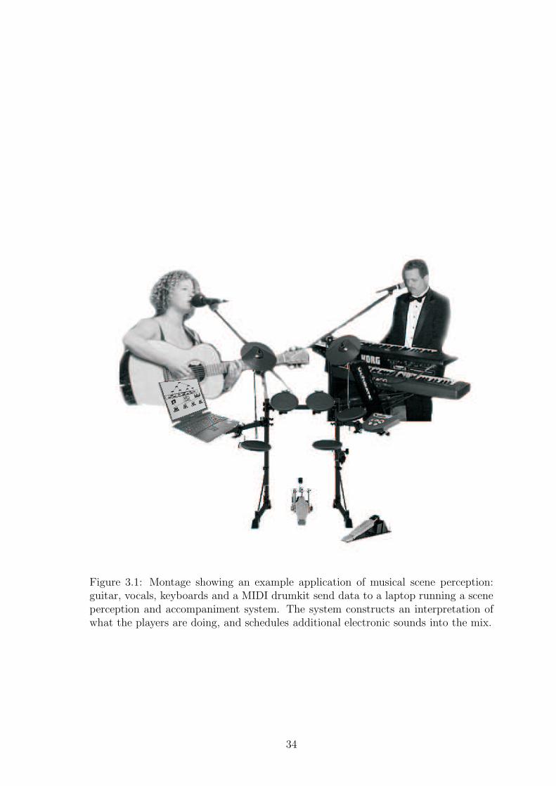
Figure 3.1: Montage showing an example application of musical scene perception:guitar, vocals, keyboards and a MIDI drumkit send data to a laptop running a sceneperception and accompaniment system. The system constructs an interpretation ofwhat the players are doing, and schedules additional electronic sounds into the mix.
34

This shows an inherent tradeoff between the spread of energy in a signal over time and
spread of energy over frequency in its transform. Thus by applying window functions
[103] which localise a signal in time, we degrade resolution in the frequency domain.
The finite discrete version, the discrete Fourier transform (DFT) is given by:
X[k] =
M/2−1∑
n=−M/2
x[t]e(−2πktj)/M (3.1)
x[t] =1
M
M/2−1∑
k=−M/2
X[k]e(−2πktj)/M (3.2)
The short-time power DFT, or spectrogram is simply the series of squared absolute
values of DFTs computed at consecutive (and possibly overlapping) windows of the
audio wave. Visually it gives a quick and useful picture of useful aspects of musical
signals, which will be used in the next section. The spectrogram is a potentially useful
feature for hash-classifiers.1
3.2.1 Musical audio signals
Here we examine and discuss sample spectrograms from various instruments, to gain
an understanding of raw musical audio data.
Human hearing responds to the energy and pitch of sounds. Energy roughly cor-
relates with subjective ‘loudness’. Pitch is more complex: many sounds, including
all musical instruments except some percussion, are generated by vibrating sources
having several simultaneous harmonic modes, ωi = iω0, i ∈ N. In general we do not
perceive harmonic components separately but perceive a single ‘pitch’ corresponding
to ωo along with a vaguer notion of ‘timbre’ corresponding to the shape of the ampli-
tude curve of the harmonics. (See [16] for highly detailed psychological investigations
into human pitch and timbre groupings.)
The guitar, piano and drums are percussive instruments: they involve hitting an
object then allowing it to sustain vibration before decaying away (either naturally or
with the aid of a controllable damping device). For these instruments, we expect to
see a strong attack in the waveform – i.e. a sudden increase in energy at the onset of
the note – which then dies away. These instruments may show transient harmonics,
which are essentially random high frequency components at the brief moment the
object is struck. This behaviour is shown in fig. 3.2(e) which shows the large-scale
1Interestingly, a related statistic, the periodogram, has a generative interpretation under strongassumptions about the source, see [17].
35

a b
c d
e f
g h
Figure 3.2: (a) Large-scale time-domain view of a single 1s trombone note. (b)Close up of trombone waveform. (c) Spectrogram of trombone scale (the previousfigures showed the first note of this scale). Sampling was at 8192Hz, windows were512 samples. Resolution is poor for the low harmonics. (d) Spectrogram of sametrombone scale, but linearly interpolated to 16384Hz and windowed at 1024 samples,improving resolution of the low harmonics at the expense of processing power. (e)Large scale waveform of the six open guitar strings, each played for about 1s. (f) Closeup of guitar waveform, for single open D string note (g) 512-point spectrogram of8192Hz-sampled guitar open strings. Resolution is poor. (h) 4096-point spectrogramof 16384Hz-resampled guitar open strings. This improves the resolution.
36

a b
c d
Figure 3.3: (a) Large scale time-domain waveform of simple 2s drum pattern: (bass,hihat, snare). (b) Close up of hihat waveform. (c) Close up of snare waveform. (d)512-point spectrogram of drum pattern. Increasing the window size has little effecton the resolution as the sounds are not harmonic.
waveform produced by playing the six open strings of a guitar in sequence, and in fig.
3.3(a) which shows drum hits on the bass, hihat, and snare.
In contrast, instruments such as the trombone, clarinet, voice and some synthe-
sisers allow the energy flow to be controlled throughout the duration of the note. Fig.
3.2(b) shows the waveform of a single trombone note: its energy is seen to increase
over time as the player’s breath power increases.
Fig. 3.2(d) shows spectrograms of a scale played on the trombone. Its harmonic
series can be seen clearly, and is roughly exponentially decaying with higher harmon-
ics.2 In contrast, the guitar spectra for the open string series in fig. 3.2(h) is less
structured, perhaps due to guitarists’ higher level of manipulation over the harmonics.
Percussive instruments are likely to have more easily recognisable onsets than wind
instruments, but wind instruments have more recognisable harmonic series once the
notes have started. (Players of the instruments see high variability as an advantageous
expressive feature, whereas for scene perception it becomes a ‘nuisance’ !)
2Interestingly, the fundamental is quieter than the first harmonic. This may be due to the shapeof the trombone bell creating a higher impedance for the very low frequencies. We will not beconcerned with such details in this thesis, but they may become important in industrial systems.
37

Figure 3.4: Left: Helmholtz space spiral representation. Right: viewed from above itshows the circle of fifths.
3.2.2 Pitch
Perception of the Western pitch system may be visualised as a three-dimensional
cylinder surface as in fig. 3.4, sometimes known as ‘Helmholtz space’3. Here the circle
of fifths is mapped around the circumference of the cylinder, while the frequency is
mapped vertically. Many musical concepts become intuitive in this representation:
notes that sound pleasant together are close; the pentatonic scale is found within a
tight band of the circumference, and the major and minor scales are found roughly
as any set of notes that is visible from one side of the cylinder.4 Melodies generally
have a ‘home’ note on which they begin and end. In terms of the Helmholtz cylinder
above, many melodies can be viewed as journeys away from the home note, taking
paths mostly of small steps around the cylinder and occasional large leaps (c.f. [121]).
3.2.3 Chords
Chords are sets of notes played together. The major and minor chords are defined as
the sets of the first, third and fifth of the major and minor scales respectively, and are
3The structure has been described by many authors, but [158] reports some of the earliest stepstowards it, in the 1885 appendix by Ellis.
4It is an interesting an open question whether some auditory neural structure exists that isisomorphic to this phenomenal model.
38
the most common chords. We will notate major chords by the lower case letter corre-
sponding to their first (e.g. c,f,g♭), and minor chords with the same lower case letter
suffixed with ‘m’ for ‘minor’ (e.g. cm,fm,g♭m).5 Modifiers can be applied by adding
additional notes to these chords. Chords form patterns on the Helmholtz surface,
and pleasant-sounding sequences of chords generally make slow gradual movements
around the surface. Like melody paths, these produce feelings of tension as they move
away from their home location, and resolution when they arrive back.
Importantly, there is more to the perception of a chord than the existence of the
note frequencies that comprise it. Chords are usually (especially in pop and jazz)
perceived as a ‘field’ covering a whole bar or half-bar of music. So even if the actual
notes are only present for a small part of the bar, and not necessarily played together,
perception of the chord ‘field’ still occurs. For example, monophonic instruments often
produce perception of chordality by playing arpeggios (i.e. sequences of chord notes).
So it is unlikely that chordality can be determined locally in a signal – the structure
and priors also play a role.
The chords derived from a major scale can be notated by Roman numerals, for
example II is the chord formed using the second note of the scale as its root note.
For a major scale this will be a minor chord, written IIm. As with melodic frag-
ments, there are many well-known chord sequence fragments which are often reused.
For example the 12-bar blues, (I,I,I,I,VI,VI,I,I,V,VI,I,V) and Pachelbel’s Cannon,
(I,V,VIm,IIm,III,VI,V) occur in countless compositions. Such sequences – even if
their presence was not determined in advance – are still recognisable by improvising
musicians, and provide strong hierarchical priors on what to expect next.
Human perception of chords tends to take place without perception of the indi-
vidual notes that comprise them (see [73] for a brief empirical study). This poses
a problem for generative model theories of perception, of the form CHORD →NOTES → DATA, which would suggest that notes must be inferred from the data
before chords. Speculatively, this can be viewed as an example of human hash-
classifiers as shortcuts in inference: it is possible to compute statistics of the data
which correlate well with the chord (such as the ‘CDV’ statistic of section 3.3.5) and
classify chord likelihoods approximately from these statistics, using the simplified
model CHORD → CDV (DATA). The information about chords can then be used
to constrain the inference over possible note combinations, and perhaps avoid some
of the combinatorial explosion from possible note combinations.
5This is because chords will be used in chapter 6 as grammar terminals, which are conventionallynotated by lower-case symbols.
39

3.2.4 Keys
The subjective experience of key is important in Western music. As with all subjective
higher-level musical concepts it is difficult to define exactly, but a workable (though
debatable) definition is as a tuple (θ, nh) comprising an angle θ around the circle of
fifths and Helmholtz cylinder, and a home note nh. Visually, imagine the Helmholtz
cylinder rotated so that θ is facing the viewer. Then, the Western major and Aeolean
scales correspond to the set of notes on the visible side of the cylinder, under certain
choices of home notes. The key effectively provides a prior, preferring notes which
are visible, and especially those near the home note. Key is not directly observable
by the listener but is inferred from the global distribution of notes and chords, whose
percepts are themselves affected by the prior from the key. Section 6.2.1 will show
that this is an important source of graph loopiness and global probability factors for
high-level inference. Music often changes key for middle sections (often called ‘middle
8’s in popular music) to provide variety. This is like temporarily rotating the cylinder.
The simplified models in this thesis will assume that key does not change and is thus
a global variable.
3.2.5 Rhythm
Rhythm perception is one of the most primitive human instincts, yet it is still hard to
capture its definition. Roughly, our music domain is assumed to consist of bars each
containing a small number of beats. Beats occur at regular score intervals throughout
the whole piece (though the speed or tempo at which the score is played may change).
Beats are positions in the music that human listener would tap along to – or change
the direction of their body movement as they dance (see [156] for a theory of beat
perception as resonance of a physical dancer due to rhythmic impulses). Typically
there are four beats in a bar. Two, three and six are less common. Other numbers
are uncommon. A bar is thus a perceptual unit of analysis: musicians break up the
sequence of beats into bars according to recognisable rhythm patterns. Whilst we
perceive four regular beats, it is often the case that the actual positions of rhythmic
events of the bar do not correspond to those beats. Fig. 3.5 shows three bars of
rhythm: the first has all the notes on the beats; the second has off-beat notes at
the end of the bar; and the third is highly off-beat (it could be used by a drummer
for special effect, to mark the end of a large-scale structure for example). So there
is a difference between the event times and the unobservable underlying beat. The
notes in the figure are drum notes; however we will see in section 3.8 that we can
also extract similar rhythmic features from other instruments. For example, guitar
40

Figure 3.5: On-beat, partially off-beat, and heavily syncopated rhythms. The rowsare hihat, snare and bass drum.
players often strike the strings at three distinctive velocities, corresponding to the
hihat, bass and snare rhythm events. Orchestral composers use similar devices to
mark the rhythm, though are usually spread over the whole orchestra rather than a
single instrument.
Perception of beats and bars is difficult because there is scope for much ambiguity.
Fig. 3.6(a) shows an example of between-bar ambiguity: a listener familiar with
military bands would probably chunk this into ‘marching’ bars beginning at the points
marked ‘*’, but a listener more accustomed to electronic dance music might chunk
it into classic ‘two-step’ drum’n’bass bars beginning at the ‘†’ points. Within-bar
ambiguity is illustrated in the two bars of fig. 3.6(b): here the rows represent different
onset types; the first bar is a standard four-beat pattern with the snare on beat 3.
The second bar is similar but the snare hit occurs later. This could be interpreted in
at least three ways: (1) the pattern could be the same standard four-beat pattern as
in bar one, but with an onset-detection error giving rise to the snare being perceived
as late; (2) the pattern may be the same standard four-beat pattern but the player
made a (possibly deliberate) mistake of playing the snare late; (3) it may be a new
pattern with the snare on beat 3.5. The difference between (2) and (3) is subtle and
even debatable: if the player makes the same ‘error’ of (2) several times then we
begin to perceive it as a new pattern as in (3). Skilled composers and performers can
exploit both kinds of ambiguity, for example by stressing certain beats to increase
their importance in our perception, and even to the extent of making music appear to
flip back and forth between rival percepts. (Famous examples include the perceived
ambiguous shift of beat position in Tchaikovsky’s Symphony Number 4 and electronic
dance music tracks ‘dropping’ the beat at unexpected locations; [76] gives a drummer’s
guide to creating many such ‘rhythmic illusions’.)
3.2.6 High-level structures
Beyond the level of bars, perception of music becomes much more subjective and
there is less agreement (both between listeners and scholars) about how it ‘should’ be
41

Figure 3.6: (a) Between-bar and (b) within-bar ambiguity.
perceived. One useful way to think of larger structures is as forming a grammatical
hierarchy. For example, many songs share an identical top-level structure (or simple
variants of it):
SONG→ {INTRO, V ERSE,CHORUS, V ERSE,CHORUS,
MIDDLE8, CHORUS,OUTRO}
whose components may be further decomposed, for example:
V ERSE → {RIFF1, RIFF2, RIFF1, RIFF2}
A riff might be broken down into parts for different instruments (played simultane-
ously, not sequentially; we notate this here using square brackets instead of braces):
RIFF → [V OCAL-MELODY,BASS-RIFF,GUITAR-CHORDS]
The guitar chords structure might comprise a sequence of bars containing chords:
GUITAR-CHORDS → {c, c, f, g}
Similarly, melodies could decompose into notes within a bar, and rhythms could be
written as types of percussive hit within a bar (possibly played in conjunction with a
chord in the case of tonal rhythmic instruments such as the rhythm guitar.) Chapter
6 will consider perception of such high-level structures in a probabilistic framework.
3.3 A menagerie of musical hash-classifiers
As discussed in section 2.5, the fullest Bayesian view of signal processing would be to
consider the set of all possible generative models {Mi} for the whole signal D, and
compute posterior beliefs P (D|Mi)P (Mi) in each of them in turn. For example, if we
know a priori that the signal consists of notes from a piano with at most r notes played
simultaneously, we could construct all possible combinations of notes at all possible
42

times as the model set, assign a prior to each based on our knowledge of the music,
and compute their likelihoods. For the general musical scene perception problem this
requires an intractable number of hypotheses. For offline musical transcription, this
type of fully Bayesian inference has been approximated using sampling on powerful
computers running for long periods of time (e.g. several days) [68]. However it is not
appropriate for real-time applications. A simplification is to use hash-classifiers. We
split the audio signal into short frames that can be analysed separately, then compute
useful statistics (features) of the frames and assume some simple classifier-proper to
map from statistics to model likelihoods as described in section 2.5. This is a common
and useful approach to take, so we here review a few statistics and classifiers-proper
(making little distinction between the two concepts) that will be used later in this
chapter. Many others can be found used in computational music contest reports such
as MIREX [47]. Each mapping is given an acronym for future reference.
3.3.1 Normalised power DFT (NPDFT)
NPDFT [t] =1
Zt|DFT (Hann(x[t−M + 1 : t]))|2
This vector-valued, temporal feature, where | · | and the squaring operator are per-
formed point-wise, is useful in measuring pitch. It is invariant to amplitude as it is
normalised by a normalising coefficient Zt. It has some theoretical basis in that the
square of the spectral values measures the physical energy carried in their frequency
bands. The Hann (or other) window is used in practice to reduce wrap-around errors.
3.3.2 Radial basis functions (RBF)
Radial basis function [11] neural networks are simply Gaussian likelihood detectors.
An RBF neuron takes a vector y as input, and output a Gaussian value N(µ− y,Σ)
which may be interpreted as a likelihood that the input y was an instance of the
multivariate Gaussian model with mean µ and covariance Σ. An RBF neuron can
be thought of as giving the strength of pattern-matching between the input and a
template model µ.
3.3.3 Normalised dot product (NDP)
This is a ‘second-layer’ statistic which is applied on top of an existing statistic f . It
is a distance measure between a vector of input statistic values f(y) and a vector of
target statistics f(s).
43

NDP =〈f(y)|f(s)〉√
|f(y)||f(s)|(3.3)
Musical examples of NDP include comparing current spectra to those of a set of
candidate score locations.
3.3.4 Chroma vectors (CHV)
DFT and similar features are good for making explicit the individual harmonic com-
ponents in a frame. However we saw that perceptual notes are made of harmonic
series of components, and typical instruments produce series with roughly exponen-
tially decaying amplitudes. Thus a chromatic scale of prototypical notes {ni}i can be
modelled as having DFT spectra:
ni[ω] =1
Z
10∑
k=1
exp(−k)N(ω; 2i12kω0, σ
2)
as shown in fig. 3.7, where N(ω;µ, σ2) is the Gaussian PDF, ω0 is the fundamental
frequency of the lowest considered pitch, and σ is chosen by hand to give a reasonable
spread but without interfering with neighbouring frequencies. (Ideally σ would be
derived from acoustic theory or fit to data.) Heuristically, 10 harmonics are used.
Taking the NDP of an input audio frame with a pre-compiled bank of note models
(e.g. one model for each note in a three-octave range) produces a statistic which can
be assumed to approximate the likelihoods of the notes occurring in the frame. It is
useful to sum over the note models from all octaves to produce an octave-independent
12-note chroma vector,
CHV [i] =∑
k
〈ni+12k|X[t]〉
3.3.5 Chordality vectors (CDV)
As we constructed the CHV from a sum of harmonic templates, so we may continue
and construct templates for whole chords as sums of their constituent chroma tem-
plates. As with CHV, chordality templates may then be used with NDP on input
audio to approximate the likelihoods P (frame|chord).
44

Figure 3.7: Note template as an exponential harmonic series blurred by a Gaussian.
3.3.6 Energy feature (E1)
E1[t] =
M+1∑
m=0
x2[t−m]
measures the total physical energy in M-sample frames, and is useful [131] for distin-
guishing between notes and rests. If suitably normalised it can be useful for distin-
guishing between loud and quiet notes or parts of notes – normalisation is typically
needed because external factors such as the players distance from the microphone and
mixer settings can alter the global level, even within a performance.
3.3.7 Novelty (NOV)
Novelty is a second-level feature, over an existing temporal feature f :
NOV (f)[t] =f [t]− µj=t−L:t(f [j])
σj=t−L:t(f [j])
It measures how many standard deviations the present value is from a running win-
dowed mean µ. It is useful for detecting musical onsets which produce sudden large
(e.g. 10σ) jumps in energy features.
3.3.8 Raphael burstiness (RB)
RB[t] =1
E1[t]
M/3∑
t=0
x2[t]− 2
2M/3∑
t=M/3+1
x2[t] +
M−1∑
t=2M/3+1
x2[t]
45

This convolves the energy signal with a hard edge detector, looking for short bursts
of energy. It is similar to many on-centre/off-surround neural receptive fields, and
was found [131] to provide useful information about note onsets.
3.3.9 Raphael generative spectra (RGS)
Another pitch-based feature [131]. Let ni[ω] be note DFT models as used in the CHV
derivation. We then treat each note ni as a candidate generative model for the FFT
frequency bins X[ω] observed in the data – this assumption leads to
P (X|ni) ∝ RGS[i] =∏
ω
ni[ω]X[ω] = exp∑
ω
X[ω] logni[ω]
3.4 Overview of existing research areas
Throughout our discussions we will make two key distinctions about automated ac-
companiment tasks. First, deterministic music is that which is written in a score
in advance and performed with little or no deviation from that score. In contrast,
improvised music is composed during the performance and is not known in advance.
Semi-improvised music will be described in detail later, but roughly is music which
has predetermined elements that are combined in an improved way during the perfor-
mance. Second, monophonic music has only one note present at each point in time;
polyphonic music may have many.
Research into score following has been active for about 20 years. This is the
task of following a deterministic musical score. The only commercial score-follower
is Dannenberg’s SmartMusic module in the Finale music software package, which
follows a monophonic, deterministic score. Academic research has focused mostly
on contemporary classical performance (being largely funded by IRCAM, the French
contemporary music institute), and has also been mostly monophonic and determin-
istic. A typical application would be a live clarinetist playing a concerto from sheet
music, with a computer following and providing the accompaniment. The leading
academic system is Raphael’s Music++, which performed this task live at the NIPS6
2001 conference [134]. Score following is reviewed in detail later. However, the sce-
narios discussed in section 3.1.1 require more advanced inference than these existing
systems as they involve semi-improvised music.
The recognition of audio notes and chords is itself a difficult problem, and com-
mercial music transcription software is notoriously unreliable. Auditory psychologists
6Advances in Neural Information Processing Systems
46

such as [43] have reached identical conclusions to their visual counterparts (e.g. [79])
– that we do not perceive low-level sense data directly, but instead perceive high-level
models, such as tones and melodies in the auditory case. [43] shows many cases where
music transcription software would fail because the tones we perceive do not even ex-
ist in the data, they exist only in our models and in the context that we hear them.
This is where a Bayesian approach will be useful as we may represent uncertainties
in the low-level description of the audio streams, and apply higher level models to
finding their best interpretation. The transcription task may be seen as complemen-
tary to deterministic score following: In score following, perception is relatively easy
as the music is deterministic, but real-time and action selection is important. Tran-
scription focuses on hard non-deterministic perception, may run offline, and requires
no action selection. Transcription will be reviewed in more detail in chapter 5 when
we discuss high-level perception. The present chapter focuses on low-level methods,
which naturally may provide input to the higher-level systems discussed later.
A sub-task of transcription which is especially relevant in real-time systems is
beat-tracking. This research assumes that the problem of finding the beat positions
can be tackled independently from the rest of transcription, for example using only
energy statistics from the audio signal and ignoring pitch. Beat-tracking aims to
provide the temporal grid for the rest of perception in which to to take place. The
semi-improvised domain may be thought of as real-time transcription of small highly-
constrained chunks, so beat-tracking can be used to find the locations of the chunks,
whose contents can then be passed to higher levels for analysis.
3.5 Score following: review and preliminary tests
As the deterministic problem is the starting point for our semi-improvised task, we
now review score following in detail. As it is difficult to obtain running code from
score-following authors, aspects of leading systems were reimplemented during this
review to gain a more detailed understanding of their strengths and weaknesses. The
examples and illustrations are drawn from these reimplementations.
3.5.1 Dynamic time warping
Dannenberg [33], [34], [36], [72], [35] published the first paper on score following
in 1984, using DTW to follow deterministic monophonic MIDI performances and
accompany them with MIDI. The task was simply to align a known sequence of
MIDI events with their observations. DTW allowed for occasional insertion and
omission of notes, or notes played in the wrong order. Three possible DTW moves
47

were considered for each state in the path matrix: horizontally forwards; straight
down; and diagonally forwards and down; rather than performing exact inference. In
real-time, the best path is noted at each new input, and the search on the next row is
constrained to nearby elements within an arbitrary window of this path. For DTWs
that can be written as HMMs, this constraint is equivalent to using a single particle
in particle filter inference. Dannenberg’s later papers extended the DTW algorithm
to run on audio data, using NDP on DFT features to follow polyphonic scores and
ensembles of players. The following section replicates some of his early experiments
to test the performance of DTW.
3.5.1.1 DTW experiments
DTW was coded as a Matlab function taking template and observation input vectors
as inputs, along with a distance measure on these vectors, and outputting an optimal
time warp map between them. Following Dannenberg, a parameterisable maximum
jump size was used, and only forward transitions were allowed. Fig. 3.8 shows a
simple example of the DTW component in action on a non-musical template (score)
sequence (1, 2, 3, 4, 5) and observation sequence (1,3,2,2,3,4,2,5,5,1). The simple dis-
tance measure 1 − δij is used (i.e. the distance is 0 between two identical numeric
symbols; and 1 between two different symbols) and the maximum jump size was 4. In
score-following, the numbers could represent musical pitches; the template would then
be the score as a sequence of ordered pitches, and the observation would be an input
stream of pitches. (DTW has no notion of note length under this interpretation.)
The cumulative distance is shown by the gray-scale, and the optimal path is plotted.
The optimal path assigns score states (1,1,2,2,3,4,5,5,5,5,5) to the observations.
A first DTW experiment used symbolic real-time MIDI data with no maximum
jump size. Again, the delta distance measure was used on the symbols. Incoming
MIDI events were streamed in real-time into Matlab and matched to a template
score. As expected, this produced good real-time alignment for small scores, and was
resilient to small errors of insertion, omission and incorrect notes (e.g. resilient to
about 6 mistakes in a 20 note score). This emulates Dannenberg’s early MIDI score
followers of the 1980s. As expected, DTW could not deal with large jumps in the
score, and could not deal with backwards jumps at all. The alignment algorithm only
runs when a new note event occurs, and is thus incapable of providing accompaniment
events at times between notes. It can provide such events on new notes, but even
then there is some latency between the note occurring and the event being scheduled
and played. We would prefer a more intelligent scheduler, capable of predicting when
notes will occur and scheduling events in advance.
48

0.5 1 1.5 2 2.5 3 3.5 4 4.5 5 5.5
1
3
2
2
3
4
2
5
5
1
obs
score:
time
Figure 3.8: Simple example of DTW algorithm. The template states are on the hori-zontal; the observations over time are vertical. Darker shades are greater cumulativedistances.
Figure 3.9: Score used in Bach performances. (Asterisks indicate accompanimentpoints.) From Cello Suite 2, BWV 1008: Prelude.
* * *
*
A second experiment tested audio DTW in an offline setting. Eleven recordings
were made of an eight-bar Bach excerpt played on the trombone (fig. 3.9). Each
recording was played in a different style, involving stretching tempos, emphasising
different phrases, and expressing different musical feelings. Deliberate mis-pitched
notes were included. The first recording was used as the template, and the others
aligned to it. The NDP on NPDFT feature was used as the distance measure. Sam-
pling was at 16kHz and 25% overlapping frames of 512 samples were used, resulting in
about 450 frames per recording. Exact DTW (i.e. using no maximum jump size and
considering all possible positions at each step) was slower than real-time. Examples of
local and total distances using exact DTW are shown in figure 3.10 with the optimal
warp path overlaid on the total distance image. The alignment was approximately
correct (as judged by the performer) on 8 of the 10 exact DTW runs.
To regain real-time execution for the audio case, the maximum jump was set to
4 frames, and the single particle assumption was used. The real-time system was
49
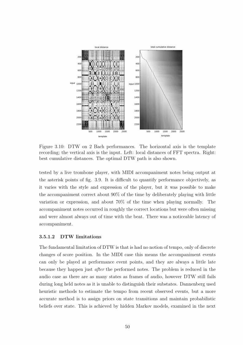
500 1000 1500 2000 2500
200
400
600
800
1000
1200
1400
1600
1800
2000
2200
500 1000 1500 2000 2500
200
400
600
800
1000
1200
1400
1600
1800
2000
2200
template
input
template
input
local distance total cumulative distance
Figure 3.10: DTW on 2 Bach performances. The horizontal axis is the templaterecording; the vertical axis is the input. Left: local distances of FFT spectra. Right:best cumulative distances. The optimal DTW path is also shown.
tested by a live trombone player, with MIDI accompaniment notes being output at
the asterisk points of fig. 3.9. It is difficult to quantify performance objectively, as
it varies with the style and expression of the player, but it was possible to make
the accompaniment correct about 90% of the time by deliberately playing with little
variation or expression, and about 70% of the time when playing normally. The
accompaniment notes occurred in roughly the correct locations but were often missing
and were almost always out of time with the beat. There was a noticeable latency of
accompaniment.
3.5.1.2 DTW limitations
The fundamental limitation of DTW is that is had no notion of tempo, only of discrete
changes of score position. In the MIDI case this means the accompaniment events
can only be played at performance event points, and they are always a little late
because they happen just after the performed notes. The problem is reduced in the
audio case as there are as many states as frames of audio, however DTW still fails
during long held notes as it is unable to distinguish their substates. Dannenberg used
heuristic methods to estimate the tempo from recent observed events, but a more
accurate method is to assign priors on state transitions and maintain probabilistic
beliefs over state. This is achieved by hidden Markov models, examined in the next
50

Figure 3.11: C major scale played in note classification test
section. Importantly, another problem – to which practical HMMs are equally prone
– is that when particle-based tracking becomes lost it is unlikely ever to return.
3.5.2 Hidden Markov models
In real-time, DTW algorithms typically consider only a fixed window (of perhaps
100 audio frames) about the previous best point. For DTWs which constrain the
path so that each move is from row i to i + 1, this constraint can be thought of
as a HMM finite plateau transition prior centred around the previous MAP point.
Importantly, this heuristic specifies not only a prior belief but also a computational
simplification: it tells us to consider only those hypotheses in the plateau rather
than all possible generating score states. HMMs allow us to generalise from this
plateau prior to an arbitrary state transition matrix, with the ‘distance’ measures
now interpreted as likelihoods. Such models are used in state-of-the-art academic
(but closed-source) score followers. Rather than use score audio frames as states (as
in DTW), score-following HMM researchers have tended to use a reduced model of
the score, with one or several states per note [131], [123], and CHV or RGS statistics
used as likelihood functions. Transitions are typically allowed between consecutive
score states, self-transitions, and jumps to the end of the note, and their parameters
fitted to previous performances. These models may be thought of as hidden semi
Markov models (HSMMs). As with DTW, the next section tests a simple version of
this architecture.
3.5.2.1 HMM experiments
We first implemented and tested a CHV model. Fig. 3.11 shows a scale played on the
trombone; fig. 3.12(a) shows its spectra. Sampling was at 8kHz and large 0.5s non-
overlapping windows were used). CHV values are shown in 3.12(b) and fig. 3.12(c)
shows the maximum likelihood (ML) chroma. The ML solution is all correct except
for the penultimate played note, which has been split into two parts (at around 25s on
the horizontal time axis), the first part of which is incorrect. There is a stray ML note
51
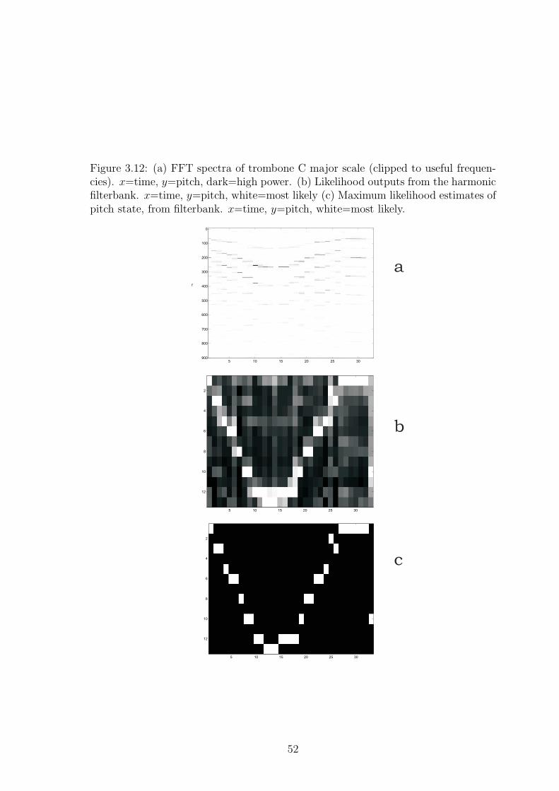
Figure 3.12: (a) FFT spectra of trombone C major scale (clipped to useful frequen-cies). x=time, y=pitch, dark=high power. (b) Likelihood outputs from the harmonicfilterbank. x=time, y=pitch, white=most likely (c) Maximum likelihood estimates ofpitch state, from filterbank. x=time, y=pitch, white=most likely.
5 10 15 20 25 30
0
100
200
300
400
500
600
700
800
900
f
time window (0.5 second windows)
5 10 15 20 25 30
2
4
6
8
10
12
5 10 15 20 25 30
2
4
6
8
10
12
b
c
a
52

Figure 3.13: Left: Score position transition matrix. Note there are two types ofrow: for one-beat events and two-beat events. Right: PDF model for ‘tied’ pitchobservations conditioned on score state.
d
2 4 6 8 10 12 14 16
2
4
6
8
10
12
14
16
from
state
to state2 4 6 8 10 12
2
4
6
8
10
12
14
16
score
state
P(obs pitch)
at the end of the performance, corresponding to silence in the audio. As likelihoods
are normalised and there is no explicit ‘silence’ model, an essentially random note
is produced in the ML interpretation. We noted the limitations of the FFT in the
audio review section – specifically for bass instruments like the trombone we get poor
resolution of low notes. Here a large window of 0.5s was used to compensate; though
such a large time uncertainty would not not good enough for a real time system.
In a second experiment, an offline HMM score follower was constructed using
the CHVs. The ascending and descending scale of fig. 3.11 was recorded, and a
corresponding HMM constructed with one score state per note. Its transition matrix,
shown in fig. 3.13(left) was tuned by hand to perform as well as possible. Following
Raphael, ‘tied’ states were used, meaning that CHVs were conditioned only on the
pitch of each score state rather than the score state itself. For example, the note D
occurs twice in the score but these two states have identical CHV profiles. This was
implemented by adding an extra layer of Bayesian network nodes between the hidden
score states and the CHV observations (HMMs are a special case of BNs, and our
HMM was implemented using a generic BN tool written for these experiments), as
shown in fig. 3.14. These ‘pitch’ nodes have just 12 chroma states, rather than states
for each score note, and have the transitions of fig. 3.13right. Using the large 0.5s
frames as before, the HMM was able to infer correct score positions for the simple
scale score as seen in fig. 3.14, using forward messages only.
A third experiment tested the CDV feature. A guitar was used to generate a
performance of the chord sequence ccggccffccgfccgfcc for testing. To test robustness,
the guitar was deliberately slightly out of tune and played quite badly, with around
53

Figure 3.14: Screenshot from the HMM software implementation, using similar graph-ical display to fig. 2.1 in the previous chapter. The Bayesian nodes have three sec-tions, showing prior, likelihood and posterior distributions, from top to bottom. Thetwo-sectioned LINKS show the prior (top) and likelihood (bottom) messages betweennodes. For example, the top left node, initScore shows the prior score position atthe start the performance: its prior and posterior are delta functions indicating cer-tainty that the score state is the first note. (Its likelihood component however alsosuggests that the last note is also likely, being of the same pitch.) Moving to the right– through time – from the initScore node, we see the priors suggesting movementalong the score, giving a high prior on the score position immediately after the high-est posterior position of the previous node. The marginal maximum likelihood scorepositions for the seven time windows shown here are (1,2,2,3,3,3,4) corresponding tothe first four notes of the score, (C,D,E,F).
54

one in five chords played having one or more incorrect notes. There were also some
brief open-string chords in the changeovers. The final c was held for about 2 seconds
to fade out. Fig. 3.15(a) shows the 0.5s FFTs of the signal. The lowest string, E,
on the guitar has fundamental 82Hz, and the low C of the first c chord has 128Hz.
Corresponding CHV and CDV values are shown in figs. 3.15(c) and 3.15(d). The
maximum likelihood CDVs are shown in fig. 3.15(e). The ‘ground truth’ chords
actually played are shown in fig. 3.15(f) for comparison. CDVs ran in real-time with
about 0.5s latency (the size of the FFT frames), allowing displays such as fig. 3.15(b)
to show the currently-played CDV and ML chord estimate. The results show that
the ML estimate is accurate about 85% of frames, and suggests that the errors could
be corrected with temporal smoothing as in HMMs.
A fourth experiment, noting the reasonable accuracy of chordality recognition
from a single guitar, tried applying it to a complete audio mix. This could allow
transcription of chords symbols from MP3 recordings for example. A recording of
The Beatles’ three chord trick, I Saw Her Standing There was used as input to the
previous ML-CDV system and its results are shown in fig 3.16. The detection is
poor – many chords are completely incorrect and there is much random jumping
around between likelihoods. In contrast, humans have no trouble perceiving the song
as a simple series of three chords, showing that our perception of chords is not just
based on instantaneous filterbanks and frequencies: we can still perceive a chord
as e even if there are very few of e’s notes in it, and the sound is cluttered with
improvisations, non-chordal notes, and rhythm sounds. In particular, humans seem
to perceive ‘chordality’ as a field covering whole bars, combining notes from all time-
slices within them, rather than within single frames.
A fifth experiment tried to use the previous HMM implementation to follow the
chord sequence in real time. In the previous scale-following test, the individual notes
were used quite successfully as hidden states of the HMM. This worked for the simple
test case because the audio frames were large (0.5s) and approximately the same
duration as the notes themselves. The symbols from the chord sequence were similarly
modelled by single hidden states. But in this case, the model failed due to an effect
which we call sandboxing. This problem arises when performed symbol durations are
much longer than frame lengths – in this case each chord symbol was played for a
bar lasting about 2s. This means that each hidden score state must typically make
four self-transitions before moving to the next score state. This is an inherently
non-Markovian prior. It was possible to set the expected mean number of frames
per hidden state by reducing its transition probability to the next state, p, but this
does not capture the correct semantics. Instead, it gives a Poisson distribution over
55

Figure 3.15: (a) FFT spectrograms of chord signal. x=time, y=frequency. Dark=highpower. (c) Octave-neutral pitches present. x=time, y=pitch, white=most likely. (d)Chord likelihoods. x=time, y=chord, white=most likely. (e) Maximum likelihoodchord recovery. x=time, y=chord, white=most likely. (f) Ideal chord recovery. (b)(top right) Real-time chord detection: The caption reads ‘I think you are playing D#major’. This is a screenshot from an animated Matlab screen, updated every 0.5s.
5 10 15 20 25 30 35 40 45 50
0
100
200
300
400
500
600
5 10 15 20 25 30 35 40 45 50
1
2
3
4
5
6
7
8
9
10
11
E
F
G
C
5 10 15 20 25 30 35 40 45 50
1
2
3
4
5
6
7
8
9
10
11
E
F
G
C
5 10 15 20 25 30 35 40 45 50
1
2
3
4
5
6
7
8
9
10
11
E
F
G
C
a b
c d
e f
d
56

Figure 3.16: Left: Maximum likelihood chords for I Saw Her Standing There. Right:Corresponding notated (‘ground truth’) chords.
a
100 200 300 400 500 600
2
4
6
8
10
12
E (I)
A (IV)
B (V)
bridge v3 solo bridge v4 refrainsv1 v2
time spent in each state, which tends to make the score state priors dilute rapidly
over time, as can be seen in fig. 3.17. (We named the effect ‘sandboxing’ because
the priors resemble a stack of sand in the initial case, which is gradually tipped over
time, spreading out into a wide pile.)
3.5.2.2 HMM limitations
The sandboxing problem can be fixed approximately by introducing multiple sub-
states within each score symbol, as in Raphael’s system, which uses about 10-20
substates per note7 to obtain high accuracy with small frame lengths. Such an ap-
proach is similar to that used in DTW, where each note in the template has many
audio frames. The only difference is that in DTW each template frame has its own
statistic vector, but in note-based HMMs the statistics are generated from idealised
note models rather than a prerecorded score. As with DTW, exact inference in such
many-state HMMs then becomes impossible, so the set of hypotheses under consid-
eration must be limited heuristically. Again, such limitations reduce the ability to
recover from large jumps in the performance.
Accompaniment applications require very high accuracy predictions about near-
future accompaniment time to allow advance scheduling and avoid latency. Unlike
DTW, HMMs can be used to make such predictions ahead of time, by propagating
forward messages beyond the current time to infer probable score states of near-future
frames. However the accuracy is still limited to the resolution of individual frames,
which may not provide the millisecond accuracy required by professional performers.
7Raphael, personal communication.
57

Figure 3.17: HMM for chord sequences, showing belief sandboxing on the score nodepriors. (These are the top distribution in the score nodes; observe that the priorsspread out to the right, like a pile of sand being tipped over in a box)
58
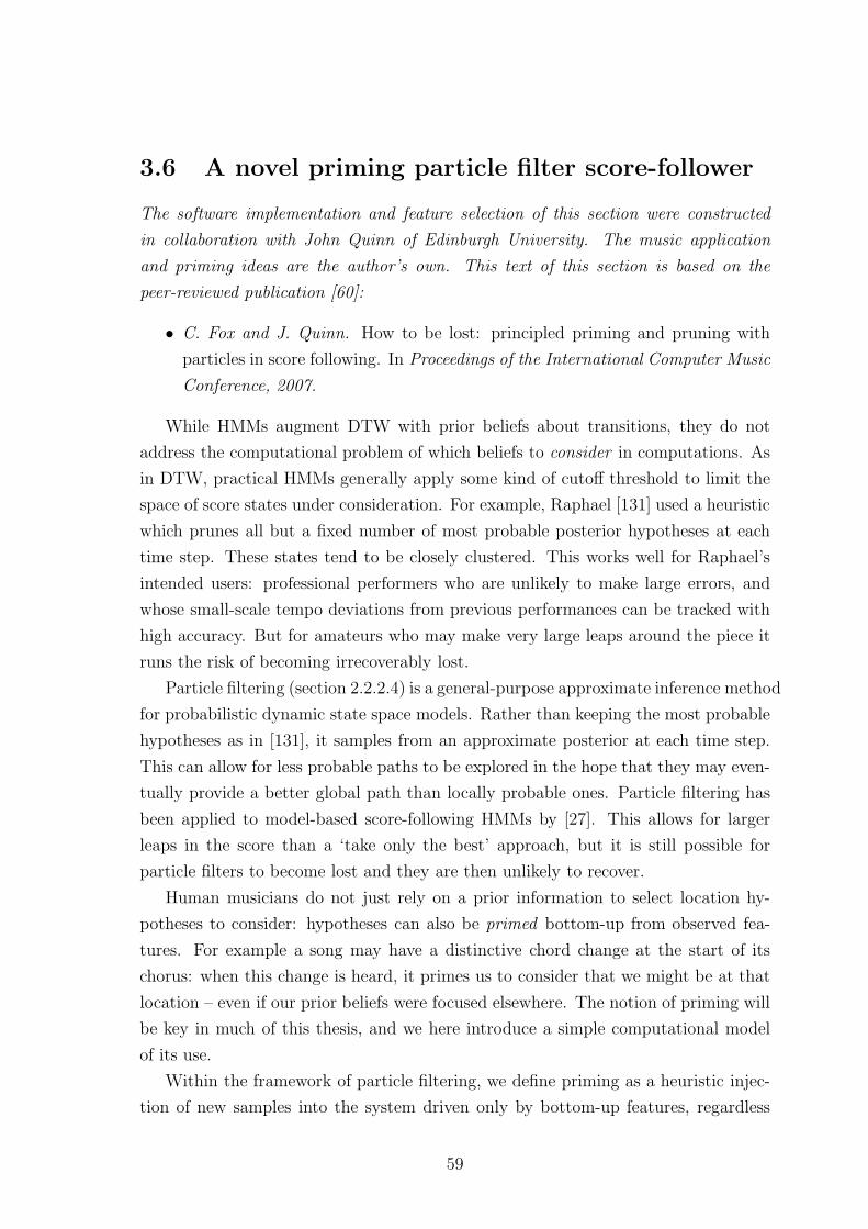
3.6 A novel priming particle filter score-follower
The software implementation and feature selection of this section were constructed
in collaboration with John Quinn of Edinburgh University. The music application
and priming ideas are the author’s own. This text of this section is based on the
peer-reviewed publication [60]:
• C. Fox and J. Quinn. How to be lost: principled priming and pruning with
particles in score following. In Proceedings of the International Computer Music
Conference, 2007.
While HMMs augment DTW with prior beliefs about transitions, they do not
address the computational problem of which beliefs to consider in computations. As
in DTW, practical HMMs generally apply some kind of cutoff threshold to limit the
space of score states under consideration. For example, Raphael [131] used a heuristic
which prunes all but a fixed number of most probable posterior hypotheses at each
time step. These states tend to be closely clustered. This works well for Raphael’s
intended users: professional performers who are unlikely to make large errors, and
whose small-scale tempo deviations from previous performances can be tracked with
high accuracy. But for amateurs who may make very large leaps around the piece it
runs the risk of becoming irrecoverably lost.
Particle filtering (section 2.2.2.4) is a general-purpose approximate inference method
for probabilistic dynamic state space models. Rather than keeping the most probable
hypotheses as in [131], it samples from an approximate posterior at each time step.
This can allow for less probable paths to be explored in the hope that they may even-
tually provide a better global path than locally probable ones. Particle filtering has
been applied to model-based score-following HMMs by [27]. This allows for larger
leaps in the score than a ‘take only the best’ approach, but it is still possible for
particle filters to become lost and they are then unlikely to recover.
Human musicians do not just rely on a prior information to select location hy-
potheses to consider: hypotheses can also be primed bottom-up from observed fea-
tures. For example a song may have a distinctive chord change at the start of its
chorus: when this change is heard, it primes us to consider that we might be at that
location – even if our prior beliefs were focused elsewhere. The notion of priming will
be key in much of this thesis, and we here introduce a simple computational model
of its use.
Within the framework of particle filtering, we define priming as a heuristic injec-
tion of new samples into the system driven only by bottom-up features, regardless
59

of their priors.8 We present a novel priming particle filter (PPF) which uses this
technique to recover from being lost by recognising and allowing a probability for its
own error, then creating new hypotheses based on bottom-up note changes. Unlike
existing HMM score-followers, we have returned to the DTW-style audio-based score,
and avoid the need for explicit note-based score models. To demonstrate the priming
particle filter, we have used relatively simple features for likelihood computations,
but we suggest that the PPF could be a useful addition to all state-of-the-art score
followers with more advanced features.
3.6.1 Tempo model
At each time step of live performance time t(l), the hidden state is the position in
score time, t(s) and the current tempo . We write the score time as a function of the
live time, t(s)[t(l)], and write the current tempo as t(s)[t(l)]. The hidden state evolves
as the damped switching stochastic process:
t(s)[t(l)] = t(s)[t(l) − 1] + t(s)[t(l) − 1] + ǫt(l)
t(s)[t(l)] = ρ(t(s)[t(l) − 1] + ǫt(l) − 1) + 1
where ρ is a damping coefficient and ǫt(s) are from the Gaussian N(0, σ20) and ǫ ˙t(s)
are
from the switching mixture of Gaussians α1N(0, σ21) + α2N(0, σ2
2) with α1 + α2 = 1
and ∀i.αi ≥ 0. The two mixture components model a small tempo drift due to player
or tracking errors and a separate large tempo change due to performer style changes.
A mixture is used to encourage occasional large changes (e.g. at new phrases) whilst
discouraging gradual large tempo changes (e.g. during notes). We do not perform
any learning of parameters – they are simply set by hand (ρ = 0.999, α1 = 0.99, σ0 =
0.7, σ1 = 0.1, σ2 = 1.5, with time measured in frames). Particles contain the 2-element
state (t(s)[t(l)], t(s)[t(l)]), i.e. a position and speed in the score.
3.6.2 Likelihoods
Offline score x(s) and online live x(l) audio is sampled at 2756.3Hz (=44.1kHz÷16) and
cut into 512-point frames y[t] with 448 point overlaps. We use the NDP feature on
chroma vectors (CHV) as an approximate spectral likelihood λs(X(s)[t(s)], X(l)[t(l)]).
E1 energy features e[t] are computed and used to compute a further NOV feature v.
We use a Gaussian approximation of energy likelihoods:
λv(v(s), v(l)) =
1
Zexp−(v(s) − v(l))2
2σ2v
8This may destroy theoretical convergence properties in the infinite sample limit.
60

And assume that the total likelihood is the product of these spectral and energy
likelihoods:
P (t(l)|t(s)) ≈ λs(X(s)[t(s)], X(l)[t(l)])λv(v
(s)[t(s)], v(l)[t(l)]).
3.6.3 Injecting primed particles
A fundamental assumption in Bayesian inference is that we possess the exhaustive set
of hypotheses {Hi} to explain some data D. It is this exhaustiveness that allows us to
convert likelihoods into posterior probabilities. However in realtime score following we
do not have computational resources to consider all possible score position hypotheses,
we must consider only a subset of them. Previous models have used heuristics to
choose this subset: we (with [27]) use sequential importance samples (particles) to
make this choice in a principled way. The standard particle filter assumes that the
particles form the exhaustive hypothesis set at each step. But this does not allow
the model to represent the possibility of its own failure: in practice it is possible for
a particle filter to get lost, and for the best hypothesis (and even the whole area
around it) to be excluded from consideration. But the particle filter is blind to this
– it assumes that the particles are an exhaustive set of explanations.
A precise definition of what it is to be lost is difficult when the state space is
continuous. For discrete states, lostness at time t is easily defined: it occurs exactly
when the ground truth state at t is s and there is no particle representing s at t. For
a continuous space, no particle can ever represent the exact ground truth state, so
some notion of an acceptable region must be used such that lostness can be defined
as the condition of having no particle in the acceptable region around the ground
truth state. For score following, one way to define this region is simply to ask users
of the system what region would be acceptable to them, in the sense of having an
accompaniment part played at the position and speed from that region. As we later
approximate the probability of being lost heuristically, rather than compute it, there
is no need to obtain the acceptability criterion explicitly. Instead, we may choose
the heuristic approximation to maximise user utility directly. We assume that user’s
prefer a close match in positions between inferred states and ground truth throughout
the whole score and choose a heuristic to approximately maximise this.
Ideally, we would like to compute the probability that all particles have irrecov-
erably failed (according to the acceptability criterion), P (lost), and treat ‘being lost’
as an alternative explanation. When we know we are lost we will then consider a
number of newly injected particles {H∗j } based on bottom-up priming, with
P (H∗j |D,C) = P (lost|D,C)P (H∗
j |lost,D, C)
61

Figure 3.18: Chroma and change points of score performance(a) Score pitches
score time r / samples
pitc
h
100 200 300 400 500 600 700 800
2
4
6
8
10
12
(b) Winner−take−all smoothed score pitches
score time r / samples
pitc
h
100 200 300 400 500 600 700 800
2
4
6
8
10
12
P (H∗j |lost,D, C) =
1
ZP ′(H∗
j |feature(D))P ′(H∗|C)
where C is the context (i.e. the previous state for dynamic networks like HMMs),
feature(D) is some bottom-up priming feature computed from the data, and P ′ are
probability factors (i.e. they are not necessarily normalised). In practice, all of the
above terms are intractable (in the sense that computing them would require an exact
solution of the very inference problem that the particle filter is approximating) but
can be approximated from domain knowledge or historical statistics.
We approximate P (lost|D,C) by looking at a windowed running average data
likelihood. We use an exponentially weighted moving average of P (D[t]|H[t]), the ev-
idence of the MAP hypothesis at each step. When this average falls below a threshold
we consider that we might be lost with a fixed probability. In practice we approximate
this be removing the worst m particles from the set and replacing them with newly
primed particles, where m is the number of these primes. (More detailed methods
could model how probable being lost is given how far below threshold we are, and
learn this model from historical data.)
P ′(H∗j |feature[D]) is approximated by a simple bottom-up priming scheme. We
use sparse Boolean features and assume that all score states having the feature are
equally likely given the presence of the feature when lost. For our score-following task,
62

Figure 3.19: Chroma and change points of live performance(a) Live pitches
live time y / samples
pitc
h
100 200 300 400 500 600 700 800
2
4
6
8
10
12
(b) Winner−take−all smoothed live pitches
live time y / samples
pitc
h
100 200 300 400 500 600 700 800
2
4
6
8
10
12
we use changes in the maximum windowed running average pitch as features. These
roughly correspond to onsets of new notes. We maintain a cache of known positions of
these features in the score, and consider these positions as hypotheses when the same
features are found in a lost live performance. Speeds are created for these particles
assuming that the tempo has been constant since the point of becoming lost.
P ′(H∗|C) can be approximated in score-following by considering how far removed
the primed hypothesis H* is from where the particle filter’s previous MAP estimate
was, and penalising very large jumps. Our system uses a simple plateau function
to allow only primes within a fixed distance of the previous MAP location. (In the
results given below, the plateau allowed primes up to 200 frames either side of the
MAP location).
3.6.4 Results
We demonstrate the priming particle filter on the first seven bars of the Andante
Cantable from the Rimsky Korsakov Trombone Concerto. Recall that no symbolic
score is required: an audio recording is used as the score. Fig. 3.18 shows the chroma
vectors and priming features from the audio score; fig. 3.19 shows the same for the
live recording.
63

Figure 3.20: Alignment without priming
Live time y / frames
Sco
re ti
me
r / f
ram
es
100 200 300 400 500 600 700 800
100
200
300
400
500
600
700
800
The live recording contains a short error around frame 200. Running the standard
particle filter with 5 particles results in getting lost at this point as shown in fig. 3.20.
The figure shows the complete spectral similarity matrix in the background, in which
the central white diagonal stripe is the true path. The particles are plotted as dots and
the MAP particle path is drawn as a line. Fig. 3.21 shows the same example running
under the priming particle filter. The large jumps are where lostness recognition and
priming has occurred. It can be seen that the filter gets lost several times but is able
to recover every time.
3.6.5 Discussion
We have demonstrated the priming particle filter on a simple example for illustra-
tion purposes only, and running with more than 5 particles on this example generally
avoids getting lost in the first place. Our demonstration PPF is a relatively simple
score follower using very basic likelihood features and a Markov hidden state in con-
trast to state-of-the-art score followers such as [134], [28] which have more advanced
features and higher-level state models. However we suggest that all state-of-the-art
models could benefit from the simple addition of a PPF to allow them to recover
from being lost when used by non-professional performers. Our HMM also illustrates
how DTW-like audio templates can be used as HMM states, in contrast to existing
64

Figure 3.21: Alignment with priming
Live time y / frames
Sco
re ti
me
r / f
ram
es
100 200 300 400 500 600 700 800
100
200
300
400
500
600
700
800
HMM systems which use symbolic scores with note templates. The notions of priming
hypotheses and pruning improbable ones will recur throughout the rest of this thesis
(though outside the context of particle filters).
3.7 Higher-level models in Music++
Having reviewed and evaluated simple DTW and HMM methods, it is useful to review
a complete state-of-the-art score-following system in detail. It is useful to see what
algorithms and heuristics are currently state-of-the-art, and in particular to see what
kinds of special cases must be bolted on to standard algorithms to make them function
in the real world. As the focus of this thesis is on hierarchical models of perception, it
is also useful to see what higher-level models are deployed in a state-of-the-art system.
Raphael’s Music++ is perhaps the most prominent academic score-following sys-
tem, taking the form of a closed-source, 65,000-line C program which performs mono-
phonic deterministic following well enough to perform live accompaniment for Schu-
mann’s 1st Romance at the NIPS 2001 conference [134]. The perception part of the
program consists of an HMM and a higher-level Gaussian Bayesian network, driven
by spectral and energy features from FFTs.
Music++ is aimed at professional and semi-professional classical musicians who
make relatively few errors, and are musically competent to take control of a concerto’s
65

tempo and expressivity, expecting the accompaniment to follow them. As input it
takes a MIDI score and a prerecording of the accompaniment (for example, a full
orchestral backing track). Its aim is to output the same sounds as a conducted
orchestra would do when accompanying a professional concerto soloist, in real time.
Raphael has been developing the program since 1999 and whilst the source code
was undocumented and not publicly available, parts of it are documented at the
algorithmic level in a series of conference and journal articles [141, 138, 135, 140,
139, 136, 132, 137, 133]. I was able to obtain access to Raphael’s source code and
to interview Raphael9 while employed by him at Indiana University to write the first
source-level documentation of Music++ [61]. Raphael’s system has evolved over time
so his papers may contain apparent contradictions – the following gives an original
and coherent overview of the perceptual parts of the system as of late 2005.
A large part of the code base is a ‘mini operating system’ providing C functions for
custom memory allocation and for scheduling the HMM and BN as well as controlling
the audio accompaniment output. With our focus on scene perception we will not
discuss these functions other than to take a warning that implementing real-time sys-
tems to industrial standards requires substantial time-consuming software engineering
effort, and should be avoided in a thesis of the present scope to give preference to
theory and concepts. Similarly we will not discuss training of model parameters or
audio output generation here.
3.7.1 Architecture
Music++’s HMM takes the soloist’s sound signal as input, and outputs a list of MAP
estimated score note onset times, with variable latency. Latency varies because an
onset is only reported once confidence in its position reaches some threshold. This
generally requires waiting for some time after the onset has completed, and backwards
messages are passed through the HMM to provide the extra information about recent
onsets. Each onset is reported only once, when its threshold is reached.
The Bayesian network consists of Gaussian nodes which maintain marginal beliefs
about the positions of performance and accompaniment notes. It takes the onset
estimates from the HMM as observations and outputs an estimate of the predicted
time of the next accompaniment note. Why is this network needed, when other
systems (such as those used by IRCAM) claim to perform score-following using only
an HMM? Raphael’s experiments10 suggest that whilst HMMs work well for localising
9under a non-disclosure agreement – the content of this section has been reviewed and approvedfor disclosure by Raphael.
10Raphael, personal communication.
66

the score state to the note or sub-note level, they do not give the millisecond precision
demanded by professional classical musicians, typically because they must discretise
the score states to a lesser accuracy. (Our priming particle filter has shown that
continuous state space is possible in HMMs – however we certainly do not claim to
have achieved professional quality accuracy with a real-time number of particles. We
also note that IRCAM’s score followers are generally used for contemporary electronic
music which has less clearly defined beat and note positions than classical Western
music.) By switching from a dynamic-state to a position-in-time model (section 1.3),
the accuracy can be perfected, as the Bayesian network infers the expected times of
each note rather than the expected (discretised) score state at each time.
The spilt between hard HMM onset reports and the Bayesian network is also use-
ful with regard to action selection. Dynamic-state models – such as the HMM and
the priming particle filter – can be used to report the most probable future states of
the world, by making inferences over nodes representing the future. However these
predictions may fluctuate rapidly. When action selection – rather than just predic-
tion – is required, this becomes problematic because newly scheduled actions may be
incompatible with previously scheduled actions, based on different fluctuating per-
cepts. It is better to choose one interpretation and make a whole sequence of actions
based on it. Ideally, such actions should be selected using the full posterior over fu-
ture states, together with the set of already-scheduled actions and a utility function
which penalises frequent switching between actions matching different percepts. The
hard onset-reporting step may be viewed as a heuristic approximation to this scheme,
reducing the amount of action switching because the data provided to the Bayesian
network is updated only occasionally, when hard onsets are reported. (Section 6.3.1
will consider an explicit formulation of this type of task, modelling action coherence
utilities as additional factors in a graphical model.)
3.7.2 Hidden Markov model
The sandboxing problem is reduced by modelling each score note as around 10-20
sequential substates. Most substates have a self transition probability p and a ‘next
substate’ transition probability (1−p), where p is a parameter shared by all substates
of the note. Hence notes are parametrised by the tuple (n, p) where n is the number
of substates used. Each substate thus has a discrete exponential distribution on its
duration, and the distribution of the whole note length (i.e. the sum of substate
lengths) is negative binomial,
P (T = t) =
(
t− 1n− 1
)
pt−n(1− p)n.
67

Figure 3.22: States for regular (top) and short (bottom) note models.
While it is unlikely that real performed musical notes happen to follow this conve-
niently parametrised distribution, its two parameters can be easily moment-matched
to the mean and variance of empirical data to give a useful approximation.
The full note model, shown in fig. 3.22(top), is slightly more complex than a single
chain of substates. It distinguishes between the attack and sustain parts of the note
(left and right in the figure) which have different data-generating properties. It also
distinguishes between notes whose attack follows immediately from a previous note
(a rearticulation) and whose attack follows a rest – shown by the upper and lower
left chains in the figure. Finally, the two right chains of the figure show two different
paths for the sustained part of the note: the lower chain is of silent states, which
occur if the player terminates the note early (e.g. to take a breath, or for a staccato
effect.) The path may switch from the played sustain to the rests at any point during
the sustain, but may not move back again. Very short notes (of around 15 frames
long) are modelled differently as shown in fig. 3.22(bottom): these transitions allow
performance to jump to the end of the note from any state, allowing for the whole
note could be played as short as a single frame of audio. (The negative binomial
model, even in the fastest case, is required to proceed through all states in sequence,
giving an upper limit of n frames for its performance length.) These are examples of
the fine details required by industrial-strength score-followers.
Input audio is sampled at 8kHz, and cut into 50% overlapping 512-point frames
(32 frames/sec) and used to compute the three FFT-based features E1, RB and RGS.
68

E1 and RB are initially continuous valued, but are discretised. The combined vector
of all the features is used as a single feature, and likelihoods P (E1, RB,RGS|s) are
used where s ranges over the quadrants of the note model in fig. 3.22 at possible
pitch. Another real-life detail is optional additional conditioning on the most recent
audio output of the accompaniment, ai, which during non-headphone performance is
likely to feed back into the input and must be accounted for.
Public descriptions of Music++ do not explain how hidden state beliefs and the
transition matrix are implemented in code. As discussed earlier, naıve implementation
of the transitions as a matrix would become very slow due to the large number of
states in the model. For example, a piece with 500 notes might have 20 nodes per
note, giving a 10,000×10,000 transition matrix, and hidden 10,000 states per node,
needing to be updated 32 times per second, which is infeasible on current computers.
Detailed examination of the source code found a crucial heuristic contained in this
small function (reprinted with permission):
static void graph prune list(list) {/*both dp cutoffs and low probability cutoffs */
ACTLIST *list;
int i,l;
qsort(list->el,list->length,sizeof(NODEPTR),probcomp);
for (i=list->length-1; i >= maxnodes; i--) del list(list,i);
if (list->length > 1)
while(list->el[list->length-1]->prob<TEENY&&list->length>MIN NODES)
del list(list,list->length-1); }Here list is a list of ‘active hypotheses’ (i.e. those under computational con-
sideration) having posterior probabilities probcomp; qsort is a quick-sort function;
del list removes elements from lists, and maxnodes is a threshold parameter. This
function prunes all but some maxnodes most probable hypotheses, and shows that
P (s) is represented as a list of hypotheses rather than a naıve vector containing
all possible states. We can view this is a crude form of particle filter, which always
samples the max nodes most probable hypotheses.
The most probable hypotheses tend to be closely clustered, and taking the most
probable ones removes the ability to recover from large jumps in the score. For Mu-
sic++’s target audience of professional performances of deterministic scores, this is
rarely causes problems as professional players are unlikely to cause such errors in the
first place. However for amateurs this is a problem and the system can become irrecov-
erably lost following some small errors. We suggest the use of the priming particle
filter presented earlier as a possible cure for this problem with amateur musicians.
69

Figure 3.23: The Gaussian Bayesian network structure used in Music++.
Raphael’s HMM shows up how low-level audio classification can be considered as
a separate task from higher-level inference: there is no feedback information sent to
the HMM from higher systems. The HMM functions in isolation as a smoothed onset
detector, whose onset reports may be treated as symbols at the higher levels.
3.7.3 Gaussian Bayesian network
The Gaussian Bayesian network uses the stream of onset estimates from the HMM
to predict and output the time and tempo of near-future accompaniment events. A
typical fragment of the network is shown in fig. 3.23. Each note of the solo score is
represented by a node, containing a PDF over its onset time and local tempo. Onset
estimates are treated as noisy observations. The network also includes a node for each
accompaniment event in the accompaniment score. This is because the system’s own
actions (playing accompaniment notes) will affect the performer’s behaviour which in
turn affects the predictions – the system’s own behaviour thus becomes a feedback
input for its later predictions. The solo and accompaniment onsets are treated as
noisy observations of an underlying Markovian score process.
A real-time optimised version of the Pearl Gaussian message-passing algorithm
(i.e. a Kalman filter) is employed to quickly obtain the marginal PDF for the onset
time of the next unplayed accompaniment event in the score. This algorithm passes
only the messages that are useful for updating the required note, and does not waste
time updating other notes. The time of this next note, along with that of the latest
observed note, is then used to estimate the current position and tempo.
70

Real music has several special cases where the regular GBN inference breaks down
and custom behaviour is implemented. Once again we list such details an an illustra-
tion of the complexity of industrial score-followers. First, at a cue point, the temporal
link along the backbone is completely severed and the new tempo prior is made uni-
form and thus independent of the previous backbone state. This is typically used at
the first solo note after a cadenza. Second, an exchange point is similar to a cue,
but is less severe: the tempo part of the state transition is severed in the backbone,
but the time part is left connected. This is used for a tempos and to reweight the
solo/accompaniment control balance. Finally, gated accompaniment notes use the
same transition structure and inference mechanism as regular accompaniment notes,
but have a specified gating solo note preceding them, and are never played until the
gating note has been explicitly reported by the HMM – even if the top-down inference
in the GBN believes that its time has come.
Raphael’s Gaussian Bayesian networks are deformable, position-in-time models
of the performance. Similar deformable models have been used in vision [109], [155]
[29], where they are visualised as wire-frames having elastic springs connecting their
vertices. In the vision case, fitting the model is generally done by gradient descent on
the ‘energy’ in the springs, corresponding to a prior probability over configurations.
In the music case, the model is deformed over time rather than space. In contrast,
Raphael’s deformable model maintains marginal belief distributions over the ‘vertex’
positions (i.e. the notes of the model). It is possible to do this exactly using a
Gaussian form of the Pearl equations because his models have no loops, existing only
in one dimension rather than two-dimensions as in images.
For a deterministic score there is a single large accompaniment model. For our
semi-improvised task, we are interested in recognising and accompanying collections
of small fragments of music. This naturally suggests the idea of extending Raphael’s
models to a a collection of fragments, which could be dynamically assembled to con-
struct a percept. We will see in chapter 4 that such score-free models need to make
higher-level inferences than deterministic score models, as they must infer the posi-
tions of the underlying beats as well as the notes. Because of this they will be loopy,
like visual deformable models. Unlike many visual tasks, their ‘energy’ surface will
have many local minima so gradient descent is of little use. Maintaining beliefs over
the parameters – like Raphael – will be useful but approximate inference methods
must be used when large loops are present.
71

3.8 Onset detection and classification
Raphael’s system provides the key concept of separating low and high-level inference
mechanisms, using an HMM to report approximate onset times. We will use the
success of his approach, and the success of experiments of this chapter, as justification
for focusing in this thesis on higher-level mechanism, and assuming that similar low-
level systems are available to report onsets and chroma. For semi-improvised music
there is however an important difference: as no score is known in advance, we require
methods which operate with no prior score information. This section gives a brief
confirmation that this is possible. For segmentation into musical bars we would like
to be given a list of estimated onsets and their types, similar to those produced by
Raphael’s HMM but with no prior score. We here provide a simple proof-of-concept
method to obtain this type of information. Once again we do not aim to re-implement
or extend the state-of-the-art, but merely confirm that it is possible.
As an illustration, we consider the task of constructing onset percepts from a
rhythm guitar signal (though similar methods would be applicable to other instru-
ments, especially drums). Rhythm guitars generally play bars containing chords,
played with different rhythms which contain different types of hits of the strings.
These hit types include: strumming all six strings together; strumming the bass
strings only; strumming the top strings only; finger-picking single strings; rasgueado
(flamenco strumming using finger nails); and ‘ghost’ hits where the strings are hit but
muted with the left hand to make a percussive sound. These loosely correspond to
various drum sounds found during similar rhythms.11 There are two required tasks:
first, to find the onset locations; second, to classify them by hit type.
88 bars of rhythm guitar audio were played, comprising a sequence of five 16-bar
blues progressions playing using different rhythmic styles12 and an eight-bar ending.
It was sampled at 2756.3Hz (=44.1kHz÷16) and cut into 512-point frames with 448
point overlaps. NPDFT and NOV(E1) statistics were computed. Where NOV(E1)
exceeded a threshold, an onset was declared. The NPDFT in a 16-frame region centred
on the onset was re-quantised into four large frequency bins. These 4-dimensional
vectors were input to a standard k-means unsupervised classifier (k = 4) [11].
A closeup of the results from the first eight bars is shown in fig. 3.24, and results
for the whole audio file are shown in fig. 3.25. The closeup is shown with a subjective,
11An interesting piece of future work could be to automatically construct drum accompanimentto match such guitar hits.
12The blues is usually played using 12-bar progressions but programmers prefer 16 to simplify thearithmetic.
72

bars
DF
T b
ins
1 2 3 4 5 6 7 8 9
50
100
150
200
250
1 2 3 4 5 6 7 8 9
bass
snare
bars
hand
labe
ls
Figure 3.24: Onset detection and classification in first eight bars of guitar chordstrumming. Above: detected onsets are shown as vertical lines, superimposed on theDFT spectrogram. Line colour indicates the class assigned by unsupervised k-meanslearning. Roughly, blue corresponds to bass strums and finger-picks; magenta to full(snare-like) strums and rasgueados; yellow to upper string and ghost notes (hihat-like); and red to muted finger-picked notes. For comparison, a subjective human bassand snare interpretation of the rhythm is shown below.
two-class human interpretation of the rhythms, in the sense of ‘if you were to play
the same rhythm with just a bass and snare drum, what would you play?’.
It can be seen from the close-up that constructed onsets correspond well to played
onsets in the spectrogram. The classes corresponded roughly to full strums, bass
sounds, high sounds, and muted picks. (Larger k values failed to yield satisfactory
clustering into human-recognisable hit types using the relatively crude feature set –
k = 4 yielded the most meaningful clusters.) The view of the whole file shows that
the different style sections are distinguishable by the populations of hit types.
While this is a crude example of onset location and classification, it is sufficient
for the purposes of this thesis as it shows that such perception is possible in principle.
See [8] for current state-of-the art methods. In particular, improvements could be
made using HMM smoothing as in Music++ – the results presented here use only
local frame information.
3.9 Beat Tracking Research
Beat tracking aims to segment non-deterministic performances into a unitary, coher-
ent grid of bars and beats. Jukebox programs such as XMMS (www.xmms.org) have
used simple bottom-up methods including peak-picking from audio signal energy auto-
correlation. Generic generative models [22], [73] assume a hidden beat state similar
to Raphael’s Bayesian network, and assign generic probabilities for notes to be ob-
73

bars
DF
T b
ins
8 16 24 32 40 48 56 64 72 80
50
100
150
200
250
strumming fingerpicking flamenco strumming fingerpicking muted
Figure 3.25: Onset detection and classification in the complete 88 bars of guitarchord strumming, finger-picking arpeggios and flamenco styles. The 16-bar sectionsare clearly visible from the distribution of onset types. Subjective human labels ofthe styles are shown above.
served on beats and at intervals between them. In contrast, Goto’s non-probabilistic
and highly heuristic BTS program [70] used a database of known rhythmic patterns
to match against the input. Unlike generic models, BTS is able to deal with highly
syncopated performances in which note locations rarely correspond to beat locations.
It is able to perceive the notes as instances of models and infer the beats from those
models.
3.10 Towards semi-improvised score following
Fig. 3.26 shows a sketch of an envisaged ‘vertical iguana slice’ architecture for semi-
improvised, almost-known scene perception applied to the minidomain. Full genera-
tive inference is intractable as it requires exponential combinations of possible struc-
tures to explain the time series data. Several approximate speedups are used. DSP
hash-classifiers reduce the data to useful features including onset positions and types.
Rather than integrate over every possible bar-line segmentation, a unitary coherent
rhythm grid is created from this bottom-up onset information only. ‘Chordality’ is
approximated by a bottom-up feature within each bar. Larger-scale structures are
constructed by agents on a blackboard (reviewed in detail in chapter 5) using prim-
ing hypothesis creation and testing. At this structural level this thesis is concerned
only with chords, but similar methods could process melodic and other notes. Such a
minidomain scene perception system could be used as a component in an automated
accompaniment system if appropriate musical and synthesis modules were added. The
architecture’s three stages – features, segmentation and blackboard – are intended to
be highly general to many forms of scene perception.
74

chordality
rhythm types
create grid
hashclassifiers
priming
High-level hierarchical percepts on blackboard:blackboard anneals and collapses to MAP regularly
DSP
rhythmmelody
modelbase
soloist guitarist
MIDI
synthesis
audio out
automatedaccompaniment
event models
drummerkeyboard
Figure 3.26: Architecture sketch.
This chapter has discussed the lowest of these levels. Chapter 4 gives a method
for segmentation using Variational Bayes. Chapter 6 gives a framework for the black-
board and examples of inference using Gibbs and Variational methods. Chapter 7
shows how novel hardware could generalise both these methods to give increased
inference speed in the blackboard component.
75

Chapter 4
Application of variational Bayesto segmentation of rhythmic scenes
The text of this chapter is based on the following peer-reviewed publication [62]. Rezek
provided advice on standard theory only, Roberts provided advice on standard theory
and on debugging techniques only:
• C. Fox, I. Rezek, and S. Roberts. Drum’n’bayes: Online variational inference
for beat tracking and rhythm recognition. In Proceedings of the International
Computer Music Conference, 2007.
It is useful for music perception and automated accompaniment systems to per-
ceive a music stream as a series of bars containing beats. This is a form of segmen-
tation which allows higher-level methods to construct hierarchical percepts on the
temporal grid established by these bars and beats. This chapter presents a proof-of-
concept implementation, RhythmKitten, of a system for simultaneous beat tracking
and rhythm pattern recognition in the domain of semi-improvised rhythms. These
are rhythms which consist mostly of known bar-long rhythm patterns in an impro-
vised order, and with occasional unknown patterns. It applies Variational Bayes for
perform inference. RhythmKitten uses position-in-time Bayesian network fragments
representing individual bars and infers beat positions within them. Model posteri-
ors provide principled model competition, and the system may be seen providing a
Bayesian rationale for agent-based and blackboard systems – ideas which will be key
in chapters 5 and 6. The psychological notion of priming is used to instantiate new
candidate models.
As discussed in chapter 3, perception of beats and bars is difficult because there
is scope for both within-bar and between-bar ambiguity. Both types of ambiguity are
usually resolved by prior information. The genre of the performance favours certain
patterns: a composition is unlikely to switch from military march to drum’n’bass
76

in consecutive bars. We expect – very strongly – that each new pattern will begin
at exactly the time that the previous pattern ends, and – less strongly – that it
will have a similar tempo. We formalise these ideas using Bayesian network models
of single-bar rhythms to infer within-bar beat positions, together with a blackboard
framework to select between these models. The required networks are highly loopy
so exact inference is intractable. The variational Bayes inference approximation is
applied because it seeks an estimate of the joint rather than the marginals, and in
scene perception we are more interested in coherent explanations of whole bars than
of individual notes. VB is fast enough to run in real-time, unlike sampling methods
which may be very time consuming. VB runs iteratively, so may be terminated early
(‘anytime’) to read off a ‘best decision so far’ which is useful in the real-time setting.
Finally, in the semi-improvised setting we must compare rival explanations of bars
and VB can provide a computationally cheap lower bound on the model likelihood
using byproducts of its parameter computations. The real-time music perception
systems reviewed in chapter 3 generally use one of two architectures. Dynamic-state
models (e.g. [123] and the hidden Markov model component of [137]) update the
state of the music at each point in time (typically each frame of audio). In contrast,
position-in-time models (e.g. [22] and the Bayesian network component of [137])
maintain beliefs about the positions of a set of musical events – such as note onset
or beat times. RhythmKitten is a position-in-time method, but unlike these previous
systems it deals with semi-improvised music: rather than require the performance
to be aligned with a fixed score, we consider sequences of known (and occasionally
unknown) drum patterns played in an improvised sequence. Within each pattern,
notes may also be omitted from or inserted into the standard pattern. In particular
this means that unlike previous systems, we cannot assume a given mapping from
input notes to model notes. We consider multiple rhythm models as hypotheses to
explain the data: when the models are viewed as ‘agents’ this is a similar approach
to non-probabilistic agent-based methods such as Goto [70] and Reis [142]. However
our models have rigorous probabilistic semantics, for their internal parameters – in
the manner of [137] and [22] – but also for their model posteriors. It is the latter that
provides a rigorous probabilistic basis for agent competition.
We assume that some lower-level system is available (as shown in section 3.8)
which reports incoming onsets with a belief over their time of occurrence and a discrete
classification between bass, snare and hihat type hits. These could be extracted from
drum audio or from other rhythmic instruments such as guitar chord strums.
77

4.1 Single models
We model the whole performance as a series of Bayesian networks, stitched together.
Each network models a known four-beat, single-bar rhythmic pattern. At each bar,
we compare several models to find the best fitting one, and the MAP values of its
parameters. These parameters may then be used to extract the model’s estimate of
the past, present and future beat locations as required. (We leave aside the question
of how and when to instantiate models, but will return to it in section 4.3.)
Fig. 4.1 shows a model for a very simple rhythm consisting of just two hihat
(hh) notes. Fixed nodes are shown as squares and hidden nodes are circles. The
diamond-shaped multiplexer nodes will be discussed later: for now, we may assume
they simply forward incoming and outgoing messages unchanged.
The goal is to infer the beat positions {bi}i=1:5, along with the start time s and
tempo τ . To utilise the efficiency of conjugate-exponential models, we work with the
inverse tempo, τ−1 instead of τ . Both s and τ−1 are modelled as Gaussians, with
fixed mean and precision priors.
The beat positions are modelled as linear combinations, bi = s + iτ−1, and note
positions are modelled as the weighted linear combination of their two nearest beats,
nj = bi(j) + wj(bi(j)+1 − bi(j)) where i(j) is now a function specifying the latest beat
number i before the jth note, and wj is a rational weight with 0 < wj < 1.
Incoming observations are shown in the lowest layer of fig. 4.1. We assume that
an external system reports onset times xk with associated detection precisions γDk and
discrete classes ck (with values for bass, snare and hihat). The precisions represent
possible errors in the detection process, not in any high-level sources of note deviations
such as changes in tempo or performance timing errors. Once reported, xk, γDk and
ck are modelled as fixed. Note that a more fully Bayesian system would model them
as random variables, allowing prior information from other parts of the music model
to modify the onset detector’s beliefs. In particular, priors from rival rhythm models
could affect the observations, i.e. rival models’ parameters would become dependent
on each other. This would greatly increase the complexity of inference and it does
not appear to give any practical advantages over independent models, as our task is
ultimately to select one winning model. Forwarding messages to rival models without
the usual co-parent dependency is performed by the special multiplexer nodes in the
observation layer.
78
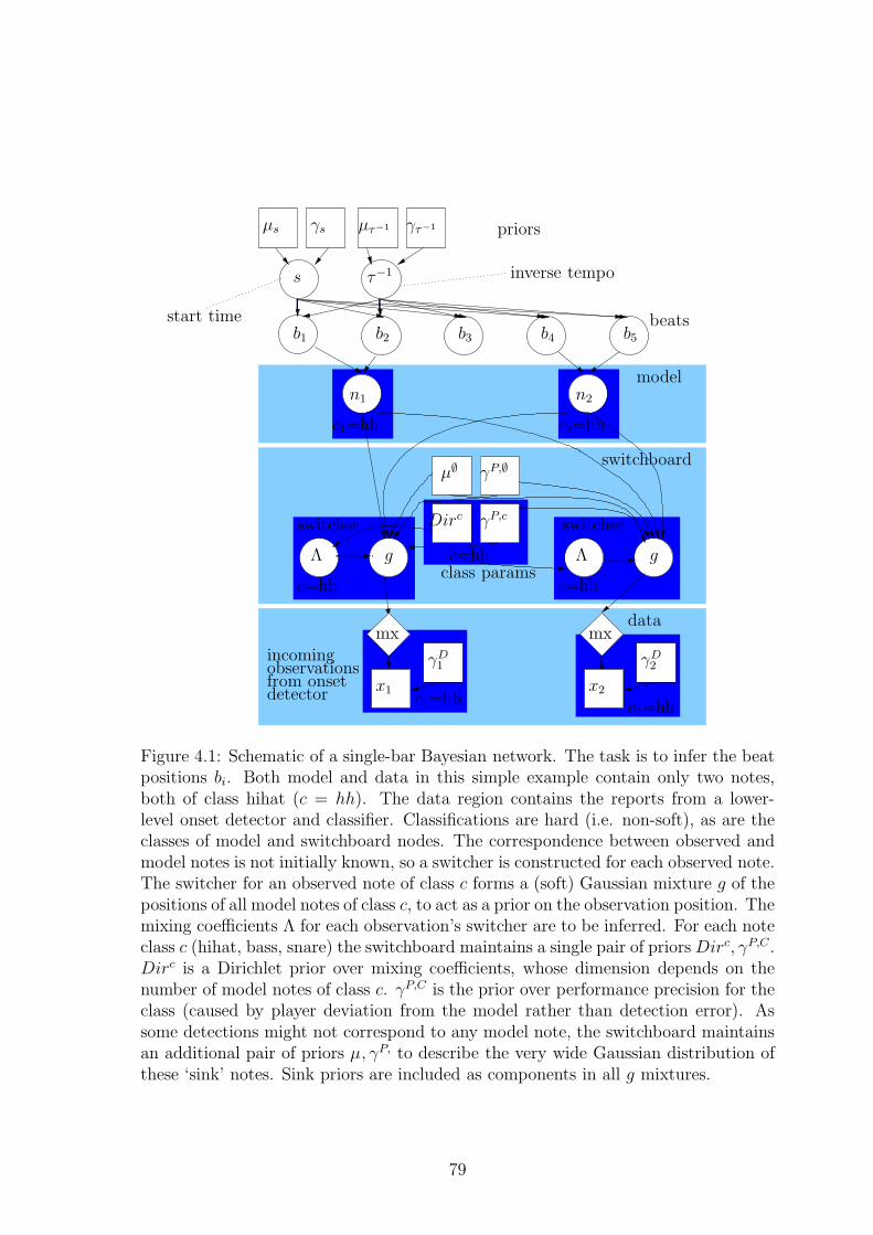
τ−1
x2
γD2
γs
n1
c=hh
c=hhc=hh
beats
model
switchboard
priors
data
γD1x1
γP,∅
switcherswitcher γP,c
µ∅
mxmx
µs
s
γτ−1µτ−1
ggΛ Λ
c1=hh
c1=hh
b1 b2 b3 b4 b5
n2
c2=hh
c2=hh
Dirc
inverse tempo
start time
incomingobservationsfrom onsetdetector
class params
Figure 4.1: Schematic of a single-bar Bayesian network. The task is to infer the beatpositions bi. Both model and data in this simple example contain only two notes,both of class hihat (c = hh). The data region contains the reports from a lower-level onset detector and classifier. Classifications are hard (i.e. non-soft), as are theclasses of model and switchboard nodes. The correspondence between observed andmodel notes is not initially known, so a switcher is constructed for each observed note.The switcher for an observed note of class c forms a (soft) Gaussian mixture g of thepositions of all model notes of class c, to act as a prior on the observation position. Themixing coefficients Λ for each observation’s switcher are to be inferred. For each noteclass c (hihat, bass, snare) the switchboard maintains a single pair of priorsDirc, γP,C.Dirc is a Dirichlet prior over mixing coefficients, whose dimension depends on thenumber of model notes of class c. γP,C is the prior over performance precision for theclass (caused by player deviation from the model rather than detection error). Assome detections might not correspond to any model note, the switchboard maintainsan additional pair of priors µ, γP, to describe the very wide Gaussian distribution ofthese ‘sink’ notes. Sink priors are included as components in all g mixtures.
79

4.1.1 Switchboard
We want to infer the positions of notes and beats from the set of observations. If each
observed note xk arrived with a label saying of which note nj of the model it was an
instantiation, this would be easy, as we could then connect the observed xk to nj and
perform inference. Hence xk would be treated as a noisy observation of nj (as in the
systems of Cemgil and Raphael). However we do not have such labels, we only have
the class ck of the observation. We are told that it is, say, a bass drum note, but
not which of the (many) bass drum notes in the bar. Further, we want to allow the
possibility that non-model notes may be played. This may occur for several reasons:
(1) extra note played by accident, e.g. the performer’s hand slipping; (2) performer
is playing a variation of a known model, with deliberate extra notes; (3) performer is
playing an unknown model. We must try to perceive the latter as a known model as
best we can for now, then perhaps consider the known model’s failings and update
the model or learn a new model from them offline.
We solve the tagging problem by modelling the belief in the observation locations
xk as a Gaussian mixture models (GMMs), with one Gaussian source from each of the
M model notes nj that have the same class as that observation. The middle shaded
layer of fig. 4.1 is called the switchboard, and consists mostly of clusters of nodes
called switchers. (There are also some extra nodes which are shared across switchers.)
One switcher is created per incoming observation k, and includes a GMM node, g,
together with a discrete mixture weight node Λ, so that its prior is
P (g|{µm}, {γPm}, {Λm}) ∝M∑
m=1
Λm exp
[
−γPm
2(g − µm)2
]
where γPm is a performance precision parameter for the mth parent (see section 4.1.2).
This distribution is not in the conjugate-exponential family, but may be approxi-
mated:
P (g|{µm}, {γPm}, {Λm}) ∝M∑
m=1
exp
[
−ΛmγPm
2(g − µm)2
]
This matches the mean and variance of the original GMM, and has the useful property
that it tends towards it as Λm → ∆mm′ , that is, as the discrete mixing vector becomes
a single peak at m′. This is useful for our task, as we wish to ultimately assign each
observation to a single class.
All Λ nodes of each class c share a fixed Dirichlet prior, Dirc, which have hand-set
parameters favouring single-source explanations.
80

u=[.01 .01 .01] u=[.1 .1 .1] u=[.5 .5 .5] u=[.9 .9 .9]
u=[.1 .1 .5]
u=[1.1 1.1 1.1]u=[10 10 10]
u=[20 20 20]
Figure 4.2: Examples of Dirichlet distributions on three variables.
P (p1:N |u1:N) =1
Z
N∏
i=1
pu1−1i
Examples of three-variable Dirichlet distributions are shown in fig. 4.2. Note that
when u = [1, 1, 1] then distribution is flat. For u components above unity, it bulges in
the centre (bottom row) encouraging mixtures of variables. For components less than
unity (top row) it favours single-variable explanations. It is the latter kind of prior
that we use here, as we want each switcher to be explained by a single component
rather than a mixture. It is possible to favour particular components by changing
relative values within the u vector, as shown in the centre row.
4.1.1.1 Sibling rivalry
In addition to this GMM formalism, we know something more about the relationship
between the observed and model notes: each model note will be instantiated at most
once in the data. Even if, say, two snare hits occur very close to each other and
to an expected model note location, only one of them can be ‘the’ instantiation of
81

the note, and the other must be a spurious extra note. The standard GMM is not
able to capture this ‘sibling rivalry’ between its children. GMMs are often used in
data-intensive statistics where the task is to infer quantities from large numbers of
noisy observations of them. In contrast, here we have at most one observation of each
model note. The sibling rivalry problem is not unique to GMMs but is a general Bayes
net problem: Bayes nets provide an automatic framework for competing parents to
inhibit one another through the well-known ‘explaining away’ effect; but do not allow
siblings to compete in any similar way.
To model our knowledge of sibling rivalry, we extend the Bayesian network into a
graphical model containing both directed and undirected links. For each note class,
we fully connect all the Λ nodes in the switchers of that class. We connect with
inhibitory links, so that if one switcher lays claim to being an instance of a model
note then it discourages other switchers from being instantiations of it. We extend
the variational update for Λ nodes to include this undirected term (rightmost):
logQ(Λ)← 〈logP (Λ|par(Λ))〉Q(par(Λ))
+∑
ch(Λ)
〈logP (ch|Λ)〉Q(ch(Λ),cop(Λ))
+∑
riv(Λ)
〈log Φ(riv,Λ)〉Q(riv(Λ))
As riv and Λ are discrete distributions parametrised by Q(Λ = Λm) = q(Λ)m ,
Q(riv = rivm) = q(riv)m with
∑
m q(Λ)m = 1 and
∑
m q(riv)m = 1, we set the additional
update terms to
〈log Φ(riv,Λ)〉Q(riv) =
1− q(riv)1
...
1− q(riv)M
whereM is the number of components. This is a heuristic whose intent is to encourage
pairs of discrete nodes to have large divergences between them (e.g. in the KL-
divergence sense). Note that this does not assign zero probability to two discrete notes
having the same component, because its effect is on the logarithm of the resulting
joint, not the joint itself. Instead, it merely discourages such similarity, and we have
found it useful enough for our purposes.
This scheme does not force any observations to match up with model notes: it
merely discourages multiple observations from explaining the same model note.
82

4.1.1.2 Sinks
To allow for the performance of non-model notes, we construct an additional sink
component for each note type. Sinks may be thought of as null hypothesis expla-
nations for observations. They are modelled by Gaussians having their mean in the
centre of the bar, and a very wide variance so that the distribution stretches all the
way across the bar in one standard deviation. This wide spread has the classic dual
effect of (a) catching observations from a wide range, enabling the sink to soak up
all observations not well accounted for by other components; (b) assigning a low
likelihood to each observation because it is so spread out; hence allowing non-null
components to be favoured in their specialist locations.
This may be viewed as a crude approximation to a fuller sink model: there is
information contained in non-model notes which we are currently throwing away. In
particular, notes do not occur at completely random places in the bar: even if not
part of an identifiable model, they still tend to occur on beats or rational subdivisions
of beats. In fact many beat identification systems have been constructed in this way.
For example Cemgil [22] constructed an intricate prior over subdivisions similar to:
P (x) =1
Z
K∑
D=1
2D∑
N=1
δ(x;N
2D) ∗ exp(−γ
2x2)
(The left part of this forms peaks at major subdivisions, whose height increases with
importance, as measured by number of factors. The right term convolves (*) with a
Gaussian to blur the spikes.) Such priors could in principle be incorporated here as
GMMs, with one GMM component per subdivision. The advantage of such a scheme
is that tempo and phase may then be inferred in a ‘model-less’ manner simply from
collections of notes and the prior. However this approach would be time-consuming
in a real-time system due to the large number of additional components to consider.
We also note that ‘model-less’ is something of a misnomer, as we would effectively be
specifying a complete, general pattern based on subdivisions: in practice we can know
most common models in advance and exploit this by using our set of particular models
instead of this general one. We have found that there is usually enough information
in the instances of model notes to infer the beats well, without having to rely on sink
notes to improve the accuracy.
There is still one problem with our single wide Gaussian approximation to this
intricate structure. As the Cemgil prior is made of peaks, this structure assigns
slightly higher priors to sink notes around rational subdivisions than our Gaussian
assigns, at the expense of having lower priors than our Gaussian at places away from
83

rational subdivisions. In practice, most (usually all) sink notes do occur at rational
subdivisions. This means that our approximation will consistently assign lower priors
to sink notes than the more accurate structure. To correct for this, we adjust the
Dirichlet prior on the Λ nodes to give sinks a slightly higher prior than model notes.
Empirically, u = [0.10, ..., 0.10, 0.12] was found to work well, where the 0.12 is the
sink component.
As discussed above, we constrain the GMMs with sibling rivalry links to prevent
multiple observations mapping to a single model note. For sinks there is no such
constraint: we allow multiple observations to be generated by the same sink. To
accomplish this, the 〈log Φ(riv,Λ)〉Q(riv) term above is modified so as not to penalise
sink-sharing.
4.1.2 Precisions
The switchboard contains two kinds of performance precision nodes. First, there is
a single fixed precision γP,∅ for sinks. This is used as an input to all GMMs, for
the precision of their sink component, regardless of their class. It is set so that the
standard deviation of the sink is one whole bar. Together with the Dirichlet prior
amplification this produces a useful sink model. Second, for each note class c there
is a fixed precision γP,c which is shared between all switchers of that class. This
performance precision models the player’s accuracy in playing notes of class c. For
example, the performer may be more accurate on the bass drum than on the hihat.
Note that future versions of the system could extend this by allowing each model
note to have its own performance precision, in the manner of Music++. This may be
useful when the patterns become more complex, and the performer may try harder to
play the on-beat notes very accurately at the expense of other more decorative notes.
Alternatively, a simplified model might share just one performance precision across
all note classes to allow faster inference.
Note that the performance precisions differ from the detection precisions γD – the
latter being a measure of the detection error rather than the human player’s deviation.
4.1.3 Visual display
The following demonstrations are illustrated using RhythmKitten’s graphical dis-
plays. The format of these displays is similar to the schematic of fig. 4.1 but extended
to show prior and posterior means and standard deviations for all positional nodes;
to display nodes from multiple note classes (hihat,snare and bass) and to show mix-
ture coefficients for the Gaussian mixture nodes in the switchers. A large quantity of
84

information is thus contained in these images, which may be difficult to read at first.
To aid comprehension, fig. 4.3 gives a cartoon example of the display format.
4.2 Example of a single model inference
The RhythmKitten screen-shots in figs. 4.4-4.5 show four inference steps on a single
model, as the message-passing progresses. Each step consists of a round of message
passing, which includes a downward pass followed by an upward pass. The input
observations consist of four hihat hits, one bass and one snare. The bass hit is
slightly after the first hihat and the snare is slightly before the third hihat. The task
is thus to find the best beat positions and assignments of noise to explain this data.
Fig. 4.6 shows the value of L, the lower bound on the log-likelihood during the
above iterations. (As the observed nodes are delta spikes we are approximating the
continuous probability density p(d|M) which may have values above unity.) Note that
– contrary to VB folklore – the lower bound does not improve monotonically, though
it does converge. The reason for non-monotonicity appears to be the presence of the
discrete switch nodes. While it is known that each individual update Qi(xi) always
improves the total Q =∏
iQi(xi), this does not account for the fact that updating
Qi then has knock-on effects on other nodes, invalidating their Qi’s. This problem is
especially apparent when discrete switches and rivalry are important.
4.2.1 Cyclic and divergent behaviour
As discussed above, variational Bayesian inference does not necessarily converge once
discrete switch nodes are brought into play. The problem can become acute for highly
ambiguous stimuli having multiple local minima, and having large loops in the graph.
Such loops take time for information to propagate around, so for example it may
take several steps before the effect of a switch node change is felt. In these cases it
becomes possible for the network to oscillate between states, and even to diverge.
Fig. 4.7 shows an example of cyclic (and possibly divergent) behaviour: an am-
biguous stimulus is presented to a standard ROCK1 model (see fig. 4.10), and nine
steps of inference are shown. The stimulus consists of just three hihat hits, with no
immediately obvious underlying beat. Given priors on the start time and tempo as
usual, the net oscillates between two configurations, labelled in the figure as L and R.
In the R screen-shots, the notes are interpreted as occurring early, before the beats.
In the L screen-shots, they are interpreted as occurring after the beats.
Fig. 4.8 shows the lower bound L during the oscillating run. Close inspection
shows that the two apparently fixed points are actually slowly diverging.
85
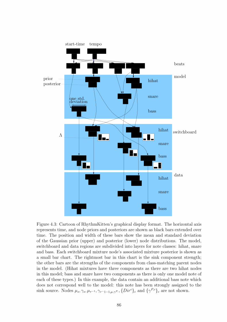
����������
����������
����
����
����������
����������
����
����������
����������
��������
����������
����
����
��������
����������
����������
switchboard
model
beats
data
tempostart-time
snare
snare
snare
bass
bass
bass
hihat
hihat
hihat
priorposterior
deviationone std.
Λ
Figure 4.3: Cartoon of RhythmKitten’s graphical display format. The horizontal axisrepresents time, and node priors and posteriors are shown as black bars extended overtime. The position and width of these bars show the mean and standard deviationof the Gaussian prior (upper) and posterior (lower) node distributions. The model,switchboard and data regions are subdivided into layers for note classes: hihat, snareand bass. Each switchboard mixture node’s associated mixture posterior is shown asa small bar chart. The rightmost bar in this chart is the sink component strength;the other bars are the strengths of the components from class-matching parent nodesin the model. (Hihat mixtures have three components as there are two hihat nodesin this model; bass and snare have two components as there is only one model note ofeach of these types.) In this example, the data contain an additional bass note whichdoes not correspond well to the model: this note has been strongly assigned to thesink source. Nodes µs, γs, µτ−1, γτ−1−1,µ,γP,, {Dirc}c and {γP,c}c are not shown.
86

(a) In the first step, the HIPHOP1 model(see fig. 4.10) has just been instantiated,with a tight prior on the start time and aloose prior on inverse tempo. HIPHOP1has hi-hats on all four beats, a snare onbeat two, and bass on beat one and justbefore the end of the bar (the latter basshit is the ‘late’ hit which provides the char-acteristic hiphop feel). The inverse tempobelief has already been greatly tightenedby the messages from the beats. The beatposition beliefs still obey the start-timeand tempo priors more than the observa-tions. This is because messages from theobservations have not yet propagated tothe beat layer. They have however propa-gated to the model layer, as its nodes showsubstantial deviation from where the beatswould predict them. The switcher nodesassign the final hihat to the sink, mis-assign the penultimate hihat to the thirdbeat instead of the forth; and are uncer-tain whether the snare was generated bythe (only) model snare on beat 2 or by thesink. Overall the model is far from thesolution and out of balance as its tempois still too slow and the beats last muchlonger than the observed notes; meanwhilethe model notes are too fast and do notlast as long as the observations.
(b) The same musical bar after a sec-ond step of inference. In the second step,the beat positions have been corrected andnow span a similar range of time to the setof observations. (Note there are five beatsrather than four as the model representsthe end of the bar as well as its internalbeat positions.) However the model noteshave sprung out beyond the observationrange – affected by the previous versionof the beat beliefs. The snare switcher isassigning a strong sink belief due to theprevious location of the model snare note,as can be seen by the bar chart next tothe snare node in the switchboard. Atthis still-early stage of inference, there isstill much uncertainty in the switchboard’sbeliefs about the third and fourth hihatnotes – even though the correspondingmodel beliefs are comparatively tight (butwrong). This is because information hasyet to propagate from the model to theswitchboard.
Figure 4.4: The first two of four steps of inference in a single-bar rhythm network.87

(a) By the third step, the oscillations havelargely calmed down, and the beat andmodel note positions now agree with eachother and with the switchboard. The snarehit is correctly assigned and so are are theother switchboard notes, which all showfairly decisive switch assignments.
(b) By the fourth step there is very littlechange in each step. All notes are cor-rectly assigned, though each note – espe-cially the snare – maintains a small proba-bility of being sink-generated. This is be-cause the played bass and snare do not co-incide exactly with the hi-hats beats so itis possible they were played intentionallyas extra non-beat notes rather than playedincorrectly as on-beat notes. Even at con-vergence, the positions of the beats growsincreasingly uncertain towards the end ofthe bar. This is because the tight start-time prior becomes diluted by the rela-tively loose tempo prior, and also as thereare few observations towards the end ofthe bar. Little visual change occurs if ad-ditional steps are run beyond this point(though numerically the network contin-ues to converge to a limit point).
Figure 4.5: The final two of four steps of inference in a single-bar rhythm network.
88

1 2 3 4 5 6 7 8−9.5
−9
−8.5
−8
−7.5
−7
−6.5
−6
−5.5
−5
−4.5
iteration
L
Figure 4.6: Log-likelihood during variational inference in the single-bar rhythm net-work.
Convergence is affected by the model priors: a main reason for the oscillation
above is that the model assigns similar priors to the L and R configurations. If
the model was instantiated with less ambiguous priors then a single optimal state
would have been found. Convergence can also be affected by node firing order. In
the run of fig. 4.7, we used the best firing order that we have found: one iteration
consists of a complete down-pass followed by a complete up-pass. Earlier versions
of the system used iterations consisting of a down-pass only, or up-pass followed by
down-pass but we found this tends to lead to oscillation more often. Indeed, under
the latter scheme, highly ambiguous tasks such that of as fig. 4.7 can sometimes
produce unstable oscillations in which the difference between the bistable percepts
grows rapidly at each step, the beat and model note positions moving towards ±∞until the program crashes due to numerical underflow errors.
4.2.2 Annealed variational message passing
To reduce the possibility of belief oscillations during message passing, we use vari-
ational annealing. In this scheme we do not seek Q ≈ P directly, rather we infer
a sequence of heated distributions Q1/Ti ≈ P 1/Ti. The temperature T begins at a
number greater than unity, and is gradually reduced to unity. Further, if an MAP
solution is sought rather than a joint approximation, T may be reduced below unity
and toward 0, in which case Q1/T (x) → δ(x; x), giving an estimate of the MAP. In
practice, this MAP estimate is a near-delta spike at a local maximum of the posterior.
As the cooling schedule slows and the initial temperature is raised, the probability of
arriving at the global maximum increases. We extend the variational message passing
89

(a) Step 1. (R config.) (b) Step 2. (L config.) (c) Step 3. (R config.)
(d) Step 4. (L config.) (e) Step 5. (R config.) (f) Step 6. (L config.)
(g) Step 7. (R config.) (h) Step 8. (L config.) (i) Step 9. (R config.)
Figure 4.7: Cyclic behaviour for an ambiguous percept and weak prior. The beatpositions oscillate between two approximately stable configurations, L and R.
90

0 5 10 15 20 25 30 35 40 45 50−8.5
−8
−7.5
−7
−6.5
−6
−5.5
−5
L
iteration
Figure 4.8: Log-likelihoods for the cyclic example. Oscillations are clearly seen: localvariational Bayes updates do not always lead to global improvements in log-likelihood.
framework to include annealing by giving each node a temperature parameter (for
our conjugate exponential models this simply multiplies the parameter vector.)
Fig. 4.9 shows a difficult three-onset inference problem: the notes fall in such
places as to be highly ambiguous under the position and tempo priors. Without
annealing this causes the network to oscillate and diverge during inference; annealing
cures this problem. The distributions on the nodes begin by becoming very wide as
messages are received; then gradually reduce as cooling takes place. (See section 4.4
for a description of the display.)
4.3 Hypothesis management
So far we have considered rhythm models of individual bars: test data was created
representing a single bar’s content of music, and the postulated model had to explain
all the data. However in the wild, the situation is more complex: we receive a stream
of events over a period of several minutes (the song) and we do not know initially
which events belong to which bar and hence to which model.
The ideal Bayesian approach would be to consider all possible models instantiated
at all possible points in time-tempo space, together with a prior on which combina-
tions of them are allowable and mixture switches to allow data points to be explained
as mixtures of models. The prior would act to allow only sets of rhythm models which
are contiguous throughout the whole song, and could further specify Markovian or
grammatical priors on the probabilities of particular sequences of models.
This approach is impractical because it requires an infinite number of models,
and even quantising the possible model instances would require a very large number
91

Figure 4.9: Seven steps of annealed variational inference on an ambiguous three-onsetproblem. As inference progresses, the heated initial beliefs converge to the correct VBposterior. Without annealing, the network can oscillate and diverge during inference.
of models. In particular the prior would have to operate on the power set of these
models which is intractable. So we must use heuristics to approximate the Bayesian
ideal.
The heuristics we use are based on the ideas of priming and pruning presented
by [142]. Reis modelled symbolic sequences using a set of agents, each agent being
a detector for a particular pattern. When an agent A successfully completes its
pattern (by observing the exact required sequence – Reis’ work was non-probabilistic)
it competes with completed rival agents, and the winner W primes all other agents
to start looking for their patterns beginning at the point that W completed. Rival
agents are those which share one or more symbols of the data stream. Losing agents
are deleted (pruned).
We extend this method to the case of continuous time events (opposed to se-
quences of symbols). We replace discrete symbol sequence detecting agents with our
variational models. Reis handled competition between models with a heuristic, but
in contrast, we are able to use the variational lower bound on model likelihood to
provide a more rigorous foundation for competition. The principal difficulty is the
lack of sharp boundaries between models together with the uncertainty in note arrival
times: in the symbolic domain is simply to say ‘if the new note time is after the end
of agent A then add it to the next agent instead of to A’ but the meaning of this
92

is less clear in our probabilistic domain: there will instead be some probability that
the new note lies inside or outside the model. Pragmatically, we simply set a prob-
ability threshold and declare the new note to be outside the model if it is exceeded.
Pseudo-code is shown in algorithm 1.
Algorithm 1 Reis-like algorithm for hypothesis management with priming and prun-ing. dM is the set of data points attached to model M and |dM | is the size of thisset.
prime initial model setset initial models to incomplete statefor each incoming note n do
for each incomplete model M doif P (n after M < threshold) then
link n to Mupdate temperature T
elseset M to completed statewinner W ← Mfor each rival model R (overlapping M) do
if R completed thenif logQ(R|dR)/|dR| > logQ(W |dW )/|dW | thenW ← Rprune R and descendants of R
end ifend if
end forprime from W
end ifend for
end for
There is an issue regarding model comparison when two rivals R and W have
different numbers of data points. Instead of raw model posteriors, we compare the
log posteriors per data point, dividing the lower bounds by the number of data. This
statistic may be thought of as an approximate log probability density per unit time,
with data points as a proxy for time. (Log posterior densities are typically negative,
so dividing them increases their value.) The reason for comparing log probability per
data point is as follows. Suppose we have N models in a sequence, M1,M2, ...,MN
which together cover a complete song. The issue is that data points near model
boundaries may fall under the model at either side of the boundary. We do not wish
to penalise either case in the ideal global distribution of models. So we note that our
statistic has this property: the score for the whole song is
93

∑Ni=1 logP (dMi
|Mi)∑N
i=1 |dMi|
From the point of view of the global distribution, the denominator is constant so does
not penalise any particular assignments of data to models. However recall that we are
using a heuristic to approximate the global distribution, namely that we make a hard
decision about which models to keep and reject at the end of each bar. And from
the viewpoint of these individual bars, the statistic does make a difference, namely
that of transforming our measure of log likelihood into log likelihood per data point
explained, which aids our greedy search through the space of sequences of models as
required.
Note that we have included the annealing schedule as part of the node linking
cycle. We want the model to start as ‘hot’ when first created, then to cool as real
time progresses, so that it reaches the true probability scale as it completes. We use
the time of the latest received note as a proxy for elapsed time, and have found that
a useful schedule is to cool linearly from T = 8 to T = 1 during the course of the bar.
4.3.1 Priming
In the present work we have used a simple Markov transition matrix to specify priors
on sequences of models. (e.g. the low probability of a drum’n’bass pattern following
a military march pattern.) There is an important practical difference between tran-
sitions of zero probability and those of small but non-zero probability. Conceptually
these are similar, but the former will not be primed whereas the latter are primed
but are unlikely to be chosen as the final winner. This makes a huge difference to
the amount of computation that takes place, but there is the classic tradeoff that
in setting unlikely transitions to a hard zero, we rule out the ability to use them
to explain uncommon situations, so in the unlikely event that those situations oc-
cur, the model will fail. (Primed models are ‘known unknowns’, as they still contain
much uncertainty but are under active consideration’; unprimed models are ‘unknown
unknowns’.)
Newly primed models are instantiated having a start time with mean equal to
the MAP end time of the previous (completed) model – shown by the dotted line in
fig. 4.1 – and inverse tempo mean equal to the MAP of the previous inverse tempo.
Parameters specify precisions of these beliefs, which at present are global and hand-
set. However it would be conceptually simple to use an EM method as in [137] to
learn precisions for each bar and also to learn priors on tempo transitions.
94

4.4 Evaluation
It is more instructive to present a walkthough of a real RhythmKitten test run than
to give only statistics of its results. A data set was recorded by a human drummer
using a MIDI kit, and standard deviations of 100ms attached to notes of all types to
simulate a level of uncertainty that would be typically be attached to onset-detected
notes (as in the experiments of section 3.8). The data consists of 48 bars of rhythms
lasting about 2 minutes and including over 250 hits, which is a typical amount of
data for beat tracking evaluations in the literature, (e.g. [26]). The rhythms begin
as simple known patterns and get progressively more complex, and more errors are
introduced. A knowledge base of six models was used, shown in fig. 4.10, which
includes three regular rhythms and three fills.
RhythmKitten is written in interpreted Lisp research code, and no effort has
yet been made to optimise its execution for real-time online inference. However the
test run was performed on a 1.6GHz Pentium in quasi-realtime of half the original
performance speed, suggesting that real-time optimisation would be possible with
further development work.
To aid understanding, figs. 4.11-4.13 give close-up pictures and discussion of the
results from the first 12 bars. Bar numbers are displayed above each model, and
only the winning models are shown, in their final collapsed form. The reader may
examine the remainder of the run in fig. 4.14, noting the near-losses of tracking
around bars 26-28 and 36 and subsequent recovery; and the eventual failure due to
complex unknown rhythms at the end.
4.4.1 Comparison with naive tracking
Fig. 4.15 shows the deviation of the played onsets from ‘ground truth’ beats (as
labelled by hand, offline), and can be seen as a measure of the accuracy of the playing.
The x axis measures fractions of a beat deviation from the nearest labelled beat.
Note the clusters around ±0.5 beats which are notes played half way between beats.
Excluding these notes, the standard deviation (player error) from the beat is 0.07
beats, corresponding to 35ms at 120bpm.
Fig. 4.16 shows a histogram of errors of the system’s MAP beat positions from
the ground truth. Only the correctly-tracked bars 1-38 are included. The standard
deviation of the errors is 0.12 beats, which corresponds to a musical semi-quaver,
or 60ms for a track played at 120bpm. However this large deviation includes the
outliers shown in the graph which arise during the near-loss of tracking around bar
27. Excluding these incorrect models gives a deviation of 0.056 beats over 129 data
95

(a) ROCK1 (b) ROCK2
(e) HIPHOP1 (f) SHUFFLE1
(d) FILL-OFFBEAT1(c) COUNT-IN
Figure 4.10: Model-base used in the evaluation. Each model is a four-beat patterncontaining hihat (top), snare (centre) and bass drum (bottom) hits. Beat positionsare shown as dotted lines.
points, equivalent to 28ms at 120bpm. This is a significant (a χ2 test gives P (s2 ≤0.0562|σ2 = 0.072, N = 129) = 0.0004) improvement from the 35ms player latency
above (for example if the raw onsets had been used as beat locations.) Typical home
music software has a latency of around 10ms in comparison. Inspection of the worst
errors shows them to occur in bars where the tempo changes within the bar rather
than at the bar-line, this is of course expected as our current model assumes a single
tempo within each bar.
4.4.2 Issues and extensions arising from the evaluation
4.4.2.1 Need for missing children penalties
In several cases we saw over-complex models being used to interpret simpler data.
For example there is no implicit penalty for using a HIPHOP1 model to explain a
ROCK1 pattern above. This can give unintended results, for example we saw this
occur in bar 3, because there is some small chance that the extra bass note was
a very early hiphop note. The problem becomes acute in cases like bar 43 where a
completely wrong rhythm has been selected because just one or two notes match; and
its remaining notes then deform the perception. In bar 43 it would have been better
96
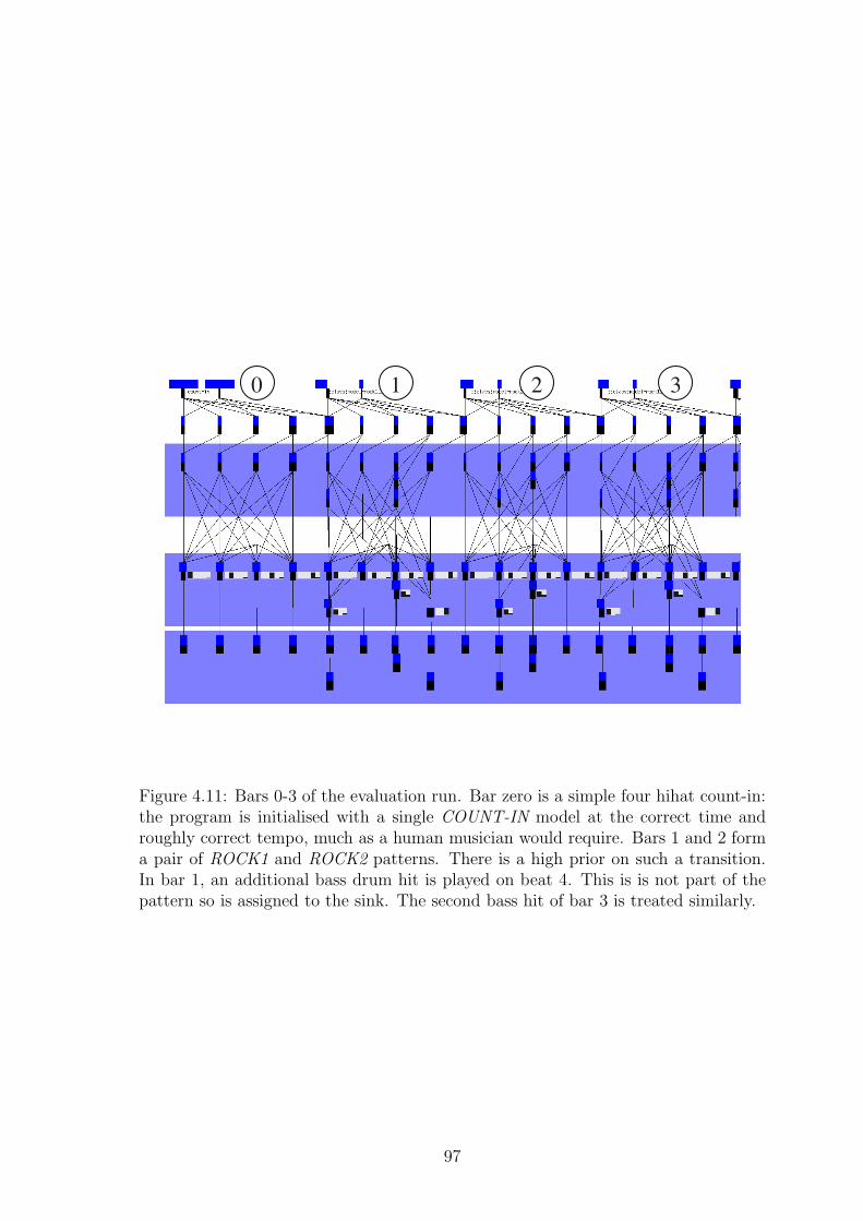
Figure 4.11: Bars 0-3 of the evaluation run. Bar zero is a simple four hihat count-in:the program is initialised with a single COUNT-IN model at the correct time androughly correct tempo, much as a human musician would require. Bars 1 and 2 forma pair of ROCK1 and ROCK2 patterns. There is a high prior on such a transition.In bar 1, an additional bass drum hit is played on beat 4. This is is not part of thepattern so is assigned to the sink. The second bass hit of bar 3 is treated similarly.
97
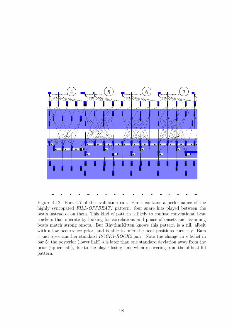
Figure 4.12: Bars 4-7 of the evaluation run. Bar 4 contains a performance of thehighly syncopated FILL-OFFBEAT1 pattern: four snare hits played between thebeats instead of on them. This kind of pattern is likely to confuse conventional beattrackers that operate by looking for correlations and phase of onsets and assumingbeats match strong onsets. But RhythmKitten knows this pattern is a fill, albeitwith a low occurrence prior, and is able to infer the beat positions correctly. Bars5 and 6 see another standard ROCK1-ROCK2 pair. Note the change in s belief inbar 5: the posterior (lower half) s is later than one standard deviation away from theprior (upper half), due to the player losing time when recovering from the offbeat fillpattern.
98
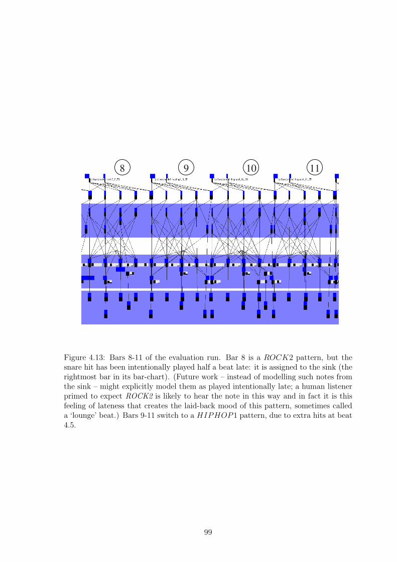
Figure 4.13: Bars 8-11 of the evaluation run. Bar 8 is a ROCK2 pattern, but thesnare hit has been intentionally played half a beat late: it is assigned to the sink (therightmost bar in its bar-chart). (Future work – instead of modelling such notes fromthe sink – might explicitly model them as played intentionally late; a human listenerprimed to expect ROCK2 is likely to hear the note in this way and in fact it is thisfeeling of lateness that creates the laid-back mood of this pattern, sometimes calleda ‘lounge’ beat.) Bars 9-11 switch to a HIPHOP1 pattern, due to extra hits at beat4.5.
99

Figure 4.14: Complete 48-bar test run results.
100

−0.8 −0.6 −0.4 −0.2 0 0.2 0.4 0.60
5
10
15
20
25
30
played−tap/beats
freq
uenc
y
Figure 4.15: Error of played onsets from hand-tagged beats.
−0.3 −0.2 −0.1 0 0.1 0.2 0.3 0.40
5
10
15
MAP−tap/beats
freq
uenc
y
Figure 4.16: Error of played onsets from auto-tagged beats.
101
to select a simple standard model (like ROCK1) to fit the few notes. RhythmKitten
could be extended to penalise models with many missing children. However the
penalty should not be too strong as humans do often ‘fill in’ their perceptions of
missing beats. For example, if listening to a HIPHOP beat for several minutes and
a ROCK1 bar is played, the ‘missing’ hiphop note will still be heard (and danced
to.) So clearly missing child penalties must balance the ability to occasionally fill in
against the problem of perceiving hugely over-complex patterns in very simple data.
4.4.2.2 Tempo changes in bars, and tempo priors
Music++ models tempo as changing at each event, and learns priors on these tempos
using an EM algorithm run after each new performance. In contrast, RhythmKitten
currently assumes that tempo is constant within each bar, and is thus unable to track
gradual tempo changes. To extend RhythmKitten towards industrial performance,
a more detailed tempo model should be constructed. This is conceptually simple
– essentially a re-implementation of Raphael’s structures – but requires additional
software engineering effort.
4.4.2.3 Learning new models
This thesis is concerned primarily with Bayesian models of perception and compu-
tation on those models – but learning is always complimentary to perception and
makes an obvious research extension. Learning new models is time-consuming from
a software engineering point of view – so we merely discuss it rather than implement
it. Future work could provide software implementations of these methods.
New concepts are usually learned as variations on existing concepts. A simple al-
gorithm to learn new models here would be as follows. Recall the generic Cemgil prior
discussed in section 4.1.1.2. A generic model based on this generative distribution
should be implemented and always primed but with a low model prior. It would then
be able to catch all bars that fall below some threshold of explanation by the other
competing models. The particular set of note types found at subdivisions would then
define a temporary new model class. As in Reis’ scheme, temporary models could be
given a fixed lifespan: if the model is useful and is found to re-occur then it is kept
and its prior grows stronger. If it was a one-off then its prior decays and the model
removed once the prior falls below a threshold.
When dealing with learned models there is always a problem that several variations
of an ideal single model may be learned separately. However it would be reasonable
simple to create a heuristic: a sub-task that periodically (like a garbage collector)
102
checks the model database for sets near-duplicates and tries to compute a generalised
replacement for them. Research from classification theory and unsupervised learning
could perhaps be applied here to make good heuristics.
A more advanced alternative to learning new models as specialisations of the
Cemgil prior would be to learn them as specialisations of other existing models. For
example, in the walkthrough we touched on the idea that patterns like the ‘lounge’
beat in bar 8 could be perceived as regular patterns with particular transformations
applied to certain notes. Swing beats, the hiphop note (when considered as a preemp-
tion of the start of the next bar), and salsa rhythms (which play notes slightly early
to drive the music forward) are further examples. Similarly, several of the bars in
the walkthrough contain a standard pattern but with notes played on different drums
than usual. For example the final snare hit in bar 15 could be seen as the hiphop
note but ‘transposed’ from the bass to the snare. Future work could consider how
to model these transforms and learn new models based on them. (The transposition
case could perhaps be handled more easily by allowing the low-level hit classifier to
report uncertainty over hit type likelihood; RhythmKitten could then change its type
assignment under prior information from the rhythm model. But a more general
transformational approach could capture both this and the positional movements of
the lounge and swings beats described above.)
4.4.2.4 Data-model mis-assignments
Mis-assignment of data to models is not a cause of failure but is a major cause of the
inability to recover from it. It prevents models from correcting themselves because
they do not have access to the data points that would help the corrections.
Within models we created a system based on GMM nodes to handle uncertainty
of mapping from data to notes within the model. A similar scheme could be used
to handle uncertainty of mappings between models, though heuristics may need to
be invented to prevent computational explosions. In this case, the multiplexer nodes
would be replaced by GMMs with switches between models, and models of previous
bars may have to be kept alive for longer to explain data pushed out of following bars.
Once multiplexers are replaced by GMMs it would also be natural to treat rival
models in this way as well. Then information could flow between rival models. This is
a more fully Bayesian approach to rivalry, however the question of whether it is useful
for this application remains to be answered. (An even more Bayesian approach could
be to have all rivals sharing the same set of beat nodes – this way, predictions of future
beats would be formed by automatically averaging over all models. However the view
of this thesis is that it is useful for perception to periodically stop and collapse its
103

inference to a single unambiguous explanation of the world rather than computing
averaged Bayesian predictions.)
4.4.2.5 Non-Markovian priming
The Markov assumption is somewhat limiting, for example most songs contain sec-
tions of four bars which use an alternate rhythm (or ‘fill’) to mark the final bar.
Similarly real songs contain larger-level structure such as verses and choruses that
are likely to have more unusual fills to mark their endings, as these endings are im-
portant musical events. The Markov assumption is unable to capture these ideas,
so if we are ever to recognise a fill, we must prime it after every bar, which can be
computationally wasteful. It is envisaged that RhythmKitten could later be used as
a mid-level, grid-establishing component in a larger music perception system, which
could include higher-level grammatical models (such as those of ThomCat in chap-
ter 6) that send prior messages back to RhythmKitten to prime models and specify
their priors. Again such connectivity is conceptually simple but is a large software
engineering task beyond the scope of the present work.
An alternate way to reduce the number of models is to prime upwards from features
in the lower level data. For example, the presence of a ‘late’ hiphop-like beat may
alert us to the possibility of a HIPHOP model, which may be primed and tested.
Bottom-up priming is explored in chapter 6.
Like most beat trackers, RhythmKitten is currently very brittle with respect to
errors of start-time phase and tempo multiples. These errors do not arise often but
once they have occurred they are usually the cause of irrecoverable error, as we saw
around bar 42. The standard solution (e.g. [70]) to make trackers more robust is to
prime additional models with different phases and multiples. For example, at each
model completion, we could prime four extra models of each type, having: phase
-1 beat; phase +1 beat; double tempo; and half tempo. The obvious problem is
that this would need to be done for each primed model type, so would increase
the amount of computation by a factor of four. This may not be a problem in a
code-optimised RhythmKitten but would have slowed down our experiments in the
research prototype. A useful technique would be to determine when the perception
is in a state of ‘crisis’, i.e. when the models posteriors are consistently falling below
some threshold, and only then switch to this more desperate form of inference. It
would also be useful to alter the annealing schedule at these time to allow a wider
range of possibilities to be considered within the models. Both the introduction
of extra primes and the higher-temperature annealing within them are examples of
‘tempering’ or ‘high-temperature thinking’: when one’s perception of the world is in
104

crisis, one must be willing to step back and consider possibilities that are a priori
more far out, in an attempt to find some new theory to make sense of the data.
For some applications it may be useful to reinterpret historical data once a crisis
is resolved. For example, if grammatical priming was active, a reinterpretation of the
genre of the last 8 bars could affect what types of models are considered in the future.
4.5 Discussion
We emphasise the general architecture of RhythmKitten: while an industrial system
for drum tracking could be built by extending it with the ideas above and more soft-
ware engineering, this is not our goal in this thesis. Rather, the aim to begin thinking
about how perception in general can construct interpretations of low-level data. We
take a Bayesian constructionist view: since Kant [87], we have been accustomed to
the idea that the world in itself (noumena) is not available to us; rather we construct
a best (phenomenal) interpretation of what reaches our senses. Kant held that the
basic framework of perceptual space and time must be hard-wired in order for the
process to begin: here we are presented with measurements of events in time. We
then construct higher-level interpretations of those events in terms of known models.
Which models are used will depend on RhythmKitten’s subjective priors: if set up
to expect drum’n’bass patterns then it will perceive them rather than military march
patterns, in the same data. This is a useful illustration of how (phenomenal) models
exist only in the head, not in the external (noumenal) world.
In making the mapping from data to model, we found it useful to employ a three-
layered system, shown by the shaded bands in the figures. The lower and upper
bands are the data and the model respectively, but intermediate between them is a
switchboard layer, which deals with selecting which data to map to which model com-
ponents, and with rivalry between explanations. This is unconventional in Bayesian
networks, and is present because we are working with a scene perception problem in
which the data-model mapping is not given a priori. We will extend the idea of the
intermediate switchboard layer into the thalamus component of ThomCat in chapter
6.
Our modified Reis scheme regularly makes ‘collapses’ of the PDF to unitary inter-
pretations. As data arrive, several competing models are active in explaining them;
as time progresses the temperature is lowered; then at the end of the period the single
best model is chosen as the winner and the others are pruned. Effectively, the pa-
rameters θ within the winning model are also collapsed to their MAP at this point as
we read off the mean belief in the beat positions and export them as RhythmKitten’s
105

Figure 4.17: Phases of annealing cycles for perception. (1) Start of cycle, high uncer-tainty; (2) temperature reduction; (3) collapse to unitary coherent percept.
output (along with the name of the model type). At this point the new batch of
models is primed from the winner and the cycle begins again.
Fig. 4.17 shows conceptually the three stages present in our approach, where
the axes show the amount of uncertainty (H) over time. At the start of the cycle (1)
several models are primed, and we are very uncertain about both the models existence
and their parameters. Over time (2) inference takes place and temperature is lowered,
creating a reduction in uncertainty. At some stage, (3) we make a hard decision based
on our best (and hopefully quite certain) belief, and collapse the percept to a single
best explanation. Immediately after this collapse, the process begins again with new
primes (the diagram shows a small gap to separate the phases, but this gap is an
infinitely small ‘moment’ in practice.) We will see these three phases reappear again
in the following chapters’ Gibbs and quantum Gibbs perception algorithms of this
thesis.
While our proof-of-concept implementation of the variational and blackboard ideas
described here is not yet of industrial quality, we have explained how and why the ap-
proach is useful for solving higher-level rhythm and beat perception tasks than those
tackled by current beat-trackers. By incorporating psychological ideas of model-based
perception, priming and a global workspace, the approach may also lead to clarifica-
tions of perceptual music psychology concepts and could even serve as a framework for
empirically modelling human rhythm perception, especially for interesting ambigu-
ous percepts. This thesis is about scene perception, and RhythmKitten has extended
the notions of priming and pruning – that we first saw in the priming particle filter
– to position-in-time models. It has also introduced the highly general concept of
the annealing cycle for perception. However RhythmKitten is Markovian in its one-
dimensional sequence of models and has no conception of perceptual hierarchies. It
is these concepts that we next explore in a study of blackboard systems.
106
Chapter 5
Blackboard systems review
5.1 From sets to sequences to hierarchies
RhythmKitten used simple Markovian transitions between hand-set pairs (2-grams)
of models. In the general scene perception task, non-local dependencies such as n-
grams and hierarchies come into play, along with completely global factors such as
the key of a musical performance or the location of a visual scene. General scenes do
not necessarily consist of sequences of models: there may be areas of the scene which
are unexplained, and models which are ‘free-floating’ – i.e. not part of any larger
structure such as a sequence or hierarchy. Auditory scenes may allow some types of
model to exist simultaneously at the same location, for example a chord and a rhythm
played simultaneously; or two notes played simultaneously. Alternatively it is useful
to think of the scene as existing in more than one dimension with non-overlapping
explanations: for example, we might think of the musical score as a 2D piano-roll type
grid, where previously overlapping notes now exist at separate vertical coordinates on
the pitch axis. Similarly we can allow separate scene areas for rhythms and chords.
This approach brings the auditory scene perception task closer to the visual scene
perception task, which also has high dimensions, free-floaters, and global factors. We
stress that this is part of our intention: to model the general scene perception process,
not just the example minidomain of semi-improvised musical scene perception.
This chapter discusses the concepts involved in moving to general, hierarchical
scene perception, and reviews existing relevant work. We will see that classic AI
work from the 1970s and 1980s laid the groundwork before lying dormant during
most of the Bayesian revolution – but can be usefully fused with the latter into the
domain of ‘Bayesian blackboards’.
107

5.1.1 Music-related issues
Most work on scene perception has focused on the special case of visual scene per-
ception, neglecting other domains such as auditory and tactile scene perception, and
more abstract domains such as the perception of analogies, mathematical proofs and
scientific theories. While most of the visual concepts carry across to other domains,
including our music minidomain, much vision work has focused on static image per-
ception, neglecting the temporal aspect of perception which is of crucial importance
in the general case. For example, in tactile scene perception, a rat finding its way
around in the dark using its whiskers receives only a small about of information at
each point in time, but still constructs (and presumably perceives) a complete map of
its environment. For tactile scenes, active perception is important – choosing where
to focus attention in order to construct the scene. Recent visual systems [13] have
begun to model the movement of attention over time, in both static images (like a
human moving the fovea around a photograph) and more challengingly, in video clips.
However these scenes are still usually static at each moment of time: the percept is of
the state of the world at the moment that perception is taking place. The auditory
case (and video scenes, if done properly) is different: the percept is of an interval of
time, which may or may not contain the moment that the perception is happening at.
For example, in music, we are usually aware of the last four bars or so of music, and
also of a prediction of what will happen next. Our percept is of an interval of time
stretching four bars into the past and maybe on bar into the future. Less typically,
we might ‘cast our minds back’ to what happened in the previous verse, in which
case our percept consists of the four bars that happened some time ago, and we are
mostly ignorant of what is happening around us at the time of this percept (like the
absent-minded History professor oblivious to the traffic around him as he perceives
some medieval battle in the past). Importantly, we may recall the past in two ways:
first, by recalling the same actual interpretation of a historical event as we did at the
time of the event itself; or second – and more usually – by reconstructing an interpre-
tation of recalled models in terms of our currently available model set. For example,
humans who have changed their politics towards libertarianism over the last ten years
are likely to recall their teenage activism as part of their current framework than their
actual teenage socialist framework: ‘Yes I’ve always marched for freedom, it wasn’t
the corporations we were protesting against but the government’s involvement with
them’, (c.f. [54]). We may also focus our perception onto the future, or onto a dif-
ferent place than our actual location, for example when we are making distant plans
108

or guessing what our friend is doing in the states right now. Most visual scene per-
ception programmes have completely ignored this aspect of scene analysis, and the
music minidomain provides a way of bringing it to the fore, as it as of unavoidable
importance in our task.
Questions about creativity and ‘where models come from’ have an interesting
perspective brought upon them from the music perception task. Previous work [56]
constructed a genetic algorithm for musical composition, in which random changes
were proposed to an L-system representation of a musical scene, and human listen-
ers provided an acceptance function. The system evolved new compositions from
initial, existing compositions. However a notable omission from the work was that
the existing compositions had to be hand-parsed by human music experts into the
L-system form. So the work of perception was pushed out of the system onto human
pre-processing, along with the work of artistic judgement. The supposedly ‘creative’
composing stage of making random changes was much easier to automate than the
two listening (parsing and acceptance) stages. There is a great similarity between
the two human stages: they both involve perceiving the music as a hierarchy, that
is, they are musical scene perception tasks. They both require creativity in the sense
of choosing what models to use in the percept – whereas the automated composing
stage only shuffles around these models. So there is a sense in which good listening is
harder than composing – and good perception in general may form the hardest part
of creativity.
5.2 Blackboard systems
Many constructionist ideas were realised in the classic Hearsay-II speech recogni-
tion system [51] during the 1970s. Hearsay-II was designed to recognise sentences
from a known simple grammar and a 1000 word vocabulary. It operated by first
performing a heuristic hard segmentation of the audio signal into syllables (analo-
gous to our hard segmentation of music into bars) then assigned a likelihood vector
P (segment|syllable) to each segment (analogous to assigning chord likelihoods to
bars of music, for example). A probabilistic grammar was used to define probabil-
ities of the segment sequence under all possible sentences. Rather than instantiate
all possible words and sentences in all possible positions, hypotheses are primed in
various ways when they may be useful. Priming schemes include bottom-up (for ex-
ample, a syllable with likelihood above a threshold primes all possible words that
contain it); top-down (a sentence primes word hypotheses); and sideways (a word
primes neighbouring words from 2-gram probabilities). Likelihoods are propagated
109

upwards through the hypotheses, in a similar style to the Inside-Outside algorithm.
When no more hypotheses can be created, or the program runs out of resources, there
may be one or more complete sentence hypotheses on the blackboard that explain
the complete data set (all others are ignored), and the one with the highest proba-
bility is chosen as the winner. (The authors mention other prior probability sources
such as priors on what sentences are common in the domain, which can convert the
propagated likelihoods into posterior beliefs.)
The likelihood propagation used is both a strength and a limitation. Its strength is
that it is a tractable exact probabilistic algorithm (given the model that is constructed
heuristically). Its weaknesses are critical in the general scene perception problem
(including our music task), outside the limited domain of speech recognition. First,
there is no allowance for global factors, such as the global musical key or the location
of a visual scene. Second – crucially – the use of a limited grammar prevents the
perception of free-floating objects. In speech (at least where the generating grammar
is known exactly) this is not a problem, as sentences are single entities which fill the
scene exactly from the start of the data to the end of the data. But other scenes
do not have such a global grammar – at least not of tractable size. For example, a
grammar which specified all the possible positions of houses in a photograph would
need a huge number of rule applications to do this. (It could be done with few
rules, using recursive rules, but the likelihood propagation would no longer work in
that case.) In music, we must allow the possibility for non-grammatical events to
occur free-floating, for example it is possible for a player to insert an extra bar on
the fly. Initially we must perceive this as exactly that – as an extra bar free-floating
between a VERSE and CHORUS. Once we have done this we may proceed to consider
learning a new rule SONG→VERSE,EXTRA-BAR,CHORUS to better explain the
floater. Music is less grammatically rigid than speech, so we must emphasise such
possibilities. (Though they do also occur in speech, for example when we are first
exposed to new regional dialects and grammars that need to be learned.)
Hearsay-II thus appears to have the same grammatical power as the inside-outside
(IO) algorithm, i.e. it makes inferences about SCFGs. It is a heuristic approximation
to IO as it uses thresholds to prime only locally probable hypotheses, whereas IO
considers all possible hypotheses at each start and end location. As such, it may
be seen as essentially the same algorithm as the Early parser [50], which likewise
uses priming heuristics (taken from standard symbolic chart parsers) to restrict the
inside-outside hypotheses to be tested.
Two further criticisms of the SCFG approach in general – including Hearsay and
Earley-like methods – are as follows. First – like our rhythm segmentation and
110

Raphael’s onset detector – they rely on initial hard segmentations of near-continuous
input data to convert it into a sequence of symbols. This appears to be wasting
information, as no top-down information can be used to guide the segmentation. Ide-
ally, segmentation and parsing should occur simultaneously, and inform one another.
However this is an open and probably intractable problem, as the space of possible
segmentations is O(tN) where t is the number of discretised time steps and N is the
maximum number of allowed segment boundaries. t is generally very large, for ex-
ample speech may be sampled at 8000 steps per second. (Though it may perhaps be
possible to use some form of coarse-to-fine search to approximate the segmentations
in the future?) In vision too, the idea of hard initial segmentation is popular, for
example [99] where good results have been achieved without the need for top-down
segmentation priors.
The second, more serious problem is that the SCFG approach to inference does
not generalise to multiple dimensions. IO and its relatives all exploit the fact that
each hypothesis has only two parameters: its start and end times; hence there are
O(Ns2) hypotheses to consider, where N is the number of models and s is the number
of segments. However objects in spaces of two or more dimensions do not collapse
into such a simple parametrisation. A shape in a 2D image or spectrogram can
have many corners whose positions would all be parameters. Even highly symbolic
representations of music tend to have at least two dimensions, to allow for multiple
notes to be active at the same time. The centre-surround algorithm [149] used IO
extended with an EM algorithm to perform 2D parsing, where each area is subdivided
by a line at an EM-optimised angle. Position-encoded dynamic trees [151] similarly
provide 2D parsing, assuming each node is modelled as the centre of a Gaussian
which generates a cluster of children, and a fixed number of nodes with probabilistic
connections between them – this approach does not use SCFG semantics but models
images in a similar spirit (variational Bayes was used to approximate the NP-hard
inference problem).
Hearsay-like blackboard systems have been applied heavily from the 1980s to the
mid 1990s by a group of researchers now associated with the IET Corporation, in
scene analysis domains including production line object recognition, medical imag-
ing and military battlefield analysis. [10] summarises the general principles used by
these systems, which include: hard segmentation; interest-point detection; use of the
segments and interest points as leaf nodes on the blackboard; and highly loopy graph
structures dynamically constructed to explain the scene. Much of this work was done
before the ‘inference revolution’ so heuristic approximations to the Pearl equations
were used in the loopy graphs, rather than principled modern approximations such
111

as mean-field and Monte Carlo methods. The work is also notable for introducing
the concept of utility of perceptual actions into scene perception: many of their sys-
tems are real-time so computation is a limited resource. Priming heuristics were
augmented with discounted expected utilities [100] which compute the approximate
expected utility of the prime, by considering what top-level objects (e.g. tanks) the
prime could lead to, and how useful it would be to recognise those objects at the
expense of computation time.
5.2.1 The Copycat approach to scene perception
Inspired by Hearsay-II and methods from Statistical Mechanics, Hofstadter and col-
leagues constructed a series of models [81] during the 1980s and early 1990s leading up
to the Copycat model. Though descended from the same influential Hearsay project,
the Copycat models have developed largely independently and in parallel to most
mainstream AI research, which has led to a confusion of terminology between the two
communities and under-appreciation and misunderstanding of each others’ work. One
of the aims of this thesis is to correct this misunderstanding: the ThomCat model
developed in chapter 6 will draw heavily from Copycat but will be derived entirely
from modern Bayesian AI ideas: by doing this we will demonstrate the similarity of
the two approaches and show how concepts may be translated between them. It will
emerge that many supposedly ‘modern’ ideas in the AI community are pre-dated by
Copycat and the other blackboard systems reviewed here.
Hofstadter’s training was in Statistical Physics, so he was familiar with Ising
models, Gibbs samplers and simulated annealing at a time when most of the AI
community was still working with symbolic methods such as theorem provers and
Prolog. For example, [80] refers to all of the above concepts by name (and also makes
the connection to the ‘Boltzmann Machine’, an early name for Ising Models/MRFs
used by the neural modelling community). Following the general Physics approach,
Hofstadter tried to construct an artificial (‘laboratory’) setting for the scene analysis
task, which simplified it to its bare, more easily observable essentials. This is the
microdomain approach.
In Copycat, the chosen microdomain is the perception of short sequences of letters,
for the task of making analogies between them. i.e. the task is essentially to try to
perceive pairs of strings in the ‘same’ way. Copycat has been of interest to dedicated
analogy researchers, but this thesis views the analogy-perception as a microdomain
of general scene perception. Copycat’s scenes consist of sets of letter strings, and the
task is to perceive them so as to have similar parses, and ‘fill in’ the missing percepts.
112

However, the specifics of the analogy task may distract more general scene perception
researchers, so we will examine one of Copycat’s simpler predecessors, Numbo, in its
place.
5.2.2 Numbo: an example of the Copycat family
Numbo solves the mathematical game of Le compte est bon, also known as ‘the num-
bers game’ on British television’s Countdown game-show. The player is given six
integers between 1 and 10, and a larger target integer between 1 and 500. The goal
is to combine the given integers using the operators {+,−,×,÷} into an expression
which evaluates to an integer as close to the target as possible. Each number can
only be used once in the expression, and there is a time limit of a few minutes.
While it is probably possible to solve the problem with a brute force tree-search
method on a fast processor, this approach would not scale to larger problems, and
does not appear to be how humans solve it. Rather, we use our powers of ‘perception
as’ to guide our search though the space. We maintain a ‘knowledge-base’ of rote facts
about small numbers (such as ‘6=2×3’, a fact about the number 6) and about certain
classes of large numbers (e.g. ‘numbers ending in 5 are divisible by 5’). These allow
us to perceive number as playing roles within these facts. For example, perceiving
the number 2 as ‘the number which, when multiplied by 3, gives 6’. We use certain
well-known numbers as ‘landmarks’ or intermediate solutions. For example, if the
target is 128, it is useful to try and make 100 first to get into the right ‘ball park’,
because we know many facts about 100. The facts are heuristics used to guide the
search. If we have the number 6 available this may prime 2 and 3 because they occur
in a fact with 6; if we seek 128 and we know the fact ‘128 is a power of 2’, then 2 will
be primed again – so we make a connection, and will now become very interested in
thinking about how to make a 3. We have started to perceive 6 and 128 as powers of 2.
We are constructing a ‘mathematical scene’ containing objects (instantiated numbers
and operators) that eventually make up the required expression. Unlike visual and
auditory scenes, this scene exists in an abstract space rather than Euclidean space or
time. However this space still has many general properties such as: rivalry – a number
cannot be used twice in the derivation, so different percepts of it must compete to
‘explain’ it; and the unitary coherent requirements of the solution.
The Numbo architecture seeks to simulate this mathematical scene perception pro-
cess. It consists of three main components, which are general across the whole Copycat
family of models. First, a slipnet stores permanent known (non-parametric) models.
These include numbers and models representing rote facts about them. Weighted
113

association links are maintained between concepts. (The Copycat models do not ad-
dress the issue of how to learn such models, instead they are hand-coded.) Second,
the workspace is an area of memory where object instances of models can be placed.
Objects may be ‘explained’ by instantiated mathematical relations connecting them.
Construction, connection and removal of model instances is performed by the third
structure, the set of codelets. The workspace always represents the current best solu-
tion, in terms of parts of the final expression tree that are under consideration.
When models are instantiated on the workspace, their activation in the slipnet in-
creases and spreads to neighbouring models via association links. Construction agents
select random highly-active models and try to instantiate them on the workspace – a
form of priming. For example, if 128 and 6 are instantiated and active, the number 2
and the relations ‘×’ and ‘power of’ will become active and may become instantiated
as ‘explanations’ of the previous objects. If explanations are already present, these
new instantiations are rivals. Heuristic ‘energies’ are defined to measure the quality
of explanation, and rivalry is resolved by taking the lowest energy option (though
with an annealing-like acceptance system to allow escape from local minima).
The percept is thus constructed by small codelet changes, changing a lot at first,
and stabilising into a solution. Temperature is controlled by simulated tempering:
unlike simulated annealing, it forms a feedback loop with the system; if the system
becomes stuck in a local minimum and shows so signs of changing, the temperature
is increased until it can escape.
Substituting ‘blackboard’ for ‘workspace’, and ‘knowledge base’ for ‘slipnet’ and
‘priming and pruning heuristics’ for ‘codelets’, the Copycat/Numbo architecture can
be seen as a blackboard system running something very similar to Gibbs sampling
with simulated tempering.
5.3 Blackboards in musical scene perception
5.3.1 Pre-Bayesian blackboard music models
The blackboard architecture has been applied to low-level music perception in at-
tempts to build automated polyphonic transcription systems. This task is to recover
the notes from a recording, offline, as accurately as possible. It is complicated by the
fact that notes are made of harmonics, some of which may be missing, and it must
be decided which harmonic belongs to which note.
Early work was done in Japan by Katayose and Inokuchi [90] but is not available
in English. The Machine Listening group at MIT continued Katayose and Inokuchi’s
114

approach [106] [107]. Their model base consists of track, partial, note, interval and
chord models. ‘Track’ here refers to the raw DFT or AR-like spectra, hard-segmented
by bottom-up methods as in chapter 3. Like Numbo’s codelets, they employ around
20 ‘agents’ which bring models on and off the blackboard, depending on its current
content. (However there is no concept of spreading activation – rather the experts
preconditions are tested in a simple cycle until one of them is triggered to act. This
simple scheduling does not scale. Probabilities are not used, instead there are various
ad-hoc ‘ratings’ and thresholds. The closest concept to activation is heuristic ‘sources
of uncertainty’, which tag blackboard elements, and instructs other experts to ignore
them if they are very uncertain.) The system can transcribe simple polyphonic tonal
music which has been synthesised by a known piano synthesiser (so the exact gen-
erative model of the note harmonics is available). Like humans, it has difficultly
distinguishing between octaves, so is limited to a two octave range. The system is
intended as an extensible proof of concept, not a full solution.
The OMRAS project [46], [6], [7], [128] takes up such an extension of the MIT
transcription work. As in the MIT systems, segmentation is hard, onset-based, and
bottom-up only; and ad-hoc non-probabilistic ‘ratings’ are used to score hypothe-
ses. For priming, they add an MLP neural network which hash-classifies 256-point
DFT frames directly to a bank of top-level chord hypotheses – bypassing the causal
chain (DFT←track←partial←note←interval←chord). The intermediate structures
are then constructed top-down from the chord hypotheses. The MLP acts as a cheap
priming device; more rigorous (though non-Bayesian) work is then done by the ‘ex-
perts’ to fit these models in more detail. It appears to be a small step to make a
Bayesian system from this architecture, though this has not yet been done. The
interesting innovation here is the demonstration that priming does not always need
to be local. This quick-recognition-plus-top-down-fitting scheme seems to fit well
with human experiments (e.g. [73]) which show human transcribers tend to recognise
chordality first, before fitting (or simply making up) individual notes.
Reis [142] worked in the domain of higher-level music blackboard perception, as-
suming a series of symbolic notes was available, and grouping them into hierarchical
structures. Frequentist probabilities were used to score competing hypotheses, based
on actual counts of previous occurrences. ‘Agents’ competed for positions on a uni-
tary blackboard; as in RhythmKitten, rival agents were allowed to remain active
until they completed, then competition and pruning of losers was performed. As in
RhythmKitten, this is a heuristic that gains speed at the expense of long-range cor-
relation modelling. Reis’ priming was from all possible explanations and children of
active agents using an inverse dictionary. Reis’ agents have no domain knowledge: all
115

symbols appear the same to them, and they simply respond to repeated sequences
of symbols (and recursively, to sequences of lower-level agents). The same domain of
symbolic pitch sequences is used in the recent Copycat descendant, Seek-Well [94],
[122]. Unlike Reis agents, Seek-Well agents have some musical domain knowledge,
such as preferring notes from the tonic chord of a key, and preferring to perceive
pre-defined structures such perceptual musical ‘forces’ of ‘gravity, inertia and mag-
netism’ that have been identified by Music Psychology [94]. At the time of writing,
the detailed design and implementation of Seek-Well is in progress.
5.3.2 Dynamic Bayesian network music models
Recent music models have used explicitly Bayesian models to perform blackboard-
like tasks, but using dynamic-state Bayesian networks rather than position-in-time
blackboards.
Kashino and colleagues [88] used a two-level HMM structure to perform recogni-
tion of notes and chords from audio. Audio was bottom-up hard segmented as usual,
and each segment treated as an observation. A particle-filter-like scheme was used to
prime and prune hypotheses at the note and chord levels (top-down, bottom-up and
sideways), which is reminiscent of blackboard knowledge sources. The Pearl equations
are used for inference on the active hypotheses. This system is of interest because
it illustrates a mixture of Blackboard position-in-time and DBN dynamic-state ar-
chitectures. In later work [89], lateral connections were made at the note level as
well as the previous chord level, leading to a loopy DBN: in this case standard Gibbs
sampling was used for inference after the hypothesis priming step.
Cemgil [21] used a similar approach to perform more detailed polyphonic tran-
scription up to the note level, and cast the problem explicitly as a ‘switching’ Kalman
filter with pruning heuristics. Researchers at Cambridge [68] dropped the temporal
dependence between arbitrary short audio frames and used reversible-jump MCMC
(RJMCMC) to explore the space of note sets in each independent frame, using a finely
detailed note model including variable partial harmonic frequencies and amplitudes.
The RJMCMC kernel is tailored to the particular problem, and includes musically-
meaningful proposals such as adding and removing whole notes, partials, changing
overall note pitches and detuning partials. It forms another example of bringing
blackboard-like priming knowledge into the DBN framework. (This approach could
be easily extended by restoring the temporal links and Rao-Blackwellising the time-
steps using the RJMCMC within each step and standard particle filtering between
steps.)
116

A Hearsay-like blackboard approach has been used recently in the linguistics com-
munity, together with MCMC sampling, under the guise of data-oriented parsing
(DOP) [14]. We have not discussed most work in linguistics because of the special
cases it presents: in particular, the absence of the ungrammatical free-floaters which
are common in more general scene perception. However DOP can easily be extended
to allow this. DOP postulates that language is parsed as collections of known gram-
matical chunks rather than single rules. These chunks form a hierarchy, and must
be fitted together like a jigsaw puzzle to make a parse. Like most jigsaw puzzles,
this is an NP-hard problem, and loses the classic SCFG exact polynomial algorithms
– though gains the ability to represent a stronger class of language. Inference in
DOP has been run with various algorithms, including approximations to Viterbi and
various MCMC algorithms. These sampling algorithms are of interest because they
again begin to look very much like Copycat-style blackboard systems. DOP has been
applied to parsing similar symbolic melodies as input to Seek-Well and Reis’ agents
[15]. We note that, coming from linguistics, it aims to parse scenes into complete
‘sentences’, made up of known fragments. In contrast, general scenes must allow free-
floating objects. However this approach could lend itself to free-floating extensions
if we allow a non-zero probability of non-sentence level hypotheses to exist without
parents.
5.4 Inference algorithms on Bayesian logics
While not specifically aimed at scene perception, interest in Bayesian logics and in-
ference algorithms on them using dynamically constructed networks has recently ap-
peared in the Machine Learning community. Classical symbolic AI represented hard,
true facts by symbols, with no scope for uncertainty. Theorem-proving methods
were used to make hard inferences in response to queries, using heuristics to guide
the search through the space of possible proofs. Bayesian logics conserve the use of
symbolic logics (for example, first-order schemes representing objects and relations
between them) but then use them as domains over which to define PDFs.
In inference algorithms on Bayesian logics, the old search heuristics may become
priming schemes; statements about symbols and relations may become network nodes;
and proof methods such as unification may become the basis for linking the nodes
together. Posterior beliefs over query formulae may then be computed from the
constructed network.
Early work with standard diagnostic Bayesian networks soon found that it was
tiresome to manually specify networks by hand for tasks which shared similar enti-
117

ties. [69] presented a human-writable language for specifying network fragments cor-
responding to entities, from which situation-specific networks could be constructed.
Object-oriented Bayesian networks (OOBNs) [93] formalised the entities described
by these fragments into classes, including ‘is-a’ and ‘part-of’ relations. This repre-
sentation ensured that each class had a well-defined encapsulating interface, allowing
inference algorithms to automatically construct BNs for queries regarding properties
of objects.
Multi-entity Bayesian networks (MEBNs) [95] describe network fragments which
do not necessarily correspond to classes. Conditions for joining fragments together are
given by logical terms: two or more fragments can be joined if these terms are unifi-
able. As there is no longer any clean-cut notion of encapsulation (because fragments,
like DOP’s linguistic fragments – can be any shape and size, and overlap heavily),
noisy-OR and similar rules are needed to specify how priors from multiple fragments
should combine onto a common child.
As with OOBN inference algorithms, MEBN inference algorithms can construct
a standard BN in response to a query. For ideal inference on MEBNs, fragments are
retrieved and unified until observed nodes make the query nodes independent from
the rest of the network. In practice, domain-knowledge-based priming heuristics may
be used to limit the construction. The standard junction-tree algorithm may be used
to perform inference on the BNs constructed from OOBNs and MEBNs.
Similar recent Bayesian logic systems include probabilistic relational models [66],
the relational OOBN extensions implemented by SPOOK [127], and BLOG [110].
5.5 Summary
Excluding special cases such as certain linguistic ‘scenes’ which have single roots,
scene perception is generally an intractable task, so some kind of heuristics must
be used. In Blackboard systems the percept is constructed dynamically, using the
partial results of inference to guide the construction, to explore interesting areas in
more detail, once they are believed to be interesting.
Most of the models discussed feature the now-classic tripartite blackboard ar-
chitecture. First, a symbolic knowledge base such as a grammar, logic or semantic
association network, is used to look up primes – i.e. related hypotheses to those
currently under consideration – in the manner of a hash-table. Second, a blackboard
is used as a central place in which to construct the percept. At the end of inference,
the blackboard should contain a unitary coherent percept; during inference it may
contain rival alternative hypotheses, as in populations of particle filters and genetic
118

algorithms, Gibbs samplers at high-temperatures, and Pearl-like spreads of belief until
the MAP result is selected. Third, a set of priming and pruning heuristics (sometimes
called ‘agents’) are used to control the application of the knowledge base to construct-
ing the network. In very small tasks it may be possible to construct the exhaustive set
of all possible scenes, though in general, thresholds are used to limit where to make
constructions. Goal-based systems may use heuristics which approximate the value
of information from the construction. Priming is usually performed in a local sense,
with nodes priming parents, children or rivals – though some systems such as OMRAS
allow hash-table priming direct from very low to very high levels. Any hash-classifier
can be used for priming if it proves empirically useful. Pruning generally consists of
removing nodes which have low beliefs, sometimes only if sustained over time.
All the systems run using symbolic information, typically extracted from near-
continuous input (e.g. an audio or radar stream) using bottom-up hard segmentation
in the manner of RhythmKitten’s bar-line output and Raphael’s hard HMM onset
output. An open question is whether top-down information can be fused into the
segmentation, performed simultaneously with the scene analysis – though this appears
to be intractable due to the huge space of possible segmentations. Further heuristics
may however be possible to obtain useful improvements.
In early work, inference was performed approximately, using heuristic ‘rankings’ or
‘ratings’ of hypotheses, which can be thought of as approximations to posterior beliefs.
Hearsay-II used real probabilities wherever possible; Copycat’s system is essentially
Gibbs sampling so does not experience problems with loopy propagation like Hearsay.
These models were built before the invention of the junction-tree algorithm, which is
now often used as the standard inference engine. In real-time inference, the notions
of attention and temperature become important in many domains. Attention trades
off the size of active inference in an area of the scene for accuracy in computation
there. Temperature arises in relaxation methods such as annealing and tempering;
again, a slow schedule will give more accurate results at the expense of computing
time and hence size of attention.
Human perception varies according to goals. Some models – such as Bayesian
logics – construct entire networks on the fly, from scratch, in response each new
query. This means that only inference relevant to the query is performed. However in
the real world, we can usually expect a series of related ‘queries’ about what actions to
take to occur over time, and rather that construct a whole network from scratch each
time, it appears to be useful to construct and maintain an ongoing, unitary coherent
percept of the scene which may be used to answer a range of likely queries. Such
119

a scene percept is still goal-directed, but in the more general sense that is directed
towards a set of possible future goals rather than a single logical query.
This chapter has provided a unifying review of a wide range of fields, developed
by different communities using very different languages, but using similar architec-
tures. Where domain-unspecific changes have occurred, they have mostly been in
the inference methods used within the networks: the early IET work introduced
the Pearl equations; Copycat introduced Gibbs inference; more recent models have
used junction trees. The DBN community has reconstructed many blackboard ideas
by designing custom Metropolis-Hastings kernels that are equivalent to priming and
pruning heuristics, and drawing the states of system in HMM-like diagrams rather
than position-in-time blackboard diagrams. Although the basic blackboard concept
has changed little over the years, it has been re-invented and extended under new
names many times. There is much to be gained by providing a unified view of black-
board systems using contemporary Bayesian language: this will allow the different
communities to see their ideas in a common framework; and will allow the power
and wide selection of modern inference algorithms to be fused with classic architec-
tural ideas. This chapter has contributed a unifying qualitative review to this end.
The next chapter will make this view more concrete by deriving a new Bayesian
blackboard system, ThomCat, from Bayesian network principals to show quantita-
tively how the blackboard ideas emerge from well-defined Bayesian heuristics. It will
show how a Copycat-like system emerges naturally from these heuristics and Gibbs
inference. Bringing Copycat-like systems into the Bayesian framework then allows
alternative inference algorithms to be used, and as examples we will demonstrate
variational Bayes and cluster sampling in addition to standard Gibbs sampling.
120

Chapter 6
Perceptual construction andinference in Bayesian blackboards
The text of this chapter is based on the peer-reviewed publication [58]:
• C. Fox. ThomCat: A Bayesian blackboard model of hierarchical temporal per-
ception. In Proceedings of the 21st AAAI International Florida Artificial In-
telligence Research Society Conference, 2008.
Two musical perception systems have so far been constructed in this thesis. The
first was non-hierarchical, a priming particle filter for following deterministic musical
performances. This is a highly limited domain as it assumes that the structure of
the scene is known entirely in advance, up to tempo changes. However it allowed
us to construct a first Bayesian network and to illustrate the use of sampling in-
ference. It also demonstrated the concepts of priming and pruning to control the
search space and allow recovery from mistakes by allowing for a heuristic probability
of its own error. Becoming less deterministic, RhythmKitten then considered the use
of limited-depth hierarchical models in semi-improvised rhythmic scene perception.
RhythmKitten introduced simple structural generative models (i.e. tempos and beat
positions generating played and heard notes), and extended the previous priming and
pruning ideas into a simple blackboard system based on Reis’ [142] symbolic agents
algorithm.
This chapter will generalise further to fully hierarchical semi-improvised musi-
cal scene analysis. It considers the minidomain task of online perception of semi-
improvised chord sequences. These are sequences generated from an almost-known
probabilistic context sensitive grammar. In contrast to RhythmKitten, which used
discrete models chained together in a sequence by a Markov process, we now allow for
models of structure at arbitrary levels such as bars, riffs, verses and songs, and fuse
the models into a single dynamically-constructed Bayesian network. Scene perception
121

here means explaining the data in terms of the presence of these hierarchical struc-
tures. ‘Almost-known’ means that we allow for the possibility of new rules being used
in the performance that are not previously known to be in the grammar. This setting
is typical when listening to a new composition in a known genre. For example, in pop-
ular music we may maintain probabilistic rules such as SONG→VERSE,CHORUS,
VERSE,CHORUS;p=0.6 and SONG→VERSE,CHORUS,VERSE,MIDDLE8,CHORUS;
p=0.4, showing that we expect most songs to follow one of these standard patterns
with prior probabilities p. Similarly we may have VERSE→A,B,A,B;p=0.4 and
VERSE→A,A,A,B;p=0.6 indicating two well-known verse forms (where A and B are
arbitrary substructures). The grammars bottom out with terminal chord symbols, of
which we have uncertain observations.
Context sensitivity arises where there is a global (but not directly observable)
musical key which makes all chords mutually dependent. Due to this sensitivity
and the requirement to allow for new rules, standard natural language processing
techniques such as the inside-outside algorithm lack the power to model this domain.
Our concept of ‘semi-improvised’ is thus extended beyond the Markovian bars of
RhythmKitten, to allow the performer to generate chords from an almost-known
probabilistic grammar with global context. The concept of accounting for one’s own
fallibility from the priming particle filter is carried over to the ‘almost-known’ nature
of the grammar: again we must allow for things happening that we are unable to
model with our current knowledge – and perhaps try to learn new knowledge from
these occasions. Again, standard parsing methods are unable to do this.
We describe a proof-of-concept system, ThomCat, which implements these ideas.
It will emerge that the behaviour of ThomCat is very similar to that of Hofstadter’s
Copycat family of models, however we will derive it from more rigorous Bayesian prin-
ciples in contrast to the many ad-hoc heuristics used in Copycat. We view Copycat as
a pioneering exploratory model – ThomCat (named after Thomas Bayes) is intended
to build a more solid, rigorous structure on this ground. It also shows the way for
fusing other recently developed inference algorithms (such as Bethe propagation and
variational Bayes) with Copycat-like scene construction architectures.
Like RhythmKitten, ThomCat is a position-in-time model, in contrast to hier-
archical dynamic-state models such as HSMMs. As discussed in chapter 5, the two
types of structure can be made equivalent but we hold that position-in-time models
are more intuitive to work with, and could provide useful insights about real cognition.
ThomCat assumes that a sequence of bars containing chord likelihoods is known.
For example, this could be obtained by segmenting the bars with RhythmKitten,
then computing chord likelihoods as in the priming particle filter’s likelihood model.
122

It appears that this kind of pre-segmentation, while not Bayes optimal, is extremely
useful in reducing the complexity of inference.
The priming particle filter and RhythmKitten included increasingly complex no-
tions of attention and ThomCat continues to extend them further. The priming
particle filter was a dynamic-state model, running forward inference only. As such,
its only question is “what is the state of the scene right now?”. Dynamic-state mod-
els such as Raphael’s HMM [131] extend this slightly by including a short backward
pass, asking “what is the state of the scene right now and in the 100ms window be-
fore now?”. Position-in-time models, in principle, can answer queries about events
occurring at any time in the scene, though in practice inference should be limited to
a window of attention if the system is to run in real-time. We restrict on-line infer-
ence to a window around the current time, ‘freezing’ the results of inference outside
it. This is a simple version of a ‘window of attention’, and gives insight into how
attention and reconstruction of the past could operate in other domains.
ThomCat currently uses Gibbs sampling similar to Copycat, but improved to
exploit independence of causal influences (ICI) using cluster sampling. As the archi-
tecture is brought into the graphical models framework, this opens the way for other
inference algorithms to run on the same structures, which we demonstrate. The
‘almost-known’ allowance for unseen rules to be perceived in terms of their known
parts gives a framework for online learning of new rules as well as Hebbian-like learn-
ing of rule probabilities, discussed in section 6.3.2. Section 6.3.1 will further discuss
how the architecture could be extended to bias perception according to action se-
lection and rewards. Again, learning and action can be discussed in the Bayesian
framework that ThomCat provides for Copycat-like models.
The goal of this thesis is not to perform efficient inference on a serial desktop PC,
but to give a detailed, quantitative and plausible account of the general scene per-
ception process. The implementations used here are proofs of concept, illustrations,
and are used as tools for the encouraging of clear thinking during the development
of the algorithms, but are not strictly part of the thesis itself. That said, we hope
that future implementation of many parts of the algorithms will be useful for practi-
cal musical tasks. This thesis uses the computer to illustrate a distributed model of
the perceptual process. All of the inference architectures simulated in this thesis are
inherently distributed and would perform best on parallel architectures – we could
imagine fast FPGA or biological neuron implementations.
In common with many scene perception domains, the music minidomain contains
some representational complications concerning hypotheses of variables sizes, so be-
fore introducing the full musical task we will consider an even simpler microdomain
123

Figure 6.1: A single complete matchstickman.
Figure 6.2: (a) An ambiguous scene. The task is to interpret it in terms of non-overlapping matchstickmen. (b) A good interpretation: two complete matchstickmenand no clutter. (c) A poorer interpretation: two incomplete matchstickmen and twoclutter lines (dotted).
to help fix ideas about network construction and inference. We have construed an
extremely simple visual perception task, the Matchstickman problem, to illustrate the
basic architectural ideas that will be used in ThomCat. Such a domain also serves
to reinforce the point that the general architecture proposed here is transferable to
many forms of scene analysis such as vision, not just the musical minidomain.
6.1 The matchstickmen microdomain
The matchstickman microdomain is a simple 2D scene analysis task, similar to the
famous Necker cube rivalry. The scene is comprised of a number of matchstickmen,
each made of four lines, as shown in fig. 6.1.
Some of the lines may be missing, and extra clutter lines may be present. Lines
may not be shared by multiple matchstickmen. The task is to find the most probable
interpretation of the scene, assigning lines to hypothesised matchstickmen or to clutter
sources. Fig. 6.2(a) shows a scene. Fig 6.2(b) shows its best interpretation; fig. 6.2(c)
shows a sub-optimal interpretation in which there are two men each with some missing
parts and two clutter lines.
124

Figure 6.3: Matchstickman template showing cues. Cues are located in the scene andused to instantiate instances of the template as hypotheses for testing.
The matchstickman domain is simpler than ThomCat’s music domain because
there are only two levels of hierarchy: lines and matchstickmen. In the music domain
there are many levels of hierarchical hypotheses, and dealing with rivalry between
them is more complicated. Music examples grow large very quickly and are harder
to understand and debug. The scene perception networks introduced here will carry
over to the music domain, with observed musical bars analogous to visual lines; and
musical structures analogous to visual matchstick men.
6.1.1 Hypothesis generation by priming
Unlike standard inference problems, we are not initially given a graphical model –
we are only given the low level data. This is a set of lines {li}. The first task is
thus to construct a graphical model, using cues in the data to prime hypotheses
(i.e. candidate matchstickmen). The psychological literature suggests that low-level
surface features are used to create hypotheses, so we follow this approach. As in the
priming particle filter, we use informative low-level features (cues) to heuristically
hash to (prime) sets of candidate explanations. In this case we examine the data
for two features that are characteristic of matchstickmen: (a) pairs of crossed lines
(which may form the torso and arms) and (b) pairs of lines joined at acute angles
(which may form the legs). A hypothesis is defined by a candidate torso line and its
head-waist direction. Fig. 6.3 shows examples of the two cues.
Each line li also primes a free-floater hypothesis, π∅li, modelling the prior belief
that it is clutter rather than generated by an underlying matchstickman mj . (The
empty-set symbol is used as the set of higher-level generating parents is empty.) Each
line must be explained by exactly one hypothesis, so we add undirected inhibitory
(rivalry) links between all parents of each line. The matchstickmen themselves are
freefloating with priors π∅mj
. The priming process gives rise to highly-loopy graphical
models such as fig. 6.4.
125

This is a heuristic approach. Ideally we would instead model the entire scene S
by a generative process, beginning with a top-level choice from all possible match-
stickmen combinations, then adding clutter. However this would require us to model
all possible combinations of hypotheses, which is intractable. This intractability does
not require any context sensitivity, rather it arises from the intractable set of possible
scenes given by combinations of matchstickmen. For example, dynamic programming
algorithms such as inside-outside would require an exponential number of rules to
describe these scenes, of the form
S → m1(sm1) ∩m2(sm2) ∩ ... ∩mM (smM) ∩ l1(sl1) ∩ l2(sl2) ∩ ... ∩ lL(slL)
where mi(smi) means there is a matchstickman mi having position smi
and where
li(sli) means there is a clutter line li having position sli, assuming there are at most
M matchstickmen and L clutter lines in the scene. For a finite number of position
states |s| there must be O(|s|LM) rewrite rules for the high-level scene S, which is
exponential in the number of scene objects. This is sufficient for intractability. In
more general scenes the situation is even worse as the number of possible position
states may be very large or continuous, for example in vision tasks. Although inside-
outside and related dynamic programming algorithms are polynomial time in the
number of rules, this is of no use in scene perception tasks as the number of rules is
itself intractable. In contrast, we are constructing only the primed hypotheses from
the bottom-up cues, and inserting inhibitory rivalry links to compensate for the lack
of a top-level scene model.
6.1.2 Parameters
The matchstickmen and clutter hypotheses are assigned priors π∅mj∝ 0.8 and π∅
li∝ 0.1
respectively, set by hand in this case to approximate the frequencies of the objects
occurring in the scene. These should technically be improper as there is a flat con-
tinuous space of possible matchstickmen and clutter positions. However we only care
about the ratio π∅mj
: π∅li
and wish to find the MAP solution, so we may scale them
by an arbitrary factor and set π∅mj
= 0.8 and π∅li
= 0.1.
The observed lines are modelled as noisy-OR nodes, as they are caused indepen-
dently by their parent hypotheses:
P (li = 1|m1, ...mk) = 1− (1− π∅li)
k∏
j=1
(1−mjP (li = 1|mj = 1))
where k is the number of matchstickman parents mj of line li. All nodes are Boolean
valued and treated as 0 and 1 arithmetically.
126

π∅l2
π∅l3
π∅l4
π∅m3
π∅m1
π∅l1
π∅m2
l1 l2 l3
m3
l4
m2m1
Figure 6.4: Graphical model for a simple scene. We have noisy observations (shadednodes) of the four lines li. These may be explained by freefloat priors π∅
lior by primed
matchstick hypotheses mj , which themselves have freefloat priors π∅mj
. Hypothesispairs competing to explain the same datum are connected by a (dashed) inhibitoryundirected link.
For convergence of annealed inference methods, we must ensure that all probabil-
ities are soft, so we set P (li|mj) = 1− ǫ, ∀ij and give each datum a small probability
of being true even when no parents are true, P (l|m1...mk) = ǫ. Similarly, we set the
undirected rivalry link potentials to
(
1 11 ǫ
)
meaning that no penalty (a factor of 1) is applied when zero or one rivals are on,
and a factor of ǫ is applied for each pair of concurrent rivals. Empirically, for our
annealing schedules, we found ǫ = 0.01 to be a useful value.
6.1.3 Noisy-OR vs. feedforward neural networks
It is interesting to compare our generative network with classical feed-forward sig-
moidal neural networks, as it gives useful intuition about how the sigmoids emerge in
the latter.
Feed-forward networks only propagate messages upwards, from data to hypothe-
ses. In contrast, our more general noisy-OR networks also send top-down messages. If
we assume that no pairs of rival hypotheses are ever on together (as in the derivation
of inside-outside messages in section 2.4.1), the bottom-up messages are then given
by inverting the generative probabilities using Bayes theorem:
127

P (hj|xi) =P (xi|hj)P (hj)
P (xi|hj)P (hj) +∑
k 6=j P (xi|hk)P (hk)=
1
1 +∑
k 6=jP (xi|hk)P (hk)P (xi|hj)P (hj)
=1
1 + 1P (xi|hj)
[ 1P (hj)
∑
k 6=j P (xi|hk)P (hk)]
For a feedforward neural net with fully certain observed data layer and unobserved
hidden layers, the bracketed term is a constant, ln c, and we can write this in sigmoidal
form, retrieving the standard feedforward messages:
P (hj|xi) =1
1 + exp{− lnP (xi|hj) + c}However that the bracketed term is not constant in the more general Bayesian
case, where observations may be uncertain and modelled by other hypotheses; or
even missing; and hypotheses have top-down priors and interactions. Hence the
feedforward network emerges as a special case of the more general Bayesian noisy-OR
network.
6.1.4 Inference with Gibbs sampling, or ‘spiking nodes’
Scene perception graphs are highly loopy once hierarchies are present, so exact infer-
ence is generally #P-hard. Two suitable approximation methods are Gibbs sampling
and variational methods, both of which use only local message-passing operations.
The important difference between them is that Gibbs sampling can model correla-
tions between nodes whereas variational methods cannot. Variational methods are
usually faster at reaching their best approximation, because this approximation is
simpler (having no correlations) than the best approximation available to Gibbs sam-
pling. Chapter 2 reviewed two types of variational method: the variational Bayes
approximation, as used in RhythmKitten, which locally minimises KL[Q||P ] by node
updates of the form
Q(xi)← exp〈logP (xi|mb(xi))〉Q(mb(xi))
and the Bethe variational method, which approximates the node marginals using
Pearl node updates of the form
Q(xi)← 〈P (xi|mb(xi))〉Q(mb(xi)).
As with Gibbs sampling, both of these methods are easily converted to MAP searchers
by annealing. In the infinite annealing schedule limit, they should both converge to
128

a Delta spike at the MAP. Delta spikes contain no correlations so VB’s mean-field
assumption becomes irrelevant; similarly the marginals of a Delta distribution are
equal to its mean-field factors so Bethe is still appropriate. However it is question-
able – and perhaps impossible to analyse – when variational methods will behave well
and converge to the correct basin of attraction in finite-time scene perception prob-
lems. This is because of the strong influence of rivalry connections, which inherently
describe strong correlations between nodes. Such links are not well captured by non-
Delta variational models, and pilot software experiments suggested that very long
annealing schedules are needed to obtain sensible MAP solutions to matchstickman
scene perception tasks.
A further complication with variational methods on noisy-OR nets is that the
transfer function is non-linear and lacks an analytic variational expectation integral,
so the upwards messages
msgxi→hj= 〈lnP (xi, hk, hj〉Q(xi,hk∈cop(xi))
would have to be computed by brute-force summation,
∑
xi,hk∈cop(xi)
(
∏
k
Q(hk)
)
Q(xi) lnP (xi, hk, hj)
where the sum is over the exponentially-sized configuration space of the hypotheses.
Further approximations [83] to this integral are possible using methods from convex
analysis, but this adds to the code complexity of the implementation, reduces the
quality of the approximation, and is applicable to particular cases only.
Due to these drawbacks with variational scene perception, annealed Gibbs sam-
pling was chosen as the primary inference algorithm for our task, examples of vari-
ational inference attempts will be given in section 6.2.8.3. It was found empirically
that a useful Gibbs annealing schedule for the matchstickman task was β = 0.0005 to
β = 3.0000 with steps of ∆β = 0.0005, where β is the inverse temperature, modifying
acceptance probabilities by P → 1ZP β.
6.1.5 Matchstickmen results
Fig. 6.5 shows the four most probable results from many runs of the matchstickman
scene with Gibbs sampling. Following Mitchell [111] we show a simple bar chart
of their probabilities. We could easily increase the probabilities of the best solutions
arbitrarily – at the expense of computation time – by using longer annealing schedules.
129

Figure 6.5: The four most probable results of the matchstickman scene, from about100 trials. Winning hypotheses are shown by circles at their head positions. Dashedlines are explained as noise.
Such an increase occurs for two reasons. First, assuming the Markov chain converges
at each temperature, the final distribution of scenes states S is
P (S) =1
ZP (S)β
so the increased inverse temperature β can be see to produce an arbitrary sharpening
of the observed annealed scene probabilities. Second, fixing the maximum value of
β but decreasing the step size (or similarly, performing multiple sampling rounds
at each temperature) gives improved observation probabilities up to a point. This
is because the first explanation assumed perfect Markov chain convergence at each
step, which only occurs in the infinite limit. Faster annealing deviates further from
this ideal and is noted empirically to produce poorer solutions.
6.2 The music minidomain
The Matchstickman microdomain shows the basic idea of how hierarchical scene per-
ception networks may be constructed and inference performed on them with annealed
Gibbs sampling. We now consider scaling up to the larger-scale musical understand-
ing minidomain. The task is to listen to a sequence of incoming chords from a ‘semi-
improvised’ performance of an ‘almost-known’ probabilistic grammar with context-
sensitive factors, and make sense of the performance. Semi-improvised here means
that the performer is using known fragments of a composition (such as verses and
choruses, or sub-verse fragments, or chord substitutions) and improvising the order
they are played in according to conventions for that performance. This could occur
in simple jazz performances, or to a lesser extent in pop/rock bands who may decide
to insert or omit extra sections and play variations on them. Almost-known means
that we must be able to account for the performance of occasional unknown rules,
and preferably be able to learn these new rules. This is analogous to the allowance
for clutter in the matchstickman domain, and as with that domain, would require an
130

exponential number of scene description rules if written as a fully-known grammar
with explicit rules for scenes containing freefloaters. Context-sensitive factors are im-
portant in music as in most kinds of scenes (with the notable exception of artificially
simplified context-free sentences in linguistics). In music, such factors include the
global musical key, and the use of repeated musical motifs throughout the piece (in
Copycat, non-local factors were referred to as the ‘national mood’).
In particular, the requirements for almost-known-ness and context-sensitive fac-
tors exclude the possibility of using polynomial-time dynamic programming algo-
rithms such as inside-outside variants for general scene perception.
We assume we are given the positions of incoming bars of music, and a set of chord
likelihoods for each bar. We do not attempt to track melody or anything else other
than chordality here. We also assume we have prior knowledge of a context-sensitive
probabilistic grammar describing the song being played. This is specified by a basic
context-free grammar together with a set of global modulatory potentials. The task is
to construct the MAP interpretation of the scene. Note that the hierarchical grammar
plays the analogous role to Marr’s visual hierarchies [105] – but by choosing the music
microdomain we avoid large amounts of low-level processing – we are concerned with
high-level perception here.
6.2.1 Formal task specification
The task is to perceive a sequence of incoming chord observations as the maximum
a posteriori (MAP) unitary coherent structure which generated them, or as close an
approximation to it as possible. We assume that a musical bar segmentation (such
as provided by RhythmKitten) and chord likelihoods within those bars (such as the
hash-classifier likelihoods used by the priming particle filter) are available as input.
At each bar t, we receive a set of chord likelihoods {(ci, λi)}Nt
i=1, where ci are chord
symbols (such as em, g, a♭) and λi are likelihoods λi = P (D|ci) with D being the
raw data received by the chord detector, such as a sound wave or MIDI stream. We
allow for major and minor chords from each of the 12 possible root notes. (There
are no more complex chords such as dominant sevenths – such chords if encountered
will be reported as the best-fitting chords from the allowed set by the external chord
detector module.)
We are given a prior SCFG generation model, modified to become context sensitive
with a set of key coherence factors and to allow for ‘almost-known’ structures. We
also known that the data may occasionally be generated by rules which are missing
from the grammar. The SCFG is a set of rewrite rules of the form (Xi → {Yk}k, pi, π∅i )
131
where X and Y are symbols. If a symbol ever appears as the left hand side (LHS)
Xi of some rule i then it is called a non-terminal. If it does not appear in this way it
is called a terminal, and is assumed to be a lowest-level chord symbol. Terminals are
written in lower-case type to distinguish them from non-terminals. pi is the transition
probability P ({Yk}k|Xi, ), that is, the probability that the LHS term is rewritten as
the RHS sequence rather than as some other RHS sequence, given that the LHS
already exists.
The π∅i values in the rewrite rules are free-floating probabilities, used in under-
standing ‘almost-known’ structures which allow the possibility of occasional new rules
being used in the performance which are not known to be part of the grammar. We
consider the case of new rules whose RHS are comprised of known symbols. To allow
the possibility of learning such rules, we must first be able to perceive the sequence
of RHS structures as existing in perceptual space, but with no parent structure (e.g
the K in fig. 6.11). Such percepts are called free-floating, and we allow each known
symbol Xi to free-float with probability π∅i . This is an important feature in general
scene perception tasks. For example, in visual scenes there is usually no explicit
top-level grammatical structure, rather the scene is made of objects at arbitrary po-
sitions in space, which in turn are comprised of hierarchies of sub-objects. This is a
key difference between scene perception and language processing, the latter almost
always assuming the existence of some top level ‘sentence’ structure which ultimately
generates everything in the linguistic ‘scene’.
We assume that the whole performance is in a single musical key κ, which affects
the chord percepts ci via compatibility factors,∏
i φ(κ, ci) so the total probability of a
scene interpretation is given by the probability product of all the rewrite and floating
rules used in the derivation, multiplied by this factor and normalised. We assume a
flat prior over 12 keys, assuming relative major and minor keys to be identical1. This
gives rise to dependencies between all chord percepts and hence to context sensitivity.
We require quasi-realtime inference, meaning that complexity should not increase
as the performance progresses. (However ThomCat is presented as a perceptual model
rather than a practical application, so is not currently required to run in real-time on
a desktop PC). Scene perception is generally used to make predictions of the near-
future, so to illustrate this we will require a near-optimal prediction of the musical
structure of the next bar, and preferably a rough prediction of the structure of the
entire future performance.
1In reality they would generate slightly different PDFs over the same set of scale notes due tothe change of emphasised home note.
132

6.2.1.1 Example song
In this text we will refer to the following simple complete song grammar, where lower
case symbols are terminal major and minor single-bar chords, and S, V, C represent
a simple song, verse and chorus:
p(S → V, C, V ) = 1
p(V → A,A,B) =3
4
p(V → B,B,A,A) =1
4p(C → K,L,K, L) = 1
p(A→ c) = 1
p(B → c, g) = 1
p(K → f, am) = 1
p(L→ f, g) = 1
The song is simple because it has only a four possible forms:
S → V, C, V → A,A,B,K, L,K, L,A,A,B
S → V, C, V → B,B,A,A,K, L,K, L,A,A,B
S → V, C, V → A,A,B,K, L,K, L,B,B,A,A
S → V, C, V → B,B,A,A,K, L,K, L,B,B,A,A
6.2.1.2 Freefloat priors
For all songs we assume that the free-floating probabilities are a function of the
level of each rule, defined as the minimum (over all possible rewrite sequences) of
the maximum number of rewrite applications needed to reach a nonterminal (over
all nonterminals given by the rewrite sequence). In the example song, the levels of
A,B,K and L are 1, the levels of V and C are 2, and the level of S is 3. We assume
that larger structures are a priori more probable to exist as free-floaters than smaller
structures. For example, performers will more frequently insert an extra verse or
chorus into a song than insert an extra riff into a verse or an extra bar into a riff. The
prior of a freefloating song should be especially high as we expect there to be a song
in the scene with no further explanation. Hence we set the freefloat prior for rule r
to
π∅r =
1
20level(r)
133

which is a heuristic that has been found to give useful results.
6.2.1.3 Key factors
We assume there are 12 possible major keys and that the 24 major and minor chords
are the only chord symbols. The table below shows the assumed chord factors φ(κ, c)
which are unnormalised factors, set by hand based on the statistics of typical popular
music.
φ(κ, c) I II♭ II III♭ III IV V♭ V VI♭ VI VII♭ VII
major 8 1 1 1 1 5 1 6 1 1 2 1minor 2 1 4 1 4 1 1 1 1 5 1 1
6.2.1.4 Simplifications
The example song and factors described above is a highly simplified domain based on
real music, but chosen to illustrate the important properties of the music perception
and general scene perception tasks. Real music may have many more context-sensitive
factors, which would operate with similar machinery to the key factors. For example,
real music tends to repeatedly apply the same forms of transform from the probabilis-
tic rewrite rules (e.g. preferring to always use the same verse rewrite rule from the two
available in the example song). Real music may change key during the piece but our
model assumes a single global key. Real music may have more complex chords than
just major and minor, and more possible keys than just major ones. The example
song is a grammar with only one nondeterministic rewrite rule; real semi-improvised
songs may have many more. In particular the architecture is intended to be applicable
to grammar representing whole genres of songs which are highly nondeterministic but
still characterisable by loose grammars with many freefloaters. We work with single
sequences of chord symbols, arranged in the time dimension. Again the architecture
could easily be extended to allow for simultaneous objects such as melodies, chords
and rhythms.
6.2.2 ThomCat architecture: static structures
We view the scene generation process as (causal) Bayesian networks as shown in the
example of fig. 6.6. The existence of each musical structure (called a hypothesis), such
as a SONG causes its components to exist, with a probability given by the grammat-
ical rewrite rule. Each possible hypothesis can also exist as a free-floater, with a
134

c1
c1c1c1g1
g1
g1g1
observed data
chords
V ERSE4 → A1A1B2 CHORUS4 → K1L1K1L1
SONG12
V ERSE6 → B2B2A1A1
V ERSE6 → B2B2A1A1
A1 A1A1A1
B2
B2B2
Figure 6.6: A network instantiated from the test grammar
probability2 π∅. The probability of a hypothesis is given by the noisy-OR function of
its parents and its free-floating probability as in the matchstickman domain.
The lowest level hypotheses are the chords reported by the external bar and chord
classifier. To handle these in the same framework as the rest of the grammar, we
construct a lowest-level set of nodes called ‘observed bars’ or ObsBars which repre-
sent the raw data observed by the external classifier. ObsBars then have transition
probabilities conditioned on the reported possible chords ci, P (obsBar|ci) which are
set to the reported likelihoods from the classifier.
As in the matchstick example, the dashed links in the figure connect pairs of
rival hypotheses. As a unitary coherent explanation of the scene is required, we
cannot allow the existence of pairs of hypotheses which overlap in time and level of
explanation. Formally, these links represent pairwise probability factors, φ(h1, h2) =
ǫh1h2 + (1 − h1h2), as in section 6.1.2, which when multiplied into the scene joint
distribution, set scenes with overlapping rivals to have probability zero, and have no
effect otherwise.
6.2.2.1 Internal and external hypothesis parameters
In the matchstickman (MM) domain, a hypothesis described a matchstickman occu-
pying a particular position, scale and orientation in 2D space. These parameters can
2In our microdomain these are probabilities as the possible structure locations and sizes arediscretised by the bars. In more general scene analysis this is not the case, and probability densitieswould be used over continuous space and size.
135

Figure 6.7: MM hypotheses with identical external parameters and variable internalparameters.
be thought of as ‘externally’ visible, meaning that they would be of interest to higher-
level entities (discussed below). In contrast, ‘internally’, its sub-components could be
thought of as having various parameterisations controlling how the matchstickman’s
total space is shared out by the sub-components. For example, three matchstickmen
with identical external parameters but differing internal parameters are shown in fig
6.7. The external parameters in this case are location, orientation and scale. These
parameters define a bounding box around the matchstickman. Inside (internally) the
coordinate frames of the boxes, the matchstickmen are different. In the coordinate
frame of the whole, (externally) they are identical. Fig. 6.8 shows the converse:
the external parameters (the bounding box) vary, while the internal parameters (the
positions of the sub-components) are identical.
The concept of external and internal parameters was unimportant in the match-
stickman domain because inference stopped at the level of matchstickmen: there
were no higher level explanations of why those matchstickmen were there. For exam-
ple, there could instead have been a discrete ‘karma sutra position number’ variable
which selected a global configuration of positions of multiple persons. When such
higher-level hypotheses come into play, the distinction becomes important: only the
external parameters of the nth layer affect the likelihoods of the (n+1)th layer, whilst
the internal parameters are irrelevant. This is a case of shared optimal substructure:
we may aggregate the effects of multiple level n instances to pass to level (n + 1).
The distinction becomes important in general scene perception, including the music
minidomain.
In the music domain, a hypotheses is an instantiation of a rule, whose external
features are its starting position in time and its total length. It also has internal
parameters which describe what subcomponents it has. Importantly, the notion of
‘which subcomponents’ is specified using the external parameters of the subcompo-
nents: two subcomponents with identical external parameters are treated as identical
136

Figure 6.8: MM hypotheses with different external parameters and identical internalparameters.
CHORUS8
CHORUS8
V ERSE6
V ERSE6
SONG18 :
SONG18 : V ERSE4
Figure 6.9: Two SONG hypotheses with identical external parameters and variableinternal parameters.
V ERSE6 V ERSE6
V ERSE6CHORUS8
CHORUS8
CHORUS8V ERSE4
V ERSE4
V ERSE4
SONG18 :
SONG20 :
SONG16 :
Figure 6.10: Three SONG hypotheses with differing external parameters.
137

for this purpose. For example, fig.6.9 shows two SONG hypotheses with differing
internal parameters but identical external parameters. It is possible to generate both
from the example grammar. Fig. 6.10 shows three SONG hypotheses with different
external parameters which can be generated from the grammar. Hypothesis lengths
in bars are shown as subscripts in the figure.
6.2.2.2 Lengthened grammars
ThomCat’s scene hypotheses are of the form ‘there is a structure of type X which ex-
ists in temporal space starting at time t and having length L’. In general, grammars
allow the same type X to exist having different lengths, depending on how it becomes
expanded later. In our framework this is important because such alternative expan-
sions give rise to rival hypotheses such as the two V ERSE structures at the start of
fig. 6.6, of lengths four and six bars. So hypotheses do not use the raw grammars
as seen so far, but instead make use of compiled lengthened grammars (l-grammars),
constructed from SCFGs. l-grammars split up SCFG rules which can exist in different
lengths – into sets of individual rules which make the lengths explicit – and convert
the transition and free-float probabilities appropriately.
This section shows how to construct an l-grammar from an SCFG, by running
a novel message passing scheme on an intermediate structure called a lengthened p-
stripped grammar. This structure contains all possible lengthened rules but lacks
any probability information. It is constructed from the original SCFG. First the
probability information is removed from the SCFG. Then recursively, the set of all
possible lengths for each rule in the grammar is constructed, beginning with the
lowest level rules and working upwards. We then run algorithm 2 for each rule in the
lengthened p-stripped grammar, which constructs a derivation tree where each node
contains a partially re-written version of the rule.
Algorithm 2 Construction of lengthened grammars
create top level hypotheses node from the rulewhile any leave nodes contain nonterminals do
for each leaf node l dox← the leftmost nonterminal in llook up all rules which rewrite xfor each of these rules r do
create child of l, in which the RHS of r replaces xend for
end forend while
138

On this derivation tree, we then perform a top-down, dissipative (α) round of
message passing followed by an upwards agglomerative (β) round with
αn = αpar(n)TG(par(n)→G(n))
and
βn =
{ ∑
m∈ch(n) βm : for non-leaves
αn : for leaves
where n ranges over nodes and we introduce the notation G(par(n)) → G(n)) to
indicate the rule R in the unlengthened grammar G whose LHS is the symbol in
par(n) which was substituted in the transition to the RHS of R. At the end of
this process we obtain β values in the first layer of children which summarise the the
probabilities of those parameterisations of the top-level rule, and sum to 1 (so β at the
root node is 1). The child β values are the required transition probabilities to insert
into the lengthened grammar. Having formed the tree above and passed messages, it
is simple to obtain the lengthened π∅ by π∅(S9.5) = π∅(S).β(S9.5). This works because
the top-level β(LR) for lengthened rules LR compute the prior P (LR|R) where R is
the corresponding unlengthened rules.
The following shows the l-grammar constructed by this scheme from the example
grammar used throughout this chapter:
S16 → V4C8V4 : p = 1.0, π∅ = 0.253
S18 → V4C8V6 : p = 0.5, π∅ = 0.084
S18 → V6C8V4 : p = 0.5π∅ = 0.084
S20 → V6C8V6 : p = 1, π∅ = 0.028
V4 → A1A1B2 : p = 1, π∅ = 0.15
V6 → B2B2A1A1 : p = 1, π∅ = 0.05
C8 → K2L2K2L2 : p = 1, π∅ = 0.2
A1 → c1 : p = 1, π∅ = 0.05;B2 → c1g1 : p = 1, π∅ = 0.05
K2 → f1am1 : p = 1, π∅ = 0.05;L2 → f1g1 : p = 1, π∅ = 0.05
In addition to musical structure hypotheses, we also model beliefs about the global
key. There are 12 possible keys, each is either true or false, and all are mutual rivals
so that only one key is allowed in a single coherent scene. Undirected links are added
to the chord-level hypotheses, connecting them to the 12 key nodes and applying the
pairwise compatibility potentials from section 6.2.1. A flat prior is placed over the
keys by giving each key an equal π∅ probability factor.
139
6.2.2.3 Discussion of the static structure
The scene network is a causal Bayesian network in the sense that it respects Pearl’s do
semantics [125]. It is a position-in-time model rather than a dynamic-state model as
it conceives of the nodes as existing in a temporal space, and makes inferences about
what exists in each part of space. There is much independence of causal influence
[166] in the network which might be exploitable by the various inference algorithms
we may choose to run on it3.
The multiple hypotheses that may be instantiated from these lengthened rules
are similar to those which appear in the context-free inside-outside algorithm, which
instantiates every possible rule at every possible start time and every possible length.
The l-grammar method is generally more efficient as it only ever instantiates hy-
potheses which can actually ever exist. In the example grammar, there is no way
that a SONG of length less than 12 can ever exist, so it is wasteful to consider such
hypotheses. This speedup is especially important when we move away from polyno-
mial solvable context free structures to NP-hard context sensitive ones. Ideally, we
would instantiate all possible hypotheses allowable by the l-grammar, giving rise to
a single, large Bayesian network (not as large as that used by inside-outside – but
lacking polynomial-time dynamic programming algorithms) and run inference on it.
However such a network would still grow as O(RT 2) like inside-outside, with R the
number of lengthened rules and T the total number of bars, both of which are likely
to be large in music and other domains of scenes, rendering even approximate infer-
ence impractical [32]. Worse still, to generalise away from the music microdomain to
continuous scene analysis domains such as vision, an infinite continuum of hypotheses
would be needed which is clearly uncomputable.
6.2.3 ThomCat architecture: structural dynamics
Rather than instantiate all possible hypotheses from the outset, we turn to the black-
board architecture for heuristics. Blackboard systems such as Copycat aimed to
construct a single unitary percept by allowing multiple agents to add, change and
remove parts of the percept. Each agent, when called upon, searches the blackboard
for any changes it could contribute. If the changes improve the percept, they are
made; if they make it worse, they may be made anyway, according to some heuris-
tic, to help escape from local minima. Randomising the orderings of agents to call
upon also adds stochasticity which helps to break symmetries and escape such min-
ima. In Copycat, changes proposed by agents are accepted with approximate Gibbs
3ICI is also known as ‘causal independence’ in older literature.
140

probability P = 1Z
exp(−E/T ) where T is a variable temperature parameter and E
is a heuristic ‘energy’ function. (Copycat’s exact tempering equations are found in
the functions get-temperature-adjusted-probability and update-temperature
in source file formulae.l in [112]). Extending the simulated annealing algorithm
to simulated tempering, Copycat defined temperature as a function of the current
‘stuck-ness’ of the inference: if there is little change, suggesting a local minimum,
then temperature is increased to escape from it.
Classical blackboard systems always maintained a unitary coherent state, even if
that state is unlikely and is part of a path between local minima. Each proposal in se-
quence was either accepted and updated on the blackboard, or rejected and forgotten.
In Copycat, proposals occur rapidly and repeatedly, resulting in a ‘flickering halo’ [81]
of accepted proposals flashing briefly into existence around the local minimum. This
set of nearby potential but usually-unrealised percepts is analogous to James’ [85]
notion of the fringe of awareness: the set of percepts which could be easily perceived
if required – and which may now be quantified using psycho-physical priming experi-
ments, which show faster responses to fringe members than to non-members [159]. In
Copycat and other classical blackboards, this fringe is an implicit notion, defined by
an observer of the program to be the set of hypotheses which tend to flicker around
the current solution.
ThomCat provides a new formulation of the fringe, derived from a heuristic that
makes its network structures tractable. We discussed above how instantiating all
possible hypotheses is intractable. But luckily there is some domain knowledge in
scene analysis tasks that may inform a heuristic to limit the size of this search space
at each step of inference. The implicit search space will remain the same, but at any
point during inference, only a small subset of it will be instantiated and used to run
inference. Recall that the task is to seek MAP solutions, not full joints. Consider a
candidate solution set X of hypotheses that together explain the data (i.e. a set of
nodes all having value ‘true’). Now consider solution set X ′ = X ∩ xd where xd is a
‘dead’ hypothesis. A dead hypothesis is one with no ‘true’ parents or children. Recall
that all hypotheses in our models have small free-float priors, in this case π∅(xd).
Because the hypothesis is floating, setting its value to ‘true’ will always decrease the
total network configuration probability. So as we only seek the MAP solution we
know that we can exclude configurations with floating nodes from consideration and
computation.
This fact gives a rigorous foundation for a Bayesian blackboard approach. The hy-
pothesis nodes may be treated as objects on a blackboard, which may be inserted and
removed during inference. Cues in ‘true’ low-level hypotheses prime (i.e. instantiate)
141

V ERSE4 → A1A1B2
K1
B2A1
Figure 6.11: A missing child, and a floating replacement.
higher-level hypotheses and vice-versa, known as bottom-up and top-down priming
respectively.4 This gives rise to a ‘spreading activation’ of hypotheses, starting at the
lowest level of received observations, and spreading up the levels of abstraction, and
down again to their top-down predictions. Some of these top-down predictions will
eventually reach the lowest level of perception and provide us with the ‘what chords
come next’ prediction that is our ultimate goal. Hypotheses from the exhaustive set
now fall into three classes: instantiated-and-‘true’ (the current percepts, as in classi-
cal blackboards), instantiated-but-‘false’ (the fringe, now explicitly instantiated), and
uninstantiated.
Priming may be done by any hash-classifier that rapidly and approximately maps
from a central object to the set of its fringe members. In classic blackboard systems,
Hopfield-like association networks and semantic networks were popular; classical neu-
ral networks are also useful hash-classifiers for priming. The grammatical nature of
the music minidomain allows an especially simple form of priming: when a (length-
ened) term is asked to prime, we simply search the grammar for all rules containing
it in their LHS or RHS, and instantiate them at the appropriate locations. Pruning is
performed in two ways. First, Conway pruning (after Conway’s Life [67]) removes hy-
potheses which are ‘false’ and have no ‘true’ neighbours. Second, a garbage-collection
sweep removes any resulting islands of nodes having no chain of connectivity to ob-
served data.
In music as with most scene domains, it is unlikely that an object (hypothesis)
would exist without one of its constituent parts. Initially it may appear that the model
lacks a mechanism for penalising such omissions. In a visual example, a TABLE with
a missing LEG is improbable: but if there was data and instantiated hypotheses only
about three legs, and the scene probability was
π∅(TABLE)3∏
i=1
P (LEGi|TABLE)
4Sideways temporal priming – as used in RhythmKitten – is also a possibility but is not used inthe current ThomCat architecture.
142

then this scene would be assigned a higher probability than a similar scene with
data about four legs, because the latter scene would include an extra term in the
product from the fourth leg. To handle such cases, we may wish to include extra
probability factors into the joint (as with keys) which specifically penalise the absence
of components. The former visual scene would then be assigned probability
1
Zπ∅(TABLE)φmc
3∏
i=1
P (LEGi|TABLE)
where φmc is an explicit ‘missing component’ penalty. Early implementations of
our system included such penalties, but they are in fact superfluous in the music
minidomain because we are guaranteed that every bar will contain some chord, and
require some explanation. Fig. 6.11 shows an example: the hypothesis corresponding
to rule V ERSE4 → A1, A1, B2 is instantiated, but one of the A structures is missing,
and a free-floating K takes its place in explaining that bar. However for the K to be
‘true’ it must have been generated by the free-float prior, which is small compared to
the top-down prior on its rival A, so the scene as a whole does receive a penalty. In
practice, the missing A will generally be instantiated anyway if the parent V ERSE
is ‘true’ due to the fringe priming method, in which case a penalty will be received
because P (A|V ERSE) is high so 1− P (A|V ERSE) is low.
6.2.4 Inference
So far, descriptions of hypothesis states as being ‘true’ and ‘false’ (for example,,
during decisions about what to prime) have been used informally, as the discussion
has been on the network structure and construction rather than inference. We now
consider inference over the structures, which gives meaning to these node states. In
the present implementation, hypotheses contain an abstract inferlet object, which
provides a standard event-based API which may be implemented by various inference
algorithms. Events include ‘hypothesis just created’, ‘request made to run a local
inference step (fire)’, and ‘tell me if you are ‘true’ or ‘false”.
The nearest inference method to classical blackboard systems is annealed Gibbs
sampling, in which each instantiated node has a single Boolean state, updated accord-
ing to the Gibbs probabilities given its Markov blanket. In this particular case, ‘true’
and ‘false’ are simply these Boolean Gibbs states at the moment the node is queried.
We extend standard Gibbs to sample from clusters of co-parents rather than single
nodes. The rivalry links impose a strong form of independence of causal influences
on the network: we know a priori that pairs of rivals will never be on together, so we
need not consider these scenarios – they are not part of the ‘feasible set’.
143

Unlike Copycat, ThomCat runs online, updating its percept on the arrival of each
new bar (about 2s of music). Inference runs under an annealing cycle: at the ini-
tial arrival of the chord likelihood data, the temperature is raised to its maximum.
Sampling and cooling run during the bar, and a schedule is chosen so that it reaches
near-freezing just before the arrival of the next bar. At this point the Gibbs distri-
bution is almost a Delta function, at a local (and hopefully global) maximum scene
probability. An additional ‘collapse’ step is performed which sets this to an exact
delta function, yielding the MAP estimate.
Two other inference algorithms have been implemented in ThomCat, annealed
Bethe and annealed variational Bayes [11], using different inferlet classes. The notion
of hypotheses being ‘true’ or ‘false’ as used in the priming mechanism now become
vaguer, and we use the heuristic that hypotheses with Qi(hi) > 0.5 are classed as
‘true’ for this purpose only. Many typical grammars have troublesome symmetries in
their generating probabilities, which can cause variational methods to get stuck at
an average between two solutions, or diverge, or converge very slowly. Empirically it
was found that adding a small stochastic component to each node’s P (hi|pa(hi)) at
each step is a useful way to break these symmetries and allow convergence to a single
solution.
6.2.5 Attention
Real-time domains require that complexity of inference does not increase over time
as the scene grows, so we cannot keep growing the network and running inference on
all of it as more and more data is received. Rather, it is better to focus attention on
a fixed-size region of interest. Attention in this case means computing power used to
run inference on nodes. It is not usually useful to focus on distant past events, rather
we should focus on the region around the current events.
ThomCat assumes that the region of interest consists of a few bars either side
of the most recently received bar: this is where it is worth applying most effort to
get good MAP approximations. We typically take six bars of the recent past, and
two bars of the immediate future as the ‘window’ of attention. Hypotheses having
any part inside the window are treated as active, and their inferlets participate in
inference. Interactions between attention and priming and pruning need to be handled
carefully. Fig. 6.12 shows an example of the window around the current time. It is
important that the high level nodes such as V ERSE still receive likelihoods from
out-of-attention past events that are ‘true’, such as the leftmost A structure. Such
information acts as part of the prior when interpreting the current window. However,
144

A1A1
c1c1
c1 c1g1
g1
em1
K2
am1
B2
window of attention
SONG14
V ERSE4 → A1A1B2 CHORUS4 → K2L2K2L2
f1
ObsBars up to current time
Figure 6.12: Attention includes the recent past and near future.
‘false’ past hypotheses can be pruned once they fall outside the window, as they
contribute no such prior and can never become ‘true’ again (unless a movable, ‘mind-
wandering’ window was implemented – but in that case they would become re-primed
when their region is attended to.) Similarly, new hypotheses are not primed outside
the window, including in the future. We do however prime hypotheses in the near
future inside the window, such as the K, f and am of fig. 6.12. Inference runs as
usual on these hypotheses (though there are no ObsBars yet to provide bottom-level
likelihoods) and the inferred state gives a prediction of the future, which could be
used for example to schedule automated accompaniment actions to play along with the
performer. The window moves along by one bar each time an ObsBar is received – at
the same time as the annealing schedule is reset to its starting maximum temperature.
6.2.6 ‘Thalamus’ and ‘hippocampus’ as structural speedups
After naive implementation of the system with simple data structures, profiling, and
optimising language-dependent constructions, it became apparent that structural al-
gorithms were consuming vastly more processor time than inference proper, partic-
ularly during the single task of searching for pairs of rivals in a global hypothesis
list. A large speed gain was made by constructing a central topographical map of
the temporal space, and using it to hash (i.e. map directly from a location to a list
of objects at that location) the locations of all hypotheses to allow rapid look-up of
rivals. We call this structure ‘thalamus’ as it has a similar structural connectivity to
the hypothesis space as the biological thalamus has to cortex.
145

A similar performance gain was made by pre-caching hash maps of all possible
primes from each l-grammar rule in a ‘hippocampus’ structure to avoid online look-
up. Again this name come from the biological analogy: the biological hippocampus
is believed to provide fast associative look-ups amongst other functions.
Once these speedups were implemented, the number of inference rounds per struc-
tural update was balanced so as to make the structural updates insignificant with
respect to inference proper.
6.2.7 Software architecture
The large-scale architecture of ThomCat is shown in fig. 6.13. The architecture has
been designed to be extensible to other domains, priming schemes and inference al-
gorithms. The major structure is the blackboard, instantiated as a singleton. The
blackboard maintains a collection of instantiated percepts, which have a Boolean
gibbsState indicating whether they are ‘on’ or ‘off’, where ‘off’ percepts correspond
to the fringe. (We will see later how different inference algorithms will make use of this
state variable in different ways.) The public interface of the blackboard allows it to
receive new ObsBars and to run inference, priming and pruning. Keeping the parent-
child links between percepts up to date is one of the major structural tasks, and may
be combined with priming for speed since both tasks involve searching for possible or
actual candidate neighbours. The thalamus and hippocampus singletons maintain
fast look-up tables for active percepts and potential primes respectively. Percept is an
abstract class providing a standard interface which is specialised by the various partic-
ular types of Percept. The methods getPGivenPars and getTotalPContribution
get part of all the percept’s contributions to the total network or cluster probability,
using the percept’s own gibbsState and the gibbsStates of its Markov blanket.
Care is taken to avoid double counting of pairwise factors. The Hyp class represents
unobserved temporal structure hypotheses; ChordHyp is a special subclass for chord-
level hypotheses, which receive extra factors due to the global key. Keys are also a
type of Percept, but are not Hyps as they do not exist in temporal ‘space’.
Percepts do not perform any inference themselves – instead they contain an
Inferlet which handles inference. Inferlet is an abstract class, providing an inter-
face which is implemented (in the object-oriented programming sense) by subclasses
containing different inference algorithms. InferletGibbs implements fire() as the
clustered Gibbs sampling described earlier. It uses the Boolean gibbsState variable
of its owner’s Markov blanket along with the Percept functions getPGivenPars and
getTotalPContribution to compute and draw from the cluster posterior.
146

Hyp� rule : Rule� children : Percept***+ getLengthInBars()
ChordHyp� keyPars : Key**
KeyObsBar
Inferlet
+ fire()+ isPriming()()
Blackboard� percepts : Percept**� thalamus : Thalamus� hippocampus : Hippocampus+ runPrimingAndRelinking()+ receiveObsBar(obsBar : ObsBar)+ runInference()+ runGarbageCollection()
Thalamus� hyps : hyp***+ getHysInAttention()+ getRivals(hyp)()
InferletGibbs
InferletVariational� Q : float� markovBlanketCache : Percept**� markovBlanketStateCache : bool**+ variationalFunction()
InferletVB InferletBethe
Hippocampus
+ getPrimesForHyp(hyp : Hyp)Percept
� inferlet : Inferlet� pars : Percept**� startTime : int� gibbsState : bool+ isPriming()+ getMarkovBlanket()+ isObserved()+ getRivalryFactor()+ getTotalPContribution(cluster : Percept**)+ getPGivenPars(new_parameter : )
Figure 6.13: Simplified UML diagram showing large-scale ThomCat implementationarchitecture
The two types of variational inferlet – VB and Bethe – differ only in their imple-
mentations of their variationalFunction(Ps,Qs) and share the rest of their code.
Variational inferlets must consider all possible Boolean configurations of their Markov
blankets rather than just its current gibbsStates. The gibbsState variables are used
as temporary states, and the inferlet iteratively set these states to each possible con-
figuration during their computations of the variational expectations. The result of
these computations is stored in their Q variables, representing Q(on).
6.2.8 Results
This section presents detailed walkthroughs of the Gibbs and VB run modes, along
with statistics for the Gibbs version and a demonstration of recognising freefloaters.
(Statistics from large numbers of complete runs are provided later in section 6.2.8.6.)
The walkthroughs are illustrated using 3D visualisations of the blackboard. True and
false hypotheses are shown as red and blue respectively when in attention, and grey
147

when outside attention (all past out-of-attention hypotheses are true as false ones are
removed.) In the VB case, there is a continuum of Q values between true and false,
shown by shades of red, magenta and blue. The current time is always that of the
latest observed bar, and the latest set of chord hypotheses. A window of attention of
6 bars of past and 2 bars of future is used in these trials, as it was found to be a useful
size. The current temperature, β−1, is shown graphically by the level of a graphical
thermometer. β always runs from 0 to 1.5, though various step sizes are tested. Early
test ran to 1.0 but were found to give occasional non-optimal samples, so the extra
cooling to 1.5 is used to approximate the ‘collapse’ of the Gibbs distribution to the
required Delta spike at the MAP probability. The figures also show the musical key
hypotheses – limited to just C and G in these examples – below the thermometer.
Note that unlike the structural hypotheses, the key hypotheses are non-‘spatial’ as
they refer to global properties of the scene rather than existing ‘in’ it. (Philosophers
who insist that all percepts must be spatio-temporal may be interested by this.) The
walkthroughs were generated by a single random trial and commented upon during
the runs. The first such trial was reported to avoid reporting selection bias. Our
presentation of walkthroughs followed by success statistics is based on the Copycat
evaluation chapters of [111].
6.2.8.1 Gibbs walkthrough
This walkthough, shown in figs. 6.14 - 6.21, shows snapshots of the blackboard
running in Gibbs mode, with a step size of ∆β = 0.05. A new bar of evidence arrives
at the end of each annealing cycle, then a new cycle begins. Each cycle consists of
several rounds in which all nodes are fired (in a random order) at one temperature
in the annealing schedule. At most medium to low temperature steps there is little
change in the blackboard state, so after the initial high-temperature fluctuations,
snapshots are generally taken only when something changes.
6.2.8.2 Gibbs bar-end collapsed percepts
The walkthough gave snapshots during the inference process, occurring mostly within
bars. Complementing it, fig. 6.22 shows the state of the blackboard at the end
of each bar’s annealing cycles (i.e. when ‘collapse’ to a single interpretation has
approximately occurred – as can be seen by the zero readings on the thermometer
graphics). These states are important as they are the ones on which actions would
be based, for example if this perception scheme was used to drive an automated
accompaniment system. The end-of-bar percepts are all correct except for bar 5 (fig.
148

(a) The start of the simulation. Percep-tual time is shown left to right. Threebars have been heard before inference isstarted. The ground truth chords (as gen-erated from the grammar) are c,c,c. Theyare corrupted by the hypothetical chorddetector, which reports the normalisedlikelihoods of the correct chords as about0.8, with the remainder of unity in eachbar given to random confuser chords, inthis case f,g and g. Chord hypotheses arecreated for the reported likelihoods, andinitialised to the off state (blue). The twospheres marked C and G on the left arekey hypotheses, also initialised to off. Thetemperature is at is maximum as an an-nealing cycle is about to start – this isshown by the fully-red thermometer on theleft.
(b) Six hypotheses have fired so far, stillwithin the first round of inference in theannealing cycle. Three of them haveswitched to the on states. The two cs arecorrect, the f is incorrect, but is acceptedas the temperature is very high.
Figure 6.14: Gibbs walkthrough.
149

(a) After another 12 firings, the first inferenceround is over. Temperature is reduced to thenext member of the schedule, shown by the ther-mometer dropping (temperature is reduced expo-nentially over time so the first drop appears verylarge). At the start of the new round, primingand pruning is performed. There is no pruningyet, but each of the on hypotheses primes its pos-sible parents. These are initialised in the off state,and form a ‘fringe’ or ‘conceptual halo’ around thecurrent on percepts. The key percepts have alsohad chance to fire by now, and the C key is cur-rently on.
(b) A further 12 firings have passed within thisround. Temperature is still high so an unusual in-terpretation is currently instantiated, with all thechords perceived wrongly, and an L2 structureactivated to explain the first two incorrect per-cepts. This incorrect structure could become aself-reinforcing local minimum as it grows larger– luckily the temperature is still high so there istime for it to be eroded.
Figure 6.15: Gibbs walkthrough.
150

(a) Another 12 firingshave passed, at the sametemperature; the latest chas jumped back to theground truth interpreta-tion, the others are un-changed.
(b) Another 4 firings havepassed. As the tempera-ture is high, two rival hy-potheses are allowed to beon together on the right.The key has also jumpedto G, due to the predom-inance of ‘true’ g chords.
(c) Another 45 firings havepassed, the inference roundhas completed, tempera-ture is reduced and primingand pruning occurs.
(d) Another 70 firings havepassed, and a new roundhas begun. The groundtruth V4 hypothesis hasbeen primed and is cur-rently on. However thefirst two bars are still incor-rect and are mutually rein-forcing with the L2 expla-nation and the G key.
(e) 40 more firings. Thethird bar now has a correctB2 explanation, though thefirst two bars and key arestill stuck in the wrong ex-planation.
(f) 50 more firings. An al-ternative explanation, A1,of the third bar’s c is beingexplored.
Figure 6.16: Gibbs walkthrough.
151

(a) 80 more firings. Prim-ing has just occurred.
(b) 20 more firings.The incorrect mutually-reinforcing block in thefirst two bars is breakingdown.
(c) 30 more firings. Allchord hypotheses nowhappen to be matchingthe ground truth, how-ever there is not muchexplanation above them.
(d) 50 more firings. Prim-ing and pruning have justoccurred, this time there isa large amount of pruning.The A1 and B2 hypothesesare both correct.
(e) 50 more firings. Prim-ing has just occurred.
(f) 50 more firings. Notethat between most of theseillustrated steps there is lit-tle change in the state – im-ages are taken when some-thing interesting happens.
Figure 6.17: Gibbs walkthrough.
152

(a) 50 more firings. Prim-ing just occurred.
(b) 20 more firings. Thefirst two bars are now be-ing correctly explained bythe high-level V4 hypoth-esis. Bar three is stillwrongly explained by an-other A1 – it should be B2.
(c) 20 more firings, includ-ing a new round. Temper-ature is now getting low,but the correct A1, A1, B2
explanations are in place(though we have lost theirhigher-level V4 hypothesis).
(d) 10 more firings. Thecorrect V4 is now on – thewhole explanation is cur-rently correct (but could beimproved by postulating aSONG to generate the V4instead of it freefloating)
(e) 30 firings. In thisperiod the annealing cyclecompleted and a new barhas been delivered. Itsground truth chord is g andits confuser is am. The an-nealing cycle begins again,so the temperature is max-imum.
(f) 40 firings. As tem-perature is high many hy-potheses are being consid-ered and concurrent rivalsare allowed.
Figure 6.18: Gibbs walkthrough.
153

(a) 70 firings. Thefirst round at maximumtemperature has just com-pleted; the temperaturehas just decreased but isstill very high.
(b) 70 firings. Temperatureis still very high.
(c) 100 firings.
(d) 100 firings. Temper-ature still high; correctV4 has reappeared at thestart.
(e) 100 firings. The com-plete correct V4 explana-tion is showing.
(f) 30 firings. The V4 hasprimed a SONG18 hypoth-esis – we now have a com-plete explanation of thescene, which can be usedto make predictions aboutevents right up to the endof the song if required.
Figure 6.19: Gibbs walkthrough.
154

(a) 150 firings. There isnow very little change instate, except for occasionalflickerings between the tworival SONG hypotheses(of different lengths; bothequally well supported bythe evidence, though hav-ing different priors) andsometimes both SONGsare ‘false’ allowing theverse to freefloat.
(b) 150 firings. Temper-ature now very low, oc-casional flickerings of thesongs as above. The V4
freefloat hypothesis is goodat this stage as there isnot yet a chorus or secondverse to support a SONGhypothesis.
(c) 120 firings. The end ofthe annealing cycle – a newbar has arrived, having cor-rect chord f and confuserchord em. A new anneal-ing cycle has started; tem-perature is at maximumso much change and explo-ration is occurring.
(d) 80 firings. Temper-ature still high, primingand pruning recently takenplace.
(e) 150 firings. The lat-est chord (f) is the start ofa chorus, which has the L2
structure to start it.
(f) 250 firings. Ap-parently stuck in a lo-cal minimum, havingB2 as the first twobars. Temperaturestill medium so theremay be time to escape.
Figure 6.20: Gibbs walkthrough.
155

(a) 60 firings. End of an-nealing cycle; first two barsstill wrongly perceived asB2 at collapse. Howeverthe newly arrived bar isreinforcing the K2 struc-ture and its parent cho-rus, which may prime asong again, which in turnwill provide strong top-down priors to correct theinterpretation of the firsttwo bars.
(b) 60 firings. Temperatureat max, many hypothesesbeing explored. Note thatthe attention window (6bars of past) now encom-passes all the received bars– when the next bar ar-rives, the window will leavethe earlier part of the song.
(c) 120 firings. Tempera-ture still high, much explo-ration taking place.
(d) A further 120 fir-ings. Temperature ismedium, some explo-ration taking place.
(e) 350 firings. Tempera-ture is quite low, and thestate is now fairly stableat the correct explanation.Stability is stronger andoccurs earlier in the anneal-ing cycle now that morebars of evidence are avail-able.
(f) 200 firings. End of an-nealing cycle, the interpre-tation is unchanged sincethe previous image.
Figure 6.21: Gibbs walkthrough.
156

6.22(05)) in which the first few bars are being interpreted as V6 → B2B2A1A1 rather
than the ground truth V4 → A1A1B2 – probably as a consequence of high noise in
the evidence making the former temporarily more probable. This percepts is rapidly
overruled by later data which alters the noisy chord data by top-down priors. The
correct key of C is perceived by the end of all the bars.
6.2.8.3 VB walkthrough
As predicted by our preliminary experiments, the variational methods – VB and Bethe
– did not perform well in the ThomCat minidomain. Inference steps were extremely
slow, often taking 30 minutes of computation time per step. This is because of the
brute-force summations required in the update equations, which are computationally
exponential in the size of the Markov Blanket. It is not uncommon for hypotheses to
have 10 to 18 neighbours (in the Markov Blanket sense) once all rivals and possible
children are taken into account. This can give 218 = 262144 elements in the sum,
required to update a single node! Another problem is that even on very simple scenes
with small-step annealing schedules, convergence can still be much slower than the
analogous Gibbs inference if there are multiple solutions having similar posteriors.
In this case, the network state oscillates slightly between them, converging in the
infinite limit to the single best one, but spending most of its finite runtime in a
mean-field average of the two. These intermediate averages are not very useful if
computation is halted early, as they ignore rivalry correlations between hypotheses.
A particular problem in our minidomain was that being a small domain, many pairs
of hypotheses have exactly equal probabilities, causing variational methods to get
completely stuck ‘on the fence’ at the average of the two solutions – opposed to Gibbs,
which randomly falls into one or the other. This problem was solved by adding a small
random perturbation to every computed Q, which breaks the symmetry and allows
convergence to begin. (Interestingly, this can be seen as a simple kind of variational-
Gibbs hybrid method – if the perturbation was made larger and dependent on the
Markov Blanket, inference would behave more and more like a Gibbs sampler and
less like a variational method.)
The inference speed could be improved in future versions by using Jordan’s QMR
approximation, and possibly by designing a cluster-variational algorithm (as dis-
cussed, though not implemented by [161], and roughly analogous to the cluster Gibbs
speedup used earlier in ThomCat). Such a speedup would allow more gradual an-
nealing schedules and so possibly improve the mean-field problem by allowing closer
convergence to individual minima that is currently possible. However the purpose of
the variational implementations here is not to beat the Gibbs algorithm, but merely to
157

Figure 6.22: Gibbs end-of-bar collapsed percepts
158

illustrate how Copycat-like blackboard systems may benefit from a rigorous Bayesian
formulation by allowing other standard algorithms to be run on them. The variational
implementations are simple proofs-of-concept that this can be done, which we hope
will encourage other authors to consider importing more detailed and appropriate
fast algorithms into Copycat-like domains.
We have been unable to distinguish any difference in performance between VB and
Bethe implementations, as both run extremely slowly and only a few bars of single
runs can be computed. Hence we present only a short walkthrough and end-of-bar
states for the VB implementation on a few bars. The walkthrough is shown in figs.
6.23 and 6.26 and commentated on below.
6.2.8.4 VB bar-end collapsed percepts
The end-of-bars states of the VB run are shown in fig. 6.27. The majority have
converged to single Delta-like near-collapsed states (seen from the binary red and
blue decisions); of note is bar 3 (03) in which the V6 hypothesis is still around 0.5
belief, due to the slow convergence properties discussed above. In this case, its rivals
are the overlapping V6 as well as all the freefloat priors of its children (not shown in
the figures).
6.2.8.5 Effects of annealing schedule on Gibbs performance
As noted earlier, the speed of Gibbs annealing is a tradeoff between accuracy and
running time. For real-time applications such as musical scene analysis the latter
is especially important. To test the effects of different annealing schedules, we ran
repeated trials of various schedules with various noise levels on samples drawn from
the example song grammar (with no freefloaters). We wish to infer the probability of
successful perceptions occurring for each (schedule, noise level) scenario. A successful
percept is defined as on which matches exactly the generative sampling ground truth
at the end of the song. (There are many other ways to define success which could
equally well have been chosen. For example considering the state of the percept at
the end of each bar rather than at the end of the song.) For each scenario we assume
a flat Beta prior on π = P (success), run n trials and observe x successful trials,
having a Binomial distribution given the Beta prior. We may then plot our beliefs in
the mean and standard deviation of the success probability for each scenario in fig.
6.2.8.5 using the standard equations for this Beta statistics as shown below. For each
schedule, we also note the average running time and express as beats per minute, a
standard measure of musical tempo. Most popular music has tempo between 100 and
159

(a) Initial state, no infer-ence has started yet, justone bar is presented (toreduce the computationalcomplexity of this demon-stration). Nodes are in-stantiated with Q = 0.
(b) c has fired and in-creased its Q, since its rivalf is still completely off.
(c) f fires and increases itsQ slightly, though not asmuch as c
(d) 20 firings later. (e) Another 10 firings later.c is winning the contestwith f: as c strengthens, fweakens.
(f) 10 firings. The abovetrend continues, and c’sexplanation, B2, growsstringer with c. UnlikeGibbs sampling this alltakes place very smoothly.
Figure 6.23: VB walkthrough.
160

(a) 5 firings. A1 has gradu-ally taken belief away fromB2.
(b) 5 firings. Annealing cy-cle has completed, a newbar is received and temper-ature is set back to max-imum. A1 has primed averse to explain it.
(c) 10 firings.
(d) 10 firings. The secondc bar has grown strong andprimed an A1 explanation,which fits with the high-level V4.
(e) 30 firings. An alterna-tive explanation of the sec-ond c is under considera-tion using a B2 structure.This is able to take beliefaway from its rival A1 ifit has a stronger freefloatprior, or through the ran-dom variational perturba-tions implemented to es-cape local minima.
(f) 50 firings. The B2 hasfaded again, being beatenby the A1. Temperature isgetting low – it is nearlytime to receive the nextbar.
Figure 6.24: VB walkthrough.
161
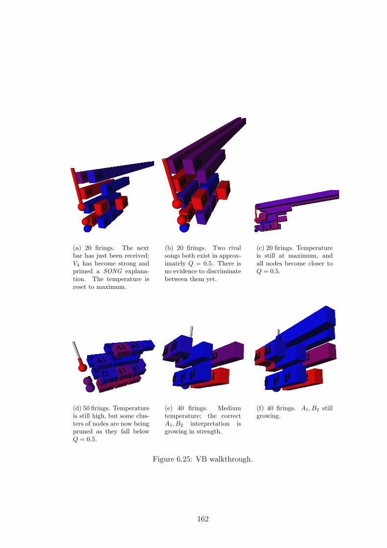
(a) 20 firings. The nextbar has just been received;V4 has become strong andprimed a SONG explana-tion. The temperature isreset to maximum.
(b) 20 firings. Two rivalsongs both exist in approx-imately Q = 0.5. There isno evidence to discriminatebetween them yet.
(c) 20 firings. Temperatureis still at maximum, andall nodes become closer toQ = 0.5.
(d) 50 firings. Temperatureis still high, but some clus-ters of nodes are now beingpruned as they fall belowQ = 0.5.
(e) 40 firings. Mediumtemperature; the correctA1, B2 interpretation isgrowing in strength.
(f) 40 firings. A1, B2 stillgrowing.
Figure 6.25: VB walkthrough.
162

(a) 110 firings. The nextbar has arrived and thenetwork is heated up again.
(b) 150 firings. Tempera-ture is getting low. Cor-rect A1, A1, B2 in place; V4
not fired recently enough topick it up.
(c) 150 firings. V4 becameactive, and primed songparents. A new bar re-cently arrived and the net-work is heated up again.
(d) 150 firings. Tempera-ture is still high. Inferenceis starting to become slug-gish.
(e) 150 firings. The correctsolution’s strength is grow-ing, including V4 at startand K2 at bar 5. Temper-ature is very low, an theannealing cycle is almostcomplete. (V4 is still weakat it has multiple good ri-vals which affect it.)
(f) 100 firings. The nextbar has arrived, and thenetwork is heated up again.Inference is now very slow(taking more than 10 min-utes for 100 firings). Thetrial was aborted here.
Figure 6.26: VB walkthrough.
163

Figure 6.27: VB end-of-bar collapsed percepts
164
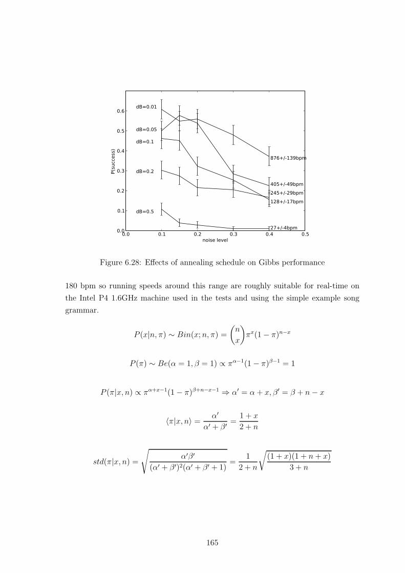
0.0 0.1 0.2 0.3 0.4 0.5
noise level
0.0
0.1
0.2
0.3
0.4
0.5
0.6P(s
uccess)
dB=0.5
dB=0.2
dB=0.1
dB=0.05
dB=0.01
27+/-4bpm
128+/-17bpm
245+/-29bpm
405+/-49bpm
876+/-139bpm
Figure 6.28: Effects of annealing schedule on Gibbs performance
180 bpm so running speeds around this range are roughly suitable for real-time on
the Intel P4 1.6GHz machine used in the tests and using the simple example song
grammar.
P (x|n, π) ∼ Bin(x;n, π) =
(
n
x
)
πx(1− π)n−x
P (π) ∼ Be(α = 1, β = 1) ∝ πα−1(1− π)β−1 = 1
P (π|x, n) ∝ πα+x−1(1− π)β+n−x−1 ⇒ α′ = α + x, β ′ = β + n− x
〈π|x, n〉 =α′
α′ + β ′ =1 + x
2 + n
std(π|x, n) =
√
α′β ′
(α′ + β ′)2(α′ + β ′ + 1)=
1
2 + n
√
(1 + x)(1 + n+ x)
3 + n
165

6.2.8.6 Performance with freefloaters
In the above trials, sample performances were generated from the SCFG to be inter-
preted by ThomCat. Although noise was added to the individual chord bar likeli-
hoods, there were no freefloaters in play. We give results which do include freefloaters.
First we must define a generator of samples which include freefloaters. Recall that the
purpose of allowing freefloaters is to provide the ability to understand almost-known
scenes which include known structures but in unknown combinations. For example,
the grammar used in this chapter does not include the rule S→C,C,V but a performer
may decide to play such a structure, comprised of known verse and chorus structures.
In this case, the C,C and V should be perceived as freefloaters (and future systems
may perhaps hypothesise a new song form from this percept). To draw samples in-
cluding freefloaters we must specify sample probabilities. Domain knowledge tells us
that changes tend to be more a priori probable at higher structural levels than lower
levels. Performers more frequently insert and remove extra verses and choruses than
insert extra riff repetitions within those structures; and more frequently change the
arrangement of the riffs than the individual bars comprising them. This knowledge
was encoded in the perception system by assigning higher freefloat priors to larger
structures. We use a similar scheme to draw samples with freefloaters. Beginning
with a sample from the SCFG as before, we proceed to make alterations to each of
the rule applications used in that sample. Each application of a rule of level l has
probability
p(mutate|l) = p(mutate|L) ∗ 1
2L−l
where L is the level of the top-level song. Essentially this means that the top-
level song mutates with some constant p(mutate|l) (set to 0.2 in our trials), then the
probability of mutations at successively lower layers is divided by 2. This typically
produces one or two mutations in samples from the example grammar of this chapter,
mostly occurring at high levels. One a mutation is determined to occur, it type
is drawn (uniformly) from three options: (1) deletion of a random RHS term; (2)
insertion at random location of a new random RHS term (having the same level as
a neighbouring term); (3) substitution of a random RHS term for another RHS term
of the same level. (These mutations are similar to, and influenced by, the genetic
algorithm proposal distributions used in previous work [56].)
A trial is defined to be a success if the following two conditions are met. (1) All
subcomponents of mutated and non-mutated rules are perceived as in the sample;
(2) All hypotheses that have no mutated descendants are perceived as in the sample.
166
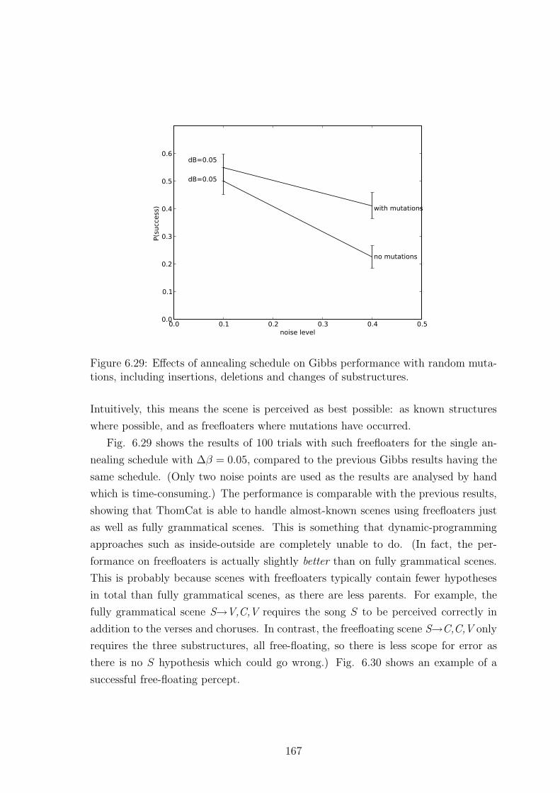
0.0 0.1 0.2 0.3 0.4 0.5
noise level
0.0
0.1
0.2
0.3
0.4
0.5
0.6P(s
uccess)
dB=0.05
dB=0.05
no mutations
with mutations
Figure 6.29: Effects of annealing schedule on Gibbs performance with random muta-tions, including insertions, deletions and changes of substructures.
Intuitively, this means the scene is perceived as best possible: as known structures
where possible, and as freefloaters where mutations have occurred.
Fig. 6.29 shows the results of 100 trials with such freefloaters for the single an-
nealing schedule with ∆β = 0.05, compared to the previous Gibbs results having the
same schedule. (Only two noise points are used as the results are analysed by hand
which is time-consuming.) The performance is comparable with the previous results,
showing that ThomCat is able to handle almost-known scenes using freefloaters just
as well as fully grammatical scenes. This is something that dynamic-programming
approaches such as inside-outside are completely unable to do. (In fact, the per-
formance on freefloaters is actually slightly better than on fully grammatical scenes.
This is probably because scenes with freefloaters typically contain fewer hypotheses
in total than fully grammatical scenes, as there are less parents. For example, the
fully grammatical scene S→V,C,V requires the song S to be perceived correctly in
addition to the verses and choruses. In contrast, the freefloating scene S→C,C,V only
requires the three substructures, all free-floating, so there is less scope for error as
there is no S hypothesis which could go wrong.) Fig. 6.30 shows an example of a
successful free-floating percept.
167

Figure 6.30: A successful freefloating percept. The mutation is high-level, S →C,C, V . The substructures C,C, V have been perceived correctly as freefloaters.(The perceived S is ignored in classifying success as it has mutated descendants.)
6.3 Future extensions
This chapter concludes by discussing some possible future extensions to ThomCat, for
which outlines of concepts and algorithms are provided, but no software implemen-
tation. It discusses the extension of the architecture from a passive scene perception
system into an active decision maker based on the scenes; how to perform various
types of learning; the movement of attention; and larger musical domains. These
extensions could be implemented in ThomCat to make further progress towards an
integrated musical listening and accompaniment system, for more varied styles of
music, and perhaps – eventually – fully improvised music. Discussion and refinement
of the concepts may contribute to clarifying the corresponding human psychological
ideas; and the following also serves as an example of how formalisms such as ThomCat
can contribute to such discussions.
6.3.1 Action and utility
“There are five fingers there. Do you see five fingers?”
“Yes”
And [Smith] did see them ... a moment of luminous certainty, when each
new suggestion of O’Brien’s had filled up a patch of emptiness and become
absolute truth, and when two and two could have been three as easily as
five, if that were what was needed.
– George Orwell, 1984
Standard graphical models represent the joint PDFs Q(x1:N ) over variables. Nor-
mally this is used to model Q(x) = P (x), a true distribution; we have seen how it can
168

be cooled to Q(x) = δ(x) as a means of finding the MAP solution, i.e. the most prob-
able percept of the scene. However in real-world scene analysis we are less interested
in the most probable interpretation of the data than in the most useful one. For ex-
ample, a hungry agent has a vested interest in perceiving an uncertain object an food
rather than a ball, because this can initiate an action to try eating it, which prevents
the animal from dying of starvation. Similarly, a trombonist who has got slightly
lost in the sheet music has an interest in perceiving his place as being at the quiet
flute section rather than the loud brass fanfare entry, because it is more damaging to
the performance (and the trombonist’s pay cheque) to play a loud part over a quiet
one than vice versa. Even when the data strongly favour a perception, utility can
overrule it. Like Orwell’s Smith, we really can and should perceive improbable things
if it it is strongly in our interests to do so. In this section we discuss how ThomCat’s
Q(x) could be altered to model these ideas and to produce high utility actions if,
for example, used in an automated musical accompaniment system. We will see that
unitary coherent percepts are of no use in finding the ideal but typically intractable
maximum expected utility plans, but may be useful for quickly finding maximum
utility percept-plan pairs, which often give useful though suboptimal plans.
6.3.1.1 Tree searching and hashing in AI
The text of this section is based on the peer-reviewed publication [59]:
• C. Fox, N. Girdhar, and K. Gurney. A causal Bayesian network view of re-
inforcement learning.. In Proceedings of the 21st AAAI International Florida
Artificial Intelligence Research Society Conference, 2008.
Action selection is a classic problem in AI, Economics and Operations Research.
It can be shown [9] that the only coherent, optimal way for an agent to act is to
maximise an expected utility function, when suitably defined. When sequences of
actions (plans) are considered, this is generally an intractable problem. Classical AI
[147] made heavy use of tree-searching methods to search over all possible combina-
tions of actions, and showed that some combinations could be omitted (for example
in ‘alpha-beta’ pruning). In the probabilistic domain, this requires that each plan
be evaluated against all possible worlds, and the expected utility computed for each
plan. This is doubly intractable because both the set of plans and the set of possible
scenes (in scene analysis) is exponential in size. We can view classical tree search as
a dynamic Bayesian network (DBN) with decision nodes as in fig. 6.31(a). (In some
tasks, actions such as asking questions may affect the amount of information available
about the state of the world. If this is the case, then the state must be expanded
169

to model future states of knowledge about the world, and the model is known as a
partially observable Markov decision process [153].) An external global controller
fixes plans {at}1:T into the action nodes, then infers the current expected utility, or
‘value’, v1:
v1({aτ}1:T ) = 〈∑
τ=1:T
ρtrτ 〉{sτ ,aτ}1:T
where ρ is an temporal discounting factor. The global controller then resets the action
nodes to the next possible plan and runs inference again, and repeats until all plans
(perhaps with some pruning or sharing of partial computations between plans) have
been simulated. The plan with the highest v1 is then selected, and the first action of
that plan is performed. If new information arrives about the state, then the whole
decision process is rerun. We may compute v1 by assigning similar value nodes to
each future point in time:
vt({aτ}t:T ) = 〈rt + ρt+1vt+1〉{sτ ,atau}t:T.
This way of computing the value is shown in the figure. (Curiously, the links between
values are causal, respecting Pearl’s do semantics, even through they flow backwards
though time. This is because the current discounted value is a construct which de-
liberately measures future expectations, and is therefore dependent on future events,
and caused by our pre-perception of those events. This is a strange form of causality
but is not paradoxical because nothing in the ‘real world’ is causing previous events:
the events and causations are all within the phenomenal world of perception.)
An alternative, heuristic, method of action selection in AI is to assume there is
some hash-classifier vt ≈ v(st, at, θ) where s is the current state of the world and θ
is a learnable parameter, and try to optimise this with respect to θ to give the best
actions, by trial and error. Reinforcement learning (RL) [152] is one way to do this.
These methods have the advantage that once learned, they are very fast, as they
simply call the hash function to obtain actions direct from states. A novel view of
RL is show in fig. 6.31(b)-(c) (which encompasses both ‘classical RL’ [152] and the
‘Bayesian RL’ of [39]). It consists of two phases, which change the structure of the
previous tree-searching net in different ways to approximate the full solution. In the
acting phase (a), all links are removed, and replaced by the hashing function. This is
an acausal directed link (it does not respect the Pearl semantics) but allows a rapid
search for a the next single action at to maximise the approximated value. Then in
170

(a)
(b) (c)
r1r1
r1
r2r2r2r2
r2r2
v1v1
v1
v2v2v2
v2v2
v2
s1s1
s1
s2s2s2
s2s2
s2
a1a1
a1
a2a2a2a2
a2a2
Figure 6.31: (a) Classical tree-searching may be viewed as instantiating a sequences ofplans {ai} and computing their present value v1. (b) The action step of reinforcementlearning may be viewed as cutting links and replacing them with acausal hash links.(c) The learning step of reinforcement learning reinstantiates the relevant causal links.
the learning phase, the obtained value vt is then used along with the previous step’s
reward rt−1 to update the hashing function for the previous value (with 0 < α < 1):
vt−1(st−1, at−1)← αvt−1(st−1, at−1) + (1− α)(rt−1 + ρmaxat
vt(st, at))
It is generally accepted (e.g. [37]) that real humans and animals use both tree-
searching and hashing methods for action selection, with tree-searching for novel,
high-level tasks, and hashing for low-level routine tasks. Tree-searching itself in clas-
sical AI generally ‘bottoms-out’ as a heuristic, hash-classifier evaluation function,
essentially combining some tree-searching with some hashing. (For example in chess
programs, the hash-classifier is some learned mapping from board state to valuation.)
6.3.1.2 Unitary coherent scenes vs. optimal actions
An interesting recent extension of the junction-tree algorithm [97] extends it with
action and reward nodes, and passes pairs of messages which result in a ‘locally opti-
mal’ plan being computed (in the sense that changing any single action would reduce
171

the expected utility). This algorithm operates on a similar graph to fig. 6.31(a) but
without the value nodes. The first element of the message is identical to the stan-
dard junction-tree algorithm, and passes marginal probabilities. The second element
passes corresponding expected utilities. From the perspective of this thesis, there are
several problems with this approach. First, the solution is only locally optimal. Sec-
ond, it requires junction-trees to be computed, which is NP-hard and seemingly not
biologically plausible. Third, it requires two independent sets of messages to be sent
between nodes, which again seems biologically difficult. Most importantly, it does
not compute an MAP scene description, as all the nodes represent marginal probabil-
ities. This raises an interesting question: if we can compute good approximate plans
without computing a unitary coherent (MAP) scene, then why does real perception
bother to do so? Why not just compute marginals and expected utility maximising
plans? But yet we know from our own perception of the world that we do perceive a
unitary coherent percept rather than a ‘Bayesian blur’ of possibilities. So what could
this unitary coherent percept be for?
This is a deep question at the heart of cognition, and we do not expect to give a
solution here, though we tentatively suggest that a coherent unitary scene interpreta-
tion lends itself to fast, simple priming of actions, and also ensures that actions in a
plan are compatible with each other. For example, Raphael’s music accompaniment
system [132] includes additional heuristic code to prevent the played accompaniment
from jumping around in the score, even if the marginal beliefs about the position
jump around. Even if the individual notes are played according to their MAP loca-
tions, there is an additional penalty for non-smooth playing that must be accounted
for.
There appear to be at least three forms of action selection and perception used
by humans. First: very low-level actions in response to low-level stimuli, for example
at the level of psychophysics experiments. Humans are known to perform almost
optimally in many such experiments [48] but are unable to report justifications for
these actions. Such low-level perception may involve hashing functions and does not
appear to use scene perception. Second: immediate, reportable scene perception-
driven action selection. For example, seeing a unitary coherent scene containing food
and therefore reaching out to grab it. Actions based on single percept cannot be
optimal as they do not depend on the distribution of scenes. However they may be
useful for the reasons given above, and will will show how ThomCat could be extended
to model them. Third: very high-level, reportable action selection based on conscious
consideration of the distribution of scenes. For example, although perception of the
face/vase stimulus is never instantaneously ambiguous or incoherent, we may use
172

our memory and high-level cognition to notice that over time we are considering
different interpretations, and may use reportable mathematics and probability theory
to work out a maximum utility action over them. Such actions are very difficult to
compute, for making complex actuarial tasks only skilled mathematicians armed with
large computers are able to make good decisions. (These three forms bear a passing
similarity to the Freudian id’s unconscious decisions; the ego’s conscious decision
making; and the super-ego’s meta-level monitoring of ego activity.)
Unitary coherent scene-driven actions may thus be viewed as a useful heuristic for
quickly finding good but suboptimal sets of coherent actions. The following gives a
brief sketch of a theory of unitary scene-driven actions in the ThomCat framework,
which could be extended and implemented in future work. The sketched system
computes annealed approximations to
arg maxs,a
P (s)R(s, a)
which is the maximum utility percept and plan (where both scene and plan are made
of multiple components), as opposed to the optimal but intractable and non-unitary
MEU solution,
arg maxa
∑
s
P (s)R(s, a).
6.3.1.3 Network extension
Fig. 6.32 shows how action and reward nodes could be used to extend the ThomCat
network. Note that both actions and rewards can depend on scene structures at many
levels, not just low-level chords. For example, it may be important to play a VERSE
accompaniment pattern as well as playing that pattern in the chord of em.
The figure shows actions and rewards as single nodes for each bar, assuming
that the bar is the smallest unit of alternative actions. In this type of network, all
possible actions for the ith bar are grouped into a single multistate node ai, and
the reward node ri is a function of these multistates and all possible relevant scene
configurations. (Relevance is shown by links from scene to reward nodes, and means
the scene nodes whose states alter the reward under any action.) An equivalent
architecture – more in keeping with ThomCat but requiring a more complicated
figure to explain – would be to convert these action and reward nodes into collections
of Boolean nodes corresponding to each state of the multistate nodes; and add rivalry
links between them. The latter are suggested for parsimonious implementation with
ThomCat.
173

r2 r3r1 r4
CHORUS
CHORUS
V ERSE
V ERSE
r12 r23 r34
SONG
SONG
A
A
Dm
Dm
Em
Em
G
G
a2 a3 a4a1
Figure 6.32: A simple ThomCat scene extended with action and reward nodes.
We wish to find the configuration of the whole network – both scene and action
nodes – with the maximum utility,
arg maxs,a
P (s)R(s, a)
As usual, the scene probability is
P (s) =∏
i
P (si|pa(si))
where s = {si} are all the hypothesis and observed data nodes. Assume that the
total reward R for a plan a = {aj} under a scene percept s is written as a product of
local ri factors as in the figure, R(s, a) =∏
k rk. Then we have
P (s)R(s, a) =∏
i
P (si|pa(si))∏
k
rk(s, a)
which is of the same form as a Bayesian network with joint
P (s, a) =∏
i
P (si|pa(si))∏
k
Pk(s, a)
when Pk(s, a) = rk(s, a). That is, we may treat the local reward components exactly
as if they were probabilities. The reward nodes can thus be modelled as regular
Bayesian network nodes with CPTs containing their local rewards, and regular an-
nealing will converge to give the maximum utility scene and plan combination.
174

The conversion of reward into probability may be of interest to pragmatist philoso-
phers (c.f [84]) who have argued qualitatively that truth and utility are the same thing.
This Bayesian network formalism shows quantitatively how this idea could be useful
for action selection. Pragmatism is often summarised by the maxim ‘truth is mea-
sured in dollars’, meaning that we should take a model as being ‘true’ if and only
if it does some good – which ultimately translates into monetary value. Our reward
factors are multiplicative but if we consider
rk = expmk
where mk are monetary rewards such as dollars, then we can make these monetary
rewards additive as would be expected of a currency. Under this interpretation, each
ln 2 currency units corresponds to a doubling of the probability, so we are saying that
we prefer an outcome having ln 2 units two times as much as we prefer an outcome
having zero units (and four times as much as an outcome having − ln 2 units etc.)
This suggests that within the maximum utility approximation scheme, and assuming
such a mapping from currency to preferences, James’ notion can be written more
accurately as ‘log truth is measured in dollars’ !
Future work could perhaps extend the ideas above to produce different, related
types of approximation, and perhaps look for signs of their existence in human be-
haviours. In particular, could we quantify the mapping from actual dollars to proba-
bility – what is the empirical ‘exchange rate’?
As discussed, the reason for the existence of unitary coherent percepts – useless
for MEU action selection – is one of the biggest questions in Cognitive Science and
the detailed study of such approximations could perhaps shed some light upon it.
6.3.2 Learning
ThomCat as currently presented requires a user-specified SCFG prior. In determinis-
tic music, this will be a deterministic grammar, having only one parse which specifies
the whole composition. In general semi-improvised music there will be some non-
unitary probabilities allowing for a specified distribution of possible performances.
There is a continuum from ‘semi-improvised’ to ‘improvised’ music as the distribu-
tion increases in entropy: even the most apparently ‘free’ jazz solo is usually made
up of at least some recognisable motifs and transforms of those motifs. For practi-
cal musical applications it is inconvenient and probably inaccurate to rely on human
specification of these SCFGs. Instead, it would be useful to automate at least some of
the specification by learning from previous performances, and fine-tuning the learn-
ing during later additional performances (even during a live accompaniment concert).
175

From a cognitive viewpoint, it is again useful to consider such extensions as a way to
model and test human learning behavioural concepts and performance.
This section considers several types of learning, from tuning of parameters to
creation of new models. These discussions are relevant not only to ThomCat, but
to the other music perception models constructed in this thesis: the priming particle
filter score-follower and RhythmKitten, and are intended to be relevant to general
hierarchical perception systems. Perceptual model creation has been debated by
philosophers for centuries so we do not expect to give a definitive account, but we
will at least suggest some potentially useful heuristic methods, applicable to both the
engineering application and as candidate cognitive theories.
6.3.2.1 Tuning parameters
The simplest and best-understood form of learning in the Bayesian framework is
parameter updating. If we have a top-level node X with prior π(X), the standard way
to learn is to parametrise the prior, for example adding new Dirac Delta nodes {θi}as parents of X so that π(X) = f({θi}). This structure was used (though not yet for
learning) in RhythmKitten’s rhythm networks (fig. 4.1) to specify the start time and
tempo priors, and Dirichlet mixture priors. A method to (locally) optimise the priors
for a single model in a single performance is to use the EM algorithm. Usually though
we wish to learn parameters which are useful in a variety of performances (including
unobserved future performances). A naive way to approximate this is to compute the
optimal θi(Di) for each available performance i, and update θ ← (1−α)θ+αθi where
α is a heuristic ‘learning rate’. A more rigorous method is to maintain a count of the
number of training examples seen for each parameter, and update in accordance with
this (e.g. see [98]).
This method was used by Raphael [131] to train his low-level HMM segmenter
and to update his high-level Bayesian network score model. Identical methods could
be added to the priming particle-filter score follower and to RhythmKitten as well
as ThomCat. A similar method is used by the inside-outside algorithm [4] to train
its grammar, and we could carry it over to ThomCat to update its grammatical –
and other – probabilities. Essentially parametric learning simply updates the priors to
make them more compatible with the current data, hence making them suggest similar
data in the future. (This is similar to biological and simulated Hebbian learning [38],
in which neural weights are modified to make the current configuration more probable
in future.)
Of particular interest in ThomCat are the free-float priors, π∅, which allow for
free-floating structures that do not appear in linguistic models such as inside-outside.
176

Strengthening these priors for structures which appear to free-float regularly could
play a useful role in higher-level model learning, discussed next.
6.3.2.2 Learning new models
Much less well understood than tuning – and probably intractable – is the problem of
learning new models. In the data mining literature (e.g. [75]) heuristic methods such
as genetic algorithms are often used to search some large candidate space of network
structures to explain data, with some approximate prior assigned to each structure
(for example, as a function of the number and types of operations used to construct
it). These methods typically require operations that make small and hopefully useful
changes to existing candidate models, or combine existing models. This issue was
introduced in section 4.4.2.3; here we make further suggestions about possibly useful
operations for altering music models and for constructing new models from scratch.
First though, is the question of when to bother creating a new model, rather than
using an existing one and accepting that it may be a poor fit. In science this is
the question of when to perform a ‘paradigm shift’. For example we may have a
ROCK1 rhythm in RhythmKitten that is repeatedly failing to explain a re-occurring
extra snare drum note at beat 3.5; or in which one of the bass drum hits is regularly
missing; despite being the best available explanation. One option is to continue to
use the model, updating its parameters to allow for this wider set of data to be
generated from it. The alternative is to consider the probability that our own model
base is incomplete, and try adding a new model. Computing such a probability is
intractable, and the issue is similar to that faced in the priming particle filter, that
we must consider an approximate probability of our own failure. As in the PPF, we
suggest simply using some hash-classifier P (failure|circumstances, θ), where θ and
the function form are set by trial-and-error to be empirically useful.
One way to create new models is as variations on the previous best fitting model.
In RhythmKitten, the models make inferences about which data points are unex-
plained (i.e. assigned to sink priors) and which model notes are missing from the
data, so an obvious way to create candidate changes is to produce models that in-
clude extra notes at the positions of unexplained data, and which omit missing data.
The analogous situation in ThomCat arises when a rule repeatedly has a missing
child in the same place, and a the same free-floater in that location. For example,
the rule VERSE → A,A,B may repeatedly be perceived as VERSE → A,∅,B (where
∅ denotes a missing child) but with a free-floating K structure at that location as in
fig. 6.11. This suggests creating a new rule VERSE → A,K,B as an alternative, with
a probability influenced (somehow) by the free-floater’s learned π∅ prior. If the new
177

rule is successful in later performances, the free-floater’s π∅ prior should also then be
reduced by the parametric learning described earlier.
Another way to create new models is based on bottom-up regularities. For ex-
ample, if we notice that the freefloaters A,B,A,B often occur in that sequence with
no rule to explain them, then we could postulate the rule NEWRULE → A,B,A,B
to explain them. Once postulated, NEWRULE will then appear as a free-floater it-
self (having an appropriately heuristic, tunable π∅ prior, based on its frequency of
occurrence) and may later become part of larger structures using the variations and
bottom-up rules described here.
To avoid an explosion in the number of models, we need methods to remove as
well as create models. Pruning of models could occur if they have not been used for
some heuristic period of time. More interestingly, pairs of models could be merged
if they grow to resemble each other via parameter learning. Again, the question of
when two models are alike enough to be seen as “the same thing” is a deep cognitive
and philosophical one [64]. In robotics, the problem of ‘loop closure’ [120] is similar
to this: deciding when two known locations are the same; in science, realising that
concepts such as temperature and molecular motion refer to the same thing is a key
type of innovation. Again we suggest the use of some empirically useful hash-classifier
to take the place of this philosophising.
6.3.3 Extended musical structures
ThomCat currently operates in the highly constrained minidomain of semi-improvised
musical scene perception from chord-bar sequences. But as a general scene perception
architecture it could be applied to other, more difficult musical scene perception tasks,
of which we give some examples.
Parallel input percepts have already been mentioned: for example considering both
rhythmic types (from RhythmKitten) and the chords played within them, possibly
by multiple instruments.
Rather than following large-grained bars of chords, another musical task is to
perceive scenes of melodies of smaller-grained notes and their relationships. A new
Copycat descendant, Seek-Well, is currently under development [121] which groups
melodic notes into percepts such as rising and falling streams, ‘leaps’ and ‘steps’, and
possibly higher-level relations between these structures. These ideas could be brought
into ThomCat’s Bayesian blackboard framework, along with the melodic agent ideas
of Reis [142].
178
Melodies – and to a lesser extent, chord sequences – may exist in transformed
instantiations in many musical styles. Transforms include shifting pitch and time-
stretching existing structures. (In Baroque music especially, more advanced trans-
forms include reversing and harmonically inverting melodies.) Such transforms have
been modelled in automated composition systems as extensions to grammars simi-
lar to those used by ThomCat [56]. Perception systems could try to perceive such
structures by considering the space of transformed hypotheses in addition to their
standard forms. New priming hash-classifiers would be needed to navigate through
the enlarged search space.
Moving from notes to even lower-level structures, blackboard systems have pre-
viously been used for musical transcription directly from sound waves, for example
by constructing hypotheses about individual harmonics, notes and chords, without
the use of pre-processing or segmentation. The ThomCat architecture could be used
to provide principled handling of rivalry, which has often been handled heuristically
in other systems. For example, the matchstickman network of fig. 6.4 could equally
well refer to individual harmonics li being explained by the presence of notes mj .
This task is a little harder than the matchstickmen because the latter assumed each
Boolean li was generated by at most one mj. In the harmonics case the li may have
continuous energy, generated by the sum of several sources, so ThomCat would need
to be extended to account for this.
Modelling global correlations is an important aspect of scene perception. Thom-
Cat included just one – key – as a proof-of-concept. Real musical scenes have many
other global factors including identity of the players (what are their favourite chords
and riffs?), venue of performance (rock riffs are unlikely in a concert hall) and perhaps
most importantly, consistency of rewrite rule selection (if rule V → A,A,B was used
to form the first verse, the changes of it being used in the second increase.) All can
be modelled similarly to global key in ThomCat.
A highly challenging task would be to extend ThomCat to perceive unknown
musical compositions in real time, based only on a general stylistic grammar. For ex-
ample, such an extended ThomCat could perceive an unknown pop song on the radio
using only knowledge of the pop genre in general. Such music – whilst determinis-
tic from the performers viewpoint – is effectively semi-improvised from the listener’s
view. Indeed while the ‘semi-improvised’ concept used throughout this thesis has
appeared somewhat artificial, it is this ‘semi-improvised’ perception of determinis-
tic music through uncertain priors that forms the bulk of everyday human musical
perception.
179

6.3.4 (Re)constructing the past and future
The current implementation of ThomCat assumes that the region of interest is always
around the current position in real time: its ‘window of attention’ is always centred
on the latest bar of observed data. Although this is usually the case in human music
perception – we attend to the current state of the world – there are occasions when
we ‘cast our mind’ back to what happened in the past (“I just noticed this movement
is in a different key... so did I play all those notes wrong at the beginning?”), or
‘think ahead’ to predict what will happen in the distant future (“I have 50 bars rest
but then there’s a difficult brass fanfare, how does that go...?” or “what should I do
in my next jazz solo if the guitarist keeps making that chord substitution?”). For
such cases, ThomCat could be extended to move the window of attention around
to focus inference where it is needed. The need for controlled movement of atten-
tion is of course more evident in domains such as (foveal) visual scene perception,
but a ThomCat-like system would capable of capturing the idea in simpler musical
minidomains. Choice of where to place the focus of attention should be based on the
expected utility of the decision, such as the (hash-classified) value of information to
be found there, and the value of the actions made there.
ThomCat does not currently remove winning structures from the past when the
window of attention moves on from them: they are left in the computer’s memory (and
appear in the graphical parse as ‘frozen’). This works well for our chosen minidomain
but there may be cases when memory is limited and non-attended objects should
be pruned. If this occurs, then attention is moved back to the past, the historic
scene must be reconstructed. Reconstruction could be based on the current high-
level percept acting as a top down prior on what happened (for example, if I know I
am three minutes into a SONG, then I can reconstruct the VERSE at its start based
on the grammar and the position of the whole SONG). A limited form of memory
may also be of use, remembering particularly unusual deviations of the data from the
most probable top-down construction. In general the reconstructed past will not form
the same percept as was originally perceived, because new top-down information is
available and the set of models used to perceive it may have changed through learning.
6.3.5 Modelling human cognition
A recent movement in Psychology is Bayesian Cognitive Science [24], [57] which as-
sumes that humans behave in a Bayesian (near-)optimal way, then seeks to extract
details of what models, parameters and heuristics are being used under this assump-
tion. As ThomCat has been designed based on ideas about human cognition, it could
180

perhaps form the basis of a Bayesian Cognitive Science study, and could be extended
to try to model human percepts and actions as accurately as possible.
More speculatively, architectural concepts from ThomCat might be used as broad-
brush predictions about what biological neurons might be doing. In particular, it has
been speculated that cortical columns might perform Pearl message passing [77].
ThomCat’s considerations of loopiness, rivalry and correlations suggest that a Gibbs
inference engine on these Bayesian columns may be more appropriate for scene per-
ception.
6.4 Discussion
The ThomCat architecture continues the MAP-seeking annealing-cycle approach to
scene perception used by RhythmKitten (and to a lesser extent, the priming particle
filter). The approach is extended to hierarchical scenes featuring global correlations.
The generative Bayesian networks for such scenes are highly loopy, and intractably
large if all possible hypotheses are instantiated. They feature strong correlations
due to rivalry, but contain much independence of causal influences which may be
exploited by inference algorithms. This set of properties leads to annealed Gibbs
sampling being a useful inference method. We extended standard Gibbs sampling
to sample from clusters of co-parents (to exploit ICI) and fused dynamic structure-
building ideas from blackboard systems into the Gibbs sampler itself, choosing active
Gibbs nodes to prime from.
Questions about the use of MAP percepts in action selection were discussed. An
important open question in Cognitive Science is why humans bother to perceive a
unitary coherent scene at all, when Bayesian theory shows that optimal actions are
only achieved by considering the ‘Bayesian blur’ of all possible worlds. However such
computations are highly intractable. Extending ThomCat with action and reward
nodes tentatively suggests that unitary coherent percepts may produce fast ways of
selecting good but suboptimal actions.
Even with these priming, pruning and cluster-sampling speedups, inference in
ThomCat is still very slow, requiring longer than real-time to run on the relatively
simple musical minidomain problems discussed here. At least on classical computers,
slowness seems to be unavoidable due to the NP-hardness of the underlying loopy
networks. This presents an apparent dead-end for more realistic scene perception
models. However, the next chapter will investigate another, even more impressive
speedup for Gibbs sampling, making use of quantum computational hardware, which
181

we will see achieves a quadratic speedup over the classical case, so could make larger
scene problems amenable to real-time perception.
182

Chapter 7
A quantum generalisationspeeds up scene perception
The text of this chapter is based on the following peer-reviewed publication [63]. Rezek
and Roberts provided advice on standard Bayesian theory and on presentation only.
• C. Fox, I. Rezek, and S. Roberts. Local quantum computing for fast proba-
bly map inference in graphical models. In Proceedings of the Second AAAI
Symposium on Quantum Interaction, 2008.
We have examined the general problem of hierarchical perception in a Bayesian
framework, using the minidomain of semi-improvised musical scenes as a recurring
example. The view developed here of how scene perception could work has com-
prised three levels of computation: First, low-level approaches to raw data hash-
classification as in chapter 3. These are useful because low-level data is usually
large and full Bayesian inference (for example, considering all possible instruments,
physical locations, environments and playing styles that could generate a raw sound
wave) is intractable at this level in real time. Heuristic hash-classifiers can rapidly
(though approximately) map the raw data to a higher level of abstraction. In the
music minidomain, these are chords and drum onsets; in vision, the analogous classes
would be low-level edge and corner detectors, and perhaps features such as SIFT fea-
tures [101]. Second, chapter 4 discussed segmentation at the mid-level. This makes
a hard decision about region boundaries. In the music minidomain, RhythmKitten
segmented the input into bars. In vision [99] segmentation can be done using colour
boundaries for example. The segmentation step is useful to reduce the complexity of
the third stage, hierarchical scene construction. Given the mid-level set of segmented
objects (chords in bars in the music minidomain; visual regions with their proper-
ties in vision), hierarchical perception dynamically constructs a Bayesian network of
candidate phenomenal objects using priming and pruning.
183
The key problem with this view is what happens next. Chapter 6 showed how to
construct the network and move a window of attention around it, and the next task
as that of finding a maximum utility percept of the contents of this window, which
can be formulated as an MAP problem given suitable utility and action percepts.
The key problem is that this MAP task is unavoidably #P-hard. Chapter 2 reviewed
the inside-outside and CYK algorithms, which solves the hierarchical perception task
in polynomial time but only for a very limited class of percepts, i.e. those which are
context-free. General hierarchical scene perception does not have this property. For
example in the music case there are global properties such as musical key and style;
in vision research there is the analogous ideas of global ‘gist’ [114].
We have seen several methods for approximate MAP inference in Bayesian net-
works, as required in hierarchical scene perception: deterministic annealing in Bethe
message passing; annealed variational Bayes, and annealed Gibbs sampling. When
running in real time, all of these methods take the form of a rapid series of annealing
cycles: the network is ‘heated’ then cooled during inference towards a Dirac delta
distribution. The near-delta distribution is then ‘collapsed’ to the MAP by reading
off the node modes. The collapsed state is then used as the starting point for the next
cycle (as all these algorithms have multiple local minima and are sensitive to starting
point) and to schedule actions in response to the percept. However it is known [32]
that even such approximate inference in Bayesian networks is still #P-hard, in the
sense of number of computations required to reach an arbitrary error rate. This is a
very serious problem for a theory of perception: after all our work in low-level heuris-
tics, segmentation, network construction and attention restriction, we are still stuck
with an #P-hard problem to complete the inference. The experiments with Thom-
Cat in particular showed that even simple minidomain tasks such as chord sequence
perception can become slower than real-time on a modern PC once more than about
seven objects with their fringes are inside the attention window.
One commonly discussed possibility for speeding up such inference in Bayesian
networks (and hence hierarchical scene perception) is the use of massively parallel
computer hardware. All of the above algorithms are effectively parallel algorithms
anyway – when implemented on a serial computer they run by choosing some random
update ordering or clocking scheme to simulate the parallelism – so implementation on
a parallel machine is simple. While this has achieved useful speedups (for example,
Google’s large Bayesian networks1) it still only provides a linear speedup: with N
machines we can do N times as much computation, where N is the number of nodes.
1Details not publicly available.
184

A radically new idea to speed up hierarchical scene perception is to make use of
another new kind of hardware: quantum computing. We consider this due to des-
peration and beauty: desperation as we are stuck with an #P-hard problem at the
highest level of perception, and approximations and parallel hardware do not seem
good enough to solve it efficiently; beauty because we will see that the fundamen-
tal structure of quantum computing theory is intriguingly close to that of Bayesian
theory. Quantum computing theory was developed in the 1980s and in recent years
has become a working, implemented commercial technology [31] – though the size,
expense and speed of current devices still resemble the room-sized paper-tape and
mercury-line machines that first implemented Turing machines. However there is
every reason to believe that like those machines, quantum hardware will in time re-
duce in scale and cost. We should not be put off discussing useful algorithms for
our theoretical problem of hierarchical scene perception just because the commercial
hardware market cannot yet sell us equipment on which to run them at an affordable
price. (We can of course simulate them, albeit slowly, on a current PC to provide
proofs of concept.)
After reviewing the relevant yet simple concepts of quantum computing theory
and previous work, this chapter will present a novel algorithm for speeding up the
MAP inference task required in hierarchical perception by a quadratic factor: in the
sense that only√N cycles are needed to obtain the same trajectory probabilities as
the classical Gibbs sampler used in ThomCat. Unlike standard quantum algorithms
for search [71] that achieve similar speedups but requiring complex global operations,
our algorithm uses only small, local messages as in regular Bayesian networks. The
algorithm combines aspects of the other approximation methods discussed so far. Re-
call that the fundamental problem of Bayesian computation is that joint distributions
have a size exponential in the number of nodes, so representing and computing with
them is unavoidably exponentially hard. We have discussed how the approximations
try to work around this. The Pearl/Bethe approach does not attempt to represent
the joint, but approximates its marginals. The mean-field approach represents an
approximate joint as the cross product of its marginals, but at the expense of los-
ing all representation of correlation between nodes. The MCMC approach represents
the joint by a sequence of samples – a path – drawn from it over exponential time.
Like Bethe, the quantum algorithm will represent node marginals at each node. Like
mean-field, the marginals will also represent part of the joint. But unlike mean-field,
the quantum algorithm is able to represent the correlations between nodes. Like all
the algorithms, the quantum algorithm will use rapid annealing cycles, beginning
185

with the previous MAP solution and ending with a collapse step to reduce a near-
delta distribution to a pure delta spike. Like the Gibbs sampler, each node’s state
will make transitions according to the Gibbs probability given its neighbours, and
this proposal is always accepted. However it extends the Gibbs sampler by exploring
all possible sample paths simultaneously using quantum parallelism. The quantum
algorithm solves the same hierarchical perception problem as the other approxima-
tion methods: MAP inference in an attentional window –and has been developed as
a generalisation of all of them. As such it forms the culmination of this thesis.
Strictly in passing, we note that a form of quantum perception has been proposed
in a highly speculative, vague, qualitative sense by several authors [126, 74] as a
candidate mechanism for biological perception, though largely for prior philosophical
reasons rather than computational gains. The constructive engineering approach of
this thesis cannot say anything about the biological plausibility of these ideas – that
is clearly an empirical question for empirical scientists. However if we can show
that a quantum version of our existing perceptual approximation schemes can give a
significant improvement in speed, then this would make these speculative claims more
likely because there would then have been a higher chance of them being selected by
evolution. While the claims are extremely speculative, they have a potentially large
impact on major problems in philosophy if they do turn out to be correct; however
that is not the focus of this thesis: we are instead merely concerned with making our
existing hierarchical scene perception algorithms run as fast as possible in spite of
their #P-hardness.
7.1 Quantum computing theory
We begin with a brief overview of quantum computing theory. Despite the huge
amount of intellectual effort that was required to develop quantum mechanics and
quantum computing, the theory delivered to us by its inventors is in fact very simple,
being couched only in ‘high-school’ finite-dimension linear algebra. Because of this
form it is highly amenable to representation in the Matlab programming language,
which is strongly based around vectors and matrix structures. To aid the development
of the quantum perception algorithm, a Matlab library, QCF [55], was developed to
simulate quantum computer operations. We give QCF examples of the basic concepts,
to show how simple quantum computing is from the Machine Learning programmer’s
point of view. QCF programs could in theory be run on real quantum computers;
here we use the QCF simulator on a classical machine to give the same results but
186

>> phi_1=bin2vec(’011’)
0
0
0
1
0
0
0
0
>> phi_2 = dec2vec(5, 3) %second argument is how many bits in the register
0
0
0
0
0
1
0
0
Figure 7.1: QCF representation conversion functions, called from a Matlab session.
requiring much longer to run. For a more detailed review of quantum computing
theory, see [119].
A classical (non-quantum) computational register of bits exists in a single state,
for example, a three-bit register could store a configuration of three Boolean MRF
nodes such as 101 (also notated as the decimal 5). Such classical states may also be
thought of as basis vectors in an 23-dimensional space. To emphasise this view we
use ‘ket’ notation2:
|101〉 ≡ |5〉 ≡ [00000100]T
where T denotes a transposition from row to column vector. Here, the three bits of the
classical register provide 23 = 8 basis vectors, representing numbers from 0 to 7. The
number 5 is the sixth such number (as the first is zero) so the vector representation
contains a ‘1’ in the sixth element and zeros in the others.
In QCF, the functions bin2vec and dec2vec convert binary and decimal numbers
into ket (i.e. vector) representation as shown in fig. 7.1.
Classical operations that map register states to register states may then be repre-
sented by a 23 permutation matrix. For example, the operation ‘subtract 1 (mod 8)’
is represented by:
2Ket notation is a hangover from Quantum Mechanics, in which it generalises to infinite-dimensionHilbert space. Quantum Computing works only with finite-dimension vectors, so for our purposesthe ket is synonymous with a column vector.
187

U =
0 1 0 0 0 0 0 00 0 1 0 0 0 0 00 0 0 1 0 0 0 00 0 0 0 1 0 0 00 0 0 0 0 1 0 00 0 0 0 0 0 1 00 0 0 0 0 0 0 11 0 0 0 0 0 0 0
and when applied to the previous 5 state we compute 5-1=4:
U |5〉 = |4〉
0 1 0 0 0 0 0 00 0 1 0 0 0 0 00 0 0 1 0 0 0 00 0 0 0 1 0 0 00 0 0 0 0 1 0 00 0 0 0 0 0 1 00 0 0 0 0 0 0 11 0 0 0 0 0 0 0
00000100
=
00001000
Note that U is unitary (i.e. U †U = I) – only unitary operations are allowed in
quantum computing. Note that the ket and unitary operation representations are
similar to those used in hidden Markov models, having state vectors and transition
matrices.
When two registers are brought together and considered as a single system, the
Kronecker (or ‘tensor’) product – notated ⊗, or kron in Matlab – of their state vectors
gives the state vector for the combined system. This is the same operation used in
Bayesian networks when we consider and iterate over the combined state space of a set
of parent nodes. The ⊗ symbol can be omitted, and the ‘bringing together’ property
means that the product can be written as a single ket containing a concatenation of
the bits:
|10〉 ⊗ |01〉 ≡ |10〉 |01〉 ≡ |1001〉
[0010]T ⊗ [0100]T = [0000000001000000]T = |1001〉
It follows that the operation U comprised of two independent operations U1 and
U2 acting on separate subspaces is given by U = U1 ⊗ U2, so that
188

U1 |a〉 ⊗ U2 |b〉 = U |ab〉
So far the discussion has been equally applicable to classical and quantum comput-
ers: we have simply notated classical registers and operations as vectors and unitary
matrices. Classical computing is a special case of quantum computing in which states
are limited to the basis vectors of the register (i.e. the vectors always contain exactly
one ‘1‘’and the other elements are ‘0’; and the unitary matrices are permutation ma-
trices). Unlike classical computing, quantum computing allows systems to exist at
any point on the complex unit radius hypersphere in the state space, rather than just
the classical basis vectors. For example a register can be in a superposition of basis
states |000〉 and |110〉:
|Ψ〉 = α000 |000〉+ α110 |110〉
where the α are complex numbers chosen to describe a hypersphere location,∑
i |αi|2 =
1. General unitary matrices may operate on the state vectors rather than just the
special permutation cases. Unitary matrices may be thought of as rotations on the
hypersphere. For example, the Hadamard matrices Hn map n-bit classical states to
superpositions:
H1 |0〉 =1√2|0〉+ 1√
2|1〉
Hadamard operators are defined recursively by
H1 =1√2
[
1 11 −1
]
, Hn+1 = Hn ⊗H1
and QCF provides a function hadamard(n) to generate them, e.g.:
>> hadamard(2)
ans =
0.5000 0.5000 0.5000 0.5000
0.5000 -0.5000 0.5000 -0.5000
0.5000 0.5000 -0.5000 -0.5000
0.5000 -0.5000 -0.5000 0.5000
Each |αi|2 describes the probability of an observation collapsing the register into
state |i〉. An observation is a random non-linear operator, which when applied, draws
a probability from this distribution, and changes the state to the classical basis vector
189

|i〉.3 This is the only non-linear operator allowed in this form of quantum computing
theory4. Its physical meaning is still debated by philosophers [3] but empirically
it appears to correlate with the act of a subject looking at, or otherwise obtaining
information from the system. Note that the observed vector is drawn from the set of
basis vectors for the system as a whole, rather than drawing bits independently. For
example, making an observation on the state√
32|00〉+ 1
2|11〉 gives the following joint
observation distribution on the two bits:
P (00) =3
4, P (01) = 0, P (10) = 0, P (11) =
1
4
In this case the values of the two observed bits are perfectly correlated. After ob-
serving one bit’s value, we know for certain that the other bit has the same value.
This is a form of entanglement: we say that the two qubits are entangled because
observation of one affects the observation distribution of the other.
The QCF measure function simulates the nonlinear observation operation by com-
puting these probabilities then randomly drawing from them, for example:
phi = sqrt(3)/2 * bin2vec(’00’) + 1/2*bin2vec(’11’)
phi =
0.8660
0
0
0.5000
>> pretty(phi)
ans =
0.86603|00> + 0.5|11>
>> phi=measure(phi)
phi =
1
0
0
0
>> pretty(phi)
ans =
1|00>
3In general, observations in arbitrary bases and subspaces are possible, however we do not needthese in our algorithm.
4See [119] for a discussion of general ‘POVM’ measurements. We assume that all observationsare made in the standard basis here.
190

This will give the above result, |00〉, three quarters of the time, and the other possible
result, |11〉 one quarter of the time. (The QCF pretty printing function converts the
vector representation back to binary ket notation for display.)
7.1.1 Summary of quantum computing theory
The above discussed all the postulates of quantum computing theory, which can be
seen to be merely simple applications of linear algebra and probability theory. The
theory can be written concisely as four postulates (based on [119]) in addition to
standard linear algebra:
1. Associated with any finite physical system – such as a collection of discrete
Bayesian network nodes – is a complex vector state space. The system is completely
described by its state vector, which is a unit vector in this space.
2. Except for observations, all operations on the system are described by unitary
operators.
3. The state of a composite system having substates |a〉 and |b〉 is the Kronecker
product |a〉 ⊗ |b〉.4. An observation of state
∑
i αi |i〉 changes the state to |i〉 with probability |αi|2and the resulting state is knowable by the observer.
Note that in general, states are unknowable, because observing them generally
changes them. We have seen that using entanglement, states are able to represent
and compute with the set of all possible classical states each with an amplitude,
but we cannot generally read all of this information. We can compute with it, but
making an observation reduces it to a single basis state that we can know. This is
extremely interesting from the view of our task of hierarchical perception, because
we wish to make computations on the joint distribution of many nodes, but we do
not need to report the joint. We only want to report a particular function of it,
namely the location of the MAP state. This is the beautiful structural similarity
between Bayesian theory and quantum computing theory: they both compute with
exponentially large joints, but only report the result of a function of those joints. It
is therefore worth considering how this structural similarity can be exploited in our
hierarchical perception task.
7.1.2 Comparison to existing work
Quantum optimisation methods have been featured in the physics literature in recent
years (e.g. [82], [49], [20]). However this work has not generally been framed in the
context of discrete local quantum computation, the MAP Bayesian network task, or
191

the language of the Machine Learning community. The novel contribution of this
chapter is to give a purely quantum-computational algorithm for graphical model
MAP optimisation as required in the general hierarchical perception task, which gen-
eralises the previous approximate algorithms and which we show achieves a quadratic
speedup over the classical Gibbs sampler. The algorithm uses only local operators, in
contrast to various extensions of the standard Grover algorithm to parameter search.
Grover’s algorithm was one of the first quantum algorithms, used as the basis for
many others, so we review it below; this review also provides a first example of a
quantum algorithm in action, implemented and simulated in QCF.
7.1.2.1 Grover’s algorithm
Grover demonstrated that quantum computers can perform unstructured database
search faster than their classical counterparts, which must consider each element in
turn taking O(n) computation. In this simple example of Grover’s algorithm, we use
a function, haystack, to represent the database. We are searching for a needle in the
haystack, i.e. there is one element of the database that we require. The haystack
function returns 1 if queried with the correct needle element, and 0 for all the other
elements. In this example, haystack is defined for a 5-qubit input, and returns 1 for
element 8 (‘00100’ in binary):
haystack(i) =
{
1 : i = 80 : i 6= 8
Grover makes use of the fact that for any function f with a binary string input
and a Boolean output, we can define a corresponding unitary matrix Vf , whose action
on input strings |i〉 is to invert their amplitudes if and only if f(i) = 1; otherwise, it
does nothing:
Vf(|i〉) =
{
|i〉 : f(i) = 1− |i〉 : f(i) = 0
The QCF library provides a function vf to create such matrices. First the Boolean
function is defined, continuing our example:
function b = haystack(i)
if i==8
b=1;
else
b=0;
end
192

Figure 7.2: Graphical display of matrices used in Grover’s algorithm for 5-bit searchspace. White=+1, black=-1.
Then vf converts it into unitary matrix form (where n specifies the number of
bits to act on):
n=5;
V_haystack = vf(’haystack’, n);
The output in this case is a 32×32 matrix (too large to write out here, but shown
graphically in fig. 7.2 as Vhaystack) which can be seen as an identity matrix but having
Vhaystack(8, 8) = −1 instead of the usual 1.
The other operation used by Grover is an ‘inversion about the average’ matrix,
DN , defined by
DN
a0
a1
...a2N−1
=1
N
∑2N−1i=0 ai − a0
∑2N−1i=0 ai − a1
...∑2N−1
i=0 ai − a2N−1
where N is the number of bits to be operated on. Continuing our example, we
construct an inversion about the average operator for three bits, D3 using the QCF
command
D = ia(5)
Again this produces a large 32×32 matrix, shown graphically in fig. 7.2. We will also
make use of a 5-bit Hadamard operator H5 as shown in the same figure:
H = hadamard(5)
Grover’s algorithms works by iteratively applying Vhaystack and D to the current
state. Each iteration amplifies the probability of a measurement collapsing the state
to the correct ‘needle’ value. Grover showed that performing a measurement after√
(2N)π/4 iterations is highly likely to give the correct result. Here is the algorithm
in QCF:
193

Figure 7.3: Results of Grover’s algorithm simulated in QCF. At each time step, thegraph shows the probabilities of an observation giving each of the 32 states. Theamplitude of the sought state, |8〉, increases over time relative to the others, reachinga maximum at
√
(2N)π/4 ≈ 4 iterations.
phi = bin2vec(’00000’);
phi = H*phi;
for i=t:10
phi=V_haystack*phi;
phi=D*phi;
end
phi=measure(phi);
Fig. 7.3 shows the amplitudes of the different ‘needle’ candidates over time (i.e.
number of iterations). We chose to keep the algorithm running for 10 iterations, but
note that the amplitude for 8 (the correct needle value) reaches its peak at about√
(2N)π/4 ≈ 4 iterations, as predicted by Grover. The N bits can represent n = 2N
numbers (from 0 to 31 in our case), so rather than the classical O(n) search speed we
have reached O(√n).
Grover’s algorithm is general in that it can be used to search any discrete finite
space for any property representable by a Vf function. It was generalised by [82] to
optimisation search problems (which are #P-hard rather than NP-hard so do not
have an available f function). This work reported heuristic results that were, unim-
pressivly, ‘at least comparable to classical heuristics’. A similar generalisation [49]
reported a quadratic speedup. [145] noted that it could be used to search for weights
in a neural network. However these Grover-like algorithms are still problematic in
194

practice because they require large global unitary operators to be constructed. Much
of quantum computing research is devoted to finding collections of smaller, local op-
erators which are easier to implement. But it is not known what the smallest local
operators are to achieve Grover-like speedups. We note that classical message passing
in Bayesian networks has already been formulated as a set of operators [143], so a
good question to ask is if this approach can be extended to the quantum domain.
7.1.2.2 Adiabatic optimisation
A recent development in quantum optimisation is the adiabatic method [52], which
uses a different global operator to match Grover’s√N unstructured search speedup
[146]. This speedup is dependent on prior information on the difference in probability
between the first and second most likely states, and would not be achieved for general
optimisation such as MAP inference. It is an open question how it could be exploited
in those particular inference tasks where we do have some such information. (The
private Canadian company D-Wave claims to have demonstrated a working 16-bit
adiabatic machine [31].)
7.1.2.3 Physical annealing
Physical quantum annealing (e.g.[20]) uses continuous quantum mechanics (rather
than discrete quantum computing theory) and physical temperatures (rather than
temperature as an abstract numerical parameter) to physically cool systems towards
their ground states. This work is fascinating but has been couched in the language
of continuous physics and is generally inaccessible to AI researchers. Our algorithm
achieves a similar goal to this work but using pure quantum computing operators.
Furthermore, it is presented to be accessible to AI researchers and as a ThomCat
speedup, and as a generalisation of the variational and Gibbs approximate inference
methods seen so far.
7.1.2.4 Bayesian models of quantum systems
In contrast to our algorithm and the above work, another strand of research [154],
[96] has generalised Bayesian networks to make inferences about quantum systems.
7.2 Quantum hierarchical scene perception
The hierarchical scene perception task requires us to find the MAP state of a graphical
model. We will present a quantum computational algorithm capable of performing
195

MAP inference in graphical models. The algorithm quickly finds a probably MAP or
near-MAP configuration with a quadratic speedup over classical Gibbs sampling, in
the sense that after the same number of sampling steps it yields observation proba-
bilities 1ZProbs(τ)
2 of trajectories τ where Probs(τ) are the classical Gibbs observation
probabilities and Z is a normalising coefficient. A trajectory specifies the history of
the sample as well as its final state, as quantum computing is reversible. The algo-
rithm uses only small local operators and makes essential use of decoherence – which
is usually thought of as a hindrance rather than a feature in quantum computation.
Unlike Grover and other algorithms, all state amplitudes remain real and positive
throughout.
Simulating quantum computing on a classical machine is an extremely intensive
task – this is of course to be expected as the whole point of quantum computing is to
be faster than classical machines. Simulation is intensive of both memory and time,
as all possible register states must be modelled. This means that even a 16-bit regis-
ter requires 216 complex-values amplitudes to represent it: and a single operation on
it requires a 232 ≈ 4.3× 10⁹ element complex-valued matrix. Because of these huge
computational requirements, we must at this point abandon the music minidomain,
as running simulations on typical ThomCat windows of attention would require un-
available computational resources. Instead we will simulate very small toy problems
which will serve as a proof of concept for a future quantum ThomCat (which must
surely be named ‘ErwinCat’). To simplify the size of the simulations further, we will
switch from working with Bayesian networks to Markov random fields. Any graphi-
cal model can be written in MRF form (e.g. [117]), by introducing more nodes and
simplifying the links potentials. MRFs have only one link type, specifying undirected
pairwise potentials: this is simpler to work with that the full Pearl equations which
require priors and likelihoods to be distinguished. However throughout the discus-
sion it should be borne in mind that a real quantum computer would be capable of
working directly with ThomCat’s analogous directed Bayesian networks, without the
need for conversion.
We work with an undirected, loopy, pairwise Markov random field withN Boolean-
valued nodes Xi. Let nodes have potentials φii and links have potentials φij so that
the joint is
P (x1:N) =1
Z
∏
i
φii∏
ij
φij
where Z is a normalisation coefficient. We restrict our discussion to potentials which
may be defined by integer-valued energies Eii and Eij such that
196

φii = exp (−Eii), φij = exp (−Eij)
We wish to find the MAP configuration x1:N to maximise P (x1:N). This is generally
NP-hard [148].
Our quantum notation uses upper and lower case letters as follows: A refers to a
state space; |A〉 is a general vector in that space; a is an integer (in decimal or binary
notation) denoting a basis state; |a〉 is the basis vector in A with coding a. (Such
binary codings will be used to represent Boolean MRF configurations.) We write true
and cooled model probabilities as P (a) and Q(a) respectively, in contrast to quantum
observation probabilities Probs(a) = |αa|2.
7.3 Representing joints by superpositions
A quantum register of N qubits (‘quantum bits’) is able to store and represent am-
plitudes of all its 2N possible classical configurations simultaneously. A fundamental
problem in machine learning is that the joint distribution of N variables has expo-
nential size. The structure of quantum amplitudes is very similar to that of joints
so we can use the αi to store our probabilities (up to normalisation; recall that our
probabilities normalise to 1 but amplitudes normalise so that∑
i |αi|2 = 1), requiring
only N qubits instead of exponential resources. We will try to set the αi so that
αi = 1√ZQ(i) where Q is some probability distribution of interest over the space of
binary registers I, and Z is chosen for correct normalisation of the amplitudes. Dis-
tributions Q of interest include the true joint Q(i) = P (i) and the MAP-Dirac delta
joint, Q(i) = δ(i; i). The latter is of interest because it guarantees that an obser-
vation on the system will yield the MAP state, |i〉. We may move gradually from
a flat Q(i) to Q(i) = P (i) then to Q(i) = δ(i; i) via a series of cooled distributions,
Q(i) = P (i)1/T .
We have seen that it is possible to represent joints in linear resources on a quantum
register. The problem is how to bring the register into such a representational state.
Grover’s method [71] performs quantum unstructured search over N items in
O(√N). However this algorithm requires the use of large operations over the whole
space, applied in series. It also only finds target values whose target-ness is a function
of their value only, rather than of their relationship to other values as in optimisation
problems. In contrast, we present an algorithm using small local operators which
may be applied in parallel during each overall sequential step, as in the local node
updates of an annealed Gibbs sampler or Boltzmann machine [78]; and which seeks
targets that are global and near-global MAP states.
197

Figure 7.4: Top: A unitary operator that maps states to a superposition of themselvesand the state reached by flipping their rightmost bit. Bottom: A similar operator forthe leftmost bit.
7.4 Side-stepping the unitary requirement by ex-
tending the state space
The key idea is to construct and apply operators which transfer low-probability (high-
energy) states to high-probability (low-energy) states. A difficulty with this is that
quantum operators must be unitary. This means that as much amplitude must flow
out of each state as flows in, in a similar sense to ‘global balance’ in Markov chain
theory. Initially this may seem to prevent our approach being possible, as the high-
energy states must ultimately flow back to low-energy states. This is indeed the case
when a fixed-size system is considered. Consider fig. 7.4(top) and fig. 7.4(bottom),
which respectively illustrate unitary operations acting on single qubits to flip the left
and right qubits of a two-qubit register. In general, single-qubit operators may have
some portion of self-transition as well, shown by the thin loops. The widths of the
arrows illustrate the transition probabilities. (Note that this state transition dia-
gram is not an MRF, but could represent moves between configurations of a Boolean
MRF with two nodes.) Suppose the two variables are elements from an MRF whose
configuration energies satisfy
E(|00〉) > E(|01〉) = E(|10〉) > E(|11〉)
where E(|ψ〉) =∑
iEii(|ψ〉) +∑
i,j Eij(|ψ〉) with the second sum over linked pairs of
nodes.
198

Figure 7.5: The same operators as fig. 7.4, plotted together as a single figure. Notethat unitarity is equivalent to the requirement that there is an equal amount of totalflow into and out of each node.
In this case we would like to design operators that tend to make the probability
amplitudes flow away from the high-energy state |00〉 and down towards the low-
energy state |11〉. This is not possible with ordinary unitary operators on the 2-qubit
space because unitary operators must have as much flow out of states as into them.
However by adding new bits to the system at every operation we will be able to
make the state space grow and keep on providing new places for the accumulating
high-probability states to flow to. The algorithm is reminiscent of – and inspired by
– the idea of blowing a constant stream of coolant particles over a machine to cool it.
The particles then flow away as garbage (or ‘exhaust’), carrying away information (cf.
Feynman’s heat computers, [53]). They can then be ignored for the final measurement,
but their existence is the key part of the algorithm. This process of spreading the
superposition across a large garbage space is a form of decoherence (e.g. see [119]).
As we are considering only operators which – like the Gibbs sampler – flip only
single qubits (and/or don’t flip them) we may depict whole collections of such oper-
ators by a single diagram, as in fig. 7.5. Depending which of the bits is chosen to be
considered next, one may read off the appropriate flow arrows without ambiguity.
Fig. 7.6 shows how the 2-variable system from fig. 7.5 may be extended with a
garbage qubit to achieve the desired flows. This qubit is notated by the rightmost
bit in the state labels, and is initialised to |0〉. Our node operators now act on the
combined space of the node together with the garbage bit – i.e. the garbage bit’s value
may change as well as the node of interest. The figure shows how the low-energy state
|11〉 may now act an attractor: the flow out of |11〉 |0〉 does equal its flow in, but most
of this flow is into |11〉 |1〉, which maintains the |11〉 state of the nodes. We don’t care
about the resulting value of the garbage bit. For each operation a new, fresh garbage
qubit, initialised to |0〉, is introduced to the system.
199

Figure 7.6: The rightmost qubit is new, introduced to extend the state space.
Because we are introducing new qubits at each step, we are able to control all of
their initial states – setting them to |0〉. So we know that the initial complete state
will have all its amplitude in the left half of the diagram. We can set up our unitary
operator to have large flows from the left half to the right half, and vice versa. But
we know that the flows from right to left (called ‘shadow flows’ and not shown on the
diagram) will never actually be used. The states in the right half are called ‘shadow
states’ and are never realised as initial states, only as resulting states.
7.5 Intuitive explanation
The algorithm is based on a simplified analogy to physical atoms being bombarded by
photons. Each new coolant is like a photon; each node is like an atom. At each step,
one coolant and one node (and its neighbours) interact, and like Gibbs sampling, the
node may or may not flip as a result.
If the energy of the coolant/photon is exactly zero and an energy emission is
possible from the atom/node, then the node flips and energy {emission} occurs. If
the coolant has zero energy but the node is unable to emit energy then {no emission}occurs.
If the energy of the coolant is exactly the right amount to raise the atom/node
to a higher energy state, then the node flips and {absorption} occurs. If coolant has
energy but not the exact amount then {no absorption} occurs.5
5There is one special subcase where flipping the node would ‘emit’ zero energy, i.e. flippingmakes no energy difference. In this case we make a superposed transition, {both flip and not flip}simultaneously. Amplitude thus disperses over equiprobable states, and this is required to escapefrom plateaux in the PDF. An alternative would be to always flip in such cases, but this would leadto undesirable random-walk MCMC behaviour as discussed in [118].
200

Figure 7.7: Top left: the x = 000 test MRF. Top right: x = 010 test. Bottom:x = 1010 test. White and black links prefer same and differing nodes respectively.Nodes are labelled with optimal values.
The terms in braces above refer to cases in the algorithm pseudo-code in section
7.6.2. Note that they refer to transitions between basis configurations of nodes and
coolants: in the general quantum setting, nodes and coolants will be in a superposition
of states, so all of these cases can occur simultaneously. As in classical Gibbs sampling,
we would like to encourage the emissions to occur more often, and absorptions to occur
less often, whilst still allowing energy increases to escape from local minima. We can
control the rates of emissions and absorptions by manipulating the composition of
the coolant superpositions. Initially we create ‘hot’ coolants with relatively high
amplitudes of high energy states. Then we reduce the temperature to make the low-
energy states more likely. Use of the term ‘temperature’ is analogical: the algorithm
itself may run on a standard quantum computer.
As discussed above, all operators are required to be unitary. As well as ‘energy
bits’, our coolants contain ‘change bits’ which act as in fig. 7.5 to construct shadow
states and transitions. As before these states are never realised as inputs, but exist
as outputs; they are a book-keeping device to allow unitarity to be maintained. The
algorithm in section 7.6.2 is a constructive proof that this is possible.
201

7.6 Formal algorithm description
We consider Boolean MRFs so each node may exist in state |0〉 (false) or |1〉 (true).
Initially, the system state space Ψ0 is just the state space of the nodes:
Ψ0 = X1 ⊗X2 ⊗ ...⊗XN
This system state is initialised by an N -bit Hadamard transform HN to a super-
position of all possible configurations (this may be though of as the limit of high
temperature, the flat distribution):
|Ψ0〉 := HN |00...0〉 =1√Z
2N−1∑
ψ=0
|ψ〉
At each step s of the algorithm we extend the state space with a new coolant state
space (Γs ⊗ Cs), so as the algorithm progresses, the space grows very large:
Ψs = Ψ0 ⊗ (Γ1 ⊗ C1)⊗ (Γ2 ⊗ C2)...⊗ (Γs ⊗ Cs)
Each coolant has two parts: |Γ〉 is generally made of several qubits, and is called
the energy register. It is analogous to a fresh particle being blown over the system to
heat or cool it; or to a photon striking an atom to transfer energy in or out of it. |C〉is a single qubit and is called the change bit because we will use it as a book-keeping
device to record whether the node changed state (allowing us to create ‘shadow states’
and to make our operators unitary). Initially each of the coolants are created in the
state:
|ΓC〉 =1√Z
∆maxE−1∑
γ=0
exp(−γ/T ) |γ〉 |0〉
(where as usual Z is chosen so that the sum of squared amplitude moduli is unity).
The amplitudes follow a Boltzmann distribution. T is a temperature parameter, and is
chosen so that∑∆maxE−1
γ=1 exp(−γ/T ) > 1.6 As in classical Gibbs annealing, T will be
gradually reduced. It should be follow a similar schedule as used in classical Gibbs;
these schedules are generally heuristic. We will show that the quantum algorithm
produces a speedup for the same schedule as its classical counterpart. ∆maxE is chosen
to be the first power of two above the highest possible change in network energy that
would occur from flipping one Boolean node, log2 ∆maxE = maxi,xi,mi⌈log2 ∆E⌉, with
∆E = |Ei(xi, mi)− Ei(xi, mi)|, described in section 7.6.2.
6This is to encourage more energy emission than absorption.
202

7.6.1 Algorithm
First construct an operator Ui for each node Xi as detailed in section 7.6.2. At each
iteration k, choose a random node ordering (as in classical Gibbs sampling). For
each node Xi in the ordering, create a new coolant and add it to the system. The
size of the state space thus keeps growing. Apply the node’s associated operator
Ui to the subspace consisting of Xi and its neighbours Mi. Ignore old coolants –
they are garbage. When all nodes in the ordering have been operated on, lower the
temperature according to the cooling schedule and progress to the next iteration.
With appropriate hardware, each iteration’s operations could be applied in parallel
instead of random series.
The system converges to a superposition of local minima, and usually to a global
minimum with high amplitude. Unlike the classical Gibbs sampler, all possible his-
tories of proposal acceptances and rejections are explored in parallel by the superpo-
sition.7
7.6.2 Constructing the local operators
Before running the quantum iterations we first define one operator Ui corresponding
to each node Xi. These operators are local in the sense that they act only on the
reduced state space Ψi comprising the node Xi, its neighbours Mi =⊗
Xj∈neigh(Xi)Xj ,
and a coolant system (Γ⊗ C):
Ψi = Xi ⊗Mi ⊗ Γ⊗ C
Define Ei(xi, mi) to be the energy contribution due to the prior on Xi and the
links to its neighbours:
Ei(xi, mi) = Eii(xi) +∑
Xj∈neigh(Xi)
Eij(xi, xj)
Each Ui is constructed by algorithm 3 (refer to section 7.5 for descriptions of the
cases):
As part of the purpose of this chapter is to present the QCF library, and show
how simple quantum computer programming can be, we give the Matlab/QCF code
for the algorithm in Appendix A.
7This is reminiscent of an ‘exact particle filter’, which adds new particles at each step to ensureall possible histories are explored. Information carried away by coolants could be used to recoverthe trajectory histories.
203
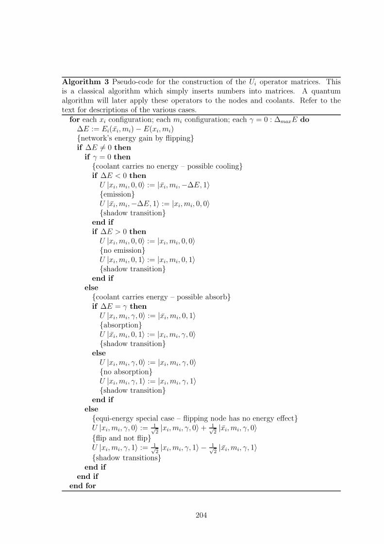
Algorithm 3 Pseudo-code for the construction of the Ui operator matrices. Thisis a classical algorithm which simply inserts numbers into matrices. A quantumalgorithm will later apply these operators to the nodes and coolants. Refer to thetext for descriptions of the various cases.
for each xi configuration; each mi configuration; each γ = 0 : ∆maxE do∆E := Ei(xi, mi)− E(xi, mi){network’s energy gain by flipping}if ∆E 6= 0 then
if γ = 0 then{coolant carries no energy – possible cooling}if ∆E < 0 thenU |xi, mi, 0, 0〉 := |xi, mi,−∆E, 1〉{emission}U |xi, mi,−∆E, 1〉 := |xi, mi, 0, 0〉{shadow transition}
end ifif ∆E > 0 thenU |xi, mi, 0, 0〉 := |xi, mi, 0, 0〉{no emission}U |xi, mi, 0, 1〉 := |xi, mi, 0, 1〉{shadow transition}
end ifelse{coolant carries energy – possible absorb}if ∆E = γ thenU |xi, mi, γ, 0〉 := |xi, mi, 0, 1〉{absorption}U |xi, mi, 0, 1〉 := |xi, mi, γ, 0〉{shadow transition}
elseU |xi, mi, γ, 0〉 := |xi, mi, γ, 0〉{no absorption}U |xi, mi, γ, 1〉 := |xi, mi, γ, 1〉{shadow transition}
end ifelse{equi-energy special case – flipping node has no energy effect}U |xi, mi, γ, 0〉 := 1√
2|xi, mi, γ, 0〉+ 1√
2|xi, mi, γ, 0〉
{flip and not flip}U |xi, mi, γ, 1〉 := 1√
2|xi, mi, γ, 1〉 − 1√
2|xi, mi, γ, 1〉
{shadow transitions}end if
end ifend for
204

20 40 60 80 100 120
20
40
60
80
100
120
20 40 60 80 100 120
20
40
60
80
100
120
20 40 60 80 100 120
20
40
60
80
100
120
Figure 7.8: Operators U0, U1 and U2 constructed for the x = 010 task by the algorithmin section 7.6.2. There is one operator for each node. In this simple case the matrixrepresentations of the operators are all of size 120×120. Matrix elements are always0 or 1 (except in special equi-energy cases). After the operators are constructed,the quantum computing itself may run. Applying Ui to node i and its neighbours isanalogous to a classical Gibbs step of updating one node.
7.7 Results
Simulations were performed using the above QCF/Matlab code. Due to the expo-
nential resources required to simulate quantum devices, the present work is restricted
to giving only proof of concept demonstrations. We consider the 3-node and 4-node
Boolean MRFs in fig. 7.7. The first net has unit energy penalties for nodes with
value 1 and for links whose neighbours are different, i.e. Ei = xi, Eij = ∆(xi, xj),
so its MAP state is 000. The second net has asymmetric penalties and MAP state
010. The third is a more complex net with MAP state 1010. Fig. 7.8 shows the three
operators constructed for the x = 010 task.
A naive state-vector-based computer simulation would require resources expo-
nential in the number of iterations, due to the expanding state space from the new
coolants (e.g. of size about 250 after 4 iterations of the 4-node net). However as we
don’t care about the resulting states of the coolant – they are garbage – we may make
use of the density matrix formulation of quantum computing (e.g. see [119]), which
allows us to ‘trace out’ over these coolant states. This essentially provides us with
the analogous operator to the ‘sum’ in the ‘sum-product’ algorithm (the ‘products’
corresponding to the unitary operators). It is the lack of ability to sum out states –
which reduces information – that prevents us from using quantum algorithms without
garbage bits to do inference. Summing these traces uses the bulk of computing time
on a classical computer simulation.
The performance of the quantum algorithm was compared to the analogous clas-
sical Gibbs sampler, as currently used in ThomCat, whose acceptance probabilities
are 1Z
exp(−E/T ). The same arbitrary cooling schedule was used in both algorithms,
and was chosen prior to the experiments: at the kth iteration we set T = 1k+1
. Each
205

classical sampler was run for 100,000 trials, each trial initialised with a random con-
figuration. The table below shows the empirical probability of the classical sampler
(C) reaching the MAP solution after the final iteration, compared with the (determin-
istic) quantum observation probabilities (Q), for the three tasks with MAP targets
000, 010 and 1010. The quantum algorithm appears to lag the classical sampler for
the first two iterations before overtaking.
000 010 1010step C Q C Q C Q1 .68 .51 .68 .43 .63 .352 .80 .76 .81 .70 .84 .723 .84 .84 .82 .86 .89 .924 .84 .87 .84 .92 .92 .985 .84 .89 .84 .94 .94 .996 .85 .89 .84 .96 .95 .999
7.8 Discussion
7.8.1 Comparison to classical Gibbs sampling
A fundamental problem in Machine Learning is that the joint over N nodes generally
requires exponential resources to represent it – whether as a brute-force table or the
classical Gibbs sampler’s use of ensembles of N -node configurations over exponential
time. We have shown how by using quantum amplitudes to represent joint probabili-
ties, it is possible to represent the exponential-sized joint of N nodes instantaneously
using only N physical nodes. However, moving the state vector into this represen-
tation is non-trivial and we showed how to use a unitary quantum analog of Gibbs
sampling to get there. Further, we showed how it can be cooled towards the MAP
solution, Q(x)→ δ(x; x).8
The algorithm does not make use of phase cancellations (all amplitudes are positive
real), so trajectories in the state space starting from each of the superposed initial
states evolve almost completely independently of each other.9 When we make a
measurement after the cooling, we are therefore selecting just a single trajectory
history to have occurred, and discarding the others.10 It may be asked what advantage
this has over the classical Gibbs method of simply sampling a single s-step trajectory
8Q(x) ≈ P (x)1/T is represented implicitly as the marginal of the explicit Q(τ) = Q(x, γ1:s, c1:s).The coolant space was introduced as it was not possible to carry out marginalisation explicitly byunitary operators.
9The unimportant exception being the special plateaux case.10The computation is reversible, so reachable basis states including coolants specify historical
trajectories.
206

τ = {x1:N}1:s without the need for quantum hardware – what is the use of the
unobserved trajectories? The answer is that as we are representing cooled model
probabilities Q(τ) by amplitudes, ατ , our probability of observing a particular τ is
given by the (renormalised) squared probability of its occurrence in the corresponding
classical sampler, Probs(τ) = α2τ = Q(τ)2. This gives a quadratic amplification of the
probabilities Q(τ) from the classical sampler. This quadratic speed-up appears to fit
in spirit with the result [165] that the optimal quantum search speedup is O(√N),
however full mathematical analysis of the algorithm’s nature could form the basis of
future work. Such analysis could also try to explain why the first two iterations give
poorer results than the classical sampler: we believe this is due to the sub-optimal
nature of our sampling, as for simplicity we excluded the possibility of low but non-
zero energy states absorbing energy.
7.8.2 Comparison to variational inference
Although we have presented the algorithm largely as a quantum extension of the
classical Gibbs sampler, an alternative and interesting view is as a quantum exten-
sion of classical variational methods [11] such as variational Bayes and loopy (Bethe)
message passing. Such methods approximate the true joint P (x1:N) by a product
Q(x1:N ) =∏N
i=1Qi(xi) which ignores correlation structure but is typically more
tractable to compute. In the Gibbs analogy, we view our algorithm as a multitude of
Gibbs samplers, running in ‘parallel worlds’. An alternative view is to consider the
amplitudes over individual node subspaces as being like variational Qi factors. How-
ever they are extended from classical variational methods because they are entangled
with the other nodes, so representing the correlation structure. A re-derivation of the
algorithm from this perspective could be interesting future work.
207

Chapter 8
Conclusion
We presented an architecture for unitary coherent scene perception, in the context
of a minidomain. The architecture comprises three stages: features, segmentation
and blackboard, and is intended to generalise to other domains. Bayesian theory was
used within all stages and to join them together. The stages would be unnecessary in
ideal inference, which would consider the exhaustive set of explanations. But we have
viewed features, segmentation and blackboards as heuristics to approximate inference
in practical computation time.
The blackboard heuristics in particular shed light on two philosophical issues. The
attention heuristic shows how reports about the past are subject to change, providing
an alternate view to those of Dennett [40]. Treating rewards as likelihoods to infer
the unitary coherent percept with maximum utility gives a quantitative version of
James’s pragmatism [84]. ThomCat as a whole provides a constructive demonstration
of rigorous Bayesian foundations for Hofstadter’s Copycat research programme.
The quantum algorithm gives a quadratic speedup in the blackboard stage, using
the quantum ability to represent complete N node joints instantaneously with only N
physical nodes. While other quantum annealing methods exist, ours is a pure quan-
tum computing method, presented in the language of Machine Learning, and we hope
that it will contribute to mutual understanding between the two fields. It generalises
the variational and Gibbs methods. Although non-toy simulations are not currently
possible, we gave proof of concept examples to illustrate the speedup that a future
‘ErwinCat’ blackboard would have over its classical ThomCat counterpart. Such an
annealed quantum, Bayesian message passing, hierarchical priming and pruning sys-
tem would fuse the fields of quantum computing, Machine Learning and blackboard
systems and would truly be an Entangled Bayesian Gestalt.
208

Appendix A: Matlab/QCF code
Listing 8.1: MATLAB/QCF code implementing the quantum algorithm.
function rho phi=run net ( node , l i nk , E max , E b i t s )
%compile a l i s t o f ne i ghbor s o f each node from the l i n k sfor i =1: length ( node )
node ( i ) . ne igh=i ;end
for i =1: length ( l i n k )node1 = l i n k ( i ) . node1 ;node2 = l i n k ( i ) . node2 ;node ( node1 ) . ne igh = [ node ( node1 ) . ne igh node2 ] ;node ( node2 ) . ne igh = [ node ( node2 ) . ne igh node1 ] ;
end
for i =1: length ( node )node ( i ) . E phi=zeros (2ˆ( length ( node ( i ) . ne igh ) ) , 1 ) ;
end
%make l i n k s b i d i r e c t i o n a l ( speed up search ing )L=length ( l i n k ) ;for i =1:L
l i n k (L+i ) . node1 = l i n k ( i ) . node2 ;l i n k (L+i ) . node2 = l i n k ( i ) . node1 ;l i n k (L+i ) .E = l i n k ( i ) .E ’ ;
end
%phi format i s : | i , 1 , n2 , . . . , nm> f o r node i wi th neighbours n
for i =1: length ( node )
%make a t a b l e o f en e r g i e s f o r each s t a t en ne igh = length ( node ( i ) . ne igh ) ;for phi dec =0:2ˆ( n ne igh)−1
ph i b in = dec2bin ( phi dec , n ne igh ) ;E phi = compute energy ( i , node , ph i b in , l i n k ) ;node ( i ) . E phi ( phi dec +1) = E phi ; %NB o f f s e t
end
%i n i t U i . The l a s t b i t i s change b i tU i = zeros ( 2ˆ length ( ph i b in ) ∗ 2ˆ E b i t s ∗ 2ˆ1 ) ;
%make U i
209

%for each input | in> = | phi >∗|E>∗|0> ( f i n a l b i t i s change b i t )%make outpu t | out>for phi dec =0:2ˆ( n ne igh)−1
ph i b in = dec2bin ( phi dec , n ne igh ) ;
%cons ider the p o s s i b l e ou tpu t | ps i> got by f l i p p i n g node ip s i b i n = ph i b in ;p s i b i n (1 ) = num2str( not (str2num( p s i b i n ( 1 ) ) ) ) ;p s i d e c = bin2dec ( p s i b i n ) ;%lookup energy o f | phi> and | ps i>E phi = node ( i ) . E phi ( phi dec +1);E ps i = node ( i ) . E phi ( p s i d e c +1);dE = E ps i − E phi ; %energy gain BY the system
%E=0 i s the p o s s i b l e emmission case −− d i f f e r e n t from the r e s tfor E=0:E max
%complete | in> s t a t ei n b i n = [ ph i b in dec2bin (E, E b i t s ) ’ 0 ’ ] ;
b s p l i t=f a l s e ; %f l a g f o r sepc case o f equ ienergy
i f (dE˜=0)i f (E==0) %po s s i b l e emission , or equ ienergy f l i p
i f (dE<0) %energy l o s t by system −− t r a n s i t i o nout b in = [ p s i b i n dec2bin(−dE , E b i t s ) ’ 1 ’ ] ;
s h i n b i n = out bin ; %shadow t r an s i t i o nsh out b in = in b in ;
else %no change , E>0out b in = in b in ; %s e l f t r a n s i t i o n
s h i n b i n = [ ph i b in dec2bin (E, E b i t s ) ’ 1 ’ ] ;s h out b in = sh i n b i n ; %shadow s e l f t r a n s i t i o n
end
else %E>0 are p o s s i b l e ab sorb t ion casesi f (dE==E) %energy absorbed by system −− t r a n s i t i o n
out b in = [ p s i b i n dec2bin (0 , E b i t s ) ’ 1 ’ ] ;
s h i n b i n = out bin ;sh out b in = in b in ;
else %no changeout b in = in b in ; %s e l f t r a n s i t i o n
s h i n b i n = [ ph i b in dec2bin (E, E b i t s ) ’ 1 ’ ] ;s h out b in = sh i n b i n ; %shadow t r an s i t i o n
end
end
else %dE==0, any Eb s p l i t=true ;
out b in = [ p s i b i n dec2bin (E, E b i t s ) ’ 1 ’ ] ;s h i n b i n = out bin ; %shadow s ta t e , oppo s i t e t r an s i t i o nsh out b in = in b in ;
210

end
%complete | out> and | shadow out> s t a t e si n dec = bin2dec ( i n b i n ) ;s h i n de c = bin2dec ( s h i n b i n ) ;out dec = bin2dec ( out b in ) ;sh out dec = bin2dec ( sh out b in ) ;
%in s e r t t r an s i t i o n in to U (+1 ad ju s t matlab idx )i f (˜ b s p l i t )
U i ( in dec +1, out dec+1) = 1 ;U i ( s h i n de c +1, sh out dec +1) = 1 ;
else %spe c i a l case o f equ ienergyU i ( in dec +1, out dec+1) = 1/ sqrt ( 2 ) ; %f l i pU i ( in dec +1, in dec +1) = 1/ sqrt ( 2 ) ; %dont f l i pU i ( s h i n de c +1, sh out dec +1) = 1/ sqrt ( 2 ) ; %f l i p shadowU i ( s h i n de c +1, s h i n de c +1) = −1/sqrt ( 2 ) ; %f l i p shadow
end
node ( i ) .U = U i ;
end
end
end
%now we need to s c a l e up U to the whole net ; and add new garbage . . .
% | i 1 i2 i3 > |E> | g1> | g2> . . . | gn>
%i n i t phiphi = zeros (2ˆ length ( node ) , 1 ) ; %bin2vec ( ’0000 ’ ) ;phi (1 ,1 )=1 ;H = hadamard( length ( node ) ) ;phi=H∗phi ; %crea t e s u pe r po s i t i on o f node s t a t e s
%t h i s i s always cons tant now we ’ ve moved to den s i t y ver s ion :i d x E b i t s t a r t = log2 ( length ( phi ))+1; %index o f 1 s t new E b i t in | in>
rho phi = phi∗phi ’ ; %den s i t y r ep r e s en t a t i on
temperature = 1/2 ; %at 1/2 no change w i l l occur ?
for i t e r =1:160 % ∗∗∗ THE MAIN QUANTUM COMPUTATION LOOP ∗∗∗
temperature = 1/(1+ i t e r ) ;
%update each node , by f i r i n g a NEW energy chunk and NEW change b i t a t i tfor i =1: length ( node )
E = temperature . ˆ ( 0 : 2 ˆ ( E b i t s )−1) ’ ; %exp supe rpo s i t i on o f energyE = reno rma l i s e (E) ;ch = bin2vec ( ’ 0 ’ ) ; %change b i t
rho E = E∗E ’ ; %den s i t y v e r s i on s
211

rho ch = ch∗ch ’ ;
r ho in = kron ( rho phi , rho E ) ;rho in = kron ( rho in , rho ch ) ; %crea t e whole system den s i t y
nb i t s i n = log2 ( length ( rho in ) ) ;idx new garbage = i d x E b i t s t a r t : n b i t s i n ;
%now expand U to a l l t he q u b i t s%and permute i t so i t a p p l i e s to the r i g h t b i t s%dont change the r e s t o f the q u b i t s − i e the r e s t o f the net and%o ld garbageI r e s t = i d e n t i t y ( nb i t s i n− ( length ( node ( i ) . ne igh)+E bi t s +1) ) ;U raw = kron ( node ( i ) .U, I r e s t ) ;perm = [ node ( i ) . ne igh idx new garbage ] ;perm = [ perm s e t d i f f ( 1 : nb i t s i n , perm ) ] ;U = permute matr ix b i t s (U raw , perm ) ;% U i s now in same b a s i s as | in>
%apply coo lan t operator to den s i t y matrixrho out = U∗ rho in ∗U’ ;
%trace out energy and ch b i t srho phi = t r a c e ou t ( rho out , E b i t s +1);
disp ( i t e r ) ;disp ( temperature ) ;disp (diag ( rho phi ) ) ;
end
end
212

Bibliography
[1] Emile Aarts and Jan Korst. Simulated Annealing and Boltzmann Machines.
Wiley, 1988.
[2] Hagai Attias. A variational Bayesian framework for graphical models. In Ad-
vances in Neural Information Processing Systems. MIT Press, 2000.
[3] Jim Baggott. The meaning of quantum theory. Oxford University Press, 1992.
[4] J. Baker. Trainable grammars for speech recognition. In J. J. Wolf and D. H.
Klatt, editors, Speech communication papers presented at the 97th meeting of
the Acoustical Society of America, pages 547–550. MIT Press, 1979.
[5] Adrian Barbu and Song-Chun Zhu. Cluster sampling and its applications in
image analysis. Technical Report 409, Dept. of Statistics, UCLA, 2004.
[6] J. B. Bello and M. Sandler. Blackboard system and top-down processing for the
transcription of simple polyphonic music. Proc. COST G-6. Conf. on Digital
Audio Effects, 2000.
[7] J. B. Bello and M. Sandler. Techniques for automated music transcription.
International Symposium on Music Information Retrieval, 2000.
[8] J.P. Bello, L. Daudet, S. Abdallah, C. Duxbury, M. Davies, and M.B. Sandler.
A tutorial on onset detection in music signals. IEEE Transactions on Speech
and Audio Processing, 13(5):1035–1047, 2005.
[9] J.M. Bernardo and A.F.M. Smith. Bayesian Theory. Wiley, 2000.
[10] Thomas Binford and Tod Levitt. Evidential reasoning for object recognition.
IEEE Tranactions on Pattern Analysis and Machine Intelligence, 2003.
[11] Chris Bishop. Pattern Recognition and Machine Learning. Springer, 2006.
213

[12] C.M Bishop, J.M.Winn, and D. Spiegelhalter. VIBES: A variational inference
engine for Bayesian networks. In Advances in Neural Information Processing
Systems, 2002.
[13] Andrew Blake and Alan L. Yuille, editors. Active Vision. MIT Press, 1993.
[14] Rens Bod. Beyond Grammar: An Experience-Based Theory of Language. Cen-
ter for the Study of Language and Information Publications, Stanford CA, 1998.
[15] Rens Bod. A unified model of structural organization in language and music.
Journal of Artificial Intelligence Research, 17:289–308, 2002.
[16] A.S. Bregman. Auditory Scene Analysis. MIT Press, 1990.
[17] G. L. Bretthorst. Bayesian Spectral Analysis. Springer-Verlag, 1985.
[18] Rodney Brookes. The whole iguana. In Michael Brady, editor, Robotics Science.
MIT Press, 1989.
[19] Stephen G. Brush. History of the Lenz-Ising model. Reviews of Modern Physics
(American Physical Society), 39:883–893, 1967.
[20] Giuseppe Castagnoli and David Ritz Finkelstein. Quantum-statistical compu-
tation. Proceedings of the Royal Society A, 459(2040):3099–3108, 2003.
[21] Ali Taylan Cemgil, H. Kappen, and D. Barber. A generative model for music
transcription. IEEE Transactions on Speech and Audio Processing, 2004.
[22] A.T. Cemgil. Bayesian Music Transcription. PhD thesis, Radboud University
of Nijmegen, 2004.
[23] D. Chalmers, R. French, and D. Hofstadter. High level perception, representa-
tion and analogy. In Fluid Concepts and Creative Analogies [81].
[24] Nick Chater, Joshua B. Tenenbaum, and Alan Yuille. Probabilistic models of
cognition: where next? Trends in Cognitive Sciences, 10(7):292–293, 2006.
[25] R. Chatterjee. Statistical Thought. Oxford University Press, 2003.
[26] Nick Collins. Drumtrack: Beat induction from an acoustic drum kit with syn-
chronised scheduling. In Proceedings of the International Computer Music Con-
ference, 2005.
214

[27] A. Cont. Realtime audio to score alignment for polyphonic music instruments
using sparse non-negative constraints and hierarchical HMMs. In IEEE Int.
Conf. Acoustics and Speech Sig. Proc., 2006.
[28] A. Cont and D. Schwarz. Score following at IRCAM. In International Sympo-
sium on Music Information Retreival, 2006.
[29] T. F. Cootes, G. J. Edwards, and C. J. Taylor. Active appearance models.
Lecture Notes in Computer Science, 1407, 1998.
[30] R. Cowell. Advanced inference in Bayesian networks. Learning in Graphical
Models, ed. Jordan, 2001.
[31] D-Wave. World’s first commercial quantum computer demonstrated.
http://www.dwavesys.com/, 2007.
[32] Paul Dagum and Michael Luby. Approximating probabilistic inference in
Bayesian belief networks is NP-hard. Artificial Intelligence, 60(1):141–153,
1993.
[33] R. Dannenberg. An on-line algorithm for real-time accompaniment. Proceedings
of the International Computer Music Conference, 1984.
[34] R. Dannenberg. Real-time computer accompaniment of keyboard performances.
Proceedings of the International Computer Music Conference, 1985.
[35] R. Dannenberg. A stochastic method of tracking a vocal performer. Proceedings
of the International Computer Music Conference, 1997.
[36] R. Dannenberg and N. Hu. Polyphonic audio matching for score following and
intelligient audio editors. Proceedings of the International Computer Music
Conference, 2003.
[37] N.D. Daw, Y. Niv, and P. Dayan. Uncertainty-based competition between
prefrontal and dorsolateral striatal systems for behavioral control. Nature Neu-
roscience, 8:1704–1711, 2005.
[38] P. Dayan and L.F. Abbott. Theoretical Neuroscience. MIT Press, 2005.
[39] Richard Dearden, Nir Friedman, and Stuart J. Russell. Bayesian Q-learning.
In AAAI/IAAI, pages 761–768, 1998.
[40] Daniel C. Dennett. Consciousness Explained. Penguin, 1998.
215

[41] Department of Chemistry, University of Oxford. Quantum Pharmacology - 30
years on. (A Special Conference in Honour of Prof. W. Graham Richards),
2006.
[42] David Deutsch. The Fabric of Reality. Penguin, 1997.
[43] Diane Deutsch. Muscial Illusions and Paradoxes. Philomel Records, 1995.
[44] D.J.MacKay. Learning in Bayesian Networks, Ed. M.I. Jordan, chapter Intro-
duction to Monte Carlo Methods. MIT Press, 1999.
[45] A. Doucet, J.F.G. de Freitas, and N.J. Gordon, editors. Sequential Monte Carlo
Methods in Practice. Springer-Verlag, 2001.
[46] M. Dovey, T. Crawford, D. Byrd, J. Montal, J. Pickens, J. Bello, G. Monti, and
M. Sandler. Overview of the OMRAS project. Journal of the American Society
for Information Science and Technology, 2004.
[47] J. Stephen Downie, Kris West, Andreas Ehmann, and Emmanuel Vincent. The
2005 music information retrieval evaluation exchange: Preliminary overview.
In J.D. Reiss and G.A.Wiggins, editors, Proceedings of the 2005 International
Symposium on Music Information Retreival, pages 320–323, 2005.
[48] Kenji Doya, Shin Ishii, Alexandre Pouget, and Rajesh P. N. Rao, editors.
Bayesian Brain. MIT Press, 2007.
[49] Christoph Durr and Peter Hoyer. A quantum algorithm for finding the mini-
mum, 1996.
[50] Jay Earley. An efficient context-free parsing algorithm. Communications of the
ACM, 13(2):94–102, 1970.
[51] Lee Erman, Fredrick Hayes-Roth, Victor Lesser, and Raj Reddy. The Hearsay-
II speech understanding system: Integrating knowledge to resolve uncertainty.
ACM Computing Surveys, 12(2), June 1980.
[52] Edward Farhi, Jeffrey Goldstone, Sam Gutmann, and Michael Sipser. Quantum
computation by adiabatic evolution, 2000.
[53] Richard Phillips Feynman. Feynman Lectures on Computation. Addison-Wesley
Longman Publishing Co., Inc., Boston, MA, USA, 1996.
216

[54] Cordelia Fine. A Mind of its Own: How your brain distorts and deceives. Icon
Books, 2005.
[55] Charles Fox. QCF: Quantum computing functions for Matlab. Technical Report
PARG-03-02, Robotics Research Group, Oxford University, 2003.
[56] Charles Fox. Genetic hierarchical music structures. In Proceedings of the Inter-
national Florida Artificial Intelligence Society Conference, 2006.
[57] Charles Fox. Review of ‘Bayesian Brain’. Connection Science, 20(1):67–68,
2008.
[58] Charles Fox. ThomCat: A Bayesian blackboard model of hierarchical temporal
perception. In Proceedings of the 21st International Florida Artificial Intelli-
gence Research Society Conference, 2008.
[59] Charles Fox, Neil Girdhar, and Kevin Gurney. A causal Bayesian network
view of reinforcement learning. In Proceedings of the 21st International Florida
Artificial Intelligence Research Society Conference, 2008.
[60] Charles Fox and John Quinn. How to be lost: principled priming and pruning
with particles in score following. In Proceedings of the International Computer
Music Conference, 2007.
[61] Charles Fox and Chris Raphael. Music++ technical documentation. Technical
report, Indiana University (Confidential), 2005.
[62] Charles Fox, Iead Rezek, and Stephen Roberts. Drum’n’bayes: Online varia-
tional inference for beat tracking and rhythm recognition. In Proceedings of the
International Computer Music Conference, 2007.
[63] Charles Fox, Iead Rezek, and Stephen Roberts. Local quantum computing for
fast probably map inference in graphical models. In Proceedings of the Second
AAAI Symposium on Quantum Interaction, 2008.
[64] Bob French. The Subtlety of Sameness: A Theory and Computer Model of
Analogy-Making. MIT Press, 1995.
[65] B.J. Frey and D.J.C.MacKay. A revolution: Belief propagation in graphs with
cycles. In M.I.Jordan, M.S.Kearns, and S.A.Solla, editors, Advances in Neural
Information Processing Systems, volume 10. MIT Press, 1998.
217

[66] Nir Friedman, Lise Gentoor, Daphne Koller, and Avi Pfeffer. Learning prob-
abilistic relational models. In Proceedings of the Sixteenth International Joint
Conference on Artificial Intelligence, 1999.
[67] Martin Gardner. The fantastic combinations of John Conway’s new solitaire
game ‘life’. Scientific American, 223:120–123, 1970.
[68] Simon Godsill and Manuel Davy. Bayesian harmonic models for musical pitch
estimation and analysis. In Proceedings of the IEEE International Conference
on Acoustics, Speech and Signal Processing, 2002.
[69] R.P. Goldman and E. Charniak. A language for construction of belief networks.
IEEE Transactions on Pattern Analysis and Machine Intelligence, 15(3):196–
207, 1993.
[70] M. Goto. An audio-based real-time beat tracking system for music with or
without drumsounds. Journal of New Music Research, 30(2):159–171, 2001.
[71] Lov K. Grover. A fast quantum mechanical algorithm for database search.
In Proceedings of the Twenty-Eighth Annual ACM Symposium on Theory of
Computing, pages 212–219, 1996.
[72] L. Grubb and R. Dannenberg. Enhanced vocal performance tracking using
multiple information sources. Proceedings of the International Computer Music
Conference, 1998.
[73] S. Hainsworth. Techniques for the Analysis of Musical Audio. PhD thesis,
Unviersity of Cambridge, 2003.
[74] S. Hameroff. Anaesthesia, consciousness and hydrophobic pockets - a unitary
quantum hypothesis an anaesthetic action. Toxicology Letters, 100-101, 1998.
[75] David J. Hand, Heikki Mannila, and Padhraic Smyth. Principles of Data Min-
ing. MIT Press, 2001.
[76] Gavin Harrison. Rhythmic Illusions. Warner Bros. Publications, 1998.
[77] Jeff Hawkins and Sandra Blakeslee. On Intelligence. Times Books, 2004.
[78] G. E. Hinton and T. J. Sejnowski. Learning and relearning in Boltzmann ma-
chines. In Parallel distributed processing: Explorations in the microstructure
of cognition, vol. 1: foundations, pages 282–317. MIT Press, Cambridge, MA,
USA, 1986.
218

[79] Donald D. Hoffman. Visual Intelligence: How we create what we see. W.W.
Norton and Company, 1998.
[80] Douglas Hofstadter. A non-deterministic approach to analogy, involving the
Ising model of ferromagnetism. In E. Caianiello, editor, The Physics of Cognitive
Processes. World Scientific, 1987.
[81] D.R. Hofstadter and the Fluid Analogies Research Group. Fluid Concepts and
Creative Analogies. Basic Books, 1995.
[82] Tad Hogg and Mehmet Yanik. Local search methods for quantum computers,
1998.
[83] T. Jaakkola and M. Jordan. Variational methods and the QMR-DT database.
Journal of Artificial Intelligence Research, 10:291–322, 1999.
[84] William James. Pragmatism: A New Name for Some Old Ways of Thinking.
Reprinted Dover, 1995, 1907.
[85] William James. Principles of Psychology. New York: Holt, 1980.
[86] M.I. Jordan and C. Bishop. An Introduction to Graphical Models. Unpublished
book, forthcoming.
[87] I. Kant. Critique of Pure Reason. Reprinted by Project Guttenberg, 1781.
[88] K. Kashino, K. Nakadai, T. Kinoshita, and H. Tanaka. Organization of hier-
achical perceptual sounds. Proceedings of the International Joint Conference
on Artificial Intelligence, 1995.
[89] Kunio Kashino and Norihiro Hagati. A music scene analysis system with the
mrf-based information integration scheme. Proceedings of the IEEE Interna-
tional Conference on Pattern Recognition, 1996.
[90] Katayose. Unknown publications, in Japanese only, 1989.
[91] S. Kirkpatrick, C.D Gellat, and M.C. Vecchi. Optimization by simulated an-
nealing. Science, 220:671–680, 1983.
[92] Will Knight. Entangled photons secure money transfer.
http://www.newscientist.com/channel/fundamentals/quantum-world/dn4914.
[93] D. Koller and A. Pfeffer. Object-oriented Bayesian networks. In Proceedings of
Uncertainty in Artificial Intelligence, 1997.
219
[94] Steve Larson. Seek well: A creative microdomain for studying expressive mean-
ing in music. Technical Report CRCC-77, Center for Research on Concepts and
Cognition, University of Indiana, 1993.
[95] K. B. Laskey. MEBN: A language for first-order Bayesian knowledge bases.
Artificial Intelligence, 172(2-3):140–178, 2007.
[96] Kathryn Blackmond Laskey. Quantum causal networks. In Proceedings of the
2007 AAAI Spring Symposium on Quantum Interaction, 2007.
[97] Steffen L. Lauritzen and Dennis Nilsson. Representing and solving decision
problems with limited information. Management Science, 47(9):1235–1251,
2001.
[98] Peter M. Lee. Bayesian Statistics: An introduction. Arnold Publishers, third
edition, 2003.
[99] Tai Sing Lee and Alan L. Yuille. Efficient coding of visual scenes by grouping
and segmentation. In Doya et al. [48].
[100] Tod Levitt, Thomas Binford, and Gil Ettinger. Utility-based control for com-
puter vision. In Uncertainty in Artificial Intelligence 4, 1990.
[101] David G. Lowe. Object recognition from local scale-invariant features. In In-
ternational Conference on Computer Vision, 1999.
[102] Per-Olov Lwdin, editor. Quantum Biology and Quantum Pharmacology - Quan-
tum Biology Symposium Proceedings No. 17. Wiley, 1991.
[103] Stephane Mallat. A Wavelet Tour of Signal Processing. Academic Press, 1999.
[104] E. Mariani and G. Parsi. Simulated tempering: A new monte carlo scheme.
Europhysics Letters, 19:451–468, 1992.
[105] D. Marr. Vision. MIT, 1985.
[106] K.D. Martin. A blackboard system for automated transcription of polyphonic
music. MIT Media Lab Tech. Report 385, 1995.
[107] K.D. Martin. Automatic transcription of simple polyphonic music. Third Joint
Meeting of the Acoustical Societies of America and Japan, 1996.
220
[108] David McAllester, Michael Collins, and Fernando Pereira. Case-factor diagrams
for structured probabalistic modelling. In Proceedings of the Annual Conference
on Uncertainty in Artificial Intelligence, 2004.
[109] T. McInerey and D. Terzopoulos. Deformable Models in Medical Image Analy-
sis: A Survey. Medical Image Analysis, 1996.
[110] Brian Milch. Probabilisitic Models with Unknown Objects. PhD thesis, UC
Berkeley, 2006.
[111] Melanie Mitchell. Analogy-Making as Perception. MIT, 1993.
[112] Melanie Mitchell. Copycat source code. http://web.cecs.pdx.edu/ mm/ccat-
src/, 1993.
[113] Samuel K. Moore. Prototype quantum computer demo’ed.
http://www.spectrum.ieee.org/feb07/comments/1710.
[114] K. Murphy, A. Torralba, and W. Freeman. Using the forrest to see the trees:
A graphical model relating features, object, and scenes. In Advances in Neural
Information Processing Systems, 2003.
[115] Kevin Murphy. Dynamic Bayesian Networks: Representation, Inference and
Learning. PhD thesis, UC Berkeley, 2002.
[116] Kevin Murphy, Yair Weiss, and Michael I. Jordan. Loopy belief propagation
for approximate inference: an empirical study. In Proceedings of the Annual
Conference on Uncertainty in Artificial Intelligence, pages 467–475, Stockholm,
1999.
[117] P. Myllymaki and H. Tirri. Massively parallel case-based reasoning with prob-
abilistic similarity metrics. In K. Althoff, M. Richter, and S. Wess, editors,
Proceedings of the First European Workshop on Case-Based Reasoning, 1993.
[118] R. Neal. Suppressing random walks in Markov Chain Monte Carlo using ordered
overrelaxation. Technical report, Dept. of Statistics, University of Toronto,
1995.
[119] M. Neilsen and I. Chuang. Quantum Computing and Quantum Information.
Cambridge University Press, 2000.
221

[120] P. Newman and Kin Ho. SLAM loop closing with visually salient features.
In Proceedings of the 2005 IEEE International Conference on Robotics and
Automation, pages 635–642, 2005.
[121] Eric P. Nichols. Modeling melodic expectation and preference: A pilot study
based on Larson’s musical forces. Technical Report CRCC-124, Center for
Research into Concepts and Cognition, Indiana University, 2007.
[122] Eric Nicols. Dynamic melodic expectation in the creative microdomain seek
well. Technical Report CRCC-138, Center for Research on Concepts and Cog-
nition, University of Indiana, 2005.
[123] N. Orio and F. Dechelle. Score following using spectral analysis and hidden
Markov models. Proceedings of the International Computer Music Conference,
2001.
[124] J. Pearl. Intelligient Reasoning with Probabalistic Networks. Morgan Kaufmann,
1988.
[125] J. Pearl. Causality. Cambridge University Press, 2000.
[126] Roger Penrose. Shadows of the Mind. Oxford University Press, 1994.
[127] Avi Pfeffer, Daphne Koller, Brian Milch, and Ken T. Takusagawa. SPOOK:
A system for probabilistic object-oriented knowledge representation. In Uncer-
tainty in Artificial Intelligence, 1999.
[128] J. Pickens, J.B. Bello, T. Crawford, M. Dovey, G. Monti, and M. Sandler. Poly-
phonic score retreival using polyphonic qudio queries: A harmonic modelling
approach. ISMIR, 2002.
[129] L. Rabiner. A tutorial on hidden Markov models. Proceedings of the IEEE,
77:257–286, 1989.
[130] L. Rabiner and B. Juang. Fundamentals of Speech Recognition. Prentice Hall,
1993.
[131] C. Raphael. Automatic segmentation of acoustic musical signals using hidden
markov models. IEEE PAMI, 1999.
[132] C Raphael. A probabalistic system for automatic musical accompaniment. J.
Comp. Graph. Stats., 1999.
222

[133] C. Raphael. Automated rhythm transcription. Ann.Symp.Mus.Res., 2001.
[134] C. Raphael. A Bayesian network for real-time musical accompaniment. In
Advances in Neural Information Processing Systems. MIT Press, 2001.
[135] C. Raphael. Can the computer learn to play music expressively? In Proc. of
Eighth Int. Workshop on Artif. Intel. and Stats., 2001.
[136] C Raphael. Coarse-to-fine dynamic programming. IEEE Transactions on Pat-
tern Analysis and Machine Intelligence, 2001.
[137] C. Raphael. Music plus one: A system for expressive and flexible musical ac-
companiment. In Proceedings of the International Computer Music Conference,
2001.
[138] C. Raphael. Harmonic analysis with probabalistic graphical models. In Pro-
ceedings of the International Symposium on Music Information Retreival, 2003.
[139] C Raphael. Orchestra in a box: A system for real-time musical accompaniment.
In Proceedings of the International Joint Conference on Artificial Intelligence,
2003.
[140] C. Raphael. Orchestral musical accompaniment from synthesized audio. In
Proceedings of the International Computer Music Conference, 2003.
[141] C. Raphael. Aligning musical scores with audio using hybrid graphical models.
Machine Learning, 65(2-3), 2006.
[142] Ben Y. Reis. A multi-agent system for on-line modeling, parsing and prediction
of discrete time series data. In Intelligent Image Processing, Data Analysis and
Information Retrieval, pages pp. 164–169. IOS Press Holland, 1999.
[143] Iead Rezek and Stephen Roberts. An operator interpretation of message passing.
Technical Report PARG-03-01, Robotics Research Group, University of Oxford,
2003.
[144] Elaine Rich and Kevin Knight. Artificial Intelligence. McGraw-Hill, 1990.
[145] Bob Ricks and Dan Ventura. Training a quantum neural network. In Sebastian
Thrun, Lawrence Saul, and Bernhard Scholkopf, editors, Advances in Neural
Information Processing Systems 16. MIT Press, Cambridge, MA, 2004.
223

[146] Jeremie Roland and Nicolas J. Cerf. Quantum search by local adiabatic evolu-
tion. Phys. Rev. A, 65(4):042308, 2002.
[147] S. Russell and P. Norvig. Artificial Intelligience: A Modern Approach. Prentice
Hall, 2002.
[148] Solomon E. Shimony. Finding MAPs for belief networks is NP-hard. Artificial
Intelligence, 68(2):399–410, 1994.
[149] J Siskind, J Sherman, I Pollak, and C Bouman. Hierarchical perceptual organi-
zation with the center-surround algorithm. In Proceedings of the International
Conference on Computer Vision, 2003.
[150] Squarepusher. Ultravisitor. Audio CD: Warp records, 2004.
[151] Amos Storkey and Chris Williams. Image modelling with position-encoded dy-
namic trees. IEEE Transactions of Pattern Analysis and Machine Intelligence,
25(7):859–871, 2003.
[152] R.S. Sutton and A. G. Barto. Reinforcement Learning. MIT, 1998.
[153] Sebastian Thrun, Wolfram Burgard, and Dieter Fox. Probabilistic Robotics.
MIT Press, 2006.
[154] Robert R. Tucci. Quantum Bayesian networks. International Journal of Modern
Physics B, 9(3):295–337, 1995.
[155] Shimon Ullman. High-level vision: Object recognition and visual cognition. MIT
Press, 1996.
[156] L. Van Noorden and D. Moelants. Resonance in the perception of musical pulse.
Journal of New Music Research, 28(1):43–66, 1999.
[157] Lieven M. K. Vandersypen, Matthias Steffen, Gregory Breyta, Costantino S.
Yannoni, Mark H. Sherwood, and Isaac L. Chuang. Experimental realization of
shor’s quantum factoring algorithm using nuclear magnetic resonance. Nature,
414:883, 2001.
[158] Herman von Helmholtz. On the sensations of tone. Dover (reprint), 1888.
[159] C. Wiggs and A. Martin. Properties and mechanisms of perceptual priming.
Current Opinion in Neurobiology (CNS), 8:227–233, 1998.
224
[160] J. Winn and C. Bishop. Variational message passing. Journal of Machine
Learning Research, 6:661–694, 2005.
[161] John Winn. Variational message passing and its applications. PhD thesis,
University of Cambridge, 2003.
[162] J.S. Yedidia, W.T.Freeman, and Y.Weiss. Understanding belief propagation and
its generalisations. In Gerhard Lakenmeyer and Bernhard Nebel, editors, Ex-
ploring Artificial Intelligence in the New Millenium. Morgan Kaufmann, 2003.
[163] Daniel H. Younger. Recognition and parsing of context-free languages in time
n3. Information and Control, 10(2):189–208, 1967.
[164] Alan L. Yuille. A double-loop algorithm to minimize the Bethe free energy.
In Proceedings of the Third Energy Minimization Methods in Computer Vision
and Pattern Recognition, Sophia-Antipolis. France, 2001.
[165] Christof Zalka. Grover’s quantum searching algorithm is optimal. Phys. Rev.
A, 60:2746, 1999.
[166] N.L. Zhang and David Poole. Exploiting causal independence in Bayesian net-
work inference. Journal of Artificial Intelligence Research, 5:301–328, 1996.
225