Embed Size (px)
Citation preview
University of Natal (Durban)Graduate School of Business
AN EMPIRICAL STUDY OF CAPITAL ASSET PRICING'MODEL ANOMALIES ON THE JSE
A dissertation presented to:
The Graduate School of BusinessUniversity of Natal
In partial fulfillment of theRequirements for the degree of
MASTER OF BUSINESS ADMINISTRATIONUNIVERSITY OF NATAL
By
PAUL LYES
5 July 2000
\

University of Natal (Durban)Gradua te School of Business
1. PROBLEM STATEM ENT AND OBJECTIVES OF
STUDY.
2. THEORETICAL BACKROUND.
3. REVIEW OF PRIOR RESEARCH.
4. REVIEW OF SOUTH AFRICAN LITERATURE.
5. METHODOLOGY AND DATA.
6. RESULTS AND CONCLUSION
7. APPENDICES AND BIBLIOG RAPHY.

University of Natal (Durban)Graduate School of Business
Abstract
The introduction of the Capital Asset Pricing Model in 1964, .and its
subsequent study by hundreds of thousands if not .millions of people at
universities throughout the world, has had far reaching consequences in
terms of the way portfolios were constructed for many insurance and
pension funds . It has affected the investment philosophies of large
numbers of investors as well as influenced the calculations of firms costs of
capital. Countless investment proposals have been accepted or rejected
based on what the Capita l Asset Pricing model has calculated the minimum
return demanded by shareholders to be. This dissertation looks at the
empirical evidence supporting the debate about the usefulness of the
Capital Asset Pricing model, as well as presenting evidence as to any
possible anomalies to this model on the JSE.

University of Natal (Durban)Graduate School of Business
An empirical study of Capital As set Pricing Modei ano·rna.lies on the
JSE.
Introduction
One financial theory has dominated academic literature and influenced
greatly the practical world of finance and business for over three decades
since it was first expounded by the Nobel prizewinner William Sharpe. This
is the Capital Asset Pricing Model (CAPM). At its heart the CAPM has an
old and common observation - the returns on a financial asset increases
with risk. The breakthrough in the 60's was to define risk in a very precise
way. It was no longer enough to rely on standard deviation after the work of
Markowitz and others had shown the benefits of diversification. The
argument goes that it is illogical to be less than fully diversified so investors
tend to create large portfolios. William Sharpe extended modern portfolio
theory to introduce the notions of systematic and specific risk. Essentially
the CAPM describes the way prices of individual assets are determined in
an efficient market, based on their relative riskiness in comparison with the
return on the risk-free assets. According to this model, prices are
determined in such a way that risk premiums are proportional to systematic
risk as measured by the beta coefficient.

University of Natal (Durban)Graduate School of Business
CAPM considers a simplified world where, there are no transaction costs,
all investors have identical investment horizons and all investors have
identical perceptions regarding the expected returns, volatili ties and
correlations of available risky investments.
In such a world all investors will hold the market portfolio leveraging and
de-Ieveraging it with positions in the risk free asset. CAPM divides the risk
of holding risky assets into systematic and specific risk. Systematic risk is
the risk associated with holding the market portfolio, where as specific risk
or unsystematic risk is the risk unique to an individual asset.
By divers ifying his portfolio an investor can effectively elimina te
unsystematic risk and is thus left with only systematic risk. One can thus
measure the risk of an individual share by its Beta W) which is an index of
a securities respons iveness to a change of returns in the market portfolio.
Thus the CAPM is a risk based pricing model which attempts to expla in the
cross section of expected stock returns through a single factortjl).
University of Natal (Durban)Graduate School of Business
1. Problem statement and objectives of th e study
Despite efforts to explain the cross section of expected stock returns via
risk based asset pricing models , several empirical anomalies seem to
remain at odds with the risk based explanations . Of these anomalies the
three most cited by researchers are those of size, book-to-market and
momentum. Although some researchers claim these anomalies are related
to risk, others reject such claims in favour of explanations related to
investor behavior. The aim of this study is to empirically identify anomal ies
to the capital asset pricing model using historical monthly returns earned
on the shares traded on the JSE industrial index as well as
macro-economic data over the period 1982-1999.
University of Natal (Durban)Graduate School of Business
2. Theoretical Background
Sharpe (1964) introduced the world to the CAPM the derivation of which as
shown by Jagannathan (1999) is: Start with the simple problem of choosing
a portfolio of assets for an investor. In order to set up the problem we need
a few definitions. Let Ro be the return (that is, one plus the rate of return)
on the risk-free asset (asset 0). Thus by investing $1 the investor will get
$Ro for sure. In addition, assume that the number of risky assets is n. The
risky assets have returns that are not known with certainty at the time the
investments are made. Let (Xi be the fraction of the investors initial wealth
that is allocated to asset i. Then R, is the return on asset i. Let Rm be the
return on the entire market portfolio of risky assets. Here Ri is a random
variable with an expected value ERj and variance Var(R j) , where variance
is a measure of the volatility of the return. The covariance between the
return of asset i and the return of asset j is represented by cov(Ri,Rj) .
Covariance provides a measure of how the returns on the two assets i
and j move together.
Suppose that the investors utility can be represented as a function of the
expected return on the investor's portfolio and its variance. In order to
simplify notation without losing generality, assume that the investor can

University of Natal (Durban)Graduate School of Business
choose to allocate wealth to three assets: i= 0, 1, or 2. Then the problem is
to choose fractions aa , a 1' and az that maximise
subject to
(2) a o + a1 +ao = 1
The objective function V is increasing in the expected return, aV/BERm> 0;
decreasing in the variance of the return , BV/Bvar(Rm) < 0; and concave.
These properties imply that there is a trade-off between expected returns.
The constraint in equation (2) ensures that the fractions sum to 1.
Equations (3) and (4) follow from the definition of the rate of return on the
wealth portfolio of the investor Rm.
Substituting 1-a1 - a2 for ao in equation (1) and taking the derivative of V
with respect to a1 and a2 yields the following conditions that must hold at
an optimum:

University of Natal (Durban)Graduate School of Business
VVhere Vj is the part ial derivative of V with respect to its Jth argument, for j =
1,2. Now consider multiplying equation (5) by a1 and equation (6) by a 2 and
.summing the results :
Using the definitions of ERmand var(R m), we can wr ite this more succinctly:
The expressions in (5), (6), and (8) can all be written as explicit functions of
the ratio V2N1, and then the first two expressions [from (5) and (6)] can be
equated to the third [from (8)]. This yields the following two relationships:
for i = 1,2. In fact, even for the more general case, where n is not
necessarily equal to 2, equation (9) holds. Let cov(Rj,Rm)/varRmbe the beta
of asset i or Pi' Then we have
for all i =1,,, .n

University of Natal (Durban)Graduate School of Business
A portfolio is said to be on the mean variance frontier of the
return/variance relationship if no other choice of weights lXo ,lXj (for j =
1,2, .. .n) yields a lower variance for the same expected return. The
portfolio is said to be on the efficien t part of the fron tier if, in addition, no
other portfolio has a higher return. The optimally chosen portfolio for the
problem in equations (1) - (4) has this property. In fact equation (10) will
continue to hold if the return Rm is replaced by the return on any mean
variance portfolio other than the risk-free asset.
Note that the return Rm in (10) is the return for one investors wealth
portfolio. But equation (10) holds for every mean-variance efficient
portfo lio, and V need not be the same for all investors. A property of mean
variance efficient portfolios is that portfolios of them are also mean
variance efficient. If we define the market portfo lio to be the weighted sum
of individual portfolios with the weights being determined by the fractions
of total wealth held by the individual, the market portfolio is also mean
var iance efficient. Therefore an equation of the form given by (10) also
holds for the market portfolio. In fact, equation (10) with Rm equal to the
return on the market portfolio is the key relation for the CAPM. This
relation implies that all assets i have the same ratios of reward, measured
as the expected return in excess of the risk free rate (ER j - Ro), to risk (Pi) '
This is consistent with the notion that the investors trade off return for risk.

Universi ty of Natal (Durban)Graduate School of Business
When the CAPM assumptions are satisfied, everyone in the economy will
hold risky assets in the same proportion. Hence the Beta's computed with
reference to every individuals portfolio will be the same, and we might as
well compute Beta's using the .market portfolio of all assets in the
economy. The CAPM predicts that the ratio of the risk premium to the beta
of every asset is the same. That is every investment opportunity provides
the same amount of compensation for any given level of risk.

University of Natal (Durban)Graduate School of Business
3. Review of Prior Research
Efforts to explain the cross section of expected returns via a multi-factor
linear asset pricing model have generally failed due to the existence of
several empirical anomalies. The Capital Asset Pricing Model (CAPM) of
Sharpe (1964), Lintner 1965, and Black (1972) states that the covariance
of a security's return with the return on the market (~) should be sufficient
to describe the cross-section of expected returns.
International studies
South African finance research has in the past taken its lead from that
conducted in the international arena particularly the US. Many empirical
studies have contradicted the CAPM .
One of the first empirical studies of the CAPM is that of Black, Jensen and
Scholes (1972). They used all the stocks on the New York Stock
Exchange during the period 1931-1965 to form 10 portfolios. They then
estimated the beta of these portfolios using historical data. Using the 30
day T-bill as an approximation of the risk free asset, they regressed the
average monthly excess returns on beta. They used an average monthly
University of Natal (Durban)Graduate School of Business
excess return on the market of 1.42 percent. The slope of the resulting
regression line was 1.08 percent instead of 1.42 percent as predicted by
the CAPM. The estimated intercept was 0.519 percent instead of zero. The
t-statistlcs that Black, Jensen and Scho!es report indicate that the slope of
the regression line and the intercept are significantly different from their
theoretical values.
As Black points out this does not necessarily mean that the data does not
support the CAPM, he offers two plausible reasons for this anomaly. One is
measurement and model specification error, due to the fact that a proxy
was used instead of the actual market portfolio. This error influences the
slope of the regression line towards zero and its intercept away from zero .
.The second possibility is that there are no risk free assets and in the
absence of such the CAPM does not predict an intercept of zero. Ultimately
Black Jensen and Scholes concluded that data was consistent with Black's
(1972) vers ion of the model.
Jagarnath and Mcgrattan (1995) conducted a similar study using the same
approach as Black, Jensen and Scholes (1972) extending the sample of
data to the period 1926-1991 found that the results were consistent with
the predictions of the CAPM.

University of Natal (Durban)Graduate School of Business
Fama and Macbeth (1973) examined whether there is a positive relation
between average return and beta, and whether the squared value of beta
and the volatility of the return on an asset can explain the residual variation
in average returns across assets that is not explained by beta alone. Fama
and MacBeth found, using data for the period 1926-1968 for stocks traded
on the NYSE, that the data supported the CAPM.
Banz (1981) investigated whether size (market capitalization) has any
additional explanatory power over market pfor describing the cross-section
of expected stock returns. Banz challenged the CAPM by showing that size
does indeed hold additional explanatory power over market p of the cross
section of returns. Banz Found during the period 1936-1975 the average
return to stocks of small firms(those with low market capitalisation) was
substantially higher than the average return to stocks of large firms after
adjusting for the risks using the CAPM. Banz conducted his research using
an approach similar to that used by Black, Jensen and Scholes. He
constructed two portfolios each with 20 assets. One portfolio contained
only stocks of small firms, while the other portfolio consisted of stocks of
large firms. The two portfolios were constructed in such a way that they
both had the same beta. Banz found that the small firms over the period
University of Natal (Durban)Graduate School of Business
1936-1975 earned on average 1.48 percent per month more than large
firms. Banz concluded that size was a missing factor in the CAPM.
Fama and French (1992) found that the ratio of the book value of a firms
common equity to its market value could account for a substantial portion
of the cross-sectional variation in average returns. Interestingly Fama and
French used the same procedure as Fama and McBeth (1973) the only
difference being the sample periods used in the two studies. Thus over the
period 1926-1968 Fama and McBeth found a positive relationship between
return and risk, whereas over the period 1963-1990 Fama and French
found that there was no relationship between return and risk.
Jaggannathan and McGratten (1995) considered these findings and tested
them over various periods . They found that over the period 1926-1990
there was a positive relationship between return and risk on the NYSE.
However during the sub-period 1976-1980 no relationship could be found
between the two. During this period it was found that small-firms had
produced unusually high returns in relation to the S&P 500 index. Next they
considered the sub-period 1981-1991 during this period it was found that
the size effect disappeared all together with small firms under-performing
University of Natal (Durban)Graduate School of Business
the S&P 500. They concluded that although we find empirical support for
the CAPM over a long horison (1926-1991 ),.there are periods in which we
do not find it.
Other Studies by Bhandari (1988), Stattman (1980) and Rosenberg, Reid
and Lanstein (1985) found that leverage, the book value to market value of
equity (B/M) and earnings-price ratios all have additional explanatory
power over pand size.
Baker and Haugen (1996:435-436) examine over fifty candidate factors
and conclude "... it is noteworthy that none of the factors related to sensitivities
to macro-economic variables seem to be important determinants of expected
stock returns". Haugen and Baker identified the twelve most important
predictors of the cross-section of returns to be: (i) the past months excess
returns; (ii) the market to book ratio; (iii) the past twelve months excess
returns; (iv) the cash flow to price ratio; (v) the price to earnings ratio; (vi)
sales to price; (vii) past three months excess earnings; (viii) the debt to
equity ratio; (ix) the variance of total returns; (x) the variance of residual
returns; (xi) the past five years expected returns; (xii) the return on equity.

University of Natal (Durban)Graduate School of Business
Fama and French (1992:428) in a widely acclaimed study found that
between 1963 and 1990, the anomalies, size, PIE, leverage (D~E) and B/M
were found to have strong individual relationships with the average returns
realized on portfolios sorted according to these characteristics. It was found
that portfolios ranked according to PIE and M/B are not closely related to
market betas. When examining the aggregate accounting ratios ofB ranked
portfolios, it was found that less risky shares were the higher performing
value stocks.
The Primary contribution of Fama and French (1992) was however not the
identification of the anomal ies but rather the finding that market betas were
unable to explain the cross sectional variation in equity returns, ". ..the most
basic prediction of the [Sharpe,Lintner,Black] model". Farna and French
suggest that betas role need be redefined "...if there is a role for 13 in average
returns, it is likely to be found in a multifactor model that transforms the flat
simple relation between average return and 13 into a positively sloped conditional
relation" (1992:449).
University of Natal (Durban)Graduate School of Business
Arguments have been put forward to explain these anomalies, for instance
Jegadeesh and Titman (1993) offer a behavioral explanation for
momentum claiming that positive stock return auto-correlation is driven by
"delayed price reactions to firm specific information" (p. 67). However if this
were the case and investors consistently .under reacted to firm specific
information, then rational investors can profit from their irrational
counterparts, these arbitrage opportunities would lead to riskless profits
being made.
Banz and Breen (1986) and Korthari, Shanken and Sloan (1995) raised the
issues of 'survivorship' and 'look-ahead' bias. Look-ahead bias the more
important of the two occurs when predictor variables are used which were
unknown to market participants at the time they are dated in the data set.
For example if a firm makes an announcement of high earnings which
leads to an increase in its share price and this earnings figure is used to
calculate the firms PE ratio at a time prior to it having been announced, the
firm will be ascribed a misleadingly low multiple. Thus the fact that the firm
made high earnings over a period does not mean that this information was
reflected in the share price at all times during that period.
University of Natal (Durban). Graduate School of Business
Chan, Jegadeesh and Lakonishok (1995) studied the effects of
survivorship bias. Survivorship bias is caused by the fact that the sample of
data used will not include securities which have gone into liquidation or
delisted. Findings however suggest that survivorship bias does not have a
distorting influence particularly in the case of South African studies where
large non-thinly traded securities are used.
In the South African context thin trading is of a major concern. Due to the
lack of activity on the JSE many shares are not vigorously traded and as a
result their price might not be a fair reflection of their market value, in order
to overcome this bias it is important that one select only those non-thinly
traded share in ones sample.
University of Natal (Durban)Graduate School of Business
4. Review of South African Literature
South African research has to a large degree been driven by studies
conducted in the United States. And as such there has been very little in
the way of empirical studies in this area of research.
In their test of the CAPM on the JSE, Bradfield , Barr and Affleck-Graves
(1988) found no evidence of dividend yield, firm size or liquidity 'anomalies'
over the period 1973 to 1984. Page and Palmer (1991) also found no
evidence of a size effect on the JSE but did find that a PIE effect existed.
Over the period 1978 to 1987 they found that a portfolio of low PIE
securities outperformed a portfolio of high PIE securities by 6.5% per
annum. Fraser and Page (1999) investigated the interaction of value (Iow
B/M and DIP) and momentum (prior year returns) for industrial JSE shares.
It was found that low B/M shares produced higher returns, but that this
relation did not hold when DIP was used as a measure of value. Higher
momentum shares were found to produce higher returns.

University of Natal (Durban)Graduate School of Business
5. Methodology and Data
This study aims to extend existing South African research by investigating
the ability of a relatively broad range of firm-specific factors to influence the
cross section of JSE industrial returns. The time series returns of portfolios
ranked by these characteristics will be examined to obtain some insight into
the time variation of the rewards to the factor exposures.
The following categories of candidate factors are selected (i) Measures of
value/growth; (ii) Measures of expected future earnings growth; (iii)
Measure of investor 'irrationality' (iv) Measures of momentum (A list of
factors tested can be seen in Appendix A)
Monthly share return data from February 1982 to February 1999 on JSE
industrial shares are employed in the analysis. All raw data is obtained
from INET. A tradability filter of omitting those least traded shares that
cumulatively account for 5% of median monthly Rand value of total trade
on the JSE is applied. To avoid look ahead bias it was insured that all
accounting information used in the construction of the portfolio is obtained
from a financial year end at least three months prior to the date of portfolio
construction.

University of Natal (Durban)Graduate School of Business
In the case of shares that delisted during the sample period, a return of
(-100%) was earned in the period of delisting and any liquidation dividend
was added to the portfolio's returns in the period it was paid, mitigating the
influence of survivorship bias.
The portfolio's are formed by ranking all the shares in a particular month by
the factor concerned and forming three equally weighted portfolios, with the
top one third of shares according to this ranking being portfolio 1 (high
portfolio) and the lowest one third .being in portfolio 3 (Iow portfolio). The
returns on these portfolios are calculated and the portfolios are re-balanced
at the last trading day of the next month, repeating the procedure. Thus for
every factor there are two portfolios a high portfolio (portfolio 1) and a low
portfolio (portfolio 3). The excess returns on these portfolios is calculated
by deducting the monthly risk free rate from the monthly portfolio returns .
The monthly risk free rate is calculated by using the BA rate at the end of
the month divided by 12 to get a monthly rate. These excess returns are
then regressed using multiple regression methodology against excess
returns on the market portfolio .

University of Natal (Durban)Graduate School of Business
The excess returns on the market portfolio are derived by deducting the
monthly risk free rate (as calculated above) from the monthly returns on the
All Share Index (ALSI). The Monthly returns on the ALSI are calculated by
dividing the change in the index by the index value at the beginning of the
month.
The t statistic is employed to ascertain whether the intercept term
(constant) is significantly different from nil. If the CAPM holds true then a
regression based on these factors should have an intercept of nil. Thus any
factors for which an intercept term exists which is significantly different from
nil will qualify as an anomaly. Once anomalies have been identified further
research will be conducted using cluster analysis to identify whether
portfolios derived based on these factors consistently earn excess returns .
The initial data already stratified in terms of the factors listed in appendix
(A) was tabulated using Microsoft Excel in a format that would enable it to
be read by the SPSS statistical software package.
Once the data had been tabulated, the regressions were performed using
SPSS. The results of the regressions can be seen in (Appendix B)

University of Natal (Durban)Graduate School of Business
6. Results
The complete results can be seen in appendix (B). A summary of the
results of the empirical research carried out can be seen in Table (A) In
total 58 sets of data were tested, of these using a 95% confidence interval
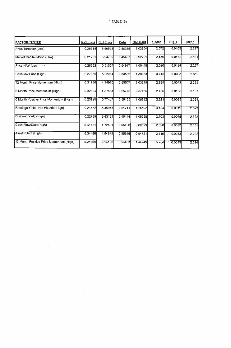
"17 were identified as anomalies. A summary of these factors can be seen
in Table (B) at a confidence interval of 98% the number of factors identified
as anomalies is reduced to 12, these can be seen in Table (C).
If one considers the anomalies at the 95% and 98% confidence interval,
four distinct categories emerge. Factors associated with high momentum,
factors associated with low value, factors associated with small size and
other factors.

University of Natal (Durban)Graduate School of Business
Value Factors
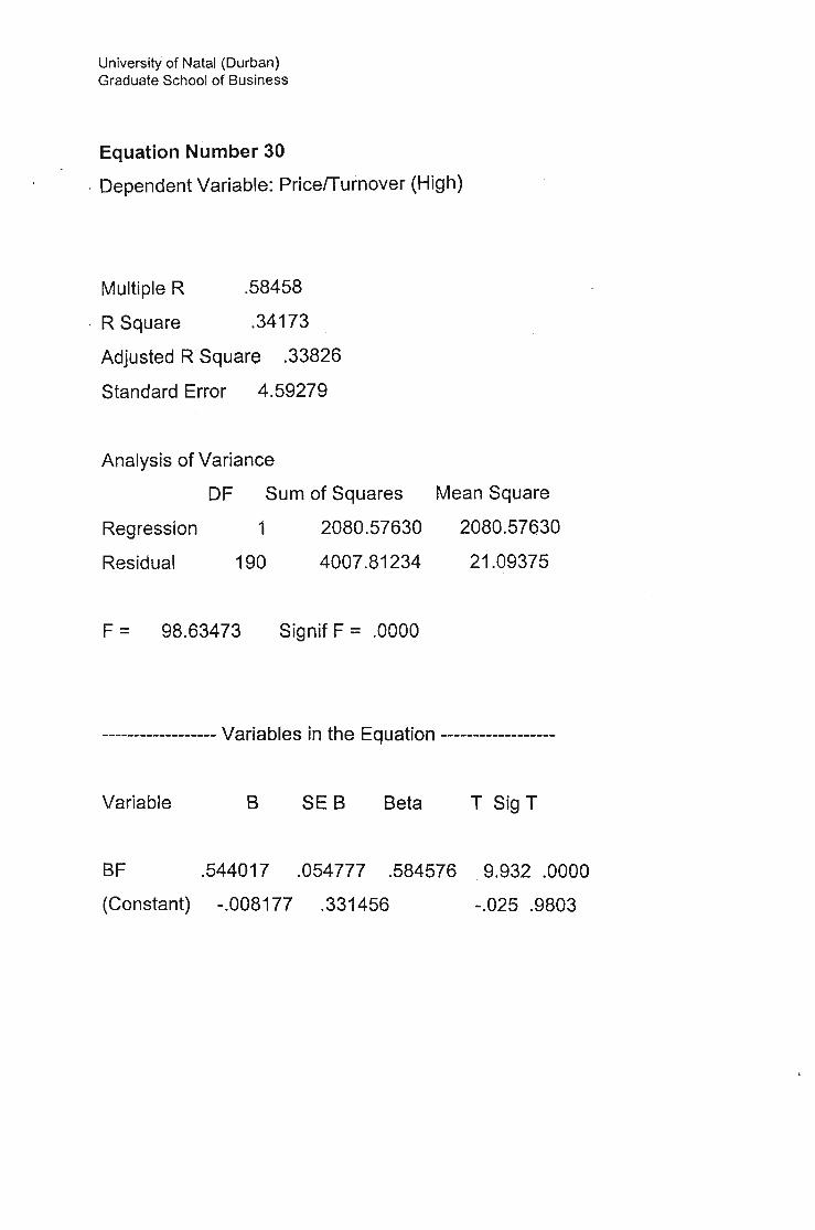
Price I Turnover
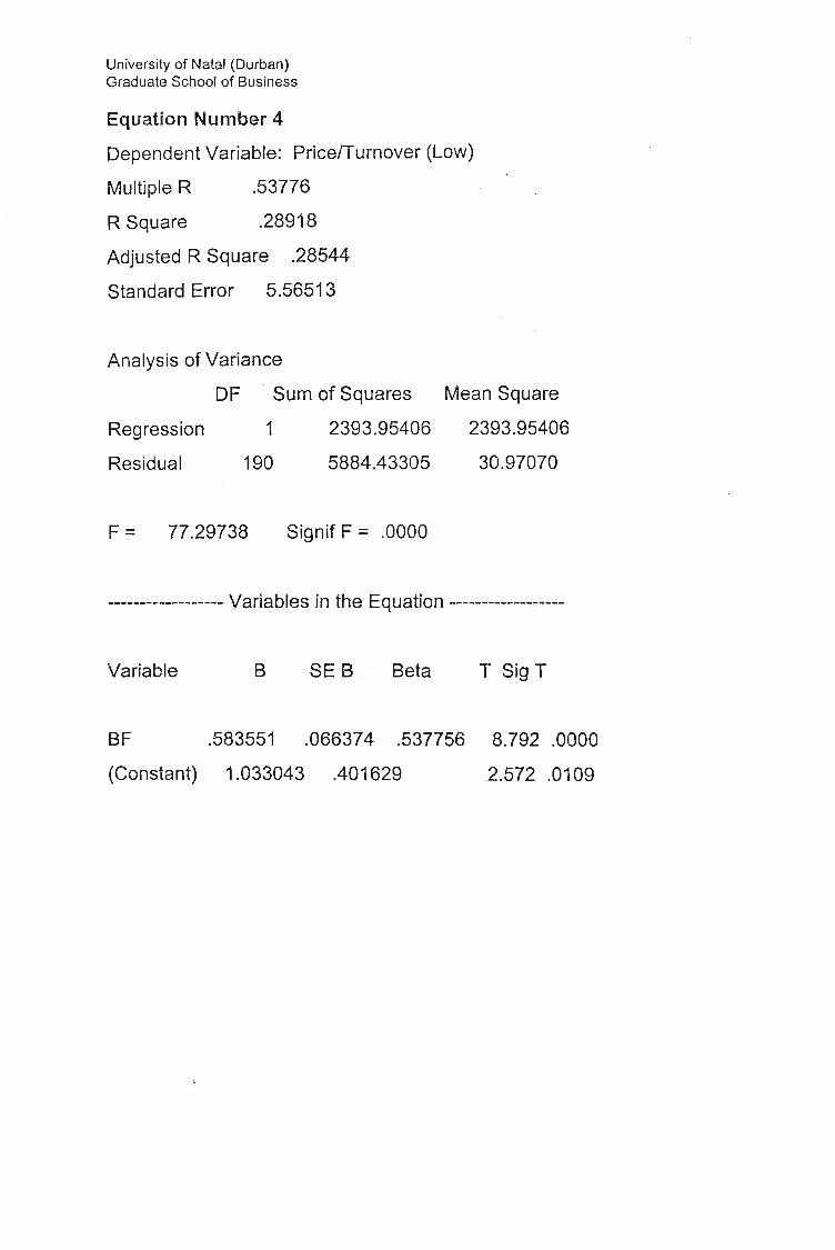
The first of the value factors tried was price/turnover.
It was found that share with a low price per Rand of turnover managed
to achieve a 1.033% return . premium over the market as a whole. This
further supports the earlier findings of Bradfield, Barr and Affleck-Graves,
who found both size and value to be strong factors in explaining the cross-
section of returns. The mean monthly return for shares selected based on
low price/turnover was 2.287% which equates to an annual return of in the
region of 27.44% over the 16 year period. The Beta of this portfolio is
0.58355, which is slightly above the average Beta of shares on the
industrial index of 0.53. This is to be expected as value shares generally
represent the more risky securities on the market.
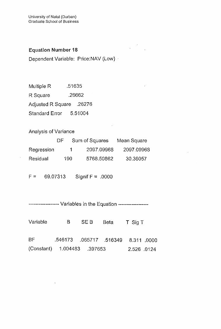
Price: NAV
The second of the value factors was Price: Net Asset Value.
Again · it was found that shares with low price in relation to their NAV
produced a premium over and above that explained by the CAPM. In this
case a premium of 1.004 was found at a confidence interval of 98.5%. The

University of Natal (Durban)Graduate School of Business
average return on such a portfolio was 2.237% per month or 26,84%
annually over the 16 year period. The Beta for this portfolio was again
marginally higher than the Beta for the industrial index as a whole.
Interestingly it was found that the opposite effect was not found when one
considered the high value shares. Thus when one looked at those shares
. with a high price to turnover ratio or high price to NAV it was found that
these share returns behaved very much in line with the CAPM.
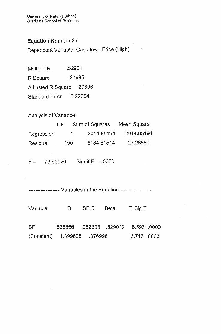
Cash-flow:Price
The third of the value factors which came up as an anomaly was cash-
f1ow:price. In this case it was found that share with high cash-flow in
relation to their price, (thus low price:cash-flow) produced excess returns of
1.4% over and above those predicted by the CAPM. Of all the value factors
tested this one proved to be the most conclusive anomaly with a
significance level of 99.97%. The mean monthly returns on this portfolio
were 2.625 or 31.5% on an annual basis, with a Beta of only 53.536% a
portfolio of shares with high cash-flow to price ratio would have produced a
very high return at a relatively low risk over the last 16 years.
University of Natal (Durban)Gradua te School of Business
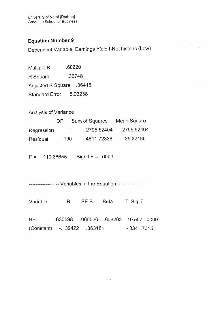
Earnings Yield
The fourth of the value factors at the 95% confidence interval was the
Earnings yield , this is a measure of a companies earnings in relation to its
share price. As expected those companies with low price in relation to their
earnings (value companies), those with high earnings yield, produced
excess returns other than those explained by the CAPM. Excess returns of
1.25% were earned by the portfolio of companies weighted on the basis of
high earnings yield . The mean return on such a portfolio was 2.523% or
30.28% on an annual basis, the Beta on such a portfolio was 0.5174 or
slightly less than the industrial index average. The significance of the
portfolio was again high with a confidence level of 99.81%.
Dividend yield
The last of the value factors to show an anomaly at the 95% confidence
level was dividend yield. A measure of a companies dividend payout in
relation to its market price. A portfolio of shares with high dividend yields
would have gained an investor excess returns of 1.059% over and above
those expected under the CAPM. While not as strong an indicator of value
as the other factors considered the significance at a level of over 99% was
still very high. Mean returns on a portfolio thus weighted would have been
2.322% per month or 27.86% per annum over the last 16 years. The Beta
University of Natal (Durban)Graduate School of Business
on this portfolio was .48444 one of the lowest Beta 's of the portfolios
tested.
Overall the evidence collected further substantiates research carried out
bot locally and internationally, with reguard to value shares. It is possible
for one to obtain excess returns by investing in 'value' shares, furthermore
the evidence suggests that the best means of assessing 'value' is through
the cash-fJow:price ratio and earnings yield.
Investing in 'non-value' shares did not however lead to returns less than
those expected in terms of the CAPM.
University of Natal (Durban)Graduate School of Business
Size Factors
The second factor identified by Bradfield, Barr and Affleck-Graves, as an
anomaly to the CAPM in the South African context was size. It was
discovered that smaller firms tended to make better returns than their
larger counterparts.
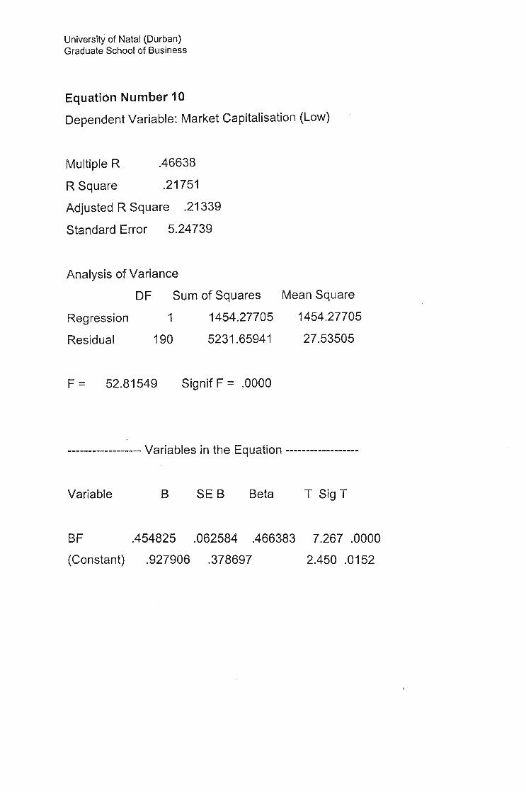
Market Capitalisation
Market capitalisation was used as the primary measure of size for the
purposes of this research. It was found that excess returns of 0.92791 %
could be obtained by investing in a portfolio of low market capitalisation
shares. This was very much in line with the conclusions drawn by Bradfield,
Barr and Affleck-Graves. The Beta of such a portfolio was 0.45483 and the
mean monthly returns earned was 2.161 or 25.932% on an annual basis.
University of Natal (Durban)Graduate School of Business
Other factors
Other factors, these were factors that did not fit into any of the other three
categories. Interestingly three of the four factors relate to accounting
measures of solvency and liquidity and could be categorised as
representing the perceived financial risk of the business.
Cash-flow/Debt
A high cash-flow/debt was found to be a strong anomaly. Thus shares with
good cash-flow or low debt generated excess returns on the CAPM. A
portfolio of such shares would produce a mean monthly return of 2.151% at
a beta of 0.654, this would equate to an excess monthly return of 0.896%
on those predicted by the CAPM at a confidence level of 99.1%.
Assets/debt
Again with assets to debt it was found that shares with hlqh assets to debt
ratio's produced excess returns on those predicted under the CAPM. In this
case monthly returns of 2.02% could be made at a beta of 0.556, an
excess return of 0.947% on that predicted by the CAPM. The confidence
level for such excess returns was 99.4%.

University of Natal (Durban)Graduate School of Business
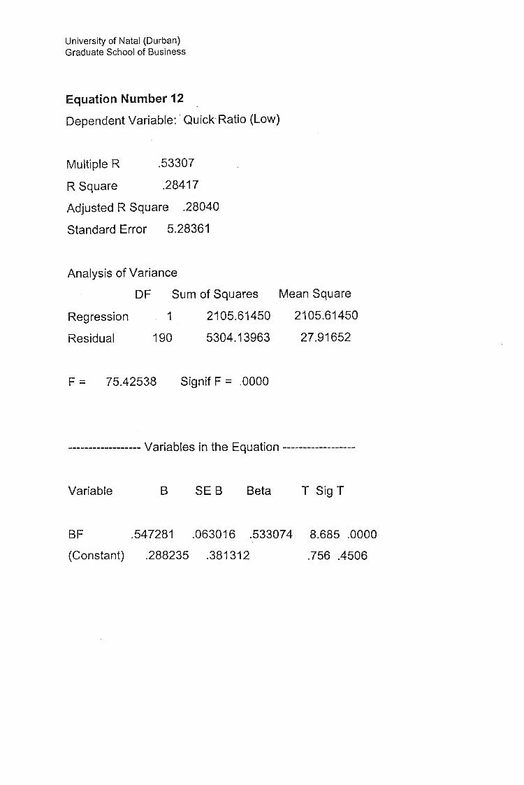
Quick Ratio
The final of the three financial risk indicators which proved to be an
anomaly was the quick ratio. It was found that a portfolio of shares chosen
on the basis of a high quick ratio (liquidity level) would outperform the
CAPM by 0.69%, at a confidence level of 96%, offering monthly returns of
1.94% at a beta of 0.488.
Trade-ability
The last of the four other factors found to be an anomaly was trade-ability.
It was found that share with a low trade-ability (shares which were not
traded often) produced excess returns on the CAPM. This was not
unexpected as the price of such shares would not be a true reflection of
their value due to the fact that they were not being traded. A portfolio of
such shares would offer monthly returns of 1.956% at a beta of 0.388.

University of Natal (Durban)Graduate School of Business
Momentum
In an effort to corroborate the earlier study by Fraser and Page (1999),
which found that shares with higher momentum tended to produce higher
returns than those forecast under the CAPM, a number of momentum
based factors were tested.
These included factors measuring 1 month, 3 months, 6 months, 12
months and 24 months momentum. The objective of studying these factors
was to discover firstly whether momentum was an anomaly, and secondly if
it is which measure of momentum produced the greatest excess returns.
A second set of factors comprising shares ranked by positive momentum
only was also introduced for each of the time periods. The results of the
regression of these factors against the market can be seen in Table (0),
although both high momentum and low momentum was tested for as can
be seen in Table (A) all factors involving low momentum produced negative
results when testing for anomalies and so no further consideration is given
to them.

University of Natal (Durban)Graduate School of Business
Results of high momentum strategies
1 month price momentum
1 month positive price momentum, was proved to not be an anomaly with
only a 9% significance level and a very low constant of only 0.042.This is in
line with the results obtained by Fraser and Page which suggested that
only long term momentum held any additional explanatory power over the
CAPM.
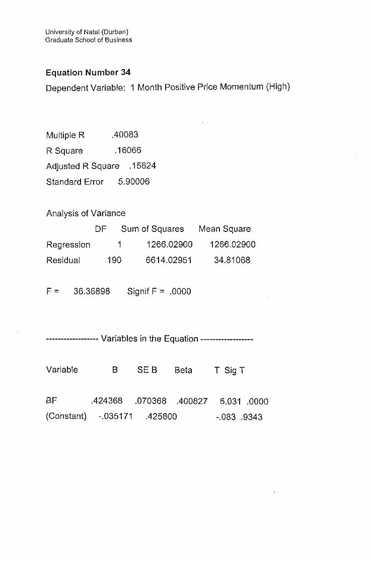
1 Month positive price momentum
As expected like 1 month price momentum, 1 month positive price
momentum was also show to be a factor which held no additional
explanatory power over the CAPM. Interestingly its level of significance
was even lower than that of the one month price momentum at only 7%
and its constant was a Negative one at -0.04.
3 Month price momentum
Although the evidence was not sufficient to warrant calling 3 month price
momentum and anomaly, it level of significance was far higher than that
obtained on the 1 month strategies. The confidence interval moved from
less than 10% for the one month strategies to over 80% for 3 Months, the
value of its constant also increased to 0.45.

University of Natal (Durban)Graduate School of Business
3 Month positive price momentum
Similar to the one month momentum factors the 3 month positive price
momentum was outperformed by 3 month price momentum. It had a level
of significance of close on 75% and a constant of 1.1. Again there was a
noticeable improvement on the results obtained using the 1 month
strategies.
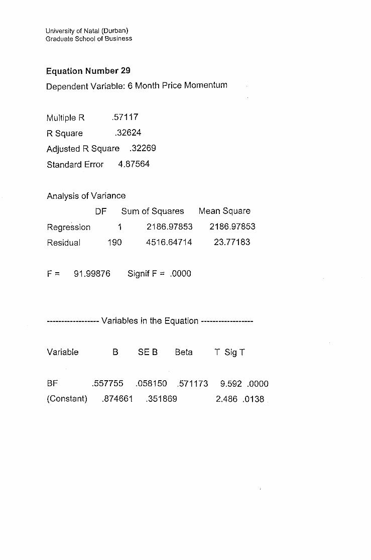
6 Month price momentum
When extending the analysis to shares showing high momentum over a six
month period the first of the momentum anomalies was found. The level of
significance was 98%, and a portfolio of shares purchased using high six
month momentum as its determining factor would have produced excess
returns on the CAPM of 0.88%. The beta of such a portfolio would have
been 0.55 which is a medium risk portfolio and the mean gross return on
such a portfolio would have been 2.137% per month over the period 1983-
1999.

University of Natal (Durban)Graduate School of Business
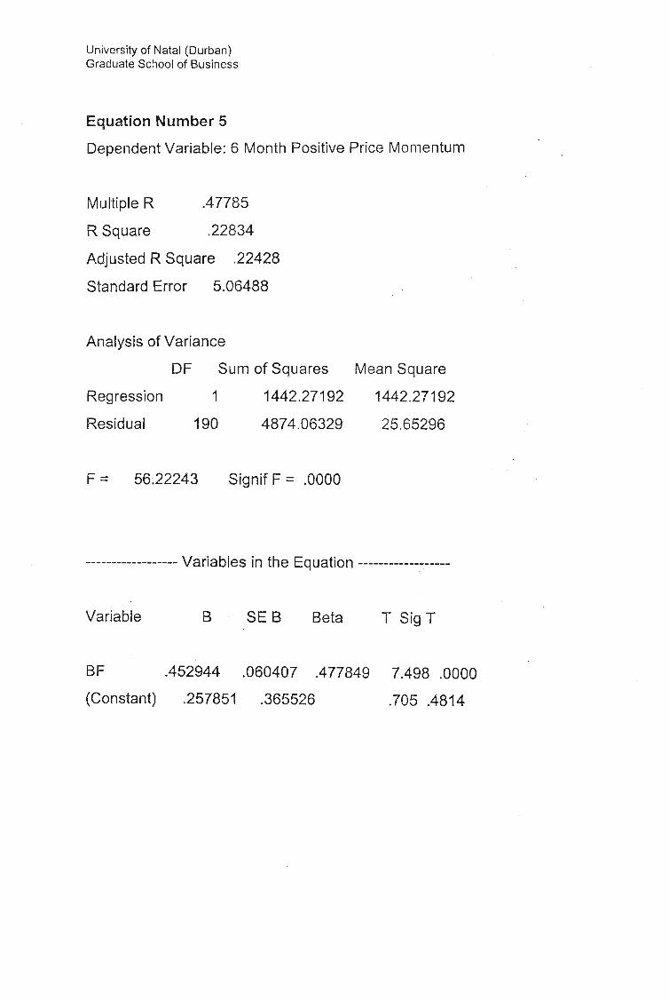
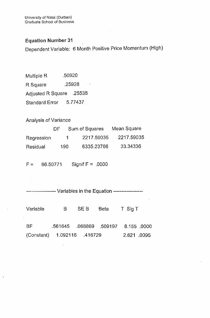
6 Month positive price momentum.
With the 6 month momentum factors the positive momentum, proved to be
more of an anomaly than the ordinary price momentum, with a 99%
significance level. The excess returns over the CAPM (constant) was 1.09
and the beta of this portfolio was 0.56. The average monthly return on such
a portfolio was 2.354% over the 16 year period.
12 month price momentum
The 12 month momentum strategies proved to be the strongest of all the
momentum strategies tested. 12 month price momentum had a constant of
1.033 at a confidence level of 99.5%, a definite anomaly. A portfolio of
shares based on high 12 month price momentum would net a monthly
return of 2.28% and have a beta 0.55.
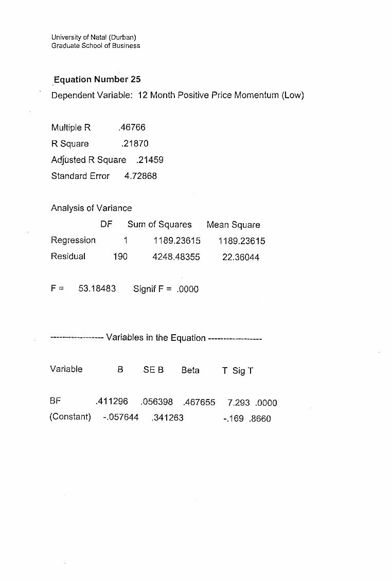
12 Month positive price momentum
Of all the factors tested, including the momentum factors, 12 month
positive price momentum proved to be the strongest anomaly discovered. It
had a constant of 1.44 at a 99.9% level of significance, producing monthly
mean returns of 2.694 at a beta of only 0.534. Thus by investing in a

University of Natal (Durban)Graduate School of Business
portfolio of shares based on high 12 month positive price momentum and
investor could expect to outperform the CAPM by 1.44% monthly.
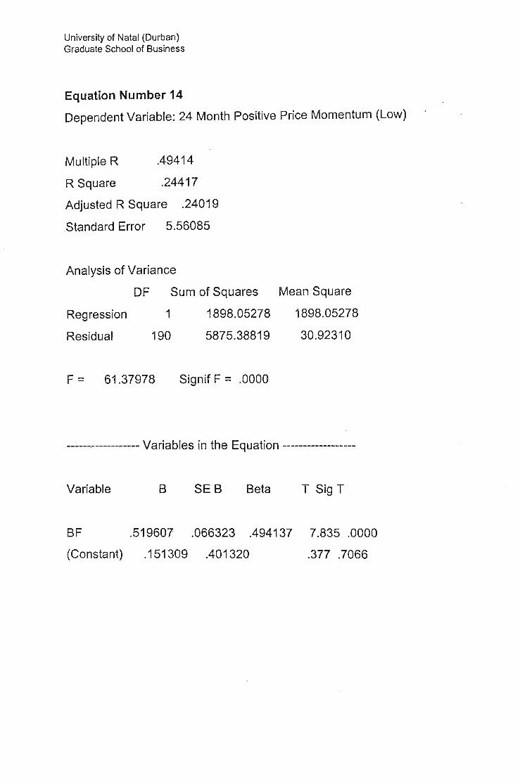
24 Month price momentum and 24 month positive price momentum
24 Month price momentum, proved to be an anomaly at the 95% level of
significance. The mean for this data set was 1.909% at a beta level 0.5349.
The level of significance was 95.9%, providing increased returns on the
CAPM of 0.65420%. As an anomaly 24 month momentum was slightly less
significant than 6 month price momentum but more significant than 3 month
strategies. Interestingly the data obtained from testing 24 month positive
price momentum was identical to that obtained from 24 month price
momentum, therefore these results have not been recorded separately.
Summary of momentum strategies
The results of the testing of the various momentum strategies as shown in
table (0), based on JSE industrial stocks, are very much in line with the
results obtained by leading American research into momentum strategies.
Of all the momentum strategies tested 12 month positive price momentum
proved to be the strongest anomaly followed by 12 month price
momentum, and the 6 month momentum strategies. Thus if one is to use
momentum to earn excess returns on the JSE industrial shares 12 month

Univers ity of Natal (Durban)Graduate School of Business
positive price momentum would be the best factor to use to determine such
momentum. In terms of the 98% confidence interval used to determine an
anomaly both the 12 and 6 month strategies were identified as anomalies.
The graph in appendix (C) shows the various strengths of the momentum
strategies tested, the 6, 12 and 24 month strategies all showed strongly.

University of Natal (Durban)Graduate School of Business
Conclusion
The Capital Asset Pricing Model, first proposed by Sharpe (1964), has
been the cornerstone of academic study into asset pricing. The appeal of
this model lies in its postulation of a simple measurable relationship
between risk and return. Although the key variables can be easily obtained,
there has particularly in the South African context been very little in the way
of empirical studies into the effectiveness of the Model.
South African Research has to a large extent been led by that carried out in
foreign markets, particularly the US market. The majority of research
carried out to date has focused on one or two perceived anomalies, which
have been tested with the results proving largely inconclusive. The reasons
for this can be attributed to the lack of data available on which to conduct
such research. The availability of such data in this case has enabled a far
more comprehensive study of the Capital Asset Pricing Model and its ability
to accurately predict returns on the JSE industrial index.
At the predefined confidence level of 98%, 12 anomalies were identified.
Bye further extending the analysis to a 95% level of confidence a further 5

University of Natal (Durban)Graduate School of Business
anomalies were identified giving a total of 17 anomalies. These anomalies
could be broken down into four cateqories, value, size momentum and
other factors .
. The results obtained and discussed earlier fall very much in line with those
obtained in leading international empirical research. Essentially what these
results mean is that an investor can earn a greater return at the same level
of risk by investing in a portfolio of shares weighted by the 17 factors
identified.
If one assumes that investors are compensated for additional systematic
risk based on the beta of their portfolio, then it is possible for such investors
to make a seemingly risk-less profit by investing in a portfolio weighted by
the anomalies identified. By doing so they are able to achieve a portfolio
with the same Beta as their current portfolio, yet which offers a higher
return.
Of the factors tested the strongest anomalies found were those of 1 year
positive price momentum and the ratio of cashflow:price.
What does this mean for the CAPM? For some time it has been suggested
both by academics and investment managers that the assumptions of the
University of Natal (Durban)Graduate School of Business
model are too restrictive, .as a result of which the model cannot really be
tested empirically. Many investment managers find it difficult to believe that
risk can be fully captured in a single factor, sensitivity to the market.
Alternative models to the CAPM have been suggested, foremost among
these is Arbitrage Pricing Theory (APT) devised by 8teven Ross (1977).
Ross suggested that returns vary from suggested levels because of
unanticipated changes in production, inflation, term structure and other
basic economic forces. Then assuming that decision makers take
advantage of all arbitrage opportunities to hold portfolios that offer higher
returns, Ross built a model of risk and return based on an assets sensitivity
to these factors.
Practically .however APT has not taken off, due to the fact that unlike the
CAPM one cannot easily identify the factors which influence risk. It seems
that a multi-factor model is called for however, the identification of what
factors to include and how they should relate to one another is the
stumbling block which currently prevents such models from being applied.
Thus it appears that although empirical evidence may suggest that the
Capital Asset Pricing Model has its shortcomings, as an academic model of

University of Natal (Durban)Graduate School of Business
the relationship between risk and return it will be with us for sometime yet.
The simplicity with which it can be used to predict portfolio returns makes it
a useful tool and ready starting point for investment analysis.
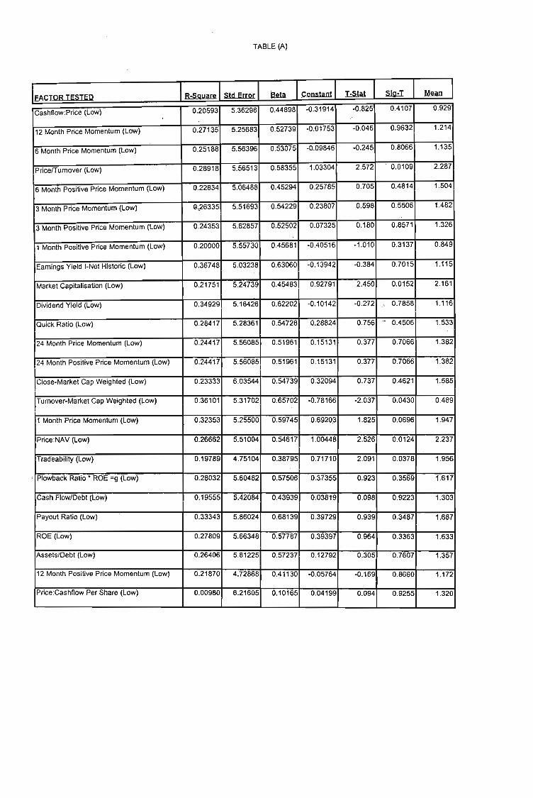
TABLE (A)
IConstant I !:Sja1 I ID9=! I ~ IIR-SQuare IStd Error IIFACTOR TESTED
Cashfiow:Price (Low) 0.20593 5.36298 0.44898 -0.31914 -0.825 0.4107 0.929
12 Month Price Momentum (Low) 0.27135 5.25683 0.52739 -0.01753 -0.046 0.9632 1.214
6 Month Price Momentum (Low) 0.25188 5.56396 0.53075 -0.09846 -0.245 0.8066 1.135
PricelTurnover (Low) 0.28918 5.56513 0.58355 1.03304 2.572 0.0109 2.287
6 Month Positive Price Momentum (Low) 0.22834 5.06488 0.45294 0.25785 0.705 0.4814 1.504
3 Month Price Momentum (Low) G,26335 5.51693 0.54229 0.23807 0.598 0.5506 1.482
3 Month Positive Price Momentum (Low) 0.24353 5.62857 0.52502 0.07325 0.180 0.8571 1.326
1 Month Positive Price Momentum (Low) 0.20000 5.55730 0.45681 ·0.40516 -1.010 0.3137 0.849
Earnings Yield I-Net Historic (Low) 0.36748 5.03238 0.63060 -0.13942 -0.384 0.70 15 1.115
Market Capitalisation (Low) 0.21751 5.24739 0.45483 0.92791 2.450 0.0152 2.161
Dividend Yield (Low) 0.34929 5.16426 0.62202 -0.10142 -0.272 . . 0.7858 1.116
Quick Ratio (Low) 0.28417 5.28361 0.54728 0.28824 0.756 - 0.4506 1.533
24 Month Price Momentum (Low) 0.24417 5.56085 0.51961 0.15131 0.377 0.7066 1.382
24 Month Positive Price Momentum (Low) 0.24417 5.56085 0.51961 0.15131 0.377 0.7066 1.382
Close-Market Cap Weighted (Low) 0.23333 6.03544 0.54739 0.32094 0.737 0.4621 1.585
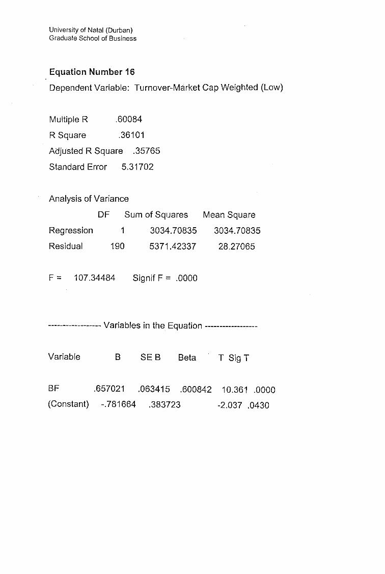
Turnover-Market Cap Weighted (Low) 0.36101 5.31702 0.65702 -0.78166 -2.037 0.0430 0.489
1 Month Price Momentum (Low) 0.32353 5.25500 0.59745 0.69203 1.825 0.0696 1.947
Price:NAV (Low) 0.26662 5.51004 0.54617 1.00448 2.526 0.0124 2.237
Tradeability (Low) 0.19789 4.75104 0.38795 0.71710 2.091 0.0378 1.956
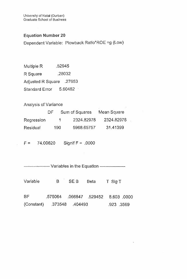
, Plowback Ratio' ROE =g (Low) 0.28032 5.60482 0.57506 0.37355 0.923 0.3569 1.617
Cash Flow/Debt (Low) 0.19555 5.42084 0.43939 0.03819 0.098 0.9223 1.303
Payout Ratio (Low) 0.33343 5.86024 0.68139 0.39729 0.939 0.3487 1.687
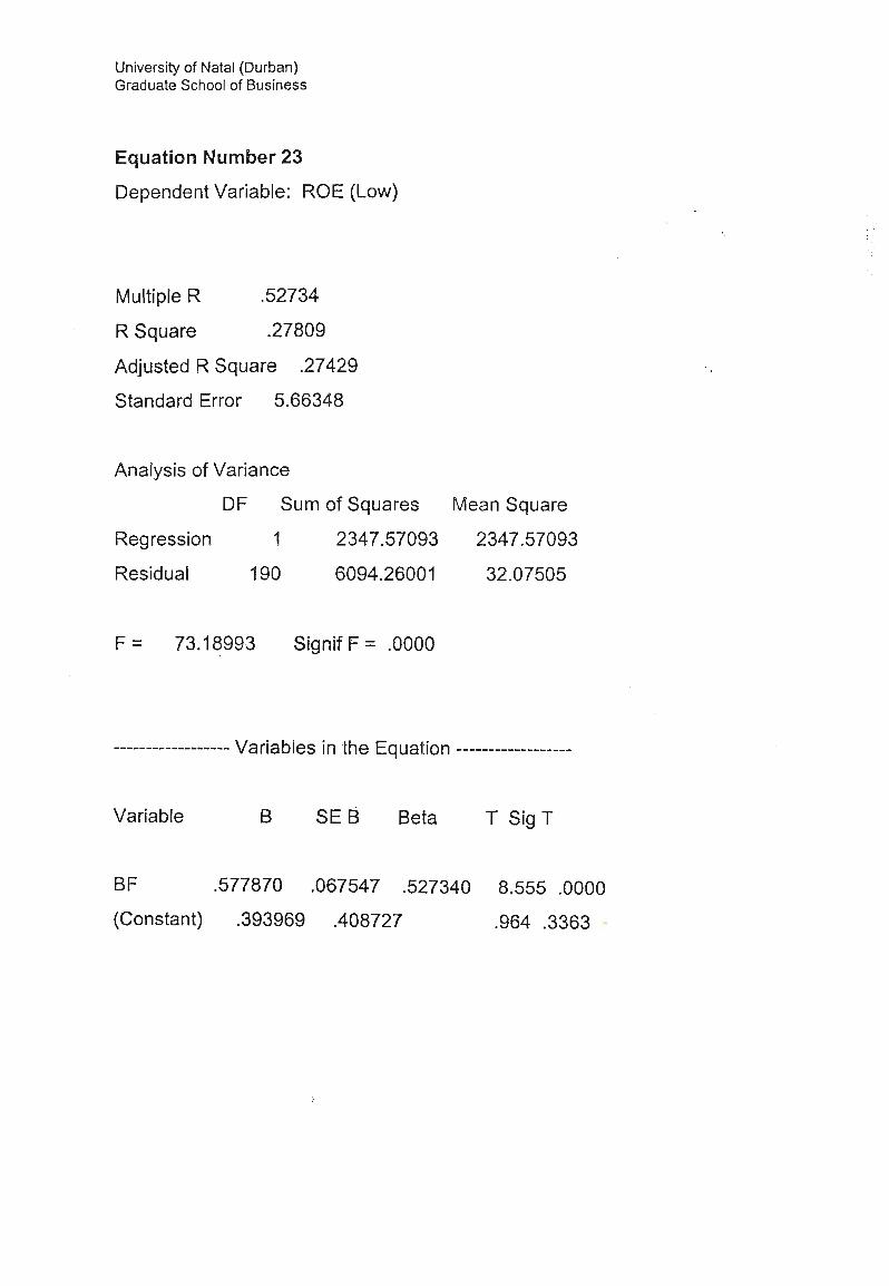
ROE (Low) 0.27809 5.66348 0.57787 0.39397 0.964 0.3363 1.633
Assets/Debt (Low) 0.26406 5.81225 0.57237 0.12792 0.305 0.7607 1.357
12 Month Positive Price Momentum (Low) 0.21870 4.72868 0.41130 -0.05764 -0.169 0.8660 1.172
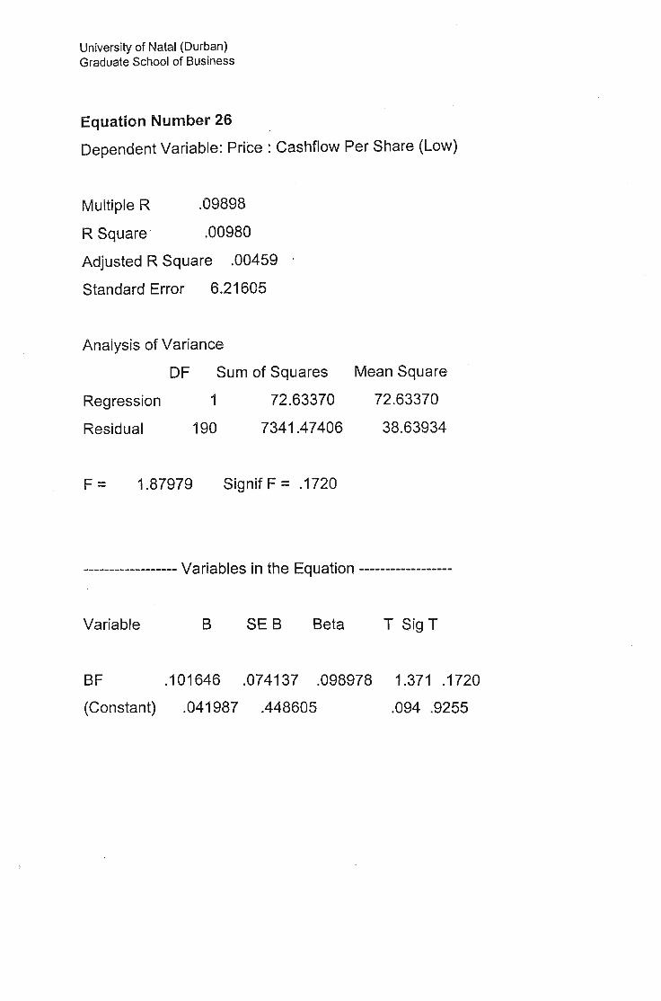
Price:Cashfiow Per Share (Low) 0.00980 6.21605 0.10165 0.04199 0.094 0.9255 1.320
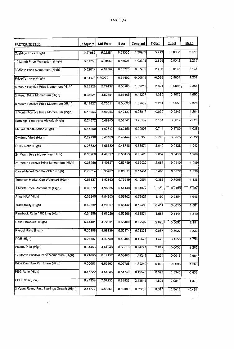
TABLE (A)
FACTOR TESTED R-SQyare Std Error em Constant I:Sta.t Sl9=I Mean
Cashflow ;Price (High) 0.27985 5.22384 0.53536 1.39983 3.713 0.0003 2.652
12 Month Price Momentum (High) 0.31756 4.94960 0.55507 1.03398 2.895 0.0042 2.288
6 Month Price Momentum (High) 0.32624 4.87564 0.55776 0.87466 2.486 0.0138 2.137
Price/Turnover (High) 0.34173 4,59279 0.54402 -0.00818 -0.025 0.9803 1.231
6 Month Positive Price Momentum (High) 0.25928 5.77437 0.56165 1.09212 2.621 0.0095 2.354
3 Month Price Momentum (High) 0.34021 4.52401 0.53406 0.45227 1.385 0.1676 1.690
3 Month Positive Price Momentum (High) 0.18627 6.75011 0.53093 1.09669 2.251 0.2550 2.328
1 Month Positive Price Momentum (High) 0.16066 5.90006 0.42437 -0.03517 -0.830 0.9343 1.204
Earnings Yield I-Net Historic (High) 0.24672 5.49943 0.51741 1.25162 3.154 0.0019 2.523
Market Capitalisation (High) 0.46260 4.07517 0.62158 -0.20907 -0.711 0.4780 1.038
Dividend Yield (High) 0.22739 5.43163 0.48444 1.05958 2.703 0.0075 2.322-
Quick Ratio (High) 0.28632 4.68532 0.48788 0.68974 2.040 0.0428 1.943
24 Month Price Momentum (High) 0.35260 4.40627 0.53459 0.65420 2.057 0.0410 1.909
24 Month Posit ive Price Momentum (High) 0.35260 4.40627 0.53459 0.65420 2.057 0.0410 1.909
Close-Market Cap Weighted (High) 0.78054 3.93762 0.8083 1 0.11461 0.403 0.6872 1.338
Turnover-Market Cap Weighted (High) 0.57827 3.93853 0.75819 0.10951 0.385 0.7005 1.336
1 Month Price Momentum (High) 0.30372 4.98685 0.54146 0.04072 0.113 0.9100 1.287
Price:NAV (High) 0.35246 4.54303 0.55102 0.39027 1.190 0.2354 1.649
Tradeability (High) 0.49332 4.20067 0.68142 0.12463 0.411 0.6815 1.381
Plowback Ratio· ROE =g (High) 0.31658 4.68029 0.52368 0.53574 1.586 0.1144 1.819
Cash Flow/Debt (High) 0.41481 4.72501 0.65400 0.89599 2.628 0.0093 2.151
Payout Ratio (High) 0.30908 4.58136 0.50374 0.28326 0.857 0.3927 1.533
ROE (High) 0.28807 4.43750 0.46405 0.45673 1.426 0.1555 1.730
Assets/Debt (High) 0.34466 4.64648 0.55516 0.94721 2.819 0.0053 2.202
12 Month Positive Price Momentum (High) 0.21860 6.14152 0.53403 1.44243 3.254 0.0013 2.694
Price;Cashflow Per Share (Hi9h) 0.00067 6.52967 -0.02788 1.30249 0.000 0.9998 1.266
PEG Ratio (High) 0.45729 4.51285 0.54740 0.49578 0.628 0.5345 -0.635
PEG Ratio (Low) 0.27939 7.57233 0.61923 2.43649 1.804 0.0810 1.370
2 Years Rolled Past Earnings Growth (High) 0.48773 4.83860 0.62389 0.52265 0.617 0.5413 -0.484

TABLE (A)
FACTOR TESTED R-5Qyare Std Error am Constant !=SW .slll:I M9n2 Years Rolled Past .Earnings Growth (Low) 0.14694 7.37134 0.40427 1.80396 1.399 0.1715 1.172
Expected 1 Years Earnings Growth (High) 0.32231 6.09572 0.55550 1.82070 1.707 0.0974 0.971
Expected 1 Years Earnings Growth (Low) 0.08717 7.06558 0.28852 0.93259 0.754 0.4561 0.492
IFACTOR TESTED
· TABLE (B)
IR-Slluare IStd Error I IConstant I Hlat I S19=I I Mnn IPrice/Turnover (Low) 0.28918 5.56513 0.58355 1.03304 2.572 0.0109 2.287
Market Cap italisation (Low) 0.21751 5.24739 0.45483 0.92791 2.450 0.0152 2.161
Price :NAV (Low) 0.26662 5.51004 0.54617 1.00448 2.526 0.0124 2.237
Cashflow:Price (High) 0 .27985 5.22384 0.53536 1.39983 3.713 0.0003 2.652
'12 Month Price Momentum (High) 0.31756 4.94960 0.55507 1.03398 2.895 0.0042 2.288
6 Month Price Momentum (High) 0.32624 4.87564 0.55776 0.87466 2.486 0.0138 2.137
6 Month Positive Price Momentum (High) 0.25928 5.77437 0.56165 1.09212 2.621 0.0095 2.354
Earnings Yield l-Net Historic (High) 0.24672 5.49943 0.51741 1.25162 3.154 0.0019 2.523
Dividend Yield (High) 0.22739 5.43163 0.48444 1.05958 2.703 0.0075 2.322
Cash Flow/Debt (High) 0.41481 4.72501 0.65400 0.89599 2.628 0.0093 2.151
Assets/Debt (High) 0.34466 4.64648 0.55516 0.94721 2.819 ~ 0.0053 2.202
12 Month Positive Price Momentum (High) 0.21860 6.14152 0.53403 1.44243 3.254 - 0.0013 2.694

TABLE (C)
IConstand I:Sla1 I ID9=! I Mnn IIR-SQuare IStd Error I -PricefTurnover (Low) 0.28918 5.56513 0.58355 1.03304 2.572 0.0109 2.287
Market Capitalisation (Low) 0.21751 5.24739 0.45483 0.92791 2.450 0.0152 2.161
Price:NAV (Low) 0.26662 5.51004 0.54617 1.00448 2.526 0.012'; 2.237
Cashflow:Price (High) 0.27985 5.22384 0.53536 1.39983 3.713 0.0003 2.652
12 Month Price Momentum (High) 0.31756 4.94960 0.55507 1.03398 2.895 0.0042 2.288
6 Month Price Momentum (High) 0.32624 4.87564 0.55776 0.87466 2.486 0.0138 2.137
6 Month Positive Price Momentum (High) 0.25928 5.77437 0.56165 1.09212 2.621 0.0095 2.354
Earnings Yield I-Net Historic (High) 0.24672 5.49943 0.51741 1.25162 3.154 0.0019 2.523
Dividend Yield (High) 0.22739 5.43163 0.48444 1.05958 2.703 0.0075 2.322
Cash Flow/Debt (High) 0.41481 4.72501 0.65400 0.89599 2.628 0.0093 2.151
Assets/Debt (High) 0.34466 4.64648 0.55516 0.94721 2.819 0 0.0053 2.202
12 Month Positive Price Momentum (High) 0.21860 6.14152 0.53403 1.44243 3.254 0.0013 2.694
Quick Ratio (High) 0.28632 4.68532 0.48788 0.68974 2.040 0.0428 1.943
24 Month Price Momentum (High) 0.35260 4.40627 0.53459 0.65420 2.057 0.0410 1.909
24 Month Positive Price Momentum (High) 0.35260 4.40627 0.53459 0.65420 2.057 0.0410 1.909
Tradeability (Low) 0.19789 4.75104 0.38795 0.71710 2.091 0.0378 1.956
Turnover-Market Cap Weighted (Low) 0.36101 5.31702 0.65702 -0.78166 -2.037 0.0430 0.489
IFACTOR TESTED
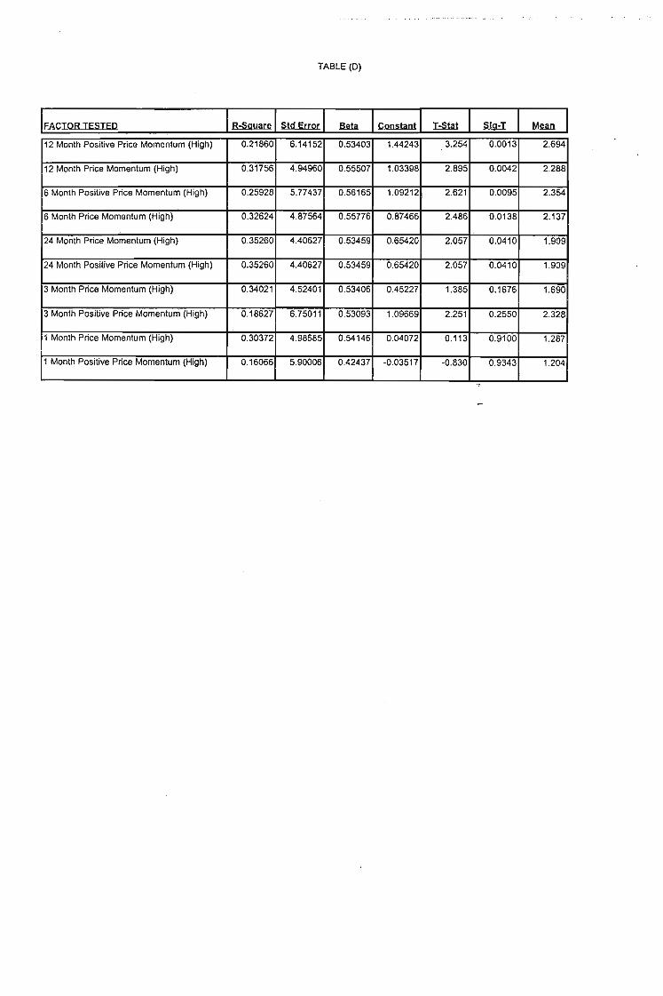
TABLE (D)
IConstant I H1a1 I ~ I ~ IIR-SQuare IStd Error I -12 Month Positive Price Momentum (High) 0.21860 6.14152 0.53403 1.44243 3.254 0.0013 2.694
12 Month Price Momentum (High) 0.31756 4.94960 0.55507 1.03398 2.895 0.0042 2.288
6 Month Positive Price Momentum (High) 0.25928 5.77437 0.56165 1.09212 2.62 1 0.0095 2.354
6 Month Price Momentum (High) 0.32624 4.87564 0.55776 0.87466 2.486 0.0138 2.137
24 Month Price Momentum (High) 0.35260 4.40627 0.53459 0.65420 2.057 0.0410 1.909
24 Month Positive Price Momentum (High) 0.35260 4.40627 0.53459 0.65420 2.057 0.0410 1.909
3 Month Price Momentum (High) 0.34021 4.52401 0.53406 0.45227 1.385 0.1676 1.690
3 Month Positive Price Momentum (High) 0.18627 6.75011 0.53093 1.09669 2.251 0.2550 2.328
1 Month Price Momentum (High) 0.30372 4.98685 0.54146 0.04072 0.113 0.9100 1.287
1 Month Positive Price Momentum (High) 0.16066 5.90006 0.42437 -0.03517 -0.830 0.9343 1.204
..
IFACTOR TESTED

APPENDIX A
FACTOR TESTED1 to..."./ CF:PR1CE (INDUSTRiALS ONLY)2 LOW 12 MONTHPRICEMOMENTUM (iNDUSTRiALS ONlYi3 lOW 6 MONTHPRICEMOMENTUM (INDUSTRIAL ONlYi4 lOW PRiCE/TURNOVER (iNDUSTRIALONLY)5 lOW 6 MONTH PRiCE Mm,JlENTUM (POSiTiVE iNDUSTRIALS ONLY)6 lOW 3 MONTHPRICEt"iOMENTUM (INDUSTRIALS ONLY)7 LOW 3 MONTHPRICEMOMENTUM (pOSITIVE iNDUSTRIALS ONLY)8 lOVV 1 MONTHPRICE MO~"iENTUM (POSITIVE INDUSTRIALS ONLYi9 lOVV EARNiNGS YIELD (I-NET HiSTORiC, INDUSTRIALS ONLV)
10 LOW MARKETCAP (CALCULATED, INDUSTRIALS ONLY)11 LOW DIVIDEND YIELD (INDUSTRIALS ONLY)12 LOW QUICKRATIO (INDUSTRIALS ONLY)13 lOW 24 MONTHPRICEr,,10MENTUM (INDUSTRiALS ONLY)14 LOW 24 MONTHPRICEMOMENTUM (POSITIVE INDUSTRIALS ONLY)15 LOW CLOSE(r..1ARKET CAP VVEIGHTED, INDUSTRIALS ONLY)16 LOW TURNOVER (MARKETCAP WEIGHTED, INDUSTRIALS ONLY)17 LOW 1 MONTHPRICEMOMENTUM (INDUSTRIALS ONLY)18 LOW PRICE:NAV (INDUSTRIALS ONLY)19 lOW TRADEABiUTY (INDUSTRIALS ONLY)20 LOW PLOWBAKRATIO'" ROE =g (INDUSTRIALS ONLY):21 LOW CASH FLOW/DEBT(iNDUSTRIALS ONLY):22 LOW PAYOUTRATIO (INDUSTRiALS ONLY):23 LOW ROE (INDUSTRIALS ONLY):24 LOW ASSETS/DEBT (iNDUSTRIALS ONLY):25 LOW 12 MONTHPRICE f,,10MENTUM (POSITIVE iNDUSTRiALS ONLY)26 LOW PRICE:CASSFLOW PER SHARE27 HiGH CF:PRICE (INDUSTRIALS ONLY)23 HIGH 12 MONTHPRICEMOMENTU~.;i (iNDUSTRIALS ONLY)29 HIGH 6 MONTHPRICEMDr,,1ENTUM (INDUSTRIAL ONLY)30 HiGH PRICEITURNOVER (INDUSTRIAL ONlYi31 HIGH 6 MONTHPRiCE MOMENTUM (POSITIVE iNDUSTRIALS ONLYi32 HIGH 3 MONTHPRICEMOf",1ENTUM (INDUSTRIALS ONLY)33 HiGH 3 MONTHPRiCE MOMENTUM (POSITIVE INDUSTRiALS ONLY)34 HIGH i MONTHPRICE MOMENTUM (POSITIVE INDUSTRiALS ONLY)35 HiGH EARNINGS YiELD (i-NET HISTORIC, iNDUSTRIALS ONLY)36 HIGH MARKETCAP (CALCULATED, INDUSTRIALS ONLY)37 HIGH DiVIDENDYIELD (iNDUSTRiALS ONLY)38 HiGH QUICK RATIO (INDUSTRIALS ONLY)39 HIGH 24 MONTH PRICE MOMENTUM (INDUSTRiALS ONLY)40 HIGH 24 MONTHPRICEMOMENTUM (POSITIVE INDUSTRIALS ONLYi41 HIGH CLOSE (MARKET CAP WEIGHTED, INDUSTRIALS ONLY; .42 HIGH TURNOVER (MARKET CAP WEIGHTED, INDUSTRIALS ONLY)43 HiGH i MONTHPRiCE MOMENTUM (iNDUSTRIALS ONLYi44 HIGH PRICE:NAV (iNDUSTRIALS ONLY) .

45 HIGH TRADEA8lLlTY (iNDUSTRiALS ONL'\'146 HIGH PLOWBAK RATiO'" ROE = 9 (INDUSTRIALS ONLV):47 HIGH CASH Flo\iWDE8T (iNDUSTRIALS ONLY):48 HIGH PAYOUT RATIO (INDUSTRiALS ONLY):49 HIGH ROE (INDUSTRIALS ONLY):50 HIGH ASSETS/DEBT (iNDUSTRiALS ONLY):51 HIGH 12 f·iiONTH PRICE MOMENTUfvI (POSITIVE iNDUSTRIALS ONLY)52 HIGH PRICE:CASSFLOVV PER SHARE53 HIGH PEG RATIO54 LOW PEG RA.TIO55 HIGH 2 YEARS ROLLED PAST EARNINGS GROWTH56 LOW 2 YEARS ROLLED PAST E.1\RNINGS GROiJI.fTH57 HIGH EXPECTED i YEARS EARNINGS GRO\!\JTH58 lOW EXPECTED 1 YEARS EARNiNGS GROi;VTH
University of Natal (Durban)Graduate School of Business
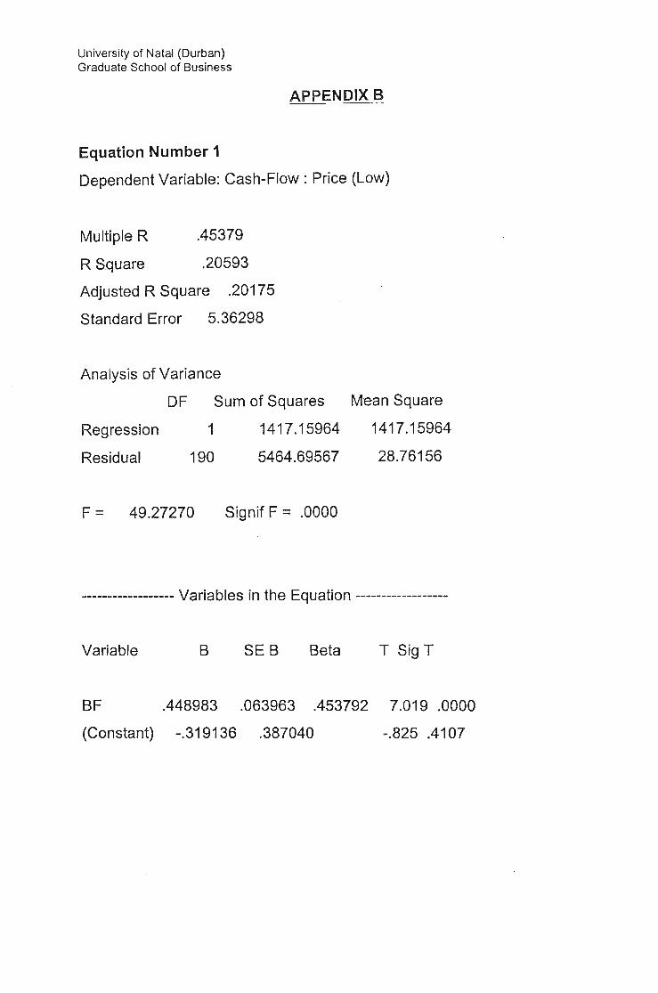
APPENDIX B
Equation Number 1
Dependent Variable: Cash-Flow: Price (Low)
Multiple R .45379
R Square .20593
Adjusted R Square .20175
Standard Error 5.36298
Regression
Residual
Analysis of Variance
OF Sum of Squares
1 1417.15964
190 5464.69567
Mean Square
1417.15964
28.76156
F = 49.27270 Signif F = .0000
------------------ Variables in the Equation ------------------
. Variable B SE B Beta T SigT
BF .448983 .063963 .453792
(Constant) -.319136 .387040
7.019 .0000
-.825 .4107
University of Natal (Durban)Graduate School of Business
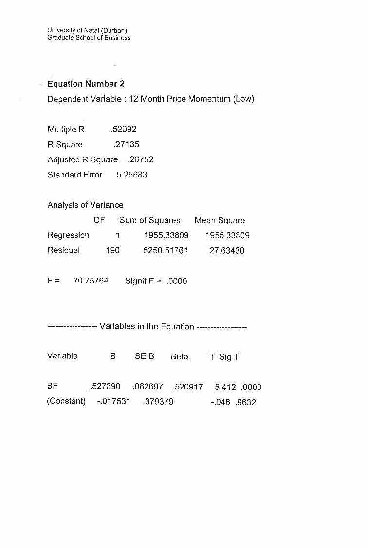
Equation Number 2
Dependent Variable: 12 Month Price Momentum (Low)
Multiple R .52092
R Square .27135
Adjusted R Square .26752
Standard Error 5.25683
Analysis of Variance
OF Sum of Squares
Regression 1 1955.33809
Residual 190 5250.51761
Mean Square
1955.33809
27.63430
F = 70.75764 Signif F = .0000
------------------ Variables in the Equation ------------------
Variable B SE B Beta T Sig T
SF
(Constant)
.527390 .062697 .520917
-.017531 .379379
8.412 .0000
-.046 .9632

University of Natal (Durban)Graduate School of Business
Equation Number 3
Dependent Variable: 6 Month Price Momentum (Low)
Multiple R .50187
R Square .25188
Adjusted R Square .24794
Standard Error 5.56396
Analysis of Variance
OF Sum of Squares Mean Square
Regression
Residual
1
190
1980.31228
5881.95570
1980.31228
30.95766
F = 63.96841 Signif F = .0000
------------------ Variables in the Equation ------------------
Variable B SEB Beta T SigT
SF
(Constant)
.530747 .066360 .501872
-.098462 .401544
7.998 .0000
-.245 .8066
University of Natal (Durban)Graduate School of Business
Equation Number 4
Dependent Variable: PricelTurnover (Low)
Multiple R .53776
R Square .28918
Adjusted R Square .28544
Standard Error 5.56513
Regression
Residual
Analysis of Variance
OF Sum of Squares
1 2393.95406
190 5884.43305
Mean Square
2393.95406
30.97070
F = 77.29738 Signif F = .0000
------------------ Variables in the Equation ------------------
Variable B SE B Beta T SigT
BF
(Constant)
.583551 .066374 .537756
1.033043 .401629
8.792 .0000
2.572 .0109
University of Natal (Durban)Graduate School of Business
Equation Number 5
Dependent Variable: 6 Month Positive Price Momentum
Multiple R .47785
R Square .22834
Adjusted R Square .22428
Standard Error 5.06488
Regression
Residual
Analysis of Variance
OF Sum of Squares
1 1442.27192
190 4874.06329
Mean Square
1442.27192
25.65296
F = 56.22243 Signif F = .0000
------------------ Variables in the Equation ------------~-----
Variable B SE B Beta T Sig T
BF
(Constant)
.452944 .060407 .477849
.257851 .365526
7.498 .0000
.705 .4814

University of Natal (Durban)Graduate School of Business
Equation Number 6
Dependent Variable: 3 Month Price Momentum (Low)
Multiple R .51318
R Square .26335
Adjusted R Square .25947
Standard Error 5.51693
Analysis of Variance
DF Sum of Squares Mean Square
Regression
Residual
1
190
2067.39428
5782.94536
2067.39428
30.43655
F = 67.92471 Signif F = .0000
.;----------------- Variables in the Equation ------------------
Variable B SE B Beta T SigT
BF .542291 .065799 .513177
(Constant) .238070 .398150
8.242 .0000
.598 .5506

University of Natal (Durban)Graduate School of Business
Equation Number 7
Dependent Variable: 3 Month Positive Price Momentum (Low)
Multiple R .49349
R Square .24353
Adjusted R Square .23955
Standard Error 5.62857
Reqression
Residual
Analysis of Variance
OF Sum of Squares
1 1937.81512
190 6019.34197
F = 61.16696 . Signif F = .0000
Mean Square
1937.81512
31.68075
------------------ Variables in the Equation ------------------
Variable B SEB Beta T SigT
SF
(Constant)
.525021 .067130 .493489
.073246 .406207
7.821 .0000
.180 .8571

University of Natal (Durban)Graduate School of Business
Equation Number 8
Dependent Variable: 1 Month Positive Price Momentum (Low)
Multiple R .44722
R Square .20000
Adjusted R Square .19579
Standard Error 5.55730
Regression
Residual
Analysis of Variance
DF Sum of Squares
1 1466.98428
190 5867 .88712
Mean Square
1466.98428
30.88362
F = 47.50040 Signif F = .0000
------------------ Variables in the Equation ------------------
Variable B SE B Beta T SigT
BF
(Constant)
.456808 .066280 .447215
-.405163 .401064
6.892 .0000
-1.010 .3137
University of Natal (Durban)Graduate School of Business
Equation Number 9
Dependent Variable: Earnings Yield I-Net historic (Low)
Multiple R .60620
R Square .36748
Adjusted R Square .36415
Standard Error 5.03238
Regression
Residual
Analysis of Variance
OF Sum of Squares
1 2795 .52404
190 4811.72338
Mean Square
2795.52404
25.32486
F = 110.38655 Signif F = .0000
------------------ Variables in the Equation ------------------
Variable B SEB Beta T SigT
SF .630598 .060020 .606203 10.507 .0000
(Constant) -.139422 .363181 -.384 .7015
University of Natal (Durban)Graduate School of Business
Equation Number 10
Dependent Variable: Market Capitalisation (Low)
Multiple R .46638
R Square .21751
Adjusted R Square .21339
Standard Error 5.24739
Regression
Residual
Analysis of Variance
OF Sum of Squares
1 1454.27705
190 5231.65941
Mean Square
1454.27705
27.53505
F = 52.81549 Signif F = .0000
------------------ Variables in the Equation ------------------
Variable B SE B Beta T SigT
SF
(Constant)
.454825 .062584 .466383
.927906 .378697
7.267 .0000
2.450 .0152

University of Natal (Durban)Graduate School of Business
Equation Number 11
Dependent Variable: Dividend Yield (Low)
Multiple R .59100
R Square .34929
Adjusted R Square .34586
Standard Error 5.16426
Analysis of Variance
DF Sum of Squares
Regression 1 2719 .94798
Residual 190 5067.21820
Mean Square
2719.94798
26.66957
F = 101.98695 Signif F = .0000
------------------ Variables in the Equation ------------------
Variable B SE B . Beta T Sig T
BF .622015 .061593 .591004 10.099 .0000
(Constant) -.101417 .372698 -.272 .7858
University of Natal (Durban)Graduate School of Business
Equation Number 12
Dependent Variable: ' Quick'Ratio (Low)
Multiple R .53307
R Square .28417
Adjusted R Square .28040
Standard Error 5.28361
Analysis of Variance
OF Sum of Squares Mean Square
Regression
Residual
1
190
2105.61450
5304.13963
2105.61450
27.91652
F = 75.42538 Signif F = .0000
------------------ Variables in the Equation ------------------
Variable B SE B Beta T SigT
BF .547281 .063016 .533074
(Constant) .288235 .381312
8.685 .0000
.756 .4506

University of Natal (Durban)Graduate School of Business
Equation Number 13
Dependent Variable: 24 Month Price Momentum
Multiple R .49414
R Square .24417
Adjusted R Square .24019
Standard Error 5.56085
Analysis of Variance
OF Sum of Squares Mean Square
Regression
Residual
1
190
1898.05278
5875.38819
1898.05278
30.92310
F = 61.37978 Signif F = .0000
------------------ Variables in the Equation ----------~-------
Variable B SE B Beta T SigT
BF .519607 .066323 .494137
(Constant) .151309 .401320
7.835 .0000
.377 .7066
University of Natal (Durban)Graduate School of Business
Equation Number 14
Dependent Variable: 24 Month Positive Price Momentum (Low)
Multiple R .49414
R Square .24417
Adjusted R Square .24019
Standard Error 5.56085
Analysis of Variance
OF Sum of Squares
Regression 1 1898.05278
Residual 190 5875.38819
Mean Square
1898.05278
30.92310
F = 61.37978 Signif F = .0000
--:.--------------- Variables in the Equation ------------------
Variable B SE B Beta T Sig T
BF
(Constant)
.519607 .066323 .494137
.151309 .401320
7.835 .0000
.377 .7066

University of Natal (Durban)Graduate School of Business
Equation Number 15
Dependent Variable: Close-Market Cap Weighted (Low)
Multiple R .48305
R Square .23333
Adjusted R Square .22930
Standard Error 6.03544 ·
Regression
Residual
Analysis of Variance
OF Sum of Squares
1 2106.41494
190 6921.04075
Mean Square
2106.41494
36.42653
F = 57.82640 Signif F = .0000
------------------ Variables in the Equation ------------------
Variable B SEB Beta T SigT
BF .547385 .071983 .483047
(Constant) .320944 .435570
7.604 .0000
.737 .4621
University of Natal (Durban)Graduate School of Business
Equation Number 16
Dependent Variable: Turnover-Market Cap Weighted (Low)
Multiple R .60084
R Square .36101
Adjusted R Square .35765
Standard Error 5.31702
Analysis of Variance
OF Sum of Squares
Regression 1 3034.70835
Residual 190 5371.42337
Mean Square
3034.70835
28.27065
F = 107.34484 Signif F = .0000
------------------ Variables in the Equation ------------------
Variable B SE B Beta T SigT
SF .657021 .063415 .600842 10.361 .0000
(Constant) -.781664 .383723 -2.037 .0430

University of Natal (Durban)Graduate School of Business
Equation Number 17
Dependent Variable: 1- Month Price Momentum (Low)
Multiple R .56879
R Square .32353
Adjusted R Square .31997
Standard Error 5.25500
Analysis of Variance
OF Sum of Squares
Regression 1 2509 .34051
Residual 190 5246.85765
Mean Square
2509.34051
27.61504
F = 90.86862 Signif F = .0000
------------------ Variables in the Equation ------------------
Variable B SE B Beta T SigT
SF
(Constant)
.597449 .062675 .568794
.692027 .379247
9.533 .0000
1.825 .0696
University of Natal (Durban)Graduate School of Business
Equation Number 18
Dependent Variable: Price:NAV (Low)
Multiple R .51635
R Square .26662
Adjusted R Square .26276
Standard Error ·5.51004
Analysis of Variance
OF Sum of Squares
Regression 1 2097.09968
Residual 190 5768.50862
Mean Square
2097.09968
30.36057
F = 69.07313 Signif F = .0000
------------------ Variables in the Equation ------------------
Variable B SEB Beta T Sig T
BF .546173 .065717 .516349
(Constant) 1.004483 .397653
8.311 .0000
2.526 .0124

University of Natal (Durban)Graduate School of Business
Equation Number 19
Dependent Variable: Tradebility (Low)
Multiple R .44485
R Square .19789
Adjusted R Square .19367
Standard Error 4.75104
Analysis of Variance
OF Sum of Squares
Regression 1 1058.07205
Residual 190 4288.74588
Mean Square
1058.07205
22.57235
F = 46.87470 Signif F = .0000
------------------ Variables in the Equation -----..;------------
Variable B SE B Beta T SigT
BF .387952 .056664 .444846
(Constant) .717104 .342877
6.847 .0000
2.091 .0378
Regression
Residual
University of Natal (Durban)Graduate School of Business
Equation Number 20
Dependent Variable: Plowback Ratio*ROE =g (Low)
Multiple R .52945
R Square .28032
Adjusted R Square .27653
Standard Error 5.60482
Analysis of Variance
OF Sum of Squares . Mean Square
1 2324.82978 2324.82978
190 5968 .65757 31.41399
F = . 74.00620 Signif F = .0000
------------------ Variables in the Equation ------------------
Variable B SE B Beta T SigT
SF
(Constant)
.575064 .066847 .529452
.373548 .404493
8.603 .0000
.923 .3569

University of Natal (Durban)Graduate School of Business
Equation Number 21
Dependent Variable: Cash Flow/Debt (Low)
Multiple R .44221
•. < R Square .19555
Adjusted R Square .19132
Standard Error 5.42084
Analysis of Variance
OF Sum of Squares
Regression 1 1357.21318
Residual 190 5583.23675
Mean Square
1357.21318
29.38546
F = 46.18656 Signif F = .0000
----~------------- Variables in the Equation ------------------
Variable B SE B Beta T SigT
SF .439385 .064653 .442212
(Constant) .038190 .391215
6.796 .0000
.098 .9223

..
University of Natal (Durban)Graduate School of Business
Equation Number 2? .
Dependent Variable: Payout Ratio (Low)
Multiple R .57744
R Square .33343
Adjusted R Square .32993
Standard Error 5.86024
Regression
Residual
Ana lysis of Variance
DF Sum of Squares
1 3264.00404
190 6525.05712
Mean Square
3264.00404
34.34241
F = 95.04296 Signif F = .0000
------------------ Variables in the Equation ------------------
Variable B SE B Beta T SigT
BF
(Constant)
.681391 .069893 .577437
.397288 .422926
9.749 .0000
.939 .3487
University of Natal (Durban)Graduate School of Business
Equation Number 23
Dependent Variable: ROE (Low)
Multiple R .52734
R Square .27809
Adjusted R Square .27429
Standard Error 5.66348
Analysis of Variance
OF Sum of Squares
Regression 1 2347.57093
Residual 190 6094.26001
Mean Square
2347.57093
32.07505
F = 73.18993 Signif F = .0000
------------------ Variables in the Equation ------------------
Variable B SEB Beta T Sig T
BF
(Constant)
.577870 .067547 .527340
.393969 .408727
8.555 .0000
.964 .3363 -

University of Natal (Durban)Graduate School of Business
Equation Number 24
Dependent Variable: Assets/Debt (Low)
Multiple R .51387
R Square .26406
Adjusted R Square .26019
Standard Error 5.81225
Regression
Residual
Analysis of Variance
DF Sum of Squares
1 2303.09904
190 6418.63235
Mean Square
2303.09904
33.78228
F = 68.17478 Signif F = .0000
------------------ Variables in the Equation ------------------
Variable B SE B Beta T SigT
BF .572370 .069321 .513872
(Constant) .127918 .419463
8.257 .0000
.305 .7607
University of Natal (Durban)Graduate School of Business
Equation Number 25
Dependent Variable: 12 Month Positive Price Momentum (Low)
Multiple R .46766
R Square .21870
Adjusted R Square .21459
Standard Error 4.72868
Regression
Residual
Analysis of Variance
DF Sum of Squares
1 1189.23615
190 4248.48355
Mean Square
1189.23615
22.36044
F = 53.18483 Signif F = .0000
--.,--------------- Variables in the Equation ------------------
Variable B SE B Beta T SigT
BF .411296 .056398 .467655
(Constant) -.057644 .341263
7.293 .0000
-.169 .8660
University of Natal (Durban)Graduate School of Business
Equation Number 26
Dependent Variable: Price: Cashflow Per Share (Low)
Multiple R .09898
R Square .00980
Adjusted R Square .00459
Standard Error 6.21605
Analysis of Variance
OF Sum of Squares
Regression 1 72.63370
Residual 190 7341.47406
Mean Square
72.63370
38.63934
F= 1.87979 Signif F = .1720
------------------ Variables in the Equation ------------------
Variable B SE B Beta T SigT
BF .101646 .074137 .098978
(Constant) .041987 .448605
1.371 .1720
.094 .9255
University of Natal (Durban)Graduate School of Business
Equation Number 27
Dependent Variable: Cashflow : Price (High)
Multiple R .52901
R Square .27985
Adjusted R Square .27606
Standard Error 5.22384
Regression
Residual
Analysis of Variance
OF Sum of Squares
1 2014.85194
190 · 5184.81514
Mean Square
2014.85194
27.28850
F = 73.83520 Signif F = .0000
------------------ Variables in the Equation ------------------
Variable B SE B Beta T SigT
SF .535356 .062303 .529012
(Constant) 1.399828 .376998
8.593 .0000
3.713 .0003

University of Natal (Durban)Graduate School of Business
Equation Number 28
Dependent Variable: 12 Month Price Momentum (High)
Multiple R .56352
R Square .31756
Adjusted R Square .31397
Standard Error 4.94960
Regression
Residual
Analysis of Variance
OF Sum of Squares
1 . 2165.97620
190 4654.71500
Mean Square
2165.97620
24.49850
F = 88.41260 Signif F = .0000
------------------ Variables in the Equation ------------------
Variable B SE B Beta T Sig T
SF .555070 .059032 .563524
(Constant) 1.033979 .357206
9.403 .0000
2.895 .0042
University of Natal (Durban)Graduate School of Business
Equation Number 29
Dependent Variable: 6 Month Price Momentum
Multiple R .57117
R Square .32624
Adjusted R Square .32269
Standard Error 4.87564
. Regression
Residual
Analysis of Var iance
OF Sum of Squares
1 2186.97853
190 4516.64714
Mean Square
2186.97853
23.77183
F = 91.99876 Signif F = .0000
------------------ Variables in the Equation ------------------
Variable B SE B Beta T SigT
SF .557755 .058150 .571173
(Constant) .874661 .351869
9.592 .0000
2.486 .0138 .
University of Natal (Durban)Graduate School of Business
Equation Number 30
. Dependent Variable: Price/Turnover (High)
Multiple R .58458
. R Square .34173
Adjusted R Square .33826
Standard Error 4.59279
Analysis of Variance
OF Sum of Squares
Regression 1 2080.57630
Residual 190 4007.81234
Mean Square
2080.57630
21.09375
F = 98.63473 Signif F = .0000
------------------ Variables in the Equation ------------------
Variable B SEB Beta T Sig T
SF
(Constant)
.544017 .054777 .584576 _9.932 .0000
-.008177 .331456 -.025 .9803
University of Natal (Durban)Graduate School of Business
Equation Number 31
Dependent Variable: 6 Month Positive Price Momentum (High)
Multiple R .50920
R Square .25928
Adjusted R Square .25538
Standard Error 5.77437
Regression
Residual
Analysis of Variance
OF Sum of Squares
1 2217.59035
190 6335.23766
Mean Square
2217.59035
33.34336
F = 66.50771 Signif F = .0000
------------------ Variables in the Equation ------------------
Variable B SEB Beta T Sig T
SF
(Constant)
.561645 .068869 .509197
1.092116 .416729
8.155 .0000
2.621 .0095

University of Natal (Durban)Graduate School of Business
Equation Number 32
Dependent Variable: 3 Month Price Momentum (High)
Multiple R .58327
R Square .34021
Adjusted R Square .33674
Standard Error 4.52401
Regression
Residual
Analysis of Variance
OF Sum of Squares
1 2005.11583
190 3888.65812
Mean Square
2005.11583
20.46662
F = 97.97004 Signif F = .0000
------------------ Variables in the Equation ------------------
Variable B SE B Beta T SigT
BF .534061 .053957 .583275
(Constant) .452273 .326492
9.898 .0000
1.385 .1676

University of Natal (Durban)Graduate School of Business
Equation Number 33 .
Dependent Variable: 3 Month Positive Price Momentum (High)
Multiple R .43159
R Square .18627
Adjusted R Square .18199
Standard Error 6.75011
Analysis of Variance
OF Sum of Squares Mean Square
Regression
Residual
1
190
1981.69353
8657.15426
1981.69353
45.56397
F = 43.49256 Signif F = .0000
------------------ Variables in the Equation ------------------
Variable B SEB Beta T SigT
BF
(Constant)
.530932 .080507 .431590
1.096694 .487147
6.595 .0000
2.251 .0255
University of Natal (Durban)Graduate School of Business
Equation Number 34
Dependent Variable: 1 Month Positive Price Momentum (High)
Multiple R .40083
R Square .16066
Adjusted R Square .15624
Standard Error 5.90006
Analysis of Variance
OF Sum of Squares
Regression 1 1266.02900
Residual 190 6614.02951
Mean Square
1266.02900
34.81068
. F = 36.36898 Signif F= .0000
------------------ Variables in the Equation ------------------
Variable B SEB Beta T SigT
SF
(Constant)
.424368 .070368 .400827
-.035171 .425800
6.031 .0000
-.083 .9343
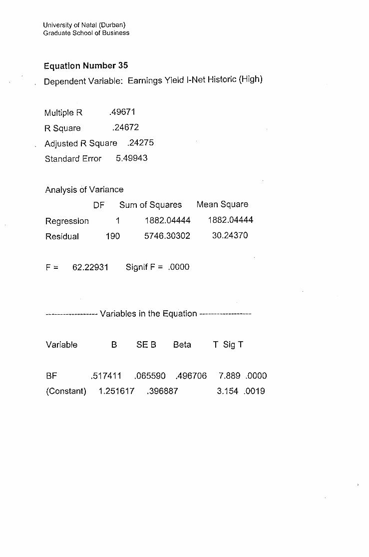
University of Natal (Durban)Graduate School of Business
Equation Number 35
Dependent Variable: Earnings Yield I-Net Historic (High)
Multiple R .49671
R Square .24672
Adjusted R Square .24275
Standard Error 5.49943
Analysis of Variance
OF Sum of Squares
Regression 1 1882.04444
Residual 190 5746.30302
Mean Square
1882.04444
30.24370
F = 62.22931 Signif F = .0000
------------------ Variables in the Equation ------------------
Variable B SE B Beta T Sig T
BF .517411 .065590 .496706
(Constant) 1.251617 .396887
7.889 .0000
3.154 .0019
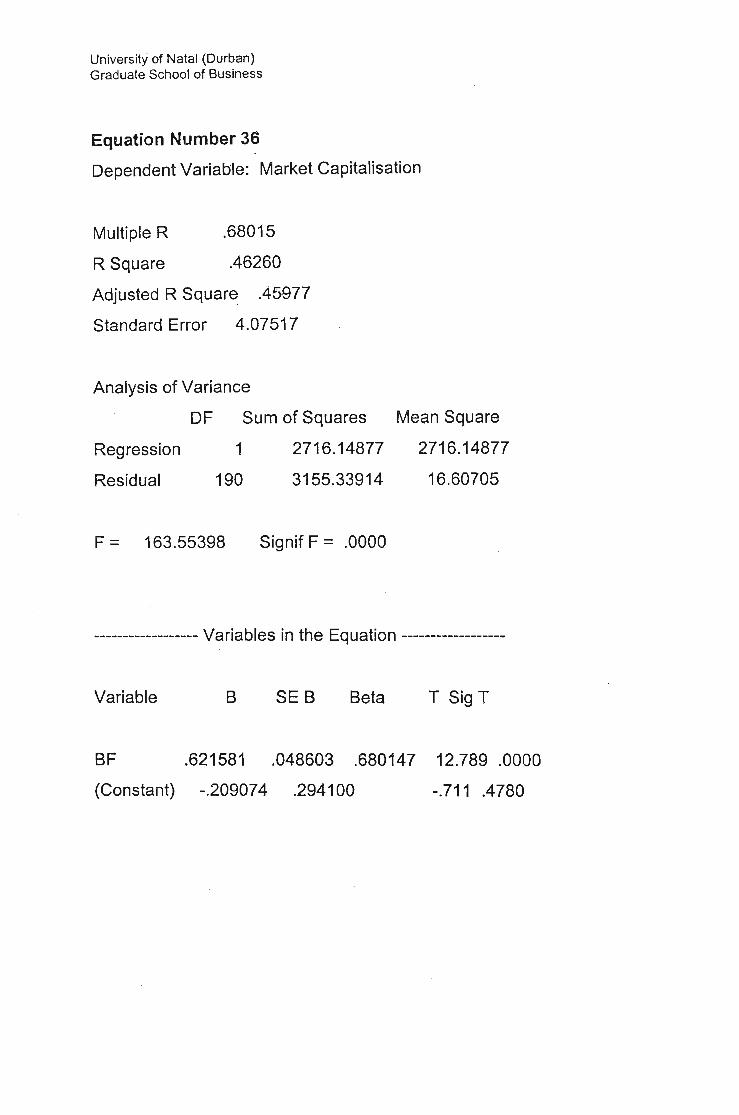
University of Natal (Durban)Graduate School of Business
Equation Number 36
Dependent Variable: Market Capitalisation
Multiple R .68015
R Square .46260
Adjusted R Square .45977
Standard Error 4.07517
Analysis of Variance
OF Sum of Squares
Regression
Residual
1
190
2716.14877
3155.33914
Mean Square
2716.14877
16.60705
F = 163.55398 Signif F = .0000
------------------ Variables in the Equation ------------------
Variable B SE B Beta T SigT
BF .621581 .048603 .680147 12.789 .0000
(Constant) -.209074 .294100 -.711 .4780
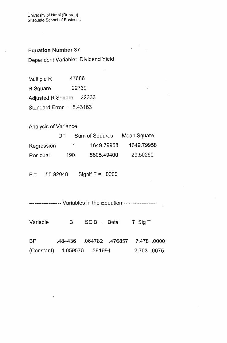
University of Natal (Durban)Graduate School of Business
Equation Number 37
Dependent Variable: Dividend Yield
Multiple R .47686
R Square ..22739
Adjusted R Square .22333
Standard Error 5.43163
Analysis of Variance
OF Sum of Squares Mean Square
Regression
Residual
1
190
1649.79958
5605.49400
1649.79958
29.50260
F = 55.92048 Signif F = .0000
------------------ Variables in the Equation ------------------
Variable B SE B Beta T SigT
BF .484436 .064782 .476857
(Constant) 1.059576 .391994
7.478 .0000
2.703 .0075
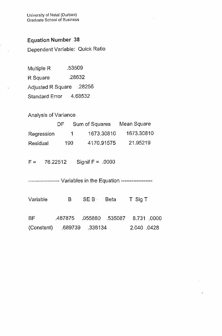
University of Natal (Durban)Graduate School of Business
Equation Number 38
Dependent Variable: Quick Ratio
Multiple R .53509
R Square .28632
Adjusted R Square .28256
Standard Error 4.68532
Analysis of Variance
OF Sum of Squares Mean Square
Regression
Residual
1
190
1673.30810
4170.91575
1673.30810
21.95219
F = 76.22512 Signif F = .0000
------------------ Variables in the Equation ------------------
Variable B SE B Beta T SigT
SF .487875 .055880 .535087
(Constant) .689739 .338134
8.731 .0000
2.040 .0428
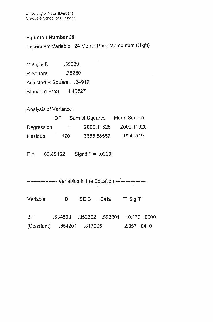
University of Natal (Durban)Graduate School of Business
Equation Number 39
Dependent Variable: 24 Month Price Momentum (High)
Multiple R .59380
R Square .35260
Adjusted R Square , .34919
Standard Error 4.40627
Analysis of Variance
OF Sum of Squares Mean Square
Regression
Residual
1
190
2009.11326
3688.88587
2009.11326
19.41519
F = 103.48152 Signif F = .0000
------------------ Variables in the Equation ------------------
Variable B SE B Beta T SigT
BF.534593 .052552 .593801
(Constant) .654201 .317995
10.173 .0000
2.057 .0410
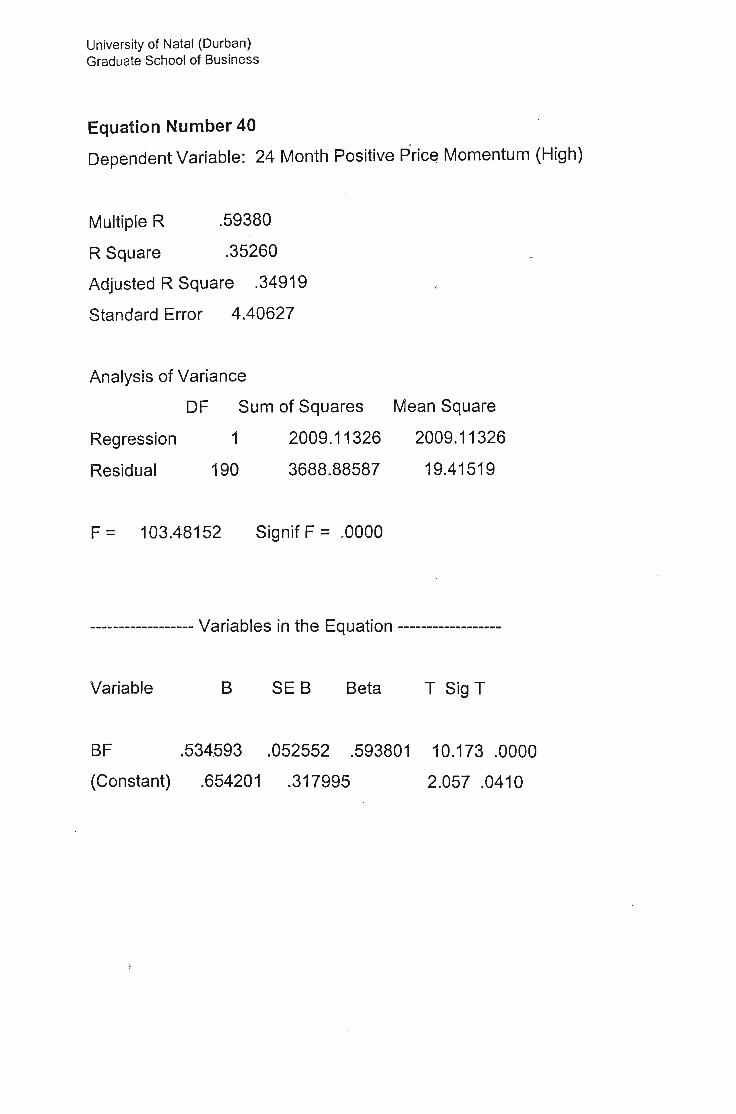
University of Natal (Durban)Graduate School of Business
Equation Number 40
Dependent Variable: 24 Month Positive Price Momentum (High)
Multiple R .59380
R Square .35260
Adjusted R Square .34919
Standard Error 4.40627
Analysis of Variance
OF Sum of Squares
Regression 1 2009.11326
Residual 190 3688.88587
Mean Square
2009.11326
19.41519
F = 103.48152 Signif F = .0000
------------------ Variables in the Equation ------------------
Variable B SEB Beta T Sig T
SF
(Constant)
.534593 .052552 .593801
.654201 .317995
10.173 .0000
2.057 .0410
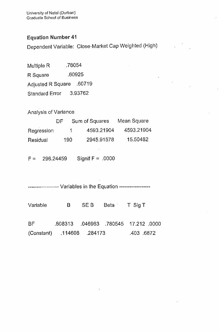
University of Natal (Durban)Graduate School of Business
Equation Number 41
Dependent Variable: Close-Market Cap Weighted (High)
Multiple R .78054
R Square .60925
Adjusted R Square .60719
Standard Error 3.93762
Analysis of Variance
OF Sum of Squares Mean Square
Regression
Residual
1
190
4593.21904
2945.91578
4593.21904
15.50482
F = 296.24459 Signif F = .0000
------------------ Variables in the Equation ------------------
Variable B SEB Beta T Sig T
SF .808313 .046963 .780545 17.212 .0000
(Constant) .114608 .284173 .403 .6872
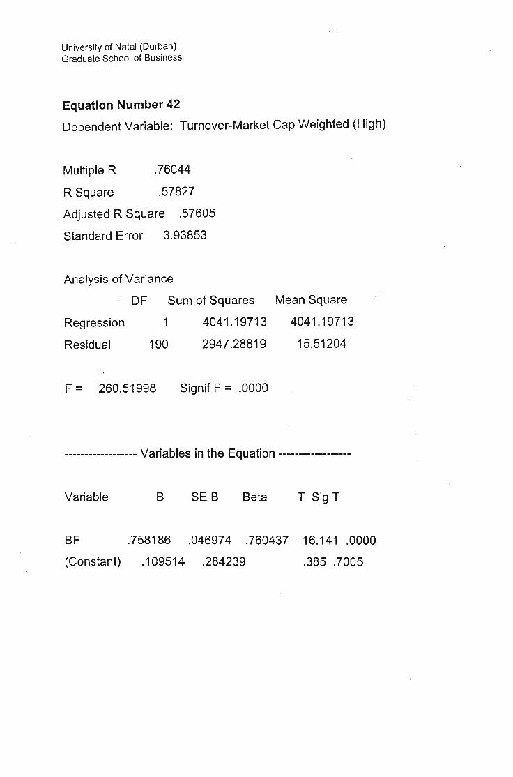
University of Natal (Durban)Graduate School of Business
Equation Number 42
Dependent Variable: Turnover-Market Cap Weighted (High)
Multiple R .76044
R Square .57827
Adjusted R Square .57605
Standard Error 3.93853
Analysis of Variance
OF Sum of Squares
Regression 1 4041.19713
Residual 190 2947.28819
Mean Square
4041.19713
15.51204
F = 260.51998 Signif F = .0000
------------------ Variables in the Equation ------------------
Variable B SE B Beta T SigT
BF .758186 .046974 .760437 16.141 .0000
(Constant) .109514 .284239 .385 .7005
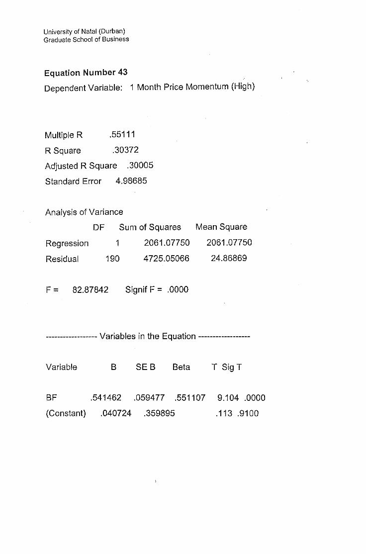
University of Natal (Durban)Graduate School of Business
Equation Number 43
Dependent Variable: 1 Month Price Momentum (High)
Multiple R .55111
R Square .30372
Adjusted R Square .30005
Standard Error 4.98685
Analysis of Variance
OF Sum of Squares
Regression 1 2061.07750
Residual 190 4725.05066
Mean Square
2061.07750
24.86869
F = 82.87842 Signif F= .0000
------------------ Variables in the Equation ------------------
Variable B SE B Beta T SigT
SF
(Constant)
.541462 .059477 .551107
.040724 .359895
9.104 .0000
.113 .9100
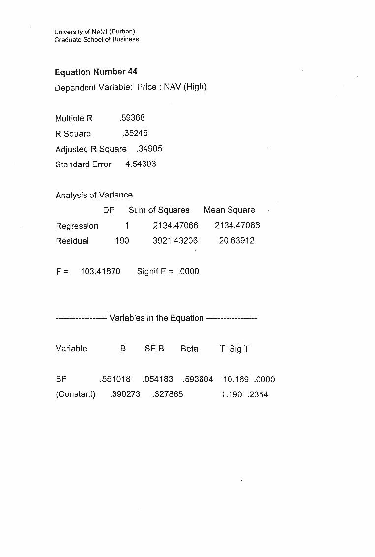
University of Natal (Durban)Graduate School of Business
Equation Number 44
Dependent Variable: Price: NAV (High)
Multiple R .59368
R Square .35246
Adjusted R Square .34905
Standard Error 4.54303
Analysis of Variance
DF Sum of Squares
Regression 1 2134.47066
Residual 1903921.43206
Mean Square
2134.47066
20.63912
F = 103.41870 Signif F = .0000
------------------ Variables in the Equation ------------------
Variable B SE B Beta T Sig T
SF .551018 .054183 .593684 10.169 .0000
(Constant) .390273 .327865 1.190 .2354

University of Natal (Durban)Graduate School of Business
Equation Number 45
Dependent Variable: Tradeability (High)
Multiple R .70237
R Square .49332
Adjusted R Square .49065
Standard Error 4.20067
Analysis of Variance
OF Sum of Squares
Regression 1 3264.25310
Residual 190 3352.67028
Mean Square
3264.25310
17.64563
F = 184.98929 Signif F = .0000
------------------ Variables in the Equation ------------------
Variable B SE B Beta T SigT
BF .681417 .050100 .702367 13.601 .0000
(Constant) .124631 .303157 .411 .6815
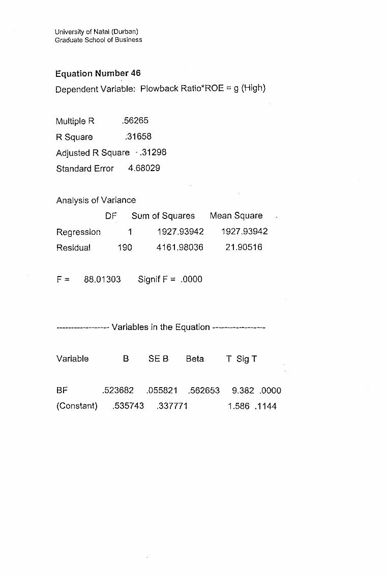
University of Natal (Durban)Graduate School of Business
.Equation Number 46
Dependent Variable: Plowback Ratio*ROE =g (High)
Multiple R .56265
R Square .31658
Adjusted R Square < .31298
Standard Error 4.68029
Analysis of Variance
DF Sum of Squares
Regression 1 1927.93942
Residual 190 4161.98036
Mean Square
1927.93942
21.90516
F = 88.01303 Signif F = .0000
------------------ Variables in the Equation ------------------
Variable B SE B Beta T SigT
BF .523682 .055821 .562653
(Constant) .535743 .337771
9.382 .0000
1.586 .1144

University of Natal (Durban)Graduate School of Business
Equation Number 47
Dependent Variable' Cashflow/Debt (High)
Multiple R .64406
R Square .41481
Adjusted R Square .41173
Standard Error 4.72501
.Regression
Residual
Analysis of Variance
OF Sum of Squares
1 3006.85480
190 4241.89395
Mean Square
3006 .85480
22.32576
F = 134.68097 Signif F = .0000
------------------ Variables in the Equation ------------------
Variable B SE B Beta T SigT
SF
(Constant)
.653999 .056354 .644058 11.605 .0000
.895987 .340999 2.628 .0093

University of Natal (Durban)Graduate School of Business
Equation Number 48
Dependent Variable: Payout Ratio (High)
Multiple R .55595
R Square .30908
Adjusted R Square .30544
Standard Error 4.58136
Regression
Residual
Analysis of Variance
OF Sum of Squares
1 1783.92942
190 3987.87728
Mean Square
1783.92942
20.98883
F = 84.99424 Signif F = .0000
------------------ Variables in the Equation ------------------
Variable 8 SE 8 Beta T SigT
SF .503744 .054641 .555946
(Constant) .283258 .330631
9.219 .0000
.857 .3927
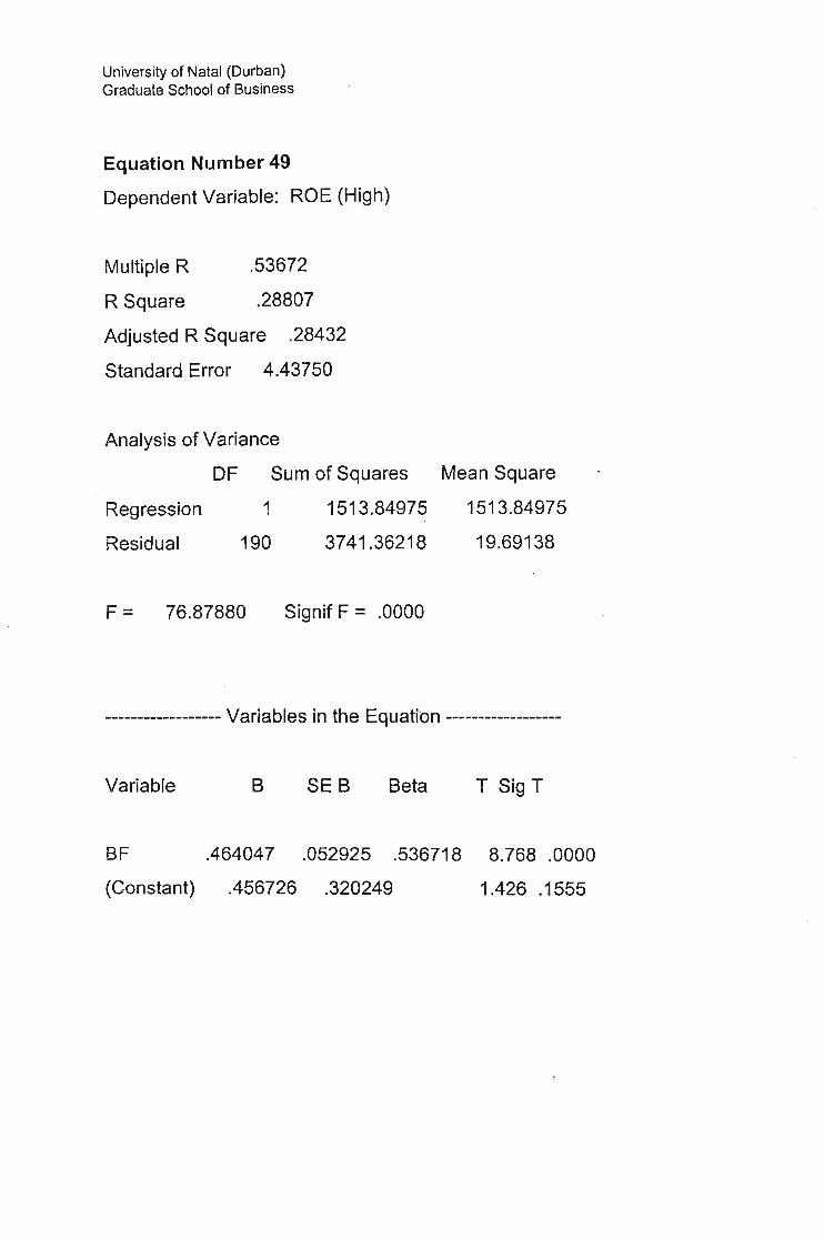
Regression
Residual
University of Natal (Durban)Graduate School of Business
Equation Number 49
Dependent Variable: ROE (High)
Multiple R .53672
R Square .28807
Adjusted R Square .28432
Standard Error 4.43750
Analysis of Variance
OF Sum of Squares
1 1513.84975
190 3741.36218
Mean Square
1513.84975
19.69138
F = 76.87880 Signif F = .0000
------------------ Variables in the Equation ------------------
Variable B SE B Beta T SigT
SF .464047 .052925 .536718
(Constant) .456726 .320249
8.768 .0000
1.426 .1555
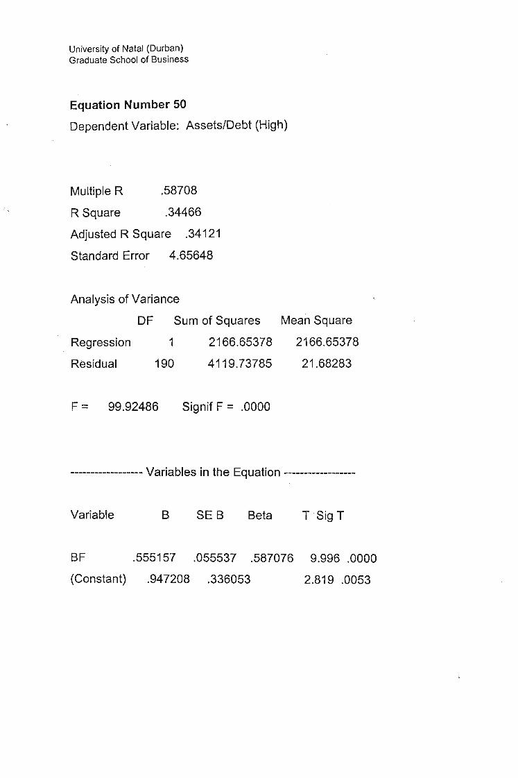
University of Natal (Durban)Graduate School of Business
Equation Number 50
Dependent Variable: Assets/Debt (High)
Multiple R .58708
R Square .34466
Adjusted R Square .34121
Standard Error 4.65648
Regression
Residual
Analysis of Variance
OF Sum of Squares
1 2166.65378
190 4119.73785
Mean Square
2166.65378
21.68283
F = 99.92486 Signif F = .0000
------------------ Variables in the Equation ------------------
Variable B SE B Beta TSigT
SF
(Constant)
.555157 .055537 .587076
.947208 .336053
9.996 .0000
2.819 .0053
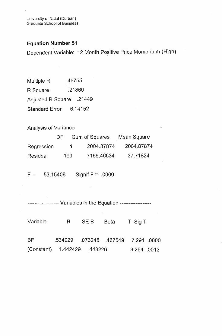
University of Natal (Durban)Graduate School of Business
Equation Number 51
Dependent Variable: 12 Month Positive Price Momentum (High)
Multiple R .46755
R Square :21860
Adjusted R Square ,21449
Standard Error 6,14152
Analysis of Variance
OF Sum of Squares
Regression 1 2004,87874
Residual 190 7166.46634
Mean Square
2004,87874
37.71824
F = 53,15408 Signif F = ,0000
------------------ Variables in the Equation ------------------
Variable B SE B Beta T SigT
SF ,534029 ,073248 .467549
(Constant) 1.442429 .443226
7,291 .0000
3.254 .0013
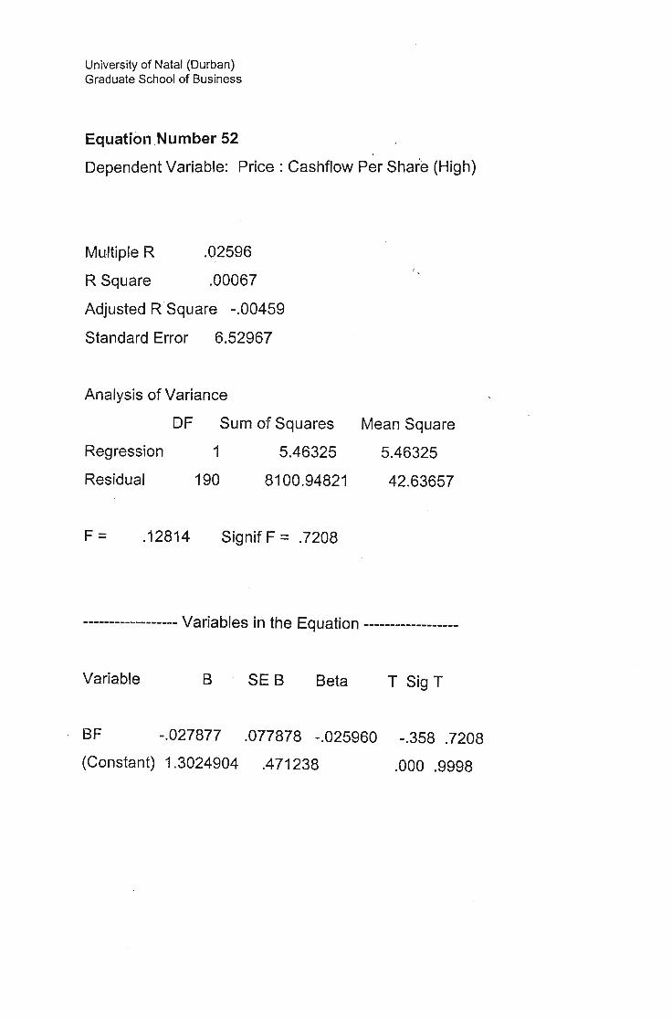
University of Natal (Durban)Graduate School of Business
Equation Number 52
Dependent Variable: Price: Cashflow Per Share (High)
Multiple R .02596
R Square .00067
Adjusted R Square -.00459
Standard Error 6.52967
Analysis of Variance
DF Sum of Squares Mean Square
Regression
Residual
1
190
5.46325
8100.94821
5.46325
42.63657
F= .12814 Signif F =.7208
------------------ Variables in the Equation ------------------
Variable B SE B Beta T SigT
SF -.027877 .077878 -.025960
(Constant) 1.3024904 .471238
-.358 .7208
.000 .9998

University of Natal (Durban)Graduate School of Business
Equation Number 53
Dependent Variable: PEG Ratio (High)
Multiple R .67623
R Square .45729
Adjusted R Square .44033
Standard Error 4.51285
Analysis of Variance
DF Sum of Squares Mean Square
Regression
Residual
1
32
549.12835
651.70620
549.12835
20.36582
F = 26.96323 Signif F = .0000
------------------ Variables in the Equation ------------------
Variable B SE B Beta T SigT
H .547398 .105419 .676231
(Constant) .495779 .789474
5.193 .0000
.628 .5345
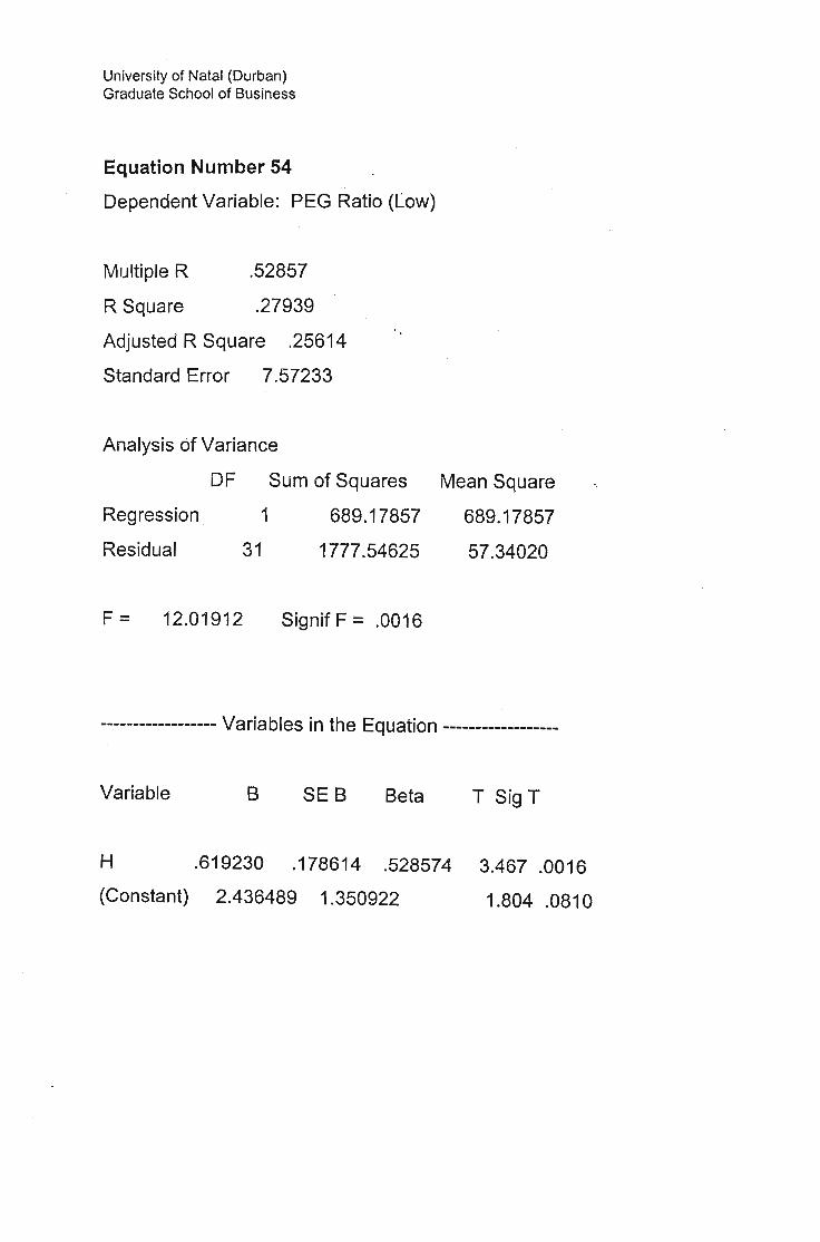
Regression
Residual
University of Natal (Durban)Graduate School of Business
Equation Number 54
Dependent Variable: PEG Ratio (Low)
Multiple R .52857
R Square .27939
Adjusted R Square .25614
Standard Error 7.57233
Analysis of Variance
DF Sum of Squares
1 689.17857
31 1777.54625
Mean Square
689.17857
57.34020
F = 12.01912 Signif F = .0016
------------------ Variables in the Equation ------------------
Variable B SEB Beta T Sig T
H .619230 .178614 .528574
(Constant) 2.436489 1.350922
3.467 .0016
1.804 .0810
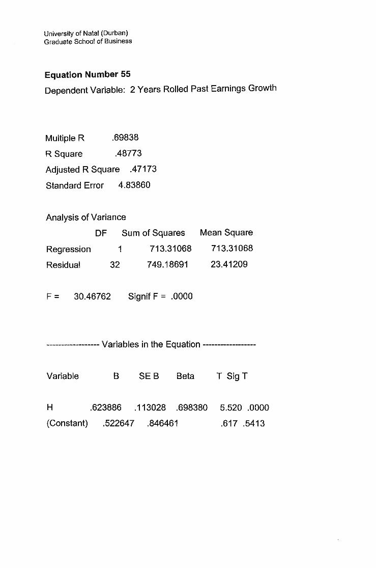
University of Natal (Durban )Graduate School of Business
Equation Number 55
Dependent Variable: 2 Years Rolled Past Earnings Growth
Multiple R .69838
R Square .48773
Adjusted R Square .47173
Standard Error 4.83860
Analysis of Variance
DF Sum of Squares
Regression 1 713.31068
Residual 32 749.18691
Mean Square
713.31068
23.41209
F = 30.46762 Signif F = .0000
------------------ Variab les in the Equation ------------------
Variable B SEB Beta T Sig T
H .623886 .113028 .698380
(Constant) .522647 .846461
5.520 .0000
.617 .5413

University of Natal (Durban)Graduate School of Business
Equation Number 56
Dependent Variable: 2 Years Rolled Past Earnings Growth (Low)
Multiple R .38333
R Square .14694
Adjusted R Square .12029
Standard Error 7.37 134
Analysis of Variance
DF Sum of Squares
Regression 1 299.51308
Residual 32 1738.77330
Mean Square
299 .51308
54.33667
F = 5.51217 Signif F = .0252
------------------ Variables in the Equation ------------------
Variable B SE B Beta T Sig T
H .404272 .172192 .383332
(Constant) 1.803956 1.289535
2.348 .0252
1.399 .1715
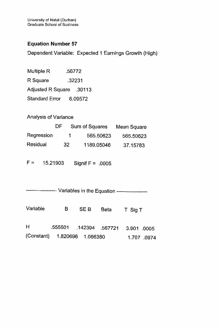
University of Natal (Durban )Graduate School of Business
Equation Number 57
Dependent Variable: Expected 1 Earnings Growth (High)
Multiple R .56772
R Square .32231
Adjusted R Square .30113
Standard Error 6.09572
Analysis of Variance
OF Sum of Squares
Regression 1 565.50623
Residual 32 1189.05046
Mean Square
565.50623
37.15783
F = 15.21903 Signif F = .0005
------------------ Variables in the Equation ------------------
Variable B SEB Beta T SigT
H .555501 .142394 .567721
(Constant) 1.820696 1.066380
3.901 .0005
1.707 .0974

University of Natal (Durban)Graduate School of Business
Equation Number 58
Dependent Variable: Expected 1 Years Earnings Growth (Low)
Multiple R .29525
R Square .08717
Adjusted R Square .05865
Standard Error 7.06558
Analysis of Variance
DF Sum of Squares
Regression 1 152.55725
Residual 32 1597.51856
Mean Square
152.55725
49.92245
F= 3.05588 Signif F = .0900
------------------ Variables in the Equation ------------------
Variable B SE B Beta T SigT
H .288524 .165049 .295249
(Constant) .932594 1.236046
1.748 .0900
.754 .4561

0/0 Confidence
~ ~
1\.)~(J')(X)01\.)
0000000o ., Q a El lJ Cl
0000000?f2.?f2.?f2.?f2.?f2.?f2.?f2. s:
o3CD~r+e3tnr+..,Q)r+CD
CC--CDtnQ)
-C-CCD~
C.--><----...o...........,
II

Bibliography
Black, F, Jensen M and Scholes M: The Capital Asset Pricing Model: Some
Empirical Test, in MC Jensen (ed.) Studies on the theory of Capital Market (New
York 1972)
Black, F : Capital Market Equilibrium with Restricted Borrowing, Journal of
Business (45: 1972)
Bollerslev, T, Engel, Rand Wooldridge, J : Capital Asset Pricing Model with the
time varying Co-variances, Journal ofPolitical Economy (96: 1988)
Fama, E and French, R The Cross Section of Expected Return, Journal of
Finance (47 : 1992)
Fama, E : Risk, Return Equilibrium, Journal of Political Economy (79: 1972)
Fama, E and Macbeth, J : Risk Return and Equilibrium: Empirical Test, Journal
of Political Economy (71: 1973)
Gibbons, M : Multivariate tests of financial models: A new Approach, Journal of
Financial Economics (10: 1982)
Litner, J : Inflation and Stock Return, Journal of Finance (30 : 1975)
Litner, J : (i) Security Prices, Risk and Maximum Gains from diversification,
Journal of Finance ( 20 : 1965) (ii) the valuation of risk assets and the selectio~ of
risky investments in stock portfolios and capital budgets review of economics and
statistics ( 47 : 1965)
Owen, J and Rabinovitch, R : On the Class of Elliptical Distribution and their
application in the theory ofportfolio choice, Journal of Finance (38: 1983)
Mossin, J : Equilibrium in a Capital Asset Market, Econometrica (34: 1966)
Rosenburg, Band Rudd, A: The Corporate Use of Beta, Journal of Finance (36 :
1985)
Ross, S : Mutual Fund Separation in Financial Theory - The separating
distribution, Journal of Economic Theory (17: 1978)
Sauer, A and Murphy, A : An Empirical Comparison of Alternative Models of
capital asset pricing, German Journal of Banking and Finance (16:1992)
Sharpe, W : Portfolio Theory and Capital markets (New York, 1970)
Walker, J : How the option markets work: Institute of Finance (New York, 1991)