An Efficient and Parallel Gaussian Sampler for Lattices

Chris Peikert∗

April 13, 2011

Abstract

At the heart of many recent lattice-based cryptographic schemes is a polynomial-time algorithm that,given a ‘high-quality’ basis, generates a lattice point according to a Gaussian-like distribution. Unlikemost other operations in lattice-based cryptography, however, the known algorithm for this task (due toGentry, Peikert, and Vaikuntanathan; STOC 2008) is rather inefficient, and is inherently sequential.

We present a new Gaussian sampling algorithm for lattices that is efficient and highly parallelizable.We also show that in most cryptographic applications, the algorithm’s efficiency comes at almost no cost inasymptotic security. At a high level, our algorithm resembles the “perturbation” heuristic proposed as partof NTRUSign (Hoffstein et al., CT-RSA 2003), though the details are quite different. To our knowledge,this is the first algorithm and rigorous analysis demonstrating the security of a perturbation-like technique.

1 Introduction

In recent years, there has been rapid development in the use of lattices for constructing rich crypto-graphic schemes.1 These include digital signatures (both ‘tree-based’ [LM08] and ‘hash-and-sign’ [GPV08,CHKP10]), identity-based encryption [GPV08] and hierarchical IBE [CHKP10, ABB10], noninteractivezero knowledge [PV08], and even a fully homomorphic cryptosystem [Gen09].

The cornerstone of many of these schemes (particularly, but not exclusive to, those that ‘answer queries’)is the polynomial-time algorithm of [GPV08] that samples from a so-called discrete Gaussian probabilitydistribution over a lattice Λ. More precisely, for a vector c ∈ Rn and a “width” parameter s > 0, thedistributionDΛ+c,s assigns a probability proportional to exp(−π‖v‖2/s2) to each v ∈ Λ+c (and probabilityzero elsewhere). Given c, a basis B of Λ, and a sufficiently large s (related to the ‘quality’ of B), the GPValgorithm outputs a sample from a distribution statistically close to DΛ+c,s. (Equivalently, by subtracting cfrom the output, it samples a lattice point from a Gaussian distribution centered at −c.) Informally speaking,the sampling algorithm is ‘zero-knowledge’ in the sense that it leaks no information about its input basis B(aside from a bound on its quality), because DΛ+c,s is defined without reference to any particular basis. Thiszero-knowledge property accounts for its broad utility in lattice-based cryptography.

While the sampling algorithm of [GPV08] has numerous applications in cryptography and beyond, forboth practical and theoretical purposes it also has some drawbacks:∗School of Computer Science, College of Computing, Georgia Institute of Technology. Email: cpeikert@cc.gatech.edu.

This material is based upon work supported by the National Science Foundation under Grant CNS-0716786. Any opinions, findings,and conclusions or recommendations expressed in this material are those of the author(s) and do not necessarily reflect the views ofthe National Science Foundation.

1A lattice Λ ⊂ Rn is a periodic ‘grid’ of points, or more formally, a discrete subgroup of Rn under addition. It is generated by a(not necessarily unique) basis B ⊂ Rn×k of k linearly independent vectors, as Λ = Bz : z ∈ Zk. In this paper we are concernedonly with full-rank lattices, i.e., where k = n.

1

• First, it is rather inefficient: on an n-dimensional lattice, a straightforward implementation requiresexact arithmetic on an n × n matrix having Ω(n)-bit entries (even ignoring some additional log nfactors). While approximate arithmetic and other optimizations may be possible in certain cases, greatcare would be needed to maintain the proper output distribution, and the algorithm’s essential structureappears difficult to make truly practical.

• Second, it is inherently sequential: to generate a sample, the algorithm performs n adaptive iterations,where the choices made in each iteration affect the values used in the next. This stands in stark contrastto other ‘embarrassingly parallelizable’ operations that are typical of lattice-based cryptography.

1.1 Contributions

We present a new algorithm that samples from a discrete Gaussian distribution DΛ+c,s over a lattice, given a‘high-quality’ basis for Λ. The algorithm is especially well-suited to ‘q-ary’ integer lattices, i.e., sublatticesof Zn that themselves contain qZn as a sublattice, for some known and typically small q ≥ 2. Theseinclude NTRU lattices [HPS98] and the family of random lattices that enjoy ‘worst-case hardness,’ as firstdemonstrated by Ajtai [Ajt96]. Most modern lattice-based cryptographic schemes (including those that relyon Gaussian sampling) are designed around q-ary lattices, so they are a natural target for optimization.

The key features of our algorithm, as specialized to n-dimensional q-ary lattices, are as follows. It is:

• Offline / online: when the lattice basis is known in advance of the point c (which is the norm incryptographic applications), most of the work can be performed as offline precomputation. In fact, theoffline phase may be viewed simply as an extension of the application’s key-generation algorithm.

• Simple and efficient: the online phase involves onlyO(n2) integer additions and multiplications moduloq or q2, where the O-notation hides a small constant ≈ 4.

• Fully parallelizable: for any P up to n2, the online phase can allocate O(n2/P ) of its operations toeach of P processors.

• High-quality: for random bases that are commonly used in cryptographic schemes, our algorithm cansample from a Gaussian of essentially the same ‘quality’ as the prior GPV algorithm; this is importantfor the concrete security of applications. See Section 1.2.1 below for a full discussion.

We emphasize that for a practical implementation, parallelized operations on small integers representa significant performance advantage. Most modern computer processors have built-in support for “vector”instructions (also known as “single instruction, multiple data”), which perform simple operations on entirevectors of small data elements simultaneously. Our algorithm can exploit these operations very naturally. Fora detailed efficiency comparison between our algorithm and that of [GPV08], see Section 1.2.2 below.

At a very high level, our algorithm resembles the “perturbation” heuristic proposed for the NTRUSignsignature scheme [HHGP+03], but the details differ significantly; see Section 1.3 for a comparison. To ourknowledge, this is the first algorithm and analysis to demonstrate the theoretical soundness of a perturbation-like technique. Finally, the analysis of our algorithm relies on some new general facts about ‘convolutions’ ofdiscrete Gaussians, which we expect will be applicable elsewhere. For example, these facts allow for the useof a clean discrete Gaussian error distribution (rather than a ‘rounded’ Gaussian) in the “learning with errors”problem [Reg05], which may be useful in certain applications.

2

1.2 Comparison with the GPV Algorithm

Here we give a detailed comparison of our new sampling algorithm to the previous one of [GPV08]. The twomain points of comparison are the width (‘quality’) of the sampled Gaussian, and the algorithmic efficiency.

1.2.1 Gaussian Width

One of the important properties of a discrete Gaussian sampling algorithm is the width s of the distributionit generates, as a function of the input basis. In cryptographic applications, the width is the main quantitygoverning the concrete security and, if applicable, the approximation factor of the underlying worst-caselattice problems. This is because in order for the scheme to be secure, it must hard for an adversary to find alattice point within the likely radius s

√n of the Gaussian (i.e., after truncating its negligibly likely tail). The

wider the distribution, the more leeway the adversary has in an attack, and the larger the scheme’s parametersmust be to compensate. On the other hand, a more efficient sampling algorithm can potentially allow for theuse of larger parameters without sacrificing performance.

The prior sampling algorithm of [GPV08], given a lattice basis B = b1, . . . ,bn, can sample froma discrete Gaussian having width as small as ‖B‖ = maxi‖bi‖, where B denotes the Gram-Schmidtorthogonalization of B.2 (Actually, the width also includes a small ω(

√log n) factor, which is also present in

our new algorithm, so for simplicity we ignore it in this summary.) As a point of comparison, ‖B‖ is alwaysat most maxi‖bi‖, and in some cases it can be substantially smaller.

In contrast, our new algorithm works for a width s as small as the largest singular value s1(B) of thebasis B, or equivalently, the square root of the largest eigenvalue of the Gram matrix BBt. It is easy toshow that s1(B) is always at least maxi‖bi‖, so our new algorithm cannot sample from a narrower Gaussianthan the GPV algorithm can. At the same time, any basis B can always be efficiently processed (withoutincreasing ‖B‖) to guarantee that s1(B) ≤ n · ‖B‖, so our algorithm is at worst an n factor looser than thatof [GPV08].

While a factor of n gap between the two algorithms may seem rather large, in cryptographic applicationsthis worst-case ratio is actually immaterial; what matters is the relative performance on the random basesthat are used as secret keys. Here the situation is much more favorable. First, we consider the basis-generation algorithms of [AP09] (following [Ajt99]) for ‘worst-case-hard’ q-ary lattices, which are usedin most theoretically sound cryptographic applications. We show that with a minor modification, one ofthe algorithms from [AP09] outputs (with overwhelming probability) a basis B for which s1(B) is only anO(√

log q) factor larger than ‖B‖ (which itself is asymptotically optimal, as shown in [AP09]). Becauseq is typically a small polynomial in n, this amounts to a cost of only an O(

√log n) factor in the width of

the Gaussian. Similarly, when the vectors of B are themselves drawn from a discrete Gaussian, as in thebasis-delegation technique of [CHKP10], we can show that s1(B) is only a ω(

√log n) factor larger than ‖B‖

(with overwhelming probability). Therefore, in cryptographic applications the performance improvementsof our algorithm can come at almost no asymptotic cost in security. Of course, a concrete evaluation of theperformance/security trade-off for real-world parameters would require careful analysis and experiments,which we leave for later work.

1.2.2 Efficiency

We now compare the efficiency of the two known sampling algorithms. We focus on the most common case ofq-ary n-dimensional integer lattices, where a ‘good’ lattice basis (whose vectors having length much less than

2In the Gram-Schmidt orthogonalization B of B, the vector bi is the projection of bi orthogonally to span(b1, . . . ,bi−1).

3

q) is initially given in an offline phase, followed by an online phase in which a desired center c ∈ Zn is given.This scenario allows for certain optimizations in both algorithms, which we include for a fair comparison.

The sampling algorithm from [GPV08] can use the offline phase to compute the Gram-Schmidt orthogo-nalization of its given basis; this requires Ω(n4 log2 q) bit operations and Ω(n3) bits of intermediate storage.The online phase performs n sequential iterations, each of which computes an inner product between aGram-Schmidt vector having Ω(n)-bit entries, and an integer vector whose entries have magnitude at most q.In total, these operations require Ω(n3 log q) bit operations. In addition, each iteration performs a certainrandomized-rounding operation, which, while asymptotically poly(log n)-time, is not especially practical(nor precomputable) because it uses rejection sampling on a value that is not known until the online phase.Lastly, while the work within each iteration may be parallelized, the iterations themselves must be performedsequentially.

Our algorithm is more efficient and practical in the running time of both phases, and in the amount ofintermediate storage between phases. The offline phase first computes a matrix inverse modulo q2, and a‘square root’ of a matrix whose entries have magnitude at most q; these can be computed in O(n3 log2 q) bitoperations. Next, it generates and stores one or more short integer ‘perturbation’ vectors (one per future callto the online phase), and optionally discards the matrix square root. The intermediate storage is thereforeas small as O(n2 log q) bits for the matrix inverse, plus O(n log q) bits per perturbation vector. Optionally,the offline phase can also precompute the randomized-rounding operations, due to the small number ofpossibilities that can occur online. The online phase simply computes about 4n2 integer additions andmultiplications (2n2 of each) modulo q or q2, which can be fully parallelized among up to n2 processors.

Lastly, we mention that our sampling algorithm translates very naturally to the setting of compact q-arylattices and bases over certain rings R that are larger than Z, where security is based on the worst-casehardness of ideal lattices in R (see, e.g., [Mic02, SSTX09, LPR10]). In contrast to GPV, our algorithm candirectly take advantage of the ring structure for further efficiency, yielding a savings of an Ω(n) factor in thecomputation times and intermediate storage.

1.3 Overview of the Algorithm

The GPV sampling algorithm [GPV08] is based closely on Babai’s “nearest-plane” decoding algorithm forlattices [Bab86]. Babai’s algorithm takes a point c ∈ Rn and a lattice basis B = b1, . . . ,bn, and fori = n, . . . , 1 computes a coefficient zi ∈ Z for bi by iteratively projecting (‘rounding’) c orthogonally to thenearest hyperplane of the form zibi + span(b1, . . . ,bi−1). The output is the lattice vector

∑i zibi, whose

distance from the original c can be bounded by the quality of B. The GPV algorithm, whose goal is insteadto sample from a discrete Gaussian centered at c, uses randomized rounding in each iteration to select a‘nearby’ plane, under a carefully defined probability distribution. (This technique is also related to anotherrandomized-rounding algorithm of Klein [Kle00] for a different decoding problem.)

In addition to his nearest-plane algorithm, Babai also proposed a simpler (but somewhat looser) latticedecoding algorithm, which we call “simple rounding.” In this algorithm, a given point c ∈ Rn is rounded tothe lattice point BbB−1ce, where each coordinate of B−1c ∈ Rn is independently rounded to its nearestinteger. With precomputation of B−1, this algorithm can be quite practical — especially on q-ary lattices,where several more optimizations are possible. Moreover, it is trivially parallelized among up to n2 processors.Unfortunately, its deterministic form it turns out to be completely insecure for ‘answering queries’ (e.g.,digital signatures), as demonstrated by Nguyen and Regev [NR06].

A natural question, given the approach of [GPV08], is whether a randomized variant of Babai’s simple-rounding algorithm is secure. Specifically, the natural way of randomizing the algorithm is to round eachcoordinate of B−1c to a nearby integer (under a discrete Gaussian distribution over Z, which can be sampled

4

efficiently), then left-multiply by B as before. Unlike with the randomized nearest-plane algorithm, though,the resulting probability distribution here is unfortunately not spherical, nor does it leak zero knowledge.Instead, it is a ‘skewed’ (elliptical) Gaussian, where the skew mirrors the ‘geometry’ of the basis. Moreprecisely, the covariance matrix Ex[(x− c)(x− c)t] of the distribution (about its center c) is approximatelyBBt, which captures the entire geometry of the basis B, up to rigid rotation. Because covariance can bemeasured efficiently from only a small number of samples, the randomized simple-rounding algorithm leaksthis geometry.3

Our solution prevents such leakage, in a manner inspired by the following facts. Recall that ifX and Y aretwo independent random variables, the probability distribution of their sum X + Y is the convolution of theirindividual distributions. In addition, for continuous (not necessarily spherical) Gaussians, covariance matricesare additive under convolution. In particular, if Σ1 and Σ2 are covariance matrices such that Σ1 + Σ2 = s2I,then the convolution of two Gaussians with covariance matrices Σ1, Σ2 (respectively) is a spherical Gaussianwith standard deviation s.

The above facts give the basic idea for our algorithm, which is to convolve the output of the randomizedsimple-rounding algorithm with a suitable non-spherical (continuous) Gaussian, yielding a sphericallydistributed output. However, note that we want the algorithm to generate a discrete distribution — i.e., itmust output a lattice point — so we should not alter the output of the randomized-rounding step. Instead,we first perturb the desired center c by a suitable non-spherical Gaussian, then apply randomized roundingto the resulting perturbed point. Strictly speaking this is not a true convolution, because the rounding stepdepends on the output of the perturbation step, but we can reduce the analysis to a true convolution usingbounds related to the “smoothing parameter” of the lattice [MR04].

The main remaining question is: for a given covariance matrix Σ1 = BBt (corresponding to therounding step), for what values of s is there an efficiently sampleable Gaussian having covariance matrixΣ2 = s2I − Σ1? The covariance matrix of any (non-degenerate) Gaussian is symmetric positive definite,i.e., all its eigenvalues are positive. Conversely, every positive definite matrix is the covariance of someGaussian, which can sampled efficiently by computing a ‘square root’ of the covariance matrix. Since anyeigenvector of Σ1 (with eigenvalue σ2 > 0) is also an eigenvector of s2I (with eigenvalue s2), it must be aneigenvector of Σ2 (with eigenvalue s2 − σ2) as well. Therefore, a necessary and sufficient condition is thatall the eigenvalues of Σ1 be less than s2. Equivalently, the algorithm works for any s that exceeds the largestsingular value of the given basis B. More generally, it can sample any (possibly non-spherical) discreteGaussian with covariance matrix Σ > Σ1 (i.e., Σ− Σ1 is positive definite).

In retrospect, the high-level structure of our algorithm resembles the “perturbation” heuristic proposedfor NTRUSign [HHGP+03], though the details are quite different. First, the perturbation and rounding stepsin NTRUSign are both deterministic with respect to two or more bases, and there is evidence that this isinsecure [MPSW09], at least for a large polynomial number of signatures. Interestingly, randomization alsoallows for improved efficiency, since our perturbations can be chosen with offline precomputation (as opposedto the deterministic method of [HHGP+03], which is inherently online). Second, the signing and perturbationbases used in NTRUSign are chosen independently, whereas our perturbations are carefully chosen to concealthe statistics that would otherwise be leaked by randomized rounding.

3Given the above, one might still wonder whether the covariance BBt could be simulated efficiently (without any privilegedknowledge about the lattice) when B is itself drawn from a ‘nice’ distribution, such as a discrete Gaussian. Indeed, if the vectors ofB were drawn independently from a continuous Gaussian, the matrix BBt would have the so-called Wishart distribution, which canbe generated ‘obliviously’ (without knowledge of B itself) using the Bartlett decomposition. (See, e.g., [Ksh59] and referencestherein). Unfortunately, these facts do not quite seem to carry over to discrete Gaussians, though they may be useful in anothercryptographic context.

5

1.4 Organization

Section 2 reviews the necessary linear algebra and lattice background. In Section 3 we prove some generalfacts about ‘convolutions’ of discrete Gaussians, which are used in the analysis of our sampling algorithm. InSection 4 we describe new sampling algorithms and analyze their complexity under suggested optimizations.In Section 5 we give bounds on the largest singular value of a basis relative to other important quantities,both in general and for particular constructions of bases used in cryptographic schemes.

2 Preliminaries

2.1 Notation

For a countable set X and a real-valued function f , we write f(X) to denote∑

x∈X f(x). A nonnegativefunction f : N → R is called negligible, written f(n) = negl(n), if it vanishes faster than any inversepolynomial, i.e., f(n) = o(n−c) for every constant c ≥ 0. A function g : N→ [0, 1] is called overwhelmingif it is 1−negl(n). The statistical distance between two distributions X and Y (or two random variables havethose distributions, respectively) is defined as ∆(X,Y ) = supA⊆D|X(A)− Y (A)|. When D is a countableset, we have ∆(X,Y ) = 1

2

∑d∈D|X(d)− Y (d)|.

We use bold lower-case letters (e.g., x) to denote vectors in Rn, for an undetermined positive integerdimension n that remains the same throughout the paper. We use bold upper-case letters (e.g., B) for orderedsets of vectors, and identify the set with the matrix having the vectors as its columns. We frequently useupper-case Greek letters such as Σ to denote (symmetric) positive (semi)definite matrices, defined below. Incontexts where a matrix is expected, we sometimes use a scalar s ∈ R to denote s · I, where I is the identitymatrix of appropriate dimension. We let ‖B‖ = maxi‖bi‖, where ‖·‖ denotes the Euclidean norm.

2.2 Linear Algebra

A symmetric matrix Σ ∈ Rn×n is positive definite, written Σ > 0, if xtΣx > 0 for all nonzero x ∈ Rn.Equivalently, its spectral decomposition is

Σ = QD2Q−1 = QD2Qt,

where Q ∈ Rn×n is an orthogonal matrix (i.e., one for which QtQ = QQt = I) whose columns areeigenvectors of Σ, and D is the real diagonal matrix of the square roots of the corresponding eigenvalues,all of which are positive. We have Σ > 0 if and only if Σ−1 > 0. We say that Σ is positive semidefinite,written Σ ≥ 0, if xtΣx ≥ 0 for all x ∈ Rn; such a matrix may not be invertible. Positive (semi)definitenessdefines a partial ordering on symmetric matrices: we say that Σ1 > Σ2 if (Σ1 − Σ2) > 0, and likewise forΣ1 ≥ Σ2. It is the case that Σ1 ≥ Σ2 > 0 if and only if Σ−1

2 ≥ Σ−11 > 0, and likewise for the analogous

strict inequalities.For any nonsingular matrix B ∈ Rn×n, the symmetric matrix Σ = BBt is positive definite, because

xtΣx = 〈Btx,Btx〉 = ‖Btx‖2 > 0

for nonzero x ∈ Rn. We say that B is a square root of Σ > 0, written B =√

Σ, if BBt = Σ. EveryΣ > 0 has a square root B = QD, where Σ = QD2Qt is the spectral decomposition of Σ as above.Moreover, the square root is unique up to right-multiplication by an orthogonal matrix, i.e., B′ =

√Σ if

and only if B′ = BP for some orthogonal matrix P. A square root of particular interest is given by the

6

Cholesky decomposition Σ = LLt, where L is a (unique) lower-triangular matrix. Given Σ, its Choleskydecomposition can be computed efficiently in fewer than n3 multiplication and addition operations (on realnumbers of sufficient precision).

For a nonsingular matrix B, a singular value decomposition is B = QDPt, where Q,P ∈ Rn×nare orthogonal matrices, and D is a diagonal matrix with positive entries si > 0 (called the singularvalues) on the diagonal, in non-increasing order. Under this convention, D is uniquely determined, ands1(B) = maxu‖Bu‖ = maxu‖Btu‖, where the maximum is taken over all unit vectors u ∈ Rn. Note that

Σ = BBt = QDPtPDtQt = QD2Qt,

so the eigenvalues of Σ are the squares of the singular values of B.

2.3 Lattices

A lattice Λ is a discrete additive subgroup of Rn. In this work we are only concerned with full-rank lattices,which are generated by some nonsingular basis B ∈ Rn×n, as the set Λ = B · Zn = Bz : z ∈ Zn. Whenn ≥ 2, every lattice has infinitely many bases, which are related by unimodular transformations: B′ and Bgenerate the same lattice if and only if B′ = BU for some unimodular U ∈ Zn×n.

The dual lattice of Λ, denoted Λ∗, is defined as Λ∗ = w ∈ Rn : 〈x,w〉 ∈ Z ∀ x ∈ Λ. (We only needthis notion for defining the smoothing parameter of a lattice; see below.)

2.4 Gaussians

The n-dimensional Gaussian function ρ : Rn → (0, 1] is defined as

ρ(x)∆= exp(−π · ‖x‖2) = exp(−π · 〈x,x〉).

Applying a linear transformation given by a nonsingular matrix B yields the Gaussian function

ρB(x)∆= ρ(B−1x) = exp

(−π ·

⟨B−1x,B−1x

⟩)= exp

(−π · xtΣ−1x

),

where Σ = BBt > 0. Because ρB is distinguished only up to Σ, we usually refer to it as ρ√Σ.Normalizing ρ√Σ by its total measure

∫Rn ρ√Σ(x) dx =

√det Σ over Rn, we obtain the probability

distribution function of the (continuous) Gaussian distribution D√Σ. It is easy to check that a randomvariable x having distribution D√Σ can be written as

√Σ · z, where z has spherical Gaussian distribution D1.

Therefore, the random variable x has covariance

Ex∼D√Σ

[x · xt

]=√

Σ · Ez∼D1

[z · zt

]·√

Σt

=√

Σ · I

2π·√

Σt

=Σ

2π,

by linearity of expectation. (The I2π covariance of z ∼ D1 arises from the independence of its entries, which

are each distributed as D1 in one dimension, and have variance 12π .) For convenience, in this paper we

implicitly scale all covariance matrices by a 2π factor, and refer to Σ as the covariance matrix of D√Σ.The following standard fact, which will be central to the analysis of our sampling algorithms, characterizes

the product of two Gaussian functions.

Fact 2.1. Let Σ1,Σ2 > 0 be positive definite matrices, let Σ0 = Σ1 + Σ2 > 0 and Σ−13 = Σ−1

1 + Σ−12 > 0,

let x, c1, c2 ∈ Rn be arbitrary, and let c3 ∈ Rn be such that Σ−13 c3 = Σ−1

1 c1 + Σ−12 c2. Then

ρ√Σ1(x− c1) · ρ√Σ2

(x− c2) = ρ√Σ0(c1 − c2) · ρ√Σ3

(x− c3).

7

Proof. By the definition of ρ√Σ, it suffices to check that

(x− c1)tΣ−11 (x− c1) + (x− c2)tΣ−1

2 (x− c2) =

(c1 − c2)tΣ−10 (c1 − c2) + (x− c3)tΣ−1

3 (x− c3).

This may be verified by a routine calculation, using the matrix identity

Σ−13 = Σ−1

1 + Σ−12 = Σ−1

1 · (Σ1 + Σ2) · Σ−12 = Σ−1

1 · Σ0 · Σ−12 .

2.5 Gaussians on Lattices

Let Λ ⊂ Rn be a lattice, let c ∈ Rn, and let Σ > 0 be a positive definite matrix. The discrete Gaussiandistribution DΛ+c,

√Σ is simply the Gaussian distribution D√Σ restricted so that its support is the coset Λ + c.

That is, for all x ∈ Λ + c,

DΛ+c,√

Σ(x) =ρ√Σ(x)

ρ√Σ(Λ + c)∝ ρ√Σ(x).

We recall the definition of the smoothing parameter from [MR04].

Definition 2.2. For a lattice Λ and positive real ε > 0, the smoothing parameter ηε(Λ) is the smallest reals > 0 such that ρ1/s(Λ

∗\0) ≤ ε.

Observe that if Λ1 is a sublattice of a lattice Λ0, then ηε(Λ1) ≥ ηε(Λ0) for any ε > 0, because Λ∗0 ⊆ Λ∗1and hence ρ1/s(Λ

∗0 \ 0) ≤ ρ1/s(Λ

∗1 \ 0) by positivity of ρ1/s.

Note that the smoothing parameter as defined above is a scalar. In this work we need to extend the notionto positive definite matrices.

Definition 2.3. Let Σ > 0 be any positive definite matrix. We say that√

Σ ≥ ηε(Λ) if ηε(√

Σ−1 · Λ) ≤ 1,

i.e., if ρ(√

Σt · Λ∗\0) = ρ√

Σ−1(Λ∗\0) ≤ ε.

The following lemma says that when the standard deviation√

Σ exceeds the smoothing parameter of Λ,the Gaussian measure on each coset of Λ is essentially the same.

Lemma 2.4 (Corollary of [MR04, Lemma 4.4]). Let Λ be any n-dimensional lattice. For any ε ∈ (0, 1),Σ > 0 such that

√Σ ≥ ηε(Λ), and any c ∈ Rn,

ρ√Σ(Λ + c) ∈ [1−ε1+ε , 1] · ρ√Σ(Λ).

Proof. Follows directly by applying√

Σ−1

as a linear transform to Λ, and by ηε(√

Σ−1 · Λ) ≤ 1.

Finally, we will need the following tight bound on the smoothing parameter of the integer lattice Zn.

Lemma 2.5 (Special case of [MR04, Lemma 3.3]). For any ε > 0,

ηε(Zn) ≤√

ln(2n(1 + 1/ε))/π.

In particular, for any ω(√

log n) function, there is a negligible ε = ε(n) such that ηε(Zn) ≤ ω(√

log n).

8

3 Analysis of ‘Convolved’ Discrete Gaussians

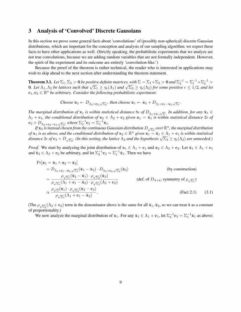
In this section we prove some general facts about ‘convolutions’ of (possibly non-spherical) discrete Gaussiandistributions, which are important for the conception and analysis of our sampling algorithm; we expect thesefacts to have other applications as well. (Strictly speaking, the probabilistic experiments that we analyze arenot true convolutions, because we are adding random variables that are not formally independent. However,the spirit of the experiment and its outcome are entirely ‘convolution-like.’)

Because the proof of the theorem is rather technical, the reader who is interested in applications maywish to skip ahead to the next section after understanding the theorem statement.

Theorem 3.1. Let Σ1,Σ2 > 0 be positive definite matrices, with Σ = Σ1+Σ2 > 0 and Σ−13 = Σ−1

1 +Σ−12 >

0. Let Λ1,Λ2 be lattices such that√

Σ1 ≥ ηε(Λ1) and√

Σ3 ≥ ηε(Λ2) for some positive ε ≤ 1/2, and letc1, c2 ∈ Rn be arbitrary. Consider the following probabilistic experiment:

Choose x2 ← DΛ2+c2,√

Σ2, then choose x1 ← x2 +DΛ1+c1−x2,

√Σ1.

The marginal distribution of x1 is within statistical distance 8ε of DΛ1+c1,√

Σ. In addition, for any x1 ∈Λ1 + c1, the conditional distribution of x2 ∈ Λ2 + c2 given x1 = x1 is within statistical distance 2ε ofc3 +DΛ2+c2−c3,

√Σ3

, where Σ−13 c3 = Σ−1

1 x1.If x2 is instead chosen from the continuous Gaussian distributionD√Σ2

over Rn, the marginal distributionof x1 is as above, and the conditional distribution of x2 ∈ Rn given x1 = x1 ∈ Λ1 + c1 is within statisticaldistance 2ε of c3 +D√Σ3

. (In this setting, the lattice Λ2 and the hypothesis√

Σ3 ≥ ηε(Λ2) are unneeded.)

Proof. We start by analyzing the joint distribution of x1 ∈ Λ1 + c1 and x2 ∈ Λ2 + c2. Let x1 ∈ Λ1 + c1

and x2 ∈ Λ2 + c2 be arbitrary, and let Σ−13 c3 = Σ−1

1 x1. Then we have

Pr[x1 = x1 ∧ x2 = x2]

= DΛ1+c1−x2,√

Σ1(x1 − x2) ·DΛ2+c2,

√Σ2

(x2) (by construction)

=ρ√Σ1

(x2 − x1) · ρ√Σ2(x2)

ρ√Σ1(Λ1 + c1 − x2) · ρ√Σ2

(Λ2 + c2)(def. of DΛ+c, symmetry of ρ√Σ1

)

∝ρ√Σ(x1) · ρ√Σ3

(x2 − c3)

ρ√Σ1(Λ1 + c1 − x2)

. (Fact 2.1) (3.1)

(The ρ√Σ2(Λ2 + c2) term in the denominator above is the same for all x1, x2, so we can treat it as a constant

of proportionality.)We now analyze the marginal distribution of x1. For any x1 ∈ Λ1 + c1, let Σ−1

3 c3 = Σ−11 x1 as above;

9

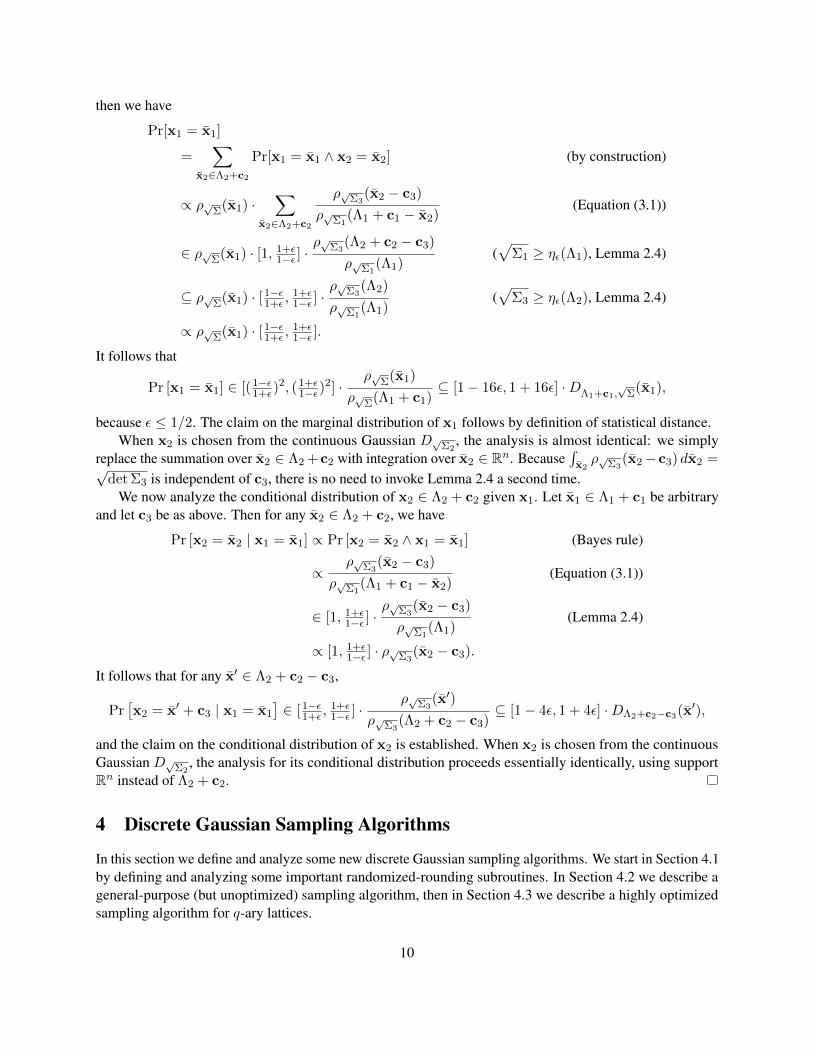
then we have

Pr[x1 = x1]

=∑

x2∈Λ2+c2

Pr[x1 = x1 ∧ x2 = x2] (by construction)

∝ ρ√Σ(x1) ·∑

x2∈Λ2+c2

ρ√Σ3(x2 − c3)

ρ√Σ1(Λ1 + c1 − x2)

(Equation (3.1))

∈ ρ√Σ(x1) · [1, 1+ε1−ε ] ·

ρ√Σ3(Λ2 + c2 − c3)

ρ√Σ1(Λ1)

(√

Σ1 ≥ ηε(Λ1), Lemma 2.4)

⊆ ρ√Σ(x1) · [1−ε1+ε ,

1+ε1−ε ] ·

ρ√Σ3(Λ2)

ρ√Σ1(Λ1)

(√

Σ3 ≥ ηε(Λ2), Lemma 2.4)

∝ ρ√Σ(x1) · [1−ε1+ε ,

1+ε1−ε ].

It follows that

Pr [x1 = x1] ∈ [(1−ε1+ε)

2, (1+ε1−ε)

2] ·ρ√Σ(x1)

ρ√Σ(Λ1 + c1)⊆ [1− 16ε, 1 + 16ε] ·DΛ1+c1,

√Σ(x1),

because ε ≤ 1/2. The claim on the marginal distribution of x1 follows by definition of statistical distance.When x2 is chosen from the continuous Gaussian D√Σ2

, the analysis is almost identical: we simplyreplace the summation over x2 ∈ Λ2 +c2 with integration over x2 ∈ Rn. Because

∫x2ρ√Σ3

(x2−c3) dx2 =√det Σ3 is independent of c3, there is no need to invoke Lemma 2.4 a second time.

We now analyze the conditional distribution of x2 ∈ Λ2 + c2 given x1. Let x1 ∈ Λ1 + c1 be arbitraryand let c3 be as above. Then for any x2 ∈ Λ2 + c2, we have

Pr [x2 = x2 | x1 = x1] ∝ Pr [x2 = x2 ∧ x1 = x1] (Bayes rule)

∝ρ√Σ3

(x2 − c3)

ρ√Σ1(Λ1 + c1 − x2)

(Equation (3.1))

∈ [1, 1+ε1−ε ] ·

ρ√Σ3(x2 − c3)

ρ√Σ1(Λ1)

(Lemma 2.4)

∝ [1, 1+ε1−ε ] · ρ√Σ3

(x2 − c3).

It follows that for any x′ ∈ Λ2 + c2 − c3,

Pr[x2 = x′ + c3 | x1 = x1

]∈ [1−ε

1+ε ,1+ε1−ε ] ·

ρ√Σ3(x′)

ρ√Σ3(Λ2 + c2 − c3)

⊆ [1− 4ε, 1 + 4ε] ·DΛ2+c2−c3(x′),

and the claim on the conditional distribution of x2 is established. When x2 is chosen from the continuousGaussian D√Σ2

, the analysis for its conditional distribution proceeds essentially identically, using supportRn instead of Λ2 + c2.

4 Discrete Gaussian Sampling Algorithms

In this section we define and analyze some new discrete Gaussian sampling algorithms. We start in Section 4.1by defining and analyzing some important randomized-rounding subroutines. In Section 4.2 we describe ageneral-purpose (but unoptimized) sampling algorithm, then in Section 4.3 we describe a highly optimizedsampling algorithm for q-ary lattices.

10

4.1 Randomized Rounding

We first need to define and analyze some simple ‘randomized-rounding’ operations from the reals to lattices,which are an important component of our sampling algorithms.

We start with a basic rounding operation from R to the integers Z, denoted bver for v ∈ R and somepositive real ‘rounding parameter’ r > 0. The output of this operation is a random variable over Z havingdistribution v +DZ−v,r. Observe that for any integer z ∈ Z, the random variables bz + ver and z + bver areidentically distributed; therefore, we sometimes assume that v ∈ [0, 1) without loss of generality. We extendthe rounding operation coordinate-wise to vectors v ∈ Rn, where each entry is rounded independently. Itfollows that for any v ∈ Rn and z ∈ Zn,

Pr [bver = z] ∝∏i∈[n]

ρr(zi − vi) = exp(−π∑i∈[n]

(zi − vi)2/r2) = exp(−π‖z− v‖2/r2) = ρr(z− v).

That is, bver has distribution v +DZn−v,r, because the standard basis for Zn is orthonormal.The next lemma characterizes the distribution obtained by randomized rounding to an arbitrary lattice,

using an arbitrary (possibly non-orthonormal) basis.

Lemma 4.1. Let B be a basis of a lattice Λ = L(B), let Σ = r2 ·BBt for some real r > 0, and let t ∈ Rnbe arbitrary. The random variable x = t−BbB−1ter has distribution DΛ+t,

√Σ.

Proof. Let v = B−1t. The support of bver is Zn, so the support of x is t−B · Zn = Λ + t. Now for anyx = t − Bz where z ∈ Zn, we have x = x if and only if bver = z. As desired, this event occurs withprobability proportional to

ρr(z− v) = ρr(B−1(t− x)−B−1t) = ρr(−B−1x) = ρrB(x) = ρ√Σ(x).

Efficient rounding. In [GPV08] it is shown how to sample from DZ−v,r for any v ∈ R and r > 0, byrejection sampling. While the algorithm requires only poly(log n) iterations before terminating, its concreterunning time and randomness complexity are not entirely suitable for practical implementations.

In this work, we can sample from v + DZ−v,r more efficiently because r is always fixed, known inadvance, and relatively small (about

√log n). Specifically, given r and v ∈ R we can (pre)compute a compact

table of the approximate cumulative distribution function of bver, i.e., the probabilities

pz := Pr[v +DZ−v,r ≤ z]

for each z ∈ Z in an interval [v − r · ω(√

log n), v + r · ω(√

log n)]. (Outside of that interval are the tails ofthe distribution, which carry negligible probability mass.) Then we can sample directly from v + DZ−v,rby choosing a uniformly random x ∈ [0, 1) and performing a binary search through the table for the z ∈ Zsuch that x ∈ [pz−1, pz). Moreover, the bits of x may be chosen ‘lazily,’ from most- to least-significant, untilz is determined uniquely. To sample within a negl(n) statistical distance of the desired distribution, theseoperations can all be implemented in time poly(log n).

4.2 Generic Sampling Algorithm

Here we apply Theorem 3.1 to sample from a discrete Gaussian of any sufficiently large covariance, givena good enough basis of the lattice. This procedure, described in Algorithm 1, serves mainly as a ‘proof of

11

Algorithm 1 Generic algorithm SampleD(B1, r,Σ, c) for sampling from a discrete Gaussian distribution.Input:

Offline phase: Basis B1 of a lattice Λ = L(B1), rounding parameter r = ω(√

log n), and positivedefinite covariance matrix Σ > Σ1 = r2 ·B1B

t1.

Online phase: a vector c ∈ Rn.Output: A vector x ∈ Λ + c drawn from a distribution within negl(n) statistical distance of DΛ+c,

√Σ.

Offline phase:1: Let Σ2 = Σ− Σ1 > 0, and compute some B2 =

√Σ2 (e.g., using the Cholesky decomposition).

2: Before each call to the online phase, choose a fresh x2 ← D√Σ2, i.e., let x2 ← B2 ·D1.

Online phase:3: return x← c−B1bB−1

1 (c− x2)er.

concept’ and a warm-up for our main algorithm on q-ary lattices. As such, it is not optimized for runtimeefficiency (because it uses arbitrary-precision real operations), though it is still fully parallelizable andoffline/online.

Theorem 4.2. Algorithm 1 is correct, and for any P ∈ [1, n2], its online phase can be executed in parallelby P processors that each perform O(n2/P ) operations on real numbers (of sufficiently high precision).

Proof. We first show correctness. Let Σ,Σ1,Σ2 be as in Algorithm 1. The output x is distributed as

x = x2 + (c− x2)−B1

⌊B−1

1 (c− x2)⌉r,

where x2 has distribution D√Σ2. By Lemma 4.1 with t = (c − x2), we see that x has distribution

x2 + DΛ+c−x2,√

Σ1. Now because Λ = L(B1) = B1 · Zn, we have

√Σ1 = rB1 ≥ ηε(Λ) for some

negligible ε = ε(n), by Definition 2.3 and Lemma 2.5. Therefore, by the second part of Theorem 3.1, x hasdistribution within negl(n) statistical distance of DΛ+c,

√Σ.

To parallelize the algorithm, simply observe that B−11 can be precomputed in the offline phase, and that

the matrix-vector products and randomized rounding can all be executed in parallel on P processors in thenatural way.

4.3 Efficient Sampling Algorithm for q-ary Lattices

Algorithm 2 is an optimized sampling algorithm for q-ary (integral) lattices Λ, i.e., lattices for whichqZn ⊆ Λ ⊆ Zn for some positive integer q. These include NTRU lattices [HPS98], as well as the family oflattices for which Ajtai [Ajt96] first demonstrated worst-case hardness.

Note that Algorithm 2 samples from the coset Λ + c for a given integral vector c ∈ Zn; as we shall see,this allows for certain optimizations. Fortunately, all known cryptographic applications of Gaussian samplingover q-ary lattices use an integral c. Also note that the algorithm will typically be used to sample from aspherical discrete Gaussian, i.e., one for which the covariance matrix Σ = s2I for some real s > 0. As longas s slightly exceeds the largest singular value of B1, i.e., s ≥ r · (2s1(B1) + 1) for some r = ω(

√log n),

then we have Σ ≥ r2 · (4B1Bt1 + I) as required by the algorithm.

Theorem 4.3. Algorithm 2 is correct, and for any P ∈ [1, n2], its online phase can be implemented inparallel by P processors that each perform at most dn/P e randomized-rounding operations on rationalnumbers from the set 0

q ,1q , . . . ,

q−1q , and O(n2/P ) integer operations.

12

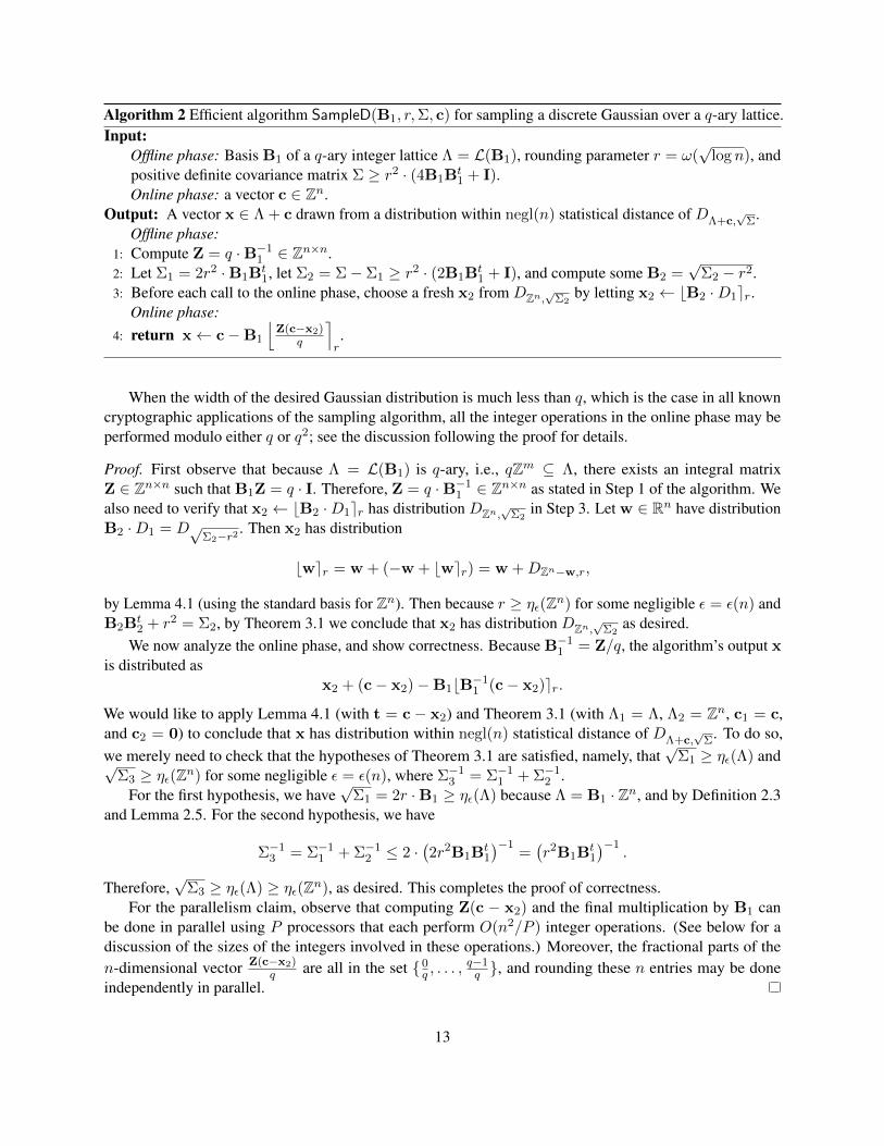
Algorithm 2 Efficient algorithm SampleD(B1, r,Σ, c) for sampling a discrete Gaussian over a q-ary lattice.Input:

Offline phase: Basis B1 of a q-ary integer lattice Λ = L(B1), rounding parameter r = ω(√

log n), andpositive definite covariance matrix Σ ≥ r2 · (4B1B

t1 + I).

Online phase: a vector c ∈ Zn.Output: A vector x ∈ Λ + c drawn from a distribution within negl(n) statistical distance of DΛ+c,

√Σ.

Offline phase:1: Compute Z = q ·B−1

1 ∈ Zn×n.2: Let Σ1 = 2r2 ·B1B

t1, let Σ2 = Σ− Σ1 ≥ r2 · (2B1B

t1 + I), and compute some B2 =

√Σ2 − r2.

3: Before each call to the online phase, choose a fresh x2 from DZn,√

Σ2by letting x2 ← bB2 ·D1er.

Online phase:4: return x← c−B1

⌊Z(c−x2)

q

⌉r.

When the width of the desired Gaussian distribution is much less than q, which is the case in all knowncryptographic applications of the sampling algorithm, all the integer operations in the online phase may beperformed modulo either q or q2; see the discussion following the proof for details.

Proof. First observe that because Λ = L(B1) is q-ary, i.e., qZm ⊆ Λ, there exists an integral matrixZ ∈ Zn×n such that B1Z = q · I. Therefore, Z = q ·B−1

1 ∈ Zn×n as stated in Step 1 of the algorithm. Wealso need to verify that x2 ← bB2 ·D1er has distribution DZn,

√Σ2

in Step 3. Let w ∈ Rn have distributionB2 ·D1 = D√

Σ2−r2 . Then x2 has distribution

bwer = w + (−w + bwer) = w +DZn−w,r,

by Lemma 4.1 (using the standard basis for Zn). Then because r ≥ ηε(Zn) for some negligible ε = ε(n) andB2B

t2 + r2 = Σ2, by Theorem 3.1 we conclude that x2 has distribution DZn,

√Σ2

as desired.We now analyze the online phase, and show correctness. Because B−1

1 = Z/q, the algorithm’s output xis distributed as

x2 + (c− x2)−B1bB−11 (c− x2)er.

We would like to apply Lemma 4.1 (with t = c − x2) and Theorem 3.1 (with Λ1 = Λ, Λ2 = Zn, c1 = c,and c2 = 0) to conclude that x has distribution within negl(n) statistical distance of DΛ+c,

√Σ. To do so,

we merely need to check that the hypotheses of Theorem 3.1 are satisfied, namely, that√

Σ1 ≥ ηε(Λ) and√Σ3 ≥ ηε(Zn) for some negligible ε = ε(n), where Σ−1

3 = Σ−11 + Σ−1

2 .For the first hypothesis, we have

√Σ1 = 2r ·B1 ≥ ηε(Λ) because Λ = B1 · Zn, and by Definition 2.3

and Lemma 2.5. For the second hypothesis, we have

Σ−13 = Σ−1

1 + Σ−12 ≤ 2 ·

(2r2B1B

t1

)−1=(r2B1B

t1

)−1.

Therefore,√

Σ3 ≥ ηε(Λ) ≥ ηε(Zn), as desired. This completes the proof of correctness.For the parallelism claim, observe that computing Z(c − x2) and the final multiplication by B1 can

be done in parallel using P processors that each perform O(n2/P ) integer operations. (See below for adiscussion of the sizes of the integers involved in these operations.) Moreover, the fractional parts of then-dimensional vector Z(c−x2)

q are all in the set 0q , . . . ,

q−1q , and rounding these n entries may be done

independently in parallel.

13

Implementation notes. For a practical implementation, Algorithm 2 admits several additional optimiza-tions, which we discuss briefly here.

In all cryptographic applications of Gaussian sampling on q-ary lattices, the length of the sampled vectoris significantly shorter than q, i.e., its entries lie within a narrow interval around 0. Therefore, it suffices forthe sampling algorithm to compute its output modulo q, using the integers −b q2c, . . . , b

q−12 c as the set

of canonical representatives. For this purpose, the final multiplication by the input basis B1 need only beperformed modulo q. Similarly, Z and Z(c− x2) need only be computed modulo q2, because we are onlyconcerned with the value of Z(c−x2)

q modulo q.Because all the randomized-rounding steps are performed on rationals whose fractional parts are in

0q , . . . ,

q−1q , if q is reasonably small it may be worthwhile (for faster rounding) to precompute the tables

of the cumulative distribution functions for all q possibilities. Alternatively (or in addition), during theoffline phase the algorithm could precompute and cache a few rounded samples for each of the q possibilities,consuming them as needed in the online phase.

5 Singular Value Bounds

In this section we give bounds on the largest singular value of a basis B and relate them to other geometricquantities that are relevant to the prior sampling algorithm of [GPV08].

5.1 General Bounds

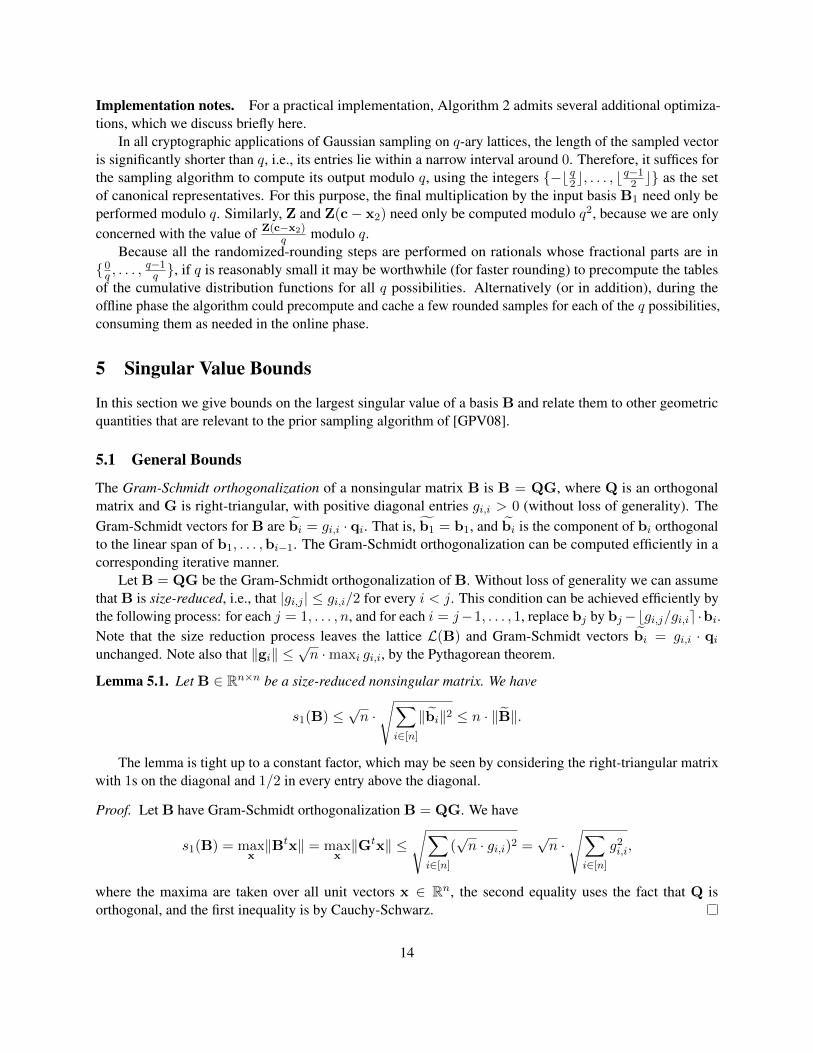
The Gram-Schmidt orthogonalization of a nonsingular matrix B is B = QG, where Q is an orthogonalmatrix and G is right-triangular, with positive diagonal entries gi,i > 0 (without loss of generality). TheGram-Schmidt vectors for B are bi = gi,i · qi. That is, b1 = b1, and bi is the component of bi orthogonalto the linear span of b1, . . . ,bi−1. The Gram-Schmidt orthogonalization can be computed efficiently in acorresponding iterative manner.

Let B = QG be the Gram-Schmidt orthogonalization of B. Without loss of generality we can assumethat B is size-reduced, i.e., that |gi,j | ≤ gi,i/2 for every i < j. This condition can be achieved efficiently bythe following process: for each j = 1, . . . , n, and for each i = j−1, . . . , 1, replace bj by bj−bgi,j/gi,ie ·bi.Note that the size reduction process leaves the lattice L(B) and Gram-Schmidt vectors bi = gi,i · qiunchanged. Note also that ‖gi‖ ≤

√n ·maxi gi,i, by the Pythagorean theorem.

Lemma 5.1. Let B ∈ Rn×n be a size-reduced nonsingular matrix. We have

s1(B) ≤√n ·√∑i∈[n]

‖bi‖2 ≤ n · ‖B‖.

The lemma is tight up to a constant factor, which may be seen by considering the right-triangular matrixwith 1s on the diagonal and 1/2 in every entry above the diagonal.

Proof. Let B have Gram-Schmidt orthogonalization B = QG. We have

s1(B) = maxx‖Btx‖ = max

x‖Gtx‖ ≤

√∑i∈[n]

(√n · gi,i)2 =

√n ·√∑i∈[n]

g2i,i,

where the maxima are taken over all unit vectors x ∈ Rn, the second equality uses the fact that Q isorthogonal, and the first inequality is by Cauchy-Schwarz.

14

5.2 Bases for Cryptographic Lattices

Ajtai [Ajt99] gave a procedure for generating a uniformly random q-ary lattice from a certain family of‘worst-case-hard’ cryptographic lattices, together with a relatively short basis B. Alwen and Peikert [AP09]recently improved and extended the construction to yield asymptotically optimal bounds on ‖B‖ = maxi‖bi‖and ‖B‖ = maxi‖bi‖. Here we show that with a small modification, one of the constructions of [AP09]yields (with overwhelming probability) a basis whose largest singular value is within an O(

√log q) factor of

‖B‖. It follows that our efficient Gaussian sampling algorithm is essentially as tight as the GPV algorithm onsuch bases.

Lemma 5.2. The construction of [AP09, Section 3.2] (modified as described below) outputs a basis B suchthat s1(B) = O(

√log q) · ‖B‖ with overwhelming probability.

Proof. For concreteness, we focus on the version of the construction that uses base r = 2, though similarbounds can be obtained for any r ≥ 2. In the construction, there are matrices G and U where the columnsof G include the columns of an (efficiently computable) ‘bad’ basis H of a certain lattice, and GU is arectangular 0-1 matrix containing the binary representation of H. As described in [AP09], H actually neednot be a basis; any full-rank set of lattice vectors suffices. In this case, the output is then a q-ary latticetogether with a short full-rank set of lattice vectors, which can be efficiently converted to a basis withoutincreasing the largest singular value (see Lemma 5.4 below).

We modify the construction so that the columns of G include all the columns of qI (rather than H),which are a full-rank set of lattice vectors as required by the construction. Similarly, GU is rectangularmatrix containing the binary representation of qI. More formally, GU = I ⊗ qt, where ⊗ denotes theKronecker product and qt is the dlg qe-dimensional row vector containing the binary representation ofq. These modifications do not affect the (asymptotically optimal) bounds on ‖B‖ and ‖B‖ establishedin [AP09].

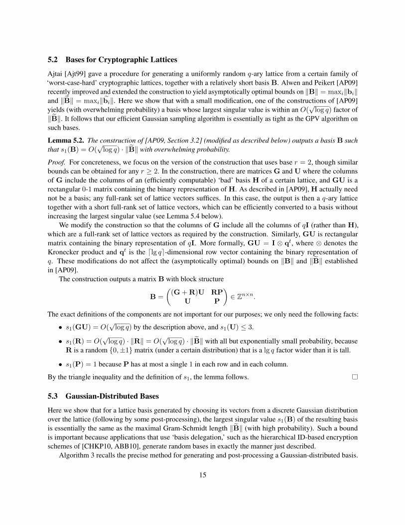
The construction outputs a matrix B with block structure

B =

((G + R)U RP

U P

)∈ Zn×n.

The exact definitions of the components are not important for our purposes; we only need the following facts:

• s1(GU) = O(√

log q) by the description above, and s1(U) ≤ 3.

• s1(R) = O(√

log q) · ‖R‖ = O(√

log q) · ‖B‖ with all but exponentially small probability, becauseR is a random 0,±1 matrix (under a certain distribution) that is a lg q factor wider than it is tall.

• s1(P) = 1 because P has at most a single 1 in each row and in each column.

By the triangle inequality and the definition of s1, the lemma follows.

5.3 Gaussian-Distributed Bases

Here we show that for a lattice basis generated by choosing its vectors from a discrete Gaussian distributionover the lattice (following by some post-processing), the largest singular value s1(B) of the resulting basisis essentially the same as the maximal Gram-Schmidt length ‖B‖ (with high probability). Such a boundis important because applications that use ‘basis delegation,’ such as the hierarchical ID-based encryptionschemes of [CHKP10, ABB10], generate random bases in exactly the manner just described.

Algorithm 3 recalls the precise method for generating and post-processing a Gaussian-distributed basis.

15

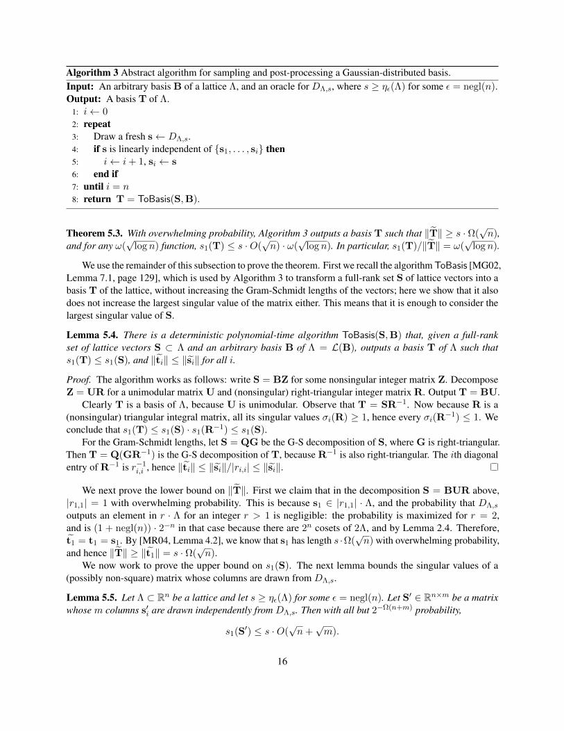
Algorithm 3 Abstract algorithm for sampling and post-processing a Gaussian-distributed basis.Input: An arbitrary basis B of a lattice Λ, and an oracle for DΛ,s, where s ≥ ηε(Λ) for some ε = negl(n).Output: A basis T of Λ.

1: i← 02: repeat3: Draw a fresh s← DΛ,s.4: if s is linearly independent of s1, . . . , si then5: i← i+ 1, si ← s6: end if7: until i = n8: return T = ToBasis(S,B).

Theorem 5.3. With overwhelming probability, Algorithm 3 outputs a basis T such that ‖T‖ ≥ s · Ω(√n),

and for any ω(√

log n) function, s1(T) ≤ s ·O(√n) · ω(

√log n). In particular, s1(T)/‖T‖ = ω(

√log n).

We use the remainder of this subsection to prove the theorem. First we recall the algorithm ToBasis [MG02,Lemma 7.1, page 129], which is used by Algorithm 3 to transform a full-rank set S of lattice vectors into abasis T of the lattice, without increasing the Gram-Schmidt lengths of the vectors; here we show that it alsodoes not increase the largest singular value of the matrix either. This means that it is enough to consider thelargest singular value of S.

Lemma 5.4. There is a deterministic polynomial-time algorithm ToBasis(S,B) that, given a full-rankset of lattice vectors S ⊂ Λ and an arbitrary basis B of Λ = L(B), outputs a basis T of Λ such thats1(T) ≤ s1(S), and ‖ti‖ ≤ ‖si‖ for all i.

Proof. The algorithm works as follows: write S = BZ for some nonsingular integer matrix Z. DecomposeZ = UR for a unimodular matrix U and (nonsingular) right-triangular integer matrix R. Output T = BU.

Clearly T is a basis of Λ, because U is unimodular. Observe that T = SR−1. Now because R is a(nonsingular) triangular integral matrix, all its singular values σi(R) ≥ 1, hence every σi(R−1) ≤ 1. Weconclude that s1(T) ≤ s1(S) · s1(R−1) ≤ s1(S).

For the Gram-Schmidt lengths, let S = QG be the G-S decomposition of S, where G is right-triangular.Then T = Q(GR−1) is the G-S decomposition of T, because R−1 is also right-triangular. The ith diagonalentry of R−1 is r−1

i,i , hence ‖ti‖ ≤ ‖si‖/|ri,i| ≤ ‖si‖.

We next prove the lower bound on ‖T‖. First we claim that in the decomposition S = BUR above,|r1,1| = 1 with overwhelming probability. This is because s1 ∈ |r1,1| · Λ, and the probability that DΛ,s

outputs an element in r · Λ for an integer r > 1 is negligible: the probability is maximized for r = 2,and is (1 + negl(n)) · 2−n in that case because there are 2n cosets of 2Λ, and by Lemma 2.4. Therefore,t1 = t1 = s1. By [MR04, Lemma 4.2], we know that s1 has length s ·Ω(

√n) with overwhelming probability,

and hence ‖T‖ ≥ ‖t1‖ = s · Ω(√n).

We now work to prove the upper bound on s1(S). The next lemma bounds the singular values of a(possibly non-square) matrix whose columns are drawn from DΛ,s.

Lemma 5.5. Let Λ ⊂ Rn be a lattice and let s ≥ ηε(Λ) for some ε = negl(n). Let S′ ∈ Rn×m be a matrixwhose m columns s′i are drawn independently from DΛ,s. Then with all but 2−Ω(n+m) probability,

s1(S′) ≤ s ·O(√n+√m).

16

Proof sketch. We give an outline of the proof, whose details are standard in random matrix theory; see forexample [Ver07, Lecture 6]. Without loss of generality, assume that s = 1. The first fact we need is that thedistribution DΛ is subgaussian in every direction, i.e., for any unit vector u, we have Prx∼DΛ

[|〈x,u〉| >t] ≤ C · exp(−πt2) for some fixed constant C and any t > 0. This fact is established in [Pei07, Lemma 5.1],using techniques of [Ban95].

The second fact we need is that an n-by-m matrix S′ with independent subgaussian columns has largestsingular value O(

√n +√m) with all but 2−Ω(m+n) probability. The largest singular value of S′ is the

maximum of utS′v over all unit vectors u ∈ Rn, v ∈ Rm. This maximum is bounded by first observingthat for any fixed u,v, the random variable utS′v is itself subgaussian, and therefore has absolute valueO(√n+√m) except with probability 2−Ω(m+n). By then taking a union bound over 2O(m+n) points in a

suitable ε-net, the bound extends to all u,v simultaneously.

Now let S′ ∈ Rn×m be the matrix consisting of every vector s ← DΛ,s chosen by Algorithm 3,irrespective of whether it is linearly independent of its predecessors. Because S is made up of a subset of thecolumns of S′, it follows immediately from the definition that s1(S) ≤ s1(S′).

It simply remains to bound the total number m of samples that Algorithm 3 draws from DΛ,s. By [Reg05,Lemma 3.15], each sample s is linearly independent of s1, . . . , si with probability at least 1/10. Therefore, forany ω(log n) function, the algorithm draws a total of n · ω(log n) samples, except with negligible probability.By Lemma 5.5, we conclude that s1(S′) ≤ s · O(

√n) · ω(

√log n) with overwhelming probability. This

completes the proof.

6 Acknowledgments

The author thanks Phong Nguyen, Xiang Xie, and the anonymous CRYPTO’10 reviewers for helpfulcomments.

References

[ABB10] S. Agrawal, D. Boneh, and X. Boyen. Efficient lattice (H)IBE in the standard model. InEUROCRYPT. 2010. To appear.

[Ajt96] M. Ajtai. Generating hard instances of lattice problems. Quaderni di Matematica, 13:1–32,2004. Preliminary version in STOC 1996.

[Ajt99] M. Ajtai. Generating hard instances of the short basis problem. In ICALP, pages 1–9. 1999.

[AP09] J. Alwen and C. Peikert. Generating shorter bases for hard random lattices. In STACS, pages75–86. 2009.

[Bab86] L. Babai. On Lovasz’ lattice reduction and the nearest lattice point problem. Combinatorica,6(1):1–13, 1986.

[Ban95] W. Banaszczyk. Inequalites for convex bodies and polar reciprocal lattices in Rn. Discrete &Computational Geometry, 13:217–231, 1995.

[CHKP10] D. Cash, D. Hofheinz, E. Kiltz, and C. Peikert. Bonsai trees, or how to delegate a lattice basis.In EUROCRYPT. 2010. To appear.

17

[Gen09] C. Gentry. Fully homomorphic encryption using ideal lattices. In STOC, pages 169–178. 2009.

[GPV08] C. Gentry, C. Peikert, and V. Vaikuntanathan. Trapdoors for hard lattices and new cryptographicconstructions. In STOC, pages 197–206. 2008.

[HHGP+03] J. Hoffstein, N. Howgrave-Graham, J. Pipher, J. H. Silverman, and W. Whyte. NTRUSIGN:Digital signatures using the NTRU lattice. In CT-RSA, pages 122–140. 2003.

[HPS98] J. Hoffstein, J. Pipher, and J. H. Silverman. NTRU: A ring-based public key cryptosystem. InANTS, pages 267–288. 1998.

[Kle00] P. N. Klein. Finding the closest lattice vector when it’s unusually close. In SODA, pages937–941. 2000.

[Ksh59] A. M. Kshirsagar. Bartlett decomposition and Wishart distribution. The Annals of MathematicalStatistics, 30(1):239–241, March 1959. Available at http://www.jstor.org/stable/2237140.

[LM08] V. Lyubashevsky and D. Micciancio. Asymptotically efficient lattice-based digital signatures.In TCC, pages 37–54. 2008.

[LPR10] V. Lyubashevsky, C. Peikert, and O. Regev. On ideal lattices and learning with errors over rings.In EUROCRYPT. 2010. To appear.

[MG02] D. Micciancio and S. Goldwasser. Complexity of Lattice Problems: a cryptographic perspective,volume 671 of The Kluwer International Series in Engineering and Computer Science. KluwerAcademic Publishers, Boston, Massachusetts, 2002.

[Mic02] D. Micciancio. Generalized compact knapsacks, cyclic lattices, and efficient one-way functions.Computational Complexity, 16(4):365–411, 2007. Preliminary version in FOCS 2002.

[MPSW09] T. Malkin, C. Peikert, R. A. Servedio, and A. Wan. Learning an overcomplete basis: Analysisof lattice-based signatures with perturbations, 2009. Manuscript.

[MR04] D. Micciancio and O. Regev. Worst-case to average-case reductions based on Gaussianmeasures. SIAM J. Comput., 37(1):267–302, 2007. Preliminary version in FOCS 2004.

[NR06] P. Q. Nguyen and O. Regev. Learning a parallelepiped: Cryptanalysis of GGH and NTRUsignatures. J. Cryptology, 22(2):139–160, 2009. Preliminary version in Eurocrypt 2006.

[Pei07] C. Peikert. Limits on the hardness of lattice problems in `p norms. Computational Complexity,17(2):300–351, May 2008. Preliminary version in CCC 2007.

[PV08] C. Peikert and V. Vaikuntanathan. Noninteractive statistical zero-knowledge proofs for latticeproblems. In CRYPTO, pages 536–553. 2008.

[Reg05] O. Regev. On lattices, learning with errors, random linear codes, and cryptography. J. ACM,56(6), 2009. Preliminary version in STOC 2005.

[SSTX09] D. Stehle, R. Steinfeld, K. Tanaka, and K. Xagawa. Efficient public key encryption based onideal lattices. In ASIACRYPT, pages 617–635. 2009.

18

[Ver07] R. Vershynin. Lecture notes on non-asymptotic theory of random matrices, 2007. Available athttp://www-personal.umich.edu/˜romanv/teaching/2006-07/280/, lastaccessed 17 Feb 2010.

19