Pergamon Computers Math. Applic. Vol. 29, No. 7, pp. 39-54, 1995

Copyright©1995 Elsevier Science Ltd Printed in Great Britain. All rights reserved

0898-1221/95 $9.50 + 0.00 0898-1221(95)00017-8

A N e w Gaussian El iminat ion-Based Algor i thm for Parallel Solution of Linear Equat ions

K. N. BALASUBRAMANYA MURTHY AND

C . SIVA R A M MURTHY* Department of Computer Science and Engineering

Indian Institute of Technology, Madras-600 036, India *murthy~iitm. ex~aet, in

(Received February 1994; accepted July 1994)

A b s t r a c t - - I n this paper, a variant of Gaussian Elimination (GE) called Successive Gaussian Elim- ination (SGE) algorithm for parallel solution of linear equations is presented. Unlike the conventional GE algorithm, the SGE algorithm does not have a separate back substitution phase, which requires O(N) steps using O(N) processors or O (log 2 N) steps using O (N 3) processors, for solving a system of linear algebraic equations. It replaces the back substitution phase by only one step division and possesses numerical stability through partial pivoting. Further, in this paper, the SGE algorithm is shown to produce the diagonal form in the same amount of parallel time required for producing triangular form using the conventional parallel GE algorithm. Finally, the effectiveness of the SGE algorithm is demonstrated by studying its performance on a hypercube multiprocessor system.

K e y w o r d s - - L i n e a r equations, Triangulation, Back substitution, Gaussian elimination, Numerical stability, Pivoting, Task system, Scheduling, Multiprocessor system.

1. I N T R O D U C T I O N

The problem of solving a set of linear algebraic equations A x = b (where A is a known N x N matrix, x and b are unknown and known N vectors, respectively) is one of the central problems in computational mathematics and computer science. Efficient numerical methods for solving this problem on uniprocessor systems have been developed, and many reliable and high quality codes are available for different cases of linear systems. Recent advances in VLSI and networking technology have led to widespread interest in the use of multiprocessor systems for solving many

practical problems. Bertsekas and Tsitsiklis [1], Heller [2], Lakshmivarahan and Dhall [3], and Sameh and Kuck [4], describe the current s tate of art in parallel numerical algebra. In this paper, we present a new algorithm called Successive Gaussian Elimination (SGE) for solving dense system of linear algebraic equations on multiprocessor systems. Most importantly, the algorithm permits partial pivoting to improve numerical stability. The SGE algorithm is essentially a variant of the Gaussian Elimination (GE) algorithm and does not require a separate back substi tut ion phase to find the complete solution vector. I t may be noted tha t the back substi tution phase requires O(N) steps using O(N) processors or O(log 2 N) steps using O ( N 3) processors [2,4].

The rest of the paper is organized as follows. In the next section, we first define the problem

and then discuss the relevant work. Section 3 presents the SGE algorithm for the problem. In Section 4, the memory requirements and error analysis of the SGE algorithm are described.

This work was supported by the Indian National Science Academy and the Department of Science and Technology.

Typeset by .Ah/e.%TEX

39

40 K . N . BALASUBRAMANYA MURTHY AND C. SIVA RAM MURTHY

Section 5 describes, in detail, a method for scheduling the computational tasks in the algorithm onto the processors for efficient implementation on a multiprocessor system. Section 6 presents the performance evaluation of the SGE algorithm. Finally, in Section 7, we present our conclusions.

2. P R O B L E M D E F I N I T I O N A N D R E L A T E D W O R K

The problem in solving a set of linear algebraic equations is to find the vector x in the equation A x = b, where A is an N × N matrix, x is an unknown N vector, and b is a known N vector.

The solution of A x = b can be obtained by using classical methods such as GE, Ganss- Jordan (G J), Cramer's rule (CR), and LU decomposition [1-12]. The solution process of A x = b

by these methods (except GJ and CR algorithms) essentially consists of triangulation phase followed by back substitution phase. Therefore, the total time taken for solving the problem on a multiprocessor system is the sum of parallel times taken for triangulation and back substitution phases. Further, the classical methods require pivoting to assure numerical stability.

Most of the existing algorithms available in the literature for parallel solution of linear equations consider only the computational intensive triangulation phase assuming that efficient algorithms exist for the simple back substitution phase. However, it is important to note that both the phases using different efficient algorithms may not optimally be implemented on any given multiprocessor system as these algorithms were developed for different multiprocessor configurations.

Recently, two back substitution free algorithms based on GJ and CR are discussed in [10,12]. The parallel CR algorithm [12], which does not support pivoting, is applicable only for diagonally dominant systems while the parallel GJ algorithm [10] permits the partial pivoting in which the maximum element is found among the subdiagonal elements of the pivot column and the pivot column element (instead of finding the maximum element in the entire pivot column).

In this paper, we present a back substitution-free SGE algorithm, which supports partial pivoting, to produce the diagonal form in O(N 2) steps using O ( N ) processors against the same number of steps required for producing the triangular form in the existing methods.

3. S U C C E S S I V E G A U S S I A N E L I M I N A T I O N ( S G E ) A L G O R I T H M

It is clear while solving A x = b that the value of x~ depends on the value of xk (k = 1, 2 , . . . , N and k ¢ i) indicating (N - 1) th level dependency. It is obvious, in the GE method, the value of xi (i --- 1, 2 , . . . , N) is found by eliminating its dependency on xk for (k < i) in the triangulation phase and xk for (k > i) in the back substitution phase.

In the SGE algorithm, the dependencies of all the unknowns are reduced to half at every stage and finally to zero in log 2 N stages (i.e., N linear independent equations at Stage 1 are replaced by two sets of N / 2 linear independent equations at Stage 2, by four sets of N / 4 linear independent equations at Stage 3, etc.) which is accomplished by using the concept of forward (left to right) and backward (right to left) eliminations.

In this section, we explain how to obtain the diagonal form of coefficient matrix A in the equation A x = b. For better exposition, we assume that N = 2 ~, where c~ is an integer and later, we relax this assumption. The proposed algorithm consists of the following steps.

STEP 1. We form two matrices namely A0 and A1 identical to the coefficient matrix A and find the maximum element in the pivot column of A0 and A1, and exchange the pivot row with the row in which maximum element is found.

STEP 2. Using the GE method (subtracting fractions of pivot row elements from nonpivot elements), we triangulate A0 in the forward direction to eliminate the subdiagonal elements in the pivot columns (note that partial pivoting is carried out before each column is being eliminated) 1,2, 3 , . . . , N / 2 (by taking a11, a 2 2 , . . . ,aN/2,N/2 as pivot elements) to reduce its order to N / 2 (ignoring the eliminated columns and the corresponding rows). Concurrently, we triangulate A1 in the backward direction to eliminate the superdiagonal elements in the pivot columns (again

New Gaussian Algorithm 41

note that partial pivoting is carried out before any column is being eliminated) N, N - 1, N - 2 , . . . , N/2 + 1 (by taking a N N , a g - l , g - 1 , . . . , aN/2+I,N/2+I as pivot elements) to reduce the order of A1 also to N/2 (again ignoring the eliminated columns and the corresponding rows). With this, modified A0 may be treated as a new coefficient matrix (we call it reduced A0) with columns and rows N / 2 + 1, N/2+2, . . . . N and, similarly, modified A1 as a new coefficient matrix (we call it reduced A1) with columns and rows 1, 2 , . . . , N/2.

STEP 3. We duplicate the reduced matrices A0 to form A00 and A01 , and A1 to form Alo and An (each of these duplicated matrices will be of the same order, i.e., N/2). We now (note that partial pivoting is carried out before each column being eliminated) triangulate A00 and A10 in the forward direction, and A01 and An in the backward direction through N/4 pivot columns using GE, thus reducing the order of each of these matrices to half of their original size, i.e., N/4. Note that the above four matrices are reduced in parallel.

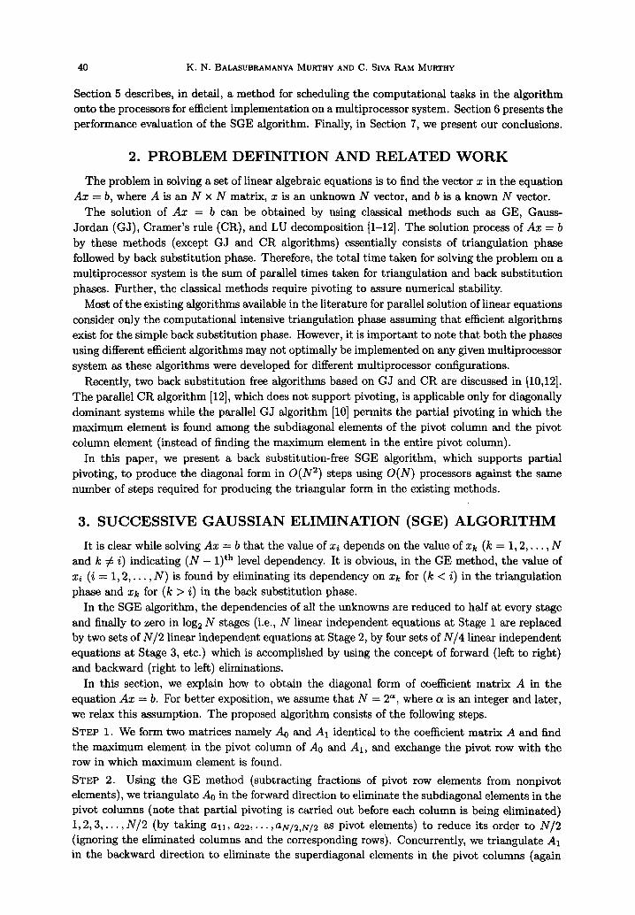
STEP 4. We continue this process of halving the size of submatrices (using partial pivoting at each step) and doubling the number of submatrices for log 2 N times so that we end up with N submatrices each of order 1. These N submatrices represent the diagonal form of the coefficient matrix A in the equation Ax = b. To obtain an idea about the nature of computations during each step of the SGE algorithm, we give procedures for forward elimination and backward elimination below by taking the order of the matrix as m.

PROCEDURE forward-elimination;

BEGIN

FOR k : 1 TO m/2 DO BEGIN

find q such that

laq,kl = max of (la+,kl, lak+1,kl,-.., la,+,,+,,,,:l) exchange row k and row q FOR q = (k + 1) T0 .m DO

aq,k = a q , k / a k , k F O R j = ( k + I ) T0mD0

F O R i : ( k + I ) T0mD0

a i d = a i d -- a i , k * a k , j END (* of for loop with index k *)

END(* of procedure forward-elimination *)

PROCEDURE backward-elimination;

BEGIN

FOR k = m DOWNT0 (m/2 + I) DO BEGIN

find q such that

la+,kl = ma~ of (lak,kl, la~-1,kl,.-., lal,kl) exchange row k and row q FOR q = (k - i) D0WNT0 1 DO

aq, k = a q , k / a k , k FOR j : (k - 1) DOWNT0 1 D0

FOR i = (k - I) D0WNTO 1 DO

a i , j = a i , j -- ai ,k * a k , j END (* of for loop with index k *)

END(* of procedure backward-elimination *)

T*k__k+l

*i T~-k+l

Z9:7-0

42 K. N. BALASUBRAMANYA MURTHY AND C. SIVA RAM MURTHY

I I x I + 1 3 x z - 4 x 3 + 8 x a - - 4

x I + 9 x z - 5 x 3 - 3 x • 8

- 2 1 x - 12 x z + 5 x - x a = - 8

4 x z + 31 x z + 7 x 3 + 3 x • = 17

U s e p a r t i a l plvotlng and

GE to eliminate x and x I 2

in the forward dlrectlon

|

10 x 3 - 3 . 8 7 x a = 3 . 0 8

Use partial plvotlng & GE to ellmlnate x a in forward

direction

Use p a r t i a l plvotlng a n d

GE to ellmlnate x and x 3 4

in the backward dlrectlon

J - 1 9 . 5 6 x 1 - 2 4 . 2 1 x z = - 1 8 . 2 9 [ I

= 2 0 . 6 5 5.03 x t + 3 3 . 8 5 x 2 I U s e p a r t i a l U s e p a r t i a l pivot ing & GE plvotlnE & GE t o e l i m i n a t e t o e l i m i n a t e x In backward x in forward

• 1

d i r e c t i o n d i r e c t i o n

U s e p a r t i a l p l v o t l n g & GE to e l lmlnate x z i n b a c k w a r d

dlrectlon

1"" x, I-"" '' x

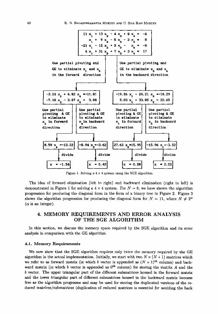
I .0.,ol Figure 1. Solving a 4 x 4 system using the SGE algorithm.

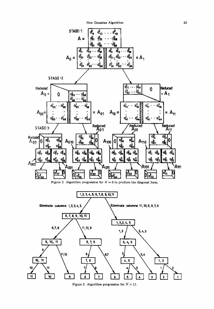
The idea of forward elimination (left to right) and backward elimination (right to left) is demonstrated in Figure 1 for solving a 4 x 4 system. For N = 8, we have shown the algorithm progression for producing the diagonal form in the form of a binary tree in Figure 2. Figure 3 shows the algorithm progression for producing the diagonal form for N = 11, where N ¢ 2 ~ (a is an integer).

4. M E M O R Y R E Q U I R E M E N T S A N D E R R O R ANALYSIS OF THE SGE A L G O R I T H M

In this section, we discuss the memory space required by the SGE algorithm and its error analysis in comparison with the GE algorithm.

4.1. M e m o r y R e q u i r e m e n t s

We now show that the SGE algorithm requires only twice the memory required by the GE algorithm in the actual implementation. Initially, we start with two N × (N + 1) matrices which we refer to as forward matrix (in which b vector is appended as (N + 1) th column) and back- ward matrix (in which b vector is appended as 0 th column) for storing the matrix A and the b vector. The upper triangular part of the different submatrices housed in the forward matr ix and the lower triangular part of different submatrices housed in the backward matr ix become free as the algorithm progresses and may be used for storing the duplicated versions of the re- duced matrices/submatrices (duplication of reduced matrices is essential for avoiding the back

New Gaussian Algorithm

ST~E-1 ~', ~, , ' ' " ~. I A= ~, e , ' , . . . ~ !

I,~, , ; , . . .~ ,~ , ,~,..-,~,1

Reduced I ~ _ _ _ _ J A° =~~~

AOO= = A 0

R ~ , ~ : ~ _ .~ ~,1,,I

i o~7

• ooo "Aool / 1

Figure 2. Algorithm progression for N = 8 to produce the diagonal form.

43

~111

1,2, 3, 4, 5, 6,7,8, 9,10,11

10 / \11

BIminote columns 1, 2, 3, 4, S Eliminate columns 11,10,9,8,7,6

6,7,8

90 10, 11

6, 7, 8, 9, 10, 11

11,10, 9

6,~,8

11,10 6

i I

Figure 3. Algorithm progression for N = 11.

44 K . N . BALASUBRAMANYA MURTHY AND C. SIVA RAM MURTHY

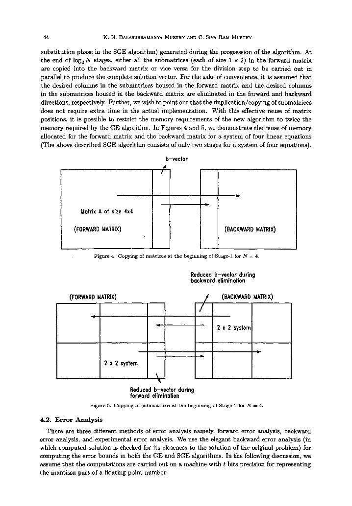
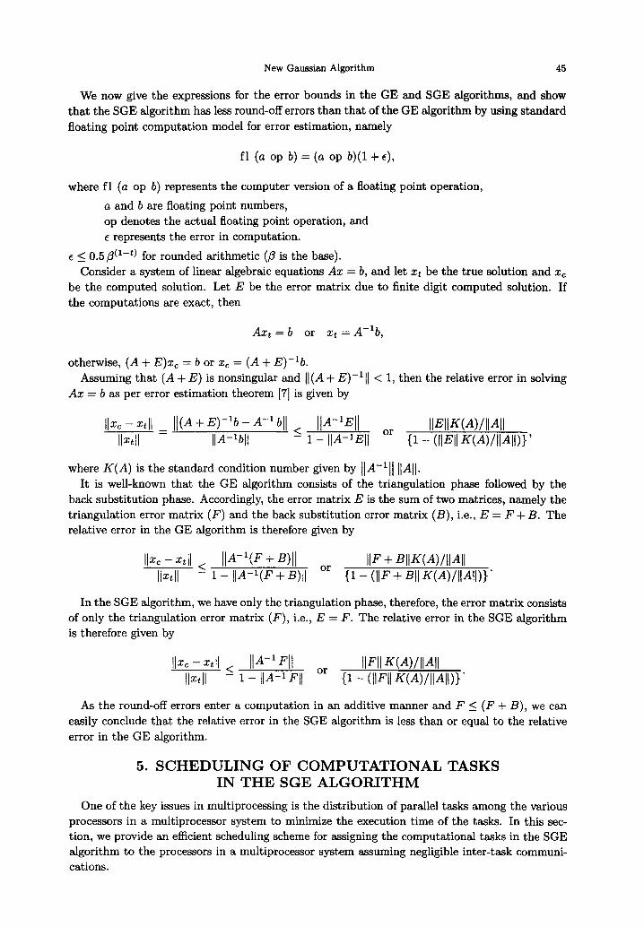
substitution phase in the SGE algorithm) generated during the progression of the algorithm. At the end of log 2 N stages, either all the submatrices (each of size 1 x 2) in the forward matrix are copied into the backward matrix or vice versa for the division step to be carried out in parallel to produce the complete solution vector. For the sake of convenience, it is assumed that the desired columns in the submatrices housed in the forward matrix and the desired columns in the submatrices housed in the backward matrix are eliminated in the forward and backward directions, respectively. Further, we wish to point out that the duplication/copying of submatrices does not require extra time in the actual implementation. With this effective reuse of matrix positions, it is possible to restrict the memory requirements of the new algorithm to twice the memory required by the GE algorithm. In Figures 4 and 5, we demonstrate the reuse of memory allocated for the forward matrix and the backward matrix for a system of four linear equations (The above described SGE algorithm consists of only two stages for a system of four equations).

b-vector , /

Matrix A of size 4x4

(FORWARD MATRIX) (BACKWARD MATRIX)

Figure 4. Copying of matrices at the beginning of Stage-1 for N = 4.

Reduced b-vector during backward elimination

(FORWARD MATRIX)

2 x 2 system

\

/ (BACKWARD MATRIX)

2 x 2 system

Reduced b-vector during forward elimination

Figure 5. Copying of submatrices at the beginning of Stage-2 for N = 4.

4.2. Error Analysis

There are three different methods of error analysis namely, forward error analysis, backward error analysis, and experimental error analysis. We use the elegant backward error analysis (in which computed solution is checked for its closeness to the solution of the original problem) for computing the error bounds in both the GE and SGE algorithms. In the following discussion, we assume that the computations are carried out on a machine with t bits precision for representing the mantissa part of a floating point number.

New Gaussian Algorithm 45

We now give the expressions for the error bounds in the GE and SGE algorithms, and show that the SGE algorithm has less round-off errors than that of the GE algorithm by using standard floating point computation model for error estimation, namely

fl (a op b) = (a op b)(1 + e),

where fl (a op b) represents the computer version of a floating point operation,

a and b are floating point numbers, op denotes the actual floating point operation, and e represents the error in computation.

¢ _< 0.5 f~(1-0 for rounded arithmetic (f~ is the base). Consider a system of linear algebraic equations A x -- b, and let xt be the true solution and xc

be the computed solution. Let E be the error matrix due to finite digit computed solution. If the computations are exact, then

A x t = b or xt -- A - l b ,

otherwise, (A + E)xc = b or xc = (A + E ) - l b . Assuming that (A + E) is nonsingular and II(A + E)- l l l < 1, then the relative error in solving

A x = b as per error estimation theorem [7] is given by

[Ixc - xtl[ _ I[( A + E) - l b - A - l b l l < IIA-1EII or IIEIIK(A)/IIAII

IIx~ll IIA-lblt - 1 - IIA-~Ell {1 - (IIEII K(A)/IIAII)}'

where K ( A ) is the standard condition number given by I[A-I[I IIAII. It is well-known that the GE algorithm consists of the triangulation phase followed by the

back substitution phase. Accordingly, the error matrix E is the sum of two matrices, namely the triangulation error matrix (F) and the back substitution error matrix (B), i.e., E = F + B. The relative error in the GE algorithm is therefore given by

Ilxc- x~ll < [IA-I(F+ B)[I Ilxtll - 1 - IIA-I(F+B)II

or IIF + BIIK(A)/IIA[I

{1 - (IIF + BII K(A) / I IA t l ) }"

In the SGE algorithm, we have only the triangulation phase, therefore, the error matrix consists of only the triangulation error matrix (F), i.e., E -- F. The relative error in the SGE algorithm is therefore given by

Nxc- xttl < IIA-1FII or IIF]IK(A)/IIAII IIx~ll - 1 - IIA -1FII {1 - (IIFII K(A) / I IAII )}"

As the round-off errors enter a computation in an additive manner and F _< (F + B), we can easily conclude that the relative error in the SGE algorithm is less than or equal to the relative error in the GE algorithm.

5. S C H E D U L I N G O F C O M P U T A T I O N A L T A S K S I N T H E S G E A L G O R I T H M

One of the key issues in multiprocessing is the distribution of parallel tasks among the various processors in a multiprocessor system to minimize the execution time of the tasks. In this sec- tion, we provide an efficient scheduling scheme for assigning the computational tasks in the SGE algorithm to the processors in a multiprocessor system assuming negligible inter-task communi- cations.

46 K. N, BALASUBRAMANYA MUB.THY AND C. SIVA RAM MUK'THY

From the binary tree representation of the solution process (as shown in Figure 2 for N = 8), we make the following observations.

C a) There are a(= log 2 N) stages with 2 8-1 submatrices at any stage s each of order 2 ~-8+1. Each submatrix is duplicated and reduced to half its size through forward and backward eliminations. From hereafter, we call these submatrices as matrix nodes.

(b) There are a matrix nodes along any path from the root matrix node to a leaf matrix node (including the root matrix node at Stage 1 and excluding the leaf matrix node at Stage ol + 1).

As there are no standard task sizes (since task size varies from a program segment to an arith- metic operation and is mostly decided on the structure of the multiprocessor used for executing the task system without violating the precedence constraints), in our model, we assume a task to represent either a set of comparisons and divisions in the pivot column or a set of update operations (subtraction and multiplication) in a nonpivot column (as marked in the forward and backward elimination procedures). The computational tasks, along with their precedence con- straints in the algorithm, may be represented as a task system. Further, we assume that each of the basic operations namely, comparison, division, multiplication, addition, and subtraction takes one unit of time. Instead of considering the task system of the entire algorithm, we examine the task system of only one matrix node and its scheduling onto processors. This is because the task system and scheduling of tasks among the processors are essentially of the same nature for all the matrix nodes.

Let rn be the order of a matrix node which is duplicated and reduced to the order m/2 by eliminating m/2 pivot columns using GE in the forward direction on one copy and in the backward direction on the other copy. We denote the task system of forward elimination as (Jm, <) and backward elimination as (J~n, <*), where Jm and Jm represent the set of tasks in forward and backward eliminations, respectively.

< and <* indicate the precedence relations among the computational tasks in forward and backward eliminations, respectively.

The above-mentioned task systems are described by the following expressions.

Forward e l iminat ion task sys tem is (J, <).

Jm= I I < k < ~ and k<_j<m

< = , J I i < k < ~ and k + l < _ j < m

Backward e l iminat ion task sys tem is (J*, <*).

Jm = _ k + l l m > k > - ~ + l and k > j > l

<,= {(T.k ,j ) m } k m-k+l 'Tm-k+l [ m > k > ~ + l and k - l > j > _ l

.j .j m 2) and k 1 > 1}

We define the following task sequences for the purpose of scheduling.

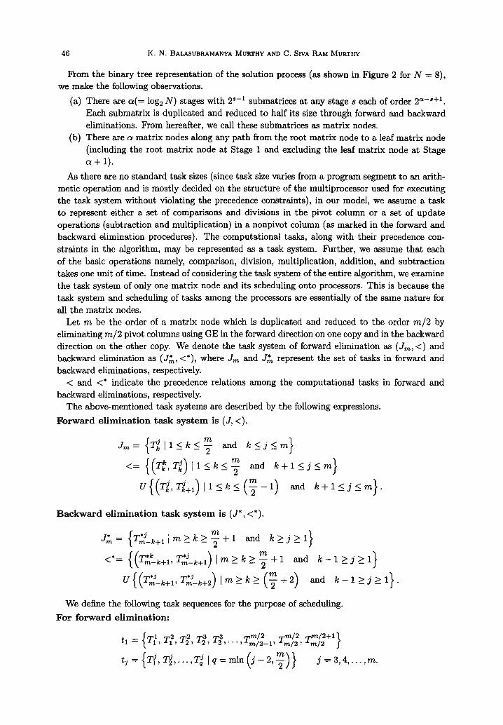
For forward el imination:

11 = T,', TL TL . . . """'/' ,-,-,,-,,/, ,-r,,,,/,+i ' "~mla-l ' ~m12 ' ~m12 I

New Gaussian Algorithm 47

For b a c k w a r d e l i m i n a t i o n : {T~ T~m-1, q'*m-1 q.*m/2+l T*m/2+l *m/2} t * = m, ~2 , ' " ' ~ m / 2 - 1 ' m/2 'T=/2

tj {TlJ , T~ j, T ~ J l q m i n ( 2 ) } * = . . . , = , m - j - 1 , j = m - 2 , m - 3 , . . . 1 .

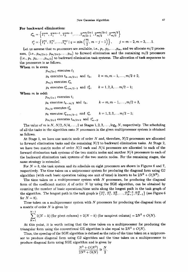
Let us assume that m processors are available, i.e., Pl, P2, . . . ,Pm, and we allocate m / 2 proces- sors, (i.e., Pro~2+1, Pro~2+2,... ;Pro) to forward elimination and the remaining m / 2 processors (i.e., Pl, P 2 , . . . ,Pm/2) to backward elimination task systems. The allocation of task sequences to the processors is as follows. W h e n m is e v e n

Pm/2+l executes tl

pk executestk_m/2+l and tk, k = m , m - 1 , . . . , m / 2 + 2 ,

Pro~2 executes t~

Pk executes t~+m/2_ 1 and t~, k = 1 , 2 , 3 , . . . m / 2 - 1;

W h e n m is odd: Pm/2+l executes tl

Pk executes tk-m/2 and tk, k = m, m - 1 , . . . , m / 2 + 3,

Pro~2 executes t m

Pk executes t*k+m/2_ 1 and t~, k = 1, 2, 3 , . . . m / 2 - 1;

Pm/2+2 executes tin/2+ 2 and t* m--2"

The value of m is N, N/2, N / 4 , . . . , 2 at Stages 1, 2, 3 . . . . , log 2 N, respectively. The scheduling of all the tasks in the algorithm onto N processors in the given multiprocessor system is obtained as follows.

At Stage 1, we have one matrix node of order N and, therefore, N/2 processors are allocated to forward elimination tasks and the remaining N/2 to backward elimination tasks. At Stage 2, we have two matrix nodes of order N /2 each and N / 4 processors are allocated to each of the forward elimination task systems of the two matrix nodes and another N / 4 processors to each of the backward elimination task systems of the two matrix nodes. For the remaining stages, the same strategy is extended.

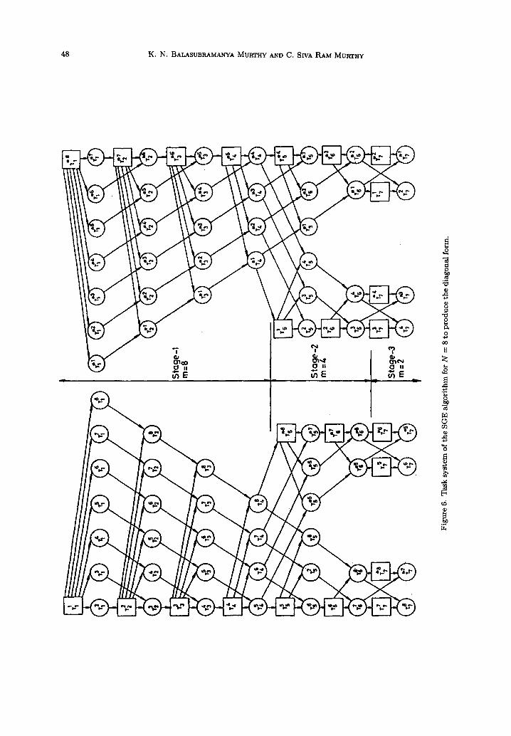
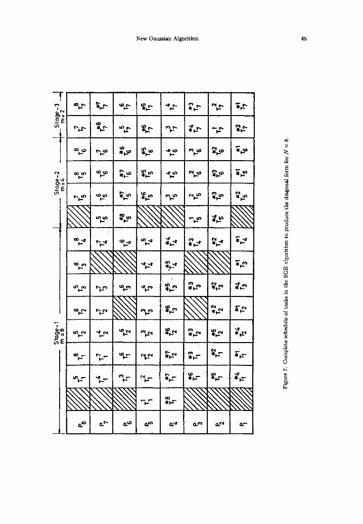
For N = 8, the task system and its schedule on eight processors are shown in Figures 6 and 7, respectively. The time taken on a uniprocessor system for producing the diagonal form using GJ algorithm (with each basic operation taking one unit of time) is known to be 2N 3 + O(N2).

The time taken on a multiprocessor system with N processors, for producing the diagonal form of the coefficient matrix A of order N by using the SGE algorithm, can be obtained by counting the number of basic operations/time units along the longest path in the task graph of the algorithm. The longest path in the task graph is {T~, T 2, T2, . . g -1 ., T•_I, T~_ x } (see Figure 6 for N -- 8).

Time taken on a multiprocessor system with N processors for producing the diagonal form of a matrix of order N is given by

N-1 2(N - k) (for pivot column) + 2(Y - k) (for nonpivot column) = 2N 2 + O(N) .

K=I

At this point, it is worth noting that the time taken on a multiprocessor for producing the triangular form using the conventional GE algorithm is also equal to 2N 2 + O(N) .

Thus, the speedup of the SGE algorithm is defined as the ratio of the time taken on a uniproces- sor to produce diagonal form using GJ algorithm and the time taken on a multiprocessor to produce diagonal form using SGE algorithm and is given by

N 3 + O ( N 2) ~ N 2N 2 + O ( N ) - 2"

48 K . N . BALASUBRAMANYA MURTHY AND C. SIVA RAM MURTI-n'

V l t -

~o

o. e~

o0

H

~o

~d

<5

New Gaussian Algorithm 49

~ | ! , ,

~ E

(:~ II

~ e

"T

E

¢g

II

O

u

o

O

O ~9

50 K . N . BALASUBRAMANYA MUB.THY AND C. SIVA RAM MuB~rHY

1.20

1.15

•Q-I.10 mQ'l.05

1.00

0.95

==== GE Algorithm .~c._.c SGE ~gorlthrn

r- -- -- = :3

E : C - 1 : 5

........ ! ......... ~ ......... ~ ......... +, .. . . . . . . . ~ .........

d i m e n s i o n o f t h e h y p e r c u b e

(0

2.00

1,80

1.60

1.40

1.20

t . 0 0

0 .80

A

E :

: : : : : GE Al<:JoHthm . . . . . SGE Algor i thm

. . . . . . . . I . . . . . . . . . ~ . . . . . . . . . + . . . . . . . . . ~" . . . . . . . . + . . . . . . . . .

dimension of the hypercube (~)

m

2 . 8 0

2 . 4 0

2 . 0 0 .

1 . 6 0 ,

1 . 2 0 ' A =- ' - ' - '= SGE Rgorlthm

0 . 8 0 , E : C = 1 : I

0 . 4 o . . . . . . . . . 4 . . . . . . . . . :~ . . . . . . . . . :.4 . . . . . . . . . ~ . . . . . . . . . ++ . . . . . . . . .

dimension of the hypercube (a)

ol

3 . 0 0

2 .50 ¸

2 .00

1.50

1 . 0 0 ,

_•_ JL

w _ -

~ c = : : : GE Algor i thm / :-:'--': SGE Algorithm

E : C = 2 : !

0,50 . . . . . . . : ' I . . . . . . . . . +, . . . . . . . . . . ~ . . . . . . . . . ,I. . . . . . . . . . i" . . . . . . . "~

dimension of the hypercube

3.50

3.00

2.50

"0 2.00

01 1.50

1.00

0 .50

E : G - 5 : I

0 . . . . . . . . . t . . . . . . . . . i . . . . . . . . . ~ . . . . . . . . . ~ . . . . . . . . . ~ ........ "+ dimension o f t h e hypercube

(v)

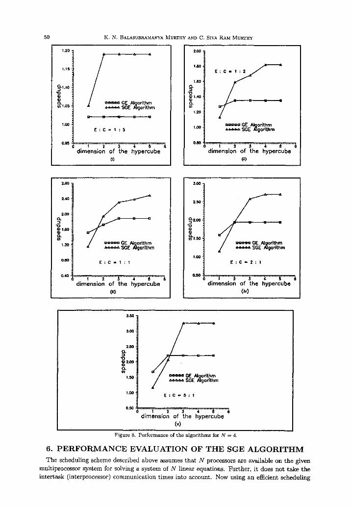
Figure 8. Performance of the algorithms for N -- 4.

6. P E R F O R M A N C E E V A L U A T I O N OF T H E S Q E A L G O R I T H M

T h e schedul ing scheme descr ibed above assumes t h a t N processors ave avai lable on the given

mul t ip rocessor sys tem for solving a sys tem of N l inear equat ions . Fur the r , i t does no t t ake the

i n t e r t a sk ( in terprocessor) communica t ion t imes into account . Now using an efficient schedul ing

N e w G a u s s i a n A l g o r i t h m 5 1

1.80

1.60

.~t.40

1.00

0,~

O,ILO

( : C - - 1 : 5

......... ~ ........ 'i ......... $' ....... '~ ......... i ......... i dimension of the hypercube

3.00

2,50

~0"1.50

1.00

0.5O

f: o

E : C - I : 2

......... i ........ "~ ......... .~ ......... ,t ........ !~" ........ II

dimension of the hypercube (,)

4.oo ,q

4 1

3.00 -I

1.o0-.I

@E Algorithm SGE Ngortthm

E : C = I : I

. . . . . . . . . t . . . . . . . . ' t . . . . . . . . . $ . . . . . . . . ' g . . . . . . . . ~" . . . . . . . . dimension of the hypercube

(i,)

5,00

4,00 -J

1,00 -I

O.O0

E : C = 2 : t r = ~ =

....... :'t ........ 1 ........ 3 ......... 1 ........ "ll ......... II dimension of the hypercube

5.00.

4,oo

•Q-3.00 a)

1,00

0.00

[ : C - 6 : 1

......... I ........ 'i ........ "~' ........ I ........ '~, ......... i

dimension of the hypercube (v)

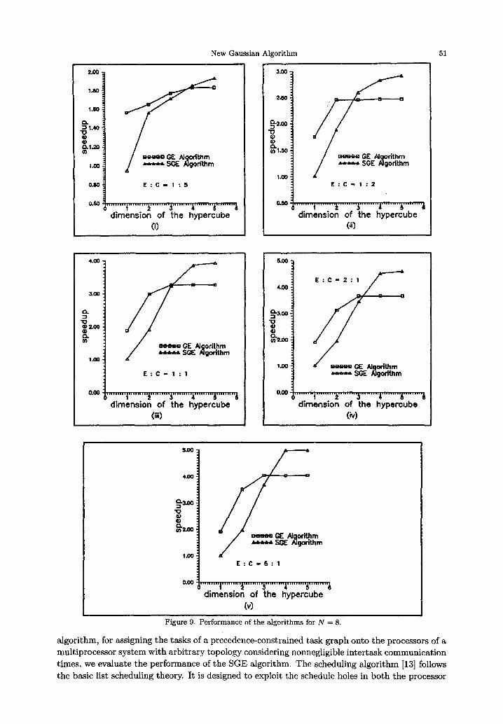
Figure 9. Pe r fo rmance of the a lgo r i thms for N = 8.

algorithm, for assigning the tasks of a precedence-constrained task graph onto the processors of a multiprocessor system with arbitrary topology considering nonnegligible intertask communication times, we evaluate the performance of the SGE algorithm. The scheduling algorithm [13] follows the basic list scheduling theory. It is designed to exploit the schedule holes in both the processor

52 K.N. BALASUBRAMANYA MURTHY AND C. SIVA RAM MURTn'Y

3.50

3.00

2.5O

.~2.00

~/ A.:.:_": SGE /t~Jorlthm

0.50 E : C = 1 : 5

o.oo ........ l ........ '~ ......... ~ ........ '~ ......... ~ .........

dimension of the hypercube O)

6.00

5.00] 4.00 E :C == 1 : 2

2.00.

1.oo - - - - " GE Algodthm

o . o o . . . . . . . . . 4 . . . . . . . . . i . . . . . . . . . 3 . . . . . . . . . l . . . . . . . . "A . . . . . . . . .

dimension of the hypercube

8,00,

IE~,

ZOO ̧

E'C,,, l : t

~ - G E Noorithm SGE A]gorRhm

0 . 0 0 : . . . . . . . . t . . . . . . . . "i . . . . . . . . . ~" . . . . . . . "~" . . . . . . . . ~' . . . . . . . .

dimension of the hypercube (,,)

10.00

B.00

i e.O0

4.00

2.00

O.O0

E : C = 2 : 1

. . . . . . . . . ~ . . . . . . . . . i . . . . . . . . "~" . . . . . . . ";" . . . . . . . . 6" . . . . . . . . 6 dimension of the hypercube

(~)

10.00

8.00,

•Q" (!,00 "10 (B ¢L IR 4.00,

2.00,

0.00

E : C , , 5 : 1 ~

. . . . . . . . ! . . . . . . . . . I . . . . . . . . . ~ . . . . . . . . "I . . . . . . . . "~" . . . . . . . . 6 dimension of the hypercube

(v)

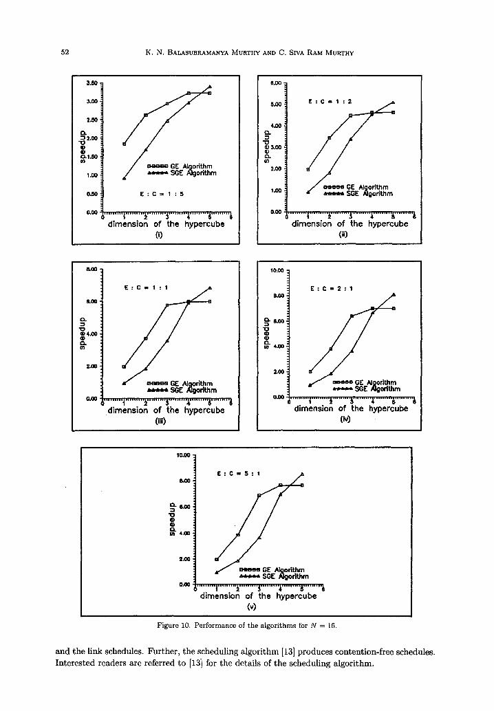
Figure 10. Performance of the algorithms for N ---- 16.

a n d t h e l ink schedules . F u r t h e r , t h e schedu l ing a l g o r i t h m [13] p r o d u c e s con ten t ion - f r ee schedules .

I n t e r e s t e d readers are referred to [13] for the de ta i l s of the s chedu l ing a lgo r i t hm.

New Gaussian Algorithm 53

In order to evaluate the performance of the SGE algorithm, we conducted the following exper- iments on a network of SUN workstations.

(1) We generated task graphs for both GE and SGE algorithms for various problem sizes, and scheduled them onto a hypercube multiprocessor system using the scheduling algo- rithm [13]. We assumed that each floating point arithmetic operation (E) takes one unit of time and the transfer of a floating point number between two adjacent processors (C) takes 5, 2, 1, 1/2, and 1/5 units of time for the purpose of generating the task schedules.

(2) We implemented the task schedules obtained above on a network of SUN workstations using P4 (Portable Programs for Parallel Processors) software for verifying the correctness of the algorithms. P4, developed at Argonne National Laboratory, is a library of macros and subroutines for programming a variety of parallel machines including a network of workstations.

The speedup of a parallel algorithm is measured as the ratio of the completion time of a task graph of the sequential GE algorithm on one processor and the completion time of the task graph of the parallel algorithm on a hypercube multiprocessor system. We have presented the results obtained with the two algorithms as plots of speedup versus dimension of the hypercube for different values of (E : C, N) in Figures 8-10. From these graphs, we can clearly see that the speedup obtained by using the SGE algorithm is always greater than the speedup of the GE algorithm when the number of processors is greater than the number of equations in the system. This increase in speedup is due to the fact that the SGE algorithm has higher degree of inherent parallelism and the intertask communication becomes more localized as the algorithm progresses (see Figure 6 for N = 8).

7. C O N C L U S I O N S

We have presented a new parallel algorithm called Successive Gaussian Elimination (SGE) for the solution of linear equations.

The main features of the SGE algorithm are:

(a) It produces diagonal form in O(N 2) time steps using O(N) processors against the same number of time steps and processors required for producing the triangular form in the existing methods.

(b) The back substitution phase, which takes O ( Y ) steps using O(N) processors or O (log 2 N) steps using O(N 3) processors [2,4], is completely replaced by one step division in the SGE algorithm.

(c) The algorithm supports partial pivoting to improve numerical stability. (d) The SGE algorithm permits pivot column tasks to be executed in parallel with nonpivot

column tasks. Our scheduling strategy cleverly exploits this parallelism in the algorithm using minimum number of processors.

(e) In the SGE algorithm, all xi (i = 1, 2 , . . . , N) are found simultaneously, unlike in the conventional GE algorithm in which xi (i = N, N - 1 , . . . , 2) is used for finding xj (j = 1, 2 , . . . , i - 1). Hence, the SGE algorithm is expected to have better numerical stability characteristics than the conventional GE algorithm.

R E F E R E N C E S

1. D.P. Bertsekas and J.N. Tsitsiklis, Parallel and Distributed Computations--Numerical Methods, Prentice Hall, New Jersey, (1989).

2. D. Heller, A survey of parallel algorithms in numerical linear algebra, SIAM Review 20 (4), 740-777 (October 1978).

3. S. Lakshmivarahan and S.K. Dhall, Analysis and Design of Parallel Algorithms--Arithmetic and Matrix Problems, McGraw-Hill, New York, (1990).

4. A.H. Sameh and D.J. Kuck, Parallel direct linear system solvers--A survey, In Parallel Computers--Parallel Mathematics, (Edited by Feilmeier), pp. 25-30, (1977).

54 K.N. BALASUBRAMANYA MURTHY AND C. SIVA RAM MURTh'Y

5. E. Chu and A. George, Gaussian elimination with partial pivoting and load balancing on a multiprocessor, Parallel Computing 5 (1/2), 65-74 (July 1987).

6. K.A. Gallivan, R.J. Plemmons and A.H. Sameh, Parallel algorithms for dense linear algebra computations, SIAM Review 32 (1), 54-135 (March 1990).

7. G.H. Golub and C.F. Van Loan, Matrix Computations, John Hopkins University Press, (1989). 8. R.E. Lord, J.S. Kowalik and S.P. Kumar, Solving linear algebraic equations on a MIMD computer, Journal

of ACM 30 (1), 103-117 (January 1983). 9. M. Veldhorst, Gaussian elimination with partial pivoting on an MIMD computer, Journal of Parallel and

Distributed Computing 6 (1), 62-68 (February 1989). 10. R. Melhem, Parallel Gauss-Jordan elimination for solution of dense linear equations, Parallel Computing 4

(3), 339-343 (June 1987). 11. A.H. Sameh and D.J. Kuck, On stable parallel linear system solvers, Journal of ACM25 (1), 81-91 (January

1978). 12. M.K. Sridhar, A new algorithm for parallel solution of linear equations, Information Processing Letters 24,

407-412 (1987). 13. C. Siva Ram Murthy, K.N. Balasubramanya Murthy and A. Srinivas, Scheduling of precedence-constrained

parallel program tasks on multiprocessors, Microprocessing and Microprogramming 36 (2), 93-104 (March 1993).