Journal of King Saud University – Computer and Information Sciences (2014) 26, 41–54

King Saud University

Journal of King Saud University –

Computer and Information Scienceswww.ksu.edu.sa

www.sciencedirect.com

ORIGINAL ARTICLE

Performance modeling and analysis of parallel Gaussian

elimination on multi-core computers

Fadi N. Sibai *

P&CSD Dept. Center, Saudi Aramco, Dhahran 31311, Saudi Arabia

Received 16 October 2012; revised 2 February 2013; accepted 12 March 2013Available online 20 March 2013

*

E

Pe

13

ht

KEYWORDS

Gaussian elimination;

Multi-core computing;

Performance modeling and

analysis

Tel.: +966 3 8808523; fax:

-mail address: fadi.sibai@ar

er review under responsibilit

Production an

19-1578 ª 2013 Production

tp://dx.doi.org/10.1016/j.jksu

+966 3

amco.com

y of King

d hostin

and hosti

ci.2013.0

Abstract Gaussian elimination is used in many applications and in particular in the solution of

systems of linear equations. This paper presents mathematical performance models and analysis

of four parallel Gaussian Elimination methods (precisely the Original method and the new Meet

in the Middle –MiM– algorithms and their variants with SIMD vectorization) on multi-core sys-

tems. Analytical performance models of the four methods are formulated and presented followed

by evaluations of these models with modern multi-core systems’ operation latencies. Our results

reveal that the four methods generally exhibit good performance scaling with increasing matrix size

and number of cores. SIMD vectorization only makes a large difference in performance for low

number of cores. For a large matrix size (n P 16 K), the performance difference between the

MiM and Original methods falls from 16· with four cores to 4· with 16 K cores. The efficiencies

of all four methods are low with 1 K cores or more stressing a major problem of multi-core systems

where the network-on-chip and memory latencies are too high in relation to basic arithmetic oper-

ations. Thus Gaussian Elimination can greatly benefit from the resources of multi-core systems, but

higher performance gains can be achieved if multi-core systems can be designed with lower memory

operation, synchronization, and interconnect communication latencies, requirements of utmost

importance and challenge in the exascale computing age.ª 2013 Production and hosting by Elsevier B.V. on behalf of King Saud University.

1. Introduction

The large majority of modern microprocessors integrate multi-ple processing cores on the same package leading to great per-formance/power ratio gains. Today both central processing

8758302.

.

Saud University.

g by Elsevier

ng by Elsevier B.V. on behalf of K

3.002

units (CPUs) and graphic processing units (GPUs) integrate

multiple processing cores.Multi-core processors implement var-ious types of parallelism including instruction-level parallelism,thread-level parallelism, and data-level parallelism. While the

trend toward increasing number of cores per processor is strong,it is an interesting and important problem to identify the perfor-mance weaknesses of multi-core processors in order to keep theincreasing number of cores per processor trend going and avoid

themulticore performance ‘‘wall.’’While real application profil-ing and scalability measurement are accurate performance indi-cators, they are time consuming in particular when exploring

application scalability over a very large number of cores.Amoreflexible and faster method is analytical performance modeling

ing Saud University.

42 F.N. Sibai

which captures the essence of the performance-impacting com-ponents of the software application and underlying hardwaremodels, and provides sufficiently accurate answers in particular

with regard to trends andkey performance impactors. In this pa-per, wemodel the performance of parallel Gaussian Elimination(GE) onmodernmulti-core processors, and derive speedups ver-

sus increasing number of cores and derive learnings for futuremulticore processor designs.

Gaussian elimination (Grama, 2003; Quinn, 1994) is an effi-

cient mathematical technique for solving a system of linearequations. Given the matrix set A · X= B, where X is the var-iable matrix and A and B are constant matrices, Gaussianelimination (GE) solves for the elements of the X matrix.

Gaussian Elimination has also other uses for it is also usedin computing the inverse of a matrix. The algorithm is com-posed of two steps. The first step combines rows eliminating

a variable in the process and reducing the linear equation byone variable at a time. This reduction step is repeated untilthe left side (A · X) is a triangular matrix. The second step is

a back substitution of the solved X variables into upper rowsuntil further X variables can be solved.

The algorithm generally works and is stable and can be made

more stable by performing partial pivoting. The pivot is the left-most non-zeromatrix element in a matrix row available for reduc-tion. When the pivot is zero (non-zero), exchanging the pivot rowwith another row usually with the largest absolute value in the pi-

vot position may be required.When two rows are combined to re-duce the equation by one variable, a multiplication of all elementsin the pivot row by a constant and then subtracting all elements in

the row by the ones in the other row are performed resulting in anew reduced row.During back substitution, a number of divisions,multiplications and subtractions are performed to eliminate solved

variables and solve for a new one.Partial pivoting works as follows. First the diagonal ele-

ment in the pivot column with the largest absolute value is lo-

cated and is referred to as the Pivot. In the Pivot row which isthe row containing the pivot, every element is divided by thepivot to get a new pivot row with a 1 in the pivot position.The next step consists of replacing each 1 below the pivot by

a 0. This is achieved by subtracting a multiple of the pivotrow from each of the rows below it.

Because partial pivoting requires more steps and consumes

more time and because without partial pivoting GaussianElimination is acceptably stable, we ignore partial pivotingherein and accept to trade off performance for stability.

The numerical instability is proportional to the size of the Land U matrices with known worst-case bounds. For the casewithout pivoting, it is not possible to provide a priori boundsfor Yeung and Chan (1997) provide a probabilistic analysis of

the case without pivoting.Sankar (2004) proved that it is unlikely that A has a large

growth factor under Gaussian elimination without pivoting.

His results improve upon the average-case analysis of Gauss-ian elimination without pivoting presented by Yeung andChan (1997).

Xiaoye and Demmel (1998) proposed a number of tech-niques in place of partial pivoting to stabilize sparse Gaussianelimination. They propose to not pivot dynamically thereby

enabling static data structure optimization, graph manipula-tion and load balancing while remaining numerically stable.Stability is kept by a variety of techniques: pre-pivoting largeelements to the diagonal, iterative refinement, using extra pre-

cision when needed, and allowing low rank modifications withcorrections at the end.

Geraci (2008) also avoids partial pivoting and recently

achieved a performance of 3.2Gflops with a matrix size of33500 on the Cell Broadband Engine.

Parallel solutions of numerical linear algebra problems are

discussed in Demmel (1993), Duff and Van der Vorst (1999).While the Gaussian Elimination method yields an exact solu-tion to the A · X= B problem, iterative techniques trade off

execution time for solution accuracy. Parallel iterative tech-niques are discussed in Barrett (1994), Greenbaum (1997),Saad (2003), Van der Vorst and Chan (1997). These techniquesstart with initial conditions for the X vector and keep refining

the X solution with each iteration until the X vector convergesto a solution vector. The different selections of the initial val-ues of the X vector result in a variety of preconditioning tech-

niques with various performance yields.Further performance gains can be achieved when the matri-

ces are sparse with many zero elements. Sparse matrix compu-

tation techniques are discussed in Heath (1997), Gupta (1997),Gupta et al. (1998), Demmel et al. (1999).

In this paper, we analyze the performance of Parallel

Gaussian Elimination and an improved version on multi-corecomputers with increasing number of cores, and with andwithout SIMD vectorization. Section 2 reviews relevant litera-ture. Section 3 presents the multi-core processor model on

which the parallel GE algorithms are executed. Section 4 re-views the parallel GE algorithm and presents a new improvedversion: Meet in the Middle algorithm. Section 5 presents the

mathematical performance model of the parallel GE algo-rithm. Section 6 presents the mathematical performance modelof the improved parallel GE algorithm version. Section 7 states

the assumptions made in this performance modeling study.Section 8 presents the parallel GE algorithms’ performance re-sults on the multicore processor model with 4–16 K cores, and

their analysis. The paper concludes in Section 9.

2. Related background

Various performance analysis tools and methods are available(Prinslow, 2011). Profiling and scalability measurements ofreal application performance lead to accurate results. Applica-

tion profiling can be achieved by tools such as Intel VTune,AMD Code Analyst, or GNU gprof. However this requiresimplementation of the application, and running it on variousmachines with various configurations, such as processors with

various number of cores, a process which consumes long timeand extensive resources. More importantly, this approach can-not be adopted in our study as we wish to analyze the applica-

tion scalability up to 16 K cores, and current hardware limitsour exploration to only about 10 cores. Benchmarks are alsovery efficient in studying computer performance. However

they cannot be used in our study for the same reason as realapplications: lacking scalable hardware. Simulators can pro-vide up to cycle accurate performance but they require a very

long time to develop and are a suitable approach when the sim-ulator is intended to be used extensively. Analytic performancemodeling provides a quick and fairly accurate method foridentifying trends and the key performance impactors. It is

flexible and allows for very large of cores to be modeled, morethan currently available in the market. For these reasons weemploy analytic performance modeling in this study.

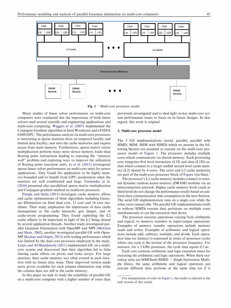
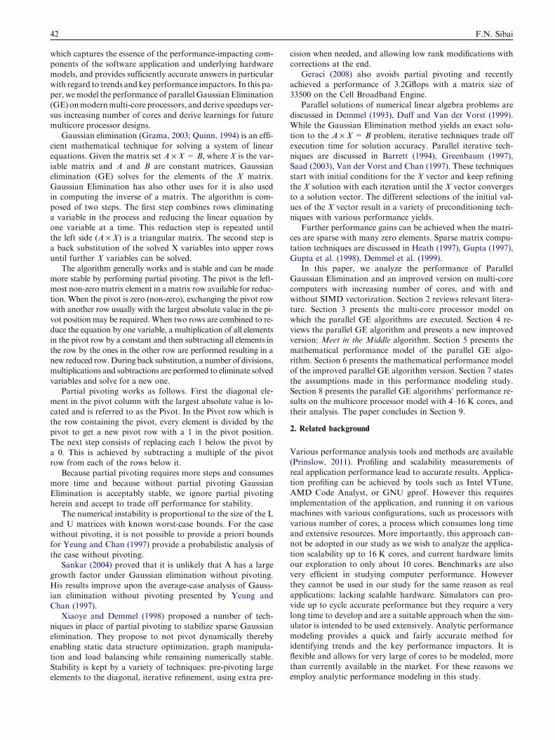
Fig. 1 Multi-core processor model.

1 For interpretation of color in Figure 1, the reader is referred to the

Performance modeling and analysis of parallel Gaussian elimination on multi-core computers 43

Many studies of linear solver performance on multi-corecomputers were conducted due the importance of both linear

solvers used several scientific and engineering applications andmulti-core computing. Wiggers et al. (2007) implemented theConjugate Gradient algorithm in Intel Woodcrest and nVIDIA

G680 GPU. The performance analysis on multi-core processorsis interesting as sparse matrices show no temporal locality andlimited data locality, and miss the cache memories and require

access from main memory. Furthermore, sparse matrix vectormultiplication perform many more slower memory loads thanfloating point instructions leading to exposing the ‘‘memorywall’’ problem and exploring ways to improve the utilization

of floating point execution units. Li et al. (2011) investigatedsparse linear solver performance on multi-core units for powerapplications. They found the application to be highly mem-

ory-bounded and to benefit from GPU acceleration when thematrices are well conditioned and large. Fernandez et al.(2010) presented also parallelized sparse matrix multiplication

and Conjugate gradient method on multicore processor.Pimple and Sathe (2011) investigate cache memory effects

and cache optimizations of three algorithms including Gauss-ian Elimination on Intel dual core, 12 core and 16 core ma-

chines. Their study emphasizes the importance of data cachemanagement as the cache hierarchy gets deeper, and ofcache-aware programming. They found exploiting the L2

cache affinity to be important in light of the L2 being sharedby several application threads. Another study investigated par-allel Gaussian Elimination with OpenMP and MPI (McGinn

and Shaw, 2002), another investigated parallel GE with Open-MP (Kumar and Gupta, 2012) with scaling performance whichwas limited by the dual core processor employed in the study.

Laure and Al-Shandawely (2011) implemented GE on a multi-core system and discovered that their algorithm led to falsesharing cache effects on pivots and locks arrays. For largematrices, their cache memory was often evicted in each itera-

tion with no future data reuse. Their improved version mademore pivots available for each column elimination step whilethe column data are still in the cache memory.

In this paper we seek to study the scalability of parallel GEon a multi-core computer with a higher number of cores than

previously investigated and to shed light on key multi-core sys-tem performance issues to focus on in future designs. In that

regard, this work is original.

3. Multi-core processor model

The 5 GE implementations (serial, parallel, parallel withSIMD, MIM, MIM with SIMD) which we present in the fol-lowing Section are assumed to execute on the multi-core pro-

cessor model of Figure 1. The processor includes multiplecores which communicate via shared memory. Each processingcore integrates first level instruction (L1I) and data (L1D) ca-

ches which connect to a larger unified second level cache mem-ory (L2) shared by 4 cores. The cores and L2 cache memoriesare part of the multi-core processor block of Figure 1(in blue).1

The processor’s L2 cache memory modules connect to exter-

nal dynamic random access memory (DRAM) modules via aninterconnection network. Higher cache memory levels (such asthird level) do not change the performance results based on uni-

form data communication time assumption in the next Section.The serial GE implementation runs on a single core while theother cores remain idle. The parallel GE implementations (with

or without SIMD) execute data partitions on multiple coressimultaneously to cut the execution time down.

The processor executes operations varying from arithmetic

and logical, to memory transfers to input/output operations.Examples of memory transfer operations include memoryreads and writes. Examples of arithmetic and logical opera-tions include add, subtract, multiply, and divide. Each opera-

tion time (or latency) is expressed in terms of processor cycleswhere one cycle is the inverse of the processor frequency. Forinstance, for a 2 GHz processor, the cycle time equals 0.5 ns.

Each core contains arithmetic and logic execution times forexecuting the arithmetic and logic operations. When these exe-cution units are SIMDised (SIMD = Single Instruction Multi-

ple Data), the same arithmetic and logical operation canexecute different data portions at the same time (as if it

web version of this article.

44 F.N. Sibai

operates on a data vector), also reducing the execution time. Forinstance, four or more adds of different data can be performedsimultaneously on the SIMD execution unit of each core.

4. Parallel GE algorithms

Given a system of linear equations A · X= BwhereA is an n · n

matrix of constants,X is a n · 1matrix of unknown variables, andB is an n · 1matrix of constants, the augmentedmatrix can be ob-tained by merging the Bmatrix with theAmatrix to facilitate rep-

resentation and consolidate storage. For instance when n is six, theaugmented matrix is structured as follows

a11 a12 a13 a14 a15 a16 j b1

a21 a22 a23 a24 a25 a26 j b2

a31 a32 a33 a34 a35 a36 j b3

a41 a42 a43 a44 a45 a46 j b4

a51 a52 a53 a54 a55 a56 j b5

a61 a62 a63 a64 a65 a66 j b6

2666666664

3777777775

ð1Þ

The B matrix appears as the seventh column in the above aug-mented matrix. This augmented matrix is a compact represen-tation of the following system of linear equationsa11 a12 a13 a14 a15 a16

a21 a22 a23 a24 a25 a26

a31 a32 a33 a34 a35 a36

a41 a42 a43 a44 a45 a46

a51 a52 a53 a54 a55 a56

a61 a62 a63 a64 a65 a66

2666666664

3777777775�

x1

x2

x3

x4

x5

x6

2666666664

3777777775¼

b1

b2

b3

b4

b5

b6

2666666664

3777777775

ð2Þ

where x1, . . . ,x6 are the unknown variables to be solved. Apair of rows can be combined together eliminating the x1 var-iable in the process and yielding n � 1 unknown X variables.

Given that

Fig. 2 Reduction: data row partitionin

(i) there are s processing cores in a multi-core systems;

(ii) each pair of rows already yields n � 1 unknown vari-ables (after 1 reduction);

(iii) n � 1 pairs of rows are needed to solve the remaining

n � 1 variables, x2, . . . ,xn; and(iv) n is a power of 2 for simplicity,

the augmented matrix can be partitioned into ðn�1Þs

l msets of

pairs of augmented rows where each set is assigned to a corefor processing (reduction).

For instance, in the example of (1), the 6 � 1 = 5 pairs of

rows (1, 2), (3, 4), (5, 6), (2, 3), and (4, 5) can be assignedand distributed among the five cores as shown in Figure 2.

On the top of Figure 2 is the augmented matrix. Below the

augmented matrix are the pairs of augmented row partitionsallocated to each core. As a result of reduction, each pair ofrows results in one reduced augmented row with n � 1 un-

known variables. Each core keeps its reduced augmentedrow and communicates its reduced augmented row to its rightneighbor (the rightmost core communicates its reduced aug-

mented row to the leftmost core). As each core now has a pairof reduced augmented rows, the one it kept from the previousiteration and the one communicated by its left neighbor (bothreduced rows with a ‘‘0’’ in the leftmost ‘‘reduced’’ position),

another round of reduction can start in the next position rep-resented by a ‘‘�’’. The unprocessed positions to be processedin the future are represented by a ‘‘.’’. These steps are repeated

until the augmented matrix consists of all zeros and a single‘‘�’’.

The back substitution step can be parallelized but we keep

the serial version which runs on the leftmost core 1 which al-ready has solutions of all unknown (x1, . . . ,xn) variables. In

g and distribution among the cores.

Performance modeling and analysis of parallel Gaussian elimination on multi-core computers 45

the serial version of back substitution no communication orsynchronization calls are required among the cores as all sub-stitutions occur serially in reverse order from n down to 1 on

the same core. We refer to this GE algorithm with serial backsubstitution as the Original method. The performance of theOriginal method is limited by the serial back substitution time

as dictated by Amdahl’s law.One way to improve the performance of the serial back sub-

stitution is to perform it on two cores, one solving for xn down

to xn/2, and the other simultaneously solving for xn to xn/2�1.As the two cores solve for the two halves concurrently andin opposite directions and meet at the n/2 position, we referto this technique as the meet in the middle (MiM) method.

Given that the two cores involved in the back substitutionmust have different solution sets and given that cores are plenti-ful in the multi-core era and that communication and synchro-

nization operations are very costly, we choose to performMiM as follows. The s cores are divided in two equal sets, whereboth sets of s/2 cores redundantly perform the reduction sets in

order for one core in each set to have the solutions of all n · vari-ables. The two sets of cores perform the reduction on augmentedmatrices in opposite orders, one with rows 1 to n, and the other

with rows n down to 1. This one core in each set (specifically,cores 1 and n/2, respectively) then performs the serial back sub-stitution, one solving for xn down to xn/2, and the other solvingfor xn to xn/2�1. Recall that in case the total number of cores

s> n � 1, only n � 1 cores are used and involved in GE whilethe rest remain idle or can be used to run other workloads.

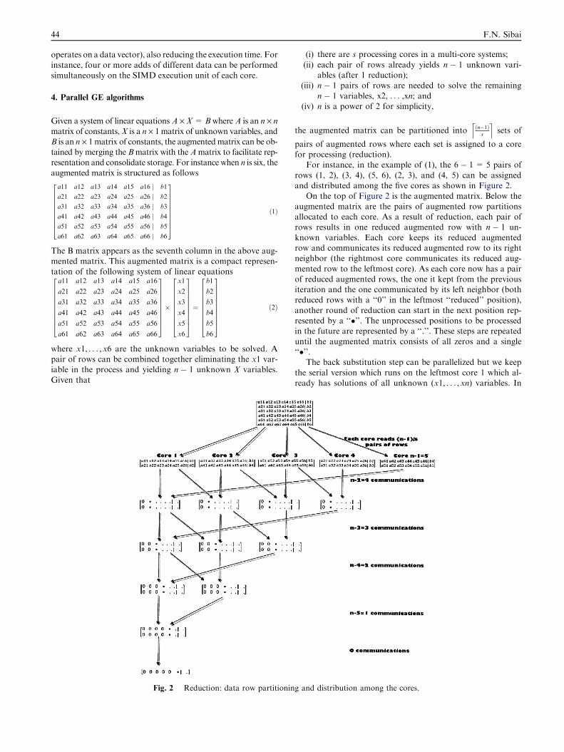
Figure 3 shows the example forMiMwith 10 cores. n� 1 = 6

cores are needed in each set to initially process the six pairs of aug-mented rows. Cores 1–5 perform the reduction on the augmentedmatrix starting with row 1 and ending with row 6. Cores 6–10 per-

form the reduction on the augmented matrix starting with row 6and ending with row 1. Reduction is performed as in Figure 2.At the end of reduction, Cores 1 and 6 have all reduced augmented

Fig. 3 Meet in the middle reductio

rows and can solve for all n unknownx variables.However, Core 1only solves for x1 up to x3, while Core 6 simultaneously solves forx6 down to x4. Note that no cores between the two sets need to

communicate or synchronize during the back substitution (exceptat the end) resulting in a big performance savings. Communicationand synchronization are only required between cores in the same

set as in the original method. These operations in each set takeplace concurrently. This performance enhancement occurs at theexpense of doubling the number of cores needed to perform

reduction but this is a low cost to pay in the era ofmany core pro-cessors. Another advantage of this MiMmethod is its program-ming simplicity.

5. Performance modeling: serial and parallel algorithms

In this Section and the next Section, we model the performance

of both Original and MiM versions of Parallel Gaussian Elim-ination on a multi-core computer with and without SIMD vec-torization. In this Section, we focus on the performance

modeling of the serial and parallel GE algorithms.For each n · (n+ 1) augmented matrix, a number of reduc-

tions combining each a pair of augmented matrix rows represent-ing linear equations, followedby anumber of substitutions to solve

for unknown variables x1, . . . ,xn�1 take place.We assume that n isa power of 2, and that during back substitution anynecessary read-ing of the parameters of previously reduced rows from the local

cache also overlaps with the external communication.One reduction is composed of

ðnþ 1Þ multiplications � 2 rowsþ ðnþ 1Þ subtractions:

where the ‘‘+1’’ in ‘‘(n + 1)’’ corresponds to the ‘‘b’’ (right-

most) coefficient of each row. Under SIMD vectorization,and assuming that n is a multiple of 4, this number reduces to

ðn=4þ 1Þ multiplications� 2 rowsþ ðn=4þ 1Þ subtractions:

n: distribution among 10 cores.

46 F.N. Sibai

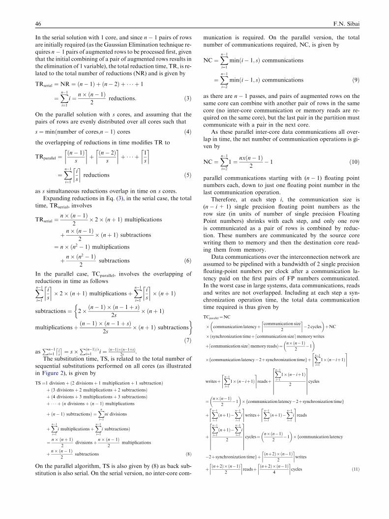
In the serial solution with 1 core, and since n � 1 pairs of rows

are initially required (as the Gaussian Elimination technique re-quires n � 1 pairs of augmented rows to be processed first, giventhat the initial combining of a pair of augmented rows results in

the elimination of 1 variable), the total reduction time, TR, is re-lated to the total number of reductions (NR) and is given by

TRserial ¼ NR ¼ ðn� 1Þ þ ðn� 2Þ þ � � � þ 1

¼Xn�1i¼1

i ¼ n� ðn� 1Þ2

reductions: ð3Þ

On the parallel solution with s cores, and assuming that the

pairs of rows are evenly distributed over all cores such that

s ¼ minðnumber of cores;n� 1Þ cores ð4Þ

the overlapping of reductions in time modifies TR to

TRparallel ¼ðn� 1Þ

s

� �þ ðn� 2Þ

s

� �þ � � � þ 1

s

� �

¼Xn�1i¼1

i

s

� �reductions ð5Þ

as s simultaneous reductions overlap in time on s cores.Expanding reductions in Eq. (3), in the serial case, the total

time, TRserial, involves

TRserial ¼n� ðn� 1Þ

2� 2� ðnþ 1Þ multiplications

þ n� ðn� 1Þ2

� ðnþ 1Þ subtractions

¼ n� ðn2 � 1Þ multiplications

þ n� ðn2 � 1Þ2

subtractions ð6Þ

In the parallel case, TCparallel, involves the overlapping of

reductions in time as followsXn�1i¼1

i

s

� �� 2� ðnþ 1Þ multiplicationsþ

Xn�1i¼1

i

s

� �� ðnþ 1Þ

subtractions ¼ 2� ðn� 1Þ � ðn� 1þ sÞ2s

� ðnþ 1Þ�

multiplicationsþ ðn� 1Þ � ðn� 1þ sÞ2s

� ðnþ 1Þ subtractions�ð7Þ

asPn�1

i¼1is

� �¼ s�

Pðn�1Þ=si¼1 i ¼ ðn�1Þ�ðn�1þsÞ

2s.

The substitution time, TS, is related to the total number of

sequential substitutions performed on all cores (as illustratedin Figure 2), is given by

TS ¼1 divisionþ ð2 divisions þ 1 multiplicationþ 1 subtractionÞþ ð3 divisions þ 2 multiplicationsþ 2 subtractionsÞþ ð4 divisions þ 3 multiplicationsþ 3 subtractionsÞþ � � � þ ðn divisions þ ðn� 1Þ multiplications

þ ðn� 1Þ subtractionsÞ ¼Xni¼1

ni divisions

þXn�1i¼1

i multiplicationsþXn�1i¼1

i subtractionsÞ

¼ n� ðnþ 1Þ2

divisions þ n� ðn� 1Þ2

multiplications

þ n� ðn� 1Þ2

subtractions ð8Þ

On the parallel algorithm, TS is also given by (8) as back sub-stitution is also serial. On the serial version, no inter-core com-

munication is required. On the parallel version, the total

number of communications required, NC, is given by

NC ¼Xn�1i¼1

minði� 1; sÞ communications

¼Xn�1i¼2

minði� 1; sÞ communications ð9Þ

as there are n � 1 passes, and pairs of augmented rows on the

same core can combine with another pair of rows in the samecore (no inter-core communication or memory reads are re-quired on the same core), but the last pair in the partition must

communicate with a pair in the next core.As these parallel inter-core data communications all over-

lap in time, the net number of communication operations is gi-ven by

NC ¼Xn�1i¼2

1 ¼ nxðn� 1Þ2

� 1 ð10Þ

parallel communications starting with (n � 1) floating pointnumbers each, down to just one floating point number in the

last communication operation.Therefore, at each step i, the communication size is

(n � i + 1) single precision floating point numbers as therow size (in units of number of single precision Floating

Point numbers) shrinks with each step, and only one rowis communicated as a pair of rows is combined by reduc-tion. These numbers are communicated by the source core

writing them to memory and then the destination core read-ing them from memory.

Data communications over the interconnection network are

assumed to be pipelined with a bandwidth of 2 single precisionfloating-point numbers per clock after a communication la-tency paid on the first pairs of FP numbers communicated.In the worst case in large systems, data communications, reads

and writes are not overlapped. Including at each step a syn-chronization operation time, the total data communicationtime required is thus given by

TCparallel¼NC

� communication latencyþ communication size

2

� ��2 cycles

� þNC

� synchronization timeþdcommunication sizeememorywritesð

þdcommunication sizeememory readsÞ¼ n�ðn�1Þ2

�1

�

�fcommunication latency�2þ synchronization timegþXn�1i¼1

1�ðn� iþ1Þ& ’

writesþXn�1i¼1

1�ðn� iþ1Þ& ’

readsþ

Xn�1i¼1

1�ðn� iþ1Þ

2

26666666

37777777cycles

¼ n�ðn�1Þ2

�1

� �fcommunication latency�2þsynchronization timeg

þXn�1i¼1ðnþ1Þ�

Xn�1i¼1

i

& ’writesþ

Xn�1i¼1ðnþ1Þ�

Xn�1i¼1

i

& ’reads

þ

Xn�1i¼1ðnþ1Þ�

Xn�1i¼1

i

2

26666666

37777777cycles¼ n�ðn�1Þ

2�1

� �fcommunication latency

�2þsynchronization timegþ ðnþ2Þ�ðn�1Þ2

� �writes

þ ðnþ2Þ�ðn�1Þ2

� �readsþ ðnþ2Þ�ðn�1Þ

4

� �cycles ð11Þ

Performance modeling and analysis of parallel Gaussian elimination on multi-core computers 47

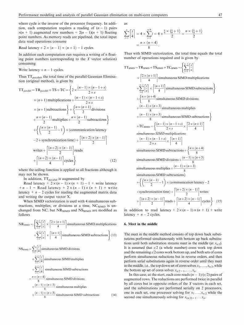
where cycle is the inverse of the processor frequency. In addi-

tion, each computation requires a reading of (n � 1) pairs·(n + 1) augmented row numbers = 2(n � 1)(n + 1) floatingpoint numbers. As memory reads are pipelined, the total input

data read operations consume

Read latencyþ 2� ðn� 1Þ � ðnþ 1Þ � 1 cycles:

In addition each computation run requires a writing of n float-ing point numbers (corresponding to the X vector solution)consuming

Write latencyþ n� 1 cycles:

Thus TTparallel, the total time of the parallel Gaussian Elimina-tion (original method), is given by

TTparallel¼TRparallelþTSþTC¼ 2�ðn�1Þ�ðn�1þsÞ2�s

�

�ðnþ1Þmultiplicationsþðn�1Þ�ðn�1þsÞ2�s

�ðnþ1Þsubtractions�þ n�ðnþ1Þ

2divisions

�

þn�ðn�1Þ2

multipliesþn�ðn�1Þ2

subtractions

�

þ n�ðn�1Þ2

�1

� �ðcommunication latency

�

�2þsynchronization timeÞþ ðnþ2Þ�ðn�1Þ2

� �

writesþ ðnþ2Þ�ðn�1Þ2

� �reads

þ ðnþ2Þ�ðn�1Þ4

� �cycles

�ð12Þ

where the ceiling function is applied to all fractions although itmay not be shown.

In addition, TTparallel is augmented by

Read latency + 2 · (n � 1) · (n + 1) � 1 + write latency+n � 1 = Read latency + 2 · (n � 1) · (n + 1) + writelatency + n � 2 cycles for reading the augmented matrix dataand writing the output vector X.

When SIMD vectorization is used with 4 simultaneous sub-tractions, multiplies, or divisions at a time, NCSIMD is un-changed from NC, but NRSIMD and NSSIMD are modified as

follows

NRSIMD¼Xn�1i¼1

i

s

� �� 2�ðnþ1Þ

4

� �simultaneous SIMDmultiplications

(

þXn�1i¼1

i

s

� �� ðnþ1Þ

4

� �simultaneous SIMD subtractions

)ð13Þ

NSSIMD ¼Xni¼1

i

4

� �simultaneous SIMD divisions

þXn�1i¼1

i

4

� �simultaneous SIMDmultiplies

þXn�1i¼1

i

4

� �simultaneous SIMD subtractions

¼ n�ðnþ4Þ8

simultaneous SIMD divisions

þðn�1Þ�ðnþ3Þ8

simultaneous multiplies

þðn�1Þ�ðnþ3Þ8

simultaneous SIMD subtractions ð14Þ

as

Xni¼1

i

4

� �¼ 4�

Xn=4i¼1

i ¼ 4�n4� n

4þ 1

�2

¼n� n

4þ 1

�2

¼ n� ðnþ 4Þ8

:

Thus with SIMD vectorization, the total time equals the totalnumber of operations required and is given by

TTSIMD¼TRSIMDþTSSIMDþTCSIMD¼Xn�1i¼1

i

s

� �(

� 2�ðnþ1Þ4

� �simultaneous SIMDmultiplications

þXn�1i¼1

i

s

� �� ðnþ1Þ

4

� �simultaneous SIMDsubtractions

)

þ n�ðnþ4Þ8

simultaneous SIMDdivisions

�

þðn�1Þ�ðnþ3Þ8

simultaneousmultiplies

þðn�1Þ�ðnþ3Þ8

simultaneous SIMD subtractions

�

þTCSIMD¼ðn�1Þ�ðn�1þsÞ

2�s� 2�ðnþ1Þ

4

� ��simultaneousSIMDmultiplications

þðn�1Þ�ðn�1þsÞ2�s

� ðnþ1Þ4

� �

simultaneous SIMDsubtractionsþ n�ðnþ4Þ8

�

simultaneous SIMDdivisionsþðn�1Þ�ðnþ3Þ8

simultaneousmultipliesþðn�1Þ�ðnþ3Þ8

simultaneous SIMD subtractionsg

þ n�ðn�1Þ2

�1

� �ðcommunication latency�2

�

þsynchronization timeÞþ ðnþ2Þ�ðn�1Þ2

� �writes

þ ðnþ2Þ�ðn�1Þ2

� �readsþ ðnþ2Þ�ðn�1Þ

4

� �cycles

�ð15Þ

in addition to read latency + 2 · (n � 1) · (n+ 1) + writelatency + n � 2 cycles.

6. Meet in the middle

The meet in the middle method consists of top down back substi-

tutions performed simultaneously with bottom up back substitu-tions until both substitution streams meet in the middle (at xn/2).It is assumed that s/2 (a whole number) cores work top down

and the remaining s/2 coresworkbottomup, and both sets of coresperform simultaneous reductions but in reverse orders, and thenperform serial substitutions again in reverse order until they meetin themiddle, i.e., the topdown set of cores solvesx1, . . . ,xn/2,whilethe bottom up set of cores solves xn/2+1, . . . ,xn.

In this case, at the start, each core reads (n � 1)/(s/2) pairs ofaugmented rows. The reductions are performed twice in parallel

by all cores but in opposite orders of the X vectors in each set,and the substitutions are performed serially on 2 processors,one in each set, one processor solving for x1 . . . ,xn/2 while the

second one simultaneously solving for x(n/2)+1 . . .xn.

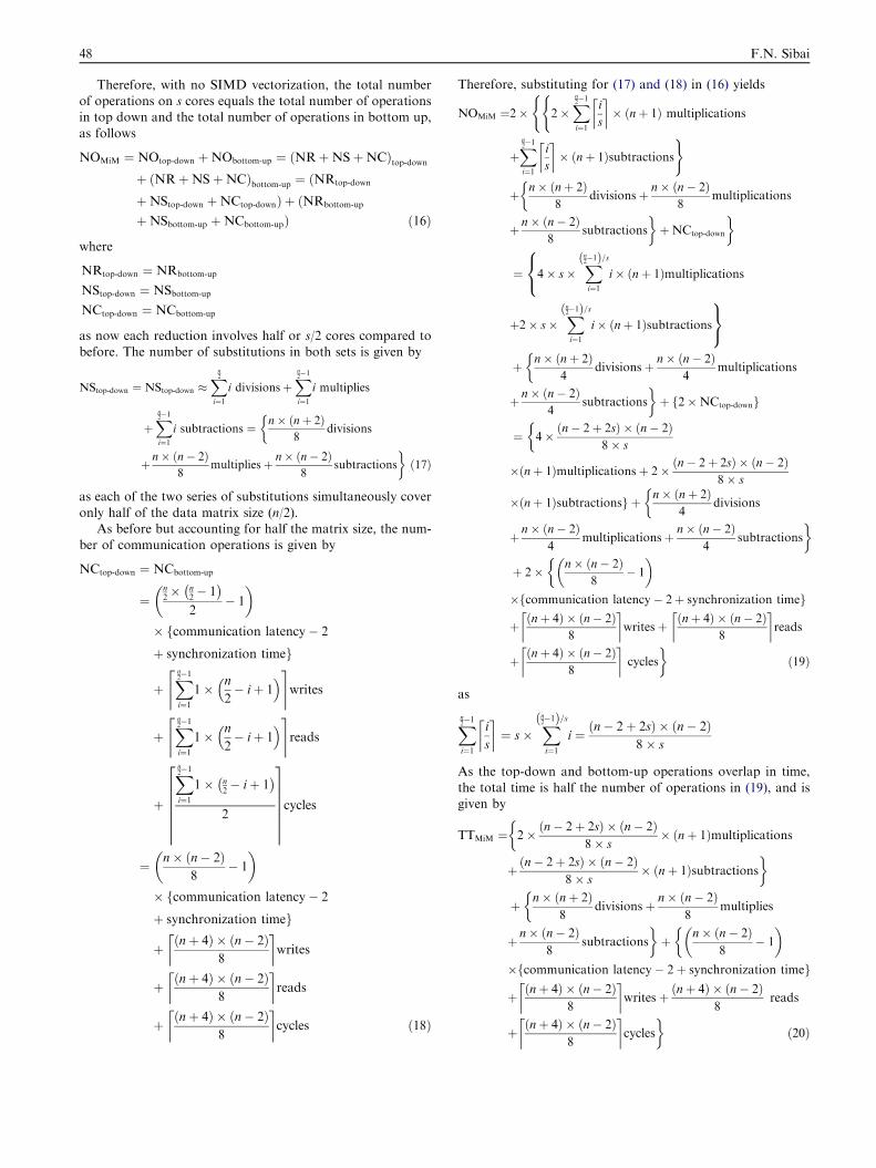
48 F.N. Sibai

Therefore, with no SIMD vectorization, the total numberof operations on s cores equals the total number of operationsin top down and the total number of operations in bottom up,

as follows

NOMiM ¼ NOtop-down þNObottom-up ¼ ðNRþNSþNCÞtop-downþ ðNRþNSþNCÞbottom-up ¼ ðNRtop-down

þNStop-down þNCtop-downÞ þ ðNRbottom-up

þNSbottom-up þNCbottom-upÞ ð16Þ

where

NRtop-down ¼ NRbottom-up

NStop-down ¼ NSbottom-up

NCtop-down ¼ NCbottom-up

as now each reduction involves half or s/2 cores compared tobefore. The number of substitutions in both sets is given by

NStop-down ¼ NStop-down �Xn

2

i¼1i divisionsþ

Xn2�1i¼1

i multiplies

þXn2�1i¼1

i subtractions ¼ n� ðnþ 2Þ8

divisions

�

þ n� ðn� 2Þ8

multiplies þ n� ðn� 2Þ8

subtractions

�ð17Þ

as each of the two series of substitutions simultaneously cover

only half of the data matrix size (n/2).As before but accounting for half the matrix size, the num-

ber of communication operations is given by

NCtop-down ¼ NCbottom-up

¼n2� n

2� 1

�2

� 1

� � fcommunication latency� 2

þ synchronization timeg

þXn2�1i¼1

1� n

2� iþ 1

� & ’writes

þXn2�1i¼1

1� n

2� iþ 1

� & ’reads

þ

Xn2�1i¼1

1� n2� iþ 1

�2

26666666

37777777cycles

¼ n� ðn� 2Þ8

� 1

� � fcommunication latency� 2

þ synchronization timeg

þ ðnþ 4Þ � ðn� 2Þ8

� �writes

þ ðnþ 4Þ � ðn� 2Þ8

� �reads

þ ðnþ 4Þ � ðn� 2Þ8

� �cycles ð18Þ

Therefore, substituting for (17) and (18) in (16) yields

NOMiM ¼2� 2�Xn2�1i¼1

i

s

� �� ðnþ 1Þ multiplications

((

þXn2�1i¼1

i

s

� �� ðnþ 1Þsubtractions

)

þ n� ðnþ 2Þ8

divisionsþ n� ðn� 2Þ8

multiplications

�

þ n� ðn� 2Þ8

subtractions

�þNCtop-down

�

¼ 4� s�Xn2�1ð Þ=si¼1

i� ðnþ 1Þmultiplications

8<:

þ2� s�Xn2�1ð Þ=si¼1

i� ðnþ 1Þsubtractions

9=;

þ n� ðnþ 2Þ4

divisionsþ n� ðn� 2Þ4

multiplications

�

þ n� ðn� 2Þ4

subtractions

�þ f2�NCtop-downg

¼ 4� ðn� 2þ 2sÞ � ðn� 2Þ8� s

�

�ðnþ 1Þmultiplicationsþ 2� ðn� 2þ 2sÞ � ðn� 2Þ8� s

�ðnþ 1Þsubtractionsg þ n� ðnþ 2Þ4

divisions

�

þ n� ðn� 2Þ4

multiplicationsþ n� ðn� 2Þ4

subtractions

�

þ 2� n� ðn� 2Þ8

� 1

� ��fcommunication latency� 2þ synchronization timeg

þ ðnþ 4Þ � ðn� 2Þ8

� �writesþ ðnþ 4Þ � ðn� 2Þ

8

� �reads

þ ðnþ 4Þ � ðn� 2Þ8

� �cycles

�ð19Þ

as

Xn2�1i¼1

i

s

� �¼ s�

Xn2�1ð Þ=si¼1

i ¼ ðn� 2þ 2sÞ � ðn� 2Þ8� s

As the top-down and bottom-up operations overlap in time,

the total time is half the number of operations in (19), and isgiven by

TTMiM ¼ 2� ðn� 2þ 2sÞ � ðn� 2Þ8� s

� ðnþ 1Þmultiplications

�

þðn� 2þ 2sÞ � ðn� 2Þ8� s

� ðnþ 1Þsubtractions�

þ n� ðnþ 2Þ8

divisionsþ n� ðn� 2Þ8

multiplies

�

þ n� ðn� 2Þ8

subtractions

�þ n� ðn� 2Þ

8� 1

� ��fcommunication latency� 2þ synchronization timeg

þ ðnþ 4Þ � ðn� 2Þ8

� �writesþ ðnþ 4Þ � ðn� 2Þ

8reads

þ ðnþ 4Þ � ðn� 2Þ8

� �cycles

�ð20Þ

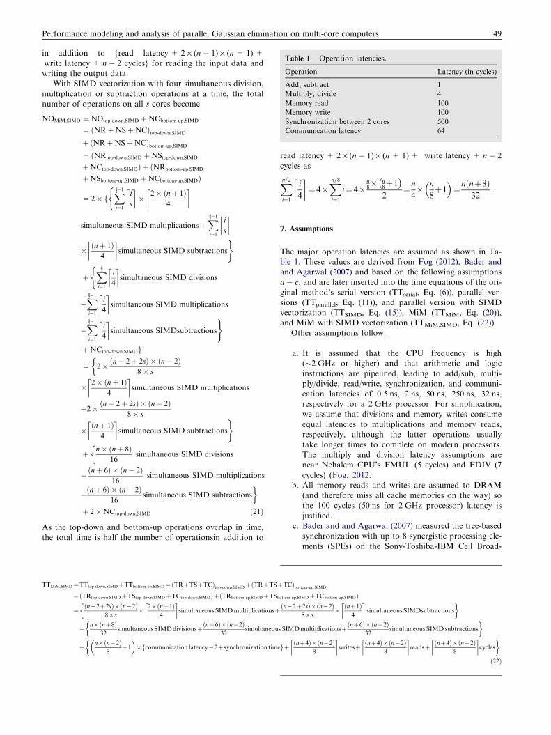
Table 1 Operation latencies.

Operation Latency (in cycles)

Add, subtract 1

Multiply, divide 4

Memory read 100

Memory write 100

Synchronization between 2 cores 500

Communication latency 64

Performance modeling and analysis of parallel Gaussian elimination on multi-core computers 49

in addition to {read latency + 2 · (n � 1) · (n+ 1) +

write latency + n � 2 cycles} for reading the input data andwriting the output data.

With SIMD vectorization with four simultaneous division,

multiplication or subtraction operations at a time, the totalnumber of operations on all s cores become

NOMiM;SIMD ¼ NOtop-down;SIMD þNObottom-up;SIMD

¼ ðNRþNSþNCÞtop-down;SIMD

þ ðNRþNSþNCÞbottom-up;SIMD

¼ ðNRtop-down;SIMD þNStop-down;SIMD

þNCtop-down;SIMDÞ þ ðNRbottom-up;SIMD

þNSbottom-up;SIMD þNCbottom-up;SIMDÞ

¼ 2� fXn2�1i¼1

i

s

� �� 2� ðnþ 1Þ

4

� �(

simultaneous SIMD multiplicationsþXn2�1i¼1

i

s

� �

� ðnþ 1Þ4

� �simultaneous SIMD subtractions

)

þXn

2

i¼1

i

4

� �simultaneous SIMD divisions

(

þXn2�1i¼1

i

4

� �simultaneous SIMD multiplications

þXn2�1i¼1

i

4

� �simultaneous SIMDsubtractions

)

þNCtop-down;SIMDg

¼ 2� ðn� 2þ 2sÞ � ðn� 2Þ8� s

�

� 2� ðnþ 1Þ4

� �simultaneous SIMD multiplications

þ2� ðn� 2þ 2sÞ � ðn� 2Þ8� s

� ðnþ 1Þ4

� �simultaneous SIMD subtractions

)

þ n� ðnþ 8Þ16

simultaneous SIMD divisions

�

þðnþ 6Þ � ðn� 2Þ16

simultaneous SIMD multiplications

þðnþ 6Þ � ðn� 2Þ16

simultaneous SIMD subtractions

�þ 2�NCtop-down;SIMD ð21Þ

As the top-down and bottom-up operations overlap in time,the total time is half the number of operationsin addition to

TTMiM;SIMD¼TTtop-down;SIMDþTTbottom-up;SIMD¼ðTRþTSþTCÞtop-down;SIMDþðTRþTSþ¼ðTRtop-down;SIMDþTStop-down;SIMDþTCtop-down;SIMDÞþðTRbottom-up;SIMDþTSb

¼ ðn�2þ2sÞ�ðn�2Þ8�s

� 2�ðnþ1Þ4

� �simultaneous SIMDmultiplicationsþ

�

þ n�ðnþ8Þ32

simultaneous SIMDdivisionsþðnþ6Þ�ðn�2Þ32

simultaneou

�

þ n�ðn�2Þ8

�1

� �fcommunication latency�2þsynchronization time

�

read latency + 2 · (n � 1) · (n+ 1) + write latency + n � 2cycles as

Xn=2i¼1

i

4

� �¼4�

Xn=8i¼1

i¼4�n8� n

8þ1

�2

¼n

4� n

8þ1

� ¼nðnþ8Þ

32:

7. Assumptions

The major operation latencies are assumed as shown in Ta-ble 1. These values are derived from Fog (2012), Bader and

and Agarwal (2007) and based on the following assumptionsa � c, and are later inserted into the time equations of the ori-ginal method’s serial version (TTserial, Eq. (6)), parallel ver-

sions (TTparallel, Eq. (11)), and parallel version with SIMDvectorization (TTSIMD, Eq. (15)), MiM (TTMiM, Eq. (20)),and MiM with SIMD vectorization (TTMiM,SIMD, Eq. (22)).

Other assumptions follow.

a. It is assumed that the CPU frequency is high(�2 GHz or higher) and that arithmetic and logic

instructions are pipelined, leading to add/sub, multi-ply/divide, read/write, synchronization, and communi-cation latencies of 0.5 ns, 2 ns, 50 ns, 250 ns, 32 ns,

respectively for a 2 GHz processor. For simplification,we assume that divisions and memory writes consumeequal latencies to multiplications and memory reads,

respectively, although the latter operations usuallytake longer times to complete on modern processors.The multiply and division latency assumptions arenear Nehalem CPU’s FMUL (5 cycles) and FDIV (7

cycles) (Fog, 2012.b. All memory reads and writes are assumed to DRAM

(and therefore miss all cache memories on the way) so

the 100 cycles (50 ns for 2 GHz processor) latency isjustified.

c. Bader and and Agarwal (2007) measured the tree-based

synchronization with up to 8 synergistic processing ele-ments (SPEs) on the Sony-Toshiba-IBM Cell Broad-

TCÞbottom-up;SIMD

ottom-up;SIMDþTCbottom-up;SIMDÞðn�2þ2sÞ�ðn�2Þ

8�s � ðnþ1Þ4

� �simultaneous SIMDsubtractions

�

s SIMDmultiplicationsþðnþ6Þ�ðn�2Þ32

simultaneous SIMD subtractions

�

gþ ðnþ4Þ�ðn�2Þ8

� �writesþ ðnþ4Þ�ðn�2Þ

8

� �readsþ ðnþ4Þ�ðn�2Þ

8

� �cycles

�ð22Þ

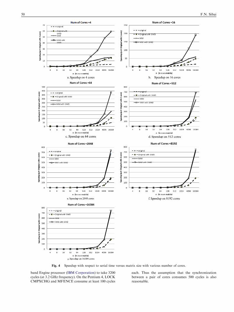
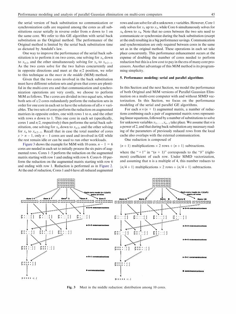
Fig. 4 Speedup with respect to serial time versus matrix size with various number of cores.

50 F.N. Sibai

band Engine processor (IBM Corporation) to take 3200cycles (at 3.2 GHz frequency). On the Pentium 4, LOCKCMPXCHG and MFENCE consume at least 100 cycles

each. Thus the assumption that the synchronizationbetween a pair of cores consumes 500 cycles is alsoreasonable.

Performance modeling and analysis of parallel Gaussian elimination on multi-core computers 51

d. For simplification, we assume that synchronization

times and communication latencies are constant andindependent of the number of cores.

e. With SIMD vectorization, the arithmetic operations

take the same amount of time (cycles) except that itis assumed that 4 such operations can be performedsimultaneously per core in the above number ofcycles.

f. The major operation times are included in the perfor-mance model in order to assess their impact on the over-all performance scalability with number of cores. Other

secondary operations are omitted. The execution timesalso include the reading of the input data and the writingof the output data times. Dynamic random memory

(DRAM) space is assumed to be sufficient to avoid vir-tual memory effects.

g. Inter-core data communication time is assumed to beuniform, pipelined with 2 single precision floating point

numbers communicated per clock after initial communi-cation latency elapses, and is integrated in the model’sTC equations (see Eqs. (1)–(22)).

h. The performance models include the effects of thread-level and data-level parallelisms. Thread managementtimes are ignored. Moreover, instruction-level parallel-

ism is ignored in the performance models of both serialand parallel algorithms.

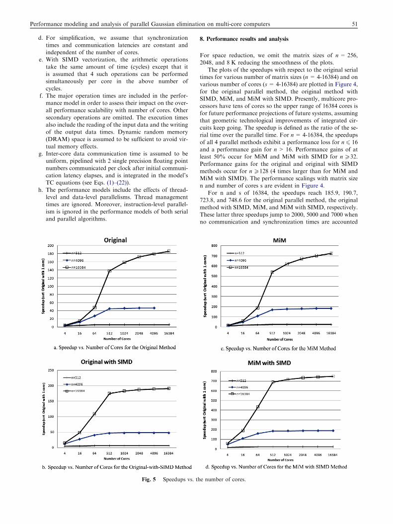
Fig. 5 Speedups vs. th

8. Performance results and analysis

For space reduction, we omit the matrix sizes of n= 256,2048, and 8 K reducing the smoothness of the plots.

The plots of the speedups with respect to the original serialtimes for various number of matrix sizes (n = 4-16384) and onvarious number of cores (s= 4-16384) are plotted in Figure 4,

for the original parallel method, the original method withSIMD, MiM, and MiM with SIMD. Presently, multicore pro-cessors have tens of cores so the upper range of 16384 cores isfor future performance projections of future systems, assuming

that geometric technological improvements of integrated cir-cuits keep going. The speedup is defined as the ratio of the se-rial time over the parallel time. For n= 4-16384, the speedups

of all 4 parallel methods exhibit a performance loss for n 6 16and a performance gain for n > 16. Performance gains of atleast 50% occur for MiM and MiM with SIMD for n P32.

Performance gains for the original and original with SIMDmethods occur for n P128 (4 times larger than for MiM andMiM with SIMD). The performance scalings with matrix size

n and number of cores s are evident in Figure 4.For n and s of 16384, the speedups reach 185.9, 190.7,

723.8, and 748.6 for the original parallel method, the originalmethod with SIMD, MiM, and MiM with SIMD, respectively.

These latter three speedups jump to 2000, 5000 and 7000 whenno communication and synchronization times are accounted

e number of cores.

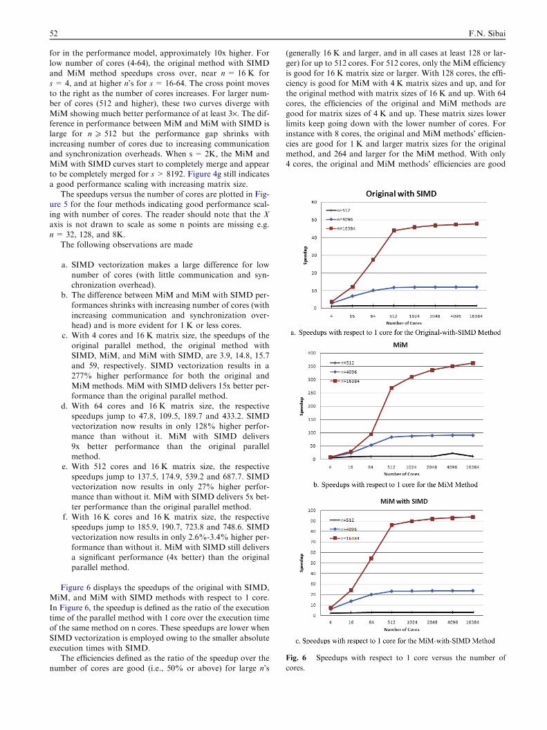
Fig. 6 Speedups with respect to 1 core versus the number of

cores.

52 F.N. Sibai

for in the performance model, approximately 10x higher. Forlow number of cores (4-64), the original method with SIMDand MiM method speedups cross over, near n = 16 K for

s= 4, and at higher n’s for s = 16-64. The cross point movesto the right as the number of cores increases. For larger num-ber of cores (512 and higher), these two curves diverge with

MiM showing much better performance of at least 3·. The dif-ference in performance between MiM and MiM with SIMD islarge for n P 512 but the performance gap shrinks with

increasing number of cores due to increasing communicationand synchronization overheads. When s = 2K, the MiM andMiM with SIMD curves start to completely merge and appearto be completely merged for s > 8192. Figure 4g still indicates

a good performance scaling with increasing matrix size.The speedups versus the number of cores are plotted in Fig-

ure 5 for the four methods indicating good performance scal-

ing with number of cores. The reader should note that the Xaxis is not drawn to scale as some n points are missing e.g.n= 32, 128, and 8K.

The following observations are made

a. SIMD vectorization makes a large difference for low

number of cores (with little communication and syn-chronization overhead).

b. The difference between MiM and MiM with SIMD per-formances shrinks with increasing number of cores (with

increasing communication and synchronization over-head) and is more evident for 1 K or less cores.

c. With 4 cores and 16 K matrix size, the speedups of the

original parallel method, the original method withSIMD, MiM, and MiM with SIMD, are 3.9, 14.8, 15.7and 59, respectively. SIMD vectorization results in a

277% higher performance for both the original andMiM methods. MiM with SIMD delivers 15x better per-formance than the original parallel method.

d. With 64 cores and 16 K matrix size, the respectivespeedups jump to 47.8, 109.5, 189.7 and 433.2. SIMDvectorization now results in only 128% higher perfor-mance than without it. MiM with SIMD delivers

9x better performance than the original parallelmethod.

e. With 512 cores and 16 K matrix size, the respective

speedups jump to 137.5, 174.9, 539.2 and 687.7. SIMDvectorization now results in only 27% higher perfor-mance than without it. MiM with SIMD delivers 5x bet-

ter performance than the original parallel method.f. With 16 K cores and 16 K matrix size, the respective

speedups jump to 185.9, 190.7, 723.8 and 748.6. SIMDvectorization now results in only 2.6%-3.4% higher per-

formance than without it. MiM with SIMD still deliversa significant performance (4x better) than the originalparallel method.

Figure 6 displays the speedups of the original with SIMD,MiM, and MiM with SIMD methods with respect to 1 core.

In Figure 6, the speedup is defined as the ratio of the executiontime of the parallel method with 1 core over the execution timeof the same method on n cores. These speedups are lower when

SIMD vectorization is employed owing to the smaller absoluteexecution times with SIMD.

The efficiencies defined as the ratio of the speedup over thenumber of cores are good (i.e., 50% or above) for large n’s

(generally 16 K and larger, and in all cases at least 128 or lar-ger) for up to 512 cores. For 512 cores, only the MiM efficiencyis good for 16 K matrix size or larger. With 128 cores, the effi-

ciency is good for MiM with 4 K matrix sizes and up, and forthe original method with matrix sizes of 16 K and up. With 64cores, the efficiencies of the original and MiM methods are

good for matrix sizes of 4 K and up. These matrix sizes lowerlimits keep going down with the lower number of cores. Forinstance with 8 cores, the original and MiM methods’ efficien-

cies are good for 1 K and larger matrix sizes for the originalmethod, and 264 and larger for the MiM method. With only4 cores, the original and MiM methods’ efficiencies are good

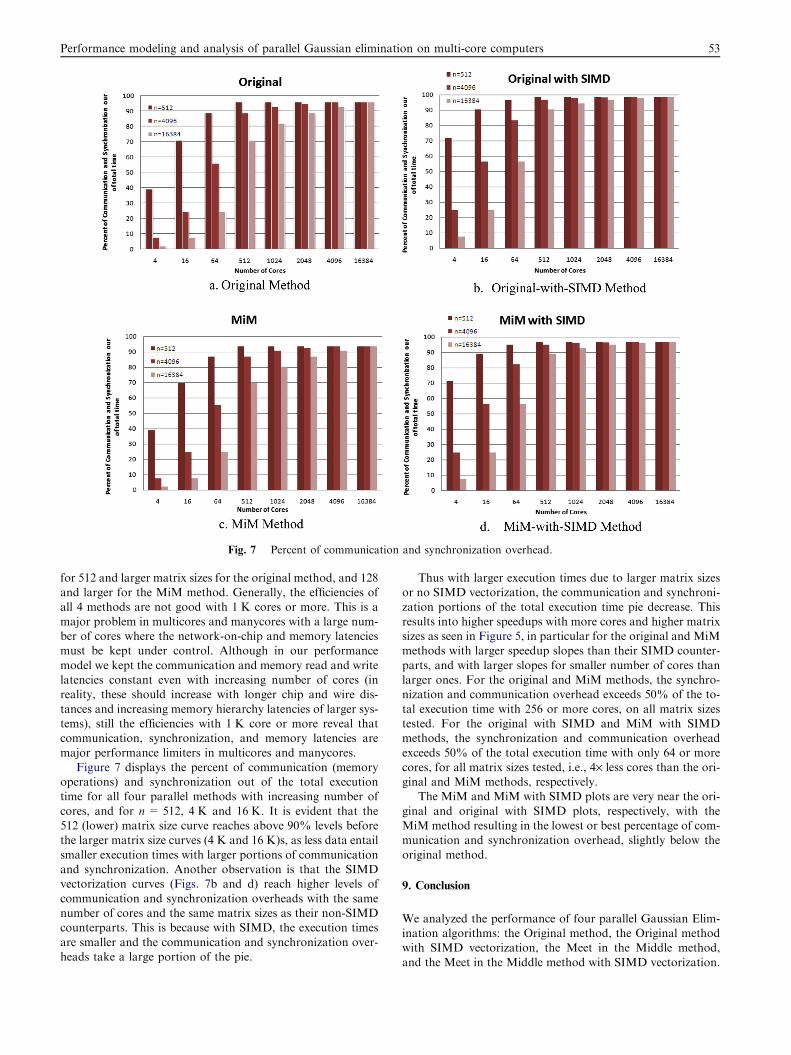
Fig. 7 Percent of communication and synchronization overhead.

Performance modeling and analysis of parallel Gaussian elimination on multi-core computers 53

for 512 and larger matrix sizes for the original method, and 128and larger for the MiM method. Generally, the efficiencies ofall 4 methods are not good with 1 K cores or more. This is a

major problem in multicores and manycores with a large num-ber of cores where the network-on-chip and memory latenciesmust be kept under control. Although in our performance

model we kept the communication and memory read and writelatencies constant even with increasing number of cores (inreality, these should increase with longer chip and wire dis-

tances and increasing memory hierarchy latencies of larger sys-tems), still the efficiencies with 1 K core or more reveal thatcommunication, synchronization, and memory latencies are

major performance limiters in multicores and manycores.Figure 7 displays the percent of communication (memory

operations) and synchronization out of the total executiontime for all four parallel methods with increasing number of

cores, and for n= 512, 4 K and 16 K. It is evident that the512 (lower) matrix size curve reaches above 90% levels beforethe larger matrix size curves (4 K and 16 K)s, as less data entail

smaller execution times with larger portions of communicationand synchronization. Another observation is that the SIMDvectorization curves (Figs. 7b and d) reach higher levels of

communication and synchronization overheads with the samenumber of cores and the same matrix sizes as their non-SIMDcounterparts. This is because with SIMD, the execution times

are smaller and the communication and synchronization over-heads take a large portion of the pie.

Thus with larger execution times due to larger matrix sizesor no SIMD vectorization, the communication and synchroni-zation portions of the total execution time pie decrease. This

results into higher speedups with more cores and higher matrixsizes as seen in Figure 5, in particular for the original and MiMmethods with larger speedup slopes than their SIMD counter-

parts, and with larger slopes for smaller number of cores thanlarger ones. For the original and MiM methods, the synchro-nization and communication overhead exceeds 50% of the to-

tal execution time with 256 or more cores, on all matrix sizestested. For the original with SIMD and MiM with SIMDmethods, the synchronization and communication overhead

exceeds 50% of the total execution time with only 64 or morecores, for all matrix sizes tested, i.e., 4· less cores than the ori-ginal and MiM methods, respectively.

The MiM and MiM with SIMD plots are very near the ori-

ginal and original with SIMD plots, respectively, with theMiM method resulting in the lowest or best percentage of com-munication and synchronization overhead, slightly below the

original method.

9. Conclusion

We analyzed the performance of four parallel Gaussian Elim-ination algorithms: the Original method, the Original methodwith SIMD vectorization, the Meet in the Middle method,

and the Meet in the Middle method with SIMD vectorization.

54 F.N. Sibai

We developed a performance model for each of those methodsand computed the speedups with respect to the serial originalGE algorithm time, and speedups with respect to the same

method on 1 core.For large n and s (16 K), the speedups reach 185.9, 190.7,

723.8, and 748.6 for the original parallel method, the original

method with SIMD, MiM, and MiM with SIMD, respectively,approximately 10x times lower than when no communicationand synchronization times are accounted for in the perfor-

mance model. SIMD vectorization makes a large differencefor low number of cores (up to 1 K cores, with relatively smal-ler communication and synchronization overheads than largersystems) but the difference in performance between MiM and

MiM with SIMD shrinks with increasing number of cores.The efficiencies are good for large n’s for up to 512 cores.

The efficiencies of all four methods are low with 1 K cores

or more stressing a major problem of highly parallel multi-coresystems where the network-on-chip and memory latencies arestill too high in relation to basic arithmetic operations. The

efficiencies with 1 K core or more reveal that communication,synchronization, and memory latencies are major performancelimiters in multi-core systems. The synchronization and com-

munication overheads exceed 50% of the total execution timestarting with 64 (256) or more cores for the SIMD methods(non-SIMD methods).

Thus the need exits to design multi-core systems with lower

memory (and interconnect) operation latencies as both commu-nication and synchronization steps involve memory operations.As the speedup does not increase much between 512 cores and

16 K cores, we question the reasoning behind exclusively inte-grating more cores in future submicron chips rather than inte-grating both processing cores and DRAM on the same chip.

Although memory hiding techniques such as Geraci’s (2008) in-Core LU solver and double buffering (Vianney et al., 2008) areeffective in overlapping computation with memory operations,

these techniques are not simple for the average parallel program-mer, in addition to synchronization consuming longer and long-er times. Improving memory and synchronization latencies aretwo key issues for future multi-core system designs as we ap-

proach the exascale computing age.

References

Bader, D. and Agarwal, V., 2007. FFTC: Fastest Fourier Transform

for the IBM Cell Broadband Engine, HiPC 2007, LNCS 4873,

Springer-Verlag, pp. 172–184.

Barrett, R. et al, 1994. Templates for the Solution of Linear Systems:

Building Blocks for Iterative Methods. SIAM.

Demmel, J. et al, 1993. Parallel numerical linear algebra. Acta Numer.

2, 111–197.

Demmel, J., Gilbert, J., Li, X., 1999. An asynchronous parallel

supernodal algorithm for sparse Gaussian elimination. SIAM J.

Matrix Anal. Appl. 20 (4), 915–952.

Duff, I., Van der Vorst, H., 1999. Developments and trends in the

parallel solution of linear systems. Parallel Comput. 25, 1931–1970.

Fernandez, D.M., Giannacopoulos, D., Gross, W.J., 2010. Multicore

Acceleration of CG Algorithms Using Blocked-Pipeline-Matching

Techniques. IEEE Trans. Magnet. 46 (8), 3057–3060.

Fog, A., 2012. Instruction tables -Lists of instruction latencies,

throughputs and micro-operation breakdowns for Intel, AMD

and VIA CPUs, http://www.agner.org/optimize/instruction_

tables.pdf.

Geraci, J., 2008. A Comparison of Parallel Gaussian Elimination

Solvers for the Computation of Electrochemical Battery Models on

the Cell Processor, Ph.D. Dissertation, EECS Department, Mas-

sachussets Institute of Technology.

Grama, A. et al, 2003. Introduction to Parallel Computing, 2nd ed.

Addison Wesley.

Greenbaum, A., 1997. Iterative Methods for Solving Linear Systems.

SIAM.

Gupta, A. et al, 1997. Highly scalable parallel algorithms for sparse

matrix factorization. IEEE Trans. Parallel Distrib. Syst. 8 (5), 502–

520.

Gupta, A., et al., 1998. Design and implementation of a scalable

parallel direct solver for sparse symmetric positive definite systems,

Research Report UMSI 98/16, University of Minnesota Super-

computing Institute.

Heath, M., 1997. Parallel direct methods for sparse linear systems. In:

Keyes, D.E., Sameh, A., Venkatakrishnan, V. (Eds.), Parallel

Numerical Algorithms. Kluwer Academic Publishers., Boston, pp.

55–90.

IBM Corporation. Cell Broadband Engine technology. http://

www.alphaworks.ibm.com/topics/cell.

Kumar, S., Gupta, K., 2012. Performance Analysis of Parallel

Algorithms on Multi-core System Using OpenMP. Int. J. Comput.

Sci. Eng. Inform. Technol. 2 (5), 55–64.

Laure, E., Al-Shandawely, M., 2011. Improving Gaussian Elimination

on Multi-Core Systems, Fourth Swedish Workshop on Multicore

Computing (MCC-2011), Linkoping University.

Li, Z., Donde, V., Tournier, J.-C., Yang, F., 2011. On limitations of

traditional multi-core and potential of many-core processing

architectures for sparse linear solvers used in large-scale power

system applications, IEEE Power and Energy Society General

Meeting, pp. 1–8.

McGinn, S.F., Shaw, R.E., 2002. Parallel Gaussian elimination using

OpenMP and MPI. High Performance, 2002. Proceedings. 16th

Annual International Symposium on Computing Systems and

Applications, pp. 169–173.

Pimple, M., Sathe, S., 2011. Architecture Aware Programming on

Multi-core Systems. Int. J. Adv. Comput. Sci. Appl. 2 (6), 105–111.

Prinslow, G., 2011. Overview of Performance Measurement and

Analytical Modeling Techniques for Multi-core Processors, http://

www.cse.wustl.edu/ � jain/cse567-11/ftp/multcore. pdf.

Quinn, M., 1994. Parallel Computing. McGraw Hill.

Saad, Y., 2003. Iterative Methods for Sparse Linear Systems, 2nd ed.

SIAM.

Sankar, A., 2004. Smoothed Analysis of Gaussian Elimination, Ph.D.

Dissertation, Math Department, Massachussets Institute of

Technology.

Van der Vorst, H., Chan, T., 1997. Linear system solvers: sparse

iterative methods. In: Keyes, D.E., Sameh, A., Venkatakrishnan,

V. (Eds.), Parallel Numerical Algorithms. Kluwer, pp. 91–118.

Vianney, D., et al., 2008. Performance analysis and visualization tools

for Cell/B.E.multicore environment. ACMIFMT ’08, Cairo, Egypt.

Wiggers, W., et al. 2007. Implementing the conjugate gradient

algorithm on multi-core systems, IEEE International Symposium

on System-on-Chip, pp. 1–4.

Xiaoye, S., Demmel, J., 1998. Making sparse Gaussian elimination

scalable by static pivoting, IEEE/ACM Conference on

Supercomputing.

Yeung, M., Chan, T., 1997. Probabilistic Analysis of Gaussian

Elimination without Pivoting. SIAM J. Matrix Anal. Appl., 499–

517.