An Analytical Solution for Non-Darcian Flow in a Confined

Available online at www.sciencedirect.com

www.elsevier.com/locate/advwatres

Advances in Water Resources 31 (2008) 44–55

An analytical solution for non-Darcian flow in a confinedaquifer using the power law function

Zhang Wen a,b, Guanhua Huang a,b,*, Hongbin Zhan c

a Department of Irrigation and Drainage, College of Water Conservancy and Civil Engineering, China Agricultural University, Beijing, 100083, PR Chinab Chinese–Israeli International Center for Research in Agriculture, China Agricultural University, Beijing, 100083, PR China

c Department of Geology and Geophysics, Texas A&M University, College Station, TX 77843-3115, USA

Received 26 February 2007; received in revised form 3 May 2007; accepted 25 June 2007Available online 30 June 2007

Abstract

We have developed a new method to analyze the power law based non-Darcian flow toward a well in a confined aquifer with andwithout wellbore storage. This method is based on a combination of the linearization approximation of the non-Darcian flow equationand the Laplace transform. Analytical solutions of steady-state and late time drawdowns are obtained. Semi-analytical solutions of thedrawdowns at any distance and time are computed by using the Stehfest numerical inverse Laplace transform. The results of this studyagree perfectly with previous Theis solution for an infinitesimal well and with the Papadopulos and Cooper’s solution for a finite-diam-eter well under the special case of Darcian flow. The Boltzmann transform, which is commonly employed for solving non-Darcian flowproblems before, is problematic for studying radial non-Darcian flow. Comparison of drawdowns obtained by our proposed method andthe Boltzmann transform method suggests that the Boltzmann transform method differs from the linearization method at early and mod-erate times, and it yields similar results as the linearization method at late times. If the power index n and the quasi hydraulic conductivityk get larger, drawdowns at late times will become less, regardless of the wellbore storage. When n is larger, flow approaches steady stateearlier. The drawdown at steady state is approximately proportional to r1�n, where r is the radial distance from the pumping well. Thelate time drawdown is a superposition of the steady-state solution and a negative time-dependent term that is proportional to t(1�n)/(3�n),where t is the time.� 2007 Elsevier Ltd. All rights reserved.

Keywords: Non-Darcian flow; Power law; Laplace transform; Linearization method

1. Introduction

Scientists and engineers have been fascinated with non-Darcian flow for more than one hundred years [8] andthere are still plenty of unanswered questions. Amongmany difficulties encountered in dealing with non-Darcianflow, two of them are notable. One of them is to adequatelycharacterize non-Darcian flow using physically measurable

0309-1708/$ - see front matter � 2007 Elsevier Ltd. All rights reserved.

doi:10.1016/j.advwatres.2007.06.002

* Corresponding author. Address: Department of Irrigation and Drain-age, College of Water Conservancy and Civil Engineering, ChinaAgricultural University, Beijing, 100083, PR China. Tel.: +86 1062737144; fax: +86 10 62737138.

E-mail address: [email protected] (G. Huang).

parameters. The other is to find a robust mathematical toolto solve the non-Darcian flow governing equation.

Non-Darcian flow can arise from a number of differentways. For flow at low rates in fine-grained media such asclay and silt aquitards, the non-Darcian flow may be attrib-uted to the electro-chemical surface effect between the fluidand the solid, and is named pre-linear flow [32,36]. The pre-linear flow has also been extensively investigated in thepetroleum engineering [35,5]. For flow at high rates incoarse grained and fractured media, or near pumping wells,the non-Darcian flow may be caused by the inertial effectand the onset of turbulent flow, and is subsequently namedpost-linear flow [1,14,24,36,39].

Many formulas have been proposed to quantify the rela-tionship between the hydraulic gradient and the specific

mailto:[email protected]

Nomenclature

A ¼ Sm

nk

Q2pm

� �n�1, a parameter used in Eq. (10)

B ¼ 2prwmk Q2pmrw

h ið1�nÞ, a parameter used in Eq. (22)

C a parameter defined in Appendix Eq. (A10) andused in Eq. (27)

C0, C1, C2 integration constantsk quasi hydraulic conductivity, an empirical con-

stant in the Izbash equation [(L/T)n]m aquifer thickness [L]n power index, an empirical constant in the Izbash

equationp Laplace variableq(r,t) specific discharge [L/T]

Q pumping discharge [L3/T]r distance from the center of the well [L]rc radius of well casing [L]rw effective radius of well screen [L]R radius of influence of the pumping well [L]s(r,t) drawdown [L]sw(t) drawdown inside well [L]S Aquifer storage coefficientt pumping time [T]C Gamma functionIm(x) the first kind order m modified Bessel functionKm(x) the second kind order m modified Bessel function

Z. Wen et al. / Advances in Water Resources 31 (2008) 44–55 45

discharge for non-Darcian flow. The most commonly usedones are the Forchheimer equation [8] and the Izbash equa-tion [13]. The Forchheimer equation states that the hydrau-lic gradient is a second-order polynomial function of thespecific discharge; while the Izbash equation states thatthe hydraulic gradient is a power function of the specificdischarge. Many investigators preferred to choose theForchheimer equation to describe non-Darcian flow basedon the argument that the Forchheimer equation includesboth the viscous and inertial effects and is an expansionof the linear Darcy’s law e.g. [25,37,38,9,20]. The choiceof the Izbash equation is based on a different philosophicalargument: many post-linear non-Darcian flows are causedpredominately by turbulent effects, which are convenientlymodeled by power law functions [17,6,24]. In some cases,the Forchheimer equation is favored; in other cases, theIzbash equation is a better choice; and in certain circum-stances, both equations can describe non-Darcian flowequally well [2,27].

In terms of the mathematical tool to study the non-Dar-cian flow, the Boltzmann transform has been regarded asan appropriate analytical method to solve the non-Darcianflow governing equation e.g. [25–28]. The Boltzmann trans-form is a special member of a family named ‘‘similaritymethod’’ that has been broadly used in solving diffusiontype of problems [19,36]. The idea of the Boltzmann trans-form is to combine the spatial coordinate (denoted as r)and the temporal coordinate (denoted as t) into a newBoltzmann variable g ¼ r=

ffiffitp

and to change the partial dif-ferential equation of flow into an ordinary differentialequation. Although theoretically appealing, the Boltzmanntransform is rather restrictive because it requires that allthe initial and boundary conditions can also be simulta-neously transformed into forms only containing the Boltz-mann variable g. Unfortunately, such a requirement hasoften not be rigorously checked or even ignored in manystudies. This has caused considerable confusion in the liter-atures on non-Darcian flow. It is unclear how much errorwill be introduced when such a requirement is not satisfied.

A careful review of previous studies of non-Darcian flowindicates that the Boltzmann transform works very wellwhen flow field is planar. For instance, Sen [25,28] andWen et al. [36] have successfully applied the Boltzmanntransform to study non-Darcian flow to a single fracture.However, the Boltzmann transform seems to be problem-atic when radial non-Darcian flow is considered, such asthose near the pumping wells. When the groundwater flowpartial differential governing equation is converted into anordinary differential equation after the Boltzmann trans-form, integration is often the next step to yield the solutionwith an unknown integration ‘‘constant’’ that must bedetermined via the boundary condition. For a radial non-Darcian flow problem, the boundary condition near thepumping well can not be transformed into a form onlydepending on the Boltzmann variable. This will make theintegration ‘‘constant’’ to be temporal or spatially depen-dent. For instance, the integration ‘‘constant’’ in Eq. (7)of Sen [26] is actually a function of time (see Eq. (9) ofSen [26]). Several scientists including Camacho-V and Vas-quez-C [3] have noticed this problem before.

If the Boltzmann transform is found to be inappropriatefor a particular non-Darcian flow problem, then one has tofind an alternative mathematical tool to solve the non-Darcian flow problem. Fortunately, we have noticed thatmany non-Newtonian flow problems resemble similarnon-linearity characteristics as the non-Darcian flow prob-lems. The linearization approximation method has beenproven to be a successful tool to deal with the non-linearityof the non-Newtonian flow e.g. [12,18,34]. To our knowl-edge, the linearization approximation method has rarelybeen used to investigate the non-Darcian flow, particularlyfor the Izbash type of non-Darcian flow. The purpose ofthis paper is to develop a new method for solving the powerlaw based radial non-Darcian flow near a pumping wellcombining the linearization approximation with theLaplace transform. The results of the non-Darcian flowwill be compared with that of the Darcian flow. The impor-tance of different non-Darcian flow parameters will be

46 Z. Wen et al. / Advances in Water Resources 31 (2008) 44–55

assessed. We will also compare this method with the Boltz-mann transform method used before.

2. Conceptual and mathematical models

2.1. Problem statement and solutions

Considering a vertical pumping well in a confinedaquifer, the thickness of the aquifer is m. The aquifer ishomogeneous and isotropic. The physical system is thesame as that of Sen [26], as shown in Fig. 1a. The continu-ity equation can be expressed as:

oqðr; tÞor

þ qðr; tÞr¼ S

mosðr; tÞ

ot; ð1Þ

where q(r,t) is the specific discharge at radial distance r andtime t, s(r,t) is the drawdown, and S is the storage coeffi-cient of the aquifer. With the assumptions used in Sen[26], the initial and boundary conditions can be written as:

sðr; 0Þ ¼ 0; ð2Þsð1; tÞ ¼ 0; ð3Þ

Confined Aquifer

m

Confined Aquifer

s

r

Land SurfaceLand Surface

Confined Aquifer

m

Confined Aquifer

sws

2rw

r

2rc

Land SurfaceLand Surface Q

Q

Fig. 1. The schematic diagrams of the problem (a) without wellborestorage and (b) with wellbore storage.

limr!0½2pmrqðr; tÞ� ¼ �Q: ð4Þ

where Q is the pumping rate of the well, which is assumedto be constant during the pumping period. Eq. (4) indicatesthat the wellbore storage is not considered here, all thepumping rate comes from the aquifer. We employ thepower law to describe the non-Darcian flow:

½qðr; tÞ�n ¼ kosðr; tÞ

or; ð5Þ

in which k and n are constants and n is between one andtwo. Further discussion of Eq. (5) and the parameters k

and n are given by several studies including Wen et al.[36]. When n goes to one, flow is Darcian, and k becomesthe hydraulic conductivity. Thus, k can be regarded as aquasi hydraulic conductivity term [36], which reflects howeasy the aquifer can transmit water. When n is less thanone, flow is called pre-linear flow. When n is between oneand two, flow is post-linear flow. If n approaches two, flowis fully developed turbulent, meaning that the hydraulicgradient of flow is independent of the Reynolds number[6,17]. The fully developed turbulent flow is likely to occurunder certain cases such as very close to the pumping well,near a dam, preferential flow, etc. In some cases, k and nare not real constants, and depend on the property of themedia and the velocities. Moutsopoulos and Tsihrintzis[16] suggested that the assumption of constant n and k

was more likely not justified if a boundary condition ofknown piezometric head was considered, whereas it wasprobably justified if a known flux was considered, such asin this study. If there is strong evidence that k and/or n

are not constant for the flow regime, alternative ap-proaches other than Eq. (5) are needed. Nevertheless, k

and n are treated as constants in this study. Eq. (5) canbe expressed in an alternative way as:

½qðr; tÞ� ¼ k1=n osðr; tÞor

� �1=n

: ð6Þ

Substituting Eq. (6) to Eq. (1) will yield:

o2s

or2þ n

rosor¼ S

mn

k1=n

osor

� �n�1n os

ot: ð7Þ

Now one must deal with the osor

� �n�1n term on the right hand

side of Eq. (7) which is a non-linear governing equation.One possible way to linearize Eq. (7) is to replace os/or

on the right hand side of Eq. (7) by a time-independentapproximation term as follows:

osðr; tÞor

¼ ½qðr; tÞ�n

k� �

Q2prm

� �n

k: ð8Þ

Eq. (8) is referred to as the linearization approximation.This approximation means that the amount of waterpassed through any radial face per unit time is treated asQ regardless of how far away from the center of the well.In a rigorous sense, the flow rate is equal to Q only atthe pumping wellbore. Similar linearization approxima-tions have been commonly used in studying non-


Newtonian flow e.g. [12,18,34]. Finite difference solutionsin non-Newtonian flow studies indicated that the errorscaused by the approximation are generally small[12,18,34]. This approximation works the best at placesnear the pumping well and/or at late times. It will be lessaccurate at early times when drawdown changes rapidlywith time. With this approximation, Eq. (7) can be changedto:

o2sor2þ n

rosor¼ S

mnk

Q2pm

� �n�1

r1�n osot: ð9Þ

Eq. (9) is a linear partial differential equation, which can besolved by Laplace transform. With the Laplace transformfor time t, one has:

d2�sdr2þ n

rd�sdr¼ Ar1�np�s ð10Þ

where A ¼ Sm

nk

Q2pm

� �n�1, p is the Laplace variable, over bar of

variable s means the Laplace transform of s. The initialcondition has been used in the Laplace transform. Withthis transform, the boundary conditions can be changed to:

�sð1; pÞ ¼ 0; ð11Þ

limr!0

rn d�sdr

� �¼ �

Q2pm

� �n

kp: ð12Þ

Eq. (10) is a form of Bessel’s equation. Its ordinary solu-tion has been given in previous studies on non-Newtonianflow [12]. Carslaw and Jaeger p. 414, case V [4] have alsoprovided a solution for this problem, which is

�sðr;pÞ¼ r1�n

2 C1I 1�n3�n

2

3�nr

3�n2

ffiffiffiffiffiffiAp

p� �þC2K1�n

3�n

2

3�nr

3�n2


p� �� ;

ð13Þ

in which I 1�n3�nðxÞ and K1�n

3�nðxÞ are the first and second kind

modified Bessel function with the order 1�n3�n, respectively.

C1 and C2 are the integration constants depending on theboundary conditions. In terms of the boundary conditionof Eq. (11), C1 = 0. Then, Eq. (13) becomes:

�sðr; pÞ ¼ r1�n

2 C2K1�n3�n

2

3� nr

3�n2


p� �� : ð14Þ

Applying Eq. (12) in Eq. (14), one has:

C2rn 1� n2

r�1�n

2 K1�n3�n

2

3� nr

3�n2


p� ��

þ r1�n

2 K 01�n3�n

2

3� nr

3�n2


p� �r

1�n2


p �

¼ �Q

2pm

� �n

kp; for r! 0: ð15Þ

With the properties of the modified Bessel functions: xdKm

(x)/dx + mKm(x) = �xKm�1(x) and Km(x) = K�m(x) p. 505[29], Eq. (15) can be reduced to:

C2rn �r1�nffiffiffiffiffiffiAp

pK 2

3�n

2

3�nr

3�n2


p� �� ¼�

Q2pm

� �n

kp; for r!0:

ð16Þ

According to the property of the second kind modifiedBessel function KmðxÞ � CðmÞ

2x2

� ��m; m > 0 when x goes to zero

p. 505 [29], in which C() is the gamma function, one has:

C2 ¼2 Q

2pm

� �nffiffiffiffiApp3�n

� � 23�n

kpffiffiffiffiffiffiApp

C 23�n

� � : ð17Þ

Therefore, one can determine the solution of the drawdownin Laplace domain accordingly:

�sðr; pÞ ¼2 Q

2pm

� �nffiffiffiffiApp3�n

� � 23�n

kpffiffiffiffiffiffiApp

C 23�n

� � r1�n

2 K1�n3�n

2

3� nr

3�n2


p� �: ð18Þ

Eq. (18) can be solved by using either the analytical or thenumerical Laplace inversion methods. Luan [15] has usedan analytical Laplace inversion method to investigatenon-Newtonian flow in a double-porosity formation.However, the analytical inversion is often complex andnot always available. It is proven that the numericalmethods are very efficient and useful for such inversionproblems e.g. [30,31,7]. We have evaluated Eq. (18) byusing the Stehfest method [30,31], the drawdowns at anygiven distance r and time t can be obtained when theparameters of the aquifer are known.

We have developed a MATLAB program to computethe drawdown by using this inversion method. The Stehfestmethod requires a choice of N which is the number of termsused in the inversion. Our numerical exercise shows thatN = 18 gives the most accurate and stable solution, thuswill be used in all the following calculation. The MATLABprogram is simple and straightforward with the Stehfestmethod as the primary component. The program is freeof charge from the authors upon request.

2.2. Solutions with wellbore storage

When the well radius is relatively large, the wellborestorage can not be ignored. Large diameter wells are com-monly used all over the world, especially in developingcountries such as India and China e.g. [11,10]. Similar tothe physical system of Papadopulos and Cooper [21], theschematic diagram is shown in Fig. 1b. If the wellborestorage is considered, the boundary condition will beexpressed as:

2prwmk1=n osðr; tÞor

� r!rw

#1=n

� pr2c

oswðtÞot¼ �Q; t > 0:

ð19Þ

in which rw is the effective radius of the well screen and rc isthe radius of the well casing. In most cases, rc is not equalto and often much larger than rw. sw(t) is the drawdown inthe well, which is equal to the drawdown at the face of well-bore in the aquifer s(rw,t). With the Laplace transform, Eq.(19) becomes


2prwmk1=n d�sðr; tÞdr

� r!rw

#1=n

� pr2cp�swðtÞ ¼ �

Qp: ð20Þ

Eq. (20) is a non-linear boundary condition. The solution isstill in the form of Eq. (13) with C1 = 0. However, it seemsdifficult to obtain the integration constant C2 of Eq. (13)directly from the non-linear boundary condition Eq. (20).In light of the linearization method as shown in Eq. (8),then Eq. (19) can be simplified to

2prwmkQ

2pmrw

� �ð1�nÞosðr; tÞ

or

r!rw

� pr2c

oswðtÞot� �Q: ð21Þ

Taking the Laplace transform of Eq. (21), one has

Bd�sðr; tÞ

dr

r!rw

� pr2cp�sðrw; pÞ ¼ �

Qp; ð22Þ

in which B ¼ 2prwmk Q2pmrw

h ið1�nÞ. Substituting Eq. (22) into

Eq. (13), one has:

C2¼Q

p Br1�nw

ffiffiffiffiffiffiApp

K 23�n

23�nr

3�n2

w

ffiffiffiffiffiffiApp �

þpr2cpr

1�n2

w K1�n3�n

23�nr

3�n2

w

ffiffiffiffiffiffiApp �n o:ð23Þ

After obtaining C2, the solution with wellbore storage inLaplace domain can be written as

�sðr;pÞ¼Qr

1�n2 K1�n

3�n

23�nr

3�n2ffiffiffiffiffiffiApp �

p Br1�nw

ffiffiffiffiffiffiApp

K 23�n

23�nr

3�n2

w

ffiffiffiffiffiffiApp �

þpr2cpr

1�n2

w K1�n3�n

23�nr

3�n2

w

ffiffiffiffiffiffiApp �n o:ð24Þ

When n approaches 1, flow becomes Darcian. Eq. (24) canbe approximated by

�sðr;pÞ¼QK0 r

ffiffiffiffiffiffiffiS

mk pq �

p 2prwmkffiffiffiffiffiffiffiS

mk pq

K1 rw


mk pq �

þpr2cpK0 rw


mk pq �n o :

ð25ÞEq. (25) is the same as the solution of Papadopulos andCooper [21] in Laplace domain. Eq. (24) can also be eval-uated by the numerical inversion which is included in theMATLAB program.

2.3. Approximate analytical solutions at steady state and late

times

Before the discussion of the results, it is necessary toobtain the analytical solutions at steady state and latetimes. For steady-state flow, the drawdown does notdepend on time t, thus os

ot ¼ 0. Appendix shows the detailedderivation of obtaining the steady-state drawdown which is

sðrÞ ¼ Q2pm

� �n 1

kðn� 1Þ1

rn�1� 1

Rn�1

� �; rw 6 r 6 R;

ð26Þ

where rw is the effective radius of the well screen and R isthe radius of influence of the well at which the drawdownis negligible. Notice that 1 < n 6 2, thus the drawdowndecreases with distance with a power of (n � 1). For thespecial case of Darcian flow, n is approaching 1, andEq. (26) can be simplified as follows. Recalling the identitythat limn!1ð1=rn�1Þ ¼ limn!1fexp½�ðn�1Þlnr�gffi1�ðn�1Þln r, thus Eq. (26) becomes the well known steady-state

solution for Darcian flow to a well: sðrÞ ¼ Q2pmk

� �lnðr=RÞ.

A minor issue to point out is that the radius of influenceR must be used when discussing the steady-state Darcianflow in a confined aquifer; otherwise, the drawdown willbecome infinity when r goes to infinity.

It is notable that van Poollen and Jargon [33] have pro-vided an analytical solution of steady-state non-Newtonianfluid flow. They have also provided a numerical solution oftransient non-Newtonian fluid flow. Eq. (26) indicates thatthe steady-state drawdown will increase with the pumpingrate Q, and decrease with the quasi hydraulic conductivityk and the thickness of the aquifer m. Taking the derivativewith respect to r on both sides of Eq. (26), it is found thatdsðrÞ

dr ¼ �ðQ=2pmrÞn

k , which is consistent with Eq. (8).

In addition to the steady-state solution, it is also inter-esting to derive the time-dependent late time solution whichmay be very useful in well testing analysis because the latetime solution is normally accurate enough after a certaintime of pumping, as demonstrated by Wu [37]. The latetime analytical solution can be obtained by conductingthe inverse Laplace transform of Eq. (18) by allowing theLaplace transform parameter p to be sufficiently small.The Appendix has given the detailed derivation of the latertime analytical solution which is

sðr; tÞ ¼ Q2pm

� �n1

kðn� 1Þ1

rn�1� C

tn�13�n

� �; ð27Þ

where the constant C is given in Eq. (A10) of the Appendix.It is interesting to see that the late time drawdown is

simply a superposition of the steady-state solution and anegative term that decreases with time with a power of(n � 1)/(3 � n). Interestingly, the time-dependent decreas-ing term in Eq. (27) is independent of spatial coordinate.Since the wellbore storage will not affect the steady-stateand late time drawdowns. Above solutions Eqs. (26) and(27) are also valid for the case with the wellbore storage.

3. Results and discussion

There are two different ways to present the results. Oneway is to present the dimensionless drawdown versusdimensionless time in log–log scales, the so-called typecurves, as often done in Darcian flow studies. The otherway is to analyze the result in dimensional forms. For Dar-cian flow, one of the advantages of using type curves isbased on the consideration that the dimensionless draw-down is often a function of dimensionless time only in aconfined aquifer, provided that other effects such as leak-


age across the aquifer boundaries are not considered. Fornon-Darcian flow discussed here, the benefits of using typecurves are not always obvious because of the non-linearpower law relationship between the discharge and thehydraulic gradient. Furthermore, it is straightforward totest the sensitivity of the solutions to two parameters nand k in dimensional forms. Therefore, we prefer a dimen-sional analysis for most parts of the following analysis. Thetype curves are only used when the results are comparedwith previous solutions of Darcian flow under the specialcase of n = 1.

Nevertheless, the type curves for non-Darcian flow canbe easily obtained based on the dimensional analysis ifthe dimensionless terms can be adequately defined. Withthe developed MATLAB program for the numericalLaplace inversion, we have obtained the drawdown valuesagainst time which are presented in log–log scales, asshown in Figs. 2–13. In the following discussion, we onlyconsider the case that n is larger than one, because pre-lin-ear flow is unlikely to occur near the pumping wells.

Fig. 3. Comparison of the drawdowns obtained by the proposedlinearization and Laplace transform method and the Boltzmann transformmethod with n = 2.0, Q = 50 m3/h, m = 50 m, k = 0.1(m/h)n, andS = 0.001 for the distances r = 10 m and 100 m, respectively.

3.1. Drawdowns without wellbore storage

3.1.1. Comparison of the non-linear type curves with Theis

curves

When n approaches one, flow is approaching Darcian.The result of Eq. (18) will approach the classical Theis solu-tion in the Laplace domain. We have compared our resultsfor n = 1 with the Theis type curves as shown in Fig. 2,which has the same axes as those defined in Theis typecurves, i.e. u ¼ r2S

4mkt and W ðuÞ ¼ 4pmkQ sðr; tÞ. It is clear to

see that our results agree perfectly with the Theis typecurves. This indicates that our MATLAB program based

Fig. 2. Comparison of the type curves for non-Darcian flow and Theistype curves.

Fig. 4. Drawdowns versus r2/t with n = 1.5, Q = 50 m3/h, m = 50 m,k = 0.1(m/h)n, and S = 0.001 for the distances r = 10 m, 20 m, 50 m, and100 m, respectively.

on the numerical inversion is applicable. On the otherhand, it may suggest that the errors of the linearizationapproximation are negligible at least when n is close toone. In the following analysis, we consider the linearizationsolutions as ‘‘quasi-exact’’ solutions when comparing to theresults of the Boltzmann method.

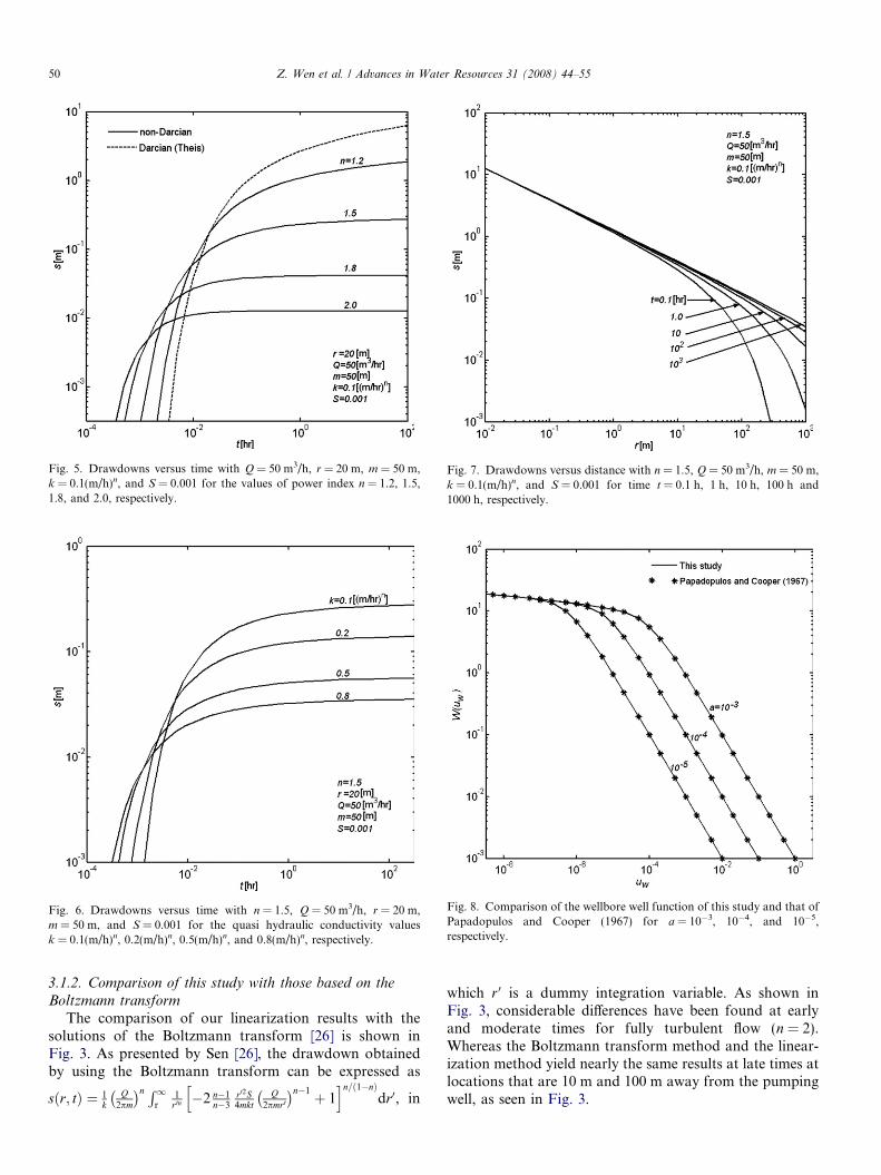
Fig. 5. Drawdowns versus time with Q = 50 m3/h, r = 20 m, m = 50 m,k = 0.1(m/h)n, and S = 0.001 for the values of power index n = 1.2, 1.5,1.8, and 2.0, respectively.

Fig. 6. Drawdowns versus time with n = 1.5, Q = 50 m3/h, r = 20 m,m = 50 m, and S = 0.001 for the quasi hydraulic conductivity valuesk = 0.1(m/h)n, 0.2(m/h)n, 0.5(m/h)n, and 0.8(m/h)n, respectively.

ig. 7. Drawdowns versus distance with n = 1.5, Q = 50 m3/h, m = 50 m,= 0.1(m/h)n, and S = 0.001 for time t = 0.1 h, 1 h, 10 h, 100 h and

000 h, respectively.

Fig. 8. Comparison of the wellbore well function of this study and that ofPapadopulos and Cooper (1967) for a = 10�3, 10�4, and 10�5,respectively.


3.1.2. Comparison of this study with those based on the

Boltzmann transform

The comparison of our linearization results with thesolutions of the Boltzmann transform [26] is shown inFig. 3. As presented by Sen [26], the drawdown obtainedby using the Boltzmann transform can be expressed as

sðr; tÞ ¼ 1k

Q2pm

� �n R1r

1r0n �2 n�1

n�3r02S4mkt

Q2pmr0

� �n�1 þ 1h in=ð1�nÞ

dr0, in

Fk

1

which r 0 is a dummy integration variable. As shown inFig. 3, considerable differences have been found at earlyand moderate times for fully turbulent flow (n = 2).Whereas the Boltzmann transform method and the linear-ization method yield nearly the same results at late times atlocations that are 10 m and 100 m away from the pumpingwell, as seen in Fig. 3.

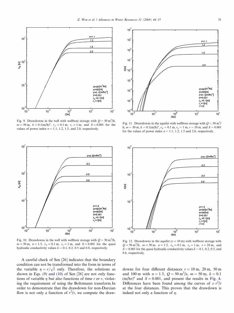
Fig. 9. Drawdowns in the well with wellbore storage with Q = 50 m3/h,m = 50 m, k = 0.1(m/h)n, rw = 0.1 m, rc = 1 m, and S = 0.001 for thevalues of power index n = 1.1, 1.2, 1.5, and 2.0, respectively.

Fig. 10. Drawdowns in the well with wellbore storage with Q = 50 m3/h,m = 50 m, n = 1.5, rw = 0.1 m, rc = 1 m, and S = 0.001 for the quasihydraulic conductivity values k = 0.1, 0.2, 0.5 and 0.8, respectively.

Fig. 11. Drawdowns in the aquifer with wellbore storage with Q = 50 m3/h, m = 50 m, k = 0.1(m/h)n, rw = 0.1 m, rc = 1 m, r = 10 m, and S = 0.001for the values of power index n = 1.1, 1.2, 1.5 and 2.0, respectively.

Fig. 12. Drawdowns in the aquifer (r = 10 m) with wellbore storage withQ = 50 m3/h, m = 50 m, n = 1.5, rw = 0.1 m, rc = 1 m, r = 10 m, andS = 0.001 for the quasi hydraulic conductivity values k = 0.1, 0.2, 0.5, and0.8, respectively.


A careful check of Sen [26] indicates that the boundarycondition can not be transformed into the form in terms ofthe variable g ¼ r=

ffiffitp

only. Therefore, the solutions asshown in Eqs. (9) and (10) of Sen [26] are not only func-tions of variable g but also functions of time t or r, violat-ing the requirement of using the Boltzmann transform.Inorder to demonstrate that the drawdown for non-Darcianflow is not only a function of r2/t, we compute the draw-

downs for four different distances r = 10 m, 20 m, 50 mand 100 m with n = 1.5, Q = 50 m3/s, m = 50 m, k = 0.1(m/hr)n and S = 0.001, and present the results in Fig. 4.Differences have been found among the curves of s–r2/tat the four distances. This proves that the drawdown isindeed not only a function of g.

Fig. 13. Drawdowns at t = 105 h versus distance with Q = 50 m3/h,m = 50 m, k = 0.1(m/h)n, and S = 0.001 for the values of power indexn = 1.1, 1.2, 1.5 and 2.0, respectively.


Interestingly, despite of the problems associated with theBoltzmann transform, the results obtained from the linear-ization method seem to agree reasonably well with thoseobtained from the Boltzmann transform method at latetimes, as reflected in Fig. 3. However, when the wellborestorage is included, we have found that the linearizationmethod gives the same drawdown at the pumping wellboreas that of Papadopulos and Cooper [21] for Darcian flow(see detailed discussion in Section 3.2); on the contrary,the Boltzmann transform method can not reproduce thesame wellbore drawdown as predicted by Papadopulosand Cooper [21] for Darcian flow.

3.1.3. Effect of the power index n and the quasi hydraulicconductivity k

The sensitivity of the drawdown versus n is shown inFig. 5 with n = 1.2, 1.5, 1.8 and 2.0, respectively. Asshown in this figure, the late time drawdown decreaseswhen n increases at any given distance. This finding is con-sistent with the steady-state solution Eq. (26) and the latetime solution Eq. (27). Physically speaking, this is alsounderstandable. A greater n value implies greater devia-tion from Darcian flow and greater degree of turbulenceof flow, indicating that flow near the well will experiencegreater degree of resistance. As a result, the cone ofdepression of the pumping well will be shrunk to a smallervolume surrounding the well. In another word, the draw-down will drop to zero faster when moving away from thewell. The consequence of this is a smaller drawdown atany given distance r and time t.

Fig. 5 also shows that when n is larger, flow approachessteady state more quickly. This finding is proved by the

analytical solution Eq. (27) in which the time-dependentterm drops to zero faster when n gets larger.

The impact of the quasi hydraulic conductivity k on thedrawdown is also analyzed. The results are shown in Fig. 6.At early times, the drawdown is greater when the value of k

is larger; while at late times, the drawdown is less when k islarger. This finding is similar to the influence of the powerindex n on the drawdown.

3.1.4. Drawdowns versus distance

All the discussion above is about the drawdown versustime t. It is equally important to analyze the drawdown versusdistance r. We have analyzed the drawdowns versus distance r

at five given times, as shown in Fig. 7. It is interesting to noticethat for flow near the pumping well, all the curves approachthe same asymptotic value in Fig. 7. This simply reflects thefact that the drawdowns at places very close to the pumpingwell reach steady state shortly after the start of pumping.

3.2. Drawdowns with wellbore storage

3.2.1. Drawdown in the wellWhen n approaches one, flow is Darcian, then the flow

model with wellbore storage is the same as that of Papado-pulos and Cooper [21] for Darcian flow to a large diameterwell. We can use the analytical solutions of Papadopulosand Cooper [21] to verify our results. In order to make thiscomparison feasible, we use the same dimensionless vari-ables as that of Papadopulos and Cooper [21]: the wellborewell function W ðuwÞ ¼ 4pmk

Q swðtÞ, the dimensionless time fac-

tor uw ¼ r2wS

4mkt, and a ¼ r2wSr2

c. The computed type curves based

on both the numerical inversion of Eq. (25) and the analyt-ical solutions of Papadopulos and Cooper [21] are shown inFig. 8. It is obvious to notice that our numerical inversionresults under Darcian flow case (n = 1) agree very well withthe solutions of Papadopulos and Cooper [21].

The sensitivity analysis of the power index n and thequasi hydraulic conductivity k on the drawdown in the wellare shown in Figs. 9 and 10, respectively. In these two fig-ures, all the diagrams in log–log scales can be divided intothree portions. For the first portion at early times, all thelines are straight and approach the same asymptotic values,reflecting the fact that the pumped water comes from thewellbore storage entirely during this period. Similar resultshave been found by Park and Zhan [22,23] in horizontalwells. For the second portion at moderate time, all thecurves start to deviate from the straight lines, meaning thatthe pumping rate is partially from the wellbore storage andpartially from the aquifer. While at late times, the thirdportion, a larger n or k value leads to a smaller drawdownin the well. This finding is consistent with the late time ana-lytical solution of Eq. (27).

3.2.2. Drawdowns in the aquifer

We have also analyzed the drawdown in the aquifer withdifferent n and k values, as shown in Figs. 11 and 12 by


using distance r = 10 m as an example. It can be found thatthe drawdown in the aquifer is less when n or k are greaterat late times; while the opposite is true at early times. Thisfinding is similar to that of the drawdown in the aquiferwithout considering wellbore storage.

3.3. Drawdowns versus distances at late times

To demonstrate the late time behavior of the draw-downs, we compute the drawdowns with different n valuesat t = 105 h for both Eqs. (14) and (23), the results areshown in Fig. 13. The approximate analytical solutionEq. (26) for steady-state flow is also included in this figure.The subtle difference for the case of n = 1.2 might due tothat flow is still at unsteady stage even for time as largeas 105 h. When the time is longer than 105 h, the numericalinversion results approach the steady-state analyticalresults. This indicates when n is smaller, it will take longertime to approach the steady state.

It can also be found that all the drawdown curves arenearly straight with different n values in log–log scales. Thisagain can be explained by the approximate analytical solu-tion of Eq. (26) in which the drawdown is proportional tor1 � n. When plotted in log–log scales, the relationshipbetween the drawdown and the distance is a straight linewith a slope of 1 � n.

4. Summary and conclusions

We have developed a method to compute the drawdownof the power law based non-Darcian flow toward a well ina confined aquifer with and without wellbore storage. Touse this method, one first has to approximate the non-Darcian flow equation with a linearization equation, thento obtain the solutions of the linearization equation inLaplace domain, and finally to obtain the drawdowns byusing a numerical inverse Laplace transform method. TheMATALAB based program has been developed to facili-tate the numerical computation. Drawdowns obtained byour proposed method have been compared with thoseobtained by using the Boltzmann transform method. Wehave also analyzed the sensitivity of the drawdowns bothin the well and in the aquifer to a number of parameterssuch as the power law index n and the quasi hydraulic con-ductivity k.

Several findings can be drawn from this study. Thedrawdown for the power law based non-Darcian radialflow can not be expressed as a function of g ¼ r=

ffiffitp

, thismeans that the drawdown can not be obtained by directlysolving the non-Darcian radial flow equation with theBoltzmann transform. The Boltzmann transform methoddiffers from the linearization method considerably at earlyand moderate times, but it yields nearly the same results asthe linearization method at late times. The results of thisnew method for the special Darcian flow case (n = 1) agreeperfectly with that of the Theis solution for an infinitesi-mally small pumping well, and with that of the Papadopu-

los and Cooper solution [21] for a finite-diameter pumpingwell. If the power index n and the quasi hydraulic conduc-tivity k get larger, drawdowns at early times will getgreater; whereas drawdowns at late times will become less,regardless of the wellbore storage. When n is larger, flowapproaches steady state earlier. And the drawdown isapproximately proportional to r1 � n at steady state. Thelate time drawdown is a superposition of the steady-statesolution and a negative time-dependent term that is pro-portional to t(1 � n)/(3 � n).

Acknowledgements

This research was partly supported by the National Nat-ural Science Foundation of China (Grant Numbers50428907 and 50479011) and the Program for New Cen-tury Excellent Talents in University (Grant NumberNCET-05-0125). We would like to thank Dr. Yu-Shu Wufor bringing us attention of the study on non-Newtonianflow. The constructive comments from five anonymousreviewers and the Editor are also gratefully acknowledged,which help us improve the quality of the manuscript.

Appendix A. Derivation of the analytical solutions at steady

state and late times

For steady-state flow, one has osot ¼ 0. Then Eq. (9) can

be changed to

o2sor2þ n

rosor¼ 0; ðA1Þ

or,

o

orrn os

or

� �¼ 0: ðA2Þ

Then one has

rn osor¼ C0; or

osor¼ C0

rn; ðA3Þ

where C0 is a constant, which can be obtained by theboundary condition Eq. (8). Substituting Eq. (A3) to Eq.(8), one has

C0 ¼ �Q

2pm

� �n

k: ðA4Þ

For steady-state flow, the drawdown at a sufficiently fardistance R from the well will be essentially be zero, whereR is often called the radius of influence of the well. There-fore, integrating Eq. (A3) leads to the final steady-statesolution as

sðrÞ ¼ Q2pm

� �n1

kðn� 1Þ1

rn�1� 1

Rn�1

� �; rw 6 r 6 R

ðA5ÞThe approximate analytical solution at late times can beobtained by allowing the Laplace transform parameter p


to be very small in Eq. (18). Recalling the following twoterm approximation of Km(x) p. 505, 51:9:2 [29]:

KmðxÞ �Cð�mÞxm

21þm þ CðmÞx�m

21�m ; 0 < jmj < 1; for small x

ðA6ÞThen

K1�n3�n

2

3� nr

3�n2


p� �¼

C n�13�n

� �2

r3�n

2ffiffiffiffiffiffiApp

3� n

!1�n3�n

þC 1�n

3�n

� �2

r3�n

2ffiffiffiffiffiffiApp

3� n

!n�13�n

; ðA7Þ

and Eq. (18) becomes:

�sðr;pÞ¼ Q2pm

� �n1

k1

pðn�1Þrn�1þ

C 1�n3�n

� �C 2

3�n

� �� An�13�n

ð3�nÞnþ13�n

� 1

p4�2n3�n

!:

ðA8ÞRecalling the following inverse Laplace transform identi-ties L�1[1/p] = 1, L�1[1/pd] = td�1/C(d), and consideringthe properties of the Gamma function p. 414 [29], the in-verse Laplace transform of Eq. (A8) becomes:

sðr; tÞ ¼ Q2pm

� �n1

kðn� 1Þ1

rn�1� C

tn�13�n

� �; ðA9Þ

where the constant C equals:

C ¼ An�13�n

ð3� nÞ2n�23�n C 2

3�n

� � : ðA10Þ

Since the wellbore storage will not affect the steady-stateand late time drawdowns. Above derived solutions of(A5) and (A10) are also valid for the case with the wellborestorage.

References

[1] Basak P. Steady non-Darcian seepage through embankments. J IrriDrain Div 1976;102:435–43.

[2] Bordier C, Zimmer D. Drainage equations and non-Darcian mod-eling in coarse porous media or geosynthetic materials. J Hydrol2000;228:174–87.

[3] Camacho VRG, Vasquez CM. Comment on analytical solutionincorporating non-linear radial flow in confined aquifers by ZekaiSen. Water Resour Res 1992;28(12):3337–8.

[4] Carslaw HS, Jaeger JC. Conduction of heat in solids. London,UK: Oxford University Press; 1959.

[5] Choi ES, Cheema T, Islam MR. A new dual-porosity/dual perme-ability model with non-Darcian flow through fractures. J Petrol SciEng 1997;17(3-4):331–44.

[6] Chen C, Wan J, Zhan H. Theoretical and experimental studies ofcoupled seepage-pipe flow to a horizontal well. J Hydrol2003;281:159–71.

[7] Crump KS. Numerical inversion of Laplace transforms using aFourier series approximation. J ACM 1976;23(1):89–96.

[8] Forchheimer PH. Wasserbewegun durch Boden. Zeitsch-rift desVereines Deutscher Ingenieure 1901;49(1736–1749 & 50):1781–8.

[9] Fourar M, Radilla G, Lenormand R, Moyne C. On the non-linearbehavior of a laminar single-phase flow through two and three-dimensional porous media. Adv Water Resour 2004;27:669–77.

[10] Gupta CP, Singh VS. Flow regime associated with partiallypenetrating large diameter wells in hard rocks. J Hydrol 1988;103:209–17.

[11] Herbert R, Kitching R. Determination of aquifer parameters fromlarge diameter dug well pumping tests. Ground Water 1981;19(6):593–9.

[12] Ikoku CU, Ramey Jr HJ. Transient flow of non-Newtonain power-law fluids in porous media. SPEJ 1979:pp–174.

[13] Izbash SV. O filtracii V Kropnozernstom Materiale. Leningrad,USSR 1931(in Russian).

[14] Kohl T, Evans KF, Hopkirk RJ, Jung R, Ryback L. Observation andsimulation of non-Darcian flow transients in fractured rock. WaterResour Res 1997;33(3):407–18.

[15] Luan Z. Analytical solution for transient flow of non-Newtonianfluids in naturally fractured reservoirs. Acta Petrolei Sinica1981;2:75–9. in Chinese.

[16] Moutsopoulos KN, Tsihrintzis VA. Approximate analytical solutionsof the Forchheimer equation. J Hydrol 2005;309:93–103.

[17] Munson BP, Young DF, Okiishi TH. Fundamentals of fluidmechanics. third ed. New York, USA: Wiley; 1998.

[18] Odeh AS, Yang HT. Flow of non-Newtonian power-law fluidsthrough porous media. SPEJ 1979:155–63.

[19] Ozisik MN. Boundary value problems of heat conduction. NewYork, USA: Dover; 1989.

[20] Panfilov M, Fourar M. Physical splitting of non-linear effects in high-velocity stable flow through porous media. Adv Water Resour2006;29:30–41.

[21] Papadopulos IS, Cooper HH. Drawdown in a well of large diameter.Water Resour Res 1967;3(1):241–4.

[22] Park E, Zhan H. Hydraulics of a finite-diameter horizontal well withwellbore storage and skin effect. Adv Water Resour 2002;25:389–400.

[23] Park E, Zhan H. Hydraulics of horizontal wells in fractured shallowaquifer systems. J Hydrol 2003;281:147–58.

[24] Qian J, Zhan H, Zhao W, Sun F. Experimental study of turbulentunconfined groundwater flow in a single fracture. J Hydrol2005;311:134–42.

[25] Sen Z. Non-Darcian flow in fractured rocks with a linear flowpattern. J Hydrol 1987;92:43–57.

[26] Sen Z. Non-linear flow toward wells. J Hydrol Eng 1989;115(2):193–209.

[27] Sen Z. Non-linear radial flow in confined aquifers toward largediameter wells. Water Resour Res 1990;26(5):1103–9.

[28] Sen Z. Unsteady groundwater flow towards extended wells. GroundWater 1992;30(1):61–7.

[29] Spanier J, Oldham KB. An atlas of functions. New York,USA: Hemisphere; 1987.

[30] Stehfest H. Algorithm 368 numerical inversion of Laplace transforms.Communications of ACM 1970;13(1):47–9.

[31] Stehfest H. Remark on algorithm 368 numerical inversion of Laplacetransforms. Communications of ACM 1970;13(10):624–5.

[32] Teh CI, Nie X. Coupled consolidation theory with non-Darcian flow.Comput Geotech 2002;29:169–209.

[33] van Poollen HK, Jargon JR. Steady-state and unsteady-stateflow of non-Newtonian fluids through porous media. SPE J1969;246:80–8.

[34] Vongvuthipornchai S, Raghavan R. Well test analysis of datadominated by storage and skin: non-Newtonian power-law fluids.SPE Format Eval 1987:618–28.

[35] Wattenbarger RA, Ramey Jr HJ. Well test interpretation of verticallyfractured gas wells. J Pet Tech AIME 1969;246:625–32.

[36] Wen Z, Huang G, Zhan H. Non-Darcian flow in a single confinedvertical fracture toward a well. J Hydrol 2006;330:698–708.

[37] Wu YS. An approximate analytical solution for non-Darcy flowtoward a well in fractured media. Water Resour Res 2002;38(3):1023.doi:10.1029/2001WR000713.

http://dx.doi.org/10.1029/2001WR000713


[38] Wu YS. Numerical simulation of single-phase and multiphase non-Darcy flow in porous and fractured reservoirs. Transport in PorousMedia 2002;49:209–40.

[39] Yamada H, Nakamura F, Watanabe Y, Murakami M, Nogami T.Measuring hydraulic permeability in a streambed using the packertest. Hydrol Process 2005;19:2507–24.

Documents

An Analytical Solution for Non-Darcian Flow in a Confined