LUND UNIVERSITY

PO Box 117221 00 Lund+46 46-222 00 00

An accurate boundary value problem solver applied to scattering from cylinders withcorners

Helsing, Johan; Karlsson, Anders

Published: 2012-01-01

Link to publication

Citation for published version (APA):Helsing, J., & Karlsson, A. (2012). An accurate boundary value problem solver applied to scattering fromcylinders with corners. (Technical Report LUTEDX/(TEAT-7221)/1-16/(2012); Vol. TEAT-7221). [Publisherinformation missing].

General rightsCopyright and moral rights for the publications made accessible in the public portal are retained by the authorsand/or other copyright owners and it is a condition of accessing publications that users recognise and abide by thelegal requirements associated with these rights.

• Users may download and print one copy of any publication from the public portal for the purpose of privatestudy or research. • You may not further distribute the material or use it for any profit-making activity or commercial gain • You may freely distribute the URL identifying the publication in the public portal

Take down policyIf you believe that this document breaches copyright please contact us providing details, and we will removeaccess to the work immediately and investigate your claim.

Download date: 30. Aug. 2018

Electromagnetic TheoryDepartment of Electrical and Information TechnologyLund UniversitySweden

CODEN:LUTEDX/(TEAT-7221)/1-16/(2012)

An accurate boundary value problemsolver applied to scattering fromcylinders with corners

Johan Helsing and Anders Karlsson

Johan Helsinghelsing@maths.lth.se

Centre for Mathematical SciencesLund UniversityP.O. Box 118SE-221 00 LundSweden

Anders Karlssonanders.karlsson@eit.lth.se

Department of Electrical and Information TechnologyElectromagnetic TheoryLund UniversityP.O. Box 118SE-221 00 LundSweden

Editor: Gerhard Kristenssonc© Johan Helsing and Anders Karlsson, Lund, November 18, 2012

1

Abstract

In this paper we consider the classic problem of scattering of waves from per-

fectly conducting cylinders with piecewise smooth boundaries. The scattering

problems are formulated as integral equations and solved using a Nyström

scheme, where the corners of the cylinders are eciently handled by a method

referred to as Recursively Compressed Inverse Preconditioning (RCIP). This

method has been very successful in treating static problems in non-smooth do-

mains and the present paper shows that it works equally well for the Helmholtz

equation. In the numerical examples we focus on scattering of E- and H-waves

from a cylinder with one corner. Even at a size kd = 1000, where k is the

wavenumber and d the diameter, the scheme produces at least 13 digits of

accuracy in the electric and magnetic elds everywhere outside the cylinder.

1 Introduction

The numerical simulation of scattering from cylinders has a long history in compu-tational electromagnetics. As early as 1881, Lord Rayleigh treated the scattering oflight from a circular dielectric cylinder [24]. He considered an incident plane E-wave,i.e., the electric eld is parallel to the cylinder, and a permittivity and permeabilityof the cylinder that departed only slightly from those of the surrounding medium.This approach enabled him to nd an approximate solution that today is referred toas the Born approximation and can be viewed as spectral method solution with onlyone basis function, c.f. [28, Section 8.3.4]. The theory of scattering from circularcylinders and spheres, conducting or dielectric, was soon after that fully understoodby using expansions of the incident and scattered waves in partial waves, c.f. [23].Since then, a large number of papers have been published that solve scattering prob-lems in electromagnetics, as well as in acoustics and elastodynamics, using dierentnumerical techniques. All with the common goal of constructing faster and more ac-curate solvers for ever more detailed and complex geometries in two and three spacedimensions. In particular, integral equation methods have become very importanttools. In electromagnetics such methods were made popular by the contributionsof Harrington, c.f. [10]. The mathematical foundations of the scattering problemsand the integral equation formulations are discussed in the books by Colton andKress [5, 6].

The present paper is about scattering from piecewise smooth perfectly conduct-ing objects. The presence of boundary singularities, such as corners, tends to causecomplicated asymptotics in quantities used to represent the solution. Intense meshrenement might be needed for resolution, but this is costly and can easily lead toinstabilities and the loss of precision in the computed eld. In the context of integralequation solvers, regions close to the boundary are the most problematic. On theapplication side, scattering from non-smooth metal objects is of great importance inradar imaging of objects with sharp corners such as airplanes, vessels and vehicles.Sharp corners that are oriented perpendicular to the line of sight of a monostaticradar may create reections that are large enough to be detected by the radar. Thetwo-dimensional approximations can be used for elongated objects like wings but

2

also in the evaluation of elds in the near zone of smaller objects. Other importanttwo-dimensional problems are wave propagation in rectangular waveguides, photonicband gap structures, and substrate integrated waveguides.

The numerical solver used in this paper takes its starting point in a Fredholm sec-ond kind integral equation. The integral operators are compact away from boundarysingularities and the unknown quantity is a layer density representing the solution tothe original problem. The integral equation is discretized using a Nyström schemeand composite GaussLegendre quadrature. At the heart of the solver lies a methodcalled Recursively Compressed Inverse Preconditioning (RCIP). This method modi-es the kernels of the integral operators so that the layer density becomes piecewisesmooth and simple to resolve by polynomials. Loosely speaking one can say thatRCIP makes it possible to solve elliptic boundary value problems in piecewise smoothdomains as cheaply and accurately as they can be solved in smooth domains. TheRCIP method originated in 2008 [15] and has been extended and successfully ap-plied to electrostatic and elastostatic problems which, at rst glance, might seemimpossible. For example, the eective conductivity of a high-contrast conductingcheckerboard with a million randomly placed squares in the unit cell was computedon a regular workstation with a relative accuracy of 10−9 [13]. In [17], a new recordwas established for the three-dimensional problem of determining the capacitance ofthe unit cube 13 digits compared to the seven digits that were previously known.

When we now apply the RCIP method to the Helmholtz equation we do thisin a two-dimensional setting. We consider scattering of time-harmonic E- and H-waves from an innitely long perfectly conducting cylinder. Scattering problemsare harder to solve than electrostatic problems, all other things held equal. Planarproblems provide a good testing ground prior to a move up to three dimensions [19].As we shall see, the transition from Laplace's equation to the Helmholtz equationis surprisingly straightforward and the results, presented in Section 4 below, are asgood as the ones obtained for electrostatics.

Our numerical solver meets ve important criteria. The rst criterion is thatit can handle cylinders with general shapes. In practice this means cylinders withpiecewise smooth boundaries and a nite, but arbitrary, number of corners. Thesecond criterion is that it can treat frequencies ranging from zero up to large valuesof kd, where k is the wavenumber and d the diameter of the object. We have foundthat kd = 1000 is easy to reach and for most cylinders this frequency range overlapsthe frequency band where approximate high frequency methods, e.g., unied theoryof diraction in combination with physical optics, can be applied with reasonableaccuracy. The third criterion is that the method can deliver accurate results forthe scattered eld everywhere outside the object. Even close to a corner and atkd = 1000 the scattered eld is calculated with at least 13 digits of accuracy inIEEE double precision arithmetic (16 digit precision). The fourth criterion is thatthe method enables fast solvers. In the present implementation the solver is fast onlyin the sense that the cost for modifying the kernels of the integral operators growslinearly with the number of corners in the computational domain. The method canbe made fast in toto by incorporating fast multipole techniques [3, 4] or perhaps evenfast direct solvers [1, 7, 22]. The fth criterion is that the method is automatized and

3

exible and it requires only a minimum of adjustments as operators and geometrieschange.

It is beyond the scope of the present paper to review the RCIP method in itsentirety. In Section 3 we give a brief overview and a few details on discretizationissues particular to Hankel kernels. For a more thorough exposition, we refer readersto the research papers [12, 1416] and to a newly written tutorial [11].

There are several recent journal papers that focus on speed and accuracy fortwo-dimensional scattering problems in complex geometries. In [25] scattering fromtwo-dimensional smooth strips are treated using integral equations and a Nyströmmethod. In [26] the approach of [25] is generalized to smooth slotted cylinders. Asimilar problem is treated in [27]. The schemes used in these papers give accurateresults but they cannot, in a simple way, be generalized to non-smooth geometries.In [1] and in [8], on the other hand, very fast and also exible and accurate numericalschemes are developed for the solution of integral equations modeling scatteringfrom general objects with both corners and multi-material junctions. These papers,however, do not address the problem of accurate near eld evaluation.

2 Formulation of the problems

We consider in-plane waves scattered by a bounded perfectly conducting cylinderwith a piecewise smooth boundary Γ. The region outside the object is denoted Ωex,the time dependence is e−iωt and r = (x, y). Both E-waves, often referred to asTM-waves, and H-waves, often referred to as TE-waves, are treated. We decomposethe electric and magnetic elds into a sum of the incident eld, denoted Uinc(r),generated by a source in Ωex, and the scattered eld, denoted Usca(r) in both cases.

2.1 E-waves

We let the electric eld be parallel to the cylinder, E(r) = zU(r), and let U(r) =Uinc(r)+Usca(r). The scattered eld Usca(r) satises the following exterior Dirichletproblem:

∇2Usca(r) + k2Usca(r) = 0, r ∈ Ωex (2.1)

Usca(r) = −Uinc(r), r ∈ Γ (2.2)

lim|r|→∞

(∂

∂r− ik

)Usca(r) = 0. (2.3)

We write the solution as the combined integral representation [6, eq. (3.25)].

Usca(r) =

∫Γ

∂Φk(r, r′)

∂νr′ρ(r′)d`′ − i

k

2

∫Γ

Φk(r, r′)ρ(r′)d`′, r ∈ Ωex, (2.4)

where Φk(r, r′) =

i

4H

(1)0 (k|r−r′|) is the free space Green function for the Helmholz

equation in two dimensions, H(1)0 is the Hankel function of the rst kind of order

4

zero, and d` is an element of arc length. The index k indicates that the quantityor function depends on the wavenumber k = ω/c. Insertion of (2.4) into (2.2) givesthe integral equation for the layer density ρ(r)

(I +Kk − ik

2Sk)ρ(r) = −2Uinc(r), r ∈ Γ, (2.5)

where

Kkρ(r) = 2

∫Γ

∂Φk(r, r′)

∂νr′ρ(r′)d`′ (2.6)

Skρ(r) = 2

∫Γ

Φk(r, r′)ρ(r′)d`′. (2.7)

The second term on the right hand side in (2.4) corresponds to the term ik

2Sk in (2.5)

and is added in order to ensure a unique solution for all k. The equation (2.5) isoften referred to as an indirect combined eld integral equation (ICFIE).

2.2 H-waves

We let the magnetic eld be parallel to the cylinder,H(r) = zU(r), and let U(r) =Uinc(r)+Usca(r). The scattered eld Usca(r) satises the following exterior Neumannproblem

∇2Usca(r) + k2Usca(r) = 0, r ∈ Ωex (2.8)

∂Usca(r)

∂νr= −∂Uinc(r)

∂νr, r ∈ Γ (2.9)

lim|r|→∞

(∂

∂r− ik

)Usca(r) = 0, (2.10)

where∂Usca(r)

∂νris the normal derivative of Usca. There are several ways to model

this problem as an integral equation. We use a regularized combined eld integralequation since it is always uniquely solvable. The scattered eld is then obtainedfrom the representation [2]

Usca(r) =

∫Γ

Φ(r, r′)ρ(r′)d`′ + i

∫Γ

∂Φ(r, r′)

∂νr′Sikρ(r′)d`′, r ∈ Ωex, (2.11)

which after insertion into (2.9) gives the integral equation

(I −K ′k − iTkSik)ρ(r) = 2∂Uinc(r)

∂νr. (2.12)

Here K ′k is the adjoint to the double layer integral operator Kk in (2.6)

K ′kρ(r) = 2

∫Γ

∂Φk(r, r′)

∂νrρ(r′)d`′ (2.13)

5

and

Tkρ(r) =∂

∂νrKkρ(r). (2.14)

The equation (2.12) is sometimes referred to as ICFIE-R [2].The hypersingular operator Tk in (2.14) can be expressed as a sum of a simple

operator and an operator that requires dierentiation with respect to arc lengthonly [21]

Tkρ(r) = 2k2

∫Γ

Φk(r, r′)(νr · νr′)ρ(r′)d`′ + 2

d

d`

∫Γ

Φk(r, r′)

dρ(r′)

d`′d`′.

We may then rewrite (2.12) in a form more amenable to discretization

(I + Ak − iBkSik − iCkCik)ρ(r) = 2∂Uinc(r)

∂νr, r ∈ Γ, (2.15)

where Ak = −K ′k and

Bkρ(r) = 2k2

∫Γ

Φk(r, r′)(νr · νr′)ρ(r)d`′ (2.16)

Ckρ(r) = 2d

d`

∫Γ

Φk(r, r′)ρ(r′)d`′. (2.17)

3 Numerical scheme

This section briey reviews the RCIP method, for obtaining accurate solutions tointegral equations on piecewise smooth surfaces, with a focus on basic concepts andon some details particular to the Helmholtz equation. A more complete description,along with demo codes in Matlab, can be found in [11].

3.1 Basics of the RCIP method

Assume that we have an integral representation of a eld U(r), r ∈ Ωex, in terms ofa layer density ρ(r) on a piecewise smooth boundary Γ, and that this representationleads to a Fredholm second kind integral equation

(I +K) ρ(r) = g(r) , r ∈ Γ. (3.1)

Here I is the identity, g is a piecewise smooth right hand side, and K is some integraloperator with kernel K(r, r′) on Γ that is compact away from a nite number ofcorners. Let us split the kernel

K(r, r′) = K?(r, r′) +K(r, r′) (3.2)

in such a way that K?(r, r′) is zero except for when r and r′ both lie close tothe same corner vertex. In this latter case K(r, r′) is zero. The kernel split (3.2)corresponds to an operator split

K = K? +K, (3.3)

6

where K is a compact operator. The variable substitution

ρ(r) = (I +K?)−1 ρ(r) (3.4)

allows us to rewrite (3.1) as a right preconditioned integral equation

ρ(r) +K(I +K?)−1ρ(r) = g(r) , r ∈ Γ, (3.5)

where the composition K(I +K?)−1 is compact.Let us discretize (3.5) using a Nyström scheme with composite 16-point Gauss

Legendre quadrature. The quantities ρ, K, and g should be simple to discretize andresolve accurately on a coarse mesh made of quadrature panels Γp of approximatelyequal length. Only the inverse (I + K?)−1 needs ne local meshes for its accurateresolution. We arrive at

(Icoa + KcoaR) ρcoa = gcoa, (3.6)

where the block-diagonal compressed weighted inverse matrix R is given by

R = PTW (Ifin + K?

fin)−1 P. (3.7)

In (3.6) and (3.7) subscript coa indicates a grid on the coarse mesh, subscript nindicates grids on ne local meshes, the prolongation matrix P performs polynomialinterpolation from the coarse grid to ne grids and PT

W is the transpose of a weightedprolongation matrix. See [11, Section 4 and 5] for details. Once (3.6) is solved forρcoa, a discrete weight-corrected version of the original layer density can be obtainedfrom

ρcoa = Rρcoa. (3.8)

The solution U(r) can then be recovered in most of the computational domain usingρcoa in a discretized version of the integral representation for U(r).

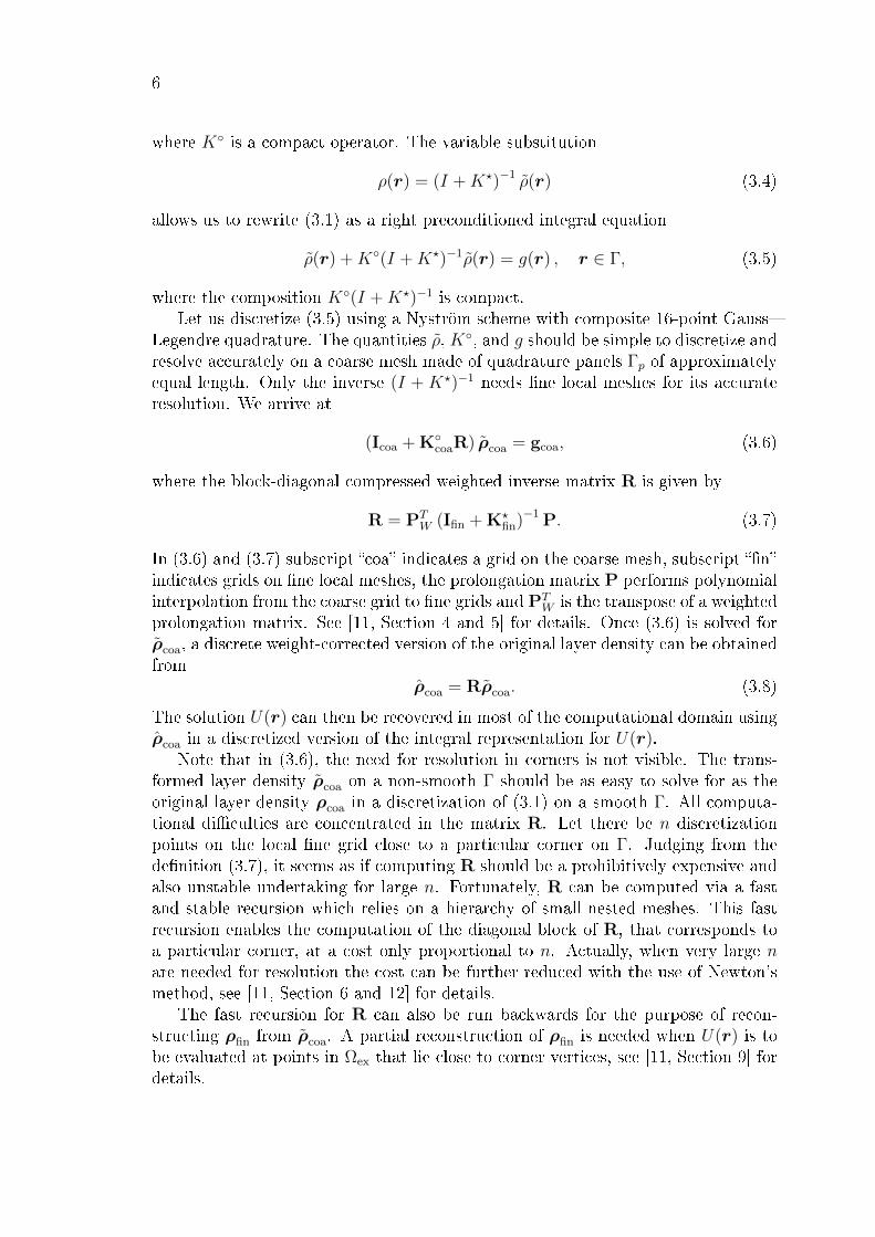
Note that in (3.6), the need for resolution in corners is not visible. The trans-formed layer density ρcoa on a non-smooth Γ should be as easy to solve for as theoriginal layer density ρcoa in a discretization of (3.1) on a smooth Γ. All computa-tional diculties are concentrated in the matrix R. Let there be n discretizationpoints on the local ne grid close to a particular corner on Γ. Judging from thedenition (3.7), it seems as if computing R should be a prohibitively expensive andalso unstable undertaking for large n. Fortunately, R can be computed via a fastand stable recursion which relies on a hierarchy of small nested meshes. This fastrecursion enables the computation of the diagonal block of R, that corresponds toa particular corner, at a cost only proportional to n. Actually, when very large nare needed for resolution the cost can be further reduced with the use of Newton'smethod, see [11, Section 6 and 12] for details.

The fast recursion for R can also be run backwards for the purpose of recon-structing ρfin from ρcoa. A partial reconstruction of ρfin is needed when U(r) is tobe evaluated at points in Ωex that lie close to corner vertices, see [11, Section 9] fordetails.

7

We remark that the integral equations (2.5) and (2.15), which are to be solvedin this paper, have a more complicated appearance than the model equation (3.1).In practice this poses no problems for RCIP just some extra work. The twointegral operators in (2.5) can, for programming purposes, be combined into a singleoperator. The composition of integral operators in (2.15) can be treated with anexpansion technique. With the help of two new temporary layer densities, one canarrive at a recursion for an expanded compressed inverse matrix R with the samestructure as (3.7). Once R is computed one can extract separate blocks from it anduse them in a more involved version of (3.6) that still uses only a single transformedglobal density ρcoa. See [11, Section 14 and 17] for details.

3.2 The discretization of Hankel kernels

High-order accurate Nyström discretization of boundary integral equations asso-ciated with the Helmholtz equation is a topic that has received much attentionrecently. See [9] for a comparison of various 2D schemes. We now present our pre-ferred scheme by showing how to discretize the operator Kk of (2.6) and the rstoperator on the right hand side of (2.4). The other integral operators of Section 2are discretized in similar ways.

The kernel of Kk is twice that of the rst operator in (2.4) and can, modulo aconstant of i/2, be expressed as

Kk(r, r′) = k|r − r′|H(1)

1 (k|r − r′|)(r − r′) · νr′|r − r′|2

, (3.9)

where H(1)1 is the Hankel function of the rst kind of order one. When r ∈ Γ, it is

instructive to write (3.9) in the form

Kk(r, r′) = f(r, r′) +

2i

πlog |r − r′|Re Kk(r, r

′) . (3.10)

For a xed r ∈ Γ, we see from (3.9) and a series representation of H(1)1 that f(r, r′)

and Re Kk(r, r′) are smooth functions of r′ ∈ Γ and that

limr′→r

log |r − r′|Re Kk(r, r′) = 0. (3.11)

Consider now the integral Ip(r) over a quadrature panel Γp

Ip(r) =

∫Γp

Kk(r, r′)ρ(r′) d`′. (3.12)

Let r(t) be a parameterization of Γ. Discretizing Kk means being able to evalu-ate (3.12) for all r of interest, given a set of values ρ(r(tj)) on each Γp.

If r is a point away from Γp, then Kk(r, r′) is a smooth function of r′ ∈ Γp and

Ip(r) can be evaluated to high accuracy using 16-point GaussLegendre quadrature

Ip(r) ≈∑j

Kk(r, rj)ρjsjwj, (3.13)

8

where rj = r(tj), ρj = ρ(r(tj)), sj = |dr(tj)/dt|, and tj and wj are nodes andweights on Γp.

If ri is a discretization point close to Γp or on Γp, then Kk(ri, r′) is not a

(suciently) smooth function of r′ ∈ Γp and we use (3.10) to arrive at

Ip(ri) ≈∑j

f(ri, rj)ρjsjwj +2i

π

∑j

Re Kk(ri, rj) ρjwijL, (3.14)

where wijL are high-order product integration weights for the logarithmic opera-tor which can be constructed using the analytic method in [12, Section 2.3]. Theformula (3.14) can be rearranged into a particularly convenient form

Ip(ri) ≈∑j

Kk(ri, rj)ρjsjwj +2i

π

∑j

Re Kk(ri, rj) ρjsjwjwcorrijL , (3.15)

where the weight corrections,

wcorrijL =

(wijLsjwj

− log |ri − rj|), (3.16)

are cheap to compute and depend only on the relative length (in parameter) ofneighboring quadrature panels and on nodes and weights on a canonical panel. Theformula (3.13) with r = ri and (3.15) summarize our Nyström discretization of Kk

on Γ.If r is a point not on Γ but in Ωex close to Γp, we write (3.9) in the form

Kk(r, r′) = g(r, r′) +

2i

πlog |r − r′|Re Kk(r, r

′)+2i

π

(r′ − r) · νr′|r′ − r|2

. (3.17)

We see from (3.9) and a series representation of H(1)1 that g(r, r′) and Re Kk(r, r

′)are smooth functions of r′. In analogy with (3.15) one can write

Ip(r) ≈∑j

Kk(r, rj)ρ(rj)sjwj +2i

π

∑j

Re Kk(r, rj) ρ(rj)sjwjwcorrjL (r)

+2i

π

∑j

ρ(rj)

(wjC(r)−

(rj − r) · νrj|rj − r|2

sjwj

), (3.18)

where wcorrjL (r) are weight corrections as in (3.16), but with ri replaced by r, and

wjC(r) are high-order product integration weights for the Cauchy singular operatorwhich can be constructed using the analytic method in [12, Section 2.1]. The formu-las (3.13) and (3.18) are used to discretize the rst operator in (2.4) when producingeld plots.

3.3 Convergence and error estimates

Our solver shows a stable behavior. The solution converges rapidly with coarse meshrenement up until a point beyond which no further improvement occurs. Actually,

9

beyond this optimal point there will be a slow decay in the quality of the solution,due to accumulated roundo error. The precise location of the optimal point is hardto determine a priori. It depends on the geometry, on the boundary conditions,and on the wave number. The optimal point is determined experimentally in thenumerical examples of Section 4.

We have estimated the accuracy in our solutions U(r) rather thoroughly. Thetutorial [11, Section 18] contains error plots for exterior problems in non-smoothdomains produced in a direct way. These are achieved by generating the boundaryconditions on Γ via line sources inside Γ so that the exact solution is known. In theplane-wave scattering examples of Section 4.1, below, no exact results are known.Therefore we proceed as follows; we rst compute a solution U(r) using a numberof coarse panels on Γ deemed sucient for resolution. We then increase the numberof panels with 50 % and solve again. The dierence between the resolved valueof U(r) and the overresolved value of U(r) is used as an indirect pointwise errorestimate. When kd = 1000 we found that 900 panels on Γ, corresponding to 37.4points per wavelength, gave the best possible resolution. Yet an indirect method toestimate the (overall) precision in the computations is by comparing the scatteringcross section computed from its denition (close to Γ) with its value obtained viathe optical theorem (at innity). See, further, Section 4.2. As it turns out, thevarious error estimates seem to agree well.

4 Numerical examples

We shall now solve (2.5) and (2.15) for the unknown density ρ(r), using the methodof Section 3, and then evaluate the scattered elds of (2.4) and (2.11). We restrict thenumerical examples to scattering from an innite straight cylinder with boundaryΓ described by

r(t) = sin(πt) (cos((t− 0.5)π/2), sin((t− 0.5)π/2)) , t ∈ [0, 1] , (4.1)

and to the incident plane wave Uinc(r) = eiky for both E-waves and H-waves. Theobject parameterized in (4.1) has a corner with opening angle θ = π/2 at r = 0 anda diameter d = 1, in arbitrary length units, so that kd = k. The examples coversizes from kd = 1 up to kd = 1000. We have seen that at kd = 1000 the frequencyis high enough such that the uniform theory of diraction theory can be applied.All numerical examples are executed in MATLAB on a workstation equipped withan IntelXeon E5430 CPU at 2.66 GHz and 32 GB of memory.

4.1 Near eld

In many applications it is required that the numerical method can calculate theelectric and magnetic elds everywhere in Ωex. Figures 1 and 2 show the totalelectric eld for the E-wave and total magnetic eld for the H-wave in the vicinityof the scattering object and the corresponding errors. The scattering object itselfappears in green color in the left images and in white color in the right images. The

10

x

y

E−wave with k=10

a)

−1 −0.5 0 0.5 1 1.5 2−1.5

−1

−0.5

0

0.5

1

1.5

−1.5

−1

−0.5

0

0.5

1

1.5

x

y

log10

of error in U for E−wave with k=10

b)

−1 −0.5 0 0.5 1 1.5 2−1.5

−1

−0.5

0

0.5

1

1.5

−15.6

−15.4

−15.2

−15

−14.8

−14.6

−14.4

−14.2

−14

−13.8

−13.6

x

y

E−wave with k=100

c)

−0.15 −0.1 −0.05 0 0.05 0.1 0.15−0.1

−0.05

0

0.05

0.1

0.15

0.2

−1.5

−1

−0.5

0

0.5

1

1.5

x

ylog

10 of error in U for E−wave with k=100

d)

−0.15 −0.1 −0.05 0 0.05 0.1 0.15−0.1

−0.05

0

0.05

0.1

0.15

0.2

−15.6

−15.4

−15.2

−15

−14.8

−14.6

−14.4

−14.2

−14

−13.8

x

y

E−wave with k=1000

e)

−0.015 −0.01 −0.005 0 0.005 0.01 0.015−0.01

−0.005

0

0.005

0.01

0.015

0.02

−2

−1.5

−1

−0.5

0

0.5

1

1.5

2

x

y

log10

of error in U for E−wave with k=1000

f)

−0.015 −0.01 −0.005 0 0.005 0.01 0.015−0.01

−0.005

0

0.005

0.01

0.015

0.02

−15.5

−15

−14.5

−14

−13.5

−13

Figure 1: Left: a), c), e) show Re U(r) for a plane E-wave Uinc(r) = eiky incidenton the perfectly conducting cylinder with boundary Γ given by (4.1). Right: b), d),f) show absolute errors.

11

x

y

H−wave with k=10

a)

−1 −0.5 0 0.5 1 1.5 2−1.5

−1

−0.5

0

0.5

1

1.5

−1.5

−1

−0.5

0

0.5

1

1.5

x

y

log10

of error in U for H−wave with k=10

b)

−1 −0.5 0 0.5 1 1.5 2−1.5

−1

−0.5

0

0.5

1

1.5

−15.6

−15.4

−15.2

−15

−14.8

−14.6

x

y

H−wave with k=100

c)

−0.15 −0.1 −0.05 0 0.05 0.1 0.15−0.1

−0.05

0

0.05

0.1

0.15

0.2

−2

−1.5

−1

−0.5

0

0.5

1

1.5

2

x

y

log10

of error in U for H−wave with k=100

d)

−0.15 −0.1 −0.05 0 0.05 0.1 0.15−0.1

−0.05

0

0.05

0.1

0.15

0.2

−15.6

−15.4

−15.2

−15

−14.8

−14.6

−14.4

−14.2

−14

−13.8

x

y

H−wave with k=1000

e)

−0.015 −0.01 −0.005 0 0.005 0.01 0.015−0.01

−0.005

0

0.005

0.01

0.015

0.02

−2

−1.5

−1

−0.5

0

0.5

1

1.5

2

x

y

log10

of error in U for H−wave with k=1000

f)

−0.015 −0.01 −0.005 0 0.005 0.01 0.015−0.01

−0.005

0

0.005

0.01

0.015

0.02

−15.5

−15

−14.5

−14

−13.5

−13

−12.5

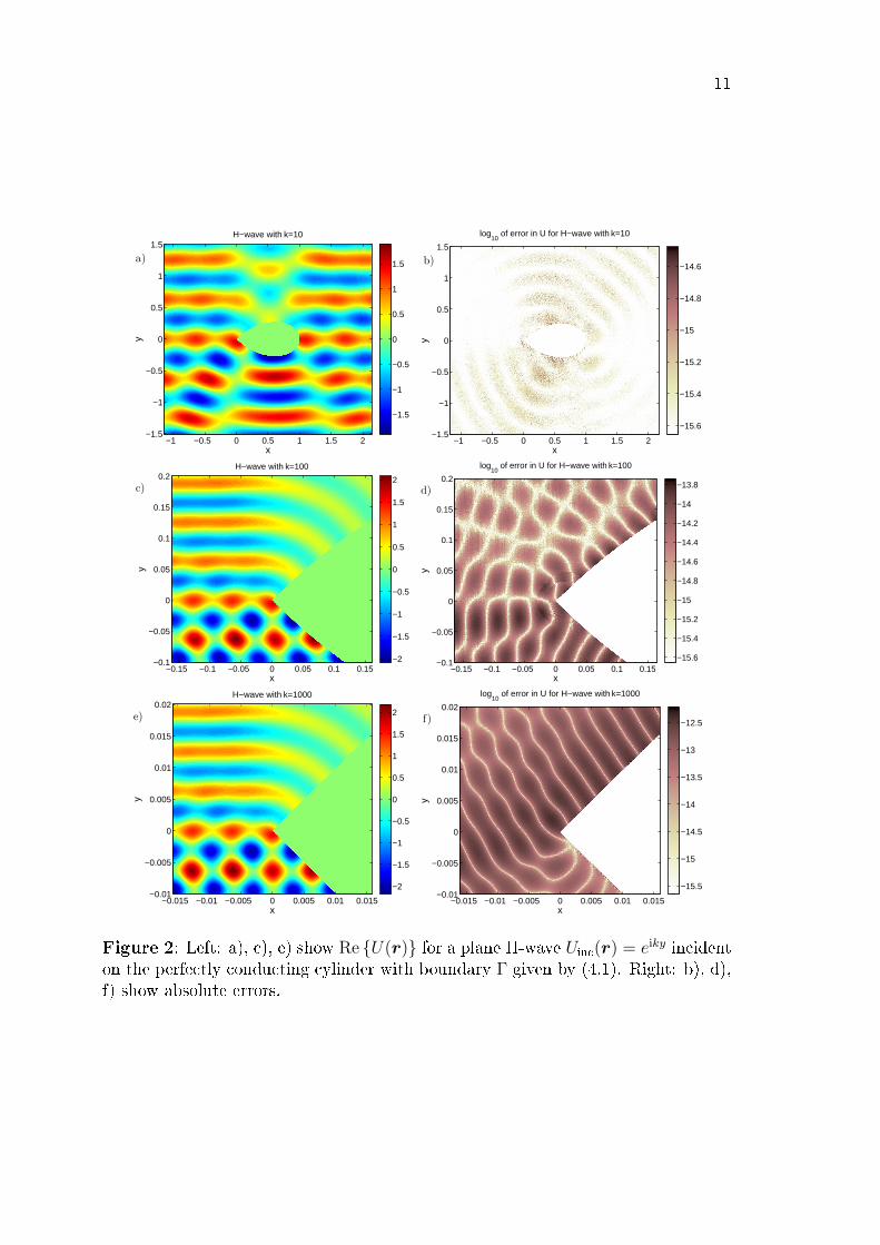
Figure 2: Left: a), c), e) show Re U(r) for a plane H-wave Uinc(r) = eiky incidenton the perfectly conducting cylinder with boundary Γ given by (4.1). Right: b), d),f) show absolute errors.

12

100

101

102

103

1.9

2

2.1

2.2

2.3

2.4

2.5

2.6

2.7

2.8

2.9

cross section E−waves

k

σ sca

a)

100

101

102

103

10−15

10−10

10−5

100

cross section E−waves: errors

k

optic

al th

eore

m r

elat

ive

mis

mat

ch

b)

100

101

102

103

0

0.2

0.4

0.6

0.8

1

1.2

1.4

1.6

1.8

2

cross section H−waves

k

σ sca

c)

100

101

102

103

10−15

10−10

10−5

100

cross section H−waves: errors

k

optic

al th

eore

m r

elat

ive

mis

mat

ch

d)

Figure 3: The scattering cross sections σsca for the E-wave, a), and H-wave, c),calculated by the optical theorem (4.3) and the relative error, b) and d), comparedto the values from equation (4.2)

number of spatial points in each image is 106. It is encouraging to see, in the rightimages of Figures 1 and 2, that the accuracy is high even close to the boundaryand, in particular, close to the corner. The integrals in (2.4) and (2.11) are oftenthought of as dicult to evaluate close to the boundary due to the singularities inthe Hankel functions when r′ = r. However, the present method circumvents theseproblems using the high-order analytic quadrature outlined in Section 3.2.

In Figures 1 a), c), and e) the real part of the total electric eld U(r) for theE-wave case is plotted for kd = 10, 100, and 1000. To capture the diraction patternin the vicinity of the corner, the eld is plotted in a rectangular region with sidelength proportional to 1/k and center at the tip of the corner. At kd = 10 the erroris very small, as seen from Figure 1 b). The errors increase slightly with kd but evenat kd = 1000 we get 14 digits or better almost everywhere, as depicted in Figure1 f). For H-waves the accuracy is almost as good as for the E-waves, as seen fromFigure 2.

For kd = 100 and 1000 we can interpret the eld plots in Figures 1 c), e) and 2c), e) through the theory of diraction. Thus, the outer region Ωex is divided intothree subregions separated by the reection boundary and the shadow boundary.

13

4.2 Scattering cross section and optical theorem

In two dimensions the scattering cross section reads

σsca =Psca

Sinc · y= Re

i

ω

∫Γcirc

Usca(r′)∂U∗

sca(r′)

∂νr′d`′, (4.2)

where Psca is the scattered power per unit length, Sinc · y is the y−componentof the Poynting vector of the incident eld, i.e. the incident power density, theboundary Γcirc is a closed curve that circumscribes the boundary Γ, and the stardenotes complex conjugation. The expression holds for both E- and H-waves. In anumerical experiment with the cylinder of (4.1) we let Γcirc be a circle of radius 0.55and with center at r = (0.5, 0). Since the diameter of the scatterer is d = 1, thesmallest distance between the Γ and Γcirc is 0.05 and it occurs at the corner vertexand at a point opposite to the corner vertex. For evaluation points r′ so close to theboundary, the eld Usca(r

′) and its normal derivative are in general hard to evaluate.But, as we have already seen in Section 4.1, the RCIP method and the high-orderanalytic quadrature outlined in Section 3.2 should allow for high accuracy.

By utilizing the optical theorem we get an alternative expression for the scatter-ing cross section

σsca = − limy→∞

Re

4

ωUsca(0, y)

√πωy

2e−i(ωy−π/4)

(4.3)

which should be even simpler to evaluate than (4.2) since it only involves the fareld. The mismatch between the scattering cross sections computed via (4.2) andvia (4.3) can be used as an error estimate for both expressions. The cross sectionsfor the E-waves along with such error estimates are given in Figure 3 a) and b)and the corresponding data for the H-waves are given in Figures 3 c) and d). Themismatch error is on the order of 10−15. The cross sections in Figures 3 a) and c)show the well known behaviors for large and small values of k.

5 Conclusions

We have shown how the basic problems of scattering of E- and H-waves from per-fectly conducting cylinders with corners can be solved numerically to high accuracyon a mesh that on a global level is not rened close to corner vertices. We giveexamples where the scattered electric and magnetic elds from a cylinder with onecorner and with a diameter of up to 160 wavelengths is obtained with 14 digits ofaccuracy almost everywhere outside the cylinder. This success is achieved by

1. choosing a suitable integral representation of the scattered eld in terms of anunknown layer density

2. formulating the scattering problem as a Fredholm second kind integral equa-tion with operators that are compact away from the corners

14

3. discretizing with a Nyström scheme and a mix of composite GaussLegendrequadrature and high-order analytic product rules

4. modifying the discretized integral equation so that the new unknown, a trans-formed layer density, is piecewise smooth

5. solving the resulting well-conditioned linear system iteratively for the trans-formed layer density

6. partially reconstructing the original layer density from the transformed layerdensity

7. evaluating the scattered eld from a discretization of its integral representationwhich, again, relies on a mix of composite GaussLegendre quadrature andhigh-order analytic product rules

While some steps in this scheme are standard, step 4, 6, and 7 are unique to therecently developed RCIP method. Conceptually, step 4 and 5 correspond to apply-ing a fast direct solver [20] locally to regions with troublesome geometry and thenapplying a global iterative method. This gives us many of the advantages of fast di-rect methods, for example the ability to deal with certain classes of operators whosespectra make them unsuitable for iterative methods. In addition, this approach istypically much faster than using only a fast direct solver.

Our numerical scheme can be extended to related problems of importance ine.g. band-gap structures, axially symmetric cavities for accelerators, and remotesensing of underground objects. Thus we can extend the method to scattering fromhomogeneous dielectric cylinders, scattering from multiple cylinders, scattering fromcylinders in layered structures (c.f. [18]), scattering of plane waves at oblique anglesfrom cylinders, and scattering from axially symmetric three-dimensional geometries.Some of these problems will be addressed in forthcoming papers.

Acknowledgment

This work was supported in part by the Swedish Research Council under contract621-2011-5516.

References

[1] J. Bremer. A fast direct solver for the integral equations of scattering theory onplanar curves with corners. Journal of Computational Physics, 231, 18791899,2012.

[2] O. Bruno, T. Elling, and C. Turc. Regularized integral equations and fasthigh-order solvers for sound-hard acoustic scattering problems. International

Journal for Numerical Methods in Engineering, 91(10), 10451072, 2012.

15

[3] J. Carrier, L. Greengard, and V. Rokhlin. A fast adaptive multipole algorithmfor particle simulations. SIAM Journal on Scientic and Statistical Computing,9(4), 669686, 1988.

[4] H. Cheng, W. Crutcheld, Z. Gimbutas, L. Greengard, J. Huang, V. Rokhlin,N. Yarvin, and J. Zhao. Remarks on the implementation of the wideband FMMfor the Helmholtz equation in two dimensions. Contemporary Mathematics,408, 99, 2006.

[5] D. Colton and R. Kress. Integral Equation Methods in Scattering Theory. JohnWiley & Sons, New York, 1983.

[6] D. Colton and R. Kress. Inverse Acoustic and Electromagnetic Scattering The-

ory. Springer-Verlag, Berlin, 1992.

[7] A. Gillman, P. Young, and P. Martinsson. A direct solver with O(N) complexityfor integral equations on one-dimensional domains. Front. Math. China, 7, 217 247, 2012.

[8] L. Greengard and J.-Y. Lee. Stable and accurate integral equation methodsfor scattering problems with multiple material interfaces in two dimensions.Journal of Computational Physics, 231(6), 2389 2395, 2012.

[9] S. Hao, P. G. Martinsson, and P. Young. High-order accurate Nystrom dis-cretization of integral equations with weakly singular kernels on smooth curvesin the plane. December. arXiv:1112.6262 (2011).

[10] R. F. Harrington. Field Computation by Moment Methods. Macmillan, NewYork, 1968.

[11] J. Helsing. Solving integral equations on piecewise smooth boundaries usingthe RCIP method: a tutorial. July. arXiv:1207.6737 (2012).

[12] J. Helsing. Integral equation methods for elliptic problems with boundary con-ditions of mixed type. Journal of Computational Physics, 228(23), 8892 8907,2009.

[13] J. Helsing. The eective conductivity of arrays of squares: Large random unitcells and extreme contrast ratios. Journal of Computational Physics, 230(20),7533 7547, 2011.

[14] J. Helsing. A fast and stable solver for singular integral equations on piecewisesmooth curves. SIAM Journal on Scientic Computing, 33(1), 153174, 2011.

[15] J. Helsing and R. Ojala. Corner singularities for elliptic problems: Integralequations, graded meshes, quadrature, and compressed inverse preconditioning.Journal of Computational Physics, 227(20), 8820 8840, 2008.

16

[16] J. Helsing and R. Ojala. Elastostatic computations on aggregates of grains withsharp interfaces, corners, and triple-junctions. International Journal of Solids

and Structures, 46(25â26), 4437 4450, 2009.

[17] J. Helsing and K.-M. Perfekt. On the polarizability and capacitance of thecube. Applied and Computational Harmonic Analysis, (0). (in press 2012).

[18] A. Karlsson. Scattering from inhomogeneities in layered structures. The Jour-

nal of the Acoustical Society of America, 71(5), 10831092, 1982.

[19] A. Klöckner, A. Barnett, L. Greengard, and M. O'Neil. Quadrature byExpansion: A New Method for the Evaluation of Layer Potentials. July.arXiv:1207.4461 (2012).

[20] W. Y. Kong, J. Bremer, and V. Rokhlin. An adaptive fast direct solver forboundary integral equations in two dimensions. Applied and Computational

Harmonic Analysis, 31(3), 346 369, 2011.

[21] R. Kress. On the numerical solution of a hypersingular integral equation inscattering theory. Journal of Computational and Applied Mathematics, 61(3),345 360, 1995.

[22] P. Martinsson and V. Rokhlin. A fast direct solver for boundary integral equa-tions in two dimensions. Journal of Computational Physics, 205(1), 1 23,2005.

[23] G. Mie. Beiträge zur Optik trüber Medien, speziell kolloidaler Metallösungen.Ann. Phys. Leipzig, 25, 377445, 1908.

[24] L. Rayleigh. On the electromagnetic theory of light. Phil. Mag., 12, 81, 1881.

[25] J. L. Tsalamengas. Exponentially converging Nyström methods in scatteringfrom innite curved smooth stripsPart 1:TM-case. IEEE Trans. Antennas

Propagat., 58, 32653274, 2010.

[26] J. L. Tsalamengas and C. V. Nanakos. Nyström solution to oblique scatteringof arbitrarily polarized waves by dielectric-lled slotted cylinders. IEEE Trans.

Antennas Propagat., 60, 28022813, 2012.

[27] M. S. Tsong and W. C. Chew. Nyström method with edge condition for elec-tromagnetic scattering by 2D open structures. Progress in Electromagnetics

Research, 62, 4968, 2006.

[28] J. van Bladel. Electromagnetic Fields. Hemisphere Publication Corporation,New York, 1986. Revised Printing.