Embed Size (px)
Citation preview

AN ABSTRACT OF THE THESIS OF
DUANE FRANK STARR for the DOCTOR OF PHILOSOPHY(Name) (Degree)
in CHEMISTRY presented on ,s6 a /. 2u61,4_, / 9(Major) (Dat
Title: A THEORETICAL STUDY OF VIBRATIONAL RELAXATION
IN GASEOUS AMMONIARedacted for privacy
Abstract approved:7 J. C. Decius
By means of simple collision models, we have tested the
hypothesis that the rapid vibrational deactivation of ammonia and
deutero-ammonia is related to the inversion motion of these molecules.
Our study shows that if only short-range repulsive forces are impor-
tant during a collision, then the inversion phenomenon does not suffice
to explain the deviation of these molecules from the Lambert-Salter
plot for simple hydrides and deuterides. Our calculations indicate
that transitions between the nearly degenerate states of inversion
doublets are highly probable. However, these almost resonant pro-
cesses have no appreciable effect on the results of acoustical experi-
ments.
To facilitate our calculations, we constructed a one-dimensional
representation of the collision of two ammonia molecules. Energy
transfer during a collision was assumed to take place between the

rotational motion of one molecule and the vibrational motion of the
other. To judge the effect of inversion on vibrational relaxation, two
models of the inversion mode of ammonia were employed. The first
model was an inverting diatomic molecule, and the second was a
harmonic oscillator diatomic molecule. Vibrational transition prob-
abilities were found by numerical solution of the one-dimensional
scattering equations associated with these collision models. The
thermal averages of these probabilities were found by integrating over
a Boltzmann distribution of rotational energies. From these thermal
averages, we calculated Z1"O(NH3) = 3 x 10² and
Z (ND ) = 6 x 10² at 300°K--one or two orders of magnitude
greater than the experimental results.
Assuming a "hard spheres" collision frequency, the rate con-
stants for vibrational de-excitation processes were determined.
These rate constants were then used to calculate the vibrational
velocity dispersion and absorption index for each of the models. Com-
parison of these calculated experimental results showed little differ-
ence between the inverting and non-inverting models of ammonia and
deutero-ammonia.
The fact that our calculated values of Z1-0 (NH3) and
Z1y0(ND3) correlate well with other hydrides and deuterides in a
Lambert-Salter plot indicates that a successful theory of vibrational
relaxation in ammonia and deutero-ammonia must include more cou-
pling than that due to short-range repulsive forces.

A Theoretical Study of Vibrational Relaxation inGaseous Ammonia
by
Duane Frank Starr
A THESIS
submitted to
Oregon State University
in partial fulfillment ofthe requirements for the
degree of
Doctor of Philosophy
June 1973

APPROVED:
Redacted for privacy
Protestor of ChemistryJ,-
in charge of major
Redacted for privacy
Chairman of Department of Chemistry
Redacted for privacy
Dean of Graduate School
Date thesis is presented 973
Typed by Clover Redfern for Duane Frank Starr

ACKNOWLEDGMENT
I wish to thank Dr. J. C. Decius for the advice and encourage-
ment he has given in the course of this research.
I am also grateful to the members of the Electron Diffraction
Group for their assistance in my struggles with FORTRAN IV.
Considerable help has also be given by staff members of the Oregon
State University Computer Center and the University of Oregon
Computing Center.
This work was supported by the Office of Naval Research and
the National Science Foundation. Grants of computer time were
donated by the Oregon State University Computer Center.

DEDICATION
This thesis is dedicated to my wife and my parents.

TABLE OF CONTENTS
Chapter
I. INTRODUCTION
II. CONSTRUCTION OF THE COLLISION MODEL
III. DERIVATION OF THE SCATTERING EQUATION
IV. CALCULATION OF THE INTERACTION MATRIX
V. SOLUTION OF THE SCATTERING EQUATION
VI. CALCULATED TRANSITION PROBABILITIES
VII. CALCULATION OF THE VIBRATIONAL VELOCITYDISPERSION AND ABSORPTION INDEX
VIII. CONCLUSIONS
BIBLIOGRAPHY
APPENDICESAppendix A:Appendix B:
Appendix C:
Appendix D:
Appendix E:
Vibrational Relaxation Data at 300°KInternal Energies and Interaction Matricesfor the Inverting Models of Ammonia and.Deutero-AmmoniaInternal Energies and Interaction Matricesfor the Non-Inverting Models of Ammoniaand Deutero-AmmoniaAn Integral Solution of a Multi-ChannelSchroedinger EquationThe Method of Calculating the VelocityDispersion and Absorption Index
Page
1
13
29
45
59
77
99
115
116
119119
121
123
124
127

LIST OF TABLES
Table Page
1. Experimental values of the reduced vibrationalrelaxation time, forfor NH3 and ND3 at 300°K. 7
2. Values of Z10 (NH3
) and Z110(ND3)at 300°K
calculated from experimental data. 9
3. Values of the exponential range parameter, L, fromviscosity measurements.
4. Vibrational potential energy parameters for NH3
andND 3.
5. A comparison of calculated and experimental inversionmode energies of NH3 and ND3.
6. The u, uof NH3.
7. The u, Uof NDT-3
and uAC
and uAC
matrices for the inverting model
matrices for the inverting model
8. The u,A Di
and uAC matrices for the non-inverting
s"-*-
model of NH3.
9. The u, uAB and uAC matrices for the non-inverting
17
50
53
55
56
57
model of ND3. 58
10. Catalog of transition probability graphs. 78
11. Calculated values of PI_.F(T) at 300°K. 104
12. Calculated values of kIF at 300°K. 107

LIST OF FIGURES
Figure Page
1. Lambert-Salter plot for simple molecules. 4
2. A simple collision model. 15
3. Interaction energies of He-He and. He-Ne. 19
4. Coordinates of the He-H2
system. 20
5. The structure of ammonia. 21
6. A simple model of two colliding ammonia molecules. 24
7. The relationship of r and 0 for ammonia. 26
8. A physical interpretation of the collision model. 28
9. Wavefunctions and potential energy of the inversion modeof ammonia. 51
10. Probability of the transition I F for NH3; I = 0+;F = 0+, 0-. 79
11. Probability of the transition I --' F for =NH3; I 0;F = 0+, 0-. 80
12. Probability of the transition I F for NH3; I = 1+;F = 1+, 1 -. 81
13. Probability of the transition I F for NH3; I = 1 ;
F = 1+, 82
14. Probability of the transition I F for ND3; I = 0 ;
F = 0+, 0. 83
15. Probability of the transition I F for ND3; I = 0;F = 0+, 0-. 84
16. Probability of the transition I F for ND3; I = 1+;F = 1+, 1-. 85

Fig= Page
17, Probability of the transition I F for ND3; I = 1-;F = 1+, 1-. 86
18. Probability of the transition I --- F for NH3; I = 0+;F = 1+, F, 2+, 2-. 87
19. Probability of the transition I ~ F for NH3; I = 0;F= 1+, 1-, 2+, 2-. 88
20. Probability of the transition I --P- F for NH3; I = 1 +;
F= 0+, 0-, 2+, 2-. 89
21. Probability of the transition I F for NH3; I = 1F= 0+, 0, 2+, 2-. 90
22. Probability of the transition I F for ND3; I = 0+;F= 1+, 1-, 2+, 2-. 91
23. Probability of the transition I F for ND3; I = 0F = 1+, 1', 2+, 2. 92
24. Probability of the transition I F for ND3;
I = 1 +;F= 0+, 0-, 2+, 2-. 93
25. Probability of the transition I F for ND3; I = 1F= 0+, 0-, 2+, 94
26. Probability of the transition I F for NH3; I = 0;F = 0, 1, 2. 95
27. Probability of the transition I F for NH3; I = 1;F = 0, 1, 2. 96
28. Probability of the transition I F for ND3; I = 0;F = 0, 1, 2. 97
29. Probability of the transition L ~ F for ND3; I = 1;F = 0, 1, 2. 98
30. Thermally weighted 1 ~ 0 transition probability fornon-inverting NH3. 103

Figure page
31. Absorption index for the inverting and non-invertingmodels of NH3.
32. Velocity dispersion for the inverting and non-invertingmodels of NH3.
33. Absorption index for the inverting and non-invertingmodels of ND
3.
34. Velocity dispersion for the inverting and non-invertingmodels of ND
3.
111
112
113
114

A THEORETICAL STUDY OF VIBRATIONALRELAXATION IN GASEOUS AMMONIA
I. INTRODUCTION
Vibrational energy transfer in gases has been extensively
analyzed via classical, semi-classical and quantum mechanical
models. Cottrell and. McCoubrey (I), Herzfeld and Litovitz (2) and,
most recently, Rapp and. Kas sal (3) have reviewed much of this work.
The earliest studies were fruitful in that they established a number of
useful concepts and semi-quantitative correlations of experimental
data. Within the past decade, the development of fast computer pro-
grams for solving scattering equations has brought about substantial
progress in the theory of vibrational energy transfer. Loosely
speaking, the development of these programs has served primarily to
improve the accuracy of earlier approximate calculations for rather
simple models. Consequently the progress due to these programs is
of a limited nature. They have made possible a more critical com-
parison of simple models with experimental results, but thus far
their use has not led to the discovery of any new fundamental rela-
tionships.
On the surface, our theoretical study of ammonia and deutero-
ammonia seems to be merely the numerical solution of scattering
equations associated with simple models. It will be seen, however,

2
that the collision models were constructed using relationships devel-
oped before the current Renaissance in computer studies of vibra-
tionally inelastic collisions. Below are briefly stated two well-founded
generalizations which have helped guide our research.
The first generalization concerns the concept of adiabatic and
non-adiabatic perturbations.-1 / Landau and. Teller (4) extended the
earlier work of Ehrenfest (5) to explain why molecular collisions are
usually inefficient in causing vibrational transitions. Ehrenfest had
shown that if an oscillator were subjected to a perturbing force which
was initially zero, increased slowly (taking the period of oscillation
as the unit of time) and slowly returned to zero, then the initial and
final energies of the oscillator would be the same. This type of
perturbation is called adiabatic. Conversely, if the increase and
decrease of the disturbance were rapid, the initial and final energies
of the oscillator might differ. Consequently this kind of perturbation
(referred to as non-adiabatic) can bring about vibrational transitions.
Landau and Teller suggested that in a- molecular collision, the per-
turbation rises and falls in a time span given by L/v, where L
is the characteristic length of the short-range repulsive forces
between molecules and v is the relative velocity of the colliding
molecules. They reasoned that the smaller the ratio of this time span
1/This discussion follows that given in Herzfeld and Litovitz (2,
p. 260-267).

3
to the period of vibration, the more non-adiabatic the collision and
the more likely a vibrational transition. Since the characteristic
length, L, is about the same for most simple molecules, the fol-
lowing two deductions can be made-
1) The greater the relative velocity of a collision, the more
probable a transition becomes.
2) The lower the vibrational frequency of a molecule, the more
likely it is that a collision will cause a transition.
The second generalization comes from the work of Lambert and.
Salter (6). They found that at a fixed temperature there exists a
strong correlation between the average number of collisions, Z1_.0
required to relax the lowest excited vibrational state for a molecule
and the molecule's lowest vibrational frequency, v . Figure 1min
shows the Lambert-Salter plot for several simple molecules at 300° K,
using data compiled by Lambert (7)A/ From this plot, it is apparent
that these molecules fall into two classes- -those which contain hydro-
gen or deuterium and those that do not. More extensive studies (1,
p. 166-167; 7) show that in a Lambert-Salter plot, molecules contain-
ing no hydrogen atoms form one group, those containing two or more
hydrogens form another group, and those molecules with only one
hydrogen tend to fall in the same group as those with no hydrogens.
2/The data used in constructing this plot are given in Appendix A.

N
bn0
5
4
3
2
1
0
4
Molecules containing neither hydrogen nor deuterium
o Molecules containing hydrogen
O Molecules containing deuterium
AA
LL
A A
0coo
0 0oo0
0
0Qt
0
0
0
ND3
0 NH3
0
300 600 900 1200
vinin (cm-1)
Figure 1. Lambert-Salter plot for simple molecules.
1500

5
Considering the Landau-Teller argument, it is not surprising to see
the tendency of Z1 to become smaller as v decreases.1-0What is unexpected is that, as a class, the hydrides and deuterides
tend to require fewer collisions for vibrational deactivation than other
molecules. Also, for a given hydride-deuteride pair, the hydride will
undergo vibrational deactivation faster than the deuteride--even
though v for a given hydride is larger than v for the cor-min min
responding deuteride. Most extraordinary is the behavior of ammonia
and, to a lesser extent, deutero-ammonia.
Cottrell and Matheson (8) and Moore (9) have suggested the rea,
son for this unusual behavior of the hydrides and deuterides is that the
most important process in the vibrational relaxation of these mole-
cules is the interconversion of vibrational and rotational energies,
rather than the interconversion of vibrational and translational ener-
gies. Moore demonstrated that the average velocities of the hydrogen
atoms in compounds with small moments of inertia (e. g. , HBr, CH4
and SiH4) are about an order of magnitude larger than the average
translational velocities of these molecules. Furthermore the rota-
tional velocities of the deuterium atoms of the corresponding deute-
rides are somewhat smaller, but still much greater than the transla-
tional velocities of the deuterides. Therefore, for these compounds,
it seems plausible that vibration-rotation energy transfer is faster
than vibration-translation energy transfer. Lambert (7) has

6
criticized this explanation, noting that acetylene and deutero-acetylene
have comparatively large moments of inertia, yet their positions on
the Lambert-Salter plot suggest they follow the same relaxation
mechanism as other hydrides and deuterides. Notwithstanding this
disturbing criticism, we believe that a model which attempts to treat
vibrational energy transfer in molecules with small moments of
inertia must take into account the interaction of vibrational and rota-
tional motions during a collision.
Even considering the above, ammonia and deutero-ammonia
behave exceptionally. Before discussing the- rationalizations of this
behavior, we first summarize the experimental results for these two
molecules. In an acoustical experiment, the relaxation time, T
for an energy transfer process is found by measuring the velocity3/dispersion or the absorption of sound waves in a gas as a function of
the frequency of the sound divided by the pressure of the gas (f/p).
In most polyatomic molecules, the overall rate of vibrational relaxa-
tion is determined by the rate at which the lowest excited vibrational
state relaxes to the ground vibrational state. The relaxation time,
pi' for this latter process is related to the experimental relaxation
time, T, by 131 = (Civib / C.
ibbinwhich Cv. i is the
3/Cottrell and McCoubrey (1) and Herzfeld and Litovitz (2) dis-cuss the theory and practice of these methods.

7
vibrational heat capacity of the i-th vibrational mode and the label
1 denotes the lowest frequency vibrational mode. Table 1 lists the
values of the reduced relaxation time, p 1,at 300° K found in the
recent literature.
Table 1. Experimental values of the reduced vibrationalrelaxation time, 131, for NH3 and. ND3 at300° K.
Molecule p1
(nsec) Experimental Method. Reference
NH3 <2 velocity 10
NH3 <1.2 velocity 11
NH3 0.735 velocity, absorption 12
NH3
1.8 absorption 13
ND3
8 velocity 11
For ammonia, Hancock and. Decius (10) and Cottrell and
Matheson (11) observed no change in the velocity of sound attributable
to vibrational relaxation. Thus they were only able to assign an
upper bound to the relaxation time. Jones, Lambert, Saksena and
Stretton (12) interpreted their data in terms of a single relaxation
time for both vibrational and rotational relaxations, while Bass and
Winter (13) assigned separate, but comparable, values to these
relaxation times. It should be noted that neither Jones et al. nor
Bass and Winter were able to cover the entire f/p range of interest
and their data at large f/p values show considerable scatter. Thus

8
the discrepancies of the 131
values for ammonia are not surprising.
Cottrell and Matheson (11) were able to study only the lower
third of the velocity dispersion of deutero-ammonia. Because of
this, they estimated an uncertainty of 10% in their reported relaxation
time.
If k1
1-0 is the rate constant for the v = 1"v = 0 transition
of the lowest frequency vibrational mode of a polyatomic harmonic
oscillator molecule, then it can be shown (1, p. 76) that k1 is
related to P1 by
1 /kl1-0 = f31
{1-exp(-hvnu.n/ k T)}
and that Z11-0 can be found from
(1) zl1-0 1= Z/k 1
0= ZI3
1{1-exp(-hv . /kT)}
where Z is the total number of collisions per unit time. (For
ammonia and deutero-ammonia at room temperature, the term,
exp(-hv . / k T), is less than 0.03 and may be neglected without
changing Z 1'0 1significantly.) The value of Z10 is strongly
dependent on the method used to calculate Z. The "hard spheres"
calculation of Z uses a simple hard sphere model of the gas. The
"viscosity" method assumes a Lennard-Jones intermolecular potential
energy function and allows the calculation of Z directly from

9
viscosity measurements. Since the Lennard-Jones potential is a more
realistic interaction than that of hard spheres, values of Z calcu-
lated using the "viscosity" method may be considered more reliable
than those found by a "hard spheres" calculation. Table 2 gives the
values of Z1 determined from the relaxation times listed in1-0Table 1. From this table, it is apparent that Z11 _,,,o(NH3) and
Z11-0(ND3
) are not known with great precision. However, consider-
ing the difficulty of the experiment and the differences in data analy-
sis, these values of Z110 may be said to be in rough agreement.
More importantly, all of the results given in Table 2 indicate that
ammonia and deutero-ammonia undergo vibrational relaxation much
more rapidly than would be expected on the basis of the Lambert-
Salter correlation.
1Table 2. Values of Z1- 0(NH3) and Z-0 (ND3) at 300°K
calculated from experimental data.
Molecule Method of Calculation
NH3 vis cos ity
NH3 viscosityNH3 hard spheresNH3 hard spheresND
3viscosity
ND3
hard spheres
z 1
1-0 Reference
<14 11
22 13
4.9 12
12 13
90 11
49 12a
a This calculation is based on the experimental relaxationtime of Cottrell and Matheson (11).

10
Several rationalizations have been advanced to explain the small1values of Z1 _.0(NH3) and Z1- 0(ND3) . It may be that dipole-
dipole interactions play an important role in the vibrational deactiva-
tion of ammonia. DeWette and Slawsky (14) concluded that, in gen-
eral, long-range attractive forces between molecules (such as dipole -
dipole interactions) are adiabatic perturbations and that only the
short-range repulsive forces in a collision can bring about vibrational
transitions. Nevertheless, they pointed out, long-range forces are
important because of what is called the "acceleration" effect. In
short, the principle effect of long-range forces is to cause an increase
in the relative velocity of two molecules as they come together in a
collision. Thus when the molecules enter the region of short-range
forces, the collision is more non-adiabatic than if there were no
attractive forces. Monchick and. Mason (15) have used viscosity data
of ammonia to determine the parameters of a 12-6-3 potential. With
these parameters, Jones et al. have calculated that Z1_0(NH3) =3.0
and Z10
(ND3
) = 2.3 at 300° K. This calculation is based on an1
approximate quantum mechanical equation developed by Schwartz,
Slawsky and. H,.=,rzfeld (16) for finding vibrational transition probabili-
ties associated with molecular collisions. Based on the comparison1of the calculated and experimental values of 1-0 for ND 3, H2O
and D20, Jones et al. concluded the agreement of the calculated and

11
experimental value of Z1 for NH3 is most likely fortuitous. In1"0addition, they note that the equation of Schwartz, Slawsky and
Herzfeld is felt to be unreliable for large transition probabilities.-4/
There is some evidence of the presence of a dimer in ammonia
gas. Lambert and Strong (48) have calculated the second virial coef-
ficient of ammonia over a range of temperatures from compressibility
measurements. They interpret their results as showing the forma-
tion of a dimer (enthalpy of dimerization = -4400 calories/mole).
They attribute the stability of the dimer to hydrogen bonding.
A third possible explanation of ammonia's anomalous behavior
was put forth by Cottrell and Matheson (11). Using qualitative argu-
ments, they reasoned that the rapid vibrational relaxation of ammonia
is linked to its well-known ability to invert (17, p. 221-224). Roughly
speaking, they felt that during a collision an ammonia molecule might
undergo one or two inversions and that this inversion motion could
make the collision more non - adiabatic -- resulting in a greater transi-
tion probability. In deutero-ammonia, they argued, such inversions
occur less frequently and consequently the probability of a vibrational
transition would be lower.
While their rationalization did lead them to predictions in rough
4 /Rapp and Kassal (3) thoroughly discuss the limitations of theapproximate transition probability equations most commonly encoun-tered in the theory of vibrational energy transfer.

12
agreement with experiment, we felt it desirable to subject their ideas
to a more challenging test. Thus we have constructed two models for
both ammonia and deutero-ammonia. In the first model, the molecule
is allowed to invert. The second model is a harmonic oscillator
representation. In it there is no possibility of inversion. Rather
than relying on approximate solutions of the quantum mechanical
scattering equations associated with these simple models, we have
chosen to use a numerical technique recently developed by Gordon
(18) which calculates exact solutions of these equations.
At this point, we mention that the use of the word "exact" in
the previous sentence may be misleading. We wish to emphasize that
the final results of our calculation are very approximate. Some parts
of the calculation are quite exact, other sections are very inexact.
For example, the method of computing transition probabilities for our
model is quite accurate, as is the technique for calculating the
velocity dispersion and absorption of sound from rate constants for
vibrational relaxation processes. However, the method of combining
these transition probabilities to obtain the relaxation rate constants is
relatively inexact and the model for which the transition probabilities
are calculated is very approximate. Hence we will attach little impor-
tance to the results for individual models --taken by themselves. The
greatest significance will be given to comparing the results of the
various models, since all models are treated in the same manner.

13
II. CONSTRUCTION OF THE COLLISION MODEL
At this time, a three-dimensional quantum mechanical scatter-
ing equation appropriate to a study of vibrational energy transfer has
been solved exactly for only one collision system- -He -H2 (19). While
such calculations are of considerable interest, they are of limited
value in predicting acoustical properties associated with vibrational
energy transfer. Cottrell and McCoubrey (1) and Herzfeld and
Litovitz (2) demonstrate that for the vibrational relaxation time of a
molecule to be determinable in an acoustic experiment, the vibra-
tional heat capacity of the molecule must be appreciable. Thus the
acoustic experiment is facilitated by small vibrational energy spac-
ings. However, a complete three-dimensional calculation of acoustic
observables must include all of the rotational states having a signifi-
cant population. Consequently the number of states to be included in
such a calculation is small for a molecule with large rotational energy
spacings and the cost of computation is minimal. Because molecules
with small vibrational energy spacings tend to have small rotational
energy spacings, those molecules which are computationally conven-
ient tend to be experimentally impractical and vice versa. As a first
example, we consider hydrogen. To predict its acoustical properties
at room temperature would require only about 30 vibration-rotation

14
states.5/ Unfortunately there are no experimental results to compare
with this rather simple calculation. The small room temperature
vibrational heat capacity of hydrogen (-3 x 10⁻⁷R) would frustrate
any attempt to measure the velocity dispersion or absorption of sound
waves associated with vibrational relaxation. A second example is
chlorine. With its large room temperature vibrational heat capacity
(-6 x 10⁻¹R), the vibrational velocity dispersion and absorption are
well defined (20, 21). A complete theoretical calculation of these
quantities, however, would require on the order of 300 vibration-
rotation states- -a very expensive calculation. Therefore it is desir-
able to construct a less rigorous collision model--one which is mathe-
matically simpler, yet retains the essentials of the relaxation
mechanism.
The one-dimensional system depicted in Figure 2 is often used
for the calculation of collision-induced vibrational transition proba-
bilities. It consists of an inert gas atom, A, colliding with a
diatomic oscillator, BC. Rapp and Kassal (3) have given an excel-
lent review of recent theoretical studies of this system. When repre-
senting a single component ideal gas, the A atom is usually taken
to be another BC molecule whose internal structure is ignored.
Hence the molecular weight and collision cross-section of A and
5/Two vibrational states and eight rotational states are neededfor both molecules in a collision.

BC are assumed to be equal.
Figure 2, A simple collision model,
15
Ignoring the internal structure of A forces the model to
allow only one molecule to make a transition during a collision. This
has both a direct and an indirect effect on the calculation of this
model's acoustical properties. The direct effect is that the rate
constants are set equal to zero for all processes which involve transi-
tions in both molecules. Of those processes which are thus neglected,
resonant or near-resonant processes (those for which the reactants
and products have the same or nearly the same vibrational energy)
will most likely have the largest rate constants. Fortunately these
processes are of little importance in acoustical experiments because
(1) they are much faster than the slow rate-determining processes in
the relaxation mechanism and (2) there is very little gain or loss of
vibrational energy in resonant or near-resonant collisions. The

16
indirect effect of disregarding the internal structure of A is that it
simplifies the quantum mechanical equations to be solved. This is
desirable in that it reduces the amount of computer time needed to
solve the equations. It is undesirable to the extent that the coupling
among the internal states of the molecules is lessened. This can
bring about changes in transition probabilities even for those transi-
tions in which only one of the molecules changes its vibrational state.
Qualitatively one might expect that reducing the coupling among the
vibrational states would decrease the amount of inelastic scattering.
Riley and Kuppermann (22) have solved exactly for the transition
probabilities of a pair of diatomic oscillators undergoing a collinear
collision. The limited results they have published do not permit much
generalization.
There are several plausible types of interaction between atom
A and atoms B and C. Hirschfelder, Curtiss and Bird (23) discuss
those which have been most widely used. The choice is somewhat
arbitrary. In Section III it will be seen that the repulsive exponential
interaction is a particularly convenient choice. We write the inter-
action potential for the collinear collision of A and BC as-6/
6/It would be more precise to express the interaction as a func-tion of the distances between atoms, rather than the differences intheir coordinates (i. e. , I x
B-x
Arather than (xB- x
A)). In our
models, we assume A is always to the left of B and C (as in Fig-ure 2). Consequently (x
B -x A) is equivalent to IxB
-xA
I and is alsosomewhat easier to work with than I xB-x .

(2)(x
, xB'
xC
) = VAB
(xB
-xA
) + VAC
(xC
-xA
)VA-BC
= VAB
(xB -xA
)/LAB
)
VAC+ VA
exp(-(xC
-xA )/LAL)
The range parameters, LAB and LAC'
17
are usually given values
of about 0.2 Angstrom. McCoubrey, Milward and Ubbelohde (24)
have tabulated exponential potential parameters derived from viscosity
measurements. These parameters were found by fitting an exponen-
tial function to a Lennard-Jones 6-12 function. Conversion of their
results to the range parameter, L, gives the values listed in Table
3.
Table 3. Values of the exponential rangeparameter, L, from viscositymeasurements (24).
Molecule L (Angstrom)
02 0. 18
N2 0. 20
C12 0. 20
Br2
0. 20
N20 0. 20
COS 0. 20
CS2
0.21
CH4 0. 20
CF4 0. 24
C2H4 0. 23
C3
H6 0. 25

18
There is also some theoretical evidence which supports the use
of an exponential interaction. Self-consistent field calculations by
Gilbert and Wahl (25) for a He-He system and by Matcha and. Nesbet
(26) for a He-Ne system can both be fit over the range of thermally
important energies (-20 cm-1 to -20,000 cm-1) by exponential func-
tions having the same range parameter --L = 0.228 Angstrom. Fig-
ure 3 shows the theoretical interaction energies and the exponential
functions which were fit to them. The excellence of the fit is fortui-
tous, but convenient for our work.
Gordon and Secrest (27) used both a self-consistent field method
and a configuration-interaction calculation to evaluate the interaction
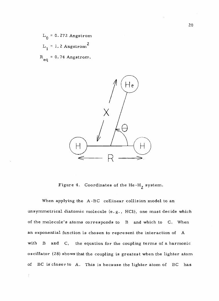
energy of the He-H2 system. Their coordinate system is shown in
Figure 4. The results of their two separate calculations were very
similar. They found that, over the range 1.5 < X < 3.7 Angstroms
and 0.53 < R < 0.95 Angstrom, the interaction function could be
represented by
where
VHe-H (X' R, 0) = C[A(0)+rB(0)] exp(-(X/L0)
+ (Xr/L1)) ,
2
r = R Req
C = 2.43 x 106 cm-1
A(9) = 1 + 0.251 P2(cos
B(0) = -0.316[1-0.778P2(cos 0)]

3
0
2
19
He-Ne (ref. 26)
0 He-He (ref. 25)
V(R) = 7.58 x 10⁶ -1X exp(-R/0.228) cm
---V(R) = 3.11 x 10⁶ -1X exp(-R/0.228) cm
0
0
2
R (Angstroms)3
Figure 3. Interaction energies of He-He and. He-Ne.
20
Lo = 0.272 Angstrom
L1
= 1.2 Angstrom2
Req = 0.74 Angstrom.
Figure 4. Coordinates of the He-H2
system.
When applying the A-BC collinear collision model to an
unsymmetrical diatomic molecule (e.g., HC1), one must decide which
of the molecule's atoms corresponds to B and which to C. When
an exponential function is chosen to represent the interaction of A
with B and C, the equation for the coupling terms of a harmonic
oscillator (28) shows that the coupling is greatest when the lighter atom
of BC is closer to A. This is because the lighter atom of BC has

21
the larger amplitude of vibration. In the case of an inverting diatom,
the inversion process makes it impossible to talk of one atom of BC
being closer to A than the other, and the assignment of B and
C is arbitrary. For convenience, atom B will always be taken
as the lighter atom of the diatom.
Studies of the ammonia molecule (as compiled by Herzberg (17))
show its structure to be that of a pyramidthe nitrogen atom situated
at the apex and the three hydrogen atoms forming the base (see Figure
5). The N-H distance is 1.014 Angstrom and the distance from the N
atom to the plane of H atoms is 0.381 Angstrom (17, p. 439). A dis-
cussion of its vibrational frequencies is deferred until Section IV. We
do mention now that its lowest frequency vibrational mode (which is
the mode we expect to determine largely the rate of vibrational
relaxation) is also the mode most closely tied to the inversion of
ammonia, viz. the symmetric bending mode, v2,
Figure 5. The structure of ammonia.

22
In attempting to evaluate the effect of inversion on vibrational
energy transfer, it was felt advantageous to retain the simplicity of
the A-BC collision system discussed above. To obtain a diatomic
representation of ammonia, the three H atoms are brought together
along the three-fold symmetry axis so that the distance from the N
atom to the three coalesced. H atoms- is the same as the distance from
the N atom to the plane of H atoms in ammonia. Thus our diatomic
model has the following properties: mB = 3mH, mC = mN,
equilibrium BC distance = 0.381 Angstrom. It was mentioned earlier
that two models of ammonia will be madeone which allows inversion
and one which does not. At this point it is not proper to give a
detailed description of how this will be done, but that part of the
modeling will only involve the vibrational potential energy function of
BC, and the structural parameters of both models will be the same.
It will be remembered that Cottrell and. Matheson (8) and Moore
(9) noted the large rotational velocities of hydrogen atoms in simple
hydrides and proposed that vibration-rotation energy transfer may be
the most important process in the vibrational relaxation of these
molecules. This suggests that the A atom should represent the
hydrogen atoms in simple hydrides and that the relative kinetic energy
of a collision should be related to the rotational energy of the hydride.
For some hydrides, the application of this model is fairly straight-
forward. It can be easily shown that in an HX molecule having a total

rotational energy, Erot,
23
the rotational kinetic energy of the hydro-mXgen atom is (m +m ) Erot. Thus if X is much more massiveH X
than H, almost all of the rotational energy goes into the kinetic
energy of H. For a polyatomic hydride with three equal moments
of inertia (tetrahedral or octahedral symmetry), all of the rotational
energy appears as the kinetic energy of the H atoms and the applica-
tion of the model is once again quite direct. Ammonia, however, has
two equal moments of inertia (corresponding to rotations about axes
perpendicular to the symmetry axis) and one unique moment of inertia
(for rotation about the symmetry axis). A question arises as to which
kind of rotational motion should be used in the simple collision model.
This difficulty can be resolved by considering the following:
1) Rotation about an axis perpendicular to the symmetry axis
involves motion of the N atom in addition to that of the H
atoms;
2) Rotation about the symmetry axis consists only of motion of
the H atoms.
Consequently a given amount of rotational energy will produce greater
H velocities if it is used for rotation about the symmetry axis than if
it goes into other rotational motions. Since we are interested in the
model which has the greatest probability of causing a transition during
a collision, it seems appropriate to give atom A the velocity associ
ated with rotation about the symmetry axis of ammonia. The

24
remaining parameter to be assigned is the mass of A. We assume
rotation about the symmetry axis to take place with the H atoms locked
in position relative to one another. Hence any force tending to slow
down one H atom must overcome the inertia of all three H atoms.
Thus it seems reasonable to set the mass of A equal to the mass of
three H atoms. Figure 6 depicts the simple collision model for
ammonia used in our work.
Figure 6. A simple model of two colliding ammonia molecules.
Our model of the interaction of the two ammonia molecules as
they collide is also roughhewn. We assume the H-H interaction can be
approximated by the exponential function used to fit the calculations of
Gilbert and Wahl (25) for He-He collisions. The H-N interaction is
taken to be the exponential function fitted to the values calculated by
Matcha and Nesbet (26) for He-Ne collisions. Furthermore, N-N

25
interactions are ignored. No attractive terms are included. In short,
the A-BC interaction energy is reduced to
(3) VA-BC (xA'
xB' x
C) = (CONSTANT)(3Vo
ABexp(-(x
B-x
A)/L)
+ V°AC
exp(-(xC
-xA
)/L) ).
It will be shown in Section III that any positive value of "CONSTANT"
in the above equation will yield the same transition probabilities.
The factor of three which precedes VAB
in the above equation
represents the interaction of a colliding atom with all three hydrogen
atoms of an ammonia molecule. The calculated points of Gilbert and.
Wahl (25) and Matcha and Nesbet (26) were found to be well fit by the
parameters
(4) VAB
= 3.11 x 10 6 cm -1
VAC = 7.58 x 10 6 cm -1
L = 0.228 Angstrom,
and these values were adopted for our calculations.
Another approximation concerns the relationship between the
normal coordinate, Q2,
and the distance,
of the symmetric bending mode of ammonia
between the nitrogen atom and the plane of
hydrogen atoms. The calculation of the coupling of the vibrational
states during a collision would be greatly simplified if Q2 were

26
simply proportional to To a good approximation (29),
Q2 = p.1/2r0,
in which
= the reduced mass of the diatomic model of ammonia;
r = the N-H distance in the ammonia molecule;
0 = the angle between the N-H bond and the plane of H atoms
in the ammonia molecule.
As can be seen from Figure 7, = r sin O. For small 0, this
becomes = r0 and, therefore, Q2 = 1/2. The potential
minima of both ammonia and deutero-ammonia are at
Om = ± sin-1(0. 381 Angstrom/1. 014 Angstrom) = 0 . 39 radians.
03 05Since sin 0 = 0 - 3i + 5i - it follows that the approximation
sin 0 z 0 is justified for these molecules.
Figure 7. The relationship of r and 0 for ammonia.

27
Moore (9) has assumed a classical distribution of rotational
energies for the molecule represented by atom A. It could be argued
that a quantum mechanical distribution of rotational energies should
be used for molecules with small moments of inertia. This argument
might be persuasive if we had confidence in the exactness of our
model. It is felt, however, that the model's structure is rather
crude. In addition, the model considers only the rotational motion of
one of the colliding molecules. It neglects the rotational motion of
the other molecule and the relative translational motion of the collid-
ing pair. It is not clear just how these other motions should be taken
into account, but we do question the appropriateness of treating only
the motion of A. A model which included relative translational motion
might show a more suitable energy distribution to be a somewhat
blurred version of the sharp distribution of quantum mechanical rota-
tional energies. At any rate, in ignorance of a more satisfactory
approach, we follow Moore in adopting a classical distribution of
rotational energy for the molecule represented by atom A and neglect
other rotational and translational motions.
A physical interpretation of the present model is depicted in
Figure 8. An ammonia molecule (total mass = 3mH+mN)
and a flat
plate (total mass = 3mH) move towards each other with a relative
kinetic energy equal to the rotational energy of the molecule corres-
ponding to atom A. The plate and the atoms of the ammonia molecule

28
repel each other through the interaction given by Equations 3 and 4.
While this model is admittedly crude, it still contains the essentials
of a collision between two ammonia molecules, viz, the relative
kinetic energy of the collision is related to a rotational kinetic energy
and the interaction of the hydrogen atoms of one molecule with the
hydrogen atoms and nitrogen atom of the other molecule is repre-
sented.
An exactly analogous model was used for deutero-ammonia.
Figure 8. A physical interpretation of the collision model.
29
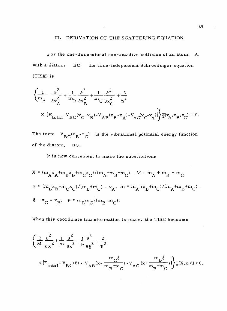
III. DERIVATION OF THE SCATTERING EQUATION
For the one-dimensional non-reactive collision of an atom, A,
with a diatom, BC, the time-independent Schroedinger equation
(TISE) is
1 a2 1 a2 1 a2 2(m
A ax2 mBax 2 rn 2 2
AC ax
- VBC
( xC
xB
)- VAB
(xB
-xA
) -VAC
(xC-x
AT(x
A,x
B,x
C) 0.X[Etotal
The term VBC(xB-xC) is the vibrational potential energy function
of the diatom, BC.
It is now convenient to make the substitutions
X = ( mA xA +mB x +m cx ) mA +mB+rn ) , M = mA + mB + mC
x = (mBxB+rricxc)/(mB+nac) - xA, m = mA(mB+mc)/(mA+mB+m )
xC xB' rnBmCi(mB+rnC)
When this coordinate transformation is made, the TISE becomes
r 1 82 82 2
+VT +2M axe axe N. 2 2
mC mBX [Etotal- VBC() - V
AB mB+mC(x- ) -VAC
(x+m B+mC
)] T(X,x,) = 0.

30
Conceptually this transformation has taken the original three atoms
and mixed them to form three new particles The first of these par-
ticles has a mass, M, equal to the total mass of the atom-diatom
system, and its coordinate, X, is the center of mass of the colli-
sion system. The second particle has a mass, m, which is the
reduced mass of the atom-diatom system. Its coordinate, x, is
the distance between the atom and the center of mass of the diatom.
The third particle has a mass,
the diatom, and a coordinate,
which is the reduced mass of
which is the distance between the
atoms in the diatom. Inspection of the above TISE shows that the
particle of mass, M, and coordinate, X, does not interact with
the other two particles, and hence it may be dealt with separately.
The remaining two particles are coupled by the interaction
mC11113(x-
AB mB+mC ) + VAC(x+ mB+mC
In the language of group theory, the transformation could be said to
take the old three-particle representation and reduce it to a one
particle representation plus a two-particle representation. In this
reduced form, the TISE's of the collision system are

1 82
1 82
2(5) ( +m ax n
and
(6)
-V () -V (x-BC AB m +mB C
rriB-VAC(x+mB+mc )1) Toc, = 0
2( 1 a
2 + 2 [Etotal-E] F(X) °ax
31
with the understanding that DX, x, = F(X)yx, The coordinates
X, x and will be referred to as the center of mass coordinate, the
collision coordinate and the internal coordinate. The TISE involving
the center of mass coordinate (Equation 6) yields no information about
transition probabilities and will be ignored in what follows.mC mB
The interactions VAB(x-m+m ) and VAC(x+ mB+mC
)
B Care taken to be short-range in nature, i. e. , for large values of their
variables, they go rapidly to zero. Consequently when x becomes
large and is limited, the two-particle TISE (Equation 5) can be
further reduced to
(7)
and
21 8 2,
2[Eint-V( n (I)() = 0
(-1.1 a -h4
( 21 a
m 21
.)+2 [E-Ei. nt] G(x) = 0.
ax
Only some of the solutions of Equation 7 are allowable, Labelling the

permissible solutions and energies with the index, n, we have
(8)z
a4
+ ®2 [En-V()] 4)11() = 0
32
Equation 8 is the TISE of the internal coordinate. For any
physically realistic vibrational potential energy function, the complete
set of solutions to this equation will include some solutions which
correspond to bound states and others which correspond to unbound
states. Thus a complete calculation of collision-induced transition
probabilities cannot be limited to coupling among the bound states,
but must also take into account the unbound states Fortunately if
one is interested only in transitions among the lower energy bound
states of a stable molecule (as is the case with this study), then only a
few of the higher energy bound states and none of the unbound states
have a significant effect on the calculated transition probabilities of
interest. The actual number of states which must be included in the
calculation is found by trial. For example, if one wished to calculate
transition probabilities for the lowest K bound states, one might do
the calculation first with the lowest K bound states, then using the
lowest K+1 bound states, etc. , until it was found that including the
7/The label, n, on the solutions of this equation may be con-tinuous or discrete, depending on whether En is above or below thedissociation energy of the diatom.

33
lowest K+L bound states satisfied some desired criterion of con-
vergence.
Suppose then our calculation is to involve the lowest N bound
states of the diatom. For convenience, the energies and the normal-
ized wavefunctions of the states are labelled E E . , E and2' N
and are ordered so that E1 < E2 < < EN.(I)1( t) 1)2( , (ON(
The N solutions of Equation 5 can then be written as
(9) n(x' ( I ) ) 2 (OLP/ n(x), n = 1, 2, . . . , N. I/
Substituting Equation 9 into Equation 5, we have
a2
1 82
2(m 2 2 + 2ax dt
niCt mB
X [E-VBC(°--VAB(x- m+m)-VAC(xi- m+m (I) /( 04)/21(x)=
B C B C= 1
Moving the summation sign to the far left and making use of Equation
8 changes the above equation to
8/A more complete equation would include unbound states, giv-
ing Tn(x, t) = (PI (t)iiin(x)
bound states
&it./ (t)Lpin(x).
unbound states

N
( a2 2 r niCt
max
2 +112 LE-E1 -VABsx- mB+mC= 1
mB- V
AC(x+ m +m
B C)]) 'Of (t)1P1 n(X) = 0.
This equation is now left-multiplied by (1)k(t)
all a-space, yielding
r +00 Q2
ci(1)1c(t)em 2f =1 ax
-G°
mr,tX [E-E -V (x- )-V
AC(x+/ AB m
BmC
N1 d2 2 2
1m̀-
- 2- V,_1 (x)) LP n(x)rn dx xf =1
and integrated over
mBt
m B+mC
=0
or
where
)]) ( ) )11i n(x)
N622
22m
+ .5 V (x) 11.)/ ])kJ
112Id n
(x) = 0 ,
= Idx
34
+corrIC mB
(10) VId (x) -=
k()[V.
AB(x- m +m )+V
AB(x+ m +m )14),e()
_00 B C B C

35
With the definition
E =
El
E2,.
0
0
the above set of coupled differential equations can be summarized by
the matrix equation
d+
22 2mE m
- ---2-(E+V(x)11ip(x) = () .
dx
The particular form of VAB(xB-xA) and VAc(xc-XA)
chosen for this calculation (given in Equation 3) will now be seen to be
particularly convenient. Substituting Equation 3 into Equation 10, we
have
+00 mVice (x) = J d (i)k( (CONSTANT[3VoAB
exp(-(x-m +m ) /L)-00 B C
which implies
(12)
in which
mB+ V°AC exp(-(x+ m+m )/L)])4)
B C
Vk/ (x) z- CONSTANT exp(-x/L)u. ,

36
+oo
(13) ukf =S* c114)kA()
(3V° Bexp[+( )/L]
-oo rnB+InC
A
rriB+ VAC exp[-( ) /LA]) (I)
rnB+mc
The matrix, u, will be referred to as the interaction matrix. The
result of inserting the above into Equation 11 is
22 m(14) [(
x2
+ )1 - (E + CONSTANT exp(-x/L)ulili(x) = 0 .
d /5.2
mE
15.2
This is a proper place to make a rather lengthy digression on
the asymptotic behavior of the solutions of the above equation. This
equation is a linear differential equation and, therefore, if one solu-
tion,1(x), is found, an equivalent solution, 4,2(x), can be gen-
erated by right-multiplying the original solution by a non-singular
matrix, C, whose elements are constants. Since C is non -
singular, then in principle 4i2(x) contains the same information as
4,1(x). 9/ Though the information contained in iiii(x) and 4J2(x) is
the same, it may be more easily extracted from one of them than from
the other. Consequently it is worthwhile to construct the solution,
Lii(x), of Equation 14 in a form which can be readily interpreted.
9 /This follows because if C is non-singular, then C1 existsand 4J 1(x) can be regenerated from 4J 2(x) (i. e. , 1(x) = 2
(x)C-1).

In the asymptotic limit x +00, Equation 14 becomes
2
L(d + E)1- E]4i(x) = O.
dx
Following Gordon (18), we write the general solution of the
above equation as
(15) x +0oJ(x) ,eNJ a(x)a +ap,ob ,
in which at(x) and a(x) are diagonal matrices whose diagonal
elements are
Wix))/in 1/2 exp( -iknx), kn [2m
(E -En )]112
1
1
ail(onnkn
1/2 exP(+iknx)
and
1 2(0110 ))nn 1/2= exo(+Knx) K [11; (En -E )11
n
(x))1
exp(-Knx)nn 1/2n
37
for 1 < n < NOPEN
for
NOPEN + 1 < n < N
and a and b are matrices whose elements are constants. The
quantity, NOPEN, is defined to be the number of states for which
En < E. Those states labelled 1, 2, ... , NOPEN are called open
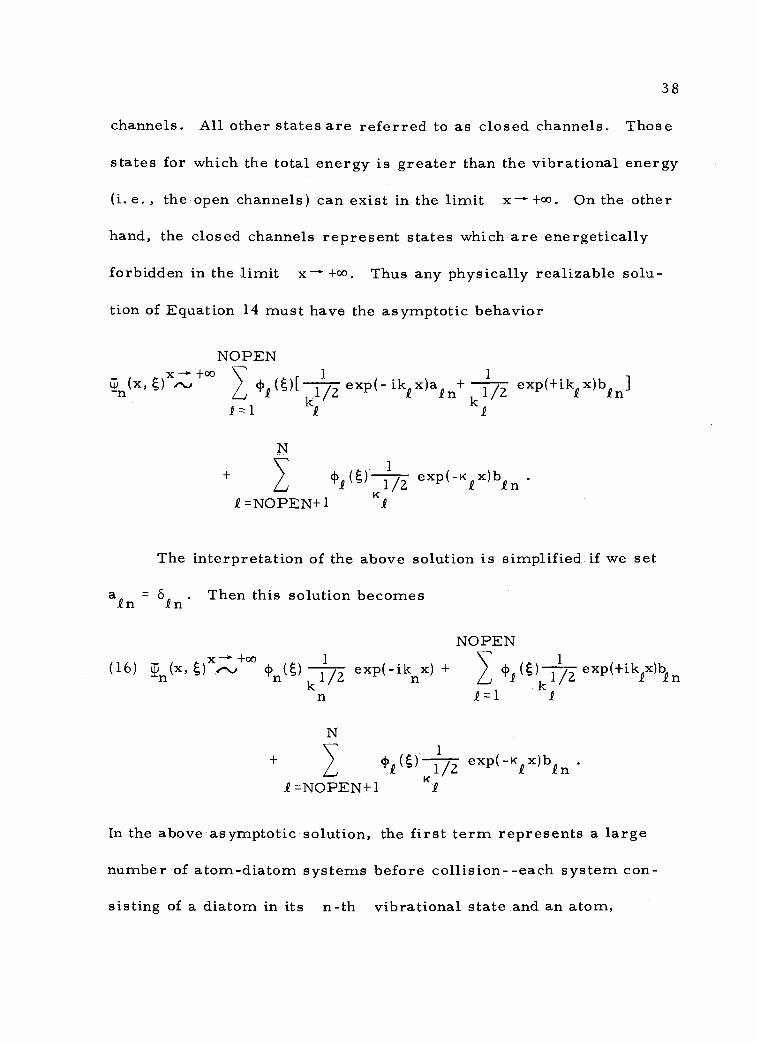
38
channels. All other states are referred to as closed channels. Those
states for which the total energy is greater than the vibrational energy
(i.e., the open channels) can exist in the limit x-- +00. On the other
hand, the closed channels represent states which are energetically
forbidden in the limit x +00. Thus any physically realizable solu-
tion of Equation 14 must have the asymptotic behavior
NOPEN+oo 1 exp(+ik x)bi,enjgn(x' )3c^J eP,e()[ /2 exP(- ik x)a +
k1.V =1
k1/2
N
( ) 11/2 exp(-Kix)ben .
=NOPEN+1 KQ
The interpretation of the above solution is simplified if we set
a.en = 8/n. Then this solution becomes
NOPEN
(16) gn(x, +00 1(1)n(6) 1/2 exp(-ikx) + (1)/()--1-
1-77 exp(+ikex)ben
1=1k
nk
411(6) 1/2 exp( x)bin
/=NOPEN+1
In the above asymptotic solution, the first term represents a large
number of atom-diatom systems before collision--each system con-
sisting of a diatom in its n-th vibrational state and an atom,

39
moving towards each other with a relative kinetic energy equal to
E - En. The second term denotes the observed results of this large
number of atom-diatom collisions --a fraction 'bin 2 of the sys-
tems will have been scattered from the n-th open channel into the
1-th open channel. In other words, the first term represents the
incoming wave, the diatom being definitely in the state n, and the
second term (sum over open channels) represents the outgoing wave,
in which the diatom system may be either in its initial state, I = n,
or in any of the energetically allowed states, 1 < < NOPEN. The
final term (sum over closed channels) symbolizes the significance of
transitions into closed channels--the effect of these transitions is
important only where the atom-diatom interaction is appreciable and
this effect decays rapidly outside of this region. Naturally we require
the number of systems before collision to equal the number of sys-
tems after collision. Mathematically this means that the physically
interesting solutions (viz.,
should satisfy the requirement(x' T2(x' 'INOPEN(x) )
NOPEN
= 1 .
The other asymptotic limit, is also of importance.
The solutions 11(x, g2(x, I\TopEN(x, must go
asymptotically to zero as This forces every term in the

expansion
N
1.3.(x, ()4J.en(x); n = 1, 2, NOPEN
1=1
to go to zero in this limit. Otherwise put
lim (x) = 0; 1 <1 < N; 1 < n < NOPEN.x -00
Thus far the asymptotic natures of
T1(x' NOPEN(x'
40
have been discussed, but nothing
has been said of the solutions which are not physically realizable--
INOPEN+ 1(x' °' I\1*(x'Since the solutions for
1 < n < NOPEN will yield the desired transition probabilities, the
remaining solutions are somewhat arbitrary. It is usually convenient
to require
limx -00
)= 0; 1 <f <N; NOPEN+1 < n < N.
Thus the general asymptotic behavior of Lp(x) is taken to be
lim tp(x) = 0.
The solution of Equation 14 is usually obtained by integrating
the equation from one asymptotic limit, to the other,
x +00, and then matching the solution matrix to the asymptotic
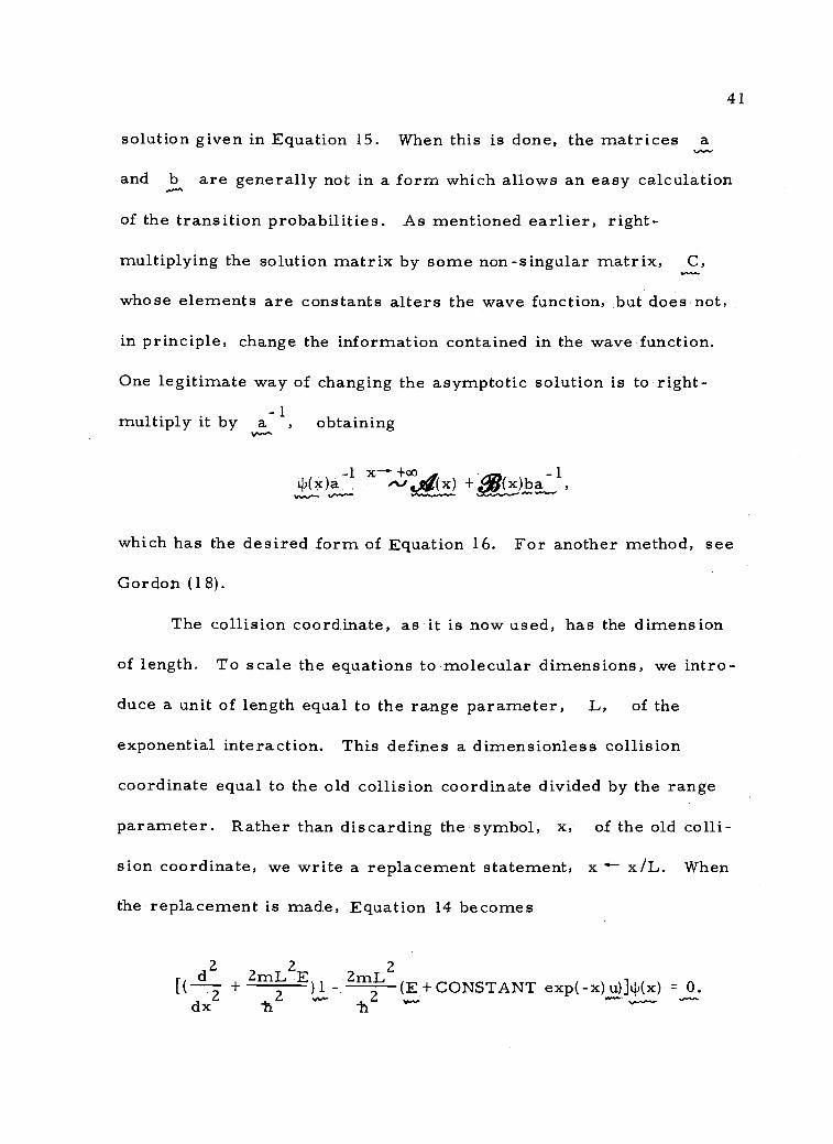
41
solution given in Equation 15. When this is done, the matrices a
and b are generally not in a form which allows an easy calculation
of the transition probabilities. As mentioned earlier, right-
multiplying the solution matrix by some non-singular matrix, C,
whose elements are constants alters the wave function, but does not,
in principle, change the information contained in the wave function.
One legitimate way of changing the asymptotic solution is to right-
multiply it by a-1, obtainingv-1
11)(x)a+oo
x) Xfx)ba ,-which has the desired form of Equation 16. For another method, see
Gordon (18).
The collision coordinate, as it is now used, has the dimension
of length. To scale the equations to molecular dimensions, we intro-
duce a unit of length equal to the range parameter, L, of the
exponential interaction. This defines a dimensionless collision
coordinate equal to the old collision coordinate divided by the range
parameter. Rather than discarding the symbol, x, of the old colli-
sion coordinate, we write a replacement statement, x x/L. When
the replacement is made, Equation 14 becomes
d2 2mL2E 2mL 2
dx7[( 2 2E +CONSTANT exp(-x) u.dtp(x) = 0.

42
To simplify this equation further, we define a molecular unit of energy2
.2equal to2
Making the replacements E `-"-* ERII
)and
2mL ZmL-
E E /( -t2L2)
, we have2m
22m L
2[(
dx2+ E) 1 - (E + CONSTANT exp(-x) u)11,(x) = 0.
---2
The final change to be made in deriving the scattering equation
is another redefinition of the collision coordinate. The factor,2mL2
CONSTANT, is a positive constant. Therefore there is some112
L2number, x0, such that 2mCONSTANT = exp(+x0) and
ti22mL2
CONSTANT exp(-x) may be written as exp(-(x-x0)). The11.2
trivial replacement, x (x-x0), then brings the matrix TISE into
its final form--
2
(17) +E)1- (E+exp(-x)untp(x) = 0 .dx
Furthermore, should it be useful to pull a positive factor out of the
interaction matrix, u, the argument just presented shows this will
have an inconsequential effect on the matrix TISE.
The above equation has asymptotic solutions similar to those of
Equation 14. Inspection will show that if one requires
(18) lim = 0

and
(19)
with
x))nn1
1 /2kn
k1 /2
+00kii(X)ejfil(X)a eR(X)bWY*
exp ( -iknx), kn = (E -En) 1/2
exp(+iknx)
(ejltx))nn 1
1
/2 exp(+Knx), Kn = (En-E l 1/2
Kn
1(ge(x))nn =1 /2
exp(-Knx)Kn
1 < n < NOPEN
NOPEN+1 < n < N
43
then the calculation of transition probabilities is exactly analogous to
the method outlined in the earlier discussion of asymptotic solutions.
In particular, the probability of a collision-induced transition from the2open channel, n, to the open channel, I, is lbin I .
It is worthwhile now to review the derivation of Equation 17 from
the original atom-diatom system. The principal assumptions are
1) We need be concerned only with coupling among the lowest
N bound states of the diatom, BC;
2) The interaction between the atom, A, and the diatom can
be represented as a sum of an AB interaction and an AC
interaction. Both of these interactions are exponential
repulsions with the same range parameter, L.

44
In addition, there have been three coordinate transformations which
have simplified the equations, viz.,
1) A reduction of the original system of three interacting atoms
to a system of one independent particle and a system of two
coupled particles, leading to the definition of a center of
mass coordinate, a collision coordinate and an internal
coordinate;
2) A redefinition of the collision coordinate, scaling the equa-
tions to molecular dimensions;
3) A translation along the collision coordinate, eliminating an
unnecessary constant multiplying the interaction matrix.
The other principal parts of the derivation were
1) Elimination of the center of mass coordinate, X;
2) Converting a scalar partial differential equation in x and
t to a matrix differential equation in x;
3) Expressing the total energy of the system and the internal
energies of the diatom in a molecular unit of energy.
45
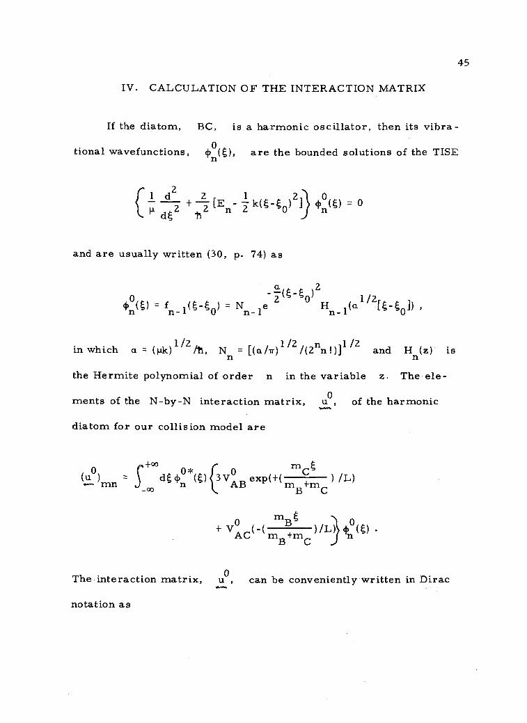
IV. CALCULATION OF THE INTERACTION MATRIX
If the diatom, BC, is a harmonic oscillator, then its vibra-
tional wavefunctions, are the bounded solutions of the TISE
21-9--de +
1122- [En 2
k(- 0 n)
2]) 0(e)
and are usually written (30, p. 74) as
0fri
1/2-1(0) Nn-le
2 0Hn-1 R-t0 ,
in which a = ( pk)1 /2
th, Nn = [(a /701/2 /(2nn !)] 1 /2 and Hn(z) is
the Hermite polynomial of order n in the variable The ele-
ments of the N-by-N interaction matrix, u0,
diatom for our collision model are
of the harmonic
+00In0 0* 0
n(u )m S delan (() 3VAB exp(+( mm ) IL)
_00 BCm
The interaction matrix,
notation as
m+ (-( )/L +n,
0(t) .AC m
B
B C
0u , can be conveniently written in Dirac

u0 =
46
mCgm )/LVAC exp(-( m
mBgm /L)14)
0( ,B
<(1)(01317A0 exp(+( mB+C C B+C
where 04) (g)> is the row vector (1(1)2(g)>,14)2(0>, ,14)N(t)>)
Rapp and Sharp (28) have demonstrated that
<fm(-go)lexPN/(-go)lifn(t-Y>
= exp(i32)(2n-mm!
in !) 1/2pn-mL (-zp2
), for n > m.n-m
In the above equation
Laguerre polynomial (31,
21 / 2
2 ilk
p. 509) 10 /
zand ) is the generalized
With this relationship, the ele-0ments of u are found to be (for n > m)
(20) (u0) = (Anm
+m0 CgO 2 n-m(m-1)!/(n-1)!] 1/2
B+m exP(PAB42
= 3VAB
exp( mCn-m n-m 2
XpAB Lm-1 (2p
AB)
+ V exp( 0 2
AC mB+m )exp(r3AC )[2
n-m (m-1) ! /(n-1) ! 1 /2
B C
X pn-mLn-m(-2P2 )AC m-1 AC
10/There are two types of generalized. Laguerre polynomials inthe literature. The polynomial given in Abramowitz and Stegun (31) isthe correct one for this purpose.

47
in which
mB 21 4"fmC 11. 1 /4 ti
PAB = 2 m +m )L c) and
SACB C
2(mB
+mC)
Thus the calculation of the u matrix for a harmonic oscillator is
fairly straightforward.
For an anharmonic oscillator, the calculation of u is more
complicated, but still quite tractableif the oscillator can be treated
as a perturbed harmonic oscillator. An outline of the method is as
follows:
0Call the unperturbed harmonic oscillator Hamiltonian H (t) and the
perturbation V(t). Let E0n and En be the n-th energy eigen-
values so that El < E 0 ...< EN and. E1
< E2
< < EN. The
orthonormal wavefunctions associated with the unperturbed and per-() 0turbed systems are 4)1(0,4320 (0, ,4)N(0 and
4'1(0,4)2(0, 4)N(0. For convenience, let 1 (1)°(0> and 14)(0>
denote the row vectors ( °(t) >, I +°(t)>, , I (i)0)>) and
(14)1() >, 14)2() >, 14N(0>) What is desired is to find a 100>
which satisfies the following two conditions:
1 ) (El ( t)+v( 0 )1 4)() > = .01( t)>, Ezi 4)2( >, , EN I (pN(t)>)
/El
2
0
EN
= I (o(t)>E

and
(21) 2) <C01(1)(t)>= 1
48
Left-operating on the first condition with <4(t)I and making use ofVthe second condition, we find
(22) <4)(t)Iii°(t)+V(t)14)(t)> = E.
Assuming the perturbed wavefunctions can be expressed as linear
combinations of the unperturbed wavefunctions, we write
I(I)()>= 14)0(0>c ,
where C is a real N-by-N square matrix. On substituting this
expression into Equations 21 and 22, the result is
(23) CT<43.°(t)I4)0(t)>C = CT=1SA,* ,,,,,*
and
(24) , 0T<$.°(t)1H°(t)+V(t)I4) (t)>C
= cT[<4)°(t)I FP(01(1)°(t)>+ <4)
o(t)Iv(t)1(1)o(t)>]c,
low.",-
= CT[E0+<4)0() 1v(t)14)o (t)>JC%.,.= E.
Equations 23 and 24 show that the diagonal elements of the diagonal
matrix E are the eigenvalues and the columns of the C matrix

49
are the orthonormal eigenvectors of the matrix0 0
°1
E <44) (t)1V() 1(1)(t)>. Once the matrix C is known, the calcu-
lation of u is easily done
m rnBtu = <4)(t)13V°
ABexpk
rnB
+mC A( )/L] +V°
Cexp[-(m +m )/IA1(1)(t)>
B C
1.11 C111B t
= CT
<c)0
() 1 3V° expH /IA + V° expf -( VI-d100>CAB m +m AC 1T1 +mB C B C
= CT
u0 C .
Using simple diatomic models of ammonia and deutero-ammonia
greatly facilitates the calculation of their interaction matrices. Coon,
Naugle and McKenzie (29) found they could reproduce quite closely the
inversion mode vibrational energy spacings for these molecules using
the one-dimensional representations of ammonia and deutero-ammonia
described in Section II. They preferred writing their equations in
Q = p.
1 /2tterms of the mass-weighted coordinate,
able, they took the Hamiltonian of the oscillator to be
1'12 d2
X2+ -2- Q
2 +A exp(-a 2Q2) .
dQ
With this vari-
Conceptually this is a harmonic oscillator perturbed by a Gaussian
barrier. Rather than working with the parameters X, A and a,
Coon and his co-workers defined three other parameters p, v0
and

B by
p = ln(2a 2Ant)
vo = X1 /2 /2n-c
B = (A/hcv, ) -13)/eP ,
50
They found the parameters listed in Table 4 to be appropriate for
ammonia and deutero-ammonia. Also given in this table are the cal-
culated barrier heights, b, of the inversion mode and the calculated
distance, h , between the nitrogen atom and the plane of hydrogen
(deuterium) atoms. Their calculated values of b and h are inm
good agreement with the experimental value of h = 0.381 Angstromm
(32) and other calculations of b for ammonia
and 2076 cm -1(34) ).
(e.g., 2020 cm-1(33)
Table 4. Vibrational potential energy parameters for NH3and. ND3.
Parameter NH3 ND3
p 0.6 0.6974.8 c111-1 1
110739.1 cm
B 2.083 2.682b 103 1 cm -1 1982 cm -1
hm 0.386 Angstrom 0.386 Angstrom
Figure 9 shows the four lowest energy wavefunctions (0+, 0,1+, 1-) for the above model of ammonia. These wavefunctions were

51
_(Q)0
V(Q)
Figure 9. Wavefunctions and potential energy of the inversionmode of ammonia.

52
calculated and plotted using the Oregon State University Department
of Physics GROPE system. Also included in Figure 9 is a plot of the
potential energy function, showing the locations of E(0+), E(0 ),
E(1+) and E(1 ). It will be noticed that this plot does not resolve the
difference between E(0 ) and E(0 ).
To test the convergence of E and u as the number, N,
of harmonic oscillator states is increased, we have written a
FORTRAN IV computer program, incorporating the recursion rela-
tions given in Coon, Naugle and McKenzie (29) for the elements of
E° + <4:°() I V()1 (I) (0> . To determine the eigenvalues and eigen-1vectors of the matrix E 0
+ <c)0
()1 V() 1(1)0() >, we used the sub-
routine HDIAG (35) (modified to order the eigenvalues in ascending
order). This subroutine diagonalizes symmetric real matrices, via
the method of Jacobi rotations. Appendix B contains the results of
these calculations for the ten lowest energy states of the inverting
ammonia and deutero-ammonia models for N = 16, 20 and 24.
These results demonstrate that the elements of E and u corres-
ponding to these ten states converge rapidly as N is increased. In
our scattering equations, we used the results calculated for N = 24.
Table 5 compares the values of E(0 ),E(0 ), ) calculated
in our work with experimental values and calculated values given in
reference 29. It is felt that the difference between our calculated
energies and those calculated in reference 29 may be due to small
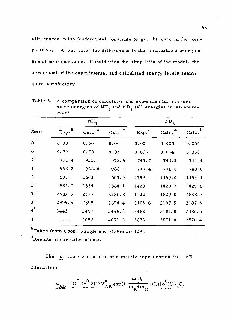
53
differences in the fundamental constants (e. g. , h) used in the com-
putations. At any rate, the differences in these calculated energies
are of no importance. Considering the simplicity of the model, the
agreement of the experimental and calculated energy levels seems
quite satisfactory.
Table 5. A comparison of calculated and experimental inversionmode energies of NH3 and ND3 (all energies in wavenum-bers).
State
NH3 ND3
aExp. Calc. a Calc.b Exp. a Calc.a Calc. b
o 0.00 0.00 0.00 0.00 0.000 0.0000 0. 79 0. 78 0. 83 0.053 0.074 0.056
+1 932.4 932 4 932.6 745.7 744.3 744.41 968. 2 968 8 968.3 749.4 748.0 748.02+ 1602 1603 1603.0 1359 1359.0 1359.3
2 1882.2 1884 1884. 1 1429 1429.7 1429. 6
3+ 23 83.5 23 87 23 86.8 1830 1829.0 1828. 7
3 2895.5 2895 2894.4 2106.6 2107.5 2107.3
4+
3442 3457 3456.6 2482 2481.0 2480.54 4052 4051.6 2876 2871.0 2870.4aTaken from Coon, Naugle and McKenzie (29).
bResults of our calculations.
The u matrix is a sum of a matrix representing the AB
interaction,
mCT<°() 13V° exp(+( )/L)1(1)
0 ()> C,AB - AB mB+mC

54
and a matrix representing the AC interaction,
IT1CuAC = C
T «p°( )I vAC +m° exp(-( m /14 (I)°()> C .
B C
To gain a qualitative understanding of the relative importance of these
two interactions, uAB and uAC were calculated in addition to
their sum, u. The elements of these matrices which couple the
0 +, 0 , 1 +, 1 , 2 and 2 states are shown for ammonia in Table 6
and for deutero-ammonia in Table 7. The fact that the (0+, 0+) ele-
ment of u for both ammonia and deutero-ammonia is unity merely
shows that a constant factor has been removed from these matrices.
It was demonstrated in Section III that this sort of "normalization"
has no effect on the calculated transition probabilities.
To see the effect of the inversion phenomenon on vibrational
energy transfer, we created two fictitious molecules. These mole-
cules have the same molecular structures as ammonia and deutero-
ammonia, and differ from them only in that they are harmonic oscil-
lators. To imitate the inverting molecules, we felt it reasonable to
set their fundamental frequencies equal to the average of the calcu-
lated 1+ and 1 energy levels minus the average of the calculated 0+
and 0 energy levels of the corresponding inverting molecules, i.e.,
1 1 +v = [v(1 +H-v( )] - [v(0 +) +v(0 )] .

55
Table 6. The u,-A^of NH3.
uAB
and--
uAC
matrices for the inverting model
0+ 0 1+ 1 2+ 2
o+ 1.000 0.551 0.179 0.188 0.074 0.058
0 0.551 1.001 0.186 0.184 0.067 0.064+
1 0.179 0.186 0.938 0.492 0.226 0.231
1 0.188 0.184 0.492 0.980 0.283 0.251
2+ 0.074 0.067 0.226 0.283 0.859 0.413
2 0.058 0.064 0.231 0.251 0.413 1.004
,Do' 0.720 0.632 0.174 0.205 0.072 0.060
0 0.632 0.721 0.204 0.179 0.071 0.063
1+1 0.174 0.204 0.660 0.561 0.220 0.252
1 0.205 0.179 0.561 0.701 0.316 0.244
2+ 0.072 0.071 0.220 0.316 0.584 0.467
2 0.060 0.063 0.252 0.244 0.467 0.724u
AC_L
0,281 -0.080 0.005 -0.018 0.002 -0.002
0 -0.080 0.281 -0.018 0.005 -0.004 0.001+
1 0.005 -0.018 0.278 -0.069 0.006 -0.0221- -0.018 0.005 -0.069 0.279 -0.033 0.0072
+ 0.002 -0.004 0.006 -0.033 0.276 -0.0542 -0.002 0.001 -0.022 0.007 -0.054 0.280

56
Table 7. The u, uAB andof ND3.-
uAC
matrices for the inverting model
0+ 0 1+ 1 2
0+ 1.000 0.390 0.131 0.111 0.038 0.0280- 0.390 1.000 0.111 0.131 0.028 0.0381
+ 0.131 0.111 0.975 0.364 0.166 0.1521- 0.111 0.131 0.364 0.980 0.152 0.178
2+ 0.038 0.028 0.166 0.152 0.893 0.303
2 0.028 0.038 0.152 0.178 0.303 0.962
0 0.663 0.547 0.116 0.143 0.034 0.033
0- 0.547 0.663 0.143 0.117 0.033 0.034+
1 0.116 0.143 0.641 0.508 0.148 0.1971 0.143 0.117 0.508 0.646 0.199 0.1582
+ 0.034 0.033 0.148 0.199 0.569 0.4202 0.033 0.034 0.197 0.158 0.420 0.631
0 0.337 -0.157 0.015 -0.032 0.004 -0.0040 -0.157 0.337 -0.032 0.015 -0.004 0.0041+ 0.015 -0.032 0.333 -0.144 0.019 -0.0451 -0.032 0.015 -0.144 0.334 -0.047 0.0202
+ 0.004 -0.004 0.019 -0.047 0.323 -0.1172- -0.004 0.004 -0.045 0.020 -0.117 0.331

57
For the harmonic model of ammonia, this hypothesis gave
v = 950.5 cm-1 and for deutero-ammonia, v = 746.2 cm 1. The
interaction matrix, u, was determined for both of these fictitious
molecules and the contributions of the AB and AC interactions,
uAB and uAC' were also found. These elements of these matrices
which couple the 0, land 2 states are given in Tables 8 and 9. The
(0, 0) element of the u matrices is unity because of a convenient
"normalization" of these matrices. Appendix C contains the elements
of the E and u matrices for the non-inverting models of ammonia
and deutero-ammonia used in our calculations.
Table 8. The u, uAB and uAc matrices forthe non-inverting model of NH3.
0 1 2
u0 1.000 0.257 0.0581 0.257 1.082 0.3812 0.058 0.381 1.167
0.872 0.266 0.05701 0.266 0.953 0.3932
uAC
1
0.057
0.128-0.008
0.393
-0.0080.128
1.038
0.000-0.012
2 0.000 -0.012 0.129

58
Table 9. The u, uAB
and u ACmatrices for
the non-inverting model of ND3.
0
1
2
CAB1
2
0
1
2
0 1 2
1.000 0.182 0.0320.182 1.045 0.2650.032 0.265 1.091
0.870 0.195 0.0310.195 0.914 0.2830.031 0.283 0.958
0.130 -0.013 0.001-0.013 0.131 -0.0180.001 -0.018 0.133

59
V. SOLUTION OF THE SCATTERING EQUATION
It was seen in Section III that the collision-induced transition
probabilities for our simple models can be found by solving the N-
channel scatter ing equation
2(25) [(d +E)1-(e+e -x u)4(x) = 0 .
NAM.,dx
In 193 2 Jackson and Mott (36) obtained an approximate analytic solu-
tion of this type of equation for the collision of an inert gas and a
harmonic oscillator, via the method of "distorted waves. " The
method of Secrest and Johnson (37) in 1966 was the first of a number
of exact numerical solutions of scattering equations for vibrationally
inelastic atom-diatom collisions. The most notable techniques have
been developed by Sams and Kouri (3 8) and Gordon (18). The methods
of Jackson and Mott and Gordon will be discussed later in this section.
To facilitate our discussion of how Equation 25 was solved in-xour research, we rewrite the above equation, setting u(x) = E +e u.
Thus we obtain
d2
(26) [(-2- +E )l-u(x)4(x) = 0 ,001,..
with the understanding that (u(x))..-- +00 as -co and
(E ).. 6.. as x- +00.1.]

60
At this point, we consider the solutions of Equation 26 when
u(x) is a diagonal matrix. These solutions will be used later to find
approximate solutions of Equation 26 for a non-diagonal u(x).
We first note how much simpler the calculation would be if the
equation to be solved were
2(27) +E)l-uo(x)40(x) =dx
in which u0
(x) is a diagonal matrix. Then the above matrix equa-
tion could be exactly separated into N2 equations of the type
d2(28)dx 2 0
+E - Unn i(ti
0 nrn = 0; n = 1,2, , , ;
m= 1,2, ... ,
For a linear second-order differential equation such as the above, it
is well-known that there exist two linearly independent solutions 11 /
(which we shall call A n(x) and Bn(x) ) and that the general solu-
tion of the above equation is
(4,0(x))nrn = An(x)anrn + Bn(x)bnin
where a and b are arbitrary constants. From this itnm nm
11/Messiah (39, vol. 1, p. 98-113) discusses some generalproperties of these solutions.

61
follows that the general solution of Equation 27 is
(29) Lp (x) = A(x)a + B(x)b ,0 ....---- ......--
where A(x) and. B(x) are the diagonal matrices whose elements
are (A(x)) = A (x)6 and (B(x)) = B (x)5 , and a andnm n nm nm n nm
b are square matrices whose elements are arbitrary constants. In
addition, the Wronskians of these solutions,
W = A (x)B' (x) - A' (x)B (x), are non-zero constants. Hence then n n n n
matrix, W = A(x)131(x) - A'(x)B(x), is a non-singular diagonal
matrix, with constant elements.
The approach used in solving Equation 26 over some interval of
x, the collision coordinate, is to choose a diagonal matrix, uo(x),
which approximates u(x) within the interval. If u(x) is a good
approximation of u(x), then the solution of Equation 27 will be a
good zeroth-order solution of Equation 26. Furthermore, it will be
seen shortly that if a suitable choice of u0
(x) is made, it is possible
to calculate a correction for the difference between u0
(x) and u(x).
Thus the approach used here is analogous to the usual first-order
bound state perturbation method, in which a potential energy, u(
is approximated by a more convenient function, u0
(x), and a cor-
rection for this approximation is found using the solution associated
with u0
(x).
With the above in mind, we consider some interval of the x-axis,

62
say x1
< x < x2
, over which we wish to solve Equation 26. It is
assumed that some appropriate diagonal matrix, u0
(x), has been
chosen for this interval. In Appendix D, it is demonstrated that the
general solution of Equation 26 can be written as the integral equation
(30) q(x) = A(x)a + B(x)b + W -1 S [A(y)B (x) -A (x)B (y)]xi
X [u(y)-uo(y)]4J(Y)dY
The term, A(x)a + B(x)b, in this integral equation is the solution of
the equation corresponding to the approximate diagonal potential
energy matrix, u0
(x), and the integral is the correction for the
difference between u0(x) and the actual potential energy matrix,
u(x). We emphasize that the above equation is an exact solution of the
TISE for u(x), and, as yet, no approximations have been introduced.
Since the solution, qi(y), appears within the integral, this integral
solution is not an explicit expression for 4,(x). However, if
u(x) - u0(x) is small throughout the interval of integration, then the
integral in Equation 30 will also be small, and q(x) z A(x)a + B(x)b.
This suggests that for the purposes of calculating the correction for
u(x) u0
(x), the solution, ii(y), within the integral can be replaced
by the approximate solution, A(y)a + B(y)b, giving

63
_r(31) tp(x) A(x)a + B(x)b + W ix
[A(y)B(x)-A(x)B(Y)][u(Y)-u(Y).1V
X1
X [A(y)a+B(y)b]dy
It is reasonable to expect that if a u0
(x) is found for which
u(x) - u0
(x) is very small over a large interval, then the solution,
ip(x), given in the above equation will be nearly exact throughout the
entire interval. Conversely, if u0(x) is a poor approximation of
u(x), then to minimize the error of the above equation, the size of
the interval must be small.
In a one-dimensional collision of an inert gas atom and a
diatomic harmonic oscillator molecule during which the oscillator12/states are weakly coupled, the diagonal elements of the interaction
matrix, u, are approximately equal and the off-diagonal elements
are small in comparison with the diagonal elements. For this system,
Jackson and Mott (36) applied a technique (referred to as the method
of "distorted waves") which is essentially equivalent to the integral
approximation described above. As the approximate diagonal potential
energy matrix, they chose u0
(x) E exp(-x)1. With this u0
(x),,..,
the approximate TISE (Equation 27) can be solved in terms of the
modified. Bessel functions, K v(z) and Iv
(z). Because of their
12/Weak coupling corresponds to a small value of PAB and
PAC in Equation 20.

64
judicious choice of u0
(x), the solutions of their approximate TISE
enabled them to analytically find the correction term for
u(x) - u0
(x) over the interval "0 < x < +00
The method of Jackson and Mott has been a very useful approxi-
mation and forms the basis of what is known as the SSH theory (16).
Comparisons with exact solutions of Equation 26 show this method is
in serious error when
1) The coupling among vibrational states is not small;
2) Vibrational transition probabilities between non-adjacent
energy levels are calculated.
For collisions involving strong coupling among states, the interaction
matrix u is no longer almost a constant matrix. Consequently
when u.0
(x) is taken to be E exp(-x)1, the quantity u(x) - u0
(x)
is not small. Thus it is not surprising that the technique of Jackson
and Mott is inaccurate under these conditions. The difficulty encoun-
tered for transitions between non-adjacent energy levels comes about
because this formalism considers only direct transitions from one
state to another during a collision. In a collision, a given transition
may take place via a number of possible paths. For example, the
transition v = 0 v = 2 may be thought of as occurring through the
sequences 0 2 or 0 1 2 or 0 3 2 or any of a mul-
titude of other possibilities. The actual transition probability of the
0 2 transition depends primarily on the most probable of these

65
possibilities. It is usually found that a path consisting of steps for
which Ls v = ±1 and which contains the fewest possible steps will be
the most important path for a given transition.
In addition to the above difficulties of the method of Jackson and
Mott, Rapp and Kassal (3) point out a mass-dependent error. They
suggest that, for v = 0 v = 1 transitions, the transition probabili-
ties are more accurately given as exp(-1.685m) times the Jackson13/and Mott probabilities, where the dimensionless parameter,
is
(32)rn
Am
Cm
Trl
for the A-BC collision system. Even with this modification, Rapp
and Kassal conclude the v = 0 v = 1 calculation is unreliable for
probabilities above 0.05.
Notwithstanding all of the limitations mentioned here, the results
of Jackson and Mott have been of great value in the theory of vibra-
tional energy transfer for the following reasons:
1) For many molecular collisions, the vibrational coupling is
small.
2) Vibrational energy transfer is dominated by transitions for
13/This use of the symbol, m, is not to be confused with themass associated with the collision coordinate x.

66
which Lv = t 1. Those transitions for which Av = 0 do
not result in excitation or de-excitation, and those for which
Ev = ±2,±3, ... are relatively improbable.
3) The mass parameter, m, given in Equation 31 is energy
independent. Consequently a thermal averaging of the
unmodified Jackson and Mott transition probabilities will be
qualitatively correct.
Because of the unknown effects of inversion doubling on transi-
tion probabilities and the substantial coupling of the internal states14/during a collision of ammonia or deutero-ammonia molecules, it
was decided to use Gordon's method (18) to solve Equation 25. It will
be seen that this method is very similar to that of "distorted waves"
and can be thought of as a series of "local distorted waves" calcula-
tions, propagating the wave function from one asymptotic limit
(x -00) to the other (x +00).
Following Gordon, we again consider solving Equation 26 over
some interval, x1
< x < x2. In general, the off-diagonal elements
of u(x) may be large enough that there is no diagonal matrix, u0
(x),
which is a good approximation of u(x) over the interval. Since u(x)
is a real symmetric matrix,
be found which diagonalizes
an orthogonal matrix, S, can always
u(x) at the midpoint, xmid , of the
14/For our diatomic models, pABin Equation 20 was about
0.21 for ammonia and about 0.16 for deutero-ammonia.

interval. When this transformation is applied to Equation 26, the
result is
d2
+E)1-S Tu(x)S1S = 0 .d.x
After defining
v(x) = STu(x)S
and
(33) 4(x) = ST4(x)
the above equation becomes
,2(34) +E)l-v(x)14)(x) = 0 .
dx
Since v(xmid) is diagonal, v(x) will be approximately diagonal
over the interval (assuming the interval is not too large).
Having obtained a nearly diagonal matrix, v(x), there still
remains the choice of an approximate diagonal matrix v0
(x). Once
the v0
(x) is decided upon, the general solution
of the equation
(35)
0(x) = A(x)a + B(x)b
d2
dx2
+E) 1 -v0
(x)](I)0(x) = 0
67

68
can be found. With this general solution associated with v0
(x), the
approximate integral solution
(36) (I)(x) z A(x)a + B(x)b + W1 S[A(y)B(x)-A(x)B(y)liv(y)-v,,1.1
(y)]
X1
X [A(y)a+B(y)b]dy
can be calculated. To simplify the integration of the above equation,
Gordon chose for v0
(x) the matrix whose elements are
(37) (v0(x))nm = [v(xw0 '(xmid)]nm6nm
In short, he linearized v(x) and neglected off-diagonal terms. With
this choice, the diagonal terms of the operator in Equation 35 are
d2(38) + E - (v(x ) -X v'(x )) X(V f(X ))dx2 mid mid mid nn mid' nn
The solutions associated with this operator are the Airy functions (31,
p. 446), A.(an [x-xmid n]) and B.(an [x-xmid n ]), with
1
a = (v '(x . ))1 /3
and p = [(v(xi.d nn))-d(v'(x ))-1 Thereforen mid nn mid mid nnthe general solution of Equation 35 is
(39) (I) (x) = A(x)a + B(x)b ,
where
(A(x)) = A.(a [x-x +P 1)6nm 1 n mid n nm
and
(B(x)) = B.(a [x-x +p ])6nm B1 (an mid n nm
To evaluate the integral in Equation 36, the function
69
v(y) - v0(y) is expanded in a power series about the point y = xmid..Gordon has found explicit equations for correction terms involving
constant and linear terms in (y-xdmi) for off-diagonal corrections
and constant, linear and quadratic terms in (y-xmid ) for diagonal
corrections.
The usefulness of Gordon's method is dependent on the speed of
zcalculationof the Airy functions, A.(z) and. B.( z). In evaluating
the correction terms, one often subtracts large, nearly equal numbers
--resulting in considerable loss of precision. Gordon has overcome
this problem by deriving a new method of calculating the Airy func-
tions, using the method of generalized Gaussian quadratures (18,40).
zThismethod allows fast double-precision calculation of A.( z) and
zB.( ) accurate to fourteen digits.
The following shows more explicitly how a solution is propa-
gated from one end of the interval (x = x1) to the other (x = x2).
We assume that iji(x 1) ) and 4,1(x ) are known. Equation 33 shows
that (I)(x) = S Tqi(x) and (1)1(x,) =Tiii(x,) or
J. 1 ." J.

(40)(1)(x)
(1)1(x))x=x1
ST 0 q(x)
0 ST 4JI(x)) x-x1
Differentiation of Equation 36 yields
x(pl(x) = A 1(x)a + B l(x)b + [A(y)B 1(x) -A I(x)B(y)Jjy(y)-vo(y)]
X [A(y)a+B(y)b]d.y.
Evaluating the above equation and. Equation 36 at x1 and x2, we
find
(1)(3ci) = A(xda + B(xdb
cl;(xi) = A '(x, )a + B l(x, )b,...--
10,0,110./
(1)(x 2) = A(x )a + B(x2)b + W -12
and
x2
[A(y)B(x2)-A(x2)B(y)][v(y)-v0(y)]
1
X [A(y)a+B(y)b]dy
70
x2
.4),(x2) = A'(x2)a + 131(x )b + W 1 [ A( y )B'(x2)-A'(x2)B(y)][v(y)- v0(y)]X
1
X [A(y)a+B(y)b]dy
The matrices A(x), B(x), A'(x), BI(x) and W -1 are all
diagonal and therefore commute. This allows the integrals in the
above equation to be rearranged, obtaining

71
cf(x2) = A(x 2)a + B(x2)b + A(x 2)[ -A v a-A v b]BA,.- BB
%.60.
+ B(x2)[+L vAAa+A vAB12]
and
4:1)'(x2) = At(x,)a + B'(x2
)b + vBAa vBBID1
+ B t(x )[+P v +A v b]2 AA. AB.
in which
x2
(41) .6vmoo,.m.
= W 1 tc B(y)[v(y)-vnv (y)1A(y)dy,
xl
etc. The above equations for 13.(x1), (I)'(x ), 4(x2) and 01(x2) can
be more conveniently written as
(42)
and
(43)
(1)(x) / A(x) B(x) a
(1)'(x) Al(x) 1() k_11
1
cl:(x) A(x) B(x)
4'(x)) A '(x) B'(x)x2 x=x2
X
1 0
0 1
vBA(v
AA
-Ls vBB
+.AvAB
"Th
r.
(
a
b
Because A(x), B(x), A'(x), B'(x) and W are diagonal, Equation
42 can be solved for a and b--

72
/ a W-1 0 / 131(x) -B(x) (I)(x)(44)
b 0 W-1
-A1(x) A(x) (44)'(x))x-x1
Thus if one wishes to propagate the solution, 4(x), and the
derivative of the solution, 41'(x), of Equation 26 from xl to x2,,..,...
Gordon's method proceeds as follows:
1) The matrix, S, which diagonalizesmid) found.
2) The S matrix is used to transform ip(x1)
and (pl(x )
into 4(x1) and (I)'(x1) (Equation 40).SA...yrs `"
3) The matrices v(xm. ), v'(xm. ) and the diagonal elementsid id
of v"(xmid ) are found, where v(x) = STu(x)S.
4) With the diagonal elements of v(xmid) and vl(xmid), themid
appropriate Airy functions and their derivatives are found,
thus determining A(x1), B(xi), Al(xi), BI(xi), A(x2), B(x2),
A'(x2), B'(x2) and W (Equations 37, 38 and 39).
5) The coefficient matrices, a and b, are calculated
(Equation 44).
6) The corrections for v(x) v0
(x) are found (Equation 41).
The corrections include constant and linear off-diagonal
terms of the series expansion of v(x) - v0
(x) in powers of,x - xmid and constant, linear and quadratic diagonal terms.
7) The functions (I)(x2) and (I)'(x2)
are then calculated
(Equation 43).

73
8) Finally q(x2) and Iiii(x2) are evaluated by transforming....(I)(x2) and (1)'(x2)--
Lp(x) s
(IJI(x)1 0x=x2
(I)'(x)X=X2
If the term v(y) v0(y) in Equation 36 were zero, the solu-
tion outlined above would be exact. The solution obtained with
Gordon's method is inexact to the extent that A(y)a + B(y)b is not a
good approximation to tp(y) (which is to say, to the extent that v(y)
and v (y) differ). If the correction matrices0 '6vAA' AvAB'
o vBA and .6 vBB are small, then it is reasonable to assume that to
a good approximation q(y) = A(y)a + B(y)b, and therefore the error
of the propagation of the solution from x = x1
to x = x2 is small.
Gordon found the effect of the correction varies roughly as the cube
of the interval size and, furthermore, does not change rapidly from
one interval to the next. In his method, a maximum correction is
specified for the wavefunction. When the solution is propagated over
an interval, the effect of the correction terms is compared with the
desired maximum. If the size of the correction terms indicates the
interval size was too large (small), the size of the following interval
is decreased (increased) accordingly.
The calculation is initiated at a point well within the classically
forbidden region. As the solutions propagate towards the classically

74
allowed region, those solutions which are the most classically forbid-
den tend to grow the fastest. Were nothing done to control this
growth, serious numerical errors would result. Gordon has adapted
a method ascribed to Householder (41, p. 233) to construct a stabiliz-
ing transformation which circumvents this difficulty.
The amount of computer time required to diagonalize the poten-
tial energy matrix, u(x), is large. If it were necessary to perform
these diagonalizations for every value of the dimensionless total
energy, the calculation would be rather expensive. Fortunately
the correction terms in a given interval do not vary greatly over a
range of E. For this reason, the diagonalizing transformations and
the potential energy matrix terms are stored during the first of a
series of calculations and used in subsequent calculations -thus saving
a considerable amount of computer time. Allison (42) has compared
Gordon's method with a variation of the step-by-step Numerov tech-
nique for solving coupled differential equations. For solutions of
moderate accuracy, he concluded that in a series of calculations,
Gordon's method is faster than step-by-step methods.
In addition to his original paper (18), Gordon has written another
very useful description of his method (43).
Through the helpfulness of Mr. R. Jay Murray of the Oregon
State University Computer Center, we obtained a copy of Gordon's
program (44) from the Quantum Chemistry Program Exchange. This

75
program was written to evaluate rotational transition probabilities for
the three-dimensional collision of an inert gas atom and a diatomic
rigid rotator. The program is written mostly in FORTRAN IV
language, although the user is given the option of using either
FORTRAN IV or assembly language for a number of simple subrou-
tines. We chose to use the FORTRAN IV versions of these subrou-
tines.
Two major modifications of the original program were made.
The first was changing the program to calculate transition probabili-
ties associated with Equation 25. The second modification involved
the method of propagating solutions. As was mentioned above, when
calculations are made for a range of values of the dimensionless total
energy, E, the first calculation determines quantities used in the
other calculations. In the original program of Gordon, the method of
propagating the wavefunction for the second, third, etc. values of E
was not the same method that was used for the first value of The
method for the first calculation is the technique described above and
is fairly straightforward. Subsequent calculations used the same
parameters as the initial calculation, but were carried out in a man-
ner not well understood by us. The most puzzling aspect of this latter
technique is that it avoids calculation of off-diagonal correction terms.
In the initial calculation, these off-diagonal terms account for much of
the coupling between two states. Because of our confidence in the
76
method for the initial calculation and our misgivings about the other
technique, it was decided to modify the program so that all calcula-
tions were carried out in the manner of the first.
The original program contained several errors and more were
introduced via our modifications. After considerable debugging, the
program was successfully run--essentially duplicating the results of15Secrest and. Johnson (37) given in their Table VII. / All of our cal-
culations with this program were done on the IBM-360/50 computer at
the University of Oregon Computing Center.
The results of the calculations for the models of ammonia and
deutero-ammonia are presented in the next section.
15/This table lists exact transition probabilities for the one-dimensional collision of an inert gas atom (mass = 2 a. m. u.) with ahomonuclear diatomic harmonic oscillator molecule (total mass = 24a. m. u.) whose vibrational frequency is about 1750 cm-1. The rangeparameter, L, of the repulsive exponential interaction energy is0.2214 Angstrom.

77
VI. CALCULATED TRANSITION PROBABILITIES
During preliminary calculations with harmonic oscillator
models, it was noticed that reliable transition probabilities were
obtained when a calculation included at least one closed channel.
Consequently, for the non-inverting models, the number of closed
channels was always at least one. Since the inversion phenomenon
splits the lower vibrational states of the vz mode of ammonia into
nearly degenerate pairs of states, the minimum number of closed
channels was two in calculations for the inverting models.
The parameter which represents the desired size of the correc-
tion terms (called " TOLHI" in the original program) was set at
1. 0 x 10-3 in calculating the results shown below.
Table 10 summarizes the contents of Figures 10 through 29.

78
Table 10. Catalog of transition probability graphs.
Figure Molecule Model Initial State Final States
10 NH3 Inverting 0+ 0 +, 0
11 NH3 Inverting 0 0 +, 0
12 NH3 Inverting 1+ 1+, 1
13 NH3 Inverting 1- 1+, 1
14 ND3
Inverting 0+
0+, 015 ND
3Inverting 0 0 +, 0
16 ND3
Inverting 1+ 1+, 1
17 ND3
Inverting 1 1+, 1-
18 NH3 Inverting 0+
1+, 1, 2+, 2
19 NH3 Inverting 0 1+, 1, 2+, 2
20 NH3 Inverting 1+ 0+, 0, 2+, 2-
21 NH3 Inverting 1 0 +, 0, 2+, 2
22 ND3
Inverting 0+
1+, 1, 2+, 2
23 ND3
Inverting 0 1+, 1, 2+, 2
24 ND3
Inverting 1+ 0+, 0, 2+, 2
25 ND3
Inverting 1 0+, 0, 2+, 2
26 NH3 Non-inverting 0 0, 1, 2
27 NH3 Non-inverting 1 0, 1, 228 ND
3Non-inverting 0 0, 1, 2
29 ND3
Non-inverting 1 0, 1, 2

1.0
0. 5
0.00
AA
A
A
A A
A
0
0
0
A
A
A
A
A
A
A
A
o AA
AoQ3 I i A /1\ _1 1 I IL L
1500 3000Relative kinetic energy, v (cm-1)
A
0
Figure 10. Probability of the transition IF for NH3; I = 0+; F = 0+, 0

1.0
00
0
0.5
A
A
A
AAA A A
0 . 0 e i 0 co i I A IA I I
1500-1 3000
Relative kinetic energy, v (cm )
A
0
A
0
A
0
A
A
0
A
0
0
0
0
0
0
0
0 0 0
A 0 0
A
A
A
A A
A
A
Figure 11. Probability of the transition I---"F for NH3; I = 0-; F = 0+, 0-.

1.0
0
0. 5
A
A
A
A
A
a
0
0
1 1
A 1+ 1_
0
A
A A
A0. 0 I
I 1
0 1000 2000Relative kinetic energy, v (cm-1)
A0
A
0
Figure 12. Probability of the transition IF for NH3; I = 1+; F = ,1-.

1.0
v )
0.5
0.00
0
A
0 1
A 1-
0
0
0
0
10I i i
1
1
i
0
a
0
1
Figure 13.
1000Relative kinetic energy, v (cm-1)
Probability of the transition IMF for NH3; I = 1-; F =
2000
1+, 1-.

1.0
p (v)
0. 5
AAA
A
A
A0
0 00
0
0
A
A
A A0
0 1500 -1 3000Relative kinetic energy, v (cm )
0
A
0
A
A
0
A
0
0
A o+ o-
A A
+ -Figure 14. Probability of the transition IF for ND3; I = 0+; F = 0 , 0 . co

F(v)
1.0-
0.5
0
O
0
A
A0.0 /1\ I I1' 4
0 1500 3000Relative kinetic energy, v (cm-1)
Figure 15. Probability of the transition I--"F for ND3; I = 0-; F = 0+, 0-.
A
0
0
0
0
0
o 0 0+
A 0-
0

1. 0
0. 5
0.00
A
A
0
A
A
0
A
0
A
0
A
A
b 1 ~ 1
A 1 1
A0i
1000Relative kinetic energy, v (cm-1)
0
A
A
0
A
0
A
2000
Figure 16. Probability of the transition I"F for ND,, I = 1+; F = 1+, 1

0
0
0
A
0
A p 1-
1+
A p L 1 1-
1000Relative kinetic energy, v (cm-1)
0
Figure 17. Probability of the transition for ND3; I = 1-;
0
2000

Relative
0
A 0o 0 1 .tV
1500kinetic energy, v (cm-1)
A
0
A A0
0V
0
00
0
V1
3000
-Figure 18. Probability of the transition IF for NH3; I = 0+; F = 1+
, 1 , 2+
, 2 .oo

0.150
F(v)
0.075
0.000
0- 1
A 0 ~ 1o 0 2
V 0 2
A
0
0A
A 0
'a'0 0
AAA ni
1511`' T t0 V'1500
-1Relative kinetic energy, v (cm )
A
0
V
V
A
0
0
V
A A
a
3000
Figure 1 9 . Probability of the transition IF for NH3; I = 0 ; F = 1+
, 1-
, 2+
2-

(v)
0.30
+ +1 0
A 1+y0-o 1+ 2+
+V 1 1-2
0
0.15 00
0
0. 0000 6 Ala g1000
0
V
A
V
Relative kinetic energy, v (cm -1
0A
V
A
0
0(
2000
Figure 20. Probability of the transition I--"F for NHS; I = 1+; F = 0+, 0-, 2+, 2

0.30
- +1 --' 0
A 1- ~ 0O 1- 2+
V 1 ~ 2-
( v )0
0.15 1- 0 0
0.00 $1-
0
A te 0
1000-1 2000
Relative kinetic energy, v (cm
V
V
A
V
0
V
V
A
V
A
0
0
Figure 21. Probability of the transition I ~F for NH3' 1 ; F = 0 + ,0 ,2 +,2

0.150
0.075
+ +0+ - 1A 0 - 1
+ +0 0 - 2V 0 --- 2-
0
D A
0
O
O
O
D A Y 00. 000 1 il Li -4:),, A A A '0 -34x- .-sz-----1,- v-----1-1500
i
30001
0, 1,Relative kinetic energy, v lcrn 1
0
V
0
Figure 22, Probability of the transition IF for ND3I I = 0+; F = 1+, 1-, 2+,

p
0.150
0.075
0.0000
0 1p 0 1
+o 0 2
v. 0 2
A
0
0
AA
0
0A
VV
AA V 0
°11 6 0ci
1500Relative kinetic energy, v (cm-1)
Figure 23. Probability of the transition 1'1- for ND3; I = 0; F = 1+,1-
3000

0.30+ +
1+ 0-A 1+ 0+o 1 2
'7 1 2
0.15
V
0 yq 0
1000
00. 00
Relative kinetic energy, v (cm
V
0
0
0 0
2000
+ -Figure 24. Probability of the transition I"F for ND3; I = F = 0 , 0

0. 30
0. 15
0.00
- +o 1 ~ 0A 1 " 0-o 1- 2+
V 1
V
V
V V
0CA A
AO
A0 c c7 0 0 0
1000 2000-1Relative kinetic energy, v (cm )
Figure 25. Probability of the transition 1'1- for ND3; I = 1-; F = 0+, 0-, 2+, 2 -,C)

1.0
( v )
0.5
0.00
0 0 0
A 0 1
0 0
4, A
00
A
0
A
00
A
0
A
s..) C.)
1500 3000Relative kinetic energy, v (cm.-1)
Figure 26. Probability of the transition I--"F for NH3; I = 0; F = 0,1, 2.

1.0
F(v)0. 5
AA
00
0 00 0
CI 0
0 1500 3000Relative kinetic energy, v (cm-1)
Figure 27. Probability of the transition IF for NH3; I = 1; F = 0,1,2.

1.0 0
0-" 0L 0 1
o 0 2pIF(v)
0.5
a 0
A AA
0.0 A `(4 oo o do 01 00 1500 3000
Relative kinetic energy, v (cm-1)
00
O
A
0
Figure 28. Probability of the transition IF for ND3; I = 0; F = 0,1,2.

1.0 AAAAAAAA
1 0
A 1 1
o 1 2
p IF(v)0.5
A A
A
o0.0 o a al o a 01
0 1500Relative kinetic energy,
AA
0
v (cm -1)3000
Figure 29. Probability of the transition I"F for ND31 I = 1 s F = 0,1,2.

99
VII. CALCULATION OF THE VIBRATIONAL VELOCITYDISPERSION AND ABSORPTION INDEX
Once the relationship between one-dimensional transition
probabilities and one-dimensional relative kinetic energies has been
determined, it is possible to average these transition probabilities
over a thermal distribution of relative kinetic energies and obtain
rate constants for reactions of the general form
(45) A + BC(I) A + BC(F)
Before discussing this averaging in detail, we briefly review some of
the concepts and approximations of the model.
The objective of this research is to construct a simple model of
collision processes in ammonia, from which the velocity dispersion
and absorption index due to vibrational relaxation can be calculated.
Thus far the model contains these features:
1) The gas for which this calculation is being done contains only
one component, whose molecules follow a classical mechani-
cal distribution of translational and rotational energies and
a quantum mechanical distribution of vibrational energies.
2) To simplify the calculation, collisions in which both mole-
cules undergo vibrational transitions are ignored.

100
Furthermore, by not giving a vibrational label to molecule
A 16/ in Equation 45, we imply that the rate for this reaction
is independent of the vibrational state of A.
3) In one of these simplified collisions, the ammonia molecule
which can undergo a vibrational transition is approximated by
a diatomic molecule, BC, in which the B atom repre-
sents the three hydrogen atoms and the C atom is taken to
be the nitrogen atom. The other ammonia molecule is
approximated by atom A, whose mass is that of three
hydrogen atoms.
4) For this calculation, the relative kinetic energy of a collision
is taken to be the rotational energy of the A molecule about
its symmetry axis.
The rate constant associated with the reaction in Equation 45
can be written as
(46)dn
dt KI'FnAnBC(I)
in which n. is the number of molecules of component i per unit
volume andF is the rate constant of the reaction.
16/In this section, "A" will refer to both an atom and a mole-cule. In calculating transition probabilities for a collision of an Amolecule with a BC molecule, the molecule A is represented by theatom A.

101
The rate of this reaction can be calculated from statistical
mechanics and the transition probabilities found in this research. If,
in all encounters, the rotational energy of the A molecule could be
fixed at some value, Erot, then the reaction rate would be
doI'-Fat ZA,BC(I) P (E rot) ,
where Z A, BC(I) is the total number of A-BC(I) collisions per
unit volume per unit time, and pIF (E rot) is the probability that
if the A atom has relative kinetic energy, E rot, then its colli-
sion with a BC(I) molecule will result in a BC(F) molecule. As
mentioned above, it is assumed that the rotational energies of the A
molecules follow a classical mechanical distribution, i.e., if
N(E rot)dE rot is the fraction of A molecules with rotational
energies between Erot and Erot + d.Erot, then
N(E rot )dE rot RT= exp(-Erot /RT)dErot
Hence the correct rate of reaction is found by averaging pt_F(Erot)
over the values of Erot, using the weighting factor of the above
equation. We refer to the result of this thermal averaging of
pIF (E rot) as PIF(T), given by

102
(47) 1co
F(T) = RT pI F(Erot) exp( -Erot /RT)dErot0
The relationship between PIF(T) and Z F(T) (the average
number of collisions in a gas at temperature T needed to bring
about a transition from state I to state F) is simply
(48) = 1/PIF (T) .
The unit of energy in this part of the calculations is the wave-
number. With this unit of energy, Equation 47 is written as
oo
( 4 9 ) ( T ) -1.4388
T p1 -'F(v) exp( -1.4388v /T)dv .0
Figure 30 shows the function, 1.4388T P1-*.0
(v)exp(-1.4388v/T), for
the non-inverting model of ammonia at 300°K for the relative kinetic
energies at which the scattering equation was solved. The integral
in Equation 49 was evaluated from these points by means of the
trapezoidal rule. This is admittedly a rough approximation to the
integral, but this quadrature does not introduce a significant error
into the calculation. Table 11 gives the values of Pi__F(T) for
transitions of importance in the remaining parts of the calculation.

H
coco
7r,
(I)
O
coccM H
0
0
0
0
0
00
1000 2000Relative kinetic energy, v (cm-1)
Figure 30. Thermally weighted 1 --- 0 transition probability for non-inverting NH3.

104
Table 11. Calculated values of PI (T) at 300°K.
Reaction Model NH3 ND3
0 -- 0 + Inverting 0.64 0.641 --I. 1+ Inverting 0.59 0.58
+1
+0 Inverting 1. 6 x 10⁻³ I. 2 x 10⁻³
+I -' 0 Inverting 1.7 x 10⁻³ 0.8 x 10⁻³
1 0+
Inverting 4.0 x 10⁻³ 0.9 x 10⁻³
1 ---*. 0 Inverting 3.8 x 10⁻³ 1.4 x 1031 0 Non-inverting 3.1 x 10⁻³ I. 7 x 10⁻³
The above table appears to show that the inverting models of
ammonia and deutero-ammonia do not give rise to calculated transi-
tion probabilities for reactions of the type 1 -" 0 which differ
greatly from those calculated for non-inverting models. It does seem
clear that our simple models correctly predict that a 1 -" 0 type
transition during a collision is more likely for ammonia than for
deutero-ammonia. Substituting the values P 1-"0 (T) for the non-
inverting models into Equation 48, we find
Z1-0(NH3) = 3 x 10² and. Z1-4-0(ND3) = 6 x 10² at 300° K. Com-
parison with the experimental values in Table 2 shows the theoretical
values of Z 1-0 to be orders of magnitude too large. It will be
noticed, however, that the theoretical values of Z 1-0 fit the
Lambert-Salter plots (Figure 1) for hydrides and deuterides quite
well.
Continuing the calculation of rate constants, we assume a hard

105
sphere model for ammonia molecules. From Davidson's equations
(45, p. 164), it can be shown that
TrRT 1/2 2= 4() nzA,BC(I)A
nBC(I)
in which M is the molecular weight and Cr is the effective colli-
sion diameter. In the present work, we use o- = 2.925 Angstroms- -
the same value used by Jones et al. (12) and. Bass and. Winter (13) in
their "hard spheres" calculation of Z1
-0 from experimental data.1
The thermally averaged rate of reaction is then
TrRT 1/2 2 P (T)dt 4(- a- nA
nBC(I)
Comparing this equation with Equation 46, one finds
RT 1/2 2(50) KIF 4(Tr) o- P (T)
00
= 4(Tr ) 1/2C
2
R1Tr
PIF(Erot) exP(-Erot /RT)dEroto
Had we considered vibration-translation energy transfer instead
of vibration-rotation energy transfer, the expression for the rate con-
stant would have been
TrRT 1 /2 2 1
KIL-F M ' 6 RT0
pI'}-(Etrans) exp(-Etrans /RT)dEtrans

The prime on p'IF IF(E) signifies that p (E) in
this equation is not the same as PIF(E) in Equation 50. The
transition probability, p' (E), refers to a collision of two
106
molecules--both of which have the mass of an ammonia molecule.
One the other hand, pI_.F(E) refers to a collision of two molecules
--one having the mass of an ammonia molecule and the other having
the mass of a cluster of three hydrogen atoms. Given that these two
types of collision have the same relative kinetic energy, E, the
relative velocity of the particles in the collision involving the cluster
of hydrogen atoms would be greater. Consequently, for ammonia, a
collision which couples vibrational and rotational motions is expected
to be more non-adiabatic than a collision which couples vibrational
and translational motions. Thus we expect that pI_..F(E) is greater
than p' (E) and. KIF is greater than
The rate constant, K F refers to Equation 46, in which
concentrations are usually expressed in molecules per cubic centi-
meter. For use in the formalism to follow, the rate equation must be
converted to
dt kIFpA
pBC(I)
in which p. is the partial pressure of component i in atmos-i
pheres. Some straightforward algebra shows that kI is related0,
Kby k ,/hF RT (NO = Avogadro's number).

107
The following table gives the rate constants for processes of
interest calculated at 300°K for the models of ammonia and deutero-
ammonia.
Table 12. Calculated values of at 300° K.
Process ModelNH3
atm-1sec -1
ND3
tm-'sec -1a
0 0+--.- 0 Inverting 3.64 x 10⁹ 3.35 x 10⁹
1 - 1+ Inverting 3.35 x 10⁹ 3.06 x 10⁹
1+
0+0 Inverting 0.91 x 10⁷ 0.63 x 10⁷+
1 .- 0 Inverting 0.97 x 10⁷ 0.43 x 10⁷
1 0+---..- 0 Inverting 2.28 x 10⁷ 0.48 x 10⁷
1 --,- 0 Inverting 2.14 x 10⁷ 0.73 x 10⁷
1 ---.- 0 Non-inverting 1.79 x 10⁷ 0.91 x 10⁷
Bauer and Bass (46) have developed a useful formalism for cal-
culating the velocity dispersion and absorption index of a gas. In
their method, one sets down the N internal energy levels to be
included (E1, ...,Ei, , EN) and the M reactions which connect
these energies, viz. ,
k1reaction 1 A + BC(I
1) A + BC(F1)
kreaction a A + BC(I
a ) A + BC(F a )
kreaction M A + BC(IM) A + BC(FM)

108
In these reactions, Ia and Fa signify the initial and final states of
the a-th reaction. By convention, these reactions are written as
exothermic. Four matrices, u, x, K and v, are then constructed.
The matrix,
*M,
u, is an N-by-1 matrix whose elements are merely.4
the internal energy levels (with respect to some arbitrary zero of
energy). The matrix, x, is an N-by-N diagonal matrix whose
i-th diagonal element is the mole fraction, x., associated with the
i-th energy level, Ei.. The matrix, K, is an M-by-M sym-
metric matrix. For the simple reactions dealt with in this research,
K reduces to a diagonal matrix. The a-th diagonal element of
this matrix is the forward rate of the a-th reaction,
k XA
XBC(I)' expressed in mole fractions rather than partiala
pressures. The matrix, v, is an N-by-M matrix. It serves to
connect the populations of the internal states with the reactions
involving them. The a-th column of this matrix contains the
stoichiometry of the a-th reaction. If state i is a product of the
a-th reaction, then (v) is = +1. If state i is a reactant in the
a-th reaction, then (v). = -1. If state i is neither a product norisa reactant in the a-th reaction, then (a). = 0.is
With these matrices, Bauer and Bass have used irreversible
thermodynamics to show that when a sound wave passes through a gas,
the dynamic heat capacity of the gas is given by

109
C (w) = C (co) + R(RTT
u ) (iw
1 + vKv Tx -1)-1 vKv
T(
1u
in which w is the frequency of the sound wave in radians per sec-
and and p is the pressure of the gas in atmospheres. Bauer (47)17/has demonstrated that vKvT is necessarily singular. To avoid
numerical difficulties at low frequencies requires special mathemati-
cal treatment (summarized in Appendix E). Suffice it to say, we have
overcome any instability problems and have no difficulty calculating
dynamic heat capacities.
The relationship between the sound velocity, v(w), and the
absorption, a(w), and the dynamic heat capacity for an ideal gas
given by Bauer and Bass is
2(
1 ia(w) 2 y(00)(51) (v(x)) v(w) )
(xwhere y(w) = Cp
(w)/Cv
(w) For an ideal gas, Y )2 )I(°)2
and(v(0))
C (w) = Cv(w) + R. Substituting these relations into Equation 51, a
little algebra will show that
C (0) C (w)-R(v((0)))2(i ia(w)v(w))2C (w) C (0)-R
P p
17/This singularity is related to the conservation of the totalnumber of BC molecules.

The velocity dispersion and absorption index may be defined asv(0) 2( )v(w)
and a(w) >(w). Using the equation, v(w) = (2.7)X(0),
be seen that
(v(0) )2(v(w)
ia(0)X(co) 2 C,(0) CP
(0) -R)
C (w) C (0)-Rp p
110
it can
By equating the real and imaginary parts of this equation, the velocity
dispersion and absorption index can be determined from the dynamic
heat capacity.
With the method described above, the velocity dispersion and
absorption index for each of the models were found from the rate con-
stants listed in Table 11. The results of these calculations are shown
in Figures 31 through 34.
Comparing the results of the inverting and non-inverting models
of ammonia and deutero-ammonia, it can be seen that, aside from a
slight shift in the inflection point of the dispersion curve and the maxi-
mum of absorption curve, the inversion process shows no effect,
qualitative or quantitative, on the velocity dispersion or the absorp-
tion index. For example, the absorption index has the same shape,
the same maximum value and the same width for both the inverting and
non-inverting models.

0. 03
0. 02
0. 01
0. 00
Non-invertingmodel
111
Inverting model
4 5 6 7 8
log10 (f /p)
Units of f/p: Hz/atm
Figure 31. Absorption index for the inverting and non-invertingmodels of NH3*

112
Non-inverting model
Inverting model
4 5 6 7 8 9
log10 (f/p)
Units of f/p: Hz/atm
Figure 32. Velocity dispersion for the inverting and non-invertingmodels of NH3.

0. 05
113
Non-inverting model
Inverting model
log10(f /P)
Units of f/p: Hz/atm
8 9
Figure 33. Absorption index for the inverting and non-invertingmodels of ND3.

1.00
0.99
0.98
0.97 1
4 5 6 7
log10 (f/p)
Units of f/p: Hz/atm
Non-inverting model
Inverting model
8 9
114
Figure 34. Velocity dispersion for the inverting and non-invertingmodels of ND 3.

115
VIII. CONCLUSIONS
From the results of the calculations for our simple models of
ammonia and deutero-ammonia, we conclude that the rationalization
put forth by Cottrell and Matheson (11) does not suffice to explain the
very fast vibrational relaxation of these molecules. We do not claim
that the inversion phenomenon does not play a significant role in
energy transfer processes. Rather, our work indicates that if
only short-range repulsive forces couple vibrational states during a
collision, then the effect of inversion on vibrational relaxation is mini-
mal.
It is expecially interesting to note that the theoretical values of
Z 1-0 (NH3
) and. Z1-0 (ND3) fall much closer to the Lambert-Salter
plots for hydrides and deuterides than do the experimental values.
This strongly suggests that the explanation of their very rapid relaxa-
tions is to be found either in the hypothesis of dimerization (48) or in
some other collision mechanism. In this connection, it is important to
remember that Jones et al (12) and. Bass and Winter (13) found that
vibrational and rotational relaxations occur at almost the same rate.
An interaction which is usually neglected on the grounds it is too adia-
batic, namely dipole-dipole coupling, may conceivably be of impor-
tance because it couples translational, rotational and vibrational
motions. Nevertheless, it is difficult to see how this interaction would
greatly increase transitions probabilities for I Lvl > 0 transitions.
116
BIBLIOGRAPHY
1. T. L. Cottrell and J. C. McCoubrey, "Molecular Energy Trans-fer in Gases, " Butterworth, London, 1961.
2. K. Herzfeld and T. A. Litovitz, "Absorption and Dispersion ofUltrasonic Waves, " Academic Press, New York, 1959.
3. D. Rapp and T. Kassal, Chem. Rev. 69, 61 (1969).
4. L. Landau and E. Teller, Physik. Z. Sowjetunion 10, 34 (1936).
5. P. Ehrenfest, Koninkle. Ned. Akad. Wetenschap. , Proc. 16,591 (1914).
6. J. D. Lambert and R. Salter, Proc. Roy. Soc. A253, 277 (1959).
7. J. D. Lambert, J. Chem. Soc. , Faraday Trans. II, 68, 364(1972).
8. T. L. Cottrell and A. J. Matheson, Trans. Faraday Soc. 58,2336 (1962).
9. C. B. Moore, J. Chem. Phys. 43, 2979 (1965).
10. J. K. Hancock and J. C. Decius, J. Chem. Phys. 51, 5374 (1969).
11. T. L. Cottrell and A. J. Matheson, Trans. Faraday Soc. 59,824 (1963).
12. D. G. Jones, J. D. Lambert, M. P. Saks ena and. J. L. Stretton,Trans. Faraday Soc. 65, 965 (1969).
13. H.E. Bass and T.G. Winter, J. Chem. Phys. 56, 3619 (1972).
14. F.W. DeWette and Z.I. Slawsky, Physica 20, 1169 (1954).
15. L. Monchick and. E. A. Mason, J. Chem. Phys. 35, 1676 (1961).
16. R. N. Schwartz, Z. Slawsky and K. F. Herzfeld, J. Chem. Phys.20, 1591 (1952).
17. G. Herzberg, "Infra-red and Raman Spectra, " Van Nostrand,Princeton, 1945.

117
18. R.G. Gordon, J. Chem. Phys. 51, 14 (1969).
19. W. Eastes and D. Secrest, J. Chem. Phys. 56, 640 (1972).
20. F.D. Shields, J. Acoust. Soc. Amer. 32, 180 (1960).
21. E.G. Richardson, J. Acoust. Soc. Amer. 31, 152 (1959).
22. M. E. Riley and A. Kuppermann, Chem. Phys. Letters 1, 537(1968).
23. 3. 0. Hirschfelder, C. R. Curtiss and R. B. Bird, "MolecularTheory of Gases and. Liquids, " Wiley, New York, 1954.
24, J. C. McCoubrey, R. Milward and A.R. Ubbelohde, Trans.Faraday Soc. 57, 1472 (1961).
25. T. A. Gilbert and A. C. Wahl, J. Chem. Phys. 47, 3425 (1967).
26. R. L. Matcha and R. K. Nesbet, Phys. Rev. 160, 72 (1967).
27. M.D. Gordon and. D. Secrest, J. Chem. Phys. 52, 120 (1970).M.D. Gordon and D. Secrest, J. Chem. Phys. 53, 4408 (1970).
28. D. Rapp and T.E. Sharp, J. Chem. Phys. 38, 2641 (1963).
29. J. B. Coon, N. W. Naugle and. R. D. McKenzie, J. Mol. Spectry.20, 107 (1966).
30. L. Pauling and E. B. Wilson, "Introduction to Quantum Mechan-ics, " McGraw-Hill, New York, 1935.
31. M. Abramowitz and I. A. Stegun (Eds.), "Handbook of Mathe-matical Functions, " Appl. Math. Ser. 55, Nat. Bur. Stand. ,
U. S. Govt. Print. Off. , Washington, D. C. , 1964.
32. W.S. Benedict and E.K. Plyler, Can. J. Phys. 35, 1235 (1957).
33. J.D. Swalen and J.A. Ibers, J. Chem. Phys. 36, 1914 (1962).
34. M. F. Manning, J. Chem. Phys. 3, 136 (1935).

118
35. J. H. Schachtschneider, "Vibrational Analysis of PolyatomicMolecules. VI. Fortran IV Programs for Solving the VibrationalSecular Equation and the Least-Squares Refinement of ForceConstrants, " Technical Report No. 57-65, Shell DevelopmentCompany, Emeryville, California. (n. d. )
36. J. D. Jackson and N. F. Mott, Proc. Roy. Soc. A137, 703 (1932).
37. D. Secrest and B.R. Johnson, J. Chem. Phys. 45, 4556 (1966).
38. W. N. Sams and. D.J. Kouri, J. Chem. Phys. 51, 4815 (1969).
39. A. Messiah, "Quantum Mechanics, " Wiley, New York, 1968.
40. R.G. Gordon, J. Math. Phys. 9, 655 (1968).R.G. Gordon, J. Math. Phys. 9, 1087 (1968).
41. J. H. Wilkinson, "The Algebraic Eigenvalue Problem, " OxfordUniversity Press, Oxford, England, 1965.
42. A. C. Allison, J. Comput. Phys. 6, 378 (1970).
43. R.G. Gordon, "Methods in Computational Physics. Vol. 10.Atomic and Molecular Scattering, " pp. 81-109, Academic Press,New York, 1971.
44. Quantum Chemistry Program Exchange, Department of Chemistry,Indiana University, Bloomington, Indiana, 47401.
45. N. Davidson, "Statistical Mechanics, " McGraw-Hill, New York,1962.
46. H. J. Bauer and. H.E. Bass, J. Chem. Phys. 57, 1763 (1972).
47. H. J. Bauer, J. Chem. Phys. 57, 3130 (1972).
48. J. D. Lambert and E. D. T. Strong, Proc. Roy. Soc. A200, 566(1950).

APPENDICES

119
APPENDIX A
VIBRATIONAL RELAXATION DATA AT 300°K 18/
Molecule cvmin ( m -1) 1°g10 Z1-0
Molecule containing neither hydrogen nor deuteriumCO2 673 4.70C12 556 4.67
COS 527 4.12Br
2321 3.73
CS2
397 3.47
CF4 437 3.32
SF6
344 3.02CF
3C1 356 2.62
CC14 218 1.93
CF2
C12 261 1.83
SiC14 150 1.30
Molecules containing hydrogen
CH4 1306 4.18
CH3F 1048 3.68
C2
H4 810 2.99
PH3 991 2.95
AsH3
905 2.78
SiH4 914 2.76
CH3C1 732 2.76
C2
H2 612 2.45
CH3Br 611 2.28
18 / The data in these tables were compiled by Lambert (7).

120
Molecule v (cm -1) '0 gi 0 Z1 ~0
Molecules containing hydrogen (continued)
CH3
I 533
NH3 950
Molecules containing deuterium
1.89
0.70
CD4 996 4. 34
PD3
728 3.09CD
3C1 699 2. 94
SiD4 675 2. 91
C2
D4 584 2. 59
AsD3
660 2. 53
C2
D2
511 2, 49
CD3Br 577 2.34
ND3
748 1.69

APPENDIX 8
INTERNAL ENERGIES AND INTERACTION MATRICES FOR THE INVERTING MODELS OF AMMONIA AND DEUTERO-AMMONIA
INTERNAL ENERGIES (IN WAVENUMBERS) OF INVERTING AMMONIA FOR 16, 20 AND 24 HARMONIC OSCILLATOR NAVEFUNCTIONS
V = 0+ V = V = 1+ V = 1- V = 2+ V = 2- V = 3+ V = 3- V = 4+ =N = 16 t
N = 20 8
N = 24 I
INTERACTION
.00000 .72362 934.51719 968.65854 1610.14407 1889.65541 2433.08827 2938.14381 3678.46292 4273.45187
.00000 .83510 932.64862 968.28094 1603.02286 1884.14702 2386.87575 2894.45403 3459.06455 4053.-36739
.00000 .83510 932.64856 968.28091 1603.02046 1884.14688 2386.78692 2894.41433 3456.63028 4051.60989
MATRIX OF INVERTING AMMONIA FOR 16 HARMONIC OSCILLATOR NAVEFUNCTIONS
1.00000 .55140 .17757 .18674 .07310 .05658 .03333 .01525 .00998 .00275.55140 1.00156 .18509 .18400. .06737 .06354 .03194 .01773 .01101 .00465.17757 .18509 .93297 .48790 .21835 .22170 .13584 .06870 .04492 .01414.18674 .18400 .48790 .97898 .27938 .24746 .14647 .09436 .05412 .02630.07310 .06737 .21835 .27938 .84355 .39419 .23379 .14525 .09410 .03277.05658 .06394 .22170. .24746 .39419 .99033 .42666 .28264 .17116 .09641.03333 .03194 .13584 .14647 .23379 .42666 .95886 .42958 .25371 .10683.01525 .01773 .06870 .09436 .14525 .28264 .42958 1.02873 .46142 .28581.00998 .01101 .04492 .05412 .09410 .17116 .25371 .46142 .96080 .38846.00275 .00465 .01414 .02630 .03277 .09641 .10683 .28581 .38846 1.00213
INTERACTION MATRIX OF INVERTING AMMONIA FOR 20 HARMONIC OSCILLATOR NAVEFUNCTIONS
1.00000 .55142 .17874 .18758 .07388 .057E5 .03312 .01655 .00788 .00333.55142 1.00120 .18565 .18423 .06738 .06424 .03073 .01738 .00781 .00330.17874 .18565 .93829 .49187 .22585 .23055 .14320 .07846 .04429 .02003.18758 .18423 .49187 .98032 .28347 .25111 .14758 .09686 .04669 .02346.07388 .06738 .22585 .28347 .85931 .41258 .25867 .17310 .10767 .05168.05795 .06424 .23055 .25111 .41298 1.00392 .45214 .30441 .17501 .10393.03312 .03073 .14320 .14758 .25867 .45214 1.02272 .50645 .32807 .18315.01655 .01738 .07546 .09686 .17310 .30441 .50645 1.09724 .55641 .36346.00788 .00781 .04429 .04669 .10767 .17501 .32807 .55641 1.14251 .59734.00333 .00330 .02003 .02346 .05168 .10393 .18315 .36346 .59734 1.20122
INTERACTION MATRIX OF INVERTING AMMONIA FOR 24 HARMONIC OSCILLATOR NAVEFUNCTIONS
1.00000 .55142 .17874 .18758 .07388 .05795 .03312 .01654 .00787 .00332.55142 1.00120 .18565 .18423 .06738 .06424 .03073 .01738 .00781 .00329.17874 .18565 .93829 .49187 .22586 .23055 .14323 .07847. .04433 .02006.18758 .18423 .49187 .98032 .28348 .25111 .14760 .09687 .04673 .02346.07388 .06738 .22586 .28348 .85933 .41300 .25879 .17319 .10795 .05189.05795 .06424 .23355 .25111 .41300 1.00352 .45228 .30446 .17539 .10408.03312 .03073 .14323 .14760 .25879 .45228 1.02330 .50707 .32990 .18477.01654 .01738 o07847 .09687 .17319 .30446 .50707 1.09759 .55893 .36483.00787 .00781 .04433 .04673 .10795 .17539 .32990 .55893 1.15167 .60754.00332 .00329 .02006 .02346 .05189 .10408 .18477 .36483 .60754 1.20900

INTERNAL ENERGIES (IN NAVENUMBERS) OF INVERTING DEUTERO- AMMONIA FOR 16, 20 AND 24 HARMONIC OSCILLATOR NAVEFUNCTIONS
V = 0+ V = 0- V = 1+ V = 1 V = 2+ V = 2- V = 3+ V = 3- V = 4+ V = 4-N = 16 .00000 - 2.99689 774.32647 759.07154 1426.00771 1485.76453 1978.45186 2281.08595 2921.35189 3334.57424N = 20 t .00000 .03940 744.83186 748.06870 1361.77465 1430.71371 1837.54295 2115.20590 2528.00855 2915.59541N= 24 : .00000 .05625 744.38850 747.99070 1359.30351 1429.64225 1828.71309 2107.27634 2480.52562 2870.39965
INTERACTION MATRIX OF INVERTING DEUTERO - AMMONIA FOR 16 HARMONIC OSCILLATOR NAVEFUNCTIONS
1.00000 .38820 .12219 .10219 .03633 .02183 .01925 .00384 .00944 .00109.38820 1.00402 .10918 .12758 .03172 .03751 .01946 .01260 .01234 .00558.12219 .10918 .94121 .33868 .13137 .11353 .07907 .02451 .03476 - 0.00015.10219 .12758 .33868 .96458 .13809 .15635 .07893 .06071 .04353 .02262.03633 .03172 .13137 .13809 .81950 .23198 .13022 .06683 .06434 .00659.02183 .03751 .11353 .15635 .23198 .90640 .20250 .15620 .09906 .05152.01925 .01946 .07907 .07893 .13022 .20250 .82823 .18797 .12474 002523.00384 .01260 .02451 .06071 .06683 .15620 .18797 .88231 .22267 .14314.00944 .01234 .03476 .04353 .06434 .09906 .12474 .22267 .84665 .16896.00109 .00558 - 0.00015 .02262 .00659 .05952 .02523 .14314 .16896 .86470
INTERACTION MATRIX OF INVERTING OEUTERO - AMMONIA FOR 20 HARMONIC OSCILLATOR NAVEFUNCTIONS
1.00000 .38964 .13062 .11101 .03778 .02820 .01521 .00766 .00485 .00154.38964 1.00014 .11090 .13130 .02840 .03783 .01204 .00971 .00440 .00211.13062 .11090 .97358 .36350 .16428 .14993 .08806 .04684 .03405 .01159.11101 .13130 .36350 .97965 .15099 .17744 .06947 .06567 .02840 .01718.03778 .02840 .16428 .15099 .88620 .29807 .18252 .13126 .09810 .03670.02820 .03783 .14993 .17744 .29807 .95941 .22862 .20586 .10344 .07438.01521 .01204 .08806 .06947 .18252 .22862 .88693 .27125 .19221 .08735.00766 .00971 .04684 .06567 .13126 .20586 .27125 .97659 .29757 .22169.00485 .00440 .03405 .02840 .09810 .10344 .19221 .29757 .95932 .28821.00154 .00211 .01159 .01718 .03670 .07438 .08735 .22169 .28821 .99712
INTERACTION MATRIX OF INVERTING DEUTERO- AMMONIA FOR 24 HARMONIC OSCILLATOR NAVEFUNCTIONS
1.00000 .38965 .13081 .11113 .03792 .02840 .01502 .00787 .00431 .00170.38965 1.00009 .11096 .13134 .02838 .03787 .01176 .00963 .00377 .00182.13081 .11096 .97476 .36416 .16642 .15161 .08922 .04887 .03355 .01326.11113 .13134 .36416 .97991 .15185 .17814 .06915 . .06611 .02649 .01641.03792 .02838 .16642 .15185 .89253 .30278 .19006 .13937 .10407 .04386.02840 .03787 .15161 .17814 .30278 .96226 .23240 .21054 .10338 .07625.01502 .01176 .08922 .06915 .19006 .23240 .90187 .28711 .21322 .10737.00787 .00963 .04887 .06611 .13937 .21054 .28711 .99185 .31732 .24131.00431 .00377 .03355 .02649 .10407 .10328 .21322 .31732 1.01419 .34311.00170 .00182 .01326 .01641 .04386 .07625 .10737 .24131 .34311 1.05421
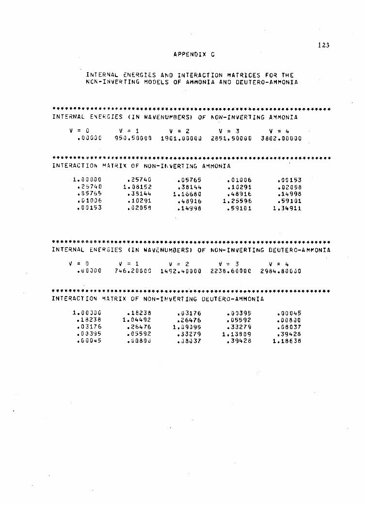
123
APPENDIX C
INTERNAL ENERGIES AND INTERACTION MATRICES FOR THENCN-INVERTING MODELS OF AMMONIA ANO DEUTERO-AMMONIA
*44********44444.4******************4444****************************
INTERNAL ENERGIES (IN WAVENUMBERS) OF NON-INVERTING AMMONIA
V= 0 V= 1 V= 2 V = 3 V= 4.00000 950.50000 1961.30003 2851.50000 3802.00600
************4444******************4444.********44444*44**4444*44**4INTERACTION MATRIX OF NON-INVERTING AMMONIA
1.00000 .25740 .05765 .01006 .00153.25740 1.08152 .38144 .10291 .02058.05765 .38144 1.16680 .48916 .14998.01006 .10291 .48916 1.25596 .59101.00153 .02058 .14998 .59101 1.34911
*******************444*********************************************
INTERNAL ENERGIES (IN WAVENUMBERS) OF NON-INVERTING DEUTERO-AMMONIA
V = 0.00000
V = 1 V = 2 V= 3 V= 4746.20000 1492.40000 2238.60000 2984.80600
4***************************************************************44*INTERACTION MATRIX OF NON-INVERTING DEUTERO-AMMONIA
1.00000 .18238 .03176 .00395 .00045.18238 1.04492 .26476 .05592 .00800.03176 .26476 1.09095 .33279 .08037.00395 .05592 .33279 1.13809 .39428.60045 .00800 .08037 .39428 1.18638

124
APPENDIX D
AN INTEGRAL SOLUTION OF A MULTI-CHANNELSCHROEDINGER EQUATION
Briefly restating what was said in Section V, the general solu-
tion of the diagonal matrix equation
2(52) [(T + 01-u. (3014) (x) = odx
is a linear combination of the diagonal matrices A(x) and B(x),
A(x)a + B(x)b
The n-th diagonal elements of A(x) and B(x) are two linearly
independent solutions of the equation
d2r+Edx
u (x)) }f(x) = 0 .nn
The Wronskian matrix of these solutions,
W = A(x)B1(x) - Al(x)B(x)
is also diagonal. Its diagonal elements are non-zero constants.
To show that

(53) tp(x) = A(x)a + B(x)b + W -1[A(y)B(x)-A(x)B(y)][u(y)-un(Y)}
x1
X tp(y)dy
is a general solution of the equation
d2
(54) [(-2- + E)1-u(x)itli(x) = 0 ,
we differentiate Equation 53 once,
LP' (x) = Al(x)a + B'(x)b + W-1
1
and then once more, obtaining
[A(y)B'(x)-A1(x)B(y)]
X [u(y)- uo(y)4(y)dy
(x) = A"(x)a + B"(x)b + W-1[A(x)B'(x)-Al(x)B(x)][u(x)-u.0(x)4(x)
-1+ W [A(y)Bn (x) -A" (x)B(y)][ u(y)- uo(y)]li(y)dy
xl
= A"(x)a + B"(x)b + [u(x)-un(x)]11,(x)
W-1
[A(y)B"(x)-A"(x)B(y)][u(y)-un(y)10y)dy--.. "*. Vxl
125
Since A(x) and B(x) are solutions of Equations 52, it follows that

126
A"(x) = [u,v (x)-E 1]A(x) and B"(x) = [u..,(x)- El]B(x).
Making these substitutions into the above equation and using the fact
that A(x), B(x) and W are diagonal and hence commute, we find
LP"(x) = [ur,(x)-E 1 ][A(x)a+B(x)b] + [u(x)-u (x)]ip(x)0
('+ [u0(x)-E1]W-
1 5[A(y)B(x)-A(x)13(Y)][u(y)-u0(y)] .p(y)dy
= [uo(x)-E l][A(x)a+B(x)b] + [u( (x)]iii(x)
+ [uo(x)-E 1][41(x)-A(x)a-B(x)b]
= [u(x)-uo(x)4(x) + [uo(x)-E 1]41(X)
= [U (X) ]ll/(X),
which is equivalent to Equation 54.
Since the integral solution, tp(x), given in Equation 53 con-
tains matrices a and b, whose elements are arbitrary constants,
qi(x) is indeed a general solution of Equation 54.

127
APPENDIX E
THE METHOD OF CALCULATING THE VELOCITYDISPERSION AND ABSORPTION INDEX
If energies are expressed in units of RT and heat capacities
in units of R, then the equation of Bauer and Bass (46) can be writ-
ten as
C (w) = C (co) + A C (w),
-1AC (w) = uT[i 1+ vKv
Tx I
vKyT
up
If the number of energy levels is N and the number of reactions is
M, then u is an N-by-1 matrix, 1 is the N-by-N unit matrix,
x is an N-by-N diagonal matrix, v is an N-by-M matrix and
K is an M-by-M symmetric matrix.
The contribution, A C (w), of the internal modes to the
dynamic heat capacity, C (w), can also be expressed as
T 1/2 -1/2 co T 1,-1x1/2)(x-1/2vKvTx-1/2)(x1/2uAC (w) = (u x )(x [il+vKv x j
1/2 T w -1/2 T -1/2 -1 -1/2 T -1/2 1/2= (x u) vKv x (x vKv x )(x u)P
= w 1+R]-1Rv,13
whe re v = x 1 /2uand R = x -1 /2vKv Tx -1 /2. Since x is diagonal

128
and K is symmetric, it follows that R is symmetric. Hence an
orthogonal transformation, 5, can be found which diagonalizes
R. Otherwise put, S has the properties
and
STRS = A, (A).. = X.8..
13 1 13
5 S = 1 .
With S, A C (w) may be transformed top
DC (vTs)(s- 92 ls)(sTRs)(sTo
P PTT w T= (S v [i 1+S RS] (S
TRS)(STv)
_ Tw
r w 1+AriA
= X(i
+X )-1
w2
,n p nn
in which w = STv. There will always be some zero eigenvalues
(corresponding to conservation laws). Bauer (47) has shown how
these may be recognized. Once it is known which eigenvalues corres-
pond to conservation laws, they may be eliminated from the sum in
the above equation.
We have written a program for this calculation in FORTRAN IV
for use with the CDC-3300 computer at the Oregon State University
129
Computer Center. This program utilizes the subroutine HDIAG (35)
described in Section IV to diagonalize the R matrix. The program
was tested on two systems whose velocity dispersions and absorption
indexes are exactly known--the two-state system and the linearized
harmonic oscillator system (Z, pp. 83-90). The results of these cal-
culations are in excellent agreement with the exact results. To cal-
culate the velocity dispersion and absorption index at 100 values of
f/p took about 12 seconds for the two-state system. The harmonic
oscillator calculation was made for the lowest energy 20 states. The
calculation for 100 values of f/p took about 30 seconds, but it is
felt that a large portion of this time was consumed in the diagonaliza-
tion of the 20 -by -20 matrix. In regions far removed from dispersion
and absorption, this program has shown no instabilities.