Embed Size (px)
Citation preview

Amber 10Users’ Manual
Principal contributors to the current codes:
David A. Case (The Scripps Research Institute)
Tom Darden (NIEHS)
Thomas E. Cheatham III (Utah)
Carlos Simmerling (Stony Brook)
Junmei Wang (UT Southwestern Medical Center)
Robert E. Duke (NIEHS and UNC-Chapel Hill)
Ray Luo (UC Irvine)
Mike Crowley (NREL)
Ross Walker (SDSC)
Wei Zhang (TSRI)
Kenneth M. Merz (Florida)
Bing Wang (Florida)
Seth Hayik (Florida)
Adrian Roitberg (Florida)
Gustavo Seabra (Florida)
István Kolossváry (Budapest and D.E. Shaw)
Kim F. Wong (University of Utah)
Francesco Paesani (University of Utah)
Jiri Vanicek (EPL-Lausanne)
Xiongwu Wu (NIH)
Scott R. Brozell (TSRI)
Thomas Steinbrecher (TSRI)
Holger Gohlke (Kiel)
Lijiang Yang (UC Irvine)
Chunhu Tan (UC Irvine)
John Mongan (UC San Diego)
Viktor Hornak (Stony Brook)
Guanglei Cui (Stony Brook)
David H. Mathews (Rochester)
Matthew G. Seetin (Rochester)
Celeste Sagui (North Carolina State)
Volodymyr Babin (North Carolina State)
Peter A. Kollman (UC San Francisco)
Additional key contributors to earlier versions:
David A. Pearlman (UC San Francisco)
Robert V. Stanton (UC San Francisco)
Jed Pitera (UC San Francisco)
Irina Massova (UC San Francisco)
Ailan Cheng (Penn State)
James J. Vincent (Penn State)
Paul Beroza (Telik)
Vickie Tsui (TSRI)
Christian Schafmeister (Pitt)
Wilson S. Ross (UC San Francisco)
Randall Radmer (UC San Francisco)
George L. Seibel (UC San Francisco)
James W. Caldwell (UC San Francisco)
U. Chandra Singh (UC San Francisco)
Paul Weiner (UC San Francisco)
Additional key people involved in force field development:
Piotr Cieplak (Burnham Institute)
Yong Duan (U.C. Davis)
Rob Woods (Georgia)
Karl Kirschner (Georgia)
Sarah M. Tschampel (Georgia)
Alexey Onufriev (Virginia Tech.)
Christopher Bayly (Merck-Frost)
Wendy Cornell (UC San Francisco)
Scott Weiner (UC San Francisco)
Austin Yongye (Georgia)
Matthew Tessier (Georgia)
1

Acknowledgments
Research support from DARPA, NIH and NSF for Peter Kollman is gratefully acknowledged,
as is support from NIH, NSF, ONR and DOE for David Case. Use of the facilities of the UCSF
Computer Graphics Laboratory (Thomas Ferrin, PI) is appreciated. The pseudocontact shift
code was provided by Ivano Bertini of the University of Florence. We thank Chris Bayly and
Merck-Frosst, Canada for permission to include charge increments for the AM1-BCC charge
scheme. Many people helped add features to various codes; these contributions are described in
the documentation for the individual programs; see also http://amber.scripps.edu/contributors.html.
Recommended Citations:
When citing Amber Version 10 in the literature, the following citation should be used:
D.A. Case, T.A. Darden, T.E. Cheatham, III, C.L. Simmerling, J. Wang, R.E. Duke, R. Luo,
M. Crowley, R.C. Walker, W. Zhang, K.M. Merz, B. Wang, S. Hayik, A. Roitberg, G. Seabra, I.
Kolossváry, K.F. Wong, F. Paesani, J. Vanicek, X. Wu, S.R. Brozell, T. Steinbrecher, H. Gohlke,
L. Yang, C. Tan, J. Mongan, V. Hornak, G. Cui, D.H. Mathews, M.G. Seetin, C. Sagui, V. Babin,
and P.A. Kollman (2008), AMBER 10, University of California, San Francisco.
The history of the codes and a basic description of the methods can be found in two papers:
• D.A. Pearlman, D.A. Case, J.W. Caldwell, W.S. Ross, T.E. Cheatham, III, S. DeBolt,
D. Ferguson, G. Seibel, and P. Kollman. AMBER, a package of computer programs for
applying molecular mechanics, normal mode analysis, molecular dynamics and free en-
ergy calculations to simulate the structural and energetic properties of molecules. Comp.Phys. Commun. 91, 1-41 (1995).
• D.A. Case, T. Cheatham, T. Darden, H. Gohlke, R. Luo, K.M. Merz, Jr., A. Onufriev, C.
Simmerling, B. Wang and R. Woods. The Amber biomolecular simulation programs. J.Computat. Chem. 26, 1668-1688 (2005).
Peter Kollman died unexpectedly in May, 2001. We dedicate Amber to his memory.
Cover Illustration
The cover shows E. coli KAS I (FabB) fatty acid synthase (pdb code 1fj4), a drug target of
particular interest for the development of novel antibiotics. Overlaying the enzyme the chemical
formula of a naturally occurring inhibitor, thiolactomycin, is drawn with six "computational
alchemy" ligand transformations recently studied by free energy calculations. [1, 2] The picture
was prepared by Thomas Steinbrecher using VMD, povray 3.6 and ChemDraw.
2
Contents
Contents 3
1. Introduction 91.1. What to read next . . . . . . . . . . . . . . . . . . . . . . . . . . . . . . . . . 10
1.2. Information flow in Amber . . . . . . . . . . . . . . . . . . . . . . . . . . . . 10
1.2.1. Preparatory programs . . . . . . . . . . . . . . . . . . . . . . . . . . . 11
1.2.2. Simulation programs . . . . . . . . . . . . . . . . . . . . . . . . . . . 11
1.2.3. Analysis programs . . . . . . . . . . . . . . . . . . . . . . . . . . . . 12
1.3. Installation of Amber 10 . . . . . . . . . . . . . . . . . . . . . . . . . . . . . 12
1.3.1. More information on parallel machines or clusters . . . . . . . . . . . 14
1.3.2. Installing Non-Standard Features . . . . . . . . . . . . . . . . . . . . 15
1.3.3. Installing on Microsoft Windows . . . . . . . . . . . . . . . . . . . . . 15
1.3.4. Testing . . . . . . . . . . . . . . . . . . . . . . . . . . . . . . . . . . 16
1.3.5. Memory Requirements . . . . . . . . . . . . . . . . . . . . . . . . . . 16
1.4. Basic tutorials . . . . . . . . . . . . . . . . . . . . . . . . . . . . . . . . . . . 16
2. Sander basics 192.1. Introduction . . . . . . . . . . . . . . . . . . . . . . . . . . . . . . . . . . . . 19
2.2. Credits . . . . . . . . . . . . . . . . . . . . . . . . . . . . . . . . . . . . . . . 21
2.3. File usage . . . . . . . . . . . . . . . . . . . . . . . . . . . . . . . . . . . . . 21
2.4. Example input files . . . . . . . . . . . . . . . . . . . . . . . . . . . . . . . . 22
2.5. Overview of the information in the input file . . . . . . . . . . . . . . . . . . . 23
2.6. General minimization and dynamics parameters . . . . . . . . . . . . . . . . . 23
2.6.1. General flags describing the calculation . . . . . . . . . . . . . . . . . 23
2.6.2. Nature and format of the input . . . . . . . . . . . . . . . . . . . . . . 24
2.6.3. Nature and format of the output . . . . . . . . . . . . . . . . . . . . . 25
2.6.4. Frozen or restrained atoms . . . . . . . . . . . . . . . . . . . . . . . . 27
2.6.5. Energy minimization . . . . . . . . . . . . . . . . . . . . . . . . . . . 27
2.6.6. Molecular dynamics . . . . . . . . . . . . . . . . . . . . . . . . . . . 28
2.6.7. Self-Guided Langevin dynamics . . . . . . . . . . . . . . . . . . . . . 28
2.6.8. Temperature regulation . . . . . . . . . . . . . . . . . . . . . . . . . . 29
2.6.9. Pressure regulation . . . . . . . . . . . . . . . . . . . . . . . . . . . . 31
2.6.10. SHAKE bond length constraints . . . . . . . . . . . . . . . . . . . . . 32
2.6.11. Water cap . . . . . . . . . . . . . . . . . . . . . . . . . . . . . . . . . 33
2.6.12. NMR refinement options . . . . . . . . . . . . . . . . . . . . . . . . . 34
2.7. Potential function parameters . . . . . . . . . . . . . . . . . . . . . . . . . . . 34
2.7.1. Generic parameters . . . . . . . . . . . . . . . . . . . . . . . . . . . . 35
2.7.2. Particle Mesh Ewald . . . . . . . . . . . . . . . . . . . . . . . . . . . 36
3

CONTENTS
2.7.3. Using IPS for the calculation of nonbonded interactions . . . . . . . . 38
2.7.4. Extra point options . . . . . . . . . . . . . . . . . . . . . . . . . . . . 39
2.7.5. Polarizable potentials . . . . . . . . . . . . . . . . . . . . . . . . . . . 39
2.7.6. Dipole Printing . . . . . . . . . . . . . . . . . . . . . . . . . . . . . . 40
2.7.7. Detailed MPI Timings . . . . . . . . . . . . . . . . . . . . . . . . . . 41
2.8. Varying conditions . . . . . . . . . . . . . . . . . . . . . . . . . . . . . . . . 41
2.9. File redirection commands . . . . . . . . . . . . . . . . . . . . . . . . . . . . 46
2.10. Getting debugging information . . . . . . . . . . . . . . . . . . . . . . . . . . 46
3. Force field modifications 513.1. The Generalized Born/Surface Area Model . . . . . . . . . . . . . . . . . . . 51
3.1.1. GB/SA input parameters . . . . . . . . . . . . . . . . . . . . . . . . . 53
3.1.2. ALPB (Analytical Linearized Poisson-Boltzmann) . . . . . . . . . . . 56
3.2. Poisson-Boltzmann calculations . . . . . . . . . . . . . . . . . . . . . . . . . 57
3.2.1. Introduction . . . . . . . . . . . . . . . . . . . . . . . . . . . . . . . . 57
3.2.2. Usage and keywords . . . . . . . . . . . . . . . . . . . . . . . . . . . 60
3.2.3. Example inputs . . . . . . . . . . . . . . . . . . . . . . . . . . . . . . 66
3.3. Empirical Valence Bond . . . . . . . . . . . . . . . . . . . . . . . . . . . . . 69
3.3.1. Introduction . . . . . . . . . . . . . . . . . . . . . . . . . . . . . . . . 69
3.3.2. General usage description . . . . . . . . . . . . . . . . . . . . . . . . 70
3.3.3. Biased sampling . . . . . . . . . . . . . . . . . . . . . . . . . . . . . 73
3.3.4. Quantization of nuclear degrees of freedom . . . . . . . . . . . . . . . 75
3.3.5. Distributed Gaussian EVB . . . . . . . . . . . . . . . . . . . . . . . . 76
3.3.6. EVB input variables and interdependencies . . . . . . . . . . . . . . . 78
3.4. Using the AMOEBA force field . . . . . . . . . . . . . . . . . . . . . . . . . 84
3.5. QM/MM calculations . . . . . . . . . . . . . . . . . . . . . . . . . . . . . . . 86
3.5.1. The hybrid QM/MM potential . . . . . . . . . . . . . . . . . . . . . . 87
3.5.2. The QM/MM interface and link atoms . . . . . . . . . . . . . . . . . . 88
3.5.3. Generalized Born implicit solvent . . . . . . . . . . . . . . . . . . . . 89
3.5.4. Ewald and PME . . . . . . . . . . . . . . . . . . . . . . . . . . . . . 89
3.5.5. Hints for running successful QM/MM calculations . . . . . . . . . . . 90
3.5.6. General QM/MM &qmmm Namelist Variables . . . . . . . . . . . . . 91
3.5.7. Link Atom Specific QM/MM &qmmm Namelist Variables . . . . . . . 97
4. Sampling and free energies 994.1. Thermodynamic integration . . . . . . . . . . . . . . . . . . . . . . . . . . . . 99
4.1.1. Basic inputs for thermodynamic integration . . . . . . . . . . . . . . . 100
4.1.2. Softcore Potentials in Thermodynamic Integration . . . . . . . . . . . 102
4.2. Umbrella sampling . . . . . . . . . . . . . . . . . . . . . . . . . . . . . . . . 105
4.3. Targeted MD . . . . . . . . . . . . . . . . . . . . . . . . . . . . . . . . . . . 107
4.4. Steered Molecular Dynamics (SMD) and the Jarzynski Relationship . . . . . . 108
4.4.1. Background . . . . . . . . . . . . . . . . . . . . . . . . . . . . . . . . 108
4.4.2. Implementation and usage . . . . . . . . . . . . . . . . . . . . . . . . 109
4.5. Replica Exchange Molecular Dynamics (REMD) . . . . . . . . . . . . . . . . 110
4.5.1. Changes to REMD in Amber 10 . . . . . . . . . . . . . . . . . . . . . 111
4.5.2. Running REMD simulations . . . . . . . . . . . . . . . . . . . . . . . 112
4
CONTENTS
4.5.3. Restarting REMD simulations . . . . . . . . . . . . . . . . . . . . . . 113
4.5.4. Content of the output files . . . . . . . . . . . . . . . . . . . . . . . . 113
4.5.5. Major changes from sander when using replica exchange . . . . . . . . 114
4.5.6. Cautions when using replica exchange . . . . . . . . . . . . . . . . . . 115
4.5.7. Replica exchange example . . . . . . . . . . . . . . . . . . . . . . . . 115
4.5.8. Replica exchange using a hybrid solvent model . . . . . . . . . . . . . 117
4.5.9. Changes to hybrid REMD in Amber 10 . . . . . . . . . . . . . . . . . 118
4.5.10. Cautions for hybrid solvent replica exchange . . . . . . . . . . . . . . 118
4.5.11. Reservoir REMD . . . . . . . . . . . . . . . . . . . . . . . . . . . . . 119
4.6. Adaptively biased MD, steered MD, and umbrella sampling with REMD . . . . 121
4.6.1. Overview . . . . . . . . . . . . . . . . . . . . . . . . . . . . . . . . . 121
4.6.2. Reaction Coordinates . . . . . . . . . . . . . . . . . . . . . . . . . . . 122
4.6.3. Steered Molecular Dynamics . . . . . . . . . . . . . . . . . . . . . . . 125
4.6.4. Umbrella sampling . . . . . . . . . . . . . . . . . . . . . . . . . . . . 126
4.6.5. Adaptively Biased Molecular Dynamics . . . . . . . . . . . . . . . . . 127
4.7. Nudged elastic band calculations . . . . . . . . . . . . . . . . . . . . . . . . . 130
4.7.1. Background . . . . . . . . . . . . . . . . . . . . . . . . . . . . . . . . 130
4.7.2. Preparing input files for NEB . . . . . . . . . . . . . . . . . . . . . . 132
4.7.3. Input Variables . . . . . . . . . . . . . . . . . . . . . . . . . . . . . . 133
4.8. Constant pH calculations . . . . . . . . . . . . . . . . . . . . . . . . . . . . . 133
4.8.1. Background . . . . . . . . . . . . . . . . . . . . . . . . . . . . . . . . 133
4.8.2. Preparing a system for constant pH . . . . . . . . . . . . . . . . . . . 134
4.8.3. Running at constant pH . . . . . . . . . . . . . . . . . . . . . . . . . . 135
4.8.4. Analyzing constant pH simulations . . . . . . . . . . . . . . . . . . . 136
4.8.5. Extending constant pH to additional titratable groups . . . . . . . . . . 137
4.9. Low-MODe (LMOD) methods . . . . . . . . . . . . . . . . . . . . . . . . . . 139
4.9.1. LMOD conformational searching and flexible docking . . . . . . . . . 139
4.9.2. LMOD Procedure . . . . . . . . . . . . . . . . . . . . . . . . . . . . . 140
4.9.3. XMIN . . . . . . . . . . . . . . . . . . . . . . . . . . . . . . . . . . . 141
4.9.4. LMOD . . . . . . . . . . . . . . . . . . . . . . . . . . . . . . . . . . 142
4.9.5. Tricks of the trade of running LMOD searches . . . . . . . . . . . . . 145
5. Quantum dynamics 1475.1. Path-Integral Molecular Dynamics . . . . . . . . . . . . . . . . . . . . . . . . 147
5.1.1. General theory . . . . . . . . . . . . . . . . . . . . . . . . . . . . . . 147
5.1.2. How PIMD works in Amber . . . . . . . . . . . . . . . . . . . . . . . 149
5.2. Centroid Molecular Dynamics (CMD) . . . . . . . . . . . . . . . . . . . . . . 153
5.2.1. Implementation and input/output files . . . . . . . . . . . . . . . . . . 154
5.2.2. Examples . . . . . . . . . . . . . . . . . . . . . . . . . . . . . . . . . 155
5.3. Ring Polymer Molecular Dynamics (RPMD) . . . . . . . . . . . . . . . . . . 156
5.3.1. Input parameters . . . . . . . . . . . . . . . . . . . . . . . . . . . . . 156
5.3.2. Examples . . . . . . . . . . . . . . . . . . . . . . . . . . . . . . . . . 156
5.4. Reactive Dynamics . . . . . . . . . . . . . . . . . . . . . . . . . . . . . . . . 156
5.4.1. Path integral quantum transition state theory . . . . . . . . . . . . . . . 156
5.4.2. Quantum Instanton . . . . . . . . . . . . . . . . . . . . . . . . . . . . 157
5.5. Isotope effects . . . . . . . . . . . . . . . . . . . . . . . . . . . . . . . . . . . 160
5

CONTENTS
5.5.1. Thermodynamic integration with respect to mass . . . . . . . . . . . . 160
5.5.2. AMBER implementation . . . . . . . . . . . . . . . . . . . . . . . . . 162
5.5.3. Equilibrium isotope effects . . . . . . . . . . . . . . . . . . . . . . . . 162
5.5.4. Kinetic isotope effects . . . . . . . . . . . . . . . . . . . . . . . . . . 163
5.5.5. Estimating the kinetic isotope effect using EVB/LES-PIMD . . . . . . 164
6. NMR and X-ray refinement using SANDER 1676.1. Distance, angle and torsional restraints . . . . . . . . . . . . . . . . . . . . . . 168
6.1.1. Variables in the &rst namelist: . . . . . . . . . . . . . . . . . . . . . . 168
6.2. NOESY volume restraints . . . . . . . . . . . . . . . . . . . . . . . . . . . . 174
6.3. Chemical shift restraints . . . . . . . . . . . . . . . . . . . . . . . . . . . . . 177
6.4. Pseudocontact shift restraints . . . . . . . . . . . . . . . . . . . . . . . . . . . 178
6.5. Direct dipolar coupling restraints . . . . . . . . . . . . . . . . . . . . . . . . . 180
6.6. Residual CSA or pseudo-CSA restraints . . . . . . . . . . . . . . . . . . . . . 182
6.7. Preparing restraint files for Sander . . . . . . . . . . . . . . . . . . . . . . . . 183
6.7.1. Preparing distance restraints: makeDIST_RST . . . . . . . . . . . . . 183
6.7.2. Preparing torsion angle restraints: makeANG_RST . . . . . . . . . . . 187
6.7.3. Chirality restraints: makeCHIR_RST . . . . . . . . . . . . . . . . . . 189
6.7.4. Direct dipolar coupling restraints: makeDIP_RST . . . . . . . . . . . . 189
6.8. Getting summaries of NMR violations . . . . . . . . . . . . . . . . . . . . . . 190
6.9. Time-averaged restraints . . . . . . . . . . . . . . . . . . . . . . . . . . . . . 190
6.10. Multiple copies refinement using LES . . . . . . . . . . . . . . . . . . . . . . 192
6.11. Some sample input files . . . . . . . . . . . . . . . . . . . . . . . . . . . . . . 192
6.11.1. 1. Simulated annealing NMR refinement . . . . . . . . . . . . . . . . 192
6.11.2. Part of the RST.f file referred to above . . . . . . . . . . . . . . . . . 193
6.11.3. 3. Sample NOESY intensity input file . . . . . . . . . . . . . . . . . . 195
6.11.4. Residual dipolar restraints, prepared by makeDIP_RST: . . . . . . . . 195
6.11.5. A more complicated constraint . . . . . . . . . . . . . . . . . . . . . 196
6.12. X-ray Crystallography Refinement using SANDER . . . . . . . . . . . . . . . 197
7. PMEMD 1997.1. Introduction . . . . . . . . . . . . . . . . . . . . . . . . . . . . . . . . . . . . 199
7.2. Functionality . . . . . . . . . . . . . . . . . . . . . . . . . . . . . . . . . . . 199
7.3. PMEMD-specific namelist variables . . . . . . . . . . . . . . . . . . . . . . . 201
7.4. Slightly changed functionality . . . . . . . . . . . . . . . . . . . . . . . . . . 203
7.5. Parallel performance tuning and hints . . . . . . . . . . . . . . . . . . . . . . 204
7.6. Installation . . . . . . . . . . . . . . . . . . . . . . . . . . . . . . . . . . . . 204
7.7. Acknowledgements . . . . . . . . . . . . . . . . . . . . . . . . . . . . . . . . 205
8. MM_PBSA 2078.1. General instructions . . . . . . . . . . . . . . . . . . . . . . . . . . . . . . . . 208
8.2. Input explanations . . . . . . . . . . . . . . . . . . . . . . . . . . . . . . . . . 209
8.2.1. General . . . . . . . . . . . . . . . . . . . . . . . . . . . . . . . . . . 209
8.2.2. Energy Decomposition Parameters . . . . . . . . . . . . . . . . . . . . 210
8.2.3. Poisson-Boltzmann Parameters . . . . . . . . . . . . . . . . . . . . . 211
8.2.4. Molecular Mechanics Parameters . . . . . . . . . . . . . . . . . . . . 213
6

CONTENTS
8.2.5. Generalized Born Parameters . . . . . . . . . . . . . . . . . . . . . . 213
8.2.6. Molsurf Parameters . . . . . . . . . . . . . . . . . . . . . . . . . . . . 213
8.2.7. NMODE Parameters . . . . . . . . . . . . . . . . . . . . . . . . . . . 213
8.2.8. Parameters for Snapshot Generation . . . . . . . . . . . . . . . . . . . 213
8.2.9. Parameters for Alanine Scanning . . . . . . . . . . . . . . . . . . . . 214
8.2.10. Trajectory Specification . . . . . . . . . . . . . . . . . . . . . . . . . 215
8.3. Preparing the input file . . . . . . . . . . . . . . . . . . . . . . . . . . . . . . 215
8.4. Auxiliary programs used by MM_PBSA . . . . . . . . . . . . . . . . . . . . . 222
8.5. APBS as an alternate PB solver in Sander . . . . . . . . . . . . . . . . . . . . 222
9. LES 2259.1. Preparing to use LES with AMBER . . . . . . . . . . . . . . . . . . . . . . . 225
9.2. Using the ADDLES program . . . . . . . . . . . . . . . . . . . . . . . . . . . 226
9.3. More information on the ADDLES commands and options . . . . . . . . . . . 229
9.4. Using the new topology/coordinate files with SANDER . . . . . . . . . . . . . 230
9.5. Using LES with the Generalized Born solvation model . . . . . . . . . . . . . 231
9.6. Case studies: Examples of application of LES . . . . . . . . . . . . . . . . . . 232
9.6.1. Enhanced sampling for individual functional groups: Glucose . . . . . 232
9.6.2. Enhanced sampling for a small region: Application of LES to a nucleic
acid loop . . . . . . . . . . . . . . . . . . . . . . . . . . . . . . . . . 233
9.6.3. Improving conformational sampling in a small peptide . . . . . . . . . 234
10. Divcon 23710.1. Introduction . . . . . . . . . . . . . . . . . . . . . . . . . . . . . . . . . . . . 237
10.2. Getting Started . . . . . . . . . . . . . . . . . . . . . . . . . . . . . . . . . . 237
10.2.1. Standard Jobs . . . . . . . . . . . . . . . . . . . . . . . . . . . . . . . 238
10.2.2. Divide and Conquer Jobs . . . . . . . . . . . . . . . . . . . . . . . . . 238
10.3. Keywords . . . . . . . . . . . . . . . . . . . . . . . . . . . . . . . . . . . . . 239
10.3.1. Hamiltonians . . . . . . . . . . . . . . . . . . . . . . . . . . . . . . . 239
10.3.2. Convergence Criterion . . . . . . . . . . . . . . . . . . . . . . . . . . 239
10.3.3. Restrained Atoms . . . . . . . . . . . . . . . . . . . . . . . . . . . . . 239
10.3.4. Output . . . . . . . . . . . . . . . . . . . . . . . . . . . . . . . . . . 240
10.3.5. General . . . . . . . . . . . . . . . . . . . . . . . . . . . . . . . . . . 242
10.3.6. Gradient . . . . . . . . . . . . . . . . . . . . . . . . . . . . . . . . . . 245
10.3.7. Atomic Charges . . . . . . . . . . . . . . . . . . . . . . . . . . . . . 245
10.3.8. Subsetting . . . . . . . . . . . . . . . . . . . . . . . . . . . . . . . . . 245
10.4. Solvation . . . . . . . . . . . . . . . . . . . . . . . . . . . . . . . . . . . . . 247
10.5. Nuclear Magnetic Resonance(NMR) . . . . . . . . . . . . . . . . . . . . . . . 248
10.5.1. Default Keywords . . . . . . . . . . . . . . . . . . . . . . . . . . . . 248
10.6. Citation Information . . . . . . . . . . . . . . . . . . . . . . . . . . . . . . . 249
11. Miscellaneous 25111.1. ambpdb . . . . . . . . . . . . . . . . . . . . . . . . . . . . . . . . . . . . . . 251
11.2. protonate . . . . . . . . . . . . . . . . . . . . . . . . . . . . . . . . . . . . . 253
11.3. ambmask . . . . . . . . . . . . . . . . . . . . . . . . . . . . . . . . . . . . . 254
11.4. pol_h and gwh . . . . . . . . . . . . . . . . . . . . . . . . . . . . . . . . . . 257
7
CONTENTS
11.5. fantasian . . . . . . . . . . . . . . . . . . . . . . . . . . . . . . . . . . . . . . 258
11.6. elsize . . . . . . . . . . . . . . . . . . . . . . . . . . . . . . . . . . . . . . . 259
A. Namelist Input Syntax 261
B. GROUP Specification 263
C. EVB output file specifications 267
D. Distributed Gaussian EVB format specifications 271D.1. Cartesian coordinate representation . . . . . . . . . . . . . . . . . . . . . . . . 271
D.2. Internal coordinate representation . . . . . . . . . . . . . . . . . . . . . . . . 273
E. AMBER Trajectory NetCDF Format 275E.1. Introduction . . . . . . . . . . . . . . . . . . . . . . . . . . . . . . . . . . . . 275
E.2. Program behavior . . . . . . . . . . . . . . . . . . . . . . . . . . . . . . . . . 275
E.3. NetCDF file encoding . . . . . . . . . . . . . . . . . . . . . . . . . . . . . . . 276
E.4. Global attributes . . . . . . . . . . . . . . . . . . . . . . . . . . . . . . . . . . 276
E.5. Dimensions . . . . . . . . . . . . . . . . . . . . . . . . . . . . . . . . . . . . 277
E.6. Variables . . . . . . . . . . . . . . . . . . . . . . . . . . . . . . . . . . . . . 278
E.6.1. Label variables . . . . . . . . . . . . . . . . . . . . . . . . . . . . . . 278
E.6.2. Data variables . . . . . . . . . . . . . . . . . . . . . . . . . . . . . . . 278
E.7. Example . . . . . . . . . . . . . . . . . . . . . . . . . . . . . . . . . . . . . . 279
E.8. Extensions and modifications . . . . . . . . . . . . . . . . . . . . . . . . . . . 280
E.9. Revision history . . . . . . . . . . . . . . . . . . . . . . . . . . . . . . . . . . 280
Bibliography 283
Index 300
8

1. Introduction
Amber is the collective name for a suite of programs that allow users to carry out moleculardynamics simulations, particularly on biomolecules. None of the individual programs carries
this name, but the various parts work reasonably well together, and provide a powerful frame-
work for many common calculations. [3, 4] The term amber is also sometimes used to refer tothe empirical force fields that are implemented here. [5, 6] It should be recognized however,
that the code and force field are separate: several other computer packages have implemented
the amber force fields, and other force fields can be implemented with the amber programs.Further, the force fields are in the public domain, whereas the codes are distributed under a
license agreement.
The Amber software suite is now divided into two parts: AmberTools, a collection of freelyavailable programs mostly under the GPL license, and Amber10, which is centered around thesander and pmemd simulation programs, and which continues to be licensed as before, under amore restrictive license. You need to install both parts, starting with AmberTools.
Amber 10 (2008) represents a significant change from the most recent previous version, Am-ber 9, which was released in March, 2006. Briefly, the major differences include:
1. New free energy tools, that incorporate soft-core potentials and remove the requirement
to create dummy atoms under most circumstances. Calculations can use either “single”
or “dual” topology models.
2. Much better performance and parallel scaling in pmemd, which has support for off-centercharges (as in TIP4P or TIP5P) and for generalized Born calculations. A pmemd.ambaversion includes (modest) parallel support for the Amoeba protein potentials.
3. A new suite of conformational clustering tools in ptraj, and new analysis tools for MM-PBSA.
4. Better integration of “low-mode” (LMOD) conformational search tools, based on follow-
ing low-frequency normal modes.
5. Re-worked replica exchange dynamics (REMD), and new methods for enhanced confor-
mational searches using biased molecular dynamics. Non-Boltzmann reservoirs can be
involved in exchanges.
6. More accurate nonpolar implicit solvent models in pbsa.
7. Inclusion of NAB (Nucleic Acid Builder), which provides second derivatives of gener-alized Born potentials, new methods of normal mode analysis, and a model-building
environment for proteins and nucleic acids.
8. New codes and data structures for manipulating molecules, including sleap, a replace-ment and extension for tleap.
9

1. Introduction
9. Updated force fields for carbohydrates, lipids, nucleic acids, and ions and water.
10. Expanded QM/MM support with support for PME and GB based DFTB calculations, as
well as improved performance and parallelization.
1.1. What to read next
If you are installing this package see Section 1.3. New users should continue with this Chap-
ter, and should consult the tutorial information in Section 1.4. There are also tips and exam-
ples on the Amber Web pages at http://ambermd.org. Although Amber may appear dauntinglycomplex at first, it has become easier to use over the past few years, and overall is reasonably
straightforward once you understand the basic architecture and option choices. In particular, we
have worked hard on the tutorials to make them accessible to new users. Hundreds of people
have learned to use Amber; don’t be easily discouraged.
If you want to learn more about basic biochemical simulation techniques, there are a vari-
ety of good books to consult, ranging from introductory descriptions, [7, 8] to standard works
on liquid state simulation methods, [9, 10] to multi-author compilations that cover many im-
portant aspects of biomolecular modelling. [11–13] Looking for "paradigm" papers that report
simulations similar to ones you may want to undertake is also generally a good idea.
1.2. Information flow in Amber
Understanding where to begin in Amber is primarily a problem of managing the flow of
information in this package–see Fig. 1.1. You first need to understand what information is
needed by the simulation programs (sander and pmemd). You need to know where it comesfrom, and how it gets into the form that the energy programs require. This section is meant to
orient the new user and is not a substitute for the individual program documentation.
Information that all the simulation programs need:
1. Cartesian coordinates for each atom in the system. These usually come from X-ray crys-
tallography, NMR spectroscopy, or model-building. They should be in Protein Databank
(PDB) or Tripos "mol2" format. The program LEaP provides a platform for carrying outsome of these modeling tasks, but users may wish to consider other programs as well,
including the NAB programming environment in AmberTools.
2. "Topology": connectivity, atom names, atom types, residue names, and charges. This in-
formation comes from the database, which is found in the amber10/dat/leap/prep direc-tory, and is described in Chapter 2 of the AmberToolsmanual. It contains topology for thestandard amino acids as well as N- and C-terminal charged amino acids, DNA, RNA, and
common sugars. The database contains default internal coordinates for these monomer
units, but coordinate information is usually obtained from PDB files. Topology informa-
tion for other molecules (not found in the standard database) is kept in user-generated
"residue files", which are generally created using antechamber.
3. Force field: Parameters for all of the bonds, angles, dihedrals, and atom types in the sys-
tem. The standard parameters for several force fields are found in the amber10/dat/leap/parm
10

1.2. Information flow in Amber
pdb antechamber,LEaP
LESinfo
NMR orXRAY info
prmtopprmcrd
sander,nab,
pmemd
ptrajmm-pbsa
Figure 1.1: Basic information flow in Amber
directory; consult Chapter 2 of the AmberTools manual for more information. These filesmay be used "as is" for proteins and nucleic acids, or users may prepare their own files
that contain modifications to the standard force fields.
4. Commands: The user specifies the procedural options and state parameters desired. These
are specified in the input files (usually called mdin) to the sander or pmemd programs.
1.2.1. Preparatory programs
LEaP is the primary program to create a new system in Amber, or to modify old systems. It
combines the functionality of prep, link, edit, and parm from earlier versions. A new
code, sleap, is designed as a replacement program for tleap.
ANTECHAMBER is the main program from the Antechamber suite. If your system contains
more than just standard nucleic acids or proteins, this may help you prepare the input for
LEaP.
1.2.2. Simulation programs
SANDER is the basic energy minimizer and molecular dynamics program. This program re-
laxes the structure by iteratively moving the atoms down the energy gradient until a suffi-
ciently low average gradient is obtained. The molecular dynamics portion generates con-
figurations of the system by integrating Newtonian equations of motion. MD will sample
11

1. Introduction
more configurational space than minimization, and will allow the structure to cross over
small potential energy barriers. Configurations may be saved at regular intervals during
the simulation for later analysis, and basic free energy calculations using thermodynamic
integration may be performed. More elaborate conformational searching and modeling
MD studies can also be carried out using the SANDER module. This allows a variety of
constraints to be added to the basic force field, and has been designed especially for the
types of calculations involved in NMR structure refinement.
PMEMD is a version of sander that is optimized for speed and for parallel scaling. The namestands for "Particle Mesh Ewald Molecular Dynamics," but this code can now also carry
out generalized Born simulations. The input and output have only a few changes from
sander.
1.2.3. Analysis programs
PTRAJ is a general purpose utility for analyzing and processing trajectory or coordinate files
created from MD simulations (or from various other sources), carrying out superposi-
tions, extractions of coordinates, calculation of bond/angle/dihedral values, atomic posi-
tional fluctuations, correlation functions, clustering, analysis of hydrogen bonds, etc. The
same executable, when named rdparm (from which the program evolved), can examine
and modify prmtop files.
MM-PBSA is a script that automates energy analysis of snapshots from a molecular dynamics
simulation using ideas generated from continuum solvent models.
1.3. Installation of Amber 10
If you have not yet done so, unpack and install AmberTools. This package contains filesand codes that you will need for Amber10 as well. Both the AmberTools and Amber10 tar filesunpack into the same directory tree, with amber10 at its root.
To compile the basic AMBER distribution, do the following:
1. Set up the AMBERHOME environment variable to point to where the Amber tree resides
on your machine. For example
Using csh, tcsh, etc: setenv AMBERHOME /usr/local/amber10
Using bash, sh, zsh, etc: set AMBERHOME=/usr/local/amber10
export AMBERHOME
NOTE: Be sure to replace the "/usr/local" part above with whatever path is appropriate
for your machine. You should then add $AMBERHOME/exe to your PATH.
2. Go to the Amber web site, http://amber.scripps.edu, and download any bug fixes for ver-
sion 10 that may have been posted. There will be a file called "bugfix.all", which is used
as follows:
cd $AMBERHOME
patch -p0 -N -r patch-rejects < bugfix.all
12
1.3. Installation of Amber 10
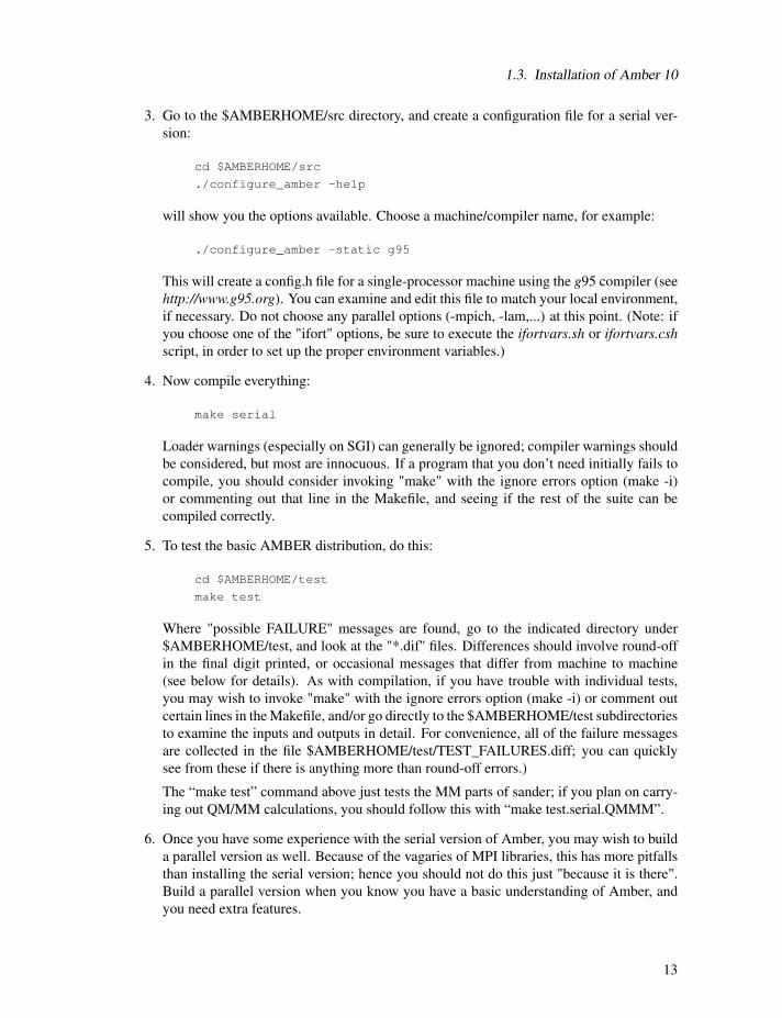
3. Go to the $AMBERHOME/src directory, and create a configuration file for a serial ver-
sion:
cd $AMBERHOME/src
./configure_amber -help
will show you the options available. Choose a machine/compiler name, for example:
./configure_amber -static g95
This will create a config.h file for a single-processor machine using the g95 compiler (seehttp://www.g95.org). You can examine and edit this file to match your local environment,if necessary. Do not choose any parallel options (-mpich, -lam,...) at this point. (Note: if
you choose one of the "ifort" options, be sure to execute the ifortvars.sh or ifortvars.cshscript, in order to set up the proper environment variables.)
4. Now compile everything:
make serial
Loader warnings (especially on SGI) can generally be ignored; compiler warnings should
be considered, but most are innocuous. If a program that you don’t need initially fails to
compile, you should consider invoking "make" with the ignore errors option (make -i)
or commenting out that line in the Makefile, and seeing if the rest of the suite can be
compiled correctly.
5. To test the basic AMBER distribution, do this:
cd $AMBERHOME/test
make test
Where "possible FAILURE" messages are found, go to the indicated directory under
$AMBERHOME/test, and look at the "*.dif" files. Differences should involve round-off
in the final digit printed, or occasional messages that differ from machine to machine
(see below for details). As with compilation, if you have trouble with individual tests,
you may wish to invoke "make" with the ignore errors option (make -i) or comment out
certain lines in theMakefile, and/or go directly to the $AMBERHOME/test subdirectories
to examine the inputs and outputs in detail. For convenience, all of the failure messages
are collected in the file $AMBERHOME/test/TEST_FAILURES.diff; you can quickly
see from these if there is anything more than round-off errors.)
The “make test” command above just tests the MM parts of sander; if you plan on carry-
ing out QM/MM calculations, you should follow this with “make test.serial.QMMM”.
6. Once you have some experience with the serial version of Amber, you may wish to build
a parallel version as well. Because of the vagaries of MPI libraries, this has more pitfalls
than installing the serial version; hence you should not do this just "because it is there".
Build a parallel version when you know you have a basic understanding of Amber, and
you need extra features.
13

1. Introduction
Also note this: you may want to build a parallel version even for a machine with asingle cpu. The free energy and empirical valence bond (EVB) facilities require a parallelinstallation, but these will generally run fine using two threads on a single-cpu machine.
It is also the case (especially if you have an Intel CPU with hyper-threading enabled)
that you will get a modest speedup by running an MPI job with two threads, even on a
machine with just one physical CPU.
To build a parallel version, do the following: First, you need to install an MPI library, if
one is not already present on your machine. We have included lam-7.1.3 in Amber10, and
recommend that you start with this if you are unfamiliar with MPI. Once that is working,
you can later replace it with something else if needed.
cd $AMBERHOME/src
make clean (important! don’t neglect this step)
./configure_amber -lamsource g95 (as an example)
./configure_lam (only needed if you used the -lamsource flag)
make parallel
This creates two new executables: sander.MPI and sander.LES.MPI. The serial versionswill still be available in $AMBERHOME/exe, just without the "MPI" extension.
To test parallel programs, you need first to set the DO_PARALLEL environment variable
as follows:
cd $AMBERHOME/test
setenv DO_PARALLEL ’mpirun -np 4’
make test.parallel.MM < /dev/null
The integer is the number of processors; if your command to run MPI jobs is something
different than mpirun (e.g. it is mpiexec for some MPI’s), use the command appropriatefor your machine. See the next section for the explanation of the input redirection in the
last command. As with the serial testing, the above commands test the MM portion of
sander; type “make test.parallel.QMMM” to test the QM/MM portions.
7. At this point, you should also compile the PMEMD (particle-mesh Ewald molecular
dynamics) program. (Note that, in spite of its name, this code now can do implicit solvent
GB calculations as well.) See Chapter 7 and $AMBERHOME/src/pmemd/README for
instructions.
1.3.1. More information on parallel machines or clusters
This section contains notes about the various parallel implementations supplied in the current
release. Only sander and pmemd are parallel programs; all others are single threaded. NOTE:Parallel machines and networks fail in unexpected ways. PLEASE check short parallel runs
against a single-processor version of Amber before embarking on long parallel simulations!
The MPI (message passing) version was initially developed by James Vincent and Ken Merz,
based on 4.0 and later an early prerelease 4.1 version. [14] This version was optimized, inte-
grated and extended by James Vincent, Dave Case, Tom Cheatham, Scott Brozell, and Mike
Crowley, with input from Thomas Huber, Asiri Nanyakkar, and Nathalie Godbout.
14

1.3. Installation of Amber 10
The bonds, angles, dihedrals, SHAKE (only on bonds involving hydrogen), nonbonded ener-
gies and forces, pairlist creation, and integration steps are parallelized. The code is pure SPMD
(single program multiple data) using a master/slave, replicated data model. Basically, the mas-
ter node does all of the initial set-up and performs all the I/O. Depending on the version and/or
what particular input options are chosen, either all the non-master nodes execute force() in par-allel, or all nodes do both the forces and the dynamics in parallel. Communication is done to
accumulate partial forces, update coordinates, etc.
For reasons we don’t understand, someMPI implementations require a null file for stdin, even
though sander doesn’t take any input from there. This is true for some SGI and HP machines.If you receive a message like "stopped, tty input", try the following:
mpirun -np <num-proc> sander.MPI [ options ] < /dev/null
1.3.2. Installing Non-Standard Features
The source files of some Amber programs contain multiple code paths. These code paths are
guarded by directives to the C preprocessor. All Amber programs regardless of source language
use the C preprocessor. The activation of non-standard features in guarded code paths can be
controlled at build time via the -D preprocessor option. For example, to enable the use of a
Lennard-Jones 10-12 potential with the sander program the HAS_10_12 preprocessor guard
must be activated with -DHAS_10_12.
To ease the installers burden we provide a hook into the build process. The hook is the envi-
ronment variable AMBERBUILDFLAGS. For example, to build sander with -DHAS_10_12,assuming that a correct configuration file has already been created, do the following:
cd $AMBERHOME/src/sander
make clean
make AMBERBUILDFLAGS=’-DHAS_10_12’ sander
Note that AMBERBUILDFLAGS is accessed by all stages of the build process: preprocess-
ing, compiling, and linking. In rare cases a stage may emit warnings for unknown options in
AMBERBUILDFLAGS; these may usually be ignored.
1.3.3. Installing on Microsoft Windows
All of Amber (including the X-windows parts) will compile and run on Windows using the
Cygwin development tools: see http://sources.redhat.com/cygwin. We recommend (certainlyas a first step) using the g95 compiler (see http://www.g95.org) along with the gcc compiler thatcomes with cygwin.
Note that Cygwin provides a POSIX-compatible environment for Windows. Effective use
of this environment requires a basic familiarity with the principles of Linux or Unix operating
systems. Building the Windows version is thus somewhat more complex (not simpler) than
building under other operating systems. You should only attempt this after you have a basicfamiliarity with the cygwin environment. The only MPI packages that seems to compile cleanly
under cygwin is LAM.
15

1. Introduction
1.3.4. Testing
We have installed and tested Amber 9 on a number of platforms, using UNIX, Linux, Mi-
crosoft Windows or Macintosh OSX operating systems. However, owing to time and access
limitations, not all combinations of code, compilers, and operating systems have been tested.
Therefore we recommend running the test suites.
The distribution contains a validation suite that can be used to help verify correctness. The
nature of molecular dynamics, is such that the course of the calculation is very dependent on
the order of arithmetical operations and the machine arithmetic implementation, i.e. the methodused for roundoff. Because each step of the calculation depends on the results of the previous
step, the slightest difference will eventually lead to a divergence in trajectories. As an initially
identical dynamics run progresses on two different machines, the trajectories will eventually
become completely uncorrelated. Neither of them are "wrong;" they are just exploring different
regions of phase space. Hence, states at the end of long simulations are not very useful for
verifying correctness. Averages are meaningful, provided that normal statistical fluctuations are
taken into account. "Different machines" in this context means any difference in floating point
hardware, word size, or rounding modes, as well as any differences in compilers or libraries.
Differences in the order of arithmetic operations will affect roundoff behavior; (a + b) + c is not
necessarily the same as a + (b + c). Different optimization levels will affect operation order,
and may therefore affect the course of the calculations.
All initial values reported as integers should be identical. The energies and temperatures
on the first cycle should be identical. The RMS and MAX gradients reported in sander are
often more precision sensitive than the energies, and may vary by 1 in the last figure on some
machines. In minimization and dynamics calculations, it is not unusual to see small divergences
in behavior after as little as 100-200 cycles.
1.3.5. Memory Requirements
The Amber 10 programs mainly use dynamic memory allocation, and do not generally need
to be compiled for any specific size of problem. Some sizes related to NMR refinements are
defined in nmr.h If you receive error messages directing you to look at these files, you may need
to edit them, then recompile.
If you get a "Killed" (or similar) message immediately upon starting a program (particularly
if this happens with no arguments), you may not have enough memory to run the program. The
"size" command will show you the size of the executable. Also check the limits of your shell;
you may need to increase these (especially stacksize, which is sometimes set to quite small
values).
1.4. Basic tutorials
AMBER is a suite of programs for use in molecular modeling and molecular simulations. It
consists of a substructure database, a force field parameter file, and a variety of useful programs.
Here we give some commented sample runs to provide an overview of how things are carried
out. The examples only cover a fraction of the things that it is possible to do with AMBER. The
formats of the example files shown are described in detail later in the manual, in the chapters
16

1.4. Basic tutorials
pertaining to the programs. Tom Cheatham, Bernie Brooks and Peter Kollman have prepared
some detailed information on simulation protocols that should also be consulted. [15]
Additional tutorial examples are available at http://amber.scripps.edu. Because the web canprovide a richer interface than one can get on the printed page (with screen shots, links to the
actual input and output files, etc.), most of our recent efforts have been devoted to updating the
tutorials on the web site. In particular, new users are advised to look at the following, which can
be found at both the web site listed above, and on the distribution CD, under amber10/tutorial.As a basic example, we consider here the minimization of a protein in a simple solvent model.
The procedure consists of three steps:
Step 1. Generate some starting coordinates.
The first step is to obtain starting coordinates. We begin with the bovine pancreatic trypsin
inhibitor, and consider the file 6pti.pdb, exactly as distributed by the Protein Data Bank. Thisfile (as with most PDB files) needs some editing before it can be used by Amber. First,alternate conformations are provided for residues 39 and 50, so we need to figure out which
one we want. For this example, we choose the "A" conformation, and manually edit the file to
remove the alternate conformers. Second, coordinates are provided for a phosphate group and
a variety of water molecules. These are not needed for the calculation we are pursuing here,
so we also edit the file to remove these. Third, the cysteine residues are involved in disulfide
bonds, and need to have their residue names changed in an editor from CYS to CYX to reflect
this. Finally, since we removed the phosphate groups, some of the CONECT records now
refer to non-existent atoms; if you are not sure that the CONECT records are all correct then
it may be safest to remove all of them, as we do for this example. Let’s call this modified file
6pti.mod.pdb.Although Amber tries hard to understand pdb-format files, it is typical to have to do some
manual editing before proceeding. A general prescription is: "keep running the loadPdb step inLEaP (see step 2, below), and editing the pdb file, until there are no error messages."
Step 2. Run LEaP to generate the parameter and topology file.
This is a fairly straightforward exercise in loading in the pdb file, adding the disulfide cross
links, and saving the resulting files. Typing the following commands should work in either tleapor xleap:
source leaprc.ff03
bpti = loadPdb 6pti.mod.pdb
bond bpti.5.SG bpti.55.SG
bond bpti.14.SG bpti.38.SG
bond bpti.30.SG bpti.51.SG
saveAmberParm bpti prmtop prmcrd
quit
Step 3. Perform some minimization.
Use this script:
17

1. Introduction
# Running minimization for BPTI
cat << eof > min.in
# 200 steps of minimization, generalized Born solvent model
&cntrl
maxcyc=200, imin=1, cut=12.0, igb=1, ntb=0, ntpr=10,
/
eof
sander -i min.in -o 6pti.min1.out -c prmcrd -r 6pti.min1.xyz
/bin/rm min.in
This will perform minimization (imin=1) for 200 steps (maxcyc), using a nonbonded cutoff of
12 Å(cut), a generalized Born solvent model (igb=1), and no periodic boundary (ntb=0); inter-
mediate results will be printed every 10 steps (ntpr). Text output will go to file 6pti.min1.out,and the final coordinates to file 6pti.min1.xyz. The "out" file is intended to be read by humans,and gives a summary of the input parameters and a history of the progress of the minimization.
Of course, Amber can do much more than the above minimization. This example illustrates
the basic information flow in Amber: Cartesian coordinate preparation (Step 1.), topology andforce field selection (Step 2.), and simulation program command specification (Step 3.). Typ-ically the subsequent steps are several stages of equilibration, production molecular dynamics
runs, and analyses of trajectories. The tutorials in amber10/tutorial should be consulted forexamples of these latter steps.
18
2. Sander basics
2.1. Introduction
This is a guide to sander, the Amber module which carries out energy minimization, molecu-lar dynamics, and NMR refinements. The acronym stands for Simulated Annealing with NMR-Derived EnergyRestraints, but this module is used for a variety of simulations that have nothingto do with NMR refinement. Some general features are outlined in the following paragraphs:
1. Sander provides direct support for several force fields for proteins and nucleic acids, andfor several water models and other organic solvents. The basic force field implemented
here has the following form, which is about the simplest functional form that preserves
the essential nature of molecules in condensed phases:
V (r) = ∑bonds
Kb(b−b0)2+ ∑angles
Kθ (θ −θo)2
+ ∑dihedrals
(Vn/2)(1+ cos[nφ −δ ]
+ ∑nonbi j
(Ai j/r12i j )− (Bi j/r6i j)+(qiq j/ri j)
"Non-additive" force fields based on atom-centered dipole polarizabilities can also be
used. These add a "polarization" term to what was given above:
Epol =−2∑i
μi ·Eio
where μi is an induced atomic dipole. In addition, charges that are not centered on atoms,
but are off-center (as for lone-pairs or "extra points") can be included in the force field.
2. The particle-mesh Ewald (PME) procedure (or, optionally, a "true" Ewald sum) is used to
handle long-range electrostatic interactions. Long-range van der Waals interactions are
estimated by a continuum model. Biomolecular simulations in the NVE ensemble (i.e.with Newtonian dynamics) conserve energy well over multi-nanosecond runs without
modification of the equations of motion.
3. Two periodic imaging geometries are included: rectangular parallelepiped and truncated
octahedron (box with corners chopped off). (Sander itself can handle many other periodically-replicating boxes, but input and output support in LEaP and ptraj is only available rightnow for these two.) The size of the repeating unit can be coupled to a given external pres-
sure, and velocities can be coupled to a given external temperature by several schemes.
19

2. Sander basics
The external conditions and coupling constants can be varied over time, so various simu-
lated annealing protocols can be specified in a simple and flexible manner.
4. It is also possible to carry out non-periodic simulations in which aqueous solvation ef-
fects are represented implicitly by a generalized Born/ surface area model by adding thefollowing two terms to the "vacuum" potential function:
ΔGsol = ∑i j
(1− 1ε)(qiq j/ fGB(ri j)+A∑
iσi
The first term accounts for the polar part of solvation (free) energy, designed to provide
an approximation for the reaction field potential, and the second represents the non-polar
contribution which is taken to be proportional to the surface area of the molecule.
5. Users can define internal restraints on bonds, valence angles, and torsions, and the force
constants and target values for the restraints can vary during the simulation. The rela-
tive weights of various terms in the force field can be varied over time, allowing one to
implement a variety of simulated annealing protocols in a single run.
6. Internal restraints can be defined to be "time-averaged", that is, restraint forces are applied
based on the averaged value of an internal coordinate over the course of the dynamics tra-
jectory, not only on its current value. Alternatively, restraints can be "ensemble-averaged"
using the locally-enhanced-sampling (LES) option.
7. Restraints can be directly defined in terms of NOESY intensities (calculated with a relax-
ation matrix technique), residual dipolar couplings, scalar coupling constants and proton
chemical shifts. There are provisions for handling overlapping peaks or ambiguous as-
signments. In conjunction with distance and angle constraints, this provides a powerful
and flexible approach to NMR structural refinements.
8. Replica exchange calculations can allow simultaneous sampling at a variety of conditions
(such as temperature), and allow the user to construct Boltzmann samples in ways that
converge more quickly than standard MD simulations. Other variants of biased MD
simulations can also be used to improve sampling.
9. Restraints can also be defined in terms of the root-mean-square coordinate distance from
some reference structure. This allows one to bias trajectories either towards or away from
some target. Free energies can be estimated from non-equilibrium simulations based on
targetting restraints.
10. Free energy calculations, using thermodynamic integration (TI) with a linear or non-
linear mixing of the "unperturbed" and "perturbed" Hamiltonian, can be carried out. Al-
ternatively, potentials of mean force can be computed using umbrella sampling.
11. The empirical valence bond (EVB) scheme can be used to mix "diabatic" states into a
potential that can represent many types of chemical reactions that take place in enzymes.
12. QMMM Calculations where part of the system can be treated quantum mechanically
allowing bond breaking and formation during a simulation. Semi-empirical and DFTB
Hamiltonians are provided.
20

2.2. Credits
13. Nuclear quantum effects can be included through path-integral molecular dynamics (PIMD)
simulations, and estimates of quantum time-correlation functions can be computed.
2.2. Credits
Since sander forms the core of the Amber simulation programs, almost everyone on thetitle page of this manual has contributed to it in one way or another. A detailed breakdown
of contributions can be found at http://ambermd.org/contributors.html. A general history ofsander and its components can also be found in Refs. [3, 4].
2.3. File usage
sander [-help] [-O] [-A] -i mdin -o mdout -p prmtop -c inpcrd -r restrt
-ref refc -x mdcrd -y inptraj -v mdvel -e mden -inf mdinfo -radii radii
-cpin cpin -cpout cpout -cprestrt cprestrt -evbin evbin
-O Overwrite output files if they exist.
-A Append output files if they exist, (used mainly for replica exchange).
Here is a brief description of the files referred to above; the first five files are used for every run,
whereas the remainder are only used when certain options are chosen.
mdin input control data for the min/md run
mdout output user readable state info and diagnostics -o stdout will send output to stdout (tothe terminal) instead of to a file.
mdinfo output latest mdout-format energy info
prmtop input molecular topology, force field, periodic box type, atom and residue names
inpcrd input initial coordinates and (optionally) velocities and periodic box size
refc input (optional) reference coords for position restraints; also used for targeted MD
mdcrd output coordinate sets saved over trajectory
inptraj input input coordinate sets in trajectory format, when imin=5
mdvel output velocity sets saved over trajectory
mden output extensive energy data over trajectory
restrt output final coordinates, velocity, and box dimensions if any - for restarting run
inpdip input polarizable dipole file, when indmeth=3
rstdip output polarizable dipole file, when indmeth=3
cpin input protonation state definitions
21

2. Sander basics
cprestrt protonation state definitions, final protonation states for restart (same format as cpin)
cpout output protonation state data saved over trajectory
evbin input input for EVB potentials
2.4. Example input files
Here are a couple of sample files, just to establish a basic syntax and appearance. There are
more examples of NMR-related files later in this chapter.
1. Simple restrained minimization
Minimization with Cartesian restraints
&cntrl
imin=1, maxcyc=200, (invoke minimization)
ntpr=5, (print frequency)
ntr=1, (turn on Cartesian restraints)
restraint_wt=1.0, (force constant for restraint)
restraintmask=’:1-58’, (atoms in residues 1-58 restrained)
/
2. "Plain" molecular dynamics run
molecular dynamics run
&cntrl
imin=0, irest=1, ntx=5, (restart MD)
ntt=3, temp0=300.0, gamma_ln=5.0, (temperature control)
ntp=1, taup=2.0, (pressure control)
ntb=2, ntc=2, ntf=2, (SHAKE, periodic bc.)
nstlim=500000, (run for 0.5 nsec)
ntwe=100, ntwx=1000, ntpr=200, (output frequency)
/
3. Self-guided Langevin dynamics run
Self-guided Langevin dynamics run
&cntrl
imin=0, irest=0, ntx=1, (start LD)
ntt=3, temp0=300.0,gamma_ln=1.0 (temperature control)
ntc=3, ntf=3, (SHAKE)
nstlim=500000, (run for 0.5 nsec)
ntwe=100, ntwx=1000, ntpr=200, (output frequency)
isgld=1, tsgavg=0.2,tempsg=1.0 (SGLD)
/
22

2.5. Overview of the information in the input file
2.5. Overview of the information in the input file
General minimization and dynamics input
One or more title lines, followed by the (required) &cntrl and (optional) &pb, &ewald,
&qmmm, &amoeba or &debugf namelist blocks. Described in Sections 2.6 and 2.7.
Varying conditions
Parameters for changing temperature, restraint weights, etc. during the MD run. Each
parameter is specified by a separate &wt namelist block, ending with &wt type=’END’,
/. Described in Section 2.8.
File redirection
TYPE=filename lines. Section ends with the first non-blank line which does not corre-spond to a recognized redirection. Described in Section 2.9.
Group information
Read if ntr, ibelly or idecomp are set to non-zero values, and if some other conditions aresatisfied; see sections on these variables, below. Described in Appendix B.
2.6. General minimization and dynamics parameters
Each of the variables listed below is input in a namelist statement with the namelist identifier
&cntrl. You can enter the parameters in any order, using keyword identifiers. Variables that are
not given in the namelist input retain their default values. Support for namelist input is included
in almost all current Fortran compilers, and is a standard feature of Fortran 90. A detailed
description of the namelist convention is given in Appendix A.
In general, namelist input consists of an arbitrary number of comment cards, followed by a
record whose first seven characters after a " &" (e.g. " &cntrl ") name a group of variables that
can be set by name. This is followed by statements of the form " maxcyc=500, diel=2.0, ... ",
and is concluded by an " / " token. The first line of input contains a title, which is then followed
by the &cntrl namelist. Note that the first character on each line of a namelist block must be a
blank.
Some of the options and variables are much more important, and commonly modified, than
are others. We have denoted the "common" options by printing them in boldface below. Ingeneral, you can skip reading about the non-bold options on a first pass, and you should change
these from their defaults only if you think you know what you are doing.
2.6.1. General flags describing the calculation
imin Flag to run minimization
= 0 No minimization (only do molecular dynamics; default)
= 1 Perform minimization (and no molecular dynamics)
23

2. Sander basics
= 5 Read in a trajectory for analysis.
Although sander will write energy information in the output files (using ntpr),it is often desirable to calculate the energies of a set of structures at a later
point. In particular, one may wish to post-process a set of structures using a
different energy function than was used to generate the structures. A exam-
ple of this is MM-PBSA analysis, where the explicit water is removed and
replaced with a continuum model.
When imin is set to 5 sander will expect to read a trajectory file from the
inptraj file (specified using -y on the command line), and will perform the
functions described in the mdin file for each of the structures in the trajectoryfile. The final structures from each minimization will be written to the normal
mdcrd file.For example, when imin=5 and maxcyc=1000, sander will minimize eachstructure in the trajectory for 1000 steps and write a minimized coordinate
set for each frame to the mdcrd file. If maxcyc=1, then the output file can beused to extract the energies of each of the coordinate sets in the inptraj file.
nmropt
= 0 no nmr-type analysis will be done; default.
> 0 NMR restraints/weight changes will be read
= 2 NOESY volume, chemical shift or residual dipolar restraints will be read as
well
2.6.2. Nature and format of the input
ntx Option to read the initial coordinates, velocities and box size from the "inpcrd" file.
The options 1-2 must be used when one is starting from minimized or model-built
coordinates. If an MD restrt file is used as inpcrd, then options 4-7 may be used.
Only options 1 and 5 are in common use.
= 1 X is read formatted with no initial velocity information (default)
= 2 X is read unformatted with no initial velocity information
= 4 X and V are read unformatted.
= 5 X and V are read formatted; box information will be read if ntb>0. The ve-locity information will only be used if irest=1.
= 6 X, V and BOX(1..3) are read unformatted; in other respects, this is the same
as option "5".
irest Flag to restart the run.
= 0 No effect (default)
= 1 restart calculation. Requires velocities in coordinate input file, so you also
may need to reset NTX if restarting MD
24

2.6. General minimization and dynamics parameters
ntrx Format of the Cartesian coordinates for restraint from file "refc". Note: the pro-
gram expects file "refc" to contain coordinates for all the atoms in the system. A
subset for the actual restraints is selected by restraintmask in the control namelist.
= 0 Unformatted (binary) form
= 1 Formatted (ascii, default) form
2.6.3. Nature and format of the output
ntxo Format of the final coordinates, velocities, and box size (if constant volume or
pressure run) written to file "restrt".
= 0 Unformatted (no longer recommended or allowed: please use formatted restart
files)
= 1 Formatted (default).
ntpr Every NTPR steps energy information will be printed in human-readable form to
files "mdout" and "mdinfo". "mdinfo" is closed and reopened each time, so it
always contains the most recent energy and temperature. Default 50.
ntave Every NTAVE steps of dynamics, running averages of average energies and fluc-
tuations over the last NTAVE steps will be printed out. Default value of 0 disables
this printout. Setting NTAVE to a value 1/2 or 1/4 of NSTLIM provides a simple
way to look at convergence during the simulation.
ntwr Every NTWR steps during dynamics, the "restrt" file will be written, ensuring that
recovery from a crash will not be so painful. In any case, restrt is written every
NSTLIM steps for both dynamics and minimization calculations. If NTWR<0, aunique copy of the file, restrt_nstep, is written every abs(NTWR) steps. This option
is useful if for example one wants to run free energy perturbations from multiple
starting points or save a series of restrt files for minimization. Default 500.
iwrap If set to 1, the coordinates written to the restart and trajectory files will be "wrapped"
into a primary box. This means that for each molecule, the image closest to the
middle of the "primary box" [with x coordinates between 0 and a, y coordinates
between 0 and b, and z coordinates between 0 and c] will be the one written to the
output file. This often makes the resulting structures look better visually, but has
no effect on the energy or forces. Performing such wrapping, however, can mess
up diffusion and other calculations. The default (when iwrap=0) is to not performany such manipulations; in this case it is typical to use ptraj as a post-processingprogram to translate molecules back to the primary box. For very long runs, set-
ting iwrap=1 may be required to keep the coordinate output from overflowing thetrajectory and restart file formats.
ntwx Every NTWX steps the coordinates will be written to file "mdcrd". NTWX=0
inhibits all output. Default 0.
25

2. Sander basics
ntwv Every NTWV steps the velocities will be written to file "mdvel". NTWV=0 inhibits
all output. Default 0. NTWV=-1 will write velocities into a combined coordinate
and velocity file "mdcrd" at the interval defined by NTWX. This option is available
only for binary NetCDF output (IOUTFM=1). Most users will have no need to
write a velocity file and so can safely leave NTWV at the default of zero.
ntwe Every NTWE steps the energies and temperatures will be written to file "mden" in
compact form. NTWE=0 inhibits all output. Default 0.
ioutfm Format of velocity and coordinate sets. As of Amber 9, the binary format used in
previous versions is no longer supported; binary output is now in NetCDF trajec-
tory format. Binary trajectory files are smaller, higher precision and much faster to
read and write than formatted trajectories.
= 0 Formatted (default)
= 1 Binary NetCDF trajectory
ntwprt Coordinate/velocity archive limit flag. This flag can be used to decrease the size ofthe coordinate / velocity archive files, by only including that portion of the system of
greatest interest. (E.g. one can print only the solute and not the solvent, if so desired).
The Coord/velocity archives will include:
= 0 all atoms of the system (default).
> 0 only atoms 1→NTWPRT.
idecomp Flag for setting an energy decomposition scheme. In former distributions this option
was only really useful in conjunction with mm_pbsa, where it is turned on automatically
if required. Now, a decomposition of 〈∂V/∂λ 〉 on a per-residue basis in thermodynamicintegration (TI) simulations is also possible. [16] The options are:
= 0 Do nothing (default).
= 1 Decompose energies on a per-residue basis; 1-4 EEL + 1-4 VDW are added to inter-
nal (bond, angle, dihedral) energies. (Not available in TI.)
= 2 Decompose energies on a per-residue basis; 1-4 EEL + 1-4 VDW are added to EEL
and VDW. (Not available in TI.)
= 3 Decompose energies on a pairwise per-residue basis; the rest is equal to "1".
= 4 Decompose energies on a pairwise per-residue basis; the rest is equal to "2".
If decomp is switched on, residues may be chosen by the RRES and/or LRES card. The
RES card determines about which residues information is finally output. See chapters 4.1
or 8 for more information. Use of idecomp > 0 is incompatible with ntr > 0 or ibelly >0.
26

2.6. General minimization and dynamics parameters
2.6.4. Frozen or restrained atoms
ibelly Flag for belly type dynamics. If set to 1, a subset of the atoms in the system will
be allowed to move, and the coordinates of the rest will be frozen. The movingatoms are specified bellymask. This option is not available when igb>0. Note alsothat this option does not provide any significant speed advantage, and is maintainedprimarily for backwards compatibility with older version of Amber. Most applica-
tions should use the ntr variable instead to restrain parts of the system to stay closeto some initial configuration. Default = 0.
ntr Flag for restraining specified atoms in Cartesian space using a harmonic potential,
if ntr > 0. The restrained atoms are determined by the restraintmask string. Theforce constant is given by restraint_wt. The coordinates are read in "restrt" formatfrom the "refc" file (see NTRX, above). Default = 0.
restraint_wt The weight (in kcal/mol−Å2) for the positional restraints. The restraint is of theform k(Δx)2, where k is the value given by this variable, and Δx is the differencebetween one of the Cartesian coordinates of a restrained atom and its reference
position. There is a term like this for each Cartesian coordinate of each restrainted
atom.
restraintmask String that specifies the restrained atoms when ntr=1.
bellymask String that specifies the moving atoms when ibelly=1.
The syntax for both restraintmask and bellymask is given in Section 11.3. Notethat these mask strings are limited to a maximum of 256 characters.
2.6.5. Energy minimization
maxcyc The maximum number of cycles of minimization. Default = 1.
ncyc If NTMIN is 1 then the method of minimization will be switched from steepest
descent to conjugate gradient after NCYC cycles. Default 10.
ntmin Flag for the method of minimization.
= 0 Full conjugate gradient minimization. The first 4 cycles are steepest descent at
the start of the run and after every nonbonded pairlist update.
= 1 For NCYC cycles the steepest descent method is used then conjugate gradient
is switched on (default).
= 2 Only the steepest descent method is used.
= 3 The XMIN method is used, see Section 4.9.3.
= 4 The LMOD method is used, see Section 4.9.4.
dx0 The initial step length. If the initial step length is too big then will give a huge
energy; however the minimizer is smart enough to adjust itself. Default 0.01.
drms The convergence criterion for the energy gradient: minimization will halt when
the root-mean-square of the Cartesian elements of the gradient is less than DRMS.
Default 1.0E-4 kcal/mole-Å
27

2. Sander basics
2.6.6. Molecular dynamics
nstlim Number of MD-steps to be performed. Default 1.
nscm Flag for the removal of translational and rotational center-of-mass (COM) motion
at regular intervals (default is 1000). For non-periodic simulations, after every
NSCM steps, translational and rotational motion will be removed. For periodic
systems, just the translational center-of-mass motion will be removed. This flag is
ignored for belly simulations.
For Langevin dynamics, the position of the center-of-mass of the molecule is re-set to zero every NSCM steps, but the velocities are not affected. Hence there
is no change to either the translation or rotational components of the momenta.
(Doing anything else would destroy the way in which temperature is regulated in
a Langevin dynamics system.) The only reason to even reset the coordinates is to
prevent the molecule from diffusing so far away from the origin that its coordinates
overflow the format used in restart or trajectory files.
t The time at the start (psec) this is for your own reference and is not critical. Start
time is taken from the coordinate input file if IREST=1. Default 0.0.
dt The time step (psec). Recommended MAXIMUM is .002 if SHAKE is used, or
.001 if it isn’t. Note that for temperatures above 300K, the step size should be
reduced since greater temperatures mean increased velocities and longer distance
traveled between each force evaluation, which can lead to anomalously high ener-
gies and system blowup. Default 0.001.
nrespa This variable allows the user to evaluate slowly-varying terms in the force field
less frequently. For PME, "slowly-varying" (now) means the reciprocal sum. For
generalized Born runs, the "slowly-varying" forces are those involving derivatives
with respect to the effective radii, and pair interactions whose distances are greater
than the "inner" cutoff, currently hard-wired at 8 Å. If NRESPA>1 these slowly-varying forces are evaluated every nrespa steps. The forces are adjusted appropri-ately, leading to an impulse at that step. If nrespa*dt is less than or equal to 4 fsthe energy conservation is not seriously compromised. However if nrespa*dt > 4
fs the simulation becomes less stable. Note that energies and related quantities are
only accessible every nrespa steps, since the values at other times are meaningless.
2.6.7. Self-Guided Langevin dynamics
Self-guided Langevin dynamics (SGLD) can be used to enhance conformational search ef-
ficiency in either a molecular dynamics (MD) simulation (when gamma_ln=0) or Langevindynamics (LD) simulation (when gamma_ln>0). This method applies a guiding force calcu-lated during a simulation to accelerate the systematic motion for more efficient conformational
sampling. [17] The guiding force can be applied to a part of a simulation system starting from
atom isgsta to atom isgend. The strength of the guiding force is defined by either tempsg orsgft. A smaller tempsg or sgft will produce results closer to a normal MD or LD simulation.Normally, tempsg or sgft is set to the limit that accelerates slow events to an affordable timescale.
28
2.6. General minimization and dynamics parameters
isgld The default value of zero disables self-guiding; a positive value enables this feature.
tsgavg Local averaging time (psec) for the guiding force calculation. Default 0.2 psec. Alarger value defines a slower motion to be enhanced.
tempsg Guiding temperature (K). Defines the strength of the guiding force in tempera-ture unit. Default 1.0 K. The default value is recommended for a noticeable en-
hancement in conformational search. Once tempsg is set, sgft will fluctuate and beprinted out in the output file.
sgft Guiding factor. Defines the strength of the guiding force when tempsg=0. Default0.0. tempsg>0 will override sgft. Because sgft varies with systems and simulationconditions, it is recommended to read sgft values from the output file of a SGLDsimulation with tempsg=1 K. Setting tempsg=0 K and sgft=0.0 will reduce thesimulation to a normal MD or LD. Only experienced users should use the sgftvariable; for most purposes, setting tempsg should be sufficient.
isgsta The first atom index of SGLD region. Default 1.
isgend The last atom index of SGLD region. Default is natom.
2.6.8. Temperature regulation
ntt Switch for temperature scaling. Note that setting ntt=0 corresponds to the micro-canonical (NVE) ensemble (which should approach the canonical one for large
numbers of degrees of freedom). Some aspects of the "weak-coupling ensemble"
(ntt=1) have been examined, and roughly interpolate between the microcanoni-cal and canonical ensembles. [18, 19] The ntt=2 and 3 options correspond to thecanonical (constant T) ensemble.
= 0 Constant total energy classical dynamics (assuming that ntb<2, as shouldprobably always be the case when ntt=0).
= 1 Constant temperature, using the weak-coupling algorithm. [20] A single scal-
ing factor is used for all atoms. Note that this algorithm just ensures that the
total kinetic energy is appropriate for the desired temperature; it does nothing
to ensure that the temperature is even over all parts of the molecule. Atomic
collisions will tend to ensure an even temperature distribution, but this is not
guaranteed, and there are many subtle problems that can arise with weak tem-
perature coupling. [21] Using ntt=1 is especially dangerous for generalizedBorn simulations, where there are no collisions with solvent to aid in ther-
malization.) Other temperature coupling options (especially ntt=3) should beused instead.
= 2 Andersen temperature coupling scheme, [22] in which imaginary "collisions"
randomize the velocities to a distribution corresponding to temp0 every vrandsteps. Note that in between these "massive collisions", the dynamics is New-
tonian. Hence, time correlation functions (etc.) can be computed in these
sections, and the results averaged over an initial canonical distribution. Note
also that too high a collision rate (too small a value of vrand) will slow down
29

2. Sander basics
the speed at which the molecules explore configuration space, whereas too
low a rate means that the canonical distribution of energies will be sampled
slowly. A discussion of this rate is given by Andersen. [23]
= 3 Use Langevin dynamics with the collision frequency γ given by gamma_ln,discussed below. Note that when γ has its default value of zero, this is thesame as setting ntt = 0. Since Langevin simulations are potentially susceptibleto "synchronization" artifacts, [24] you should explicitly set the ig variable(described below) to a different value at each restart of a given simulation.
temp0 Reference temperature at which the system is to be kept, if ntt > 0. Note that for
temperatures above 300K, the step size should be reduced since increased distance
traveled between evaluations can lead to SHAKE and other problems. Default 300.
temp0les This is the target temperature for all LES particles (see Chapter 6). If temp0les<0,a single temperature bath is used for all atoms, otherwise separate thermostats
are used for LES and non-LES particles. Default is -1, corresponding to a sin-
gle (weak-coupling) temperature bath.
tempi Initial temperature. For the initial dynamics run, (NTX .lt. 3) the velocities are
assigned from a Maxwellian distribution at TEMPI K. If TEMPI = 0.0, the veloci-
ties will be calculated from the forces instead. TEMPI has no effect if NTX .gt. 3.
Default 0.0.
ig The seed for the pseudo-random number generator. The MD starting velocity is
dependent on the random number generator seed if NTX .lt. 3 .and. TEMPI .ne.
0.0. The value of this seed also affects the set of pseudo-random values used for
Langevin dynamics or Andersen coupling, and hence should be set to a different
value on each restart if ntt = 2 or 3. Default 71277. If ig=-1, the random seed willbe based on the current date and time, and hence will be different for every run.
tautp Time constant, in ps, for heat bath coupling for the system, if ntt = 1. Default is 1.0.Generally, values for TAUTP should be in the range of 0.5-5.0 ps, with a smaller
value providing tighter coupling to the heat bath and, thus, faster heating and a
less natural trajectory. Smaller values of TAUTP result in smaller fluctuations in
kinetic energy, but larger fluctuations in the total energy. Values much larger than
the length of the simulation result in a return to constant energy conditions.
gamma_ln The collision frequency γ , in ps−1, when ntt = 3. A simple Leapfrog integrator isused to propagate the dynamics, with the kinetic energy adjusted to be correct for
the harmonic oscillator case. [25, 26] Note that it is not necessary that γ approxi-mate the physical collision frequency, which is about 50 ps−1 for liquid water. Infact, it is often advantageous, in terms of sampling or stability of integration, to use
much smaller values, around 2 to 5 ps−1. [26, 27] Default is 0.
vrand If vrand>0 and ntt=2, the velocities will be randomized to temperature TEMP0every vrand steps.
30

2.6. General minimization and dynamics parameters
vlimit If not equal to 0.0, then any component of the velocity that is greater than abs(VLIMIT)
will be reduced to VLIMIT (preserving the sign). This can be used to avoid occa-
sional instabilities in molecular dynamics runs. VLIMIT should generally be set to
a value like 20 (the default), which is well above the most probable velocity in a
Maxwell-Boltzmann distribution at room temperature. A warning message will be
printed whenever the velocities are modified. Runs that have more than a few such
warnings should be carefully examined.
2.6.9. Pressure regulation
In "constant pressure" dynamics, the volume of the unit cell is adjusted (by small amounts
on each step) to make the computed pressure approach the target pressure, pres0. Equilibrationwith ntp > 0 is generally necessary to adjust the density of the system to appropriate values.
Note that fluctuations in the instantaneous pressure on each step will appear to be large (several
hundred bar), but the average value over many steps should be close to the target pressure.
Pressure regulation only applies when Constant Pressure periodic boundary conditions are used
(ntb = 2). Pressure coupling algorithms used in Amber are of the "weak-coupling" variety,analogous to temperature coupling. [20] Please note: in general you will need to equilibrate
the temperature to something like the final temperature using constant volume (ntp=0) beforeswitching on constant pressure simulations to adjust the system to the correct density. If you
fail to do this, the program will try to adjust the density too quickly, and bad things (such as
SHAKE failures) are likely to happen.
ntp Flag for constant pressure dynamics. This option should be set to 1 or 2 when
Constant Pressure periodic boundary conditions are used (NTB = 2).
= 0 Used with NTB not = 2 (default); no pressure scaling
= 1 md with isotropic position scaling
= 2 md with anisotropic (x-,y-,z-) pressure scaling: this should only be used with
orthogonal boxes (i.e. with all angles set to 90 o ). Anisotropic scaling is
primarily intended for non-isotropic systems, such as membrane simulations,
where the surface tensions are different in different directions; it is generally
not appropriate for solutes dissolved in water.
pres0 Reference pressure (in units of bars, where 1 bar 1 atm) at which the system is
maintained ( when NTP > 0). Default 1.0.
comp compressibility of the system when NTP> 0. The units are in 1.0E-06/bar; a value
of 44.6 (default) is appropriate for water.
taup Pressure relaxation time (in ps), when NTP > 0. The recommended value is be-
tween 1.0 and 5.0 psec. Default value is 1.0, but larger values may sometimes be
necessary (if your trajectories seem unstable).
31
2. Sander basics
2.6.10. SHAKE bond length constraints
ntc Flag for SHAKE to perform bond length constraints. [28] (See also NTF in the
Potential function section. In particular, typically NTF = NTC.) The SHAKEoption should be used for most MD calculations. The size of the MD timestep
is determined by the fastest motions in the system. SHAKE removes the bond
stretching freedom, which is the fastest motion, and consequently allows a larger
timestep to be used. For water models, a special "three-point" algorithm is used.
[29] Consequently, to employ TIP3P set NTF = NTC = 2.
Since SHAKE is an algorithm based on dynamics, the minimizer is not aware of
what SHAKE is doing; for this reason, minimizations generally should be carried
out without SHAKE. One exception is short minimizations whose purpose is to
remove bad contacts before dynamics can begin.
For parallel versions of sander only intramolecular atoms can be constrained. Thus,such atoms must be in the same chain of the originating PDB file.
= 1 SHAKE is not performed (default)
= 2 bonds involving hydrogen are constrained
= 3 all bonds are constrained (not available for parallel or qmmm runs in sander)
tol Relative geometrical tolerance for coordinate resetting in shake. Recommended
maximum: <0.00005 Angstrom Default 0.00001.
jfastw Fast water definition flag. By default, the system is searched for water residues,
and special routines are used to SHAKE these systems. [29]
= 0 Normal operation. Waters are identified by the default names (given below),
unless they are redefined, as described below.
= 4 Do not use the fast SHAKE routines for waters.
The following variables allow redefinition of the default residue and atom names
used by the program to determine which residues are waters.
WATNAM The residue name the program expects for water. Default ’WAT ’.
OWTNM The atom name the program expects for the oxygen of water. Default ’O
’.
HWTNM1 The atom name the program expects for the 1st H of water. Default ’H1
’.
HWTNM2 The atom name the program expects for the 2nd H of water. Default
’H2 ’.
noshakemask String that specifies atoms that are not to be shaken (assuming that ntc>1). Anybond that would otherwise be shaken by virtue of the ntc flag, but which involves anatom flagged here, will *not* be shaken. The syntax for this string is given in Chap.
13.5. Default is an empty string, which matches nothing. A typical use would be
to remove SHAKE constraints from all or part of a solute, while still shaking rigid
32

2.6. General minimization and dynamics parameters
water models like TIPnP or SPC/E. Another use would be to turn off SHAKE
constraints for the parts of the system that are being changed with thermodynamic
integration, or which are the EVB or quantum regions of the system.
If this option is invoked, then all parts of the potential must be evaluated, that is,
ntf must be one. The code enforces this by setting ntf to 1 when a noshakemaskstring is present in the input.
If you want the noshakemask to apply to all or part of the water molecules, you mustalso set jfastw=4, to turn off the special code for water SHAKE. (If you are notshaking waters, you presumably also want to issue the "set default FlexibleWater
on" command in LEaP; see that chapter for more information.)
2.6.11. Water cap
ivcap Flag to control cap option. The "cap" refers to a spherical portion of water centered
on a point in the solute and restrained by a soft half-harmonic potential. For the
best physical realism, this option should be combined with igb=10, in order toinclude the reaction field of waters that are beyond the cap radius.
= 0 Cap will be in effect if it is in the prmtop file (default).
= 1 With this option, a cap can be excised from a larger box of water. For this,
cutcap (i.e., the radius of the cap), xcap, ycap, and zcap (i.e., the location
of the center of the cap) need to be specified in the &cntrl namelist. Note
that the cap parameters must be chosen such that the whole solute is covered
by solvent. Solvent molecules (and counterions) located outside the cap are
ignored. Although this option also works for minimization and dynamics
calculations in general, it is intended to post-process snapshots in the realm
of MM-PBSA to get a linear-response approximation of the solvation free
energy, output as ’Protein-solvent interactions’.
= 2 Cap will be inactivated, even if parameters are present in the prmtop file.
= 5 With this option, a shell of water around a solute can be excised from a larger
box of water. For this, cutcap (i.e., the thickness of the shell) needs to be
specified in the &cntrl namelist. Solvent molecules (and counterions) located
outside the cap are ignored. This option only works for a single-step mini-
mization. It is intended to post-process snapshots in the realm of MM-PBSA
to get a linear-response approximation of the solvation free energy, output as
’Protein-solvent interactions’.
fcap The force constant for the cap restraint potential.
cutcap Radius of the cap, if ivcap=1 is used.
xcap,ycap,zcap Location of the cap center, if ivcap=1 is used.
33
2. Sander basics
2.6.12. NMR refinement options
(Users to should consult the section NMR refinement to see the context of how the following
parameters would be used.)
iscale Number of additional variables to optimize beyond the 3N structural parameters.
(Default = 0). At present, this is only used with residual dipolar coupling and CSA
or pseudo-CSA restraints.
noeskp The NOESY volumes will only be evaluated if mod(nstep, noeskp) = 0; otherwise
the last computed values for intensities and derivatives will be used. (default = 1,
i.e. evaluate volumes at every step)
ipnlty This parameter determines the the functional form of the penalty function for
NOESY volume and chemical shift restraints.
= 1 the program will minimize the sum of the absolute values of the errors; this is
akin to minimizing the crystallographic R-factor (default).
= 2 the program will optimize the sum of the squares of the errors.
= 3 For NOESY intensities, the penalty will be of the form awt[I1/6c −I1/6o ]2. Chem-ical shift penalties will be as for ipnlty=1.
mxsub Maximum number of submolecules that will be used. This is used to determine
how much space to allocate for the NOESY calculations. Default 1.
scalm "Mass" for the additional scaling parameters. Right now they are restricted to all
have the same value. The larger this value, the slower these extra variables will
respond to their environment. Default 100 amu.
pencut In the summaries of the constraint deviations, entries will only be made if the
penalty for that term is greater than PENCUT. Default 0.1.
tausw For noesy volume calculations (NMROPT = 2), intensities with mixing times lessthat TAUSW (in seconds) will be computed using perturbation theory, whereas
those greater than TAUSWwill use a more exact theory. See the theory section (be-
low) for details. To always use the "exact" intensities and derivatives, set TAUSW
= 0.0; to always use perturbation theory, set TAUSW to a value larger than the
largest mixing time in the input. Default is TAUSW of 0.1 second, which should
work pretty well for most systems.
2.7. Potential function parameters
The parameters in this section generally control what sort of force field (or potential function)
is used for the simulation.
34

2.7. Potential function parameters
2.7.1. Generic parameters
ntf Force evaluation. Note: If SHAKE is used (see NTC), it is not necessary to calcu-
late forces for the constrained bonds.
= 1 complete interaction is calculated (default)
= 2 bond interactions involving H-atoms omitted (use with NTC=2)
= 3 all the bond interactions are omitted (use with NTC=3)
= 4 angle involving H-atoms and all bonds are omitted
= 5 all bond and angle interactions are omitted
= 6 dihedrals involving H-atoms and all bonds and all angle interactions are omit-
ted
= 7 all bond, angle and dihedral interactions are omitted
= 8 all bond, angle, dihedral and non-bonded interactions are omitted
ntb Periodic boundary. If NTB .EQ. 0 then a boundary is NOT applied regardless of
any boundary condition information in the topology file. The value of NTB speci-
fies whether constant volume or constant pressure dynamics will be used. Options
for constant pressure are described in a separate section below.
= 0 no periodicity is applied and PME is off
= 1 constant volume (default)
= 2 constant pressure
If NTB .NE. 0, there must be a periodic boundary in the topology file. Constant
pressure is not used in minimization (IMIN=1, above).
For a periodic system, constant pressure is the only way to equilibrate density if the
starting state is not correct. For example, the solvent packing scheme used in LEaP
can result in a net void when solvent molecules are subtracted which can aggregate
into "vacuum bubbles" in a constant volume run. Another potential problem are
small gaps at the edges of the box. The upshot is that almost every system needs
to be equilibrated at constant pressure (ntb=2, ntp>0) to get to a proper density.But be sure to equilibrate first (at constant volume) to something close to the final
temperature, before turning on constant pressure.
dielc Dielectric multiplicative constant for the electrostatic interactions. Default is 1.0.
Please note this is NOT related to dielectric constants for generalized Born simu-
lations.
cut This is used to specify the nonbonded cutoff, in Angstroms. For PME, the cutoff
is used to limit direct space sum, and the default value of 8.0 is usually a good
value. When igb>0, the cutoff is used to truncate nonbonded pairs (on an atom-by-atom basis); here a larger value than the default is generally required. A separate
parameter (RGBMAX) controls the maximum distance between atom pairs that
will be considered in carrying out the pairwise summation involved in calculating
the effective Born radii, see the generalized Born section below.
35

2. Sander basics
scnb 1-4 vdw interactions are divided by SCNB. Default 2.0.
scee 1-4 electrostatic interactions are divided by SCEE; the 1991 and previous force
fields used 2.0, while the 1994 force field uses 1.2. Default is 1.2.
nsnb Determines the frequency of nonbonded list updates when igb=0 and nbflag=0;see the description of nbflag for more information. Default is 25.
ipol When set to 1, use a polarizable force field. See Section 2.7.5 for more information.
Default is 0.
ifqnt Flag for QM/MM run; if set to 1, you must also include a &qmmm namelist. See
Section 6.4 for details on this option. Default is 0.
igb Flag for using the generalized Born or Poisson-Boltzmann implicit solvent models.
See Section 3.1 for information about using this option. Default is 0.
ievb If set to 1, use the empirical valence bond method to compute energies and forces.
See Section 6.3 for information about this option. Default is 0.
iamoeba Flag for using the amoeba polarizable potentials of Ren and Ponder. [30, 31] Whenthis option is set to 1, you need to prepare an amoeba namelist with additional
parameters. Also, the prmtop file is built in a special way. See Section 3.4 for moreinformation about this option. Default is 0.
2.7.2. Particle Mesh Ewald
The Particle Mesh Ewald (PME) method is always "on", unless ntb = 0. PME is a fastimplementation of the Ewald summation method for calculating the full electrostatic energy
of a unit cell (periodic box) in a macroscopic lattice of repeating images. The PME method
is fast since the reciprocal space Ewald sums are B-spline interpolated on a grid and since the
convolutions necessary to evaluate the sums are calculated via fast Fourier transforms. Note
that the accuracy of the PME is related to the density of the charge grid (NFFT1, NFFT2, and
NFFT3), the spline interpolation order (ORDER), and the direct sum tolerance (DSUM_TOL);
see the descriptions below for more information.
The particle mesh Ewald (PME) method was implemented originally in Amber 3a by Tom
Darden, and has been developed in subsequent versions of Amber by many people, in particular
by Tom Darden, Celeste Sagui, Tom Cheatham and Mike Crowley. [32–35] Generalizations of
this method to systems with polarizable dipoles and electrostatic multipoles is described in
Refs. [36, 37].
The &ewald namelist is read immediately after the &cntrl namelist. We have tried hard to
make the defaults for these parameters appropriate for solvated simulations. Please take carein changing any values from their defaults. The &ewald namelist has the following variables:
nfft1, nfft2, nfft3 These give the size of the charge grid (upon which the reciprocal sums are
interpolated) in each dimension. Higher values lead to higher accuracy (when the
DSUM_TOL is also lowered) but considerably slow the calculation. Generally
it has been found that reasonable results are obtained when NFFT1, NFFT2 and
36
2.7. Potential function parameters
NFFT3 are approximately equal to A, B and C, respectively, leading to a grid spac-
ing (A/NFFT1, etc) of 1.0 Å. Significant performance enhancement in the calcula-
tion of the fast Fourier transform is obtained by having each of the integer NFFT1,
NFFT2 and NFFT3 values be a product of powers of 2, 3, and 5. If the values arenot given, the program will chose values to meet these criteria.
order The order of the B-spline interpolation. The higher the order, the better the accu-
racy (unless the charge grid is too coarse). The minimum order is 3. An order of 4
(the default) implies a cubic spline approximation which is a good standard value.
Note that the cost of the PME goes as roughly the order to the third power.
verbose Standard use is to have VERBOSE = 0. Setting VERBOSE to higher values (up to
a maximum of 3) leads to voluminous output of information about the PME run.
ew_type Standard use is to have EW_TYPE = 0 which turns on the particle mesh ewald
(PME) method. When EW_TYPE = 1, instead of the approximate, interpolated
PME, a regular Ewald calculation is run. The number of reciprocal vectors useddepends upon RSUM_TOL, or can be set by the user. The exact Ewald summation
is present mainly to serve as an accuracy check allowing users to determine if
the PME grid spacing, order and direct sum tolerance lead to acceptable results.
Although the cost of the exact Ewald method formally increases with system size
at a much higher rate than the PME, it may be faster for small numbers of atoms
(< 500). For larger, macromolecular systems, with > 500 atoms, the PME method
is significantly faster.
dsum_tol This relates to the width of the direct sum part of the Ewald sum, requiring that
the value of the direct sum at the Lennard-Jones cutoff value (specified in CUT
as during standard dynamics) be less than DSUM_TOL. In practice it has been
found that the relative error in the Ewald forces (RMS) due to cutting off the direct
sum at CUT is between 10.0 and 50.0 times DSUM_TOL. Standard values for
DSUM_TOL are in the range of 10−6 to 10−5 , leading to estimated RMS deviationforce errors of 0.00001 to 0.0005. Default is 10−5.
rsum_tol This serves as a way to generate the number of reciprocal vectors used in an
Ewald sum. Typically the relative RMS reciprocal sum error is about 5-10 times
RSUM_TOL. Default is 5 x 10⁻⁵.
mlimit(1,2,3) This allows the user to explicitly set the number of reciprocal vectors used in a
regular Ewald run. Note that the sum goes from -MLIMIT(2) to MLIMIT(2) and
-MLIMIT(3) to MLIMIT(3) with symmetry being used in first dimension. Note
also the sum is truncated outside an automatically chosen sphere.
ew_coeff Ewald coefficient, in Å−1. Default is determined by dsum_tol and cutoff. If it is
explicitly inputed then that value is used, and dsum_tol is computed from ew_coeffand cutoff.
nbflag If nbflag = 0, construct the direct sum nonbonded list in the "old" way, i.e. updatethe list every nsnb steps. If nbflag = 1 (the default when imin = 0 or ntb > 0),nsnb is ignored, and the list is updated whenever any atom has moved more than1/2 skinnb since the last list update.
37

2. Sander basics
skinnb Width of the nonbonded "skin". The direct sum nonbonded list is extended to cut+ skinnb, and the van der Waals and direct electrostatic interactions are truncatedat cut. Default is 2.0 Å. Use of this parameter is required for energy conservation,and recommended for all PME runs.
nbtell If nbtell = 1, a message is printed when any atom has moved far enough to trigger alist update. Use only for debugging or analysis. Default of 0 inhibits the message.
netfrc The basic "smooth" PME implementation used here does not necessarily conserve
momentum. If netfrc = 1, (the default) the total force on the system is artificiallyremoved at every step. This parameter is set to 0 if minimization is requested,
which implies that the gradient is an accurate derivative of the energy. You should
only change this parameter if you really know what you are doing.
vdwmeth Determines the method used for van der Waals interactions beyond those included
in the direct sum. A value of 0 includes no correction; the default value of 1 uses a
continuum model correction for energy and pressure.
eedmeth Determines how the switch function for the direct sum Coulomb interaction is eval-
uated. The default value of 1 uses a cubic spline. A value of 2 implies a linear
table lookup. A value of three implies use of an "exact" subroutine call. When
eedmeth=4, no switch is used (i.e. the bare Coulomb potential is evaluated in thedirect sum, cut off sharply at CUT). When eedmeth=5, there is no switch, and adistance-dependent dielectric is used (i.e. the distance dependence is 1/r 2 ratherthan 1/r). The last two options are intended for non-periodic calculations, where
no reciprocal term is computed.
eedtbdns Density of spline or linear lookup table, if eedmeth is 1 or 2. Default is 500 pointsper unit.
column_fft 1 or 0 flag to turn on or off, respectively, column-mode fft for parallel runs. The
default mode is slab mode which is efficient for low processor counts. The column
method can be faster for larger processor counts since there can be more columns
than slabs and the communications pattern is less congested. This flag has no effect
on non-parallel runs. Users should test the efficiency of the method in comparison
to the default method before performing long calculations. Default is 0 (off).
2.7.3. Using IPS for the calculation of nonbonded interactions
Isotropic Periodic Sum (IPS) is a method for long-range interaction calculation. [38–40] Un-
like Ewald method, which uses periodic boundary images to calculate long range interactions,
IPS uses isotropic periodic images of a local region to calculate the long-range contribution
beyond the cutoff distance cut.
ips Flag to control nonbonded interaction calculation method. The cut value will beused to define the IPS radius. When IPS is used for electrostatic interaction, PME
will be turned off.
= 0 IPS will not be used (default).
38
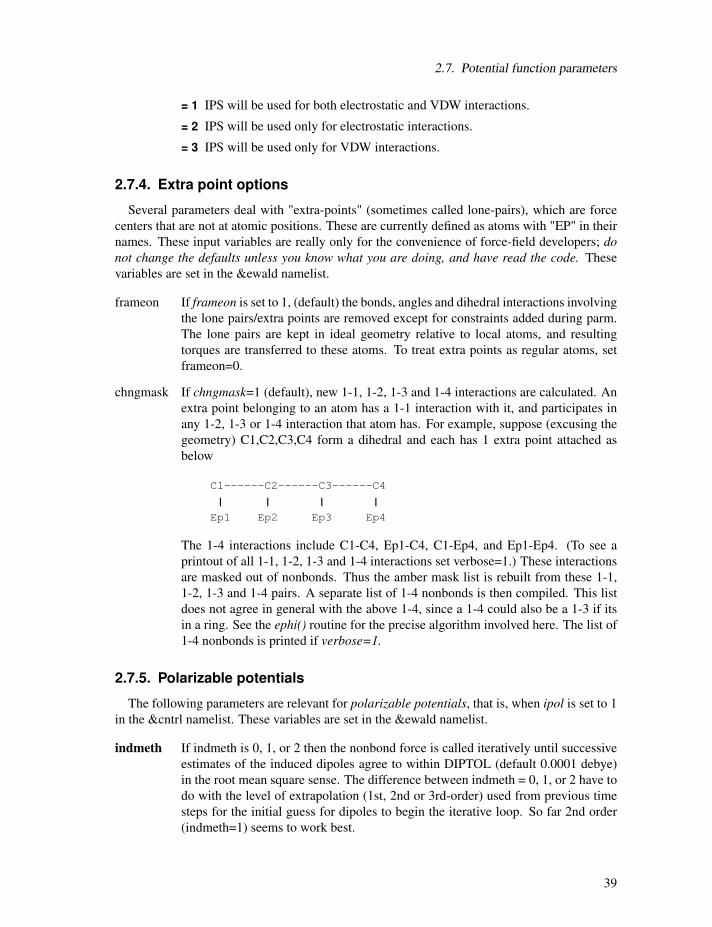
2.7. Potential function parameters
= 1 IPS will be used for both electrostatic and VDW interactions.
= 2 IPS will be used only for electrostatic interactions.
= 3 IPS will be used only for VDW interactions.
2.7.4. Extra point options
Several parameters deal with "extra-points" (sometimes called lone-pairs), which are force
centers that are not at atomic positions. These are currently defined as atoms with "EP" in their
names. These input variables are really only for the convenience of force-field developers; donot change the defaults unless you know what you are doing, and have read the code. Thesevariables are set in the &ewald namelist.
frameon If frameon is set to 1, (default) the bonds, angles and dihedral interactions involvingthe lone pairs/extra points are removed except for constraints added during parm.
The lone pairs are kept in ideal geometry relative to local atoms, and resulting
torques are transferred to these atoms. To treat extra points as regular atoms, set
frameon=0.
chngmask If chngmask=1 (default), new 1-1, 1-2, 1-3 and 1-4 interactions are calculated. Anextra point belonging to an atom has a 1-1 interaction with it, and participates in
any 1-2, 1-3 or 1-4 interaction that atom has. For example, suppose (excusing the
geometry) C1,C2,C3,C4 form a dihedral and each has 1 extra point attached as
below
C1------C2------C3------C4
| | | |Ep1 Ep2 Ep3 Ep4
The 1-4 interactions include C1-C4, Ep1-C4, C1-Ep4, and Ep1-Ep4. (To see a
printout of all 1-1, 1-2, 1-3 and 1-4 interactions set verbose=1.) These interactions
are masked out of nonbonds. Thus the amber mask list is rebuilt from these 1-1,
1-2, 1-3 and 1-4 pairs. A separate list of 1-4 nonbonds is then compiled. This list
does not agree in general with the above 1-4, since a 1-4 could also be a 1-3 if its
in a ring. See the ephi() routine for the precise algorithm involved here. The list of1-4 nonbonds is printed if verbose=1.
2.7.5. Polarizable potentials
The following parameters are relevant for polarizable potentials, that is, when ipol is set to 1in the &cntrl namelist. These variables are set in the &ewald namelist.
indmeth If indmeth is 0, 1, or 2 then the nonbond force is called iteratively until successive
estimates of the induced dipoles agree to within DIPTOL (default 0.0001 debye)
in the root mean square sense. The difference between indmeth = 0, 1, or 2 have to
do with the level of extrapolation (1st, 2nd or 3rd-order) used from previous time
steps for the initial guess for dipoles to begin the iterative loop. So far 2nd order
(indmeth=1) seems to work best.
39

2. Sander basics
If indmeth = 3, use a Car-Parinello scheme wherein dipoles are assigned a fictitious
mass and integrated each time step. This is much more efficient and is the current
default. Note that this method is unstable for dt > 1 fs.
diptol Convergence criterion for dipoles in the iterative methods. Default is 0.0001 De-
bye.
maxiter For iterative methods (indmeth<3), this is the maximum number of iterations al-
lowed per time step. Default is 20.
dipmass The fictitious mass assigned to dipoles. Default value is 0.33, which works well
for 1fs time steps. If dipmass is set much below this, the dynamics are rapidly
unstable. If set much above this the dynamics of the system are affected.
diptau This is used for temperature control of the dipoles (for indmeth=3). If diptau isgreater than 10 (ps units) temperature control of dipoles is turned off. Experiments
so far indicate that running the system in NVE with no temperature control on
induced dipoles leads to a slow heating, barely noticeable on the 100ps time scale.
For runs of length 10ps, the energy conservation with this method rivals that of
SPME for standard fixed charge systems. For long runs, we recommend setting a
weak temperature control (e.g. 9.99 ps) on dipoles as well as on the atoms. Note
that to achieve good energy conservation with iterative method, the diptol must be
below 10 -7 debye, which is much more expensive. Default is 11 ps (i.e. default isturned off).
irstdip If indmeth=3, a restart file for dipole positions and velocities is written along with
the restart for atomic coordinates and velocities. If irstdip=1, the dipolar positions
and velocities from the inpdip file are read in. If irstdip=0, an iterative method is
used for step 1, after which Car-Parrinello is used.
scaldip To scale 1-4 charge-dipole and dipole-dipole interactions the same as 1-4 charge-
charge (i.e. divided by scee) set scaldip=1 (default). If scaldip=0 the 1-4 charge-
dipole and dipole-dipole interactions are treated the same as other dipolar interac-
tions (i.e. divided by 1).
2.7.6. Dipole Printing
By including a &dipoles namelist containing a series of groups, at the end of the input file,
the printing of permanent, induced and total dipoles is enabled.
The X, Y and Z components of the dipole (in debye) for each group will be written to mdout
every NTPR steps. In order to avoid ambiguity with charged groups all of the dipoles for a
given group are calculated with respect to the centre of mass of that group.
It should be noted that the permanent, inducible and total dipoles will be printed regardless
of whether a polarizable potential is in use. However, only the permanent dipole will have anyphysical meaning when non-polarizable potentials are in use.It should also be noted that the groups used in the dipole printing routines are not exclusive
to these routines and so the dipole printing procedure can only be used when group input is notin use for something else (i.e. restraints).
40

2.8. Varying conditions
2.7.7. Detailed MPI Timings
profile_mpi Adjusts whether detailed per thread timings should be written to a file called pro-
file_mpi when running sander in parallel. By default only average timings are
printed to the output file. This is done for performance reasons, especially when
running multisander runs. However for development it is useful to know the indi-
vidual timings for each mpi thread. When running in serial the value of profile_mpi
is ignored.
= 0 No detailed MPI timings will be written (default).
= 1 A detailed breakdown of the timings for each MPI thread will be written to the
file: profile_mpi.
2.8. Varying conditions
This section of information is read (if NMROPT > 0) as a series of namelist specifications,with name "&wt". This namelist is read repeatedly until a namelist &wt statement is found with
TYPE=END.
TYPE Defines quantity being varied; valid options are listed below.
ISTEP1,ISTEP2 This change is applied over steps/iterations ISTEP1 through ISTEP2. If IS-
TEP2 = 0, this change will remain in effect from step ISTEP1 to the end of the run
at a value of VALUE1 (VALUE2 is ignored in this case). (default= both 0)
VALUE1,VALUE2 Values of the change corresponding to ISTEP1 and ISTEP2, respectively.
If ISTEP2=0, the change is fixed at VALUE1 for the remainder of the run, once
step ISTEP1 is reached.
IINC If IINC> 0, then the change is applied as a step function, with IINC steps/iterationsbetween each change in the target VALUE (ignored if ISTEP2=0). If IINC =0, the
change is done continuously. (default=0)
IMULT If IMULT=0, then the change will be linearly interpolated fromVALUE1 to VALUE2
as the step number increases from ISTEP1 to ISTEP2. (default) If IMULT=1, thenthe change will be effected by a series of multiplicative scalings, using a single
factor, R, for all scalings. i.e.
VALUE2 = (R**INCREMENTS) * VALUE1.
INCREMENTS is the number of times the target value changes, which is deter-
mined by ISTEP1, ISTEP2, and IINC.
The remainder of this section describes the options for the TYPE parameter. For a few types of
cards, the meanings of the other variables differ from that described above; such differences are
noted below. Valid Options for TYPE (you must use uppercase) are:
BOND Varies the relative weighting of bond energy terms.
41

2. Sander basics
ANGLE Varies the relative weighting of valence angle energy terms.
TORSION Varies the relative weighting of torsion (and J-coupling) energy terms. Note that
any restraints defined in the input to the PARM program are included in the above.
Improper torsions are handled separately (IMPROP).
IMPROP Varies the relative weighting of the "improper" torsional terms. These are not in-
cluded in TORSION.
VDW Varies the relative weighting of van der Waals energy terms. This is equivalent to
changing the well depth (epsilon) by the given factor.
HB Varies the relative weighting of hydrogen-bonding energy terms.
ELEC Varies the relative weighting of electrostatic energy terms.
NB Varies the relative weights of the non-bonded (VDW, HB, and ELEC) terms.
ATTRACT Varies the relative weights of the attractive parts of the van der waals and h-bond
terms.
REPULSE Varies the relative weights of the repulsive parts of the van der waals and h-bond
terms.
RSTAR Varies the effective van der Waals radii for the van der Waals (VDW) interactions
by the given factor. Note that this is done by changing the relative attractive and
repulsive coefficients, so ATTRACT/REPULSE should not be used over the same
step range as RSTAR.
INTERN Varies the relative weights of the BOND, ANGLE and TORSION terms. "Im-
proper" torsions (IMPROP) must be varied separately.
ALL Varies the relative weights of all the energy terms above (BOND, ANGLE, TOR-
SION, VDW, HB, and ELEC; does not affect RSTAR or IMPROP).
REST Varies the relative weights of *all* the NMR restraint energy terms.
RESTS Varies the weights of the "short-range" NMR restraints. Short- range restraints are
defined by the SHORT instruction (see below).
RESTL Varies the weights of any NMR restraints which are not defined as "short range" by
the SHORT instruction (see below). When no SHORT instruction is given, RESTL
is equivalent to REST.
NOESY Varies the overall weight for NOESY volume restraints. Note that this value mul-
tiplies the individual weights read into the "awt" array. (Only if NMROPT=2; see
Section 4 below).
SHIFTS Varies the overall weight for chemical shift restraints. Note that this value mul-
tiplies the individual weights read into the "wt" array. (Only if NMROPT=2; see
section 4 below).
42

2.8. Varying conditions
SHORT Defines the short-range restraints. For this instruction, ISTEP1, ISTEP2, VALUE1,
and VALUE2 have different meanings. A short-range restraint can be defined in
two ways.
(1) If the residues containing each pair of bonded atoms comprising the restraint
are close enough in the primary sequence:
ISTEP1 ≤ ABS(delta_residue) ≤ ISTEP2,
where delta_residue is the difference in the numbers of the residues containing the
pair of bonded atoms.
(2) If the distances between each pair of bonded atoms in the restraint fall within a
prescribed range:
VALUE1 ≤ distance ≤ VALUE2.
Only one SHORT command can be issued, and the values of ISTEP1, ISTEP2,
VALUE1, and VALUE2 remain fixed throughout the run. However, if IINC>0,then the short-range interaction list will be re-evaluated every IINC steps.
TGTRMSD Varies the RMSD target value for targeted MD.
TEMP0 Varies the target temperature TEMP0.
TEMP0LES Varies the LES target temperature TEMP0LES.
TAUTP Varies the coupling parameter, TAUTP, used in temperature scaling when temper-
ature coupling options NTT=1 is used.
CUT Varies the non-bonded cutoff distance.
NSTEP0 If present, this instruction will reset the initial value of the step counter (against
which ISTEP1/ISTEP2 and NSTEP1/NSTEP2 are compared) to the value ISTEP1.
An NSTEP0 instruction only has an effect at the beginning of a run. For this card
(only) ISTEP2, VALUE1, VALUE2 and IINC are ignored. If this card is omitted,
NSTEP0 = 0. This card can be useful for simulation restarts, where NSTEP0 is set
to the final step on the previous run.
STPMLT If present, the NMR step counter will be changed in increments of STPMLT for
each actual dynamics step. For this card, only VALUE1 is read. ISTEP1, ISTEP2,
VALUE2, IINC, and IMULT are ignored. Default = 1.0.
DISAVE, ANGAVE, TORAVE If present, then by default time-averaged values (rather than
instantaneous values) for the appropriate set of restraints will be used. DISAVE
controls distance data, ANGAVE controls angle data, TORAVE controls torsion
data. See below for the functional form used in generating time-averaged data.
For these cards: VALUE1 = τ (characteristic time for exponential decay) VALUE2= POWER (power used in averaging; the nearest integer of value2 is used) Note
that the range (ISTEP1→ISTEP2) applies only to TAU; The value of POWER is
43

2. Sander basics
not changed by subsequent cards with the same ITYPE field, and time-averaging
will always be turned on for the entire run if one of these cards appears.
Note also that, due to the way that the time averaged internals are calculated, chang-
ing τ at any time after the start of the run will only affect the relative weighting ofsteps occurring after the change in τ . Separate values for τ and POWER are usedfor bond, angle, and torsion averaging.
The default value of τ (if it is 0.0 here) is 1.0D+6, which results in no exponentialdecay weighting. Any value of τ ≥ 1.D+6 will result in no exponential decay.If DISAVE,ANGAVE, or TORAVE is chosen, one can still force use of an instanta-
neous value for specific restraints of the particular type (bond, angle, or torsion) by
setting the IFNTYP field to "1" when the restraint is defined (IFNTYP is defined
in the DISANG file).
If time-averaging for a particular class of restraints is being performed, all restraints
of that class that are being averaged (that is, all restraints of that class except those
for which IFNTYP=1) *must* have the same values of NSTEP1 and NSTEP2
(NSTEP1 and NSTEP2 are defined below). (For these cards, IINC and IMULT are
ignored) See the discussion of time-averaged restraints following the input descrip-
tions.
DISAVI, ANGAVI, TORAVI
ISTEP1: Ignored.
ISTEP2: Sets IDMPAV. If IDMPAV > 0, and a dump file has been specified(DUMPAVE is set in the file redirection section below), then the time-averaged
values of the restraints will be written every IDMPAV steps. Only one value
of IDMPAV can be set (corresponding to the first DISAVI/ANGAVI/TORAVI
card with ISTEP2 > 0), and all restraints (even those with IFNTYP=1) willbe "dumped" to this file every IDMPAV steps. The values reported reflect the
current value of τ .VALUE1: The integral which gives the time-averaged values is undefined for the
first step. By default, for each time-averaged internal, the integral is assigned
the current value of the internal on the first step. If VALUE1 �=0, this initialvalue of internal r is reset as follows:
-1000. < VALUE1 < 1000.: Initial value = r_initial + VALUE
VALUE1 <= -1000.: Initial value = r_target + 1000.
1000. <= VALUE1 : Initial value = r_target - 1000.
r_target is the target value of the internal, given by R2+R3 (or just R3, if R2
is 0). VALUE1 is in angstroms for bonds, in degrees for angles.
VALUE2: This field can be used to set the value of τ used in calculating thetime-averaged values of the internal restraints reported at the end of a sim-
ulation (if LISTOUT is specified in the redirection section below). By de-
fault, no exponential decay weighting is used in calculating the final reported
values, regardless of what value of τ was used during the simulation. If
44

2.8. Varying conditions
VALUE2>0, then τ = VALUE2 will be used in calculating these final re-ported averages. Note that the value of VALUE2 = τ specified here onlyaffects the reported averaged values in at the end of a simulation. It does not
affect the time-averaged values used during the simulation (those are changed
by the VALUE1 field of DISAVE, ANGAVE and TORAVE instructions).
IINC: If IINC = 0, then forces for the class of time-averaged restraints will be cal-culated exactly as (dE/dr_ave) (dr_ave/dx). If IINC = 1, then then forces
for the class of time-averaged restraints will be calculated as (dE/dr_ave)
(dr(t)/dx). Note that this latter method results in a non-conservative force, and
does not integrate to a standard form. But this latter formulation helps avoid
the large forces due to the (1+i) term in the exact derivative calculation–andmay avert instabilities in the molecular dynamics trajectory for some systems.
See the discussion of time-averaged restraints following the input description.
Note that the DISAVI, ANGAVI, and TORAVI instructions will have no af-
fect unless the corresponding time average request card (DISAVE, ANGAVE
or TORAVE, respectively) is also present.
DUMPFREQ Istep1 is the only parameter read, and it sets the frequency at which the coor-
dinates in the distance or angle restraints are dumped to the file specified by the
DUMPAVE command in the I/O redirection section. (For these cards, ISTEP1 and
IMULT are ignored).
END END of this section.
NOTES:
1. All weights are relative to a default of 1.0 in the standard force field.
2. Weights are not cumulative.
3. For any range where the weight of a term is not modified by the above, the weight reverts
to 1.0. For any range where TEMP0, SOFTR or CUTOFF is not specified, the value of
the relevant constant is set to that specified in the input file.
4. If a weight is set to 0.0, it is set internally to 1.0D-7. This can be overridden by setting the
weight to a negative number. In this case, a weight of exactly 0.0 will be used. However, ifany weight is set to exactly 0.0, it cannot be changed again during this run of the program.
5. If two (or more) cards change a particular weight over the same range, the weight given
on the last applicable card will be the one used.
6. Once any weight change for which NSTEP2=0 becomes active (i.e. one which will be
effective for the remainder of the run), the weight of this term cannot be further modified
by other instructions.
7. Changes to RSTAR result in exponential weighting changes to the attractive and repulsive
terms (proportional to the scale factor**6 and **12, respectively). For this reason, scaling
RSTAR to a very small value (e.g. ≤0.1) may result in a zeroing-out of the vdw term.
45

2. Sander basics
2.9. File redirection commands
Input/output redirection information can be read as described here. Redirection cards must
follow the end of the weight change information. Redirection card input is terminated by the
first non-blank line which does not start with a recognized redirection TYPE (e.g. LISTIN,
LISTOUT, etc.).
The format of the redirection cards is
TYPE = filename
where TYPE is any valid redirection keyword (see below), and filename is any character
string. The equals sign ("=") is required, and TYPE must be given in uppercase letters.Valid redirection keywords are:
LISTIN An output listing of the restraints which have been read, and their deviations from
the target distances before the simulation has been run. By default, this listing isnot printed. If POUT is used for the filename, these deviations will be printed in
the normal output file.
LISTOUT An output listing of the restraints which have been read, and their deviations from
the target distances _after the simulation has finished. By default, this listing is notprinted. If POUT is used for the filename, these deviations will be printed in the
normal output file.
DISANG The file from which the distance and angle restraint information described below
(Section 6.1) will be read.
NOESY File from which NOESY volume information (Section 6.2) will be read.
SHIFTS File from which chemical shift information (Section 6.3) will be read.
PCSHIFT File from which paramagnetic shift information (Section 6.3) will be read.
DIPOLE File from which residual dipolar couplings (Section 6.5) will be read.
CSA File from which CSA or pseduo-CSA restraints (Section 6.6) will be read.
DUMPAVE File to which the time-averaged values of all restraints will be written. If DISAVI
/ ANGAVI / TORAVI has been used to set IDMPAV �=0, then averaged values willbe output. If the DUMPFREQ command has been used, the instantaneous values
will be output.
2.10. Getting debugging information
The debug options in sander are there principally to help developers test new options or totest results between two machines or versions of code, but can also be useful to users who want
to test the effect of parameters on the accuracy of their ewald or pme calculations. If the debug
options are set, sander will exit after performing the debug tasks set by the user.To access the debug options, include a &debugf namelist. Input parameters are:
46

2.10. Getting debugging information
do_debugf Flag to perform this module. Possible values are zero or one. Default is zero. Set
to one to turn on debug options.
One set of options is to test that the atomic forces agree with numerical differentiation of energy.
atomn Array of atom numbers to test atomic forces on. Up to 25 atom numbers can be
specified, separated by commas.
nranatm number of random atoms to test atomic forces on. Atom numbers are generated via
a random number generator.
ranseed seed of random number generator used in generating atom numbers default is
71277
neglgdel negative log of delta used in numerical differentiating; e.g. 4 means delta is 10−4Angstroms. Default is 5. Note: In general it does no good to set nelgdel larger thanabout 6. This is because the relative force error is at best the square root of the
numerical error in the energy, which ranges from 10−15 up to 10−12 for energiesinvolving a large number of terms.
chkvir Flag to test the atomic and molecular virials numerically. Default is zero. Set to
one to test virials.
dumpfrc Flag to dump energies, forces and virials, as well as components of forces (bond,
angle forces etc.) to the file "forcedump.dat" This produces an ascii file. Default is
zero. Set to one to dump forces.
rmsfrc Flag to compare energies forces and virials as well as components of forces (bond,
angle forces etc.) to those in the file "forcedump.dat". Default is zero. Set to one
to compare forces.
Several other options are also possible to modify the calculated forces.
zerochg Flag to zero all charges before calculating forces. Default zero. Set to one to
remove charges.
zerovdw Flag to remove all van der Waals interactions before calculating forces. Default
zero. Set to one to remove van der Waals.
zerodip Flag to remove all atomic dipoles before calculating forces. Only relevant when
polarizability is invoked.
do_dir, do_rec, do_adj, do_self, do_bond, do_cbond, do_angle, do_ephi, do_xconst, do_cap These
are flags which turn on or off the subroutines they refer to. The defaults are one.
Set to zero to prevent a subroutine from running. For example, set do_dir=0 to
turn off the direct sum interactions (van der Waals as well as electrostatic). Thes
options, as well as the zerochg, zerovdw,zerodip flags, can be used to fine tune a
test of forces, accuracy etc.
EXAMPLES:
This input list tests the reciprocal sum forces on atom 14 numerically, using a delta of 10 -4.
47
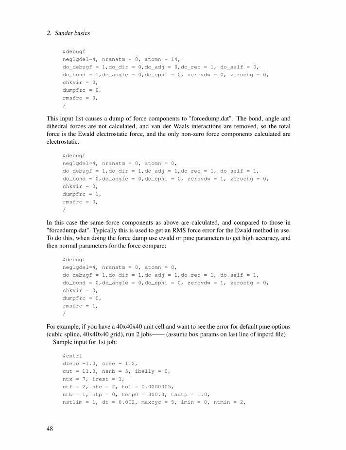
2. Sander basics
&debugf
neglgdel=4, nranatm = 0, atomn = 14,
do_debugf = 1,do_dir = 0,do_adj = 0,do_rec = 1, do_self = 0,
do_bond = 1,do_angle = 0,do_ephi = 0, zerovdw = 0, zerochg = 0,
chkvir = 0,
dumpfrc = 0,
rmsfrc = 0,
/
This input list causes a dump of force components to "forcedump.dat". The bond, angle and
dihedral forces are not calculated, and van der Waals interactions are removed, so the total
force is the Ewald electrostatic force, and the only non-zero force components calculated are
electrostatic.
&debugf
neglgdel=4, nranatm = 0, atomn = 0,
do_debugf = 1,do_dir = 1,do_adj = 1,do_rec = 1, do_self = 1,
do_bond = 0,do_angle = 0,do_ephi = 0, zerovdw = 1, zerochg = 0,
chkvir = 0,
dumpfrc = 1,
rmsfrc = 0,
/
In this case the same force components as above are calculated, and compared to those in
"forcedump.dat". Typically this is used to get an RMS force error for the Ewald method in use.
To do this, when doing the force dump use ewald or pme parameters to get high accuracy, and
then normal parameters for the force compare:
&debugf
neglgdel=4, nranatm = 0, atomn = 0,
do_debugf = 1,do_dir = 1,do_adj = 1,do_rec = 1, do_self = 1,
do_bond = 0,do_angle = 0,do_ephi = 0, zerovdw = 1, zerochg = 0,
chkvir = 0,
dumpfrc = 0,
rmsfrc = 1,
/
For example, if you have a 40x40x40 unit cell and want to see the error for default pme options
(cubic spline, 40x40x40 grid), run 2 jobs—— (assume box params on last line of inpcrd file)
Sample input for 1st job:
&cntrl
dielc =1.0, scee = 1.2,
cut = 11.0, nsnb = 5, ibelly = 0,
ntx = 7, irest = 1,
ntf = 2, ntc = 2, tol = 0.0000005,
ntb = 1, ntp = 0, temp0 = 300.0, tautp = 1.0,
nstlim = 1, dt = 0.002, maxcyc = 5, imin = 0, ntmin = 2,
48

2.10. Getting debugging information
ntpr = 1, ntwx = 0, ntt = 0, ntr = 0,
jfastw = 0, nmrmax=0, ntave = 25,
/
&debugf
do_debugf = 1,do_dir = 1,do_adj = 1,do_rec = 1, do_self = 1,
do_bond = 0,do_angle = 0,do_ephi = 0, zerovdw = 1, zerochg = 0,
chkvir = 0,
dumpfrc = 1,
rmsfrc = 0,
/
&ewald
nfft1=60,nfft2=60,nfft3=60,order=6, ew_coeff=0.35,
/
Sample input for 2nd job:
&cntrl
dielc =1.0, scee = 1.2,
cut = 8.0, nsnb = 5, ibelly = 0,
ntx = 7, irest = 1,
ntf = 2, ntc = 2, tol = 0.0000005,
ntb = 1, ntp = 0, temp0 = 300.0, tautp = 1.0,
nstlim = 1, dt = 0.002, maxcyc = 5, imin = 0, ntmin = 2,
ntpr = 1, ntwx = 0, ntt = 0, ntr = 0,
jfastw = 0, nmrmax=0, ntave = 25,
/
&debugf
do_debugf = 1,do_dir = 1,do_adj = 1,do_rec = 1, do_self = 1,
do_bond = 0,do_angle = 0,do_ephi = 0, zerovdw = 1, zerochg = 0,
chkvir = 0,
dumpfrc = 0,
rmsfrc = 1,
/
&ewald
ew_coeff=0.35,
/
Note that an Ewald coefficient of 0.35 is close to the default error for an 8 Angstrom cutoff.
However, the first job used an 11 Angstrom cutoff. The direct sum forces calculated in the
2nd job are compared to these, giving the RMS error due to an 8 Angstrom cutoff, with this
value of ew_coeff. The reciprocal sum error calculated in the 2nd job is with respect to the pme
reciprocal forces in the 1st job considered as "exact".
Note further that if in these two jobs you had not specified "ew_coeff" sander would havecalculated ew_coeff according to the cutoff and the direct sum tolerance, defaulted to 10−5. Thiswould give two different ewald coefficients. Under these circumstances the direct, reciprocal
and adjust energies and forces would not agree well between the two jobs. However the total
49

2. Sander basics
energy and forces should agree reasonably, (forces to within about 5x10⁻⁴ relative RMS forceerror) Since the totals are invariant to the coefficient.
Finally, note that if other force components are calculated, such as van der Waals, bond, angle
etc. The total force will include these, and the relative RMS force errors will be with respect to
this total force in the denominator.
50

3. Force field modifications
This chapter provides a number of sections describing how to use sander for particular typesof problems. It should be read in conjunction with the previous chapter.
3.1. The Generalized Born/Surface Area Model
The generalized Born solvation model can be used instead of explicit water for non-polarizable
force fields such as ff94 or ff99. To estimate the total solvation free energy of a molecule,
ΔGsolv, one typically assumes that it can be decomposed into the "electrostatic" and "non-
electrostatic" parts:
ΔGsolv = ΔGel +ΔGnonel (3.1)
where ΔGnonel is the free energy of solvating a molecule from which all charges have been
removed (i.e. partial charges of every atom are set to zero), and ΔGel is the free energy of first
removing all charges in the vacuum, and then adding them back in the presence of a continuum
solvent environment. Generally speaking, ΔGnonel comes from the combined effect of two types
of interaction: the favorable van der Waals attraction between the solute and solvent molecules,
and the unfavorable cost of breaking the structure of the solvent (water) around the solute. In
the current Amber codes, this is taken to be proportional to the total solvent accessible surface
area (SA) of the molecule, with a proportionality constant derived from experimental solvation
energies of small non-polar molecules, and uses a fast LCPO algorithm [41] to compute an
analytical approximation to the solvent accessible area of the molecule.
The Poisson-Boltzmann approach described in the next section has traditionally been used in
calculating ΔGel . However, in molecular dynamics applications, the associated computational
costs are often very high, as the Poisson-Boltzmann equation needs to be solved every time the
conformation of the molecule changes. Amber developers have pursued an alternative approach,
the analytic generalized Born (GB) method, to obtain a reasonable, computationally efficient
estimate to be used in molecular dynamics simulations. The methodology has become popular,
[42–49] especially in molecular dynamics applications, [50–53] due to its relative simplicity
and computational efficiency, compared to the more standard numerical solution of the Poisson-
Boltzmann equation. Within Amber GB models, each atom in a molecule is represented as a
sphere of radius Ri with a charge qi at its center; the interior of the atom is assumed to be filled
uniformly with a material of dielectric constant 1. The molecule is surrounded by a solvent of
a high dielectric ε (80 for water at 300 K). The GB model approximates ΔGel by an analytical
formula, [42, 54]
ΔGel =−12
∑i j
qiq j
fGB(ri j,Ri,R j)
(1− exp[−κ fGB]
ε
)(3.2)
51
3. Force field modifications
where ri jis the distance between atoms i and j , the Ri are the so-called effective Born radii,and fGB() is a certain smooth function of its arguments. The electrostatic screening effects of(monovalent) salt are incorporated [54] via the Debye-Huckel screening parameter κ .A common choice [42] of fGB is
fGB =[r2i j +RiR j exp(−r2i j/4RiR j)
]1/2(3.3)
although other expressions have been tried. [45, 55] The effective Born radius of an atom reflects
the degree of its burial inside the molecule: for an isolated ion, it is equal to its van der Waals
(VDW) radius ρi. Then one obtains the particularly simple form:
ΔGel =− q2i2ρi
(1− 1
ε
)(3.4)
where we assumed κ = 0 (pure water). This is the famous expression due to Born for the
solvation energy of a single ion. The function fGB() is designed to interpolate, in a clevermanner, between the limit ri j → 0, when atomic spheres merge into one, and the opposite
extreme ri j →∞, when the ions can be treated as point charges obeying the Coulomb’s law. [48]For deeply buried atoms, the effective radii are large, Ri � ρi, and for such atoms one can use
a rough estimate Ri ≈ Li, where Li is the distance from the atom to the molecular surface.
Closer to the surface, the effective radii become smaller, and for a completely solvent exposed
side-chain one can expect Ri to approach ρi.
The effective radii depend on the molecule’s conformation, and so have to be re-computed
every time the conformation changes. This makes the computational efficiency a critical issue,
and various approximations are normally made that facilitate an effective estimate of Ri. In
particular, the so-called Coulomb field approximation, or CFA, is often used, which replaces thetrue electric displacement around the atom by the Coulomb field. Within this assumption, the
following expression can be derived: [48]
R−1i = ρ−1i − 1
4π
∫θ(|r|−ρi)r−4dr (3.5)
where the integral is over the solute volume surrounding atom i. For a realistic molecule, thesolute boundary (molecular surface) is anything but trivial, and so further approximations are
made to obtain a closed-form analytical expression for the above equation, e.g. the so-calledpairwise de-screening approach of Hawkins, Cramer and Truhlar, [56] which leads to a GB
model implemented in Amber with igb=1. The 3D integral used in the estimation of the effec-tive radii is performed over the van der Waals (VDW) spheres of solute atoms, which implies a
definition of the solute volume in terms of a set of spheres, rather than the complex molecular
surface, [57] commonly used in the PB calculations. For macromolecules, this approach tends
to underestimate the effective radii for buried atoms, [48] arguably because the standard inte-
gration procedure treats the small vacuum–filled crevices between the van der Waals (VDW)
spheres of protein atoms as being filled with water, even for structures with large interior. [55]
This error is expected to be greatest for deeply buried atoms characterized by large effective
radii, while for the surface atoms it is largely canceled by the opposing error arising from the
Coulomb approximation, which tends [43, 47, 58] to overestimate Ri.
The deficiency of the model described above can, to some extent, be corrected by noticing
that even the optimal packing of hard spheres, which is a reasonable assumption for biomolecules,
52

3.1. The Generalized Born/Surface Area Model
still occupies only about three quarters of the space, and so "scaling-up" of the integral by a fac-
tor of four thirds should effectively increase the underestimated radii by about the right amount,
without any loss of computational efficiency. This idea was developed and applied in the context
of pH titration, [48] where it was shown to improve the performance of the GB approximation
in calculating pKa values of protein sidechains. However, the one-parameter correction intro-
duced in Ref. [48] was not optimal in keeping the model’s established performance on small
molecules. It was therefore proposed [53] to re-scale the effective radii with the re-scaling pa-
rameters being proportional to the degree of the atom’s burial, as quantified by the value Ii of
the 3D integral. The latter is large for the deeply buried atoms and small for exposed ones. Con-
sequently, one seeks a well-behaved re-scaling function, such that Ri ≈ (ρ−1i − Ii)−1 for smallIi, and Ri > (ρ−1i − Ii)−1 when Ii becomes large. The following simple, infinitely differentiable
re-scaling function was chosen to replace the model’s original expression for the effective radii:
R−1i = ρ−1i −ρ−1i tanh(αΨ−βΨ2+ γΨ3) (3.6)
where Ψ = Iiρi, and α , β , γ are treated as adjustable dimensionless parameters which wereoptimized using the guidelines mentioned earlier (primarily agreement with the PB). Currently,
Amber supports two GBmodels ( termed OBC ) based on this idea. These differ by the values of
α , β , γ , and are invoked by setting igb to either igb=2 or igb=5. The details of the optimizationprocedure and the performance of the OBC model relative to the PB treatment and in MD
simulations on proteins is described in Ref. [53]; an independent comparison to the PB in
calculating the electrostatic part of solvation free energy on a large data set of proteins can be
found in Ref. [59].
The generalized Born models used here are based on the "pairwise" model introduced by
Hawkins, Cramer and Truhlar, [56, 60] which in turn is based on earlier ideas by Still and others.
[42, 47, 58, 61] The so-called overlap parameters for most models are taken from the TINKER
molecular modeling package (http://tinker.wustl.edu). The effects of added monovalent salt
are included at a level that approximates the solutions of the linearized Poisson-Boltzmann
equation. [54] The original implementation was by David Case, who thanks Charlie Brooks
for inspiration. Details of our implementation of generalized Born models can be found in
Refs. [62, 63].
3.1.1. GB/SA input parameters
As outlined above, there are several "flavors" of GB available, depending upon the value of
igb. The version that has been most extensively tested corresponds to igb=1; the "OBC" models(igb=2 and 5) are newer, but appear to give significant improvements and are recommendedfor most projects (certainly for peptides or proteins). The newest, most advanced, and least
extensively tested model, GBn (igb=7), yields results in considerably better agreement withmolecular surface Poisson-Boltzmann and explicit solvent results than the "OBC" models under
many circumstances. [64] The GBn model was parameterized for peptide and protein systemsand is not recommended for use with nucleic acids. Users should understand that all (current)
GB models have limitations and should proceed with caution. Generalized Born simulations
can only be run for non-periodic systems, i.e. where ntb=0. The nonbonded cutoff for GBcalculations should be greater than that for PME calculations, perhaps cut=16. The slowly-varying forces generally do not have to be evaluated at every step for GB, either nrespa=2 or4.
53

3. Force field modifications
igb
= 0 No generalized Born term is used. (Default)
= 1 The Hawkins, Cramer, Truhlar [56, 60] pairwise generalized Born model is
used, with parameters described by Tsui and Case. [62] This model uses the
default radii set up by LEaP. It is slightly different from the GB model that
was included in Amber6. If you want to compare to Amber 6, or need to
continue an ongoing simulation, you should use the command "set default
PBradii amber6" in LEaP, and set igb=1 in sander. For reference, the Amber6values are those used by an earlier Tsui and Case paper. [51]
= 2 Use a modified GB model developed by A. Onufriev, D. Bashford and D.A.
Case; the main idea was published earlier, [48] but the actual implementation
here [53] is an elaboration of this initial idea. Within this model, the effective
Born radii are re-scaled to account for the interstitial spaces between atom
spheres missed by the GBHCT approximation. In that sense, GBOBC is in-
tended to be a closer approximation to true molecular volume, albeit in an
average sense. With igb=2, the inverse of the effective Born radius is givenby:
R−1i = ρ−1i − tanh(αΨ−βΨ2+ γΨ3)/ρi
where ρ i = ρi− o f f set, and Ψ = Iρi, with I given in our earlier paper. Theparameters α , β , and γ were determined by empirical fits, and have the values0.8, 0.0, and 2.909125. This corresponds to model I in Ref [53]. With this
option, you should use the LEaP command "set default PBradii mbondi2" or
"set default PBradii bondi" to prepare the prmtop file.
= 3 or 4 These values are unused; they were used in Amber 7 for parameter sets
that are no longer supported.
= 5 Same as igb=2, except that now α,β ,γ are 1.0, 0.8, and 4.85. This correspondsto model II in Ref [53]. With this option, you should use the command "set
default PBradii mbondi2" in setting up the prmtop file, although "set defaultPBradii bondi" is also OK. When tested in MD simulations of several pro-
teins, [53] both of the above parameterizations of the "OBC" model showed
equal performance, although further tests [59] on an extensive set of pro-
tein structures revealed that the igb=5 variant agrees better with the Poisson-Boltzmann treatment in calculating the electrostatic part of the solvation free
energy.
= 6 With this option, there is no continuum solvent model used at all; this corre-
sponds to a non-periodic, "vacuum", model where the non-bonded interac-
tions are just Lennard-Jones and Coulomb interactions. This option is logi-
cally equivalent to setting igb=0 and eedmeth=4, although the implementa-tion (and computational efficiency) is not the same.
= 7 The GBn model described by Mongan, Simmerling, McCammon, Case andOnufriev [65] is employed. This model uses a pairwise correction term to
GBHCT to approximate a molecular surface dielectric boundary; that is to
eliminate interstitial regions of high dielectric smaller than a solvent molecule.
54
3.1. The Generalized Born/Surface Area Model
This correction affects all atoms and is geometry-specific, going beyond the
geometry-free, "average" re-scaling approach of GBOBC, which mostly af-
fects buried atoms. With this method, you should use the bondi radii set.
The overlap or screening parameters in the prmtop file are ignored, and themodel-specific GBn optimized values are substituted. The model carries littleadditional computational overhead relative to the other GB models described
above. [65] This method is not recommended for systems involving nucleic
acids.
=10 Calculate the reaction field and nonbonded interactions using a numerical
Poisson-Boltzmann solver. This option is described in Section 6.2, below.
Note that this is not a generalized Born simulation, in spite of its use of igb;it is rather an alternative continuum solvent model.
intdiel Sets the interior dielectric constant of the molecule of interest. Default is 1.0. Other
values have not been extensively tested.
extdiel Sets the exterior or solvent dielectric constant. Default is 78.5.
saltcon Sets the concentration (M) of 1-1 mobile counterions in solution, using a modified
generalized Born theory based on the Debye-Hückel limiting law for ion screening
of interactions. [54] Default is 0.0 M (i.e. no Debye-Hückel screening.) Settingsaltcon to a non-zero value does result in some increase in computation time.
rgbmax This parameter controls the maximum distance between atom pairs that will be
considered in carrying out the pairwise summation involved in calculating the ef-
fective Born radii. Atoms whose associated spheres are farther way than rgbmaxfrom given atom will not contribute to that atom’s effective Born radius. This is
implemented in a "smooth" fashion (thanks mainly to W.A. Svrcek-Seiler), so that
when part of an atom’s atomic sphere lies inside rgbmax cutoff, that part contributesto the low-dielectric region that determines the effective Born radius. The default is
25 Å, which is usually plenty for single-domain proteins of a few hundred residues.
Even smaller values (of 10-15 Å) are reasonable, changing the functional form of
the generalized Born theory a little bit, in exchange for a considerable speed-up in
efficiency, and without introducing the usual cut-off artifacts such as drifts in the
total energy.
The rgbmax parameter affects only the effective Born radii (and the derivatives ofthese values with respect to atomic coordinates). The cut parameter, on the otherhand, determines the maximum distance for the electrostatic, van der Waals and
"off-diagonal" terms of the generalized Born interaction. The value of rgbmaxmight be either greater or smaller than that of cut: these two parameters are inde-pendent of each other. However, values of cut that are too small are more likelyto lead to artifacts than are small values of rgbmax; therefore one typically setsrgbmax <= cut.
rbornstat If rbornstat = 1, the statistics of the effective Born radii for each atom of the
molecule throughout the molecular dynamics simulation are reported in the output
file. Default is 0.
55

3. Force field modifications
offset The dielectric radii for generalized Born calculations are decreased by a uniform
value "offset" to give the "intrinsic radii" used to obtain effective Born radii. De-
fault is 0.09 Å.
gbsa Option to carry out GB/SA (generalized Born/surface area) simulations. For the
default value of 0, surface area will not be computed and will not be included in
the solvation term. If gbsa = 1, surface area will be computed using the LCPOmodel. [41] If gbsa = 2, surface area will be computed by recursively approximat-ing a sphere around an atom, starting from an icosahedra. Note that no forces are
generated in this case, hence, gbsa = 2 only works for a single point energy calcula-tion and is mainly intended for energy decomposition in the realm of MM_GBSA.
surften Surface tension used to calculate the nonpolar contribution to the free energy of
solvation (when gbsa = 1), as Enp = surften*SA. The default is 0.005 kcal/mol/A2.[66]
rdt This parameter is only used for GB simulations with LES (Locally Enhanced Sam-
pling). In GB+LES simulations, non-LES atoms require multiple effective Born
radii due to alternate descreening effects of different LES copies. When the multi-
ple radii for a non-LES atom differ by less than RDT, only a single radius will be
used for that atom. See the LES portion of the manual for more details. Default is
0.0 Å.
3.1.2. ALPB (Analytical Linearized Poisson-Boltzmann)
Like the GB model, the ALPB approximation [67, 68] can be used to replace the need for
explicit solvent, with similar benefits (such as enhanced conformational sampling) and caveats.
The basic ALPB equation that approximates the electrostatic part of the solvation free energy is
ΔGel ≈ ΔGal pb =−12
(1
εin− 1
εex
)1
1+αβ ∑i j
qiq j
(1
fGB+
αβA
)
where β = εin/εex is the ratio of the internal and external dielectrics, α=0.571412, and A isthe so-called effective electrostatic size of the molecule, see the definition of Arad below. HerefGB is the same smooth function as in the GB model. The GB approximation is then just the
special case of ALPB when the solvent dielectric is infinite; however, for finite values of solvent
dielectric the ALPB tends to be more accurate. For aqueous solvation, the accuracy advantage
offered by the ALPB is still noticeable, and becomes more pronounced for less polar solvents.
Statistically significant tests on macromolecular structures [68] have shown that ALPB is more
likely to be a better approximation to PB than GB. At the same time, ALPB has virtually no
additional computational overhead relative to GB. However, users should realize that at this
point the new model has not yet been tested nearly as extensively as the GB model, and is
therefore in its experimental stage. The model can potentially replace GB in the energy analysis
of snapshots via the MM-GB/SA scheme. The electrostatic screening effects of monovalent salt
are currently introduced into the ALPB in the same manner as in the GB, and are determined
by the parameter saltcon .
alpb Flag for using ALPB to handle electrostatic interactions within the implicit solvent
model.
56

3.2. Poisson-Boltzmann calculations
= 0 No ALPB (default).
= 1 ALPB is turned on. Requires that one of the GB models is also used to com-
pute the effective Born radii, that is one must set igb=1,2,5, or 7. The ALPBuses the same sets of radii as required by the particular GB model.
arad Effective electrostatic size (radius) of the molecule. Characterizes its over-all di-
mensions and global shape, and is not to be confused with the effective Born radius
of an atom. An appropriate value of Arad must be set if alpb=1: this can be con-veniently estimated for your input structure with the utility elsize that comes withthe main distribution. The default is 15 Å. While Arad may change during thecourse of a simulation, these changes are usually not very large; the accuracy of
the ALPB is found to be rather insensitive to these variations. In the current ver-
sion of Amber Arad is treated as constant throughout the simulation, the validity ofthis assumption is discussed in Ref. [68]. Currently, the effective electrostatic size
is only defined for "single-connected" molecules. However, the ALPB model can
still be used to treat the important case of complex formation. In the docked state,
the compound is considered as one, with its electrostatic size well defined. When
the ligand and receptor become infinitely separated, each can be assigned its own
value of Arad.
3.2. Poisson-Boltzmann calculations
An efficient finite-difference numerical solver [69, 70] is implemented in pbsa/sander for var-ious applications of the Poisson-Boltzmann (PB) method. In the following, a brief introduction
to the PB method and the numerical solver is given first. This is followed by a brief discussion
of the supported PB applications and a detailed description of the keywords. Finally example
input files are explained for typical PB applications. For more background information and how
to use the PB method, please consult cited references and online Amber PB tutorial pages.
3.2.1. Introduction
Solvation interactions, especially solvent-mediated dielectric screening and Debye-Huckel
screening, are thought to be one of the essential determinants of the structure and function of
proteins and nucleic acids. [71] Ideally, one would like to provide a detailed description of
solvent through explicit simulation of a large number of solvent molecules. This approach is
frequently used in molecular dynamics simulations of solution systems. In many applications,
however, the solute is the focus of interest, and the detailed properties of the solvent are not
of central importance. In such cases, a simplified representation of the solvent, based on an
approximation of the mean-force potential for the solvation interactions, can be employed to
accelerate the computation. The mean-force potential averages out the degrees of freedom of
solvent molecules, so that they are often called implicit or continuum solvents.
The Poisson-Boltzmann (PB) solvents are a class of widely used implicit solvents. [72, 73]
They have been demonstrated to be reliable in reproducing the energetics and conformations as
compared with explicit solvent simulations and experimental measurements for a wide range
of systems. In these models, a solute is represented by an atomic-detail model as in a molecu-
lar mechanics force field, while the solvent molecules and any dissolved electrolyte are treated
57

3. Force field modifications
as a structureless continuum. The solute intramolecular interactions are computed by the usual
molecular mechanics force field terms, while the solute-solvent and solvent-solvent interactions
are computed by a mean-field approximation through the use of the PB electrostatic theory. The
electrostatic model represents the solute as a dielectric body whose shape is defined by atomic
coordinates and atomic cavity radii. [74] The solute contains a set of point charges at atomic
centers that produce an electrostatic field in the solute region and the solvent region. The elec-
trostatic fields in such a system, including the solvent reaction field and the Coulombic field,
may be computed by solving the PB equation. [75, 76] The nonelectrostatic or nonpolar sol-
vation interactions are typically modeled with a term proportional to the solvent accessible
surface area. An alternative method to model the nonpolar solvation interactions is also im-
plemented in this release. [77] The new method separates the nonpolar solvation interactions
into two terms: the attractive (dispersion) and repulsive (cavity) interactions. Doing so signifi-
cantly improves the correlation between the cavity free energies and solvent accessible surface
areas for branched and cyclic organic molecules. [78] This is in contrast to the commonly used
strategy that correlates total nonpolar solvation energies with solvent accessible surface areas,
which only correlates well for linear aliphatic molecules. [66] In the new method, the attractive
free energy is computed by a numerical integration over the solvent accessible surface area that
accounts for solvation attractive interactions with an infinite cutoff. [79]
The formalism with which a PB solvent can be applied in molecular mechanics simulations is
based on a rigorous foundation in statistical mechanics, at least for additive molecular mechan-
ics force fields. PB solvents approximate the solvent-induced electrostatic mean-force potential
by computing the reversible work done in the process of charging the atomic charges in a solute
molecule as 12 ∑ j Q jφ jwith j running over all atomic charges. The electrostatic potential φ iscomputed by solving the PB equation:
∇ε(r)∇φ(r) =−4πρ(r)−4π ∑i
zici exp(−ziφ(r)/kBT ) (3.7)
where ε(r) is the dielectric constant, φ(r) is the electrostatic potential, ρ(r) is the solute charge,zi is the charge of ion type i, ci is the number density of ion type i far from the solute, kB is the
Boltzmann constant, and T is the temperature; the summation is over all different ion types. Inthis release, only the linearized form of the PB equation is supported.
Many numerical methods may be used to solve the linearized PB equation. The finite-
difference (FD) method is one of the most popular methods in computational studies of biomolecules.
[80–82] It involves the following steps: mapping atomic charges to the FD grid points (termed
grid charges below); assigning non-periodic/periodic boundary conditions, i.e. electrostatic po-
tentials on the boundary surfaces of the finite-difference grid; and applying a dielectric model to
define the boundary between high-dielectric (i.e. water) and low-dielectric (i.e. solute interior)
regions. [83]
These steps allow the partial differential equation to be converted into a linear system Ax =b with the electrostatic potential on grid points, x as unknowns, the charge distribution on thegrid points as the source b, and the dielectric constant on the grid edges and salt-related termswrapped into the coefficient matrix A, which is a seven-banded symmetric matrix. Once thelinear system is solved, the solution is used to compute the electrostatic energies and forces.
It has been shown that the total electrostatic energy of a solute molecule can be approx-
imated through the FD approach by subtracting the self FD Coulombic energy (GFDcoul,shel f )
and the short-range FD Coulombic energy (GFDcoul,short ) from the total FD electrostatic energy
58

3.2. Poisson-Boltzmann calculations
(GFDcoul,total), and adding back the analytical short-range Coulombic energy (G
anacoul,short ) (see for
example [70]). The self FD Coulombic energy is due to interactions of grid charges within one
single atom. The self energy exists even when the atomic charge is exactly positioned on one
grid point. It also exists in the absence of solvent and any other charges. It apparently is a pure
artifact of the FD approach and must be removed. The short-range FD Coulombic energy is due
to interactions between grid charges in two different atoms that are separated by a short dis-
tance, usually less than 14 grid units. The short-range Coulombic energy is inaccurate because
the atomic charges are mapped onto their eight nearest FD grids, thus causing deviation from
the analytical Coulomb energy. The correction of GFDcoul,shel f and GFD
coul,short is made possible by
the work of Luty and McCammon’s analytical approach to compute FD Coulombic interac-
tions. [84] Therefore, the PB electrostatic interactions include both Coulombic interactions and
reaction field interactions for all atoms of the solute. The total electrostatic energy is given in
the energy component EEL(EC) in the output file. The term that is reserved for the reaction
field energy, EPB, is zero if this method is used. If you want to know how much of EEL(EC) is
the reaction field energy, you can run FDPB twice, once with epsout = 80, and once with epsout= 1.
An alternative method of computing the total electrostatic interactions is also implemented
in this release. In this method, the reaction field energy is computed directly after the induced
surface charges are first computed at the dielectric boundary (i.e. the surface that separates
solute and solvent). These surface charges are then used to compute the reaction field energy,
[71] and is given as the EPB term. It has been shown that doing so improves the convergence of
reaction field energy with respect to the FD grid spacing. However, a drawback of this method
is that the Coulombic energy has to be recomputed analytically with a pairwise summation
procedure. When this method is used, the EEL(EC) term only gives the Coulombic energy with
a cutoff distance provided in the input file.
If requested, the ECAVITY term returns either the total nonpolar solvation free energy or
the cavity solvation free energy, and the EDISPER term returns the dispersion solvation free
energy.
Note that the accuracy of PB is related to the FD grid spacing, the convergence criterion
for the PB solver, and the method used for computing total electrostatic interactions. In Lu
and Luo, [70] the accuracy of the first method for total electrostatic interactions is discussed in
detail. In the second method presented above, the total electrostatic interactions strongly depend
on the cutoff distance used in the pairwise summations of charge-charge interactions. The
accuracy of nonpolar solvation energy depends on the quality of solvent accessible surface area
which is computed numerically by representing each atomic surface by spherically distributed
dots. Thus a higher dot density gives more accurate atomic surface area and molecular surface
area. However, it is found by the Amber developers that the default setting for the dot density
is quite sufficient for typical applications. [77]
PB calculations are memory intensive for macromolecules. Thus, the efficiency of PB de-
pends on how much memory is allocated for it and the performance of the memory subsystem.
The option that is directly related to its memory allocation is the finite-difference grid spacing.
To make PB run faster, it is possible to change the PB code to single precision as in many
widely available numerical PB solvers. Make sure you have successfully installed pbsa/sanderby running all related test cases before you do this.
59
3. Force field modifications
3.2.2. Usage and keywords
The PB procedure can be turned on by setting igb = 10. The procedure can be used for bothstatic (single point) and dynamic applications. The default setting of keywords is for static
calculations, so please carefully follow the keyword descriptions and examples to change the
input files for dynamic applications.
The current PB implementation can be used both as a pure implicit solvent just as GB (see
section 3.1) and as a limited hybrid explicit-implicit solvent for water CAP simulations (see
section 2.6.11). The water CAP should be set up in Leap using the solvateCap option (see
example inputs in the next section).
Static calculations
The PB procedure can be invoked by using IMIN = 1 or 5 for static calculations. It is rec-
ommended that the second method (DBFOPT = 1) for total electrostatic interactions be used
for static calculations. As discussed above, the cutoff distance for charge-charge interactions
strongly influences the accuracy of electrostatic interactions. The default setting is infinity, i.e.
no cutoff is used (CUTNB = 0). In this method, the convergence of the reaction field energy
with respect to the grid spacing (SPACE) is much better than that of the first method. Our ex-
perience shows that the reaction field energy converges within 1% for over 800 tested proteins,
protein domains, and nucleic acids at a grid spacing of 0.5. The reaction field energy computed
with this method is also in excellent agreement with the Delphi program for the tested systems.Examples showing this comparison are in the amber10/examples/pbsa-delphi subdirectory.For static calculations, NPOPT can be set to nonzero to choose one of the two treatments of
nonpolar solvation interactions. [77] You can use the molecular solvent-accessible-surface area
(SASA) to correlate total nonpolar solvation free energy. I.e. Gnp= NP_TENSION * SASA
+ NP_OFFSET as in PARSE. [66] You can also use SASA to correlate the cavity term only
and use a surface-integration approach to compute the dispersion term. [77] I.e. Gnp= Gdisp+
Gcavity, with Gcavity= CAVITY_TENSION * SASA + CAVITY_OFFSET. When this option
is used, RADIOPT has to be set to 1, i.e. the radii set optimized by Tan and Luo to mimic
Gnpin the TIP3P explicit solvent. [77] Otherwise, there is no guarantee of consistence between
the implemented nonpolar implicit solvent and the TIP3P explicit solvent. In this release, more
options are added in the second approach, i.e. when NPOPT = 2. See the discussion of keywords
following NPOPT below. These options are described in Ref. [77].
Dynamic calculations
The PB procedure can also be invoked by setting IMIN = 0 for dynamics calculations. Since
the nonpolar solvation energy has not been implemented for dynamics, please set NPOPT to
0 to turn it off. It is recommended that the first method (DBFOPT = 0) for total electrostatic
interactions be used for hybrid explicit-implicit solvent for water CAP simulations. This isa special case of the procedure described by Lu and Luo. [70] Specifically, the electrostatic
energies and forces are determined with the first method described in the Introduction, but the
dielectric surface is fixed at the boundary of the CAP waters. That is, in regions of space that
are less than CAP radius from the CAP center (both of these are set with the "solvateCap"
command in LEaP), the dielectric is taken to be EPSIN (typically 1.0); otherwise, the dielectric
is EPSOUT (typically 80). This means that all electrostatic interactions are computed, and that
60

3.2. Poisson-Boltzmann calculations
the electrostatic cutoffs (CUTRES and CUTFD, below) are just used to partition the electrostatic
interactions into "short-range" and "long-range" contributions. (This is analogous to the way
the CUT variable is used in PME.) Covalent interactions are computed in the usual way, and
the Lennard-Jones interactions are computed out to a distance CUTNB, with no long-range
correction for the missing dispersion terms.
It should be pointed out that "solvateCap" can be used to solvate either a small portion of a
solute or all of a solute, depending on the center and radius of the water CAP. The two scenarios
require very different implementations for efficiency even if the fundamental algorithm is the
same. The implementation in this release is for the situation where a solute is solvated com-
pletely by the water CAP. If the water CAP option is detected in the prmtop file, i.e. IFCAP >0, the PB procedure will ignore atoms outside the water CAP for its dielectric setup.
Because PB treats regions outside the water CAP (augmented by a buffer) as continuum,
the explicit water molecules should stay inside the water CAP throughout a simulation. Thus
a strong restraining harmonic potential should be used, the recommended value for FCAP is
10 kcal/mol-2. Note that the restraining force is only turned on when a water molecule moves
outside the water CAP, so that its interference to the solute dynamics is small. Incidentally, this
is also why the water CAP is augmented by a buffer in the definition of low dielectric region.
Users interested in dynamics simulations with pure implicit solvent are encouraged to testout the second method (DBFOPT = 1) for total electrostatic interactions with an infinite cutoff
distance (CUTNB = 0). Doing so would be slow for most systems, but this is a safe way to
perform PB dynamics due to the second method’s very good convergence behavior. The first
method (DBFOPT = 0) for total electrostatic interactions is not implemented for pure implicit
solvent dynamics simulations in this release. Also keep in mind that NPOPT should be set to
zero to turn off nonpolar solvation treatments just as dynamics simulations in hybrid solvent
mentioned above.
All PB options described below can be defined in the &pb namelist, which is read immedi-
ately after the &cntrl namelist. We have tried hard to make the defaults for these parameters
appropriate for solvated simulations. Please take care in changing any values. Note that it is not
necessary to use the &pb namelist at all to turn on PB as long as igb = 10. Of course, this meansthat you only want to use default options for default applications of PB. The &pb namelist has
the following variables:
epsin Sets the dielectric constant of the solute region, default to 1.0. The solute region is
defined to be the solvent excluded volume which in turn is computed numerically
based on a numerical solvent accessible surface area represented as surface dots.
epsout Sets the implicit solvent dielectric constant, default to 80. The solvent region is
defined to be the space not occupied the solute region. I.e. only two dielectric
regions are allowed in the current release.
istrng Sets the ionic strength (in mM) for the Poisson-Boltzmann solvent; default is 0
mM.
pbtemp Temperature used for the PB equation, needed to compute the Boltzmann factor
for salt effects; default is 300 K.
radiopt The option to set up atomic radii.
61

3. Force field modifications
= 0 Use radii from the prmtop file for both the PB calculation and for the NP
calculation (see below on NPOPT).
= 1 Use atom-type/charge-based radii by Tan and Luo [85] for the PB calculation.
Note that the radii are optimized for Amber atom types as in standard residues
from the Amber database. If a residue is build by antechamber, i.e. if GAFFatom types are used, radii from the prmtop file will be used. Please see [85]
on how these radii are optimized. The procedure in [85] can also be used to
optimize radii for non-standard residues. These optimized radii can be read in
if they are incorporated into the prmtop file. This option also instructs sanderto use van der Waals radii from the prmtop file for nonpolar solvation energy
calculations (see below on NPOPT and USE_RMIN). Default.
dprob Solvent probe radius for molecular surface used to define the dielectric boundary
between solute and solvent, default to 1.6 Å, the sigma value of TIP3P water. To
be backward compatible with Amber 9, DPROB = SPROB by default, i.e. it is set
to be equal to SPROB if DPROB is not specified in the input file. In this release,
SPROB has been reserved for the calculation of nonpolar solvation energy. See
below.
maxsph The PB procedure uses a numerical method to compute solvent accessible surface
area. [77] MAXSPH variable gives the approximate number of dots to represent
the maximum atomic solvent accessible surface, default to 400. These dots are
first checked against covalently bonded atoms to see whether any of the dots are
buried. The exposed dots from the first step are then checked against a nonbonded
pair list with a cutoff distance of 9 to see whether any of the exposed dots from
the first step are buried. The exposed dots of each atom after the second step then
represent the solvent accessible portion of the atom and are used to compute the
SASA of the atom. The molecular SASA is simply a summation of the atomic
SASA’s. A molecular SASA is used for both PB dielectric map assignment and for
NP calculations.
smoothopt instructs PB how to set up dielectric values for finite-difference edges that are lo-
cated on the dielectric boundary.
= 0 The dielectric constant of the boundary edges is always set to the harmonic
average of EPSIN and EPSOUT. Default.
= 1 A weighted harmonic average of EPSIN and EPSOUT is used. The weights
for EPSIN and EPSOUT are fractions of the boundary edges that are inside
or outside the solute. [73]
fillratio The ratio between the longest dimension of the rectangular finite-difference grid
and that of the solute. Default to 2.0. It is suggested that a larger FILLRATIO, for
example 4.0, be used for a small solute. Otherwise, part of the small solute may lie
outside of the finite-difference grid, causing the finite-difference solver to fail.
space Sets the grid spacing for the finite difference solver; default is 0.5.
62

3.2. Poisson-Boltzmann calculations
nbuffer Sets how far away (in grid units) the boundary of the finite difference grid is away
from the solute surface; default is 0 grids, i.e. automatically set to be at least a
solvent probe (diameter) away.
accept Sets the convergence criterion (relative) for the finite difference solver; default is
0.001.
maxitn Sets the maximum number of iterations for the finite difference solver, default to
100. If MAXITN is reached during a simulation (with an accept value of 0.001), it
usually indicates there is something wrong in the installation of the program.
dbfopt Option to compute total electrostatic energy and forces.
= 0 Compute total electrostatic energy and forces with an infinite cutoff distance
with the particle-particle particle-mesh procedure outlined in Lu and Luo.
[70] In doing so, energy term EPB in the output file is set to zero, while
EEL(EC) includes both reaction field energy and Coulombic energy.
= 1 Use dielectric boundary surface charges to compute reaction field energy and
forces with an infinite cutoff distance. Default. Energy term EPB in the
output file is reaction field energy. EEL(EC) is Coulombic energy computed
according to the cutoff distance as specified by CUTNB below.
scalec Option to compute reaction field energy and forces.
= 0 Do not scale dielectric boundary surface charges before computing reaction
field energy and forces. Default.
= 1 Scale dielectric boundary surface charges using Gauss’s law before computing
reaction field energy and forces.
npbgrid Sets how often the finite-difference grid is regenerated; default is 1 steps. For
molecular dynamics simulations, it is recommended to be set to at least 100. If
IFCAP is nonzero, a value as high as 1000 can be used because the water CAP
dimension does not change during simulation. Note that the PB solver effectively
takes advantage of the fact that the electrostatic potential distribution varies very
slowly during dynamics simulations. This requires that the finite-difference grid
be fixed in space for the code to be efficient. However, molecules do move freely
in simulations. Thus, it is necessary to set up the finite-difference grid once in a
while to make sure a molecule is well within the grid.
nsnbr Sets how often residue-based pairlist is generated; default is 1 steps. For molecular
dynamics simulations, a value of 25 is recommended.
nsnba Sets how often atom-based pairlist is generated; default is 1 steps. For molecular
dynamics simulations, a value of 5 is recommended.
cutres Residue-based cutoff distance; default is 12 Å. The residue-based nonbonded list
is used to make the generation of the atom-based cutoff list efficient.
63

3. Force field modifications
cutfd Atom-based cutoff distance to remove short-range finite-difference Coulombic in-
teractions, and to add pairwise Coulombic interactions, default is 5 Å. See Eqn (20)
in Lu and Luo. [70]
cutnb Atom-based cutoff distance for van der Waals interactions, and pairwise Coulom-
bic interactions when DBFOPT = 1. Default to 0. When CUTNB is set to the
default value of 0, no cutoff will be used for van der Waals and Coulombic interac-
tions, i.e. all pairwise interactions will be included. When DBFOPT = 0, this is the
cutoff distance used for van der Waals interactions only. Coulombic interactions
are computed without cutoff.
npopt Option to select different methods to compute nonpolar solvation free energy.
= 0 No nonpolar solvation free energy is computed.
= 1 The total nonpolar solvation free energy is modeled as a single term linearly
proportional to the solvent accessible surface area, as in the PARSE parameter
set. See above.
= 2 The total nonpolar solvation free energy is modeled as two terms: the cav-
ity term and the dispersion term. Default. The dispersion term is computed
with a surface-based integration method [77] closely related to the PCM sol-
vent for quantum chemical programs. [79] Under this framework, the cavity
term is still computed as a term linearly proportional to the molecular sur-
face (SASA) or the molecular volume enclosed by SASA. With this option,
please do not use RADIOPT = 0, i.e. the radii in the prmtop file. Otherwise,
a warning will be issued in the output file.
decompopt Option to select different decomposition schemes when NPOPT = 2. See [77]
for detailed discussion of the different schemes. The default is 1, to be backward
compatible with Amber 9. However, the recommended option is DECOMPOPT =
2, the σ decomposition scheme, which is the best of the three schemes studied. [77]As discussed in Ref. [77], DECOMPOPT = 1 is not a very accurate approach even
if it is more straightforward to understand the decomposition.
= 1 The 6/12 decomposition scheme.
= 2 The σ decomposition scheme.= 3 The WCA decomposition scheme.
use_rmin The option to set up van der Waals radii for NPOPT = 2. The default is not to use
rmin to be backward compatible with Amber 9. However, use of rmin improvesthe agreement with TIP3P [77], so it is recommended.
= 0 Use atomic van der Waals σ values. Default.= 1 Use atomic van der Waals rmin values.
sprob Solvent probe radius for molecular surface (SASA) used to compute the dispersion
term, default to 1.6 Å, the sigma value of the TIP3P OW atom. The recommended
64

3.2. Poisson-Boltzmann calculations
value is 0.557 Å in the σ decomposition scheme as optimized in [77] with re-
spect to the TIP3P solvent in PME. Recommended values for other decomposition
schemes can be found in Table 4 of [77]. If USE_SAV = 0 (see below), SPROB
can be used to compute SASA for the cavity term as well. Unfortunately, the rec-
ommended value is different from that used in the dispersion term calculation as
documented in Ref. [77] Thus two separate calculations are needed, one for the
dispersion term and one for the cavity term when USE_SAV = 0. Therefore, please
carefully read Ref. [77] before proceeding with the option of USE_AVE = 0. Note
that SPROB was used for ALL three terms of solvation free energies, i.e. elec-
trostatic, attractive, and repulsive terms in Amber 9. However, it was found in a
more recent study [77] that it was impossible to use the same probe radii for all
three terms after each term was calibrated and validated with respect to the TIP3P
solvent. [77, 85]
vprob Solvent probe radius for molecular volume (the volume enclosed by SASA) used
to compute nonpolar cavity solvation free energy, default to 1.300 Å, the value
optimized in [77] with respect to the TIP3P solvent. Recommended values for other
decomposition schemes can be found in Tables 1-3 of [77]. See the discussion in
SPROB above.
rhow_effect Effective water density used in the nonpolar dispersion term calculation, default
to 1.000. The recommended value is 1.129 for DECOMPOPT = 2, the σscheme.This was optimized in [77] with respect to the TIP3P solvent in PME. Optimized
values for other decomposition schemes can be found in Table 4 of [77].
use_sav The option to use molecular volume (the volume enclosed by SASA) or to use
molecular surface (SASA) for cavity term calculation. The default is to use SASA
to be backward compatible with Amber 9. Recent study shows that the molecu-
lar volume approach transfers better from small training molecules to biomacro-
molecules (Tan and Luo, In Preparation).
= 0 Use the molecular surface (SASA) to estimate cavity free energy. Default.
= 1 Use the molecular volume enclosed by SASA.
cavity_surften The regression coefficient for the linear relation between the total nonpolar
solvation free energy (NPOPT = 1) or the cavity free energy (NPOPT = 2) and
SASA/volume enclosed by SASA. The default value is for NPOPT = 2 and set to
be backward compatible with Amber 9, but not for NPOPT = 1. The recommended
value is 0.0378 when DECOMPOPT = 2, USE_RMIN = 1, and USE_SAV = 1. See
recommended values in Tables 1-3 for other combinations of options.
cavity_offset The regression offset for the linear relation between the total nonpolar solvation
free energy (NPOPT = 1) or the cavity free energy (NPOPT = 2) and SASA/vol-
ume enclosed by SASA. The default value is for NPOPT = 2 and set to be back-
ward compatible with Amber 9, but not for NPOPT = 1. The recommended value
is -0.5692 when DECOMPOPT = 2, USE_RMIN = 1, and USE_SAV = 1. See
recommended values in Tables 1-3 for other combinations of options.
65
3. Force field modifications
phiout The PB procedure can be used to output spacial distribution of electrostatic poten-
tial for visualization.
= 0 No potential file is printed out. Default.
= 1 Electrostatic potential will be printed out in a file named pbsa.phi. Please seeAmber PB tutorials on how to display electrostatic potential on molecular
surface.
phiform Controls the format of the electrostatic potential file.
= 0 The electrostatic potential (kT/mol-e) is printed in the Delphi binary format.Default.
= 1 The electrostatic potential (kcal/mol-e) is printed in the Amber ascii format.
npbverb When set to 1, turns on verbose mode for PB calculations; default is 0.
3.2.3. Example inputs
Static calculations.Here is a sample input file that might be used to perform single structure calculations.
Sample single point PB calculation
&cntrl
ntx=1, irest=0,
imin=1, ntmin=2, maxcyc=0,
ntpr=1, igb=10, ntb=0,
ntc=1, ntf=1
/
&pb
npbverb=1, istrng=0, epsout=80.0, epsin=1.0,
radiopt=1, dprob=1.6
space=0.5, nbuffer=0, fillratio=4,
accept=0.001,
cutnb=0, dbfopt=1,
npopt=2, decomopt=2, use_rmin=1, sprob=0.557, vprob=1.300,
rhow_effect=1.129, use_sav=1,
cavity_surften=0.0378, cavity_offset=-0.5692
/
Note that NPBVERB = 1 above. This generates many detailed information in the output file
for the PB and NP calculations. A useful printout is atomic SASA data for both PB and NP
calculations which may or may not use the same atomic radius definition. Since the FD solver
for PB is called twice to perform electrostatic focus calculations, two PB printouts are shown
for each single point calculation. For the PB calculation, a common error is the use of the
default value of 2 for FILLRATIO for small molecules. This may cause a solute lie outside of
the focusing finite-difference grid.
66
3.2. Poisson-Boltzmann calculations
In this example NPOPT is set to the default value of 2, which calls for nonpolar solvation
calculation with the new method that separates cavity and dispersion interactions. The EDIS-
PER term gives the dispersion solvation free energy, and the ECAVITY term gives the cavity
solvation free energy. The sample input options above for the NP calculation are set to the
recommended values for the σdecomposition scheme and to use molecular volume to correlatewith cavity free energy. You can find recommended values for other decomposition schemes
and other options in Tables 1-4 of [77]. If NPOPT is set to 1, the ECAVITY term would give
the total nonpolar solvation free energy.
If IMIN is set to be 5, the above input file can also be used to post-process a sander tra-jectory. Also keep in mind that such calculations are usually for structures without explicit
water molecules. You can use ptraj to generate water-free inpcrd and trajectory files for thesecalculations.
You can also use sander to produce an electrostatic potential map for visualization in pymolwhen setting PHIOUT = 1. By default, sander outputs a file pbsa.phi in the Delphi binaryformat. The sample input file is listed below:
Sample PB visualization input
&cntrl
ntx=1, irest=0,
imin=1, ntmin=2, maxcyc=0,
ntpr=1, igb=10, ntb=0,
ntc=1, ntf=1
/
&pb
npbverb=1, istrng=0, epsout=80.0, epsin=1.0,
space=1., accept=0.001,
sprob=1.4, cutnb=9,
phiout=1, phiform=0
/
To be consistent with the surface routine of pymol, the option PHIOUT = 1 instructs sander touse the radii as defined in pymol. The finite-difference grid is also set to be cubic as in Delphi.The SPROB value should be set to that used in pymol, 1.4 Å. A large grid spacing, e.g. 1 Å orhigher, is recommended for visualization purposes. Otherwise, the potential file would be very
large. In principle, it is possible to visualize the potential file in VMD, but we have not validatedthis program. More detailed information on static single-point PB calculations can be found on
online Amber PB tutorial pages.
Dynamic calculations.Since the PB procedure is called for static calculations by default, several default options
must be changed if you want to test the procedure for dynamics simulations. For hybrid explicit-
implicit solvent dynamics simulations, the following sample input file can be used:
Sample water CAP simulation with PB reaction field correction
&cntrl
ntx=1, irest=0, imin=0,
ntpr=500, ntwx=1000, ntwr=5000,
nstlim=1000, dt=0.001,
67

3. Force field modifications
ntt=1, temp0=300, tempi=0, tautp=0.1,
igb=10, ntb=0, cut=0, fcap=10.0, ivcap=0,
ntc=2, ntf=2, tol=0.000001
/
&pb
npbverb=0, npbgrid=1000, nsnbr=25, nsnba=5,
epsin=1.0, epsout=80.0,
space=0.7, accept=0.001,
smoothopt=1, dbfopt=0,
npopt=0,
cutres=12, cutnb=9, cutfd=9
/
Here NPOPT should be set to zero to turn off nonpolar solvation because the nonpolar imple-
mentations are not ready for dynamics simulations and also because the nonpolar interactions
are supposed to be taken care of by explicit solvent molecules in the systems. The second
point is that DBFOPT should be set to zero to use the procedure in Lu and Luo. [70] A related
keyword is SMOOTHOPT that has to be set to 1 to turn on the weighted harmonic averaging
of dielectric constants for boundary dielectric edges when using DBFOPT = 0 for dynamics.
Finally the cutoff distances and their update frequencies should be set as in the input file.
The PB procedure implemented in sander can be invoked for pure implicit solvent dynamicssimulations as well. Here is a sample input:
Sample PB implicit solvent dynamics
&cntrl
ntx=1, irest=0, imin=0,
ntpr=500, ntwx=1000, nscm=100, ntwr=5000,
dt=0.001, nstlim=1000,
temp0=300, tempi=0, ntt=1, tautp=0.1,
igb=10, cut=0, ntb=0,
ntc=2, ntf=2, tol=0.000001
/
&pb
npbverb=0, nsnbr=25, nsnba=5, npbgrid=100,
npopt=0, istrng=0, epsout=80.0, epsin=1.0,
space=1., fillratio=2,
sprob=1.6, radiopt=1,
accept=0.001
/
Note here NPOPT is also set to turn off nonpolar solvation interactions. DBFOPT is the de-
fault value of 1, i.e. induced surface charges are first computed for reaction field energy and
forces. For dynamics simulation of small molecules, it might be necessary to set FILLRATIO
to 4. Since CUTNB is set to the default value of zero, an infinite cutoff distance is used for
both Coulombic and van der Waals interactions. Note that the surface routine also needs the
nonbonded list, though with a much shorter cutoff distance (9 Å), so the nonbonded list needs
regular updates as specified in the input file.
68

3.3. Empirical Valence Bond
CC
C
OO
H
H
9
7
5
13
8
4
2
6
RS PS
H
HC
CC
OO
H
H
9
7
5
13
8
4
2
6
H
H
Figure 3.1: Intramolecular proton transfer in malonaldehyde.
3.3. Empirical Valence Bond
3.3.1. Introduction
Chemical reactivity can be formulated within the empirical valence bond (EVB) model [86,
87], whereby the reactive surface is defined as the lowest adiabatic surface obtained by diag-
onalization of the potential energy matrix in the representation of non-reactive diabatic states.
These diabatic states can be described by a force field approach, such as Amber, or by a pre-
scription incorporating information from ab initio calculations. The coupling elements in the
matrix embody all the physics needed for describing transitions between the diabatic states.
As an example, the intramolecular proton transfer reaction in malonaldehyde (Figure 3.1)
can be described by a two-state EVB matrix
V =[
V11 V12V21 V22
](3.8)
where valence bond state 1 represents the reactant state (RS) with the proton H9 bonded to O8
and valence bond state 2 represents the product state (PS) with the proton bonded to O7. The
matrix elements V11 and V22 are simply the energies of the reactant and product systems. Theoff-diagonal elements of this symmetric matrix, i.e. V12 = V21, couple these diabatic states.Amber provides several options for computing the V12 resonance integrals. In its simplest
form, V12 is set to a constant value which provides an EVB surface that reproduces experimen-tal or ab initio barrier heights. More flexibility can be introduced into V12 by employing anexponential or Gaussian function of the coordinates. It has recently been shown [88, 89] that a
linear combination of distributed Gaussian functions is the most accurate and flexible form for
V12. With a set of distributed Gaussians, V12 can be fit to high-level electronic structure datausing the following form,
V 212(q) = ∑
K
NDim
∑i≥ j≥0
Bi jK g(q,qK , i, j,αK) (3.9)
V 212(q) = [V11(q)−V (q)] [V22(q)−V (q)] (3.10)
69

3. Force field modifications
g(q,qK ,0,0,αK) =(1+
1
2αK |q−qK |2
)exp
[−12
αK |q−qK |2]
(3.11)
g(q,qK , i,0,αK) = (q−qK)i exp
[−12
αK |q−qK |2]
(3.12)
g(q,qK , i, j,αK) = (q−qK)i (q−qK) j exp
[−12
αK |q−qK |2]
(3.13)
where g(q,qK , i, j,αK) are s-, p-, and d-type Gaussians at a number of points, qK , on the poten-
tial energy surface, NDim is the total number of internal coordinates, V is the ab initio energy
and B is a vector of coefficients. It is important to note that a nonstandard s-type Gaussian is
employed to precondition the resulting set of linear equations that is passed to a GMRES [90]
(aka DIIS [91, 92]) solver. For a more exhaustive discussion of the DG EVB method please
see reference [89]. Additionally, the EVB facility in Amber can perform MD or energy op-
timization on the EVB ground-state surface and biased sampling along a predefined reaction
coordinate (RC). Nuclear quantization based on the Feynman path integral formalism [93–95]
is also possible.
3.3.2. General usage description
The EVB facility is built on top of the multisander infrastructure in Amber. As such, the userwill need to build the parallel version of sander in order to utilize the EVB feature. Informationfor each EVB diabatic state is obtained from separate (simultaneous) instances of sander. Theenergies and forces of all the states are communicated via MPI to the master node, which is
responsible for computing the EVB energy and forces and broadcasting these to the other nodes
for the next MD step.
The required input files are (1) an EVB multisander group file containing per line all thecommand line options for each sander job, (2) the mdin, coordinate, and parmtop files specifiedin the group file, and (3) the EVB input files. At the top level, an EVB calculation is invoked as
follows:
mpirun -np <# procs> sander.MPI -ng <# groups> -groupfile <EVB group file>
The contents of the EVB group file is similar to that for a conventional multisander execution,with the addition of a command line flag -evbin for specifying the name of the EVB input file.Below is an example of an EVB group file:
# Malonaldehyde RS: H9 bonded to O8
-O -i mdin -p mr.top -c mr.crd -o mr.out -r mr.rst -evbin input.mr
# Malonaldehyde PS: H9 bonded to O7
-O -i mdin -p mp.top -c mr.crd -o mp.out -r mp.rst -evbin input.mp
70

3.3. Empirical Valence Bond
Each line corresponds to a diabatic state, and comments are preceded by a # symbol in thefirst column of a line. Now, it is important to notice in the above example that the starting
configurations for both sander jobs are the same, although the topology files are different. Thisconstraint guarantees that the system starts in a physically meaningful part of configuration
space. Furthermore, it is critical that the atom numbers (delineating the atom locations in the
coordinate and parmtop files) are identical among the EVB diabatic states. In Figure 3.1, for
example, the atom numbers of the RS and PS malonaldehydes are identical. The only additional
flag in the &cntrl namelist of the mdin file is ievb, which has the following values
ievb Flag to run EVB
= 0 No effect (default)
= 1 Enable EVB. The value of imin specifies if the sander calculation is amolecular dynamics (imin=0) or an energy minimization (imin=1).The variable evb_dyn in the &evb namelist of the EVB input filerefines this choice to specify if the calculation type is on the EVB
ground-state surface, on a mapping potential, or on a biased potential.
The argument of the command line flag -evbin provides the name of the EVB input file. Cor-responding to the above group file example, the inputs for EVB state 1 are provided in the file
input.mr and those for EVB state 2 are provided in input.mp. For the case of constant couplingbetween the EVB states, the file input.mr may look like the following:
# Malonaldehyde RS: proton (H9) bound to O8
&evb nevb = 2, nbias = 1, nmorse = 1, nmodvdw = 1, ntw_evb = 50,
xch_type = "constant",
evb_dyn = "egap_umb",
dia_shift(1)%st = 1, dia_shift(1)%nrg_offset = 0.0,
dia_shift(2)%st = 2, dia_shift(2)%nrg_offset = 0.0,
xch_cnst(1)%ist = 1, xch_cnst(1)%jst = 2,
xch_cnst(1)%xcnst = 12.5,
egap_umb(1)%ist = 1, egap_umb(1)%jst = 2,
egap_umb(1)%k = 0.005, egap_umb(1)%ezero = 0.0,
morsify(1)%iatom = 8, morsify(1)%jatom = 9, morsify(1)%D = 356.570,
morsify(1)%a = 1.046, morsify(1)%r0 = 1.000,
modvdw(1)%iatom = 9, modvdw(1)%jatom = 7,
/
and the file input.mp may appear as follows:
# Malonaldehyde PS: proton (H9) bound to O7
&evb nevb = 2, nbias = 1, nmorse = 1, nmodvdw = 1, ntw_evb = 50,
xch_type = "constant",
evb_dyn = "egap_umb",
dia_shift(1)%st = 1, dia_shift(1)%nrg_offset = 0.0,
71
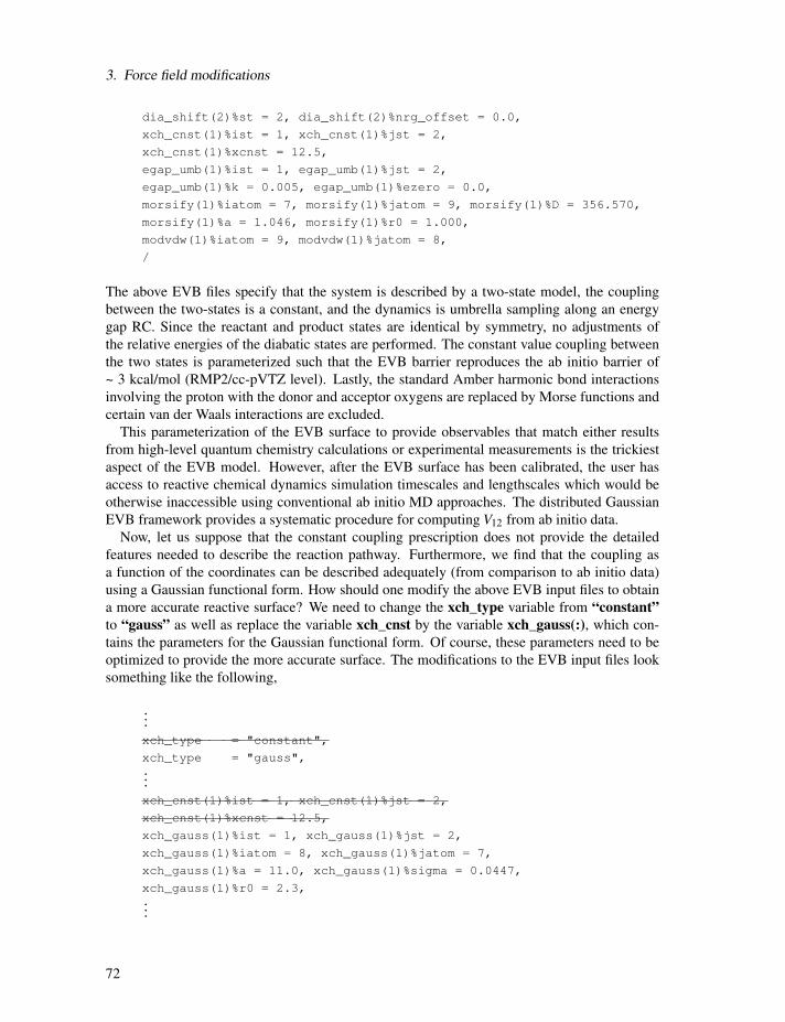
3. Force field modifications
dia_shift(2)%st = 2, dia_shift(2)%nrg_offset = 0.0,
xch_cnst(1)%ist = 1, xch_cnst(1)%jst = 2,
xch_cnst(1)%xcnst = 12.5,
egap_umb(1)%ist = 1, egap_umb(1)%jst = 2,
egap_umb(1)%k = 0.005, egap_umb(1)%ezero = 0.0,
morsify(1)%iatom = 7, morsify(1)%jatom = 9, morsify(1)%D = 356.570,
morsify(1)%a = 1.046, morsify(1)%r0 = 1.000,
modvdw(1)%iatom = 9, modvdw(1)%jatom = 8,
/
The above EVB files specify that the system is described by a two-state model, the coupling
between the two-states is a constant, and the dynamics is umbrella sampling along an energy
gap RC. Since the reactant and product states are identical by symmetry, no adjustments of
the relative energies of the diabatic states are performed. The constant value coupling between
the two states is parameterized such that the EVB barrier reproduces the ab initio barrier of
~ 3 kcal/mol (RMP2/cc-pVTZ level). Lastly, the standard Amber harmonic bond interactions
involving the proton with the donor and acceptor oxygens are replaced by Morse functions and
certain van der Waals interactions are excluded.
This parameterization of the EVB surface to provide observables that match either results
from high-level quantum chemistry calculations or experimental measurements is the trickiest
aspect of the EVB model. However, after the EVB surface has been calibrated, the user has
access to reactive chemical dynamics simulation timescales and lengthscales which would be
otherwise inaccessible using conventional ab initio MD approaches. The distributed Gaussian
EVB framework provides a systematic procedure for computing V12 from ab initio data.Now, let us suppose that the constant coupling prescription does not provide the detailed
features needed to describe the reaction pathway. Furthermore, we find that the coupling as
a function of the coordinates can be described adequately (from comparison to ab initio data)
using a Gaussian functional form. How should one modify the above EVB input files to obtain
a more accurate reactive surface? We need to change the xch_type variable from “constant”to “gauss” as well as replace the variable xch_cnst by the variable xch_gauss(:), which con-tains the parameters for the Gaussian functional form. Of course, these parameters need to be
optimized to provide the more accurate surface. The modifications to the EVB input files look
something like the following,
...
xch_type = "constant",
xch_type = "gauss",...
xch_cnst(1)%ist = 1, xch_cnst(1)%jst = 2,
xch_cnst(1)%xcnst = 12.5,
xch_gauss(1)%ist = 1, xch_gauss(1)%jst = 2,
xch_gauss(1)%iatom = 8, xch_gauss(1)%jatom = 7,
xch_gauss(1)%a = 11.0, xch_gauss(1)%sigma = 0.0447,
xch_gauss(1)%r0 = 2.3,...
72

3.3. Empirical Valence Bond
-75 -50 -25 0 25 50 75
Collective Reaction Coordinate [kcal/mol]
0
1
2
3
Pote
ntia
l of M
ean
Forc
e [k
cal/m
ol]
Figure 3.2: Potential of mean force along an energy gap RC for the intramolecular protontransfer in malonaldehyde as obtained from a series of mapping potential simulations.
where the cross-through lines have been replaced by those below them. Access to the exponen-
tial functional form or the distributed Gaussian approximation to V12 entails similar changes tothe input files. Please see $AMBERHOME/test/evb for examples.
3.3.3. Biased sampling
When a reactive event is described by an intrinsic high free energy barrier, molecular dynam-
ics on the EVB ground-state surface will not adequately sample the important transition state
region. Under these conditions, chemical reactions are rare events and sampling on the EVB
surface effectively reduces to sampling on a diabatic surface. One framework for enhancing the
sampling of rare events is through modification of the system Hamiltonian with the addition of
biasing potentials. The EVB facility in Amber offers several options for biased sampling: (1)
Ariel Warshel’s mapping potential approach [86] (2) Dave Case’s umbrella sampling on an en-
ergy gap RC (3) umbrella sampling on a distance RC and (4) umbrella sampling on a difference
of distances RC.
In the mapping potential framework, the system Hamiltonian (and hence, the molecular dy-
namics) is described by the modified potential
Vλ = (1−λ )Vii +λVf f (3.14)
where Vii is the EVB matrix element for the initial state and Vf f is the EVB matrix element
for the final state. As the value of the mapping potential parameter λ changes from 0 to 1,
the system evolves from the initial state to the final state. As an example, for λ = 0.50, thesystem Hamiltonian is an equal linear combination of the initial and final states and molecular
dynamics sample the region in the vicinity of the transition state. Each mapping potential Vλsamples only a portion of the reaction coordinate. In practice, a series of mapping potentials are
73

3. Force field modifications
-75 -50 -25 0 25 50 75
Collective Reaction Coordinate [kcal/mol]
0
1
2
3
Pote
ntia
l of M
ean
Forc
e [k
cal/m
ol]
Figure 3.3: Potential of mean force for the intramolecular proton transfer in malonaldehyde asobtained from a series of umbrella sampling simulations along an energy gap RC. The distri-butions of the RC from all the windows are combined using the WHAM procedure.
used to bias the sampling across the entire range of the RC. The average distribution of the RC
for each mapping potential is then unbiased and the set of unbiased distributions are combinedto give the potential of mean force (PMF) on the EVB ground-state surface. Figure 3.2 shows a
PMF for the malonaldehyde intramolecular proton transfer reaction as obtained from 9 mapping
potential simulations with λ ranging from 0.10 to 0.90 at 0.10 intervals.In the umbrella sampling framework, the system Hamiltonian is described by the modified
potential
V (n)biased(q) = Vel0(q)+V (n)
umb(q)
= Vel0(q)+1
2k(n)
[RC(q)−RC(n)
0
]2(3.15)
where q is the set of system coordinates, k is the harmonic force constant parameter, and V (n)umb
is an umbrella potential that is added to the original system potential Vel0 (obtained from diag-onalization of the EVB matrix) to bias the sampling towards a particular value of the reaction
coordinate RC(n)0 . The superscript (n) denotes that a series of biased simulations, each enhanc-
ing the sampling of a particular window of the RC, is required to map out the entire PMF. The
number of umbrella sampling windows as well as the choice of values for the force constant pa-
rameter and the RC equilibrium position will depend ultimately on the nature of the free energy
landscape of the system in question.
Results from the biased samplings then can be unbiased and combined using the weighted
histogram analysis method (WHAM) [96–98] to generate the PMF describing chemistry on
the physically relevant EVB ground-state potential energy surface, Vel0. Figure 3.3 depictsthe PMF for the malonaldehyde intramolecular proton transfer that is obtained from 13 um-
brella sampling simulations with RC(n)0 spanning the range -60 kcal/mol to +60 kcal/mol at 10
74
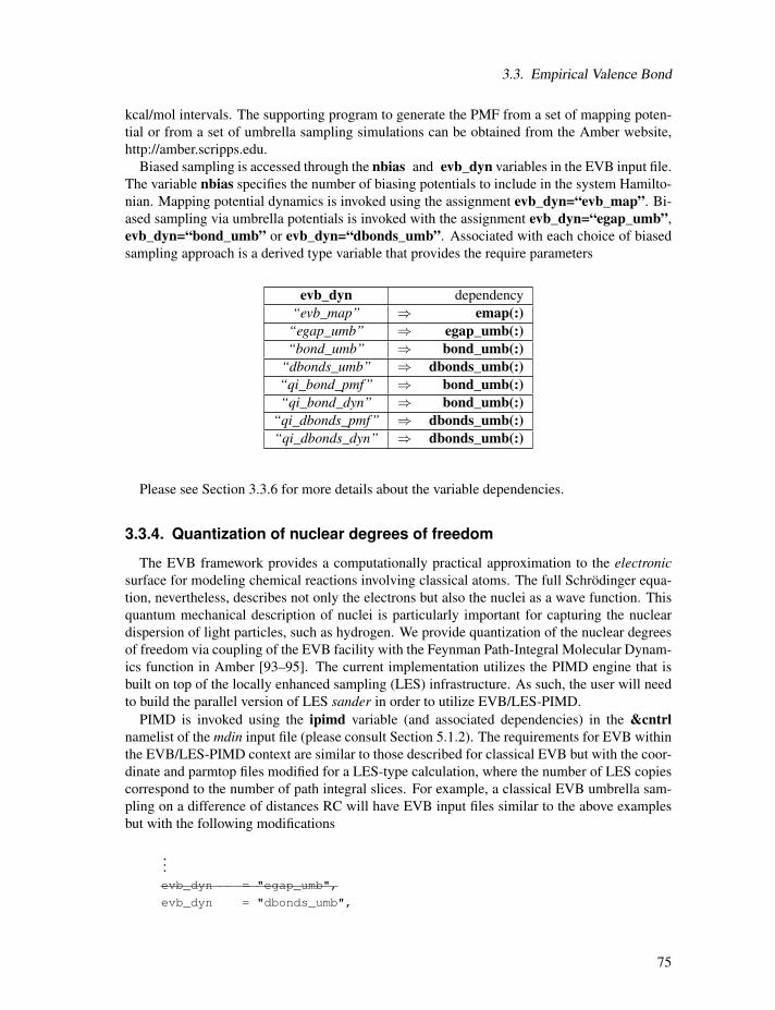
3.3. Empirical Valence Bond
kcal/mol intervals. The supporting program to generate the PMF from a set of mapping poten-
tial or from a set of umbrella sampling simulations can be obtained from the Amber website,
http://amber.scripps.edu.
Biased sampling is accessed through the nbias and evb_dyn variables in the EVB input file.The variable nbias specifies the number of biasing potentials to include in the system Hamilto-nian. Mapping potential dynamics is invoked using the assignment evb_dyn=“evb_map”. Bi-ased sampling via umbrella potentials is invoked with the assignment evb_dyn=“egap_umb”,evb_dyn=“bond_umb” or evb_dyn=“dbonds_umb”. Associated with each choice of biasedsampling approach is a derived type variable that provides the require parameters
evb_dyn dependency
“evb_map” ⇒ emap(:)“egap_umb” ⇒ egap_umb(:)“bond_umb” ⇒ bond_umb(:)
“dbonds_umb” ⇒ dbonds_umb(:)“qi_bond_pmf” ⇒ bond_umb(:)“qi_bond_dyn” ⇒ bond_umb(:)
“qi_dbonds_pmf” ⇒ dbonds_umb(:)“qi_dbonds_dyn” ⇒ dbonds_umb(:)
Please see Section 3.3.6 for more details about the variable dependencies.
3.3.4. Quantization of nuclear degrees of freedom
The EVB framework provides a computationally practical approximation to the electronicsurface for modeling chemical reactions involving classical atoms. The full Schrödinger equa-
tion, nevertheless, describes not only the electrons but also the nuclei as a wave function. This
quantum mechanical description of nuclei is particularly important for capturing the nuclear
dispersion of light particles, such as hydrogen. We provide quantization of the nuclear degrees
of freedom via coupling of the EVB facility with the Feynman Path-Integral Molecular Dynam-
ics function in Amber [93–95]. The current implementation utilizes the PIMD engine that is
built on top of the locally enhanced sampling (LES) infrastructure. As such, the user will need
to build the parallel version of LES sander in order to utilize EVB/LES-PIMD.PIMD is invoked using the ipimd variable (and associated dependencies) in the &cntrl
namelist of the mdin input file (please consult Section 5.1.2). The requirements for EVB withinthe EVB/LES-PIMD context are similar to those described for classical EVB but with the coor-
dinate and parmtop files modified for a LES-type calculation, where the number of LES copies
correspond to the number of path integral slices. For example, a classical EVB umbrella sam-
pling on a difference of distances RC will have EVB input files similar to the above examples
but with the following modifications
...
evb_dyn = "egap_umb",
evb_dyn = "dbonds_umb",
75

3. Force field modifications
...
egap_umb(1)%ist = 1, egap_umb(1)%jst = 2,
egap_umb(1)%k = 0.005, egap_umb(1)%ezero = 0.0,
dbonds_umb(1)%iatom = 8, dbonds_umb(1)%jatom = 9, dbonds_umb(1)%katom = 7,
dbonds_umb(1)%k = 100.000, dbonds_umb(1)%ezero = -.20,...
EVB/LES-PIMD utilizes these same EVB input files. The EVB group file evb.grpfile, however,has been modified to point to the LES coordinate and parmtop files
# 32-bead Malonaldehyde RS: H9 bonded to O8
-O -i mdin -p mr_les.top -c mr_les.crd -o mr_les.out -r mr_les.rst \
-evbin input.mr
# 32-bead Malonaldehyde PS: H9 bonded to O7
-O -i mdin -p mp_les.top -c mr_les.crd -o mp_les.out -r mp_les.rst \
-evbin input.mp
Additionally, the -nslice <# PIMD slices> variable must be passed to the sander executable:
mpirun -np 2 sander.LES.MPI -ng 2 -nslice 32 -groupfile evb.grpfile
Here, the atoms of the malonaldehyde system have been replicated into 32 copies using the
addles utility (see Section 5.1.2) and each of the EVB diabatic states now use the correspondingLES coordinate and parmtop files. Nuclear quantization lowers the free energy barrier due to
quantum mechanical effects, such as zero point motion and tunneling. Figure 3.4 compares the
PMFs for the malonaldehyde proton transfer reaction along a difference of distances RC from
classical EVB and EVB/PIMD umbrella sampling simulations. Currently, only the distance and
difference of distances RCs are supported in EVB/PIMD. The energy gap RC is not supported
because the theoretical formulation of quantum transition state theory based on an energy gap
RC has not yet been worked out.
3.3.5. Distributed Gaussian EVB
As briefly mentioned in the Introduction to EVB,V12 can be fit to high-level electronic struc-ture data using a set of s-, p-, and d-type Gaussians as the fitting basis functions. The current
incarnation of DG EVB is limited to two-state gas-phase systems. Current efforts to extend this
approach to the condensed phase will provide a practical systematic procedure for constructing
a reactive surface from ab initio information. The curious student is encouraged to read the
original papers on this method for the theoretical formulation [88, 89]. Here, we only provide
an example of this approach for constructing an ab initio-inspired surface describing the proton
transfer reaction in malonaldehyde. All the previously described EVB functionalities are acces-
sible to this method. For example, the key elements of the RS input.mr file for biased samplingalong a distance RC on the DG EVB surface may look something like the following:
...
76
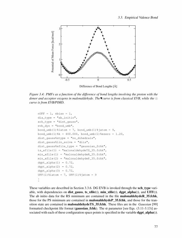
3.3. Empirical Valence Bond
-0.5 0 0.5
Difference of Bond Lengths [Å]
0
1
2
3
Pote
ntia
l of M
ean
Forc
e [k
cal/m
ol]
Figure 3.4: PMFs as a function of the difference of bond lengths involving the proton with thedonor and acceptor oxygens in malonaldehyde. The�curve is from classical EVB, while the �curve is from EVB/PIMD.
nUFF = 1, nbias = 1,
dia_type = "ab_initio",
xch_type = "dist_gauss",
evb_dyn = "bond_umb",
bond_umb(1)%iatom = 7, bond_umb(1)%jatom = 9,
bond_umb(1)%k = 400.000, bond_umb(1)%ezero = 1.20,
dist_gauss%stype = "no_dihedrals",
dist_gauss%lin_solve = "diis",
dist_gauss%xfile_type = "gaussian_fchk",
ts_xfile(1) = "malonaldehydeTS_35.fchk",
min_xfile(1) = "malonaldehydeR_35.fchk",
min_xfile(2) = "malonaldehydeP_35.fchk",
dgpt_alpha(1) = 0.72,
dgpt_alpha(2) = 0.72,
dgpt_alpha(3) = 0.72,
UFF(1)%iatom = 7, UFF(1)%jatom = 9...
These variables are described in Section 3.3.6. DG EVB is invoked through the xch_type vari-able, with dependencies on dist_gauss, ts_xfile(:), min_xfile(:), dgpt_alpha(:), and UFF(:).The ab initio data for the RS minimum are contained in the file malonaldehydeR_35.fchk,those for the PS minimum are contained in malonaldehydeP_35.fchk, and those for the tran-sition state are contained in malonaldehydeTS_35.fchk. These files are in the Gaussian [99]formatted checkpoint file format (gaussian_fchk). The α parameter [see Eqs. (3.11-3.13)] as-
sociated with each of these configuration space points is specified in the variable dgpt_alpha(:).
77

3. Force field modifications
Figure 3.5: PMF as a function of the distance between atoms H9 and O7 in malonaldehyde. Thepotential energy surface was constructed from ab initio data using the DG EVB approach.
If we wish to include additional ab initio data points along the reaction path, we can specify the
file names for those points in the variable xdg_xfile(:). The α parameters associated with thesepoints can be specified in dgpt_alpha(:). It is important to keep in mind that the α parame-
ters are ordered as follows: dgpt_alpha(ts_xfile(1), min_xfile(1), min_xfile(2), xdg_xfile(:)).Lastly, the UFF variable requests the inclusion of a Universal Force Field [100] repulsive terminV11 between the transferred proton (H9) and the acceptor (O7). The input.mp file for the PSV22is identical to the above, but with theUFF variable changed to reflect the identity of the acceptoratom from the perspective of the product state topology: UFF(1)%iatom = 8, UFF(1)%jatom= 9. In practice, the inclusion of this term to Vii provides a more optimal DG EVB surface for
molecular dynamics sampling. Figure 3.5 shows the PMF for shortening the rH9−O7 distance ofthe malonaldehyde RS from 1.8 Å to 1.0 Å using umbrella sampling of this RC. Note that the
PMF is not symmetric because this choice of RC breaks the intrinsic symmetry of the reaction.
The difference of distances RC involving atoms O8, H9 and O7 does provide a symmetric PMF
and this is shown in Figure 5.1 within the context of kinetic isotope effect (Section 5.5.5).
3.3.6. EVB input variables and interdependencies
The variables in the &evb namelist of the EVB input file are described below. The style ofthe input file is similar to the traditionalmdin used in a sander run. Assignment to character typevariables need to be encapsulated within quotation marks (for example, evb_dyn=“groundstate”).Array variables are denoted below by a colon enclosed within parentheses [for example, dia_shift(:)].Derived type variables can be assigned element-wise, i.e., dia_shift(1)%st = 1, dia_shift(1)%nrg_offset= 0.0. In the specifications below, the data type of each variable is enclosed in {· · ·}, while thesize of each array variable is enclosed in [· · · ].
78

3.3. Empirical Valence Bond
ntw_evb {integer}. MD step interval for writing to the EVB output file evbout.
nevb {integer}. Number of EVB states. For example, nevb = 3 specifies that the systemis described by a 3× 3 EVB matrix in the representation of three diabatic states.The EVB group file will contain three lines of sander command line options spec-ifying the mdin, coordinate, parmtop, and EVB input files.
nmorse {integer}. Number of Amber harmonic bond interactions that will be changed to a
Morse type interaction. Requires additional inputs from the variable morsify(:).
nbias {integer}. Number of biasing potentials to include in the system Hamiltonian. The
supported biased sampling approaches include (1) mapping potential, (2) umbrella
sampling along an energy gap RC, (3) umbrella sampling along a distance RC,
and (4) umbrella sampling along a difference of distances RC. See evb_dyn forassociated dependencies.
nmodvdw {integer}. Number of van der Waals terms to exclude in the calculation of Vii.
Requires additional inputs from the variable modvdw(:).
nuff {integer}. Number of Universal Force Field [100] repulsive terms to include in the
harmonic expansion of Vii about the ab initio minimum. Requires additional inputs
from the variable uff(:).
xch_type {character*512}. Coupling element type.
= “constant” Vi j is a constant. Requires additional inputs from the variable xch_cnst(:).
= “exp” Vi j(rkl) = Ai j exp[−ui j
(rkl− r(0,i j)
kl
)]. Requires additional inputs from
the variable xch_exp(:).
= “gauss” Vi j(rkl) = Ai j exp
[− 1
σ2i j
(rkl− r(0,i j)
kl
)2]. Requires additional inputs
from the variable xch_gauss(:).= “dist_gauss” Vi j is described by the Schlegel-Sonnenberg distributed Gaussian
approach. Requires additional inputs from the variables dist_gauss,ts_xfile(:), min_xfile(:), xdg_xfile(:), dgpt_alpha(:), uff(:).
evb_dyn {character*512}. EVB dynamics type.
79

3. Force field modifications
= “groundstate” Dynamics on the EVB ground-state potential energy surface.
= “evb_map” Biased sampling based on Ariel Warshel’s mapping potential ap-
proach. Requires additional inputs from the variable emap(:).= “egap_umb” Umbrella sampling along an energy gap reaction coordinate. Re-
quires additional inputs from the variable egap_umb(:).= “bond_umb” Umbrella sampling along a distance reaction coordinate. Requires
additional inputs from the variable bond_umb(:).= “dbonds_umb” Umbrella sampling along a difference of two distances reaction
coordinate. Requires additional inputs from the variable dbonds_umb(:).= “qi_bond_pmf” For generating the QI joint distribution function along the dis-
tance RCs of the P and P/2 slices (see Section 5.4.2). Requires addi-tional inputs from the variable bond_umb(:).
= “qi_bond_dyn” For sampling of the QI fv, F and G factors with the P and P/2slices constrained to the dividing surfaces along the distance RCs (see
Section 5.4.2). Requires additional inputs from the variable bond_umb(:).= “qi_dbonds_pmf” For generating the QI joint distribution function along the
difference of distances RCs of the P and P/2 slices (see Section 5.4.2).Requires additional inputs from the variable dbonds_umb(:).
= “qi_dbonds_dyn” For sampling of the QI fv, F and G factors with the P andP/2 slices constrained to the dividing surfaces along the difference ofdistances RCs (see Section 5.4.2). Requires additional inputs from the
variable dbonds_umb(:).
dia_shift(:) {derived type}, [nevb]. Diabatic state energy shift.
%st {integer}. Diabatic state index.
%nrg_offset {real}. Energy offset for EVB state.
xch_cnst(:) {derived type}, [nxch]. Constant coupling. The size of this derived type array isnxch, which is calculated internally as nevb(nevb−1)/2.
%ist {integer}. Diabatic state index involved in the coupling.
%jst {integer}. Diabatic state index involved in the coupling.
%xcnst {real}. Constant exchange parameter.
xch_exp(:) {derived type}, [nxch]. Parameters for the exponential functional form of the cou-pling term, Vi j(rkl) = Ai j exp
[−ui j
(rkl− r(0,i j)
kl
)]. The size of this derived type
array is nxch, which is calculated internally as nevb(nevb−1)/2.
80
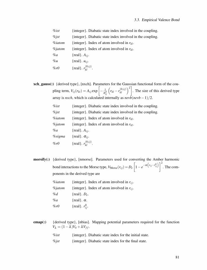
3.3. Empirical Valence Bond
%ist {integer}. Diabatic state index involved in the coupling.
%jst {integer}. Diabatic state index involved in the coupling.
%iatom {integer}. Index of atom involved in rkl .
%jatom {integer}. Index of atom involved in rkl .
%a {real}. Ai j.
%u {real}. ui j.
%r0 {real}. r(0,i j)kl .
xch_gauss(:) {derived type}, [nxch]. Parameters for the Gaussian functional form of the cou-
pling term, Vi j(rkl) = Ai j exp
[− 1
σ2i j
(rkl− r(0,i j)
kl
)2]. The size of this derived type
array is nxch, which is calculated internally as nevb(nevb−1)/2.%ist {integer}. Diabatic state index involved in the coupling.
%jst {integer}. Diabatic state index involved in the coupling.
%iatom {integer}. Index of atom involved in rkl .
%jatom {integer}. Index of atom involved in rkl .
%a {real}. Ai j.
%sigma {real}. σi j.
%r0 {real}. r(0,i j)kl .
morsify(:) {derived type}, [nmorse]. Parameters used for converting the Amber harmonic
bond interactions to theMorse type,VMorse(ri j) = De
[1− e−α
(ri j−r0i j
)]2. The com-
ponents in the derived type are
%iatom {integer}. Index of atom involved in ri j.
%jatom {integer}. Index of atom involved in ri j.
%d {real}. De.
%a {real}. α .%r0 {real}. r0i j.
emap(:) {derived type}, [nbias]. Mapping potential parameters required for the function
Vλ = (1−λ )Vii +λVf f .
%ist {integer}. Diabatic state index for the initial state.
%jst {integer}. Diabatic state index for the final state.
81
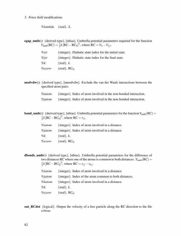
3. Force field modifications
%lambda {real}. λ .
egap_umb(:) {derived type}, [nbias]. Umbrella potential parameters required for the functionVumb(RC) = 1
2k [RC−RC0]2, where RC= Vii−Vf f .
%ist {integer}. Diabatic state index for the initial state.
%jst {integer}. Diabatic state index for the final state.
%k {real}. k.
%ezero {real}. RC0.
modvdw(:) {derived type}, [nmodvdw]. Exclude the van der Waals interactions between thespecified atom pairs.
%iatom {integer}. Index of atom involved in the non-bonded interaction.
%jatom {integer}. Index of atom involved in the non-bonded interaction.
bond_umb(:) {derived type}, [nbias]. Umbrella potential parameters for the functionVumb(RC) =12k [RC−RC0]2, where RC= ri j.
%iatom {integer}. Index of atom involved in a distance.
%jatom {integer}. Index of atom involved in a distance.
%k {real}. k.
%ezero {real}. RC0.
dbonds_umb(:) {derived type}, [nbias]. Umbrella potential parameters for the difference oftwo distances RCwhere one of the atoms is common to both distances. Vumb(RC) =12k [RC−RC0]2, where RC= ri j− rk j.
%iatom {integer}. Index of atom involved in a distance.
%jatom {integer}. Index of the atom common to both distances.
%katom {integer}. Index of atom involved in a distance.
%k {real}. k.
%ezero {real}. RC0.
out_RCdot {logical}. Output the velocity of a free particle along the RC direction to the fileevbout.
82

3.3. Empirical Valence Bond
dist_gauss {derived type}. Schlegel-Sonnenberg distributed Gaussian specifications.
%stype {character*512}. Coordinate selection type. Supported coordinate se-
lection types include “all_coords”, “bonds_only”,“no_dihedrals”,“react-product”,“react-ts-product”.
%stol {real}. Coordinate selection tolerance for stype=“react-product” orstype=“react-ts-product”. For stype=“react-product”, a particular in-ternal coordinate is used in the DG EVB procedure if the difference
between the reactant and product structures is > stol. For the case ofstype=“react-ts-product”, the intersection of the selected set of coor-dinates from react-ts > stol and product-ts > stol will be used for theDG EVB procedure.
%xfile_type {character*512}. File type of external ab initio data. Supported filetypes are “gaussian_fchk” and “EVB” (see Section D).
ts_xfile(:) {character*512}, [*]. Name of the file containing the ab initio data corresponding
to the transition state.
min_xfile(:) {character*512}, [*]. Name of the file containing the ab initio data correspondingto the minimum, i.e. V11 and V22.
xdg_xfile(:) {character*512}, [*]. Name of the file containing the ab initio data correspondingto additional points along the IRC.
dgpt_alpha(:) {real}, [*]. Optimized α parameters associated with the distributed Gaussian
data points.
uff(:) {derived type}, [nuff]. Include a UFF repulsive term between the specified atom
pairs in the harmonic expansion of Vii about the ab initio minimum.
%iatom {integer}. Index of atom involved in the non-bonded interaction.
%jatom {integer}. Index of atom involved in the non-bonded interaction.
83

3. Force field modifications
3.4. Using the AMOEBA force field
The Amoeba force field is a recently developed polarizable force field with parameters for
water, univalent ions, small organic molecules and proteins. [30, 31, 101, 102] Differences from
the current amber force fields include more complex valence terms including anharmonic bond
and angle corrections and bond angle and bond dihedral cross terms, and a two dimensional
spline fit for the phi-psi bitorsional energy. The differences in the nonbond treatment include
the use of atomic multipoles up to quadrupole order, induced dipoles using a Tholé screening
model, and the use of the Halgren buffered 7-14 functional form for van der Waals interactions.
The PME implementation used here, as well as a multigrid approach for atomic multipoles, is
described in Ref. [37].
Preparation of the necessary coordinate and parameter files for performing simulations using
the amoeba forcefield is now very simple (unlike in Amber 9), but does require that you use
sleap in place of tleap. The procedure is now almost like any other force field: you load
leaprc.amoeba in place of other leaprc files at the beginning; at the end, use saveamoebaparmin place of saveamberparm.With the use of Amoeba, minimization as well as usual sander methods of molecular dynam-
ics can be used, including constant temperature and pressure simulations. In addition, with the
amoeba implementation it is possible to use the Beeman dynamics integrator, which is helpful in
making detailed comparisons to Tinker results. Note that the Amoeba forcefield is parametrized
for fully flexible molecules. At this time it is not possible to use SHAKE with this forcefield.
The parameters ew_coeff, nfft1, nfft2, nfft3, and order from the &ewald section of input all
relate to the accuracy of the PME method, which is used in the Amoeba implementation in
sander. Due to the use of atomic quadrupoles, order (i.e. the B-spline polynomial degree plusone) needs to be at least 5 since the B-spline needs 3 continuous derivatives. The ew_coefftogether with the direct sum cutoff (see below) controls the accuracy in the Ewald direct sum,
and ew_coeff together with the PME grid dimensions nfft1,2,3 and order controls the accuracyin the reciprocal sum. Since Amoeba atomic multipoles are typically dominated by the charges,
experience gained in the usual use of PME is pertinent. Typical values we have used for a good
cost vs. accuracy balance are ew_coeff=0.45, order=5, and nfft1,2,3 approximately 1.25 timesthe cell length in that direction.
Some specific amoeba-related input parameters are given here. They should be placed in the
&amoeba namelist, following the &cntrl namelist where iamoeba has been set to 1.
beeman_integrator Setting this to be one turns on the Beeman integrator. This is the default
integrator for Amoeba in Tinker. In sander this integrator can be used for NVE
simulations, or for NVT or NTP simulations using the Berendson coupling scheme.
(This means that you must set ntt to 0 or 1 if you use the Beeman integrator.) Bydefault, beeman_integrator=0, and the usual velocity Verlet integration scheme isused instead.
amoeba_verbose In addition to the usual sander output, by setting amoeba_verbose=1, energy
and virial components can be output. By default, amoeba_verbose=0.
ee_dsum_cut This is the ewald direct sum cutoff. In the amoeba implementation this is allowed
to be different from the nonbond cutoff specified by cut. It should be less than orequal to the latter. (Note, this feature does not apply to the direct sum for standard
84
3.4. Using the AMOEBA force field
amber force fields, which use the nonbond cutoff for the Ewald direct sum as well
as van der Waals interactions. The default is 7.0 Angstroms, which is conservative
for energy conservation with ew_coeff=0.45.
dipole_scf_tol The induced dipoles in the amoeba force field are solutions to a set of linear
equations (like the Applequist model but modified by Tholé damping for close
dipole-dipole interactions). These equations are solved iteratively by the method
of successive over-relaxation. dipole_scf_tol is the convergence criterion for theiterative solution to the linear equations. The iterations towards convergence stop
when the RMS difference between successive sets of induced dipoles is less than
this tolerance in Debye. The default is set to 0.01 Debye, which has been seen to
give reasonable energetics and dynamics, but requires mild temperature restraints.
Good energy conservation in NVE simulations requires a tolerance of about 10−6Debye tolerance.
sor_coefficient This is the successive over-relaxation parameter. This can be adjusted to op-
timize the number of iterations needed to achieve convergence. Default value is
0.75. Productive values seem to be in the range 0.6-0.8 .The optimal values seem
to depend on the polarizabilities of the system atoms.
dipole_scf_iter_max This prevents infinite iterations when the polarization equations are some-
how not converging. A possible reason for this is a bad sor_coefficient, exacerbated
by a close contact. Default is 50. For comparison, with typical sor_coefficient val-
ues and an equilibrated system it should take 4-7 iterations to achieve 0.01 Debye
convergence and 18-25 iterations to achieve 10−6 Debye.
ee_damped_cut This is used to cutoff the Tholé damping interactions. The default value is 4.5
Angstroms, which should work for the typical sized polarizabilities encountered,
and the default Tholé screening parameter (0.39).
do_vdw_taper Amoeba uses a Halgren buffered 7-14 form for the van der Waals interactions.
In the Tinker code these are typically evaluated out to 12 Angstroms, with a ta-
per turned on and no long-range isotropic continuum corrections to the energy and
virial. In the sander implementation, the usual nonbond cutoff from the &cntrl
namelist is used for van der Waals interactions. The long range correction is avail-
able to allow for shorter cutoffs. Setting do_vdw_taper to one causes VDW inter-
actions to be tapered to zero beginning at 0.9 times the van der waals cutoff. The
taper is a 5th order polynomial switch on the energy term, which gets differentiated
for the forces (atom based switching). Its turned on by default.
do_vdw_longrange Setting this to one causes the long-range isotropic continuum correction
to be turned on. This adjusts the energy and virial, and in most cases will result
in energies and virials that are fairly invariant to van der Waals cutoff, with or
without the above taper function. The integrals involved in this correction are done
numerically.
85

3. Force field modifications
3.5. QM/MM calculations
Sander supports the option of allowing part of the system to be described quantum mechan-
ically in an approach known as a hybid (or coupled potential) QM/MM simulation. QM/MM
calculations are implemented via two interfaces. The first interface provides seamless semi-
empirical QM/MM integration via a &qmmm namelist supplied in the regular mdin file. Thisinterface is accessed by setting ifqnt=1 and idc=0. The second interface provides support forQM/MM simulations via the DivCon library. This interface is accessed by setting idc>0, andspecifying additional parameters in a divcon.in file. Chapter 10 discusses DivCon, and the restof this section assumes that idc=0.Support currently exists for gas phase, generalized Born and PME periodic simulations.
Available semi- empirical Hamiltonians are PM3, [103] AM1, [104] RM1, [105] MNDO, [106]
PDDG/PM3, [107] PDDG/MNDO, [107] and PM3CARB1. [108] Support is also available for
the Density Functional Theory-based-tight- binding (DFTB) Hamiltonian, [109–111] as well
as the Self-Consistent-Charge version, SCC-DFTB. [112] DFTB/SCC-DFTB also supports ap-
proximate inclusion of dispersion effects, [113] as well as reporting CM3 charges [114] for
molecules containing only the H, C, N, O, S and P atoms.
The elements supported by each QM method are:
MNDO: H, Li, Be, B, C, N, O, F, Al, Si, P, S, Cl, Zn, Ge, Br, Sn, I, Hg, Pb
AM1: H, C, N, O, F, Al, Si, P, S, Cl, Zn, Ge, Br, I, Hg
PM3: H, Be, C, N, O, F, Mg, Al, Si, P, S, Cl, Zn, Ga, Ge, As, Se, Br, Cd,
In, Sn, Sb, Te, I, Hg, Tl, Pb, Bi
PDDG/PM3: H, C, N, O, F, Si, P, S, Cl, Br, I
PDDG/MNDO: H, C, N, O, F, Cl, Br, I
RM1: H, C, N, O, P, S, F, Cl, Br, I
PM3CARB1: H, C, O
DFTB/SCC-DFTB: (Any atom set available from the www.dftb.org website)
The DFTB/SCC-DFTB code was originally based on the DFT/DYLAX code by Marcus El-
stner et al.. but has since been extensively re-written and optimized. In order to use DFTB(qm_theory=DFTB) a set of integral parameter files are required. These are not distributedwith Amber and must be obtained from the www.dftb.org website and placed in the $AMBER-HOME/dat/slko directory. Dispersion parameters for H, C, N, O, P and S are available in the$AMBERHOME/dat/slko/DISPERSION.INP_ONCHSP file, and CM3 parameters for the sameatoms are in the $AMBERHOME/dat/slko/CM3_PARAMETERS.DAT file.The built-in semi-empirical QM/MM support was written by Ross Walker and Mike Crow-
ley, [115] based originally on public-domain MOPAC codes of J.J.P. Stewart. The QM/MM
Generalised Born implementation uses the model described by Pellegrini and Field [116] while
regular QM/MM Ewald support is based on the work of Nam et al. [117] with QM/MM PME
support based on the work of Walker et al. [115]. SCC-DFTB support was written by Gus-tavo Seabra, Ross Walker and Adrian Roitberg, [109] and is based on earlier work of Marcus
Elstner. [112, 118]
86

3.5. QM/MM calculations
3.5.1. The hybrid QM/MM potential
When running a QM/MM simulation in Sander the system is partitioned into two regions, a
QM region consisting of the atoms defined by either the qmmask or iqmatoms keyword, and aMM region consisting of all the atoms that are not part of the QM region. For a typical protein
simulation in explicit solvent the number of MM atoms will be much greater than the number
of QM atoms. Either region can contain zero atoms, giving either a pure QM simulation or a
standard classical simulation. For periodic simulations, the quantum region must be compact, sothat the extent (or diameter) of the QM region (in any direction) plus twice the QM/MM cutoff
must be less than the box size. Hence, you can define an "active site" to be the QM region,
but in most cases could not ask that all cysteine residues (for example) be quantum objects.
The restrictions are looser for non-periodic (gas-phase or generalized Born) simulations, but
the codes are written and tested for the case of a single, compact quantum region.
The partitioned system is characterized by an effective Hamiltonian which operates on the
system’s wavefunction Ψ, which is dependent on the position of the MM and QM nuclei, to
yield the system energy Ee f f :
He f f Ψ(xe,xQM,xMM) = E(xQM,xMM)Ψ(xe,xQM,xMM) (3.16)
The effective Hamiltonian consists of three components - one for the QM region, one for the
MM region and a term that describes the interaction of the QM and MM regions, implying that
likewise the energy of the system can be divided into three components. If the total energy of
the system is re-written as the expectation value of He f f then the MM term can be removed
from the integral since it is independent of the position of the electrons:
Ee f f =⟨Ψ|HQM +HQM/MM|Ψ
⟩+EMM (3.17)
In the QM/MM implementation in sander, EMM is calculated classically from the MM atom
positions using the Amber force field equation and parameters, whereas HQM is evaluated using
the chosen QM method.
The interaction term HQM/MM is more complicated, representing the interaction of the MM
point charges with the electron cloud of the QM atoms as well as the interaction between MM
point charges and the QM atomic cores. For the case where there are no covalent bonds between
the atoms of the QM andMM regions this term is the sum of an electrostatic term and a Lennard-
Jones (VDW) term and can be written as:
HQM/MM =−∑q
∑m
[qmhelectron(xe,xMM)+ zqqmhcore(xQM,xMM)+
(A
r12qm− B
r6qm
)](3.18)
where the subscripts e, m and q refer to the electrons, the MM nuclei and the QM nuclei re-
spectively. Here qm is the charge on MM atom m, zq is the core charge (nucleus minus core
electrons) on QM atom q, rqm is the distance between atoms q and m, and A and B are Lennard-Jones interaction parameters. For systems that have covalent bonds between the QM and MM
regions, the situation is more complicated, as discussed later. If one evaluates the expectation
values in Eq. 3.17 over a single determinant built from molecular orbitals
φi = ∑j
ci jχ j (3.19)
87

3. Force field modifications
where the ci j are molecular orbital coefficients and the χ j are atomic basis functions, the total
energy depends upon the ci j and on the positions xMM and xQM of the atoms. Once the energy is
known, the forces on the atoms can be obtained by using the chain rule and setting ∂Ee f f /∂ci jto zero. This leads to a self-consistent (SCF) procedure to determine the ci j, (with a modified
Fock matrix that contains the electric field arising from the MM charges).
The main subtlety that arises is that, for a periodic system, there are formally an infinite
number of QM/MM interactions; even for a non-periodic system, the (finite) number of such
interactions may be prohibitively large. These problems are addressed in a manner analogous
to that used for pure MM systems: a PME approach is used for periodic systems, and a (large)
cutoff may be invoked for non-periodic systems. Some details are discussed below.
3.5.2. The QM/MM interface and link atoms
The sections above dealt with situations where there are no covalent bonds between the QM
and MM regions. In many protein simulations, however, it is necessary to have the QM/MM
boundary cut covalent bonds, and a number of additional approximations have to be made.
There are a variety of approaches to this problem, including hybrid orbitals, capping potentials,
and explicit link atoms. The last option is the method available in sander.There are a number of ways to implement a link atom approach that deal with the way the link
atom is positioned, the way the forces on the link atom are propagated, and the way non-bonding
interactions around the link atom are treated. Each time an energy or gradient calculation is to
be done, the link atom coordinates are re-generated from the current coordinates of the QM and
MM atoms making up the QM-MM covalent pair. The link atom is placed along the bond vector
joining the QM and MM atom, at a distance dL−QM from the QM atom. By default dL−QM is set
to the equilibrium distance of a methyl C-H atom pair (1.09 Å) but this can be set in the input
file. The default link atom type is hydrogen, but this can also be specified as an input.
Since the link atom position is a function of the coordinates of the "real" atoms, it does not
introduce any new degrees of freedom into the system. The chain rule is used to re-write forces
on the link atom itself in terms of forces on the two real atoms that define its position. This is
analogous to the way in which "extra points" or "lone-pairs" are handled in MM force fields.
The remaining details of how the QM-MM boundary is treated are as follows: for the in-
teractions surrounding the link atom, the MM bond term between the QM and MM atoms is
calculated classically using the Amber force field parameters, as are any angle or dihedral terms
that include at least one MM atom. The Lennard-Jones interactions between QM-MM atom
pairs are calculated in the same way as described in the section above with exclusion of 1-2
and 1-3 interactions and scaling of 1-4 interactions. What remains is to specify the electrostatic
interactions between QM and MM atoms around the region of the link atom.
A number of different schemes have been proposed for handling link-atom electrostatics.
Many of these have been tested or calibrated on (small) gas-phase systems, but such testing
can neglect some considerations that are very important for more extended, condensed-phase
simulations. In choosing our scheme, we wanted to ensure that the total charge of the system
is rigorously conserved (at the correct value) during an MD simulation. Further, we strove to
have the Mulliken charge on the link atom (and the polarity of its bond to the nearest QM atom)
adopt reasonable values and to exhibit only small fluctuations during MD simulations. Link
atoms interact with the MM field in exactly the same was as regular QM atoms. That is they
interact with the electrostatic field due to all the MM atoms that are within the cutoff, with the
88

3.5. QM/MM calculations
exception of the MM link pair atoms (MM atoms that are bound directly to QM atoms). VDW
interactions are not calculated for link atoms. These are calculated between all real QM atoms
and ALL MM atoms, including the MM link pair atoms. For Generalized Born simulations the
effective Born radii for the link atoms are calculated using the intrinsic radii for the MM link
pair atoms that they are replacing.
Since the MM atoms that make up the QM region (including the MM link pair atom) have
their charges from the prmtop file essentially replaced with Mulliken charges it is important to
consider the issue of charge conservation. The QM region (including the link atoms) by defini-
tion must have an integer charge. This is defined by the &qmmm namelist variable qmcharge.If the MM atoms (including the MM link pair atoms) that make up the QM region have prm-
top charges that sum to the value of qmcharge then there is no problem. If not, there are twooptions for dealing with this charge, defined by the namelist variable adjust_q. A value of 1will distribute the difference in charge equally between the nearest nlink MM atoms to the MM
link pair atoms. A value of 2 will distribute this charge equally over all of the MM atoms in the
simulation (excluding MM link pair atoms).
3.5.3. Generalized Born implicit solvent
The implementation of Generalized Born (GB) for QM/MM calculations is based on the
method described by Pellegrini and Field. [116] Here, the total energy is taken to be Ee f ffrom Eq. 3.17 plus Egb from Eq. 3.2. In Egb, charges on the QM atoms are taken to be the
Mulliken charges determined from the quantum calculation; hence these charges depend upon
the molecular orbital coefficients ci j as well as the positions of the atoms.
As with conventional QM/MM simulations, one then solves for the ci j by setting ∂Ee f f /∂ci j =0. This leads to a set of SCF equations with a Fock matrix modified not only by the presence
of MM atoms (as in "ordinary" QM/MM simulations), but also modified by the presence of the
GB polarization terms. Once self-consistency is achieved, the resulting Mulliken charges can
be used in the ordinary way to compute the GB contribution to the total energy and forces on
the atoms.
3.5.4. Ewald and PME
The support for long range electrostatics in QM/MM calculations is based on a modification
of the Nam, Gao and York Ewald method for QM/MM calculations. [117] This approach works
in a similar fashion to GB in that Mulliken charges are used to represent long range interactions.
Within the cut off, interactions between QM andMM atoms are calculated using a full multipole
treatment. Outside of the cut off the interaction is based on pairwise point charge interactions.
This leads to a slight discontinuity at the QM/MM cut off boundary but this does not so far
seem to be a significant limitation.
The implementation in Ref [117] uses an Ewald sum for both QM/QM and QM/MM elec-
trostatic interactions. This can be expensive for large MM regions, and thus sander uses amodification of this method by Walker and Crowley [115] that uses a PME model (rather than
an Ewald sum) for QM/MM interactions. This is controlled by the qm_pme variable discussedbelow.
89

3. Force field modifications
3.5.5. Hints for running successful QM/MM calculations
Required Parameters and Prmtop Creation
QM/MM calculations without link atoms require only mass, van der Waals and GB radii in
the prmtop file. All charges and bonds, angles, and dihedrals parameters involving QM atoms
are neglected. (Note that when SHAKE is applied, the bonds are constrained to the ideal MM
values, even when these are part of a QM region; hence, for this case, it is important to have
correct bond parameters in the QM region.) The simplest general prescription for setting things
up is to use antehcamber and LEaP to create a reference force field, since "placeholders" arerequired in the prmtop file even for things that will be neglected. This also allows you to runcomparison simulations between pure MM and QM/MM simulations, which can be helpful if
problems are encountered in the QM/MM calculations.
The use of antechamber to construct a pure MM reference system is even more useful when
there are link atoms, since here MM parameters for bonds, angles and dihedrals that cross the
QM/MM boundary are also needed.
Choosing the QM region
There are no good universal rules here. Generally, one might want to have as large a QM re-
gion as possible, but having more than 80-100 atoms in the QM region will lead to simulations
that are very expensive. One should also remember that for many features of conformational
analysis, a good MM force field may be better than a semiempirical or DFTB quantum descrip-
tion. In choosing the QM/MM boundary, it is better to cut non-polar bonds (such as C-C single
bonds) than to cut unsaturated or polar bonds. Link atoms are not placed between bonds to
hydrogen. Thus cutting across a C-H bond will NOT give you a link atom across that bond.
(This is not currently tested for in the code and so it is up to the user to avoid such a situation.)
Furthermore, link atoms are restricted to one per MM link pair atom. This is tested for during
the detection of link atoms and an error is generated if this requirement is violated. This would
seem to be a sensible policy otherwise you could have two link atoms too close together. See
the comments in qm_link_atoms.f for a more in-depth discussion of this limitation.
Choice of electrostatic cutoff
The implementation of the non-bonded cut off in QM/MM simulations is slightly different
than in regular MM simulations. The cut off between MM-MM atoms is still handled in a
pairwise fashion. However, for QM atoms any MM atom that is within qmcut of ANY QMatom is included in the interaction list for all QM atoms. This means that the value of qmcutessentially specifies a shell around the QM region rather than a spherical shell around each
individual QM atom. Ideally the cut off should be large enough that the energy as a function
of the cutoff has converged. For non-periodic, generalized Born simulations, a cutoff of 15
to 20 Åseems sufficient in some tests. (Remember that long-range electrostatic interactions
are reduced by a factor of 80 from their gas-phase counterparts, and by more if a non-zero salt
concentration is used.) For periodic simulations, the cutoff only serves to divide the interactions
between "direct" and "reciprocal" parts; as with pure MM calculations, a cutoff of 8 or 9 Åis
sufficient here.
90

3.5. QM/MM calculations
Parallel simulations
The built-in QM/MM implementation currently supports execution in parallel, however, the
implementation is not fully parallel. At present all parts of the QM simulation (for idc=0) areparallel except the density matrix build and the matrix diagonalisation. For small QM systems
these two operations do not take a large percentage of time and so acceptable scaling can be
seen to around 8 cpus (depending on interconnect speed). However, for large QM systems the
matrix diagonalisation time will dominate and so the scaling will not be as good.
3.5.6. General QM/MM &qmmm Namelist Variables
An example input file for running a simple QM/MMMD simulation is shown here:
&cntrl
imin=0, nstlim=10000, (perform MD for 10,000 steps)
dt=0.002, (2 fs time step)
ntt=1, tempi=0.1, temp0=300.0 (Berendsen temperature control)
ntb=1, (Constant volume periodic boundaries)
ntf=2, ntc=2, (Shake hydrogen atoms)
cut=8.0, (8 angstrom classical non-bond cut off)
ifqnt=1 (Switch on QM/MM coupled potential)
/
&qmmm
qmmask=’:753’ (Residue 753 should be treated using QM)
qmcharge=-2, (Charge on QM region is -2)
qm_theory=’PM3’, (Use the PM3 semi-empirical Hamiltonian)
qmcut=8.0 (Use 8 angstrom cut off for QM region)
/
The &qmmm namelist contains variables that allow you to control the options used for a
QM/MM simulation. This namelist must be present when running QM/MM simulations and
at the very least must contain either the iqmatoms or qmmask variable which define the region
to be treated quantum mechanically. If ifqnt is set to zero then the contents of this namelist are
ignored.
QM region definition. Specify one of either iqmatoms or qmmask. Link atoms will be added
automatically along bonds (as defined in the prmtop file) that cross the QM/MM boundary.
iqmatoms comma-separated integer list containing the atom numbers (from the prmtop file)
of the atoms to be treated quantum mechanically.
qmmask Mask specifying the quantum atoms. E.g. :1-2, = residues 1 and 2. See mask
documentation for more info.
idc Specifies use of the Amber built-in or DivCon for QM/MM calculations.
= 0 (default) Use the built-in Amber QM/MM code.
= 1 Use standard DivCon for QM/MM calculations. You must prepare a separate
divcon.in file to specify DivCon keywords; see Chapter 10 for a full discus-sion of these options.
91

3. Force field modifications
= 2 Use divide and conquer DivCon QM/MM calculations. It also requires a div-con.in file for DivCon keywords; see Chapter 10.
qmcut Specifies the size of the electrostatic cutoff in Angstroms for QM/MM electrostatic
interactions. By default this is the same as the value of cut chosen for the classi-
cal region, and the default generally does not need to be changed. Any classical
atom that is within qmcut of any QM atom is included in the pair list. For PME
calculations, this parameter just affects the division of forces between direct and
reciprocal space. Note: this option only effects the electrostatic interactions be-tween the QM and MM regions. Within the QM region all QM atoms see all other
QM atoms regardless of their separation. QM-MM van der Waals interactions are
handled classically, using the cutoff value specified by cut.
qm_ewald This option specifies how long range electrostatics for the QM region should be
treated.
= 0 Use a real-space cutoff for QM-QM and QM-MM long range interactions. In
this situation QM atoms do not see their images and QM-MM interactions
are truncated at the cutoff. This is the default for non-periodic simulations.
= 1 (default) Use PME or an Ewald sum to calculate long range QM-QM and QM-
MM electrostatic interactions. This is the default when running QM/MMwith
periodic boundaries and PME.
= 2 This option is similar to option 1 but instead of varying the charges on the QM
images as the central QM region changes the QM image charges are fixed
at the Mulliken charges obtained from the previous MD step. This approach
offers a speed improvement over qm_ewald=1, since the SCF typically con-verges in fewer steps, with only a minor loss of accuracy in the long range
electrostatics. This option has not been extensively tested, although it be-
comes increasingly accurate as the box size gets larger.
kmaxqx,y,z Specifies the maximum number of kspace vectors to use in the x, y and z dimen-
sions respectively when doing an Ewald sum for QM-MM and QM-QM interac-
tions. Higher values give greater accuracy in the long range electrostatics but at the
expense of calculation speed. The default value of 5 should be optimal for most
systems.
ksqmaxq Specifies the maximum number of K squared values for the spherical cut off in
reciprocal space when doing a QM-MMEwald sum. The default value of 27 should
be optimal for most systems.
qm_pme Specifies whether a PME approach or regular Ewald approach should be used for
calculating the long range QM-QM and QM-MM electrostatic interactions.
= 0 Use a regular Ewald approach for calculating QM-MM and QM-QM long
range electrostatics. Note this option is often much slower than a pme ap-
proach and typically requires very large amounts of memory. It is recom-
mended only for testing purposes.
92

3.5. QM/MM calculations
= 1 (default) Use a QM compatible PME approach to calculate the long range QM-
MM electrostatic energies and forces and the long range QM-QM forces. The
long range QM-QM energies are calculated using a regular Ewald approach.
qmgb Specifies how the QM region should treated with generalized Born.
= 2 (default) As described above, the electrostatic and "polarization" fields from
the MM charges and the exterior dielectric (respectively) are included in the
Fock matrix for the QM Hamiltonian.
= 3 This is intended as a debugging option and should only be used for single point
calculations. With this option the GB energy is calculated using the Mulliken
charges as with option 2 above but the fock matrix is NOT modified by the
GB field. This allows one to calculate what the GB energy would be for a
given structure using the gas phase quantum charges. When combined with a
simulation using qmgb=2, this allows the strain energy from solvation to becalculated.
qm_theory Level of theory to use for the QM region of the simulation. (Hamiltonian). Default
is to use the semi-empirical hamiltonian PM3. Options are AM1, RM1, MNDO,
PM3-PDDG, MNDO-PDDG, PM3-CARB1, and DFTB.
qmmm_int Controls the way in which QM/MM interactions are handled in the direct space
QMMM sum. This controls only the electrostatic interactions. VDW interactions
are always calculated classically using the standard 6-12 potential. Note: with the
exception of qmmm_int=0 DFTB calculations (qm_theory=DFTB) always use a
simple mulliken charge - resp charge interaction and the value of qmmm_int has
no influence.
= 0 This turns off all electrostatic interaction between QM and MM atoms in the
direct space sum. Note QM-MM VDW interactions will still be calculated
classically.
= 1 (default) QM-MM interactions in direct space are calculated in the same way
for all of the various semi-empirical hamiltonians. The interaction is calcu-
lated in an analogous way to the the core-core interaction between QM atoms.
The MM resp charges are included in the one electron hamiltonian so that
QMcore-MMResp and QMelectron-MMResp interactions are calculated.
= 2 This is the same as for 1 above except that when AM1, PM3 or Hamiltonians
derived from these are in use the extra Gaussian terms that are introduced in
these methods to improve the core-core repulsion term in QM-QM interac-
tions are also included for the QM-MM interactions. This is the equivalent to
the QM-MM interaction method used in CHARMM and DYNAMO. It tends
to slightly reduce the repulsion between QM and MM atoms at small dis-
tances. For distances above approximately 3.5 angstroms it makes almost no
difference.
dftb_disper Flag turning on (1) or off (0) the use of a dispersion correction to the DFTB/SCC-
DFTB energy. Requires qm_theory=DFTB. It is assumed that you have the file
93
3. Force field modifications
DISPERSION.INP_ONCHSP in your $AMBERHOME/dat/slko/ directory. This
file must be obtained directly form Marcus Elstner, as described in the beginning
of this chapter. Not available for the Zn atom. (Default = 0)
dftb_chg Flag to choose the type of charges to report when doing a DFTB calculation.
= 0 (default) - Print Mulliken charges
= 2 Print CM3 charges. Only available for H, C, N, O, S and P.
dftb_telec Electronic temperature, in K, used to accelerate SCC convergence in DFTB calcu-
lations. The electronic temperature affects the Fermi distribution promoting some
HOMO/LUMO mixing, which can accelerate the convergence in difficult cases.
In most cases, a low telec (around 100K) is enough. Should be used only whennecessary, and the results checked carefully. Default: 0.0K
dftb_maxiter Maximum number of SCC iterations before resetting Broyden in DFTB calcula-
tions. (default: 70 )
qmcharge Charge on the QM system in electron units (must be an integer). (Default = 0)
spin Multiplicity of the QM system. Currently only singlet calculations are possible
and so the default value of 1 is the only available option. Note that this option
is ignored by DFTB/SCC-DFTB, which allows only ground state calculations. In
this case, the spin state will be calculated from the number of electrons and orbital
occupancy.
qmqmdx Flag for whether to calculate QM-QM derivatives analytically or pseudo numeri-
cally. Note QM-MM derivatives can only be done analytically so there is no flag for
these. The default (and recommended) option is to use ANALYTICAL QM-QM
derivatives.
= 1 (default) - Use analytical derivatives for QM-QM forces.
= 2 Use numerical derivatives for QM-QM forces. Note: the numerical derivative
code has not been optimised as aggressively as the analytical code and as such
is significantly slower. Numerical derivatives are intended mainly for testing
purposes.
verbosity Controls the verbosity of QM/MM related output. Warning: Values of 2 or higherwill produce a lot of output.
= 0 (default) - only minimal information is printed - Initial QM geometry and link
atom positions as well as the SCF energy at every ntpr steps.
= 1 Print SCF energy at every step to many more significant figures than usual.
Also print the number of SCF cycles needed on each step.
= 2 As 1 but also print info about memory reallocations, number of pairs per QM
atom. Also prints QM core - QM core energy, QM core - MM charge energy
and total energy.
94
3.5. QM/MM calculations
= 3 As 2 but also print SCF convergence information at every step.
= 4 As 3 but also print forces on QM atoms due to the SCF calculation and the
coordinates of the link atoms at every step.
= 5 As 4 but also print all of the info in KJ/mol as well as KCal/mol.
tight_p_conv Controls the tightness of the convergence criteria on the density matrix in the
SCF.
=0 (default) - loose convergence on the density matrix (or Mulliken charges, in
case of a SCC-DFTB calculation). SCF will converge if the energy is con-
verged to within scfconv and the largest change in the density matrix is within
0.05*sqrt(scfconv).
= 1 Tight convergence on density(or Mulliken charges, in case of a SCC-DFTB
calculation). Use same convergence (scfconv) for both energy and density
(charges) in SCF. Note: in the SCC-DFTB case, this option can lead to insta-
bilities.
scfconv Controls the convergence criteria for the SCF calculation, in kcal/mol. In order to
conserve energy in a dynamics simulation with no thermostat it is often necessary
to use a convergence criterion of 1.0d-9 or tighter. Note, the tighter the conver-
gence the longer the calculation will take. Values tighter than 1.0d-11 are not
recommended as these can lead to oscillations in the SCF, due to limitations in ma-
chine precision, that can lead to convergence failures. Default is 1.0d-8 kcal/mol.
Minimum usable value is 1.0d-14.
pseudo_diag Controls the use of ’fast’ pseudo diagonalisations in the SCF routine. By default
the code will attempt to do pseudo diagonalisations whenever possible. However,
if you experience convergence problems then turning this option off may help. Not
available for DFTB/SCC-DFTB.
= 0 Always do full diagonalisation.
= 1 Do pseudo diagonalisations when possible (default).
pseudo_diag_criteria Float controlling criteria used to determine if a pseudo diagonalisation
can be done. If the difference in the largest density matrix element between two
SCF iterations is less than this criteria then a pseudo diagonalisation can be done.
This is really a tuning parameter designed for expert use only. Most users should
have no cause to adjust this parameter. (Not applicable to DFTB/SCC-DFTB cal-
culations.) Default = 0.05
diag_routine Controls which diagonalization routine should be used during the SCF procedure.
This is an advanced option which has no effect on the results but can be used to fine
tune performance. The speed of each diagonalizer is both a function of the number
and type of QM atoms as well as the LAPACK library that Sander was linked
to. As such there is not always an obvious choice to obtain the best performance.
The simplest option is to set diag_routine = 0 in which case Sander will test each
diagonalizer in turn, including the pseudo diagonalizer, and select the one that gives
95

3. Force field modifications
optimum performance. This should ideally be the default behavior but this option
has not been tested on sufficient architectures to be certain that it will always work.
Not available for DFTB/SCC-DFTB.
= 0 Automatically select the fastest routine (recommended).
= 1 Use internal diagonalization routine (default).
= 2 Use lapack dspev.
= 3 Use lapack dspevd.
= 4 Use lapack dspevx.
= 5 Use lapack dsyev.
= 6 Use lapack dsyevd.
= 7 Use lapack dsyevr.
printcharges
= 0 Don’t print any info about QM atom charges to the output file (default)
= 1 Print Mulliken QM atom charges to output file every ntpr steps.
peptide_corr
= 0 Don’t apply MM correction to peptide linkages. (default)
= 1 Apply a MM correction to peptide linkages. This correction is of the form
Esc f = Esc f +htype(itype)sin2 φ , where φ is the dihedral angle of the H-N-C-Olinkage and htype is a constant dependent on the Hamiltonian used. (Recom-
mended, except for DFTB/SCC-DFTB.)
itrmax Integer specifying the maximum number of SCF iterations to perform before as-
suming that convergence has failed. Default is 1000. Typically higher values will
not do much good since if the SCF hasn’t converged after 1000 steps it is unlikely
to. If the convergence criteria have not been met after itrmax steps the SCF will
stop and the MD or minimisation will proceed with the gradient at itrmax. Hence
if you have a system which does not converge well you can set itrmax smaller so
less time is wasted before assuming the system won’t converge. In this way you
may be able to get out of a bad geometry quite quickly. Once in a better geometry
SCF convergence should improve.
qmshake Controls whether shake is applied to QM atoms. Using shake on the QM region
will allow you to use larger time steps such as 2 fs with NTC=2. If, however, you
expect bonds involving hydrogen to be broken during a simulation you should not
SHAKE the QM region. WARNING: the shake routine uses the equilibrium bond
lengths as specified in the prmtop file to reset the atom positions. Thus while bond
force constants and equilibrium distances are not used in the energy calculation for
QM atoms the equilibrium bond length is still required if QM shake is on.
= 0 Do not shake QM H atoms.
96
3.5. QM/MM calculations
= 1 Shake QM H atoms if shake is turned on (NTC>1) (default).
writepdb
= 0 Do not write a pdb file of the selected QM region. (default).
= 1 Write a pdb file of the QM region. This option is designed to act as an aid
to the user to allow easy checking of what atoms were included in the QM
region. When this option is set a crude pdb file of the atoms in the QM region
will be written on the very first step to the file qmmm_region.pdb.
3.5.7. Link Atom Specific QM/MM &qmmm Namelist Variables
The following options go in the qmmm namelist and control the link atom behaviour.
lnk_dis Distance in Åfrom the QM atom to its link atom. Currently all link atoms must be
placed at the same distance. Default = 1.09 Å.
lnk_atomic_no The atomic number of the link atoms. This selects what element the link atoms
are to be. Default = 1 (Hydrogen). Note this must be an integer and an atomic
number supported by the chosen qm theory.
adjust_q This controls how charge is conserved during a QMMM calculation involving link
atoms. When the QM region is defined the QM atoms and any MM atoms involved
in link bonds have their RESP charges zeroed. If the sum of these RESP charges
does not exactly match the value of qmcharge then the total charge of the systemwill not be correct.
= 0 No adjustment of the charge is done.
= 1 The charge correction is applied to the nearest nlink MM atoms to MM atoms
that form link pairs. Typically this will be any MM atom that is bonded to
a MM link pair atom (a MM atom that is part of a QM-MM bond). This
results in the total charge of QM+QMlink+MM equaling the original total
system charge from the prmtop file. Requires natom-nquant-nlink >= nlinkand nlink>0.
= 2 (default) - This option is similar to option 1 but instead the correction is divided
among all MM atoms (except for those adjacent to link atoms). As with
option 1 this ensures that the total charge of the QM/MM system is the same
as that in the prmtop file. Requires natom-nquant-nlink >= nlink.
97

3. Force field modifications
98

4. Sampling and free energies
4.1. Thermodynamic integration
Sander has the capability of doing simple thermodynamic free energy calculations, usingeither PME or generalized Born potentials. When icfe is set to 1, information useful for doingthermodynamic integration estimates of free energy changes will be computed. You must use
the "multisander" capability to create two groups, one corresponding to the starting state, and
a second corresponding to the ending state; you will need a prmtop file for each of these twoend points. Then a mixing parameter λ is used to interpolate between the "unperturbed" and
"perturbed" potential functions.
There are now two different ways to prepare a thermodynamic integration free energy cal-
culation. The first is unchanged from previous versions of Amber: Here, the two prmtop files
that you create must have the same number of atoms, and the atoms must appear in the sameorder in the two files. This is because there is only one set of coordinates that are propagated inthe molecular dynamics algorithm. If there are more atoms in the initial state than in the final,
"dummy" atoms must be introduced into the final state to make up the difference. Although
there is quite a bit of flexibility in choosing the initial and final states, it is important in general
that the system be able to morph "smoothly" from the initial to the final state. Alternatively,
you can set up your system to use the softcore potential algorithm described below. This will
remove the requirement to prepare "dummy" atoms and allows the two prmtop files to havedifferent numbers of atoms.
In a free energy calculation, the system evolves according to a mixed potential (such as in
Eqs. 4.3 or 4.4, below). The essence of free energy calculations is to record and analyze the
fluctuations in the values of V0 and V1 (that is, what the energies would have been with theendpoint potentials) as the simulation progresses. For thermodynamic integration (which is a
very straightforward form of analysis) the required averages can be computed "on-the-fly" (as
the simulation progresses), and printed out at the end of a run. For more complex analyses (such
as the Bennett acceptance ratio scheme), one needs to write out the history of the values of V0and V1 to a file, and later post-process this file to obtain the final free energy estimates.There is not room here to discuss the theory of free energy simulations, and there are many
excellent discussions elsewhere. [10, 119, 120] There are also plenty of recent examples to con-
sult. [121, 122] Such calculations are demanding, both in terms of computer time, and in a
level of sophistication to avoid pitfalls that can lead to poor convergence. Since there is no one
"best way" to estimate free energies, sander primarily provides the tools to collect the statisticsthat are needed. Assembling these into a final answer, and assessing the accuracy and signifi-
cance of the results, generally requires some calculations outside of what Amber provides, perse. The discussion here will assume a certain level of familiarity with the basis of free energycalculations.
The basics of the multisander functionality are given below, but the mechanics are really
quite simple. You start a free energy calculation as follows:
99

4. Sampling and free energies
mpirun -np 4 sander -ng 2 -groupfile <filename>
Since there are 4 total cpu’s in this example, each of the two groups will run in parallel with 2
cpu’s each. The number of processors must be a multiple of two. The groups file might looklike this:
-O -i mdin -p prmtop.0 -c eq1.x -o md1.o -r md1.x -inf mdinfo
-O -i mdin -p prmtop.1 -c eq1.x -o md1b.o -r md1b.x -inf mdinfob
The input (mdin) and starting coordinate files must be the same for the two groups. Furthermore,the two prmtop files must have the same number number of atoms, in the same order (since onecommon set of coordinates will be used for both.) The simulation will use the masses found in
the first prmtop file; in classical statistical mechanics, the Boltzmann distribution in coordinatesis independent of the masses so this should not represent any real restriction.
On output, the two restart files should be identical, and the two output files should differ only
in trivial ways such as timings; there should be no differences in any energy-related quantities,
except if energy decomposition is turned on (idecomp > 0; then only the output file of the firstgroup contains the per residue contributions to 〈∂V/∂λ 〉. For our example, this means that onecould delete themd1b.o andmd1b.x files, since the information they contain is also inmd1.o andmd1.x. (It is a good practice, however, to check these file identities, to make sure that nothinghas gone wrong.)
4.1.1. Basic inputs for thermodynamic integration
icfe The basic flag for free energy calculations. The default value of 0 skips such cal-
culations. Setting this flag to 1 turns them on, using the mixing rules in Eq. (5),
below.
clambda The value of λ for this run, as in Eqs. (6.21) and (6.22), below. Zero correspondsto the unperturbed Hamiltonian (or the first of the two multisander groups) λ=1corresponds to the perturbed Hamiltonian, or the second of the two multisander
groups.
klambda The exponent in Eq. (6.22), below.
idecomp Flag that turns on/off decomposition of 〈∂V/∂λ 〉 on a per-residue level. The de-fault value of 0 turns off energy decomposition. A value of 1 turns the decompo-
sition on, and 1-4 nonbonded energies are added to internal energies (bond, angle,
torsional). A value of 2 turns the decomposition on, and 1-4 nonbonded energies
are added to EEL and VDW energies, respectively. The frequency by which val-
ues of 〈∂V/∂λ 〉 are included into the decomposition is determined by the NTPRflag. This ensures that the sum of all contributions equals the average of all to-
tal 〈∂V/∂λ 〉 values output every NTPR steps. All residues, including solventmolecules, have to be chosen by the RRES card to be considered for decompo-
sition. The RES card determines which residue information is finally output. The
output comes at the end of the mdout file. For each residue contributions of inter-nal -, VdW-, and electrostatic energies to 〈∂V/∂λ 〉 are given as an average overall (NSTLIM/NTPR) steps. In a first section total per residue values are output fol-
lowed below by further decomposed values from backbone and sidechain atoms.
100
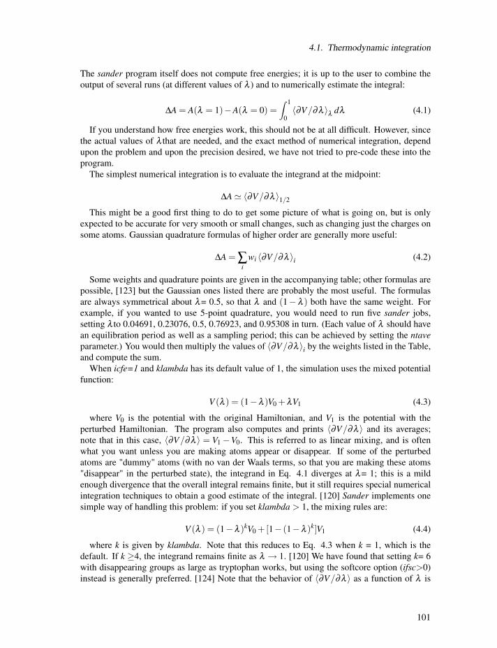
4.1. Thermodynamic integration
The sander program itself does not compute free energies; it is up to the user to combine theoutput of several runs (at different values of λ ) and to numerically estimate the integral:
ΔA = A(λ = 1)−A(λ = 0) =∫ 1
0〈∂V/∂λ 〉λ dλ (4.1)
If you understand how free energies work, this should not be at all difficult. However, since
the actual values of λ that are needed, and the exact method of numerical integration, dependupon the problem and upon the precision desired, we have not tried to pre-code these into the
program.
The simplest numerical integration is to evaluate the integrand at the midpoint:
ΔA� 〈∂V/∂λ 〉1/2This might be a good first thing to do to get some picture of what is going on, but is only
expected to be accurate for very smooth or small changes, such as changing just the charges on
some atoms. Gaussian quadrature formulas of higher order are generally more useful:
ΔA = ∑i
wi 〈∂V/∂λ 〉i (4.2)
Some weights and quadrature points are given in the accompanying table; other formulas are
possible, [123] but the Gaussian ones listed there are probably the most useful. The formulas
are always symmetrical about λ= 0.5, so that λ and (1−λ ) both have the same weight. Forexample, if you wanted to use 5-point quadrature, you would need to run five sander jobs,setting λ to 0.04691, 0.23076, 0.5, 0.76923, and 0.95308 in turn. (Each value of λ should havean equilibration period as well as a sampling period; this can be achieved by setting the ntaveparameter.) You would then multiply the values of 〈∂V/∂λ 〉i by the weights listed in the Table,and compute the sum.
When icfe=1 and klambda has its default value of 1, the simulation uses the mixed potentialfunction:
V (λ ) = (1−λ )V0+λV1 (4.3)
where V0 is the potential with the original Hamiltonian, and V1 is the potential with theperturbed Hamiltonian. The program also computes and prints 〈∂V/∂λ 〉 and its averages;note that in this case, 〈∂V/∂λ 〉 = V1−V0. This is referred to as linear mixing, and is oftenwhat you want unless you are making atoms appear or disappear. If some of the perturbed
atoms are "dummy" atoms (with no van der Waals terms, so that you are making these atoms
"disappear" in the perturbed state), the integrand in Eq. 4.1 diverges at λ= 1; this is a mildenough divergence that the overall integral remains finite, but it still requires special numerical
integration techniques to obtain a good estimate of the integral. [120] Sander implements onesimple way of handling this problem: if you set klambda > 1, the mixing rules are:
V (λ ) = (1−λ )kV0+[1− (1−λ )k]V1 (4.4)
where k is given by klambda. Note that this reduces to Eq. 4.3 when k = 1, which is thedefault. If k ≥4, the integrand remains finite as λ → 1. [120] We have found that setting k= 6with disappearing groups as large as tryptophan works, but using the softcore option (ifsc>0)instead is generally preferred. [124] Note that the behavior of 〈∂V/∂λ 〉 as a function of λ is
101
4. Sampling and free energies
not monotonic when klambda > 1. You may need a fairly fine quadrature to get converged
results for the integral, and you may want to sample more carefully in regions where 〈∂V/∂λ 〉is changing rapidly.
Notes:
1. This capability in sander is implemented by calling the force() routine twice on eachstep, once for V0 and once for V1. This increases the cost of the simulation, but involvesextremely simple coding.
2. Eq. 4.4 is designed for having dummy atoms in the perturbed Hamiltonian, and "real"
atoms in the regular Hamiltonian. You must ensure that this is the case when you set up
the system in LEaP. (See the softcore section, below, for a more general way to handle
disappearing atoms, which does not require dummy atoms at all.)
3. One common application of this model is to pKa calculations, where the charges are
mutated from the protonated to the deprotonated form. Since H atoms bonded to oxygen
already have zero van der Waals radii (in the Amber force fields and in TIP3P water),
once their charge is removed (in the deprotonated form) they are really then like dummy
atoms. For this special situation, there is no need to use klambda > 1: since the van
der Waals terms are missing from both the perturbed and unperturbed states, the proton’s
position can never lead to the large contributions to 〈∂V/∂λ 〉 that can occur when one ischanging from a zero van der Waals term to a finite one.
4. The implementation requires that the masses of all atoms be the same on all threads. To
enforce this, the masses found in the first prmtop file (for V0) are used for V1 as well.In classical statistical mechanics, the canonical distribution of configurations (and hence
of potential energies) is unaffected by changes in the masses, so this should not pose a
limitation. Since the masses in the second prmtop file are ignored, they do not have tomatch those in the first prmtop file.
5. Special care needs to be taken when using SHAKE for atoms whose force field parame-
ters differ in the two end points. The same bonds must be SHAKEN in both cases, and the
equilibrium bond lengths must also be the same. The easiest way to ensure this is to use
the noshakemask input to remove SHAKE from the regions that are being perturbed. Youmust do this manually, as the current code does not have any internal idea of "perturbed"
and "unperturbed" atoms. (This is a change from earlier versions of Amber, which used
a pertprmtop file, and which automatically removed SHAKE from the perturbed parts ofthe system.)
4.1.2. Softcore Potentials in Thermodynamic Integration
Softcore potentials provide an additional way to perform thermodynamic integration calcula-
tions in Amber. The system setup has been simplified so that appearing and disappearing atoms
can be present at the same time and no dummy atoms need to be introduced. Two prmtop files,
corresponding to the start and end states (V0 and V1) of the desired transformation need to beused. The common atoms that are present in both states need to appear in the same order in both
prmtop files and must have identical starting positions. In addition to the common atoms, each
process can have any number of unique soft core atoms, as specified by scmask. A modified
102
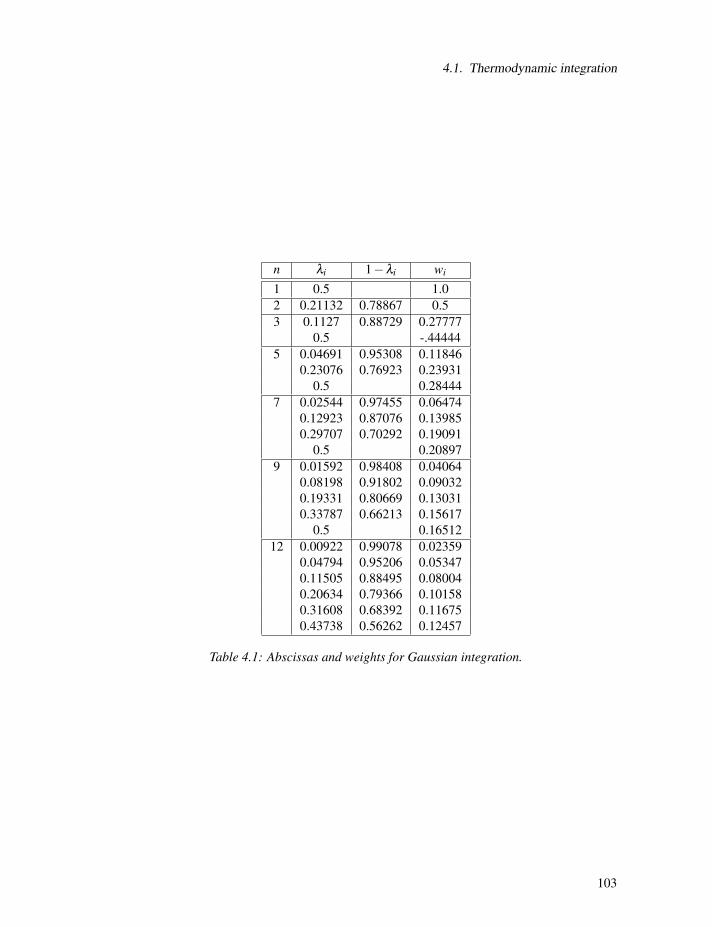
4.1. Thermodynamic integration
n λi 1−λi wi
1 0.5 1.0
2 0.21132 0.78867 0.5
3 0.1127 0.88729 0.27777
0.5 -.44444
5 0.04691 0.95308 0.11846
0.23076 0.76923 0.23931
0.5 0.28444
7 0.02544 0.97455 0.06474
0.12923 0.87076 0.13985
0.29707 0.70292 0.19091
0.5 0.20897
9 0.01592 0.98408 0.04064
0.08198 0.91802 0.09032
0.19331 0.80669 0.13031
0.33787 0.66213 0.15617
0.5 0.16512
12 0.00922 0.99078 0.02359
0.04794 0.95206 0.05347
0.11505 0.88495 0.08004
0.20634 0.79366 0.10158
0.31608 0.68392 0.11675
0.43738 0.56262 0.12457
Table 4.1: Abscissas and weights for Gaussian integration.
103

4. Sampling and free energies
version of the vdW equation is used to smoothly switch off non-bonded interactions of these
atoms with their common atom neighbors:
VV0,disappearing = 4ε(1−λ )
⎡⎢⎣ 1[
αλ +( ri j
σ)6]2 − 1
αλ +( ri jσ )6
⎤⎥⎦ (4.5)
VV1,appearing = 4ελ
⎡⎢⎣ 1[
α(1−λ )+( ri j
σ)6]2 − 1
α(1−λ )+( ri jσ )6
⎤⎥⎦ (4.6)
Please refer to Ref [124] for a description of the implementation and performance testing
when compared to the TI methods described above. All bonded interactions of the unique
atoms are recorded separately in the output file (see below). This is a consequence of the dual-
topology approach to TI. It means that any bond, angle, dihedral or 1-4 term that involves at
least one appearing or disappearing atom is not scaled by λ and does not contribute to 〈∂V/∂λ 〉.Therefore, output from both processes will not be identical when soft core potentials are used.
Softcore transformations avoid the origin singularity effect and therefore linear mixing can (and
should) always be used with them. Since the unique atoms become decoupled from their sur-
roundings at high or low lambdas and energy exchange between them and surrounding solvent
becomes inefficient, a Berendsen type thermostat should not be used for SC calculations. Any
SHAKE constraints applying to bonds between common and unique atoms will be removed
before the simulation, but SHAKE constraints for bonds between unique atoms are unchanged.
The icfe and klambda parameters should be set to 1 for a soft core run and the desired lambda
value will be specified by clambda. When using softcore potentials, λ values should be pickedso that 0.01 < clambda < 0.99. Additionally, the following parameters are available to control
the TI calculation:
ifsc Flag for soft core potentials
= 0 SC potentials are not used (default)
= 1 SC potentials are used. Note that a different setup is required, so prmtop files
for non soft core simulations cannot be used with soft core potentials and vice
versa.
= 2 A special case for perturbing a system to nothing. Since no V1-prmtop exists,this case can be run with icfe=0 and without using the groupfile input format.
scalpha The α parameter in 4.5 and 4.6, its default value is 0.5. Other values have not beenextensively tested
scmask Specifies the unique atoms for this process in ambmask format. This, along with
crgmask, is the only parameter that will frequently be different in the two mdin
files for V0 and V1. It is valid to set scmask to an empty string. A summary of theatoms in scmask is printed at the end of mdout.
logdvdl If set to .ne. 0, a summary of all ∂V/∂λ values calculated during every step of therun will be printed out at the end of the simulation for postprocessing.
104

4.2. Umbrella sampling
dvdl_norest If set to .ne. 0, the potential energy from positional restraints set by the &wt
namelists will not be counted into 〈∂V/∂λ 〉. This can be convenient in calcula-tions of absolute binding free energies as in Ref . [125] Please note that the force
constants of restraints are divided by lambda if soft core potentials are switched
on. This results in the restraint being applied in full to the disappearing atoms at
any lambda.
dynlmb If set to a value .gt. zero, clambda is increased by dynlmb every ntave steps. This
can be used to perform simulations with dynamically changing lambdas.
crgmask Specifies a number of atoms (in ambmask format) that will have their atomic partial
charges set to zero. This is mainly for convenience because it removes the need to
build additional prmtop files with uncharged atoms for TI calculations involving
the removal of partial charges.
The force field potential energy contributions for the unique atoms in each process will be
evaluated separately during the simulation and are recorded after the complete system energy is
given:
Softcore part of the system: 15 atoms, TEMP(K) = 459.76
SC_BOND = 2.0634 SC_ANGLE = 7.0386 SC_DIHED = 4.2087
SC_14NB = 3.3948 SC_14EEL = 0.0000 SC_EKIN = 16.9021
SC_VDW = -0.3269 SC_DERIV = -9.9847
The temperatures reported are calculated for the SC atoms only and fluctuate strongly for small
numbers of unique atoms. The energies in the first two lines include all terms that involve at
least one unique atom, but SC_VDW gives the vdW energy for pairs of unique atoms only
which are subject to the standard 12-6 LJ potential. The vdW potential between soft core / non
soft core atoms (as given by equation 4.5) is part of the regular VDWAALS term and is counted
for dV/dl. SC_DERIV is an additional λ -dependent contribution to 〈∂V/∂λ 〉 that arises fromthe form of the SC-potential. For more information on how to perform and setup calculations,
please consult the tutorial written by Thomas Steinbrecher at http://ambermd.org.
4.2. Umbrella sampling
Another free energy quantity that is accessible within sander is the ability to compute po-tentials of mean force (at least for simple distance, angle, or torsion variables) using umbrella
sampling. The basic idea is as follows. You add an artificial restraint to the system to bias it
to sample some coordinate in a certain range of values, and you keep track of the distribution
of values of this coordinate during the simulation. Then, you repeatedly move the minimum of
the biasing potential to different ranges of the coordinate of interest, and carry out more simu-
lations. These different simulations (often called "windows") must have some overlap; that is,
any particular value of the coordinate must be sampled to a significant extent in more than one
window. After the fact, you can remove the effect of the bias sing potential, and construct a
potential of mean force, which is the free energy profile along the chosen coordinate.
The basic ideas have been presented in many places, [96–98, 126, 127] and will not be re-
peated here. The implementation in sander follows two main steps. First, restraints are set
105
4. Sampling and free energies
up (using the distance and angle restraint files) and the DUMPFREQ parameter is used to
create "history" files that contain sampled values of the restraint coordinate. Second, a col-
lection of these history files is analyzed (using the so-called "weighted histogram" or WHAM
method [96–98]) to generate the potentials of mean force. As with thermodynamic integration,
the sander program itself does not compute these free energies; it is up to the user to combinethe output of several windows into a final result. For many problems, the programs prepared
by Alan Grossfield (http://membrane.urmc.rochester.edu/) are very convenient, and the sanderoutput files are compatible with these codes. Other methods of analysis, besides WHAM, may
also be used. [128]
A simple example. The input below shows how one window of a potential of mean forcemight be carried out. The coordinate of interest here is the chi angle of a base in an RNA
duplex. Here is the mdin file:
test of umbrella sampling of a chi torsion angle
&cntrl
nstlim=50000, cut=20.0, igb=1, saltcon=0.1,
ntpr=1, ntwr=100000, ntt=3, gamma_ln=0.2,
ntx=5, irest=1,
ntc=2, ntf=2, tol=0.000001,
dt=0.001, ntb=0,
nmropt=1,
/
&wt type=’DUMPFREQ’, istep1=10 /
&wt type=’END’ /
DISANG=chi.RST
DUMPAVE=chi_vs_t.170
The items in the&cntrl namelist are pretty standard, and not important here, except for specify-ing nmropt=1, which allows restraints to be defined. (The name of this variable is an historicalartifact: distance and angle restraints were originally introduced to allow NMR-related struc-
ture calculations to be carried out. But they are also very useful for cases, like this one, that
have nothing to do with NMR.) The DUMPFREQ command is used to request a separate file
be created to hold values of the torsion angle; this will have the name chi_vs_t.170 given in theDUMPAVE file redirection command.
The torsion angle restraint itself is given in the chi.RST file:
# torsion restraint for chi of residue 2
&rst iat=39,40,42,43, r1=0., r2=170., r3=170., r4=360., rk2 = 30.,
rk3 = 30., /
The iat variable gives the atom numbers of the four atoms that define the torsion of interest. Weset r2 = r3 and rk2 = rk3 to obtain a harmonic bias sing potential, with a minimum at 170 o .The values r1 and r4 should be far away from 170, so that the potential is essentially harmoniceverywhere. (It is not required that bias sing potentials be harmonic, but Dr. Grossfield’s
programs assume that they are, so we enforce that here.) Subsequent runs would change the
minimum in the potential to values other than 170, creating other chi_vs_t files. These fileswould then be used to create potentials of mean force. Note that the conventionally defined
106

4.3. Targeted MD
"force constant" is twice the value rk2, and that the Grossfield program uses force constants
measured in degrees, rather than radians. So you must perform a unit conversion in using those
programs, multiplying rk2 by 0.0006092 ( = 2(π/180)2) to get a equivalent force constant fora torsional restraint.
4.3. Targeted MD
The targeted MD option adds an additional term to the energy function based on the mass-
weighted root mean square deviation of a set of atoms in the current structure compared to a
reference structure. The reference structure is specified using the -ref flag in the same manner asis used for Cartesian coordinate restraints (NTR=1). Targeted MD can be used with or without
positional restraints. If positional restraints are not applied (ntr=0), sander performs a best-fit ofthe reference structure to the simulation structure based on selection in tgtfitmask and calculatesthe RMSD for the atoms selected by tgtrmsmask. The two masks can be identical or different.This way, fitting to one part of the structure but calculating the RMSD (and thus restraint force)
for another part of the structure is possible. If targetedMD is used in conjunction with positional
restraints (ntr=1), only tgtrmsmask should be given in the control input because the molecule is’fitted’ implicitly by applying positional restraints to atoms specified in restraintmask.The energy term has the form:
E = 0.5 * TGTMDFRC * NATTGTRMS * (RMSD-TGTRMSD)**2
The energy will be added to the RESTRAINT term. Note that the energy is weighted by the
number of atoms that were specified in the tgtrmsmask (NATTGTRMS). The RMSD is the rootmean square deviation and is mass weighted. The force constant is defined using the tgtmdfrcvariable (see below). This option can be used with molecular dynamics or minimization. When
targeted MD is used, sander will print the current values for the actual and target RMSD to theenergy summary in the output file.
itgtmd
= 0 no targeted MD (default)
= 1 use targeted MD
tgtrmsd Value of the target RMSD. The default value is 0. This value can be changed during
the simulation by using the weight change option.
tgtmdfrc This is the force constant for targeted MD. The default value is 0, which will result
in no penalty for structure deviations regardless of the RMSD value. Note that this
value can be negative, which would force the coordinates AWAY from the reference
structure.
tgtfitmask Define the atoms that will be used for the rms superposition between the current
structure and the reference structure. Syntax is in Chapter 11.3.
tgtrmsmask Define the atoms that will be used for the rms difference calculation (and hence
the restraint force), as outlined above. Syntax is in Chapter 11.3.
107

4. Sampling and free energies
One can imagine many uses for this option, but a few things should be kept in mind. Since there
is currently only one reference coordinate set, there is no way to force the coordinates to any
specific structure other than the reference. To move a structure toward a reference coordinate
set, one might use an initial tgtrmsd value corresponding to the actual RMSD between the inputand reference (inpcrd and refc). Then the weight change option could be used to decrease thisvalue to 0 during the simulation. To move a structure away from the reference, one can increase
tgtrmsd to values larger than zero. The minimum for this energy term will then be at structureswith an RMSD value that matches tgtrmsd. Keep in mind that many different structures mayhave similar RMSD values to the reference, and therefore one cannot be sure that increasing
tgtrmsd to a given value will result in a particular structure that has that RMSD value. In
this case it is probably wiser to use the final structure, rather than the initial structure, as the
reference coordinate set, and decrease tgtrmsd during the simulation. A negative force constanttgtmdfrc can be used, but this can cause problems since the energy will continue to decrease asthe RMSD to the reference increases.
Also keep in mind that phase space for molecular systems can be quite complex, and this
method does not guarantee that a low energy path between initial and target structures will be
followed. It is possible for the simulation to become unstable if the restraint energies become
too large if a low-energy path between a simulated structure and the reference is not accessible.
Note also that the input and reference coordinates are expected to match the prmtop file andhave atoms in the same sequence. No provision is made for symmetry; rotation of a methyl
group by 120° would result in a non-zero RMSD value.
4.4. Steered Molecular Dynamics (SMD) and the JarzynskiRelationship
4.4.1. Background
SMD applies an external force onto a physical system, and drives a change in coordinates
within a certain time. Several applications have come from Klaus Schulten’s group. [129] An
implementation where the coordinate in question changes in time at constant velocity is coded
in this version of Amber. The present implementation has been done by the group of Prof. Dario
Estrin in Buenos Aires<[email protected]> byMarceloMarti<[email protected]>and Alejandro Crespo<[email protected]>, and in the group of Prof. Adrian Roitberg at theUniversity of Florida <[email protected]>. [130]
The method should be thought of as an umbrella sampling where the center of the restraint is
time-dependent as in:
Vrest(t) = (1/2)k[x− x0(t)]2
where x could be a distance, an angle, or a torsion between atoms or groups of atoms.This methodology can be used then to drive a physical process such as ion diffusion, confor-
mational changes and many other applications. By integrating the force over time (or distance),
a generalized work can be computed. This work can be used to compute free energy differences
using the so-called Jarzynski relationship. [131–133] This method states that the free energy
difference between two states A and B (differing in their values of the generalized coordinate
x) can be calculated as
108

4.4. Steered Molecular Dynamics (SMD) and the Jarzynski Relationship
exp(−ΔG/kBT ) = 〈exp(−W/kBT )〉A (4.7)
This means that by computing the work between the two states in question, and averaging
over the initial state, equilibrium free energies can be extracted from non-equilibrium calcula-
tions. In order to make use of this feature, SMD calculations should be done, with different
starting coordinates taken from equilibrium simulations. This can be done by running sander
multiple times, or by running multisander. There are examples of the various modes of action
under the test/jar directories in the amber distribution.
4.4.2. Implementation and usage
To set up a SMD run, set the jar variable in the &cntrl namelist to 1. The change in coordi-nates is performed from a starting to an end value in nstlim steps.
To specify the type and conditions of the restraint an additional ".RST" file is used as in
nmropt=1. (Note that jar=1 internally sets nmropt=1.) The restraint file is similar to that ofNMR restraints (see Section 6.1), but fewer parameters are required. For instance, the following
RST file could be used:
# Change distance between atoms 485 and 134 from 15 A to 20 A
&rst iat=485,134, r2=15., rk2 = 5000., r2a=20. /
Note that only r2,r2a and rk2 are required; rk3 and r3 are set equal to these so that the harmonicrestraint is always symmetric, and r1 and r4 are internally set so that the restrain is alwaysoperative. An SMD run changing an angle, would use three iat entries, and one changing atorsion needs four. As in the case of NMR restraints, group inputs can also be used, using
iat<0 and defining the corresponding groups using the igr flag.The output file differs substantially from that used in the case of nmr restraints. It contains
4 columns: x0(t), x, force, work. Here work is computed as the integrated force over distances(or angle, or torsion). These files can be used for later processing in order to obtain the free
energy along the selected reaction coordinate using Jarzynski’s equality.
ExampleThe following example changes the distance between two atoms along 1000 steps:
Sample pulling input
&cntrl
nstlim=1000, cut=99.0, igb=1, saltcon=0.1,
ntpr=100, ntwr=100000, ntt=3, gamma_ln=5.0,
ntx=5, irest=1, ig = 256251,
ntc=2, ntf=2, tol=0.000001,
dt=0.002, ntb=0, tempi=300., temp0=300.,
jar=1,
/
&wt type=’DUMPFREQ’, istep1=1, /
&wt type=’END’, /
DISANG=dist.RST
DUMPAVE=dist_vs_t
109

4. Sampling and free energies
LISTIN=POUT
LISTOUT=POUT
Note that the flag jar is set to 1, and redirections to the dist.RST file are given. In this examplethe values in the output file dist_vs_t are written every istep=1 steps.The restraint file dist.RST in this example is:
# Change distance between atoms 485 and 134 from 15 A to 20.0 A
&rst iat=485,134, r2=15., rk2 = 5000., r2a=20.0, /
and the output dist_vs_t file might contain:
15.00000 15.12396 -1239.55482 0.00000
15.00500 14.75768 2470.68119 3.07782
15.01000 15.13490 -1246.46571 6.13835
15.01500 15.15041 -1350.03026 -0.35289
15.02000 14.77085 2481.56731 2.47596
15.02500 15.12423 -987.34073 6.21152
15.03000 15.18296 -1520.41603 -0.05787
15.03500 14.79016 2431.22399 2.21915
.......
19.97000 19.89329 4.60255 67.01305
19.97500 19.87926 4.78696 67.03652
19.98000 19.86629 4.54839 67.05986
19.98500 19.85980 3.75589 67.08062
19.99000 19.86077 2.58457 67.09647
19.99500 19.86732 1.27678 67.10612
In this example, the work of pulling from 15.0 to 20.0 (over 2 ps) was 67.1 kcal/mol. One
would need to repeat this calculation many times, starting from different snapshots from an
equilibrium trajectory constrained at the initial distance value. This could be done with a long
MD or a REMD simulation, and postprocessing with ptraj to extract snapshots. Once the work
is computed, it should be averaged using Eq. (6.27) to get the final estimate of the free energy
difference. The number of simulations, the strenght of the constraint, and the rate of change are
all important factors. The user should read the appropriate literature before using this method.
It is recommended that the width of the work distribution do not exceed 5-10% for faster con-
vergence. An example using multisander to run two of these simulations at the same time is
presented under $AMBERHOME/test. In many cases, umbrella sampling (see Section 4.2) may
be a better way to estimate the free energy of a conformational change.
4.5. Replica Exchange Molecular Dynamics (REMD)
In the one dimensional replica-exchange method, noninteracting copies of the system (repli-
cas) are simulated concurrently at different values of some independent variable, such as tem-
perature. Replicas are subjected to Monte Carlo move evaluation periodically, thus effecting ex-
change between values of the independent variable. The replica-exchange method enables sim-
ulation in a generalized ensemble — one in which states may be weighted by non-Boltzmann
110

4.5. Replica Exchange Molecular Dynamics (REMD)
probabilities. (However, one advantage of replica-exchange is the simplicity inherent in its use
of Boltzmann factors.) Consequently, local potential energy wells may not dominate traversal
through phase space because a replica trapped in a local minimum can escape via exchange
to a different value of the independent variable. [134] The multisander approach runs multiplesander jobs concurrently under a single MPI program. This can be used to just run unconnectedparallel jobs, but it is more useful to use this as a platform for the replica exchange method.The replica exchange method in temperature space for molecular dynamics (REMD) [134–
136] has been implemented on top of the framework that multisander provides. N non-interacting
replicas are simultaneously simulated in N separate MPI groups, each of which has its own set
of input and output files. One process from each MPI group is chosen to form another MPI
group (called the master group), in which exchanges are attempted.
4.5.1. Changes to REMD in Amber 10
IMPORTANT NOTE: The implementation of REMD has changed significantly in Amber 10.In the previous REMD implementation, sander was called as a subroutine from multisanderprogram. At the start of previous replica exchange runs, sander was called once to obtain thecurrent potential energies of each of the input coordinates. Multisander then entered a loop overthe number of exchange attempts, calling sander each time. In each loop, the first step was tocalculate the exchange probabilities between neighboring pairs of temperatures.
In the current REMD implementation the loop over exchanges is done using calls to runmdinside sander. As before, there is an initial call to runmd which obtains energies for the first ex-change only; no dynamics are performed. Also as before, the exchange calculation is performed
before dynamics. This implementation has several advantages. In the previous implementation,
each time a call was made to sander from multisander processes like reading the topology file,memory allocation, etc. had to be repeated. This could result in significant slowdown, par-ticularly with intensive file I/O on NFS filesystems (due to buffering issues). In the current
implementation there is only one call to multisander from sander, avoiding these problems.This also makes it so that output and info (MDOUT and MDINFO) files behave normally (i.e.as they do in standard MD runs - Note: This is the opposite behaviour to REMD in AMBER 9).
However, it is important to note that due to these changes all output is currently by replicaonly, not by temperature! This is equivalent to the repcrd &cntrl namelist variable being set to1. Setting repcrd = 0 currently has no effect and will generate a warning message in the output
file. To facilitate post-processing of trajectory data by temperature a header line is written to
each frame just before the coordinates. This header line has the format:
REMD <replica#> <exchange#> <step#> <Temperature>
PTRAJ will be able to read trajectories with this new format.
The ability to run REMD with a structure reservoir has been implemented; this is described
in detail in a following section.
The value for irest no longer needs to be 1. An irest value of 1 will cause the replica temper-
atures to be read from the restart files - otherwise the replica temperatures will be read from the
input files.
111
4. Sampling and free energies
4.5.2. Running REMD simulations
The N replicas are first sorted in an array by their target temperatures. Half of the N replicas
(replicas with even array indices) are chosen to be exchange initiators. These initiators pair
with their right and left neighbors alternatively after each runmd call. Topologically, the Ntemperature-sorted replicas form a loop, in which the first and the last replicas are neighbors.
Therefore, N/2 exchanges are attempted in each iteration. The current potential energies and
target (temp0) temperatures are used in a Metropolis-type calculation to determine the probabil-
ity of making the exchange. If the exchange is allowed between the pair, the target temperatures
for the two replicas are swapped before the next runmd call. The velocities of each replica in-volved in successful exchange are then adjusted by a scaling factor related to the previous and
new target temperatures. After the exchange calculation, runmd is called to perform MD fol-lowing the mdin file. After this runmd run, the exchange probability is calculated again, and soon.
Before starting a replica exchange simulation, an optimal set of target temperatures should be
determined so that the exchange ratio is roughly a constant. These target temperatures determine
the probability of exchange among the replicas, and the user is referred to the literature for a
more complete description of the influence of various factors on the exchange probability.
Each replica requires (for input files) or generates (for output files) its own mdin, inpcrd,mdout, mdcrd, restrt, mdinfo, and associated files. The names are provided through the speci-fication of a groupfile on the command line with the -groupfile groupfile option. The groupfilefile contains a separate command line for each of the replicas or multisander instances, one per
line (with no extra lines except for comments, which must have a ’#’ in the first column). To
choose the number of replicas or multisander instances, the -ng N command line option is used
(in this case to specify N separate instances.) If the number of processors (for the MPI run)
is larger than N (and also a multiple of N), each replica or multisander instance will run on anumber of processors equal to the total specified on the command line divided by N. Note thatin the groupfile, the -np option is currently ignored, i.e. each replica or multisander instance iscurrently hardcoded to run on an equivalent number of processors.
For example, an 4-replica REMD job will need 4 mdin and 4 inpcrd files. Then, the groupfile
might look like this:
#
# multisander or replica exchange group file
#
-O -i mdin.rep1 -o mdout.rep1 -c inpcrd.rep1 -r restrt.rep1 -x mdcrd.rep1
-O -i mdin.rep2 -o mdout.rep2 -c inpcrd.rep2 -r restrt.rep2 -x mdcrd.rep2
-O -i mdin.rep3 -o mdout.rep3 -c inpcrd.rep3 -r restrt.rep3 -x mdcrd.rep3
-O -i mdin.rep4 -o mdout.rep4 -c inpcrd.rep4 -r restrt.rep4 -x mdcrd.rep4
Note that the mdin and inpcrd files are not required to be ordered by their target temperaturessince the temperatures of the replicas will not remain sorted during the simulation. Sorting
is performed automatically at each REMD iteration as described above. Thus one can restart
REMD simulations without modifying the restart files from the previous REMD run (see below
for more information about restarting REMD).
It is important to ensure that the target temperature (specified using temp0) is the only differ-ence among the mdin files for the replicas, otherwise the outcome of an REMD simulation may
112
4.5. Replica Exchange Molecular Dynamics (REMD)
be unpredictable since each replica may be performing a different type of simulation. However,
in order to accommodate advanced users, the input files are not explicitly compared.
4.5.3. Restarting REMD simulations
It is recommended that each REMD run generate a new set of output files (such as mdcrd),
but for convenience one may use -A in the command line in order to append output to existing
output files. This can be a useful option when restarting REMD simulations. If -A is used,
files that were present before starting the REMD simulation are appended to throughout the
new simulation. Note that this can seriously affect performance on systems where the file
writing becomes rate limiting, although the new implementation of REMD should help with
this somewhat. If -O is used, any files present are overwritten during the first iteration, and then
subsequent iterations append to these new files.
At the end of a REMD simulation, the target temperature of each replica is most likely not
the same as it was at the start of the simulation (due to exchanges). If one wishes to continue
this simulation, sander will need to know that the target temperatures have changed. Since the
target temperature is normally specified in the mdin file (using temp0), the previous mdin files
would all need to be modified to reflect changes in target temperature of each replica. In order
to simplify this process, the program will write the current target temperature as additional
information in the restart files during an REMD simulation. When an REMD simulation is
started, the program will check to see if the target temperature is present in the restart file. If
it is present, this value will override the target temperature specified using temp0 in the mdin
file. In this manner, one can restart the simulation from the set of restart files and the program
will automatically update the target temperature of each replica to correspond to the final target
temperature from the previous run. If the target temperature is not present (as would be the case
for the first REMD run), the correct values should be present in the mdin files.
4.5.4. Content of the output files
As noted above, the current implementation of REMD restores the normal behavior of output
and info (MDOUT and MDINFO) files. Again, it is important to note that in the current im-
plementation of REMD all output is currently BY REPLICA ONLY, NOT BY TEMPERATURE!This is equivalent to the repcrd &cntrl namelist variable being set to 1. Setting repcrd = 0 cur-
rently has no effect and will generate a warning message in the output file. To facilitate post
processing of trajectory data by temperature, a header line is written to each frame just before
the coordinates. This header line has the format:
REMD <replica#> <exchange#> <step#> <Temperature>
PTRAJ will be able to read trajectories with this new format.
Output files will now contain information pertaining to the current replica for each exchange.
For example:
==========================REMD EXCHANGE CALCULATION==========================
Exch= 5 RREMD= 0
Replica Temp= 386.40 Indx= 2 Rep#= 1 EPot= -1518.88
113

4. Sampling and free energies
Partner Temp= 393.50 Indx= 3 Rep#= 3 EPot= -1485.53
Metrop= 0.456848E+00 delta= 0.783404E+00 o_scaling= 0.99
Rand= 0.191995E+00 MyScaling= 1.01 Success= T
========================END REMD EXCHANGE CALCULATION========================
Here, Exch is the current exchange and RREMD is the type of Reservoir employed (0 indicates
no reservoir, i.e. standard REMD; see section on Reservoir REMD for more details). Next,
the Replica line gives information about the current replica: the temperature, temperature index
(Indx), the replica#, and the potential energy. The Partner line gives the same information for
this replica’s current partner. If this replica is controlling the exchange (Indx is even) then the
Metropolis factor, the delta, random number, and scaling values are also printed.
4.5.5. Major changes from sander when using replica exchange
Within an MPI job, as discussed above, it is now possible to run multiple sander jobs at once,
such that each job gets a subset of the total processors. To run multisander and replica exchange,
there are three command-line arguments:
-ng specifies the number of sander runs (replicas) to perform concurrently. Note that at present,
the number of replicas must be a divisor of the total number of processors (specified by
the MPI run command). The input and output file information must be provided in a
groupfile (as described earlier in this section).
-rem specifies the type of replica exchange simulation. Only two options are currently avail-
able. 0, no replica exchange (standard MD) (default behavior if -rem is not specified on
command line); 1, regular replica exchange (requires -ng).
-remlog specifies the filename of a log file. This file records from left to right, for every replica
and every exchange attempt, the velocity scaling factor (negative if the exchange attempt
failed), current actual temperature, current potential energy, current target temperature,
and the new target temperature. The default value is rem.log.
-remtype specifies a filename for the remtype file; this file provides helpful information about
the current replica run. For reservoir REMD runs it also prints reservoir information.
Default is "rem.type"
Next, there are new variables in the &cntrl namelist:
repcrd This variable is temporarily disabled.
numexchg The number of exchange attempts, default 0.
nstlim the number of MD steps *between exchange attempts*. Note that NSTLIM is not
a new variable for REMD, but the meaning is somewhat different. The total length
of the REMD simulation will be nstlim*numexchg steps long.
114

4.5. Replica Exchange Molecular Dynamics (REMD)
4.5.6. Cautions when using replica exchange
While many variations of replica exchange have been tested with sander, all possible vari-
ations have not been tested and the option is intended for use by advanced researchers that
already have a comprehensive understanding of standard molecular dynamics simulations. Cau-
tion should be used when creating REMD input files. Amber will check for the most obvious
errors but due to the nature of the multiple output files the reason for the error may not be readily
apparent. The following is only a subset of things that users should keep in mind:
1. The number of replicas must be an even number (so that all replicas have a partner for
exchange).
2. Temp0 values for each replica must be unique.
3. Other than temp0, mdin files should normally be identical.
4. Temp0 values should not be changed in the nmropt=1 weight change section.
5. As of Amber 10 the value of irest does not have to be 1. If irest is 1, the replica tem-
peratures will be read from the restart files. If irest is 0, the replica temperatures will be
read from the input files. This means that it is no longer necessary for inpcrd files to have
velocities.
6. A groupfile is required (this was not the case in Amber8).
7. If high temperatures are used, it may be necessary to use a smaller time step and possibly
restraints to prevent cis/trans isomerization or chirality inversion.
8. Due to increased diffusion rates at high temperature, it may be good to use iwrap=1 to
prevent coordinates from becoming too large to fit in the restart format.
9. Note that the optimal temperature range and spacing will depend on the system. The user
is strongly recommended to read the literature in this area.
10. Constant pressure is not supported for REMD simulations. This means NTB must be 0
or 1.
4.5.7. Replica exchange example
Below is an example of an 8-replica REMD run on 16 processors, assuming that relevant
environment variables have been properly set.
$MPIRUN -np 16 sander -ng 8 -groupfile groupfile
Here is the groupfile:
#
# multisander or replica exchange group file
#
-O -rem 1 -i mdin.rep1 -o mdout.rep1 -c inpcrd.rep1 -r restrt.rep1 -x mdcrd.rep1
-O -rem 1 -i mdin.rep2 -o mdout.rep2 -c inpcrd.rep2 -r restrt.rep2 -x mdcrd.rep2
115

4. Sampling and free energies
-O -rem 1 -i mdin.rep3 -o mdout.rep3 -c inpcrd.rep3 -r restrt.rep3 -x mdcrd.rep3
-O -rem 1 -i mdin.rep4 -o mdout.rep4 -c inpcrd.rep4 -r restrt.rep4 -x mdcrd.rep4
-O -rem 1 -i mdin.rep5 -o mdout.rep5 -c inpcrd.rep5 -r restrt.rep5 -x mdcrd.rep5
-O -rem 1 -i mdin.rep6 -o mdout.rep6 -c inpcrd.rep6 -r restrt.rep6 -x mdcrd.rep6
-O -rem 1 -i mdin.rep7 -o mdout.rep7 -c inpcrd.rep7 -r restrt.rep7 -x mdcrd.rep7
-O -rem 1 -i mdin.rep8 -o mdout.rep8 -c inpcrd.rep8 -r restrt.rep8 -x mdcrd.rep8
This input specifies that REMD should be used (-rem 1), with 8 replicas (-ng 8) and 2 processors
per replica (-np 16). Note that the total number of processors should always be a multiple of
the number of replicas.
Here is a section of a sample rem.log file produced by Amber:
# replica exchange log file
# Replica #, Velocity Scaling, T, Eptot, Temp0, NewTemp0, Success rate (i,i+1)
# exchange 1
1 1.46 0.00 -541.20 269.50 570.90 0.00
2 1.06 0.00 -541.20 300.00 334.00 2.00
3 0.95 0.00 -541.20 334.00 300.00 0.00
4 1.06 0.00 -541.20 371.80 413.90 2.00
5 0.95 0.00 -541.20 413.90 371.80 0.00
6 1.06 0.00 -541.20 460.70 512.90 2.00
7 0.95 0.00 -541.20 512.90 460.70 0.00
8 0.69 0.00 -541.20 570.90 269.50 2.00
# exchange 2
1 -1.00 0.00 -491.39 570.90 570.90 1.00
2 -1.00 0.00 -547.98 334.00 334.00 0.00
3 -1.00 0.00 -553.87 300.00 300.00 1.00
4 -1.00 0.00 -518.92 413.90 413.90 0.00
5 -1.00 0.00 -538.17 371.80 371.80 1.00
6 -1.00 0.00 -494.00 512.90 512.90 0.00
7 -1.00 0.00 -498.12 460.70 460.70 1.00
8 -1.00 0.00 -567.18 269.50 269.50 0.00
# exchange 3
1 -1.00 0.00 -462.14 570.90 570.90 0.67
2 0.95 0.00 -539.83 334.00 300.00 0.00
3 1.06 0.00 -537.76 300.00 334.00 1.33
4 -1.00 0.00 -510.33 413.90 413.90 0.00
5 -1.00 0.00 -540.74 371.80 371.80 0.67
6 -1.00 0.00 -491.99 512.90 512.90 0.00
7 -1.00 0.00 -522.01 460.70 460.70 0.67
8 -1.00 0.00 -568.87 269.50 269.50 0.00
Note that a section of the log file is written for each exchange attempt. For each exchange, the
log contains a line for each replica. This line lists the replica number, the velocity scaling factor,
the actual instantaneous temperature, the potential energy, the old and new target temperatures,
and the current overall success rate for exchange between this temperature and the next higher
116
4.5. Replica Exchange Molecular Dynamics (REMD)
temperature. Note that the velocity scaling factor will be -1.0 if the exchange was not successful.
In that case, the old and new target temperatures will be identical.
In this particular example, all of the inpcrd files were identical, and thus the potential energies
listed for exchange 1 are identical. For this reason, all of the exchanges are successful. After
this exchange, MD is performed for nstlim steps, and so the potential energies are no longer
identical at exchange #2.
Note that the exchange success rate may be larger than 1.0 during the first few attempts, since
each particular pair is considered only every other attempt. The success rate is the number of
accepted exchanges for the pair divided by the total number of exchange attempts, multiplied
by 2 to account for the alternating neighbors.
4.5.8. Replica exchange using a hybrid solvent model
This section describes an advanced feature of Amber that is currently under development.
[137, 138] Users that are not already comfortable with standard replica exchange simulations
should likely get more experience with them before attempting hybrid solvent REMD calcula-
tions.
For large systems, REMD becomes intractable since the number of replicas needed to span
a given temperature range increases roughly with the square root of the number of degrees of
freedom in the system. Recognizing that the main difficulty in applying REMD with explicit
solvent lies in the number of simulations required, rather than just the complexity of each sim-
ulation, we recently developed a new approach in which each replica is simulated in explicit
solvent using standard methods such as periodic boundary conditions and inclusion of long-
range electrostatic interactions using PME. However, the calculation of exchange probabilities
(which determines the temperature spacing and thus the number of replicas) is handled dif-
ferently. Only a subset of closest water molecules is retained, with the remainder temporarily
replaced by a continuum representation. The energy is calculated using the hybrid model, and
the exchange probability is determined. The original solvent coordinates are then restored and
the simulation proceeds as a continuous trajectory with fully explicit solvation. This way the
perceived system size for evaluation of exchange probability is dramatically reduced and fewer
replicas are needed.
An important difference from existing hybrid solvent models is that the system is fully sol-
vated throughout the entire MD simulation, and thus the distribution functions and solvent
properties should not be affected by the use of the hybrid model in the exchange calculation. In
addition, no restraints of any type are needed for the solvent, and the solute shape and volume
may change since the solvation shells are generated for each replica on the fly at every exchange
calculation. Nearly no computational overhead is involved since the calculation is performed
infrequently as compared to the normal force evaluations. Thus the hybrid REMD approach
can employ more accurate continuum models that are too computationally demanding for use
in each time step of a standard molecular dynamics simulation. However, since the Hamilto-
nian used for the exchange differs from that employed during dynamics, these simulations are
approximate and are not guaranteed to provide correct canonical ensembles.
117

4. Sampling and free energies
4.5.9. Changes to hybrid REMD in Amber 10
Previously, in order to use hybrid solvent REMD in Amber 9, 2 sets of topology and input
files were needed; one for the fully solvated system and one for the "stripped" system containing
the desired number of water molecules. Now that REMD has been implemented completely
inside sander, only one set of files (the ones for the fully solvated system) is needed. All
information for the hybrid calculation is taken from these files. In particular this means that
the correct GB radii must be specified in the fully solvated topology file, since they will be readfrom this file. The GB model is specified by the new &cntrl namelist variable hybridgb.This means that 1) The user no longer needs to create a separate topology file for the stripped
system and 2) the .strip files containing the coordinates of the stripped system are no longer writ-
ten every exchange, which reduces file I/O during a hybrid REMD run. If desired, the stripped
coordinates can be dumped to a trajectory file by using the -hybridtraj <FILE> command line
option.
At each exchange calculation sander will create the hybrid system based on the current co-
ordinates for the fully solvated system. This is done by calculating the distance of each water
oxygen to the nearest solute atom, and sorting the water by increasing shortest distance. The
closest numwatkeep are retained and the potential energy is calculated using the GB modelspecified by hybridgb. After the energy calculation the fully solvated system is restored.For a more complete example, users are directed to the hybridREMD test case (in the rem_hybrid
subdirectory) in the Amber test directory.
numwatkeep The number of explicit waters that should be retained for the calculation of poten-
tial energy to be used for the exchange calculation. Before each exchange attempt,
the closest numwatkeep waters will be retained (closest to the solute) and the rest
will be temporarily removed and then replaced after the exchange probability has
been calculated. The default value is -1, indicating that all waters should be re-
tained (standard REMD). A value of 0 would direct Amber to remove all of the
explicit water (as in MM-PBSA) while a non-zero value will result in some water
close to the solute being retained while the rest is removed. Currently it is not pos-
sible to select a subset of solute atoms for determining which waters are "close".
Determining the optimal numwatkeep value is a topic of current research.
hybridgb Specifies which GB model should be used for calculating the PE of the stripped
coordinates, equivalent to the igb variable. Currently only hybridgb values of 1, 2,and 5 are supported.
4.5.10. Cautions for hybrid solvent replica exchange
This option has not been extensively tested. The following would not be expected to work
without further modification of the code:
1. Only the water is imaged for the creation of the stripped system. Care should be taken
with dimers (such as DNA duplexes) to ensure that the imaging is correct.
2. Explicit counterions should probably not be used.
3. The choice of implicit solvent model will likely have a large effect on the resulting en-
semble.
118
4.5. Replica Exchange Molecular Dynamics (REMD)
4.5.11. Reservoir REMD
The ability to perform REMD with a structure reservoir [139, 140] has been implemented
in Amber 10. Although REMD can significantly increase the efficiency of conformational
sampling, obtaining converged data can still be challenging. This is particularly true for larger
systems, as the number of replicas needed to span a given temperature range increases with the
square root of the number of degrees of freedom in the system. Another consideration is that
the folding rate of a peptide tends not to be as dependent on temperature as the unfolding rate,
making the search for native peptide structures in higher temperature replicas more problematic;
in the case where a native-like structure is found it will almost always be exchanged to a lower
temperature replica, requiring a repeat of the search process. In addition, the exchange criterion
in REMD assumes a Boltzmann-weighted ensemble of structures, which is typically not the
case at the start of a REMD simulation. Although the exchange criterion will eventually drive
each replica toward a Boltzmann-weighted ensemble of structures, this essentially means that
until all of the replicas are converged, none of the replicas are converged.
Reservoir REMD is a method which can significantly enhance the rate of convergence and re-
duce the high computational expense of standard REMD simulations. An ensemble of structures
(or reservoir) is generated at high temperature, then linked to lower temperatures via REMD.
Periodic exchanges are attempted between randomly chosen structures in the reservoir and the
highest temperature replica. If the structure reservoir is already Boltzmann-weighted, [139]
convergence is significantly enhanced as the lower temperature replicas simply act to re-weight
the reservoir ensemble - in essence all of the searching has been accomplished from the start.
This is in contrast to standard REMD where all the replicas are run simultaneously, and the
computational expense for running long simulations must be paid for each of the replicas even
though only a few high-temperature ones may be contributing to sampling of new basins.
One major advantage of this approach is that a converged ensemble of conformations needs
to be generated only once and only for one temperature. Typically this temperature should
be high enough to facilitate crossing of energy barriers, but low enough that there is still a
measureable fraction of native structure present. Another advantage is that exchanges with the
reservoir do not need to be time-correlated with the replica simulations; folding events sampled
during reservoir generation can provide multiple native structures for the other replicas.
It may not always be possible however to generate a Boltzmann-weighted ensemble of struc-
tures (e.g. for a large molecule in explicit solvent). In such cases it is possible to use a non-
Boltzmann weighted reservoir by modifying only the exchange criterion between the reservoir
and the highest temperature replica (see Ref. ? for further details). If the weight of all struc-
tures in the reservoir is set to 1, this corresponds to a completely flat distribution across the free
energy landscape. Alternatively, weights can be assigned to structures based on various struc-
tural properties. In the current implementation, weights are assigned to structures via dihedral
bin clustering, wherein clusters are identified by unique configurations of user-defined dihedral
angles.
There are several new command line arguments that pertain to Reservoir REMD:
-rremd Type of reservoir to use.
= 0 No reservoir (Default)
= 1 Boltzmann-weighted reservoir
119

4. Sampling and free energies
= 2 Non-Boltzmann weighted reservoir where the weight of each structure in the reser-
voir is assumed to be 1/N
= 3 Non-Boltzmann weighted reservoir with weights defined by dihedral angle binning.
-reservoir Specifies the file name prefix for reservoir structures. Reservoir structure files
should be in the restart file format MDRESTRT, and are expected to be named accordingto the format<name>.XXXXXX, where XXXXXX is a 6 digit integer, e.g. frame.000001.Default is "reserv/frame". IMPORTANT NOTE: Structure numbering should begin at1.
-saveene specifies the file containing energies of the structures in the reservoir (default file-
name is "saveene"). This file must contain a header line with format:
<# reservoir structures> <reservoir T> <#atoms><random seed> <velocity flag>
If the velocity flag =1 then velocity information will be read from the reservoir structure
files, otherwise (if velocity flag =0) velocities will be assigned to the structure based
on the reservoir temperature. After the header line there should be a line containing the
potential energy of each reservoir structure. IMPORTANT NOTE: For reservoir REMDwith dihedral bin clustering (rremd==3) each potential energy should be followed by the
cluster # that reservoir structure belongs to.
-clusterinfo For reservoir REMD with dihedral bin clustering (rremd==3) this file specifies
what dihedrals are used and the binsize, as well as what cluster each reservoir structure
belongs to. Default is "cluster.info". File has the following format:
<# Dihedral Angles><atom# 1> <atom# 2> <atom# 3> <atom# 4> [Dihedral 1]
. .
. .
. .
<atom# 1> <atom# 2> <atom# 3><atom# 4> [# Dihedral Angles]
<Total # Clusters><Cluster #> <Weight><Bin1><Bin2>...<Bin #Dihedral Angles> [Cluster 1]
. .
. .
. .
<Cluster #> <Weight><Bin1><Bin2>...<Bin #Dihedral Angles> [# Clusters]
The first line is the number of dihedral angles that will be binned, following the definition
of those dihedral angles (4 atoms using sander atom #s, starting from 1) and the bin
size for each dihedral angle. Next is the total # of clusters followed by lines providing
information about each cluster: the cluster number, weight and ID as defined by dihedral
binning. The ID is composed of consecutive 3 digit integers, 1 for each dihedral angle.
120

4.6. Adaptively biased MD, steered MD, and umbrella sampling with REMD
For example, a structure belonging to cluster 7 with a weight of 2 with 2 dihedral angles
that fall in bins 3 and 8 would look like:
7 2 003008
4.6. Adaptively biased MD, steered MD, and umbrellasampling with REMD
4.6.1. Overview
The following describes a suite of modules useful for the calculation of the free energy as-
sociated with a reaction coordinate σ(r1, . . . ,rN) (which is defined as a smooth function of theatomic positions r1, . . . ,rN):
f (ξ ) =−kBT ln⟨δ [ξ −σ(r1, . . . ,rN)]
⟩,
(the angular brackets denote an ensemble average, kB is the Boltzmann constant and T is the
temperature) that is also frequently referred to as the potential of mean force.Specifically, new frameworks are provided for equilibrium umbrella sampling and steered
molecular dynamics that enhance the functionality delivered by earlier implementations (de-
scribed earlier in this manual), along with a new Adaptively Biased Molecular Dynamics (ABMD)
method [141] that belongs to the general category of umbrella sampling methods with a time-
dependent potential. Such methods were first introduced by Huber, Torda and van Gunsteren
(the Local Elevation Method [142]) in the molecular dynamics (MD) context, and by Wang and
Landau in the context of Monte Carlo simulations [143]. More recent approaches include the
adaptive force bias method [144], and the metadynamics method [145, 146]. All these methods
estimate the free energy of a reaction coordinate from an evolving ensemble of realizations,
and use that estimate to bias the system dynamics to flatten an effective free energy surface.
Collectively, these methods may all be considered to be umbrella sampling methods with an
evolving potential.
The ABMDmethod grew out of attempts to speed up and streamline the metadynamics method
for free energy calculations with a controllable accuracy. It is characterized by a favorablescaling in time, and only a few (two) control parameters. It is formulated in terms of the
following equations:
mad2ra
dt2= Fa +
∂∂ra
U[t|σ (r1, . . . ,rN)
],
∂U(t|ξ )∂ t
=kBTτF
G[ξ −σ (r1, . . . ,rN)
],
where the first ones represent Newton’s equations that govern ordinary MD (temperature and
pressure regulation terms are not shown) augmented with an additional force coming from the
time dependent biasing potential U(t|ξ ) [U(t = 0|ξ ) = 0], whose time evolution is given by
the second equation. G(ξ ) is a positive definite and symmetric kernel, which may be thoughtof as a smoothed Dirac delta function. For large enough τF (the flooding timescale) and small
enough kernel width, the biasing potentialU(t|ξ ) converges towards − f (ξ ) as t → ∞.
121

4. Sampling and free energies
Our numerical implementation of the ABMD method involves the use of a bi-weight kernel
along with the use of cubic B-splines (or products thereof) to discretize the biasing potential
U(t|ξ ) w.r.t. ξ , and an Euler-like scheme for time integration. ABMD admits two important ex-tensions, which lead to a more uniform flattening ofU(t|ξ )+ f (ξ ) due to an improved samplingof the “evolving” canonical distribution. The first extension is identical in spirit to the multiplewalkers metadynamics [147, 148]. It amounts to carrying out several different MD simulationsbiased by the sameU(t|ξ ), which evolves via:
∂U(t|ξ )∂ t
=kBTτF
∑α
G[ξ −σ (rα
1 , . . . ,rαN)
],
where α labels different MD trajectories. A second extension is to gather several different MD
trajectories, each bearing its own biasing potential and, if desired, its own distinct collective
variable, into a generalized ensemble for “replica exchange” with modified “exchange” rules
[149–151]. Both extensions are advantageous and lead to a more uniform flattening ofU(t|ξ )+f (ξ ).In order to assess and improve the accuracy of the free energies, the ABMD simulations may
need to be followed up with equilibrium umbrella sampling runs, which make use of the bi-
asing potential U(t|ξ ) as is. Such a procedure is very much in the spirit of adaptive umbrellasampling. With these runs, one calculates the biased probability density:
pB(ξ ) =⟨δ [ξ −σ(r1, . . . ,rN)]
⟩B.
The idea here is that if, as a result of an ABMD run, f (ξ )+U(t|ξ ) = 0 exactly, then the biased
probability density pB(ξ ) would be flat (constant). In practice, this is typically not the case, butone can use pB(ξ ) to “correct” the free energy via:
f (ξ ) =−U(ξ )− kBT ln pB(ξ ).
This procedure has previously been successfully used to calculate accurate free energy maps
for a number of molecules including several short peptides.
If you find any of these modules useful, we would ask you to kindly consider quoting the
following paper: V. Babin, C. Roland, and C. Sagui, “Adaptively biased molecular dynamicsfor free energy calculations”, J. Chem. Phys. 128, 134101 (2008).
4.6.2. Reaction Coordinates
A reaction coordinate is defined in the variable section (see Fig. 4.1). This section must
contain a type keyword along with a value of type STRING and a list of integers i (the number
of integers vary depending on the variable type). For some types of reaction coordinates the
variable section must also contain a list of real numbers, r, whose length depends on the
specific type.
The following reaction coordinates are currently implemented1:
• type = DISTANCE : distance (in Å) between two atoms whose indexes are read from the
list i.
1It is really easy to program another one, if desired.
122
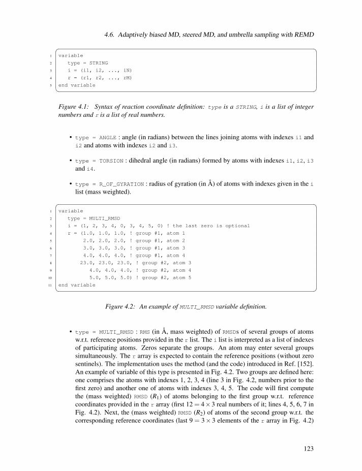
4.6. Adaptively biased MD, steered MD, and umbrella sampling with REMD� �1 variable
2 type = STRING
3 i = (i1, i2, ..., iN)
4 r = (r1, r2, ..., rM)
5 end variable� �Figure 4.1: Syntax of reaction coordinate definition: type is a STRING, i is a list of integernumbers and r is a list of real numbers.
• type = ANGLE : angle (in radians) between the lines joining atoms with indexes i1 and
i2 and atoms with indexes i2 and i3.
• type = TORSION : dihedral angle (in radians) formed by atoms with indexes i1, i2, i3
and i4.
• type = R_OF_GYRATION : radius of gyration (in Å) of atoms with indexes given in the i
list (mass weighted).� �1 variable
2 type = MULTI_RMSD
3 i = (1, 2, 3, 4, 0, 3, 4, 5, 0) ! the last zero is optional
4 r = (1.0, 1.0, 1.0, ! group #1, atom 1
5 2.0, 2.0, 2.0, ! group #1, atom 2
6 3.0, 3.0, 3.0, ! group #1, atom 3
7 4.0, 4.0, 4.0, ! group #1, atom 4
8 23.0, 23.0, 23.0, ! group #2, atom 3
9 4.0, 4.0, 4.0, ! group #2, atom 4
10 5.0, 5.0, 5.0) ! group #2, atom 5
11 end variable� �Figure 4.2: An example of MULTI_RMSD variable definition.
• type = MULTI_RMSD : RMS (in Å, mass weighted) of RMSDs of several groups of atoms
w.r.t. reference positions provided in the r list. The i list is interpreted as a list of indexes
of participating atoms. Zeros separate the groups. An atom may enter several groups
simultaneously. The r array is expected to contain the reference positions (without zero
sentinels). The implementation uses the method (and the code) introduced in Ref. [152].
An example of variable of this type is presented in Fig. 4.2. Two groups are defined here:
one comprises the atoms with indexes 1, 2, 3, 4 (line 3 in Fig. 4.2, numbers prior to the
first zero) and another one of atoms with indexes 3, 4, 5. The code will first compute
the (mass weighted) RMSD (R1) of atoms belonging to the first group w.r.t. referencecoordinates provided in the r array (first 12= 4×3 real numbers of it; lines 4, 5, 6, 7 inFig. 4.2). Next, the (mass weighted) RMSD (R2) of atoms of the second group w.r.t. thecorresponding reference coordinates (last 9 = 3× 3 elements of the r array in Fig. 4.2)
123

4. Sampling and free energies
will be computed. Finally, the code will compute the value of the variable as follows:
value=√
M1
M1+M2R21+
M2
M1+M2R22 ,
where M1 and M2 are the total masses of atoms in the corresponding groups.
• type = N_OF_BONDS :
value= ∑p
1−(
rp
/r0)6
1−(
rp
/r0)12 ,
where the sum runs over pairs of atoms p, rp denotes distance between the atoms of pair
p and r0 is a parameter measured in Å. The r array must contain exactly one element thatis interpreted as r0. The i array is expected to contain pairs of indexes of participatingatoms. For example, if 1 and 2 are the indexes of Oxygen atoms and 3, 4, 5 are the
indexes of Hydrogen atoms and one intents to count all possible O-H bonds, the i list
must be (1, 3, 1, 4, 1, 5, 2, 3, 2, 4, 2, 5), that is, it must explicitly list all the pairs to be
counted.
• type = HANDEDNESS :
value= ∑a
ua,3 · [ua,1×ua,2]|ua,1| |ua,2| |ua,3| ,
where
ua,1 = ra+1− ra
ua,2 = ra+3− ra+2
ua,3 = (1−w)(ra+2− ra+1)+w(ra+3− ra) ,
and ra denote the positions of participating atoms. The i array is supposed to contain
indexes of the atoms and the r array may provide the value of w (0 ≤ w ≤ 1, the defaultis zero).
• type = N_OF_STRUCTURES :
value= ∑g
1−(
Rg
/R0,g
)61−
(Rg
/R0,g
)12 ,
where the sum runs over groups of atoms, Rg denotes the RMSD of the group g w.r.t. somereference coordinates and R0,g are positive parameters measured in Å. The i array is ex-pected to contain indexes of participating atoms with zeros separating different groups.
The elements of the r array are interpreted as the reference coordinates of the first group
followed by their corresponding R0; then followed by the reference coordinates of theatoms of the second group, followed by the second R0, and so forth. To make the pre-sentation clearer, let us consider the example presented in Fig. 4.3. The atomic groups
and reference coordinates are the same as the ones shown in Fig. 4.2. Lines 7 and 11 in
124

4.6. Adaptively biased MD, steered MD, and umbrella sampling with REMD� �1 variable
2 type = N_OF_STRUCTURES
3 i = (1, 2, 3, 4, 0, 3, 4, 5, 0) ! the last zero is optional
4 r = (1.0, 1.0, 1.0, ! group #1, atom 1
5 2.0, 2.0, 2.0, ! group #1, atom 2
6 3.0, 3.0, 3.0, ! group #1, atom 3
7 4.0, 4.0, 4.0, ! group #1, atom 4
8 1.0, ! R0 for group #1
9 23.0, 23.0, 23.0, ! group #2, atom 3
10 4.0, 4.0, 4.0, ! group #2, atom 4
11 5.0, 5.0, 5.0, ! group #2, atom 5
12 2.0) ! R0 for group #2
13 end variable� �Figure 4.3: An example of N_OF_STRUCTURES variable.
Fig. 4.3 contain additional entries that set the values of the threshold distances R0,1 andR0,2. To compute the variable, the code first computes the mass weighted RMSD values R1and R2 for both groups –much like in the MULTI_RMSD case– and then combines those ina manner similar to that used in the N_OF_BONDS variable.
value=1−
(R1
/R0,1
)61−
(R1
/R0,1
)12 +1−
(R2
/R0,2
)61−
(R2
/R0,2
)12 .
In other words, the variable “counts” the number of structures that match (stay close in
RMSD sense) with the reference structures.
4.6.3. Steered Molecular Dynamics
The ncsu_smd section, if present in the MDIN file, activates the steered MD code (the method it-
self is extensively described in the literature: see for example Ref. [153] and references therein).
Apart from the variable subsection(s), the following is recognized within this section:
• output_file = STRING : sets the output file name.
• output_freq = INTEGER : sets the output frequency (in MD steps).
There must be at least one reaction coordinate defined within this section (that is, there must be
at least one variable subsection in the ncsu_smd section). The steered MD code requires that
additional entries be present in the variable subsections:
• path = (REAL|X, REAL|X, ..., REAL|X) : the steering path whose elements must be
either real numbers or letter X. The latter will be substituted by the value of the reaction
coordinate at the beginning of the run. The path must include at least two elements. There
is no upper limit on the number of entries. The elements define Catmull-Rom spline used
for steering.
125

4. Sampling and free energies
• harm = (REAL, REAL, ..., REAL) : this variable specifies the harmonic constant. If
a single number is provided, e.g., harm = (10.0), then it is constant throughout the run.
If two or more numbers are provided, e.g., harm = (10.0, 20.0), then the harmonic
constant follows Catmull-Rom spline built upon the provided values.
An example of MDIN file for steered MD is shown in Fig. 4.4. The reaction coordinate here is
the distance between 5th and 9th atoms. The spring constant is set constant throughout the run
in line 14 and the steering path is configured in line 13 (the letter X in this context means “take
the value of the variable at the beginning of the run”). The values of the reaction coordinate,
harmonic constant and the work performed on the system are requested to be dumped to the
smd.txt file every 50 MD steps.� �1 title line
2 &cntrl
3 ...
4 /
5
6 ncsu_smd
7 output_file = ’smd.txt’
8 output_freq = 50
9
10 variable
11 type = DISTANCE
12 i = (5, 9)
13 path = (X, 3.0)
14 harm = (10.0)
15 end variable
16 end ncsu_smd� �Figure 4.4: An example MDIN file for steered MD. Only the relevant part is shown.
4.6.4. Umbrella sampling
To activate the umbrella sampling code, the ncsu_pmd section must be present in the MDIN
file. The ncsu_pmd section must contain at least one variable subsection. Apart from variable,
output_file and output_freq entries are recognized like in the steered MD case presented
earlier. For umbrella sampling, the variable section(s) must contain two additional entries:
• anchor_position = REAL : real number that sets the position of the minimum of the
umbrella (harmonic) potential.
• anchor_strength = REAL : non-negative real number that sets the harmonic constant
for the umbrella (harmonic) potential.
An example of an MDIN file for an umbrella sampling simulation is shown in Fig. 4.5. The first
reaction coordinate here is the angle formed by the lines joining the 5th with 9th and 9th with
126
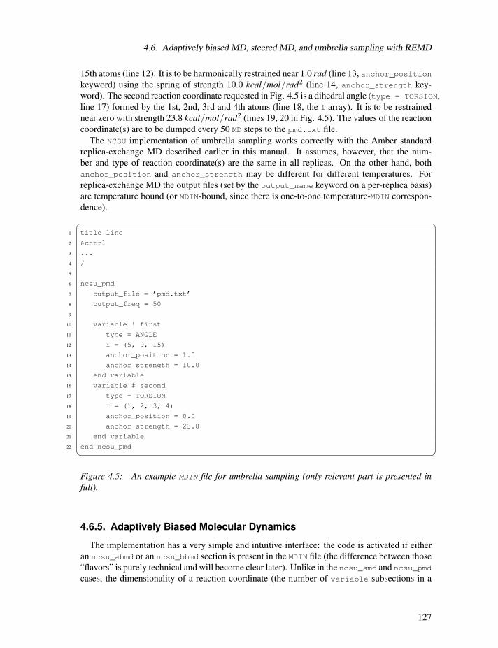
4.6. Adaptively biased MD, steered MD, and umbrella sampling with REMD
15th atoms (line 12). It is to be harmonically restrained near 1.0 rad (line 13, anchor_positionkeyword) using the spring of strength 10.0 kcal/mol/rad2 (line 14, anchor_strength key-word). The second reaction coordinate requested in Fig. 4.5 is a dihedral angle (type = TORSION,
line 17) formed by the 1st, 2nd, 3rd and 4th atoms (line 18, the i array). It is to be restrained
near zero with strength 23.8 kcal/mol/rad2 (lines 19, 20 in Fig. 4.5). The values of the reactioncoordinate(s) are to be dumped every 50 MD steps to the pmd.txt file.
The NCSU implementation of umbrella sampling works correctly with the Amber standard
replica-exchange MD described earlier in this manual. It assumes, however, that the num-
ber and type of reaction coordinate(s) are the same in all replicas. On the other hand, both
anchor_position and anchor_strength may be different for different temperatures. For
replica-exchange MD the output files (set by the output_name keyword on a per-replica basis)
are temperature bound (or MDIN-bound, since there is one-to-one temperature-MDIN correspon-
dence).� �1 title line
2 &cntrl
3 ...
4 /
5
6 ncsu_pmd
7 output_file = ’pmd.txt’
8 output_freq = 50
9
10 variable ! first
11 type = ANGLE
12 i = (5, 9, 15)
13 anchor_position = 1.0
14 anchor_strength = 10.0
15 end variable
16 variable # second
17 type = TORSION
18 i = (1, 2, 3, 4)
19 anchor_position = 0.0
20 anchor_strength = 23.8
21 end variable
22 end ncsu_pmd� �Figure 4.5: An example MDIN file for umbrella sampling (only relevant part is presented infull).
4.6.5. Adaptively Biased Molecular Dynamics
The implementation has a very simple and intuitive interface: the code is activated if either
an ncsu_abmd or an ncsu_bbmd section is present in the MDIN file (the difference between those
“flavors” is purely technical and will become clear later). Unlike in the ncsu_smd and ncsu_pmd
cases, the dimensionality of a reaction coordinate (the number of variable subsections in a
127

4. Sampling and free energies
ncsu_abmd or ncsu_bbmd section) cannot exceed five (though three is already hardly useful
due to statistical reasons).
The following entries are recognized within the ncsu_abmd (or ncsu_bbmd) section:
• mode = ANALYSIS | UMBRELLA | FLOODING : sets the execution mode. In ANALYSIS
mode the dynamics is not altered. The only effect of this mode is that the value(s) of
the reaction coordinate(s) is(are) dumped every monitor_freq to monitor_file. In
UMBRELLAmode, biasing potential from the umbrella_file is used to bias the simulation
(τF = ∞, biasing potential does not change). In FLOODING mode the adaptive biasing isenabled.
• monitor_file = STRING : sets the name of the file to which value(s) of reaction coor-
dinate(s) (along with the magnitude of biasing potential in FLOODINGmode) are dumped.
• monitor_freq = INTEGER : the frequency of the output to the monitor_file.
• timescale = REAL : τF , the flooding timescale in picoseconds (only required in FLOODING
mode).
• umbrella_file = STRING : biasing potential file name (the file must exist for the UMBRELLA
mode).
In FLOODING mode, the variable subsections of the ncsu_abmd section must also contain the
following entries:
• min = REAL : smallest desired value of the reaction coordinate (required, unless the re-
action coordinate is limited from below).
• max = REAL : largest desired value of the reaction coordinate (required, unless the reac-
tion coordinate is limited from above).
• resolution = REAL : the “spatial” resolution for the reaction coordinate.
To access the biasing potential files created in the course of FLOODING simulations, the ncsu-umbrella-slice
utility is provided (it prints a short description of itself if invoked with --help option).
An example MDIN file for the ncsu_abmd flavor of ABMD is shown in the Fig. 4.6.
The reaction coordinate is defined in lines 17, 18 as the distance between the 5th and 9th
atoms (more than one reaction coordinates might be requested by mere inclusion of additional
variable subsections). The mode is set to FLOODING thus enabling the adaptive biasing with
flooding timescale τF = 100ps (line 14). The region of interest of the reaction coordinateis specified to be between -1Åand 10Å(line 19) and the resolution is set to 0.5Å(line 20).
The lower bound (-1Å) could have been omitted for DISTANCE variable: the default value
of zero would be used in such case. The code will try to load the biasing potential from the
umbrella.nc file (line 12) and use it as the value of U(t|ξ ) at the beginning of the run. Thebiasing potential built in the course of simulation will be saved to the same file (umbrella.nc)
every time the RESTRT file is written. The ncsu-umbrella-slice utility can then be used to
access its content. An MDIN file for the follow up biased run at equilibrium would look much
like the one shown in the Fig. 4.6, but with mode changed from FLOODING to UMBRELLA.
128

4.6. Adaptively biased MD, steered MD, and umbrella sampling with REMD� �1 title line
2 &cntrl
3 ...
4 /
5
6 ncsu_abmd
7 mode = FLOODING
8
9 monitor_file = ’abmd.txt’
10 monitor_freq = 33
11
12 umbrella_file = ’umbrella.nc’
13
14 timescale = 100.0 ! in ps
15
16 variable
17 type = DISTANCE
18 i = (5, 9)
19 min = -1.0 max = 10.0 ! min is not needed for DISTANCE
20 resolution = 0.5 ! required for mode = FLOODING
21 end variable
22 end ncsu_abmd� �Figure 4.6: An example MDIN file for ABMD (only the relevant part is presented in full).
The ncsu_abmd code works correctly with replica-exchange (that is, for -rem flag set to 1).
In such case the monitor and umbrella files are temperature-bound (unlike, e.g., MDOUT and
MDCRD files that require post processing). If number of sander groups exceeds one (the flag
-ng is greater than one) and -rem flag is set to zero, the code runs multiple walkers ABMD. Inboth cases the number and type(s) of variable(s) must be the same across all replicas.
Finally, the ncsu_bbmd flavor allows one to run replica-exchange (AB)MD with different reac-
tion coordinates and different modes (ANALYSIS, UMBRELLA or FLOODING) in different replicas
(along with different temperatures, if desired). To this end, the -rem flag must be set to zero and
the ncsu_bbmd sections must be present in all MDIN files. The MDIN file for the replica of rank
zero (first line in the group file) is expected to contain additional information as compared to
ncsu_abmd case (an example of such MDIN file for replica zero is shown in Fig. 4.7). The MDIN
files for all other replicas except zero do not need any additional information, and therefore
take the same form as in the ncsu_abmd flavor (except that the section name is changed from
ncsu_abmd to ncsu_bbmd, thus activating a slightly different code path). Each MDIN file may
define its own reaction coordinates, have different mode and temperature if desired.
Within the first replica ncsu_bbmd section the following additional entries are recognized:
• exchange_freq = INTEGER : number of MD steps between the exchange attempts.
• exchange_log_file = STRING : the name of the file to which exchange statistics is to
be reported.
• exchange_log_freq = INTEGER : frequency of exchange_log_file updates.
129

4. Sampling and free energies� �1 title line
2 &cntrl
3 ...
4 /
5
6 ncsu_bbmd
7
8 ! 0th replica only
9
10 exchange_freq = 100 ! try for exchange every 100 steps
11
12 exchange_log_file = ’bbmd.log’
13 exchange_log_freq = 25
14
15 mt19937seed = 123455 ! random generator seed
16 mt19937file = ’mt19937.nc’ ! file to store/load the PRG
17
18 ! not specific for 0th replica
19
20 mode = ANALYSIS
21
22 monitorfile = ’bbmd.01.txt’ ! it is wise to have different
23 ! names in different replicas
24 monitor_freq = 123
25
26 variable
27 type = DISTANCE
28 i = (5, 9)
29 end variable
30 end ncsu_bbmd� �Figure 4.7: An example MDIN file for ncsu_bbmd flavor of ABMD (only the relevant part ispresented in full).
• mt19937_seed = INTEGER : seed for the random generator (Mersenne twister [154]).
• mt19937_file = STRING : the name of the file to which the state of theMersenne twister
is dumped periodically (for restarts).
The MDOUT, MDCRD, RESTRT, umbrella_file and monitor_file files are MDIN-bound in course
of the ncsu_bbmd-enabled run.
4.7. Nudged elastic band calculations
4.7.1. Background
In the nudged elastic band method (NEB), [155, 156] the path for a conformational change
is approximated with a series of images of the molecule describing the path. Minimization,
130
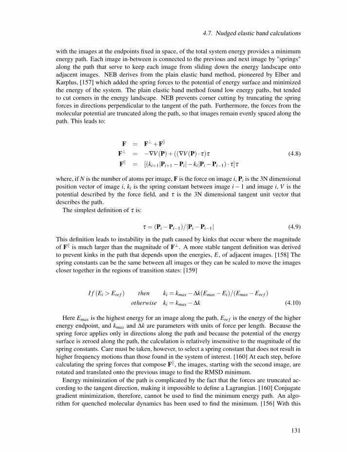
4.7. Nudged elastic band calculations
with the images at the endpoints fixed in space, of the total system energy provides a minimum
energy path. Each image in-between is connected to the previous and next image by "springs"
along the path that serve to keep each image from sliding down the energy landscape onto
adjacent images. NEB derives from the plain elastic band method, pioneered by Elber and
Karplus, [157] which added the spring forces to the potential of energy surface and minimized
the energy of the system. The plain elastic band method found low energy paths, but tended
to cut corners in the energy landscape. NEB prevents corner cutting by truncating the spring
forces in directions perpendicular to the tangent of the path. Furthermore, the forces from the
molecular potential are truncated along the path, so that images remain evenly spaced along the
path. This leads to:
F = F⊥+F‖
F⊥ = −∇V (P)+((∇V (P) · τ)τ (4.8)
F‖ = [(ki+1|Pi+1−Pi|− ki|Pi−Pi−1) · τ]τ
where, if N is the number of atoms per image, F is the force on image i, Pi is the 3N dimensional
position vector of image i, ki is the spring constant between image i− 1 and image i, V is the
potential described by the force field, and τ is the 3N dimensional tangent unit vector that
describes the path.
The simplest definition of τ is:
τ = (Pi−Pi−1)/|Pi−Pi−1| (4.9)
This definition leads to instability in the path caused by kinks that occur where the magnitude
of F‖ is much larger than the magnitude of F⊥. A more stable tangent definition was derivedto prevent kinks in the path that depends upon the energies, E, of adjacent images. [158] Thespring constants can be the same between all images or they can be scaled to move the images
closer together in the regions of transition states: [159]
I f (Ei > Ere f ) then ki = kmax−Δk(Emax−Ei)/(Emax−Ere f )otherwise ki = kmax−Δk (4.10)
Here Emax is the highest energy for an image along the path, Ere f is the energy of the higher
energy endpoint, and kmax and Δk are parameters with units of force per length. Because thespring force applies only in directions along the path and because the potential of the energy
surface is zeroed along the path, the calculation is relatively insensitive to the magnitude of the
spring constants. Care must be taken, however, to select a spring constant that does not result in
higher frequency motions than those found in the system of interest. [160] At each step, before
calculating the spring forces that compose F‖, the images, starting with the second image, arerotated and translated onto the previous image to find the RMSD minimum.
Energy minimization of the path is complicated by the fact that the forces are truncated ac-
cording to the tangent direction, making it impossible to define a Lagrangian. [160] Conjugate
gradient minimization, therefore, cannot be used to find the minimum energy path. An algo-
rithm for quenched molecular dynamics has been used to find the minimum. [156] With this
131

4. Sampling and free energies
method, the component of the velocity parallel to the force is kept, but perpendicular compo-
nents are scaled:
I f (v · f > 0) then v = (v · f)fotherwise v = x(v · f)f (4.11)
where f is the 3N-dimensional unit force vector, v is the 3N-dimensional velocity vector, and xis a scaling factor less than one. Recently, a super-linear minimization method was described
using an adopted basis Newton-Raphson minimizer. [160]
The implementation of NEB in sander.MPI [161] allows minimization by simulated anneal-ing. This requires no hypothesis for a starting path, but does require careful judgment of the
temperature and length of time required to populate the minimum energy path. The initial co-
ordinates can have multiple copies of the structure superimposed on the start and endpoints.
When adjacent structures are superimposed, the tangent, τ is 0 in every direction. This case isexplicitly handled so that the calculation is stable.
4.7.2. Preparing input files for NEB
The NEB capability is implemented inside sander.MPI because of the similarity betweenPIMD and NEB. Input prmtop and inpcrd files for NEB should be generated using addles. Touse addles to generate a prmtop and inpcrd file suitable for NEB you need as a minimum a
prmtop for a single image of your molecule and two inpcrd files representing each end of thepathway. You can build these files using Leap. You should then append the second inpcrd fileto the end of the first inpcrd file giving you a single inpcrd file containing both structures. Youshould then use this inpcrd file and the single image prmtop file with the following addles script(addles.in), adjusted for your needs, to create your NEB prmtop and inpcrd file.
file rprm name=(input.prmtop) read
file rcrd name=(input.inpcrd) pack=2 read
file wprm name=(neb.prmtop) wovr
file wcrd name=(neb.inpcrd) wovr
action
use original mass
omas
pimd
make 20 copies of atom 1 to 22 (the whole system)
space numc=20 pick #prt 1 22 done
*EOD
For a full description of addles please refer to Section 9.2, the following are some notes forpreparing NEB input files:
1. Always turn on the pimd tag, otherwise you may get an unexpectedly big prmtop file
because of a huge nonbond exclusion list containing all atoms in different copies.
2. Make sure your are making copies of the whole system, since for now the PIMD im-
plementation of sander is an all-or-nothing thing, meaning you can’t run partial NEB
simulations at present.
132

4.8. Constant pH calculations
3. Make use of the pack option of rcrd(rcvd,rcbd,rcvb) to assign different coordinates for
different copies. It is necessary for NEB that different images be assigned different con-
figurations, that is why the option "pack" is added to "rcrd". To use this option, the user
needs to first concatenate the desired inpcrds together, then specify the number of coordi-nate sets via "pack=n", addles will then assign coordinates to images in appropriate sizedblocks. For example, if the inpcrd file has 4 sets of coordinates and you have 20 images.
Then image 1-5 will have coordinate set 1, image 6-10 have set 2, and so on.
4.7.3. Input Variables
ineb Flag for nudged elastic band. A value of 0 (default) means that no nudged elastic
band will be used. A value of 1 means that a NEB simulation is being performed.
skmax Spring constant or kmax from above (100 by default).
skmin If skmin = skmax, a fixed spring constant is used. Otherwise, skmin is taken from
above for scaled spring constants (50 by default).
tmode If 1 (default), use the revised tangent definition that prevents kinks. For any other
value, use the simple (original) tangent definition.
vv If this is 1, use the quenched velocity Verlet minimization; otherwise, do not.
vfac Scaling factor for quenched velocity Verlet algorithm. (0.0 by default).
4.8. Constant pH calculations
The constant pH molecular dynamics method has been implemented in sander by John Mon-gan. [162] Constant pH is limited to implicit solvent simulations. Using the constant pH method
requires minor modifications to the process of generating the prmtop file, as well as generation
of a second input file from the prmtop file, describing the titrating residues.
4.8.1. Background
Traditionally, molecular dynamics simulations have employed constant protonation states
for titratable residues. This approach has many drawbacks. First, assigning protonation states
requires knowledge of pK a values for the protein’s titratable groups. Second, if any of these
pK a values are near the solvent pH there may be no single protonation state that adequately
represents the ensemble of protonation states appropriate at that pH. Finally, since protonation
states are constant, this approach decouples the dynamic dependence of pK a and protonation
state on conformation.
The constant pH method implemented in sander addresses these issues through Monte Carlosampling of the Boltzmann distribution of protonation states concurrent with the molecular
dynamics simulation. The nature of the distribution is affected by solvent pH, which is set as
an external parameter. Residue protonation states are changed by changing the partial charges
on the atoms.
133

4. Sampling and free energies
4.8.2. Preparing a system for constant pH
Amber provides definitions for titrating side chains of ASP, GLU, HIS, LYS and TYR. See
below if you need other titrating groups.
Begin by preparing your PDB file as you normally would for use with LEaP. Edit the PDB
file, replacing all histidine residue names (HIS, HID, or HIE) with HIP. Change all ASP and
ASH to AS4 and all GLU and GLH to GL4. This ensures that the prmtop file will have a
hydrogen defined at every possible point of protonation.
Run leap, and enter the following commands:
source leaprc.ff99
loadAmberParams frcmod.mod_phipsi.1
set default PBRadii mbondi2
loadoff constph.lib
loadamberparams frcmod.constph
This loads constph.lib, which contains residue definitions for AS4 and GL4 (aspartate and glu-
tamate residues with syn and anti hydrogens on each carboxyl oxygen), and frcmod.constph
which defines improper torsions to keep the syn and anti protons on AS4 and GL4 from rotat-
ing into the same position. Now load your edited PDB file and proceed as usual to create the
prmtop and prmcrd files.
Once you have the prmtop file, you need to generate a cpin file. The cpin file describes which
residues should titrate, and defines the possible protonation states and their relative energies.
A perl script, cpinutil.pl, is provided to generate this file. It takes a PDB file as input, eitheron the command line or on STDIN, and writes the cpin file to STDOUT. Note that you mustgenerate this PDB file from the prmtop file; do not use your original PDB file. Since LEaP has
inserted extra hydrogens, the atom numbering in your original PDB file will not correspond to
the prmtop file. Here is an example of generating the PDB file and using it to create the cpin
file in a single step:
ambpdb -p prmtop < prmcrd | cpinutil.pl > cpin
The cpinutil.pl program accepts a number of flags that modify its behavior. By default, all
residues start in protonation state 0: deprotonated for ASP and GLU, protonated for LYS and
TYR, doubly protonated for HIS (i.e. HIP). Initial protonation states can be specified using the
-states flag followed by a comma delimited list of initial protonation states (see below for more
about protonation state definitions) as follows:
ambpdb -p prmtop < prmcrd | cpinutil.pl -states 1,3,0,0,0,1 > cpin
The -system flag can be used to provide a name for the titrating system. If experimental pKa
values have been defined for the system (see below), they will be written into the cpin file. Note
that experimental pKa values are used only by the analysis scripts to calculate pKa prediction
error; they are not used in any way by sander and do not need to be included.
ambpdb -p prmtop < prmcrd | cpinutil.pl -system HEWL > cpin
134

4.8. Constant pH calculations
A number of flags are available for filtering which residues are included in the cpin file. All
residues in the cpin file, and only the residues in the cpin file, will be titrated. In general it is
safe to exclude TYR and LYS for acidic simulations and GL4 and AS4 for basic simulations.
HIP should be included in all except very acidic simulations. Note that there is currently no
support for titrating N or C terminal residues. If you have an N or C terminal residue with a
titratable sidechain, you should explicitly exclude it from the cpin file. The -resnum flag may be
used to specify which residue numbers should be retained; all others are deleted. Conversely,
the -notresnum flag can be used to specify which residue numbers are deleted; all others are
retained. Residue number refers to the numbering in the PDB file, not the index number among
titrating residues. Similarly, -resname and -notresname can be used to filter by residue type. For
instance, -notresname TYR,LYS would eliminate basic residues from the cpin file. If experi-
mental pKa values are known through use of the -system flag, the -minpka and -maxpka flags
can be used to filter residues by experimental pK a values.
cpinutil.pl can also take an existing cpin file as input, allowing modification or further filter-ing of existing cpin files. See cpinutil.pl -h for a summary of options and flags.
4.8.3. Running at constant pH
Running constant pH under sander has few differences from normal operation. In the mdinfile, you must set icnstph=1 to turn on constant pH. solvph is used to set the solvent pH value.You must also specify the period for Monte Carlo steps, ntcnstph (for period n, a Monte Carlostep is performed every n steps). Note that only one residue is examined on each step, so youshould decrease the step period as the number of titrating residues increases to maintain a con-
stant effective step period for each residue. We have seen good results with fairly short periods,
in the neighborhood of 100 fs effective period for each residue (e.g. ntcnstph=5, dt=0.002 withabout 10 residues titrating).
In order to avoid having to calculate non-electrostatic contributions to protonation state tran-
sition energies, this method uses correction factors based on the relative energy differences of
the different protonation states in the Amber force field. These relative energies were calculated
under the following parameters:
cut=30.0, scee=1.2, igb=2, saltcon=0.1,
ntb=0, dt=0.002, nrespa=1,
ntt=1, tempi=300.0, temp0 = 300., tautp=2.0,
ntc=2, ntf=2, tol=0.000001,
Deviations from these parameters, or from the force field or GB radii specified above may
affect the relative energies of the protonation states, which will cause erroneous results. If
you must deviate from these settings, you can test whether your changes will cause problems
by running long (multiple ns) titrations of the model compounds, with solvent pH equal to
the model compound pKa value. The model compounds are ACE-X-NME, where X is AS4,
GL4, HIP, LYS or TYR. If these titrations predict the model pKa value (4.0, 4.4, 6.5, 10.4 and
9.6, respectively), then the parameter set is probably OK. If not, you must either change the
parameter set or recalculate the relative energies (see section below).
Some additional command line flags have been added to sander to support constant pH op-eration. The cpin file must be specified using the -cpin option. Additionally, a history of the
protonation states sampled is written to the filename specified by -cpout. Finally, a constant
135
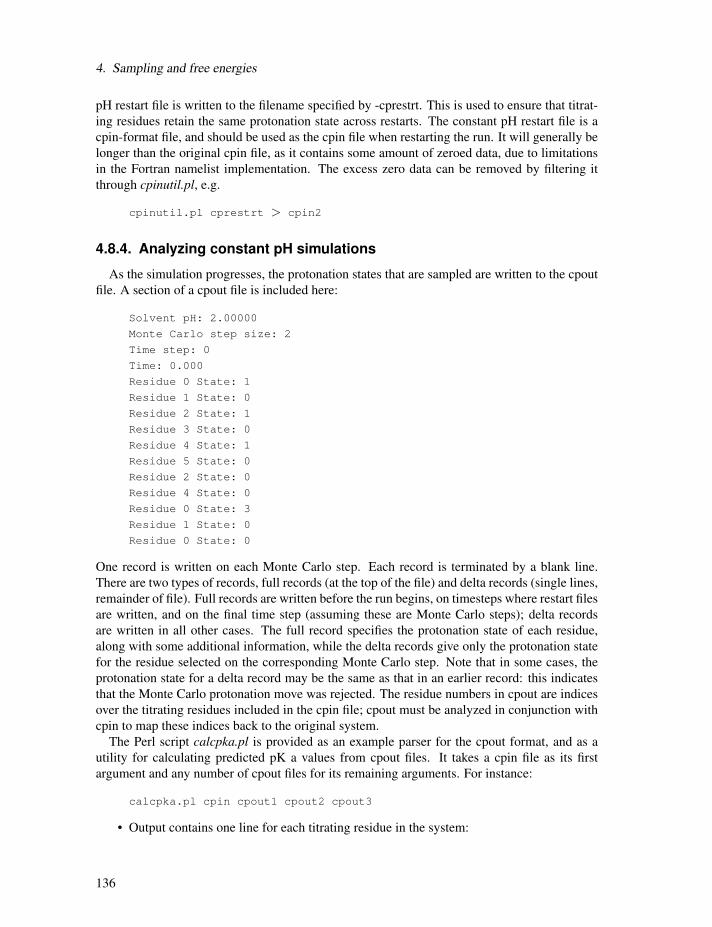
4. Sampling and free energies
pH restart file is written to the filename specified by -cprestrt. This is used to ensure that titrat-
ing residues retain the same protonation state across restarts. The constant pH restart file is a
cpin-format file, and should be used as the cpin file when restarting the run. It will generally be
longer than the original cpin file, as it contains some amount of zeroed data, due to limitations
in the Fortran namelist implementation. The excess zero data can be removed by filtering it
through cpinutil.pl, e.g.
cpinutil.pl cprestrt > cpin2
4.8.4. Analyzing constant pH simulations
As the simulation progresses, the protonation states that are sampled are written to the cpout
file. A section of a cpout file is included here:
Solvent pH: 2.00000
Monte Carlo step size: 2
Time step: 0
Time: 0.000
Residue 0 State: 1
Residue 1 State: 0
Residue 2 State: 1
Residue 3 State: 0
Residue 4 State: 1
Residue 5 State: 0
Residue 2 State: 0
Residue 4 State: 0
Residue 0 State: 3
Residue 1 State: 0
Residue 0 State: 0
One record is written on each Monte Carlo step. Each record is terminated by a blank line.
There are two types of records, full records (at the top of the file) and delta records (single lines,
remainder of file). Full records are written before the run begins, on timesteps where restart files
are written, and on the final time step (assuming these are Monte Carlo steps); delta records
are written in all other cases. The full record specifies the protonation state of each residue,
along with some additional information, while the delta records give only the protonation state
for the residue selected on the corresponding Monte Carlo step. Note that in some cases, the
protonation state for a delta record may be the same as that in an earlier record: this indicates
that the Monte Carlo protonation move was rejected. The residue numbers in cpout are indices
over the titrating residues included in the cpin file; cpout must be analyzed in conjunction with
cpin to map these indices back to the original system.
The Perl script calcpka.pl is provided as an example parser for the cpout format, and as autility for calculating predicted pK a values from cpout files. It takes a cpin file as its first
argument and any number of cpout files for its remaining arguments. For instance:
calcpka.pl cpin cpout1 cpout2 cpout3
• Output contains one line for each titrating residue in the system:
136

4.8. Constant pH calculations
Offset is the difference between the predicted pK a and the system pH.
Pred is the predicted pKa. Note that predictions are calculated assuming Henderson-
Hasselbalch titration curves. Predictions are most accurate when the absolute
value of the offset is less than 2.0. If experimental pK a values have been
defined for the system (see following), then experimental and error values
are also printed.
Frac Prot is the fraction of time the residue spends protonated and
Transitions gives the number of accepted protonation state transitions. Note that tran-sitions between states with the same total protonation (e.g. syn and antiprotonated states of a carboxylic acid) are not included in this total.
Average total molecular protonation is the sum of the fractional protonations. It ranges
between zero and the number of titrating residues, and gives the average
protonation of the molecule as a whole.
4.8.5. Extending constant pH to additional titratable groups
There are two major components to defining a new titrating group for constant pH. First you
must define the partial charges for each atom in the residue for each protonation state. Then
you must set the relative energies of each state.
Defining charge sets
Partial charges are most easily calculated using Antechamber and Gaussian. You must set up
a model to calculate charges for each protonation state. If the titrating group you are defining
is a polymer subunit (e.g. amino acid residue), you must adjust the charges on atoms that have
bonded interactions (including 1-4) with atoms in neighboring residues. The charges on these
atoms must be changed so they are constant across all protonation states - otherwise relative
energies of protonation states become sequence dependent. For an amino acid, this means that
all backbone atoms must have constant charges. For the residues defined here, we arbitrarily
selected the backbone charges of the protonated state to be used across all protonation states.
The total charge difference between states should remain 1; we achieved this by adjusting the
charge on the beta carbon.
Calculating relative energies
Relative energies are used to calibrate the method such that when a model compound is
titrated at pH equal to its pK a , the energies (and thus populations) of the protonated and
deprotonated states are equal. Relative energies of the different protonation states are calculated
using thermodynamic integration of a model compound between the charge sets defined for the
different protonation states. The model compound should be a small molecule that mimics the
bonded environment of the titratable group of interest, and for which experimental pK a data are
available. For instance, the model compound for an amino acid X is generally ACE-X-NME;
the model compound for a ligand might be the free ligand. The thermodynamic integration
calculations must be performed using exactly the same parameters and force field as you plan
to use in your constant pH simulations. Once the relative energies of the states are calculated
137

4. Sampling and free energies
by thermodynamic integration, the energy difference must be adjusted to account for the pKa :
the energy of the more protonated states should be increased by pKaRT ln(10).For example suppose one were developing a model for an artificial amino acid, ART, with
pK a 3.5 and two protonation states: ARP, having one proton and ARD having zero protons.
After calculating partial charges as above, you would construct a model compound having the
sequence ACE-ARP-NME and generate a prmtop file where the ARP charges were perturbed
to the ARD values. You would then use sander to perform thermodynamic integration between
ARP and ARD. Suppose that this showed that the energy of ARD relative to ARPwas -6.3 kcal/-
mol. You would assign a relative energy of -6.3 to ARD and a relative energy of 3.5RTln(10)
to ARP.
Testing the titratable group definitions
Prior to large scale use of your new titratable group definition, it’s a good idea to test it by
performing a constant pH simulation on your model compound, with pH set to the model pK
a . Doing this requires generation of a cpin file, so this is a good point to modify the table of
titratable group definitions used by cpinutil.pl. These tables are found near the end of CPin.pm.The table is a perl hash of 2D arrays. Each hash entry is an array of states that define a titratable
group. Each state array consists of the relative energy, the relative protonation, and the partial
charges for the state, in that order. An entry for the example given above might look like (charge
list shortened for brevity):
"ARP" => [
# State 0, ARP
[3.5 * 1.3818, # Relative energy (300K)
1, # Relative protonation
-0.4157, 0.2719, -0.0014, 0.0876, -0.0152, 0.0295, ],
# State 1, ARD
[-6.3, # Energy
0, # Protonation
-0.4157, 0.2719, -0.0014, 0.0876, -0.0858, 0.019, ]
]
Below this table is another table of experimental pK a values. Entries for new systems can
be created following the example already present for HEWL (the keys are residue numbers,
the values are their pK a values). As discussed above, this is optional and does not affect the
constant pH simulations - these data are used only by calcpka.pl and cpinutil.pl.Having added your titratable group definition to the table, you should be able to prepare
a cpin file as described above, run your simulation and calculate the predicted pK a using
calcpka.pl. Since the model compound is usually very small, runs of tens of nanosecondsare easily accessible for these tests. In general, the run to run variation of predicted pK a
values is a few hundredths of a pK a unit for long runs with pH near pK a . In most cases,
the thermodynamic integration procedure described above yields acceptable results, but if your
predicted pK a differs significantly from the model pK a , you may want to adjust your relative
energies, regenerate your cpin file and rerun the test until you achieve good predictions.
138

4.9. Low-MODe (LMOD) methods
4.9. Low-MODe (LMOD) methods
István Kolossváry’s LMOD methods for minimization, conformational searching, and flexi-
ble docking [163–166] are now fully implemented in AMBER. The centerpiece of LMOD is a
conformational search algorithm based on eigenvector following of low frequency vibrational
modes. It has been applied to a spectrum of computational chemistry domains including protein
loop optimization and flexible active site docking. The search method is implemented without
explicit computation of a Hessian matrix and with gradient evaluations via the Arnoldi package
(ARPACK), http://www.caam.rice.edu/software/ARPACK/.
4.9.1. LMOD conformational searching and flexible docking
The LMOD conformational search procedure is based on gentle, but very effective struc-
tural perturbations applied to molecular systems in order to explore their conformational space.
LMOD perturbations are derived from low-frequency vibrational modes representing large-
amplitude, concerted atomic movements. Unlike essential dynamics where such low modes are
derived from long molecular dynamics simulations, LMOD calculates the modes directly and
utilizes them to improve Monte Carlo sampling.
LMOD has been developed primarily for macromolecules, with its main focus on protein
loop optimization. However, it can be applied to any kind of molecular system,s including
complexes and flexible docking where it has found widespread use. The LMOD procedure starts
with an initial molecular model, which is energy minimized. The minimized structure is then
subjected to an ARPACK calculation to find a user-specified number of low-mode eigenvectors
of the Hessian matrix. The Hessian matrix is never computed; ARPACK makes only implicit
reference to it through its product with a series of vectors. Hv, where v is an arbitrary unitvector, is calculated via a finite-difference formula as follows,
Hv = [∇(xmin +h)−∇(xmin)]/h
where xmin is the coordinate vector at the energy minimized conformation and h denotes ma-chine precision. The computational cost of Eq. 1 requires a single gradient calculation at the
energy minimum point and one additional gradient calculation for each new vector. Note that
�x is never 0, because minimization is stopped at a finite gradient RMS, which is typically setto 0.1-1.0 kcal/mol-Å in most calculations.
The low-mode eigenvectors of the Hessian matrix are stored and can be re-used throughout
the LMOD search. Note that although ARPACK is very fast in relative terms, a single ARPACK
calculation may take several hours on an absolute CPU time scale. Therefore, it would be im-
practical to recalculate the low-mode eigenvectors for each new structure. Visual inspection of
the low-frequency vibrational modes of different, randomly generated conformations of pro-
tein molecules showed very similar, collective motions clearly suggesting that low modes of
one particular conformation were transferable to other conformations for LMOD use. This im-
portant finding implies that the time limiting factor in LMOD is energy minimization, not the
eigenvector calculation.
139

4. Sampling and free energies
4.9.2. LMOD Procedure
Given the energy-minimized structure of an initial protein model, protein-ligand complex,
or any other molecular system and its low-mode Hessian eigenvectors, LMOD proceeds as
follows. For each of the first n low-modes repeat steps 1-3 until convergence:
1. Perturb the energy-minimized starting structure by moving along the ith (i =1-n) Hes-
sian eigenvector in either of the two opposite directions to a certain distance. The 3N-
dimensional (N is equal to the number of atoms) travel distance along the eigenvector is
scaled to move the fastest moving atom of the selected mode in 3-dimensional space to a
randomly chosen distance between a user-specified minimum and maximum value.
Note: A single LMOD move inherently involves excessive bond stretching and bond an-
gle bending in Cartesian space. Therefore the primarily torsional trajectory drawn by the
low modes of vibration on the PES is severely contaminated by this naive, linear approx-
imation and, therefore, the actual Cartesian LMOD trajectory often misses its target by
climbing walls rather than crossing over into neighboring valleys at not too high altitudes.
The current implementation of LMOD employs a so-called ZIG-ZAG algorithm, which
consists of a series of alternating short LMOD moves along the low-mode eigenvector
(ZIG) followed by a few steps of minimization (ZAG), which has been found to relax
excessive stretches and bends more than reversing the torsional move. Therefore, it is
expected that such a ZIG- ZAG trajectory will eventually be dominated by concerted tor-
sional movements and will carry the molecule over the energy barrier in a way that is
not too different from finding a saddle point and crossing over into the next valley like
passing through a mountain pass.
Barrier crossing check: The LMOD algorithm checks barrier crossing by evaluating the
following criterion: IF the current endpoint of the zigzag trajectory is lower than the
energy of the starting structure, OR, the endpoint is at least lower than it was in the
previous ZIG-ZAG iteration step AND the molecule has also moved farther away from
the starting structure in terms of all-atom superposition RMS than at the previous position
THEN it is assumed that the LMOD ZIG-ZAG trajectory has crossed an energy barrier.
2. Energy-minimize the perturbed structure at the endpoint of the ZIG-ZAG trajectory.
3. Save the new minimum-energy structure and return to step 1. Note that LMOD saves
only low-energy structures within a user-specified energy window above the then current
global minimum of the ongoing search.
After exploring the modes of a single structure, LMOD goes on to the next starting structure,
which is selected from the set of previously found low-energy structures. The selection is based
on either the Metropolis criterion, or simply the than lowest energy structure is used. LMOD
terminates when the user-defined number of steps has been completed or when the user-defined
number of low-energy conformations has been collected.
Note that for flexible docking calculations LMOD applies explicit translations and rotations
of the ligand(s) on top of the low-mode perturbations.
140

4.9. Low-MODe (LMOD) methods
4.9.3. XMIN
The XMIN methods for minimization are traditional and manifold in the field of uncon-
strained optimization: PRCG is a Polak-Ribiere nonlinear Conjugate Gradient algorithm, [167]
LBFGS is a Limited-memory Broyden-Fletcher-Goldfarb-Shanno quasi-Newton algorithm, [168]
and TNCG is a Truncated Newton linear Conjugate Gradient method with optional LBFGS pre-
conditioning. [169]
Some of the &cntrl namelist variables that control AMBER’s other minimization facilities
also control XMIN. Consequently, non-experts can employ the default XMIN method merely
by specifying ntmin = 3.
maxcyc The maximum number of cycles of minimization. Default is 1 to be consistent with
AMBER’s other minimization facilities although it may be unrealistically short.
ntmin The flag for the method of minimization.
= 3 The XMIN method is used.
= 4 The LMODmethod is used. The LMOD procedure employs XMIN for energy
relaxation and minimization.
drms The convergence criterion for the energy gradient: minimization will halt when
the root-mean-square of the Cartesian elements of the gradient is less than DRMS.
Default is 1.0E-4 kcal/mole Åto be consistent with AMBER’s other minimization
facilities although it may be unrealistically strict.
Other options that control XMIN are in the scope of the &lmod namelist. These parameters
enable expert control of XMIN.
lbfgs_memory_depth The depth of the LBFGS memory for LBFGS minimization, or LBFGS
preconditioning in TNCG minimization. Default is 3. Suggested alternate value is
5. The value 0 turns off LBFGS preconditioning in TNCG minimization.
matrix_vector_product_method The finite difference Hv matrix-vector product method: "for-
ward" = forward difference, "central" = central difference. Default is forward dif-
ference.
xmin_method The minimization method: "PRCG" = Polak-Ribiere Conjugate Gradient, "LBFGS"
= Limited-memory Broyden-Fletcher-Goldfarb-Shanno, and "TNCG" = Option-
ally LBFGS-preconditioned Truncated Newton Conjugate Gradient. Default is
LBFGS.
xmin_verbosity The verbosity of the internal status output from the XMIN package: 0 = none,
1 = minimization details, and 2 = minimization and line search details plus CG
details in TNCG. Currently, the XMIN status output may be disordered with re-
spect to AMBER’s output. Default is 0, no output of the XMIN package internal
status. Note that XMIN is also available in Amber Tools, in the NAB package. An
annotated example output corresponding to XMIN_VERBOSITY=2 can be found
in the NAB documentation.
141

4. Sampling and free energies
4.9.4. LMOD
Some of the options that control LMOD have the same names as AMBER’s other minimiza-
tion facilities. See the XMIN section immediately above. Other options that control LMOD are
in the scope of the &lmod namelist. These parameters enable expert control of LMOD.
arnoldi_dimension The dimension of the ARPACK Arnoldi factorization. Zero specifies the
whole space, that is, three times the number of atoms. Default is 0, the whole space.
Basically, the ARPACK package used for the eigenvector calculations solves mul-
tiple "small" eigenvalue problems instead of a single "large" problem, which is the
diagonalization of the three times the number of atoms by three times the number of
atoms Hessian matrix. This parameter is the user specified dimension of the "small"
problem. The allowed range is total_low_modes + 1 <= arnoldi_dimension <=three times the number of atoms. The default means that the "small" problem
and the "large" problem are identical. This is the preferred, i.e., fastest, calcula-
tion for small to medium size systems, because ARPACK is guaranteed to con-
verge in a single iteration. The ARPACK calculation scales with three times the
number of atoms times the arnoldi_dimension squared and, therefore, for larger
molecules there is an optimal arnoldi_dimension much less than three times the
number of atoms that converges much faster in multiple iterations (possibly thou-
sands or tens of thousands of iterations). The key to good performance is to select
an arnoldi_dimension such that all the ARPACK storage fits in memory. For pro-
teins, arnoldi_dimension=1000 is generally a good value, but often a very small
50-100 Arnoldi dimension provides the fastest net computational cost with very
many iterations.
conflib_filename The user-given filename of the LMOD conformational library. The file for-
mat is standard AMBER trajectory file. The conformations are stored in energetic
order (global minimum energy structure first), the number of conformations <=conflib_size. The default filename is conflib.
conflib_size The number of conformations to store in conflib. Default is 3.
energy_window The energy window for conformation storage; the energy of a stored structure
will be in the interval [global_min, global_min + energy_window]. Default is 0,
only storage of the global minimum structure.
explored_low_modes The number of low frequency vibrational modes used per LMOD itera-
tion. Default is 3.
frequency_eigenvector_recalc The frequency, measured in LMOD iterations, of the recalcula-
tion of eigenvectors. Default is 3.
frequency_ligand_rotrans The frequency, measured in LMOD iterations, of the application of
rigid-body rotational and translational motions to the ligand(s). At each frequency_ligand_rotrans-
th LMOD iteration number_ligand_rotrans rotations and translations are applied to
the ligand(s). Default is 1, ligand(s) are rotated and translated at every LMOD
iteration.
142

4.9. Low-MODe (LMOD) methods
lmod_job_title The user-given title for the job that goes in the first line of the conflib and
lmod_trajectory files. The default job title is "job_title_goes_here".
lmod_minimize_grms The gradient RMS convergence criterion of structure minimization. De-
fault is 0.1.
lmod_relax_grms The gradient RMS convergence criterion of structure relaxation. Default is
1.0.
lmod_restart_frequency The frequency, in LMOD iterations, of conflib updating and LMOD
restarting with a randomly chosen structure from the pool. Default is 5.
lmod_step_size_max The maximum length of a single LMOD ZIG move. Default is 5.0 Å.
lmod_step_size_min The minimum length of a single LMOD ZIG move. Default is 2.0 Å.
lmod_trajectory_filename The filename of the LMOD pseudo trajectory. The file format is
standard AMBER trajectory file. The conformations in this file show the progress
of the LMOD search. The number of conformations = number_lmod_iterations +
1. The default filename is lmod_trajectory.
lmod_verbosity The verbosity of the internal status output from the LMOD package: 0 = none,
1 = some details, 2 = more details, 3 = everything including ARPACK information.
Currently, the LMOD status output may be disordered with respect to AMBER’s
output. Default is 0, no output of the LMOD package internal status. Note that
LMOD is also available in Amber Tools, in the NAB package. An annotated ex-
ample output corresponding to LMOD_VERBOSITY=2 can be found in the NAB
documentation.
monte_carlo_method The Monte Carlo method: "Metropolis" = Metropolis Monte Carlo, "To-
tal_Quench" = the LMOD trajectory always proceeds towards the lowest lying
neighbor of a particular energy well found after exhaustive search along all of the
low modes, and "Quick_Quench" = the LMOD trajectory proceeds towards the
first neighbor found, which is lower in energy than the current point on the path,
without exploring the remaining modes. Default is Metropolis Monte Carlo.
number_free_rotrans_modes The number of rotational and translational degrees of freedom.
This is related to the number of frozen or tethered atoms in the system: 0 atoms
dof=6, 1 atom dof=3, 2 atoms dof=1, >=3 atoms dof=0. Default is 6, no frozenatoms.
number_ligand_rotrans The number of rigid-body rotational and translational motions applied
to the ligand(s). Such applications occur at each frequency_ligand_rotrans-th LMOD
iteration. Default is 0, no rigid-body motions applied to the ligand(s).
number_ligands The number of ligands for flexible docking. Default is 0, no ligand(s).
number_lmod_iterations The number of LMOD iterations. Default is 10. Note that setting
number_lmod_iterations = 0 will result in a single energy minimization.
143

4. Sampling and free energies
number_lmod_moves The number of LMOD ZIG-ZAG moves. Zero means that the number
of ZIG-ZAG moves is not pre-defined, instead LMOD will attempt to cross the
barrier in as many ZIG-ZAG moves as it is necessary. The criterion of crossing
an energy barrier is stated above in the "LMOD Procedure" background section.
number_lmod_moves> 0 means that multiple barriers may be crossed and LMOD
can carry the molecule to a large distance on the potential energy surface without
severely distorting the geometry. Default is 0, LMODwill determine automatically
where to stop the ZIG-ZAG sequence.
random_seed The seed of the random number generator. Default is 314159.
restart_pool_size The size of the pool of lowest-energy structures to be used for restarting.
Default is 3.
rtemperature The value of RT in AMBER energy units. This is utilized in the Metropolis
criterion. Default is 1.5.
total_low_modes The total number of low frequency vibrational modes to be used. Default
is the minimum of 10 and three times the number of atoms minus the number of
rotational and translational degrees of freedom (number_free_rotrans_modes).
The following commands are part of the &lmod namelist. These commands control the way
LMOD applies explicit translations and rotations to one or more ligands and take effect only if
number_ligands>= 1. All commands are lists in square brackets, separated by commas such as[1, 33, 198], however, the list is read by Sander as a string and, therefore, it should be enclosed
in single quotes.
ligstart_list, ligend_list The serial number(s) of the first/last atom(s) of the ligand(s). Type
integer. The number(s) should correspond to the numbering in the AMBER input
files prmtop and inpcrd/restart. For example, if there is only one ligand and it
starts at atom 193, the command should be ligstart_list = ’[193]’. If there are three
ligands, the command should be, e.g., ’[193, 244, 1435]’. The same format holds
for all of the following commands. Note that the ligand(s) can be anywhere in the
atom list, however, a single ligand must have continuous numbering between the
corresponding ligstart_list and ligend_list values. For example, ligstar_list = ’[193,
244, 1435]’ and ligend_list = ’[217, 302, 1473]’.
ligcent_list The serial number(s) of the atom(s) of the ligand(s), which serves as the center of
rotation. Type integer. The value zero means that the center of rotation will be the
geometric center of gravity of the ligand.
rotmin_list, rotmax_list The range of random rotation of a particular ligand about the origin
defined by the corresponding ligcent_list value is specified by the commands rot-
min_list and rotmax_list. The angle is given in +/- degrees. Type float. For ex-
ample, in case of a single ligand and ligcent_list = ’[0]’, rotmin_list = ’[30.0]’
and rotmax_list = ’[180.0]’ means that random rotations by an angle +/- 30-180
degrees about the center of gravity of the ligand, will be applied. Similarly, with
number_ligands = 2, ligcent_list= 120.0]’ means that the first ligand will be ro-
tated like in the single ligand example in this paragraph, but a second ligand will
be rotated about its atom number 201, by an angle +/- 60-120 degrees.
144
4.9. Low-MODe (LMOD) methods
trmin_list, trmax_list The range of random translation(s) of ligand(s) is defined by the same
way as rotation. For example, with number_ligand = 1, trmin_list = ’[0.1]’ and
trmax_list = ’[1.0]’ means that a single ligand is translated in a random direction
by a random distance between 0.1 and 1.0 Angstroms.
4.9.5. Tricks of the trade of running LMOD searches
1. (1) The AMBER atom types HO, HW, and ho all have zero van der Waals parameters in
all of the AMBER (and some other) force fields. Corresponding Aij and Bij coefficients
in the prmtop file are set to zero. This means there is no repulsive wall to prevent two
oppositely charged atoms, one being of type HO, HW or ho, to fuse as a result of the
ever decreasing electrostatic energy as they come closer and closer to each other. This
potential problem is circumvented in molecular dynamics simulations in ways that are in-
compatible with LMOD. Therefore, before running an LMOD simulation, the prmtop file
(let’s call it prmtop.in) must be processed by running $AMBERHOME/exe/lmodprmtopprmtop.in prmtop.out. This script will replace all the repulsive Aij coefficients set to zeroin the prmtop file with a high value of 1e03 in order to re-create the van der Waals wall.
It is understood that this procedure is parameter fudging, however, note that the primary
goal of using LMOD is the quick generation of approximate, low-energy structure that
can be further refined by high-accuracy MD.
2. (2) AMBER uses atom-based, abrupt cut-offs for computing non-bonded interactions.
MD integrators in AMBER are rather tolerant to the resulting discontinuities (using
NSNB >> 1), but LMOD is not. LMOD requires that the potential surface is contin-
uous everywhere to a great degree. Currently, there are two ways of achieving a smooth
LMOD run in this respect. (a) When using a vacuum calculation set CUT to a large
enough value that corresponds to infinite cut-off and never do a non-bonded update (e.g.,
NSNB=999999). It does make sense to run quick and dirty LMOD searches in vacuo
to generate low-energy starting structures for MD runs. (b) For large structures where
infinite cut-off is prohibitive use CUT = 15 and IGB = 2. This combination seems to
be smooth enough for LMOD. Even larger cut-offs can further help. Note that the most
likely symptom of discontinuities causing a problem is when sander is grabbing CPU
time, but the LMOD search does not seem to progress. This is the result of NaN’s that
often can be seen when LMOD_VERBOSITY is set to > 0.
3. (3) LMOD is NOT INTENDED to be used with explicit water models and periodic
boundary conditions. Always set NTB = 0. Although explicit-water solvation is not rec-
ommended, LMOD docking can be readily used with crystallographic water molecules
as ligands.
4. (4) Conformations in the conflib and lmod_trajectory files can have very different ori-
entations. One trick to keep them in a common orientation is to restrain the position
of, e.g., a single benzene ring. This will ensure that the molecule cannot be trans-
lated or rotated as a whole. However, when applying this trick you should set NUM-
BER_FREE_ROTRANS_MODES = 0. See the example in the vancomycin_lmod_dock
test.
145

4. Sampling and free energies
5. (5) The restart file of an LMOD run will always contain the global minimum structure
found during the search. If number_lmod_iterations is set to zero, a single energy mini-
mization is performed and the minimized structure is written to the restart file.
6. (6) Flexible docking of a protein-ligand system should normally be done with most of
the protein molecule restrained. The ligand(s), the active site and an additonal shell of
residues should be allowed to move freely, but the rest of the protein should be restrained
with the NTR, RESTRAINT_WT, and RESTRAINTMASK commands, see 3.6.4. DO
NOT use the IBELLY option.
146

5. Quantum dynamics
5.1. Path-Integral Molecular Dynamics
5.1.1. General theory
Based on Feynman’s formulation of quantum statistical mechanics in terms of path-integrals,
Path-Integral Molecular Dynamics (PIMD) is a computationally efficient method for calculating
equilibrium (e.g., thermodynamic and structural) properties of a quantum many-body system.
In the following we will briefly illustrate the basic principles, and we will derive the funda-
mental equations underlying its implementation using standard molecular dynamics methods.
We strongly recommend the user to consult the relevant literature for a more rigorous descrip-
tion [93–95].
For sake of simplicity, we restrict ourselves to a PIMD formulation of the canonical (NVT)
ensemble, and we will consider a single quantum particle of mass m, with momentum p and co-ordinate x, which moves in a one-dimensional potential v(x). Generalization to other ensemblesand/or multidimensional many-particle systems is straightforward.
In the NVT ensemble, the canonical partition function Z is expressed as
Z = ∑i
e−βEi (5.1)
where β = 1/kBT , and the corresponding density matrix is defined as
ρ =e−βEi
Z(5.2)
The expectation value of any operator A can thus be computed as
〈A〉= Tr (ρA) =1
ZTr
(Ae−βH
)(5.3)
with H being the Hamiltonian for the one-dimensional system:
H =p2
2m+ v(x) = T +V (5.4)
In Eq. (5.4) T and V are the kinetic and potential operators, respectively. Using the coordinatebasis set {| x〉}, the canonical partition function can be computed as
Z =∫
dx〈x | e−βH | x〉=∫
dx〈x | e−β (T+V ) | x〉 (5.5)
In general T and V do not commute, i.e. [T,V ] �= 0, and consequently e−β (T+V )cannot be
calculated directly. However, using he Trotter formula [170] it is possible to demonstrate that
147

5. Quantum dynamics
Z = limP→∞
∫dx〈x |
(e−
βV2P e−
βAP e−
βV2P
)P| x〉 (5.6)
After some algebra and using the completeness of the coordinate basis, the quantum canonical
partition function can be written as
Z = limP→∞
∫dx1dx2 . . .dxP
(mPh2β
) P2
e−∑P
i=1
[mPβ h2
(xi+1−xi)2+ β
P v(xi)]
xP+1=x1 (5.7)
Defining a "chain" frequency ωP =√
Pβ h and an effective potential as
Ue f f (x1, . . . ,xP) =P
∑i=1
[1
2mω2
P (xi+1− xi)2+
βP
v(xi)]
xP+1=x1
(5.8)
the canonical partition function is finally expressed as
Z = limP→∞
∫dx1dx2 . . .dxP
(mPh2β
) P2
e−βUe f f (x1,...,xP) (5.9)
In this form, the quantum partition function is isomorphic with a classical configurational par-
tition function for a P-particle systems, where the P particles (generally referred to as "beads")are discrete points along a cyclic path [171]. Each bead is coupled to its nearest neighbors by
harmonic springs with frequency ωP , and is subject to the external potential v(x). It is pos-sible to make the connection between the quantum partition function and a fictitious classical
P-particle system even more manifest by introducing a set of P Gaussian integrals:
Z = limP→∞
Λ∫
d p1d p2 . . .d pP
∫dx1dx2 . . .dxP
(mPh2β
) P2
e−β
[∑P
i=1p2i2μi
+Ue f f (x1,...,xP)]
(5.10)
The new Gaussian variables are regarded as fictitious classical "momenta" and, consequently,
the constants μi have units of mass and are generally referred to as fictitious masses. Since these
Gaussian integrals are uncoupled and can be calculated analytically, the overall constant Λ canbe chosen so as to reproduce the correct prefactor. Therefore, one has complete freedom to
choose μi.
>From Eq. (5.5) it follows that the quantum partition function can be evaluated using classi-
cal molecular dynamics based on equations of motion derived from a fictitious classical Hamil-
tonian of the form
H(p,x) =P
∑i=1
p2i2μi
+Ue f f (x1, . . . ,xP) (5.11)
However, ordinary MD generates a microcanonical distribution of H, i.e., a distribution func-tion of the form δ (H (p,x)−E), where E is the conserved energy. This is clearly not the formappearing in the quantum partition function that requires a canonical distribution of the form
eβH . In order to satisfy this condition, the system has to be coupled to a thermostat which
guarantees that the canonical distribution is rigorously obtained.
148
5.1. Path-Integral Molecular Dynamics
As shown above, the exact quantum partition function is obtained in the limit of an infinite
number of beads P. In practice this is obviously not possible, and therefore P must be chosenlarge enough that all thermodynamic properties are converged. Since P is directly related tothe quantum nature of the system under consideration, a larger number of beads is necessary
for systems containing light atoms (e.g., hydrogen and deuterium) and for simulations at low
temperatures.
Two different implementations of PIMD are currently available in Amber. The first one
corresponds to the so-called primitive approximation (PRIMPIMD) [172] which is directly ob-
tained from the formulation provided above with the fictitious mass of each bead chosen as
μi = m/P, where m is the particle mass. In PRIMPIMD, the canonical distribution is obtained
by either using a Langevin thermostat or Nosé-Hoover chains of thermostats coupled to each
degree of freedom of the system according to the algorithm of Ref. [173]. The latter is the
recommended option. The second implementation, which is called Normal Mode Path-Integral
Molecular Dynamics (NMPIMD) [174], makes use of a normal mode transformation that un-
couples the harmonic term in Eq. (5.8). As a consequence the fictitious masses are different. In
the current implementation of NMPIMD, the canonical distribution is obtained by using Nosé-
Hoover chains of thermostats coupled to each degree of freedom of the system. We note here
that NMPIMD is preferred over PRIMPIMD because it guarantees a more efficient sampling of
the phase space.
In both PRIMPIMD and NMPIMD, the equations of motion are propagated using the Leapfrog
algorithm, and the quantum energies of the system (total, kinetic and potential energy) are com-
puted using the so-called "virial estimator" [172, 175].
All the force fields available for regular MD in Amber can also be used for PRIMPIMD
and NMPIMD simulations. However, we note here that the common empirical force fields may
require an additional re-parameterization (see Ref. [176] for a more detailed discussion). A sim-
ple charge, flexible water model specifically developed in Ref. [176] for investigating nuclear
quantum effects is already implemented in the current version of Amber (see Sec. 2.9 of the
AmberTools Users’ manual) and it is recommended for PRIMPIMD and NMPIMD simulations
of aqueous systems.
5.1.2. How PIMD works in Amber
Implementation and input/output files
The current implementation of PRIMPIMD and NMPIMD allows the “quantization” of either
the whole system or just a part of it. In both cases the mdin input is the same as for a regular(classical MD) run. However, additional flags are required, which will be described in Section
5.1.2.
For cases where the whole system is quantized, the most efficient way to perform PRIMPIMD
and NMPIMD simulations is with sander.MPI exploiting the multisander scheme. You must usethe same prmtop file as in the corresponding classical simulation, while P separate coordinatefiles (one for each of the P beads) are required. The number of beads to get converged resultsfor typical systems at ambient conditions vary between 16 and 32. However, other aspects
of quantum behavior may be observed with fewer beads. Therefore, some experimentation on
your system may be required to find the optimal number. In order to run the simulation you also
need a multisander groupfile containing (per line) all the options for each sander job. As output,
149

5. Quantum dynamics
sander.MPI generates the same files as a regular (classical MD) run. The only difference is thatthere are now P of such files, one for each bead. Therefore, you will have P mdout files withthe bead contributions to the quantum energies, P rst files with the coordinates of each bead forrestart, and P trajectory files (mdcrd and mdvel) with the bead coordinates and velocities savedduring the run. It is important to note that for both PRIMPIMD and NMPIMD the velocities do
not correspond to the real-time velocities of the system but are just fictitious velocities needed to
solve the integral in Eq. (5.5). sander.MPI also writes a general pimdout file, which reports thequantum results for the whole system (i.e., total, kinetic and potential energy, pressure, volume,
density...). If Nosé-Hoover chains of thermostats are employed, an additional file (NHC.dat) isprinted with the conserved energy for the extended system. You must carefully check that the
timestep used in the simulation is small enough to guarantee conservation of this quantity.
For cases where only a part of the system is quantized, both PRIMPIMD and NMPIMD are
implemented within the LES scheme (see Chapter 9). Therefore, you must use either sander.LESor sander.LES.MPI, and prepare the prmtop file in a special way. The input files are generatedusing addles. Basically, regular topology and coordinate files are needed, then a control script(usually named addles.in) should be written. The necessary input files can then be generatedby running "addles < addles.in". The following is what a typical addles.in will look like (linesstart with a “~” are comments):
~ designate regular topology file
file rprm name=(input.prmtop) read
~ designate normal coordinate file
file rcrd name=(input.inpcrd) read
~ where to put PIMD topology file
file wprm name=(pimd.prmtop) wovr
~ where to put PIMD coordinate file
file wcrd name=(pimd.inpcrd) wovr
action
~ use original mass(it is required by PIMD)
omas
~ make 4 copies of atom 1-648(should be the whole system)
space numc=4 pick #prt 1 648 done
*EOD
Several things should be emphasized here about writing addles.in for PRIMPIMD and NMPIMD:
1. If copies of the whole system are made, it means that the whole system is quantized. In
this case, sander.MPI offers a more efficient way to perform PRIMPIMD and NMPIMDsimulations without using LES (see above). We note here, that sander.LES (and sander.LES.MPI)should be used when you are interested in quantizing only a part of your system.
2. The current implementation requires that the “omas” tag must be turned on to make every
atom use original mass during the simulation.
3. As mentioned above, how many copies to create is a tradeoff between accuracy and ef-
ficiency. To get converged total energies, 16-32 copies may be required; however, other
aspects of quantum behavior may be seen with fewer copies. Be prepared to experiment
on your system to see what is required.
150

5.1. Path-Integral Molecular Dynamics
As output, sander.LES (and sander.LES.MPI) generates the same files as a regular (classicalMD) run. The mdout file contains the quantum results for the whole system (i.e., total, kineticand potential energy, pressure, volume, density...). while the rst file contains the coordinatesof all beads for restart. The trajectory files (mdcrd and mdvel) contain the coordinates andvelocities of all beads saved during the run. If Nosé-Hoover chains of thermostats are employed,
an additional file (NHC.dat) is printed with the conserved energy for the extended system. Youmust carefully check that the timestep used in the simulation is small enough to guarantee
conservation of this quantity.
Input parameters
In order to perform PRIMPIMD and NMPIMD simulations, an additional flag is required in
the mdin file, which distinguishes among the different methodologies based on the path-integralformalism.
ipimd Flag for the different methodologies based on the path-integral formalism. See
Sections 5.2.1 and 5.3.1 for the other values.
= 0 defines regular MD (default).
= 1 defines PRIMPIMD.
= 2 defines NMPIMD.
As described above, in order to guarantee a proper canonical sampling of the phase space the
quantum system must be coupled to a thermostat. In the current implementation, two schemes
are available: Langevin thermostat and Nosé-Hoover chains of thermostats coupled to each de-
gree of freedom of the system. As for any regular MD run, the flag that activates the thermostat
is ntt. A Langevin thermostat is switched on using ntt=3, and defining a collision frequency.To activate the Nosé-Hoover chains of thermostats, you must specify ntt=4 and provide thenumber of thermostats (nchain) in each chain. Use of Nosé-Hoover chains of thermostats isrcommended and is the only option currently available for NMPIMD (ipimd=2). The choice ofan appropriate number of chains depends on the system. Typically, 4 thermostats (nchain=4)are sufficient to guarantee an efficient sampling of the phase space.
In summary:
ntt Switch for temperature scaling. See Section 2.6.8 for other options.
= 3 defines a Langevin thermostat and also requires the definition of gamma_ln.Available for PRIMPIMD (ipimd=1) only.
= 4 defines Nosé-Hoover chains of thermostats. Available for PRIMPIMD (ip-imd=1) and NMPIMD (ipimd=2). It also requires the number of thermostatsin a chain (nchain).
nchain = 2-8 number of thermostats in each Nosé-Hoover chain of thermostats (default 2,
recommended ≥ 4).Quantum simulations in the isothermic-isobaric (NPT) ensemble are possible only for NMPIMD
(ipimd=2) and for rectangular periodic boundary conditions (ntb=2) with isotropic positionscaling (ntp=1). All the other flags are identical to those for a classical MD simulation. The cur-rent implementation of NMPIMD for the NPT ensemble is based on the derivation of Ref [177].
151

5. Quantum dynamics
Examples
In the following examples of input files for PRIMPIMD and NMPIMD are shown. You are
also encouraged to check the test cases in $AMBERHOME/test/PIMD.
a) PRIMPIMD input for sander.LES. No periodic boundary conditions.
Test: $AMBERHOME/test/PIMD/part_pimd_water.
ipimd = 1 ! PRIMPIMD
ntb = 0
ntx = 1, irest = 0
cut = 100.
temp0 = 300., tempi = 300., temp0les = -1.
ntt = 3, gamma_ln = 20. ! Langevin thermostat
dt = 0.0001, nstlim = 1000
ntpr = 100, ntwr = 100, ntwx = 100
b) PRIMPIMD input for sander.LES. NVT simulation for water with only the hydrogen atomsbeing quantized.
Test: $AMBERHOME/test/PIMD/part_pimd_spcfw.
ipimd = 1 ! PRIMPIMD
ntx = 5, irest = 0
temp0 = 300., tempi = 300., temp0les = -1.
dt = 0.0002, nstlim 10
cut = 7.
ntt = 3, gamma_ln = 20. ! Langevin thermostat
ntpr = 1, ntwr = 5, ntwx = 1
c) NMPIMD input for sander.LES. NPT simulation for liquid butane.
Test: $AMBERHOME/test/PIMD/part_nmpimd_ntp.
ipimd = 2 ! NMPIMD
ntb = 2, ntp = 1 ! isotropic position scaling
ntx = 5, irest = 0
cut = 8.
temp0 = 80., tempi = 80., temp0les = -1.
ntt = 4, nchain = 4. ! Nose’-Hoover chains
dt = 0.0002, nstlim = 50
ntpr = 5, ntwr = 5, ntwx = 1
d) NMPIMD input for sander.MPI. NPT simulation for liquid water.
Test: $AMBERHOME/test/PIMD/full_pimd_ntp_water.
152

5.2. Centroid Molecular Dynamics (CMD)
ipimd = 2 ! NMPIMD
ntb = 2, ntp = 1 ! isotropic position scaling
ntx = 5, irest = 1
cut = 7.
temp0 = 298.15
ntt = 4, nchain = 4. ! Nose’-Hoover chains
dt = 0.0002, nstlim = 10
ntpr = 1, ntwr = 5, ntwx = 5
5.2. Centroid Molecular Dynamics (CMD)
Two methods based on the path-integral formalism are available to perform approximate
quantum dynamical calculations: Centroid Molecular Dynamics (CMD) [178] and Ring Poly-
mer Molecular Dynamics (RPMD) [179].
The CMD method developed by Voth and coworkers draws upon the prescription of quan-
tum distribution functions, in which the exact quantum expressions are cast into a phase space
representation leading to a classical-like physical interpretation of the variables of interest. In
particular, an approximate quantum dynamics is obtained by propagating the centroid variables
(i.e., positions and velocities of the center of mass of the bead polymer) according to classical-
like equations of motion. The current implementation is the so-called Adiabatic CMD [180]
that makes use of a normal mode representation of path-integrals where the fictitious mass of
the zero-frequency mode (i.e., the centroid of the bead polymer) is given the actual mass of
the atom and, contrary to NMPIMD, the fictitious masses of all the non-zero frequency modes
are scaled by an adiabaticity parameter, γ < 0. This procedure decouples the centroid motion
from that of the other normal modes in the same spirit of the Car-Parrinello method. Although
the centroid variables move following Newton’s equations of motion, Nosé-Hoover chains of
thermostats must be attached to each non-zero frequency normal mode. The user is strongly
encouraged to refer to the relevant literature (Ref. [178] and references therein) for a more
rigorous derivation of the CMD method.
The RPMD method developed by Manolopoulos and coworkers is based on primitive PIMD.
However, there are two fundamental differences: 1) each bead is given a fictitious mass equal
to the actual mass of the atom (i.e., μ = m), 2) the dynamics of the system is strictly determinedby the fictitious Hamiltonian of Eq. (5.11), i.e., no thermostats are employed. Also in this case,
the user is strongly encouraged to refer to the relevant literature for a detailed derivation of this
method [179].
Both CMD and RPMD simulations provide an efficient route for the calculation of approx-
imate Kubo transformed correlation functions, which can then be related to the true quantum
correlation functions. Importantly, running several independent trajectories is required for both
CMD and RPMD to guarantee a proper canonical average of the initial conditions and, con-
sequently, to obtain converged results (see Refs. [176] and [181] for examples of CMD and
RPMD simulations, respectively).
All the force fields available for regular MD simulations in Amber can be used for CMD
and RPMD. However, we also note here that the common empirical force fields may require an
additional reparameterization (see Ref. [176] for a more detailed discussion). A simple charge,
flexible water model specifically developed in Ref. [176] for investigating nuclear quantum
153

5. Quantum dynamics
effects is already implemented in the current version of Amber (see Sec. 2.9 of the AmberTools
Users’ manual) and it is recommended for CMD and RPMD simulations of aqueous systems.
5.2.1. Implementation and input/output files
The implementation of CMD and the input/output files are identical to those of NMPIMD
(see Section 5.1.2), with few differences. In addition to the NMPIMD output files, two other
files are generated for CMD:CMD_position.dat containing the centroid positions, andCMD_velocity.datcontaining the centroid velocities saved along the trajectory. The format of these files is iden-
tical to that of a classical MD simulation (mdcrd and mdvel), and the frequency with whichthese information are saved is determined by ntpr. The mdin input is the same as for a regular(classical MD) run. However, additional flags are required as described below.
In order to perform CMD simulations the following flags are required in the mdin file:
ipimd Flag for the different methodologies based on the path-integral formalism. See
Section 5.1.2 for the other values.
= 3 defines CMD.
adiab_param This defines the so-called adiabaticity parameter (γ) used to make the fictitiousmasses of the non-zero frequency normal modes small enough to decouple their
motion from that of the centroid. It has been shown that γ ≤ 1/2P (where P is thetotal number of beads) is sufficiently small to get converged results. As a conse-
quence of this, a smaller timestep is required. During the equilibration run (see
below) you must carefully check that the timestep employed is small enough to
guarantee the energy conservation of the extended system reported in the NHC.datfile (see Section 5.1.2). Default is 1, but you need to specify this, since default
value is not appropriate.
ntt Switch for temperature scaling.
= 4 defines Nosé-Hoover chains of thermostats. It also requires the number of ther-
mostats in a chain (nchain). For CMD, Nosé-Hoover chains of thermostatsmust be attached to each non-zero frequency normal mode.
nchain = 2-8 number of thermostats in each Nosé-Hoover chain of thermostats (default 2,
recommended ≥ 4).eq_cmd This flag must be used during the CMD equilibration to generate a canonical dis-
tribution of the centroid variables before an actual CMD run. Default is .false.
restart_cmd Flag necessary for restarting a CMD simulation.
In order to run a CMD simulation, you must first generate an equilibrated quantum configuration
of your system using NMPIMD (see Section 5.1.2). A canonical distribution of the centroid
variables must then be obtained from a CMD simulation with the equilib_cmd flag on. Afterthis equilibration, the final configuration is then used as initial configuration for the actual CMD
simulation. For restarting a CMD run the restart_cmd flag in the mdin file is required.Importantly, for CMD simulations it is necessary that ntb=1, which is the default value.
154

5.2. Centroid Molecular Dynamics (CMD)
5.2.2. Examples
In the following examples of input files for CMD are shown. You are also encouraged to
check the test cases in $AMBERHOME/test/PIMD.
a) CMD for sander.LES. Equilibration of the centroid variables.
Test: $AMBERHOME/test/PIMD/part_cmd_water/equilib.
ipimd = 3 ! CMD
ntx = 5, irest = 0
ntb = 1
temp0 = 298.15, tempi = 298.15, temp0les = -1.
cut = 7.0
ntt = 4, nchain = 4. ! Nose’-Hoover chains
dt = 0.00005, nstlim = 100
eq_cmd = .true. ! equilibration for CMD
adiab_param = 0.5 ! adiabaticity parameter
ntpr = 20, ntwr = 20
b) CMD input for sander.LES. Start of an actual CMD simulation after equilibration.
Test: $AMBERHOME/test/PIMD/part_cmd_water/start.
ipimd = 3 ! CMD
ntx = 5, irest = 1
ntb = 1
temp0 = 298.15, tempi = 298.15, temp0les = -1.
cut = 7.0
ntt = 4, nchain = 4. ! Nose’-Hoover chains
dt = 0.00005, nstlim = 100
eq_cmd = .false. ! actual CMD
adiab_param = 0.5 ! adiabaticity parameter
ntpr = 20, ntwr = 20
c) CMD input for sander.LES. Restart of an actual CMD.
Test: $AMBERHOME/test/PIMD/part_cmd_water/restart.
ipimd = 3 ! CMD
ntx = 5, irest = 1
ntb = 1
temp0 = 298.15, tempi = 298.15, temp0les = -1.
cut = 7.0
ntt = 4, nchain = 4. ! Nose’-Hoover chains
dt = 0.00005, nstlim = 100
eq_cmd = .false. ! actual CMD
restart_cmd = .true. ! restart
adiab_param = 0.5 ! adiabaticity parameter
ntpr = 20, ntwr = 20
155

5. Quantum dynamics
5.3. Ring Polymer Molecular Dynamics (RPMD)
The implementation of RPMD and the necessary input/output files are identical to those of
PRIMPIMD (see Section 5.1.2). The mdin input is the same as for a PRIMPIMD with only fewdifferences described below.
5.3.1. Input parameters
In order to perform RPMD the following flags are required in the mdin file:
ipimd Flag for the different methodologies based on the path-integral formalism. See
Section 5.1.2 for the other values.
= 4 defines RPMD.
ntt Set this to 0, for constant energy dynamics
nscm Set this to 0, to avoid removing translational and rotational center-of-mass motion.
Youmust first generate an equilibrated quantum configuration of your system using PRIMPIMD
(see Section 5.1.2), which is then used as initial configuration for the actual RPMD simulation.
5.3.2. Examples
In the following examples of input files for RPMD are shown. You are also encouraged to
check the test cases in $AMBERHOME/test/PIMD.
a) RPMD input for sander.LES.
Test: $AMBERHOME/test/PIMD/part_rpmd_water.
ipimd = 4 ! RPMD
ntx = 5, irest = 0
ntt = 0
nscm = 0
temp0 = 300., temp0les = -1.
cut = 7.0
dt = 0.0002, nstlim = 10
ntpr = 1, ntwr = 5, ntwx = 1, ntwv = 1
5.4. Reactive Dynamics
5.4.1. Path integral quantum transition state theory
The path integral quantum transition state theory rate [182] is given by
kPI−QTST = 1/2⟨∣∣∣ξ ∣∣∣⟩
ξ ‡ρc
(ξ ‡
)(5.12)
156

5.4. Reactive Dynamics
where the centroid density
ρc (ξ ) =
∫dr(1)dr(2) · · ·dr(P) exp
[−βΦ(r(1), . . . ,r(P))
]δ[ξc(r(1), . . . ,r(P))−ξ
]∫
dr(1)dr(2) · · ·dr(P) exp[−βΦ(r(1), . . . ,r(P))
]h[ξ ‡− ξc(r(1), . . . ,r(P))
] (5.13)
is related to the potential of mean force w(ξ ) as
ρc (ξ ) =exp [−βw(ξ )]∫ ξ ‡
−∞ dξ exp [−βw(ξ )](5.14)
In Eq. (5.13), β = 1/kBT ,Φ is the effective potential (see Eqs. 5.8 and 5.34), h is the Heavisidestep function, ξ ‡ is the location of the dividing surface that partitions the reactant and productregions and ξc is the value of the reaction coordinate as a function of the centroid coordinates
r(c) = 1P
P
∑s=1
r(s). As Eq. (5.14) suggests, the centroid density factor can be computed using
umbrella sampling approaches to generate a set of biased distributions that then can be com-
bined into a PMF using the WHAM approach [96–98]. The dynamical frequency factor can be
approximated by the velocity of a free particle along the reaction coordinate direction
⟨∣∣∣ξ ∣∣∣⟩ξ ‡
=(2
πβ
)1/2⟨⎛⎝ 3N
∑i=1
1
mi
(∂ ξc
∂ r(c)i
)2⎞⎠
1/2⟩ξ ‡
(5.15)
where 〈· · · 〉ξ ‡ denotes the conditional average computed at the dividing surface ξ ‡. Both factorsin the PI-QTST rate expression can be computed using the EVB/LES-PIMD facility in Amber
(see Section 3.3.4). The value of the centroid reaction coordinate and the velocity of a free
particle along the centroid RC direction are written to the file evbout (see Section C). To output∣∣∣ξ ∣∣∣, set the variable out_RCdot = .true. in the EVB input file.
5.4.2. Quantum Instanton
The Quantum Instanton (QI) is a theoretical approach for computing thermal reaction rates
in complex molecular systems, which is related to an older semiclassical (SC) theory of reac-
tion rates that came to be known as the “instanton” approximation [183]. The SC instanton
approximation is based on a SC approximation for the Boltzmann operator, exp(−βH), whichinvolves a classical periodic orbit in pure imaginary time (or equivalently in real time on the
upside-down potential energy surface) plus harmonic fluctuations about it [183]. The essential
feature of the QI rate constant [184] is that it is expressed wholly in terms of the quantum Boltz-
mann operator, which can be evaluated for complex molecular systems using the path-integral
methods described in Sec. 5.1.
In the following we will briefly illustrate the basic principles, and we will derive the funda-
mentals of the QI approach. We strongly recommend the user to consult the relevant literature
for a more rigorous description [184, 185].
The derivation begins with the following formally exact expression of the quantum mechan-
ical thermal rate constant [183]:
157

5. Quantum dynamics
k(T )Qr(T )≡ kQr =1
2π�
∫dEe−βEN(E), (5.16)
where Qr(T ) is the reactant partition function per unit volume at temperature T, β is the inversetemperature 1/kBT , and N(E) is the cumulative reaction probability at total energy E [186]:
N(E) =(2π�)2
2tr[Faδ
(E− H
)Fbδ
(E− H
)]. (5.17)
In Eq. 5.17 the flux operators Fa and Fb are defined by
Fγ =i�
[H,h
(ξγ (q)
)], (5.18)
where γ = a,b, h(ξγ)is the Heaviside function, and His the Hamiltonian of the system. We
note that Eqs. 5.17 and 5.18 involve two dividing surfaces ξa (q) = 0 and ξb (q) = 0. The
microcanonical density operator δ(E− H
)in Eq. 5.17 as well as the integral over the total
energy in Eq. 5.16 can be computed using a semiclassical approximation, which results in the
following quantum instanton expression for the rate constant:
k � kQI ≡ 1
QrCf f (0)
√π2
�
ΔH. (5.19)
In Eq. 5.19, Cf f (0) is the zero time value of the flux-flux correlation function generalized tothe case of two separate dividing surfaces,
Cf f (t) = tr[e−β H/2Fae−β H/2eiHt/�Fbe−iHt/�
], (5.20)
and ΔH is a specific type of energy variance given by
ΔH2 =tr[Δae−β H/2H2Δbe−β H/2
]− tr
[Δae−β H/2HΔbe−β H/2H
]tr[Δae−β H/2Δbe−β H/2
] (5.21)
with Δa and Δbbeing a modified version of the Dirac delta function:
Δγ = Δ(ξγ (q)
)≡ δ(ξγ (q)
) | m−1/2�ξγ (q) | (5.22)
where γ = a,b. It has been shown that ΔH can also be expressed in terms of the “delta-delta”
correlation function [185].
The QI rate constant [Eq. (5.19)] can be rewritten in the form [185]
kQI =Cdd(0)
Qr
{Cf f (0)Cdd(0)
√π2
h�H
}(5.23)
where
Cdd(0;ξa,ξb)Qr
=
∫dr(1)dr(2) · · ·dr(P) exp
[−βΦ(r(1), . . . ,r(P))
]δ[ξ (r(P))−ξa
]δ[ξ (r(P/2))−ξb
]∫
dr(1)dr(2) · · ·dr(P) exp[−βΦ(r(1), . . . ,r(P))
]h[ξ ‡− ξ (r(P))
]h[ξ ‡− ξ (r(P/2))
](5.24)
158

5.4. Reactive Dynamics
Cf f (0)/Cdd(0) =⟨
fv
(r(1), . . . ,r(P)
)⟩ξ ‡(P),ξ
‡(P/2)
(5.25)
�H2 =1
2
⟨F(
r(1), . . . ,r(P))2
+G(
r(1), . . . ,r(P))⟩
ξ ‡(P),ξ‡(P/2)
(5.26)
The conditional average 〈· · · 〉ξ ‡(P),ξ‡(P/2)
is computed from the ensemble sampled with the P and
P/2 slices constrained to the dividing surface
〈· · · 〉ξ ‡(P),ξ‡(P/2)
=
∫dr(1)dr(2) · · ·dr(P) exp
[−βΦ(r(1), . . . ,r(P))
]δ[ξ (r(P))−ξa
]δ[ξ (r(P/2))−ξb
]× (· · ·)∫
dr(1)dr(2) · · ·dr(P) exp[−βΦ(r(1), . . . ,r(P))
]δ[ξ (r(P))−ξa
]δ[ξ (r(P/2))−ξb
]where the quantities within the average (for the simple case of a single quantized nuclear parti-
cle) are defined as follows:
fv
(r(1), . . . ,r(P)
)= m
(iP2hβ
)2∇ξa
(r(P)
)·(
r(1)− r(P−1))×∇ξb
(r(P/2)
)·(
r(P/2+1)− r(P/2−1))
(5.27)
F(
r(1), . . . ,r(P))
=− mPh2β 2
{P/2
∑k=1−
P
∑k=P/2+1
}(r(k)− r(k−1)
)2+2
P
{P/2−1∑k=1
−P−1∑
k=P/2+1
}V(
r(k))
(5.28)
G(
r(1), . . . ,r(P))
=2dPβ 2
− 4mPh2β 3
P
∑k=1
(r(k)− r(k−1)
)2(5.29)
All factors needed to calculate the QI rate can be obtained from the EVB/LES-PIMD facility
in Amber (see Section 3.3.4). For example, the joint distribution function [Eq. (5.24)] is com-
puted using umbrella sampling along the reaction coordinates of the P and P/2 slices. The DGEVB input file of the RS malonaldehyde system may contain the following specifications:
&evb nevb = 2, nUFF = 1, nbias = 2, ntw_evb = 50,
dia_type = "ab_initio",
xch_type = "dist_gauss",
evb_dyn = "qi_dbonds_pmf",
dia_shift(1)%st = 1, dia_shift(1)%nrg_offset = 0.0,
dia_shift(2)%st = 2, dia_shift(2)%nrg_offset = 0.0,
dbonds_umb(1)%iatom = 8, dbonds_umb(1)%jatom = 9, dbonds_umb(1)%katom = 7,
dbonds_umb(1)%k = 100.0, dbonds_umb(1)%ezero = -.20,
dbonds_umb(2)%iatom = 8, dbonds_umb(2)%jatom = 9, dbonds_umb(2)%katom = 7,
dbonds_umb(2)%k = 100.0, dbonds_umb(2)%ezero = .40,
dist_gauss%stype = "no_dihedrals",
dist_gauss%lin_solve = "diis",
159
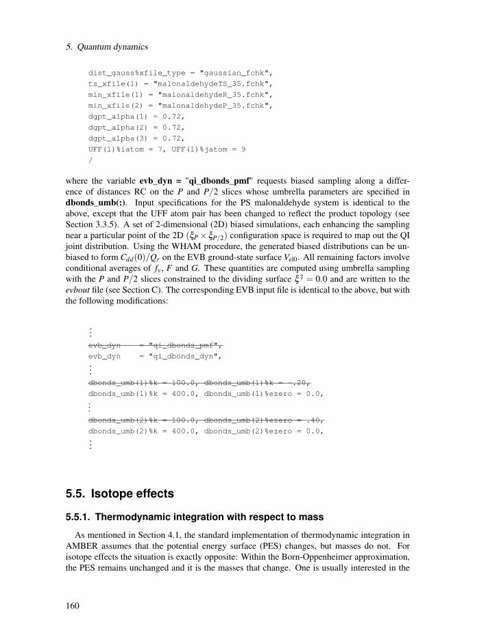
5. Quantum dynamics
dist_gauss%xfile_type = "gaussian_fchk",
ts_xfile(1) = "malonaldehydeTS_35.fchk",
min_xfile(1) = "malonaldehydeR_35.fchk",
min_xfile(2) = "malonaldehydeP_35.fchk",
dgpt_alpha(1) = 0.72,
dgpt_alpha(2) = 0.72,
dgpt_alpha(3) = 0.72,
UFF(1)%iatom = 7, UFF(1)%jatom = 9
/
where the variable evb_dyn = "qi_dbonds_pmf" requests biased sampling along a differ-ence of distances RC on the P and P/2 slices whose umbrella parameters are specified indbonds_umb(:). Input specifications for the PS malonaldehyde system is identical to the
above, except that the UFF atom pair has been changed to reflect the product topology (see
Section 3.3.5). A set of 2-dimensional (2D) biased simulations, each enhancing the sampling
near a particular point of the 2D (ξP×ξP/2) configuration space is required to map out the QIjoint distribution. Using the WHAM procedure, the generated biased distributions can be un-
biased to form Cdd(0)/Qr on the EVB ground-state surface Vel0. All remaining factors involveconditional averages of fv, F and G. These quantities are computed using umbrella samplingwith the P and P/2 slices constrained to the dividing surface ξ ‡ = 0.0 and are written to theevbout file (see Section C). The corresponding EVB input file is identical to the above, but withthe following modifications:
...
evb_dyn = "qi_dbonds_pmf",
evb_dyn = "qi_dbonds_dyn",...
dbonds_umb(1)%k = 100.0, dbonds_umb(1)%k = -.20,
dbonds_umb(1)%k = 400.0, dbonds_umb(1)%ezero = 0.0,...
dbonds_umb(2)%k = 100.0, dbonds_umb(2)%ezero = .40,
dbonds_umb(2)%k = 400.0, dbonds_umb(2)%ezero = 0.0,...
5.5. Isotope effects
5.5.1. Thermodynamic integration with respect to mass
As mentioned in Section 4.1, the standard implementation of thermodynamic integration in
AMBER assumes that the potential energy surface (PES) changes, but masses do not. For
isotope effects the situation is exactly opposite: Within the Born-Oppenheimer approximation,
the PES remains unchanged and it is the masses that change. One is usually interested in the
160
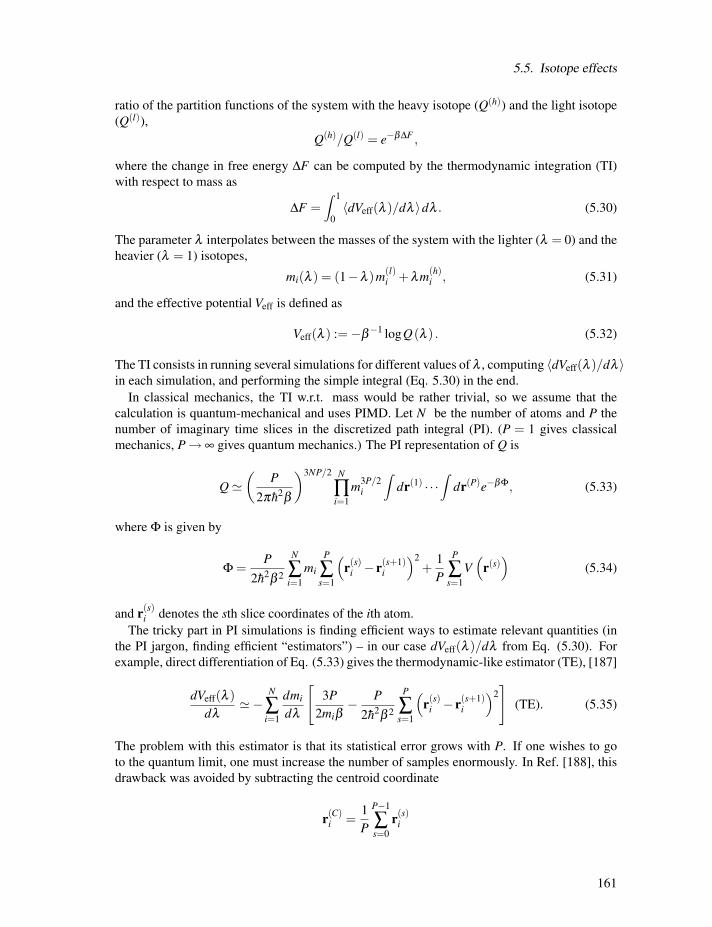
5.5. Isotope effects
ratio of the partition functions of the system with the heavy isotope (Q(h)) and the light isotope
(Q(l)),
Q(h)/Q(l) = e−βΔF ,
where the change in free energy ΔF can be computed by the thermodynamic integration (TI)
with respect to mass as
ΔF =∫ 1
0〈dVeff(λ )/dλ 〉dλ . (5.30)
The parameter λ interpolates between the masses of the system with the lighter (λ = 0) and theheavier (λ = 1) isotopes,
mi(λ ) = (1−λ )m(l)i +λm(h)
i , (5.31)
and the effective potential Veff is defined as
Veff(λ ) :=−β−1 logQ(λ ) . (5.32)
The TI consists in running several simulations for different values of λ , computing 〈dVeff(λ )/dλ 〉in each simulation, and performing the simple integral (Eq. 5.30) in the end.
In classical mechanics, the TI w.r.t. mass would be rather trivial, so we assume that the
calculation is quantum-mechanical and uses PIMD. Let N be the number of atoms and P thenumber of imaginary time slices in the discretized path integral (PI). (P = 1 gives classical
mechanics, P→ ∞ gives quantum mechanics.) The PI representation of Q is
Q�(
P2π h2β
)3NP/2 N
∏i=1
m3P/2i
∫dr(1) · · ·
∫dr(P)e−βΦ, (5.33)
where Φ is given by
Φ =P
2h2β 2N
∑i=1
mi
P
∑s=1
(r(s)
i − r(s+1)i
)2+1
P
P
∑s=1
V(
r(s))
(5.34)
and r(s)i denotes the sth slice coordinates of the ith atom.
The tricky part in PI simulations is finding efficient ways to estimate relevant quantities (in
the PI jargon, finding efficient “estimators”) – in our case dVeff(λ )/dλ from Eq. (5.30). For
example, direct differentiation of Eq. (5.33) gives the thermodynamic-like estimator (TE), [187]
dVeff(λ )dλ
�−N
∑i=1
dmi
dλ
[3P2miβ
− P2h2β 2
P
∑s=1
(r(s)
i − r(s+1)i
)2](TE). (5.35)
The problem with this estimator is that its statistical error grows with P. If one wishes to goto the quantum limit, one must increase the number of samples enormously. In Ref. [188], this
drawback was avoided by subtracting the centroid coordinate
r(C)i =
1
P
P−1∑s=0
r(s)i
161

5. Quantum dynamics
and using mass-scaled coordinates in Eq. (5.33). The resulting virial-like estimator (VE),
dVeff(λ )dλ
�−N
∑i=1
dmi/dλmi
⎡⎣ 3
2β+1
2P
⟨P
∑s=1
(r(s)
i − r(C)i
)·
∂V(
r(s))
∂r(s)i
⟩⎤⎦ (VE), (5.36)
has the advantage that the statistical error is independent of P. Compared to TE, the virial-likeestimator requires the gradient of the potential, but at no additional cost, since the gradient is
already needed for the PIMD. Both types of estimators are implemented in AMBER in order to
provide an independent comparison, but in general the virial estimator is preferred.
Strictly speaking, the preceding derivation was for a system bound in an external potential.
In molecular systems with internal interactions only, the partition function can only be defined
per unit volume because the center-of-mass coordinate is unbound. However, if the sampling is
done in Cartesian coordinates as in AMBER, the preceding estimators remain unchanged. This
can be justified by considering a finite volume V and taking a limit V → ∞.
5.5.2. AMBER implementation
The thermodynamic integration w.r.t. mass is run in AMBER as any other PIMD simulation
with the following changes.
1. In the mdin file, ITIMASS and CLAMBDA must be set.
ITIMASS = 0 No thermodynamic integration w.r.t. mass (default).
ITIMASS = 1 Run TI w.r.t. mass using the efficient virial estimator (5.36). This is
the preferred value.
ITIMASS = 2 Run TI w.r.t. mass using the simple thermodynamic estimator (5.35).
This option should only be used for testing. The virial estimator (option 1) has much
smaller statistical error.
CLAMBDA Contains the value of λ for TI (0.0≤ λ ≤ 1.0) from Eq. (5.31).2. In the prmtop (topology) file, a flag TI_MASS with the perturbed masses must be added.In other words, the current flag MASS includes the masses for the first (unperturbed)
isotopic system (m(l)i ), and TI_MASS includes the masses for the second (perturbed)
isotopic system (m(h)i ). Note that unlike the standard TI for which the force field changes,
the TI w.r.t. mass requires only one topology file.
3. The output dVeff/dλ from Eqs. (5.35) and (5.36) for the TI is printed as “DV/DL” in themdout file (as for the standard TI).
Note: Currently, the TI w.r.t. mass can be used with both implementations of the PIMD (that isthe full PIMD and the LES PIMD). There are examples of both in the directory test/ti_mass.
5.5.3. Equilibrium isotope effects
Equilibrium (or thermodynamic) isotope effect (EIE) is the effect of isotopic substitution on
the equilibrium constant K of a chemical reaction. Denoting the quantities pertaining to the
162

5.5. Isotope effects
reaction with the lighter (heavier) isotope by a superscript l (h), the EIE is defined as the ratioof the equilibrium constants
EIE :=K(l)
K(h) . (5.37)
Within the Born-Oppenheimer approximation, the potential energy surfaces of isotopic molecules
are identical, and so the EIE is only due to the effect of the isotopic mass on the nuclear motion
of the reactants and products. The EIE can be expressed as the ratio
EIE =Q(l)
p /Q(h)p
Q(l)r /Q(h)
r
. (5.38)
where Qr and Qp denote the reactant and product partition functions, respectively. Equation
(5.37) suggests that the EIE can be found in practice by performing two thermodynamic inte-
grations: for the reactants, Q(l)r /Q(h)
r , and for the products, Q(l)p /Q(h)
p .
5.5.4. Kinetic isotope effects
Similarly, the kinetic isotope effect (KIE) is the effect of isotopic substitution on the rate
constant k of a chemical reaction, and is defined as
KIE :=k(l)
k(h) .
The exact quantum-mechanical expression for the rate constant is
k = Q−1r tr(
e−β H FP)
where H is the Hamiltonian operator and FP is the reactive flux operator. Unfortunately, theexact k cannot be computed even for fairly small molecules. There exists, however, a veryaccurate Quantum Instanton (QI) approximation for the rate constant [184], given by
kQI =1
2
√π h
Cff (0)QrΔH
. (5.39)
In this expression, Cf f (t) is the flux-flux correlation function and ΔH is a specific type of
energy variance, defined in Ref. [184]. A path-integral implementation of the QI approximation
to compute KIEs has been developed in Refs. [187] and [188]. Within this approximation, the
KIE is written as a product of several factors,
KIEQI =k(l)QI
k(h)QI
=Q(l)
r
Q(h)r
× ΔH(h)
ΔH(l) ×C(l)dd (0)
C(h)dd (0)
× C(l)ff (0)/C(l)
dd (0)
C(h)ff (0)/C(h)
dd (0), (5.40)
where for convenience we have multiplied and divided by so-called delta-delta correlation
function Cdd (t). Using the PIMD implementation in AMBER, quantities such as ΔH(h) or
C(l)ff (0)/C(l)
dd (0), can be computed directly in a constrained PIMD simulation because they arethermodynamic averages (see Section 5.4.2 on the QI evaluation of the rate constant). The ratio
Q(l)r /Q(h)
r must be computed by the TI with respect to mass. Finally, the correlation function
Cdd (t) is defined very similarly to the partition function Q, with the exception that it is con-strained to two dividing surfaces for the reaction. Consequently, the ratioC(l)
dd (0)/C(h)dd (0)must
be computed by a TI but with a constrained PIMD.
163

5. Quantum dynamics
-0.5 0 0.5
Difference of Bond Lengths [Å]
0
0.5
1
1.5
2
Pote
ntia
l of M
ean
Forc
e [k
cal/m
ol]
Figure 5.1: PMFs for proton (� curve) and deuterium (� curve) transfer in malonaldehydeusing DG EVB/LES-PIMD.
5.5.5. Estimating the kinetic isotope effect using EVB/LES-PIMD
The kinetic isotope effect is defined as the ratio of the rate of reaction involving the lighter
isotope compared to the rate involving the heavier isotope, KIE = k(l)/k(h) . Within the PI-
QTST approximation, the KIE involves the ratio of dynamical frequency factors and the ratio
of centroid densities [see Eqs. (5.12-5.15)]. Each frequency factor can be computed using bi-
ased sampling EVB/LES-PIMD, where the umbrella potential constrains the sampling along
the dividing surface. The ratio of the centroid densities can be computed by employing biased
sampling (see Sections 3.3.3 and 3.3.4) to map out the PMFs for both isotope reactions or by
thermodynamic integration with respect to mass (see Sections 5.5.1 and 5.5.2). The former case
involves two separate PMF calculations where the respective isotope masses are specified in the
%FLAG MASS section of the parmtop files. Figure 5.1 compares the PMFs for the isotopic sub-
stitution of the transferring proton to a deuterium. All simulation parameters used in generating
the PMFs are identical, with the exception that the transferring proton mass was changed from
1.008 amu to 2.014 amu in the deuterium parmtop file. The ratio of the centroid densities using
Eq. (5.14) provide a value of 2.52.
Thermodynamic integration with respect to mass is discussed in detail in Sections 5.5.1 and
5.5.2. The key quantities we need to estimate the ratio of the centroid densities are embodied in
the equation [188, 189]
ρ(l)c
(ξ ‡
)ρ(h)
c (ξ ‡)= exp
[−β
∫ 1
0dλ
(⟨dVeff(λ )
dλ
⟩RS
−⟨
dVeff(λ )dλ
⟩ξ ‡
)](5.41)
Thus two separate TI by mass simulations are required, one that samples dVeff/dλ in the re-
actant region and the other which samples along the dividing surface ξ ‡. The former case re-quires ground-state EVB/LES-PIMD dynamics (i.e., evb_dyn=“groundstate”) on the reactant
164
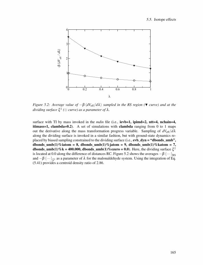
5.5. Isotope effects
0 0.2 0.4 0.6 0.8 1
λ
0
1
2
3
4
-β ⟨d
V eff /
dλ⟩
Figure 5.2: Average value of −β 〈dVeff/dλ 〉 sampled in the RS region (� curve) and at thedividing surface ξ ‡ (� curve) as a parameter of λ .
surface with TI by mass invoked in the mdin file (i.e., ievb=1, ipimd=2, ntt=4, nchain=4,itimass=1, clambda=0.2). A set of simulations with clambda ranging from 0 to 1 maps
out the derivative along the mass transformation progress variable. Sampling of dVeff/dλalong the dividing surface is invoked in a similar fashion, but with ground-state dynamics re-
placed by biased sampling constrained to the dividing surface (i.e., evb_dyn = “dbonds_umb”,dbonds_umb(1)%iatom = 8, dbonds_umb(1)%jatom = 9, dbonds_umb(1)%katom = 7,dbonds_umb(1)%k = 400.000, dbonds_umb(1)%ezero = 0.0). Here, the dividing surface ξ ‡is located at 0.0 along the difference of distances RC. Figure 5.2 shows the averages−β 〈· · · 〉RSand −β 〈· · · 〉ξ ‡ as a parameter of λ for the malonaldehyde system. Using the integration of Eq.(5.41) provides a centroid density ratio of 2.86.
165

5. Quantum dynamics
166

6. NMR and X-ray refinement usingSANDER
We find the sander module to be a flexible way of incorporating a variety of restraints into aoptimization procedure that includes energy minimization and dynamical simulated annealing.
The "standard" sorts of NMR restraints, derived from NOE and J-coupling data, can be entered
in a way very similar to that of programs like DISGEO, DIANA or X-PLOR; an aliasing syn-
tax allows for definitions of pseudo-atoms, connections with peak numbers in spectra, and the
use of "ambiguous" constraints from incompletely-assigned spectra. More "advanced" features
include the use of time-averaged constraints, use of multiple copies (LES) in conjunction with
NMR refinement, and direct refinement against NOESY intensities, paramagnetic and diamag-
netic chemical shifts, or residual dipolar couplings. In addition, a key strength of the program
is its ability to carry out the refinements (usually near the final stages) using an explicit-solvent
representation that incorporates force fields and simulation protocols that are known to give
pretty accurate results in many cases for unconstrained simulations; this ability should improve
predictions in regions of low constraint density and should help reduce the number of places
where the force field and the NMR constraints are in "competition" with one another.
Since there is no generally-accepted "recipe" for obtaining solution structures from NMR
data, the comments below are intended to provide a guide to some commonly-used procedures.
Generally speaking, the programs that need to be run to obtain NMR structures can be divided
into three parts:
1. front-end modules, which interact with NMR databases that provide information aboutassignments, chemical shifts, coupling constants, NOESY intensities, and so on. We have
tried to make the general format of the input straightforward enough so that it could be
interfaced to a variety of programs. At TSRI, we generally use the FELIX and NMRView
codes, but the principles should be similar for other ways of keeping track of a database
of NMR spectral information. As the flow-chart on the next page indicates, there are
only a few files that need to be created for NMR restraints; these are indicated by the
solid rectangles. The primary distance and torsion angle files have a fairly simple format
that is largely compatible with the DIANA programs; if one wishes to use information
from ambiguous or overlapped peaks, there is an additional "MAP" file that makes a
translation from peak identifiers to ambiguous (or partial) assignments. Finally, there
are some specialized (but still pretty straightforward) file formats for chemical shift or
residual dipolar coupling restraints.
There are a variety of tools, besides the ones described below, that can assist in preparing
input for structure refinement in Amber.
• The SANE (Structure Assisted NOE Evaluation) package, http://ambermd.org/sane.zip,is widely used at The Scripps Research Institute. [190]
167

6. NMR and X-ray refinement using SANDER
• If you use Bruce Johnson’s NmrView package, you might also want to look at the
TSRI additions to that: http://garbanzo.scripps.edu/nmrgrp/wisdom/pipe/tips_scripts.html.In particular, the xpkTOupl and starTOupl scripts there convert NmrView peak listsinto the "7-column" needed for input to makeDIST_RST.
• Users of the MARDIGRAS programs from UCSF can use the mardi2amber pro-gram to do conversion to Amber format: http://picasso.ucsf.edu/mardihome.html
2. restrained molecular dynamics, which is at the heart of the conformational searchingprocedures. This is the part that sander itself handles.
3. back-end routines that do things like compare families of structures, generate statistics,simulate spectra, and the like. For many purposes, such as visualization, or the running
of procheck-NMR, the "interface" to such programs is just the set of pdb-format files that
contain the family of structures to be analyzed. These general-purpose structure analy-
sis programs are available in many locations and are not discussed here. The principal
sander-specific tool is sviol, which prepares tables and statistics of energies, restraintviolations, and the like.
6.1. Distance, angle and torsional restraints
Distance, angle, and other restraints are read from the DISANG file if nmropt > 0. Namelist
rst ("&rst") contains the following variables; it is read repeatedly until a namelist &rst statement
is found with IAT(1)=0, or until reaching the end of the DISANG file.
If you wish to include weight changes but have no internal constraints, set nmropt=1, but donot include a DISANG line in the file redirection section. (Note that, unlike earlier versions of
Amber, the &rst namelists must be in the DISANG file, and not in the mdin file.)In many cases, the user will not prepare this section of the input by hand, but will use the
auxiliary programsmakeDIST_RST, makeANG_RST andmakeCHIR_RST to prepare input fromsimpler files.
There have been several additions made to restraints in AMBER 10. These additions have
only been made to sander and not to pmemd.
6.1.1. Variables in the &rst namelist:
iat(1)→iat(8)
• If IRESID = 0 (normal operation): The atoms defining the restraint. Type of restraint isdetermined (in order) by:
1. If IAT(3) = 0, this is a distance restraint.
2. If IAT(4) = 0, this is an angle restraint.
3. If IAT(5) = 0, this is a torsional (or J-coupling, if desired) restraint or a genereralized
distance restraint of 4 atoms, a type of restraint new to AMBER10 (sander only, seebelow).
168

6.1. Distance, angle and torsional restraints
4. If IAT(6) = 0, this is a plane-point angle restraint, a second restraint new to AMBER
10 (sander only). The angle is measured between the normal of a plane defined byIAT(1)..IAT(4) and the vector from the center of mass of atoms IAT(1)..IAT(4) to
the position of IAT(5). The normal is defined by (r1 - r2)× (r3 - r4), where rn is theposition of IAT(n).
5. If IAT(7) = 0, this is a generalized distance restraint of 6 atoms (see below).
6. Otherwise, if IAT(1)..IAT(8) are all non-zero, this is a plane- plane angle restraint,
a third new restraint type for AMBER 10 (sander only, or a generalized distancerestraint of 8 atoms (see below). For the plane-plane restraint, the angle is measured
between the two normals of the two planes, which are defined by (r1 - r2) × (r3 -r4) and (r5 - r6) × (r7 - r8). In the case of either planar restraint, the plane may bedefined using three atoms instead of four simply by using one atom twice.
If any of IAT(n) are < 0, then a corresponding group of atoms is defined below, and
the coordinate- averaged position of this group will be used in place of atom IAT(n). A
new feature in AMBER 10, atom groups may be used not only in distance restraints,
but also in angle, torsion, the new plane restraints, or the new generalized restraints. If
this is a distance restraint, and IAT1 <0, then a group of atoms is defined below, andthe coordinate-averaged position of this group will be used in place of the coordinates of
atom 1 [IAT(1)]. Similarly, if IAT(2) < 0, a group of atoms will be defined below whose
coordinate-averaged position will be used in place of the coordinates for atom 2 [IAT(2)].
• If IRESID=1: IAT(1)..IAT(8) point to the *residues* containing the atoms comprisingthe internal. Residue numbers are the absolute in the entire system. In this case, the
variables ATNAM(1)..ATNAM(8) must be specified and give the character names of the
atoms within the respective residues. If any of IAT(n) are less than zero, then group input
will still be read in place of the corresponding atom, as described below.
• Defaults for IAT(1)→IAT(8) are 0.
rstwt(1)→rstwt(4) New to AMBER 10 (sander only), users may now define a single restraintthat is a function of multiple distance restraints, called a "generalized distance co-
ordinate" restraint. The energy of such a restraint has the following form:
U = k(w1|r1− r2|+w2|r3− r4|+w3|r5− r6|+w4|r7− r8|− r0)2
where the weights wnare given in rstwt(1)..rstwt(4) and the positions rnare the po-sitions of the atoms in iat(1)..iat(8).
Generalized distance coordinate restraints must be defined with either 4, 6, or 8
atoms and 2, 3, or 4 corresponding non-zero weights in rstwt(1)..rstwt(4). Weights
may be any positive or negative real number.
If all the weights in rstwt(1)..rstwt(4) are zero and four atoms are given in iat(1)..iat(4)
for the restraint, the restraint is a torsional or J-coupling restraint. If eight atoms are
given in iat(1)..iat(8) and all weights are zero, the restraint is a plane-plane angle
restraint. However, if the weights are non-zero, the restraint will be a generalized
distance coordinate restraint.
Default for rstwt(1)..rstwt(4) is 0.0
169
6. NMR and X-ray refinement using SANDER
restraint New to AMBER 10 (sander only), users may now use a "natural language" systemto define restraints by using the RESTRAINT character variable. Valid restraints
defined in this manner will begin with a "distance( )" "angle( )" "torsion( )" or "co-
ordinate( )" keyword. Within the parentheses, the atoms that make up the restraint
are specified. Atoms may be defined either with an explicit atom number or by us-
ing ambmask format, namely :(residue#)@(atom name). Atoms may be separated
by commas, spaces, or parentheses. Additionally, negative integers may be used if
atom groupings are defined in other variables in the namelist as described below. In
addition to the principle distance, angle, torsion, and coordinate keywords, Some
keywords may be used within the principle keywords to define more complicated
restraints. The keyword "plane( )" may be used once or twice within the paren-
theses of the "angle( ) keyword to define a planar restraint. Defining one plane
grouping plus one other atom in this manner will create a plane-point angle re-
straint as described above. Defining two plane groupings will create a plane-plane
angle restraint. The keyword "plane( )" may only be used inside of "angle( )," and
is necessary to define either a plane-point or plane-plane restraint.
Within the "coordinate( )" keyword, the user must use 2 to 4 "distance( )" keywords
to define a generalized distance coordinate restraint. The "distance( )" keyword
functions just like it does when used to define a traditional distance restraint. The
user may specify any two atom numbers, masks, or negative numbers correspond-
ing to atom groups defined outside of RESTRAINT. Additionally, following each
"distance( )" keyword inside "coordinate( )" the user must specify a real-number
weight to be applied to each distance making up the generalized coordinate.
The "com( )" keyword may be used within any other keyword to define a cen-
ter of mass grouping of atoms. Within the parenthesis, the user will enter a list
of atom numbers or masks. Negative numbers, which correspond to externally-
defined groups, may not be used.
Any type of parenthetical character, i.e., ( ), [ ], or { }, may be used wherever
parentheses have been used above.
The following are all examples of valid restraint definitions:
restraint = "distance( (45) (49) )"
= "angle (:21@C5’ :21@C4’ 108)"
= "torsion[-1,-1,-1, com(67, 68, 69)]"
= "angle( -1, plane(81, 85, 87, 90) )"
= "angle(plane(com(9,10),:5@CA,31,32),plane(14,15,15,16))"
= "coordinate(distance(:5@C3’,:6@O5’),-1.0,distance(134,-1),1.0)"
There is a 256 character limit on RESTRAINT, so if a particularly large atom
grouping is desired, it is necessary to specify a negative number instead of "com(
)" and define the group as described below. RESTRAINT will only be parsed if
IAT(1) = 0, otherwise the information in IAT(1) .. IAT(8) will define the restraint.
Default for restraint is ’ ’.
atnam If IRESID = 1, then the character names of the atoms defining the internal are
contained in ATNAM(1)→ATNAM(8). Residue IAT(1) is searched for atom name
170

6.1. Distance, angle and torsional restraints
ATNAM(1); residue IAT(2) is searched for atom name ATNAM(2); etc. Defaultsfor ATNAM(1)→ATNAM(8) are ’ ’.
iresid Indicates whether IAT(I) points to an atom # or a residue #. See descriptions of
IAT() and ATNAM() above. If RESTRAINT is used to define the internal instead of
IAT(), IRESID has no effect on how RESTRAINT is parsed. However, it will affect
the behavior of atom group definitions as described below if negative numbers are
specified within RESTRAINT. Default = 0.
nstep1, nstep2 This restraint is applied for steps/iterations NSTEP1 through NSTEP2. If NSTEP2
= 0, the restraint will be applied fromNSTEP1 through the end of the run. Note that
the first step/iteration is considered step zero (0). Defaults for NSTEP1, NSTEP2are both 0.
irstyp Normally, the restraint target values defined below (R1→R4) are used directly. IfIRSTYP = 1, the values given for R1→R4 define relative displacements from thecurrent value (value determined from the starting coordinates) of the restrained
internal. For example, if IRSTYP=1, the current value of a restrained distance is
1.25, and R1 (below) is -0.20, then a value of R1=1.05 will be used. Default isIRSTYP=0.
ialtd Determines what happens when a distance restraint gets very large. If IALTD=1,
then the potential "flattens out", and there is no force for large violations; this al-
lows for errors in constraint lists, but might tend to ignore constraints that should beincluded to pull a bad initial structure towards a more correct one. When IALTD=0
the penalty energy continues to rise for large violations. See below for the detailed
functional forms that are used for distance restraints. Set IALTD=0 to recover the
behavior of earlier versions of sander. Default value is 0, or the last value that wasexplicitly set in a previous restraint. This value is set to 1 if makeDIST_RST is
called with the -altdis flag.
ifvari If IFVARI > 0, then the force constants/positions of the restraint will vary with
step number. Otherwise, they are constant throughout the run. If IFVARI >0, thenthe values R1A→R4A, RK2A, and RK3A must be specified (see below). Defaultis IFVARI=0.
ninc If IFVARI > and NINC > 0, then the change in the target values of of R1→R4and K2,K3 is applied as a step function, with NINC steps/ iterations between each
change in the target values. If NINC = 0, the change is effected continuously
(at every step). Default for NINC is the value assigned to NINC in the most recentnamelist where NINC was specified. If NINC has not been specified in any namelist,it defaults to 0.
imult If IMULT=0, and the values of force constants RK2 and RK3 are changing with
step number, then the changes in the force constants will be linearly interpolated
from rk2→rk2a and rk3→rk3a as the step number changes. If IMULT=1 and theforce constants are changing with step number, then the changes in the force con-
stants will be effected by a series of multiplicative scalings, using a single factor,
R, for all scalings. i.e.
171

6. NMR and X-ray refinement using SANDER
rk2a = R**INCREMENTS * rk2
rk3a = R**INCREMENTS * rk3.
INCREMENTS is the number of times the target value changes, which is deter-
mined by NSTEP1, NSTEP2, and NINC. Default for IMULT is the value assignedto IMULT in the most recent namelist where IMULT was specified. If IMULT hasnot been specified in any namelist, it defaults to 0.
r1→r4, rk2, rk3, r1a→r4a, rk2a, rk3a If IALTD=0, the restraint is a well with a square bottomwith parabolic sides out to a defined distance, and then linear sides beyond that. If
R is the value of the restraint in question:
• R < r1 Linear, with the slope of the "left-hand" parabola at the point R=r1.
• r1 <= R < r2 Parabolic, with restraint energy k2(R− r2)2.• r2 <= R < r3 E = 0.
• r3 <= R < r4 Parabolic, with restraint energy k3(R− r3)2.• r4<= R Linear, with the slope of the "right-hand" parabola at the point R=r4.
For torsional restraints, the value of the torsion is translated by +-n*360, if nec-
essary, so that it falls closest to the mean of r2 and r3. Specified distances are in
Angstroms. Specified angles are in degrees. Force constants for distances are in
kcal/mol-Å2 Force constants for angles are in kcal/mol-rad 2 . (Note that angle po-
sitions are specified in degrees, but force constants are in radians, consistent with
typical reporting procedures in the literature).
If IALTD=1, distance restraints are interpreted in a slightly different fashion. Again,
If R is the value of the restraint in question:
• R < r2 Parabolic, with restraint energy k2(R− r2)2.• r2 <= R < r3 E = 0.
• r3 <= R < r4 Parabolic, with restraint energy k3(R− r3)2.• r4 <= R Hyperbolic, with energy k3[b/(R− r3)+ a], where a = 3(r4− r3)2
and b = −2(r4 − r3)3. This function matches smoothly to the parabola atR = r4, and tends to an asymptote of ak3at large R. The functional form is
adapted from that suggested by Michael Nilges, Prot. Eng. 2, 27-38 (1988).Note that if ialtd=1, the value of r1 is ignored.
ifvari
= 0 The values of r1→r4, rk2, and rk3 will remain constant throughout the run.> 0 The values r1a, r2a, r3a, r4a, r2ka and r3ka are also used. These variables are
defined as for r1→r4 and rk2, rk3, but correspond to the values appropriate forNSTEP = NSTEP2: e.g., if IVARI >0, then the value of r1 will vary betweenNSTEP1 and NSTEP2, so that, e.g. r1(NSTEP1) = r1 and r1(NSTEP2) =
r1a. Note that you must specify an explicit value for nstep1 and nstep2 if youuse this option. Defaults for r1→r4,rk2,rk3,r1a→r4a,rk2a and rk3a are thevalues assigned to them in the most recent namelist where they were specified.They should always be specified in the first &rst namelist.
172

6.1. Distance, angle and torsional restraints
r0, k0, r0a, k0a New to AMBER 10 (sander only), the user may more easily specify a largeparabolic well if desired by using R0 and K0, and then R0A and K0A if IFVARI >
0. The parabolic well will have its zero at R = R0 and a force constant of K0. These
variables simply map the disired parabolic well into r1→r4, rk2, rk3, r1a→r4a, rk2a, andrk3a in the following manner:
• R1 = 0 for distance, angle, and planar restraints, R1 = R0 - 180 for torsion
restraints
• R1A = 0 for distance, angle, and planar restraints, R1A = R0A - 180 for
torsion restraints
• R2 = R0; R3 = R0
• R2A = R0A; R3A = R0A
• R4 = R0 + 500 for distance restraints, R4 = 180 for angle and planar restraints,
R4 = R0 + 180 for torsion restraints
• RK2 = K0; RK3 = K0
• RK2A = K0A; RK3A = K0A
rjcoef(1)→rjcoef(3) By default, 4-atom sequences specify torsional restraints. It is also pos-
sible to impose restraints on the vicinal 3 J-coupling value related to the underly-
ing torsion. J is related to the torsion τ by the approximate Karplus relationship:J = Acos2(τ)+Bcos(τ)+C. If you specify a non-zero value for either RJCOEF(1)or RJCOEF(2), then a J-coupling restraint, rather than a torsional restraint, will be
imposed. At every MD step, J will be calculated from the Karplus relationship with
A = RJCOEF(1), B = RJCOEF(2) and C = RJCOEF(3). In this case, the target val-
ues (R1->R4, R1A->R4A) and force constants (RK2, RK3, RK2A, RK3A) referto J-values for this restraint. RJCOEF(1)->RJCOEF(3) must be set individually foreach torsion for which you wish to apply a J-coupling restraint, and RJCOEF(1)-
>RJCOEF(3) may be different for each J-coupling restraint. With respect to otheroptions and reporting, J-coupling restraints are treated identically to torsional re-
straints. This means that if time-averaging is requested for torsional restraints, it
will apply to J-coupling restraints as well. The J-coupling restraint contribution to
the energy is included in the "torsional" total. And changes in the relative weights
of the torsional force constants also change the relative weights of the J-coupling
restraint terms. Setting RJCOEF has no effect for distance and angle restraints.
Defaults for RJCOEF(1)->RJCOEF(3) are 0.0.
igr1(i),i=1→200, igr2(i),i=1→200, ... igr8(i),i..1=1→200 If IAT(n) < 0, then IGRn() gives the
atoms defining the group whose coordinate averaged position is used to define
"atom n" in a restraint. Alternatively, if RESTRAINT is used to define the internal,
then if the nth atom specified is a number less than zero, IGRn() gives the atoms
defining the group whose coordinate averaged position is used to define "atom n" in
a restraint. If IRESID = 0, absolute atom numbers are specified by the elements of
IGRn(). If IRESID = 1, then IGRn(I) specifies the number of the residue containing
atom I, and the name of atom I must be specified using GRNAMn(I). A maximum
of 200 atoms are allowed in any group. Only specify those atoms that are needed.
Default value for any unspecified element of IGRn(i) is 0.
173

6. NMR and X-ray refinement using SANDER
grnam1(i),i=1→200, grnam2(i),i=1→200, ... grnam8(i),i=1→200 If group input is being spec-ified (IGRn(1) > 0), and IRESID = 1, then the character names of the atoms defin-ing the group are contained in GRNAMn(i), as described above. In the case IAT(1)
< 0, each residue IGR1(i) is searched for an atom name GRNAM1(i) and added
to the first group list. In the case IAT(2) < 0, each residue IGR2(i) is searched
for an atom name GRNAM2(i) and added to the second group list. Defaults forGRNAMn(i) are ’ ’.
ir6 If a group coordinate-averaged position is being used (see IGR1 and IGR2 above),
the average position can be calculated in either of two manners: If IR6 = 0, center-
of-mass averaging will be used. If IR6=1, the⟨r−6
⟩−1/6average of all interaction
distances to atoms of the group will be used. Default for IR6 is the value assignedto IR6 in the most recent namelist where IR6 was specified. If IR6 has not beenspecified in any namelist, it defaults to 0.
ifntyp If time-averaged restraints have been requested (see DISAVE/ANGAVE/TORAVE
above), they are, by default, applied to all restraints of the class specified. Time-
averaging can be overridden for specific internals of that class by setting IFNTYP
for that internal to 1. IFNTYP has no effect if time-averaged restraint are not being
used. Default value is IFNTYP=0.
ixpk, nxpk These are user-defined integers than can be set for each constraint. They are typ-
ically the "peak number" and "spectrum number" associated with the cross-peak
that led to this particular distance restraint. Nothing is ever done with them except
to print them out in the "violation summaries", so that NMR people can more easily
go from a constraint violation to the corresponding peak in their spectral database.
Default values are zero.
iconstr If iconstr > 0, (default is 0) a Lagrangian multiplier is also applied to the two-centerinternal coordinate defined by IAT(1) and IAT(2). The effect of this Lagrangian
multiplier is to maintain the initial orientation of the internal coordinate. The ro-
tation of the vector IAT(1)->IAT(2) is prohibited, though translation is allowed.For each defined two-center internal coordinate, a separate Lagrangian multiplier
is used. Therefore, although one can use as many multipliers as needed, defining
centers should NOT appear in more than one multiplier. This option is compatible
with mass centers (i.e., negative IAT(1) or IAT(2)). ICONSTR can be used together
with harmonic restraints. RK2 and RK3 should be set to 0.0 if the two-center in-
ternal coordinate is a simple Lagrangian multiplier. An example has been included
in $AMBERHOME/example/lagmul.
Namelist &rst is read for each restraint. Restraint input ends when a namelist statement with
iat(1) = 0 (or iat(1) not specified) is found. Note that comments can precede or follow any
namelist statement, allowing comments and restraint definitions to be freely mixed.
6.2. NOESY volume restraints
After the previous section, NOESY volume restraints may be read. This data described in this
section is only read if NMROPT = 2. The molecule may be broken in overlapping submolecules,
174

6.2. NOESY volume restraints
in order to reduce time and space requirements. Input for each submolecule consists of namelist"&noeexp", followed immediately by standard Amber "group" cards defining the atoms in thesubmolecule. In addition to the submolecule input ("&noeexp"), you may also need to specify
some additional variables in the cntrl namelist; see the "NMR variables" description in that
section.
In many cases, the user will not prepare this section of the input by hand, but will use the
auxiliary program makeDIST_RST to prepare input from simpler files.
Variables in the &noeexp namelist:
For each submolecule, the namelist "&noeexp" is read (either from stdin or from the NOESYredirection file) which contains the following variables. There are no effective defaults for
npeak, emix, ihp, jhp, and aexp: you must specify these.
npeak(imix) Number of peaks for each of the "imix" mixing times; if the last mixing time ismxmix, set NPEAK(mxmix+1) = -1. End the input when NPEAK(1) < 0.
emix(imix) Mixing times (in seconds) for each mixing time.
ihp(imix,ipeak), jhp(imix,ipeak) Atom numbers for the atoms involved in cross-peak "ipeak" atmixing time "imix"
aexp(imix,ipeak) Experimental target integrated intensity for this cross peak. If AEXP is nega-
tive, this cross peak is part of a set of overlapped peaks. The computed intensity is
added to the peak that follows; the next time a peak with AEXP> 0 is encountered,
the running sum for the calculated peaks will be compared to the value of AEXP
for that last peak in the list. In other words, a set of overlapped peaks is represented
by one or more peaks with AEXP < 0 followed by a peak with AEXP > 0. The
computed total intensity for these peaks will be compared to the value of AEXP
for the final peak.
arange(imix,ipeak) "Uncertainty" range for this peak: if the calculated value is within±ARANGEof AEXP, then no penalty will be assessed. Default uncertainties are all zero.
awt(imix,ipeak) Relative weight for this cross peak. Note that this will be multiplied by theoverall weight given by the NOESY weight change cards in the weight changes
section (Section 1). Default values are 1.0, unless INVWT1,INVWT2 are set (see
below), in which case the input values of AWT are ignored.
invwt1,invwt2 Lower and upper bounds on the weights for the peaks respectively, such that
the relative weight for each peak is 1/intensity if 1/intensity lies between the lower
and upper bounds. This is the intensity after being scaled by oscale. The inverseweighing scheme adopted by this option prevents placing too much influence on the
strong peaks at the expense of weaker peaks and was previously invoked using the
compilation flag "INVWGT". Default values are INVWT1=INVWT2=1.0, placing
equal weights on all peaks.
omega Spectrometer frequency, in Mhz. Default is 500. It is possible for different sub-
molecules to have different frequencies, but omega will only change when it is
175
6. NMR and X-ray refinement using SANDER
explicitly re-set. Hence, if all of your data is at 600 Mhz, you need only set omegato 600. in the first submolecule.
taurot Rotational tumbling time of the molecule, in nsec. Default is 1.0 nsec. Like omega,this value is "sticky", so that a value set in one submolecule will remain until it is
explicitly reset.
taumet Correlation time for methyl jump motion, in ns. This is only used in computing
the intra-methyl contribution to the rate matrix. The ideas of Woessner are used,
specifically as recommended by Kalk & Berendsen. [191] Default is 0.0001 ns,
which is effectively the fast motion limit. The default is consistent with the way
the rest of the rate matrix elements are determined (also in the fast motion limit,)
but probably is not the best value to use, since methyl groups appear to have T1
values that are systematically shorter than other protons, and this is likely to arise
from the fact that the methyl correlation time can be near to the inverse of the
spectrometer frequency. A value of 0.02 - 0.05 ns is probably better than 0.0001,
but this is still an active research area, and you are on your own here, and should
consult the literature for further discussion. [192] As with omega, taumet can bedifferent for different sub-molecules, but will only change when it is explicitly
re-set.
id2o Flag for determining if exchangeable protons are to be included in the spin-diffusion
calculation. If ID2O=0 (default) then all protons are included. If ID2O=1, then all
protons bonded to nitrogen or oxygen are assumed to not be present for the pur-
poses of computing the relaxation matrix. No other options exist at present, but
they could easily be added to the subroutine indexn. Alternatively, you can manu-ally rename hydrogens in the prmtop file so that they do not begin with "H": suchprotons will not be included in the relaxation matrix. (Note: for technical reasons,the HOH proton of tyrosine must always be present, so setting ID2O=1 will not
remove it; we hope that this limitation will be of minor importance to most users.)
The id2o variable retains its value across namelist reads, i.e. its value will onlychange if it is explicitly reset.
oscale overall scaling factor between experimental and computed volume units. The ex-
perimental intensities are multiplied by oscale before being compared to calculatedintensities. This means that the weights WNOESY and AWT always refer to "theo-
retical" intensity scales rather than to the (arbitrary) experimental units. The oscalevariable retains its value across namelist reads, i.e. its value will only change if itis explicitly reset. The initial (default) value is 1.0.
The atom numbers ihp and jhp are the absolute atom numbers. For methyl groups, use the
number of the last proton of the group; for the delta and epsilon protons of aromatic rings,
use the delta-2 or epsilon-2 atom numbers. Since this input requires you to know the absolute
atom numbers assigned by Amber to each of the protons, you may wish to use the separate
makeDIST_RST program which provides a facility for more turning human-readable input intothe required file for sander.Following the &noeexp namelist, give the Amber "group" cards that identify this submolecule.
This combination of "&noeexp" and "group" cards can be repeated as often as needed for many
176

6.3. Chemical shift restraints
submolecules, subject to the limits described in the nmr.h file. As mentioned above, this inputsection ends when NPEAK(1) < 0, or when and end-of-file is reached.
6.3. Chemical shift restraints
After reading NOESY restraints above (if any), read the chemical shift restraints in namelist
&shf, or the pseudocontact restraints in namelist &pcshift. Reading this input is triggered bythe presence of a SHIFTS line in the I/O redirection section. In many cases, the user will
not prepare this section of the input by hand, but will use the auxiliary programs makeSHF orfantasian to prepare input from simpler files.
Variables in the &shf namelist.
(Defaults are only available for shrang, wt, nter, and shcut; you must specify the rest.)
nring Number of rings in the system.
natr(i) Number of atoms in the i-th ring.
iatr( j, i) Absolute atom number for the j-th atom of the i-th ring.
namr(i) Eight-character string that labels the i-th ring. The first three characters give theresidue name (in caps); the next three characters contain the residue number (right
justified); column 7 is blank; column 8 may optionally contain an extra letter to
distinguish the two rings of trp, or the 5 or 8 rings of the heme group.
str(i) Ring current intensity factor for the i-th ring. Older values are summarized byCross and Wright; [193] more recent empirical parametrizations seem to give im-
proved results. [194, 195]
nprot Number of protons for which penalty functions are to be set up.
iprot(i) Absolute atom number of the i-th proton whose shifts are to be evaluated. Forequivalent protons, such as methyl groups or rapidly flipping phenylalanine rings,
enter all two or three atom numbers in sequence; averaging will be controlled by
the wt parameter, described below.
obs(i) Observed secondary shift for the i-th proton. This is typically calculated as theobserved value minus a random coil reference value.
shrang(i) "Uncertainty" range for the observed shift: if the calculated shift is within±SHRANGof the observed shift, then no penalty will be imposed. The default value is zero
for all shifts.
wt(i) Weight to be assigned to this penalty function. Note that this value will be multi-
plied by the overall weight (if any) given by the SHIFTS command in the assign-
ment of weights (above). Default values are 1.0. For sets of equivalent protons,
give a negative weight for all but the last proton in the group; the last proton gets a
normal, positive value. The average computed shift of the group will be compared
to obs entered for the last proton.
177
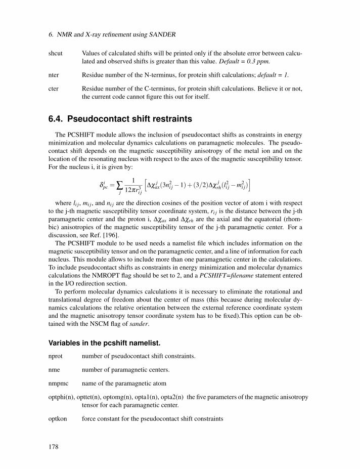
6. NMR and X-ray refinement using SANDER
shcut Values of calculated shifts will be printed only if the absolute error between calcu-
lated and observed shifts is greater than this value. Default = 0.3 ppm.
nter Residue number of the N-terminus, for protein shift calculations; default = 1.
cter Residue number of the C-terminus, for protein shift calculations. Believe it or not,
the current code cannot figure this out for itself.
6.4. Pseudocontact shift restraints
The PCSHIFT module allows the inclusion of pseudocontact shifts as constraints in energy
minimization and molecular dynamics calculations on paramagnetic molecules. The pseudo-
contact shift depends on the magnetic susceptibility anisotropy of the metal ion and on the
location of the resonating nucleus with respect to the axes of the magnetic susceptibility tensor.
For the nucleus i, it is given by:
δ ipc = ∑
j
1
12πr3i j
[Δχ j
ax(3n2i j−1)+(3/2)Δχ jrh(l
2i j−m2i j)
]
where li j, mi j, and ni j are the direction cosines of the position vector of atom i with respect
to the j-th magnetic susceptibility tensor coordinate system, ri j is the distance between the j-th
paramagnetic center and the proton i, Δχax and Δχrh are the axial and the equatorial (rhom-
bic) anisotropies of the magnetic susceptibility tensor of the j-th paramagnetic center. For a
discussion, see Ref. [196].
The PCSHIFT module to be used needs a namelist file which includes information on the
magnetic susceptibility tensor and on the paramagnetic center, and a line of information for each
nucleus. This module allows to include more than one paramagnetic center in the calculations.
To include pseudocontact shifts as constraints in energy minimization and molecular dynamics
calculations the NMROPT flag should be set to 2, and a PCSHIFT=filename statement enteredin the I/O redirection section.
To perform molecular dynamics calculations it is necessary to eliminate the rotational and
translational degree of freedom about the center of mass (this because during molecular dy-
namics calculations the relative orientation between the external reference coordinate system
and the magnetic anisotropy tensor coordinate system has to be fixed).This option can be ob-
tained with the NSCM flag of sander.
Variables in the pcshift namelist.
nprot number of pseudocontact shift constraints.
nme number of paramagnetic centers.
nmpmc name of the paramagnetic atom
optphi(n), opttet(n), optomg(n), opta1(n), opta2(n) the five parameters of the magnetic anisotropy
tensor for each paramagnetic center.
optkon force constant for the pseudocontact shift constraints
178

6.4. Pseudocontact shift restraints
Following this, there is a line for each nucleus for which the pseudocontact shift information is
given has to be added. Each line contains :
iprot(i) atom number of the i-th proton whose shift is to be used as constraint.
obs(i) observed pseudocontact shift value, in ppm
wt(i) relative weight
tolpro(i) relative tolerance ix mltpro
mltpro(i) multiplicity of the NMR signal (for example the protons of a methyl group have
mltprot(i)=3)
Example. Here is a &pcshf namelist example: a molecule with three paramagnetic centers and205 pseudocontact shift constraints.
&pcshf
nprot=205,
nme=3,
nmpcm=’FE ’,
optphi(1)=-0.315416,
opttet(1)=0.407499,
optomg(1)=0.0251676,
opta1(1)=-71.233,
opta2(1)=1214.511,
optphi(2)=0.567127,
opttet(2)=-0.750526,
optomg(2)=0.355576,
opta1(2)=-60.390,
opta2(2)=377.459,
optphi(3)=0.451203,
opttet(3)=-0.0113097,
optomg(3)=0.334824,
opta1(3)=-8.657,
opta2(3)=704.786,
optkon=30,
iprot(1)=26, obs(1)=1.140, wt(1)=1.000, tolpro(1)=1.00, mltpro(1)=1,
iprot(2)=28, obs(2)=2.740, wt(2)=1.000, tolpro(2)=.500, mltpro(2)=1,
iprot(3)=30, obs(3)=1.170, wt(3)=1.000, tolpro(3)=.500, mltpro(3)=1,
iprot(4)=32, obs(4)=1.060, wt(4)=1.000, tolpro(4)=.500, mltpro(4)=3,
iprot(5)=33, obs(5)=1.060, wt(5)=1.000, tolpro(5)=.500, mltpro(5)=3,
iprot(6)=34, obs(6)=1.060, wt(6)=1.000, tolpro(6)=.500, mltpro(6)=3,
...
...
iprot(205)=1215, obs(205)=.730, wt(205)=1.000, tolpro(205)=.500,
mltpro(205)=1,
/
179

6. NMR and X-ray refinement using SANDER
An mdin file that might go along with this, to perform a maximum of 5000 minimization cycles,
starting with 500 cycles of steepest descent. PCSHIFT=./pcs.in redirects the input from the
namelist "pcs.in" which contains the pseudocontact shift information.
Example of minimization including pseudocontact shift constraints
&cntrl
ibelly=0,imin=1,ntpr=100,
ntr=0,maxcyc=500,
ncyc=50,ntmin=1,dx0=0.0001,
drms=.1,cut=10.,scee=2.0,
nmropt=2,pencut=0.1, ipnlty=2,
/
&wt type=’REST’, istep1=0,istep2=1,value1=0.,
value2=1.0, /
&wt type=’END’ /
DISANG=./noe.in
PCSHIFT=./pcs.in
LISTOUT=POUT
6.5. Direct dipolar coupling restraints
Energy restraints based on direct dipolar coupling constants are entered in this section. All
variables are in the namelist &align; reading of this section is triggered by the presence of a
DIPOLE line in the I/O redirection section.
When dipolar coupling restraints are turned on, the five unique elements of the alignment
tensor are treated as additional variables, and are optimized along with the structural parameters.
Their effective masses are determined by the scalm parameter entered in the &cntrl namelist.
Unlike some other programs, the variables used are the Cartesian components of the alignment
tensor in the axis system defined by the molecule itself: e.g. Smn ≡ 〈(3cosθm cosθn−δmn)/2〉,where θx is the angle between the x axis and the spectrometer field. [197] The factor of 105
is just to make the values commensurate with atomic coordinates, since both the coordinates
and the alignment tensor values will be updated during the refinement. The calculated dipolar
splitting is then
Dcalc =−(10−5γiγ jh2π2r3i j
)∑
m,n=xyzcosφm ·Smn · cosφn
where φx is the angle between the internuclear vector and the x axis. Geometrically, thesplitting is proportional to the transformation of the alignment tensor onto the internuclear axis.
This is just Eqs. (5) and (13) of the above reference, with any internal motion corrections (which
might be a part of Ssystem) set to unity. If there is an internal motion correction which is the same
for all observations, this can be assimilated into the alignment tensor. The current code does
not allow for variable corrections for internal motion. See Ref. [198] for a fuller discussion of
these issues.
At the end of the calculation, the alignment tensor is diagonalized to obtain information about
its principal components. This allows the alignment tensor to be written in terms of the "axial"
180

6.5. Direct dipolar coupling restraints
and "rhombic" components that are often used to describe alignment.
Variables in the &align namelist.
ndip Number of observed dipolar couplings to be used as restraints.
id,jd Atom numbers of the two atoms involved in the dipolar coupling.
dobsl, dobsu Limiting values for the observed dipolar splitting, in Hz. If the calculated cou-
pling is less than dobsl, the energy penalty is proportional to (Dcalc−Dobs,l)2; ifit is larger than dobsu, the penalty is proportional to (Dcalc−Dobs,lu)2. Calculatedvalues between dobsl and dobsu are not penalized. Note that dobsl must be lessthan dobsu; for example, if the observed coupling is -6 Hz, and a 1 Hz "buffer" isdesired, you could set dobsl to -7 and dobsu to -5.
dwt The relative weight of each observed value. Default is 1.0. The penalty function is
thus:
Eialign = Di
wt(Dicalc−Di
obs(u,l))2
where Dwt may vary from one observed value to the next. Note that the default
value is arbitrary, and a smaller value may be required to avoid overfitting the
dipolar coupling data. [198]
dataset Each dipolar peak can be associated with a "dataset", and a separate alignment
tensor will be computed for each dataset. This is generally used if there are several
sets of experiments, each with a different sample or temperature, etc., that would
imply a different value for the alignment tensor. By default, there is one dataset to
which each observed value is assigned.
num_datasets The number of datasets in the constraint list. Default is 1.
s11,s12,s13,s22,s23 Initial values for the Cartesian components of the alignment tensor. The
tensor is traceless, so S33 is calculated as -(S11+S22). In order to have the or-
der of magnitude of the S values be roughly commensurate with coordinates in
Angstroms, the alignment tensor values must be multiplied by 10 5 .
gigj Product of the nuclear "g" factors for this dipolar coupling restraint. These are
related to the nuclear gyromagnetic rations by γN = gNβN/h. Common values are1H = 5.5856, 13C = 1.4048, 15N = -0.5663, 31P = 2.2632.
dij The internuclear distance for observed dipolar coupling. If a non-zero value is
given, the distance is considered to be fixed at the given value. If a dij value iszero, its value is computed from the structure, and it is assumed to be a variable
distance. For one-bond couplings, it is usually best to treat the bond distance as
"fixed" to an effective zero-point vibration value. [199]
dcut Controls printing of calculated and observed dipolar couplings. Only values where
abs(dobs(u,l) - dcalc) is greater than dcut will be printed. Default is 0.1 Hz. Set toa negative value to print all dipolar restraint information.
181

6. NMR and X-ray refinement using SANDER
freezemol If this is set to .true., the molecular coordinates are not allowed to vary duringdynamics or minimization: only the elements of the alignment tensor will change.
This is useful to fit just an alignment tensor to a given structure. Default is .false..
6.6. Residual CSA or pseudo-CSA restraints
Resonance positions in partially aligned media will be shifted from their positions in isotropic
media, and this can provide information that is very similar to residual dipolar coupling constri-
ants. This section shows how to input these sorts of restraints. The entry of the alignment tensor
is done as in Section 6.5, so you must have a DIPOLE file (with an &align namelist) even if
you don’t have any RDC restraints. Then, if there is a CSA line in I/O redirection section, that
file will be read with the following inputs:
Variables in the &csa namelist.
ncsa Number of observed residual CSA peaks to be used as restraints.
icsa,jcsa,kcsa Atom numbers for the csa of interest: jcsa is the atom whose Δσ value has beenmeasured; icsa and kcsa are two atoms bonded to it, used to define the local axisframe for the CSA tensor. See amber10/test/pcsa/RST.csa for examples of how toset these.
cobsl, cobsu Limiting values for the observed residual CSA, in Hz (not ppm or ppb!). If the
calculated value of Δσ is less than cobsl, the energy penalty is proportional to(Δσcalc−Δσobs,l)2; if it is larger than cobsu, the penalty is proportional to (Δσcalc−Δσobs,u)2. Calculated values between cobsl and cobsu are not penalized. Note thatcobsl must be less than cobsu.
cwt The relative weight of each observed value. Default is 1.0. The penalty function is
thus:
Eicsa = Ci
wt(Δσ icalc−Δσ i
obs(u,l))2
where Cwt may vary from one observed value to the next. Note that the default
value is arbitrary, and a smaller value may be required to avoid overfitting the data.
datasetc Each residual CSA can be associated with a "dataset", and a separate alignment
tensor will be computed for each dataset. This is generally used if there are several
sets of experiments, each with a different sample or temperature, etc., that would
imply a different value for the alignment tensor. By default, there is one dataset
to which each observed value is assigned. The tensors themselves are entered for
each dataset in the DIPOLE file.
field Magnetic field (in MHz) for the residual CSA being considered here. This is in-
dexed from 1 to ncsa, and is nucleus dependent. For example, if the proton fre-quency is 600 MHz, then field for 13C would be 150, and that for 15N would be60.
182

6.7. Preparing restraint files for Sander
sigma11, sigma22, sigma12, sigma13, sigma23 Values of the CSA tensor (in ppm) for atom
icsa, in the local coordinate frame defined by atoms icsa, jcsa and kcsa. See am-ber10/test/pcsa/RST.csa for examples of how to set these.
ccut Controls printing of calculated and observed residual CSAs. Only values where
abs(cobs(u,l) - ccalc) is greater than ccut will be printed. Default is 0.1 Hz. Set toa negative value to print all information.
The residual CSA facility is new to Amber 10, and has not been used as much as other parts of
the NMR refinement package. You should study the example files listed above to see how things
work. The residual CSA values should closely match those found by the RAMAH package
(http://www-personal.umich.edu/~hashimi/Software.html), and testing this should be a first stepin making sure you have entered the data correctly.
6.7. Preparing restraint files for Sander
Fig. 6.1 shows the general information flow for auxiliary programs that help prepare the
restraint files. Once the restraint files are made, Fig. 6.2 shows a flow-chart of the general way
in which sander refinements are carried out.The basic ideas of this scheme owe a lot to the general experience of the NMR community
over the past decade. Several papers outline procedures in the Scripps group, from which a
lot of the NMR parts of sander are derived. [190, 200–204] They are by no means the onlyway to proceed. We hope that the flexibility incorporated into sander will encourage folks toexperiment with refinement protocols.
6.7.1. Preparing distance restraints: makeDIST_RST
The makeDIST_RST program converts a simplified description of distance bounds into a
detailed input for sander. A variety of input and output filenames may be specified on the
command line:
input:
-upb <filename> 7-col file of upper distance bounds, OR
-ual <filename> 8-col file of upper and lower bounds, OR
-vol <filename> 7-col file of NOESY volumes
-pdb <filename> Brookhaven format file
-map <filename> MAP file (default:map.DG-AMBER)
-les <filename> LES atom mappings, made by addles
output:
-dgm <filename> DGEOM95 restraint format
-rst <filename> SANDER restraint format
-svf <filename> Sander Volume Format, for NOESY refinement
other options:
183

6. NMR and X-ray refinement using SANDER
NOESYpeak-list
various
calibrations
7/8 columndistancebounds
makeDIST_RST distancerestraints
makeDIST_RST volumerestraints
chemicalshift
restraints
chemicalshifts
analyze
ambiguities
MAPfile
defaultMAP file
SHIFTS or
FANTASIAN
spectr um5 columncouplingconstants
makeANG_RST J-couplingrestraints
DISANGfile
defaultchiralityinfor m.
makeCHIR_RST chiralityrestraints
directdipolar
couplings
makeDIP_RST alignmentrestraints
Figure 6.1: Notation: circles represent logical information, whose format might differ from oneproject to the next; solid rectangles are in a specific format (largely compatible with DIANAand other programs), and are intended to be read and edited by the user; ellipses are specific tosander, and are generally not intended to be read or edited manually. The conversion of NOESYvolumes to distance bounds can be carried out by a variety of programs such as mardigras orxpk2bound that are not included with Amber. Similarly, the analysis and partial assignmentof ambiguous or overlapped peaks is a separate task; at TSRI, these are typically carried outusing the programs xpkasgn and filter.pl
184

6.7. Preparing restraint files for Sander
gener icPDB-file
protonate AmberPDB-file
LEaP pr mtop &pr mcrd
files
sandercontrol
fileSANDER NMR
restraints
sanderoutput
sviolviolationstatistics
Ambercoordinates
ambpdb outputpdb-files
Figure 6.2: General organization of NMR refinement calculations.
-help (gives you this explanation, overrides other parameters)
-report (gives you short runtime diagnostic output)
-nocorr (do not correct upper bound for r**-6 averaging)
-altdis (use alternative form for the distance restraints)
The 7/8 column distance bound file is essentially that used by the DIANA or DISGEO pro-grams. It consists of one-line per restraint, which would typically look like the following:
23 ALA HA 52 VAL H 3.8 # comments go here
The first three columns identify the first proton, the next three the second proton, and the sev-
enth column gives the upper bound. Only the first three letters of the residue name are used,
so that DIANA files that contain residues like "ASP-" will be correctly interpreted. An alter-
nate, 8-column, format has both upper and lower bounds as the seventh and eighth columns,
respectively. A typical line might in an "8-col" file might look like this:
23 ALA HA 52 VAL H 3.2 3.8 # comments go here
Here the lower bound is 3.2 Åand the upper bound is 3.8 Å. Comments typically identify the
spectrum and peak-number or other identification that allow cross-referencing back to the ap-
propriate spectrum. If the comment contains the pattern "<integer>:<integer>", then the firstinteger is treated as a peak-identifier, and the second as a spectrum-identifier. These identifiers
go into the ixpk and nxpk variables, and will later be printed out in sander, to facilitate goingback to the original spectra to track down violations, etc.
The format for the -vol option is the same as for the -upb option except that the seventhcolumn holds a peak intensity (volume) value, rather than a distance upper bound.
185

6. NMR and X-ray refinement using SANDER
The input pdb file must exactly match the Amber prmtop file that will be used; use theambpdb -aatm command to create this.
If all peaks involved just single protons, and were fully assigned, this is all that one would
need. In general, though, some peaks (especially methyl groups or fast-rotating aromatic rings)
represent contributions from more than one proton, and many other peaks may not be fully
assigned. Sander handles both of these situations in the same way, through the notion of an"ambiguous" peak, that may correspond to several assignments. These peaks are given two
types of special names in the 7/8-column format file:
1. Commonly-occurring ambiguities, like the lack of stereospecific assignments to twomethy-
lene protons, are given names defined in the default MAP file. These names, also more-
or-less consistent with DIANA, are like the names of "pseudo-atoms" that have long been
used to identify such partially assigned peaks, e.g. "QB" refers to the (HB2,HB3) com-
bination in most residues, and "MG1" in valine refers collectively to the three methyl
protons at position CG1, etc.
2. There are generally also molecule-specific ambiguities, arising from potential overlap in
a NOESY spectrum. Here, the user assigns a unique name to each such ambiguity or
overlap, and prepares a list of the potential assignments. The names are arbitrary, but
might be constructed, for example, from the chemical shifts that identify the peak, e.g.
"p_2.52" might identify the set of protons that could contribute to a peak at 2.52 ppm.
The chemical shift list can be used to prepare a list of potential assignments, and these
lists can often be pruned by comparison to approximate or initial structures.
The default and molecule-specific MAP files are combined into a single file, which is used,
along with the 7-column restraint file, the the program makeDIST_RST to construct the actualsander input files. You should consult the help file for makeDIST_RST for more information.For example, here are some lines added to the MAP file for a recent TSRI refinement:
AMBIG n2:68 = HE 86 HZ 86
AMBIG n2:72 = HE 24 HD 24 HZ 24
AMBIG n2:73 = HN 81 HZ 13 HE 13 HD 13 HZ 24
AMBIG n2:78 = HN 76 HZ 13 HE 13 HZ 24
AMBIG n2:83 = HN 96 HN 97 HD 97 HD 91
AMBIG n2:86 = HD1 66 HZ2 66
AMBIG n2:87 = HN 71 HH2 66 HZ3 66 HD1 66
Here the spectrum name and peak number were used to construct a label for each ambiguous
peak. Then, an entry in the restraint file might look like this:
123 GLY HN 0 AMB n2:68 5.5
indicating a 5.5 Åupper bound between the amide proton of Gly 123 and a second proton,
which might be either the HE or HZ protons of residue 86. (The "zero" residue number just
serves as a placeholder, so that there will be the same number of columns as for non-ambiguous
restraints.) If it is possible that the ambiguous list might not be exhaustive (e.g. if some protons
have not been assigned), it is safest to set ialtd=1, which will allow "mistakes" to be present in
186

6.7. Preparing restraint files for Sander
the constraint list. On the other hand, if you want to be sure that every violation is "active", set
ialtd=0.If the -les flag is set, the program will prepare distance restraints for multiple copies (LES)
simulations. In this case, the input pdb file is one without LES copies, i.e. with just a singlecopy of the molecule. The "lesfile" specified by this flag is created by the addles program, andcontains a mapping from original atom numbers into the copy numbers used in the multiple-
copies simulation.
The -rst and -svf flags specify outputs for sander, for distance restraints and NOESY re-straints, respectively. In each case, you may need to hand-edit the outputs to add additional
parameters. You should make it a habit to compare the outputs with the descriptions given
earlier in this chapter to make sure that the restraints are what you want them to be.
It is common to run makeDIST_RST several times, with different inputs that correspond to
different spectra, different mixing times, etc. It is then expected that you will manually edit the
various output files to combine them into the single file required by sander.
6.7.2. Preparing torsion angle restraints: makeANG_RST
There are fewer "standards" for representing coupling constant information. We have fol-
lowed the DIANA convention in the program makeANG_RST. This program takes as input a
five-column torsion angle constraint file along with an Amber pdb file of the molecule. It cre-
ates as output (to standard out) a list of constraints in RST format that is readable by Amber.
Usage: makeANG_RST -help
makeANG_RST -pdb ambpdb_file [-con constraint] [-lib libfile]
[-les lesfile ]
The input torsion angle constraint file can be read from standard in or from a file specified by
the -con option on the command line. The input constraint file should look something like this:
1 GUA PPA 111.5 144.0
2 CYT EPSILN 20.9 100.0
2 CYT PPA 115.9 134.2
3 THY ALPHA 20.4 35.6
4 ADE GAMMA 54.7 78.8
5 GLY PHI 30.5 60.3
6 ALA CHI 20.0 50.0
....
Lines beginning with "#" are ignored. The first column is the residue number; the second is the
residue name (three letter code, or as defined in your personal torsion library file). Only the first
three letters of the residue name are used, so that DIANA files that contain residues like "ASP-"
will be correctly interpreted. Third is the angle name (taken from the torsion library described
below).The fourth column contains the lower bound, and the fifth column specifies the upper
bound. Additional material on the line is (presently) ignored.
Note: It is assumed that the lower bound and the upper bound define a region of allowedconformation on the unit circle that is swept out in a clockwise direction from lb→ ub. If thenumber in the lb column is greater than the the number in the ub column, 360°will successively
187
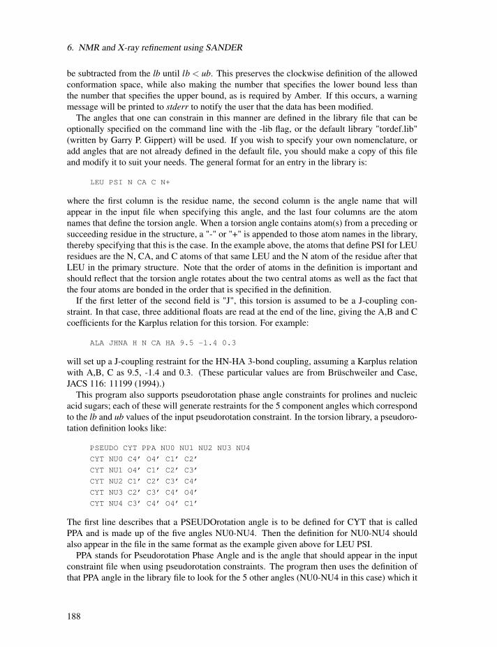
6. NMR and X-ray refinement using SANDER
be subtracted from the lb until lb < ub. This preserves the clockwise definition of the allowedconformation space, while also making the number that specifies the lower bound less than
the number that specifies the upper bound, as is required by Amber. If this occurs, a warning
message will be printed to stderr to notify the user that the data has been modified.The angles that one can constrain in this manner are defined in the library file that can be
optionally specified on the command line with the -lib flag, or the default library "tordef.lib"
(written by Garry P. Gippert) will be used. If you wish to specify your own nomenclature, or
add angles that are not already defined in the default file, you should make a copy of this file
and modify it to suit your needs. The general format for an entry in the library is:
LEU PSI N CA C N+
where the first column is the residue name, the second column is the angle name that will
appear in the input file when specifying this angle, and the last four columns are the atom
names that define the torsion angle. When a torsion angle contains atom(s) from a preceding or
succeeding residue in the structure, a "-" or "+" is appended to those atom names in the library,
thereby specifying that this is the case. In the example above, the atoms that define PSI for LEU
residues are the N, CA, and C atoms of that same LEU and the N atom of the residue after that
LEU in the primary structure. Note that the order of atoms in the definition is important and
should reflect that the torsion angle rotates about the two central atoms as well as the fact that
the four atoms are bonded in the order that is specified in the definition.
If the first letter of the second field is "J", this torsion is assumed to be a J-coupling con-
straint. In that case, three additional floats are read at the end of the line, giving the A,B and C
coefficients for the Karplus relation for this torsion. For example:
ALA JHNA H N CA HA 9.5 -1.4 0.3
will set up a J-coupling restraint for the HN-HA 3-bond coupling, assuming a Karplus relation
with A,B, C as 9.5, -1.4 and 0.3. (These particular values are from Brüschweiler and Case,
JACS 116: 11199 (1994).)
This program also supports pseudorotation phase angle constraints for prolines and nucleic
acid sugars; each of these will generate restraints for the 5 component angles which correspond
to the lb and ub values of the input pseudorotation constraint. In the torsion library, a pseudoro-tation definition looks like:
PSEUDO CYT PPA NU0 NU1 NU2 NU3 NU4
CYT NU0 C4’ O4’ C1’ C2’
CYT NU1 O4’ C1’ C2’ C3’
CYT NU2 C1’ C2’ C3’ C4’
CYT NU3 C2’ C3’ C4’ O4’
CYT NU4 C3’ C4’ O4’ C1’
The first line describes that a PSEUDOrotation angle is to be defined for CYT that is called
PPA and is made up of the five angles NU0-NU4. Then the definition for NU0-NU4 should
also appear in the file in the same format as the example given above for LEU PSI.
PPA stands for Pseudorotation Phase Angle and is the angle that should appear in the input
constraint file when using pseudorotation constraints. The program then uses the definition of
that PPA angle in the library file to look for the 5 other angles (NU0-NU4 in this case) which it
188

6.7. Preparing restraint files for Sander
then generates restraints for. PPA for proline residues is included in the standard library as well
as for the DNA nucleotides.
If the -les flag is set, the program will prepare torsion angle restraints for multiple copies
(LES) simulations. In this case, the input pdb file is one without LES copies, i.e. with justa single copy of the molecule. The "lesfile" specified by this flag is created by the addlesprogram, and contains a mapping from original atom numbers into the copy numbers used in
the multiple-copies simulation.
Torsion angle constraints defined here cannot span two different copy sets, i.e., there cannot
be some atoms of a particular torsion that are in one multiple copy set, and other atoms from
the same torsion that are in other copy sets. It is OK to have some atoms with single copies,and others with multiple copies in the same torsion. The program will create as many duplicate
torsions as there are copies.
A good alternative to interpreting J-coupling constants in terms of torsion angle restraints
is to refine directly against the coupling constants themselves, using an appropriate Karplus
relation. See the discussion of the variable RJCOEF, above.
6.7.3. Chirality restraints: makeCHIR_RST
Usage: makeCHIR_RST <pdb-file> <output-constraint-file>
We also find it useful to add chirality constraints and trans-peptide ω constraints (where appro-
priate) to prevent chirality inversions or peptide bond flips during the high-temperature portions
of simulated annealing runs. The program makeCHIR_RST will create these constraints. Notethat you may have to edit the output of this program to change trans peptide constraints to cis,as appropriate.
6.7.4. Direct dipolar coupling restraints: makeDIP_RST
For simulations with residual dipolar coupling restraints, themakeDIP_RST.protein,makeDIP_RST.dnaand makeDIP_RST.diana are simple codes to prepare the input file. Use -help to obtain a moredetailed description of the usage. For now, this code only handles backbone NH and CαH data.The header specifying values for various parameters needs to be manually added to the output
of makeDIP_RST.Use of residual dipolar coupling restraints is new both for Amber and for the general NMR
community. Refinement against these data should be carried out with care, and the optimal
values for the force constant, penalty function, and initial guesses for the alignment tensor
components are still under investigation. Here are some suggestions from the experiences so
far:
1. Beware of overfitting the dipolar coupling data in the expense of Amber force field en-
ergy. These dipolar coupling data are very sensitive to tiny changes in the structure.
It is often possible to drastically improve the fitting by making small distortions in the
backbone angles. We recommend inclusion of explicit angle restraints to enforce ideal
backbone geometry, especially for those residues that have corresponding residual dipolar
coupling data.
189

6. NMR and X-ray refinement using SANDER
2. The initial values for the Cartesian components of the alignment tensor can influence the
final structure and alignment if the structure is not fixed (ibelly = 0). For a fixed structure
(ibelly = 1), these values do not matter. Therefore, the current "best" strategy is to fit the
experimental data to the fixed starting structure, and use the alignment tensor[s] obtained
from this fitting as the initial guesses for further refinement.
3. Amber is capable of simultaneously fitting more than one set of alignment data. This al-
lows the use of individually obtained datasets with different alignment tensors. However,
if the different sets of data have equal directions of alignment but different magnitudes,
using an overall scaling factor for these data with a single alignment tensor could greatly
reduce the number of fitting parameters.
4. Because the dipolar coupling splittings depend on the square root of the order parameters
(0≤ S2≤1), these order parameters describing internal motion of individual residues areoften neglected (N. Tjandra and A. Bax, Science 278, 1111-1113, 1997). However, thesquare root of a small number can still be noticeably smaller than 1, so this may introduce
undesirable errors in the calculations.
6.8. Getting summaries of NMR violations
If you specify LISTOUT=POUT when running sander, the output file will contain a lot ofdetailed information about the remaining restraint violations at the end of the run. When running
a family of structures, it can be useful to process these output files with sviol, which takes a listof sander output files on the command line, and sends a summary of energies and violations toSTDOUT. If you have more than 20 or so structures to analyze, the output from sviol becomesunwieldy. In this case you may also wish to use sviol2, which prints out somewhat less detailedinformation, but which can be used on larger families of structures. The senergy script gives amore detailed view of force-field energies from a series of structures. (We thank the TSRI NMR
community for helping to put these scripts together, and for providing many useful suggestions.)
6.9. Time-averaged restraints
The model of the previous sections involves the "single-average-structure" idea, and tries to
fit all constraints to a single model, with minimal deviations. A generalization of this model
treats distance constraints arising from fromNOE crosspeaks (for example) as being the average
distance determined from a trajectory, rather than as the single distance derived from an average
structure.
Time-averaged bonds and angles are calculated as
r = (1/C){∫ t
0e(t ′−t)/τ r(t ′)−idt ′
}−1/i
(6.1)
where
r = time-averaged value of the internal coordinate (distance or angle)
t = the current time
190

6.9. Time-averaged restraints
τ = the exponential decay constant
r(t ′) = the value of the internal coordinate at time t’
i = average is over internals to the inverse of i. Usually i = 3 or 6 for NOE distances,and -1 (linear averaging) for angles and torsions.
C = a normalization integral.
Time-averaged torsions are calculated as
< ϕ >= tan−1 (< sin(φ) > / < cos(φ) >)
where φ is the torsion, and < sin(φ) > and < cos(φ) > are calculated using the equation
above with sin(φ(t ′)) or cos(φ(t ′)) substituted for r(t ′).Forces for time-averaged restraints can be calculated either of two ways. This option is
chosen with the DISAVI / ANGAVI / TORAVI commands. In the first (the default),
∂E/∂x = (∂E/∂ r)(∂ r/∂ r(t))(∂ r(t)/∂x) (6.2)
(and analogously for y and z). The forces then correspond to the standard flat-bottomed well
functional form, with the instantaneous value of the internal replaced by the time-averaged
value. For example, when r3 < r < r4,
E = k3(r− r3)2
and similarly for other ranges of r.When the second option for calculating forces is chosen (IINC = 1 on a DISAVI, ANGAVI
or TORAVI card), forces are calculated as
∂E/∂x = (∂E/∂ r)(∂ r(t)/∂x) (6.3)
For example, when r3 < r < r4,
∂E/∂x = 2k3(r− r3)(∂ r(t)/∂x)
Integration of this equation does not give Eq. 6.2, but rather a non-intuitive expression for the
energy (although one that still forces the bond to the target range). The reason that it may
sometimes be preferable to use this second option is that the term ∂ r/∂ r(t), which occurs inthe exact expression [Eq. 6.2], varies as (r/r(t))1+i. When i=3, this means the forces canbe varying with the fourth power the distance, which can possibly lead to very large transient
forces and instabilities in the molecular dynamics trajectory. [Note that this will not be the case
when linear scaling is performed, i.e. when i = −1, as is generally the case for valence andtorsion angles. Thus, for linear scaling, the default (exact) force calculation should be used].
It should be noted that forces calculated using Eq. 6.3 are not conservative forces, and would
cause the system to gradually heat up, if no velocity rescaling were performed. The temperature
coupling algorithm should act to maintain the average temperature near the target value. At any
rate, this heating tendency should not be a problem in simulations, such as fitting NMR data,
where MD is being used to sample conformational space rather than to extract thermodynamic
data.
This section has described the methods of time-averaged restraints. For more discussion, the
interested user is urged to consult studies where this method has been used. [205–209]
191
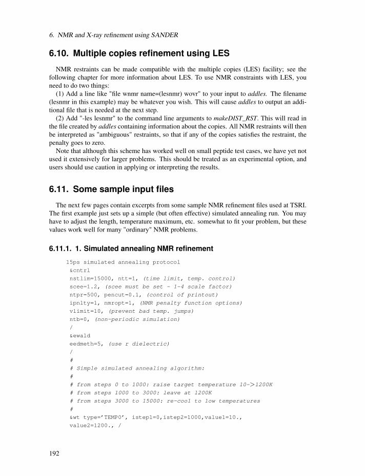
6. NMR and X-ray refinement using SANDER
6.10. Multiple copies refinement using LES
NMR restraints can be made compatible with the multiple copies (LES) facility; see the
following chapter for more information about LES. To use NMR constraints with LES, you
need to do two things:
(1) Add a line like "file wnmr name=(lesnmr) wovr" to your input to addles. The filename(lesnmr in this example) may be whatever you wish. This will cause addles to output an addi-tional file that is needed at the next step.
(2) Add "-les lesnmr" to the command line arguments to makeDIST_RST. This will read inthe file created by addles containing information about the copies. All NMR restraints will thenbe interpreted as "ambiguous" restraints, so that if any of the copies satisfies the restraint, the
penalty goes to zero.
Note that although this scheme has worked well on small peptide test cases, we have yet not
used it extensively for larger problems. This should be treated as an experimental option, and
users should use caution in applying or interpreting the results.
6.11. Some sample input files
The next few pages contain excerpts from some sample NMR refinement files used at TSRI.
The first example just sets up a simple (but often effective) simulated annealing run. You may
have to adjust the length, temperature maximum, etc. somewhat to fit your problem, but these
values work well for many "ordinary" NMR problems.
6.11.1. 1. Simulated annealing NMR refinement
15ps simulated annealing protocol
&cntrl
nstlim=15000, ntt=1, (time limit, temp. control)
scee=1.2, (scee must be set - 1-4 scale factor)
ntpr=500, pencut=0.1, (control of printout)
ipnlty=1, nmropt=1, (NMR penalty function options)
vlimit=10, (prevent bad temp. jumps)
ntb=0, (non-periodic simulation)
/
&ewald
eedmeth=5, (use r dielectric)
/
#
# Simple simulated annealing algorithm:
#
# from steps 0 to 1000: raise target temperature 10->1200K
# from steps 1000 to 3000: leave at 1200K
# from steps 3000 to 15000: re-cool to low temperatures
#
&wt type=’TEMP0’, istep1=0,istep2=1000,value1=10.,
value2=1200., /
192

6.11. Some sample input files
&wt type=’TEMP0’, istep1=1001, istep2=3000, value1=1200.,
value2=1200.0, /
&wt type=’TEMP0’, istep1=3001, istep2=15000, value1=0.,
value2=0.0, /
#
# Strength of temperature coupling:
# steps 0 to 3000: tight coupling for heating and equilibration
# steps 3000 to 11000: slow cooling phase
# steps 11000 to 13000: somewhat faster cooling
# steps 13000 to 15000: fast cooling, like a minimization
#
&wt type=’TAUTP’, istep1=0,istep2=3000,value1=0.2,
value2=0.2, /
&wt type=’TAUTP’, istep1=3001,istep2=11000,value1=4.0,
value2=2.0, /
&wt type=’TAUTP’, istep1=11001,istep2=13000,value1=1.0,
value2=1.0, /
&wt type=’TAUTP’, istep1=13001,istep2=14000,value1=0.5,
value2=0.5, /
&wt type=’TAUTP’, istep1=14001,istep2=15000,value1=0.05,
value2=0.05, /
#
# "Ramp up" the restraints over the first 3000 steps:
#
&wt type=’REST’, istep1=0,istep2=3000,value1=0.1,
value2=1.0, /
&wt type=’REST’, istep1=3001,istep2=15000,value1=1.0,
value2=1.0, /
&wt type=’END’ /
LISTOUT=POUT (get restraint violation list)
DISANG=RST.f (file containing NMR restraints)
The next example just shows some parts of the actual RST file that sander would read. Thisfile would ordinarily not be made or edited by hand; rather, run the programs makeDIST_RST,makeANG_RST and makeCHIR_RST, combining the three outputs together to construct theRST file.
6.11.2. Part of the RST.f file referred to above
# first, some distance constraints prepared by makeDIST_RST:
# (comment line is input to makeRST, &rst namelist is output)
#
#( proton 1 proton 2 upper bound)
#---------------------------------------------
#
# 2 ILE HA 3 ALA HN 4.00
#
193
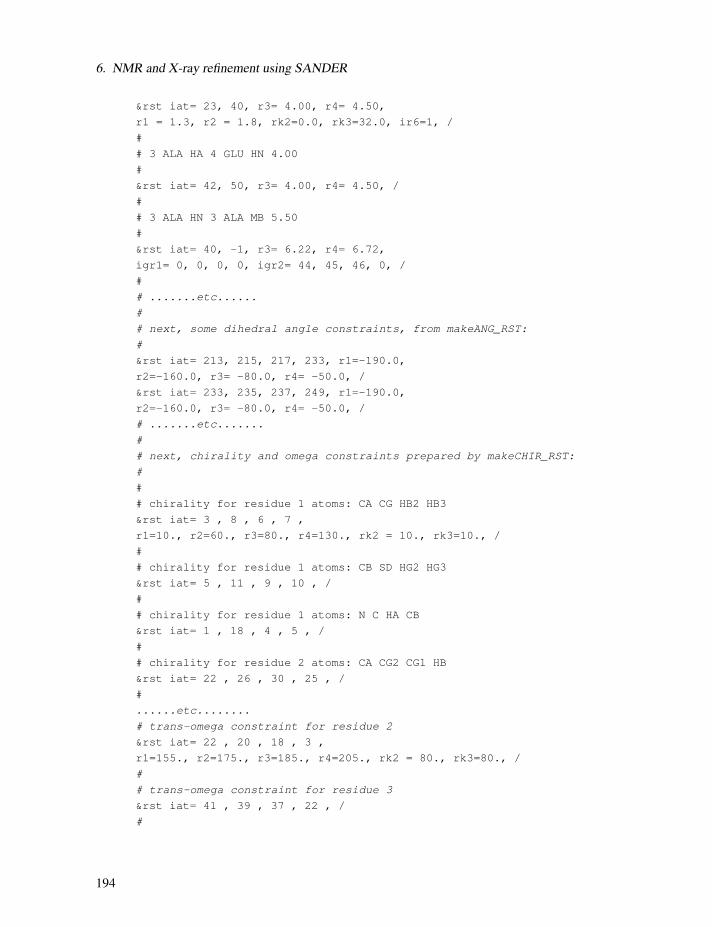
6. NMR and X-ray refinement using SANDER
&rst iat= 23, 40, r3= 4.00, r4= 4.50,
r1 = 1.3, r2 = 1.8, rk2=0.0, rk3=32.0, ir6=1, /
#
# 3 ALA HA 4 GLU HN 4.00
#
&rst iat= 42, 50, r3= 4.00, r4= 4.50, /
#
# 3 ALA HN 3 ALA MB 5.50
#
&rst iat= 40, -1, r3= 6.22, r4= 6.72,
igr1= 0, 0, 0, 0, igr2= 44, 45, 46, 0, /
#
# .......etc......
#
# next, some dihedral angle constraints, from makeANG_RST:
#
&rst iat= 213, 215, 217, 233, r1=-190.0,
r2=-160.0, r3= -80.0, r4= -50.0, /
&rst iat= 233, 235, 237, 249, r1=-190.0,
r2=-160.0, r3= -80.0, r4= -50.0, /
# .......etc.......
#
# next, chirality and omega constraints prepared by makeCHIR_RST:
#
#
# chirality for residue 1 atoms: CA CG HB2 HB3
&rst iat= 3 , 8 , 6 , 7 ,
r1=10., r2=60., r3=80., r4=130., rk2 = 10., rk3=10., /
#
# chirality for residue 1 atoms: CB SD HG2 HG3
&rst iat= 5 , 11 , 9 , 10 , /
#
# chirality for residue 1 atoms: N C HA CB
&rst iat= 1 , 18 , 4 , 5 , /
#
# chirality for residue 2 atoms: CA CG2 CG1 HB
&rst iat= 22 , 26 , 30 , 25 , /
#
......etc........
# trans-omega constraint for residue 2
&rst iat= 22 , 20 , 18 , 3 ,
r1=155., r2=175., r3=185., r4=205., rk2 = 80., rk3=80., /
#
# trans-omega constraint for residue 3
&rst iat= 41 , 39 , 37 , 22 , /
#
194
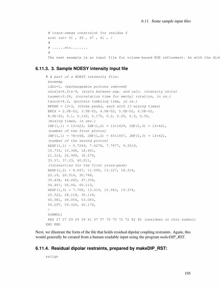
6.11. Some sample input files
# trans-omega constraint for residue 4
&rst iat= 51 , 49 , 47 , 41 , /
#
# ......etc........
#
The next example is an input file for volume-based NOE refinement. As with the dist
6.11.3. 3. Sample NOESY intensity input file
# A part of a NOESY intensity file:
&noeexp
id2o=1, (exchangeable protons removed)
oscale=6.21e-4, (scale between exp. and calc. intensity units)
taumet=0.04, (correlation time for methyl rotation, in ns.)
taurot=4.2, (protein tumbling time, in ns.)
NPEAK = 13*3, (three peaks, each with 13 mixing times)
EMIX = 2.0E-02, 3.0E-02, 4.0E-02, 5.0E-02, 6.0E-02,
8.0E-02, 0.1, 0.126, 0.175, 0.2, 0.25, 0.3, 0.35,
(mixing times, in sec.)
IHP(1,1) = 13*423, IHP(1,2) = 13*1029, IHP(1,3) = 13*421,
(number of the first proton)
JHP(1,1) = 78*568, JHP(1,2) = 65*1057, JHP(1,3) = 13*421,
(number of the second proton)
AEXP(1,1) = 5.7244, 7.6276, 7.7677, 9.3519,
10.733, 15.348, 18.601,
21.314, 26.999, 30.579,
33.57, 37.23, 40.011,
(intensities for the first cross-peak)
AEXP(1,2) = 8.067, 11.095, 13.127, 18.316,
22.19, 26.514, 30.748,
39.438, 44.065, 47.336,
54.467, 56.06, 60.113,
AEXP(1,3) = 7.708, 13.019, 15.943, 19.374,
25.322, 28.118, 35.118,
40.581, 49.054, 53.083,
56.297, 59.326, 62.174,
/
SUBMOL1
RES 27 27 29 29 39 41 57 57 70 70 72 72 82 82 (residues in this submol)
END END
Next, we illustrate the form of the file that holds residual dipolar coupling restraints. Again, this
would generally be created from a human-readable input using the program makeDIP_RST.
6.11.4. Residual dipolar restraints, prepared by makeDIP_RST:
&align
195
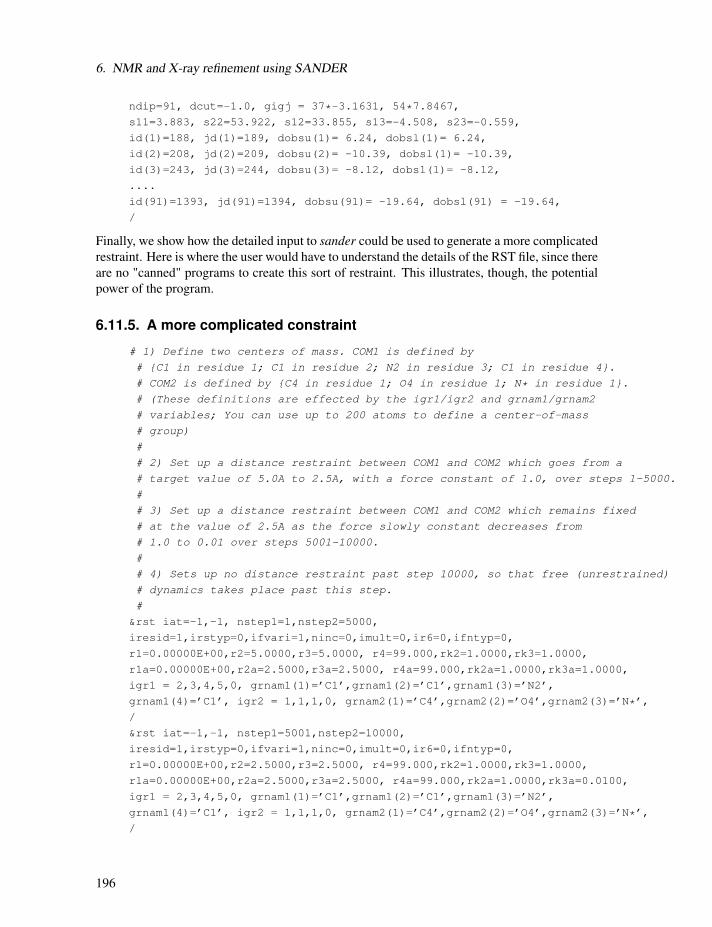
6. NMR and X-ray refinement using SANDER
ndip=91, dcut=-1.0, gigj = 37*-3.1631, 54*7.8467,
s11=3.883, s22=53.922, s12=33.855, s13=-4.508, s23=-0.559,
id(1)=188, jd(1)=189, dobsu(1)= 6.24, dobsl(1)= 6.24,
id(2)=208, jd(2)=209, dobsu(2)= -10.39, dobsl(1)= -10.39,
id(3)=243, jd(3)=244, dobsu(3)= -8.12, dobsl(1)= -8.12,
....
id(91)=1393, jd(91)=1394, dobsu(91)= -19.64, dobsl(91) = -19.64,
/
Finally, we show how the detailed input to sander could be used to generate a more complicatedrestraint. Here is where the user would have to understand the details of the RST file, since there
are no "canned" programs to create this sort of restraint. This illustrates, though, the potential
power of the program.
6.11.5. A more complicated constraint
# 1) Define two centers of mass. COM1 is defined by
# {C1 in residue 1; C1 in residue 2; N2 in residue 3; C1 in residue 4}.
# COM2 is defined by {C4 in residue 1; O4 in residue 1; N* in residue 1}.
# (These definitions are effected by the igr1/igr2 and grnam1/grnam2
# variables; You can use up to 200 atoms to define a center-of-mass
# group)
#
# 2) Set up a distance restraint between COM1 and COM2 which goes from a
# target value of 5.0A to 2.5A, with a force constant of 1.0, over steps 1-5000.
#
# 3) Set up a distance restraint between COM1 and COM2 which remains fixed
# at the value of 2.5A as the force slowly constant decreases from
# 1.0 to 0.01 over steps 5001-10000.
#
# 4) Sets up no distance restraint past step 10000, so that free (unrestrained)
# dynamics takes place past this step.
#
&rst iat=-1,-1, nstep1=1,nstep2=5000,
iresid=1,irstyp=0,ifvari=1,ninc=0,imult=0,ir6=0,ifntyp=0,
r1=0.00000E+00,r2=5.0000,r3=5.0000, r4=99.000,rk2=1.0000,rk3=1.0000,
r1a=0.00000E+00,r2a=2.5000,r3a=2.5000, r4a=99.000,rk2a=1.0000,rk3a=1.0000,
igr1 = 2,3,4,5,0, grnam1(1)=’C1’,grnam1(2)=’C1’,grnam1(3)=’N2’,
grnam1(4)=’C1’, igr2 = 1,1,1,0, grnam2(1)=’C4’,grnam2(2)=’O4’,grnam2(3)=’N*’,
/
&rst iat=-1,-1, nstep1=5001,nstep2=10000,
iresid=1,irstyp=0,ifvari=1,ninc=0,imult=0,ir6=0,ifntyp=0,
r1=0.00000E+00,r2=2.5000,r3=2.5000, r4=99.000,rk2=1.0000,rk3=1.0000,
r1a=0.00000E+00,r2a=2.5000,r3a=2.5000, r4a=99.000,rk2a=1.0000,rk3a=0.0100,
igr1 = 2,3,4,5,0, grnam1(1)=’C1’,grnam1(2)=’C1’,grnam1(3)=’N2’,
grnam1(4)=’C1’, igr2 = 1,1,1,0, grnam2(1)=’C4’,grnam2(2)=’O4’,grnam2(3)=’N*’,
/
196
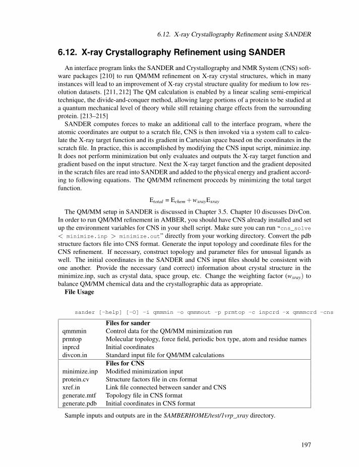
6.12. X-ray Crystallography Refinement using SANDER
6.12. X-ray Crystallography Refinement using SANDER
An interface program links the SANDER and Crystallography and NMR System (CNS) soft-
ware packages [210] to run QM/MM refinement on X-ray crystal structures, which in many
instances will lead to an improvement of X-ray crystal structure quality for medium to low res-
olution datasets. [211, 212] The QM calculation is enabled by a linear scaling semi-empirical
technique, the divide-and-conquer method, allowing large portions of a protein to be studied at
a quantum mechanical level of theory while still retaining charge effects from the surrounding
protein. [213–215]
SANDER computes forces to make an additional call to the interface program, where the
atomic coordinates are output to a scratch file, CNS is then invoked via a system call to calcu-
late the X-ray target function and its gradient in Cartesian space based on the coordinates in the
scratch file. In practice, this is accomplished by modifying the CNS input script, minimize.inp.
It does not perform minimization but only evaluates and outputs the X-ray target function and
gradient based on the input structure. Next the X-ray target function and the gradient deposited
in the scratch files are read into SANDER and added to the physical energy and gradient accord-
ing to following equations. The QM/MM refinement proceeds by minimizing the total target
function.
Etotal = Echem +wxrayExray
The QM/MM setup in SANDER is discussed in Chapter 3.5. Chapter 10 discusses DivCon.
In order to run QM/MM refinement in AMBER, you should have CNS already installed and set
up the environment variables for CNS in your shell script. Make sure you can run “cns_solve
< minimize.inp > minimize.out” directly from your working directory. Convert the pdb
structure factors file into CNS format. Generate the input topology and coordinate files for the
CNS refinement. If necessary, construct topology and parameter files for unusual ligands as
well. The initial coordinates in the SANDER and CNS input files should be consistent with
one another. Provide the necessary (and correct) information about crystal structure in the
minimize.inp, such as crystal data, space group, etc. Change the weighting factor (wxray) tobalance QM/MM chemical data and the crystallographic data as appropriate.
File Usage
sander [-help] [-O] -i qmmmin -o qmmmout -p prmtop -c inpcrd -x qmmmcrd -cns
Files for sanderqmmmin Control data for the QM/MM minimization run
prmtop Molecular topology, force field, periodic box type, atom and residue names
inprcd Initial coordinates
divcon.in Standard input file for QM/MM calculations
Files for CNSminimize.inp Modified minimization input
protein.cv Structure factors file in cns format
xref.in Link file connected between sander and CNS
generate.mtf Topology file in CNS format
generate.pdb Initial coordinates in CNS format
Sample inputs and outputs are in the $AMBERHOME/test/1vrp_xray directory.
197

6. NMR and X-ray refinement using SANDER
198

7. PMEMD
7.1. Introduction
PMEMD (Particle Mesh Ewald Molecular Dynamics) is a reimplementation of a subset of
sander functionality that has been written with the major goal of improving the performance
of the most frequently used methods of sander. In release 10, pmemd supports Particle Mesh
Ewald simulations, Generalized Born simulations, and ALPB (Analytical Linearized Poisson-
Boltzmann) simulations. The most significant new functionality is support for extra points, or
force centers that are not at atomic positions, within a PME context. Thus we now have a fast
PME implementation that supports both the TIP4P and TIP5P water models as well as other
structures defined in GAFF that require extra points. We also now support the AMOEBA polar-
izable force field, but in a separate pmemd executable, pmemd.amba, which is basically pmemd
9 with AMOEBA support included (thus other new features of pmemd 10 will not be found in
pmemd.amba). The decision was made to branch AMOEBA into a separate executable partly
due to its tremendous complexity, and partly because it is not feasible to use the high scal-
ing features of pmemd with AMOEBA, given its design constraints. We recommend trying
pmemd.amba on up to about 20 processors. AMOEBA is currently the only supported polariz-
able forcefield in pmemd. For standard PME simulations performance and scaling with pmemd
is significantly better than with sander, and modest gains in performance and scaling have been
made in release 10. For Generalized Born and ALPB simulations, not much optimization work
has been done yet, but performance is typically better. For the supported functionality, the in-
put required and output produced are intended to exactly replicate sander 10 within the limits
of roundoff errors. PMEMD just runs more rapidly, scales better on parallel processors using
MPI, can be used profitably on significantly higher numbers of processors, and uses less res-
ident memory. Dynamic memory allocation is used so memory configuration is not required.
PMEMD is ideal for molecular dynamics simulations of large solvated systems for long periods
of time, especially if supercomputer resources are available. Benchmark data will be posted at
the Amber website, amber.scripps.edu, after release.
PMEMD accepts Amber 10 sander input files (mdin, prmtop, inpcrd, refc), and is also back-
ward compatible in regard to input to the same extent as sander 10. All options documented in
the sander section of this manual should be properly parsed.
7.2. Functionality
As mentioned above, pmemd is not a complete implementation of sander 10. Instead, it is
intended to be a fast implementation of the functionality most likely to be used by someone
doing simulations on large solvated systems.
The following functionality is missing entirely:
imin=5 In &cntrl. Trajectory analysis is not supported.
199
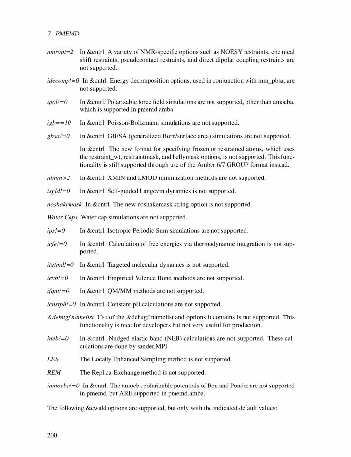
7. PMEMD
nmropt=2 In &cntrl. A variety of NMR-specific options such as NOESY restraints, chemical
shift restraints, pseudocontact restraints, and direct dipolar coupling restraints are
not supported.
idecomp!=0 In &cntrl. Energy decomposition options, used in conjunction with mm_pbsa, are
not supported.
ipol!=0 In &cntrl. Polarizable force field simulations are not supported, other than amoeba,
which is supported in pmemd.amba.
igb==10 In &cntrl. Poisson-Boltzmann simulations are not supported.
gbsa!=0 In &cntrl. GB/SA (generalized Born/surface area) simulations are not supported.
In &cntrl. The new format for specifying frozen or restrained atoms, which uses
the restraint_wt, restraintmask, and bellymask options, is not supported. This func-
tionality is still supported through use of the Amber 6/7 GROUP format instead.
ntmin>2 In &cntrl. XMIN and LMOD minimization methods are not supported.
isgld!=0 In &cntrl. Self-guided Langevin dynamics is not supported.
noshakemask In &cntrl. The new noshakemask string option is not supported.
Water Caps Water cap simulations are not supported.
ips!=0 In &cntrl. Isotropic Periodic Sum simulations are not supported.
icfe!=0 In &cntrl. Calculation of free energies via thermodynamic integration is not sup-
ported.
itgtmd!=0 In &cntrl. Targeted molecular dynamics is not supported.
ievb!=0 In &cntrl. Empirical Valence Bond methods are not supported.
ifqnt!=0 In &cntrl. QM/MM methods are not supported.
icnstph!=0 In &cntrl. Constant pH calculations are not supported.
&debugf namelist Use of the &debugf namelist and options it contains is not supported. Thisfunctionality is nice for developers but not very useful for production.
ineb!=0 In &cntrl. Nudged elastic band (NEB) calculations are not supported. These cal-
culations are done by sander.MPI.
LES The Locally Enhanced Sampling method is not supported.
REM The Replica-Exchange method is not supported.
iamoeba!=0 In &cntrl. The amoeba polarizable potentials of Ren and Ponder are not supported
in pmemd, but ARE supported in pmemd.amba.
The following &ewald options are supported, but only with the indicated default values:
200
7.3. PMEMD-specific namelist variables
ew_type=0 Only Particle Mesh Ewald calculations are supported. ew_type = 1 (regular Ewald
calculations) must be done in sander 10.
nbflag=1 The nbflag option is basically ignored, and all nonbonded list updates are sched-
uled based on "skin" checks. This is more reliable and has little cost. The variable
nsnb still can be set and has an influence on minimizations. For PME calcula-
tions, list building may also be scheduled based on heuristics to suit load balancing
requirements in multiprocessor runs.
nbtell=0 The nbtell option is not particularly useful and is ignored.
eedmeth=1 Only a cubic spline switch function (eedmeth = 1) for the direct sum Coulomb
interaction is supported. This is the default, and most widely used setting for eed-
meth. On some machine architectures, we actually spline energies and forces as
a function of r**2 to a higher precision than the cubic spline switch. One conse-
quence of only supporting eedmeth 1 is that vacuum simulations cannot be done
(though generalized Born nonperiodic simulations are available).
column_fft=0 This is a sander-specific performance optimization option. PMEMD uses differ-
ent mechanisms to enhance performance, and ignores this option.
I would strongly suggest that new PMEMD users simply take an existing sander 10 mdin file
and attempt a short 10-30 step run. The output will tell you whether or not PMEMD will handle
the particular problem at hand for all the functionality that is supported by "standard" sander.
For functionality that requires special builds of sander or sander-derived executables (LES),
there may be failures in namelist parsing.
7.3. PMEMD-specific namelist variables
mdout_flush_interval In &cntrl, this variable can be used to control the minimum time in in-
teger seconds between "flushes" of the mdout file. PMEMD DOES NOT use file
flush() calls at all because flush functionality does not work for all fortran com-
pilers used in building pmemd. Thus, pmemd does an open/close cycle on mdout
at a default minimum interval of 300 seconds. This interval can be changed with
this variable if desired in the range of 0-3600. If mdout_flush_interval is set to 0,then mdout will be reopened and closed for each printed step. This functionality is
provided in pmemd because some large systems have such large file i/o buffers that
mdout will have 0 length on the disk through 100’s of psec of simulated time. The
default of 300 seconds provides a good compromise between efficiency and being
able to observe the progress of the simulation.
mdinfo_flush_interval In &cntrl, this variable can be used to control the minimum time in in-teger seconds between "flushes" of the mdinfo file. PMEMD DOES NOT use file
flush() calls at all because flush functionality does not work for all fortran compil-
ers used in building pmemd. Thus, pmemd does an open/close cycle on mdinfo
at a default minimum interval of 60 seconds. This interval can be changed with
this variable if desired in the range of 0-3600. Note that mdinfo under pmemd
201

7. PMEMD
simply serves as a heartbeat for the simulation at mdinfo_flush_interval, and md-info probably will not be updated with the last step data at the end of a run. If
mdinfo_flush_interval is set to 0, then mdinfo will be reopened and closed for eachprinted step.
es_cutoff, vdw_cutoff In &cntrl, these variables can be used to control the cutoffs used for vdwand electrostatic direct force interactions in PME calculations separately. If you
specify these variables, you should not specify the cut variable, and there is a re-
quirement that vdw_cutoff >= es_cutoff. These were introduced anticipating theneed to support force fields where the direct force calculations are more expensive.
For the current force fields, one can get slightly improved performance and about
the same accuracy as one would get using a single cutoff. A good example would
be using vdw_cutoff=9.0, es_cutoff=8.0. For this scenario, one gets about the accu-racy in calculations associated with 9.0 angstrom cutoffs, but at a cost intermediate
between an 8.0 and a 9.0 angstrom cutoff.
no_intermolecular_bonds In &cntrl. New variable controlling molecule definition. If 1, anymolecules (ie., molecules as defined by the prmtop) joined by a covalent bond are
fused to form a single molecule for purposes of pressure and virial-related op-
erations; if 0 then the old behaviour (use prmtop molecule definitions) pertains.
The default is 1; a value of 0 is not supported with forcefields using extra points.
This option was necessitated in order to efficiently parallelize model systems with
extra points. This redefinition of molecules actually allows for a more correct
treatment of molecules during pressure adjustments and should produce better re-
sults with less strain on covalent bonds joining prmtop-defined molecules, but if
the default value is used for a NTP simulation, results will differ slightly rela-
tive to sander if any intermolecular bonding was applied in forming the prmtop
(eg., a cyx-cyx bridge was added between two peptides that originated in a pdb,
with each peptide having its own "TER" card). If consistency with sander is more
important to you, and you are not using extra points, then you may want to set
no_intermolecular_bonds to 0.
ene_avg_sampling In &cntrl. New variable controlling the number of steps between energy
samples used in energy averages. If not specified, then ntpr is used (default). To
match the behaviour of earlier releases, this variable should be set to 1. This vari-
able is only used for MD, not minimization and will also effectively be turned off
if ntave is in use (non-0) or RESPA is in use (nrespa > 1) or if you are not runningPME. It is a fairly common situation that it is completely unnecessary to sample
the energies every step to get a good average during production, and this is costly
in terms of performance. Thus, performance can be improved (with greatest im-
provements for the ensembles in the order NVE > NVT > NTP) without really
losing anything of value by using the new default for energy average sampling
(specify nothing).
use_axis_opt In &ewald. For parallel runs, the most favorable orientation of an orthogonalunit cell is with the longest side in the Z direction. Starting with pmemd 3.00,
we were actually reorienting internal coordinates to take advantage of this, and in
202
7.4. Slightly changed functionality
high processor count runs on oblong unit cells, using axis optimization can im-
prove performance on the order of 10%. However, if a system has hotspots, the
results produced with axes oriented differently may vary by on the order of 0.05%
relatively quickly. This effect has to do with the fact that axis optimization changes
the order of LOTS of operations and also the fft slab layout, and under mpi if the
system has serious hotspots, shake will come up with slightly different coordinate
sets. This is really only a problem in pathological situations, and then it is proba-
bly mostly telling you that the situation is pathological, and neither set of results
is more correct (typically the ewald error term is also high). In routine regression
testing with over a dozen tests, axis reorientation has no effect on results. Nonethe-
less, we have changed defaults recently to be in favor of higher reproducibility of
results. Now, axis optimization is only done for mpi runs in which an orthogonal
unit cell has an aspect ratio of at least 3 to 2. It is turned off for all minimization
runs and for runs in which velocities are randomized (ntt = 2 or 3). If you want to
force axis optimization, you may set use_axis_opt = 1 in the &ewald namelist. Ifyou set it to 0, you will force it off in scenarios where it would otherwise be used.
fft_grids_per_ang In &ewald. This variable may be used to set the desired reciprocal space fft
grid density in terms of fft grids/angstrom. The nearest grid dimensions, given the
prime factors supported by the underlying fft implementation, that meet or exceed
this density will be used (ie., nfft1,2,3 are set based on this specification). Thedefault value is 1.0 grids/angstrom and gives very reasonable accuracy. PMEMD
is actually more stringent now than sander in that it will meet or exceed the desired
density instead of just approximating it. Thus, to get identical results with sander,
one may have to specify grid dimensions to be used with the nfft1,2,3 variables.
7.4. Slightly changed functionality
An I/O optimization has been introduced into PMEMD. The NTWR default value (frequency
of writing the restart file) has been modified such that the default minimum is 500 steps, and
this value is increased incrementally for multiprocessor runs. In general, frequent writes of
restrt, especially in runs with a high processor count, is wasteful. Also, if the mden file is being
written, it is always written as formatted output, regardless of the value of ioutfm. SANDERnow conforms to this convention regarding ioutfm and mden.
In addition, there are two command-line options unique to pmemd:
-l <logfile name> A name may be assigned to the log file on the command line.
-suffix <output files suffix> A suffix may now be appended, following a ".", to all the default
output file names for a pmemd run by simply entering the -suffix option. The suffix will
apply to mdout, restrt, mdcrd, mdvel, mden, mdinfo, and logfile names. However, if an
output file name is explicitly provided on the command line, the provided name takes
precedence. Entering "pmemd -suffix foo" will write mdout output to mdout.foo, and so
on. This provides an easy way to group output files with minimal effort.
203
7. PMEMD
7.5. Parallel performance tuning and hints
In order to achieve higher scaling, pmemd 10 has implemented several new algorithms, the
most notable of which is the option of using a "block" or pencil fft rather than the usual slab fft
algorithm. The block fft algorithm allows the reciprocal space and fft workload to be distributed
to more processors, but at a cost of higher communications overhead, both in terms of the dis-
tributed fft transpose cost and in terms of communication of the data necessary to set up the fft
grids in the first place. A number of variables in the &ewald namelist can be used to control
whether the slab or block fft algorithm is used, how the block division occurs, whether direct
force work is also assigned to tasks doing reciprocal space and fft work, whether the master is
given any force and energy computation work to do, as opposed to being reserved strictly for
handling output and loadbalancing, and the frequency of atom ownership reassignment, an op-
eration that counteracts rising communications costs caused by diffusion. The various namelist
variables involved have all been assigned defaults that adapt to run conditions, and in general it
is probably best that the user just use the defaults and not attempt to make adjustments. How-
ever, in some instances, fine tuning may yield slightly better performance. The variables in-
volved include block_fft, fft_blk_y_divisor, excl_recip, excl_master, and atm_redist_freq. Theseare described further in the README under pmemd/src as well as in the sourcecode itself.
Performance depends not only on proper setup of hardware and software, but also on making
good choices in simulation configuration. There are many tradeoffs between accuracy and cost,
as one might expect, and understanding all of these comes with experience. However, I would
like to suggest a couple of good choices for your simulations, if you have facilities where you
can routinely run at high processor count, say 32 processors or more. First of all, there is an
implementation of binary trajectory files in pmemd and sander, based on the netCDF binary
file format. This is invoked now using ioutfm == 1, assuming you have built either pmemd
or sander with "bintraj" support. Using this output format, i/o from the master process will be
more efficient and your filesize will be about half what it would otherwise be. In Amber 10, ptraj
can read these new netCDF trajectory files, but if you want to visualize them you may have to
wait until viewers support the format. At really high processor count though, using this format
can be on the order of 10% more efficient than using the standard formatted trajectory output.
Secondly, other simulation packages standardly use respa methods as an efficiency measure.
These methods basically sample reciprocal space forces for PME less frequently. This can
slightly improve performance for pmemd at low processor count, but at higher processor counts
using respa actually makes loadbalancing difficult, and there can be a net loss of performance.
If you wish to use respa for pme simulations (done typically by setting nrespa to 2 or 4), thenyou should check whether you actually get better performance. You may well not, and it will be
at a cost of a loss in accuracy. Using respa for generalized Born simulations is fine in all cases,
however.
7.6. Installation
The build process for PMEMD is similar to the build process for the rest of Amber 10, but
must be invoked separately in the src/pmemd directory. There is a configure script that generates
a config.h header that is used in the build process. Generation of config.h files is dependendenton use of information in the src/pmemd/config_data database. This system is similar to the old
204
7.7. Acknowledgements
Amber MACHINE files configuration system, but is a bit more automated in that the configure
script will set up config.h for a lot of common machine setups. The PMEMD installation pro-
cess has remained separate from the Amber 10 installation process because PMEMD does not
support all systems that can be automatically configured by Amber 10, and vice versa. Also,
there is an emphasis on performance in PMEMD, and there was a desire to be able to fine
tune the optimization process to a larger extent than was possible with the Amber 9 config-
uration process. Finally, user definition of configuration files in the src/config_data database
is a fairly simple process, and this allows users to easily target new machines or machines
with unusual configuration requirements. For more PMEMD installation details, please read
src/pmemd/README. Note that pmemd.amba, located in src/pmemd.amba, must also be built
separately. Building pmemd.amba even more closely follows the pmemd 9 build process than
does the pmemd 10 process, as little was changed before the split in the code trees.
7.7. Acknowledgements
This code was developed by Dr. Robert Duke of Prof. Lee Pedersen’s Lab at UNC-Chapel
Hill and Dr. Tom Darden’s Lab at NIEHS, starting from the version of sander in Amber 6. I
would like to thank Prof. Pedersen for his support in the development of this code, and would
also like to acknowledge funding support from NIH grant HL-06350 (PPG) and NSF grant
0121361 (ITR/AP). I would also like to acknowledge Dr. Lalith Perera and Divi Venkateswarlu
in the Pedersen Lab for helpful conversations and a willingness to actually use early releases
of PMEMD. Since Amber 8 shipped, continued support for development has also come from
Dr. Tom Darden and his laboratory at NIEHS in the form of intramural NIH funding. Drs.
Tom Darden, Lee Pedersen, Lalith Perera, Coray Colina, Chang Jun Lee, Ping Lin and Vasu
Chandrasekaran have all been helpful in providing suggestions and being willing to use early
releases of pmemd 9 and 10. This work has required the availability of large piles of proces-
sors of many different types. I would like to thank UNC-Chapel Hill, the National Institute of
Environmental Health Sciences, the Edinburgh Parallel Computing Centre, the Pittsburgh Su-
percomputing Center, the National Energy Research Scientific Computing Center, the National
Center for Supercomputing Applications, the San Diego Supercomputer Center at the Univer-
sity of California, San Diego, the Center for High Performance Computing at the University of
Utah, the Texas Advanced Computing Center at the University of Texas, Austin, the Scripps
Research Institute, the IBM Blue Gene Capacity on Demand Center in Rochester, Minnesota,
and the Intel and SGI Parallel Application Center for making resources available that were used
in the development, test, and benchmarking of this software.
When citing PMEMD (Particle Mesh Ewald Molecular Dynamics) in the literature, please
use the Amber Version 10 citation given in the Amber 10 manual.
205

7. PMEMD
206

8. MM_PBSA
The MM_PBSA approach represents the postprocessing method to evaluate free energies
of binding or to calculate absolute free energies of molecules in solution. The sets of struc-
tures are usually collected with molecular dynamics or Monte Carlo methods. However, the
collections of structures should be stored in the format of an AMBER trajectory file. The
MM_PBSA/GBSA method combines the molecular mechanical energies with the continuum
solvent approaches. The molecular mechanical energies are determined with the sander pro-gram from AMBER and represent the internal energy (bond, angle and dihedral), and van der
Waals and electrostatic interactions. An infinite cutoff for all interactions is used. The elec-
trostatic contribution to the solvation free energy is calculated with a numerical solver for the
Poisson-Boltzmann (PB) method, for example, as implemented in the pbsa program [69] or
by generalized Born (GB) methods implemented in sander. Previous MM_PBSA applicationswere mostly performed with a numerical PB solver in the widely used DelPhi program, [71]which has been shown by AMBER developers to be numerically consistent with the pbsaprogram. The nonpolar contribution to the solvation free energy has been determined with
solvent-accessible-surface-area-dependent terms. [66] The surface area is computed with Paul
Beroza’s molsurf program, which is based on analytical ideas primarily developed by MikeConnolly. [216] An alternative method for nonpolar solvation energy is also included here (Tan
and Luo, in preparation). The new method separates nonpolar contribution into two terms: the
attractive (dispersion) and repulsive (cavity) interactions. Doing so significantly improves the
correlation between the cavity free energies and solvent accessible surface areas for branched
and cyclic organic molecules. [78] This is in contrast to the commonly used strategy that cor-
relates total nonpolar solvation energies with solvent accessible surface areas, which only cor-
relates well for linear aliphatic molecules. [66] In the new method, the attractive interaction is
computed by a numerical integration over the solvent accessible surface area that accounts for
solute solvent attractive interactions with an infinite cutoff. [79] Finally, estimates of conforma-
tional entropies can be made with the nmode module from AMBER.
Although the basic ideas here have many precedents, the first application of this model in its
present form was to the A- and B-forms of RNA and DNA, where many details of the basic
method are given. [217] You may also wish to refer to a review summarizing many of the initial
applications of this model, [218] as well as to papers describing more recent applications. [219–
223]
The initial MM_PBSA scripts were written by Irina Massova. These were later modified
and mostly turned into Perl scripts by Holger Gohlke, who also added GB/SA (generalized
Born/surface area) options, and techniques to decompose energies into pairwise contributions
from groups (where possible).
207

8. MM_PBSA
8.1. General instructions
The general procedure is to edit the mm_pbsa.in file (see below), and then to run the code asfollows:
mm_pbsa.pl mm_pbsa.in > mm_pbsa.log
The mm_pbsa.in file refers to "receptor", "ligand" and "complex", but the chemical nature ofthese is up to the user, and these could equally well be referred to as "A", "B", and "AB". The
procedure can also be used to estimate the free energy of a single species, and this is usually
considered to be the "receptor".
The user also needs to prepare prmtop files for receptor, ligand, and complex using LEaP; ifyou are just doing "stability" calculations, only one of the prmtop files is required.The output files are labeled ".out", and the most useful summaries are in the "statistics.out"
files. These give averages and standard deviations for various quantities, using the following
labeling scheme:
*** Abbreviations for mm_pbsa output ***ELE - non-bonded electrostatic energy + 1,4-electrostatic energy
VDW - non-bonded van der Waals energy + 1,4-van der Waals energy
INT - bond, angle, dihedral energies
GAS - ELE + VDW + INT
PBSUR - hydrophobic contrib. to solv. free energy for PB calculations
PBCAL - reaction field energy calculated by PB
PBSOL - PBSUR + PBCAL
PBELE - PBCAL + ELE
PBTOT - PBSOL + GAS
GBSUR - hydrophobic contrib. to solv. free energy for GB calculations
GB - reaction field energy calculated by GB
GBSOL - GBSUR + GB
GBELE - GB + ELE
GBTOT - GBSOL + GAS
TSTRA - translational entropy (as calculated by nmode) times temperature
TSROT - rotational entropy (as calculated by nmode) times temperature
TSVIB - vibrational entropy (as calculated by nmode) times temperature
*** Prefixes in front of abbreviations for energy decomposition ***"T" - energy part due to _T_otal residue
"S" - energy part due to _S_idechain atoms
"B" - energy part due to _B_ackbone atoms
The $AMBERHOME/src/mm_pbsa/Examples directory shows examples of running a "Stabil-ity" calculation (i.e., estimating the free energy of one species), a "Binding" calculation (esti-mating ΔG for A + B→AB), an "Nmode" calculation (to estimate entropies), and two exam-ples of how total energies can be decomposed (either by residue, or pair-wise by residue). You
should study the inputs and outputs in these directories to see how the program is typically used.
208

8.2. Input explanations
8.2. Input explanations
Below is a description of the input parameters for MM-PB/SA. A sample file can be found at
$AMBERHOME/src/mm_pbsa/Examples/mm_pbsa.in. The input file is structured into sectionsfor different purposes. The parameters in the general section control which kind of operations
are executed. Additional parameters for the chosen operations have to be defined in the later
sections.
8.2.1. General
VERBOSE If set to 1, input and output files are not removed. This is useful for debugging
purposes.
specifying snapshot location and naming
PREFIX To the prefix of the snapshots, "{_com, _rec, _lig}.crd.Number" is added during
generation of snapshots as well as during mm_pbsa calculations.
PATH Specifies the location where to store or get snapshots.
selecting subsets of snapshots
START Specifies the first snapshot to be used in energy calculations (optional, default is
1).
STOP Specifies the last snapshot to be used in energy calculations (optional, default is
10e10).
OFFSET Specifies the offset between snapshots in energy calculations (optional, default is
1).
calculation of energy differences or absolute energies
COMPLEX Set to 1 if free energy difference is calculated.
RECEPTOR Set to 1 if either (absolute) free energy or free energy difference are calculated.
LIGAND Set to 1 if free energy difference is calculated.
selection of parameter and topology files
COMPT Parmtop file for the complex (not necessary for option GC).
RECPT Parmtop file for the receptor (not necessary for option GC).
LIGPT Parmtop file for the ligand (not necessary for option GC).
209

8. MM_PBSA
specification of operations/calculations
GC Snapshots are generated from trajectories (see below).
AS Residues are mutated during generation of snapshots from trajectories.
DC Decompose the free energies into individual contributions (only works with MM,
GB and PB with the pbsa program of AMBER).
MM Calculation of gas phase energies using sander.
GB Calculation of desolvation free energies using the GBmodels in sander (see below).
PB Calculation of desolvation free energies using delphi (see below). Calculation of
nonpolar solvation free energies according to the NPOPT option in pbsa (see be-
low).
MS Calculation of nonpolar contributions to desolvation using molsurf (see below). If
MS = 0 and GB = 1, nonpolar contributions are calculated with the LCPO method
in sander. If MS = 0 and PB = 1, nonpolar contributions are calculated according
the NPOPT option in pbsa (see below).
NM Calculation of entropies with nmode.
8.2.2. Energy Decomposition Parameters
Energy decomposition is performed for gasphase energies, desolvation free energies cal-
culated with GB or PB (using the pbsa program of AMBER), and nonpolar contributions to
desolvation using the LCPO method. For amino acids and nucleotides, decomposition is also
performed with respect to backbone and sidechain atoms. When doing a pairwise decompo-
sition of the PB reaction field energy, one should note that for each included residue the PB
equation has to be solved once per snapshot. Also a further decomposition into backbone and
sidechain contributions has not been implemented for a pairwise PB decomposition.
specification of decomposition modus
DCTYPE Values of 1 or 2 yield a decomposition on a per-residue basis.
Values of 3 or 4 yield a decomposition on a pairwise basis. So far the number of
pairs must not exceed the number of residues in the molecule considered.
Values 1 or 3 add 1-4 interactions to bond contributions.
Values 2 or 4 add 1-4 interactions to either electrostatic or vdW contributions.
residue assignment
COMREC Residues belonging to the receptor molecule IN THE COMPLEX.
COMLIG Residues belonging to the ligand molecule IN THE COMPLEX.
RECRES Residues in the receptor molecule.
210

8.2. Input explanations
LIGRES Residues in the ligand molecule.
{REC,LIG}MAP Residues in the complex which are equivalent to the residues in the receptor
molecule or the ligand molecule.
output filter
{COM,REC,LIG}PRI Residues considered for output.
8.2.3. Poisson-Boltzmann Parameters
The following parameters are passed to the PB solver. Additional input parameters may also
be added here. See the sander PB documentation for more options.
PROC Determines which method is used for solving the PB equation. By default (PROC
= 2) the pbsa program of the AMBER suite is used.
REFE Determines which reference state is taken for the PB calculation. By default (REFE
= 0) reaction field energy is calculated with EXDI/INDI. Here, INDI must agree
with DIELC from the MM section.
INDI Dielectric constant for the solute.
EXDI Dielectric constant for the surrounding solvent.
ISTRNG Ionic strength (in mM) for the Poisson-Boltzmann solvent.
PRBRAD Solvent probe radius in Angstrom:
1.4 with the radii in the prmtop files (default);
1.6 with the radii optimized by Tan and Luo (in preparation).
See RADIOPT on how to choose a cavity radii set.
RADIOPT Option to set up radii for PB calc:
0 uses the radii from the prmtop file (default);
1 uses the radii optimized by Tan and Luo (in preparation) with respect to the re-
action field energies computed in the TIP3P explicit solvents. Note that these
optimized radii are based on AMBER atom types (upper case) and charges.
Radii from the ~.prmtop files are used if the atom types are defined by an-
techamber (lower case).
SCALE Lattice spacing in number of grids per Angstrom.
LINIT Number of iterations with the linear PB equation.
211
8. MM_PBSA
hybrid solvation model
IVCAP If set to 1, a solvent sphere (specified by CUTCAP, XCAP, YCAP, and ZCAP) is
excised from a box of water.
If set to 5, a solvent shell is excised, specified by CUTCAP (the thickness of the
shell in A). The electrostatic part of the solvation free energy is estimated from a
linear response approximation using the explicit water plus a reaction field contri-
bution from outside the sphere (i.e., a hybrid solvation approach is pursued).
In addition, the nonpolar contribution is estimated from a sum of (attractive) dis-
persion interactions calculated between the solute and the solvent molecules plus
a (repulsive) cavity contribution. For the latter, the surface calculation must be
done with MS = 1 and the PROBE should be set to 1.4 to get the solvent excluded
surface.
CUTCAP Radius of the water sphere or thickness of the water shell. Note that the sphere
must enclose the whole solute.
XCAP/YCAP/ZCAP Location of the center of the water sphere.
NPOPT Option for modeling nonpolar solvation free energy. See sander PB documentation
for more information on the implementations by Tan and Luo (in preparation).
1: uses the solvent-accessible-surface area to correlate total nonpolar solvation freeenergy: Gnp = SURFTEN * SASA + SURFOFF. Default.
2: uses the solvent-accessible-surface area to correlate the repulsive (cavity) termonly, and uses a surface-integration approach to compute the attractive (dis-
persion) term: Gnp = Gdisp + Gcavity = Gdisp + SURFTEN * SASA +
SURFOFF. When this option is used, RADIOPT has to be set to 1, i.e. the
radii set optimized by Tan and Luo to mimic Gnp in TIP3P explicit solvents.
Otherwise, there is no guarantee that Gnp matches that in explicit solvents.
nonpolar solvation
SURFTEN/SURFOFF Values used to compute the nonpolar contribution Gnp to the desolva-
tion according to either
(I) Gnp = SURFTEN * SASA + SURFOFF (if IVCAP = 0) or
(II) Gnp = Gdisp + Gcavity = Gdisp + SURFTEN * SASA + SURFOFF (if IVCAP
> 0).
In the case of (I), use parameters that fit with the radii from the reaction field
calculation. E.g., use SURFTEN: 0.00542, SURFOFF: 0.92 for PARSE radii or
use SURFTEN: 0.005, SURFOFF: 0.86 for Tan & Luo radii. In the case of (II),
use SURFTEN: 0.069; SURFOFF: 0.00 for calculating the Gcavity contribution.
212

8.2. Input explanations
8.2.4. Molecular Mechanics Parameters
The following parameters are passed to sander. For further details see the sander documen-
tation.
DIELC Dielectric constant for electrostatic interactions. Note: This is not related to GB
calculations.
8.2.5. Generalized Born Parameters
IGB Switches between Tsui’s GB (1) and Onufriev’s GB (2, 5).
GBSA Switches between LCPO (1) and ICOSA (2) method for SASA calculation. De-
composition only works with ICOSA.
SALTCON Concentration (in M) of 1-1 mobile counterions in solution.
EXTDIEL Dielectric constant for the solvent.
INTDIEL Dielectric constant for the solute.
SURFTEN/SURFOFF Values used to compute the nonpolar contribution Gnp to the desolva-
tion free energy according to Gnp = SURFTEN * SASA + SURFOFF.
8.2.6. Molsurf Parameters
PROBE Radius of the probe sphere used to calculate the SAS. In general, since Bondi radii
are already augmented by 1.4A, PROBE should be 0.0 In IVCAP = 1 or 5, the
solvent excluded surface is required for calculating the cavity contribution. Bondi
radii are not augmented in this case and PROBE should be 1.4.
8.2.7. NMODE Parameters
The following parameters are passed to sander (for minimization) and nmode (for entropy
calculation using gasphase statistical mechanics). For further details see documentation.
DIELC (Distance-dependent) dielectric constant.
MAXCYC Maximum number of cycles of minimization.
DRMS Convergence criterion for the energy gradient.
8.2.8. Parameters for Snapshot Generation
BOX "YES": means that periodic boundary conditions were used during MD simulation
and that box information has been printed in the trajectory files; "NO": means
opposite.
NTOTAL Total number of atoms per snapshot printed in the trajectory file (including water,
ions, ...).
213

8. MM_PBSA
NSTART Start structure extraction from NSTART snapshot.
NSTOP Stop structure extraction at NSTOP snapshot.
NFREQ Every NFREQ structure will be extracted from the trajectory.
NUMBER_LIG_GROUPS Number of subsequent LSTART/LSTOP combinations to extract
atoms belonging to the ligand.
LSTART Number of first ligand atom in the trajectory entry.
LSTOP Number of last ligand atom in the trajectory entry.
NUMBER_REC_GROUPS Number of subsequent RSTART/RSTOP combinations to extract
atoms belonging to the receptor.
RSTART Number of first receptor atom in the trajectory entry.
RSTOP Number of last receptor atom in the trajectory entry.
Note: If only one molecular species is extracted, use only the receptor parameters (NUM-
BER_REC_GROUPS, RSTART, RSTOP).
8.2.9. Parameters for Alanine Scanning
The following parameters are additionally passed to make_crd_hg in conjunction with the
ones from the snapshot generation section if "alanine scanning" is requested. The description
of the parameters is taken from Irina Massova.
NUMBER_MUTANT_GROUPS Total number of mutated residues. For each mutated residue,
the following four parameters must be given subsequently.
MUTANT_ATOM1 If residue is mutated to Ala then this is: a pointer on the CG atom of the
mutated residue for all residues except Thr, Ile and Val; a pointer to CG2 if Thr,
Ile or Val residue is mutated to Ala; or a pointer to OG if Ser residue is mutated to
Ala. If residue is mutated to Gly then this is a pointer on CB.
MUTANT_ATOM2 If residue is mutated to Ala then this is: zero for all mutated residues
except Thr, Val, and Ile; a pointer on OG1 if Thr residue is mutated to Ala; or a
pointer on CG1 if Val or Ile residue is mutated to Ala. If residue is mutated to Gly
then this should be always zero.
MUTANT_KEEP A pointer on the C atom (carbonyl atom) for the mutated residue.
MUTANT_REFERENCE If residue is mutated to Ala then this is a pointer on CB atom for the
mutated residue. If residue is mutated to Gly then this is a pointer on CA atom for
the mutated residue.
Note: The method will not work for a smaller residue mutation to a bigger for example Gly ->
Ala mutation. Note: Maximum number of the simultaneously mutated residues is 40.
214

8.3. Preparing the input file
8.2.10. Trajectory Specification
The specified trajectories are used to extract snapshots with "make_crd_hg"
TRAJECTORY Each trajectory file name must be preceeded by the TRAJECTORY card. Sub-
sequent trajectories are considered together. Trajectories may be in ascii as well as
in .gz format. To be able to identify the title line, it must be identical in all files.
8.3. Preparing the input file
Below is a prototype mm_pbsa.in file; items in boldface would typically vary from run to
run.
#
# Input parameters for mm_pbsa.pl
#
# Holger Gohlke
# 08.01.2002
#
################################################################################
@GENERAL
#
# General parameters
# 0: means NO; >0: means YES
#
# mm_pbsa allows to calculate (absolute) free energies for one molecular
# species or a free energy difference according to:
#
# Receptor + Ligand = Complex,
# DeltaG = G(Complex) - G(Receptor) - G(Ligand).
#
# VERBOSE - If set to 1, input and output files are not removed. This is useful for
# debugging purposes.
#
# PREFIX - To the prefix, "{_com, _rec, _lig}.crd.Number" is added during
# generation of snapshots as well as during mm_pbsa calculations.
# PATH - Specifies the location where to store or get snapshots.
# START - Specifies the first snapshot to be used in energy calculations
(optional, defaults to 1).
# STOP - Specifies the last snapshot to be used in energy calculations
(optional, defaults to 10e10).
# OFFSET - Specifies the offset between snapshots in energy calculations
(optional, defaults to 1).
#
# COMPLEX - Set to 1 if free energy difference is calculated.
# RECEPTOR - Set to 1 if either (absolute) free energy or free energy
# difference are calculated.
# LIGAND - Set to 1 if free energy difference is calculated.
#
# COMPT - parmtop file for the complex (not necessary for option GC).
# RECPT - parmtop file for the receptor (not necessary for option GC).
# LIGPT - parmtop file for the ligand (not necessary for option GC).
#
# GC - Snapshots are generated from trajectories (see below).
# AS - Residues are mutated during generation of snapshots from trajectories.
215
8. MM_PBSA
# DC - Decompose the free energies into individual contributions
# (only works with MM and GB).
#
# MM - Calculation of gas phase energies using sander.
# GB - Calculation of desolvation free energies using the GB models in sander
# (see below).
# PB - Calculation of polar solvation free energies by using pbsa (see below).
# Calculation of nonpolar solvation free energies according to
# the NPOPT option in pbsa (see below).
# MS - Calculation of nonpolar contributions to desolvation using molsurf
# (see below).
# If MS == 0 and GB == 1, nonpolar contributions are calculated with the
# LCPO method in sander.
# If MS == 0 and PB == 1, nonpolar contributions are calculated according
# the NPOPT option in pbsa (see below).
# NM - Calculation of entropies with nmode.
#
VERBOSE 0#
PREFIX snapshotPATH ./START 1STOP 5OFFSET 1#
COMPLEX 1RECEPTOR 1LIGAND 1#
COMPT ./parm_com.topRECPT ./parm_rec.topLIGPT ./parm_lig.top#
GC 0AS 0DC 0#
MM 1GB 0PB 1MS 0#
NM 0#
################################################################################
@DECOMP
#
# Energy decomposition parameters (this section is only relevant if DC = 1 above)
#
# Energy decomposition is performed for gasphase energies, desolvation free
# energies calculated with GB, and nonpolar contributions to desolvation
# using the LCPO method.
# For amino acids, decomposition is also performed with respect to backbone
# and sidechain atoms.
#
# DCTYPE - Values of 1 or 2 yield a decomposition on a per-residue basis,
# values of 3 or 4 yield a decomposition on a pairwise per-residue
# basis. For the latter, so far the number of pairs must not
216
8.3. Preparing the input file
# exceed the number of residues in the molecule considered.
# Values 1 or 3 add 1-4 interactions to bond contributions.
# Values 2 or 4 add 1-4 interactions to either electrostatic or vdW
# contributions.
#
# COMREC - Residues belonging to the receptor molecule IN THE COMPLEX.
# COMLIG - Residues belonging to the ligand molecule IN THE COMPLEX.
# RECRES - Residues in the receptor molecule.
# LIGRES - Residues in the ligand molecule.
# {COM,REC,LIG}PRI - Residues considered for output.
# {REC,LIG}MAP - Residues in the complex which are equivalent to the residues
# in the receptor molecule or the ligand molecule.
#
DCTYPE 2#
COMREC 1-166 254-255COMLIG 167-253COMPRI 1-255RECRES 1-168RECPRI 1-168RECMAP 1-166 254-255LIGRES 1-87LIGPRI 1-87LIGMAP 167-253################################################################################
@PB
#
# PB parameters (this section is only relevant if PB = 1 above)
#
# The following parameters are passed to the PB solver.
# Additional input parameters may also be added here. See the sander PB
# documentation for more options.
#
# PROC - Determines which method is used for solving the PB equation:
# By default, PROC = 2, the pbsa program of the AMBER suite is used.
# REFE - Determines which reference state is taken for PB calc:
# By default, REFE = 0, reaction field energy is calculated with
# EXDI/INDI. Here, INDI must agree with DIELC from MM part.
# INDI - Dielectric constant for the solute.
# EXDI - Dielectric constant for the surrounding solvent.
# ISTRNG - Ionic strength (in mM) for the Poisson-Boltzmann solvent.
# PRBRAD - Solvent probe radius in Angstrom:
# 1.4: with the radii in the prmtop files. Default.
# 1.6: with the radii optimized by Tan and Luo (In preparation).
# See RADIOPT on how to choose a cavity radii set.
# RADIOPT - Option to set up radii for PB calc:
# 0: uses the radii from the prmtop file. Default.
# 1: uses the radii optimized by Tan and Luo (In preparation)
# with respect to the reaction field energies computed
# in the TIP3P explicit solvents. Note that optimized radii
# are based on AMBER atom types (upper case) and charges.
# Radii from the prmtop files are used if the atom types
# are defined by antechamber (lower case).
# SCALE - Lattice spacing in no. of grids per Angstrom.
# LINIT - No. of iterations with linear PB equation.
# IVCAP - If set to 1, a solvent sphere (specified by CUTCAP,XCAP,YCAP,
# and ZCAP) is excised from a box of water. If set to 5, a solvent shell
# is excised, specified by CUTCAP (the thickness of the shell in A).
217

8. MM_PBSA
# The electrostatic part
# of the solvation free energy is estimated from a linear response
# approximation using the explicit water plus a reaction field
# contribution from outside the sphere (i.e., a hybrid solvation approach
# is pursued). In addition, the nonpolar
# contribution is estimated from a sum of (attractive) dispersion
# interactions calc. between the solute and the solvent molecules
# plus a (repulsive) cavity contribution. For the latter,
# the surface calculation must be done with MS = 1 and the PROBE should
# be set to 1.4 to get the solvent excluded surface.
# CUTCAP - Radius of the water sphere or thickness of the water shell.
# Note that the sphere must enclose the whole solute.
# XCAP - Location of the center of the water sphere.
# YCAP
# ZCAP
#
# NP Parameters for nonpolar solvation energies if MS = 0
#
# NPOPT - Option for modeling nonpolar solvation free energy.
# See sander PB documentation for more information on the
# implementations by Tan and Luo (In preparation).
# 1: uses the solvent-accessible-surface area to correlate total
# nonpolar solvation free energy:
# Gnp = CAVITY_SURFTEN * SASA + CAVITY_OFFSET. Default.
# 2: uses the solvent-accessible-surface area to correlate the
# repulsive (cavity) term only, and uses a surface-integration
# approach to compute the attractive (dispersion) term:
# Gnp = Gdisp + Gcavity
# = Gdisp + CAVITY_SURFTEN * SASA + CAVITY_OFFSET.
# When this option is used, RADIOPT has to be set to 1,
# i.e. the radii set optimized by Tan and Luo to mimic Gnp
# in TIP3P explicit solvents. Otherwise, there is no guarantee
# that Gnp matches that in explicit solvents.
# CAVITY_SURFTEN/CAVITY_OFFSET - Values used to compute the nonpolar
# solvation free energy Gnp according NPOPT. The default values
# are for NPOPT set to 0 and RADIOPT set to 0 (see above).
# If NPOPT is set to 1 and RADIOPT set to 1, these two lines
# can be removed, i.e. use the default values set in pbsa
# for this nonpolar solvation model. Otherwise, please
# set these to the following:
# CAVITY_SURFTEN: 0.04356
# CAVITY_OFFSET: -1.008
#
# NP Parameters for nonpolar solvation energies if MS = 1
#
# SURFTEN/SURFOFF - Values used to compute the nonpolar contribution Gnp to
# the desolvation according to Gnp = SURFTEN * SASA + SURFOFF.
#
PROC 2REFE 0INDI 1.0EXDI 80.0SCALE 2LINIT 1000PRBRAD 1.4ISTRNG 0.0RADIOPT 0NPOPT 1
218
8.3. Preparing the input file
CAVITY_SURFTEN 0.0072CAVITY_OFFSET 0.00#
SURFTEN 0.0072SURFOFF 0.00#
IVCAP 0CUTCAP -1.0XCAP 0.0YCAP 0.0ZCAP 0.0#
################################################################################
@MM
#
# MM parameters (this section is only relevant if MM = 1 above)
#
# The following parameters are passed to sander.
# For further details see the sander documentation.
#
# DIELC - Dielectric constant for electrostatic interactions.
# Note: This is not related to GB calculations.
#
DIELC 1.0#
################################################################################
@GB
#
# GB parameters (this section is only relevant if GB = 1 above)
#
# The first group of the following parameters are passed to sander.
# For further details see the sander documentation.
#
# IGB - Switches between Tsui’s GB (1) and Onufriev’s GB (2, 5).
# GBSA - Switches between LCPO (1) and ICOSA (2) method for SASA calc.
# Decomposition only works with ICOSA.
# SALTCON - Concentration (in M) of 1-1 mobile counterions in solution.
# EXTDIEL - Dielectricity constant for the surrounding solvent.
# INTDIEL - Dielectricity constant for the solute.
#
# SURFTEN / SURFOFF - Values used to compute the nonpolar contribution Gnp to
# the desolvation according to Gnp = SURFTEN * SASA + SURFOFF.
#
IGB 2GBSA 1SALTCON 0.00EXTDIEL 80.0INTDIEL 1.0#
SURFTEN 0.0072SURFOFF 0.00#
################################################################################
@MS
#
# Molsurf parameters (this section is only relevant if MS = 1 above)
#
# PROBE - Radius of the probe sphere used to calculate the SAS.
219
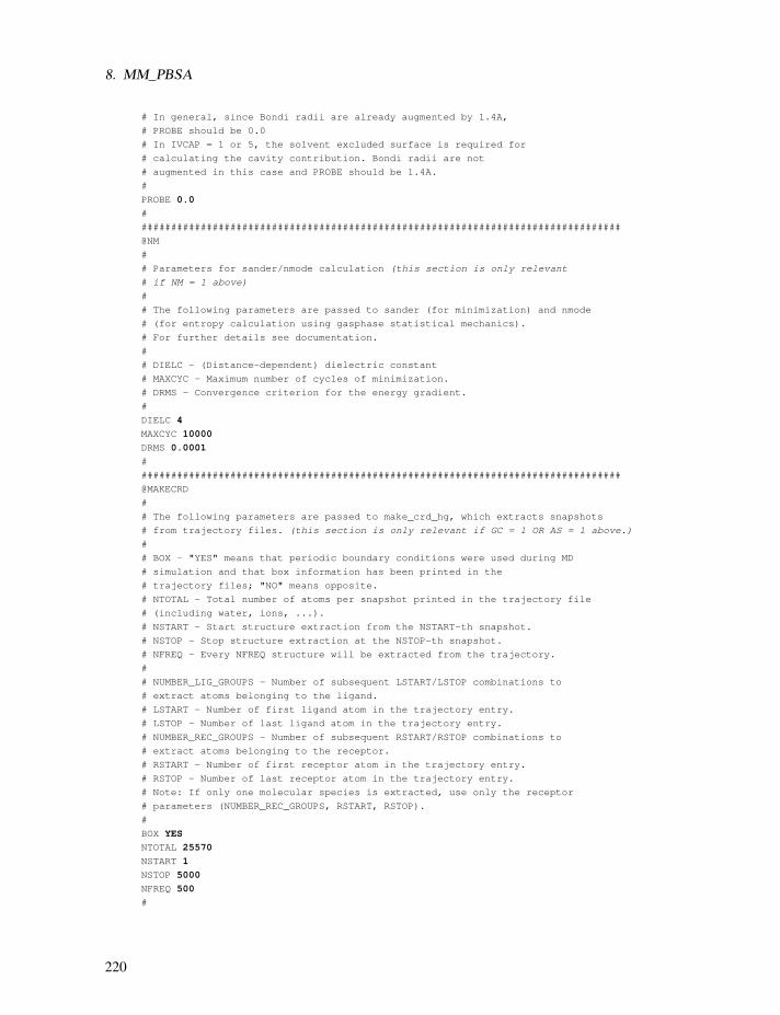
8. MM_PBSA
# In general, since Bondi radii are already augmented by 1.4A,
# PROBE should be 0.0
# In IVCAP = 1 or 5, the solvent excluded surface is required for
# calculating the cavity contribution. Bondi radii are not
# augmented in this case and PROBE should be 1.4A.
#
PROBE 0.0#
#################################################################################
@NM
#
# Parameters for sander/nmode calculation (this section is only relevant
# if NM = 1 above)
#
# The following parameters are passed to sander (for minimization) and nmode
# (for entropy calculation using gasphase statistical mechanics).
# For further details see documentation.
#
# DIELC - (Distance-dependent) dielectric constant
# MAXCYC - Maximum number of cycles of minimization.
# DRMS - Convergence criterion for the energy gradient.
#
DIELC 4MAXCYC 10000DRMS 0.0001#
#################################################################################
@MAKECRD
#
# The following parameters are passed to make_crd_hg, which extracts snapshots
# from trajectory files. (this section is only relevant if GC = 1 OR AS = 1 above.)
#
# BOX - "YES" means that periodic boundary conditions were used during MD
# simulation and that box information has been printed in the
# trajectory files; "NO" means opposite.
# NTOTAL - Total number of atoms per snapshot printed in the trajectory file
# (including water, ions, ...).
# NSTART - Start structure extraction from the NSTART-th snapshot.
# NSTOP - Stop structure extraction at the NSTOP-th snapshot.
# NFREQ - Every NFREQ structure will be extracted from the trajectory.
#
# NUMBER_LIG_GROUPS - Number of subsequent LSTART/LSTOP combinations to
# extract atoms belonging to the ligand.
# LSTART - Number of first ligand atom in the trajectory entry.
# LSTOP - Number of last ligand atom in the trajectory entry.
# NUMBER_REC_GROUPS - Number of subsequent RSTART/RSTOP combinations to
# extract atoms belonging to the receptor.
# RSTART - Number of first receptor atom in the trajectory entry.
# RSTOP - Number of last receptor atom in the trajectory entry.
# Note: If only one molecular species is extracted, use only the receptor
# parameters (NUMBER_REC_GROUPS, RSTART, RSTOP).
#
BOX YESNTOTAL 25570NSTART 1NSTOP 5000NFREQ 500#
220

8.3. Preparing the input file
NUMBER_LIG_GROUPS 0LSTART 0LSTOP 0NUMBER_REC_GROUPS 1RSTART 1RSTOP 2666#
#################################################################################
@ALASCAN
#
# The following parameters are additionally passed to make_crd_hg in conjunction
# with the ones from the @MAKECRD section if "alanine scanning" is requested.
# (this section is only relevant if AS = 1 above.)
#
# The description of the parameters is taken from Irina Massova.
#
# NUMBER_MUTANT_GROUPS - Total number of mutated residues. For each mutated
# residue, the following four parameters must be given
# subsequently.
# MUTANT_ATOM1 - If residue is mutated to Ala then this is a pointer on CG
# atom of the mutated residue for all residues except Thr,
# Ile and Val.
# A pointer to CG2 if Thr, Ile or Val residue is mutated to Ala
# If residue is mutated to Gly then this is a pointer on CB.
# MUTANT_ATOM2 - If residue is mutated to Ala then this should be zero for
# all mutated residues except Thr and VAL.
# A pointer on OG1 if Thr residue is mutated to Ala.
# A pointer on CG1 if VAL or ILE residue is mutated to Ala.
# If residue is mutated to Gly then this should be always zero.
# MUTANT_KEEP - A pointer on C atom (carbonyl atom) for the mutated residue.
# MUTANT_REFERENCE - If residue is mutated to Ala then this is a pointer on
# CB atom for the mutated residue.
# If residue is mutated to Gly then this is a pointer on
# CA atom for the mutated residue.
# Note: The method will not work for a smaller residue mutation to a bigger
# for example Gly -> Ala mutation.
# Note: Maximum number of the simultaneously mutated residues is 40.
#
NUMBER_MUTANT_GROUPS 3MUTANT_ATOM1 1480MUTANT_ATOM2 0MUTANT_KEEP 1486MUTANT_REFERENCE 1477MUTANT_ATOM2 1498MUTANT_ATOM1 1494MUTANT_KEEP 1500MUTANT_REFERENCE 1492MUTANT_ATOM1 1552MUTANT_ATOM2 0MUTANT_KEEP 1562MUTANT_REFERENCE 1549#
#################################################################################
@TRAJECTORY
#
# Trajectory names
#
# The following trajectories are used to extract snapshots with "make_crd_hg":
221

8. MM_PBSA
# Each trajectory name must be preceded by the TRAJECTORY card.
# Subsequent trajectories are considered together; trajectories may be
# in ascii as well as in .gz format.
# To be able to identify the title line, it must be identical in all files.
#
TRAJECTORY ../prod_II/md_nvt_prod_pme_01.mdcrd.gzTRAJECTORY ../prod_II/md_nvt_prod_pme_02.mdcrd.gzTRAJECTORY ../prod_II/md_nvt_prod_pme_03.mdcrd.gzTRAJECTORY ../prod_II/md_nvt_prod_pme_04.mdcrd.gzTRAJECTORY ../prod_II/md_nvt_prod_pme_05.mdcrd.gz#
################################################################################
@PROGRAMS
#
# Additional program executables can be defined here
#
#
################################################################################
8.4. Auxiliary programs used by MM_PBSA
Several programs can be used to compute numerical solutions to the Poisson-Boltzmann
equation. The default is pbsa, which is a stand-alone program that is much like sander withthe IGB = 10 option. Please see sander PB pages in Section 6.2 for detailed description. Otherprograms for computing numerical Poisson-Boltzmann results are also available, such as Del-phi,MEAD and UHBD. These could be merged into the Perl scripts developed here with a littlework. See:
• http://honiglab.cpmc.columbia.edu/ (for DELPHI)
• http://www.scripps.edu/bashford (for MEAD)
• http://adrik.bchs.uh.edu/uhbd.html (for UHBD)
8.5. APBS as an alternate PB solver in Sander
APBS is a robust, numerical Poisson-Boltzmann solver with many features (for more de-
tails see http://apbs.sourceforge.net/). APBS can be used as an alternative PB solver in sander
when compiled with sander using iAPBS. sander.APBS can be then used for implicit solvent
MD simulations, calculation of solvation energies and electrostatic properties and to generate
electrostatic potential maps for visualization. It can also be used in the MM_PBSA approach
to estimate solvation and apolar (GAMMA * SASA) energy contributions to free energies of
binding.
Please see APBS documentation (http://apbs.sourceforge.net/doc/user-guide/index.html) for
definition of APBS input parameters and iAPBS documentation (http://mccammon.ucsd.edu/iapbs/)
on how to build sander.APBS and how to use it.
To use mm_pbsa.pl script with sander.APBS the following is necessary:
• - sander.APBS must be installed in $AMBERHOME/exe directory.
222

8.5. APBS as an alternate PB solver in Sander
• - @GENERAL and @PB sections in input file need to be modified.
• - PQR files for ligand, receptor and complex need to be prepared if an
• alternate charge/radius scheme is used (which is recommended).
Input file description
The mm_pbsa.in input file which is included in the Amber distribution can be used with the
following modifications:
(1) Turn on PB and turn off GB and MS calculations in the @GENERAL section of the input
file:
@GENERAL
MM 1
GB 0
PB 1
MS 0
(2) Input file @PB section:
#
@PB
#
#
# PROC = 3 uses sander.APBS as the PB solver
# REFE - REFE = 0 is always used with sander.APBS
# INDI and EXDI are solute and solvent dielectric constants
# SCALE - grid spacing in number of grid points per A
# LINIT - no effect
# PRBRAD - solvent probe radius in A
# ISTRNG - ionic strength in mM
#
# RADIOPT - option to set up radii and charges for PB calculation:
# 0: uses the radii from prmtop files
# 2: reads in PQR files with radii/charges information from
# lig.pqr, rec.pqr and com.pqr PQR files
#
# APBS options:
# BCFL, SRFM, CHGM, SWIN, GAMMA - see APBS and iAPBS documentation for details
# GAMMA is surface tension for apolar energies (in kJ/mol/A**2),
# defaults to 0.105 (Please note the units!)
#
PROC 3
REFE 0
INDI 1.0
EXDI 80.0
SCALE 2
223

8. MM_PBSA
LINIT 1000
PRBRAD 1.4
ISTRNG 0.0
#
RADIOPT 0
#
BCFL 2
SRFM 1
CHGM 1
SWIN 0.3
GAMMA 0.105
#
PQR files
With RADIOPT=2 three PQR files are required: lig.pqr, rec.pqr and com.pqr with charge/ra-
dius information for the ligand, receptor and complex, respectively. This is the recommended
option to get better estimates of solvation energies.
The PQR files can be created with pdb2pqr utility:
pdb2pqr.py --assign-only --ff=amber com.pdb com.pqr
pdb2pqr.py --assign-only --ff=amber rec.pdb rec.pqr
pdb2pqr.py --assign-only --ff=amber lig.pdb lig.pqr
where –ff=amber is the requested force field charge/radius parameters. Several options are
available (Amber, CHARMM, PARSE, etc.) and also a user defined charge/radius scheme is
supported (with –ff=myff option).
pdb2pqr.py can be obtained from http://pdb2pqr.sourceforge.net/. PDB2PQR service is also
available on the web at http://nbcr.net/pdb2pqr/. The PDB files (com.pdb, rec.pdb and lig.pdb)
can be generated using ambpdb utility.
224

9. LES
The LES functionality for sander was written by Carlos Simmerling. It basically functions
by modifying the prmtop file using the program addles. The modified prmtop file is then usedwith a slightly modified version of sander called sander.LES.
9.1. Preparing to use LES with AMBER
The first decision that must be made is whether LES is an appropriate technique for the
system that you are studying. For further guidance, you may wish to consult published articles
to see where LES has proven useful in the past. Several examples will also be given at the end
of this section in order to provide models that you may wish to follow.
There are three main issues to consider before running the ADDLES module of AMBER.
1. What should be copied?
2. How many copies should be used?
3. How many regions should be defined?
A brief summary of my experience with LES follows.
1. You should make copies of flexible regions of interest. This sounds obvious, and in some
cases it is. If you are interested in determining the conformation of a protein loop, copy
the loop region. If you need to determine the position of a side chain in a protein after a
single point mutation, copy that side chain. If the entire biomolecule needs refinement,
then copy the entire molecule. Some other cases may not be obvious- you may need to
decide how far away from a particular site structural changes may propagate, and how far
to extend the LES region.
2. You should use as few copies as are necessary. While this doesn’t sound useful, it illus-
trates the general point–too few copies and you won’t get the full advantages of LES, and
too many will not only increase your system size unnecessarily but will also flatten the
energy surface to the point where minima are no longer well defined and a wide variety of
structures become populated. In addition, remember that LES is an approximation, and
more copies make it more approximate. Luckily, published articles that explore the sensi-
tivity of the results to the number of copies show that 3-10 copies are usually reasonable
and provide similar results, with 5 copies being a good place to start.
3. Placing the divisions between regions can be the most difficult choice when using LES.
This is essentially a compromise between surface smoothing and copy independence.
The most effective surface-smoothing in LES takes places between LES regions. This
225

9. LES
is because Na copies in region A interact with all Nb copies in region B, resulting in
Na*Nb interactions, with each scaled by 1/(Na*Nb) compared to the original interaction.
This is better both from the statistics of how many different versions of this interaction
contribute to the LES average, and how much the barriers are reduced. Remember that
since the copies of a given region do not interact with different copies of that same region,
interactions inside a region are only scaled by 1/N.
The other thing to consider is whether these enhanced statistics are actually helpful. For exam-
ple, if the copies cannot move apart, you will obtain many copies of the same conformation–
obviously not very helpful. This will also result in less effective reduction in barriers, since the
average energy barriers will be very similar to the non-average barrier. The independence of
the copies is also related to how the copies are attached. For example, different copies of an
amino acid side chain are free to rotate independently (at least within restrictions imposed by
the surroundings and intrinsic potential) and therefore each side chain in the sequence could be
placed into a separate LES region. If you are interested in backbone motion, however, placing
each amino acid into a separate region is not the best choice. Each copy of a given amino acid
will be bonded to the neighbor residues on each side. This restriction means that the copies are
not very independent, since the endpoints for each copy need to be in nearly the same places.
A better choice is to use regions of 2-4 amino acids. As the regions get larger, each copy can
start to have more variety in conformation- for example, one segment may have some copies in
a helical conformation while others are more strand-like or turn-like. The general rule is that
larger regions are more independent, though you need to consider what types of motions you
expect to see.
The best way to approach the division of the atoms that you wish to copy into regions is
to make sure that you have several LES regions (unless you are copying a very small region
such as a short loop or a small ligand). This will ensure plenty of inter-copy averaging. Larger
regions permit wider variations in structure, but result in less surface smoothing. A subtle point
should be addressed here- the statistical improvement available with LES is not a benefit in all
cases and care must be taken in the choice of regions. For example, consider a ligand exiting
a protein cavity in which a side chain acts as a gate and needs to move before the ligand canescape. If we make multiple copies of the gate, and do not copy the ligand, the ligand will
interact in an average way with the gates. If the gate was so large that even the softer copiescan block the exit, then the ligand would have to wait until ALL of the gate copies opened in
order to exit. This may be more statistically difficult than waiting for the original, single gate
to open despite the reduced barriers. Another way to envision this is to consider the ligand
trying to escape against a true probability distribution of the gate- if it was open 50% of the
time and closed 50%, then the exit may still be completely blocked. Continuum representations
are therefore not always the best choice.
Specific examples will be given later to illustrate how these decisions can be made for a
particular system.
9.2. Using the ADDLES program
The ADDLES module of AMBER is used to prepare input for simulations using LES. A
non-LES prmtop and prmcrd file are generated using a program such as LEaP. This prmtop file
is then given to ADDLES and replaced by a new prmtop file corresponding to the LES system.
226
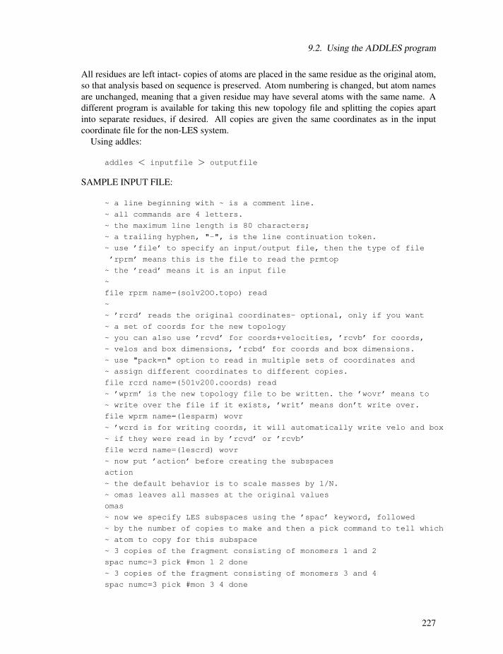
9.2. Using the ADDLES program
All residues are left intact- copies of atoms are placed in the same residue as the original atom,
so that analysis based on sequence is preserved. Atom numbering is changed, but atom names
are unchanged, meaning that a given residue may have several atoms with the same name. A
different program is available for taking this new topology file and splitting the copies apart
into separate residues, if desired. All copies are given the same coordinates as in the input
coordinate file for the non-LES system.
Using addles:
addles < inputfile > outputfile
SAMPLE INPUT FILE:
~ a line beginning with ~ is a comment line.
~ all commands are 4 letters.
~ the maximum line length is 80 characters;
~ a trailing hyphen, "-", is the line continuation token.
~ use ’file’ to specify an input/output file, then the type of file
’rprm’ means this is the file to read the prmtop
~ the ’read’ means it is an input file
~
file rprm name=(solv2OO.topo) read
~
~ ’rcrd’ reads the original coordinates- optional, only if you want
~ a set of coords for the new topology
~ you can also use ’rcvd’ for coords+velocities, ’rcvb’ for coords,
~ velos and box dimensions, ’rcbd’ for coords and box dimensions.
~ use "pack=n" option to read in multiple sets of coordinates and
~ assign different coordinates to different copies.
file rcrd name=(501v200.coords) read
~ ’wprm’ is the new topology file to be written. the ’wovr’ means to
~ write over the file if it exists, ’writ’ means don’t write over.
file wprm name=(lesparm) wovr
~ ’wcrd is for writing coords, it will automatically write velo and box
~ if they were read in by ’rcvd’ or ’rcvb’
file wcrd name=(lescrd) wovr
~ now put ’action’ before creating the subspaces
action
~ the default behavior is to scale masses by 1/N.
~ omas leaves all masses at the original values
omas
~ now we specify LES subspaces using the ’spac’ keyword, followed
~ by the number of copies to make and then a pick command to tell which
~ atom to copy for this subspace
~ 3 copies of the fragment consisting of monomers 1 and 2
spac numc=3 pick #mon 1 2 done
~ 3 copies of the fragment consisting of monomers 3 and 4
spac numc=3 pick #mon 3 4 done
227

9. LES
~ 3 copies of the fragment consisting of residues 5 and 6
spac numc=3 pick #mon 5 6 done
~ 2 copies of the side chain on residue 1
~ note that this replaces each of the side chains ON EACH OF THE 3
~ COPIES MADE ABOVE with 2 copies - net 6 copies
~ each of the 3 copies of residue 1-2 has 2 side chain copies.
~ the ’#sid’ command picks all atoms in the residue except
~ C,O,CA,HA,N,H and HN.
spac numc=2 pick #sid 1 1 done
spac numc=2 pick *sid 2 2 done
spac numc=2 pick #sid 3 3 done
spac numc=2 pick #sid 4 4 done
spac numc=2 pick #sid 5 5 done
~ use the *EOD to end the input
*EOD
What this does: all of the force constants are scaled in the new prmtop file by 1/N for N copies,
so that this scaling does not need to be done for each pair during the nonbond calculation.
Charges and VDW epsilon values are also scaled. New bond, angle, torsion and atom types
are created. Any of the original types that were not used are discarded. Since each LES copy
should not interact with other copies of the SAME subspace, the other copies are placed in the
exclusion list. If you define very large LES regions, the exclusion list will get large and you
may have trouble with the fixed length for this entry in the prmtop file- currently 8 digits.
The coordinates are simply copied - that means that all of the LES copies initially occupy the
same positions in space. In this setup, the potential energy should be identical to the original
system- this is a good test to make sure everything is functioning properly. Do a single energy
evaluation of the LES system and the original system, using the copied coordinate file. All
terms should be nearly identical (to within machine precision and roundoff). With PME on non-
neutral systems, all charges are slightly modified to neutralize the system. For LES, there are
a different number of atoms than in the original system, and therefore this charge modification
to each atom will differ from the non-LES system and electrostatic energies will not match
perfectly.
IMPORTANT: After creating the LES system, the copies will all feel the same forces, and
since the coordinates are identical, they will move together unless the initial velocities are dif-
ferent. If you are initializing velocities using INIT=3 and TEMPI>0, this is not a problem. Inorder to circumvent this problem, addles slightly (and randomly) modifies the copy velocities
if they were read from the coordinate input file. If the keyword "nomodv" is specified, the
program will leave all of the velocities in the same values as the original file. If you do not
read velocities, make sure to assign an initial non-zero temperature to the system. You should
think about this and change the behavior to suit your needs. In addition, the program scales
the velocities by sqrt(N) for N copies to maintain the correct thermal energy (mv2), but only
when the masses are scaled (not using omas option). Again, this requires some thought and
you may want different behavior. Regardless of what options are used for the velocities, further
equilibration should be carried out. These options are simple attempts to keep the system close
to the original state. [224]
Sometimes it is critical that different copies can have different initial coordinates (NEB for
example), this is why the option "pack" is added to command rcrd(rcvd,rcvb,rcbd). To use this
228

9.3. More information on the ADDLES commands and options
option, user need first concatenate different coordinates into a single file, and use "pack=n" to
indicate how many sets of coordinates there are in the file, like the following example:
file rcrd name=(input.inpcrd) pack=4 read
Then addles will assign coordinates averagely. For example, if 4 sets coordinates exists in input
file, and 20 copies are generated, then copy 1-5 will have coordinate set 1, copy 6-10 will have
coordinates set 2, and so on. Note this option can’t work with multiple copy regions now.
It is important to understand that each subsequent pick command acts on the ORIGINAL
particle numbers. Making a copy of a given atom number also makes copies of all copies of
that atom that were already created. This was the simplest way to be able to have a hierarchical
LES setup, but you can’t make extra copies of part of one of the copies already made. I’m
not sure why you would want to, or if it is even correct to do so, but you should be warned.
Copies can be anything -spanning residues, copies of fragments already copied, non-contiguous
fragments, etc. Pay attention to the order in which you make the copies, and look carefully at
the output to make sure you get what you had in mind. Addles will provide a list at the end of
all atoms, the original parent atom, and how many copies were made.
There are array size limits in the file SIZE.h, I apologize in advance for the poor documenta-
tion on these. Mail [email protected] if you have any questions or problems.
9.3. More information on the ADDLES commands andoptions
file: open a file, also use one of
rcrd: read coords from this file
rcvd: read coords + velo from file
rcvb: read coords, velo and box from file
wcrd: write coords (and more if rcvd, rcvb) to file
wprm: write new topology file
action: start run, all of the following options must come AFTER action
nomodv: do NOT slightly randomize the velocities of the copies
spac: add a new subspace definition, using a pick command (see below).
follow with numc=# pickcmd where # is the number of copies to make
and pickcmd is a pick command that selects the group of atoms to copy.
omas: leave all masses at original values (otherwise scale 1/N)
pimd: write an prmtop file for PIMD simulation, which contains a much smaller non-
bond exclusion list, atoms from other copy will not be included in this non-bond
exclusion list.
229

9. LES
Syntax for ’pick’ commandsCurrently, the syntax for picking atoms is somewhat limited. Simple Boolean logic is fol-
lowed, but operations are carried out in order and parentheses are not allowed.
#prt A B picks the atom range from A to B by atom number
#mon A B picks the residue range from A to B by residue number
#cca A B picks the residue range from A to B by residue number, but dividing the residue
between CA and C; the CO for A is included, and the CO for monomer B is not.
See Simmerling and Elber, 1994 for an example of where this can be useful.
chem prtc A picks all atoms named A, case sensitive
chem mono A picks all residues named A, case sensitive
Completion wildcards are acceptable for names: H* picks H, HA, etc. Note that H*2 will select
all atoms starting with H and ignore the 2.
Boolean logic:
| or atoms in either group are selected
& and atoms must be in both groups to be selected
!= not A != B will pick all atoms in A that are NOT in B
The user should carefully check the output file to ensure that the proper atoms were selected.
Examples:
pick commandatoms selected
pick #mon 4 19 done all atoms in residues 4 through 19
pick #mon 1 50 & chem mono GLY done only GLY in residues 1 to 50
pick chem mono LYS | chem mono GLU done any GLU or LYS residue
pick #mon 1 5 != #prt 1 3 done residues 1 to 5 but not atoms 1 to 3
so, a full command to add a new subspace (LES region) with 4 copies of atoms 15 to 35 is:
spac numc=4 pick #prt 15 35 done
9.4. Using the new topology/coordinate files with SANDER
These topology files are ready to use in Sander with one exception: all of the FF parameters
have been scaled by 1/N for N copies. This is done to provide the energy of the new system as
an average of the energies of the individual copies (note that it is an average energy or force,
not the energy or force from an average copy coordinate). However, one additional correction is
required for interactions between pairs of atoms in the same LES region. Sander will make these
corrections for you, and this information is just to explain what is being done. For example,
consider a system where you make 2 copies of a sidechain in a protein. Each charge is scaled
by 1/2. For these atoms interacting with the rest of the system, each interaction is scaled by
230
9.5. Using LES with the Generalized Born solvation model
1/2 and there are 2 such interactions. For a pair of particles inside the sub-space, however, the
interaction is scaled by 1/2*1/2=1/4, and since the copies do not interact, there are only 2 such
interactions and the sum does not correspond to the correct average. Therefore, the interaction
must be scaled up by a factor of N. When the PME technique is requested, this simple scaling
cannot be used since the entire charge set is used in the construction of the PME grid and
individual charges are not used in the reciprocal space calculation. Therefore, the intra-copy
energies and forces are corrected in a separate step for PME calculations. Sander will print
out the number of correction interactions that need to be calculated, and very large amounts of
these will make the calculation run more slowly. PME also needs to do a separate correction
calculation for excluded atom pairs (atoms that should not have a nonbonded interaction, such
as those that are connected by a bond). Large LES regions result in large numbers of excluded
atoms, and these will result in a larger computational penalty for LES compared to non-LES
simulations. For both of these reasons, it is more efficient computationally to use smaller LES
regions- but see the discussion above for how region size affects simulation efficiency. These
changes are included in the LES version of Sander (sander.LES). Each particle is assigned a LES
’type’ (each new set of copies is a new type), and for each pair of types there is a scaling factor
for the nonbond interactions between LES particles of those types. Most of the scaling factors
are 1.0, but some are not - such as the diagonal terms which correspond to interactions inside a
given subspace, and also off-diagonal terms where only some of the copies are in common. An
example of this type is the side chain example given above- each of the 3 backbone copies has 2
sidechains, and while interactions inside the side chains need a factor of 6, interactions between
the side chain and backbone need a factor of 3. This matrix of scaling factors is stored in the
new topology file, along with the type for each atom, and the number of types. The changes
made in sander relate to reading and using these scale factors.
9.5. Using LES with the Generalized Born solvation model
LES simulations can be performed using the GB solvent model, with some limitations. Com-
pared to LES simulations in explicit water, using GB with LES provides several advantages.
The most important is how each of the copies interacts with the solvent. With explicit water,
the water is normally not copied and therefore interacts in an average way with all LES copies.
This has important consequences for solvation of the copies. If the copies move apart, water
cannot overlap any of them and therefore the water cavity will be that defined by the union of
the space occupied by the copies. This has two consequences. First, moving the copies apart
requires creation of a larger solvent cavity and therefore copies have a greater tendency to re-
main together, reducing the effectiveness of LES. Second, when the copies do move apart, each
copy will not be individually solvated.
These effects arise because the water interacts with all of the copies; for each copy to be
solvated independently of the other copies would require copying the water molecules. This
is normally not a good idea, since copying all of the water would result in very significant
computational expense. Copying only water near the solute would be tractable, but one would
need to ensure that the copied waters did not exchange with non-LES bulk waters.
Using GB with LES largely overcomes these problems since each copy can be individually
solvated with the continuum model. Thus when one copy moves, the solvation of the other
copies are not affected. This results in a more reasonable solvation of each copy and also
231

9. LES
improves the independence of the copies. Of course the resulting simulations do retain all of
the limitations that accompany the GB models.
The current code allows igb values of 1, 5 or 7 when using LES. Surface area calculations are
not yet supported with LES. Only a single LES region is permitted for GB+LES simulations.
A new namelist variable was introduced (RDT) in sander to control the compromise of speed
and accuracy for GB+LES simulations. The article referenced below provides more detail
on the function of this variable. RDT is the effective radii deviation threshold. When using
GB+LES, non-LES atoms require multiple effective Born radii for an exact calculation. Using
these multiple radii can significantly increase calculation time required for GB calculations.
When the difference between the multiple radii for a non-LES atom is less than RDT, only a
single effective radius will be used. A value of 0.01 has been found to provide a reasonable
compromise between speed and accuracy, and is the default value. Before using this method, it
is strongly recommended that the user read the article describing the derivation of the GB+LES
approach. [225]
9.6. Case studies: Examples of application of LES
9.6.1. Enhanced sampling for individual functional groups: Glucose
The first example will deal with enhancing sampling for small parts of a molecule, such as
individual functional groups or protein side chains. In this case we wanted to carry out separate
simulations of α and β (not converting between anomers, only for conversions involving rota-tions about bonds) glucose, but the 5 hydroxyl groups and the strong hydrogen bonds between
neighboring hydroxyls make conversion between different rotamers slow relative to affordable
simulation times. The eventual goal was to carry out free energy simulations converting be-
tween anomers, but we need to ensure that each window during the Gibbs calculation would be
able to sample all relevant orientations of hydroxyl groups in their proper Boltzmann-weighted
populations. We were initially unsure how many different types of structures should be popu-
lated and carried out non-LES simulations starting from different conformations. We found that
transitions between different conformations were separated by several hundred picoseconds, far
too long to expect converged populations during each window of the free energy calculation.
We therefore decided to enhance conformational sampling for each hydroxyl group by mak-
ing 5 copies of each hydroxyl hydrogen and also 5 copies of the entire hydroxymethyl group.
Since the hydroxyl rotamer for each copy should be relatively independent, we decided to place
each group in a different LES region. This meant that each hydroxyl copy interacted with all
copies of the neighboring groups, with a total of 5*5*5*5*5 or 3125 structural combinations
contributing to the LES average energy at each point in time. The input file is given below.
file rprm name=(parm.solv.top) read
file rcvb name=(glucose.solv.equ.crd) read
file wprm name=(les.prmtop) wovr
file wcrd name=(glucose.les.crd) wovr
action
omas
~ 5 copies of each hydroxyl hydrogen- copying oxygen will make no difference
~ since they will not be able to move significantly apart anyway
232

9.6. Case studies: Examples of application of LES
spac numc=5 pick chem prtc HO1 done
spac numc=5 pick chem prtc HO2 done
spac numc=5 pick chem prtc HO3 done
spac numc=5 pick chem prtc HO4 done
~ take the entire hydroxy methyl group
spac numc=5 pick #prt 20 24 done
*EOD
This worked quite well, with transitions now occurring every few ps and populations that were
essentially independent of initial conformation. [226]
9.6.2. Enhanced sampling for a small region: Application of LES to anucleic acid loop
In this example, we consider a biomolecule (in this case a single RNA strand) for which part
of the structure is reliable and another part is potentially less accurate. This can be the case
in a number of different modeling situations, such as with homologous proteins or when the
experimental data is incomplete. In this case two different structures were available for the same
RNA sequence. While both structures were hairpins with a tetraloop, the loop conformations
differed, and one was more accurate. We tested whether MD would be able to show that one
structure was not stable and would convert to the other on an affordable timescale.
Standard MD simulations of several ns were not able to undergo any conversion between
these two structures (the initial structure was always retained). Since the stem portion of the
RNA was considered to be accurate, LES was only applied to the tetraloop region. In this case,
both of the ends of the LES region would be attached to the same locations in space, and there
was no concern about copies diffusing too far apart to re-converge to the same positions after
optimization. The issues that need to be addressed once again are the number of copies to
use, and how to place the LES region(s). I usually start with the simplest choices and used 5
LES copies and only a single LES region consisting of the entire loop. If each half of the loop
was copied, then it might become too crowded with copies near the base-pair hydrogen bondsand conformational changes that required moving a base through this regions could become
even more difficult (see the background section for details). Therefore, one region was chosen,
and the RNA stem, counterions and solvent were not copied. The ADDLES input file is given
below.
file rprm name=(prm.top) read
file rcvb name=(rna.crd) read
file wprm name=(les.parm) wovr
file wcrd name=(les.crd) wovr
action
omas
~ copy the UUCG loop region- residues 5 to 8.
~ pick by atom number, though #mon 5 8 would work the same way
spac numc=5 pick #prt 131 255 done
*EOD
Subsequent LES simulations were able to reproducibly convert from what was known to be the
incorrect structure to the correct one, and stay in the correct structure in simulations that started
233
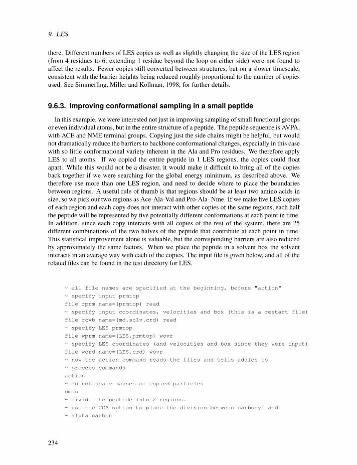
9. LES
there. Different numbers of LES copies as well as slightly changing the size of the LES region
(from 4 residues to 6, extending 1 residue beyond the loop on either side) were not found to
affect the results. Fewer copies still converted between structures, but on a slower timescale,
consistent with the barrier heights being reduced roughly proportional to the number of copies
used. See Simmerling, Miller and Kollman, 1998, for further details.
9.6.3. Improving conformational sampling in a small peptide
In this example, we were interested not just in improving sampling of small functional groups
or even individual atoms, but in the entire structure of a peptide. The peptide sequence is AVPA,
with ACE and NME terminal groups. Copying just the side chains might be helpful, but would
not dramatically reduce the barriers to backbone conformational changes, especially in this case
with so little conformational variety inherent in the Ala and Pro residues. We therefore apply
LES to all atoms. If we copied the entire peptide in 1 LES regions, the copies could float
apart. While this would not be a disaster, it would make it difficult to bring all of the copies
back together if we were searching for the global energy minimum, as described above. We
therefore use more than one LES region, and need to decide where to place the boundaries
between regions. A useful rule of thumb is that regions should be at least two amino acids in
size, so we pick our two regions as Ace-Ala-Val and Pro-Ala- Nme. If we make five LES copies
of each region and each copy does not interact with other copies of the same regions, each half
the peptide will be represented by five potentially different conformations at each point in time.
In addition, since each copy interacts with all copies of the rest of the system, there are 25
different combinations of the two halves of the peptide that contribute at each point in time.
This statistical improvement alone is valuable, but the corresponding barriers are also reduced
by approximately the same factors. When we place the peptide in a solvent box the solvent
interacts in an average way with each of the copies. The input file is given below, and all of the
related files can be found in the test directory for LES.
~ all file names are specified at the beginning, before "action"
~ specify input prmtop
file rprm name=(prmtop) read
~ specify input coordinates, velocities and box (this is a restart file)
file rcvb name=(md.solv.crd) read
~ specify LES prmtop
file wprm name=(LES.prmtop) wovr
~ specify LES coordinates (and velocities and box since they were input)
file wcrd name=(LES.crd) wovr
~ now the action command reads the files and tells addles to
~ process commands
action
~ do not scale masses of copied particles
omas
~ divide the peptide into 2 regions.
~ use the CCA option to place the division between carbonyl and
~ alpha carbon
234

9.6. Case studies: Examples of application of LES
~ use the "or" to make sure all atoms in the terminal residues
~ are included since the CCA option places the region division at C/CA
~ and we want all of the terminal residue included on each end
~
~ make 5 copies of each half
~ "spac" defines a LES subspace (or region)
spac numc=5 pick #cca 1 3 | #mon 1 1 done
spac numc=5 pick #cca 4 6 | #mon 6 6 done
~ the following line is required at the end
*EOD
This example brings up several important questions:
1. Should I make LES copies before or after adding solvent? Since LEaP is used to add
solvent, and LEaP will not be able to load and understand a LES structure, you must run
ADDLES after you have solvated the peptide in LEaP. ADDLES should be the last step
before running SANDER.
2. Which structure should be used as input to ADDLES? If you will also be carrying out
non-LES simulations, then you can equilibrate the non-LES simulation and carry out
any amount of production simulation desired before taking the structure and running
ADDLES. At the point you may switch to only LES simulations, or continue both LES
and non-LES from the same point (using different versions of SANDER). Typically I
equilibrate my systemwithout LES to ensure that it has initial stability and that everything
looks OK, then switch to LES afterward. This way I separate any potential problems from
incorrect LES setup from those arising from problems with the non-LES setup, such as
in initial coordinates, LEaP setup, solvent box dimensions and equilibration protocols.
3. How can I analyze the resulting LES simulation? This is probably the most difficult
part of using LES. With all of the extra atoms, most programs will have difficulty. For
example, a given amino acid with LES will have multiple phi and psi backbone dihedral
angles. There are basically two options: first, you can process your trajectory such that
you obtain a single structure (non-LES). This might be just extracting one of the copies,
or it might be one by taking the average of the LES copies. After that, you can proceed to
traditional analysis but must keep in mind that the average structure may be non-physical
and may not represent any actual structure being sampled by the copies, especially if they
move apart significantly. A better way is to use LES-friendly analysis tools, such as those
developed in the group of Carlos Simmerling. The visualization program MOIL-View
(http://morita.chem.sunysb.edu/carlos/moil-view.html) is one example of these programs,and has many analysis tools that are fully LES compatible. Read the program web page
or manual for more details. A version of MOIL-View is included on the Amber 8 CD.
1.7. Unresolved issues with LES in AMBER
1. Sander can’t currently maintain groups of particles at different temperatures (important
for dynamics, less so for optimization.) [227, 228] Users can set temp0les to maintain allLES atoms at a temperature that is different from that for the system as a whole, but all
LES atoms are then coupled to the same bath.
235

9. LES
2. Initial velocity issues as mentioned above- works properly, user must be careful.
3. Analysis programsmay not be compatible. See http://morita.chem.sunysb.edu/carlos/moil-view.html for an LES-friendly analysis and visualization program.
4. Visualization can be difficult, especially with programs that use distance-based algo-
rithms to determine bonds. See #3 above.
5. Water should not be copied- the fast water routines have not been modified. For most
users this won’t matter.
6. Copies should not span different ’molecules’ for pressure coupling and periodic imaging
issues. Copies of an entire ’molecule’ should result in the copies being placed in new,
separate molecules- currently this is not done. This would include copying things such
as counterions and entire protein or nucleic acid chains.
7. Copies are placed into the same residue as the original atoms- this can make some
residues much larger than others, and may result in less efficient parallelization with
algorithms that assign nonbond workload based on residue numbers.
236

10. Divcon
10.1. Introduction
DivCon is a linear scaling semi-empirical program for calculation of energies, charges and
geometries of systems up to 20,000 atoms. Available features include:
1. Linear scaling Divide and Conquer (D&C) calculations. [213–215]
2. Cubic scaling standard calculations. [103, 104, 106]
3. Single point AM1, [104] PM3, [103] or MNDO [106] calculations.
4. Geometry Optimization (steepest decent, conjugate gradient, BFGS, and LBFGS avail-
able)
5. Mulliken, CM1 [229] and CM2 [230] charge analysis
6. Nuclear Magnetic Resonance prediction and simulation
The program was mainly developed by Steve Dixon. His work includes the development of
the semiempirical Divide and Conquer algorithm, implementation of the D&C and standard
energy and gradient calculations, geometry optimization routines, Mulliken charge analysis,
cluster based subsetting strategy and front end of the program. Arjan van der Vaart added the
Monte Carlo routines (single and multi processing), Particle Mesh Ewald routines, grid based
subsetting routines, extension of the cluster based subsetting schemes, CM1 and CM2 charge
analysis, density matrix build routines, density of state analysis, frozen density matrix routines
the interaction energy decomposition routines (serial and parallel), and Talman’s algorithm.
Valentin Gogonea added the SCRF routines. Jim Vincent parallellized the single point energy
and geometry optimization routines, the transition state routines and the sodium parameters.
Ed Brothers added dipole and ionization potential routines, the parametrization routines and
the sodium parameters. Dimas Sua’rez added the LBFGS optimization routines, the transition
state routines and the frequency calculation routines. Ning Liao has added support for a na-
tive Poisson-Boltzmann(PB) implementation, and Andrew Wollocott has added support for re-
strained minimization. Subsequently, Hwanho Kim and Lance Westerhoff of QuantumBio Inc.
fully audited, optimized, and modernized much of the source code in order to impart increased
stability and extensibility upon the application. QuantumBio continues to develop DivCon with
these same principles in mind.
10.2. Getting Started
DivCon05 packaged with AMBER is capable of performing mixed quantum mechanics/-
molecular mechanics(QM/MM) linear scaling Semi-Empirical calculations. This allows large
237

10. Divcon
patches of a protein to be studied at a quantum mechanical level of theory while still retaining
charge effects from the surrounding protein. DivCon contains many options that may aid in
the simulation of protein systems with large quantum patches whose keywords can be found
within this manual for a more detailed discussion of their applications and uses. This section
will provide a brief overview of how to get started using DivCon with AMBER. This section
should only be used as a starting point for QM/MM calculations involving DivCon after which
the manual may be consulted for more options and uses. These examples should be a good
starting point for the divcon.in files needed for these QM/MM jobs. DivCon has several default
keywords that can be found in the Keywords section of the manual that are good for general
uses, but can easily be changed if desired.
To install Divcon, you need to do the following:
cd $AMBERHOME/src/dcqtp
make clean
make install
10.2.1. Standard Jobs
These jobs are run without the use of DivCon’s linear scaling feature. Standard should only
be used for smaller patches(around 250-300 atoms), after which it will become quite expensive.
Below there is a simple divcon.in file for use in standard jobs when running QM/MM calcula-
tions. This may not be the best input file for every application, just a place to get started when
using DivCon. The manual should be consulted for a more detailed discussion of the keywords
used in this divcon.in file.
DIRECT CARTESIAN AM1 CHARGE=0.0 &
STANDARD CUTBOND=9.0 SHIFT=3.0
END_COORD
10.2.2. Divide and Conquer Jobs
One of DivCon’s best features is the ability to scale linearly to system size for Semi-Empirical
calculations. This is an excellent feature for larger systems(>∼300 atoms) which maybe notbe able to be calculated in other programs. Using divide and conquer requires that the system
be broken into smaller subsystems which is done by keywords in the divcon.in file. The most
common, and easiest, clustering system for proteins is to make each residue a subsystem. These
subsystems are then surrounded by a buffer to be considered in the subsystem calculations, the
size of which can be declared in the divcon.in file. For more information on the Divide and
Conquer or buffering methods references 1,2, and 3 should be consulted. Again, the example
below is a place to get started on using DivCon and more detailed calculations may require
different keywords and/or values which can be found in the Keywords section of this manual.
DIRECT CARTESIAN AM1 CHARGE=0.0 &
RESIDUE CLUSTER CUTBOND=9.0 SHIFT=3.0
END_COORD
CLUSTER
NCORE=1
238

10.3. Keywords
DBUFF1=4.5 DBUFF2=2.0
END_CLUSTER
More detailed information on all these keywords and more can be found within the Keywords
section. Also, the keywords that are used by default can be found in the manual along with
directions how to change and use them. These simple examples will give a good starting point
for doing general QM/MM calculations using DivCon and should be acceptable in many cases,
but are not, by any means, a complete input file for DivCon.
10.3. Keywords
10.3.1. Hamiltonians
AM1 AM1 Hamiltonian to be used.
PM3 PM3 Hamiltonian to be used.
MNDO MNDO Hamiltonian to be used.
MNDO/d MNDO/d Hamiltonian to be used.
PDDG-PM3 PDDG-PM3 Hamiltonian to be used.
NOTE: One Hamiltonian must be selected. There is no default.
10.3.2. Convergence Criterion
ETEST=FLOAT user defined geometry optimization energy change criterion. Default : 0.002
kcal/mol.
GTEST=FLOAT user defined maximum gradient component criterion. Default : 0.500 kcal/
(mol A).
XTEST=FLOAT user defined geometry optimization coordinate change criterion. Default :
0.001 A / 0.001 degrees.
10.3.3. Restrained Atoms
BELLY A subset of the atoms in the system, the belly group, will be allowed to relax their
position during optimization while the rest of the atoms will be kept at fixed posi-
tions by zeroing the corresponding forces. Currently, the BELLY option requires
optimization of both minimum or transition structures using cartesian coordinates
(a FREQ calculation can be also subjected to the BELLY option).
The BELLY parameter must be included in the input file in order to specify the BELLY group.
Two formats are possible:
BELLY
ATOMS 144-178 310-332
END_BELLY
239
10. Divcon
This means that the BELLY group of moving atoms will be constituted from atom 144 to atom
178, and from atom 310 to atom 332. Alternatively, the BELLY group can be selected using
residue numbering:
BELLY
RESIDUES 10-13 20
END_BELLY
Only residues from 10 to 13 and residue 20 will be allowed to move during minimization.
10.3.4. Output
PRTSUB print subsystem atom lists.
PRTVEC print final eigenvectors. All eigenvectors and eigenvalues will be printed by de-
fault. If the input file contains PRTVEC parameters, only some eigenvectors will
be printed:
PRTVEC
1-458 all
558-960 -15.0 -10.0
45-460 ef 10.0
END_PRTVEC
The first line indicates that only the eigenvectors for atoms 1-458 need to be printed.
These are all eigenvectors when a standard calculation is performed. For a D&C
calculations, these are the eigenstates for subsystems that contain atoms 1-458.
The second line indicates that the eigenstates for atoms 558 through 960 will be
printed if the associated eigenvalues are between ?15.0 and -10.0 eV. The third line
indicates that the eigenvectors of atoms 45-460 will be printed if the associated
eigenvalues are within 10 eV of the Fermi energy.
DOS perform a density of state analysis. By default, a DOS analysis will be performed
on all eigenvalues for all atoms, with interval of 0.5 eV. Intervals and extend of the
DOS analysis can be set by the DOS parameters:
DOS
1-435 0.2
1015-4452 0.3
END_DOS
Here the DOS will be printed for all subsystems that contain atoms 1-435 with
interval of 0.2 eV and for all subsystems that contain atoms 1015 through 4452
with interval of 0.3 eV. Note that for a standard calculation the DOS will always
extend over all atoms.
DIPOLE calculate the magnitude of the molecular dipole moment using all three charge
methods.
240
10.3. Keywords
IP calculate ionization potential
HOMOLUMO calculate homo-lumo gap. For a D&C run, the homo-lumo gap of all subsys-
tems will be printed.
PRTCOORDS print atomic coordinates .
PRTPAR Print the AM1/PM3/MNDO parameters for all atom types that are found in the
input file.
SCREEN output vital information to screen. If not included DivCon will run silently and
only reture access to the user once the job is complete.
WRTPDB write final coordinates of an optimization in a "standard" pdb format.
DUMP=INT write restart file (divcon.rst) every INT cycles.
PDUMP=INT write density matrix file (divcon.dmx) every INT SCF iteration
SNAPGEOM Write coordinates during energy optimization (divcon_snapshot.N) at every N-th
optimization step. This can be useful when optimizing very large systems.
TRAJECTORY dump coordinates to trajectory file (divcon.trj) at restart points.
GEOCALC Calculates geometric parameters. Input takes the form (after the END_COORD
line):
GEO
DISTANCE
1-2
END_DISTANCE
ANGLE
1-2-3
END_ANGLE
DIHEDRAL
1-2-4-3
END_DIHEDRAL
END_GEO
Note that if an equals sign is included after the atom numbers (i.e. 1-2=2.0) then a
set of differences between the calculated values and these numbers are returned.
ERROR Calculates the difference between accepted and calculated values. An example list
is shown below, with each component being explained afterward. Note this is only
usable with standard calculations, and this list follows the END_COORDS line.
ERROR
HEAT=FLOAT
IP=FLOAT
DIPOLE=FLOAT
ASSOCIATION=FLOAT
241

10. Divcon
FILExINTEGER
FILExINTEGER
END_ASSOC
ETOTDIFF=FLOAT
FILExINTEGER
FILExINTEGER
END_ETOTDIFF
END_ERROR
HEAT is the heat of formation in kcal/mol. IP is ionization potential. DIPOLE is
the Mulliken dipole. ASSOCIATION is the energy of association, and the lines
following it are the files to be used to calculate it. For instance, if the association
energy of a methanol-2 water complex was to calculated, and methanol was in
divcon001.in and water was in divcon002.in, the values on the two subsequent line
would be 1x1 and 2x2. ETOTDIFF is the total energy difference, and it’s files are
designated the same way. Note also that a geometry list can be placed inside the
ERROR/END_ERROR delimiters using the format given above.
ZMAKE output a z-matrix using the DivCon z-matrix format. Note that this uses the first
three atoms as the defining atoms, and thus they may not be collinear.
10.3.5. General
ADDMM add MM correction to peptide torsional barrier. (on by default)
NOMM do not use MM correction to peptide torsional barrier.
CARTESIAN Cartesian coordinate format. DivCon reads cartesian coordinates in the format
shown in the following example:
1 N -0.26120 -0.98976 0.00000
2 C 0.64694 0.01940 0.00000
3 C -0.47100 1.06738 0.00000
4 C -1.44202 -0.13945 0.00000
5 O 1.83331 0.04003 0.00000
6 H -0.13870 -1.97802 0.00000
7 H -0.49385 1.68899 -0.88436
8 H -0.49385 1.68899 0.88436
9 H -2.05887 -0.23715 -0.88402
10 H -2.05887 -0.23715 0.88402
Coordinates are in A. The specification of symbols and coordinates is format free and the max-
imum characters per line is 80.
RMIN=FLOAT The minimum allowed distance between atoms (results in an error for single
point calculations and geometry optimizations, configuration will be rejected in an
MC-run when a smaller distance is encountered).
242

10.3. Keywords
ECRIT=FLOAT set the convergence for the energy in units of eV. (default value is 4x10⁻⁶
eV). The actual value of ECRIT will be relaxed if the gradient norm is large and
the structure is not tiny. This should speed up convergence without any loss of
accuracy
DCRIT=FLOAT set the convergence for the density matrix in atomic units (default value 5x10-
4 e). The actual value of DCRIT will be relaxed if the gradient norm is large and
the structure is not tiny. This should speed up convergence without any loss of
accuracy.
DESCF=FLOAT related to ECRIT in that it defines the SCF energy convergence criterion.
However, unlike ECRIT, this values is considered absolute(in eV). In affect, the
SCF calculation will not stop until this criterion is reached.
DPSCF=FLOAT related to DCRIT in that it defines the SCF energy convergence criterion.
However, unlike DCRIT, this values is considered absolute(in eV). In affect, the
SCF calculation will not stop until this criterion is reached.
CUTREPUL=FLOAT set the [xy|xy], [xz|xz], [xx|yy], [xx|zz],[zz|xx], [xx|xx] and [zz|zz] in-tegrals to zero when the interatomic distance is larger than FLOAT. The CUTRE-
PUL keyword can be used to speed up a DivCon simulation by limiting the number
of calculations performed.
CUTBOND=FLOAT cutoff bonding for the H, P and F matrices beyond FLOAT angstroms.
The CUTBOND keyword can be used to speed up a DivCon simulation by limiting
the number of calculations performed.
DIRECT causes all 2-electron integrals to be kept in memory and recalculated at each step
instead of being written out to file. This is the suggested approad as generally with
how fast processor are today and how much memory users have at their disposal,
accessing disk may be more expensive.
FULLSCF turns off pseudo diagonalizations and turns on full diagonalizations. This is more
expensive than pseudo diagonalizations but may be necessary sometimes.
RESIDUE stores residue pointers within DivCon. Also requires that the user denote the be-
ginning of each residue in the input file by using the "RES" delimiter after the "z"
coordinate.
CHKRES check inter-atomic distances for each residue.
TEMPK=FLOAT user defined divide and conquer temperature. Units are Kelvin, and default
is 1000K.
TESTRUN do setup work and stop before first energy evaluation.
TMAX=FLOAT user defined maximum CPU time in seconds.
SHIFT=FLOAT user defined initial dynamic level shift parameter, in eV. [231]
XYZSPACE do all operations in xyz space.
243

10. Divcon
MAXIT=INT Set the maximum number of SCF iterations (default: 100). If it takes more than
100 SCF iterations to converge, it is generally thought that the system will probably
not converge and is exhibiting problems.
DOUBLE=INT Perform a double SCF step during a certain number (int) of SCF iterations. If
INT=0, a double SCF will be done for every SCF iteration (only for non-geometry
optimizations). This will aid in convergence as it guarantees that the values cal-
culated at each step are based completely on the current step. By default the first
step of an SCF calculation will be a double. Please note, using DOUBLE will
significantly increase the CPU time required to execute a DivCon job.
1SCF Perform only the first SCF iteration, i.e. calculate the energy through E = 0.5(H+F)P.
Note that this is not equivalent to MAXIT=1, since no diagonalization is per-
formed.
GUESS Build the initial density matrix from one or more density matrix files. These files
are listed by means of the GUESS parameters:
GUESS
A.dmx
b.dmx
END_GUESS
Build the initial density matrix from the files A.dmx and b.dmx. The density matrix
elements of atoms 1 through a are read from A.dmx, for atoms a+1 through n from
file b.dmx.
GUESS
2-10 A.dmx 33-41 f
20-30 b.dmx 1-11
END_GUESS
Density matrix information for atoms 2-10 is read from the density matrix elements
of atoms 33-41 of file A.dmx, density matrix information for atoms 20-30 is read
from the density matrix elements of atoms 1- 11 from file b.dmx. Missing density
matrix elements are auto-initialized and a correction will be applied to constrain
the total number of electrons. The density matrix elements of atoms 2-10 will
be kept constant during the SCF iterations by using the Frozen Density Matrix
approximation. [232] It is imperative that the number of orbitals on a certain atom
in the divcon.in file and density matrix file are the same, i.e. the number of orbitals
on atom 2 from divcon.in and atom 33 from A.dmx should be identical.
Note that the maximum length of a density matrix file name is 20 characters, no
dashes ("-") are allowed in the density matrix file name.
INTGLS=string The INTGLS keyword can have two values. If the value is "INTGLS=TALMAN"
then the Talmanmethod of integrals will be used. If the Value is "INTGLS=STEWART"
then the Stewart integrals will be used. The default, and recommended value is Tal-
man integrals as this approach has been found to be the most stable and accurate.
244

10.3. Keywords
PUSH Only in combination with the CLUSTER keyword (page 22) and when multiple
cores (i.e. multiple cluster groups) are defined. Push the different cluster groups
apart. Default is 106 A, the user can define this distance by using PUSH=FLOAT.
When more than two cluster groups are defined, each group is place on a gridpoint
with gridspacing of 106 A or the user defined value.
10.3.6. Gradient
GRADIENT output final gradient. (Note: The gradient for MC calculations contains only
intermolecular terms. No intramolecular terms are involved.)
CENTRAL use central difference in gradient calculation
10.3.7. Atomic Charges
CHARGE=INT a net charge is to be placed on system.
MULLIKEN write Mulliken charges to output file and/or use Mulliken charges in DivPB.
CM1 write CM1 charges to output file and/or use CM1 charges in DivPB
CM2 write CM2 charges to output file and/or us CM2 charges in DivPB. This is the
default charge model for DivPB calculations.
10.3.8. Subsetting
This is the basis of divide and conquer methodology. Subsetting can be performed by hand
through the SUB parameters (page 30), or automatically through the keywords listed below.
Subsystems consists of a core surrounded by an inner and outer buffer.
CLUSTER do cluster based subsetting. Specification of the cluster based subsetting is through
the cluster parameters:
CLUSTER
NCORE=3 DBUFF1=4.0 DBUFF2=2.0
END_CLUSTER
This means that the cores will be build from 3 residues, the first buffer region
extends 4.0 A from the core, the second buffer region 2.0 A from the first buffer
region. Multiple cores (i.e. multiple cluster groups) can be defined by:
CLUSTER
NCORE=2 (1-6 7 8 12-14)
NCORE=3 (9 10 15-25 )
NCORE=1 (26 27)
DBUFF1=4.3 DBUFF2=2.0
END_CLUSTER
245
10. Divcon
Cores will be build from 2 residues for residues 1-6, 7, 8, 12-14, from 3 residues
for residues 9, 10, 15-25 and from 1 core for residue 26 and 27. The first buffer
region is 4.3 A, the second 2.0 A. Note that all residues should be used (and only
once) in this syntax.
CLUSTER
NCORE=1 (1-20) [-1]
NCORE=1 (21-100) [0]
END_CLUSTER
Cores will be build from 1 residue for residues 1-20 and from 1 residue for residues
21-100. Moreover, the charge of the subsystems build from residues 1-20 will be
constrained to ?1 electron and the charge of the subsystems build from residues
21-100 to 0 electrons. Only effective when the NO-OVERLAP keyword is used
(see page 23). Charges are constrained by use of multiple Fermi energies. [233]
NO-OVERLAP Only in combination with the CLUSTER keyword.
CLUSTER
NCORE=1 (1-10)
NCORE=1 (11-20)
END_CLUSTER
When the NO-OVERLAP keyword is used, subsystems made from residues 1-10
only overlap with subsystems made from residues 1-10 and subsystems made from
residues 11-20 only overlap with subsystems made from residues 11-20. In other
words, density matrix elements between subsystems 1-10 and 11-20 are zero.
ATGRID do grid based, atom-wise subsetting (core and buffers will be build from atoms).
RESGRID do grid based, residue-wise subsetting (core and buffers will be build from residues).
MIXGRID do grid based, residue-wise subsetting for cores, grid based, atom-wise subsetting
for buffers.
NOTE: Specify Grid parameters when a grid based subsetting is selected. The
syntax for these parameters is:
GRID
XCORE=4.0 YCORE=4.0 ZCORE=4.0 OVERLAP=0.5
DBUFF1=2.5 DBUFF2=1.0
END_GRID
Meaning that the total system will be divided into rectangular boxes of 4.0_4.0_4.0
A that overlap 0.5 A in each dimension. The first buffer region is 2.5 A wide, the
second 1.0 A.
NOTE: InMonte Carlo simulations only a residue-wise grid-based subsetting scheme
is allowed. Reason for this is rather subtle: Imagine that during the MC-simulation
a molecule would penetrate the box, such that the geometric center is still inside
246

10.4. Solvation
the box, but some atoms are outside the box. If an atom based subsetting was per-
formed, the atoms outside the box wouldn’t be included in any subsystem. Making
the "grid-subsetting"-box artificially larger than the pbc-box wouldn’t work either:
in that case there’s is an artificially larger distance between the molecules and the
(virtual, pbc) images of other molecules. This would mean that some atoms will
be skipped in making the buffer regions: atoms that, according to their pbc-image
should be included. This will lead to non-optimal subsettings and can have a rather
drastic effect on energies as was found experimentally.
COMBSUB do a combination subsetting; certain residues will be subsetted grid based, others
cluster based. Use the combsub parameters to specify this subsetting:
COMBSUB
CLUSTER
1-10 13
RESGRID
11-12 14-20
END_COMBSUB
Here, cluster based subsetting will be done for residues 1-10 and 13, gridbased
residue-wise subsetting will be done for residues 11-12 and 14-20. The cores
of the subsystems will be selected from the specified residues, buffers from all
residues / atoms of the system. COMBSUB can only be defined as a combination
of CLUSTER with one of RESGRID, ATGRID of MIXGRID. Note that you have
to specify the CLUSTER and GRID parameters when you use COMBSUB. Note
that all residues should be used (and only once) in COMBSUB.
STANDARD standard closed-shell calculation (no divide and conquer). All subsetting param-
eters are ignored, only one subsystem containing all atoms will be generated.
10.4. Solvation
This section details the Poisson-Boltzmann SCRF implicit solvation method available in AM-
BER through the QM/MM interface. This method allows charges in the QM region to fluctuate
under the influence of the MM region and the continuum solvent surrounding the solute while
keeping the charges in the MM region fixed at their initial values. This method is not as fast as
the PB solver available in sander and therefore may not be suitable for MD simulations. This
must be activated in the sander input file with the presence of divpb=1 in the &qmmm namelist
along with the desired parameters listed below in the divcon.in file.
SCRF requests a self-consistent reaction field calculation. This activates the PB solver
and gives solvated charges and solvation free energy
DIVPB use in addition to SCRF to use the PB solver native to DivCon. By default CM2
charges will be used, specify CM1 to calculate solvation free energy based on that
charge model. It is recommended that Mulliken charges are not used for these
calculations.
247

10. Divcon
INDI=INT used to set the internal dielectric constant. The default value is 1.
EXDI=INT used to set the external dielectric constant. The default value is 80.
SCALE=DOUBLE used to set the grid space (per angstrom) in the SCRF calculation. The
default value is 2.5.
PROBRAD=DOUBLE used to set the probe radius for the surface charges. The default value
is 1.4.
ION=DOUBLE used to set the ionic strength (mol/L) of the solvent. The default value is 0.0
10.5. Nuclear Magnetic Resonance(NMR)
This section details the current NMR facilities found in the DivCon application. This func-
tionality is under active research and development.
NMR used to activate NMR functionality. The keyword will cause DivCon to perform
an NMR shielding calculation on the atoms denated in the NMR parameters entry
at the end of the divcon.in file. In the first example, the shielding calculation will
be performed on a number of atoms. In the second example below the calculation
will instead be performed on a residue basis.
Example 1:
NMR
Atom 1-100 150-255
END_NMR
Example 2:
NMR
Residue 1-10 12-34
Residue 40-45
END_NMR
CALNUC
set what atoms chemical shifts are calculated for. CALNUC=1 for proton chemical shift calcu-
lations CLANUC=2 for carbon-13 chemical shift calculations
10.5.1. Default Keywords
The keywords in the following section represent keywords on by default in DivCon and the
values that they are given when applicable. The sections above should be consulted for more
information on the keywords presented below.
ECRIT Default value=4.0e-6.
DCRIT Default value=5.0e-4.
248

10.6. Citation Information
MAXIT Default value=100.
TEMPK Default value=1000.0.
ADDMM On by default.
RMIN Default value=0.5.
INTGLS Default setting is TALMAN.
10.6. Citation Information
Should you publish data generated using DivCon, please include references , [214, 215] along
with the general citation: B. Wang, K. Raha, N. Liao, M.B. Peters, H. Kim, L.M. Westerhoff, A.
M. Wollacott, A. van der Vaart, V. Gogonea, D. Suarez, S.L. Dixon, J.J. Vincent, E.N. Brothers
and K.M. Merz Jr., DivCon
When executing a pairwise energy decomposition calculation using the PWD module, add
references [233, 234]; when using the NMR module, you should add references [235–237].
249

10. Divcon
250
11. Miscellaneous
11.1. ambpdb
NAME ambpdb - convert amber-format coordinate files to pdb format
SYNOPSIS
ambpdb [ -p prmtop-file ][ -tit title ] [ -pqr|-bnd|-atm][ -aatm ] [-bres ] [-noter] [-offset #] [-bin] [-first]
ambpdb is a filter to take a coordinate "restart" file from an AMBER dynamics or minimizationrun (on STDIN) and prepare a pdb-format file (on STDOUT). The program assumes that a
prmtop file is available, from which it gets atom and residue names.
OPTIONS
-tit The title, if given, will be output as a REMARK at the top of the file. It should be
protected by quotes or double quotes if it contains spaces or special characters.
-pqr If -pqr is set, output will be in the format needed for the MEAD suite of programscreated by Don Bashford. The -atm option creates files used by Mike Connolly’s
surface area/volume programs. The -bnd option creates a file that lists the bonds inthe molecule, one per line.
-aatm This switch controls whether the output atom names follow Amber or Brookhaven
(PDB) formats. With the default (when this switch is not set), atom names will be
placed into four columns in an approximation to the rules used by the Protein Data
Base. This gives files that look very much like PDB files, EXCEPT that PDB uses
"1" and "2" for amino-acid beta-protons (for example) whereas the standard Amber
database (along with many in the NMR field) use "2" and "3", i.e. we have 2HB
and 3HB, whereas Brookhaven files use 1HB and 2HB. The protonate program canbe used to check and re-name proton names to various conventions.
If -aatm is set, Amber atom names will be left-justified in the output file, starting
in column 13.
Generally speaking, Amber programs that read PDB files (like protonate and LEaP,work with either style of atom names. Programs like RASMOL, that expect more
strict conformance to Brookhaven standards, require the default behavior; some
other programs may work better with -aatm set, so that (for example) all hydrogen
atoms begin with "H", etc.
251

11. Miscellaneous
-bin If -bin is set, an unformatted (binary) "restart" file is read instead of a formattedone (default). Please note that no detection of the byte ordering happens, so binary
files should be read on the machine they were created on.
-bres If -bres (Brookhaven-residue-names) is not set (the default), Amber-specific atomnames (like CYX, HIE, DG5, etc.) will be kept in the pdb file; otherwise, these will
be converted to PDB-standard names (CYS, HIS, G, in the above example). Note
that setting -bres creates a naming ambiguity between protonated and unprotonated
forms of amino acids, and between DNA and RNA.
If you plan to re-read the pdb file back into Amber programs, you should use the
default behavior; for programs that demand stricter conformance to Brookhaven
standards, set -bres.
-first If -first is set, a pdb file augmented by additional information about hydrogenbonds, salt bridges, and hydrophobic tethers is generated, which can serve as input
to the stand alone version of the FIRST software by D. J. Jacobs, L. A. Kuhn, and
M. F. Thorpe to analyze the rigidity / flexibility of protein and nucleic acid struc-
tures. [238, 239] The criteria to include hydrophobic tethers differ for protein and
nucleic acid structures. Note that currently not all modified RNA nucleosides are
explicitly considered and that DNA structures are treated according to a parame-
terization derived for RNA structures. Details about the RNA parameterization can
be found in ref. [240] .
-noter If -noter is set, the output PDB file not include TER cards between molecules.Otherwise, TER cards will be added whenever there is not bond between adja-
cent residues. Note that this means there will be a TER card between each water
molecule, for example, unless -noter is set. The PDB is idiosyncratic about TERcards: they are generally present between separate protein chains, but generally not
present between cofactors or solvent molecules. This behavior is not mimicked by
ambpdb.
-offset If a number is given here, it will be added to all residue numbers in the output
pdb file. This is useful if you want the first residue (which is always "1" in an
Amber prmtop file, to be a larger number, (say to more closely match a file from
Brookhaven, where initial residues may be missing). Note that the number you
provide is one less than what you want the first residue to have.
Residue numbers greater than 9999 will not "fit" into the Brookhaven format;
ambpdb actually prints mod(resno,10000); that is, after 9999, the residue number
re-cycles to 0.
FILES Assumes that a prmtop file (with that name, or the one given in the −p option) existsin the current directory; reads AMBER coordinates from STDIN, and writes pdb-file to
STDOUT.
BUGS Inevitably, various niceties of the Brookhaven format are not as well supported as they
should be. The protonate program can be used to fix up hydrogen atom names, but thatfunctionality should really be integrated here. There is no good solution to the PDB
problem of using the same residue name for different chemical species; depending on
252
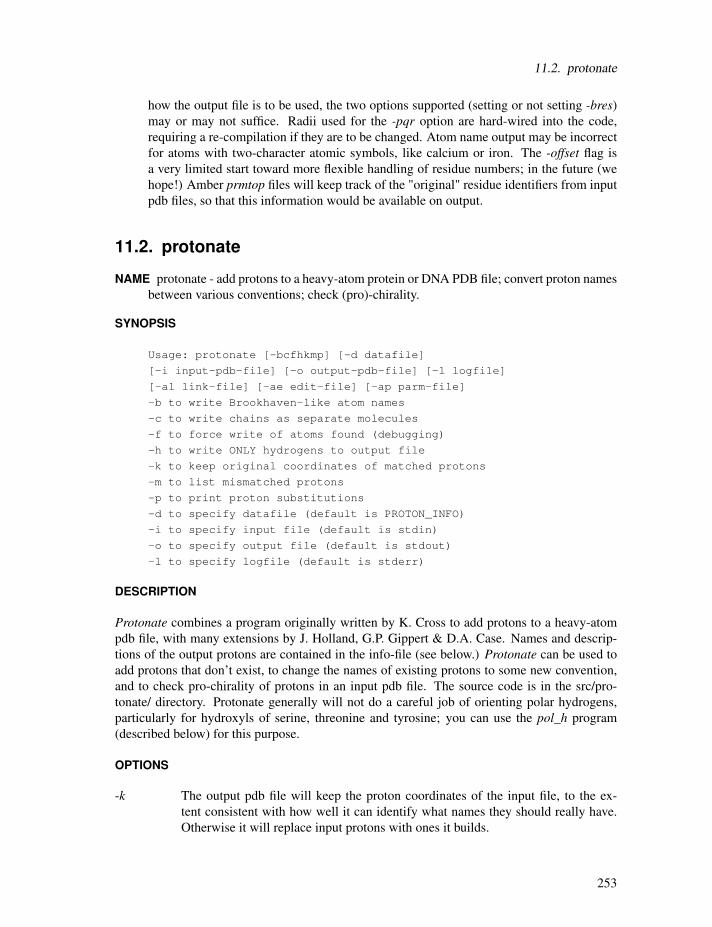
11.2. protonate
how the output file is to be used, the two options supported (setting or not setting -bres)may or may not suffice. Radii used for the -pqr option are hard-wired into the code,requiring a re-compilation if they are to be changed. Atom name output may be incorrect
for atoms with two-character atomic symbols, like calcium or iron. The -offset flag isa very limited start toward more flexible handling of residue numbers; in the future (we
hope!) Amber prmtop files will keep track of the "original" residue identifiers from inputpdb files, so that this information would be available on output.
11.2. protonate
NAME protonate - add protons to a heavy-atom protein or DNA PDB file; convert proton names
between various conventions; check (pro)-chirality.
SYNOPSIS
Usage: protonate [-bcfhkmp] [-d datafile]
[-i input-pdb-file] [-o output-pdb-file] [-l logfile]
[-al link-file] [-ae edit-file] [-ap parm-file]
-b to write Brookhaven-like atom names
-c to write chains as separate molecules
-f to force write of atoms found (debugging)
-h to write ONLY hydrogens to output file
-k to keep original coordinates of matched protons
-m to list mismatched protons
-p to print proton substitutions
-d to specify datafile (default is PROTON_INFO)
-i to specify input file (default is stdin)
-o to specify output file (default is stdout)
-l to specify logfile (default is stderr)
DESCRIPTION
Protonate combines a program originally written by K. Cross to add protons to a heavy-atompdb file, with many extensions by J. Holland, G.P. Gippert & D.A. Case. Names and descrip-
tions of the output protons are contained in the info-file (see below.) Protonate can be used toadd protons that don’t exist, to change the names of existing protons to some new convention,
and to check pro-chirality of protons in an input pdb file. The source code is in the src/pro-
tonate/ directory. Protonate generally will not do a careful job of orienting polar hydrogens,
particularly for hydroxyls of serine, threonine and tyrosine; you can use the pol_h program(described below) for this purpose.
OPTIONS
-k The output pdb file will keep the proton coordinates of the input file, to the ex-
tent consistent with how well it can identify what names they should really have.
Otherwise it will replace input protons with ones it builds.
253

11. Miscellaneous
-b The program will insert a space before the name of each heavy atom in the output
file. This is most often used to convert input files whose atom names begin in col-
umn 13 to the Brookhaven format where most heavy atom names begin in column
14. NOTE: two-letter heavy atom names (like FE or CA [calcium]) will not be
correct; the resulting output file must be hand-edited to check for this.
-d info_file Specifies the file containing information on how to build and name pro-tons. The default name is PROTON_INFO. This information used to determine
where on the amino acids the protons should be placed. The file provided handles
funny Amber residue names like HIE, HIP and HID and HEM. Other files provided
include PROTON_INFO.Brook, which uses Brookhaven proton naming conven-
tion (such as 1HB, etc.), and PROTON_INFO.oldnames, which uses old amber
names. For example, to take an Amber pdb file and convert to the Brookhaven
naming convention, set -d PROTON_INFO.Brook. Output to LOGFILE includes
matches of protons the program builds with any found in the input file, plus a list
of any input protons that could not be matched. Questionable matches are flagged
and should be checked manually.
BUGS Format of the PROTON_INFO file is not obvious unless you have read the code. Methyl
protons are built in a staggered conformation; hydroxyl protons in a arbitrary (and gen-
erally sub-optimal) conformation. A program like pol_h or its equivalent should be used(if desired) to place polar hydrogens on LYS, SER, THR, and SER residues. HIS in the
input file is assumed to be HID. Users should generally explicitly figure out the desired
protonation state for histidines. No attempt is made to identify heavy atoms in the input
file that have two-letter element names; this means that Brookhaven-style output may re-
quire some hand-editing if atoms like calcium or iron are present. It is assumed that the
alternate conformer flag in column 17 of the PDB file is either blank, or A. The program
needs to be recompiled to change this; perhaps this should become an input option.
11.3. ambmask
NAME
ambmask - test group input FIND mask (or mask string given in the &cntrl section) and dump
the resulting atom selection in a given format
SYNOPSIS
ambmask -p prmtop -c inpcrd -prnlev [0-3] -out [short| pdb| amber] -find [maskstr]
DESCRIPTION
ambmask acts as a filter which takes amber topology and coordinate "restart" file and appliesthe "maskstr" selection string (similar syntactically to UCSF Chimera/Midas) to select specific
atoms or residues. Residues can be selected by their numbers or names. Atoms can be selected
by numbers, names, or amber (forcefield) type. Selections are case insensitive. The selected
254

11.3. ambmask
atoms are printed to stdout (by default, in amber-style pdb format). Atom and residue namesand numbers are taken from amber topology. Beware that selection string works on those
names and not the ones from the original pdb file. If you are not sure how atoms or residues are
named or numbered in the amber topology, use ambmask with a selection string ":*" (whichis the default) to dump the whole pdb file with corresponding amber atom/residue names and
numbers.
The "maskstr" selection expression is composed of "elementary selections". These start with
":" to select by residues, or "@" to select by atoms. Residues can be selected by numbers (given
as numbers separated by commas, or as ranges separated by a dash) or by names (given as a
list of residue names separated by commas). The same holds true for atom selections by atom
numbers or atom names. In addition, atoms can be selected by amber atom type, in which case
"@" must be immediately followed by "%". ":*" means all residues and "@*" means all atoms.
The following examples show the usage of this syntax. Square brackets should not be used in
actual expressions, they are only used for clarity here:
:{residue numlist} [:1-10] [:1,3,5] [:1-3,5,7-9]
:{residue namelist} [:LYS] [:ARG,ALA,GLY]
@{atom numlist} [@12,17] [@54-85] [@12,54-85,90]
@{atom namelist} [@CA] [@CA,C,O,N,H]
@%{atom typelist} [@%CT] [@%N*,N3]
These "elementary selections" can be combined into more complex selections using binary
operators "&" (and) and "|" (or), unary operator "!" (negation), distance binary operators "<:",">:", "<@", ">@", and parentheses. Spaces around operators are irrelevant. Parentheses havethe highest priority, followed by distance operators ("<:", ">:", "<@", ">@"), "!" (negation),"&" (and) and "|" (or) in order of descending priority. A wildcard "=" in an atom or residue
name matches any name starting with a given character (or characters). For example, [:AS=]
would match all aspartic acid residues (ASP), and asparagines (ASN); [@H=] would match all
atom names starting with H (which are effectively all hydrogens). It cannot be used to match
the end part of names (such as [:=A]). Some examples of more complex selections follow:
[@C= ~& ~!@CA,C]
.. all carbons except backbone alpha and carbonyl carbon
[(:1-3@CA | :5-7@CB)]
.. alpha carbons in residues 1-3 and beta carbons in residues 5-7
[:CYS,ARG & !(:1-10 | @CA,CB)]
.. all CYS and ARG atoms except those which are in residues 1-10 and which are CA or CB
[:* & !@H=] or [!@H=]
.. all heavy atoms (i.e. except hydrogens)
[:5 <@4.5]
255

11. Miscellaneous
.. all atoms within 4.5A from residue 5
[(:1-55 <:3.0) & :WAT]
.. all water molecules within 3A from residues 1-55
Compound expressions of the following type are also allowed:
:{residue numlist|namelist}@{atom numlist|namelist|typelist}[:1-10@CA] is equivalent to [:1-10 & @CA]
[:LYS@H=] is equivalent to [:LYS & @H=]
OPTIONS
The program needs an amber topology file and coordinates (restrt format). The filename spec-
ified with the -p option is amber topology, while the filename given with the -c option is acoordinate file. If -p or -c options are not given, the program expects that files "prmtop" and/or"inpcrd" exist in the current directory, which will be taken as topology and coordinate files
correspondingly. If no command line options are given, the program prints the usage statement.
The option -prnlev specifies how much (debugging) information is printed to stdout. If itis 0, only selected atoms are printed. More verbose output (which might be useful for debug-
ging purposes) is achieved with higher values: 1 prints original "maskstr" in its tokenized (with
operands enclosed in square brackets) and postfix (or Reverse Polish Notation) forms; number
of atoms and residues in the topology file and number of selected atoms are also printed to
stdout. 2 prints the resulting mask array, which is an array of integer values, with ’1’ repre-senting a selected atom, and ’0’ an unselected one. Value of 3, in addition, prints mask arrays
as they are pushed or popped from the stack (this is really only useful for tracing the problems
occurring during stack operations). The -prnlev values of 0 or 1 should suffice for most uses.The option -out specifies the format of printed atoms. "short" means a condensed output
using residue (:) and atom (@) designators followed by residue ranges and atom names. "pdb"
(default) prints atoms in amber-like pdb format with the original "maskstr" printed as a RE-
MARK at the top of the pdb file, and "amber" prints atom/residue ranges in the format suitable
for copying into group input section of amber input file.
The option -find is followed by "maskstr" expression. This is a string where some charactershave a special meaning and thus express what parts (atoms/residues) of the molecule will get
selected. The syntax of this string is explained in the section above (DESCRIPTION). If this
option is left out, it defaults to ":*", which selects all atoms in the given topology file. The length
of "maskstr" is limited to 80 characters. If the "maskstr" contains spaces or special characters
(which would be expanded by the shell), it should be protected by single or double quotes
(depending on the shell). In addition, for C-shells even a quoted exclamation character may
be expanded for history substitution. Thus, it is recommended that the operand of the negation
operator always be enclosed in parentheses so that "!" is always followed by a "(" to produce
"!(" which disables the special history interpretation. For example, [@C= & !(@CA,C)] selects
all carbons except backbone alpha and carbonyl carbon; the parentheses are redundant but shell
safe. Another approach is to precede "!" with " man page indicates further ways to disable
history substitution. FILES
Assumes that prmtop and inpcrd files exists in the current directory if they are not specifiedwith -p and -c options. Resulting (i.e. selected) atoms are written to stdout.
256

11.4. pol_h and gwh
BUGS
Because all atom names are left justified in amber topology and the selections are case insensi-
tive, there is no way to distinguish some atom names: alpha carbon CA and a calcium ion Ca
are a notorious example of that.
11.4. pol_h and gwh
NAME
pol_h - set positions of polar hydrogens in proteins
gwh - set positions of polar hydrogens onto water oxygen positions
SYNOPSIS
pol_h < input-pqr-file > output-pdb-file
gwh [-p <prmtop>] [-w <water.pdb>] [-c] [-e] < input_pdb_file
> output_pdb_file DESCRIPTION
The program pol_h resets positions of polar hydrogens of protein residues (Lys, Ser, Tyr andThr), by optimizing simple electrostatic interactions. The input pqr file can be created byambpdb. The program gwh sets positions of water hydrogens onto water oxygen positionsthat may be present in PDB files, by optimizing simple electrostatic interactions. If the -w flag
is set, the program reads water oxygen positions from the file water-position-file, rather thanthe default name watpdb. If −c is set, a constant dielectric will be used to construct potentials,otherwise the (default) distant-dependent dielectric will be used. If −e is set, the electrostaticpotential will be used to determine which hydrogens are placed first; otherwise, a distance
criterion will be used.
Accuracy of pol_h & gwh:
* In the following the results for BPTI and RSA(ribonuclease A) are
given together with those of Karplus(1) and Ornstein(2) groups.
In the case of Ornstein’s method, it handles only some of hydrogens
in question and therefore I normalized(scaled) their results using
expected values for random generation. The rms deviation from the
experimental positions (neutron diffraction) and the number of
hydrogens are shown below.
BPTI Lys Ser Tyr Thr Wat
----------------------------------------------------------
# of H 12 1 4 3 112 (4∼)Pol_H 0.39 0.36 1.08 0.20 0.98(0.38)
Karplus 0.25 0.71 0.81 0.19 - (0.35)
Ornstein 0.22 0.96 0.00 0.07 -
Ornstn(scaled) 0.51 0.96 1.28 0.07 (1.17)
----------------------------------------------------------
internal waters. by random generation
257
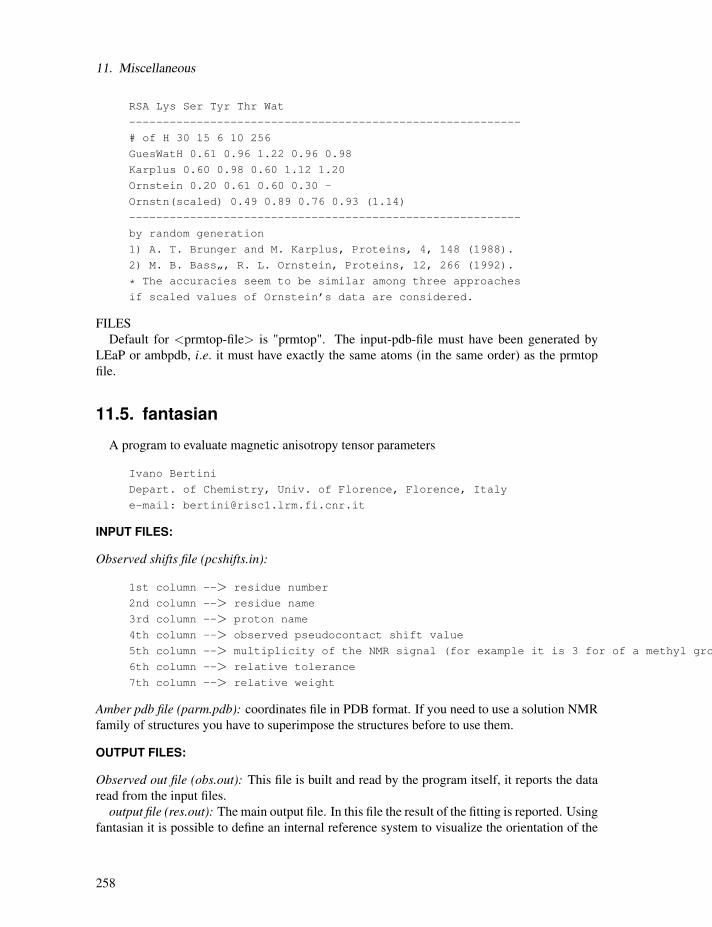
11. Miscellaneous
RSA Lys Ser Tyr Thr Wat
----------------------------------------------------------
# of H 30 15 6 10 256
GuesWatH 0.61 0.96 1.22 0.96 0.98
Karplus 0.60 0.98 0.60 1.12 1.20
Ornstein 0.20 0.61 0.60 0.30 -
Ornstn(scaled) 0.49 0.89 0.76 0.93 (1.14)
----------------------------------------------------------
by random generation
1) A. T. Brunger and M. Karplus, Proteins, 4, 148 (1988).
2) M. B. Bass„, R. L. Ornstein, Proteins, 12, 266 (1992).
* The accuracies seem to be similar among three approaches
if scaled values of Ornstein’s data are considered.
FILES
Default for <prmtop-file> is "prmtop". The input-pdb-file must have been generated by
LEaP or ambpdb, i.e. it must have exactly the same atoms (in the same order) as the prmtopfile.
11.5. fantasian
A program to evaluate magnetic anisotropy tensor parameters
Ivano Bertini
Depart. of Chemistry, Univ. of Florence, Florence, Italy
e-mail: [email protected]
INPUT FILES:
Observed shifts file (pcshifts.in):
1st column --> residue number
2nd column --> residue name
3rd column --> proton name
4th column --> observed pseudocontact shift value
5th column --> multiplicity of the NMR signal (for example it is 3 for of a methyl gro
6th column --> relative tolerance
7th column --> relative weight
Amber pdb file (parm.pdb): coordinates file in PDB format. If you need to use a solution NMRfamily of structures you have to superimpose the structures before to use them.
OUTPUT FILES:
Observed out file (obs.out): This file is built and read by the program itself, it reports the dataread from the input files.
output file (res.out): The main output file. In this file the result of the fitting is reported. Usingfantasian it is possible to define an internal reference system to visualize the orientation of the
258

11.6. elsize
tensor axes. Then in this file you can find PDB format lines (ATOM) which can be included
in a PDB file to visualize the internal reference system and the tensor axes. In the main output
file all the three equivalent permutations of the tensor parameters with respect to the reference
system are reported. The summary of the minimum and maximum errors and that of squared
errors are also reported.
Example files: in the directory example there are all the files necessary to run a fantasiancalculation:
fantasian.com --> run file
pcshifts.in --> observed shifts file
parm.pdb --> coordinate file in PDB format
obs.out --> data read from input files
res.out --> main output file ~
11.6. elsize
NAME
elsize - Given the structure, estimates its effective electrostatic size (parameter
SYNOPSIS
Usage: elsize input-pqr-file [-options]
-det an estimate based on structural invariants. DEFAULT.
-ell an estimate via elliptic integral (numerical).
-elf same as above, but via elementary functions.
-abc prints semi-axes of the effective ellipsoid.
-tab prints all of the above into a table without header.
-hea prints same table as -tab but with a header.
-deb prints same as -tab with some debugging information.
-xyz uses a file containing only XYZ coordinates.
DESCRIPTION
elsize is a program originally written by G. Sigalov to estimate the effective electrostatic size
of a structure via a quick, analytical method. The algorithm is presented in detail in Ref. . [68]
You will need your structure in a pqr format as input, which can be easily obtained from the
prmtop and inpcrd files using ambpdb utility described above:
ambpdb -p prmtop -pqr < inpcrd > input-file-pqr
After that you can simply do: elsize input-file-pqr , the value of electrostatic size in Angstromswill be output on stdout. The source code is in the src/etc/ directory, its comments contain
more extensive description of the options and give an outline of the algorithm. A somewhat less
accurate estimate uses just the XYZ coordinates of the molecule and assumes the default radius
size of for all atoms:
259

11. Miscellaneous
elsize input-file-xyz
This option is not recommended for very small compounds. The code should not be used on
structures made up of two or more completely disjoint" compounds – while the code will still
produce a finite value of Arad , it is not very meaningful. Instead, one should obtain estimatesfor each compound separately.
260

A. Namelist Input Syntax
Namelist provides list-directed input, and convenient specification of default values. It dates
back to the early 1960’s on the IBM 709, but was regrettably not part of Fortran 77. It is a part
of the Fortran 90 standard, and is supported as well by most Fortran 77 compilers (including
g77).
Namelist input groups take the form:
&name
var1=value, var2=value, var3(sub)=value,
var4(sub,sub,sub)=value,value,
var5=repeat*value,value,
/
The variables must be names in the Namelist variable list. The order of the variables in the input
list is of no significance, except that if a variable is specified more than once, later assignments
may overwrite earlier ones. Blanks may occur anywhere in the input, except embedded in
constants (other than string constants, where they count as ordinary characters).
It is common in older inputs for the ending "/" to be replaced by "&end"; this is non-standard-
conforming.
Letter case is ignored in all character comparisons, but case is preserved in string constants.
String constants must be enclosed by single quotes (’). If the text string itself contains single
quotes, indicate them by two consecutive single quotes, e.g. C1’ becomes ’C1”’ as a character
string constant.
Array variables may be subscripted or unsubscripted. An unsubscripted array variable is
the same as if the subscript (1) had been specified. If a subscript list is given, it must have
either one constant, or exactly as many as the number in the declared dimension of the array.
Bounds checking is performed for ALL subscript positions, although if only one is given for a
multi-dimension array, the check is against the entire array size, not against the first dimension.
If more than one constant appears after an array assignment, the values go into successive
locations of the array. It is NOT necessary to input all elements of an array.
Any constant may optionally be preceded by a positive (1,2,3,..) integer repeat factor, so that,
for example, 25*3.1415 is equivalent to twenty-five successive values 3.1415. The repeat count
separator, *, may be preceded and followed by 0 or more blanks. Valid LOGICAL constants
are 0, F, .F., .FALSE., 1, T, .T., and .TRUE.; lower case versions of these also work.
261

A. Namelist Input Syntax
262

B. GROUP Specification
This section describes the format used to define groups of atoms in various AMBER pro-
grams. In sander, a group can be specified as a movable "belly" while the other atoms are fixedabsolutely in space (aside from scaling caused by constant pressure simulation), and/or a group
of movable atoms can independently restrained (held by a potential) at their positions. In anal,groups can be defined for energy analysis.
Except in the analysis module where different groups of atoms are considered with different
group numbers for energy decomposition, in all other places the groups of atoms defined are
considered as marked atoms to be included for certain types of calculations. In the case of
constrained minimization or dynamics, the atoms to be constrained are read as groups with a
different weight for each group.
Reading of groups is performed by the routine RGROUP, and you are advised to consult it if
there is still some ambiguity in the documentation.
Input description:
- 1 - Title format(20a4)
ITITL Group title for identification.
Setting ITITL = ’END’ ends group input.
------------------------------------------------------------------------
- 1A - Weight format(f)
This line is only provided/read when using GROUP input to
define restrained atoms.
WT The harmonic force constants in kcal/mol-A**2 for the group
of atoms for restraining to a reference position.
------------------------------------------------------------------------
- 1B - Control to define the group
KTYPG , (IGRP(I) , JGRP(I) , I = 1,7) format(a,14i)
KTYPG Type of atom selection performed. A molecule can be
defined by using only ’ATOM’ or ’RES’, or part of the
molecule can be defined by ’ATOM’ and part by ’RES’.
’ATOM’ The group is defined in terms of atom numbers. The atom
number list is given in igrp and jgrp.
’RES’ The group is defined in terms of residue numbers. The
residue number list is given in igrp and jgrp.
’FIND’ This control is used to make additional conditions
(apart from the ’ATOM’ and ’RES’ controls) which a given
atom must satisfy to be included in the current group.
The conditions are read in the next section (1C) and are
terminated by a SEARCH card.
Note that the conditions defined by FIND filter any set(s) of atoms
defined by the following ATOM/RES instructions. For example,
-- group input: select main chain atoms --
FIND
263

B. GROUP Specification
* * M *SEARCH
RES 1 999
END
END
’END’ End input for the current group. Followed by either another
group definition (starting again with line 1 above), or by a second
’END’ "card", which terminates all group input.
IGRP(I) , JGRP(I)
The atom or residue pointers. If ktypg .eq. ’ATOM’ all
atoms numbered from igrp(i) to jgrp(i) will be put into
the current group. If ktypg .eq. ’RES’ all atoms in the
residues numbered from igrp(i) to jgrp(i) will be put
into the current group. If igrp(i) = 0 the next control
card is read.
It is not necessary to fill groups according to the
numerical order of the residues. In other words, Group 1
could contain residues 40-95 of a protein, Group 2 could
contain residues 1-40 and Group 3 could contain residues
96-105.
If ktypg .eq. ’RES’, then associating a minus sign with
igrp(i) will cause all residues igrp(i) through jgrp(i)
to be placed in separate groups.
In the analysis modules, all atoms not explicitly defined
as members of a group will be combined as a unit in the
(n + 1) group, where the (n) group in the last defined
group.
------------------------------------------------------------------------
- 1C - Section to read atom characteristics
***** Read only if KTYPG = ’FIND’ *****JGRAPH(I) , JSYMBL(I) , JTREE(I) , JRESNM(I) format(4a)
A series of filter specifications are read. Each filter consists
of four fields (JGRAPH,JSYMBL,JTREE,JRESNM), and each filter is placed
on a separate line. Filter specification is terminated by a line with
JGRAPH = ’SEARCH’. A maximum of 10 filters may be specified for a
single ’FIND’ command.
The union of the filter specifications is applied to the atoms defined
by the following ATOM/RES cards. I.e. if an atom satisfies any of the
filters, it will be included in the current group. Otherwise, it is not
included. For example, to select all non main chain atoms from residues
1 through 999:
-- group input: select non main chain atoms --
FIND
* * S *
* * B *
* * 3 *
* * E *SEARCH
RES 1 999
END
264
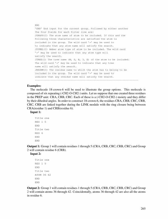
END
’END’ End input for the current group. Followed by either another
The four fields for each filter line are:
JGRAPH(I) The atom name of atom to be included. If this and the
following three characteristics are satisfied the atom is
included in the group. The wild card ’*’ may be used to
to indicate that any atom name will satisfy the search.
JSYMBL(I) Amber atom type of atom to be included. The wild card
’*’ may be used to indicate that any atom type will
satisfy the search.
JTREE(I) The tree name (M, S, B, 3, E) of the atom to be included.
The wild card ’*’ may be used to indicate that any tree
name will satisfy the search.
JRESNM(I) The residue name to which the atom has to belong to be
included in the group. The wild card ’*’ may be used to
indicate that any residue name will satisfy the search.
------------------------------------------------------------------------
Examples:The molecule 18-crown-6 will be used to illustrate the group options. This molecule is
composed of six repeating (-CH2-O-CH2-) units. Let us suppose that one created three residues
in the PREP unit: CRA, CRB, CRC. Each of these is a (-CH2-O-CH2-) moiety and they differ
by their dihedral angles. In order to construct 18-crown-6, the residues CRA, CRB, CRC, CRB,
CRC, CRB are linked together during the LINK module with the ring closure being between
CRA(residue 1) and CRB(residue 6).
Input 1:
Title one
RES 1 5
END
Title two
RES 6
END
END
Output 1: Group 1 will contain residues 1 through 5 (CRA, CRB, CRC, CRB, CRC) and Group2 will contain residue 6 (CRB).
Input 2:
Title one
RES 1 5
END
Title two
ATOM 36 42
END
END
Output 2: Group 1 will contain residues 1 through 5 (CRA, CRB, CRC, CRB, CRC) and Group2 will contain atoms 36 through 42. Coincidentally, atoms 36 through 42 are also all the atoms
in residue 6.
265

B. GROUP Specification
Input 3:
Title one
RES -1 6
END
END
Output 3: Six groups will be created; Group 1: CRA, Group 2: CRB,..., Group 6: CRB.Input 4:
Title one
FIND
O2 OS M CRA
SEARCH
RES 1 6
END
END
Output 4: Group 1 will contain those atoms with the atom name ’O2’, atom type ’OS’, tree
name ’M’ and residue name ’CRA’.
Input 5:
Title one
FIND
O2 OS * *SEARCH
RES 1 6
END
END
Output 5: Group 1 will contain those atoms with the atom name ’O2’, atom type ’OS’, any
tree name and any residue name.
266

C. EVB output file specifications
This section describes the contents of the EVB output file evbout. The data type of eachvariable is enclosed in {· · ·}, while the size of each array variable is enclosed in [· · · ]. Beloware the formatting specifications for the output data:
100 format( A/, A )
200 format( A/, I8 )
300 format( A/, 3(2X,I8), 2X, F14.8 )
400 format( A/, 2I8, F14.8 )
500 format( A/, 2I8, F14.8, 2X, F14.8 )
600 format( A/, 3I8, F14.8, 2X, F14.8 )
888 format( A, 2X, I10, 2X, A, 2X, F20.8 )
1000 format( A/, (5(2X,F20.8)) )
The EVB output file begins with the following header information:
�
�
�
write(evb_unit,’(/)’)
write(evb_unit, 100) ’ [DYNAMICS TYPE]: ’, trim( adjustl(evb_dyn) )
write(evb_unit,’(/)’)
write(evb_unit, 200) ’ [NBEAD]: ’, ncopy
write(evb_unit,’(/)’)
write(evb_unit,300) ’ [NEVB] [NBIAS] [NTW_EVB] [DT]: ’ &
, nevb, nbias, ntw_evb, dt
write(evb_unit,’(/)’)
evb_dyn : {character*512} EVB dynamics specification.
ncopy : {integer} No. of PIMD slices. Classical EVB ⇒ ncopy = 1.
nevb : {integer} No. of diabatic states.
nbias : {integer} No. of biasing potentials included in Vel0.ntw_evb : {integer} No. of MD steps between output to evbout file.
dt : {real} MD time step size (ps).�
�
�
! Output ONLY if performing mapping potential dynamics.
do n = 1, nbias
write(evb_unit,400) ’ [MAPPING POTENTIAL]: ni, nf, lambda ’ &
, bias_ndx(n,1), bias_ndx(n,2), lambda(n)
enddo
! Output ONLY if performing umbrella sampling on an energy gap RC.
do n = 1, nbias
write(evb_unit,500) ’ [NRG_GAP UMBRELLA]: ni, nf, k, ezero ’ &
, bias_ndx(n,1), bias_ndx(n,2), k_umb(n), r0_umb(n)
enddo
267

C. EVB output file specifications
bias_ndx(:,:) : {integer}, [nbias,2]. Valence bond state index.
lambda(:) : {real}, [nbias]. Vλ = (1−λ )Vii +λVf f .
k0_umb(:) : {real}, [nbias]. Umbrella force constant.
r0_umb(:) : {real}, [nbias]. RC anchor point for umbrella sampling.�
�
�
! Output ONLY if sampling involves the difference of distances RC.
do n = 1, nbias
write(evb_unit,600) &
’ [DBONDS UMBRELLA]: iatom, jatom, katom, k, ezero ’ &
, dbonds_RC(n)%iatom, dbonds_RC(n)%jatom &
, dbonds_RC(n)%katom, k_umb(n), r0_umb(n)
enddo
! Output ONLY if sampling involves a distance RC.
do n = 1, nbias
write(evb_unit,500) ’ [BOND UMBRELLA]: iatom, jatom, k, ezero ’ &
, bond_RC(n)%iatom, bond_RC(n)%jatom, k_umb(n), r0_umb(n)
enddo
dbonds_RC(:) : {derived type}, [nbias].
%iatom {integer} index of atom involved in ri j.
%jatom {integer} index of atom involved in ri j.
%katom {integer} index of atom involved in rk j.
bond_RC(:) : {derived type}, [nbias].
%iatom {integer} index of atom involved in ri j.
%jatom {integer} index of atom involved in ri j.
k0_umb(:) : {real}, [nbias]. Umbrella force constant.
r0_umb(:) : {real}, [nbias]. RC anchor point for umbrella sampling.
The following data is output every ntw_evb steps:
�
� write(evb_unit,’(/)’)
write(evb_unit,888) ’{NSTEP}: ’, nstep, ’{TIME}: ’, nstep*dt
nstep : {integer}. MD step counter.
nstep*dt : {real}. Time (ps).�
�
�
�! Output ONLY if the nuclei are NOT quantized.
write(evb_unit,’(A)’)
write(evb_unit,1000) ’ [EVB MATRIX]’, evb_Hmat%evb_mat(:,:)
write(evb_unit,’(A)’)
write(evb_unit,1000) ’ [EVB VEC_0]’, evb_Hmat%evb_vec0(:)
evb_Hmat%evb_mat(:,:) : {real},[nevb,nevb]. EVB matrix elements.
evb_Hmat%evb_vec0(:) : {real},[nevb]. ground-state EVB vector.��
��
! Output ONLY if the nuclei are quantized.
write(evb_unit,’(A)’)
write(evb_unit,1000) ’ [EVB MATRIX]’, evb_matrix(:,:) write(evb_unit,’(A)’)
write(evb_unit,1000) ’ [EVB VEC_0^2]’, evb_pop(:) * nbead_inv
268
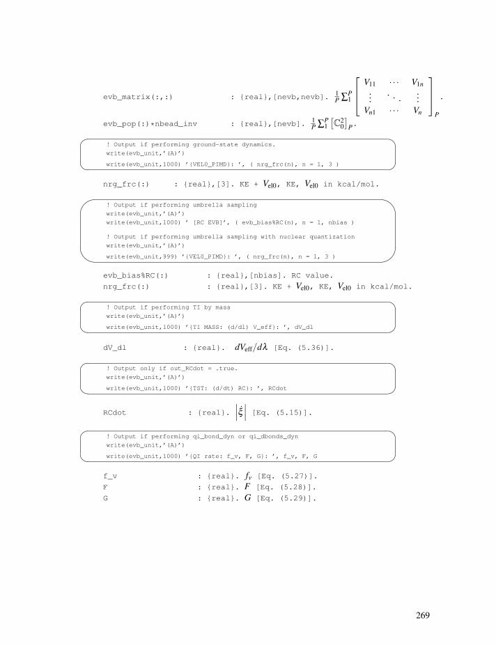
evb_matrix(:,:) : {real},[nevb,nevb]. 1P ∑P
1
⎡⎢⎣
V11 · · · V1n...
......
Vn1 · · · Vn
⎤⎥⎦
P
.
evb_pop(:)*nbead_inv : {real},[nevb]. 1P ∑P
1
[C20
]P.�
���
! Output if performing ground-state dynamics.
write(evb_unit,’(A)’)
write(evb_unit,1000) ’{VEL0_PIMD}: ’, ( nrg_frc(n), n = 1, 3 )
nrg_frc(:) : {real},[3]. KE + Vel0, KE, Vel0 in kcal/mol.�
�
�
�
! Output if performing umbrella sampling
write(evb_unit,’(A)’)
write(evb_unit,1000) ’ [RC EVB]’, ( evb_bias%RC(n), n = 1, nbias )
! Output if performing umbrella sampling with nuclear quantization
write(evb_unit,’(A)’)
write(evb_unit,999) ’{VEL0_PIMD}: ’, ( nrg_frc(n), n = 1, 3 )
evb_bias%RC(:) : {real},[nbias]. RC value.
nrg_frc(:) : {real},[3]. KE + Vel0, KE, Vel0 in kcal/mol.��
��
! Output if performing TI by mass
write(evb_unit,’(A)’)
write(evb_unit,1000) ’{TI MASS: (d/dl) V_eff}: ’, dV_dl
dV_dl : {real}. dVeff/dλ [Eq. (5.36)].��
��
! Output only if out_RCdot = .true.
write(evb_unit,’(A)’)
write(evb_unit,1000) ’{TST: (d/dt) RC}: ’, RCdot
RCdot : {real}.
∣∣∣ξ ∣∣∣ [Eq. (5.15)].��
��
! Output if performing qi_bond_dyn or qi_dbonds_dyn
write(evb_unit,’(A)’)
write(evb_unit,1000) ’{QI rate: f_v, F, G}: ’, f_v, F, G
f_v : {real}. fv [Eq. (5.27)].
F : {real}. F [Eq. (5.28)].
G : {real}. G [Eq. (5.29)].
269

C. EVB output file specifications
270
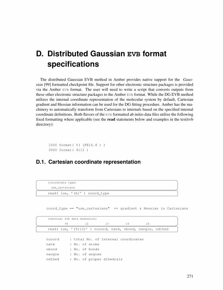
D. Distributed Gaussian EVB formatspecifications
The distributed Gaussian EVB method in Amber provides native support for the Gaus-sian [99] formatted checkpoint file. Support for other electronic structure packages is providedvia the Amber EVB format. The user will need to write a script that converts outputs from
these other electronic structure packages to the Amber EVB format. While the DG EVB method
utilizes the internal coordinate representation of the molecular system by default, Cartesian
gradient and Hessian information can be used for the DG fitting procedure. Amber has the ma-
chinery to automatically transform from Cartesians to internals based on the specified internal
coordinate definitions. Both flavors of the EVB formatted ab initio data files utilize the following
fixed formatting where applicable (see the read statements below and examples in the test/evbdirectory):
1000 format( 5( 1PE16.8 ) )
3000 format( 4I12 )
D.1. Cartesian coordinate representation
�
� [coordinate type]
use_cartesians�� !read( ioe, ’(A)’ ) coord_type
coord_type == "use_cartesians" => gradient & Hessian in Cartesians�
� [external evb data dimension]
56 12 13 19 24�� !read( ioe, ’(5I12)’ ) ncoord, natm, nbond, nangle, ndihed
ncoord : total No. of internal coordinates
natm : No. of atoms
nbond : No. of bonds
nangle : No. of angles
ndihed : No. of proper dihedrals
271
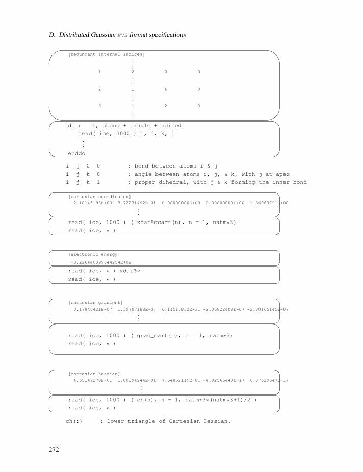
D. Distributed Gaussian EVB format specifications
�
�
�
[redundant internal indices]...
1 2 0 0...
2 1 6 0...
6 1 2 3...�
�
�
�do n = 1, nbond + nangle + ndihed
read( ioe, 3000 ) i, j, k, l...
enddo
i j 0 0 : bond between atoms i & j
i j k 0 : angle between atoms i, j, & k, with j at apex
i j k l : proper dihedral, with j & k forming the inner bond��
��
[cartesian coordinates]
-2.10145193E+00 3.72231492E-01 0.00000000E+00 0.00000000E+00 1.86063791E+00...
�� read( ioe, 1000 ) ( xdat%qcart(n), n = 1, natm*3)
read( ioe, * )
�
� [electronic energy]
-3.226440399344254E+02�
� read( ioe, * ) xdat%v
read( ioe, * )
��
��
[cartesian gradient]
3.17848421E-07 1.39797188E-07 6.11516832E-31 -2.06822408E-07 -2.80165145E-07...�
���
read( ioe, 1000 ) ( grad_cart(n), n = 1, natm*3)
read( ioe, * )
��
��
[cartesian hessian]
4.65149270E-01 1.00394244E-01 7.54852119E-01 -4.82566443E-17 6.87529647E-17...
�� read( ioe, 1000 ) ( ch(n), n = 1, natm*3*(natm*3+1)/2 )
read( ioe, * )
ch(:) : lower triangle of Cartesian Hessian.
272

D.2. Internal coordinate representation
D.2. Internal coordinate representation
�
� [coordinate type]
use_internals�� !read( ioe, ’(A)’ ) coord_type
coord_type == "use_internals" => gradient & Hessian in internals�
� [external evb data dimension]
56 12 13 19 24�� !read( ioe, ’(5I12)’ ) ncoord, natm, nbond, nangle, ndihed
ncoord : total No. of internal coordinates
natm : No. of atoms
nbond : No. of bonds
nangle : No. of angles
ndihed : No. of proper dihedrals�
�
�
[redundant internal indices]...
1 2 0 0...
2 1 6 0...
6 1 2 3...�
�
�
�do n = 1, nbond + nangle + ndihed
read( ioe, 3000 ) i, j, k, l...
enddo
i j 0 0 : bond between atoms i & j
i j k 0 : angle between atoms i, j, & k, with j at apex
i j k l : proper dihedral, with j & k forming the inner bond��
��
[cartesian coordinates]
-2.10145193E+00 3.72231492E-01 0.00000000E+00 0.00000000E+00 1.86063791E+00...
�� read( ioe, 1000 ) ( xdat%qcart(n), n = 1, natm*3)
read( ioe, * )
273
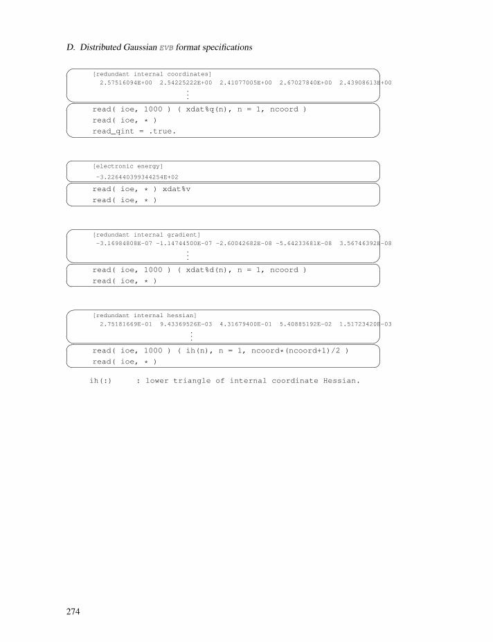
D. Distributed Gaussian EVB format specifications
��
��
[redundant internal coordinates]
2.57516094E+00 2.54225222E+00 2.41077005E+00 2.67027840E+00 2.43908613E+00...�
���
read( ioe, 1000 ) ( xdat%q(n), n = 1, ncoord )
read( ioe, * )
read_qint = .true.
�
� [electronic energy]
-3.226440399344254E+02�
� read( ioe, * ) xdat%v
read( ioe, * )
��
��
[redundant internal gradient]
-3.16984808E-07 -1.14744500E-07 -2.60042682E-08 -5.64233681E-08 3.56746392E-08...
�� read( ioe, 1000 ) ( xdat%d(n), n = 1, ncoord )
read( ioe, * )
��
��
[redundant internal hessian]
2.75181669E-01 9.43369526E-03 4.31679400E-01 5.40885192E-02 1.51723420E-03...
�� read( ioe, 1000 ) ( ih(n), n = 1, ncoord*(ncoord+1)/2 )
read( ioe, * )
ih(:) : lower triangle of internal coordinate Hessian.
274

E. AMBER Trajectory NetCDF Format
John Mongan ([email protected])
E.1. Introduction
The file format described in this document was developed for storing data generated by
molecular dynamics simulations. It was introduced in version 9 of the AMBER suite of pro-
grams (http://amber.scripps.edu).
The primary design goals of this format are:
• Efficient input and output
• Compact, high-precision representation of data
• Portability of data files across different machine architectures
• Extensibility of the format (ability to add additional data without re-writing parsers)
• Compatibility with existing tools and formats
The file format is based on the NetCDF (Network Common Data Form) developed by Unidata
(http://www.unidata.ucar.edu/software/netcdf/). NetCDF is designed for representation of arbi-
trary array-based data. Unidata provides libraries with bindings in C, C++, Fortran (F77 and
F90), Java, Python, Perl, Ruby and MATLAB for reading and writing NetCDF files. The de-
sign goals above are largely met by NetCDF and the libraries that implement it. It is expected
that all I/O of the format described here will occur through these libraries; this specification
describes the file format at a high level in terms of the API implemented by version 3.6 of these
libraries. In NetCDF terms, this document is a “Convention,” describing the names, dimensions
and attributes of the arrays that may be present in the file.
E.2. Program behavior
Programs creating trajectory files (“creators”) shall adhere strictly to the requirements of this
document. Programs reading trajectory files (“readers”) shall be as permissive as possible in
applying the requirements of this document. Readers may emit warnings if out-of-spec files
are encountered; these warnings should include information about the program that originally
created the file (see Global attributes, section E.4). Readers shall not fail to read a file unless
the required information cannot be located or interpreted. In particular, to ensure forward com-
patibility with later extensions of the format, readers shall not fail or emit warnings if elements
not described in this document are present in the file.
275

E. AMBER Trajectory NetCDF Format
E.3. NetCDF file encoding
Trajectory files shall be encoded in the manner employed by NetCDFversion 3.x.
Those using NetCDF versions 4 or later should take care to ensure that files are read and
written using this encoding, and not the HDF5 encoding.
Trajectory files shall use 64 bit offsets
This can be accomplished by setting a flag during file creation; refer to API docs for details.
E.4. Global attributes
Global attributes shall have type character string. Spelling and capitalization of attribute
names shall be exactly as appears below. Creators shall include all attributes marked required
and may include attributes marked optional. Creators shall not write an attribute string having
a length greater than 80 characters. Readers may warn about missing required attributes, but
shall not fail, except in the case of a missing or unexpected Conventions or ConventionVersionattributes.
Conventions (required)
Contents of this attribute are a comma or space delimited list of tokens representing all of the
conventions to which the file conforms. Creators shall include the string AMBER as one of thetokens in this list. In the usual case, where the file conforms only to this convention, the value
of the attribute will simply be “AMBER”. Readers may fail if this attribute is not present or
none of the tokens in the list are AMBER. Optionally, if the reader does not expect NetCDF filesother than those conforming to the AMBER convention, it may emit a warning and attempt to
read the file even when the Conventions attribute is missing.
ConventionVersion (required)
Contents are a string representation of the version number of this convention. Future revi-
sions of this convention having the same version number may include definitions of additional
variables, dimensions or attributes, but are guaranteed to have no incompatible changes to vari-
ables, dimensions or attributes specified in previous revisions. Creators shall set this attribute to
“1.0”. If this attribute is present and has a value other than “1.0”, readers may fail or may emit
a warning and continue. It is expected that the version of this convention will change rarely, if
ever.
application (optional)
If the creator is part of a suite of programs or modules, this attribute shall be set to the name
of the suite.
276

E.5. Dimensions
program (required)
Creators shall set this attribute to the name of the creating program or module.
programVersion (required)
Creators shall set this attribute to the preferred textual formatting of the current version num-
ber of the creating program or module.
title (optional)
Creators may set use this attribute to represent a user-defined title for the data represented in
the file. Absence of a title may be indicated by omitting the attribute or by including it with an
empty string value.
E.5. Dimensions
frame (required, length unlimited)
Coordinates along the frame dimension will generally represent data taken from different
time steps, but may represent arbitrary conformation numbers when the trajectory file does not
represent a true trajectory but rather a collection of conformations (e.g. from clustering).
spatial (required, length 3)
This dimension represents the three spatial dimensions (X,Y,Z), in that order.
atom (required, length set as appropriate)
Coordinates along this dimension are the indices of particles for which data is stored in the
file. The length of this dimension may be different (generally smaller) than the actual number
of particles in the simulation if the user chooses to store data for only a subset of particles.
cell_spatial (optional, length 3)
This dimension represents the three lengths (a,b,c) that define the size of the unit cell.
cell_angular (optional, length 3)
This dimension represents the three angles (alpha,beta,gamma) that define the shape of the
unit cell.
label (optional, length set as appropriate)
This dimension is used for character strings in label variables where the label is longer than a
single character. The length of this dimension is equal to the length of the longest label string.
277
E. AMBER Trajectory NetCDF Format
E.6. Variables
Variables are described below as <type> <name>(<dimension> [,<dimension>..])
Note that the order of dimensions corresponds to the CDL and C APIs. When using the
Fortran APIs, the order of dimensions should be reversed.
E.6.1. Label variables
Label variables shall be written by creators whenever their corresponding dimension is present.
These variables are for self-description purposes, so readers may generally ignore them. Labels
requiring more than one character per coordinate shall use the label dimension. Individual co-
ordinate labels that are shorter than the length of the label dimension shall be space padded to
the length of the label dimension.
char spatial(spatial)
Creators shall write the string “xyz” to this variable, indicating the labels for coordinates
along the spatial dimension.
char cell_spatial(cell_spatial)
Creators shall write the string “abc” to this variable, indicating the labels for the three lengths
defining the size of the unit cell.
char cell_angular(cell_angular, label)
Creators shall write the strings “alpha”, “beta”, “gamma” to this variable, naming the angles
defining the shape of the unit cell.
E.6.2. Data variables
All data variables are optional. Some data variables have dependencies on other data vari-
ables, as described below. Creators shall define a units attribute of type character string for eachvariable as described below. Creators may define a scale_factor attribute of type float for eachvariable. Creators shall ensure that the units of data values, after being multiplied by the value
of scale_factor (if it exists) are equal to that described by the units attribute. If a scale_factorattribute exists for a variable, readers shall multiply data values by the value of the scale_factorattribute before interpreting the data. This scaling burden is placed on the reader rather than the
creator, as writing data is expected to be a more time-sensitive operation than reading it.
It is left as an implementation detail whether creators create a separate file for each variable
grouping (e.g. coordinates and velocities) or a single file containing all variables. Some creators
may allow the user to select the approach. Readers should support reading both styles, that is,
combining data from multiple files or reading it all from a single file.
278

E.7. Example
float time(frame) units = ”picosecond”
When coordinates on the frame dimension have a temporal sequence (e.g. they form a molec-
ular dynamics trajectory), creators shall define this dimension and write a float for each frame
coordinate representing the number of picoseconds of simulated time elapsed since the start of
the trajectory. When the file stores a collection of conformations having no temporal sequence,
creators shall omit this variable.
float coordinates(frame, atom, spatial) units = ”angstrom”
This variable shall contain the Cartesian coordinates of the specified particle for the specified
frame.
float cell_lengths(frame, cell_spatial) units = ”angstrom”
When the coordinates variable is included and the data in the coordinates variable comefrom a simulation with periodic boundaries, creators shall include this variable. This variable
shall represent the lengths (a,b,c) of the unit cell for each frame. When each of the angles in
cell_angles is 90, a, b and c are parallel to the x, y and z axes, respectively. If the simulationhas one or two dimensional periodicity, then the length(s) corresponding to spatial dimensions
in which there is no periodicity shall be set to zero.
float cell_angles(frame, cell_angular) units = ”degree”
Creators shall include this variable if and only if they include the cell_lengths variable. Thisvariable shall represent the angles (α,β ,γ) defining the unit cell for each frame. α defines the
angle between the a-b and a-c planes, β defines the angle between the a-b and b-c planes andγ defines the angle between the a-c and b-c planes. Angles that are undefined due to less thanthree dimensional periodicity shall be set to zero.
float velocities(frame, atom, spatial) units = ”angstrom/picosecond”
When the velocities variable is present, it shall represent the cartesian components of thevelocity for the specified particle and frame. It is recognized that due to the nature of commonly
used integrators in molecular dynamics, it may not be possible for the creator to write a set of
velocities corresponding to exactly the same point in time as defined by the time variable andrepresented in the coordinates variable. In such cases, the creator shall write a set of velocitiesfrom the nearest point in time to that represented by the specified frame.
E.7. Example
The following is an example of the CDL for a trajectory file conforming to the preceding
specification and containing most of the elements described in this document. This CDL was
generated using ncdump -h <trajectory file>.
279

E. AMBER Trajectory NetCDF Format
netcdf mdtrj {
dimensions:
frame = UNLIMITED ; // (10 currently)
spatial = 3 ;
atom = 28 ;
cell_spatial = 3 ;
cell_angular = 3 ;
label = 5 ;
variables:
char spatial(spatial) ;
char cell_spatial(cell_spatial) ;
char cell_angular(cell_angular, label) ;
float time(frame) ;
time:units = "picosecond" ;
float coordinates(frame, atom, spatial) ;
coordinates:units = "angstrom" ;
float cell_lengths(frame, cell_spatial) ;
cell_lengths:units = "angstrom" ;
float cell_angles(frame, cell_angular) ;
cell_angles:units = "degree" ;
float velocities(frame, atom, spatial) ;
velocities:units = "angstrom/picosecond" ;
velocities:scale_factor = 20.455f ;
// global attributes:
:title = "netCDF output test" ;
:application = "AMBER" ;
:program = "sander" ;
:programVersion = "9.0" ;
:Conventions = "AMBER" ;
:ConventionVersion = "1.0" ;
}
E.8. Extensions and modifications
Standards and formats are most useful when they are supported widely, and become less
useful and more burdensome if they fragment into multiple dialects. If you plan to support ad-
ditional variables, dimensions or attributes beyond those described here in a publicly released
creator or reader program, please contact the author ([email protected]) for in-
clusion of these elements into a future revision of this document.
E.9. Revision history
• Revision A, February 9, 2006: Initial document
280

E.9. Revision history
• Revision B, February 15, 2006: Better self-description for unit cells in periodic simula-
tions; standards for indicating one and two dimensional periodicity.
281

E. AMBER Trajectory NetCDF Format
282

Bibliography
[1] Dormann, K.L.; Brueckner, R. Variable Synthesis of the Optically Active Thiotetronic
Acid Antibiotics Thiolactomycin, Thiotetromycin, and 834-B1. Angew. Chem. Int. Ed.,2007, 46, 1160–1163.
[2] Dormann, K.L.; Steinbrecher, T.; Grond, S.; Labahn, A.; Brueckner, R. Undecided.
Chemistry (in preparation), 2008.
[3] Pearlman, D.A.; Case, D.A.; Caldwell, J.W.; Ross, W.S.; Cheatham, T.E. III; DeBolt,
S.; Ferguson, D.; Seibel, G.; Kollman, P. AMBER, a package of computer programs for
applying molecular mechanics, normal mode analysis, molecular dynamics and free en-
ergy calculations to simulate the structural and energetic properties of molecules. Comp.Phys. Commun., 1995, 91, 1–41.
[4] Case, D.A.; Cheatham, T.; Darden, T.; Gohlke, H.; Luo, R.; Merz, K.M. Jr.; Onufriev, A.;
Simmerling, C.; Wang, B.; Woods, R. The Amber biomolecular simulation programs. J.Computat. Chem., 2005, 26, 1668–1688.
[5] Ponder, J.W.; Case, D.A. Force fields for protein simulations. Adv. Prot. Chem., 2003,66, 27–85.
[6] Cheatham, T.E. III; Young, M.A. Molecular dynamics simulation of nucleic acids: Suc-
cesses, limitations and promise. Biopolymers, 2001, 56, 232–256.
[7] Harvey, S.; McCammon, J.A. Dynamics of Proteins and Nucleic Acids. CambridgeUniversity Press, Cambridge, 1987.
[8] Leach, A.R. Molecular Modelling. Principles and Applications, Second Edition.Prentice-Hall, Harlow, England, 2001.
[9] Allen, M.P.; Tildesley, D.J. Computer Simulation of Liquids. Clarendon Press, Oxford,1987.
[10] Frenkel, D.; Smit, B. Understanding Molecular Simulation: From Algorithms to Appli-cations. Second edition. Academic Press, San Diego, 2002.
[11] van Gunsteren, W.F.; Weiner, P.K.; Wilkinson, A.J. eds. Computer Simulations ofBiomolecular Systems, Vol. 3. ESCOM Science Publishers, Leiden, 1997.
[12] Pratt, L.R.; Hummer, G. eds. Simulation and Theory of Electrostatic Interactions inSolution. American Institute of Physics, Melville, NY, 1999.
[13] Becker, O.; MacKerell, A.D.; Roux, B.; Watanabe, M. eds. Computational Biochemistryand Biophysics. Marcel Dekker, New York, 2001.
283

Bibliography
[14] Vincent, J.J.; Merz, K.M. Jr. A highly portable parallel implementation of AMBER4
using the message passing interface standard. J. Comput. Chem., 1995, 16, 1420–1427.
[15] Cheatham, T.E. III; Brooks, B.R.; Kollman, P.A. in Current Protocols in Nucleic AcidChemistry, pp Sections 7.5, 7.8, 7.9, 7.10. Wiley, New York, 1999.
[16] Kopitz, H.; Zivkovic, A.; Engels, J.W.; Gohlke, H. Determinants of the unexpected
stability of RNA fluorobenzene self pairs: Unveiling the Janus face of organic fluorine.
in preparation, 2008.
[17] Wu, X.; Brooks, B.R. Self-guided Langevin dynamics simulation method. Chem. Phys.Lett., 2003, 381, 512–518.
[18] Morishita, T. Fluctuation formulas in molecular-dynamics simulations with the weak
coupling heat bath. J. Chem. Phys., 2000, 113, 2976.
[19] Mudi, A.; Chakravarty, C. Effect of the Berendsen thermostat on the dynamical proper-
ties of water. Mol. Phys., 2004, 102, 681–685.
[20] Berendsen, H.J.C.; Postma, J.P.M.; van Gunsteren, W.F.; DiNola, A.; Haak, J.R. Molec-
ular dynamics with coupling to an external bath. J. Chem. Phys., 1984, 81, 3684–3690.
[21] Harvey, S.C.; Tan, R.K.; Cheatham, T.E. III. The flying ice cube: Velocity rescaling in
molecular dynamics leads to violation of energy equipartition. J. Comput. Chem., 1998,19, 726–740.
[22] Andrea, T.A.; Swope, W.C.; Andersen, H.C. The role of long ranged forces in determin-
ing the structure and properties of liquid water. J. Chem. Phys., 1983, 79, 4576–4584.
[23] Andersen, H.C. Molecular dynamics simulations at constant pressure and/or tempera-
ture. J. Chem. Phys., 1980, 72, 2384–2393.
[24] Uberuaga, B.P.; Anghel, M.; Voter, A.F. Synchronization of trajectories in canonical
molecular-dynamics simulations: Observation, explanation, and exploitation. J. Chem.Phys., 2004, 120, 6363–6374.
[25] Pastor, R.W.; Brooks, B.R.; Szabo, A. An analysis of the accuracy of Langevin and
molecular dynamics algorithms. Mol. Phys., 1988, 65, 1409–1419.
[26] Loncharich, R.J.; Brooks, B.R.; Pastor, R.W. Langevin dynamics of peptides: The fric-
tional dependence of isomerization rates of N-actylananyl-N’-methylamide. Biopoly-mers, 1992, 32, 523–535.
[27] Izaguirre, J.A.; Catarello, D.P.; Wozniak, J.M.; Skeel, R.D. Langevin stabilization of
molecular dynamics. J. Chem. Phys., 2001, 114, 2090–2098.
[28] Ryckaert, J.-P.; Ciccotti, G.; Berendsen, H.J.C. Numerical integration of the cartesian
equations of motion of a system with constraints: Molecular dynamics of n-alkanes. J.Comput. Phys., 1977, 23, 327–341.
[29] Miyamoto, S.; Kollman, P.A. SETTLE: An analytical version of the SHAKE and RAT-
TLE algorithm for rigid water models. J. Comput. Chem., 1992, 13, 952–962.
284

Bibliography
[30] Ren, P.; Ponder, J.W. Consistent treatment of inter- and intramolecular polarization in
molecular mechanics calculations. J. Comput. Chem., 2002, 23, 1497–1506.
[31] Ren, P.; Ponder, J.W. Temperature and pressure dependence of the AMOEBA water
model. J. Phys. Chem. B, 2004, 108, 13427–13437.
[32] Darden, T.; York, D.; Pedersen, L. Particle mesh Ewald–an Nlog(N) method for Ewald
sums in large systems. J. Chem. Phys., 1993, 98, 10089–10092.
[33] Essmann, U.; Perera, L.; Berkowitz, M.L.; Darden, T.; Lee, H.; Pedersen, L.G. A smooth
particle mesh Ewald method. J. Chem. Phys., 1995, 103, 8577–8593.
[34] Crowley, M.F.; Darden, T.A.; Cheatham, T.E. III; Deerfield, D.W. II. Adventures in
improving the scaling and accuracy of a parallel molecular dynamics program. J. Super-comput., 1997, 11, 255–278.
[35] Sagui, C.; Darden, T.A. in Simulation and Theory of Electrostatic Interactions in Solu-tion, Pratt, L.R.; Hummer, G., Eds., pp 104–113. American Institute of Physics, Melville,NY, 1999.
[36] Toukmaji, A.; Sagui, C.; Board, J.; Darden, T. Efficient particle-mesh Ewald based
approach to fixed and induced dipolar interactions. J. Chem. Phys., 2000, 113, 10913–10927.
[37] Sagui, C.; Pedersen, L.G.; Darden, T.A. Towards an accurate representation of elec-
trostatics in classical force fields: Efficient implementation of multipolar interactions in
biomolecular simulations. J. Chem. Phys., 2004, 120, 73–87.
[38] Wu, X.; Brooks, B.R. Isotropic periodic sum: A method for the calculation of long-range
interactions. J. Chem. Phys., 2005, 122, 044107.
[39] Klauda, J.B.; Wu, X.; Pastor, R.W.; Brooks, B.R. Long-Range Lennard-Jones and Elec-
trostatic Interactions in Interfaces:. J. Phys. Chem. B, 2007, 111, 4393–4400.
[40] Takahashi, K.; Yasuoka, K.; Narumi, T. Cutoff radius effect of isotropic periodic sum
method for transport. J. Chem. Phys., 2007, 127, 114511.
[41] Weiser, J.; Shenkin, P.S.; Still, W.C. Approximate Atomic Surfaces from Linear Combi-
nations of Pairwise Overlaps (LCPO). J. Computat. Chem., 1999, 20, 217–230.
[42] Still, W.C.; Tempczyk, A.; Hawley, R.C.; Hendrickson, T. Semianalytical treatment of
solvation for molecular mechanics and dynamics. J. Am. Chem. Soc., 1990, 112, 6127–6129.
[43] Schaefer, M.; Karplus, M. A comprehensive analytical treatment of continuum electro-
statics. J. Phys. Chem., 1996, 100, 1578–1599.
[44] Edinger, S.R.; Cortis, C.; Shenkin, P.S.; Friesner, R.A. Solvation free energies of pep-
tides: Comparison of approximate continuum solvation models with accurate solution of
the Poisson-Boltzmann equation. J. Phys. Chem. B, 1997, 101, 1190–1197.
285

Bibliography
[45] Jayaram, B.; Sprous, D.; Beveridge, D.L. Solvation free energy of biomacromolecules:
Parameters for a modified generalized Born model consistent with the AMBER force
field. J. Phys. Chem. B, 1998, 102, 9571–9576.
[46] Cramer, C.J.; Truhlar, D.G. Implicit solvation models: Equilibria, structure, spectra, and
dynamics. Chem. Rev., 1999, 99, 2161–2200.
[47] Bashford, D.; Case, D.A. Generalized Born models of macromolecular solvation effects.
Annu. Rev. Phys. Chem., 2000, 51, 129–152.
[48] Onufriev, A.; Bashford, D.; Case, D.A. Modification of the generalized Born model
suitable for macromolecules. J. Phys. Chem. B, 2000, 104, 3712–3720.
[49] Lee, M.S.; Salsbury, F.R. Jr.; Brooks, C.L. III. Novel generalized Born methods. J.Chem. Phys., 2002, 116, 10606–10614.
[50] Dominy, B.N.; Brooks, C.L. III. Development of a generalized Born model parameteri-
zation for proteins and nucleic acids. J. Phys. Chem. B, 1999, 103, 3765–3773.
[51] Tsui, V.; Case, D.A. Molecular dynamics simulations of nucleic acids using a generalized
Born solvation model. J. Am. Chem. Soc., 2000, 122, 2489–2498.
[52] Calimet, N.; Schaefer, M.; Simonson, T. Protein molecular dynamics with the general-
ized Born/ACE solvent model. Proteins, 2001, 45, 144–158.
[53] Onufriev, A.; Bashford, D.; Case, D.A. Exploring protein native states and large-scale
conformational changes with a modified generalized Born model. Proteins, 2004, 55,383–394.
[54] Srinivasan, J.; Trevathan, M.W.; Beroza, P.; Case, D.A. Application of a pairwise gener-
alized Born model to proteins and nucleic acids: inclusion of salt effects. Theor. Chem.Acc., 1999, 101, 426–434.
[55] Onufriev, A.; Case, D.A.; Bashford, D. Effective Born radii in the generalized Born
approximation: The importance of being perfect. J. Comput. Chem., 2002, 23, 1297–1304.
[56] Hawkins, G.D.; Cramer, C.J.; Truhlar, D.G. Parametrized models of aqueous free ener-
gies of solvation based on pairwise descreening of solute atomic charges from a dielectric
medium. J. Phys. Chem., 1996, 100, 19824–19839.
[57] Richards, F.M. Areas, volumes, packing, and protein structure. Ann. Rev. Biophys.Bioeng., 1977, 6, 151–176.
[58] Schaefer, M.; Froemmel, C. A precise analytical method for calculating the electrostatic
energy of macromolecules in aqueous solution. J. Mol. Biol., 1990, 216, 1045–1066.
[59] Feig, M.; Onufriev, A.; Lee, M.; Im, W.; Case, D.A.; Brooks, C.L. III. Performance
comparison of the generalized Born and Poisson methods in the calculation of the elec-
trostatic solvation energies for protein structures. J. Comput. Chem., 2004, 25, 265–284.
286

Bibliography
[60] Hawkins, G.D.; Cramer, C.J.; Truhlar, D.G. Pairwise solute descreening of solute charges
from a dielectric medium. Chem. Phys. Lett., 1995, 246, 122–129.
[61] Schaefer, M.; Van Vlijmen, H.W.T.; Karplus, M. Electrostatic contributions to molecular
free energies in solution. Adv. Protein Chem., 1998, 51, 1–57.
[62] Tsui, V.; Case, D.A. Theory and applications of the generalized Born solvation model in
macromolecular simulations. Biopolymers (Nucl. Acid. Sci.), 2001, 56, 275–291.
[63] Sosa, C.P.; Hewitt, T.; Lee, M.S.; Case, D.A. Vectorization of the generalized
Born model for molecular dynamics on shared-memory computers. J. Mol. Struct.(Theochem), 2001, 549, 193–201.
[64] Roe, D.R.; Okur, A.; Wickstrom, L.; Hornak, V.; Simmerling, C. Secondary Structure
Bias in Generalized Born Solvent Models: Comparison of Conformational Ensembles
and Free Energy of Solvent Polarization from Explicit and Implicit Solvation. J. Phys.Chem. B, 2007, 111, 1846–1857.
[65] Mongan, J.; Simmerling, C.; A. McCammon, J.; A. Case, D.; Onufriev, A. Generalized
Born with a simple, robust molecular volume correction. J. Chem. Theory Comput.,2006, 3, 156–169.
[66] Sitkoff, D.; Sharp, K.A.; Honig, B. Accurate calculation of hydration free energies using
macroscopic solvent models. J. Phys. Chem., 1994, 98, 1978–1988.
[67] Sigalov, G.; Scheffel, P.; Onufriev, A. Incorporating variable environments into the
generalized Born model. J. Chem. Phys., 2005, 122, 094511.
[68] Sigalov, G.; Fenley, A.; Onufriev, A. Analytical electrostatics for biomolecules: Beyond
the generalized Born approximation . J. Chem. Phys., 2006, 124, 124902.
[69] Luo, R.; David, L.; Gilson, M.K. Accelerated Poisson-Boltzmann calculations for static
and dynamic systems. J. Comput. Chem., 2002, 23, 1244–1253.
[70] Lu, Q.; Luo, R. A Poisson-Boltzmann dynamics method with nonperiodic boundary
condition. J. Chem. Phys., 2003, 119, 11035–11047.
[71] Honig, B.; Nicholls, A. Classical electrostatics in biology and chemistry. Science, 1995,268, 1144–1149.
[72] Sharp, K.A.; Honig, B. Electrostatic interactions in macromolecules: Theory and exper-
iment. Annu. Rev. Biophys. Biophys. Chem., 1990, 19, 301–332.
[73] Davis, M.E.; McCammon, J.A. Electrostatics in biomolecular structure and dynamics.
Chem. Rev., 1990, 90, 509–521.
[74] Gilson, M.K.; Sharp, K.A.; Honig, B.H. Calculating the electrostatic potential of
molecules in solution: method. J. Comput. Chem., 1988, 9, 327–35.
[75] Warwicker, J.; Watson, H.C. Calculation of the electric potential in the active site cleft
due to. J. Mol. Biol., 1982, 157, 671–679.
287

Bibliography
[76] Klapper, I.; Hagstrom, R.; Fine, R.; Sharp, K.; Honig, B. Focussing of electric fields in
the active stie of Cu, Zn superoxide dismutase. Proteins, 1986, 1, 47–59.
[77] Tan, C. H.; Tan, Y. H.; Luo, R. Implicit nonpolar solvent models. J. Phys. Chem. B,2007, 111, 12263–12274.
[78] Gallicchio, E.; Kubo, M.M.; Levy, R.M. Enthalpy-entropy and cavity decomposition
of alkane hydration free energies: Numerical results and implications for theories of
hydrophobic solvation. J. Phys. Chem., 2000, 104, 6271–6285.
[79] Floris, F.; Tomasi, J. Evaluation of the dispersion contribution to the solvation energy. A
simple computational model in the continuum approximation. J. Comput. Chem., 1989,10, 616–627.
[80] Davis, M.E.; McCammon, J.A. Solving the finite-difference linearized Poisson-
Boltzmann equation – a comparison of relaxation and conjugate gradient methods. J.Comput. Chem., 1989, 10, 386–391.
[81] Nicholls, A.; Honig, B. A rapid finite difference algorithm, utilizing successive over-
relaxation to solve the Poisson-Boltzmann equation. J. Comput. Chem., 1991, 12, 435–445.
[82] Bashford, D. An object-oriented programming suite for electrostatic effects in biological
molecules. Lect. Notes Comput. Sci., 1997, 1343, 233–240.
[83] Davis, M.E.; McCammon, J.A. Dielectric boundary smoothing in finite difference so-
lutions of the Poisson equation: An approach to improve accuracy and convergence. J.Comput. Chem., 1991, 12, 909–912.
[84] Luty, B.A.; Davis, M.E.; McCammon, J.A. Electrostatic energy calculations by a finite-
difference method: Rapid calculation of charge-solvent interaction energies. J. Comput.Chem., 1992, 13, 768–771.
[85] Tan, C. H.; Yang, L. J.; Luo, R. How well does Poisson-Boltzmann implicit solvent agree
with explicit solvent? A quantitative analysis. J. Phys. Chem. B, 2006, 110, 18680–18687.
[86] Warshel, A. Computer Modeling of Chemical Reactions in Enzymes and Solutions. JohnWiley and Sons, New York, 1991.
[87] Billeter, S.R.; Webb, S.P.; Iordanov, T.; Agarwal, P.K.; Hammes-Schiffer, S. Hybrid
approach for including electronic and nuclear quantum effects in molecular dynamics
simulations of hydrogen transfer reactions in enzymes. J. Chem. Phys., 2001, 114, 6925.
[88] Schlegel, H.B.; Sonnenberg, J.L. Empirical valence-bond models for reactive potential
energy surfaces using distributed Gaussians. J. Chem. Theory Comput., 2006, 2, 905.
[89] Sonnenberg, J.L.; Schlegel, H.B. Empirical valence bond models for reactive potential
energy surfaces. II. Intramolecular proton transfer in pyridone and the Claisen reaction
of allyl vinyl ether. Mol. Phys., 2007, 105, 2719.
288
Bibliography
[90] Saad, Y.; Schultz, M.H. GMRES: A generalized minimal residual algorithm for solving
nonsymmetric linear systems. SIAM J. Sci. Stat. Comput., 1986, 7, 856.
[91] Pulay, P. Convergence acceleration of iterative sequencies. The case of SCF iteration.
Chem. Phys. Lett., 1980, 73, 393.
[92] Pulay, P. Improved SCF convergence acceleration. J. Comput. Chem., 1982, 3, 556.
[93] Feynman, R.P.; Hibbs, A.R. Quantum Mechanics and Path Integrals. McGraw-Hill,New York, 1965.
[94] Feynman, R.P. Statistcal Mechanics. Benjamin, Reading, MA, 1972.
[95] Kleinert, H. Path Integrals in Quantum Mechanics, Statistics, and Polymer Physics.World Scientific, Singapore, 1995.
[96] Kumar, S.; Bouzida, D.; Swendsen, R.H.; Kollman, P.A.; Rosenberg, J.M. The weighted
histogram analysis method for free-energy calculations on biomolecules. I. The method.
J. Comput. Chem., 1992, 13, 1011–1021.
[97] Kumar, S.; Rosenberg, J.M.; Bouzida, D.; Swendsen, R.H.; Kollman, P.A. Multidi-
mensional free-energy calculations using the weighted histogram analysis method. J.Comput. Chem., 1995, 16, 1339–1350.
[98] Roux, B. The calculation of the potential of mean force using computer simulations.
Comput. Phys. Comm., 1995, 91, 275–282.
[99] Frisch, M. J.; Trucks, G. W.; Schlegel, H. B.; Scuseria, G. E.; Robb, M. A.; Cheeseman,
J. R.; Montgomery, J. A. Jr.; Vreven, T.; Kudin, K. N.; Burant, J. C.; Millam, J. M.;
Iyengar, S. S.; Tomasi, J.; Barone, V.; Mennucci, B.; Cossi, M.; Scalmani, G.; Rega, N.;
Petersson, G. A.; Nakatsuji, H.; Hada, M.; Ehara, M.; Toyota, K.; Fukuda, R.; Hasegawa,
J.; Ishida, M.; Nakajima, T.; Honda, Y.; Kitao, O.; Nakai, H.; Klene, M.; Li, X.; Knox,
J. E.; Hratchian, H. P.; Cross, J. B.; Bakken, V.; Adamo, C.; Jaramillo, J.; Gomperts, R.;
Stratmann, R. E.; Yazyev, O.; Austin, A. J.; Cammi, R.; Pomelli, C.; Ochterski, J. W.;
Ayala, P. Y.; Morokuma, K.; Voth, G. A.; Salvador, P.; Dannenberg, J. J.; Zakrzewski,
V. G.; Dapprich, S.; Daniels, A. D.; Strain, M. C.; Farkas, O.; Malick, D. K.; Rabuck,
A. D.; Raghavachari, K.; Foresman, J. B.; Ortiz, J. V.; Cui, Q.; Baboul, A. G.; Clifford,
S.; Cioslowski, J.; Stefanov, B. B.; Liu, G.; Liashenko, A.; Piskorz, P.; Komaromi, I.;
Martin, R. L.; Fox, D. J.; Keith, T.; Al-Laham, M. A.; Peng, C. Y.; Nanayakkara, A.;
Challacombe, M.; Gill, P. M. W.; Johnson, B.; Chen, W.; Wong, M. W.; Gonzalez, C.;
Pople, J. A. Gaussian 03, Revision C.02. Gaussian, Inc., Wallingford, CT, 2004.
[100] Rappe, A.K.; Casewit, C.J.; Colwell, K.S.; Goddard III, W.A.; Skiff, W.M. UFF, a Full
Periodic Table Force Field for Molecular Mechanics and Molecular Dynamics Simula-
tions. J. Am. Chem. Soc., 1992, 114, 10024–10035.
[101] Ren, P.Y.; Ponder, J.W. Polarizable atomic multipole water model for molecular me-
chanics simulation. J. Phys. Chem. B, 2003, 107, 5933–5947.
[102] Ren, P.Y.; Ponder, J.W. Tinker polarizable atomic multipole force field for proteins. tobe published., 2006.
289
Bibliography
[103] Stewart, J.J.P. Optimization of parameters for semiempirical methods I. Method. J.Comput. Chem., 1989, 10, 209–220.
[104] Dewar, M.J.S.; Zoebisch, E.G.; Healy, E.F.; Stewart, J.J.P. AM1: A new general purpose
quantum mechanical molecular model. J. Am. Chem. Soc., 1985, 107, 3902–3909.
[105] Rocha, G.B.; Freire, R.O.; Simas, A.M.; Stewart, J.J.P. RM1: A Reparameterization of
AM1 for H, C, N, O, P, S, F, Cl, Br and I. J. Comp. Chem., 2006, 27, 1101–1111.
[106] Dewar, M.J.S.; Thiel, W. Ground states of molecules. 38. The MNDO method, approxi-
mations and parameters. J. Am. Chem. Soc., 1977, 99, 4899–4907.
[107] Repasky, M.P.; Chandrasekhar, J.; Jorgensen, W.L. PDDG/PM3 and PDDG/MNDO:
Improved semiempirical methods. J. Comput. Chem., 2002, 23, 1601–1622.
[108] McNamara, J.P.; Muslim, A.M.; Abdel-Aal, H.; Wang, H.; Mohr, M.; Hillier, I.H.;
Bryce, R.A. Towards a quantum mechanical force field for carbohydrates: A reparame-
terized semiempirical MO approach. Chem. Phys. Lett., 2004, 394, 429–436.
[109] Seabra, G.M.; Walker, R.C.; Elstner, M.; Case, D.A.; Roitberg, A.E. Implementation of
the SCC-DFTB Method for Hybrid QM/MM Simulations within the Amber Molecular
Dynamics Package. J. Phys. Chem. A., 2007, 20, 5655–5664.
[110] Porezag, D.; Frauenheim, T.; Kohler, T.; Seifert, G.; Kaschner, R. Construction of tight-
binding-like potentials on the basis of density-functional-theory: Applications to carbon.
Phys. Rev. B, 1995, 51, 12947.
[111] Seifert, G.; Porezag, D.; Frauenheim, T. Calculations of molecules, clusters and solids
with a simplified LCAO-DFT-LDA scheme. Int. J. Quantum Chem., 1996, 58, 185.
[112] Elstner, M.; Porezag, D.; Jungnickel, G.; Elsner, J.; Haugk, M.; Frauenheim, T.; Suhai,
S.; Seifert, G. Self-consistent charge density functional tight-binding method for simu-
lation of complex material properties. Phys. Rev. B, 1998, 58, 7260.
[113] Elstner, M.; Hobza, P.; Frauenheim, T.; Suhai, S.; Kaxiras, E. Hydrogen bonding and
stacking interactions of nucleic acid base pairs: a density-functional-theory based treat-
ment. J. Chem. Phys., 2001, 114, 5149.
[114] Kalinowski, J.A.; Lesyng, B.; Thompson, J.D.; Cramer, C.J.; Truhlar, D.G. Class IV
charge model for the self-consistent charge density-functional tight-binding method. J.Phys. Chem. A, 2004, 108, 2545–2549.
[115] Walker, R.C.; Crowley, M.F.; Case, D.A. The implementation of a fast and efficient
hybrid QM/MM potential method within The Amber 9.0 sander module. J. Computat.Chem., 2008, 29, 1019–1031.
[116] Pellegrini, E.; J. Field, M. A generalized-Born solvation model for macromolecular
hybrid-potential calculations. J. Phys. Chem. A., 2002, 106, 1316–1326.
[117] Nam, K.; Gao, J.; York, D. An efficient linear-scaling Ewald method for long-range
electrostatic interactions in combined QM/MM calculations. J. Chem. Theory Comput.,2005, 1, 2–13.
290

Bibliography
[118] Kruger, T.; Elstner, M.; Schiffels, P.; Frauenheim, T. Validation of the density-functional
based tight-binding approximation. J. Chem. Phys., 2005, 122, 114110.
[119] Kollman, P. Free energy calculations: Applications to chemical and biochemical phe-
nomena. Chem. Rev., 1993, 93, 2395–2417.
[120] Simonson, T. in Computational Biochemistry and Biophysics, Becker, O.; MacKerell,A.D.; Roux, B.; Watanabe, M., Eds. Marcel Dekker, New York, 2001.
[121] Steinbrecher, T.; Case, D.A.; Labahn, A. A multistep approach to structure-based drug
design: Studying ligand binding at the human neutrophil elastase. J. Med.. Chem., 2006,49, 1837–1844.
[122] Steinbrecher, T.; Hrenn, A.; Dormann, K.; Merfort, I.; Labahn, A. Bornyl (3,4,5-
trihydroxy)-cinnamate - An optimized human neutrophil elastase inhibitor designed by
free energy calculations. Bioorg. Med. Chem., 2008, in press.
[123] Hummer, G.; Szabo, A. Calculation of free-energy differences from computer simula-
tions of initial and final states. J. Chem. Phys., 1996, 105, 2004–2010.
[124] Steinbrecher, T.; Mobley, D.L.; Case, D.A. Non-linear scaling schemes for Lennard-
Jones interactions in free energy calculations. J. Chem. Phys., 2007, 127, 214108.
[125] Deng, Y.; Roux, B. Calculation of standard binding free energies: Aromatic molecules
in the T4 lysozyme L99A mutant. J. Chem. Theor. Comput., 2006, 2, 1255–1273.
[126] Valleau, J.P.; Torrie, G.M. in Modern Theoretical Chemistry, Vol. 5: Statistical Mechan-ics, Part A,, Berne, B.J., Ed. Plenum Press, New York, 1977.
[127] Kottalam, J.; Case, D.A. Dynamics of ligand escape from the heme pocket of myoglobin.
J. Am. Chem. Soc., 1988, 110, 7690–7697.
[128] Kästner, J.; Thiel, W. Bridiging the gap between thermodynamic integration and um-
brella sampling provides a novel analysis method: "Umbrella integration". J. Chem.Phys., 2005, 123, 144104.
[129] Jensen, M.O.; Park, S.; d, E.Tajkhorshi; Schulten, K. Energetics of glycerol conduction
through aquaglyceroporin GlpF. Proc. Natl. Acad. Sci. USA, 2002, 99, 6731–6736.
[130] Crespo, A.; Marti, M.A.; Estrin, D.A.; Roitberg, A.E. Multiple-steering QM-MM cal-
culation of the free energy profile in chorismate mutase. J. Am. Chem. Soc., 2005, 127,6940–6941.
[131] Jarzynski, C. Nonequilibrium equality for free energy differences. Phys. Rev. Lett., 1997,78, 2690–2693.
[132] Hummer, G.; Szabo, A. Free energy reconstruction from nonequilibrium single-molecule
pulling experiments. Proc. Natl. Acad. Sci. USA, 2001, 98, 3658.
[133] Hummer, G.; Szabo, A. Kinetics from nonequilibrium single-molecule pulling experi-
ments. Biophys. J., 2003, 85, 5–15.
291

Bibliography
[134] Mitsutake, A.; Sugita, Y.; Okamoto, Y. Generalized-ensemble algorithms for molecular
simulations of biopolymers. Biopolymers, 2001, 60, 96–123.
[135] Nymeyer, H.; Gnanakaran, S.; García, A.E. Atomic simulations of protein folding using
the replica exchange algorithm. Meth. Enzymol., 2004, 383, 119–149.
[136] Cheng, X.; Cui, G.; Hornak, V.; Simmerling, C. Modified replica exchange simulation
methods for local structure refinement. J. Phys. Chem. B, 2005, 109, 8220–8230.
[137] Okur, A.; Wickstrom, L.; Layten, M.; Geney, R.; Song, K.; Hornak, V.; Simmerling, C.
Improved efficiency of replica exchange simulations through use of a hybrid explicit/im-
plicit solvation model. J. Chem. Theory Comput., 2006, 2, 420–433.
[138] Okur, A.; Wickstrom, L.; Simmerling, C. Evaluation of salt bridge structure and ener-
getics in peptides using explicit, implicit and hybrid solvation models. J. Chem. TheoryComput., 2008, 4, 488–498.
[139] Okur, A.; Roe, D.R.; Cui, G.; Hornak, V.; Simmerling, C. Improving convergence of
replica-exchange simulations through coupling to a high-temperature structure reservoir.
J. Chem. Theory comput., 2007, 3, 557–568.
[140] Roitberg, A.E.; Okur, A.; Simmerling, C. Coupling of replica exchange simulations to a
non-Boltzmann structure reservoir. J. Phys. Chem. B, 2007, 111, 2415–2418.
[141] Babin, V.; Roland, C.; Sagui, C. Adaptively biased molecular dynamics for free energy
calculations. J. Chem. Phys., 2008, 128, X–X.
[142] Huber, Thomas; Torda, Andrew E.; van Gunsteren, Wilfred F. Local elevation: a method
for improving the searching properties of molecular dynamics simulation. J. Comput.Aided. Mol. Des., 1994, 8, 695–708.
[143] Wang, Fugao; Landau, D. P. Efficient, multiple-range randomwalk algorithm to calculate
the density of states. Phys. Rev. Lett., Mar 2001, 86(10), 2050–2053.
[144] Darve, Eric; Pohorille, Andrew. Calculating free energies using average force. J. Chem.Phys., 2001, 115(20), 9169–9183.
[145] Laio, A.; Parrinello, M. Escaping free-energy minima. Proc. Natl. Acad. Sci., 2002, 99,12562–12566.
[146] Iannuzzi, M.; Laio, A.; Parrinello, M. Efficient exploration of reactive potential energy
surfaces using car-parrinello molecular dynamics. Phys. Rev. Lett., 2003, 90, 238302–1.
[147] Lelièvre, Tony; Rousset, Mathias; Stoltz, Gabriel. Computation of free energy profiles
with parallel adaptive dynamics. J. Chem. Phys., 2007, 126, 134111.
[148] Raiteri, Paolo; Laio, Alessandro; Gervasio, Francesco Luigi; Micheletti, Cristian; Par-
rinello, Michele. Efficient reconstruction of complex free energy landscapes by multiple
walkers metadynamics. J. Phys. Chem., 2006, 110, 3533–3539.
[149] Sugita, Yuji; Kitao, Akio; Okamoto, Yuko. Multidimensional replica-exchange method
for free-energy calculations. J. Chem. Phys., 2000, 113(15), 6042–6051.
292
Bibliography
[150] Bussi, Giovanni; Gervasio, Francesco Luigi; Laio, Alessandro; Parrinello, Michele.
Free-energy landscape for β hairpin folding from combined parallel tempering and meta-dynamics. J. Am. Chem. Soc., 2006, 128, 13435–13441.
[151] Piana, S.; Laio, A. A bias-exchange approach to protein folding. J. Phys. Chem. B, 2007,111, 4553–4559.
[152] Coutsias, E. A.; Seok, C.; Dill, K. A. Using quaternions to calculate RMSD. J. Comput.Chem., 2004, 25(15), 1849–1857.
[153] Park, Sanghyun; Khalili-Araghi, Fatemeh; Tajkhorshid, Emad; Schulten, Klaus. Free en-
ergy calculation from steered molecular dynamics simulations using Jarzynski’s equality.
J. Chem. Phys., 2003, 119(6), 3559–3566.
[154] Matsumoto, Makoto; Nishimura, Takuji. Mersenne twister: a 623-dimensionally
equidistributed uniform pseudo-random number generator. ACM Trans. Model. Com-put. Simul., 1998, 8(1), 3–30.
[155] Mills, G.; Jónsson, H. Quantum and thermal effects in H2 dissociative adsorption: Eval-
uation of free energy barriers in multidimensional quantum systems. Phys. Rev. Lett.,1994, 72, 1124–1127.
[156] Jónsson, H.; Mills, G.; Jacobsen, K.W. in Classical and Quantum Dynamics in Con-densed Phase Simulations, Berne, B.J.; Ciccoti, G.; Coker, D.F., Eds., pp 385–404.World Scientific, Singapore, 1998.
[157] Elber, R.; Karplus M, M. A method for determining reaction paths in large molecules:
Application to myoglobin. Chem. Phys. Lett., 1987, 139, 375–380.
[158] Henkelman, G.; Jónsson, H. Improved tangent estimate in the nudged elastic band
method for finding minimum energy paths and saddle points. J. Chem. Phys., 2000,113, 9978–9985.
[159] Henkelman, G.; Uberuaga, B.P.; Jónsson, H. A climbing image nudged elastic band
method for finding saddle points and minimum energy paths. J. Chem. Phys., 2000, 113,9901–9904.
[160] Chu, J.; Trout, B.L.; Brooks, B.R. A super-linear minimization scheme for the nudged
elastic band method. J. Chem. Phys., 2003, 119, 12708–12717.
[161] Mathews, D.H.; Case, D.A. Nudged Elastic Band calculation of minimal energy path-
ways for the conformational change of a GG mismatch. J. Mol. Biol., 2006, 357, 1683–1693.
[162] Mongan, J.; Case, D.A.; McCammon, J.A. Constant pH molecular dynamics in general-
ized Born implicit solvent. J. Comput. Chem., 2004, 25, 2038–2048.
[163] Kolossváry, I.; Guida, W.C. Low mode search. An efficient, automated computational
method for conformational analysis: Application to cyclic and acyclic alkanes and cyclic
peptides. J. Am. Chem. Soc., 1996, 118, 5011–5019.
293
Bibliography
[164] Kolossváry, I.; Guida, W.C. Low-mode conformatinoal search elucidated: Application to
C39H80 and flexible docking of 9-deazaguanine inhibitors into PNP. J. Comput. Chem.,1999, 20, 1671–1684.
[165] Kolossváry, I.; Keserü, G.M. Hessian-free low-mode conformational search for large-
scale protein loop optimization: Application to c-jun N-terminal kinase JNK3. J. Com-put. Chem., 2001, 22, 21–30.
[166] Keserü, G.M.; Kolossváry, I. Fully flexible low-mode docking: Application to induced
fit in HIV integrase. J. Am. Chem. Soc., 2001, 123, 12708–12709.
[167] Press, W.H.; Flannery, B.P.; Teukolsky, S.A.; Vetterling, W.T. Numerical Recipes: TheArt of Scientific Computing. Cambridge University Press, New York, 1989.
[168] Liu, D.C.; Nocedal, J. On the limited memory method for large scale optimization. Math.Programming B, 1989, 45, 503–528.
[169] Nocedal, J.; L. Morales, J. Automatic preconditioning by limited memory quasi-Newton
updating. SIAM J. Opt., 2000, 10, 1079–1096.
[170] Schulman, L.S. Techniques and Applications of Path Integration. Wiley & Sons, NewYork, 1996.
[171] Chandler, D.; Wolynes, P.G. Exploiting the isomorphism between quantum theory and
classical statistical mechanics of polyatomic fluids. J. Chem. Phys., 1981, 74, 4078–4095.
[172] Ceperley, D.M. Path integrals in the theory of condensed helium. Rev. Mod. Phys., 1995,67, 279–355.
[173] Martyna, G.J.; Klein, M.L.; Tuckerman, M. Nosé-Hoover chains: The canonical ensem-
ble via continuous dynamics. J. Chem. Phys., 1992, 97, 2635.
[174] Berne, B.J.; Thirumalai, D. On the simulation of quantum systems: path integral meth-
ods. Annu. Rev. Phys. Chem., 1986, 37, 401.
[175] Cao, J.; Berne, B.J. On energy estimators in path integral Monte Carlo simulations:
Dependence of accuracy on algorithm. J. Chem. Phys., 1989, 91, 6359–6366.
[176] Paesani, F.; Zhang, W.; Case, D.A.; Cheatham, T.E.; Voth, G.A. An accurate and simple
quantum model for liquid water. J. Chem. Phys., 2006, 125, 184507.
[177] Martyna, G.J.; Hughes, A.; Tuckerman, M.E. Molecular dynamics algorithms for path
integrals at constant pressure. J. Chem. Phys., 1999, 110, 3275.
[178] Voth, G.A. Path-integral centroid methods in quantum statistcal mechanics and dynam-
ics. Adv. Chem. Phys., 1996, 93, 135.
[179] Craig, I.R.; Manolopoulos, D.E. Quantum statistics and classical mechnanics: Real time
correlation functions from ring polymer molecular dynamics. J. Chem. Phys., 2004, 121,3368.
294

Bibliography
[180] Cao, J.; Voth, G.A. The formulation of quantum statistical mechanics based on the Feyn-
man path centroid density. IV. Algorithms for centroid molecular dynamics. J. Chem.Phys., 1994, 101, 6168.
[181] Miller, T.F.; Manolopoulos, D.E. Quantum diffusion in liquid water from ring polymer
molecular dynamics. J. Chem. Phys., 2005, 123, 154504.
[182] Voth, G.A.; Chandler, D.; Miller, W.H. Rigorous Formulation of Quantum Transition
State Theory and Its Dynamical Corrections. J. Chem. Phys., 1989, 91, 7749–7760.
[183] Miller, W.H. Semiclassical limit of quantum mechanical transition state theory for non-
separable systems. J. Chem. Phys., 1975, 62, 1899.
[184] Miller, W.H.; Zhao, Y.; Ceotto, M.; Yang, S. Quantum instanton approximation for
thermal rate constants of chemical. J. Chem. Phys., 2003, 119, 1329–1342.
[185] Yamamoto, T.; Miller, W.H. On the efficient path integral evaluation of thermal rate
constants with the quantum instanton approximation. J. Chem. Phys., 2004, 120, 3086–3099.
[186] Miller, W.H.; Schwartz, S.D.; Tromp, J.W. Quantum mechanical rate constants for bi-
molecular reactions. J. Chem. Phys., 1983, 79, 4889–4898.
[187] Vanícek, J.; Miller, W.H.; Castillo, J.F.; Aoiz, F.J. Quantum-instanton evalution of the
kinetic isotope effects. J. Chem. Phys., 2005, 123, 054108.
[188] Vanícek, J.; Miller, W.H. Efficient estimators for quantum instanton evaluation of the
kinetic isotope effects: application to the intramolecular hydrogen transfer in pentadiene.
J. Chem. Phys., 2007, 127, 114309.
[189] Yamamoto, T.; Miller, W.H. Path integral evaluation of the quantum instanton rate con-
stant for proton transfer in a polar solvent. J. Chem. Phys., 2005, 122, 044106.
[190] Duggan, B.M.; Legge, G.B.; Dyson, H.J.; Wright, P.E. SANE (Structure Assisted NOE
Evaluation): An automated model-based approach for NOE assignment. J. Biomol.NMR, 2001, 19, 321–329.
[191] Kalk, A.; Berendsen, H.J.C. Proton magnetic relaxation and spin diffusion in proteins.
J. Magn. Reson., 1976, 24, 343–366.
[192] Olejniczak, E.T.; Weiss, M.A. Are methyl groups relaxation sinks in small proteins? J.Magn. Reson., 1990, 86, 148–155.
[193] Cross, K.J.; Wright, P.E. Calibration of ring-current models for the heme ring. J. Magn.Reson., 1985, 64, 220–231.
[194] Ösapay, K.; Case, D.A. A new analysis of proton chemical shifts in proteins. J. Am.Chem. Soc., 1991, 113, 9436–9444.
[195] Case, D.A. Calibration of ring-current effects in proteins and nucleic acids. J. Biomol.NMR, 1995, 6, 341–346.
295

Bibliography
[196] Banci, L.; Bertini, I.; Gori-Savellini, G.; Romagnoli, A.; Turano, P.; Cremonini, M.A.;
Luchinat, C.; Gray, H.B. Pseudocontact shifts as constraints for energy minimization and
molecular dynamics calculations on solution structures of paramagnetic metalloproteins.
Proteins, 1997, 29, 68.
[197] Sanders, C.R. II; Hare, B.J.; Howard, K.P.; Prestegard, J.H. Magnetically-oriented phos-
pholipid micelles as a tool for the study of membrane-associated molecules. Prog. NMRSpectr., 1994, 26, 421–444.
[198] Tsui, V.; Zhu, L.; Huang, T.H.; Wright, P.E.; Case, D.A. Assessment of zinc finger
orientations by residual dipolar coupling constants. J. Biomol. NMR, 2000, 16, 9–21.
[199] Case, D.A. Calculations of NMR dipolar coupling strengths in model peptides. J.Biomol. NMR, 1999, 15, 95–102.
[200] Gippert, G.P.; Yip, P.F.; Wright, P.E.; Case, D.A. Computational methods for determin-
ing protein structures from NMR data. Biochem. Pharm., 1990, 40, 15–22.
[201] Case, D.A.; Wright, P.E. in NMR in Proteins, Clore, G.M.; Gronenborn, A., Eds., pp53–91. MacMillan, New York, 1993.
[202] Case, D.A.; Dyson, H.J.; Wright, P.E. Use of chemical shifts and coupling constants in
nuclear magnetic resonance structural studies on peptides and proteins. Meth. Enzymol.,1994, 239, 392–416.
[203] Brüschweiler, R.; Case, D.A. Characterization of biomolecular structure and dynamics
by NMR cross-relaxation. Prog. NMR Spectr., 1994, 26, 27–58.
[204] Case, D.A. The use of chemical shifts and their anisotropies in biomolecular structure
determination. Curr. Opin. Struct. Biol., 1998, 8, 624–630.
[205] Torda, A.E.; Scheek, R.M.; VanGunsteren, W.F. Time-dependent distance restraints in
molecular dynamics simulations. Chem. Phys. Lett., 1989, 157, 289–294.
[206] Pearlman, D.A.; Kollman, P.A. Are time-averaged restraints necessary for nuclear mag-
netic resonance refinement? A model study for DNA. J. Mol. Biol., 1991, 220, 457–479.
[207] Torda, A.E.; Brunne, R.M.; Huber, T.; Kessler, H.; van Gunsteren, W.F. Structure re-
finement using time-averaged J-coupling constant restraints. J. Biomol. NMR, 1993, 3,55–66.
[208] Pearlman, D.A. How well to time-averaged J-coupling restraints work? J. Biomol. NMR,1994, 4, 279–299.
[209] Pearlman, D.A. How is an NMR structure best defined? An analysis of molecular dy-
namics distance-based approaches. J. Biomol. NMR, 1994, 4, 1–16.
[210] Brünger, A.T.; Adams, P.D.; Clore, G.M.; Delano, W.L.; Gros, P.; Grosse-Kunstleve,
R.W.; Jiang, J.-S.; Kuszewski, J.; Nilges, M.; Pannu, N.S.; Read, R.J.; Rice, L.M.;
Simonson, T.; Warren, G.L. Crystallography and NMR system (CNS): A new software
system for macromolecular structure determination. Acta Cryst. D, 1998, 54, 905–921.
296

Bibliography
[211] Yu, N.; Yennawar, H.P.; Merz, K.M. Jr. Refinement of protein crystal structures using
energy restraints derived from linear-scaling quantum mechanics . Acta Cryst. D, 2005,61, 322–332.
[212] Yu, N.; Li, X.; Cui, G.; Hayik, S.; Merz, K.M. Jr. Critical assessment of quantum
mechanics based energy restraints in protein crystal structure refinement. Prot. Sci.,2006, 15, 2773–2784.
[213] Yang, W.; Lee, T.-S. A density-matrix divide-and-conquer approach for electronic struc-
ture calculations of large molecules. J. Chem. Phys., 1995, 103, 5674–5678.
[214] Dixon, S.L.; Merz, K.M. Jr. Semiempirical molecular orbital calculations with linear
system size scaling. J. Chem. Phys., 1996, 104, 6643–6649.
[215] Dixon, S.L.; Merz, K.M. Jr. Fast, accurate semiempirical molecular orbital calculations
for macromolecules. J. Chem. Phys., 1997, 107, 879–893.
[216] Connolly, M.L. Analytical molecular surface calculation. J. Appl. Cryst., 1983, 16,548–558.
[217] Srinivasan, J.; Cheatham, T.E. III; Cieplak, P.; Kollman, P.; Case, D.A. Continuum
solvent studies of the stability of DNA, RNA, and phosphoramidate–DNA helices. J.Am. Chem. Soc., 1998, 120, 9401–9409.
[218] Kollman, P.A.; Massova, I.; Reyes, C.; Kuhn, B.; Huo, S.; Chong, L.; Lee, M.; Lee,
T.; Duan, Y.; Wang, W.; Donini, O.; Cieplak, P.; Srinivasan, J.; Case, D.A.; Cheatham,
T.E. III. Calculating structures and free energies of complex molecules: Combining
molecular mechanics and continuum models. Accts. Chem. Res., 2000, 33, 889–897.
[219] Wang, W.; Kollman, P. Free energy calculations on dimer stability of the HIV protease
using molecular dynamics and a continuum solvent model. J. Mol. Biol., 2000, 303, 567.
[220] Reyes, C.; Kollman, P. Structure and thermodynamics of RNA-protein binding: Using
molecular dynamics and free energy analyses to calculate the free energies of binding
and conformational change. J. Mol. Biol., 2000, 297, 1145–1158.
[221] Lee, M.R.; Duan, Y.; Kollman, P.A. Use of MM-PB/SA in estimating the free energies
of proteins: Application to native, intermediates, and unfolded vilin headpiece. Proteins,2000, 39, 309–316.
[222] Wang, J.; Morin, P.; Wang, W.; Kollman, P.A. Use of MM-PBSA in reproducing the
binding free energies to HIV-1 RT of TIBO derivatives and predicting the binding mode
to HIV-1 RT of efavirenz by docking and MM-PBSA. J. Am. Chem. Soc., 2001, 123,5221–5230.
[223] Marinelli, L.; Cosconati, S.; Steinbrecher, T.; Limongelli, V.; Bertamino, A.; Novellino,
E.; Case, D.A. Homology Modeling of NR2B Modulatory Domain of NMDA Receptor
and Analysis of Ifenprodil Binding. ChemMedChem, 2007, 2,, 1498–1510.
[224] Miranker, A.; Karplus, M. Functionality maps of binding sites: A multiple copy simul-
taneous search method. Proteins: Str. Funct. Gen., 1991, 11, 29–34.
297
Bibliography
[225] Cheng, X.; Hornak, V.; Simmerling, C. Improved conformational sampling through an
efficient combination of mean-field simulation approaches. J. Phys. Chem. B, 2004, 108.
[226] Simmerling, C.; Fox, T.; Kollman, P.A. Use of Locally Enhanced Sampling in Free
Energy Calculations: Testing and Application of the alpha to beta Anomerization of
Glucose. J. Am. Chem. Soc., 1998, 120, 5771–5782.
[227] Straub, J.E.; Karplus, M. Enery partitioning in the classical time-dependent Hartree
approximation. J. Chem. Phys., 1991, 94, 6737.
[228] Ulitsky, A.; Elber, R. The thermal equilibrium aspects of the time-dependent Hartree
and the locally enhanced sampling approximations: Formal properties, a correction, and
computational examples for rare gas clusters. J. Chem. Phys., 1993, 98, 3380.
[229] Storer, J.W.; Giesen, D.J.; Cramer, C.J.; Truhlar, D.G. Class IV charge models: A new
semiempirical approach in quantum chemistry. J. Comput.-Aided Mol. Design, 1995, 9,87–110.
[230] Li, J.; Cramer, C.J.; Truhlar, D.G. New class IV charge model for extracting accurate
partial charges from Wave Functions. J. Phys. Chem. A., 1998, 102, 1820–1831.
[231] Mitin, A.V. The dynamic level shift method for improving the convergence of the SCF
procedure. J. Comput. Chem., 1988, 9, 107–110.
[232] Ermolaeva, M.D.; van der Vaart, A.; Merz, K.M. Jr. Implementation and testing of a
frozen density matrix - divide and conquer algorithm. J. Phys. Chem., 1999, 103, 1868–1875.
[233] van der Vaart, A.; Merz, K.M. Jr. Divide and conquer interaction energy decomposition.
J. Phys. Chem. A, 1999, 103, 3321–3329.
[234] Raha, K.; van der Vaart, A.; E. Riley, K.; B. Peters, M.; M. Westerhoff, L.; Kim, H.;
Merz Jr., K.M. Pairwise decomposition of residue interaction energies using semiempir-
ical quantum mechanical methods in studies of protein-ligand interaction. J. Am. Chem.Soc., 2005, 127, 6583–6594.
[235] Wang, B.; Brothers, E.N.; van der Vaart, A.; Merz Jr., K.M. Fast semiempirical calcu-
lations for nuclear magnetic resonance chemical shifts: A divide-and-conquer approach.
J. Chem. Phys., 2004, 120, 11392–11400.
[236] Wang, B.; Raha, K.; Merz Jr., K.M. Pose scoring by NMR. J. Am. Chem. Soc., 2004,126, 11430–11431.
[237] Wang, B.; Merz, K.M. Jr. A fast QM/MM (quantum mechanical/molecular mechanical)
approach to calculate nuclear magnetic resonance chemical shifts for macromolecules.
J. Chem. Theory Comput., 2006, 2, 209–215.
[238] Gohlke, H.; Kuhn, L. A.; Case, D. A. Change in protein flexibility upon complex for-
mation: Analysis of Ras-Raf using molecular dynamics and a molecular framework ap-
proach. Proteins, 2004, 56, 322–327.
298

Bibliography
[239] Ahmed, A.; Gohlke, H. Multiscale modeling of macromolecular conformational changes
combining concepts from rigidity and elastic network theory. Proteins, 2006, 63, 1038–1051.
[240] Fulle, S.; Gohlke, H. Analyzing the flexibility of RNA structures by constraint counting.
Biophys. J., 2008, DOI:10.1529/biophysj.107.113415.
299

Index
accept, 63
aexp, 175
alpb, 56
alpha, 104
amoeba_verbose, 84
arad, 57
arange, 175
arnoldi_dimension, 142
atnam, 170
atomn, 47
awt, 175
beeman_integrator, 84
bellymask, 27
bond_umb, 82
ccut, 183
chkvir, 47
chngmask, 39
clambda, 100
cobsl, 182
coeff, 37
comp, 31
conflib_filename, 142
conflib_size, 142
conv, 95
corr, 96
crgmask, 105
criteria, 95
cter, 178
cut, 35
cutcap, 33
cutfd, 64
cutnb, 64
cutres, 63
cwt, 182
dataset, 181
datasetc, 182
dbfopt, 63
dbonds_umb, 82
dcut, 181
decompopt, 64
dftb_chg, 94
dftb_maxiter, 94
dftb_telec, 94
dgpt_alpha, 83
dia_shift, 80
diag, 95
diag_routine, 95
dielc, 35
dij, 181
dipmass, 40
dipole_scf_iter_max, 85
dipole_scf_tol, 85
diptau, 40
diptol, 40
dis, 97
disper, 93
dist_gauss, 83
do_debugf, 47
do_vdw_longrange, 85
do_vdw_taper, 85
dobsl, 181
dprob, 62
drms, 27, 141
dt, 28
dumpfrc, 47
dwt, 181
dx0, 27
dynlmb, 105
ee_damped_cut, 85
ee_dsum_cut, 84
eedmeth, 38
eedtbdns, 38
egap_umb, 82
300

INDEX
emap, 81
emix, 175
ene_avg_sampling, 202
energy_window, 142
epsin, 61
epsout, 61
eq_cmd, 154
es_cutoff, 202
evb_dyn, 79
ewald, 92
explored_low_modes, 142
extdiel, 55
fcap, 33
fft, 38
fft_grids_per_ang, 203
fillratio, 62
frameon, 39
freezemol, 181
frequency_eigenvector_recalc, 142
frequency_ligand_rotrans, 142
gbsa, 56
gigj, 181
grnam1, 174
hybridgb, 118
ialtd, 171
iamoeba, 36
iat, 168
iatr, 177
ibelly, 27
icfe, 100
iconstr, 174
icsa, 182
id, 181
id2o, 176
idc, 91
idecomp, 26, 100
ievb, 36, 71
ifntyp, 174
ifqnt, 36
ifsc, 104
ifvari, 171, 172
ig, 30
igb, 36, 54
igr1, 173
ihp, 175
imin, 23
imult, 171
indmeth, 39
ineb, 133
int, 93
intdiel, 55
invwt1, 175
ioutfm, 26
ipimd, 151, 154, 156
ipnlty, 34
ipol, 36
iprot, 177, 179
ips, 38
iqmatoms, 91
ir6, 174
iresid, 171
irest, 24
irstdip, 40
irstyp, 171
iscale, 34
isgend, 29
isgld, 29
isgsta, 29
istrng, 61
itgtmd, 107
itrmax, 96
ivcap, 33
iwrap, 25
ixpk, 174
jfastw, 32
klambda, 100
kmaxqx, 92
ksqmaxq, 92
lbfgs_memory_depth, 141
ligcent_list, 144
ligstart_list, 144
lmod_job_title, 143
lmod_minimize_grms, 143
lmod_relax_grms, 143
lmod_restart_frequency, 143
lmod_step_size_max, 143
lmod_step_size_min, 143
301
INDEX
lmod_trajectory_filename, 143
lmod_verbosity, 143
ln, 30
logdvdl, 104
matrix_vector_product_method, 141
maxcyc, 27, 141
maxiter, 40
maxitn, 63
maxsph, 62
mdinfo_flush_interval, 201
mdout_flush_interval, 201
min_xfile, 83
mlimit, 37
mltpro, 179
modvdw, 82
monte_carlo_method, 143
morsify, 81
mpi, 41
mxsub, 34
namr, 177
natr, 177
nbflag, 37
nbias, 79
nbtell, 38
nbuffer, 63
nchain, 154
ncyc, 27
ndip, 181, 182
neglgdel, 47
netfrc, 38
nevb, 79
nfft3, 36
ninc, 171
nme, 178
nmodvdw, 79
nmorse, 79
nmpmc, 178
nmropt, 24
no, 97
no_intermolecular_bonds, 202
noeskp, 34
norest, 105
noshakemask, 32
npbgrid, 63
npbverb, 66
npeak, 175
npopt, 64
nprot, 177, 178
nranatm, 47
nrespa, 28
nring, 177
nscm, 28, 156
nsnb, 36
nsnba, 63
nsnbr, 63
nstep1, 171
nstlim, 28, 114
ntave, 25
ntb, 35
ntc, 32
nter, 178
ntf, 35
ntmin, 27, 141
ntp, 31
ntpr, 25
ntr, 27
ntrx, 25
ntt, 29, 151, 154, 156
ntw_evb, 79
ntwe, 26
ntwprt, 26
ntwr, 25
ntwv, 26
ntwx, 25
ntx, 24
ntxo, 25
nuff, 79
num_datasets, 181
number_free_rotrans_modes, 143
number_ligand_rotrans, 143
number_ligands, 143
number_lmod_iterations, 143
number_lmod_moves, 144
numexchg, 114
numwatkeep, 118
nxpk, 174
obs, 177, 179
offset, 56, 65
omega, 175
302

INDEX
optkon, 178
optphi, 178
order, 37
oscale, 176
out_RCdot, 82
param, 154
pbtemp, 61
pencut, 34
phiform, 66
phiout, 65
pme, 92
pres0, 31
printcharges, 96
q, 97
qmcharge, 94
qmcut, 92
qmgb, 93
qmmask, 91
qmqmdx, 94
qmshake, 96
r0, 173
radiopt, 61
random_seed, 144
ranseed, 47
rbornstat, 55
rdt, 56
repcrd, 114
restart_pool_size, 144
restraint, 170
restraintmask, 27
restrt_cmd, 154
rgbmax, 55
rhow_effect, 65
rjcoef, 173
rmsfrc, 47
rotmin_list, 144
rstwt, 169
rtemperature, 144
s11, 181
saltcon, 55
scaldip, 40
scalec, 63
scalm, 34
scee, 36
scfconv, 95
scmask, 104
scnb, 36
sgft, 29
shcut, 177
shrang, 177
skinnb, 38
skmax, 133
skmin, 133
smoothopt, 62
sor_coefficient, 85
space, 62
spin, 94
sprob, 64
str, 177
surften, 56, 65
t, 28
taumet, 176
taup, 31
taurot, 176
tausw, 34
tautp, 30
temp0, 30
temp0les, 30
tempi, 30
tempsg, 29
tgtfitmask, 107
tgtmdfrc, 107
tgtrmsd, 107
tgtrmsmask, 107
theory, 93
tmode, 133
tol, 32, 37
tolpro, 179
total_low_modes, 144
trmin_list, 145
ts_xfile, 83
tsgavg, 29
type, 37
uff, 83
use_axis_opt, 202
use_rmin, 64
use_sav, 65
303

INDEX
vdw_cutoff, 202
vdwmeth, 38
verbose, 37
verbosity, 94
vfac, 133
vlimit, 31
vprob, 65
vrand, 30
vv, 133
writepdb, 97
wt, 27, 177, 179
xch_cnst, 80
xch_exp, 80
xch_gauss, 81
xch_type, 79
xdg_xfile, 83
xmin_method, 141
xmin_verbosity, 141
zcap, 33
zerochg, 47
zerodip, 47
zerovdw, 47
304