Alternative Asymptotics and the Partially LinearModel with Many Regressors1

Matias D. Cattaneo, Department of Economics, University of Michigan, cattaneo@umich.edu.

Michael Jansson, Department of Economics, UC Berkeley, mjansson@econ.berkeley.edu.

Whitney K. Newey, Department of Economics, MIT, wnewey@mit.edu.

July, 2010

Revised November, 2010

JEL classi�cation: C13, C31.

Keywords: partially linear model, many terms, adjusted variance.

1The authors thank comments from Alfonso Flores-Lagunes, seminar participants at Indiana, Michiganand MSU, and conference participants at the 2010 Joint Statistical Meetings and the 2010 LACEA ImpactEvaluation Network Conference.

Proposed Running Head: Semiparametric Asymptotics

Corresponding Author:

Whitney K. Newey

Department of Economics

MIT, E52-262D

Cambridge, MA 02142-1347

Abstract

1

1 Introduction

Many instrument asymptotics, where the number of instruments grows as fast as the sample

size, has proven useful for instrumental variable estimators. Kunitomo (1980) and Morimune

(1983) derived asymptotic variances that are larger than the usual formulae when the number

of instruments and sample size grow at the same rate, and Bekker (1994) and others pro-

vided consistent estimators of these larger variances. Hansen, Hausman, and Newey (2008)

showed that using many instrument standard errors provides a theoretical improvement for

a range of number of instruments and a practical improvement for estimating the returns to

schooling. Thus, many instrument asymptotics and the associated standard errors have been

demonstrated to be a useful alternative to the usual asymptotics for instrumental variables.

Instrumental variable estimators implicitly depend on a nonparametric series estimator.

Many instrument asymptotics has the number of series terms growing so fast that the se-

ries estimator is not consistent. Analogous asymptotics for kernel density weighted average

derivative estimators has been considered by Cattaneo, Crump, and Jansson (2010). They

�nd that when the bandwidth shrinks faster than needed for consistency of the kernel es-

timator the variance of the estimator is larger than the usual formula. They also �nd that

correcting the variance provides an improvement over standard asymptotics for a range of

bandwidths.

The purpose of this paper is to show that these results share a common structure and that

this structure can be used to derive new results. The common structure is that the object

determining the limiting distribution is a V-statistic, with a remainder that is a asymptot-

ically normal degenerate U-statistic. Asymptotic normality of the remainder distinguishes

this setting from other ones with V-statistics. Here the asymptotically normal remainder

comes from the number of series terms going to in�nity (or bandwidth shrinking to zero),

while the behavior of a degenerate U-statistic is more complicated in other settings. When

the number of terms grows as fast as the sample size the remainder has the same magnitude

as the leading term, resulting in an asymptotic variance larger than just the variance of

the leading term. The many instrument and small bandwidth results share this structure.

In keeping with this common structure, we will henceforth refer to such results under the

general heading of alternative asymptotics.

Applying the common structure to a series estimator of the partially linear model leads

to new results. These results allow the number of terms in the series approximation to

grow as fast as the sample size. The asymptotic distribution of the estimator is derived

2

and it is shown that it has a larger asymptotic variance than the usual formula. When

the disturbance is homoskedastic this larger variance is consistently estimated by using by

the usual homoskedasticity consistent estimator with the proper degrees of freedom. This

provides a large sample justi�cation for the use of a degrees of freedom correction without

normality of disturbances. It is also found that the White (1980) variance estimator is

inconsistent with many regressors, being too small when the disturbance is homoskedastic.

We give a variance estimator that is heteroskedasticity consistent when the number of series

terms grows as fast as the sample size. We also show that the new variance estimator provides

an improvement when the number of terms grows slower than the sample size. These results

suggest that the new standard errors should be useful for inference for a partially linear

model with many regressors.

In Section 2 we describe the common structure of many instrument and small bandwidth

asymptotics. In Section 3 we show how the structure leads to new results for the partially

linear model. Section 4 describes previous results for the partially linear model and Section 5

gives the new results. Section 6 provides some Monte Carlo evidence and Section 7 concludes.

2 A Common Structure

To describe the common structure of many instrument and small bandwidth asymptotics,

let W1; :::;Wn denote independent data observations. Also, let � denote an estimator and �0a corresponding true value. We consider estimators that satisfy

pn (�� �0) = �

�1Sn; Sn =nX

i;j=1

unij(Wi;Wj); (1)

where unij(wi; wj) is a function of a pair of observations that can depend on i; j; and n. We

allow u to depend on n to account for number of terms or bandwidths that change with the

sample size. Also, we allow u to vary with i and j to account for dependence on variables

that are being conditioned on in the asymptotics, and so treated as nonrandom. We will

illustrate in examples to follow.

We will assume throughout that �p�! � non-singular and focus on the V-statistic Sn:

That V-statistic has a well known decomposition that we describe here because it is an

essential feature of the common structure. For notational implicitly we will drop the Wi and

Wj arguments and let unij = unij(Wi;Wj) and ~unij = unij + unji � E[unij + unji]. We have the

3

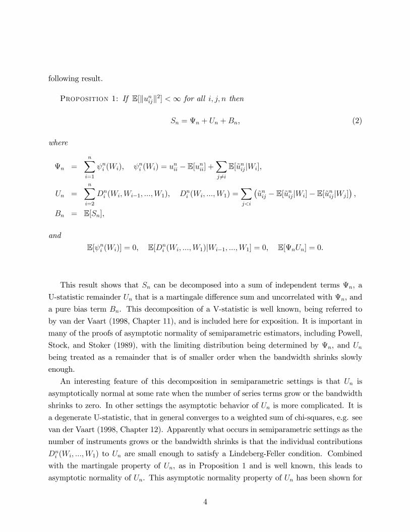
following result.

Proposition 1: If E[kunijk2] <1 for all i; j; n then

Sn = n + Un +Bn, (2)

where

n =nXi=1

ni (Wi), ni (Wi) = unii � E[unii] +Xj 6=i

E[~unijjWi],

Un =

nXi=2

Dni (Wi;Wi�1; :::;W1), Dn

i (Wi; :::;W1) =Xj<i

�~unij � E[~unijjWi]� E[~unijjWj]

�,

Bn = E[Sn],

and

E[ ni (Wi)] = 0, E[Dni (Wi; :::;W1)jWi�1; :::;W1] = 0, E[nUn] = 0.

This result shows that Sn can be decomposed into a sum of independent terms n, a

U-statistic remainder Un that is a martingale di¤erence sum and uncorrelated with n, and

a pure bias term Bn. This decomposition of a V-statistic is well known, being referred to

by van der Vaart (1998, Chapter 11), and is included here for exposition. It is important in

many of the proofs of asymptotic normality of semiparametric estimators, including Powell,

Stock, and Stoker (1989), with the limiting distribution being determined by n, and Unbeing treated as a remainder that is of smaller order when the bandwidth shrinks slowly

enough.

An interesting feature of this decomposition in semiparametric settings is that Un is

asymptotically normal at some rate when the number of series terms grow or the bandwidth

shrinks to zero. In other settings the asymptotic behavior of Un is more complicated. It is

a degenerate U-statistic, that in general converges to a weighted sum of chi-squares, e.g. see

van der Vaart (1998, Chapter 12). Apparently what occurs in semiparametric settings as the

number of instruments grows or the bandwidth shrinks is that the individual contributions

Dni (Wi; :::;W1) to Un are small enough to satisfy a Lindeberg-Feller condition. Combined

with the martingale property of Un, as in Proposition 1 and is well known, this leads to

asymptotic normality of Un. This asymptotic normality property of Un has been shown for

4

both series and kernel estimators, as further explained below.

Alternative asymptotics occurs when the number of series terms grows or the bandwidth

shrinks fast enough that n and Un have the same magnitude in the limit. Because of

uncorrelatedness of n and Un the asymptotic variance will be larger than the usual formula

which is limn�!1V[n]. Thus, consistent variance estimation under alternative asymptoticsrequires accounting for the presence of Un.

Accounting for the presence of Un should also yield improvements when numbers of series

terms and bandwidths do not satisfy the knife-edge conditions of alternative asymptotics.

Intuitively, if the number of series terms grows just slightly slower than the sample size or the

bandwidth shrinks slightly slower than 1=n. then accounting for the presence of Un should

still give a better large sample approximation. Hansen, Hausman, and Newey (2008) show

such an improvement for many instrument asymptotics. It would be good to consider such

improved approximations more generally, though it is beyond the scope of this paper to do

so.

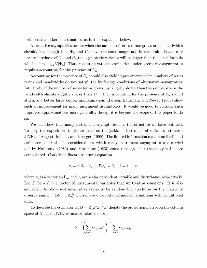
We can show that many instrument asymptotics has the structure we have outlined.

To keep the exposition simple we focus on the jackknife instrumental variables estimator

JIVE2 of Angrist, Imbens, and Krueger (1999). The limited information maximum likelihood

estimator could also be considered, for which many instrument asymptotics was carried

out by Kunitomo (1980) and Morimune (1983) some time ago, but the analysis is more

complicated. Consider a linear structural equation

yi = x0i�0 + "i, E["i] = 0, i = 1; :::; n,

where xi is a vector and yi and "i are scalar dependent variable and disturbance respectively.

Let Zi be a K � 1 vector of instrumental variables that we treat as constants. It is alsoequivalent to allow instrumental variables to be random but condition on the matrix of

observations Z = [Z1; :::; Zn]0 and replace unconditional moment conditions with conditional

ones.

To describe the estimator letQ = Z(Z 0Z)�Z 0 denote the projection matrix on the column

space of Z. The JIVE2 estimator takes the form

� =

Xi6=j

Qijxix0j

!�1Xi6=j

Qijxiyj.

5

Substituting for yj and collecting terms gives

pn(� � �0) =

Xi6=j

Qijxix0j=n

!�1Xi6=j

Qijxi"j=pn.

Here we can see that that JIVE2 is a special case of equation (1) with

�n = �0, � =Xi6=j

Qijxix0j=n, unii(Wi;Wi) = 0, unij(Wi;Wj) = Qijxi"j=

pn, i 6= j.

Note that E[unij(Wi;Wj)] = 0 and for �i = E[xi],

E[unij(Wi;Wj)jWi] = QijxiE["i] = 0, E[unij(Wi;Wj)jWj] = Qij�i"j=pn.

Here �i can be interpreted as the reduced form for observation i. Let vi = xi��i. ApplyingProposition 1, and using symmetry of the matrix Q, we �nd that equation (2) is satis�ed

with

ni (Wi) =

Xj 6=i

Qij�j

!"i = �i(1�Qii)"i=

pn�

�i �

Xi

Qij�j

!"i=pn,

Dni (Wi; :::;W1) =

Xj<i

Qij (vi"j + vj"i) =pn, Bn = 0.

Note that �i�P

iQij�j is the i-th residual from regressing the reduced form observations

on Z; so that by appropriate de�nition of the reduced form this can generally be assumed

to go to zero as the sample size grows. In that case

n =Xi

�i(1�Qii)"i=pn+ op(1).

Furthermore, under standard asymptotics Qii will go to zero, so the variance of this does

indeed correspond to the usual asymptotic variance for IV.

The degenerate U-statistic term is

Un =nXi=1

Xj<i

Qij (vi"j + vj"i) =pn.

Chao, Swanson, Hausman, Newey, and Woutersen (2010) apply the martingale central limit

6

theorem to show that this Un will be asymptotically normal when xi and "i have uniformly

bounded fourth moments, rank(Q) = dim(Z) = K �! 1, and Qii is bounded away from 1

uniformly in i and n. The conditions of the martingale central limit theorem are veri�ed by

showing that certain linear combinations with coe¢ cients depending on the elements of Q

go to zero as K �!1. In the proof, this makes individual terms asymptotically negligible,with a Lindeberg-Feller condition being satis�ed. Alternative asymptotics occurs when K

grows as fast as n, resulting in n and Un having the same magnitude in the limit.

As mentioned above, small bandwidth asymptotics for kernel estimators also has the

structure outlined above. To illustrate this we consider kernel estimation of the integrated

squared density. We use this example to keep the exposition relatively simple and because it

shares the common structure with the more interesting density weighted average derivative

estimator of Powell, Stock, and Stoker (1989) treated in Cattaneo, Crump, and Jansson

(2010). In this example the parameter of interest is

�0 =

Zf0(w)

2dw = E[f0(Wi)],

where Wi denotes a continuously distributed random variable with pdf f0. A �leave one out

estimator,�analogous to that of Powell, Stock, and Stoker (1989), is

� =Xi6=j

Kh(Wi �Wj)=n(n� 1);

where K(u) be a symmetric kernel with K(�u) = K(u) and Kh(u) = h�dK(u=h). This

estimator has the V-statistic form of equation (1) with

�0 =

Zf0(w)

2dw, � = 1, unii(Wi;Wi) = 0, unij(Wi;Wj) = Kh(Wi�Wj)=pn(n�1), i 6= j.

De�ne

fh(w) =

ZK(u)f(w + hu)du.

Note that by symmetry of K(u),

E[unij(Wi;Wj)jWi] = fh(Wi)=pn(n� 1), E[unij(Wi;Wj)jWj] = fh(Wj)=

pn(n� 1),

E[unij(Wi;Wj)] = E[fh(Xi)]=pn(n� 1).

7

Applying Proposition 1, and using symmetry of K(u), we �nd that equation (2) is satis�ed

with

ni (Wi) = 2ffh(Wi)� E[fh(Wi)]g=pn,

Dni (Wi; :::;W1) = 2

Xj<i

fKh(Wi �Wj)� fh(Wi)� fh(Wj) + E[fh(Wi)]g=pn(n� 1),

Bn =pnfE[fh(Wi)]� �0g.

Note that 2ffh(Wi)�E[fh(Wi)]g is an approximation to the well known in�uence function2[f0(Wi)��0] for estimators of the integrated squared density. As h! 0 we will have fh(Wi)

converging to f0(Wi) in mean square, so that

n =Xi

2[f0(Wi)� �0]=pn+ op(1).

The asymptotic variance of this leading term does correspond to the usual asymptotic vari-

ance for estimators of the integrated square density.

The degenerate U-statistic term is

Un = 2nXi=1

Xj<i

fKh(Wi �Wj)� fh(Wi)� fh(Wj) + E[fh(Wi)]g=pn(n� 1).

The martingale central limit theorem can be applied as in Cattaneo, Crump, and Jansson

(2010) to show that this Un will be asymptotically normal as h ! 0 and n ! 1 growing.

Intuitively, the bandwidth shrinking leads to Kh(Wi � Wj) being small except when Wi

and Wj are close, so that tail of the distribution ofpnDn

i (Wi; :::;W1) becomes thin and a

Lindeberg-Feller condition is satis�ed. Alternative asymptotics occurs when h shrinks as

fast as 1=n; resulting in n and Un having the same magnitude in the limit.

This pair of examples shows how several estimators share the common structure outlined

above. We now show how that structure can be applied to derive new results.

3 Series Estimation of the Partially Linear Model

To describe the partially linear model let (yi; x0i; z0i)0, i = 1; : : : ; n, be a random sample of the

random vector (y; x0; z0)0, where y 2 R is a dependent variable, and x 2 Rdx�1 and z 2 Rdz�1

8

are explanatory variables. The model is given by

yi = x0i� + g(zi) + "i, E ["ijxi; zi] = 0, �2(xi; zi) = E�"2i jxi; zi

�,

where vi = xi � h(zi), with h(zi) = E [xijzi].2 A series estimator of � is obtained by

regressing yi on xi and approximating functions of zi. To describe the estimator let pK(z) =

(pK1(z); : : : ; pKK(z))0 be an approximating functions, such as polynomials or splines, where

K denotes the number of terms in the regression. Here the unknown function g(z) will

be approximated by a linear combination of pkK(z). Also, let Y = [y1; � � � ; yn]0 2 Rn�1,X = [x1; � � � ; xn]0 2 Rn�dx, P = [pK(z1); : : : ; pK(zn)]0. A series estimator of � is given by

� = (X 0MX)�1X 0MY , M = I �Q, Q = P (P 0P )�P 0,

where A� denotes a generalized inverse of a matrix A (satisfying AA�A = A) and X 0MX

will be non-singular with probability approaching one under conditions given below. Donald

and Newey (1994) gave conditions for the asymptotic normality of this estimator.

Conditional on Z = [z1; :::; zn]0 this estimator has the structure outlined earlier. For

this reason we will condition on Z throughout the following discussion so that expectations

are implicitly conditional on Z. To explain how � �ts within the common structure, let

hi = E[xi] and vi = xi � hi: Also let gi = g(zi),

G = [g1; � � � ; gn]0, " = ["1; � � � ; "n]0, H = [h1; � � � ; hn]0, V = [v1; � � � ; vn]0.

By Y = X� +G+ " we have

pn(� � �) = (X 0MX=n)�1X 0M("+G)=

pn = ��1Sn,

� = X 0MX=n, Sn =Xi;j

xiMij(gj + "j)=pn.

This estimator has the V-statistic form of equation (1) with Wi = (yi; xi) and

�0 = �, � = X 0MX=n, unij(Wi;Wj) = xiMij(gj + "j)=pn.

By E["ijxi] = 0 we have E[xi"i] = 0. Therefore, letting unij = unij(Wi;Wj) as we have done

2See Robinson (1988) for the analysis of this model when using kernel regression, and Linton (1995) forthe corresponding higher-order properties.

9

previously, we have

E[unij] = HiMijgj=pn, unij � E[unij] =Mij (vigj + xi"j) =

pn,

~uij =Mij (vjgi + vigj + xj"i + xi"j) =pn, E[~uijjWi] =Mij (vigj + hj"i) .

Plugging these expressions into the formulas on Proposition 1 we obtain

ni (Wi) = Mii (vigi + hi"i + vi"i) =pn+

Xj 6=i

Mij (vigj + "ihj) =pn

=

"viMii"i + vi

Xj

Mijgj + "iXj

hjMij

#=pn,

Dni (Wi; :::;W1) =

Xj<i

Mij (vi"j + vj"i) =pn;Bn = H 0MG=

pn.

Summing up ni (Wi) it follows that

n =Xi

Miivi"i=pn+ (V 0MG+H 0M") =

pn.

The last term in this expression has mean zero and will converge to zero in mean square as

K grows, as further discussed below. Therefore, by Mii = 1�Qii;

n =Xi

(1�Qii)vi"i=pn+ op(1). (3)

Under standard asymptotics Qii will go to zero and hence the variance of this corresponds

to the usual asymptotic variance.

Noting that for j < i, Mij = �Qij, plugging in we �nd that the degenerate U-statisticterm is

Un = �nXi=1

Xj<i

Qij (vi"j + vj"i) =pn.

Remarkably this term is essentially the same as the degenerate U-statistic term for JIVE2

that was shown above. Consequently, the central limit theorem of Chao, Swanson, Hausman,

Newey, and Woutersen (2010) applies immediately to show that Un is asymptotically normal

as K �!1. This leads to many regressor asymptotics for series estimators of the partiallylinear model. It also illustrates the usefulness of the common structure, showing how that

10

structure can be used to derive new results.

4 Standard Asymptotics for the Series Estimator

The estimator � may be intuitively interpreted as a two-step semiparametric estimator with

smoothing parameter pK (�) and tuning parameter K, because the unknown (regression)functions g(�) and h (�) are non-parametrically estimated in a preliminary step by the se-ries estimator. In particular, the following assumption characterizes the rate at which the

approximation error of series estimator should vanish.

Assumption B. (i) For some �h > 0, there exists �h so that

1

nH 0MH =

1

nmin�kH � P�k2 = 1

n

nXi=1

h (zi)� pK (zi)0 �h 2 = Oas(K

�2�h).

(ii) For some �g > 0, there exists �g so that

1

nG0MG =

1

nmin�kG� P�k2 = 1

n

nXi=1

�g (zi)� pK (zi)

0 �g�2= Oas(K

�2�g).

The conditions required in Assumption B are implied by conventional assumptions from

the series-based nonparametric literature (e.g., Newey (1997, Assumption 3)). Thus, under

appropriate assumptions, commonly used basis of approximation such as polynomials or

splines will satisfy Assumption B with �h = dz=sh and �g = dz=sg, where sh and sg denotes

the number of continuous derivatives of h and g, respectively.

Under regularity conditions (given below) and Assumption B, Donald and Newey (1994)

obtained the following (infeasible) classical asymptotic approximation for � corresponding

to equation (3): If

nK�2(�h+�g) ! 0 andK

n! 0 (4)

thenpn(� � �) =

1pn

nXi=1

i + op(1)!d N (0;) , = ��1���1, (5)

where

i = ��1vi"i, � = E [viv0i] , � = E [viV ["jX;Z] v0i] .

11

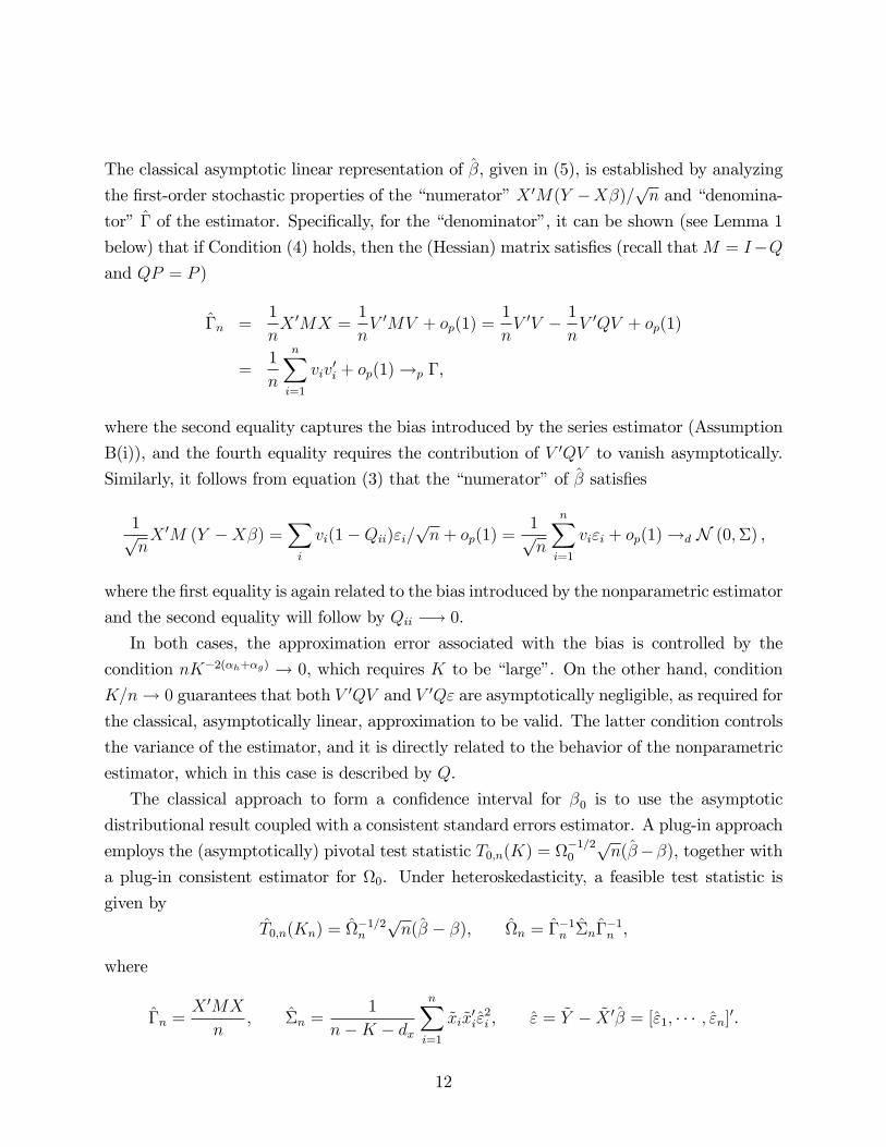
The classical asymptotic linear representation of �, given in (5), is established by analyzing

the �rst-order stochastic properties of the �numerator�X 0M(Y �X�)=pn and �denomina-

tor� � of the estimator. Speci�cally, for the �denominator�, it can be shown (see Lemma 1

below) that if Condition (4) holds, then the (Hessian) matrix satis�es (recall thatM = I�Qand QP = P )

�n =1

nX 0MX =

1

nV 0MV + op(1) =

1

nV 0V � 1

nV 0QV + op(1)

=1

n

nXi=1

viv0i + op(1)!p �,

where the second equality captures the bias introduced by the series estimator (Assumption

B(i)), and the fourth equality requires the contribution of V 0QV to vanish asymptotically.

Similarly, it follows from equation (3) that the �numerator�of � satis�es

1pnX 0M (Y �X�) =

Xi

vi(1�Qii)"i=pn+ op(1) =

1pn

nXi=1

vi"i + op(1)!d N (0;�) ,

where the �rst equality is again related to the bias introduced by the nonparametric estimator

and the second equality will follow by Qii �! 0.

In both cases, the approximation error associated with the bias is controlled by the

condition nK�2(�h+�g) ! 0, which requires K to be �large�. On the other hand, condition

K=n! 0 guarantees that both V 0QV and V 0Q" are asymptotically negligible, as required for

the classical, asymptotically linear, approximation to be valid. The latter condition controls

the variance of the estimator, and it is directly related to the behavior of the nonparametric

estimator, which in this case is described by Q.

The classical approach to form a con�dence interval for �0 is to use the asymptotic

distributional result coupled with a consistent standard errors estimator. A plug-in approach

employs the (asymptotically) pivotal test statistic T0;n(K) = �1=20

pn(���), together with

a plug-in consistent estimator for 0. Under heteroskedasticity, a feasible test statistic is

given by

T0;n(Kn) = �1=2n

pn(� � �), n = �

�1n �n�

�1n ,

where

�n =X 0MX

n, �n =

1

n�K � dx

nXi=1

~xi~x0i"2i , " = ~Y � ~X 0� = ["1; � � � ; "n]0.

12

In this case, the standard error estimator is the classical Heteroskedasticity-Robust (HR)

standard errors estimator commonly used in regression analysis. Under Condition (4) it is

not di¢ cult to show that �1n 0 !p Idx.

5 Many Regressor Asymptotics

This section derives a generalized asymptotic distribution forpn(� � �), which relaxes the

condition Kn=n! 0. This non-standard asymptotic theory encompasses the classical result

discussed in the previous section, and also captures the e¤ect of the degenerate U-statistic

term of the expansion, which is negligible when K=n �! 0. Intuitively, this asymptotic

experiment captures the e¤ect of K �large�(relative to n) by breaking down the asymptotic

linearity of the estimator.

To characterize the generalized central limit theory, it is natural to study the stochastic

behavior of the estimatorpn(� � �) as a �ratio�of two bilinear forms:

pn(� � �) =

�1

nX 0MX

��1pnX 0M (Y �X�) = ��n

1pnX 0M (Y �X�) .

The following lemma characterizes the behavior of the Hessian matrix �n under quite

weak conditions.

Lemma 1. Suppose that E[kvik4] � Cv <1 (a.s.) and Assumption B(i) holds. Then,

�n =1

nX 0MX = �n + op(K=n), �n =

1

n

nXi=1

MiiE [viv0ijzi] = Oas(1 +K=n).

This lemma characterizes the stochastic behavior of the Hessian matrix under conditions

that are weaker than those entertained by the classical, asymptotically linear, distribution

theory. Speci�cally, because M = I � Q is an idempotent symmetric matrix, Mii 2 (0; 1)and

Pni=1Mii � n � K, Lemma 1 implies that �n remains asymptotically bounded even

when K=n 6! 0. In particular, �n = E [viv0i] + op (1) when K=n ! 0. Moreover, in the

case of homoskedasticity of vi, that is, if E [viv0ijzi] = E [viv0i] (and rank (Q) = K), then

�n = (1�K=n)E [viv0i]. Finally, if �min (E [viv0ijzi]) � FV > 0 and Mii = 1 � Qii � FQ > 0

(a.s.) then �min (�n) � FQFV > 0. (�min (A) denotes the minimum eigenvalue of a matrix

A.)

13

To fully characterize the asymptotic behavior of the �numerator� ofpn(� � �) it is

convenient to proceed in two steps. First, under appropriate bias assumptions, it is possible

to show that the numerator is asymptotically equivalent to a quadratic form based on mean-

zero random variables.

Lemma 2. Suppose the assumptions of Lemma 1 hold, and E["4i ] � C" < 1 (a.s.) and

Assumption B(ii) holds. Then,

(V 0MG+H 0M"+H 0MG) =pn = Op(

pnK�(�h+�g) +K��h +K��g).

As in Lemma 1, this result only requires bounded moments and a bias condition. In

this case, the bias arises from the approximation of both unknown functions h and g. As

mentioned above, the high-level Assumption B is implied by the standard assumption of best

approximation from the sieve literature. Interestingly, in this model there is a trade-o¤ in

terms of curse of dimensionality: provided that min f�h; �gg > 0, the bias condition is givenbypnK�(�h+�g) ! 0, which implies a trade-o¤ between smoothness and dimensionality

between h and g.

Lemma 2 justi�es focusing on the bilinear form

�n =1pnV 0M" =

1pn

nXi=1

nXj=1

Mijvi"j,

where E [�njZ;X] = 0. Moreover, under the assumptions imposed in Lemma 2, a simple

variance calculation yields

�n = V [�njZ] =1

n

nXi=1

nXj=1

M2ijE[viv0i"2j ] = Oas (1 +K=n) .

In particular, if K=n! 0 then

�n =1

n

nXi=1

M2iiE�viv

0i"2i jzi�+ op (1) = E

�viv

0i"2i

�+ op (1) = � + op (1) ,

as given in Section 2. Moreover, under homoskedasticity, that is, if E ["2i jxi; zi] = �2, then

V�1pnV 0M"

����X;Z� = �2

nV 0MV ,

14

and

�n =�2

n

nXi=1

nXj=1

M2ijE [viv0ijzi] = �2�n,

becausePn

j=1M2ij = Mii. Furthermore, if E ["2i jxi; zi] = �2 and E [viv0ijzi] = E [viv0i] (and

rank (Q) = K (a.s.)), then �n = �2 (1�K=n)E [viv0i]. Finally, if �min (E [viv0i"2jzi]) � FV " >

0 and Mii = 1�Qii � FQ > 0 (a.s.), then �min (�n) � F 2QFV " > 0.

The following Lemma characterizes the asymptotic distribution of the bilinear form �n.

Lemma 3. Suppose the assumptions of Lemma 2 hold, and Mii > FM > 0 (a.s.) and

�min (�n) > F� > 0 (a.s.). Then,

��1=2n

1pnV 0M"!d N (0; Idx) .

The following theorem is a direct consequence of the previous lemmas and Slutsky The-

orem, and constitutes the main result of this section.

Theorem 1. Suppose the assumptions of Lemma 3 hold and suppose �min (�n) > FH > 0.

Then, if

nK�2(�x+�g) ! 0 andK

n! � 2 [0; 1) (6)

then

�1=2n (� � �)!d N (0; Idx) . (7)

If, moreover, (�n;�n) = (�1;�1) + op (1) for some (�1;�1), then

pn(� � �)!d N (0;1) , 1 = �

�11 �1�

�11 .

If, moreover, E ["2i jxi; zi] = �2 for some �2, then

pn(� � �)!d N

�0; �2��11

�.

Theorem 1 shows that the central limit theorem for � holds under the weaker condition

(6). (Compare to Condition (4).) This result does not rely on asymptotic linearity, nor on

the actual convergence of the matrices �n and �n. However, if K=n ! 0, then (�n;�n) =

(�;�)+op (1) with � = E [viv0i] and � = E [viv0i"2i ], and the resulting large sample distributiontheory does rely on the asymptotically linear representation of �, as given in (5).

15

Importantly, if K=n 9 0 and (�n;�n) = (�;�) + op (1), then � 6= E [viv0i] and � 6=E [viv0i"2i ], in general. For instance, if (vi; "i) is independent of zi, then �n = (1�K=n)E [viv0i]and

�n =

�1� K

n

�E�viv

0i"2i

�+

1

n

nXi=1

Q2ii �K

n

!�E�viv

0i"2i

�� E [viv0i]E

�"2i��.

6 Standard Errors

This section discusses di¤erent homoskedastic- and heteroskedastic- standard errors estima-

tors, and their properties under the generalized asymptotics studied in this paper.

6.1 Homoskedasticity

If E ["2i jxi; zi] = �2 for all i = 1; 2; � � � ; n, then �n = �2��n . Thus, a natural plug-in estimator

is given by VHOM = �2��, where �2 is chosen so that �2 = �2 + op (1). The usual OLS

estimator is

�2n =1

n�K � dx

nXi=1

"2i =1

n�K � dx"0".

As shown in Lemma 1, �n = �n + op(1) under the many terms asymptotics discussed in

this paper (Condition (6)), and therefore it remains to verify that �2n is also consistent under

this generalized asymptotic experiment. This estimator is consistent because

"0" = (Y �X�)0M(Y �X�) = "0M"+ op(1) = (n�K)�2 + op(1),

where the �rst approximation is based on thepn-consistency of � and the approximation

bias of the series estimator, while the second approximation is based on the fact that the

bilinear form "0M" = "0(I �Q)" is dominated by its diagonal.

Theorem 2. Suppose the assumptions of Theorem 1 hold. Then, �2n = �2 + op (1).

It follows by Lemma 1, Theorem 2 and Slutsky Theorem that

VHOM = �2��n + op (1) = �n + op (1) ,

and therefore

V�1=2HOM(� � �0)!d N (0; Id) ,

16

under Condition (6). Thus, under known homoskedasticity, the usual �nite sample stan-

dard errors estimator from least squares theory turns out to be valid even when K is large.

However, the �consistent�but biased standard errors estimator ("0"=n)��n will not be con-

sistent unless K=n! 0, which implies that using the �nite sample, unbiased standard errors

estimator under homoskedasticity is important even in large samples when the degrees of

freedom is small (i.e., when K is large).

6.2 Heteroskedasticity

Under heteroskedasticity of unknown form, a natural candidate for standard errors estimator

is the (family of) Eicker-Huber-White estimators given by

VHR = ( ~X0 ~X)� ~X 0� ~X( ~X 0 ~X)� =

1

n��n �n�

�n ,

�n =1

nX 0M�MX, � = diag

�!1"

21; � � � ; !n"2n

�=

2664!1"

21

. . .

!n"2n

3775where f!i : i = 1; � � � ; ng are appropriate weights. Classical choices of weights include !i = 1,!i = n=(n � K � dx), !i = M�1

ii , etc. Since �n = �n + op(1) according to Lemma 1, it

only remains to characterized the middle matrix of this classical sandwich formula. The

asymptotic properties of �n are given by

�n =1

n

nXi=1

!i~xi~x0i"2i =

1

n

nXi=1

!i~vi~v0i~"2i + op(1) =

1

n

nXi=1

E�!i~vi~v

0i~"2i

��Z�+ op(1),

where, as before, the �rst approximation captures the bias of the series estimator and removes

the estimation error of �, and the second approximation shows that a (conditional) law of

large numbers holds in this case (i.e., a variance condition). This results is summarized in

the following theorem.

Theorem 3. Suppose the assumptions of Theorem 1 hold, nK�2(�g+�h)+1 ! 0 withminf�g; �hg >1=2, and !i 2 � (Z) for all i with j!ij � C!. Then, �n = ~�n + op(1), where

~�n =1

n

nXi=1

nXj=1

nX`=1

!iM2i`M

2j`

!E�viv

0i"2j

�� zi; zj� .17

Recall that the population asymptotic middle matrix �n is given by

�n =1

n

nXi=1

nXj=1

M2ijE[viv0i"2j jzi; zj],

which implies that the classical HR standard errors will not be consistent in general when

Condition (6). For example, the bias may be characterized under homoskedasticity: assum-

ing E ["2i jxi; zi] = �2 and !i = 1, a simple calculation yields

�n =�2

n

nXi=1

MiiE [viv0ijzi] ,

while, using basic properties of idempotent matrices, it is easy to verify that

~�n = �n �1

n

nXi=1

nXj=1

M2ij (1�Mjj)E [viv0ijzi] < �n.

As a consequence, the classical Eicker-Huber-White estimator is downward biased when K

is �large�. It is important to note that this result continue to hold in a simple linear model

where the number of regressors is �large�when compared to the sample size. Therefore, there

is an important sense in which the classical HR standard errors estimator is not robust, even

in a simple linear model.

On the other hand, if K=n! 0, then the asymptotic results presented above imply that~�n = �n + op(1), which veri�es that the classical HR standard errors estimator is indeed

consistent under heteroskedasticity of unknown form.

6.3 HR and Many Terms Robust Standard Errors

Intuitively, the failure of the classical HR standard errors estimator is due to the fact that

both ~xi and "i are estimated with too much error when K=n 6! 0. Thus, it is possible to �x

this problem by considering alternative (consistent) estimators for either ~xi or "i. To describe

the new estimators, let Kg and Kh be two choices of truncation for an approximation series,

and let~X = (I �Qh)X, Qh = PKh

(P 0KhPKh

)�P 0Kh, Mh = I �Qh,

" = (I �Qg)", Qg = PKg(P0KgPKg)

�P 0Kg, Mg = I �Qg.

18

Using this notation, Theorem 3 may be extended to the following result.

Theorem 4. Suppose the assumptions of Theorem 1 hold, nK1=2g K

�2�gg K

1=2h K�2�h

h ! 0

with minf�g; �hg > 1=2, and !i 2 � (Z) for all i with j!ij � C!. Then

��n =1

n

nXi=1

nXj=1

nX`=1

!iM2h;i`M

2g;j`

!E�viv

0i"2j jzi; zj

�.

This theorem leads naturally to two alternative recipes for heteroskedasticity and many

terms robust estimators. Speci�cally, for !i = 1, ifminfKh; Kgg = o (n) andmaxfKh; Kgg =K, then ��n = �n + op(1). This result implies that

V�1=2HET (� � �0)!d N (0; Id) , VHET =

1

n��n��n�

�n .

7 Simulations

To explore the consequences of using many terms in the partially linear model, or alterna-

tively using many covariates in a linear model, this section reports preliminary results from

a Monte Carlo experiment. Speci�cally, the simulations consider the following model:

yi = x0i� + g(zi) + "i, "i = �" (xi; zi)u1i,

xi = h (zi) + vi, vi = �v (zi)u2i,

with dx = 1, dz = 10, g (z) = 1, h (z) = 0, and u = (u1i; u1i)0 � N (0; I2) and zi � U (�1; 1)independently of u. Note that this data generating process does not have smoothing bias.

Four models of heteroskedasticity are considered, as given in Table 1 (with � = (1; 1; � � � ; 1)0 2Rdz).

Table 1: Simulation Models ()

�2v (zi) = 1 �2v (zi) = (z0i�)

2

�2" (xi; zi) = 1 Model 1 Model 3

�2" (xi; zi) = (z0i�+ xi)

2 Model 2 Model 4

For simplicity, the simulations consider additive-separable power series, that is, the

unknown function g(zi) is assumed to satisfy g(zi) = 1 + g1 (z1i) + � � � + gdz (zdzi) and

each component is estimated by gj (zji) � pK (zji)0 j, j = 1; 2; � � � ; dz, with pK (zji) =

(0; zji; z2ji; � � � ; zK�1ji )0.

19

We consider the classical least squares homoskedasticity-consistent standard errors esti-

mators

VHO1 ="0"

n�� and VHO2 =

"0"

n�K � dx��,

and the classical heteroskedasticity-consistent standard errors estimators

VHR1 = �� ~X 0� ~X��, � = diag ("1; � � � ; "n) =n,

VHR2 = �� ~X 0� ~X��, � = diag ("1; � � � ; "n) =(n�K � dx).

Also, we report the two alternative heteroskedasticity- and many terms- robust standard

errors estimators proposed in Theorem 4. These estimators are given by

VCJN1 = �� ~X 0� ~X��, � = diag ("1; � � � ; "n) =n, Kh = KCV , Kg = K,

VCJN2 = �� ~X 0� ~X��, � = diag ("1; � � � ; "n) =n, Kh = K, Kg = KCV ,

where KCV represents a cross-validation estimate of the optimal K.

The results are presented in Figure 1, for a grid of K = (0; 1; 2; � � � ; 20). The e¤ectivedegrees of freedom is determined by the choice of K and dz.

20

8 Technical Appendix

All statements involving conditional expectations are understood to hold almost surely. Recall that M =

I �Q is symmetric and idempotent, and therefore jMiij � 1, n�K =Pn

i=1Mii and Mij =Pn

`=1Mi`M`j .

Proof of Lemma 1. It follows from H 0MH=n = op (1) and the Cauchy-Schwarz inequality that

X 0MX=n = (V +H)0M (V +H) =n = V 0MV=n + H 0MH=n + 2H 0MV=n = V 0MV=n + op (1), provided

that

V 0MV=n =nXi=1

Miiviv0i=n+

nXi=1

Xj 6=i

Mijviv0j=n = Op(1).

Using jMiij � 1 and the Markov inequality,

nXi=1

Miiviv0i=n =

nXi=1

MiiE [viv0ijzi] =n+ op (1) ,

because

V

"nXi=1

Mii kvik2 =n�����Z#=

nXi=1

M2iiV[kvik

2 jzi]=n2 = Oas�n�1

�,

whilenXi=1

Xj 6=i

Mijviv0j=n = Op(n

�1K1=2) = op (1)

by Lemma A1 of Chao, Swanson, Hausman, Newey, and Woutersen (2010). �

Proof of Lemma 2. First note that

X 0M (Y �X�0) =pn = V 0M"=

pn+H 0M"=

pn+X 0MG=

pn,

where H 0M"=pn = Op (K

��h) because

Eh H 0M"=

pn 2���Zi = tr (H 0ME[""0jZ]MH) =n � C" tr (H 0MH) =n = O

�K�2�hn

�.

Next,

X 0Mg=pn = V 0MG=

pn+ �X 0MG=

pn = Op

�K��g +

pnK�(�X+�g)

�,

because

Eh V 0MG=pn 2���Zi = G0ME [V V 0jZ]MG=n � CvG0MG=n = Oas �K�2�g

�,

and

H 0MG=pn �

pnpH 0MH=n

pG0MG=n = Oas

�pnK�(�X+�g)

�,

which completes the proof. �

Proof of Lemma 3. Follows from Lemma A2 in Chao, Swanson, Hausman, Newey, and Woutersen

(2010). �

21

Proof of Theorem 1. Follows by standard arguments from Lemmas 1�3. �

Proof of Theorem 2. First, it follows from G0MG=n = op (1) and the Cauchy-Schwarz inequality that

"0"=n = (Y �X�)0M(Y �X�)=n

= (Y �X� �G)0M(Y �X� �G)=n+G0MG=n� 2(Y �X� �G)0MG=n

= (Y �X� �G)0M(Y �X� �G)=n+ op(1),

provided (Y �X� � G)0M(Y �X� � G)=n = Op (1). Next, note that Lemma 1 and � � � = op(1) imply(� � �)0X 0MX(� � �)=n = op (1), which together with the Cauchy-Schwarz inequality gives

(Y �X� �G)0M(Y �X� �G)=n

= "0M"=n+ (� � �)0X 0MX(� � �)=n� 2(Y �X(� � �)�G)0M(� � �)=n

= "0M"=n+ op(1) = ~"0~"=n+ op(1).

Finally, consider the bilinear form

~"0~"=n = "0M"=n =Xi

Mii"2i =n+

Xi

Xj 6=i

"iMij"j=n.

Using jMiij � 1 and the Markov inequality,Xi

Mii"2i =n =

Xi

MiiE�"2i jzi

�=n+ op (1) =

n�Kn

�2 + op(1)

because

E

"V

"Xi

Mii"2i =n

�����Z##= E

"Xi

M2iiV["2i jzi]=n2

#�Xi

E�V["2i jzi]

�=n2 � Cv=n = o (1) ,

while Xi

Xj 6=i

Mij"i"j=n = Op

�n�1K1=2

�= op (1) ,

by Lemma A1 of Chao, Swanson, Hausman, Newey, and Woutersen (2010). Therefore, since (n�K)=(n�K � dx)! 1, �2 = "0"=(n�K � d) = �2 + op(1), which completes the proof. �

Proof of Theorem 3. Apply Theorem 4 with Kg = Kh = K. �

Proof of Theorem 4. First note that " = ~Y � ~X 0� = ~" � ~X 0(� � �) + ~g0, for ~X = (I � Qg)X and

~g = (I �Qg)g. Thus, �n = T1;n + T2;n + T3;n + T4;n + T5;n + T6;n, where

T1;n =1

n

Xi

wi~"2i ~vi~v

0i, T2;n =

1

n

Xi

wi~"2i ~vi (~xi � ~vi)

0 , T3;n =1

n

Xi

wi~"2i (~xi � ~vi) ~v0i,

22

T4;n =1

n

Xi

wi~"2i (~xi � ~vi) (~xi � ~vi)

0 , T5;n =1

n

Xi

wi

�~x0i(� � �) + ~gi

�2~xi~x

0i,

T6;n =1

n

Xi

wi~"i

�~x0i(� � �) + ~gi

�~xi~x

0i,

with ~X = (I �Qh)X = [~x1; � � � ; ~xn]0 and ~V = (I �Qh)V = [~v1; � � � ; ~vn]0.First consider the leading term T1;n. Note that T1;n = T11;n + T12;n + T13;n, where

T1;n =1

n

Xi

wi

0@Xj

M2g;ij"

2j

1A Xk

M2h;ikvkv

0k

!,

T2;n =1

n

Xi

wi

0@Xj

M2g;ij"

2j

1A0@Xk1

Xk2 6=k1

Mh;ik1Mh;ik2vk1v0k2

1A ,T3;n =

1

n

Xi

wi

0@Xj1

Xj2 6=j1

Mg;ij1Mg;ij2"j1"j2

1A0@Xk1;k2

Mh;ik1Mh;ik2vk1v0k2

1A ,with E [T12;njZ] = 0 = E [T13;njZ]. Moreover,

T11;n = E [T11;njZ] + op (1) , E [T11;njZ] =1

n

Xi;j

X`

w`M2g;`iM

2h;`j

!E["2i vjv0j jzi; zj ],

because V[T11;njZ] = oas(1). To see this last result, let a1;ij =P

` w`M2g;`iM

2h;`j and A1;ij = "2i vjv

0j �

E["2i vjv0j jZ], and note after expanding the sums and collecting terms,

V[T11;njZ] =1

n2E

264 Xi;j

aijAij

2�������Z375 � C

n2

Xi;j;k

[aijaik + aikaji + aijajk + aikajk] � Cn�1,

because ������Xi;j;k

aijaik

������ =

������Xi;j;k

X`1

w`1M2g;`1iM

2h;`1j

! X`2

w`2M2g;`2jM

2h;`2k

!������� C

Xi

X`1

M2g;`1i

Xj

M2h;`1j

X`2

M2g;`2j

Xk

M2h;`2k � Cn,

and similarly for the other terms.

Next, T12;n = op (1) because E [T2;njZ] = 0 and E[kT2;nk2 jZ] � Cn�1=2. To see the last conclusion, leta2;ijk = 1 (j 6= k)

P` w`M

2g;`iMh;`jMh;`k and A2;ijk = "2i vjv

0k, and observe that aijk = aikj . Expanding the

23

sums, using the mean-zero property of A2;ijk, and collecting terms gives

E[kT2;nk2 jZ] �C

n2E

264 Xi

Xj 6=i

a2;iji"2i viv

0j

2�������Z375+ C

n2E

264 Xi

Xj 6=i

Xk 6=i;k 6=j

a2;ijkA2;ijk

2�������Z375 .

Now, for the �rst term, de�ne a2;ij = 1 (i 6= j) a2;iji and A2;ij = "2i viv0j , and expanding the sums and

collecting non-mean-zero terms

1

n2E

264 Xi

Xj 6=i

a2;ij"2i viv

0j

2�������Z375 � C

n2

Xi

Xj 6=i[a22;ij + a2;ija2;ji] +

C

n2

Xi

Xj 6=i

Xk 6=i;k 6=j

a2;ika2;jk

� Cn�1 + Cn�1=2,

while for the second term

1

n2E

264 Xi

Xj 6=i

Xk 6=i;k 6=j

a2;ijkA2;ijk

2�������Z375 � C

n2

Xi

Xj 6=i

Xk 6=i;k 6=j

[a2ijk + aijkajik] +C

n2

Xi

Xj 6=i

Xk 6=i;k 6=j

Xl 6=i;l 6=j;l 6=k

aijkaljk

� Cn�1=2 + Cn�1,

where the �nal bounds as a function of n are obtained by properties of the idempotent matrix M as above.

Finally, T3;n = op (1) because E [T3;njZ] = 0 and E[ kT3;nk2 jZ] � Cn�1. To see the last conclusion,

�rst let a3;ij = "i"j and A3;ij = 1 (i 6= j)P

` w`Mg;`iMg;`j

�Pk1

Pk2Mh;`k1Mh;`k2vk1v

0k2

�, and observe that

a3;ij = a3;ji and A3;ij = A3;ji = A03;ij = A03;ji. Then, expanding the sums and collecting non-mean-zero

terms,

E[kT3;nk2 jZ] = E

264 1nXi

Xj

a3;ijA3;ij

2�������Z375 = 2

n2

Xi

Xj

E[a23;ij kA3;ijk2 jZ]

� C

n2

Xi

Xj 6=i

E

24 X`

w`Mg;`iMg;`j

Xk1

Xk2

Mh;`k1Mh;`k2vk1v0k2

! 2������Z35 .

Next, for each (i; j) let a3;ijkl =P

` w`Mg;`iMg;`jMh;`kMh;`l and A3;kl = vkv0l, and note that a3;ijkl =

24

a3;ijlk and A3;kl = A03;lk. Thus, expanding the sums and collecting non-mean-zero terms,

E[kT3;nk2 jZ] � C

n2

Xi

Xj 6=i

E

24 nXk=1

nXl=1

a3;ijklA3;kl

2������Z35

� C

n2

Xi

Xj 6=i

E

24 Xk

a3;ijkkA3;kk

2������Z35+ C

n2

Xi

Xj 6=i

E

264 Xk

Xl 6=k

a3;ijklA3;kl

2�������Z375

� C

n2

Xi

Xj 6=i

Xk

a2ijkk +C

n2

Xi

Xj 6=i

Xk

Xl 6=k

a2ijkl � Cn�1,

where the last inequality follows by properties of the idempotent matrix M as above.

Next, consider the smaller order terms Tk;n, k = 2; � � � ; 6. By ~"i = Mg;ii"i +Pn

j=1;j 6=iMg;ij"j with

E ["ij zi] = 0,E�~"4i��Z� � CX

j

Xk

M2g;ijM

2g;ikE["2j"2kjzj ; zk] � C,

by properties of the idempotent matrix M . Similarly, E[k~vik4jZ] � C. For terms T2;n and T3;n, using

~xi � ~vi =M 0h;iH =M 0

h;i(H � P 0Kh�h), it follows that for k = 2; 3,

E [kTk;nkjZ] � 1

n

Xi

jwijE[~"2i k ~VikjZ] M 0

h;i(H � P 0Kh�h)

� C

n

Xi

Xk

jMh;ikj kh(zk)� pKh(zk)

0�hk � CK1=2h K��h

h ,

by Cauchy-Schwarz inequality, and therefore T2;n = op (1) and T3;n = op (1). Also, by the same arguments,

E [kT4;nkjZ] � C

n

Xi

E�~"2i��Z� M 0

h;i(H � P 0Kh�h) 2

� C

n

Xi

Mh;ii

Xk

kh(zk)� pKh(zk)

0�hk2 � CKhK�2�hh

which implies that T4;n = op (1).

Therefore, it remains to show that T5;n = op(1), which then implies by the Cauchy-Schwarz inequality

that T6;n = op (1). To this end, note that

T5;n =1

n

Xi

wi

�~x0i(� � �) + ~gi

�2~xi~x

0i = Op(n

�1 +KhK�4�hh +K1=2

g K�2�gg + nK1=2

g K�2�gg K

1=2h K�2�h

h ),

25

because, using � � �0 = Op�n�1=2

�, E[k~vik4jZ] � C,

1

n

Xi

jwij k~x0i(� � �0)k2k~xik2 � Ck� � �0k21

n

Xi

k~vik4 + Ck� � �0k21

n

Xi

kM 0h;i(H � P 0Kh

�h)k4

� Op(n�1) +Op(1)

1

n2

Xi

M2h;ii

Xk

kh(zk)� pKh(zk)

0�hk2!2

= Op(n�1 +KhK

�4�hh ),

and

1

n

Xi

jwij j~gij2k~xik2 � C

vuutXi

M2g;ii

Xk

kg(zk)� pKg(zk)0�gk2

!2s1

n2

Xi

k~xik4

� CpKg

Xk

kg(zk)� pKg(zk)

0�gk2!Op(n

�1 +K1=2h K�2�h

h )

= Op(K1=2g K�2�g

g + nK1=2g K�2�g

g K1=2h K�2�h

h ).

This concludes the proof. �

26

ReferencesAngrist, J., G. W. Imbens, and A. Krueger (1999): �Jackknife Instrumental Variables Estimation,�Journal of Applied Econometrics, 14(1), 57�67.

Bekker, P. A. (1994): �Alternative Approximations to the Distributions of Instrumental Variables Esti-

mators,�Econometrica, 62, 657�681.

Cattaneo, M. D., R. K. Crump, and M. Jansson (2010): �Small Bandwidth Asymptotics for Density-Weighted Average Derivatives,�working paper.

Chao, J. C., N. R. Swanson, J. A. Hausman, W. K. Newey, and T. Woutersen (2010): �Asymp-totic Distribution of JIVE in a Heteroskedastic IV Regression with Many Instruments,� forthcoming in

Econometric Theory.

Donald, S. G., and W. K. Newey (1994): �Series Estimation of Semilinear Models,�Journal of Multi-variate Analysis, 50(1), 30�40.

Hansen, C., J. Hausman, and W. K. Newey (2008): �Estimation with Many Instrumental Variables,�Journal of Business and Economic Statistics, 26(4), 398�422.

Kunitomo, N. (1980): �Asymptotic Expansions of the Distributions of Estimators in a Linear Functional

Relationship and Simultaneous Equations,� Journal of the American Statistical Association, 75(371),

693�7000.

Linton, O. (1995): �Second Order Approximation in the Partialy Linear Regression Model,�Econometrica,

63(5), 1079�1112.

Morimune, K. (1983): �Approximate Distributions of k-Class Estimators when the Degree of Overidenti-

�ability is Large Compared with the Sample Size,�Econometrica, 51(3), 821�841.

Newey, W. K. (1997): �Convergence Rates and Asymptotic Normality for Series Estimators,�Journal of

Econometrics, 79, 147�168.

Powell, J. L., J. H. Stock, and T. M. Stoker (1989): �Semiparametric Estimation of Index Coe¢ -cients,�Econometrica, 57(6), 1403�1430.

Robinson, P. M. (1988): �Root-N-Consistent Semiparametric Regression,�Econometrica, 56(4), 931�954.

van der Vaart, A. W. (1998): Asymptotic Statistics. Cambridge University Press, New York.

White, H. (1980): �A Heteroskedasticity-Consistent Covariance Matrix Estimator and a Direct Test for

Heteroskedasticity,�Econometrica, 48(4), 817�838.

27

0.0

0.1

0.2

0.3

0.4

0.5

0.6

0.7

0.8

0.9

1.0

Mo

del

1

Kn

Empirical Coverage

0.95

VH

O1

VH

O2

VH

R1

VH

R2

VC

JN

1

VC

JN

2

0.0

0.1

0.2

0.3

0.4

0.5

0.6

0.7

0.8

0.9

1.0

Mo

del

2

Kn

Empirical Coverage

0.95

0.0

0.1

0.2

0.3

0.4

0.5

0.6

0.7

0.8

0.9

1.0

Mo

del

3

Kn

Empirical Coverage

0.95

0.0

0.1

0.2

0.3

0.4

0.5

0.6

0.7

0.8

0.9

1.0

Mo

del

4

Kn

Empirical Coverage

0.95

Figure1:EmpiricalCoverageRatesfor95%Con�denceIntervals:n=500,S=3;000

28