Algorithms, Operators and

Transfer Matrices

Richard P. Brent

MSI & RSISE

ANU

11 October 2007

Outline

Average-case analysis of algorithms usestechniques that may have applications in otherareas, such as statistical mechanics. Toillustrate this, we consider the analysis of onenontrivial algorithm, the binary Euclideanalgorithm.

• The binary Euclidean algorithm –results of Brent & Maze

• Ruelle operators – results of Vallee

• Possible connection with TransferMatrices

Notation

lg(x) denotes log2(x).

N, n, u, v are positive integers.

Val2(u) denotes the dyadic valuation of thepositive integer u, i.e. the greatest integer jsuch that 2j | u.

2

The Binary Euclidean Algorithm

The idea of the binary Euclidean algorithm is toavoid the “division” operation r ← m mod n ofthe classical algorithm, but retain O(log N)worst (and average) case.

We assume that the algorithm is implementedon a binary computer so division by a power oftwo is easy. In particular, we assume that the“shift right until odd” operation

u← u/2Val2(u)

or equivalently

while even(u) do u← u/2

can be performed in constant time, althoughtime O(Val2(u)) would be sufficient.

3

Definition

There are several almost equivalent ways todefine the algorithm. It is easy to take accountof the largest power of two dividing the inputs,so for simplicity we assume that u and v are odd

positive integers.

Following is a simplified version of thealgorithm given in Knuth, §4.5.2.

Algorithm B

B1. t← |u− v|;if t = 0 terminate with result u

B2. t← t/2Val2(t)

B3. if u ≥ v then u← t else v ← t;go to B1.

4

A Heuristic Continuous Model

To analyse the expected behaviour ofAlgorithm B, we can follow what Gauss did forthe classical algorithm. This was first attemptedin my 1976 paper1 and there is a summary inKnuth (Vol. 2, third edition, §4.5.2).

Assume that the initial inputs u0, v0 toAlgorithm B are uniformly and independentlydistributed in (0, N), apart from the restrictionthat they are odd. Let (un, vn) be the value of(u, v) after n iterations of step B3.

Let

xn =min(un, vn)

max(un, vn)

and let Fn(x) be the probability distributionfunction of xn (in the limit as N →∞). ThusF0(x) = x for x ∈ [0, 1].

1R. P. Brent, Analysis of the Binary Euclidean Algo-rithm, New Directions and Recent Results in Algorithms

and Complexity, (J. F. Traub, editor), Academic Press,New York, 1976, 321–355.

5

Plausible Assumption

We make the plausible assumption2 that Val2(t)takes the value k with probability 2−k atstep B2.

It is plausible because Val2(t) at step B2depends on the least significant bits of u and v,whereas the comparison at step B3 depends onthe most significant bits, so one would expectthe steps to be (almost) independent.

2Not proved by Brent (1976), but later justified byVallee’s results (c. 1998).

6

The Recurrence for Fn

Consider the effect of steps B2 and B3. We canassume that u > v so t = u− v. If Val2(t) = kthen X = v/u is transformed to

X ′ = min

(u− v

2kv,

2kv

u− v

)

= min

(1−X

2kX,

2kX

1−X

).

It follows that X ′ < x iff

X <1

1 + 2k/xor X >

1

1 + 2kx.

Thus, the recurrence for Fn(x) = 1− Fn(x) is

Fn+1(x) =∑

k≥1

2−k

(Fn

(1

1 + 2k/x

)− Fn

(1

1 + 2kx

))

and F 0(x) = 1− x for x ∈ [0, 1].

7

The Recurrence for fn

Differentiating the recurrence for Fn we obtain(formally) a recurrence for the probability

density fn(x) = F ′n(x) = −F

′n(x):

fn+1(x) =∑

k≥1

(1

x + 2k

)2

fn

(x

x + 2k

)

+∑

k≥1

(1

1 + 2kx

)2

fn

(1

1 + 2kx

).

Operator Notation

The recurrence for fn may be written as

fn+1 = B2fn,

where the operator B2 is the case s = 2 of amore general operator Bs which will be definedlater.

8

Convergence Results

In my 1976 paper I gave numerical and analyticevidence that Fn(x) converges to a limitingdistribution F (x) as n→∞, and that fn(x)converges to the corresponding probabilitydensity f(x) = F ′(x) (note that f = B2f so f isa “fixed point” of the operator B2).

Proofs of these results were eventually given byGerard Maze3. However, today I will discuss adifferent (and slightly earlier) approach due toBrigitte Vallee.

3G. Maze, Existence of a limiting distribution for thebinary GCD algorithm, J. of Discrete Algorithms 5 (2007),176–186.

9

Expected number of iterations

The expected number of iterations ofAlgorithm B is ∼ K lg N as N →∞, whereK = 0.705 . . . is a constant defined by

K = ln 2/E∞ ,

and

E∞ = ln 2 +

∫ 1

0

(∞∑

k=2

(1− 2−k

1 + (2k − 1)x

)−

1

2(1 + x)

)F (x) dx .

We can simplify the expression for K to obtain

K = 2/b ,

where

b = 2−

∫ 1

0lg(1− x)f(x) dx ≈ 2.833 .

10

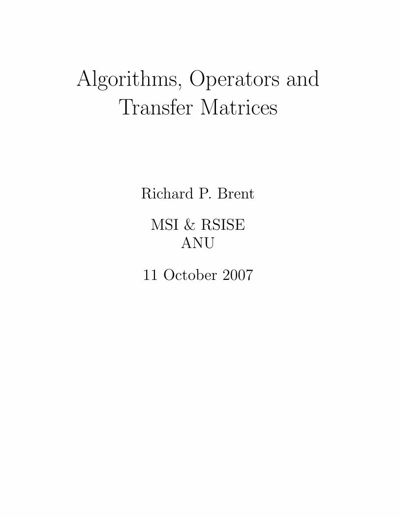
Another Formulation – Algorithm V

It will be useful to rewrite Algorithm B in thefollowing equivalent form (using pseudo-Pascal):

Algorithm V { Assume u ≤ v }

while u 6= v do

begin

while u < v do

begin

j ← Val2(v − u);v ← (v − u)/2j ;end;

u↔ v;end;

return u.

Continued Fractions

Vallee (Algorithmica, 1998) shows a connectionbetween Algorithm V and continued fractions ofa certain form:

u

v= 1/a1 + 2k1/a2 + 2k2/ . . . /ar + 2kr ,

where aj is odd, kj > 0, and 0 < aj < 2kj .

11

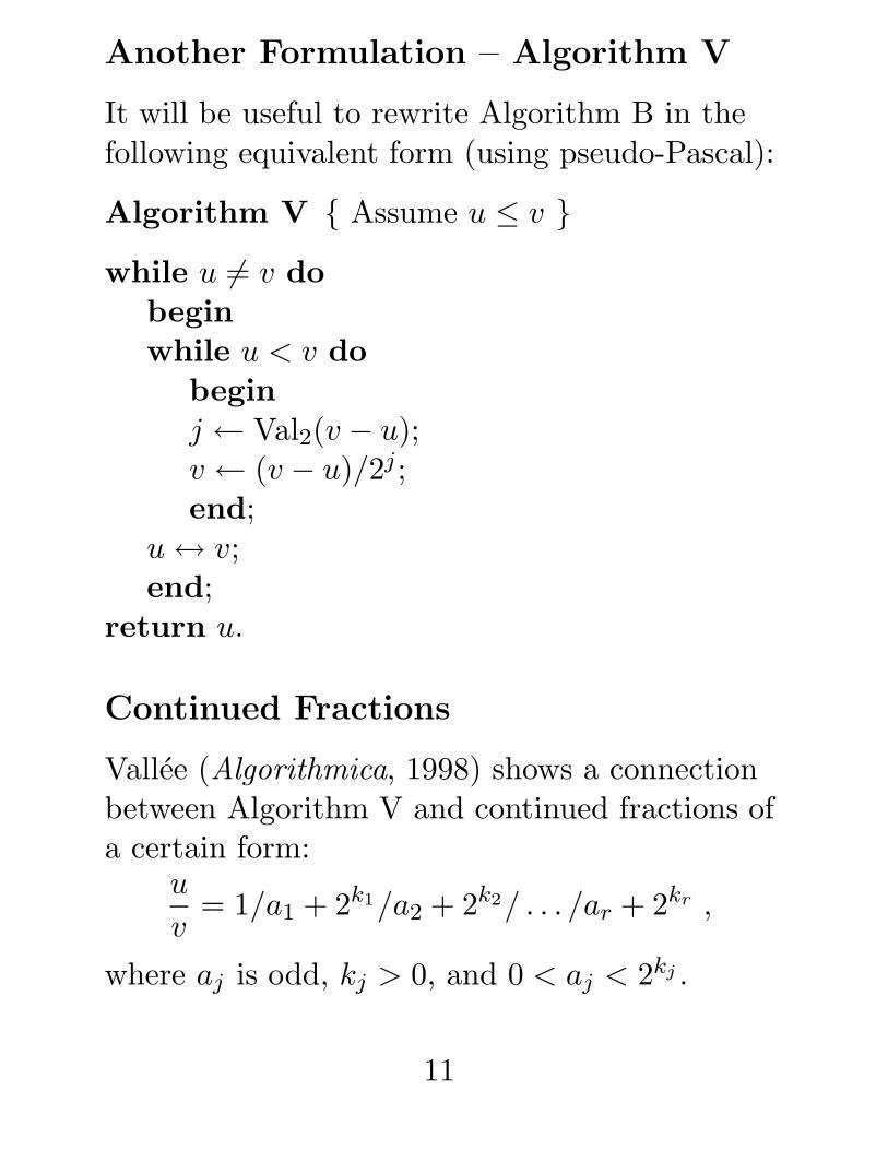
Some Useful Operators

Operators Bs, Us, Us, Vs, useful in the analysisof the binary Euclidean algorithm, are definedon suitable function spaces by

Us[f ](x) =∑

k≥1

(1

1 + 2kx

)s

f

(1

1 + 2kx

), (1)

Us[f ](x) =

(1

x

)s

Us[f ]

(1

x

), (2)

Bs = Us + Us,

Vs[f ](x) =∑

k≥1

∑

a odd,

0<a<2k

(1

a + 2kx

)s

f

(1

a + 2kx

).

(3)In these definitions s is a complex variable, andthe operators act linearly on certain functionspaces (in fact Hardy spaces H2(D) where D isa suitable open disk).

The case s = 2 is of particular interest. B2

encodes the effect of one iteration of the inner“while” loop of Algorithm V, and V2 encodesthe effect of one iteration of the outer “while”loop.

12

History and Notation

B2 (denoted T ) was introduced in my 1976paper and was generalised to Bs by Vallee.Vs was introduced by Vallee. We shall call

• B2 the binary Euclidean operator and

• Vs Vallee’s operator.

In the context of dynamical systems4, Vs iscalled the Ruelle operator relative to thesystem. The generating functions of interestinvolve the quasi-inverse operator

Λs = (I − Vs)−1 .

Vallee studied partial sums of coefficients ofthese Dirichlet series, and her results come fromthe application of Tauberian theorems due toDelange.

4David Ruelle, Thermodynamic Formalism, Addison-Wesley, 1978.

13

Relation Between the Operators

The operators are closely related, as thefollowing results show.

Lemma 1

Vs = VsUs + Us.

The Lemma can be proved algebraically, andthere is also a nice algorithmic interpretation inthe case s = 2.

The following Theorem gives a simplerelationship between Bs, Vs and Us. The proofis immediate from Lemma 1 and the definitionsof the operators.

Theorem 1

(Vs − I)Us = Vs(Bs − I) .

14

Fixed Points

It follows immediately from Theorem 1 that, if

g = U2f,

then(V2 − I)g = V2(B2 − I)f.

Thus, if f is a fixed point of the operator B2,then g is a fixed point of the operator V2. Froma result of Vallee we know that V2, acting on acertain Hardy space H2(D), has a uniquepositive dominant simple eigenvalue 1, so gmust be (a constant multiple of) thecorresponding eigenfunction (providedg ∈ H2(D)). Also, from the definitions of B2

and U2, we have

λ = f(1) = 2g(1)

which is useful for proving the consistency oftwo of the expressions for K given below.

15

Some Results of Vallee

Using her operator Vs, Vallee proved that

K =2 ln 2

π2g(1)

∑

a odd,

a>0

2−⌊lg a⌋G

(1

a

)

where g is a nonzero fixed point of V2 (i.e.g = V2g 6= 0) and G(x) =

∫ x0 g(t) dt . This is the

only expression for K which has been rigorouslyproved.

Because Vs can be proved to have nice spectralproperties, the existence and uniqueness (up toscaling) of g can be proved rigorously.

16

A Conjecture of Vallee

Let λ = f(1), where f is the limiting probabilitydensity (conjectured to exist) as above. Vallee(see Knuth, third edition, §4.5.2(61))conjectured that

λ

b=

2 ln 2

π2,

or equivalently that

K =4 ln 2

π2λ. (4)

Vallee proved the conjecture under theassumption that the operator Bs satisfies acertain spectral condition.

17

Numerical Results

Using an improvement of the “discretizationmethod” of my 1976 paper, and the MPpackage with the equivalent of more than 50decimal places (50D) working precision, Icomputed the limiting probability density f ,then K, λ = f(1), and Kλ. The results were

K = 0.7059712461 0191639152 9314135852 8817666677

λ = 0.3979226811 8831664407 6707161142 6549823098

Kλ = 0.2809219710 9073150563 5754397987 9880385315

These are believed to be correctly roundedvalues.

Vallee’s conjecture (4) is that

Kλ = 4 ln 2/π2 .

The computed value of Kλ agrees with 4 ln 2/π2

to 40 decimals!

18

Open Problems

Since the work of Vallee and Maze, analysis ofthe average behaviour of the binary Euclideanalgorithm has a rigorous foundation. However,some interesting open questions remain.

For example, does the binary Euclideanoperator B2 have a unique positive dominantsimple eigenvalue 1? Vallee has proved thecorresponding result for her operator V2.

In order to estimate the speed of convergence offn to f (assuming f exists), we need moreinformation on the spectrum of B2. What canbe proved ? Preliminary numerical resultsindicate that the sub-dominant eigenvalue(s)are a complex conjugate pair:

λ2 = λ3 = 0.1735± 0.0884i ,

with |λ2| = |λ3| = 0.1948 to 4D.

Vallee has proved related results for some otheralgorithms (variants of the Euclidean algorithm,algorithms for computing the Jacobi symbol),but many analogous questions remain open.

19

Transfer Matrices

Transfer matrices are used in statisticalmechanics to generate series expansions forcertain models. The argument z of the series isa parameter of the model (e.g. temperature).(Of course, there may be several parameters.)

Usually we need to find or approximate thelargest one or two eigenvalues of an N ×Nmatrix, and we are interested in thethermodynamic limit as N →∞. In the limit,we are not strictly dealing with matrices, butwith linear operators.

Compare our discussion of the binary Euclideanalgorithm: the operators Bs and Vs are linearoperators on certain function spaces, and toobtain numerical results (as in the numericalverification of Vallee’s conjecture) weapproximate these operators by (large)matrices. In some cases we know that theoperators have an dominant eigenvalue 1, butwe are interested in whether there is a “spectralgap”, i.e. whether the other eigenvalues λsatisfy |λ| ≤ c < 1.

20

Research Topic

Is the analogy between transfer matrices andVallee’s operator useful ? Can we transfer someof the techniques used in analysis of algorithmsto statistical mechanics (or vice versa) ?

21

References

[1] Richard P. Brent, Analysis of the BinaryEuclidean Algorithm, New Directions and

Recent Results in Algorithms and

Complexity, (J. F. Traub, editor), AcademicPress, New York, 1976, 321–355.

[2] Richard P. Brent, Further analysis of the

Binary Euclidean algorithm, ReportPRG-TR-7-99, Oxford UniversityComputing Laboratory, Nov. 1999.

[3] Yao-ban Chan, Selected Problems in Lattice

Statistical Mechanics, Ph.D. thesis,Mathematics and Statistics, Univ. ofMelbourne, Sept. 2005.

[4] Donald E. Knuth, The Art of Computer

Programming, Volume 2: Seminumerical

Algorithms (third edition). Addison-Wesley,Menlo Park, 1997.

22

[5] Gerard Maze, Existence of a limitingdistribution for the binary GCD algorithm,J. of Discrete Algorithms 5, 1 (March 2007),176–186.

[6] David Ruelle, Thermodynamic Formalism,Addison Wesley, 1978.

[7] Brigitte Vallee, The complete analysis of theBinary Euclidean Algorithm, Proc.

ANTS’98, Lecture Notes in Computer

Science 1423, Springer-Verlag, 1998, 77–94.

[8] Brigitte Vallee, Dynamics of the binaryEuclidean algorithm: functional analysis andoperators, Algorithmica 22 (1998), 660–685.

23