1

Relational Operators

2

Outline• Logical/physical operators• Cost parameters and sorting • One-pass algorithms • Nested-loop joins • Two-pass algorithms

3

Query Execution

Query compiler

Execution engine

Index/record mgr.

Buffer manager

Storage manager

storage

User/Application

Queryor update

Query executionplan

Record, indexrequests

Page commands

Read/writepages

4

Logical v.s. Physical Operators• Logical operators

– what they do– e.g., union, selection, project, join, grouping

• Physical operators– how they do it– e.g., nested loop join, sort-merge join, hash join,

index join

5

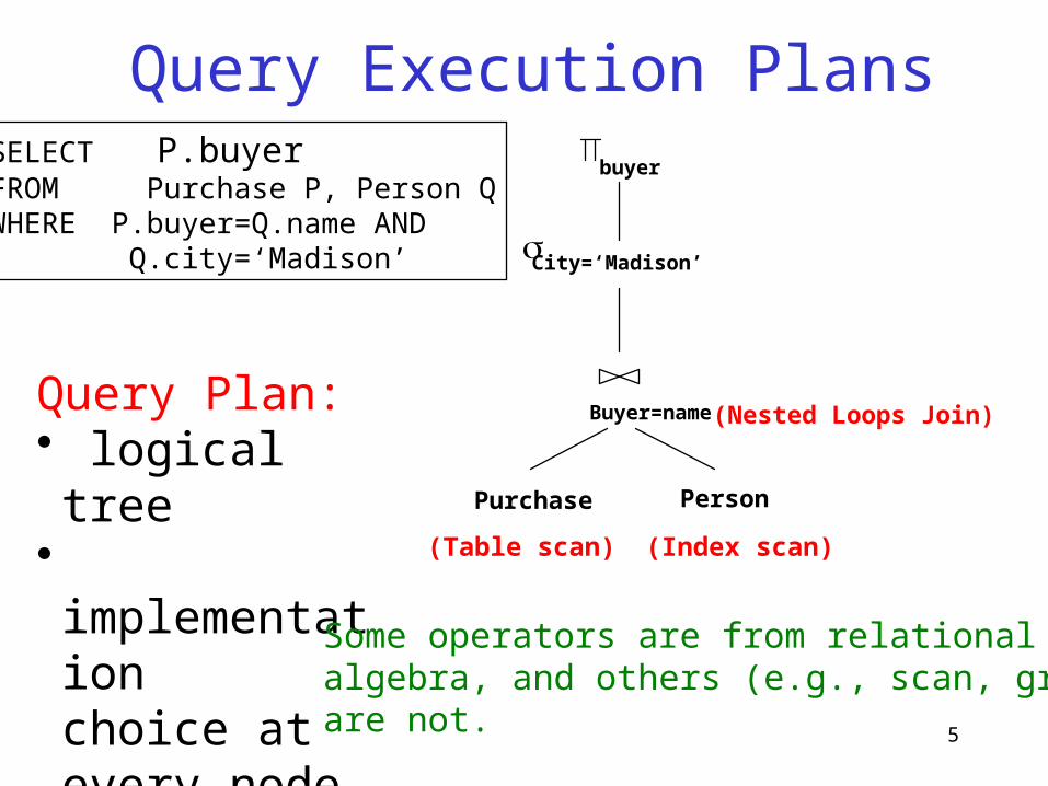
Query Execution Plans

Purchase Person

Buyer=name

City=‘Madison’

buyer

(Nested Loops Join)

SELECT P.buyerFROM Purchase P, Person QWHERE P.buyer=Q.name AND Q.city=‘Madison’

Query Plan:• logical tree• implementation

choice at every node

• scheduling of operations.

(Table scan) (Index scan)

Some operators are from relationalalgebra, and others (e.g., scan, group)are not.

6

How do We Combine Operations?

• The iterator model. Each operation is implemented by 3 functions:– Open: sets up the data structures and performs

initializations– GetNext: returns the the next tuple of the result.– Close: ends the operations. Cleans up the data

structures.• Enables pipelining!• Contrast with data-driven materialize model.

7

Cost Parameters

• Cost parameters – M = number of blocks that fit in main memory– B(R) = number of blocks holding R– T(R) = number of tuples in R– V(R,a) = number of distinct values of the attribute a

• Estimating the cost:– Important in optimization (next lecture)– Compute I/O cost only– We compute the cost to read the tables – We don’t compute the cost to write the result (because pipelining)

8

Reminder: Sorting• Two pass multi-way merge sort• Step 1:

– Read M blocks at a time, sort, write– Result: have runs of length M on disk

• Step 2:– Merge M-1 at a time, write to disk– Result: have runs of length M(M-1)M2

• Cost: 3B(R), Assumption: B(R) M2

9

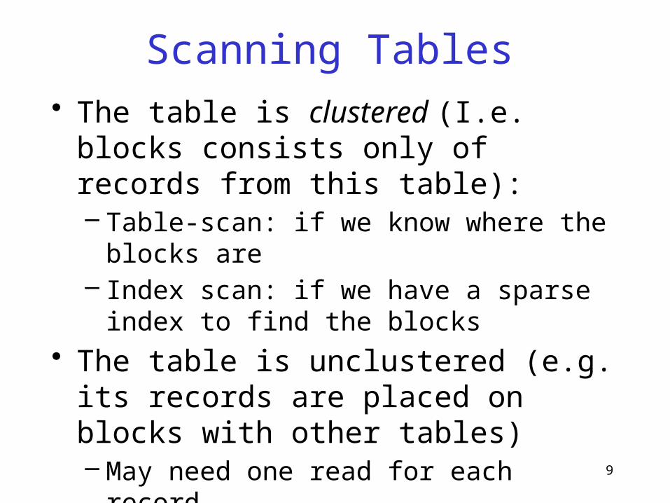
Scanning Tables• The table is clustered (I.e. blocks consists

only of records from this table):– Table-scan: if we know where the blocks are– Index scan: if we have a sparse index to find the

blocks

• The table is unclustered (e.g. its records are placed on blocks with other tables)– May need one read for each record

10

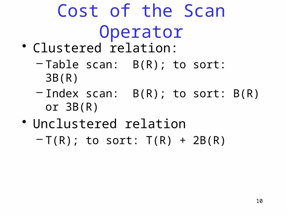
Cost of the Scan Operator• Clustered relation:

– Table scan: B(R); to sort: 3B(R)– Index scan: B(R); to sort: B(R) or 3B(R)

• Unclustered relation– T(R); to sort: T(R) + 2B(R)

11

One pass algorithm

12

One-pass Algorithms

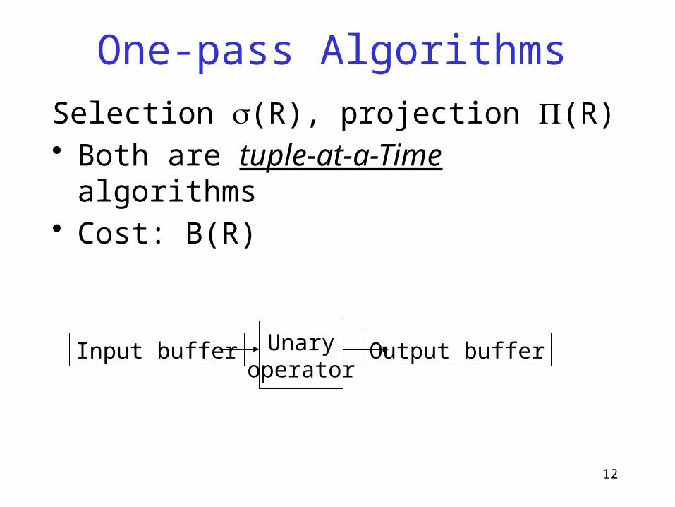
Selection s(R), projection P(R)• Both are tuple-at-a-Time algorithms• Cost: B(R)

Input buffer Output bufferUnaryoperator

13

One-pass Algorithms

Duplicate elimination d(R)• Need to keep a dictionary in memory:

– balanced search tree– hash table– etc

• Cost: B(R)• Assumption: B(d(R)) <= M

14

One-pass Algorithms

Grouping: gcity, sum(price) (R)

• Need to keep a dictionary in memory• Also store the sum(price) for each city• Cost: B(R)• Assumption: number of cities fits in

memory

15

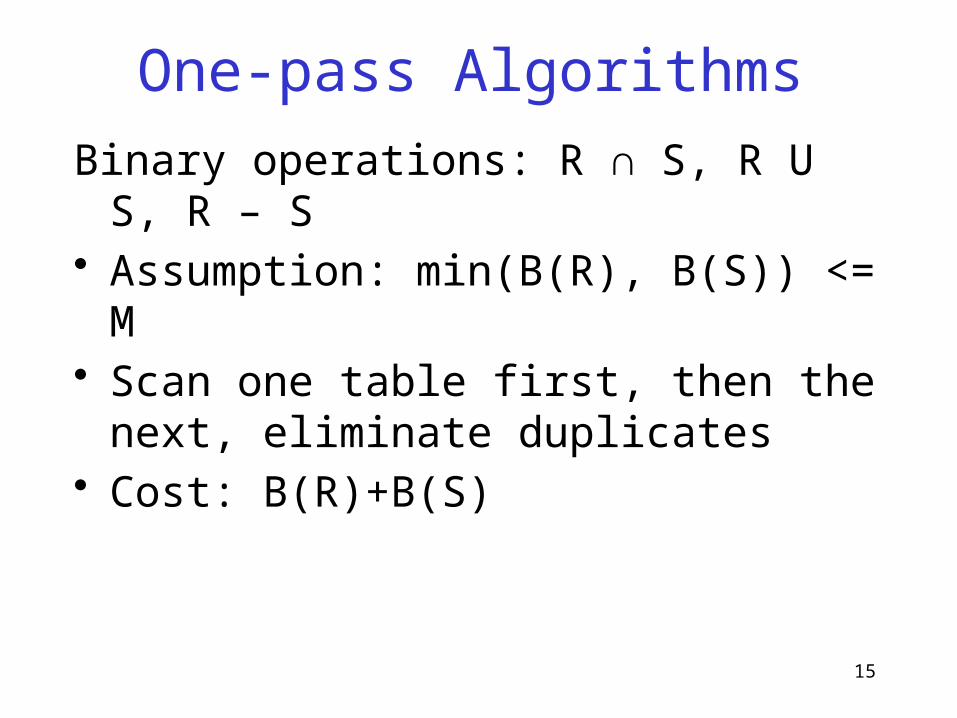
One-pass Algorithms

Binary operations: R ∩ S, R U S, R – S• Assumption: min(B(R), B(S)) <= M• Scan one table first, then the next, eliminate

duplicates• Cost: B(R)+B(S)

16

Nested loop join

17

Nested Loop Joins• Tuple-based nested loop R S

for each tuple r in R do

for each tuple s in S do

if r and s join then output (r,s)

• Cost: T(R) T(S), sometimes T(R) B(S)

18

Nested Loop Joins• Block-based Nested Loop Join

for each (M-1) blocks bs of S do

for each block br of R do

for each tuple s in bs do

for each tuple r in br do

if r and s join then output(r,s)

19

Nested Loop Joins

. . .

. . .

R & SHash table for block of S

(k < B-1 pages)

Input buffer for R Output buffer

. . .

Join Result

20

Nested Loop Joins

• Block-based Nested Loop Join• Cost:

– Read S once: cost B(S)– Outer loop runs B(S)/(M-2) times, and each

time need to read R: costs B(S)B(R)/(M-2)– Total cost: B(S) + B(S)B(R)/(M-2)

• Notice: it is better to iterate over the smaller relation first

• S R: S=outer relation, R=inner relation

21

Two pass algorithm

22

Two-Pass Algorithms Based on Sorting

Duplicate elimination d(R)• Simple idea: sort first, then eliminate duplicates• Step 1: sort runs of size M, write

– Cost: 2B(R)• Step 2: merge M-1 runs, but include each tuple

only once– Cost: B(R)– Some complications...

• Total cost: 3B(R), Assumption: B(R) <= M2

23

Two-Pass Algorithms Based on Sorting

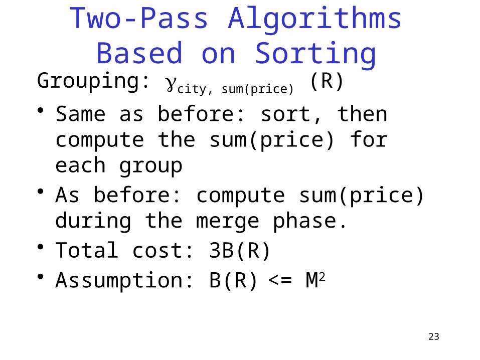
Grouping: gcity, sum(price) (R)

• Same as before: sort, then compute the sum(price) for each group

• As before: compute sum(price) during the merge phase.

• Total cost: 3B(R)• Assumption: B(R) <= M2

24

Two-Pass Algorithms Based on Sorting

Binary operations: R ∩ S, R U S, R – S• Idea: sort R, sort S, then do the right thing• A closer look:

– Step 1: split R into runs of size M, then split S into runs of size M. Cost: 2B(R) + 2B(S)

– Step 2: merge M/2 runs from R; merge M/2 runs from S; ouput a tuple on a case by cases basis

• Total cost: 3B(R)+3B(S)• Assumption: B(R)+B(S)<= M2

25

Two-Pass Algorithms Based on Sorting

Join R S• Start by sorting both R and S on the join attribute:

– Cost: 4B(R)+4B(S) (because need to write to disk)• Read both relations in sorted order, match tuples

– Cost: B(R)+B(S)• Difficulty: many tuples in R may match many in S

– If at least one set of tuples fits in M, we are OK– Otherwise need nested loop, higher cost

• Total cost: 5B(R)+5B(S)• Assumption: B(R) <= M2, B(S) <= M2

26

Two-Pass Algorithms Based on Sorting

Join R S• If the number of tuples in R matching those

in S is small (or vice versa) we can compute the join during the merge phase

• Total cost: 3B(R)+3B(S) • Assumption: B(R) + B(S) <= M2

27

Two Pass Algorithms Based on Hashing

• Idea: partition a relation R into buckets, on disk• Each bucket has size approx. B(R)/M

• Does each bucket fit in main memory ?– Yes if B(R)/M <= M, i.e. B(R) <= M2

M main memory buffers DiskDisk

Relation ROUTPUT

2INPUT

1

hashfunction

h M-1

Partitions

1

2

M-1

. . .

1

2

B(R)

28

Hash Based Algorithms for d• Recall: d(R) = duplicate elimination • Step 1. Partition R into buckets• Step 2. Apply d to each bucket (may read in

main memory)

• Cost: 3B(R)• Assumption:B(R) <= M2

29

Hash Based Algorithms for g• Recall: g(R) = grouping and aggregation• Step 1. Partition R into buckets• Step 2. Apply g to each bucket (may read in

main memory)

• Cost: 3B(R)• Assumption:B(R) <= M2

30

Hash-based Join• R S• Recall the main memory hash-based join:

– Scan S, build buckets in main memory– Then scan R and join

31

Partitioned Hash JoinR S• Step 1:

– Hash S into M-1 buckets– send all buckets to disk

• Step 2– Hash R into M-1 buckets– Send all buckets to disk

• Step 3– Join every pair of buckets

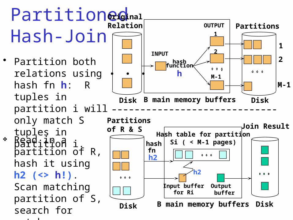
PartitionedHash-Join

• Partition both relations using hash fn h: R tuples in partition i will only match S tuples in partition i.

Read in a partition of R, hash it using h2 (<> h!). Scan matching partition of S, search for matches.

Partitionsof R & S

Input bufferfor Ri

Hash table for partitionSi ( < M-1 pages)

B main memory buffersDisk

Output buffer

Disk

Join Result

hashfnh2

h2

B main memory buffers DiskDisk

Original Relation OUTPUT

2INPUT

1

hashfunction

h M-1

Partitions

1

2

M-1

. . .

33

Partitioned Hash Join• Cost: 3B(R) + 3B(S)• Assumption: min(B(R), B(S)) <= M2

34

Hybrid Hash Join Algorithm• When we have more memory: B(S) << M2

• Partition S into k buckets• But keep first bucket S1 in memory, k-1 buckets to

disk• Partition R into k buckets

– First bucket R1 is joined immediately with S1 – Other k-1 buckets go to disk

• Finally, join k-1 pairs of buckets:– (R2,S2), (R3,S3), …, (Rk,Sk)

35

Hybrid Join Algorithm• How big should we choose k ?• Average bucket size for S is B(S)/k• Need to fit B(S)/k + (k-1) blocks in memory

– B(S)/k + (k-1) <= M– k slightly smaller than B(S)/M

36

Hybrid Join Algorithm• How many I/Os ?• Recall: cost of partitioned hash join:

– 3B(R) + 3B(S)

• Now we save 2 disk operations for one bucket• Recall there are k buckets• Hence we save 2/k(B(R) + B(S))• Cost: (3-2/k)(B(R) + B(S)) =

(3-2M/B(S))(B(R) + B(S))

37

Indexed Based Algorithms• In a clustered index all tuples with the same

value of the key are clustered on as few blocks as possible

a a a a a a a a a a

38

Index Based Selection• Selection on equality: sa=v(R)

• Clustered index on a: cost B(R)/V(R,a)• Unclustered index on a: cost T(R)/V(R,a)

39

Index Based Selection• Example: B(R) = 2000, T(R) = 100,000, V(R, a) =

20, compute the cost of sa=v(R)• Cost of table scan:

– If R is clustered: B(R) = 2000 I/Os– If R is unclustered: T(R) = 100,000 I/Os

• Cost of index based selection:– If index is clustered: B(R)/V(R,a) = 100– If index is unclustered: T(R)/V(R,a) = 5000

• Notice: when V(R,a) is small, then unclustered index is useless

40

Index Based Join• R S• Assume S has an index on the join attribute• Iterate over R, for each tuple fetch

corresponding tuple(s) from S• Assume R is clustered. Cost:

– If index is clustered: B(R) + T(R)B(S)/V(S,a)– If index is unclustered: B(R) + T(R)T(S)/V(S,a)

41

Index Based Join• Assume both R and S have a sorted index

(B+ tree) on the join attribute• Then perform a merge join (called zig-zag

join)• Cost: B(R) + B(S)