Embed Size (px)
Citation preview
Algebraic Combinatorics Lecture Notes
Lecturer: Sara Billey, et al; written and edited by Josh Swanson
September 30, 2014
Abstract
The following notes were taking during a course on Algebraic Combinatorics at the University ofWashington in Spring 2014. Please send any corrections to [email protected]. Thanks!
Contents
March 31st, 2014: Diagram Algebras and Hopf Algebras Intro . . . . . . . . . . . . . . . . . . . . . 2
April 2nd, 2014: Group Representations Summary; Sn-Representations Intro . . . . . . . . . . . . 4
April 4th, 2014: Mλ Decomposition and Specht Modules . . . . . . . . . . . . . . . . . . . . . . . 7
April 7th, 2014: Fundamental Specht Module Properties and Branching Rules . . . . . . . . . . . . 10
April 9th, 2014: Representation Ring for Sn and its Pieri Formula . . . . . . . . . . . . . . . . . . 14
April 11th, 2014: Pieri for Schurs; Kostka Numbers; Dual Bases; Cauchy Identity . . . . . . . . . . 17
April 14th, 2014: Finishing Cauchy; R ∼= SYM; Littlewood-Richardson Rule; Frobenius Characteris-tic Map . . . . . . . . . . . . . . . . . . . . . . . . . . . . . . . . . . . . . . . . . . . . . . . . 20
April 16th, 2014: Algebras and Coalgebras Intro . . . . . . . . . . . . . . . . . . . . . . . . . . . . 24
April 18th, 2014: Skew Schur Functions and Comultiplication; Sweedler Notation; k-CoalgebraHomomorphisms . . . . . . . . . . . . . . . . . . . . . . . . . . . . . . . . . . . . . . . . . . . 26
April 21st, 2014: Subcoalgebras, Coideals, Bialgebras . . . . . . . . . . . . . . . . . . . . . . . . . . 31
April 23rd, 2014: Bialgebra Examples; Hopf Algebras Defined . . . . . . . . . . . . . . . . . . . . . 33
April 25th, 2014: Properties of Antipodes and Takeuchi’s Formula . . . . . . . . . . . . . . . . . . 36
April 28th, 2014: Homological Properties of Hopf Algebras: projdim, injdim, gldim,GKdim, . . . . . 40
Aside: Dual Algebras, Coalgebras, Bialgebras, and Hopf Algebras . . . . . . . . . . . . . . . . . . . 42
April 30th, 2014: (Left) Integrals; from GK0 to GK1 and Beyond . . . . . . . . . . . . . . . . . . 44
May 2nd, 2014: Dual Hopf Algebras and QSYM . . . . . . . . . . . . . . . . . . . . . . . . . . . . 46
May 5th, 2014: Rock Breaking, Markov Chains, and the Hopf Squared Map . . . . . . . . . . . . . 49
Aside: Hopf Algebras for k[x, y, z] and Hom(A,A) Invariants . . . . . . . . . . . . . . . . . . . . . 52
May 7th, 2014: Chromatic Polynomials and applications of Mobius inversion . . . . . . . . . . . . 53
1
May 9th, 2014: Reduced Incidence Coalgebras; Section Coefficients; Matroids and HereditaryClasses; Many Examples . . . . . . . . . . . . . . . . . . . . . . . . . . . . . . . . . . . . . . . 57
May 12th, 2014—Two Homomorphisms from Iranked to QSYM; Mobius Functions on Posets . . . . 60
May 14th, 2014: Characters; Combinatorial Hopf Algebras; (QSYM, ζQ) as Terminal Object; Evenand Odd Subalgebras; Dehn–Sommerville Relations . . . . . . . . . . . . . . . . . . . . . . . . 63
May 16th, 2014: The Centralizer Theorem; Schur-Weyl Duality; Partition Algebras . . . . . . . . . 66
May 19th, 2014: Internal Product on SYM; P -partitions; Factorizations with Prescribed Descent Sets 68
May 21, 2014: (Special) Double Posets, E-Partitions, Pictures, Yamanouchi Words, and a Littlewood-Richardson Rule . . . . . . . . . . . . . . . . . . . . . . . . . . . . . . . . . . . . . . . . . . . 71
Aside: Affine Group Schemes and Commutative Hopf Algebras . . . . . . . . . . . . . . . . . . . . 73
May 23rd, 2014: Open Problem Day . . . . . . . . . . . . . . . . . . . . . . . . . . . . . . . . . . . 74
May 28th, 2014: Hecke Algebra of Sn; Kazhdan-Lusztig Polynomials; Cells . . . . . . . . . . . . . 75
May 30th, 2014—Immaculate Basis for QSYM; (Standard) Immaculate Tableaux; Representationsof 0-Hecke Algebras . . . . . . . . . . . . . . . . . . . . . . . . . . . . . . . . . . . . . . . . . 77
June 2nd, 2014—Plethysms; P vs. NP vs. #P ; Standardization and Matrices . . . . . . . . . . . . 80
June 4th, 2014—Counting Reduced Words; Stanley Symmetric Functions; Little Bumps; k-VexillaryPermutations . . . . . . . . . . . . . . . . . . . . . . . . . . . . . . . . . . . . . . . . . . . . . 84
June 7th, 2014—QSYM∗, the Concatenation Hopf Algebra, and Solomon Descent Algebras . . . . 87
List of Symbols 96
Index 100
March 31st, 2014: Diagram Algebras and Hopf Algebras Intro
1 RemarkStudents will present something this quarter; see web site for topics. Will roughly focus on “diagramalgebras” and Hopf algebras bumping in to representation theory and topology. Homework for thecourse will essentially be studying and presenting papers, possibly in small groups. Sara will givebackground for the first few weeks.
2 RemarkThe rough idea is that objects from enumerative combinatorics index bases for algebras, and converselyimportant algebraic bases are indexed by combinatorial objects.
Definition 3. A diagram algebra (not necessarily standard terminology) is as follows.
(i) The quitessential example is the group algebra C[Sn], with basis given by permutations. Multi-plication can be thought of by concatenating string diagrams. The generators are the adjacenttranspositions (i, i + 1), whose string diagrams have a single crossing. Their relations aresisi+1si = si+1sisi+1, with sisj = sjsi if |i− j| > 1, and s2
i = 1.
2
(ii) For another example, consider the Hecke algebra 0-Hecke algebra. The basis again will be
indexed by permutations. Use generators T1, T2, . . . , Tn−1 with relations as with the si except forT 2i = Ti. A real-life example of this algebra comes from sorting a list by putting adjacent pairs in
order. Diagram multiplication can be done similarly, but a crossing concatenated with itself issomehow just itself.
(iii) A generalization of the previous examples, roughly: the Hecke algebra is given by T 2i =
qTid + (1− q)Ti. Setting q = 0 gives the 0-Hecke algebra; q = 1 gives the symmetric group.
(iv) The Temperly-Lieb algebra TLn(C). The basis is given by non-crossing matchings on 2n vertices
arranged in two columns. (That means we connect each vertex to precisely one vertex by a string.)Multiplication is given by concatenation. One fiddle is you can get “islands” when concatenatingsometimes; in that case, formally multiply the diagram by δ for each island and erase the islands.What are the generators? Ui is the diagram going straight across except we connect i and i+ 1;i+ n and i+ n+ 1. One checks
UiUi+1Ui = Ui, UiUi−1Ui = Ui, U2i = δUi, UiUj = UjUi
for |i− j| > 1. This comes up in topological quantum field theory.
How large is the basis? Match 1 with i and separate the vertexes into two “halves”; this givesthe Catalan number recurrence Cn+1 =
∑ni=0 CiCn−i.
(v) The Brauer algebra Bn: same as the Temperly-Lieb algebra, but allow non-crossing matchings.
Ignore loops, i.e. set δ = 1. Multiplication remains by concatenation. This algebra comes up inthe representation theory of On. (There is a q-deformation where we don’t require δ = 1.)
Definition 4. Vauge first definition: a Hopf algebra is an algebra, so it has addition and multiplication,
and it has a coalgebra structure, so it has a coproduct and a counit, and it has an antipode. Somemotivation: given an algebra A, multiplication is a map A⊗A→ A. The coproduct is ∆: A→ A⊗Agoing the other way. A good pair of motivating examples is the following.
(i) Hopf algebra on words in some alphabet, say a, b, c. (Maybe infinite, maybe not.) The basis isgiven by words in the alphabet (with an empty word), multiplication given by concatenation, eg.“base × ball = baseball”, so m(y1 · · · yk ⊗ zi · · · zj) = y1 · · · ykz1 · · · zj . A good comultiplication
is ∆(y1 · · · yk) =∑kj=0 y1 · · · yj ⊗ yj+1 · · · yk. Doing this to “baseball” gives 1 ⊗ baseball + b ⊗
aseball + · · ·+ baseball⊗ 1. (1 is the empty word.) Note: This comultiplication was incorrect;see the remark at the start of the next lecture.
In this case the counit is given by setting ε(y1 · · · yk) to 1 on the empty word and 0 elsewhere (i.e.it sets y1 = · · · = yk = 0). In our example, this gives
(1⊗ ε)∆(baseball) = baseball⊗ 1.
An antipode will be s(y1 · · · yk) = (−1)ky1 · · · yk, which is an involution A→ A.
(ii) The symmetric functions SYM. This is an algebra sitting inside C[[x1, x2, . . .]]. Take all permu-tations and take their direct limit S∞ (gives permutations P → P fixing all but finitely manynaturals). Define an S∞ action by
si · f(. . . , xi, xi+1, . . .) := f(. . . , xi+1, xi, . . .).
(Variables in . . . fixed.) Let SYM be the set of power series with bounded degree in these variableswhich are fixed by all si.
An easy source of elements of SYM are the elementary symmetric functions
ek :=∑
xj1 · · ·xjk ,
where the sum is over k-subsets of the positive integers P with ji strictly increasing.
3
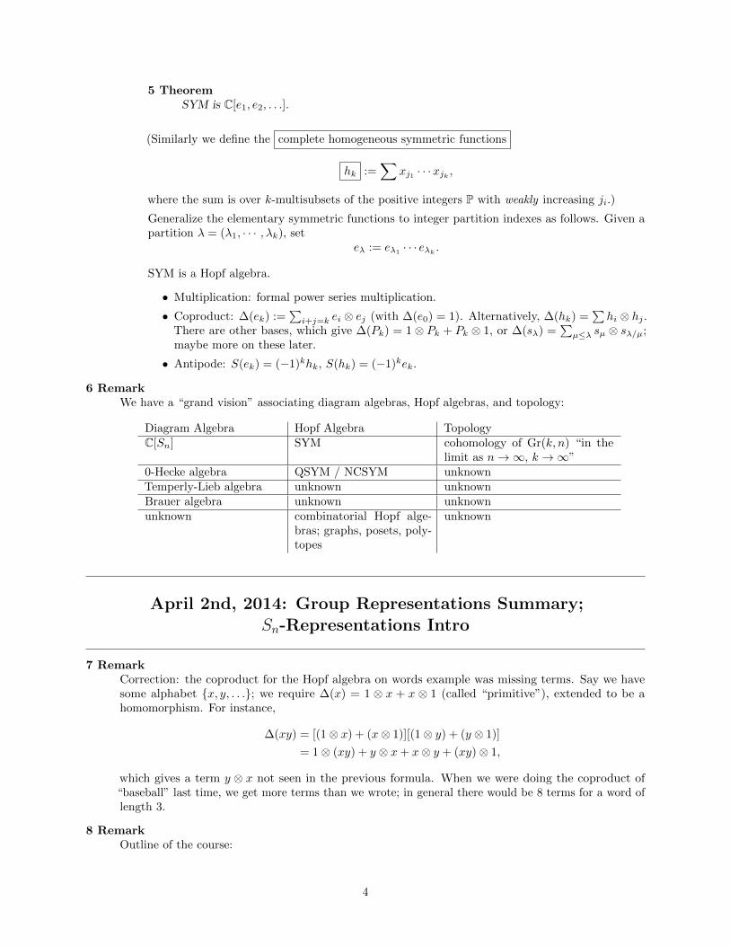
5 TheoremSYM is C[e1, e2, . . .].
(Similarly we define the complete homogeneous symmetric functions
hk :=∑
xj1 · · ·xjk ,
where the sum is over k-multisubsets of the positive integers P with weakly increasing ji.)
Generalize the elementary symmetric functions to integer partition indexes as follows. Given apartition λ = (λ1, · · · , λk), set
eλ := eλ1· · · eλk .
SYM is a Hopf algebra.
• Multiplication: formal power series multiplication.
• Coproduct: ∆(ek) :=∑i+j=k ei ⊗ ej (with ∆(e0) = 1). Alternatively, ∆(hk) =
∑hi ⊗ hj .
There are other bases, which give ∆(Pk) = 1⊗ Pk + Pk ⊗ 1, or ∆(sλ) =∑µ≤λ sµ ⊗ sλ/µ;
maybe more on these later.
• Antipode: S(ek) = (−1)khk, S(hk) = (−1)kek.
6 RemarkWe have a “grand vision” associating diagram algebras, Hopf algebras, and topology:
Diagram Algebra Hopf Algebra TopologyC[Sn] SYM cohomology of Gr(k, n) “in the
limit as n→∞, k →∞”0-Hecke algebra QSYM / NCSYM unknownTemperly-Lieb algebra unknown unknownBrauer algebra unknown unknownunknown combinatorial Hopf alge-
bras; graphs, posets, poly-topes
unknown
April 2nd, 2014: Group Representations Summary;Sn-Representations Intro
7 RemarkCorrection: the coproduct for the Hopf algebra on words example was missing terms. Say we havesome alphabet x, y, . . .; we require ∆(x) = 1 ⊗ x + x ⊗ 1 (called “primitive”), extended to be ahomomorphism. For instance,
∆(xy) = [(1⊗ x) + (x⊗ 1)][(1⊗ y) + (y ⊗ 1)]
= 1⊗ (xy) + y ⊗ x+ x⊗ y + (xy)⊗ 1,
which gives a term y ⊗ x not seen in the previous formula. When we were doing the coproduct of“baseball” last time, we get more terms than we wrote; in general there would be 8 terms for a word oflength 3.
8 RemarkOutline of the course:
4
1. Sn-representation theory
2. SYM
3. Hopf algebra
4. QSYM
5. James Zhang’s view
6. Student lectures
7. Monty McGovern lectures
8. Edward Witten lecture on Jones polynomials,connection with topological quantum fieldtheory.
9 RemarkToday: Sn representation theory in a nutshell. There’s a very nice book by Bruce Sagan, “TheSymmetric Group”. (Unfortunately, there doesn’t seem to be a free version. SpringerLink doesn’t giveus access either.)
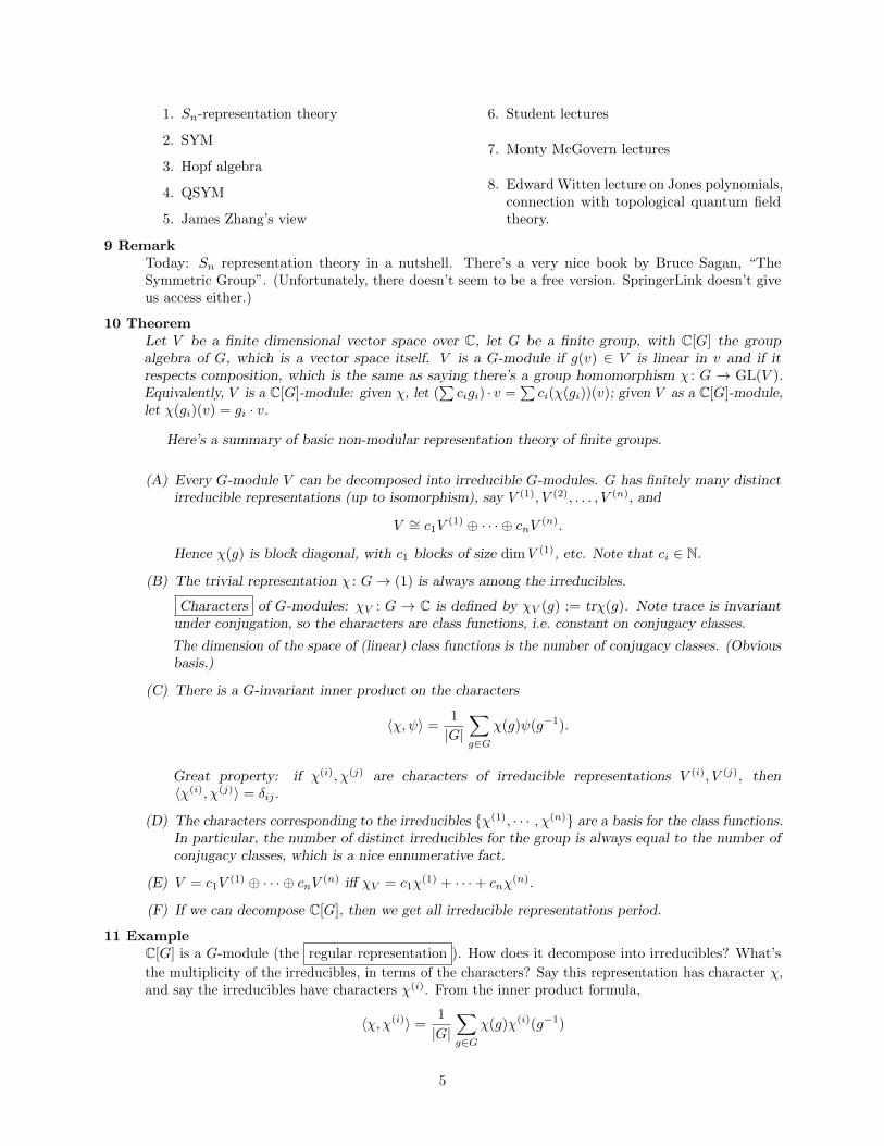
10 TheoremLet V be a finite dimensional vector space over C, let G be a finite group, with C[G] the groupalgebra of G, which is a vector space itself. V is a G-module if g(v) ∈ V is linear in v and if itrespects composition, which is the same as saying there’s a group homomorphism χ : G → GL(V ).Equivalently, V is a C[G]-module: given χ, let (
∑cigi) · v =
∑ci(χ(gi))(v); given V as a C[G]-module,
let χ(gi)(v) = gi · v.
Here’s a summary of basic non-modular representation theory of finite groups.
(A) Every G-module V can be decomposed into irreducible G-modules. G has finitely many distinctirreducible representations (up to isomorphism), say V (1), V (2), . . . , V (n), and
V ∼= c1V(1) ⊕ · · · ⊕ cnV (n).
Hence χ(g) is block diagonal, with c1 blocks of size dimV (1), etc. Note that ci ∈ N.
(B) The trivial representation χ : G→ (1) is always among the irreducibles.
Characters of G-modules: χV : G → C is defined by χV (g) := trχ(g). Note trace is invariantunder conjugation, so the characters are class functions, i.e. constant on conjugacy classes.
The dimension of the space of (linear) class functions is the number of conjugacy classes. (Obviousbasis.)
(C) There is a G-invariant inner product on the characters
〈χ, ψ〉 =1
|G|∑g∈G
χ(g)ψ(g−1).
Great property: if χ(i), χ(j) are characters of irreducible representations V (i), V (j), then〈χ(i), χ(j)〉 = δij .
(D) The characters corresponding to the irreducibles χ(1), · · · , χ(n) are a basis for the class functions.In particular, the number of distinct irreducibles for the group is always equal to the number ofconjugacy classes, which is a nice ennumerative fact.
(E) V = c1V(1) ⊕ · · · ⊕ cnV (n) iff χV = c1χ
(1) + · · ·+ cnχ(n).
(F) If we can decompose C[G], then we get all irreducible representations period.
11 ExampleC[G] is a G-module (the regular representation ). How does it decompose into irreducibles? What’s
the multiplicity of the irreducibles, in terms of the characters? Say this representation has character χ,and say the irreducibles have characters χ(i). From the inner product formula,
〈χ, χ(i)〉 =1
|G|∑g∈G
χ(g)χ(i)(g−1)
5
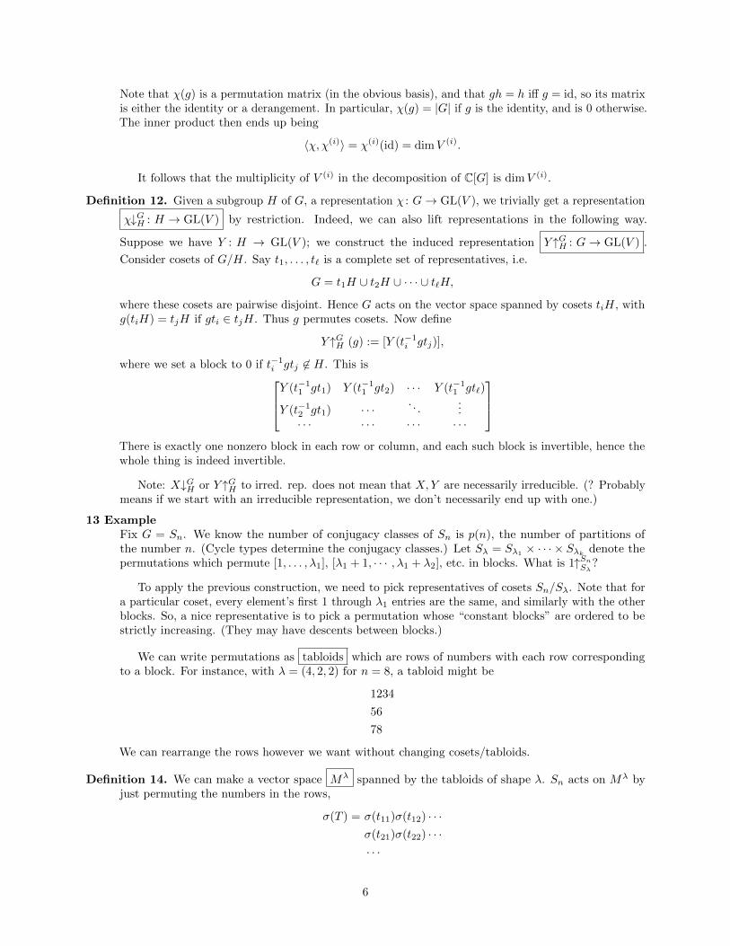
Note that χ(g) is a permutation matrix (in the obvious basis), and that gh = h iff g = id, so its matrixis either the identity or a derangement. In particular, χ(g) = |G| if g is the identity, and is 0 otherwise.The inner product then ends up being
〈χ, χ(i)〉 = χ(i)(id) = dimV (i).
It follows that the multiplicity of V (i) in the decomposition of C[G] is dimV (i).
Definition 12. Given a subgroup H of G, a representation χ : G→ GL(V ), we trivially get a representation
χ↓GH : H → GL(V ) by restriction. Indeed, we can also lift representations in the following way.
Suppose we have Y : H → GL(V ); we construct the induced representation Y ↑GH : G→ GL(V ) .
Consider cosets of G/H. Say t1, . . . , t` is a complete set of representatives, i.e.
G = t1H ∪ t2H ∪ · · · ∪ t`H,
where these cosets are pairwise disjoint. Hence G acts on the vector space spanned by cosets tiH, withg(tiH) = tjH if gti ∈ tjH. Thus g permutes cosets. Now define
Y ↑GH (g) := [Y (t−1i gtj)],
where we set a block to 0 if t−1i gtj 6∈ H. This isY (t−1
1 gt1) Y (t−11 gt2) · · · Y (t−1
1 gt`)
Y (t−12 gt1) · · ·
. . ....
· · · · · · · · · · · ·
There is exactly one nonzero block in each row or column, and each such block is invertible, hence thewhole thing is indeed invertible.
Note: X↓GH or Y ↑GH to irred. rep. does not mean that X,Y are necessarily irreducible. (? Probablymeans if we start with an irreducible representation, we don’t necessarily end up with one.)
13 ExampleFix G = Sn. We know the number of conjugacy classes of Sn is p(n), the number of partitions ofthe number n. (Cycle types determine the conjugacy classes.) Let Sλ = Sλ1 × · · · × Sλk denote thepermutations which permute [1, . . . , λ1], [λ1 + 1, · · · , λ1 + λ2], etc. in blocks. What is 1↑SnSλ?
To apply the previous construction, we need to pick representatives of cosets Sn/Sλ. Note that fora particular coset, every element’s first 1 through λ1 entries are the same, and similarly with the otherblocks. So, a nice representative is to pick a permutation whose “constant blocks” are ordered to bestrictly increasing. (They may have descents between blocks.)
We can write permutations as tabloids which are rows of numbers with each row correspondingto a block. For instance, with λ = (4, 2, 2) for n = 8, a tabloid might be
1234
56
78
We can rearrange the rows however we want without changing cosets/tabloids.
Definition 14. We can make a vector space Mλ spanned by the tabloids of shape λ. Sn acts on Mλ byjust permuting the numbers in the rows,
σ(T ) = σ(t11)σ(t12) · · ·σ(t21)σ(t22) · · ·· · ·
6
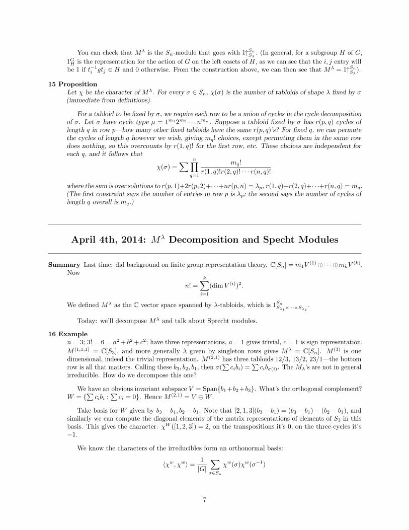
You can check that Mλ is the Sn-module that goes with 1↑SnSλ . (In general, for a subgroup H of G,
1GH is the representation for the action of G on the left cosets of H, as we can see that the i, j entry willbe 1 if t−1
i gtj ∈ H and 0 otherwise. From the construction above, we can then see that Mλ = 1↑SnSλ ).
15 PropositionLet χ be the character of Mλ. For every σ ∈ Sn, χ(σ) is the number of tabloids of shape λ fixed by σ(immediate from definitions).
For a tabloid to be fixed by σ, we require each row to be a union of cycles in the cycle decompositionof σ. Let σ have cycle type µ = 1m12m2 · · ·nmn . Suppose a tabloid fixed by σ has r(p, q) cycles oflength q in row p—how many other fixed tabloids have the same r(p, q)’s? For fixed q, we can permutethe cycles of length q however we wish, giving mq! choices, except permuting them in the same rowdoes nothing, so this overcounts by r(1, q)! for the first row, etc. These choices are independent foreach q, and it follows that
χ(σ) =∑ n∏
q=1
mq!
r(1, q)!r(2, q)! · · · r(n, q)!
where the sum is over solutions to r(p, 1)+2r(p, 2)+· · ·+nr(p, n) = λp, r(1, q)+r(2, q)+· · ·+r(n, q) = mq.(The first constraint says the number of entries in row p is λp; the second says the number of cycles oflength q overall is mq.)
April 4th, 2014: Mλ Decomposition and Specht Modules
Summary Last time: did background on finite group representation theory. C[Sn] = m1V(1)⊕· · ·⊕mkV
(k).Now
n! =
k∑i=1
(dimV (i))2.
We defined Mλ as the C vector space spanned by λ-tabloids, which is 1SnSλ1×···×Sλk.
Today: we’ll decompose Mλ and talk about Sprecht modules.
16 Examplen = 3; 3! = 6 = a2 + b2 + c2; have three representations, a = 1 gives trivial, c = 1 is sign representation.
M (1,1,1) = C[S3], and more generally λ given by singleton rows gives Mλ = C[Sn]. M (3) is onedimensional, indeed the trivial representation. M (2,1) has three tabloids 12/3, 13/2, 23/1—the bottomrow is all that matters. Calling these b3, b2, b1, then σ(
∑cibi) =
∑cibσ(i). The Mλ’s are not in general
irreducible. How do we decompose this one?
We have an obvious invariant subspace V = Spanb1 +b2 +b3. What’s the orthogonal complement?W =
∑cibi :
∑ci = 0. Hence M (2,1) = V ⊕W .
Take basis for W given by b3 − b1, b2 − b1. Note that [2, 1, 3](b3 − b1) = (b3 − b1)− (b2 − b1), andsimilarly we can compute the diagonal elements of the matrix representations of elements of S3 in thisbasis. This gives the character: χW ([1, 2, 3]) = 2, on the transpositions it’s 0, on the three-cycles it’s−1.
We know the characters of the irreducibles form an orthonormal basis:
〈χw, χw〉 =1
|G|∑σ∈Sn
χw(σ)χw(σ−1)
7
which in this case simplifies to just taking the dot product (since inverses stay in the same conjugacyclass). Doing this computation here gives
1
6(2,−1,−1, 0, 0, 0) · (2,−1,−1, 0, 0, 0) = (4 + 1 + 1)/6 = 1.
This shows W is actually irreducible! Hence M (1,1,1) = V (1) ⊕ V (2) ⊕ 2V (3) (letting W be the thirdsummand). Indeed, M (n−1,1) = V (1) ⊕ V (2) in general.
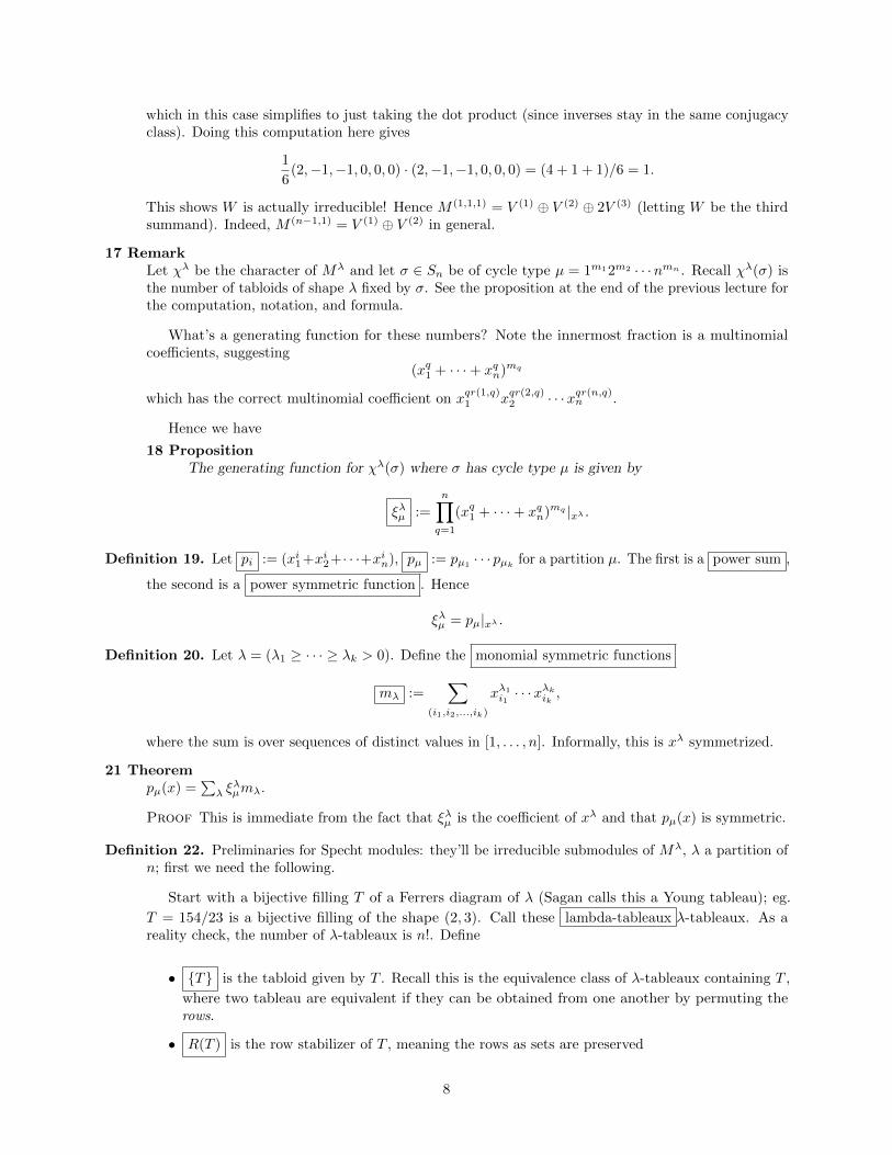
17 RemarkLet χλ be the character of Mλ and let σ ∈ Sn be of cycle type µ = 1m12m2 · · ·nmn . Recall χλ(σ) isthe number of tabloids of shape λ fixed by σ. See the proposition at the end of the previous lecture forthe computation, notation, and formula.
What’s a generating function for these numbers? Note the innermost fraction is a multinomialcoefficients, suggesting
(xq1 + · · ·+ xqn)mq
which has the correct multinomial coefficient on xqr(1,q)1 x
qr(2,q)2 · · ·xqr(n,q)n .
Hence we have
18 PropositionThe generating function for χλ(σ) where σ has cycle type µ is given by
ξλµ :=
n∏q=1
(xq1 + · · ·+ xqn)mq |xλ .
Definition 19. Let pi := (xi1+xi2+· · ·+xin), pµ := pµ1 · · · pµk for a partition µ. The first is a power sum ,
the second is a power symmetric function . Hence
ξλµ = pµ|xλ .
Definition 20. Let λ = (λ1 ≥ · · · ≥ λk > 0). Define the monomial symmetric functions
mλ :=∑
(i1,i2,...,ik)
xλ1i1· · ·xλkik ,
where the sum is over sequences of distinct values in [1, . . . , n]. Informally, this is xλ symmetrized.
21 Theorempµ(x) =
∑λ ξ
λµmλ.
Proof This is immediate from the fact that ξλµ is the coefficient of xλ and that pµ(x) is symmetric.
Definition 22. Preliminaries for Specht modules: they’ll be irreducible submodules of Mλ, λ a partition ofn; first we need the following.
Start with a bijective filling T of a Ferrers diagram of λ (Sagan calls this a Young tableau); eg.
T = 154/23 is a bijective filling of the shape (2, 3). Call these lambda-tableaux λ-tableaux. As areality check, the number of λ-tableaux is n!. Define
• T is the tabloid given by T . Recall this is the equivalence class of λ-tableaux containing T ,
where two tableau are equivalent if they can be obtained from one another by permuting therows.
• R(T ) is the row stabilizer of T , meaning the rows as sets are preserved
8
• C(T ) is the column stabilizer of T , meaning the columns as sets are preserved
• aT :=∑π∈R(T ) π
• bT :=∑π∈C(T ) sgn(π)π
For example, C(154/23) = S12 × S35 × S4. Note C[Sn] · T = Mλ roughly by definition, if T isa λ-tableau. bT will be a very important element in our construction of the Specht modules.
Definition 23. Given a Young tableau T of shape λ, define
eT := bT · T =∑
π∈C(T )
sgn(π)πT.
Check:σ · eT = eσ(T ).
Proof Set wσ = σπσ−1 and observe
σ · eT =∑
π∈C(T )
sgn(π) · σπT
=∑
wσ∈σ−1C(T )σ
sgn(π)wσσT
Note σC(T )σ−1 = C(σT ). Hence the right-hand side is precisely eσ(T ).
Definition 24. Define the Specht module
Sλ := SpaneT : T is a λ-tableau = C[Sn] · eT .
(The second equality follows from the observation in the previous definition.)
25 ExampleLet λ = (1n), T = 1/2/3/ · · · /n. Hence C(T ) = Sn. Now
σ · eT = eσ(T ) =∑π∈Sn
sgn(π)πσT
=∑w
sgn(w) sgn(σ)wT
= sgn(σ)eT .
Hence we recovered the sign representation!
Note: the πT appearing above are distinct as π ∈ C(T ) varies, so the coefficients really are ±1.
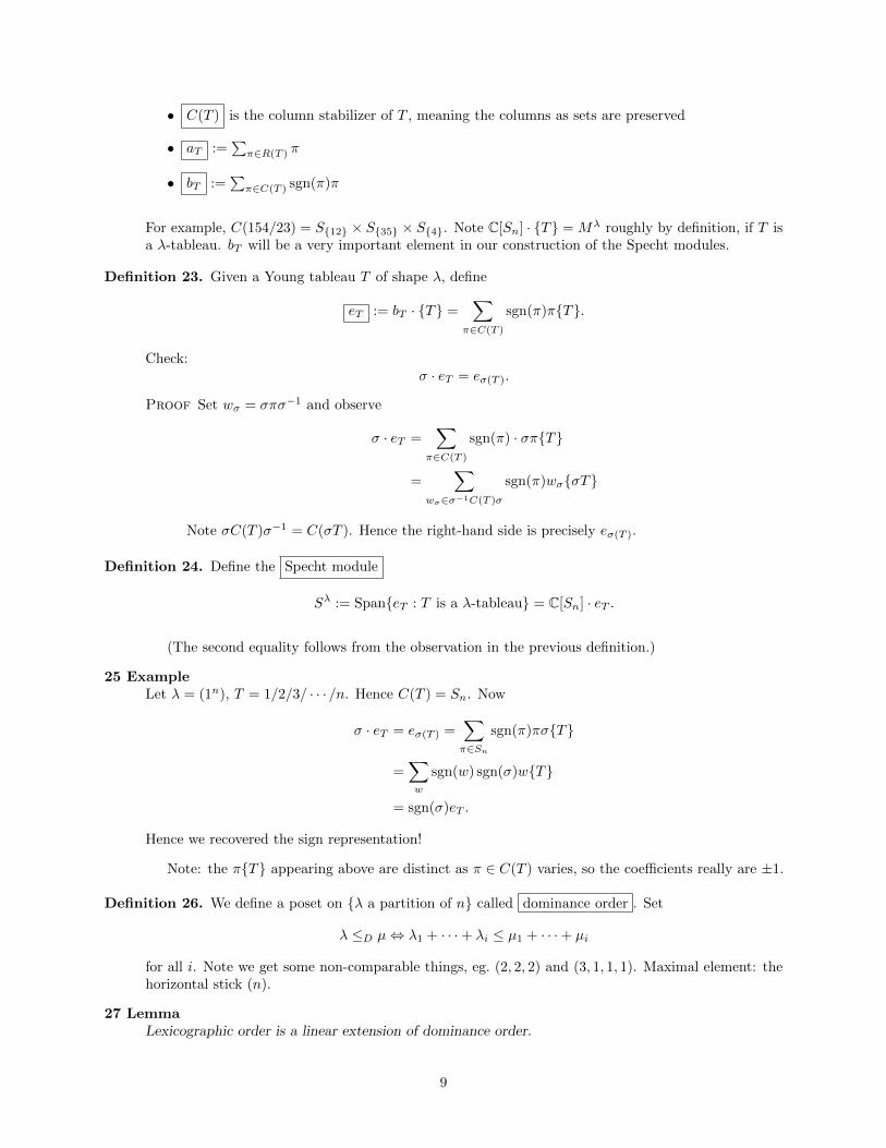
Definition 26. We define a poset on λ a partition of n called dominance order . Set
λ ≤D µ⇔ λ1 + · · ·+ λi ≤ µ1 + · · ·+ µi
for all i. Note we get some non-comparable things, eg. (2, 2, 2) and (3, 1, 1, 1). Maximal element: thehorizontal stick (n).
27 LemmaLexicographic order is a linear extension of dominance order.
9
Proof By contrapositive: if λ <L µ (in Lexicographic order), then there exists λj < µj and λi = µifor all i < j. Then we can’t have µ < λ in dominance, since it just went over at the jth spot.
28 LemmaSay T, T ′ are Young tableaux with shapes λ, λ′, respectively. Then bT T ′ is as follows:
• bT T ′ = ±eT if λ = λ′ and no tij ∈ R(T ′) ∩ C(T ) (i.e. no two numbers simultaneously appearin the same row of T ′ and the same column of T ).
• bT T ′ = 0 if λ <L λ′ or λ = λ′, tij ∈ R(T ′) ∩ C(T ).
Note bT T ′ 6= 0 implies λ ≥D λ′.
Proof If i < j appear in the same row of T ′ and the same column of T , consider bT · tij . This is −bTsince it just permutes the sum (and flips the signs). We’ll finish this next time.
April 7th, 2014: Fundamental Specht Module Properties andBranching Rules
Summary Recall: last time, we defined Specht modules
Sλ := SpaneT : T bijective filling of λ ⊂Mλ.
Today’s goals:
A) Sλ is irreducible
B) Sλ ∼= Sµ implies λ = µ
C) Induction and restriction work on Sλ
Definition 29. Recall dominance order on partitions of size n, where
λ ≤D µ⇔ λ1 + · · ·+ λi ≤ µ1 + · · ·+ µi, ∀i.
Last time we said lexicographic extends dominance order.
30 Lemma(See last lemma from previous lecture.) Say T, T ′ are Young tableau of shapes λ, λ′ ` n. ThenbT · T ′ = 0 if there exists tij ∈ R(T ′) ∩C(T ), i.e. if there are two numbers which are simultaneouslyin the same row of T ′ and the same column of T .
Proof tij ∈ C(T ) implies bT tij = −bT ; tij ∈ R(T ) implies tij · T ′ = T ′. Hence bT · T ′ =bT · tijT ′ = −bT T ′, so bT T ′ = 0.
31 CorollaryIf λ, λ′ ` n, T is a λ-tableau, T ′ is a λ′-tableau, then bT · T ′ 6= 0 implies λ ≥D λ′.
Proof For each box in T , imagine annotating that box with the index of the row in which that box’sentry appears in T ′ using red ink. We can permute T by some σ ∈ C(T ) at the cost of changingbT by at most a sign, so we can assume the red annotations appear in weakly increasing orderin each column. From the lemma, there is no i, j appearing in the same row of T ′ and the samecolumn of T , so the red annotations actually increase strictly. By the pigeonhole principle, the
10
first k rows of T contain all red annotations numbered 1, . . . , k, i.e. there is an injection fromthe first k rows of T ′ to the first k rows of T . But this just says
λ1 + · · ·+ λk ≥ λ′1 + · · ·λ′k,
so λ ≥D λ′.
Note: this proof holds for the weaker hypothesis that 6 ∃ tij ∈ R(T ′) ∩ C(T ).
32 LemmaIf T, T ′ are Young tableau of the same shape λ and no tij ∈ R(T ′)∩C(T ) exists, then bT · T ′ = ±eT .
Proof By hypothesis, every value in row 1 of T ′ is in a distinct column of T . So, there existsa permutation π(1) ∈ C(T ) such that π(1)T and T ′ have the same first row. Induct on theremaining rows to get some permutation π ∈ C(T ) such that πT = T ′. Then bT · T ′ =bT · πT = sgn(π)eT .
33 CorollaryFor T a Young tableau of shape λ,
bTMλ′ = bTS
λ′ = 0 if λ <L λ′
andbTM
λ = bTSλ = SpaneT 6= 0.
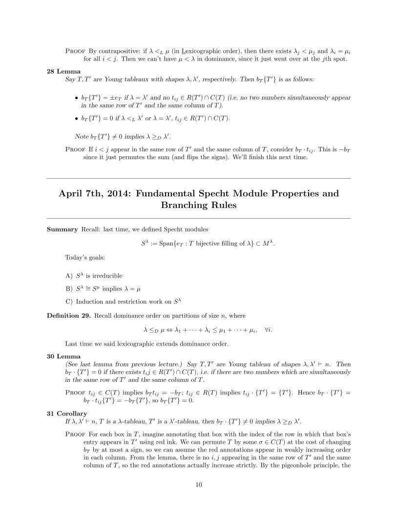
34 TheoremSλ is irreducible for each partition λ of n. (Note: it’s important that we’re working over C.)
Proof Suppose Sλ = V ⊕W , T a Young tableau of shape λ. By the corollary above,
Span eT = bTSλ = bTV ⊕ bTW.
Since bTV, bTW, Span et are all vector spaces over C and SpanT is one dimensional, eT must bein bTV ⊂ V or bTW ⊂W , with the other 0. Hence eT ∈ V or eT ∈W , so C[Sn] · eT = Sλ ⊂ Vor W , giving the result.
35 TheoremSλ ∼= Sµ ⇒ λ = µ.
Proof Sλ ∼= Sµ implies there is a non-zero homomorphism Θ: Sλ →Mµ. Extend Θ: Mλ →Mµ by
w ∈ (Sλ)⊥ ⇒ Θ(w) = 0.
Now Θ non-zero implies there is some eT ∈ Sλ such that Θ(eT ) 6= 0, so
0 6= Θ(eT ) = Θ(bT · T) = bTΘ(T) = bT · (∑i
ciSi),
where Si are distinct tabloids of shape µ. At least one ci is non-zero, so bT · Si 6= 0, so λ ≥D µby the corollary above. By symmetry of this argument, λ = µ.
36 ExampleLet T be a Young tableau of shape λ. Note that we can write bT · T =
∑S where the sum is over
some S which are column-increasing. For instance, let T = 462/35/1, S = 152/36/4. These S don’tform a basis, unfortunately; too much redundancy.
Definition 37. T is a standard Young tableau , SYT(λ), if T is a bijective filling of λ with rows and
columns increasing. Set fλ := #SY T (λ). Recall the hook length formula,
fλ =n!∏c∈λ hc
.
11
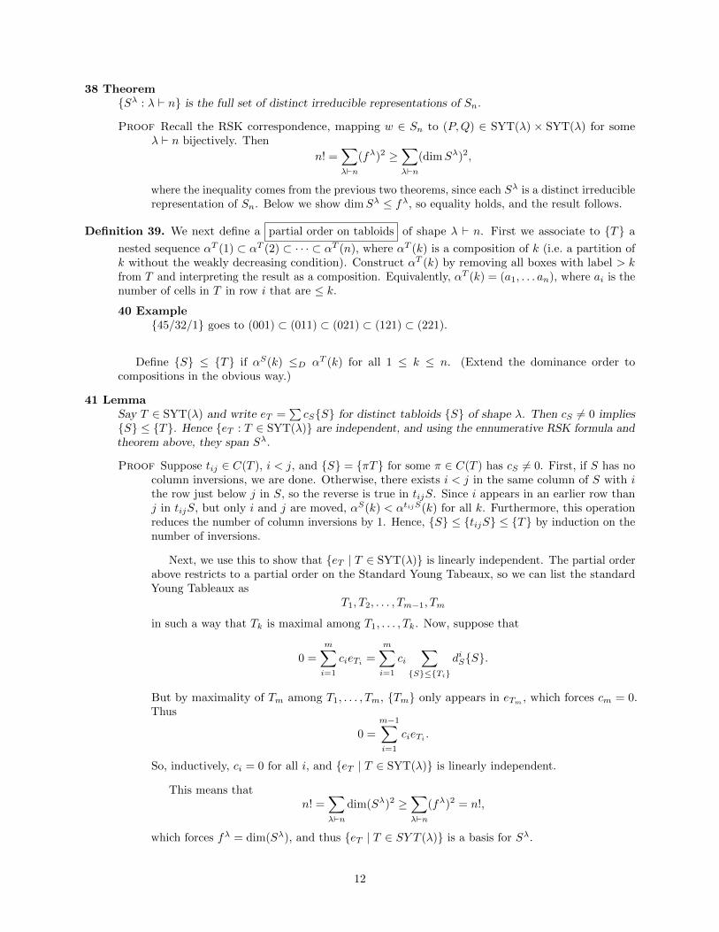
38 TheoremSλ : λ ` n is the full set of distinct irreducible representations of Sn.
Proof Recall the RSK correspondence, mapping w ∈ Sn to (P,Q) ∈ SYT(λ) × SYT(λ) for someλ ` n bijectively. Then
n! =∑λ`n
(fλ)2 ≥∑λ`n
(dimSλ)2,
where the inequality comes from the previous two theorems, since each Sλ is a distinct irreduciblerepresentation of Sn. Below we show dimSλ ≤ fλ, so equality holds, and the result follows.
Definition 39. We next define a partial order on tabloids of shape λ ` n. First we associate to T a
nested sequence αT (1) ⊂ αT (2) ⊂ · · · ⊂ αT (n), where αT (k) is a composition of k (i.e. a partition ofk without the weakly decreasing condition). Construct αT (k) by removing all boxes with label > kfrom T and interpreting the result as a composition. Equivalently, αT (k) = (a1, . . . an), where ai is thenumber of cells in T in row i that are ≤ k.
40 Example45/32/1 goes to (001) ⊂ (011) ⊂ (021) ⊂ (121) ⊂ (221).
Define S ≤ T if αS(k) ≤D αT (k) for all 1 ≤ k ≤ n. (Extend the dominance order tocompositions in the obvious way.)
41 LemmaSay T ∈ SYT(λ) and write eT =
∑cSS for distinct tabloids S of shape λ. Then cS 6= 0 implies
S ≤ T. Hence eT : T ∈ SYT(λ) are independent, and using the ennumerative RSK formula andtheorem above, they span Sλ.
Proof Suppose tij ∈ C(T ), i < j, and S = πT for some π ∈ C(T ) has cS 6= 0. First, if S has nocolumn inversions, we are done. Otherwise, there exists i < j in the same column of S with ithe row just below j in S, so the reverse is true in tijS. Since i appears in an earlier row thanj in tijS, but only i and j are moved, αS(k) < αtijS(k) for all k. Furthermore, this operationreduces the number of column inversions by 1. Hence, S ≤ tijS ≤ T by induction on thenumber of inversions.
Next, we use this to show that eT | T ∈ SYT(λ) is linearly independent. The partial orderabove restricts to a partial order on the Standard Young Tabeaux, so we can list the standardYoung Tableaux as
T1, T2, . . . , Tm−1, Tm
in such a way that Tk is maximal among T1, . . . , Tk. Now, suppose that
0 =
m∑i=1
cieTi =
m∑i=1
ci∑
S≤Ti
diSS.
But by maximality of Tm among T1, . . . , Tm, Tm only appears in eTm , which forces cm = 0.Thus
0 =
m−1∑i=1
cieTi .
So, inductively, ci = 0 for all i, and eT | T ∈ SYT(λ) is linearly independent.
This means thatn! =
∑λ`n
dim(Sλ)2 ≥∑λ`n
(fλ)2 = n!,
which forces fλ = dim(Sλ), and thus eT | T ∈ SY T (λ) is a basis for Sλ.
12
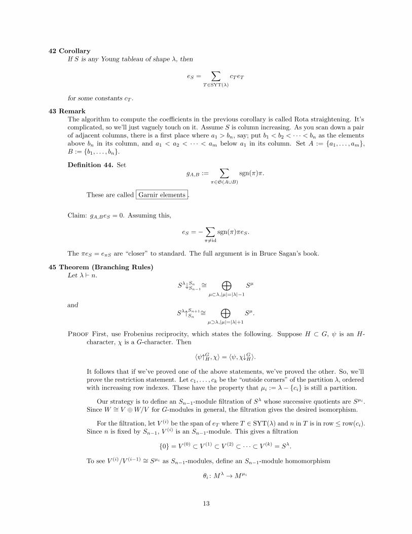
42 CorollaryIf S is any Young tableau of shape λ, then
eS =∑
T∈SYT(λ)
cT eT
for some constants cT .
43 RemarkThe algorithm to compute the coefficients in the previous corollary is called Rota straightening. It’scomplicated, so we’ll just vaguely touch on it. Assume S is column increasing. As you scan down a pairof adjacent columns, there is a first place where a1 > bn, say; put b1 < b2 < · · · < bn as the elementsabove bn in its column, and a1 < a2 < · · · < am below a1 in its column. Set A := a1, . . . , am,B := b1, . . . , bn.
Definition 44. SetgA,B :=
∑π∈S(A∪B)
sgn(π)π.
These are called Garnir elements .
Claim: gA,BeS = 0. Assuming this,
eS = −∑π 6=id
sgn(π)πeS .
The πeS = eπS are “closer” to standard. The full argument is in Bruce Sagan’s book.
45 Theorem (Branching Rules)Let λ ` n.
Sλ↓SnSn−1
∼=⊕
µ⊂λ,|µ|=|λ|−1
Sµ
andSλ↑Sn+1
Sn∼=
⊕µ⊃λ,|µ|=|λ|+1
Sµ.
Proof First, use Frobenius reciprocity, which states the following. Suppose H ⊂ G, ψ is an H-character, χ is a G-character. Then
〈ψ↑GH , χ〉 = 〈ψ, χ↓GH〉.
It follows that if we’ve proved one of the above statements, we’ve proved the other. So, we’llprove the restriction statement. Let c1, . . . , ck be the “outside corners” of the partition λ, orderedwith increasing row indexes. These have the property that µi := λ− ci is still a partition.
Our strategy is to define an Sn−1-module filtration of Sλ whose successive quotients are Sµi .Since W ∼= V ⊕W/V for G-modules in general, the filtration gives the desired isomorphism.
For the filtration, let V (i) be the span of eT where T ∈ SYT(λ) and n in T is in row ≤ row(ci).Since n is fixed by Sn−1, V (i) is an Sn−1-module. This gives a filtration
0 = V (0) ⊂ V (1) ⊂ V (2) ⊂ · · · ⊂ V (k) = Sλ.
To see V (i)/V (i−1) ∼= Sµi as Sn−1-modules, define an Sn−1-module homomorphism
θi : Mλ →Mµi
13
as follows. If n is in row(ci) of T , by tabloid equivalence say T has n in ci and set θi(T) =T − n. Otherwise, set θi(T) = 0.
V (i−1) is spanned by eT which are by definition annihilated by θi, so ker θi ⊃ V (i−1). ForT SYT(λ) with n in row ci, we find θi(eT ) = eT−n as follows. n must be in box ci, so π ∈ C(T )either (i) leaves it fixed or (ii) moves it up. Hence
θi(eT ) = θi
∑π∈C(T )−C(T−n)
sgn(π)πT
+ θi
∑π∈C(T−n)
sgn(π)πT
= 0 + eT−n,
whence θi(V(i)) = Sµi .
Indeed, the map V (i) θi→ Sµi gives the isomorphism V (i)/(V (i) ∩ ker θi) ∼= Sµi , which is ofdimension fµi . We’d like V (i) ∩ ker θi = V (i−1), which is true as follows. We can extend ourprevious filtration to
0 ⊂ V (0) ⊆ V (1) ∩ ker θ1 ⊂ V (1) ⊆ V (2) ∩ ker θ2 ⊂ V (2) ⊂ · · · ⊂ V (k) = Sλ.
But then the successive quotients V (i)/(V (i) ∩ ker θi) account for∑fµi = fλ dimensions, i.e.
all of them. So, the inclusions V (i−1) ⊆ V (i) ∩ ker θi must be equalities, giving the result.
46 ExerciseLet c be a corner of λ ` n. Is the map Sλ → Sλ−c defined by sendng eT to 0 if T ∈ SYT(λ) does nothave n in c, and by sending eT to eT−n otherwise an Sn−1-module morphism? Similarly, is the mapSλ−c → Sλ defined by eT−c 7→ eT an Sn−1-module morphism?
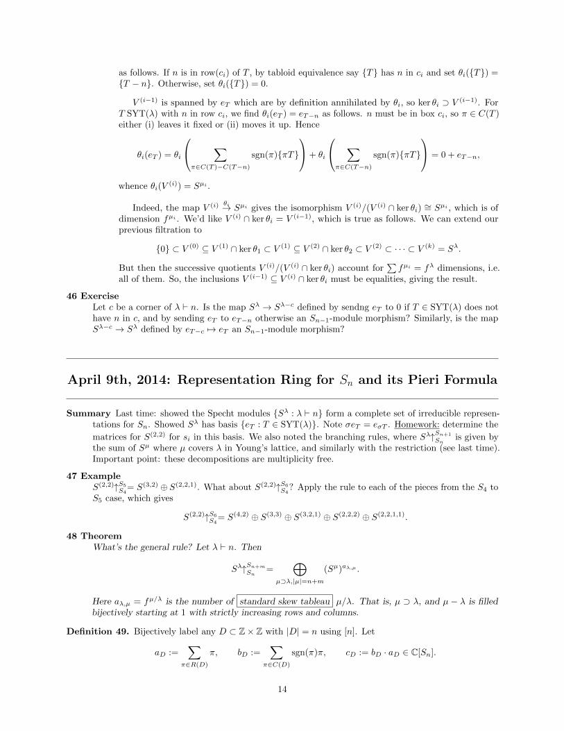
April 9th, 2014: Representation Ring for Sn and its Pieri Formula
Summary Last time: showed the Specht modules Sλ : λ ` n form a complete set of irreducible represen-tations for Sn. Showed Sλ has basis eT : T ∈ SYT(λ). Note σeT = eσT . Homework: determine the
matrices for S(2,2) for si in this basis. We also noted the branching rules, where Sλ↑Sn+1
Snis given by
the sum of Sµ where µ covers λ in Young’s lattice, and similarly with the restriction (see last time).Important point: these decompositions are multiplicity free.
47 ExampleS(2,2)↑S5
S4= S(3,2) ⊕ S(2,2,1). What about S(2,2)↑S6
S4? Apply the rule to each of the pieces from the S4 to
S5 case, which gives
S(2,2)↑S6
S4= S(4,2) ⊕ S(3,3) ⊕ S(3,2,1) ⊕ S(2,2,2) ⊕ S(2,2,1,1).
48 TheoremWhat’s the general rule? Let λ ` n. Then
Sλ↑Sn+m
Sn=
⊕µ⊃λ,|µ|=n+m
(Sµ)aλ,µ .
Here aλ,µ = fµ/λ is the number of standard skew tableau µ/λ. That is, µ ⊃ λ, and µ − λ is filledbijectively starting at 1 with strictly increasing rows and columns.
Definition 49. Bijectively label any D ⊂ Z× Z with |D| = n using [n]. Let
aD :=∑
π∈R(D)
π, bD :=∑
π∈C(D)
sgn(π)π, cD := bD · aD ∈ C[Sn].
14
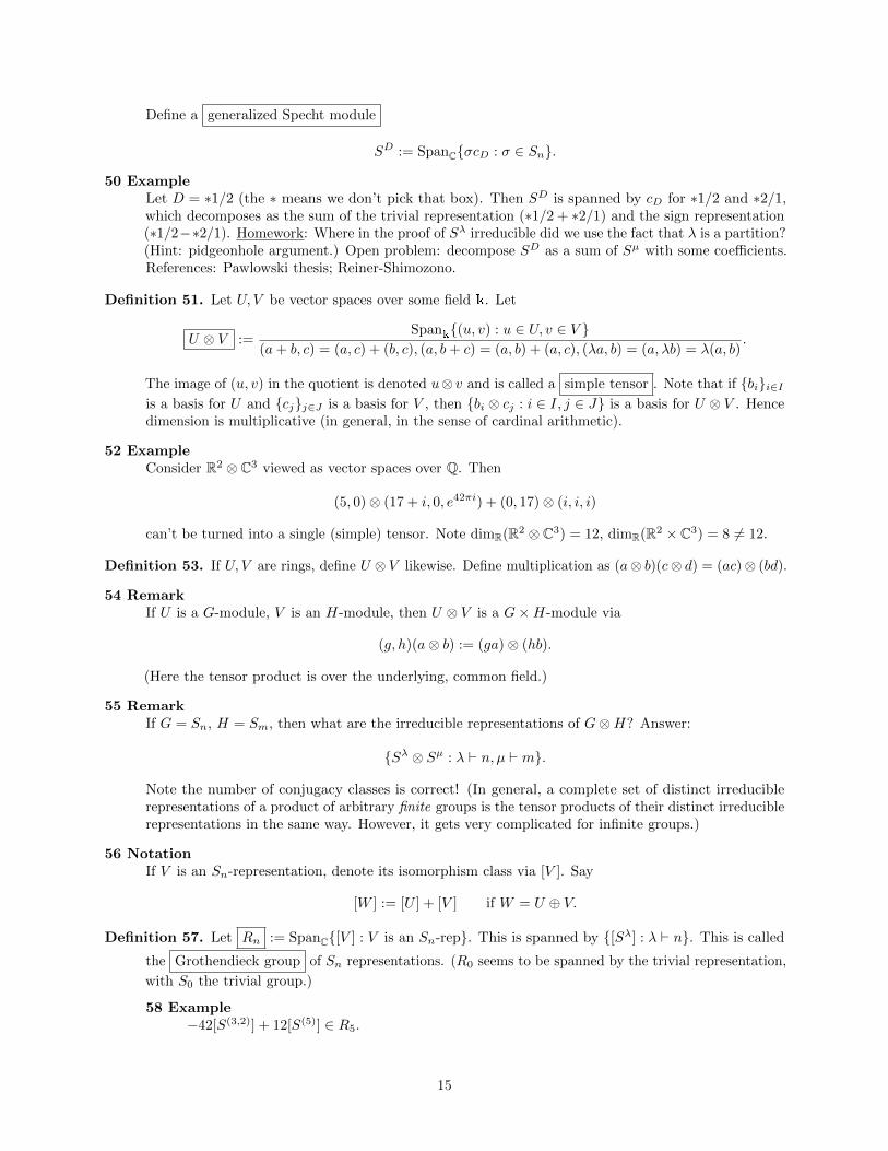
Define a generalized Specht module
SD := SpanCσcD : σ ∈ Sn.
50 ExampleLet D = ∗1/2 (the ∗ means we don’t pick that box). Then SD is spanned by cD for ∗1/2 and ∗2/1,which decomposes as the sum of the trivial representation (∗1/2 + ∗2/1) and the sign representation(∗1/2−∗2/1). Homework: Where in the proof of Sλ irreducible did we use the fact that λ is a partition?(Hint: pidgeonhole argument.) Open problem: decompose SD as a sum of Sµ with some coefficients.References: Pawlowski thesis; Reiner-Shimozono.
Definition 51. Let U, V be vector spaces over some field k. Let
U ⊗ V :=Span
k(u, v) : u ∈ U, v ∈ V
(a+ b, c) = (a, c) + (b, c), (a, b+ c) = (a, b) + (a, c), (λa, b) = (a, λb) = λ(a, b).
The image of (u, v) in the quotient is denoted u⊗ v and is called a simple tensor . Note that if bii∈Iis a basis for U and cjj∈J is a basis for V , then bi ⊗ cj : i ∈ I, j ∈ J is a basis for U ⊗ V . Hencedimension is multiplicative (in general, in the sense of cardinal arithmetic).
52 ExampleConsider R2 ⊗ C3 viewed as vector spaces over Q. Then
(5, 0)⊗ (17 + i, 0, e42πi) + (0, 17)⊗ (i, i, i)
can’t be turned into a single (simple) tensor. Note dimR(R2 ⊗ C3) = 12, dimR(R2 × C3) = 8 6= 12.
Definition 53. If U, V are rings, define U ⊗ V likewise. Define multiplication as (a⊗ b)(c⊗ d) = (ac)⊗ (bd).
54 RemarkIf U is a G-module, V is an H-module, then U ⊗ V is a G×H-module via
(g, h)(a⊗ b) := (ga)⊗ (hb).
(Here the tensor product is over the underlying, common field.)
55 RemarkIf G = Sn, H = Sm, then what are the irreducible representations of G⊗H? Answer:
Sλ ⊗ Sµ : λ ` n, µ ` m.
Note the number of conjugacy classes is correct! (In general, a complete set of distinct irreduciblerepresentations of a product of arbitrary finite groups is the tensor products of their distinct irreduciblerepresentations in the same way. However, it gets very complicated for infinite groups.)
56 NotationIf V is an Sn-representation, denote its isomorphism class via [V ]. Say
[W ] := [U ] + [V ] if W = U ⊕ V.
Definition 57. Let Rn := SpanC[V ] : V is an Sn-rep. This is spanned by [Sλ] : λ ` n. This is called
the Grothendieck group of Sn representations. (R0 seems to be spanned by the trivial representation,
with S0 the trivial group.)
58 Example−42[S(3,2)] + 12[S(5)] ∈ R5.
15
Define R as ⊕n≥0Rn as the ring of representations . Addition is formal addition. Multiplication
is given by Rn ×Rm → Rn+m where
[V ] · [W ] = [(V ⊗W )↑Sn+m
Sn×Sm ].
Homework: show
(V ⊗W )↑Sn+m
Sn×Sm= C[Sn+m]⊗C[Sn×Sm] (V ⊗W ).
59 Proposition• R is commutative: quick from commutativity of tensor product.
• R is associative: uses associativity of tensor product, that induction is transitive, etc.
• R has a unit, 1 ∈ C corresponding to the trivial representation in R0.
60 Theorem
(Sλ ⊗ S(m))↑Sn+m
Sn×Sm=⊕
Sµ,
where the sum is over µ ⊃ λ such that |µ| = |λ| + m = n + m and where µ − λ is a collection of
horizontal strips (i.e. no two boxes appear in the same column). We’ll call this the Pieri formula .
Proof (Thanks to Brendan.) By Frobenius reciprocity,
(Sλ ⊗ S(m))↑Sn+m
Sn×Sm=⊕
µ`n+m
(Sµ)aλ,m,µ
andSµ↓Sn+m
Sn×Sm=⊕
λ′`n,ν`m
(Sλ′⊗ Sν)cλ′ ,ν,µ
have the same coefficients aλ,m,µ = cλ,(m),µ. So let V = Sµ↓Sn+m
Sn×Sm for µ ` n + m. That is,
Sn × Sm acts on V = SpanCeT : T ∈ SYT(µ). Now V may include Sλ′ ⊗ Sν for ν 6= (m) or
λ′ 6= λ, but we can “filter out” these extra representations by looking at the subspace V 1×Sm
fixed by 1n × Sn, which gives us precisely
V 1×Sm = ⊕(Sλ ⊗ S(m))cλ,(m),µ.
Hence we need only decompose V 1×Sn and show that the non-zero multiplicites are precisely onefor exactly λ with the conditions in the theorem statement. We’ll decompose V 1×Sn by settingz :=
∑π∈1n×Sm π, noting V 1×Sn = zV = SpanzeT : T ∈ SYT(λ). When does zeT = zeS?
Well, certainly when S, T agree on [1, n]. Moreover, if i, j ∈ [n+ 1,m] are in the same column ofT , then z = ztij and zeT = ztijeT = −zeT , so zeT = 0. This motivates...
61 TheoremV 1×Sm is the span of zeT for T ∈ SYT(µ) where µ/λ is a horizontal strip and the valuesin µ/λ increase from left to right; indeed this is a basis.
We end up withV 1×Sm = ⊕(Sλ ⊗ S(m))
with the sum over λ ⊂ µ, µ/λ a horizontal strip, |µ| = |λ|+m. The multiplicity is 1 using thebasis for the tensor product, giving the result.
16
62 RemarkThis suggests a basis for symmetric polynomials, since none of our given bases obviously mimic the
Pieri rule. The Schur functions are the answer. Recall
sλ :=∑
T∈SSYT(λ)
xT .
Next time: we’ll show sλs(m) satisfies the Pieri formula. (Recall we also used a non-intersecting latticepath definition/proof from Autumn quarter—see beginning of next lecture.)
April 11th, 2014: Pieri for Schurs; Kostka Numbers; Dual Bases;Cauchy Identity
Summary Last time, we defined the representation ring of symmetric groups, R = ⊕Rn, where Rn isspanned by equivalence classes [Sλ] is irreducible representations of Sn, λ ` n, with multiplicationgiven by tensor product followed by induction, addition splitting over direct sums.
Hence[Sµ][Sν ] = [(Sµ ⊗ Sν)↑Sn+m
Sn×Sm ] =∑
λ`n+m
cλµ,ν [Sλ],
µ ` n, ν ` m for some cλµ,ν ∈ N. Eventual goal: show the representation ring is isomorphic to the ringof symmetric functions.
Today: Pieri formula for Schur functions and Cauchy’s identity involving Schur functions.
Definition 63. Let SSYT(λ) be the set of semistandard Young tableaux of shape λ, meaning fillings of a
partition λ with P such that rows weakly increase and columns strictly increase. Associate a monomialto each such object in the obvious way:
64 ExampleT = 133/25 of shape λ = (3, 2). The associated monomial is xT = x1
1x12x
23x
15.
Definition 65. We recalled the definition of the Schur functions at the end of last time. (To get comfortablewith them, Sara recommends computing any 10 by hand.) Recall also the Jacobi-Trudi formula,
sλ(x) = det(hλi−i+j(x))1≤i,j≤k,
which we proved last quarter. (Here λ has k parts.) Note: there’s also a notion of Schur polynomialswhere we restrict the alphabet filling the SSYT’s to eg. [n]. We’re using the infinite alphabet P. Sara’sexercise may be easier with a restricted alphabet.
66 PropositionThe sλ are symmetric. This is immediate from the Jacobi-Trudi formula, but it’s not obvious from theSSYT definition. Homework: prove symmetry from the SSYT definition; find appropriate bijections.
67 Example• s(m) = hm
• s1m = em
using the definitions from the first day of class.
17
68 Theorem (Pieri Formula)
sλs(m) =∑
sµ,
where the sum is over µ/λ which is a horizontal strip with m boxes as in the previous Pieri formula.
Proof We’ll define a bijection
SSYT(λ)× SSYT((m))→ ∪SSYT(µ),
where the union is over λ from the theorem statement; the result follows from the definitionof the Schur functions. We do so by successively inserting elements into rows and “bumping”elements down. Suppose we have a row a1 ≤ a2 ≤ · · · ≤ ak and we want to insert b. If b ≥ akthen add b to the end of the row. Otherwise, replace aj by b for the smallest j such that aj > band insert aj into the next row.
69 ExampleStarting with T = 123/45, let’s insert 225. 2 replaces the 3 in the first row, and the 3 isthen inserted in the row below, which bumps the 4, and 4 is inserted on the last line, sowe have 122/33/4 after these “bumps”. Inserting 25 results in 12225/33/4. Note that weadded the horizontal strip ∗ ∗ ∗25/ ∗ ∗/4.
Claim: suppose inserting a row i1 ≤ · · · ≤ im into an SSYT T gives S; it’s straightforward tocheck that S is an SSYT of shape sh(S) containing the shape of T . One can check that indeedsh(S)/ sh(T ) is a sequence of m horizontal strips. (Rough outline: the “bumping path” for i2 isalways strictly to the right of the bumping path for i1. Draw some pictures to convince yourself;better than a formal proof.)
Hence indeed we have a weight-preserving map
RSK: SSYT(λ)× SSYT((m))→ ∪SSYT(µ).
Why is it reversible? The cells of sh(S)/ sh(T ) must have been created from left to right, so wecan “unbump” them to undo the operation.
70 CorollaryRecall hµ = hµ1hµ2 · · ·hµk by definition. What are the coefficients hµ :=
∑Kλ,µsλ?
Kλ,µ := #T ∈ SSYT(λ) : xT = xµ.
In particular, Kλ,λ = 1 and Kλ,µ = 0 unless λ ≥D µ. These are called the Kostka numbers .
Proof Imagine repeatedly applying the Pieri rule, starting with hµk · 1 = s(µk); label the new cells inthe first application 1, in the second application 2, etc. We get horizontal strips of µ1 1’s, µ2 2’s,etc. In this way we get an SSYT of weight µ, and indeed all such SSYT arise in this way.
For Kλ,λ, there’s just one way to fill λ with λ1 1’s: all in the first row; etc.
71 CorollaryLet λ ` n. Then
sλ =∑
T∈SSYT(λ)
xT =∑αn
Kλ,αxα
=∑µ`n
Kλ,µmµ
(Recall mµ were the monomial symmetric functions, and α n means α is a composition of n, whichis a partition without the weakly decreasing requirement.)
18
Definition 72. The Hall inner product is by definition 〈sλsµ〉 = δλ,µ, extended sesquilinearly (i.e. linearly
in the first argument, conjugate-linearly in the second).
73 PropositionFrom the corollary,
〈hµ, sλ〉 = Kλ,µ
and〈mµ, sλ〉 = K−1
µ,λ
(inverse matrix). Hence
〈hµ,mγ〉 =∑λ
Kλ,µ〈sλ,mγ〉 =∑
Kλ,µK−1γ,λ = δµ,γ .
Thus hµ and mλ are dual bases.
74 TheoremThe Cauchy identity says
∏i≥1
∏j≥1
1
1− xiyj(A)=∑λ
sλ(x)sλ(y)
(B)=∑λ
hλ(x)mλ(y)
(C)=∑λ
pλ(x)pλ(y)
zλ,
where x = (x1, x2, . . .), y = (y1, y2, . . .) and zλ = (1m12m2 · · · )(m1!m2! · · · ) for λ = (1m1 , 2m2 , · · · ) (i.e.m1 one’s, m2 two’s, etc.). The sums are over λ ` n for n ≥ 0.
Proof Today we’ll prove equality A. Note∏i
∏j
1
1− xiyj=∏ij
(1 + xiyj + (xiyj)2 + · · · ) =
∑(xi1yj1)k1(xi2yj2)k2 · · · ,
where the sum is over all “biwords” in the alphabet of “biletters” (ij
): i ≥ 1, j ≥ 1 written in
weakly increasing lexicographic order, where the k` are multiplicities. (Not to be confused with“bywords”!)
75 Example(12
)(12
)(12
)(14
)(23
)(37
)(37
)corresponds to the monomial (x1y2)3(x1y4)(x2y3)(x3y7)2.
To prove A, we’ll exhibit a “bi”weight-preserving bijection between finite biwords in lexico-graphic order to pairs (P,Q) of semistandard Young tableaux of the same shape. Under thisbijection, label i of P corresponds to xi, and label j of Q corresponds to xj . Start with(
i1j1
)(i2j2
)· · ·(ikjk
).
In particular, i1 ≤ i2 ≤ · · · ≤ ik. To get P , insert the letters of j1j2 · · · jk successively into theempty tableau using our earlier RSK insertion algorithm. Let Q′ be the recording tableaux forthis process, i.e. its labels indicate when the corresponding element of P was inserted. Get Q byreplacing ` in Q′ with i`.
76 ExampleWith the previous word, P becomes 222377/4. The recording tableau Q′ was 123467/5(denotes order of insertion). Hence Q = 111133/2.
19
P is a semistandard tableau as before. Q is certainly weakly increasing along rows. Whatabout columns? Recall the bumping path for inserting j1 ≤ · · · ≤ jk to T ; they give a horizontalstrip. It follows that Q is column strict and has the same shape as P . (But we don’t havej1 ≤ · · · ≤ jk?) This algorithm is invertible.
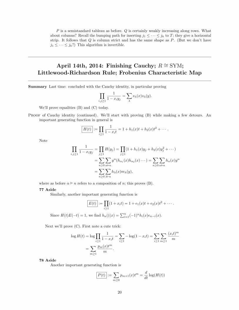
April 14th, 2014: Finishing Cauchy; R ∼= SYM;Littlewood-Richardson Rule; Frobenius Characteristic Map
Summary Last time: concluded with the Cauchy identity, in particular proving∏i,j≥1
1
1− xiyj=∑λ
sλ(x)sλ(y).
We’ll prove equalities (B) and (C) today.
Proof of Cauchy identity (continued). We’ll start with proving (B) while making a few detours. Animportant generating function in general is
H(t) :=∏i≥1
1
1− xit= 1 + h1(x)t+ h2(x)t2 + · · · .
Note ∏i,j≥1
1
1− xiyj=∏j≥1
H(yj) =∏j≥1
(1 + h1(x)yj + h2(x)y2j + · · · )
=∑n≥0
∑αn
yα(hα1(x)hα2(x) · · · ) =∑n≥0
∑αn
hα(x)yα
=∑n≥0
∑λ`n
hλ(x)mλ(y),
where as before α n refers to a composition of n; this proves (B).
77 AsideSimilarly, another important generating function is
E(t) :=∏i≥1
(1 + xit) = 1 + e1(x)t+ e2(x)t2 + · · · .
Since H(t)E(−t) = 1, we find hn(((x) =∑ni=1(−1)nhi(x)en−i(x).
Next we’ll prove (C). First note a cute trick:
logH(t) = log∏i≥1
1
1− xit=∑i≥1
− log(1− xit) =∑i≥1
∑m≥1
(xit)m
m
=∑m≥1
pm(x)tm
m.
78 AsideAnother important generating function is
P (t) :=∑m≥0
pm+1(x)tm =d
dtlog(H(t))
20
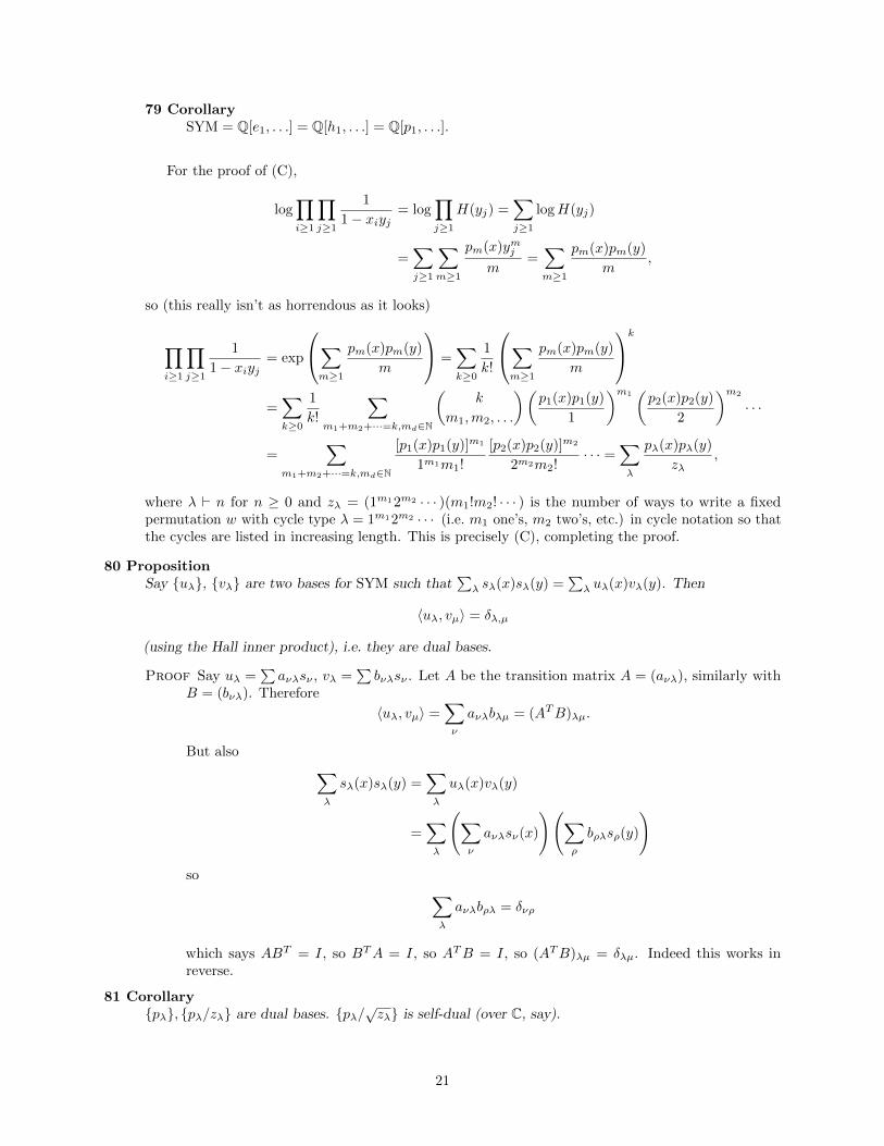
79 CorollarySYM = Q[e1, . . .] = Q[h1, . . .] = Q[p1, . . .].
For the proof of (C),
log∏i≥1
∏j≥1
1
1− xiyj= log
∏j≥1
H(yj) =∑j≥1
logH(yj)
=∑j≥1
∑m≥1
pm(x)ymjm
=∑m≥1
pm(x)pm(y)
m,
so (this really isn’t as horrendous as it looks)
∏i≥1
∏j≥1
1
1− xiyj= exp
∑m≥1
pm(x)pm(y)
m
=∑k≥0
1
k!
∑m≥1
pm(x)pm(y)
m
k
=∑k≥0
1
k!
∑m1+m2+···=k,md∈N
(k
m1,m2, . . .
)(p1(x)p1(y)
1
)m1(p2(x)p2(y)
2
)m2
· · ·
=∑
m1+m2+···=k,md∈N
[p1(x)p1(y)]m1
1m1m1!
[p2(x)p2(y)]m2
2m2m2!· · · =
∑λ
pλ(x)pλ(y)
zλ,
where λ ` n for n ≥ 0 and zλ = (1m12m2 · · · )(m1!m2! · · · ) is the number of ways to write a fixedpermutation w with cycle type λ = 1m12m2 · · · (i.e. m1 one’s, m2 two’s, etc.) in cycle notation so thatthe cycles are listed in increasing length. This is precisely (C), completing the proof.
80 PropositionSay uλ, vλ are two bases for SYM such that
∑λ sλ(x)sλ(y) =
∑λ uλ(x)vλ(y). Then
〈uλ, vµ〉 = δλ,µ
(using the Hall inner product), i.e. they are dual bases.
Proof Say uλ =∑aνλsν , vλ =
∑bνλsν . Let A be the transition matrix A = (aνλ), similarly with
B = (bνλ). Therefore
〈uλ, vµ〉 =∑ν
aνλbλµ = (ATB)λµ.
But also ∑λ
sλ(x)sλ(y) =∑λ
uλ(x)vλ(y)
=∑λ
(∑ν
aνλsν(x)
)(∑ρ
bρλsρ(y)
)so ∑
λ
aνλbρλ = δνρ
which says ABT = I, so BTA = I, so ATB = I, so (ATB)λµ = δλµ. Indeed this works inreverse.
81 Corollarypλ, pλ/zλ are dual bases. pλ/
√zλ is self-dual (over C, say).
21
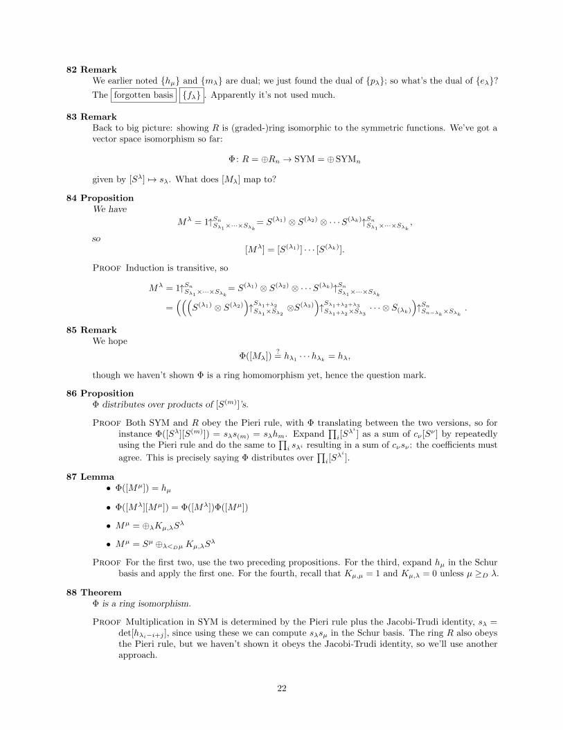
82 RemarkWe earlier noted hµ and mλ are dual; we just found the dual of pλ; so what’s the dual of eλ?The forgotten basis fλ . Apparently it’s not used much.
83 RemarkBack to big picture: showing R is (graded-)ring isomorphic to the symmetric functions. We’ve got avector space isomorphism so far:
Φ: R = ⊕Rn → SYM = ⊕SYMn
given by [Sλ] 7→ sλ. What does [Mλ] map to?
84 PropositionWe have
Mλ = 1↑SnSλ1×···×Sλk= S(λ1) ⊗ S(λ2) ⊗ · · ·S(λk)↑SnSλ1×···×Sλk ,
so[Mλ] = [S(λ1)] · · · [S(λk)].
Proof Induction is transitive, so
Mλ = 1↑SnSλ1×···×Sλk= S(λ1) ⊗ S(λ2) ⊗ · · ·S(λk)↑SnSλ1×···×Sλk=(((
S(λ1) ⊗ S(λ2))↑Sλ1+λ2
Sλ1×Sλ2⊗S(λ3)
)↑Sλ1+λ2+λ3
Sλ1+λ2×Sλ3
· · · ⊗ S(λk)
)↑SnSn−λk×Sλk .
85 RemarkWe hope
Φ([Mλ])?= hλ1 · · ·hλk = hλ,
though we haven’t shown Φ is a ring homomorphism yet, hence the question mark.
86 PropositionΦ distributes over products of [S(m)]’s.
Proof Both SYM and R obey the Pieri rule, with Φ translating between the two versions, so forinstance Φ([Sλ][S(m)]) = sλs(m) = sλhm. Expand
∏i[S
λi ] as a sum of cν [Sν ] by repeatedlyusing the Pieri rule and do the same to
∏i sλi resulting in a sum of cνsν : the coefficients must
agree. This is precisely saying Φ distributes over∏i[S
λi ].
87 Lemma• Φ([Mµ]) = hµ
• Φ([Mλ][Mµ]) = Φ([Mλ])Φ([Mµ])
• Mµ = ⊕λKµ,λSλ
• Mµ = Sµ ⊕λ<Dµ Kµ,λSλ
Proof For the first two, use the two preceding propositions. For the third, expand hµ in the Schurbasis and apply the first one. For the fourth, recall that Kµ,µ = 1 and Kµ,λ = 0 unless µ ≥D λ.
88 TheoremΦ is a ring isomorphism.
Proof Multiplication in SYM is determined by the Pieri rule plus the Jacobi-Trudi identity, sλ =det[hλi−i+j ], since using these we can compute sλsµ in the Schur basis. The ring R also obeysthe Pieri rule, but we haven’t shown it obeys the Jacobi-Trudi identity, so we’ll use anotherapproach.
22
To see that Φ is a ring homomorphism, it suffices to show Φ is multiplicative on [Sλ][Sµ]’s.By the fourth part of the lemma,
[Mλ][Mµ] = [Sλ][Sµ] + lower terms,
where the lower terms are of the form [Sλ′][Sµ
′] for λ′ ≤D λ, µ′ ≤D µ with at least one strict.
Suppose inductively Φ is multiplicative on these lower terms. From the second part of thelemma, Φ is multiplicative on [Mλ][Mµ]. Apply Φ to the entire equation: the left-hand sidebecomes hλhµ, which we may expand as products of Schur functions using the Kostka numbers.Ignoring [Sλ][Sµ], this operation agrees with the result of applying Φ to the right-hand sideusing the inductive hypothesis and the third part of the lemma. This forces Φ([Sλ][Sµ]) = sλsµ,as desired.
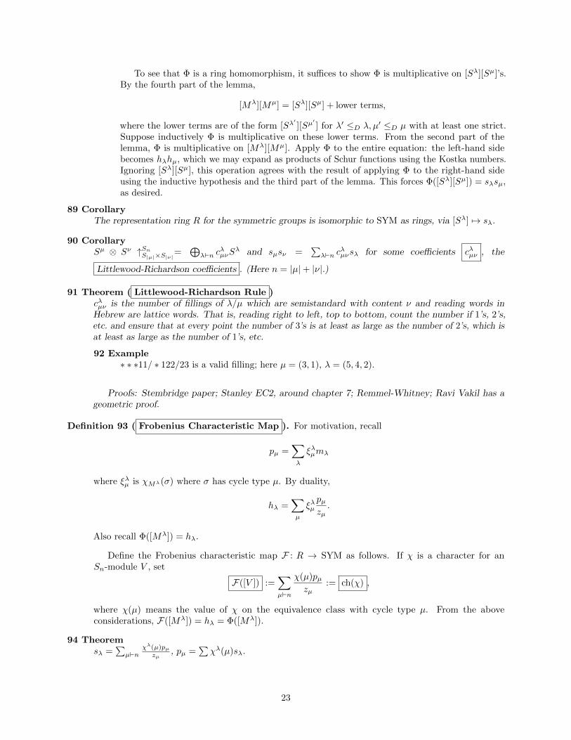
89 CorollaryThe representation ring R for the symmetric groups is isomorphic to SYM as rings, via [Sλ] 7→ sλ.
90 CorollarySµ ⊗ Sν ↑SnS|µ|×S|ν|=
⊕λ`n c
λµνS
λ and sµsν =∑λ`n c
λµνsλ for some coefficients cλµν , the
Littlewood-Richardson coefficients . (Here n = |µ|+ |ν|.)
91 Theorem ( Littlewood-Richardson Rule )cλµν is the number of fillings of λ/µ which are semistandard with content ν and reading words inHebrew are lattice words. That is, reading right to left, top to bottom, count the number if 1’s, 2’s,etc. and ensure that at every point the number of 3’s is at least as large as the number of 2’s, which isat least as large as the number of 1’s, etc.
92 Example∗ ∗ ∗11/ ∗ 122/23 is a valid filling; here µ = (3, 1), λ = (5, 4, 2).
Proofs: Stembridge paper; Stanley EC2, around chapter 7; Remmel-Whitney; Ravi Vakil has ageometric proof.
Definition 93 ( Frobenius Characteristic Map ). For motivation, recall
pµ =∑λ
ξλµmλ
where ξλµ is χMλ(σ) where σ has cycle type µ. By duality,
hλ =∑µ
ξλµpµzµ.
Also recall Φ([Mλ]) = hλ.
Define the Frobenius characteristic map F : R → SYM as follows. If χ is a character for anSn-module V , set
F([V ]) :=∑µ`n
χ(µ)pµzµ
:= ch(χ) ,
where χ(µ) means the value of χ on the equivalence class with cycle type µ. From the aboveconsiderations, F([Mλ]) = hλ = Φ([Mλ]).
94 Theoremsλ =
∑µ`n
χλ(µ)pµzµ
, pµ =∑χλ(µ)sλ.
23
April 16th, 2014: Algebras and Coalgebras Intro
Summary Last time: finished Cauchy identities; showed pµ, pµ/zµ are dual bases, pµ =∑λ χ
λ(µ)sλ.
Also important: Murnaghan-Nakayama rule for computing entries in the character table for Sλ;see Sagan or Macdonald for details.
95 FactLet G be a finite group. G acts on itself by conjugation. If ΨG is the character of this representation
and ξλ is the set of irreducible characters, then
〈ψG, ξλ〉 =∑K
ξλ(K)
where the sum is over conjugacy classes of G. (This is a good exercise.) Hence the sum on theright-hand side is in N.
96 Open ProblemFind a combinatorial interpretation of the fact that
∑µ`n χ
λ(µ) ∈ N, say using the Murnaghan-Nakayama rule or using SYM.
Richard Stanley’s “Positivity Problems and Conjectures in Algebraic Combinatorics”, problem 12,discusses this briefly.
97 FactGiven Sn-modules U, V , then U ⊗k V is an Sn-module (different from our earlier operations) with(“diagonal”) action
σ(u⊗ v) = σ(u)⊗ σ(v).
In particular, Sλ⊗Sµ = ⊕gλ,µ,νSν , and the same sort of thing holds for any finite group. The coefficients
gλ,µ,ν ∈ N are called the Kronecker coefficients . Problem: find an efficient, combinatorial, manifestly
positive rule for computing the Kronecker coefficients.
98 Exampleχλχµ =
∑gλ,µ,νχ
ν , so we can just throw linear algebra at it, but for instance this isn’t clearlypositive.
99 RemarkWe’ll switch to algebras and coalgebras for a bit, giving some background. Sources:
• Hopf lectures by Federico Ardila.
• Darij Grinberg and Vic Reiner notes, “Hopf Algebras in Combinatorics”
• Moss Sweedler from 1969, a breakthrough book for its day making the field more accessible.
Definition 100. Let k be a field (though “hold yourself open” to other rings). A is an associative k-algebra
if it is
(1) a k-vector space
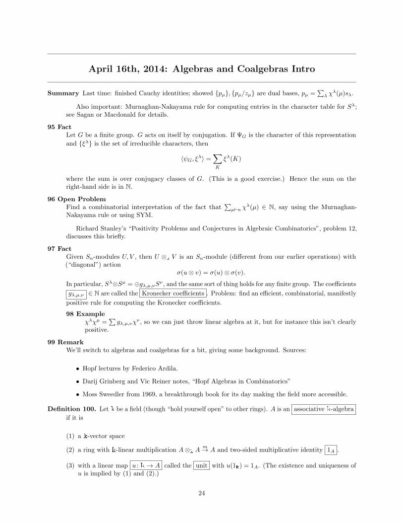
(2) a ring with k-linear multiplication A⊗k Am→ A and two-sided multiplicative identity 1A .
(3) with a linear map u : k→ A called the unit with u(1k) = 1A. (The existence and uniqueness ofu is implied by (1) and (2).)
24
This is summarized by the following diagrams:
A⊗A⊗A
A⊗A A⊗A
A
m⊗id id⊗m
m m
A⊗k k A k⊗k A
A⊗A A A⊗A
id⊗u
∼ ∼
id u⊗id
m m
For instance, if we run a ∈ A through the left square of the right diagram, we find
a 7→ a⊗ 1k 7→ a⊗ u(1k) 7→ au(1k) = a,
so that u(1k) is a (hence, the) two-sided identity of A.
101 Example• k[x] has u(c) = c
• C[Sn]: multiplication is associative, identity is the identity permutation, so u(c) = c[1, 2, . . . , n].
• M22, two by two matrices over Qp, say, taken as a Q-vector space. Usual addition, multiplication,Q-module action all works. Unit is the identity matrix, so u(c) is the diagonal matrix with c’s onthe diagonal.
• If A,B are k-algebras, then so is A⊗k B with multiplication defined via
mA⊗B [(a⊗ b)⊗ (a′ ⊗ b′)] = aa′ ⊗ bb′.
Hence 1A⊗B = 1A ⊗ 1B . This is indeed associative:
mA⊗B = mA ⊗mB (1⊗ T ⊗ 1)
where T = B ⊗A→ A⊗B is the “twist” operation. For practice with the above diagrams, it’sgood to check this explicitly by tracing through the above. The unit is uA⊗B(c) = uA(c)⊗uB(c) ∈A⊗B—actually, this is incorrect; see the beginning of the next lecture.
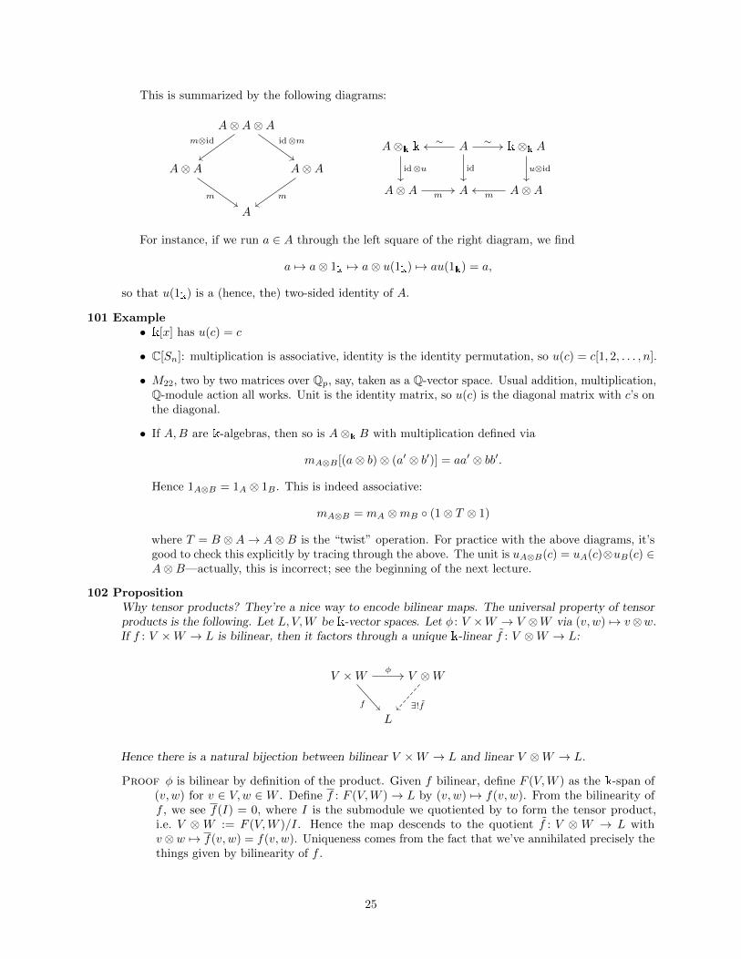
102 PropositionWhy tensor products? They’re a nice way to encode bilinear maps. The universal property of tensorproducts is the following. Let L, V,W be k-vector spaces. Let φ : V ×W → V ⊗W via (v, w) 7→ v⊗w.If f : V ×W → L is bilinear, then it factors through a unique k-linear f : V ⊗W → L:
V ×W V ⊗W
L
φ
f ∃!f
Hence there is a natural bijection between bilinear V ×W → L and linear V ⊗W → L.
Proof φ is bilinear by definition of the product. Given f bilinear, define F (V,W ) as the k-span of(v, w) for v ∈ V,w ∈ W . Define f : F (V,W )→ L by (v, w) 7→ f(v, w). From the bilinearity off , we see f(I) = 0, where I is the submodule we quotiented by to form the tensor product,i.e. V ⊗ W := F (V,W )/I. Hence the map descends to the quotient f : V ⊗ W → L withv⊗w 7→ f(v, w) = f(v, w). Uniqueness comes from the fact that we’ve annihilated precisely thethings given by bilinearity of f .
25
103 RemarkWeird thing: p : V ⊗W → V given by v ⊗ w 7→ v is not well-defined. However, if g : W → k is linear,then p : V ⊗W → V given by v⊗w 7→ g(w) · v is linear. Homework: If g is an algebra homomorphism,then p is as well.
For instance, p1 : C ⊗k k → C given by c ⊗ k 7→ k · c is the inverse of C → C ⊗k k given byc 7→ c⊗ 1k.
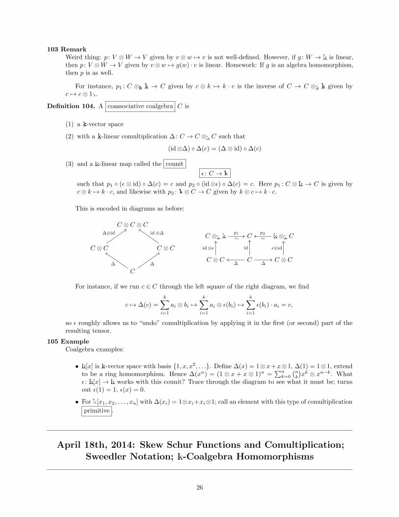
Definition 104. A coassociative coalgebra C is
(1) a k-vector space
(2) with a k-linear comultiplication ∆: C → C ⊗k C such that
(id⊗∆) ∆(c) = (∆⊗ id) ∆(c)
(3) and a k-linear map called the counit
ε : C → k
such that p1 (ε ⊗ id) ∆(c) = c and p2 (id⊗ε) ∆(c) = c. Here p1 : C ⊗ k → C is given byc⊗ k 7→ k · c, and likewise with p2 : k⊗ C → C given by k ⊗ c 7→ k · c.
This is encoded in diagrams as before:
C ⊗ C ⊗ C
C ⊗ C C ⊗ C
C
∆⊗id id⊗∆
∆ ∆
C ⊗k k C k⊗k C
C ⊗ C C C ⊗ C
p1∼ ∼
p2
id⊗ε id
∆ ∆
ε⊗id
For instance, if we run c ∈ C through the left square of the right diagram, we find
c 7→ ∆(c) =
k∑i=1
ai ⊗ bi 7→k∑i=1
ai ⊗ ε(bi) 7→k∑i=1
ε(bi) · ai = c,
so ε roughly allows us to “undo” comultiplication by applying it in the first (or second) part of theresulting tensor.
105 ExampleCoalgebra examples:
• k[x] is k-vector space with basis 1, x, x2, . . .. Define ∆(x) = 1⊗x+x⊗ 1, ∆(1) = 1⊗ 1, extendto be a ring homomorphism. Hence ∆(xn) = (1 ⊗ x + x ⊗ 1)n =
∑nk=0
(nk
)xk ⊗ xn−k. What
ε : k[x]→ k works with this counit? Trace through the diagram to see what it must be; turnsout ε(1) = 1, ε(x) = 0.
• For k[x1, x2, . . . , xn] with ∆(xi) = 1⊗xi+xi⊗1; call an element with this type of comultiplication
primitive .
April 18th, 2014: Skew Schur Functions and Comultiplication;Sweedler Notation; k-Coalgebra Homomorphisms
26
106 RemarkCorrection: in A⊗B, we have uA⊗B(1) = 1A⊗B = 1A ⊗AB, so uA⊗B(c) = c(1A ⊗ 1B), which is notequal to uA(c)⊗ uB(c) = c2(1A ⊗ 1B).
107 ExampleAt the end of last lecture, we started defining comultiplication on k[x1, . . . , xn] by declaring each xiprimitive. For another example, C[Sn] is a C-vector space, and we can define comultiplication by∆(σ) = σ ⊗ σ. What’s the counit? Seems like we’re forced to have ε(σ) = 1.
108 ExampleFor SYM(t) = Q[p1(t), p2(t), . . .], if pi is primitive, that means ∆(pi) = 1 ⊗ pi(t) + pi(t) ⊗ 1 =∑j≥1 1⊗ tij +
∑j≥1 t
ij ⊗ 1, which you can think of as pi(y) + pi(x) where the y variables correspond to
1⊗tij (i.e. yij ↔ 1⊗tij) and the x variables correspond to tij⊗1. We have SYM(t)⊗SYM(t) ∼= SYM(x+y)under this correspondence, where x+ y := x ∪ y, whence
SYM(t)⊗ SYM(t) ∼= Q[p1(x), p1(y), p2(x), p2(y), . . .].
Indeed, this comultiplication comes about from declaring ∆(f) = f(x + y) for f ∈ SYM, which iswell-defined since f is symmetric so the order in which we plug in variables is irrelevant. That is,
∆(f)|tα⊗tβ := f(x+ y)|xαyβ .
109 ExampleWhat are hn(x+ y) and en(x+ y)? Let’s say x1 < x2 < · · · < y1 < y2 < · · · . Then it’s easy to see
hn(x+ y) =
n∑i=0
hi(x)hn−i(y), en(x+ y) =
n∑i=0
ei(x)en−i(y).
Likewise we can see
∆(hn) =
n∑i=0
hi(t)⊗ hn−i(t), ∆(en) =
n∑i=0
ei(t)⊗ en−i(t).
Indeed, if m : SYM(t)⊗SYM(t)→ SYM(x+y) is the above isomorphism, we’ve shown m∆(hn(t)) =hn(x+ y), so by linearity m∆(f(t)) = f(x+ y) for all f ∈ SYM.
One can think it through to see ∆(sλ) =∑µ⊂λ sµ(t)⊗ sλ/µ(t) where...
Definition 110. A skew partition λ/µ means λ, µ are partitions and λ ⊃ µ. The set SSYT(λ/µ)
of skew tableau of shape λ/µ consists of fillings of λ− µ from P which weakly increase along
rows and strictly increase along columns. Then the skew Schur function associated to the skewpartition λ/µ is
sλ/µ :=∑
T∈SSYT(λ/µ)
xT .
Homework: show sλ/µ = det(hλi−µj−i+j).
111 Theorem∆(sλ) =
∑µ⊂λ;ν c
λµνsµ ⊗ sν if and only if sλ/µ =
∑µ⊂λ c
λµνsν if and only if sµsν =
∑cλµνsλ. Hence
the Littlewood-Richardson coefficients arise extremely naturally in terms of comultiplication.
27
Proof Assume the third equality. Use the Cauchy identity twice to see∏i,j≥1
1
1− xizj
∏i,j≥1
1
1− yizj
=
(∑µ
sµ(x)sµ(z)
)(∑ν
sν(y)sν(z)
)
=∑µ,ν
sµ(x)sν(y)sµ(z)sν(z)
=∑µ,ν
sµ(x)sν(y)
(∑λ
cλµνsλ(z)
)=∑µ,ν,λ
cλµνsµ(x)sν(y)sλ(z).
On the other hand, suppose sλ/µ =∑dλµνsν . Then from the comment in the previous example,
∆(sλ) =∑µ⊂λ
sµ(t)⊗ sλ/µ(t) =∑µ⊂λ
sµ(t)⊗
(∑ν
dλµνsν(t)
)=∑µ⊂λ;ν
dλµνsµ(t)⊗ sν(t),
(This is essentially the first equation in the theorem statement.) But by the remark in theprevious example, m∆(sλ(t)) = sλ(x+ y), so if we apply m to the previous equation, we find
sλ(x+ y) =∑µ⊂λ;ν
dλµνsµ(x)sν(y).
Finally, consider the left-hand side of the first product in this proof, the product of 1/(1−`izj)where ` = x or ` = y. Stated this way, we can apply the Cauchy identity to the alphabets x+ yand z to get
LHS =∑λ
sλ(x+ y)sλ(z) =∑λ
(∑µ,ν
dλµνsµ(x)sν(y)
)sλ(z)
=∑λ,µ,ν
dλµνsµ(x)sν(y)sλ(z).
Now compare coefficients of sµ(x)sν(y)sλ(z) to see that cλµν = dλµν , completing the proof.
112 HomeworkFigure out the “(?)” in terms of other things that we know in∏
i,j,k≥1
1
1− xiyjzk=∑λ,µ,ν
(?)sλ(x)sµ(y)sν(z).
113 ExampleWhat’s the counit for the above comultiplication? ε(pi) = 0.
114 HomeworkWhat if we defined the ei’s to be primitive, i.e. ∆(ei) = 1⊗ei+ei⊗1? Is the coalgebra structurereally different?
115 ExampleLet P be a poset. Recall Int(P ) is the set of intervals in P , i.e. the set of [x, y] = c : x ≤ c ≤ y.Define C as the k-span of Int(P ). For instance, 12[a, a] + 6[a, b] + 17[a, e] ∈ C for the poset witha < b < c, a < d < e, b < e.
28
Define the coproduct structure by “breaking chains” or “rock breaking”:
∆([x, z]) :=∑
x≤y≤z
[x, y]⊗ [y, z].
Coassociativity works perfectly well, eg.
(id ∆) ∆([w, z]) =∑
w≤x≤y≤z
[w, x]⊗ [x, y]⊗ [y, z].
What’s the counit? We must have
(id⊗ε) (∆([x, z])) = [x, z]⊗ 1.
Since∆([x, z]) = [x, x]⊗ [x, z] + [x, y]⊗ [y, z] + · · ·+ [x, z]⊗ [z, z],
we’re strongly encouraged to make ε([a, a′]) = 1 if a = a′ and 0 otherwise. This is called the
incidence coalgebra .
There doesn’t seem to be a natural algebra structure—how do you multiply two arbitrary intervals?
116 Notation ( Sweedler Notation )Let C be a coalgebra. We have c =
∑nci=0 ai ⊗ bi for some nc ≥ 0 and ai, bi ∈ C. Let (c) = 0, . . . , nc
and let ci(1) = ai, ci(2) = bi. We can write this as c =
∑i∈(c) c
i(1) ⊗ c
i(2) or, making the indexes implicit,
c =∑(c)
c(1) ⊗ c(2) .
Note that ci(1) ∈ C for i ∈ (c), so we can use the same conventions to write
ci(1) =∑
(ci(1)
)
(ci(1))(1) ⊗ (ci(1))(2).
This is rather verbose; we can unambiguously drop the i and ignore some parentheses to get c(1) =∑(c(1))
c(1)(1) ⊗ c(1)(2). Coassociativity then reads∑(c)
∑(c(2))
c(1) ⊗ c(2)(1) ⊗ c(2)(2) =∑(c)
∑(c(1))
c(1)(1) ⊗ c(1)(2) ⊗ c(2).
This is still rather verbose; we must sum over (c) to evaluate the c(1) or c(2), so we can drop the outersum without losing information. Likewise we can drop the inner sum, so a lazy form of Sweedlernotation for coassociativity reads
∆2(c) := c(1) ⊗ c(2)(1) ⊗ c(2)(2) = c(1)(1) ⊗ c(1)(2) ⊗ c(2).
Here ∆2(c) is an iterated comultiplication , which has the obvious definition in general. Up to this
point, Sweedler notation has been perfectly well-defined and unambiguous, even though it’s veryimplicit. Some people even drop the parentheses and/or the tensor product symbols!
However, the notation becomes context-sensitive with iterated comultiplication. In particular,we set ∆(2)(c) =
∑(c) c(1) ⊗ c(2) ⊗ c(3). Compared to ∆(c) =
∑(c) c(1) ⊗ c(2), each of the symbols
(c), c(1), c(2) have new meanings. The presence of (3) is at least a clue as to which definition of thesymbols to use. More generally, we write
∆n−1 (c) :=∑(c)
c(1) ⊗ · · · ⊗ c(n).
Note: using∑
(c)n cn(1) ⊗ · · · ⊗ c
n(n) would at least be unambiguous, and we could write (cn(1))
m(2) as
cnm(1)(2), though nothing like this seems to be in actual use.
29
117 ExampleIn this notation, (id⊗ε) ∆(c) = c⊗ 1 becomes∑
(c)
c(1) ⊗ ε(c(2)) = c⊗ 1 or∑(c)
c(1)ε(c(2)) = c,
among other possibilities.
118 Example∆n−1[x, y] =
∑x=x1≤···≤xn=y[x1, x2] ⊗ [x2, x3] ⊗ · · · ⊗ [xn−1, xn]. ∆n−1(σ) = σ ⊗ · · · ⊗ σ (n
terms) for σ ∈ Sn with the previous comultiplication.
Definition 119. Let A,B be k-algebras. A k-linear map f : A→ B is a k-algebra homomorphism k-algebra
homomorphism if and only if f(aa′) = f(a)f(a′) and f(1A) = 1B . In diagrams,
A⊗A
A B ⊗B
B
mA f⊗f
f mB
k
A
B
uB
uA
f
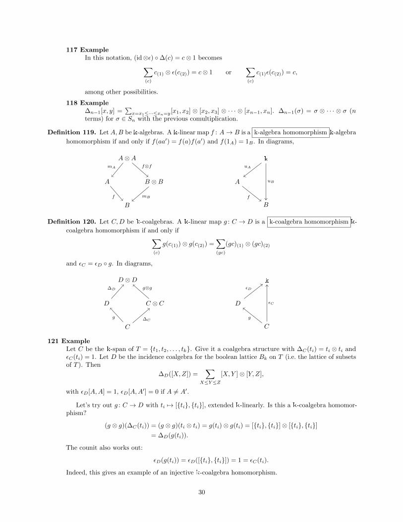
Definition 120. Let C,D be k-coalgebras. A k-linear map g : C → D is a k-coalgebra homomorphism k-
coalgebra homomorphism if and only if∑(c)
g(c(1))⊗ g(c(2)) =∑(gc)
(gc)(1) ⊗ (gc)(2)
and εC = εD g. In diagrams,
D ⊗D
D C ⊗ C
C
∆D g⊗g
∆Cg
k
D
C
εD
εC
g
121 ExampleLet C be the k-span of T = t1, t2, . . . , tk. Give it a coalgebra structure with ∆C(ti) = ti ⊗ ti andεC(ti) = 1. Let D be the incidence coalgebra for the boolean lattice Bk on T (i.e. the lattice of subsetsof T ). Then
∆D([X,Z]) =∑
X≤Y≤Z
[X,Y ]⊗ [Y, Z],
with εD[A,A] = 1, εD[A,A′] = 0 if A 6= A′.
Let’s try out g : C → D with ti 7→ [ti, ti], extended k-linearly. Is this a k-coalgebra homomor-phism?
(g ⊗ g)(∆C(ti)) = (g ⊗ g)(ti ⊗ ti) = g(ti)⊗ g(ti) = [ti, ti]⊗ [ti, ti]= ∆D(g(ti)).
The counit also works out:
εD(g(ti)) = εD([ti, ti]) = 1 = εC(ti).
Indeed, this gives an example of an injective k-coalgebra homomorphism.
30
April 21st, 2014: Subcoalgebras, Coideals, Bialgebras
122 RemarkToday: (1) we’ll discuss ker(f), im(f), coideals, subcoalgebras, etc. (2) we’ll introduce bialgebras.
123 NotationToday, C,D are k-coalgebras, B ⊂ C is a k-subspace.
Definition 124. A k-subspace B is a subcoalgebra of a k-coalgebra C if ∆(B) ⊂ B ⊗B and εB : B → K
is given by restricting εC : C → k. B is a coideal if ∆(B) ⊂ B ⊗C +C ⊗B and ε(B) = 0. Note thata subcoalgebra is a coideal iff ε(B) = 0.
125 ExampleConsider k[G] as a coalgebra using the diagonal comultiplication, where recall ε(g) = 1. If g ∈ G, thenk[g] is a subcoalgebra since ∆(cg) = cg ⊗ g ∈ k[g]⊗ k[g]. However, ε(k[g]) = k 6= 0, so it’s not quite acoideal.
What about k[hn] ⊂ SYMk? It’s a k-subspace only. What do we have to add to make it asubcoalgebra? Need k[h1, . . . , hn]. Recall ε annihilates each pn except ε(1) = 1.
What about the k-span of pn? It’s a coideal, but it’s not a subcoalgebra, since ∆(pn) =1⊗ pn + pn ⊗ 1. We can make it a subcoalgebra if we take the k-span of 1, pn. Similarly with thek-span of hλ where λ is a non-empty partition.
126 PropositionLet f : C → D be a coalgebra homomorphism.
1. ker(f) is a coideal;
2. im(f) is a subcoalgebra.
Proof First, a lemma.
127 Lemma (“Useful Lemma”)Let f : V → V ′, g : W →W ′ be linear maps. Then f ⊗ g : V ⊗W → V ′ ⊗W ′ satisfies
i) im(f ⊗ g) = im(f)⊗ im(g)
ii) ker(f ⊗ g) = ker(f)⊗W + V ⊗ ker(g)
Proof Homework.
Proof of (1): c ∈ ker(f) implies f(c) = 0, so 0 = ∆D f(c) = (f ⊗ f)(∆C(c)), so ∆C(C) ∈ker(f ⊗ f) = ker f ⊗ C + C ⊗ ker f from the useful lemma, which is precisely what we needed.Also, εC(c) = εD(f(c)) = εD(0) = 0, so indeed εC(ker f) = 0.
Proof of (2): say f(c) ∈ im(f). Then ∆f(c) = (f ⊗ f)∆(c) =∑
(c) f(c(1)) ⊗ f(c(2)) ∈im(f)⊗ im(f), which is again what we needed.
128 PropositionIf I is a coideal of C, then C/I is a coalgebra, with ∆C/I inherited from ∆C .
Proof Our hope is
C C ⊗ C
C/I C/I ⊗ C/I
∆C
π π⊗π
∆C/I
∃!
31
Claim: (π ⊗ π) ∆C descends to C/I if the composite annihilates I. To see this, let i ∈ I, andnote ∆(i) ∈ I ⊗ C + C ⊗ I, so (π ⊗ π)(∆(i)) is indeed zero. εC/I(a+ I) = εC(a) is well-definedsince εC(I) = 0.
129 Theorem (Fundamental Theorem of Coalgebras)If f : C → D is a coalgebra homomorphism, then
im(f) ∼= C/ ker(f)
as coalgebras.
Proof It’s an isomorphism as k-vector spaces. Both are coalgebras. Check that α : C/ ker(f)→ im(f)is a morphism of coalgebras; α−1 exists, so check it’s a morphism of coalgebras.
130 HomeworkIf f : C → D is an isomorphism of vector spaces and f is a coalgebra morphism, is it acoalgebra isomorphism?
131 RemarkRecall that we earlier defined a natural k-algebra structure on the tensor product A⊗A of a k-algebraA. Explicitly,
mA⊗A := (mA ⊗mA) (1⊗ T ⊗ 1)
using the “twist” operator T given by a⊗ a′ 7→ a′ ⊗ a, and uA⊗A(k) = k(1A ⊗ 1A). Alternatively, wehave
uA⊗A : k→ k⊗k kuA⊗uA→ A⊗A
where kk→ ⊗kk is the natural isomorphism, since then
uA⊗A(k) 7→ k ⊗ 1k = 1k ⊗ k 7→ uA(k)⊗ uA(1k) = uA(1k)⊗ uA(k) = k(1A ⊗ 1A) = k(1A⊗A).
Likewise, given a coalgebra C, we can give C ⊗ C a natural coalgebra structure with
∆C⊗C := (id⊗T ⊗ id) ∆C ⊗∆C
and whereεC⊗C : C ⊗ C εC⊗εC→ k⊗k k→ k.
Definition 132. Suppose (B,m, u) is an algebra and further suppose (B,∆, ε) is a coalgebra. Then
(B,m, u,∆, ε) is a bialgebra if
(1) m and u are coalgebra homomorphisms, and
(2) ∆ and ε are algebra homomorphisms
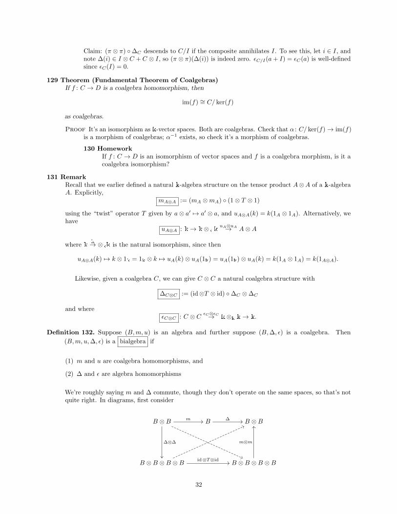
We’re roughly saying m and ∆ commute, though they don’t operate on the same spaces, so that’s notquite right. In diagrams, first consider
B ⊗B B B ⊗B
B ⊗B ⊗B ⊗B B ⊗B ⊗B ⊗B
m
∆⊗∆
∆
id⊗T⊗id
m⊗m
32
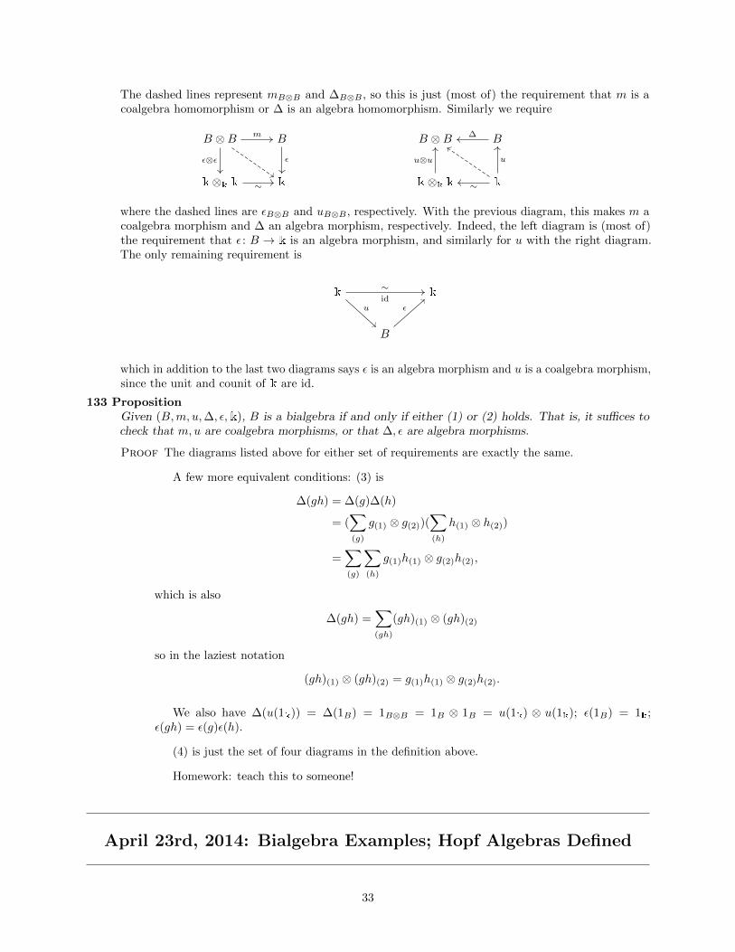
The dashed lines represent mB⊗B and ∆B⊗B, so this is just (most of) the requirement that m is acoalgebra homomorphism or ∆ is an algebra homomorphism. Similarly we require
B ⊗B B
k⊗k k k
m
ε⊗ε ε
∼
B ⊗B B
k⊗k k k
∆
u⊗u
∼
u
where the dashed lines are εB⊗B and uB⊗B , respectively. With the previous diagram, this makes m acoalgebra morphism and ∆ an algebra morphism, respectively. Indeed, the left diagram is (most of)the requirement that ε : B → k is an algebra morphism, and similarly for u with the right diagram.The only remaining requirement is
k k
B
∼id
u ε
which in addition to the last two diagrams says ε is an algebra morphism and u is a coalgebra morphism,since the unit and counit of k are id.
133 PropositionGiven (B,m, u,∆, ε,k), B is a bialgebra if and only if either (1) or (2) holds. That is, it suffices tocheck that m,u are coalgebra morphisms, or that ∆, ε are algebra morphisms.
Proof The diagrams listed above for either set of requirements are exactly the same.
A few more equivalent conditions: (3) is
∆(gh) = ∆(g)∆(h)
= (∑(g)
g(1) ⊗ g(2))(∑(h)
h(1) ⊗ h(2))
=∑(g)
∑(h)
g(1)h(1) ⊗ g(2)h(2),
which is also
∆(gh) =∑(gh)
(gh)(1) ⊗ (gh)(2)
so in the laziest notation
(gh)(1) ⊗ (gh)(2) = g(1)h(1) ⊗ g(2)h(2).
We also have ∆(u(1k)) = ∆(1B) = 1B⊗B = 1B ⊗ 1B = u(1k) ⊗ u(1k); ε(1B) = 1k;ε(gh) = ε(g)ε(h).
(4) is just the set of four diagrams in the definition above.
Homework: teach this to someone!
April 23rd, 2014: Bialgebra Examples; Hopf Algebras Defined
33
134 RemarkLast time: did bialgebras. Today: more examples; Hopf algebras.
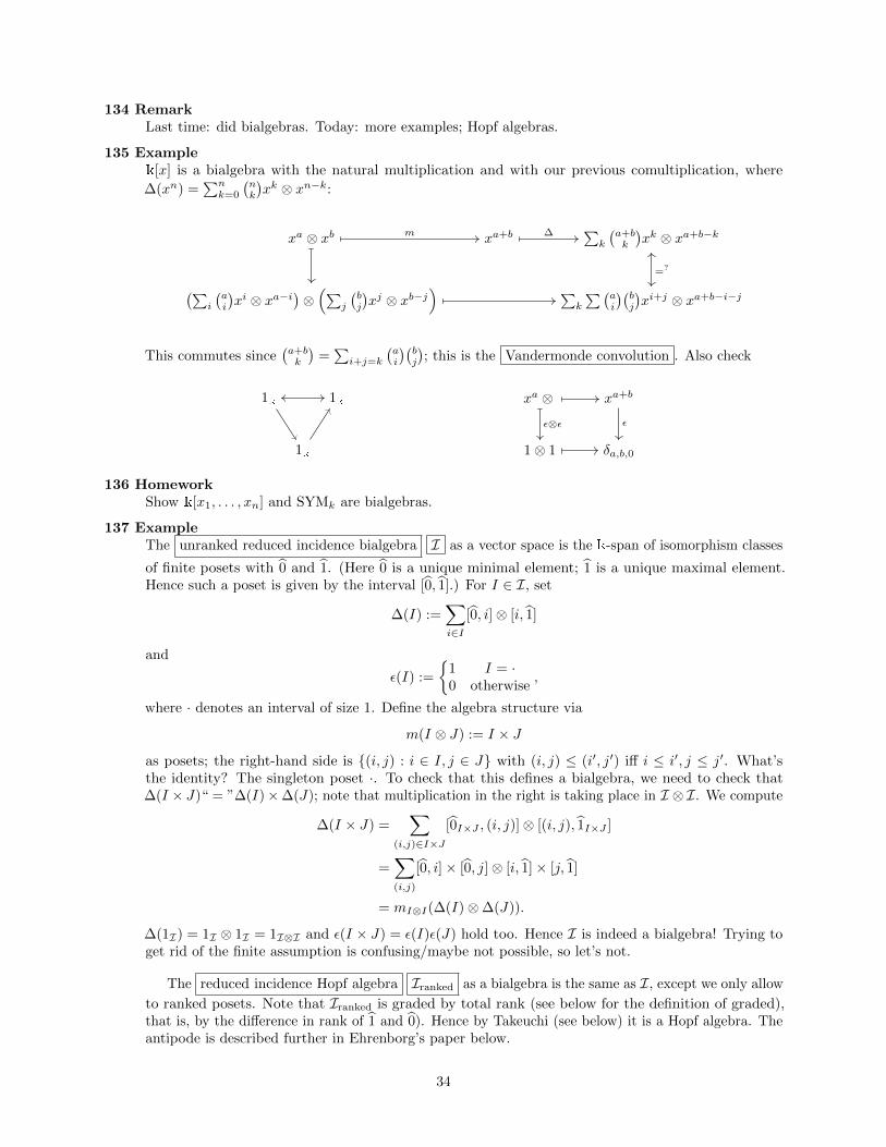
135 Examplek[x] is a bialgebra with the natural multiplication and with our previous comultiplication, where
∆(xn) =∑nk=0
(nk
)xk ⊗ xn−k:
xa ⊗ xb xa+b∑k
(a+bk
)xk ⊗ xa+b−k
(∑i
(ai
)xi ⊗ xa−i
)⊗(∑
j
(bj
)xj ⊗ xb−j
) ∑k
∑(ai
)(bj
)xi+j ⊗ xa+b−i−j
m ∆
=?
This commutes since(a+bk
)=∑i+j=k
(ai
)(bj
); this is the Vandermonde convolution . Also check
1k 1k
1k
xa ⊗ xa+b
1⊗ 1 δa,b,0
ε⊗ε ε
136 HomeworkShow k[x1, . . . , xn] and SYMk are bialgebras.
137 ExampleThe unranked reduced incidence bialgebra I as a vector space is the k-span of isomorphism classes
of finite posets with 0 and 1. (Here 0 is a unique minimal element; 1 is a unique maximal element.Hence such a poset is given by the interval [0, 1].) For I ∈ I, set
∆(I) :=∑i∈I
[0, i]⊗ [i, 1]
and
ε(I) :=
1 I = ·0 otherwise
,
where · denotes an interval of size 1. Define the algebra structure via
m(I ⊗ J) := I × J
as posets; the right-hand side is (i, j) : i ∈ I, j ∈ J with (i, j) ≤ (i′, j′) iff i ≤ i′, j ≤ j′. What’sthe identity? The singleton poset ·. To check that this defines a bialgebra, we need to check that∆(I × J)“ = ”∆(I)×∆(J); note that multiplication in the right is taking place in I ⊗ I. We compute
∆(I × J) =∑
(i,j)∈I×J
[0I×J , (i, j)]⊗ [(i, j), 1I×J ]
=∑(i,j)
[0, i]× [0, j]⊗ [i, 1]× [j, 1]
= mI⊗I(∆(I)⊗∆(J)).
∆(1I) = 1I ⊗ 1I = 1I⊗I and ε(I × J) = ε(I)ε(J) hold too. Hence I is indeed a bialgebra! Trying toget rid of the finite assumption is confusing/maybe not possible, so let’s not.
The reduced incidence Hopf algebra Iranked as a bialgebra is the same as I, except we only allow
to ranked posets. Note that Iranked is graded by total rank (see below for the definition of graded),that is, by the difference in rank of 1 and 0). Hence by Takeuchi (see below) it is a Hopf algebra. Theantipode is described further in Ehrenborg’s paper below.
34
138 ExampleLet Pn be the k-span of w ∈ Sn, let P∞ or Perms be ⊕∞n=0Pn graded. For u ∈ Sm, v ∈ Sn, define
u v :=∑
shuffles s of u,v s, where a shuffle is roughly an “interleaving” of the one-line notations forthe two permutations, as in the example:
139 ExampleImage [4321] = [7654]. We have
[312] [4321] = 3127654 + 3176254 + 3172654 + 7312654 + · · ·
with 35 =(
73
)terms.
What about comultiplication? For w ∈ Sn, use
∆(w) =
n∑i=0
fl(w|[i])⊗ fl(w|[i+1,n])
where fl denotes flattening , meaning if a1, . . . , ap ∈ Rp are distinct, use fl(a1, . . . , ap) := v1 · · · vp ∈ Spwhere ai < aj ⇔ vi < vj . Here w|[i] = w1w2 · · ·wi except w|[0] is the “identity” element in S0, call it
•ι.
140 Example
∆(312) =•ι⊗ 312 + fl(3)⊗ fl(12) + fl(31)⊗ fl(2) + 312⊗ •ι =
•ι⊗ 312 + 1⊗ 12 + 21⊗ 1 + 312⊗ •ι.
Again we’re more or less forced to pick
ε(w) =
1 w =
•ι
0 otherwise
So, we have an algebra and a coalgebra! Is it a bialgebra? Is ∆(u v)“=”∆(u) ∆(v)? Wecompute
∆
∑s of u,v
s
=∑s
∑(s)
fl(s(1))⊗ fl(s(2))
= u⊗ v + · · ·
=∑
a1 . . . aj ⊗ b1 . . . bk, j + k = n+m
On the other hand,
mP∞⊗P∞(∆(u)⊗∆(v)) = m(∑(u)
∑(v)
u(1) ⊗ u(2) ⊗ v(1) ⊗ v(2))
and
∆(u)∆(v) =∑∑
(u(1) v(1))⊗ (u(2) ⊗ v(2))
so these two are equal, and they’re equal to ∆(u v).
141 HomeworkCheck the other three diagrams.
142 HomeworkDefine fl on the relative positions of the values 1, . . . , i in one-line notation rather than w1, . . . , wi. Set∆(w) =
∑w|[i] ⊗ fl(w|[i+1,n]). How does P∞ relate to this structure? Is it the dual? (Note: we did
not forget an fl on the first factor: it’s just the identity using this new definition.)
35
143 Remarkk[x] and P∞ are graded; k[x] is commutative but P∞ is not.
Definition 144. A coalgebra C is cocommutative if
∆(c) =∑(c)
c(1) ⊗ c(2) =∑(c)
c(2) ⊗ c(1).
145 Examplek[x] is cocommutative; P∞ is not. What about k[G]?
Commutative Cocommutative Gradedk[G] no yes nok[x] yes yes yesIranked yes no yesP∞ no no yes
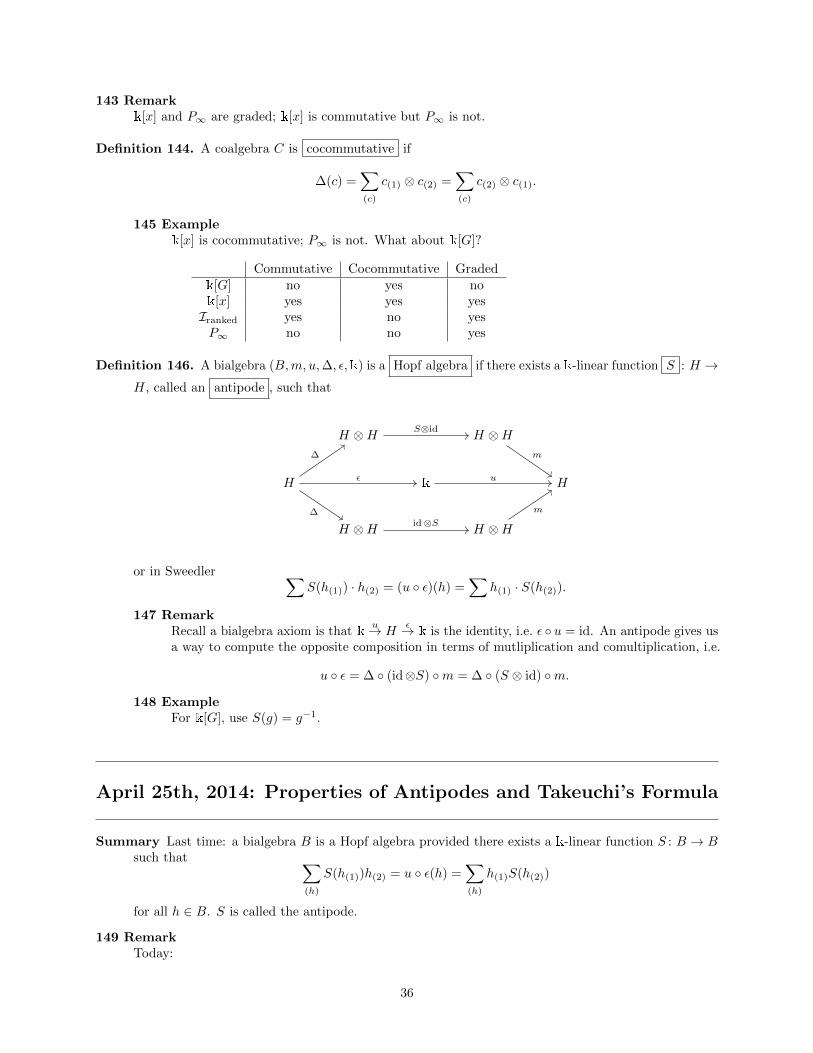
Definition 146. A bialgebra (B,m, u,∆, ε,k) is a Hopf algebra if there exists a k-linear function S : H →H, called an antipode , such that
H ⊗H H ⊗H
H k H
H ⊗H H ⊗H
S⊗id
m
ε
∆
∆
u
id⊗Sm
or in Sweedler ∑S(h(1)) · h(2) = (u ε)(h) =
∑h(1) · S(h(2)).
147 RemarkRecall a bialgebra axiom is that k
u→ Hε→ k is the identity, i.e. ε u = id. An antipode gives us
a way to compute the opposite composition in terms of mutliplication and comultiplication, i.e.
u ε = ∆ (id⊗S) m = ∆ (S ⊗ id) m.
148 ExampleFor k[G], use S(g) = g−1.
April 25th, 2014: Properties of Antipodes and Takeuchi’s Formula
Summary Last time: a bialgebra B is a Hopf algebra provided there exists a k-linear function S : B → Bsuch that ∑
(h)
S(h(1))h(2) = u ε(h) =∑(h)
h(1)S(h(2))
for all h ∈ B. S is called the antipode.
149 RemarkToday:
36
1) Properties of antipodes.
2) Hopf algebras are plentiful, i.e. Takeuchi’s theorem.
150 HomeworkIs every bialgebra a Hopf algebra?
Definition 151. Let C be a k-coalgebra (∆, ε) and A be a k-alegbra (m,u). The set Homk(C,A) of k-linear
maps from C to A can be given an algebra structure as follows, which will be denoted Hom(C,A) . It
is a k-vector space as usual. Define the algebra multiplication through convolution
(f ∗ g)(c) :=∑(c)
f(c(1))g(c(2)),
i.e. f ∗g = m (f ⊗g)∆. What is the identity of this algebra, if it has one? We find 1Hom(C,A) = u ε:
f ∗ (u ε)(c) = m (f ⊗ (u ε))
∑(c)
c(1) ⊗ c(2)
= m
∑(c)
f(c(1))⊗ uε(c(2))
= m
∑(c)
ε(c(2))f(c(1))⊗ u(1k)
=∑(c)
ε(c(2))f(c(1)) = f
∑(c)
(c(1)ε(c(2))
= f(c),
and likewise on the other side.
Warning: the multiplicative identity of Hom(C,A) is not in general the identity map even if C = A.
152 NotationHom(U, V ),Hom(C,D),Hom(A,B),Hom(C,A) can be ambiguous or hard to decipher: they may bek-linear, coalgebra, algebra or bialgebra, or k-linear or algebra maps, respectively. Such is life :(.
153 PropositionLet B be a bialgebra. Let id : B → B. S is an antipode for B if and only if
S ∗ id = u ε = 1Hom(B,B) = id ∗S.
Phrased this way, a Hopf algebra is precisely a bialgebra where the identity map in Hom(B,B) has atwo-sided multiplicative inverse.
Proof Immediate from the definitions.
154 CorollaryIf S exists, it’s unique.
Proof If S, S′ are antipodes, then S = S ∗ (id ∗S′) = (S ∗ id) ∗ S′ = S′ since S ∗ id and id ∗S′ areboth u ε, which is the identity. Really this is just the uniqueness of two-sided inverses: S andS′ are inverses of id under the convolution.
155 PropositionIn any Hopf algebra H,
(1) S(gh) = S(h)S(g)
(2) S u = u
(3) ε S = ε
37
(4) ∆ S(h) =∑
(h) S(h(2))⊗ S(h(1)) = S ⊗ S T ∆(h)
Proof (1) Consider k-linear maps in Hom(H ⊗Hc, Hc) (where Hc indicates we’re thinking of thecoalgebra structure on H). We have three maps
m(g ⊗ h) = gh
N(g ⊗ h) := S(h)S(g)
P (g ⊗ h) := S(gh).
That is, N := m (S ⊗ S) T , P := S m. Outline: a) P ∗m = 1Hom(H⊗H,H) (where thisidentity is u m ε⊗ ε(g ⊗ h) = ε(g)ε(h) · 1H). b) m ∗N = 1Hom(H⊗H,H). c) left and rightinverses agree in an associative algebra with 1, so P = N . For a), we compute
P ∗m(g ⊗ h) =∑
(g⊗h)
P ((g ⊗ h)(1))m((g ⊗ h)(2))
=∑(g)
∑(h)
P (g(1) ⊗ h(1))m(g(2) ⊗ h(2))
=∑(g)
∑(h)
S(g(1)h(1))g(2)h(2)
=∑(gh)
S((gh)(1))(gh)(2)
= S ∗ id(gh) = u ε(gh) = ε(g)ε(h) · 1H
where the second equality is true because
∆H⊗H(g ⊗ h) = id T id (∆⊗∆)(g ⊗ h)
= id T id∑
g(1) ⊗ g(2) ⊗ h(1) ⊗ h(2)
=∑
g(1) ⊗ h(2) ⊗ g(2) ⊗ h(2)
and the fourth equality is true because
∆(gh) = ∆(g) ·∆(h)
=∑
g(1) ⊗ h(1) ⊗ g(2) ⊗ h(2)
=∑(gh)
(gh)(1) ⊗ (gh)(2)
For b), we compute
m ∗N(g ⊗ h) =∑g⊗h
m((g ⊗ h)(1))N((g ⊗ h)(2))
=∑(g)
∑(h)
m(g(1) ⊗ h(1))N(g(2) ⊗ h(2))
=∑(g)
∑(h)
g(1)(h(1)S(h(2)))S(g(2))
=∑(g)
g(1)(ε(h)1H)S(g(2))
= ε(g)ε(h) · 1H
(2) Similar / homework.
38
(3) Similar / homework.
(4) Similar / homework.
156 HomeworkIf H is commutative or cocommutative, then S S = id.
157 PropositionS cannot have odd order > 1.
Proof Suppose S2k+1 = id. Then
gh = S2k+1(gh) = S2k(S(h)S(g)) = S2k+1(h)S2k+1(g) = hg
so H is commutative, hence S has order 1 or 2, a contradiction.
158 Theorem (Taft 1971)There are Hopf algebras with antipode of order 2, 4, 6, . . . ,∞.
Definition 159. A graded k-bialgebra B = ⊕n≥0Bn is a bialgebra where BiBj ⊂ Bi+j and ∆(Bn) ⊂⊕i+j=nBi ⊗ Bj . We say B is connected if B0
∼= k and this respects the bialgebra structure in thesense that u ε = idB0 . (The direct sum is as k-vector spaces.)
160 Remarkε(Bn) = 0 for all n > 0 for a graded k-bialgebra, which can be proved by chasing around thecounit and coproduct diagrams. Hence H is connected iff u ε = idB , i.e. iff u = ε−1.
The terminology probably comes from topology, where a space is connected if and only if its0th homotopy group is Z.
161 Theorem ( Takeuchi’s Formula )A graded connected bialgebra is a Hopf algebra with antipode
S =∑n≥0
(−1)n ·m(n−1) f⊗n ∆(n−1)
where m0 := id, ∆0 := id, m−1 := u, ∆−1 := ε, f := id−u ε ∈ Hom(Hc, H), so f(h) = h− ε(h)1H .
162 RemarkWhat does f do to the graded pieces Bn for n ≥ 0? For c ∈ B0, we have f(c) = c− ε(c)1H = 0,and f(Bn) = Bn is the identity for n > 0. If k is large enough compared to m, we see
f⊗k∆(k−1)(Bm) ∈∑
i1+···+ik=m
Bi1 ⊗ · · · ⊗Bik .
If k > m, then some ij = 0, so f kills it. Hence the sum is well-defined.
Proof First note
m(n−1)f⊗n∆(n−1)(h) =∑(h)
f(h(1))f(h(2)) · · · f(h(n))
= f∗n(h).
Hence S =∑n≥0(−1)nf∗n, so
S ∗ id =
∑n≥0
(−1)nf∗n
∗ (f + u ε)
=∑n≥0
(−1)nf∗(n+1) +∑n≥1
(−1)nf∗n
= f∗0 = u ε,
and similarly on the other side.
39
163 HomeworkLook at what this formula implies for k[x]–what is the antipode of x? Also do it for the gradedbialgebra we called Perms or P∞. Also do it for (ranked) posets Iranked.
April 28th, 2014: Homological Properties of Hopf Algebras:projdim, injdim, gldim,GKdim, . . .
164 RemarkToday is James Zhang’s first guest lecture. He’ll discuss homological properties of Hopf algebras.
165 ExampleSome more examples of Hopf algebras:
• G a group and k[G] the group algebra where k is a field. We have ∆g = g ⊗ g for all g ∈ G, andS(g) = g−1. Since this is cocommutative, S2 = id, which is of course also immediate.
• Algebraic geometry: let G be an algebraic group, O(G) the regular functions on G; commutativeimplies S2 = id.
• Lie theory: if L is a Lie algebra, let U(L) be the universal enveloping algebra, namely the freealgebra k〈L〉 modulo xy − yx− [x, y] for all x, y ∈ L. This is a Hopf algebra with a coproductgiven by
∆(x) = x⊗ 1 + 1⊗ x
for all x ∈ L. Note, for instance, that ∆(x2) = (∆x)2 = x2 ⊗ 1 + 2x ⊗ x + 1 ⊗ x2. Note thatS(x) = −x for all x ∈ L. This is again cocommutative, and again we can see directly thatS2 = id.
• S2 6= id sometimes: for “quantum groups”, Og(G) where G is a semisimple Lie group or Uq(L)where L is a semisimple Lie algebra and q ∈ kx, the order of S depends on q2. It turns outthat O1(G) = O(G) but U1(L) is not generally U(L). For instance, if q = −1, then S2 = id (forboth?).
• Fp[x]/(xp) for p prime has two possible Hopf structures. First comes from ∆x = x⊗ 1 + 1⊗ x,and second uses ∆x = x⊗ 1 + 1⊗ x+ x⊗ x. Again S2 = id in either case.
166 RemarkThe homological properties of Hopf algebras are connected to many areas of math: noncommutativealgebra, algebraic geometry, invariant theory, string theory. Our goal for this lecture and the next willbe to find common features of Hopf algebras, to find hidden invariants, and to see some open questionswhich will be our homework.
167 NotationH will be a Hopf algebra over k with multiplication m, unit µ, comultiplication ∆, counit ε, antipodeS.
168 Open ProblemIf H is Noetherian (as a ring), is S bijective? Open question in general, known in some special cases:graded connected case, finite dimensional case, “pi”, “semi-prime”.
Definition 169. Let M be a left H-module. The projective dimension of M is defined to be
projdimM := minn : 0→ pn → pn−1 → · · · → p0 →M → 0
40
where the minimum is over projective resolutions of M , i.e. the pi’s are projective modules and the
sequence is exact. This may well be ∞. Likewise, the injective dimension of M is defined to be
injdimM := minn : 0→M → I0 → · · · → In → 0
where the minimum is over injective resolutions of M , i.e. the Ii are injective modules and the sequence
is exact. Similarly, the global dimension of H is
gldimH := maxprojdimM : M ∈ H -mod.
(You can use injdim instead of projdim.) We also define the Gelfand-Kirillov dimension or GK dimensionof H to be
GKdimH := lim supn→∞
log(dimV n)
log n
where V 3 1 is any finite dimensional generating space of H, meaning H = ∪n≥0Vn. This turns out
to be independent of V , so long as it exists.
170 PropositionAssume H is finitely generated over k. Then V exists. In this case,
GKdimH = 0⇔ dimkH <∞.
171 Examplek[x1, . . . , xn] has GKdim of n.
172 Open ProblemIf GKdimH <∞, is GKdimH ∈ N?
173 ExampleH = U(L) implies GKdimH = gldimH = dimk L.
174 FactIf A is a commutative finitely generated k-algebra, then GKdimA is the Krull dimension of A.
175 Open ProblemIs GKdimH ≥ gldimH if gldim <∞?
176 Open ProblemSuppose H is Noetherian. Is it true that GKdimH ≥ KdimH, where Kdim is the Krull dimension fora not necessarily commutative ring?
Definition 177. A Hopf algebra H is Frobenius if H is finite dimension and the left H-module of the dualvector space H∗ is isomorphic to H as a left H-module. (You might call this “left Frobenius”.) (Seethe aside following this lecture for a discussion of H∗ in the finite dimensional case.)
178 Homework(1) There is one Hopf algebra structure on k[x1, x2] where chark = 0 up to isomorphism. (Assume
the standard algebra structure, and hunt for coalgebra/bialgebra/Hopf algebra structures.)
(2) There exist two Hopf algebra structures on k[x1, x2, x3] up to isomorphism where chark = 0.
179 RemarkHomological properties in GK0 , meaning Hopf algebras with GKdim = 0. (H finite impliesGKdimH = 0, as noted above.)
180 Theorem (Larson-Sweedler)A finite dimensional Hopf algebra H is Frobenius.
41

181 LemmaBeing Frobenius is equivalent to saying injdimH = 0, where H is viewed as either a left or rightH-module. This is the same as saying HH is injective. (H finite dimensional?)
Definition 182. (a) H is Gorenstein if injdimHH = injdimHH <∞.
(b) H is regular if gldimH <∞.
(c) H is semisimple if H = ⊕Mni(Di) is a direct sum of matrix rings over division rings. (This is in
analogy with Artin-Wedderburn.)
183 Theorem (Larson-Radford)Suppose char k = 0 and H is finite dimensional over k. Then the following are equivalent:
(a) H is semisimple.
(b) H is regular of dimension (gldim) 0.
(c) H is cosemisimple. (This means H∗ is semisimple, where H∗ is the dual Hopf algebra; see below.)
(d) H is S2 = id.
Proof If H is semisimple, every module is both projective and injective, so the global dimension isimmediately 0. The rest are harder.
184 ExampleThis fails if chark = p > 0. Take H = Fp[x]/(xp); this has non-trivial nilradical, hence is notsemisimple. However, S2 = id since it’s cocommutative.
185 RemarkIs there a more general homological theorem that applies when S2 6= id?
186 Theorem (Maschke)Let G be a finite group. Take H = k[G] the group ring of G viewed as a Hopf algebra. Then H issemisimple if and only if char k - dimH.
187 Open ProblemSuppose H is Noetherian and injdimHH ≤ 1. Is GKdimH ≤ 1?
Aside: Dual Algebras, Coalgebras, Bialgebras, and Hopf Algebras
Definition 188. Let (A,m, u) be a finite dimensional associative k-algebra. There is a natural finitedimensional coassociative k-coalgebra structure, which we’ll call (A∗,m∗, u∗) by a minor abuse ofnotation. More precisely, the comultiplication and counit are given by
A∗m∗→ (A⊗A)∗
∼→ A∗ ⊗A∗, A∗u∗→ k
∗ ∼→ k,
where ∗ indicates the k-dual functor.
Proof Apply the −∗ := Homk(−,k) functor to the diagrams defining the algebra structure of A. Wesee a problem immediately:
42
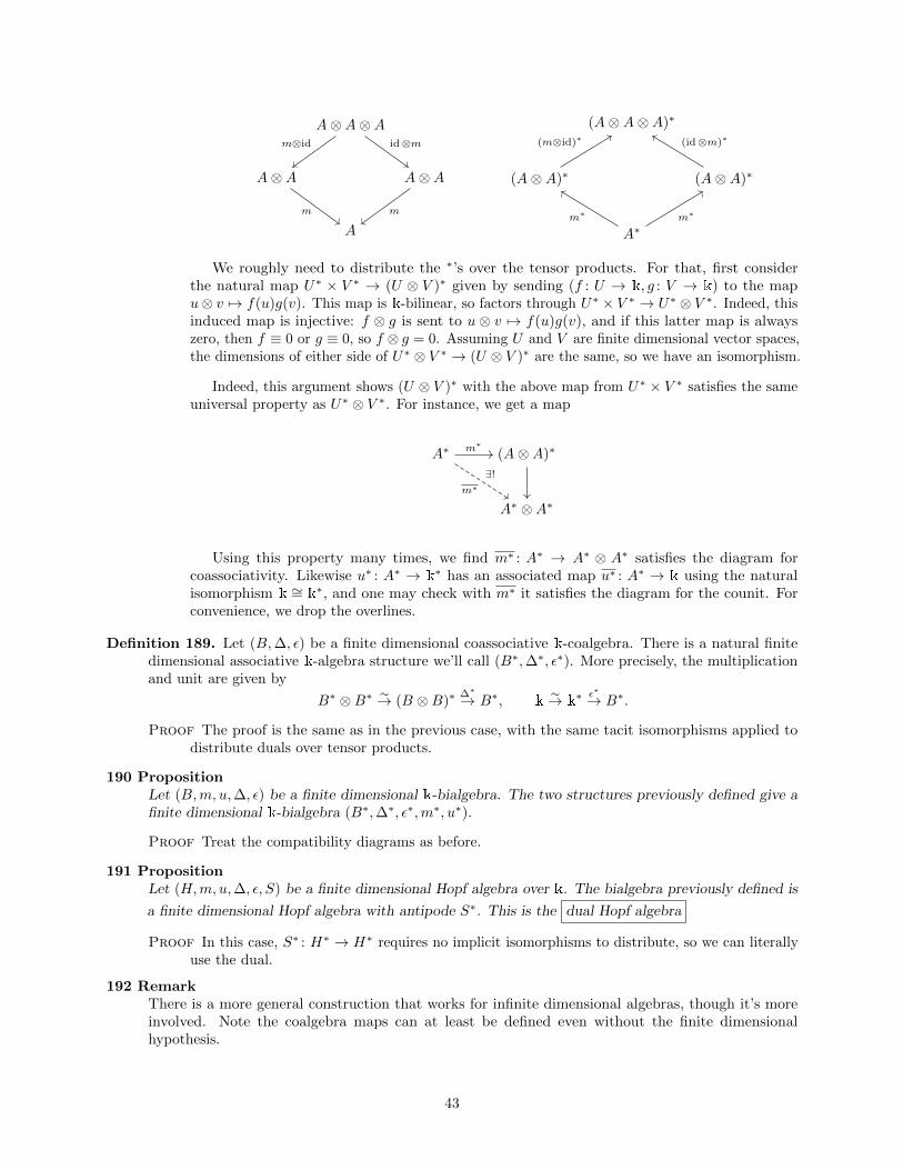
A⊗A⊗A
A⊗A A⊗A
A
m⊗id id⊗m
m m
(A⊗A⊗A)∗
(A⊗A)∗ (A⊗A)∗
A∗
(m⊗id)∗ (id⊗m)∗
m∗m∗
We roughly need to distribute the ∗’s over the tensor products. For that, first considerthe natural map U∗ × V ∗ → (U ⊗ V )∗ given by sending (f : U → k, g : V → k) to the mapu⊗ v 7→ f(u)g(v). This map is k-bilinear, so factors through U∗ × V ∗ → U∗ ⊗ V ∗. Indeed, thisinduced map is injective: f ⊗ g is sent to u ⊗ v 7→ f(u)g(v), and if this latter map is alwayszero, then f ≡ 0 or g ≡ 0, so f ⊗ g = 0. Assuming U and V are finite dimensional vector spaces,the dimensions of either side of U∗ ⊗ V ∗ → (U ⊗ V )∗ are the same, so we have an isomorphism.
Indeed, this argument shows (U ⊗ V )∗ with the above map from U∗ × V ∗ satisfies the sameuniversal property as U∗ ⊗ V ∗. For instance, we get a map
A∗ (A⊗A)∗
A∗ ⊗A∗
m∗
∃!m∗
Using this property many times, we find m∗ : A∗ → A∗ ⊗ A∗ satisfies the diagram forcoassociativity. Likewise u∗ : A∗ → k
∗ has an associated map u∗ : A∗ → k using the naturalisomorphism k ∼= k
∗, and one may check with m∗ it satisfies the diagram for the counit. Forconvenience, we drop the overlines.
Definition 189. Let (B,∆, ε) be a finite dimensional coassociative k-coalgebra. There is a natural finitedimensional associative k-algebra structure we’ll call (B∗,∆∗, ε∗). More precisely, the multiplicationand unit are given by
B∗ ⊗B∗ ∼→ (B ⊗B)∗∆∗→ B∗, k
∼→ k∗ ε∗→ B∗.
Proof The proof is the same as in the previous case, with the same tacit isomorphisms applied todistribute duals over tensor products.
190 PropositionLet (B,m, u,∆, ε) be a finite dimensional k-bialgebra. The two structures previously defined give afinite dimensional k-bialgebra (B∗,∆∗, ε∗,m∗, u∗).
Proof Treat the compatibility diagrams as before.
191 PropositionLet (H,m, u,∆, ε, S) be a finite dimensional Hopf algebra over k. The bialgebra previously defined is
a finite dimensional Hopf algebra with antipode S∗. This is the dual Hopf algebra
Proof In this case, S∗ : H∗ → H∗ requires no implicit isomorphisms to distribute, so we can literallyuse the dual.
192 RemarkThere is a more general construction that works for infinite dimensional algebras, though it’s moreinvolved. Note the coalgebra maps can at least be defined even without the finite dimensionalhypothesis.
43
April 30th, 2014: (Left) Integrals; from GK0 to GK1 and Beyond
193 RemarkJames Zhang, second guest lecture.
194 RemarkWe’ll tacitly assume frequently that GK0 is equivalent to finite dimensional. Technically GK0 justmeans GKdim is 0, but as mentioned last time if H is a finitely generated k-algebra, they are equivalent.(Warning: there may be missing assumptions or other minor errors in this lecture. Double-check withthe literature to be sure.)
195 RemarkWe’ll compare the following theorems from last time to infinite versions today.
196 Theorem (Larson-Sweedler)Every GK0 (i.e. finite dimensional) Hopf algebra is Gorenstein of injdim 0.
197 Theorem (Larson-Radford)Suppose char k = 0 and GKdimH = 0. The following are equivalent:
(a) H is semisimple, i.e. H = ⊕Mni×ni(Di) for division rings Di.
(b) H is regular of gldim 0.
(c) H is cosemisimple.
(d) S2 = id.
Definition 198. A left integral element in a Hopf algebra H is some t ∈ H such that
ht = ε(h)t, ∀h ∈ H.
That is, t is an eigenvector of the “trivial character” ε. We use
∫ `
for the space of left integrals in
H. Note that 0 is trivially left integral, though frequently we don’t want to consider it. Of course,this space is a k-vector space. “’integral’ is the most important invariant in the study of GK0 Hopfalgebras.”
199 LemmaIf H has GK0, then
∫ `is one-dimensional, i.e. there is a unique (up to scalar) non-trivial left integral.
200 ExampleLet H = k[G] for G a finite group. Then
∫ `is spanned by
∑g∈G g.
201 NotationAt least in the GK0 case, we have several abuses of notation:
(i)∫ `
can refer to an arbitrary non-trivial left integral.
(ii)∫ `
may also refer to itself as an H/AnnR(∫ `
) module.
(iii)∫ `
may also refer to the map H → H/AnnR(∫ `
).
202 Theorem (Maschke Restated)H is semisimple ⇔ ε(
∫ `) 6= 0.
44
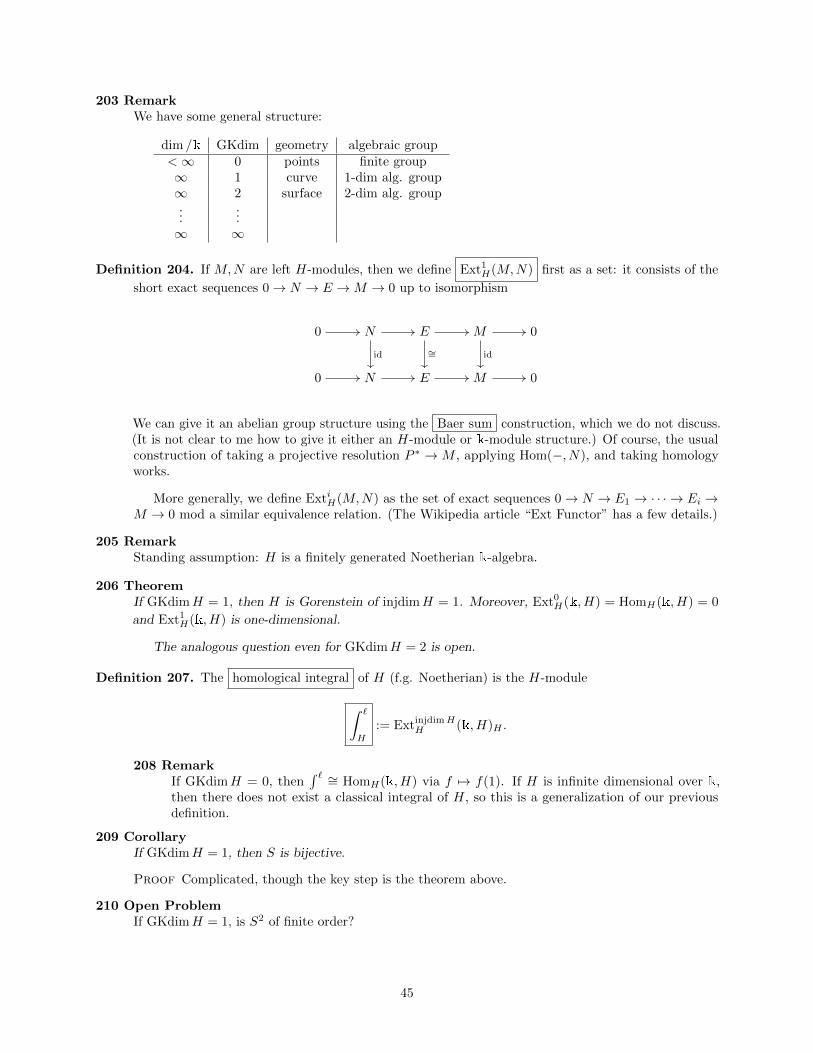
203 RemarkWe have some general structure:
dim /k GKdim geometry algebraic group<∞ 0 points finite group∞ 1 curve 1-dim alg. group∞ 2 surface 2-dim alg. group...
...∞ ∞
Definition 204. If M,N are left H-modules, then we define Ext1H(M,N) first as a set: it consists of the
short exact sequences 0→ N → E →M → 0 up to isomorphism
0 N E M 0
0 N E M 0
id ∼= id
We can give it an abelian group structure using the Baer sum construction, which we do not discuss.(It is not clear to me how to give it either an H-module or k-module structure.) Of course, the usualconstruction of taking a projective resolution P ∗ →M , applying Hom(−, N), and taking homologyworks.
More generally, we define ExtiH(M,N) as the set of exact sequences 0→ N → E1 → · · · → Ei →M → 0 mod a similar equivalence relation. (The Wikipedia article “Ext Functor” has a few details.)
205 RemarkStanding assumption: H is a finitely generated Noetherian k-algebra.
206 TheoremIf GKdimH = 1, then H is Gorenstein of injdimH = 1. Moreover, Ext0
H(k, H) = HomH(k, H) = 0
and Ext1H(k, H) is one-dimensional.
The analogous question even for GKdimH = 2 is open.
Definition 207. The homological integral of H (f.g. Noetherian) is the H-module
∫ `
H
:= ExtinjdimHH (k, H)H .
208 RemarkIf GKdimH = 0, then
∫ ` ∼= HomH(k, H) via f 7→ f(1). If H is infinite dimensional over k,then there does not exist a classical integral of H, so this is a generalization of our previousdefinition.
209 CorollaryIf GKdimH = 1, then S is bijective.
Proof Complicated, though the key step is the theorem above.
210 Open ProblemIf GKdimH = 1, is S2 of finite order?
45
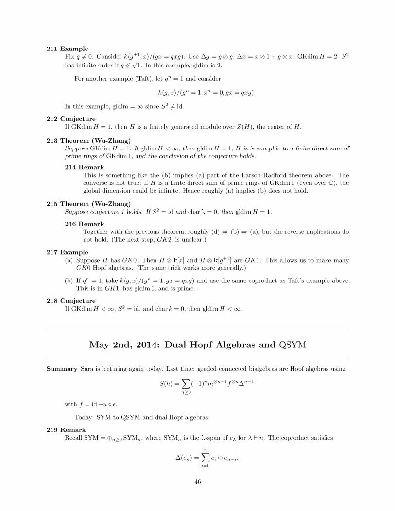
211 ExampleFix q 6= 0. Consider k〈g±1, x〉/(gx = qxg). Use ∆g = g ⊗ g, ∆x = x⊗ 1 + g ⊗ x. GKdimH = 2. S2
has infinite order if q 6∈√
1. In this example, gldim is 2.
For another example (Taft), let qn = 1 and consider
k〈g, x〉/(gn = 1, xn = 0, gx = qxg).
In this example, gldim =∞ since S2 6= id.
212 ConjectureIf GKdimH = 1, then H is a finitely generated module over Z(H), the center of H.
213 Theorem (Wu-Zhang)Suppose GKdimH = 1. If gldimH <∞, then gldimH = 1, H is isomorphic to a finite direct sum ofprime rings of GKdim 1, and the conclusion of the conjecture holds.
214 RemarkThis is something like the (b) implies (a) part of the Larson-Radford theorem above. Theconverse is not true: if H is a finite direct sum of prime rings of GKdim 1 (even over C), theglobal dimension could be infinite. Hence roughly (a) implies (b) does not hold.
215 Theorem (Wu-Zhang)Suppose conjecture 1 holds. If S2 = id and chark = 0, then gldimH = 1.
216 RemarkTogether with the previous theorem, roughly (d) ⇒ (b) ⇒ (a), but the reverse implications donot hold. (The next step, GK2, is unclear.)
217 Example(a) Suppose H has GK0. Then H ⊗ k[x] and H ⊗ k[g±1] are GK1. This allows us to make many
GK0 Hopf algebras. (The same trick works more generally.)
(b) If qn = 1, take k〈g, x〉/(gn = 1, gx = qxg) and use the same coproduct as Taft’s example above.This is in GK1, has gldim 1, and is prime.
218 ConjectureIf GKdimH <∞, S2 = id, and char k = 0, then gldimH <∞.
May 2nd, 2014: Dual Hopf Algebras and QSYM
Summary Sara is lecturing again today. Last time: graded connected bialgebras are Hopf algebras using
S(h) =∑n≥0
(−1)nm⊗n−1f⊗n∆n−1
with f = id−u ε.
Today: SYM to QSYM and dual Hopf algebras.
219 RemarkRecall SYM = ⊕n≥0 SYMn, where SYMn is the k-span of eλ for λ ` n. The coproduct satisfies
∆(en) =
n∑i=0
ei ⊗ en−i.
46
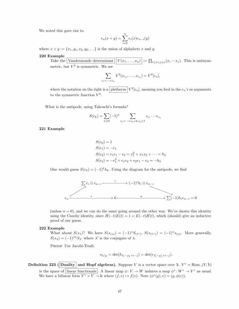
We noted this gave rise to
en(x+ y) =
n∑i=0
ei(x)en−i(y)
where x+ y := x1, y1, x2, y2, . . . is the union of alphabets x and y.
220 ExampleTake the Vandermonde determinant V (x1, . . . , xn) :=
∏1≤i<j≤n(xi − xj). This is antisym-
metric, but V 2 is symmetric. We see∑i1<···<in
V 2(xi1 , . . . , xin) = V 2[en],
where the notation on the right is a plethsym V 2[en], meaning you feed in the en’s as arguments
to the symmetric function V 2.
What is the antipode, using Takeuchi’s formula?
S(ek) =∑n≥0
(−1)n∑
i1+···+in=k,ij≥1
ei1 · · · ein
221 Example
S(e0) = 1
S(e1) = −e1
S(e2) = e1e1 − e2 = x21 + x1x2 + · · · = h2
S(e3) = −e31 + e1e2 + e2e1 − e3 = −h3
One would guess S(ek) = (−1)khk. Using the diagram for the antipode, we find
∑ei ⊗ en−i (−1)ihi ⊗ en−i
en 0∑
(−1)hien−i = 0
?
ε u
(unless n = 0), and we can do the same going around the other way. We’ve shown this identityusing the Cauchy identity, since H(−t)E(t) = 1 = E(−t)H(t), which (should) give an inductiveproof of our guess.
222 ExampleWhat about S(sλ)? We have S(s(n)) = (−1)nS(1n), S(s(1n)) = (−1)ns(n). More generally,
S(sλ) = (−1)|λ|Sλ′ where λ′ is the conjugate of λ.
Proof Use Jacobi-Trudi:
sλ/µ = det(hλi−µj+i−j) = det(eλ′i−µ′j+i−j).
Definition 223 ( Duality and Hopf algebras). Suppose V is a vector space over k. V ∗ = Homk(V,k)
is the space of linear functionals . A linear map φ : V → W induces a map φ∗ : W ∗ → V ∗ as usual.We have a bilinear form V ∗ × V → k where (f, v) 7→ f(v). Note (φ∗(g), v) = (g, φ(v)).
47
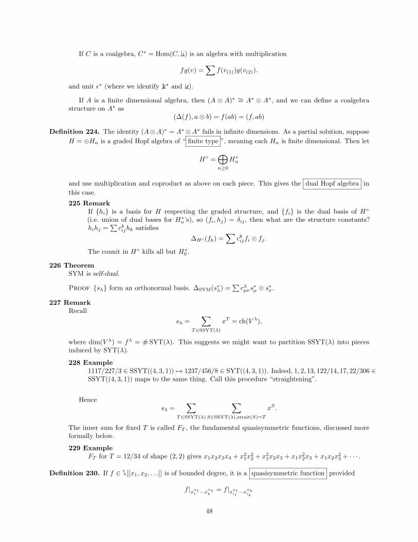
If C is a coalgebra, C∗ = Hom(C,k) is an algebra with multiplication
fg(v) =∑
f(v(1))g(v(2)).
and unit ε∗ (where we identify k∗ and k).
If A is a finite dimensional algebra, then (A ⊗ A)∗ ∼= A∗ ⊗ A∗, and we can define a coalgebrastructure on A∗ as
(∆(f), a⊗ b) = f(ab) = (f, ab)
Definition 224. The identity (A⊗A)∗ = A∗⊗A∗ fails in infinite dimensions. As a partial solution, suppose
H = ⊕Hn is a graded Hopf algebra of “ finite type ”, meaning each Hn is finite dimensional. Then let
H =⊕n≥0
H∗n
and use multiplication and coproduct as above on each piece. This gives the dual Hopf algebra in
this case.
225 RemarkIf hi is a basis for H respecting the graded structure, and fi is the dual basis of H
(i.e. union of dual bases for H∗n’s), so (fi, hj) = δij , then what are the structure constants?hihj =
∑ckijhk satisfies
∆H(fk) =∑
ckijfi ⊗ fj .
The counit in H kills all but H∗0 .
226 TheoremSYM is self-dual.
Proof sλ form an orthonormal basis. ∆SYM(s∗λ) =∑cλµνs
∗µ ⊗ s∗ν .
227 RemarkRecall
sλ =∑
T∈SSYT(λ)
xT = ch(V λ),
where dim(V λ) = fλ = # SYT(λ). This suggests we might want to partition SSYT(λ) into piecesinduced by SYT(λ).
228 Example1117/227/3 ∈ SSYT((4, 3, 1)) 7→ 1237/456/8 ∈ SYT((4, 3, 1)). Indeed, 1, 2, 13, 122/14, 17, 22/306 ∈SSYT((4, 3, 1)) maps to the same thing. Call this procedure “straightening”.
Hencesλ =
∑T∈SSYT(λ)
∑S∈SSYT(λ),strait(S)=T
xS .
The inner sum for fixed T is called FT , the fundamental quasisymmetric functions, discussed moreformally below.
229 ExampleFT for T = 12/34 of shape (2, 2) gives x1x2x3x4 + x2
1x22 + x2
1x2x3 + x1x22x3 + x1x2x
23 + · · · .
Definition 230. If f ∈ k[[x1, x2, . . .]] is of bounded degree, it is a quasisymmetric function provided
f |xα11 ···x
αkk
= f |xα1i1···xαkik
48
for all 1 ≤ i1 < · · · ik and α = (α1, . . . , αk) is a composition (i.e. αj ≥ 1).
QSYM is the set of all quasisymmetric functions. It comes with a grading QSYM = ⊕n≥0 QSYMn
where QSYMn consists of the homogeneous quasisymmetric functions of degree n. Note QSYM0 = k.QSYM is a graded connected algebra. The multiplication is just multiplication of power series. Thecomultiplication ∆(f) is determined by f(x ∪ y), just as for SYM above. This gives a bialgebrastructure, so it must be a Hopf algebra.
It comes with a (homogeneous) basis of monomial quasisymmetric functions
Mα := xα11 xα2
2 · · ·xαkk + all shifts
where α n. Hence dim(QSYMn) is the number of compositions of n, which is 2n−1 by taking subsetsof [n− 1].
231 HomeworkDescribe multiplication and coproduct on Mα’s, and the antipode too!
232 RemarkNote FS = FT is possible. For instance, this holds if S = 1237/456/8 and T = 1237/4568, whichrequires a moment’s thought. However, FT is not equal to FU for U = 12378/456. For instance,x5
1x32 ∈ FU but not in FT . When are they equal, and when are they not?
Definition 233. Given T ∈ SYT(λ), define Des(T ) , the descent set of T , as the set of j where j + 1
is lower than j in T (i.e. strictly south, weakly west, in English notation). Note that if λ ` n,Des(λ) ⊂ [n − 1]. There is a natural way to associate a composition of n with Des(λ), defined byexample below.
234 ExampleDes(1237/456/8) = 3, 7, Des(1237/4568) = 3, 7, and Des(12378/456) = 3. Write out∗ ∗ 3| ∗ ∗ ∗ 7|∗ for the first, giving associated composition 3 + 4 + 1. Similarly we get 3 + 4 + 1and 3 + 5 for the second and third.
Definition 235. The fundamental quasisymmetric function for α n is defined as follows. Let set(α)
mean the set corresponding to the composition α. Define
Fα := FDes(T ) =∑
1≤i1≤···≤in
xi1 · · ·xin
where we require strict inequality ij < ij+1 to hold for j ∈ set(α). The previous FT for T ∈ SYT(λ)are related to these by letting α be the composition associated to Des(T ).
(Note: this was copied from lecture, but I can’t make it make sense. To be updated.) (Reply: Wehave strict inequality in the case where j ∈ set(α).)
236 Theorem (Gessel)sλ =
∑T∈SYT(λ) FDes(T ).
237 RemarkExpand sµ[sλ] =
∑dνµλsν ; this is super hard and the coefficients are unknown except in the most basic
of cases.
May 5th, 2014: Rock Breaking, Markov Chains, and the HopfSquared Map
49
238 RemarkEric and Chris are presenting today on “Hopf algebras and Markov chains: two examples and theory”by Diaconis, Pang, and Ram.
Definition 239. We start with the Hopf squared map of a bialgebra H,
ψ2 : H → H := m∆
240 Exampleψ2(en) =
∑ni=0 eien−i for SYM. More generally, ∆(eλ) =
∑α⊂λ eα ⊗ eλ−α where the α are
weak compositions which are subsets of the partition λ in the obvious sense.
241 Exampleψ2 on k〈x1, . . . , xn〉 with coproduct given by xi primitive: then
∆(xi1 · · ·xik) =∑
S⊂1,...,k
∏j∈S
xij ⊗∏j∈Sc
xij ,
so that for instance
m∆(x1x2x3) = x1x2x3 + x1x2x3 + x2x1x3 + x3x1x2
+ x1x2x3 + x1x3x2 + x2x3x1 + x1x2x3
= 4x1x2x3 + x2x1x3 + x3x1x2 + x1x3x2
(The underlined terms come from the Sc term.)
Definition 242 ( Markov Chains ). Let Ω denote a finite “state space”. A sequence xkk≥0 is a Markovchain if
P(xi = y : xi−1 = y′) = P(xi = y : x0 = y′).
In words, the probability that you go to a new state only depends on where you are, not when you getthere.
243 ExampleFrom the previous example, divide by 23 so the coefficients sum to 1. You can construct aMarkov chain by giving the conditional probabilities above in a matrix with y vs. y′. For instance,we can use the result of m∆(x1x2x3) to fill in such a matrix, where the row corresponding tox1x2x3 is includes 1/2, 1/8, 1/8, 1/8, 0, 0, 0, 0.
244 RemarkSuppose f =
∑aifi where the fi : Ω→ R are eigenfunctions (of the transition matrix) with eigenvalues
βi. We can compute the expected value of f after k steps starting at x0 as
Ex0(f(xk)) =
∑i
aiEx0(fi(xk)) =
∑i
aiEx0(βif(xk−1))
=∑i
aiβki Ex0(f(x0)).
Definition 245 ( Rock breaking process ). Let (n) be an object of mass n, which can be broken into
two parts, (j) on the left and (n − j) on the right. Let the probability that we go from (n) to (j)and (n− j) be
(nj
)/2n. At the next step, (j) breaks up into (j1), (j − j1) with probability
(jj1
)/2j and
(n− j) breaks up into (j2), (n− j − j2) with probability(n−jj2
)/2n−j . Note it’s possible for j = 0, in
which case we just get (n).
This is defined on partitions by breaking each part independently and interpreting the result asa partition. Note that 1n is the final state. For instance, one could ask what the expected time forreaching this state is from some initial state.
50
246 RemarkOur goal is to find a basis for SYMn in which the (scaled) comultiplication map 1
2nψ2 : SYMn → SYMn
corresponds to the transition matrix of the rock breaking process defined above. In the n = 2 case, ournaive basis is e12 , e2, and ψ2(e12) = 4e12 , ψ2(e2) = e12 + 2e2. ψ2/22 in this basis is(
1 01/4 1/2
)The second row doesn’t add up to 1, so this isn’t a transition matrix. Since we understand our
present basis well, let’s just rescale it by some φ : e12 , e2 → R>0 where eλ := eλ/φ(eλ). Start with
φ(e12) = 1 = φ(e1)2. Then
ψ2(e2) = φ(e2)−1(e12 + 2e2) = φ(e2)−1e12 + 2φ(e2)−1e2
= φ(e2)−1e12 + 2e2.
The matrix is now (1 0
φ(e2)−1/4 1/2
)forcing φ(e2) = 1/2.
What about the n = 3 case? We know e13 , e12, and we can solve for the remaining element.
247 TheoremLet H be a Hopf algebra over R that is either a polynomial algebra or a cocommutative free associativealgebra. Also suppose we have a basis B such that ∆(c) has non-negative coefficients, and given any basis
element c of degree greater than 1, then ∆ c)PrimitivelyTwistedCoproduct := ∆(c)−1⊗c−c⊗1 6= 0.
A result of the paper is that there is a new basis B which is a rescaled version of the original suchthat ψ2/2n : Bn → Bn has as matrix a transition function for some Markov chain.
248 PropositionFor any generator, we have the right eigenvector
e(x) =∑n≥1
(−1)a−1/am[a]∆[a]
(x)
249 HomeworkIf H is commutative, check ψa is an algebra homomorphism. If H is cocommutative, check that
ψa is a coalgebra homomorphism. (To be clear, ∆[a]
= (id⊗ · · · ⊗∆) ∆[n−1]
.
250 Example (Rock-breaking example)Use ei = i!ei so φ(ei) = 1/i!. Now
ψ2(en) = n!m
(n∑i=0
eien−i
)
=
n∑i=0
(n
i
)eien−i
In particular, this gives part of the transition matrix for the rock-breaking Markov process.
251 PropositionIf µ, λ are partitions of n, then the right eigenfunction associated to µ evaluated at λ is
fµ(λ) =1∏i µi!
∑∏j
λj !
a1(µj)! · · · aλj (µj)!,
where the sum is over all sets µj such that µj is a partition of λj ,∐µj = µ, and ai(µ
j) is thenumber of parts of size i in µj .
51
252 ExampleSay µ = 1n−22. For any λ, fµ(λ) =
∑j
(λj2
). This has associated eigenvalue 1/2 and is non-zero
on all λ except the trivial partition 1n.
For instance, if x0 = (n), we find
P(xk 6= 1n) = P(fµ(xk) ≥ 1) ≤ E(fµ(xk)) = 1/2kfµ(x0)
=
(n
2
)/2k.
(The inequality uses Markov’s inequality.)
Aside: Hopf Algebras for k[x, y, z] and Hom(A,A) Invariants
253 PropositionLet A,A′ be algebras, C ′, C coalgebras, all over k. As before, endow Homk(C,A) with an algebrastructure. An algebra morphism A→ A′ induces an algebra morphism Homk(C,A)→ Homk(C,A′),a coalgebra morphism C ′ → C induces an algebra morphism Homk(C,A)→ Homk(C ′, A), and theseoperations are both functorial (the former covariant, the latter contravariant).
In particular, if A and B are bialgebras and φ : A→ B is an isomorphism of bialgebras, then wehave
Hom(A,A) Hom(A,B)
Hom(B,A) Hom(B,B)
φ−
−φ
φ−
−φ
and every arrow is an isomorphism. Indeed, the composite φ∗ : Hom(A,A)→ Hom(B,B) sends idA toidB . If A,B are also Hopf algebras with antipodes SA, SB , then φ∗SA = SB .
254 PropositionSuppose φ : A → B is an isomorphism of Hopf algebras with antipodes SA, SB. φ∗ induces anisomorphism
k[SA, idA]φ∗→ k[SB , idB ]
which acts via SA 7→ SB , idA 7→ idB. (For instance, the left-hand side is isomorphic to a quotient ofk[x, x−1].)
255 ExampleConsider A = k[x1, x2, . . .], given the usual Hopf algebra structure where each xi is primitive. LetPn := Span
k∏nj=1 xij. If S denotes the antipode, then
S(q) = (−1)nq if q ∈ Pn.
Hence S⊗S = id⊗ id for all q⊗ q ∈ A⊗A, and if chark = 2, then S2− id2 = 0 ∈ Hom(A,A) trivially.
If chark 6= 2, then for instance
(S ⊗ S)(1⊗ x1) = 1⊗ (−x1) 6= 1⊗ x1 = (id⊗ id)(1⊗ x1),
whence S2(x1) = −2x1 while id2(x1) = 2x1. In this case, S2 − id2 6= 0 ∈ Hom(A,A).
52
256 ExampleConsider B = k[e1, e2, e3], given a Hopf algebra structure via ∆(ek) =
∑ki=0 ei ⊗ ek−i (e0 = 1). The
antipode satisfies
S(e1) = −e1 S2(e1) = −2e1
S(e2) = e21 − e2 S2(e2) = 3e2
1 − 2e2
S(e3) = 2e1e2 − e31 − e3 S2(e3) = 6e1e2 − 4e3
1 − 2e3.
(Here as usual S2 denotes S · S ∈ Hom(B,B).)
In particular, (S2 − id2)(e2) = (3e21 − 2e2)− (e2
1 + 2e2) = 2e21 − 4e2. This is zero iff chark = 2.
257 RemarkIf A (with three variables) and B are isomorphic and chark = 2, then S2
B−id2B = 0 ∈ Hom(B,B).
Proof If φ : A→ B were an isomorphism, the induced map φ∗ : k[SA, idA]→ k[SB , idB ] wouldsend S2
A − id2A = 0 to S2
B − id2B .
258 RemarkIdentifying B with the subalgebra of symmetric polynomials in three variables generated bye1, e2, e3, we may alternatively use power sum symmetric polynomials p1, p2, p3 as algebraicbasis. Recall these are primitive with repect to the comultiplication above. From Newton’sIdentities, it follows that
e1 = p1
e2 =1
2(p2
1 − p2)
e3 =1
6(p3
1 − 3p1p2 + 2p3)
Hence if chark 6= 2, 3, we may identify xi with pi and use these formulas to construct a bialgebra,hence Hopf algebra, isomorphism from A to B.
259 RemarkSome haphazard thoughts: a Hopf algebra A has a “primitive subspace” spanned by primitive elements,where the antipode is particularly well-behaved. There are relations between S, id, 1 ∈ Hom(A,A) onthis subspace. Powers of this subspace are also interesting. There are still relations between S, id, 1on the powers, but I wasn’t able to find a nice general pattern. Maps between Hopf algebras sendthe primitive subspace of the source into the primitive subspace of the target. Perhaps other notionsbesides “primitive” have similar properties and induce similar “filtrations” which in good situationsare non-trivial. The two Hopf algebras above both have at least one non-zero primitive element, whichseems important.
Addendum from Darij Grinberg: a commutative cocommutative graded connected Hopf algebra incharacteristic 0 is the symmetric algebra of its space of primitive elements, which follows, for instance,from the Milnor-Moore theorem. There is more freedom in positive characteristic, for instance usingk[x]/(xp) for chark = p.
May 7th, 2014: Chromatic Polynomials and applications ofMobius inversion
260 RemarkKolya and Connor are lecturing today on Stanley’s “Symmetric Function Generalization of theChromatic Polynomial of a Graph”.
53
Definition 261. Let G be a graph with vertices V , edges E. A coloring of G is a function k : V → P; a
proper coloring is a coloring such that for all ab ∈ E, k(a) 6= k(b), i.e. no vertexes connected by an
edge have the same color. χG(n) is the number of colorings V → [n].
262 Example
(1) Take a (connected) tree G with d vertices, so d− 1 edges. Claim: χG(n) = n(n− 1)d−1. One cansee this by deletion-contraction (below) and induction. Alternatively, simply color some vertex oneof n colors, so each adjacent vertex can have (n− 1) colors, and we will always have (n− 1) colorsfor the next vertex since we have no cycles.
(2) Take G with four vertexes, with one being a “central” vertex connected to each of the others, andno other edges. Values of χG(n) for n = 1, 2, 3, . . . are 0, 2, 24, . . ..
263 PropositionGiven a graph G, for any edge e in G,
χG = χG−e − χG/e
where G/e means G with the edge e “contracted” (i.e. its two vertices identified) and G− e means Gwith the edge e removed.
Proof Easy ennumerative exercise.
Definition 264. Given a graph G = (V,E), define the chromatic polynomial
XG :=∑κ
xκ(v1) · · ·xκ(vn)
where the sum is over proper colorings of G and the product is over all vertices. This is symmetric andhomogeneous of degree #V .
265 ExampleLet G be a “bow tie” graph, where the crossing point is a vertex. Then
XG = 4m(2,2,1) + 24m(2,1,1,1) + 120m(1,1,1,1,1)
(using the monomial symmetric functions).
266 ExampleLet G be a square with one diagonal edge added in. Add a vertex with a single edge to one ofthe box’s vertices which wasn’t used when adding the diagonal edge. Then XG is the same asfor the previous example, so G 7→ XG is not in general injective.
Definition 267. A stable partition of V (G), the vertex set of G, is a set partition of V (G) where no two
vertices in the partition are connected by an edge. We set aλ as the number of stable partitions
of V (G) of “type” λ ` n (where n = #V ). Now XG =∑λ`n aλmλ where mλ = mλr1!r2! · · · if
λ = (r1, r2, . . .).
Definition 268. Let G be the k-span of [G] where G is a finite simple graph. Define multiplication bycartesian product. Define a coproduct as follows:
∆([G]) =∑
V1∐V2=V (G)
G|V1⊗G|V2
,
where G|V1 refers to the induced subgraph of G with respect to V1. That is, remove all other verticesnot in V1.
54
269 ExampleIf G is a triangle with an edge removed, then ∆(G) is 1⊗ [G]+2(·⊗−)+[G]⊗1+2(−⊗·)+(· ·⊗·).
270 PropositionThe map G → SYM given by G 7→ XG is a Hopf algebra morphism. Indeed, G is graded by number ofvertices and connected, so is a Hopf algebra.
271 Theorem (Humpert-Martin)Let M be the graphic matroid of G. (It is the set of subsets F of edges such that if v and v′ are
connected in that subset, possibly by a sequence of several edges, then vv′ is in that subset.) Then theantipode is
S[G] =∑F
(−1)|V |−|F |acyc(G/F )GV,F
where acyc refers to the number of acyclic orientations and the sum is over F in the graphic matroid.
272 Theorem (Reiner)G is self-dual via [G] 7→
∑[H]∗ where the sum is over all H where V (H) = V (G) and E(H)∩E(G) = ∅.
For instance, the triangle with an edge removed maps to the sum of three disjoint points’s dual plus−∐·’s dual.
273 Theorem
XG =∑S⊂E
(−1)#Spλ(S)
where λ(S) is a partition whose parts are the sizes of components of GS , and the p’s are powersymmetric functions.
Proof Let KS be the set of colorings which are monochromatic on components of GS . Set xα =xα(v1) · · ·xα(vn). Then ∑
α∈KS
xα = pλ(S)
since we get a factor of pm for each component of size m. The right-hand side of the formula inthe theorem is ∑
S⊂E(−1)#S
∑α∈KS
xα =∑
β : V→Pxβ
∑S⊂Eβ
(−1)#S
Here, we have reversed the order of the sum with Eβ := (u, v) ∈ E : β(u) = β(v). Thisequality oocurs because β is monochromatic on the components of GS if and only if all edges inS are between vertices of the same color in β. Hence,∑
S⊂E(−1)#Spλ(S) =
∑β : V→P
xβδEβ=∅
However, Eβ = ∅ if and only if β is a proper coloring. Hence, we conclude that
XG =∑S⊂E
(−1)#Spλ(S).
Definition 274. Let I be our interval bialgebra as before on some poset P , where the coproduct of aninterval was given by breaking it up into two pieces in all possible ways. Let Hom(I,k) be an algebrausing convolution (pre- and post-composing with ∆: I → I ⊗ I and m : k⊗ k→ k, using −⊗ id inbetween), which in particular has identity
1([s, t]) = δs=t
The zeta function is Z([s, t]) = δs≤t. The Mobius function is the inverse of the zeta function in thisalgebra,
µZ = Zµ = 1.
55
275 Propositionµ(s, s) = 1 and
µ([s, t]) = −∑s≤x≤t
µ([s, x]).
276 PropositionFor any f, g : P → k, we have
g(t) =∑s≤t
f(s) ⇔ f(t) =∑s≤t
g(s)µ(s, t).
This is called Mobius inversion .
Definition 277. Define the lattice of contractions LG as the set of connected (set) partitions of the verticesof a graph G ordered by refinement; it is a sublattice of the partition lattice. The type is as usual theobvious associated integer partition of #V (G).
278 ExampleFor the square with four vertices (and four edges), the elements of LG with three blocks are
12|3|4 13|2|4 1|3|24 1|2|34
279 TheoremWe have XG =
∑π∈LG µ([0, π])ptype(π), where µ([0, π]) is the Mobius function on LG.
Proof Use Mobius inversion. For σ ∈ LG, let
Yσ =∑α∈Jσ
xα
where α ∈ Jσ iff α is a coloring where the blocks of σ are precisely the monochromatic connectedpieces of α. Now
ptype(π) =∑α
xα =∑σ≥π
Yσ
where the α are monochromatic on blocks of π. One can see this by conditioning on what themonochromatic connected blocks of α are. By Mobius inversion,
Yσ =∑σ≥π
µ(π, σ)ptype(σ).
Now notice Y0 =∑α x
α where the α’s are monochromatic connected pieces are 1|2| · · · |n. Butthis is just equivalent to being a proper coloring, so
XG =∑π∈LG
µ(0, π)ptype(π)
280 Example (Forests)Let G be a forest. We show XG =
∑λ`d eλbλpλ where eλ = (−1)d−|λ| = µ(0, π) for any type(π) = λ
and bλ is the number of connected partitions of type λ. First, observe that LG is a Boolean algebra,by the poset isomorphism where each connected partition is sent to the edges its blocks contain. Itfollows that we have the Mobius function µ(0, π) = (−1)d−|λ| for any type(π) = λ. The result thenfollows from the preceding theorem.
56
281 ConjectureXG 6= XH for two non-isomorphic trees G,H.
282 RemarkXG = XH iff bλ(G) = bλ(H).
Definition 283. Consider some labeling γ on the edges of a graph G. Call S ⊂ E a broken circuitif it is a cycle with its largest edge removed, with respect to the labeling γ. Furthermore, letBG denote the set of all subsets of E which do not contain a broken circuit.
284 TheoremWe have XG =
∑S∈BG(−1)#Spλ(S)
Proof From other results, we have that
µ(0, π) =∑S
(−1)#S
where the sum is over all S ∈ BG such that GS has the blocks of π as its connectedcomponents. The result then follows from using the preceding theorem.
May 9th, 2014: Reduced Incidence Coalgebras; SectionCoefficients; Matroids and Hereditary Classes; Many Examples
285 RemarkNeil is presenting on “Coalgebras and Bialgebras in Combinatorics” by Joni and Rota. No particularbig result; just a lengthy collection of interesting examples and observations.
Definition 286. Recall that if P is a poset, then we can form the incidence coalgebra of P , denoted C(P ) ,
as follows. It is the free k-vector space spanned by the segments [x, y] of P , with comultiplicationdefined by breaking up the segments,
∆[x, y] =∑
[x, z]⊗ [z, y].
(For this sum to be finite, P must be locally finite, i.e. P must have finite intervals.)
Definition 287. An equivalence relation ∼ on intervals of a poset P is order-compatible if
[x, y]− [u, v] : [x, y] ∼ [u, v]
is a coideal. Given such a relation, we define the reduced incidence coalgebra as the quotient coalgebra
C(P )/∼, abbreviated as RIC.
288 ExampleThe standard RIC is the RIC defined by the equivalence relation [x, y] ∼ [u, v] iff [x, y] ∼= [u, v]as posets.
Definition 289. A collection of section coefficients (i|j, k) on a set G is a map
(i, j, k) 7→ (i|j, k) ∈ Z≥0
such that
(1) For all i, #(j, k) : (i|j, k) 6= 0 <∞.
57
(2)∑k(i|j, k)(k|p, q) =
∑s(i|s, q)(s|j, p); this quantity is called (i|j, p, q) , a multisection coefficient .
Intuitively, we “cut i into pieces j and k”. Given a coalgebra with basis xi, we can take (i|j, k) to bethe coefficient of xj ⊗ xk in ∆(xi), so long as those coefficients are in Z≥0.
Definition 290. If G is a semigroup, bisection coefficients additionally require
(3) (i+ j|p, q) =∑
(i|p1, q1)(j|p2, q2),
where the sum is over p1 + p2 = p and q1 + q2 = q.
291 ExampleThe binomial coefficients are bisection coefficients: (n|j, k) = n!/(j!k!) if j + k = n and 0 otherwise.The bisection condition is Vandermonde’s convolution identity,(
i+ j
p
)=
∑p1+p2=p
(i
p1
)(j
p2
).
292 ExampleWe define a system of section coefficients on the incidence coalgebra using
([x1, x2]|[y1, y2], [z1, z2]) =
1 if x1 = y1, x2 = z2, y2 = z1
0 otherwise
293 PropositionIf there is a map ε : G→ k which satisfies∑
j
(i|j, k)ε(j) = δi,k and∑k
(i|j, k)ε(k) = δi,j ,
then we can form a coalgebra from the free k-vector space spanned by elements of G with coproduct∆xi =
∑(i|j, k)xj ⊗ xk. This is cocommutative if and only if (i|j, k) = (i|k, j). If we use bisection
coefficients, we get a bialgebra structure using xixj = xi+j as our multiplication.
294 ExampleLet B be the boolean lattice on P, and consider C(B).
(1) The boolean coalgebra on B uses
∆A =∑
A1∐A2=A
A1 ⊗A2.
This arises as a quotient of C(B) using [A,B] ∼ [C,D] if B −A = D − C.
(2) The binomial coalgebra is given as follows. Let s > 0. Define Bs using the k-vector space
k[x1, . . . , xs] and comultiplication given by
∆(xn11 · · ·xnss ) =
∑(n1
m1
)· · ·(nsms
)xm1
1 · · ·xmss ⊗ xn−m11 · · ·xn−mss ,
where the sum is over (m1, . . . ,ms) ≤ (n1, . . . , ns).
This arises as the quotient of C(B) by the equivalence relation where [A,B] ∼ [C,D] if for allk = 1, . . . , s, the number of i ∈ B −A where i ≡s k is the same as the number of j ∈ D−C wherej ≡s k.
For instance, if s = 1, we have [A,B] ∼ [C,D] iff |B−A| = |D−C|. If s = 2, we have [A,B] ∼ [C,D]iff the number of even (respectively, odd) integers in B −A is the same as the number in D − C.
58
295 ExampleSome coalgebras arise as duals of formal power series.
(1) The divided powers coalgebra D is the standard RIC of C(Z≥0) (standard order). One can check
that, using a coproduct on k[x] given by
∆xn =
n∑k=0
xk ⊗ xn−k,
D∗ ∼= k[[x]] as algebras.
(2) The Dirichlet coalgebra D is defined as follows. Order P by divisibility. Use [i, j] ∼ [k, l] iff
j/i = l/k. Set D = C(P)/∼. An isomorphic description is to take the k-span of formal symbolsnx : n ∈ Z≥0 using
∆nx =∑pq=n
px ⊗ qx.
This suggests an algebra structure given by nxmx = (nm)x, which unfortunately does not give abialgebra, but does give the identity
∆(nxmx) = ∆(nx)∆(mx)
whenever (n,m) = 1.
In this case, D∗ is isomorphic as an algebra to the algebra of formal Dirichlet series via f 7→∑n f(ns)/ns.
Definition 296. Let S be a set. A matroid M(S) is a “closure relation” on S, meaning a map associating
a subset A of S to its “closure” A, such that the following holds:
1. A ⊂ A; A = A; A ⊂ B implies A ⊂ B; and
2. If A ⊂ S and p, q ∈ S, and p ∈ A ∪ q, then p ∈ A implies q ∈ A ∪ p.
Definition 297. Let A,B ∈M(S) with A ⊂ B. A segment M(A,B;S) is the matroid defined on B −Aas follows. If C ⊂ B −A, then C := C ∪A−A.
Isomorphism classes of matroids are called types ; lattices of closed sets are called geometric lattices
(i.e. starting from a matroid, form a lattice by inclusion using the closure of the union).
Definition 298. Given a geometric lattice L, let S be the atoms of L, that is, the elements covering 0.
For A ⊂ S, let A := p ∈ S : p ≤ supA, where supA is the join of the atoms. The result is the
combinatorial geometry of L.
Definition 299. A hereditary class H is a family of types of combinatorial geometries such that
(1) If α, β ∈ H, then α+ β ∈ H.
(2) If [M(S)] ∈ H, A,B ⊂M(S), then [M(A,B;S)] ∈ H.
(3) If α ∈ H and α = α1 + α2, then α1, α2 ∈ H.
300 PropositionGiven a hereditary class of matroids, we can form section coefficients (α|β, γ) as follows. If [M(S)] = α,let the section coefficients be the number of closed sets A of such that β = [M(∅, A;S)] and γ =[M(A,S;S)].
59
May 12th, 2014—Two Homomorphisms from Iranked to QSYM;Mobius Functions on Posets
Summary Hailun is presenting “On Posets and Hopf Algebras” by Ehrenborg. Previous work includedSchmidt’s “Antipodes and Incidence Coalgebra” from 1987 and Gessel’s “Multipartite P -partitionsand inner products of skew Schur functions” from 1984. The main results presented today are:
(1) There is a Hopf algebra homomorphism from the reduced incidence Hopf algebra of posets toQSYM.
(2) There is a “twisted” version of the Hopf algebra homomorphism from (1), and a connection to theZeta polynomial of a poset.
301 RemarkLet Iranked be the reduced incidence Hopf algebra defined above. The bialgebra structure and gradinghave already been given explicitly. The antipode by definition (using Sweedler notation and · formultiplication) satisfies
ε(P ) · 1 =∑(P )
S(P(1)) · P(2).
This can be thought of as a recursive formula for defining the antipode, made precise in the followingrecursive version of Takeuchi’s formula:
302 LemmaSuppose B = ⊕n≥0Bn is a graded bialgebra (so B0 = k, Bi · Bj ⊂ Bi+j , and ∆(Bn) ⊂⊕i+j=nBi ⊗Bj). Then B is a Hopf algebra with antipode recursively defined by S(1) = 1 and,for x ∈ Bn with n ≥ 1,
S(x) = −m∑i=1
S(yi) · zi,
where
∆(x) = x⊗ 1 +
m∑i=1
yi ⊗ zi
and deg yi < deg x.
For convenience, we’ll denote Iranked by H today.
303 RemarkFurther recall the Mobius function for a poset P with finite intervals: µ : P × P → Z is given by
µ(x, y) =
−∑x≤z<y µ(x, z) x < y
1 x = y
(We aren’t particularly interested in µ(x, y) for x > y; set it to 0 in that case if you wish.) Write
µ(P ) := µ(0, 1), assuming 0, 1 exist in P .
Likewise recall the zeta function on I, given by Z(P ) = 1 for all P , extended linearly. As before,Z and µ are inverses in the Hom(H,k) algebra.
In fact, one can check Z(S(P )) = µ(P ), so the antipode is a sort of generalization of the Mobiusfunction.
60
Definition 304 (QSYM recap). QSYM is a graded bialgebra (a Hopf algebra) as usual; for instance, inthe monomial basis Ma indexed by compositions, the coproduct is “rock breaking”. Fundamentalbasis elements Fa satisfy
Fa =∑b≤a
Mb.
For convenience, we’ll use
Ma := (−1)m−k∑b≤a
Mb = (−1)m−kFa,
where a is a composition of m into k parts.
305 PropositionThe antipode S for QSYM is given in the monomial basis by
S(Ma) = (−1)`(a)∑b≤a
Mb∗ ,
where if b = (b1, . . . , bk), then b∗ := (bk, . . . , b1), and the sum is over refinements b of the compositiona. (`(a) denotes the number of parts of a.)
Proof Use the recursive version of the antipode formula from the previous lemma and induct. SeeProposition 3.4 in the paper for more details.
306 RemarkThe first main result of the paper is the following theorem. It associates to each ranked finite poset P
with 0 and 1 a corresponding quasisymemtric function, and the resulting map respects the bialgebrastructures involved.
Here ρ (x) for x ∈ P is the rank of P , normalized so ρ(0) = 0. We write
ρ(x, y) := ρ(y)− ρ(x),
which is the rank of the interval [x, y]. Similarly ρ(P ) := ρ(0, 1) is the rank of the poset P . (Recall
that H is graded by poset rank.)
307 TheoremThere is a Hopf algebra homomorphism F : H → QSYM defined as follows:
F (P ) =∑
M(ρ(x0,x1),...,ρ(xn−1,xn)),
where the sum is over chains 0 = x0 < x1 < · · · < xn = 1.
Proof Clearly F (1) = 1, and it’s easy to see F commutes with the counit. We must show F respectsmultiplication and comultiplication.
Note that QSYM is the inverse limit of QSYMn (where QSYMn is the same as QSYM butwe only use n variables). We have projection maps QSYM→ QSYMn, which just set the unused
variables to 0. Let Fn be the composite H F→ QSYM→ QSYMn.
For multiplication, it then suffices to show Fn : H → QSYMn is an algebra homomorphism.One may show that
Fn(P ; t1, . . . , tn) =∑
tρ(x0,x1)1 · · · tρ(xn−1,xn)
n ,
where the sum is over chains as above. Letting κi : H → k[ti] via κi(P ) = tρ(P )i , we see the κi
are multiplicative, and moreover we have
Fn = µn (κ1 ⊗ · · · ⊗ κn) ∆n,
61
and each map in the composite is multiplicative.
Finally, we show F is a coalgebra homomorphism. We compute as follows (this isn’t nearlyas bad as it looks):
(F ⊗ F ) ∆(P ) =∑
0≤x≤1
F ([0, x])⊗ F ([x, 1])
=∑
0≤x≤1
∑0=y0<···<yk=x
M(ρ(y0,y1),...,ρ(yk−1,yk))
⊗
∑x=z0<···<zn=1
M(ρ(z0,z1),...,ρ(zk−1,zk))
=
∑1=x0<···<xn=0
n∑k=0
M(ρ(x0,x1),...,ρ(xk−1,xk))
⊗M(ρ(xk,xk+1),...,ρ(xn−1,xn))
=∑
∆(M(ρ(x0,x1),...,ρ(xn−1,xn)))
= ∆(F (P )).
Definition 308. Let P be a finite ranked poset with 0, 1. Pick S ⊂ [ρ(P )−1], and define the rank-selected poset
P (S) by
P (S) := x ∈ P : ρ(x) ∈ S ∪ 0, 1.
Further, let α(S) denote the number of maximal chains in P (S).
309 LemmaLet P be a ranked poset of rank m. Then
F (P ) =∑
S⊂[m−1]
α(S)Mω(S),
where ω(S) is the composition of m corresponding to S via the “stars and bars” bijection (see below).
Definition 310. Let Ω: QSYM→ QSYM be the involution given by
Ω(Ma) = Ma.
Let F : H → QSYM be the sign-twisted version of F given by
F (P ) =∑
(−1)ρ(P )µ(x0, x1) · · ·µ(xn−1, xn)Mρ(x0,x1)···ρ(xn−1,xn),
where the sum is over chains as before.
311 PropositionThe following diagram commutes:
H QSYM
QSYM
F
FΩ
62
Proof One main ingredient is Philip Hall’s formula for the Mobius function,
µ(a, b) =∑
a=y0<···<yn=b
(−1)n.
For further details, see Proposition 5.1 of Ehrenborg.
312 CorollaryMalvenuto and Reutenauer showed Ω is a Hopf algebra homomorphism, so F is as well.
Definition 313. Call the vector (1, 1, . . . , 1, 0, 0, . . .) with x initial one’s and zeros everywhere after 1x. Notethat
Ma(1x) =
(x
`(a)
),
which can be interpreted as a polynomial identity. Hence we may define a k-linear function Ψ: QSYM→k[x] by “evaluating at 1x”, or more formally by sending Ma to
(x`(a)
).
Definition 314. The Zeta polynomial of a finite poset with 0 and 1 is defined to evaluate to the number
of multichains from 0 to 1 (where a “multichain” is a chain as above but where ≤ is used instead of <).
315 PropositionThe Zeta polynomial for a poset P as above is given by Ψ F (P ).
Proof See proof of Corollary 6.2 in Ehrenborg.
May 14th, 2014: Characters; Combinatorial Hopf Algebras;(QSYM, ζQ) as Terminal Object; Even and Odd Subalgebras;
Dehn–Sommerville Relations
Summary Jose is lecturing today on “Combinatorial Hopf algebras and generalized Dehn–Sommervillerelations” by Aguiar, N. Bergeron, and Sottile. Today’s outline:
(1) Character group
(2) Combinatorial Hopf algebras
(3) (QSYM, ζ) as terminal object
(4) Dehn–Sommerville relations
316 Notation(H,m, u,∆, ε, S) is a graded, connected Hopf algebra throughout this lecture, and our Hopf algebrasare generally graded connected today.
Definition 317. A character of H is a linear map ζ : H → k which is an algebra map, i.e. ζ(ab) = ζ(a)ζ(b)and ζ(1) = 1. We can multiply linear functionals φ, ψ : H → k using convolution:
φψ : H∆→ H ⊗H φ⊗ψ→ k⊗ k m→ k.
Let χ(H) be the set of characters on H. The convolution gives it a group structure with identity ε
and inverse ζ−1 = ζ S.
If H is cocommutative, then χ(H) is commutative. If α : H ′ → H is a Hopf algebra morphism,there is an induced morphism α∗ : χ(H)→ χ(H ′) given by ζ 7→ ζ α. Indeed, this is a contravariantfunctor from the category of Hopf algebras to the category of groups.
63
Definition 318. Let (·) : H → H be the involution defined by h 7→ h := (−1)nh for h ∈ Hn. This is linear,
so induces an automorphism χ(H) → χ(H), which we’ll denote ζ 7→ ζ. Call a character ζ even iff
ζ = ζ, and call it odd iff ζ = ζ−1.
Definition 319. Let χ+(H) be the set of even characters in χ(H), which is a subgroup in general, and let
χ−(H) be the set of odd characters, which is a subgroup when H is cocommutative.
A character ζ comes with two other induced characters, namely
ν := ζ−1ζ (odd)
χ := ζζ (even).
320 TheoremEvery character ζ can be written uniquely as a product of an even and odd character,
ζ = ζ+ζ−
Definition 321. A combinatorial Hopf algebra (CHA) is a pair (H, ζ) where H is a Hopf algebra and ζ
is a character. We define the category of CHA’s using these objects and the following morphisms.α : (H ′, ζ ′) → (H, ζ) is a morphism when α : H ′ → H is a graded Hopf algebra morphism and α iscompatible with the characters in the sense that
H ′ H
k
α
ζ′ ζ
Definition 322. Given a CHA (H, ζ), call ζ the zeta character , call ζ−1 the Mobius character , call
χ = ζζ the Euler character , and call ν = ζ−1ζ the odd character . (Minor note: ζ−1 = ζ−1
.)
Some motivation for this notation: let R be the Hopf algebra of posets from last time. Thenζ(P ) := 1, the Mobius character is ζ−1(P ) = µ([0p, 1p]), we can define a simplicial complex from a posetwhose Euler characteristic is given by χ(P ), and the odd character is related to the Dehn–Sommervillerelations.
Definition 323. The (Hopf) algebra of Non-commutative symmetric functions NSYM (also written H )
is the free algebra over non-commutative variables H1, H2, . . . graded by Hi ∈ Hi. Use the “rock-breaking” coproduct
∆(Hn) :=
n∑i=0
Hi ⊗Hn−i.
Here we write H0 for 1H for convenience. There is a map NSYM → SYM given by Hn 7→ hn; thekernel is the commutator subalgebra, so essentially SYM is just making NSYM commutative.
324 RemarkLet H be a Hopf algebra. Recall that H∗ = ⊕∞n=0H
∗n (so long as the graded pieces are each finite
dimensional). There is a mapNSYM→ (QSYM)∗
given by Hi 7→M∗(i), Hα 7→M∗α where α is a composition and Hα := Hα1· · ·Hαn . Indeed, this is an
isomorphism!
64
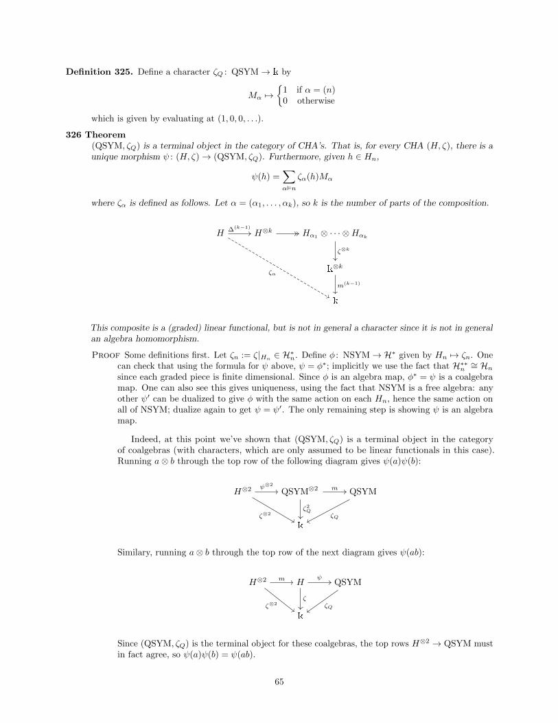
Definition 325. Define a character ζQ : QSYM→ k by
Mα 7→
1 if α = (n)0 otherwise
which is given by evaluating at (1, 0, 0, . . .).
326 Theorem(QSYM, ζQ) is a terminal object in the category of CHA’s. That is, for every CHA (H, ζ), there is aunique morphism ψ : (H, ζ)→ (QSYM, ζQ). Furthermore, given h ∈ Hn,
ψ(h) =∑αn
ζα(h)Mα
where ζα is defined as follows. Let α = (α1, . . . , αk), so k is the number of parts of the composition.
H H⊗k Hα1⊗ · · · ⊗Hαk
k⊗k
k
∆(k−1)
ζα
ζ⊗k
m(k−1)
This composite is a (graded) linear functional, but is not in general a character since it is not in generalan algebra homomorphism.
Proof Some definitions first. Let ζn := ζ|Hn ∈ H∗n. Define φ : NSYM→ H∗ given by Hn 7→ ζn. Onecan check that using the formula for ψ above, ψ = φ∗; implicitly we use the fact that H∗∗n ∼= Hnsince each graded piece is finite dimensional. Since φ is an algebra map, φ∗ = ψ is a coalgebramap. One can also see this gives uniqueness, using the fact that NSYM is a free algebra: anyother ψ′ can be dualized to give φ with the same action on each Hn, hence the same action onall of NSYM; dualize again to get ψ = ψ′. The only remaining step is showing ψ is an algebramap.
Indeed, at this point we’ve shown that (QSYM, ζQ) is a terminal object in the categoryof coalgebras (with characters, which are only assumed to be linear functionals in this case).Running a⊗ b through the top row of the following diagram gives ψ(a)ψ(b):
H⊗2 QSYM⊗2 QSYM
k
ψ⊗2
ζ⊗2
m
ζ2QζQ
Similary, running a⊗ b through the top row of the next diagram gives ψ(ab):
H⊗2 H QSYM
k
m
ζ⊗2ζ
ψ
ζQ
Since (QSYM, ζQ) is the terminal object for these coalgebras, the top rows H⊗2 → QSYM mustin fact agree, so ψ(a)ψ(b) = ψ(ab).
65
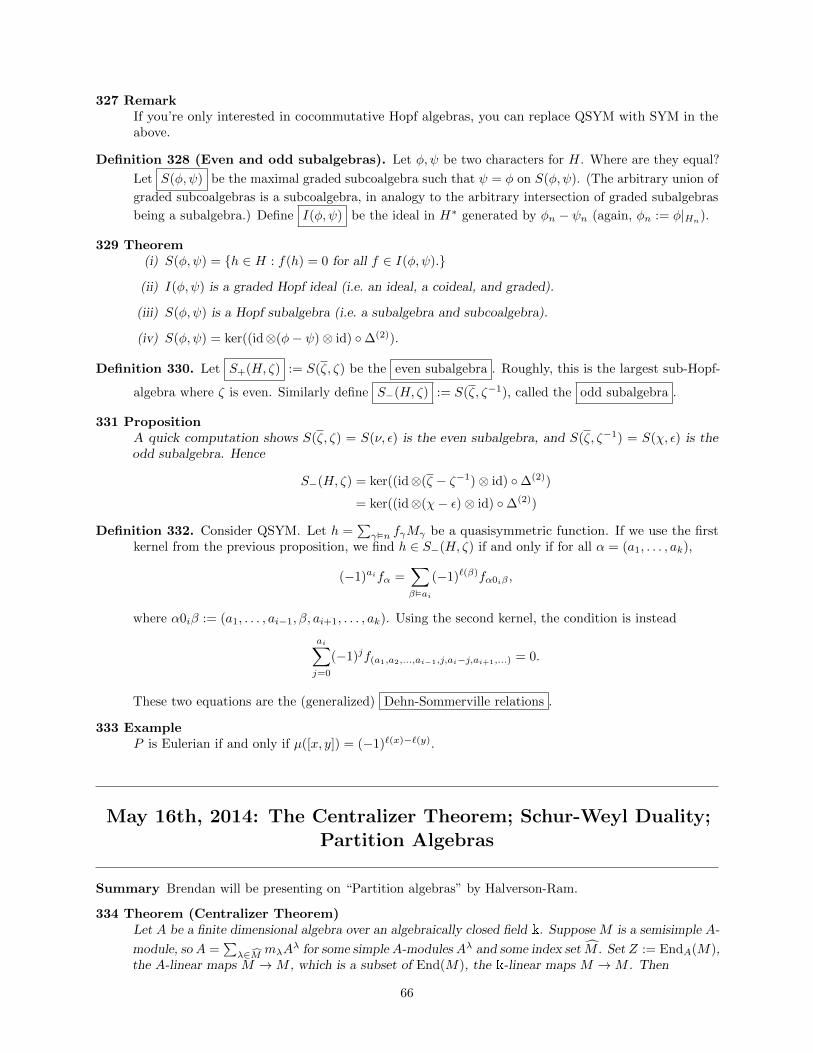
327 RemarkIf you’re only interested in cocommutative Hopf algebras, you can replace QSYM with SYM in theabove.
Definition 328 (Even and odd subalgebras). Let φ, ψ be two characters for H. Where are they equal?
Let S(φ, ψ) be the maximal graded subcoalgebra such that ψ = φ on S(φ, ψ). (The arbitrary union of
graded subcoalgebras is a subcoalgebra, in analogy to the arbitrary intersection of graded subalgebras
being a subalgebra.) Define I(φ, ψ) be the ideal in H∗ generated by φn − ψn (again, φn := φ|Hn).
329 Theorem(i) S(φ, ψ) = h ∈ H : f(h) = 0 for all f ∈ I(φ, ψ).
(ii) I(φ, ψ) is a graded Hopf ideal (i.e. an ideal, a coideal, and graded).
(iii) S(φ, ψ) is a Hopf subalgebra (i.e. a subalgebra and subcoalgebra).
(iv) S(φ, ψ) = ker((id⊗(φ− ψ)⊗ id) ∆(2)).
Definition 330. Let S+(H, ζ) := S(ζ, ζ) be the even subalgebra . Roughly, this is the largest sub-Hopf-
algebra where ζ is even. Similarly define S−(H, ζ) := S(ζ, ζ−1), called the odd subalgebra .
331 PropositionA quick computation shows S(ζ, ζ) = S(ν, ε) is the even subalgebra, and S(ζ, ζ−1) = S(χ, ε) is theodd subalgebra. Hence
S−(H, ζ) = ker((id⊗(ζ − ζ−1)⊗ id) ∆(2))
= ker((id⊗(χ− ε)⊗ id) ∆(2))
Definition 332. Consider QSYM. Let h =∑γn fγMγ be a quasisymmetric function. If we use the first
kernel from the previous proposition, we find h ∈ S−(H, ζ) if and only if for all α = (a1, . . . , ak),
(−1)aifα =∑βai
(−1)`(β)fα0iβ ,
where α0iβ := (a1, . . . , ai−1, β, ai+1, . . . , ak). Using the second kernel, the condition is instead
ai∑j=0
(−1)jf(a1,a2,...,ai−1,j,ai−j,ai+1,...) = 0.
These two equations are the (generalized) Dehn-Sommerville relations .
333 ExampleP is Eulerian if and only if µ([x, y]) = (−1)`(x)−`(y).
May 16th, 2014: The Centralizer Theorem; Schur-Weyl Duality;Partition Algebras
Summary Brendan will be presenting on “Partition algebras” by Halverson-Ram.
334 Theorem (Centralizer Theorem)Let A be a finite dimensional algebra over an algebraically closed field k. Suppose M is a semisimple A-
module, so A =∑λ∈M mλA
λ for some simple A-modules Aλ and some index set M . Set Z := EndA(M),the A-linear maps M →M , which is a subset of End(M), the k-linear maps M →M . Then
66
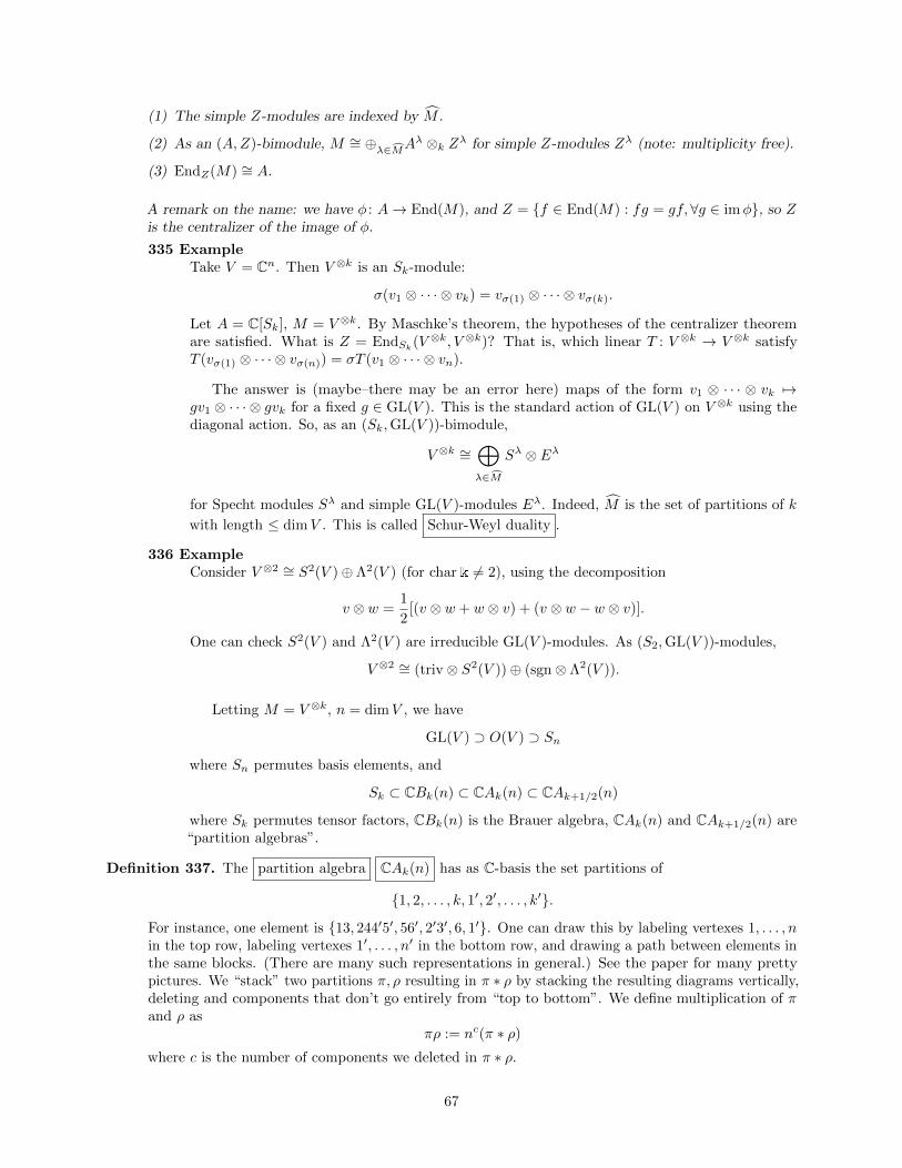
(1) The simple Z-modules are indexed by M .
(2) As an (A,Z)-bimodule, M ∼= ⊕λ∈MAλ ⊗k Zλ for simple Z-modules Zλ (note: multiplicity free).
(3) EndZ(M) ∼= A.
A remark on the name: we have φ : A→ End(M), and Z = f ∈ End(M) : fg = gf,∀g ∈ imφ, so Zis the centralizer of the image of φ.
335 ExampleTake V = Cn. Then V ⊗k is an Sk-module:
σ(v1 ⊗ · · · ⊗ vk) = vσ(1) ⊗ · · · ⊗ vσ(k).
Let A = C[Sk], M = V ⊗k. By Maschke’s theorem, the hypotheses of the centralizer theoremare satisfied. What is Z = EndSk(V ⊗k, V ⊗k)? That is, which linear T : V ⊗k → V ⊗k satisfyT (vσ(1) ⊗ · · · ⊗ vσ(n)) = σT (v1 ⊗ · · · ⊗ vn).
The answer is (maybe–there may be an error here) maps of the form v1 ⊗ · · · ⊗ vk 7→gv1 ⊗ · · · ⊗ gvk for a fixed g ∈ GL(V ). This is the standard action of GL(V ) on V ⊗k using thediagonal action. So, as an (Sk,GL(V ))-bimodule,
V ⊗k ∼=⊕λ∈M
Sλ ⊗ Eλ
for Specht modules Sλ and simple GL(V )-modules Eλ. Indeed, M is the set of partitions of k
with length ≤ dimV . This is called Schur-Weyl duality .
336 ExampleConsider V ⊗2 ∼= S2(V )⊕ Λ2(V ) (for chark 6= 2), using the decomposition
v ⊗ w =1
2[(v ⊗ w + w ⊗ v) + (v ⊗ w − w ⊗ v)].
One can check S2(V ) and Λ2(V ) are irreducible GL(V )-modules. As (S2,GL(V ))-modules,
V ⊗2 ∼= (triv⊗ S2(V ))⊕ (sgn⊗ Λ2(V )).
Letting M = V ⊗k, n = dimV , we have
GL(V ) ⊃ O(V ) ⊃ Sn
where Sn permutes basis elements, and
Sk ⊂ CBk(n) ⊂ CAk(n) ⊂ CAk+1/2(n)
where Sk permutes tensor factors, CBk(n) is the Brauer algebra, CAk(n) and CAk+1/2(n) are“partition algebras”.
Definition 337. The partition algebra CAk(n) has as C-basis the set partitions of
1, 2, . . . , k, 1′, 2′, . . . , k′.
For instance, one element is 13, 244′5′, 56′, 2′3′, 6, 1′. One can draw this by labeling vertexes 1, . . . , nin the top row, labeling vertexes 1′, . . . , n′ in the bottom row, and drawing a path between elements inthe same blocks. (There are many such representations in general.) See the paper for many prettypictures. We “stack” two partitions π, ρ resulting in π ∗ ρ by stacking the resulting diagrams vertically,deleting and components that don’t go entirely from “top to bottom”. We define multiplication of πand ρ as
πρ := nc(π ∗ ρ)
where c is the number of components we deleted in π ∗ ρ.
67
Definition 338. We define an action of CAk(n) on V ⊗k as follows. Suppose v1, . . . , vn is a basis of V withdimV = n. Now k-tuples I ∈ [n]k index a basis for V ⊗k,
vI := vi1 ⊗ · · · ⊗ vik if I = (i1, . . . , ik).
View (I, J) as a function 1, 2, . . . , k, 1′, 2′, . . . , k′ → [n] where I corresponds to the unprimed elementsand J to the primed elements. For π a partition, define
(π)IJ =
1 if (I, J) is constant on blocks of π0 else
Then π : V ⊗k → V ⊗k viaπvI =
∑J
(π)IJvJ .
339 ExampleLet π = 1′, 122′, 33′, k = 3, n = 2. Then πv112 = v112 + v212. Now consider applying thetransposition (2, 1) ∈ S2; this gives πv221 = v221 + v121. So, the CAk(n)-action and the actionof Sn commute.
340 TheoremThe above-defined map CAk(n)→ End(V ⊗k) has image EndSn(V ⊗k). We can decompose V ⊗k as a(CAk(n), Sn)-bimodule
V ⊗k ∼=⊕
λ∈Ak(n)
Aλk(n)⊗ Sλ
where the Aλk(n) are simple modules and the Sλ are Specht modules. As Sn-modules,
V ⊗k ∼=⊕
λ∈Ak(n)
dim(Aλk(n))Sλ.
A relatively easy computation gives (as Sn-modules)
V ⊗k ∼= (IndSnSn−1ResSnSn−1
)k1,
which is analogous to the Pieri formula.
May 19th, 2014: Internal Product on SYM; P -partitions;Factorizations with Prescribed Descent Sets
Summary Jair is presenting “Multipartite P -partitions and inner products of skew Schur functions” byGessel, 1984.
341 RemarkRecall Λ (the symmetric functions in countably many variables t = t1, t2, . . .) is a bialgebra usingthe usual multiplication and the following comultiplication. First view Λ⊗ Λ as Λ on the alphabetx ∪ y = x1, y1, x2, y2, . . .. Given f(t), we define ∆(f(t)) = f(x ∪ y); since f is symmetric, the order inwhich we substitute variables is irrelevant, so this is well-defined. An alternate coproduct ∆′ is givenby ∆′f(t) = f(xy), where we interpret the right-hand side as being over xy := xiyj : xi ∈ x, yj ∈ y.
Recall that, for the usual coproduct, pi is primitive, so ∆pi = 1⊗ pi + pi ⊗ 1. For this alternatecoproduct, we have
∆′pi = ∆′(ti1 + ti2 + · · · ) = ∆′((x1y1)i + (x1y2)i + (x2y1)i + · · ·
= xi1(yi1 + yi2 + · · · ) + xi2(· · · ) + · · · = pi(x)pi(y).
68
Hence ∆′pi = pi(x)⊗ pi(y), so pi is grouplike under ∆′.
Fact: (Λ,m,∆′, u, ε) is a bialgebra.
Definition 342. We have a multiplication on Λ∗ induced by ∆′. We also have an isomorphism
Λ→ Λ∗
f 7→ 〈f,−〉
using the Hall inner product. This induces a multiplication ∗ on Λ as the unique solution to
〈f ∗ g, h〉 = 〈f ⊗ g,∆′h〉.
Consider this operation on the pi’s. Recall that pλ and pλ/zλ are dual bases, where if λ =1m12m2 · · · , then zλ = 1m1m1!2m2m2! · · · . Hence
〈pµ ∗ pν , pλ〉 = 〈pµ ⊗ pν , pλ ⊗ pλ〉= 〈pµ, pλ〉〈pν , pλ〉= δµλzλδνλzλ.
Thus pµ ∗ pν = 0 if µ 6= ν, and otherwise
〈pµ ∗ pµ, pλ〉 = z2λδµλ = 〈zµpµ, pλ〉,
so that pµ ∗ pν = δµνzµpµ. Call the ∗ operation the internal product .
343 PropositionFact: ∗ is equivalent to tensoring Sn-representations, in the following sense. Recall the Frobeniuscharacteristic map
chχ =∑µ
χ(µ)
zµpµ,
where χ is a class function on Sn and the sum is over conjugacy classes.
Claim:chχ1 ⊗ χ2 = chχ1 ∗ chχ2
andch(V1 ⊗ V2) = chV1 ∗ chV2
for Sn-modules V1, V2. (Compare to our earlier definition,
ch(V1 ⊗ V2)↑Sn+m
Sn×Sm= (chV1)(chV2).)
Proof (of claim). Recall sλ =∑ χλ(µ)
zµpµ = chχλ, where the χλ are the irreducible characters. Hence
sλ ∗ sν =∑µ1,µ2
χλ(µ1)χν(µ2)
zµ1zµ2
pµ1 ∗ pµ2
=∑µ
χλ(µ)χν(µ)
zµpµ
= chχλ ⊗ χν .
Definition 344. If π is a permutation on n letters, let D(π) denote the usual descent set of π, which is asubset [n− 1]. There is a standard “stars and bars” bijection between n-compositions and subsets of[n− 1], so we may consider D(π) as an n-composition.
If α = (α1, α2, . . .) is a composition, let R(α) be the corresponding ribbon λ/µ, defined as in
the following example:
69
345 ExampleR(3214) is −− − ∗ ∗ ∗ ∗/ −− − ∗/ −− ∗ ∗/ ∗ ∗∗ where the ∗’s indicate boxes taken and the−’s indicate boxes skipped, and the /’s indicate new rows; this is in English notation. Note thenumber of ∗’s, read bottom-to-top, is 3214. Further, 3214 corresponds via stars and bars to
∗ ∗ ∗ | ∗ ∗ | ∗ | ∗ ∗ ∗ ∗
A function f : [10]→ P is “compatible” with this if
f(1) ≤ f(2) ≤ f(3) > f(4) ≤ f(5) > f(6) > f(7) ≤ f(8) ≤ f(9) ≤ f(10).
Filling R(3214) subject to these inequalities corresponds precisely to filling R(3214) weaklyincreasing along rows and strictly increasing down columns. This property characterizes R(3214).Moreover, the pattern of ∗’s form a “ribbon” in an obvious way.
346 TheoremLet π ∈ Sn and supposeD1, . . . , Dk ⊂ [n−1]. The (“absurd fact”) number of factorizations π = π1 · · ·πkwhere D(πi) = Di for all i is
〈sR(D(π)), sR(D1) ∗ · · · ∗ sR(Dk)〉.
Proof Lengthy; we’ll just hit a few high points for the rest of the lecture.
Definition 347. Let P be a poset P = ([n],≤P ). A partition P -partition is a function
f : [n]→ P
which is
i. weakly increasing, so i ≤p j implies f(i) ≤ f(j);
ii. “squishes nicely”, so that if i < j (in [n]) with f(i) = f(j), then i <p j.
Equivalently, if i <p j and i > j, then f(i) < f(j).
348 ExampleLet P have vertices 1, 2, 3, 4 with covering relations 1 < 2, 1 < 3, 3 < 4. Then a P -partition mustsatisfy f(1) ≤ f(2), f(1) ≤ f(4), f(4) < f(3).
Definition 349. Let A(P ) = P-partitions and let ΓP be the generating function
ΓP :=∑
f∈A(p)
n∏i=1
xf(i) ∈ QSYM .
If π ∈ Sn, form a poset π(1) < π(2) < π(3) < · · · . Then Γπ = FD(π), the fundamental quasisymmetricfunction associated with the descents of π.
350 RemarkHow do these P -partitions connect to counting factorizations? The idea is
∆′(FD(π)) =∑
τσ=π∈Sn
FD(τ)(x)FD(σ)(y).
351 ExampleGiven skew shape λ/µ, take labeled poset Pλ/µ by −− ∗ ∗ ∗/ ∗ ∗ ∗ /∗ which maps to the posetwith covering relations 2 < 1, 2 < 3, 3 < 4, 5 < 4, 5 < 6, 6 < 7. Then ΓPλ/µ = sλ/µ.
352 ConjectureOnly the skew shapes give posets with symmetric associated quasisymmetric functions; seeStanley.
70
May 21, 2014: (Special) Double Posets, E-Partitions, Pictures,Yamanouchi Words, and a Littlewood-Richardson Rule
Summary Today, Michael is lecturing on “A Self Paired Hopf Algebra on Double Posets and a Littlewood-Richardson Rule” by Malvenuto and Reutenauer. Outline:
(1) ZD is a graded Hopf algebra
(2) ZDS is a special case
(3) Connection to L-R rule
Definition 353. A double poset is a triple (E,<1, <2) where E is finite, <1 and <2 are two partial orders
on E. (Today, E will typically refer to a double poset.) Define a morphism between double posetsas one which is order-preserving for both partial orders, so we have a notion of isomorphism. Todaywe’ll tacitly take double posets only up to isomorphism, i.e. we’ll implicitly use isomorphism classes ofdouble posets.
Let D be be the set of double posets, and ZD the formal Z-linear combinations of double posets.
354 ExampleGiven a poset, label the vertices giving a total order; use the original order as <1, and use thelabeling order for <2.
Definition 355. Let E,F ∈ D. Define EF to be the poset (E ∪ F,<1, <2) where <1 compares pairs ofelements of E or of F using their first orders and pairs consisting of one element of E and one elementof F are incomparable. <2 is the same using the second orders, except e <2 f for any e ∈ E, f ∈ F .
Definition 356. Suppose (E,<) is a poset. An inferior order ideal I is a subset of E which is closed under
<, i.e. if y ∈ I and x < y, then x ∈ I. Likewise a superior order ideal is closed under >. Define (I, S)
to be a decomposition of E if I is an inferior order ideal, S is a superior order ideal, and E is the
disjoint union of I and S. (Hence I and S are complements.)
Definition 357. Let (E,<1, <2) be a double poset. Define a decomposition of E to be a decomposition of(E,<2), but endow I, S with partial orders <1 and <2 by restriction, yielding double posets.
Definition 358. We define a comultiplication ∆: ZD → ZD ⊗ ZD by breaking into decompositions:
∆(E,<1, <2) =∑
(I,S) of (E,<1,<2)
(I,<1, <2)⊗ (S,<1, <2).
359 TheoremZD is a graded Hopf algebra over Z (graded by size of E). (This is different from our usual assumptionthat Hopf algebras are over fields, but it works out.) See the paper for a terminal morphism to QSYM.
Definition 360. Let E ∈ D. If <2 is a total order, then E is called a special double poset . This is just a
labeled poset. Let ZDS be the subset of ZD spanned by special posets.
Definition 361. A linear extension of a special double poset E is a total order on E that extends <1.Given a linear extension, write the elements of E in increasing order, e1 <1 e2 <1 e3 <1 · · · . Now letω : E → [#E] be the labelling given by <2. Define σ ∈ S#E by σ(i) = ω(ei). For instance, with the“Y”-shaped poset labeled 1 at the bottom, 2 at the branch, and 3 and 4 at the tips, extend the poset toa linear order by taking 3 > 4. Then σ in one-line notation is 1243.
71
362 TheoremZDS is a sub-bialgebra of ZD, and there is a bialgebra homomorphism
ZDS → ZS
which sends a special double poset to the sum of all its linear extensions.
Definition 363. A Yamanouchi word is as usual: it’s a word in P such that when read left to right thenumber of 1’s always weekly exceeds the number of 2’s, which always weekly exceeds the number of
3’s, etc. For instance, w = 11122132 is Yamanouchi. It has weight 142331. The complement of a
word in P is given by replacing i by k − i+ 1, where k is the maximum element of P appearing in theword. For instance, the complement of w is 33322312.
Definition 364. If E ∈ D, a map χ : E → X (where X is a totally ordered set) is an partition E-partition
if
(1) e <1 e′ ⇒ χ(e) ≤ χ(e′), and
(2) e <1 e′ and e ≥2 e
′ together imply χ(e) < χ(e′).
(Compare to the previous lecture’s P -partitions. There <2 comes from the standard ordering on [n],though this is a little more general.)
Definition 365. Given a special double poset (E,<1, <2) with labeling ω (i.e. ω encodes the total order <2
as above) and a word w = a1 · · · an on a totally ordered alphabet A, we say w fits into E if the mape 7→ aw(e) is an E-partition.
366 ExampleConsider the case when the word is the one-line notation of a permutation in Sn. The mapto consider takes e to τω(e). Since τ is bijective, the second condition for an E-partition isvacuously satisfied, so we just need the map (E,<1)→ [n] to be weakly increasing.
Definition 367. Given a partition ν of n, we can construct a special double poset as follows. Let Eν bethe Ferrers diagram of ν. For concreteness, use French notation and consider Eν ⊂ N⊗ N. Let <1 bethe partial order induced by the component-wise order on N× N. Let <2 be the partial order inducedby (x, y) <2 (x′, y′) if and only if y > y′ or y = y′ and x < x′. Hence Eν is a double poset.
Definition 368. A picture between two double posets E,F is a bijection φ : E → F such that (1) e <1
e′ ⇒ φ(e) <2 φ(e′) and (2) f <1 f′ ⇒ φ−1(f) ≤2 φ
−1(f ′). (The origin of the term “picture” is unclear;originally due to Zelevinsky in 1981.)
Given a double poset E, define E to be E but using the opposite posets for both <1 and <2.
369 TheoremLet E be a special double poset. Suppose ν is a partition. Then the number of pictures from E to Eνis
i. the number of Yamanouchi words of weight ν whose complement fits into E;
ii. the number of Yamanouchi words whose mirror image fits into E
Note: Zelevinsky says (ii) gives the Littlewood-Richardson coefficients. We only have one partition νhere, so we need two more: these can be encoded in the special double poset E, though it seems thetranslation is not entirely immediate.
Proof See paper. We’ll just discuss one proposition it relies on.
72
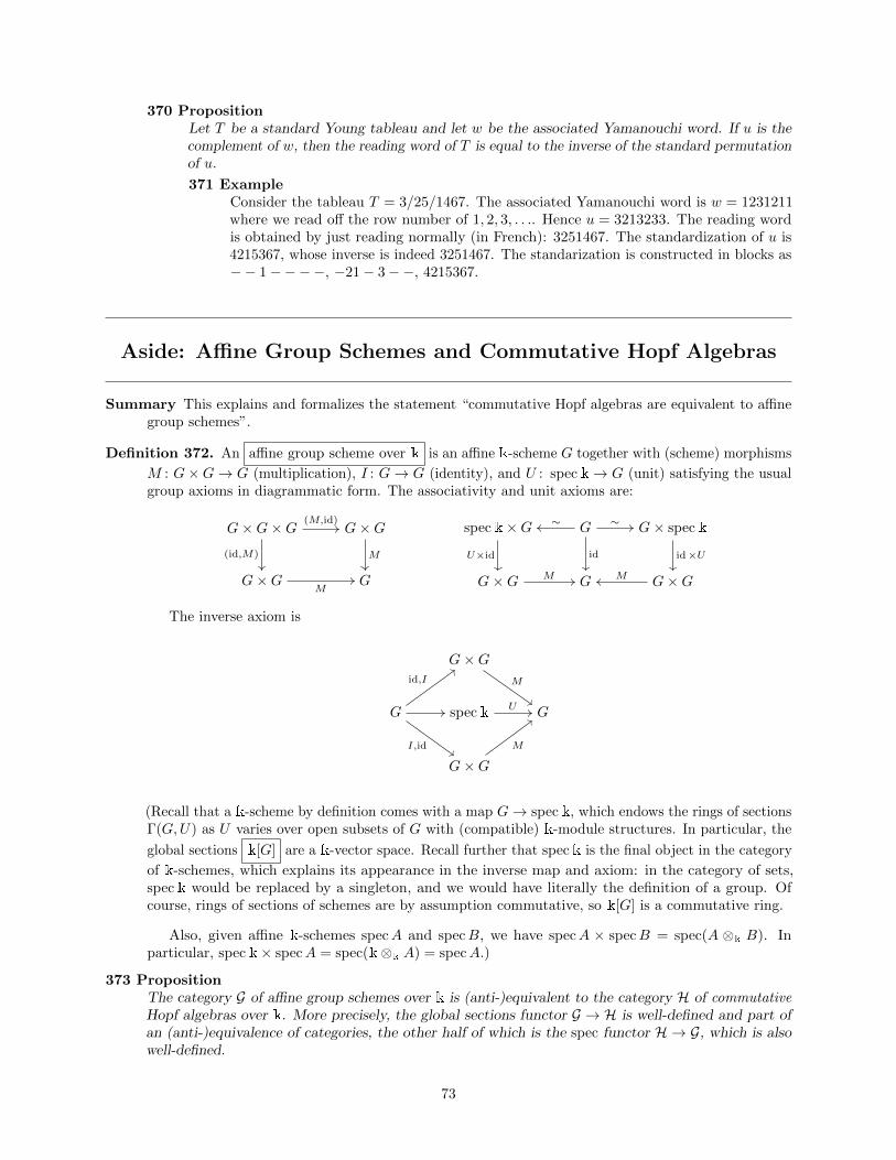
370 PropositionLet T be a standard Young tableau and let w be the associated Yamanouchi word. If u is thecomplement of w, then the reading word of T is equal to the inverse of the standard permutationof u.
371 ExampleConsider the tableau T = 3/25/1467. The associated Yamanouchi word is w = 1231211where we read off the row number of 1, 2, 3, . . .. Hence u = 3213233. The reading wordis obtained by just reading normally (in French): 3251467. The standardization of u is4215367, whose inverse is indeed 3251467. The standarization is constructed in blocks as−− 1−−−−, −21− 3−−, 4215367.
Aside: Affine Group Schemes and Commutative Hopf Algebras
Summary This explains and formalizes the statement “commutative Hopf algebras are equivalent to affinegroup schemes”.
Definition 372. An affine group scheme over k is an affine k-scheme G together with (scheme) morphisms
M : G×G→ G (multiplication), I : G→ G (identity), and U : speck→ G (unit) satisfying the usualgroup axioms in diagrammatic form. The associativity and unit axioms are:
G×G×G G×G
G×G G
(M,id)
(id,M) M
M
speck×G G G× speck
G×G G G×G
U×id
∼
id
∼
id×U
M M
The inverse axiom is
G×G
G speck G
G×G
Mid,I
I,id
U
M
(Recall that a k-scheme by definition comes with a map G→ speck, which endows the rings of sectionsΓ(G,U) as U varies over open subsets of G with (compatible) k-module structures. In particular, the
global sections k[G] are a k-vector space. Recall further that speck is the final object in the category
of k-schemes, which explains its appearance in the inverse map and axiom: in the category of sets,speck would be replaced by a singleton, and we would have literally the definition of a group. Ofcourse, rings of sections of schemes are by assumption commutative, so k[G] is a commutative ring.
Also, given affine k-schemes specA and specB, we have specA × specB = spec(A ⊗k B). Inparticular, speck× specA = spec(k⊗k A) = specA.)
373 PropositionThe category G of affine group schemes over k is (anti-)equivalent to the category H of commutativeHopf algebras over k. More precisely, the global sections functor G → H is well-defined and part ofan (anti-)equivalence of categories, the other half of which is the spec functor H → G, which is alsowell-defined.
73
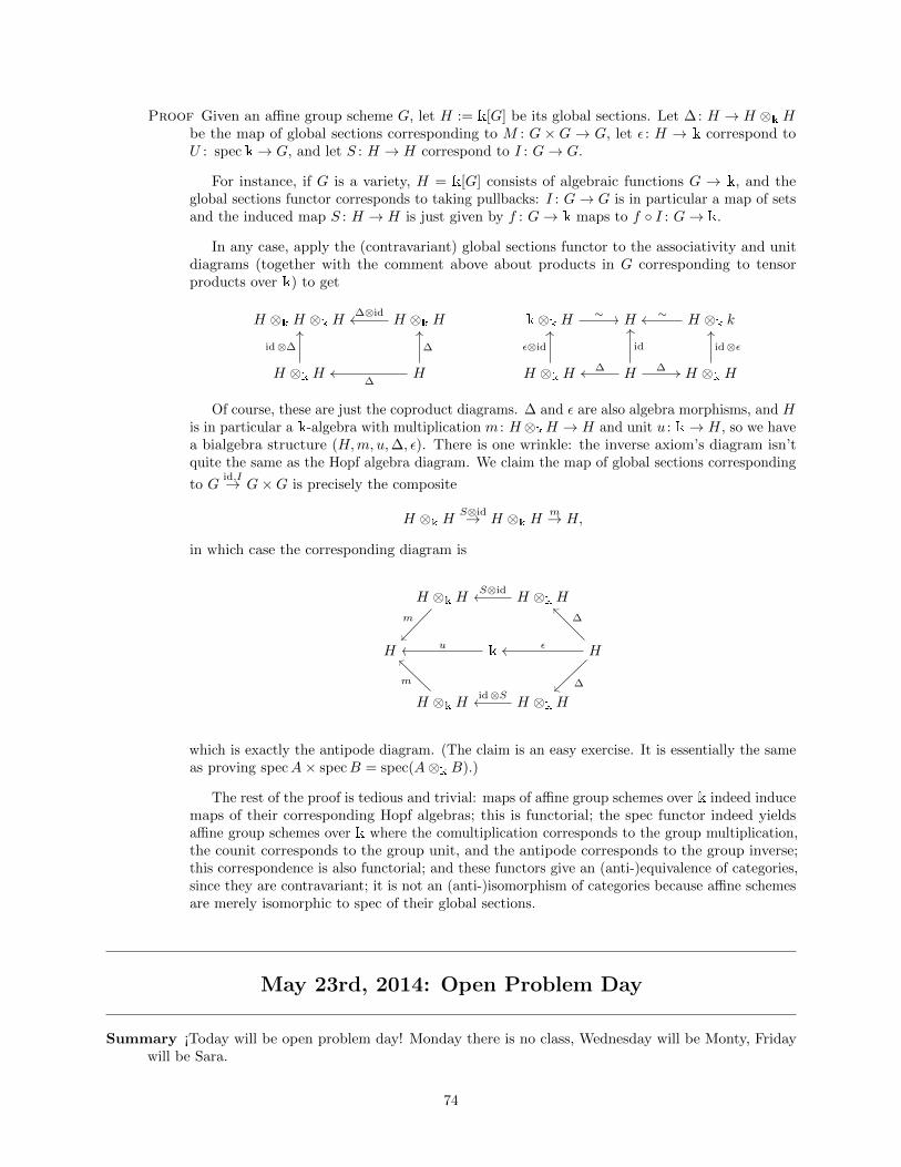
Proof Given an affine group scheme G, let H := k[G] be its global sections. Let ∆: H → H ⊗k Hbe the map of global sections corresponding to M : G × G → G, let ε : H → k correspond toU : speck→ G, and let S : H → H correspond to I : G→ G.
For instance, if G is a variety, H = k[G] consists of algebraic functions G → k, and theglobal sections functor corresponds to taking pullbacks: I : G→ G is in particular a map of setsand the induced map S : H → H is just given by f : G→ k maps to f I : G→ k.
In any case, apply the (contravariant) global sections functor to the associativity and unitdiagrams (together with the comment above about products in G corresponding to tensorproducts over k) to get
H ⊗k H ⊗k H H ⊗k H
H ⊗k H H
∆⊗id
id⊗∆
∆
∆
k⊗k H H H ⊗k k
H ⊗k H H H ⊗k H
∼ ∼
ε⊗id
∆
id
∆
id⊗ε
Of course, these are just the coproduct diagrams. ∆ and ε are also algebra morphisms, and His in particular a k-algebra with multiplication m : H⊗kH → H and unit u : k→ H, so we havea bialgebra structure (H,m, u,∆, ε). There is one wrinkle: the inverse axiom’s diagram isn’tquite the same as the Hopf algebra diagram. We claim the map of global sections corresponding
to Gid,I→ G×G is precisely the composite
H ⊗k HS⊗id→ H ⊗k H
m→ H,
in which case the corresponding diagram is
H ⊗k H H ⊗k H
H k H
H ⊗k H H ⊗k H
m
S⊗id
u ε
∆
∆m
id⊗S
which is exactly the antipode diagram. (The claim is an easy exercise. It is essentially the sameas proving specA× specB = spec(A⊗k B).)
The rest of the proof is tedious and trivial: maps of affine group schemes over k indeed inducemaps of their corresponding Hopf algebras; this is functorial; the spec functor indeed yieldsaffine group schemes over k where the comultiplication corresponds to the group multiplication,the counit corresponds to the group unit, and the antipode corresponds to the group inverse;this correspondence is also functorial; and these functors give an (anti-)equivalence of categories,since they are contravariant; it is not an (anti-)isomorphism of categories because affine schemesare merely isomorphic to spec of their global sections.
May 23rd, 2014: Open Problem Day
Summary ¡Today will be open problem day! Monday there is no class, Wednesday will be Monty, Fridaywill be Sara.
74
374 RemarkSadly, these notes have been redacted. They were distributed in an email to the class, though.
May 28th, 2014: Hecke Algebra of Sn; Kazhdan-LusztigPolynomials; Cells
Summary Monty McGovern is lecturing on the Kazhdan-Lusztig polynomials today.
375 RemarkRecall the standard presentation for the symmetric group expressing it as a Coxeter group, Sn =〈s1, . . . , sn−1 : s2
i = 1, (sisj)mij = 1〉 where mij is 2 if |i− j| ≥ 2 and 3 if |i− j| = 1 for i 6= j.
Definition 376. The Hecke algebra H attached to Sn is the following structure. It is an algebra overZ[q, q−1] generated by T1, . . . , Tn−1 subject to relations
(Ti + 1)(Ti − q) = 0, (TiTj)mij = 1 (i 6= j)
with mij as above. Then we may set Twi = Tsi1 · · ·Tsik if w = si1 · · · sik is a reduced expression for w.
Claim: Tw is independent of the choice of decomposition, and the Tw form a free basis for H overZ[q, q−1].
377 RemarkWe will produce a (Kazhdan-Lusztig) basis of H, also indexed by Sn, with triangular change of basismatrix to Tw, such that we can find quotients of certain left ideals spanned by the Cw (the new basisvectors) which are irreducible H-modules.
Definition 378. Recall the Bruhat order on Sn, in the following guise. Given a reduced decompositionw = si1 · · · sik , the elements v < w in Bruhat order are precisely the subexpressions of this reducedword (i.e. “cross off” some of the factors sij ).
Definition 379. Define an involution ι on H as follows. Unusually, ι does not fix the base ring of the algebraH, but instead ιq = q−1. Also use ιTw = T−1
w−1 .
Proof These operations preserve the defining operations.
We will find a new basis of H indexed by W := Sn consisting of elements fixed by ι. SinceT−1s = q−1Ts − (1 − q−1) is asymmetric, we need to enlarge our scalars to find ι-fixed elements. In
particular, use Z[q1/2, q−1/2].
Definition 380. Let Cs := q−1/2(Ts − q). One can check this is fixed by ι. Naively, we might try usingCw = Csi1 · · ·Csik for w = si1 · · · sik , but this is not independent of reduced decomposition. However,we will take this as a “first approximation” and tweak it.
381 NotationLet ε(w) := (−1)`(w), which is 1 if w is even and −1 if w is odd. Let qw := q`(w) where `(w) is the
length of a reduced decomposition for w.
382 Theorem (Kazhdan-Lusztig, Inv. Math 53 (1979), 105-184)For each w ∈ Sn, there is a unique Cw ∈ H such that
(a) ιCw = Cw
75
(b) Cw = εwq1/2w∑x≤w εxq
−1x Px,wTx where Pw,w = 1, Px,w ∈ N[q] has degree ≤ 1/2(`(w)− `(x)− 1)
if x < w, and Px,w = ιPx,w. Finally, Px,z = 0 if x 6≤ z.
Requirement (b) is a refinement of the statement above that the change of basis matrix between Cwand Tx is triangular. The Px,w are the Kazhdan-Lusztig polynomials .
383 PropositionTheir proof of existence yields an inductive formula for the Kazhdan-Lusztig polynomials,
Px,z = q1−cPsx,sw + qcPx,sw −∑z<swsz<z
µ(z, sw)q−1/2z q1/2
w Px,z
where: s is a transposition chosen so that sw < w; c = 0 if x < sx and c = 1 if x > sx; µ(z, sw) :=coefficient of q1/2(`(sw)−`(z)−1) in Pz,sw. (One may argue that indeed the Px,w involve only integralpowers of q, hence they are honest polynomials in q.)
384 CorollaryAll constant terms of non-zero Px,w are 1. Moreover, Px,w = 0 iff x 6≤ w.
(Indeed, a result of Polo says that every polynomial in N[x] with constant term 1 is a Kazhdan-Lusztig polynomial for some Coxeter group.)
385 PropositionUsing the Kazhdan-Lusztig basis (it is indeed a basis from the triangular relationship (b) above), wecan deduce an “almost triangular” formula for the left action of H on a Cw (there is a similar formulafor the right action). In particular,
TsCw =
−Cw sw < wqCw + q1/2Csw + q1/2
∑z<wsz<z
µ(z, w)Cz sw > w
Roughly, much of the complicated information that goes into constructing the polynomials gets washedout by this action.
Definition 386. Write x ≤L w if the left ideal HCw contains an element involving Cx. Similarly we define
x ≤R w if the right ideal CwH contains an element involving Cx. Likewise define x ≤LR w if HCwH
(the set of sums of products hCwh′) contains a term involving Cx.
387 PropositionWe can decompose H into left ideals spanned by Cw. It is clear that
Z[q1/2, q−1/2]Cx : x ≤L w
is a left ideal of H, called the left cone over w. Similarly we have the right cone and the
two-sided cone .
Definition 388. To make these cones irreducible (as H-modules), we pass to the corresponding “cells”, asfollows. Define x <L w if x ≤L w but w 6≤L x (this is essentially fixing up antisymmetry). Then thespan of all Cx with x ≤L w modulo the span of all Cx with x <L w is a quotient by the constructionof left ideals of H, so is a left module for H, which at least has a better chance of being irreducible.
We call this quotient or the set of x with x ∼L w (meaning x ≤L w and w ≤L x) the left cell of w .
We similarly define right cells and two-sided cells or double cells , giving equivalence relations∼R,∼LR.
These relations have “many, many, many applications to representation theory of left cells”.
76
389 PropositionFor W = Sn, the left cells are irreducible H-modules, and likewise for right and two-sided cells.Moreover, the left, right, and two-sided cells may be computed by RSK, w 7→ (TI(w), TR(w)) where TIis the insertion tableau, TR is the recording tableau. In particular, w is in the same left cell as v (i.e.w ∼L v) iff TI(w) = TI(v), w is in the same right cell as v iff TR(w) = TR(v), and w and v are in thesame double cell iff TI(w) = TI(v), TR(w) = TR(v).
390 RemarkThis implies that left, right, and two-sided cells as modules are irreducible. (Note that two-sidedcells are bimodules, so they use both left and right actions.) There are generalizations to othergroups, for instance the hyperoctahedral group, but these are no longer irreducible in general.
More information on this comes from Chapter 7 of Humphreys “Reflection Groups andCoxeter Groups”, 1990.
May 30th, 2014—Immaculate Basis for QSYM; (Standard)Immaculate Tableaux; Representations of 0-Hecke Algebras
Summary Sara is lecturing again today. She will be presenting on “Indecomposable Modules for the DualImmaculate Basis of QSYM”, by Berg, N. Bergeron, Saliola, Serreno, Zabrocki (BBSSZ).
391 RemarkThe following will be assumed as known background on QSYM.
Recall QSYM is defined to be the Q-span of all
Mα :=∑
i1<···<im
xα1i1xα2i2· · ·
where α = (α1, . . . , αm) ∈ Pm is a (strong) composition of n, written α n. Compositions are orderedby refinement (where refining a composition decreases it in this order). We define the fundamentalquasisymmetric functions in terms of the monomial quasisymmetric functions as
Fα :=∑β≤α
Mβ
=∑
i1≤···≤ij
xi1 · · ·xin
where if j ∈ ω(α), we require ij < ij+1. Here ω(α) := α1, α1 + α2, · · · , α1 + · · ·+ αm−1. (We don’tneed to include αm, since α n implies it.)
We can multiply fundamental quasisymmetric functions using
FαFβ = FD(u)FD(v) =∑
w∈uvFD(w),
where u ∈ S|α|, v ∈ S|β|, D(u) = α, D(v) = β, and u v is the shuffle product of u and v. Thecoproduct is
∆(Fα) =∑
Fγ ⊗ Fβ
where the sum is over compositions (γ, β) such that the ribbon corresponding to α can be cut intoribbons corresponding to γ and β.
77
The antipode is given byS(Fα) = (−1)|α|Fω(α).
Also recall Perms is the Hopf algebra of permutations, defined to have basis Pw for w ∈ ∪nSn. Ithas the “shuffle product” and the “cut coproduct”.
SYM := Q[h1, h2, . . .] and NSYM := Q〈H1, H2, . . .〉 with ∆(Hn) :=∑i+j=nHi ⊗Hj .
392 Theorem (Ditters Conjecture, proved by Hazewinkel)QSYM is freely generated as a polynomial ring. They’re indexed by compositions which arecertain Lyndon words.
393 Open ProblemHow do you write Hazewinkel’s generators of QSYM using Mα or Fα?
Definition 394. BBSSZ previously defined the immaculate basis Sα for NSYM (see BBSSZ’s “The
immaculate basis of the non-commutative symmetric functions”). Note that NSYM SYM → QSYMnaturally. Moreover, Perm maps surjectively onto QSYM via pw 7→ FD(w). This suggests NSYM maymap into Perm. Indeed,
NSYM Perm
SYM QSYM
dual
via
Hα
∑D(w)=ω(α) Pw
hα hα
Hence there are some Kα,β such that
Hβ =∑
Kα,βSα,
since the Sα are a basis. In fact, Kα,β is the number of “immaculate tableaux” (defined below) of
shape α content β. We define S∗a as the dual immaculate basis element.
Definition 395. Let α, β n (to be clear, strong compositions). An immaculate tableau of shape α andcontent β is a filling of the diagram of α with β1 one’s, β2 two’s, etc., such that
(i) each row is weakly increasing
(ii) the first column is strictly increasing from top to bottom
396 ExampleConsider 112/35/4445. (Since α is just a composition, the row lengths do not have to be weaklymonotonic.) Here α = (3, 2, 4) and β = (2, 1, 1, 3, 2).
Let Dα,β be defined to be the number of immaculate tableaux of shape α, content β. An immaculate
tableau T of content 1n is standard (and is highly restricted). For instance, T = 1235/4/67.
The descent set of an immaculate tableau T is the set of all i such that i+ 1 is in a row strictlybelow i. For T above, D(T ) = 3, 5.
78

397 PropositionS∗α =
∑T FD(T ), where the sum is over standard immaculate tableaux of shape α.
398 Theorem (BBSSZ-2013)S∗α is the Frobenius character of an indecomposable representation of Hn(0), the 0-Hecke algebra.
399 RemarkRecall Hn(q), the Hecke algebra of Sn, was defined last time, with generators Ti for 1 ≤ i ≤ n−1with certain relations, or as the span of Tw for w ∈ Sn where
TsiTw =
Tsi,w siw > wqTsiw + (q − 1)Tw siw < w
At q = 1, we just get the group algebra of Sn. At q = 0, we get the relations T 2i = −Ti, and
TiTj = TjTi. (There are several slightly different conventions; for instance, we used a differentone on the first day.) Another presentation: Hn(0) = 〈πi : 1 ≤ i < n〉 subject to π2
i = πi (useπi ↔ 1 + Ti).
400 Theorem (Norton, 1979)The irreducible representations of Hn(0) are indexed by compositions α. Each irreducible Lα isone-dimensional and spanned by vα ∈ Lα such that
πi(vα) =
0 i ∈ ω(α)vα otherwise
401 RemarkLet Gn := the Grothendieck group of finite dimensional representations of Hn(0) up to isomorphism
with addition given by exact sequences. In particular, it is the span of [A] where A is a finite dimensionalrepresentation of Hn(0), modded out by [B] = [A] + [C] when
0→ A→ B → C → 0
is an exact sequence of Hn(0)-modules. Let G := ⊕Gn
402 Remark[N ][M ] = Ind
Hn+m(0)Hn(0)⊗Hm(0)(N ⊗M), in exact analogy with the Sn representation ring above.
By Norton’s theorem, G is spanned by Lα : α is a composition.
403 Theorem (Duchamp-Krob-Leclere-Thibon, 1996)F : G→ QSYM given by [Lα] 7→ Fα is a graded Hopf algebra isomorphism.
404 PropositionHn(0) acts on the standard immaculate tableaux via
πi(T ) =
0 i, i+ 1 in first columnT if i is in a row weakly below i+ 1si(T ) otherwise
405 ExampleLet T = 129/3567/48; π1(T ) = T ; π2(T ) = 139/2567/48; π3(T ) = 0, etc.
406 NotationLet SIT(α) denote the set of standard immaculate tableaux of shape α.
407 PropositionThere is a natural partial order on SIT(α), where S < T if there exists σ ∈ Sn such that πσ(T ) = S.Take a linear extension and list SIT(α) as T1, T2, . . . , Tp.
79
408 ExampleT = 1234/56/789 is maximal for α = (4, 2, 3).
Let Mj be the span of Ti for i ≤ j. We have a filtration
0 ⊂M1 ⊂M2 ⊂ · · · ⊂Mp := V α,
where dim(Mj/Mj−1) = 1 (spanned by Tj). It follows that
πi(Tj +Mj−1) =
0 i ∈ D(Tj)Tj otherwise
So, [Mj/Mj−1] = [Lcomp(D(Tj))].
409 RemarkDifferent linear orders may give rise to different successive quotients, but the collection of themis unique up to isomorphism.
410 HomeworkCount # SIT(α). (Hopefully reasonable.)
411 Theorem (BBSSZ)In the above notation, F [V α] =
∑T∈SIT(α) FD(T ).
412 CorollaryV α is a cyclic module.
413 TheoremV α is indecomposable as an Hn(0)-module.
Definition 414. Given a composition α = (α1, . . . , αm), a Y-word Y -word is a word in [m] with j appearingαj times such that the first instance of j appears before the first instance of j + 1 for every j.
To each Y -word w, there is a unique corresponding standard immaculate tableau whose shape isgiven by the word’s content and which has a j in row wj .
415 ExampleThe SIT T = 129/3567/48 corresponds to the Y -word 11232223 (where we read off the rownumbers of 1, 2, . . . successively).
416 RemarkThey define a space Wordsαn given by the span of words w1 · · ·wn for wi ∈ [m] of content α =(α1, . . . , αm). There is an Hn(0)-action on this space
π(w1 · · ·wn) =
w wi+1 ≥ wiwsi wi+1 < wi
where wsi is w with the i and i+ 1st letters interchanged. What is F [Wordsαn]? What if we know
[Wordsαn] = [IndHα1⊗···⊗Hαn(0)L(α1) ⊗ · · · ⊗ L(αm)]?
(Exercise: prove this.) Then F [Wordsαn] = F(α1) · · ·F(αm) = hα.
June 2nd, 2014—Plethysms; P vs. NP vs. #P ; Standardizationand Matrices
80
Summary Sara is lecturing again today. Unfortunately Ed Witten had to cancel Wednesday’s lecture. Sarawill be presenting some lectures for Bogata on quasisymmetric functions instead.
417 RemarkThere are numerous analogues between SYM and QSYM: the representations of Sn and GLn vs. the0-Hecke algebra; the monomials mλ and the fundamentals Fα both expand nicely in terms of monomialquasisymmetric functions; the Schurs decompose very nicely using the fundamental basis.
Definition 418. Given two symmetric functions f(x1, x2, . . .) and g(x1, x2, . . .) = xa + xb + xc + · · · , define
the plethysm of f and g to be the function
f [g] := f(xa, xb, xc, . . .).
Then f [g] is again a symmetric function.
419 ExampleExpand h2[e2(X)] on X = x1, x2, x3. Then
h2[e2(x1, x2, x3)] = h2(x1x2 + x1x3 + x2x3)
= h2(x1x2, x1x3, x2x3)
= (x1x2)2 + (x1x3)2 + (x2x3)2 + x21x2x3 + x1x
22 + x3 + x1x2x
23
= s(2,2)(x1, x2, x3).
These computations get nasty by hand quickly. Using the infinite Schur functions (for instance),Sage tells us there is an s(1,1,1,1) term, but we didn’t have enough variables for this to show up.Doing some more examples, we see these plethysms seem to be Schur-positive, not multiplicityfree, and the number of terms can get horrendous quickly. Schur-positivity follows from showingsµ[sν ] is the character of a GLN representation: see Fulton-Harris, 1991.
420 Open ProblemFind a combinatorial or “optimal” formula for the coefficients dλµ,ν in the exapansion
sµ[sν ] =∑λ
dλµ,νsλ.
421 Theorem (Thrall, 1942)h2[hn(X)] has a very nice explicit formula.
Definition 422. P is the set of all questions which can be decided in polynomial time depending on theinput size. NP is the set of all questions for which one can test a proposed solution in polynomialtime depending on the input size. #P is the set of all questions of the form, “How many solutionsdoes X have?” where X is in NP .
423 Example
1. Does a permutation w ∈ Sn contain another v ∈ Sk? NP-complete; Bose-Buss-Lubiw, 1998.In NP .
2. How many instances of the permutation v ∈ Sk does w ∈ Sn have? Bose-Buss-Lubiw, 1998.This is in #P .
3. Does a permutation w ∈ Sn contain a fixed v ∈ Sk? Guillemot-Marx, 2013. In P . (Found alinear time algorithm!)
4. Does a graph G have a planar embedding? Kuratowski 1930, in P . Hopcroft-Tarjan 1974.
5. Does G have a 3-coloring? NP-complete, Gary-Johnson-Stockmeyer, 1976.
81
6. How many k-colorings does G have for k = 1, 2, 3, . . .? #P .
7. What are the coefficients of the chromatic polynomial? Jaeger-Vertifan-Welsh, 1990. Harderthan any #P − complete problem.
8. What is the determinant of an n× n matrix? (Williams 2012, Cohn-Umans 2013.) In P .
9. What is the permanent of an n × n matrix? (Valiant 1979) #P − complete. (Computepermanent by using cofactor expansion without negative signs.)
424 Open ProblemDoes P = NP? Does NP = #P? Does P = #P? All unknown. Millenium prize: $1,000,000 in USdollars for P vs NP problem.
425 RemarkMulmuley-Sohoni (2001-2002) have an approach to P 6= NP :
1. Homogeneous degree n polynomials form a vector space with a GLN action. Here N is the numberof monomials of degree n.
2. The determinant of an n× n matrix is a homogeneous polynomial of degree n2 which is computablein O(n3) time, perhaps O(n2+ε). (Cohn-Kleinberg-Szegedy-Umans 2005.)
3. The permanent of an n× n matrix is a homogeneous polynomial of degree n2. Its computation is a#P -complete problem. (Valiant, 1979a.)
4. Every formula f of size u can be written as a determinant of some k × k matrix Mf with entriesdepending linearly on the original inputs where k ≤ 2u. (Valiant, 1979b.)
5. Use GLN representation theory to study the orbit of the permanent vs. determinant.
426 Theorem (Loehr-Warrington, 2012)For any two partitions µ, ν,
sµ[sν(X)] =∑
A∈S(a,b)(µ,ν)
FDes(rw(A)−1).
(See their paper for definitions.)
427 RemarkThe plethysm sµ[sν ] is the generating function for semistandard tableaux with entries which aresemistandard tableaux. The weight of such a tableau is the product of the weights of each entry. If νis a fixed partition shape, we can identify T ∈ SSYT(ν) with its reading word, eg. T = 6/23/113 goesto 623113. For a tableau µ = (2, 2) with entries which are tableaux of shape ν = (3, 2, 1), we mighthave V ′ = (633222)(735244)/(423112)(423112). Let SSYTW (ν)(µ) be the set of all tableaux of shape µwith entries which are words associated to semistandard Young tableaux of shape ν. One an obtain amatrix from such an element by sticking the words into rows of a matrix. Let M(µ, ν) be the matricesobtained in this way. (We order the inner tableaux using lexicographic order.)
428 RemarkLet Wordsn be the words of length n in P. Define weight in the obvious way. Clearly
f(X) :=∑
w∈Wordsn
xw
is a symmetric function. How do we collect terms into a finite sum? (Question: what’s the Schurexpansion?)
Goal: partition the set Wordsn by standardizing them as above:
std: Wordsn → Sn.
82
429 Examplew = 331241123 maps to [671492358]. In steps,
331241123 7→ ..1..11.. 7→ ..1..23..
7→ · · ·
What are the fibers of this map? We can “lift” every letter by some amount so long as the relativeordering is the same, as in the quasisymmetric function shifting definition.
430 LemmaWe have
f(X) :=∑
w∈Wordsn
xw =∑π∈Sn
FDes(π−1)(X).
The left-hand side is the generating function for Wordsn. The right-hand side is the generating functionfor pairs (π, u) where π ∈ Sn and u = u1 . . . un is a weakly increasing word of length n such thatui < ui+1 whenever i ∈ Des(π−1). Let Iπ be the set of such pairs (π, u). Construct a weight preservingbijective function
g : Wordsn → ∪π∈SnIπw = w1 . . . wn ∈Wordsn 7→ (π, u) = (std(w), sort(w)).
431 Exampleg(331241123) = ([671492358], 111223334).
Question: does g−1 exist? A moment’s thought says yes. sort(w) is really just telling us how manyof each letter there were.
432 PropositionWe have
f(X) :=∑
w∈Wordsn
xw =∑π∈Sn
FDes(π−1)(X) =∑λ`n
fλsλ
where fλ is the number of standard tableaux of shape λ.
Proof Bijective proof relies on two important facts:
1. sλ =∑T∈SYT(λ) FDes(T )
2. RSK is a bijection roughly preserving descents.
433 RemarkWe would like to standardize elements of M(µ, ν) by standardizing the reading word. The most obviousway does not land in M(µ, ν). With more thought, there is a standardization algorithm which doeswork. An example computation:
434 ExampleLet
A =
8 7 2 106 1 9 412 5 11 3
∈ S3,4.
Then rw(A) = 6, 12, 8; 7, 1, 5; 11, 9, 2; 10, 4, 3.
Similarly we can produce a standardization of a matrix, for instance via
83
435 Example
M =
1 1 3 3 51 2 2 2 42 2 3 3 3
⇒ std(M) =
1 3 10 12 152 5 7 8 144 6 9 11 13
See Loehr-Warrington for more details.
Proof (of Loehr-Warrington’s theorem.) Bijective proof. Two things to check
1. The map S taking M ∈Ma,b to (std(M), sort(M)) is invertible.
2. The map std on Ma,b maps M(µ, ν) into Sa,b(µ, ν). (Sa,b(µ, ν) refers to the standard matrices.)
From here neither step is particularly involved!
436 Open ProblemExpand sµ[sν(X)] in Schur basis and relate back to P vs NP .
437 RemarkRecently established methods:
1. Use Dual Equivalence Graphs. (Assaf 2008-2013, Roberts 2013-2014.)
2. Flip Fα to sα ∈ 1, 0,−1ssort(alpha). (Egge-Loehr-Warrington, 2010.)
3. Find a quasi-Schur expansion: sλ =∑α:sort(α)=λ Sα. (Haglund-Luoto-Mason-van Willigenburg
2011, book 2013.)
438 Open ProblemOther similar open problems:
1. Find the Schur expansion of Macdonald polynomials
Hµ(X; q, t) :=∑π∈Sn
q−1µ (π)tmajµ(π)FDes(π−1)
(See Macdonald 1988, Haiman-Haglund-Loehr 2005.)
2. See also LLT polynomial expansions in same paper.
3. Find the Schur expansion of k-Schur functions
S(k)λ (X; q) =
∑S∗∈SST(µ,k)
qspin(S∗)FD(S∗).
(Lam-Lapointe-Morse-Shimozono + Lascoux, 2003-2010, Assaf-Billey 2012.) (Remark: there arecurrently five different definitions of k-Schurs that are conjecturally the same.)
439 Open ProblemEasier open problem: for a partition λ, find the Schur expansion of∑
π∈Sn:cycle(π)=λ
FDes(π).
June 4th, 2014—Counting Reduced Words; Stanley SymmetricFunctions; Little Bumps; k-Vexillary Permutations
84
Summary Sara is giving another Colombia lecture.
Definition 440. Every permutation w ∈ S∞ := ∪n>0Sn can be written as a finite product of adjacenttranspositions si = (i, i+ 1), sometimes in many ways. Her favorite permutation is
ν = [2, 1, 5, 4, 3] = s1s3s4s3 = s1s4s3s4 = s4s1s3s4 = s34s1s3s4.
There are evidently some relations involved: s2i = 1 (“involution”), sisj = sjsi when |i − j| > 1
(“commutation”), and sisi+1si = si+1sisi+1 (“braid”). Indeed, these are the only relations in the sensethat they give a presentation of S∞.
A minimal length expression for w is said to be reduced . The length `(w) is the number of
inversions. If w = sa1 · · · sap is reduced, we say the sequence (a1, . . . , ap) is a reduced word for w.
Let R(w) denote the set of reduced words for w.
441 RemarkToday’s questions: how many reduced words are there? What structure do they have?
442 Theorem (Tit’s Theorem)The graph with vertices indexed by reduced words in R(w) (for fixed w) and edges connecting twowords if they differ by a commutation move or a braid move is connected. If w = [2, 1, 5, 4, 3], thenR(w) has 8 elements arranged in a cycle,
1343− 1434− 4134− 4314− 4341− 3431− 3413− 3143− 1343.
443 Example[7, 1, 2, 3, 4, 6] has reduced word (6, 5, 4, 3, 2, 1), and we clearly can’t apply braid relations orcommutations, so there is precisely one such word. While we can count the number of reducedwords this way, we have to generate all of them, which is inefficient.
444 RemarkThere is one reduced word for the identity. For any other permutation,
#R(w) =∑
i∈Des(w)
#R(wsi).
This is not quite as “efficient as possible”, since we might compute #R(w′) multiple times while werecurse.
445 TheoremStanley’s first observation: R([n, n− 1, . . . , 3, 2, 1]) is the same as the number of standard tableaux ofthe staircase shape (n− 1, n− 2, . . . , 2, 1), which is(
n2
)!
1n−13n−2 · · · (2n− 3)!.
Definition 446. (Stanley 1984.) For any w ∈ Sn, define
Gw(X) :=∑
a∈R(w)
FDes(a)(X).
447 ExampleFor w = [7, 1, 2, 3, 4, 5, 6], Gw(X) = F(1,2,3,4,5)(X) = F(16)(X) = s16(X).
448 TheoremStanley’s second observation: Gw is a symmetric function with positive Schur expansion. They are
now called Stanley symmetric functions .
85
449 Theorem (Edelman-Greene 1987)Gw has positive Schur expansion,
Gw =∑λ
aλ,wsλ, aλ,w ∈ N.
Corollary: |R(w)| =∑λ aλ,wf
λ where fλ is the number of standard tableaux of shape λ.
450 ExampleIf w = w0, then Gw = sδ where δ is the staircase shape with n− 1 rows.
Proof They construct an injective map from R(w) to pairs of tableaux (P,Q) of the same shapewhere P is row- and column-strict and Q is standard. For each P every single standard tableauxof the same shape occurs as Q in the image.
Algorithm: Edelman-Greene insertion is a variation on RSK. The only difference is wheninserting i into a row with i and i+ 1 already, skip that row and insert i+ 1 into the next row.
451 ExampleFor 4314, we get 4, 4/3, 4/3/1, 4/3/14 = P with Q = 3/2/14.
If a maps to (P,Q) under Edelman-Greene, then Des(w) = Des(Q).
Definition 452. The Coxeter-Knuth graph for w has vertices R(w). If two reduced words differ by a braid
relation, they have an edge between them. We only allow edges for “witnessed commutations”, whereroughly two reduced words are connected by an edge labeled i if they agree in all positions except fora single Coxeter-Knuth relation starting in position i.
453 Theorem (Edelman-Greene 1987)Two words a, b ∈ R(w) have the same P -tableau if and only if they are in the same component of theCoxeter-Knuth graph for w.
454 TheoremThe Coxeter-Knuth graphs in type A are dual equivalence graphs and the isomorphism is given by theQ tableaux in Edelman-Greene insertion. Furthermore, descent sets are preserved.
In type A this is a nice corollary of (Roberts, 2014) and (Hamaker-Young, 2014).
455 NotationLet 1×w = [1, w1 + 1, . . . , wn + 1]. There is a bijection from R(w) to R(1×w) that preserves descentsets, so Gw = G1×w.
456 Theorem (Lascoux-Schuztenberger)If w is vexillary, then Gw = sλ(w). Otherwise,
Gw =∑
Gw′
where the sum is over all w′ such that `(w) = `(w′) and w′ = tirtrsw with 0 < i < r. Call this setT (w). In the case T (w) is empty, replace w by 1× w.
457 RemarkWe can apply this formula recursively, forming a tree where the leaves correspond to vexiillarypermutations.
Some nice corollaries: if w doesn’t contain any 2143 pattern, then T (w) has one element w′
which also avoids 2143. If w is vexillary, #R(w) = fλ(w) as before. The proof Sara’s outlinedisn’t bijective.
Is there a bijection from R(w) to ∪w′∈T (w)R(w′) which preserves the descent set, the Coxeter-Knuth classes, and the Q-tableau? Yes! It’s called Little’s bijection, named for David Little(Little, 2003) + (Hamaker-Young, 2013).
86
Definition 458 (Little Bump Algorithm). Given a reduced word, there is an associated reduced wiringdiagram. Very roughly, “push” crossings, checking if the resulting word is reduced and stopping whenit is. The Little bijection initiates a Little bump at the crossing (r, s) of the lexicographically largestinversion.
459 ExampleLittle’s bijection could be used to prove the transition equation. There is an identity (Macdonald 1991,Fomin-Stanley 1994, Young 2014). For w0 the longest word,∑
a1...ap∈R(w0)
a1 · · · ap =
(n
2
)!
(Young, 2014) There exists an algorithm based on the Little bijection to choose a reduced worda = a1 · · · ap ∈ R(w0) with probability distribution a1 · · · ap/
(n2
)!.
(Macdonald 1991, Fomin-Stanley 1994.) For any permutation w of length p,∑a1···ap∈R(w)
a1 · · · ap = p!Sw(1, 1, . . . , 1)
where Sw(x1, . . . , xn) is the Schubert polynomial for w. Open problem: find a bijective proof.
460 RemarkThe Schubert polynomial
Sw =∑
a∈R(w)
∑i1≤···≤ip
x1 · · ·xp =∑
T∈RC(w)
xT
where the sum is over ij < ij+1 if aj < aj+1, ij ≤ aj . Lascoux and Schutzenberger originallydefined these, and Billey-Jokusch-Stanley proved the above equivalent formula. The secondequality uses rc-graphs; see Billey-Bergeron’s rc-graphs paper for more on that.
Definition 461. A permutation is k-vexillary k-vexillary if Fw =∑aλ,wsλ and aλ,w ≤ k.
462 Theorem (Billey-Pawlowski)A permutation w is k-vexillary iff w avoids a particular finite set of patterns Vk.
463 Example2-vexillary permutations have expansion Fw = sλ(w) + sλ(w−1)′ . 3-vexillary permutations aremultiplicity free.
Proof One step: James-Peel use generalized Specht modules. For D(w) the diagram of w, it happensthat
SD(w) = ⊕(Sλ)aλ,w .
June 7th, 2014—QSYM∗, the Concatenation Hopf Algebra, andSolomon Descent Algebras
Summary Josh is presenting on Malvenuto and Reutenauer’s “Duality between Quasi-Symmetric Functionsand the Solomon Descent Algebra”.
There is a bialgebra structure (QSYMQ,m, u, γ, ε) which dualizes to give a bialgebra
(QSYM∗Q, γ∗, ε∗,m∗, u∗).
87
This is isomorphic as a bialgebra to the bialgebra Q〈t1, t2, . . .〉 where deg ti = i and each ti is primitive.They are both Hopf algebras; the latter is called the concatenation Hopf algebra. Note that the maindifference between
NSYMQ := Q〈H1, H2, . . .〉
and the concatenation Hopf algebra is that the coproducts differ (rock-breaking vs. primitive).
There is a second coproduct γ′ on QSYM with counit ε′. Dualizing gives a ring structure(QSYM∗, (γ′)∗, (ε′)∗). Gessel showed the Solomon Descent Algebras Σn have a ring structure isomorphicto (QSYM∗n, (γ
′)∗, (ε′)∗). (Indeed, this second coproduct and counit give a second bialgebra structure(QSYM,m, u, γ′, ε′), which gives a second bialgebra structure (QSYM∗, (γ′)∗, (ε′)∗,m∗, u∗).)
There is a different multiplication ∗ and a coproduct ∆ on Σ (with unit and counit) such that(Σ, ∗,∆) forms a Hopf algebra isomorphic to (QSYM∗, γ∗, ε∗,m∗, u∗).
464 RemarkOutline:
1. Define QSYM∗ with bialgebra structure.
2. Show (1) is naturally isomorphic to the concatenation Hopf algebra Q〈T 〉.
3. Corollaries: QSYMQ is a free algebra and a free SYMQ-module; antipode formula for QSYM.
4. Define QSYM∗ with second algebra structure.
5. Define Solomon Descent Algebra Σ, which is naturally isomorphic to (4).
6. Define a Hopf algebra structure on Σ agreeing with (1).
(Note: only 1, 2, and part of 3 were presented in class.)
Definition 465. Let T be a countable totally ordered set. QSYM(T ) is the subring of formal power series
F (T ) over Z in commuting variables T which are of bounded degree and which have the property that,if tc11 · · · t
ckk is a monomial in F (T ) (here ci ≥ 1), then uc11 · · ·u
ckk is a monomial in F (T ) with the same
coefficient, for any u1 < · · · < uk in T . An element of QSYM is a quasisymmetric function .
To each (strong) composition C = (c1, . . . , ck), we associate a quasisymmetric function MTC in
QSYM(T ) given by∑t1<···<tk t
c11 · · · t
ckk . These are the monomial quasisymmetric functions, and they
form a Z-basis for QSYM(T ).
Note that QSYM(X) and QSYM(Y ) are canonically isomorphic, for any totally ordered sets Xand Y (even if there is no order-preserving bijection between them). In particular, send MX
C to MYC .
466 RemarkConsider the tensor product QSYM(X)⊗QSYM(Y ) (tensored over Z). An element xa11 · · · ⊗ y
b11 · · ·
with x1 < x2 < · · · , y1 < y2 < · · · can naturally be identified with the element xa11 · · · yb11 · · · of
QSYM(X ∪ Y ) where X ∪ Y is totally ordered by declaring xi < yj for all i, j. This gives a ringisomorphism QSYM(X)⊗QSYM(Y ) ∼= QSYM(X ∪ Y ). It operates via
MX∪YC 7→
∑C=AB
MXA ⊗MY
B
where AB denotes the concatenation of compositions A and B.
Definition 467. Define γ : QSYM(T )→ QSYM(X)⊗QSYM(Y ) to be the composite
QSYM(T )∼→ QSYM(X ∪ Y )→ QSYM(X)⊗QSYM(Y )
∼→ QSYM(T )⊗QSYM(T ).
88
We call γ the outer coproduct . One can check
γ(MTC ) =
∑C=AB
MTA ⊗MT
B .
From now on, we drop the alphabet from the notation when disambiguation is not needed.
468 RemarkThe counit ε of γ is evaluation at 0, i.e. it gives the constant coefficient. Indeed, (QSYM,m, u, γ, ε)is a bialgebra, where m denotes the usual multiplication and u the natural inclusion Z→ QSYM.
469 RemarkQSYM is a graded Z-algebra, with homogeneous Z-basis consisting of MC of degree |C| :=
∑ci. (We
allow M∅ = 1.) Moreover each homogeneous component QSYMn of QSYM is finite dimensional.
Definition 470. The graded dual of QSYM is
QSYM∗ :=∞⊕n=0
QSYM∗n
as a Z-module, where QSYM∗n := HomZ(QSYMn,Z).
471 RemarkThe maps m,u, γ, ε above respect the grading, so we may dualize them as well. (Note that(QSYM⊗QSYM)n := ⊕p+q=n QSYMp⊗QSYMq.) Since each component has finite rank, thenatural map QSYM∗p⊗QSYM∗q → (QSYMp⊗QSYMq)
∗ is an isomorphism, allowing us to viewm∗ as a coproduct with counit u∗. Similarly (QSYM∗, γ∗, ε∗,m∗, u∗) is a bialgebra.
472 RemarkSince QSYMn is finite dimensional, QSYM∗n is isomorphic as a Z-module to QSYMn. Similarly,QSYM∗∗ is canonically isomorphic to QSYM as a bialgebra. Graded duals V ∗ of other gradedZ-modules, algebras, or coalgebras, with finite rank in each (free) component, are defined in thesame way. Note that V ∗ ⊗ V ∗ is canonically isomorphic to (V ⊗ V )∗ for such an object.
473 RemarkWe have a dual Z-basis M∗C of QSYM∗, which is the Z-linear function QSYM → Z whichis 1 on MC and 0 on MD for D 6= C. Throughout, we use the isomorphism (of Z-modules)QSYM
∼→ QSYM∗ given by MC 7→M∗C .
As usual, the dual is non-canonically isomorphic (as a Z-module) to the original object: weseem to like the monomial basis, so we choose it to give a “pseduo-canonical” isomorphism.However, we could theoretically use the fundamental basis, giving a different isomorphism, andneither choice is clearly “correct”.
Definition 474. If V is a Z-module, define the pairing (i.e. Z-bilinear map)
〈−,−〉 : V ∗ × V → Z〈φ, v〉 7→ φ(v).
If the graded dual of V exists in the above sense, this naturally induces a pairing
〈− ⊗ −,−⊗−〉 : (V ∗ ⊗ V ∗)× (V ⊗ V )→ Z〈φ⊗ ψ, v ⊗ w〉 7→ 〈φ, v〉〈ψ,w〉
= φ(v)ψ(w).
89
475 RemarkSuppose V,W have graded duals V ∗,W ∗. If Γ: V →W , the dual Γ∗ : W ∗ → V ∗ is defined by
(φ : W → Z) 7→ (φ Γ: V →W → Z).
In particular, Γ∗(φ)(v) = φ(Γ(v)). In terms of the pairing,
〈Γ∗(φ), v〉 = 〈φ(Γ), v〉,
and this condition characterizes Γ∗.
476 RemarkDenote the product γ∗ : QSYM∗⊗QSYM∗ → QSYM∗ by juxtaposition. It is characterized by
〈φψ, F 〉 = 〈φ⊗ ψ, γ(F )〉
for all F . Likewise, the coproduct m∗ can be defined by requiring
〈 m∗(φ) , F ⊗G〉 = 〈φ, FG〉
for all F ⊗G. The unit remains obvious. The counit is given by u∗(φ) = φ(1).
Definition 477. Let T be a set of noncommuting variables and consider the free associative Z-algebra Z〈T 〉.Define coproduct δ(ti) = ti⊗1 + 1⊗ ti, counit ti 7→ 0, 1 7→ 1, and antipode S(t1 · · · tn) = (−1)ntn · · · t1,
which gives the concatenation Hopf algebra over Z. (This is similar to NSYM, except we use a
primitive rather than rock-breaking coproduct.)
478 RemarkZ in the above may be replaced by Q (or any field) with no change whatsoever. We use SYMQ,QSYMQ, QSYM∗Q and the like to denote these versions.
479 Theorem (2.1)QSYM∗Q is canonically isomorphic as a bialgebra to the concatenation Hopf algebra Q〈T 〉, whereT = tn : n ≥ 1 and deg tn = n.
Explicitly, the isomorphism is given by
tn 7→∑|C|=n
(−1)`(C)−1
`(C)M∗C =: P(n) ,
where `(C) = k for C = (c1, . . . , ck).
480 RemarkNote that Q〈T 〉 is finitely generated in each component, and indeed dim(Q〈T 〉)n is the numberof (strong) compositions of size n.
Proof There are three main steps:
(1) M∗AM∗B = M∗AB .
(2) ∆(M∗(n)) =∑p+q=nM
∗(p) ⊗M
∗(q) for n ≥ 1.
(3) The elements P ∗(n) ∈ QSYM∗Q, n ≥ 1 from the theorem statement are primitive.
Note that from (1) we may define an isomorphism of algebras NSYMQ → QSYM∗Q given bytn 7→ M∗(n). Jose asserted this is an isomorphism of Hopf algebras. (2) is a weak form of the
coalgebra isomorphism. Roughly, (3) goes from the rock-breaking coproduct on NSYM to theprimitive coproduct on Q〈T 〉.
90
(1) Follows since
〈M∗AM∗B ,MC〉 = 〈M∗A ⊗M∗B , γ(MC)〉
=∑
C=A′B′
〈M∗A ⊗M∗B ,MA′ ⊗MB′〉
=∑
C=A′B′
δAA′δBB′ = δAB,C
= 〈M∗AB ,MC〉.
Thus QSYM∗Q is freely generated as a Z-algebra by M∗(i) : i ≥ 1.
(2) is similar to (1) and not worth the time to discuss.
(3) begins by defining the P ∗(n) through a generating function,∑n≥1
P ∗(n)tn = log(1 +M∗(1)t+M∗(2)t
2 + · · · ),
where these expressions live in QSYM∗[[t]]. By comparing coefficients and using (1), the formulafrom the theorem statement follows, so in particular Pn is homogeneous of degree n. Theseelements are primitive:
∑n≥1
∆(P ∗(n))tn = ∆(log
∑i≥0
M∗(i)ti) = log
∑i≥0
∆(M∗(i))ti
= log
∑p,q≥0
M∗(p)tp ⊗M∗(q)t
q
= log
(∑p≥0
(M∗(p)tp ⊗ 1)(1⊗
∑q≥0
M∗(q)tq)
= log
∑p≥0
M∗(p)tp ⊗ 1
+ log
1⊗∑q≥0
M∗(q)tq
= log
∑p≥0
M∗(p)tp
⊗ 1 + 1⊗ log
∑q≥0
M∗(q)tq
=∑n≥1
P ∗(n)tn ⊗ 1 + 1⊗
∑n≥1
P ∗(n)tn.
(The fifth equality uses the fact that log(ab) = log(a) + log(b) when a, b commute.)
Applying exp to the generating function defining Pn, we find
M∗(n) =∑|C|=n
1
`(C)!P ∗C .
Hence each M∗(i) is a polynomial combination of Pn’s, so we’ve found a primitive generating set.Apparently it’s free; they say this follows from the formula in the theorem statement, but Idon’t see it immediately.
481 CorollaryQSYMQ has a free generating set containing a free generating set of SYMQ. In particular, QSYMQ isa free commutative algebra and a free SYMQ-module.
91
Proof Identify QSYM∗Q and Q〈T 〉 as in the theorem. Define tC := tc1 · · · tck for C = (c1, . . . , ck).Note tC is a Q-basis, essentially by definition. Let PC denote its dual basis in QSYMQ.
Take L to be the set of Lyndon compositions , which is to say, the set of compositions which
are Lyndon words (with respect to the natural ordering on P), which is to say the set of
compositions which are lexicographically smaller than all of their rotations. Then P` : ` ∈ Lis a free generating set for QSYM as an algebra: see Reutenauer, “Free Lie Algbras”, Theorem6.1(i).
We claim P(n) = M(n). Since this is just the usual power symmetric functions of degree n,these are free generators of SYMQ, giving the first part of the corollary. To prove the claim,roughly, use the formula for M∗(n) in terms of P ∗C to write M∗D as a certain sum of P ∗C , where
the sum is over C ≤ D (ordered by refinement). Hence the transition matrix from M∗D to P ∗C isupper triangular. Taking duals just transposes the matrix, whence PC is a sum over C ≤ D ofMD. Since C = (n) is as coarse as possible for n-compositions, the sum has one term, and infact the coefficient is 1.
The second part of the corollary is just saying
QSYMQ = Q[P`] = Q[P(n)][P` − P(n)] = SYMQ[P` − P(n)],
so QSYMQ is a free SYMQ-algebra, and in particular a free SYMQ-module.
Definition 482. Let FC denote the fundamental quasisymmetric function indexed by C, let I be the usual
stars and bars bijection between (strong) compositions of n and subsets of [n−1]. Courting ambiguity,
we denote both I and its inverse by the same letter I, relying on context to disambiguate. Let Cdenote the reverse of the composition C. Define ω to be the involution on n-compositions given byapplying I, taking the complement in [n− 1], applying I, and reversing the resulting composition.
483 Exampleω((2, 1, 3, 2, 1)) = (2, 2, 1, 3, 1):
2 + 1 + 3 + 2 + 1 7→ ∗ ∗ | ∗ | ∗ ∗ ∗ | ∗ ∗|∗7→ ∗| ∗ ∗ ∗ | ∗ | ∗ ∗| ∗ ∗7→ 1 + 3 + 1 + 2 + 2
7→ 2 + 2 + 1 + 3 + 1.
484 CorollaryQSYMQ is a Hopf algebra with antipode S equivalently defined by either
S(MC) :=∑C≤D
(−1)`(C)MD or S(FC) := (−1)|C|Fω(C).
Proof The concatenation Hopf algebra Q〈T 〉 from the theorem has antipode S∗ given by S∗(t1 · · · tk) =(−1)ktk · · · t1, which is the unique anti-automorphism of Q〈T 〉 such that S∗(tn) = −tn. HenceQSYM∗Q is a Hopf algebra with antipode S∗ determined by S∗(P ∗(n)) = −P ∗(n). Since QSYM∗∗Qis canonically isomorphic to QSYMQ as a bialgebra, QSYMQ is a Hopf algebra with antipodeS∗∗ = S, which we now compute.
Using generating functions, one may show
S∗(M∗(n)) =∑|C|=n
(−1)`(C)M∗C .
It follows thatS∗(M∗D) =
∑C≤D
(−1)`(C)M∗C
;
92
the C comes from the fact that S∗ is an antiautomorphism; eg. try the D = (n,m) case.Applying duality (and reversing all compositions in sight) gives the first formula. The secondformula follows with a little more work; see the paper for details.
Definition 485. Define ω : QSYMQ → QSYMQ to be the linear map given by ω(FC) = Fω(C).
486 Corollaryω is an antiautomorphism of QSYMQ which extends the usual conjugation automorphism of SYMQ.
Proof Since ω(FC) = (−1)|C|S(FC), ω is an antiautomorphism. Since ω(n) = (1n), we haveω(F(n)) = F1n , which is ω(hn) = en using the complete homogeneous and elementary symmetricpolynomials. This property characterizes the usual conjugation automorphism.
487 RemarkThe theorem was useful. Our next goal is to define the Solomon Descent Algebras, recall previousresults, and endow it with a new Hopf algebra structure making it isomorphic to QSYM∗Q from above.
Definition 488. Let X,Y be countable totally ordered sets. Define XY as X × Y with lecicographic order.Recall the canonical map Z[XY ] → Z[X ∪ Y ] given by MXY
C 7→ MX∪YC . Suppressing other similar
canonical maps, define a second coproduct γ′ on QSYM to be the composite
γ′ : QSYM(T )→ QSYM(T )⊗QSYM(T )
QSYM(XY )→ QSYM(X ∪ Y )→ QSYM(X)⊗QSYM(Y )
→ QSYM(Y )⊗QSYM(X).
Let ε′ be the counit determined by ε′(F(n)) = 1 and ε′(FC) = 0 for `(C) ≥ 2.
489 RemarkMore concretely, Gessel showed (and Jair said)
γ′(FD(π)) =∑στ=π
FD(σ) ⊗ FD(τ)
where D(π) := I(Des(π)).
These operations give QSYM∗ a second bialgebra structure (QSYM,m, u, γ′, ε′).
Definition 490. Let n ≥ 0 and I ⊂ [n− 1]. Define
DI :=∑σ∈Sn
Des(σ)=I
σ ∈ ZSn.
Say degDi := n. Let Σn := SpanZDI be a Solomon Descent Algebra . (Note: it is not obvious
that this is closed under multiplication.)
491 Theorem (Solomon, 1976)Σn is a subalgebra of ZSn.
492 RemarkSee for instance Schocker 2004, “The Descent Algebra of the Symmetric Group”, for asurvey of relatively recent work, a formula for the expansion coefficients, and much more.Note he uses (ZSn)op. This algebra is also implemented in Sage; see “Descent Algebras”.Solomon in fact defined similar algebras for all Coxeter groups.
93
493 RemarkMalvenuto and Reutenauer define Σ := ⊕n≥0Σn with a (non-unital) ring structure given byστ = 0 if σ, τ do not belong to the same Sn. They claim in Theorem 3.2 that Σ is isomorphicto QSYM∗((γ′)∗) as a not-necessarily-unital ring, but since γ′ had a counit ε′, the latter is aunital ring, forcing the former to be as well, a contradiction. More concretely, if you computethe product of two elements from different homogeneous components of QSYM∗ using theirbijection, you always get 0 on the Σ side, which is nonsense.
They almost surely meant the slight variation below, given by (Gessel, 1984). They do notuse this theorem for anything more than motivation.
494 Theorem (Gessel, 1984)(QSYM∗n, (γ
′)∗) is isomorphic as a ring to Σn, with F ∗C ↔ DC .
495 RemarkLetting juxtaposition denote (γ′)∗, as before this product on QSYM∗n is characterized by
〈φψ, F 〉 = 〈φ⊗ ψ, γ′(F )〉.
Using φ = F ∗A, ψ = F ∗B , F = FC , and applying the theorem, the right-hand side is the coefficientof FA ⊗ FB in γ′(FC) and the left-hand side is the coefficient of DC in the product DADB.Compactly,
(γ′(FC))A⊗B = (DADB)C .
496 TheoremLet ZS := ⊕n≥0ZSn as a Z-module. There is a product ∗ and coproduct ∆ on ZS (with unit andcounit) which make ZS into a Hopf algebra. Indeed, Σ := ⊕n≥0Σn ⊂ ZS is a Hopf subalgebra, and(QSYM∗, γ∗, ε∗,m∗, u∗) is isomorphic to Σ as a Hopf algebra via F ∗C ↔ DC .
497 RemarkNote that Σ no longer has a product induced by the group algebra in any sense.
Proof Lengthy; main tool is the “shuffle Hopf algebra”; they connect ∗ to the convolution inEnd(Z〈T 〉) and consider a second (ultimately dual) bialgebra structure on ZS; see their paperfor details. We merely define the operations involved.
Definition 498. Let str denote the straightening in Sn of a word (of length n) on a totally ordered
alphabet. Call str(w) the standard permutation of w.
499 ExamplePIAZZA 7→ − − 1−−2 7→ −31−−2 7→ 431−−2 7→ 431562 = str(PIAZZA).
Definition 500. For σ ∈ Sn and I ⊂ [n], let σ|I denote the word obtained from σ (viewed as a word on
[n] in one-line notation) where only letters in I are kept.
Definition 501. Define a coproduct ∆ on ZS by
∆ (σ) :=
n∑i=0
σ|[1, i]⊗ str(σ|[i+ 1, n]).
502 Example
∆(3124) = λ⊗ 3124 + 1⊗ str(324) + 12⊗ str(34) + 312⊗ str(4) + 3124⊗ λ= λ⊗ 3124 + 1⊗ 213 + 12⊗ 12 + 312⊗ 1 + 3124⊗ λ.
Here λ ∈ S0 is the empty word. The associated counit is given by λ 7→ 1 and σ 7→ 0 for σ ∈ Snwith n ≥ 1.
94
Definition 503. Define a product ∗ on ZS as follows. For σ ∈ Sn, τ ∈ Sm, let
σ ∗ τ =∑
uv
where the sum is over words u, v in [n + q] such that u, v together are a disjoint union of [n + q],str(u) = σ, and str(v) = τ .
504 Example12 ∗ 12 = 1234 + 1324 + 1423 + 2314 + 2413 + 3412.
Evidently λ is the identity.
95
List of Symbols
(f ∗ g)(c) Convolution in Hom(C,A) Algebra, page 37
∗ Product on Combined Solomon Descent Algebra, page 95
1A Identity of the k-algebra A, page 24
C(T ) Column Stabilizer of Tableau T , page 9
Cs Kazhdan-Lusztig Basis Simple Element, page 75
Cw Kazhdan-Lusztig Basis Element, page 75
D Set of Double Posets, page 71
DI Solomon Descent Algebra Basis Element, page 93
Dα,β Number of Immaculate Tableaux of Shape α and Content β, page 78
E(t) Generating Function for ei’s, page 20
Eν Ferrers Diagram of ν, page 72
G Grothendieck Group of Finite Dimensional Representations of Hn(0), page 79
GK0 Hopf Algebras with GKdim = 0; Possibly Finite-Dimensional, page 41
Gn nth Grothendieck Group of Hn(0), page 79
H Hecke Algebra, page 75
H(t) Generating Function for hi’s, page 20
I(φ, ψ) Homogeneous Difference Ideal, page 66
Kα,β Number of Immaculate Tableaux of Shape α and Content β, page 78
Kλ,µ Kostka Numbers, page 18
Mλ Tabloid Vector Space, page 6
MTC Monomial Quasisymmetric Function in QSYM(T ), page 88
Mα Monomial Quasisymmetric Functions, page 49
P (S) Rank-Selected Poset, page 62
P (t) Generating Function for pm+1’s, page 20
P∞ Permutation Bialgebra, page 35
P(n) Malvenuto-Reutenauer Primitive Basis Elements, page 90
Px,w Kazhdan-Lusztig Polynomials, page 76
R Representation Ring of Sn’s, page 16
R(T ) Row Stabilizer of Tableau T , page 8
R(α) Ribbon, page 69
R(w) Reduced Words for w, page 85
Rn Representation Ring of Sn, page 15
96
S Antipode, page 36
S(φ, ψ) Equalizer Subcoalgebra, page 66
S+(H, ζ) Even Subalgebra, page 66
S−(H, ζ) Odd Subalgebra, page 66
U ⊗ V Tensor Product of Vector Spaces, page 15
V (x1, . . . , xn) Vandermonde Determinant, page 47
XG Chromatic Polynomial, page 54
Y ↑GH : G→ GL(V ) Induced Representation, page 6
∆ Coproduct on Combined Solomon Descent Algebra, page 94
∆2(c) Iterated Comultiplication, page 29
∆C⊗C Tensor Product Coalgebra Comultiplication, page 32
∆n−1 Iterated Comultiplication, page 29
Des(T ) Descent Set of Standard Young Tableau T , page 49
Ext1H(M,N) An Ext Group, page 45
GKdimH Gelfand-Kirillov or GK dimension, page 41
Hom(C,A) Algebra of Morphisms from a Coalgebra to an Algebra, page 37
NSYM Non-Commutative Symmetric Functions, page 64
Perms Permutation Bialgebra, page 35
QSYM Quasisymmetric Functions, page 49
QSYM(T ) Quasisymmetric Functions, page 88
QSYM∗ Dual of QSYM, page 89
SIT(α) Standard Immaculate Tableaux of Shape α, page 79
SSYT(λ) Semistandard Young Tableaux of Shape λ, page 17
SSYT(λ/µ) Semistandard Skew Young Tableaux, page 27
Σn Solomon Descent Algebras, page 93
α(S) Count of Maximal Chains in Rank-Selected Poset, page 62
CAk(n) Partition Algebra, page 67
ZDS (Span of) Special Double Posets, page 71
k[G] Global Sections, page 73
C(P ) Incidence Coalgebra of P , page 57
F([V ]) Frobenius Characteristic Map, page 23
G Finite Simple Graph Hopf Algebra, page 54
H Alternate Notation for Iranked, page 60
97
H Non-Commutative Symmetric Functions, page 64
I (Unranked) Reduced Indcidence Bialgebra, page 34
Iranked Reduced Incidence Hopf Algebra, page 34
ch(χ) Frobenius Characteristic Map, page 23
χ Even Induced Character, page 64
χ(H) Set of Characters of H, page 63
χ↓GH : H → GL(V ) Restricted Representation, page 6
χ+(H) Even Characters in χ(H), page 64
χ−(H) Odd Characters in χ(H), page 64
χG(n) Chromatic Number, page 54
ε′ Alternate Counit on QSYM, page 93
ε(w) Sign of w, page 75
ε : C → k Counit of Coalgebra C, page 26
εC⊗C Tensor Product Coalgebra Counit, page 32
Sα Immaculate Basis Element for NSYM, page 78
S∗a Dual Immaculate Basis Element, page 78
fl Flattening Operator, page 35
γ Outer Coproduct in QSYM, page 88
γ′ Alternate Coproduct on QSYM, page 93
gldimH Global Dimension of Ring H, page 41
eλ Scaled Basis for SYMn, page 51
injdimM Injective Dimension of Module M , page 41∫ `Left Integrals of Hopf Algebra H, page 44∫ `
HHomological Integral, page 45
λ/µ Skew Tableaux, page 27
µ(P ) Mobius function on a Poset, page 60
ν Odd Induced Character, page 64
ω Involution on QSYMQ, page 93
ω Involution on Compositions, page 92
(·) Natural Involution for a Graded Hopf Algebra, page 64
∆ (, page 51
projdimM Projective Dimension of Module M , page 40
ψ2 Hopf Squared Map, page 50
98
ρ (Normalized) Rank Function for a Poset, page 61
ρ(P ) Rank of a Poset, page 61
str Straightening Operator, page 94
E Opposite Double Poset, page 72
Ma Sign Toggled Fundamental Quasisymmetric Function, page 61
ξλµ Generating Function for Characters of Specht Modules, page 8
T Tabloid of Tableau T , page 8
fλ Forgotten Basis for SYM, page 22
aT Sum of Row Stabilizers of Tableau T , page 9
aλ Count of Stable Partitions, page 54
bT Sum of Column Stabilizers of Tableau T , page 9
c =∑
(c) c(1) ⊗ c(2) Sweedler Notation, page 29
cλµν Littlewood-Richardson Coefficients, page 23
dλµ,ν Schur Plethysm Expansion Coefficients, page 81
eT Specht Module Basis Element, page 9
f [g] Plethysm of f and g, page 81
fλ # SYT(λ), page 11
gλ,µ,ν Kronecker Coefficients, page 24
hk Complete Homogeneous Symmetric Functions, page 4
m∗(φ) Coproduct in QSYM∗, page 90
mλ Monomial Symmetric Function, page 8
mA⊗A Tensor Product Algebra Multiplication, page 32
pµ Power Symmetric Function, page 8
pi Power Sum, page 8
qw Weight of w, page 75
sλ Schur Function, page 17
sλ/µ Skew Schur Function, page 27
u : k→ A Unit of the k-algebra A, page 24
u v Shuffle Sum, page 35
uA⊗A Tensor Product Algebra Unit, page 32
x <L w Left Antisymmetric Kazhdan-Lusztig Order, page 76
x ≤L w Left Kazhdan-Lusztig Order, page 76
x ≤R w Right Kazhdan-Lusztig Order, page 76
x ≤LR w Two-Sided Kazhdan-Lusztig Order, page 76
99
Index
acyclic orientations, 55affine group scheme over k, 73antipode, 36associative k-algebra, 24atoms, 59
Baer sum, 45bialgebra, 32binomial coalgebra, 58bisection coefficients, 58boolean coalgebra, 58Brauer algebra, 3broken circuit, 57
Cauchy identity, 19character, 63Characters, 5chromatic polynomial, 54coassociative coalgebra, 26cocommutative, 36coideal, 31coloring, 54combinatorial geometry, 59combinatorial Hopf algebra, 64complement, 72complete homogeneous symmetric functions, 4concatenation Hopf algebra, 90connected, 39convolution, 37counit, 26Coxeter-Knuth graph, 86
decomposition, 71Dehn-Sommerville relations, 66descent set, 78descent set of T , 49diagram algebra, 2Dirichlet coalgebra, 59divided powers coalgebra, 59dominance order, 9double cells, 76double poset, 71dual Hopf algebra, 43, 48Duality, 47
elementary symmetric functions, 3Euler character, 64even, 64even subalgebra, 66
finite type, 48fits into, 72
flattening, 35forgotten basis, 22Frobenius, 41Frobenius Characteristic Map, 23fundamental quasisymmetric function, 49
Garnir elements, 13Gelfand-Kirillov dimension, 41generalized Specht module, 15generating space, 41geometric lattices, 59GK dimension, 41global dimension, 41Gorenstein, 42graded k-bialgebra, 39graded dual, 89graphic matroid, 55Grothendieck group, 15
Hall inner product, 19Hecke algebra, 3hereditary class, 59homological integral, 45Hopf algebra, 3, 36Hopf squared map, 50
immaculate basis, 78immaculate tableau, 78incidence coalgebra, 29incidence coalgebra of P , 57inferior order ideal, 71injective dimension, 41internal product, 69intervals, 28iterated comultiplication, 29
k-algebra homomorphism, 30k-coalgebra homomorphism, 30k-vexillary, 87Kazhdan-Lusztig polynomials, 76Kostka numbers, 18Kronecker coefficients, 24
lambda-tableaux, 8lattice of contractions, 56left cell of w, 76left cone, 76left integral, 44length, 85linear extension, 71linear functionals, 47Littlewood-Richardson coefficients, 23
100
Littlewood-Richardson Rule, 23Lyndon compositions, 92Lyndon words, 92
Markov Chains, 50matroid, 59Mobius character, 64Mobius function, 55, 60Mobius inversion, 56monomial quasisymmetric functions, 49monomial symmetric functions, 8multisection coefficient, 58
Non-commutative symmetric functions, 64
odd, 64odd character, 64odd subalgebra, 66order-compatible, 57outer coproduct, 89
pairing, 89partial order on tabloids, 12partition, 70, 72partition algebra, 67picture, 72Pieri formula, 16plethsym, 47plethysm, 81power sum, 8power symmetric function, 8primitive, 26projective dimension, 40proper coloring, 54
quasisymmetric function, 48, 88
rank-selected poset, 62reduced, 85reduced incidence coalgebra, 57reduced incidence Hopf algebra, 34reduced word, 85regular, 42regular representation, 5ribbon, 69right cells, 76right cone, 76ring of representations, 16Rock breaking process, 50
Schur functions, 17Schur-Weyl duality, 67section coefficients, 57segment, 59semisimple, 42
shuffle, 35simple tensor, 15skew partition, 27skew Schur function, 27skew tableau, 27Solomon Descent Algebra, 93Specht module, 9special double poset, 71stable partition, 54standard, 78standard permutation, 94standard RIC, 57standard skew tableau, 14standard Young tableau, 11standardizing, 82Stanley symmetric functions, 85stars and bars bijection, 92straightening, 94subcoalgebra, 31superior order ideal, 71Sweedler Notation, 29
tabloids, 6Takeuchi’s Formula, 39Temperly-Lieb algebra, 3two-sided cells, 76two-sided cone, 76types, 59
unit, 24unranked reduced incidence bialgebra, 34
Vandermonde convolution, 34Vandermonde determinant, 47
weight, 72
Y-word, 80Yamanouchi word, 72
zeta character, 64zeta function, 55, 60Zeta polynomial, 63
101