Modular Data: The Algebraic Combinatorics of Conformal ... · MODULAR DATA: THE ALGEBRAIC COMBINATORICS 213 whereq¯ is the complex conjugate ofq.Now as mentioned above, Hhas the

Journal of Algebraic Combinatorics, 22, 211–250, 2005c© 2005 Springer Science + Business Media, Inc. Manufactured in The Netherlands.

Modular Data: The Algebraic Combinatoricsof Conformal Field Theory

TERRY GANNON [email protected] of Mathematical Sciences, University of Alberta, Edmonton, Canada, T6G 1G8

Received November 27, 2001; Revised February 15, 2005; Accepted March 2, 2005

Abstract. This paper is primarily intended as an introduction for mathematicians to some of the rich algebraiccombinatorics arising in for instance conformal field theory (CFT). It tries to refine, modernise, and bridge the gapbetween papers [6] and [55]. Our paper is essentially self-contained, apart from some of the background motivation(Section 1) and examples (Section 3) which are included to give the reader a sense of the context. Detailed proofswill appear elsewhere. The theory is still a work-in-progress, and emphasis is given here to several open questionsand problems.

Keywords: fusion ring, modular data, conformal field theory, affine Kac-Moody algebra

1. Introduction

In Segal’s axioms of CFT [105], any Riemann surface with boundary is assigned a certain lin-ear homomorphism. Roughly speaking, Borcherds [21] and Frenkel-Lepowsky-Meurman[53] axiomatised this data corresponding to a sphere with 3 disks removed, and the resultis called a vertex operator algebra. Here we do the same with the data corresponding to atorus (and to a lesser extent a cylinder). The result is considerably simpler, as we shall see.

Moonshine in its more general sense involves the assignment of modular (automorphic)functions or forms to certain algebraic structures, e.g. theta functions to lattices, or vector-valued Jacobi forms to affine algebras, or Hauptmoduls to the Monster. This paper exploresan important facet of Moonshine theory: the associated modular group representation. Fromthis perspective, Monstrous Moonshine [22] is maximally uninteresting: the correspondingrepresentation is completely trivial!

Let’s focus now on the former context. It is unfortunate but unavoidable that this in-troductory section contains many terms most readers will find unfamiliar. This section ismotivational, supplying some of the background physical context, and many of the termshere will be mathematically addressed in later sections. It is intended to be skimmed.

A rational conformal field theory (RCFT) has two vertex operator algebras (VOAs)V,V ′.For simplicity we will take them to be isomorphic (otherwise the RCFT is called ‘heterotic’).The VOA V will have finitely many irreducible modules A. Consider their (normalised)characters

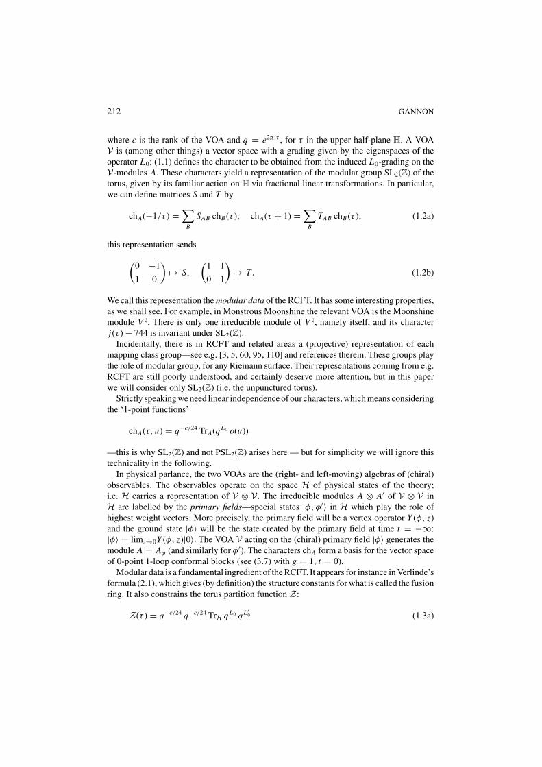
chA(τ ) = q−c/24 TrAq L0 (1.1)

212 GANNON

where c is the rank of the VOA and q = e2π iτ , for τ in the upper half-plane H. A VOAV is (among other things) a vector space with a grading given by the eigenspaces of theoperator L0; (1.1) defines the character to be obtained from the induced L0-grading on theV-modules A. These characters yield a representation of the modular group SL2(Z) of thetorus, given by its familiar action on H via fractional linear transformations. In particular,we can define matrices S and T by

chA(−1/τ ) =∑

B

SAB chB(τ ), chA(τ + 1) =∑

B

TAB chB(τ ); (1.2a)

this representation sends

(0 −1

1 0

)�→ S,

(1 1

0 1

)�→ T . (1.2b)

We call this representation the modular data of the RCFT. It has some interesting properties,as we shall see. For example, in Monstrous Moonshine the relevant VOA is the Moonshinemodule V �. There is only one irreducible module of V �, namely itself, and its characterj(τ ) − 744 is invariant under SL2(Z).

Incidentally, there is in RCFT and related areas a (projective) representation of eachmapping class group—see e.g. [3, 5, 60, 95, 110] and references therein. These groups playthe role of modular group, for any Riemann surface. Their representations coming from e.g.RCFT are still poorly understood, and certainly deserve more attention, but in this paperwe will consider only SL2(Z) (i.e. the unpunctured torus).

Strictly speaking we need linear independence of our characters, which means consideringthe ‘1-point functions’

chA(τ, u) = q−c/24 TrA(q L0 o(u))

—this is why SL2(Z) and not PSL2(Z) arises here — but for simplicity we will ignore thistechnicality in the following.

In physical parlance, the two VOAs are the (right- and left-moving) algebras of (chiral)observables. The observables operate on the space H of physical states of the theory;i.e. H carries a representation of V ⊗ V . The irreducible modules A ⊗ A′ of V ⊗ V inH are labelled by the primary fields—special states |φ, φ′〉 in H which play the role ofhighest weight vectors. More precisely, the primary field will be a vertex operator Y (φ, z)and the ground state |φ〉 will be the state created by the primary field at time t = −∞:|φ〉 = limz→0Y (φ, z)|0〉. The VOA V acting on the (chiral) primary field |φ〉 generates themodule A = Aφ (and similarly for φ′). The characters chA form a basis for the vector spaceof 0-point 1-loop conformal blocks (see (3.7) with g = 1, t = 0).

Modular data is a fundamental ingredient of the RCFT. It appears for instance in Verlinde’sformula (2.1), which gives (by definition) the structure constants for what is called the fusionring. It also constrains the torus partition function Z:

Z(τ ) = q−c/24 q−c/24 TrH q L0 q L ′0 (1.3a)

MODULAR DATA: THE ALGEBRAIC COMBINATORICS 213

where q is the complex conjugate of q. Now as mentioned above, H has the decomposition

H = ⊕A,B MAB A ⊗ B (1.3b)

into V-modules, where the MAB are multiplicities, and so

Z(τ ) =∑A,B

MAB chA(τ ) chB(τ ) (1.3c)

Physically, Z is the 1-loop vacuum-to-vacuum amplitude of the closed string (or rather, theamplitude would be

∫Z(τ ) dτ ). ‘Amplitudes’ are the fundamental numerical quantities in

quantum theories, from which the probabilities are obtained; it is through probabilities thatthe theory makes contact with experiment. In Segal’s formalism, the torus C/(Z + τZ) isassigned the homomorphism C → C corresponding to multiplication by Z(τ ). We will seein Section 5 that Z must be invariant under the action (1.2a) of the modular group SL2(Z),and so we call it (or equivalently its matrix M of multiplicities) a modular invariant.

Another elementary but fundamental quantity is the 1-loop vacuum-to-vacuum ampli-tude Zαβ of the open string, to whose ends are attached ‘boundary states’ |α〉, |β〉—thiscylindrical partition function looks like

Zαβ(t) =∑

A

N β

Aα chA(it) (1.4)

where these multiplicities N β

Aα have something to do with Verlinde’s formula (2.1). Thesefunctions Zαβ (or equivalently their matrices (NA)αβ = N β

Aα of coefficients) are calledfusion graphs or nim-reps, for reasons that will be explained in Section 5.

We define modular invariants and nim-reps axiomatically in Section 5. Classifying themis essentially the same as classifying (boundary) RCFTs, and is an interesting and accessiblechallenge. All of this will be explained more thoroughly and rigourously in the course ofthis paper.

In this paper we survey the basic theory and examples of modular data and fusion rings. Inour context, modular data is much more fundamental as it contains much more information.Basic (combinatorial) things to do with modular data are to construct and classify themand their associated modular invariants and nim-reps. Certainly, we are still missing keyideas here, and in part this paper is a call for help. We sketch the basic theory of modularinvariants and nim-reps. Finally, we specialise to the modular data associated to affineKac-Moody algebras, and discuss what is known about their modular invariant and nim-repclassifications. A familiarity with RCFT is not needed to read this paper (apart from thisintroduction!).

The mathematics of CFT is extremely rich, but what isn’t always appreciated is howmuch of it is combinatorial. This paper certainly doesn’t exhaust all of this combinatorialcontent—for this, the reader should study the Moore-Seiberg data [95] (for a mathematicaltreatment, see especially [5]). In this paper we focus on the most accessible, and probablymost important, part of this, namely those aspects related to SL2(Z) and fusion rings.

214 GANNON

The theory of fusion rings in its purest form is the study of the algebraic consequencesof requiring structure constants to obey the constraints of positivity and integrality, as wellas imposing some sort of self-duality condition identifying the ring with its dual. But oneof the thoughts running through this note is that we don’t know yet its correct definition(nor, more importantly, that of modular data). In the next section is given the most standarddefinition, but surely it can be improved. How to determine the correct definition is clear:we probe it from the ‘inside’—i.e. with strange examples which we probably want to callmodular data—and also from the ‘outside’—i.e. with examples probably too dangerousto include in the fold. Some of these critical examples will be described in the followingsections.Notational Remarks: Throughout the paper we let Z≥ denote the nonnegative integers,and x denote the complex conjugate of x . The transpose of a matrix A will be written At .

2. Modular data and fusion rings

The most basic structure considered in this paper is that of modular data; the particularvariant studied here—and the most common one in the literature—is given in Definition 1.But there are alternatives, and a natural general one is given by MD1′, MD2′, MD3, andMD4. In the more limited context of e.g. RCFT, axioms MD1, MD2′, and MD3-MD6 aremore appropriate.

Definition 1 Let � be a finite set of labels, one of which—we will denote it 0 and callit the ‘identity’—is distinguished. By modular data we mean matrices S = (Sab)a,b∈�,T = (Tab)a,b∈� of complex numbers such that:

MD1. S is unitary and symmetric, and T is diagonal and of finite order: i.e. T N = I forsome N ;

MD2. S0a > 0 for all a ∈ �;MD3. S2 = (ST )3;MD4. The numbers defined by

N cab =

∑d∈�

Sad Sbd Scd

S0d(2.1)

are in Z≥.

The matrix S is more important than T . The name ‘modular data’ is chosen because Sand T give a representation of the modular group SL2(Z)—as MD3 strongly hints and aswe will see in Section 4. Trying to remain consistent with the terminology of RCFT, wewill call (2.1) ‘Verlinde’s formula’, the N c

ab ‘fusion coefficients’, and the a ∈ � ‘primaries’.The distinguished primary ‘0’ is called the ‘identity’ because of its role in the associatedfusion ring, defined below. A possible fifth axiom will be proposed shortly, and later wewill propose refinements to MD1 and MD2, as well as a possible 6th axiom, but in thispaper we will limit ourselves to the consequences of MD1–MD4.


Modular data arises directly in many places in math—some of these will be reviewedin the next section. In many of these interpretations, there is for each primary a ∈ � afunction (a ‘character’) χa : H → C which yields the matrices S and T as in (1.2a). Also,in many examples, to each triple a, b, c ∈ � we get a vector space Hc

ab (an ‘intertwinerspace’ or ‘multiplicity module’) with dim(Hc

ab) = N cab, and with natural isomorphisms

between Hcab, Hc

ba , etc. In many of these examples, we have ‘6j-symbols’, i.e. for any 6-tuple a, b, c, d, e, f ∈ � we have a homomorphism { a

dbe

cf } from He

cd ⊗ Hcab to He

a f ⊗H f

bd obeying several conditions (see e.g. [110, 47] for a general treatment). Classically, 6j-symbols explicitly described the change between the two natural bases of the tensor product(Lλ ⊗ Lµ) ⊗ Lν

∼= Lλ ⊗ (Lµ ⊗ Lν) of modules of a Lie group, and our 6j-symbols are theirnatural extension to e.g. quantum groups. Characters, intertwiner spaces, and 6j-symbolsdon’t play any role in this paper.

If MD2 looks unnatural, think of it in the following way. It is easy to show (using MD1and MD4 and Perron-Frobenius theory [75]) that some column of S is nowhere 0 andof constant phase (i.e. Arg(S�b) is constant for some b ∈ �); MD2 tells us that it is the0 column, and that the phase is 0 (so these entries are positive). The ratios Sa0/S00 aresometimes called q(uantum)-dimensions (see (4.2b) below).

If MD4 looks peculiar, think of it in the following way. For each a ∈ �, define matricesNa by (Na)bc = N c

ab. These are usually called fusion matrices. Then MD4 tells us theseNa’s are simultaneously diagonalised by S, with eigenvalues Sad/S0d .

The key to modular data is Eq. (2.1). It should look familiar from the character theoryof finite groups: Let G be any finite group, let K1, . . . , Kh be the conjugacy classes of G,and write ki for the formal sum

∑g∈Ki

g. These ki ’s form a basis for the centre of the groupalgebra CG of G. If we write

ki k j =∑

�

ci j�k�

then the structure constants ci j� are nonnegative integers, and we obtain

ci j� = ‖Ki‖ ‖K j‖ ‖K�‖‖G‖

∑χ∈Irr G

χ (gi ) χ (g j ) χ (g�)

χ (e)

where gi ∈ Ki . This resembles (2.1), with Sab replaced with Si,χ = χ (gi ) and the identity 0replaced with the group identity e. This formal relation between finite groups and Verlinde’sformula seems to have first been noticed in [89]; we will return to it later this section.

The matrix T is fairly poorly constrained by MD1–MD4. There are however many otherindependent properties which the modular data coming from RCFT is known to obey. Themost important of these is that, for any a ∈ �, the quantity∑

b,c∈�

N abc S0b S0cT 2

ccT −2bb

lies in {0, ±1} (this doesn’t follow from MD1–MD4) and plays the role of the Frobenius–Schur indicator here [9]. Another axiom, also obeyed by any RCFT [36], is sometimes

216 GANNON

introduced, though it also won’t be adopted here:

MD5. For all choices a, b, c, d ∈ �,

(Taa TbbTccTdd T −1

00

)Nabcd =∏e∈�

T Nabcd,eee

where

Nabcd :=∑e∈�

N eab N d

ce , Nabcd,e := N eab N d

ce + N ebc N d

ae + N eac N d

be

From MD5 it can be proved that T has finite order (take a = b = c = d), so ad-mitting MD5 permits us to remove that statement from MD1. But it doesn’t have anyother interesting consequences that this author knows—though perhaps it will be usefulin proving the Congruence Subgroup Property given below, or give us some finitenessresult.

Intimately related to modular data are the fusion rings. There is no standard terminol-ogy here and this does occassionally cause confusion; we suggest the following as beingunambiguous and yet close to most treatments in the literature.

Definition 2 A fusion algebra A = F(β, N ) is an associative commutative Q-algebra Awith unity 1, together with a finite basis β = {x0, x1, . . . , xn} with x0 = 1, such that:

F1. The structure constants N cab ∈ Q, defined by xa xb = ∑n

c=0 N cabxc, are all nonnegative;

F2. There is a ring endomorphism x �→ x∗ stabilising the basis β (write x∗a = xa∗ );

F3. N 0ab = δb,a∗ ;

F4. There is a symmetric unitary matrix S, S = St , such that Verlinde’s formula (2.1) holdsfor all a, b, c ∈ � := {0, 1, . . . , n}.

We usually will be interested in the ‘fusion coefficients’ N cab being (nonnegative) integers.

In this case it will usually be convenient to consider the Z-span of β. The resulting freeZ-module with basis β and structure constants N c

ab will be called a fusion ring. In those raresituations where we are interested more generally in the scalars being e.g. real or complex,i.e. when A is an R- or C-algebra, we will speak of R-fusion algebras and C-fusion algebras,respectively (of course positivity F1 requires in all cases that the N c

ab be real).If the algebra A obeys only F1–F3 we’ll call it a generalised fusion algebra. We will

see shortly that given any generalised fusion algebra, there is a unitary matrix S suchthat (2.1) holds ∀a, b, c ∈ �, so the content of the important F4 is that this matrix Scan be chosen to be symmetric. We will see later that algebraically this is a self-dualitycondition.

RCFT is much more interested in fusion rings than generalised fusion algebra, and theremainder of the paper after this section will specialise to them. However, generalised fusionalgebras do appear in RCFT and so perhaps deserve more attention there. For instance, the


subrings of fusion rings will typically be generalised fusion rings—e.g. consider the subringspanned by the ‘even’ primaries {0, 2, . . . , k} of the affine algebra A(1)

1 at even level k (see(3.5) below). Also, the ‘classifying algebra’ in boundary conformal field theory [17] can bea generalised fusion ring. Much more general fusion-like rings arise naturally in subfactors(see Example 6 below) and nonrational logarithmic CFT (see e.g. [57, 66]) so there is amuch broader theory here to be developed, and of course the people to do this are algebraiccombinatorists.

That x �→ x∗ is an involution is clear from F3 and commutativity of A. Axiom F3 andassociativity of A imply N c

ab = N b∗ac∗ (a.k.a. Frobenius reciprocity or Poincare duality);

hence the numbers Nabc := N c∗ab will be symmetric in a, b, c. Axiom F3 is equivalent to

the existence on A of a linear functional ‘Tr’ for which β is orthonormal: Tr(xa x∗b ) = δa,b

∀a, b ∈ β. Then N cab = Tr(xa xbx∗

c ).As an abstract algebra, A is not very interesting: in particular, because A is commutative

and associative, the fusion matrices (Na)bc = N cab pairwise commute; because of F2,

(Na)t = Na∗ . Thus they are normal and can be simultaneously diagonalised. Hence Ais semisimple, and will be isomorphic to a direct sum of number fields (see Example7 below). For example, the fusion algebra for A(1)

1 level k (see (3.5c)) is isomorphic to⊕dQ[cos(π d

k+2 )], where d runs over all divisors of 2(k + 2) in the interval 1 ≤ d < k + 2.Likewise, the C-fusion algebra A⊗Q C is isomorphic as a C-algebra to C‖β‖ with operationsdefined component-wise. Of course what is important for fusion rings is that they have apreferred basis β.

(Generalised) fusion algebras are closely related to association schemes and C-algebras(as first noted in [34, 35], and independently in [6]), hypergroups [115], table algebras,etc. That is to say, their axiomatic systems are similar. In particular, a generalised fusionalgebra is a table algebra [2], with structure constants in Q and normalised appropriately;a fusion algebra obeys in addition a strong self-duality. However, the exploration of anaxiomatic system is influenced not merely by its intrinsic nature (i.e. its formal list ofaxioms and their logical consequences), but also by what are perceived by the local re-search community to be its characteristic examples. There always is a context to math;the development of formal structure is directed by its implicit context. The prototypicalexamples of a table algebra are the space of class functions of a finite group or the centreof the group algebra, while that of modular data corresponds to the SL2(Z) representationassociated to an affine Kac-Moody algebra at level k ∈ Z≥ (Example 2 below). Nev-ertheless it can be expected that techniques and questions from one of these areas canbe profitably carried over to the other, and solidifying that bridge is this paper’s raisond’etre. Surely, implicit or explicit in the literature on e.g. table algebras, there are resultswhich to CFT people would be new and interesting. This paper tries to explain the rele-vant CFT language, and describe questions conformal field theorists would find natural andimportant.

To give one interesting disparity, the commutative association schemes have been clas-sified up to 23 vertices [79], while modular data is known for only 3 primaries [27] (andthat proof assumes additional axioms)! In fact we still don’t have a finiteness theorem: for agiven cardinality ‖�‖, are there only finitely many possible modular data? (We know thereare infinitely many fusion rings in each dimension >1.)

218 GANNON

Consider for the next several paragraphs that A is a generalised C-fusion algebra (tensor-ing by C if necessary). Our treatment will roughly follow that of Kawada’s C-algebras asgiven in [8]. The fusion matrices Na are linearly independent, by F3. Let yi , for 0 ≤ i ≤ n,be a basis of common eigenvectors, with eigenvalues �i (a). Normalise all vectors yi to haveunit length (there remains an ambiguity of phase which we will fix below), and let y0 bethe Perron-Frobenius one—since

∑a Na > 0 here, we can choose y0 to be strictly positive.

Let S be the matrix whose i th column is yi , and L the eigenmatrix Lai = �i (a). Then Sis unitary and L is invertible. Note that for each i , the map a �→ �i (a) defines a linearrepresentation of A. That means that each column of L will be a common eigenvector of allNa , with eigenvalue �i (a), and hence must equal a scalar multiple of the i th column of S (seethe Basic Fact in Section 4). Note that each L0i = 1; therefore each S0i will be nonzeroand we may uniquely determine S (up to the ordering of the columns) by demanding thateach S0i > 0. Then Lai = Sai/S0i . Therefore we get (2.1).

Note though that the rows of S are indexed by the basis indices � := {0, 1, . . . , n}, butits columns are indexed by the eigenvectors. Like the character table of a group, althoughS is a square matrix it is not (for generalised fusion algebras) ‘truly square’. This simpleobservation will be valuable for the paragraph after Proposition 1.

The involution a �→ a∗ in F2 appears in the matrix Cl := SSt : (Cl)ab = δb,a∗ . The matrixCr := St S is also an order 2 permutation, and

Sai = SCl a,i = Sa,Cr i (1.2)

For a proof of those statements, see (4.4) below.Let A be the set of all linear maps of A ⊗Q C into C, equivalently the set of all maps

� → C. A has the structure of an (n + 1)-dimensional commutative algebra over C, usingthe product ( f g)(xa) = f (xa) g(xa). A basis β of A consists of the functions a �→ Sai

Sa0, for

each 0 ≤ i ≤ n—denote this function i . The resulting structure constants are

N ki j

=∑a∈�

Sai Saj Sak

Sa0=: N k

i j (1.3)

In other words, we have replaced S in (2.1) with St . It is easy to verify that A = F(β, N )obeys all axioms of a generalised C-fusion algebra, except possibly that some structureconstants N k

i j may be negative. They will all necessarily be real, however. We call A =F(β, N ) the dual of A = F(�, N ). Note that A can always be naturally identified with theoriginal generalised C-fusion algebra A.

We call A = F(β, N ) self-dual if A = F(β, N ) is isomorphic as a generalised C-fusionalgebra to A—equivalently, if there is a bijection ι : β → β such that N c

ab = N ιcιa,ιb (see the

definition of ‘fusion-isomorphism’ in Section 4).

Proposition 1. Given any generalised C-fusion algebra A = F(β, N ), there is a unique(up to ordering of the columns) unitary matrix S obeying (2.1) and all S0i and Sa0 are


positive. The generalised fusion algebra A = F(β, N ) is self-dual iff the correspondingmatrix S obeys

Sa,ι′b = Sb,ιa for all a, b ∈ β (1.4)

for some bijections ι, ι′ : β → β.

What this tells us is that there isn’t a natural algebraic interpretation for our precisecondition S = St in MD1; this study of (generalised) fusion algebras strongly suggests thatthe definition of modular data (and fusion algebra) be extended to the more general settingwhere ‘S = St ’ is replaced with (2.4). Fortunately, all properties of fusion rings extendnaturally to this new setting. But what should T look like then? A priori this isn’t so clear.But requiring the existence of a representation of SL2(Z) really forces matters. In particularnote that, when S is not symmetric, the matrices S and T themselves cannot be expectedto give a natural representation of any group (modular or otherwise) since for instance theexpression S2 really isn’t sensible—S is not ‘truly square’. Write P and Q for the matricesPa,i = δi,ιa and Qa,i = δi,ι′a , and let m be the order of the permutation ι−1 ◦ ι′. Then for anyk, S = SQt (P Qt )k is ‘truly square’ and its square S2 = Cl(P Qt )k is a permutation matrix,where Cl is as in (2.2). We also want S4 = I , which requires m = 2k + 1 or m = 4k + 2. Ineither of those cases, T = T Pt (Q Pt )k defines with S a representation of SL2(Z) providedT St T St T = S(Qt P)2k+1. (When 4 divides m, the best we will get in general will be arepresentation of some extension of SL2(Z).) But S is only determined by the generalisedfusion algebra up to permutation of the columns, so we may as well replace it with S. Dolikewise with T . So it seems that we can and should replace MD1 with:

MD1′. S is unitary, St = S P where P is a permutation matrix of order a power of 2, andT is diagonal and of finite order;

and leave MD2–MD4 intact. That simple change seems to provide the natural generalisationof modular data to any self-dual generalised fusion ring. Let m be the order of P; thenm = 1 recovers modular data, m ≤ 2 yields a representation of SL2(Z), and m > 2 yields arepresentation of a central extension of SL2(Z). In the interests of notational simplicity wewill adopt in later sections the standard MD1 rather than the new MD1′, although everythingwe discuss below has an analogue for this more general setting.

If we don’t require an SL2(Z) representation, then of course we get much more freedom.It is very unclear though what T should look like when the generalised fusion ring is notself-dual, which probably indicates that the definition of fusion algebra should include someself-duality constraint. This is of course the attitude we adopt, although in the mathematicalliterature it is unfortunately common to ignore it, and this difference can cause confusion.

Incidentally, the natural appearance of a self-duality constraint here perhaps should notbe surprising in hindsight. Drinfeld’s ‘quantum double’ construction has analogues inseveral contexts related to RCFT, and is a way of generating algebraic structures whichpossess modular data (see examples next section). It always involves combining a given(inadequate) algebraic structure with its dual in an appropriate way. A general categor-

220 GANNON

ical interpretation of quantum double is the centre construction, described for instancein [88]; it assigns to a tensor category a braided tensor category. It would be interest-ing to interpret this construction at the more base level of fusion algebra—it could sup-ply a general way for obtaining self-dual generalised fusion algebras from non-self-dualones.

In Example 4 of Section 3 we will propose a further generalisation of modular data. Inthis paper however, we will restrict for convenience to the consequences of the standardaxioms MD1–MD4.

In any case, a fusion ring is completely equivalent to a unitary and symmetric matrixS obeying MD2 and satisfying MD4. This special case of Proposition 1 was known toBannai and Zuber. More generally, ι−1 ◦ ι′ will define a fusion-automorphism of a self-dualgeneralised fusion algebra A = F(β, N ). Note that an unfortunate choice of matrix S in [6]led to an inaccurate conclusion there regarding fusion rings and Verlinde’s formula (2.1).In fact, Verlinde’s formula will hold with a unitary matrix S obeying S0i > 0, even if wedrop nonnegativity F1.

Proposition 1 shows that although (2.1) looks mysterious, it is quite canonical, and thatthe depth of Verlinde’s formula lies in the interpretation given to S and N (for instance(1.2a) and N c

ab = dim(Hcab)) within the given context.

The two-dimensional generalised fusion algebras F({0, 1}, N ) are classified by theirvalue of r = N 1

11—there is a unique fusion ring for every r ∈ Q, r ≥ 0. All are self-dual inthe strong sense, and so are in fact fusion algebras. A diagonal unitary matrix T satisfyingMD3 exists, iff 0 ≤ r ≤ 2√

3. However, T will in addition be of finite order, i.e. S and T will

constitute modular data, iff r = 0 (realised e.g. by the affine algebras A(1)1 and E (1)

7 at level1) or r = 1 (realised e.g. by affine algebras G(1)

2 and F (1)4 at level 1). Both r = 0, 1 have six

possibilities for the matrix T (T can always be multiplied by a third root of unity). All 12sets of modular data with two primaries can be realised by affine algebras (see Example 2below). This seeming omnipresence of the affine algebras is an accident of small numbersof primaries; even when ‖β‖ = 3 we find non-affine algebra modular data. The fusionalgebras given here can be regarded as a deformation interpolating between e.g. the A(1)

1and G(1)

2 level 1 fusion rings; similar deformations are typical in higher dimensions. Forexample in 3-dimensions, the A(1)

2 level 1 fusion ring lies in a family of fusion algebrasparametrised by the Pythagorean triples.

Classifying modular data and fusion rings for small sets of primaries, or at least obtainingnew explicit families beyond Examples 1–3 given next section, is perhaps the most vitalchallenge in the theory.

3. Examples of modular data and fusion rings

We can find (2.1), if not modular data in its full splendor, in a wide variety of contexts. Inthis section we sketch several of these. Historically for the subject, Example 2 has been themost important. As with the introductory section, this presentation cannot be self-containedand should be treated as an annotated guide to the literature. So don’t be concerned if mostof these examples aren’t familiar—Section 4 is largely independent of them.


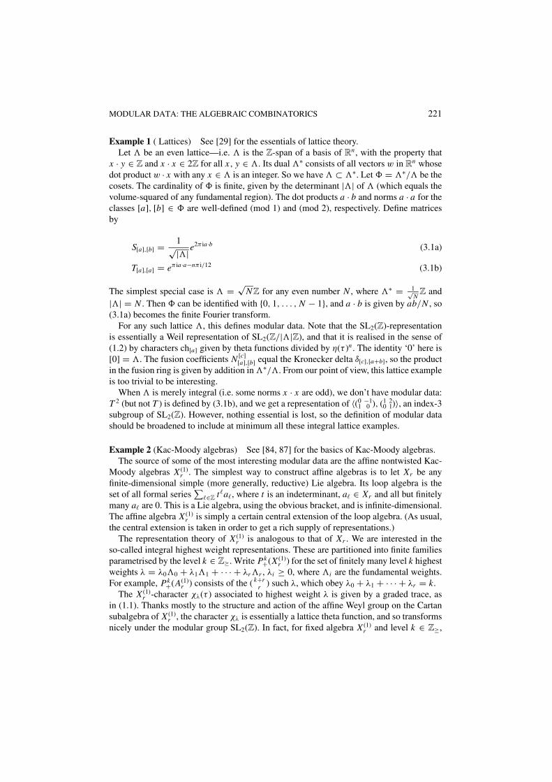
Example 1 ( Lattices) See [29] for the essentials of lattice theory.Let � be an even lattice—i.e. � is the Z-span of a basis of Rn , with the property that

x · y ∈ Z and x · x ∈ 2Z for all x, y ∈ �. Its dual �∗ consists of all vectors w in Rn whosedot product w · x with any x ∈ � is an integer. So we have � ⊂ �∗. Let � = �∗/� be thecosets. The cardinality of � is finite, given by the determinant |�| of � (which equals thevolume-squared of any fundamental region). The dot products a · b and norms a · a for theclasses [a], [b] ∈ � are well-defined (mod 1) and (mod 2), respectively. Define matricesby

S[a],[b] = 1√|�|e2π ia·b (3.1a)

T[a],[a] = eπ ia·a−nπ i/12 (3.1b)

The simplest special case is � = √NZ for any even number N , where �∗ = 1√

NZ and

|�| = N . Then � can be identified with {0, 1, . . . , N − 1}, and a · b is given by ab/N , so(3.1a) becomes the finite Fourier transform.

For any such lattice �, this defines modular data. Note that the SL2(Z)-representationis essentially a Weil representation of SL2(Z/|�|Z), and that it is realised in the sense of(1.2) by characters ch[a] given by theta functions divided by η(τ )n . The identity ‘0’ here is[0] = �. The fusion coefficients N [c]

[a],[b] equal the Kronecker delta δ[c],[a+b], so the productin the fusion ring is given by addition in �∗/�. From our point of view, this lattice exampleis too trivial to be interesting.

When � is merely integral (i.e. some norms x · x are odd), we don’t have modular data:T 2 (but not T ) is defined by (3.1b), and we get a representation of 〈(0 −1

1 0 ), (1 20 1)〉, an index-3

subgroup of SL2(Z). However, nothing essential is lost, so the definition of modular datashould be broadened to include at minimum all these integral lattice examples.

Example 2 (Kac-Moody algebras) See [84, 87] for the basics of Kac-Moody algebras.The source of some of the most interesting modular data are the affine nontwisted Kac-

Moody algebras X (1)r . The simplest way to construct affine algebras is to let Xr be any

finite-dimensional simple (more generally, reductive) Lie algebra. Its loop algebra is theset of all formal series

∑�∈Z t�a�, where t is an indeterminant, a� ∈ Xr and all but finitely

many a� are 0. This is a Lie algebra, using the obvious bracket, and is infinite-dimensional.The affine algebra X (1)

r is simply a certain central extension of the loop algebra. (As usual,the central extension is taken in order to get a rich supply of representations.)

The representation theory of X (1)r is analogous to that of Xr . We are interested in the

so-called integral highest weight representations. These are partitioned into finite familiesparametrised by the level k ∈ Z≥. Write Pk

+(X (1)r ) for the set of finitely many level k highest

weights λ = λ0�0 + λ1�1 + · · · + λr�r , λi ≥ 0, where �i are the fundamental weights.For example, Pk

+(A(1)r ) consists of the ( k+r

r ) such λ, which obey λ0 + λ1 + · · · + λr = k.The X (1)

r -character χλ(τ ) associated to highest weight λ is given by a graded trace, asin (1.1). Thanks mostly to the structure and action of the affine Weyl group on the Cartansubalgebra of X (1)

r , the character χλ is essentially a lattice theta function, and so transformsnicely under the modular group SL2(Z). In fact, for fixed algebra X (1)

r and level k ∈ Z≥,

222 GANNON

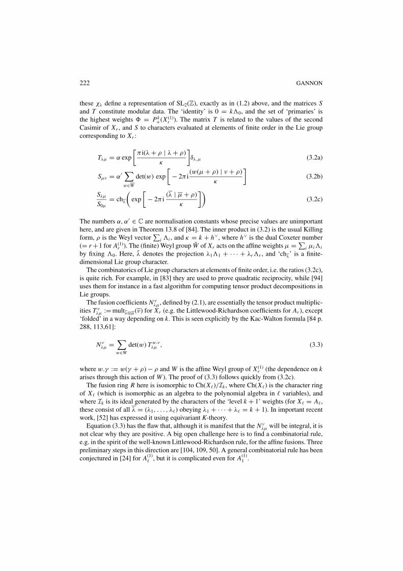
these χλ define a representation of SL2(Z), exactly as in (1.2) above, and the matrices Sand T constitute modular data. The ‘identity’ is 0 = k�0, and the set of ‘primaries’ isthe highest weights � = Pk

+(X (1)r ). The matrix T is related to the values of the second

Casimir of Xr , and S to characters evaluated at elements of finite order in the Lie groupcorresponding to Xr :

Tλµ = α exp

[π i(λ + ρ | λ + ρ)

κ

]δλ,µ (3.2a)

Sµν = α′ ∑w∈W

det(w) exp

[− 2π i

(w(µ + ρ) | ν + ρ)

κ

](3.2b)

Sλµ

S0µ

= chλ

(exp

[− 2π i

(λ | µ + ρ)

κ

])(3.2c)

The numbers α, α′ ∈ C are normalisation constants whose precise values are unimportanthere, and are given in Theorem 13.8 of [84]. The inner product in (3.2) is the usual Killingform, ρ is the Weyl vector

∑i �i , and κ = k + h∨, where h∨ is the dual Coxeter number

(= r +1 for A(1)r ). The (finite) Weyl group W of Xr acts on the affine weights µ = ∑

i µi�i

by fixing �0. Here, λ denotes the projection λ1�1 + · · · + λr�r , and ‘chλ’ is a finite-dimensional Lie group character.

The combinatorics of Lie group characters at elements of finite order, i.e. the ratios (3.2c),is quite rich. For example, in [83] they are used to prove quadratic reciprocity, while [94]uses them for instance in a fast algorithm for computing tensor product decompositions inLie groups.

The fusion coefficients N νλµ, defined by (2.1), are essentially the tensor product multiplic-

ities T νλµ := multλ⊗µ(ν) for Xr (e.g. the Littlewood-Richardson coefficients for Ar ), except

‘folded’ in a way depending on k. This is seen explicitly by the Kac-Walton formula [84 p.288, 113,61]:

N νλµ =

∑w∈W

det(w) T w.νλµ , (3.3)

where w.γ := w(γ + ρ) − ρ and W is the affine Weyl group of X (1)r (the dependence on k

arises through this action of W ). The proof of (3.3) follows quickly from (3.2c).The fusion ring R here is isomorphic to Ch(X�)/Ik , where Ch(X�) is the character ring

of X� (which is isomorphic as an algebra to the polynomial algebra in � variables), andwhere Ik is its ideal generated by the characters of the ‘level k + 1’ weights (for X� = A�,these consist of all λ = (λ1, . . . , λ�) obeying λ1 + · · · + λ� = k + 1). In important recentwork, [52] has expressed it using equivariant K-theory.

Equation (3.3) has the flaw that, although it is manifest that the N νλµ will be integral, it is

not clear why they are positive. A big open challenge here is to find a combinatorial rule,e.g. in the spirit of the well-known Littlewood-Richardson rule, for the affine fusions. Threepreliminary steps in this direction are [104, 109, 50]. A general combinatorial rule has beenconjectured in [24] for A(1)

� , but it is complicated even for A(1)1 .


Identical numbers N νλµ appear in several other contexts. For instance, Finkelberg [51]

proved that the affine fusion ring is isomorphic to the K-ring of Kazhdan-Lusztig’s categoryO−k of level−k integrable highest weight X (1)

r -modules, and to Gelfand-Kazhdan’s categoryOq coming from finite-dimensional modules of the quantum group Uq (Xr ) specialised tothe root of unity q = exp[iπ/mκ] for appropriate choice of m ∈ {1, 2, 3}. Because of theseisomorphisms, we know that the N ν

λµ do indeed lie in Z≥, for any affine algebra. We alsoknow [54] that they increase with k, with limit T ν

λµ.Also, they arise as dimensions of spaces of generalised theta functions [48], as tensor

product coefficients in quantum groups [61] and Hecke algebras [78] at roots of 1 andChevalley groups for Fp [76], and in quantum cohomology [116, 16].

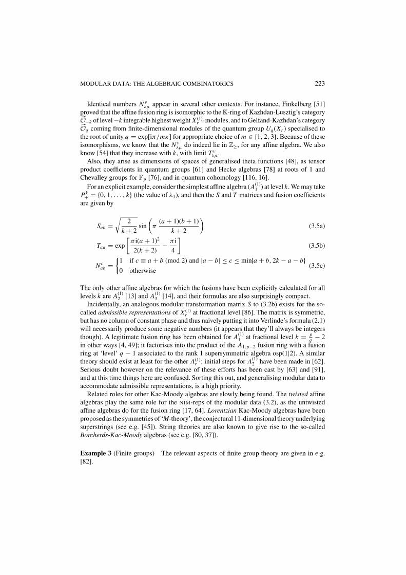
For an explicit example, consider the simplest affine algebra (A(1)1 ) at level k. We may take

Pk+ = {0, 1, . . . , k} (the value of λ1), and then the S and T matrices and fusion coefficients

are given by

Sab =√

2

k + 2sin

(π

(a + 1)(b + 1)

k + 2

)(3.5a)

Taa = exp

[π i(a + 1)2

2(k + 2)− π i

4

](3.5b)

N cab =

{1 if c ≡ a + b (mod 2) and |a − b| ≤ c ≤ min{a + b, 2k − a − b}0 otherwise

(3.5c)

The only other affine algebras for which the fusions have been explicitly calculated for alllevels k are A(1)

2 [13] and A(1)3 [14], and their formulas are also surprisingly compact.

Incidentally, an analogous modular transformation matrix S to (3.2b) exists for the so-called admissible representations of X (1)

r at fractional level [86]. The matrix is symmetric,but has no column of constant phase and thus naively putting it into Verlinde’s formula (2.1)will necessarily produce some negative numbers (it appears that they’ll always be integersthough). A legitimate fusion ring has been obtained for A(1)

1 at fractional level k = pq − 2

in other ways [4, 49]; it factorises into the product of the A1,p−2 fusion ring with a fusionring at ‘level’ q − 1 associated to the rank 1 supersymmetric algebra osp(1|2). A similartheory should exist at least for the other A(1)

r ; initial steps for A(1)2 have been made in [62].

Serious doubt however on the relevance of these efforts has been cast by [63] and [91],and at this time things here are confused. Sorting this out, and generalising modular data toaccommodate admissible representations, is a high priority.

Related roles for other Kac-Moody algebras are slowly being found. The twisted affinealgebras play the same role for the nim-reps of the modular data (3.2), as the untwistedaffine algebras do for the fusion ring [17, 64]. Lorentzian Kac-Moody algebras have beenproposed as the symmetries of ‘M-theory’, the conjectural 11-dimensional theory underlyingsuperstrings (see e.g. [45]). String theories are also known to give rise to the so-calledBorcherds-Kac-Moody algebras (see e.g. [80, 37]).

Example 3 (Finite groups) The relevant aspects of finite group theory are given in e.g.[82].

224 GANNON

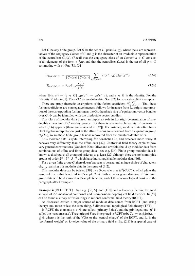
Let G be any finite group. Let � be the set of all pairs (a, χ ), where the a are represen-tatives of the conjugacy classes of G and χ is the character of an irreducible representationof the centraliser CG(a). (Recall that the conjugacy class of an element a ∈ G consistsof all elements of the form g−1ag, and that the centraliser CG(a) is the set of all g ∈ Gcommuting with a.) Put [38, 93]

S(a,χ ),(a′,χ ′) = 1

‖CG(a)‖ ‖CG(a′)‖∑

g∈G(a,a′)

χ ′(g−1ag) χ (ga′g−1) (3.6a)

T(a,χ ),(a′,χ ′) = δa,a′δχ,χ ′χ (a)

χ (e)(3.6b)

where G(a, a′) = {g ∈ G | aga′g−1 = ga′g−1a}, and e ∈ G is the identity. For the‘identity’ 0 take (e, 1). Then (3.6) is modular data. See [32] for several explicit examples.

There are group-theoretic descriptions of the fusion coefficient N (c,χ ′′)(a,χ ),(b,χ ′). That these

fusion coefficients are nonnegative integers, follows for instance from Lusztig’s interpreta-tion of the corresponding fusion ring as the Grothendieck ring of equivariant vector bundlesover G: � can be identified with the irreducible vector bundles.

This class of modular data played an important role in Lusztig’s determination of irre-ducible characters of Chevalley groups. But there is a remarkable variety of contexts inwhich (3.6) appears (these are reviewed in [32]). For instance, modular data often has aHopf algebra interpretation: just as the affine fusions are recovered from the quantum groupUq (Xr ), so are these finite group fusions recovered from the quantum-double of G.

This modular data is quite interesting for nonabelian G, and deserves more study. Itbehaves very differently than the affine data [32]. Conformal field theory explains howvery general constructions (Goddard-Kent-Olive and orbifold) build up modular data fromcombinations of affine and finite group data—see e.g. [36]. Finite group modular data isknown to distinguish all groups of order up to at least 127, although there are nonisomorphicgroups of order 215 · 34 · 5 · 7 which have indistinguishable modular data [46].

For a given finite group G, there doesn’t appear to be a natural unique choice of charactersch(a,χ ) realising this modular data in the sense of (1.2).

This modular data can be twisted [39] by a 3-cocycle α ∈ H 3(G, C×), which plays thesame role here that level did in Example 2. A further major generalisation of this finitegroup data will be discussed in Example 6 below, and of this cohomological twist α in theparagraph after Example 6.

Example 4 (RCFT, TFT.) See e.g. [36, 5], and [110], and references therein, for goodsurveys of 2-dimensional conformal and 3-dimensional topological field theories. In [55]can be found a survey of fusion rings in rational conformal field theory (RCFT).

As discussed earlier, a major source of modular data comes from RCFT (and stringtheory) and, more or less the same thing, 3-dimensional topological field theory (TFT).

In RCFT, the elements a ∈ � are called ‘primary fields’, and the privileged one ‘0’ iscalled the ‘vacuum state’. The entries of T are interpreted in RCFT to be Taa = exp[2π i(ha−c

24 )], where c is the rank of the VOA or the ‘central charge’ of the RCFT, and ha is the‘conformal weight’ or L0-eigenvalue of the primary field a. Eq. (2.1) is a special case of


the so-called Verlinde’s formula [112]:

V (g)a1···at =

∑b∈�

(S0b)2(1−g) Sa1b

S0b· · · Sat b

S0b(3.7)

It arose first in RCFT as an extremely useful expression for the dimensions of the space ofconformal blocks on a genus g surface with t punctures, labelled with primaries ai ∈ �—the fusions N c

ab correspond to a sphere with 3 punctures. All the V (g)’s are nonnegativeintegers iff all the N c

ab’s are. In RCFT, our unused axiom MD5 is derived by applyingDehn twists to a sphere with 4 punctures to obtain an Nabcd × Nabcd matrix equation on thecorresponding space of conformal blocks; MD5 is the determinant of that Equation [111].

Example 1 corresponds to the string theory of n free bosons compactified on the torusRn/�. Example 2 corresponds to Wess-Zumino-Witten RCFT [77] where a closed stringlives on a Lie group manifold. Example 3 corresponds to the untwisted sector in an orbifoldof a holomorphic RCFT (a holomorphic theory has trivial modular data—e.g. a lattice theorywhen the lattice � = �∗ is self-dual) by G [38]. The RCFT interpretation of fractionallevel affine algebra modular data isn’t understood yet, despite considerable effort (in [91]though it is suggested that they form a ‘nonunitary quasi-rational conformal field theory’).

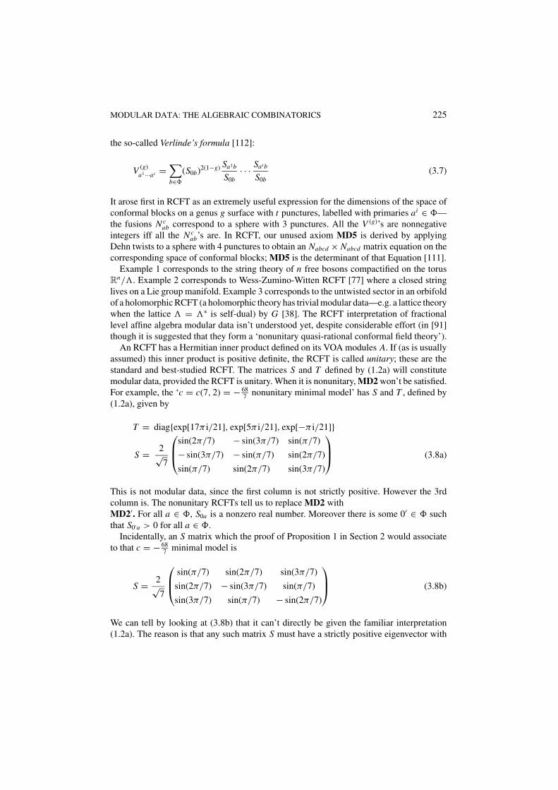
An RCFT has a Hermitian inner product defined on its VOA modules A. If (as is usuallyassumed) this inner product is positive definite, the RCFT is called unitary; these are thestandard and best-studied RCFT. The matrices S and T defined by (1.2a) will constitutemodular data, provided the RCFT is unitary. When it is nonunitary, MD2 won’t be satisfied.For example, the ‘c = c(7, 2) = − 68

7 nonunitary minimal model’ has S and T , defined by(1.2a), given by

T = diag{exp[17π i/21], exp[5π i/21], exp[−π i/21]}

S = 2√7

sin(2π/7) − sin(3π/7) sin(π/7)

− sin(3π/7) − sin(π/7) sin(2π/7)

sin(π/7) sin(2π/7) sin(3π/7)

(3.8a)

This is not modular data, since the first column is not strictly positive. However the 3rdcolumn is. The nonunitary RCFTs tell us to replace MD2 withMD2′. For all a ∈ �, S0a is a nonzero real number. Moreover there is some 0′ ∈ � suchthat S0′a > 0 for all a ∈ �.

Incidentally, an S matrix which the proof of Proposition 1 in Section 2 would associateto that c = − 68

7 minimal model is

S = 2√7

sin(π/7) sin(2π/7) sin(3π/7)

sin(2π/7) − sin(3π/7) sin(π/7)

sin(3π/7) sin(π/7) − sin(2π/7)

(3.8b)

We can tell by looking at (3.8b) that it can’t directly be given the familiar interpretation(1.2a). The reason is that any such matrix S must have a strictly positive eigenvector with

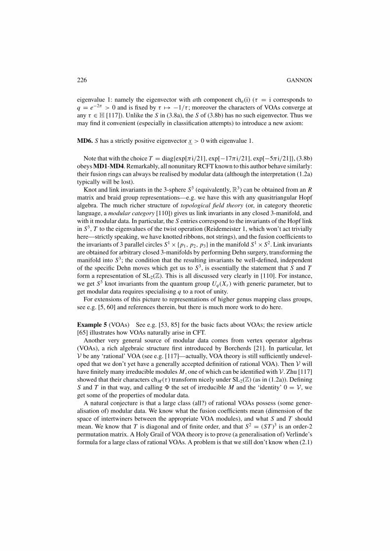
226 GANNON

eigenvalue 1: namely the eigenvector with ath component cha(i) (τ = i corresponds toq = e−2π > 0 and is fixed by τ �→ −1/τ ; moreover the characters of VOAs converge atany τ ∈ H [117]). Unlike the S in (3.8a), the S of (3.8b) has no such eigenvector. Thus wemay find it convenient (especially in classification attempts) to introduce a new axiom:

MD6. S has a strictly positive eigenvector x > 0 with eigenvalue 1.

Note that with the choice T = diag{exp[π i/21], exp[−17π i/21], exp[−5π i/21]}, (3.8b)obeys MD1-MD4. Remarkably, all nonunitary RCFT known to this author behave similarly:their fusion rings can always be realised by modular data (although the interpretation (1.2a)typically will be lost).

Knot and link invariants in the 3-sphere S3 (equivalently, R3) can be obtained from an Rmatrix and braid group representations—e.g. we have this with any quasitriangular Hopfalgebra. The much richer structure of topological field theory (or, in category theoreticlanguage, a modular category [110]) gives us link invariants in any closed 3-manifold, andwith it modular data. In particular, the S entries correspond to the invariants of the Hopf linkin S3, T to the eigenvalues of the twist operation (Reidemeister 1, which won’t act triviallyhere—strictly speaking, we have knotted ribbons, not strings), and the fusion coefficients tothe invariants of 3 parallel circles S1 ×{p1, p2, p3} in the manifold S1 × S2. Link invariantsare obtained for arbitrary closed 3-manifolds by performing Dehn surgery, transforming themanifold into S3; the condition that the resulting invariants be well-defined, independentof the specific Dehn moves which get us to S3, is essentially the statement that S and Tform a representation of SL2(Z). This is all discussed very clearly in [110]. For instance,we get S3 knot invariants from the quantum group Uq (Xr ) with generic parameter, but toget modular data requires specialising q to a root of unity.

For extensions of this picture to representations of higher genus mapping class groups,see e.g. [5, 60] and references therein, but there is much more work to do here.

Example 5 (VOAs) See e.g. [53, 85] for the basic facts about VOAs; the review article[65] illustrates how VOAs naturally arise in CFT.

Another very general source of modular data comes from vertex operator algebras(VOAs), a rich algebraic structure first introduced by Borcherds [21]. In particular, letV be any ‘rational’ VOA (see e.g. [117]—actually, VOA theory is still sufficiently undevel-oped that we don’t yet have a generally accepted definition of rational VOA). Then V willhave finitely many irreducible modules M , one of which can be identified with V . Zhu [117]showed that their characters chM (τ ) transform nicely under SL2(Z) (as in (1.2a)). DefiningS and T in that way, and calling � the set of irreducible M and the ‘identity’ 0 = V , weget some of the properties of modular data.

A natural conjecture is that a large class (all?) of rational VOAs possess (some gener-alisation of) modular data. We know what the fusion coefficients mean (dimension of thespace of intertwiners between the appropriate VOA modules), and what S and T shouldmean. We know that T is diagonal and of finite order, and that S2 = (ST )3 is an order-2permutation matrix. A Holy Grail of VOA theory is to prove (a generalisation of) Verlinde’sformula for a large class of rational VOAs. A problem is that we still don’t know when (2.1)


here is even defined (i.e. whether all S0,M �= 0). However, suppose V has the additional(natural) property that any irreducible module M �= V has positive conformal weight hM

(hM −c/24 is the smallest power of q in the Fourier expansion of the (normalised) characterchM (τ ) = q−c/24 ∑∞

n=0 aMn qn+hM ). This holds for instance in all VOAs associated to unitary

RCFTs. Then consider the behaviour of chM (τ ) for τ → 0 along the positive imaginaryaxis: since each Fourier coefficient aM

n is a nonnegative number, chM (τ ) will go to +∞.But this is equivalent to considering the limit of

∑N SM N chN (τ ) as τ → i∞ along the

positive imaginary axis. By hypothesis, this latter limit is dominated by SM0 a00q−c/24, at

least when SM0 �= 0. So what we find is that, under this hypothesis, the 0-column of Sconsists of nonnegative real numbers (and also that the rank c is positive).

In this context, Example 1 corresponds to the VOA associated to the lattice � [40].Example 2 is recovered by [54], who find a VOA structure on the highest weight X (1)

r -module L(k�0); the other level k X (1)

r -modules M = L(λ) all have the structure of VOAmodules of V := L(k�0). Example 3 arises for example in the orbifold of a self-dual latticeVOA by a subgroup G of the automorphism group of � (see e.g. [43]). An interpretationof fractional level affine algebra data could be possible along the lines of [42], who did itfor A(1)

1 (but once again see [63, 91]).

Example 6 (Subfactors) See e.g. [47, 19, 20] for good reviews of the subfactor ↔ CFTrelation.

The final general source of modular data which we will discuss comes from subfactortheory. To start with, let N ⊂ M be an inclusion of II1 factors with finite Jones index[M : N ]. Even though M and N will often be isomorphic as factors, Jones showed thatthere is rich combinatorics surrounding how N is embedded in M . Write M−1 = N ⊂ M =M0 ⊂ M1 ⊂ . . . for the tower arising from the ‘basic construction’. Let �M denote the set ofequivalence classes of irreducible M − M submodules of ⊕n≥0 M L2(Mn)M , and �N that forthe irreducible N−N submodules of ⊕n≥−1 N L2(Mn)N . WriteHC

AB for the intertwiner spaceHomM−M (C, A ⊗M B). For any A, B ∈ �M , the Connes’ relative tensor product A ⊗M Bcan be decomposed into a direct sum

∑C∈�M

N CABC , where N C

AB = dimHCAB ∈ Z≥ are

the multiplicities. The identity is the bimodule M L2(M)M . Assume in addition that �M isfinite (i.e. that N ⊂ M has ‘finite depth’). Then all axioms of a fusion ring will be obeyed,except possibly commutativity: unfortunately in general A ⊗M B �∼= B ⊗M A.

We are interested in M and N being hyperfinite. An intricate subfactor invariant calleda paragroup (see e.g. [97, 47]) can be formulated in terms of 6j-symbols and fusion rings[47], and resembles exactly solvable lattice models in statistical mechanics. One way to getmodular data is by passing from N ⊂ M to the asymptotic inclusion 〈M, M ′∩M∞〉 ⊂ M∞;its paragroup will essentially be an RCFT. Asymptotic inclusion plays the role of quantum-double here, and corresponds physically to taking the continuum limit of the lattice model,yielding the CFT from the underlying statistical mechanical model. More recently [98],Ocneanu has significantly refined this construction, generalising 6j-symbols to what arecalled Ocneanu cells, and extending the context to subparagroups. His new cells have beeninterpreted by [99] in terms of Moore-Seiberg-Lewellen data [95, 92].

A very similar but simpler theory has been developed for type III factors (see e.g. thereviews [19, 20]). Bimodules now are equivalent to ‘sectors’, i.e. equivalence classes of

228 GANNON

endomorphisms λ : N → N (the corresponding subfactor is λ(N ) ⊂ N ). This use ofendomorphisms is the key difference (and simplification) between the type II and type IIIfusion theories. Given λ, µ ∈ End(N ), we define 〈λ, µ〉 to be the dimension of the vectorspace of intertwiners, i.e. all t ∈ N such that tλ(n) = µ(n)t ∀n ∈ N . The endomorphismλ ∈ End(N ) is irreducible if 〈λ, λ〉 = 1. Let � = N χN be a finite set of irreducible sectors.The fusion product is given by composition λ ◦ µ; addition can also be defined, and thefusion coefficient N ν

λµ will then be the dimension 〈λµ, ν〉. The ‘identity’ 0 is the identityidN . Restricting to a finite set � of irreducible sectors, closed under fusion in the obviousway, the result is similar to a fusion ring, except again it is not necessarily commutative(after all, why should the compositions λ◦µ and µ◦λ be related). The missing ingredientsare nondegenerate braidings ε±(λ, µ) ∈ Hom(λµ, µλ), which say roughly that λ and µ

nearly commute (the ε± must also obey some compatibility conditions, e.g. the Yang-Baxter equations). Once we have a nondegenerate braiding, Rehren [100] proved that wewill automatically have modular data.

We will return to subfactors in Section 5. It is probably too optimistic to hope to see inthe subfactor picture to what the characters (1.1) correspond—different VOAs and RCFTscan correspond to the same subfactors. To give a simple example, the VOA associated toany self-dual lattice will correspond to the trivial subfactor N = M , where M is the uniquehyperfinite II1 factor. With this in mind, it would be interesting to find an S matrix arisinghere which violates axiom MD6 given earlier, or the Congruence Subgroup Property ofSection 4.

Jones and Wassermann have explicitly constructed the affine algebra subfactors (both typeII and III) of Example 2, at least for A(1)

r , and Wassermann and students Loke and ToledanoLaredo later showed that they recover the affine algebra fusions (see e.g. [114] for a review).Also, to any subgroup-group pair H < G, we can obtain a subfactor R × H ⊂ R×G ofcrossed products, where R is the type II1 hyperfinite factor, and thus a (not necessarilycommutative) fusion-like ring [90]. This subfactor R×H ⊂ R×G can be thought of asgiving a grouplike interpretation to G/H even when H is not normal. Sometimes it willhave a braiding—e.g. the diagonal embedding G < G × G recovers the finite group dataof Example 3. What is intriguing is that some other pairs H < G probably also have abraiding, generalising Example 3. There is a general suspicion, due originally perhaps toMoore and Seiberg [95] and in the spirit of Tannaka-Krein duality, that RCFTs can alwaysbe constructed in standard ways (Goddard-Kent-Olive cosets and finite group orbifolds)from lattice and affine algebra models. These crossed product subfactors could conceiv-ably provide reams of counterexamples, suggesting that the orbifold construction can beconsiderably generalised.

A uniform construction of the affine algebra and finite group modular data is providedin [39] where a 3-dimensional TFT is associated to any topological group G (G will be acompact Lie group in the affine case; G is given discrete topology in the finite case). Therewe see that the level k and twist α both play the same role, and are given by a cocycle inH 3(G, C×). Crane-Yetter [33] are developing a theory of cohomological ‘deformations’ ofmodular data (more precisely, of modular categories). In [33] they discuss the infinitesimaldeformations of tensor categories, where the objects are untouched but the arrows are


deformed, though their ultimate interest would be in global deformations and in particularin specialising to the especially interesting ones—much as we deform the enveloping algebraU (g) to get the quantum group Uq (g) and then specialise to roots of unity to get e.g. modulardata. Their work is still in preliminary stages and it probably needs to be generalised further(e.g. they don’t seem to recover the level of affine algebras), but it looks very promising.Ultimately it can be hoped that some discrete H 3 group will be identified which parametrisesthe different quantum doubles of a given symmetric tensor category.

Incidentally, the fact that H 3(G, C×) is a group strongly suggests that it should be mean-ingful to compare the modular data for different cocycles—e.g. to fix the affine algebra andvary k. This idea still hasn’t been seriously exploited (but e.g. see ‘threshold level’ in [13,14]).

There are many examples of ‘modular-like data’. These are interesting for probing thequestion of just what should be the definition of fusion algebra or modular data. Here is anintriguing example, inspired by (4.4) below.

Example 7 [72] (Number fields) A basic introduction to algebraic number theory isprovided by e.g. [28].

Choose any finite normal extension L of Q, and find any totally positive α ∈ L withTr(|α|2) = 1 (total positivity will turn out to be necessary for F1). Now find any Q-basisx1 = 1, x2, . . . , xn of a subfield K of L, where n = deg(K), the xi being orthonormalwith respect to the trace 〈x, y〉α := Tr(|α|2x y) (orthonormality will guarantee F3 to besatisfied). Let G denote the set of n distinct embeddings K → C. Our construction requirescomplex conjugation to commute with all embeddings. Under these conditions |α|−2 =∑

i |xi |2. Then we get a fusion-like algebra with primaries β = {x1, . . . , xn}, ‘∗’ given bycomplex conjugation, and structure constants N k

i j = Tr(|α|2xi x j xk) ∈ Q given by ordinarymultiplication and addition: xi x j = ∑

k N ki j xk . Call the resulting fusion-like algebra K(β).

It is easy to see that all the properties of a generalised fusion algeba are satisfied, ex-cept possibly N k

i j ∈ Q≥. The fusion coefficients N ki j will be integers iff the Z-span of

the xi form an ‘order’ of K. We also find that the matrix Sig = g(αxi ), for g ∈ G (lifteach g arbitrarily to L), diagonalises these fusion matrices Nxi . This matrix S is uni-tary, but (unless K is an abelian extension of Q) the dual fusions N in (2.3) won’t berational.

Positivity F1 requires one of the columns of S to be positive; permuting with g, we mayrequire all basis elements xi > 0. Hence K(β) will have a chance of being a generalisedfusion algebra only when K is ‘totally real’.

Incidentally this example is more general than it looks: it is easy to show

Proposition 2 Let A be a generalised fusion algebra which is isomorphic as a Q-algebrato a field K. Then A is isomorphic as a generalised fusion algebra to some K(�).

More generally, recall that a generalised fusion algebra is isomorphic as a Q-algebra to adirect sum of number fields. So an approach to studying (generalised) fusion algebras couldbe to study how they are built up from number fields. It would be very interesting to classifyall generalised fusion algebras which are isomorphic as a Q-algebra to a field. For example,take K = Q[

√N ], where N is not a perfect square, and where also any prime divisor

230 GANNON

p ≡ −1 (mod 4) of N occurs with even multiplicity. Then we can find positive integersa, b such that N = a2 + b2. Take � = {1, b

a + 1a

√N }, then K(�) is a fusion algebra with

N 222 = 2b

a . Note that this construction exhausts all 2-dimensional fusion algebras, except

when√

(N 222)2 + 4 is rational, which corresponds to the Q-algebra Q ⊕ Q (e.g. the fusion

ring of affine algebra A(1)1 at level 1). For N = 5 and a = 2, we recover the fusion ring of

affine algebra F (1)4 or G(1)

2 at level 1.

4. Modular data: Basic theory

In this section we sketch the basic theory of modular data. Most of these results are elemen-tary and can be proved quickly from the axioms; many appear in greater generality in theC-algebra/table algebra/... literature. For example, Eqs. (2.2) and (2.3) are in [18]. All ofthe following statements can be generalised to self-dual generalised fusion rings, and manyto generalised fusion algebras, but we will focus on the case of greatest interest to RCFT:when S = St and N c

ab ∈ Z≥.It is important to reinterpret (2.1) in matrix form. For each a ∈ �, define the fusion

matrix Na by

(Na)b,c = N cab.

Then (2.1) says that the Na are simultaneously diagonalised by S. More precisely, the bthcolumn S�,b of S is an eigenvector of each Na , with eigenvalue Sab

S0b. Unitarity of S tells us:

SabS0b

= SacS0c

holds for all a ∈ �, iff b = c. In other words:Basic Fact. All simultaneous eigenspaces are of dimension 1, and are spanned by eachcolumn S�,b .

Take the complex conjugate of (2.1): we find that S also simultaneously diagonalises thefusion matrices Na . Hence there is some permutation of �, which we will denote by C andcall conjugation, and some complex numbers αb, such that

Sab = αb Sa,Cb.

Unitarity forces each |αb| = 1. Looking at a = 0 and applying MD2, we see that the αb

must be positive. Hence

Sab = Sa,Cb = SCa,b (4.1)

and so C = S2. The conjugation C is trivial iff S is real. Note also that C , like complexconjugation, is an involution, and that C00 = 1. Some easy formulae are N0 = I , N 0

ab =Cab, and N Cc

Ca,Cb = N cab. Because C = S2 = (ST )3, C commutes with both S and T :

SCa,Cb = Sa,b and TCa,Cb = Ta,b.For example, in Example 1, C[a] = [−a], while for A(1)

1 the matrix S is real and soC = I . More generally, for the affine algebra X (1)

r the conjugation C corresponds to asymmetry of the Dynkin diagram of Xr . For finite groups (Example 3), C takes (a, χ ) to


(a−1, χ ). In RCFT, C is called charge-conjugation; it’s a symmetry in quantum field theorywhich interchanges particles with their antiparticles (and so reverses the sign of the charge,hence the name).

Because C is an involution, we know that the assignment (1.2b) defines a finite-dimensional representation of SL2(Z), for any choice of modular data—hence the name.A surprising fact is that this representation usually (always?) seems to factor through acongruence subgroup. We’ll return to this at the end of this section.

Perron-Frobenius theory, i.e. the spectral theory of nonnegative matrices (see e.g. [75]),has some immediate consequences. By MD2 and our Basic Fact, the Perron-Frobeniuseigenvalue of Na is Sa0

S00; hence we obtain the important inequality

Sa0S0b ≥ |Sab| S00. (4.2a)

Unitarity of S applied to (4.2a) forces

mina∈�Sa0 = S00. (4.2b)

In other words the q-dimensions, defined to be the ratios Sa0S00

, are bounded below by 1. Thename ‘q-dimension’ comes from quantum groups (and also affine algebras (3.2c)), whereone finds a q-deformed Weyl dimension formula. In RCFT, Sa0

S00= limτ→0+i

cha (τ )ch0(τ ) . In the

subfactor picture (Example 6), the Jones index is the square of the q-dimension.Cauchy-Schwarz and unitarity, together with (4.2a), gives us the curious inequality

∑e∈�

N eac N e

bd ≤ Sa0

S00

Sb0

S00(4.2c)

for all a, b, c, d ∈ �. So for instance N cab ≤ min{ Sa0

S00, Sb0

S00, Sc0

S00}. Equality holds in (4.2c)

only if Sa0 = Sb0 = S00 (i.e. only if a and b are units—see below), since it is only when ais a unit that equality in (4.2a) holds for all b ∈ �. Other inequalities are possible, thoughperhaps not useful: e.g. Holder gives us for all a ∈ � and k, m = 1, 2, 3, . . . the followingbounds on traces of powers of fusion matrices:

(Tr

(N k

a

))m ≤ ‖�‖m−1 Tr(N km

a

)(4.2d)

The equality (4.2b) suggests that we look at those primaries a ∈ � obeying the equalitySa0 = S00. Such primaries are called simple-currents in RCFT parlance (see e.g. [103, 36]and references therein), and in the table algebra literature are called linear [2], but the termwe regard as more natural is units. To any unit j ∈ �, there is a phase ϕ j : � → C and apermutation J of � such that j = J0 and

SJa,b = ϕ j (b) Sa,b (4.3a)

TJa,Ja Taa = ϕ j (a) Tj j T00 (4.3b)

(Tj j T00)2 = ϕ j ( j) (4.3c)

232 GANNON

Moreover, if J is of order n, then ϕ j (a) is an nth root of unity and TJa,Ja Taa is a 2nth root of1; when n is odd, the latter will in fact be an nth root of 1. To reflect the physics heritage, thepermutation J corresponding to a unit j ∈ � will be called a simple-current. The set of allsimple-currents or units forms an abelian group (using composition of the permutations),called the centre of the modular data. Note that C J = J−1C , and N J J ′c

Ja,J ′b = N cab for any

simple-currents J, J ′.For instance, for a lattice �, all [a] ∈ � are units, corresponding to permutation

J[a]([b]) = [a +b] and phase ϕ[a]([b]) = e2π ia·b. For the affine algebra A(1)1 at level k (recall

(3.5)), there is precisely one nontrivial unit, namely j = k, corresponding to J (a) = k − aand ϕ j (a) = (−1)a . More generally, to any affine algebra (except for E (1)

8 at k = 2), theunits correspond to symmetries of the extended Dynkin diagram. For A(1)

1 this symmetryinterchanges the 0th and 1st nodes, i.e. J (λ0�0+λ1�1) = λ1�0+λ0�1 (recall a = λ1); forA(1)

r the centre is Z/(r + 1)Z. In the finite group modular data, the units are the pairs (z, ψ)where z lies in the centre Z (G) of G, and ψ is a dimension-1 character of G. It correspondsto simple-current J(z,ψ)(a, χ ) = (za, ψχ ) and phase ϕ(z,ψ)(a, χ ) = ψ(a) χ (z)/χ (e). Thecentre of this modular data will thus be isomorphic to the direct product Z (G) × (G/G ′),where G ′ = 〈ghg−1h−1〉 is the commutator subgroup of G.

To see (4.3a), note first that (4.2a) tells us S0b ≥ |Sjb| for any unit j , and any b ∈ �.However, unitarity then forces S0b = |Sjb|, i.e. (4.3a) holds for a = 0 (with J0 defined tobe j), and some numbers ϕ j (b) with modulus 1. Putting this into (2.1), we get N j NC j = I ,the identity matrix. But the only nonnegative integer matrices whose inverses are alsononnegative integer matrices, are the permutation matrices. This defines the permutation Jof �. Eq. (4.3a) now follows from Cauchy-Schwartz applied to

1 = N Jaj,a =

∑d∈�

ϕ j (d) Sad SJa,d

The reason J ◦ J ′ = J ′ ◦ J is because the fusion matrices commute: NJ (J ′0) = NJ0 NJ ′0 =NJ ′0 NJ0 = NJ ′(J0).

To see (4.3b), first write (ST )3 = C as ST S = T ST , then use that and (4.3a) to show(T ST )Ja,0 = (T ST )a,J0. To see (4.3c), use (4.3b) with a = J−10, together with the fact thatC commutes with T . Note that ϕ j ( j ′) = Sj, j ′/S00 = ϕ j ′ ( j) and ϕJ J ′0(a) = ϕ j (a) ϕ j ′ (a), soϕJ k 0(a) = (ϕ j (a))k ; from all these and (4.3b) we get that

1 = TJ n0,J n0 T00 = ϕ j ( j) n(n−1)/2(Tj j T00)n

Equations (4.2a) and (4.3b) also follow from the curious equation

Sab Taa Tbb T00 =∑c∈�

N cab Tcc Sc0

which is derived from (2.1) and ST S = T ST .Simple-currents and units play an important role in the theory of modular data and fusion

rings. One place they appear is gradings. By a grading on � we mean a map ϕ : � → C×

with the property that if N cab �= 0 then ϕ(c) = ϕ(a) ϕ(b). The phase ϕ j coming from a unit


is clearly a grading; a little more work [72] shows that any grading ϕ of � corresponds to aunit j in this way. The multiplicative group of gradings, and the group of simple-currents(the centre), are naturally isomorphic. (This is not true of generalised fusion algebras.)

Next, we will generalise the conjugation symmetry argument, to other Galois automor-phisms. In particular, write Q[S] for the field generated over Q by all entries Sab. Then forany Galois automorphism σ ∈ Gal(Q[S]/Q),

σ (Sab) = εσ (a) Sσa,b = εσ (b) Sa,σb (4.4)

for some permutation c �→ σc of �, and some signs εσ : � → {±1}. Moreover, thecomplex numbers Sab will necessarily lie in the cyclotomic extension Q[ξn] of Q, for someroot of unity ξn := exp[2π i/n]. This follows from the Kronecker-Weber Theorem and thecalculation from (4.4) that

σσ ′Sab = εσ (a) εσ ′ (b) Sσa,σ ′b = σ ′σ Sab.

For a field extension K of Q, Gal(K/Q) denotes the automorphisms σ of K fixing allrationals. Recall that each automorphism σ ∈ Gal(Q[ξn]/Q) corresponds to an integer1 ≤ � ≤ n coprime to n, acting by σ (ξn) = ξ�

n . Note that Eq. (4.4) tells us the powerσ 2‖�‖! will act trivially on each entry Sab. In other words, the degree of the field extension[Q[S] : Q] is bounded by (in fact divides) 2‖�‖!. This is perhaps the closest we have to afiniteness result for modular data (see however [10] which obtains a bound for n in termsof ‖�‖, for the modular data arising in RCFT).

In other incarnations, this Galois action appears in the χ (g) �→ χ (g�) symmetry of thecharacter table of a finite group, and of the action of SL2(Z/NZ) on level N modularfunctions. Equation (4.4) was first shown in [30] and a related symmetry for commutativeassociation schemes was found in [96]. The analogue of cyclotomy isn’t known for asso-ciation schemes. The reason is the additional ‘self-duality’ property of the fusion ring, i.e.the fact that S = St or more generally (2.4).

Recall from Section 2 that a fusion ring R = F(�, N ) is isomorphic to a direct sum ofnumber fields. The Galois orbits determine these fields. In particular, for any Galois orbit[d] in �, let K[d] denote the field generated by all numbers of the form Sab

S0bfor a ∈ � and

b ∈ [d]. Then R is isomorphic as a Q-algebra to the direct sum ⊕[d]K[d]. We gave the A(1)1

level k example in Section 2.The Galois action for the lattice modular data is simple: the Galois automorphisms σ = σ�

correspond to integers � coprime to the determinant |�|; σ� takes [a] to [�a], and all paritiesε�([a]) = +1. The Galois action for the affine algebras is quite interesting (see e.g. [1]),and can be expressed geometrically using the action of the affine Weyl group on the weightlattice of Xr . Both ε�(λ) = ±1 will occur. For finite groups, σ� takes (a, χ ) to (a�, σ� ◦ χ ),and again all ε�(a, χ ) = +1.

The presence of the Galois action (4.4) is an effective criterion (necessary and sufficient)on the matrix S for the numbers in (2.1) to be rational. It would be very desirable to findeffective conditions on S such that the fusion coefficients are nonnegative, or integral. Atpresent the best results along these lines are, respectively, the inequalities (4.2), and the fact

234 GANNON

that the ratios SabS0b

are algebraic integers (since they are eigenvalues of integer matrices).When there are units, then (4.3a) provides an additional strong constraint on nonnegativity.

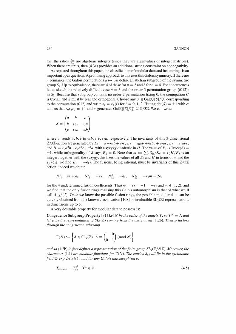
As repeated throughout this paper, the classification of modular data and fusion rings is animportant open question. A promising approach to this uses this Galois symmetry. If there aren primaries, the Galois permutations a �→ σa define an abelian subgroup of the symmetricgroup Sn . Up to equivalence, there are 4 of these for n = 3 and 8 for n = 4. For concretenesslet us sketch the relatively difficult case n = 3 and the order-3 permutation group 〈(012)〉in S3. Because that subgroup contains no order-2 permutation fixing 0, the conjugation Cis trivial, and S must be real and orthogonal. Choose any σ ∈ Gal(Q[S]/Q) correspondingto the permutation (012) and write εi = εσ (i) for i = 0, 1, 2. Hitting det(S) = ±1 with σ

tells us that ε0ε1ε2 = +1 and σ generates Gal(Q[S]/Q) ∼= Z/3Z. We can write

S =

a b c

b ε2c ε1a

c ε1a ε0b

where σ sends a, b, c to ε0b, ε1c, ε2a, respectively. The invariants of this 3-dimensionalZ/3Z-action are generated by E1 = a + ε0b + ε2c, E2 = ε0ab + ε1bc + ε2ac, E3 = ε1abc,and H = ε0a2b+ε2b2c+c2a, with a syzygy quadratic in H . The value of E1 is Trace(S) =±1, while orthogonality of S says E2 = 0. Note that m := ∑

i S1i/S0i = ε0 H/E3 is aninteger; together with the syzygy, this fixes the values of all Ei and H in terms of m and theε j (e.g. we find E1 = −ε1). The fusions, being rational, must be invariants of this Z/3Z

action; indeed we obtain

N 111 = m + ε0, N 2

11 = −ε2, N 212 = −ε0, N 2

22 = −ε1m − 2ε2

for the 4 undetermined fusion coefficients. Thus ε0 = ε2 = −1 = −ε1 and m ∈ {1, 2}, andwe find that the only fusion rings realising this Galois automorphism is that of what we’llcall A1,5/〈J 〉. Once we know the possible fusion rings, the possible modular data can bequickly obtained from the known classification [108] of irreducible SL2(Z) representationsin dimensions up to 5.

A very desirable property for modular data to possess is:

Congruence Subgroup Property [31] Let N be the order of the matrix T , so T N = I , andlet ρ be the representation of SL2(Z) coming from the assignment (1.2b). Then ρ factorsthrough the congruence subgroup

�(N ) :={

A ∈ SL2(Z) | A ≡(

1 0

0 1

)(mod N )

}

and so (1.2b) in fact defines a representation of the finite group SL2(Z/NZ). Moreover, thecharacters (1.1) are modular functions for �(N ). The entries Sab all lie in the cyclotomicfield Q[exp(2π i/N )], and for any Galois automorphism σ�,

Tσ�a,σ�a = T �2

aa ∀a ∈ � (4.5)


For example, the modular data from Examples 1–3 in Section 3 all obey this property.In particular, affine algebra characters χλ are essentially lattice theta functions. It wouldbe valuable to find examples of modular data which do not obey this property. For muchmore discussion, see [31, 10]. In those papers, considerable progress was made towardsclarifying its role (and existence) in modular data. For example:

Proposition 3 [31] Consider any modular data] Let N be the order of T , and suppose thatN is either coprime to p = 2 or p = 3. Then the corresponding SL2(Z) representationfactors through �(N ), provided (4.5) holds for � = p.

In the remaining case, i.e. when 6 divides N , more conditions are needed; these are alsogiven in [31]. Assuming some additional structure from RCFT, [10] recently establishedthe congruence property ([31] had previously proved the �(N ) part when T has odd order).Though this is clearly an impressive feat, what it means in the more general context ofmodular data isn’t clear: it is difficult to explicitly write down the additional axioms neededto supplement our definition of modular data, in order that the necessary calculations gothrough.

It is tempting to think that the congruence property is a good approach to verifying thatrational VOA characters are modular functions. It also leads, via [44], to another promisingapproach to classifying modular data.

Let us conclude this section with some general remarks on the algebraic structure of thefusion ring. Whenever a structure is studied, of fundamental importance are the structure-preserving maps. It is through these maps that different examples of the structure can becompared. By a fusion-homomorphism π between fusion rings F(�, N ) and F(�′, N ′)we mean a ring homomorphism for which π (�) ⊆ �′. Fusion-isomorphisms and fusion-automorphisms are defined in the obvious ways. All fusion-isomorphisms between affinealgebra fusion rings are known. Most of them are in fact fusion-automorphisms, and areconstructed in simple ways from the symmetries of the Dynkin diagrams. Here are somebasic general facts about fusion-homomorphisms:

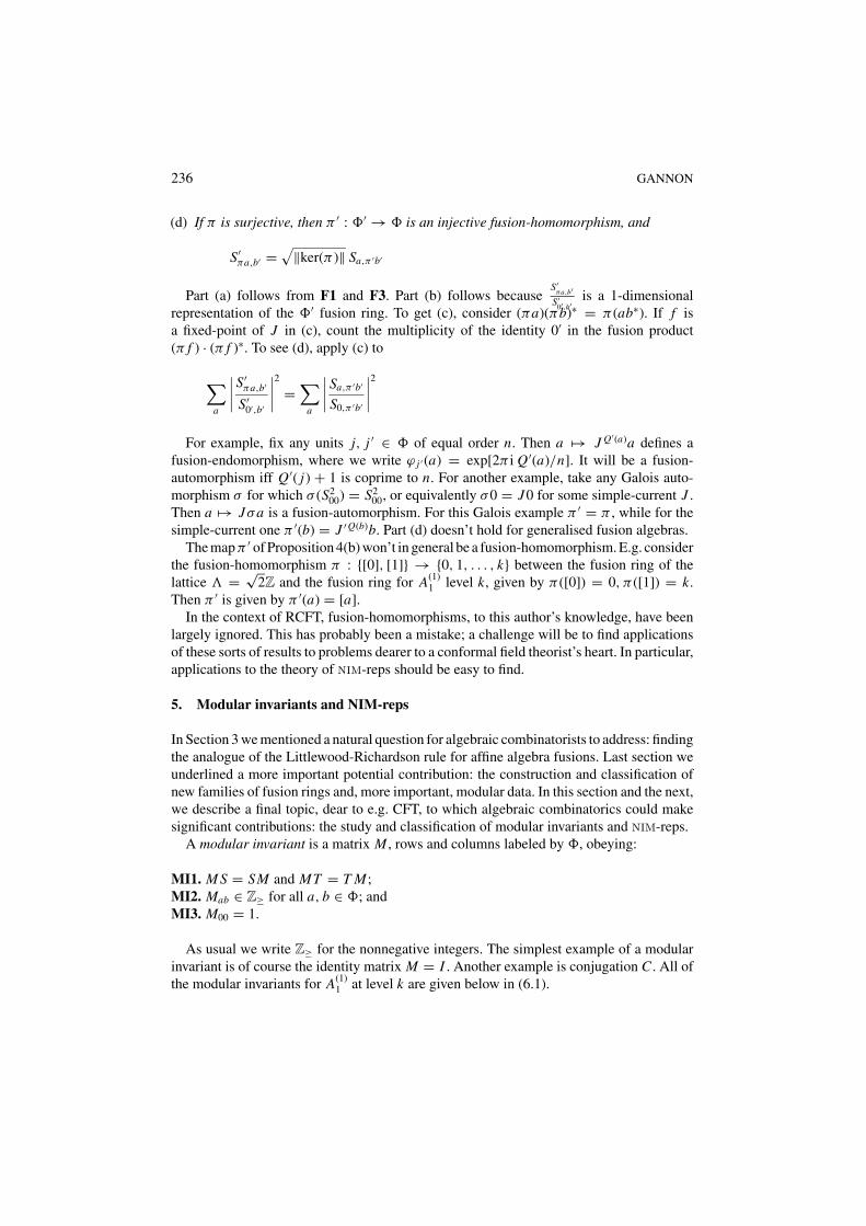
Proposition 4 Let π : � → �′ be a fusion-homomorphism between any two fusion rings.Then

(a) π0 = 0′ and π (a∗) = π (a)∗, and π takes units of � to units of �′.(b) There exists a map π ′ : �′ → � such that

S′πa,b′

S′0′,b′

= Sa,π ′b′

S0,π ′b′∀a ∈ �, b′ ∈ �′

(c) If πa = πb, then b = Ja for some simple-current J . In addition, this J will obeyπ (Jd) = π (d) for all d ∈ �, and (provided J is nontrivial) there can be no J-fixed-points in �.

236 GANNON

(d) If π is surjective, then π ′ : �′ → � is an injective fusion-homomorphism, and

S′πa,b′ =

√‖ker(π )‖ Sa,π ′b′

Part (a) follows from F1 and F3. Part (b) follows becauseS′

πa,b′S′

0′ ,b′is a 1-dimensional

representation of the �′ fusion ring. To get (c), consider (πa)(πb)∗ = π (ab∗). If f isa fixed-point of J in (c), count the multiplicity of the identity 0′ in the fusion product(π f ) · (π f )∗. To see (d), apply (c) to

∑a

∣∣∣∣ S′πa,b′

S′0′,b′

∣∣∣∣2

=∑

a

∣∣∣∣ Sa,π ′b′

S0,π ′b′

∣∣∣∣2

For example, fix any units j, j ′ ∈ � of equal order n. Then a �→ J Q′(a)a defines afusion-endomorphism, where we write ϕ j ′ (a) = exp[2π i Q′(a)/n]. It will be a fusion-automorphism iff Q′( j) + 1 is coprime to n. For another example, take any Galois auto-morphism σ for which σ (S2

00) = S200, or equivalently σ0 = J0 for some simple-current J .

Then a �→ Jσa is a fusion-automorphism. For this Galois example π ′ = π , while for thesimple-current one π ′(b) = J ′Q(b)b. Part (d) doesn’t hold for generalised fusion algebras.

The mapπ ′ of Proposition 4(b) won’t in general be a fusion-homomorphism. E.g. considerthe fusion-homomorphism π : {[0], [1]} → {0, 1, . . . , k} between the fusion ring of thelattice � = √

2Z and the fusion ring for A(1)1 level k, given by π ([0]) = 0, π ([1]) = k.

Then π ′ is given by π ′(a) = [a].In the context of RCFT, fusion-homomorphisms, to this author’s knowledge, have been

largely ignored. This has probably been a mistake; a challenge will be to find applicationsof these sorts of results to problems dearer to a conformal field theorist’s heart. In particular,applications to the theory of nim-reps should be easy to find.

5. Modular invariants and NIM-reps

In Section 3 we mentioned a natural question for algebraic combinatorists to address: findingthe analogue of the Littlewood-Richardson rule for affine algebra fusions. Last section weunderlined a more important potential contribution: the construction and classification ofnew families of fusion rings and, more important, modular data. In this section and the next,we describe a final topic, dear to e.g. CFT, to which algebraic combinatorics could makesignificant contributions: the study and classification of modular invariants and nim-reps.

A modular invariant is a matrix M , rows and columns labeled by �, obeying:

MI1. M S = SM and MT = T M ;MI2. Mab ∈ Z≥ for all a, b ∈ �; andMI3. M00 = 1.

As usual we write Z≥ for the nonnegative integers. The simplest example of a modularinvariant is of course the identity matrix M = I . Another example is conjugation C . All ofthe modular invariants for A(1)

1 at level k are given below in (6.1).


Why are modular invariants interesting? Most importantly, they are central to the task ofclassifying RCFTs. The genus-1 ‘vacuum-to-vacuum amplitude’(=partition function)Z(τ )of the theory looks like (1.3c). It assigns to the torus C/(Z+Zτ ) the complex number Z(τ ).But the moduli space of conformally equivalent tori is the orbit space SL2(Z)\H, wherethe action is given by (a b

c d)τ = aτ+bcτ+d . Thus the partition function Z(τ ) must be invariant

under this natural action of the modular group SL2(Z), which gives us MI1. The coeffi-cients Mab count the primary fields |φa, φb〉 in the state space H, i.e. the number of timesthe module Aa ⊗ Ab of left chiral algebra×right chiral algebra, appears in H. That gives usMI2. And the uniqueness of the vacuum |0, 0〉 means MI3. That is to say, the coefficientmatrix M of an RCFT partition function is a modular invariant. An RCFT is uniquely spec-ified by the knowledge of its partition function, its (left and right) chiral algebras(=VOAs),and the so-called structure constants. Thus, an important fingerprint of the RCFT is itspartition function Z , i.e. its modular invariant M . From the related point of view ofstring theory, modular invariants describe the consistent ‘first-quantised perturbative stringtheories’.

Another motivation for studying modular invariants is the extensions V ⊂ V ′ of rationalVOAs (similar remarks hold for braided subfactors). Let Mi and M ′

j be the irreduciblemodules of V and V ′, respectively. Then each M ′

j will be a V-module. A rational VOAshould have the complete reducibility property, so each M ′

j should be expressible as adirect sum of Mi ’s—these are called the branching rules. As mentioned in Example 5,we would expect that the characters (1.1) of a rational VOA should yield (some form of)modular data via (1.2a). So the diagonal sum

∑j |ch′

M ′j|2 should be invariant under the

SL2(Z)-action; rewriting the ch′M ′

j’s in terms of the chMi ’s via the branching rules yields a

modular invariant for V .For instance, the VOA L(�0)′ corresponding to the affine algebra G(1)

2 level 1 containsthe VOA L(28�0) corresponding to A(1)

1 at level 28. We get the branching rules L(�0)′ =L(0) ⊕ L(10) ⊕ L(18) ⊕ L(28) and L(�2)′ = L(6) ⊕ L(12) ⊕ L(16) ⊕ L(22), whereL(λ1) := L(λ). This corresponds to the A(1)

1 level 28 modular invariant given below in(6.1f).

So knowing the modular invariants for some VOA V gives considerable informationconcerning its possible ‘nice’ extensions V ′. For instance, we are learning that the onlyfinite ‘rational’ extensions of a generic affine VOA are those studied in [41] (‘simple-currentextensions’) and whose modular data is conjecturally given in [58].

Another reason for studying modular invariants is that the answers are often surprising.Lists arising in math from complete classifications tend to be about as stale as phonebooks,but to give some samples:

• the A(1)1 modular invariants fall into the A-D-E metapattern;

• the A(1)2 modular invariants have connections with Jacobians of Fermat curves; and

• the (U (1) ⊕ · · · ⊕ U (1))(1) modular invariants correspond to rational points on Grass-mannians.

We will discuss this point a little more next section. These ‘coincidences’, presumably, havesomething to do with the nontrivial connections between RCFT and several areas of math,

238 GANNON

but it also is due to the beauty of the combinatorics of Lie characters evaluated at elementsof finite order (3.2c).

In any case, in this section we will study the modular invariants corresponding to a givenchoice of modular data. For lattices, the classification is easy (use (5.2) below). For manyfinite groups, the classification typically will be hopeless—e.g. the quantum-double of thealternating group A5, which has only 22 primaries, has a remarkably high number (8719)of modular invariants [7]. For affine algebra modular data, the classification of modularinvariants seems to be just barely possible, and the answer is that (generically) the onlymodular invariants are constructed in straightforward ways from symmetries of the Dynkindiagrams.

Commutation with T is trivial to solve, since T is diagonal: it yields the selection rule

Mab �= 0 ⇒ Taa = Tbb (5.1)

This isn’t as useful as it looks; commutation with S (or equivalently, the equation SMS = M)is more subtle, but far more valuable.

An immediate observation is that there are only finitely many modular invariants associ-ated to given modular data. This follows for instance from

1 = M00 =∑

a,b∈�

S0a Mab Sb0 ≥ S200

∑a,b∈�

Mab

We will find that each basic symmetry of the S matrix yields a symmetry of the modularinvariants, a selection rule telling us that certain entries of M must vanish, and a way toconstruct new modular invariants.

First consider simple-currents J, J ′. Equation (4.3a) and positivity tell us

MJ0,J ′0 =∣∣∣∣∣

∑c,d∈�

ϕJ (c) S0c Mcd Sd0 ϕJ ′ (d)

∣∣∣∣∣ ≤∑c,d

S0c Mcd Sd0 = M00 = 1 (5.2a)

Thus MJ0,J ′0 �= 0 implies MJ0,J ′0 = 1, as well as the selection rule

Mcd �= 0 ⇒ ϕJ (c) = ϕJ ′ (d) (5.2b)

A similar calculation yields the symmetry

MJ0,J ′0 �= 0 ⇒ MJa,J ′b = Mab ∀a, b ∈ � (5.2c)

The most useful application of simple-currents to modular invariants is to their construc-tion. In particular, let J be a simple-current of order n. Then we learned in (4.3) that ϕ j (a)is an nth root of 1, and that (Tj j T00)2n = 1 and in fact (Tj j T00)n = 1 when n is odd. That isto say, we can find integers r j and Q j (a) obeying

ϕ j (a) = exp

[2π i

Q j (a)

n

], Tj j T00 = exp

[π i r j

n − 1

n

]


For n odd, choose r j to be even (by adding n to it if necessary). Now define the matrixM[J ] by [103]

M[J ]ab =n∑

�=1

δJ �a,b δ

(Q j (a)

n+ �

2nr j

)(5.3)

where δ(x) = 1 when x ∈ Z and is 0 otherwise. This matrix M[J ] will be a modularinvariant iff (Tj j T00)n = 1 (i.e. iff r j is even), and a permutation matrix iff Tj j T00 is aprimitive nth root of 1. When n is even, (4.3c) says (Tj j T00)n = 1 iff ϕ j ( j)n/2 = 1.

For instance, taking J = id we get M[id] = I . The affine algebra A(1)1 at level k has

a simple-current with r j = k given by Ja = k − a; for even k the matrix M[J ] is themodular invariant called D k

2 +2 below in (6.1b), (6.1c).Now look at the consequences of Galois. Applying the Galois automorphism σ to M =

SM S yields from (4.4) and Mab ∈ Q the fundamental equation

Mab =∑

c,d∈�

εσ (a) Sσa,c Mcd Sd,σb εσ (b) = εσ (a) εσ (b) Mσa,σb (5.4a)

Because Mab ≥ 0, we obtain the selection rule

Mab �= 0 ⇒ εσ (a) = εσ (b) ∀σ (5.4b)

and the symmetry

Mσa,σb = Mab ∀σ (5.4c)

Of all the Eqs. (5.2) and (5.4), (5.4b) is the most valuable. A way to construct modularinvariants from Galois was first given in [56] but isn’t useful for constructing affine algebramodular invariants and so won’t be repeated here.

There are other very useful facts, which space prevents us from describing. For instance,we have the inequality

∑b∈�

Sab Mb0 ≥ 0 (5.5)

Perron-Frobenius tells us many things, e.g. that any modular invariant M obeying M0a = δ0a

must be a permutation matrix. For affine algebra modular invariants, the Lie theory of theunderlying finite-dimensional Lie algebra plays a crucial role, thanks largely to (3.2c).

Closely related to modular invariants is the notion of nim-rep (short for ‘nonnegativeinteger representation’ [19, 20]) or equivalently fusion graph. These originally arose in twoa priori unrelated contexts: the analysis, starting with Cardy’s fundamental paper [26], ofboundary RCFT; and Di Francesco–Zuber’s largely empirical attempt [34, 35] to understandand generalise the A-D-E metapattern appearing in A(1) modular invariants, by attachinggraphs to each conformal field theory.

240 GANNON

A nim-rep N is a nonnegative integer representation of the fusion ring, that is, an as-signment a �→ Na to each a ∈ � of a matrix Na with nonnegative integer entries, obeyingNaNb = ∑

c N cabNc. In addition we require thatN0 = I and that transpose and conjugation

be related by N ta = NCa , for all a ∈ �.

Two obvious examples of nim-reps are the fusion matrices, a �→ Na , and their transposesa �→ N t

a . The rows and columns of most nim-reps however won’t be labelled by �, in factwe will see that the dimension of the nim-rep should equal the trace Tr(M) of some modularinvariant.

Just as it is convenient to replace a Cartan matrix by its Dynkin diagram, so too is itconvenient to realise Na by a (directed multi-)graph: we put a node for each row/column,and draw (Na)αβ edges directed from α to β. We replace each pair of arrows α → β, β → α,with a single undirected edge connecting α and β. These graphs are called fusion graphs,and are often quite striking.

nim-reps correspond in RCFT to the 1-loop vacuum-to-vacuum amplitude Zαβ(t) of anopen string, or equivalently of a cylinder whose edge circles are labelled by ‘conformallyinvariant boundary states’ |α〉, |β〉 [26, 102, 59, 15]. In string theory these are called the‘Chan-Paton degrees-of-freedom’ and are placed at the endpoints of open strings. The realvariable −∞ < t < ∞ here is the modular parameter for the cylinder, and plays thesame role here that τ ∈ H plays in Z(τ ). In particular we get (1.4), where the matrices(Na)αβ = N β

aα define a nim-rep. These (finitely many) boundary states α are the indices forthe rows and columns of each matrixNa . In the language of string theory, nim-reps describethe possible ‘D-branes’ respecting the appropriate chiral algebra (VOA) symmetry.

Related to nim-reps are what string theory calls the charges of symmetry-preservingD-branes living on Lie group manifolds (see e.g. [23]). Mathematically, these are nontrivialring homomorphisms from the fusion ring into Z/mZ for some m. Partition functionsassociated to nonorientable surfaces (especially the Mobius strip and Klein bottle) are alsoimportant in boundary RCFT or open string theory—see e.g. [102, 107]. We won’t discussthese additional developments further in this paper.

By the usual arguments (see Section 4) we can simultaneously diagonalise all Na , andthe eigenvalues of Na will be Sab/S0b for b in some multi-set E = E(N ) (i.e. the elementsof E come with multiplicities). This multi-set E depends only on N (i.e. is independent ofa ∈ �), and is called the exponents of the nim-rep.

Two nim-reps N ,N ′ are regarded as equivalent if there is a simultaneous permutationπ of the rows and columns such that πNaπ

−1 = N ′a for all a ∈ �. For example, the two

nim-reps given earlier are equivalent: N ta = C NaC−1. We write N = N ′ ⊕N ′′, and call N

reducible, if the matrices Na can be simultaneously written as direct sums Na = N ′a ⊕N ′′

a .Necessarily, the summands N ′ and N ′′ themselves will be nim-reps. Irreducibility is equiv-alent to demanding that the identity 0 occurs in E(N ) with multiplicity 1. We are interestedin irreducible equivalence classes of nim-reps—there will be only finitely many [70].

Two useful facts are: the Perron-Frobenius eigenvalue ofNa is the q-dimension Sa0S00

(we’llsee this used next section); and for all a ∈ �,

∑b∈E

Sab

S0b= Tr (Na) ∈ Z≥ (5.6)


The consequences of the simple-current and Galois symmetries are also important and areworked out in [70].

By the exponents of a modular invariant M we mean the multi-set EM where a ∈ �

appears with multiplicity Maa . RCFT [26, 15] is thought to require that each modularinvariant M have a companion nim-rep N with the property that

EM = E(N ) (5.7)

So the size of the matricesNa , i.e. the dimension of thenim-rep, should equal the trace Tr(M)of the modular invariant. For instance, the fusion matrix nim-rep a �→ Na corresponds tothe modular invariant M = I . However, there doesn’t seem to be a general expression forthe nim-rep (if it exists) of the next simplest modular invariant, the conjugation M = C .

Incidentally, the inequality (5.6) is automatically obeyed by the exponents E = EM ofany modular invariant M :

∑b∈EM

Sab

S0b= Tr(MDa) = Tr(SSMDa) = Tr(MSDa S) = Tr(MNa) ∈ Z≥

where Da is the diagonal matrix with entries Sab/S0b.Note that the nim-rep definition depends on S, while a modular invariant also sees T .

One consequence of this is the following. Suppose there is a primary a ∈ � such that

Tbb = Tcc ⇒ Sab Sac ≥ 0 ∀b, c ∈ � (5.8)

Then Maa = ∑b,c Sab Mbc Sac > 0 and so a ∈ EM . It is thus natural to require of a

nim-rep N that any such primary a ∈ � must appear in E(N ) with multiplicity ≥ 1,because otherwise no modular invariant M could be found obeying (5.7). We’ll see anexample next section.

An independent justification for studying modular invariants and nim-reps comes fromthe subfactor picture (Example 6), where they appear very naturally [47, 98, 19, 20]. Inthis remarkable picture it is possible to interpret not only the diagonal entries of the mod-ular invariant, as in (5.7), but in fact all entries [97,19,20] (this was already anticipatedin [34, 35]). Extend the setting of Example 6 by considering a braided system of endo-morphisms for a type III subfactor N ⊂ M . Here, the primaries � = N χN consist ofirreducible endomorphisms of N , while the rows and columns of our nim-rep will be in-dexed by irreducible homomorphisms a ∈ MχN , a : N → M . The fusion-like ring ofN χN will be commutative, i.e. be a true fusion ring; that of MχM however will generallybe noncommutative. There is a simple expression [19, 20] for the corresponding modularinvariant using ‘α-induction’ (a process of inducing an endomorphism from N to M usingthe braiding ε±): we get Mλµ = 〈α+

λ , α−µ 〉 where the dimension 〈, 〉 is defined in Example 6.

Then the (complexified) fusion algebra of MχM will be isomorphic (as a complex algebra)to ⊕λ,µGLMλµ

(C). The nim-rep is essentially α: (Nλ)a,b = 〈b, α±λ a〉 (either choice of α±

gives the same matrix) [19, 20]. This nim-rep arises as a natural action of MχM on MχN .As these partition functions of tori and cylinders appear so nicely here, it is tempting to ask

242 GANNON

about other surfaces, especially the Mobius band and Klein bottle, which also play a basicrole in boundary RCFT [102, 107].

We won’t speak much more here about nim-reps—see e.g. [34, 35, 15, 70] and referencestherein for more of the theory and classifications (and graphs!). What has happened in mostof the classifications obtained thus far is that, at least for affine algebra modular data, thereare slightly more nim-reps than modular invariants, but otherwise their classifications matchsurprisingly well. For instance, as we’ll see next section, the irreducible nim-reps of A(1)

1haveN1 equal to the incidence matrix of the A-D-E Dynkin graphs and tadpoles (line graphswith a loop at an end) [34, 35]—apart from the tadpole, this is in perfect agreement with thelist of modular invariants for A(1)

1 in (6.1)! However we know few nim-rep classificationsand this pleasant correspondence may break down as we go to higher rank and level. Forinstance, the complete list of nim-reps for A(1)

2 are known only for levels 1, 2, 3, andalthough the nim-reps and modular invariants match up perfectly for levels 1 and 2, thereare 8 nim-reps at level 3 and only 4 modular invariants. This discrepancy may get worseas the level rises—clearly, more work along this line is needed. Moreover, there are somemodular invariants which lack a corresponding nim-rep. The simplest examples of modularinvariants lacking nim-reps occur for affine algebra B(1)

4 at level 2, and the quantum-doubleof the symmetric group S3 [70].

A tempting guess is that almost all of the enormous numbers of modular invariantsassociated to finite group modular data will likewise fail to have a corresponding nim-rep.Recall that the Galois parities ε� for the finite group modular data are all +1, and hencethe constraint (5.4b) becomes trivial. As a general rule, the number of modular invariantsis inversely related to the severity (5.4b) possesses for that choice of modular data.

The moral of the story seems to be the following. The definition of modular invariantsdidn’t come to us from God; it came to us from men like Witten, Cardy, ... The surprisingthing is that so often their classification yields interesting answers. A modular invariantmay not correspond to a CFT (we have infinitely many examples where it fails to), andthe modular invariant may correspond to different CFTs (though all known examples ofthis are artificial, due to our characters depending on too few variables to distinguish therepresentations of the maximally extended VOAs). But—at least for most affine algebrasand levels—it seems they’re usually in one-to-one correspondence.

In any case, classifying modular invariants, and comparing their lists to those of nim-reps,is a natural task and has led to interesting findings (see e.g. the review [118]).

6. Affine algebra modular invariant classifications

The most famous modular invariant classification was the first. In (3.5) we gave explicitlythe modular data for the affine algebra A(1)

1 at level k. Its complete list of modular invariantsis [25] (using the simple-current Ja = k − a)

Ak+1 =k∑

a=0

|χa|2 , ∀k ≥ 1 (6.1a)

D k2 +2 =

k∑a=0

χa χJ aa , wheneverk

2is odd (6.1b)


D k2 +2 = |χ0 + χJ0|2 + |χ2 + χJ2|2 + · · · + 2|χ k

2|2 , whenever

k

2is even (6.1c)

E6 = |χ0 + χ6|2 + |χ3 + χ7|2 + |χ4 + χ10|2 , for k = 10 (6.1d)

E7 = |χ0 + χ16|2 + |χ4 + χ12|2 + |χ6 + χ10|2+χ8 (χ2 + χ14) + (χ2 + χ14) χ8 + |χ8|2 , for k = 16 (6.1e)

E8 = |χ0 + χ10 + χ18 + χ28|2 + |χ6 + χ12 + χ16 + χ22|2, for k = 28 (6.1f)

Each of these is identified with a (finite) Dynkin diagram, in such a way that the Coxeternumber h of the diagram equals k + 2, and the exponents of the corresponding Lie algebraare given by 1 + EM (recall the definition of exponents EM of a modular invariant, givenat the end of last section). The exponents of the Lie algebra are the numbers mi , where4 sin2(π mi

h ) are the eigenvalues of the Cartan matrix. For instance, the Dynkin diagramD8 has Coxeter number 14 and exponents 1, 3, 5, 7, 7, while D8 occurs at level 12 and hasexponents E = {0, 2, 4, 6, 6}.

The A-D-E pattern appears in many places in math and mathematical physics [81, 106]:besides the simply-laced Lie algebras and A(1)

1 modular invariants, these diagrams alsoclassify simple singularities, finite subgroups of SU2(C), subfactors with Jones index <4,representations of quivers, etc. There seem to be two more-or-less inequivalent A-D-Epatterns, one corresponding to the finite A-D-E diagrams, and the other correspondingto the affine (=extended) A-D-E diagrams. For instance, the modular invariants identifywith the finite ones, while the finite subgroups of SU2(C) match with the affine ones. Thissuggests that a direct relation between e.g. the modular invariants and those finite subgroupscould be a little forced. Patterns such as A-D-E are usually explained by identifying anunderlying combinatorial fact which is responsible for its various incarnations. The A-D-Ecombinatorial fact is probably the classification of symmetric matrices over Z≥, with zerodiagonals, and with maximal eigenvalue <2 (for the finite diagrams) and =2 (for the affineones). Perhaps the only A-D-E classification which still resists this ‘explanation’ is that ofA(1)

1 modular invariants. This is in spite of considerable effort (and some progress) by manypeople. The present state of affairs, and also a much simpler proof on the lines sketched inthe previous section, is provided by [69].

Many other classes of affine algebras and levels have been classified. The main ones are:A(1)

2 , (A1 + A1)(1), and (U (1) + · · · + U (1))(1), for all levels k; and A(1)r , B(1)

r , D(1)r for all

ranks r , but with levels restricted to k ≤ 3. See e.g. [68] for references to these results.Has A-D-E been spotted in these other lists? No. However, a remarkable connection

[101, 12] has been observed between the A(1)2 level k modular invariants, and the Jacobian

of the Fermat curve xk+3 + yk+3 + zk+3 = 0. In particular, the A(1)2 Galois selection rule

(5.4b) and the analysis of the simple factors in the Jacobian are essentially the same. Thislink between Fermat and A(1)

2 is still unexplained, and how it extends to the other algebras,e.g. perhaps A(1)

r level k relates to xk+r+11 + xk+r+1

2 + · · · + xk+r+1r+1 = 0?, is still unclear.

However, Batyrev [11] has suggested some possibilities involving toric geometry.The third ‘sample’ listed last section (relating (U (1)⊕· · ·⊕U (1))(1) modular invariants to

the Grassmannians) suggests a different link with geometry. The Grassmannian is essentiallythe moduli space of Narain compactifications of a (classical) string theory, so perhaps other

244 GANNON

families of modular invariants can be regarded as special points on other finite-dimensionalmoduli spaces.

Though there are no other appearances of A-D-E, there is a rather natural way to assign(multi-di)graphs to modular invariants, generalising the A-D-E pattern for A(1)

1 . Note firstthat we can classify the A(1)

1 nim-reps [34, 35]: N1 must be symmetric and have Perron-Frobenius eigenvalue S10

S00= 2 cos( π

k+2 ) < 2; thus the graph associated to N1 must bean A-D-E Dynkin diagram, or a tadpole. The tadpoles can be discarded, since they don’tcorrespond via (5.7) to a modular invariant. Given N1, all other Na can be recursivelyobtained using the special case N1Ni = Ni+1 + Ni−1 of (3.5c). The result is a nim-rep.

In this way, we find that the Dynkin diagram which (6.1) assigned to a given A(1)1 modular

invariant M is precisely the graph whose adjacency matrix equals the generator N1 of theunique nim-rep compatible with M in the sense of (5.7). Likewise, we should assign to themodular invariants of e.g. A(1)

2 the multi-digraph N�1 generating the corresponding nim-rep. The nim-reps for A(1)

2 are not yet classified, but at least one has been found for each M[34, 35, 98, 15, 19, 20].

There is a simple reason why the tadpole can’t correspond to an A(1)1 modular invariant.

Note that the unit a = k satisfies (5.8), and thus will lie in any EM . However, k is notan exponent of the tadpole, and thus there can be no solution M in (5.7) for the choiceN = tadpole.

By the way, submodular invariants can usually be found for nim-reps which lack a truemodular invariant. For example, the seemingly extraneous n-vertex tadpole mentioned inthe previous paragraph corresponds to the algebra A(1)

1 at level 2n − 1, and the submodularinvariant Mab = δb,J aa . Perhaps a reasonable interpretation can be found by both thesubfactor and boundary CFT camps for nim-reps corresponding to matrices M commutingwith certain small-index subgroups of SL2(Z). Recall that we anticipated this thought at theend of Example 1.

Most of the modular invariant classification effort has been directed not at specific algebrasand levels, but at the general argument. The major result obtained thus far is:

Theorem 5 ([67, 71, 74]) Choose any affine algebra X (1)r and level k. Let M be any

modular invariant, obeying the constraint that the only primaries a ∈ � for which M0a �= 0or Ma0 �= 0, are units. Then M lies on an explicit list.

Note that, of the A(1)1 modular invariants, all but E6 and E8 obey the constraint of Theo-

rem 5. That pattern seems to continue for the other algebras and levels: the list of modularinvariants covered by Theorem 5 exhausts almost every modular invariant yet discovered.

There are very few exceptional modular invariants in the list of Theorem 5. Almost all ofthe modular invariants there are simple-current ones (5.3), and the product of these by theconjugation C (strictly speaking, any symmetry of the unextended Dynkin diagram can beused here in place of C).

Theorem 5 is important because, for generic choice of algebra and level, the variousconstraints we have on the 0-row and 0-column of a modular invariant (most importantly,Galois (5.4b), T (5.1), and the inequality (5.5)) force the condition of Theorem 5 to besatisfied.


Indeed, if we impose the full structure of Ocneanu cells [98] (this should be equivalentto saying that an RCFT exists with partition function given by M , although to this author’sknowledge this hasn’t been rigourously shown yet), we obtain Ocneanu’s inequality [98]:∑

µ∈clearing

Nµ

λ,Cλ Sµ0 ≤ Sλ0 (6.2)

where λ is any weight�= 0 obeying Mλ0 �= 0 with λ0 as large as possible, and where‘clearing’ is a subset of Pk

+ close to 0: µ is in the clearing if 2(k − µ0) ≤ k − λ0. Theproof of this important inequality has not appeared in print yet. The left-side of (6.2) growsapproximately quadratically with Sλ0/S00, while the right-side is only linear, so it tendsto force Sλ0 to be small; Eq. (5.1) on the other hand tends to force Sλ0 to be large. Thisapparently implies (although the details of the argument have also not yet appeared in print)that, for fixed algebra X (1)

r , there is a K (depending on the algebra) such that ∀k > K , theconstraint of Theorem 5 will be obeyed! Thus, assuming these two announced claims, weobtain:

Corollary 6 All possible modular invariants appearing in RCFT (or the subfactorinterpretation), corresponding to any fixed choice of affine algebra X (1)

r , and all sufficientlyhigh levels, are known.

In other words, what Corollary 6 tells us is that, apart from some low level exceptionalmodular invariants, all affine algebra modular invariants appearing in RCFT can be con-structed in straightforward and known ways from the symmetries of the correspondingaffine Dynkin diagram!

Theorem 5 has another consequence. It makes it relatively easy to find all modularinvariants (using only conditions MI1-MI3) at ‘small’ levels, when the rank of the algebraisn’t too large [73]. For example, all modular invariants for E (1)

8 at all levels k ≤ 380can be determined. This isn’t completely trivial: E (1)

8 at k = 380 has over 1012 highestweights=primaries, so the S and M matrices have a number of entries approximately equalto Avogadro’s number! And each of these entries of S, given by (3.2b), involves a sum of 109

complex numbers. The fact that we can reach such high levels isn’t a sign of programmingprowess, but rather to how close we are to a complete classification of these (unrestricted)affine algebra modular invariants. In [73] the modular invariants are given for all exceptionalalgebras, and the classical algebras of rank ≤6.

The big surprise here is how rare the affine algebra modular invariants are (for comparison,recall that there are over 8000 modular invariants for the finite group A5). In the Tablewe’ve summarised the modular invariant classifications for various algebras of small rank.It describes the complete list of modular invariants for these algebras, when the level issufficiently small (these limits are given in the Table). A very safe conjecture though is thatthe Table gives the complete classification for those algebras, for all levels k (at the timeof writing, E (1)

7 level 42 and E (1)8 level 90 still have not been eliminated). Our hope is that

this Table (or more realistically, the paper [73] where more results are given and in moredetail) will inspire someone to spot a new coincidence involving modular invariants andsome other area of mathematics. For example, note in A(1)

1 that the exceptionals appear at

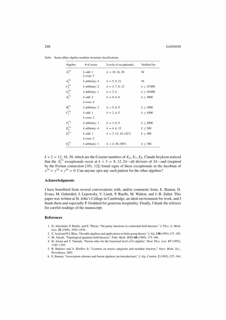
246 GANNON

Table Some affine algebra modular invariant classifications.

Algebra # of series Levels of exceptionals Verified for:

A(1)1 k odd: 1 k = 10, 16, 28 ∀k

k even: 2

A(1)2 k arbitrary: 4 k = 5, 9, 21 ∀k

C (1)2 k arbitrary: 2 k = 3, 7, 8, 12 k ≤ 25 000

G(1)2 k arbitrary: 1 k = 3, 4 k ≤ 30 000

A(1)3 k odd: 2 k = 4, 6, 8 k ≤ 4000

k even: 4

B(1)3 k arbitrary: 2 k = 5, 8, 9 k ≤ 3000

C (1)3 k odd: 1 k = 2, 4, 5 k ≤ 4500

k even: 2

F (1)4 k arbitrary: 1 k = 3, 6, 9 k ≤ 2000

E (1)6 k arbitrary: 4 k = 4, 6, 12 k ≤ 500

E (1)7 k odd: 1 k = 3, 12, 18, (42?) k ≤ 400

k even: 2

E (1)8 k arbitrary: 1 k = 4, 30, (90?) k ≤ 380

k + 2 = 12, 18, 30, which are the Coxeter numbers of E6, E7, E8. Claude Itzykson noticedthat the A(1)

2 exceptionals occur at k + 3 = 8, 12, 24—all divisors of 24—and (inspiredby the Fermat connection [101, 12]) found signs of these exceptionals in the Jacobian ofx24 + y24 + z24 = 0. Can anyone spot any such pattern for the other algebras?

Acknowledgments

I have benefitted from several conversations with, and/or comments from, E. Bannai, D.Evans, M. Gaberdiel, J. Lepowsky, V. Linek, P. Ruelle, M. Walton, and J.-B. Zuber. Thispaper was written at St. John’s College in Cambridge, an ideal environment for work, and Ithank them and especially P. Goddard for generous hospitality. Finally, I thank the refereesfor careful readings of the manuscript.

References

1. D. Altschuler, P. Ruelle, and E. Thiran, “On parity functions in conformal field theories,” J. Phys. A: Math.Gen. 32 (1999), 3555–3570.

2. Z. Arad and H.I. Blau, “On table algebras and applications to finite group theory,” J. Alg. 138 (1991) 137–185.3. M. Atiyah, “Topological quantum field theories,” Publ. Math. IHES 68 (1989), 175–186.4. H. Awata and Y. Yamada, “Fusion rules for the fractional level ˆsl(2) algebra,” Mod. Phys. Lett. A7 (1992),

1185–1195.5. B. Bakalov and A. Kirillov Jr, “Lectures on tensor categories and modular functors,” Amer. Math. Soc.,

Providence, 2001.6. E. Bannai, “Association schemes and fusion algebras (an introduction),” J. Alg. Combin. 2 (1993), 327–344.


7. E. Bannai, E. Bannai, O. Shimabukuro, and M. Tagami, “Modular invariants of the modular data of finitegroups,” preprint.

8. E. Bannai and T. Ito, Algebraic Combinatorics I: Association Schemes, Benjamin-Cummings, Menlo ParkCalifornia, 1984.

9. P. Bantay, “The Frobenius-Schur indicator in conformal field theory,” Phys. Lett. B394 (1997) 87–88.10. P. Bantay, “The kernel of the modular representation and the Galois action in RCFT,” Commun. Math. Phys.

233 (2003), 423–438.11. V. Batyrev, “Vertex algebras and mirror symmetry,” (talk, University of Warwick, October 1999).12. M. Bauer, A. Coste, C. Itzykson and P. Ruelle, “Comments on the links between SU(3) modular invariants,

simple factors in the Jacobian of Fermat curves, and rational triangular billiards,” J. Geom. Phys. 22 (1997),134–189.

13. L. Begin, P. Mathieu, and M.A. Walton, “ ˆsu(3)k fusion coefficients,” Mod. Phys. Lett. A7 (1992), 3255–3265.14. L. Begin, A.N. Kirillov, P. Mathieu, and M.A. Walton, “Berenstein-Zelevinsky triangles, elementary cou-

plings, and fusion rules,” Lett. Math. Phys. 28 (1993), 257–268.15. R.E. Behrend, P.A. Pearce, V.B. Petkova, and J.-B. Zuber, “Boundary conditions in rational conformal field

theories,” Nucl. Phys. B579 (2000), 707–773.16. B. Bertram, I. Ciocan-Fontanine, and W. Fulton, “Quantum multiplication of Schur polynomials,” J. Alg.

219 (1999), 728–746.17. L. Birke, J. Fuchs, and C. Schweigert, “Symmetry breaking boundary conditions and WZW orbifolds,” Adv.

Theor. Math. Phys. 3 (1999), 671–726.18. H.I. Blau, “Quotient structures in C-algebras,” J. Alg. 175 (1995), 297–337.19. J. Bockenhauer and D.E. Evans, “Modular invariants and subfactors,” in Mathematical Physics in Mathe-

matics and Physics, R. Longo (Ed.), Amer. Math. Soc., Providence, 2001, pp. 11–37.20. J. Bockenhauer and D.E. Evans, “Modular invariants from subfactors,” in Quantum Symmetries in Theoret-

ical Physics and Mathematics, R. Coquereaux et al. (Eds.), Amer. Math. Soc., Providence, 2002, pp. 95–131.

21. R.E. Borcherds, “Vertex algebras, Kac-Moody algebras, and the Monster,” Proc. Natl. Acad. Sci. (USA) 83(1986), 3068–3071.

22. R.E. Borcherds, “What is Moonshine?,” in Proc. Intern. Congr. Math., Berlin, 1998, pp. 607–615.23. P. Bouwknegt, P. Dawson, and D. Ridout, “D-branes on group manifolds and fusion rings,” J. High Energy

Phys. 0212 (2002), 065.24. A.S. Buch, A. Kresch, and H. Tamvakis, “Gromov-Witten invariants on Grassmannians,” J. Amer. Math.

Soc. 16 (2003), 901–915.25. A. Cappelli, C. Itzykson, and J.-B. Zuber, “The A-D-E classification of minimal and A(1)

1 conformal invarianttheories,” Commun. Math. Phys. 113 (1987), 1–26.

26. J. Cardy, “Boundary conditions, fusion rules and the Verlinde formula,” Nucl. Phys. B324 (1989), 581–596.27. M. Caselle and G. Ponzano, “Analyticity, modular invariance and the classification of three operator fusion

algebras,” Phys. Lett. B242 (1990), 52–58.28. H. Cohn, A Classical Invitation to Algebraic Numbers and Class Fields, Springer, New York, 1988.29. J.H. Conway and N.J.A. Sloane, Sphere Packings, Lattices and Groups, 3rd edn, Springer, Berlin, 1999.30. A. Coste and T. Gannon, “Remarks on Galois in rational conformal field theories,” Phys. Lett. B323 (1994),

316–321.31. A. Coste and T. Gannon, “Congruence subgroups and conformal field theory,” preprint (math.QA/0002044).32. A. Coste, T. Gannon, and P. Ruelle, “Finite group modular data,” Nucl. Phys. B581 (2000), 679–717.33. L. Crane and D.N. Yetter, “Deformations of (bi)tensor categories,” Cah. Top. Geom. Diff. Categ. 39 (1998),

163–180.34. P. Di Francesco and J.-B. Zuber, “SU(N ) lattice integrable models associated with graphs,” Nucl. Phys. B338

(1990), 602–646.35. P. Di Francesco and J.-B. Zuber, “SU(N ) lattice integrable models and modular invariance,” in Recent

Developments in Conformal Field Theory, World Scientific, (1990), pp. 179–215.36. Ph. Di Francesco, P. Mathieu, and D. Senechal, Conformal Field Theory, Springer, New York, 1997.37. R. Dijkgraaf, “The mathematics of fivebranes,” in Proc. Intern. Congr. Math., Berlin, Vol. III, (1998),

pp. 133–142.

248 GANNON

38. R. Dijkgraaf, C. Vafa, E. Verlinde, and H. Verlinde, “The operator algebra of orbifold models,” Commun.Math. Phys. 123 (1989), 485–526.

39. R. Dijkgraaf and E. Witten, “Topological gauge theories and group cohomology,” Commun. Math. Phys. 129(1990), 393–429.

40. C. Dong, “Vertex algebras associated with even lattices,” J. Alg. 160 (1993), 245–265.41. C. Dong, H. Li, and G. Mason, “Simple currents and extensions of vertex operator algebras,” Commun.

Math. Phys. 180 (1996), 671–707.42. C. Dong, H. Li, and G. Mason, “Vertex operator algebras associated to admissible representations of ˆsl2,”

Commun. Math. Phys. 184 (1997), 65–93.43. C. Dong, H. Li, and G. Mason, “Modular-invariance of trace functions in orbifold theory and generalised

moonshine,” Commun. Math. Phys. 214 (2000), 1–56.44. W. Eholzer, “On the classification of modular fusion algebras,” Commun. Math. Phys. 172 (1995), 623–660.45. F. Englert, L. Houart, A. Taormina, and P. West, “The symmetry of M-theories,” J. High Energy Phys. 9

(2003), 020.46. P. Etingof and S. Gelaki, “Isocategorical groups,” Intern. Math. Res. Notices (2) (2001), 59–76.47. D.E. Evans and Y. Kawahigashi, Quantum Symmetries on Operator Algebras, Oxford University Press, 1998.48. G. Faltings, “A proof for the Verlinde formula,” J. Alg. Geom. 3 (1994), 347–374.49. B. Feigin and F. Malikov, “Modular functor and representation theory of sl(2) at a rational level,” in Operads,

Contemp. Math. 202, Amer. Math. Soc., Providence, 1997, pp. 357–405.50. A.J. Feingold and M.D. Weiner, “Type A fusion rules from elementary group theory,” in Recent Developments

in Infinite-Dimensional Lie algebras and Conformal Field Theory, S. Berman et al. (Eds.), Amer. Math. Soc.,Providence, 2002, pp. 97–115.

51. M. Finkelberg, “An equivalence of fusion categories,” Geom. Funct. Anal. 6 (1996), 249–267.52. D.S. Freed, M.J. Hopkins, and C. Teleman, “Twisted K-theory and loop group representations,”

math.AT/0312155.53. I.B. Frenkel, J. Lepowsky, and A. Meurman, Vertex Operator Algebras and the Monster, Pure and Applied

Math, Vol. 134, Academic Press, London-New York, 1988.54. I.B. Frenkel and Y. Zhu, “Vertex operator algebras associated to representations of affine and Virasoro

algebras,” Duke Math. J. 66 (1992), 123–168.55. J. Fuchs, “Fusion rules in conformal field theory,” Fortsch. Phys. 42 (1994), 1–48.56. J. Fuchs, B. Gato-Rivera, B. Schellekens, and C. Schweigert, “Modular invariants and fusion rule automor-

phisms from Galois theory,” Phys. Lett. B334 (1994), 113–120.57. J. Fuchs, S. Hwang, A.M. Semikhatov, and I.Y.U. Tipunin, “Nonsemisimple fusion algebras and the Verlinde

formula,” hep-th/0306274.58. J. Fuchs, A.N. Schellekens, and C. Schweigert, “From Dynkin diagram symmetries to fixed point structures,”

Commun. Math. Phys. 180 (1996), 39–97.59. J. Fuchs and C. Schweigert, “Branes: from free fields to general backgrounds,” Nucl. Phys. B530 (1998),

99–136.60. L. Funar, “On the TQFT representations of the mapping class groups,” Pac. J. Math. 188 (1999), 251–274.61. P. Furlan, A. Ganchev, and V. Petkova, “Quantum groups and fusion rules multiplicitites,” Nucl. Phys. B343

(1990), 205–227.62. P. Furlan, A. Ganchev, and V.B. Petkova, “An extension of the character ring of sl(3) and its quantisation,”

Commun. Math. Phys. 202 (1999), 701–733.63. M.R. Gaberdiel, “Fusion rules and logarithmic representations of a WZW model at fractional level,” Nucl.

Phys. B618 (2001), 407–436.64. M.R. Gaberdiel and T. Gannon, “Boundary states for WZW models,” Nucl. Phys. 639 (2002), 471–501.65. M.R. Gaberdiel and P. Goddard, “An introduction to meromorphic conformal field theory and its rep-

resentations,” in Conformal Field Theory, Y. Nutka et al. (Eds.), Perseus Publishing, Cambridge MA,2000.

66. M.R. Gaberdiel and H.G. Kausch, “A rational logarithmic conformal field theory,” Phys. Lett. B386 (1996),131–137.

67. T. Gannon, “Symmetries of the Kac-Peterson modular matrices of affine algebras,” Invent. Math. 122 (1995),341–357.


68. T. Gannon, “The level 2 and 3 modular invariants for the orthogonal algebras,” Canad. J. Math. 52 (2000),503–521.

69. T. Gannon, “The Cappelli-Itzykson-Zuber A-D-E classification,” Rev. Math. Phys. 12 (2000), 739–748.70. T. Gannon, “Boundary conformal field theory and fusion ring representations,” Nucl. Phys. B627 (2002),

506–564.71. T. Gannon, “The ADE7 modular invariants of the affine algebras” (in preparation).72. T. Gannon, “The theory of fusion rings and modular data” (in preparation).73. T. Gannon, “The modular invariants for the low rank affine algebras” (in preparation).74. T. Gannon, Ph. Ruelle, and M.A. Walton, “Automorphism modular invariants of current algebras,” Commun.

Math. Phys. 179 (1996), 121–156.75. F.R. Gantmacher, The Theory of Matrices, Chesea Publishing, New York, 1990.76. G. Georgiev and O. Mathieu, “Categorie de fusion pour les groupes de Chevalley,” C. R. Acad. Sci. Paris

315 (1992), 659–662.77. D. Gepner and E. Witten, “Strings on group manifolds,” Nucl. Phys. B278 (1986), 493–549.78. F.M. Goodman and H. Wenzl, “Littlewood-Richardson coefficients for Hecke algebras at roots of unity,”

Adv. Math. 82 (1990), 244–265.79. A. Hanaki and I. Miyamoto, “Classification of primitive association schemes of order up to 22,” Kyushu J.

Math. 54 (2000), 81–86.80. J.A. Harvey and G. Moore, “Algebras, BPS states, and strings,” Nucl. Phys. 463 (1996), 315–368.81. M. Hazewinkel, W. Hesselink, D. Siersma, and F.D. Veldkamp, “The ubiquity of Coxeter-Dynkin diagrams

(an introduction to the A-D-E problem),” Nieuw Arch. Wisk. 25 (1977), 257–307.82. I.M. Isaacs, Character Theory of Finite Groups, Academic Press, New York, 1976.83. V.G. Kac, “Simple Lie groups and the Legendre symbol,” in Algebra, Lecture Notes in Math 848, Springer,

New York, 1981, pp. 110–123.84. V.G. Kac, Infinite Dimensional Lie Algebras, 3rd edition, Cambridge University Press, Cambridge, 1990.85. V.G. Kac, Vertex Algebras for Beginners, 2nd edn (AMS, Providence, 1998).86. V.G. Kac and M. Wakimoto, “Modular invariant representations of infinite-dimensional Lie algebras and

superalgebras,” Proc. Natl. Acad. Sci. USA 85 (1988), 4956–4960.87. S. Kass, R.V. Moody, J. Patera, and R. Slansky, Affine Lie Algebras, Weight Multiplicities, and Branching

Rules, Vol. 1, Univ. Calif. Press, Berkeley, 1990.88. C. Kassel, Quantum Groups, Springer, New York, 1995.89. T. Kawai, “On the structure of fusion algebras,” Phys. Lett. B217 (1989), 247–251.90. H. Kosaki, A. Munemasa, and S. Yamagami, “On fusion algebras associated to finite group actions,” Pac. J.

Math. 177 (1997), 269–290.91. F. Lesage, P. Mathieu, J. Rasmussen, and H. Saleur, “The su(2)−1/2 WZW model and beta-gamma system,”

Nucl. Phys. B647 (2002), 363–403.92. D.C. Lewellen, “Sewing constraints for conformal field theories on surfaces with boundaries,” Nucl. Phys.

B372 (1992), 654–682.93. G. Lusztig, “Exotic Fourier Transform,” Duke Math. J. 73 (1994), 227–241.94. R.V. Moody and J. Patera, “Computation of character decompositions of class functions on campact semisim-

ple Lie groups,” Math. Comput. 48 (1987), 799–827.95. G. Moore and N. Seiberg, “Classical and quantum conformal field theory,” Commun. Math. Phys. 123 (1989),

177–254.96. A. Munemasa, “Splitting fields of association schemes,” J. Combin. Th. A57 (1991), 157–161.97. A. Ocneanu, “Paths on Coxeter diagrams: From Platonic solids and singularities to minimal models and

subfactors,” in Lectures on Operator Theory, Amer. Math. Soc., Providence, 1999.98. A. Ocneanu, “The classification of subgroups of quantum SU (N ),” in Quantum Symmetries in Theoretical

Physics and Mathematics, R. Coquereaux et al. (Eds.), Amer. Math. Soc., Providence, 2002.99. V.B. Petkova and J.-B. Zuber, “The many faces of Ocneanu cells,” Nucl. Phys. B603 (2001), 449–496.

100. K.-H. Rehren, “Braid group statistics and their superselection rules,” in The Algebraic Theory of Superse-lection Sectors, D. Kastler (Ed.), World Scientific, Singapore, 1990, pp. 333–355.

101. P. Ruelle, E. Thiran, and J. Weyers, “Implications of an arithmetic symmetry of the commutant for modularinvariants,” Nucl. Phys. B402 (1993), 693–708.

250 GANNON

102. A. Sagnotti, Y.S. Stanev, “Open descendents in conformal field theory,” preprint (hep-th/9605042).103. A.N. Schellekens and S. Yankielowicz, “Modular invariants from simple currents. An explicit proof,” Phys.

Lett. B227 (1989), 387–391.104. A. Schilling and M. Shimozono, “Bosonic formula for level restricted paths,” in Combinatorial Methods in

Representation Theory, Math. Soc. Japan, Tokyo, 2000, pp. 305–325.105. G. Segal, “The definition of conformal field theory,” in Topology, Geometry and Quantum Field Theory

(Oxford, 2002), Cambridge University Press, Cambridge, 2004, pp. 423–577.106. P. Slodowy, “Platonic solids, Kleinian singularities, and Lie groups,” in Algebraic Geometry, Lecture Notes

in Math 1008, Springer, Berlin, 1983, pp. 102–138.107. N. Sousa and A.N. Schellekens, “Orientation matters for NIMreps,” Nucl. Phys. B653 (2003), 339–368.108. I. Tuba and H. Wenzl, “Representations of the braid group B3 and of SL(2, Z ),” Pac. J. Math. 197 (2001),

491–510.109. G. Tudose, “A special case of sl(n)-fusion coefficients,” preprint (math.CO/0008034).110. V.G. Turaev, Quantum Invariants of Knots and 3-Manifolds, de Gruyter Studies in Math. 18, Berlin, 1994.111. C. Vafa, “Toward a classification of conformal theories,” Phys. Lett. 206B (1988), 421–426.112. E. Verlinde, “Fusion rules and modular transformations in 2D conformal field theory,” Nucl. Phys. B300

(1988), 360–376.113. M.A. Walton, “Algorithm for WZW fusion rules: a proof,” Phys. Lett. B241 (1990), 365–368.114. A.J. Wassermann, “Operator algebras and conformal field theory,” in Proc. Intern. Congr. Math, Zurich,

Birkhauser, Basel, 1995, pp. 966–979.115. N.J. Wildberger, “Duality and entropy of finite commutative hypergroups and fusion rule algebras,” J. London

Math. Soc. 56 (1997), 275–291.116. E. Witten, “The Verlinde formula and the cohomology of the Grassmannian,” in Geometry, Topology and

Physics, Conf. Proc. Lecture Notes in Geom. Top. Vol. VI (1995), pp. 357–422.117. Y. Zhu, “Modular invariance of characters of vertex operator algebras,” J. Amer. Math. Soc. 9 (1996), 237–302.118. J.-B. Zuber, “Conformal, integrable and topological theories, graphs and Coxeter groups,” in Proc. Intern.

Conf. of Math. Phys., D. Iagnolnitzer (Ed.), Intern. Press, Cambridge MA, 1995, pp. 674–689.

Documents

Modular Data: The Algebraic Combinatorics of Conformal ... · MODULAR DATA: THE ALGEBRAIC COMBINATORICS 213 whereq¯ is the complex conjugate ofq.Now as mentioned above, Hhas the