Lecture Notes on Algebraic Combinatorics

Lecture Notes on Algebraic Combinatorics

Jeremy L. Martin

University of Kansas

[email protected]

Copyright ©2010–2020 by Jeremy L. Martin (last updated September 29, 2021). Licensed under aCreative Commons Attribution-NonCommercial-ShareAlike 3.0 Unported License.

http://creativecommons.org/licenses/by-nc-sa/3.0/deed.en_US

Contents

1 Posets and Lattices 61.1 Posets . . . . . . . . . . . . . . . . . . . . . . . . . . . . . . . . . . . . . . . . . . . . . . . . . 61.2 Lattices . . . . . . . . . . . . . . . . . . . . . . . . . . . . . . . . . . . . . . . . . . . . . . . . 101.3 Distributive lattices . . . . . . . . . . . . . . . . . . . . . . . . . . . . . . . . . . . . . . . . . 171.4 Modular lattices . . . . . . . . . . . . . . . . . . . . . . . . . . . . . . . . . . . . . . . . . . . 201.5 Semimodular lattices . . . . . . . . . . . . . . . . . . . . . . . . . . . . . . . . . . . . . . . . . 231.6 Geometric lattices . . . . . . . . . . . . . . . . . . . . . . . . . . . . . . . . . . . . . . . . . . 271.7 Exercises . . . . . . . . . . . . . . . . . . . . . . . . . . . . . . . . . . . . . . . . . . . . . . . 29

2 Poset Algebra 332.1 The incidence algebra of a poset . . . . . . . . . . . . . . . . . . . . . . . . . . . . . . . . . . 332.2 The Mobius function . . . . . . . . . . . . . . . . . . . . . . . . . . . . . . . . . . . . . . . . . 362.3 Mobius inversion and the characteristic polynomial . . . . . . . . . . . . . . . . . . . . . . . . 392.4 Mobius functions of lattices . . . . . . . . . . . . . . . . . . . . . . . . . . . . . . . . . . . . . 442.5 Exercises . . . . . . . . . . . . . . . . . . . . . . . . . . . . . . . . . . . . . . . . . . . . . . . 47

3 Matroids 503.1 Closure operators . . . . . . . . . . . . . . . . . . . . . . . . . . . . . . . . . . . . . . . . . . . 503.2 Matroids and geometric lattices . . . . . . . . . . . . . . . . . . . . . . . . . . . . . . . . . . . 513.3 Graphic matroids . . . . . . . . . . . . . . . . . . . . . . . . . . . . . . . . . . . . . . . . . . . 543.4 Matroid independence, basis and circuit systems . . . . . . . . . . . . . . . . . . . . . . . . . 553.5 Representability and regularity . . . . . . . . . . . . . . . . . . . . . . . . . . . . . . . . . . . 603.6 Direct sum . . . . . . . . . . . . . . . . . . . . . . . . . . . . . . . . . . . . . . . . . . . . . . 643.7 Duality . . . . . . . . . . . . . . . . . . . . . . . . . . . . . . . . . . . . . . . . . . . . . . . . 653.8 Deletion and contraction . . . . . . . . . . . . . . . . . . . . . . . . . . . . . . . . . . . . . . . 683.9 Exercises . . . . . . . . . . . . . . . . . . . . . . . . . . . . . . . . . . . . . . . . . . . . . . . 70

4 The Tutte Polynomial 724.1 The two definitions of the Tutte polynomial . . . . . . . . . . . . . . . . . . . . . . . . . . . . 724.2 Recipes . . . . . . . . . . . . . . . . . . . . . . . . . . . . . . . . . . . . . . . . . . . . . . . . 774.3 Basis activities . . . . . . . . . . . . . . . . . . . . . . . . . . . . . . . . . . . . . . . . . . . . 784.4 The characteristic and chromatic polynomials . . . . . . . . . . . . . . . . . . . . . . . . . . . 804.5 Acyclic orientations . . . . . . . . . . . . . . . . . . . . . . . . . . . . . . . . . . . . . . . . . 824.6 The Tutte polynomial and linear codes . . . . . . . . . . . . . . . . . . . . . . . . . . . . . . . 844.7 Exercises . . . . . . . . . . . . . . . . . . . . . . . . . . . . . . . . . . . . . . . . . . . . . . . 85

5 Hyperplane Arrangements 875.1 Basic definitions . . . . . . . . . . . . . . . . . . . . . . . . . . . . . . . . . . . . . . . . . . . 875.2 Counting regions: examples . . . . . . . . . . . . . . . . . . . . . . . . . . . . . . . . . . . . . 915.3 Zaslavsky’s Theorem(s) . . . . . . . . . . . . . . . . . . . . . . . . . . . . . . . . . . . . . . . 935.4 The finite field method . . . . . . . . . . . . . . . . . . . . . . . . . . . . . . . . . . . . . . . . 99

2

5.5 Supersolvable lattices and arrangements . . . . . . . . . . . . . . . . . . . . . . . . . . . . . . 1015.6 A brief taste of arrangements over C . . . . . . . . . . . . . . . . . . . . . . . . . . . . . . . . 1045.7 Faces and the big face lattice . . . . . . . . . . . . . . . . . . . . . . . . . . . . . . . . . . . . 1055.8 Faces of the braid arrangement . . . . . . . . . . . . . . . . . . . . . . . . . . . . . . . . . . . 1065.9 Oriented matroids . . . . . . . . . . . . . . . . . . . . . . . . . . . . . . . . . . . . . . . . . . 108

5.9.1 Oriented matroid covectors from hyperplane arrangements . . . . . . . . . . . . . . . . 1085.9.2 Oriented matroid circuits . . . . . . . . . . . . . . . . . . . . . . . . . . . . . . . . . . 1105.9.3 Oriented matroids from graphs . . . . . . . . . . . . . . . . . . . . . . . . . . . . . . . 112

5.10 Exercises . . . . . . . . . . . . . . . . . . . . . . . . . . . . . . . . . . . . . . . . . . . . . . . 112

6 Simplicial Complexes 1146.1 Basic definitions and terminology . . . . . . . . . . . . . . . . . . . . . . . . . . . . . . . . . . 1146.2 Simplicial homology . . . . . . . . . . . . . . . . . . . . . . . . . . . . . . . . . . . . . . . . . 1166.3 Stanley-Reisner theory . . . . . . . . . . . . . . . . . . . . . . . . . . . . . . . . . . . . . . . . 1186.4 Shellable and Cohen-Macaulay simplicial complexes . . . . . . . . . . . . . . . . . . . . . . . 1206.5 Matroid complexes . . . . . . . . . . . . . . . . . . . . . . . . . . . . . . . . . . . . . . . . . . 1236.6 Combinatorial Laplacians . . . . . . . . . . . . . . . . . . . . . . . . . . . . . . . . . . . . . . 1246.7 Exercises . . . . . . . . . . . . . . . . . . . . . . . . . . . . . . . . . . . . . . . . . . . . . . . 124

7 Polytopes and Polyhedra 1267.1 The basics . . . . . . . . . . . . . . . . . . . . . . . . . . . . . . . . . . . . . . . . . . . . . . . 1267.2 Shelling simplicial polytopes . . . . . . . . . . . . . . . . . . . . . . . . . . . . . . . . . . . . . 1297.3 The normal fan and generalized permutahedra . . . . . . . . . . . . . . . . . . . . . . . . . . 1307.4 Ehrhart theory (contributed by Margaret Bayer) . . . . . . . . . . . . . . . . . . . . . . . . . 1327.5 Exercises . . . . . . . . . . . . . . . . . . . . . . . . . . . . . . . . . . . . . . . . . . . . . . . 136

8 Group Representations 1388.1 Basic definitions . . . . . . . . . . . . . . . . . . . . . . . . . . . . . . . . . . . . . . . . . . . 1388.2 Homomorphisms and isomorphisms of representations . . . . . . . . . . . . . . . . . . . . . . 1408.3 Irreducibility, indecomposability and Maschke’s theorem . . . . . . . . . . . . . . . . . . . . . 1428.4 Characters . . . . . . . . . . . . . . . . . . . . . . . . . . . . . . . . . . . . . . . . . . . . . . . 1448.5 New representations and characters from old . . . . . . . . . . . . . . . . . . . . . . . . . . . 1468.6 The Fundamental Theorem of Character Theory . . . . . . . . . . . . . . . . . . . . . . . . . 1488.7 Computing character tables . . . . . . . . . . . . . . . . . . . . . . . . . . . . . . . . . . . . . 1528.8 One-dimensional characters . . . . . . . . . . . . . . . . . . . . . . . . . . . . . . . . . . . . . 1548.9 Restriction, induction, and Frobenius reciprocity . . . . . . . . . . . . . . . . . . . . . . . . . 1568.10 Characters of the symmetric group . . . . . . . . . . . . . . . . . . . . . . . . . . . . . . . . . 1618.11 Exercises . . . . . . . . . . . . . . . . . . . . . . . . . . . . . . . . . . . . . . . . . . . . . . . 165

9 Symmetric Functions 1679.1 Prelude: Symmetric polynomials . . . . . . . . . . . . . . . . . . . . . . . . . . . . . . . . . . 1679.2 Formal power series . . . . . . . . . . . . . . . . . . . . . . . . . . . . . . . . . . . . . . . . . 1689.3 Symmetric functions . . . . . . . . . . . . . . . . . . . . . . . . . . . . . . . . . . . . . . . . . 1689.4 Elementary symmetric functions . . . . . . . . . . . . . . . . . . . . . . . . . . . . . . . . . . 1699.5 Complete homogeneous symmetric functions . . . . . . . . . . . . . . . . . . . . . . . . . . . . 1719.6 Power-sum symmetric functions . . . . . . . . . . . . . . . . . . . . . . . . . . . . . . . . . . . 1739.7 Schur functions and skew Schur functions . . . . . . . . . . . . . . . . . . . . . . . . . . . . . 1749.8 The Jacobi–Trudi determinant formula . . . . . . . . . . . . . . . . . . . . . . . . . . . . . . . 1769.9 The Cauchy kernel and the Hall inner product . . . . . . . . . . . . . . . . . . . . . . . . . . 1829.10 The RSK Correspondence . . . . . . . . . . . . . . . . . . . . . . . . . . . . . . . . . . . . . . 1859.11 Alternants and the classical definition of Schur functions . . . . . . . . . . . . . . . . . . . . . 1909.12 The Frobenius characteristic . . . . . . . . . . . . . . . . . . . . . . . . . . . . . . . . . . . . . 193

3

9.13 What’s next . . . . . . . . . . . . . . . . . . . . . . . . . . . . . . . . . . . . . . . . . . . . . . 1969.14 The Murnaghan-Nakayama Rule . . . . . . . . . . . . . . . . . . . . . . . . . . . . . . . . . . 1979.15 The Hook-Length Formula . . . . . . . . . . . . . . . . . . . . . . . . . . . . . . . . . . . . . . 1999.16 The Littlewood-Richardson Rule . . . . . . . . . . . . . . . . . . . . . . . . . . . . . . . . . . 2029.17 Knuth equivalence and jeu de taquin . . . . . . . . . . . . . . . . . . . . . . . . . . . . . . . . 2049.18 Yet another version of RSK . . . . . . . . . . . . . . . . . . . . . . . . . . . . . . . . . . . . . 2069.19 Quasisymmetric functions . . . . . . . . . . . . . . . . . . . . . . . . . . . . . . . . . . . . . . 2089.20 Exercises . . . . . . . . . . . . . . . . . . . . . . . . . . . . . . . . . . . . . . . . . . . . . . . 209

10 Combinatorial Hopf Theory 21110.1 Hopf algebras . . . . . . . . . . . . . . . . . . . . . . . . . . . . . . . . . . . . . . . . . . . . . 21110.2 Characters . . . . . . . . . . . . . . . . . . . . . . . . . . . . . . . . . . . . . . . . . . . . . . . 21710.3 Hopf monoids . . . . . . . . . . . . . . . . . . . . . . . . . . . . . . . . . . . . . . . . . . . . . 21810.4 Exercises . . . . . . . . . . . . . . . . . . . . . . . . . . . . . . . . . . . . . . . . . . . . . . . 221

11 More Topics 22211.1 The Max-Flow/Min-Cut Theorem . . . . . . . . . . . . . . . . . . . . . . . . . . . . . . . . . 22211.2 Min-max theorems on posets . . . . . . . . . . . . . . . . . . . . . . . . . . . . . . . . . . . . 22611.3 Group actions and Polya theory . . . . . . . . . . . . . . . . . . . . . . . . . . . . . . . . . . . 22811.4 Grassmannians . . . . . . . . . . . . . . . . . . . . . . . . . . . . . . . . . . . . . . . . . . . . 23111.5 Flag varieties . . . . . . . . . . . . . . . . . . . . . . . . . . . . . . . . . . . . . . . . . . . . . 23511.6 Exercises . . . . . . . . . . . . . . . . . . . . . . . . . . . . . . . . . . . . . . . . . . . . . . . 239

4

Foreword

These lecture notes began as my notes from Vic Reiner’s Algebraic Combinatorics course at the Universityof Minnesota in Fall 2003. I currently use them for graduate courses at the University of Kansas. Theywill always be a work in progress. Please use them and share them freely for any research purpose. Ihave added and subtracted some material from Vic’s course to suit my tastes, but any mistakes are myown; if you find one, please contact me at [email protected] so I can fix it. Thanks to those who havesuggested additions and pointed out errors, including but not limited to: Kevin Adams, Nitin Aggarwal,Trevor Arrigoni, Dylan Beck, Jonah Berggren, Lucas Chaffee, Geoffrey Critzer, Mark Denker, Souvik Dey,Joseph Doolittle, Ken Duna, Monalisa Dutta, Josh Fenton, Logan Godkin, Bennet Goeckner, Darij Grinberg(especially!), Brent Holmes, Arturo Jaramillo, Alex Lazar, Kevin Marshall, George Nasr (especially!), NickPackauskas, Abraham Pascoe, Smita Praharaj, John Portin, Billy Sanders, Tony Se, and Amanda Wilkens.Marge Bayer contributed the material on Ehrhart theory in §7.4.

5

Chapter 1

Posets and Lattices

1.1 Posets

Definition 1.1.1. A partially ordered set or poset is a set P equipped with a relation ≤ that is reflexive,antisymmetric, and transitive. That is, for all x, y, z ∈ P :

1. x ≤ x (reflexivity).2. If x ≤ y and y ≤ x, then x = y (antisymmetry).3. If x ≤ y and y ≤ z, then x ≤ z (transitivity).

We say that x is covered by y, written x ⋖ y, if x < y and there exists no z such that x < z < y. Twoposets P,Q are isomorphic if there is a bijection ϕ : P → Q that is order-preserving; that is, x ≤ y in P iffϕ(x) ≤ ϕ(y) in Q. A subposet of P is a subset P ′ ⊆ P equipped with the order relation given by restrictionfrom P .

We’ll usually assume that P is finite. Sometimes a weaker assumption suffices, such that P is chain-finite(every chain is finite) or locally finite (every interval is finite). (We’ll say what “chains” and “intervals”are soon.)

Definition 1.1.2. A poset L is a lattice if every pair x, y ∈ L (i) has a unique largest common lower bound,called their meet and written x ∧ y; (ii) has a unique smallest common upper bound, called their join andwritten x ∨ y. That is, for all z ∈ L,

z ≤ x and z ≤ y ⇒ z ≤ x ∧ y,z ≥ x and z ≥ y ⇒ z ≥ x ∨ y,

We’ll have a lot more to say about lattices soon.

Example 1.1.3 (Boolean algebras). Let [n] = 1, 2, . . . , n (a standard piece of notation in combinatorics)and let 2[n] be the power set of [n]. We can partially order 2[n] by writing S ≤ T if S ⊆ T . A poset isomorphicto 2[n] is called a Boolean algebra of rank n, denoted here by the symbol Booln. We may also use BoolSfor the Boolean algebra of subsets of any finite set S; clearly BoolS ∼= Booln. The cardinality of S is calledthe rank of BoolS ; it is not hard to see that every Boolean algebra is determined up to isomorphism by itsrank.

6

∅

1 2

12

Bool2

∅

1 2 3

12 13 23

123

Bool3

∅

1 2 3

12 13 23

123

Note that 2[n] is a lattice, with meet and join given by intersection and union respectively.

The first two pictures are Hasse diagrams: graphs whose vertices are the elements of the poset and whoseedges represent the covering relations, which are enough to generate all the relations in the poset bytransitivity. (As you can see on the right, including all the relations would make the diagram unnecessarilycomplicated.) By convention, bigger elements in P are at the top of the picture.

The Boolean algebra 2S has a unique minimum element (namely ∅) and a unique maximum element (namelyS). Not every poset has to have such elements, but if a poset does, we will call them 0 and 1 respectively(or if necessary 0P and 1P ).

Definition 1.1.4. A poset that has both a 0 and a 1 is called bounded.1 An element that covers 0 iscalled an atom, and an element that is covered by 1 is called a coatom. For example, the atoms in 2S arethe singleton subsets of S, and the coatoms are the subsets of cardinality |S| − 1.

We can make a poset P bounded: define a new poset P by adjoining new elements 0, 1 such that 0 < x < 1for every x ∈ P . Meanwhile, sometimes we have a bounded poset and want to delete the bottom and topelements.

Definition 1.1.5. Let x, y ∈ P with x ≤ y. The interval from x to y is

[x, y] := z ∈ P : x ≤ z ≤ y.

This formula makes sense if x ≤ y, when [x, y] = ∅, but typically we don’t want to think of the empty set asa bona fide interval. Also, [x, y] is a singleton set if and only if x = y.

Definition 1.1.6. A subset C ⊆ P (or P itself) is called a chain if its elements are pairwise comparable.Thus every chain is of the form C = x0, . . . , xn, where x0 < · · · < xn. The number n is called the lengthof the chain; notice that the length is one less than the cardinality of the chain. The chain C is calledsaturated if x0 ⋖ · · · ⋖ xn; equivalently, C is maximal among all chains with bottom element x0 and topelement xn. (Note that not all such chains necessarily have the same length — we will get back to thatsoon.) An antichain is a subset of P (or, again, P itself) in which no two of its elements are comparable.2

For example, in the Boolean algebra Bool3, the subset3 ∅, 3, 123 is a chain of length 2 (note that it is notsaturated), while 12, 3 and 12, 13, 23 are antichains. The subset 12, 13, 3 is neither a chain nor anantichain: 13 is comparable to 3 but not to 12.

1This has nothing to do with the more typical metric-space definition of “bounded”.2To set theorists, “antichain” means something stronger: a set of elements such that no two have a common lower bound.

This concept does not typically arise in combinatorics, where one frequently wants to talk about antichains in a bounded posets.3It is very common to drop the braces and commas from subsets of [n], since it is easier and cleaner to write ∅, 3, 123

rather than ∅, 3, 1, 2, 3.

7

∅

1 2 3

12 13 23

123

chain

∅

1 2 3

12 13 23

123

antichain

∅

1 2 3

12 13 23

123

antichain

∅

1 2 3

12 13 23

123

neither

One of the many nice properties of the Boolean algebra Booln is that its elements fall into horizontal slices(sorted by their cardinalities). Whenever S ⋖ T , it is the case that |T | = |S|+ 1. A poset for which we cando this is called a ranked poset. However, it would be tautological to define a ranked poset to be a posetin which we can rank the elements! The actual definition of rankedness is a little more subtle, but makesperfect sense after a little thought, particularly after looking at an example of how a poset might fail to beranked:

x

z

y

0

1

You can see what goes wrong — the chains 0⋖ x⋖ z ⋖ 1 and 0⋖ y ⋖ 1 have the same bottom and top andare both saturated, but have different lengths. So the “rank” of 1 is not well-defined; it could be either it 2or 3 more than the “rank” of 0. Saturated chains are thus a key element in defining what “ranked” means.

Definition 1.1.7. A poset P is ranked if for every x, y ∈ P , all saturated chains with bottom element xand top element y have the same length. A poset is graded if it is ranked and bounded.

In practice, most ranked posets we will consider are graded, or at least have a bottom element. To define arank function r : P → Z, one can choose the rank of any single element arbitrarily, then assign the rest ofthe ranks by ensuring that

x⋖ y =⇒ r(y) = r(x) + 1; (1.1)

it is an exercise to prove that this definition results in no contradiction. It is standard to define r(0) = 0so that all ranks are nonnegative; then r(x) is the length of any saturated chain from 0 to x. (Recall fromDefinition 1.1.6 that “length” means the number of steps, not the number of elements — i.e., edges ratherthan vertices in the Hasse diagram.)

Definition 1.1.8. Let P be a ranked poset with rank function r. The rank-generating function of P isthe formal power series

FP (q) =∑x∈P

qr(x).

Thus, for each k, the coefficient of qk is the number of elements at rank k.

8

Order ideal (generators) Order filter (generators) Interval (endpoints)

Figure 1.1: Order ideals, order filters, and intervals.

For example, the Boolean algebra is ranked by cardinality, with

FBooln(q) =∑S⊆[n]

q|S| = (1 + q)n.

The expansion of this polynomial is palindromic, because the coefficients are a row of Pascal’s Triangle.That is, Booln is rank-symmetric. Rank-symmetry also follows from the self-duality of Booln.

More generally, if P and Q are ranked, then P × Q is ranked, with rP×Q(x, y) = rP (x) + rQ(y), andFP×Q = FPFQ.

Definition 1.1.9. A linear extension of a poset P is a total order ≺ on the set P that refines <P : thatis, if x <P y then x ≺ y. The set of all linear extensions is denoted L (P ) (and sometimes called theJordan-Holder set of P ).

If P is a chain then L (P ) = P, while if P is an antichain then L (P ) = SP , the set of all permutations(= linear orders) of P . In general, the more relations P has, the fewer linear extensions.

Definition 1.1.10. An order ideal (resp., an order filter) of P is a subposet Q ⊆ P with the propertythat if x, y ∈ P , x ∈ Q, and y ≤ x (resp., y ≥ x) then y ∈ Q.

Colloquially, an order ideal is a subset of P “closed under going down”. Note that a subset of P is an orderideal if and only if its complement is an order filter. The order ideal generated by Q ⊆ P is the smallestorder ideal containing it, namely ⟨Q⟩ = x ∈ P : x ≤ q for some q ∈ Q. Conversely, every order ideal hasa unique minimal set of generators, namely its maximal elements (which form an antichain).

Example 1.1.11. Let F1, . . . , Fk be a nonempty family of subsets of [n]. The order ideal they generate is

∆ = ⟨F1, . . . , Fk⟩ = G ⊆ [n] : G ⊆ Fi for some i .

These order ideals are called abstract simplicial complexes, and are the standard combinatorial modelsfor topological spaces (at least well-behaved ones). If each Fi is regarded as a simplex (i.e., the convex hullof a set of affinely independent points) then the order-ideal condition says that if ∆ contains a simplex, thenit contains all sub-simplices. For example, ∆ cannot contain a triangle without also containing its edgesand vertices. Simplicial complexes are the fundamental objects of topological combinatorics, and we’ll havemuch more to say about them in Chapter 6.

9

There are several ways to make new posets out of old ones. Here are some of the most basic.

Definition 1.1.12. Let P,Q be posets.

• The dual P ∗ of P is obtained by reversing all the order relations: x ≤P∗ y iff x ≥P y. The Hassediagram of P ∗ is the same as that of P , turned upside down. A poset is self-dual if P ∼= P ∗; themap realizing the self-duality is called an anti-automorphism. For example, chains and antichainsare self-dual, as is Booln (via the anti-automorphism S 7→ [n] \ S).

• The disjoint union P + Q is the poset on P ∪· Q that inherits the relations from P and Q but noothers, so that elements of P are incomparable with elements of Q. The Hasse diagram of P +Q canbe obtained by drawing the Hasse diagrams of P and Q side by side.

• The Cartesian product P × Q has a poset structure as follows: (p, q) ≤ (p′, q′) if p ≤P p′ andq ≤Q q′. This is a very natural and useful operation. For example, it is not hard to check thatBoolk × Boolℓ ∼= Boolk+ℓ.

• Assume that P has a 1 and Q has a 0. Then the ordinal sum P ⊕Q is defined by identifying 1P = 0Q

and setting p ≤ q for all p ∈ P and q ∈ Q. Note that this operation is not in general commutative(although it is associative).

P Q P ×Q P ⊕Q

Figure 1.2: Direct product × and ordinal sum ⊕.

1.2 Lattices

Definition 1.2.1. A poset L is a lattice if every pair x, y ∈ L has a unique meet x ∧ y and join x ∨ y.That is,

x ∧ y = maxz ∈ L | z ≤ x and z ≤ y,x ∨ y = minz ∈ L | z ≥ x and z ≥ y.

Note that, e.g., x∧y = x if and only if x ≤ y. Meet and join are easily seen to be commutative and associative,so for any finite M ⊆ L, the meet ∧M and join ∨M are well-defined elements of L. In particular, everyfinite lattice is bounded, with 0 = ∧L and 1 = ∨L. (In an infinite lattice, the join or meet of an infinite setof elements may not be well-defined.) For convenience, we set ∧∅ = 1 and ∨∅ = 0.

As mentioned earlier, the Boolean algebra Booln is a lattice, with meet and join given by intersection andunion respectively (note that the symbols ∧ and ∨ resemble ∩ and ∪ respectively).

10

Example 1.2.2 (The partition lattice). An [unordered] set partition of S is a set of pairwise-disjoint,non-empty sets (“blocks”) whose union is S. It is the same data as an equivalence relation on S, whoseequivalence classes are the blocks. It is important to keep in mind that neither the blocks, nor the elementsof each block, are ordered.

Let Πn be the poset of all set partitions of [n]. For example, two elements of Π5 are

π =1, 3, 4, 2, 5

(abbr.: 134|25)

σ =1, 3, 4, 2, 5

(abbr.: 13|4|25)

We can impose a partial order on Πn as follows: σ ≤ π if every block of σ is contained in a block of π; forshort, σ refines π (as here). To put it another way, σ can be formed by further splitting up π, or equivalentlyevery block of σ is a subset of some block of π.

1234

123 123|4 124|3 134|2 234|1 12|34 13|24 14|23

12|3 1|23 13|2 12|3|4 13|2|4 23|1|4 14|2|3 24|1|3 34|1|2

1|2|3 Π3 1|2|3|4 Π4

Observe that Πn is bounded, with 0 = 1|2| · · · |n and 1 = 12 · · ·n. For each set partition σ, the partitionsthat cover σ in Πn are those obtained from σ by merging two of its blocks into a single block. Therefore,Πn is ranked (hence graded), with rank function r(π) = n − |π|. The coefficients of the rank-generatingfunction of Πn are by definition the Stirling numbers of the second kind. Recall that S(n, k) is the numberof partitions of [n] into k blocks, so

FΠn(q) =

n∑k=1

S(n, k)qn−k.

Furthermore, Πn is a lattice: any two set partitions π, σ have a unique coarsest common refinement

π ∧ σ = A ∩B : A ∈ π, B ∈ σ, A ∩B = ∅.

Meanwhile, π ∨ σ is defined as the transitive closure of the union of the equivalence relations correspondingto π and σ.

Finally, for any finite set, we can define ΠX to be the poset of set partitions of X, ordered by reverserefinement; evidently ΠX

∼= Π|X|.

Example 1.2.3 (The connectivity lattice of a graph). Let G = (V,E) be a graph. Recall that forX ⊆ V , the induced subgraph G|X is the graph on vertex set X, with two edges adjacent in G|X if and onlyif they are adjacent in G. The connectivity lattice of G is the subposet of ΠV defined by

K(G) = π ∈ ΠV : G|X is connected for every block X ∈ π.

11

1

2

3

4

1|2|3|4

12|3|4 13|2|4 1|23|4 1|24|3

123|4 124|3 1|234 13|24

1234

K(G)

Figure 1.3: A graph and its connectivity lattice.

For an example, see Figure 1.3. It is not hard to see that K(G) = ΠV if and only if G is the complete graphKV , and K(G) is Boolean if and only if G is acyclic. Also, if H is a subgraph of G then K(H) is a subposetof K(G). The proof that K(G) is in fact a lattice (justifying the terminology) is left as an exercise.

Example 1.2.4 (Partitions, tableaux, and Young’s lattice). An (integer) partition is a sequenceλ = (λ1, . . . , λℓ) of weakly decreasing positive integers: i.e., λ1 ≥ · · · ≥ λℓ > 0. If n = λ1 + · · ·+λℓ, we writeλ ⊢ n and/or n = |λ|. For convenience, we often set λi = 0 for all i > ℓ.

Partitions are fundamental objects that will come up in many contexts. Let Y be the set of all partitions,partially ordered by λ ≥ µ if λi ≥ µi for all i = 1, 2, . . . . Then Y is a ranked lattice, with rank functionr(λ) = |λ|. Join and meet are given by component-wise max and min — we’ll shortly see another descriptionof the lattice operations.

This is an infinite poset, but the number of partitions at any given rank is finite. So in particular Y is locallyfinite (if X is any adjective, then “poset P is locally X” means “every interval in P is X”). Moreover, therank-generating function ∑

λ

q|λ| =∑n≥0

∑λ⊢n

qn

is a well-defined formal power series, and it is given by the justly celebrated formula

∞∏k=1

1

1− qk .

There is a nice pictorial way to look at Young’s lattice. Instead of thinking about partitions as sequence ofnumbers, view them as their corresponding Ferrers diagrams (or Young diagrams): northwest-justifiedpiles of boxes whose ith row contains λi boxes. The northwest-justification convention is called “Englishnotation”, and I will use that throughout, but a significant minority of combinatorialists prefer “Frenchnotation”, in which the vertical axis is reversed. For example, the partition (5, 5, 4, 2) is represented by theFerrers diagram

(English) or (French).

Now the order relation in Young’s lattice is as follows: λ ≥ µ if and only if the Ferrers diagram of λ containsthat of µ. The bottom part of the Hasse diagram of Y looks like this:

12

In terms of Ferrers diagrams, join and meet are simply union and intersection respectively.

Young’s lattice Y has a nontrivial automorphism λ 7→ λ called conjugation. This is most easily describedin terms of Ferrers diagrams: reflect across the line x+ y = 0 so as to swap rows and columns. It is easy tocheck that if λ ≥ µ, then λ ≥ µ.

A maximal chain from ∅ to λ in Young’s lattice can be represented by a standard tableau: a filling ofλ with the numbers 1, 2, . . . , |λ|, using each number once, with every row increasing to the right and everycolumn increasing downward. The kth element in the chain is the Ferrers diagram containing the numbers1, . . . , k. For example:

∅ ⋖ ⋖ ⋖ ⋖ ⋖ ←→ 1 2 4

3 5.

Example 1.2.5 (Subspace lattices). Let q be a prime power, let Fq be the field of order q, and letV = Fn

q (a vector space of dimension n over Fq). The subspace lattice LV (q) = Ln(q) is the set of allvector subspaces of V , ordered by inclusion. (We could replace Fq with an infinite field. The resulting posetis infinite, although chain-finite.)

The meet and join operations on Ln(q) are given by W ∧W ′ =W ∩W ′ and W ∨W ′ =W +W ′. We couldconstruct analogous posets by ordering the (normal) subgroups of a group, or the prime ideals of a ring, orthe submodules of a module, by inclusion. (However, these posets are not necessarily ranked, while Ln(q) isranked, by dimension.)

The simplest example is when q = 2 and n = 2, so that V = (0, 0), (0, 1), (1, 0), (1, 1). Of course V has onesubspace of dimension 2 (itself) and one of dimension 0 (the zero space). Meanwhile, it has three subspacesof dimension 1; each consists of the zero vector and one nonzero vector. Therefore, L2(2) ∼=M5.

M5

Note that Ln(q) is self-dual, under the anti-automorphism W → W⊥ (the orthogonal complement withrespect to any non-degenerate bilinear form).

13

Example 1.2.6 (The lattice of ordered set partitions). An ordered set partition (OSP) of S is an orderedlist of pairwise-disjoint, non-empty sets (“blocks”) whose union is S. Note the difference from unorderedset partitions (Example 1.2.2). We use the same notation for OSPs as for their unordered cousins, butnow, for example, 14|235 and 235|14 represent different OSPs. The set On of OSPs of [n] is a poset underrefinement: σ refines π if π can be obtained from σ by removing zero or more separator bars. For example,16|247|389|5 ≤ 16|2|4|7|38|9|5, but 1|23|45 and 12|345 are incomparable. The Hasse diagram for O3 is asfollows.

1|2|3 2|1|3 1|3|2 2|3|1 3|1|2 3|2|1

12|3 1|23 2|13 13|2 23|1 3|12

123

This poset is ranked, with rank function r(π) = |π|−1 (i.e., the number of bars, or one less than the numberof blocks, just like Πn). Technically On is not a lattice but only a meet-semilattice, since join is not alwayswell-defined. However, we can make it into a true lattice by appending an artificial 1 at rank n.

Note that every interval [π, σ] is a Boolean algebra, whose atoms correspond to the bars that appear in σbut not in π.

There is a nice geometric way to picture On. Every point x = (x1, . . . , xn) ∈ Rn gives rise to an OSPϕ(x) that describes which coordinates are less than, equal to, or greater than others. For example, ifx = (6, 6, 0, 4, 7) ∈ R5, then ϕ(x) = 3|4|12|5, since x3 < x4 < x1 = x2 < x5. Let Cπ = ϕ−1(x) ⊂ Rn; thatis, Cπ is the set of points whose relative order of coordinates is given by π. The Cπ decompose Rn, so theygive a good picture of On. For example, the picture for n = 3 looks like this. (I am just looking at the planex1 + x2 + x3 = 0, which gives the full structure.)

x > y

x < yx = y

y > z

y < z

y = z

x < z

x > z

x = z

12|3

1|2313|2

3|12

23|1 2|31

1|2|3

1|3|2

3|1|2

3|2|1

2|3|1

2|1|3

123

14

The topology matches the combinatorics: for example, each Cπ is a |π|-dimensional space, and π ≤ σ in On

if and only if Cπ ⊆ Cσ (where the bar means closure). We’ll come back to this in more detail when we studyhyperplane arrangements in Chapter 5; see especially §5.8.

Example 1.2.7. Lattices don’t have to be ranked. For example, the poset N5 shown below is a perfectlygood lattice.

N5

Proposition 1.2.8 (Absorption laws). Let L be a lattice and x, y ∈ L. Then x ∨ (x ∧ y) = x andx ∧ (x ∨ y) = x. (Proof left to the reader.)

The following result is a very common way of proving that a poset is a lattice.

Proposition 1.2.9. Let P be a bounded poset that is a meet-semilattice (i.e., every nonempty B ⊆ P has awell-defined meet ∧B). Then every nonempty subset of P has a well-defined join, and consequently P is alattice. Similarly, every bounded join-semilattice is a lattice.

Proof. Let P be a bounded meet-semilattice. Let A ⊆ P , and let B = b ∈ P : b ≥ a for all a ∈ A. Notethat B = ∅ because 1 ∈ B. Then ∧B is the unique least upper bound for A, for the following reasons. First,∧B ≥ a for all a ∈ A by definition of B and of meet. Second, if x ≥ a for all a ∈ A, then x ∈ B and sox ≥ ∧B. So every bounded meet-semilattice is a lattice, and the dual argument shows that every boundedjoin-semilattice is a lattice,

This statement can be weakened slightly: any poset that has a unique top element and a well-defined meetoperation is a lattice (the bottom element comes free as the meet of the entire set), as is any poset with aunique bottom element and a well-defined join.

Definition 1.2.10. Let L be a lattice. A sublattice of L is a subposet L′ ⊆ L that (a) is a lattice and (b)inherits its meet and join operations from L. That is,

x ∧L′ y = x ∧L y and x ∨L′ y = x ∨L y ∀x, y ∈ L′.

Equivalently, a sublattice of L is a subset that is closed under meet and join.

Note that the maximum and minimum elements of a sublattice of L need not be the same as those of L. Asan important example, every interval L′ = [x, z] ⊆ L (i.e., L′ = y ∈ L : x ≤ y ≤ z) is a sublattice withminimum element x and maximum element z. (We might write 0L′ = x and 1L′ = z.)

Example 1.2.11. Young’s lattice Y is an infinite lattice. Meets of arbitrary sets are well-defined, as arefinite joins. There is a 0 element (the empty Ferrers diagram), but no 1. On the other hand, Y is locallyfinite — every interval [λ, µ] ⊆ Y is finite. Similarly, the set of natural numbers, partially ordered bydivisibility, is an infinite, locally finite lattice with a 0.

15

Example 1.2.12. Consider the set M = A ⊆ [4] : A has even size. This is a lattice, but it is not asublattice of Bool4, because for example 12 ∧M 13 = ∅ while 12 ∧Bool4 13 = 1.

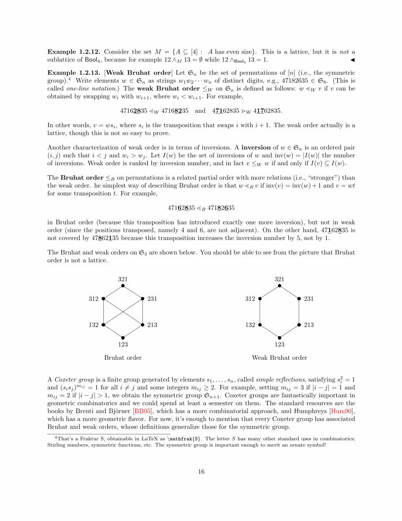
Example 1.2.13. [Weak Bruhat order] Let Sn be the set of permutations of [n] (i.e., the symmetricgroup).4 Write elements w ∈ Sn as strings w1w2 · · ·wn of distinct digits, e.g., 47182635 ∈ S8. (This iscalled one-line notation.) The weak Bruhat order ≤W on Sn is defined as follows: w ⋖W v if v can beobtained by swapping wi with wi+1, where wi < wi+1. For example,

47162835⋖W 47168235 and 47162835⋗W 41762835.

In other words, v = wsi, where si is the transposition that swaps i with i+ 1. The weak order actually is alattice, though this is not so easy to prove.

Another characterization of weak order is in terms of inversions. A inversion of w ∈ Sn is an ordered pair(i, j) such that i < j and wi > wj . Let I(w) be the set of inversions of w and inv(w) = |I(w)| the numberof inversions. Weak order is ranked by inversion number, and in fact v ≤W w if and only if I(v) ⊆ I(w).

The Bruhat order ≤B on permutations is a related partial order with more relations (i.e., “stronger”) thanthe weak order. he simplest way of describing Bruhat order is that w⋖B v if inv(v) = inv(w)+1 and v = wtfor some transposition t. For example,

47162835⋖B 47182635

in Bruhat order (because this transposition has introduced exactly one more inversion), but not in weakorder (since the positions transposed, namely 4 and 6, are not adjacent). On the other hand, 47162835 isnot covered by 47862135 because this transposition increases the inversion number by 5, not by 1.

The Bruhat and weak orders on S3 are shown below. You should be able to see from the picture that Bruhatorder is not a lattice.

123

132 213

312 231

321

Bruhat order

123

132 213

312 231

321

Weak Bruhat order

A Coxeter group is a finite group generated by elements s1, . . . , sn, called simple reflections, satisfying s2i = 1and (sisj)

mij = 1 for all i = j and some integers mij ≥ 2. For example, setting mij = 3 if |i − j| = 1 andmij = 2 if |i− j| > 1, we obtain the symmetric group Sn+1. Coxeter groups are fantastically important ingeometric combinatorics and we could spend at least a semester on them. The standard resources are thebooks by Brenti and Bjorner [BB05], which has a more combinatorial approach, and Humphreys [Hum90],which has a more geometric flavor. For now, it’s enough to mention that every Coxeter group has associatedBruhat and weak orders, whose definitions generalize those for the symmetric group.

4That’s a Fraktur S, obtainable in LaTeX as \mathfrakS. The letter S has many other standard uses in combinatorics:Stirling numbers, symmetric functions, etc. The symmetric group is important enough to merit an ornate symbol!

16

The Bruhat and weak order give graded, self-dual poset structures on Sn, both ranked by number ofinversions:

r(w) =∣∣∣i, j : i < j and wi > wj

∣∣∣.(For a general Coxeter group, the rank of an element w is the minimum number r such that w is the productof r simple reflections.) The rank-generating function of Sn is a very nice polynomial called the q-factorial:

FSn(q) = 1(1 + q)(1 + q + q2) · · · (1 + q + · · ·+ qn−1) =

n∏i=1

1− qi1− q .

1.3 Distributive lattices

Definition 1.3.1. A lattice L is distributive if the following two equivalent conditions hold:

x ∧ (y ∨ z) = (x ∧ y) ∨ (x ∧ z) ∀x, y, z ∈ L, (1.2a)

x ∨ (y ∧ z) = (x ∨ y) ∧ (x ∨ z) ∀x, y, z ∈ L. (1.2b)

Proving that the two conditions (1.2a) and (1.2b) are equivalent is not too hard, but is not trivial (Exer-cise 1.9). Note that replacing the equalities with ≥ and ≤ respectively gives statements that are true for alllattices.

The condition of distributivity seems natural, but in fact distributive lattices are quite special.

1. The Boolean algebra 2[n] is a distributive lattice, because the set-theoretic operations of union andintersection are distributive over each other.

2. Every sublattice of a distributive lattice is distributive. In particular, Young’s lattice Y is distributivebecause it is a sublattice of a Boolean lattice (recall that meet and join in Y are given by intersectionand union on Ferrers diagrams).

3. The lattices M5 and N5 are not distributive:

x

zy a b c

(x ∨ y) ∧ z = 1 ∧ z = z (a ∨ b) ∧ c = c

(x ∧ z) ∨ (y ∧ z) = x ∨ 0 = x (a ∧ c) ∨ (b ∧ c) = 0.

4. The partition lattice Πn is not distributive for n ≥ 3, because Π3∼= M5, and for n ≥ 4 every Πn

contains a sublattice isomorphic to Π3 (see Exercise 1.1). Likewise, if n ≥ 2 then the subspace latticeLn(q) contains a copy of M5 (take any plane together with three distinct lines in it), hence is notdistributive.

5. The set Dn of all positive integer divisors of a fixed integer n, ordered by divisibility, is a distributivelattice (Exercise 1.4).

17

Every poset P gives rise to a distributive lattice in the following way. The set J(P ) of order ideals of P (seeDefinition 1.1.10) is itself a bounded poset, ordered by containment. In fact J(P ) is a distributive lattice:the union or intersection of order ideals is an order ideal (this is easy to check) which means that J(P ) is asublattice of the distributive lattice BoolP . (See Figure 1.4 for an example.)

a

b

c

d

P

∅

a c

ac cd

abc acd

abcd

J(P )

Figure 1.4: A poset P and the corresponding distributive lattice J(P ).

For example, if P is an antichain, then every subset is an order ideal, so J(P ) = BoolP , while if P is a chainwith n elements, then J(P ) is a chain with n + 1 elements. As an infinite example, if P = N2 with theproduct ordering (i.e., (x, y) ≤ (x′, y′) if x ≤ x′ and y ≤ y′), then J(P ) is Young’s lattice Y .

Remark 1.3.2. There is a natural bijection between J(P ) and the set of antichains of P , since the maximalelements of any order ideal form an antichain that generates it. (Recall that an antichain is a set of elementsthat are pairwise incomparable.) Moreover, for each order ideal I, the order ideals covered by I in J(P ) areprecisely those of the form I ′ = I \ x, where x is a maximal element of I. In particular |I ′| = |I| − 1 forall such I ′, and it follows by induction that J(P ) is ranked by cardinality.

We will shortly prove Birkhoff’s theorem (Theorem 1.3.7), a.k.a. the Fundamental Theorem of Finite Dis-tributive Lattices: the finite distributive lattices are exactly the lattices of the form J(P ), where P is a finiteposet.

Definition 1.3.3. Let L be a lattice. An element x ∈ L is join-irreducible if it cannot be written as thejoin of two other elements. That is, if x = y ∨ z then either x = y or x = z. The subposet (not sublattice!)of L consisting of all join-irreducible elements is denoted Irr(L). Here is an example.

a c

e d

b f

L

a

b

c

d

Irr(L)

If L is finite, then an element of L is join-irreducible if it covers exactly one other element. (This is not truein a lattice such as R under the natural order, in which there are no covering relations!) The condition offiniteness can be relaxed; see Exercise 1.11.

18

Definition 1.3.4. A factorization of x ∈ L is an equation of the form

x = p1 ∨ · · · ∨ pnwhere p1, . . . , pn ∈ Irr(L). The factorization is irredundant if the pi form an antichain.

In analogy with ring theory, call a lattice Artinian if it has no infinite descending chains. (For example, Lis Artinian if it is finite, or chain-finite, or locally finite and has a 0.) If L is Artinian, then every elementx ∈ L has a factorization — if x itself is not join-irreducible, express it as a join of two smaller elements,then repeat. Moreover, every factorization can be reduced to an irredundant factorization by deleting eachfactor strictly less than another (which does not change the join of the factors). Throughout the rest ofthe section, we will assume that L is Artinian.

For general lattices, irredundant factorizations need not be unique. For example, the 1 element of M5 canbe factored irredundantly as the join of any two atoms. On the other hand, distributive lattices do exhibitunique factorization, as we will soon prove (Proposition 1.3.6).

Proposition 1.3.5. Let L be a distributive lattice and let p ∈ Irr(L). Suppose that p ≤ q1 ∨ · · · ∨ qn. Thenp ≤ qi for some i.

Proof. By distributivity,p = p ∧ (q1 ∨ · · · ∨ qn) = (p ∧ q1) ∨ · · · ∨ (p ∧ qn)

and since p is join-irreducible, it must equal p ∧ qi for some i, whence p ≤ qi.

Proposition 1.3.5 is a lattice-theoretic analogue of the statement that if a prime p divides a product ofpositive numbers, then it divides at least one of them. (This is in fact exactly what the result says whenapplied to the divisor lattice Dn.)

Proposition 1.3.6 (Unique factorization for distributive lattices). Let L be a distributive lattice. Thenevery x ∈ L can be written uniquely as an irredundant join of join-irreducible elements.

Proof. Suppose that we have two irredundant factorizations

x = p1 ∨ · · · ∨ pn = q1 ∨ · · · ∨ qm (1.3)

with pi, qj ∈ Irr(L) for all i, j. Then p1 ≤ x = q1 ∨ · · · ∨ qm, so by Proposition 1.3.5, p1 ≤ qj for some j.Again by Proposition 1.3.5, qj ≤ pi for some i. If i = 1, then p1 ⪇ pi, which contradicts the fact that the piform an antichain. Therefore p1 = qj . This argument implies that each pi is one of the qj ’s, and vice versa.Therefore, the two factorizations in (1.3) must be identical.

Theorem 1.3.7 (Birkhoff 1933). Up to isomorphism, the finite distributive lattices are exactly the latticesJ(P ), where P is a finite poset. Moreover, L ∼= J(Irr(L)) for every lattice L and P ∼= Irr(J(P )) for everyposet P .

Sketch of proof. The lattice isomorphism L→ J(Irr(L)) is given by

ϕ(x) = p ∈ Irr(L) : p ≤ x.

Meanwhile, the join-irreducible order ideals in P are just the principal order ideals, i.e., those generated bya single element. So the poset isomorphism P → Irr(J(P )) is given by

ψ(y) = ⟨y⟩.

These facts need to be checked; the details are left to the reader (Exercise 1.13).

19

Corollary 1.3.8. Every finite distributive lattice L is graded.

Proof. The FTFDL says that L ∼= J(P ) for some finite poset P . Then L is ranked by Remark 1.3.2, and itis bounded with 0 = ∅ and 1 = P .

Corollary 1.3.9. Let L be a finite distributive lattice. The following are equivalent:

1. L is a Boolean algebra.2. Irr(L) is an antichain.3. L is atomic (i.e., every element in L is the join of atoms). Equivalently, every join-irreducible element

is an atom.4. L is complemented. That is, for each x ∈ L, there exists a unique element x ∈ L such that x∨ x = 1

and x ∧ x = 0.5. L is relatively complemented. That is, for every interval [y, z] ⊆ L and every x ∈ [y, z], there exists

a unique element u ∈ [y, z] such that x ∨ u = z and x ∧ u = y.

Proof. (5) =⇒ (4): Take [x, y] = [0, 1].

(4) =⇒ (3): Suppose that L is complemented, and suppose that y ∈ Irr(L) is not an atom. Let x be an atom

in [0, y]. Then

(x ∨ x) ∧ y = 1 ∧ y = y

(x ∨ x) ∧ y = (x ∧ y) ∨ (x ∧ y) = x ∨ (x ∧ y)

by distributivity. So y = x ∨ (x ∧ y), which is a factorization of y, but y is join-irreducible, which impliesx ∧ y = y, i.e., x ≥ y. But then x ≥ x and x ∧ x = x = 0, a contradiction.

(3) =⇒ (2): This follows from the observation that no two atoms are comparable.

(2) =⇒ (1): By the FTFDL, since L = J(Irr(L)).

(1) =⇒ (5): If X ⊆ Y ⊆ Z are sets, then let U = X ∪ (Y \ Z). Then Y ∩ U = X and Y ∪ U = Z.

Join and meet could have been interchanged throughout this section. For example, the dual of Proposi-tion 1.3.6 says that every element in a distributive lattice L has a unique “cofactorization” as an irredundantmeet of meet-irreducible elements, and L is Boolean iff every element is the meet of coatoms. (In this casewe would require L to be Noetherian instead of Artinian — i.e., to contain no infinite increasing chains. Forexample, Young’s lattice is Artinian but not Noetherian.)

1.4 Modular lattices

Definition 1.4.1. A lattice L is modular if every x, y, z ∈ L with x ≤ z satisfy the modular equation:

x ∨ (y ∧ z) = (x ∨ y) ∧ z. (1.4)

Note that for all lattices, if x ≤ z, then x∨ (y∧z) ≤ (x∨y)∧z. Modularity says that, in fact, equality holds.

20

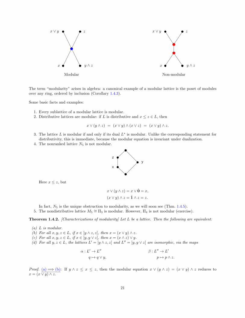
z

x y ∧ z

x ∨ y

Modular

z

x y ∧ z

x ∨ y

Non-modular

The term “modularity” arises in algebra: a canonical example of a modular lattice is the poset of modulesover any ring, ordered by inclusion (Corollary 1.4.3).

Some basic facts and examples:

1. Every sublattice of a modular lattice is modular.2. Distributive lattices are modular: if L is distributive and x ≤ z ∈ L, then

x ∨ (y ∧ z) = (x ∨ y) ∧ (x ∨ z) = (x ∨ y) ∧ z.

3. The lattice L is modular if and only if its dual L∗ is modular. Unlike the corresponding statement fordistributivity, this is immediate, because the modular equation is invariant under dualization.

4. The nonranked lattice N5 is not modular.

x

zy

Here x ≤ z, but

x ∨ (y ∧ z) = x ∨ 0 = x,

(x ∨ y) ∧ z = 1 ∧ z = z.

In fact, N5 is the unique obstruction to modularity, as we will soon see (Thm. 1.4.5).5. The nondistributive lattice M5

∼= Π3 is modular. However, Π4 is not modular (exercise).

Theorem 1.4.2. [Characterizations of modularity] Let L be a lattice. Then the following are equivalent:

(a) L is modular.(b) For all x, y, z ∈ L, if x ∈ [y ∧ z, z], then x = (x ∨ y) ∧ z.(c) For all x, y, z ∈ L, if x ∈ [y, y ∨ z], then x = (x ∧ z) ∨ y.(d) For all y, z ∈ L, the lattices L′ = [y ∧ z, z] and L′′ = [y, y ∨ z] are isomorphic, via the maps

α : L′ → L′′ β : L′′ → L′

q 7→ q ∨ y, p 7→ p ∧ z.

Proof. (a) =⇒ (b): If y ∧ z ≤ x ≤ z, then the modular equation x ∨ (y ∧ z) = (x ∨ y) ∧ z reduces tox = (x ∨ y) ∧ z.

21

(b) =⇒ (a): Suppose that (b) holds. Let a, b, c ∈ L with a ≤ c. Then

b ∧ c ≤ a ∨ (b ∧ c) ≤ c ∨ c = c

so applying (b) with y = b, z = c, x = a ∨ (b ∧ c) gives

a ∨ (b ∧ c) =((a ∨ (b ∧ c)) ∨ b

)∧ c = (a ∨ b) ∧ c

which is the modular equation for a, b, c.

(b)⇐⇒ (c): These two conditions are duals of each other (i.e., L satisfies (b) iff L∗ satisfies (c)), andmodularity is a self-dual condition.

(b)+(c)⇐⇒ (d): The functions α and β are always order-preserving functions with the stated domains and

ranges. Conditions (b) and (c) say respectively that β α and αβ are the identities on L′ and L′′; together,these conditions are equivalent to condition (d).

Corollary 1.4.3. Let R be a (not necessarily commutative) ring and M a (left) R-submodule. Then the(possibly infinite) poset L(M) of (left) R-submodules of M , ordered by inclusion, is a modular lattice withoperations Y ∨ Z = Y + Z and Y ∧ Z = Y ∩ Z.

Proof. The Second Isomorphism Theorem says that Z/(Y ∩Z) ∼= (Y +Z)/Y for all Y,Z ∈ L(M). Therefore

[Y ∩ Z,Z] ∼= L(Z/(Y ∩ Z)) ∼= L((Y + Z)/Y ) ∼= [Y, Y + Z]

so L(M) satisfies condition (d) of Theorem 1.4.2.

In particular, the subspace lattices Ln(q) are modular (see Example 1.2.5).

Example 1.4.4. For a (finite) group G, let L(G) denote the lattice of subgroups of G, with operationsH ∧K = H ∩K and H ∨K = HK (i.e., the group generated by H ∪K). If G is abelian then L(G) is alwaysmodular, but if G is non-abelian then modularity can fail.

For example, let G = S4, let X and Y be the cyclic subgroups generated by the cycles (1 2 3) and (3 4)respectively, and let Z = A4 (the alternating group). Then (XY )∩Z = Z but X(Y ∩Z) = Z. Indeed, thesegroups generate a sublattice of L(S4) isomorphic to N5:

S4

A4

⟨(3 4)⟩⟨(1 2 3)⟩

Id

In fact, an occurrence of N5 is the only obstruction to modularity:

Theorem 1.4.5. Let L be a lattice.

1. L is modular if and only if it contains no sublattice isomorphic to N5.2. L is distributive if and only if it contains no sublattice isomorphic to N5 or M5.

22

Proof. Both =⇒ directions are easy, because distributivity and modularity are conditions inherited bysublattices, and N5 is not modular and M5 is not distributive.

Suppose that x, y, z is a triple for which modularity fails. One can check that

x ∨ y

(x ∨ y) ∧ z

y

x

x ∧ y

is a sublattice (details left to the reader), and it is isomorphic to N5.

Suppose that L is not distributive. If it isn’t modular then it contains an N5, so there is nothing to prove.If it is modular, then choose x, y, z such that

x ∧ (y ∨ z) > (x ∧ y) ∨ (x ∧ z).You can then show that

1. this inequality is invariant under permuting x, y, z;2. (x∧ (y ∨ z))∨ (y ∧ z) and the two other lattice elements obtained by permuting x, y, z form a cochain;3. x ∨ y = x ∨ z = y ∨ z, and likewise for meets.

Hence, we have constructed a sublattice of L isomorphic to M5.

x ∨ y ∨ z

(x ∧ (y ∨ z)) ∨ (y ∧ z) (y ∧ (x ∨ z)) ∨ (x ∧ z) (z ∧ (x ∨ y)) ∨ (x ∧ y)

x ∧ y ∧ z

A corollary is that every modular lattice is graded, because a non-graded lattice must contain a sublatticeisomorphic to N5. The details are left to the reader; we will eventually prove the stronger statement thatevery semimodular lattice is graded.

1.5 Semimodular lattices

Recall that the notation x⋖y means that x is covered by y, i.e., x < y and there exists no z strictly betweenx, y (i.e., such that x < z < y).

Definition 1.5.1. A lattice L is (upper) semimodular if for all incomparable x, y ∈ L,x ∧ y ⋖ y =⇒ x⋖ x ∨ y. (1.5)

Conversely, L is lower semimodular if the converse holds.

23

Note that both upper and lower semimodularity are inherited by sublattices, and that L is upper semimodularif and only if its dual L∗ is lower semimodular. Also, the implication (1.5) is trivially true if x and y arecomparable. If they are incomparable (as we will often assume), then there are several useful colloquialrephrasings of semimodularity:

• “If meeting with x merely nudges y down, then joining with y merely nudges x up.”• In the interval [x ∧ y, x ∨ y] ⊆ L pictured below, if the southeast relation is a cover, then so is thenorthwest relation.

x ∨ y•

x ⇐=

y

x ∧ y•

(1.6)

• This condition is often used symmetrically: if x, y are incomparable and they both cover x ∧ y, thenthey are both covered by x ∨ y.

• Contrapositively, “If there is other stuff between x and x ∨ y, then there is also other stuff betweenx ∧ y and y.”

Example 1.5.2. The partition lattice Πn is an important example of an upper semimodular lattice. To seethat it is USM, let π and σ be incomparable set partitions of [n], and suppose that σ⋗σ∧π. Recall that thismeans that σ ∧ π can be obtained from σ by splitting some block B ∈ σ into two sub-blocks B′, B′′. Morespecifically, we can write σ = A1| · · · |Ak|B and σ ∧ π = A1| · · · |Ak|B′|B′′, where B is the disjoint union ofB′ and B′′. Since σ ∧ π refines π but σ does not, we know that A1, . . . , Ak, B

′, B′′ are all subsets of blocksof π but B is not; in particular B′ and B′′ are subsets of different blocks of π, say C ′ and C ′′ respectively.But then merging C ′ and C ′′ produces a partition τ that covers π and is refined by σ, so it must be the casethat τ = σ ∨ π, and we have proved that Πn is USM.

Lemma 1.5.3. If a lattice L is modular, then it is both upper and lower semimodular.

Proof. If x ∧ y ⋖ y, then the sublattice [x ∧ y, y] has only two elements. If L is modular, then condition (d)of the characterization of modularity (Theorem 1.4.2) implies that [x∧ y, y] ∼= [x, x∨ y], so x⋖ x∨ y. HenceL is upper semimodular. The dual argument proves that L is lower semimodular.

In fact, upper and lower semimodularity together imply modularity. We will show that any of these threeconditions on a lattice L implies that it is graded, and that its rank function r satisfies

r(x ∨ y) + r(x ∧ y) ≤ r(x) + r(y) iff L is USM,

r(x ∨ y) + r(x ∧ y) ≥ r(x) + r(y) iff L is LSM,

r(x ∨ y) + r(x ∧ y) = r(x) + r(y) iff L is modular.

Lemma 1.5.4. Suppose L is USM and let q, r, s ∈ L. If q ⋖ r, then either q ∨ s = r ∨ s or q ∨ s⋖ r ∨ s.

In other words, if it only takes one step to walk up from q to r, then it takes at most one step to walk fromq ∨ s to r ∨ s.

Proof. Let p = (q ∨ s) ∧ r, so that q ≤ p ≤ r. Since q is covered by r, it follows that either p = q or p = r.

24

• If p = r, then q ∨ s ≥ r. So q ∨ s = r ∨ (q ∨ s) = (r ∨ q) ∨ s = r ∨ s.• If p = q, then p = (q∨ s)∧ r = q⋖ r. Applying semimodularity to the diamond figure below, we obtain(q ∨ s)⋖ (q ∨ s) ∨ r = r ∨ s.

r ∨ s•

q ∨ s r

p = (q ∨ s) ∧ r = q

•

Theorem 1.5.5. Let L be a finite lattice. Then L is USM if and only if it is ranked, with rank function rsatisfying the submodular inequality or semimodular inequality

r(x ∨ y) + r(x ∧ y) ≤ r(x) + r(y) ∀x, y ∈ L. (1.7)

Proof. (⇐= ) Suppose that L is a ranked lattice with rank function r satisfying (1.7). Suppose that x, y areincomparable and x∧y⋖y so that r(y) = r(x∧y)+1. Incomparability implies x∨y > x, so r(x∨y)−r(x) > 0.On the other hand, rearranging (1.7) gives

0 < r(x ∨ y)− r(x) ≤ r(y)− r(x ∧ y) = 1

so r(x ∨ y)− r(x) = 1, i.e., x ∨ y ⋗ x.

( =⇒ ) For later use, observe that if L is semimodular, then

x ∧ y ⋖ x, y =⇒ x, y ⋖ x ∨ y. (1.8)

Denote by c(L) the maximum length5 of a chain in L. We will induct on c(L). For the base cases, if c(L) = 0then L has one element, while if c(L) = 1 then L has two elements. If c(L) = 2 then L = 0, 1, x1, . . . , xn,where n ≥ 1 and 0⋖xi⋖ 1 for all i. It is easy to see that these lattices are ranked, USM and satisfy (1.7) (infact equality holds and these lattices are modular). Therefore, suppose c(L) = n ≥ 3. Assume inductivelythat if L is USM and c(L) < c(L), then L is ranked and its rank function satisfies (1.7).

First, we show that L is ranked.

Let X = 0 = x0 ⋖ x1 ⋖ · · ·⋖ xn−1 ⋖ xn = 1 be a chain of maximum length. Let Y = 0 = y0 ⋖ y1 ⋖ · · ·⋖ym−1 ⋖ ym = 1 be any maximal chain in L. We wish to show that m = n.

Let L′ = [x1, 1] and L′′ = [y1, 1]. (See Figure 1.5.) By induction, these sublattices are both ranked.Moreover, c(L′) = n − 1. If x1 = y1 then Y and X are both saturated chains in the ranked lattice L′ andwe are done, so suppose that x1 = y1. Let z2 = x1 ∨ y1. By (1.8), z2 covers both x1 and y1. Let z2, . . . , 1be a saturated chain in L (thus, in L′ ∩ L′′).

Since L′ is ranked and z⋗x1, the chain z1, . . . , 1 has length n−2. So the chain y1, z1, . . . , 1 has length n−1.

On the other hand, L′′ is ranked and y1, y2, . . . , 1 is a saturated chain, so it also has length n− 1. Thereforethe chain 0, y1, . . . , 1 has length n as desired.

Second, we show that the rank function r of L satisfies (1.7). Let x, y ∈ L and take a saturated chain

x ∧ y = c0 ⋖ c1 ⋖ · · ·⋖ cn−1 ⋖ cn = x.

5Recall that the length of a saturated chain is the number of minimal relations in it, which is one less than its cardinality asa subset of L. For example, c(2[n]) = n, not n+ 1.

25

0

1

x1

x2

x3

xn−1

y1

y2

ym−1

z2

z3

L′ L′′

Figure 1.5: A semimodular lattice.

Note that n = r(x)− r(x ∧ y). Then there is a chain

y = c0 ∨ y ≤ c1 ∨ y ≤ · · · ≤ cn ∨ y = x ∨ y.

By Lemma 1.5.4, each ≤ in this chain is either an equality or a covering relation. Therefore, the distinctelements ci ∨ y form a saturated chain from y to x ∨ y, whose length must be ≤ n. Hence

r(x ∨ y)− r(y) ≤ n = r(x)− r(x ∧ y)

which implies the submodular inequality (1.7).

The same argument shows that L is lower semimodular if and only if it is ranked, with a rank functionsatisfying the reverse inequality of (1.7).

Theorem 1.5.6. L is modular if and only if it is ranked, with rank function r satisfying the modularequality

r(x ∨ y) + r(x ∧ y) = r(x) + r(y) ∀x, y ∈ L. (1.9)

Proof. If L is modular, then it is both upper and lower semimodular, so the conclusion follows by Theo-rem 1.5.5. On the other hand, suppose that L is a lattice whose rank function r satisfies (1.9). Let x ≤ z ∈ L.We already know that x∨ (y ∧ z) ≤ (x∨ y)∧ z, so it suffices to show that these two elements have the samerank. Indeed,

r(x ∨ (y ∧ z)) = r(x) + r(y ∧ z)− r(x ∧ y ∧ z)= r(x) + r(y ∧ z)− r(x ∧ y)= r(x) + r(y) + r(z)− r(y ∨ z)− r(x ∧ y)

26

and

r((x ∨ y) ∧ z) = r(x ∨ y) + r(z)− r(x ∨ y ∨ z)= r(x ∨ y) + r(z)− r(y ∨ z)= r(x) + r(y)− r(x ∧ y) + r(z)− r(y ∨ z).

1.6 Geometric lattices

The following construction gives the prototype of a geometric lattice. Let k be a field, let V be a vectorspace over k, and let E be a finite subset of V (with repeated elements allowed). Say that a flat is a subsetof E of the form W ∩ E, where W ⊆ E is a vector subspace. Define the vector lattice of E as

L(E) = W ∩ E : W ⊆ V is a vector subspace. (1.10)

Then L(E) is a subposet of BoolE . Moreover,

L(E) ∼= W ∩ E : W ⊆ V is a vector subspace. (1.11)

the family of vector subspaces of V generated by subsets of E. (Of course, different subspaces of W canhave the same intersection with E, and different subsets of E can span the same vector space.) The posetL(E) is easily checked to be a lattice under the operations

(W ∩ E) ∧ (X ∩ E) = (W ∩X) ∩ E, (W ∩ E) ∨ (X ∩ E) = (W +X) ∩ E.

The elements of L(E) are called flats. Certainly E = V ∩ E is a flat, hence the top element of L(E). Thebottom element is O ∩ E, where O ⊆ V is the zero subspace; thus O ∩ E consists of the copies of the zerovector in E.

The tricky thing about the isomorphism (1.11) is that it is not so obvious which elements of E are flats. Forevery A ⊆ E, there is a unique minimal flat containing A, namely A := kA∩E — that is, the set of elementsof E in the linear span of A. On the other hand, if v, w, x ∈ E with v + w = x, then v, w is not a flat,because any vector subspace that contains both v and w must also contain x. So, an equivalent definitionof “flat” is that A ⊆ E is a flat if no vector in E \A is in the linear span of the vectors in A.

The lattice L(E) is submodular, with rank function r(A) = dim kA. (Exercise: Check that r satisfies thesubmodular inequality.) It is not in general modular; e.g., see Example 1.6.3 below. On the other hand,L(E) is always an atomic lattice: every element is the join of atoms. This is a consequence of the simplefact that k⟨v1, . . . , vk⟩ = kv1 + · · ·+ kvk. This motivates the following definition:

Definition 1.6.1. A lattice L is geometric if it is (upper) semimodular and atomic. If L ∼= L(E) for someset of vectors E, we say that E is a (linear) representation of L.

For example, the set E = (0, 1), (1, 0), (1, 1) ⊆ F22 is a linear representation of the geometric lattice M5.

(For that matter, so is any set of three nonzero vectors in a two-dimensional space over any field, providednone is a scalar multiple of another.)

A closely related construction is the affine lattice of E, defined by

Laff(E) =W ∩ E : W ⊆ V is an affine subspace

.

(An affine subspace of V is a translate of a vector subspace; for example, a line or plane not necessarilycontaining the origin.) In fact, any lattice of the form Laff(E) can be expressed in the form L(E), where E is

27

a certain point set constructed from E (homework problem). However, the dimension of the affine span of aset A ⊆ E is one less than its rank — which means that we can draw geometric lattices of rank 3 convenientlyas planar point configurations. If L ∼= Laff(E), we could say that E is a (affine) representation of L.

Example 1.6.2. Let E = a, b, c, d, where a, b, c are collinear but no other set of three points is. ThenLaff(E) is the lattice shown below (which happens to be modular).

a

b

c

d

∅

a b c d

abc ad bd cd

abcd

Example 1.6.3. If E is the point configuration on the left with the only collinear triples a, b, c anda, d, e, then Laff(E) is the lattice on the right.

a b c

d

e

∅

b c a d e

abc bd be cd ce ade

abcde

This lattice is not modular: consider the two elements bd and ce.

Example 1.6.4. Recall from Example 1.5.2 that the partition lattice Πn is USM for all n. In fact it isgeometric. To see that it is atomic, observe that the atoms are the set partitions with n−1 blocks, necessarilyone doubleton block and n − 2 singletons; let πij denote the atom whose doubleton block is i, j. Thenevery set partition σ is the join of the set πij : i ∼σ j.

In fact, Πn is a vector lattice. Let k be any field, llet e1, . . . , en be the standard basis of V = kn, letpij = ei−ej for all 1 ≤ i < j ≤ n, and let E be the set of all such vectors pij .. Then in fact Πn

∼= L(E). Theatoms πij of Πn correspond to the atoms k⟨pij⟩ of L(E); the rest of the isomorphism is left as Exercise 1.17.Note that this construction works over any field k.

More generally, if G is any simple graph on vertex set [n] then the connectivity lattice K(G) is isomorphicto L(EG), where EG = aij : ij is an edge of G.

28

1.7 Exercises

Posets

Exercise 1.1. (a) Prove that every nonempty interval in a Boolean algebra is itself isomorphic to aBoolean algebra.

(b) Prove that every interval in the subspace lattice Ln(q) is isomorphic to a subspace lattice.(c) Prove that every interval in the partition lattice Πn is isomorphic to a product of partition lattices.

(The product of posets P1, . . . , Pk is the Cartesian product P1 × · · · × Pk, equipped with the partialorder (x1, . . . , xk) ≤ (y1, . . . , yk) if xi ≤Pi

yi for all i ∈ [k].)

Exercise 1.2. A directed acyclic graph (or DAG) is a pair G = (V,E), where V is a set of vertices; Eis a set of edges, each of which is an ordered pair of distinct vertices; and E contains no directed cycles, i.e.,no subsets of the form (v1, v2), (v2, v3), . . . , (vn−1, vn), (vn, v1) for any v1, . . . , vn ∈ V .

(a) Let P be a poset with order relation <. Let E = (v, w) : v, w ∈ P, v < w. Prove that the pair(P,E) is a DAG.

(b) Let G = (V,E) be a DAG. Define a relation < on V by setting v < w iff there is some directed pathfrom v to w in G, i.e., iff E has a subset of the form (v = v1, v2), (v2, v3), . . . , (vn−1, vn = w) withall vi distinct. Prove that this relation makes V into a poset.

(This problem is purely a technical exercise and is almost tautological, but it does show that posets andDAGs are essentially the same thing.)

Exercise 1.3. Recall from Definition 1.1.9 that L (P ) means the set of linear extensions of a poset P .

(a) Let P and Q be posets. Describe L (P + Q) and L (P ⊕ Q) in terms of L (P ) and L (Q). (Hint:Start by working out some small examples explicitly. The problem is nontrivial even when P and Qare both chains of length 1.)

(b) Give a concrete combinatorial description of L (Booln).

Exercise 1.4. Let n be a positive integer. Let Dn be the set of all positive-integer divisors of n (including nitself), partially ordered by divisibility.

(a) Prove that Dn is a ranked poset, and describe the rank function.(b) For which values of n is Dn (i) a chain; (ii) a Boolean algebra? For which values of n,m is it the case

that Dn∼= Dm?

(c) Prove that Dn is a distributive lattice. Describe its meet and join operations and its join-irreducibleelements.

(d) Prove that Dn is self-dual, i.e., there is a bijection f : Dn → Dn such that f(x) ≤ f(y) if and only ifx ≥ y.

Exercise 1.5. Let G be a graph on vertex set V = [n]. Recall from Example 1.2.3 that the connectivitylattice of a graph is the subposet K(G) of Πn consisting of set partitions in which every block induces aconnected subgraph of G. Prove that K(G) is a lattice. Is it a sublattice of Πn?

Exercise 1.6. LetA be a finite family of sets. ForA′ ⊆ A, define ∪A′ =⋃

A∈A′ A. Let U(A) = ∪A′ : A′ ⊆A, considered as a poset ordered by inclusion.

(a) Prove that U(A) is a lattice. (Hint: Don’t try to specify the meet operation explicitly.)(b) Construct a set family A such that U(A) is isomorphic to weak Bruhat order on S3 (see Example

2.11).(c) Construct a set family A such that U(A) is not ranked.

29

(d) Is every finite lattice of this form?

Exercise 1.7. For 1 ≤ i ≤ n − 1, let si be the transposition in Sn that swaps i with i + 1. (The si arecalled elementary transpositions.) You probably know that s1, . . . , sn−1 is a generating set for Sn (and ifyou don’t, you will shortly prove it). For w ∈ Sn, an expression w = si1 · · · sik is called a reduced word ifthere is no way to express w as a product of fewer than k generators.

(a) Show that every reduced word for w has length equal to inv(w). (For the definition of inv(w), seeExample 1.2.13.)

(b) Define a partial order ≺ on Sn as follows: w ≺ v if there exists a reduced word si1 · · · sik for v suchthat w is the product of some subword w = sij1 · · · sijℓ . (Sorry about the triple subscripts; this justmeans that v is obtained by deleting some of the letters from the reduced word for w.) Prove that ≺is precisely Bruhat order on Sn.

Exercise 1.8. Prove that the rank-generating functions of weak order and Bruhat order on Sn are both

∑w∈Sn

qr(w) =

n∏i=1

1− qi1− q

where r(w) = #i, j : i < j and wi > wj. (Hint: Induct on n, and use one-line notation for permutations,not cycle notation.)

Distributive lattices

Exercise 1.9. Prove that the two formulations (1.2a) and (1.2b) of distributivity of a lattice L are equivalent,i.e.,

x ∧ (y ∨ z) = (x ∧ y) ∨ (x ∧ z) ∀x, y, z ∈ L ⇐⇒ x ∨ (y ∧ z) = (x ∨ y) ∧ (x ∨ z) ∀x, y, z ∈ L.

Exercise 1.10. In Exercise 1.4 you proved that the divisor lattice Dn is distributive. Characterize all posetsP such that J(P ) ∼= Dn for some n ∈ N. (In other words, prove a statement of the form “A distributivelattice L = J(P ) is isomorphic to a divisor lattice if and only if the poset P = Irr(L) is .”)

Exercise 1.11. Let L be a finite lattice and x ∈ L. Prove that x is join-irreducible if it covers exactly oneother element. What weaker conditions than “finite” suffice?

Exercise 1.12. Let Y be Young’s lattice (which we know is distributive).

(a) Describe the join-irreducible elements of Young’s lattice Y .(b) Let λ ∈ Y . If λ = µ1 ∨ · · · ∨ µk is an irredundant factorization, then what quantity does k correspond

to in the Ferrers diagram of λ?(c) Let λ be a 2× n rectangle. Show that the number of maximal chains in the interval [∅, λ] ⊆ Y is the

Catalan number Cn.(d) Count the maximal chains in the interval [∅, λ] ⊆ Y if λ is a hook shape (i.e., λ = (n + 1, 1, 1, . . . , 1),

with a total of m copies of 1).

Exercise 1.13. Fill in the details in the proof of the FTFDL (Theorem 1.3.7) by showing the followingfacts.

(a) For a finite distributive lattice L, show that the map ϕ : L→ J(Irr(L)) given by

ϕ(x) = ⟨p : p ∈ Irr(L), p ≤ x⟩

is indeed a lattice isomorphism.

30

(b) For a finite poset P , show that an order ideal in P is join-irreducible in J(P ) if and only if it is principal(i.e., generated by a single element).

Exercise 1.14. Let L be a sublattice of Booln that is accessible: if S ∈ L \ ∅ then there exists somex ∈ S such that S \ x ∈ L. Construct a poset P on [n] such that J(P ) = L. (Notice that I wrote “= L”,not “∼= L.” It is not enough to invoke Birkhoff’s theorem to say that such a P must exist! The point is toexplicitly construct a poset P on [n] whose order ideals are the sets in L.)

Modular lattices

Exercise 1.15. Let Ln(q) be the poset of subspaces of an n-dimensional vector space over the finite fieldFq (so Ln(q) is a modular lattice by Corollary 1.4.3).

(a) Prove directly from the definition of modularity that Ln(q) is modular. (I.e., verify algebraically thatthe join and meet operations obey the modular equation (1.4).)

(b) Calculate the rank-generating function

∑V ∈Ln(q)

xdimV =

n∑k=0

xk#V ∈ Ln(q) : dimV = k.

Hint: Every vector space of dimension k is determined by an ordered basis v1, . . . , vk. How manyordered bases does each k-dimensional vector space V ∈ Ln(q) have? How many sequences of vectorsin Fn

q are ordered bases for some k-dimensional subspace?(c) Count the maximal chains in Ln(q).

Exercise 1.16. Verify that the lattice Π4 is not modular.

Semimodular and geometric lattices

Exercise 1.17. Prove that the lattices Πn and L(E) are isomorphic, where E is the vector set described inExample 1.6.4. To do this, you need to characterize the vector spaces spanned by subsets of A ⊆ E and showthat they are in bijection with set partitions. Hint: It may be useful to look at the orthogonal complementsof those vector spaces under the standard inner product on kn.

Exercise 1.18. The purpose of this exercise is to show that the constructions L and Laff produce the sameclass of lattices. Let k be a field and let E = e1, . . . , en ⊆ kd.

(a) The augmentation of a vector ei = (ei1, . . . , eid) is the vector ei = (1, ei1, . . . , eid) ∈ kd+1. Prove thatLaff(E) = L(E), where E = e1, . . . , en.

(b) Let v be a vector in kd that is not a scalar multiple of any ei, let H Let H ⊆ kd be a generic affinehyperplane, let ei be the projection of ei onto H, and let E = e1, . . . , en. Prove that L(E) = Laff(E).(The first part is figuring out what “generic” means. A generic hyperplane might not exist for all fields,but if k is infinite then almost all hyperplanes are generic.)

Exercise 1.19. Recall from Corollary 1.3.9 that a lattice L is relatively complemented if, whenever y ∈[x, z] ⊆ L, there exists u ∈ [x, z] such that y ∧ u = x and y ∨ u = z. Prove that a finite semimodular latticeis atomic (hence geometric) if and only if it is relatively complemented.

(Here is the geometric interpretation of being relatively complemented. Suppose that V is a vector space,L = L(E) for some point set E ⊆ V , and that X ⊆ Y ⊆ Z ⊆ V are vector subspaces spanned by flats of

31

L(E). For starters, consider the case that X = O. Then we can choose a basis B of the space Y and extendit to a basis B′ of Z, and the vector set B′ \ B spans a subspace of Z that is complementary to Y . Moregenerally, if X is any subspace, we can choose a basis B for X, extend it to a basis B′ of Y , and extend B′

to a basis B′′ of Z. Then B ∪ (B′′ \B′) spans a subspace U ⊆ Z that is relatively complementary to Y , i.e.,U ∩ Y = X and U + Y = Z.)

32

Chapter 2

Poset Algebra

Throughout this chapter, every poset we consider will be assumed to be locally finite, i.e., every intervalis finite.

2.1 The incidence algebra of a poset

Let P be a poset and let Int(P ) denote the set of (nonempty) intervals of P . Recall that an interval is asubset of P of the form [x, y] := z ∈ P : x ≤ z ≤ y; if x ≤ y then [x, y] = ∅.

Definition 2.1.1. The incidence algebra I(P ) is the set of functions α : Int(P ) → C (“incidence func-tions”)1, made into a C-vector space with pointwise addition, subtraction and scalar multiplication, andequipped with the convolution product:

(α ∗ β)(x, y) =∑

z∈[x,y]

α(x, z)β(z, y).

Here we abbreviate α([x, y]) by α(x, y), and it is often convenient to set α(x, y) = 0 if x ≤ y. Note thatthe assumption of local finiteness is both necessary and sufficient for convolution to be well-defined for allincidence functions.

Proposition 2.1.2. Convolution is associative (although it is not in general commutative).

1More generally, we could allow incidence functions to take values in any (commutative) ring.

33

Proof. The basic idea is to reverse the order of summation:

[(α ∗ β) ∗ γ](x, y) =∑

z∈[x,y]

(α ∗ β)(x, z) · γ(z, y)

=∑

z∈[x,y]

∑w∈[x,z]

α(x,w)β(w, z)

γ(z, y)

=∑

w,z: x≤w≤z≤y

α(x,w)β(w, z)γ(z, y)

=∑

w∈[x,y]

α(x,w)

∑z∈[w,y]

β(w, z)γ(z, y)

=

∑w∈[x,y]

α(x,w) · (β ∗ γ)(w, y)

= [α ∗ (β ∗ γ)](x, y).

The multiplicative identity of I(P ) is the Kronecker delta function, regarded as an incidence function:

δ(x, y) =

1 if x = y,

0 if x = y.

Therefore, we sometimes write 1 for δ.

Proposition 2.1.3. An incidence function α ∈ I(P ) has a left/right/two-sided convolution inverse if andonly if α(x, x) = 0 for all x (the “nonzero condition”). In that case, the inverse is given by the recursiveformula

α−1(x, y) =

α(x, x)−1 if x = y,

−α(y, y)−1∑

z: x≤z<y α−1(x, z)α(z, y) if x < y.

(2.1)

This formula is well-defined by induction on the size of [x, y], with the cases x = y and x = y serving as thebase case and inductive step respectively.

Proof. Let β be a left convolution inverse of α. In particular, α(x, x) = β(x, x)−1 for all x (use the equation(α ∗ β)(x, x) = δ(x, x) = 1), so the nonzero condition is necessary. On the other hand, if x < y, then

(β ∗ α)(x, y) =∑

z∈[x,y]

β(x, z)α(z, y) = δ(x, y) = 0

and solving for β(x, y) gives the formula (2.1) (pull the term β(x, y)α(y, y) out of the sum), which is well-defined provided that α(y, y) = 0. So the nonzero condition is also sufficient. A similar argument shows thatthe nonzero condition is necessary and sufficient for α to have a right convolution inverse. Moreover, the leftand right inverses coincide: if β ∗ α = δ = α ∗ γ then β = β ∗ δ = β ∗ α ∗ γ = γ by associativity.

The zeta function and eta function of P are defined as

ζ(x, y) =

1 if x ≤ y,0 if x ≤ y, η(x, y) =

1 if x < y,

0 if x < y,

i.e., η = ζ − 1 = ζ − δ. Note that ζ is invertible and η is not.

34

These trivial-looking incidence functions are useful because their convolution powers count important things,namely multichains and chains in P In other words, enumerative questions about posets can be expressedalgebraically. Specifically,

ζ2(x, y) =∑

z∈[x,y]

ζ(x, z)ζ(z, y) =∑

z∈[x,y]

1

= #z : x ≤ z ≤ y,ζ3(x, y) =

∑z∈[x,y]

∑w∈[z,y]

ζ(x, z)ζ(z, w)ζ(w, y) =∑

x≤z≤w≤y

1

= #(z, w) : x ≤ z ≤ w ≤ y,ζk(x, y) = #(x1, . . . , xk−1) : x ≤ x1 ≤ x2 ≤ · · · ≤ xk−1 ≤ y.

That is, ζk(x, y) counts the number of multichains of length k between x and y (chains with possiblerepeats) . If we replace ζ with η, then the calculations all work the same way, except that all the ≤’s arereplaced with <’s, so we get

ηk(x, y) = #(x1, . . . , xk−1) : x < x1 < x2 < · · · < xk−1 < y,the number of chains of length k (not necessarily saturated) between x and y. In particular, if the chainsof P are bounded in length, then ηn = 0 for n≫ 0.

Direct products of posets play nicely with the incidence algebra construction. Specifically, let P,Q bebounded finite posets. For α ∈ I(P ) and ϕ ∈ I(Q), define αϕ ∈ I(P ×Q) by

αϕ[(x, x′), (y, y′)] = α(x, y)ϕ(x′, y′).

This defines a linear transformation F : I(P )⊗I(Q)→ I(P ×Q). 2 In other words, (α+β)ϕ = αϕ+βϕ, andα(ϕ + ψ) = αϕ + αψ, and α(cϕ) = (cα)ϕ = c(αϕ) for all c ∈ C. It is actually a vector space isomorphism,because there is a bijection Int(P )× Int(Q)→ Int(P ×Q) given by (I, J)→ I × J , and F (χI ⊗ χJ) = χI×J

(where χI is the characteristic function of I, i.e., the incidence function that is 1 on I and zero on otherintervals). In fact, more is true:

Proposition 2.1.4. The map F just defined is a ring isomorphism. That is, for all α, β ∈ I(P ) andϕ, ψ ∈ I(Q),

αϕ ∗ βψ = (α ∗ β)(ϕ ∗ ψ).Furthermore, the incidence functions δ and ζ are multiplicative on direct products, i.e.,

δP×Q = δP δQ and ζP×Q = ζP ζQ.

Proof. Let (x, x′) and (y, y′) be elements of P ×Q. Then

(αϕ ∗ βψ)[(x, x′), (y, y′)] =∑

(z,z′)∈[(x,x′),(y,y′)]

αϕ[(x, x′), (z, z′)] · βψ[(z, z′), (y, y′)]

=∑

z∈[x,y]

∑z′∈[x′,y′]

α(x, z)ϕ(x′, z′)β(z, y)ψ(z′, y′)

=

∑z∈[x,y]

α(x, z)β(z, y)

∑z′∈[x′,y′]

ϕ(x′, z′)ψ(z′, y′)

= (α ∗ β(x, y)) · (ϕ ∗ ψ(x′, y′)).

Multiplicativity of δ and ζ is immediate from their definitions.2See §8.5 for an extremely brief introduction to the tensor product operation ⊗.

35

2.2 The Mobius function

The Mobius function µP of a poset P is defined as the convolution inverse of its zeta function: µP = ζ−1P .

This turns out to be one of the most important incidence functions on a poset. For a bounded poset, weabbreviate µP (x) = µP (0, x) and µ(P ) = µP (0, 1). Proposition 2.1.3 provides a recursive formula for µ:

µ(x, y) =

0 if y ≥ x (i.e., if [x, y] = ∅),1 if y = x,

−∑z: x≤z<y µ(x, z) if x < y.

(2.2)

This is equivalent to the familiar recursive formula: to find µP (x), add up the values of µP at all elements< x, then change the sign.

Example 2.2.1. If P = 0 < 1 < 2 < · · · is a chain, then its Mobius function is given by µ(x, x) = 1,µ(x, x+ 1) = −1, and µ(x, y) = 0 otherwise.

Example 2.2.2. Here are the Mobius functions µP (x) = µP (0, x) for the lattices N5 and M5:

1

−1

0

−1

1

N51

−1 −1 −1

2

M5

And here are the Boolean lattice Bool3 and the divisor lattice D24:

1

−1 −1 −1

1 1 1

−1

Bool3

24

12

6

3

8

4

2

1

0

0

1

−1

0

0

−1

1 D24

Example 2.2.3 (Mobius functions of partition lattices). What is µ(Πn) in terms of n? Clearly µ(Π1) = 1and µ(Π2) = −1, and µ(Π3) = µ(M5) = 2. For n = 4, we calculate µ(Π4) from (2.2). The value of µΠ4

(0, π)depends only on the block sizes of π, in fact, [0, π] ∼= Ππ1

× · · · ×Ππk. We will use the fact that the Mobius

function is multiplicative on direct products; we will prove this shortly (Prop. 2.2.5).

36

Block sizes Number of π’s Isomorphism type of [0, π] µ(0, π)1,1,1,1 1 Π1 12,1,1 6 Π2 −12,2 3 Π2 ×Π2 13,1 4 Π3 2

Therefore, µ(Π4) = −(1 · 1− 1 · 6 + 1 · 3 + 2 · 4) = −6. Let’s try n = 5:

Block sizes Number of π’s µ(0, π) Contribution to −µ(Π5)1,1,1,1,1 1 µ(Π1) = 1 12,1,1,1 10 µ(Π2) = −1 −102,2,1 15 µ(Π2 ×Π2) = 1 153,1,1 10 µ(Π3) = 2 203,2 10 µ(Π3 ×Π2) = −2 −204,1 5 µ(Π4) = −6 -30

Adding up the last column and multiplying by −1 gives µ(Π5) = 24. At this point you might guess thatµ(Πn) = (−1)n−1(n− 1)!, and you would be right. We will prove this soon.

The Mobius function is useful in many ways. It can be used to formulate a more general version of inclusion-exclusion called Mobius inversion. It behaves nicely under poset operations such as product, and hasgeometric and topological applications. Even just the single number µ(P ) = µP (0, 1) tells you a lot about abounded poset P . Confusingly, this number itself is sometimes called the “Mobius function” of P (a betterterm would be “Mobius number”). Here is the reason.

Definition 2.2.4. A family F of posets is hereditary if, for each P ∈ F , every interval in P is isomorphicto some [other] poset in F . It is semi-hereditary if every interval in a member of F is isomorphic to aproduct of members of F .

For example, the families of Boolean lattices, divisor lattices, and subspace lattices are all hereditary, and thefamily of partition lattices is semi-hereditary. Knowing the Mobius number for every poset in a hereditaryfamily is equivalent to knowing their full Mobius functions. The same is true for semi-hereditary families,for the following reason.

Proposition 2.2.5. The Mobius function is multiplicative on direct products, i.e., µP×Q = µPµQ (in thenotation of Proposition 2.1.4).

Proof.ζP×Q ∗ µPµQ = ζP ζQ ∗ µPµQ = (ζP ∗ µP )(ζQ ∗ µQ) = δP δQ = δP×Q

which says that µPµQ = ζ−1P×Q = µP×Q. (It is also possible to prove that µPµQ = µP×Q directly from the

definition.)

For example, the interval [1|2|3|4|5|678|9, 123|45|6789] ⊆ Π9 is isomorphic to Π3 × Π2 × Π2, so its Mobiusnumber is µ(Π3)µ(Π2)

2.

Since µ(Bool1) = −1 and Booln is a product of n copies of Bool1, an immediate consequence of Proposi-tion 2.2.5 is the formula

µ(Booln) = (−1)n.

37

This can also be proved by induction on n (with the cases n = 0 and n = 1 easy). If n > 0, then

µ(Booln) = −∑

A⊊[n]

(−1)|A| = −n−1∑k=0

(−1)k(n

k

)(by induction)

= (−1)n −n∑

k=0

(−1)k(n

k

)= (−1)n − (1− 1)n = (−1)n.

In particular, the full Mobius function of the Boolean algebra BoolS is given by µ(A,B) = µ(Bool|B\A|) =(−1)|B\A| for all A ⊆ B ⊆ S.

Example 2.2.6. Let P be a product of k chains of lengths a1, . . . , ak. Equivalently,

P = x = (x1, . . . , xk) : 0 ≤ xi ≤ ai for all i ∈ [k],

ordered by x ≤ y iff xi ≤ yi for all i. (Recall that the length of a chain is the number of covering relations,which is one less than the number of elements; see Definition 1.1.6.) Then Prop. 2.2.5 together with theformula for the Mobius function of a chain (above) gives

µ(0,x) =

0 if xi ≥ 2 for at least one i;

(−1)s if x consists of s 1’s and k − s 0’s.

(The Boolean algebra is the special case that ai = 1 for every i.) This conforms to the definition of Mobiusfunction that you may have seen in enumerative combinatorics or number theory, since products of chainsare precisely divisor lattices. As mentioned above, the family of divisor lattices is hereditary: [a, b] ∼= Db/a

for all a, b ∈ Dn with a|b.

Here are a couple of enumerative applications of the Mobius function.

Theorem 2.2.7 (Philip Hall’s Theorem). [Sta12, Prop. 3.8.5] Let P be a finite bounded poset with at leasttwo elements. For k ≥ 1, let

ck = ck(P ) =∣∣∣(x0, . . . , xk) : 0 = x0 < x1 < · · · < xk = 1

∣∣∣,the number of chains of length k between 0 and 1. Then

µP (0, 1) =∑k

(−1)kck.

Proof. Recall that ck = ηk(0, 1) = (ζ − δ)k(0, 1). The trick is to use the geometric series expansion1/(1 + h) = 1 − h + h2 − h3 + h4 − · · · . Clearing both denominators and replacing h with η and 1 with δ,we get

(δ + η)−1 =

( ∞∑k=0

(−1)kηk).

Despite looking like an infinite power series, this is actually a valid polynomial equation in I(P ), becauseηk = 0 for k sufficiently large. Evaluating both sides on [0, 1] gives

∞∑k=0

(−1)kck =

∞∑k=0

(−1)kηk(0, 1) = (δ + η)−1(0, 1) = ζ−1(0, 1) = µ(0, 1).

38

This alternating sum looks like an Euler characteristic (see (6.2) below). In fact it is.

Corollary 2.2.8. Let P be a finite bounded poset with at least two elements, and let ∆(P ) be its ordercomplex, i.e., the simplicial complex (see Example 1.1.11) whose vertices are the elements of P \ 0, 1 andwhose simplices are chains. Each chain x0 = 0 < x1 < · · · < xk = 1 gives rise to a simplex x1, . . . , xk−1of ∆(P ) of dimension k − 2. Hence fk−2(∆(P )) = ck(P ) for all k ≥ 1, and the reduced Euler characteristicof ∆(P ) is

χ(∆(P ))def≡

∑k≥−1

(−1)kfk(∆(P )) =∑k≥1

(−1)k−2ck(P ) = µP (0, 1).

Example 2.2.9. For the Boolean algebra P = Bool3 (see Example 2.2.2), we have c0 = 0, c1 = 1, c2 = 6,c3 = 6, and ck = 0 for k > 3. So c0 − c1 + c2 − c3 = −1 = µP (0, 1).

Corollary 2.2.10. If P is any finite poset, then µ(P ) = µ(P ∗).

Proof. This is immediate from Philip Hall’s theorem, since ck(P ) = ck(P∗) for all k. (One can also prove

this fact by comparing the algebras I(P ) and I(P ∗); see Exercise 2.3.)

2.3 Mobius inversion and the characteristic polynomial

The following result is one of the most frequent applications of the Mobius function.

Theorem 2.3.1 (Mobius inversion formula). Let P be a locally finite3, poset, let V be any C-vectorspace (usually, but not always, C itself) and let f, g : P → V . Then

g(x) =∑

y: y≤x

f(y) ∀x ∈ P ⇐⇒ f(x) =∑

y: y≤x

µ(y, x)g(y) ∀x ∈ P, (2.3a)

g(x) =∑

y: y≥x

f(y) ∀x ∈ P ⇐⇒ f(x) =∑

y: y≥x

µ(x, y)g(y) ∀x ∈ P. (2.3b)

Proof. Stanley calls the proof “A trivial observation in linear algebra”. Let V be the vector space V offunctions f : P → C. Consider the right action • and the left action • of I(P ) on V by

(f •α)(x) =∑

y: y≤x

α(y, x)f(y),

(α • f)(x) =∑

y: y≥x

α(x, y)f(y).

for incidence functions, snd extended linearly to I(P ). In terms of these actions, formulas (2.3a) and (2.3b)are respectively just the “trivial” observations

g = f • ζ ⇐⇒ f = g •µ, (2.4a)

g = ζ • f ⇐⇒ f = µ • g. (2.4b)

We just have to prove that these actions are indeed actions, i.e.,

f • (α ∗ β) = (f •α) •β and (α ∗ β) • f = α • (β • f).3In fact (2.3a) requires only that every principal order ideal is finite (for (2.3b), every principal order filter).

39

We prove the first identity:

(f • (α ∗ β))(y) =∑

x: x≤y

(α ∗ β)(x, y)f(x)

=∑

x: x≤y

∑z: z∈[x,y]

α(x, z)β(z, y)f(x)

=∑

z: z≤y

∑x: x≤z

α(x, z)f(x)

β(z, y)

=∑

z: z≤y

(f •α)(z)β(z, y) = ((f •α) •β)(y).

and the other verification is a mirror image of this one.

In the case P = 2[n], Mobius inversion says that

g(x) =∑B⊆A

f(B) ∀A ⊆ [n] ⇐⇒ f(x) =∑B⊆A

(−1)|B\A|g(B) ∀A ⊆ [n]

which is nothing more or less than the inclusion-exclusion formula. So Mobius inversion can be thought ofas a generalized form of inclusion-exclusion in which the Boolean algebra is replaced by an arbitrary locallyfinite poset P . If we know the Mobius function of P , then knowing a combinatorial formula for either for g allows us to write down a formula for the other one. This is frequently useful when we can express anenumerative problem in terms of a function on a poset.

Remark 2.3.2. The proof of Mobius inversion goes through more generally for functions f, g : P → X,where X is any C-vector space (for example, polynomials over C).

Example 2.3.3. Here’s an oldie-but-goodie. A derangement is a permutation σ ∈ Sn with no fixedpoints. If Dn is the set of derangements in Sn, then

|D1| = 0,

|D2| = 1 = |21|,|D3| = 2 = |231, 312|,|D4| = 9 = |2341, 2314, 2413, 3142, 3412, 3421, 4123, 4312, 4321|,. . .

The problem is to determine |Dn| in general. For S ⊆ [n], let

f(S) = |σ ∈ Sn : σ(i) = i iff i ∈ S|,g(S) = |σ ∈ Sn : σ(i) = i if i ∈ S|.

Thus Dn = f(∅).

It is easy to calculate g(S) directly. If s = |S|, then a permutation fixing the elements of S is equivalent toa permutation on [n] \ S, so g(S) = (n− s)!.

It is hard to calculate f(S) directly. However,

g(S) =∑R⊇S

f(R).

40

Rewritten in the incidence algebra I(2[n]), this is just g = ζ • f . Thus f = µ • g, or in terms of the Mobiusinversion formula (2.3b),

f(S) =∑R⊇S

µ(S,R)g(R) =∑R⊇S

(−1)|R|−|S|(n− |R|)! =

n∑r=s

(n− sr − s

)(−1)r−s(n− r)! .

The number of derangements is then f(∅), which is given by the well-known formula

n∑r=0

(n

r

)(−1)r(n− r)!

Example 2.3.4. As a number-theoretic application, we will use Mobius inversion to compute the closedformula for Euler’s totient function

ϕ(n) = #a ∈ [n] : gcd(a, n) = 1.

Let n = pa11 · · · pas

s be the prime factorization of n, and let P = p1, . . . , ps. We work in the latticeDn∼= Ca1

× · · · × Cas. Warning: To avoid confusion with the cardinality symbol, we will use the symbol

≤ to mean the order relation in Dn: i.e., x ≤ y means that x divides y. For x ∈ Dn, define

f(x) = #a ∈ [n] : x = gcd(a, n),g(x) = #a ∈ [n] : x ≤ gcd(a, n) =

∑y≥x

f(y).

Applying formulation (2.3b) of Mobius inversion gives

f(x) =∑y≥x

µ(x, y)g(y).

On the other hand g(x) = n/x, since x ≤ gcd(a, n) iff a is a multiple of x. Moreover, ϕ(n) = f(1), and

µ(1, y) =

(−1)q if y is a product of distinct elements of P ,

0 otherwise (i.e., if p2i ≤ y for some i).

Therefore,

ϕ(n) = f(1) =∑y∈Dn

µ(1, y)(n/y)

= n∑Q⊆P

(−1)|Q|∏pi∈Q pi

=n

p1 · · · pr∑Q⊆P

(−1)|Q| p1 · · · pr∏pi∈Q pi

=n

p1 · · · pr∑

S=P\Q⊆P

(−1)r−|S| ∏pi∈S

pi

=n

p1 · · · pr(−1)r

r∏i=1

(1− pi)

= pa1−11 · · · par−1

r (p1 − 1) · · · (pr − 1)

as is well known.

41

Example 2.3.5. Let G = (V,E) be a finite graph with V = [n]. We may as well assume that G is simple(no loops or parallel edges) and connected. A coloring of G with t colors, or for short a t-coloring isjust a function κ : V (G) → [t]. An edge xy is monochromatic with respect to κ if κ(x) = κ(y), and acoloring is proper if it has no monochromatic edges. What can we say about the number pG(t) of propert-colorings?

This question can be expressed in terms of the connectivity latticeK(G) (see Example 1.2.3 and Exercise 1.5).For each t-coloring κ, let Gκ be the subgraph of G induced by the monochromatic edges, and let P (κ) bethe set partition of V (G) whose blocks are the components of Gκ; then P (κ) is an element of K(G). Thecoloring κ is proper if and only if P (κ) = 0K(G), the partition of V (G) into singleton blocks. Accordingly,if we define f : K(G)→ N≥0 by

f(π) = |P−1(π)| = #t-colorings κ : P (κ) = π,

then the number of proper t-colorings is f(0). We can find another expression for this number by Mobiusinversion. Let

g(π) = #κ : P (κ) ≥ π =∑σ≥π

f(σ).

The condition P (κ) ≥ π is equivalent to saying that the vertices in each block of π are colored the same. Thenumber of such colorings is just t|π| (choosing a color for each block, not necessarily different). Therefore,Mobius inversion (version (2.3b)) says that

pG(t) = f(0) =∑

π∈K(G)

µ(0, π)g(π) =∑

π∈K(G)

µ(0, π)t|π|.

While this formula is not necessarily easy to calculate, it does show that pG(t) is a polynomial in t; it is calledthe chromatic polynomial. This fact can be proved in other ways; for example, Mark Denker pointed outto the author that

pG(t) =∑k

ck(G)t(t− 1)(t− 2) · · · (t− k + 1)

where ck(G) is the number of ways of properly coloring G using exactly k colors (i.e., proper colorings thatare surjective functions κ : V (G)→ [k]).

If G = Kn is the complete graph, then the connectivity lattice K(Kn) is just the full partition lattice Πn. Onthe other hand, we can calculate the chromatic polynomial of Kn directly: it is pG(t) = t(t−1)(t−2) · · · (t−n+1) (since a proper coloring must assign different colors to all vertices). Equating our two expressions forpG(t) gives ∑

π∈K(G)

µ(0, π)t|π| = t(t− 1)(t− 2) · · · (t− n+ 1).

This is an identity of polynomials in t. Extracting the coefficients of the lowest degree (t1) terms on eachside gives

µ(0, 1) = (−1)n−1(n− 1)!

so we have calculated the Mobius number of the partition lattice! There are many other ways to obtain thisresult.

Example 2.3.6. Here is another way to use Mobius inversion to compute the Mobius function itself. Inthis example, we will do this for the lattice Ln(q).

For small n, it is possible to work out the Mobius function of Ln(q) by hand. For instance, µ(L1(q)) =µ(Bool1) = −1, and L2(q) is a poset of rank 2 with q+1 elements in the middle (since each line in F2

q is definedby a nonzero vector up to scalar multiples, so there are (q2−1)/(q−1) lines), so µ(L2(q)) = −(q+1)−1 = q.

42

With a moderate amount of effort, one can check that µ(L3(q)) = −q3 and µ(L4(q)) = q6. Here is a wayto calculate µ(Ln(q)) for general n, which will lead into the discussion of the characteristic polynomial of aranked poset.

Let V = Fnq , let L = Ln(q) (ranked by dimension) and let X be a Fq-vector space of cardinality t (yes,

cardinality, not dimension!) Let

g(W ) = #Fq-linear maps ϕ : V → X | kerϕ ⊇W= #Fq-linear maps ϕ : V/W → X= tn−dimW

since ϕ is determined by its values on a basis of V/W . Now let

f(W ) = #Fq-linear maps ϕ : V → X | kerϕ =Wso that

g(W ) =∑U⊇W

f(U)

and by Mobius inversion

f(W ) =∑

U : V⊇U⊇W

µL(W,U)tn−dimU .

In particular, if we take W to be the zero subspace 0 = 0L, we obtain

f(0) =∑U∈L

µL(0, U)tn−dimU

= #1-1 linear maps V → X= (t− 1)(t− q)(t− q2) · · · (t− qn−1). (2.5)

For this last count, choose an ordered basis v1, . . . , vn for V , and send each vi to a vector in X not in thelinear span of ϕ(v1), . . . , ϕ(vi−1); there are t − qi−1 such vectors. The identity (2.5) holds for infinitelymany integer values of t and is thus an identity of polynomials in the ring Q[t]. Therefore, it remains trueupon setting t to 0 (even though no vector space can have cardinality zero!), whereupon the second andfourth terms in the equality (2.5) become

µLn(q)(0, 1) = (−1)nq(n2)

which is consistent with the n ≤ 4 cases given at the start of the example.

The two previous examples suggest that in order to understand a finite graded poset P , one should studythe following polynomial.

Definition 2.3.7. Let P be a graded poset with rank function r. Its characteristic polynomial is

χ(P ; t) =∑x∈P

µ(0, x)tr(1)−r(x).

In particular,χ(P, 0) = µ(P ). (2.6)

So far, we have shown that

t · χ(Πn; t) = t(t− 1) · (t− n+ 1),

t · χ(K(G); t) = pG(t),

χ(Ln(q); t) = (t− 1)(t− q)(t− q2) · · · (t− qn−1).

43

Moreover, the characteristic polynomial of the Boolean lattice Booln is

χ(Booln; t) =n∑

j=0

(−1)j(n

j

)tn−j = (t− 1)n.

In fact, since the Mobius function is multiplicative on direct products of posets (Proposition 2.1.4), so is thecharacteristic polynomial.

The characteristic polynomial generalizes the Mobius number of a poset and contains additional informationas well. For example, let A be a hyperplane arrangement in Rn: a finite collection of affine linear spaces ofdimension n−1. The arrangement separates Rn into regions, the connected components ofX = Rn\⋃H∈AH.Let P be the poset of intersections of hyperplanes in H, ordered by reverse refinement. A famous result ofZaslavsky, which we will prove in Chapter 5, is that |χP (−1)| and |χP (1)| count the number of regions andbounded regions of X, respectively.

2.4 Mobius functions of lattices

There are additional techniques we can use for computing Mobius functions and characteristic polynomialsof lattices, particularly lattices with good structural properties (e.g., semimodular). The main algebraicobject is the following ring.

Definition 2.4.1. Let L be a lattice. The Mobius algebra Mob(L) is the vector space of formal C-linearcombinations of elements of L, with multiplication given by the meet operation and extended linearly. (Inparticular, 1 is the multiplicative unit of Mob(L).)

The elements of L form a vector space basis of Mob(L) consisting of idempotents (elements that are theirown squares), since x ∧ x = x for all x ∈ L. For example, if L = 2[n] then Mob(L) ∼= C[x1, . . . , xn]/(x21 −x1, . . . , x

2n − xn), with a natural vector space basis given by squarefree monomials.

It seems as though Mob(L) could have a complicated ring structure, but actually it is quite simple.

Proposition 2.4.2. Let L be a finite lattice. For x ∈ L, define

εx =∑y≤x

µ(y, x)y ∈ Mob(L).

Then the set B = εx : x ∈ L is a C-vector space basis for Mob(L), with εxεy = δxyεx. In particular,Mob(L) ∼= C|L| as rings.

Proof. Define functions f, g : L → Mob(L) by f(x) = εx and g(x) = x. Then the definition of ε(x) isequivalent to f(x) =

∑y≤x µ(y, x)g(y), so by Mobius inversion4

x =∑y≤x

εy (2.7)

so B is a vector space basis for Mob(L) as claimed. Let Cx be a copy of C with unit 1x, so that we canidentify C|L| with

∏x∈L Cx. This is the direct product of rings, with multiplication 1x1y = δxy1x. We claim

that the C-linear map ϕ : Mob(L)→ C|L| given by

ϕ(εx) = 1x

4Here the vector space V of Theorem 2.3.1 is not C itself, but rather another vector space, namely A(L).

44

is a ring isomorphism. It is certainly a vector space isomorphism, and (2.7) implies that

ϕ(x)ϕ(y) = ϕ

∑w≤x

εw

ϕ

∑z≤y

εz

=

∑w≤x

1w

∑z≤y

1z

=∑

v≤x∧y

1v = ϕ(x ∧ y).

This proof looks like sleight-of-hand, since we never calculated εxεy explicitly!

Remark 2.4.3. Darij Grinberg observes that Prop. 2.4.2 goes through if L is assumed merely to be a(finite) meet-semilattice, rather than a lattice. Interestingly, since L need not have a top element, it is notimmediate from the definition of Mob(L) that it must have a unit, but the existence of a unit is implied bythe isomorphism Mob(L) ∼= C|L| (in fact the unit is

∑x∈L εx).

The Mobius algebra leads to useful identities that rely on translating between the “combinatorial” basis L andthe “algebraic” basis B. Some of these identities permit computation of µ(x, y) by summing over a cleverlychosen subset of [x, y], rather than the entire interval. Of course we know that µ(P ) = −∑x =1 µ(0, x) forany poset P , but calculating µ(P ) explicitly using this formula requires a recursive computation that canbe quite inefficient. The special structure of a lattice L leads to much more streamlined expressions forµ(L). The first of these, Weisner’s theorem (Prop. 2.4.4), reduces the number of summands substantially;it is easy to prove and has useful consequences, but is still recursive. The second, Rota’s crosscut theorem(Thm. 2.4.9), requires more setup but is non-recursive, which makes it a more versatile tool.

Proposition 2.4.4 (Weisner’s theorem). Let L be a finite lattice with at least two elements. Then forevery a ∈ L \ 1 we have the equation ∑

x∈L:x∧a=0

µ(x, 1) = 0. (2.8)

In particular, pulling off the x = 0 summand gives

µ(L) = µL(0, 1) = −∑

x∈L\0:x∧a=0

µ(x, 1). (2.9)

Proof. We work in Mob(L) and calculate aε1 in two ways. On the one hand

aε1 =

∑b≤a

εb

ε1 = 0.

On the other handaε1 = a

∑x∈L

µ(x, 1)x =∑x∈L

µ(x, 1)x ∧ a.

Now taking the coefficient of 0 on both sides gives (2.8), and (2.9) follows immediately.

Example 2.4.5 (The Mobius function of the partition lattice Πn). Let a = 1|23 · · ·n ∈ Πn. Thenthe partitions x that show up in the sum of (2.9) are just the atoms whose non-singleton block is 1, i forsome i > 1. For each such x, the interval [x, 1] ⊆ Πn is isomorphic to Πn−1, so (2.9) gives

µ(Πn) = − (n− 1)µ(Πn−1)

from which it follows by induction that

µ(Πn) = (−1)n−1(n− 1)!.

(Wasn’t that easy?)

45

Example 2.4.6 (The Mobius function of the subspace lattice Ln(q)). Let L = Ln(q), and letA = (v1, . . . , vn) ∈ Fn

q : vn = 0. Then dimA = n− 1, i.e., A is a coatom in L. If X is a nonzero subspacesuch that X ∩ A = 0, then X must be a line spanned by some vector (u1, . . . , un) with un = 0. We may aswell assume un = 1 and choose u1, . . . , un−1 arbitrarily, so there are qn−1 such lines. Moreover, the interval[X, 1] ⊆ L is isomorphic to Ln−1(q). Therefore (2.9) gives

µ(Ln(q)) = − qn−1µ(Ln−1(q))

and by induction

µ(Ln(q)) = (−1)nq(n2).

Here is an important consequence of Weisner’s theorem.

Theorem 2.4.7. The Mobius function of any upper semimodular lattice L weakly alternates in sign. Thatis, (−1)r(x)µ(0, x) ≥ 0 for all x ∈ L.

Proof. It is sufficient to prove that (−1)r(L)µ(L) ≥ 0, since every interval in a USM lattice is USM.

Let a ∈ L\0. Applying Weisner’s theorem to L∗ and using the fact that µ(P ) = µ(P ∗) (Corollary 2.2.10),we see that ∑

x∈L: x∨a=1

µ(0, x) = 0. (2.10)

Now, suppose L is USM of rank n. The theorem is certainly true if n ≤ 1, so we proceed by induction.Take a to be an atom. If x ∨ a = 1, then

r(x) ≥ r(x ∨ a) + r(x ∧ a)− r(a)= n+ r(x ∧ a)− 1

≥ n− 1

so either x = 1, or else x is a coatom whose meet with a is 0. Therefore, we can solve for µ(0, 1) in (2.10)to get

µ(0, 1) = −∑

coatoms x: x∧a=1

µ(0, x).

But each interval [0, x] is itself a USM lattice of rank n−1, so by induction each summand has sign (−1)n−1,which completes the proof.

A drawback of Weisner’s theorem is that it is still recursive; the right-hand side of (2.9) involves other valuesof the Mobius function. This is not a problem for integer-indexed families of lattices Ln such that everyrank-k element x ∈ Ln has [0, x] ∼= Lk (as we have just seen), but this is too much to hope for in general.The next result, Rota’s crosscut theorem, gives a non-recursive way of computing the Mobius function.

Definition 2.4.8. Let L be a lattice. An upper crosscut of L is a setX ⊆ L\1 such that if y ∈ L\X\1,then y < x for some x ∈ X. A lower crosscut of L is a set X ⊆ L \ 0 such that if y ∈ L \X \ 0, theny > x for some x ∈ X.

It would be simpler to define an upper (resp., lower) crosscut as a set that contains all coatoms (resp.,atoms), but in practice the formulation in the previous definition is typically a convenient way to show thata particular set is a crosscut.

46

Theorem 2.4.9 (Rota’s crosscut theorem). Let L be a finite lattice and X ⊂ L an upper crosscut. Then

µ(L) =∑

A⊆X:∧

A=0

(−1)|A|. (2.11a)

Dually, if X is a lower crosscut, then

µ(L) =∑

A⊆X:∨

A=1

(−1)|A|. (2.11b)

Proof. We prove only (2.11a); the proof of (2.11b) is dual. Fix x ∈ L and start with the following equationin Mob(L) (recalling (2.7)):

1− x =∑y∈L

εy −∑y≤x

εy =∑y ≤x

εy.

Therefore, for any X ⊆ L, ∏x∈X

(1− x) =∏x∈X

∑y ≤x

εy =∑y∈Y

εy

where Y = y ∈ L : y ≤ x for all x ∈ X. (Expand the sum and recall that εyεy′ = δyy′εy.) But if X is anupper crosscut, then Y = 1, and this last equation becomes∏

x∈X

(1− x) = ε1 =∑y∈L

µ(y, 1)y. (2.12)

On the other hand, a direct binomial expansion gives∏x∈X

(1− x) =∑A⊆X

(−1)|A|∧A. (2.13)

Now equating the coefficients of 0 on the right-hand sides of (2.12) and (2.13) yields (2.11a).

Corollary 2.4.10 (Some Mobius functions are boring). Let L be a lattice in which 1 is not a join ofatoms (for example, a distributive lattice that is not Boolean, or almost any principal order ideal in Young’slattice). Then µ(L) = 0.

The crosscut theorem will be useful in studying hyperplane arrangements. Another topological applicationis the following result due to J. Folkman (1966), whose proof (omitted) uses the crosscut theorem.

Theorem 2.4.11. Let L be a geometric lattice of rank r, and let P = L \ 0, 1. Then

Hi(∆(P ),Z) ∼=Z|µ(L)| if i = r − 2,

0 otherwise

where Hi denotes reduced simplicial homology. That is, ∆(P ) has the homology type of the wedge of µ(L)spheres of dimension r − 2.

2.5 Exercises

Exercise 2.1. Let P be a locally finite poset. Consider the incidence function κ ∈ I(P ) defined by

κ(x, y) =

1 if x⋖ y,

0 otherwise.

47

(a) Give a combinatorial interpretation of κn(x, y) for all x, y ∈ P and n ∈ N.(b) How can you tell from κ and its convolution powers whether P is ranked?(c) Give combinatorial interpretations of κ ∗ ζ(x, y) and ζ ∗ κ(x, y).

Exercise 2.2. Prove that the Mobius function is multiplicative on direct products (i.e., µP×Q = µPµQ inthe notation of Proposition 2.1.4) directly from the definition of µ.

Exercise 2.3. Let P be a finite bounded poset and let P ∗ be its dual; recall that this means that x ≤P yif and only if y ≤P∗ x. Consider the vector space map F : I(P )→ I(P ∗) given by F (α)(y, x) = α(x, y).

(a) Show that F is an anti-isomorphism of algebras, i.e., it is a vector space isomorphism and F (α ∗ β) =F (β) ∗ F (α).

(b) Show that F (δP ) = δP∗ and F (ζP ) = ζP∗ . Conclude that F (µP ) = µP∗ and therefore that µ(P ) =µ(P ∗).

Exercise 2.4. A set partition in Πn is a noncrossing partition (NCP) if its associated equivalence relation∼ satisfies the following condition: for all i < j < k < ℓ, if i ∼ k and j ∼ ℓ then i ∼ j ∼ k ∼ ℓ. The set of allNCPs of order n is denoted NCn. Ordering by reverse refinement makes NCn into a subposet of the partitionlattice Πn. Note that NCn = Πn for n ≤ 3 (the smallest partition that is not noncrossing is 13|24 ∈ Π4).NCPs can be represented pictorially by chord diagrams. The chord diagram of ξ = 1|2 5|3|4|6 8 12|7|9|10 11 ∈NC12 is shown in Figure 2.1(a).

1

2

3

4

56

7

8

9

10

1112

(a) 11’

2

2’

3

3’

44’

55’66’

77’

8

8’

9

9’

1010’

1111’ 12 12’

(b)

Figure 2.1: (a) A noncrossing partition ξ ∈ NC12. (b) Kreweras complementation.

(a) Prove that NCn is a ranked lattice. Is it a sublattice of Πn?(b) Prove that the numbers ncn = |NCn| satisfy the Catalan recurrence

ncn = ncn−1 +

n−1∑k=1

nckncn−k;

therefore, ncn is the nth Catalan number Cn = 1n+1

(2nn

).

(c) Prove that the operation of Kreweras complementation is an anti-automorphism of NCn. To definethe Kreweras complement K(π) of π ∈ NCn, start with the chord diagram of π and insert a pointlabeled i′ between the points i and i + 1 (mod n) for i = 1, 2, . . . , n. Then a, b lie in the same blockof K(π) if it is possible to walk from a′ to b′ without crossing an arc of π. For instance, the Krewerascomplement of the noncrossing partition ξ ∈ NC12 shown above is K(ξ) = 1 5 12|2 3 4|6 7|8 9 11|10(see Figure 2.1(b)).

(d) Use Weisner’s theorem to prove that µ(NCn) = (−1)n−1Cn−1 for all n ≥ 1.

The characteristic polynomial of NCn satisfies a version of the Catalan recurrence. For details see [LS00](this might make a good end-of-semester project).

48

Exercise 2.5. This problem is about how far Proposition 2.4.2 can be extended. Suppose that R is acommutative C-algebra of finite dimension n as a C-vector space, and that x1, . . . , xn ∈ R are linearlyindependent idempotents (i.e., x2i = xi for all i). Prove that R ∼= Cn as rings.

Exercise 2.6. The q-binomial coefficient is the rational function[n

k

]q

=(qn − 1)(qn − q) · · · (qn − qk−1)

(qk − 1)(qk − q) · · · (qk − qk−1).

(a) Check that setting q = 1 (after canceling out common terms), or equivalently applying limq→1, recoversthe ordinary binomial coefficient

(nk

).

(b) Prove the q-Pascal identities:[n

k

]q

= qk[n− 1

k

]q

+

[n− 1

k − 1

]q

and

[n

k

]q

=

[n− 1

k

]q

+ qn−k

[n− 1

k − 1

]q

.

Deduce that[nk

]qis actually a polynomial in q (not merely a rational function).

(c) (Stanley, EC1, 2nd ed., 3.119) Prove the q-binomial theorem:

n−1∏k=0

(x− qk) =

n∑k=0

[n

k

]q

(−1)kq(k2)xn−k.

(Hint: Let V = Fnq and let X be a vector space over Fq with x elements. Count the number of

one-to-one linear transformations V → X in two ways.)

Exercise 2.7. (Stanley, EC1, 3.129) Here is a cute application of combinatorics to elementary numbertheory. Let P be a finite poset, and let P = P ∪0, 1. Suppose that P has a fixed-point-free automorphismσ : P → P of prime order p; that is, σ(x) = x and σp(x) = x for all x ∈ P . Prove that µP (0, 1) ≡ −1(mod p). What does this say in the case that P = Πp?

49

Chapter 3

Matroids

The motivating example of a geometric lattice is the lattice of flats of a finite set E of vectors. The underlyingcombinatorial data of this lattice can be expressed in terms of the rank function, which says the dimensionof the space spanned by every subset of E. However, there are many other equivalent ways to describethe “combinatorial linear algebra” of a set of vectors: the family of linearly independent sets; the family ofsets that form bases; which vectors lie in the span of which sets; etc. Each of these data sets defines thestructure of a matroid on E. Matroids can also be regarded as generalizations of graphs, and are importantin combinatorial optimization as well. A standard reference on matroid theory is [Oxl92], although I firstlearned the basics of the subject from an unusual (but very good) source, namely chapter 3 of [GSS93].

Conventions: Unless otherwise specified, E always denotes a finite set. We will be doing a lot of addingelements to and removing elements e from sets A, so for convenience we define A + e = A ∪ e andA− e = A \ e.

3.1 Closure operators

Definition 3.1.1. Let E be a finite set. A closure operator on E is a map 2E → 2E , written A 7→ A,such that

(i) A ⊆ A;(ii) A = ¯A; and(iii) if A ⊆ B, then A ⊆ B

for all A,B ⊆ E. A set A is called closed or a flat if A = A. A matroid closure operator is a closureoperator that satisfies in addition

if e ∈ A but e ∈ A+ e′, then e′ ∈ A+ e. (3.1)

A matroid M is a set E (the “ground set”) together with a matroid closure operator on E. A matroid issimple if the empty set and all singleton sets are closed.

For any closure operator (not necessarily matroidal), any two subsets A,B ⊆ E satisfy A ∩B ⊆ A andA ∩B ⊆ B (by (iii)), hence A ∩B ⊆ A ∩B. In particular, if F and G are flats, then

F ∩G ⊆ F ∩G = F ∩G (3.2)

50

so equality holds. That is, the intersection of flats is a flat.

Example 3.1.2. Vector matroids. Let V be a vector space over a field k, and let E ⊆ V be a finite set.Then

A 7→ A := kA ∩ Eis a matroid closure operator on E. It is easy to check the conditions for a closure operator. To checkcondition (3.1), if e ∈ A+ e′, then there is a linear equation

e = ce′e′ +∑a∈A

caa

where ce′ and all the ca are scalars in k. The condition e ∈ A implies that ce′ = 0 in any equation of thisform. Therefore, the equation can be rewritten to express f ′ as a linear combination of the vectors in A+ e,obtaining (3.1). A matroid arising in this way (or, more generally, isomorphic to such a matroid) is called avector matroid, linear matroid or representable matroid.1

A vector matroid records information about linear dependence (i.e., which vectors belong to the linearspans of other sets of vectors) without having to worry about the actual coordinates of the vectors. Moregenerally, a matroid can be thought of as a combinatorial, coordinate-free abstraction of linear dependenceand independence. Note that a vector matroid is simple if none of the vectors is zero (so that ∅ = ∅) and ifno vector is a scalar multiple of another (so that all singleton sets are closed).

3.2 Matroids and geometric lattices

The following theorem says that simple matroids and geometric lattices are essentially the same things. InRota’s language, they are “cryptomorphic”: their definitions look very different, but they carry the sameinformation. We will see many more ways to axiomatize the same information: rank functions, indepen-dence systems, basis systems, etc. Working with matroids theory requires a solid level of comfort with thecryptomorphisms between these various definitions of a matroid.

Theorem 3.2.1. 1. LetM be a simple matroid with finite ground set E. Let L(M) be the poset of flats ofM ,ordered by inclusion. Then L(M) is a geometric lattice, under the operations F ∧G = F ∩G, F ∨G = F ∪G.

2. Let L be a geometric lattice and let E be its set of atoms. Then the function A 7→ A = e ∈ E : e ≤ ∨Ais a matroid closure operator for a simple matroid on E.

3. These constructions are mutual inverses.

Proof. (1) Let M be a simple matroid on E.

First, we show that L(M) is an atomic lattice. The intersection of flats is a flat by (3.2), so the operationF ∧G = F ∩G makes L(M) into a meet-semilattice. It’s bounded (with 0 = ∅ and 1 = E), so it’s a latticeby Proposition 1.2.9. By the way, the join operation is F ∨ G = F ∪G, which is by definition the smallestflat containing F ∪G, so it is the meet of all flats containing both F and G. (Note that this argument showsthat any closure operator, not necessarily matroidal, gives rise to a lattice.)

By definition of a simple matroid, the singleton subsets of E are atoms in L(M). Every flat is the join ofthe atoms corresponding to its elements, so L(M) is atomic.

1Usually one of the first two terms is used for a matroid defined by a set of vectors; “representable” suggests that the matroidcould be represented in that way.

51

At this point we prove a useful lemma about covering relations in L(M)

Lemma 3.2.2. If F ∈ L(M) and e ∈ E \ F (so that F < F ∨ e), then in fact F ⋖ F ∨ e.

Proof. Suppose that there is a flat G such that

F ⊊ G ⊆ F ∨ e = F + e. (3.3)

Let e′ ∈ G \ F . Then e′ ∈ F + e, so the exchange axiom (3.1) implies e ∈ F + e′, which in turn implies thatF ∨ e ⊆ F ∨ e′ ⊆ G. Hence the ⊆ in (3.3) is actually an equality. We have shown that there are no flatsstrictly between F and F ∨ e, proving the claim.

Of course, if F ⋖G then G = F ∨ e for any e ∈ G \ F . So we have essentially characterized all the coveringrelations in L(M), which is very useful.

Suppose now that F and G are incomparable and that G⋗ F ∧G. Then G is of the form (F ∧G) ∨ e, andwe can take e to be any element of G \F . In particular F < F ∨ e, so by Lemma 3.2.2, F ⋖F ∨ e. Moreover,

F ∨G = F ∨ ((F ∧G) ∨ e) = (F ∨ e) ∨ (F ∧G) = F ∨ e.

We have just proved that L(M) is semimodular. Here is the diamond picture (cf. (1.6)):

F ∨G = F ∨ e•

F G = (F ∧G) ∨ e

F ∧G

•

In particular, L(M) is ranked, with rank function

r(F ) = min|B| : B ⊆ E, F =

∨B.

Such a set B is called a basis of F .

(2) Let L be a geometric lattice with atoms E, and define A = e ∈ E : e ≤ ∨A for A ⊆ E. It is easy tocheck that A 7→ A is a closure operator, and that A = A whenever |A| ≤ 1. So the only nontrivial part is toestablish the exchange axiom (3.1).

Recall that if L is semimodular and x, e ∈ L with e an atom and x ≥ e (so that x < x ∨ e), then in factx⋖ x ∨ e, because

r(x ∨ e)− r(x) ≤ r(e)− r(x ∧ e) = 1− 0 = 1.

Accordingly, let A ⊆ E and let e, f ∈ E \ A. Suppose that e ∈ A+ f ; we must show that f ∈ A+ e. Letx =

∨A ∈ L. Then

x⋖ x ∨ f (by the previous remark) and x < x ∨ e ≤ x ∨ f,

which together imply that x ∨ f = x ∨ e. In particular f ≤ x ∨ e, i.e., f ∈ A+ e, proving that we have amatroid closure operator.

Part (3) is left as an exercise.

52

In view of Theorem 3.2.1, we can describe a matroid on ground set E by the function A 7→ r(A), where ris the rank function of the associated geometric lattice. It is standard to abuse notation by calling thisfunction r as well. Formally:

Definition 3.2.3. A matroid rank function on E is a function r : 2E → N satisfying the following conditionsfor all A,B ⊆ E:

(R1) r(A) ≤ |A|.(R2) If A ⊆ B then r(A) ≤ r(B).(R3) r(A) + r(B) ≥ r(A ∩B) + r(A ∪B) (the submodular inequality).

If r is a matroid rank function on E, then the corresponding matroid closure operator is given by

A = e ∈ E : r(A+ e) = r(A).

Moreover, this matroid is simple if and only if r(A) = |A| whenever |A| ≤ 2.

Conversely, if A 7→ A is a matroid closure operator on E, then the corresponding matroid rank function r is

r(A) = min|B| : B = A.

Example 3.2.4. Let n = |E| and 0 ≤ k ≤ n, and define

r(A) = min(k, |A|).

It is easy to check that this satisfies the conditions of Definition 3.2.3. The corresponding matroid is calledthe uniform matroid Uk(n). Its closure operator is

A =

A if |A| < k,

E if |A| ≥ k.

So the flats of M are the sets of cardinality < k, as well as E itself. Therefore, the lattice of flats looks likea Boolean algebra 2[n] that has been truncated at the kth rank: that is, all elements of rank ≥ k have beendeleted and replaced with a single 1. For n = 3 and k = 2, this lattice is M5. For n = 4 and k = 3, theHasse diagram is as shown below.

∅

1 2 3 4

12 13 14 23 24 34

1234

If E is a set of n vectors in general position in kk, then the corresponding linear matroid is isomorphic toUk(n). This sentence is tautological, in the sense that it can be taken as a definition of “general position”.If k is infinite and the points are chosen randomly (in some reasonable measure-theoretic sense), then L(E)will be isomorphic to Uk(n) with probability 1. On the other hand, k must be sufficiently large (in termsof n) in order for kk to have n points in general position: for instance, U2(4) cannot be represented as amatroid over F2 simply because F2

2 contains only three nonzero vectors.

53

At this point, let us formalize what isomorphism of matroids means.

Definition 3.2.5. Let M,M ′ be matroids on ground sets E,E′ respectively. We say that M and M ′ areisomorphic, written M ∼=M ′, if there is a bijection f : E → E′ meeting any (hence all) of the following:

1. There is a lattice isomorphism L(M) ∼= L(M ′);2. r(A) = r(f(A)) for all A ⊆ E. (Here f(A) = f(a) : a ∈ A.)3. f(A) = f(A) for all A ⊆ E.

In general, every definition of “matroid” (and there are several more coming) will induce a correspondingnotion of “isomorphic”.

3.3 Graphic matroids

Let G be a finite graph with vertices V and edges E. For convenience, we will write e = xy to mean “e isan edge with endpoints x, y”. This notation does not exclude the possibility that e is a loop (i.e., x = y) orthat some other edge might have the same pair of endpoints.

Definition 3.3.1. For each subset A ⊆ E, the corresponding induced subgraph of G is the graph G|Awith vertices V and edges A. The graphic matroid or complete connectivity matroid M(G) on E isdefined by the closure operator

A = e = xy ∈ E : x, y belong to the same component of G|A. (3.4)

Equivalently, an edge e = xy belongs to A if there is a path between x and y consisting of edges in A (forshort, an A-path). For example, in the graph, 14 ∈ A because 12, 24 ⊆ A.

1

2 3

4 5

G = (V,E)

1

2 3

4 5

A

1

2 3

4 5

A

Proposition 3.3.2. The operator A 7→ A defined by (3.4) is a matroid closure operator.

Proof. It is easy to check that A ⊆ A for all A, and that A ⊆ B =⇒ A ⊆ B. If e = xy ∈ ¯A, then x, y canbe joined by an A-path P , and each edge in P can be replaced with an A-path, giving an A-path betweenx and y.

Finally, suppose e = xy ∈ A but e ∈ A+ f . Let P be an (A + f)-path from x to y. Then f ∈ P (becausethere is no A-path from x to y) and P + e is a cycle. Deleting f produces an (A + e)-path between theendpoints of f . (See Figure 3.1.)

The rank function of the graphic matroid is given by

r(A) = min|B| : B ⊆ A, B = A.

54

A

fe P

Figure 3.1: The matroid closure axiom for a graphic matroid. Note that A consists of all edges shown excepte and f .

Such a subset B is called a spanning forest2 of A (or ofG|A). They are the bases of the graphic matroidM(G).(I haven’t yet said what a basis is — see the next section.)

Theorem 3.3.3. Let B ⊆ A. Then any two of the following conditions imply the third (and characterizespanning forests of A):

1. r(B) = r(A);2. B is acyclic;3. |B| = |V | − c, where c is the number of connected components of A.

The flats of M(G) correspond to the subgraphs of G in which every component is an induced subgraphof G. In other words, the geometric lattice corresponding to the graphic matroid M(G) is precisely theconnectivity lattice K(G) introduced in Example 1.2.3.

Example 3.3.4. If G is a forest (a graph with no cycles), then no two vertices are joined by more than onepath. Therefore, every edge set is a flat, and M(G) ∼= Un(n).

Example 3.3.5. If G is a cycle of length n, then every edge set of size < n− 1 is a flat, but the closure ofa set of size n− 1 is the entire edge set. Therefore, M(G) ∼= Un−1(n).

Example 3.3.6. If G = Kn (the complete graph on n vertices), then a flat of M(G) is the same thing asan equivalence relation on [n]. Therefore, M(Kn) is naturally isomorphic to the partition lattice Πn.

3.4 Matroid independence, basis and circuit systems

In addition to rank functions, lattices of flats, and closure operators, there are many other equivalent waysto define a matroid on a finite ground set E. In the fundamental example of a linear matroid M , some ofthese definitions correspond to linear-algebraic notions such as linear independence and bases.

Definition 3.4.1. A (matroid) independence system I is a family of subsets of E such that

(I1) ∅ ∈ I ;(I2) if I ∈ I and I ′ ⊆ I, then I ′ ∈ I ;(I3) (“Donation”) if I, J ∈ I and |I| < |J |, then there is some x ∈ J \ I such that I ∪ x ∈ I .

2This terminology can cause confusion. By definition a subgraph H of G is spanning if V (H) = V (G), but not every acyclicspanning subgraph is a spanning forest. A more accurate term would be “maximal forest”.

55

Note that conditions (I1) and (I2) say that I is an abstract simplicial complex on E (see Example 1.1.11).

If E is a finite subset of a vector space, then the linearly independent subsets of E form a matroid indepen-dence system. Conditions (I1) and (I2) are clear. For (I3), the span of J has greater dimension than thatof I, so there must be some x ∈ J outside the span of I, and then I ∪ x is linearly independent.

The next lemma generalizes the statement that any linearly independent set of vectors can be extended toa basis of any space containing it.

Lemma 3.4.2. Let I be a matroid independence system on E. Suppose that I ∈ I and I ⊆ X ⊆ E. ThenI can be extended to a maximum independent subset of X.

Proof. If I already has maximum cardinality then we are done. Otherwise, let J be a maximum independentsubset of X. Then |J | > |I|, so by (I3) there is some x ∈ J \ I with I ∪x independent. Replace I with I ∪xand repeat.

The argument shows also that for every X ⊆ E, all maximal independent subsets (or bases) of X havethe same cardinality (so there is no irksome difference between “maximal” and “maximum”). In simplicialcomplex terms, every induced subcomplex of I is pure — an induced subcomplex is something of the formI |X = I ∈ I : I ⊆ X, for X ⊆ E, and “pure” means that all maximal faces have the same cardinality.This condition actually characterizes matroid independence complexes; we will take this up again in §6.5.

A matroid independence system records the same combinatorial structure on E as a matroid rank function:

Proposition 3.4.3. Let E be a finite set.

1. If r is a matroid rank function on E, then

I = A ⊆ E : r(A) = |A| (3.5a)

is an independence system.2. If I is an independence system on E, then

r(A) = max|I| : I ⊆ A, I ∈ I (3.5b)

is a matroid rank function.3. These constructions are mutual inverses.

Proof. Part 1: Let r be a matroid rank function on E and define I as in (3.5a). First, r(I) ≤ |I| forall I ⊆ E, so (I1) follows immediately. Second, suppose I ∈ I and I ′ ⊆ I; say I ′ = x1, . . . , xk andI = x1, . . . , xn. Consider the “flag” (nested family of subsets)

∅ ⊊ x1 ⊊ x1, x2 ⊊ · · · ⊊ I ′ ⊊ · · · ⊊ I.

The rank starts at 0 and increases at most 1 each time by submodularity. But since r(I) = |I|, it mustincrease by exactly 1 each time. In particular r(I ′) = k = |I ′| and so I ′ ∈ I , establishing (I2).

To show (I3), let I, J ∈ I with |I| < |J | and let J \ I = x1, . . . , xn. If n = 1 then J = I + x1 and thereis nothing to show. Now suppose that n ≥ 2 and r(I + xk) = r(I) for every k ∈ [n]. By submodularity,

r(I + x1 + x2) ≤ r(I + x1) + r(I + x2)− r(I) = r(I),

r(I + x1 + x2 + x3) ≤ r(I + x1 + x2) + r(I + x3)− r(I) = r(I),

· · ·r(I + x1 + x2 + · · ·+ xn) ≤ r(I + x1 + · · ·+ xn−1) + r(I + xn)− r(I) = r(I),

56

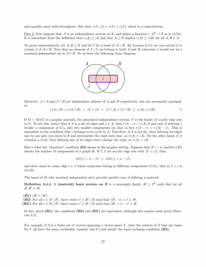
and equality must hold throughout. But then r(I ∪ J) = r(I) < r(J), which is a contradiction.

Part 2: Now suppose that I is an independence system on E, and define a function r : 2E → Z as in (3.5b).It is immediate from the definition that r(A) ≤ |A| and that A ⊆ B implies r(A) ≤ r(B) for all A,B ∈ I .

To prove submodularity, let A,B ⊆ E and let I be a basis of A ∩ B. By Lemma 3.4.2, we can extend I toa basis J of A ∪B. Note that no element of J \ I can belong to both A and B, otherwise I would not be amaximal independent set in A ∩B. So we have the following Venn diagram:

A B

I

J

Moreover, J ∩ A and J ∩ B are independent subsets of A and B respectively, but not necessarily maximal,so

r(A ∪B) + r(A ∩B) = |I|+ |J | = |J ∩A|+ |J ∩B| ≤ r(A) + r(B).

If M =M(G) is a graphic matroid, the associated independence system I is the family of acyclic edge setsin G. To see this, notice that if A is a set of edges and e ∈ A, then r(A− e) < r(A) if and only if deleting ebreaks a component of G|A into two smaller components (so that in fact r(A − e) = r(A) − 1). This isequivalent to the condition that e belongs to no cycle in A. Therefore, if A is acyclic, then deleting its edgesone by one gets you down to ∅ and decrements the rank each time, so r(A) = |A|. On the other hand, if Acontains a cycle, then deleting any of its edges won’t change the rank, so r(A) < |A|.

Here’s what the “donation” condition (I3) means in the graphic setting. Suppose that |V | = n, and let c(H)denote the number of components of a graph H. If I, J are acyclic edge sets with |I| < |J |, then

c(G|I) = n− |I| > c(G|J) = n− |J |,

and there must be some edge e ∈ J whose endpoints belong to different components of G|I ; that is, I + e isacyclic.

The bases of M (the maximal independent sets) provide another way of defining a matroid.

Definition 3.4.4. A (matroid) basis system on E is a nonempty family B ⊆ 2E such that for allB,B′ ∈ B,

(B1) |B| = |B′|;(B2) For all e ∈ B \B′, there exists e′ ∈ B′ \B such that (B − e) + e′ ∈ B;(B2′) For all e ∈ B \B′, there exists e′ ∈ B′ \B such that (B′ + e)− e′ ∈ B.

In fact, given (B1), the conditions (B2) and (B2′) are equivalent, although this require some proof (Exer-cise 3.2).

For example, if S is a finite set of vectors spanning a vector space V , then the subsets of S that are basesfor V all have the same cardinality (namely dimV ) and satisfy the basis exchange condition (B2).

57

If G is a graph, then the bases of M(G) are its spanning forests, i.e., its maximal acyclic edge sets. If Gis connected (which, as we will see, we may as well assume when studying graphic matroids) then the basesof M(G) are its spanning trees.

B B′

Here is the graph-theoretic interpretation of (B2). Let G be a connected graph, let B,B′ be spanning trees,and let e ∈ B \B′. Then B − e has exactly two connected components. Since B′ is connected, it must havesome edge e′ with one endpoint in each of those components, and then B − e + e′ is a spanning tree. SeeFigure 3.2.

B

e

B\e B′

Figure 3.2: An example of basis axiom (B2) in a graphic matroid. The green edges are the possibilitiesfor e′ such that B\e+ e′ is a spanning tree.

As for (B2′), if e ∈ B \B′, then B′+e must contain a unique cycle C (formed by e together with the uniquepath P in B′ between the endpoints of e). Deleting any edge e′ ∈ P will produce a spanning tree, and theremust be at least one such edge e′ ∈ B (otherwise B contains the cycle C). See Figure 3.3.

B

e

B′ B′ ∪ e

∗ ∗

Figure 3.3: An example of basis axiom (B2′) in a graphic matroid. The path P is shown in green. Theedges of P \B, marked with stars, are valid choices for e′.

58

If G is a graph with edge set E and M =M(G) is its graphic matroid, then

I = A ⊆ E : A is acyclic,B = A ⊆ E : A is a spanning forest of G.

If S is a set of vectors and M =M(S) is the corresponding linear matroid, then

I = A ⊆ S : A is linearly independent,B = A ⊆ S : A is a basis for span(S).


1. If I is an independence system on E, then the family of maximal elements of I is a basis system.2. If B is a basis system, then I =

⋃B∈B 2B is an independence system.

3. These constructions are mutual inverses.

The proof is left as an exercise. We already have seen that an independence system on E is equivalent toa matroid rank function; Proposition 3.4.5 asserts that a basis system provides the same structure on E.Bases turn out to be especially convenient for describing fundamental operations on matroids such as duality,direct sum, and deletion/contraction (all of which are coming soon).

Instead of specifying the bases (maximal independent sets), a matroid can be defined by its minimal depen-dent sets, which are called circuits. These too can be axiomatized:

Definition 3.4.6. A (matroid) circuit system on E is a family C ⊆ 2E such that, for all C,C ′ ∈ C ,

(C1) ∅ ∈ C :(C2) C ⊆ C ′;(C3) For all e ∈ C ∩ C ′, the set (C ∪ C ′)− e contains an element of C .

In a linear matroid, the circuits are the minimal dependent sets of vectors. Indeed, if C,C ′ are such sets ande ∈ C ∩ C ′, then we can find two expressions for e as nontrivial linear combinations of vectors in C and inC ′, and equating these expressions and eliminating e shows that (C ∪ C ′)− e is dependent, hence containsa circuit.

In a graph, if two cycles C,C ′ meet in a (non-loop) edge e = xy, then C − e and C ′− e are paths between xand y, so concatenating them forms a closed path. This path is not necessarily itself a cycle, but mustcontain some cycle.


1. If I is an independence system on E, then C ∈ I : C ′ ∈ I ∀C ′ ⊊ C is a circuit system.2. If C is a circuit system, then I ⊆ E : C ⊆ I ∀C ∈ C is an independence system.3. These constructions are mutual inverses.

In other words, the circuits are the minimal nonfaces of the independence complex (hence they correspondto the generators of the Stanley-Reisner ideal; see Defn. 6.3.1). The proof is left as an exercise.

The final definition of a matroid is different from what has come before, and gives a taste of the importanceof matroids in combinatorial optimization.

Let E be a finite set and let ∆ be an abstract simplicial complex on E (see Definition 3.4.1). Let w :E → R≥0 be a function, which we regard as assigning weights to the elements of E, and for A ⊆ E, define

59

w(A) =∑

e∈A w(e). Consider the problem of maximizing w(A) over all subsets A ∈ ∆; the maximum willcertainly be achieved on a facet. A naive approach to find a maximal-weight A, which may or may not workfor a given ∆ and w, is the following “greedy” algorithm (known as Kruskal’s algorithm):

1. Let A = ∅.2. If A is a facet of ∆, stop.

Otherwise, find e ∈ E \A of maximal weight such that A+ e ∈ ∆ (if there are several such e, pick oneat random), and replace A with A+ e.

3. Repeat step 2 until A is a facet of ∆.

Proposition 3.4.8. ∆ is a matroid independence system if and only if Kruskal’s algorithm produces a facetof maximal weight for every weight function w.

The proof is left as an exercise, as is the construction of a simplicial complex and a weight function forwhich the greedy algorithm does not produce a facet of maximal weight. This interpretation can be usefulin algebraic combinatorics; see Example 9.19.2 below.

Summary of Matroid Axiomatizations

• Geometric lattice: lattice that is atomic and semimodular. Corresponds to a simple matroid.• Rank function: function r : 2E → N such that r(A) ≤ |A| and r(A)+r(B) ≥ r(A∪B)+r(A∩B).Simple if r(A) = |A| whenever |A| ≤ 2.

• Closure operator : function 2E → 2E , A 7→ A such that A ⊆ A = A; A ⊆ B =⇒ A ⊆ B; andx ∈ A, x ∈ A ∪ y =⇒ y ∈ A ∪ x. Simple if A = A whenever |A| ≤ 1.

• Independence system: set family I ⊆ 2E such that ∅ ∈ I ; I ∈ I , I ′ ⊆ I =⇒ I ′ ∈ I ; andI, J ∈ I , |I| < |J | =⇒ ∃x ∈ J \ I : I ∪ x ∈ I . Simple if A ∈ I whenever |A| ≤ 2.

• Basis system: set family I ⊆ 2E such that ∅ ∈ I ; I ∈ I , I ′ ⊆ I =⇒ I ′ ∈ I ; and I, J ∈ I ,|I| < |J | =⇒ ∃x ∈ J \ I : I ∪ x ∈ I . Simple if every element and every pair of elementsbelong to some basis.

• Circuit system: set family C ⊆ 2E such that no element contains any other, and C.C ′ ∈ C ,e ∈ C ∩ C ′ =⇒ ∃C ′′ ∈ C : C ′′ ⊆ (C ∪ C ′)− e. Simple if all elements have size at least 3.

• Greedy algorithm: simplicial complex ∆ on E such that the greedy algorithm successfullyconstructs a maximum-weight facet for every weight function w : E → R≥0.

3.5 Representability and regularity

The motivating example of a matroid is a finite collection of vectors in Rn. What if we work over a differentfield? What if we turn this question on its head by specifying a matroid M purely combinatorially and thenasking which fields give rise to vector sets whose matroid is M?

Definition 3.5.1. Let M be a matroid and V a vector space over a field k. A set of vectors S ⊆ Vrepresents or realizes M over k if the linear matroid M(S) associated with S is isomorphic to M .

For example:

• The matroid U2(3) is representable over any field F. Set S = (1, 0), (0, 1), (1, 1); any two of thesevectors form a basis of F2.

• If k has at least three elements, then U2(4) is representable, by, e.g., S = (1, 0), (0, 1), (1, 1), (1, a).where a ∈ k \ 0, 1. Again, any two of these vectors form a basis of k2.

60

• On the other hand, U2(4) is not representable over F2, because F22 doesn’t contain four nonzero elements.

More generally, suppose thatM is a simple matroid with n elements (i.e., the ground set E has |E| = n) andrank r (i.e., every basis of M has size r) that is representable over the finite field Fq of order q. Then eachelement of E must be represented by some nonzero vector in Fn

q , and no two vectors can be scalar multiplesof each other. Therefore,

n ≤ qr − 1

q − 1.

Example 3.5.2. The Fano plane. Consider the affine point configuration with 7 points and 7 lines (one ofwhich looks like a circle), as shown:

5

1 3

46

2

7

This point configuration cannot be represented over R. If you try to draw seven non-collinear points in R2

such that the six triples 123, 345, 156, 147, 257, 367 are each collinear, then 246 will not be collinear —try it. The same thing will happen over any field of characteristic = 2. On the other hand, over a field ofcharacteristic 2, if the first six triples are collinear then 246 must be collinear. The configuration can beexplicitly represented over F2 by the columns of the matrix1 1 0 0 0 1 1

0 1 1 1 0 0 10 0 0 1 1 1 1

∈ (F2)3×7

for which each of the seven triples of columns listed above is linearly dependent, and that each other tripleis a column basis. (Note that over R, the submatrix consisting of columns 2,4,6 has determinant 2.) Theresulting matroid is called the Fano plane or Fano matroid. Note that each line in the Fano matroidcorresponds to a 2-dimensional subspace of F3

2.

Viewed as a matroid, the Fano plane has rank 3. Its bases are the(73

)−7 = 28 noncollinear triples of points.

Its circuits are the seven collinear triples and their complements (known as ovals). For instance, 4567 is anoval: it is too big to be independent, but on the other hand every three-element subset of it forms a basis(in particular, is independent), so it is a circuit.

The Fano plane is self-dual in the sense of discrete geometry3: the lines can be labeled 1, . . . , 7 so that point ilies on line j if and only if point j lies on line i. Here’s how: recall that the points and lines of the Fano planecorrespond respectively to 1- and 2-dimensional subspaces of F3

2, and assign the same label to orthogonallycomplementary spaces under the standard inner product.

Example 3.5.3 (Finite projective planes). Let q ≥ 2 be a positive integer. A projective plane of orderq consists of a collection P of points and a collection L of lines, each of which is a subset of P , such that:

3But not self-dual as a matroid in the sense to be defined in §3.7.

61

• |P | = |L| = q2 + q + 1;• Each line contains q + 1 points, and each point lies in q + 1 lines;• Any two points determine a unique line, and any two lines determine a unique point.

The Fano plane is thus a projective plane of order 2. More generally, if Fq is any finite field, then one can definea projective plane P2

q whose points and lines are the 1- and 2-dimensional subspaces F3q, respectively. Note

that the number of lines is the number of nonzero vectors up to scalar multiplication, hence (q3−1)/(q−1) =q2 + q + 1.

A notorious open question is whether any other finite projective planes exist. The best general result knownis the Bruck–Ryser–Chowla theorem (1949), which states that if q ≡ 1 or 2 (mod 4), then q must be thesum of two squares. In particular, there exists no projective plane of order 6. Order 10 is also known to beimpossible thanks to computer calculation, but the problem is open for other non-prime-power orders. It isalso open whether there exists a projective plane of prime-power order that is not isomorphic to P2

q. Onereadily available survey of the subject is by Perrott [Per16].

Representability can be tricky. As we have seen, U2(4) can be represented over any field other than F2,while the Fano plane is representable only over fields of characteristic 2. The point configuration below isan affine representation of a rank-3 matroid over R, but the matroid is not representable over Q [Gru03,pp. 93–94]. Put simply, it is impossible to construct a set of points with rational coordinates and exactlythese collinearities.

A regular matroid is one that is representable over every field. (For instance, we will see that graphicmatroids are regular.) For some matroids, the choice of field matters. For example, every uniform matroidis representable over every infinite field, but as we have seen before, Uk(n) can be represented over Fq onlyif n ≤ (qk − 1)/(q− 1). (For example, U2(4) is not representable over F2.) However, this inequality does notsuffice for representability; as mentioned above, the Fano plane cannot be represented over, say, F101.

Recall that a minor of a matrix is the determinant of some square submatrix of M . A matrix is calledtotally unimodular if every minor is either 0, 1, or −1.Theorem 3.5.4. A matroid M is regular if and only if it can be represented by the columns of a totallyunimodular matrix.

One direction is easy: if M has a unimodular representation then the coefficients can be interpreted as lyingin any field, and the linear dependence of a set of columns does not depend on the choice of field (because−1 = 0 and 1 = 0 in every field). The reverse direction is harder (see [Oxl92, chapter 6]), and the proof isomitted. In fact, something more is true: M is regular if and only if it is binary (representable over F2) andrepresentable over at least one field of characteristic = 2.

62

Theorem 3.5.5. Graphic matroids are regular.

Proof. Let G = (V,E) be a graph on vertex set V = [n], and let M = M(G) be the corresponding graphicmatroid. We can representM by the matrix X whose columns are the vectors ei−ej for ij ∈ E. (Or ej−ei;it doesn’t matter, since scaling a vector does not change the matroid.) Here e1, . . . , en is the standardbasis for Rn.

Consider any square submatrix XWB of X with rowsW ⊆ V and columns B ⊆ A, where |W | = |B| = k > 0.If B contains a cycle v1, . . . , vk then the columns are linearly dependent, because

(ev1 − ev2) + (ev2 − ev3) + · · ·+ (evn − ev1) = 0,

so detXWB = 0. On the other hand, if B is acyclic, then I claim that detXWB ∈ 0,±1, which we willprove by induction on k. The base case k = 1 follows because all entries of X are 0 or ±1. For k > 1, ifthere is some vertex of W with no incident edge in B, then the corresponding row of XWB is zero and thedeterminant vanishes. Otherwise, by the handshaking theorem, there must be some vertex w ∈ W incidentto exactly one edge b ∈ B. The corresponding row of XWB will have one entry ±1 and the rest zero.Expanding on that row gives detXWB = ±detW\w,B\b, and we are done by induction. The same argumentshows that any set of columns corresponding to an acyclic edge set will in fact be linearly independent.

Example 3.5.6. The matrix [1 0 1 10 1 1 −1

]represents U2(4) over any field of characteristic = 2, but the last two columns are dependent (in fact equal)in characteristic 2.

Example 3.5.7. There exist matroids that are not representable over any field. The smallest ones haveground sets of size 8; one of these is the rank-4 Vamos matroid V8 [Oxl92, p. 511]. The smallest rank-3example is the non-Pappus matroid.

Pappus’ Theorem from Euclidean geometry says that if a, b, c, A,B,C are distinct points in R2 such thata, b, c and A,B,C are collinear, then x, y, z are collinear, where

x = aB ∩Ab, y = aC ∩Ac, z = bC ∩Bc.

c

zy

x

AB

C

ba

63

Accordingly, there is a rank-3 simple matroid on ground set E = a, b, c, A,B,C, x, y, z whose flats are

∅, a, b, c, a, b, c, x, y, z, abc, ABC, aBx, Abx, aCy, Acy, bCz, Bcz, xyz, E.

It turns out that deleting xyz from this list produces the family of closed sets of a matroid, called thenon-Pappus matroid NP. Since Pappus’ theorem can be proven using analytic geometry, and the equationsthat say that x, y, z are collinear are valid over any field (i.e., involve only ±1 coefficients), it follows thatNP is not representable over any field.

3.6 Direct sum

There are several ways to construct new matroids from old ones. We’ll begin with a boring but useful one(direct sum) and then move on to the more exciting constructions of duality and deletion/contraction.

Definition 3.6.1. Let M1,M2 be matroids on disjoint sets E1, E2, with basis systems B1,B2. The directsum M1 ⊕M2 is the matroid on E1 ∪ E2 with basis system

B = B1 ∪B2 : B1 ∈ B1, B2 ∈ B2.

I will omit the routine proof that B is a basis system.

If M1,M2 are linear matroids whose ground sets span vector spaces V1, V2 respectively, then M1⊕M2 is thematroid you get by regarding the vectors as living in V1 ⊕ V2: the linear relations have to come either fromV1 or from V2.

If G1, G2 are graphs, then M(G1)⊕M(G2) ∼= M(G1 +G2), where + denotes disjoint union. Actually, youcan identify any vertex of G1 with any vertex of G2 and still get a graph whose associated graphic matroidis M(G1)⊕M(G2) (such as G in the following figure).

G1 G2 G

A useful corollary is that every graphic matroid arises from a connected graph. Actually, there may be manydifferent connected graphs that give rise to the same matroid, since in the previous construction it did notmatter which vertices of G1 and G2 were identified. This raises an interesting question: when does theisomorphism type of a graphic matroid M(G) determine the graph G up to isomorphism?

Definition 3.6.2. A matroid that cannot be written nontrivially as a direct sum of two smaller matroids iscalled connected or indecomposable.4

Proposition 3.6.3. Let G = (V,E) be a loopless graph. Then M(G) is indecomposable if and only if G is2-connected — i.e., not only is it connected, but so is every subgraph obtained by deleting a single vertex.

4The first term is more common among matroid theorists, but I prefer “indecomposable” to avoid potential confusion withthe graph-theoretic meaning of “connected”.

64

The “only if” direction is immediate: the discussion above implies that

M(G) =⊕H

M(H)

where H ranges over all the blocks (maximal 2-connected subgraphs) of G.

We’ll prove the other direction later (maybe).

Remark 3.6.4. If G ∼= H as graphs, then clearly M(G) ∼=M(H). The converse is not true: if T is any tree(or even forest) on n vertices, then every set of edges is acyclic, so the independence complex is the Booleanalgebra 2[n] (and, for that matter, so is the lattice of flats).

In light of Proposition 3.6.3, it is natural to suspect that every 2-connected graph is determined up toisomorphism by its graphic matroid, but even this is not true; the two 2-connected graphs below are notisomorphic, but have isomorphic graphic matroids.

As you should expect from an operation called “direct sum,” properties ofM1⊕M2 should be easily deduciblefrom those of its summands. In particular, direct sum is easy to describe in terms of the other matroidaxiomatizations we have studied. It is additive on rank functions: if A1 ⊆ E1 and A2 ⊆ E2, then

rM1⊕M2(A1 ∪A2) = rM1

(A1) + rM2(A2).

Similarly, the closure operator is A1 ∪A2 = A1 ∪ A2. The circuit system of the direct sum is just the(necessarily disjoint) union of the circuit systems of the summands. Finally, the geometric lattice of a directsum is just the poset product of the lattices of the summands, i.e.,

L(M1 ⊕M2) ∼= L(M1)× L(M2),

subject to the order relations (F1, F2) ≤ (F ′1, F

′2) iff Fi ≤ F ′

i in L(Mi) for each i.

3.7 Duality

Definition 3.7.1. Let M be a matroid on ground set |E| with basis system B. The dual matroid of M(also known as the orthogonal matroid) is the matroid M∗ on E with basis system

B∗ = E \B : B ∈ B.

65

We often write e∗ for elements of the ground set when talking about their behavior in the dual matroid.

Clearly the elements of B∗ all have cardinality |E| − r(M) (where r is the rank), and complementationswaps the basis exchange conditions (B2) and (B2′), so if you believe that those conditions are logicallyequivalent (Exercise 3.2) then you also believe that B∗ is a matroid basis system.

It is immediate from the definition that (M∗)∗ = M . In addition, the independent sets of M are thecomplements of the spanning sets of M∗ (since A ⊆ B for some B ∈ B if and only if E \ A ⊇ E \ B), andvice versa. The rank function r∗ of the dual is given by

r∗(A) = r(E \A) + |A| − r(E) ∀A ⊆ E. (3.6)

The proof is left as Exercise 3.7.

The dual of a vector matroid has an explicit description. Let E = v1, . . . , vn ⊆ kr, and let M = M(E).We may as well assume that E spans kr, so r ≤ n, and the representing matrix X = [v1| · · · |vn] ∈ kr×n hasfull row rank r.

Let Y be any (n − r) × n matrix with rowspace(Y ) = nullspace(X). That is, the rows of Y span theorthogonal complement of rowspace(X) with respect to the standard inner product.

Theorem 3.7.2. With this setup, the columns of Y are a representation for M∗.

Before proving this theorem, we’ll do an example that will make things clearer.

Example 3.7.3. Let E = v1, . . . , v5 be the set of column vectors of the following matrix (over R, say):

X =

1 0 0 2 10 1 0 2 10 0 1 0 0

.Notice that X has full row rank (it’s in row-echelon form, after all), so it represents a matroid of rank 3 on5 elements. We could take Y to be the matrix

Y =

[0 0 0 1 −21 1 0 0 −1

].

Then Y has rank 2. Call its columns v∗1 , . . . , v∗5; then the column bases are

v∗1 , v∗4, v∗1 , v∗5, v∗2 , v∗4, v∗2 , v∗5, v∗4 , v∗5,

whose (unstarred) complements (e.g., v2, v3, v5, etc.) are precisely the column bases for X. In particular,every basis of M contains v3 (so v3 is a coloop), which corresponds to the fact that no basis of M∗ containsv∗3 (so v∗3 is a loop). This makes sense linear-algebraically: v3 is linearly independent of all the columns, sono vector with a nonzero entry in the 3rd position is orthogonal to any row ofM , so v∗3 is the zero vector.

Proof of Theorem 3.7.2. First, note that invertible row operations on a matrix X ∈ kr×n (i.e., multiplicationon the left by an element of GLr(k)) do not change the matroid represented by its columns; they simplychange the basis of kr.

Let B be a basis ofM , and reindex so that B = v1, . . . , vr. We can then perform invertible row-operationsto put X into reduced row-echelon form, i.e.,

X = [Ir | A]

66

where Ir is the r×r identity matrix and A is arbitrary. It is easy to check that nullspaceX = (rowspaceX∗)T ,where

X∗ = [−AT | In−r],

(this is a standard recipe). But then the last n− r elements of X∗, i.e., E∗ \B∗, are clearly a column basis.By the same logic, every basis of X is the complement of a column basis of Y , and the converse is truebecause X can be obtained from X∗ in the same way that X∗ is obtained from X. Therefore the columnsof X and X∗ represent dual matroids. Meanwhile, any matrix Y with the same rowspace as X∗ can beobtained from it by invertible row operations, hence represents the same matroid.

In particular, representability over a particular field is unchanged by dualization.

Duality and graphic matroids. Let G be a connected planar graph, i.e., one that can be drawn in theplane with no crossing edges. The planar dual is the graph G∗ whose vertices are the regions into which Gdivides the plane, with two vertices of G∗ joined by an edge e∗ if the corresponding faces of G are separatedby an edge e of G. (So e∗ is drawn across e in the construction.)

G*

*e

f*

G

e

f

Some facts to check about planar duality:

• A ⊆ E is acyclic if and only if E∗ \A∗ is connected.• A ⊆ E is connected if and only if E∗ \A∗ is acyclic.• G∗∗ is naturally isomorphic to G.• e is a loop (bridge) if and only if e∗ is a bridge (loop).

If G is not planar then in fact M(G)∗ is not a graphic matroid (although it is certainly regular).

Definition 3.7.4. Let M be a matroid on E. A loop is an element of E that does not belongs to any basisof M . A coloop is an element of E that belongs to every basis of M . An element of E that is neither aloop nor a coloop is called ordinary (probably not standard terminology, but natural and useful).

In a linear matroid, a loop is a copy of the zero vector, while a coloop is a vector that is not in the span ofall the other vectors.

A cocircuit of M is by definition a circuit of the dual matroid M∗. A matroid can be described by itscocircuit system, which satisfy the same axioms as those for circuits (Definition 3.4.6). Set-theoretically, acocircuit is a minimal set not contained in any basis of M∗, so it is a minimal set that intersects every basisof M nontrivially. For a connected graph G, the cocircuits of the graphic matroid M(G) are the bondsof G: the minimal edge sets K such that G−K is not connected. Every bond C∗ is of the following form:there is a partition V (G) = X ∪· Y such that C∗ is the set of edges with one endpoint in each of X and Y ,and both G|X and G|Y are connected.

67

3.8 Deletion and contraction

Definition 3.8.1. Let M be a matroid on E with independence system I , and let e ∈ E.

1. The deletion of e is the matroid M\e on E − e with independence system I ∈ I : e ∈ I.2. The contraction of e is the matroidM/e on E−e is defined as follows. If e is a loop then I (M/e) = I .

Otherwise, the independence system of M/e is I ⊂ E − e : I + e ∈ I .

We can also describe deletion and contraction on the level of basis systems:

B(M\e) =B ∈ B(M) : e ∈ B if e is not a coloop,

B − e : B ∈ B(M) if e is a coloop,

B(M/e) =

B − e : B ∈ B(M), e ∈ B if e is not a loop,

B : B ∈ B(M) if e is a loop.

Again, the terms come from graph theory. Deleting an edge e of a graph G means removing it from thegraph, while contracting an edge means to shrink it down so that its two endpoints merge into one. Theresulting graphs are called G\e and G/e, and these operations are consistent with the effect on graphicmatroids, i.e.,

M(G\e) =M(G)\e, M(G/e) =M(G)/e. (3.7)

G / eG − eG

ve

x xx

y yyz z zv v

w w

w

Notice that contracting can cause some edges to become parallel, and can cause other edges (namely, thoseparallel to the edge being contracted) to become loops. In matroid language, deleting an element from asimple matroid always yields a simple matroid, but the same is not true for contraction.

We can define deletion and contraction of sets as well as single elements. To delete (resp., contract) a set,simply delete (resp., contract) each of its elements in some order.

Proposition 3.8.2. Let M be a matroid on E.

1. For each A ⊆ E, the deletion M\A and contraction M/A are well-defined (i.e., do not depend on theorder in which elements of A are deleted or contracted).

2. In particular

I (M\A) = I ⊆ E \A : I ∈ I (M),I (M/A) = I ⊆ E \A : I ∪B ∈ I (M)

where B is some (or, equivalently, any) basis of M |A.

68

3. Deletion and contraction commute in the following sense: for every e, f ∈ E we have (M/e)\f ∼=(M\f)/e.

4. Deletion and contraction are interchanged by duality:

(M\e)∗ ∼=M∗/e∗ and (M/e)∗ ∼=M∗\e∗.

The proof is left as an exercise.

Here is what deletion and contraction mean for vector matroids. Let V be a vector space over a field k, letE ⊆ V be a set of vectors spanning V , let M =M(E), and let e ∈ E. Then:

1. M\e =M(E − e). (If we want to preserve the condition that the ground set spans the ambient space,then e must not be a coloop.)

2. M/e is the matroid represented by the images of E − e in the quotient space V/ke. (Note that if e isa loop then this quotient space is just V itself.)

Thus both operations preserve representability over k. For instance, to find an explicit representation ofM/e,apply a change of basis to V so that e is the ith standard basis vector, then simply erase the ith coordinateof every vector in E − e.

Any matroid M ′ obtained from M by some sequence of deletions and contractions is called a minor of M .

Proposition 3.8.3. Every minor of a graphic (resp., linear, uniform) matroid is graphic (resp., linear,uniform).

Proof. The graphic case follows from (3.7), and the linear case from the previous discussion. For uniformmatroids, the definitions imply that

Uk(n)\e ∼= Uk(n− 1) and Uk(n)/e ∼= Uk−1(n− 1)

for every ground set element e.

.

Many invariants of matroids can be expressed recursively in terms of deletion and contraction. The followingfact is immediate from Definition 3.8.1.

Proposition 3.8.4. Let M be a matroid on ground set E, and let b(M) denote the number of bases of M .Let e ∈ E; then

b(M) =

b(M\e) if e is a loop;

b(M/e) if e is a coloop;

b(M\e) + b(M/e) otherwise.

Example 3.8.5. If M ∼= Uk(n), then b(M) =(nk

), and the recurrence of Proposition 3.8.4 is just the Pascal

relation(nk

)=(n−1k

)+(n−1k−1

).

Many other matroid invariants satisfy analogous recurrences involving deletion and contraction. In fact,Proposition 3.8.4 is the tip of an iceberg that we will explore in Chapter 4.

69

3.9 Exercises

Exercise 3.1. Determine, with proof, all pairs of integers k ≤ n such that there exists a graph G withM(G) ∼= Uk(n). (Here Uk(n) denotes the uniform matroid of rank k on n elements; see Example 3.2.4.).Hint: Use Proposition 3.8.3.

Exercise 3.2. Prove the equivalence of the two forms of the basis exchange condition (B2) and (B2′).(Hint: Examine |B \B′|.)Exercise 3.3. (Proposed by Kevin Adams.) Let B,B′ be bases of a matroid M . Prove that there exists abijection ϕ : B \B′ → B′ \B such that B − e+ ϕ(e) is a basis of M for every e ∈ B \B′.

Exercise 3.4. Prove Proposition 3.4.5, which describes the cryptomorphism between matroid independencesystems and matroid basis systems.

Exercise 3.5. Prove Proposition 3.4.7, which describes the cryptomorphism between matroid independencesystems and matroid circuit systems. (Hint: The hardest part is showing that if C is a matroid circuit systemthen the family I of sets containing no circuit satisfies (I3). Under the assumption that (I3) fails for somepair I, J with |I| < |J |, use circuit exchange to build a sequence of collections of circuits in I ∪ J that avoidmore and more elements of I, eventually producing a circuit in J and thus producing a contradiction.)

Exercise 3.6. Let M be a matroid on ground set E. Suppose there is a partition of E into disjoint setsE1, . . . , En such that r(E) = r(E1) + · · · + r(Ek). Prove that M =

⊕ni=1Mi, where Mi = M |Ei . (Note:

This fact provides an algorithm, albeit not necessarily an efficient one, for testing whether a matroid isconnected.)

Exercise 3.7. Let M be a matroid on ground set E with rank function r : 2E → N. Prove that the rankfunction r∗ of the dual matroid M∗ is given by r∗(A) = r(E \A) + |A| − r(E) for all A ⊆ E.

Exercise 3.8. Let M be a matroid on E. A set S ⊆ E is called spanning if it contains a basis. Let S bethe set of all spanning sets.

(a) Express S in terms of (i) the rank function r of M ; (ii) its closure operator A 7→ A; (iii) its lattice offlats L. (You don’t have to prove anything — just give the construction.)

(b) Formulate axioms that could be used to define a matroid via its system of spanning sets. (Hint:Describe spanning sets in terms of the dual matroid M∗.)

Exercise 3.9. Let E be a finite set and let ∆ be an abstract simplicial complex on E. Let w : E → R≥0

be any function; think of w(e) as the “weight” of e. For A ⊆ E, define w(A) =∑

e∈A w(e). Consider theproblem of maximizing w(A) over all facets A. A naive approach is the following greedy algorithm:

Step 1: Let A = ∅.Step 2: If A is a facet of ∆, stop.

Otherwise, find e ∈ E \A of maximal weight such that A+ e ∈ ∆(if there are several such e, pick one at random), and replace A with A+ e.

Step 3: Repeat Step 2 until A is a facet of ∆.

This algorithm may or may not work for a given ∆ and w. Prove the following facts:

(a) Construct a simplicial complex and a weight function for which this algorithm does not produce a facetof maximal weight. (Hint: The smallest example has |E| = 3.)

(b) Prove that the following two conditions are equivalent:(i) The greedy algorithm produces a facet of maximal weight for every weight function w.(ii) ∆ is a matroid independence system.

70

Note: This result does follow from Theorem 6.5.1. However, that is a substantial result, so don’t use itunless you first do Exercise 6.8. It is possible to do this exercise by working directly with the definition of amatroid independence system.

Exercise 3.10. Prove Proposition 3.8.2.

Exercise 3.11. Let X and Y be disjoint sets of vertices, and let B be an X,Y -bipartite graph: that is,every edge of B has one endpoint in each of X and Y . For V = x1, . . . , xn ⊆ X, a transversal of V is aset W = y1, . . . , yn ⊆ Y such that xiyi is an edge of B. (The set of all edges xiyi is called a matching.)Let I be the family of all subsets of X that have a transversal; in particular I is a simplicial complex.

Prove that I is in fact a matroid independence system by verifying that the donation condition (I3) holds.(Suggestion: Write down an example or two of a pair of independent sets I, J with |I| < |J |, and use thecorresponding matchings to find a systematic way of choosing a vertex that J can donate to I.) Thesematroids are called transversal matroids; along with linear and graphic matroids, they are the other“classical” examples of matroids in combinatorics.

Exercise 3.12. Fix positive integers n ≥ r.

(a) Let B be a family of subsets of([n]r

)satisfying the following property: if C,C ′ ∈

([n]r

)\B and C = C ′,

then |CC ′| ≥ 4). Prove that B is a matroid basis system. (Such a matroid is called a sparse pavingmatroid.)

(b) More generally, let j ∈ 0, . . . , n− r and let S ⊂([n]k+j

), such that |SS′| ≥ 2j + 4 for all S, S′ ∈ S .

Prove that

B =

B ∈

([n]

k

) ∣∣∣ B ⊆ S ∀S ∈ S

is a matroid basis system. (The j = 0 case is part (a).) This construction is due to George Nasr.

Exercise 3.13. (Requires a bit of abstract algebra.) Let n be a positive integer, and let ζ be a primitive nthroot of unity. The cyclotomic matroid Yn is represented over Q by the numbers 1, ζ, ζ2, . . . , ζn−1, regarded aselements of the cyclotomic field extension Q(ζ). Thus, the rank of Yn is the dimension of Q(ζ) as a Q-vectorspace, which is given by the Euler ϕ function. Prove the following:

(a) if n is prime, then Yn ∼= Un−1(n).(b) if m is the squarefree part of n (i.e., the product of all the distinct primes dividing n — e.g., the

squarefree part of 56 = 23 · 7 is 2 · 7 = 14) then Yn is the direct sum of n/m copies of Ym.(c) if n = pq, where p, q are distinct primes, then Yn ∼= M(Kp,q)

∗ — that is, the dual of the graphicmatroid of the complete bipartite graph Kp,q.

This problem is near and dear to my heart; the answer (more generally, a characterization of Yn for all n)appears in [MR05].

71

https://en.wikipedia.org/wiki/Euler's_totient_function

Chapter 4

The Tutte Polynomial

Throughout this section, let M be a matroid on ground set E with rank function r, and let n = |E|.

4.1 The two definitions of the Tutte polynomial

For A ⊆ E, we define

corankA = r(E)− r(A),nullityA = |A| − r(A).

Corank and nullity measure how far A is from being spanning and independent, respectively. That is, thecorank is the minimum number of elements needed to adjoin to A to produce a spanning set (i.e., to intersectall cocircuits), while the nullity is the minimum number of elements needed to delete from A to produce anindependent set (i.e., to break all circuits).

Definition 4.1.1. The Tutte polynomial of M is

TM = TM (x, y) :=∑A⊆E

(x− 1)r(E)−r(A)(y − 1)|A|−r(A). (4.1)

Example 4.1.2. If E = ∅ then TM (x, y) = 1. Mildly less trivially, if every element is a coloop, thenr(A) = |A| for all A, so

TM =∑A⊆E

(x− 1)n−|A| = (x− 1 + 1)n = xn

by the binomial theorem. If every element is a loop, then the rank function is identically zero and we get

TM∑A⊆E

(y − 1)|A| = yn.

Example 4.1.3. For uniform matroids, corank and nullity depend only on cardinality, making their Tuttepolynomials easy to compute. U1(2) has one set with corank 1 and nullity 0 (the empty set), two singletonsets with corank 0 and nullity 0, and one doubleton with corank 0 and nullity 1, so

TU1(2) = (x− 1) + 2 + (y − 1) = x+ y.

72

Similarly,

TU1(3) = (x− 1) + 3 + 3(y − 1) + (y − 1)2 = x+ y + y2,

TU2(3) = (x− 1)2 + 3(x− 1) + 3 + (y − 1) = x2 + x+ y.

Example 4.1.4. Let G be the graph below (known as the “diamond”):

a

d

c

b

e

The formula (4.1) gives

A |A| r(A) 3− r(A) |A| − r(A) contribution to (4.1)

1 empty set 0 0 3 0 1(x− 1)3(y − 1)0 = x3 − 3x2 + 3x− 15 singletons 1 1 2 0 5(x− 1)2(y − 1)0 = 5x2 − 10x+ 510 doubletons 2 2 1 0 10(x− 1)1(y − 1)0 = 10x− 102 triangles 3 2 1 1 2(x− 1)1(y − 1)1 = 2xy − 2x− 2y + 2

8 spanning trees 3 3 0 0 8(x− 1)0(y − 1)0 = 85 quadrupletons 4 3 0 1 5(x− 1)0(y − 1)1 = 5y − 5

1 whole set 5 3 0 2 1(x− 1)0(y − 1)2 = y2 − 2y + 1

Total x3 + 2x2 + x+ 2xy + y2 + y

Many invariants of M can be obtained by specializing the variables x, y appropriately. Some easy ones:

1. TM (2, 2) =∑

A⊆E 1 = 2|E|. (Or, if you like, |E| = log2 TM (2, 2).)2. Consider TM (1, 1). This kills off all summands whose corank is nonzero (i.e., all non-spanning sets)

and whose nullity is nonzero (i.e., all non-independent sets). What’s left are the bases, each of whichcontributes a summand of 1. So TM (1, 1) = b(M), the number of bases. We previously observed thatthis quantity satisfies a deletion/contraction recurrence (Prop. 3.8.4); this will show up again soon.

3. Similarly, TM (1, 2) and TM (2, 1) count respectively the number of spanning sets and the number ofindependent sets.

4. A little more generally, we can enumerate independent and spanning sets by their cardinality:∑A⊆E independent

q|A| = qr(M)T (1/q + 1, 1);

∑A⊆E spanning

q|A| = qr(M)T (1, 1/q + 1).

5. TM (0, 1) is (up to a sign) the reduced Euler characteristic (see (6.2)) of the independence complex

73

of M :

TM (0, 1) =∑A⊆E

(−1)r(E)−r(A)0|A|−r(A) =∑

A⊆E independent

(−1)r(E)−r(A)

= (−1)r(E)∑

A∈I (M)

(−1)|A|

= (−1)r(E)−1χ(I (M)). (4.2)

The fundamental theorem about the Tutte polynomial is that it satisfies a deletion/contraction recurrence.In a sense it is the most general such invariant — we will give a “recipe theorem” that expresses anydeletion/contraction invariant as a Tutte polynomial specialization (more or less).

Theorem 4.1.5. The Tutte polynomial satisfies (and can be computed by) the following Tutte recurrence:

(T1) If E = ∅, then TM = 1.(T2a) If e ∈ E is a loop, then TM = yTM\e.(T2b) If e ∈ E is a coloop, then TM = xTM/e.(T3) If e ∈ E is ordinary, then TM = TM\e + TM/e.

We can use this recurrence to compute the Tutte polynomial, by picking one element at a time to delete andcontract. The miracle is that it doesn’t matter what order we choose on the elements of E — all orders willgive the same final result! (In the case that M is a uniform matroid, then it is clear at this point that TMis well-defined by the Tutte recurrence, because, up to isomorphism, M\e and M/e are independent of thechoices of e ∈ E.)

Before proving the theorem, here are some examples.

Example 4.1.6. Suppose thatM ∼= Un(n), that is, every element is a coloop. By induction, TM (x, y) = xn.Dually, if M ∼= U0(n) (every element is a loop), then TM (x, y) = yn.

Example 4.1.7. Let M ∼= U1(2) (the graphic matroid of the “digon”, two vertices joined by two paralleledges). Let e ∈ E; then

TM = TM\e + TM/e

= T (U1(1)) + T (U0(1)) = x+ y.

Next, letM ∼= U2(3) (the graphic matroid of K3, as well as the matroid associated with the geometric latticeΠ3∼=M5). Applying the Tutte recurrence for any e ∈ E gives

T (U2(3)) = T (U2(2)) + T (U1(2)) = x2 + x+ y.

On the other hand,T (U1(3)) = T (U1(2)) + T (U0(2)) = x+ y + y2.

Note that these calculations agree with those of Example (4.1.3).

The Tutte recurrence says we can represent a calculation of TM by a binary tree in which moving downcorresponds to deleting or contracting:

M

M\e M\f

M\e\f...

M\e/f...

M/e\f...

M/e/f...

74

Example 4.1.8. Consider the diamond of Example 4.1.4. One possibility is to recurse on edge a (orequivalently on b, c, or d). When we delete a, the edge d becomes a coloop, and contracting it produces acopy of K3. Therefore

T (G\a) = x(x2 + x+ y)

by Example 4.1.7. Next, apply the Tutte recurrence to the edge b in G/a. The graph G/a\b has a coloop c,contracting which produces a digon. Meanwhile, M(G/a/b) ∼= U1(3). Therefore

T (G/a\b) = x(x+ y) and T (G/a/b) = x+ y + y2.

Putting it all together, we get

T (G) = T (G\a) + T (G/a)

= T (G\a) + T (G/a\b) + T (G/a/b)

= x(x2 + x+ y) + x(x+ y) + (x+ y + y2)

= x3 + 2x2 + 2xy + x+ y + y2.

x(x2 + x+ y)

x(x+ y) x+ y + y2

On the other hand, we could have recursed first on e, getting

T (G) = T (G\e) + T (G/e)

= T (G\e\c) + T (G\e/c) + T (G/e\c) + T (G/e/c)

= x3 + (x2 + x+ y) + x(x+ y) + y(x+ y)

= x3 + 2x2 + 2xy + x+ y + y2.

75

x3 x2 + x+ y x(x+ y) y(x+ y)

Proof of Theorem 4.1.5. Let M be a matroid on ground set E, let e ∈ E, and let r′ and r′′ be the rankfunctions of M\e and M/e respectively. The definitions of rank function, deletion, and contraction implythe following, for A ⊆ E − e:

1. If e is not a coloop, then r′(A) = rM (A).2. If e is not a loop, then r′′(A) = rM (A+ e)− 1.

To save space, set X = x− 1, Y = y − 1. We already know that if E = ∅, then TM = 1.

For (T2a), let e be a loop. Then

TM =∑A⊆E

Xr(E)−r(A)Y |A|−r(A)

=∑

A⊆E: e ∈A

Xr(E)−r(A)Y |A|−r(A) +∑

B⊆E: e∈B

Xr(E)−r(B)Y |B|−r(B)

=∑

A⊆E−e

Xr′(E−e)−r′(A)Y |A|−r′(A) +∑

A⊆E−e

Xr′(E−e)−r′(A)Y |A|+1−r′(A)

= (1 + Y )∑

A⊆E−e

Xr′(E−e)−r′(A)Y |A|−r′(A) = yTM\e.

For (T2b), let e be a coloop. Then

TM =∑A⊆E


=∑

e ∈A⊆E

Xr(E)−r(A)Y |A|−r(A) +∑

e∈B⊆E

Xr(E)−r(B)Y |B|−r(B)

=∑

A⊆E−e

X(r′′(E−e)+1)−r′′(A)Y |A|−r′′(A) +∑

A⊆E−e

X(r′′(E−e)+1)−(r′′(A)+1)Y |A|+1−(r′′(A)+1)

=∑

A⊆E−e

Xr′′(E−e)+1−r′′(A)Y |A|−r′′(A) +∑

A⊆E−e

Xr′′(E−e)−r′′(A)Y |A|−r′′(A)

= (X + 1)∑

A⊆E−e

Xr′′(E−e)−r′′(A)Y |A|−r′′(A) = xTM/e.

76

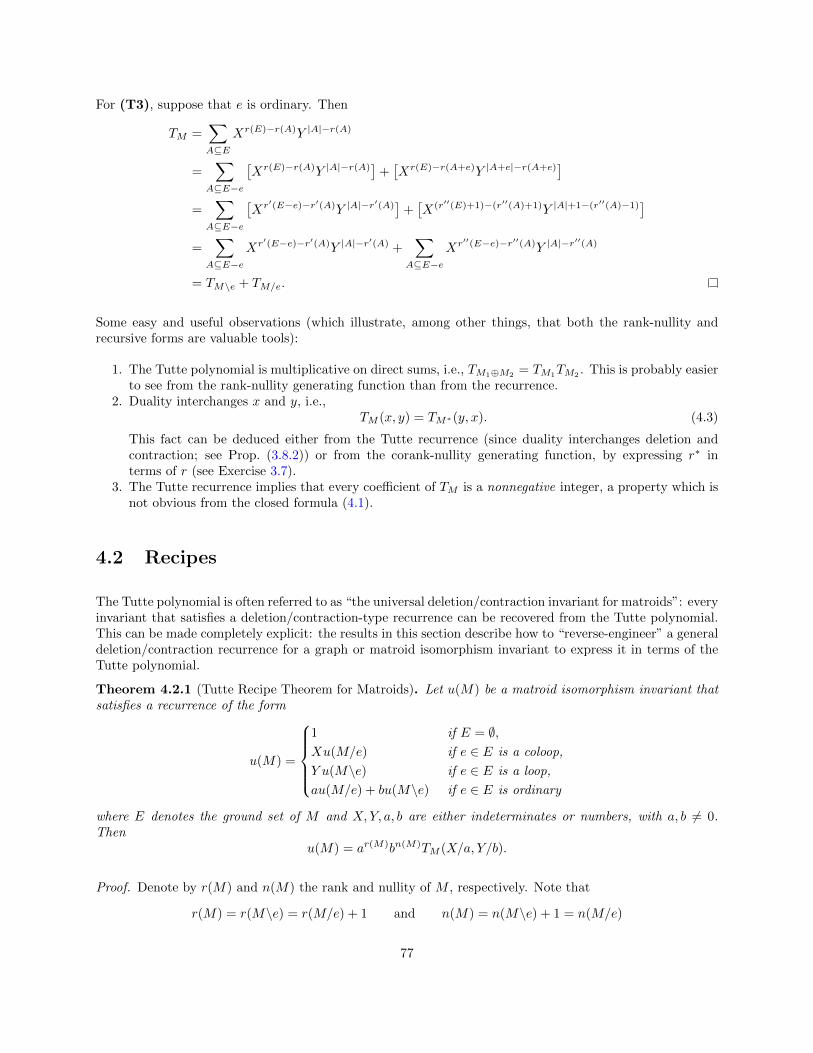
For (T3), suppose that e is ordinary. Then

TM =∑A⊆E


=∑

A⊆E−e

[Xr(E)−r(A)Y |A|−r(A)

]+[Xr(E)−r(A+e)Y |A+e|−r(A+e)

]=

∑A⊆E−e

[Xr′(E−e)−r′(A)Y |A|−r′(A)

]+[X(r′′(E)+1)−(r′′(A)+1)Y |A|+1−(r′′(A)−1)

]=

∑A⊆E−e

Xr′(E−e)−r′(A)Y |A|−r′(A) +∑

A⊆E−e

Xr′′(E−e)−r′′(A)Y |A|−r′′(A)

= TM\e + TM/e.

Some easy and useful observations (which illustrate, among other things, that both the rank-nullity andrecursive forms are valuable tools):

1. The Tutte polynomial is multiplicative on direct sums, i.e., TM1⊕M2= TM1

TM2. This is probably easier

to see from the rank-nullity generating function than from the recurrence.2. Duality interchanges x and y, i.e.,

TM (x, y) = TM∗(y, x). (4.3)

This fact can be deduced either from the Tutte recurrence (since duality interchanges deletion andcontraction; see Prop. (3.8.2)) or from the corank-nullity generating function, by expressing r∗ interms of r (see Exercise 3.7).

3. The Tutte recurrence implies that every coefficient of TM is a nonnegative integer, a property which isnot obvious from the closed formula (4.1).

4.2 Recipes

The Tutte polynomial is often referred to as “the universal deletion/contraction invariant for matroids”: everyinvariant that satisfies a deletion/contraction-type recurrence can be recovered from the Tutte polynomial.This can be made completely explicit: the results in this section describe how to “reverse-engineer” a generaldeletion/contraction recurrence for a graph or matroid isomorphism invariant to express it in terms of theTutte polynomial.

Theorem 4.2.1 (Tutte Recipe Theorem for Matroids). Let u(M) be a matroid isomorphism invariant thatsatisfies a recurrence of the form

u(M) =

1 if E = ∅,Xu(M/e) if e ∈ E is a coloop,

Y u(M\e) if e ∈ E is a loop,

au(M/e) + bu(M\e) if e ∈ E is ordinary

where E denotes the ground set of M and X,Y, a, b are either indeterminates or numbers, with a, b = 0.Then

u(M) = ar(M)bn(M)TM (X/a, Y/b).

Proof. Denote by r(M) and n(M) the rank and nullity of M , respectively. Note that

r(M) = r(M\e) = r(M/e) + 1 and n(M) = n(M\e) + 1 = n(M/e)

77

whenever deletion and contraction are well-defined. Define a new matroid invariant

u(M) = a−r(M)b−n(M)u(M)

and rewrite the recurrence in terms of u, abbreviating r = r(M) and n = n(M), to obtain

arbnu(M) =

1 if E = ∅,Xar−1bnu(M/e) if e ∈ E is a coloop,

Y arbn−1u(M\e) if e ∈ E is a loop,

arbnu(M/e) + arbnu(M\e) if e ∈ E is ordinary.

Setting X = xa and Y = yb, we see that u(M) = TM (x, y) = TM (X/a, Y/b) by Theorem 4.1.5, and rewritingin terms of u(M) gives the desired formula.

Bollobas [Bol98, p.340] gives an analogous result for graphs:

Theorem 4.2.2 (Tutte Recipe Theorem for Graphs). Let u(G) be a graph isomorphism invariant thatsatisfies a recurrence of the form

u(G) =

a|V | if E = ∅,Xu(G\e) if e ∈ E is a coloop,

Y u(G\e) if e ∈ E is a loop,

bu(G\e) + cu(G/e) if e ∈ E is ordinary,

where G = (V,E) and X,Y, a, b, c are either indeterminates or numbers (with b, c = 0). Then

u(G) = ak(G)bn(G)cr(G)TG(aX/c, Y/b).

We omit the proof, which is similar to that of the previous result. A couple of minor complications are thatmany deletion/contraction graph invariants involve the numbers of vertices or components, which cannot bededuced from the matroid of a graph. Also, while deletion and contraction of a cut-edge of a graph producetwo isomorphic matroids, they do not produce two isomorphic graphs (so, no, that’s not a misprint in thecoloop case of Theorem 4.2.2). The invariant U is described by Bollobas as “the universal form of the Tuttepolynomial.”

4.3 Basis activities

We know that TM (x, y) has nonnegative integer coefficients and that TM (1, 1) is the number of bases of M .These observations suggest that we should be able to interpret the Tutte polynomial as a generating functionfor bases: that is, there should be combinatorially defined functions i, e : B(M)→ N such that

TM (x, y) =∑

B∈B(M)

xi(B)ye(B).

In fact, this is the case. The tricky part is that i(B) and e(B) must be defined with respect to a total ordere1 < · · · < en on the ground set E, so they are not really invariants of B itself. However, another miracleoccurs: the Tutte polynomial itself is independent of the choice of total order.

78

Definition 4.3.1. Let M be a matroid on E with basis system B and let B ∈ B. For e ∈ B, thefundamental cocircuit of e with respect to B, denoted C∗(e,B), is the unique cocircuit in (E \ B) + e.That is,

C∗(e,B) = e′ : B − e+ e′ ∈ B.Dually, for e ∈ B, then the fundamental circuit of e with respect to B, denoted C(e,B), is the uniquecircuit in B + e. That is,

C(e,B) = e′ : B + e− e′ ∈ B.

In other words, the fundamental cocircuit consists of e together with all elements outside B that can replace ein a basis exchange, while the fundamental circuit consists of e together with all elements outside B thatcan be replaced by e.

Suppose thatM =M(G), where G its a connected graph, and B is a spanning tree. For all e ∈ B, the graphB − e has two components, say X and Y , and C∗(e,B) is the set of all edges with one endpoint in each ofX and Y . Dually, if e ∈ B, then B + e has exactly one cycle, and that cycle is C(e,B).

If M is a vector matroid, then C∗(e,B) consists of all vectors not in the codimension-1 subspace spannedby B − e, and C(e,B) is the unique linearly dependent subset of B + e.

Definition 4.3.2. Let M be a matroid on a totally ordered vertex set E = e1 < · · · < en, and let Bbe a basis of M . An element e ∈ B is internally active with respect to B if e is the minimal element ofC∗(e,B). An element e ∈ B is externally active with respect to B if e is the minimal element of C(e,B).We set

i(B) = #e ∈ B : e is internally active with respect to B= #edges of B that cannot be replaced by anything smaller outside B,

e(B) = #e ∈ E \B : e is externally active with respect to B= #edges of E \B that cannot replaced anything smaller inside B.

Note that these numbers depend on the choice of ordering of E.

Example 4.3.3. Let G be the graph with edges labeled as shown below, and let B be the spanning treee2, e4, e5 shown in red. The middle figure shows C(e1, B), and the right-hand figure shows C∗(e5, B).

e2

e3

e4

e1

e5e2

e3

e4

e1

e5e2

e3

e4

e1

e5

Here are some fundamental circuits and cocircuits:

C(e1, B) = e1, e4, e5 so e1 is externally active;

C(e3, B) = e2, e3, e5 so e3 is not externally active;

C∗(e2, B) = e2, e3 so e2 is internally active;

C∗(e4, B) = e1, e4 so e4 is not internally active;

C∗(e5, B) = e1, e3, e5 so e5 is not internally active.

79

Theorem 4.3.4 (Tutte). Let M be a matroid on E. Fix a total ordering of E and let e(B) and i(B) denoterespectively the number of externally active and internally active elements with respect to B. Then

TM (x, y) =∑

B∈B(M)

xi(B)ye(B). (4.4)

For instance, in Example 4.3.3, the spanning tree B contributes the monomial xy = x1y1 to T (G; x, y).

Tutte’s original paper [Tut54] actually defined the Tutte polynomial (which he called the “dichromate”)as∑

B∈B(M) xi(B)ye(B) (rather than the corank-nullity generating function), then proved it that obeys the

deletion/contraction recurrence. Like the proof of Theorem 4.1.5, this result requires careful bookkeepingbut is not conceptually difficult. Note in particular that if e is a loop (resp. coloop), then e ∈ B (resp. e ∈ B)for every basis B, and C(e,B) = e (resp. C∗(e,B) = e), so e is externally (resp. internally) active withrespect to B, so the generating function (4.4) is divisible by y (resp. x).

4.4 The characteristic and chromatic polynomials

We first show that the characteristic polynomial of a geometric lattice is a specialization of the Tuttepolynomial of the corresponding matroid.

Theorem 4.4.1. Let M be a simple matroid on E with rank function r and lattice of flats !L. Then

χ(L; k) = (−1)r(M)TM (1− k, 0).

Proof. Let A 7→ A be the matroid closure operator of M . Observe that

(−1)r(M)TM (1− k, 0) = (−1)r(M)∑A⊆E

(−k)r(M)−r(A)(−1)|A|−r(A)

=∑A⊆E

(−1)|A|kr(M)−r(A)

=∑K∈L

∑A⊆E: A=K

(−1)|A|

︸︷︷︸

f(K)

kr(M)−r(K).

We now claim that f(K) = µL(0,K). For each flat K ∈ L, let

g(K) =∑

J∈L: J⊆K

f(J)

so that by Mobius inversion (2.3a)

f(K) =∑

J∈L: J⊆K

µ(J,K)g(J). (4.5)

But on the other hand

g(J) =∑

I∈L: I⊆J

∑A⊆E: A=I

(−1)|A| =∑

A⊆E: A⊆J

(−1)|A| =∑A⊆J

(−1)|A| = (1− 1)|J| = δJ,∅.

So (4.5) simplifies to f(K) = µ(0,K), completing the proof.

80

Theorem 4.4.1 gives another proof that the Mobius function of a semimodular lattice L weakly alternates insign, or specifically that (−1)r(L)µ(L) ≥ 0 (Theorem 2.4.7). First, if L is not geometric, or equivalently notatomic, then by Corollary 2.4.10 µ(L) = 0. Second, if L is geometric, then by (2.6) and Theorem 4.4.1

(−1)r(L)µ(L) = (−1)r(L)χ(L; 0) = TM (1, 0). (4.6)

But TM (1, 0) ≥ 0 for every matroid M , because TM ∈ N[x, y].

The characteristic polynomial of a graphic matroid has a classical combinatorial interpretation in terms ofcolorings. Let G = (V,E) be a connected graph. Recall that a k-coloring of G is a function f : V → [k], anda coloring is proper if f(v) = f(w) whenever vertices v and w are adjacent. We showed in Example 2.3.5that the function

pG(k) = number of proper k-colorings of G

is a polynomial in k, called the chromatic polynomial of G. In fact pG(k) = k · χK(G)(k). We can alsoprove this fact via deletion/contraction.

First, note some important special cases:

• If G has a loop, then its endpoints automatically have the same color, so it’s impossible to color Gproperly and pG(k) = 0.

• If G = Kn, then all vertices must have different colors. There are k choices for f(1), k − 1 choices forf(2), etc., so pKn(k) = k(k − 1)(k − 2) · · · (k − n+ 1).

• At the other extreme, the graph G = Kn with n vertices and no edges has chromatic polynomial kn,since every coloring is proper.

• If T is a tree with n vertices, then pick any vertex as the root; this imposes a partial order on thevertices in which the root is 1 and each non-root vertex v is covered by exactly one other vertex p(v)(its “parent”). There are k choices for the color of the root, and once we know f(p(v)) there are k− 1choices for f(v). Therefore pT (k) = k(k − 1)n−1.

• If G has connected components G1, . . . , Gs, then pG(k) =∏s

i=1 pGi(k). Equivalently, pG+H(k) =

pG(k)pH(k), where + denotes disjoint union of graphs.

Theorem 4.4.2. For every graph G

pG(k) = (−1)n−ckc · TG(1− k, 0)

where n is the number of vertices of G and c is the number of components. In particular, pG(k) is a polynomialfunction of k.

Proof. First, we show that the chromatic function satisfies the recurrence

pG(k) = kn if E = ∅; (4.7)

pG(k) = 0 if G has a loop; (4.8)

pG(k) = (k − 1)pG/e(k) if e is a coloop; (4.9)

pG(k) = pG\e(k)− pG/e(k) otherwise. (4.10)

We already know (4.7) and (4.8). Suppose e = xy is not a loop. Let f be a proper k-coloring of G \ e. Iff(x) = f(y), then we can identify x and y to obtain a proper k-coloring of G/e. If f(x) = f(y), then f is aproper k-coloring of G. So (4.10) follows.

This argument applies even if e is a coloop. In that case, however, the component H of G containing ebecomes two components H ′ and H ′′ of G \ e, whose colorings can be chosen independently of each other.So the probability that f(x) = f(y) in any proper coloring is 1/k, implying (4.9).

81

The graph G \ e has n vertices and either c + 1 or c components, according as e is or is not a coloop.Meanwhile, G/e has n− 1 vertices and c components. By induction,

(−1)n−ckcTG(1− k, 0) =

kn if E = ∅,0 if e is a loop,

(1− k)(−1)n+1−c kc TG/e(1− k, 0) if e is a coloop,

(−1)n−ckc(TG\e(1− k, 0) + TG/e(1− k, 0)

)otherwise

=

kn if E = ∅,0 if e is a loop,

(k − 1)pG/e(k) if e is a coloop,

pG\e(k)− pG/e(k) otherwise

which is exactly the recurrence satisfied by the chromatic polynomial.

Remark 4.4.3. It is also possible to prove Theorem 4.4.2 by invoking the Tutte Recipe Theorem forGraphs (Theorem 4.2.2). To do so, one would need to replace case (4.9) of the chromatic recurrence withthe statement pG(k) =

k−1k pG−e(k).

More generally, if G is a graph with n vertices and c components, then its graphic matroid M =M(G) hasrank n− c, whose associated geometric lattice is the connectivity lattice K(G). Combining Theorems 4.4.1and 4.4.2 gives

pG(k) = kc χ(K(G); k).

4.5 Acyclic orientations

An orientation O of a graph G = (V,E) is an assignment of a direction to each edge xy ∈ E (either xy oryx). A directed cycle is a sequence (x0, x1, . . . , xn−1) of vertices such that xixi+1 is a directed edge forevery i. (Here the indices are taken modulo n.)

An orientation is acyclic if it has no directed cycles. Let A(G) be the set of acyclic orientations of G, andlet a(G) = |A(G)|.

For example:

1. If G has a loop then a(G) = 0.2. If G has no loops, then every total order on the vertices gives rise to an acyclic orientation: orient each

edge from smaller to larger vertex. Of course, different total orders can produce the same a.o.3. If G has no edges than a(G) = 1. Otherwise, a(G) is even, since reversing all edges is a fixed-point free

involution on A(G).4. Removing parallel copies of an edge does not change a(G), since all parallel copies would have to be

oriented in the same direction to avoid any 2-cycles.5. If G is a forest then every orientation is acyclic, so a(G) = 2|E(G).6. If G = Kn then the acyclic orientations are in bijection with the total orderings, so a(G) = n!.7. If G = Cn (the cycle of graph of length n) then it has 2n orientations, of which exactly two are not

acyclic, so a(Cn) = 2n − 2.

Colorings and orientations are intimately connected. Given a proper coloring f : V (G) → [k], one cannaturally define an acyclic orientation by directing each edge from the smaller to the larger color. (So #2 in

82

the above list is a special case of this.) The connection between them is the prototypical example of what iscalled combinatorial reciprocity.

A (compatible) k-pair for a graph G = (V,E) is a pair (O, f), where O is an acyclic orientation of G andf : V → [k] is a coloring such that f(x) ≤ f(y) for every directed edge x→ y in D. Let C(G) = C(G, k) bethe set of compatible k-pairs of G (we can safely drop k from the notation)

Theorem 4.5.1 (Stanley’s Acyclic Orientation Theorem). For every graph G and positive integer k,

|C(G, k)| = (−1)npG(−k) = kcTG(1 + k, 0). (4.11)

Proof. The second equality follows from Theorem 4.4.2, so we prove the first one. Let n = |G|.

If G has no edges then |C(G)| = kn = (−1)n(−k)n = (−1)npG(−k), confirming (4.11).

If G has a loop then it has no acyclic orientations, hence no k-pairs for any k, so both sides of (4.11) arezero.

Let e = xy be an edge of G that is not a loop. Denote the left-hand side of (4.11) by pG(k). Then

pG(k) = (−1)npG(−k) = (−1)n(pG\e(−k)− pG/e(−k))= (−1)n((−1)npG\e(k)− (−1)n−1pG/e(k))

= pG\e(k) + pG/e(k)

so we need to show that |C(G)| satisfies the same recurrence. Write

Say that a pair (O, f) ∈ C(G) is reversible (with respect to e) if reversing e produces a compatible pair(O′, f); otherwise it is irreversible. (Reversibility is equivalent to saying that f(x) = f(y) and that G doesnot contain a directed path from either endpoint of e to the other.) Let Crev(G) and Cirr(G) denote the setsof reversible and irreversible compatible pairs, respectively.

If e is reversible, then contracting it to a vertex z and defining f(z)−f(x)−f(y) produces a compatible pair ofG/e. (The resulting orientation is acyclic because any directed cycle lifts to either a directed cycle in G, or anoriented path between the endpoints of e, neither of which exists.) This defines a map ψ : Crev(G)→ C(G/e),which is 2-to-1 because ψ(O, f) = ψ(O′, f). Moreover, ψ is onto: any (O, f) ∈ C(G/e) can be lifted to(Of) ∈ C(G) by defining f(x) = f(y) = f(z) and orienting e in either direction (the acyclicity of O meansthat there is no oriented path from either x or y to the other in O). We conclude that

|C(G/e)| = |Crev(G)|2

. (4.12)

There is a map ω : C(G) → C(G − e) given by deleting e. I claim that ω is surjective, which is equivalentto saying that it is always possible to extend any element of C(G − e) to C(G) by choosing an appropriateorientation for e. (If f(x) < f(y), then O has no y, x-path by compatibility. If f(x) = f(y) and neitherorientation of e is acyclic, then O must contain a directed path from each of x, y to the other, hence is notacyclic.) The map ω is 1-to-1 on Cirr(G) but 2-to-1 on Crev(G) (for the same reason as ψ). Therefore,

|C(G− e)| = |Cirr(G)|+|Crev(G)|

2. (4.13)

Combining (4.12) and (4.13) gives

|C(G− e)|+ |C(G/e)| = |Cirr(G)|+ |Crev(G)| = |C(G)|as desired.

83

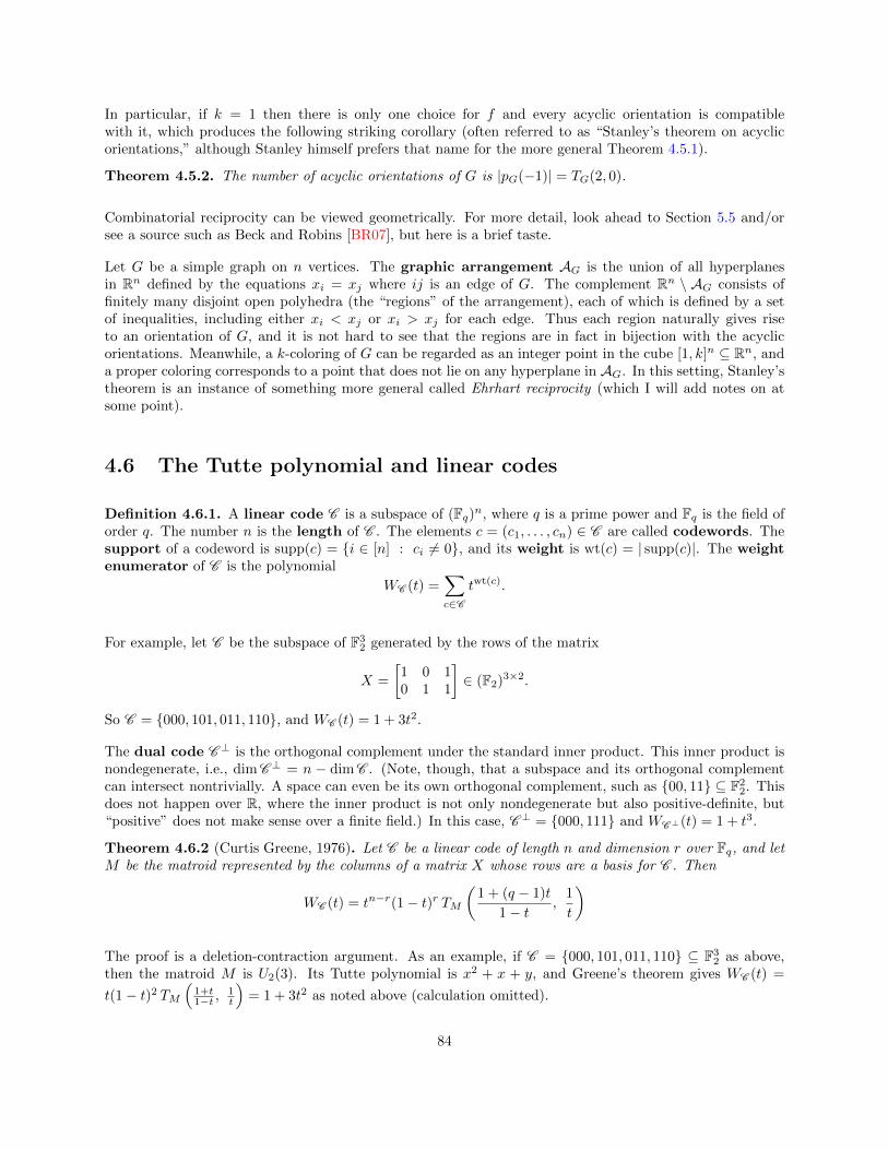
In particular, if k = 1 then there is only one choice for f and every acyclic orientation is compatiblewith it, which produces the following striking corollary (often referred to as “Stanley’s theorem on acyclicorientations,” although Stanley himself prefers that name for the more general Theorem 4.5.1).

Theorem 4.5.2. The number of acyclic orientations of G is |pG(−1)| = TG(2, 0).

Combinatorial reciprocity can be viewed geometrically. For more detail, look ahead to Section 5.5 and/orsee a source such as Beck and Robins [BR07], but here is a brief taste.

Let G be a simple graph on n vertices. The graphic arrangement AG is the union of all hyperplanesin Rn defined by the equations xi = xj where ij is an edge of G. The complement Rn \ AG consists offinitely many disjoint open polyhedra (the “regions” of the arrangement), each of which is defined by a setof inequalities, including either xi < xj or xi > xj for each edge. Thus each region naturally gives riseto an orientation of G, and it is not hard to see that the regions are in fact in bijection with the acyclicorientations. Meanwhile, a k-coloring of G can be regarded as an integer point in the cube [1, k]n ⊆ Rn, anda proper coloring corresponds to a point that does not lie on any hyperplane in AG. In this setting, Stanley’stheorem is an instance of something more general called Ehrhart reciprocity (which I will add notes on atsome point).

4.6 The Tutte polynomial and linear codes

Definition 4.6.1. A linear code C is a subspace of (Fq)n, where q is a prime power and Fq is the field of

order q. The number n is the length of C . The elements c = (c1, . . . , cn) ∈ C are called codewords. Thesupport of a codeword is supp(c) = i ∈ [n] : ci = 0, and its weight is wt(c) = | supp(c)|. The weightenumerator of C is the polynomial

WC (t) =∑c∈C

twt(c).

For example, let C be the subspace of F32 generated by the rows of the matrix

X =

[1 0 10 1 1

]∈ (F2)

3×2.

So C = 000, 101, 011, 110, and WC (t) = 1 + 3t2.

The dual code C⊥ is the orthogonal complement under the standard inner product. This inner product isnondegenerate, i.e., dimC⊥ = n − dimC . (Note, though, that a subspace and its orthogonal complementcan intersect nontrivially. A space can even be its own orthogonal complement, such as 00, 11 ⊆ F2

2. Thisdoes not happen over R, where the inner product is not only nondegenerate but also positive-definite, but“positive” does not make sense over a finite field.) In this case, C⊥ = 000, 111 and WC⊥(t) = 1 + t3.

Theorem 4.6.2 (Curtis Greene, 1976). Let C be a linear code of length n and dimension r over Fq, and letM be the matroid represented by the columns of a matrix X whose rows are a basis for C . Then

WC (t) = tn−r(1− t)r TM(1 + (q − 1)t

1− t ,1

t

)

The proof is a deletion-contraction argument. As an example, if C = 000, 101, 011, 110 ⊆ F32 as above,

then the matroid M is U2(3). Its Tutte polynomial is x2 + x + y, and Greene’s theorem gives WC (t) =

t(1− t)2 TM(

1+t1−t ,

1t

)= 1 + 3t2 as noted above (calculation omitted).

84

If X⊥ is a matrix whose rows are a basis for the dual code, then the corresponding matroid M⊥ is preciselythe dual matroid to M . We know that TM (x, y) = TM⊥(y, x) by (4.3), so setting s = (1− t)/(1 + (q − 1)t)(so t = (1− s)/(1 + (q − 1)s); isn’t that convenient?) gives

WC⊥(t) = tr(1− t)n−r TM

(1 + (q − 1)s

1− s ,1

s

)= tr(1− t)n−rsr−n(1− s)−rWC (s),

or rewriting in terms of t,

WC⊥(t) =1 + (q − 1)tn

qrWC

(1− t

1 + (q − 1)t

)which is known as the MacWilliams identity and is important in coding theory.

4.7 Exercises

Exercise 4.1. An orientation of a graph is called totally cyclic if every edge belongs to a directed cycle.Prove that the number of totally cyclic orientations of G is TG(0, 2).

Exercise 4.2. Let G be a finite graph with n vertices, r edges, and k components. Fix an orientation Oon E(G). Let I(v) (resp., O(v)) denote the set of edges entering (resp., leaving) each vertex v. Let q be apositive integer and Zq = Z/qZ. A nowhere-zero q-flow (or q-NZF) on G (with respect to O) is a functionϕ : E(G)→ Zq \ 0 satisfying the conservation law∑

e∈I(v)

ϕ(e) =∑

e∈O(v)

ϕ(e)

for every v ∈ V (G). Let FOG (q) denote the set of nowhere-zero q-flows and fOG (q) = |FO

G (q)|.

(i) Prove that fOG (q) depends only on the graph G, not on the choice of orientation (so we are justified inwriting fG(q)).

(ii) Prove that fG(q) = (−1)r−n+kTG(0, 1− q).

(Interestingly, Z/qZ can be replaced with any abelian group of cardinality q without affecting the result.)

Exercise 4.3. Let G = (V,E) be a graph with n vertices and c components. For a vertex coloring f : V → P,let i(f) denote the number of “improper” edges, i.e., whose endpoints are assigned the same color. The(Crapo) coboundary polynomial of G is

χG(q; t) = q−c∑

f :V→[q]

ti(f).

This is evidently a stronger invariant than the chromatic polynomial of G, which can be obtained as qχG(q, 0).In fact, the coboundary polynomial provides the same information as the Tutte polynomial. Prove that

χG(q; t) = (t− 1)n−cTG

(q + t− 1

t− 1, t

)by finding a deletion/contraction recurrence for the coboundary polynomial.

85

Exercise 4.4. Let M be a matroid on E and let 0 ≤ p ≤ 1. The reliability polynomial RM (p) is theprobability that the rank of M stays the same when each ground set element is independently retained withprobability p and deleted with probability 1− p. (In other words, we have a family of i.i.d. random variablesXe : e ∈ E, each of which is 1 with probability p and 0 with probability 1−p. Let A = e ∈ E : Xe = 1.Then RM (p) is the probability that r(A) = r(E).) Give a formula for RM (p) in terms of the Tutte polynomial,using

(a) the definition of the Tutte polynomial as the corank/nullity generating function;(b) the Tutte Recipe Theorem.

Exercise 4.5. Prove Merino’s theorem on critical configurations of the chip-firing game. (This needs details!)

Exercise 4.6. Prove Theorem 4.3.4.


Much, much more about the Tutte polynomial can be found in [BO92], the MR review of which begins,“The reviewer, having once worked on that polynomial himself, is awed by this exposition of its presentimportance in combinatorial theory.” (The reviewer was one W.T. Tutte.)

86

Chapter 5

Hyperplane Arrangements

An excellent source for the combinatorial theory of hyperplane arrangements is Stanley’s book chapter[Sta07], which is accessible to newcomers, and includes a self-contained treatment of topics such as theMobius function and characteristic polynomial. Another canonical (but harder) source is the monograph byOrlik and Terao [OT92].

5.1 Basic definitions

Definition 5.1.1. Let k be a field, typically either R or C, and let n ≥ 1. A linear hyperplane in knis a vector subspace of codimension 1. An affine hyperplane is a translate of a linear hyperplane. Ahyperplane arrangement A ⊆ kn is a finite set of (distinct) hyperplanes H1, . . . ,Hk ⊆ kn. The number nis called the dimension of A, and the space kn is its ambient space. The intersection poset L(A) is theposet of all intersections of subsets of A, ordered by reverse inclusion. If B ⊆ A is a subset of hyperplanes,we write ∩B for

⋂H∈BH. The characteristic polynomial of A is

χA(t) =∑

x∈L(A)

µ(0, x)tdim x. (5.1)

This is essentially the same as the characteristic polynomial of L(A), up to a correction factor that we willexplain soon.

Example 5.1.2. Two line arrangements in R2 are shown in Figure 5.1. The arrangement A1 consists ofthe lines x = 0, y = 0, and x = y. The arrangement A2 consists of the four lines ℓ1, ℓ2, ℓ3, ℓ4 given by theequations y = 1, x = y, x = −y, y = −1 respectively. The intersection posets L(A1) and L(A2) are shownin Figure 5.2; the characteristic polynomials are t2 − 3t+ 2 and t2 − 4t+ 5 respectively.

Example 5.1.3. The Boolean arrangement Booln (or coordinate arrangement) consists of the ncoordinate hyperplanes in n-space. Its intersection poset is the Boolean algebra Booln (I make no apologiesfor abusing notation by referring to the arrangement and the poset with the same symbol). More generally,any arrangement whose intersection poset is Boolean might be referred to as a Boolean arrangement.

Example 5.1.4. The braid arrangement Brn consists of the(n2

)hyperplanes xi = xj in n-space. Its

intersection poset is naturally identified with the partition lattice Πn. This is simply because any set ofequalities among x1, . . . , xn defines an equivalence relation on [n], and certainly every equivalence relationcan be obtained in this way. For instance, the intersection poset of Br3 is as follows:

87

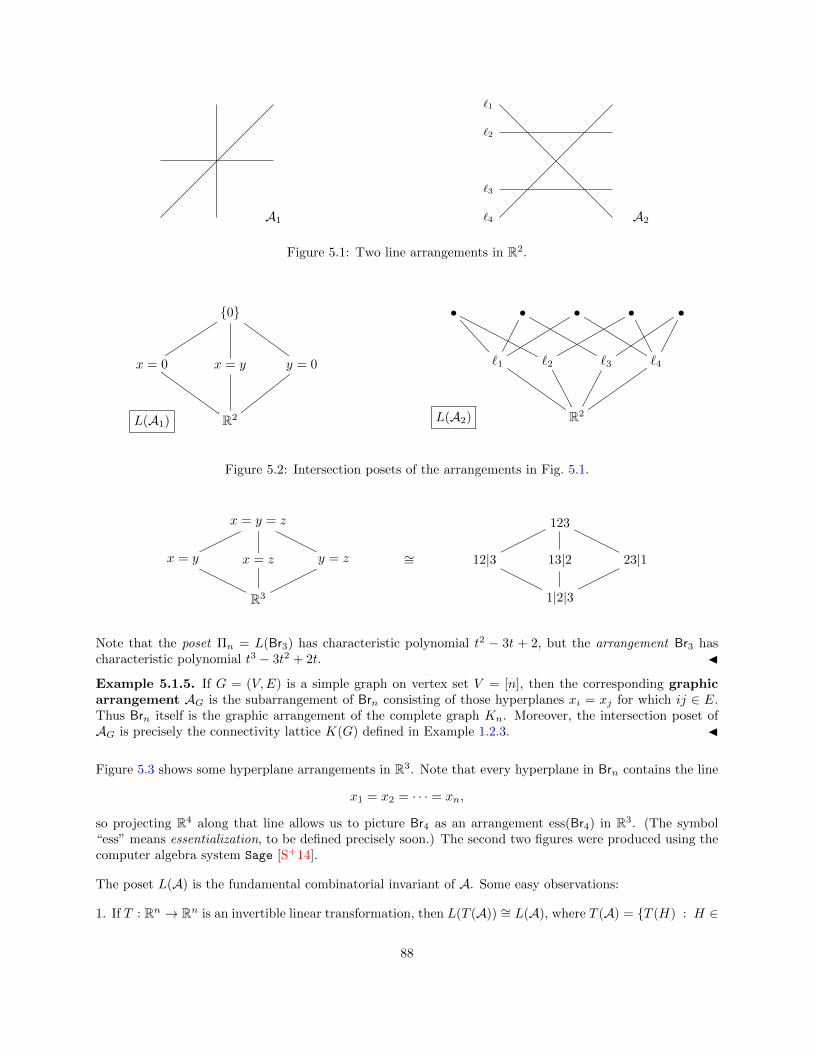
A1 A2

`1

`2

`3

`4

Figure 5.1: Two line arrangements in R2.

0

x = 0 x = y y = 0

L(A1) R2

• • • • •

ℓ1 ℓ2 ℓ3 ℓ4

L(A2) R2

Figure 5.2: Intersection posets of the arrangements in Fig. 5.1.

x = y x = z y = z

x = y = z

R3

∼= 12|3 13|2 23|1

123

1|2|3

Note that the poset Πn = L(Br3) has characteristic polynomial t2 − 3t + 2, but the arrangement Br3 hascharacteristic polynomial t3 − 3t2 + 2t.

Example 5.1.5. If G = (V,E) is a simple graph on vertex set V = [n], then the corresponding graphicarrangement AG is the subarrangement of Brn consisting of those hyperplanes xi = xj for which ij ∈ E.Thus Brn itself is the graphic arrangement of the complete graph Kn. Moreover, the intersection poset ofAG is precisely the connectivity lattice K(G) defined in Example 1.2.3.

Figure 5.3 shows some hyperplane arrangements in R3. Note that every hyperplane in Brn contains the line

x1 = x2 = · · · = xn,

so projecting R4 along that line allows us to picture Br4 as an arrangement ess(Br4) in R3. (The symbol“ess” means essentialization, to be defined precisely soon.) The second two figures were produced using thecomputer algebra system Sage [S+14].

The poset L(A) is the fundamental combinatorial invariant of A. Some easy observations:

1. If T : Rn → Rn is an invertible linear transformation, then L(T (A)) ∼= L(A), where T (A) = T (H) : H ∈

88

Bool3 Br3 ess(Br4)

Figure 5.3: Three hyperplane arrangements in R3.

A. In fact, the intersection poset is invariant under any affine transformation. (The group of affinetransformations is generated by the invertible linear transformations together with translations.)

2. The poset L(A) is a meet-semilattice, with meet given by ∩B ∧ ∩C = ∩(B ∩ C) for all B, C ⊆ A. Its 0element is ∩∅, which by convention is kn.

3. L(A) is ranked, with rank function r(X) = n − dimX. To see this, observe that each covering relationX ⋖ Y comes from intersecting an affine linear subspace X with a hyperplane H that neither contains noris disjoint from X, so that dim(X ∩H) = dimX − 1.

4. L(A) has a 1 element if and only if the center ∩A is nonempty. Such an arrangement is called central.In this case L(A) is a lattice (and may be referred to as the intersection lattice of A). Since translationdoes not affect whether an arrangement is central (or indeed any of its combinatorial structure), we willtypically assume that ∩A contains the zero vector, which is to say that every hyperplane in A is a linearhyperplane in kn. (So an arrangement is central if and only if it is a translation of an arrangement of linearhyperplanes.)

5. When A is central, the lattice L(A) is geometric. It is atomic by definition, and it is submodular becauseit is a sublattice of the chain-finite modular lattice L(kn)∗ (the lattice of all subspaces of kn ordered byreverse inclusion). The associated matroid M(A) =M(L(A)) is represented over k by any family of vectorsnH : H ∈ A where nH is normal to H. (That is, H⊥ = k⟨nH⟩ with respect to some fixed non-degeneratebilinear form on kn.) Any normals will do, since the matroid is unchanged by scaling the nH independently.

Therefore, all of the tools we have developed for looking at posets, lattices and matroids can be applied tostudy hyperplane arrangements.

The dimension of an arrangement is not a combinatorial invariant; that is, it cannot be extracted fromthe intersection poset. If Br4 were a “genuine” 4-dimensional arrangement then we would not be able torepresent it in R3. However, we can do so because the center of Br4 has positive dimension, so squashing thecenter to a point reduces the ambient dimension without changing the intersection poset. This observationmotivates the following definition.

Definition 5.1.6. Let A ⊆ kn be an arrangement and let N(A) = k⟨nH : H ∈ A⟩, where nH is normalto H. The essentialization of A is the arrangement

ess(A) = H ∩N(A) : H ∈ A ⊆ N(A).

89

We say that A is essential if ess(A) = A, or equivalently if N(A) = kn. Note that L(ess(A)) ∼= L(A) asposets. The rank of A is the dimension of its essentialization.

We can now explain the correction factor in the characteristic polynomial: it is

χA(t) = tdimN(A)χL(A)(t) = tdimA−rankAχ

L(A)(t). (5.2)

The two polynomials coincide for essential arrangements. For example, rankBrn = dim ess(Brn) = n − 1,and rankAG = r(G) = |V (G)| − c, where c is the number of connected components of G.

If A is linear, then we could define the essentialization by setting V = N(A)⊥ = ∩A, and then definingess(A) = H/V : H ∈ A ⊆ kn/V . Thus A is essential if and only if ∩A = 0. Moreover, if A is linearthen rank(A) is the rank of its intersection lattice — so rank is a combinatorial invariant, unlike dimension.

There are two natural operations that go back and forth between central and non-central arrangements,called projectivization and coning.

Definition 5.1.7. Let k be a field and n ≥ 1. The set of lines through the origin in kn is called n-dimensional projective space over k and denoted by Pn−1k.

If k = R, we can regard Pn−1R as the unit sphere Sn−1 with opposite points identified. (In particular, it isan (n− 1)-dimensional manifold, although it is orientable only if n is even.)

Algebraically, write x ∼ y if x and y are nonzero scalar multiples of each other. Then ∼ is an equivalencerelation on kn \ 0, and Pn−1 is the set of equivalence classes.

Linear hyperplanes in kn correspond to affine hyperplanes in Pn−1k. Thus, given a central arrangementA ⊆ kn, we can construct its projectivization proj(A) ⊆ Pn−1k.

Projectivization supplies a nice way to draw central 3-dimensional real arrangements. Let S be the unitsphere, so that H ∩ S is a great circle for every H ∈ A; then regard H0 ∩ S as the equator and project thenorthern hemisphere into your piece of paper. Several examples as shown below. Of course, a diagram ofproj(A) only shows the upper half of A; we can recover A from proj(A) by “reflecting the interior of thedisc to the exterior” (Stanley); e.g., for the Boolean arrangement A = Bool3, the picture is as shown in thefourth figure below. In general, r(proj(A)) = 1

2r(A).

proj(Bool3) proj(Br3) proj(ess(Br4)) Bool3 from proj(Bool3)

The operation of coning is a sort of inverse of projectivization. It lets us turn a non-central arrangementinto a central arrangement, at the price of increasing the dimension by 1.

90

Definition 5.1.8. Let A ⊆ kn be a hyperplane arrangement, not necessarily central. The cone cA is thecentral arrangement in kn+1 defined as follows:

• Geometrically: Make a copy of A in kn+1, choose a point p not in any hyperplane of A, and replaceeach H ∈ A with the affine span H ′ of p and H (which will be a hyperplane in kn+1). Then, toss inone more hyperplane containing p and in general position with respect to every H ′.

• Algebraically: For H = x : L(x) = ai ∈ A (with L a homogeneous linear form on kn and ai ∈ k),construct a hyperplane H ′ = (x1, . . . , xn, y) : L(x) = aiy ⊆ kn+1 in cA. Then, toss in thehyperplane y = 0.

For example, if A consists of the points x = 0, x = −3 and x = 1 in R1 (shown in red), then cA consists ofthe lines x = y, x = −5y, x = 3y, and y = 0 in R2 (shown in blue).

y = 0

y = 1

Proposition 5.1.9. χcA(k) = (k − 1)χA(k).

5.2 Counting regions: examples

Let A ⊆ Rn be a real hyperplane arrangement. The regions of A are the connected components of Rn \ A.Each component is the interior of a (bounded or unbounded) polyhedron; in particular, it is homeomorphicto Rn. We call a region relatively bounded if the corresponding region in ess(A) is bounded. (If A isnot essential then every region is unbounded, because it contains a translate of W⊥, where W is the spacedefined in Definition 5.1.6. Therefore passing to the essentialization is necessary to make the problem ofcounting bounded regions nontrivial for all arrangements.) Let

r(A) = number of regions of A,b(A) = number of relatively bounded regions of A.

Example 5.2.1. For the arrangements A1 and A2 shown in Example 5.1.2,

r(A1) = 6, r(A2) = 10,

b(A1) = 0, b(A2) = 2.

Example 5.2.2. The Boolean arrangement Booln consists of the n coordinate hyperplanes in Rn. It isa central, essential arrangement whose intersection lattice is the Boolean lattice of rank n; accordingly,χBooln(t) = (t − 1)n. The complement Rn \ Booln is (x1, . . . , xn) : xi = 0 for all i, and the connectedcomponents are the open orthants, specified by the signs of the n coordinates. Therefore, r(Booln) = 2n andb(Booln) = 0.

Example 5.2.3. Let A consist of m lines in R2 in general position: that is, no two lines are parallel and nothree are coincident. Draw the dual graph G, whose vertices are the regions of A, with an edge betweenevery two regions that share a common border.

91

A

G

Let r = r(A) and b = b(A), and let v, e, f denote the numbers of vertices, edges and faces of G, respectively.(In the example above, (v, e, f) = (11, 16, 7).) Each bounded face of G is a quadrilateral that contains exactlyone point where two lines of A meet, and the unbounded face is a cycle of length r − b. Therefore,

v = r, (5.3a)

f = 1 +

(m

2

)=m2 −m+ 2

2(5.3b)

4(f − 1) + (r − b) = 2e. (5.3c)

Moreover, the number r − b of unbounded region of As is just 2m. (Take a walk around a very large circle.You will enter each unbounded region once, and will cross each line twice.) Therefore, from (5.3c) and (5.3b)we obtain

e = m+ 2(f − 1) = m2. (5.3d)

Euler’s formula for planar graphs says that v − e + f = 2. Substituting in (5.3a), (5.3b) and (5.3d) andsolving for r gives

r =m2 +m+ 2

2and therefore

b = r − 2m =m2 − 3m+ 2

2=

(m− 1

2

).

Example 5.2.4. The braid arrangement Brn consists of the(n2

)hyperplanes Hij = x : xi = xj in Rn.

The complement Rn \ Brn consists of all vectors in Rn with no two coordinates equal, and the connectedcomponents of this set are specified by the ordering of the set of coordinates as real numbers:

z = y

y = x

z = x

x < z < y

x < y < zy < x < z

y < z < x

z < y < x z < x < y

92

Therefore, r(Brn) = n!. (Stanley: “Rarely is it so easy to compute the number of regions!”) Furthermore,

χBrn(t) = t(t− 1)(t− 2) · · · (t− n+ 1).

Note that the braid arrangement is central but not essential; its center is the line x1 = x2 = · · · = xn, so itsrank is n− 1.

Example 5.2.5. Let G = (V,E) be a simple graph with V = [n], and let AG be its graphic arrangement(see Example 5.1.5). The characteristic polynomial of L(AG) is precisely the chromatic polynomial of G (seeSection 4.4). We will see another explanation for this fact later; see Example 5.4.4.

The regions of Rn \AG are the open polyhedra whose defining inequalities include either xi < xj or xi > xjfor each edge ij ∈ E. Those inequalities give rise to an orientation of G, and it is not hard to check thatthis correspondence is a bijection between regions and acyclic orientations. Hence

r(AG) = number of acyclic orientations of G = |χL(AG)(−1)|.

5.3 Zaslavsky’s Theorem(s)

Example 5.2.5 motivates the main result of this section, Theorem 5.3.6, which was historically the first majortheorem about hyperplane arrangements, due to Zaslavsky [Zas75]. Let A be a real hyperplane arrangement,and let χA be the characteristic polynomial of its intersection poset. Zaslavsky’s Theorem(s) say(s) that thenumbers of regions and relatively bounded regions are given by

r(A) = (−1)dimAχA(−1),b(A) = (−1)rankAχA(1).

The proof combines geometry and combinatorics. Here is an overview of the steps:

1. Show that r and b satisfy restriction/contraction recurrences in terms of associated hyperplane ar-rangements A′ and A′′ (Prop. 5.3.2).

2. Rewrite the characteristic polynomial χA(k) as a sum over central subarrangements of A (the “Whitneyformula”, Prop. 5.3.3).

3. Show that the Whitney formula obeys a restriction/contraction recurrence (Prop. 5.3.4) and compareit with those for r and b.

Let x ∈ L(A), i.e., x is a nonempty affine space formed by intersecting some of the hyperplanes in A. Define

Ax = H ∈ A : H ⊇ x,Ax = H ∩ x : H ∈ A \ Ax.

(5.4)

In other words, Ax is obtained by deleting the hyperplanes not containing x, while Ax is obtained byrestricting A to x so as to get an arrangement whose ambient space is x itself. The notation is mnemonic:L(Ax) and L(Ax) are isomorphic respectively to the principal order ideal and principal order filter generatedby x in L(A). That is,

L(Ax) ∼= y ∈ L(A) : y ≤ x, L(Ax) ∼= y ∈ L(A) : y ≥ x.

Example 5.3.1. Let A be the 2-dimensional arrangement shown on the left, with the line H and point pas shown. Then Ap and AH are shown on the right.

93

H

p

A

p

Ap

H

AH

The lattice L(A) and its subposets (in this case, sublattices) L(Ap) and L(AH) are shown below.

p

L(Ap)

H

L(AH)

Let M(A) be the matroid represented by normal vectors nH : H ∈ A. Fix a hyperplane H ∈ A and letA′ = A \H and A′′ = AH .

Proposition 5.3.2. The invariants r and b satisfy the following recurrences:

1. r(A) = r(A′) + r(A′′).

2. b(A) =

0 if rankA = rankA′ + 1 (i.e., if nH is a coloop in M(A)),b(A′) + b(A′′) if rankA = rankA′ (i.e., if it isn’t).

Proof. (1) Consider what happens when we add H to A′ to obtain A. Some regions of A′ will remain thesame, while others will be split into two regions.

A′unsplit

unsplitsplit

unsplit

unsplitsplit

A′

H

split

unsplit

Let S and U be the numbers of split and unsplit regions of A′ (in the figure above, S = 2 and U = 4).The unsplit regions each contribute 1 to r(A). The split regions each contribute 2 to r(A), but they also

94

correspond bijectively to the regions of A′′. (See, e.g., Example 5.3.1.) So

r(A′) = S + U, r(A) = 2S + U, r(A′′) = S

and so r(A) = r(A′) + r(A′′), proving the first assertion of Proposition 5.3.2. By the way, if (and only if) His a coloop then it borders every region of A, so r(A) = 2r(A′) in this case.

(2) Now we count bounded regions. If rankA = rankA′ + 1, then N(A′) ⊊ Rn, i.e., A′ is not essential. Inthat case, every region of A′ must contain a line (or possibly a bigger space) orthogonal to N(A′), which getssquashed down to a point upon essentialization. Therefore, every region of A contains a ray, and b(A) = 0.This takes care of the first case. In the second case, the bounded regions of A come in a few different flavors.

• If W is a bounded region not bordered by H, then it is also a bounded region of A′.• If X,Y are two bounded regions separated by part of H, then they merge into one bounded region XYin A′. Also, the part of H that separates them (namely s = ∂X ∩ H = ∂Y ∩ H) is itself a boundedregion of A′′.

• If Z is a bounded region of A whose neighbor across H is an unbounded region U, then the mergedregion ZU is unbounded in A′, but ∂Z ∩H is nevertheless bounded in A′′.

WX

Y

Z

U

A

Hs

W

XYZU

A′

In short, here are the possibilities:

Contributions to. . .Description b(A) b(A′) b(A′′)

(W) bounded regions that don’t touch H 1 1 0(X,Y) pairs of bounded regions separated by H 2 1 1

(Z) bounded, neighbor across H is unbounded 1 0 1

In all cases the contribution to b(A) equals the sum of those to b(A′) and b(A′′), establishing the seconddesired recurrence.

Proposition 5.3.2 looks a lot like a Tutte polynomial deletion/contraction recurrence. This suggests that weshould be able to extract r(A) and b(A) from the characteristic polynomial χA. The first step is to find amore convenient form for the characteristic polynomial.

Proposition 5.3.3 (Whitney formula for χA). For any hyperplane arrangement A,

χA(t) =∑

central B⊆A(−1)|B|tdimA−rankB.

95

Proof. The atoms in the interval [0, x] are the hyperplanes of A containing x, and they form a lower crosscutof [0, x]. Therefore

χA(t) =∑

x∈L(A)

µ(0, x)tdim x

=∑

x∈L(A)

∑B⊆A: x=

⋂B(−1)|B|tdim x

(by the second form of Thm. 2.4.9; note that 1[0,x] = x)

=∑

B⊆A:⋂B=0

(−1)|B|tdim(⋂B)

=∑

central B⊆A(−1)|B|tdimA−rankB

as desired. Note that the empty subarrangement is considered central for the purpose of this formula,corresponding to the summand x = 0 and giving rise to the leading term tdimA of χA(t).

Proposition 5.3.4. Let A be a hyperplane arrangement in kn. Then χA(t) = χA′(t)− χA′′(t).

Sketch of proof. Splitting up Whitney’s formula gives

χA(t) =∑

central B⊆A: H ∈B(−1)|B|tn−rankB

︸︷︷︸Σ1

+∑

central B⊆A: H∈B(−1)|B|tn−rankB

︸︷︷︸Σ2

.

Then Σ1 = χA′(t) (it is just Whitney’s formula for A′), so it remains to show that Σ2 = −χA′′(t). This is alittle trickier, because different hyperplanes in A can have the same intersection with H, which means thatmultiple subarrangements of A can give rise to the same subarrangement of A′′.

Label the hyperplanes of A′′ (which, remember, are codimension-1 subspaces of H) as K1, . . . ,Ks. For eachi ∈ [s] let Ai = J ∈ A : J ∩ H = Ki. Each arrangement B arising as a summand of Σ2 gives rise to acentral subarrangement of A′′, namely

π(B) = J ∩H : J ∈ B,

that depends only on the family of Ai’s for which Ai ∩ B = ∅. That is, for each central subarrangementB′′ ⊆ A′′, the summands B of Σ2 such that π(B) = B′′ are precisely the arrangements of the form

H ∪⋃

i: Ki∈B′′

Bi

where ∅ ⊊ Bi ⊆ Ai for all i. Moreover, in this case,

n− rankB = dim(∩B) = dim(∩π(B)) = dimH − rankB′′. (5.5)

96

Now we break up the sum Σ2 into subsums depending on π(B):

Σ2 =∑

central B′′⊆A′′

∑B∈π−1(B′′)

(−1)|B|tn−rankB

=∑B′′

∑B∈π−1(B′′)

(−1)|B|

tdimH−rankB′′

= −∑B′′

∏i: Ki∈B′

∑∅=Bi⊆Ai

(−1)|Bi|

tdimH−rankB′′

(to see this, expand the product and observe that equals the inner sum in the previous line; the outer minussign is contributed by H, which is an element of B). But∑∅=Bi⊆Ai

(−1)|Bi| = −1, because it is the binomial

expansion of (1 − 1)|Ai| = 0, with one +1 term (namely Bi = ∅) removed. (Note that Ai = ∅.) Therefore,the whole thing boils down to

−∑B′′

(−1)|B′′|tdimH−rankB′′

which is just Whitney’s formula for −χA′′(t).

Remark 5.3.5. This recurrence is strongly reminiscent of the chromatic recurrence (4.10). Indeed, ifA = AG is a graphic arrangement in Rn, e is an edge of G, and He is the corresponding hyperplane in AG,then it is clear that AG\e = AG \He. In addition, two hyperplanes Hf , Hf ′ will have the same intersectionwith He if and only if f, f ′ become parallel upon contracting e, so AG/e can be identified with (AG)

He (wherethe coordinates on He

∼= Rn−1 are given by equating the coordinates for the two endpoints of e).

We can now finish the proof of the main result. We have already done the hard work, and just need to putall the pieces together.

Theorem 5.3.6 (Zaslavsky’s Theorem). Let A be a real hyperplane arrangement, and let χA be the char-acteristic polynomial of its intersection poset. Then

r(A) = (−1)dimAχA(−1) and (5.6)

b(A) = (−1)rankAχA(1). (5.7)

Proof. Let r(A) and b(A) denote the numbers on the right-hand sides of (5.6) and (5.6).

If |A| = 1, then L(A) is the lattice with two elements, namely Rn and a single hyperplane H, and itscharacteristic polynomial is tn − tn−1. Thus r(A) = (−1)n((−1)n − (−1)n−1) = 2 and b(A) = −(1− 1) = 0,which match r(A) and b(A).

For the general case, we just need to show that r and b satisfy the same recurrences as r and b (see Prop. 5.3.2).First,

r(A) = (−1)dimAχA(−1)= (−1)dimA(χA′(−1)− χA′′(−1)

)(by Prop. 5.3.4)

= (−1)dimA′χA′(−1) + (−1)dimA′′

χA′′(−1) (since dimA′′ = dimA− 1)

= r(A′) + r(A′′).

As for b, if rankA = rankA′ + 1, then in fact A′ and A′′ have the same essentialization, hence the samerank, and their characteristic polynomials only differ by a factor of t. The deletion/restriction recurrence(Prop. 5.3.4) therefore implies b(A) = 0.

97

On the other hand, if rankA = rankA′, then rankA′′ = rankA − 1 and a calculation similar to that for r(replacing dimension with rank) shows that b(A) = b(A′) + b(A′′).

Corollary 5.3.7. Let A ⊆ Rn be a central hyperplane arrangement and let M = M(A) be the matroidrepresented by normals. Then r(A) = TM (2, 0) and b(A) = 0.

Proof. Combine Zaslavsky’s theorem with the formula χA(t) = (−1)nTM (1 − t, 0), and use the fact thatTM (0, 0) = 0 for any matroid M with nonempty ground set.

Remark 5.3.8. The formula for r(A) could be obtained from the Tutte Recipe Theorem (Thm. 4.2.1). Butthis would not work for b(A), which is not an invariant of M(A). (The matroid M(A) is not as meaningfulwhen A is not central, which is precisely the case that b(A) is interesting.)

Example 5.3.9. Let s ≥ n, and let A be an arrangement of s linear hyperplanes in general positionin Rn; that is, every k hyperplanes intersect in a space of dimension n − k (or 0 if k > n). Equivalently,the corresponding matroid M is Un(s), whose rank function r : 2[s] → N is given by r(A) = min(n, |A|).Therefore,

r(A) = TM (2, 0) =∑A⊆[s]

(2− 1)n−r(A)(0− 1)|A|−r(A)

=∑A⊆[s]

(−1)|A|−r(A)

=

s∑k=0

(s

k

)(−1)k−min(n,k)

=

n∑k=0

(s

k

)+

s∑k=n+1

(s

k

)(−1)k−n

=

n∑k=0

(s

k

)(1− (−1)k−n) +

s∑k=0

(s

k

)(−1)k−n

︸︷︷︸=0

= 2

((s

n− 1

)+

(s

n− 3

)+

(s

n− 5

)+ · · ·

).

For instance, if n = 3 then

r(A) = 2

(s

2

)+ 2

(s

0

)= s2 − s+ 2.

Notice that this is not the same as the number of regions formed by s affine lines in general position in R2.The calculation of r(A) and b(A) for that arrangement is left to the reader (Exercise 5.1).

Corollary 5.3.10. Let A be an arrangement in which no two hyperplanes are parallel. Then A has atleast one relatively bounded region if and only if it is noncentral. Prove this and find a place for it —assuming it is true. The non-parallel assumption is necessary since the conclusion fails forthe arrangement with hyperplanes x = 0, y = 0, y = 1.

98

5.4 The finite field method

The following very important result is implicit in the work of Crapo and Rota [CR70] and was statedexplicitly by Athanasiadis [Ath96]:

Theorem 5.4.1. Let Fq be the finite field of order q, and let A ⊆ Fnq be a hyperplane arrangement. Then

|Fnq \ A| = χA(q).

This result gives a combinatorial interpretation of the values of the characteristic polynomial. In practice,it is often used to calculate the characteristic polynomial of a hyperplane arrangement by counting pointsin its complement over Fq (which can be regarded as regions of the complement, if you endow Fn

q with thediscrete topology).

Proof #1. By inclusion-exclusion,

|Fnq \ A| =

∑B⊆A

(−1)|B|∣∣∣⋂B∣∣∣ .

If B is not central, then by definition |⋂B| = 0. Otherwise, |⋂B| = qn−rankB. So the sum becomes

|Fnq \ A| =

∑central B⊆A

(−1)|B|qn−rankB

which is just Whitney’s formula for χA(q) (Prop. 5.3.3).

Proof #2. Start with the definition of the characteristic polynomial, letting r be the rank function in L(A):

χA(q) =∑

x∈L(A)

µ(0, x)qn−r(x)

=∑

x∈L(A)

µ(0, x)qdim x

=∑

x∈L(A)

µ(0, x)|x|

=∑p∈Fn

q

∑x∈L(A): p∈x

µ(0, x)

=∑p∈Fn

q

∑x∈[0,yp]

µ(0, x)

where yp =

⋂H⊇pH. By definition of the Mobius function, the parenthesized sum is 1 if yp = 0 and 0

otherwise. Therefore

χA(q) = #p ∈ Fnq : yp = 0 = #p ∈ Fn

q : p ∈ H ∀H ∈ A = |Fnq \ A|.

This fact has a much more general application, which was systematically mined by Athanasiadis, e.g., [Ath96].

Definition 5.4.2. Let A ⊆ Rn be an integral hyperplane arrangement (i.e., whose hyperplanes are definedby equations with integer coefficients). For a prime p, let Ap = A ⊗ Fp be the arrangement in Fn

p definedby regarding the equations in A as equations over Fp. We say that A reduces correctly modulo p ifL(Ap) ∼= L(A).

99

A sufficient condition for correct reduction is that no minor of the matrix of normal vectors is a nonzeromultiple of p (so that rank calculations are the same over Fp as over Z). In particular, to choose p largerthan the absolute value of any minor of M , so that a set of columns of M is linearly independent over Fp iffit is independent over Q. There are infinitely many such primes, implying the following highly useful result:

Theorem 5.4.3 (The finite field method). Let A ⊆ Rn be an integral hyperplane arrangement and q apower of a large enough prime. Then χA(q) is the polynomial that counts points in the complement of Aq..

Example 5.4.4. Let G = ([n], E) be a simple graph and let AG be the corresponding graphic arrangementin Rn. Note that AG reduces correctly over every finite field Fq (because graphic matroids are regular).A point (x1, . . . , xn) ∈ Fn

q can be regarded as the q-coloring of G that assigns color xi to vertex i. Theproper q-colorings are precisely the points of Fn

q \AG. The number of such colorings is pG(k) (the chromaticpolynomial of G evaluated at q). On the other hand, by Theorem 5.4.1, it is also the characteristic polynomialχAG

(q). Since pG(k) = χAG(q) for infinitely many q (namely, all integer prime powers), the polynomials

must be equal.

Example 5.4.5. The Shi arrangement is the arrangement of n(n− 1) hyperplanes in Rn defined by

Shin = xi = xj , xi = xj + 1 | 1 ≤ i < j ≤ n .In other words, take the braid arrangement, clone it, and nudge each of the cloned hyperplanes a little bit inthe direction of the bigger coordinate. The Shi arrangement has rank n−1 (every hyperplane in it contains aline parallel to the all-ones vector), so we may project along that line to obtain the essentialization in Rn−1.Thus ess(Shi2) consists of two points on a line, while ess(Shi3) is shown below.

x = y x = y + 1

y = z + 1

y = z

x = z + 1

x = z

ess(Shi3)

We will prove that the characteristic polynomial of the Shi arrangement is

χShin(q) = q(q − n)n−1. (5.8)

In particular, the numbers of regions and bounded regions are respectively

r(Shin) = |χ(−1)| = (n+ 1)n−1, b(Shin) = |χ(1)| = (n− 1)n−1. (5.9)

(The number (n + 1)n−1 may look familiar; by Cayley’s formula, it is the number of spanning trees ofthe complete graph Kn+1. It also counts many other things of combinatorial interest, including parkingfunctions.)

The following proof is from [Sta07, §5.2]. By Theorem 5.4.3, it suffices to count the points in Fnq \ Shin for

a large enough prime q. Let x = (x1, . . . , xn) ∈ Fnq \ Shin. Draw a necklace with q beads labeled by the

elements 0, 1, . . . , q− 1 ∈ Fq, and for each k ∈ [n], put a big red k on the xk-th bead. For example, let n = 6and q = 11. Then the necklace for x = (2, 5, 6, 10, 3, 7) is as follows:

100

0

1

2

3

4

56

7

8

9

10

1

5

23

6

4

The requirement that x avoids the hyperplanes xi = xj implies that the red numbers are all on differentbeads. If we read the red numbers clockwise, starting at 1 and putting in a divider sign | for each beadwithout a red number, we get

15 | 236 | | 4 |which can be regarded as the ordered weak partition (or OWP)

Π(x) = 15, 236, ∅, 4, ∅

that is, a (q − n)-tuple B1, . . . , Bq−n, where the Bi are pairwise disjoint sets (possibly empty; that’s whatthe “weak” means) whose union is [n], and 1 ∈ B1. (We’ve omitted the divider corresponding to the beadjust counterclockwise of 1; stay tuned.)

Note that each block of Π(x) corresponds to a contiguous set of values among the coordinates of x. Forexample, the block 236 occurs because the values 5,6,7 occur in coordinates x2, x3, x6. In order to avoid thehyperplanes xi = xj + 1 for i < j, each contiguous block of beads must have its red numbers in strictlyincreasing order counterclockwise. (In particular the bead just counterclockwise of 1 must be unlabeled,which is why we could omit that divider.)

Thus we have bijections

Fnq \ Shin ←→ necklaces ←→ OWPs of [n] with q − n blocks.

To get a necklace from an OWP, write out each block in increasing order, with bars between successiveblocks.

Meanwhile, an OWP is given by a function f : [n]→ [q−n], where f(i) is the index of the block containing i(so f(1) = 1). There are (q − n)n−1 such things. Since there are q choices for the bead containing the red1, we obtain ∣∣Fn

q \ Shin∣∣ = q(q − n)n−1 = χShin(q).

This proves (5.8), and (5.9) follows from Zaslavsky’s theorems.

5.5 Supersolvable lattices and arrangements

We have seen that for a simple graph G = ([n], E), the chromatic polynomial pG(k) is precisely the char-acteristic polynomial of the graphic arrangement AG. For some graphs, the chromatic polynomial factorsinto linear terms over Z. For example, if G = Kn, then pG(k) = k(k − 1)(k − 2) · · · (k − n+ 1), and if G is

101

a forest with n vertices and c components, then pG(k) = kc(k − 1)n−c. This property does not hold for allgraphs. For example, it is easy to work out that the chromatic polynomial of C4 (the cycle with four verticesand four edges) is k4 − 4k3 + 6k2 − 3k = k(k − 1)(k2 − 3k + k), which does not factor further over Z. Isthere a structural condition on a graph or a central arrangement (or really, on a geometric lattice) that willguarantee that its characteristic polynomial factors completely? It turns out that supersolvable geometriclattices have this good property.

Definition 5.5.1. Let L be a ranked lattice. An element x ∈ L is a modular element if r(x) + r(y) =r(x ∨ y) + r(x ∧ y) for every y ∈ L.

For example:

• By Theorem 1.5.6, a ranked lattice L is modular iff all elements are modular.• The elements 0 and 1 are clearly modular in any lattice.• If L is geometric, then every atom x is modular. Indeed, for y ∈ L, if y ≥ x, then y = x ∨ y andx = x ∧ y, while if y ≥ x then y ∧ x = 0 and y ∨ x⋗ y.

• The coatoms of a geometric lattice need not be modular. For example, let L = Πn, and recall thatΠn has rank function r(π) = n − |π|. Let x = 12|34, y = 13|24 ∈ Π4. Then r(x) = r(y) = 2, butr(x ∨ y) = r(1) = 3 and r(x ∧ y) = r(0) = 0. So x is not a modular element.

Proposition 5.5.2. The modular elements of Πn are exactly the partitions with at most one nonsingletonblock.

Proof. Suppose that π ∈ Πn has one nonsingleton block B. For σ ∈ Πn, let

X = C ∈ σ : C ∩B = ∅, Y = C ∈ σ : C ∩B = ∅.

Then

π ∧ σ =C ∩B : C ∈ X

∪i : i ∈ B

, π ∨ σ =

⋃C∈X

C

∪ Y

so

|π ∧ σ|+ |π ∨ σ| = (|X|+ n− |B|) + (1 + |Y |)= (n− |B|+ 1) + (|X|+ |Y |) = |π|+ |σ|,

proving that π is a modular element.

For the converse, suppose B,C are nonsingleton blocks of π, with i, j ∈ B and k, ℓ ∈ C. Let σ be thepartition with exactly two nonsingleton blocks i, k, j, ℓ. Then r(σ) = 2 and r(π ∧ σ) = r(0) = 0, but

r(π ∨ σ) = r(π) + 1 < r(π) + r(σ)− r(π ∧ σ)

so π is not a modular element.

Modular elements are useful because they lead to factorizations of the characteristic polynomial of L.

Theorem 5.5.3. Let L be a geometric lattice of rank n, and let z ∈ L be a modular element. Then

χL(k) = χ[0,z](k)

∑y: y∧z=0

µL(0, y)kn−r(z)−r(y). (5.10)

102

Here is a sketch of the proof; for the full details, see [Sta07, pp. 440–441]. We work in the dual Mobius algebraA∗(L) = A(L∗); that is, the vector space of C-linear combinations of elements of L, with multiplication givenby join (rather than meet as in §2.4). Thus the “algebraic” basis of A∗(L) is

σydef≡

∑x: x≥y

µ(y, x)x : y ∈ L.

First, show by direct calculation that

σ0 =∑x∈L

µ(x)x =

∑v: v≤z

µ(v)v

∑y: y∧z=0

µ(y)y

(5.11)

for any z ∈ L. Second, for z, y, v ∈ L such that z is modular, v ≤ z, and y ∧ z = 0, one shows first thatz ∧ (v ∨ y) = v (by rank considerations) and then that rank(v ∨ y) = rank(v) + rank(y). Third, makethe substitutions v 7→ krank z−rank v and y 7→ kn−rank y−rank z in the two sums on the RHS of (5.11). Sincevy = v ∨ y, the last observation implies that substituting x 7→ kn−rank x on the LHS preserves the product,and the equation becomes (5.10).

In particular, every atom a is modular, so

χL(k) = (k − 1)∑

x: x ≥a

µL(0, x)kr(L)−1−r(x).

This does not really tell us anything new, because we already knew that k − 1 had to be a factor of χL(k),because χL(1) =

∑x∈L µL(0, x) = 0. Also, the sum in the expression is not the characteristic polynomial of

a lattice.

On the other hand, if we have a modular coatom, then Theorem 5.5.3 is much more useful, since we canidentify an interesting linear factor and describe what is left after factoring it out.

Corollary 5.5.4. Let L be a geometric lattice, and let z ∈ L be a coatom that is a modular element. Then

χL(k) = (k − e)χ[0,z](k),

where e is the number of atoms a ∈ L such that a ≤ z.

If we are extremely lucky, then L will have a saturated chain of modular elements

0 = x0 ⋖ x1 ⋖ · · ·⋖ xn−1 ⋖ xn = 1.

In this case, we can apply Corollary 5.5.4 successively with z = xn−1, z = xn−2, . . . , z = x1 to split thecharacteristic polynomial completely into linear factors:

χL(k) = (k − en−1)χ[0,xn−1](k)

= (k − en−1)(k − en−2)χ[0,xn−2](k)

= . . .

= (k − en−1)(k − en−2) · · · (k − e0),

where

ei = #atoms a of [0, xi+1] : a ≤ xi= #a ∈ A : a ≤ xi+1, a ≤ xi.

103

Definition 5.5.5. A geometric lattice L is supersolvable if it has a modular chain, that is, a maximalchain 0 = x0⋖x1⋖ · · ·⋖xn = 1 such that every xi is a modular element. A central hyperplane arrangementA is called supersolvable if L(A) is supersolvable.Example 5.5.6. Every modular lattice is supersolvable, because every maximal chain is modular. Inparticular, the characteristic polynomial of every modular lattice splits into linear factors.

Example 5.5.7. The partition lattice Πn (and therefore the associated hyperplane arrangement Brn) issupersolvable by induction. Let z be the coatom with blocks [n− 1] and n, which is a modular element byProposition 5.5.2. There are n − 1 atoms a ≤ z, namely the partitions whose non-singleton block is i, nfor some i ∈ [n− 1], so we obtain

χΠn(k) = (k − n+ 1)χΠn−1

(k)

and by inductionχΠn(k) = (k − 1)(k − 2) · · · (k − n+ 1).

Example 5.5.8. Let G = C4 (a cycle with four vertices and four edges), and let A = AG. Then L(A) isthe lattice of flats of the matroid U3(4); i.e.,

L = F ⊆ [4] : |F | = 3with r(F ) = min(|F |, 3). This lattice is not supersolvable, because no element at rank 2 is modular. Forexample, let x = 12 and y = 34; then r(x) = r(y) = 2 but r(x ∨ y) = 3 and r(x ∧ y) = 0. (We have alreadyseen that the characteristic polynomial of L does not split.)

Theorem 5.5.9. Let G = (V,E) be a simple graph. Then AG is supersolvable if and only if the vertices ofG can be ordered v1, . . . , vn such that for every i > 1, the set

Ci := vj : j ≤ i, vivj ∈ Eforms a clique in G.

Such an ordering is called a perfect elimination ordering. The proof of Theorem 5.5.9 is left as an exercise(see Stanley, pp. 55–57). An equivalent condition is that G is a chordal graph: if C ⊆ G is a cycle oflength ≥ 4, then some pair of vertices that are not adjacent in C are in fact adjacent in G. This equivalence issometimes known as Dirac’s theorem. It is fairly easy to prove that supersolvable graphs are chordal, but theconverse is somewhat harder; see, e.g., [Wes96, pp. 224–226]. There are other graph-theoretic formulations ofthis property; see, e.g., [Dir61]. See the recent paper [HS15] for much more about factoring the characteristicpolynomial of lattices in general.

If G satisfies the condition of Theorem 5.5.9, then we can see directly why its chromatic polynomial χ(G; k)splits into linear factors. Consider what happens when we color the vertices in order. When we color vertexvi, it has |Ci| neighbors that have already been colored, and they all have received different colors becausethey form a clique. Therefore, there are k − |Ci| possible colors available for vi, and we see that

χ(G; k) =

n∏i=1

(k − |Ci|).

5.6 A brief taste of arrangements over C

Let A ⊆ Cn is a complex hyperplane arrangement? Since the hyperplanes of A have codimension 2 asreal vector subspaces, the complement X = Cn \ A is a connected topological space, but not simply con-nected. Thus instead of counting regions, we should count holes, as expressed by the homology groups.Brieskorn [Bri73] solved this problem completely:

104

Theorem 5.6.1 (Brieskorn [Bri73]). The homology groups Hi(X,Z) are free abelian, and the Poincarepolynomial of X is the characteristic polynomial backwards:

n∑i=0

rankZHi(X,Z)qi = (−q)nχL(A)(−1/q).

In a very famous paper, Orlik and Solomon [OS80] strengthened Brieskorn’s result by giving a presentationof the cohomology ring H∗(X,Z) in terms of L(A), thereby proving that the cohomology is a combinatorialinvariant of A. (Brieskorn’s theorem says only that the additive structure of H∗(X,Z) is a combinatorialinvariant.) By the way, the homotopy type of X is not a combinatorial invariant; Rybnikov [Ryb11] con-structed arrangements with isomorphic lattices of flats but different fundamental groups. There is muchmore to say on this topic!

5.7 Faces and the big face lattice

Consider the two arrangements A1,A2 ⊂ R2 shown in Figure 5.4. Their intersection posets are isomorphic(the labelings in the figure give an isomorphism). Therefore, by Zaslavsky’s theorems they have the samenumbers of regions and bounded regions (this can of course be checked directly). However, there is goodreason not to consider the two arrangements isomorphic. For example, both bounded regions in A1 aretriangles, while A2 has a triangle and a trapezoid. Also, the point H1 ∩H2 ∩H4 lies between the lines H3

and H5 in A1, while it lies below both of them in A2. The intersection poset lacks the power to modelgeometric data like “between,” “below,” “triangle” and “trapezoid.” Accordingly, we need to define astronger combinatorial invariant.

H1

H3

H4

H5

H2

p

q r

s t

A1

H1

H3

H4

H5

H2

p

q r

t s

A2

Figure 5.4: Two different arrangements with isomorphic intersection posets.

First we fix notation. Let A = H1, . . . ,Hn be an essential hyperplane arrangement in Rd, with normalvectors n1, . . . ,nn. For each i, let λi be an affine linear functional on Rn such that Hi = x ∈ Rd : λi(x) =0. (If ∩A = 0 then we may define λi(x) = ni · x.)

The intersections of hyperplanes in A, together with its regions, decompose Rd as a polyhedral cellcomplex: a disjoint union of polyhedra, each homeomorphic to Re for some e ≤ d (that’s what “cell” means),such that the boundary of any cell is a union of other cells. We can encode each cell by recording whetherthe linear functionals λ1, . . . , λn are positive, negative or zero on it. Specifically, for k = (k1, . . . , kn) ∈

105

+,−, 0n, define a (possibly empty) subset of Rd by

F = F (k) =

x ∈ Rd∣∣∣ λi(x) > 0 if ki = + ⇐⇒ i ∈ k+

λi(x) < 0 if ki = − ⇐⇒ i ∈ k−λi(x) = 0 if ki = 0 ⇐⇒ i ∈ k0

.

This formula can be taken as the definition of k+, k−, and k0. A convenient shorthand (“digital notation”)is to represent k by the list of digits i for which ki = 0, placing a bar over the digits for which ki < 0. Forinstance, k = 0 +−00−+0 would be abbreviated 2367; here k+ = 2, 7 and k− = 3, 6.

If F = ∅ then it is called a face of A, and k = k(F ) is the corresponding covector. The set of all faces is

denoted F (A). The poset F (A) = F (A) ∪ 0, 1, ordered by containment of closures (F ≤ F ′ if F ⊆ F ′),is a lattice, called the (big) face lattice1 of A. If A is central, then F (A) already has a unique minimalelement and we don’t add an extra one. For example, the big face lattice of Bool2 is shown in Figure 5.5.

Bool2

12

12

12

12

11

2

2

1

12 12 12 12

1 2 2 1

∅ F (Bool2)

Figure 5.5: The Boolean arrangement Bool2 and its big face lattice.

Combinatorially, the order relation in F (A) is given by k ≤ l if k+ ⊆ l+ and k− ⊆ l−. (This is very easy toread off using digital notation.) The maximal covectors (or topes) are precisely those with no zeroes; theycorrespond to the regions of A.

The big face lattice captures more of the geometry of A than the intersection poset; for instance, the twoarrangements A1,A2 shown above have isomorphic intersection posets but non-isomorphic face lattices.(This may be clear to you now; there are lots of possible explanations and we’ll see one soon.)

5.8 Faces of the braid arrangement

The faces of the braid arrangement Brn (see Example 5.1.4) have an explicit combinatorial description interms of set compositions. If F is a face, then F lies either below, above, or on each hyperplane Hij — i.e.,either xi < xj , xi = xj , or xi > xj holds on F — and this data describes F exactly. In fact, we can record Fby a set composition of [n], i.e., an ordered list A of nonempty sets A1| . . . |Ak whose disjoint union is [n].(We write A |= [n] for short.) For example, the set composition

569 | 3 | 14 | 28 | 71That is, the big lattice of faces, not the lattice of big faces.

106

x > y

x < yx = y

y > z

y < z

y = z

x < z

x > z

x = z

12|3

1|2313|2

3|12

23|1 2|31

1|2|3

1|3|2

3|1|2

3|2|1

2|3|1

2|1|3

1231|23

1|2|3

12|3

2|1|3

2|13

2|3|1

23|1

3|2|1

3|12

3|1|2

13|2

1|3|2

123

Figure 5.6: Br3 and its big face lattice (the lattice of set compositions).

represents the face FA of Br9 defined by the equations and inequalities

x5 = x6 = x9 < x3 < x1 = x4 < x2 = x8 < x7.

Note that the number of blocks of A (in this case, 5) equals dimFA, since that is the number of freecoordinates. In fact, FA is linearly equivalent to a maximal region of Br5, say the principal region, under thelinear transformation R5 → R9 given by (a, b, c, d, e) 7→ (c, d, b, c, a, a, e, d, a); in particular it is a simplicialpolyhedron.

In the extreme case that dimA = n, the set composition has only singleton parts, hence is equivalent to apermutation (this confirms what we already know, that Brn has n! regions).

The correspondence between faces of Brn and set compositions A |= [n] is a bijection. In fact, the big facelattice of Brn is isomorphic to the lattice of set compositions ordered by refinement; see Figure 5.6.

Consider a system of linear equalities and inequalities of the form xi = xj and xi < xj . If such a systemis consistent, it gives rise to a nonempty polyhedron that is a convex union of faces of Br9. Such a systemcan be described by a preposet, which is a relation < on [n] that is reflexive, transitive, but not necessarilyantisymmetric (compare Defn. 1.1.1). In other words, x ≤ y and y ≤ x does not imply x = y. This relationhas a Hasse diagram, just like a poset, except that multiple elements of the ground set can be put in thesame “box” (whenever there is a failure of antisymmetry). For example, the system

x1 = x5, x4 < x6, x5 < x7, x6 = x8, x2 = x6, x9 < x8, x2 < x7.

corresponds to the preposet whose Hasse diagram is

3 15

7

4

268

9

107

and this gives rise to a 6-dimensional convex polyhedron P consisting of faces of Br9. (Each box in the Hassediagram represents a coordinate that can vary (locally) freely, which is why the dimension is 6.) The maximalfaces in P correspond to the linear extensions of the preposet, expressed as set compositions: 15|3|4|9|268|7,4|9|268|3|15|7, etc.

5.9 Oriented matroids

Oriented matroids are a vast topic; these notes just scratch the surface. The canonical resource is thebook [BLVS+99]; an excellent free source is Reiner’s lecture notes [Rei] and another good brief referenceis [RGZ97].

5.9.1 Oriented matroid covectors from hyperplane arrangements

Consider the linear forms λi that were used in representing each face by a covector. Recall that specifying λiis equivalent to specifying a normal vector ni to the hyperplane Hi (with λi(x) = ni · x). As we know,the vectors ni represent a matroid whose lattice of flats is precisely L(A). Scaling ni (equivalently, λi) bya nonzero constant c ∈ R has no effect on the matroid represented by the ni’s, but what does it do tothe covectors? If c > 0, then nothing happens, but if c < 0, then we have to switch + and − signs inthe ith position of every covector. So, in order to figure out the covectors, we need not just the normalvectors ni, but an orientation for each one — hence the term “oriented matroid”. Equivalently, for eachhyperplane Hi, we are designating one of the two corresponding halfspaces (i.e., connected components ofRd \Hi) as positive and the other as negative.

See Figure 5.7 for examples. (The normal vectors all have positive z-coordinate, so “above” means “above.”)For instance, the trapezoidal bounded region in A2 has covector ++++− because it lies above hyperplanesH1, H2, H3, H4 but below H5. Its top side has covector + + ++ 0, its bottom ++ 0 +−, etc.

H1

H3

H4

H5

H2

p

q r

s t

− + + + + + + + + + + − + + +

− + − + +

+ + − + +

+ − − + +

− + − − +

− − − + +

+ − − − +

− + − − − − − − − − + − − − −

A1

H1

H3

H4

H5

H2

p

q r

t s

− + + + + + + + + + + − + + +

− + + + − + + + + − + − + + −

− + − + −+ + − + −

+ − − + −

− + − − − − − − − − + − − − −

A2

Figure 5.7: Covectors correspond to faces of a hyperplane arrangement.

Proposition 5.9.1. Suppose that no two hyperplanes in A are parallel. Then the maximal covectors whosenegatives are also covectors are precisely those that correspond to relatively-unbounded faces. In particular,

108

A is central if and only if every negative of a covector is a covector.

Proof. Assume without loss of generality that A is essential.

Suppose R is an unbounded region, with k the corresponding covector. Fix a point x ∈ R and choose adirection v in which R is unbounded. By perturbing v slightly, we can assume that v is not orthogonal toany normal vector ni for which ki = 0. (This perturbation step is where we use the assumption that notwo hyperplanes are parallel.) In other words, if we walk in the direction of v then the values of λi increasewithout bound, decrease without bound, or remain zero according as i belongs to k+, k−, or k0. But then ifwe walk in the direction of −ni, then “increase” and “decrease” are reversed. Therefore, walking sufficientlyfar in that direction arrives in an (unbounded) region with covector −k.

Conversely, suppose that k and −k are covectors of regions R and S. Pick points x ∈ R and y ∈ S andconsider the line ℓ joining x and y. The functionals λi are identically zero on ℓ for i ∈ k0 = (−k)0, butotherwise increase or decrease (necessarily without bound). Therefore the ray pointing from x away from y(resp., from y away from x) is contained in R (resp., S). It follows that both R and S are unbounded.

The second assertion now follows from Corollary 5.3.10. WHICH IS FALSE

(It would be nice to modify the statement to handle the case that A has parallel hyperplanes. Here theconclusion fails, since for example in A1 or A2 above, every ray in the region with covector + − − − + ishorizontal, hence orthogonal to the normals to H3, H4.H5, so the functionals λ3, λ4 are constant and positive— hence do not become negative upon walking in the other direction; the “opposite” unbounded region hascovector − + − − +. It is still true that any pair of opposite covectors correspond to opposite unboundedregions, but I think this condition holds only for unbounded regions that contain more than one direction’sworth of rays.)

Just like circuits, bases, etc., of a matroid, oriented matroid covectors can be axiomatized purely combina-torially. First some preliminaries. For k, l ∈ +, 0,−n, define the composition k l by

(k l)i =ki if ki = 0,

li if ki = 0.

This somewhat odd-looking definition models something geometric: if k, l correspond to faces R,R′ of ahyperplane arrangement then k l corresponds to the face you are in if you start at a point in R and takeone very small step towards R′. Also, define S(k, l) = i ∈ [n] : ki = −li = 0; this corresponds to the setof (pseudo)hyperplanes separating R and R′.

The axioms are as follows [RGZ97, §7.2.1]: a collection K ⊆ +,−, 0n is a covector system if for allk, l ∈ K :

(K1) 0 = (0, 0, . . . , 0) ∈ K ;(K2) −k ∈ K ;(K3) k l ∈ K ;(K4) If i ∈ S(k, l) then there exists m ∈ K with (a) mi = 0 and (b) mj = (k l)j for j ∈ [n] \ S(k, l).

Note that (K1) and (K2) are really properties of central hyperplane arrangements. However, any non-central arrangement A can be turned into a central one by coning (see Definition 5.1.8), and if K (A) is theset of covectors of A then

K (cA) = (k,+) : k ∈ K (A) ∪ (−k,−) : k ∈ K (A) ∪ 0

and by the way, K (A) = k : (k,+) ∈ K (cA).

109

5.9.2 Oriented matroid circuits

The cones over the arrangements A1 and A2 (not including the new hyperplane introduced in coning) arecentral, essential arrangements in R3, whose matroids of normals can be represented respectively by thematrices

X1=

n1 n2 n3 n4 n5[ ]1 −1 0 0 01 1 1 1 10 0 1 0 −1

, X2=

n′1 n′

2 n′3 n′

4 n′5[ ]1 −1 0 0 0

1 1 1 1 10 0 1 0 2

Evidently the matroids represented by X1 and X2 are isomorphic, with circuit system 124, 345, 1235.However, they are not isomorphic as oriented matroids. The minimal linear dependencies realizing thecircuits in each case are

n1 + n2 − 2n4 = 0 n′1 + n′

2 − 2n′4 = 0

n3 − 2n4 + n5 = 0 2n′3 − n′

4 − n′5 = 0

n1 + n2 − n3 − n5 = 0 n′1 + n′

2 − 4n′3 + 2n′

5 = 0

An oriented circuit keeps track not just of minimal linear dependencies, but of how to orient the vectorsin the circuit so that all the signs are positive. Thus 124 is a oriented circuit in both cases. However, in thefirst case 345 is a circuit, while in the second it is 345. Note that if c is a circuit then so is −c, where, e.g.,−124 = 124. In summary, the oriented circuit systems for CA1 and CA2 are respectively

C1 = 124, 124, 345, 345, 1235, 1235,C2 = 124, 124, 345, 345, 1235, 1235.

Oriented circuits are minimal obstructions to covector-ness. For example, 124 is a circuit of A1 because thelinear functionals defining its hyperplanes satisfy λ1 + λ2 − 2λ4 = 0. But if a covector of A1 contains 124,then any point in the corresponding face of A would have λ1, λ2,−λ4 all positive, which is impossible.

Oriented circuits can be axiomatized too:

Definition 5.9.2. Let n be a positive integer. A oriented circuit system is a collection C of n-tuplesc ∈ +,−, 0n satisfying the following properties for all c, c′ ∈ C with c = c′:

(OC1) 0 ∈ C .

(OC2) −c ∈ C .(OC3) Either c+ ⊆ c′+ or c− ⊆ c′−.

(OC4) If ci = + and c′i = −, then there exists d ∈ C such that (a) di = 0 and (b) for all j = i, d+ ⊆ c+ ∪ c′+and d− ⊆ c− ∪ c′−.

Again, the idea is to record not just the linearly dependent subsets of a set λi, . . . , λn of linear forms, butalso the sign patterns of the corresponding linear dependences (“syzygies”). The first two are elementary:(OC1) says that the empty set is linearly independent and (OC2) says that multiplying any syzygy by−1 gives a syzygy. Condition (OC3) must hold if we want circuits to record signed syzygies with minimalsupport, as for circuits in an unoriented matroid,

110

(OC4) is the oriented version of circuit exchange. Suppose that we have two syzygies

n∑j=1

γjλj =

n∑j=1

γ′jλj = 0

with γi > 0 and γ′i < 0 for some i. Multiplying by positive scalars if necessary (hence not changing the signpatterns), we may assume that γi = −γ′i. Then adding the two syzygies gives

n∑j=1

δjλj = 0,

where δj = γj + γ′j . In particular, δi = 0, and δj is positive (resp., negative) if and only if at least one ofγj , γ

′j is positive (resp., negative).

Remark 5.9.3. If C is an oriented circuit system, then C = c+ ∪ c− : c ∈ C is a circuit system for anordinary matroid with ground set [n]. (I.e., just erase all the bars.) This is called the underlying matroid

of the oriented matroid with circuit system C .

As in the unoriented setting, the circuits of an oriented matroid represent minimal obstructions to being acovector. That is, every real hyperplane arrangement A gives rise to an oriented circuit system C such thatif k is a covector of A and c is a circuit, then it is not the case that k+ ⊇ c+ and k− ⊇ c−.

More generally, one can construct an oriented matroid from any real pseudosphere arrangement, or collectionof homotopy (d− 1)-spheres embedded in Rn such that the intersection of the closures of the spheres in anysubcollection is either connected or empty — i.e., a thing like this:

Again this arrangement gives rise to a cellular decomposition of Rn, and each cell corresponds to a covectorwhich describes whether the cell is inside, outside, or on each pseudocircle.

In fact, the Topological Representation Theorem of Folkman and Lawrence (1978) says that every combi-natorial oriented matroid can be represented by such a pseudosphere arrangement. However, there existoriented matroids that cannot be represented as hyperplane arrangements. For example, recall the construc-tion of the non-Pappus matroid (Example 3.5.7). If we bend the line xyz a little so that it meets x and ybut not z (and no other points), the result is a pseudoline arrangement whose oriented matroidM cannotbe represented by means of a line arrangement.

111

5.9.3 Oriented matroids from graphs

Recall (§3.3) that every graph G = (V,E) gives rise to a graphic matroid M(G) with ground set E. Corre-

spondingly, every directed graph G gives rise to an oriented matroid, whose circuit system C is the familyof oriented cycles. This is best shown by an example.

1 3

5

2

4

Oriented circuits

124 345 1235

124 345 1235

For example, 135 is a circuit because the clockwise orientation of the northwest triangle in G includes edges1 and 3 forward, and edge 5 backward. In fact, this circuit system is identical to the circuit system C1

seen previously. More generally, for every oriented graph G, the signed set system C formed in this waysatisfies the axioms of Definition 5.9.2. To understand axiom (4) of that definition, suppose e is an edge thatoccurs forward in c and backward in c′. Then c − e and c′ − e are paths between the two endpoints of e,with opposite starting and ending points, so when concatenated, they form an closed walk in G, which mustcontain an oriented cycle.

Reversing the orientation of edge e corresponds to interchanging e and e in the circuit system; this is calleda reorientation. For example, reversing edge 5 produces the previously seen oriented circuit system C2.

An oriented matroid is called acyclic if every circuit has at least one barred and at least one unbarredelement; this is equivalent to G having no directed cycles (i.e., being an acyclic orientation of its underlyinggraph G). In fact, for any ordinary unoriented matroid M , one can define an orientation of M as anoriented matroid whose underlying matroid is M ; the number of acyclic orientations is TM (2, 0) [Rei, §3.1.6,p.29], just as for graphs.

The covectors of the circuit system for a directed graph are in fact the faces of the (essentialization of) the

graphic arrangement associated to G, in which the orientation of each edge determines the orientation ofthe corresponding normal vector — if ıȷ is an edge in G then the hyperplane xi = xj is assigned the normalvector ei − ej . The maximal covectors are precisely the regions of the graphic arrangement.

5.10 Exercises

Exercise 5.1. Let m > n, and let A be the arrangement of m affine hyperplanes in general position in Rn.Here “general position” means that every k of the hyperplanes intersect in an affine linear space of dimensionn− k; if k > n then the intersection is empty. (Compare Example 5.3.9, where the hyperplanes are linear.)Calculate χA(k), r(A), and b(A).

Exercise 5.2. (Stanley, HA, 2.5) Let G be a graph on n vertices, let AG be its graphic arrangement in Rn,and let BG = Booln ∪AG. (That is, B consists of the coordinate hyperplanes xi = 0 in Rn together with thehyperplanes xi = xj for all edges ij of G.) Calculate χBG

(q) in terms of χAG(q).

Exercise 5.3. (Stanley, EC2, 3.115) Determine the characteristic polynomial and the number of regions of

112

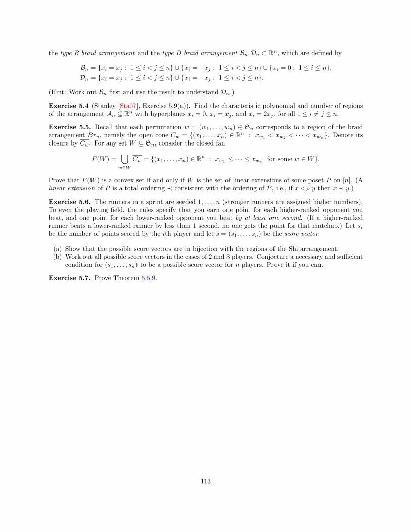
the type B braid arrangement and the type D braid arrangement Bn,Dn ⊂ Rn, which are defined by

Bn = xi = xj : 1 ≤ i < j ≤ n ∪ xi = −xj : 1 ≤ i < j ≤ n ∪ xi = 0 : 1 ≤ i ≤ n,Dn = xi = xj : 1 ≤ i < j ≤ n ∪ xi = −xj : 1 ≤ i < j ≤ n.

(Hint: Work out Bn first and use the result to understand Dn.)

Exercise 5.4 (Stanley [Sta07], Exercise 5.9(a)). Find the characteristic polynomial and number of regionsof the arrangement An ⊆ Rn with hyperplanes xi = 0, xi = xj , and xi = 2xj , for all 1 ≤ i = j ≤ n.

Exercise 5.5. Recall that each permutation w = (w1, . . . , wn) ∈ Sn corresponds to a region of the braidarrangement Brn, namely the open cone Cw = (x1, . . . , xn) ∈ Rn : xw1

< xw2< · · · < xwn

. Denote itsclosure by Cw. For any set W ⊆ Sn, consider the closed fan

F (W ) =⋃

w∈W

Cw = (x1, . . . , xn) ∈ Rn : xw1≤ · · · ≤ xwn

for some w ∈W.

Prove that F (W ) is a convex set if and only if W is the set of linear extensions of some poset P on [n]. (Alinear extension of P is a total ordering ≺ consistent with the ordering of P , i.e., if x <P y then x ≺ y.)

Exercise 5.6. The runners in a sprint are seeded 1, . . . , n (stronger runners are assigned higher numbers).To even the playing field, the rules specify that you earn one point for each higher-ranked opponent youbeat, and one point for each lower-ranked opponent you beat by at least one second. (If a higher-rankedrunner beats a lower-ranked runner by less than 1 second, no one gets the point for that matchup.) Let sibe the number of points scored by the ith player and let s = (s1, . . . , sn) be the score vector.

(a) Show that the possible score vectors are in bijection with the regions of the Shi arrangement.(b) Work out all possible score vectors in the cases of 2 and 3 players. Conjecture a necessary and sufficient

condition for (s1, . . . , sn) to be a possible score vector for n players. Prove it if you can.


113

Chapter 6

Simplicial Complexes

The canonical references for this material are [Sta96], [BH93, Ch. 5]. See also [MS05] (for the combinatoricsand algebra) and [Hat02] (for the topology).

6.1 Basic definitions and terminology

Definition 6.1.1. Let V be a finite set of vertices. An (abstract) simplicial complex ∆ on V is anonempty family of subsets of V with the property that if σ ∈ ∆ and τ ⊆ σ, then τ ∈ ∆. Equivalently, ∆ isan order ideal in the Boolean algebra 2V . The elements of ∆ are called its faces or simplices. A face thatis maximal with respect to inclusion is called a facet.

The dimension of a face σ is dimσ = |σ| − 1. A face of dimension k is a k-face or k-simplex. Thedimension of a non-void simplicial complex ∆ is dim∆ = maxdimσ : σ ∈ ∆. (Sometimes we write∆d−1 to indicate that dim∆ = d− 1; this is a common convention since then d is the maximum number ofvertices in a face.) A complex is pure if all its facets have the same dimension.

The simplest simplicial complexes are the void complex ∆ = ∅ (which is often excluded from consideration)and the irrelevant complex ∆ = ∅. In some contexts, there is the additional requirement that everysingleton subset of V is a face (since if v ∈ V and v ∈ ∆, then v ∈ σ for all σ ∈ ∆, so you might as wellreplace V with V \ v). A simplicial complex with a single facet is also called a simplex.

The simplicial complex generated by a list of faces σ1, . . . , σr is

⟨σ1, . . . , σr⟩ =r⋃

i=1

2σi .

The set of facets of a complex is the unique minimal set of generators for it.

Simplicial complexes are combinatorial models for compact topological spaces. The vertices V = [n] canbe regarded as the points e1, . . . , en ∈ Rn, and a simplex σ = v1, . . . , vr is then the convex hull of thecorresponding points:

|σ| = convev1 , . . . , evr = c1ev1 + · · ·+ cvrer : 0 ≤ ci ≤ 1 (∀i), c1 + · · ·+ cn = 1 .

114

For example, faces of sizes 1, 2, and 3 correspond respectively to vertices, line segments, and triangles. (Thisexplains why dimσ = |σ| − 1.) Taking ei to be the standard basis of Rn gives the standard geometricrealization |∆| of ∆:

|∆| =⋃σ∈∆

convei : i ∈ σ.

It is usually possible to realize ∆ geometrically in a space of much smaller dimension. For example, everygraph can be realized in R3, and planar graphs can be realized in R2. It is common to draw geometricpictures of simplicial complexes, just as we draw pictures of graphs. We sometimes use the notation |∆| todenote any old geometric realization (i.e., any topological space homeomorphic to the standard geometricrealization). Typically, it is easiest to ignore the distinction between ∆ and |∆|; if we want to be specific wewill use terminology like “geometric realization of ∆” or “face poset of ∆”. A triangulation of a topologicalspace X is a simplicial complex whose geometric realization is homeomorphic to X.

Here are geometric realizations of the simplicial complexes ∆1 = ⟨124, 23, 24, 34⟩ and ∆2 = ⟨12, 14, 23, 24, 34⟩.

1 3

2

4

1 3

2

4

1 3

2

4∆ 1 2∆

The filled-in triangle indicates that 124 is a face of ∆1, but not of ∆2. Note that ∆2 is the subcomplex of∆1 consisting of all faces of dimensions ≤ 1 — that is, it is the 1-skeleton of ∆1.

Some basic operations on simplicial complexes are as follows:

1. For X ⊆ V , the induced subcomplex is ∆|X = σ ∈ ∆ : σ ⊆ X.2. The deletion del∆(v) is the subcomplex of all faces not containing v. Equivalently, del∆(v) = ∆|V−v.

More generally,del∆(σ) = τ ∈ ∆ : τ ∩ σ = ∅ = ∆|V \σ.

3. The link of a face σ is defined as

link∆(σ) = τ ∈ ∆ : τ ∩ σ = ∅, τ ∪ σ ∈ ∆.

The link can be thought of as “what you see if you stand in σ in look outward”; for example, if ∆ is atriangulation of a (d− 1)-dimensional manifold, then the link of every vertex is a (d− 2)-sphere, andmore generally the link of every k-dimensional face is a (d− k − 2)-sphere.

4. The join of two complexes ∆,∆′ on disjoint vertex sets is

∆ ∗∆′ = σ ∪ σ′ : σ ∈ ∆, σ′ ∈ ∆′.

This is frequently the right notion of a product (but be careful: [∆ ∗ ∆′] is not homeomorphic to[∆]× [∆]!)

And here is the basic numerical invariant of a simplicial complex.

Definition 6.1.2. Let ∆d−1 be a simplicial complex. The f-vector of ∆ is (f−1, f0, f1, . . . , fd−1), wherefi = fi(∆) is the number of faces of dimension i. The term f−1 is often omitted, because f−1 = 1 unless ∆ isthe void complex. The f-polynomial is the generating function for the nonnegative f -numbers (essentiallythe rank-generating function of ∆ as a poset):

f(∆, q) = f0 + f1q + f2q2 + · · ·+ fd−1q

d−1.

115

For instance, if ∆1,∆2 are the simplicial complexes pictured above, then

f(∆1) = (4, 5, 1) and f(∆2) = (4, 5).

Example 6.1.3. Let P be a finite poset and let ∆(P ) be the set of chains in P . Every subset of a chain is achain, so ∆(P ) is a simplicial complex, called the order complex of P . The minimal nonfaces of ∆(P ) areprecisely the pairs of incomparable elements of P ; in particular every minimal nonface has size two, whichis to say that ∆(P ) is a flag complex. Note that ∆(P ) is pure if and only if P is ranked.

If P itself is the set of faces of a simplicial complex ∆, then ∆(P (∆)) is the barycentric subdivision ofthat complex. Combinatorially, the vertices of Sd(∆) correspond to the faces of ∆; a collection of verticesof Sd(∆) forms a face if the corresponding faces of ∆ are a chain in its face poset. Topologically, Sd(∆)can be constructed by drawing a vertex in the middle of each face of ∆ and connecting them — this is bestillustrated by a picture.

(∆)∆ Sd

Each vertex (black, red, blue) of Sd(∆) corresponds to a (vertex, edge, triangle) face of ∆. Note thatbarycentric subdivision does not change the topological space itself, only the triangulation of it.

6.2 Simplicial homology

Simplicial complexes are models of topological spaces, and combinatorialists use tools from algebraic topologyto study them, in particular the machinery of simplicial homology. Here we give a “user’s guide” to the subjectthat assumes as little topology background as possible. Readers familiar with the subject will know that Iam leaving many things out. For a full theoretical treatment, I recommend Chapter 2 of Hatcher [Hat02].

Let ∆ be a simplicial complex on vertex set [n]. The kth simplicial chain group of ∆ over a field1, say R,is the vector space Ck(∆) of formal linear combinations of k-simplices in ∆. Thus dimCk(∆) = fk(∆).The elements of Ck(∆) are called k-chains. The (simplicial) boundary map ∂k : Ck(∆) → Ck−1(∆) isdefined as follows: if σ = v0, . . . , vk is a k-face, with 1 ≤ v0 < · · · < vk ≤ n, then

∂k[σ] =

k∑i=0

(−1)i[v0, . . . , vi, . . . , vk] ∈ Ck−1(∆)

where the hat denotes removal. The map is then extended linearly to all of Ck(∆).

Recall that each σ ∈ ∆ of cardinality k + 1 is realized geometrically by a simplex, which is homeomorphicto a k-dimensional ball. The chain ∂[σ] should be thought of as the (k − 1)-sphere that is its boundary,

1More generally, this could be any commutative ring, but let’s keep things simple for the moment.

116

expressed as a sum of (k − 1)-simplices with consistent orientations (as represented by the signs). Often itis convenient to abbreviate ∂k by ∂, since either the subscript is clear from context or else we want to saysomething about all boundary maps at once.

The entire collection of data Ck(∆, ∂k) is called the simplicial chain complex of ∆. For example, if∆ = ⟨123, 14, 24⟩, then the simplicial chain complex is as follows:

C2 = R1 ∂2−−−−−−−−→123

12 113 −114 023 124 0

C1 = R5 ∂1−−−−−−−−−−−−−−−−−−−−−−−→12 13 14 23 24

1 1 1 1 0 02 −1 0 0 1 13 0 −1 0 −1 04 0 0 −1 0 −1

C0 = R4 ∂0−−−−−−−−−−−−−−→1 2 3 4[ ]∅ 1 1 1 1

C−1 = R

The fundamental fact about boundary maps is that ∂k ∂k+1 for all k, a fact that is frequently writtenwithout subscripts:

∂2 = 0.

(This can be checked directly from the definition of ∂, and is a calculation that everyone should do forthemselves once.) This is precisely what the term “chain complex” means in algebra.

An equivalent condition is that ker ∂k ⊇ im ∂k+1 for all k. In particular, we can define the reducedsimplicial homology groups2

Hk(∆) = ker ∂k/ im ∂k+1.

The Hk(∆) are just R-vector spaces, so they can be described up to isomorphism by their dimensions3, whichare called the Betti numbers βk(∆). They can be calculated using the rank-nullity formula: in general

βk(∆) = dim Hk(∆) = dimker ∂k − dim im ∂k+1 = fk − rank ∂k − rank ∂k+1.

In the example above, this formula gives

β0(∆) = 4− 1− 3 = 0, β1(∆) = 5− 3− 1 = 1, β2(∆) = 1− 1− 0 = 0

(note that ∂3 is the zero map).

These numbers turn out to carry topological information about the space |∆|. In fact, they depend onlyon the homotopy type of the space |∆|. This is a fundamental theorem in topology whose proof is far tooelaborate to give here,4 but provides a crucial tool for studying simplicial complexes: we can now ask howthe topology of ∆ affects its combinatorics. To begin with, the groups Hk(∆) do not depend on the choiceof labeling of vertices and are invariant under retriangulation.

A complex all of whose homology groups vanish is called acyclic. For example, if |∆| is contractible then ∆is acyclic over every ring. If ∆ ∼= Sd (i.e., |∆| is a d-dimensional sphere), then

Hk(∆) ∼=R if k = d,

0 if k < d.(6.1)

2The unreduced homology groups Hk(∆) are defined by deleting C−1(∆) from the simplicial chain complex. This results inan extra summand of R in H0(∆) and has no effect elsewhere. Broadly speaking, reduced homology arises more naturally incombinatorics and unreduced homology is more natural in topology, but the information is equivalent.

3This would not be true if we replaced R with a ring that was not a field. Actually, the most information is available over Z.In that case βk(∆) can still be obtained as the rank of the free part if Hk(∆), but there also may be a torsion part.

4Roughly, one defines a much more abstract set of invariants called singular homology groups, which are easily seen tobe topological invariants but are well-nigh impossible to work with directly; one then shows that repeatedly barycentricallysubdividing a space allows us to approximate singular homology by simplicial homology sufficiently accurately — but on theother hand subdivision also preserves simplicial homology. See [Hat02, §2.1] for the full story. Or take my Math 821 class!

117

The (reduced) Euler characteristic of ∆ is

χ(∆) =∑k≥0

βk(∆) =∑i≥−1

fi(∆). (6.2)

The second equality here is called the Euler-Poincare theorem; despite the fancy name, it is easy to proveusing little more than the rank-nullity theorem of linear algebra (Exercise 6.9). The Euler characteristic isthe single most important numerical invariant of ∆. Many combinatorial invariants can be computed byidentifying them as the Euler characteristic of a simplicial complex whose topology is known, often one thatis acyclic (χ = 0), a sphere of dimension d (χ = (−1)d), or a wedge of spheres.

Observe that

χ(∆) =∑

σ∈∆: e ∈σ

(−1)dimσ +∑

σ∈∆: e∈σ

(−1)dimσ

=∑

σ∈del∆(e)

(−1)dimσ +∑

τ∈link∆(e)

(−1)1+dim τ

= χ(del∆(e))− χ(link∆(e)). (6.3)

which resembles a deletion/contraction recurrence. (This is no accident; see (4.2).)

6.3 Stanley-Reisner theory

The Stanley-Reisner correspondence is an extremely important connection between simplicial complexesand commutative algebra. Let R = k[x1, . . . , xn] be the ring of polynomials in n variables over your favoritefield k. Define the support of a monomial µ ∈ R as

suppµ = i : xi divides µ.

Definition 6.3.1. Let ∆ be a simplicial complex on vertex set [n]. Its Stanley-Reisner ideal in R is

I∆ = ⟨xi1 · · ·xir : i1, . . . , ir ∈ ∆⟩ .

The Stanley-Reisner ring or face ring is k[∆] := R/I∆.

Example 6.3.2. Let ∆1 and ∆2 be the complexes on the previous page. Abbreviating w, x, y, z =x1, x2, x3, x4, the Stanley-Reisner ideal of ∆1 is

I∆1 = ⟨wxyz, wxy, wyz, xyz, wy⟩ = ⟨xyz, wy⟩.

Note that the minimal generators of I∆ are the minimal nonfaces of ∆. Similarly,

I∆2= ⟨wxz, xyz, wy⟩.

If ∆ is the simplex on [n] then it has no nonfaces, so I∆ is the zero ideal and k[∆] = k[x1, . . . , xn]. In general,the more faces ∆ has, the bigger its Stanley-Reisner ring is.

Since ∆ is a simplicial complex, the monomials in I∆ are exactly those whose support is not a face of ∆.Therefore, the monomials supported on a face of ∆ are a natural vector space basis for the graded ring k[∆].

118

Its Hilbert series can be calculated by counting these monomials:

Hilb(k[∆], q)def≡

∑i≥0

qi dimk(k[∆])i =∑σ∈∆

∑monomials µ:suppµ=σ

qdeg(µ)

=∑σ∈∆

(q

1− q

)|σ|

=

d∑i=0

fi−1

(q

1− q

)i

=

d∑i=0

fi−1qi(1− q)d−i

(1− q)d =

d∑i=0

hiqi

(1− q)d

The numerator of this rational expression is a polynomial in q, called the h-polynomial of ∆ and writtenh∆(q), and its list of coefficients (h0, h1, . . . ) is called the h-vector of ∆. Clearing denominators and applyingthe binomial theorem yields a formula for the h-numbers in terms of the f -numbers:

d∑i=0

hiqi =

d∑i=0

fi−1qi(1− q)d−i =

d∑i=0

fi−1qid−i∑j=0

(d− ij

)(−1)jqj

=

d∑i=0

d−i∑j=0

(d− ij

)(−1)jqi+jfi−1

and now extracting the qk coefficient (i.e., the summand in the second sum with j = k − i) yields

hk =

k∑i=0

(d− ik − i

)(−1)k−ifi−1. (6.4)

(Note that the upper limit of summation might as well be k instead of d, since the binomial coefficient inthe summand vanishes for i > k.) These equations can be solved to give the f ’s in terms of the h’s.

fi−1 =

i∑k=0

(d− ki− k

)hk. (6.5)

So the f -vector and h-vector contain equivalent information about a complex. On the level of generatingfunctions, the conversions look like this [BH93, p. 213]:∑

i

hiqi =

∑i

fi−1qi(1− q)d−i, (6.6)∑

i

fiqi =

∑i

hiqi−1(1 + q)d−i. (6.7)

The equalities (6.4) and (6.5) can be obtained by applying the binomial theorem to the right-hand sidesof (6.6) and (6.7) and equating coefficients. Note that it is most convenient simply to sum over all i ∈ Z.

Two useful special cases are as follows: (6.4) gives

hd =

d∑i=0

(d− id− i

)(−1)d−ifi−1 = (−1)d−1χ(∆),

the reduced Euler characteristic. Also, (6.5) gives

fd−1 =

d∑k=0

hk.

119

Let’s go back to the formula for the Hilbert series in terms of the h-vector, namely

Hilb(k[∆], q) =h∆(q)

(1− q)d =

d∑i=0

hiqi

(1− q)d .

Note that 1/(1 − q)d is just the Hilbert series of the polynomial ring k[x1, . . . , xn]. More generally, if R isany graded ring and x is an indeterminate of degree 1, then

Hilb(R[x], q) =Hilb(R, q)

1− q .

These observations suggest that we should be able to regard the Stanley-Reisner ring k[∆] as a polynomialring in d variables over a base ring S whose Hilbert series is the polynomial h∆(q). In particular S wouldhave to be a finite-dimensional vector space and hi the dimension of its ith graded piece. Also, we shouldbe able to recover S by quotienting out by d linear forms, each of which would remove a factor of 1/(1− q)from the Hilbert series. For this to work, all of the hi’s would have to be nonnegative, which does not alwayshappen. The situation is hopeless if ∆ is not pure, and even purity is not enough

Example 6.3.3. The bowtie complex is the pure 2-dimensional complex ∆ = ⟨123, 145⟩ shown below,with f -vector (1, 5, 6, 2). Therefore, by (6.6), the h-polynomial is∑

i

hiqi = 1q0(1− q)3 + 5q1(1− q)2 + 6q2(1− q)1 + 2q3(1− q)0 = 1 + 2q − q2

so the h-vector is (1, 2,−1).

3

4

5

2

1

A simplicial complex where this game works is called a Cohen-Macaulay complex. This is an extremely goodcondition from the algebraic point of view, but what can we say about the combinatorics of such complexes?

6.4 Shellable and Cohen-Macaulay simplicial complexes

For certain complexes, the h-numbers themselves have a direct combinatorial interpretation. The last formulasuggests that they should enumerate facets of a pure complex in some way. Here is an important specialclass of complexes where they do.

Definition 6.4.1. A pure simplicial complex ∆d−1 is shellable if its facets can be ordered F1, . . . , Fn suchthat any of the following conditions are satisfied:

1. For every i ∈ [n], the set Ψi = ⟨Fi⟩ \ ⟨F1, . . . , Fi−1⟩ has a unique minimal element Ri.2. For every i > 1, the complex Φi = ⟨Fi⟩ ∩ ⟨F1, . . . , Fi−1⟩ is pure of dimension d− 2.

120

The proof of equivalence is left as an exercise.

Example 6.4.2. The bipyramid is the pure 2-dimensional complex B with 6 facets 124, 134, 234, 125,135, 235. Vertices 1,2,3 form the “equator”; vertices 4 and 5 are the “poles”. The complex B has manyshelling orders, one of which is

234, 124, 134, 235, 125, 135.

The bipyramid and its shelling decomposition is shown in Figure 6.1. The new edges created upon addingeach triangle are indicated in bold. The corresponding decomposition of the face poset is

[∅, 234] ∪ [1, 124] ∪ [13, 134] ∪ [5, 235] ∪ [15, 125] ∪ [135, 135]

as shown in the figure (each face is color-coded according to the interval [Ri, Fi] that contains it).

1

2

3

4

5∅

1 2 34 5

12 1314 152324 2534 35

124 134234 125 135 235

Figure 6.1: A shelling of the bipyramid.

Figure 6.2 shows another example that shows how a shelling builds up a simplicial complex (in this case theboundary of an octahedron) one step at a time. Note that each time a new triangle is attached, there is aunique minimal new face.

Proposition 6.4.3. Let ∆d−1 be shellable, with h-vector (h0, . . . , hd). Then

hj = #Fi : #Ri = j= #

Fi : ⟨Fi⟩ ∩ ⟨F1, . . . , Fi−1⟩ has j faces of dimension d− 2

.

Moreover, if hj(∆) = 0 for some j, then hk(∆) = 0 for all k > j.

The proof is left as an exercise. One consequence is that the h-vector of a shellable complex is strictlynonnegative, since its coefficients count something. This statement is emphatically not true about the Hilbertseries of arbitrary graded rings, or even arbitrary Stanley-Reisner rings of pure complexes (see Example 6.3.3above).

If a simplicial complex is shellable, then its Stanley-Reisner ring is Cohen-Macaulay (CM). This is animportant and subtle algebraic condition that can be expressed algebraically in terms of depth or localcohomology (topics beyond the scope of these notes) or in terms of simplicial homology (coming shortly).Shellability is the most common combinatorial technique for proving that a ring is CM. The constraints onthe h-vectors of CM complexes are the same as those on shellable complexes, although it is an open problemto give a general combinatorial interpretation of the h-vector of a CM complex.

The Cohen-Macaulay condition can be expressed homologically, using links:

121

a

bc1

a

bc

d

1

2

a

bc

e

d

1

2

3

a

bc

e

d

1

2

34

a

bc

e

f d

1

2

34

5

a

bc

e

f d

1

2

34

5

6

a

bc

e

f d

1

2

34

5

6

7

a

bc

e

f d

1

2

34

5

6

7

8i Fi Ri |Ri|1 abc ∅ 02 abd d 13 bde e 14 bce ce 25 acf f 16 cef ef 27 adf df 28 adf def 3

Figure 6.2: A step-by-step shelling of the octahedron with vertices a,b,c,d,e,f. Facets are labeled 1 . . . 8 inshelling order. Enumerating the sets Ri by cardinality gives the h-vector (1, 3, 3, 1).

122

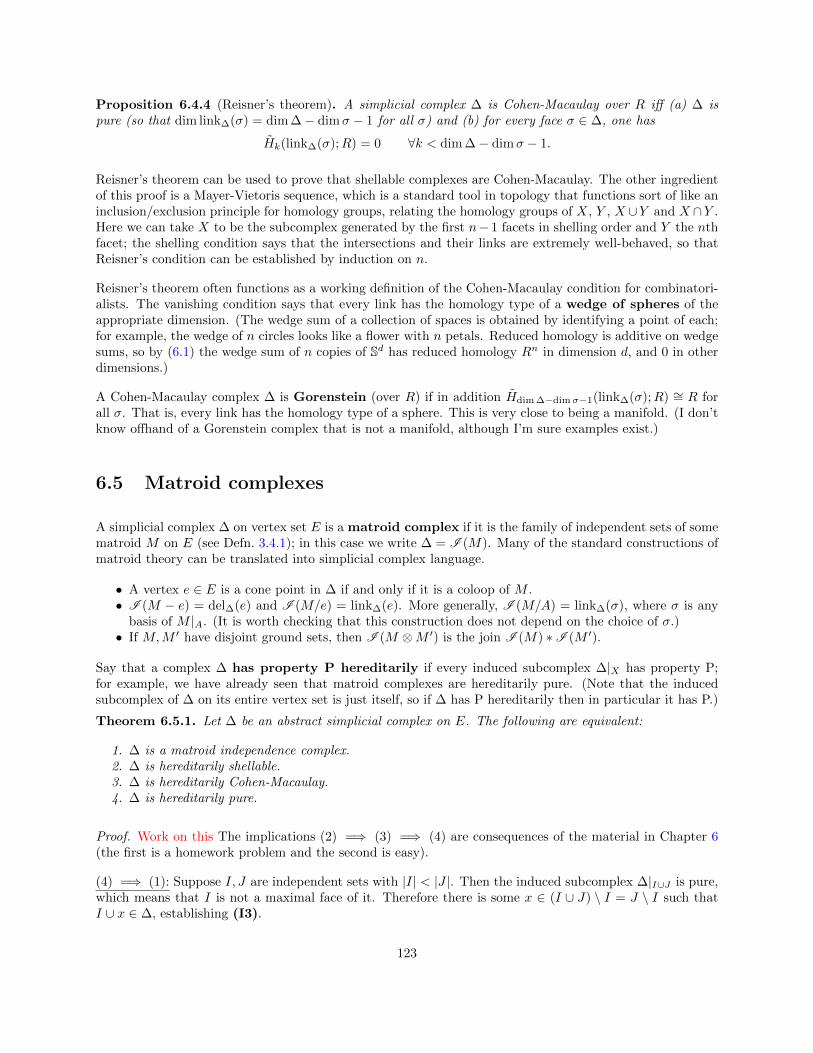
Proposition 6.4.4 (Reisner’s theorem). A simplicial complex ∆ is Cohen-Macaulay over R iff (a) ∆ ispure (so that dim link∆(σ) = dim∆− dimσ − 1 for all σ) and (b) for every face σ ∈ ∆, one has

Hk(link∆(σ);R) = 0 ∀k < dim∆− dimσ − 1.

Reisner’s theorem can be used to prove that shellable complexes are Cohen-Macaulay. The other ingredientof this proof is a Mayer-Vietoris sequence, which is a standard tool in topology that functions sort of like aninclusion/exclusion principle for homology groups, relating the homology groups of X, Y , X ∪Y and X ∩Y .Here we can take X to be the subcomplex generated by the first n− 1 facets in shelling order and Y the nthfacet; the shelling condition says that the intersections and their links are extremely well-behaved, so thatReisner’s condition can be established by induction on n.

Reisner’s theorem often functions as a working definition of the Cohen-Macaulay condition for combinatori-alists. The vanishing condition says that every link has the homology type of a wedge of spheres of theappropriate dimension. (The wedge sum of a collection of spaces is obtained by identifying a point of each;for example, the wedge of n circles looks like a flower with n petals. Reduced homology is additive on wedgesums, so by (6.1) the wedge sum of n copies of Sd has reduced homology Rn in dimension d, and 0 in otherdimensions.)

A Cohen-Macaulay complex ∆ is Gorenstein (over R) if in addition Hdim∆−dimσ−1(link∆(σ);R) ∼= R forall σ. That is, every link has the homology type of a sphere. This is very close to being a manifold. (I don’tknow offhand of a Gorenstein complex that is not a manifold, although I’m sure examples exist.)

6.5 Matroid complexes

A simplicial complex ∆ on vertex set E is a matroid complex if it is the family of independent sets of somematroid M on E (see Defn. 3.4.1); in this case we write ∆ = I (M). Many of the standard constructions ofmatroid theory can be translated into simplicial complex language.

• A vertex e ∈ E is a cone point in ∆ if and only if it is a coloop of M .• I (M − e) = del∆(e) and I (M/e) = link∆(e). More generally, I (M/A) = link∆(σ), where σ is anybasis of M |A. (It is worth checking that this construction does not depend on the choice of σ.)

• If M,M ′ have disjoint ground sets, then I (M ⊗M ′) is the join I (M) ∗I (M ′).

Say that a complex ∆ has property P hereditarily if every induced subcomplex ∆|X has property P;for example, we have already seen that matroid complexes are hereditarily pure. (Note that the inducedsubcomplex of ∆ on its entire vertex set is just itself, so if ∆ has P hereditarily then in particular it has P.)

Theorem 6.5.1. Let ∆ be an abstract simplicial complex on E. The following are equivalent:

1. ∆ is a matroid independence complex.2. ∆ is hereditarily shellable.3. ∆ is hereditarily Cohen-Macaulay.4. ∆ is hereditarily pure.

Proof. Work on this The implications (2) =⇒ (3) =⇒ (4) are consequences of the material in Chapter 6(the first is a homework problem and the second is easy).

(4) =⇒ (1): Suppose I, J are independent sets with |I| < |J |. Then the induced subcomplex ∆|I∪J is pure,which means that I is not a maximal face of it. Therefore there is some x ∈ (I ∪ J) \ I = J \ I such thatI ∪ x ∈ ∆, establishing (I3).

123

(1) =⇒ (4): Let F ⊆ E. If I is a non-maximum face of ∆|F , then we can pick J to be a maximum face,and then (I3) says that there is some x ∈ J such that I + x is a face of ∆, hence of ∆|F .

(4) =⇒ (2): More interesting; left as an exercise.

6.6 Combinatorial Laplacians

To be written

6.7 Exercises

Exercise 6.1. Let ∆ be a simplicial complex on vertex set V , and let v0 ∈ V . The cone over ∆ is thesimplicial complex C∆ generated by all faces σ + v0 for σ ∈ ∆.

(a) (Warmup) Prove that f(C∆, t) = (t+ 1)f(∆, t).(b) Prove that h(C∆, t) = h(∆, t).(c) Prove that ∆ is shellable if and only if C∆ is shellable. More specifically, F1, . . . , Fn is a shelling of ∆

if and only if F1 + v, . . . , Fn + v is a shelling of C∆.

Exercise 6.2. Let ∆ be a graph (that is, a 1-dimensional simplicial complex) with c components, v vertices,and e edges. Determine the isomorphism types of the simplicial homology groups H0(∆;R) and H1(∆;R)for any coefficient ring R.

Exercise 6.3. Construct two simplicial complexes with the same f -vector such that one is shellable andone isn’t.

Exercise 6.4. Prove that the two conditions in the definition of shellability (Defn. 6.4.1) are equivalent.


Exercise 6.6. Prove that the link operation commutes with union and intersection of complexes. That is,if X,Y are simplicial complexes that are subcomplexes of a larger complex X ∪ Y , and σ ∈ X ∪ Y , thenprove that

linkX∪Y (σ) = linkX(σ) ∪ linkY (σ) and linkX∩Y (σ) = linkX(σ) ∩ linkY (σ).

Exercise 6.7. (Requires some experience with homological algebra.) Prove that shellable simplicial com-plexes are Cohen-Macaulay. (Hint: First do the previous problem. Then use a Mayer-Vietoris sequence.)

Exercise 6.8. Complete the proof of Theorem 6.5.1 by showing that hereditarily pure simplicial complexesare shellable. (Hint: Pick a vertex v. Show that the two complexes

∆1 = del∆(v) = ⟨σ ∈ ∆ : v ∈ σ⟩,∆2 = link∆(v) = ⟨σ − v ∈ ∆ : v ∈ σ⟩

are both shellable. Then concatenate the shelling orders to produce a shelling order on ∆. You will probablyneed Exercise 6.1.) As a consequence of the construction, derive a relationship among the h-polynomials of∆, ∆1, and ∆2.

124

Exercise 6.9. Prove the Euler-Poincare formula:

χ(∆) =∑k≥−1

(−1)k dimk Hk(∆; k).

(Despite the appearance of homology, all you really need is the rank-nullity theorem from linear algebra.The choice of ground field k is immaterial, but you can take it to be R if you want.)

Exercise 6.10. Express the h-vector of a matroid complex in terms of the Tutte polynomial of the underlyingmatroid. (Hint: First figure out a deletion/contraction recurrence for the h-vector, using Exercise 6.8.)

Exercise 6.11. Let V = x11, x12, . . . , xn1, xn2. Consider the simplicial complex

∆n = σ ⊆ V : σ ⊆ xi, yi ∀i ∈ [n].

(In fact, ∆n is the boundary sphere of the crosspolytope, the convex hull of the standard basis vectors andtheir negatives in Rn.) Determine the f - and h-vectors of ∆n.

More generally, let V1, . . . , Vn be pairwise-disjoint sets of sizes c1, . . . , cn and let V = V1 ∪ · · · ∪ Vn. Thecorresponding complete colorful complex is

∆(c1, . . . , cn) = σ ⊆ V : |σ ∩ Vi| ≤ 1 ∀i ∈ [n].

(The previous problem is the case that ci = 2 for all i.) Show that ∆(c1, . . . , cn) is shellable. Determine itsf - and h-vectors.

125

Chapter 7

Polytopes and Polyhedra

7.1 The basics

Polytopes are familiar objects such as cubes, pyramids, and Platonic solids. They are central in linearprogramming and therefore in optimization, and exhibit a wealth of nice combinatorics. The classic bookon polytopes is Grunbaum [Gru03]; an equally valuable, more recent reference is Ziegler [Zie95]. A goodreference for the basics is chapter 2 of Schrijver’s notes [Sch13].

First some key terms. A subset S ⊆ Rn is convex if, for any two points in S, the line segment joining themis also a subset of S. The smallest convex set containing a given set T is called its convex hull, denotedconv(T ). Explicitly, one can show (exercise; not too hard) that

conv(x1, . . . ,xr) =

c1x1 + · · ·+ crxr : 0 ≤ ci ≤ 1 for all i and

r∑i=1

ci = 1

. (7.1)

These points are called convex linear combinations of the xi. A related definition is the affine hull ofa point set, which is the smallest affine linear space containing it:

aff(x1, . . . ,xr) =

c1x1 + · · ·+ crxr :

r∑i=1

ci = 1

. (7.2)

The interior of S as a subspace of its affine span is called the relative interior of S, denoted relintS.This concept is necessary to talk about interiors of different-dimensional polyhedra in a sensible way. Forexample, the closed line segment S = (x, 0) : 0 ≤ x ≤ 1 in R2 has empty interior as a subset of R2, butits affine span is the x-axis, so relintS = (x, 0) : 0 < x < 1.

Clearly conv(T ) ⊆ aff(T ) (in fact, the inclusion is strict if 1 < |T | < ∞). For example, the convex hull ofthree non-collinear points in Rn is a triangle, while their affine hull is the unique plane (i.e., affine 2-space)containing that triangle.

Definition 7.1.1. A polyhedron P is a nonempty intersection of finitely many closed half-spaces in Rn.Equivalently,

P = x ∈ Rn : ai1x1 + · · ·+ ainxn ≥ bi ∀i ∈ [m]where aij , bi ∈ R. These equations are often written as a single matrix equation Ax ≥ b, where A ∈ Rm×n

and b ∈ Rm.

126

Definition 7.1.2. A polytope in Rn is. . .

1. a bounded polyhedron; or2. the convex hull of a finite set of points.

Theorem 7.1.3 (The Fundamental Theorem of Polytopes). The two definitions of “polytope” in Defini-tion 7.1.2 are equivalent.

We have some work to do before getting to the proof of Theorem 7.1.3.

Definition 7.1.4. A point x in a polyhedron P is a vertex of P if x ∈ conv(P \ x).Definition 7.1.5. Let P ⊆ Rn be a polyhedron. A face of P is a subset F ⊆ P that maximizes some linearfunctional ℓ : Rn → R, i.e., ℓ(x) ≥ ℓ(y) for all x ∈ F , y ∈ P . The face is proper if ℓ is not a constant. Thedimension of a face is the dimension of its affine span.

The only improper face is P itself. Note that the union of all proper faces is the topological boundary ∂P(proof left as an exercise).

As a concrete example, suppose P is a polytope in R3. What point or set of points is highest? In otherwords, what points maximize the linear functional (x, y, z) 7→ z? The answer to this question might be asingle vertex, or an edge, or a polygonal face. Of course, there is nothing special about the z-direction. Forany direction given by a nonzero vector v, the extreme points of P in that direction are by definition themaxima of the linear functional x 7→ x · v, and the set of those points is a face.

If you pick a linear functional “at random”, then with probability 1, the face it determines will be a vertexof P . Higher-dimensional faces correspond to more special directions.

Proposition 7.1.6. Let P ⊆ Rn be a polyhedron. Then:

1. Every face of P is also a polyhedron, and every face of a face of P is a face of P .2. The intersection of any two faces is a face (provided it is nonempty).3. For each x ∈ P , there is a unique minimal face Fx ⊆ P containing x.4. x ∈ relintFx for every x ∈ P .5. The vertices of a polytope are exactly its 0-dimensional faces.6. The faces of P form a lattice under inclusion, with bottom element ∅ and top element P , and meet

given by intersection. Moreover, the face lattice is ranked by dimension (strictly speaking, the rankfunction is r(Q) = 1 + dimQ so that r(∅) = 0).

Proof. (1) Each face is defined by adding a single linear inequality to the list of inequalities defining P .

(2) Let F ′, F ′′ be two faces maximized by linear functionals ℓ′, ℓ′′ respectively, and suppose that F ′ ∩ F ′′

contains a point x. Let F be the face maximized by the functiona; ℓ = ℓ′ + ℓ′′ (in fact any positive linearcombination of ℓ′, ℓ′′ will do). Then x is a global maximum of ℓ on P , and since x also maximizes both ℓ′ andℓ′′, the face F consists exactly of those points of P maximizing both ℓ′ and ℓ′′. In other words, F = F ′ ∩F ′′,as desired.

(3) By (2), the desired face Fx is the intersection of all faces containing x.

(4) If x ∈ ∂Fx then Fx has a face G containing x, but G is also a face of P by (1), which contradicts thedefinition of Fx.

(5) Suppose that x is a 0-dimensional face, i.e., the unique maximum of some linear functional ℓ. If x is aconvex linear combination

∑ciyi of points yi ∈ P , then ℓ(x) ≥

∑ciℓ(yi), with equality only if ℓ(yi) = ℓ(x)

127

for all i — but then yi = x for all i by assumption. Therefore x is not in the convex hull of P \ x, henceis a vertex.

On the other hand, if x is a point of P that is not an 0-dimensional face, then by (4) x ∈ relintFx,hence x is a convex combination of two other points (such as x± ϵv for any vector v and some sufficientlysmall ϵ).

(6) The faces form a bounded poset under inclusion, and by (2) it is a meet-semilattice, hence a lattice byProp. 1.2.9. To prove that it is ranked. . . Insert proof

Sketch of proof of Theorem 7.1.3. Some details are left as an exercise. A full proof appears in [Sch13, §2.2].

First, let P be a intersection of finitely many half-spaces, i.e., P = x ∈ Rn : Ax ≤ b, where A ∈ Rm×n andb ∈ Rm×1. By projecting onto the orthogonal complement of the rowspace of A, we can assume WLOG thatrankA = n. For each point z ∈ P , let Az be the submatrix of A consisting of rows ai for which ai · z = bi.One must show that

z ∈ P is the unique maximum of some linear functional ⇐⇒ rankAz = n. (7.3)

(More generally, rankAz = n− dimFz.)

It follows that the vertices are all of the form A−1R bR, where R is a row basis of A and AR, bR denote

restrictions. Not every point of this form necessarily lies in P , but this argument does show that there areonly finitely many vertices v1, . . . ,vk (specifically, k ≤

(mn

)). So far, this argument applies to any polyhedron.

In the next step, one must show thatP = convv1, . . . ,vk (7.4)

using in addition the assumption that P is bounded.

Second, let P = conv(z1, . . . , zr) ⊆ Rn. Assume without loss of generality that aff(P ) = Rn (otherwise,replace Rn with the affine hull) and that the origin is in the interior of P (translating if necessary). Define

P ∗ := y ∈ Rn : x · y ≤ 1 ∀x ∈ P. (7.5)

This is called the (polar) dual of P . One must show that in fact

P ∗ = y ∈ Rn : zi · y ≤ 1 ∀i ∈ [r] (7.6)

which means that P ∗ is an intersection of finitely many half-spaces. So, by the first part of the theorem,P ∗ = conv(y1, . . . ,ys) for some y1, . . . ,ys. Meanwhile, the double dual P ∗∗ = (P ∗)∗ is defined by

P ∗∗ = x ∈ Rn : x · y ≤ 1 ∀y ∈ P ∗ = x ∈ Rn : x · yj ≤ 1 ∀j ∈ [s] (7.7)

where the second equality comes from applying the previous observation. Now one must show that

P = P ∗∗ (7.8)

so that (7.7) expresses P as the intersection of finitely many half-spaces.

Example 7.1.7. Let P be the polytope shown on the left of Figure 7.1. It can be expressed as an intersectionof hyperplanes (i.e., solution set to a system of linear inequalities) as follows:

P =

[xy

]∈ R2 :

−1 00 −11 00 11 1

[xy

]≤

11111

.

128

If we number the rows R0, . . . , R4, every pair of rows other than R0, R2 and R1, R3 is of full rank. Thepoints corresponding to the other eight pairs of rows are:

Rows Point Type Constraint on P ∗

0, 1 (−1,−1) vertex −x− y ≤ 10, 3 (−1, 1) vertex −x+ y ≤ 10, 4 (−1, 2) not in P1, 2 (1,−1) vertex x− y ≤ 11, 4 (2,−1) not in P2, 3 (1, 1) not in P2, 4 (1, 0) vertex x ≤ 13, 4 (0, 1) vertex y ≤ 1

Thus the vertices of P correspond to the bounding hyperplanes (i.e., lines) of P ∗, and vice versa.

1

1

−1

−1P

1

1

−1

−1

P ∗

Figure 7.1: A polytope P and its polar dual P ∗.

Definition 7.1.8. Let P be an n-dimensional polytope in Rn.

• A facet of P is a face of codimension 1 (that is, dimension n− 1). In this case there is a unique linearfunctional (up to scaling) that is maximized on F , given by the outward normal vector from P . Facesof codimension 2 are called ridges and faces of codimension 3 are sometimes called peaks.

• A supporting hyperplane of P is a hyperplane that meets P in a nonempty face.• P is simplicial if every face is a simplex. For example, every 2-dimensional polytope is simplicial, butof the Platonic solids in R3, only the tetrahedron, octahedron and icosahedron are simplicial — the cubeand dodecahedron are not. The boundary of a simplicial polytope is thus a simplicial (n− 1)-sphere.

• P is simple if every vertex belongs to exactly n faces. (In fact no vertex can belong to fewer than nfaces.)

Proposition 7.1.9. A polytope P is simple if and only if its dual P ∗ is simplicial. In this case the faceposet of P is the dual of the face poset of P ∗.

7.2 Shelling simplicial polytopes

One of the big questions about polytopes is to classify their possible f -vectors and, more generally, thestructure of their face posets. Here is a result of paramount importance.

Theorem 7.2.1. Let ∆ be the boundary sphere of a convex simplicial polytope P ⊆ Rd. Then ∆ is shellable,and its h-vector is a palindrome, i.e., hi = hd−i for all i.

129

These equations are the Dehn-Sommerville relations. They were first proved early in the 20th century,but the following proof, due to Bruggesser and Mani [BM71], is undoubtedly the one in the Book.

Sketch of proof. Let H be the collection of hyperplanes spanned by facets of P . Let ℓ be a line that passesthrough the interior of P and meets each hyperplane in H in a distinct point. (Note that almost any linewill do.) Imagine walking along this line, starting just outside P so that only one facet is visible. Call thatfacet F1. As you continue to walk, more and more facets become visible. Label the facets F2, . . . , Fm inthe order in which they appear (equivalently, order them in the order in which the line ℓ meets their affinespans). When you get to infinity, come back the other way (so that all of a sudden “invisible” and “visible”switch meanings) and continue to label the facets Fm+1, . . . , Fn in the order in which they disappear.

2

F1

F

F3

1

F2

3

5

4F

F

F

F

Stage 1 Stage 2

In fact F1, . . . , Fn is a shelling order (called a line shelling), because

⟨Fj⟩ ∩ ⟨F1, . . . , Fj−1⟩ =⟨ridges of Fj that appear upon crossing aff(Fj)⟩ for 1 ≤ j ≤ m,⟨ridges of Fj that disappear upon crossing aff(Fj)⟩ for m+ 1 ≤ j ≤ n.

(This assertion does need to be checked.) Moreover, each facet Fi contributes to hk(P ), where

k = k(Fi) = #j < i : Fi, Fj have a common ridge.

On the other hand, the reversal of < is another instance of this construction, hence is also a shelling order.Since each facet shares a ridge with exactly n other facets (because P is simplicial!), the previous formulasays that if facet F contributes to hi with respect to the first shelling order then it contributes to hn−i inits reversal. Since the h-vector is an invariant of P , it follows that hi = hn−i for all i.

The Dehn-Sommerville relations are a basic tool in classifying h-vectors, and therefore f -vectors, of simplicialpolytopes. Since h0 = 1 for shellable complexes, it follows immediately that the only possible h-vectors forsimplicial polytopes in R2 and R3 are (1, k, 1) and (1, k, k, 1), respectively (where k is a positive integer),and in particular the number of facets determines the h-vector (which is not the case in higher dimensions).

7.3 The normal fan and generalized permutahedra

Recall from Definition 7.1.5 that a face of a polyhedron P ⊂ Rn is defined as the subset of P that maximizesa linear functional. We can get a lot of mileage out of classifying linear functionals by which face of P theymaximize. The resulting structure N (P ) is called the normal fan of P . (Technical note: officially N (P )is a structure on the dual space (Rn)∗, but we typically identify (Rn)∗ with Rn by declaring the standardbasis to be orthonormal — equivalently, letting each vector in Rn act by the standard dot product.)

130

Given a face F ⊂ P , let σF be the collection of linear functionals maximized on F . As we will see, the setsσF are in fact the interiors of cones (convex unions of rays from the origin).

Example 7.3.1. Let P = conv(1, 1), (1,−1), (−1, 1) ⊂ R2. The polytope and its normal fan are shownbelow.

Q

R

S

x

y

z

P

σzσx

σy

σQ

σR

σS

N (P )

Figure 7.2: A polytope P and its normal fan N (P ).

The word “fan” means “collection of cones”. Multiplying a linear functional by a positive scalar does notchange the face on which it is maximized, and that if ℓ and ℓ′ are linear functionals maximized on the sameface, then so is every functional aℓ + bℓ′, where a, b are positive scalars. Therefore, each σF is a cone. Thevertices x, y, z correspond to the 2-dimensional cones, the edges Q,R, S to 1-dimensional cones (a.k.a. rays)and the polytope P itself to the trivial cone consisting of the origin alone. In general, if F is a face of apolytope P ⊆ Rn, then

dimσF = n− dimF. (7.9)

Example 7.3.2 (The normal fan of an unbounded polyhedron). Let P be the unbounded polyhedron definedby the inequalities x ≤ 1, y ≤ 1, x+ y ≤ 1 (so its vertices are x = (0, 1) and y = (1, 0)). The polytope andits normal fan are shown below.

Q y

R

x

S

P

σx

σy

σS

σR

σQ

N (P )

131

This normal fan is incomplete: it does not cover every linear functional in (R2)∗, only the ones that have awell-defined maximum on P (in this case, those in the first quadrant). It is not hard to see that the normalfan of a polyhedron is complete if and only if the polyhedron is bounded, i.e., a polytope. The dimensionformula for normal cones (7.9) is still valid in the unbounded case.

In general the normal fan of a polytope can be quite complicated, and there exist fans in Rn that are not thenormal fans of any polytope, even for n = 3; see, e.g., [Zie95, Example 7.5]. However, for some polytopes,we can describe the normal fan using other combinatorics, such as the following important class.

Definition 7.3.3. A polytope P ⊆ Rn is a generalized permutahedron if its normal fan is a coarseningof the braid fan (i.e., the fan of faces of the braid arrangement). Equivalently, for every linear functionalℓ(x) = a1x1+ · · ·+anxn the face of P maximized by ℓ is determined solely by the equalities and inequalitiesamong the coefficients ai.

The theory of generalized permutahedra is usually considered to have started with Postnikov’s paper [Pos09];other important sources include [PRW08] and [AA17]. Edmonds considered equivalent objects earlier underthe name “polymatroids” (insert citations).

Theorem 7.3.4. A polytope P ⊆ Rn is a generalized permutahedron if and only if every edge of P is parallelto ei − ej for some i, j, where e1, . . . , en is the standard basis.

Generalized permutahedra can also be described as certain degenerations of the standard permutahedron,which is the convex hull of the vectors (w1, . . . , wn), where w ranges over all permutations of [n]. The normalfan of the standard permutahedron is precisely the braid fan.

One important family of generalized permutahedra are matroid base polytopes. Given a matroid M onground set [n], let P be the convex hull of all characteristic vectors of bases of M . It turns out that P isa generalized permutahedron; in fact, the matroid base polytopes are exactly the generalized permutahedrawhose vertices are 0/1 vectors [GGMS87, Thm. 4.1]. Describing the faces of matroid polytopes in terms ofthe combinatorics of the matroid is an interesting and difficult problem; see [FS05].

7.4 Ehrhart theory (contributed by Margaret Bayer)

The central problem considered in this section is the following: How many integer or rational pointsare in a convex polytope?

Definition 7.4.1. A polytope P ⊆ RN is integral (resp. rational) if and only if all vertices of P haveinteger (resp. rational) coordinates.

For a set P ⊆ RN and a positive integer n, let nP = nx : x ∈ P. (nP is called a dilation of P .)

The (relative) boundary of P , written ∂P , is the union of proper faces of P , that is, the set of pointsx ∈ P such that for every ε > 0, the ball of radius ε (its intersection with aff(P )) contains both points of Pand points not in P . The (relative) interior of P , intP , is P \ ∂P .

For a polytope P ⊆ RN define sequences

i(P, n) = |nP ∩ ZN |i∗(P, n) = |n(intP ) ∩ ZN |

132

i(P, n) is the number of integer points in nP or, equivalently, the number of rational points in P of the form(a0n,a1n, . . . ,

aNn

). Our goal is to understand the functions i(P, n) and i∗(P, n).

We start with P a simplex, and with an easy example. Let

P = conv(0, 0, 0), (1, 1, 0), (1, 0, 1), (0, 1, 1) ∈ R3.

ThennP = conv(0, 0, 0), (n, n, 0), (n, 0, n), (0, n, n).

Each point in nP can be written as β1(n, n, 0) + β2(n, 0, n) + β3(0, n, n) + β4(0, 0, 0), with 0 ≤ βi ≤ 1 and∑βi = 1; or, alternatively, as α1(1, 1, 0) + α2(1, 0, 1) + α3(0, 1, 1), with 0 ≤ αi ≤ n and

∑αi ≤ n.

Case 1. If the αi are all integers, the resulting points are integer points and the sum of the coordinates iseven. How many such points are there? The answer is the number of monomials in four variables of degreen, that is,

(n+33

). However, there are other integer points in nP .

Case 2. We can allow the fractional part of αi to be 1/2. If any one of the αi has fractional part 1/2, theothers must be also. Writing γi = αi − 1/2, we get points of the form

(γ1 + 1/2)(1, 1, 0) + (γ2 + 1/2)(1, 0, 1) + (γ3 + 1/2)(0, 1, 1)

= γ1(1, 1, 0) + γ2(1, 0, 1) + γ3(0, 1, 1) + (1, 1, 1).

Note here that∑γi = (

∑αi) − 3/2 ≤ n − 3/2. Since the γi are integers,

∑γi ≤ n − 2. So the number of

these points equals the number of monomials in four variables of degree n− 2, that is,(n+13

).

Adding these we get

i(P, n) =

(n+ 3

3

)+

(n+ 1

3

)=

1

3n3 + n2 +

5

3n+ 1.

Note, in particular, that this is a polynomial in n.

And what about the number of integer points in the interior of P?

Note that all the points in Case 2 are interior points because each αi = γi+1/2 > 0 and their sum is at mostn− 2 + 3/2 (less than n). A point in Case 1 is an interior point if and only if all the αi > 0 and

∑αi < n.

The four-tuples (α1 − 1, α2 − 1, α3 − 1, n − 1 −∑αi) correspond to monomials in four variables of degren− 4; there are

(n−13

)of them. Thus we get

i∗(P, n) =

(n+ 1

3

)+

(n− 1

3

)=

1

3n3 − n2 + 5

3n− 1,

another polynomial. (Anything else you notice? Is it a coincidence?)

It is convenient to visualize the dilations nP of P in a cone. For P ⊆ RN an integral N -simplex, letP = (x, 1) ∈ RN+1 : x ∈ P, and let C be the simplicial cone generated by P :

C = C(P ) = ry : y ∈ P , r ∈ R, r ≥ 0.The boundary and interior of C are ∂C = ry : y ∈ ∂P and intC = C \ ∂C. Then the polytope nP can beidentified with a cross-section of C:

C ∩ (z, n) ∈ RN+1 : z ∈ RN = (z, n) ∈ RN+1 : z ∈ nP.The integer point functions are then

i(P, n) = |C ∩ (z, n) ∈ RN+1 : z ∈ ZN|i∗(P, n) = | intC ∩ (z, n) ∈ RN+1 : z ∈ ZN|.

133

We can represent all points in the cone in terms of the vertices of P .

Proposition 7.4.2. Let P be a rational N -simplex in RN , with vertices v0, v1, . . . , vN , and let C = C(P ).

A point z ∈ RN+1 is a rational point in C if and only if z =∑N

i=0 ci(vi, 1) for some nonnegative rationalnumbers ci. Furthermore, this representation of z is unique.

A slightly different representation is more useful. Let

Q =

N∑i=0

ri(vi, 1) : 0 ≤ ri < 1 ∀i.

Thus Q is a half-open parallelepiped containing 0 and P .

Proposition 7.4.3. Let P be an integral N -simplex in RN , with vertices v0, v1, . . . , vN , and let C = C(P ).

A point z ∈ ZN+1 is an integer point in C if any only if z = y +∑N

i=0 ri(v1, 1) for some y ∈ Q ∩ ZN+1 andsome nonnegative integers ri. Furthermore, this representation of z is unique.

So to count integer points in C (and hence to determine i(P, n)), we only need to know how many integerpoints are in Q with each fixed (integer) last coordinate. We call the last coordinate of z ∈ Q the degree of

z. Note that for z ∈ Q, deg z =∑N

i=0 ri for some ri, 0 ≤ ri < 1, so if deg z is an integer, 0 ≤ deg z ≤ N .

Theorem 7.4.4. Let P be an integral N -simplex in RN , with vertices v0, v1, . . . , vN , let C = C(P ), and

let Q = ∑Ni=0 ri(vi, 1) : for each i, 0 ≤ ri < 1. Let δj be the number of points of degree j in Q ∩ ZN+1.

Then ∞∑n=0

i(P, n)λn =δ0 + δ1λ+ · · ·+ δNλ

N

(1− λ)N+1.

Corollary 7.4.5. For P an integral N -simplex, i(P, n) is a polynomial in n.

Proof.

∞∑n=0

i(P, n)λn = (δ0 + δ1λ+ · · ·+ δNλN )(1 + λ+ λ2 + · · · )N+1

= (δ0 + δ1λ+ · · ·+ δNλN )

( ∞∑k−0

(k +N

N

)λk

).

The coefficient of λn on the right hand side is∑N

j=0 δj(n−j+N

N

).

For the interior of P (and of C) we use an analogous construction, but with the opposite half-open paral-lelipiped. Let

Q∗ =

N∑i=0

ri(vi, 1) : 0 < ri ≤ 1∀i.

Proposition 7.4.6. Let P be an integral N -simplex in RN , with vertices v0, v1, . . . , vN , and let C = C(P ).

A point z ∈ ZN+1 is an integer point in intC if and only if z = y +∑N

i=0 ci(v1, 1) for some y ∈ Q∗ ∩ ZN+1

and some nonnegative integers ci. Furthermore, this representation of z is unique.

So to count integer points in intC (and hence to determine i∗(P, n)), we only need to know how many integerpoints are in Q∗ with each fixed (integer) last coordinate. Note that for z ∈ Q∗, 0 < deg z ≤ N + 1.

134

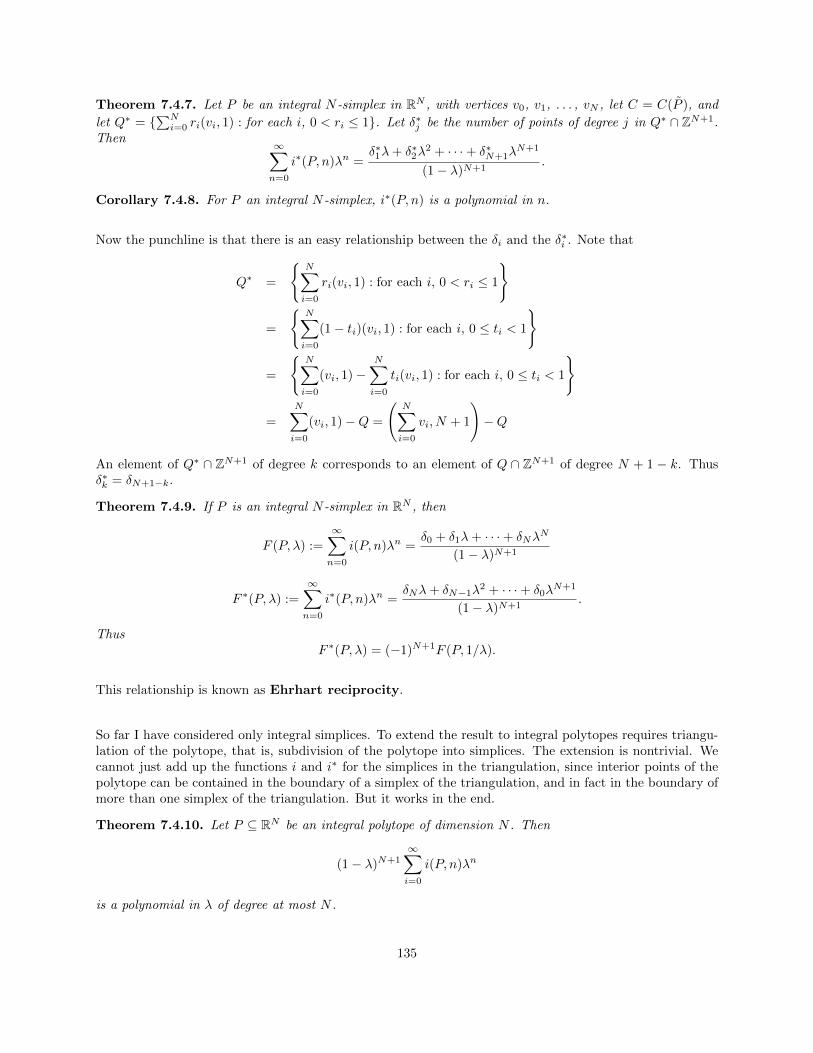
Theorem 7.4.7. Let P be an integral N -simplex in RN , with vertices v0, v1, . . . , vN , let C = C(P ), and

let Q∗ = ∑Ni=0 ri(vi, 1) : for each i, 0 < ri ≤ 1. Let δ∗j be the number of points of degree j in Q∗ ∩ ZN+1.

Then ∞∑n=0

i∗(P, n)λn =δ∗1λ+ δ∗2λ

2 + · · ·+ δ∗N+1λN+1

(1− λ)N+1.

Corollary 7.4.8. For P an integral N -simplex, i∗(P, n) is a polynomial in n.

Now the punchline is that there is an easy relationship between the δi and the δ∗i . Note that

Q∗ =

N∑i=0

ri(vi, 1) : for each i, 0 < ri ≤ 1

=

N∑i=0

(1− ti)(vi, 1) : for each i, 0 ≤ ti < 1

=

N∑i=0

(vi, 1)−N∑i=0

ti(vi, 1) : for each i, 0 ≤ ti < 1

=

N∑i=0

(vi, 1)−Q =

(N∑i=0

vi, N + 1

)−Q

An element of Q∗ ∩ ZN+1 of degree k corresponds to an element of Q ∩ ZN+1 of degree N + 1 − k. Thusδ∗k = δN+1−k.

Theorem 7.4.9. If P is an integral N -simplex in RN , then

F (P, λ) :=

∞∑n=0

i(P, n)λn =δ0 + δ1λ+ · · ·+ δNλ

N

(1− λ)N+1

F ∗(P, λ) :=∞∑

n=0

i∗(P, n)λn =δNλ+ δN−1λ

2 + · · ·+ δ0λN+1

(1− λ)N+1.

ThusF ∗(P, λ) = (−1)N+1F (P, 1/λ).

This relationship is known as Ehrhart reciprocity.

So far I have considered only integral simplices. To extend the result to integral polytopes requires triangu-lation of the polytope, that is, subdivision of the polytope into simplices. The extension is nontrivial. Wecannot just add up the functions i and i∗ for the simplices in the triangulation, since interior points of thepolytope can be contained in the boundary of a simplex of the triangulation, and in fact in the boundary ofmore than one simplex of the triangulation. But it works in the end.

Theorem 7.4.10. Let P ⊆ RN be an integral polytope of dimension N . Then

(1− λ)N+1∞∑i=0

i(P, n)λn

is a polynomial in λ of degree at most N .

135

As before, write this polynomial as∑N

j=0 δjλj . What can we say about the coefficients δj?

δ0 = i(P, 0) = 1, since this is the number of integer points in the polytope 0P = 0.

δ1 + (N + 1)δ0 = i(P, 1), so δ1 = |P ∩ ZN | − (N + 1).

Also, recall that i(P, n) =∑N

j=0 δj(n−j+N

N

). Let C be the leading coefficient of i(P, n) as a polynomial in n,

i.e.,

C =1

N !

N∑j=0

δj = limn→∞

i(P, n)

nN.

I claim C is the volume of P . To see this, note that vol(nP ) = nN vol(P ) (if P is of full dimension N). Nowthe volume of nP can be estimated by the number of lattice points in nP , that is, by i(P, n). In fact,

0 = limn→∞

i(P, n)− vol(nP )

nN= lim

n→∞i(P, n)

nN− vol(P ).

So C = limn→∞

i(P, n)

nN= vol(P ).

One last comment. The Ehrhart theory can be generalized to rational polytopes. In the more generalcase, the functions i(P, n) and i∗(P, n) need not be polynomials, but are quasipolynomials—restricted toa congruence class in some modulus (depending on the denominators occurring in the coordinates of thevertices) they are polynomials. An equivalent description is that the function i(P, n) is a polynomial in nand expressions of the form gcd(n, k), e.g.,

i(P, n) =

(n+ 1)2 n even

n2 n odd= (n+ gcd(n, 2)− 1)2.

7.5 Exercises

Exercise 7.1. Prove that the topological boundary of a polyhedron is the union of its proper faces.

Exercise 7.2. Prove that the convex hull of a finite point set X = x1, . . . ,xn is the set of convex linearcombinations of it.

Exercise 7.3. Fill in the details in the proof of Theorem 7.1.3 by proving all the assertions of the form“One must show”, i.e., (7.3), (7.4), (7.6), and (7.8). (You may use Minkowski’s Hyperplane SeparationTheorem, which states that if S ⊆ Rn is a convex set and y ∈ S, then there exists a hyperplane separatingS from y — or equivalently a linear functional ℓ : Rn → R such that ℓ(y) > 0 and ℓ(x) < 0 for all x ∈ S.)Exercise 7.4. Prove Theorem 7.3.4.

Exercise 7.5. Let M be a matroid and let P be its base polytope. Prove that P is a generalized permuta-hedron in two different ways:

1. Show that the normal fan NP coarsens the braid cone, using the properties of greedy algorithms.2. Show that every edge of P is parallel to some ei − ej , using the properties of basis exchange.

Exercise 7.6. Consider the simplex ∆n defined as the convex hull of the origin together with the n-basisvectors in Rn. That is,

∆n = x = (x1, . . . , xn) ∈ Rn : 0 ≤ xi ≤ 1, 0 ≤ x1 + · · ·+ xn ≤ 1.Calculate the Ehrhart polynomials i(∆n, k) and i

∗(∆n, k).

136

Exercise 7.7. The crosspolytope is defined as

Xn = conv±e1, . . . ,±en ⊆ Rn = (x1, . . . , xn) ∈ Rn : |xi| ≤ 1, 0 ≤ |x1|+ · · ·+ |xn| ≤ 1.

Calculate i(Xn, k) and i∗(Xn, k).

137

Chapter 8

Group Representations

8.1 Basic definitions

Definition 8.1.1. Let G be a group (typically finite) and let V ∼= kn be a finite-dimensional vector space overa field k. A representation of G on V is a group homomorphism ρ : G→ GL(V ), where GL(V ) = GLn(k)is the group of linear automorphisms of V , or equivalently the group of invertible n × n matrices over k.That is, for each g ∈ G there is an invertible n× n matrix ρ(g), satisfying

ρ(g)ρ(h) = ρ(gh) ∀g, h ∈ G.

(That’s matrix multiplication on the left side of the equation, and group multiplication in G on the right.)The number n is called the dimension (sometimes degree) of the representation, written dim ρ.

Some remarks:

• ρ specifies an action of G on V that respects its vector space structure. So we have all the accoutrementsof group actions, such as orbits and stabilizers. If there is only one representation under consideration,it is often convenient to use group-action notation and write gv instead of the bulkier ρ(g)v.

• It is common to say that ρ is a representation, or that V is a representation, or that the pair (ρ, V ) isa representation.

• ρ is faithful if it is injective as a group homomorphism.

Example 8.1.2. Let G be any group. The trivial representation is the map

ρtriv : G→ GL1(k) ∼= k×

sending g 7→ 1 for all g ∈ G.

Example 8.1.3. Let kG be the vector space of formal k-linear combinations of elements of G: that is,kG =

∑h∈G ahh : ah ∈ k

. The regular representation of G is the map ρreg : G→ GL(kG) defined by

g

(∑h∈G

ahh

)=

∑h∈G

ah(gh).

That is, g permutes the standard basis vectors of kG according to the group multiplication law. Thusdim ρreg = |G|.

138

The vector space kG is a ring, with multiplication given by multiplication in G and extended k-linearly. Inthis context it is called the group algebra of G over k.

Remark 8.1.4. A representation of G is equivalent to a (left) module over the group algebra kG. Tech-nically “representation” refers to the way G acts and “module” refers to the space on which it acts, but thetwo terms really carry the same information.

Example 8.1.5. Let G = Sn, the symmetric group on n elements. The defining representation ρdefof G on kn maps each permutation σ ∈ G to the n×n permutation matrix with 1’s in the positions (i, σ(i))for every i ∈ [n], and 0’s elsewhere.

Example 8.1.6. More generally, let G act on a finite set X. Then there is an associated permutationrepresentation on kX , the vector space with basis X, given by

g

(∑x∈X

axx

)=∑x∈X

ax(gx).

For short, we might specify the action of G on X and say that it “extends linearly” to kX . For instance, theaction of G on itself by left multiplication gives rise in this way to the regular representation, and the usualaction of Sn on an n-element set gives rise to the defining representation.

Example 8.1.7. Let G = Z/nZ be the cyclic group of order n, and let ζ ∈ k be a nth root of unity (notnecessarily primitive). Then G has a 1-dimensional representation given by ρ(x) = ζx.

Example 8.1.8. Consider the dihedral group Dn of order 2n, i.e., the group of symmetries of a regularn-gon, given in terms of generators and relations by

⟨s, r : s2 = rn = 1, srs = r−1⟩.

There are several natural representations of Dn.

1. Regarding s as a reflection and r as a rotation in R2 gives a faithful 2-dimensional representation (the“geometric representation”)

ρgeo(s) =

[1 00 −1

], ρgeo(r) =

[cos(2π/n) sin(2π/n)− sin(2π/n) cos(2π/n)

]extended by group multiplication (e.g., ρgeo(sr

2) = ρgeo(s)ρgeo(r)2, etc.).

2. Regarding Dn as the symmetries of an n-gon gives permutation representations ρV and ρE on verticesand edges respectively. These are both faithful n-dimensional representations. (Are they isomorphicto each other? What does “isomorphic” mean in this context?)

3. The n-gon has n diameters (lines of reflection symmetry). The dihedral group acts on diameters andthus gives rise to another n-dimensional permutation representation. This representation is faithful ifand only if n is odd. If n is even, then rn/2 acts by rotation by 180 and fixes all diameters.

Example 8.1.9. The symmetric group Sn has another 1-dimensional representation, the sign represen-tation, given by

ρsign(σ) =

1 if σ is even,

−1 if σ is odd.

This representation is nontrivial provided char k = 2. Note that ρsign(g) = det ρdef(g) (see Example 8.1.5).(More generally, if ρ is any representation, then det ρ is a 1-dimensional representation.)

Example 8.1.10. Let (ρ, V ) and (ρ′, V ′) be representations of G. The direct sum ρ⊕ρ′ : G→ GL(V ⊕V ′)is defined by

(ρ⊕ ρ′)(g)(v + v′) = ρ(g)(v) + ρ′(g)(v′)

139

for v ∈ V , v′ ∈ V ′. In terms of matrices, (ρ⊕ ρ′)(g) is a block-diagonal matrix:[ρ(g) 00 ρ′(g)

].

In particular, dim(ρ⊕ ρ′) = dim ρ+ dim ρ′.

Example 8.1.11. Similarly, if (ρ, V ) and (ρ′, V ′) are representations of different groups G,G′, then thereis a representation ρ× ρ′ of the direct product G×G′ on V × V ′, given by

(ρ× ρ′)(g, g′)(v + v′) = (ρ(g)(v), ρ′(g′)(v′)) or (ρ× ρ′)(g, g′) =[ρ(g) 00 ρ′(g′)

].

This construction looks superficially similar to Example 8.1.10 but really is different, hence the differentnotation. For the most part, we will be focusing on representations of a single group at a time.

8.2 Homomorphisms and isomorphisms of representations

When are two representations the same? More generally, what is a map between representations?

Definition 8.2.1. Let (ρ, V ) and (ρ′, V ′) be representations of G. A linear transformation ϕ : V → V ′ isG-equivariant, or a G-module homomorphism, or for short a G-map, if ρ′(g) · ϕ(v) = ϕ(ρ(g) · v) forall g ∈ G and v ∈ V . More concisely, gϕ = ϕg for all g ∈ G. Equivalently, the following diagram commutes:

V V ′

V V ′

ρ(g)

ϕ

ρ′(g)

ϕ

(8.1)

We sometimes use the notation ϕ : ρ→ ρ′ for a G-equivariant map. An isomorphism of G-representationsis a G-equivariant map that is a vector space isomorphism. In the language of modules, a G-equivarianttransformation is the same thing as a kG-module homomorphism.

Example 8.2.2. Trivial(-ish) examples: The identity map V → V is an automorphism for any representationV , and the zero map V →W is a homomorphism for any V,W .

Example 8.2.3. Let G = Sn act on kn by the defining representation, and on k by the trivial representation.The map kn → k given by

ϕ

(n∑

i=1

aiei

)=

n∑i=1

ai

is G-equivariant because permuting the coordinates of a vector does not change their sum.

Example 8.2.4. Let n be odd, and consider the dihedral group Dn acting on a regular n-gon (see Exam-ple 8.1.8). Label the vertices 1, . . . , n in cyclic order. Label each edge the same as its opposite vertex, as inthe figure on the left. Then the permutation action ρV on vertices is identical to the action ρE on edges.In other words, the diagram on the right commutes for all g ∈ Dn, where “opp” is the map that sends thebasis vector for a vertex to the basis vector for its opposite edge.

140

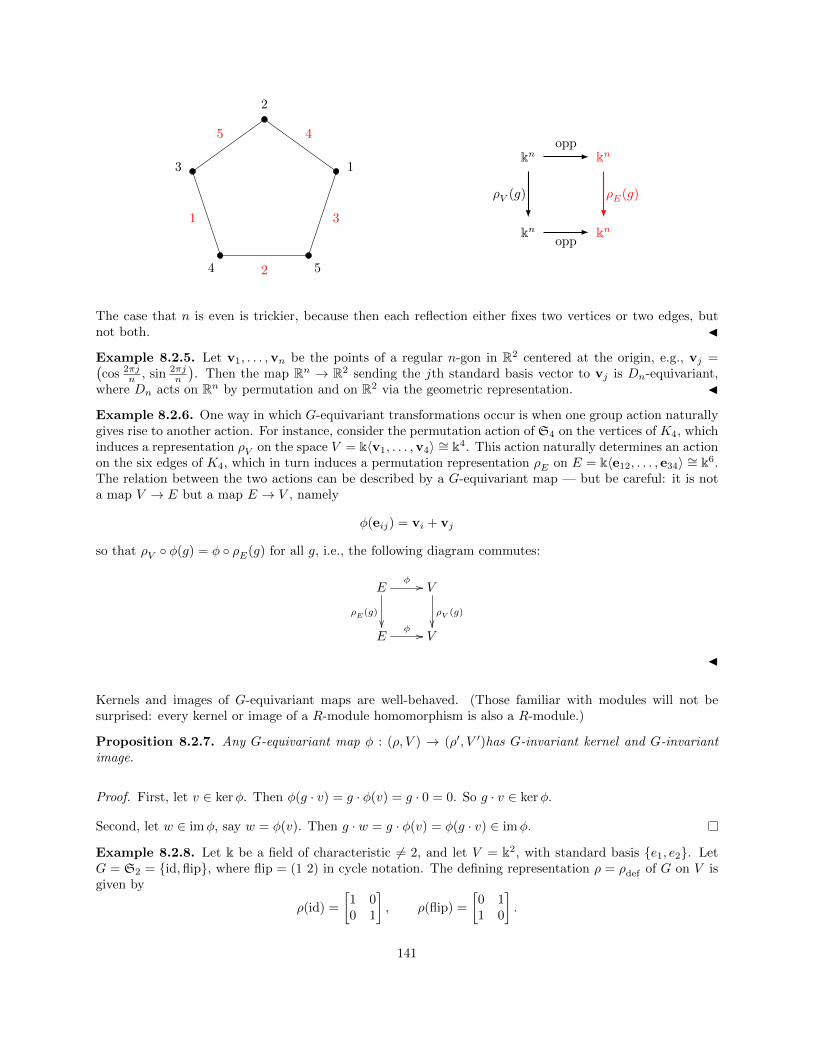
1

1

2

2

3

3

4

4

5

5

kn

kn

kn

knopp

opp

ρE(g)ρV (g)

The case that n is even is trickier, because then each reflection either fixes two vertices or two edges, butnot both.

Example 8.2.5. Let v1, . . . ,vn be the points of a regular n-gon in R2 centered at the origin, e.g., vj =(cos 2πj

n , sin 2πjn

). Then the map Rn → R2 sending the jth standard basis vector to vj is Dn-equivariant,

where Dn acts on Rn by permutation and on R2 via the geometric representation.

Example 8.2.6. One way in which G-equivariant transformations occur is when one group action naturallygives rise to another action. For instance, consider the permutation action of S4 on the vertices of K4, whichinduces a representation ρV on the space V = k⟨v1, . . . ,v4⟩ ∼= k4. This action naturally determines an actionon the six edges of K4, which in turn induces a permutation representation ρE on E = k⟨e12, . . . , e34⟩ ∼= k6.The relation between the two actions can be described by a G-equivariant map — but be careful: it is nota map V → E but a map E → V , namely

ϕ(eij) = vi + vj

so that ρV ϕ(g) = ϕ ρE(g) for all g, i.e., the following diagram commutes:

E

ρE(g)

ϕ // V

ρV (g)

E

ϕ // V

Kernels and images of G-equivariant maps are well-behaved. (Those familiar with modules will not besurprised: every kernel or image of a R-module homomorphism is also a R-module.)

Proposition 8.2.7. Any G-equivariant map ϕ : (ρ, V ) → (ρ′, V ′)has G-invariant kernel and G-invariantimage.

Proof. First, let v ∈ kerϕ. Then ϕ(g · v) = g · ϕ(v) = g · 0 = 0. So g · v ∈ kerϕ.

Second, let w ∈ imϕ, say w = ϕ(v). Then g · w = g · ϕ(v) = ϕ(g · v) ∈ imϕ.

Example 8.2.8. Let k be a field of characteristic = 2, and let V = k2, with standard basis e1, e2. LetG = S2 = id,flip, where flip = (1 2) in cycle notation. The defining representation ρ = ρdef of G on V isgiven by

ρ(id) =

[1 00 1

], ρ(flip) =

[0 11 0

].

141

On the other hand, the representation σ = ρtriv ⊕ ρsign on V (see Examples 8.1.2 and 8.1.9) is given by

σ(id) =

[1 00 1

], σ(flip) =

[1 00 −1

].

These two representations ρ and σ are in fact isomorphic. Indeed, ρ acts trivially on k⟨e1 + e2⟩ and actsby the sign representation on k⟨e1 − e2⟩. These two vectors form a basis of V (here is where we use theassumption chark = 2), and one can check that the change-of-basis map

ϕ =

[1 11 −1

]−1

=

[12

12

12 − 1

2

]is G-equivariant, hence an isomorphism ρ→ σ.

Example 8.2.9. Here is another question about the representations ρtriv and ρsign of S2 = 12, 21: Whatare the G-equivariant maps between them? In other words, which linear maps ϕ : k → k satisfy thediagram (8.1), where ρ, ρ′ ∈ ρtriv, ρsign? Each such map is of the form ϕ(v) = cv for some c ∈ k.

If ρ = ρ′, then any linear transformation ϕ : k → k (i.e., any map ϕ(v) = cv for some c ∈ k) will do. Thusthe set of G-equivariant homomorphisms is actually isomorphic to k.

Assume chark = 2 (otherwise ρtriv = ρsign and we are done at this point). If ϕ : ρtriv → ρsign is G-equivariant,then we have diagrams

V V ′

V V ′

ρtriv(12)

ϕ

ρsign(12)

ϕ

V V ′

V V ′

ρtriv(21)

ϕ

ρsign(21)

ϕ

The first diagram always commutes because ρtriv(12) = ρsign(12) is the identity map, but the second diagramsays that for every v ∈ k

ρsign(ϕ(v)) = −ϕ(v) = −cv, ϕ(ρtriv(v)) = ϕ(v) = cv

and since chark = 2 we are forced to conclude that c = 0. Therefore, there is no nontrivial G-homomorphismρtriv → ρsign.

Example 8.2.9 is the tip of an iceberg: we can use the vector space HomG(ρ, ρ′) of G-homomorphisms

ϕ : ρ→ ρ′ to measure how similar ρ and ρ′ are.

8.3 Irreducibility, indecomposability and Maschke’s theorem

Definition 8.3.1. Let (ρ, V ) be a representation of G.

• A vector subspace W ⊆ V is G-invariant if gW ⊆ W for every g ∈ G. This condition is equivalentto gW = W (because ρ(g) is invertible, hence has no kernel) for every g ∈ G. Thus (ρ|W ,W ) is arepresentation of G (the restriction of ρ to W ). In module language, W is a kG-submodule of V .

• V is decomposable if there are nontrivial G-invariant subspaces W,W⊥ ⊊ V with W ∩W⊥ = 0 andW +W⊥ = V . Here W⊥ is called the (invariant) complement of W in V . The notation does notpresuppose the existence of a scalar product.

142

• V is irreducible (or simple, or colloquially an irrep) if it has no proper G-invariant subspace.• A representation that can be decomposed into a direct sum of irreps is called semisimple or com-pletely reducible. A semisimple representation is determined up to isomorphism by the multiplicitywith which each isomorphism type of irrep appears.

Clearly, every representation can be written as the direct sum of indecomposable representations, and everyirreducible representation is indecomposable. On the other hand, there exist indecomposable representationsthat are not irreducible.

Example 8.3.2. As in Example 8.2.8, let V = e1, e2 be the standard basis for k2, where char k = 2.Recall that the defining representation of S2 = id,flip is given by

ρdef(id) =

[1 00 1

], ρdef(flip) =

[0 11 0

]and the change-of-basis map

ϕ =

[12

12

12 − 1

2

]−1

is a G-equivariant isomorphism ρdef → ρtriv ⊕ ρsign. On the other hand, if chark = 2, then the matrix ϕ isnot invertible and this argument breaks down. In fact, in this case k⟨e1 + e2⟩ is the only proper G-invariantsubspace of V , and consequently ρdef is not semisimple.

Fortunately, we can rule out this kind of pathology most of the time.

Theorem 8.3.3 (Maschke’s Theorem). Let G be a finite group, let k be a field whose characteristic does notdivide |G|, and let (ρ, V ) be a representation of G over k. Then every G-invariant subspace has a G-invariantcomplement. In particular, (ρ, V ) is semisimple.

Proof. If ρ is irreducible, then there is nothing to prove. Otherwise, let W be a G-invariant subspace, andlet π : V → W be a projection, i.e., a linear surjection that fixes the elements of W pointwise. (Such amap π can be constructed as follows: choose a basis for W , extend it to a basis for V , and let π fix all thebasis elements in W and kill all the ones in V \W .)

The map π is k-linear, but not necessarily G-equivariant. However, we can turn π into a G-equivariantprojection by “averaging over G”. (This trick will come up again and again.) Define π : V →W by

π(v) =1

|G|∑g∈G

gπ(g−1v). (8.2)

Claim 1: π is a projection V →W . For any v ∈ V and g ∈ G, we have π(g−1v) ∈W since π is a projection,

and then gπ(g−1) ∈ W because W is G-invariant. So im(π) ⊆ W . Also, if w ∈ W , then g−1w ∈ W , soπ(g−1w) = g−1w and

π(w) =1

|G|∑g∈G

gg−1w = w.

143

Claim 2: π is G-equivariant. Indeed,

π(hv) =1

|G|∑g∈G

gπ(g−1hv)

=1

|G|∑

k∈G: hk=g

(hk)π((hk)−1hv)

=1

|G| h∑k∈G

kπ(k−1v) = hπ(v).

Define W⊥ = ker ϕ. By Prop. 8.2.7, ker π is G-invariant, and V ∼= im π ⊕ ker π =W ⊕W⊥ as vector spaces(this is just linear algebra), so we have found our desired G-invariant complement.

Note that if chark does divide |G|, then the proof breaks down because the definition of π is invalid.(Removing the 1/|G| factor doesn’t work, because ∑g∈G gπ(g

−1v) = |G|v = 0.)

Maschke’s Theorem implies that, when the conditions hold, a representation ρ is determined up to iso-morphism by the multiplicity of each irreducible representation in ρ (i.e., the number of isomorphic copiesappearing as direct summands of ρ). Accordingly, to understand representations of G, we should first studyirreps.

Example 8.3.4. Let k have characteristic 0 (for simplicity), and G = Sn. The defining representation of Gon kn is not simple, because it has an invariant subspace, namely the span of the all-1’s vector, a 1-dimensionalsubspace L that is fixed pointwise by every σ ∈ Sn and therefore carries the trivial representations.1 ByMaschke’s theorem, L has a G-invariant complement. In fact, L⊥ is the orthogonal complement of L underthe standard inner product on kn, namely the space of all vectors whose coordinates sum to 0. This is called(a little confusingly) the standard representation of Sn, denoted ρstd. That is,

ρdef = ρtriv ⊕ ρstd.

Thus dim ρstd = n− 1. We will soon be able to prove that ρstd is irreducible (Exercise 8.2).

8.4 Characters

The first miracle of representation theory is that we can detect the isomorphism type of a representation ρwithout knowing every coordinate of every matrix ρ(g): it turns out that all we need to know is the tracesof the ρ(g).

Definition 8.4.1. Let (ρ, V ) be a representation of G over k. Its character is the function χρ : G → kgiven by

χρ(g) = tr ρ(g).

Note that characters are in general not group homomorphisms.

Example 8.4.2. Some simple facts and some characters we’ve seen before:

• A one-dimensional representation is its own character. (In fact these are exactly the characters thatare homomorphisms.)

• For any representation ρ, we have χρ(IdG) = dim ρ, because ρ(IdG) is the n× n identity matrix.

1For the same reason, every permutation representation of every group has a trivial summand.

144

• The defining representation ρdef of Sn has character

χdef(σ) = number of fixed points of σ.

Indeed, this is true for any permutation representation of any group.• The regular representation ρreg has character

χreg(σ) =

|G| if σ = IdG

0 otherwise.

Example 8.4.3. Consider the geometric representation ρgeo of the dihedral group Dn = ⟨r, s : rn = s2 =0, srs = r−1⟩ by rotations and reflections:

ρgeo(s) =

[1 00 −1

], ρgeo(r) =

[cos θ sin θ− sin θ cos θ

]The character of ρgeo is

χρ(rj) = 2 cos(jθ) (0 ≤ j < n), χρ(sr

j) = 0 (0 ≤ j < n).

On the other hand, if ρ′ is the n-dimensional permutation representation on the vertices, then

χρ′(g) =

n if g = 1,

0 if g is a nontrivial rotation,

1 if n is odd and g is a reflection,

0 if n is even and g is a reflection through two edges,

2 if n is even and g is a reflection through two vertices.

Proposition 8.4.4. Characters are class functions; that is, they are constant on conjugacy classes of G.Moreover, if ρ ∼= ρ′, then χρ = χρ′ .

Proof. For the first assertion, observe that

tr(ρ(hgh−1)

)= tr

(ρ(h)ρ(g)ρ(h−1)

)= tr

(ρ(h)ρ(g)ρ(h)−1

)= tr ρ(g).

because tr(ABA−1) = tr(B) for all matrices A,B with A invertible.

Now, let ϕ : ρ → ρ′ be an isomorphism represented by an invertible matrix Φ; then Φρ(g) = ρ′(g)Φ for allg ∈ G and so Φρ(g)Φ−1 = ρ′(g). Taking traces gives χρ = χρ′ .

Surprisingly, it will turns out that the converse of the second assertion is also true: a representation isdetermined up to isomorphism by its character! In fact, much, much more is true.

145

8.5 New representations and characters from old

The basic vector space functors of direct sum, duality, tensor product and Hom carry over naturally torepresentations, and behave well on their characters. Throughout this section, let (ρ, V ) and (ρ′,W ) befinite-dimensional representations of G over C, with V ∩W = 0.

1. Direct sum. To construct a basis for V ⊕W , we can take the union of a basis for V and a basis for W .Equivalently, we can write the vectors in V ⊕W as column block vectors:

V ⊕W =

[vv′

]: v ∈ V, v′ ∈W

.

Accordingly, we can define the direct sum (ρ⊕ ρ′, V ⊕W ) by

(ρ⊕ ρ′)(h) =[ρ(h) 00 ρ′(h)

].

From this it is clear that χρ⊕ρ′(h) = χρ(h) + χρ′(h).

2. Duality. The dual space V ∗ of V consists of all k-linear transformations ϕ : V → k. A G-representation(ρ, V ) gives rise to a representation (ρ∗, V ∗) given by

(hϕ)(v) = ϕ(h−1v)

for h ∈ G, ϕ ∈ V ∗, v ∈ V . Alternatively, hϕ = ϕ h−1. This is a little counterintuitive (one might expectϕ(hv) on the right-hand side) but it needs to be defined this way in order for ρ∗ to be a homomorphism, i.e.,for ρ∗(gh) to equal ρ∗(g)ρ∗(h) rather than ρ∗(h)ρ∗(g). (Try it.) The representation ρ∗ is called the dualrepresentation (or contragredient) of ρ.

Proposition 8.5.1. For every h ∈ G,χρ∗(h) = χρ(h). (8.3)

where the bar denotes complex conjugate.

Proof. Let J be the Jordan canonical form of ρ(h) (which exists since we are working over C), so thatχρ(h) = tr J . The diagonal entries Jii are its eigenvalues, which must be roots of unity since h has finite

order, so their inverses are their complex conjugates. Meanwhile, J−1 is an upper-triangular matrix with(J−1)ii = (Jii)

−1 = Jii, and trJ−1 = χρ∗(h) = χρ(h).

3. Tensor product. Fix bases e1, . . . , en and f1, . . . , fm for V and W respectively. As a vector space,we define2

V ⊗W = k ⟨ei ⊗ fj : 1 ≤ i ≤ n, 1 ≤ j ≤ m⟩ ,equipped with a multilinear action of k (that is, c(x ⊗ y) = cx ⊗ y = x ⊗ cy for c ∈ k). In particular,dim(V ⊗W ) = (dimV )(dimW ). We can accordingly define a representation (ρ⊗ ρ′, V ⊗W ) by

(ρ⊗ ρ′)(h)(v ⊗ v′) = ρ(h)(v)⊗ ρ′(h)(v′)

or more conciselyh · (v ⊗ v′) = hv ⊗ hv′

extended bilinearly to all of V ⊗W .

2The “official” definition of the tensor product is much more functorial and can be made basis-free, but this concretedefinition is more convenient for our present purposes.

146

In terms of matrices, (ρ⊗ ρ′)(h) is represented by the nm× nm matrix ρ(h)⊗ ρ′(h), defined by

(ρ(h)⊗ ρ′(h))(i,j),(k,ℓ) = (ρ(h))i,k (ρ′(h))j,ℓ.

To explain this alphabet soup, the left-hand side is the entry in the row corresponding to ei⊗ fj and columncorresponding to ek ⊗ fℓ. In particular,

χρ⊗ρ′(h) =∑

(i,j)∈[n]×[m]

(ρ(h))i,i (ρ′(h))j,j =

(n∑

i=1

(ρ(h))i,i

) m∑j=1

(ρ′(h))j,j

= χρ(h)χρ′(h). (8.4)

4. Hom. There are two kinds of Hom:

HomC(V,W ) = C-linear transformations ϕ : V →W,HomG(V,W ) = G-equivariant maps ϕ : V →W.

First, the vector space HomC(V,W ) admits a representation of G, in which h ∈ G acts on a linear transfor-mation ϕ : V →W by sending it to the map h · ϕ defined by

(h · ϕ)(v) = h(ϕ(h−1v)) = ρ′(h)(ϕ(ρ(h−1)(v))

). (8.5)

for h ∈ G, ϕ ∈ HomC(V,W ), v ∈ V . It is straightforward to verify that this is a genuine group action, i.e.,that (hh′) · ϕ = h · (h′ · ϕ).

Moreover, HomC(V,W ) ∼= V ∗ ⊗W as vector spaces and G-modules. To see this, suppose that dimV = nand dimW = m; then the elements of V ∗ and W can be regarded as 1× n and m× 1 matrices respectively(the former acting on V , which consists of n × 1 matrices, by matrix multiplication). Then the previousdescription of tensor product implies that V ∗⊗W consists of m×n matrices, which correspond to elementsof HomC(V,W ). This isomorphism is G-equivariant by (8.5), so

χHom(ρ,ρ′)(h) = χρ∗⊗ρ′(h) = χρ(h) χρ′(h). (8.6)

To summarize so far, we have seen that

χρ⊕ρ′ = χρ + χρ′ , χρ∗ = χρ,

χρ⊗ρ′ = χρ · χρ′ , χHomC(ρ,ρ′) = χρ · χρ′ .

Accordingly, we may apply the functors ⊕, ⊗, ·∗, and Hom to characters, e.g., defining χ⊗ψ by (χ⊗ψ)(g) =χ(g)ψ(g).

What about HomG(V,W ). Evidently HomG(V,W ) ⊆ HomC(V,W ), but equality need not hold. For ex-ample, if V and W are the trivial and sign representations of Sn (for n ≥ 2), then HomC(V,W ) ∼= C butHomG(V,W ) = 0. (See Example 8.2.9.)

The two Homs are related as follows. In general, when a group G acts on a vector space V , the subspaceof G-invariants is defined as

V G = v ∈ V : hv = v ∀h ∈ G.This is the largest subspace of V that carries the trivial action.

Observe that a linear map ϕ : V →W is G-equivariant if and only if hϕ = ϕ for all h ∈ G, where G acts onHomC(V,W ) as above. (The proof of this fact is left to the reader; it is nearly immediate from the definitionof that action.) That is,

HomG(V,W ) = HomC(V,W )G. (8.7)

Moreover, G acts by the identity on HomG(ρ, ρ′), so its character is a constant function whose value is

dimC HomG(ρ, ρ′). We want to understand this quantity.

147

8.6 The Fundamental Theorem of Character Theory

From now on, we assume that k = C (though everything would be true over an algebraically closed field ofcharacteristic 0), unless otherwise specified.

Recall that a class function is a function χ : G→ C that is constant on conjugacy classes of G. Define aninner product on the vector space Cℓ(G) of C-valued class functions by

⟨χ, ψ⟩G =1

|G|∑h∈G

χ(h)ψ(h) =1

|G|∑C

|C| χ(C)ψ(C) (8.8)

where C runs over all conjugacy classes. Observe that ⟨·, ·⟩G is a sesquilinear form (i.e., C-linear in thesecond term and conjugate linear in the first). It is also non-degenerate, because the indicator functions ofconjugacy classes form an orthogonal basis for Cℓ(G). Analysts might want to regard the inner product asa convolution (with summation over G as a discrete analogue of integration).

Proposition 8.6.1. Let (ρ, V ) be a representation of G. Then

dimC VG =

1

|G|∑h∈G

χρ(h) = ⟨χtriv, χρ⟩G .

Proof. The second equality follows from the definition of the inner product. For the first equality, define alinear map π : V → V by

π =1

|G|∑h∈G

ρ(h).

Note that π(v) ∈ V G for all v ∈ V , because

gπ(v) =1

|G|∑h∈G

ghv =1

|G|∑gh∈G

ghv = π(v)

and moreover if v ∈ V (G) then

π(v) =1

|G|∑h∈G

hv =1

|G|∑h∈G

v = v.

That is, π is a projection from V → V G. Choose a basis for V consisting of a basis for V G and extend it toa basis for V . With respect to that basis, π can be represented by the block matrix[

I ∗0 0

]so that

dimC VG = tr(π) =

1

|G|∑h∈G

χρ(h).

By the way, we know by Maschke’s Theorem that V is semisimple, so we can decompose it as a direct sumof irreps. Then V G is precisely the direct sum of the irreducible summands on which G acts trivially.

Example 8.6.2. Let G act on a set X, and let ρ be the corresponding permutation representation on thespace CX. For each orbit O ⊆ X, the vector vO =

∑x∈O x is fixed by G. On the other hand, any vector

148

∑x∈X axx fixed by G must have ax constant on each orbits. Therefore the vectors vO are a basis for V G,

and dimV G is the number of orbits. So Proposition 8.6.1 becomes

# orbits =1

|G|∑h∈G

# fixed points of h

which is Burnside’s Lemma from abstract algebra.

Proposition 8.6.3. For any two representations ρ, ρ′ of G, we have ⟨χρ, χρ′⟩G = dimC HomG(ρ, ρ′).

Proof. Calculate ⟨χρ, χρ′⟩G as

1

|G|∑h∈G

χρ(h)χρ′(h) =1

|G|∑h∈G

χHom(ρ,ρ′)(h) by (8.6)

= dimC Hom(ρ, ρ′)G by Proposition 8.6.1, with V = Hom(ρ, ρ′)

= dimC HomG(ρ, ρ′) by (8.7).

One intriguing observation is that this expression is symmetric in ρ and ρ′, since ⟨α, β⟩G = ⟨β, α⟩G ingeneral, but dimC HomG(ρ, ρ

′) is real. (It is not algebraically obvious that HomG(ρ, ρ′) and HomG(ρ

′, ρ)should have equal dimension.)

Proposition 8.6.4 (Schur’s Lemma). Let G be a group, and let (ρ, V ) and (ρ′, V ′) be finite-dimensionalirreps of G over a field k (not necessarily of characteristic 0).

1. Every G-equivariant map ϕ : V → V ′ is either zero or an isomorphism.2. If in addition k is algebraically closed, then

HomG(V, V′) ∼=

k if ρ ∼= ρ′

0 otherwise.

That is, the only G-equivariant maps from an G-irrep to itself are multiplication by a scalar.

Proof. For (1), recall from Proposition 8.2.7 that kerϕ and imϕ are G-invariant subspaces. But since ρ, ρ′

are simple, there are not many possibilities. Either kerϕ = 0 and imϕ = W , when ϕ is an isomorphism.Otherwise, kerϕ = V or imϕ = 0, either of which implies that ϕ = 0.

For (2), the “otherwise” case follows from (1), so suppose V ∼= V ′. Actually, for simplicity, assume V = V ′.Since k is algebraically closed, every G-equivariant map ϕ : V → V has an eigenvalue λ. Then ϕ − λI isG-equivariant and singular, hence zero by (1). So ϕ = λI is multiplication by λ.

We can now prove the following omnibus theorem, which essentially reduces the study of representations offinite groups to the study of characters.

Theorem 8.6.5 (Fundamental Theorem of Character Theory for Finite Groups). Let (ρ, V ) and(ρ′, V ′) be finite-dimensional representations of G over C.

1. If ρ and ρ′ are irreducible, then

⟨χρ, χρ′⟩G =

1 if ρ ∼= ρ′,

0 otherwise.(8.9)

In particular, there are only finitely many isomorphism classes of irreps of G.

149

2. If ρ1, . . . , ρn are distinct irreducible representations and

ρ =

n⊕i=1

(ρi ⊕ · · · ⊕ ρi︸︷︷︸mi

) =

n⊕i=1

ρ⊕mii

then

⟨χρ, χρi⟩G = mi and ⟨χρ, χρ⟩G =

n∑i=1

m2i .

In particular, ⟨χρ, χρ⟩G = 1 if and only if ρ is irreducible.3. Characters are complete invariants for their representations. That is, if χρ = χρ′ then ρ ∼= ρ′.4. Let ρ1, . . . , ρn be a complete list of irreps of G up to isomorphism. Then

ρreg∼=

n⊕i=1

ρ⊕ dim ρi

i

and consequentlyn∑

i=1

(dim ρi)2 = |G|. (8.10)

5. The irreducible characters (i.e., characters of irreps) form an orthonormal basis for Cℓ(G). In partic-ular, the number of irreducible characters equals the number of conjugacy classes of G.

Proof. For assertion (1), the equation (8.9) follows from part (2) of Schur’s Lemma together with Proposi-tion 8.6.3. It follows that the characters of isomorphism classes of irreps are an orthonormal basis for somesubspace of the finite-dimensional space Cℓ(G), so there can be only finitely many of them. (This resultcontinues to amaze me every time I think about it.)

Assertion (2) follows because the inner product is additive on direct sums. That is, every class function ψsatisfies

⟨χρ⊕ρ′ , ψ⟩G = ⟨χρ + χρ′ , ψ⟩G = ⟨χρ, ψ⟩G + ⟨χρ′ , ψ⟩G .

For (3), Maschke’s Theorem says that every complex representation ρ can be written as a direct sum ofirreducibles. Their multiplicities determine ρ up to isomorphism, and can be recovered from χρ by (2).(Again, amazing.)

For (4), recall that χreg(IdG) = |G| and χreg(g) = 0 for g = IdG. Therefore⟨χreg, ρi

⟩G=

1

|G|∑g∈G

χreg(g)ρi(g) =1

|G| |G|ρi(IdG) = dim ρi

so ρi appears in ρreg with multiplicity equal to its dimension.

For (5), the irreducible characters are orthonormal (hence linearly independent in Cℓ(G)), by Schur’s Lemmatogether with assertion (3). The trickier part is to show that they in fact span Cℓ(G). Let Y be the subspaceof Cℓ(G) spanned by the irreducible characters, and let

Z = Y ⊥ =ϕ ∈ Cℓ(G) : ⟨ϕ, χρ⟩G = 0 for every irreducible character ρ

.

We will show that Z = 0.

150

Let ϕ ∈ Z. For any representation (ρ, V ), define a map Tρ = Tρ,ϕ : V → V by

Tρ =1

|G|∑g∈G

ϕ(g) ρ(g)

or equivalently

Tρ(v) =1

|G|∑g∈G

ϕ(g)gv

(to parse this, note that ϕ(g) is a number). Our plan is to show that Tρ is the zero map (in disguise), thendeduce that ϕ = 0.

Claim 1: Tρ is G-equivariant. Let h ∈ G; then

Tρ(hv) =1

|G|∑g∈G

ϕ(g) ghv

=1

|G|h∑g∈G

ϕ(g)h−1ghv

= h1

|G|∑k∈G

ϕ(hkh−1) kv (setting k = h−1gh, hkh−1 = g)

= h1

|G|∑k∈G

ϕ(k) kv (because ϕ ∈ Cℓ(G))

= hTρ(v).

Claim 2: Tρ = 0 if ρ is irreducible. Now that we know that Tρ is G-equivariant, Schur’s Lemma implies thatit is multiplication by a scalar. On the other hand

tr(Tρ) =1

|G|∑g∈G

ϕ(g)χρ(g) = ⟨ϕ, χρ⟩G = 0

because ϕ ∈ Z = Y ⊥. Since Tρ has trace zero and is multiplication by a scalar, it is the zero map.3

Claim 3: Tρ = 0 in all cases. By Maschke’s Theorem, every complex representation ρ is semisimple, and the

definition of Tρ implies that it is additive on direct sums (that is, Tρ⊕ρ′ = Tρ + Tρ′), proving the claim.

We now apply Claim 3 to the regular representation:

0 = Tρreg(IdG) =

1

|G|∑g∈G

ϕ(g)ρreg(g).

This is an equation in the vector space of |G| × |G| matrices. Observe that the permutation matrices ρreg(g)have disjoint supports (the only group element that maps h to k is kh−1), hence are linearly independent.Therefore ϕ(g) = 0 for all g, so ϕ is the zero map.

We have now shown that Y has trivial orthogonal complement as a subspace of Cℓ(G), so Y = Cℓ(G),completing the proof.

Corollary 8.6.6. Let ρ1, . . . , ρn be the irreps of G, and let α =⊕n

i=1 ρ⊕aii and β =

⊕ni=1 ρ

⊕bii be two rep-

resentations. Then dimHomG(α, β) =∑n

i=1 aibi, and in particular HomG(α, β) is a direct sum of constantmaps between irreducible summands of α and β.

3This inference would not be valid in positive characteristic!

151

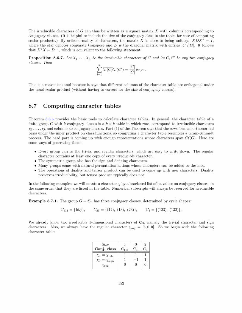
The irreducible characters of G can thus be written as a square matrix X with columns corresponding toconjugacy classes. (It is helpful to include the size of the conjugacy class in the table, for ease of computingscalar products.) By orthonormality of characters, the matrix X is close to being unitary: XDX∗ = I,where the star denotes conjugate transpose and D is the diagonal matrix with entries |C|/|G|. It followsthat X∗X = D−1, which is equivalent to the following statement:

Proposition 8.6.7. Let χ1, . . . , χn be the irreducible characters of G and let C,C ′ be any two conjugacyclasses. Then

n∑i=1

χi(C)χi(C′) =

|G||C| δC,C′ .

This is a convenient tool because it says that different columns of the character table are orthogonal underthe usual scalar product (without having to correct for the size of conjugacy classes).

8.7 Computing character tables

Theorem 8.6.5 provides the basic tools to calculate character tables. In general, the character table of afinite group G with k conjugacy classes is a k × k table in which rows correspond to irreducible charactersχ1. . . . , χk and columns to conjugacy classes. Part (1) of the Theorem says that the rows form an orthonormalbasis under the inner product on class functions, so computing a character table resembles a Gram-Schmidtprocess. The hard part is coming up with enough representations whose characters span Cℓ(G). Here aresome ways of generating them:

• Every group carries the trivial and regular characters, which are easy to write down. The regularcharacter contains at least one copy of every irreducible character.

• The symmetric group also has the sign and defining characters.• Many groups come with natural permutation actions whose characters can be added to the mix.• The operations of duality and tensor product can be used to come up with new characters. Dualitypreserves irreducibility, but tensor product typically does not.

In the following examples, we will notate a character χ by a bracketed list of its values on conjugacy classes, inthe same order that they are listed in the table. Numerical subscripts will always be reserved for irreduciblecharacters.

Example 8.7.1. The group G = S3 has three conjugacy classes, determined by cycle shapes:

C111 = IdG, C21 = (12), (13), (23), C3 = (123), (132).

We already know two irreducible 1-dimensional characters of S3, namely the trivial character and signcharacters. Also, we always have the regular character χreg = [6, 0, 0]. So we begin with the followingcharacter table:

Size 1 3 2Conj. class C111 C21 C3

χ1 = χtriv 1 1 1χ2 = χsign 1 −1 1

χreg 6 0 0

152

Equation (8.10) says that S3 has three irreps, the squares of whose dimensions add up to |S3| = 6. So weare looking for one more irreducible character χother of dimension 2. By (e) of Theorem 8.6.5, we have

χreg = χtriv + χsign + 2χother

from it which is easy to obtainχother = [2, 0,−1].

One can check that χother is irreducible by confirming that its scalar product with itself is 1. By the way,the defining representation of S3 is χdef = χtriv ⊕ χother.

Example 8.7.2. We calculate all the irreducible characters of S4. There are five conjugacy classes, cor-responding to the cycle-shapes 1111, 211, 22, 31, and 4. The squares of their dimensions must add up to|S4| = 24; the only list of five positive integers with that property is 1, 1, 2, 3, 3.

We start by writing down some characters that we know.

Size 1 6 3 8 6Conj. class C1111 C211 C22 C31 C4

χ1 = χtriv 1 1 1 1 1χ2 = χsign 1 −1 1 1 −1

χdef 4 2 0 1 0χreg 24 0 0 0 0

Of course χtriv and χsign are irreducible, since they are 1-dimensional. On the other hand, χdef can’t beirreducible because S4 doesn’t have a 4-dimensional irrep. Indeed,

⟨χdef , χdef⟩G = 2

which means that ρdef must be a direct sum of two distinct irreps. (If it were the direct sum of two copies ofthe unique 2-dimensional irrep, then ⟨χdef , χdef⟩G would be 4, not 2, by (ii) of Theorem 8.6.5.) We calculate

⟨χdef , χtriv⟩G = 1,⟨χdef , χsign

⟩G= 0.

Therefore χ3 = χdef − χtriv is an irreducible character.

Another 3-dimensional character is χ4 = χ3 ⊗ χsign. It is easy to check that ⟨χ4, χ4⟩G = 1, so χ4 isirreducible.

The other irreducible character χ5 has dimension 2. We can calculate it from the regular character and theother four irreducibles, because

χreg = (χ1 + χ2) + 3(χ3 + χ4) + 2χ5

and so

χ5 =χreg − χ1 − χ2 − 3χ3 − 3χ4

2.

and so the complete character table of S4 is as follows.

Size 1 6 3 8 6Conj. class C1111 C211 C22 C31 C4

χ1 1 1 1 1 1χ2 1 −1 1 1 −1χ3 3 1 −1 0 −1χ4 3 −1 −1 0 1χ5 2 0 2 −1 0

153

8.8 One-dimensional characters

A one-dimensional character of G is identical with the representation it comes from: a group homomorphismG→ C×. Since tensor product is multiplicative on dimension, it follows that the tensor product of two one-dimensional characters is also one-dimensional.. In fact χ ⊗ χ′(g) = χ(g)χ′(g) (this is immediate from thedefinition of tensor product) and χ⊗χ∗ = χtriv. So the set Ch(G) of characters, i.e., Ch(G) = Hom(G,C×),is an abelian group under tensor product (equivalently, pointwise multiplication), with identity χtriv.

Definition 8.8.1. The commutator of two elements a, b ∈ G is the element [a, b] = aba−1b−1. The (normal)subgroup of G generated by all commutators is called the commutator subgroup, denoted [G,G]. Thequotient Gab = G/[G,G] is the abelianization of G.

The abelianization can be regarded as the group obtained by forcing all elements G to commute, in additionto whatever relations already exist in G; in other words, it is the largest abelian quotient of G. It isroutine to check that [G,G] is indeed normal in G, and also that χ([a, b]) = IdG for all χ ∈ Ch(G) anda, b ∈ G. (In fact, this condition characterizes the elements of the commutator subgroup, as will be shownsoon.) Therefore, when studying one-dimensional characters on G, we may as well assume G is abelian (i.e.,Ch(G) ∼= Ch(Gab)).

Accordingly, let G be an abelian group of finite order n. The conjugacy classes of G are all singleton sets(since ghg−1 = h for all g, h ∈ G), so there are n distinct irreducible representations of G. By (8.10) ofTheorem 8.6.5, so in fact every irreducible character is 1-dimensional (and every representation of G is adirect sum of 1-dimensional representations). We have now reduced the problem to describing the grouphomomorphisms G→ C×.

The simplest case is that G = Z/nZ is cyclic. Write G multiplicatively, and let g be a generator. Then eachχ ∈ Ch(G) is determined by its value on g, which must be some nth root of unity. There are n possibilitiesfor χ(g), so all the irreducible characters of G arise in this way, and in fact form a group isomorphic to Z/nZ,generated by any character that maps g to a primitive nth root of unity. So Hom(G,C×) ∼= G (althoughthis isomorphism is not canonical).

Now we consider the general case. Every abelian group G can be written as

G ∼=r∏

i=1

Z/niZ.

Let gi be a generator of the ith factor, and let ζi be a primitive (ni)th root of unity. Then each character χis determined by the numbers j1, . . . , jr, where ji ∈ Z/niZ and χ(gi) = ζjii for all i. Thus Hom(G,C×) ∼= G,an isomorphism known as Pontryagin duality. More generally, for any finite group G (not necessarilyabelian), there is an isomorphism

Hom(G,C×) ∼= Gab. (8.11)

This is quite useful when computing the character table of a group: if you can figure out the commutatorsubgroup and/or the abelianization, then you can immediately write down the one-dimensional characters.Sometimes the size of the abelianization can be determined from the size of the group and the number ofconjugacy classes. (The commutator subgroup is normal, so it itself is a union of conjugacy classes.)

The description of characters of abelian groups implies that if G is abelian and g = IdG, then χ(g) = 1 forat least one character χ. Therefore, for every group G, we have

[G,G] = g ∈ G : χ(g) = 1 for all 1-dimensional characters χ

since [G,G] is the identity element of Gab. This

154

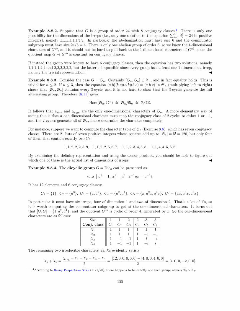
Example 8.8.2. Suppose that G is a group of order 24 with 8 conjugacy classes.4 There is only onepossibility for the dimensions of the irreps (i.e., only one solution to the equation

∑8i=1 d

2i = 24 in positive

integers), namely 1,1,1,1,1,1,3,3. In particular the abelianization must have size 6 and the commutatorsubgroup must have size 24/6 = 4. There is only one abelian group of order 6, so we know the 1-dimensionalcharacters of Gab, and it should not be hard to pull back to the 1-dimensional characters of Gab, since thequotient map G→ Gab is constant on conjugacy classes.

If instead the group were known to have 6 conjugacy classes, then the equation has two solutions, namely1,1,1,1,2,4 and 2,2,2,2,2,2, but the latter is impossible since every group has at least one 1-dimensional irrep,namely the trivial representation.

Example 8.8.3. Consider the case G = Sn. Certainly [Sn,Sn] ⊆ An, and in fact equality holds. This istrivial for n ≤ 2. If n ≤ 3, then the equation (a b)(b c)(a b)(b c) = (a b c) in Sn (multiplying left to right)shows that [Sn,Sn] contains every 3-cycle, and it is not hard to show that the 3-cycles generate the fullalternating group. Therefore (8.11) gives

Hom(Sn,C×) ∼= Sn/An∼= Z/2Z.

It follows that χtriv and χsign are the only one-dimensional characters of Sn. A more elementary way ofseeing this is that a one-dimensional character must map the conjugacy class of 2-cycles to either 1 or −1,and the 2-cycles generate all of Sn, hence determine the character completely.

For instance, suppose we want to compute the character table ofS5 (Exercise 8.6), which has seven conjugacyclasses. There are 21 lists of seven positive integers whose squares add up to |S5| = 5! = 120, but only fourof them that contain exactly two 1’s:

1, 1, 2, 2, 2, 5, 9, 1, 1, 2, 2, 5, 6, 7, 1, 1, 2, 3, 4, 5, 8, 1, 1, 4, 4, 5, 5, 6.

By examining the defining representation and using the tensor product, you should be able to figure outwhich one of these is the actual list of dimensions of irreps.

Example 8.8.4. The dicyclic group G = Dic3 can be presented as

⟨a, x∣∣ a6 = 1, x2 = a3, x−1ax = a−1⟩.

It has 12 elements and 6 conjugacy classes:

C1 = 1, C2 = a3, C3 = a, a5, C4 = a2, a4, C5 = x, a2x, a4x, C6 = ax, a3x, a5x.

In particular it must have six irreps, four of dimension 1 and two of dimension 2. That’s a lot of 1’s, soit is worth computing the commutator subgroup to get at the one-dimensional characters. It turns outthat [G,G] = 1, a2, a4, and the quotient Gab is cyclic of order 4, generated by x. So the one-dimensionalcharacters are as follows:

Size 1 1 2 2 3 3Conj. class C1 C2 C3 C4 C5 C6

χ1 1 1 1 1 1 1χ2 1 1 1 1 −1 −1χ3 1 −1 −1 1 i −iχ4 1 −1 −1 1 −i i

The remaining two irreducible characters χ5, χ6 evidently satisfy

χ5 + χ6 =χreg − χ1 − χ2 − χ3 − χ4

2=

[12, 0, 0, 0, 0, 0]− [4, 0, 0, 4, 0, 0]

2= [4, 0, 0,−2, 0, 0].

4According to Group Properties Wiki (11/1/20), there happens to be exactly one such group, namely A4 × Z2.

155

https://groupprops.subwiki.org/wiki/Linear_representation_theory_of_groups_of_order_24

Write them asχ5 = [2, a, b,−1 + c, d, e], χ6 = [2,−a,−b,−1− c,−d,−e].

Tensoring with any one-dimensional character has to either preserve or swap both χ5 and χ6, and in particulartensoring with χ2 = χ3 ⊗ χ3 must preserve it. But then d = −d and e = −e, and our lives have just gottensomewhat easier, as we can write

χ5 = [2, a, b,−1 + c, 0, 0], χ6 = [2,−a,−b,−1− c, 0, 0].

Now let’s take some scalar products:

⟨χ1, χ5⟩G = 2 + a+ 2b+ 2(−1 + c) = 0,

⟨χ3, χ5⟩G = 2− a− 2b+ 2(−1 + c) = 0.

Adding these equations gives 4 + 4(−1 + c) = 0, or c = 0; subtracting them gives a = −2b. At this pointwe know that the C3 and C4 columns of the character table are (1, 1,−1,−1, b,−b) and (1, 1, 1, 1,−1, 1)respectively. By Proposition 8.6.7 they are orthogonal, i.e., 2− 2b = 0, or b = 1. So the final character tableis as follows:

Size 1 1 2 2 3 3Conj. class C1 C2 C3 C4 C5 C6

χ1 1 1 1 1 1 1χ2 1 1 1 1 −1 −1χ3 1 −1 −1 1 i −iχ4 1 −1 −1 1 −i iχ5 2 −2 1 −1 0 0χ6 2 2 −1 1 0 0

8.9 Restriction, induction, and Frobenius reciprocity

Let H ⊆ G be finite groups. Representations of G give rise to representations of H via an (easy) processcalled restriction, and representations of H give rise to representations of G via a (somewhat more involved)process called induction. These processes are sources of more characters to put in character tables, and thetwo are related by an equation called Frobenius reciprocity.

Restriction. Let ρ : G→ GL(V ) be a representation of G. Then the restriction of ρ to H is a representationof G, denoted ResGH(ρ). Alternative notations include Res(ρ) (if the groups G and H are clear from context)and ρ↓GH . Likewise, the restriction of χ = χρ to H is a character of H denoted by ResGH(χ).

Restricting a representation does not change its character on the level of group elements. On the other hand,the restriction of an irreducible representation is not always irreducible. (Also, two elements conjugate in Gare not necessarily conjugate in a subgroup H.)

Example 8.9.1. Let Cλ denote the conjugacy class in Sn of permutations of cycle-shape λ. Recall thatthe standard representation ρstd of G = S3 has character

χstd(C111) = 2, χstd(C21) = 0, χstd(C3) = −1,

and ⟨χstd, χstd⟩G = 1 because ρstd is irreducible. On the other hand, let H = A3 ⊆ S3. This is anabelian group isomorphic to Z/3Z, so the two-dimensional representation Res(ρstd) is not irreducible. In

156

fact H = C111 ∪ C3, so ⟨χstd, χstd⟩G = (1 · 22 + 2 · (−1)2)/3 = 2. (We knew this already, since if a 2-dimensional representation is not irreducible then it must be the direct sum of two one-dimensional irreps.)The group A3 is cyclic, so its character table is

IdG (1 2 3) (1 3 2)χtriv 1 1 1χ1 1 ω ω2

χ2 1 ω2 ω

(8.12)

where ω = e2πi/3. (Note also that the conjugacy class C3 ⊆ S3 splits into two singleton conjugacy classes inA3.) Now it is evident that Res(χstd) = [2,−1,−1] = χ1 + χ2.

Induction. Let H ⊆ G be groups and let (ρ,W ) be a representation of H. We want to “lift” ρ to arepresentation of G. This is potentially very powerful because it is typically easy to get our hands onsubgroups of G (e.g., every element of G generated a cyclic subgroup) and so this lifting operation canpotentially be a rich source of representations of G.

Let V be a direct sum of copies of W , one for each (left) coset of H in G. For the sake of bookkeeping, picka set of coset representatives B = b1, . . . , bn ⊆ G, so that G = b1H ∪· · · · ∪· bnH, so that we can think of Vas a sum of copies of W , indexed by B. (Here n = [G : H] = |G|/|H|.) We will write the elements of V astensors:

V = CB ⊗W = (b1 ⊗W )⊕ · · · ⊕ (bn ⊗W ).

To say how a group element g ∈ G acts on the summand bi⊗W , we want to write gbi in the form bjh, wherej ∈ [n] and h ∈ H. We then make g act by

g(bi ⊗ w) = bj ⊗ ρ(h)(w), (8.13)

extended linearly to all of V . Heuristically, this formula is justified by the equation

g(bi ⊗ w) = gbi ⊗ w = bjh⊗ w = bj ⊗ hw = bj ⊗ ρ(h)(w).

In other words, g sends bi ⊗W to bj ⊗W , acting by h along the way. Thus we have a map IndGH(ρ) that

sends each g ∈ G to the linear transformation V → V just defined. Alternative notations for IndGH(ρ) includeInd(ρ) (if G and H are clear from context) and ρ ↑GH .

On the level of matrices, IndGH(ρ)(g) is an n× n block matrix with blocks Bij of size dim ρ, given by

Bij =

ρ(h) if gbi = bjh for some h ∈ H0 otherwise

=

ρ(b−1

j gbi) if b−1j gbi ∈ H

0 otherwise.(8.14)

Example 8.9.2. Let G = S3 and H = A3 = Id, (1 2 3), (1 3 2), and let (ρ,W ) be a representation of H,where W = C⟨e1, . . . , en⟩. Let B = b1 = Id, b2 = (1 2), so that V = b1 ⊗W ⊕ b2 ⊗W . To define theinduced representation, we need to solve the equations gbi = bjh. That is, for each g ∈ G and each bi ∈ B,we need to determine the unique pair bj , h that satisfy the equation.

i = 1 i = 2g gbi = bj h gbi = bj hId Id = b1 Id (1 2) = b2 Id

(1 2 3) (1 2 3) = b1 (1 2 3) (1 3) = b2 (1 3 2)(1 3 2) (1 3 2) = b1 (1 3 2) (2 3) = b2 (1 2 3)(1 2) (1 2) = b2 Id Id = b1 Id(1 3) (1 3) = b2 (1 2 3) (1 2 3) = b1 (1 2 3)(2 3) (2 3) = b2 (1 3 2) (1 3 2) = b1 (1 3 2)

157

Therefore, the representation IndGH(ρ) sends the elements of S3 to the following block matrices. Each blockis of size n× n; the first block corresponds to b1 ⊗W and the second block to b2 ⊗W .

Id 7→[ρ(Id) 00 ρ(Id)

](1 2 3) 7→

[ρ(1 2 3) 0

0 ρ(1 3 2)

](1 3 2) 7→

[ρ(1 3 2) 0

0 ρ(1 2 3)

]

(1 2) 7→[

0 ρ(Id)ρ(Id) 0

](1 3) 7→

[0 ρ(1 2 3)

ρ(1 2 3) 0

](2 3) 7→

[0 ρ(1 3 2)

ρ(1 3 2) 0

]

For instance, if ρ is the 1-dimensional representation (= character) χ1 of (8.12), then the character of Ind(ρ)is given on conjugacy classes in S3 by

χInd(ρ)(C111) = 2, χInd(ρ)(C21) = ω + ω2 = −1, χInd(ρ)(C3) = 0,

which implies that IndGH(ρ) is the nontrivial summand of the defining representation of S3.

Example 8.9.3. Let G = S3 and H = Id, (1 2). Let (ρ,W ) be a representation of H, where W =C⟨e1, . . . , en⟩. Let B = b1 = Id, b2 = (1 3), b3 = (2 3) and V = CB ⊗ W . To define the inducedrepresentation, we take the equations gbi = bjh, for each g and i, and solve them for bj and h:

i = 1 i = 2 i = 3g gbi = bj h gbi = bj h gbi = bj hId Id = b1 Id (1 3) = b2 Id (2 3) = b3 Id

(1 2) (1 2) = b1 (1 2) (1 3 2) = b3 (1 2) (1 2 3) = b2 (1 2)(1 3) (1 3) = b2 Id Id = b1 Id (1 3 2) = b3 (1 2)(1 2 3) (1 2 3) = b2 (1 2) (2 3) = b3 Id (1 2) = b1 (1 2)(2 3) (2 3) = b3 Id (1 2 3) = b2 (1 2) Id = b1 Id(1 3 2) (1 3 2) = b3 (1 2) (1 2) = b1 (1 2) (1 3) = b2 Id

Thus IndGH(ρ) is as follows:

Id 7→

ρ(Id) 0 00 ρ(Id) 00 0 ρ(Id)

(1 3) 7→

0 ρ(Id) 0ρ(Id) 0 00 0 ρ(1 2)

(2 3) 7→

0 0 ρ(Id)0 ρ(1 2) 0

ρ(Id) 0 0

(1 2) 7→

ρ(1 2) 0 00 0 ρ(1 2)0 ρ(1 2) 0

(1 2 3) 7→

0 ρ(1 2) 00 0 ρ(Id)

ρ(1 2) 0 0

(1 3 2) 7→

0 0 ρ(1 2)ρ(1 2) 0 0

0 ρ(Id) 0

In fact, Ind(ρ) is a representation, and there is a general formula for its character. (That is a good thing,because as you see computing the induced representation itself is a lot of work.)

Proposition 8.9.4. Let H be a subgroup of G and let (ρ,W ) be a representation of H with character χ.Then IndGH(ρ) is a representation of G, with character defined on g ∈ G by

IndGH(χ)(g) =1

|H|∑

k∈G: k−1gk∈H

χ(k−1gk).

In particular, Ind(χρ), hence Ind(ρ), is independent (up to isomorphism) of the choice of B.

158

(We know that characters are class functions, so why not write χ(g) instead of χ(k−1gk)? Because χ is afunction on H, so the former expression is not well-defined in general.)

Proof. First, we verify that Ind(ρ) is a representation. Let g, g′ ∈ G and bi⊗w ∈ V . Then there is a uniquebk ∈ B and h ∈ H such that

gbi = bkh (8.15)

and in turn there is a unique bℓ ∈ B and h′ ∈ H such that

g′bk = bℓh′. (8.16)

We need to verify that g′ · (g · (bi ⊗ w)) = (g′g) · (bi ⊗ w). Indeed,(g′ · (g · (bi ⊗ w)) = g′ · (bk ⊗ hw)

)= bℓ ⊗ h′hw.

On the other hand, by (8.15) and (8.16), gbi = bkhb−1i and g′ = bℓh

′b−1k , so

(g′g) · (bi ⊗ w) = (bℓh′hb−1

i ) · (bi ⊗ w) = bℓ ⊗ h′hw

as desired. Note by the way that

dim Ind(ρ) =|G||H| dim ρ.

Now that we know that Ind(ρ) is a representation of G on V , we calculate its character using (8.14):

Ind(χ)(g) =

r∑i=1

tr(Bi,i) =∑

i∈[r]: b−1i gbi∈H

χ(b−1i gbi)

=∑

i∈[r]: b−1i gbi∈H

1

|H|∑h∈H

χ(h−1b−1i gbih)

(because χρ is constant on conjugacy classes of H — the averaging trick again!)

=1

|H|∑

k∈G: k−1gk∈H

χ(k−1gk) (8.17)

as desired. Here k = bih runs over all elements of G as the indices of summation i, h on the previous sumrun over [r] and H respectively. (Also, k−1gk = h−1b−1

i gbih ∈ H if and only if b−1i gbi ∈ H, simply because

H is a group.) Since Ind(χ) is independent of the choice of B, so is the isomorphism type of Ind(ρ).

Corollary 8.9.5. Let H ⊆ G and let ρ be the trivial representation of H. Then

IndGH(χtriv)(g) =#k ∈ G : k−1gk ∈ H

|H| .

Corollary 8.9.6. Suppose H is a normal subgroup of G. Then

IndGH(χ)(g) =

|G||H|χ(g) if g ∈ H,0 otherwise.

Proof. Normality implies that k−1gk ∈ H if and only if g ∈ H, independently of k. If g ∈ H then the sumin (8.17) has |G| terms, all equal to χ(g); otherwise, the sum is empty. (Alternative proof: normality impliesthat left cosets and right cosets coincide, so the blocks in the block matrix Ind(ρ)(g) will all be on the maindiagonal (and equal to ρ(g)) when g ∈ H, and off the main diagonal otherwise.)

159

Example 8.9.7. Let n ≥ 2, so that An is a normal subgroup of Sn of index 2. Either Corollary 8.9.5 orCorollary 8.9.6 imply that

IndSn

An(χtriv)(g) =

2 for g ∈ A3,

0 for g ∈ A3,

which is the sum of the trivial and sign characters on Sn.

Example 8.9.8. Let G = S4 and let H be the subgroup id, (1 2), (3 4), (1 2)(3 4). Note that H isnot a normal subgroup of G. Let ρ be the trivial representation of G and χ its character. We can calculateψ = IndGH χ using Corollary 8.9.5:

ψ(C1111) = 6, ψ(C211) = 2, ψ(C22) = 2, ψ(C31) = 0, ψ(C4) = 0.

where, as usual, Cλ denotes the conjugacy class in S4 of permutations with cycle-shape λ. In the notationof Example 8.7.2, the decomposition into irreducible characters is χ1 + χ2 + 2χ5.

Restriction and induction are related by the following useful formula.

Theorem 8.9.9 (Frobenius Reciprocity). Let H ⊆ G be groups, let χ be a character of H, and let ψ be acharacter of G. Then ⟨

IndGH(χ), ψ⟩G=⟨χ, ResGH(ψ)

⟩H.

Proof.

⟨Ind(χ), ψ⟩G =1

|G|∑g∈G

Ind(χ)(g) · ψ(g)

=1

|G|∑g∈G

1

|H|∑

k∈G: k−1gk∈H

χ(k−1gk) · ψ(g) (by Prop. 8.9.4)

=1

|G||H|∑h∈H

∑k∈G

∑g∈G: k−1gk=h

χ(h) · ψ(k−1gk)

=1

|G||H|∑h∈H

∑k∈G

χ(h) · ψ(h) (i.e., g = khk−1)

=1

|H|∑h∈H

χ(h) · ψ(h) = ⟨χ, Res(ψ)⟩H .

This will be useful later; for now, here is a quick application.

Example 8.9.10. Sometimes, Frobenius reciprocity suffices to calculate the isomorphism type of an inducedrepresentation. Let G = S3 and H = A3, and let ψ, χ1 and χ2 be as in Example 8.9.1. We would like tocompute Ind(χ1). By Frobenius reciprocity

⟨Ind(χ1), ψ⟩G = ⟨χ1, Res(ψ)⟩H = 1.

But ψ is irreducible. Therefore, it must be the case that Ind(χ1) = ψ, and the corresponding representationsare isomorphic. The same is true if we replace χ1 with χ2.

160

8.10 Characters of the symmetric group

We have worked out the irreducible characters of S3, S4 and S5 ad hoc (the last as an exercise). In fact,we can do this for all n, exploiting a vast connection to the combinatorics of partitions and tableaux.

Recall (Defn. 1.2.4) that a partition of n is a sequence λ = (λ1, . . . , λℓ) of weakly decreasing positive integerswhose sum is n. We’ll sometimes drop the parentheses and commas. We write λ ⊢ n or |λ| = n to indicatethat λ is a partition of n. The number ℓ = ℓ(λ) is the length of λ. The set of all partitions of n is Par(n),and the number of partitions of n is p(n) = |Par(n)|. For example,

p(5) = |Par(5)| = |5, 41, 32, 311, 221, 2111, 11111 = 7.

We’ll write Par for the set of all partitions. (As a set this is the same as Young’s lattice, which we used tocall Y .)

For each λ ⊢ n, let Cλ be the conjugacy class in Sn consisting of all permutations with cycle shape λ. Sincethe conjugacy classes are in bijection with Par(n), it makes sense to look for a set of representations indexedby partitions.

Definition 8.10.1. Let µ = (µ1, . . . , µℓ) ⊢ n.

• The Ferrers diagram of shape µ is the top- and left-justified array of boxes with µi boxes in the ithrow.

• A (Young) tableau5 of shape µ is a Ferrers diagram with the numbers 1, 2, . . . , n placed in theboxes, one number to a box.

• Two tableaux T, T ′ of shape µ are row-equivalent, written T ∼ T ′, if the numbers in each row of Tare the same as the numbers in the corresponding row of T ′.

• A (Young) tabloid of shape µ is an equivalence class of tableaux under row-equivalence. A tabloidcan be represented as a tableau without vertical lines.

• We write sh(T ) = µ to indicate that a tableau or tabloid T is of shape µ.

1 3 6

2 7

4 5

1 3 6

2 7

4 5

Ferrers diagram Young tableau Young tabloid

A Young tabloid can be regarded as an ordered set partition (T1, . . . , Tm) of [n] in which |Ti| = µi. Theorder of the blocks Ti matters, but not the order of entries within each block. Thus the number of tabloidsof shape µ is (

n

µ

)=

n!

µ1! · · ·µm!.

The symmetric group Sn acts on tabloids by permuting the numbers. This action gives rise to a permutationrepresentation (ρµ, Vµ) ofSn, the µ-tabloid representation ofSn. Here Vµ is the vector space of all formalC-linear combinations of tabloids of shape µ. The character of ρµ will be denoted τµ.

5Terminology of tableaux is not consistent: some authors reserve the term “Young tableau” for a tableau in which thenumbers increase downward and leftward. In these notes, I will call such a tableau a “standard tableau”. For the moment, Iam not placing any restrictions on which numbers can go in which boxes: there are n! tableaux of shape µ for any µ ⊢ n.

161

Example 8.10.2. For n = 3, the characters of the tabloid representations ρµ are as follows.

Conjugacy classes

C111 C21 C3

τ3 1 1 1Characters τ21 3 1 0

τ111 6 0 0|Cµ| 1 3 2

(8.18)

Many familiar representations of Sn can be expressed in this form.

• There is a unique tabloid of shape µ = (n). Every permutation fixes it, so

ρ(n) ∼= ρtriv.

• The tabloids of shape µ = (1, 1, . . . , 1) are just the permutations of [n]. Therefore

ρ(1,1,...,1) ∼= ρreg.

• A tabloid of shape µ = (n − 1, 1) is determined by its singleton part. So the representation ρµ isisomorphic to the action on the singleton by permutation, i.e.,

ρ(n−1,1)∼= ρdef .

In fact, all tabloid representations can be obtained from induction. Some notation first. For a partitionλ = (λ1, . . . , λℓ) ⊢ n, define

λ[i] = λ1 + · · ·+ λi,

Li = [λ[i−1] + 1, λi],

Sλ = σ ∈ Sn : σ(Li) = Li ∀i,(8.19)

so that Sλ∼= Sλ1 × · · · ×Sλℓ

. This is called a Young subgroup. Note that Sλ is not a normal subgroupof Sn (unless λ = (n) or λ = (1n)), since it is conjugate to any subgroup fixing each of some collection ofintervals of sizes λ1, . . . , λℓ.

Proposition 8.10.3. Let λ = (λ1, . . . , λℓ) ⊢ n. Then IndSn

Sλ(ρtriv)

∼= ρλ.

Proof. We will show that the characters of these representations are equal, i.e., that IndSn

Sλ(χtriv) = τλ.

Assign labels 1, . . . , n to the cells of the Ferrers diagram of λ reading from left to right and top to bottom,so that the cells in the ith row are labeled by Li. For every w ∈ Sn, let Tλ,w be the tableau of shape λ inwhich cell k is filled with the number w(k).

Let g be a permutation of cycle type µ = (µ1, . . . , µk), say

g = (1 · · · µ[1])(µ[1] + 1 · · · µ[2]) · · · (µ[k−1] + 1 · · · µ[k]), (8.20)

and let Mj be the support of the jth cycle of g, i.e., Mj = [µ[j−1] + 1, µ[j]]. Then, by Corollary 8.9.5

162

(replacing w with w−1 for brevity)

IndSn

Sλ(χtriv)(g) =

1

λ1! · · ·λℓ!#w ∈ Sn : wgw−1 ∈ Sλ

=1

λ1! · · ·λℓ!#w ∈ Sn :

(w(1) · · · w(µ1)

)· · ·

(w(n− µk + 1) · · · w(n)

)∈ Sλ

=

1

λ1! · · ·λℓ!# w ∈ Sn : ∀j ∃i : w(Mj) ⊆ Li

=1

λ1! · · ·λℓ!# tableaux Tλ,w with all elements of Mj in the same row

= # tabloids of shape λ with all elements of Mj in the same row= # tabloids of shape λ fixed by g= τλ(g) = τλ(Cµ).

For n = 3, the table in (8.18) is a triangular matrix. In particular, the characters τµ are linearly independent,hence a basis, in the vector space of class functions on S3. In fact, we will prove that this is the case for alln. we first need to define two orders on the set Par(n).

Definition 8.10.4. Let λ, µ ∈ Par(n).

1. Lexicographic order on Par(n) is defined by λ < µ if for some k > 0 we have

λ1 = µ1, λ2 = µ2, . . . , λk−1 = µk−1, λk < µk.

2. Dominance order on Par(n) is defined by λ◁ µ if λ = µ and λ[k] ≤ µ[k] for all k. In this case we sayµ dominates λ.

Lex order is a total order on Par(n). For instance, if n = 5, we have

(5) > (4, 1) > (3, 2) > (3, 1, 1) > (2, 2, 1) > (2, 1, 1, 1) > (1, 1, 1, 1, 1).

(“Lex-greater partitions are short and wide; lex-smaller ones are tall and skinny.”)

Dominance is a partial order on Par(n). It first fails to be a total order for n = 6 (neither of 33 and 411dominates the other). Lexicographic order is a linear extension of dominance order: if λ◁ µ then λ < µ.

Since the tabloid representations ρµ are permutation representations, we can calculate τµ by counting fixedpoints. That is, for any permutation w ∈ Cλ, we have

τµ(Cλ) = τµ(w) = #tabloids T : sh(T ) = µ, w(T ) = T. (8.21)

Proposition 8.10.5. Let λ, µ ⊢ n. Then τµ(Cµ) = 0, and τµ(Cλ) = 0 only if λ⊴ µ (thus, only if λ ≤ µ inlexicographic order).

Proof. First, let w ∈ Cµ. Take T to be any tabloid whose blocks are the cycles of w; then wT = T . Forexample, if w = (1 3 6)(2 7)(4 5) ∈ S7, then T can be either of the following two tabloids:

1 3 6

2 7

4 5

1 3 6

4 5

2 7

163

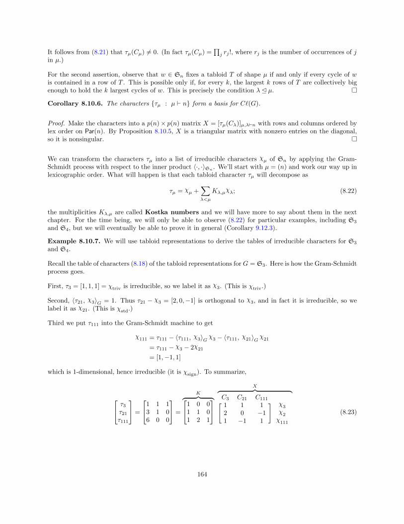
It follows from (8.21) that τµ(Cµ) = 0. (In fact τµ(Cµ) =∏

j rj !, where rj is the number of occurrences of jin µ.)

For the second assertion, observe that w ∈ Sn fixes a tabloid T of shape µ if and only if every cycle of wis contained in a row of T . This is possible only if, for every k, the largest k rows of T are collectively bigenough to hold the k largest cycles of w. This is precisely the condition λ⊴ µ.

Corollary 8.10.6. The characters τµ : µ ⊢ n form a basis for Cℓ(G).

Proof. Make the characters into a p(n)× p(n) matrix X = [τµ(Cλ)]µ,λ⊢n with rows and columns ordered bylex order on Par(n). By Proposition 8.10.5, X is a triangular matrix with nonzero entries on the diagonal,so it is nonsingular.

We can transform the characters τµ into a list of irreducible characters χµ of Sn by applying the Gram-Schmidt process with respect to the inner product ⟨·, ·⟩Sn . We’ll start with µ = (n) and work our way up inlexicographic order. What will happen is that each tabloid character τµ will decompose as

τµ = χµ +∑λ<µ

Kλ,µχλ; (8.22)

the multiplicities Kλ,µ are called Kostka numbers and we will have more to say about them in the nextchapter. For the time being, we will only be able to observe (8.22) for particular examples, including S3

and S4, but we will eventually be able to prove it in general (Corollary 9.12.3).

Example 8.10.7. We will use tabloid representations to derive the tables of irreducible characters for S3

and S4.

Recall the table of characters (8.18) of the tabloid representations for G = S3. Here is how the Gram-Schmidtprocess goes.

First, τ3 = [1, 1, 1] = χtriv is irreducible, so we label it as χ3. (This is χtriv.)

Second, ⟨τ21, χ3⟩G = 1. Thus τ21 − χ3 = [2, 0,−1] is orthogonal to χ3, and in fact it is irreducible, so welabel it as χ21. (This is χstd.)

Third we put τ111 into the Gram-Schmidt machine to get

χ111 = τ111 − ⟨τ111, χ3⟩G χ3 − ⟨τ111, χ21⟩G χ21

= τ111 − χ3 − 2χ21

= [1,−1, 1]

which is 1-dimensional, hence irreducible (it is χsign). To summarize,

τ3τ21τ111

=

1 1 13 1 06 0 0

=

K︷︸︸︷1 0 01 1 01 2 1

X︷︸︸︷

C3 C21 C111[ ]1 1 1 χ3

2 0 −1 χ2

1 −1 1 χ111

(8.23)

164

where X is the character table. For S4, the same procedure produces

τ4τ31τ22τ211τ1111

=

1 1 1 1 14 2 0 1 06 2 2 0 012 2 0 0 024 0 0 0 0

=

K︷︸︸︷1 0 0 0 01 1 0 0 01 1 1 0 01 2 1 1 01 3 2 3 1

X︷︸︸︷C4 C31 C22 C211 C1111

1 1 1 1 1 χ4

3 1 −1 0 −1 χ3

2 0 2 −1 0 χ22

3 −1 −1 0 1 χ211

1 −1 1 1 −1 χ1111

.

Note that the multiplicity of χλ in τλ is 1 in every case (i.e., that the matrix K has 1’s on the maindiagonal).

At this point you should feel a bit dissatisfied, since I have not told you what the values of the irreduciblecharacters actually are in general, just that you can obtain them from the tabloid characters plus Gram-Schmidt. That is a harder problem; the answer is given by the Murnaghan-Nakayama Rule (see §9.14),which expresses the values of the irreducible characters as signed counts of certain tableaux.

Also, what are the multiplicities of the irreps in the tabloid representations, i.e., the numbers in the matrixK? Note that S3 and S4 these matrices are unitriangular (1’s on the main diagonal and 0’s above), whichsays that the tabloid characters are not just a vector basis for the class functions, but more strongly a basis forthe free abelian group generated by irreducible characters. We will prove this eventually (in Corollary 9.12.3),by which point we will have a combinatorial description of the entries of K.

8.11 Exercises

In all exercises, unless otherwise specified, G is a finite group and (ρ, V ) and (ρ′, V ′) are finite-dimensionalrepresentations of G over C.

Exercise 8.1. Let χ be an irreducible character of G and let ψ be a one-dimensional character. Prove thatω := χ⊗ ψ is an irreducible character.

Exercise 8.2. Let n ≥ 2. Prove that the standard representation ρstd of Sn (see Example 8.3.4) isirreducible. (Hint: Compute ⟨χdef , χdef⟩ and ⟨χdef , χtriv⟩. The latter boils down to finding the expectednumber of fixed points in a permutation selected uniformly at random; this is an old classic that uses whatis essentially linearity of expectation.)

Exercise 8.3. Let G be a group of order 63. Prove that G cannot have exactly 5 conjugacy classes. (Youare encouraged to use a computer for part of this problem.)

Exercise 8.4. Let X = 12|34, 13|24, 14|23 be the set of set partitions of [4] into two doubletons, and letV = CX. The standard permutation action of S4 on 1, 2, 3, 4 induces an action on X. On the level ofrepresentations, the defining representation ρdef induces a 3-dimensional representation (ρ, V ).

(a) Compute the character of ρ.(b) Show that ρ is the direct sum of the trivial representation and one other irrep.(c) Explicitly describe all G-equivariant linear transformations ϕ : ρ→ ρdef . (Hint: Schur’s lemma should

be useful.)

Exercise 8.5. Prove that the irreps of a direct product G×H are exactly the direct products (see Exam-ple 8.1.11) of the irreps of G with irreps of H. (This was mentioned in §8.8 for abelian groups but in fact istrue in general.)

165

Exercise 8.6. Work out the character table of S5 without using any of the material in Section 8.10. (Hint:To construct another irreducible character, start by considering the action of S5 on the edges of the completegraph K5 induced by the usual permutation action on the vertices.)

Exercise 8.7. Work out the character table of the quaternion group Q; this is the group of order 8 whoseelements are ±1,±i,±j,±k with relations i2 = j2 = k2 = −1, ij = k, jk = i, ki = j.

Exercise 8.8. Work out the characters χλ of the Specht modules Spλ for all λ ⊢ 4. (Start with the charactersof the tabloid representations, then do linear algebra. Feel free to use a computer algebra system to automatethe tedious parts.) Compare your result to the character table of S4 calculated ad hoc in Example 8.7.2.Make as many observations or conjectures as you can about how the partition λ is related to the values ofthe character χλ.

Exercise 8.9. Recall that the alternating group An consists of the n!/2 even permutations in Sn, that is,those with an even number of even-length cycles.

(a) Show that the conjugacy classes in A4 are not simply the conjugacy classes in S4. (Hint: Consider thepossibilities for the dimensions of the irreducible characters of A4.)

(b) Determine the conjugacy classes in A4, and the complete list of irreducible characters.(c) Use this information to determine [A4,A4] without actually computing any commutators.

166

Chapter 9

Symmetric Functions

9.1 Prelude: Symmetric polynomials

Definition 9.1.1. LetR be an integral domain, typicallyQ or Z. A symmetric polynomial is a polynomialin R[x1, . . . , xn] that is invariant under permuting the variables.

The symmetric polynomials that are homogeneous of degree d form a finitely generated, free R-moduleΛd(R). For example, if n = 3, then up to scalar multiplication, the only symmetric polynomial of degree 1in x, y, z is x+ y + z. In degree 2, here are two:

x2 + y2 + z2, xy + xz + yz.

Every other symmetric polynomial that is homogeneous of degree 2 is a R-linear combination of thesetwo, because the coefficients of x2 and xy determine the coefficients of all other monomials. Similarly, thepolynomials

x3 + y3 + z3, x2y + xy2 + x2z + xz2 + y2z + yz2, xyz

are a basis for the space of degree 3 symmetric polynomials in R[x, y, z].

Each member of this basis is a sum of the monomials in a single orbit under the action of S3. Accordingly,we can index them by the partition whose parts are the exponents of one of its monomials. That is,

m3(x, y, z) = x3 + y3 + z3,

m21(x, y, z) = x2y + xy2 + x2z + xz2 + y2z + yz2,

m111(x, y, z) = xyz.

In general, for λ = (λ1, . . . , λℓ), we define the monomial symmetric polynomial by

mλ(x1, . . . , xn) =∑

a1,...,aℓ⊆[n]

xλ1a1xλ2a2· · ·xλℓ

aℓ.

But unfortunately, this is zero if ℓ > n. So n variables is not enough! In other words, we need a countablyinfinite set of variables x1, x2, . . . , which means that we need to work not with polynomials, but with. . .

167

9.2 Formal power series

Let R be an integral domain (typically Z or a field), and let x = x1, x2, . . . be a countably infinite set ofcommuting indeterminates. A monomial is a product xα =

∏∞i=1 x

αii , where αi ∈ N for all i and

∑i∈I αi

is finite (equivalently, all but finitely many of the αi are zero). The sequence α = (α1, α2, . . . ) is called theexponent vector of the monomial; listing the nonzero entries of α in decreasing order gives a partitionλ(α). A formal power series is an expression ∑

α

cαxα

with cα ∈ R for all α. Equivalently, a formal power series can be regarded as a function from monomialsto R, mapping xα to cα. We often use the notation

[xα]F = coefficient of monomial xα in the power series F .

The set R[[x]] of all formal power series is an abelian group under addition, and in fact an R-module,namely the direct product of countably infinitely many copies of R.1 In fact, R[[x]] is a ring as well, withmultiplication given by (∑

α∈NI

cαxα

)∑β∈NI

dβxβ

=∑γ∈NI

∑(α,β): α+β=γ

cαdβ

xγ .

because the inner sum on the right-hand side has only finitely many terms for each γ, and is thus a well-defined element of R.

We are generally not concerned with whether (or where) a formal power series converges in the sense ofcalculus, since we do not often rarely need to plug in real values for the indeterminates xi (and when wedo, analytic convergence is not usually an issue). All that matters is that every operation must producea well-defined power series, in the sense that each coefficient is given by a finite computation in the basering R. For example, multiplication of power series satisfies this criterion, as explained above.2

Familiar functions from analysis (like exp and log) can be regarded as formal power series, namely theirTaylor series. However, we will typically study them using combinatorial rather than analytic methods. Forinstance, from this point of view, we would justify equating the function 1/(1 − x) as equal to the powerseries 1 + x+ x2 + · · · not by calculating derivatives of 1/(1− x), but rather by observing that the identity(1−x)(1+x+x2+· · · ) = 1 holds in Z[[x]]. (That said, combinatorics also gets a lot of mileage out of workingwith derivative operators — but treating them formally, as linear transformations that map monomials toother monomials, rather than analytically.) Very often, analytical identities among power series can beproved using combinatorial methods; see Exercise 9.4 for an example.

9.3 Symmetric functions

We can now define symmetric functions properly, as elements of the ring of formal power series C[[x]] =C[[x1, x2, . . . ]].

1As opposed to the polynomial ring R[x], which is a direct sum of countably infinitely many copies of R.2We would have a problem with multiplication if we allowed two-way-infinite series. For example, the square of

∑n∈Z xn is

not well-defined.

168

Definition 9.3.1. Let λ ⊢ n. The monomial symmetric function mλ is the power series

mλ =∑

α: λ(α)=λ

xα.

The ring of symmetric functions over R is

Λ = ΛR(x) =⊕d≥0

Λd

where

Λd = ΛR,d(x) = degree-d symmetric functions in indeterminates x with coefficients in R.

Each Λd is a finitely generated free R-module, with basis mλ : λ ⊢ d, and their direct sum Λ is a gradedR-algebra. If we let S∞ be the group whose members are the permutations of x1, x2, . . . with only finitelymany non-fixed points (equivalently, S∞ =

⋃∞n=1 Sn), then Λ is the ring of formal power series that have

bounded degree and that are invariant under the action of S∞.

The monomial symmetric functions are the most natural basis for Λ from an algebraic point of view, butthere are many other bases that arise more frequently in combinatorics. Understanding symmetric functionsrequires familiarity with these various bases and how they interact.

One piece of terminology: we say that a basis B of Λ is an integral basis if the symmetric functions withinteger coefficients are precisely the integer linear combination of elements of B. Evidently, mλ is anintegral basis. This condition is stronger than being a vector space basis for Λ; for example, integral basesare not preserved by scaling.

9.4 Elementary symmetric functions

Definition 9.4.1. The kth elementary symmetric function ek is the sum of all squarefree monomialsof degree k. That is,

e0 = 1,

ek =∑

S⊆N>0

|S|=k

∏s∈S

xs =∑

0<i1<i2<···<ik

xi1xi2 · · ·xik = m1k for k > 0,

where 1k means the partition with k 1′s. For λ = (λ1, . . . , λℓ) ∈ Par, we define

eλ = eλ1· · · eλℓ

.

(In general, we say that a basis for Λ is multiplicative if it is defined on partitions in this way. Note thatmλ is not multiplicative!)

For example, e11 = (x1+x2+x3+ · · · )2 = (x21+x22+ · · · )+2(x1x2+x1x3+x2x3+x1x4+ · · · ) = m2+2m11.

In degree 3, we have

e111 = (x1 + x2 + x3 + · · · )3 = 6m111 + 3m21 + m3,

e21 = (x1 + x2 + x3 + · · · )(x1x2 + x1x3 + x2x3 + x1x4 + · · · ) = 3m111 + m21,

e3 =∑

i<j<k xixjxk = m111,

169

Apparently e3, e21, e111 is an R-basis for Λ3, because the transition matrix is unitriangular and thereforeinvertible over every R. This works for n = 4 as well, where

e1111e211e22e31e4

=

24 12 6 4 112 5 2 1 06 2 1 0 04 1 0 0 01 0 0 0 0

m1111

m211

m22

m31

m4

.This matrix is again unitriangular, and interestingly is symmetric across the northwest/southeast diagonal— that is, the coefficient of eλ in mµ equals the coefficient of eµ in mλ. (Is that always true?)

Sage can do this computation, by the way:

## Input

n = 3

e = SymmetricFunctions(QQ).elementary()

m = SymmetricFunctions(QQ).monomial()

for lam in Partitions(n):

m(e[lam])

## Output

m[1, 1, 1]

3*m[1, 1, 1] + m[2, 1]

6*m[1, 1, 1] + 3*m[2, 1] + m[3]

or even

## Input

n = 4

Matrix([ [m(e[lam]).coefficient(mu) for mu in Partitions(n)] for lam in Partitions(n) ])

## Output

[0, 0, 0, 0, 1]

[0, 0, 0, 1, 4]

[0, 0, 1, 2, 6]

[0, 1, 2, 5, 12]

[1, 4, 6, 12, 24]

Let ⊵ denote the dominance partial order on partitions (see Definition 8.10.4). Also, for a partition λ, let λbe its conjugate, given by transposing the Ferrers diagram (see the discussion after Example 1.2.4).

Theorem 9.4.2. Let λ, µ ⊢ n, with ℓ = ℓ(λ) and k = ℓ(µ). Let bλ,µ be the coefficient of eλ when expandedin the monomial basis, that is,

eλ =∑µ

bλ,µmµ.

Then bλ,λ = 1, and bλ,µ = 0 unless λ⊵ µ. In particular, eλ : λ ⊢ n is an integral basis for Λn.

Proof. Say that a λ-factorization of a monomial is a factorization into monomials of degrees λ1, . . . , λℓ.Let xµ = xµ1

1 · · ·xµk

k . Then

bλ,µ = coefficient of mµ in m-expansion of eλ

= [xµ]eλ1· · · eλℓ

= number of λ-factorizations of xµ into squarefree monomials xα1 , . . . , xαℓ .

170

Represent such a λ-factorization of xµ into by a tableau T of shape λ in which the ith row contains thevariables in xαi , in increasing order. For example, suppose that µ = (3, 2, 2, 1, 1) and λ = (4, 2, 2, 1). Oneλ-factorization of xµ and its associated tableau are

x31x22x

23x

14x

15 = (x1x2x3x5)(x1x3)(x2x4)(x1), T = 1 2 3 5

1 3

2 4

1

.

Thus the entries of T correspond to variables, and its rows of T correspond to factors. Observe that all the1’s in T must be in the first column; all the 2’s must be in the first or second column; etc. Thus, for every j,there must be collectively enough boxes in the first j columns of T to hold all the entries of T correspondingto the variables x1, . . . , xj . That is,

∀j : λ1 + · · ·+ λj ≥ µ1 + · · ·+ µj (9.1)

which is precisely the condition λ⊵ µ. If this fails, then no λ-factorization of xµ can exist and bλ,µ = 0.

If λ = µ, then every inequality in (9.1) is in fact an equality, which says that every entry in the jth columnis in fact j. That is, there is exactly one λ-factorization of xµ, and bλ,µ = 1.

Therefore, if we order partitions of n by any linear extension of dominance (such as lexicographic order),then the matrix [bλ,µ] will be upper unitriangular, hence invertible over any integral domain R. (This is thesame argument as in Corollary 8.10.6.) It follows that the R-module spanned by the eλ’s is the same as thatspanned by the mµ’s for any R, so eλ is an integral basis.

Corollary 9.4.3 (“Fundamental Theorem of Symmetric Functions”). The elementary symmetric functionse1, e2, . . . are algebraically independent. Therefore, Λ = R[e1, e2, . . . ] as rings.

Proof. Given any nontrivial polynomial relation among the ei’s, extracting the homogeneous pieces wouldgive a nontrivial linear relation among the eλ’s, which does not exist.

9.5 Complete homogeneous symmetric functions

Definition 9.5.1. The kth complete homogeneous symmetric function hk is the sum of all monomialsof degree k, extended multiplicatively to partitions:

h0 = 1,

hk =∑

0<i1≤i2≤···≤ik

xi1xi2 · · ·xik =∑λ⊢k

mλ for k > 0,

hλ = hλ1· · · hλℓ

for λ = (λ1, . . . , λℓ) ∈ Par.

In degrees 2 and 3, the hλ’s can be expressed in the e- and m-bases as[h11h2

]=

[1 01 −1

] [e11e2

]=

[2 11 1

] [m11

m2

],

h111h21h3

=

1 0 01 −1 01 −2 1

e111e21e3

=

6 3 13 2 11 1 1

m111

m21

m3

,The coefficient matrices above are all Z-invertible, witnessing the fact that the hλ’s are also a free R-modulebasis for Λ and that Λ = R[h1, h2, . . . , ] as a ring. We could figure out the transition matrices between the hλ

171

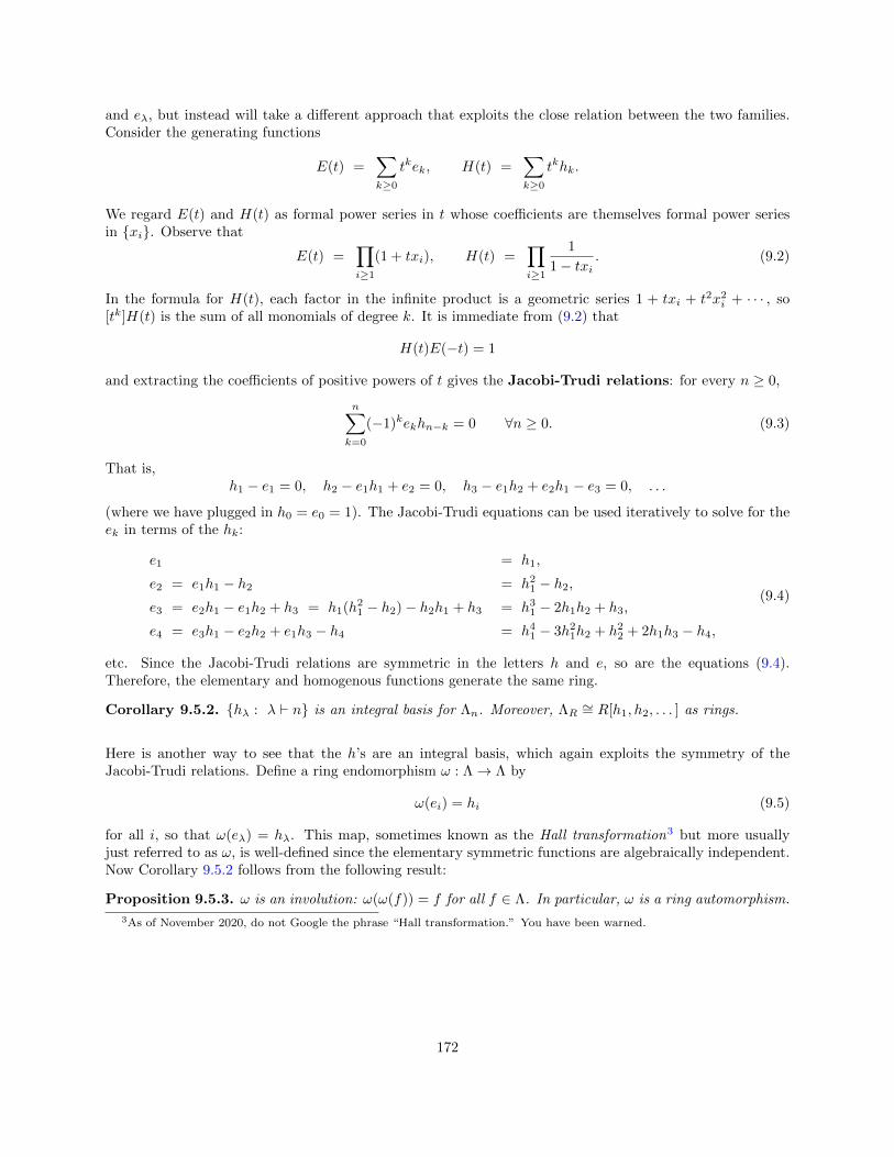
and eλ, but instead will take a different approach that exploits the close relation between the two families.Consider the generating functions

E(t) =∑k≥0

tkek, H(t) =∑k≥0

tkhk.

We regard E(t) and H(t) as formal power series in t whose coefficients are themselves formal power seriesin xi. Observe that

E(t) =∏i≥1

(1 + txi), H(t) =∏i≥1

1

1− txi. (9.2)

In the formula for H(t), each factor in the infinite product is a geometric series 1 + txi + t2x2i + · · · , so[tk]H(t) is the sum of all monomials of degree k. It is immediate from (9.2) that

H(t)E(−t) = 1

and extracting the coefficients of positive powers of t gives the Jacobi-Trudi relations: for every n ≥ 0,

n∑k=0

(−1)kekhn−k = 0 ∀n ≥ 0. (9.3)

That is,h1 − e1 = 0, h2 − e1h1 + e2 = 0, h3 − e1h2 + e2h1 − e3 = 0, . . .

(where we have plugged in h0 = e0 = 1). The Jacobi-Trudi equations can be used iteratively to solve for theek in terms of the hk:

e1 = h1,

e2 = e1h1 − h2 = h21 − h2,e3 = e2h1 − e1h2 + h3 = h1(h

21 − h2)− h2h1 + h3 = h31 − 2h1h2 + h3,

e4 = e3h1 − e2h2 + e1h3 − h4 = h41 − 3h21h2 + h22 + 2h1h3 − h4,

(9.4)

etc. Since the Jacobi-Trudi relations are symmetric in the letters h and e, so are the equations (9.4).Therefore, the elementary and homogenous functions generate the same ring.

Corollary 9.5.2. hλ : λ ⊢ n is an integral basis for Λn. Moreover, ΛR∼= R[h1, h2, . . . ] as rings.

Here is another way to see that the h’s are an integral basis, which again exploits the symmetry of theJacobi-Trudi relations. Define a ring endomorphism ω : Λ→ Λ by

ω(ei) = hi (9.5)

for all i, so that ω(eλ) = hλ. This map, sometimes known as the Hall transformation3 but more usuallyjust referred to as ω, is well-defined since the elementary symmetric functions are algebraically independent.Now Corollary 9.5.2 follows from the following result:

Proposition 9.5.3. ω is an involution: ω(ω(f)) = f for all f ∈ Λ. In particular, ω is a ring automorphism.

3As of November 2020, do not Google the phrase “Hall transformation.” You have been warned.

172

Proof. Applying ω to the Jacobi-Trudi relations (9.3), we see that for every n ≥ 1,

0 =

n∑k=0

(−1)n−kω(ek)ω(hn−k) =

n∑k=0

(−1)n−khkω(hn−k)

=

n∑k=0

(−1)khn−kω(hk) (by replacing k with n− k)

= (−1)nn∑

k=0

(−1)n−khn−kω(hk)

and comparing this last expression with the original Jacobi-Trudi relations gives ω(hk) = ek (e.g., becausesolving for ω(hk) in terms of the hk’s gives exactly (9.4), with the ek’s replaced by ω(hk)’s).

The involution ω will be extremely useful in its own right.

9.6 Power-sum symmetric functions

Definition 9.6.1. The kth power-sum symmetric function pk is the sum of the kth powers of allvariables, extended multiplicatively to partitions:

pk =

∞∑i=1

xki = mk,

pλ = pλ1 · · · pλℓfor λ = (λ1, . . . , λℓ) ∈ Par.

For example, in degrees 2 and 3, you can work out that[p11p2

]=

[2 10 1

] [m11

m2

]and

p111p21p3

=

6 3 10 1 10 0 1

m111

m21

m3

.Note that the transition matrices are invertible over Q, but not over Z: for example, m11 = (p11 − p2)/2.Thus the power-sums are not an integral basis of symmetric functions (although, as we will shortly prove,they are a vector space basis for ΛQ).

We have seen this transition matrix before: its columns are characters of tabloid representations! (See (8.23).)This is the first explicit connection we can observe between representations of Sn and symmetric functions,and it is the tip of an iceberg. It is actually not hard to prove.

Theorem 9.6.2. For λ ⊢ n, we have

pλ =∑µ⊢n

τµ(Cλ)mµ

where τµ(Cλ) means the character of the tabloid representation of shape µ on the conjugacy class Cλ ofcycle-shape λ, as in §8.10.

Proof. Let λ = (λ1, . . . , λℓ) and µ = (µ1, . . . , µk). We adopt the notation (8.19). As in Theorem 9.4.2, letxµ =

∏i x

µi

i . We calculate the coefficient

[xµ]pλ = [xµ]pλ1 · · · pλℓ

= number of λ-factorizations of xµ = xλ1c1 · · ·xλℓ

cℓ.

173

Here we will represent each such choice by a tabloid T in which the factor xλici contributes labels Li to the

cith row, so that T has shape µ. Thus the rows of T correspond to variables, while the entries correspondto positions in the factorization (in contrast to the construction of Theorem 9.4.2).

For example, let λ = (2, 1, 1, 1) and µ = (3, 2). Then [xµ]pλ = [x31x22]pλ = 4. The four λ-factorizations of xµ

are shown below with their corresponding tabloids.

x21 · x1 · x2 · x2x1 1 2 3

x2 4 5

x21 · x2 · x1 · x2x1 1 2 4

x2 3 5

x21 · x2 · x2 · x1x1 1 2 5

x2 3 4

x22 · x1 · x1 · x1x1 3 4 5

x2 1 2

These are precisely the tabloids in which each interval Li is contained in a single row, and these are preciselythose fixed by the permutation given in cycle notation as

w = (1 · · · λ1)(λ1 + 1 · · · λ1 + λ2) · · · (λ[i−1] + 1 · · · λ[i]) · · · (n− λℓ + 1 · · · n),

whose cycle-shape is λ. (Compare equation (8.20). In the example above, w is the transposition (1 2).) Inparticular, the number of such tabloids is by definition τµ(Cλ).

Corollary 9.6.3. pλ is a basis for the symmetric functions (although not an integral basis).

Proof. By Proposition 8.10.5, the transition matrix [τµ(Cλ)] from the monomial symmetric functions to thepower-sums is triangular, hence invertible (although not unitriangular).

9.7 Schur functions and skew Schur functions

The definition of Schur symmetric functions is very different from the m’s, e’s, h’s and p’s. It is not evenclear at first that they are symmetric. But in fact the Schur functions turn out to be essential in the studyof symmetric functions and in several ways are the “best” basis for Λ.

Definition 9.7.1. A column-strict tableau T of shape λ, or λ-CST for short, is a labeling of the boxesof the Ferrers diagram of λ with integers (not necessarily distinct) that is

• weakly increasing across every row; and• strictly increasing down every column.

The partition λ is called the shape of T , and the set of all column-strict tableaux of shape λ is denotedCST(λ). The content of a CST is the sequence α = (α1, α2, . . . ), where αi is the number of boxes labelled i,and the weight of T is the monomial xT = xα = xα1

1 xα22 · · · (the same information as the content, but in

monomial form). For example:

1 1 3

2 3

1 1 1

4 8

1 2 3

1 4

x21x2x23 x31x4x8 Not a CST

The terminology is not entirely standardized; column-strict tableaux are often called “semistandard tableaux”(as in, e.g. [Sta99]).

174

Definition 9.7.2. The Schur function corresponding to a partition λ is

sλ =∑

T∈CST(λ)

xT .

It is far from obvious that sλ is symmetric. Let’s see some examples.

Example 9.7.3. Suppose that λ = (n) is the partition with one part, so that the corresponding Ferrersdiagram has a single row. Each multiset of n positive integers (with repeats allowed) corresponds to exactlyone CST, in which the numbers occur left to right in increasing order. Therefore

s(n) = hn =∑λ⊢n

mλ. (9.6)

At the other extreme, suppose that λ = (1, 1, . . . , 1) is the partition with n singleton parts, so that thecorresponding Ferrers diagram has a single column. To construct a CST of this shape, we need n distinctlabels, which can be arbitrary. Therefore

s(1,1,...,1) = en = m(1,1,...,1). (9.7)

Example 9.7.4. Let λ = (2, 1). We will express sλ as a sum of the monomial symmetric functionsm3,m21,m111.

First, no tableau of shape λ can have three equal entries, so the coefficient of m3 is 0.

Second, for weight xaxbxc with a < b < c, there are two possibilities, shown below.

a b

c

a c

b

Therefore, the coefficient of m111 is 2.

Third, for every a = b ∈ N>0, there is one tableau of shape λ and weight x2axb: the one on the left if a < b,or the one on the right if a > b.

a b

b

b b

a

Therefore, s(2,1) = 2m111 +m21. Summarizing,s111s21s3

=

1 0 02 1 01 1 1

m111

m21

m3

,from which it follows that s3, s21, s111 is a Z-basis for Λ3.

It should be evident at this point that the Schur functions are quasisymmetric, i.e., that for every monomialxa1i1· · ·xak

ik(where i1 < · · · < ik), its coefficient in sλ depends only on the ordered sequence (a1, . . . , ak). To

see this, observe that if j1 < · · · < jk, then replacing is with js for all s gives a bijection from λ-CSTs withweight xa1

i1· · ·xak

ikto λ-CSTs with weight xa1

j1· · ·xak

jk.

175

In fact, the Schur functions are symmetric. Here is an elementary proof. It is enough to show that sλ isinvariant under transposing xi and xi+1 for every i ∈ N>0, since those transposition generate S∞. LetT ∈ CST(λ) and consider all the entries equal to i or +1, ignoring columns that contain both i and i + 1.For ease in depicting the the set of such entries in a single row looks like

i · · · i i+ 1 · · · i+ 1

Say that there are a instances of i and b instances of i+1. Then we can replace this part of the tableau withb instances of i and a instances of i+1. Doing this for every row gives a shape-preserving bijection betweentableaux of weight · · ·xpi xqi+1 · · · and those of weight · · ·xqixpi+1 · · · , as desired.

An important generalization of a Schur function involves a generalization of the underlying Ferrers diagramof a tableau.

Definition 9.7.5. Let λ, µ be partitions with µ ⊆ λ, i.e., λi ≥ µi for all i. There is then an associatedskew partition or skew shape λ/µ, defined via its skew Ferrers diagram, in which the ith row hasboxes in columns µi + 1, . . . , λi. A skew tableau of shape λ/µ is a filling of the skew Ferrers diagramwith numbers.

Some skew shapes are shown below; note that disconnected skew shapes are possible.

4421/21 = 4421/321 = 4421/322 =

The notion of a column-strict tableau carries over without change to skew shapes. Here is a CST of shapeλ/µ, where λ = (8, 6, 6, 5, 4, 2) and µ = (5, 3, 3, 3, 2):

2 2 3

1 1 3

2 3 4

4 4

2 6

1 1

The definition of Schur functions (Definition 9.7.1) can also be adapted to skew shapes.

Definition 9.7.6. Let CST(λ/µ) denote the set of all column-strict skew tableaux of shape λ/µ, and as

before weight each tableau T ∈ CST(λ/µ) by the monomial xT =∏

i xαi(T )i , where αi(T ) is the number of

i’s in T . The skew Schur function is then

sλ/µ =∑

T∈CST(λ/µ)

xT .

The elementary proof of symmetry of Schur functions carries over literally to skew Schur functions.

9.8 The Jacobi–Trudi determinant formula

We are next going to establish a formula for the Schur function sλ as a determinant of a matrix whose entriesare hn’s or en’s (which also proves their symmetry). This takes more work, but the proof, due to the ideas of

176

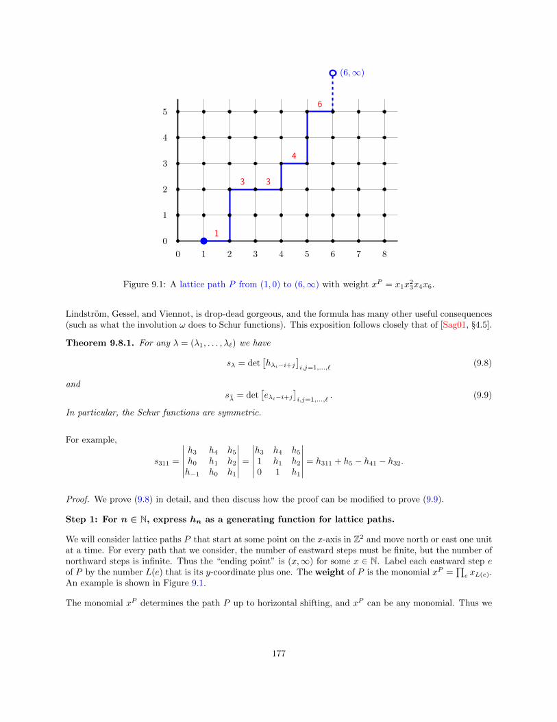
0 1 2 3 4 5 6 7 8

0

1

2

3

4

5

(6,∞)

1

3 3

4

6

Figure 9.1: A lattice path P from (1, 0) to (6,∞) with weight xP = x1x23x4x6.

Lindstrom, Gessel, and Viennot, is drop-dead gorgeous, and the formula has many other useful consequences(such as what the involution ω does to Schur functions). This exposition follows closely that of [Sag01, §4.5].

Theorem 9.8.1. For any λ = (λ1, . . . , λℓ) we have

sλ = det[hλi−i+j

]i,j=1,...,ℓ

(9.8)

andsλ = det

[eλi−i+j

]i,j=1,...,ℓ

. (9.9)

In particular, the Schur functions are symmetric.

For example,

s311 =

∣∣∣∣∣∣h3 h4 h5h0 h1 h2h−1 h0 h1

∣∣∣∣∣∣ =∣∣∣∣∣∣h3 h4 h51 h1 h20 1 h1

∣∣∣∣∣∣ = h311 + h5 − h41 − h32.

Proof. We prove (9.8) in detail, and then discuss how the proof can be modified to prove (9.9).

Step 1: For n ∈ N, express hn as a generating function for lattice paths.

We will consider lattice paths P that start at some point on the x-axis in Z2 and move north or east one unitat a time. For every path that we consider, the number of eastward steps must be finite, but the number ofnorthward steps is infinite. Thus the “ending point” is (x,∞) for some x ∈ N. Label each eastward step eof P by the number L(e) that is its y-coordinate plus one. The weight of P is the monomial xP =

∏e xL(e).

An example is shown in Figure 9.1.

The monomial xP determines the path P up to horizontal shifting, and xP can be any monomial. Thus we

177

have a bijection, and it follows that for any a ∈ N,

hn =∑

paths P from(a, 0) to (a + n,∞)

xP =∑

paths P with fixed startingpoint with n east steps

xP . (9.10)

Step 2: Express the generating function for families of lattice paths in terms of the hk’s.

For a partition λ of length ℓ, a λ-path family P = (π, P1, . . . , Pℓ) consists of the following data:

• A permutation π ∈ Sℓ;• Two sets of points U = u1, . . . , uℓ and V = v1, . . . , vℓ, defined by

ui = (ℓ− i, 0), vi = (λi + ℓ− i,∞);

• A list of lattice paths P1, . . . , Pℓ, where Pi is a path from uπ(i) to vi.

Figure 9.2 shows a λ-path family with λ = (3, 3, 2, 1) and π = 3124. (In general the paths in a family areallowed to share edges, although that is not the case in this example.)

0 1 2 3 4 5 6 7 8

0

1

2

3

4

5

v4

u4

v1

u3

v3

u2

v2

u1

P4 P3 P2 P1

Figure 9.2: A (3, 3, 2, 1)-path family (π, U, V ) with π = 2314.

Note that for each i ∈ [ℓ], the number of east steps in the path Pi from u(π(i)) to vi is

(λi + ℓ− i)− (ℓ− π(i)) = λi − i+ π(i).

Now the first miracle occurs: the signed generating function for path families is the determinant of a matrixwhose entries are complete homogeneous symmetric functions! One key observation is that any collection ofpaths P1, . . . , Pℓ in which Pi contains λi− i+ π(i) east steps gives rise to a λ-path family (π, P1, . . . , Pℓ). Inother words, if we know what π is, then Pi can be any path with the appropriate number of east steps.

For a path family P = (π, P1, . . . , Pℓ), let xP =

∏ℓi=1 x

Pi and (−1)P be the sign of π. Then:

178

∑P=(π,P1,...,Pℓ)

(−1)PxP =∑π∈Sℓ

ε(π)∑

λ-path familiesP=(π,P1,...,Pℓ)

xP1 · · ·xPℓ

=∑π∈Sℓ

ε(π)

ℓ∏i=1

∑paths Pi with

λi−i+π(i) east steps

xPi

(by the key observation above)

=∑π∈Sℓ

ε(π)

ℓ∏i=1

hλi−i+π(i) (by (9.10))

=∣∣hλi−i+j

∣∣i,j=1,...,ℓ

(look! it’s a determinant!) (9.11)

Step 3: Simplify the generating function by cancellation.

Call a path family good if no two of its paths meet in a common vertex, and bad otherwise. Note that if Pis good, then π must be the identity permutation, and in particular (−1)P = 1.

Define a sign-reversing, weight-preserving involution P 7→ P♯ on bad λ-path families as follows.

1. Of all the lattice points contained in two or more paths in P, choose the point α with the lex-greatestpair of coordinates.

2. Of all the half-paths from α to some vi, choose the two with the largest i. Interchange them. Call theresulting path family P♯.

An example is shown in the figure below. Figure 9.3.

0 1 2 3 4 5 6

0

1

2

3

4

5

v4

u4

v1

u3

v3

u2

v2

u1

α

P

0 1 2 3 4 5 6

0

1

2

3

4

5

v4

u4

v1

u3

v3

u2

v2

u1

α

P]

Figure 9.3: The involution P↔ P♯ on bad path families.

Then

• this operation is an involution on bad path families;

• xP = xP♯

; and

179

• (−1)P = −(−1)P♯

(because the two are related by a transposition).

Therefore, by the calculation of (9.11), we have

|hλi−i+j |i,j=1,...,ℓ =∑P

(−1)PxP =∑

P good

xP. (9.12)

Step 4: Enumerate weights of good path families.

For each good path family, label the east steps of each path by height as before. The labels weakly increaseas we move north along each path. Moreover, for every j the jth east step of the path Pi occurs one uniteast of that of Pi+1, so it must also occur strictly north of it (otherwise, the paths would cross). Therefore,we can construct a column-strict tableau of shape λ by reading off the labels of each path, and this givesa bijection between good λ-path families and column-strict tableaux of shape λ. An example is shown inFigure 9.4.

5

3

4

2

3

4

1 1

3

v4

u4

v3

u3

v2

u2

v1

u1

1 1 3

2 3 4

3 4

5

Figure 9.4: The bijection between good path families and column-strict tableaux.

Consequently, (9.12) implies that |hλi−i+j |i,j=1,...,ℓ = sλ, which is (9.8). Is that amazing or what?

The proof of (9.9) is similar. The key difference is that instead of labeling each east step with its height,we number all the steps (north and east) consecutively, ignoring the first i− 1 steps of Pi (those below theline y = x + ℓ − 1, which must all be northward anyway). The weight of a path is still the the product ofthe variables corresponding to its east steps. This provides a bijection between lattice paths with k eaststeps and squarefree monomials of degree k, giving an analogue of (9.10), with hn replaced by en. Bad pathfamilies cancel out by the same involution as before, and each good path family now gives rise to a tableauof shape λ in which rows strictly increase but columns weakly increase (see Figure 9.5). Transposing givesa column-strict tableau of shape λ, and (9.9) follows.

Corollary 9.8.2. For every partition λ, the involution ω interchanges sλ and sλ.

Proof. We know that ω interchanges hλ and eλ, so it interchanges the RHS’s, hence the LHS’s, of (9.8) and(9.9).

180

1

2

12

3

12

34

5

1 23

4

5

v4

u4

v3

u3

v2

u2

v1

u1

1 2 5

1 3 5

1 3

2

Figure 9.5: The dual bijection between good path families and row-strict tableaux.

The next step is to prove that the Schur functions are a basis for the symmetric functions. Now that weknow they are symmetric, they can be expressed in the monomial basis as

sλ =∑µ⊢n

Kλ,µmµ. (9.13)

Thus Kλ,µ is the number of column-strict tableaux T with shape λ and content µ. These are called theKostka numbers.

Theorem 9.8.3. The Schur functions sλ : λ ⊢ n are a Z-basis for ΛZ.

Proof. Here comes one of those triangularity arguments. First, if λ = µ, then there is exactly one possibilityfor T : fill the ith row full of i’s. Therefore

∀λ ⊢ n : Kλ,λ = 1. (9.14)

Second, observe that if T is a CST of shape λ and content µ (so in particular Kλ,µ > 0), then

• every 1 in T must appear in the 1st row;• every 2 in T must appear in the 1st or 2nd row;• . . .• every i in T must appear in one of the first i rows;• . . .

and therefore∑k

i=1 µi ≤∑k

i=1 λi, which is just the statement that λ⊵ µ (recall the definition of dominanceorder, Defn. 8.10.4). So the matrix [Kλ,µ]λ,µ⊢n is unitriangular, hence Z-invertible. Therefore the Schurfunctions are a vector space basis for ΛQ and a free module basis for ΛZ, just as in the proof of Theorem 9.4.2.

The lattice-path proof of Theorem 9.8.1 generalizes to skew shapes (although I haven’t yet figured out exactlyhow) to give Jacobi-Trudi determinant formulas for skew Schur functions:

sλ/µ = det[hλi−µi−i+j

]i,j=1,...,ℓ

, sλ/µ = det[eλi−µi−i+j

]i,j=1,...,ℓ

. (9.15)

181

9.9 The Cauchy kernel and the Hall inner product

The next step in studying the ring of symmetric functions Λ will be to define an inner product structure onit. These will come from considering the Cauchy kernel and the dual Cauchy kernel, which are formalpower series in two sets of variables x = x1, x2, . . . , y = y1, y2, . . . , defined as the following infiniteproducts:

Ω =∏i,j≥1

(1− xiyj)−1, Ω∗ =∏i,j≥1

(1 + xiyj).

The power series Ω and Ω∗ are well-defined because the coefficient of any monomial xαyβ is the numberof ways of factoring it into monomials of the form xiyj , which is clearly finite (in particular it is zero if|α| = |β|). Moreover, they are evidently bisymmetric4, i.e., symmetric with respect to each of the variablesets x = x1, x2, . . . and y = y1, y2, . . . . Thus we can write Ω and Ω∗ as power series in some basis forΛ(x) and ask which elements of Λ(y) show up as coefficients.

For later use, we observe that Ω and Ω∗ can be viewed as generating functions for infinite matrices, as follows.Let A = aij : i, j ∈ N>0 be a matrix with countably infinitely many rows and columns, both indexed bypositive integers, such that all but finitely many values of aij are zero. Define wt(A) =

∏i,j(xiyj)

aij . Thenexpanding the geometric-series factors in the Cauchy kernel and dual Cauchy kernel gives

Ω =∑

A: aij∈N

∏i,j

(xiyj)aij , Ω∗ =

∑A: aij∈0,1

∏i,j

(xiyj)aij .

For a partition λ ⊢ n, let5 ri = ri(λ) be the number of i’s in λ. Define scalars

zλ = 1r12r2 · · ·nrn r1! r2! · · · rn!,ελ = (−1)n−ℓ(λ) = (−1)r2 + r4 + r6 + ···.

(9.16)

(For the last equality, note that n−ℓ(λ) = (∑

i iri)−(∑

i ri) =∑

i(i−1)ri, which is congruent to r2+r4+· · ·modulo 2.)

For example, if λ = (3, 3, 2, 1, 1, 1) then zλ = (133!)(211!)(322!) = 216 and ελ = −1.

Proposition 9.9.1. Let λ ⊢ n and let Cλ be the corresponding conjugacy class in Sn. Then |Cλ| = n!/zλ,and ελ is the sign of each permutation in Cλ.

We omit the proof, which is straightforward.

Proposition 9.9.2. We have

Ω =∑λ

hλ(x)mλ(y) =∑λ

pλ(x)pλ(y)

zλand (9.17)

Ω∗ =∑λ

eλ(x)mλ(y) =∑λ

ελpλ(x)pλ(y)

zλ(9.18)

where the sums run over all partitions λ.

4Technically, Ω lives not in the ring Λ(x,y) of bisymmetric power series, but rather its completion, since it contains termsof arbitrarily high degree. If you don’t know what “completion” means then don’t worry about it. The key point is that Ω isstill determined by the coefficients of the bisymmetric series uλ(x)vµ(y) for any bases uλ, vµ of Λ — it is just no longertrue that all but finitely many of these coefficients are zero.

5In [Sta99], Stanley uses mi where I use ri, presumably as a mnemonic for “multiplicity.” I have changed the notation inorder to avoid conflict with the notation for monomial symmetric functions.

182

Proof. Recall from (9.2) that∏

i≥1(1− xit)−1 =∑

k≥0 hk(x)tk. Therefore

∏i,j≥1

(1− xiyj)−1 =∏j≥1

∏i≥1

(1− xit)−1∣∣∣t=yj

=

∏j≥1

∑k≥0

hk(x) ykj

=∑

α=(α1,α2,... )∈NN:∑

i αi<∞yα

∞∏i=1

hαi(x)

=∑α

yαhλ(α)(x)

=∑λ

hλ(x)mλ(y)

as desired. (Regard λ as the partition whose parts are α1, . . . , αℓ, sorted in weakly decreasing order.)

For the second equality in (9.17), recall the standard power series expansions

log(1 + q) =∑n≥1

(−1)n+1 qn

n, log(1− q) = −

∑n≥1

qn

n, exp(q) =

∑n≥0

qn

n!. (9.19)

These are formal power series that obey the rules you would expect; for instance, log(∏

i qi) =∑

i(log qi)and exp log(q) = q. (The proof of the second of these is left to the reader as Exercise 9.4.) In particular,

log Ω = log∏i,j≥1

(1− xiyj)−1 = −∑i,j≥1

log(1− xiyj)

=∑i,j≥1

∑n≥1

xni ynj

n(by (9.19))

=∑n≥1

1

n

∑i≥1

xni

∑j≥1

ynj

=∑n≥1

pn(x)pn(y)

n

and now exponentiating both sides and applying the power series expansion for exp, we get

Ω = exp

∑n≥1

pn(x)pn(y)

n

=∑k≥0

1

k!

∑n≥1

pn(x)pn(y)

n

k

=∑k≥0

1

k!

∑λ: ℓ(λ)=k

k!

r1! r2! · · ·

(p1(x)p1(y)

1

)r1 (p2(x)p2(y)2

)r2

· · ·

(by the multinomial expansion, where ri means ri(λ))

=∑λ

∞∏i=1

(pi(x)pi(y))ri

∞∏i=1

iriri!

=∑λ

pλ(x)pλ(y)

zλ.

The proofs of the identities for the dual Cauchy kernel are analogous, and are left to the reader as Exercise 9.5.

183

As a first benefit, we can express the homogeneous and elementary symmetric functions in the power-sumbasis.

Corollary 9.9.3. For all n, we have:

(a) hn =∑

λ⊢n pλ/zλ;

(b) en =∑

λ⊢n ελpλ/zλ;

(c) ω(pλ) = ελpλ (where ω is the involution of 9.5).

Proof. (a) Start with the identity of (9.17):∑λ

hλ(x)mλ(y) =∑λ

pλ(x)pλ(y)

zλ.

Set y1 = t, and yk = 0 for all k > 1. This kills all terms on the left side for which λ has more than one part,leaving only those where λ = (n), while on the right side pλ(y) specializes to t

|λ|, so we get

∑n

hn(x)tn =

∑λ

pλ(x)t|λ|

zλ

and extracting the coefficient of tn gives the desired expression for hn.

(b) Start with (9.18) and do the same thing.

(c) Let ω act on symmetric functions in x while fixing those in y. Using (9.17) and (9.18), we obtain

∑λ

pλ(x) pλ(y)

zλ=∑λ

hλ(x)mλ(y) = ω

(∑λ

eλ(x)mλ(y)

)= ω

(∑λ

ελpλ(x)pλ(y)

zλ

)

=∑λ

ελω(pλ(x)) pλ(y)

zλ

and equating the red coefficients of pλ(y)/zλ yields the desired result.

Definition 9.9.4. The Hall inner product on symmetric functions is defined by declaring hλ and mλto be dual bases. That is, we define

⟨hλ,mµ⟩Λ = δλµ

and extend by linearity to all of Λ.

Thus the Cauchy kernel can be regarded as a generating function for pairs (hλ,mµ), weighted by their innerproduct. In fact it can be used more generally to compute Hall inner products:

Proposition 9.9.5. The Hall inner product has the following properties:

(a) If uλ and vµ are graded bases for Λ indexed by partitions, such that Ω =∑

λ uλ(x)vλ(y), thenthey are dual bases with respect to the Hall inner product; i.e., ⟨uλ, vµ⟩ = δλµ.

(b) In particular, pλ and pλ/zλ are dual bases, and pλ/√zλ is self-dual, i.e., orthonormal.

(c) ⟨·, ·⟩ is a genuine inner product (in the sense of being a nondegenerate bilinear form).(d) The involution ω is an isometry with respect to the Hall inner product, i.e.,

⟨a, b⟩ = ⟨ω(a), ω(b)⟩.

184

Proof. Assertion (a) is a matter of linear algebra, and is left to the reader (Exercise 9.1). Assertion (b)follows from (a) together with (9.18), and (c) from the fact that ΛR admits an orthonormal basis. Thequickest proof of (d) uses the power-sum basis: by Corollary 9.9.3(c), we have

⟨ωpλ, ωpµ⟩ = ⟨ελpλ, εµpµ⟩ = ελεµ⟨pλ, pµ⟩ = δλµ = ⟨pλ, pµ⟩

because ελ ∈ 1,−1 for all λ.

The orthonormal basis pλ/√zλ is not particularly nice from a combinatorial point of view, because it

involves irrational coefficients. It turns out that there is a better orthonormal basis: the Schur functions!Our next goal will be to prove that

Ω =∏i,j≥1

1

1− xiyj=∑λ

sλ(x)sλ(y) (9.20)

via a marvelous bijection called the RSK correspondence.

9.10 The RSK Correspondence

Recall from Example 1.2.4 that a standard [Young] tableau of shape λ is a filling of the Ferrers diagramof λ with the numbers 1, 2, . . . , n that is increasing left-to-right and top-to-bottom. We write SYT(λ) for theset of all standard tableaux of shape λ, and set fλ = |SYT(λ)| (this symbol fλ is traditional).

For example, if λ = (3, 3), then fλ = 5; the members of SYT(λ) are as follows.

1 3 5

2 4 6

1 3 4

2 5 6

1 2 5

3 4 6

1 2 4

3 5 6

1 2 3

4 5 6

The Robinson-Schensted-Knuth (RSK) correspondence6 is a bijection between permutations oflength n and pairs of standard tableaux of the same shape λ ⊢ n:

SnRSK−−−−→

⋃λ⊢n

SYT(λ)× SYT(λ).

The main step in the RSK algorithm is row-insertion.

Definition 9.10.1. Let T be a column-strict tableau and let x ∈ N>0. The row-insertion T ← x is definedas follows:

• If T = ∅, then T ← x = x .• If x ≥ u for all entries u in the top row of T , then append x to the end of the top row.• Otherwise, find the leftmost entry u such that x < u. Replace u with x, and then insert u into thesubtableau consisting of the second and succeeding rows. In this case we say that x bumps u.

• Repeat until the bumping stops.

Got that? Now, for w = w1w2 · · ·wn ∈ Sn, let P be the tableau ((∅ ← w1) ← w2) ← · · · ← wn ∈ Sn. LetQ be the standard tableau of the same shape as P that records where a new box appears in the underlyingFerrers diagram at each step of the algorithm. The tableaux P and Q are respectively called the insertiontableau and the recording tableau, and the map w 7→ (P,Q) is the RSK correspondence.

6Different versions of the algorithm are referred to by various subsets of these three names; I am not drawing that distinction.

185

Example 9.10.2. Let w = 57214836 ∈ S8. Start with a pair (P,Q) of empty tableaux.

Step 1: Row-insert w1 = 5 into P . We do this in the obvious way. Since it is the first cell added, we add acell containing 1 to Q.

P = 5 Q = 1 (9.21a)

Step 2: Row-insert w2 = 7 into P . Since 5 < 7, we can do this by appending the new cell to the top row,and adding a cell labeled 2 to Q to record where we have put the new cell in P .

P = 5 7 Q = 1 2 (9.21b)

Step 3: Row-insert w3 = 2 into P . This is a bit trickier. We cannot just append a 2 to the first row of P ,because the result would not be a standard tableau. The 2 has to go in the top left cell, but that alreadycontains a 5. Therefore, the 2 “bumps” the 5 out of the first row into a new second row. Again, we recordthe location of the new cell by adding a cell labeled 3 to Q.

P = 2 7

5Q = 1 2

3(9.21c)

Step 4: Row-insert w4 = 1 into P . This time, the new 1 bumps the 2 out of the first row. The 2 has to gointo the second row, but again we cannot simply append it to the right. Instead, the 2 bumps the 5 out ofthe second row into the (new) third row.

P =1 7

2

5

Q =1 2

3

4

(9.21d)

Step 5: Row-insert w5 = 4 into P . The 4 bumps the 7 out of the first row. The 7, however, can comfortablyfit at the end of the second row, without any more bumping.

P = 1 4

2 7

5

Q = 1 2

3 5

4

(9.21e)

Step 6: Row-insert w6 = 8 into P . The 8 just goes at the end of the first row.

P =1 4 8

2 7

5

Q =1 2 6

3 5

4

(9.21f)

Step 7: Row-insert w7 = 3 into P . 3 bumps 4, and then 4 bumps 7.

186

P = 1 3 8

2 4

5 7

Q = 1 2 6

3 5

4 7

(9.21g)

Step 8: Row-insert w8 = 6 into P . 6 bumps 8 into the second row.

P =1 3 6

2 4 8

5 7

Q =1 2 6

3 5 8

4 7

(9.21h)

A crucial feature of the RSK correspondence is that it can be reversed. That is, given a pair (P,Q), we canrecover the permutation that gave rise to it.

Example 9.10.3. Suppose that we are given the pair of tableaux in (9.21h). What was the previous step?To get the previous Q, we just delete the 8. As for P , the last cell added must be the one containing 8.This is in the second row, so somebody must have bumped 8 out of the first row. That somebody must bethe largest number less than 8, namely 6. So 6 must have been the number inserted at this stage, and theprevious pair of tableaux must have been those in (9.21g).

Example 9.10.4. Let P be the standard tableau (with 18 boxes) shown in (a) below. Suppose that weknow that the cell labeled 16 was the last one added (because the corresponding cell in Q contains an 18).Then the “bumping path” must be as indicated in the center figure (b). (That is, the 16 was bumped bythe 15, which was bumped by the 13, and so on.) Each number in the bumping path is the rightmost onein it slow that is less than the next lowest number in the path. The previous tableau in the RSK algorithmcan now be found by “unbumping”: push every number in the bumping path up and toss out the top one,to obtain the tableau on the right (c).

(a)1 2 5 8 10 18

3 4 11 12 19

6 7 13

9 15 17

14 16

(b)1 2 5 8 10 18

3 4 11 12 19

6 7 13

9 15 17

14 16

(c)1 2 5 8 12 18

3 4 11 13 19

6 7 15

9 16 17

14

Iterating this procedure allows us to recover w from the pair (P,Q).

We have proved the following fact:

Theorem 9.10.5. The RSK correspondence is a bijection

SnRSK−−−−→

⋃λ⊢n

SYT(λ)× SYT(λ).

Corollary 9.10.6. For every n we have∑λ⊢n

(fλ)2 = n!.

(What does this remind you of?)

187

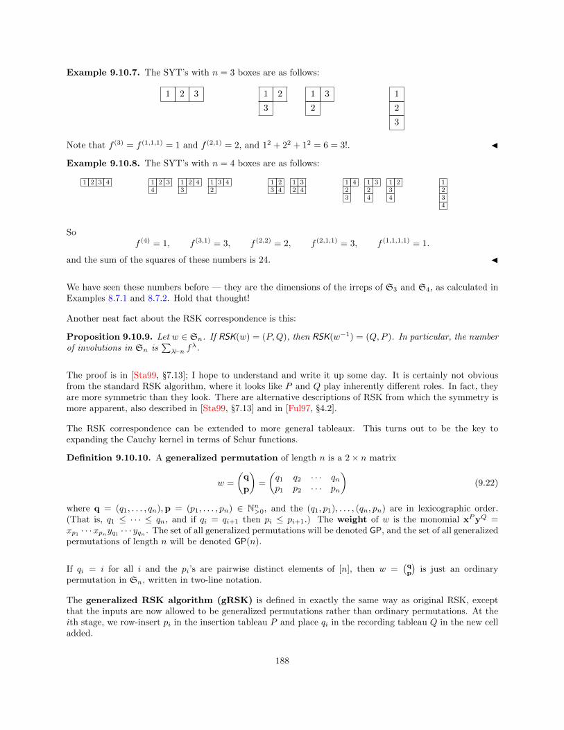
Example 9.10.7. The SYT’s with n = 3 boxes are as follows:

1 2 3 1 2

3

1 3

2

1

2

3

Note that f (3) = f (1,1,1) = 1 and f (2,1) = 2, and 12 + 22 + 12 = 6 = 3!.

Example 9.10.8. The SYT’s with n = 4 boxes are as follows:

1 2 3 4 1 2 34

1 2 43

1 3 42

1 23 4

1 32 4

1 423

1 324

1 234

1234

Sof (4) = 1, f (3,1) = 3, f (2,2) = 2, f (2,1,1) = 3, f (1,1,1,1) = 1.

and the sum of the squares of these numbers is 24.

We have seen these numbers before — they are the dimensions of the irreps of S3 and S4, as calculated inExamples 8.7.1 and 8.7.2. Hold that thought!

Another neat fact about the RSK correspondence is this:

Proposition 9.10.9. Let w ∈ Sn. If RSK(w) = (P,Q), then RSK(w−1) = (Q,P ). In particular, the numberof involutions in Sn is

∑λ⊢n f

λ.

The proof is in [Sta99, §7.13]; I hope to understand and write it up some day. It is certainly not obviousfrom the standard RSK algorithm, where it looks like P and Q play inherently different roles. In fact, theyare more symmetric than they look. There are alternative descriptions of RSK from which the symmetry ismore apparent, also described in [Sta99, §7.13] and in [Ful97, §4.2].

The RSK correspondence can be extended to more general tableaux. This turns out to be the key toexpanding the Cauchy kernel in terms of Schur functions.

Definition 9.10.10. A generalized permutation of length n is a 2× n matrix

w =

(q

p

)=

(q1 q2 · · · qnp1 p2 · · · pn

)(9.22)

where q = (q1, . . . , qn),p = (p1, . . . , pn) ∈ Nn>0, and the (q1, p1), . . . , (qn, pn) are in lexicographic order.

(That is, q1 ≤ · · · ≤ qn, and if qi = qi+1 then pi ≤ pi+1.) The weight of w is the monomial xPyQ =xp1· · ·xpn

yq1 · · · yqn . The set of all generalized permutations will be denoted GP, and the set of all generalizedpermutations of length n will be denoted GP(n).

If qi = i for all i and the pi’s are pairwise distinct elements of [n], then w =(qp

)is just an ordinary

permutation in Sn, written in two-line notation.

The generalized RSK algorithm (gRSK) is defined in exactly the same way as original RSK, exceptthat the inputs are now allowed to be generalized permutations rather than ordinary permutations. At theith stage, we row-insert pi in the insertion tableau P and place qi in the recording tableau Q in the new celladded.

188

Example 9.10.11. Consider the generalized permutation

w =

(q

p

)=

(1 1 2 4 4 4 5 5 52 4 1 1 3 3 2 2 4

)∈ GP(9).

The result of the gRSK algorithm is as follows. The unnamed tableau on the right records the step in whicheach box was added.

P = 1 1 2 2 4

2 3 3

4

Q = 1 1 4 4 5

2 4 5

5

1 2 5 6 9

3 4 8

7

The tableaux P,Q arising from gRSK will always have the same shape as each other, and will be weaklyincreasing eastward and strictly increasing southward — that is, they will be column-strict tableaux, preciselythe things for which the Schur functions are generating functions. Column-strictness of P follows from thedefinition of insertion. As for Q, it is enough to show that no label k appears more than once in the samecolumn. Indeed, all instances of k in q occur consecutively (say as qi, . . . , qj), and the corresponding entriesof p are weakly increasing, so none of them will bump any other (in fact their bumping paths will not cross),which means that each k appears to the east of all previous k’s.

This observation also suffices to show that the generalized permutation w can be recovered from the pair(P,Q): the rightmost instance of the largest entry in Q must have been the last box added. Hence thecorresponding box of P can be “unbumped” to recover the previous P and thus the last column of w.Iterating this process allows us to recover w. Therefore, generalized RSK gives a bijection

GP(n)RSK−−−−→

⋃λ⊢n(P,Q) : P,Q ∈ CST(λ) (9.23)

in which a generalized permutation(qp

)maps to a pair of tableaux P,Q with weight monomials xP and yQ.

On the other hand, a generalized permutation w =(qp

)∈ GP(n) is determined by the number of occurrences

of every column(qipi

). Therefore, it can be specified by an infinite matrixM = [mij ]i,j∈N>0

with finitely many

nonzero entries, in which mij is the number of occurrences of (qi, pj) in w (so n =∑mij). For example, the

generalized permutation w ∈ GP(9) of Example 9.10.11 corresponds to the integer matrix

0 1 0 1 0 · · ·1 0 0 0 0 · · ·0 0 0 0 0 · · ·1 0 2 0 0 · · ·0 2 0 1 0 · · ·0 0 0 0 0 · · ·...

......

......

. . .

.

Rewrite this and the previous discussion of the Cauchy kernel to get rid of the matrices; it’sas easy to work with generalized permutations. Let M denote the set of all such matrices, so thatwe have a bijection GP ↔M. Under this bijection, the weight monomial xPyQ equals

∏i,j(xiyj)

mij . Anygiven weight monomial arises from only finitely many matrices, so the generating function for matrices byweights is a well-defined power series. In fact, it is the Cauchy kernel, because∑

M=[mij ]∈M

∏i,j

(xiyj)mij =

∏i,j≥1

∞∑mij=0

(xiyj)mij =

∏i,j≥1

1

1− xiyj= Ω.

189

On the other hand,

Ω =∑

M=[mij ]

∏i,j

(xiyj)mij

=∑n∈N

∑(qp)∈GP(n)

xp1· · ·xpn

yq1 · · · yqn (by the bijection GP↔M)

=∑λ

∑P,Q ∈ CST(λ)

xPyQ (by gRSK)

=∑λ

∑P∈CST(λ)

xP

∑Q∈CST(λ)

yQ

=∑λ

sλ(x)sλ(y).

Combined with assertion (a) of Proposition 9.9.5, we have proven:

Theorem 9.10.12. The Schur functions form an orthonormal Z-basis for Λ under the Hall inner product.

In fact, the Schur functions are the only orthonormal, integral basis for Λ that is positive in the underlyingvariables x.

Corollary 9.10.13. For every µ ∈ Par we have

hµ =∑λ

Kλµsλ and eµ =∑λ

Kλµsλ.

Proof. Equation (9.13) implies that

⟨sλ, hµ⟩ =⟨∑

µ⊢nKλ,µmµ, hµ

⟩= Kλ,µ =

⟨sλ,

∑λ

Kλµsλ

⟩(9.24)

for every λ. So the two blue expressions are equal. Applying ω to both sides (using Prop. 9.9.5(d)) we get

⟨sλ, eµ⟩ =⟨ω(sλ), ω(eµ)

⟩= ⟨sλ, hµ⟩ = Kλ,µ =

⟨sλ,

∑λ

Kλµsλ

⟩(9.25)

and the two red expressions are equal.

9.11 Alternants and the classical definition of Schur functions

This section closely follows [Sta99, §7.15].

For this section, we will work with polynomials rather than power series, for a reason that will quicklybecome apparent.

Definition 9.11.1. A polynomial a ∈ k[x1, . . . , xn] is alternating, or an alternant, if w(a) = ε(w)a forall w ∈ Sn. Equivalently, interchanging any two variables xi, xj maps a to −a.

190

The definition implies that every alternant is divisible by xj−xi for each i < j, hence by the Vandermondedeterminant

∏1≤i<j≤n

(xj − xi) =

∣∣∣∣∣∣∣∣∣1 x1 x21 · · · xn−1

1

1 x2 x22 · · · xn−12

......

......

1 xn x2n · · · xn−1n

∣∣∣∣∣∣∣∣∣ .(Why does this equality hold? Interchanging xi with xj swaps two rows of the determinant, hence changes itssign. Therefore the determinant is divisible by the product on the left. On the other hand both polynomialsare homogeneous of degree

(n2

)= 0 + 1 + · · · + (n − 1), and the coefficients of x01x

12 · · ·xn−1

n are both ±1,so equality must hold.) This is why we are working with polynomials (since the infinite analogue of theVandermonde determinant, namely,

∏i<j∈N xjxi, is not a well-defined power series).

More generally, we can construct an alternant by changing the powers of variables that occur in each columnof the Vandermonde determinant: for α = (α1, . . . , αn) ∈ Nn, we define

aα = aα(x1, . . . , xn) =∣∣xαj

i

∣∣ni,j=1

=∑

w∈Sn

ε(w)w(xα).

Note that aα = 0 if (and only if) α contains some entry more than once. Moreover, the entries might as wellbe listed in decreasing order. Therefore we can write α = λ + δ, where λ = (λ1 ≥ · · · ≥ λn ≥ 0) ∈ Par andδ = (n− 1, n− 2, . . . , 1, 0), and addition is componentwise: αj = λj + δj = λj + n− j. That is,

aλ+δ =∣∣∣xλj+n−j

i

∣∣∣ni,j=1

.

In particular aδ is the Vandermonde determinant. As observed above, every alternant is divisible by aδ, sothe quotient aλ+δ/aδ is a polynomial; moreover, it is a symmetric polynomial, since each w ∈ Sn scales itby ε(w)/ε(w) = 1.

Theorem 9.11.2. For all λ, we have aλ+δ/aδ = sλ.

Proof. In light of the second assertion of Corollary 9.10.13 and the invertibility of the matrix [Kλµ], it isequivalent to show that for every µ = (µ1, . . . , µk) we have

eµ =∑λ

Kλµaλ+δ/aδ

or equivalently

aδeµ =∑λ

Kλµaλ+δ.

Both sides of the equation are alternating, so it is enough to show that for every λ, the monomial xλ+δ has thesame coefficient on both sides of this equation. On the RHS this coefficient is Kλµ since the monomial only

appears in the λ summand. On the LHS, the coefficient [xλ+δ]aδeµ is the sum of ε(w) over all factorizations

xλ+δ = w(xδ) xβ1 · · · xβk

= x0w(1) x1w(2) · · · xn−1

w(n) xβ1 · · · xβk

.

where each xβi

is a squarefree monomial of degree µi. Denote such a factorization by f(w, β) = f(w, β1, . . . , βk),and denote by F the set of all such factorizations. Thus we are trying to prove that∑

f(w,β)∈F

ε(w) = Kλµ. (9.26)

191

Let f(w, β)j denote the partial product w(xδ)xβ1 · · ·xβj

. For a monomial M , let powxi(M) denote the

power of xi that appears in M .

We now describe a sign-reversing involution on the set F . Suppose that f(w, β) is a factorization such thatfor some j ∈ [k] and some a = b

powa(f(w, β)j) = powb(f(w, β)j).

Choose (j, a, b) to be lexicographically minimal. Then interchanging xa and xb in every xβi

and multiplyingw by the transposition (a b) produces another element of F and preserves the equality condition and thepair (j, a, b), while flipping the sign of w.

For example, let n = 3, λ = (2, 2, 1), α = (4, 3, 1), µ = (2, 2, 1). There are eight factorizations, includingthree cancelling pairs:

w ε(w) w(xδ) xβ1

xβ2

xβ3

j, a, b123 1 x21x2 x1x2 x1x2 x3 −123 1 x21x2 x1x2 x1x3 x2 −123 1 x21x2 x1x3 x1x2 x2 1, 2, 3132 −1 x21x3 x1x2 x1x2 x2 1, 2, 3123 1 x21x2 x1x2 x2x3 x1 2, 1, 2213 −1 x22x1 x1x2 x1x3 x1 2, 1, 2123 1 x21x2 x2x3 x1x2 x1 1, 1, 2213 −1 x22x1 x1x3 x1x2 x1 1, 1, 2

The uncanceled factorizations f(w, β) are those for which every partial factorization involves distinct powersof variables. It follows that w = Id. Otherwise, there is some pair a, b for which

powa(xδ) = powa(f(w, β)0) = powb(f(w, β)0) = powb(x

δ) but

powa(xδ+λ) = powa(f(w, β)k) = powb(f(w, β)k) = powb(x

δ+λ)

but since the xβi

are all squarefree, there must be some j such that

powa(f(w, β)j) = powb(f(w, β)j)

(by the intermediate value theorem). Therefore, the coefficient [xλ+δ]aδeµ we are looking for is the number

of factorizations of xλ into squarefree monomials xβ1

, . . . ,xβk

of degrees µ1, . . . , µk so that for all j ≤ k wehave

pow1(xβ1 · · ·xβj

) ≥ pow2(xβ1 · · ·xβj

) ≥ · · · ≥ pown(xβ1 · · ·xβj

). (9.27)

Thus each variable xj must show up in λi of the monomials xβi

. We record the list of monomials by a

tableau of content µ whose entries correspond to monomials xβi

and whose columns correspond to variablesxj : column j contains an i if xj occurs in xαi . Thus the tableau will have shape λ, and we can arrange eachcolumn in increasing order. There are no repeats in columns because no variable occurs more than once inany xβi

. Moreover, if some row has a strict decrease a > b between the jth and (j+1)st columns, this meansthat there are more xj+1’s then xj in the first b monomials, which contradicts (9.27). Hence the tableau is

column-strict. Moreover, ever column-strict tableau of shape λ and content µ gives rise to a factorizationthat contributes 1 to the coefficient [xλ+δ]aδeµ. We conclude that the coefficient is Kλµ as desired.

192

9.12 The Frobenius characteristic

As in Section 8.6, denote by Cℓ(Sn) the vector space of C-valued class functions on the symmetric group Sn;also, let Cℓ(S0) = C. Define a graded vector space

Cℓ(S) =⊕n≥0

Cℓ(Sn)

We now want to make Cℓ(S) into a graded ring. To start, we declare that the elements of Cℓ(S0) behavelike scalars. For n1, n2 ∈ N>0 and fi ∈ Cℓ(Sni

), we would like to define a product f1f2 ∈ Cℓ(Sn), wheren = n1 + n2. First, define a function f1 × f2 : Sn1

×Sn2→ C by

(f1 × f2)(w1, w2) = f1(w1)f2(w2);

this is a class function because the conjugacy classes in G×H are just the Cartesian products of conjugacyclasses in G with those in H (this is a general fact about products of groups). The next step is to lift toSn. Identify Sn1

× Sn2with the Young subgroup Sn1,n2

⊆ Sn fixing each of the sets 1, 2, . . . , n1 andn1 + 1, n1 + 2, . . . , n1 + n2. (See (8.19).) We now define the product f1f2 ∈ Cℓ(Sn) by the formula forinduced characters (Proposition 8.9.4):

f1f2 = IndSn

Sn1,n2(f1 × f2) =

1

n1! n2!

∑g∈Sn:

g−1wg∈Sn1,n2

(f1 × f2)(g−1wg).

There is no guarantee that f1f2 is a character of Sn (unless f1 and f2 are characters), but at least thisoperation is a well-defined map on class functions, and it makes Cℓ(S) into a commutative graded C-algebra. (It is pretty clearly bilinear and commutative; it is nontrivial but not hard to check that it isassociative.)

For a partition λ ⊢ n, let 1λ ∈ Cℓ(Sn) be the indicator function on the conjugacy class Cλ ⊆ Sn, and let

Sλ = S1, ..., λ1 ×Sλ1+1, ..., λ1+λ2 × · · · ×Sn−λℓ+1, ..., n ⊆ Sn.

For a permutation w ∈ Sn, let λ(w) denote the cycle-shape of w (so λ(w) is a partition). Define a functionψ : Sn → Λn by

ψ(w) = pλ(w). (9.28)

Note that ψ is a class function (albeit with values in Λ rather than in C).

Definition 9.12.1. The Frobenius characteristic is the map

ch : CℓC(S)→ ΛC

defined on f ∈ Cℓ(Sn) by

ch(f) = ⟨f, ψ⟩Sn=

1

n!

∑w∈Sn

f(w) pλ(w) =∑λ⊢n

f(Cλ)pλzλ

where the last equality follows from Proposition 9.9.1.

Theorem 9.12.2. The Frobenius characteristic ch has the following properties:

1. ch(1λ) = pλ/zλ.

193

2. ch is an isometry, i.e., it preserves inner products:

⟨f, g⟩Sn= ⟨ch(f), ch(g)⟩Λ.

3. ch is a ring isomorphism.4. ch(IndSn

Sλχtriv) = ch(τλ) = hλ.

5. ch(IndSn

Sλχsign) = eλ.

6. Let χ be any character of Sn and let χsign be the sign character on Sn. Then ch(χ⊗χsign) = ω(ch(χ)),where ω is the involution of 9.5.

7. ch restricts to an isomorphism CℓV (S)→ ΛZ, where CℓV (S) is the Z-module generated by irreduciblecharacters (i.e., the space of virtual characters).

8. The irreducible characters of Sn are ch−1(sλ) : λ ⊢ n.

Proof. (1): Immediate from the definition. It follows that ch is (at least) a graded C-vector space isomor-phism, since 1λ : λ ⊢ n and pλ/zλ : λ ⊢ n are C-bases for Cℓ(Sn) and Λn respectively.

(2): It suffices to check the identity on a basis of Cℓ(S):

⟨1λ, 1µ⟩Sn =1

n!

∑w∈Sn

1λ(w)1µ(w) =1

n!|Cλ|δλµ = δλµ/zλ = ⟨pλ/zλ, pµ/zµ⟩Λ =

⟨ch(1λ), ch(1µ)

⟩Λ

where the penultimate equality is (9.17) (from expanding the Cauchy kernel in the power-sum bases).

(3): Let n = j+k and let f ∈ Cℓ(S[j]) and g ∈ Cℓ(S[j+1,n]) (so that elements of these two groups commute,and the cycle-type of a product is just the multiset union of the cycle-types). Then:

ch(fg) =⟨IndSn

Sj×Sk(f × g), ψ

⟩Sn

(where ψ is defined as in (9.28))

=⟨f × g, ResSn

Sj×Skψ⟩Sj×Sk

(by Frobenius reciprocity)

=1

j! k!

∑(w,x)∈Sj×Sk

f × g(w, x) · pλ(wx)

=

1

j!

∑w∈Sj

f(w) pλ(w)

( 1

k!

∑x∈Sk

g(x) pλ(x)

)(because the power-sum basis is multiplicative)

= ch(f) ch(g).

(4), (5): Denote by χntriv and χn

sign the trivial and sign characters on Sn. We calculate in parallel:

ch(χntriv) = ⟨χn

triv, ψ⟩Snch(χn

sign) =⟨χnsign, ψ

⟩Sn

(by definition of ch)

=1

n!

∑w∈Sn

pλ(w) =1

n!

∑w∈Sn

ελ(w)pλ(w) (by def’n of ψ and ⟨·, ·⟩Sn)

=∑λ⊢n

|Cλ|n!

pλ =∑λ⊢n

ελ|Cλ|n!

pλ

=∑λ⊢n

pλzλ

=∑λ⊢n

ελpλzλ

= hn = en (by Corollary 9.9.3).

194

Now

hλ =

ℓ∏i=1

hλi=

ℓ∏i=1

ch(χλi

triv) = ch

(ℓ∏

i=1

χλi

triv

)= ch(IndSn

Sλχntriv)

(the third equality since ch is a ring homomorphism) and likewise eλ = ch(IndSn

Sλχnsign).

(6): Left as an exercise.

(7), (8): Each of (4) and (5) says that ch−1(ΛZ) is contained in the space of virtual characters, because hλand eλ are Z-module bases for ΛZ, and their inverse images under ch are genuine characters. On the otherhand, sλ is also a Z-basis, so each σλ := ch−1(sλ) is a character. Moreover, since ch is an isometry wehave

⟨σλ, σµ⟩Sn= ⟨sλ, sµ⟩Λ = δλµ

which must mean that σλ : λ ⊢ n is a Z-basis for CℓV (Sn), and that each σλ is either an irreduciblecharacter or its negative. Thus, up to sign changes and permutations, the class functions σλ are just thecharacters χλ of the Specht modules indexed by λ (see §8.10). That is, σλ = ±χπ(λ), where π is a permutationof Par preserving size.

In fact, we claim that σλ = χλ for all λ. First, we confirm that the signs are positive. We can write eachSchur function as

sλ =∑µ⊢n

bλ,µpµzµ

(9.29)

for some integers bλ,µ. Applying ch−1 gives

σλ =∑µ⊢n

bλ,µ1µ, (9.30)

so that bλ,µ = ±χπ(λ)(Cµ). In particular, taking µ = (1n), the cycle-shape of the identity permutation, wehave

bλ,(1n) = ±dimχπ(λ). (9.31)

On the other hand, the only power-sum symmetric function that contains the squarefree monomial x1x2 · · ·xnis p(1n) (with coefficient z(1n) = n!). Extracting the coefficients of that monomial on both sides of (9.29)gives

fλ = bλ,µ. (9.32)

In particular, comparing (9.31) and (9.32), we see that the sign ± is positive for every λ. (We also have astrong hint that π is the identity permutation, because dimχπ(λ) = fλ.)

We can now tie up a loose end from §8.10:

Corollary 9.12.3. The Kostka numbers Kλ,µ give the multiplicities of the irreps of Sn in the tabloidrepresentations (Vµ, ρµ). In particular, the tabloid representations form a basis for the free abelian groupgenerated by invertible characters.

195

Proof. We calculate the multiplicity of each irrep in the tabloid representation using characters:

⟨ch−1(sλ), τµ⟩Sn= ⟨sλ, ch(τµ)⟩Λ (Thm. 9.12.2(2))

= ⟨sλ, hµ⟩Λ (Thm. 9.12.2(4))

=∑ν⊢n

Kλ,ν ⟨mν , hµ⟩Λ (eqn. (9.13) and bilinearity)

=∑ν⊢n

Kλ,νδνµ (Definition 9.9.4)

= Kλ,µ.

The second assertion follows because Kλ,λ = 1 for all λ by (9.14).

9.13 What’s next

The Frobenius characteristic allows us to translate back and forth between symmetric functions and charac-ters of symmetric groups. In particular, many questions about representations of Sn can now be answeredin terms of tableau combinatorics. Here are a few fundamental things we would like to know at this point.

1. Irreducible characters. What is the value of the irreducible character χλ = ch−1(sλ) on the conjugacyclass Cµ? In other words, what is the character table of Sn? We have worked out some examples (e.g.,n = 3, n = 4) and know that the values are all integers, since the Schur functions are an integral basis forΛn. A precise combinatorial formula is given by the Murnaghan-Nakayama Rule.

2. Dimensions of irreducible characters. A special case of the Murnaghan-Nakayama Rule is that theirreducible representation with character χλ has dimension fλ, the number of standard tableaux of shape λ.What are the numbers fλ? There is a beautiful interpretation called the hook-length formula of Frame,Robinson and Thrall, which again has many, many proofs in the literature.

3. Littlewood-Richardson numbers. Now that we know how important the Schur functions are froma representation-theoretic standpoint, how do we multiply them? That is, suppose that µ, ν are partitionswith |µ| = q, |ν| = r. Then sµsν ∈ Λq+r, so it has a unique expansion as a linear combination of Schurfunctions:

sµsν =∑λ

cλµ,νsλ, cλµ,ν ∈ Z. (9.33)

The cλµ,ν ∈ Z are called the Littlewood-Richardson numbers. They are the structure coefficients for Λ,

regarded as an algebra generated as a vector space by the Schur functions. The cλµ,ν must be integers, becausesµsν is certainly a Z-linear combination of the monomial symmetric functions, and the Schur functions area Z-basis.

Equation (9.33) is equivalent tocλµ,ν = ⟨sµsν , sλ⟩Λ

and applying ch−1 gives an interpretation of the cλµ,ν in terms of characters, namely

cλµ,ν =⟨IndSn

Sq×Sr(χµ ⊗ χν), χλ

⟩Sn

=⟨χµ ⊗ χν , Res

Sn

Sq×Sr(χλ)

⟩Sq×Sr

where the second equality comes from Frobenius reciprocity.

Any combinatorial interpretation for the numbers cλµν is called a Littlewood-Richardson rule; there aremany of them.

196

4. Transition matrices. What are the coefficients of the transition matrices between different bases ofΛn? We have worked out a few cases using the Cauchy kernel, and we have defined the Kostka numbers tobe the transition coefficients from the m’s to the s’s (this is just the definition of the Schur functions).

9.14 The Murnaghan-Nakayama Rule

We know from Theorem 9.12.2 that the irreducible characters of Sn are χλ = ch−1(sλ) for λ ⊢ n. We wantto compute these numbers. Via the Frobenius characteristic, this problem boils down to finding relationsbetween the Schur functions and the power-sums. It turns out that the key is to express a product sνpr asa linear combination of Schur functions (equation (9.35)).

We first state the result, then prove it. The relevant combinatorial objects are ribbons and ribbon tableau.A ribbon (or border strip or rim hook) is a connected skew shapeR with no 2×2 block. (Here “connected”means “connected with respect to sharing edges, not just diagonals”; for example, the skew shape 21/1 =

is not considered to be connected. The height h(R) is the number of rows in the ribbon.

A ribbon tableau is a decomposition of a partition into ribbons R1, . . . , Rk. Here is an example of a ribbontableau of shape λ = (8, 7, 6, 6, 4)

1 1 1 3 4 4 4 4

1 2 3 3 4 6 6

1 2 3 4 4 6

1 2 5 6 6 6

5 5 5 6

For each i, the cells labeled i form a ribbon. The sorted list µ of sizes of the ribbons is the content of theribbon tableau; here µ = (7, 7, 6, 4, 4, 3). Note that the size of Ri need not weakly decrease as i increases. LetRT (λ, µ) denote the set of ribbon tableaux of shape λ and content µ, and for T = (R1, . . . , Rk) ∈ RT (λ, µ)put

(−1)T =

k∏i=1

(−1)1+ht(Ri).

For example, the heights of R1, . . . , R6 in the ribbon tableau T shown above are 4,3,3,3,2,4. There are anodd number of even heights, so (−1)T = −1.

We first make an observation about ribbons.

Lemma 9.14.1. Consider a pair of partitions λ, ν, where λ is obtained from ν by adding a ribbon R. Supposethat the squares of R appear in rows i, i+1, . . . , j, so that λk = νk for k < i or k > j. Then λi ∈ [νi+1, νi−1],and for each k ∈ [i+ 1, j] we have λk = νk−1 + 1.

Proof. For the first assertion, we have λi ≤ λi−1 = νi−1; on the other hand, λi is obtained by adding at leastone box to νi. (In particular this interval cannot be empty — it is possible to add at least one box in theith row of ν without changing the (i− 1)st row, so it must be the case that νi−1 > νi.)

The second assertion asserts that the last box in the kth row of λ must be one column east and one columnsouth of the last box in the (k− 1)st row of ν. Indeed, any further west and R would not be connected; anyfurther east and it would have a 2× 2 block.

197

Now we can state and prove the main result.

Theorem 9.14.2 (Murnaghan-Nakayama Rule (1937)). For all λ, µ ⊢ n, the value of the irreducible char-acter χλ on the conjugacy class Cµ is

χλ(Cµ) =∑

T∈RT (λ,µ)

(−1)T .

Proof. Fix a partition ν of length ≤ n, let δ = (n− 1, n− 2, . . . , 1, 0) as usual, let α = ν + δ, and let r ∈ N.Then

aαpr(x1, . . . , xn) = aα(xr1 + · · ·+ xrn) =

n∑j=1

aα+rϵj (9.34)

where ϵj is the sequence with a 1 in position j and 0s elsewhere. If two entries of α + rϵj are equal, thenthe corresponding alternant is zero. Otherwise, there is some i < j such that (α+ rϵj)j lies strictly betweenαi−1 and αi, i.e.,

νi−1 + n− (i− 1) > νj + n− j + r > νi + n− i.Therefore, sorting the parts α in descending order means moving the jth part down to position i, whichmeans permuting by a (j − i+ 1)-cycle, which has sign (−1)j−i. That is, aα+rϵj = (−1)j−iaλ+δ, where

λ+ δ = (α1, . . . , αi−1, αj + r, αi, . . . , αj−1, αj+1, . . . , αn)

∴ λ = (ν1, . . . , νi−1, νj + i− j + r, νi + 1, . . . , νj−1 + 1, νj+1, . . . , νn).

But by Lemma 9.14.1, these partitions λ are precisely the ones for which λ/ν is a ribbon with r squaresspanning rows i, . . . , j — isn’t that convenient? Combining this observation with (9.34) we get

aν+δ pr = aα pr =

n∑j=1

aα+rϵj

=∑R,λ

(−1)ht(R)+1aλ+δ

where the sum runs over ribbons R of length r that can be added to ν to obtain a partition λ. Dividingboth sides by aδ and applying Theorem 9.11.2 gives

sν pr =∑R,λ

(−1)ht(R)+1sλ. (9.35)

(This is valid on the level of power series as well as for polynomials, since it remains valid under increasingthe number of variables, so the coefficient of every monomial in the power series is equal on both sides.)

Now, let µ = (µ1, . . . , µk), so that pµ = pµ1· · · pµk

. Iterating (9.35) gives

sν pµ =∑

R1,...,Rk,λ

k∏i=1

(−1)ht(Ri)+1sλ (9.36)

where the sum runs over k-tuples of ribbons of lengths given by the parts of µ (in some order) that can beadded to ν to obtain λ. In particular, if ν = ∅, then this is simply the statement that T = (R1, . . . , Rk) is aribbon tableau of shape λ and content µ, and the sign is (−1)T , so we get

pµ =∑λ

∑T∈RT (λ,µ)

(−1)T sλ (9.37)

198

so that ∑T∈RT (λ,µ)

(−1)T = ⟨pµ, sλ⟩Λ = ⟨ch−1(pµ), ch−1(sλ)⟩Sn

(since ch−1 is an isometry)

= ⟨zµ1µ, χλ⟩Sn(by 1 and 8 of Thm. 9.12.2)

=1

n!

∑w∈Sn

zµ1µ(w)χλ(w)

=zµn!|Cµ|χλ(w)

= χλ(w)

completing the proof of the Murnaghan-Nakayama rule.

As a first consequence, we can expand the Schur functions in the power-sum basis:

Corollary 9.14.3. For all λ ⊢ n we have

sλ =∑µ

χλ(w)pµzµ

and sλ =∑µ

χλ(w)εµpµzµ

.

Proof. Write sλ in the p-basis as∑

µ bλµpµ. Taking the Hall inner product of both sides with pµ gives

⟨sλ, pµ⟩ = bλµzµ, or bλµ = z−1µ ⟨sλ, pµ⟩, implying the first equality. Applying ω and invoking Corollaries 9.8.2

and 9.9.3(c) gives the second equality.

An important special case of the Murnaghan-Nakayama rule is when µ = (1, 1, . . . , 1), since then χλ(Cµ) =χλ(IdSn), is just the dimension of the irreducible character χλ. On the other hand, a ribbon tableau ofcontent µ is just a standard tableau. So the Murnaghan-Nakayama Rule implies the following:

Corollary 9.14.4. dimχλ = fλ, the number of standard tableaux of shape λ.

So, how do we calculate fλ?

9.15 The Hook-Length Formula

Let λ ⊢ n, let ℓ = ℓ(λ), and let SYT(λ) the set of standard tableaux of shape λ, so fλ = |SYT(λ)|. In whatfollows, we label the rows and columns of a tableau starting at 1. If c = (i, j) is the cell in the ith row andjth column of a tableau T , then T (c) or T (i, j) denotes the entry in that cell.

The hook H(c) defined by a cell c = (i, j) consists of itself together with all the cells due east or due southof it. The number of cells in the hook is the hook length, written h(c) or h(i, j). (In this section, the letterh always refers to hook lengths, never to the complete homogeneous symmetric function.) In the followingexample, h(c) = h(2, 3) = 6.

199

c

1

2

3

4

5

6

1 2 3 4 5

Explicitly, h(i, j) = λi − (i − 1) + λj − (j − 1)− 1 = λi + λj − i − j + 1 where λ is the conjugate partitionto λ (although we shall not need this formula in what follows).

Theorem 9.15.1 (Hook-Length Formula). Let λ ⊢ n. Then the number fλ of standard Young tableaux ofshape λ equals F (λ), where

F (λ) =n!∏

c∈λ

h(c).

Example 9.15.2. For λ = (5, 4, 3, 3, 1) ⊢ 16 as above, the tableau of hook lengths is

9 7 6 3 1

7 5 4 1

5 3 2

4 2 1

1

so fλ = 14!/(9 · 72 · 6 · 52 · 42 · 32 · 22 · 14) = 2288. As another example, if λ = (n, n) ⊢ 2n, the hook lengthsare n + 1, n, n − 1, . . . , 2 (in the top row) and n, n − 1, n − 2, . . . , 1 (in the bottom row). Therefore

fλ = (2n)!(n+1)! n! =

1n+1

(2nn

), the nth Catalan number (as we already know).

Before getting started, here is how not to prove the hook-length formula. Consider the discrete probabilityspace of all n! fillings of the Ferrers diagram of λ with the numbers 1, . . . , n. Let S be the event that auniformly chosen filling T is a standard tableau, and for each cell, let Xc be the event that T (c) is thesmallest number in the hook H(c). Then S =

⋂cXc, and Pr[Xc] = 1/h(c). We would like to conclude that

Pr[S] =∏

c 1/h(c), which would imply the hook-length formula. However, that inference would require thatthe events Xc are mutually independent, which they certainly are not! Still, this is a nice heuristic argument(attributed by Wikipedia to Knuth) that one can at least remember.

There are many proofs of the hook-length formula in the literature. This one is due to Greene, Nijenhuisand Wilf [GNW79].

Proof of Theorem 9.15.1. First, observe that for every T ∈ SYT(λ), the cell c ∈ T containing the numbern = |λ| must be a corner of λ (i.e., the rightmost cell in its row and the bottom cell in its column). Deleting cproduces a standard tableau of size n− 1; we will call the resulting partition λ− c. This construction givesa collection of bijections

T ∈ SYT(λ) : T (c) = n → SYT(λ− c)for each corner c.

200

We will prove by induction on n that fλ = F (λ). The base case n = 1 is clear. For the inductive step, wewish to show that

F (λ) =∑

corners c

F (λ− c) or equivalently∑

corners c

F (λ− c)F (λ)

= 1 (9.38)

since by the inductive hypothesis together with the bijections just described, the right-hand side of thisequation equals fλ.

Let c = (x, y) be a corner cell. Removing c decreases by 1 the sizes of the hooks H(c′) for cells c′ strictlynorth or west of c, and leaves all other hook sizes unchanged. Therefore,

F (λ− c)F (λ)

=(n− 1)!

n!

x−1∏i=1

h(i, y)

h(i, y)− 1

y−1∏j=1

h(x, j)

h(x, j)− 1

=1

n

x−1∏i=1

(1 +

1

h(i, y)− 1

) y−1∏j=1

(1 +

1

h(x, j)− 1

)

=1

n

∑A⊆[x−1]B⊆[y−1]

(∏i∈A

1

h(i, y)− 1

)∏j∈B

1

h(x, j)− 1

. (9.39)

Consider the following random process (called a hook walk). First choose a cell (a0, b0) uniformly from λ.Then for each t = 1, 2, . . . , move to a cell (at, bt) chosen uniformly from all other cells in H(at−1, bt−1). Theprocess stops when it reaches a corner; let pc be the probability of reaching a particular corner c. Evidently∑

c pc = 1. Our goal now becomes to show that

pc =F (λ− c)F (λ)

(9.40)

which will establish (9.38).

Consider a hook walk starting at (a, b) = (a1, b1) and ending at (am, bm) = (x, y). Let A = a1, . . . , amand B = b1, . . . , bm be the sets of rows and columns encountered (removing duplicates); call these sets thehorizontal and vertical projections of W . Let

p(A,B∣∣ a, b)

denote the probability that a hook walk starting at (a, b) has projections A and B. We claim that

p(A,B∣∣ a, b) =

∏i∈A\x

1

h(i, y)− 1

∏j∈B\y

1

h(x, j)− 1

︸︷︷︸

Φ

. (9.41)

We prove this by induction on m. If m = 1, then either A = a = x and B = b = y, and the equation

201

reduces to 1 = 1 (the RHS is the empty product), or else it reduces to 0 = 0. If m > 1, then

p(A,B∣∣ a, b) = p(A \ a1, B

∣∣ a2, b1)h(a, b)− 1︸︷︷︸

first move south to (a2, b1)

+p(A,B \ b1

∣∣ a1, b2)h(a, b)− 1︸︷︷︸

first move east to (a1, b2)

=1

h(a, b)− 1

((h(a, y)− 1)Φ + (h(x, b)− 1)Φ

)(by induction)

=

(h(a, y)− 1 + h(x, b)− 1

h(a, b)− 1

)Φ. (9.42)

To see that the parenthesized expression in (9.42) is 1, consider the following diagram, with the hooks at(a, y) and (x, b) shaded in red and blue respectively, with the corner (x, y) omitted so that there are a totalof h(a, y)−1+h(x, b)−1 shaded cells. Pushing some red cells north and some blue cells to the left producesthe hook at (a, b) with one cell omitted, as on the right.

h(a, y)− 1 + h(x, b)− 1 shaded cells

(a, b)

(x, b)

(a, y)

(x, y)

h(a, b)− 1 shaded cells

This proves (9.41). Now we compute pc, the probability that a walk ends at a particular corner c = (x, y).Equivalently, x ∈ A and y ∈ B; equivalently, A ⊆ [x] and B ⊆ [y]. Therefore, summing over all possiblestarting positions, we have

pc =1

n

∑(A,B,a,b):

A⊆[x], B⊆[y]a=minA, b=minBx=maxA, y=maxB

p(A,B∣∣ a, b)

=1

n

∑(A,B,a,b)as above

∏i∈A\x

1

h(i, y)− 1

∏j∈B\y

1

h(x, j)− 1

(by (9.41))

=1

n

∑A⊆[x−1]B⊆[y−1]

(∏i∈A

1

h(i, y)− 1

)∏j∈B

1

h(x, j)− 1

which is precisely (9.39). This establishes that pc = F (λ− c)/F (λ) (9.40) and completes the proof.

9.16 The Littlewood-Richardson Rule

UNDER CONSTRUCTION

202

Recall that the Littlewood-Richardson coefficients cλµν are the structure coefficients for Λ as an algebra withvector space basis sλ : λ ∈ Par: that is,

sµsν =∑λ

cλµνsλ.

We begin by proving an important interpretation of the Littlewood-Richardson coefficients in terms of skewSchur functions (see Definitions 9.7.5 and 9.7.6). The skew Schur function sλ/µ is symmetric, so they toocan be expanded in the Schur basis as

sλ/µ =∑ν

cλ/µ,ν sν

where cλ/µ,ν ∈ Z for all λ, µ, ν. In fact these numbers are also Littlewood-Richardson coefficients, and theyare symmetric in µ and ν (which is hardly obvious from the definition).

Proposition 9.16.1. Let x = x1, x2, . . . , y = y1, y2, . . . be two countably infinite sets of variables.Then

sλ(x,y) =∑µ⊆λ

sµ(x)sλ/µ(y).

Proof. Consider column-strict tableaux of shape λ with labels taken from the alphabet 1 < 2 < · · · < 1′ <2′ < · · · , and let the weight of such a tableau T be xαyβ , where αi (resp., βi) is the number of cells filledwith i (resp., i′). Then the left-hand side is the generating function for all schools tableaux by weight. Onthe other hand, such a tableau consists of a CST of shape µ filled with 1, 2, . . . (for some µ ⊆ λ) togetherwith a CST of shape λ/µ filled with 1′, 2′, . . . , so the RHS enumerates the same set of tableaux.

Theorem 9.16.2. For all partitions λ, µ, ν, we have

cλ/µ,ν = cλµ,ν = cλν,µ.

Equivalently,⟨sµsν , sλ⟩Λ = ⟨sν , sλ/µ⟩Λ.

Proof. We need three countably infinite sets of variables x,y, z for this. Consider the “double Cauchy kernel”

Ω(x, z)Ω(y, z) =∏i,j

(1− xizj)−1∏i,j

(1− yizj)−1.

On the one hand, expanding both factors in terms of Schur functions and then applying the definition of theLittlewood-Richardson coefficients to the z terms gives

Ω(x, z)Ω(y, z) =

(∑µ

sµ(x)sµ(z)

)(∑ν

sν(y)sν(z)

)=∑µ,ν

sµ(x)sν(y)sµ(z)sν(z)

=∑µ,ν

sµ(x)sν(y)∑λ

cλµ,νsλ(z). (9.43)

On the other hand, we also have (formally setting sλ/µ = 0 if µ ⊆ λ)

Ω(x, z)Ω(y, z) =∑λ

sλ(x,y)sλ(z) =∑λ

∑µ⊆λ

sµ(x)sλ/µ(y)sλ(z)

=∑λ

∑µ

sµ(x)sλ(z)∑ν

cλ/µ,νsν(y)

=∑µ,ν

sµ(x)sν(y)∑λ

sλ(z)cλ/µ,ν . (9.44)

203

(The first equality is perhaps clearer in reverse; think about how to express the right-hand side as an infiniteproduct over the variable sets x ∪ y and z. The second equality uses Proposition 9.16.1.) Now the theoremfollows from the equality of (9.43) and (9.44).

There are a lot of combinatorial interpretations of the Littlewood-Richardson numbers. Here is one. Aballot sequence (or Yamanouchi word, or lattice permutation) is a sequence of positive integers suchthat each initial subsequence contains at least as many 1’s as 2’s, at least as many 2’s as 3’s, et cetera.

Theorem 9.16.3 (Littlewood-Richardson Rule). cλµ,ν equals the number of column-strict tableaux T of shapeλ/µ, and content ν such that the word obtained by reading the entries of T row by row, right to left, top tobottom, is a ballot sequence.

Include a proof. There are a lot of them but they tend to be hard.

Important special cases are the Pieri rules, which describe how to multiply by the Schur function corre-sponding to a single row or column (i.e., by an h or an e.)

Theorem 9.16.4 (Pieri Rules). Let (k) denote the partition with a single row of length k, and let (1k)denote the partition with a single column of length k. Then

sµs(k) = sµhk =∑λ

sλ

where λ ranges over all partitions obtained from µ by adding k boxes, no more than one in each column; and

sµs(1k) = sµek =∑λ

sλ

where λ ranges over all partitions obtained from µ by adding k boxes, no more than one in each row.

Another important, even more special case is

sµs1 =∑λ

sλ

where λ ranges over all partitions obtained from µ by adding a single box. Via the Frobenius characteristic,this gives a “branching rule” for how the restriction of an irreducible character of Sn splits into a sum ofirreducibles when restricted:

ResSn

Sn−1(χλ) = ⊕µχµ

where now µ ranges over all partitions obtained from λ by deleting a single box. Details?

9.17 Knuth equivalence and jeu de taquin

Definition 9.17.1. Let b,b′ be finite ordered lists of positive integers (or “words in the alphabet N>0”).We say that b,b′ are Knuth equivalent, written b ∼ b′, if one can be obtained from the other by asequence of transpositions as follows:

1. If x ≤ y < z, then · · ·xzy · · · ∼ · · · zxy · · · .2. If x < y ≤ z, then · · · yxz · · · ∼ · · · yzx · · · .

(Here the notation · · ·xzy · · · means a word that contains the letters x, z, y consecutively.)

204

For example, 21221312 ∼ 21223112 by Rule 1, and 21223112 ∼ 21221312 by Rule 2 (applied in reverse).

This definition looks completely unmotivated at first, but hold that thought!

We now define an equivalence relation on column-strict skew tableaux, called jeu de taquin7. The rule isas follows:

• y

x

x≤y−−−−→ x y

•• y

x

x>y−−−−→ y •x

That is, for each inner corner of T — that is, an empty cell that has numbers to the south and east, say xand y — then we can either slide x north into the empty cell (if x ≤ y) or slide y west into the empty cell(if x > y). It is not hard to see that any such slide (hence, any sequence of slides) preserves the property ofcolumn-strictness.

For example, the following is a sequence of jeu de taquin moves. The bullets • denote the inner corner thatis being slid into.

• 1 41 2

2 3 4

→ 1 1 4• 2

2 3 4

→ 1 1 42 •

2 3 4

→ 1 1 4• 2 42 3

→ 1 1 42 2 4• 3

→ • 1 1 42 2 43

→ 1 • 1 42 2 43

→ 1 1 • 42 2 43

→ 1 1 4 42 23

(9.45)

If two skew tableaux T, T ′ can be obtained from each other by such slides (or by their reverses), we say thatthey are jeu de taquin equivalent, denoted T ≈ T ′. Note that any skew column-strict tableau T is jeu detaquin equivalent to an ordinary CST (called the rectification of T ); see, e.g., the example (9.45) above.In fact, the rectification is unique; the order in which we choose inner corners does not matter.

Definition 9.17.2. Let T be a column-strict skew tableau. The row-reading word of T , denoted row(T ),is obtained by reading the rows left to right, bottom to top.

For example, the reading words of the skew tableaux in (9.45) are

2341214, 2342114, 2342114, 2324114, 3224114, 3224114, 3224114, 3224114, 3221144.

If T is an ordinary (not skew) tableau, then it is determined by its row-reading word, since the “line breaks”occur exactly at the strict decreases of row(T ). For skew tableaux, this is not the case. Note that some ofthe slides in (9.45) do not change the row reading word; as a simpler example, the following skew tableauxboth have reading word 122:

1 2 2 21 2

2 21

On the other hand, it’s not hard to se that rectifying the second or third tableau will yield the first; therefore,they are all jeu de taquin equivalent.

For a word b on the alphabet N>0, let P (b) denote its insertion tableau under the RSK algorithm. (That is,construct a generalized permutation

(qb

)in which q is any word; run RSK; and remember only the tableau

P , so that the choice of q does not matter.)

7French for “sliding game”, roughly; it refers to the 15-square puzzle with sliding tiles that used to come standard on everyMacintosh in about 1985.

205

Theorem 9.17.3. (Knuth–Schutzenberger) For two words b,b′, the following are equivalent:

1. P (b) = P (b′).2. b ∼ b′.3. T ≈ T ′, for any (or all) column-strict skew tableaux T, T ′ with row-reading words b,b′ respectively.

This is sometimes referred to (e.g., in [Ful97]) as the equivalence of “bumping” (the RSK algorithm aspresented in Section 9.10) and “sliding” (jeu de taquin).

9.18 Yet another version of RSK

Fix w ∈ Sn. Start by drawing an n× n grid, numbering columns west to east and rows south to north. Foreach i, place an X in the i-th column and wi-th row. We are now going to label each of the (n+1)× (n+1)intersections of the grid lines with a partition, such that the partitions either stay the same or get bigger aswe move north and east. We start by labeling each intersection on the west and south sides with the emptypartition ∅.

For instance, if w = 57214836, the grid is as follows.

××

××

××

××

For each box whose SW, SE and NW corners have been labeled λ, µ, ν respectively, label the NE corner ρaccording to the following rules:

Rule 1: If λ = µ = ν and the box doesn’t contain an X, then set ρ = λ.

Rule 2: If λ ⊊ µ = ν and the box doesn’t contain an X, then it must be the case that µi = λi + 1 for some i.Obtain ρ from µ by incrementing µi+1.

Rule 3: If µ = ν, then set ρ = µ∨ν (where ∨ means the join in Young’s lattice: i.e., take the componentwisemaximum of the elements of µ and ν).

Rule X: If there is an X in the box, then it must be the case that λ = µ = ν. Obtain ρ from λ by incre-menting λ1.

Note that the underlined assertions need to be proved; this can be done by induction.

Example 9.18.1. Let n = 8 and w = 57214836. In Example 9.10.2, we found that RSK(w) = (P,Q), where

206

P = 1 3 6

2 4 8

5 7

and Q = 1 2 6

3 5 8

4 7

.

The following extremely impressive figure shows what happens when we run the alternate RSK algorithmon w. The partitions λ are shown in red. The numbers in parentheses indicate which rules were used.

0

0

0

0

0 0

0 0 0

00 0

0 0 0 0

0 0 0 0 0 0 0 00

1

1

1

0

11

1

1

1

1

1

1

1

11

11

1 1 1 1

11 11 11 11

11 11

2

21

21

11

11

111

111

2

21

21

211

211

211

211

21

21

2222

211

211

221

221

221

221

221

221

321

321

222

322

322

332

(2) (2)

(2)

(2)(2)

(2)

(2)

(3)

(3)

(3)

(3)

(3)(3)

(3)

(3)

(3)

(3)

(3)

(3) (3)

(3) (3)

(3) (3) (3)(3)

(3) (3) (3) (3)

(3)

(3)

(3)

(3)

(3) (3) (3) (3)

(3) (3) (3) (3)

(3)

(1)

(1)

(1)

(1)

(1)

(1) (1)

(1)

(1)

(1)

(1) (1)

(1)

Observe that:

• Rule 1 is used exactly in those squares that have no X either due west or due south.• For all squares s, |ρ| is the number of X’s in the rectangle whose northeast corner is s. In particular,the easternmost partition λ(k) in the kth row, and the northernmost partition µ(k) in the kth column,both have size k.

• It follows that the sequences∅ = λ(0) ⊆ λ(1) ⊆ · · · ⊆ λ(n),∅ = µ(0) ⊆ µ(1) ⊆ · · · ⊆ µ(n)

correspond to SYT’s of the same shape (in this case 332).• These SYT’s are the P and Q of the RSK correspondence!

207

9.19 Quasisymmetric functions

Definition 9.19.1. A quasisymmetric function is a formal power series F ∈ C[[x1, x2, . . . ]] with thefollowing property: if i1 < · · · < ir and j1 < · · · < jr are two sets of indices in strictly increasing order andα1, . . . , αr ∈ N, then

[xα1i1· · ·xαr

ir]F = [xα1

j1· · ·xαr

jr]F

where [µ]F denotes the coefficient of µ in F .

Symmetric functions are automatically quasisymmetric, but not vice versa. For example,∑i<j

x2ixj

is quasisymmetric but not symmetric (in fact, it is not preserved by any permutation of the variables). Onthe other hand, the set of quasisymmetric functions forms a graded ring QSym ⊆ C[[x]]. We now describea vector space basis for QSym.

A composition α is a sequence (α1, . . . , αr) of positive integers, called its parts. Unlike a partition, we donot require that the parts be in weakly decreasing order. If α1 + · · ·+αr = n, we write α |= n; the set of allcompositions of n will be denoted Comp(n). Sorting the parts of a composition in decreasing order producesa partition of n, denoted by λ(α).

Compositions are much easier to count than partitions. Consider the set of partial sums

S(α) = α1, α1 + α2, . . . , α1 + · · ·+ αr−1.

The map α 7→ S(α) is a bijection from compositions of n to subsets of [n−1]; in particular, |Comp(n)| = 2n−1.We can define a partial order on Comp(n) via S by setting α ⪯ β if S(α) ⊆ S(β); this is called refinement.The covering relations are merging two adjacent parts into one part.

The monomial quasisymmetric function of a composition α = (α1, . . . , αr) |= n is the power series

Mα =∑

i1<···<ir

xα1i1· · ·xαr

ir∈ Z[[x1, x2, . . . ]]n.

For example, the four monomial quasisymmetric functions of degree 4 are

M3 =∑i

x3i = m3, M21 =∑i<j

x2ixj , M12 =∑i<j

xix2j , M111 =

∑i<j<k

xixjxk = m111.

Just as for the monomial symmetric functions, every monomial appears in exactly one Mα, and Defini-tion 9.19.1 says precisely that a power series f is quasisymmetric if all monomials appearing in the same Mα

have the same coefficient in f . Therefore, the set Mα is a graded basis for QSym.

Example 9.19.2. LetM be a matroid on ground set E of size n. Consider weight functions f : E → N>0;one of the definitions of a matroid (see the problem set) is that a smallest-weight basis ofM can be chosenvia the following greedy algorithm (list E in weakly increasing order by weight e1, . . . , en; initialize B = ∅;for i = 1, . . . , n, if B + ei is independent, then replace B with B + ei). The Billera-Jia-Reiner invariantofM is the formal power series

W (M) =∑f

xf(1)xf(2) · · ·xf(n)

208

where the sum runs over all weight functions f for which there is a unique smallest-weight basis. Thecorrectness of the greedy algorithm implies that W (M) is quasisymmetric.

For example, let E = e1, e2, e3 andM = U2(3). The bases are e1e2, e1e3, and e2e3. Then E has a uniquesmallest-weight basis iff f has a unique maximum; it doesn’t matter if the two smaller weights are equal ornot. If the weights are all distinct then they can be assigned to E in 3! = 6 ways; if the two smaller weightsare equal then there are three choices for the heaviest element of E. Thus

W (U2(3)) =∑

i<j<k

6xixjxk +∑i<j

3xix2j = 6M111 + 3M12.

Questions: How are W (M) and W (M∗) related?

9.20 Exercises

Exercise 9.1. Prove assertion (a) of Proposition 9.9.5.

Exercise 9.2. More generally, for two graded bases uλ, vµ of Λ, show how to get the values of ⟨uλ, vµ⟩Λby expanding the Cauchy kernel.

Exercise 9.3. Let λ ⊢ n. Verify that |Cλ| = n!/zλ, where zλ is defined as in (9.16).

Exercise 9.4. Give a purely combinatorial proof that exp log(1 + x) = 1 + x. In other words, expand thecomposition exp log x as a formal power series, using the definitions of exp and log in (9.19), and computethe coefficient of xk for each k. Hint: Interpret the coefficients as counting permutations.

Exercise 9.5. Supply the proofs for the identities (9.18), i.e.,

Ω∗ =∑λ

eλ(x)mλ(y) =∑λ

ελpλ(x)pλ(y)

zλ.

Exercise 9.6. Prove part (6) of Theorem 9.12.2.

Exercise 9.7. Fill in the proofs of the underlined assertions in Rule 2 and Rule X for the alternate RSKalgorithm in Section 9.18.

Exercise 9.8. For this problem, you will probably want to use one of the alternate RSK algorithms fromSections 9.17 and 9.18.

(a) For w ∈ Sn, let (P (w), Q(w)) be the pair of tableaux produced by the RSK algorithm from w. Denoteby w∗ the reversal of w in one-line notation (for instance, if w = 57214836 then w∗ = 63841275). Provethat P (w∗) = P (w)T (where T means transpose).

(b) (Open problem) For which permutations does Q(w∗) = Q(w)? Computation indicates that the numberof such permutations is

2(n−1)/2(n− 1)!

((n− 1)/2)!2if n is odd,

0 if n is even,

but I don’t know a combinatorial (or even an algebraic) reason.(c) (Open problem) For which permutations does Q(w∗) = Q(w)T ? I have no idea what the answer is.

The sequence (q1, q2, . . . ) = (1, 2, 2, 12, 24, 136, 344, 2872, 7108, . . . ), where qn = #w ∈ Sn : Q(w∗) =Q(w)T , does not seem to appear in the Online Encyclopedia of Integer Sequences.

209

Exercise 9.9. Let G = (V,E) be a finite simple graph with vertex set V . Let C(G) denote the set ofproper colorings of G: functions κ : V → N>0 such that κ(v) = κ(w) whenever v, w are adjacent in G.Define a formal power series in indeterminates x1, x2, . . . , by

XG =∑

κ∈C(G)

∏v∈V

xκ(v)︸︷︷︸xκ

.

(a) Show thatXG is a symmetric function (this is not too hard). It is known as the chromatic symmetricfunction, and was introduced by Stanley [Sta95];

(b) Determine XG for (i) Kn; (ii) Kn (i.e., the graph with n vertices and no edges); (iii) the four simplegraphs on 3 vertices; (iv) the two trees on 4 vertices.

(c) Explain how to recover the chromatic polynomial pG(k) (see Example 2.3.5) from XG. Does pG(k)determine XG?

(d) For a set A ⊆ E, let λ(A) denote the partition whose parts are the sizes of the components of thesubgraph G|A induced by A (so λ ⊢ |V (G)| and ℓ(λ) is the number of components). Prove [Sta95,Thm. 2.5] that the expansion of XG in the power-sum basis is

XG =∑A⊆E

(−1)|A|pλ(A).

(Hint: Use inclusion/exclusion.)(e) (Unsolved) Do there exist two non-isomorphic trees T,U with XT = XU? (This problem is the biggest

bete noire of the author of these notes, having troubled his sleep since approximately 2005.)

210

Chapter 10

Combinatorial Hopf Theory

For many combinatorial structures, there is a natural way of taking apart one object into two, or combiningtwo objects into one.

• Let G = (V,E) be a (simple, undirected) graph. For any W ⊆ V , we can break G into the two piecesG|W and G|V \W . On the other hand, given two graphs, we can form their disjoint union G ∪· H.

• Let M be a matroid on ground set E. For any A ⊆ E, we can break M into the restriction M |A(equivalently, the deletion of E \ A) and the contraction M/A. Two matroids can be combined intoone by taking the direct sum.

• Let P be a ranked poset. For any x ∈ P , we can extract the intervals [0, x] and [x, 1]. (Of course, wedon’t get every element of the poset this way.) Meanwhile, two graded posets P,Q can be combinedinto one poset in many ways, such as Cartesian product (see Definition 1.1.12).

• Let α = (α1, . . . , αℓ) |= n. For 0 ≤ k ≤ ℓ, we can break α up into two sub-compositions α(k) =

(α1, . . . , αk), α(k) = (αk+1, . . . , αℓ). Of course, two compositions can be combined by concatenating

them.

In all these operations, there are lots of ways to split, but only one way to combine. Moreover, all theoperations are graded with respect to natural size functions on the objects: for instance, matroid direct sumis additive on size of ground set and on rank.

Splitting Combining

|V (G|W )|+ |V (G|V \W )| = |V (G)| |V (G ∪· H)| = |V (G)|+ |V (H)||E(M |A)|+ |E(M/A)| = |E(M) |E(M ⊕M ′)| = |E(M)|+ E(M ′)|

r([0, x]) + r([x, 1]) = r(P ) r(P ⊕Q) = r(P ) + r(Q)

|α(k)|+ |α(k)| = |α| r(αβ) = r(α) + r(β)

10.1 Hopf algebras

A Hopf algebra is a vector space H (over C, say) with two additional operations, a product µ : H⊗H → H(which represents combining) and a coproduct ∆ : H → H⊗H which represents splitting. These operations

211

are respectively associative and coassociative, and they are compatible in a certain way. Technically, allthis data defines the slightly weaker structure of a bialgebra; a Hopf algebra is a bialgebra with an additionalmap S : H → H, called the antipode. Most bialgebras that arise in combinatorics have a unique antipodeand thus a unique Hopf structure.

What is a C-algebra? It is a C-vector space A equipped with a ring structure. Its multiplication can bethought of as a C-bilinear map

µ : A⊗A→ A

that is associative, i.e., µ(µ(a, b), c) = µ(a, µ(b, c)). Associativity can be expressed as the commutativity ofthe diagram

A⊗A⊗A A⊗A

A⊗A A

µ⊗Id

Id⊗µ µ

µ

a⊗ b⊗ c ab⊗ c

a⊗ bc abc

(10.1)

where I denotes the identity map. (Diagrams like this rely on the reader to interpret notation such as µ⊗ Ias the only thing it could be possibly be; in this case, “apply µ to the first two tensor factors and tensorwhat you get with [I applied to] the third tensor factor”.)

What then is a C-coalgebra? It is a C-vector space Z equipped with a C-linear comultiplication map

∆ : Z → Z ⊗ Z

that is coassociative, a condition defined by reversing the arrows in the previous diagram:

Z ⊗ Z ⊗ Z Z ⊗ Z

Z ⊗ Z Z

∆⊗Id

Id⊗∆ ∆

∆

(10.2)

Just as an algebra has a unit, a coalgebra has a counit. To say what this is, let us diagramify the definingproperty of the multiplicative unit 1A in an algebra A: it is the image of 1C under a map u : C → A suchthat the diagram on the left commutes (where the top diagonal maps take a ∈ A to 1 ⊗ a or a ⊗ 1). Thusa counit of a coalgebra is a map ε : Z → C such that the diagram on the right commutes (where the topdiagonal maps are projections).

A

C⊗A A⊗ C

A⊗Au⊗Id Id⊗u

µ

Z

C⊗ Z Z ⊗ C

Z ⊗ Zε⊗Id Id⊗ε

∆

(10.3)

A bialgebra is a vector space B that has both a multiplication and a comultiplication, and such thatmultiplication is a coalgebra morphism and comultiplication is an algebra morphism. Both of these conditions

212

are expressible by commutativity of the diagram

B ⊗B B ⊗B ⊗B ⊗B

B B ⊗B

∆⊗∆

µ µ13⊗µ24

∆

(10.4)

where µ13 ⊗ µ24 means the map that sends a⊗ b⊗ c⊗ d to ac⊗ bd (the subscripts refer to the positions ofthe tensor factors).

Comultiplication takes some getting used to. As explained above, in combinatorial settings, one shouldgenerally think of multiplication as putting two objects together, and comultiplication as taking an objectapart into two subobjects. A unit is a trivial object (putting it together with another object has no effect),and the counit is the linear functional that picks off the coefficient of the unit.

Example 10.1.1 (The polynomial Hopf algebra). A simple example of a Hopf algebra is the polynomialring C[x]. It is an algebra in the usual way, and can be made into a coalgebra by the counit ε(f(x)) = f(0)(equivalently, mapping every polynomial to its constant term) and the coproduct ∆(x) = 1 ⊗ x + x ⊗ 1.Checking the bialgebra axioms is left as an exercise.

Example 10.1.2 (The graph Hopf algebra). For n ≥ 0, let Gn be the set of formal C-linear combinations ofunlabeled simple graphs on n vertices (or if you prefer, of isomorphism classes [G] of simple graphs G, but itis easier to drop the brackets), and let G =

⊕n≥0 Gn. Thus G is a graded vector space, which we make into a

C-algebra by defining µ(G⊗H) = G∪· H, where ∪· denotes union under the assumption V (G)∩V (H) = ∅.Theunit is the unique graph K0 with no vertices (or, technically, the map u : C → G0 sending c ∈ C to cK0).Comultiplication in G is defined by

∆(G) =∑

A,B: V (G)=A∪·BG|A ⊗G|B .

As an illustration of how the compatibility condition (10.4) works, we’ll check it for G. To avoid “overfullhbox” errors, set µ = µ13 ⊗ µ24. Then

µ(∆⊗∆(G1 ⊗G2)) = µ

∑A1∪·B1=V (G1)

G1|A1⊗G1|B1

⊗ ∑

A2∪·B2=V (G2)

G2|A2⊗G2|B2

= µ

∑A1∪·B1=V (G1)A2∪·B2=V (G2)

G1|A1 ⊗G1|B1 ⊗G2|A2 ⊗G2|B2

=

∑A1∪·B1=V (G1)A2∪·B2=V (G2)

(G1|A1 ∪· G2|A2)⊗ (G1|B1 ∪· G2|B2)

=∑

A∪·B=V (G1∪·G2)

(G1 ∪· G2)|A ⊗ (G1 ∪· G2)|B

= ∆(µ(G1 ⊗G2)).

Comultiplication in G is in fact cocommutative1. Let sw be the “switching map” that sends a ⊗ b tob⊗ a; then commutativity and cocommutativity of multiplication and comultiplication on a bialgebra B are

1There are those who call this “mmutative”.

213

expressed by the diagrams

B ⊗B B ⊗B

B

sw

µ µ

B ⊗B B ⊗B

B

sw

∆ ∆

So cocommutativity means that ∆(G) is symmetric under switching; for the graph algebra this is clearbecause A and B are interchangeable in the definition.

Example 10.1.3 (Rota’s Hopf algebra of posets). For n ≥ 0, let Pn be the vector space of formal C-linearcombinations of isomorphism classes [P ] of finite graded posets P of rank n. Thus P0 and P1 are one-dimensional (generated by the chains of lengths 0 and 1), but dimPn =∞ for n ≥ 2. We make P =

⊕n Pn

into a graded C-algebra by defining µ([P ]⊗[Q]) = [P×Q], where × denotes Cartesian product; thus u(1) = •.Comultiplication is defined by

∆[P ] =∑x∈P

[0, x]⊗ [x, 1].

Coassociativity is checked by the following calculation, which should remind you of the proof of associativityof convolution in the incidence algebra of a poset (Prop. 2.1.2):

∆⊗ I(∆(P )) = ∆⊗ I(∑

x∈P

[0, x]⊗ [x, 1]

)=∑x∈P

∆([0, x])⊗ [x, 1]

=∑x∈P

∑y∈[0,x]

[0, y]⊗ [y, x]

⊗ [x, 1]

=∑

x≤y∈P

[0, y]⊗ [y, x]⊗ [x, 1]

=∑y∈P

[0, y]⊗

∑x∈[y,1]

[y, x]⊗ [x, 1]

=∑y∈P

[0, y]⊗∆([y, 1]) = I ⊗∆(∆(P )).

This Hopf algebra is commutative, but not cocommutative; the switching map does not fix ∆(P ) unless Pis self-dual.

Example 10.1.4 (The Hopf algebra of matroids). For n ≥ 0, let Mn be the vector space of formal C-linear combinations of isomorphism classes [M ] of finite matroids M on n elements. Here dimP0 = 1 anddimPn <∞ for every n. We makeM =

⊕nMn into a graded C-algebra by defining µ([P ]⊗ [Q]) = [P ⊗Q].

The trivial matroid (with empty ground set) is the multiplicative identity. Note that multiplication iscommutative. Letting E denote the ground set of M , we define comultiplication by

∆[M ] =∑A⊆E

M |A ⊗M/A.

Coassociativity is essentially a consequence of the compatibility of deletion and contraction (Prop. 3.8.2).Note that the coproduct is not cocommutative.

214

This is a good place to introduce what is known as Sweedler notation. Often, it is highly awkward tonotate all the summands in a coproduct, particularly if we are trying to prove general facts about Hopfalgebra. The Sweedler notation for a coproduct is

∆(h) =∑

h1 ⊗ h2

which should be read as “the coproduct of h is a sum of a bunch of tensors, each of which has a first elementand a second element.” This notation looks dreadfully abusive at first, but in fact it is incredibly convenient,is unambiguous if used properly, and one soon discovers that any other way of doing things would be worse(imagine having to conjure an index set out of thin air and deal with a lot of double subscripts just to writedown a coproduct). Sweedler notation iterates well; for example, we could write

∆2(h) = (Id⊗∆)(∆(h)) = (∆⊗ Id)(∆(h)) =∑

h1 ⊗ h2 ⊗ h3

(cf. (10.2), which gives the second equality).

Example 10.1.5. The ring Λ of symmetric functions is a coalgebra in the following way. Recall that Λis a subring of the ring of formal power series C[[x]] = C[[x1, x2, . . . ]]. First, the counit is just the mapthat takes a formal power series to its constant term. To define the coproduct of F ∈ Λ, we first applythe “Hilbert Hotel substitution”: replace x1, x2, x3, x4, . . . with x1, y1, x2, y2, . . . to obtain a power seriesF (x,y) ∈ C[[x,y]] = C[[x]]⊗C[[y]]. This power series is symmetric in each of the variable sets x and y, i.e.,

Λ(x,y) ⊆ Λ(x)⊗ Λ(y).

So every symmetric function F (x,y) can be written (uniquely) in the form∑F1(x)F2(y) (in Sweedler

notation). We then define ∆(F ) =∑F1 ⊗ F2.

For example, clearly ∆(c) = c = c⊗ 1 = 1⊗ c for any scalar c. Moreover, for every k, we have

hk(x,y) =

k∑j=0

hj(x)hk−j(y), ek(x,y) =

k∑j=0

ej(x)ek−j(y)

and therefore

∆(hk) =

k∑j=0

hj ⊗ hk−j , ∆(ek) =

k∑j=0

ej ⊗ ek−j .

Definition 10.1.6. A Hopf algebra is a bialgebra H with a antipode S : H → H, which satisfies thecommutative diagram

H⊗H H⊗H

H H

C

S⊗Id

µ∆

ε u

(10.5)

In other words, to calculate the antipode of something, comultiply it to get ∆g =∑g1 ⊗ g2. Now hit every

first tensor factor with S and then multiply it out again to obtain∑

S(g1) · g2. If you started with the unit

215

then this should be 1, while if you started with any other homogeneous object then you get 0. This enablescalculating the antipode recursively. For example, in QSym:

µ(S⊗ I(∆1)) = µ(S⊗ I(1⊗ 1)) = µ(S(1)⊗ 1) = S(1)

u(ε(1)) = 1

S(1) = 1

µ((S⊗ I)(∆h1)) = µ((S⊗ I)(h1 ⊗ 1 + 1⊗ h1)) = µ(S(h1)⊗ 1 + S(1)⊗ h1) = S(h1) + h1

u(ε(h1)) = 0

S(h1) = −h1. . .

Lemma 10.1.7 (Humpert, Prop 1.4.4). Let B be a bialgebra that is graded and connected, i.e., the 0thgraded piece has dimension 1 as a vector space. Let n > 0 and let h ∈ Hn. Then

∆(h) = h⊗ 1 +∑

h1 ⊗ h2 + 1⊗ h

where the Sweedler-notation sum contains only elements of degrees strictly between 0 and n.

Proof. Refer to the diagrams for the unit and counit (10.3). In particular, the right-hand triangle gives∑h1 ⊗ ε(h2) = h. So certainly one of the summands must have h1 ∈ Hn, but then h2 ∈ H0. Since H0

∼= Cwe may as well group all those summands together; they must sum to h ⊗ 1. Meanwhile, the left-handtriangle says that grouping together all the summands of bidegree 0, n gives 1⊗ h.

Proposition 10.1.8. Let B be a connected and graded bialgebra. Then the commutative diagram (10.5)defines a unique antipode S : B → B, and thus B can be made into a Hopf algebra in a unique way.

Combinatorics features lots of graded connected bialgebras (such as all those we have seen so far), so thisproposition gives us a Hopf algebra structure “for free”.

There is a general recipe for the antipode, known as Takeuchi’s formula [Tak71]. Let π : H → H be the mapthat kills H0 and fixes each positive graded piece pointwise. Then

S = uε+∑k≥1

(−1)kµk−1π⊗k∆k−1, (10.6)

i.e.,

S(h) = u(ε(h))− π(h) +∑

π(h1)π(h2)−∑

π(h1)π(h2)π(h3) + · · ·

However, there is a lot of cancellation in this sum, making it impractical for looking at specific Hopf algebras.Therefore, one of the first things one wants in studying a particular Hopf algebra is to find a cleaner formulafor the antipode. An excellent example is the Hopf algebra of symmetric functions: our calculation of ∆(hk)says that

k∑j=0

S(hj)hk−j =

1 if k = 0,

0 if k > 0

and comparing with the Jacobi-Trudi relations (see §9.5) we see that S(hk) = (−1)kek, i.e., S = (−1)kω.

216

10.2 Characters

A character on a Hopf algebra H is a C-linear map ζ : H → C that is multiplicative, i.e., ζ(1H) = 1C andζ(h · h′) = ζ(h)ζ(h′). For example, if H is the graph Hopf algebra, then we can define a character by

ζ(G) =

1 if G has no edges,

0 if G has one or more edges,(10.7)

for a graph G, and then extending by linearity to all of G. This map is multiplicative (because G ·H has anedge iff either G or H does); it also looks kind of like a silly map. However, the reason this is interesting isthat characters can be multiplied together. The multiplication is called convolution product, defined asfollows: if h ∈ H and ∆(h) =

∑h1 ⊗ h2 in Sweedler notation, then

(ζ ∗ η)(h) =∑

ζ(h1)η(h2).

One can check that convolution is associative; the calculation resembles checking that the incidence algebraof a poset is an algebra. The counit ε is a two-sided identity for convolution, i.e., ζ ∗ ε = ε ∗ ζ = ζ for allcharacters ζ. Moreover, the definition (10.5) of the antipode implies that

ζ ∗ (ζ S) = ε

(check this too). Therefore, the set of all characters forms a group.

Why would you want to convolve characters? Consider the graph Hopf algebra with the character ζ, and letk ∈ N. The kth convolution power of ζ is given by

ζk(G) = ζ ∗ · · · ∗ ζ︸︷︷︸k times

(G) =∑

V (G)=V1∪· ···∪· Vk

ζ(G|V1) · · · ζ(G|Vk

)

=∑

V (G)=V1∪· ···∪· Vk

1 if V1, . . . , Vk are all cocliques,

0 otherwise.

(recall that a coclique is a set of vertices of which no two are adjacent). In other words, ζn(G) countsthe number of functions f : V → [k] so that f(x) = f(y) whenever x, y are adjacent. But such a thing isprecisely a proper k-coloring! I.e.,

ζn(G) = p(G; k)

where p is the chromatic polynomial (see Section 4.4). This turns out to be true as a polynomial identityin k — for instance, ζ−1(G) is the number of acyclic orientations. One can even view the Tutte polynomialT (G;x, y) as a character τx,y(G) with parameters x, y; it turns out that τkx,y(G) is itself a Tutte polynomialevaluation — see Brandon Humpert’s Ph.D. thesis [Hum11].

A combinatorial Hopf algebra, or CHA, is a pair (H, ζ), where H is a graded connected Hopf algebra

and ζ is a character. A morphism of CHA’s is a map (H, ζ) Φ−→ (H′, ζ ′) that is an algebra and coalgebramorphism and satisfies ζ ′ Φ = Φ ζ ′.

Example 10.2.1. The binomial Hopf algebra is the ring of polynomials C[x], equipped with the coprod-uct generated by ∆(x) = x⊗ 1 + 1⊗ x. To justify the name, note that

∆(xn) = ∆(x)n = (x⊗ 1 + 1⊗ x)n =

n∑k=0

(n

k

)xk ⊗ xn−k.

217

This is extended linearly, so that ∆(f(x)) = f(∆(x)) for any polynomial f . The counit is ε(f) = f(0), andthe antipode is given by S(xk) = (−1)kxk (check this). We make it into a CHA by endowing it with thecharacter ε1(f) = f(1).

For any CHA (H, ζ), there is then a canonical morphism

Pζ : (H, ζ)→ (C[x], ε1)

which maps h ∈ H to the unique polynomial P(ζ, h)(x) satisfying

Pζ,h(x) = ζk(h) ∀k ∈ Z.

For example, if H is the graph algebra and ζ the characteristic function of edgeless graphs (10.7), then Pζ isthe chromatic polynomial.

Example 10.2.2. The ring QSym of quasisymmetric functions can be made into a Hopf algebra as follows.Let α = (α1, . . . , αk) be a composition; then

∆Mα =

k∑j=0

M(α1,...,αj) ⊗M(αj+1,...,αk).

One can check (Exercise 10.2) that the Hopf algebra of symmetric functions described in Example 10.1.5 isa Hopf subalgebra of QSym; that is, this coproduct restricts to the one defined earlier on Λ. We then endowQSym with the character ζQ defined on the level of power series by ζQ(x1) = 1 and ζQ(xj) = 0 for j ≥ 2;equivalently,

ζQ(Mα) =

1 if α has at most one part,

0 otherwise.

One of the main theorems about CHAs, due to Aguiar, Bergeron and Sottile [ABS06], is that (QSym, ζQ)is a terminal object in the category of CHAs, i.e., every CHA (H, ζ) admits a canonical morphismto (QSym, ζ). For the graph algebra, this morphism is the chromatic symmetric function; for the matroidalgebra, it is the Billera-Jia-Reiner invariant.

10.3 Hopf monoids

Hopf monoids are a more recent area of research. One exhaustive reference is the book by Aguiar andMahajan [AM10]; more accessible introductions (and the main sources for these notes) include Klivans’ talkslides [Kli] and the preprint by Aguiar and Ardila [AA17]. One of the ideas behind Hopf monoids is to workwith labeled rather than unlabeled objects.

So, a Hopf monoid H consists of the following data.

First, we need a set H[I] for every finite set I. One should think of H[I] as the vector space spanned bycombinatorial objects of a certain ilk, with I as the labeling set. (For example, graphs with vertices I,matroids with ground set I, linear orderings of I, polyhedra in RI , etc.) Every bijection π : I → I ′ shouldinduce a linear isomorphism H[π] : H[I]→ H[I ′], which should be thought of as relabeling, and the associationof H[π] with π is functorial2. A functor H with these properties is called a vector species. Moreover, werequire that dimH[∅] = 1, and we identify a particular nonzero element of H[∅] as the “trivial object”.

2This is a fancy way of saying that it obeys some completely natural identities: H[IdI ] = IdH[I] and H[π σ] = H[π] H[σ].Don’t worry too much about it.

218

Then, we need to have multiplication and comultiplication maps for every decomposition I = A ∪· B:

H[A]⊗ H[B]µA,B−−−→ H[I] and H[I]

∆A,B−−−→ H[A]⊗ H[B]. (10.8)

These are subject to a whole lot of conditions. The most important of these are labeled versions of associa-tivity, coassociativity, and compatibility:

H[I]⊗ H[J ]⊗ H[K] H[I]⊗ H[J ∪· K]

H[I ∪· J ]⊗ H[K] H[I ∪· J ∪· K]

µI,J⊗IdK

IdI ⊗µJ,K IdI ⊗µI,J∪·K

µI∪· J,K

(associativity), (10.9)

H[I]⊗ H[J ]⊗ H[K] H[I]⊗ H[J ∪· K]

H[I ∪· J ]⊗ H[K] H[I ∪· J ∪· K]

∆I,J⊗IdK

IdI ⊗∆J,K ∆I,J∪·K

∆I∪· J,K

(coassociativity), (10.10)

H[I ∪· J ]⊗ H[K ∪· L] H[I]⊗ H[J ]⊗ H[K]⊗ H[L]

H[I ∪· J ∪· K ∪· L] H[I ∪· K]⊗ H[J ∪· L]

∆I,J⊗∆K,L

µI∪· J,K∪·L (µI,K⊗µJ,L)τ

∆I∪·K,J∪·L

(compatibility), (10.11)

where τ interchanges the second and third tensor factors.

Note that instead of defining a single coproduct as the sum over all possible decompositions A,B (as in theHopf algebra setup), we are keeping the different decompositions separate.

In many cases, the operations can be defined on the level of individual combinatorial objects. In otherwords, we start with a set species h — a collection of sets h[I] indexed by finite sets I, subject to theconditions that any bijection I → I ′ naturally induces a bijection h[I] → h[I ′], define multiplication andcomultiplication operations

h[A]× h[B]µA,B−−−→ h[I] and h[I]

∆A,B−−−→ h[A]× h[B]

(in contrast to eqrefvector-species-product-coproduct, these are Cartesian products of sets rather than tensorproducts of vector spaces), then define a vector species H by setting H[I] = kh[I], and define multiplicationand comultiplication on H by linear extension. Such a Hopf monoid is called linearized. This is certainlya very natural kind of Hopf monoid, but not all the Hopf monoids we care about come from a set species inthis way.

Example 10.3.1. Let ℓℓℓ[I] denote the set of linear orders on a finite set I, which we can think of as bijectionsw : [n] → I (and represent by the sequence w(1), . . . , w(n)). Given a decomposition I = A ∪· B, the mostobvious way to define product and coproduct on the set species ℓℓℓ is by concatenation and restriction. Forinstance, if A = a, b, c and B = p, q, r, s, then

µA,B(bac, prsq) = bacprsq, ∆A,B(arscqbp) = (cab, rsqp).

Linearizing this setup produces the Hopf monoid of linear orders L = kℓℓℓ.

219

Example 10.3.2. Let m[I] denote the set of matroids with ground set I, with product and coproductdefined setwise by

µ(M1,M2) =M1 ⊕M2, ∆A,B(M) = (M |A, M/A).

The linearized Hopf monoid M = km is a labeled analogue of the matroid Hopf algebra M described inExample 10.1.4.

Multiplication and comultiplication can be iterated. For any set composition A (i.e., an ordered list A =A1| . . . |An whose disjoint union is I), there are maps

n⊗i=1

H[Ai]µA−−→ H[I] and H[I]

∆A−−→n⊗

i=1

H[Ai]

that are well defined by associativity and coassociativity. (For set species, replace tensor products withCartesian products.) For example, if A = (I, J,K) then we can define µA by either traveling south theneast, or east then south, in (10.9) — we get the same answer in both cases.

The antipode in a Hopf monoid H is the following collection of maps SI : H[I]→ H[I] given by the Takeuchiformula: for x ∈ H[I],

S(x) = SI(x) =

x if I = ∅,∑

A|=I(−1)nµA(∆A(x)) if I = ∅. (10.12)

Here A |= I means that A runs over all set compositions of I with nonempty parts (in particular, there are onlyfinitely many summands). As in the Hopf algebra setting, this formula typically has massive cancellation,so in order to study a particular Hopf monoid it is desirable to find a cancellation-free formula.

Example 10.3.3. Let us calculate some antipodes in L. The trivial ordering on ∅ is trivially fixed by S,while for a singleton set I = a we have S(a) = −a (the Takeuchi formula has only one term, correspondingto the set partition of I with one block). For ab ∈ L[a, b] we have

S(ab) = −µ12(∆12(ab)) + µ1|2(∆1|2(ab)) + µ2|1(∆2|1(ab))

= −ab+ (a)(b) + (b)(a)

= −ab+ ab+ ba = ba,

while for abc ∈ L[I] the antipode is calculated by the following table:

A |A| ∆A(I) (−1)|A|µA(∆A(I))123 1 abc −abc1, 23 2 a, bc +abc2, 13 2 b, ac +bac3, 12 2 c, ab +cab12, 3 2 ab, c +abc13, 2 2 ac, b +acb23, 1 2 bc, a +bca1, 2, 3 3 a, b, c −abc1, 3, 2 3 a, c, b −acb2, 1, 3 3 b, a, c −bac2, 3, 1 3 b, c, a −bca3, 1, 2 3 c, a, b −cab3, 2, 1 3 c, b, a −cba

Total −cba

It is starting to look suspiciously as though SI = (−1)I rev, where rev denotes the map that reverses ordering.In fact this is the case (proof left as an exercise).

220

Material to be written: duality, L∗, generalized permutahedra and the Aguilar-Ardila antipode calculation,. . .

10.4 Exercises

Exercise 10.1. Confirm that the polynomial Hopf algebra (Example 10.1.1) satisfies (10.2) and (10.4), anddetermine its antipode.

Exercise 10.2. Confirm that the symmetric functions Λ are a Hopf subalgebra of the quasi symmetricfunctions QSym, as asserted in Example 10.2.2.

Exercise 10.3. Let E(M) denote the ground set of a matroid M , and call |E(M)| the order of M . LetMn be the vector space of formal C-linear combinations of isomorphism classes [M ] of matroids M oforder n. LetM =

⊕n≥0Mn. Define a graded multiplication onM by [M ][M ′] = [M ⊕M ′] and a graded

comultiplication by

∆[M ] =∑

A⊆E(M)

[M |A]⊗ [M/A]

where M |A and M/A denote restriction and contraction respectively. Check that these maps makeM intoa graded bialgebra, and therefore into a Hopf algebra by Proposition 10.1.8.

Exercise 10.4. Prove that the Billera–Jia–Reiner invariant defines a Hopf algebra morphismM→ QSym.

Exercise 10.5. Prove that the antipode in L is indeed given by SI = (−1)I rev, as in Example 10.3.3.

221

Chapter 11

More Topics

11.1 The Max-Flow/Min-Cut Theorem

The main theorem of this section is the Max-Flow/Min-Cut Theorem of Ford and Fulkerson. Strictly speak-ing, it probably belongs to graph theory or combinatorial optimization rather than algebraic combinatorics,but it is a wonderful theorem and has applications to posets and algebraic graph theory, so I can’t resistincluding it.

Definition 11.1.1. A network N consists of a directed graph (V,E), two distinct vertices s, t ∈ V (calledthe source and sink respectively), and a capacity function c : E → R≥0.

Throughout this section, we will fix the symbols V , E, s, t, and c for these purposes. We will assume thatthe network has no edges into the source or out of the sink.

A network is supposed to model the flow of “stuff”—data, traffic, liquid, electrical current, etc.—from s to t.The capacity of an edge is the maximum amount of stuff that can flow through it (or perhaps the amount ofstuff per unit time). This is a general model that can be specialized to describe cuts, connectivity, matchingsand other things in directed and undirected graphs. This interpretation is why we exclude edges into s orout of t; we will see later why this assumption is in fact justified.

If c(e) ∈ N for all e ∈ E, we say the network is integral. In what follows, we will only consider integralnetworks.

a b

c d

s t

1

1

1

2

1

1

1

Figure 11.1: A network with source s, sink t, and capacity function c.

222

Definition 11.1.2. A flow on N is a function f : E → N that satisfies the capacity constraints

0 ≤ f(e) ≤ c(e) ∀e ∈ E (11.1)

and the conservation constraints

f−(v) = f+(v) ∀v ∈ V \ s, t (11.2)

wheref−(v) =

∑e=−→uv

f(e), f+(v) =∑e=−→vw

f(e).

The value of the flow is|f | := f−(t) = f+(s)

(the equality of the second and third expressions follows from the conservation constraints, together withthe observation f+(t) = f−(s) = 0).

The number f(e) represents the amount of stuff flowing through e. That amount is bounded by the capacityof that edge, hence the constraints (11.1). Meanwhile, the conservation constraints say that stuff cannotaccumulate at any internal vertex of the network, nor can it appear out of nowhere.

The max-flow problem is to find a flow of maximum value. The dual problem is the min-cut problem,which we now describe.

Definition 11.1.3. Let N be a network. Let S, T ⊆ V with S ∪ T = V , S ∩ T = ∅, s ∈ S, and t ∈ T . Thecorresponding cut is

[S, T ] = −→xy ∈ E : x ∈ S, y ∈ Tand the capacity of that cut is

c(S, T ) =∑

e∈[S,T ]

c(e).

A cut can be thought of as a bottleneck through which all stuff must pass. For example, in the network of

Figure 11.1, we could take S = s, a, c, T = b, d, t, so that [S, T ] = −→ab,−→ad,−→cd, and c(S, T ) = 1+2+1 = 4.

The min-cut problem is to find a cut of minimum capacity. This problem is certainly feasible, since thereare only finitely many cuts and each one has finite capacity.

For A ⊆ V , define f−(A) =∑

e∈[A,A]

f(e), f+(A) =∑

e∈[A,A]

f(e).

Proposition 11.1.4. Let f be a flow, and let A ⊆ V . Then:

f+(A)− f−(A) =∑v∈A

(f+(v)− f−(v)). (11.3a)

In particular, if [S, T ] is a cut, then

f+(S)− f−(S) = f−(T )− f+(T ) = |f |, (11.3b)

|f | ≤ c(S, T ). (11.3c)

The proof (which requires little more than careful bookkeeping) is left as an exercise.

223

The inequality (11.3c) is known as weak duality; it says that the maximum value of a flow is less than orequal to the minimum capacity of a cut. (Strong duality would say that equality holds.)

Suppose that there is a path P from s to t in which no edge is being used to its full capacity. Then wecan increase the flow along every edge on that path, and thereby increase the value of the flow by the sameamount. As a simple example, we could start with the zero flow f0 on the network of Figure 11.1 and increaseflow by 1 on each edge of the path sadt; see Figure 11.2.

a b

c d

s t

1 0

1 0

1 0

2 0

1 0

1 0

1 0

|f0| = 0

a b

c d

s t

1 1

1 0

1 0

2 1

1 0

1 0

1 1

|f1| = 1

Figure 11.2: Increasing flow in the obvious way.

The problem is that there can exist flows that cannot be increased in this elementary way — but nonethelessare not maximum. The flow f1 of Figure 11.2 is an example. In every path from s to t, there is some edgee with f(e) = c(e). However, it easy to construct a flow of value 2:

a b

c d

s t

1 1

1 1

1 1

2 0

1 1

1 1

1 1

|f2| = 2

Figure 11.3: A better flow that cannot be obtained from f1 in the obvious way.

Fortunately, there is a more general way to increase the value of a flow. The key idea is that flow along anedge −→xy can be regarded as negative flow from y to x. Accordingly, all we need is a path from s to t in whicheach edge e is either pointed forward and has f(e) < c(e), or is pointed backward and has f(e) > 0. Then,increasing flow on the forward edges and decreasing flow on the backward edges will increase the value ofthe flow. This is called an augmenting path for f .

The Ford-Fulkerson Algorithm is a systematic way to construct a maximum flow by looking for aug-menting paths. The wonderful feature of the algorithm is that if a flow f has no augmenting path, thealgorithm will automatically find a cut of capacity equal to |f | — thus certifying immediately that the flowis maximum and that the cut is minimum.

Input: An integral network N .Initialization: Set f to the zero flow, i.e., f(e) = 0 for all edges e.

224

a b

c d

s t

1 1

1 0

1 0

2 1

1 0

1 0

1 1

|f1| = 1

a b

c d

s t

1 1

1 1

1 1

2 0

1 1

1 1

1 1

|f2| = 2

Figure 11.4: Exploiting the augmenting path scdabt for f1. The flow is increased by 1 on each of the“forward” edges sc, cd, ab, bt and decreased by 1 on the “backward” edge da to obtain the improved flow f2.

1. If possible, find an augmenting path, i.e., a sequence of edges and vertices

P : x0 = s, e1, x1, e2, x2, . . . , xn−1, en, xn = t

such that the xi are distinct and for every i, i = 0, . . . , n− 1, either• ei =

−−−−→xi−1xi ∈ E, and f(ei) < c(ei) (“ei is a forward edge”); or• ei =

−−−−→xixi−1 ∈ E, and f(ei) > 0 (“ei is a backward edge”).2. For each i, define the tolerance τ(ei) to be c(ei) − f(ei) if ei is forward, or f(ei) if ei is backward.

(Note that τ(ei) > 0.) Define τ(P ) = min τ(ei).3. Define f : E → N by f(e) = f(e) + τ(P ) if e appears forward in P ; f(e) = f(e) − τ(P ) if e appears

backward in P ; and f(e) = f(e) if e ∈ P . Then it is easy to verify f satisfies the capacity andconservation constraints, and that |f | = |f |+ τ(P ).

4. Repeat steps 1–3 until no augmenting path can be found.

By integrality and induction, all tolerances are integers and all flows are integer-valued. In particular, eachiteration of the loop increases the value of the best known flow by 1. Since the value of every flow is boundedby the minimum capacity of a cut (by weak duality), the algorithm is guaranteed to terminate in a finitenumber of steps. (By the way, Step 1 of the algorithm can be accomplished efficiently by a slight modificationof, say, breadth-first search.)

The next step is to prove that this algorithm actually works. That is, when it terminates, it will havecomputed a flow of maximum possible value.

Proposition 11.1.5. Suppose that f is a flow that has no augmenting path. Let

S = v ∈ V : there is an augmenting path from s to v, T = V \ S.

Then s ∈ S, t ∈ T , and c(S, T ) = |f |. In particular, f is a maximum flow and [S, T ] is a minimum cut.

Proof. Note that t ∈ S precisely because f has no augmenting path. Applying (11.3b) gives

|f | = f+(S)− f−(S) =∑

e∈[S,S]

f(e)−∑

e∈[S,S]

f(e) =∑

e∈[S,S]

f(e).

But f(e) = c(e) for every e ∈ [S, T ] (otherwise S would be bigger than what it actually is), so this lastquantity is just c(S, T ). The final assertion follows by weak duality.

We have proven:

225

Theorem 11.1.6 (Max-Flow/Min-Cut Theorem for Integral Networks (“MFMC”)). For every integralnetwork N , the maximum value of a flow equals the minimum value of a cut.

In light of this, we will call the optimum of both the max-flow and min-cut problems the value of N , written|N |. In fact MFMC holds for non-integral networks as well, although the Ford-Fulkerson algorithm may notwork in that case (the flow value might converge to |N | without ever reaching it.)

Definition 11.1.7. Let N be a network. A flow f in N is acyclic if, for every directed cycle C in N (i.e.,every set of edges x1 → x2 → · · · → xn → x1), there is some e ∈ C for which f(e) = 0. The flow f ispartitionable if there is a collection of s, t-paths P1, . . . , P|f | such that for every e ∈ E,

f(e) = #i : e ∈ Pi.

(Here “s, t-path” means “path from s to t”.) In this sense f can be regarded as the “sum” of the paths Pi,each one contributing a unit of flow.

Proposition 11.1.8. Let N be a network. Then:

1. For every flow in N , there exists an acyclic flow with the same value. In particular, N admits anacyclic flow with |f | = |N |.

2. Every acyclic integral flow is partitionable.

Proof. Suppose that some directed cycle C has positive flow on every edge. Let k = minf(e) : e ∈ C.Define f : E → N by

f(e) =

f(e)− k if e ∈ C,f(e) if e ∈ C.

Then it is easy to check that f is a flow, and that |f | = |f |. If we repeat this process, it must eventually stop(because the positive quantity

∑e∈E f(e) decreases with each iteration), which means that the resulting flow

is acyclic. This proves (1).

Given a nonzero acyclic flow f , find an s, t-path P1 along which all flow is positive. Decrement the flowon each edge of P1; doing this will also decrement |f |. Now repeat this for an s, t-path P2, etc. When theresulting flow is zero, we will have partitioned f into a collection of s, t-paths of cardinality |f |.

Remark 11.1.9. This discussion justifies our earlier assumption that there are no edges into the source orout of the sink, since every acyclic flow must be zero on all such edges. Therefore, deleting those edges froma network does not change the value of its maximum flow.

This result has many applications in graph theory: Menger’s theorems, the Konig-Egervary theorem, etc.

11.2 Min-max theorems on posets

The basic result in this area is Dilworth’s Theorem, which resembles the Max-Flow/Min-Cut Theorem (andcan indeed be derived from it; see the exercises).

Definition 11.2.1. A chain cover of a poset P is a collection of chains whose union is P . The minimumsize of a chain cover is called the width of P .

Let m(P ) denote the maximum size of an antichain in P .

226

Theorem 11.2.2 (Dilworth’s Theorem). Let P be a finite poset. Then

width(P ) = m(P ).

Proof. The “≥” direction is clear, because if A is an antichain, then no chain can meet A more than once,so P cannot be covered by fewer than |A| chains.

For the more difficult “≤” direction, we induct on n = |P |. The result is trivial if n = 1 or n = 2.

Let Y be the set of all minimal elements of P , and let Z be the set of all maximal elements. Note that Yand Z are both antichains. First, suppose that no set other than Y or Z is a maximum1 antichain; dualizingif necessary, we may assume |Y | = m(P ). Let y ∈ Y and z ∈ Z with y ≤ z. Let P ′ = P \ y, z’; thenm(P ′) = |Y | − 1. By induction, width(P ′) ≤ |Y | − 1, and taking a chain cover of P ′ and tossing in the chainy, z gives a chain cover of P of size |Y |.

Now, suppose that A is a maximum antichain other than Y or Z as a subset. Define

P+ = x ∈ P : x ≥ a for some a ∈ A,P− = x ∈ P : x ≤ a for some a ∈ A.

Then

• P+, P− = A (otherwise A equals Z or Y ).• P+ ∪ P− = P (otherwise A is contained in some larger antichain).• P+ ∩ P− = A (otherwise A isn’t an antichain).

So P+ and P− are posets smaller than P , each of which contains A as a maximum antichain. By induction,each P± has a chain cover of size |A|. So for each a ∈ A, there is a chain C+

a ⊆ P+ and a chain C−a ⊆ P−

with a ∈ C+a ∩ C−

a , and C+

a ∩ C−a : a ∈ A

is a chain cover of P of size |A|.

If we switch “chain” and “antichain”, then Dilworth’s theorem remains true and becomes a much easierresult.

Proposition 11.2.3 (Mirsky’s Theorem). In any finite poset, the minimum size of an antichain cover equalsthe maximum size of an chain.

Proof. For the ≥ direction, if C is a chain and A is an antichain cover, then no antichain in A can containmore than one element of C, so |A| ≥ |C|. On the other hand, let

Ai = x ∈ P : the longest chain headed by x has length i;

then Ai is an antichain cover whose cardinality equals the length of the longest chain in P .

There is a marvelous common generalization of Dilworth’s and Mirsky’s Theorems due to Curtis Greene andDaniel Kleitman [GK76, Gre76]. An excellent source on this topic, including multiple proofs, is the surveyarticle [BF01] by Thomas Britz and Sergey Fomin.

1I.e., a chain of size m(P ) — not merely a chain that is maximal with respect to inclusion, which might have smallercardinality.

227

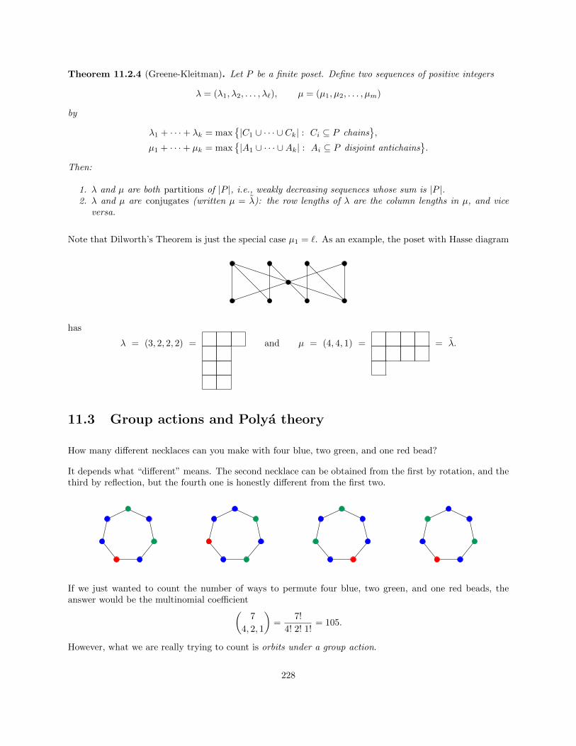
Theorem 11.2.4 (Greene-Kleitman). Let P be a finite poset. Define two sequences of positive integers

λ = (λ1, λ2, . . . , λℓ), µ = (µ1, µ2, . . . , µm)

by

λ1 + · · ·+ λk = max|C1 ∪ · · · ∪ Ck| : Ci ⊆ P chains

,

µ1 + · · ·+ µk = max|A1 ∪ · · · ∪Ak| : Ai ⊆ P disjoint antichains

.

Then:

1. λ and µ are both partitions of |P |, i.e., weakly decreasing sequences whose sum is |P |.2. λ and µ are conjugates (written µ = λ): the row lengths of λ are the column lengths in µ, and vice

versa.

Note that Dilworth’s Theorem is just the special case µ1 = ℓ. As an example, the poset with Hasse diagram

has

λ = (3, 2, 2, 2) = and µ = (4, 4, 1) = = λ.

11.3 Group actions and Polya theory

How many different necklaces can you make with four blue, two green, and one red bead?

It depends what “different” means. The second necklace can be obtained from the first by rotation, and thethird by reflection, but the fourth one is honestly different from the first two.

If we just wanted to count the number of ways to permute four blue, two green, and one red beads, theanswer would be the multinomial coefficient(

7

4, 2, 1

)=

7!

4! 2! 1!= 105.

However, what we are really trying to count is orbits under a group action.

228

Let G be a group and X a set. An action of G on X is a group homomorphism α : G→ SX , the group ofpermutations of X.

Equivalently, an action can also be regarded as a map G×X → X, sending (g, x) to gx, such that

• IdG x = x for every x ∈ X (where IdG denotes the identity element of G);• g(hx) = (gh)x for every g, h ∈ G and x ∈ X.

The orbit of x ∈ X is the setOx = gx : g ∈ G ⊆ X

and its stabilizer isSx = g ∈ G : gx = x ⊆ G,

which is a subgroup of G.

To go back to the necklace problem, we now see that “same” really means “in the same orbit”. In thiscase, X is the set of all 105 necklaces, and the group acting on them is the dihedral group D7 (the group ofsymmetries of a regular heptagon). The number we are looking for is the number of orbits of D7.

Lemma 11.3.1. Let x ∈ X. Then |Ox||Sx| = |G|.

Proof. The element gx depends only on which coset of Sx contains g, so |Ox| is the number of cosets, whichis |G|/|Sx|.

Proposition 11.3.2. [Burnside’s Theorem] The number of orbits of the action of G on X equals the averagenumber of fixed points:

1

|G|∑g∈G

#x ∈ X : gx = x

Proof. For a sentence P , let χ(P ) = 1 if P is true, or 0 if P is false (the “Garsia chi function”). Then

Number of orbits =∑x∈X

1

|Ox|=

1

|G|∑x∈X

|Sx|

=1

|G|∑x∈X

∑g∈G

χ(gx = x)

=1

|G|∑g∈G

∑x∈X

χ(gx = x) =1

|G|∑g∈G

#x ∈ X : gx = x.

Typically, it is easier to count fixed points than to count orbits directly.

Example 11.3.3. We can apply this technique to the necklace example above.

• The identity of D7 has 105 fixed points.• Each of the seven reflections in D7 has three fixed points (the single bead lying on the reflection linemust be red, and then the two green beads must be equally distant from it, one on each side).

• Each of the six nontrivial rotations has no fixed points.

229

Therefore, the number of orbits is105 + 7 · 3|D7|

=126

14= 9,

which is much more pleasant than trying to count them directly.

Example 11.3.4. Suppose we wanted to find the number of orbits of 7-bead necklaces with 3 colors, withoutspecifying how many times each color is to be used.

• The identity element of D7 has 37 = 2187 fixed points.• Each reflection fixes one bead, which can have any color. There are then three pairs of beads flipped,and we can specify the color of each pair. Therefore, there are 34 = 81 fixed points.

• Each rotation acts by a 7-cycle on the beads, so it has only three fixed points (all the beads must havethe same color).

Therefore, the number of orbits is2187 + 7 · 81 + 6 · 3

14= 198.

More generally, the number of inequivalent 7-bead necklaces with k colors allowed is

k7 + 7k4 + 6k

14. (11.4)

As this example indicates, it is helpful to look at the cycle structure of the elements of G, or more preciselyon their images α(g) ∈ SX .

Proposition 11.3.5. Let X be a finite set, and let α : G → SX be a group action. Color the elements ofX with k colors, so that G also acts on the colorings.

1. For g ∈ G, the number of fixed points of the action of g is kℓ(g), where ℓ(g) is the number of cycles inthe disjoint-cycle representation of α(g).

2. Therefore,

#equivalence classes of colorings =1

|G|∑g∈G

kℓ(g). (11.5)

Let’s rephrase Example 11.3.4 in this notation. The identity has cycle-shape 1111111 (so ℓ = 7); each of thesix reflections has cycle-shape 2221 (so ℓ = 4); and each of the seven rotations has cycle-shape 7 (so ℓ = 1).Thus (11.4) is an example of the general formula (11.5).

Example 11.3.6. How many ways are there to k-color the vertices of a tetrahedron, up to moving thetetrahedron around in space?

Here X is the set of four vertices, and the group G acting on X is the alternating group on four elements.This is the subgroup of S4 that contains the identity, of cycle-shape 1111; the eight permutations of cycle-shape 31; and the three permutations of cycle-shape 22. Therefore, the number of colorings is

k4 + 11k2

12.

230

11.4 Grassmannians

A standard reference for everything in this and the following section is Fulton [Ful97].

One motivation for the combinatorics of partitions and tableaux comes from classical enumerative geometricquestions like this:

Problem 11.4.1. Let there be given four lines L1, L2, L3, L4 in R3 in general position. How many lines Mmeet each of L1, L2, L3, L4 nontrivially?

To a combinatorialist, “general position” means “all pairs of lines are skew, and their direction vectors are aslinearly independent as possible — that is, the matroid they represent is U3(4).” To a probabilist, it means“choose the lines randomly according to some reasonable measure on the space of all lines.” So, what doesthe space of all lines look like?

In general, if V is a vector space over a field F (which we will henceforth take to be R or C), and 0 ≤ k ≤dimV , then the space of all k-dimensional vector subspaces of V is called the Grassmannian Gr(k, V ).(Warning: this notation varies considerably from source to source.) As we will see, Gr(k, V ) has many niceproperties:

• It is a smooth manifold of dimension k(n− k) over F.• It can be decomposed into pieces, called Schubert cells, each of which is naturally diffeomorphic toFj , for some appropriate j.

• The Schubert cells correspond to the interval Yk,n := [∅, kn−k] in Young’s lattice. (Here ∅ means theempty partition and kn−k means the partition with n−k parts, all of size k, so that the Ferrers diagramis a rectangle.) That is, for each partition λ there is a corresponding Schubert cell Ωλ of dimension |λ|(the number of boxes in the Ferrers diagram).

• How these cells fit together topologically is described by Yk,n in the following sense: the closure of Ωλ

is given by the formula

Ωλ =⋃µ≤λ

Ωµ

where ≤ is the usual partial order on Young’s lattice (i.e., containment of Ferrers diagrams).• When F = C, the Poincare polynomial of Gr(k,Cn), i.e., the Hilbert series of the cohomology ring ofGr(k,Cn),2 is the rank-generating function for the graded poset Yk,n, namely, the q-binomial coefficient[nk

]q.

To accomplish all this, we need some way to describe points of the Grassmannian. For as long as possible,we won’t worry about the ground field.

Let W ∈ Gr(k,Fn); that is, W is a k-dimensional subspace of V = Fn. We can describe W as the column

2If these terms don’t make sense, here is a sketch of what you need to know. The cohomology ring H∗(X) = H∗(X;Q)of a space X is just some ring that is a topological invariant of X. If X is a reasonably civilized space — say, a compactfinite-dimensional real or complex manifold, or a finite simplicial complex — then H∗(X) is a graded ring H0(X)⊕H1(X)⊕· · · ⊕Hd(X), where d = dimX, and each graded piece Hi(X) is a finite-dimensional Q-vector space. The Poincare polynomialrecords the dimensions of these vector spaces as a generating function:

Poin(X, q) =

d∑i=0

dimQ Hi(X) qi.

For lots of spaces, this polynomial has a nice combinatorial formula. For instance, take X = RP d (real projective d-space). Itturns out that H∗(X) ∼= Q[z]/(zn+1). Each graded piece Hi(X), for 0 ≤ i ≤ d, is a 1-dimensional Q-vector space (generatedby the monomial xi), and Poin(X, q) = 1 + q + q2 + · · · + qd = (1 − qd+1)/(1 − q). In general, if X is a compact orientablemanifold, then Poincare duality implies (among other things) that Poin(X, q) is a palindrome.

231

space of a n× k matrix M of full rank:

M =

m11 · · · m1k

......

mn1 · · · mnk

.However, the Grassmannian is not simply the space Z of all such matrices, because many different matricescan have the same column space. Specifically, any invertible column operation on M leaves its column spaceunchanged. On the other hand, every matrix whose column space is W can be obtained from M by somesequence of invertible column operations; that is, by multiplying on the right by some invertible k×k matrix.Accordingly, it makes sense to write

Gr(k,Fn) = Z/GLk(F). (11.6)

That is, the k-dimensional subspaces of Fn can be identified with the orbits of Z under the action of thegeneral linear group GLk(F). In fact, as one should expect from (11.6),

dimGr(k,Fn) = dimZ − dimGLk(F) = nk − k2 = k(n− k)where “dim” means dimension as a manifold over F; note that dimZ = nk because Z is a dense open subsetof Fn×k. (Technically, this dimension calculation does not follow from (11.6) alone; you need to know thatthe action of GLk(F) on Z is suitably well-behaved. Nevertheless, we will soon be able to calculate thedimension of Gr(k,Fn) more directly.)

We now want to find a canonical representative for each GLk(F)-orbit. In other words, given W ∈ Gr(k,Fn),we want the “nicest” matrix whose column space is W . How about the reduced column-echelon form? Basiclinear algebra says that we can pick any matrix with column spaceW and perform Gauss-Jordan eliminationon its columns, ending up with a uniquely determined matrix M =M(W ) with the following properties:

• colspaceM =W .• The top nonzero entry of each column of M (the pivot in that column) is 1.• Let pi be the row in which the ith column has its pivot. Then 1 ≤ p1 < p2 < · · · < pk ≤ n.• Every entry below a pivot of M is 0, as is every entry to the right of a pivot.• The remaining entries of M (i.e., other than the pivots and the 0s just described) can be anythingwhatsoever, depending on what W was in the first place.

For example, if n = 4 and k = 2, then M will have one of the following six forms:1 00 10 00 0

1 00 ⋆0 10 0

1 00 ⋆0 ⋆0 1

⋆ ⋆1 00 10 0

⋆ ⋆1 00 ⋆0 1

⋆ ⋆⋆ ⋆1 00 1

(11.7)

Note that there is only one subspace W for which M ends up with the first form. At the other extreme, ifthe ground field F is infinite and you choose the space W randomly (for a suitable definition of “random”;consult your local probabilist), then you will almost always end up with a matrix M of the last form.

Definition 11.4.2. Let 0 ≤ k ≤ n and let p = p1 < · · · < pk ∈([n]k

)(i.e., p1, . . . , pk are distinct elements

of [n], ordered least to greatest). The Schubert cell Ωp is the set of all elements W ∈ Gr(k,Fn) such that,for every i, the ith column of M(W ) has its pivot in row pi.

Theorem 11.4.3. 1. Every W ∈ Gr(k,Fn) belongs to exactly one Schubert cell; that is, Gr(k,Fn) is the

disjoint union of the subspaces Ωp, for p ∈([n]k

).

2. For every p ∈([n]k

), there is a diffeomorphismbijection

Ωp∼−→ F|p|

where |p| = (p1 − 1) + (p2 − 2) + · · ·+ (pk − k) = p1 + p2 + · · ·+ pk −(k+12

).

232

3. Define a partial order on([n]k

)as follows: for p = p1 < · · · < pk and q = q1 < · · · < qk, set p ≥ q

if pi ≥ qi for every i. Thenp ≥ q =⇒ Ωp ⊇ Ωq. (11.8)

4. The poset([n]k

)is isomorphic to the interval Yk,n in Young’s lattice.

5. Gr(k,Fn) is a compactification of the Schubert cell Ω(n−k+1,n−k+2,...,n)∼= Fk(n−k). In particular,

dimF Gr(k,Fn) = k(n− k).

The cell closures Ωp are called Schubert varieties.

Proof. (1) is immediate from the definition.

For (2), the map Ωp → F|p| is given by reading off the ⋆s in the reduced column-echelon form of M(W ).(For instance, let n = 4 and k = 2. Then the matrix representations in (11.7) give explicit diffeomorphismsof the Schubert cells of Gr(k,Fn) to F0, F1, F2, F2, F3, F4 respectively.) The number of ⋆s in the i-th columnis pi − i (pi − 1 entries above the pivot, minus i − 1 entries to the right of previous pivots), so the totalnumber of ⋆s is |p|.

For (3): This is best illustrated by an example. Consider the second matrix in (11.7):

M =

1 00 z0 10 0

where I have replaced the entry labeled ⋆ by a parameter z. Here’s the trick: Multiply the second columnof this matrix by the scalar 1/z. Doing this doesn’t change the column span, i.e.,

colspaceM = colspace

1 00 10 1/z0 0

.Now you can see that

lim|z|→∞

colspaceM = colspace lim|z|→∞

M = colspace

1 00 10 00 0

which is the first matrix in (11.7). Therefore, the Schubert cell Ω1,2 is in the closure of the Schubert cellΩ1,3. In general, decrementing a single element of p corresponds to taking a limit of column spans in this

way, so the covering relations in the poset([n]k

)give containment relations of the form (11.8).

Assertion (4) is purely combinatorial. The elements of Yk,n are partitions λ = (λ1, . . . , λk) such thatn− k ≥ λ1 > · · · > λk ≥ 0. The desired poset isomorphism is p 7→ λp = (pk − k, pk−1 − (k− 1), . . . , p1 − 1).For example, starting with (11.7)

Matrix

1 00 10 00 0

1 00 ⋆0 10 0

1 00 ⋆0 ⋆0 1

⋆ ⋆1 00 10 0

⋆ ⋆1 00 ⋆0 1

⋆ ⋆⋆ ⋆1 00 1

p 12 13 14 23 24 34

λp ∅

233

(5) now follows because p = (n− k+1, n− k+2, . . . , n) is the unique maximal element of([n]k

), and an easy

calculation shows that |p| = k(n− k).

This theorem amounts to a description of Gr(k,Fn) as a cell complex. (If you have not heard the term “cellcomplex” before, now you know what it means: a topological space that is the disjoint union of cells —that is, of homeomorphic copies of vector spaces — such that the closure of every cell is itself a union ofcells.) Furthermore, the poset isomorphism with Yk,n says that for every i, the number of cells of Gr(k,Fn)of dimension i is precisely the number of Ferrers diagrams with i blocks that fit inside the rectangle kn−k.Combinatorially, we may write this equality as follows:∑

i

(# Schubert cells of dimension i) qi =∑i

#λ ⊆ kn−k qi =

[n

k

]q

.

Example 11.4.4. If k = 1, then Gr(1,Fn) is the space of lines through the origin in Fn; that is, projectivespace FPn−1. As a cell complex, this has one cell of every dimension. For instance, the projective plane isthe union of three cells of dimensions 2, 1, and 0, i.e., a plane, a line and a point. In the standard geometricpicture, the 1-cell and 0-cell together form the “line at infinity”. Meanwhile, the interval Yk,n is a chain ofrank n− 1. Its rank-generating function is 1 + q+ q2 + · · ·+ qn−1. (For F = C, double the dimensions of allthe cells, and substitute q2 for q.)

Remark 11.4.5. If F = C, then Gr(k,Cn) is a cell complex with no odd-dimensional cells (because, topo-logically, the dimension of cells is measured over R). Therefore, readers who know some algebraic topology(see, e.g., [Hat02, §2.2]) may observe that the cellular boundary maps are all zero (because each one haseither zero domain or zero range), so the cellular homology groups are exactly the chain groups. That is, thePoincare series of Gr(k,Cn) is exactly the generating function for the dimensions of the cells. On the otherhand, If F = R, then the boundary maps need not be zero, and the homology can be more complicated.Indeed, Gr(1,Rn) = RPn−1 has torsion homology in odd dimensions.

Example 11.4.6. Let n = 4 and k = 2. Here is Yk,n:

∅

These six partitions correspond to the six matrix-types in (11.7). The rank-generating function is[4

2

]q

=(1− q4)(1− q3)(1− q2)(1− q) = 1 + q + 2q2 + q3 + q4.

Remark 11.4.7. What does all this have to do with enumerative geometry questions such as Problem 11.4.1?The answer (modulo technical details) is that the cohomology ring H∗(X) encodes intersections of sub-varieties3 of X: for every subvariety Z ⊆ Gr(k,Fn) of codimension i, there is a corresponding element

3If you are more comfortable with differential geometry than algebraic geometry, feel free to think “submanifold” instead of“subvariety”.

234

[Z] ∈ Hi(X) (the “cohomology class of Z”) such that [Z ∪ Z ′] = [Z] + [Z ′] and [Z ∩ Z ′] = [Z][Z ′]. Theseequalities hold only if Z and Z ′ are in general position with respect to each other (which has to be definedprecisely), but the consequence is that Problem 11.4.1 reduces to a computation in H∗(Gr(k,Fn)): find thecohomology class [Z] of the subvariety

Z = W ∈ Gr(2,C4) : W meets some plane in C4 nontrivially

and compare [Z]4 to the cohomology class [•] of a point. In fact, [Z]4 = 2[•]; this says that the answerto Problem 11.4.1 is two, which is hardly obvious! To carry out this calculation, one needs to calculatean explicit presentation of the ring H∗(Gr(k,Fn)) as a quotient of a polynomial ring (which requires themachinery of line bundles and Chern classes, but that’s another story) and then figure out how to expressthe cohomology classes of Schubert cells with respect to that presentation. This is the theory of Schubertpolynomials.

11.5 Flag varieties

There is a corresponding theory for the flag variety, which is the set Fℓ(n) of nested chains of vector spaces

F• = (0 = F0 ⊆ F1 ⊆ · · · ⊆ Fn = Fn)

or equivalently saturated chains in the (infinite) lattice Ln(F). The flag variety is in fact a smooth manifoldover F of dimension

(n2

). Like the Grassmannian, it has a decomposition into Schubert cells Xw, which are

indexed by permutations w ∈ Sn rather than partitions, as we now explain.

For every flag F•, we can find a vector space basis v1, . . . , vn for Fn such that Fk = F⟨v1, . . . , vk⟩ for all k,and represent F• by the invertible matrix M ∈ G = GL(n,F) whose columns are v1, . . . , vn. OTOH, anyordered basis of the form

v′1 = b11v1, v′2 = b12v1 + b22v2, . . . , v′n = b1nv1 + b2nv2 + · · ·+ bnnvn,

where bkk = 0 for all k, defines the same flag. That is, a flag is a coset of B in G, where B is the subgroupof invertible upper-triangular matrices (the Borel subgroup). Thus the flag variety can be (and often is)regarded as the quotient G/B. This immediately implies that it is an irreducible algebraic variety (as Gis irreducible, and any image of an irreducible variety is irreducible). Moreover, it is smooth (e.g., becauseevery point looks like every other point, and so either all points are smooth or all points are singular andthe latter is impossible) and its dimension is (n− 1) + (n− 2) + · · ·+ 0 =

(n2

).

As in the case of the Grassmannian, there is a canonical representative for each coset of B, obtained byGaussian elimination, and reading off its pivot entries gives a decomposition

Fℓ(n) =∐

w∈Sn

Xw.

Here the dimension of a Schubert cell Xw is the number of inversions of w, i.e.,

dimXw = inv(w) = #(i, j) : 1 ≤ i < j ≤ n and w(i) > w(j).

Recall that this is the rank function of the Bruhat and weak Bruhat orders on Sn. In fact, the (strong)Bruhat order is the cell-closure partial order (analogous to (11.8)). It follows that the Poincare polynomialof Fℓ(n) is the rank-generating function of Bruhat order, namely

(1 + q)(1 + q + q2) · · · (1 + q + · · ·+ qn−1).

235

More strongly, it can be shown that the cohomology ring H∗(Fℓ(n);Z) is the quotient of Z[x1, . . . , xn] bythe ideal generated by symmetric functions.

The Schubert varieties in Fℓ(n) are

Xw =⋃

v∈Sn: v≤w

Xv

where ≤ means (strong) Bruhat order (see Ex. 1.2.13). These are much-studied objects in combinatorics;for example, determining which Schubert varieties is singular turns out to to be a combinatorial questioninvolving the theory of pattern avoidance. Even more generally, instead of Sn, start with any finite Coxetergroup G (roughly, a group generated by elements of order two — think of them as reflections). Then G has acombinatorially well-defined partial order also called the Bruhat order, and one can construct a G-analogueof the flag variety: that is, a smooth manifold whose structure as a cell complex is given by Bruhat orderon G.

We now describe the calculation of the cohomology ring of Fℓ(n) using Chern classes. This is not intendedto be self-contained, and many facts will be presented as black boxes. The reader who wants the full storyshould see a source such as [BT82].

Definition 11.5.1. Let B and F be topological spaces. A bundle with base B and fiber F is a spaceE together with a map π : E → B such that

1. If b ∈ B, then π−1(b) ∼= F ; and, more strongly,2. Every b ∈ B has an open neighborhood U of b such that V := π−1(U) ∼= U × F , and π|V is just

projection on the first coordinate.

Think of a bundle as a family of copies of F parameterized by B and varying continuously. The simplestexample of a bundle is a Cartesian product B × F with π(b, f) = b; this is called a trivial bundle. Veryoften the fiber is a vector space of dimension d, when we call the bundle a vector bundle of rank d; whend = 1 the bundle is a line bundle.

Frequently we require all these spaces to lie in a more structured category than that of topological spaces,and we require the projection map to be a morphism in that category (e.g., manifolds with diffeomorphisms,or varieties with algebraic maps).

Example 11.5.2. An example of a nontrivial bundle is a Mobius stripM , where B = S1 is the central circleand F = [0, 1] is a line segment. Indeed, a Mobius strip looks like a bunch of line segments parameterizedby a circle, and if U is any small interval in S1 then the part of the bundle lying over U is just U × [0, 1].However, the global structure of M is not the same as the cylinder S1 × I.

Example 11.5.3. Another important example is the tautological bundle on projective space Pd−1F =

Gr(1,Fd). Recall that this is the space of lines ℓ through the origin in Fd. The tautological bundle4 T is theline bundle defined by Tℓ = ℓ. That is, the fiber over a line is just the set of points on that line.

Let F be either R or C, and let us work in the category of closed compact manifolds over F. A vectorbundle of rank d is a bundle whose fiber is Fd. (For example, the tautological bundle is a vector bundle ofrank 1.) Standard operations on vector spaces (direct sum, tensor product, dual, etc.) carry over to vectorbundles, defined fiberwise.

Let E be a rank-d vector bundle over M . Its projectivization P(E) is the bundle with fiber Pd−1F defined

byP(E)m = P(Em).

4The standard symbol for the tautological bundle is actually O(−1); let’s not get into why.

236

That is, a point in P(E) is given by a point m ∈ M and a line ℓ through the origin in Em ∼= Fd. In turn,P(E) has a tautological line bundle L = L (E) whose fiber over (ℓ,m) is ℓ.

Associated with the bundle E are certain Chern classes ci(E) ∈ H2i(M) for every i, which measure “howtwisty E is.” (The 2 happens because we are talking about a complex manifold.) I will not define theseclasses precisely (see [BT82]), but instead will treat them as a black box that lets us calculate cohomology.The Chern classes have the following properties:

1. c0(E) = 1 by convention.2. ci(E) = 0 for i > rank E .3. If E is trivial then ci(E) = 0 for i > 0.4. If 0 → E ′ → E → E ′′ → 0 is an exact sequence of M -bundles, then c(E) = c(E ′)c(E ′′), wherec(E) =∑i ci(E) (the “total Chern class”).

5. For a line bundle L, c1(L∗) = −c1(L).

Here is the main formula, which expresses the cohomology ring of a bundle as a module over the cohomologyof its base.

H∗(P(E);Z) = H∗(M ;Z)[x]/⟨xd + c1(E)xd−1 + · · ·+ cd−1(E)x+ cd(E)⟩ (11.9)

where x = c1(L ).

Example 11.5.4 (Projective space). Pd−1C is the projectivization of the trivial rank-d bundle overM = •. Of course H∗(M ;Z) = Z, so H∗(Pd−1C;Z) = Z[x]/⟨xd⟩.

Example 11.5.5 (The flag variety Fℓ(3)). Let M = P2 = Gr(1,C3). Define a bundle E2 by

E2ℓ = C3/ℓ.

Then E2 has rank 2, and P(E2) is just the flag variety Fℓ(3), because specifying a line in C3/ℓ is the samething as specifying a plane in C3 containing ℓ. Let L = L (E2). For each ℓ ∈M we have an exact sequence0→ ℓ→ C3 → C3/ℓ→ 0, which gives rise to a short exact sequence of bundles

0→ O → C3 → E2 → 0

where O is the tautological bundle on M , with c1(O) = x (the generator of H∗(M)). The rules for Chernclasses then so the rules for Chern classes tell us that

(1 + x)(1 + c1(E2) + c2(E2)) = 1

and extracting the graded pieces we get

x+ c1(E2) = 0, xc1(E2) + c2(E2) = 0

so c1(E2) = −x and c2(E2) = −xc1(E2) = x2. Now (11.9) tells us that

H∗(Fℓ(3)) = H∗(P2)[y]/⟨y2 − xy + x2⟩ = Q[x, y]/⟨x3, y2 − xy + x2⟩.

In fact this ring is isomorphic to

Q[a, b, c]/⟨a+ b+ c, ab+ ac+ bc, abc⟩.

(For the isomorphism, set a = x, b = −y, c = −x+ y.)

Example 11.5.6 (General flag varieties.). Fℓ(n) can be constructed as an iterated bundle:

X0 = •. Let E0 be the (trivial) rank-n bundle over X0.

237

X1 = P(E0). Let E1 be the rank-(n− 1) bundle whose fiber over a line E1 is Cn/E1.

X2 = P(E1). This is the partial flag variety of flags E• : 0 = E0 ⊆ E1 ⊆ E2. Let E2 be the rank-(n − 2)bundle whose fiber over E• is Cn/E2.

X3 = P(E2). And so forth.

We end up with generators x1, . . . , xn, one for the tautological bundle of each Ei. The relations turn out tobe the symmetric functions on them. That is.

H∗(Fℓ(n)) ∼= Q[x1, . . . , xn]/⟨e1, e2, . . . , en⟩

where ek is the kth elementary symmetric function, i.e.,

ek =∑

1≤i1<···<ik≤n

xi1 · · ·xik .

The Poincare polynomial of the flag variety (i.e., the Hilbert series of its cohomology ring) can be workedout explicitly. Modulo the elementary symmetric functions, every polynomial can be written as a sum ofmonomials of the form

xa11 x

a22 · · ·xan

n

where ai < i for all i. Therefore,

Poin(Fℓ(n), q) =∑k

qk dimQH2i(Fℓ(n)) = (1)(1 + q)(1 + q + q2) · · · (1 + q + · · ·+ qn−1) = [q]n!.

This expression has a lovely combinatorial interpretation:

[q]n! =∑

w∈Sn

qinv(w)

where Sn is the symmetric group on n letters and inv(w) is the number of inversions:

inv(w) = #(i, j) : 1 ≤ i < j ≤ n, w(i) > w(j).

In fact the flag variety has a natural cell decomposition into Schubert cells. Given any flag

E• : 0 = E0 ⊆ E1 ⊆ · · · ⊆ En = Cn

construct a n × n matrix [v1| · · · |vn] in which the first k columns are a basis of Ek, for every k. We cancanonicalize the matrix as follows:

• Scale the first column so that its bottom nonzero entry is 1. Say this occurs in row w1.• Add an appropriate multiple of v1 to each of v2, . . . , vn so as to kill off the entry in row w1. Note thatthis does not change the flag.

• Scale the second column so that its bottom nonzero entry is 1. Say this occurs in row w2. Note thatw2 = w1.

• Add an appropriate multiple of v2 to each of v3, . . . , vn so as to kill off the entry in row w1.• Repeat.

238

(Here we are really using the descriptionFℓ(n) = GLn/B

where B is the Borel subgroup of upper-triangular invertible matrices. The column operations that we havedone correspond to choosing a canonical element of each coset of B in GLn.)

We end up with a matrix that includes a “pivot” 1 in each row and column, with zeroes below and to theright of every 1. The pivots define a permutation w ∈ Sn. For example, if w = 4132 then the matrix willhave the form

∗ 1 0 0∗ 0 ∗ 1∗ 0 1 01 0 0 0

.The set X

3142 of all matrices of this type is a subspace of Fℓ(4) that is in fact isomorphic to C3 — the starsare affine coordinates. Thus we obtain a decomposition into Schubert cells

Fℓ(n) =∐

w∈Sn

Xw

and moreover the stars correspond precisely to inversions of w. This gives the Poincare polynomial.

The closure of a Schubert cell is called a Schubert variety. The cohomology classes of Schubert varietiesare also a vector space basis for H∗(Fℓ(n)), and there is a whole theory of how to translate between the“algebraic” basis (coming from line bundles) and the “geometric” basis (Schubert varieties).

11.6 Exercises

Max-flow/min-cut and min-max theorems on posets


Exercise 11.2. Let G(V,E) be a graph. A matching on G is a collection of edges no two of which sharean endpoint. A vertex cover is a set of vertices that include at least one endpoint of each edge of G. Letµ(G) denote the size of a maximum matching, and let β(G) denote the size of a minimum vertex cover.

(a) (Warmup) Show that µ(G) ≤ β(G) for every graph G. Exhibit a graph for which the inequality isstrict.

(b) The Konig-Egervary Theorem asserts that µ(G) = β(G) whenever G is bipartite, i.e., the verticesof G can be partitioned as X ∪ Y so that every edge has one endpoint in each of X,Y . Derive theKonig-Egervary Theorem as a consequence of the Max-Flow/Min-Cut Theorem.

(c) Prove that the Konig-Egervary Theorem and Dilworth’s Theorem imply each other.

Polya theory

Exercise 11.3. Let n ≥ 2 and for σ ∈ Sn, let f(σ) denote the number of fixed points. Prove that for everyk ≥ 1, the number 1

n!

∑σ∈Sn

f(σ)k is an integer.

Grassmannians and flag varieties

239

Appendix: Catalan Numbers

The Catalan numbers are the sequence C0, C1, . . . , defined by

Cn :=1

2n+ 1

(2n

n

).

The Catalan numbers are ubiquitous in combinatorics. A famous exercise in volume 2 of Stanley’s Enumer-ative Combinatorics [Sta99, Exercise 6.19] lists 66 combinatorial interpretations of the Catalan numbers andasks the reader to come up with

(662

)bijections between them. That was in 1999; more recently, Stanley

wrote an entire monograph [Sta15] with 214 interpretations. Here we’ll just review the basics.

A Dyck path of size n is a path from (0, 0) to (2n, 0) in R2 consisting of n up-steps and n down-stepsthat stays (weakly) above the x-axis.

Figure 11.5: A Dyck path of size 4.

We can denote Dyck paths efficiently by a list of U’s and D’s; the path P shown above is UUDUUDDD. Eachup-step can be thought of as a left parenthesis, and each down-step as a right parenthesis, so we could alsowrite P = (()(())). The requirement of staying above the x-axis then says that each right parenthesis mustclose a previous left parenthesis.

Proposition 11.6.1. The number of Dyck paths of size n is the Catalan number Cn.

Sketch of proof. The proof is an illustration of the Sheep Principle (“in order to count the sheep in a flock,count the legs and divide by four”). Consider the family L of all lattice paths from (0, 0) to (2n + 1,−1)consisting of n up-steps and n+ 1 down-steps (with no restrictions); evidently |L| =

(2n+1

n

).

Consider the action of the cyclic group Z2n+1 on L by cyclic rotation. First, the orbits all have size 2n+ 1.(There is no way that a nontrivial element of Z2n+1 can fix the locations of the up-steps, essentially becausegcd(2n + 1, n) = 1 — details left to the reader.) Second, each orbit contains exactly one augmented Dyck

240

path, i.e., a Dyck path followed by a down-step. (Of all the lowest points in a path, find the leftmost oneand call it z. Rotate so that the last step is the down-step that lands at z.)

z

z

Figure 11.6: Rotating the lattice path UDDUDD|UDU to obtain the augmented Dyck path UDU|UDDUDD.

Every (augmented) Dyck path arises in this way, so we have a bijection. The orbits are sheep and each sheephas 2n+ 1 legs, so the number of Dyck paths is

1

2n+ 1

(2n+ 1

n

)=

(2n+ 1)!

(2n+ 1) (n+ 1)! n!=

(2n)!

(n+ 1)! n!=

(2n)!

(n+ 1) n! n!=

1

n+ 1

(2n

n

).

To show that a class of combinatorial objects is enumerated by the Catalan numbers, one can now find abijection to Dyck paths. A few of the most commonly encountered interpretations of Cn are:

• Triangulations of a convex (n+ 2)-gon into n triangles using n− 1 diagonals.• Binary trees with n vertices. (“Binary” means that each vertex has at most 2 children.)• Plane trees with n vertices. (“Plane” means that each set of siblings comes with a left-to-right order.)

Others will be encountered in the course of these notes. For details, see [Sta99] or [Sta15] Another corefeature of the Catalan numbers is that they satisfy the following recurrence:

Cn = Cn−1 +

n−1∑k=1

Ck−1Cn−k for n ≥ 1. (11.10)

This equation can be checked by a banal induction argument, but it is also worthwhile seeing the combina-torial reason for it. Call a Dyck path of size n primitive if it stays strictly above the x-axis for 0 < x < 2n.If a path P is primitive, then it is of the form UP ′D for some Dyck path P ′ of size n − 1 (not necessarilyprimitive); this accounts for the Cn−1 term in the Catalan recurrence. Otherwise, let (2k, 0) be the smallestpositive x-intercept, so that 1 ≤ k ≤ n − 1. The part of the path from (0, 0) to (2k, 0) is a primitive Dyckpath of size k, and the part from (2k, 0) to (2n, 0) is a Dyck path of size n− k, not necessarily primitive.

primitive; P ′ highlighted not primitive; k = 2

Figure 11.7: Primitive and non-primitive Dyck paths.

241

Notational Index

Basics

End of an example[n] 1, . . . , nN nonnegative integers 0, 1, 2, . . . \mathbbN

N>0 positive integers 1, 2, . . . \mathbbP

2S power set of a set S (or the associated poset)∪· disjoint union \cupdot (requires header.tex) symmetric difference AB = (A ∪B) \ (A ∩B) \triangle

Sn symmetric group on n letters \mathfrakS_n(Sk

)set of k-element subsets of a set S \binomSk

Cn Catalan numbersk⟨v1, . . . ,vn⟩ k-vector space with basis v1, . . . ,vn

Posets

⋗, ⋖ “covers”, “is covered by” \gtrdot, \lessdot

0, 1 unique min and max elements of a poset \hat\mathbf0

[x, y] interval in a posetP ∗ dual poset to PΠn lattice of all set partitions of [n]K(G) connectivity lattice of a graph GY Young’s lattice of integer partitionsλ ⊢ n λ is a partition of n \vdash

λ conjugate of a partition λ

Lattices

∧,∨ meet, join \wedge, \veeBooln Boolean lattice of rank n \mathscrB_n

Dn lattice of divisors of an integer nFq finite field of order q \mathbbF_q

Ln(q) lattice of vector subspaces of Fnq

J(P ) lattice of order ideals of a poset PIrr(L) poset of join-irreducible elements in a lattice LN5 nonmodular, nonranked 5-element latticeM5 modular, ranked, nondistributive 5-element latticeL(E) geometric lattice represented by vectors ELaff(E) geometric lattice represented by affine points E

242

Poset Algebra

Int(P ) set of intervals of poset PI(P ) incidence algebra of Pf ∗ g convolution product in I(P )δ Kronecker delta function (identity of I(P ))ζ, µ zeta and Mobius functions in I(P )χP (x) characteristic polynomial of poset PMob(L) Mobius algebra of a lattice L

Matroids and the Tutte Polynomial

A− e, A+ e abbreviations for A \ e, A ∪ eA closure operator applied to AM(G) graphic matroid of a graph GI matroid independence system \mathscrI (uses mathrsfs package)B matroid basis system \mathscrB

C matroid circuit system \mathscrC

M∗ dual of a matroid MM ⊕M ′ direct sum of matroidsM\e, M/e matroid deletion and contractionUk(n) uniform matroid of rank k on set of size nTM , TM (x, y) Tutte polynomial of MpG(k) chromatic polynomial of a graph GC(e,B) fundamental circuit of e w/r/t basis BC∗(e,B) fundamental cocircuit of e w/r/t basis B

Hyperplane Arrangements

Booln Boolean arrangementBrn braid arrangementAG arrangement associated with a graph GL(A) intersection poset of arrangement Aess(A) essentialization of Ar(A) number of regions of a real arrangement Ab(A) number of relatively bounded regions of AAx, Ax See Eqn. 5.4Shin Shi arrangement

Simplicial Complexes and Polytopes

⟨· · · ⟩ simplicial complex generated by a set of faces \langle ... \rangle

|∆| (standard) geometric realization of ∆∆(P ) order complex of a poset Pk[∆] Stanley-Reisner (face) ring of ∆ over a field k \Bbbk[\Delta]

Ck(∆, R) simplicial chain groups over a ring R

Hk(∆, R) reduced simplicial homology groupsSd d-dimensional sphere \mathbbS

P ∗ dual of a polytope P

243

Representation Theory

Id identity element of a groupDn dihedral group of symmetries of a regular n-gonρtriv, ρreg trivial and regular representationsρsign, ρdef sign and defining representations of Sn

χρ or χ character of representation ρCℓ(G) space of class functions of G⟨ρ, χ⟩G inner product on Cℓ(G) (see Thm. 8.6.5)HomC(V,W ) C-linear maps V →WHomG(V,W ) G-equivariant C-linear maps V →WV G space of invariants of a G-action on V[a, b] commutator: aba−1b−1[G,G] commutator subgroup of GAn alternating group on n letters \mathfrakA_n

Par(n) partitions of nCλ conjugacy class of permutations with cycle shape λλ < µ lexicographic (total) order on partitionsλ◁ µ, λ⊴ µ dominance (partial) order on partitions \lhd, \unlhdsh(T ) shape of a tabloid T(ρµ, Vµ) tabloid representation of shape µχµ character of tabloid representationSpλ Specht moduleKλ,µ Kostka numbers

ResGH ρ, ResGH χ restricted representation/character

IndGH ρ, IndGH χ induced representation/character

Symmetric Functions

xα monomial in variables x with exponent vector αR[[x]] ring of formal power series in x with coefficients in R[xα]F coefficient of monomial xα in power series Fmλ monomial symmetric functioneλ elementary symmetric functionhλ (complete) homogeneous symmetric functionpλ power-sum symmetric functionΛd, ΛR,d(x) R-module of degree-d symmetric functions in xΛ, ΛR(x) R-algebra of symmetric functions in xω involutory automorphism Λ→ Λ swapping e’s and h’s (not to be confused with w!)CST(λ) set of column-strict tableaux of shape λsλ Schur symmetric functionΩ,Ω∗ Cauchy kernel and dual Cauchy kernelzλ size of centralizer of a partition of shape λ (see (9.16))ελ sign of a partition of shape λ (see (9.16))SYT(λ) set of standard tableaux of shape λfλ number of standard tableaux of shape λT ← x row-insertion (§9.10) T\gets x

ch Frobenius characteristic (§9.12)cλµ,ν Littlewood-Richardson coefficientsh(x) length of the hook with corner x

244

Combinatorial Algebraic Varieties

Gr(k, V ) Grassmannian of k-dimensional subspaces of VΩλ Schubert cell in a GrassmannianFℓ(n) (complete) flag variety in dimension nXw Schubert cell in a flag variety

Hopf Algebras and Monoids

µ product∆ coproductu unitε counitS antipode

245

Bibliography

[AA17] Marcelo Aguiar and Federico Ardila, Hopf monoids and generalized permutahedra, preprint,arXiv:1709.07504, 2017. 132, 218

[ABS06] Marcelo Aguiar, Nantel Bergeron, and Frank Sottile, Combinatorial Hopf algebras andgeneralized Dehn-Sommerville relations, Compos. Math. 142 (2006), no. 1, 1–30. MR 2196760218

[AM10] Marcelo Aguiar and Swapneel Mahajan, Monoidal functors, species and Hopf algebras, CRMMonograph Series, vol. 29, American Mathematical Society, Providence, RI, 2010, Withforewords by Kenneth Brown and Stephen Chase and Andre Joyal. MR 2724388 218

[Ath96] Christos A. Athanasiadis, Characteristic polynomials of subspace arrangements and finite fields,Adv. Math. 122 (1996), no. 2, 193–233. MR 1409420 (97k:52012) 99

[BB05] Anders Bjorner and Francesco Brenti, Combinatorics of Coxeter Groups, Graduate Texts inMathematics, vol. 231, Springer, New York, 2005. MR 2133266 (2006d:05001) 16

[BF01] Thomas Britz and Sergey Fomin, Finite posets and Ferrers shapes, Adv. Math. 158 (2001),no. 1, 86–127. MR 1814900 227

[BH93] Winfried Bruns and Jurgen Herzog, Cohen-Macaulay Rings, Cambridge Studies in AdvancedMathematics, vol. 39, Cambridge University Press, Cambridge, 1993. MR 1251956 (95h:13020)114, 119

[BLVS+99] Anders Bjorner, Michel Las Vergnas, Bernd Sturmfels, Neil White, and Gunter M. Ziegler,Oriented matroids, second ed., Encyclopedia of Mathematics and its Applications, vol. 46,Cambridge University Press, Cambridge, 1999. MR 1744046 108

[BM71] H. Bruggesser and P. Mani, Shellable decompositions of cells and spheres, Math. Scand. 29(1971), 197–205 (1972). MR 0328944 (48 #7286) 130

[BO92] Thomas Brylawski and James Oxley, The Tutte polynomial and its applications, Matroidapplications, Encyclopedia Math. Appl., vol. 40, Cambridge Univ. Press, Cambridge, 1992,pp. 123–225. MR 1165543 (93k:05060) 86

[Bol98] Bela Bollobas, Modern Graph Theory, Graduate Texts in Mathematics, vol. 184,Springer-Verlag, New York, 1998. MR 1633290 (99h:05001) 78

[BR07] Matthias Beck and Sinai Robins, Computing the Continuous Discretely, Undergraduate Textsin Mathematics, Springer, New York, 2007, Integer-point enumeration in polyhedra. MR2271992 (2007h:11119) 84

246

[Bri73] Egbert Brieskorn, Sur les groupes de tresses [d’apres V. I. Arnol′d], Seminaire Bourbaki,24eme annee (1971/1972), Exp. No. 401, Springer, Berlin, 1973, pp. 21–44. Lecture Notes inMath., Vol. 317. 104, 105

[BT82] Raoul Bott and Loring W. Tu, Differential Forms in Algebraic Topology, Graduate Texts inMathematics, vol. 82, Springer-Verlag, New York-Berlin, 1982. MR 658304 (83i:57016) 236, 237

[CR70] Henry H. Crapo and Gian-Carlo Rota, On the Foundations of Combinatorial Theory:Combinatorial Geometries, preliminary ed., The M.I.T. Press, Cambridge, Mass.-London, 1970.MR 0290980 99

[Dir61] G.A. Dirac, On rigid circuit graphs, Abh. Math. Sem. Univ. Hamburg 25 (1961), 71–76. MR0130190 (24 #A57) 104

[FS05] Eva Maria Feichtner and Bernd Sturmfels, Matroid polytopes, nested sets and Bergman fans,Port. Math. (N.S.) 62 (2005), no. 4, 437–468. MR 2191630 132

[Ful97] William Fulton, Young Tableaux, London Mathematical Society Student Texts, vol. 35,Cambridge University Press, Cambridge, 1997. 188, 206, 231

[GGMS87] I. M. Gel’fand, R. M. Goresky, R. D. MacPherson, and V. V. Serganova, Combinatorialgeometries, convex polyhedra, and Schubert cells, Adv. in Math. 63 (1987), no. 3, 301–316. MR877789 132

[GK76] Curtis Greene and Daniel J. Kleitman, The structure of Sperner k-families, J. Combin. TheorySer. A 20 (1976), no. 1, 41–68. 227

[GNW79] Curtis Greene, Albert Nijenhuis, and Herbert S. Wilf, A probabilistic proof of a formula for thenumber of Young tableaux of a given shape, Adv. in Math. 31 (1979), no. 1, 104–109. MR521470 200

[Gre76] Curtis Greene, Some partitions associated with a partially ordered set, J. Combin. Theory Ser.A 20 (1976), no. 1, 69–79. 227

[Gru03] Branko Grunbaum, Convex Polytopes, second ed., Graduate Texts in Mathematics, vol. 221,Springer-Verlag, New York, 2003, Prepared and with a preface by Volker Kaibel, Victor Kleeand Gunter M. Ziegler. 62, 126

[GSS93] Jack Graver, Brigitte Servatius, and Herman Servatius, Combinatorial Rigidity, GraduateStudies in Mathematics, vol. 2, American Mathematical Society, Providence, RI, 1993. MR1251062 50

[Hat02] Allen Hatcher, Algebraic Topology, Cambridge University Press, Cambridge, 2002. MR 1867354(2002k:55001) 114, 116, 117, 234

[HS15] Joshua Hallam and Bruce Sagan, Factoring the characteristic polynomial of a lattice, J.Combin. Theory Ser. A 136 (2015), 39–63. MR 3383266 104

[Hum90] James E. Humphreys, Reflection Groups and Coxeter Groups, Cambridge Studies in AdvancedMathematics, vol. 29, Cambridge University Press, Cambridge, 1990. MR 1066460 (92h:20002)16

[Hum11] Brandon Humpert, Polynomials Associated with Graph Coloring and Orientations, Ph.D.thesis, University of Kansas, 2011. 217

[Kli] Caroline J. Klivans, A quasisymmetric function for generalized permutahedra, Talk slides,http://www.dam.brown.edu/people/cklivans/birs.pdf. 218

247

http://www.dam.brown.edu/people/cklivans/birs.pdf

[LS00] Shu-Chung Liu and Bruce E. Sagan, Left-modular elements of lattices, J. Combin. Theory Ser.A 91 (2000), no. 1-2, 369–385. MR 1780030 48

[MR05] Jeremy L. Martin and Victor Reiner, Cyclotomic and simplicial matroids, Israel J. Math. 150(2005), 229–240. MR 2255809 71

[MS05] Ezra Miller and Bernd Sturmfels, Combinatorial Commutative Algebra, Graduate Texts inMathematics, vol. 227, Springer-Verlag, New York, 2005. MR 2110098 (2006d:13001) 114

[OS80] Peter Orlik and Louis Solomon, Combinatorics and topology of complements of hyperplanes,Invent. Math. 56 (1980), no. 2, 167–189. 105

[OT92] Peter Orlik and Hiroaki Terao, Arrangements of Hyperplanes, Grundlehren derMathematischen Wissenschaften [Fundamental Principles of Mathematical Sciences], vol. 300,Springer-Verlag, Berlin, 1992. 87

[Oxl92] James G. Oxley, Matroid Theory, Oxford Science Publications, The Clarendon Press OxfordUniversity Press, New York, 1992. 50, 62, 63

[Per16] Xander Perrott, Existence of projective planes, arXiv:1603.05333 (retrieved 8/26/18), 2016. 62

[Pos09] Alexander Postnikov, Permutohedra, associahedra, and beyond, Int. Math. Res. Not. (2009),no. 6, 1026–1106. MR 2487491 132

[PRW08] Alex Postnikov, Victor Reiner, and Lauren Williams, Faces of generalized permutohedra, Doc.Math. 13 (2008), 207–273. MR 2520477 132

[Rei] Victor Reiner, Lectures on matroids and oriented matroids, Lecture notes for AlgebraicCombinatorics in Europe (ACE) Summer School in Vienna, July 2005; available athttp://www-users.math.umn.edu/∼reiner/Talks/Vienna05/Lectures.pdf. 108, 112

[RGZ97] Jurgen Richter-Gebert and Gunter M. Ziegler, Oriented matroids, Handbook of discrete andcomputational geometry, CRC Press Ser. Discrete Math. Appl., CRC, Boca Raton, FL, 1997,pp. 111–132. MR 1730162 108, 109

[Ryb11] G.L. Rybnikov, On the fundamental group of the complement of a complex hyperplanearrangement, Funktsional. Anal. i Prilozhen. 45 (2011), no. 2, 71–85. 105

[S+14] W.A. Stein et al., Sage Mathematics Software (Version 6.4.1), The Sage Development Team,2014, http://www.sagemath.org. 88

[Sag01] Bruce E. Sagan, The Symmetric Group, second ed., Graduate Texts in Mathematics, vol. 203,Springer-Verlag, New York, 2001. 177

[Sch13] Alexander Schrijver, A Course in Combinatorial Optimization, Available online athttp://homepages.cwi.nl/∼lex/files/dict.pdf (retrieved 1/21/15), 2013. 126, 128

[Sta95] Richard P. Stanley, A symmetric function generalization of the chromatic polynomial of agraph, Adv. Math. 111 (1995), no. 1, 166–194. MR 1317387 210

[Sta96] , Combinatorics and Commutative Algebra, second ed., Progress in Mathematics,vol. 41, Birkhauser Boston Inc., Boston, MA, 1996. MR 1453579 (98h:05001) 114

[Sta99] , Enumerative Combinatorics. Vol. 2, Cambridge Studies in Advanced Mathematics,vol. 62, Cambridge University Press, Cambridge, 1999, With a foreword by Gian-Carlo Rotaand appendix 1 by Sergey Fomin. MR 1676282 (2000k:05026) 174, 182, 188, 190, 240, 241

248

https://arxiv.org/pdf/1603.05333.pdf

http://www-users.math.umn.edu/~reiner/Talks/Vienna05/Lectures.pdf

http://homepages.cwi.nl/~lex/files/dict.pdf

[Sta07] , An introduction to hyperplane arrangements, Geometric combinatorics, IAS/Park CityMath. Ser., vol. 13, Amer. Math. Soc., Providence, RI, 2007, Also available online:http://www-math.mit.edu/∼rstan/arrangements/arr.html, pp. 389–496. 87, 100, 103, 113

[Sta12] , Enumerative Combinatorics. Volume 1, second ed., Cambridge Studies in AdvancedMathematics, vol. 49, Cambridge University Press, Cambridge, 2012. MR 2868112 38

[Sta15] , Catalan Numbers, Cambridge University Press, New York, 2015. MR 3467982 240, 241

[Tak71] Mitsuhiro Takeuchi, Free Hopf algebras generated by coalgebras, J. Math. Soc. Japan 23 (1971),561–582. MR 0292876 216

[Tut54] W. T. Tutte, A contribution to the theory of chromatic polynomials, Canad. J. Math. 6 (1954),80–91. MR 61366 80

[Wes96] Douglas B. West, Introduction to Graph Theory, Prentice Hall, Inc., Upper Saddle River, NJ,1996. MR 1367739 (96i:05001) 104

[Zas75] Thomas Zaslavsky, Facing up to arrangements: face-count formulas for partitions of space byhyperplanes, Mem. Amer. Math. Soc. 1 (1975), no. issue 1, 154, vii+102. MR 0357135 93

[Zie95] Gunter M. Ziegler, Lectures on polytopes, Graduate Texts in Mathematics, vol. 152,Springer-Verlag, New York, 1995. MR 1311028 126, 132

249

http://www-math.mit.edu/~rstan/arrangements/arr.html

A “pointillist” picture of the essentialized braid arrangement ess(Br4), produced by a computer glitch.

250

Documents

Lecture Notes on Algebraic Combinatorics