AGSE 2013 Proceedings (pdf)

Hochschule für Technik Stuttgart

Studienbereich

Vermessung und Geoinformatik

Schellingstrasse 24

D-70174 Stuttgart

T +49 (0)711 8926 2606

F +49 (0)711 8926 2556

www.hft-stuttgart.de

[email protected]

Applied Geoinformatics for

Society and Environment

2013

Bandnummer 137 (2014)

The Geospatial Momentum for Society and Environment

The Geospatial Momentum for Society and Environment

Applied Geoinformatics for Society and Environment

AGSE 2013

Anjana Vyas, Franz-Josef Behr, Dietrich Schröder

(Editors)

Publications of Stuttgart University of Applied Sciences, Hochschule für Technik Stuttgart

No. 137

Stuttgart, Germany

2014

ISBN 978-3-940670-42-2

AGSE 2013

iv Applied Geoinformatics for Society and Environment 2013

Prof. Dr. Anajana Vyas

Center for Environmental Planning and Technology (CEPT) University,

Kasturbhai Lalbhai Campus, University Road,

Navrangpura, Ahmedabad,

Gujarat, India.

Prof. Dr. Franz-Josef Behr

Stuttgart University of Applied Sciences

Schellingstr. 24

70174 Stuttgart

Germany

Prof. Dr. Dietrich

SchröderStuttgart University of Applied Sciences

Schellingstr. 24

70174 Stuttgart

Germany

Conference Web Site. http://applied-geoinformatics.org/

Authors retain copyright over their work, while allowing the conference to place their unpublished

work under a Creative Commons Attribution License, which allows others to freely access, use, and

share the work, with an acknowledgement of the work's authorship and its initial presentation at this

conference.

Authors have the solely responsibility concerning all material included in their contribution.

The use of general descriptive names, registered names, trademarks, etc. in this publication does not

imply, even in the absence of a specific statement, that such names are exempt from the relevant

protective laws and regulations and therefore free for general use.

Table of Contents

Terrain Analysis for Flash Flood Risk Mapping 1

Dietrich Schröder, Adel Fouad Abdou Omran

Development of Web Gis Based Flood Disaster Management System Using Open Source Software 9

Anurag Aeron, R.D. Garg, D.S. Arya, S.P. Aggarwal

Holistic Visualisation of Different Utility Networks Supporting Disaster Management 16

Thomas Becker, Gerhard König, Stefan Semm

Application of Remote Sensing and GIS in River Shifting: A Case Study of River Krishna, India 25

Kajal H. Ran, Nilakshi Chatterji, Ruthika Ramnath

Analysis of Emergency Services Planning Using GIS: A Study on Expressway in Greater Noida 28

M. Kumari, N. Kikon, R. Rustogi

Aerosol Optical Thickness Variability Observed over India using Satellite Data 34

Sreeraj Thamarappilly

Pragmatic approach to storm water drainage system design under Indian scenario: a case study of

Sanand area 43

Khakhar M, Shah A. J, Vyas A

Risk Assessment of Coastal City through Remote Sensing & Geographical Information System 50

Jyoti Tirodkar, Arun Inamdar

Mobile Geo-referenced Thermal Infrared Imagery Recording for Leakage Detection in Urban District

Heating Networks 58

A. Miraliakbari, M. Hahn, J. Engels, F. Sohel, M. Bennamoun

Study of Polycyclic Aromatic Hydrocarbons in Atmospheric Particles of PM10 at Agra 66

Jitendra Dubey, Rajneesh Kumar Meena, K. Maharaj Kumari, Anita Lakhani

Flood Water Management Process Using Plc & SCADA 76

Agragesh Ramani ,R.Balakrishnan, M.Mohammed Asif, S.Sankara Narayanan

Exploring satellite-derived multi-year particulate data of Saudi Arabia 81

Y. A. Aina

Representing 'Social Catchments' of Mumbai's open spaces in Quantum GIS 88

Aniket Umesh Navalkar

Internet Based Applications and Open Source Integration 102

Buberwa Charles Buzarwa

Exploring Enterprise Resource Planning (ERP) and Geographic Information System Integration 109

Jinal Patel, Gayatri Doctor

Feasibility of Mobile Mapping System By Integrating Structure From Motion (Sfm) Approach With

Global Navigation Satellite System 116

J. J. Jariwala, A. Bhardwaj, S. Raghavendra , K. Khoshelham

Crisis Mapping using Open Source GIS Tools, GEOSMS and Volunteered Geographic Information

System 133

AGSE 2013

vi Applied Geoinformatics for Society and Environment 2013

Manjush Koshy, Aditya Kumar

Using Web based Decision Support system and a participatory tool in Harangi Irrigation Project 137

N.Sashikumar, A.S.Ravikumar

A Web Based Open Source GIS Application on Geoinformatics Education in India 144

Shailesh Chaure

Open Source GIS Initiative For Managing Infrastucture & Utility Services For Small Tows In

Bangladesh 149

Md. Z. H. Siddiquee, Saad Md. Rafiul Alam Sidrat, Md. Manirul Haque

Attribute Selection Using Texture Characteristic For Object Based Image Classification 154

Srivastava M.a, Arora M. K.a , Balasubramanian R.b 154

Platform Independent Location Based Service For Finding Pharmacies Using Open Source Tools 159

S.T. Lamahewa, N.G.C.M. Amarasinghe, K.L.V.S. Chathuranga, G.D.K.Ranasinghe, N.Fernando, S.Rajapaksha

Web Enabled Resources Information System, a Case Study of the Irrigation Sector 166

Tutu Sengupta, Sangita Rajankar, Vivekanand Ghare, Vinod Bothale, Satish Sharma

Issues and Challenges in Environmental Clearance of Real Estate Projects in India 176

Vidula Kulkarni, Subhrangsu Goswam

Industrial Location And Physical Planning: A Geospatial Analysis Of Allahabad District 184

Dileep Singh

Public Private Partnership and its role in Housing Delivery to Lower Income Groups in Kolkata 193

Amit Kaur

GIS Enabled Urban Design – Lavasa A Case Study 203

Anubandh Hambarde

Measurement Technologies for Urban Heat Islands and Impact on Urban Climate Patterns 210

Aparna Dwivedi

Geo-Spatial Dimensions of Urban Sprawl of Shimla 219

Ashwani Luthra, Ruchi Vasudeva

Impact of Land Use/Land Cover Pattern on Urban Heat Island In Nagpur City Using Remote Sensing

227

Rajashree Kotharkar, Meenal Surawar

Thematic and Geometric Capabilities of an Object-Oriented Approach To Derive a 3d City Model

From Cartosat-1 Stereo Data And Ikonos VHR Data 234

N. R. Rajpriya

Establishing Urbanization Trends in Mumbai Metropolitan Region By Temporal Geospatial Analysis

243

Priya Mendiratta, Dr. Shirish Gedam

Multi stage unsupervised classification for urban application 252

Shaily Raju Gandhi ,Dr Anjana Vyas , Shashikant A. Sharma ,Gaurav Jain

Attribute Selection Using Texture Characteristic For Object Based Image Classification 259

Srivastava M, Arora M. K, Balasubramanian R

Land Use land Cover Dynamics within Technopark Campus, Trivandrum, Kerala, India 265

AGSE 2013

Applied Geoinformatics for Society and Environment 2013 vii

N.P. Sooraj, Rakhi. K. Raj and R. Jaishanker

GIS Modeling to Assess Land Productivity Potential for Agriculture in Sub-Humid (Dry) Ecosystem of

Wardha District, Maharashtra 271

Nirmal Kumar, G. P. Obi Reddy, S. Chatterji

Food Security and the Environment 277

Adedugbe Adebiyi

Detecting spatio-temporal variation of Indian mangrove foliar phenology using time-series data 281

Chellamani Prabakaran, Chandra Prakash Singh, Hitesh A Solanki, Jai Singh Parihar

Spectral Distance and an Approach for Species Level Discrimination of Mangroves 289

K. Arun Prasad and L. Gnanappazham

Health Atlas of India: Study Using Night-Time Satellite Images 296

Koel Roychowdhury, Simon Jones

Integrating spatial strategy in Development planning for sustainable resource management 303

Ajay Kumar Katuri , Prasanth C Varughese

Management of Land And Water Resources, Henval Watershed Using Remote Sensing And GIS. 314

S. Sangita Mishra

Benefits of Earth Observation Applicationfor Post- Conflict Nepalese Society 320

Toya Nath Baral

Evaluation of Annual Soil Erosion of Panshet Watershed 329

Sandhyarani Sahoo, R N Sankhua, M.P. Punia

Delineation of Groundwater Potential Zones In Parts of Bhopal District Using AHP Technique 341

Himanshu Panwar ,.S.K.Pandey, AmitDaiman

Modelling Solar Energy Using Geospatial Technology 351

Deepak Kumar , Sulochana Shekhar

Application of DRASTIC Model Using GIS for Evaluation Of Ground Water Vulnerability: Study of

Ahmedabad District 365

TUSHAR BOSE, YASH MAJEETHIA,KHUSHBOO PATEL

Integration of Point Cloud And Stereo Imagery For Building Footprints Extraction 372

Satej Panditrao , Shefali Agrawal

Quantitative Evaluation of Tree Feature Detection Capability Of Airborne Lidar Using Very High

Resolution Worldview-2 Satellite Remote Sensing Data 378

Shridhar D. Jawak, Satej N. Panditrao, Alvarinho J. Luis

Integration of GIS, GPS and RS (3S) Tech-Stick for Visually Impaired 385

Alex Praveen P

Customization of Normalized Difference Snow Index For Extraction Of Snow Cover From Cryospheric

Surface Using Worldview-2 Data 391

Shridhar D. Jawak, Parag S. Khopkar, Sagar P. Jadhav, Alvarinho J. Luis

Teaching Tools for Web Processing Services 399

Rashid Javed, Hardy Lehmkühler and Franz‐Josef Behr

AGSE 2013

viii Applied Geoinformatics for Society and Environment 2013

Conjunctive Use of Water Source for Establishing a Sustainable Water Supply System for a Small

Town of Bangladesh 405

Jobaida Hossain, Madhusudan Debnath, Md. Z. H. Siddiquee

Effect of Ionospheric and Tropospheric delays on GNSS based positioning 412

Poompavai V

Hydro-Meteorological Disasters & Climate Change: Strategies, Prospects and Challenges 417

Anurag Aeron, R.D. Garg, D.S. Arya, S.P. Aggarwal

Analysing the distribution of Educational Infrastructure of Gulbarga city through location allocation

modelling. 423

Priya Narayanan, Mr. Krishna Udnoor

Preface

An event of celebrating AGSE 2013 with organizing an International Conference on Geospatial

Momentum for Society and Environment.

Center for Environmental Planning & Technology (CEPT) University, Ahmedabad is a leading

institution offering under graduate and post graduate degree programs in the areas of natural and

built environment and related disciplines under the Faculties of Architecture, Technology, Design,

Management and Planning. The University focuses on understanding, designing, planning,

constructing and managing human habitats. Its teaching programs build thoughtful professionals

and its research programs deepen understanding of human settlements. CEPT University also

undertakes advisory projects to further the goal of making habitats more livable. The University

comprises five faculties. The Faculty of Architecture was established as the ‘School of Architecture’

in 1962. It focuses on design in the private realm. The Faculty of Planning, focused on planning in

the public realm, was established in 1972 as the ‘School of Planning’. The Faculty of Technology,

which concentrates on engineering and construction, was established in 1982 as the ‘School of

Building Science and Technology’. The Faculty of Design was established in 1992 as the ‘School of

Interior Design’. It deals with habitat related interiors, crafts, systems, and products. Faculty of

Management is a newly established faculty from the Faculty of Technology Management and it

focuses on Habitat and Project Management. The Department of Scientific and Industrial Research

(DSIR) of the Government of India recognizes the University as a Scientific and Industrial Research

Organization (SIRO).

The Faculty of Technology offers M. Tech Degree in Geomatics. The course is designed “discipline

neutral” for interdisciplinary graduate students and professionals. It includes earth observation from

space through various remote sensing sensors. The course gives clear understanding of data

acquisition systems, remote sensing, GIS, information technology, resources application and analysis

to the inter-disciplinary graduates and professionals. Geomatics extends into more contemporary

methods including Global Positioning System, Digital Photogrammetry, LiDAR Technology,

qualitative and quantitative analysis of satellite and aerial imagery specific to earth sciences,

planning and environmental applications.

The University takes pride in being located in Ahmedabad city, a large city and former capital of

Gujarat, named after Sultan Ahmed Shah who founded it in 1411 A.D. It presents a striking blend of

the glorious past and vibrant present. The city is associated with Mahatma Gandhi, Father of the

Nation, whose Ashram is situated on the banks of River Sabarmati. During 19-20th centuries,

Ahmedabad's textile industry grew exponentially, earning it the sobriquet the Manchester of the

East. The city today is the second most prosperous city in western India and the sixth largest in the

country. Tradition and modernity coexist in perfect harmony here. The commercial importance of

Ahmedabad, together with its well-known educational institutions, industries, information

technology business, art, music and cultural organizations, makes the city an important travel and

tourist destination in India.. The Gandhi Ashram, some splendid monuments, wonderful museums,

gorgeous lakes like Nal Sarovar and Thol are places worth visiting. The Adalaj step well, the 4500-

year old city of Lothal and the bird sanctuaries are some of the places of international repute. The

city is 440 km north of Mumbai. It offers a unique style of architecture, which is a blend of Hindu and

Islamic styles. It boasts of being one the largest denim producers in the world. Many of the building

here bear the signature of world renowned architects like Le Corbusier, Louis Kahn, B.V. Doshi and

Correa.

In a recent list launched by the Forbes Magazine of The World's Fastest-Growing Cities with a focus

on the global emerging powerhouses, Ahmedabad was named as one of the three Indian cities best

positioned to prosper and grow. The city has been in the news for its superior infrastructure and

good quality of life. Gujarat International Finance Tec-City clinched the World Finance-WN Media

Awards in the category of the best industrial development and expansion. The Bus Rapid Transit

System (BRTS) started in 2009, has won the USA International Sustainable Transport Award. The

last decade has seen Ahmedabad transform into an urban modernity of international standards.

AGSE 2013

x Applied Geoinformatics for Society and Environment 2013

This International Conference is organized with the aim of promoting geospatial technologies for

society and environment and 'to offer an interdisciplinary, international forum for sharing knowledge

about the application of geoinformatics with focus on the Millennium Development Goals'. AGSE is

about empowerment and participation, and offers a platform for scientific contributions from

academia and researchers about recent developments in geospatial information technology and

applications. The AGSE2013 brought together specialists, practitioners, academics, students and the

public to this common platform. There were 125 participants from six countries and 20 states of

India, in this four-day event which comprised presentations based on a variety of topics and key note

addresses from various renowned scientists. Each theme was monitored by the Chair and Co-Chair.

The best papers were awarded during the valedictory function.

We are highly indebted to the CEPT University and University of Applied Sciences, Stuttgart for

encouraging us to organize this event. The Ministry of Earth Sciences, Department of Science and

Technology, Government of India, GIFT City has given financial support; National Remote Sensing

Centre, Indian Institute of Remote Sensing, Institute of Seismological Research has contributed in

the form of exhibition stall during the conference days.We heartily thank all these organisations.

Gujarat University Convention centre, NRUTI School of Performing Art, Satyam Dave deserve a

special mentionfor providing us excellent facilities and entertainment programmes respectively. But

for the support of the expert speakers, chairs & co-chairs, authors, this event would not have

succeeded. The students and faculty members of CEPT University, M S University, H K Arts College

are specially thanked for their efforts in making the conference a success.

We thank all participants who took part in this drive on the path of knowledge exchange on

geospatial momentum for society and environment

Prof. Anjana Vyas

Dean, Faculty of Geomatics and Space Applications

Professor, Urban and Regional Planning

CEPT University, Ahmedabad, INDIA

Terrain Analysis for Flash Flood Risk Mapping

Dietrich Schrödera, Adel Fouad Abdou Omran

b

a Department of Geomatics, Computer Science and Mathematics, University of Applied Sciences

Stuttgart, Schellingstraße 24, D-70174 Stuttgart (Germany), [email protected]

b Department of Geosciences, University of Tübingen, Hölderlinstr. 12, D-72074 Tübingen (Germany),

[email protected]

KEY WORDS: Flash flood risk mapping, Terrain analysis, Hydrological DEM analysis, GIS automated

workflow

ABSTRACT:

Due to a number of reasons the damage caused by flash floods hazards is an increasing phenomenon worldwide. Thus the demand of evaluation of areas according to their flash flood risk is getting more and more important as well. For ungauged watersheds a first and tentative analysis can be done based on the geomorphometric characteristics of the terrain. After extracting the drainage network and after the delineation of watersheds from a Digital Elevation Model (DEM) different parameters can be calculated and combined for the mapping of flash flood risks. The whole workflow can be automated in a GIS, which supports setting up geoprocessing models. Here the workflow will be discussed for ESRI’s ArcGIS, which some side notes to other GIS.

1. Introduction

Extreme rain storms are known for triggering devastating flash floods in various regions of the

world. Flash floods are defined to be flood events where the rising water occurs during a few hours

after the rainfall. Whereas many weather phenomena have specific geographical locations where

they occur, rainfall is an event that may happen nearly everywhere. If rainfall is possible, there are

going to be occasions when it becomes intense and that intensity is maintained long enough to

create the potential for flash floods.

Hydrology plays a large role in the flash flood problem; a given amount of rainfall in a given time may

or may not result in a flash flood, owing to such factors as precipitation, soil permeability, slope, and

so on. Therefore, flash flood forecasting involves both a hydrological and a meteorological forecast.

Here we will focus on the terrain characteristics as one of the important factors for flash flood risk

potential mapping. The urgency for reliable and accurate flash flood risk potential mapping is

growing, for a number of reasons. Simple population growth increases the number of citizens at risk.

Increasing urbanization alters the hydrological characteristics of an area; cities have greater

precipitation run-off than rural areas. Urban expansion is creating pressure to develop housing and

commercial use in flood-prone regions, often without inhabitants being aware of the risks they are

taking.

On the other hand e.g. the report of the Intergovernmental Panel on Climate Change (IPCC, 2013)

states that over the last decades a change of extreme weather events have been observed. In

particular, strong rain events in North America and Europe have been more frequently and with a

higher intensity than in the past. Projections in the future for different climate change scenarios (e.g.

IPCC, 2013) are showing that extreme rain events at the mid-latitudes and the humid tropics are

likely to be more intense and more frequent.

Even as our scientific capabilities to forecast flash floods are increasing, the increasing hazards

posed by expanding populations and by climate change are resulting in a steady loss of lives and a

growing financial loss associated with flash floods. A first step towards mitigation is to know, which

areas are more prone to flash floods than others. For the mapping of flash flood prone areas, the

relationship of precipitation and run-off is important. This relationship is described by so called

hydrographs, which are calculated based on observed amount of precipitation and observed run-off

at gauge stations. Unfortunately, this information is not available for many regions of the world. A

AGSE 2013

2 Applied Geoinformatics for Society and Environment 2013

first and tentative evaluation of watersheds may be based solely on the terrain characteristics.

Terrain parameters as the relief, the shape of a watershed, or the density of the drainage network

may give a first hint whether an area is more prone to a flash flood than others.

In this study, this method has been applied to Wadi Dahab region, located on the Sinai Peninsula in

Egypt. Although the area is located in the arid region, it was subjected to severe flash floods in the

past resulting in damages to buildings and infrastructure. The terrain analysis for the study area is

based on ASTER level-1b DEM with 30m resolution. The Wadi Dahab hydrographic basin covers an

area of 2085km2.

For some detail studies the area of Linach Valley located in the Black Forest in Germany has been

used as well. Here the DEM for the basin area of about 14 km2 was created based on the digitized

contour lines of a Topographic Map 1:25 000.

2. Geomorphological Parameters for Flash Flood Risk Mapping

Geomorphometry or terrain analysis involves various techniques to quantify the morphological and

hydrological aspects of a land surface. In principle, it aims to extract quantitative land surface

parameters like drainage density or bifurcation ratio of rivers and objects like watersheds or stream

networks using a DEM as input. As there is a high interaction of land form and hydrological

characteristics, geomorphometric parameters can be used to estimate the risk of flash floods of sub

basins. Typical parameters of such kind of analysis are bifurcation ratio, stream frequency, drainage

density, drainage length and shape of watershed, for instance. As the parameters are based on the

drainage network and sub basin delineation, these objects have to be extracted first from the DEM.

A list of the parameters used in this study is given in table 1.

To evaluate drainage networks and sub basins, a stream ordering method is usually applied. Widely

used is the ordering method introduced by Strahler (1952) based on the hierarchy of tributaries.

Strahler's stream ordering starts in initial links which are assigned order number one. It proceeds

downstream. At every node it verifies that there are at least two equal tributaries with maximum

order. If not it continues with highest order, if yes it increases the node's order by one and continues

downstream with new order. The order numbers are used to characterize the stream network as

well as the associated sub basins.

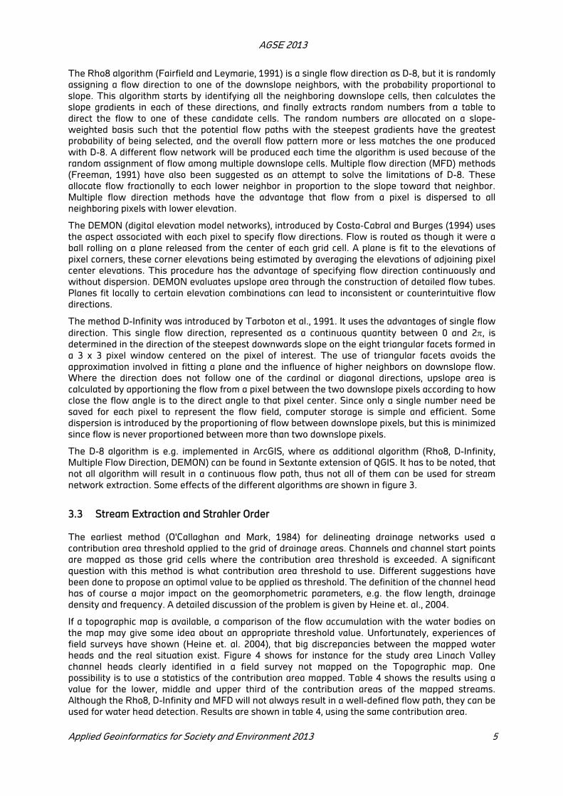
Morphometric Parameter Formula Reference

Bifurcation ratio (Rb)

Rb = Nu / Nu + 1 Nu = Total number of stream segments of order u. For sub basins with several Rb the average will be used.

SCHUMM (1956)

Drainage density (D)

D = L / A L = Total stream length of all orders A = Area of the basin

HORTON (1945)

Stream frequency (F)

F = N / A N = Total number of streams of all orders A = Area of the basin (km

2)

HORTON (1945)

Circularity ratio (Rc)

Rc = 4 A / P2

A = Area of the basin P = Perimeter of the basin

MILLER (1953)

Elongation ratio (Re)

Re = √4A/ / Lm A = Area of the basin Lm = Maximum basin length

SCHUMM (1956)

Table 1: Morphometric parameters used for flash flood risk mapping

The combination of high drainage density and frequency, and stream slope and low bifurcation ratio

might result in higher flood peaks for an equivalent rainfall input because these factors promote

rapid generation and concentration of runoff. This is so because these characteristics promote flow

concentration along drainage lines, resulting in high unit discharges over a short period of time. The

shape of a sub basin is strongly affecting the stream discharge characteristics. Circular basins will

produce larger floods than longitudinal watersheds as the discharge will accumulate within a shorter

time. The shape of a basin usually is expressed by the circularity and the elongation ratio.

AGSE 2013

Applied Geoinformatics for Society and Environment 2013 3

After calculating the parameters relevant for flash flood risk, they have to be combined for a final risk

potential map. A simple and straight forward method is to classify each parameter into three classes

(low, medium, high) according to their relation to the potential degree of risk and assigning

normalized score values 0, 0.5 and 1, respectively. A simple summing up of the score values per pixel

will result in a potential risk map based on the selected terrain parameters. Figure 1 shows the

resulting map for the study are of Wadi Dahab, where 174 sub basins have been delineated in the

previous analysis steps, see Omran, 2013. In this study, the tools of the ArcGIS extension Spatial

Analyst have been used.

3. Workflow in GIS

The calculation of the geomorphometric parameters is straightforward and it can be easily

implemented in GIS, if the characteristics of the underlying objects are known, i.e. the number of

streams and their length for each order, and the area and perimeter for all sub basins. To extract the

basic objects needed for this calculation in GIS a well-known workflow may be used:

DEM generation (if not given) -> filling of pits and depressions -> calculation of local flow directions -

> calculation of flow accumulation -> extraction of drainage network -> delineation of sub basins

based on outlet points -> vectorization of drainage network and sub basin raster layers.

Though the workflow is well known and applied in many research projects, it is worthwhile to have a

closer look at some of the basics steps. The focus of the discussion is to combine the tools to an

automated workflow, which may be implemented using e.g. ArcGIS Model Builder. On the other

hand, for some tools it is worthwhile to have a look at alternative algorithms implemented in other

GIS.

3.1 DEM Generation

Many of the geomorphological parameters are based on linear measurements of the drainage

network and of area measurements of the sub basins. Although since the work of Mandelbrot (1982)

many researcher argue about the fractal nature of landscape, for geodesists and cartographers it is

known since centuries, that there is an internal structure of the landscape expressed as ridges and

valleys of finite size and that this scale of this limit to landscape dissection varies in different

landscapes, which can be captured in a Croquis, that is a sketch of the landscape for a topographic

map.

In the overall process there are two levels where this information is important: determining a

resolution of the input DEM and determining the contribution area for a water head while extracting

the drainage network. To show the effect of resolution on the geomorphometric parameters for the

Figure 1: Flood Risk Map based on morphometric parameters for Wadi Dahab BasinFlood Risk Map

based on morphometric parameters for Wadi Dahab Basin

AGSE 2013


study area Linach Valley the parameters have been calculated for different resolutions, which are

shown in table 2. As contribution area for the water heads 200000m2 has been used, i.e. about 1.5 %

of the total accumulation at outlet point. It can be clearly seen, that the effect of different resolution

is rather small, i.e. less than 5%, up to the resolution of 50m.

Resolution 100m 50m 20m 10m 5m

Sub basin size (km2) 14.15 (1.58%) 14.34 (0.22%) 14.36 (0.01%) 14.37 (0.03%) 14.37

perimeter (km) 24.2 (5.52%) 25.3 (1.32%) 25.6 (0.15%) 25.80 (0.50%) 25.6

total length of drainage network (km)

12.2 (28.6%) 16.4 (3.8%) 16.5 (3.2%) 17.0 (0.1%) 17.0

D (1/km) 0.861 (27.5%) 1.144 (3.6%) 1.150 (3.1%) 1.186 (0.01%) 1.187

F (1/km2) 1.837 (14.8%) 2.162 (0.2%) 2.298 (6.5%) 2.296 (6.4%) 2.157

Rc 0.304 (10.5%) 0.282 (2.5%) 0.275 (0.0%) 0.272 (1.0%) 0.275

Re 0.260 (6.6%) 0.257 (5.3%) 0.252 (3.3%) 0.250 (2.5%) 0.244

Table 2: Effect of different filling algorithms

Although quite a number of cells are affected for the Wadi Dahab study area, the overall effect on the

DEM is rather small.

3.2 Flow Direction and Flow Accumulation

The use of the D-8 method for catchment area and drainage network analysis has been criticized on

the grounds that it permits flow only in one direction away from a cell. Though it gives reasonable

results in valleys, it may produce many parallel flow lines and problems near catchment boundary. It

fails to represent adequately divergent flow over convex slopes like ridges and can lead to a bias in

flow path orientation, see e.g. Fairfield and Leymarie, 1991. To overcome the problem, different

solutions have been suggested.

Figure 2: Filled pits

and depression of the

30m ASTER DEM for

Wadi Dahab study

area

Figure 3: Flow

accumulation D8

(top), MFD (middle),

Rho8 (bottom)

Figure 4: Streams (red) in the Linach Valley not

mapped on the topographic map

AGSE 2013


The Rho8 algorithm (Fairfield and Leymarie, 1991) is a single flow direction as D-8, but it is randomly

assigning a flow direction to one of the downslope neighbors, with the probability proportional to

slope. This algorithm starts by identifying all the neighboring downslope cells, then calculates the

slope gradients in each of these directions, and finally extracts random numbers from a table to

direct the flow to one of these candidate cells. The random numbers are allocated on a slope-

weighted basis such that the potential flow paths with the steepest gradients have the greatest

probability of being selected, and the overall flow pattern more or less matches the one produced

with D-8. A different flow network will be produced each time the algorithm is used because of the

random assignment of flow among multiple downslope cells. Multiple flow direction (MFD) methods

(Freeman, 1991) have also been suggested as an attempt to solve the limitations of D-8. These

allocate flow fractionally to each lower neighbor in proportion to the slope toward that neighbor.

Multiple flow direction methods have the advantage that flow from a pixel is dispersed to all

neighboring pixels with lower elevation.

The DEMON (digital elevation model networks), introduced by Costa-Cabral and Burges (1994) uses

the aspect associated with each pixel to specify flow directions. Flow is routed as though it were a

ball rolling on a plane released from the center of each grid cell. A plane is fit to the elevations of

pixel corners, these corner elevations being estimated by averaging the elevations of adjoining pixel

center elevations. This procedure has the advantage of specifying flow direction continuously and

without dispersion. DEMON evaluates upslope area through the construction of detailed flow tubes.

Planes fit locally to certain elevation combinations can lead to inconsistent or counterintuitive flow

directions.

The method D-Infinity was introduced by Tarboton et al., 1991. It uses the advantages of single flow

direction. This single flow direction, represented as a continuous quantity between 0 and 2, is

determined in the direction of the steepest downwards slope on the eight triangular facets formed in

a 3 x 3 pixel window centered on the pixel of interest. The use of triangular facets avoids the

approximation involved in fitting a plane and the influence of higher neighbors on downslope flow.

Where the direction does not follow one of the cardinal or diagonal directions, upslope area is

calculated by apportioning the flow from a pixel between the two downslope pixels according to how

close the flow angle is to the direct angle to that pixel center. Since only a single number need be

saved for each pixel to represent the flow field, computer storage is simple and efficient. Some

dispersion is introduced by the proportioning of flow between downslope pixels, but this is minimized

since flow is never proportioned between more than two downslope pixels.

The D-8 algorithm is e.g. implemented in ArcGIS, where as additional algorithm (Rho8, D-Infinity,

Multiple Flow Direction, DEMON) can be found in Sextante extension of QGIS. It has to be noted, that

not all algorithm will result in a continuous flow path, thus not all of them can be used for stream

network extraction. Some effects of the different algorithms are shown in figure 3.

3.3 Stream Extraction and Strahler Order

The earliest method (O'Callaghan and Mark, 1984) for delineating drainage networks used a

contribution area threshold applied to the grid of drainage areas. Channels and channel start points

are mapped as those grid cells where the contribution area threshold is exceeded. A significant

question with this method is what contribution area threshold to use. Different suggestions have

been done to propose an optimal value to be applied as threshold. The definition of the channel head

has of course a major impact on the geomorphometric parameters, e.g. the flow length, drainage

density and frequency. A detailed discussion of the problem is given by Heine et. al., 2004.

If a topographic map is available, a comparison of the flow accumulation with the water bodies on

the map may give some idea about an appropriate threshold value. Unfortunately, experiences of

field surveys have shown (Heine et. al. 2004), that big discrepancies between the mapped water

heads and the real situation exist. Figure 4 shows for instance for the study area Linach Valley

channel heads clearly identified in a field survey not mapped on the Topographic map. One

possibility is to use a statistics of the contribution area mapped. Table 4 shows the results using a

value for the lower, middle and upper third of the contribution areas of the mapped streams.

Although the Rho8, D-Infinity and MFD will not always result in a well-defined flow path, they can be

used for water head detection. Results are shown in table 4, using the same contribution area.

AGSE 2013


Tarboton (1991) introduces another method of determining a meaningful threshold value based on

the so called law of constant drop. To define the stream drop, the order of streams introduces by

Strahler in the 1950th is important (see above). Stream drop is defined as the difference in elevation

between the beginning and end of Strahler streams. The empirical law of constant drop, states, that

the average drop of streams for different Strahler orders is the same, i.e. the average drop of all first

order streams is the same as the average drop of second order, which is the same as third order etc.

Tarboton (1991) suggested a method, to iteratively change the threshold value for stream network

extraction and to compute for each iteration the average drop of first order streams and the average

drop for all higher order streams. The threshold value for which the two drop values coincides, is the

“optimal” threshold value for the given study area.

The concept of the Strahler stream numbering system has been explained above. For a given stream

network in connection with the D-8 flow directions, it is straightforward to assign Strahler numbers

for the different stream segments. Unfortunately, the definition of stream segments in most GIS

differs from the concept for Strahler numbers. In a GIS, a new segment will start at any confluence,

for any order of streams. Thus for an automated workflow, a re-definition of the segments is

necessary. In ArcGIS, the attribute table of the ordering tool contains all information about the

starting and ending nodes of a segment. Thus with a simple algorithm the segments to be merged

can be identified and subsequently dissolved. A description of the algorithm, implemented as a tool

for ArcGIS, can be found in Omran et al., 2012.

constant

drop

12500m2

Map 25k

upper

third

2500 m2

Map 25k

lower third

1100 m2

Map 25k

middle

third 1800

m2

Rho8

50000

m2

D-Inf

50000

m2

MFD

50000

m2

Total No of

segments

88 101 169 118 68 309 68

Total no of

Strahler segments

53 67 114 81 45 191 45

Total length 26601 27483 34910 29958 21957 28105 21264

No 1st 44 51 86 60 33 156 33

Length 1st

12047 11843 15320 13318 8660 9172 8443

No 2nd

8 12 22 16 10 27 10

Length 2nd

6294 6490 9043 7024 5754 7530 5552

No 3d 1 3 5 4 1 6 1

Length 3d 8260 1604 3002 2071 7542 3863 7269

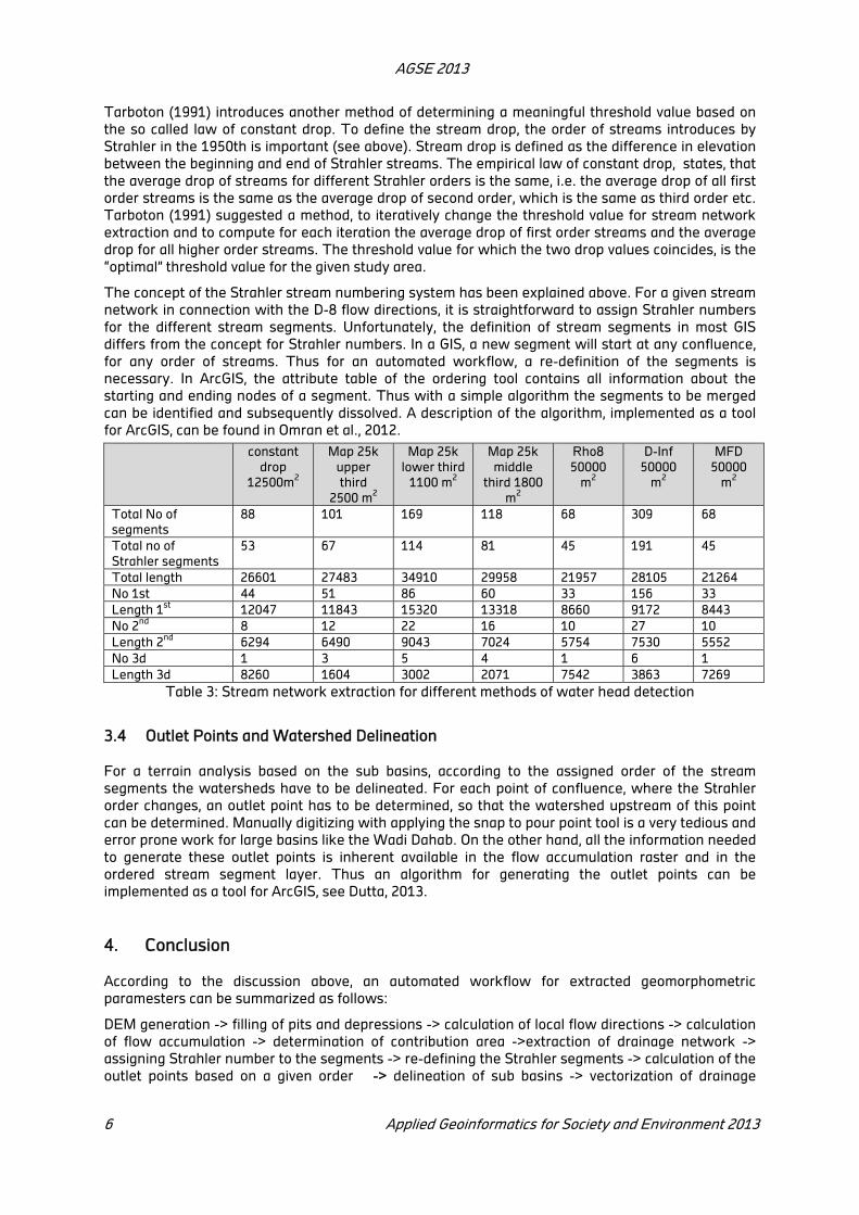
Table 3: Stream network extraction for different methods of water head detection

3.4 Outlet Points and Watershed Delineation

For a terrain analysis based on the sub basins, according to the assigned order of the stream

segments the watersheds have to be delineated. For each point of confluence, where the Strahler

order changes, an outlet point has to be determined, so that the watershed upstream of this point

can be determined. Manually digitizing with applying the snap to pour point tool is a very tedious and

error prone work for large basins like the Wadi Dahab. On the other hand, all the information needed

to generate these outlet points is inherent available in the flow accumulation raster and in the

ordered stream segment layer. Thus an algorithm for generating the outlet points can be

implemented as a tool for ArcGIS, see Dutta, 2013.

4. Conclusion

According to the discussion above, an automated workflow for extracted geomorphometric

paramesters can be summarized as follows:

DEM generation -> filling of pits and depressions -> calculation of local flow directions -> calculation

of flow accumulation -> determination of contribution area ->extraction of drainage network ->

assigning Strahler number to the segments -> re-defining the Strahler segments -> calculation of the

outlet points based on a given order -> delineation of sub basins -> vectorization of drainage

AGSE 2013


network and sub basin raster layers -> calculation of the geomorphometric parameters based on

basic GIS vector tools, like intersection, dissolving etc.

With the additional tools marked in bold, a workflow can be set up using e.g. ArcGIS Model Builder,

so that the parameters can be extracted also for larger basin areas, including a number of sub

basins. The most critical step for extracting the geomorphometric parameters, in which a flash flood

hazard analysis can be built on, is the determination of threshold value for the contributing area of a

water head. Here it may be worthwhile to have a look at alternative open source GIS like QGIS or

SAGA.

REFERENCES

Costa-Cabral M. C., and S. J. Burges, 1994. Digital Elevation Model Networks (DEMON): a Model of

Flow Over Hillslopes for Computation of Contributing and Dispersal Areas. Water Resources

Research, 30(6)

Dutta, A., 2013. Automated Watershed Delineation using ArcObjects. Unpublished Master’s Thesis,

University of Applied Sciences Stuttgart

Fairfield, J., and P. Leymarie, 1991. Drainage Networks from Grid Digital Elevation Models. Water

Resources Research, 30(6), pp.1681-1692.

Freeman, T. G., 1991. Calculating Catchment Area With Divergent Flow Based on a Regular Grid.

Computers and Geosciences, 17(3), pp.413-422.

Heine, R.A., Lant, C.L., Sengupta, R.R., 2004. Development and Comparison of Approaches for

Automated Mapping of Stream Channel Networks, Annals of the Association of American

Geographers, 94(3), 2004, pp. 477–490

Horton, R.E., 1945. Erosion development of streams and their drainage basins: hydrophysical

approach to quantitative morphology. Bull. Geol. Soc. Amer., 5, pp. 275-370

Hutchinson, M.F. ,1989. A new method for gridding elevation and stream line data with automatic

removal of spurious pits. Journal of Hydrology 106, pp. 211-232

Ignacio, R. and Luis, A., 1982. The dependence of drainage density on climate and geomorphology.

Hydrological Science - Journal des Sciences Hydrologiques, 27.

Intergraph Corporation, 2013. Learning to Use GeoMedia Grid - A Tutorial: Contours to DEM.

Intergraph User Documentation, Huntsville

IPCC, 2013: Climate Change 2013: The Physical Science Basis

http://ipcc.ch/report/ar5/wg1/#.UoD6_uIlgu9 (accessed 19 Niv. 2013)

Jenson, S.K. and Domingue, J.O., 1988. Extracting topographic structure from digital elevation data

for geographic information system analysis, Photogrammetric Engineering and Remote Sensing ,

54(11), pp. 1593-1600.

Mandelbrot, B.B. 1982. The fractal geometry of nature. New York: WH Freeman.

Miller, V.C., 1953. A quantitative geomorphic study of drainage basin characteristics in the Clinch

Mountain area. Tech. Report 3, Columbia University, New York

O'Callaghan, J.F. and Mark, D.M., 1984. The extraction of drainage networks from digital elevation

data, Computer Vision, Graphics, and Image Process. , 28(3), pp. 323-344.

Omran, A., Schröder, D., El Rayes, A. and Geriesh, M., 2012. Flood Hazard Assessment in Wadi Dahab

Based on Basin Morphometry usingg GIS techniques. Proceedings GI_Forum Symposium Applied

Geoinformatics, Salzburg, Austria, p. 1-11

Omran, A., 2013. Application of GIS and Remote Sensing for Water Resource Management in Arid

Area – Wadi Dahab Basin- South Eastern Sinai- Egypt, PhD Dissertation, University of Tübingen

(to be published)

Planchon , O. and Darboux, F., 2001. A fast, simple and versatile algorithm to fill the depressions of

digital elevation models, Elsevier, Cantena, 46, p. 159–176

AGSE 2013


Schumm, S.A., 1956. Evaluation of drainage systems and slopes in badlands at Perth Amboy- New

Jersey, Bull. Geol. Soc. Amer., 67, pp. 597-646

Strahler, A.N., 1952. Hypsometric (area-altitude) analysis of erosion topography. Geological Society

Ameriacn Bulletin, 63, pp. 1117-1142

Tarboton, D. G., R. L. Bras, and I. Rodrigues-Iturbe, 1991. On the Extraction of Channel Networks

from Digital Elevation Data. Water Resources Research, 5(1), p.81-100

Development of Web Gis Based Flood Disaster Management System

Using Open Source Software

Anurag Aerona, R.D. Garg

1, D.S. Arya

a, S.P. Aggarwal

b

a Department of Civil Engineering, Indian Institute of Technology, Roorkee

b Department of Water Resources, Indian Institute of Remote Sensing, Dehradun

[email protected], [email protected], [email protected], [email protected],

KEY WORDS: Web GIS, open source, GeoServer, Flood Disaster, Remote Sensing

ABSTRACT

This paper introduces a web GIS for flood disaster mitigation and management. It uses Apache Tomcat and GeoServer for constructing a web GIS. These tools are open source and freely available through Internet. Google Earth is used for acquiring satellite images, which is again freely available data through Google. The lower part of Mahanadi delta region of Odisha state is selected as the study area for this research paper. This area lies between 20º23Ń to 20º29Ń and 86º10É to 86º29É. The GeoServer uses PostGIS for spatial database management. It stores LULC layer, road network layer, soil layer and Google Earth layers. The web GIS can perform area extraction and distance measurement on these layers. One exclusive feature of this web GIS is that it can also find the evacuation route during flood disaster situation. The architecture of this web GIS system is also discussed in detail in this paper. The Quantum GIS software is also used for performing some operations. Some tools and plug-ins are used for extracting flood information and then this can be used in GeoServer. The user friendly interface is developed in open source software. It provides an easy way to query so a non-GIS person can also view and explore its maps and results, and can understand it in detail. This paper focuses to develop a web based spatial GIS application, which would help disaster managers and people to find geographic information during flood disaster. The timely and easy to understand information will help flood managers and emergency services to take appropriate decision at right time. Future work will focus on real time disaster conditions and realistic factors, to achieve more accurate models and to achieve high quality resul.

1. Introduction

Floods have the greatest damage potential of all natural disasters worldwide and affect the largest

number of people. Plans and efforts must be undertaken to move from post-disaster response to

disaster mitigation. More than ever, there is the need for decision makers to adopt holistic

approaches for flood disaster mitigation and management. It is recognized that comprehensive

assessments of risks from natural hazards, are needed. Assessment of risk and the involvement of

the community in the decision making, planning and implementation process can help to obtain

sustainable solutions. Solutions must reflect the human dimension and must also consider the

impacts of changing land use on flooding, erosion, and landslides. Implementation will only be

sustainable if solutions are suitable for the community at risk, over the long term. The application of

flood forecasting model require the efficient management of large spatial and temporal datasets,

which involves data acquisition, storage and processing, as well as manipulation, reporting and

display results. The complexity of flood forecasting makes it difficult for individual organization to

deal effectively with decision-making. Difficulty in linking data, analysis tools and models across

organization is one of the barriers to be overcome in developing integrated flood forecasting system.

Therefore, it is required to develop a web-based spatial decision support system for supporting

information exchange and knowledge and model sharing from different organizations on the web.

Such a DSS provide the framework within which spatially distributed real-time data accessed

remotely to prepare model input files, model calculation and evaluate model results for flood

forecasting and flood risk prediction.

AGSE 2013


In this paper, some concepts and methods are discussed to mitigate the effect of floods. Remote

Sensing, GIS, Google Earth and open source software and technologies are used for flood risk

analysis. The first part of this paper discusses the architecture of web based disaster mitigation

system. The evacuation route find by using QGIS. The next part shows the flood GIS, which is

developed by using the GeoServer and Apache Tomcat. After a critical analysis it can be concluded

that a highly integrated system is required for forecasting and manage the floods. It should integrate

geo-morphological, hydrological, meteorological, and socioeconomic aspect to provide more accurate

and effective results for decision making. It requires coordination across many agencies at national

to community levels for the system to work.

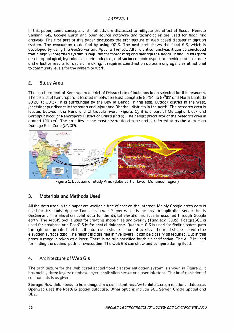
2. Study Area

The southern part of Kendrapara district of Orissa state of India has been selected for this research.

The district of Kendrapara is located in between East Longitude 86014’ to 87

001’ and North Latitude

20020’ to 20

037’. It is surrounded by the Bay of Bengal in the east, Cuttack district in the west,

Jagatsinghpur district in the south and Jajpur and Bhadrak districts in the north. The research area is

located between the Nuna and Chitrapala rivers (Figure. 1); it is a part of Marsaghai block and

Garadpur block of Kendrapara District of Orissa (India). The geographical size of the research area is

around 190 km2. The area lies in the most severe flood zone and is referred to as the Very High

Damage Risk Zone (UNDP).

Figure 1: Location of Study Area (delta part of lower Mahanadi region)

3. Materials and Methods Used

All the data used in this paper are available free of cost on the Internet. Mainly Google earth data is

used for this study. Apache Tomcat is a web Server which is the host to application server that is

GeoServer. The elevation point data for the digital elevation surface is acquired through Google

earth. The ArcGIS tool is used for creating shape files and overlay (Tang et.al.2005). PostgreSQL is

used for database and PostGIS is for spatial database. Quantum GIS is used for finding safest path

through road graph. It fetches the data as a shape file and it overlays the road shape file with the

elevation surface data. The height is classified in five layers. It can be classify as required. But in this

paper a range is taken as a layer. There is no rule specified for this classification. The AHP is used

for finding the optimal path for evacuation. The web GIS can show and compare during flood.

4. Architecture of Web Gis

The architecture for the web based spatial flood disaster mitigation system is shown in Figure 2. It

has mainly three layers: database layer, application server and user interface. The brief depiction of

components is as given.

Storage: Raw data needs to be managed in a consistent read/write data store, a relational database.

OpenGeo uses the PostGIS spatial database. Other options include SQL Server, Oracle Spatial and

DB2.

Nuna River

Chitrapala River

Mahanadi River

Paika River

AGSE 2013


Application server: The raw data needs to be accessed using web services, and rendered into

cartographic products. OpenGeo uses the GeoServer map/feature server. Other options include

ArcGIS Server, MapGuide, and MapServer.

Application cache: Performance requires the caching of intermediate results, such as map files.

OpenGeo uses the GeoWebCache tile cache. Other options include TileCache, ArcGIS Server and

MapGuide.

User interface framework: Targeted vertical applications serve one operational need and serve it

well. OpenGeo uses GeoExt/ExtJS as a platform independent user interface toolkit. Other options

include FLEX and Silverlight.

User interface map component: Mapping applications need a map component that understands

spatial features and map layers. OpenGeo uses OpenLayers. Other options include Google Maps API

and Bing Maps API.

Figure 2: Architecture of Web based flood mitigation system

The geospatial architecture provide a spatial database, data manipulation, Internet publishing and

client-server architecture incorporating a portal with several end user applications that communicate

with various application servers, which are in turn linked to the data repositories. This architecture

and functionality have been engineered specifically to publish maps, data, and metadata on the web,

is designed so that it is easy to create maps, develop web pages that communicate with the maps,

and administer a web mapping site, is also designed to be distributed across a network and to be

scalable as the demand for maps increases. There are several components in each tier of the

system.

5. Safest Route Delineation and Web Gis

The data and images used to achieve the objective are shown as a flowchart in figure.3. Google

imagery is used to extract the elevation points. In this study 60x60 grid is considered for applying the

method. Landsat images are compared with Google earth images for verification of land and river

area. The road map is developed as shapefile.

Spatial Database

Database PostgreSQL PostGIS

GIS Layer

Flood Zone Maps

Raster

Application Server and Web Apache with GeoServer

Geo Web Cache

User InternGeoExt and Open Layers

Web Browsers

Spacial Query/Statics Features to upload Data

‐‐‐‐‐‐‐‐‐‐‐‐‐‐‐‐‐‐‐‐‐‐‐‐‐‐‐‐‐‐‐‐‐‐‐‐‐‐‐‐‐‐‐‐‐‐‐‐‐‐‐‐‐‐‐‐‐‐‐‐‐‐‐‐‐‐‐‐‐‐‐‐‐‐‐‐‐‐‐‐

‐‐‐‐‐‐‐‐‐‐‐‐‐‐‐‐‐‐‐‐‐‐‐‐‐‐‐‐‐‐‐‐‐‐‐‐‐‐‐‐‐‐‐‐‐‐‐‐‐‐‐‐‐‐‐‐‐‐‐‐‐‐‐‐‐‐‐‐‐‐‐‐‐‐‐‐‐‐‐‐‐

AGSE 2013


Figure 3: Safe route delineation

At primary stage only main and wide roads are considered in the shape file. There are two areas in

which this study has been carried out. One is the Kendrapara roads and the other is the part of lower

Mahanadi delta region. The kendrapara district has several roads which have good population

density but the delta region which is prone to flood has mostly agriculture land.

The Quantum GIS software is used for finding the optimal path for evacuation. The road shape file

and the parameter values that are calculated earlier are supplied to road graph tool. It can be

explained through figure 4 that the shape file is superimposed to elevation data and then classified

on the basis of flooded and non-flooded area. The path is established through the safe zone area.

Figure 4:

Figure 5:

The Kendrapara district area which has high population spreads between 20º29´55´Ń to

20º30´30´Ń and from 86º24´35´É to 86º25´35´É. The Quantum GIS in figure.5 shows the Google

AGSE 2013


earth road network and the urban situation. Again the area is categorized based on the elevation

(height) of each road (figure.6).

Figure 6:

The blue part is surrounded by the water, which is indicated as the red region. The road graph tool of

Quantum GIS is configured for the specified road network of kendrapara district. It shows the path

which has least hindrance from one point to other. Therefore the objective for finding the path which

is fast and safe; compare to shortest path is achieved. On close investigation it is observed that the

result depends on the accuracy of road network and the elevation data. In this paper the limitation of

accuracy in freely available elevation data leads to affect the results. The method specified and

implemented in this paper achieved successful results. The open source software is integrated with

the spatial database and the application is run successfully to achieve the desired results. This paper

study both the scenario; when there is good road network and also when there is little road network.

Figure 7:

The Integration of GIS and open source software can provide enormous opportunity to develop new

application. The Google earth is the main source for raw data. The user friendly interface helps to

identify the exact path or optimum route for different flood scenario.

Figure 8:.

AGSE 2013


6. Conclusion

The application of flood decision support system requires the efficient management of large spatial

and temporal datasets, which involves data acquisition, storage and processing, as well as

manipulation, reporting and display results. The complexity of flood decision support system makes

it difficult for individual organization to deal effectively with decision-making. Difficulty in linking

data, analysis tools and models across organization is one of the barriers to be overcome in

developing integrated flood decision support system. Therefore, it is required to develop web-based

spatial decision support system, supporting information exchange and knowledge and model sharing

from different organizations on the web. Such a DSS provide the framework within which spatially

distributed real-time data accessed remotely to prepare model input files, model calculation and

evaluate model results for flood risk prediction and disaster mitigation and management.

By using AHP and ArcGIS with the integration of Quantum GIS and PostgreSQL; this paper presents

an improved evacuation route method for flood disaster. Future research will be focus on more

realistic factors to develop more accurate models and to achieve high quality results. More widely

experiments can help to verify the accuracy and applicability of the method for the flood scenario.

The primary objective of this research is to develop a web based spatial GIS application, which would

help people during flood. People who live in flood plains, can locate the point at higher altitude and

less vulnerable to the flood water. The prime outcome of this research is a web based GIS system

that can provide appropriate information to the public and local authorities. The timely and easy to

understand information will help flood managers and emergency services to take appropriate

decision at right time. The user friendly interface is developed in open source software. It provides

an easy way to query so a non-GIS person can also view and explore its maps and results and can

understand it in detail. Future work will focus on real time disaster conditions, to achieve more

reliable results from online web GIS which will be more effective in emergency situations.

This paper provides a development process for on-line flood disaster mitigation and management

system, integrating information retrieval, analysis and model analysis for information sharing and

decision-making support. Users only require a simple web browser to access data, software and

perform model analysis without the requirements of installing GIS and modeling processing software

packages. This DSS can play an important role in assisting decision makers to establish a

collaborative mechanism across organizational boundaries for on-line flood risk prediction. The

personnel evacuating plan would be implemented by the integrated system to improve the ability of

flood disaster pre-warning monitoring. In order to perfect the system, it is needed to add water depth

changing process, 3D displaying, flood inundation damage evaluation, and other functions to the

system.

REFERENCES

Binghu Huang, Peng Siling, Yinping Chen, Ke Chen, Bangshu Xu, (2010), “Decision supporting

system of Jinan urban flood control”, 18th International Conference on Geoinformatics, Vol., no.,

pp.1-5, 18-20 June 2010.

Dijkstra T.K., 2013, On the Extraction of Weights from Pairwise Comparison Matrices, Central

European Journal of Operation Research, (21), 103–123.

Jiang W., Deng L., Chen L., Wu J., Li J., (2009), “Risk assessment and validation of flood disaster based

on fuzzy mathematics”, Progress in Natural Science, Vol. 19, no.10, pp. 1419-1425.

Mirfenderesk Hamid, (2009) “Flood emergency management decision support system on the Gold

Coast, Australia”, The Australian Journal of Emergency Management, Vol. 24, no. 2, May 2009, pp

48- 58.

Moreri K.K. and Mioc D., 2008, Web Based Geographic Information Systems for a Flood Emergency

Evacuation, International Conference on Information Systems for Crisis Management, Harbin,

China, 4-6 August.

Saadatseresht M., Mansourian A. and Taleai M., 2009, Evacuation Planning Using Multiobjective

Evolutionary Optimization Approach, European Journal Of Operational Research (198), 305–314.

AGSE 2013


Saaty T.L., 2008, Decision Making with the Analytic Hierarchy Process, International Journal of

Services Sciences, (1)1, 83-98.

Tang T. and Wannemacher M., 2005, GIS Simulation and Visualization of Community Evacuation

Vulnerability in a Connected Geographic Network Model, Middle States Geographer, (38), 22-30.

Triantaphyllou E. and Mann S.H., 1995, Using The Analytic Hierarchy Process for Decision Making in

Engineering Applications: Some Challenges, International Journal of Industrial Engineering:

Applications and Practice, (2)1, 35-44.

Wang, Lei, and Qiuming Cheng., (2007), “Design and implementation of a web-based spatial decision

support system for flood forecasting and flood risk mapping”, IEEE International Geoscience and

Remote Sensing Symposium, 2007. IGARSS 2007.

Wenjing M., Yingzhuo X. and Hui X., 2009, The Optimal Path Algorithm for Emergency Rescue for

Drilling Accidents, IEEE International Conference on Network Infrastructure and Digital Content,

6-8 Nov.

Yang S. and Chunhua L., 2010, An Enhanced Routing Method with Dijkstra Algorithm and AHP

Analysis in GIS-Based Emergency Plan, 18th

International Conference on Geoinformatics, 18-20

June.

Yang, Qing, and Qiang Zhang. (2007), “Study on Decision Support System of Flood Disaster Based on

the Overall Process Emergency Management”, International Conference on Wireless

Communications, Networking and Mobile Computing, 2007. WiCom 2007.

Yuling L., Michinori H. and Okada N., 2006, Development of an Adaptive Evacuation Route Algorithm

under Flood Disaster, Annuals of Disaster Prevention Research Institute, Kyoto University, (49) B,

190-195.

Zhang D., Wel Z., Kim J.H. and Tang S., 2010, An Optimized Dijkstra Algorithm for Embedded GIS,

International Conference on Computer Design and Applications, (1)VI, 147-150.

AGSE 2013


Holistic Visualisation of Different Utility Networks Supporting Disaster

Management

Thomas Becker, Gerhard König*, Stefan Semm

Institute of Geodesy and Geoinformation Science, Technische Universität Berlin

(thomas.becker, gerhard.koenig, stefan.semm)@tu-berlin.de

KEY WORDS: disaster management, common operational picture, critical infrastructure,

visualization

ABSTRACT

Cartographic visualizations of crises are used to create a Common Operational Picture (COP) and enforce Situational Awareness (SA) by presenting relevant information to the involved actors. As nearly all crises affect geospatial entities, geo-data representations have to support location-specific analysis throughout the decision-making process. Meaningful cartographic presentation is needed for coordinating the activities of crisis manager in a highly dynamic situation, since operators’ attention span and their spatial memories are limiting factors during the perception and interpretation process. Situational Awareness of operators in conjunction with a COP are key aspects in decision-making process and essential for making well thought-out and appropriate decisions. Considering utility networks as one of the most complex and particularly frequent required systems in urban environment, meaningful cartographic presentation of multiple utility networks with respect to disaster management do not exist. Therefore, an optimized visualization of utility infrastructure for emergency response procedures is proposed. The article presents a conceptual approach on how to simplify, aggregate, and visualize multiple utility networks and their components to meet the requirements of decision-making processes and to support Situational Awareness.

1. Introduction

Threat to life or physical condition due to natural catastrophes, power cuts, unexploded ordnance

devices, international terrorism etc. are a menace to our society that cannot be avoided. Major

incidents or major crisis events require close and harmonized actions of affected organisations,

institutions and participants in state, economy, and society. Quick response by decision makers is

expected to get the situation under control, to avoid secondary damage, and particularly to save

lives. A common understanding of the current situation, occurring events, and processes is an

absolute must in order to achieve coordinated action and to avoid misunderstandings. Quick grasp of

matter under pressure and its relationships to after-effects require a restriction to minimum but

essential information. Therefore, optimised cartographic visualizations have to be introduced to

create a Common Operational Picture (COP - Steenbruggen et al. 2011) and enforce Situational

Awareness (Endsley 1995). Simplified and minimal maps that preserve the context and offer

sufficient amount of information for crisis management are required, especially for one of the most

complex systems in urban environments - utility networks. Utilities are owned privately or publicly

and therefore maintained by various companies, investors, or organisations responsible to guarantee

publicly accessible supply of energy, electricity, natural gas, water, and sewage. Utility networks are

explicitly considered as critical infrastructures since information on utility networks is not publicly

available due to data protection or to keep it secret to competitors. Facts on age and condition of the

distribution network and its technical components are generally not available as complete overview.

Experience shows that even small malfunctions can cause significant problems at the interfaces

between suppliers. Events, such as the Italian blackout in 2003 or the interruption of power supply

* Corresponding author.

AGSE 2013


chains in wide parts of Europe in 2006, demonstrate the effects of infrastructure failures to society

and the strong linkage of networks across borders. The outage of one infrastructure may influence

others through a series of cascading effects (Becker et al. 2011, Becker et al. 2012). As much as it is

difficult, it is necessary to communicate beyond one’s own system boundaries. Successful

coordination is an enormous challenge between organizations that are under time pressure, ignorant

of the structure of neighbouring companies, and facing constantly changing conditions. However,

each utility network is a highly complex system and even the cartographic representation of a single

utility network is still a challenge. Visualizing multiple utility networks based on existing tools quickly

reaches limitations in cognition and perception, which leads to substantial problems in sharing

relevant information that is essential for achieving common situational aware-ness (Overbye and

Raymond 1999).

Therefore, infrastructure assets such as pipes, cables, and canals are particularly of interest in the

decision-making process. Further damage or breakdowns at unforeseen locations may occur and

require information of all utility networks and a holistic view for strategic crisis management. The

challenge is to visualize the current scene including existing infrastructure that is suitable for

handling disaster situations, backs human beings’ perception, and is appropriate for reducing actors’

stress level.

Visualization is a domain of cartography and consequently, maps for decision making have to be

created that simplify and minimize network related information radically, while preserving as much

information as possible. The here presented conceptual approach will explain how to simplify,

aggregate, and visualize multiple utility networks and their components to meet the requirements of

the decision-making process and to support situational awareness.

2. Network hierarchies and cartographic representation

A common understanding of the current crisis situation, occurring events, structures, processes and

the available geodata is an absolute must in order to achieve coordinated action and to avoid

misunderstandings (Becker et al. 2011). Common Operational Picture forms the base for situation

assessment and situational awareness. Therefore related material has to be analysed for

applicability and suitability. Investigations of the diverse utility networks in Berlin revealed that each

utility network company uses its own cartographic representation for as-built documentation for

maintenance and repair.

2.1 Visualization analysis

Crisis situations require a quick grasp of the situation to receive a first but rough impression about

the resulting discontinuity and especially potential subsequent damage. Utility maps are a valuable

tool for decision support. Anticipated to be an as-built documentation for maintenance and repair the

cartographic representation of the various utility networks best fits to their primary application. They

contain a huge amount of detailed information that is essential if the precise location of the different

utility objects is needed (see Figure 1).

Perusing the objective to gain a quick holistic view

leads into temptation to overlay almost all available

utility maps. But the simultaneous visualisation

yields to a strongly increased object concentration.

The map gets unreadable even though colours are

used for identification of different network

affiliation as seen in Figure 1 and 2. Even qualified

persons quickly get lost due to the high information

density. Applying simultaneous representation of

multiple utility networks prevents perception of

commodity types (pipes, assets, etc.). Clutters

induce superficial symbols when two or more symbols overlap each other. Moreover, map content

changes radically when the scale is decreasing and the interpretation of the situation becomes

Figure 1: Sewage pipes, scale 1:60

AGSE 2013


difficult or even impossible. Analysis by Semm revealed that the (minimum) appropriate scale in

crisis situations is 1:2000 (Semm, 2011).

Figure 2: Simultaneous visualisation of sewage water, gas and long-distance heat, excluding

symbols (from left to right: 1:60, 1:300, and 1:800)

Cartographic aspects have to be applied: Figure 2 indicates that very large scales are needed to meet

the requirements of cartographic minimum dimension (Hake et al. 2002, Lechthaler and Stadler

2006). In the scale range 1:800 to 1:150 the minimum dimensions and distances between linear

objects were preserved, while for point objects the acceptable range is shifted from 1:300 to 1:60.

As a result, immediate scene perception is impossible and simply combining maps for decision-

making is not suitable. To overcome orientation and cluttered visualization issues different utility

networks were investigated with respect to existing network hierarchies and functional

equivalences, to be able to perform semantic and geometric generalisation.

2.2 Investigation of network hierarchies

SA and COP require a joint visualization of the needed information and objects with different spatial

extents, e.g. overview, detailed view, etc. It was argued by Fairbairn (2001), that information is

effectively deduced, transported, and refined when using different scale ranges for complex

visualizations, i.e. small- (>1:20.000), meso- (1:20.000 to 1:6.000) and large scale (<1:6.000). Each

range encodes unique and dedicated information (MacEachren 2004, MacEachren 2005), within that

specific information process chain. Hopfstock states that “the visual component of the data is used in

the data supply chain so that the graphic presentation enables a communicative, map-based

acquisition of geographic information that stimulates the visual reasoning of users and, ultimately,

supports decision making” Hopfstock (2012, page 55).

Since in emergency cases at first overview maps are needed, utility networks were analysed in order

to distinguish between network-relevant or network-descriptive objects for extracting the most

significant information. Network-relevant objects represent the primary structure of each network,

i.e. pipes, channels, tails ends, whereas network-descriptive elements characterise objects that are

not necessary for the on-going supply operation such as flange, corrosion measuring points, etc.

Subsequently identified features were classified and assigned to an appropriate map scale for

display. Three main and distinct hierarchies can be identified:

H1 = transport lines, main lines, high pressure, excess voltage

H2 = distribution, collection, medium pressure, high voltage

H3 = house service lines, low pressure, low voltage

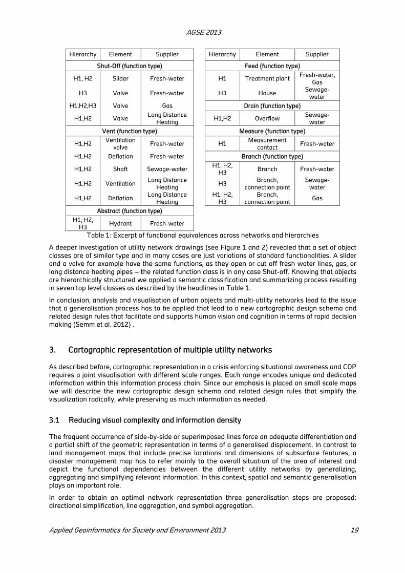
Table 1 illustrates that the different networks components appear in multiple network hierarchies

and multiple networks.

Furthermore the table indicates that a huge amount of objects have to be recognized and perceived

in crisis situations.

AGSE 2013


Hierarchy Element Supplier Hierarchy Element Supplier

Shut-Off (function type) Feed (function type)

H1, H2 Slider Fresh-water H1 Treatment plant Fresh-water,

Gas

H3 Valve Fresh-water H3 House Sewage-

water

H1,H2,H3 Valve Gas Drain (function type)

H1,H2 Valve Long Distance

Heating H1,H2 Overflow

Sewage-

water

Vent (function type) Measure (function type)

H1,H2 Ventilation

valve Fresh-water H1

Measurement

contact Fresh-water

H1,H2 Deflation Fresh-water Branch (function type)

H1,H2 Shaft Sewage-water H1, H2,

H3 Branch Fresh-water

H1,H2 Ventilation Long Distance

Heating H3

Branch,

connection point

Sewage-

water

H1,H2 Deflation Long Distance

Heating

H1, H2,

H3

Branch,

connection point Gas

Abstract (function type)

H1, H2,

H3 Hydrant Fresh-water

Table 1: Excerpt of functional equivalences across networks and hierarchies

A deeper investigation of utility network drawings (see Figure 1 and 2) revealed that a set of object

classes are of similar type and in many cases are just variations of standard functionalities. A slider

and a valve for example have the same functions, as they open or cut off fresh water lines, gas, or

long distance heating pipes – the related function class is in any case Shut-off. Knowing that objects

are hierarchically structured we applied a semantic classification and summarizing process resulting

in seven top level classes as described by the headlines in Table 1.

In conclusion, analysis and visualisation of urban objects and multi-utility networks lead to the issue

that a generalisation process has to be applied that lead to a new cartographic design schema and

related design rules that facilitate and supports human vision and cognition in terms of rapid decision

making (Semm et al. 2012) .

3. Cartographic representation of multiple utility networks

As described before, cartographic representation in a crisis enforcing situational awareness and COP

requires a joint visualisation with different scale ranges. Each range encodes unique and dedicated

information within this information process chain. Since our emphasis is placed on small scale maps

we will describe the new cartographic design schema and related design rules that simplify the

visualization radically, while preserving as much information as needed.

3.1 Reducing visual complexity and information density

The frequent occurrence of side-by-side or superimposed lines force an adequate differentiation and

a partial shift of the geometric representation in terms of a generalised displacement. In contrast to

land management maps that include precise locations and dimensions of subsurface features, a

disaster management map has to refer mainly to the overall situation of the area of interest and

depict the functional dependencies between the different utility networks by generalizing,

aggregating and simplifying relevant information. In this context, spatial and semantic generalisation

plays an important role.

In order to obtain an optimal network representation three generalisation steps are proposed:

directional simplification, line aggregation, and symbol aggregation.

AGSE 2013


Throughout the first step, curved lines are straightened and restricted to horizontal, vertical and 45°

directions. Since angular peculiarities are selectively processed by the human‘s brain, objects of

equal angular peculiarity are cognitively grouped (Heeley and Buchanan-Smith 1997, Vogels and

Orban 1985), which leads to a structured, methodical, and easier perceptible representation as

illustrated in Figure 2. This approach is similar to the design of metro maps as presented by Avelar

and Hurni (2006), and Cabello et al. (2005).

Although geometry has changed, the topology of the original information is preserved. However, the

design rules discussed by Avelar and Hurni (2006) are not fully applicable to multiple utility networks

because pipes or lines of two or more networks must not share the same direction and they must not

share any start, end or intermediate node.

Hence, utility networks should be made comparable by generalization and aggregation of lines and

network components on a semantic and geometric level. In order to distinguish between the

different networks each obtains a unique colour in accordance to the well-known and standardized

RAL-colours (RAL e.V. 2001).

Based on the classes defined in table 1 the functional equivalence of objects across multiple

networks (like slider and valve that are classified as Shut-off) should also be recognizable. For that

purpose dark / thick lines are used to point out the importance for objects of higher relevance /

hierarchy, meanwhile, light / thin lines represent objects of minor importance. As illustrated in Figure

2 this approach was applied to represent class H1 – H3 objects.

In order to guarantee visual-textual association in case objects lay in too close proximity or if thinner

lines form bundles, line aggregates are formed that include a set of adjacent features. As rule for

aggregation we propose that objects are merged if a buffer width of less than 1pt per scale type is

reached, depending on the related hierarchy. This means that at a small scale all objects of H1 will

be summarized within a buffer of 16 m - 4,8 m. Similar applies for meso-scale (1:20.000 to 1:6.000),

whereas objects within a vicinity of 4,8 m to 0,64 m will be merged. Obviously aggregates reduce the

number of objects, whilst preserving the needed object information. Aggregates were extended in

their thickness and colorized with black, ensuring the highest level of graphical dominance. To

preserve information about suppliers, color-coded box annotations at defined intervals were added

to the aggregated lines. Hierarchy can be expressed by variation of colour intensity (Figure 3).

Figure 3: Reduced schematic representation of multi

utility

Table 2: Suppliers' and new

designed common symbols for

main functions networks

AGSE 2013


3.2 Providing simultaneous cartographic representation

Dependant on the particular utility network, maps use their own symbols for objects’ representation.

These symbols are adjusted to their main purpose and were designed for as-built documentation,

rather than for rapid cognition, as it is required for disaster management. In general, we cannot

assume that decision makers responsible in crisis situations have deep knowledge of the domain

specific symbols. These symbols may cause confusion or misinterpretation and a set of standardized

symbols were designed that are associable, intuitive, and simple (Table 2). To implement the

network overarching applicability of those symbols, they were designed to be graphically neutral

using the colour grey.

3.3 Preserving information variety

Another important key aspect is symbol placement. In order to avoid symbol overlap its initial

position is replaced by a colour-coded point that retains the spatial location of a network component

(Figure 4). A point was chosen to ensure the graphical distinction of symbol placement and colour-

boxes. This allows maintaining position, network, and hierarchy information for each symbol.

Figure 4: Proposed visualization for schematic abstracted lines and symbols with design elements,

colour code, and dimensions

Graphical links between symbols of identical type (1: n relation) guarantee to keep the semantic

connection between these objects and prevent insertion of unnecessary symbols. According to

network affiliation and hierarchy, these links were colour-coded and dotted to make them

distinguishable from line objects and were thinned to reduce their graphical dominance. In order to

avoid misinterpretation, linking connection lines are not allowed to cross any lines representing

pipes or channels. Qualitative as well as quantitative object information can now be expressed by the

amount of connection lines. Based on the clearly arranged cartographic representation members of

the decision-making groups can instantly get a general idea about the complex utility networks and

their interdependency and will be able to focus on critical network sections where precautions and

prompt action have to be taken to avoid subsequent damage.

4. Combining the conceptual framework and related topography

In contrast to the already presented approaches Wolff (2013, pp 724ff) states, that geometric

information of utility networks have to be integrated into a broader context. The superior spatial

context is needed to support perception and cognition in terms of the data supply chain (Hopfstock

2012) that is realized by cadastral maps, orthophotos or topographic maps. However, our

topologically correct abstraction of the reality loses information about objects’ precise spatial

location. This may impede quick orientation (Anderson 2000, Artmann and Garbis 1998) in many

cases, especially for those who work in non-related fields. Once risk objects are identified,

instantaneous action is required. Subsequently, the accurate spatial location is important,

AGSE 2013


particularly with respect to action orders that have to be given to local task forces. At least two

solutions are proposed, assuming that the related topographic maps are stored in the background:

Figure 5: Redesigned (using centre lines of streets as additional input) representation of overlaid

utility networks on base maps (orthophoto left (Figure 5 a); topographic map right (Figure 5 b))

If the tool is implemented as an active system, appropriate map information will be displayed on

demand in auxiliary windows by a mouse click. For better orientation photos could also be added

upon request. These maps and photos can be sent to on-site task forces for guidance if automatic

control of utility network components is not possible.

In case the generalized utility map (schematic view) can be arranged above related base maps, such

as topographic maps, orthophotos, or other thematic information. This implies that the utility map

content will be graphically corrected to the underlying topographic or thematic information.

Moreover, the generalized utility network has to be adjusted to the spatially related geometry

(Figure 5). To avoid dominant appearance the background image shall be displayed with lower

colour saturation or shaded in grey (Figure 5 a).

5. Conclusion and Future Work

During a crisis response, various information sources have to be collected and combined by different

stakeholders (Paton and Flin 1999, Dransch 2007). With this study, the authors propose a new type

of simultaneous utility network representation that contributes to the assessment and

accomplishment of crisis situations. Analysing drawings of different utility networks verified

evidence that utility network maps of diverse suppliers are of limited suitability in crisis situations.

Such drawings are mainly used for as-built documentation for maintenance and repair and do not

allow for quick evaluation of how systems interact in case of emergency. It is difficult for involved

actors to understand the interrelated system behaviour of utility networks when each company uses

its own cartographic representation. The high amount of such detailed and complex information

complicates clear and quick decision-making.

Therefore, the authors have presented a framework and a conceptual solution for the design and

joint visualization of multiple utility networks and additional spatial information that supports crisis

managers during the decision-making process. Challenging problems caused by violating

cartographic minimum distances and dimensions were solved by semantic and geometric

generalization. Information variances will be reduced to ensure legibility and perception. This has led

to a map design for decision makers, which puts the focus on the main but essential network related

information by simplifying, aggregating and classifying network components while preserving as

much information as possible.

AGSE 2013


REFERENCES

Anderson, J. R., 2000. Cognitive Psychology and its Implications. W.H. Freeman & Co Ltd.

Artman, H., Garbis, C., 1998. Situation Awareness as Distributed Cognition. In: Cognition and

cooperation. Proceedings of 9th Conference of Cognitive Ergonomics. Green, T., Bannon, L.,

Warren, C. (eds.), Limerick,pp. 151-156.

Avelar, S., Hurni, L., 2006. On the Design of Schematic Transport Maps. Cartographica 41(3), pp.

217-228.

Becker, T., Nagel, C., Kolbe, T. H., 2011. Integrated 3D Modeling of Multi-utility Networks and Their

Interdependencies for Critical Infrastructure Analysis, In: Advances in 3D Geo-Information Sciences. Kolbe, T. H., König, G.,

Nagel, C. (eds), Springer Berlin, pp. 1-20.

Becker, T., Bartels, M., Hahne, M., Hempel, L., Lieb, R., 2012. Cascading effects and

interorganisational crisis management of critical infrastructure operators. Findings of a research

project. Gi4DM 2012 proceedings. CTIT Workshop Proceedings Series.

Bertin, J., 2010. Semiology of graphics: Diagrams, Networks, Maps. ESRI Press.

Cabello, S., Berg, M., Kreveld, M., 2005. Schematization of Networks. Computational Geometry,

30(3), pp. 223-238.

Dransch, D., 2007. Designing Suitable Cartographic Multimedia Presentations. In: Multimedia Cartography, Cartwright, W., Peterson, M. P., Gartner, G. (eds), Springer, Berlin-Heidelberg, pp.75-

80.

Endsley, M. R., 1995. Towards a theory of Situation Awareness in Dynamic Systems. Human Factors 37(1), pp. 32-64.

Fairbairn, D., Andrienko, G., Andrienko, N., Buziek, G., Dykes, J., 2001. Representation and its

Relationship with Cartographic Visualization: A Research Agenda. Cartography and Geographic Information Science, 28 (1), pp. 13-28

Hake, G., Grünreich, D., Meng L., 2002. Kartographie, de Gruyter, Berlin

Heeley, D. W., Buchanan-Smith, M., 1997. The oblique effect in orientation acuity. Vision Research, vol. 37, pp. 235-242.

Hopfstock, A., 2012. The Importance of Cartographic Design In the SDI environment. ArcUSER 15(1),

pp.54-57

Lechthaler, M., Stadler, A., 2006. Kartographische Gestaltung einer bildschirmgerechten

Visualisierung von Geobasisdaten. In: Kartographie als Kommunikationsmedium, Wiener Schriften zur Geographie und Kartographie, Kriz, K., Cartwright, W., Bucher A., Kinberger, M., (eds.) Wien,

Vol. 17, pp. 248-255.

MacEachren, A. M., 2004. How maps work: Representation, Visualization, and Design, Guilford

Press, New York

MacEachren, A. M., 2005. Moving geovisualization toward support for group work. In: Exploring

Geovisualization, Dykes, J., MacEachren A.M., Kraak, M.-J. (eds.), Elsevier pp. 445-461.

Overbye, T. J., Klump, R. P., Weber, J. D., 1999. A Virtual Environment for Interactive Visualization of

Power System Economic and Security Information. Power Engineering Society Summer Meeting,

IEEE, Edmonton, Alta , Canada

Paton, D., Flin, R., 1999. Disaster stress: an emergency management perspective, Disaster Prevention and Management,8(4), pp. 261 – 267

RAL e.V., 2001. German RAL Color Sets the Standard for Color Measurement. PCI Magazine, March

2001, pp. 58-59.

Semm, S. 2011. Simultaneous Visualisation of Different Utility-Networks for Disaster Management.

Unpublished Master’s Thesis, Technische Universität Berlin.

AGSE 2013


Semm, S., Becker, T., Kolbe, T. H., 2012. Simultaneous Visualisation of Different Utility Networks for

Disaster Management. ISPRS Annals of the Photogrammetry, Remote Sensing and Spatial Information Sciences Volume I, 159-164.

Steenbruggen, Y.G.M., Nijkamp, Peter, Smits, J.M., Grothe, M.J.M., 2011. Traffic incident

management: A common operational picture to support situational awareness of sustainable

mobility, No 0033, Serie Research Memoranda, VU University Amsterdam, The Netherlands,

http://hdl.handle.net/1871/23925. (accessed 20 Nov. 2013)

Vogels, R., Orban, G. A. 1985. The effect of practice on the oblique effect in line orientation

judgments. Vision Research, vol. 25, pp. 1679-1687.

Wolff, A., 2013. Graph Drawing and Cartography. In: Handbook of Graph Drawing and Visualization

(Discrete Mathematics and Its Applications), Tamassia, R. (ed), Chapman & Hall/CRC, CRC Press.

Application of Remote Sensing and GIS in River Shifting: A Case Study of

River Krishna, India

Kajal H. Ranaa,

Nilakshi Chatterjib,

Ruthika Ramnathc

a b c Symbiosis Institute of Geoinformatics

E-mail: [email protected], [email protected], [email protected]

ABSTRACT

River Krishna, one of the major rivers of peninsular India rises from Mahabaleshwar, flows eastwards through the states of Maharashtra, Karnataka and Andhra Pradesh and drains into the Bay of Bengal. The total area covered by the river in Maharashtra is 69,425 sq.km. The Satara, Sangli and Kolhapur districts of Maharashtra experiences heavy rain fall every year due to which river Krishna inundates its banks in the months of monsoon. Remote sensing and GIS are used to predict the hazardous impact of flood along with some other considerations like annual rainfall, size of watershed, river gradients and drainage density.

River shifting is an important characteristic of rivers in the flood prone zones is best exhibited during the winter months when the river contracts. So through the case study the extent of river shifting shown by Krishna river basin is put forth as it affects the demographics of the area.

KEY WORDS: River shifting, Geographical Information System (GIS), Remote sensing (RS), River

Krishna

1. Introduction

Satellite images provide information on the flood disaster footprints, which is essential for assessing

the disaster impact and taking up flood mitigation activities. The integrated study using Remote

sensing, Geological/Geophysical data and GIS has revealed that the subsurface structures have

played a significant role in shaping the contemporary surface and help in best way to mitigate the

flood disaster. River shifting mainly refers to the change in the original course of a river. The change

in the course may be due to several natural and man-made reasons. During flooding the force of the

river current cuts across the narrow bends in the river making it shift to a new channel. Sometimes

obstructions in a river will cause the current to divert and cut a new channel in a different direction.

The two best examples of river shifting in India that can be cited are:

Kosi River also known as the Sorrow of Bihar frequently changes its course. Over the last 250years it

has shifted almost 120km from the east to the west. The last shift of the river was again towards the

east which resulted in a flow along its original track.

Ganga River is another important Indian river which is known to change its course through meanders

and formation of ox-bow-lakes.

2. Case Study

The Krishna is the second largest eastward flowing river of Peninsular India. It rises from

Mahabaleshwar in Maharashtra at an elevation of 1337 m and drains into the Bay of Bengal in the

east. It flows a distance of 1400km through the states of Maharashtra, Karnataka and Andhra

Pradesh. The river drains an area of 69,425 sq.km in Maharashtra, 113,271 sq.km in Karnataka and

76,252 sq.km in Andhra Pradesh. The principle tributaries of River Krishna are Koyna, Bhima,

Mallaprabha, Yerla, Werna, Dindi, Musi, Tungabhadra and Dudhganga rivers. It is one of the oldest

rivers in India. The total discharge of the river is 1642 cubic meters per second. The mean depth of

the river basin is 23 m.

AGSE 2013


Covering nearly 8% of the country’s total

geographical area, the river basin is

predominantly rich in black soil, red soil and

lateritic soil. The delta region is one of the most

fertile regions of India. But the river basin area

largely suffers from soil erosion which is

maximum between June and August. Another

problem faced by the eastern basin is periodical

flooding due to cyclonic storms. The estuary of

river Krishna is home to the mangrove forests

which has been now declared as the Krishna

Wildlife Sanctuary. It houses several resident and

migratory birds, fishing cats, estuarine crocodiles,

spotted deer, blackbucks etc. The sanctuary also

supports plants like Rhizophora, Avicennia and

Aegiceros. Large number of dams has been built

over river Krishna.

Some of them are: Dhom Dam,

MaharashtrAlmatti Dam

Narayanpur DamSrisailam Damagarjuna Sagar Dam Prakasam Dam

3. Flood in the river

In 2009 October heavy floods occurred, isolating 350 villages and leaving millions homeless, which is

believed to be first occurrence in 1000 years. The flood resulted in heavy damage to Kurnool,

Mahabubnagar, Guntur, Krishna and Nalagonda Districts. The entire city of Kurnool was immersed in

approximately 10 feet (3.0 m) water for nearly 3 days. Water inflow of 1,110,000 cu ft/s (31,000

m3/s)st was recorded at the Prakasam Barriage, which surpassed the previous record of 1,080,000

cu ft/s (31,000 m3/s) recorded in the year 1903.

4. Discussion

The factors that may lead to a shift in the course of the river are listed below:

Natural river processes like river meandering and formation of ox-bow-lakes can cause river

shifting.

Increase in the population concentration leads to urban expansion and river is made to shift its

course.

Construction of dams and barrages along the river course leads to river shifting

Uncontrolled irrigation development

Natural disasters may also cause river shifting

River shifting has several positive and negative consequences. Some of them are as follows:

Water deficient areas become water sufficient

Area demographics is severely affected

Agricultural damage

Infrastructural damage

Death of humans and animals

5. Methodology

The methodology followed for our study is shown with the help of the following flow chart.

AGSE 2013


6. Conclusion

The Krishna River flows mainly through the Deccan Trap region of India which is made up of hard

basalt. The river finds it difficult to erode this region and as a result transported material is not much

and consequently deposition is minimal. But as rivers are prone to river shifting in the flood zones,

our study concentrates primarily on shifting of river Krishna in the districts of Andhra Pradesh. The

methodology used by us can be useful in calculating the shift of the river and finding solutions for the

problems that are faced. Satellite images can be one of the most cost-effective ways to capture the

flood disaster footprints, identification of areas vulnerable to flooding and understanding the flooding

problem in a better way. Flood inundation footprints when used in conjunction with GIS technology

can help in identifying flood persistence, marooned villages and population affected and therefore

helps decision makers and planners in prioritizing their efforts in a more judicious manner. Gridded

population dataset can provide a rapid estimate of the population affected due to floods and can be

useful in humanitarian aid. Flood mitigation in vast basins of Krishna which requires an integrated

approach involving a combination of both structural and non-structural measures to be taken making

use of the advanced technologies like remote sensing and GIS technology.

REFERENCES

Biswajit Nath1, Sultana N. Naznin

2, Paul Alak

3 (2013) Trends analysis of river bank erosion at

Chandpur, Bangladesh: A remote sensing and GIS approach in International Journal of Geomatics

and Geosciences Volume 3, No 3.

Mr. Sathish S (2012), Changing Paradigms of River Valley Settlements- Krishna River Valley,

International Journal of Social Science & Interdisciplinary Research Vol.1 Issue 7.

Susmita Sen Majumder, Application of Remote Sensing and GIS in Identification of Morphological

changes in The River Ganga, West Bengal

Davies, B., M. Thoms, and M. Meador (1992) “An Assessment of the Ecological Impacts of Inter-Basin

Water Transfers, and Their Threats to River Basin Integrity and Conservation.” Aquatic

Conservation: Marine and Freshwater Ecosystems 2 (4): 325–49.

Analysis of Emergency Services Planning Using GIS: A Study on

Expressway in Greater Noida

M. Kumaria,

N. Kikonb,

R. Rustogia

a Department of Civil Engineering, Amity School of Engineering & Technology, Amity University Uttar

Pradesh, Sector 125, Noida, Uttar Pradesh – 201303, Email: [email protected]

b Amity Institute of Geoinformatics and Remote Sensing, Amity University Uttar Pradesh, Sector 125,

Noida, Uttar Pradesh – 201303

KEY WORDS: Emergency Services, GIS, GPS, Route Information, Health Service, Greater Noida

ABSTRACT

Emergency care is an integral part of health services planning in a town. For better planning of emergency services the information on geography of that region plays a major role. With advancement in technologies, geographic information system (GIS) and remote sensing is widely being used for analyzing and planning emergency care system. The main criteria used for assessing this system is the location of emergency care center, response time of rescue service, and travel time to nearest health care center. These services gain high importance on expressway as the permissible speed of vehicle is very high thus increasing the vulnerability to the road accident. The lack of such system will result in several causalities. GIS provides the ability to prepare different thematic map from a base map like route information, ambulance depot, location of health care centers and rescue stations. Further it can be used for analyzing these data and planning appropriate emergency services.

It is important to have a well-defined expressway emergency rescue system for managing road accidents. This paper presents the analysis of emergency services planning using GIS. A study was carried out on expressways in Greater Noida to analyze the relationship between the system response time and the distribution of the health care system and rescue station. An optimal location model for location of ambulance depot and rescue station distribution is proposed as an outcome of

this study.

1. Introduction

The geographical information system (GIS) and spatial analysis methods provide a set of tools for

planning and management of health care services. GIS is being used to study the spatial and

temporal trends of various diseases, mapping risk population, identifying the factors impacting

health and more importantly to plan emergency health care centers. Emergency planning and

management is very important aspect of health industry as it serves an indicator of advancement in

this sector. One of the major part of emergency planning is handling of road accidents. With the

improving infrastructures, technological advancements in vehicles, and modernized transportation

services the cases of fatal accidents on roads are increasing. So, the emergency care services gain

high importance on expressway as the permissible speed of vehicle is very high thus increasing the

vulnerability to the road accident. The lack of such system will result in several causalities. It is

important to have a well-defined expressway emergency rescue system for managing road

accidents. The main criteria used for assessing this system is the location of emergency care center,

response time of rescue service, and travel time to nearest health care center. GIS provides the

ability to prepare different thematic map from a base map of the study region like route information,

ambulance depot, and location of health care centers and rescue stations. Further it can be used for

analyzing these data and planning appropriate emergency services

1.1 Study Area

The Greater Noida expressway is a 6 lane highway of 24.53 km long which connects Greater Noida

with Noida in Uttar Pradesh district. This expressway also connects to Yamuna expressway which is

AGSE 2013


a new and shorter route to Taj Mahal in Agra, one of the important tourist destinations in India. This

expressway connects many universities, workplaces, residential townships and independent

settlements.

1.2 Motivation

Since Greater Noida expressway connects to a lot of important places and road ways, it is witnessing

an increased traffic load day after day. This expressway has made headlines for bad reason. It is

tagged as 'killer expressway" due to rampant fatal accidents. In most of the accidents, the life is lost

either on the spot or while taking the victim to the hospital. The district police and administration has

failed to curb the fatal accidents. Based on all the factors the Greater Noida Expressway was taken

as the study area to explore the use of GIS to analyse the response time of ambulance to reach the

accident spot and then convey the victim to nearest emergency health care centre.

2. Objective

This objective of this study is to explore the use of GIS and spatial analysis tools for analysis of

emergency services planning. The case study is carried out on expressway in Greater Noida to

analyze the relationship between the system response time and the distribution of the health care

system. An optimal location model for location of ambulance depot is proposed as an outcome of this

study.

3. Tools And Data Used

3.1 Global Positioning System (GPS)

Global Positioning System (GPS) is a device for acquiring spatial data like latitudes, longitudes and

elevation of a point. It is also used to locate and plot a route or area. GPS was used to capture the

route information of Greater Noida expressway. The route information gathered using GPS was

used to validate the route information extracted from freely available source on internet. It was also

used to capture the geographical location of various health centers in the study region.

3.2 GIS Software

Geographic Information System (GIS) is a software used for linking spatial and non-spatial data

(attributes). GIS system are information systems capable of integrating, storing, editing, analyzing,

sharing and displaying geographically-referenced information. It is a tool which enables the

integration of various thematic layers and perform spatial analysis. To perform the task of GIS based

analysis of emergency system along the expressway, the software ArcGIS 10.1 was used.

3.3 Data used

For assessing the existing emergency response system, various data in the form of vector data was

collected which was then imported into the GIS software. The route information of the expressway

was extracted from google map and then converted to the format required in ArcGIS software. The

spatial data of health centers within the 5 km buffer of expressway was collected and stored as

vector data in the system. The network of roads leading the health centers from the expressway

was also stored as vector data. The non-spatial data such as road length, name of the streets and

hospitals were also acquired from Google Earth map. The vector data in the form of point and line

were integrated into the software for carrying out the analysis.

AGSE 2013


4. Methodology

The road network and the hospital layers were extracted from the Google Earth map. The various

layers were first digitized using the Google Earth sketch up tools in which the Greater Noida

expressway and the minor roads were marked using the line feature tools and the hospitals around

the expressway were marked using the point features tools. Non-spatial data such as the names of

the hospitals, street names were queried with the help of Google earth search engine and stored in

excel sheet along with spatial information of latitude and longitude of each point. The expressway

route and some of widely used routes to hospital were recorded using GPS and used for validating

the data collected from Google Earth map.

The maps with the layer information from Google earth were saved as KML files. Keyhole Mark-up

Language (KML) is an XML notation for expressing geographic annotation and visualization within

internet-based, two-dimensional maps and three-dimensional Earth browsers. The KML files were

converted into ESRI shape files (.shp) for further analysis using the Data Interoperability option in

ArcToolbox of ArcGIS software. The projection of layers were defined and then set to the Projected

Coordinate System as WGS_1984_UTM_Zone_44N. Figure 1 shows the integrated view of various

information layers generated from the collected data in the study region.

Figure 1: Study area showing Greater Noida expressway and minor routes to various hospitals.

After all the layers were projected to same coordinate system, the analysis of emergency planning

system was carried out. The split tool of ArcGIS software was used for splitting the expressway into

an equal distance of 5 km and points A to F were marked along the Greater Noida expressway.

Figure 1 shows the points on the expressway marked from A to F. The purpose of dividing the

expressway into 5 km stretch was to carryout analysis of emergency response time for every stretch

and identify the critical stretch where the fatal accidents will cause death with higher probability.

This critical stretch is identified as the best location for allocating ambulance depot.

The lengths of the routes were then measured using the measuring tools available in ArcGIS. This

attribute was added in the attribute table corresponding to routes. It was required to perform the

network analysis of the routes for reaching hospitals from any point on the expressway.

For carrying out the shortest route analysis from every point marked on the expressway, the

hospitals within a buffer of 5 km of the expressway were selected. This operation was performed

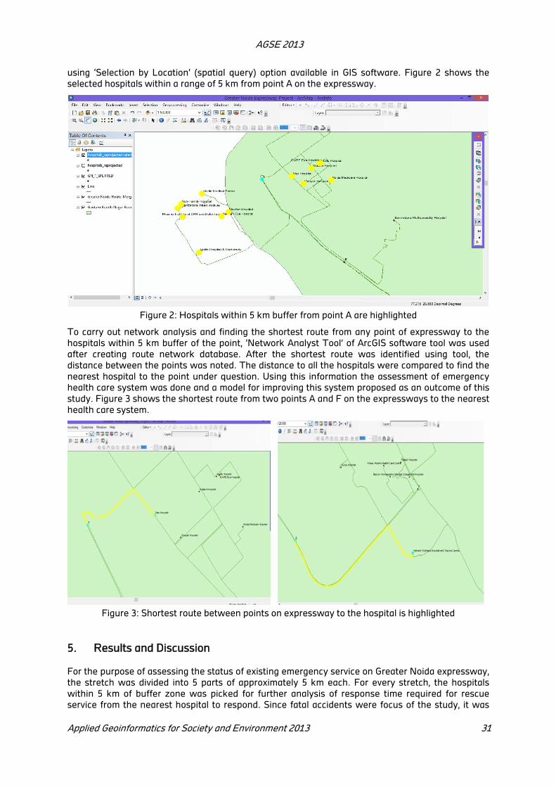
AGSE 2013


using ‘Selection by Location’ (spatial query) option available in GIS software. Figure 2 shows the

selected hospitals within a range of 5 km from point A on the expressway.

Figure 2: Hospitals within 5 km buffer from point A are highlighted

To carry out network analysis and finding the shortest route from any point of expressway to the

hospitals within 5 km buffer of the point, ‘Network Analyst Tool’ of ArcGIS software tool was used

after creating route network database. After the shortest route was identified using tool, the

distance between the points was noted. The distance to all the hospitals were compared to find the

nearest hospital to the point under question. Using this information the assessment of emergency

health care system was done and a model for improving this system proposed as an outcome of this

study. Figure 3 shows the shortest route from two points A and F on the expressways to the nearest

health care system.

Figure 3: Shortest route between points on expressway to the hospital is highlighted

5. Results and Discussion

For the purpose of assessing the status of existing emergency service on Greater Noida expressway,

the stretch was divided into 5 parts of approximately 5 km each. For every stretch, the hospitals

within 5 km of buffer zone was picked for further analysis of response time required for rescue

service from the nearest hospital to respond. Since fatal accidents were focus of the study, it was

AGSE 2013


assumed that the absence of hospital within 5 km range will result in loss of life before the victim of

accident is brought to hospital. For this reason, only the hospitals within 5 km range from the point in

question was considered. After taking the length of shortest route to every identified hospitals from

the point on expressway, the least distance was noted as the distance from the accident point on the

expressway to the nearest hospital. The result of this analysis is tabulated in Table 1.

Points on expressway

Distance from Point A(km)

Number of hospitals within 5 km buffer

Distance to nearest hospital (km)

A 0 14 1.90

B 5 7 6.33

C 10 NIL Not Applicable

D 15 NIL Not Applicable

E 20 7 5.21

F 24.5 11 0.45

Table 1: Analysis of existing emergency service on Greater Noida expressway.

The tabulated data indicates that the stretch from C to D has no hospitals within a buffer zone of 5

km which means that the probability of life loss in case of fatal accident in this stretch is very high.

Moreover, the stretch from B to C and D to E also needs attention in terms of rescue service since

the ambulance will have to travel more than 5 km from the hospital to the accident site on receiving

the message of accident and the same distance will have to be covered to reach the hospital. This

will result in long response time of emergency service. This analysis indicates that an ambulance or

rescue service should be stationed in the stretch of B to E point. The exact location can be identified

if the data of accident is made available for this stretch.

6. Conclusion

GIS is an effective tool to assess the status of emergency services along any route. This tool can be

used for effecting planning and management of this service and bring down the count of fatal

accidents due to road accidents. By integrating the statistical data of accidents with the identified

stretch for ambulance depot, effective planning can be done and the implementation of best and

economical solution can be carried out. The outcome derived from the analysis of various spatial and

non-spatial data using GIS can be used for developing a decision support system that will help

decision makers, planners, engineers, and policy makers to visualize and analyze the spatial map of

the problem and take appropriate action.

REFERENCES

Brendan GC, Daniel KA. Geographic Information Systems and Emergency Care Planning. Acad

Emerg Med. 2010; 17:1274-1278.

Cheng, M.Y., and Chang, G.L (2001), “Automating Utility Route Design and Planning Through GIS”.

Automation in Construction, 10(4), pp 507-516.

Foo CP, Ahghari M, MacDonald RD. Use of geographic information systems to determine new

helipad locations and improve timely response while mitigating risk of helicopter emergency

medical services operations. Prehosp Emerg Care. 2010; 14: 461–8.

MacEachren AM, Gahegan M, Pike W, et al. Geovisualization for knowledge construction and

decision support. IEEE Comput Graph Appl. 2004; 24:13–7.

McLafferty SL. GIS and health care. Annu Rev Public Health. 2003; 24:25–42.

Ong ME, Chiam TF, Ng FS, et al. Reducing ambulance response times using geospatial-time analysis

of ambulance deployment. Acad Emerg Med. 2010; 17:951–7.

AGSE 2013


Peters J, Hall GB. Assessment of ambulance response performance using a geographic information

system. Soc Sci Med. 1999; 49:1551–66.

Rajesh KV, Benedict P. Development of Route Information System for Ambulance Services using

GPS and GIS - a study on Thanjavaur town. Intl. Journal of Geomatics and Geosciences, Vol. 2, No.

1, 2011, ISSN 0976-4380

Rushton G. Public health, GIS, and spatial analytic tools. Annu Rev Public Health. 2003; 24:43–56.

Aerosol Optical Thickness Variability Observed over India using Satellite

Data

Sreeraj Thamarappilly

Centre For Remote Sensing, Bharathidasan University, Tiruchirappalli, Tamil Nadu- 620023, India,

Email: [email protected]

KEY WORDS: AOT, MODIS, IDL, Trend analysis

ABSTRACT:

The objective of this study is to analyze the spatial, seasonal and inter annual variability of AOT over 12 regions of India representing different atmospheric conditions. Moderate Resolution Imaging Spectroradiometer (MODIS) level 3 monthly data from 2001-2010 with a 1

0 × 1

0 spatial resolution

was analyzed by using ENVI 4.4 and by developing an Interactive Data Language (IDL) program.

The trend analysis indicates that there was no significant change of aerosol content during the period of 10 years (2001-2010), except in the case of Chennai (R

2=0.438) and Hyderabad (R

2=0.341).

New Delhi (0.729) and Kolkata (0.638) experiences the maximum mean AOT and Bangalore (0.212) experiences the minimum value. The AOT is very high (>0.8) during summer season than that of winter season in India. North India, especially Indo-Gangetic plain and Rajasthan deserts experiences very high AOT during summer. In 2009, most regions of India experiences sudden increase of AOT values with very high magnitude. The foggy conditions present over Bihar and West Bengal during winter is explained by illustrating the characteristic variation of AOT values.

The results obtained from this study are quite promising for the future research works on regional as well as global scale. Since more accurate and large area extended aerosol research will be given importance in the future, the scope of improving the accuracy for retrieving the AOT values remains very wide.

1. Introduction

The role of aerosols in climate change remains uncertain. Although the theory behind their effect on

outgoing terrestrial and incoming solar radiations is well understood, spatial and temporal variability

make it difficult to assess their magnitude with in situ observations. Satellite remote sensing is the

only means of providing the synoptic coverage needed for analysing aerosol radiative forcing at the

top of the atmosphere. Rajeev and Ramanathan (2002) discussed spatial distribution of AOT over

the open ocean (Arabian Sea and Bay of Bengal) at a spatial resolution of 1.1 km, using data for the

630 nm band of Advanced Very High Resolution Radiometer (AVHRR) on-board National Oceanic

and Atmospheric Administrations (NOAA) satellite. However, an analysis of the small-scale features

associated with aerosol distribution over optically complex areas, such as the coastal waters of the

eastern Arabian Sea, requires sensors with higher temporal and spatial resolutions (Harilal B.

Menon, Nutan Sangekar, Aneesh Lotliker, Krishnaswamy Krishnamoorthy and Ponnumani

Vethamony; 2011).

Atmospheric aerosols and trace gases play important roles in the regional as well as global radiation

budget and forcing (IPCC, 2001 and the references therein). The basic parameter that determines

the aerosol loading in the atmosphere is the column aerosol optical depth (AOD). Apart from its

varied physico-chemical characteristics, the atmospheric aerosols also have a large spatial as well as

temporal variability. Although satellite measurements provide large spatial coverage and long-term

data on aerosol and trace gas measurements, their accuracies are limited due to the retrieval and

other processes (Vachon et al., 2004). On the other hand, the ground-based fixed measurements

provide more accurate measurements but limit the spatial coverage (Sachchidanand Singh et al.,

2006).

AGSE 2013


Satellite derived column aerosol optical depth (AOD) is a cost effective way to monitor and study

aerosols distribution and effects over a long time period. Moderate Resolution Imaging

Spectroradiometer (MODIS) derived AOD is well suited for such study due to its revisit cycle of 1-2

days as a result a close estimate of AOD is made for a given region throughout the year. Monthly

average MODIS AOD has been used to investigate AOD distribution in spatio-temporal domain over

Indian subcontinent since 2000. Aerosols have an impact on cloud formation process largely

affecting monsoonal rainfall distribution over Indian subcontinent especially in the Ganga basin

(Anup K Prasad, Ramesh P Singh and Ashbindu Singh; 2004). In this study, an attempt has been

made to study the variability of aerosol optical thickness (AOT) over different regions of India using

MODIS data.

2. Objectives and Data

Due to the population growth in India and increasing urbanization as well as industrialization, the

aerosol concentration over the Indian sub-continent is found to be increasing in general. Dust storms

are common during the summer season over the Indo-Gangetic basin and are considered to be a

major health hazard to the millions of people living here, as it is one of the largest populated basins in

the world. The study was carried out to characterize the aerosol optical thickness (AOT) over India

with the following objectives.

To study the spatial distribution of AOT over 12 different regions of India representing different

atmospheric conditions.

To study the seasonal variability of AOT by analyzing the monthly AOT products.

To analyze inter annual variability of AOT for the trend analysis.

To explore the effect of land cover on AOT variability.

Modeling of regional transport using HYSPLIT back trajectory model.

MODerate resolution Imaging Spectroradiometer (MODIS) on NASA EOS Terra and Aqua missions,

launched in December 1999 and in May 2002, respectively, is a scanning spectroradiometer with 36

spectral bands between 0.645 and 14.235 μm (Kaufman et al. 1997a) with 3 spatial resolutions of

250, 500 and 1000 m. It has a swath of 2330 km across track and 10 km along track at nadir and

provides almost complete global coverage daily. The main aerosol product retrieved from MODIS is

Aerosol Optical Thickness (AOT) over land. AOTs are retrieved at 0.470 μm and 0.660 μm

wavelengths and then interpolated at 0.550 μm using Angstrom power law (Ichoku et al. 2003). The

validation data show errors in � of ±0.2* �m±0.05 over land at three of the wavelengths (Chu et al.

2002) and ±0.05* �m±0.05 over ocean at 0.550 μm wavelength (Tanre et al. 1999), where �m stands

for measured aerosol optical thickness.

AGSE 2013


3. Study Area

Figure 1: Study Area

The study was conducted over 12 regions over India to understand the spatial, seasonal and inter

annual variability of AOT. Ten years (2001-2010) MODIS Level 3 monthly AOT data of 10 ×1

0 spatial

resolution was used in the analysis.

The regions includes New Delhi, which is the capital of India; Thiruvananthapuram, which is the

capital of southernmost state of Kerala; Metropolitan cities like Bangalore, Chennai, Kolkata,

Mumbai; and the crowded cities like Hyderabad, Ahmedabad, Dehradun, Lucknow, Patna; and also

the Jodhpur, which is the city nearby the Thar desert.

AGSE 2013


4. Results

4.1 Spatial Variability

Figure 2: Spatial Variability of AOT over the study area

MONTHS NEW DELHI AHMEDABAD LUCKNOW JODHPUR PATNA DEHRADUN

January 0.47 0.35 0.44 0.23 0.34 0.34

February 0.57 0.38 0.52 0.29 0.35 0.40

March 0.85 0.46 0.80 0.36 0.52 0.64

April 1.06 0.55 0.94 0.43 0.68 0.74

May 1.31 1.06 1.07 0.71 0.89 0.90

June 0.83 0.65 0.61 0.50 0.61 0.53

July 0.54 0.47 0.47 0.27 0.40 0.37

August 0.80 0.35 0.58 0.22 0.33 0.48

September 0.70 0.32 0.67 0.23 0.39 0.39

October 0.59 0.32 0.72 0.24 0.47 0.35

November 0.56 0.34 0.63 0.23 0.45 0.33

December 0.46 0.30 0.45 0.20 0.33 0.34

Table 1 (a): Monthly average AOT values over 12 regions

AGSE 2013


MONTHS MUMBAI CHENNAI HYDERABAD KOLKATA

THIRUVANAN

THAPURAM BANGALORE

January 0.24 0.27 0.35 0.56 0.30 0.20

February 0.28 0.27 0.40 0.60 0.30 0.25

March 0.23 0.44 0.43 0.72 0.33 0.25

April 0.30 0.40 0.46 0.85 0.30 0.22

May 1.07 0.57 0.64 0.90 0.59 0.50

June 0.40 0.30 0.41 0.79 0.29 0.30

July 0.24 0.28 0.37 0.53 0.23 0.18

August 0.25 0.26 0.32 0.41 0.24 0.21

September 0.17 0.24 0.25 0.47 0.32 0.13

October 0.15 0.27 0.28 0.60 0.24 0.10

November 0.19 0.26 0.31 0.68 0.26 0.12

December 0.17 0.23 0.26 0.61 0.25 0.13

Table 1 (b): Monthly average AOT values over 12 regions

The value of AOT is relatively lower in southern India (mostly, 0.201-0.400) compared to northern

India. In the Indo-Gangetic plain, the value of AOT is very high during the summer months (>0.601).

Generally, the value of AOT in Jammu & Kashmir and in the Tibetan regions are observed to be low

(<0.400). Western parts of India and Pakistan are showing high AOT values during the summer

season (>0.801). Also, Arabian sea is more turbid compared to Bay of Bengal during the summer

months.

The AOT values of summer season are greater than that of the winter season. In all the 12 regions,

May month is showing maximum AOT. In northern part of India, generally, December and January are

showing very low AOT. The AOT values of South India are lower than that of North India. New Delhi

(1.31 during May) shows the maximum monthly average AOT value while Bangalore (0.10 during

October) shows the least value. The general pattern shows that the industrialized areas of Indian

subcontinent are showing extremely high values of AOT.

Figure 3: Variation of maximum AOT during Winter and Summer season

4.2 Interannual Variability

All the 12 regions are showing their maximum AOT during 2009. New Delhi is showing its maximum

AOT during 2009 (0.80) and 2003 (0.79), and least value is during 2006 (0.66). Ahmedabad is

showing its maximum AOT during 2009 (0.55) and 2008 (0.50), whereas 2006 and 2007 (both 0.38)

AGSE 2013


contributes to its least value of AOT. Lucknow has its maximum value during 2009 (0.77) and 2005

(0.75) and its least value during 2006 (0.58). The AOT values of Jodhpur are observed to be generally

on the lower side compared to the other North Indian regions. The AOT values of Jodhpur are very

low during 2002 (0.25), 2006 (0.26), 2008 (0.26) and 2001 (0.27). It is notable that there is a

remarkable increase of AOT in Jodhpur from 2008 (0.26) to 2009 (0.49). 2009 (0.62) and 2001 (0.56)

are showing high AOT values in Patna, whereas its minimum value is observed during 2002 and 2004

(both 0.40).

Dehradun shows its maximum AOT values during 2009 (0.59), 2001 (0.56) and 2003 (0.54); and the

value during 2006 (0.39) is the lowest one. The AOT values of Mumbai, Chennai,

Thiruvananthapuram and Bangalore are comparatively lesser than other regions. Their maximum

values are observed during the year 2009 (0.39, 0.49, 0.48 and 0.38 respectively. These 4 regions

generally show low values during 2006. Hyderabad is showing its maximum value of AOT during

2009 (0.53); while 2004 (0.31) and 2005 (0.32) observes its lowest values. Kolkata shows

comparatively very high AOT comparing to the other regions along the coastal plains. It shows its

high value during 2009 (0.75) and low values during 2002, 2006 (both 0.57) and 2008 (0.58).

Also, there is a remarkable increase in the AOT values from 2008 to 2009 in most of the regions,

especially in the case of Jodhpur and the regions in South India such as Chennai, Hyderabad,

Thiruvananthapuram and Bangalore.

REGIONS 2001 2002 2003 2004 2005 2006 2007 2008 2009 2010

NEW DELHI 0.74 0.72 0.79 0.76 0.74 0.66 0.71 0.71 0.80 0.67

AHMEDABAD 0.49 0.42 0.48 0.44 0.44 0.38 0.38 0.50 0.55 0.41

LUCKNOW 0.61 0.62 0.69 0.66 0.75 0.58 0.61 0.64 0.77 0.64

JODHPUR 0.27 0.25 0.32 0.37 0.35 0.26 0.32 0.26 0.49 0.29

PATNA 0.56 0.40 0.45 0.40 0.50 0.43 0.42 0.43 0.62 0.48

DEHRADUN 0.56 0.47 0.54 0.49 0.50 0.39 0.42 0.45 0.59 0.41

MUMBAI 0.29 0.20 0.30 0.29 0.22 0.19 0.20 0.24 0.39 0.28

CHENNAI 0.27 0.28 0.28 0.30 0.27 0.27 0.29 0.32 0.49 0.36

HYDERABAD 0.37 0.33 0.35 0.31 0.32 0.36 0.36 0.40 0.53 0.39

KOLKATA 0.68 0.57 0.67 0.61 0.61 0.57 0.63 0.58 0.75 0.73

THIRUVANANTHAPURAM 0.29 0.28 0.28 0.28 0.28 0.29 0.29 0.28 0.48 0.31

BANGALORE 0.20 0.19 0.21 0.17 0.19 0.18 0.17 0.21 0.38 0.21

Table 2:.Inter annual Variability (2001-2010) of AOT over 12 regions

REGIONS LATITUDE LONGITUDE AOT RANGE MEAN AOT SD

NEW DELHI 28.36N 77.12E 0.655-0.796 0.729 0.046

AHMEDABAD 23.00N 72.40E 0.379-0.554 0.448 0.057

LUCKNOW 26.55N 80.59E 0.575-0.773 0.657 0.063

JODHPUR 26.29N 73.03E 0.245-0.492 0.317 0.074

PATNA 25.36N 85.80E 0.395-0.622 0.470 0.074

DEHRADUN 30.19N 78.04E 0.392-0.589 0.483 0.065

MUMBAI 18.55N 72.54E 0.192-0.385 0.260 0.059

CHENNAI 13.04N 80.17E 0.273-0.487 0.314 0.067

HYDERABAD 17.22N 78.29E 0.310-0.534 0.373 0.064

KOLKATA 22.34N 88.24E 0.566-0.749 0.638 0.065

THIRUVANANTHAPURAM 8.29N 76.59E 0.275-0.480 0.304 0.063

BANGALORE 12.58N 77.38E 0.174-0.380 0.212 0.061

Table 3: Range and Mean Inter annual Variability (2001-2010) of AOT over 12 regions

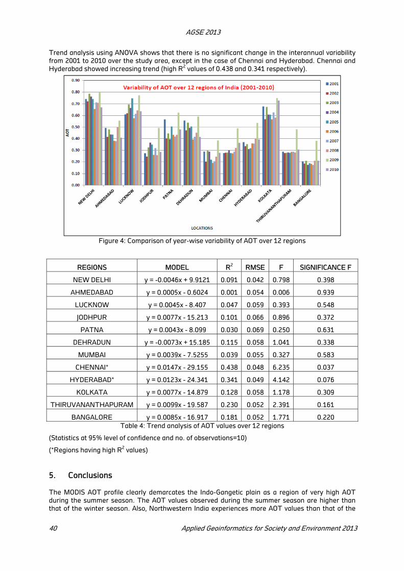
AGSE 2013


Trend analysis using ANOVA shows that there is no significant change in the interannual variability

from 2001 to 2010 over the study area, except in the case of Chennai and Hyderabad. Chennai and

Hyderabad showed increasing trend (high R2 values of 0.438 and 0.341 respectively).

Figure 4: Comparison of year-wise variability of AOT over 12 regions

REGIONS MODEL R2

RMSE F SIGNIFICANCE F

NEW DELHI y = -0.0046x + 9.9121 0.091 0.042 0.798 0.398

AHMEDABAD y = 0.0005x - 0.6024 0.001 0.054 0.006 0.939

LUCKNOW y = 0.0045x - 8.407 0.047 0.059 0.393 0.548

JODHPUR y = 0.0077x - 15.213 0.101 0.066 0.896 0.372

PATNA y = 0.0043x - 8.099 0.030 0.069 0.250 0.631

DEHRADUN y = -0.0073x + 15.185 0.115 0.058 1.041 0.338

MUMBAI y = 0.0039x - 7.5255 0.039 0.055 0.327 0.583

CHENNAI* y = 0.0147x - 29.155 0.438 0.048 6.235 0.037

HYDERABAD* y = 0.0123x - 24.341 0.341 0.049 4.142 0.076

KOLKATA y = 0.0077x - 14.879 0.128 0.058 1.178 0.309

THIRUVANANTHAPURAM y = 0.0099x - 19.587 0.230 0.052 2.391 0.161

BANGALORE y = 0.0085x - 16.917 0.181 0.052 1.771 0.220

Table 4: Trend analysis of AOT values over 12 regions

(Statistics at 95% level of confidence and no. of observations=10)

(*Regions having high R2 values)

5. Conclusions

The MODIS AOT profile clearly demarcates the Indo-Gangetic plain as a region of very high AOT

during the summer season. The AOT values observed during the summer season are higher than

that of the winter season. Also, Northwestern India experiences more AOT values than that of the

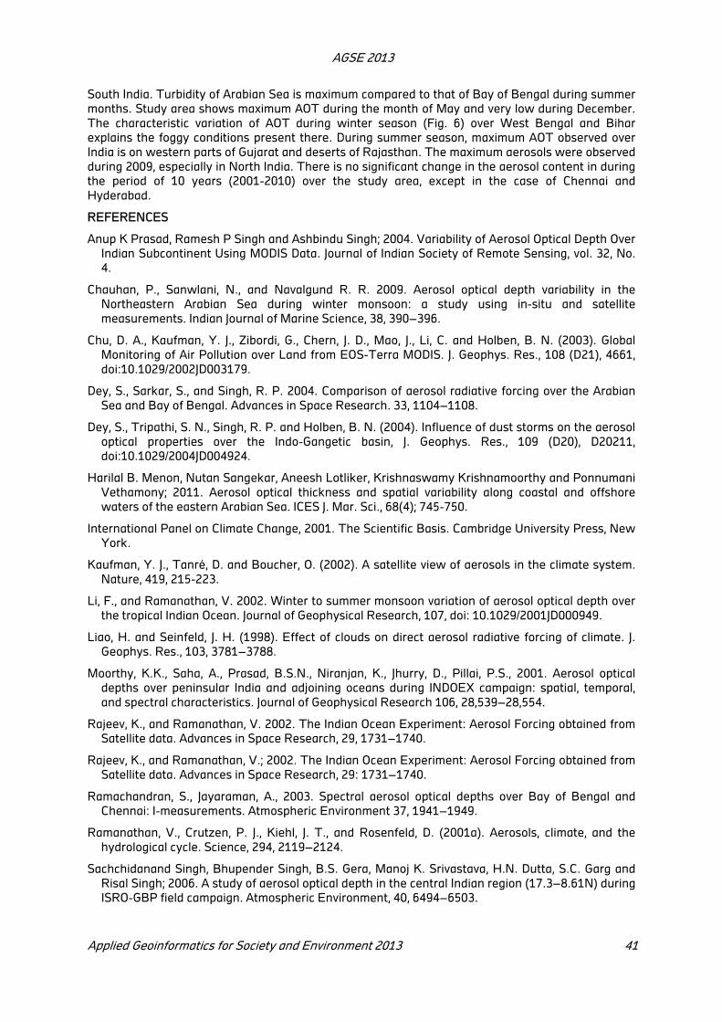
AGSE 2013


South India. Turbidity of Arabian Sea is maximum compared to that of Bay of Bengal during summer

months. Study area shows maximum AOT during the month of May and very low during December.

The characteristic variation of AOT during winter season (Fig. 6) over West Bengal and Bihar

explains the foggy conditions present there. During summer season, maximum AOT observed over

India is on western parts of Gujarat and deserts of Rajasthan. The maximum aerosols were observed

during 2009, especially in North India. There is no significant change in the aerosol content in during

the period of 10 years (2001-2010) over the study area, except in the case of Chennai and

Hyderabad.

REFERENCES

Anup K Prasad, Ramesh P Singh and Ashbindu Singh; 2004. Variability of Aerosol Optical Depth Over

Indian Subcontinent Using MODIS Data. Journal of Indian Society of Remote Sensing, vol. 32, No.

4.

Chauhan, P., Sanwlani, N., and Navalgund R. R. 2009. Aerosol optical depth variability in the

Northeastern Arabian Sea during winter monsoon: a study using in-situ and satellite

measurements. Indian Journal of Marine Science, 38, 390–396.

Chu, D. A., Kaufman, Y. J., Zibordi, G., Chern, J. D., Mao, J., Li, C. and Holben, B. N. (2003). Global

Monitoring of Air Pollution over Land from EOS-Terra MODIS. J. Geophys. Res., 108 (D21), 4661,

doi:10.1029/2002JD003179.

Dey, S., Sarkar, S., and Singh, R. P. 2004. Comparison of aerosol radiative forcing over the Arabian

Sea and Bay of Bengal. Advances in Space Research. 33, 1104–1108.

Dey, S., Tripathi, S. N., Singh, R. P. and Holben, B. N. (2004). Influence of dust storms on the aerosol

optical properties over the Indo-Gangetic basin, J. Geophys. Res., 109 (D20), D20211,

doi:10.1029/2004JD004924.

Harilal B. Menon, Nutan Sangekar, Aneesh Lotliker, Krishnaswamy Krishnamoorthy and Ponnumani

Vethamony; 2011. Aerosol optical thickness and spatial variability along coastal and offshore

waters of the eastern Arabian Sea. ICES J. Mar. Sci., 68(4); 745-750.

International Panel on Climate Change, 2001. The Scientific Basis. Cambridge University Press, New

York.

Kaufman, Y. J., Tanré, D. and Boucher, O. (2002). A satellite view of aerosols in the climate system.

Nature, 419, 215-223.

Li, F., and Ramanathan, V. 2002. Winter to summer monsoon variation of aerosol optical depth over

the tropical Indian Ocean. Journal of Geophysical Research, 107, doi: 10.1029/2001JD000949.

Liao, H. and Seinfeld, J. H. (1998). Effect of clouds on direct aerosol radiative forcing of climate. J.

Geophys. Res., 103, 3781–3788.

Moorthy, K.K., Saha, A., Prasad, B.S.N., Niranjan, K., Jhurry, D., Pillai, P.S., 2001. Aerosol optical

depths over peninsular India and adjoining oceans during INDOEX campaign: spatial, temporal,

and spectral characteristics. Journal of Geophysical Research 106, 28,539–28,554.

Rajeev, K., and Ramanathan, V. 2002. The Indian Ocean Experiment: Aerosol Forcing obtained from

Satellite data. Advances in Space Research, 29, 1731–1740.

Rajeev, K., and Ramanathan, V.; 2002. The Indian Ocean Experiment: Aerosol Forcing obtained from

Satellite data. Advances in Space Research, 29: 1731–1740.

Ramachandran, S., Jayaraman, A., 2003. Spectral aerosol optical depths over Bay of Bengal and

Chennai: I-measurements. Atmospheric Environment 37, 1941–1949.

Ramanathan, V., Crutzen, P. J., Kiehl, J. T., and Rosenfeld, D. (2001a). Aerosols, climate, and the

hydrological cycle. Science, 294, 2119–2124.

Sachchidanand Singh, Bhupender Singh, B.S. Gera, Manoj K. Srivastava, H.N. Dutta, S.C. Garg and

Risal Singh; 2006. A study of aerosol optical depth in the central Indian region (17.3–8.61N) during

ISRO-GBP field campaign. Atmospheric Environment, 40, 6494–6503.

AGSE 2013


Satheesh, S. K. and Ramanathan, V.; (2000). Large differences in tropical aerosol forcing at the top

of the atmosphere and Earth’s surface. Nature, 405, 60–63.

Singh, R.P., Dey, S., Tripathi, S.N., Tare, V., Holben, B., 2004. Variability of aerosol parameters over

Kanpur, northern India. Journal of Geophysical Research 109, D23206.

Vachon, F., Royer, A., Aube, M., Toubbe, B., O’Neill, N.T., Teillet, P.M., 2004. Remote sensing of

aerosols over North American land surfaces from POLDER and MODIS measurements.

Atmospheric Environment, 38, 3501–3515.

Pragmatic approach to storm water drainage system design under Indian

scenario: a case study of Sanand area

Khakhar M.a, *

Shah A. J. b

Vyas A.c

a Faculty of Architecture, CEPT University Ahmedabad.

b Gujarat Water Supply and Sewerage Board.

c Faculty of Technology, Co-ordinator, Post-graduate program in Geomatics, CEPT University

Ahmedabad.

KEY WORDS: Storm water, drainage, development, impervious area, topography

ABSTRACT

The effects of urbanization on storm water drainage are related to the change in the quality, runoff rate, and the volume of storm water entering the drainage system. The present study focuses on the decentralized integrated approach to - harness and dispose the storm water in line with the natural topography, alignment of major natural streams and ponds of the area for the proposed development. The study looks on the proposed new development in Sanand town in Ahmedabad in the state of Gujarat proposing a major change in the land use from the present built form of 11 % to 50% approximately in coming 5 years. This gives an opportunity to harness the maximum possible storm water falling onto the surface and convert it into a resource. The study shows that out of the total rainfall falling over the area there is potential of 66% that could be harnessed within the local area.

1. Overview

1.1 Introduction

The fast pace of urbanization imposes increasing pressures on infrastructural basic services like

water supply, sewerage, drainage, roads, bridges, transportation, health and education in urban

centers and urban agglomerations. Although, these do not generate wealth directly; but inflict a

strong base for social and economic prosperity of a town/urban area. The process of urbanization

brings along with it the building of roads, buildings and various amenities leading to great

transformation of landform from what it was prior to development. All these; in aggregate create

impermeable surfaces which reduces the area available for natural infiltration of rainfall. The

permanent physical changes lead to disturbed natural drainage pathways, increase in volume and

velocity of the runoff (Butler & Davies 2004). In the present scenario in India the storm water

drainage is taken into consideration at much later stage when it starts posing local floods.

1.2 Background

Ahmedabad accounts for 20% of the states urban population. As the city expands, the growth

centers around the main city are identified to develop as the satellite towns. Sanand town has been

identified as one of the growth centres around Ahmedabad city (AUDA 2011). The proposed

development encompasses four different town planning schemes with different land uses majorly

consisting of 75% residential and 12% industrial as compared to 40% residential and 6% industrial in

2009. The town does not have any river besides the small and big ponds in the town. The

groundwater is the major source of water having a share of 30% out of the total drinking water

supply which due to its availability at greater depths is having high TDS of 1500 to 2000 ppm1. The

* Corresponding author. [email protected]

AGSE 2013


population has changed from 32417 in 2001 to 41530 in 2011. Besides there is 41% of the district’s

industrial investment commissioned since 2008-09 is in Sanand. The proposed development

indicates the pressure on water resources and the need to plan and manage the available storm

water resource. The present study focuses on a decentralized approach to collect the storm water

zone wise formulated on the basis of topography. Besides it also proposes to integrate the existing

water bodies within the infrastructure, to retain the storm water for a longer duration of time and

gradually adding to the recharging by means of infiltration.

2. Study Area

Sanand town as a study area is located on the south western side of Ahmedabad at a latitude of

22°58´60" N and longitude of 72°22´66" E as shown in Figure 1

Figure 1: Location of Sanand with respect to Ahmedabad & surroundings (Source CDP Sanand)

Generally the town has plain topography falling in the Sabarmati basin. The altitude of the town

varies between 27m to 45 m above the mean sea level. The annual average rainfall of Sanand is 750

mm to 800mm with the rainy season spanning June through September. Geologically the area in and

around Sanand Town is composed of soft soil, recent alluvium, clay, kankar, hard murrum and

pebbles, varying in thickness up to 6 to 10 m as per data from Gujarat Water Supply and Sewerage

Board. The Sanand town is surrounded by three major ponds namely Bhadreti pond, Gadhiyu pond

and Lakshmana ponds embracing the wastewater and the storm water runoff, leading to the

deteriorated water quality. The ground water is being extracted to support irrigation, Industry and

drinking water supply requirements. However, in the present status, Sanand falls in the

overexploited zone for groundwater i.e. when the level of groundwater development is more than

100. Therefore, there is an urgent need for groundwater recharging and creating alternate sources

to enhance the availability of in the area.

3. Materials and Methods

3.1 Pre-development storm water movement

The study of toposheet and the contour map generated from the digital elevation model from the

Shuttle Radar Topography Mission (SRTM) as shown in the Figure 2 and 3 indicate the Gamtal area

of Sanand having highest elevation of the order of 45m to 47m from the mean sea level having is

gentle slope in all four directions. The terrain displays more continuous slope towards south west

direction till Nal-sarovar in south west direction.

AGSE 2013


Figure 2: Contour study of 1m interval Figure 3: Location of study area on the toposheet

Besides, the natural streams in the area were found using the hydrology tool in Arc GIS 9.3 (ESRI

1990). It was found that majority of bigger ponds which retained water; were in line with these

streams. The efforts in this study are to find opportunities to respond to the existing natural system

for the proposed development.

3.2 Present and Proposed Land use

In the present situation, out of the total 4042 hectares the built form is approximately only 488

hectares including gamtal (village). In the post-development stage the total built form is

approximately 2117 hectares which turns out to be almost 52% of the total area as shown in the

Table 1.

Sr.

No

Land Use 1997 (Area Ha) %

Area

LU in 2009

(Area Ha)

%

Area

LU 2010-15

(Area Ha)

%

Area

1 Residential

including Gamtal

165 46.3 194.53 39.8 1583 74.78

2 Commercial 18 5.1 19.58 4 34 1.61

3 Industrial 84 23.6 31.43 6.4 252 11.90

4 Public and Semi-

public spaces

51 14.3 49.79 10.2 25 1.18

5 Water Bodies 36 10.1 63.28 12.9 62 2.92

6 Transportation and

communication

(Railways, Roads)

2 0.6 130 26.6 161 7.61

7 Total Developed

area

356 100 488.6 100 2117 100

8 Remaining Area 3686 3553.4 1925

9 Total Revenue

Area

4042 100 4042 100 4042 100

Table 1: Proposed Land use post development

(Source: City Development Plan Sanand, Sanand Nagarpalika)

With given development, the natural water bodies would be deteriorated having no natural streams

to feed them being existent. Besides, the open/agricultural land around capable of infiltrating the

AGSE 2013


rainfall runoff displaying the phenomenon of attenuating the runoff from the built areas in the

present situation would be reduced to half the area post-development stage rendering the increased

rate and volume of runoff with considerable pollutants beyond the assimilating capacity of the area.

This could lead to flash flooding in local areas affecting the functioning and health of the people post

flooding (karande et al. 2003) Given this situation, the natural streams and the existing ponds in

order of the hierarchy of their water storage capacity and the proposed development are considered

together to delineate the ponds which could be proposed to be developed as the retention basins to

recharge the groundwater as well as could be accommodated as recreational areas in the proposed

development plan.

3.3 Estimation of Storm water for the proposed development

For the estimation of the storm water and proposal of the storm water network the design period

considered is 30 years i.e. till 2041 for which the population has been estimated as per the method

suggested in the “Manual on Water Supply and Treatment” by CPHEEO, Ministry of Urban

Development, New Delhi (1999) as shown below

Sr.

No.

Project

Area

Density

/ha

Popula-

tion

Density

/ha

Popula-

tion

Density

/ha

Popula-

tion

Density

/ha

Popula-

tion

Density

/ha

Popula-

tion

2001 2011 2021 2031 2041

1

Sanand

Town

488 Ha

66 32417 80 41530 120 58560 140 68320 150 73200

2

TPS

1,2,3,4

1199

Ha

TP schemes yet under

development phase 30 35970 65 77935 100 1E+05

3 Total 32417 41530 94530 1E+05 2E+05

Table 2: Projected Population for the study area

With the above population to be served, the built up area and thereby the runoff from these areas

would contribute to the storm water. The runoff for the above study has been calculated by the

rational method as mentioned below.

Q = 10CIA (1)

Q = Rate of Runoff (m3/hr)

C = Coefficient of runoff

I = Intensity of rainfall (mm/hr)

A = Area of the watershed being drained (ha)

The rational formula is favored in practice for small areas due to the definite information obtainable

of the constituent factors involved. Area can be measured from the survey of the study area and ‘I’

can be found from the study of the rainfall record and corresponding duration of storm producing

maximum run off.

3.4 Estimating Intensity

The intensity of the rain is the rate at which it is falling, the duration is the time for which it falls with

the given intensity and the frequency is the number of times it falls on a particular area. The

intensity of rainfall can be determined with the help of automatic rain gauges. Such rain gauges

automatically record the cumulative rainfall with different time intervals such as 5, 10, 15, 20, 30, 60,

90, 120 minutes and intensity can be worked out for each chosen interval. They are then converted

into the intensity duration curves for a particular area (Garg 2000). The rainfall data for the study

area was obtained for the last 20 years. The data for the rainfall for the duration less than 1 hour are

not collected by the authority at the selected station. Hence it was difficult to build inference on the

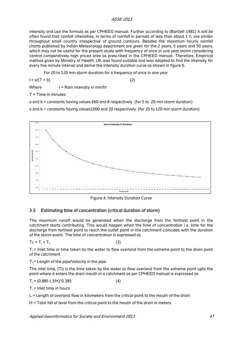
AGSE 2013


intensity and use the formula as per CPHEEO manual. Further according to (Bartlett 1981) it will be

often found that rainfall intensities, in terms of rainfall in periods of less than about 1 h, are similar

throughout small country irrespective of ground contours. Besides the maximum hourly rainfall

charts published by Indian Meteorology department are given for the 2 years, 5 years and 50 years,

which may not be useful for the present study with frequency of once in one year storm considering

central comparatively high priced area as prescribed in the CPHEEO manual. Therefore, Empirical

method given by Ministry of Health, UK was found suitable and was adapted to find the intensity for

every five minute interval and derive the intensity duration curve as shown in figure 6.

For 20 to 120 min storm duration for a frequency of once in one year

I = a/(T + b) (2)

Where i = Rain intensity in mm/hr

T = Time in minutes

a and b = constants having values 660 and 8 respectively. (for 5 to 20 min storm duration)

a and b = constants having values1000 and 20 respectively. (for 20 to 120 min storm duration)

Figure 4: Intensity Duration Curve

3.5 Estimating time of concentration (critical duration of storm)

The maximum runoff would be generated when the discharge from the farthest point in the

catchment starts contributing. This would happen when the time of concentration i.e. time for the

discharge from farthest point to reach the outlet point in the catchment coincides with the duration

of the storm event. The time of concentration is expressed as

Tc = Ti + Tf (3)

Ti = Inlet time or time taken by the water to flow overland from the extreme point to the drain point

of the catchment

Tf = Length of the pipe/Velocity in the pipe

The inlet time, (Ti) is the time taken by the water to flow overland from the extreme point upto the

point where it enters the drain mouth in a catchment as per CPHEEO manual is expressed as

Ti = (0.885 L3/H)*0.385 (4)

Ti = Inlet time in hours

L = Length of overland flow in kilometers from the critical point to the mouth of the drain

H = Total fall of level from the critical point to the mouth of the drain in meters

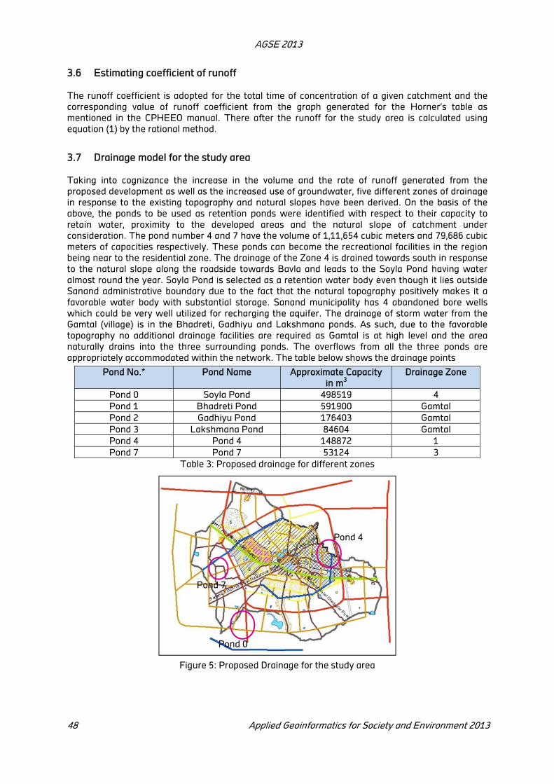
AGSE 2013


3.6 Estimating coefficient of runoff

The runoff coefficient is adopted for the total time of concentration of a given catchment and the

corresponding value of runoff coefficient from the graph generated for the Horner’s table as

mentioned in the CPHEEO manual. There after the runoff for the study area is calculated using

equation (1) by the rational method.

3.7 Drainage model for the study area

Taking into cognizance the increase in the volume and the rate of runoff generated from the

proposed development as well as the increased use of groundwater, five different zones of drainage

in response to the existing topography and natural slopes have been derived. On the basis of the

above, the ponds to be used as retention ponds were identified with respect to their capacity to

retain water, proximity to the developed areas and the natural slope of catchment under

consideration. The pond number 4 and 7 have the volume of 1,11,654 cubic meters and 79,686 cubic

meters of capacities respectively. These ponds can become the recreational facilities in the region

being near to the residential zone. The drainage of the Zone 4 is drained towards south in response

to the natural slope along the roadside towards Bavla and leads to the Soyla Pond having water

almost round the year. Soyla Pond is selected as a retention water body even though it lies outside

Sanand administrative boundary due to the fact that the natural topography positively makes it a

favorable water body with substantial storage. Sanand municipality has 4 abandoned bore wells

which could be very well utilized for recharging the aquifer. The drainage of storm water from the

Gamtal (village) is in the Bhadreti, Gadhiyu and Lakshmana ponds. As such, due to the favorable

topography no additional drainage facilities are required as Gamtal is at high level and the area

naturally drains into the three surrounding ponds. The overflows from all the three ponds are

appropriately accommodated within the network. The table below shows the drainage points

Pond No.* Pond Name Approximate Capacity

in m3

Drainage Zone

Pond 0 Soyla Pond 498519 4

Pond 1 Bhadreti Pond 591900 Gamtal

Pond 2 Gadhiyu Pond 176403 Gamtal

Pond 3 Lakshmana Pond 84604 Gamtal

Pond 4 Pond 4 148872 1

Pond 7 Pond 7 53124 3

Table 3: Proposed drainage for different zones

Figure 5: Proposed Drainage for the study area

Pond 7

Pond 4

Pond 0

AGSE 2013


4. Conclusions

1. From the above study it could be derived that out of the total rainfall 66,857 m3/hour falling over an

area of 1033 ha, 44,370 m3/hour; i.e. 66% can be harnessed within the local area. There is further

scope to raise the harnessing potential out of the total rainfall by source control measures.

2. In the above analysis the maximum calculated discharge is accommodated in the highest available

size of RCC pipe in contrast to the situation for all the storm water being led centrally to a single or

more outfalls, would have called for construction of the ducts at quite a few locations adding to high

capital costs. The system would efficiently accommodate the frequent rainfall events and would

minimize or avoid frequent occurrence of flash floods due to the developments and hence would

minimize loss to life and property.

3. The proposed system provides the identification of ponds in the area which can be perceptively

developed for several purposes of recreation, retention and groundwater recharge or infiltration in

the area contributing to improvement in the quality of life.

4. There is possibility of storm water source control measures at the institutional and the industrial

setups where the areas are large and the discharge in form of storm water runoff could be instituted

to remain within premises by appropriate policy norms or incentives to the institutional/industrial

setups for the minimizing discharge in form of storm water runoff from their premises. This would

enhance the runoff to be reduced and the costs may be decentralized.

REFERENCES

Ahmedabad Urban Development Authority (AUDA) and Space Applications Centre (ISRO). 2011

Revised Development Plan of Ahmedabad Urban Development Authority area. AUDA, Ahmedabad.

Bartlett, R. E. 1981. Surface Water Sewerage. Applied Science Publishers.

Butler, D., Davies J. W. 1981. Urban Drainage. Spon, London UK.

Central Public Health and Environmental Engineering Organization (CPHEEO) 1993 Manual on

Sewerage and Sewage Treatment. Ministry of Urban Development,

Environmental Systems Research Institute (ESRI) 1990. Understanding GIS: The Arc/Info Method.

ESRI, Redlands, California.

Garg, S. K. 2000. Hydrology and Water Resources Engineering. Khanna Publishing, New Delhi.

Karande, S., Bhatt, M., Kelkar A., Kulkarni M., Varaija A. 2003 “An Observational study to detect

leptospirosis in Mumbai, India, 2000” Archives of Diseases of Childhood 88.12: 1070-1075.

Risk Assessment of Coastal City through Remote Sensing &

Geographical Information System aJyoti Tirodkar,

bProfessor. Arun Inamdar

aCentre of Studies in Resource Engineering Indian Institute of Technology, Bombay Maharashtra,

India, Email: [email protected]

bCentre of Studies in Resource Engineering Indian Institute of Technology, Bombay Maharashtra,

India, Email: [email protected]

ABSTRACT:

Tsunamis, storms, surges, coastal flooding & rise in sea level results named as coastal hazards, disturbs social, ecological & economic balance in coastal zone. As a result human beings experiences risk of life in coastal city. Such kind of risks associated with coastal cities can be reduced with help of sustainable development & planning. Satellite Remote Sensing (SRS) & Geographical Information System (GIS) provides huge platform for planning & sustainable development of the coastal city. Analysis of Coastal geomorphology, coastal processes & coastal hazards through SRS & GIS are major part of Sustainable development of coastal city. In this paper, we have proposed system architecture for Risk Assessment & Sustainable development of Coastal city.

KEYWORDS: Satellite Remote Sensing, GIS, Shoreline Management & Planning, Coastal City,

Sustainable Development

1. Introduction

Coastal zone is rich in renewable & non renewable resources. Human beings prefer to stay in coastal

zone for privileged lifestyle. Hence coastal cities are heart of economy of a country. Coastal hazards

& rise in sea level results in risk of life in coastal city. Uncontrolled land reclamation, increase in

population & unlimited resource extraction are responsible for vulnerability of coastal city. Planning

& sustainable development of coastal zone on regular basis along with maintenance, reduces risk of

life in coastal city. Sustainable planning & development includes analysis of historical coastal

landforms, change in shoreline, coastal processes, coastal hazards & Coast Regulation zone act.

Coast protective measures provide safety to coastal city. A combination of district planning & along

with coastal zone sustainable development maintains balance between Societies, Economy &

Ecology of the coastal city. Proposed development can be done with help of Satellite Remote

Sensing & Geographical Information System in cost & time effective aspect.

In this paper, we have proposed a methodology for Risk Assessment &Sustainable development of

coastal city with help of Satellite Remote Sensing & Geographical Information System.

2. Objectives

Risk Assessment of Coastal city & Sustainable Development

Historical Analysis of change in shoreline, coastal processes, coastal hazards & coastal

landforms through Satellite Remote Sensing

3. Satellite Remote Sensing & Gis

Satellite Remote Sensing provides temporal images of study area as per requirement of user. It is

necessary to perform atmospheric & geometric correction of satellite images before analysis. Image

processing through ERDAS software is required for better image interpretation.

AGSE 2013


Statistical & visual analysis can be done through GIS. Digital elevation models can be created for

coastal landform study, with help of GIS. For analysis, all images & maps need to be digitized.GIS

allows user to present results in graphical or report format.

Figure 1: Steps of image processing

3.1 Dataset

For sustainable planning & development of coastal city following datasets are required,

1. Temporal satellite images of high resolutions

2. Toposheets

3. Bathymetry Maps, HTL & LTL maps

4. Historical Coastal Hazards data

5. Coastal Regulation Zone maps

6. District planning Maps

3.2 System architecture

Proposed system architecture analyzes historical coastal landforms, Historical coastal processes,

and coastal land use characterizations. Identification of Coastal managing Unit in coastal zone

specifies requirement of coast protective measures. Consideration of District level planning map

maintains balance between govt. plans & coastal zone planning. Sustainable Coastal city can be

developed with help of proposed system architecture.

Figure 2: System Architecture

AGSE 2013


4. Coasta Landform Unit (CLU)

Shoreline change detection analysis and coastal landform change detection analysis can be done

with help of digitized images & maps. Based on this analysis whole shoreline can be classified in to

erosion, stable coast & accretion zone. Coastal landform change detection analysis in combination

with shoreline change analysis classifies coastal zone in 6 categories with and without change in

landform.

Figure 3: Schematic of CLU

5. Coastal Process Unit (CPU)

Historical analysis & future predictions about coastal zone can be done only with analysis of coastal

processes. Coastal processes are mainly classified in two parts such as Natural Processes & Human

Activities. Analysis of coastal processes can be done with help of Bathymetry data, Tidal data &

coastal hazards details. Based on this data coastal zone can be classified in 4 parts such as High

Risk zone, Moderate risk zone, Low risk zone & No risk zone.

AGSE 2013


Figure 4: Schematic of CPU

6. Coastal Land Use CharacterizationUnit (CLUCU)

Coastal Regulations Zone (CRZ) act is enforced for conservation of coastal zone. CRZ regulation

classifies Coastal zone in 4 sectors. CRZ I,II,III are area from HTL to 500m landward side & 100m in

water body such as creek, lagoon, etc.

Figure 5: Schematic of Coastal Managing Unit (CMU)

CRZ I is ecologically sensitive zone such as turtle nesting zone, mangroves, salt marshes, etc.

CRZ II is developed zone under municipal authority

CRZ III is underdeveloped zone under rural authorities

CRZ IV is area from LTL to offshore 12 nautical miles

Coastal region can be divided in 3 categories as follows

AGSE 2013


1. Ecologically Sensitive Zone (ESZ) : Mangroves, Marshy lands, Intertidal mud flats, Sandy

beaches, etc

2. Economic Zone (EZ): Green Industry, Tourist place, Ports & Harbours, Road network, etc.

3. Social Zone (SZ): Residential Set up, Agriculture zone, Horticulture zone, Parks, Dumping

Grounds, etc.

CMU is combination of CLU, CPU, and CLUCU. As per the proposed architecture shoreline of coastal

city should be divided in Coastal Managing Unit.

Figure: 6 Schematic of CMU

Above mention schematic of CMU represents a sample of CMU. As per the proposed system

architecture 72 CMU can be identified in coastal zone.

6.1 Coast Protective Measures

While planning coastal cities one should consider coast protective measures such as sea walls,

revetments, etc. Existing development in Erosion zone can be protected with help of Coast protective

measures. Impact of coastal hazards such as storms, surges can be reduced up to certain extend

with help of coast protective measures. Low lying areas of coastal zone can be protected with sea

walls. Beach nourishment & coast protective measures together makes reduces impact of coastal

hazards in coastal city.

6.2 District Planning Map

Every district has its own planning for development. With reference to this map social zone &

economic zone of coastal region will be divided into categories formed in proposed architecture.

7. Software Implementation

In this proposed architecture following software can be used.

ENVI – This software is used to perform atmospheric correction of remotely sensed satellite

image. Band stacking can be done by this software.

ERDAS – This software is used for supervised classification of satellite image. Image Mosaicing

for study area can be done by this software.

ARC GIS – Spatial analysis satellite images can be done with this software. Various operations

such overlay of satellite images, DEM analysis can be done with this software.

DSAS – This is extension of Arc GIS software used for statistical analysis of shoreline change in

coastal city.

AGSE 2013


8. Preliminary Results

Evaluation of Coastal Managing unit divides coastal zone in two categories such as No Development

Zone “NDZ”& Development Zone “DZ”. During CMU evaluation coast protective measures should be

considered. Preliminary results of the proposed system are as follows:

1. Erosion zone: Development is permitted in No risk zone with social & economic region.

Constructionof coast protective measures in erosion zone conserves coastal habitat

EROSION ZONE WITH CHANGE IN LANDFORM

HIGH RISK MODERATE RISK LOW RISK NO RISK

ESZ EZ SZ ESZ EZ SZ ESZ EZ SZ ESZ EZ SZ

COAST PROTECTIVE MEASURES

NDZ NDZ NDZ NDZ NDZ NDZ NDZ NDZ NDZ NDZ DZ DZ

Table 1: CMU evaluation for Erosion zone with change in coastal landform

EROSION ZONE WITHOUT CHANGE IN LANDFORM



COAST PROTECTIVE MEASURES

NDZ NDZ NDZ NDZ NDZ NDZ NDZ DZ DZ NDZ DZ DZ

Table 2: CMU evaluation for Erosion zone without change in coastal landform

2. Stable Coast: Development is prohibited in ecologically sensitive zone & High risk zone.

Construction of coast protective measures is necessary for High Risk zone

STABLE COAST WITH CHANGE IN LANDFORM



COAST PROTECTIVE

MEASURES

NDZ NDZ NDZ NDZ DZ DZ NDZ DZ DZ NDZ DZ DZ

Table 3: CMU evaluation for Stable Coast zone with change in coastal landform

STABLE COAST WITHOUT CHANGE IN LANDFORM



COAST PROTECTIVE

MEASURES

NDZ DZ DZ NDZ DZ DZ NDZ DZ DZ NDZ DZ DZ

Table 4: CMU evaluation for Stable Coast zone without change in coastal landform

AGSE 2013


Accretion zone: In this zone no need of coast protective construction. Ecologically Sensitive zone &

High risk zones are only classified in NO Development Zone.

ACCRETION ZONE WITH CHANGE IN LANDFORM



NO NEED OF COAST PROTECTIVE MEASURE

NDZ NDZ NDZ NDZ DZ DZ NDZ DZ DZ NDZ DZ DZ

Table 5: CMU evaluation for Accretion Zone with change in coastal landform

ACCRETION ZONE WITHOUT CHANGE IN LANDFORM



NO NEED OF COAST PROTECTIVE MEASURE

NDZ DZ DZ NDZ DZ DZ NDZ DZ DZ NDZ DZ DZ

Table 6: CMU evaluation for Accretion Zone without change in coastal landform

9. Conclusion

Risk associated with coastal city can be reduced by implementing proposed system architecture.

Proposed planning of coastal city conserves coastal ecosystem & may arrange additional space for

social & economic development. Construction of Coast protective measures can reduce rate of

erosion along shoreline. In future, proposed development can reduce impacts of coastal hazards.

SRS & GIS makes cost effective & time effective risk assessment & sustainable development in

coastal city.

REFERENCES

Shoreline Management & Planning proposed system architecture by MR. Mike

M. A. Herlekar & R.K. Sukhatankar “Morphotectonic studies along the part of Maharashtra coast,

India”, ISSN 0974-5904, Vol. 04, No 02 - Spl issue, March 2011, pp. 61-83

Debjit Datta & Shovik Deb, “Analysis of coastal land use / land cover changes in Indian sunderbans

using remotely sensed data”, Informa Ltd Registered in England and Wales Registered Number:

1072954 Registered office: Mortimer House, 37-41 Mortimer Street, London W1T 3JH, UK

Dr. Anil Paropkari “Coastal Geomorphology & Mineral resources”

Dr. Colin Woodroffe, “ Coastal forms,, processes & evolution” Book edition 2003.

Prabaharan, Raju, Lakshumanan & Ramlingam “ Remote sensing & GIS applications on change

detection study in coastal zone using multi temporal satellite data” ,ISSN 0976-4380

Sachin Pendse “ Coastal Process & Port development In North Kokan”, ISSN 2277-2081

Wang & Zhigao “ Application of Remote sensing technology in Tianjin Binhai new area Coastal zone

monitoring”

K. Selvavinayagam “ Shoreline change monitoring in Tuticorin coast using Remote sensing & GIS tool

Kelly, Ramsey, Griffee “ Analysis of coastal processes for the chatham south coast between mill

creek and bucks creek

“Coastal & Sea Erosion” documentation by Maharashtra Govt.

AGSE 2013


“Coastal Areas Problems & Conservation (In Maharashtra with special reference to Mangrove)” By

Maharashtra govt.

“Remote Sensing for Coastal Resource Managers: an overview”, Feb 1997, US dept of Commerce

weigen Huang, Bin Fu, “Remote Senign for Coastal area Management in china”, 30:271-276,2002

M.A. Lazaridou “Image interpretation of coastal Areas”, ISRS vol XXXIX-B8,2012, XXII ISPRS

congress.

Rajesh Shriniwas “Sustainable Coastal Protection & Management Program, Maharashtra, India”for

year 2012.

Bruce Parker, Dennis Milbert, Kurt Hess & Stephen Gill ”Integrating Bathymetry, Topography and

Shoreline, and the importance of vertical Datums”

University Informatics Facility “Remote sensing Resources”

Monitoring of Coastal Marine & Estuarine Ecology of Maharashtra : Phase I”

D. Nandakumar & M. Muralikrishna “Mapping the extension of Coastal regulation zone violations of

the Indian Coast.

http://www.fao.org/docrep/010/ag127e/ag127e09.htm “Protection from Coastal Erosion” Last

access on 18th

September, 2013.

Steven, A Hughes & Nicholas, Kraurs “Frequently asked questions about coastal inlets and U.S. Army

corps of Engineers, Coastal Inlet research Program”

NWIA_ Maharashtra ATLAS for year 2010

http://www.mogaveeracommunity.com/hab.php, (Last access on 18th

September, 2013).

http://www.lib.utexas.edu/maps/ams/india/, (Last access on 20th

September, 2013).

http://www.mrsac.gov.in/en/projects/high-resolution-data-base-mapping/coastal-zone-mapping-

and-monitoring, (Last Access on 5th

October, 2013).

http://www.iomenvis.in/maharashtra-state.php, (Last access on 5th

October, 2013).

http://www.environment-agency.gov.uk/research/planning/104939.aspx, (Last Access on 5th

October,2013).

Acknowledgement

I express my deep sense of gratitude and heartfelt thanks to my guide, Prof. Arun Inamdar, for the

considerable freedom, constant encouragement and support he has provided me throughout the

course of this study. I am thankful to him for spending his valuable time and critically reviewing the

report which has helped me to improve my knowledge on the subject. I would also like to express my

gratitude for all those who provided me with valuable suggestions to help me improve my study.

Mobile Geo-referenced Thermal Infrared Imagery Recording for Leakage

Detection in Urban District Heating Networks

A. Miraliakbaria, M. Hahn

a, J. Engels

a, F. Sohel

b, M. Bennamoun

b

a Department of Geomatics, Computer Science and Mathematics, University of Applied Sciences

Stuttgart, Schellingstraße 24, D-70174 Stuttgart, Germany - (Alvand.Miraliakbari, Michael.Hahn,

Johannes.Engels)@hft-stuttgart.de

b School of Computer Science and Software Engineering, The University of Western Australia, 35

Stirling HWY, CRAWLEY, Australia - (Ferdous.Sohel, Mohammed.Bennamoun)@uwa.edu.au

KEY WORDS: Detection, GPS/INS, Imagery, Mobile, Recording, Thermal

ABSTRACT

Localization of heating networks and detection of their leakages are significantly important for energy suppliers. Traditional ways of leakage detection are time consuming and costly. It might sometimes end up with wrong detection. To address such problems, this paper represents a two-step procedure for the leakage detection in thermal images. Localization of the captured data is enabled using a GPS-aided inertial navigation system synchronized with the thermal camera. Leakage and poor insulation detection is achieved in two phases: The first phase is to register the base maps of the network to the thermal sequence and investigate the indicated temperatures surrounded by the network domain (region of interest). The second phase is to cluster the thermal image and look for the cluster of the highest temperature which suggests the heat loss. K-means clustering is selected due to its high speed of computation compared to other clustering methods. The temperatures can be grouped into 4 to 6 clusters. Three major predefined classes correspond to cold, medium and high temperature. The experimental results show that poor insulations can be successfully detected.

1. Introduction

Thermography, also known as thermal imaging, is a well-established technique for displaying

temperature distributions of object surfaces. The applications are many and varied ranging for

example from building diagnostics to veterinary applications of thermography on animals.

Energy suppliers which operate district heating networks have a major interest in maintaining their

network. If leakages occur, it is a big challenge to localize them precisely. Today well established

techniques exist for the acquisition of geo-referenced thermal images and image sequences. Two

examples may illustrate the state of the art. FLIR Company reports about the use of a thermal

infrared camera to monitor and detect leaks of underground pipes of the district heating network

system by driving through the city. A thermal camera is mounted on the roof of the vehicle (FLIR

system, 2013). Another approach is to use airborne thermography to detect the leakages and weak

isolation of the heating network. The orientation of the thermography camera is obtained by direct

geo-referencing using a GPS/INS platform (FLIR system, 2013).

In fact, the GPS/INS technology nowadays is developed to such an extent that users can assemble it

with other sensors like building blocks. In this paper we report about a case study in which we take

up this idea, combine a FLIR SC645 thermography camera with an OXTS 2002/250 GPS/INS system

and mount it on the roof of a van. Accuracy requirements for the thermography of a district heating

network system are fairly low in the order of one meter, thus aligning the coordinate systems of the

camera and GPS/INS system does not require an accurate calibration. A fundamental understanding

of why a road surface may show up with surface temperature differences is essential for the

interpretation of the thermal images. A leak in a pipeline below the road surface is not the only

possible reason for such temperature differences. Other hot spots may result from manholes,

footprints of engines which recently left a parking location or a weak isolation of a certain segment

of a pipeline.

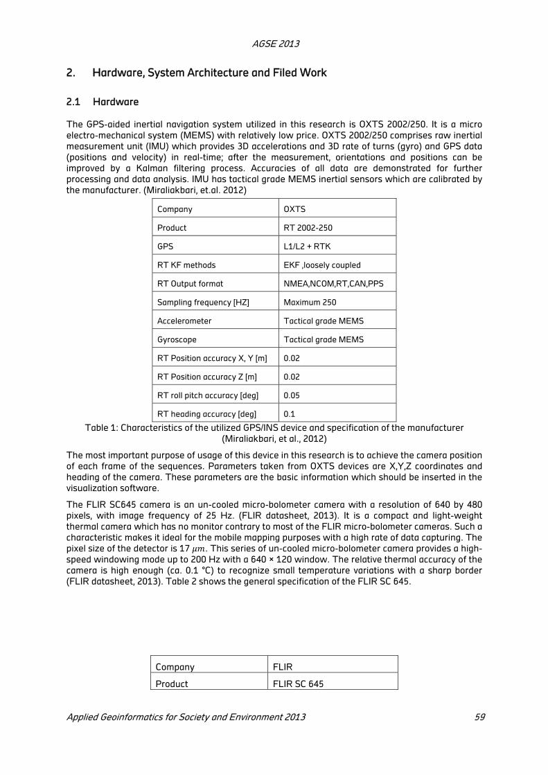
AGSE 2013


2. Hardware, System Architecture and Filed Work

2.1 Hardware

The GPS-aided inertial navigation system utilized in this research is OXTS 2002/250. It is a micro

electro-mechanical system (MEMS) with relatively low price. OXTS 2002/250 comprises raw inertial

measurement unit (IMU) which provides 3D accelerations and 3D rate of turns (gyro) and GPS data

(positions and velocity) in real-time; after the measurement, orientations and positions can be

improved by a Kalman filtering process. Accuracies of all data are demonstrated for further

processing and data analysis. IMU has tactical grade MEMS inertial sensors which are calibrated by

the manufacturer. (Miraliakbari, et.al. 2012)

Company OXTS

Product RT 2002-250

GPS L1/L2 + RTK

RT KF methods EKF ,loosely coupled

RT Output format NMEA,NCOM,RT,CAN,PPS

Sampling frequency [HZ] Maximum 250

Accelerometer Tactical grade MEMS

Gyroscope Tactical grade MEMS

RT Position accuracy X, Y [m] 0.02

RT Position accuracy Z [m] 0.02

RT roll pitch accuracy [deg] 0.05

RT heading accuracy [deg] 0.1

Table 1: Characteristics of the utilized GPS/INS device and specification of the manufacturer

(Miraliakbari, et al., 2012)

The most important purpose of usage of this device in this research is to achieve the camera position

of each frame of the sequences. Parameters taken from OXTS devices are X,Y,Z coordinates and

heading of the camera. These parameters are the basic information which should be inserted in the

visualization software.

The FLIR SC645 camera is an un-cooled micro-bolometer camera with a resolution of 640 by 480

pixels, with image frequency of 25 Hz. (FLIR datasheet, 2013). It is a compact and light-weight

thermal camera which has no monitor contrary to most of the FLIR micro-bolometer cameras. Such a

characteristic makes it ideal for the mobile mapping purposes with a high rate of data capturing. The

pixel size of the detector is 17 . This series of un-cooled micro-bolometer camera provides a high-

speed windowing mode up to 200 Hz with a 640 × 120 window. The relative thermal accuracy of the

camera is high enough (ca. 0.1 °C) to recognize small temperature variations with a sharp border

(FLIR datasheet, 2013). Table 2 shows the general specification of the FLIR SC 645.

Company FLIR

Product FLIR SC 645

AGSE 2013


Spatial resolution (IFOV) 0.68 mrad

Field of view (FOV) 25° x 18.8°

Minimum focus distance

[m]

0.4

Image frequency [HZ] 25

Focal length 24.5mm(used in this

research)

Focus Automatic/manual

Detector type Focal Plane Array (FPA)

Spectral range (μm) 7.5 – 14

Table 2: Characteristics of the utilized thermal infrared camera (FLIR datasheet, 2013)

2.2 System Architecture

The thermal camera was mounted on the roof of a vehicle and synchronized with the GPS/INS

system. The camera was looking in forward direction to capture the road surface starting at a

distance of 5 m in front of the car. The camera was fixed on the roof of the vehicle by a special

mount called ‘Fat Gecko’. Fat Gecko is a dual suction cup mount ensures the stability of the camera

mounting on the moving platform (Fat Gecko Brief, 2013). The communication between the FLIR SC

645, OXTS GPS/INS is established by the host computer. The power supply for both GPS/INS and the

thermal camera is provided by the vehicle using the cigarette lighter receptacle plug. The time

synchronization between the FLIR and OXTS devices is performed via the digital I/O plugs. It is

beneficial to send a pulse per second (PPS) signal from OXTS to the input pin of the FLIR digital I/O

plug. The input pin of FLIR is an opto-isolated pin which can accept low level signals from 0 – 1.5 V,

high level: 3 – 25 V. (Infrared training center, itc). As the rectangular signal, the raising edge of the

signal is taken as a timestamp for the synchronization.

2.3 Fieldwork Data Capturing and Office Work Data Rendering

The data recording was carried out on the evening of a cold day in January 2013. No sun effect was

included, i.e. no absorption or reflection of sun radiation deluded the indicated surface temperature

indication. The traffic jam was very light, thus the other vehicles rarely show up in the captured data.

For planning the drive along the district heating network as well as for ground truthing the location

of the pipelines a map of the network (Figure 5, right picture) was provided by the department of

public works of the city (Stadtwerke Ludwigsburg-Kornwestheim). The district network mostly

passes through the main streets with a certain distance from the street centre line shown in the

base maps. Five tracks were recorded from different street blocks in the city of Ludwigsburg, Baden-

Württemberg, Germany. Some tracks partially passed by some streets which contained no district

network. These streets were taken as cold asphalt samples which were not affected by the

leakages. The highest attention in geo-referencing of the data was given to the position of the

camera rather than the regular exterior orientation parameters. Figure 1, (left picture) shows one of

the 30 thousand images which have been recorded as a sequence with 25 Hz. The GPS/INS results

have been used to add EXIF metadata to each image. GeoSetter (www.geosetter.de) is used to

visualize the thermal image together with its location and field of view in Google maps.

AGSE 2013


Figure 5: Sample of the thermal infrared image, The EXIF header contains the geographic

coordinates and the heading used for visualization in Google maps (left), Small sample of the base

map (right) of the district heating network (courtesy, Stadtwerke Ludwigsburg-Kornwestheim

GmbH)

There are some small hot spots observed in the sequences. These hot spots are the result of

absorption of heat radiation from standing cars. Apart from these car footprints, two tracks have

been considered critical in case of leakage detection.

2.3.1 Theoretical background, intensity-temperature conversion

As we see in the Figure 5, the yellow region of the image is captivating. It is the salient region due to

the temperature difference. The unit used in this temperature image is Kelvin. The relative

temperature differences are high enough (0.1 K) to separate clusters.

The temperatures which are indicated by the camera software depend crucially on the selected

parameters viz. emissivity, reflective apparent temperature, atmospheric temperature, relative

humidity, transmission and distance of the sensor to the object. Actually the registered radiance is a

combination of the proper thermal radiation of the respective surface, the thermal radiation reflected

by this surface as well as atmospheric contributions; see e.g. (Fouad, et. al., 2012)

∙ 1 ∙ 1 ∙

(1)

Here T denotes the surface temperature, the observed radiation intensity at the sensor, the

atmospheric

transmissivity, TA the radiation temperature along the measuring path, ϵ the emissivity of the surface

material, the mean temperature of the half-space above the object (reflection temperature) for the

determination of environmental radiation . M is the function which maps the temperature on

the radiation intensity of a black body, i.e. the integral of Planck's radiation density over the

respective wavelength band with:

C 1

exp C 1

(2)

C 3.7418 ∙ 10 cm μm is the first radiation constant, C 1.4388 ∙ 10 μm the second radiation

constant, T the absolute temperature, is the wavelength. M as the integral of over the

respective wavelength range is also a function of temperature. If the radiation intensity at the

sensor, reflection temperature, transmissivity of the atmosphere as well as the emissivity of the

surface are known, it is possible to compute the surface temperature by inversion of formula (2)

(Fouad, et. al., 2012):

∙ 1 ∙

(3)

AGSE 2013


Here, M denotes the inverse function of M. This computation is essentially performed by the

camera software. However, although the emissivity may assume considerably different values for

different material surfaces, the corresponding parameter can only be selected globally for each

thermal image. In general the absolute temperature is not of interest. The necessity of using thermal

data is to identify the leakages. They can be detected based on the temperature differences relative

to the back ground. An indication of relative temperature is enough for the clustering purposes.

2.3.2 Proposed approach

In order to detect heat loss and poor insulations, a primary knowledge about the location of the

complete district network is required. The camera mount was on the roof of the vehicle and the

zenith distance of the camera was ca. 120°. Nonessential features monitored by the camera such as

building facades and pedestrians should be neglected. Accordingly we remove certain number of

rows in the upper part of the frames and focus on the ground to a feasible extend.

2.3.3 Clustering

The scenes are clustered using K-means clustering. The motivation of using K-means clustering is

its higher speed compared to the other methods such as Fuzzy C-mean clustering (Ghosh, et. al.,

2013), (Bharadwaj, et. al., 2013). The thermal frames are classified into five clusters. The decision of

choosing this number of clusters was made empirically by evaluating the clustering results in some

frames.

Figure 6: Thermal image restricted to ground regions (left), K-means clustering with 5 clusters

(middle) and 4 clusters (right)

As shown in Figure 6, because of manhole as a special feature with high temperature, the selection

of the cluster number is critical. The result of K-means with 5 clusters shows a separation between

the manhole and areas of poor insulation whereas in the right image, the manhole is grouped into

poor insulation areas.

2.3.4 Registration

In order to verify the exact location of the heating network, the base map is co-registered to the

thermal frames. Projective transformation is engaged using four identical in both images.

Figure 7: Projected part of the base map (left), the original thermal image (middle), the thermal

image overlayed onto the part of the base map image

2.3.5 Extraction of Region of Interest (ROI)

On the base map, the red line indicates the warm pipe line of the heating network which transfers

the hot water from reservoir to the public consumption. The blue lines, drawn parallel to the red

lines, conduct the consumed water back to the reservoir. ROI definition is based on accurate

digitizing of a closed polygon around the red line in the base map. A black and white masked image

AGSE 2013


is to be created using the vertices of the digitized polygon. The base map fused with the thermal

image suggests a buffer zone around the masked image to cover the heat loss area. For this

purpose, we use morphological dilation to expand the white area of the masked image (polygon).

The dilated image shown in Figure 8 (right) is considered as ROI image. The length of the structuring

element for the dilation is the same as the distance between the red line and the blue line.

Figure 8: Detail of the digitized base map (left), dilated mask derived from the closed polygon (right)

The dilated binary mask is projected onto the thermal image as before the base map. As a result, the

binary mask is registered to the respective thermal cluster image. Furthermore the clustered images

are fused with the binary mask. Hence the clusters within the ROI can be investigated extensively.

Figure 4: Binary mask registered to the clustered image (left), overlay of the cluster image (right)

2.3.6 Classification of remaining cluster

Experimentally we have considered three classes based on the indicated temperatures on the

ground. These classes called cold, medium and hot regions are to be recognized in the ROI.

Training region Mean [°K] Standard deviation[°K]

Hot 272.3741 0.4896

Medium 271.2913 0.1084

Cold 269.1089 0.0931

Table 3: Mean and standard deviation of classes defined by training regions in some thermal images

Depending on the minimum and maximum of the indicated temperature in each image, the thermal

domain of each cluster will be different. Table 2 shows the mean, standard deviation and the

minimum and maximum of the indicated temperature in each cluster.

Cluster

number

Mean Standard

deviation

Max-min

1 269.1453 0.4533 2.1730

2 270.0128 0.1668 0.6048

3 270.5475 0.1609 0.6003

4 271.1368 0.1841 1.2943

5 273.1458 0.5766 2.3904

Table 4: Mean, standard deviation and the difference between minimum and maximum of the

indicated temperature in each defined cluster.

AGSE 2013


As shown in Table 4, the highest variations between the minimum and maximum temperature are

featured by the first and fifth cluster. The variation of temperature in cluster 2, 3 and 4 is relatively

low, therefore we group these clusters and define them as medium class. The first and last clusters

are defined as cold and hot class. Table 5 shows the percentage of each class within the region of

interest.

Class Percentage in ROI

Cold 2.33

Medium 97.03

Hot 0.64

Table 5: Percentage of each class within the ROI

Hot spots on the ground such as manholes, cigarette filters or car footprints must not be

misclassified as leakages of the pipes. For this reason and because of the oblique view of the

thermal frames, further processing is necessary. Shape of the manhole in the original thermal image

is nearly linear. Therefore it is not possible to filter such an artifact using region properties (e.g.

eccentricity, minor and axis length) unless we ortho-rectify the image. Approximately, a vertical view

can be obtained by a projective transformation from thermal image to the base map. Figure 9 shows

the overlay of a thermal frame registered onto the base map.

Figure 9: Overlay of a registered thermal frame onto the base map

3. Conclusion

We demonstrated integration of a GPS-aided inertial navigation system (OXTS) and a thermal

infrared camera in a land vehicle-based mobile platform. More than 30’000 thermal images are

captured through five tracks. The geo-referencing of the thermal frames was performed using OXTS

data.

Due to the different surface material on the road, it is very difficult to determine a correct value for

emissivity and reflective apparent temperature on the ground. As a consequence, it is tedious to

perform the exact absolute temperature emitted from the road. For the purpose of leakage

detection, the relative temperature differences obtained from the thermal images are high enough to

separate the thermal features in each frame. The method which is proposed for leakage detection is

adequate for all thermal images. The critical part of this proposed approach is the selection of the

number of clusters. This numbering depends on the thermal features on the scenes. The higher the

temperature differences between the features, the bigger should be the number of clusters.

ROIs were defined by means of the base maps of the district network. The digitization is semi-

automatic so far. However it can be fully automated using a vectorized base map.

AGSE 2013


REFERENCES

Bharadwaj, M., Walia, A., Tulsani, H., Ambedkar Institute of Advanced Communication Technologies

and Research, 132-F (Top Floor), DDA Flats, Pocket -1,Mayur Vihar Phase-1, New Delhi-110091,

International Journal of Computer Applications & Information Technology Vol. 3, Issue II Aug-

September 2013 (ISSN: 2278-7720), “Comparative Research on Fuzzy C-Means and K-Means

Clustering Segmentation”, New Delhi, India,

http://www.ijcait.com/IJCAIT/index.php/www-ijcs/article/download/346/166, (accessed 01.10.2013)

Danjoux, R., External triggering for SC6X0, SC3X5 and SC6X5 with ThermaCAM Researcher 2.10,

Infrared training center, itc, Technical publication 57.

Description of GeoSetter freeware, http://www.geosetter.de/en/ (accessed 07.06.2013)

Fat Gecko Brief, http://www.fat-gecko.com/overview (accessed 19.08.2013).

Fouad, N., Richter, T., 2012, Leitfaden Thermografie im Bauwesen, Theorie, Anwendungsgebiete, praktische Umsetzung,4., überarbeitete und erweiterte Auflage, Fraunhofer IRB Verlag, ISBN 978

– 3 – 8167-8456-2

FLIR SC645 data sheet, http://mds-flir.com/datasheet/SC645%20datasheet_en.pdf (accessed

01.09.2013)

Ghosh, S., Dubey, SK., Department of Computer Science and Engineering, Amity University, Uttar

Pradesh, ((IJACSA) International Journal of Advanced Computer Science and Applications, Vol. 4,

No.4, 201, “Comparative Analysis of K-Means and Fuzzy C-Means Algorithms”, Noida, India,

http://thesai.org/Downloads/Volume4No4/Paper_6-Comparative_Analysis_of_K-

Means_and_Fuzzy_C_Means_Algorithms.pdf (accessed 05.09.2013)

Nordic district heating networks monitored from the sky with thermal imaging application story of FLIR, http://www.flir.com/uploadedFiles/Thermography/MMC/Brochures/T820381/

T820381_EN.pdf (accessed 30.03.2013).

Miraliakbari, A., Schäfer B., Hahn M.,2012, Geoinformation - Catalyst for planning, development and

good governance: Proceedings Applied Geoinformatics for Society and Environment 2012: 5

(AGSE Conferences), Applied Geoinformatics for Society and Environment (AGSE 2012), June

2012, ISBN-10: 3943321096, ISBN-13: 978-3943321098, Page 9, “A brief Note on a GPS-aided IMU

Drive through Stuttgart”, UTM Johor Bahru, Malaysia,http://www.applied-

geoinformatics.org/downloads/AGSE2012_2nd_edition_2012_08_17.pdf (accessed 10.01. 2013)

Thermography finds leaks in district heating networks, application story of FLIR,

http://www.flir.com/cs/emea/en/view/?id=43202 (accessed 06.06.2013).

Acknowledgement

The project upon which this publication is based was funded by the German Federal Ministry of

Education and Research (BMBF) under Grant Number 03FH030PX3. The responsibility for the

content of this publication lies with the authors.

Study of Polycyclic Aromatic Hydrocarbons in Atmospheric Particles of

PM10 at Agra

Jitendra Dubey, Rajneesh Kumar Meena, K. Maharaj Kumari, Anita Lakhani

Department of Chemistry, Dayalbagh Educational Institute, Dayalbagh, Agra (UP)

E-mail:- [email protected]

ABSTRACT

Polycyclic aromatic hydrocarbons (PAHs) have been widely accepted as a class of ubiquitous and mutagenic environmental pollutants and attracted much attention in previous studies on air pollution recently. PAHs are products of incomplete combustion and pyrolysis of fossil fuels such as petroleum and coal and other organic materials from natural and anthropogenic sources the urban atmosphere. Sixteen polycyclic aromatic hydrocarbons were determined in PM10 (particulate matter with aerodynamic diameter ≤ 10 μm) collected at Agra from July 2010-December 2012 using Fine Particulate Sampler (Envirotech APM550) on 47mm glass micro fibre filters The filters were extracted in ultrasonic bath with dichloromethane and analyzed by gas chromatography (Shimadzu 17A). Results show that the total PAHs concentrations varied between 20.2 ng/m

3 to 3214.1 ng/m

3

while the concentration of individual compounds ranged from 55.2 ng/m3 to163.8 ng/m

3. PAH

concentrations exhibited seasonal variation with maximum values in winter (2077.5 ng/m3) followed

by post monsoon (1624.2 ng/m3), monsoon (1578.3 ng/m

3) and summer (1425.6 ng/m

3), respectively.

Meteorological conditions such as wind speed and temperature, solar intensity, relative humidity had a strong influence on the seasonal variation. 3& 4 ring PAHs were the abundant compounds and accounted for 54–84% of TPAHs. Carcinogenic PAHs contributed 23.8% to total PAHs while the contribution of combustion derived PAHs was 43.5% to total PAHs.

1 Introduction

Particulate matter (PM) is a ubiquitous component of the atmosphere and has become a persistent

and pervasive environmental problem that imposes significant health risk attributable to the

complexity in particle size and chemical composition. Exposure to particulate matter has recently

received considerable attention as a result of epidemiological findings showing association between

ambient their concentrations and mortality (Pope, 2000; Van et al., 2004). Recent epidemiological

studies have suggested that an increase in the concentration of inhaled particles of 10 mg/ m3

is

associated with a 1% increase in premature mortality (Schwartz et al., 1996). Fine and ultrafine

aerosol particles can be transported long distances, penetrate deep into the lungs and can elicit

mutagenic and carcinogenic effects. Thus, due to its potential health impact, PM10 (particulate matter

≤10 μm in diameter) has been widely studied to assess and regulate air quality. Particles with an

aerodynamic diameter <10 μm (PM10) can deposit and accumulate in the respiratory system

representing a significant threat to human health (WHO, 2000; Hauser et al., 2001). Polycyclic

aromatic hydrocarbons [PAHs] have received serious attention owing to their potential toxic,

carcinogenic and mutagenic effects. Particulate-phase PAHs in particular are considered to be a

significant hazard to human health through breathing (Spurny, 1996). In view of this health concern,

monitoring the level of PAHs in urban areas has become more important. Thus, it is important to

understand abundance, distribution and potential sources of PAHs in PM10 so that the diverse effects

caused by particulate matter can be efficiently controlled. Many of these PAH compounds have been

classified as possible or probable carcinogens (IARC, 1983), for example benzo(a)pyrene [B(a)P] has

been directly linked to lung cancer through its selective adducts along a tumor suppressor gene

(Denissenko et al., 1996). PAHs are mainly emitted from incomplete combustion processes associated with anthropogenic and natural sources such as volcanic eruptions and forest fires (Jenkins et al.,1996; Finlayson-Pitts and Pitts, 2000). Approximately 90% of PAHs emissions are estimated to be emitted from anthropogenic sources typically including the combustion of fossil fuels, industrial processes and domestic heating systems (Benner and Wise, 1989; Rogge et al., 1993a, b). Vehicular traffic is considered to be the major contributor to the urban atmosphere (Schauer et al., 1996; Fang et al., 2004; Yang and Chen, 2004).

AGSE 2013


Atmospheric PAHs are partitioned between the particulate and the gaseous phase. PAHs emitted in

gaseous form may be condensed into the particulate phase mostly with PM2.5 (Sicre et al.,1987) and

may later accumulate on larger particle sizes (Miguel et al., 2004) and thus could be present in both

particulate (p-PAHs) and gaseous form (g-PAHs). However, the carcinogenic 5, 6- ring PAHs are predominantly associated with particles. The composition of PAHs in any phase changes significantly

according to their emission sources, this feature can be used to identify possible emission sources

(Barale et al., 1991; Venkataraman et al.,1994) which in turn serves as the basis for exposure

regulations through emission control and for public health measures. The total number of PAHs and

their individual mass concentration play important roles in exposure and risk assessment, while the

PAHs size distribution has an impact on the site and type of patho-physiological lesions in the

exposed personnel. Since the carcinogenic PAH concentrations may be taken as an ‘index’ for the

biologically active (mutagenic, genotoxic, embryo toxic) components in air particulate samples, their

high-quality monitoring data may be useful for related epidemiological studies. At Agra, urban and

suburban areas are likely to be highly polluted due to industrial activities, traffic density and firewood

combustion. The current study was implemented with the major objective of assessing the exposure

levels of 16 US EPA prioritized PAHs of respirable PM10 in ambient air. The PAH compounds under

study were: Naphthalene (Nap), Acenaphthylene (Acy), Acenaphthene (Ace), Fluorine (Flu),

Phenanthrene (Phen), Anthracene (Anth), Fluoranthene (Fla), Pyrene (Pyr), Benzo(a)anthracene

(BaA), Chrysene (Chy), Benzo(b)fluoranthene (BbF), Benzo(k)fluoranthene (BkF), Benzo(a)pyrene

(BaP), Dibenz(a,h)anthracene (DbA), Benzo(g,h,i) perylene (BghiP) and Indeno (1,2,3-c,d)pyrene (IP).

2 Methodology

Description of Sampling Site: Agra is situated in the extreme southwest corner of Uttar Pradesh. It

stretches across 26º 44’N to 27º 25’N and 77º 26’E to 78º 32’E. Its borders touch Rajasthan to its

west and south, the district of Firozabad to its East and the districts of Mathura and Etah to its

North. It is situated on the banks of river Yamuna; it has a limited forest area supporting mainly

deciduous trees. According to census 2001, the area of Agra district is 4027 km2

with a total

population of about 1,316,177 and density about 21,148 of km2

with 386,635 vehicles registered and

32,030 generator sets. In Agra, 60% pollution is due to vehicles [RTO, 2008]. Three National

Highways (NH-2, NH-11 and NH-3) pass through the city. Like most cities of north India, the

weather and climate of Agra is extreme and tropical. Agra suffers from extremities of climate with

scorching hot summers and chilly winters. It is about 169 m above the mean sea level and has a

semiarid climate with atmospheric temperature ranging from 11-48°C (maximum) and 0.7-30°C

(minimum), relative humidity 25-95%, light intensity 0.7-5.6 oktas (cloudiness) and rainfall 650 mm

per year. The climate of Agra has been broadly divided into four seasons: winter (December to

February), summer (March to June), monsoon (July to September) and post-monsoon (October to

November). During monsoon period the temperature ranges between 26 and 39°C and relative

humidity varies between 70 and 100% respectively. The winter months are cool, temperature ranges

between 2 to 15°C while relative humidity is 60 to 90%. Summers are characterized by high

temperature ranging between 23 to 45°C and low relative humidity 25 to 40%.

Sampling was conducted on the roof of the faculty building in the Institute at Dayalbagh. The site is

dominated primarily by agricultural areas towards its north but about 2 km south of the site lies a

busy roadway intersection situated on the National Highway No.2 (NH-2). NH-2 connects Delhi to

Kolkata via Agra and is one of the busiest Highways. On an average six to seven thousand vehicles

ply on this highway and comprise about 3500 light motor vehicles (LMV), 500 light commercial

vehicles (LCV’s) and 2500 heavy commercial vehicles (HCV) [NHAI, 2007]. PM10 aerosols were

collected using fine particulate sampler with Wins-Anderson Impactor (APM 550) with sharp cut

points of 10 μm and 2.5 μm. Samples were collected on desiccated and pre-weighed Whatman glass

microfiber filters (47 mm diameter) at a flow rate of 16.6 liter per minute for 24 hours. After

sampling all filters were again desiccated and weighed till constant weight. The filters were then

sealed in polyethylene zip-lock bags and stored at 4oC until analysis. From the difference of the

initial and final weights the mass concentration of fine particulate matter was calculated.

AGSE 2013


2.1 Extraction

The filters were cut into small pieces and extracted in Dichloromethane (DCM) by ultra-sonication for

about two hours with an interval of 5 minutes at every 15 minutes. The extract was filtered through

Whatman filter paper and cleaned through column chromatography employing silica gel column of

15 cm length and 1.5 cm diameter. These extracts were concentrated by rotary evaporator and

finally reduced to 2 ml under the stream of nitrogen gas and stored in a Teflon vial at a low

temperature until analysis of PAHs.

2.2 Analysis

PAHs were analyzed in the split less mode using a temperature gradient program by Gas

Chromatograph (GC, Shimadzu 17AATF, version 3.0) equipped with a FID detector and capillary

column (25 m length, 0.3 mm internal diameter: BP) with Dimethyl polysiloxane as stationary phase.

Nitrogen was the carrier gas at a flow rate of 12.7 ml min-1

. The oven temperature was held at 40°C

for 5 minutes and programmed to rise to 179°C at 10°C min-1

, held for 2 minutes and then elevated to

300°C at 9°C min-1

. The temperature of injector and detector was maintained at 210 and 310°C

respectively. The GC was calibrated with a standard solution of 16 PAH compounds (Supelco EPA

610 PAH mixture). The procured PAH mixture contained the following 16 EPA priority PAHs in mixed

solvent (methanol: dichloromethane; vol/vol, 1:1); Naphthalene (Nap), Acenapthylene (Acy),

Acenapthene (Ace), Fluorene (Flu), Phenanthrene (Phen), Anthracene (Anth), Fluoranthene (Fla),

Pyrene (Pyr), Benzo(a)anthracene (BaA), Chrysene (Chy), Benzo(b)fluranthrene (BbF),

Benzo(k)fluranthene (BkF), Benzo(a)pyrene (BaP), Dibenzo(a,h) anthracene (DbA),

Benzo(ghi)perylene (BghiP), Indeno (1,2,3-c,d)pyrene (IP). Five point calibration curves for all the

target analytes were obtained by analysis of serial dilution of PAH standard. Calibration curves were

plotted by regression analysis. 1μl of the extracted sample was injected into GC and the program

was run for 40 minutes. Individual PAH were identified by comparing their retention time with the

standard chromatogram. Each PAH compound was quantified by plotting its peak area on the

regression curve of standard.

2.3 Quality Control and Assurance

The limits of detection (LOD) for PAHs were determined through repeated runs (n=6) of respective

standard of lowest concentration. The LOD was based as three times the observed standard

deviation of six replicate analyses of the lowest standard (Notar and Leskovsek, 2000). PAH

concentrations only above their corresponding LOD are reported here.

3 Results and Discussion

3.1 Mass Concentration of PM10

PM10 were collected from July 2010-December 2012. PM10 mass concentration ranged from 24.1 to

124.0 μg/m3 in monsoon (geometric mean (GM), 49.8 ± 0.9 μg/ m

3), 35.8 to 420.9 μg /m

3 in post

monsoon (GM, 197.3 ± 1.3 μg/ m3), 18.2 to 599.5 μg/ m

3 in summer (GM, 148.0 ± 1.3 μg /m

3) and 110.9

to 593.3 μg/ m3

in winter (GM, 281.8 ± 2.1 μg /m3) with an annual average of 126.5 ± 1.1 μg/ m

3. A

comparison of the mass concentrations of PM10 in different seasons is displayed in Figure-1. 86% of

PM10 samples were found above the NAAQS standards of 40 μg/ m3. The observations are found to

be consistent with earlier studies reported in India (Sharma et al., 2007; Mohanraj et al., 2010).

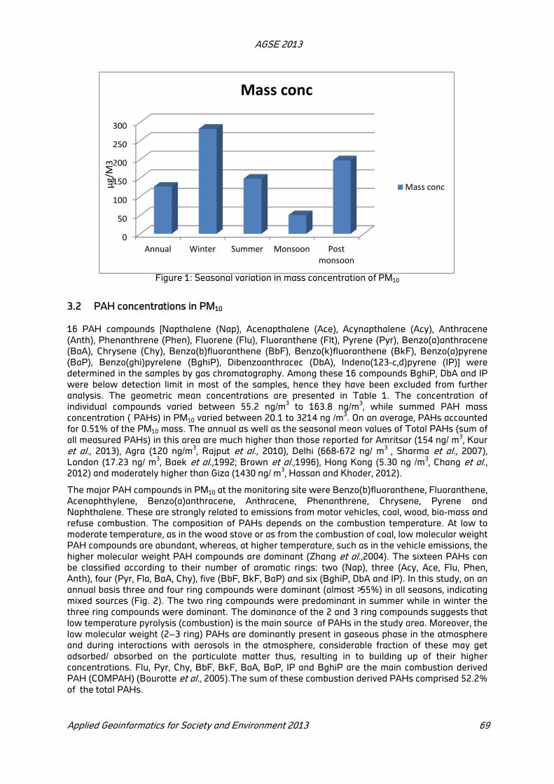
AGSE 2013


Figure 1: Seasonal variation in mass concentration of PM10

3.2 PAH concentrations in PM10

16 PAH compounds [Napthalene (Nap), Acenapthalene (Ace), Acynapthalene (Acy), Anthracene

(Anth), Phenanthrene (Phen), Fluorene (Flu), Fluoranthene (Flt), Pyrene (Pyr), Benzo(a)anthracene

(BaA), Chrysene (Chy), Benzo(b)fluoranthene (BbF), Benzo(k)fluoranthene (BkF), Benzo(a)pyrene

(BaP), Benzo(ghi)pyrelene (BghiP), Dibenzoanthracec (DbA), Indeno(123-c,d)pyrene (IP)] were

determined in the samples by gas chromatography. Among these 16 compounds BghiP, DbA and IP

were below detection limit in most of the samples, hence they have been excluded from further

analysis. The geometric mean concentrations are presented in Table 1. The concentration of

individual compounds varied between 55.2 ng/m3 to 163.8 ng/m

3, while summed PAH mass

concentration (�PAHs) in PM10 varied between 20.1 to 3214 ng /m3. On an average, PAHs accounted

for 0.51% of the PM10 mass. The annual as well as the seasonal mean values of Total PAHs (sum of

all measured PAHs) in this area are much higher than those reported for Amritsar (154 ng/ m3, Kaur

et al., 2013), Agra (120 ng/m3, Rajput et al., 2010), Delhi (668-672 ng/ m

3 , Sharma et al., 2007),

London (17.23 ng/ m3, Baek et al.,1992; Brown et al.,1996), Hong Kong (5.30 ng /m

3, Chang et al.,

2012) and moderately higher than Giza (1430 ng/ m3, Hassan and Khoder, 2012).

The major PAH compounds in PM10 at the monitoring site were Benzo(b)fluoranthene, Fluoranthene,

Acenaphthylene, Benzo(a)anthracene, Anthracene, Phenanthrene, Chrysene, Pyrene and

Naphthalene. These are strongly related to emissions from motor vehicles, coal, wood, bio-mass and

refuse combustion. The composition of PAHs depends on the combustion temperature. At low to

moderate temperature, as in the wood stove or as from the combustion of coal, low molecular weight

PAH compounds are abundant, whereas, at higher temperature, such as in the vehicle emissions, the

higher molecular weight PAH compounds are dominant (Zhang et al.,2004). The sixteen PAHs can

be classified according to their number of aromatic rings: two (Nap), three (Acy, Ace, Flu, Phen,

Anth), four (Pyr, Fla, BaA, Chy), five (BbF, BkF, BaP) and six (BghiP, DbA and IP). In this study, on an

annual basis three and four ring compounds were dominant (almost 5˃5%) in all seasons, indicating

mixed sources (Fig. 2). The two ring compounds were predominant in summer while in winter the

three ring compounds were dominant. The dominance of the 2 and 3 ring compounds suggests that

low temperature pyrolysis (combustion) is the main source of PAHs in the study area. Moreover, the

low molecular weight (2–3 ring) PAHs are dominantly present in gaseous phase in the atmosphere

and during interactions with aerosols in the atmosphere, considerable fraction of these may get

adsorbed/ absorbed on the particulate matter thus, resulting in to building up of their higher

concentrations. Flu, Pyr, Chy, BbF, BkF, BaA, BaP, IP and BghiP are the main combustion derived

PAH (COMPAH) (Bourotte et al., 2005).The sum of these combustion derived PAHs comprised 52.2%

of the total PAHs.

0

50

100

150

200

250

300

Annual Winter Summer Monsoon Postmonsoon

Mass conc

Mass concµg/M3

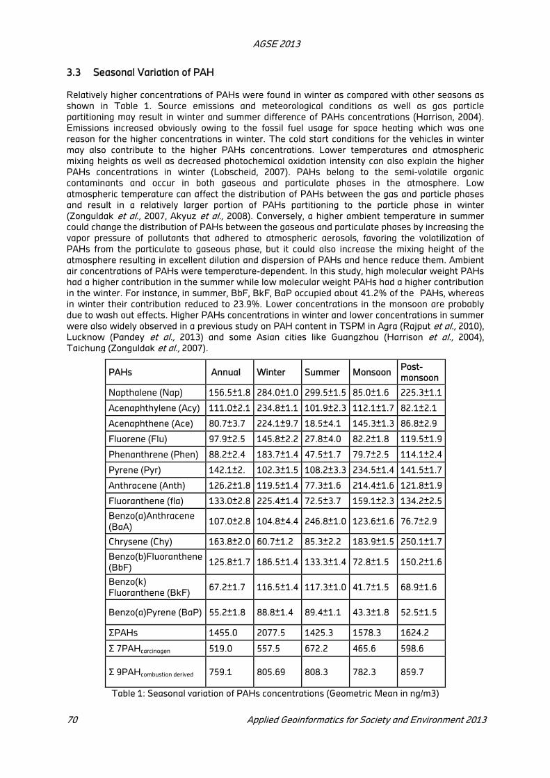
AGSE 2013


3.3 Seasonal Variation of PAH

Relatively higher concentrations of PAHs were found in winter as compared with other seasons as

shown in Table 1. Source emissions and meteorological conditions as well as gas particle

partitioning may result in winter and summer difference of PAHs concentrations (Harrison, 2004).

Emissions increased obviously owing to the fossil fuel usage for space heating which was one

reason for the higher concentrations in winter. The cold start conditions for the vehicles in winter

may also contribute to the higher PAHs concentrations. Lower temperatures and atmospheric

mixing heights as well as decreased photochemical oxidation intensity can also explain the higher

PAHs concentrations in winter (Lobscheid, 2007). PAHs belong to the semi-volatile organic

contaminants and occur in both gaseous and particulate phases in the atmosphere. Low

atmospheric temperature can affect the distribution of PAHs between the gas and particle phases

and result in a relatively larger portion of PAHs partitioning to the particle phase in winter

(Zonguldak et al., 2007, Akyuz et al., 2008). Conversely, a higher ambient temperature in summer

could change the distribution of PAHs between the gaseous and particulate phases by increasing the

vapor pressure of pollutants that adhered to atmospheric aerosols, favoring the volatilization of

PAHs from the particulate to gaseous phase, but it could also increase the mixing height of the

atmosphere resulting in excellent dilution and dispersion of PAHs and hence reduce them. Ambient

air concentrations of PAHs were temperature-dependent. In this study, high molecular weight PAHs

had a higher contribution in the summer while low molecular weight PAHs had a higher contribution

in the winter. For instance, in summer, BbF, BkF, BaP occupied about 41.2% of the �PAHs, whereas

in winter their contribution reduced to 23.9%. Lower concentrations in the monsoon are probably

due to wash out effects. Higher PAHs concentrations in winter and lower concentrations in summer

were also widely observed in a previous study on PAH content in TSPM in Agra (Rajput et al., 2010),

Lucknow (Pandey et al., 2013) and some Asian cities like Guangzhou (Harrison et al., 2004),

Taichung (Zonguldak et al., 2007).

PAHs Annual Winter Summer Monsoon Post-

monsoon

Napthalene (Nap) 156.5±1.8 284.0±1.0 299.5±1.5 85.0±1.6 225.3±1.1

Acenaphthylene (Acy) 111.0±2.1 234.8±1.1 101.9±2.3 112.1±1.7 82.1±2.1

Acenaphthene (Ace) 80.7±3.7 224.1±9.7 18.5±4.1 145.3±1.3 86.8±2.9

Fluorene (Flu) 97.9±2.5 145.8±2.2 27.8±4.0 82.2±1.8 119.5±1.9

Phenanthrene (Phen) 88.2±2.4 183.7±1.4 47.5±1.7 79.7±2.5 114.1±2.4

Pyrene (Pyr) 142.1±2. 102.3±1.5 108.2±3.3 234.5±1.4 141.5±1.7

Anthracene (Anth) 126.2±1.8 119.5±1.4 77.3±1.6 214.4±1.6 121.8±1.9

Fluoranthene (fla) 133.0±2.8 225.4±1.4 72.5±3.7 159.1±2.3 134.2±2.5

Benzo(a)Anthracene

(BaA) 107.0±2.8 104.8±4.4 246.8±1.0 123.6±1.6 76.7±2.9

Chrysene (Chy) 163.8±2.0 60.7±1.2 85.3±2.2 183.9±1.5 250.1±1.7

Benzo(b)Fluoranthene

(BbF) 125.8±1.7 186.5±1.4 133.3±1.4 72.8±1.5 150.2±1.6

Benzo(k)

Fluoranthene (BkF) 67.2±1.7 116.5±1.4 117.3±1.0 41.7±1.5 68.9±1.6

Benzo(a)Pyrene (BaP) 55.2±1.8 88.8±1.4 89.4±1.1 43.3±1.8 52.5±1.5

ƩPAHs 1455.0 2077.5 1425.3 1578.3 1624.2

Ʃ 7PAHcarcinogen 519.0 557.5 672.2 465.6 598.6

Ʃ 9PAHcombustion derived 759.1 805.69 808.3 782.3 859.7

Table 1: Seasonal variation of PAHs concentrations (Geometric Mean in ng/m3)

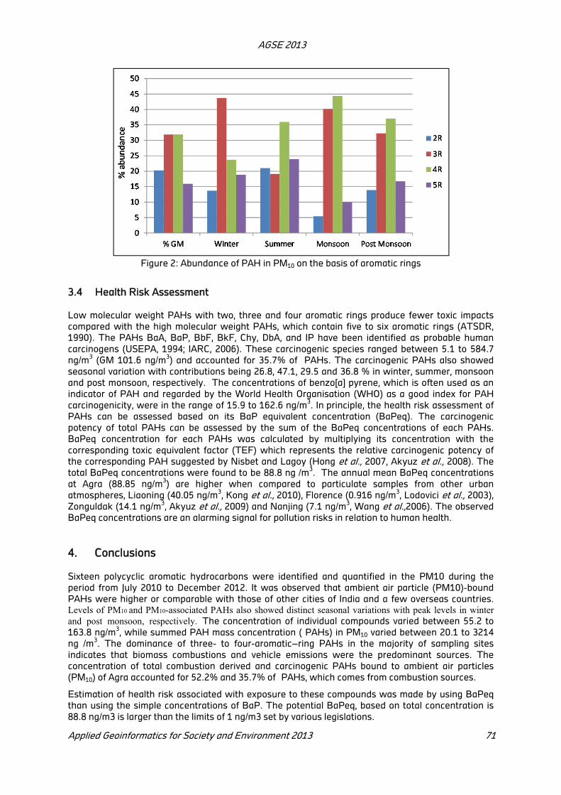
AGSE 2013


Figure 2: Abundance of PAH in PM10 on the basis of aromatic rings

3.4 Health Risk Assessment

Low molecular weight PAHs with two, three and four aromatic rings produce fewer toxic impacts

compared with the high molecular weight PAHs, which contain five to six aromatic rings (ATSDR,

1990). The PAHs BaA, BaP, BbF, BkF, Chy, DbA, and IP have been identified as probable human

carcinogens (USEPA, 1994; IARC, 2006). These carcinogenic species ranged between 5.1 to 584.7

ng/m3 (GM 101.6 ng/m

3) and accounted for 35.7% of �PAHs. The carcinogenic PAHs also showed

seasonal variation with contributions being 26.8, 47.1, 29.5 and 36.8 % in winter, summer, monsoon

and post monsoon, respectively. The concentrations of benzo[a] pyrene, which is often used as an

indicator of PAH and regarded by the World Health Organisation (WHO) as a good index for PAH

carcinogenicity, were in the range of 15.9 to 162.6 ng/m3. In principle, the health risk assessment of

PAHs can be assessed based on its BaP equivalent concentration (BaPeq). The carcinogenic

potency of total PAHs can be assessed by the sum of the BaPeq concentrations of each PAHs.

BaPeq concentration for each PAHs was calculated by multiplying its concentration with the

corresponding toxic equivalent factor (TEF) which represents the relative carcinogenic potency of

the corresponding PAH suggested by Nisbet and Lagoy (Hong et al., 2007, Akyuz et al., 2008). The

total BaPeq concentrations were found to be 88.8 ng /m3. The annual mean BaPeq concentrations

at Agra (88.85 ng/m3) are higher when compared to particulate samples from other urban

atmospheres, Liaoning (40.05 ng/m3, Kong et al., 2010), Florence (0.916 ng/m

3, Lodovici et al., 2003),

Zonguldak (14.1 ng/m3, Akyuz et al., 2009) and Nanjing (7.1 ng/m

3, Wang et al.,2006). The observed

BaPeq concentrations are an alarming signal for pollution risks in relation to human health.

4. Conclusions

Sixteen polycyclic aromatic hydrocarbons were identified and quantified in the PM10 during the

period from July 2010 to December 2012. It was observed that ambient air particle (PM10)-bound

PAHs were higher or comparable with those of other cities of India and a few overseas countries.

Levels of PM10 and PM10-associated PAHs also showed distinct seasonal variations with peak levels in winter and post monsoon, respectively. The concentration of individual compounds varied between 55.2 to

163.8 ng/m3, while summed PAH mass concentration (�PAHs) in PM10 varied between 20.1 to 3214

ng /m3. The dominance of three- to four-aromatic–ring PAHs in the majority of sampling sites

indicates that biomass combustions and vehicle emissions were the predominant sources. The

concentration of total combustion derived and carcinogenic PAHs bound to ambient air particles

(PM10) of Agra accounted for 52.2% and 35.7% of �PAHs, which comes from combustion sources.

Estimation of health risk associated with exposure to these compounds was made by using BaPeq

than using the simple concentrations of BaP. The potential BaPeq, based on total concentration is

88.8 ng/m3 is larger than the limits of 1 ng/m3 set by various legislations.

AGSE 2013


Acknowledgement

The authors are grateful to the Director, Dayalbagh Educational Institute, Dayalbagh, Agra; Head,

Department of Chemistry for facilities provided and Department of Science and Technology, DST

project No.: SR/S4/AS:282/ 07, New Delhi, for financial assistance. Mr. Jitendra Dubey acknowledges

UGC for Research fellowship for Meritorious students.

REFERENCES

Akyuz M., Cabuk H., 2008. Particle-associated polycyclic aromatic hydrocarbons in the atmospheric

environment of Zonguldak, Turkey. Science of the Total Environment. 405, 62–70.

Akyuz M., Cabuk H, 2009. Meteorological variations of PM2.5/PM10 concentrations and particle-

associated polycyclic aromatic hydrocarbons in the atmospheric environment of Zonguldak,

Turkey, J. Hazard. Mater. 170 ,13–21.

Agency for Toxic Substances and Disease Registry ,1990. Polynuclear aromatic hydrocarbon (PAH)

toxicity. Case studies in environmental health medicine #13. United States Department of Health

and Human Services.

Baek S.O., Goldstone M.E., Kirk P.W.W., Lester J.N., Perry R., 1992. Concentrations of particulate

and gaseous polycyclic aromatic hydrocarbons in London air following a reduction in the lead

content of petrol in the United Kingdom. Science of the Total Environment 111(2-3), 169-199.

Benner B.A., Gordon Jr. G.E., Wise S.A., 1989. Mobile sources of atmospheric polycyclic aromatic

hydrocarbons: a roadway tunnel study. Environmental Science and Technology 23, 1269– 1278.

Barale R., Giromini L., Ghelardini G., Scapoli C., 1991. Correlations between 15 PAHs and the

mutagenicity of the total PAH fraction in ambient air particles in La Spezia (Italy). Mutal. Res. 249,

227-241.

Bourotte C., Fortic M.C., Taniguchi S., Bıcego M.C., Lotufo P.A.,2005. A wintertime study of PAHs in

fine and coarse aerosols in Sao Paulo city, Brazil. Atmospheric Environment 39, 3799–3811.

Cheng Y, Ho KF, Wu WJ, Ho SSH, Lee SC, Huang Y et al .,2012. Real-time characterization of

particle-bound polycyclic aromatic hydrocarbons at a heavily trafficked roadside site. Aerosol Air

Qual Res 12:1181–1188.

Chow J., Chen L.A., Ho S.H., Koracin D., Zielinska B., Tang D., Perera F., Cao J. and Lee S.C.,

2006. Exposure to PM2.5 and PAHs from the Tong Liang, China Epidemiological Study. Journal of

Environmental Science and Health, Part A: Toxic/Hazardous Substances and Environmental

Engineering 41(4), 517-542.

Cincinelli A., Mandorlo S., Dickhut R.M., Lepri L., 2003. Particulate organic compounds in the

atmosphere surrounding an industrialised area of Prato (Italy). Atmospheric Environment 37 (22),

3125-3133.

Denissenko M.F., Pao A., Tang M., Pfeifer G.P., 1996. Preferential formation of benzo[a]pyrene

adducts at lung cancer mutational hotspots in P53. Science 18, 430-432.

Fang G.C. Chang K.F., Bai H.2004. Estimation of PAHs dry deposition and BaP toxic equivalency

factors (TEFs) study at urban, Industry park and rural sites in central Taiwan Taichung.

Chemosphere 55 (6),787-796.

Finlayson-Pitts B.J., Pitts Jr. J.N., 2000. Chemistry of the Upper and Lower Atmosphere. Theory,

Experiments and

Applications. Academic Press. 969 pp.

Fraser M. P., Cass G. R., Simoneit B. R. T., Rasmussen R. A., 1998. Air quality model evaluation data

for organics: 5. C6–C22 nonpolar and semipolar aromatic compounds. Environmental Science and

Technology 32, 1760–1770.

Guo H.L., Lu C.G., Yu Q. and Chen L.M., 2004. Pollution characteristics of polynuclear aromatic

Hydrocarbons on airborne particulate in Shanghai. Journal of Fudan University (Natural Science)

43, 1107-1112.

AGSE 2013


Harrison R.M., Jones A.M., Lawrence R. G., 2004. Major component composition of PM10 and PM2.5

from roadside and urban background sites. Atmospheric Environment 38, 4531–4538.

Hassan SK, Khoder MI .,2012. Gas-particle concentration, distribution, and health risk assessment of

polycyclic aromatic hydrocarbons at a traffic area of Giza, Egypt. Environ Monit Assess 184:3593–

3612.

He L.Y., Hu M., Huang X.F., Zhang Y.H., Tang X.Y., 2006. Seasonal pollution characteristics of

organic compounds in atmospheric fine particles in Beijing. Science of the Total Environment.

359(1-3), 167–176.

Hauser R., Godleski J., Hatch V., Christiani D.C., 2001. Ultrafine particles in human lung

macrophages. Arch. Environ. Health 56, 150-156.

Hong H.S., Yin H.L., Wang X. H., Ye C.X.,2007. Seasonal variation of PM10-bound PAHs in the

atmosphere of Xiamen, China, Atmo X.H.s. Res. 85, 429–441.

IARC, 1983. Polynuclear Aromatic Compounds. Part 1. Chemicals, Environmental and Experimental

Data. IARC Monographs on the Evaluation of the Carcinogenic Risk of Chemicals to Humans, vol.

32. WHO, International Agency for Research on Cancer. 155-161, 225-231.

Jenkins B.M., Jones A.D., Turn S.Q., Williams R.B., 1996. Particle concentrations, gas–particle

partitioning and species intercorrelations for polycyclic aromatic hydrocarbons (PAH) emitted

during biomass burning. Atmospheric Environment 30, 3825– 3835.

Kaur S., Senthilkumar K. ,Verma VK , Kumar B. , Kumar S., Katnoria J.K., Sharma CS, 2013.

Preliminary Analysis of Polycyclic Aromatic Hydrocarbons in Air Particles (PM10) in Amritsar,

India: Sources, Apportionment, and Possible Risk Implications to Humans. Arch Environ Contam

Toxicol DOI 10.1007/s00244-013-9912-6.

Kong S., Ding X., Bai Z., Han B., Chen L., Shi J., Zhiyong Li, 2010.A seasonal study of polycyclic

aromatic hydrocarbons in PM2.5 and PM2.5–10 in five typical cities of Liaoning Province, China.

Journal of Hazardous Materials 183, 70–80.

Li A., Schoonover T. M., Zou Q., Norlock F., Conroy L. M., Scheff P. A., Wadden R. A., 2005. Polycyclic

aromatic hydrocarbons in residential air of ten Chicago area homes: Concentrations and

influencing factors. Atmospheric Environment 39, 3491–3501.

Lobscheid A.B., McKone T. E., Vallero D.A., 2007. Exploring relationships between outdoor air

particulate associated polycyclic aromatic hydrocarbon and PM2.5: a case study of benzo(a)pyrene

in California metropolitan regions. Atmospheric Environment 41, 5659–5672.

Lodovici M., Venturini M., Marini E., Grechib D., Dolara P.,2003. Polycyclic aromatic hydrocarbons

air levels in Florence, Italy, and their correlation with other air pollutants, Chemosphere 50 , 377–

382.

Miguel A.H., Fernandez A.E., Jaques P.A., Froines J.R., Bill L., Grant P., Mayo R., Sioutas C. 2004.

Seasonal variation of the particle size distribution of polycyclic aromatic hydrocarbons and of

major aerosol species in Claremont California. Atmospheric Environment 38(20), 3241-3251.

Manti J., Chaloulakou A., Samara C., 2005. PM10-bound polycyclic aromatic hydrocarbons (PAHs) in

the Greater Area of Athens, Greece, Chemosphere 59, 593–604.

Marino f., Cecinato A., Siskos P., 2000). Nitro- PAH in PM in the atmosphere of Athenes,

Chemosphere 40,533-537.

NHAI (National Highway Authority of India), 2007. Data from Shipping, Ministry of Road Transport

and Highways, Delhi to Agra (KM 108-199.03) at Madhuvan, India, 2007.

Notor M., and Leskovsek Hermina L., 2000. Determination of polycyclic aromatic hydrocarbons in

marine sediments using anew ASE-SFE extraction technique. Fresnius Journal of Analytical

Chemistry 366, 846-850.

Pandey P., PatelD.K., Khan A.H., Barman S.C., Murthy R.C. and Kisku G.C.,2013.Temporal

distribution of fine particulates (PM2.5, PM10),potentially toxic metals, PAHs and Metal-bound

AGSE 2013


carcinogenic risk in the population of Lucknow City, India.Journal of Environmental Science and Health, Part A 48, 730–745.

Pope C.A., Burnett R.T., Thun M.I., Calle E E, Krwski D, Ito K, Thurston G D.2002. Lung cancer,

cardiopulmonary mortality, and long term exposure to fine particulate air pollution. JAMA, J.Am.

Med. Soc.287,1132-1141.

Rajput N., Lakhani A., (2010) Measurement of polycyclic aromatic hydrocarbons in an urban

atmosphere of Agra, India. Atmosfera 32,165–183.

Ravindra K., Sokhi R., Grieken R.V., 2008. Review: atmospheric polycyclic aromatic hydrocarbons:

source attribution, emission factors and regulation, Atmospheric Environment 42, 2895–2921.

Rogge W. F., Hildemann L. M., Mazurek M. A., Cass G. R., Simoneit B. R. T., 1993a. Sources of fine

organic aerosol. 5. Natural gas home applications. Environmental Science and Technology 27,

2736–2744.

Rogge W.F., Hildemann L.M., Mazurek M.A., Cass G.R., Simoneit B.R.T, 1993b. Sources of fine

organic aerosol: non-catalyst and catalyst-equipped automobiles and heavy duty diesel trucks.

Environmental Science and Technology 27, 636–651

RTO, 2008. Road Transport Office, Transport Nagar, Agra, India.

Sharma H, Jain V.K., Khan Z.H., 2007. Characterization and source identification of polycyclic

aromatic hydrocarbons (PAHs) in the urban environment of Delhi. Chemosphere 66, 302–310.

Sharma H., Jain V. K., Khan Z. H., 2007a. Identification of polycyclic aromatic hydrocarbons (PAHs) in

suspended particulate matter by synchronous fluorescence spectroscopic technique.

Spectrochimica Acta. A68, 43–49.

Sharma H., Jain V. K. Khan Z. H., 2007b. Characterization and source identification of polycyclic

aromatic hydrocarbons (PAHs) in the urban environment of Delhi. Chemosphere. 66, 302–310.

Schwartz J., Dockery D. W. and Nea, L. M., 1996. Is daily mortality associated specifically with fine

particles? Journal of the Air and Waste Management Association, 46, 927.

Schauer J.J., Rogge W.F., Hildemann L.M., Mazurek M.A., Cass G.R., Simoneit B.R.T., 1996. Source

apportionment of airborne particulate matter using organic compounds as tracers. Atmospheric

Environment 30, 3837– 3855.

Vasilakos C., Levia N., Maggos T., Hatzianestis J., Michopoulos J., Helmis C., 2007. Gas-particle

concentration and characterization of sources of PAHs in the atmosphere of a suburban area in

Athens, Greece. Journal of. Hazardous Materials 140, 45–51.

Van Dingenen R., Raes F., Putaud J.-P., 2004. A European aerosol phenomenology—1: physical

characteristics of particulate matter at kerbside, urban, rural and background sites in Europe.

Atmospheric Environment 38, 2561–2577.

Wang G.H.,Huang L.M., Zhao X., Niu H.Y., Dai Z.X., 2006. Aliphatic and polycyclic aromatic

hydrocarbons of atmospheric aerosols in five locations of Nanjing urban area, China, Atmos. Res.

81, 54–66.

Westerdahl, D., Fruin, S., Sax, T., Fine, P. M., and Sioutas, C., 2005. Mobile platform measurements of

ultrafine particles and associated pollutant concentrations on freeways and residential streets in

Los Angeles. Atmospheric Environment 39, 3597–3610

WHO, 2000. Air quality guidelines for Europe. In: European Series, second ed. WHO Regional

Publications, 91, 32-71.

Yang H.H., Chen C.M., 2004. Emission inventory and sources of polycyclic aromatic hydrocarbons in

the atmosphere at a suburban area in Taiwan. Chemosphere 56, 879– 887.

Zhang Y., Tao S., 2009. Global atmospheric emission inventory of polycyclic aromatic hydrocarbons

(PAHs) for 2004. Atmos. Environ. 43, 812–819.

Zonguldak Governorship, Environment and Forestry Management, Environment Situation Report,

Zonguldak, 2007.

AGSE 2013


USEPA. (1994) U.S. EPA toxicity data analysis software. U.S. Environmental Protection Agency.

Mohanraj V.J., Barnes T. J., Clive A. Prestidge C.A. (2010). Silica nanoparticle coated liposomes: A

new type of hybrid nanocapsule for proteins. International Journal of Pharmaceutics 392 (1–2)15 ,

285–293.

IARC(International Agency for Research on Cancer) (2006). IARC Monographs on the Evaluation of

Carcinogenic Risks to Humans. 88. Formaldehyde, 2-Butoxyethanol and 1-tert-Butoxypropan-2-

ol.

Spurný F., Bedná� J., Johansson L., Sätherberg A. 1996. Linear energy transfer spectra of

secondary particles in CR-39 track etch detectors Radiation Measurements 26 (5), 645–649

J.R. Brown, R.A. Field, M.E. Goldstone, J.N. Lester R. Perry 1996. Polycyclic aromatic hydrocarbons

in central London air during 1991 and 1992. Science of The Total Environment 177(1–3), 73–8.

Flood Water Management Process Using Plc & SCADA aAgragesh Ramani ,

bR.Balakrishnan,

cM.Mohammed Asif,

dS.Sankara Narayanan,

Department Electronics And Instrumentation, Sri Sairam Engineering College, West Tambram,

Chennai (India)

Email: [email protected],

[email protected],

[email protected],

[email protected]

KEY WORDS: PLC, SCADA, Agriculture

ABSTRACT

The prices of all vegetables have been increasing at GP rate. In times of a major flood, as occurred in Uttarkhand nothing much could be done, but the same when it comes to a flood occurring in an agricultural field, it can cause severe crop failure. This in turn causes the prices of all vegetable’s to sky rocket. So the question came to our mind, how can we prevent as minor setback as a stagnation of water from ruining our crops? This paper describes the unique idea to turn a common flood caused due to rain into a highly positive aspect both in terms of economy and other perspectives.

1. Introduction

The price of onion touches nearly to Rs.100 a kilo when unseasonal rains or sudden water-logging

comes at the onion crop-fields which destroies the production, necessitating import of this essential

commodity from Pakistan, China and other neighbouring countries. Such imports directly affect the

economy by increasing the current fiscal deficit leading to a further depreciation in Rupee value at

FOREX exchange. So the question raised here is that “Is there a way to maintain the stable

production even at times of unseasonal rains or in the times of droughts?” Well the answer to this is

the heart of our project. Our project aims to turn the tables on flood from heavy rains from a

disastrous hazard to an extensive source for a great profit for both the farmer as well as us common

people. A suction mechanism is placed in a set of agriculture fields. This suction mechanism sucks

out the excess water from the field in times of heavy rain. The suction mechanism has a two way

circuit to operate both in conventional energy source as well as non-conventional energy source; this

drastically lowers a farmer’s expense for a power source.

1.1 Current Scenario

In the current scenario as on 2013, is that crops face severe distortion in times on heavy rain, crops

like tomato, onion, paddy etc. This leads to an extensive price rise in their retail value.

A Relation between rain fall and Evaporation

The direct relation between rainfall and evaporation is what runs the natural process of water cycle.

In current scenario the rate of rainfall and evaporation has had a great difference; a graph surveyed

by CSSIR is represented as follows-

AGSE 2013


Figure 1: Rate of Rainfall Vs Rate of Evaporation

1.2 Effect of Water Stagnation

The difference in rate of rainfall and evaporation leads to a high extent of water stagnation leading

to failure of crops.

A Failure of tomato crop

Figure 2: ODR in drained and un-drained lands showing adverse effects even after removal of water

stagnation.

B Causes of Yield Decline due to Heavy Rainfall

Excessive rainfall, hailstorm and surface stagnation causes severe changes in the physio-chemical

environment of roots resulting in physical injury to the crops by hailstorm and consequently crop

lodging. Poor aeration resulting in depletion of oxygen and excess of carbon dioxide in the roots causing

plant-hypoxia. Post-stagnation ill effects due to sub optimal oxygen diffusion rate (ODR)

Figure 3: ODR in drained and un-drained lands showing adverse effects even after removal of water

stagnation

A CSSRI study revealed that ODR remained below the optimum level for an additional Period of 5.5 days after removal water stagnating in the cropland for 6 days (Fig. 3)

Leaching of essential plant nutrients resulting in lower uptake.

AGSE 2013


Decrease in redox potential resulting in reduced uptake of certain elements and Release of toxic elements in the root zone.

Thus the stagnation of water in field leads to an extensive reduction in both ODR of soil as well as

leads to crop failure.

2. Proposed Solution

Our proposed solution is to take out all the stagnated water in the field by placing suction pipes in

the corners of each field. These suction pipes are embedded with a UV level sensor which detects

the level of water present and upon reaching a certain level it starts the pump for sucking out all the

water, these pipes are also embedded with G1/2 water flow sensor to measure the flow of water to

pre-emptively counter any hazard related to flood. The suction pipes are welded together with an

underground pipe which is given pressure through suction pumps. The sucked out excess water

from the field is fed into an underground well or reservoir.The stored water can be used in times of

need through drip irrigation. This entire process is controlled by PLC and SCADA setup, being

mapped in by SCADA the entire landholdings and land mapping is possible. Thus a farmer is able to

know land holding and this will reduce activities like land grabbing.

2.1 Components

The components required for our entire process are as follows:

UV sensor

G1/2 Flow sensor

Pipes

PLC

Solar Panel

SCADA Software

Suction Pumps

2.2 Functions of Components

A. UV Sensor

The basic function of a UV sensor is to measure the level of rising water in the field. The UV rays

from the sensor are sent towards the water and due to the reflection of rays the sensor detects the

level of water .The output of sensor is fed to the SCADA system.

B. G1/2 Flow Sensor

The function of G1/2 flow sensor is to constantly measure the flow of water in an agricultural field.

This measure of flow can pre-emptively gives warning during river flood. The output of flow sensor

is constantly fed to SCADA system.

C. Pipes

Upright pipes are embedded with two valves, UV sensor and flow sensors are placed at four corners

of a field and in turn they are also welded together with underground piping which takes the flow of

suctioned water into an underground well.

D. PLC

A PLC is a Programmable Logic Device which is embedded using a program for controlling the valve

position in the upright suction pipes. The opening of valve is programmed at different percentages

with various values of level indication and flow indication. The control of pressure and the entire

process is controlled by using PLC.

E. SCADA Software

The master controlling and simulation occurs in SCADA software. The entire setup of suction

mechanism and piping connection is displayed in SCADA display. At times of warning, such as

AGSE 2013


increase in level of water in field beyond a certain fixed level there is an alert displayed in the system

and this informs the farmers of an intimate danger. The SCADA system then controls and gives

information to PLC to perform the desired tasks.

F. Suction Pumps

The suction pumps (Centrifugal) are connected to PLC. The PLC then performs the programmed

task by operating the suction pumps in times of excess water in a field. This mechanism also gives

out a flow of water for drip irrigation. Thus entire set up is operated successfully.

G. Basic block diagram

Figure 4: Basic block diagram of setup

3. Designs In Scada Simulation

For any project to be successful it must be first simulated and the result of this simulation gives a

boost to implement in real time. Here we have displayed a simulation model of a real time

implementation.

Figure 5: Basic Simulation Model

4. Advantages

Works on both convention source as well as non- conventional source of energies. Saves several times water than existing systems. Provides rain water storage for future use. Protects crops from losses due to water stagnation. Provides Drip irrigation in times of need. Cost effective. Has an extensive return in economic perspective

AGSE 2013


5. Disadvantages

Needs some skilled labor in control station. Initial investment high.

6. Limitations

In every prototype there exist a few limitations which have to be worked upon in order to overcome.

In our case the limitation is that if there is rain occurring continuously for long period of time the only

way out is to use a generator. We are working our way out of these limitations.

7. Conclusions

Paper we have also discussed a way to use this stagnant water in terms of drip irrigation for highly

effective save and use of water.

8. Future Scopes

The future scope of this paper is the entire SCADA systems warnings may be transmitted into a

mobile phone, and may also give way to automating entire farming.

REFERENCES

Zhou Hepin, Xu Xiaobo, JIAPAR Rouzi. Analysis on the Technical Test of Storing Runoff Irrigation[J].

Journal of Irrigation and Drainage, CSSIR survey an case study on water stagnation

Feng Junjie, Deng Zhong, Feng Yaozu, et al. Hydraulic Characteristics Experiment of Water-Storage

Irrigation Pipe Network[J]. Water Saving Irrigation, 2011(1):P32-36.

Austin N R, Prendergast J B. Use of Kinematic Wave Theory to Model Irrigation on Cracking Soil.

Irrigation sci, 1997, 18(1): P1-10.

(2013) The IEEE website. [Online]. Available: http://www.ieee.org/ IEEE Explore website.

http://ieeexplore.ieee.org/Xplore/home.jsp

Singh-Lubana P P, Narda N K. Model soil water dynamics under trickle emitters [J]. J. Agric. Engng.

Res. 2001,78(3):P217-232

Acknowledgments

We are great full to our Guide Ms S Subha and Ms L Priyadharshini , our Head of department and our

principal for their continues support and encouragement to bring out this project.

Exploring satellite-derived multi-year particulate data of Saudi Arabia

Y. A. Aina

a Department of Geography and Environmental Studies, University of Stellenbosch, Stellenbosch,

South Africa

b Department of Geomatics Engineering Technology, Yanbu Industrial College, Yanbu. Saudi Arabia.

[email protected]

KEY WORDS: Satellite data, Particulate matter, Air pollution, Environmental sustainability, Health

risks

ABSTRACT:

The impacts of concentrations of particulate matter on urban population cannot be overemphasized. Particulate matter exposes urban population to health risks such as respiratory and cardiovascular diseases. In order to improve the monitoring of particulate matter, efforts have been made to derive the data from satellite images through aerosol optical depth (AOD). One of such efforts is the global multi-year PM2.5 data (2001-2010) released by the Center for International Earth Science Information Network (CIESIN). This paper explores the data on Saudi Arabia to highlight the trend of PM2.5

concentration from 2001 to 2010. It also examines the changes in PM2.5 concentration in some urban population areas of Saudi Arabia. Concentrations in major cities like Riyadh, Dammam, Jeddah, Makkah, Madinah and Industrial cities of Yanbu and Jubail are analyzed. The health risks due to exposure by the populace are also examined by using the World Health Organization standard. The results show a trend of increasing concentration of PM2.5 in urban areas. There is a need to validate the satellite data with ground observations to improve the analysis.

1 Introduction

1.1 Background

The continuous monitoring of particulate matter (PM) is very vital to achieving sound environmental

health bearing in mind the adverse health effects of these particles. Exposure to fine particulate

matter (PM2.5) could cause health problems such as asthma, bronchitis, lung inflammation and other

respiratory and cardiovascular diseases. Thus, exposure of a population to particulates could result

in increases in hospital visits and mortality and thereby impacting on social and environmental

sustainability. Particulate matter monitoring is becoming more compelling due to the increasing

levels of emissions of the particles from both natural and human-induced sources. This is particularly

important for countries with high levels of PM concentrations. The issue of increasing levels of

emissions/concentrations of PM has attained international dimension as, for example, smokes from

forest fires in Indonesia impacted air quality in Malaysia and Singapore.

Conventional PM monitoring is based on ground measurements that cover limited area because

huge resources are needed to maintain wide network of measuring devices. Remote sensing is

currently being used to improve the effectiveness of particulates monitoring. Satellite imagery

supplements conventional methods of data gathering and provides opportunity for wide area of

coverage. Particulate matter is estimated from satellite images through the derivation of aerosol

optical depth (AOD). There are relationships between AOD and PM2.5 concentrations. The

relationships are explored to make quantitative estimates of PM2.5 from satellite images such as the

Moderate Resolution Imaging Spectroradiometer (MODIS). The particulate matter estimate derived

from MODIS can be calibrated by using ground measurements to compute the correlation between

satellite-derived data and field data. Such correlations are very useful in establishing satellite-based

continuous monitoring of particulate matter.

In an effort to establish a global continuous monitoring of PM2.5, the Center for International Earth

Science Information Network (CIESIN) produced a set of global annual average PM2.5 grids from

MODIS and Multi-angle Imaging SpectroRadiometer (MISR), 2001 to 2010 (Battelle Memorial

Institute and CIESIN, 2013). The data sets cover the world from Latitude 70°N to Latitude 60°S and

AGSE 2013


have spatial resolution of approximately 50km. Zell & Weber (2012) used the data to compute

country estimates of PM2.5 from 2002 to 2009. They computed 3-year moving averages for the

countries and used CIESIN’s Global Rural-Urban Mapping Project (GRUMP) 1km population grids to

compute population-weighted PM2.5 exposures. The results have been adopted by Emerson et al.

(2012) to assess air quality in the 2012 Environmental Performance Index Report.

The results indicated that air quality in Saudi Arabia is reducing as the population-weighted average

PM2.5 values increased from 13.70μg/m3 in 2002 to 15.11μg/m

3 in 2009. The results might be higher

than that if the average particulate values are weighted by recent population data. The GRUMP data

is either an estimate or old data that might not properly depict current population. Thus, this paper

uses more recent population data to explore the changes in PM2.5 concentrations and exposures

from 2002 to 2009. It also assesses changes in PM2.5 exposures in selected Saudi Arabian cities.

1.2 Related Work

The issues of concentrations of particulate matter have generated some research interests due to

the implications for sustainable development. Some studies (Wong et al., 1999; Hu, 2009; Son & Bell,

2013; Chiu & Whittaker, 2013; Franck et al., 2011; Franck et al., 2014) have highlighted the adverse

impacts of high level of particulate matter concentrations on health. The health effects depend on

the size of the particle and the physiology of the exposed population. Franck et al. (2011) suggested

that the smaller the particle size, the worse the health effect of exposure. However, Franck et al.

(2011) noted that the effects of coarse particles (PM10) last longer than the effects of finer particles.

A recent study by Son & Bell (2013) highlighted the impacts of sub-daily exposures and concluded

that exposures to PM10 were associated with cardiovascular mortality. They recommended 24 h

averaging time as a metric for health research and regulations. However, remote sensing

observations of PM are mainly suitable for monthly and yearly assessment. This is one of the

challenges highlighted by Hoff & Christopher (2009) as militating against using satellite

measurements as the sole system for PM monitoring.

Some of the studies on satellite measurement of PM values have focused on calibration of PM/AOD

relationship since the relationship varies across regions and seasons. Li et al. (2003), Gupta &

Christopher (2008), Kumar et al. (2008), Schaap et al. (2009), Natunen et al. (2010) and Lee et al.

(2011) have carried out calibration studies in Helsinki, China, India, The Netherlands and the United

States. Gupta et al. (2006) presented a global study of PM/AOD relationship by assessing the values

at 26 locations in Delhi, Hong Kong, New York, Switzerland and Sydney. They suggested that

aerosol vertical distribution data could refine their analysis. Vertical profiles were included in the

study by Van Donkelaar et al. (2010), in which they presented a continuous surface of global

estimates of fine particulate matter concentrations extended over 6 years (2001-2006). They noted

that 80% of world population resides in areas where the World Health Organization (WHO) Air

Quality Guide (AQG) of 10μg/m3

is exceeded. Also, 50% of eastern Asian population resides in areas

where the concentrations of fine particulate matter exceed WHO Air Quality Interim Target-3 of

35μg/m3

(Van Donkelaar et al., 2010). Battelle Memorial Institute and CIESIN (2013) improved the

work of Van Donkelaar et al. (2010) by using a faster algorithm for deriving PM2.5 data and extending

the years of analysis to 2010.

In the context of Saudi Arabia, most of the studies have focused on measuring the concentrations

and compositions of particulate matter in major cities (Aburas et al., 2011; Shaltout et al., 2013;

Munir et al., 2013; Rushdi et al., 2013) and assessing the impacts of major events such as Hajj

(pilgrimage) (Al-Jeelani, 2009; Othman et al., 2010; Habeebullah, 2013). For example, Rushdi et al.

(2013) showed that PM10 concentrations were higher in Riyadh than PM2.5 and the PM

concentrations were higher in 2007 than 2006. In a departure from the trend of using ground

measurements, Othman et al. (2010) developed a multispectral algorithm for generating PM10

concentrations from Landsat ETM+ imagery. The PM10 concentration values were computed for the

city of Makkah only. There is a need for more satellite-based study of particulates in Saudi Arabia

with a view to the improvement of particulate matter monitoring.

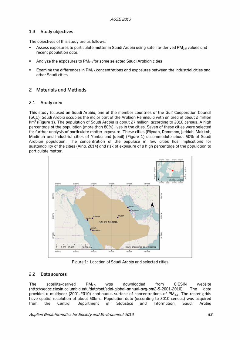
AGSE 2013


1.3 Study objectives

The objectives of this study are as follows:

Assess exposures to particulate matter in Saudi Arabia using satellite-derived PM2.5 values and

recent population data.

Analyze the exposures to PM2.5 for some selected Saudi Arabian cities

Examine the differences in PM2.5 concentrations and exposures between the industrial cities and

other Saudi cities.

2 Materials and Methods

2.1 Study area

This study focused on Saudi Arabia, one of the member countries of the Gulf Cooperation Council

(GCC). Saudi Arabia occupies the major part of the Arabian Peninsula with an area of about 2 million

km2

(Figure 1). The population of Saudi Arabia is about 27 million, according to 2010 census. A high

percentage of the population (more than 80%) lives in the cities. Seven of these cities were selected

for further analysis of particulate matter exposure. These cities (Riyadh, Dammam, Jeddah, Makkah,

Madinah and Industrial cities of Yanbu and Jubail) (Figure 1) accommodate about 50% of Saudi

Arabian population. The concentration of the populace in few cities has implications for

sustainability of the cities (Aina, 2014) and risk of exposure of a high percentage of the population to

particulate matter.

Figure 1: Location of Saudi Arabia and selected cities

2.2 Data sources

The satellite-derived PM2.5 was downloaded from CIESIN website

(http://sedac.ciesin.columbia.edu/data/set/sdei-global-annual-avg-pm2-5-2001-2010). The data

provides a multiyear (2001-2010) continuous surface of concentrations of PM2.5. The raster grids

have spatial resolution of about 50km. Population data (according to 2010 census) was acquired

from the Central Department of Statistics and Information, Saudi Arabia

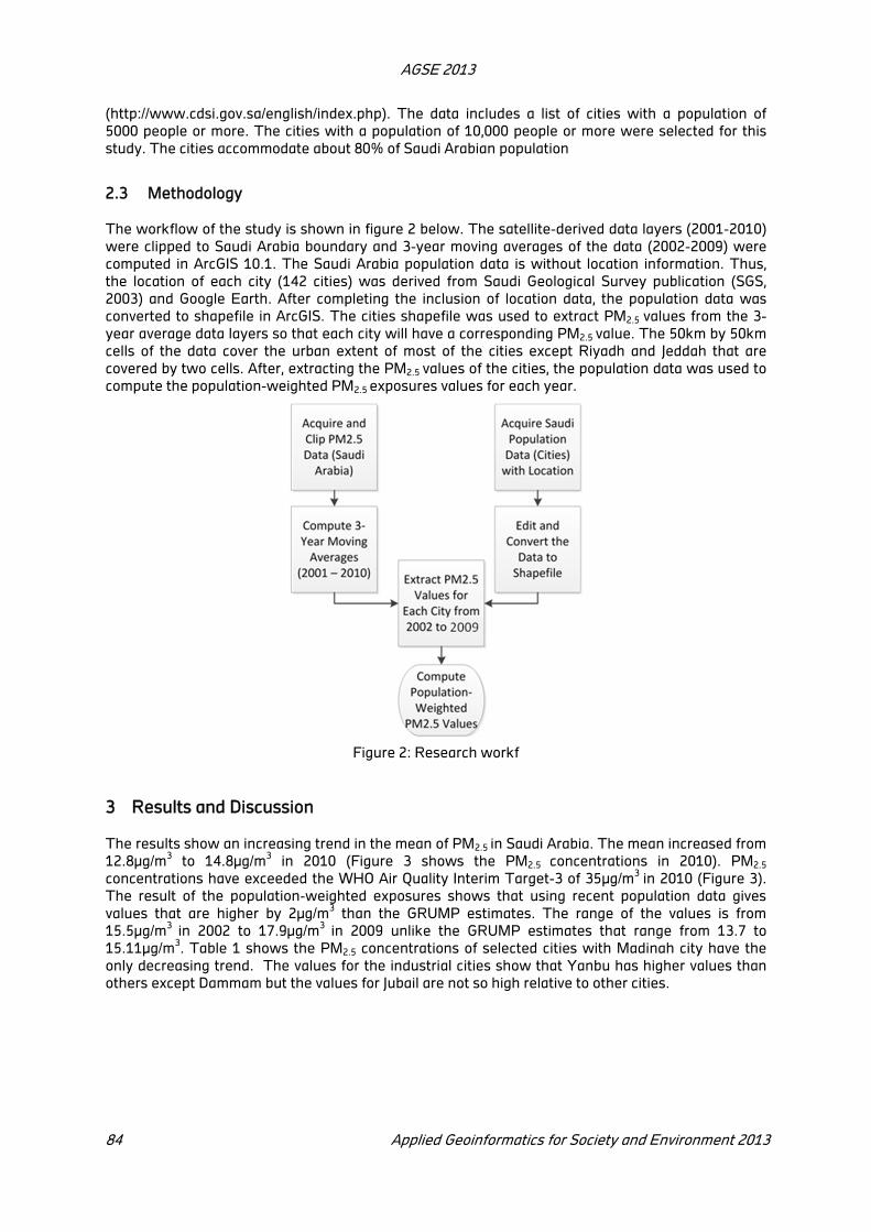
AGSE 2013


(http://www.cdsi.gov.sa/english/index.php). The data includes a list of cities with a population of

5000 people or more. The cities with a population of 10,000 people or more were selected for this

study. The cities accommodate about 80% of Saudi Arabian population

2.3 Methodology

The workflow of the study is shown in figure 2 below. The satellite-derived data layers (2001-2010)

were clipped to Saudi Arabia boundary and 3-year moving averages of the data (2002-2009) were

computed in ArcGIS 10.1. The Saudi Arabia population data is without location information. Thus,

the location of each city (142 cities) was derived from Saudi Geological Survey publication (SGS,

2003) and Google Earth. After completing the inclusion of location data, the population data was

converted to shapefile in ArcGIS. The cities shapefile was used to extract PM2.5 values from the 3-

year average data layers so that each city will have a corresponding PM2.5 value. The 50km by 50km

cells of the data cover the urban extent of most of the cities except Riyadh and Jeddah that are

covered by two cells. After, extracting the PM2.5 values of the cities, the population data was used to

compute the population-weighted PM2.5 exposures values for each year.

Figure 2: Research workf


The results show an increasing trend in the mean of PM2.5 in Saudi Arabia. The mean increased from

12.8μg/m3 to 14.8μg/m

3 in 2010 (Figure 3 shows the PM2.5 concentrations in 2010). PM2.5

concentrations have exceeded the WHO Air Quality Interim Target-3 of 35μg/m3

in 2010 (Figure 3).

The result of the population-weighted exposures shows that using recent population data gives

values that are higher by 2μg/m3 than the GRUMP estimates. The range of the values is from

15.5μg/m3

in 2002 to 17.9μg/m3

in 2009 unlike the GRUMP estimates that range from 13.7 to

15.11μg/m3. Table 1 shows the PM2.5 concentrations of selected cities with Madinah city have the

only decreasing trend. The values for the industrial cities show that Yanbu has higher values than

others except Dammam but the values for Jubail are not so high relative to other cities.

AGSE 2013


Figure 3: PM2.5 concentrations in 2010 (Green circles are selected 142 cities)

Cities Population

(2010)

2002 2003 2004 2005 2006 2007 2008 2009

Riyadh 5188286 12.4 13 13.3 13.8 13.9 14.8 15.2 15

Jeddah 3430697 17.6 17.2 21.1 20.3 20.6 17.4 18.8 19.4

Makkah 1534731 16.5 16.2 20.2 19.1 19.6 16.1 17.6 18.2

Madinah 1100093 12.8 12.4 11.6 11.7 11.4 11.1 10.1 10.8

Dammam 903312 27.8 29.6 33.4 30.3 32.5 36 40.4 40

Jubail* 142825 12.8 13.6 14.6 15.1 15 15.2 15.9 16.4

Yanbu* 73000 18.9 18.7 19.3 19.1 19.7 21.1 21.3 22.3

Table 1: PM2.5 concentrations (in μg/m3) in selected cities (*Industrial cities)

4 Conclusion

This study has used recent population data to reexamine the population-weighted PM2.5 values

computed for Saudi Arabia. It has noted that the values computed by using 2010 population data are

higher than the values computed by GRUMP data. It has also highlighted the variations in PM2.5

concentrations and exposures values of Saudi Arabian cities. The values for the industrial cities of

Jubail and Yanbu are mixed; Yanbu has relatively high values while the values for Jubail are relatively

low. There is a need for further studies to compute the PM2.5 values by using satellite data with

higher spatial resolution (similar to the one used by Wong et al. (2010)) and also calibrate satellite

values with ground measurements.

Acknowledgement

The author wishes to thank the Battelle Memorial Institute and the Center for International Earth

Science Information Network (CIESIN), Columbia University for providing the satellite-derived PM2.5

data that was used in carrying out this study.

AGSE 2013


REFERENCES

Aburas, H. M., Zytoon, M. A., & Abdulsalam, M. I., 2011. Atmospheric Lead in PM2.5 after Leaded

Gasoline Phase‐out in Jeddah City, Saudi Arabia. CLEAN–Soil, Air, Water, 39(8), pp. 711-719.

Al-Jeelani, H. A., 2009. Evaluation of air quality in the Holy Makkah during Hajj season 1425 H.

Journal of Applied Sciences Research, 5(1), pp. 115-121.

Aina, Y. A., 2014. Urban sustainability perspectives on changes in adaptation to Saudi Arabian desert

environment: the role of geospatial technologies. In: Environment, People and Development: Experiences from Desert Ecosystems, ed. Gaur, M. K., & Moharana, P. C., NIPA: New Delhi, India,

pp. 110-121.

Battelle Memorial Institute & Center for International Earth Science Information Network - CIESIN -

Columbia University, 2013. Global Annual Average PM2.5 Grids from MODIS and MISR Aerosol Optical Depth (AOD). Palisades, NY: NASA Socioeconomic Data and Applications Center (SEDAC).

http://sedac.ciesin.columbia.edu/data/set/sdei-global-annual-avg-pm2-5-2001-2010. Accessed 15

October 2013.

Chiu, H. H., & Whittaker, P., 2013. Venous Thromboembolism in an Industrial North American City:

Temporal Distribution and Association with Particulate Matter Air Pollution. PloS one, 8(7),

e68829.

Emerson, J. W., Hsu, A., Levy, M. A., de Sherbinin, A., Mara, V., Esty, D. C., & Jaiteh, M., 2012. 2012 Environmental Performance Index and Pilot Trend Environmental Performance Index. Yale Center

for Environmental Law and Policy, New Haven, USA.

Franck, U., Odeh, S., Wiedensohler, A., Wehner, B., & Herbarth, O. 2011. The effect of particle size on

cardiovascular disorders—The smaller the worse. Science of the Total Environment, 409(20), pp.

4217-4221.

Franck, U., Leitte, A. M., & Suppan, P., 2014. Multiple exposures to airborne pollutants and hospital

admissions due to diseases of the circulatory system in Santiago de Chile. Science of The Total Environment, 468, pp. 746-756.

Gupta, P., Christopher, S. A., Wang, J., Gehrig, R., Lee, Y. C., & Kumar, N., 2006. Satellite remote

sensing of particulate matter and air quality assessment over global cities. Atmospheric Environment, 40(30), pp. 5880-5892.

Gupta, P., & Christopher, S. A., 2008. Seven year particulate matter air quality assessment from

surface and satellite measurements. Atmospheric Chemistry and Physics, 8(12), pp. 3311-3324.

Habeebullah, T. M., 2013. An Analysis of Air Pollution in Makkah-a View Point of Source

Identification. EnvironmentAsia, 6(2), pp. 11-17.

Hoff, R. M., & Christopher, S. A., 2009. Remote sensing of particulate pollution from space: have we

reached the promised land?. Journal of the Air & Waste Management Association, 59(6), pp. 645-

675.

Hu, Z., 2009. Spatial analysis of MODIS aerosol optical depth, PM2.5, and chronic coronary heart

disease. International Journal of Health Geographics, 8(1), pp. 27.

Kumar, N., Chu, A., & Foster, A., 2008. Remote sensing of ambient particles in Delhi and its environs:

estimation and validation. International Journal of Remote Sensing, 29(12), pp. 3383-3405.

Lee, H. J., Liu, Y., Coull, B. A., Schwartz, J., & Koutrakis, P., 2011. A novel calibration approach of

MODIS AOD data to predict PM2.5 concentrations. Atmospheric Chemistry and Physics, 11(15), pp.

7991-8002.

Li, C., Mao, J., Lau, K. H. A., Chen, J. C., Yuan, Z., Liu, X., Zhu, A., & Liu, G. 2003. Characteristics of

distribution and seasonal variation of aerosol optical depth in eastern China with MODIS products.

Chinese Science Bulletin, 48(22), pp. 2488-2495.

Munir, S., Habeebullah, T. M., Seroji, A. R., Gabr, S. S., Mohammed, A. M., & Morsy, E. A., 2013.

Quantifying temporal trends of atmospheric pollutants in Makkah (1997–2012). Atmospheric Environment, 77, pp. 647-655.

AGSE 2013


Natunen, A., Arola, A., Mielonen, T., Huttunen, J., Komppula, M., & Lehtinen, K. E., 2010. A multi-year

comparison of PM2.5 and AOD for the Helsinki region. Boreal Environment Research, 15(6), pp.

544-552.

Othman, N., Jafri, M. Z. M., & San, L. H., 2010. Estimating Particulate Matter Concentration over Arid

Region Using Satellite Remote Sensing: A Case Study in Makkah, Saudi Arabia. Modern Applied Science, 4(11), pp. 131-142.

Rushdi, A. I., Al-Mutlaq, K. F., Al-Otaibi, M., El-Mubarak, A. H., & Simoneit, B. R., 2013. Air quality and

elemental enrichment factors of aerosol particulate matter in Riyadh City, Saudi Arabia. Arabian Journal of Geosciences, 6(2), pp. 585-599.

Saudi Geological Survey (SGS), 2003. An amateur guide to the land trips in Saudi Arabia (in Arabic).

Saudi Geological Survey, Riyadh, Saudi Arabia.

Schaap, M., Apituley, A., Timmermans, R. M. A., Koelemeijer, R. B. A., & Leeuw, G. D., 2009.

Exploring the relation between aerosol optical depth and PM2.5 at Cabauw, -the Netherlands.

Atmospheric Chemistry and Physics, 9(3), 909-925.

Shaltout, A. A., Boman, J., Dhaif-allah, R., & Shehadeh, Z. F., 2013. Elemental Composition of PM2.5

Particles Sampled in Industrial and Residential Areas of Taif, Saudi Arabia. Aerosol and Air Quality Research, 13, pp. 1356-1364.

Son, J. Y., & Bell, M. L., 2013. The relationships between short-term exposure to particulate matter

and mortality in Korea: impact of particulate matter exposure metrics for sub-daily exposures.

Environmental Research Letters, 8(1), 014015.

van Donkelaar, A., Martin, R. V., Brauer, M., Kahn, R., Levy, R., Verduzco, C., & Villeneuve, P. J., 2010.

Global estimates of ambient fine particulate matter concentrations from satellite-based aerosol

optical depth: development and application. Environmental Health Perspectives, 118(6), pp. 847-

855.

Wong, M. S., Nichol, J. E, Lee, K. H., & Li, Z. 2010. Retrieval of aerosol optical thickness using MODIS

500 × 500 m2, a study in Hong Kong and Pearl River Delta region. IEEE Transactions on

Geoscience and Remote Sensing, 46(8), pp. 3318-3327.

Wong, T. W., Lau, T. S., Yu, T. S., Neller, A., Wong, S. L., Tam, W., & Pang, S. W., 1999. Air pollution

and hospital admissions for respiratory and cardiovascular diseases in Hong Kong. Occupational and environmental medicine, 56(10), pp. 679-683.

Zell, E., & Weber, S., 2012. Country estimates of PM2.5 exposure. Battelle Memorial Institute,

Arlington, VA, USA.

Representing 'Social Catchments' of Mumbai's open spaces in Quantum

GIS

Aniket Umesh Navalkar

Academic Associate, Faculty Of Planning, Cept University

KEY WORDS: Catchment Area, Service Area Ratio, Convex Hull Algorithm, Quantum GIS, Dijkstra's

Algorithm, Network Analysis, Social Space, Henri Lefebvre.

ABSTRACT

Catchment Area’, popularly known as the service area ratio is a parameter used to understand the accessibility to an open space. The catchment is often attributed to the size, shape and other physical characteristics of the park. A model for the hierarchy of parks has evolved on the basis of catchments and other level of service standards. In this paper, I examine the real time catchments of two public parks in Mumbai which are located in different socio-economic neighborhoods by using participatory GIS methods.

Surveys and PRA (Participatory Rural Appraisal) techniques were administered for a period of one week at each park. Hence, data was captured on the routes taken by park visitors, time of journey, mode of transport, his / her satisfaction level with the park and the socio-economic background of the respondents among other things. Based on this survey, the routes from the origin to the destination were digitized in Quantum GIS 1.8 on a geo referenced raster image and the attribute table was populated accordingly for each sample.

Convex Hulls were used to aggregate source and destination points (in cases of visitors who used park as a transient stop) for representing catchment. Also, on a network topology, time was used as a cost metric in one sample. This was to examine if there is a substantial difference in the least cost based network route and the route actually taken by the park visitor. Further, routes were queried based on temporal factors, age and social group. The analysis resulted in variations in catchments across social and age groups along with temporal variations. These variations were compared across the two samples. The analysis revealed that the factors affecting catchment are dissimilar for the sample open spaces. Moreover, park catchments are not only a function of the spatial and physical characteristics of the park and the landuse, but are also heavily dependent on individual choices that members of various social groups make. Hence, ‘social catchments’ are complicated and the reasons for the same can be understood in the ‘social space’ framework of Henri Lefebvre.

1 Introduction

'Catchment Area' or ‘service area ratio’ is a parameter used to understand accessibility to open

spaces, restaurants, hospitals and other public places. The innovation of Geographic Information

Systems (GIS) gave great momentum to the shift in the urban planning paradigm from a model based

to a computer based approach (Batty, 1994). Ideas like catchment can now be graphically

represented in a vector form.

In the context of open spaces, the idea of catchment as a measure of accessibility first took shape

durig the critical evaluation of the London County Council (LCC) plan in 1954. The earlier standard of

‘an acre per thousand populations’ for assessing open spaces was abolished and the new standard

of ‘catchment area’ was brought in its place. A subsequent study in 1964 proved that the 'catchment

area' parameter is related to the size of the park itself. Parks of 0.81 – 1983 ha have catchment of up

to 0.4 km (0.25 miles); parks of 20.23 – 60.30 ha have catchment of up to 1.21 km (0.75 miles); parks

of over 60.70 hectares (150 acres) have a catchment of 3.22 – 8.05 km (2-5 miles) (Turner, 1992).

Thus the idea of Local Parks, District parks and metropolitan parks came in to being. However, this

idea had its share of criticism since it didn’t take in to account the actual movements of people to

these open spaces. In a paper presented at the 46th

conference of the International Society for Urban

and Regional Planners (ISOCARP) in 2010, Raquel Tardin and Lucia Maria Costa argue “... This

approach (of using catchment area) was highly criticized for being predominantly quantitative and

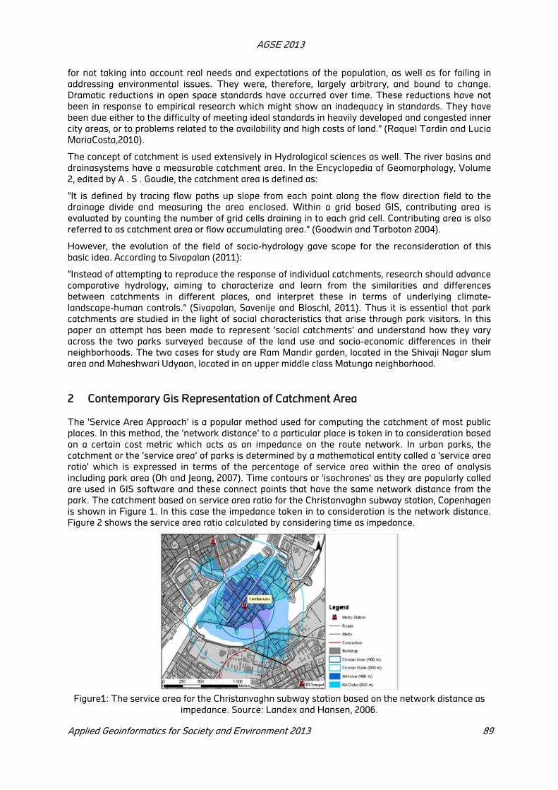
AGSE 2013


for not taking into account real needs and expectations of the population, as well as for failing in

addressing environmental issues. They were, therefore, largely arbitrary, and bound to change.

Dramatic reductions in open space standards have occurred over time. These reductions have not

been in response to empirical research which might show an inadequacy in standards. They have

been due either to the difficulty of meeting ideal standards in heavily developed and congested inner

city areas, or to problems related to the availability and high costs of land.” (Raquel Tardin and Lucia

MariaCosta,2010).

The concept of catchment is used extensively in Hydrological sciences as well. The river basins and

drainasystems have a measurable catchment area. In the Encyclopedia of Geomorphology, Volume

2, edited by A . S . Goudie, the catchment area is defined as:

“It is defined by tracing flow paths up slope from each point along the flow direction field to the

drainage divide and measuring the area enclosed. Within a grid based GIS, contributing area is

evaluated by counting the number of grid cells draining in to each grid cell. Contributing area is also

referred to as catchment area or flow accumulating area.” (Goodwin and Tarboton 2004).

However, the evolution of the field of socio-hydrology gave scope for the reconsideration of this

basic idea. According to Sivapalan (2011):

“Instead of attempting to reproduce the response of individual catchments, research should advance

comparative hydrology, aiming to characterize and learn from the similarities and differences

between catchments in different places, and interpret these in terms of underlying climate-

landscape-human controls.” (Sivapalan, Savenije and Bloschl, 2011). Thus it is essential that park

catchments are studied in the light of social characteristics that arise through park visitors. In this

paper an attempt has been made to represent ‘social catchments’ and understand how they vary

across the two parks surveyed because of the land use and socio-economic differences in their

neighborhoods. The two cases for study are Ram Mandir garden, located in the Shivaji Nagar slum

area and Maheshwari Udyaan, located in an upper middle class Matunga neighborhood.

2 Contemporary Gis Representation of Catchment Area

The ‘Service Area Approach’ is a popular method used for computing the catchment of most public

places. In this method, the ‘network distance’ to a particular place is taken in to consideration based

on a certain cost metric which acts as an impedance on the route network. In urban parks, the

catchment or the ‘service area’ of parks is determined by a mathematical entity called a 'service area

ratio' which is expressed in terms of the percentage of service area within the area of analysis

including park area (Oh and Jeong, 2007). Time contours or 'isochrones' as they are popularly called

are used in GIS software and these connect points that have the same network distance from the

park. The catchment based on service area ratio for the Christanvaghn subway station, Copenhagen

is shown in Figure 1. In this case the impedance taken in to consideration is the network distance.

Figure 2 shows the service area ratio calculated by considering time as impedance.

Figure1: The service area for the Christanvaghn subway station based on the network distance as

impedance. Source: Landex and Hansen, 2006.

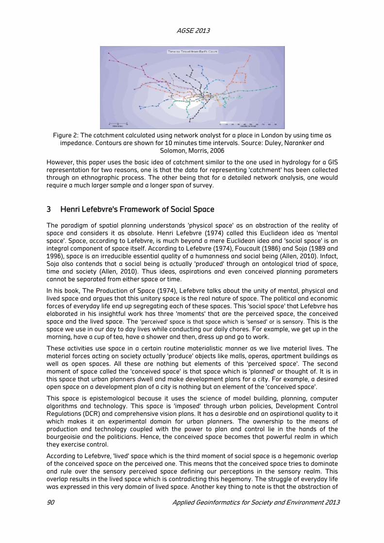
AGSE 2013


Figure 2: The catchment calculated using network analyst for a place in London by using time as

impedance. Contours are shown for 10 minutes time intervals. Source: Duley, Naranker and

Solomon, Morris, 2006

However, this paper uses the basic idea of catchment similar to the one used in hydrology for a GIS

representation for two reasons, one is that the data for representing 'catchment' has been collected

through an ethnographic process. The other being that for a detailed network analysis, one would

require a much larger sample and a longer span of survey.

3 Henri Lefebvre's Framework of Social Space

The paradigm of spatial planning understands 'physical space' as an abstraction of the reality of

space and considers it as absolute. Henri Lefebvre (1974) called this Euclidean idea as 'mental

space'. Space, according to Lefebvre, is much beyond a mere Euclidean idea and ‘social space' is an

integral component of space itself. According to Lefebvre (1974), Foucault (1986) and Soja (1989 and

1996), space is an irreducible essential quality of a humanness and social being (Allen, 2010). Infact,

Soja also contends that a social being is actually 'produced' through an ontological triad of space,

time and society (Allen, 2010). Thus ideas, aspirations and even conceived planning parameters

cannot be separated from either space or time.

In his book, The Production of Space (1974), Lefebvre talks about the unity of mental, physical and

lived space and argues that this unitary space is the real nature of space. The political and economic

forces of everyday life end up segregating each of these spaces. This 'social space' that Lefebvre has

elaborated in his insightful work has three 'moments' that are the perceived space, the conceived

space and the lived space. The 'perceived' space is that space which is 'sensed' or is sensory. This is the

space we use in our day to day lives while conducting our daily chores. For example, we get up in the

morning, have a cup of tea, have a shower and then, dress up and go to work.

These activities use space in a certain routine materialistic manner as we live material lives. The

material forces acting on society actually 'produce' objects like malls, operas, apartment buildings as

well as open spaces. All these are nothing but elements of this 'perceived space'. The second

moment of space called the 'conceived space' is that space which is 'planned' or thought of. It is in

this space that urban planners dwell and make development plans for a city. For example, a desired

open space on a development plan of a city is nothing but an element of the 'conceived space'.

This space is epistemological because it uses the science of model building, planning, computer

algorithms and technology. This space is 'imposed' through urban policies, Development Control

Regulations (DCR) and comprehensive vision plans. It has a desirable and an aspirational quality to it

which makes it an experimental domain for urban planners. The ownership to the means of

production and technology coupled with the power to plan and control lie in the hands of the

bourgeoisie and the politicians. Hence, the conceived space becomes that powerful realm in which

they exercise control.

According to Lefebvre, 'lived' space which is the third moment of social space is a hegemonic overlap

of the conceived space on the perceived one. This means that the conceived space tries to dominate

and rule over the sensory perceived space defining our perceptions in the sensory realm. This

overlap results in the lived space which is contradicting this hegemony. The struggle of everyday life

was expressed in this very domain of lived space. Another key thing to note is that the abstraction of

AGSE 2013


social space only seems separate from that of physical space. The two are intricately intertwined in

the ‘real’ space.

4 Research Methodology

The methodology involved two parts, one being data collection at the two samples through intercept

surveys and PRA techniques. The second part involved entering and representing this data in

Quantum GIS.

4.1 Data Collection

Data collection at each sample involved conducting individual and group interviews through intercept

surveys. Focus group discussions were also conducted with several social groups and this added as

an input to qualitative analysis. Besides this, casual interaction with old residents and visitors to the

open spaces turned in to an oral history session.

Two separate questionnaires were made for the individual and group interviews. In Shivaji Nagar the

approximate sample size was 44 for individual and group interviews combined. Both the

questionnaires had open ended questions. For Maheswari Udyaan, the approximate sample size was

74. A part of the questionnaire was participatory in nature. In this part, individuals and groups were

asked to rate the park on various parameters which include amenities, greenery, maintenance and

accessibility on a scale of 1 to 10.

This part also had open ended questions that probed which features of the park visitors liked the

most and their dissatisfaction (and the reasons) with certain aspects of the park. It also captured

information on the availability of parks in the localities of the residents and their satisfaction with the

same. The major difference between the group interviews and the individual interviews was that the

former were administered as a group and had more open ended questions.

In the questionnaires (individual and group), the starting point and the address of each member was

noted down along with the modal split of the journey, the route taken to reach the park and the

travel time. All the attribute data of the individual and group questionnaires was an input to the GIS

attribute table corresponding to the routes traced.

4.2 Use of Quantum GIS 1.8

Quantum GIS 1.8 'Lisboa' was used for digitizing routes on open map layers and for populating the

attribute table for each sample. This software allows for the integration of network analysis, vector

analysis and statistical analysis through plug-ins. The 'Convex Hull Analysis Tool' based on the

Convex Hull algorithm, was used for aggregating points of origin and determining the 'catchment

area' in its very basic form. The routes, road network and land use area polygons were digitized on

the open layers plug in which was rendered in WGS84, ESPG: 4326. The layers were then

reprojected in Universal Transverse Mercator (UTM), with WGS 84 as the spheroid of reference for

zone 43.

Catchments were represented with the help of vector analysis tools like the convex hull tool. The

variations and complexities in catchments were captured by using SQL like commands to filter routes

against certain queries. Thus, the temporal, age and social group variations in catchments were

obtained. For error correction on a network topology, however, Arc GIS 10.0 was used since it

enabled line by line removal of dangles and overlaps on the digitized road network. The corrected

road layers were then imported back in to Quantum GIS 1.8 in order to do a network analysis and

thus the shortest available path from each origin to the destination was calculated based on time as

the cost. This query tool is based on Dijkstra's algorithm. The network analysis was done using the

'road graph plugin' in QGIS for the Shivaji Nagar sample in order to compare the least cost paths to

the paths actually taken.

AGSE 2013


5 Complications In the Catchment of Shivaji Nagar Ground

5.1 Land use around the Shivaji Nagar ground

Shivaji Nagar lies in the M East Ward and is a slum area of Mumbai. This open space is located

between 72.918314 degrees E and 72.920117 degrees E in longitude and 19.061509 degrees N and

19.062863 degrees N in latitude (Source: Google Maps ). Within the premises of this open space,

there is Municipal School and a Gym, the locations of which are marked in the Figure 3. An important

east west link road called the 'Ghatkopar Mankhurd Link Road' cuts through this area and passes

right adjacent to the open space (see appendices for detailed landuse maps). This road is 200 ft wide

and to the south of the road lie the slums of Gautam Nagar. The hind part of the ground is

exclusively a squatter settlement. A temple called the 'Ram Mandir' temple is located to the north of

the ground as shown in the google maps image 3.

Figure 3: Google Maps satellite image of the ram mandir ground in Shivaji Nagar, Mumbai.

The land use in these plots is very mixed with toilets, shops, tea stalls, all jumbled up along with the

residential units in congested clusters. The Deonar Dumping Ground, to the far north of this ground,

assimilates the entire city's garbage. There are various slum areas to the west and the north of the

park which include Baingan Wadi, Rafique Nagar, Sanjay nagar, Chickalwadi, Indira Nagar etc. The

land in this notified slum is divided in to various numbered plots.

The social groups from the slum neighbourhood of the park predominate the park visitors. There are

a very few exceptions (say one in a hundred visitors) who live in other parts of town and travel to

Shivaji Nagar because they own some business in the locality and subsequently end up visiting this

space after work.

The gym within the boundaries of the park is very active and pretty well equipped despite of being in

a slum neighborhood. The gym is open from 6:00 am to 11:00 am in the mornings and from 4 pm to

10 pm in the evenings on all days. A BEST (BrihanMumbai Electric Supply and Transport limited) bus

stop is right outside the park and hence there's connectivity to Mankhurd Railway station (harbour

railway line) and to the Sion Trombay Link road, another important north south link road. Both,

Mankhurd and Govandi railway stations on the harbour line are at a walking distance of 10 to 15

minutes for a healthy man. These can also be seen in the GIS maps. All in all, the socio-economic

AGSE 2013


condition of the people living in the neighbourhood of the ground is very low and the administrative

ward in which this ground lies is considered to be the poorest ward in the city.

The condition of the ground is very shoddy. There are stones lying all over the ground, the facilities

that were built for the children are in a dilapidated condition and are unusable. Besides this, the

ground is used for defecation by the slum dwellers, especially children. This ground is also a hub of

illegal activities like drug and alcohol abuse which happen after sunset. The lack of street lamps in

the ground gives it an eerie feeling in the night and that is why most visitors avoid coming to this

ground after sunset. This open space is predominantly used as a play ground for cricket lovers of the

slum. There are also other visitors who come there to spend the evenings to play cards, take a walk

or to watch groups play cricket.

5.2 Effect of Neighborhood and Landuse on Catchment

The ethnographic and GIS research analysis consolidated the fact that the neighborhood has a

depressing effect on the catchment of the ground. The analysis of the results obtained from PRA

exercises, interviews and focus group discussions unanimously pointed to the fact that the visitors to

the ground at any given time of the day are essentially from the slum areas behind the park. The

ground is predominated by cricket playing groups, gym users, street vendors ('feriwalas') and anti

social elements (drug addicts, drunkards and gamblers). Almost all the people who were interviewed

or had participated in FGDs hailed from the neighboring slum pockets.

The catchments obtained by filtering the routes of gym users v/s those of non gym users and

aggregating them using the convex hull algorithm consolidated the above mentioned fact. Hence,

adding amenities like a local well equipped gym doesn't necessarily increase park catchment if the

park is located in a socio-economically poor neighborhood. This is illustrated in Figure 4.

Figure 4: Similar catchments for individual park users (right) and gym users (left) in the park.

5.3 Catchment as a measure of accessibility

A corollary to the insight that neighbourhood socio-economic factors depress the catchment of

Shivaji Nagar is: Catchment may not necessarily be a very good measure of accessibility for socio-

economically deprived neighborhoods. Another observation that confirms this is that the extent of

catchment area to the south of the Ghatkopar – Mankhurd link road is very minimal. The road

actually ends up acting as a barrier, since it is very difficult to negotiate it by foot due to the constant

flow of traffic. Hence, very few travelers from Gautam Nagar and the area around the Deonar

abattoir (south of the ground) come to the open space. This is illustrated in Figure 4.

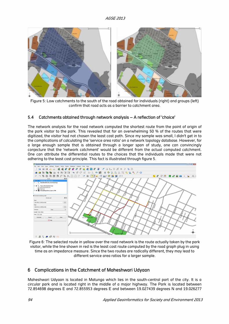
AGSE 2013


Figure 5: Low catchments to the south of the road obtained for individuals (right) and groups (left)

confirm that road acts as a barrier to catchment area.

5.4 Catchments obtained through network analysis – A reflection of 'choice'

The network analysis for the road network computed the shortest route from the point of origin of

the park visitor to the park. This revealed that for an overwhelming 50 % of the routes that were

digitized, the visitor had not chosen the least cost path. Since my sample was small, I didn't get in to

the complications of calculating the 'service area ratio' on a network topology database. However, for

a large enough sample that is obtained through a longer span of study, one can convincingly

conjecture that the 'network catchment' would be different from the actual computed catchment.

One can attribute the differential routes to the choices that the individuals made that were not

adhering to the least cost principle. This fact is illustrated through figure 5.

Figure 6: The selected route in yellow over the road network is the route actually taken by the park

visitor, while the line shown in red is the least cost route computed by the road graph plug in using

time as an impedance measure. Since the two routes are radically different, they may lead to

different service area ratios for a larger sample.

6 Complications in the Catchment of Maheshwari Udyaan

Maheshwari Udyaan is located in Matunga which lies in the south-central part of the city. It is a

circular park and is located right in the middle of a major highway. The Park is located between

72.854698 degrees E and 72.855953 degrees E and between 19.027439 degrees N and 19.026277

AGSE 2013


degrees N (Source: Google Maps).Although much smaller than the park in Shivaji Nagar,

Maheshwari Udyaan has many more amenities within its 5 acre area. The neighborhood around the

park is an upper middle class locality; however, a few kilometres away from the park, there are a

couple of socio-economically challenged neighbourhoods. These are Labour Camp, Matunga to the

North West which leads to Dharavi, the largest slum in Mumbai, Sion Koliwada to the North West

and the slums of Wadala and Antop Hill to the east. The land use around the park is mixed and is

characterized by residential buildings that have been existing since many decades. There are also

many colleges and educational institutes of repute in the area. Notable among these are engineering

institutes like the Veer Jeejamata Technology Institue (VJTI), Institute of Chemical Technology (ICT),

Khalsa College and schools like Don Bosco High School, Matunga. Because of the presence of these

institutes and up-scale neighbourhoods like the Parsi Colony, there are many gardens in the area.

The Five Gardens, the Nappu Garden and the Samosa Garden are the well known gardens of

Matunga.

Another unique feature of this udyaan is its high accessibility by public transport. The Ambedkar

road is an important North – South link and it connects suburbs like Chembur and Vashi (Navi

Mumbai) to the main city. There are three stations in the vicinity of this park. One is the Matunga

station on the central railway line to the west of the park. The other is the Wadala station on the

harbour line to the east of the park. The King Circle station which is on a connecting line between

the harbour line and the western line is located to the North of the park. All the three stations are

approximately equidistant from the park and it would take ten minutes for a healthy person to walk

to these stations from the udyaan.

There are approach roads to this udyaan and they connect it to Matunga railway station (E) to the

west, Wadala Station to the east and also to Five Gardens, which are famous open spaces

approximately one kilometre to the South East. The road around the park is a particularly dangerous

one since there is a continuous flow of traffic on it. A visitor wanting to access the park will have to

cross the road to reach the entrance of the park. Although there is a signal system on the Ambedkar

road junction, near the entrance of the park, there's no signal and this makes crossing very

dangerous. Also because of the steep curvature of the road, an incoming vehicle is not easily visible.

There are two entrances to the park, on either sides of the park, aligned with the main road, i.e. Dr

Ambedkar Road.

The over all condition and ambiance of the park is very nice. The lawns are lush green and regularly

mowed, there is a walking track that cuts through the circular garden and also forms the inner

circumference of the garden. The children's corner has many playing facilities like sea-saws, swings,

slides and an area with sand for scoping and sculpting. There's a drinking water fountain at one end

of the ground. All in all, the ground has extremely good facilities for the public and this attracts

people from all walks of life and from different social groups.

6.1 Huge Catchment of Maheshwari Udyaan – High accessibility by public transport and

land use considerations

Accessibility has two meanings in the context being discussed. One is the ease of access to an open

space in terms of negotiating crowded streets, zebra crossings, signals and traffic. The other is the

ease of access due to the connectivity and centralized location of the open space. Maheshwari

Udyaan, as mentioned earlier, has excellent connectivity due to its proximity to interconnected train

routes as well as bus stops. On the other hand, the road around the park is very difficult to negotiate,

especially for the children and the elderly. Despite this, it was observed that the park is very popular

among these two social groups. The excellent connectivity by public transport makes this park a

stop over point for many commuters who are traveling to the suburbs after work. Also, the presences

of educational institutions in this area form their own respective catchments which in turn influence

the park catchment.

The park's catchment was obtained in GIS by filtering routes of those visitors who had used public

transport and it was compared to that of visitors who had travelled using either private transport or

had come walking. The results were quite contrasting, as in, the visitors who had travelled using

public transport came from far and wide, while those who had come walking and by using private

transport hailed from the nearby neighborhoods. Thus, there were these two separate catchments

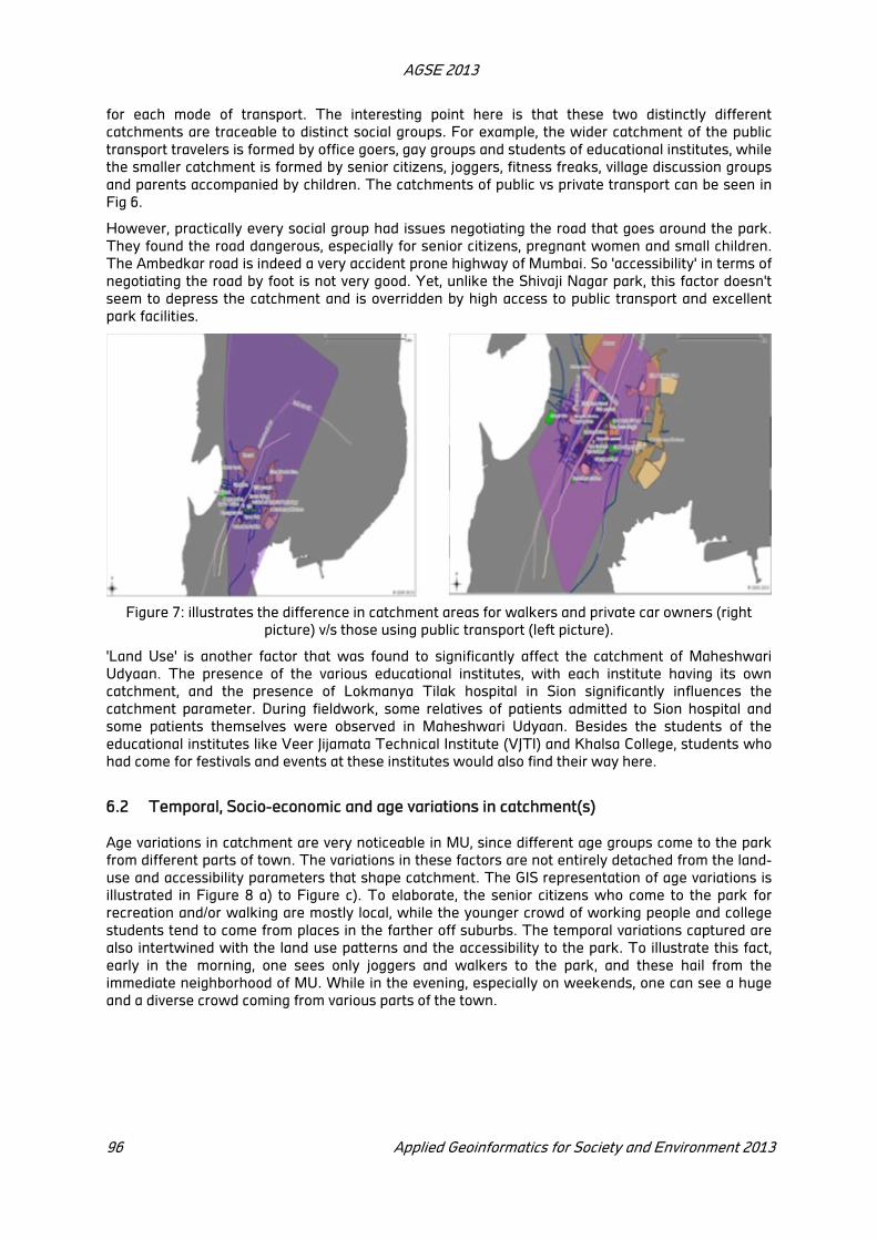
AGSE 2013


for each mode of transport. The interesting point here is that these two distinctly different

catchments are traceable to distinct social groups. For example, the wider catchment of the public

transport travelers is formed by office goers, gay groups and students of educational institutes, while

the smaller catchment is formed by senior citizens, joggers, fitness freaks, village discussion groups

and parents accompanied by children. The catchments of public vs private transport can be seen in

Fig 6.

However, practically every social group had issues negotiating the road that goes around the park.

They found the road dangerous, especially for senior citizens, pregnant women and small children.

The Ambedkar road is indeed a very accident prone highway of Mumbai. So 'accessibility' in terms of

negotiating the road by foot is not very good. Yet, unlike the Shivaji Nagar park, this factor doesn't

seem to depress the catchment and is overridden by high access to public transport and excellent

park facilities.

Figure 7: illustrates the difference in catchment areas for walkers and private car owners (right

picture) v/s those using public transport (left picture).

'Land Use' is another factor that was found to significantly affect the catchment of Maheshwari

Udyaan. The presence of the various educational institutes, with each institute having its own

catchment, and the presence of Lokmanya Tilak hospital in Sion significantly influences the

catchment parameter. During fieldwork, some relatives of patients admitted to Sion hospital and

some patients themselves were observed in Maheshwari Udyaan. Besides the students of the

educational institutes like Veer Jijamata Technical Institute (VJTI) and Khalsa College, students who

had come for festivals and events at these institutes would also find their way here.

6.2 Temporal, Socio-economic and age variations in catchment(s)

Age variations in catchment are very noticeable in MU, since different age groups come to the park

from different parts of town. The variations in these factors are not entirely detached from the land-

use and accessibility parameters that shape catchment. The GIS representation of age variations is

illustrated in Figure 8 a) to Figure c). To elaborate, the senior citizens who come to the park for

recreation and/or walking are mostly local, while the younger crowd of working people and college

students tend to come from places in the farther off suburbs. The temporal variations captured are

also intertwined with the land use patterns and the accessibility to the park. To illustrate this fact,

early in the morning, one sees only joggers and walkers to the park, and these hail from the

immediate neighborhood of MU. While in the evening, especially on weekends, one can see a huge

and a diverse crowd coming from various parts of the town.

AGSE 2013


Figure 8 a(left) represents the catchment obtained for age group less than 35 years, Figure 8 b

(centre) represents the catchment obtained for age group between 35 to 50 and Figure 8 c (right)

represents the catchment for age group greater than 50 years which includes mainly senior citizens.

Interviews and FGDs with various social groups brought about the temporal aspect of catchment

interconnected with the social variations in park. For example, the gay groups and village groups

meet up at the park on only on weekends. Individuals and couples who bring children along are

found in the evenings, mainly on weekdays. The travellers who use the park as a stop over point en

route to their home or place of work are generally seen on weekdays only. Thus, the temporal

variations in catchment can be traced to the distinct social groups that visit the parks. These

temporal variations are clearly visible in Fig 1.6-3 a), which is a weekend and fig 1.6-3 b) which is a

regular weekday.

Figure 9: Temporal variations in catchment between weekdays and weekends.

7 Conclusion

Through the catchment analysis of both the samples, it is evident that the degree by which land use

and accessibility shape catchment varies and isn't the same for all neighborhoods. For example, in

Maheshwari Udyaan, the difficulty of access created by the road around the park and the highway

doesn't seem to deter visitors coming from far and wide. However, in Shivaji Nagar, the

transportation facilities of rail (Govandi and Mankhurd stations) do not seem to contribute

significantly to its catchment. Also, the Ghatkopar – Mankhurd link road as shown in figure 1.5-3

acts as a 'depressor' of catchment.

AGSE 2013


Social diversity of the people in the park is normally indicative of the catchment of the park.

Maheshwari Udyaan has very large diversity of social groups visiting it as compared those visiting

Shivaji Nagar park. Correspondingly, the catchment of Maheshwari Udyaan is also much wider than

that of Shivaji Nagar park. The socioeconomic status of Shivaji Nagar park visitors is very constant

although the religious and ethnic group they belong to may differ. The analysis of individual routes in

Shivaji Nagar also point to the fact that park visitors may not have a proclivity to take the least cost

path. Thus catchments are more 'social' in nature and can be also formed by the choices that people

make to come to the park.

The triad of Lefebvre's 'social space' as discussed in section 1.3 can be used as a theoretical

framework to understand the complications that were observed in the representations of 'catchment

area'. In 'social space', the catchment area parameter is located in the 'conceived space'. While in

'perceived space', the realities are different for each social group visiting the parks. The experiences

of people that were collected through ethnographic methods and intercept surveys fall within this

'perceived space'. In this space, the socio-economic and spatial realities of each of the neighborhoods

of the two parks are different. Also, the parameters that shape accessibility to a park and the

physical condition of each park are different. Thus the sensory realm of the visitors of each park is

different from the other. Even within the same park, different social groups have different perceived

experiences. Therefore, because of the nature of the perceived space, catchment is difficult to

conceive as a tangible parameter.

Catchment' in the form of a measurable and a representational parameter in the conceived space is

unable to come to terms with the realities of the perceived space. The attempt to use a parameter

which renders definite results gets foiled because of the complexity and diversity of this perceived

space. The choices that people make to come to the park can be projected in the 'lived space' of the

social space triad. These choices actually end up creating a 'catchment area' which has a fragmented

representation and which illustrates their 'struggle'. The epistemological conceived space tries to

code the perceived one in an urban environment which leads people to making these choices. For

example, the lack of open spaces in certain socio-economically challenged neighbourhoods like

Dharavi and Antop hill compels people to make a choice of travelling to Maheshwari Udyaan so that

they can access the amenities that their children require.

Similarly, a traveller from work on his way home makes a choice to spend some time in Maheshwari

udyaan because it lies right in his or her way. In Shivaji Nagar, the slum population around the park

is faced with a gross lack of choices and hence, they end up going to the Ram Mandir open space to

spend time or to play cricket. In the same breath, the residents of Gautam nagar slum to the south of

the park find it difficult to negotiate the road and therefore make a choice of not visiting the ground.

This 'lived space' is that space which eventually ends up contradicting the conceived space and due

to this, the parameter of catchment loses uniformity and consistency. Therefore, understanding

these complications in the light of 'social space' as conceptualized by Lefebvre satisfy the reasons

why complexities were observed in catchment area parameter.

The GIS and the geometric representation of catchment area have a valid place in understanding the

accessibility to an open space and the performance of neighborhood parks and gardens. The

observed complications merely point at the limitations in the purely spatial ideas which do not take in

to consideration the reality of 'unitary space'. The complications have arisen because ideas on

catchment which were developed in 'mental space' consider social space as an entity disparate from

the physical one. If this parameter has to render itself as a useful tool in planning and assessing

open spaces, neighborhood parks and gardens, it needs to be re conceptualized and redefined in the

paradigm of 'unitary space'.

AGSE 2013


APPENDICES

APPENDIX 1 -1 BASIC LANDS USE OF SHIVAJI NAGAR GROUND AND ITS NEIGHBOURHOOD

APPENDIX 1-2 BASIC LAND USE / LAND COVER FEATURES OF THE AREA AROUND

MAHESHWARI UDYAAN

AGSE 2013


APPENDIX 2-1 SURVEY TIMETABLE AND DATA POINTS

Park Name Date Individual Group FGD Oral

History

Total

Data Points

Maheshwari

Udhyaan

Pilot Survey 05.01.2013 3 3 1 2 6

Main

Surveys 06.01.2013 14 11 4 1 25

07.01.2013 9 2 1 1 11

08.01.2013 9 10 1 1 19

09.01.2013 12 11 3 4 23

TOTAL =74

Shivaji

Nagar 15.01.2013 0 2 1 0 2

16.01.2013 6 4 0 2 10

17.01.2013 13 2 1 2 15

18.01.2013 1 3 2 2 4

20.01.2013 7 6 2 1 13

TOTAL 44

REFERENCES

Allen, Ricky lee. The Socio-Spatial Making and Marking of 'Us': Toward a Critical Postmodern Spatial Theory of Difference and Community. working paper., UCLA Graduate School of Education and

Information Studies, 2010. Routledge http://dx.doi.org/10.1080/13504639951482.

Banerjee, Tridib and Sanjoy Chakravorty, "Transfer of Planning Technology and Local Political

Economy: A Retrospective Analysis of Calcutta's Planning" Journal of the American Planning Association, 61:1 (2007): 71-82, http://dx.doi.org/10.1080/01944369408975553 (accessed 07

March 2012).

B- Spradley, J. The ethnographic interview. Belmont. CA: Wadsworth Cengage Learning, 1979, p31.

B- Botomore, Tom. Sociology, A guide to problems and literature, London, Allen & Unwin. 1987.

Dún Laoghaire -Rathdown City Council, DLR Open Space Strategy, Final Draft Report. 2010.

http://www.dlrcoco.ie/parks/Open_Space_Strategy/Chapter1.pdf.

Goodwin, Craig, Tarboton, David, A.S. Encyclopedia of Geomorphology, Volume 2, edited by AS Goudie, London: Routledge Publishers,, First Edition, 2004.

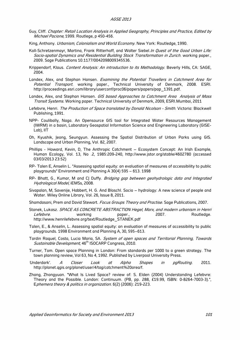
AGSE 2013


Guy, Cliff. Chapter: Retail Location Analysis in Applied Geography, Principles and Practice, Edited by Michael Pacione, 1999. Routlege, p 450-456.

King, Anthony. Urbanism, Colonialism and World Economy. New York: Routledge, 1990.

Koll-Schretzenmayr, Martina, Frank Ritterhoff, and Walter Siebel.In Quest of the Good Urban Life: Socio-spatial Dynamics and Residential Building Stock Transformation in Zurich. working paper.,

2009. Sage Publications 10.1177/0042098009345536.

Krippendorf, Klaus. Content Analysis: An introduction to its Methodology. Beverly Hills, CA: SAGE,

2004.

Landex, Alex, and Stephan Hansen. Examining the Potential Travellers in Catchment Area for Potential Transport. working paper., Technical University of Denmark, 2008. ESRI.

http://proceedings.esri.com/library/userconf/proc06/papers/papers/pap_1391.pdf.

Landex, Alex, and Stephan Hansen. GIS based Approaches to Catchment Area Analysis of Mass Transit Systems. Working paper. Technical University of Denmark, 2009, ESRI.Mumbai, 2011

Lefebvre, Henri. The Production of Space translated by Donald Nicolson - Smith. Victoria: Blackwell

Publishing, 1991.

NPP- Coulibally, Naga. An Opensource GIS tool for Integrated Water Resources Management

(IWRM) in a basin, Laboratory Geospatial Information Science and Engineering Laboratory (GISE-

Lab), IIT

Oh, Kyushik, Jeong, Seungyun. Assessing the Spatial Distribution of Urban Parks using GIS.

Landscape and Urban Planning, Vol. 82, 2007.

Phillips - Howard, Kevin, D, The Anthropic Catchment – Ecosystem Concept: An Irish Example,

Human Ecology, Vol. 13, No .2, 1985:209-240, http://www.jstor.org/stable/4602780 (accessed

03/03/2013 23:52)

RP- Talen E, Anselin L. "Assessing spatial equity: an evaluation of measures of accessibility to public

playgrounds" Environment and Planning A 30(4) 595 – 613. 1998

RP- Bhatt, G., Kumar, M and CJ Duffy. Bridging gap between geohydrologic data and Integrated Hydrological Model, iEMSs, 2008.

Sivapalan, M, Savenije, Habbert, H. G. And Bloschl. Socio – hydrology: A new science of people and

Water. Wiley Online Library, Vol. 26, Issue 8, 2011.

Shamdasani, Prem and David Stewart. Focus Groups Theory and Practise. Sage Publications, 2007.

Stanek, Lukasz. SPACE AS CONCRETE ABSTRACTION Hegel, Marx, and modern urbanism in Henri Lefebvre. working paper., 2007. Routledge.

http://www.henrilefebvre.org/text/Routledge_STANEK.pdf

Talen, E., & Anselin, L. Assessing spatial equity: an evaluation of measures of accessibility to public

playgrounds. 1998 Environment and Planning A, 30, 595–613.

Tardin Raquel, Costa, Lucia Maria, SA. System of open spaces and Territorial Planning, Towards Sustainable Development, 46

th ISOCARP Congress, 2010.

Turner, Tom. Open space Planning in London: From standards per 1000 to a green strategy. The

town planning review, Vol 63, No 4, 1992. Published by Liverpool University Press.

'Underdark'. A Closer Look at Alpha Shapes in pgRouting. 2011.

http://planet.qgis.org/planet/user/4/tag/catchment%20area/f.

Zhang, Zhongyuan. "What Is Lived Space? review of: S. Elden (2004) Understanding Lefebvre:

Theory and the Possible. London: Continuum. (PB, pp. 288, £19.99, ISBN: 0-8264-7003-3).",

Ephemera theory & politics in organization. 6(2) (2006): 219-223.

Internet Based Applications and Open Source Integration

Buberwa Charles Buzarwa

GeoData Consultants Limited, Togo Tower House 3rd

Floor

Kinondoni road/Togo str. P. O. Box 71467 Dar es Salaam Tanzania – [email protected]

KEY WORDS: Water, Point, Maping, System, OGC, GIS, Location, distance, Population, Census, MDG.

ABSTRACT

A web application is any application that uses a web browser as a client. The application can be simplest in design and development just like a message board counting number of hits on a web page or as complex as a water point mapping system that monitors Millennium Development Goals achievement and hence being a meter to government service delivery commitment to the public.

Water Point Mapping System is a web based application developed based on combination of different online applications and it is based on open source technology. It has been accepted by the government of Tanzania to be one of its decision making support system that will act as its meter for service delivery on the availability of clean and safe water to the public in rural areas of Tanzania Mainland.

The integration of the internet based application and open source tools together forming what we call Water Point Mapping System have changed the way we see and perform our daily duties. All in all is to bring information and communication technology (ICT) change the way people think but through the cheapest and modern way. That is where open source and internet based application are in action.

1 Introduction and project location

Water Point Mapping (WPM) is the process of locating water infrastructure and collecting related

information using any available technology, the information that is collected is later on subjected to

different uses. On the other hand, Water Point Mapping System (WPMS) is an integration of

hardware, software, methodologies, data, processes and users dedicated to collecting, storing,

processing and analyzing water related information and giving feedback in terms of report for public

use. Water Point Mapping System supports local level planning and can improve accountability for

water sector performance at local and national levels. Water Point Mapping (WPM) helps in

monitoring the distribution and status of water points and can be used to inform the planning of

investments to improve water supply coverage.

The project has been implemented in Tanzania mainland which is located in East Africa between

longitude 29o and 41

o East of Meridian, Latitude 1

o and 12

o south of the Equator. Tanzania has a

surface area of 94.3 million hectare subdivided into 29 regions. Each region is also subdivided into

districts and local government authorities (LGAs) which are 148.

1.1 The importance of water point mapping system (WPMS)

WPM is most often used to highlight issues of equity and functionality at district level. WPM

supports the process of establishing a baseline of water supply coverage and regular reporting as

part of sector performance monitoring (SPM). As such WPM activities can be seen as part of a

broader strategy among country programmes to engage with and influence sector dialogue towards

permanent sustainable rural water supply services at local, national and regional levels.

Water Point Mapping System (WPMS) is more than Water Point Mapping (WPM). While in the past

the two terms have been used interchangeably to mean the same thing, it is increasingly becoming

AGSE 2013


important to clearly distinguish the two. The growing demand of using this approach towards

fostering rural water supply services will in no doubt need to popularize WPMS as a panacea for

policy formulation, planning, investment and decision making. For countries and players to have a

meaningful impact from this area emphasis should be laid to ensuring that WPM Systems are in

place.

The results of WPMS form the basis for monitoring the distribution and status of water points and

can be used to inform the planning for investments to improve water supply coverage. In rural areas,

WPM is most often used to highlight issues of equity and functionality at district level. WPM

supports the process of establishing a baseline of water supply coverage and regular reporting as

part of sector performance monitoring (SPM). WPMS can help to visualize different aspects related

to access to water supply. While performance monitoring frameworks intend to measure changes in

access, it is often impossible to know whether access levels have changed based on simply adding

up the number of schemes constructed. By showing the spatial distribution of water facilities and

overlaying this point data with information about population and administrative boundaries, a picture

about differences in levels of access to water supply services can easily be obtained.

2 Water Point Mapping System (WPMS) and design aspect

The overall architecture of the Water Point Mapping System (WPM) is a three-tier architecture, in

which web applications, the middleware services and the data management are developed and

maintained as independent modules. The web applications and the middleware services use a web

application server as a deployment environment. There are two different web applications for the

public and for the system owner, which provide different views and different services of the system.

Both web applications are based on the same business logic, which is provided by the technical and

application middleware services. All vector data, metadata and user data are stored in a spatially

enabled database management system.

Figure 1: Overview of the System Architecture

The business logic consists of the following modules:

Reporting: The reporting module creates different types of reports from the current and the historic

data. These include different types of data presentation like textual or tabular data, diagrams like

Pie, Bar, Stacked Bar, Line, Area, Scatter Plot, Bubble, and Time series, and maps with an arbitrary

AGSE 2013


style. The reports can be exported as formatted documents (e.g. PDF), included in web pages or the

reports can be prepared for further processing in third-party tools (e.g. Excel, CSV, XML).

Mapping: The mapping module creates styled maps for presentation in the web applications and for

inclusion into the reports. The data included in the maps depends on the user who creates the map

request, e.g. an internal Ministry of Water user can see more layers or more details than an

anonymous user from the public interface.

Historization: The historization module traces all modifications and updates of water points and

additional data after the initial import. This is necessary so that e.g. reports showing time series can

be generated. If a data record is made invalid, its “valid from “and “valid to” attributes are updated by

the historization module.

Planning: The planning module provides services for planning of new investments. The planning

data is stored separately from the actual water points. However, it can be included in reports and

used in the web applications so that the effect of investments can be estimated.

Import/Export: The import/export module provides services for the initial import from the WPM

survey tool, for the initial import and updates of additional data like administrative data or

population. Data exports from the central database are accomplished by this module.

Quality Control: For every new record that is added to the system (via import or update), certain

quality checks must be executed. This ranges from simple geometry checks or data consistency

checks to a complex workflow where a new or updated record must be reviewed and approved by

the person in charge.

The technical services provide services that can be used in different business processes. The

technical services include the following modules:

Authentication and Authorization: Authentication is the process of identifying users of the system. In

computer systems, users are usually authenticated by their password, but other authentication

systems like smart cards or biometric identifiers are slowly winning acceptance in areas with

increased security requirements. A standards based authentication infrastructure will also profit

from functionality that increases the ease of use like single sign-on. The authorization module

decides if a user can perform a requested operation on a selected object.

Backup/Restore: The module for backup and restore supports the procedures of creating backups of

the whole system and to perform a restore of such a backup. Such support is for example a

maintenance mode, which informs the users that the system is in maintenance and which prevents

database operations.

Monitoring: The module for system monitoring supports the system administration by regularly

checking the system health, e.g. checking the connection to the database or checking the availability

of the web server. If services are not available, the monitoring module informs the system

administration.

The system has been hosted at client site which has been made through successful server

installation and commissioning. Operating system for the server computer is Ubuntu and the spatial

database is PostgreSQL. However the following applications are all Java based:

Web application server is Apache Tomcat while Web framework for generation of interactive web

pages is Apache Wicket. Report engine for template based reports containing maps, charts and tables is

JasperReports and MapServer that convert the spatial data into maps to be shown on the web page is

GeoServer.

As each browser interprets HTML code and CSS style sheets slightly different, the generated pages

are being tested for each recommended browser.

AGSE 2013


Figure 2: Schematic System Set-up

2.1 GeoServer and WPMS Interoperability

GeoServer is an open source software server written in Java that allows users to share and edit

geospatial data. Designed for interoperability, it publishes data from any major spatial data source

using open standards. GeoServer is the reference implementation of the Open Geospatial

Consortium (OGC) Web Feature Service (WFS) and Web Coverage Service (WCS) standards, as well

as a high performance certified compliant Web Map Service (WMS). GeoServer forms a core

component of the Geospatial Web.

Using GeoServer as a stand-alone web application from WPM has some disadvantages; the

GeoServer web application and the WPM web application do not share the same user session. That

means if a user authenticates to the WPM application, this authentication information cannot be

forwarded to the GeoServer web application. The user has to authenticate again to GeoServer.

Inclusion of WPM application logic into GeoServer is difficult. Inclusion of WPM libraries into the

GeoServer application is bad choice from the system design point of view, as the application logic is

spread across two different applications. This is even worse if it is difficult for the application parts to

communicate with each other.

Those difficulties have been overcome by including the GeoServer into the WPM application.

GeoServer is also available as a set of libraries that can be included in any Java application. By

including those libraries into WPM, the WPM offers geo-webservices (WMS, WFS etc.) as GeoServer

would do.

2.2 Apache Tomcat and its rationale in WPMS

Apache Tomcat is an open source software implementation of the Java Servlet and JavaServer Pages

technologies. The Java Servlet and JavaServer Pages specifications are developed under the Java

Community Process.

In WPMS the server sided system components is a Java-based web container. Several free and open

source implementations are available; the most common implementation is Apache Tomcat. WPM

application does not depend on any Tomcat specific extensions as the application but purely relies

on the Java serverlet specification. Apache Tomcat is recommended as a Java-based web container

because it is widely used as web container and it is considered to be very stable and reliable. Apache

Tomcat it is used in many other commercial and open source application servers like Apache

Geronimo, Apache TomEE oder JBoss. An installer for Ubuntu Linux is already available which

means it can easily be installed and upgraded and it is well integrated into the operating system.

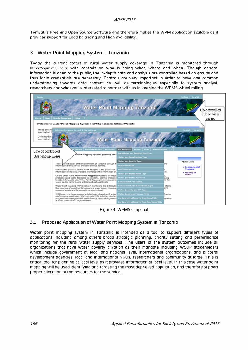
AGSE 2013


Tomcat is Free and Open Source Software and therefore makes the WPM application scalable as it

provides support for Load balancing and High availability.

3 Water Point Mapping System - Tanzania

Today the current status of rural water supply coverage in Tanzania is monitored through

https://wpm.maji.go.tz with controls on who is doing what, where and when. Though general

information is open to the public, the in-depth data and analysis are controlled based on groups and

thus login credentials are necessary. Controls are very important in order to have one common

understanding towards data content as well as terminologies especially to system analyst,

researchers and whoever is interested to partner with us in keeping the WPMS wheel rolling.

Figure 3: WPMS snapshot

3.1 Proposed Application of Water Point Mapping System in Tanzania

Water point mapping system in Tanzania is intended as a tool to support different types of

applications includind among others broad strategic planning, priority setting and performance

monitoring for the rural water supply services. The users of the system outcomes include all

organizations that have water poverty allvation as their mandate including WSDP stakeholders

which include government at local and national level, international organizations, and bilateral

development agencies, local and international NGOs, researchers and community at large. This is

critical tool for planning at local level as it provides information at local level. In this case water point

mapping will be used identifying and targeting the most deprieved population, and therefore support

proper allocation of the resources for the service.

AGSE 2013


Figure 4: WPM coverage density

Map1: Interpretation of the coverage density as captured from WPMS

4 Situation analysis in relation to other countries

Water point mapping activities are growing rapidly in almost to all developing countries in order to

help decision makers to access the service delivery to public. Apart of Tanzania, WPM project has

been carried out in several countries including Democratic Republic of Congo (DRC), Malawi, Kenya,

Rwanda, Uganda, etc. The only approach that makes Tanzania unique was its approach on the

development of the WPMS application and the way data has been collected based on the state of

the art Mobile GIS technology.

During implementation of the assignment there were some challenges that give the WPMS In

Tanzania act as a platform for the rural water supply monitoring tool as such a room for more

expansion is expected.

AGSE 2013


5 Conclusion

Water Point Mapping is a critical tool for planning, implementation and monitoring of water supply

services in rural areas where poor communities live. The sustainability of the system is critical and

therefore recommended actions plan need to be critically analyzed and putting them in practice.

It is obviously seen and appreciated by developer communities including client for using integrated

technology that give relief on the budget burdens by avoiding extra cost on the purchasing of extra

GIS software application that sometimes cost a lot of money. With this application I have to say all

mapping transactions are performed on the web browser and results are set for further application

depending to user requirement. Real it is changing the way we see.

REFERENCES

Ministry of Water Tanzania. 2013. “Water point mapping Tanzania – http://wpm.maji.go.tz

Huong, Li. 2009 “Water Point Mapping – the SNV experience in Tanzania” http://www.snvworld.org/sites/www.snvworld.org/files/publications/water_point_mapping-

_the_experience_of_snv_tanzania1.pdf

Pearce, J. and C. Howman. 2013. RWSN Water Point Mapping Group - A Synthesis of Experiences

and Lessons discussed in

Exploring Enterprise Resource Planning (ERP) and Geographic

Information System (GIS) Integration aJinal Patel,

bGayatri Doctor

aTechnology Management, CEPT University - [email protected]

bFaculty of Management, CEPT University - [email protected]

KEY WORDS: Geographic Information System, GIS, Enterprise Resource Planning, ERP, Integration

ABSTRACT:

Today, integration of information systems has become a necessity due to the fact that the big companies have developed over time, mostly, separate information systems for automation of different activities. Enterprise Resource Planning (ERP) means, techniques and concepts for integrated management of business as a whole from the viewpoint of the effective use of management resources to improve the efficiency of enterprise management. A Geographic Information System (GIS) is a technological tool for comprehending geography and making intelligent decisions. GIS organizes geographic data so that a person reading a map can select data necessary for a specific project or task, it is a location based information system. Many advances in technology have been observed in both ERP and GIS but no direct integration is observed due to the complexity involved in handling each system. Businesses are now striving to optimize their processes and improve efficiency with the ability to make informed decisions. By using ERP systems for workflow management and GIS for location based information management, that is, ERP – GIS Integration businesses can have more complete operational picture. This paper explores ERP –GIS Integration, its advantages with reference to a case study.

1 Introduction

Enterprise Resource Planning (ERP) means, techniques and concepts for integrated management of

business as a whole from the viewpoint of the effective use of management resources to improve

the efficiency of enterprise management. A Geographic Information System (GIS) is a technological

tool for comprehending geography and making intelligent decisions. GIS organizes geographic data

so that a person reading a map can select data necessary for a specific project or task, it is a location

based information system. Many advances in technology have been observed in both ERP and GIS

but no direct integration is observed due to the complexity involved in handling each system.

Businesses are now striving to optimize their processes and improve efficiency with the ability to

make informed decisions. By using ERP systems for workflow management and GIS for location

based information management, that is, ERP – GIS Integration businesses can have more complete

operational picture.

2 Enterprise Resource Planning (ERP)

ERP is an abbreviation of Enterprise Resource Planning and means, techniques and concepts for

integrated management of business as a whole from the viewpoint of the effective use of

management resources to improve the efficiency of enterprise management.(Alexis Leon, 2008)

ERP is set of tools and processes that integrate department and functions across a company into

one computer system. ERP system comprises function-specific modules designed to interact with

the other modules. These modules are purchased based on what best meets specific needs and

technical capabilities of an organization. Common ERP modules include product planning, finance,

accounting, marketing, HR, etc. (Figure 1)

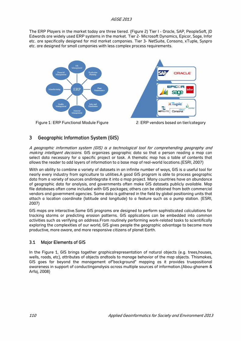
AGSE 2013


The ERP Players in the market today are three tiered. (Figure 2) Tier I - Oracle, SAP, PeopleSoft, JD

Edwards are widely used ERP systems in the market. Tier 2- Microsoft Dynamics, Epicor, Sage, Infor

etc. are specifically designed for mid market companies. Tier 3- NetSuite, Consona, xTuple, Syspro

etc. are designed for small companies with less complex process requirements.

Figure 1: ERP Functional Module Figure 2: ERP vendors based on tier/category

3 Geographic Information System (GIS)

A geographic information system (GIS) is a technological tool for comprehending geography and making intelligent decisions. GIS organizes geographic data so that a person reading a map can

select data necessary for a specific project or task. A thematic map has a table of contents that

allows the reader to add layers of information to a base map of real-world locations.(ESRI, 2007)

With an ability to combine a variety of datasets in an infinite number of ways, GIS is a useful tool for

nearly every industry from agriculture to utilities.A good GIS program is able to process geographic

data from a variety of sources andintegrate it into a map project. Many countries have an abundance

of geographic data for analysis, and governments often make GIS datasets publicly available. Map

file databases often come included with GIS packages; others can be obtained from both commercial

vendors and government agencies. Some data is gathered in the field by global positioning units that

attach a location coordinate (latitude and longitude) to a feature such as a pump station. (ESRI,

2007)

GIS maps are interactive.Some GIS programs are designed to perform sophisticated calculations for

tracking storms or predicting erosion patterns. GIS applications can be embedded into common

activities such as verifying an address.From routinely performing work-related tasks to scientifically

exploring the complexities of our world, GIS gives people the geographic advantage to become more

productive, more aware, and more responsive citizens of planet Earth.

3.1 Major Elements of GIS

In the Figure 1, GIS brings together graphicalrepresentation of natural objects (e.g. trees,houses,

wells, roads, etc), attributes of objects andtools to manage behavior of the map objects. Thismakes,

GIS goes far beyond the management of“background” mapping as it provides truepositional

awareness in support of conductinganalysis across multiple sources of information.(Abou-ghanem &

Arfaj, 2008)

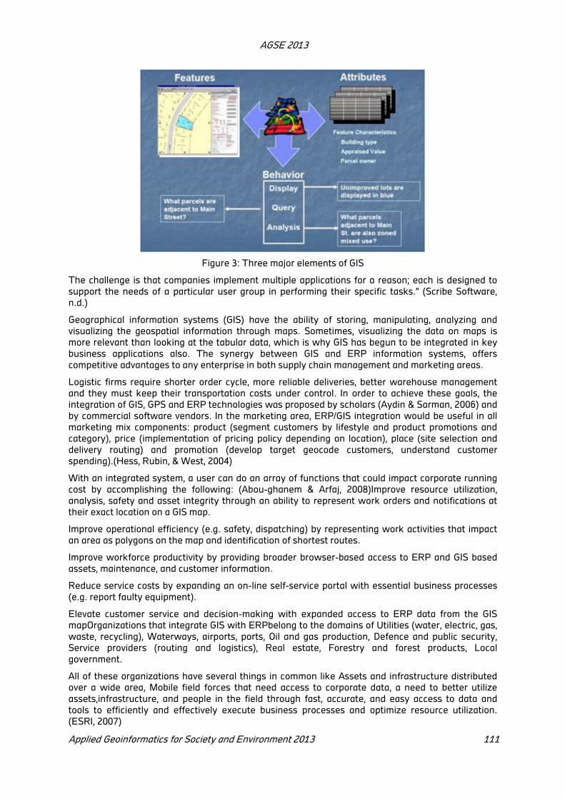
AGSE 2013


Figure 3: Three major elements of GIS

The challenge is that companies implement multiple applications for a reason; each is designed to

support the needs of a particular user group in performing their specific tasks.” (Scribe Software,

n.d.)

Geographical information systems (GIS) have the ability of storing, manipulating, analyzing and

visualizing the geospatial information through maps. Sometimes, visualizing the data on maps is

more relevant than looking at the tabular data, which is why GIS has begun to be integrated in key

business applications also. The synergy between GIS and ERP information systems, offers

competitive advantages to any enterprise in both supply chain management and marketing areas.

Logistic firms require shorter order cycle, more reliable deliveries, better warehouse management

and they must keep their transportation costs under control. In order to achieve these goals, the

integration of GIS, GPS and ERP technologies was proposed by scholars (Aydin & Sarman, 2006) and

by commercial software vendors. In the marketing area, ERP/GIS integration would be useful in all

marketing mix components: product (segment customers by lifestyle and product promotions and

category), price (implementation of pricing policy depending on location), place (site selection and

delivery routing) and promotion (develop target geocode customers, understand customer

spending).(Hess, Rubin, & West, 2004)

With an integrated system, a user can do an array of functions that could impact corporate running

cost by accomplishing the following: (Abou-ghanem & Arfaj, 2008)Improve resource utilization,

analysis, safety and asset integrity through an ability to represent work orders and notifications at

their exact location on a GIS map.

Improve operational efficiency (e.g. safety, dispatching) by representing work activities that impact

an area as polygons on the map and identification of shortest routes.

Improve workforce productivity by providing broader browser-based access to ERP and GIS based

assets, maintenance, and customer information.

Reduce service costs by expanding an on-line self-service portal with essential business processes

(e.g. report faulty equipment).

Elevate customer service and decision-making with expanded access to ERP data from the GIS

mapOrganizations that integrate GIS with ERPbelong to the domains of Utilities (water, electric, gas,

waste, recycling), Waterways, airports, ports, Oil and gas production, Defence and public security,

Service providers (routing and logistics), Real estate, Forestry and forest products, Local

government.

All of these organizations have several things in common like Assets and infrastructure distributed

over a wide area, Mobile field forces that need access to corporate data, a need to better utilize

assets,infrastructure, and people in the field through fast, accurate, and easy access to data and

tools to efficiently and effectively execute business processes and optimize resource utilization.

(ESRI, 2007)

AGSE 2013


Companies have several options for integrating GIS and ERP: build or purchase software connectors

thatdirectlyconnect a given ERP and GIS package, use passive middleware, or deploy frameworks for

comprehensiveintegration with a given GIS package from an ERP vendor(Elisabeth Horwitt, 2009).

The most successful integration GIS – ERP was done by ESRI (the world’s GIS leader) and SAP (one

of the ERP vendor’s leader). There are five main technical interfaces available for integrating SAP’s

ERP and ESRI’s GIS software. The integration technical interfaces include (ESRI, 2013):

SAP RFC connectors - RFCs (Remote Function Calls) allow for remote calls between SAP ERP and

ESRI's GIS software. The remotely callable functions are named RFMs or RFC-enabled function

modules;

Third-party connectors - Third-party connectors include the Way Control Broker (CB) from

Information Builders which is component-based and allows director connection to packaged and

legacy back-end systems. Control brokers provide an application level approach for greater control,

performance and scalability;

SAP generic GIS connector - The SAP GBC (GIS Business Connector) is a passive middleware that

mediates between SAP solutions (designed for use with SAP ERP 4.5 and higher) and ESRI's GIS

software. The method is best used when there is flexible processing modelling with existing

methods in both applications;

Third-party EAI - EAI (Enterprise Application Integration) is generally defined as the combination of

platforms, business processes, standards and applications that result in the seamless integration of

two or more enterprise systems. The EAI platform integration interface for SAP ERP and ESRI's GIS

can be utilized when there are non-standard processes that require custom development;

SAP EAI - SAP Exchange Infrastructure (XI) is SAP's enterprise application integration (EAI) software

used to facilitate the exchange of information between SAP ERP and ESRI's GIS. SAP XI is

considered an integration broker since it mediates between entities with varying requirements in

terms of protocols, connectivity and format

ESRI’s partner solutions - The SICAD-APX (application exchange) is an EAI (Enterprise Application

Integration) solution from AED-SICAD (an ESRI partner) that integrates ESRI's GIS with SAP's ERP

modules.

Sivan Design is another software developer which providescustomized GIS solutions combined with

ERP capabilities. Using its proprietary technology Geo-ERP™, Sivan Design is able to provide

turnkey solutions for establishing lands, roads, or any other infrastructures management. Geo-ERP

platform consists of threeplatforms. The independent solutions (LAPS - Land and Properties System,

IGIS - Infrastructure Geographic Information System, CMMS - Contracts Management and

Maintenance Sys) that use a mutual core and can share the same spatial database. The integration

of GIS and ERP is done by Oracle throughits database Oracle Spatial 10g. This database is able to

store and manipulate geo-spatial information because of its special datatype SDO_GEOMETRY and

spatial functions and operators. The Spatial functions can determine the relationship between two

spatial layers, the geocoding engine geocodes addresses and the spatial data mining functions allow

the searching of spatial data. Oracle’s ERP: E-Business Suite can connect to the same database, in

this way it will be assured an integrated data architecture (Fig. 4)

AGSE 2013


Figure 4: Oracle Spatial 10g Integrated Data ArchitectureWith this integrated framework, Oracle

offers thepossibility of using GIS Specialist Systems (Environmental Management, Transportation,

Crime, Health and Social Services, Education) together with the modules of its ERP System

(Logistics, Financial Management, Asset Management and Human Resources) and CRM System.

One of the most interesting features which Oracle Spatial has is the geocoding engine, which can

use the customer addresses stored in CRM’s specific tables and convert them to longitude / latitude

entries so that maps could be drawn.

4 Case Studies

Einmax Corporation, which distributes natural gas and electricity in Canada, uses this integrated

data architecture from Oracle, locating corporate data in a centralized database, reducing

redundancies and encouraging cross flows of information. (James B. Pick, 2007).

At global level, there are already many other companies which have chosen to integrate their ERP

system with a modern GIS system in order to add the spatial dimension to the business processes.

For example, a company in Germany-ivl GmbH— had successfully integrated Smallworld GIS with

SAP R/3, using a product they had developed called GISConnect™. (Litan, Velicanu, Teohari, Teohari,

& Virgolici, 2011)

GPU Energy has also integrated Smallword with SAP R/3 using two main integration pieces (virtual

database integration allows the GIS and SAP R/3 data models to be treated logically as a single

model, and business process integration, offering a complex business processes freely spread over

GIS and SAP R/3), San Diego's Street Services Division has successfully integrated a GIS with ERP.

(Litan et al., 2011)

Source: http://www.sandiego.gov/

AGSE 2013


4.1 Cochin Port Case Study

Cochin Port Trust, autonomous body under Government of India manages port of Kochi which

renders services to more than 1000 inland and foreignvessels and handles about 13 millionmetric

tons of cargo annually.With increased demands for operational efficiency, effective facility

management, comprehensive security and sensitive environmental management, Cochin Port Trust

(CoPT) realized the need for an IT system that provides detailed and up-to-date information. CoPT

embarked on Enterprise Resource Planning (ERP) implementation program to set up a fully

Integrated Port Information System (iPINS), a first-of-its-kind in India using a SAP – based ERP with

TCS’ help.

TCS integrated GIS solution with Estate Management system of SAP. The solution integrates the

Port’s operational, financial, estate and human resource systems and provides real-time interface

with Indian Customs, port users, banks and the port community system of the Indian Ports

Association.

Integrating GIS and ERP allows users to turn tabular data into maps for spatially visualizing and

analyzing. GIS solution is able to provide an integrated view of each asset, facilities such as lease

management, occupation/vacation, renewal and demand, and collection of rentals and mapped the

data spatially around the land assets. Integrated graphical representation of the Port-owned land

and water assets has made it simple to understand the status of any land asset.

4.2 Reliance Case Study

Reliance Infrastructure Limited (RInfra) distributes electricity to more than 25 million consumers

across India, including in Delhi and Mumbai. The company generates, transmits, and trades

electricity from power stations in Maharashtra, Andhra Pradesh, Kerala, Karnataka, and Goa. RInfra

is also working with partners to construct power plants as an emerging lead player in the

engineering, procurement, and construction (EPC) segment of the power sector.

Due to distributed and dispersed complex network, RInfra’s assets are spread out among scattered

customers and work sites, each with specific and diverse need. To accommodate this, it required

complete system to map, model and manages it assets, maintenance and operation. RInfra needed

to streamline its work under process- increasing accuracy of its data and improving outage response

time.

RInfra selected a geographic information system (GIS) platform from ESRI. To ensure fresh data and

enable better analysis for decision making, the company integrated GIS with its SAP® business

software and supervisory control and data acquisition (SCADA) system.

RInfra integrated GIS with SAP plant maintenance (PM) and billing/ customer care and services

(ISU/CCS). All integrated modules are Web enabled and allow one-window access to functionalities

from anywhere. GIS applications use these Microsoft® .NET Framework Web services to provide

multiple user functionalities including equipment history, creation of work orders, data table loading,

and customer billing information. RInfra then integrated GIS with its SCADA system to enhance the

problem-solving capability of the network by allowing real-time data analysis and updates from the

GIS.

The integration of SAP and GIS immensely helps staff identify work order locations and find related

faults, thereby reducing the resolution time and increasing customer satisfaction. RInfra field crews

now rely on GIS-based operations and maintenance applications to manage both planned and

unplanned outages and perform energy audits for accounting reports. Decision makers rely on the

GIS for a visual representation of the network, facility search options, and work order management.

Because of the GIS/SAP integration, SAP notifications and work orders can be retrieved through GIS

along with technical data for equipment maintained in SAP. Customer data can be retrieved from

SAP based on service points selected in the GIS. Notification of outages and work orders based on

customer calls are also enabled through this integration.

AGSE 2013


4.3 Torrent Case Study

Torrent Power, with a generation capacity of 1647.5 MW (500 MW is operational while 1147.5 MW

is under implementation), is one of the most active private sector players in the power sector of

Gujarat state. Torrent annually distributes over 10 billion units of power to Ahmedabad, Gandhinagar

and Surat. Torrent Power and GPCL (Gujarat Power Corporation Limited) is developing two more

power plants at Pipavav with 2000 MW capacity each are in the pipeline. Torrent Energy Limited

subsidiary of Torrent Power Limited commenced distribution operations in Dahej SEZ from April

2010.

Torrent has implemented a SAP-enabled ERP environment for the entire organization. The ERP

solution will incorporate certain important modules like ‘industry solution for utility and customer

service’ or ISUCCS. The ERP has been enabled to serve the customer base of 2.25 million. ERP has

been integrated with Geographical Information System (GIS) and Supervisory Control And Data

Acquisition system (SCADA), which further enhances customer service levels.

GIS provides satellite images of various locations. While these satellite images provide a broader

view; it becomes difficult to precisely locate a particular house or road. Torrent’s system digitalizes

these satellite images with respect to roads, cables, houses and services, which allows to accurately

locating areas with faults. With GIS, particular transformer can exactly be located and deciding the

sub-station to be attended in case a problem arises.

The major areas in which power utilities can be benefited from GIS are Identifying the Consumer’s

connectivity with the Network Asset, Network Mapping, Distribution Network Modeling, Load Flow

Analysis and Meter management & Outage Management. GIS technology is also in determining

technical loss, network planning, and optimization of distribution system and load forecasting, and

the resulting advantages of faster and improved decision-making.

REFERENCES

Abou-ghanem, M., & Arfaj, K. A. (2008). SAP / GIS Integration Case Studies & Techniques, (966 3), 1–

12.

Alexis Leon. (2008). ERP Demystified. Tata Macgraw Hill.

Aydin, A. O., & Sarman, S. (2006). A MANAGEMENT INFORMATION SYSTEM�:, (3050267).

Elisabeth Horwitt. (2009). ERP and GIS integration brings spatial dimension to key business apps.

Search Manufacturing ERP.

ESRI. (2007). Using GIS and SAP Table of Contents, (June).

ESRI. (2013). SAP ERP Integration Options. ESRI News for SAP.

Hess, R. L., Rubin, R. S., & West, L. a. (2004). Geographic information systems as a marketing

information system technology. Decision Support Systems, 38(2), 197–212. doi:10.1016/S0167-

9236(03)00102-7

James B. Pick. (2007). Geo-Business: GIS in the Digital Organization. John Wiley & Sons Inc.

Litan, D., Velicanu, M., Teohari, L. C., Teohari, M., & Virgolici, A. M. M. (2011). Business ’ New

Requirement�: Information Systems Integration – Methods and Technologies, 5(3).

Scribe Software. (n.d.). CRM Integration. Retrieved from

http://www.scribesoft.com/images/pdf/SuccessModelForCRMIntegration.pdf.

Feasibility of Mobile Mapping System By Integrating Structure From

Motion (Sfm) Approach With Global Navigation Satellite System

J. J. Jariwala a,*

, A. Bhardwaj b, S. Raghavendra b, K. Khoshelham

c a Photogrammetry and Remote Sensing Department & Geoinformatics Department, Indian Institute

of Remote Sensing, ISRO, Dehradun, India and ITC, University of Twente, the Netherlands -

[email protected]

b Photogrammetry and Remote Sensing Department (PRSD) Department, Indian Institute of Remote

Sensing (IIRS), ISRO, Dehradun 248 001, Uttarakhand, India - [email protected],

[email protected]

c ITC, Faculty of Geo-Information Science and Earth Observation, University of Twente, P.O. Box 217,

Enschede 7514 AE, the Netherlands - [email protected]

KEY WORDS: Mobile Mapping, Terrestrial Photogrammetry, Structure from Motion (SfM), Feature

extraction and matching, Space photo intersection, 3D similarity transformation, Direct Geo-

referencing.

ABSTRACT

Over the past few years, there is an emerging growth in mobile mapping systems which can effectively capture the geospatial data in an efficient way. A typical terrestrial mobile mapping system consists of camera, laser scanners, GNSS and INS (Inertial Navigation System). Imagery data is captured by camera and the point clouds are acquired by the laser scanners. GNSS and INS are used for measuring the positional and orientation information of the mapping sensors respectively to achieve direct geo-referencing. GNSS/INS system is very expensive which makes the overall mapping system very expensive. An alternative to make this system is to use Structure from Motion Approach (SfM), to minimize the relative cost of this system. SfM generates 3D point clouds of scene and estimate the orientation parameter for mapping sensor by using imagery data. The major issue with SfM is that it generates point clouds in arbitrary coordinate system with arbitrary scale.

Therefore, this research work was focused on feasibility of mobile mapping by integrating SfM approach (for the estimation of camera orientation parameters) with GNSS (for exposure station position) for comparatively low cost terrestrial mapping system and to make whole system (captured 3D scene) direct geo-referenced with proper scale without using ground control points (GCPs). In the first step, sequences of images were captured by measuring the exposure station positions. Then feature extractions and matching were done on the sequence of overlapping images. Bundle adjustment was then applied on it to generate the 3D scene (point clouds) of rigid body and for estimation of camera orientation parameters. The generated point clouds were in arbitrary coordinate system, so tie points were selected to transform into mapping coordinate system. Space photo intersection was applied on tie points with the use of exposure orientation parameters and matched feature points in sequence of overlapping images to transform into world coordinate system. Further, point-based similarity transformation was used to generate transformation parameters from tie points. These transformation parameters were applied on whole generated point cloud to transform it into world coordinate system with proper scale. Then the accuracy assessments on point cloud were carried out using internal and external accuracy assessment. Sometime the epipolar lines do not exactly cross at a fixed point in different overlapping images due to which a distorted 3D scene (point clouds) was created. There was an error in the estimation of orientation parameters due to no ground measurements were used in bundle adjustment. Thus it was observed that the shape of the point cloud was concaved near start and end edges of the scene. RMSE were 32.21 cm, 20.50 cm and 23.56 cm in easting, northing (depth) and height respectively.

AGSE 2013


1 Introduction

Since 1990s, Mobile Mapping Systems (MMS) have been started for both land and aerial digital

mapping. In comparison to conventional surveying, major developments were observed in mobile

mapping technology since the last decade by using multi sensor and real time multitasking systems

(Dorota et al., 2004). It is an emerging domain in modern data collection by integrating various digital

photogrammetry techniques and computer vision technologies such as structure and motion (SM).

Computer vision based structure and motion (SM) reconstruction for digital photogrammetry has

been used in the area of mapping for Geographic Information System (GIS) applications providing

new possibilities for the end users (Madani, 2001).

Terrestrial mobile mapping is very useful for capturing the exterior side of buildings or objects with

great details. With the use of high resolution satellite images or nadir airborne images, we can easily

reconstruct the three dimensional point clouds of roofs, but it’s difficult to generate facades details

(Tian et al., 2010). So there is a need for terrestrial mapping, which can capture the exterior side of

buildings with great details. Terrestrial mobile mapping systems that construct ground based point

clouds have become interesting as they represent realistic facades which contain more details than

point cloud constructed from aerial data. The manual acquisition of such data is time consuming and

expensive job, as in cities vast numbers of urban objects are present with different shapes and

structures (Brenner, 2005). While laser scanners are expensive and cannot capture texture and color

information, mapping from image sequences offers advantages such as flexibility and economic

acquisition of colored point clouds. This has been made possible by automated techniques, such as

structure from motion approach.

A typical mobile mapping system is composed of GNSS/INS system. INS use accelerometers to

measure acceleration and gyroscopes to measure the rotational velocity to sense how the

camera/laser scanner are accelerating and rotating in space (Xuexian et al., 2009). The fact that

accurate inertial sensors are very expensive makes mobile mapping in general an expensive

technology. So instead of using expensive IMU (Inertial Measurement Unit) in mobile mapping

system, SfM approach can be used as an alternative to make this process less costly. INS measures

orientation parameters using accelerometers and gyroscope; and with SfM, the parameters can be

estimated from images. There has been a great progress in structure from motion and automated

orientation of sequences of images to generate point clouds. The problem with structure from

motion is that the orientation parameters and the resulting point clouds are in an arbitrary

coordinate system with arbitrary scale. If a 3D point cloud is in arbitrary scale and arbitrary

coordinate system, it will not be useful for various GIS applications. Structure from Motion (SfM)

technique is used in a variety of applications including town planning, remote measurement,

photogrammetric survey and in the creation of automatic reconstruction of virtually real

environments from video sequences or sequence of images (Zhang et al., 2005). Therefore, this

study attempts to construct 3D cloud points by integrating GNSS/ SFM which will be used for above

mentioned applications and makes a mobile mapping system that is not expensive compared to

GNSS/INS and also provides geo-referenced data in a correct scale with the use of GNSS. Thus this

research topic focuses on the feasibility of mapping by integrating Structure from Motion approach,

which estimates camera orientation parameters from the images, and GNSS which provides scale.

2 Related work

Mapping of man-made object from aerial images has already been a topic of interest from many

years (Remondino et al., 2006). But the problem that lies in satellite and aerial images of urban area

is that only the roof (top view) can be well observed in these images and not the facades. In recent

years, there has been an interest in developing methods for generating three dimensional data using

the combination of satellite/aerial images, 2D map data and terrestrial data to improve the reliability

and accuracy of the mapping system (Zhang et al., 2005).

Till now lots of work has been done on mapping of real objects and scenes from terrestrial platforms.

For terrestrial mobile mapping, there are mainly two methods. One is based on active range data e.g.

laser scanning and other is based upon video images or image sequences. Active range based

mapping methods are very useful to directly capture 3D geometric information with highly detailed

AGSE 2013


and accurate representation of shapes (Pu et al., 2009). Laser scanner integration with IMU (Inertial

Measurement Unit)/GPS provides directly the measurement of dense point clouds in global

coordinate system but it does not give surface information like texture in laser point clouds (Xuexian

et al., 2009). Another data acquisition technique is based on CCD (charge-coupled device) camera

integration with INS/GPS system. Piras et al. (2008) developed a integrated systems with GNSS,

IMU, video camera that allows quick and accurate mapping. The GNSS with IMU integration for the

derivation of the position and attitude angles of the mapping vehicle is usually based on Kalman

filter. It allows the position of the exposure station to be surveyed, even in the loss of a GNSS signal

(Piras et al., 2008). These types of data acquisition techniques rely on expensive inertial sensors.

Another method for mapping surrounding scene is by camera integration with GNSS and SfM

(Structure from Motion) approach to overcome the cost of the whole system.

Structure from Motion (SfM) makes it possible to generate 3D point clouds from images with camera

projection matrices using corresponding 2D image points in multiple views (Sabzevari et al., 2011). It

uses corresponding image points in multiple views and a 3D point can be reconstructed by

triangulation. An important requirement is the measurement of camera pose and calibration, which

may be expressed by a projection matrix of each camera. But it’s not possible to compare each and

every pixel of one image with next image. In addition to this, there is no guarantee that each and

every point is equally well suited for automatic matching (Pollefeys et al., 2000). So there is a need of

feature extraction in image processing as a part of special form of dimensionality reduction. Common

method for feature extraction, matching and outliers’ removal between wrong feature matches are

Scale Invariant Feature Transform (SIFT) (Lowe, 1999), Approximate Nearest Neighbors (ANN)

(Arya et al., 2010) and RANdom Sample Consensus (RANSAC) respectively (Fischler et al., 1981)

which are widely used by many researchers and is known to perform well over a reasonable range of

viewpoint variations. Extracted and matched features in multiple views are used with bundle

adjustment to build a sparse three dimensional point cloud of the viewed scene to simultaneously

recover camera poses and calibration parameters. Triggs et al. (2000) reviewed bundle adjustment

technique which is a widely used technique to estimate camera pose and produced 3D point clouds

from image correspondences. Bundle adjustment is used as the last step in feature based multi-view

structure and motion estimation algorithm (Lourakis et al., 2009). Thus the simultaneous recovery of

3D points and camera projection matrices using corresponding 2D image points in multiple views is

known as the structure from motion.

3 Multiple view Geometry for SfM

Multiple view geometry is broadly described in Zisserman et al. (2001)’s book. The following section

will describe brief overview of multiple view geometry to find out camera projection matrices and

position of 3D object X as shown in Figure 1.

Consider { , , . . , } are images with reasonable overlap between images. Projection matrices

are { , , . . , }, where each = | ], is intrinsic parameters, are rotation and

translation matrices respectively.

(1)

where, 1,… , 1, . . , . Here ‘m’ images are available with reasonable overlaps of ‘n’ rigid

3D points

Figure 1: Overview of multi-view photography and geometry (Al-sadik, 2012b)

AGSE 2013


If the image measurements are noisy, the projection does not satisfy exactly.

(2)

where, is the set of camera matrices and is set of points.

Estimate the projection matrices and 3D points which are projected exactly to image point .

Bundler Adjustment (Triggs et al., 2000) will minimize distance between estimated and measured

points for every view by using.

min,

, (3)

where, , is the geometric image distance between homogenous point . min will adjust the bundle of rays between each camera centre and 3D points and vice versa.

Lease square optimization uses iterative solution to find the parameters P that minimize the

difference between the measures and estimated . There are different strategies for bundle

adjustment. The basic strategy for bundle adjustment algorithm are followed by this step (Al-sadik,

2012b):

1. Find the M tracks M = {M1, M2,.., MN}

Take pair of images { , }, :

Detect and extract the SIFT feature point in ,

Feature matching across images and outliers’ removal using RANSAC

a. Again matching features across multiple images and construct tracks for that {M1,

M2,.., MN}

Estimation of { , , . . , } and 3D position for each track

Select first pair of images { , } and consider M1’2’ are their associative overlapping tracks

b. Estimate � and � intrinsic parameters and compute { , } and 3D position of

M1’2’ from fundamental matrix.

Incrementally add new camera into the system and estimate its camera projection matrices by

direct linear transformation algorithm (DLT) and refine the existing structure.

c. Initialize new structure points and repeat (c) until all camera parameters are

estimated. Refine all structure and motion through bundle adjustment.

But there is possibility of re-projection error in projection matrices which is minimized by nonlinear

least-squares algorithms, such as Levenberg-Marquardt (LM) iteration algorithm (Madsen et al.,

2004). It minimizes the re-projection error and non-linearly optimizes the system. Lourakis et al.

(2009)’s sparse bundle adjustment uses LM algorithm and bundle adjustment (Triggs et al., 2000)

for estimation of camera parameters and 3D point of object.

a b c

Figure 2: (a) Match track points over whole image sequence (b) initialize the structure and motion

recovery and Compute camera pose and refine existing structure (c) Refine SfM through bundle

adjustment (Al-sadik, 2012b)

AGSE 2013


As presented in Lourakis et al. (2009), the LM algorithm is an insistent technique that determines a

local minimum of a multivariate function that is formulated as the sum of squares of several

nonlinear, real valued functions. Thus it has become a standard approach for nonlinear least-squares

problems, widely accepted in various fields for dealing with data-fitting applications. Bundle

Adjustment attempts to filter the visual reconstruction to produce optimal 3D structure in

conjunction with viewing parameter estimates. Optimal refers to minimizing (or maximizing) a cost

function that determines the model fitting error with respect to both camera and structure

adaptations. The name refers to the ‘bundle’ of light rays leaving each 3D feature and converge on

each camera centre, which are adapted optimally with respect to both feature and camera positions.

Bundle adjustment (BA) understates the re-projection error between the detected and foreboded

image points, which is expressed as the sum of squares of a large number of nonlinear, real valued

functions. Figure 2 show whole SfM workflow in step by step from a to c.

4 Overview of the method

The feasibility of integration of SfM approach and GNSS using space photo intersection and point-

based similarity transformation method for mapping was studied in this research. To achieve the

objectives, test scene was selected and various hardware-software tools were used in present

study. IIRS (Indian Institute of Remote Sensing) main building was used as a test scene as shown in

Figure 3.

Figure 3: Overview of IIRS Main Building (Jariwala, 2013)

Nikon D-80 SLR camera was used to capture images. Leica DGPS 510 was used to Measure position

of exposure station not for GCP points. Leica TPS 1200 was used for Evaluation of point cloud. Open

source packages like SIFT, Bundler, PMVS were used in this study for SfM approach.

The methodology follows image acquisition from the exposure stations using a pre calibrated

camera. Further images are processed for the automatic feature extraction and matching from

sequence of images and then sparse bundle adjustment is applied to generate a sparse point cloud

and to extract camera parameters which contain projection matrices at each exposure station.

Dense point cloud in local coordinate system is generated by PMVS using camera parameter files.

Further it’s transformed into global coordinate system (mapping coordinate system i.e. exposure

station coordinate system) by using space photo intersection and similarity transformation with

proper scale. Then the generated point cloud is evaluated for accuracy assessment. Detailed

methodology is shown in a flow chart in Figure 4.

4.1 Feature Extraction and Feature Matching

After the acquisition of images, SIFT is used to extract key features from images. SIFT is a most

popular features extractor from images. In this study, we used Lowe (1999)’s SIFT which is written

in C/C++ and other languages. This key-points extractor is available in the form of compiled binary

files that can be run under Linux or Windows environment. This SIFT version takes only gray-scale

image of size 1800*1800 pixels or smaller.

Snavely (2010) developed an efficient open source software Bundler, in which structure from motion

system is used to generate sparse point clouds. Bundler includes the binary distribution of the

Lourakis et al. (2009)’s Sparse Bundle Adjustment (SBA), as well as a number of other utilities and

executables. Features matching and outlier removals libraries (ANN and RANSAC) are also included

AGSE 2013


in this package. Complete package of Snavely (2010)’s bundler is used to generate sparse point

clouds with exposure station positions and orientation files in its local coordinate system. After the

key point extraction from images, result of SIFT files are used as input for bundler packages. After

the key point extraction from images, ANN (Arya et al., 2010) is used for feature matching. Features

matching have been done between pre and post sequences of images for each image pair. All

images are with approximately 80 % overlap in each pair of images. In order to increase the

dependability of those matched pair of key-points, RANSAC algorithm can be implemented to

eliminate the wrong matches when the input datasets has at most 50 % outliers (Fischler et al.,

1981). RANSAC algorithm can be applied on our features matched pairs of images to remove

outliers. ANN and RANSAC are available in C++ packages.

4.2 Sparse Bundle Adustment (SBA) Open Source Package

With the help of matched key-points pairs and based on camera multiple view model’s theory as

presented in section 1.1.1, the relative transformation and orientation of the exposure station, from

which the images are taken can be estimated. SBA package reconstructs the scene incrementally, a

few images at a time as the underlying optimization engine. SBA is generic in the sense that it gives

the user full control over the describing the defination of camera’s parameters and 3D structure. It

can support any manifestation of the multiple view reconstruction problem such as partially or fully

intrinsically calibrated cameras, arbitrary projective cameras, exterior orientation estimation from

fixed 3D points and refinement of intrinsic parameters (Lourakis et al., 2009). SBA generates 3D

colored sparse point clouds and camera exposure position with camera parameter files

(orientation/projection matrices files).

4.3 PMVS (Patch Based Multi-view Stereo) Open Source Package

PMVS is patch based multi view stereo software to generate 3D dense colored point clouds for

realistic visualization in local coordinate system. It reconstructs the 3D structure of objects with the

camera parameters. The camera parameter file which is generated from Bundler which is used as

one of the inputs for PMVS. In this method, it only searches around the seed point and in each step it

enlarges the search area. The patch matching optimization is usually done through least square

algorithm. This software automatically ignores non-rigid objects such as pedestrians in front of a

building. The software gives a set of oriented points instead of a polygonal model, where both the 3D

coordinate are estimated at each oriented point (Furukawa et al., 2010). PMVS was written in C++

by Furukawa et al. (2010). It also contains camera exterior orientation files and includes a set of

matched points with their positions, color and also from which camera this point is visible. The

positions of matched feature points are in image coordinate system where the origin is the centre of

image.

AGSE 2013


Figure 4: Overview of the method (Jariwala, 2013)

4.3 Space Photo Intersection and Point based Similarity Transformation

Space photo intersection is a technique to determine the ground coordinates of points that appears

in overlapping images based on known interior and exterior orientation parameters. Collinearity

equations are used for space photo intersection but since collinearity equations are not linear,

linearization is needed and it’s done using Taylor series. Mathematics of space photo intersection for

terrestrial photogrammetry is explained below.

Bu

nd

ler

Camera

Calibration –

Compute camera

Capturing

Overlapping

Image Sequence

Extract feature points

from each and every

frame of image

Feature matching using

ANN and outlier removal

using RANSAC

Sparse Bundle Adjustment

Optimization

PMVS2 (Patch-based

Multi-view Stereo

Software) Optimization

Sparse

colored point

cloud in local

Dense colored

point cloud in

local coordinate

system

Space Photo Intersection

(using Linearization of co

linearity equation)

Camera

Position at

Exposure

time (DGPS

C

B

Rotation

Parameters

at each

exposure

Image

coordinates of

matched point

from pair of

Selected

matching points

in Local

Selected

matching points

in Global

Estimation of similarity

transformation from point

correspondences

Generated

Orientation

Parameters (R T

Transformation of dense color point

cloud

Total Station

Survey for

Accuracy

Assessment

Internal Quality

Assessment of

point cloud

Dense colored

point cloud in

Global

Coordinate

System with

proper scale

Ground locator Points

B C

External

Assessment of

point cloud

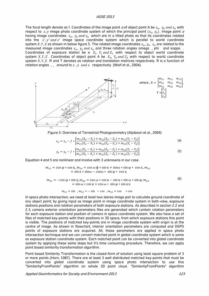
AGSE 2013


The focal length denote as f. Coordinates of the image point a of object point A be , with

respect to , image photo coordinate system of which the principal point , . Image point a

having image coordinates , which are in a tilted photo as that its coordinates rotated

into the , image space coordinate system which is parallel to world coordinate

system , , as shown in below figure 5. The rotated image coordinates � , � , � are related to the

measured image coordinates , and three rotation angles omega �, phi � and kappa �.

Coordinates of exposure station be e , with respect to object world coordinate

system , , . Coordinates of object point A be , with respect to world coordinate

system , , . R and T denotes as rotation and translation matrices respectively. R is a function of

rotation angles �,�, � around to �, � �respectively (Wolf et al., 2004).

where , ,

T =

Figure 5: Overview of Terrestrial Photogrammetry (Aljoboori et al., 2009)

∗ (4)

∗ (5)

Equation 4 and 5 are nonlinear and involve with 3 unknowns in our case.

cosφ ∗ cos қ , cos ωɸ ∗ sin қ sinω ∗ sinφ ∗ cos қ ,sin қ ∗ sinω cosω ∗ sinφ ∗ cos қ

cosφ ∗ sin қ, cosω ∗ cos қ sin қ ∗ sinω ∗ sinφ,sinω ∗ cos қ cosω ∗ sinφ ∗ sin қ қ

sin � , sin � ∗ cos �, cos � � ∗ cos �

(6)

In space photo intersection, we need at least two stereo image pair to calculate ground coordinate of

any object point; by giving input as image point in image coordinate system in both-view, exposure

stations positions and rotation parameters of both exposure stations. As described in section 2.2 and

2.3, camera exterior orientation parameters files are generated which contain rotation parameters

for each exposure station and position of camera in space coordinate system. We also have a set of

files of matched key-points with their positions in 3D space, from which exposure stations this point

is visible. The positions of matched key-points are in image coordinate system with origin is at the

centre of image. As shown in flowchart, interior orientation parameters are computed and DGPS

points of exposure stations are acquired. All, these parameters are applied in space photo

intersection technique and we can convert matched point in global coordinate system which is same

as exposure station coordinate system. Each matched point can be converted into global coordinate

system by applying these same steps but it’s time consuming procedure. Therefore, we can apply

point based similarity transformation algorithm.

Point based Similarity Transformation is the closed-form of solution using least square problem of 3

or more points (Horn, 1987). There are at least 3 well distributed matched key-points that must be

converted into global coordinate system using space photo intersection to use this

“SimilarityFromPoints” algorithm on whole 3D point cloud. “SimilarityFromPoints” algorithm

AGSE 2013


estimates 3D similarity transformation parameters between two sets of corresponding points by

minimizing the distances between the points as calculated from equation 7. These transformation

parameters are applied on whole 3D colored point cloud to generate geo-referenced point cloud with

proper scale.

∗

Where, , , is the coordinate of ith

point in

local coordinate system

, , is the coordinate of ith

point in

global/mapping coordinate system.s is a scale factor; R is

a rotation matrix. , , is translation vector between

two coordinate system.

(7)

5 Execute method and Evaluation of results

As per methodology, camera calibration was performed to generate IOPs (intrinsic orientation

parameters) which will be used in the further steps. A Nikon D80 SLR (single lens reflex) digital

camera is a non-metric camera and has to be calibrated for accurate data extraction. Camera

calibration sheet (36 inch x 36 inch) which has 140 grid points and 4 control points was used. As per

Photo-Modeler-Scanner’s manual for camera calibration, it needs minimum 6 photographs from

different angle around the calibration sheet covering 80 % of image area. B/W image is more

preferable than color image. Camera should be mounted on the tripod for better calibration result. In

the present study, B/W photographs with 8 different angles have been taken on physical focal length

of 18 mm, imported into the camera calibration module and processed automatically. After the

calibration, focal length computed 18.494 mm. Location of principal point sensor (x, y) are 12.245

mm, 8.063 mm respectively. Sizes of CCD sensor (w, h) are 23.973 mm, 16.066 mm respectively. The

maximum point marking residual is 0.491 pixels, overall point marking RMSE is 0.126 pixels and total

error is 1.051 pixels. According to the Photo-Modeler-Scanner calibration manuals, maximum point

marking residual; and the overall point marking RMSE values should be lesser than 1.5 pixels and 1

pixel respectively. Thus our values are well within the recommended values of standard

specifications. IOPs have been used in data planning and space photo intersection process.

Figure 6: (a) Image acquisition on white marked point (b)GPS base (c)GPS rover at exposure station

position (Jariwala, 2013)

Leica DGPS 510 was used for exposure station position measuring of the IIRS main building (H =11.5

m). For proper image acquisition, minimum distance from building D = H/h = 15 m and baseline B =

Scale*w = 3.88 m (maximum baseline). Total 24 points are marked on sequential distance of 2.5 m

(with the use of measuring tape) with white color cross on ground to identify the exact location of

exposure station for positioning measurement. It is seen in Figure 6 (a), plumb-bob string is used to

centre the camera tripod on the same marked point. Spirit bubble is also used to level the tripod.

Image acquisitions have been taken on 3872 * 2592 resolutions in jpeg (Joint Photographic Experts

Group) format with physically 18 mm focal length. Photographs have been taken at healthy sunny

condition with no sun/shadow of building on white marked points. The coordinates of camera

exposure station were calculated using a GPS setup over the same ground point. The base was

setup on known location as shown in Figure 6 (b). Rover was setup over each marked ground points

with centering and leveling. Total 24 exposure station positions were measured in geodetic

coordinate system with datum WGS84 in rover. The ground control measurement has been post

processed in Leica SKI-PRO software. The configurations of base GPS receiver processing

AGSE 2013


parameters were used to resolve ambiguity. In order to resolve the ambiguity of the measured

points, some satellites have been excluded and the mask angles have been changed by analyzing the

ambiguity resolve status in software. The result of DGPS measurement was the position of white

marked point; therefore a vertical offset of camera tripod (1.40 m) and camera electronic centre (6.5

cm) height has to be added to the ellipsoidal height of that point. Overall RMSE for exposure station

position marking is 4.047 cm and mean is 0.533 cm. The mean of error is near to zero that means

that there are random errors in measurements due to DGPS observation and measuring tape error.

5.1 Expected Accuracy for Stereo Photogrammetry

The theoretical accuracy is computed and it is expected that in the final oriented image the accuracy

should be within the range. So, it is necessary to calculate planimetric as well as depth accuracy

separately for both types of oriented images. Several aspects of quality are also considered as

accuracy of individual points. The sources of errors mainly appear from camera orientation and

resolution of images. Environmental factor and object properties can also contribute to total error

budget (Khoshelham, 2012). The approximations used are the simplified normal case, e.g.

horizontal/front view, same depth of camera above reference plane (Gerke et al., 2012). Expected

accuracy for re-sampled images are calculated from Gerke et al. (2012)’s ITC Lecture Note Series:

Image resolution ≈ 1704 x 1140, Pixel size, sx ≈ .

= 14.069 μm ≈ 14 μm, GSD = scale

factor*pixel size = 811*14 μm = 1.135 cm., Spx = 2 pixel size = 2 × sx = 2 × 14 μm = 28 μm. SD = ×

Mb × Spx = .

811× 28 μm = 0.136 m (Depth Accuracy). SX = Mb×sx= 811 × 14 μm ≈ 0.012 m

(Parallel Accuracy). These re-sampled theoretical values are considered in accuracy assessment. If

the values are exceed than there may be some blunders or gross errors in data set.

5.2 Feature Extraction and Feature Matching

After the completion of image acquisition and DGPS survey, SIFT v4.0 was used for feature

extraction from images in our dataset. SIFT version can process grey scale images at maximum size

1800*1800 pixels. So, images are re-sampled using Microsoft Office Picture Manager 2007 to

1704*1140 resolution. ImageMagick (1999)’s Mogrify Command-Line tool was used to convert jpeg

format image into pgm format (portable gray map format which is a simple gray scale image). SIFT

process images to generate key feature points and all information needed for matching them which

can be exported to ASCII (American Standard Code for Information Interchange) format file. SIFT has

128 descriptors for each particular extracted key point in one image. There are 24 images with total

102339 key points and 102339*128 = 13099392 descriptors which extracted in 21.86 seconds in

specified computer system. The visualization of SIFT key features are shown in Figure 7 (a).

Figure 7: Results of Features Extraction, Features Matching, Features Matching Images after RANSAC

Snavely (2010)’s Bundler v0.3 was used to run complete binary package of feature matching

algorithm and bundle adjustment (Lourakis et al. (2009)’s SBA v1.5). There are four steps involved in

generation of 3D sparse reconstruction and camera parameter files as per Bundler’s manual of

Snavely (2010). In the feature matching step of Bundler, processing between pre and post 4

sequences of images for each image was done using the ANN library. Figure 7(b) shows image pairs

(14, 18) which have 129 feature matches. Figure 8 (a) shows number of feature matching in pair of

images as bar diagram. From that plot, it is clear that matched features between consecutive images

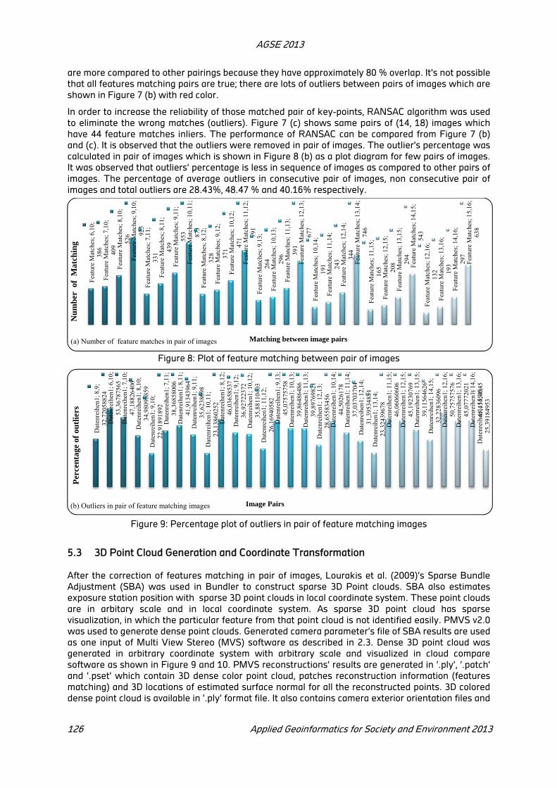
AGSE 2013


are more compared to other pairings because they have approximately 80 % overlap. It’s not possible

that all features matching pairs are true; there are lots of outliers between pairs of images which are

shown in Figure 7 (b) with red color.

In order to increase the reliability of those matched pair of key-points, RANSAC algorithm was used

to eliminate the wrong matches (outliers). Figure 7 (c) shows same pairs of (14, 18) images which

have 44 feature matches inliers. The performance of RANSAC can be compared from Figure 7 (b)

and (c). It is observed that the outliers were removed in pair of images. The outlier’s percentage was

calculated in pair of images which is shown in Figure 8 (b) as a plot diagram for few pairs of images.

It was observed that outliers’ percentage is less in sequence of images as compared to other pairs of

images. The percentage of average outliers in consecutive pair of images, non consecutive pair of

images and total outliers are 28.43%, 48.47 % and 40.16% respectively.

Figure 8: Plot of feature matching between pair of images

Figure 9: Percentage plot of outliers in pair of feature matching images

5.3 3D Point Cloud Generation and Coordinate Transformation

After the correction of features matching in pair of images, Lourakis et al. (2009)’s Sparse Bundle

Adjustment (SBA) was used in Bundler to construct sparse 3D Point clouds. SBA also estimates

exposure station position with sparse 3D point clouds in local coordinate system. These point clouds

are in arbitary scale and in local coordinate system. As sparse 3D point cloud has sparse

visualization, in which the particular feature from that point cloud is not identified easily. PMVS v2.0

was used to generate dense point clouds. Generated camera parameter’s file of SBA results are used

as one input of Multi View Stereo (MVS) software as described in 2.3. Dense 3D point cloud was

generated in arbitrary coordinate system with arbitrary scale and visualized in cloud compare

software as shown in Figure 9 and 10. PMVS reconstructions’ results are generated in ‘.ply’, ‘.patch’

and ‘.pset’ which contain 3D dense color point cloud, patches reconstruction information (features

matching) and 3D locations of estimated surface normal for all the reconstructed points. 3D colored

dense point cloud is available in ‘.ply’ format file. It also contains camera exterior orientation files and

Fea

ture

Mat

ches

; 6,1

0;

386

Fea

ture

Mat

ches

; 7,1

0;

409

Fea

ture

Mat

ches

; 8,1

0;

526

Fea

ture

Mat

ches

; 9,1

0;

925

Fea

ture

Mat

ches

; 7,1

1;

331

Fea

ture

Mat

ches

; 8,1

1;

439

Fea

ture

Mat

ches

; 9,1

1;

553

Fea

ture

Mat

ches

; 10,

11;

873

Fea

ture

Mat

ches

; 8,1

2;

328

Fea

ture

Mat

ches

; 9,1

2;

371

Fea

ture

Mat

ches

; 10,

12;

471

Fea

ture

Mat

ches

; 11,

12;

791

Fea

ture

Mat

ches

; 9,1

3;

264

Fea

ture

Mat

ches

; 10,

13;

296

Fea

ture

Mat

ches

; 11,

13;

391

Fea

ture

Mat

ches

; 12,

13;

677

Fea

ture

Mat

ches

; 10,

14;

191

Fea

ture

Mat

ches

; 11,

14;

243

Fea

ture

Mat

ches

; 12,

14;

344

Fea

ture

Mat

ches

; 13,

14;

746

Fea

ture

Mat

ches

; 11,

15;

165

Fea

ture

Mat

ches

; 12,

15;

208

Fea

ture

Mat

ches

; 13,

15;

294

Fea

ture

Mat

ches

; 14,

15;

543

Fea

ture

Mat

ches

; 12,

16;

132

Fea

ture

Mat

ches

; 13,

16;

193

Fea

ture

Mat

ches

; 14,

16;

297

Fea

ture

Mat

ches

; 15,

16;

638

Num

ber

of

Mat

chin

g

Matching between image pairs(a) Number of feature matches in pair of images

Dat

enre

ihen

1; 8

,9;

32,7

2058

824

Dat

enre

ihen

1; 6

,10;

53

,367

8756

5D

aten

reih

en1;

7,1

0;

47,1

8826

406

Dat

enre

ihen

1; 8

,10;

34

,980

9885

9D

aten

reih

en1;

9,1

0;

22,9

1891

892

Dat

enre

ihen

1; 7

,11;

38

,368

5800

6D

aten

reih

en1;

8,1

1;

41,9

1343

964

Dat

enre

ihen

1; 9

,11;

35

,623

8698

Dat

enre

ihen

1; 1

0,11

; 23

,138

6025

2D

aten

reih

en1;

8,1

2;

46,0

3658

537

Dat

enre

ihen

1; 9

,12;

36

,927

2237

2D

aten

reih

en1;

10,

12;

35,8

8110

403

Dat

enre

ihen

1; 1

1,12

; 26

,169

4058

2D

aten

reih

en1;

9,1

3;

45,0

7575

758

Dat

enre

ihen

1; 1

0,13

; 39

,864

8648

6D

aten

reih

en1;

11,

13;

39,8

9769

821

Dat

enre

ihen

1; 1

2,13

; 28

,655

8345

6D

aten

reih

en1;

10,

14;

44,5

0261

78D

aten

reih

en1;

11,

14;

37,0

3703

704

Dat

enre

ihen

1; 1

2,14

; 31

,395

3488

4D

aten

reih

en1;

13,

14;

23,3

2439

678

Dat

enre

ihen

1; 1

1,15

; 46

,060

6060

6D

aten

reih

en1;

12,

15;

45,1

9230

769

Dat

enre

ihen

1; 1

3,15

; 39

,115

6462

6D

aten

reih

en1;

14,

15;

32,2

2836

096

Dat

enre

ihen

1; 1

2,16

; 50

,757

5757

6D

aten

reih

en1;

13,

16;

45,0

7772

021

Dat

enre

ihen

1; 1

4,16

; 45

,454

5454

5D

aten

reih

en1;

15,

16;

25,3

9184

953

Per

cent

age

of o

utli

ers

Image Pairs(b) Outliers in pair of feature matching images

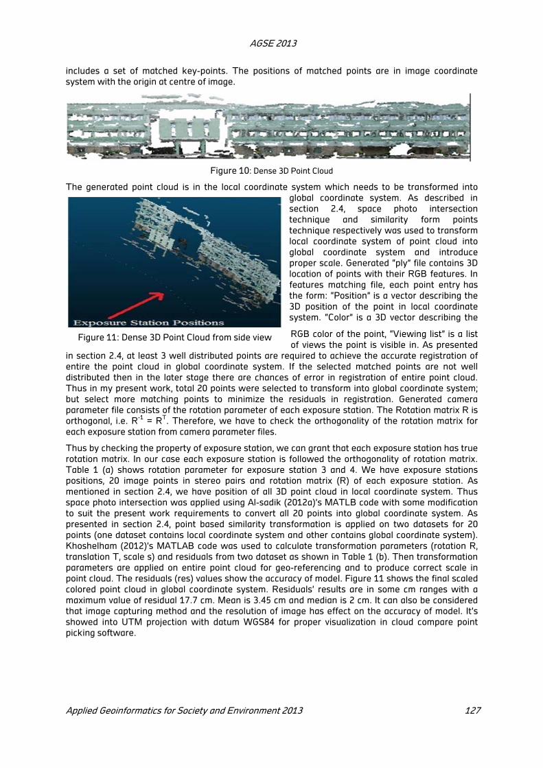
AGSE 2013


includes a set of matched key-points. The positions of matched points are in image coordinate

system with the origin at centre of image.

Figure 10: Dense 3D Point Cloud

The generated point cloud is in the local coordinate system which needs to be transformed into

global coordinate system. As described in

section 2.4, space photo intersection

technique and similarity form points

technique respectively was used to transform

local coordinate system of point cloud into

global coordinate system and introduce

proper scale. Generated “ply” file contains 3D

location of points with their RGB features. In

features matching file, each point entry has

the form: “Position” is a vector describing the

3D position of the point in local coordinate

system. “Color” is a 3D vector describing the

RGB color of the point, “Viewing list” is a list

of views the point is visible in. As presented

in section 2.4, at least 3 well distributed points are required to achieve the accurate registration of

entire the point cloud in global coordinate system. If the selected matched points are not well

distributed then in the later stage there are chances of error in registration of entire point cloud.

Thus in my present work, total 20 points were selected to transform into global coordinate system;

but select more matching points to minimize the residuals in registration. Generated camera

parameter file consists of the rotation parameter of each exposure station. The Rotation matrix R is

orthogonal, i.e. R-1

= RT. Therefore, we have to check the orthogonality of the rotation matrix for

each exposure station from camera parameter files.

Thus by checking the property of exposure station, we can grant that each exposure station has true

rotation matrix. In our case each exposure station is followed the orthogonality of rotation matrix.

Table 1 (a) shows rotation parameter for exposure station 3 and 4. We have exposure stations

positions, 20 image points in stereo pairs and rotation matrix (R) of each exposure station. As

mentioned in section 2.4, we have position of all 3D point cloud in local coordinate system. Thus

space photo intersection was applied using Al-sadik (2012a)’s MATLB code with some modification

to suit the present work requirements to convert all 20 points into global coordinate system. As

presented in section 2.4, point based similarity transformation is applied on two datasets for 20

points (one dataset contains local coordinate system and other contains global coordinate system).

Khoshelham (2012)’s MATLAB code was used to calculate transformation parameters (rotation R,

translation T, scale s) and residuals from two dataset as shown in Table 1 (b). Then transformation

parameters are applied on entire point cloud for geo-referencing and to produce correct scale in

point cloud. The residuals (res) values show the accuracy of model. Figure 11 shows the final scaled

colored point cloud in global coordinate system. Residuals’ results are in some cm ranges with a

maximum value of residual 17.7 cm. Mean is 3.45 cm and median is 2 cm. It can also be considered

that image capturing method and the resolution of image has effect on the accuracy of model. It’s

showed into UTM projection with datum WGS84 for proper visualization in cloud compare point

picking software.

Figure 11: Dense 3D Point Cloud from side view

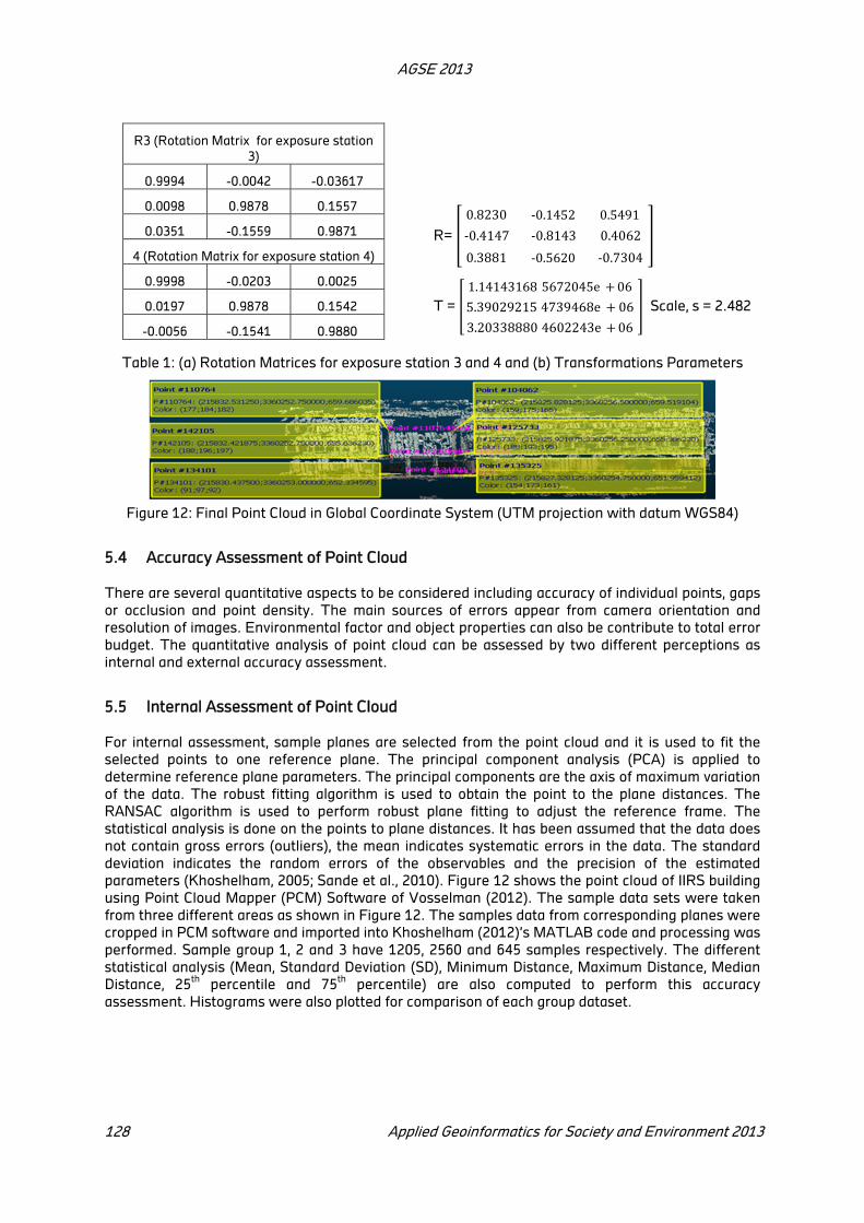
AGSE 2013


Table 1: (a) Rotation Matrices for exposure station 3 and 4 and (b) Transformations Parameters

Figure 12: Final Point Cloud in Global Coordinate System (UTM projection with datum WGS84)

5.4 Accuracy Assessment of Point Cloud

There are several quantitative aspects to be considered including accuracy of individual points, gaps

or occlusion and point density. The main sources of errors appear from camera orientation and

resolution of images. Environmental factor and object properties can also be contribute to total error

budget. The quantitative analysis of point cloud can be assessed by two different perceptions as

internal and external accuracy assessment.

5.5 Internal Assessment of Point Cloud

For internal assessment, sample planes are selected from the point cloud and it is used to fit the

selected points to one reference plane. The principal component analysis (PCA) is applied to

determine reference plane parameters. The principal components are the axis of maximum variation

of the data. The robust fitting algorithm is used to obtain the point to the plane distances. The

RANSAC algorithm is used to perform robust plane fitting to adjust the reference frame. The

statistical analysis is done on the points to plane distances. It has been assumed that the data does

not contain gross errors (outliers), the mean indicates systematic errors in the data. The standard

deviation indicates the random errors of the observables and the precision of the estimated

parameters (Khoshelham, 2005; Sande et al., 2010). Figure 12 shows the point cloud of IIRS building

using Point Cloud Mapper (PCM) Software of Vosselman (2012). The sample data sets were taken

from three different areas as shown in Figure 12. The samples data from corresponding planes were

cropped in PCM software and imported into Khoshelham (2012)’s MATLAB code and processing was

performed. Sample group 1, 2 and 3 have 1205, 2560 and 645 samples respectively. The different

statistical analysis (Mean, Standard Deviation (SD), Minimum Distance, Maximum Distance, Median

Distance, 25th

percentile and 75th

percentile) are also computed to perform this accuracy

assessment. Histograms were also plotted for comparison of each group dataset.

R=

0.8230 ‐0.1452 0.5491

‐0.4147 ‐0.8143 0.4062

0.3881 ‐0.5620 ‐0.7304

T =

065672045e1.14143168

064739468e5.39029215

064602243e3.20338880

Scale, s = 2.482

R3 (Rotation Matrix for exposure station

3)

0.9994 -0.0042 -0.03617

0.0098 0.9878 0.1557

0.0351 -0.1559 0.9871

4 (Rotation Matrix for exposure station 4)

0.9998 -0.0203 0.0025

0.0197 0.9878 0.1542

-0.0056 -0.1541 0.9880

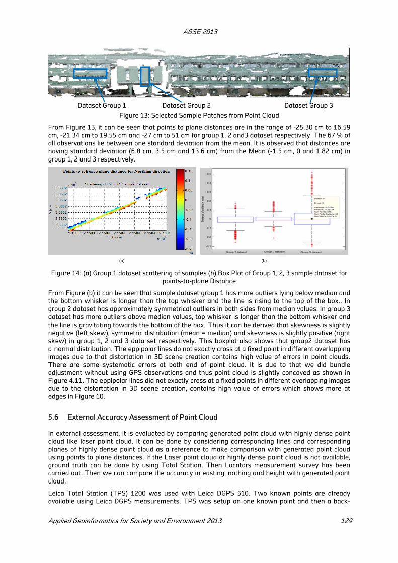
AGSE 2013


Dataset Group 1 Dataset Group 2 Dataset Group 3

Figure 13: Selected Sample Patches from Point Cloud

From Figure 13, it can be seen that points to plane distances are in the range of -25.30 cm to 16.59

cm, -21.34 cm to 19.55 cm and -27 cm to 51 cm for group 1, 2 and3 dataset respectively. The 67 % of

all observations lie between one standard deviation from the mean. It is observed that distances are

having standard deviation (6.8 cm, 3.5 cm and 13.6 cm) from the Mean (-1.5 cm, 0 and 1.82 cm) in

group 1, 2 and 3 respectively.

(a) (b)

Figure 14: (a) Group 1 dataset scattering of samples (b) Box Plot of Group 1, 2, 3 sample dataset for

points-to-plane Distance

From Figure (b) it can be seen that sample dataset group 1 has more outliers lying below median and

the bottom whisker is longer than the top whisker and the line is rising to the top of the box.. In

group 2 dataset has approximately symmetrical outliers in both sides from median values. In group 3

dataset has more outliers above median values, top whisker is longer than the bottom whisker and

the line is gravitating towards the bottom of the box. Thus it can be derived that skewness is slightly

negative (left skew), symmetric distribution (mean = median) and skewness is slightly positive (right

skew) in group 1, 2 and 3 data set respectively. This boxplot also shows that group2 dataset has

a normal distribution. The eppipolar lines do not exactly cross at a fixed point in different overlapping

images due to that distortation in 3D scene creation contains high value of errors in point clouds.

There are some systematic errors at both end of point cloud. It is due to that we did bundle

adjustment without using GPS observations and thus point cloud is slightly concaved as shown in

Figure 4.11. The eppipolar lines did not exactly cross at a fixed points in different overlapping images

due to the distortation in 3D scene creation, contains high value of errors which shows more at

edges in Figure 10.

5.6 External Accuracy Assessment of Point Cloud

In external assessment, it is evaluated by comparing generated point cloud with highly dense point

cloud like laser point cloud. It can be done by considering corresponding lines and corresponding

planes of highly dense point cloud as a reference to make comparison with generated point cloud

using points to plane distances. If the Laser point cloud or highly dense point cloud is not available,

ground truth can be done by using Total Station. Then Locators measurement survey has been

carried out. Then we can compare the accuracy in easting, nothing and height with generated point

cloud.

Leica Total Station (TPS) 1200 was used with Leica DGPS 510. Two known points are already

available using Leica DGPS measurements. TPS was setup on one known point and then a back-

AGSE 2013


sight method was used. In back-sight method, the total station orientation was done using the

observation of one (or more) back-sight known point(s). Then Ground locators measurement survey

had been started and measured 22 locators as shown in Figure 14

Figure 15: Position of Locators using Leica Total Station on IIRS main Building

The ground locator points are measured in UTM projection with WGS84 datum. Generated 3D Point

cloud is also in global coordinate system in UTM projection with WGS84 datum as shown in Figure

11 and section 3.3. Corresponding locators points from the generated point cloud was selected

manually in Girardeau-Montaut (2012)’s cloud compare software using point picking tool. Then the

accuracy of generated 3D point cloud was assessed with respect to total station locator positions in

easting, height (planimetric) and northing (depth). From statistical analysis of locator differences

between total station value and generated point cloud, the locators were measured on the both end

side of buildings contain more errors and it will effect on RMSE values. As a result of it, there was

32.2 cm RMSE in easting and 23.5 cm RMSE in northing because the image orientation done in this

software without ground control points (GCP). There was 23.56 cm RMSE in northing (depth)

direction. Thus locators which are near to ground have more height diffrence as comapred to top

locators. Errors in the measurement of total station and DGPS also contribute to the total error

budgets of different locators.

6 Conclusion

Structure from Motion is an approach to reconstruct the surrounding 3D scene from 2D images and

generate projection matrices of exposure station. In this thesis, a new technique has been

implemented for direct geo-referencing by using SfM approach and space photo intersection with

linearization of collinearity equation. Sometime the epipolar lines do not exactly cross at a fixed point

in different overlapping images and due to which a distorted 3D scene (point cloud) was created. No

ground measurements were used in bundle adjustment, thus there was an error in the estimation of

orientation parameters and it was observed that the shape of the point cloud was concaved near

first and last edges of the scene, there were major error detected in easting and northing.

Acknowledgements

First author express his hearty gratitude to Mr. Bashar Al-Sadik, Ph.D. student, ITC, University of

Twente, The Netherlands for his technical help and support during this research work. We grateful

to Dr. Y.V.N. Krishna Murthy, the Director, IIRS and Dr. P.S. Roy, Former Director, IIRS for providing

us excellent research environment and infrastructure to carry out this research work. We also would

like to show our extreme gratitude to Mr. P.L.N. Raju, Dr. S. K. Srivastava and Ms. Shefali Agarwal,

IIRS for their constant support and providing critical inputs for making this research an invaluable

experience. First author gives special thanks to Prof. dr. ir. M.G. (George) Vosselman, associated

with ITC and Editor-in-Chief of ISPRS to assess his MSc thesis on same topic; and he also honored

by receiving lectures from Vosselman and Dr. ing. M. Gerke, ITC in the field 3D Geo-Information,

Point Clouds Assessments, Computer Vision Photogrammetry. He gives deepest gratitude to his

colleagues Ankur, Priyanka, Mansi, Sharath, Dipima, Deepu, Abdalla, Sai, Pavan, Shankar, Manisha

and Mayank for directly or indirectly helping him throughout my research work.

REFERENCES

Al-sadik, B. (2012a, 26th December 2012). Space photo intersection Retrieved 10th Feb 2013, from

Available on :: http://www.mathworks.in/matlabcentral/fileexchange/39648-space-photo-

intersection

AGSE 2013


Al-sadik, B. (2012b). Structure from Motion (SfM) Notes of Module 13: 3D Geoinformation from

imagery. ITC, university of Twente, Enschede, The Netherlands.

Aljoboori, B. S., Albakry, M., & Mansour, F. (2009). Close Range Photogrametry (i. A. language,

Trans.) Analytical Photogrammetry (pp. 185-222). Iran.

Arya, S., & Mount, D. M. (2010, 28th Jan 2010). ANN: A Library for Approximate Nearest Neighbor

Searching Retrieved 10th Feb 2013, from http://www.cs.umd.edu/~mount/ANN/

Brenner, C. (2005). Building reconstruction from images and laser scanning. International Journal of Applied Earth Observation and Geoinformation, 6(3–4), 187-198. doi: 10.1016/j.jag.2004.10.006

Dorota, A., Grejner-Brzezinska, Li, R., Haala, N., & Toth, C. (2004). From Mobile Mapping to

Telegeoinformatics: Paradigm Shift in Geospatial Data Acquisition, Processing, and Management.

American Society for Photogrammetry and Remote Sensing, 70(2), 197-220.

Fischler, M. A., & Bolles, R. C. (1981). Random sample consensus: a paradigm for model fitting with

applications to image analysis and automated cartography. Commun. ACM, 24(6), 381-395. doi:

10.1145/358669.358692

Furukawa, Y., & Ponce, J. (2010). Accurate, Dense, and Robust Multi-View Stereopsis. IEEE Trans. on Pattern Analysis and Machine Intelligence, 32(8), 1362-1376.

Gerke, M., Khoshelham, K., & Alsadik, B. (2012). Module 13: 3D GeoInformation from Imagery ITC Lecture Notes: ITC.

Girardeau-Montaut, D. (2012). CloudCompare Software V2 Retrieved 10th Feb 2013, 2013, from

Available on : http://www.danielgm.net/cc

Horn, B. K. P. (1987). Closed-form solution of absolute orientation using unit quaternions. Optical Society of America A, 4, 629.

ImageMagick. (1999). ImageMagick Mogrify Command-Line Tool Retrieved 10th Feb, 2013, from

http://www.imagemagick.org/script/mogrify.php

Jariwala, J. J., 2013. Mobile Mapping by integrating SfM approach with Global Navigation Satellite

System. Unpublished Master of Science’s Thesis, ITC, University of Twente, NL & IIRS, ISRO, India

JEP, Available on: http://scholar.google.co.in/citations?hl=en&user=4CLb9_wAAAAJ

http://www.itc.nl/Pub/Home/library/Academic_output/AcademicOutput.html?p=9&y=13&l=20

Khoshelham, K. (2005). Region refinement and parametric reconstruction of building roofs by

integration of image and height data. International Archives of Photogrammetry and Remote Sensing, IAPRS : XXXVI, part 3 / W 24, 6.

Khoshelham, K. (2012). Quality of Terrestrial Point Clouds Module 13, M.Sc. Lecture Notes. : ITC.

Lourakis, M. I. A., & Argyros, A. A. (2009). SBA: A software package for generic sparse bundle

adjustment. ACM Trans. Math. Softw., 36(1), 1-30. doi: 10.1145/1486525.1486527

Lowe, D. G. (1999). Object recognition from local scale-invariant features. Paper presented at the

Computer Vision, 1999. The Proceedings of the Seventh IEEE International Conference on.

Madani, M. (2001). Importance of Digital Photogrammetry for a complete GIS. Paper presented at the

5th Global Spatial Data Infrastructure Conference, Cartagena, Columbia.

Madsen, K., Nielsen, H. B., & Tingleff, O. (2004). Methods for non-linear least square problems.

Informatics and Mathematical Modelling, Technical University of Denmark.

Piras, M., Cina, A., & Lingua, A. (2008, 5-8 May 2008). Low cost mobile mapping systems: an Italian experience. Paper presented at the Position, Location and Navigation Symposium, 2008 IEEE/ION.

Pollefeys, M., Koch, R., Vergauwen, M., & Van Gool, L. (2000). Automated reconstruction of 3D

scenes from sequences of images. Isprs Journal of Photogrammetry and Remote Sensing, 55(4),

251-267. doi: 10.1016/s0924-2716(00)00023-x

Pu, S., & Vosselman, G. (2009). Knowledge based reconstruction of building models from terrestrial

laser scanning data. Isprs Journal of Photogrammetry and Remote Sensing, 64(6), 575-584. doi:

10.1016/j.isprsjprs.2009.04.001

AGSE 2013


Remondino, F., & El-Hakim, S. (2006). Image-based 3D Modelling: A Review. The Photogrammetric Record, 21(115), 269-291. doi: 10.1111/j.1477-9730.2006.00383.x

Sabzevari, R., Bue, A. D., & Murino, V. (2011). Structure from motion and photometric stereo for dense 3D shape recovery. Paper presented at the Proceedings of the 16th international

conference on Image analysis and processing: Part I, Ravenna, Italy.

Sande, C. v. d., Soudarissanane, S., & Khoshelham, K. (2010). Assessment of Relative Accuracy of

AHN-2 Laser Scanning Data Using Planar Features. Sensors, 10(9), 8198-8214.

Snavely, N. (2010, April 25, 2010). Bundler: Structure from Motion (SfM) for Unordered Image

Collections v0.4 Version 0.4. Retrieved 10th Feb, 2013, 2013, from Available on :

http://phototour.cs.washington.edu/bundler/#S4

Tian, Y., Gerke, M., Vosselman, G., & Zhu, Q. (2010). Knowledge-based building reconstruction from

terrestrial video sequences. Isprs Journal of Photogrammetry and Remote Sensing, 65(4), 395-408.

doi: 10.1016/j.isprsjprs.2010.05.001

Triggs, B., McLauchlan, P. F., Hartley, R. I., & Fitzgibbon, A. W. (2000). Bundle Adjustment - A Modern Synthesis. Paper presented at the Proceedings of the International Workshop on Vision

Algorithms: Theory and Practice.

Vosselman, G. (2012). Point Cloud Mapper : Programme for interactive modelling of buildings in laser scanner point clouds. The Netherlands.

Wolf, P. R., & Dewitt, B. A. (2004). Space Intersection by Collinearity Elements of Photogrammetry with application in GIS. United States: McGraw Hills Publication.

Xuexian, G., & Sidong, Z. (2009, 19-20 Dec. 2009). A Mobile System Using Lidar and Photogrammetry for Urban Spatial Objects Extraction. Paper presented at the Information Engineering and

Computer Science, 2009. ICIECS 2009. International Conference on.

Zhang, Y., Zhang, Z., Zhang, J., & Wu, J. (2005). 3D Building Modelling with Digital Map, Lidar Data

and Video Image Sequences. The Photogrammetric Record, 20(111), 285-302. doi:

10.1111/j.1477-9730.2005.00316.x

Zisserman, A., & Hartley, R. (2001). Relative Orientation Multiple View Geometry in Computer Vision.

University Press, Cambridge.

Crisis Mapping using Open Source GIS Tools, GEOSMS and Volunteered

Geographic Information System

Manjush Koshy a*

, Aditya Kumar b

a Disaster Informatics Coordinator, Disaster Management Division, Centre for Advanced Remote

Sensing and Environmental Studies, Thiruvananthapuram, Kerala (India) -

[email protected]

b Disaster Management Division, Centre for Advanced Remote Sensing and Environmental Studies,

Thiruvananthapuram, Kerala (India), [email protected]

KEY WORDS: Volunteered, Geographic, Information, GeoSMS, Open Source GIS, Crisis Mapping.

ABSTRACT

The most important resource for rescue and recovery during a natural disaster is timely information. Lack of precise information greatly hindered relief efforts, Geographic Information System (GIS) is a powerful tool in crisis mapping. Mobile, social networking and open source GIS technologies and Volunteered Geographic Information (VGI) present new opportunities for data collection in disaster management. Crowd sourced geospatial information also called neo-geography in conjunction with Open source geographic information systems (OSGIS) and Geo SMS can pool vital information required for disaster response. The 2010 Haiti earthquake has brought about significant change towards the approach of VGI, Ushahidi, NOULA, Open Street Map (OSM), and other volunteer-based efforts has picked up momentum. Disaster response agencies in Japan, Samoa and Taiwan are already using similar Open Geo SMS prototypes. This paper shows how VGI generated spatial data, geo-tagged SMS and OSGIS can ease the challenges of information triage in disaster response efforts. The online application can be accessed by volunteers or people affected by the hazard and can upload the coordinates of locations to websites like Open Street Map with an Internet connection or send location tagged Short Message Service (SMS) to friends and this information can then be updated on the website which can also be used by emergency personnel. This platform can act to broadcast the voices of disaster affected populations onto a map that the world can see and respond too.

1 Introduction

Disasters like the Tsunami in Indian Ocean of December 2004, Hurricane Katrina in September 2005,

earthquakes of Haiti in January 2010, Christchurch in February 2011 and Japan in March 2011 has

revealed their damage potential. Spatial data and related technologies, particularly Geographical

Information System (GIS), have proven crucial for understanding and communicating the spatial

distribution of risks associated with an area. However, there are problems with availability, access

and usage of spatial data for disaster management. The problems with spatial data become more

serious during disaster response in which reliable and up-to-date spatial data describing current

emergency situation required for planning, decision-making, and coordination activities are

unavailable. Local Spatial Knowledge (LSK) is one of the major prerequisites in effective disaster

response. Community engagement is increasingly recognized as a pre-requisite of good disaster

preparedness, capturing spatial data has always been a challenge and time consuming exercise, the

increasingly wide reach of the mobile phone, accessible to millions through village phones, family

members, and local people could perform to cater the needs of this spatial data requirements, Mobile

coverage is increasing year on year. The advantages offered by new technologies such as GPS

handsets and smart phones in communicating with communities need to be explored.

With the combination of mobile device technology, social networking and geospatial technologies a

new phase of geo-information applications in disaster management have evolved. This paper

focuses on a specific and rapidly evolving area of geospatial data and tools, a subset of social

networking and user-generated web content that has been termed volunteered geographic

information (VGI; Good child 2007) this Crowd sourced geospatial information in conjunction with

Open source geographic information systems can pool vital information required for disaster

AGSE 2013


response. The affected people can themselves take part in creation of spatial data over the web and

data can be directly stored on main server, which can then be used as critical information for

response activities.

The 2010 Haiti earthquake has brought about significant change towards the approach of VGI,

Ushahidi, NOULA, Open Street Map (OSM), and other volunteer-based efforts has picked up

momentum. Disaster response agencies in Japan, Samoa and Taiwan are already using similar Open

Geo SMS prototypes. The people who generate this data can be called volunteers, this entire

concept of making data is called Crowd sourcing where people who are in the vicinity of the disaster

creates the data. Crowd sourced information is information that is generated by a large

heterogeneous crowd people in the disaster-struck area share reports online people all over the

world help to process and distribute information. Crowd sourcing has proven to be an efficient

approach to quickly generate huge amounts of near real-time data on a given situation problems of

data processing and information integration especially in the early phase of a disaster response. The

best suitable example is Open Street map (http://www.openstreetmap.org) here data created online

can be shared and distributed freely. With the availability of GPS and GPRS/web on the mobile, data

sharing has become much easier so people can update the geospatial inventory using their smart

phones. This concept of data preparation by the people is the key factor for crowd sourcing in

disaster relief work. During an emergency the people can update the available maps with whatever

information he has pertaining to the hazard this may be location of flooded zones, wiped out roads,

stranded people or safer routes based on ground experience this makes the data highly relevant and

current for the response team and other disaster management activities.

2 Methodology

Technologies used in developing this crisis mapping application include Open Layers API, Geo

Server, Postgre SQL/Post GIS and Geo SMS (Open Source).

Open Source has played a major role in the development of GIS technology. It has brought a free

sharing of code which has helped in the development of major GIS application in terms of Web and

Desktop technologies. Free and Open Source GIS (FOSS GIS) tools and technologies are of great help

to aid organizations, NGOs and local authorities for cost effective disaster management solution.

Various research organizations are spending a great time in developing new functionalities which is

making it advanced day by day. Open source GIS has given the developing countries the confidence

to use it for their development planning. For example Geo server, UNM Map server etc. are some of

the mature web server used for putting the data on the web. API like Open Layer is being used by

large professionals all over the world for the web development and providing functionalities to the

web application.

Open Layers is a pure JavaScript library for displaying map data in most modern web browsers, with

no server-side dependencies. Highly extensible, it serves as the foundation of all of many web

mapping interfaces. Open Layers implements a JavaScript API for building rich web-based

geographic applications, similar to the Google Maps APIs, with one important difference Open Layers

is Free Software, developed for and by the Open Source software community.

Geo Server is an open source software server written in Java that allows users to share and edit

geospatial data. Designed for interoperability, it publishes data from any major spatial data source

using open standards. Geo Server is the reference implementation of the Open Geospatial

Consortium (OGC) Web Feature Service (WFS) and Web Coverage Service (WCS) standards, as well

as a high performance certified compliant Web Map Service (WMS). Geo Server forms a core

component of the Geospatial Web.

Postgre SQL is an Open Source RDBMS database which helps us to organize the data in an

organized way. It is developed in C++ and it supports all the major platform like Windows, Linux etc.

Postgre SQL/Post GIS is an open source relational database technology with spatial capabilities. Post

GIS is the spatial extension for Postgres which helps for storing of spatial data and perform queries

on top it. Postgis helps in fast rendering of data.

Geo SMS is a specification for geo tagging SMS messages. It works by embedding locations in the

message text, where the locations are formatted as 'geo' URIs as defined in RFC 5870. It was

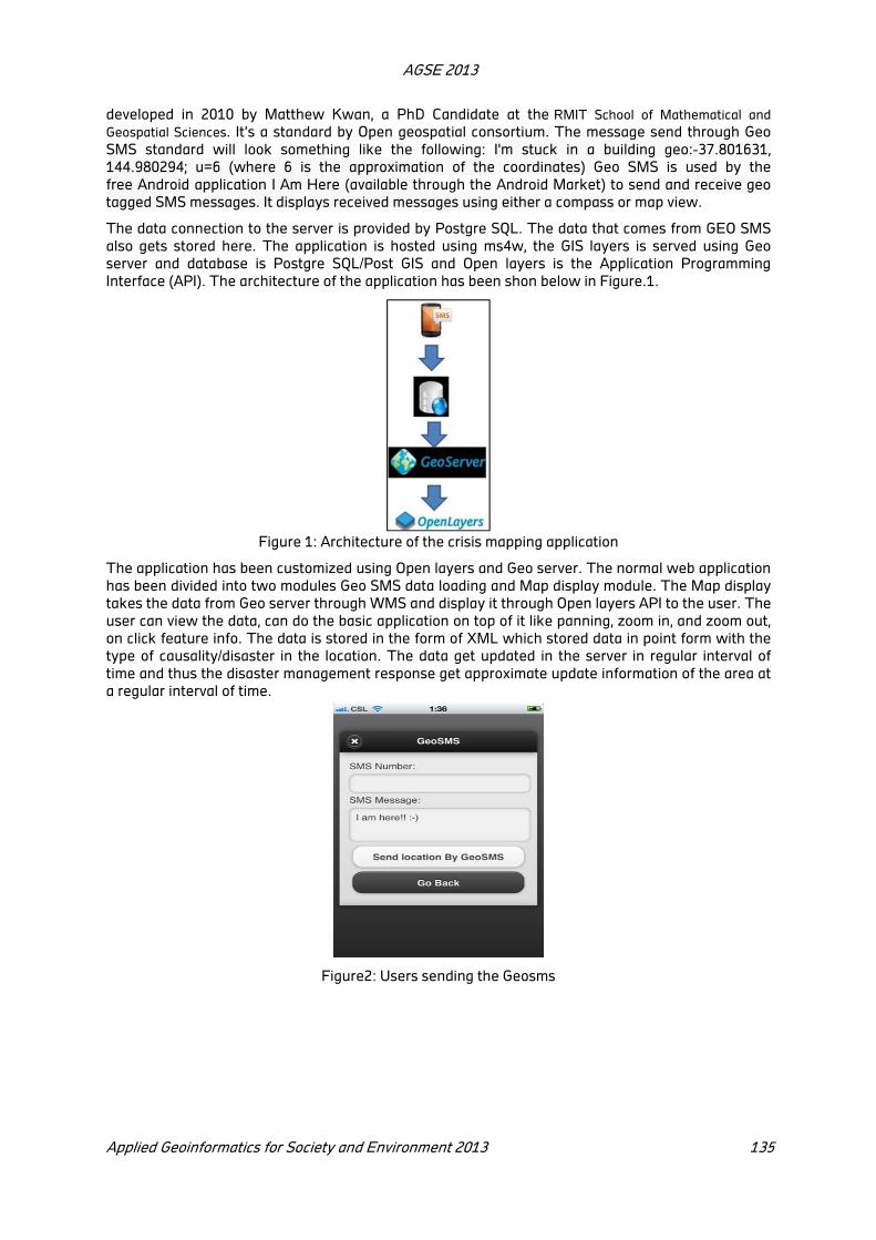
AGSE 2013


developed in 2010 by Matthew Kwan, a PhD Candidate at the RMIT School of Mathematical and

Geospatial Sciences. It’s a standard by Open geospatial consortium. The message send through Geo

SMS standard will look something like the following: I'm stuck in a building geo:-37.801631,

144.980294; u=6 (where 6 is the approximation of the coordinates) Geo SMS is used by the

free Android application I Am Here (available through the Android Market) to send and receive geo

tagged SMS messages. It displays received messages using either a compass or map view.

The data connection to the server is provided by Postgre SQL. The data that comes from GEO SMS

also gets stored here. The application is hosted using ms4w, the GIS layers is served using Geo

server and database is Postgre SQL/Post GIS and Open layers is the Application Programming

Interface (API). The architecture of the application has been shon below in Figure.1.

Figure 1: Architecture of the crisis mapping application

The application has been customized using Open layers and Geo server. The normal web application

has been divided into two modules Geo SMS data loading and Map display module. The Map display

takes the data from Geo server through WMS and display it through Open layers API to the user. The

user can view the data, can do the basic application on top of it like panning, zoom in, and zoom out,

on click feature info. The data is stored in the form of XML which stored data in point form with the

type of causality/disaster in the location. The data get updated in the server in regular interval of

time and thus the disaster management response get approximate update information of the area at

a regular interval of time.

Figure2: Users sending the Geosms

AGSE 2013


Figure3: User getting the sms from the sender Figure 4: Link gets open in the map

3 Conclusion

Disaster response agencies have limited resource and time to monitor and prepare plan during a

hazard. People in the vicinity of the hazard have the capability to respond fast with respect to data

sharing. There is a need to evolve a culture of preparedness among the people through public

awareness and training programs on the use of this system. This GEO SMS based crowd sourcing

application with GIS capabilities can be developed as a rich spatial resource base for disaster

management particularly disaster response. It is simple to use and could be given to local

organizations, NGO’s and even communities to improve resilience. The potential of crowd sourcing in

disaster response has only begun to be explored. This application can serve as a replacement for the

traditional methods of data collection and decision-making by provide instant, accurate, up-to-date

and low-cost crisis information for disaster management.

REFERENCE

Jens Ortmann, Minu Limbu, Dong Wang, and Tomi Kauppinen, Crowd sourcing Linked Open Data for Disaster Management. Institute for Geoinformatics, University of Muenster, Germany 2010.

Michael F. Good child and J. Alan Glennon, Crowd sourcing geographic information for disaster response: a research frontier- International Journal of Digital Earth, Vol. 3, No. 3, September 2010.

Ankit Sharma, Crowd sourcing Critical Success Factor Model Strategies to harness the collective intelligence of the crowd, Working Paper 1 – 2010

Kamel Boulos et al. Crowd Sourcing, Citizen Sensing and Sensor Web Technologies for public and environmental health surveillance and crisis management: trends, OGC standards and application examples- International Journal of Health Geographics 2011, 10:67

Prof. Muki Haklay, Interview on Crowd Sourcing, SDI magazine Saturday, 20 October 2012.

Using Web based Decision Support system and a participatory tool in

Harangi Irrigation Project

N.Sashikumar, A.S.Ravikumar

Department of Civil Engineering, University Visveswaraya College of Engineering, Jnanabharati

Campus

Bangalore, 560043, India, - [email protected], [email protected]

KEY WORDS: Participatory Irrigation Management, GIS, Decision Support, Earth Observation, Crop

water requirements

ABSTRACT

The rainfall zones in India vary from heavy precipitation areas to arid zones making it difficult to have an organised agriculture. Large dam projects are the main source of the irrigation. Remote sensing is used for mapping irrigated crop lands, for discriminating crop species, assessing crop stress, for monitoring temporal changes in irrigated area, develop agricultural system performance indicators for an irrigation system, estimate the yield of a major crop like rice and many other uses. But Earth Observation (EO) systems are yet to be applied as a framework of collecting and analysing multiple satellite platforms and in situ sensors to provide reliable and up to date information as user services to different stakeholders at a farm level in an Irrigation system. Hence, in the present study an attempt has been made to estimate crop water requirements for the command area of Harangi project through a web based open GIS and decision supporting system called System of Participatory Information, Decision support and Expert knowledge for irrigation River basin water management (SPIDER). This study demonstrates the use of SPIDER as a decision and stakeholder participatory tool to prioritize needs and quantity of water at branch canal, distributary, sub-distributary and field canal of Harangi command area for sustainable management of irrigation water in the command area.

1 Introduction

1.1 Agro climatic zones and river basins

Agricultural planning, research and location specific developmental activities in India are facilitated

by dividing its regions and sub-regions into 127 agro-climatic zones by National Agricultural

Research Project (NARP) of Indian Meteorological Department (IMD). The agro climatic zones are

based on the characteristics of soil, climate, rainfall and other meteorological and ecological

characteristics. The zones are delineated such that the soil type, rainfall pattern, cropping pattern

and available water for irrigation has fewer variations within a zone. The south west (SW) monsoon

accounts for 80% of the precipitation received in the country and it occurs during the months

between June and September. The uncertain and uneven rainfall distribution events with varying

agricultural water demands throughout the year necessities large storage or reservoirs for meeting

water requirements of growing crops. The National register for large dam’s shows that till January

2012 there are 5189 (completed and under construction) dams in the country. The dams or

reservoirs are built across the major rivers and streams. Entire India has been divided into 20 major

river basins comprising of 12 major basins having a combined catchment area of over 2.5 million km2.

Each of the 12 major river basins have a catchment area of above 20,000 km2.

1.2 Irrigation Infrastructure

Central Water Commission (CWC) of India estimates that Irrigation potential of the country is 140

Million Hectare (Mha), the Irrigation Potential created (IPC) is 123 Mha and Irrigation Potential

Utilised (IPU) is 91 Mha. The Net sown area and Gross sown area is estimated to be 141 Mha and

AGSE 2013


196 Mha respectively. Out of this 62 Mha is considered to be net irrigated area. The canal irrigation

remains as a source of water for 16.5 Mha. These figures are varying with other department

statistics like that of Planning Commission of India. Despite the high investment in creating irrigation

infrastructure, inadequate funding for Operation and Maintenance of the structures has resulted in

poor maintenance, poor delivery and deterioration. The crop water requirements are not met

resulting in low yield and low income to farmers. This has a direct impact on the revenue collected

for operation and maintenance. The area irrigated by major, medium and minor irrigation projects

has been stagnating or declining over the years.

1.3 Remote sensing in Irrigation development

Remote sensing is used for mapping irrigated crop lands, inventorying irrigated area from different

irrigation sources, such as surface water, groundwater, and irrigation tanks for discriminating crop

species and assessing crop stress, and for monitoring temporal changes in irrigated area. Remote

sensing along with Geographical Information system (GIS) and hydrological models offers number of

techniques for assessing irrigation potential, areal extent of irrigation, performance of irrigation

projects and management of irrigation projects. Earth Observation (EO) systems have developed into

a framework of systems collecting data from multiple sources: Multiple satellite platforms and in situ

sensors such as ground stations, air-borne and sea-borne sensors. Several countries offer Irrigation

Advisory Services (IAS) derived from EO system (Jochum and Calera, 2006). It is important that EO

derived information are made available as Irrigation Advisory Services (IAS) to farm at field level

1.4 Participatory Irrigation Management

In India, the concept of Participatory Irrigation Management(PIM) involving farmer's participation in

water distribution and management has been accepted as a water policy since 1987. Two of the

important objectives of PIM are 1) To make best use of natural precipitation and ground water in

conjunction with flow irrigation for increasing irrigation and cropping intensity and 2) To facilitate

the users to have a choice of crops, cropping sequence, timing of water supply, period of supply and

also frequency of supply, depending on soils, climate and other infrastructure facilities available in

the command areas. The planners in the Government recognized that the farmers are real

stakeholders in the irrigation system to plan crops and manage water required for growing them. A

part of the plan is also to transfer the fiscal responsibility to farmers for recovering costs of water

and use it for operation and maintenance of irrigation infrastructure. The legal framework of the PIM

provides formation of Water User Association (WUA), Distributary committee and Project committee

in an Irrigation project.

One of the important constraint on implementing PIM is that farmers are reluctant to take charge of

managing an system where already the water delivery is not reliable and responsive to farmer

needs. Further the water managers or engineers are not keen to share responsibility in managing

canal network operations and ensuring the assured water delivery to WUAs. Also head reach

farmers appropriate more water then required and maintain their status quo thus depriving the tail

enders their share of water. Lack of technical inputs and information on managing the system with

near real time assessment and feedback from the vast command area is also important factor

affecting the PIM implementation.

1.5 Overview

In this study an attempt has been made to relate crop coefficients to NDVI time series obtained for

command area of Harangi project by using a web based decision support system called System of

Participatory Information, Decision support and knowledge for irrigation River basin water

management (SPIDER). NDVI related to crop coefficients from different crop growth stages is used

to derive the crop water requirements. SPIDER is used to aggregate the vector, raster data from

multiple sensors like Landsat and IRS and field data for analysis and visualisation. Detailed cadsatral

maps of Marur Branch Canal (MBC) of Harangi with distributaries are made using high resolution

images. The analysis and visualisation of SPIDER is shared with WUA members and Irrigation

AGSE 2013


engineers and their feedback sought through a questionnaire is presented here for the irrigated

period of 2012.

2 Study area

Harangi Irrigation Project is located in Southern Indian State of Karnataka. River Harangi is a

tributary of river Cauvery. Harangi reservoir is located at latitude of 12° 29.638' N, and longitude of

75° 54.472' E. Cauvery is the important lifeline of irrigation in two southern states Karnataka and

Tamilnadu. The Cauvery originates at Talakaveri in the Western Ghats at an elevation of 1341m and

flows in the south-east direction till it reaches the shores of Bay of Bengal in Tamilnadu. The

Cauvery Basin is the second largest basin in Karnataka with 18 % of the total area of the state falling

within the basin. Cauvery basin's 42.20% of area falls within Karnataka. The command area covers

three administrative districts namely Coorg or Kodagu, Mysore and Hassan. Kodagu receives

abundant rainfall (400 cm) where as Mysore and Hassan receives rainfall of 76-114 cm. The

population of Hassan and Mysore districts depends on agriculture for their livelihoods by growing dry

crops like Ragi, Millet, etc. Efforts are made since 1884, to build a weir, Anicut, etc. The Harangi dam

constructions begin during 1972-73 forming a catchment area of 419.58 Sq. Km. The estimated

annual average yield is 37.70 billion cubic feet. Harangi reservoir gross storage capacity is 8.5 billion

cubic feet. As per the utilisation plan, wet crops are allowed for distributaries No 1 to 29 on the left

bank canal and distributaries No 1 to 10 in right bank canal including Koppa distributary. Fig.1 shows

the location map of Harangi command area. There are number of minor irrigation projects based on

tanks and anicuts having independent command areas. 50% of water is made available to these

independent command areas through tanks. Hence, the total utilisation of Harangi reservoir is

estimated to be 18 billion cubic feet for a mix of wet and dry crops. The irrigated area of Harangi is

54600 ha. Figure 1 shows the location map of Harangi command area and Figure 2 shows the

command area of Harangi

Figure 1: Location of Harangi command area

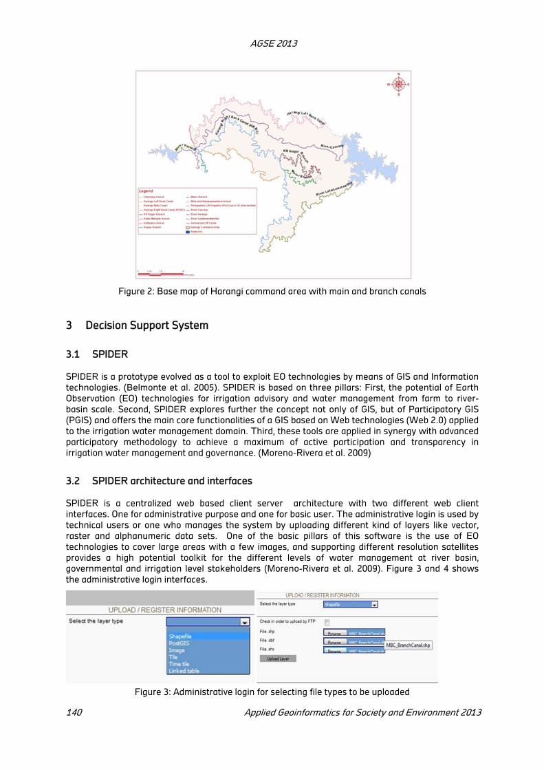
AGSE 2013


Figure 2: Base map of Harangi command area with main and branch canals

3 Decision Support System

3.1 SPIDER

SPIDER is a prototype evolved as a tool to exploit EO technologies by means of GIS and Information

technologies. (Belmonte et al. 2005). SPIDER is based on three pillars: First, the potential of Earth

Observation (EO) technologies for irrigation advisory and water management from farm to river-

basin scale. Second, SPIDER explores further the concept not only of GIS, but of Participatory GIS

(PGIS) and offers the main core functionalities of a GIS based on Web technologies (Web 2.0) applied

to the irrigation water management domain. Third, these tools are applied in synergy with advanced

participatory methodology to achieve a maximum of active participation and transparency in

irrigation water management and governance. (Moreno-Rivera et al. 2009)

3.2 SPIDER architecture and interfaces

SPIDER is a centralized web based client server architecture with two different web client

interfaces. One for administrative purpose and one for basic user. The administrative login is used by

technical users or one who manages the system by uploading different kind of layers like vector,

raster and alphanumeric data sets. One of the basic pillars of this software is the use of EO

technologies to cover large areas with a few images, and supporting different resolution satellites

provides a high potential toolkit for the different levels of water management at river basin,

governmental and irrigation level stakeholders (Moreno-Rivera et al. 2009). Figure 3 and 4 shows

the administrative login interfaces.

Figure 3: Administrative login for selecting file types to be uploaded

AGSE 2013


Figure 4: Administrative login for setting projection and layer extent

The basic client has an interface for accessing advanced information like maps, charts and reports

without a need for any technical knowledge of SPIDER. Figure 5 shows the interface for basic users

like farmers.

Figure 5: Basic user interface showing, maps, images, charts and tables for Marur branch canal of

Harangi

The features of this system are used to link time series of satellite images acquired. The chart is

interactive with link to image archives making it possible to view all images in the time series. This

helps in viewing different NDVI values and RGB images of a crop observed over a time for a point of

interest. The scale of data analysis is done from a field level to, branch canal level, to main canal and

to river basin. SPIDER is also multilingual capable, hence local language dictionary is used to display

information understandable to farmers.

4 Discussion of the application of SPIDER

4.1 NDVI relation with crop coefficient

A relationship Kc and NDVI is obtained by considering a linear relationship between the maximum

NDVI and the maximum Kc (at effective full cover) and the minimum (bare soil) NDVI and bare soil

Kc, respectively (Rocha, et al., 2010)

AGSE 2013


1.2246 ∙ 0.2203 (1)

where, Kc is crop coefficient and NDVI is Normalized differenced vegetation index

Figure 6 shows the image extract of survey plot no 200 of Marur branch canal during different

growth stages.

Figure 6: Satellite image of Survey plot no 200 in Marur branch canal showing green cover ( and

extract NDVI value) during different stages of crop growth

4.2 Feedback of stakeholders

The SPIDER analysis and visualization was presented to representatives of 27 distributaries of MBC.

About 35 stakeholders both farmers and engineers gave their feedback as given in Table 1. More

than 60% of the users felt the SPIDER tool will be very useful and informative for managing irrigation

water in their area.

Advantages of using SPIDER Very useful Useful Not useful I do not

know

in own working environment 64% 36% 0% 0%

in local community 68% 32% 0% 0%

SPIDER Ratings Very much To some

extent Very little

I do not

know

Willingness to introduce

SPIDER to others 67% 0% 33% 0%

Understanding of SPIDER

functionality 19% 58% 23% 0%

Table 1: Feedback on SPIDER from MBC stakeholders

5 Conclusion

The irrigation development has been stagnated and declining for last few years. Policy makers and

planners are desperately looking for various measures and new ways to revive the irrigation

development to ensure food security of the nation. PIM is important step to make the stakeholders

responsible for planning, managing and evaluating their irrigation systems. Tools like SPIDER with

the help of Earth observation data will enable transparent information across vast canal network and

as well as provide near real time feedback for decisions to be taken at various levels of canal

irrigation for managing and operating water releases, crop diseases or distresses.

REFERENCES

AGSE 2013


Belmonte, A. C., Jochum, A. M., GarcÍa, A. C., Rodríguez, A. M., & Fuster, P. L. 2005. Irrigation

management from space: Towards user-friendly products. Irrigation and Drainage Systems, 19(3-

4), 337-353.

Jochum, M.O. and Calera, A. 2006. Operational Space Assisted Irrigation Advisory Services:

Overview Of And Lessons Learned From The Project DEMETER. AIP Conference Proceedings,

852 (1): 3.

Moreno-Rivera, J. M., Osann, A., Calera, A., & Sanchez, A. 2009. SPIDER - An Open GIS application

use case for irrigation water management. First Open Source GIS UK Conference, Nottingham

Rocha, J., Perdigão, A., Melo, R., Henriques, C. 2010. Managing water in agriculture through remote

sensing applications. In: R. Reuter (Ed.) EARSeL symposium on remote sensing for science,

education, and natural and cultural heritage.

Acknowledgment

The authors are thankful to European Union’s Seventh Framework Programme (FP7) for funding

SIRIUS project to Bangalore University and express gratitude to Prof Anna Osann, Coordinator of

SIRIUS Project, UCLM, Albacete, Spain for continuous monitoring and encouragement to implement

the project.

A Web Based Open Source GIS Application on Geoinformatics Education

in India

Shailesh Chaure

Department of Geology, Govt. Holkar Science College, Indore, M.P. (India), -

[email protected]

KEY WORDS: Open layers, MySQL, Geoinformatics, Web-GIS

ABSTRACT:

In India Geoinformatics courses are taught at 70 places, including 60 universities, 4 NIITs/IITs and 6 central government institutes. In this paper an attempt has been made to create a spatial database of all the universities/institutes of India offering courses in Geoinformatics. To make this database available to the GIS community and the young graduates aspiring to make career in this emerging field, a web-GIS application has been developed using open source tools. Client-side programming was done using openlayers, which is a JavaScript library for displaying map data in web browsers. For server-side programming another open source scripting language PHP was used. The database was created using open source database MySQL. The database contains the fields like the name of university/institute, the university website, the name of course and the latitude and longitude of the Institute/city. The application plots the locations of universities/Institutes on the Google Maps providing the facility of interactive viewing of locations of the institutes on the map of India along with a list of relevant details. Locations can be filtered on state/course name. A tool for buffer analysis is also added to find the universities/institutes within a radius of the specified distance from a selected geographic location. This interactive open source web-GIS application is available on author’s website (http://shaileshchaure.com).

1. Introduction

Geoinformatics is relatively a young and emerging discipline whose need and importance have been

sincerely acknowledged, particularly in India only during last 10 to 12 years. Geoinformatics

encompasses fields like Cartography, Photogrammetry, Remote Sensing, Geodesy, GIS, and other

advanced mapping technologies. The rapid increase in the number of application areas and

implementation of various projects both in public and private sectors have necessitated the need for

the intensive educational and training programmes at a larger scale. As such a number of Indian

educational Institutions have incorporated courses in GIS/Remote Sensing and Geoinformatics at

different levels. Some of the institutions like IIRS, IIT Mumbai, Anna University are pioneers in

imparting education in this field.

At present the information about the courses and the Institutes is not available at one place and so; it

becomes extremely difficult for a student to search for the right course and the appropriate institute

imparting it. The primary aim of this work has been to help the GIS community and the young

graduates aspiring to make their career in this emerging field. The objective of this work is to provide

the information about the various courses and institutes in India through an interactive web based

GIS application. To achieve the objective a spatial database was created and a web application was

developed by the author using open source data base and web programming tools. This interactive

web-GIS application is available on author’s website (http://shaileshchaure.com).

At present courses related to Geoinformatics are being taught at 70 different places in India including

60 Universities, 4 IITs/NIITs and 6 Government Institutes. About 50% of the institutes are located in

the states of Andhra Pradesh, Maharashtra, Tamilnadu and Utter Pradesh. Post Graduate level

courses (M.Sc. and M.Tech.) of about 2 years duration are offered by 48 institutes. PG Diploma

courses of about 1 year duration are offered by 24 institutes. Certificate courses (of less than 1 year

duration) are provided by 8 institutes. Table 1.0 shows the number of institutes in different states

along with the type of courses offered. Many institutes offer more than one type of course.

AGSE 2013


S.No

.

Name of State/

Union Territory

Institutes

offering

M.Sc./M.Tec

h

Institutes

offering

PG

Diploma

Institutes

offering

Certificate

Total

Number of

Institutes

1 Andhra Pradesh 7 1 2 9

2

Arunachal

Pradesh - - 1 1

3 Chhattisgarh - - 1 1

4 Delhi - - 1 1

5 Gujarat 1 1 - 2

6 Hariyana 2 1 - 3

7 Jammu & Kashmir 2 1 - 2

8 Jharkhand 2 1 1 2

9 Karnataka 3 3 - 5

10 Kerla 1 1 - 2

11 Madhya Pradesh 5 - - 5

12 Maharashtra 7 2 - 9

13 Orissa 1 1 - 2

14 Punjab 1 - - 1

15 Rajasthan 3 2 - 5

16 Tamilnadu 6 4 1 8

17 Uttar Pradesh 4 3 - 7

18 Uttarakhand 1 1 1 1

19 West Bengal 2 2 - 4

Total 48 24 8 70

Table 1: Number of Institutes and courses in different States of India.

2. Database Creation

The information about the courses was gathered from the brochures and websites of the

universities and institutes. Some of the data were collected from the websites providing the

information about various courses in India. The information about the courses was also collected

from the faculties and students of various universities. The data gathered from different sources

were duly verified from the official website of the concerned Institute/University. The spatial data i.e.

the location of the Institute/University were obtained from Google maps. To use this data in a web

environment a database was created in MySQL. The database contains the fields like the name of

the department/university/institute, the university website, name of the course, name of the state,

name and latitude and longitude of the Institute/city. In case of unavailability of the exact location of

the institute on the map, the latitude and longitude of the city were used. Free maps provided by

Google were used as the base maps to display the location of the Institutes and Universities. Google

street map is used as a default base layer, however any other layer like Google Physical or Google

satellite or Google hybrid can also be used as the base layer or map.

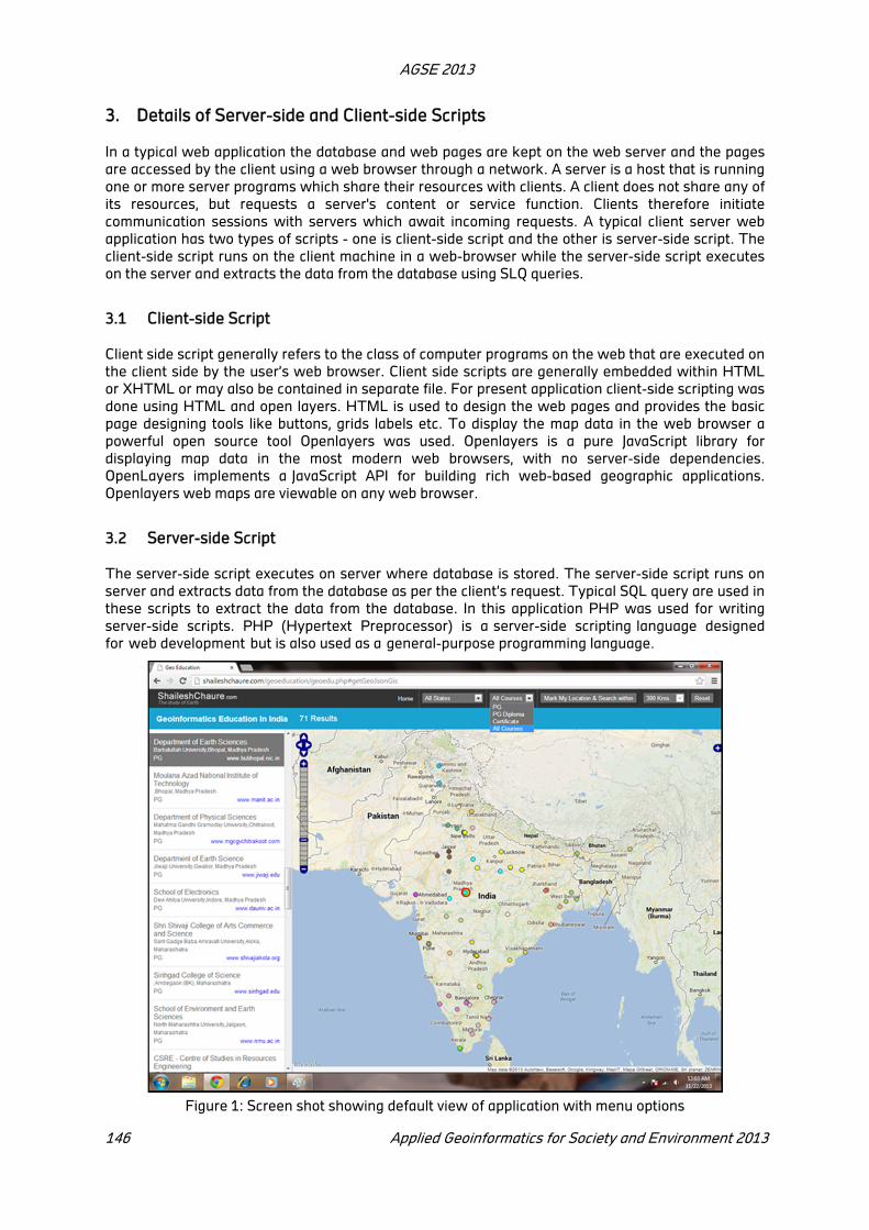
AGSE 2013


3. Details of Server-side and Client-side Scripts

In a typical web application the database and web pages are kept on the web server and the pages

are accessed by the client using a web browser through a network. A server is a host that is running

one or more server programs which share their resources with clients. A client does not share any of

its resources, but requests a server's content or service function. Clients therefore initiate

communication sessions with servers which await incoming requests. A typical client server web

application has two types of scripts - one is client-side script and the other is server-side script. The

client-side script runs on the client machine in a web-browser while the server-side script executes

on the server and extracts the data from the database using SLQ queries.

3.1 Client-side Script

Client side script generally refers to the class of computer programs on the web that are executed on

the client side by the user’s web browser. Client side scripts are generally embedded within HTML

or XHTML or may also be contained in separate file. For present application client-side scripting was

done using HTML and open layers. HTML is used to design the web pages and provides the basic

page designing tools like buttons, grids labels etc. To display the map data in the web browser a

powerful open source tool Openlayers was used. Openlayers is a pure JavaScript library for

displaying map data in the most modern web browsers, with no server-side dependencies.

OpenLayers implements a JavaScript API for building rich web-based geographic applications.

Openlayers web maps are viewable on any web browser.

3.2 Server-side Script

The server-side script executes on server where database is stored. The server-side script runs on

server and extracts data from the database as per the client’s request. Typical SQL query are used in

these scripts to extract the data from the database. In this application PHP was used for writing

server-side scripts. PHP (Hypertext Preprocessor) is a server-side scripting language designed

for web development but is also used as a general-purpose programming language.

Figure 1: Screen shot showing default view of application with menu options

AGSE 2013


4. Working of Application

Application displays a map of India along with the locations of the institutes/universities and a list of

the institutes showing details like name of department, courses offered and website. The user can

go to the institute website just by clicking on the link provided in the list on left hand side of the

screen. By default the information of all courses of all the states is shown. User can click on the point

showing the location of the institute on the map and the details of corresponding institutes are

highlighted in the list. Similarly a click on the name of the institute in the list highlights the location of

the institute on the map. User can selectively view the data of one particular state and/or particular

course. For this purpose two drop down boxes are provided on the menu bar containing a list of the

names of states and a list of the courses offered (Figure 1). Using this option the data related to the

selected state and the specific course name can be seen on the map. The list of the institutes

appearing on the left side of the page is also updated. This helps the user to filter down the

information.

Another useful option to find the universities/institutes within a radius of a specified distance from

the selected geographic location (Figure 2) is also provided. For using this option ‘Mark my location and search within’ option is available on the top menu bar. After clicking on this option user can mark

his location on the map visible in browser and a circle having radius of 300 km is drawn on the

clicked location and the places occurring within the circle are highlighted and the list is also updated.

The buffer distance i.e. the search radius can also be changed from the drop down list provided on

the top menu bar. Reset button can be used to clear the results. Controls for navigation and zooming

are provided on the map. It is possible to zoom out the map to see the location of institute on the

street map of cities.

Figure 2: Institutes within a radius of 400 km around selected location.

5. Conclusion

The database created for this analysis shows that total 80 courses are being run in India in 70

institutes/Universities. Out of the 28 States and 7 union territories, the Geoinformatics courses are

available only in 18 states and 1 union territory. Tamilnadu state has the maximum number of

AGSE 2013


courses (11 courses in 8 institutes) and the Hyderabad city of Andhra Paradesh has the maximum

number of institutes offering courses related to GIS and Remote Sensing.

References

Chanania Payal, 2012. A career in geoinformatics and remote sensing. Article in daily news paper - The Hindu. http://www.thehindu.com/todays-paper/tp-features/tp-opportunities/a-career-in-

geoinformatics-and-remote-sensing/article2992587.ece [accessed 10 March 2013]

GIS Courses in India. http://gisprog.wordpress.com/2008/09/07/giscourse/ [accessed 20 March 2013]

GIS Training Institutes in India. http://www.gisinindia.com/directory/gis-training-institutes-in-india

[accessed 26 March 2013]

Hazzard Erik, 2011. Openlayers 2.10 Beginners Guide, Packet Publishing Ltd. UK, pp. 7-9

Openlayers Documentation. http://docs.openlayers.org/ [accessed 20 April 2013]

Venugopal K., Senthil R., 2001. Geomatics Education in India – A view Point, 22nd

Conference on Remote Sensing, 5 - 9 Nov 2001, Singapore.

Open Source GIS Initiative For Managing Infrastucture & Utility Services

For Small Tows In Bangladesh

Md. Z. H. Siddiquee a,

Saad Md. Rafiul Alam Sidrata ,

Md. Manirul Haque a

a Institute of Water Modelling, House 496, Road: 32, New DOHS, Mohakhali, Dhaka-

1206,(Bangladesh), [email protected], [email protected], [email protected]

KEY WORDS: GIS, QGIS, Open Source, PostGIS, Post GreSQL, MDG, Sustainable Development,

Water Supply.

ABSTRACT:

Management of spatial data is an extremely important issue for any municipal authority with special reference to the developing countries like Bangladesh with a view to ensure sustainable development. Market leading proprietary GIS Solutions is almost unaffordable for the smaller municipalities due to the budgetary constraints. Here the necessity of open source solution comes into the scene. This study utilised an effective open source option namely QGIS for managing geo-information related to the infrastructure and utility services while PostGIS of Post GreSQL is deployed for back end database management. This approach will positively help to initiate, manage, control and plan the development in a desired direction. This will ensure the one stop services for retrieval of necessary information in a very fast and convenient way. This will help the authority to take the right decision with regards to the infrastructure and utility service management in keeping the Water Supply and Drainage Network properly functioning. Only a very few of the small towns in Bangladesh have proper water supply system. This approach will pave the way for achieving sustainable development targeted in the Millennium Development Goals (MDG) through the facilitation of better Water Supply Network management which leads to an access to the safe drinking water. The study area is located in the northern part of Bangladesh at Shibganj Pourashava under Chapai Nawabganj district where there is no piped water supply. Urban planner, city manager and utility manager can get benefited from this study.

1 Introduction

Shibganj Pourashava is small municipality lying north western part of Bangladesh with a total area

of 23.9 km and total population is projected for 2040 is 42889. The municipality is maintaining paper

based traditional management system for infrastructure and utility service information. In this way

management and planning is difficult for the authority especially in the field of infrastructure and

utility service for Water Supply and Drainage Network keep them properly functioning. Geospatial

Data makes it easier to generate and restore essential information for planning and management. In

this regard a convenient and easy to maintain geospatial data base management information system

is essential. This particular incident made us interested to carry out the study. This has been

implemented by using an open source technologies which are convenient for this small municipality.

2 Methodology

Pourashava MIS is developed by using an open source GIS (QGIS) in the front-end while an open

source database server (PostGreSQL) at the back-end. A new database is created in the PostGIS

using a username and password. Then QGIS is connected with the PostGIS database by using DB

Manager Tool. The shapefiles are then imported in the database for making it accessible by PostGIS.

The spatial data sets in the form of shapefiles are imported to template of the QGIS from PostGIS

database using add vector or raster layer tool. The MIS provides with query facilities for retrieving

information from the spatial data storage. The field calculator and query builder help to initiate

analyzing for planning and management.

AGSE 2013


3 Data and Software

This venture in developing ‘GIS based MIS’ is materialized using two major open source software,

namely QGIS and PostGreSQL. QGIS is easy and user friendly GIS solution with an interface quite

similar to the commercial GIS solutions available in market. There is also a Python console for

scripting in order to attain customise solutions. QGIS supports vector formats like OGR library,

including ESRI shape files, MapInfo, SDTS, GML and raster formats like GDAL (Geospatial Data

Abstraction Library), such as GeoTiff, Erdas Img., ArcInfo Ascii Grid, JPEG, PNG and many more The

data used in this study are Spatial data related to infrastructure and utility service, Demographic,

Hydro-geological data, Surface water related data. The courtesy shape files of the study area go to

Water Resource Planning Division, IWM.

4 Development

This section includes Data Preparation, Analysis and GIS based MIS Training.

4.1 Data Preparation

The vector and raster data set along with hydro-geological survey data and other necessary

information are imported to the QGIS for development of the initiative. The bench mark for survey is

used for data validation. Some raw GPS data are also imported to this MIS by directly connecting

GPS with QGIS using GPS tool. The layers are categorized with unique symbol and different types of

labels are used for easy identification of the features. The attribute table contain series of

information regarding the feature. The data imported are spatial data, Non-spatial data, Hydro-

geological data and others. The spatial data related to infrastructure are Road line Road type &

length, important structure; Features, Feature ID,, Bridge etc. The spatial data related to

administrative areas are Pourashava boundary, Ward boundary for individual ward of the

Pourashava, Water bodies, Major River etc. Non-spatial data are Population census data of 2001 to

2011 and predicted up to 2040. Hydro geological investigation data like Tube well design, total

depth, permeability, soil structure, boring and tube-well location etc. Drainage management data like

drain type, design, cross section of the nearby rivers and Water Supply Network management data

like pipeline network design, junction, water pump, valve, treatment plant & restorer design,

household detail survey data etc.

4.2 Analysis

A number of maps (Figure 1.2) have been prepared under this study with view to answer some of

vital questions like what is spatial distribution of natural and man-made water related future, what

are the composition of land cover as well as surface undulation of the study area. It is bookmarked in

different level of zooming for clear visibility and better impression. The maps were generated using

Bookmarks for defining layers. The bookmarks are defining like showing first country then the

district then the desired Pourashava boundary moving toward the smallest administrative unit ward

boundary to identical features, roads, water bodies and etc. Here the relevant information like area,

current population, and projected population along with other useful items will be available in pop-up

dialogue box. . If the user wants to know about specific area of a single ward he just has to click on

the ward using Identify Features tool. If the user wants to calculate a pond area, he just has to use

the Measure Area tool. New roads, water supply network, drainage distribution network and new

feature can be added to the database using QGIS drawing tools like new shape file layer tool. In this

way information retrieval and updating is easier.

At present the Shibganj Pourashava does not have any piped water supply so one of the major

focuses is on developing MIS contains information about Water Supply Network. Different symbol is

used to identify the individual designed pipe diameter, junction point, valves, pumps, reservoir,

surface water intake point, deep tube well location for better understanding the Water Supply

Network. The managers can easily take decision about the safe water source selection for municipal

water supply by just using the information system for comparing the available source like ground

AGSE 2013


water , surface water or even rainwater harvesting. For decision making of the source it displays

ground water information like soil structure condition, aquifer test result, ground water table, water

quality reports, lithology, aquifer type (Figure 1.1) etc and similarly for surface water information like

distance from the Pourashava, water quality, river cross section, water availability data for round the

year. In this information system some mathematical water modelling output data of IWM also

imported with spatial data for more effective planning and management of water resources.

The proposed network of water supply along with treatment plant and reservoir can be located in

the map and will help the authority to manage and control it for further planning and management. If

anyone asks about he’s possibility of getting a new water supply connection the authority can give

immediate response by just opening the water supply map and locating the person’s house in the

Pourashava. The authority can also see the area coverage of the proposed water pump for planning

water supply coverage for the Pourashava. Just using this MIS authority can take the decision for

selecting location of the dumping site using site selection criteria of spatial analysis. Digital Elevation

Model with respect to gravity flow and the road network give the excess for planning and

management of the drainage network (Figure 1.3) and water pipe line network design (Figure 1.5).

The existing drainage, proposed primary, secondary and tertiary drainage and the catchment’s area

of the drainage are identical because of different symbol and colour. The management professional

can see the drainage design and proposed network for estimation, reporting and to produce budget

for new projects. This information system also produces information regarding present and

projected future scenario of population that is related to infrastructure development, water demand

etc. The consolidated package of storage can provide useful information for planning, management

and monitoring of infrastructure and utility service data in both spatial and non-spatial aspect.

Figure 1: Displaying ground water condition Figure 2: Displaying physical features

4.3 GIS based MIS Training

Several training on ‘GIS based MIS’ has already been provided to the end users for better

understanding and capacity building. During training some suggestions were received from the end

users and the necessary steps have already been taken to improve the GIS based MIS’. The end

users receive the training cordially and convinced to use this approach for future in infrastructure

and utility management of the Pourashava. The venture is well appreciated by the Clients and end

users.

AGSE 2013


Figure 3: Proposed Drainages Network Figure 4: Infrastructure related information

5 Output

The information system is capable of storing of spatial data and non-spatial data like image, spread

sheet, text, audio and video. The outputs of the system can be made in the form of maps, report,

chart, processed information, specialized data support etc. There are also some predefined

cartographic items readily available for clear visibility and understanding. Some of them are stated

below.

Physical Feature Map (Figure 1.2)

Digital Elevation Model

Contour

Landuse

Water Supply Network (Figure1.5)

Drainage Network (Figure1.3)

Proposed Drainage Network

Proposed Water Supply Network

River Cross Section

Hydro-geological Information (Figure 6)

Figure 5: Displaying Water Supply Network Figure 6: Displaying spatial distribution of bore log

AGSE 2013


5.1 Limitations

The GIS based MIS could have been extended for making it functional over internet but

unfortunately this was out of the scope for our case. This can be a good point of starting for further

research in related open source initiatives.

6 Conclusions

This study envies a one stop repository for spatial data from where useful spatial and non-spatial

information can be generated with minimal effort. The end-users and management professionals of

the Pourashava can use it for quick information retrievable and generation with special focuses on

infrastructure and utility service management and planning. It can be a milestone for future open

source research initiative in Bangladesh.

REFERENCES

Government of Bangladesh, 2011.Population & Housing Census: Preliminary Results, Dhaka.

Ramsey, P. (2007). The State of Open Source GIS. Refractions Research, Victoria, BC, Canada.

Steiniger, S. and Bocher, E. (2009) An overview on current free and open source desktop

GIS developments, International Journal of Geographical Information Science.

Attribute Selection Using Texture Characteristic For Object Based Image

Classification

Srivastava M.a, Arora M. K.

a , Balasubramanian R.

b

aGeomatics Engineering, Department of Civil Engineering, IIT Roorkee, Roorkee 247667,

[email protected]

bDepartment of Mathematics, IIT Roorkee, Roorkee 247667

KEY WORDS: Object based image analysis, Attribute selection, Pearson’s correlation, and Texture

characteristics

ABSTRACT:

Object-based image classification is an approach to classify the remote sensing image on the basis of spectral, textural and contextual attributes in contrast to spectral attributes as in pixel based classification approach. There are number of attributes of an object but only few of them are effectively important to extract an object with respect to others from the segmented image. In this paper, the redundant attributes were removed by using correlation analysis and the texture attribute characteristics. To reduce the redundancy, correlation analysis was applied to detect the magnitude of the relationship between the attributes. Based on the correlation analysis, the attribute that had a high correlation coefficient with the other attributes was removed from the attribute set. For each object, out of 35 only 20 attributes including, spectral, textures, and contextual attributes for Quickbird pan image of Chandigarh area were selected. The attribute reduction and attribute selection are applied on the segmented image. The correlation analysis combined with texture characteristics is efficient in optimizing the attribute set and these attributes are further used for image classification.

1 Introduction

The conventional pixel based classification has limitation to classify high resolution satellite image as

it uses only spectral information (Scheiewe et al. 2001, Shackelford and Davis 2002). The object

based classification method is proposed to overcome this problem because they can incorporate

shape and texture information with spectral information. The spectral attribute of an image object is

the DN values, standard deviation of different image layers. However, textural attributes are

calculated using Gray Level Co-occurrence Matrix (GLCM), which is useful to detect roughness of the

object surface and the contextual attribute provides the image objects spatial information such as

shape, ratio etc. There are number of attributes of an object but only few of them are effectively

important to extract an object with respect to others from the segmented image.

The object based method can be performed in three steps. In the first step of segmentation is to

partition an image into non-overlapping, meaningful and homogeneous objects. The second step is

to remove irrelevant and redundant attributes by grouping of selected attributes. In the third step

these segments are assigned to class. The attributes used for classification in the object based

procedure are the objects characteristics, differing from those in pixel-based methods (Mueller et al.

2004, Doloca 2000).

2 Study area and data description

The area of this study is Chandigarh (India), which is the capitol of Punjab and Haryana and lies at

30o

46’ 12” N latitude and 76o

47’ 24’’E longitude. It is well planned city. Chandigarh has a robust and

well connected road and rail network with other parts of India. A cloud free high resolution (60 cm)

panchromatic band image taken by Quick-bird sensor was used for this work.

AGSE 2013


3 Methodology

3.1 Image segmentation

The basic elements of an object-oriented approach are image objects which are contiguous regions

in an image. Definiens professional uses multiresolution segmentation based on spectral and/or

spatial information and a scale parameter in combination with local and global optimization

techniques. The segmentation criterion follows pixel spatial continuity such as texture, shape, etc.

with their spectral values. Finally the image was segmented in 3418 segments at normal

segmentation mode with spectral/shape factor 0.8/0.2, compactness 0.9 and smoothness value 0.1

and scale parameter 52. The scale is the stopping criterion of segmentation, lower scale produces

large number of segments while it reduces with increase in scale value (Baatz and Schaper 1999).

The intra segment homogeneity depends on the size of the segment and inversely proportional to

the scale parameter.

3.2 Attribute Selection Using Correlation

To remove irrelevant and redundant attributes from the data set for increasing efficiency and

performance, attribute selection is generally applied. The optimum attribute set should contain the

least redundancy among attributes and the largest amount of information. To reduce the

redundancy, correlation analysis was first applied to detect the magnitude of the relationship

between the attributes (Yu and Liu 2003). A high correlation coefficient indicates that the two

attributes contain similar information, and also indicates that redundant information exists. The

Pearson’s correlation coefficient as described below has been applied for calculating the correlation

between attributes. Based on the correlation analysis, the pair of attributes with a high correlation

coefficient is first detected. The two attributes are then compared with the other attributes, and the

one that have a high correlation coefficient with the other attributes is removed from the attribute

set. The Pearson’s correlation coefficient between two attributes x and y of all N class is calculated

as;

(1)

3.3 Attribute Selection using Texture Characteristics

The Haralick grey-level co-occurrence matrix is one of the most popular second order statistics for

texture processing in remote sensing image analysis (Haralick and Shanmugam 1973). Gray Level

Co-occurrence Matrix (GLCM) texture attributes are basically divided into three groups; contrast

group, orderliness group and states group. Contrast group represents the homogeneity or contrast

within the land cover types, three texture attributes, namely; contrast, homogeneity and dissimilarity

are belongs to this group. The second group provides the information regarding the uniformity of the

land cover type surface, GLCM entropy, GLCM Angular 2nd

momentum (GLCM_ASM) and GLDV

Angular 2nd

momentum (GLDV_ASM) are belongs to this group. Third group is the states group and

provides the fundamental texture information of every land cover types. GLCM mean, GLCM

standard deviation and GLCM correlation are belongs to this group.

In the contrast group, contrast shows the homogeneity within the land cover type and varies

exponentially from 0 to 1, where 0 shows no contrast and 1represent high contrast or less

homogeneity. In similar manner dissimilarity varies linearly from 0 to 1. Entropy shows the first

order of uniformity between the land cover surfaces. High value of ASM occurs when the image

window is very orderly or uniform. The value of ASM varies from 0 for low order to 1for high order.

All three attributes, GLCM; mean, standard deviation and correlation of stats group represent

different texture characteristics. Mean reflects the brightness value, standard deviation shows the

N

yy

N

xx

N

yxxy

r2

2

2

2

AGSE 2013


variation in the data and the Correlation texture measures the linear dependency of grey levels on

those of neighboring pixels. The correlation values varies from -1 (no correlation) to +1 (high

correlation).

GLDV mean is similar to GLCM dissimilarity while GLDV contrast and GLCM contrast of an image are

calculated in similar manner and gives the same value hence Gray Level Difference Vector (GLDV)

mean and contrast have been eliminated from the list of texture attributes.


After segmenting the image with eCognition software it is exported with its 35 attributes for further

processing. Based on the characteristics of 7 different classes (road, resi_1, resi_2, barren land,

trees, shadow and water), 20 out of 35 attributes including spectral, texture, and shape have been

selected and formed attribute set. From these 20 selected attributes; 5 attributes are belongs to

spectral, whereas 9 attributes for shape and 6 for texture group.

4.1. Correlation Coefficient

The correlation coefficients between spectral and shape attributes with their correlation coefficients

are shown in table 1 and table 2 respectively. The attributes with high correlation coefficient 0.85

and above are not considered for further processing (Xiuying et al. 2010).

Mean Std deviation

Std

Deviation

to neighbor

Scene Ratio Mean diff

to neighbor

Mean 1 0.67 0.07 1 0.56

Std deviation

1 0.14 0.67 0.62

Std Dev. to

neighbor 1 0.07 0.09

Scene Ratio

1 0.56

Mean diff

neighbor 1

Table 1: correlation coefficients between selected spectral attributes

L/W

co

mp

actn

ess

Ell

ipti

ca

l fi

t

Sh

ap

e I

nd

ex

De

nsit

y

Asy

mm

etr

y

Bo

rde

r le

ng

th

Are

a

pe

rim

ete

r

L/W 1 0.07 -0.12 0.25 -0.63 0.73 0.16 -0.02 0.16

Compactness

1 -0.79 0.81 -0.67 0.2 0.41 -0.1 0.42

Elliptical fit 1 -0.8 0.77 -0.3 -0.38 0.15 -0.39

Shape Index 1 -0.69 0.3 0.68 0.01 0.68

Density 1 -0.72 -0.24 0.23 -0.24

Asymmetry 1 0.15 -0.06 0.16

Border

length 1 0.61 1

Area 1 0.61

perimeter 1

Table 2: correlation coefficients between selected shape attributes

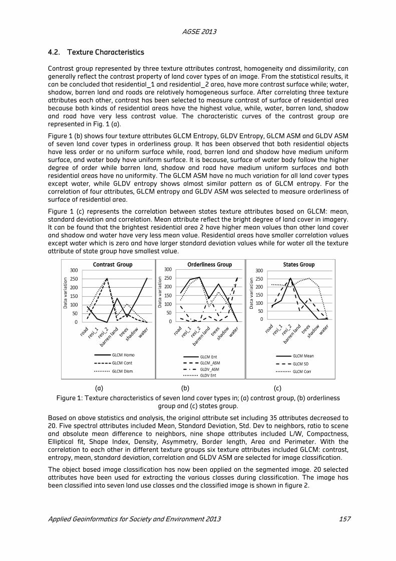
AGSE 2013


4.2. Texture Characteristics

Contrast group represented by three texture attributes contrast, homogeneity and dissimilarity, can

generally reflect the contrast property of land cover types of an image. From the statistical results, it

can be concluded that residential_1 and residential_2 area, have more contrast surface while; water,

shadow, barren land and roads are relatively homogeneous surface. After correlating three texture

attributes each other, contrast has been selected to measure contrast of surface of residential area

because both kinds of residential areas have the highest value, while, water, barren land, shadow

and road have very less contrast value. The characteristic curves of the contrast group are

represented in Fig. 1 (a).

Figure 1 (b) shows four texture attributes GLCM Entropy, GLDV Entropy, GLCM ASM and GLDV ASM

of seven land cover types in orderliness group. It has been observed that both residential objects

have less order or no uniform surface while, road, barren land and shadow have medium uniform

surface, and water body have uniform surface. It is because, surface of water body follow the higher

degree of order while barren land, shadow and road have medium uniform surfaces and both

residential areas have no uniformity. The GLCM ASM have no much variation for all land cover types

except water, while GLDV entropy shows almost similar pattern as of GLCM entropy. For the

correlation of four attributes, GLCM entropy and GLDV ASM was selected to measure orderliness of

surface of residential area.

Figure 1 (c) represents the correlation between states texture attributes based on GLCM: mean,

standard deviation and correlation. Mean attribute reflect the bright degree of land cover in imagery.

It can be found that the brightest residential area 2 have higher mean values than other land cover

and shadow and water have very less mean value. Residential areas have smaller correlation values

except water which is zero and have larger standard deviation values while for water all the texture

attribute of state group have smallest value.

(a) (b) (c)

Figure 1: Texture characteristics of seven land cover types in; (a) contrast group, (b) orderliness

group and (c) states group.

Based on above statistics and analysis, the original attribute set including 35 attributes decreased to

20. Five spectral attributes included Mean, Standard Deviation, Std. Dev to neighbors, ratio to scene

and absolute mean difference to neighbors, nine shape attributes included L/W, Compactness,

Elliptical fit, Shape Index, Density, Asymmetry, Border length, Area and Perimeter. With the

correlation to each other in different texture groups six texture attributes included GLCM: contrast,

entropy, mean, standard deviation, correlation and GLDV ASM are selected for image classification.

The object based image classification has now been applied on the segmented image. 20 selected

attributes have been used for extracting the various classes during classification. The image has

been classified into seven land use classes and the classified image is shown in figure 2.

AGSE 2013


Figure 2: Classified image

5 Conclusion

The generated attributes of all segments were divided into three groups, the spectral group, the

shape group and the texture group. The Pearson’s correlation coefficient was applied to the

attributes belong to the spectral and shape group, while the texture characteristic was used for

selecting the required attributes from the texture group. It is observed that the texture characteristic

curve appears very optimistic for selecting the attributes. Total 10 attributes belonging to texture

which are divided into three groups; the contrast, orderliness and states have been used. Six

attributes that appears different characteristics was selected for further processing.

REFERENCES

Baatz, M. and Schaper, A., 1999, Object-oriented and multi-scale image analysis in semantic

networks. In Proceedings of the 2nd International Symposium on Operationalization of Remote Sensing, 16–20 August, Enschede, The Netherlands, pp. 16–20.

Doloca, A., 2000, Feature selection for texture analysis using genetic algorithms. International Journal

of Computer Mathematics, 74, pp. 279–292.

Haralick, R.M., Shanmugam, K. and Dinstein, I., 1973, Textural features for image classification. IEEE Transactions on System, Man, and Cybernetics. SMC-3, pp. 610-621

Jon, A.B., 2003, Classification and feature extraction for remote sensing images from urban areas

based on morphological transformations. IEEE Transactions on Geoscience and Remote Sensing,

41, pp. 1940–1949

Mueller, M., Segl, K. and Kaufmann, H., 2004, Edge- and region-based segmentation technique for

the extraction of large, man-made objects in high-resolution satellite imagery. Pattern Recognition, 37, pp. 1619–1628.

Xiuying, Z., Xuezhi, F., and Hong, J., 2010, Object-oriented method for urban vegetation mapping

using IKONOS imagery. International Journal of Remote Sensing, 31, 1, pp. 177-196.

Yu, L. and Liu, H., 2003, Feature selection for high-dimensional data: a fast correlation-based filter

solution. In Proceedings of the Twentieth International Conference on Machine Learning (ICML-2003). T. Fawcett and N. Mishra (Eds.), 21–24 August 2003, Washington, DC, pp. 856–863.

Platform Independent Location Based Service For Finding Pharmacies

Using Open Source Gis Tools

S.T. Lamahewa1, N.G.C.M. Amarasinghe

2, K.L.V.S. Chathuranga

3, G.D.K.Ranasinghe

4, N.Fernando

5,

S.Rajapaksha6

Sri Lanka Institute of Information Technology, Malabe, Sri Lanka

{1sahan.lamahewa, 2

charithamadhu1, 3klvimukthies,

4dumiranasinnghe }@gmail.com , {

5nimalika.f,

6samantha.r}@sliit.lk

KEY WORDS: Medicine, Location Based Service. SMS, Low-end and High-end mobile phones,

openStreetMaps

ABSTRACT:

Finding a pharmacy which actually has the drug you want in a minimal time is a common requirement when looking for medicines, especially when the patient is in a fatal situation. It would be a lifesaving decision which may be difficult to be fulfilled by a general directory assistance service. This study propose a pharmacy finding location based service which can be accessed on any form of mobile device via multiple service modes to address the above issue. The proposed architecture consists of a location detection component, a searching engine for drug names and locations, a configuration script to feed real time drug availability from existing pharmacy inventory control systems to the system, a multi-mode result delivery component and an Administrative panel. It works in two modes, SMS and mobile Internet. In SMS mode, the location around which the medicine is searched for and the medicine name has to be send as a SMS. In the other mode, the automatic location detection based on the GPS, Cell-ID or Wi-Fi is also supported. Upon receiving the medicine name and the positioning information, location enabled searching is performed on a pharmacy location database and on drug availability records. Search results are shown in text form or as a mobile web map. A prototype is implemented based on a set of free and open source tools including OpenLayers, OpenStreetMaps and HTML5 GeoLocation API with a sample pharmacy database of Sri Lanka. It is tested successfully on several features phones and smart phones. The platform independency, support for multiple location detection methods, real time updates and use of open GIS tools are the main strengths of the proposed architecture.

1 Introduction

1.1 Background

Medicines are common requirements of any citizen of a country. While a free medical service is

available for any individual in Sri Lanka, many medicines have to be obtained at pharmacies due to

various reasons. While common medicines such as Paracetamol are available in almost all

pharmacies all kinds of medicines may not be readily available in every pharmacy of a country. The

high cost, the short life time and the non-frequent demand can be the common reasons behind the

non-availability of a medicine in a pharmacy. However, finding the medicine prescribed by a medical

doctor without delay is a lifesaving activity, especially when a patient is in a crucial situation. Even if

not, going from one pharmacy to another searching for a medicine is not a comfortable task for

anybody. This situation is aggravated when the patient is coming from a rural area to meet a medical

doctor in a main city. For him, as he may not be familiar with the surrounding, it would be difficult to

find a pharmacy to obtain his medicines. Additionally, there can be rare drugs which may be

available in some pharmacies only. Therefore, a mechanism to find a pharmacy where the drugs

required at the time being can be identified a common requirement of any person.

Information and communication technologies can be used effectively in addressing this issue

through pharmacy finding applications. As the service has to be provided to a person who may not be

at his home or office and the location of the pharmacy and the user also has to be considered, a

Location Based Service (LBS) application would be a suitable choice for a pharmacy finder

application. LBS is an intersection of three technologies, New Information and Communication

AGSE 2013


Technologies (NICTS) such as the mobile telecommunication system and hand held devices, Internet

and Geographic Information Systems (GIS) with spatial databases (Shiode et al. 2004). LBS can be

used to provide the location of the nearby pharmacies on a mobile device while the user is on the

move.

1.2 Related Work and Limitations

Mobile phone based solutions such as MyGlobeDoc (MyGlobeDoc,2012), Pharmacy Finder(Pharmacy

Finder,2012), CVS/pharmacy(CVS, 2012), Emergency Pharmacy Finder (EmergencyPharmacy-

Finder,2011), and web based solutions such as “findapharmacy” (findaPharmacy,1999) are some

already available systems to support finding pharmacies when in need.

“MyGlobeDoc” is a mobile application that covers pharmacies and medical professionals both. It finds

nearby doctors or pharmacies and links them with patients and sends information to family and

friends also. However it can be run only on iPhones and covers only USA at present. “Pharmacy

Finder” also is a USA based system with some similar functionality. “Emergency Pharmacy Finder”

shows all pharmacies in the city of Berlin on Android based mobile phones. Pharmacies are ordered

by distance based on GPS and/or WiFi positioning. “CVS Pharmacy” offers many features including

finding nearby CVS pharmacy via a iPhone app. All above solutions have used Google Maps API to

deliver the map data and map based information

One limitation of all four mobile phone based solutions above are they all run on one specific smart

mobile platform. Therefore they cannot run on any other mobile device which uses a different mobile

operation system than the platform the application is originally developed for. When it comes to

mass population and people in developing countries, smart phone may not be of much use for a

pharmacy finder application as it has to be accessed by all layers of the population. For example,

while 60% of the population of India is a mobile subscriber (mobiThinking, 2013), only 4% (Meeker,

2012) of them are smart phone users as at 2012. In such a situation, a solution which can be

accessed on both smart and non-smart phones would be more useful. Further, in all above systems

the location of the user is identified by the Global Positioning Systems (GPS) facility available in the

mobile phone. “CVS Pharmacy” considered Wi-Fi positioning also however none of the other

solutions consider any other location identification than GPS. Therefore, when the GPS facility fails,

there is no way to obtain the location information. None of the systems considers about whether a

particular medicine is available in a Pharmacy.

1.3 Proposed Solution

The proposed solution, Pharmacy Zone, is a LBS application which can be used to search nearby

pharmacies based on medicine names. It makes use of mobile Internet and Simple Messaging

Service (SMS) as the mode of communication and thereby attempts to reach a wider community. It

uses multiple methods of location identifications techniques such as GPS, Wi-Fi and Cell-ID

triangulation. This would support higher availability of the service. It further finds not just the

pharmacies nearby to user, but pharmacies with available stocks of a particular medicine. For that

real time updates of the medicine availability of different pharmacies are also considered. It offers

facility to search by city names as well so that a person can search for a pharmacy not based on the

current location but based on another location ( a city far away) also. A map of the location of the

pharmacy and the directions to reach the pharmacy are also provided for smart phone users. Freely

available open –source technologies, mapping platforms and map data are used in the

implementation of the proposed solution to make it low cost and easy extendibility.

2 Methodology

2.1 Proposed Architecture

The proposed solution consists of six main components. It offers a Mobile Internet based platform

independent mobile application and a SMS based system. Main components of the proposed system

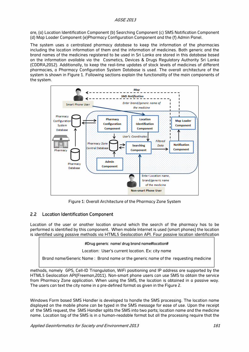
AGSE 2013


#Drug generic name/ drug brand name#location#

Location: User’s current location. Ex: city name

Brand name/Generic Name : Brand name or the generic name of the requesting medicine

are, (a) Location Identification Component (b) Searching Component (c) SMS Notification Component

(d) Map Loader Component (e)Pharmacy Configuration Component and the (f) Admin Panel.

The system uses a centralized pharmacy database to keep the information of the pharmacies

including the location information of them and the information of medicines. Both generic and the

brand names of the medicines registered to be used in Sri Lanka are stored in this database based

on the information available via the Cosmetics, Devices & Drugs Regulatory Authority Sri Lanka

(CDDRA,2012). Additionally, to keep the real-time updates of stock levels of medicines of different

pharmacies, a Pharmacy Configuration System Database is used. The overall architecture of the

system is shown in Figure 1. Following sections explain the functionality of the main components of

the system.

Figure 1: Overall Architecture of the Pharmacy Zone System

2.2 Location Identification Component

Location of the user or another location around which the search of the pharmacy has to be

performed is identified by this component. When mobile Internet is used (smart phones) the location

is identified using passive methods via HTML5 Geolocation API. Four passive location identification

methods, namely GPS, Cell-ID Triangulation, WiFi positioning and IP address are supported by the

HTML5 Geolocation API(Freeman,2011). Non-smart phone users can use SMS to obtain the service

from Pharmacy Zone application. When using the SMS, the location is obtained in a passive way.

The users can text the city name in a pre-defined format as given in the Figure 2.

Windows Form based SMS Handler is developed to handle the SMS processing. The location name

displayed on the mobile phone can be typed in the SMS message for ease of use. Upon the receipt

of the SMS request, the SMS Handler splits the SMS into two parts; location name and the medicine

name. Location tag of the SMS is in a human-readable format but all the processing require that the

AGSE 2013


location is given as coordinates. Therefore the name of the city is resolved to approximate

coordinates through a third party reverse-Geocoding service.

2.3 Searching Component

This handle the searching of pharmacies based on step1: the availability of particular medicine in a

pharmacy and the step 2: the distance between the user and the pharmacy. Step 1 uses the updated

real-time information from the Pharmacy Configuration System Database and filters the pharmacies

with the required medicine. It performs the search based on either or both generic and brand name

of the medicine which is provided by the user. If a user has misspelled a drug name/generic name

system provides guesses for those misspelled words. This facility is common for both mobile web

and the SMS service. Similar guessing is provided for location names in SMS based searching also. A

reply SMS is send in this case with possible guesses and user can re-type the message with correct

city /medicine names.

In the step 2 it filters nearest 10 pharmacies (a) based on user's current location (passive location

detection) and (b) city name provided by the user (active location detection). Either way the location

is identified by the “Location Detection Component” and is passed to searching component. The

distance between the pharmacy and the user location is identified based on the Haversine formula

(Rubin, 2006 ).

2.4 Notification Component

In the Mobile Internet based application, the notification component obtains the data from the

Search component and lists the nearby pharmacies, sorted by the distance between the pharmacy

and the location of the user. The address and the telephone number of the pharmacies are

displayed.

In SMS based solution SMS Handler process and sends the results. The system sends and receives

SMS by connecting a mobile phone or a GSM/GPRS modem to a computer and then using the

computer’s AT commands to instruct the mobile phone or the GSM/GPRS modem to send or receive

SMS messages. When user sends a SMS in the correct format as per Figure 2, the SMS Handler

receives it and generates the reply SMS according to the results received by the “Search

component”. Mobile phone or GSM/GPRS modem should be connected to the application via com

port and a configuration is done to initiate the application.

2.5 Map Loader Component

Smart phone uses are provided with the additional facility of viewing (a) a single pharmacy selected

from the search result (b) all pharmacies resulted in searching and (c) path from user location to the

pharmacy with navigation instructions. The map based results are shown in such a way that user

can clearly see the current location and the pharmacy concerned by adjusting the map extent.

2.6 Pharmacy Configuration Component

This component is used to update the availability of medicines at different pharmacies in the central

database in real time. It links a pharmacy’s database with the Pharmacy Zone central database by

installing a simple, low weight Pharmacy Configuration Database at each pharmacy. It is assumed

that pharmacies are already having a inventory control system with a Pharmacy Database. When a

client purchase a medicine from a pharmacy, pharmacy database’s quantity column will be updated

and a predefined trigger will be fired automatically. Trigger event helps to store updated data in a

Pharmacy Database into a Pharmacy Configuration Database’s temporary table. After a pre-defined

time, all the data in pharmacy configuration database’s temporary table is inserted into the

Pharmacy Zone central database by remote access protocols. In the initial configuration of the

system all the data related to generic name, brand name and quantity will update into the Pharmacy

Zone central database with pharmacy registration number.

AGSE 2013


3 Implementation

The prototype implementation of the proposed architecture is done mainly using set of open source

technologies while few components implemented in .Net environment. The mobile Internet based

application is implemented with HTML5 ,jQuery Mobile and PHP 5.5.0. The HTML5 Geocoding API

is used for location identification. The SMS Handler is implemented using Attention Commands (AT

Commands) in .Net environment. Figure 3 shows the implementation of the Haversine Formula in

PHP to access data from MySql database and do the required processing. Phone Gap, cross-platform

tool is used to build widgets for android, iOS and Windows Mobile platforms.

Figure 3: Haversing Formula implemented in PHP coding

The map data is obtained from openStreetMaps (OSM). openLayers mapping API (mobile version) is

used for map display. The TouchNavigation control in a smart phone allows to pan the map with

touch gestures on the screen’s "touchstart", "touchmove", "touchend" sequences and it also allows to

zoom in with double taps, and to zoom out with two-finger single taps. However the latter is only

available on devices supporting multi-touch and in most Android deices it is not supported when a

browser is used. Therefore the Zoom control widget of openLayers API which provides + and -

buttons for zooming in and out is used in this application. These buttons work on any device and

the zoom out button is especially needed for devices that don't support multi-touch.

The GeoNames Web Service is used for reverse geo-coding and YOURS Navigation Service is used

for path calculation. MySql is used as the Pharmacy Zone database. The Pharmacy Configuration

Component is implemented in such a way that it can access database of any technology provided the

proper connection string and the user authentication information are available.

The Pharmacy Zone database is filled with sample of 30 medicines and 22 sample Pharmacies

around city of Malabe are created for testing purposes. All these pharmacies are first mapped using

GPS coordinates obtained via a field visit.


The application is tested on several categories of smart phones, namely Windows Mobile (Nokia

Lumia 925), iPhone, Android phones(Sony Xperia L, Samsung Galaxy S II) and a Symbian phone

(Nokia C7-00) . Figure 4 shows the testing result of the application on a Android S II mobile phone.

When tested, the user is located at Isurupura, Malabe, Sri Lanka.

It can be accessed equally in all above devices as mobile Internet is used as the main mode of

application. The SMS facility is tested on all above Smart Phones and three non- smart phones ,

Nokia 5310, Nokia 1100 and Samsung Guru. All testing phones provide accessibility and the

functionally in same manner however as the screen size is large, smart phone based SMS facility

delivers better user experience.

AGSE 2013


(a) (b) (c) (d) (e)

Figure 4: Application on a Android smart phone Samsung Galaxy S II (a) start page with location

identification information,(b) Typing the medicine name, (c) Resulting Pharmacy list ( d) displaying of

selected pharmacy (Cargills Food City Pharmacy) on the map interface with the path to reach there

from the user’s current location,(e) results of SMS request for same query

Product GPS Cell-id SMS map API Offline

node

Platform Real time updates based

on availability of

medicines

MyGlobeDoc Yes No No Google Online iOS No

Emergency

Pharmacy Finder

Yes

Yes

No Google Online Android No

www.findapharma

cy.com.au

No No

No No Offline

Not

support for

No

CVS/pharmacy Yes No No Google Online Windows No

Pharmacy Zone Yes Yes Yes OSM Online runs on any

mobile

platform

Yes

Table 1: Comparison of the proposed LBS application with existing systems

5 Conclusion

The proposed LBS application assists in people of all walks of life to identify pharmacies which are

having medicines they require based on real-time updates of the medicine availability at different

pharmacies. Users can use SMS or Mobile Internet to obtain the service.The key strengths of this

architecture are (a) non-binding on any specific mobile platform and (b) the real time updates of

availability of medicines in and identification of pharmacies based on that.

Further, uses web-based GIS technologies in mobile context it shows the location of the pharmacies

and path to it also provided that the mobile device supports such functionality. The use of open APIs

and open data to implement GIS functionalities and map display enhance its accessibility as cost can

be minimized as well as it can be extended easily. The local language support and improved map

rendering with layer control would improve the quality of service of the proposed solution.

Acknowledgements

This work is done as a final year project of the of BSc.(IT) degree program of the Sri Lanka Institute

of Information Technology(SLIIT), Sri Lanka. Authors wish to acknowledge the assistance and

guidance provided by all staff members of the SLIIT in this study. The support provided by Mr.Amila

Marasinghe and the Dr. Malika Amarasinghe is also acknowledged.

AGSE 2013


REFERENCES

Cosmetics, Devices & Drugs Regulatory Authority (CDDRA),2012,http://www.cdda.gov.lk/[accessed

01.12.2013]

CVS/pharmacy,2012,http://www.cvs.com/promo/promoLandingTemplate.jsp?promoLandingId=mobil

e-apps /[accessed 01.12.2013]

Emergency Pharmacy Finder,2011 http://spreebytes.net/node/29 /[accessed 01.12.2013]

Freeman, E., 2011, Head First HTML5 Programming, “Making Your HTML Location Aware”, O'Reilly

Google. The Google Geocoding API. 11 June 2013.

https://developers.google.com/maps/documentation/geocoding

Meeker, M., Wu,L., 2012 “2012 KPCB Internet Trends Year-End Update”,

http://www.kpcb.com/insights/2012-internet-trends-update [accessed 01.12.2013]

mobiThinking, 2013, Global mobile statistics 2013 Part A: Mobile subscribers; handset market share;

mobile operators.http://mobithinking.com/mobile-marketing-tools/latest-mobile-

stats/a#indiasubs[accessed 01.12.2013]

MyGlobeDoc,2012 “MyGlobeDoc-Home” http://www.myglobedoc.com/ [accessed 01.12.2013]

OpenLayers, 2013, “OpenLayers: Free Maps for the Web” http://openlayers.org [accessed

01.12.2013]

OpenStreetMaps, 2013, http://www.openstreetmap.org/ [accessed 01.12.2013]

Pharmacy Finder,2012,

https://play.google.com/store/apps/details?id=scalardata.pharmacyfinder&hl=en /[accessed

01.12.2013]

Rubin,A, 2006 “Geo Distance Search with MySQL” http://www.scribd.com/doc/2569355/Geo-

Distance-Search-with-MySQL[accessed 01.12.2013]

Shiode,N., Li,C., Batty,M., Longley,P., and Maguire,D., 2004 “The impact and penetration of Location

Based Services,” in Telegeoinformatics, H. A. Karimi and A. Hammad, Eds. CRC Press, pp. 349-

366.

YOURS. 2012. http://wiki.openstreetmap.org/wiki/YOURS, [accessed 01.12.2013].

Web Enabled Resources Information System, a Case Study of the

Irrigation Sector

Tutu Senguptaa +

, Sangita Rajankara, Vivekanand Ghare

a, Vinod Bothale

b, Satish Sharma

c

a Maharashtra Remote Sensing Applications Centre, Nagpur

+ Research Scholar, Dept. of Physics, RTM Nagpur University, Nagpur

b National Remote Sensing Centre, ISRO, Govt. of India, Hyderabad

c Dept. of Electronics and Computer Science, RTM Nagpur University, Nagpur

KEY WORDS: Reference Model of Open Distributed Processing (RM-ODP), Unified Modeling

Language (UML), Geographic Information System (GIS), Geo-portal- Web site dealing with spatial

data, Graphic User Interface (GUI), Open GIS Consortium (OGC)

ABSTRACT

Spatial data has become the need of the hour. Whether it is planning process, implementation or monitoring, it becomes a boon if the data is represented spatially rather than mere tables, reports or discussion. Remote sensing with its capability of repetitive, synoptic and ability to view the Earth surface with different sensors of different spatial resolutions and spectral bands is an ideal tool to monitor the different Earth features. The information contents of the satellite image can then be easily converted into maps. Making intelligent maps and representation of the data on the web makes the data creation, updation and display a challenging task as the data depicted should be amenable to all. The present work deals with the creation of the database for irrigation sector and the way in which it is served through web services on the geo-portal which is a gateway to Web-based geospatial information and information services. It enables the user to view and access geospatial information and services made available by their sources on the internet. The requirements at the user end is as minimal as the internet connection with internet explorer 6.0 or higher (which is one of the most widely used web browsers), Mozilla Firefox which is a free and open source web browser, Google chrome and flash player 11.0 or higher.

1 Introduction

It has been reported that more than 80% of business and government information has some

reference to location [1]. A need has been recognised to empower civil society with geo-information

by integrating it with the IT infrastructure [2]. The metaphor of Spatial Data Infrastructure has been

widely welcomed to meet this need. Realistic and proper inventory, mapping and planning of the

existing resources are the key to success and development of any region. High end technological

tools are being continuously used for the purpose- like Remote Sensing and Geographic Information

System.

The decisions by Planners/ Scientist/Administrators can be taken if the data is available at the touch

of a button on the desktop and mostly in spatial format to visually understand the distribution of

resources. For this purpose, the web based technology of serving maps on the web along with

satellite pictures is crucial. With the introduction of the dynamic programming environment for the

web-application, some agencies have developed and implemented such applications like geo-portal

which can give the geographic information and their uses in more simplified form by displaying the

satellite images.

Tait (2005) defined a geo-portal as: “A Web site that presents an entry point to geographic content

on the Web or more simply, a Web site where geographic content can be discovered.”[3]

Geo-portal is a gateway to Web-based geospatial information and information services. It enables

user to discover, view and access geospatial information and services made available through

various sources. Sources of such information and services enable programmers to make geospatial

information and services discoverable, viewable and accessible by users via Internet.

AGSE 2013


The paper deals with the presentation of maps on the Geo-portal, being developed for state of

Maharashtra at Maharashtra Remote Sensing Applications Centre, Nagpur. The present work is

related to the Irrigation Department wherein the map data from the irrigation sector are digitized,

processed and given spatial reference, overlaid on satellite data, queried for changes in land use/

land cover and various other parameters and served to the user department via internet.

The geo-portal presents information about:

The geography of Maharashtra like its physiography, terrain, land use/ land cover, forest cover,

water bodies and drainages, geology, canal network etc.

Administrative boundaries like district, taluka, villages and cadastral and electoral boundaries of

the state.

Transport Network - Roadways and Railways, Demography status using census 2001 and

Census 2011, Disaster Management Infrastructure Mapping etc.

Agriculture is the mainstay of Indian economy with seventy percent of India’s population deriving its

livelihood from agriculture. Agriculture sector is vital for food security. Despite the importance of

agriculture in the Indian economy, however, the rate of growth of agriculture has decelerated in the

last decade to about 2% per annum as against 3.2% observed between 1980 and 1996-97. The

eleventh plan is counting on a 4% growth of the sector in the plan period to achieve its overall

growth target of 9%. Clearly, the crisis of stagnation in agriculture needs urgent attention.. For

strengthening agriculture, irrigation becomes a prerequisite for raising second and third crop in a

year and influences the cropping pattern by reducing the risk of crop failures and providing water

security. This enhances the agricultural production and may have an impact on food consumption,

life quality and socio-economic status. It is used to assist in the growing of agricultural crops,

maintenance of landscapes, and re-vegetation of disturbed soils in dry areas and during periods of

inadequate rainfall. Additionally, irrigation also has a few other uses in crop production, which

include protecting plants against frost, suppressing weed growing in grain fields and helping in

preventing soil consolidation.

In Maharashtra, most of the crops are rain-fed, failure or delay in monsoon adversely affects the

economy of the area with the impending fear of drought. A reliable and suitable irrigation water

supply can result in vast improvements in agricultural production and assure the economic vitality of

the region. Effective agronomic practices are essential components of irrigated systems.

Maharashtra is the leading industrialized state in India. The land developed so far in the state by the

large and medium-sized irrigation projects is only about 56 percent of the currently identified

ultimate potential of 4.1 million hectares. The state has a rugged terrain, and a large number of

rivers originate here, resulting in many comparatively small irrigation projects. The state spends Rs

10 to 12 billion every year to manage some 3 million hectares of surface irrigation. Hence the

continuous monitoring of the irrigation projects and their canal network along with the impact

assessment of the project need to be studied with the help of remote sensing and GIS techniques.

The information on the water and the irrigation projects need to be served on the web through

'intelligent' maps to the Planners.

Software and Data Used: Flex, PHP as frontend programming language and ArcGIS Server, MySql as

Backend support languages have been used. Also the huge repository of the digital resources

database at MRSAC has been used with ample ancillary data from Irrigation Department in the form

of maps and charts. ActionScript is an OOP language that encapsulates all of its functionality in

classes. The Flex framework includes libraries of pre-built classes that provide data retrieval and

handling, animation, GUI elements and layout, and much more. ActionScript was designed for

controlling simple 2D vector animations made in Adobe Flash with later versions added functionality

allowing for the creation of Web-based games and Rich Internet applications. MXML implements the

static aspects of any application, and ActionScript implements its dynamic aspects.

AGSE 2013


1.1 Geo-portal Objective

The geo-portal is projected to help in the following manner:

The government can have an overview of the resources of the state aided with maps. More

importantly, they can find out about the various schemes that are underway related to resources all

through a single window system available through the internet. It will also serve as an invaluable tool

while formulating new projects involving the use of resources. The state government will have the

benefit of having the access to all the data pertaining to entire state at one place and presented in a

simple form. This will be of very important in formulating new policies as well as in implementation

and monitoring of the existing ones. This system is supposed to improve the effectiveness and an

efficient usage of resource information. It is a tool consisting of data / information, point-and-click

interfaces that connect directly to the data for decision making. It facilitates to access the

information about demographic conditions of year 2001 and year 2011.

2 Methodology

The methodology consisted of designing screen by screen web pages for the utilisation of the

various maps and attribute data available at MRSAC and the various irrigation departments The aim

is to display the drainages and water bodies, along with the various commands. The geo-portal has

several widgets and drop-down menus arranged to facilitate the user like various

thematic layer display, zoom in, zoom out, pan, search, map tip, charts, legend, create .pdf/.png

options, geo-processing tools like buffer around point, line, polygon, measurement, draw etc. It has

customised GIS for various departments like Health, Animal Husbandry, Irrigation, Education

(schools) etc.

The various modules developed for irrigation department are as follows with different widgets and

are shown in snap shots

Maharashtra state at a glance - Physiography from Space Shuttle Radar Terrain Mapper (SRTM)

data, state, district, taluka and village boundaries, cadastral boundariesfrom MRSAC data repository.

Thematic layers like land use/land cover, water bodies and drainages, canal network, wastelands,

forests, observation wells, commands of major and medium irrigation projects etc., can be put on and

off based on condition of the check box. The draping facility helps identify village wise parcel

boundaries going under submergence of irrigation projects; land use/ land cover changes.

Search for a command by attribute - The details like command wise ERR (Economic rate of Return),

BC (Benefit to Cost) ratio, Cost with AA (Administrative Approval), Present Cost of the project is

attached to the spatial data. It is the textual search that takes the input in the form of string or in

numeric form entered by the user. The search operation is performed by matching the entered string

within the database. The result is displayed in the form of result set and is also highlighted in the

map to view its geographical location.

A village in Command - This tool provides facility to find Villages in Command of a district. User can

select a district and see village wise and parcel wise submergence area. This tool also generates

statistics of submergence area. User can also find land type information of submergence area for

analysis.

Command Search- User can search a particular command or all commands of a corporation. It is

further categorized in two categories:

Search by Feature: It is the graphical search that takes the spatial input in the form of Geometric

shapes drawn by the user. The search operation takes place over the selected area on the basis of

command area selected. The output is displayed in the form of result set containing the details of the

irrigation project in the selected area. User can also get zoom in facility here.

Chart for Command Area- This tool provides the user to see charts and compare values. The chart is

drawn on the basis of Area in Hectares vs. District Name. The Chart Icon on the Toolbox allows the

user to visualize various charts as per his requirements. It generates charts for area under different

commands in a district. Charts would require spatial input from the database. Based on these inputs

AGSE 2013


the data will be retrieved and displayed in form of a chart. Once generated, these charts can be

depicted in various types such as Bar Charts, Column Charts, Pie Chart and Line Chart etc.

3 Result

3.1 Advantages of the system

Viewing and analysis of the information is much faster and easier, thus reducing decision time.

It facilitates the government organizations, private organizations and users to gather the

complete information about irrigation command of Maharashtra. It includes the facility of

searching, querying and preparing charts, for eg. Area in hectares wrt., District Name. o The

government can have an overall view of the resources status of the state aided with maps. More

importantly, they can find out about the various schemes that are underway related to resources

all through a single window system available through the internet thus bringing in more clarity in

the sanctioning of the schemes leading to better e-governance.

Thus, time saving, quick and spatial visualization, comprehensive data analysis using charts and

graphs are some of the basic advantages of the system.

APPENDICES

Snap Shots: MRSAC geo-portal at a glance

a. Maharashtra - physiography

AGSE 2013


b. Different widgets as drop down with various menus

c. Different widgets as drop down with various menus

AGSE 2013


d. Zooming to district level

e. Forest distribution in Maharashtra, g. Water Bodies at a glance

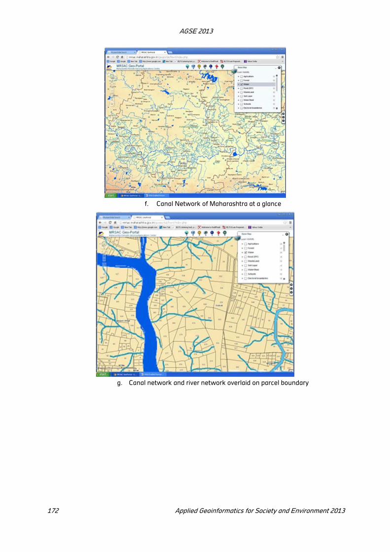
AGSE 2013


f. Canal Network of Maharashtra at a glance

g. Canal network and river network overlaid on parcel boundary

AGSE 2013


h. Flood Affected villages in Maharashtra

i. Land use / land cover classes in Maharashtra

AGSE 2013


j. Satellite data of Maharashtra

k. Major and Medium Irrigation Commands of Maharashtra

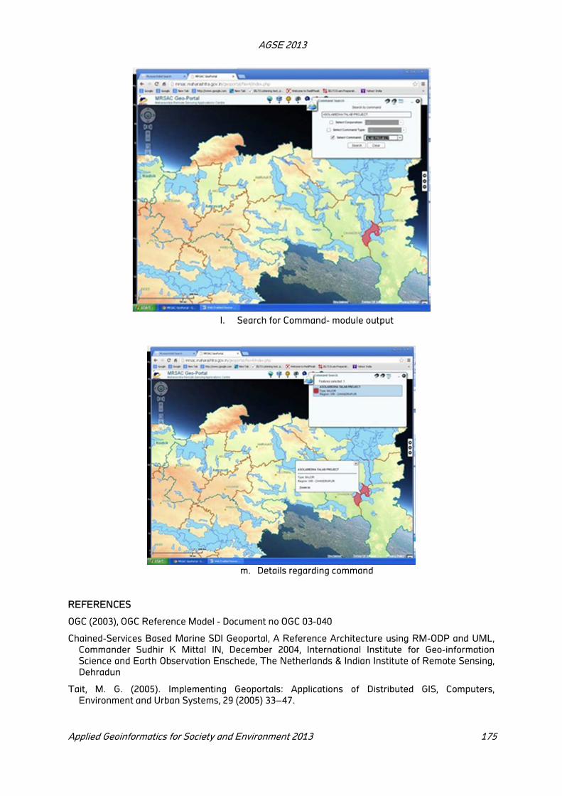
AGSE 2013


l. Search for Command- module output

m. Details regarding command

REFERENCES

OGC (2003), OGC Reference Model - Document no OGC 03-040

Chained-Services Based Marine SDI Geoportal, A Reference Architecture using RM-ODP and UML,

Commander Sudhir K Mittal IN, December 2004, International Institute for Geo-information

Science and Earth Observation Enschede, The Netherlands & Indian Institute of Remote Sensing,

Dehradun

Tait, M. G. (2005). Implementing Geoportals: Applications of Distributed GIS, Computers,

Environment and Urban Systems, 29 (2005) 33–47.

Issues and Challenges in Environmental Clearance of Real Estate

Projects in India 1Vidula Kulkarni,

2Subhrangsu Goswami

1Programme Officer, PRUDA- AIILSG, Pune. Maharashtra, India. Email: [email protected]

2Assistant Professor, Faculty of Planning, CEPT University, Ahmedabad, Gujarat, India. Email:

[email protected]

KEYWORDS: Environmental Clearance, Environmental Impact Assessment, Real-estate Projects,

EIA Notification

ABSTRACT:

Due to increasing urbanization and favourable demographics, the real estate sector is urban India is turning into one of the most appealing investment areas for domestic as well as foreign investors. It is also evident from the increasing number of real-estate and construction projects for which Environmental Clearance (EC) has been granted by respective state governments. Government of India (GoI) recognized the growth and environmental consequences of such projects and introduced threshold limits for construction projects for which EC and Environmental Impact Assessment (EIA) need to be obtained by project proponent from concerned authority.

While bigger construction projects have to pass through EIA processes, considerable number of smaller construction projects with greater immediate environmental impacts is receiving easy environmental clearance. The primary objective of this paper is therefore to examine the rationale of having threshold value of Built up Area (BUA), and also to examine the efficiency of the EC process, in terms of project appraisal, impact assessment, and monitoring. In this study, EC for real estate projects from two states namely Gujarat and Maharashtra has been examined. Secondary as well as primary data has been used to examine the above mentioned objectives. Major findings of the paper suggests that the concept of threshold need to be reworked at the policy level, and It is also important to strengthen the EC process, impact assessment, impact monitoring and management plan, to achieve the very objective of EC & EIA.

1 Introduction

Due to increasing urbanization and favourable demographics, the real estate sector in urban India is

turning into one of the most appealing investment areas for domestic as well as foreign investors.

While as per census 2011, India is 31.16 percent urbanised and hosting 7935 urban centers, it is

obvious that Residential, Commercial and Corporate real estate sectors are experiencing a

considerable growth in urban India. It should be noted that, these projects have potential negative

environmental externalities of different scales which is quite visible during construction as well as

operation phase. It is evident that these not so big real estate projects are changing the urban

landscape of the country, with significant immediate environmental and social impacts (Kulkarni,

2011). Therefore, an attempt has been made in this paper to examine the efficiency of EC process

followed in the country for real estate projects.

2 Environmental Clearance, EIA & Real Estate Projects

2.1 Relevance and Historical Perspective

Economic development in developing countries has been focused on immediate economic gains.

Environmental protection has not been a priority because the economic losses from environmental

degradation often occur long after the economic benefits of development have been realized.

(Lohani et al, 1997) The past failure of development planning processes to take adequate account of

the detrimental impacts of economic development activities led to the advent of EC processes. EIA

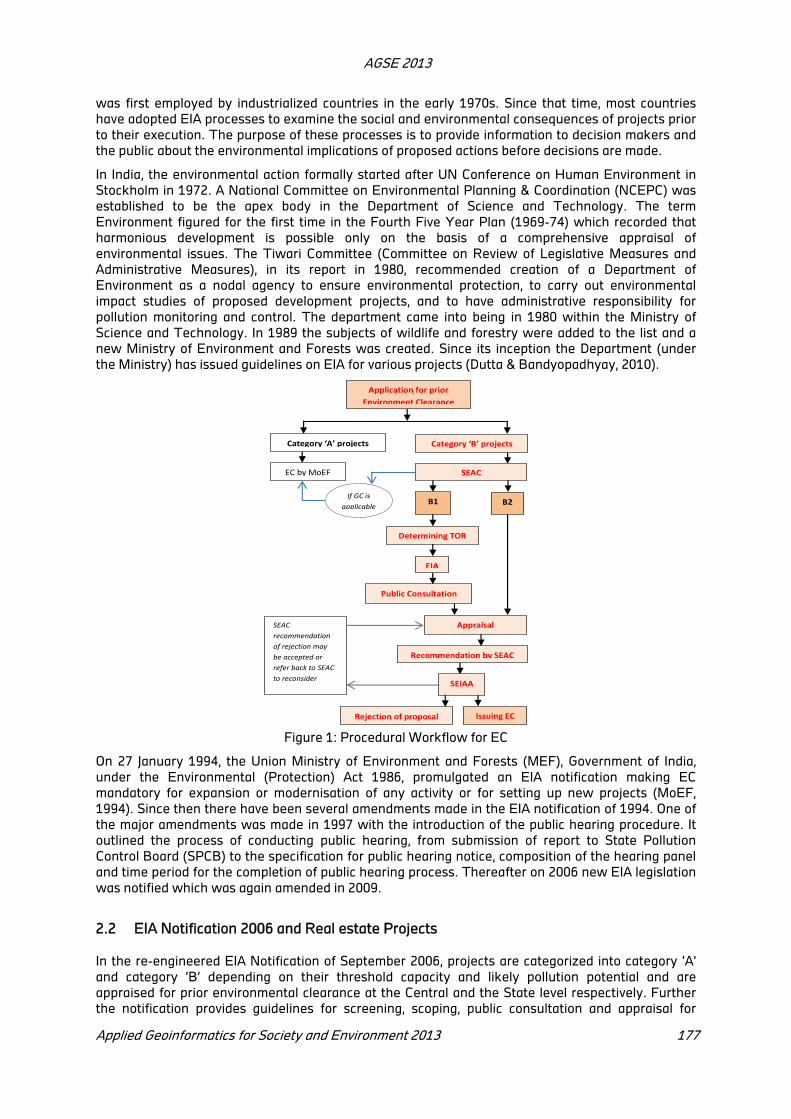
AGSE 2013


was first employed by industrialized countries in the early 1970s. Since that time, most countries

have adopted EIA processes to examine the social and environmental consequences of projects prior

to their execution. The purpose of these processes is to provide information to decision makers and

the public about the environmental implications of proposed actions before decisions are made.

In India, the environmental action formally started after UN Conference on Human Environment in

Stockholm in 1972. A National Committee on Environmental Planning & Coordination (NCEPC) was

established to be the apex body in the Department of Science and Technology. The term

Environment figured for the first time in the Fourth Five Year Plan (1969-74) which recorded that

harmonious development is possible only on the basis of a comprehensive appraisal of

environmental issues. The Tiwari Committee (Committee on Review of Legislative Measures and

Administrative Measures), in its report in 1980, recommended creation of a Department of

Environment as a nodal agency to ensure environmental protection, to carry out environmental

impact studies of proposed development projects, and to have administrative responsibility for

pollution monitoring and control. The department came into being in 1980 within the Ministry of

Science and Technology. In 1989 the subjects of wildlife and forestry were added to the list and a

new Ministry of Environment and Forests was created. Since its inception the Department (under

the Ministry) has issued guidelines on EIA for various projects (Dutta & Bandyopadhyay, 2010).

Figure 1: Procedural Workflow for EC

On 27 January 1994, the Union Ministry of Environment and Forests (MEF), Government of India,

under the Environmental (Protection) Act 1986, promulgated an EIA notification making EC

mandatory for expansion or modernisation of any activity or for setting up new projects (MoEF,

1994). Since then there have been several amendments made in the EIA notification of 1994. One of

the major amendments was made in 1997 with the introduction of the public hearing procedure. It

outlined the process of conducting public hearing, from submission of report to State Pollution

Control Board (SPCB) to the specification for public hearing notice, composition of the hearing panel

and time period for the completion of public hearing process. Thereafter on 2006 new EIA legislation

was notified which was again amended in 2009.

2.2 EIA Notification 2006 and Real estate Projects

In the re-engineered EIA Notification of September 2006, projects are categorized into category ‘A’

and category ‘B’ depending on their threshold capacity and likely pollution potential and are

appraised for prior environmental clearance at the Central and the State level respectively. Further

the notification provides guidelines for screening, scoping, public consultation and appraisal for

Application for prior

Environment Clearance

Category ‘A’ projects Category ‘B’ projects

SEAC

If GC is

applicable

EC by MoEF

B1 B2

Determining TOR

EIA

Public Consultation

Appraisal

Recommendation by SEAC

Issuing EC

SEIAA

Rejection of proposal

SEAC

recommendation

of rejection may

be accepted or

refer back to SEAC

to reconsider

AGSE 2013


category ‘B’ projects and activities. In case of Category ‘B’ projects or activities, project proponent

will have to submit application seeking prior environmental clearance in Form 1. Based on the

information provided in form 1, concerned State level Expert Appraisal Committee (SEAC)

determines whether or not the project or activity requires further environmental studies for

preparation of an EIA for its appraisal prior to the grant of EC depending up on the nature and

location specificity of the project. The projects requiring an EIA report is termed Category ‘B1’ and

remaining projects is termed Category ‘B2’, which do not require an EIA report (MoEF, 2006). Based

on the recommendations of SEAC, State Level Environmental Impact Assessment Authority (SEIAA)

issue EC or reject the proposal. Procedural work flow for environmental clearance is given in Figure

1.

Project/ Activity Category with threshold limit Conditions if any

A B

8(a) Building and

Construction projects

≥20000 sq m and <1,50,000

sq m of built-up area #

#(built up area for covered

construction; in the case of facilities

open to the sky, it will be the activity

area )

8(b) Townships and Area

Development projects.

Covering an area ≥ 50 ha

and or built up area

≥1,50,000 sq m ++

++All projects under Item 8(b) shall be

appraised as Category B1

Table 1: Status of Building /Construction projects/Area Development projects and Townships in EIA

Notification 2006, Source: MoEF, 2006 (EIA Notification 2006

Real Estate Projects: As per EIA notification 2006, EC is not required for projects with built up area

(BUA) less than 20,000 sq m. As can be seen from the table above (Table 1), the item 8a ( Building

and construction projects) having BUA more than or equal to 20,000 sq m come under purview of EC

and need to fill up form 1 and 1A. Form 1A is a detailed questionnaire, almost a mini-EIA based on

secondary environmental data along with a detailed Environmental Management Plan (EMP) and

Environmental Monitoring Plan and also a Disaster Management Plan. Item 8b (Townships and area

development projects) covering area more than or equal to 50 ha or BUA more than 1,50,000 sq m

come under EIA purview. As per the notification, though EIA is made mandatory for item 8b

(category B1-requiring EIA report), item 8a may require EIA only if the construction area is more than

150000 sq m.

It is important to note here that, public hearing is not required for any construction project

(MoEF,2006). The application is reviewed by SEIAA and is sent to the SEAC for appraisal. SEIAA

grants the in principle EC after getting green signal from SEAC. After receiving the EC, as per

guidelines, the project proponent is supposed to submit half yearly monitoring reports to concerned

authorities.

3 Rationale, Approach and Methodology

While the main goal of EIA is to influence development decision-making by providing sound

information on environmental impacts and the means for preventing or reducing those impacts, it is

fundamental that the impact assessment is done with maximum precision. It is evident that

government is continuously trying to make the process better and efficient*. However some issues

and challenges are yet to be addressed specially in case of projects in construction and real-estate

sector. Increasing number of such projects and its exposure to larger population in the vicinity makes

* In 2011 GoI made it mandatory that, all the Consultants/public Sector Undertakings (PSUs) / Universities & Research

Institutes working in the area of Environment Impact Assessment are required to get themselves registered under the scheme

of Accreditation and Registration of the National Accreditation Board of Education and Training (NABET) and the Quality

Council of India (QCI). No EIA/EMP Reports prepared by such Consultants who are not registered with NABET/QCI shall be

considered by the Ministry after 30th June, 2011.

AGSE 2013


it all the more crucial. An effort have been made in this paper therefore to answer the following

research questions; 1) How appropriate is the Built Up Area criterion mentioned in the EIA

Notification as a screening parameter for construction projects? 2) How effective is the

environmental clearance process as an environmental management tool? 3) How effective are the

EMP proposed by the proponents in EC documents?

Environmental Clearance documents (form 1 and form 1A), of 10 per cent of total EC granted to

construction projects ie, 102 projects from Gujarat and Maharashtra was accessed from official

websites of state governments of Gujarat and Maharashtra respectively. Relevant data from these

documents were analysed to examine parameters like, Resource Consumption (Energy & Water),

Pollution potential (Waste water and solid waste generation). Bivariate and multivariate analysis

was done to examine the relationships. Out of 102 projects, five projects were selected as case study

to explore the ground scenario. These case studies represent both the category of projects i.e., B1

and B2. It also represent the type of project e.g., residential projects and commercial projects.

Stakeholders were identified and interviewed for all the five case studies. Ground scenario was also

examined against the EMP proposed in form 1A in respective projects. Online survey with designed

questionnaires was conducted to capture the diverse perspective of Project Proponents,

Environmental Consultants, SEAC Members, Government officials. Neighborhood residents of each

project were also interviewed. Major findings of the analysis have been discussed in the section

below.

Figure 2: Approach & Methodology

4. Analysis & Discussion

4.1 Changing Status of Environmental Clearances in Gujarat & Maharashtra

EC related data available on the official website of Gujarat and Maharashtra was analysed to

examine the status. The following graphs show the share of environmental clearance (EC) granted

to real estate and construction projects in the state of Gujarat and Maharashtra. It is evident from

Figure 3a, that there is an unprecedented increase in number of EC granted to Real estate projects

in Gujarat after 2010. Figure 3b and 3c show the cumulative numbers of sector wise granted ECs.

Updated data for Gujarat is available in SEIAA website, which shows that till July 2013, maximum

number of ECs was granted to projects from construction sector in the state. Updated data for

Maharashtra state is not available till 2013, however the numbers available till 2011 shows similar

trend as Gujarat.

AGSE 2013


Figure 3a: Increasing number of EC Granted

to Real Estate projects in Gujarat Source: http://seiaa.gujarat.gov.in

Figure 3b: Sector wise

number of ECs granted in

Gujarat, till July 2013 Source:http://ec.maharashtra.go

v.in

Figure 3c: Sector wise

number of ECs granted in

Maharashtra, till Decmber

2011 Source:http://ec.maharashtra.go

v.in

4.2 Relationship between Built up Area and Environmental Impact

It is important to note that the notification suggests that the project proponent will have to conduct

EIA, only if the BUA is more than 1,50,000 sq m. While many of the environmental experts in the

country are unaware of the rationale behind these area criteria, it is evident that, the criteria are

apparently based on the understanding that construction projects with larger BUA create more

environmental impact. An effort has been made therefore to examine, whether this assumption is

correct. Therefore available data in EC document were analysed to examine the probable impacts

from two perspectives, as follows, namely resource consumption (water demand & energy demand);

and pollution potential (solid and liquid waste generation).

Due to lack of suitable data, correlation analysis was not done, however multivariate tables were

used. Since absolute values are not comparable, indicators (per unit area per day) were developed to

capture the resource consumption and pollution potential. Number of projects showing above

average values in four different indicators during operation phase (Figure 4), reflect the fact that,

there are considerable number of smaller projects (with smaller BUA), with larger resource

consumption and pollution potential (per unit area per day). Average value was calculated for all the

four parameters based on data available in 102 EC documents, as mentioned in Section 3. The

observations from case studies justify these facts. It is evident that commercial buildings like

shopping malls and multiplexes with much lesser area compare to a residential apartment, consume

much more energy due to huge volume of air conditioning, ambient lighting (even during the day

time), escalators etc. As far as waste generation is concerned, many of these commercial buildings

house considerable number of shops and restaurants generating huge amount of food waste and

paper / packaging waste (Kulkarni, 2011).

Figure 4: Number of projects with pollution potential and energy consumption more than average

values (per 1000 sq m per day)

2008 2009 2010 2011 2012

Others 6 9 5 7 7

Industrial 95 103 48 79 61

Construction 15 9 19 98 264

0%

20%

40%

60%

80%

100%Percentage

Share

38

435

569

114 103

479

Water requirement more than average

(6.98 cu m)

Waste Water generation more than average (5.17

cu m)

Solid Waste generation more

than average (24.99 kg)

Energy requirement more than average

(61.67 kw)

20,000 to 50,000 sq m 12 14 3 5

50,001 to 1,00,000 sq m 9 8 2 6

1,00,001 to 1,49,999 sq m 2 2 1 4

>=1,50,000 sq m 14 9 9 7

0

2

4

6

8

10

12

14

Number of Projects

AGSE 2013


4.3 Inappropriate Impact Assessment due to Partial Availability of Data

As per the guidelines, the project proponents need to submit form 1 and form 1A, to SEIAA for

environmental clearance. These forms are supposed to contain important information to know and

predict environmental impact of the project. However most of the submitted applications by

proponents are silent about essential and crucial information. It is evident from the analysis (Figure

5), that very few proponents provided information on energy requirement and waste water

generation during construction phase. As far as operation phase is concerned lowest number of

proponents provided information about energy requirement. Unavailability of data is more

prominent in case of commercial projects.

While many proponents do not disclose the total amount of water required during the construction

and operational phase and more over very conveniently indicate that water will be supplied by local

authority. Same is the case with waste water generation. However in practice many of these projects end up

using ground water by drilling bore well in the project site, simply because many of these projects are located at

the out skirts of the city where water supply and sewerage network is not present only. It is observed that, all

the four case study projects from Ahmedabad are located in a region termed as ‘over exploited’ in terms of

ground water potential (CGWB, 2011). Three out of four projects from Ahmedabad reported to depend only on

the bore well in a site for its complete water requirement. The case project from Maharashtra is located in

Haveli Taluka, which is experiencing fall in water level up to 20 cm/year in major parts of the district (CGWB,

2009). However EC has failed to capture this crucial information and the implications.

Figure 5: Percentage of EC Letters with complete information on crucial environmental Parameters

4.4 Inefficient Environment Management Plan

As part of the EC process, Project proponent is supposed to prepare an Environmental Management

Plan (EMP), which is supposed to assure minimum environmental damage due to the project during

construction as well as operational phase. However it was observed while examining the EMPs

submitted by different proponents, that all proposed EMPs look same, irrespective of the nature and

scale of the project activities. More over many good environmental management practices are

proposed in the EMP without proper understanding of feasibility and applicability of the same.

Most common environmental management practise proposed to be implemented during the

construction phase, are measures like sprinkling of water to avoid dust, methods for noise reduction

etc., however most of the time these are completely missing at the project site. As far as operational

phase of the project is concerned, it is evident, that many of the proposed management interventions

are either missing or non-functioning on the site. For example most of the projects propose green

belt development by planting suitable tree species in adequate number. However in practise on site,

one will find very few trees, especially in case of commercial buildings. Another very interesting

0.0

20.0

40.0

60.0

80.0

100.0

Water requirem

ent

Energy requirem

ent

Waste water generation

Water requirem

ent

Energy requirem

ent

solid waste generation

Waste water generation

Construction phase Operation phase

Residential Projects

Residential cum Commercial Projects

Commercial Projects

AGSE 2013


observation is that, following the rules, suitable rainwater harvesting techniques are proposed in

many such projects, however from the case studies, it is evident that, most of the time they are non

functional on the site. It is simply because the proponent never ensures that it is properly designed,

located and maintained. In case of commercial buildings most of the time ownership is retained with

the project proponent, however in case of most of the residential projects, developer handover all

responsibilities to the residents or the society. Majority of residents have no information about the

environmental clearance process that the proponent had to follow and about the proposed EMP.

Therefore residents are also unaware about the need for operation and maintenance of such

facilities and the cost to be incurred for the same (Kulkarni, 2011).

4.5 Surrounding Land use and Assessment of Cumulative Impact

EC process addresses the issues related to individual projects to certain extent. However the

cumulative environmental impact of many such projects coming up in vicinity is never assessed. One

of the most important cumulative impacts is visible on the roads in terms of increasing traffic and on-

road parking. This impact has multiple induced environmental impacts like air and noise pollution,

increasing accidents and conflicts, and most importantly it allows very little space for safe movement

of pedestrian and cyclist. However carrying capacity of a particular road or junction is never taken

into account while granting EC.

Figure 6a: Pre-project Site Conditions Source: Google Earth 20/04/2006

Figure 6b: Post-project Site Conditions Source: Google Earth 12/02/2013

Figure 6a. and 6b. explain the coexistence of three different and distinct land use in Vastrapur area

of Ahmedabad City. While the lake and the amphitheatre was created to provide ward level green

infrastructure and entertainment, Alfa one mall covering 35,000 sq m area, launched to cater

shopping, entertainment and hospitality. The area is surrounded by low rise and high rise residential

apartments. It was evident from the case study, that the mall attracts huge amount of traffic which

results into similar issues as discussed above.

4.6 Issues in the Clearance Process and Monitoring

While the very purpose of Environmental clearance is to minimize environmental damage caused by

the proposed project and to safeguard the quality of life, it is contradictory that, the construction

projects do not require public consultation at any stage of EC. As a result anticipated impacts

envisaged by the people staying in the vicinity are never accounted for. It was observed during

stakeholder consultation that, the SEACs are loaded with too many projects to be appraised in a

given time period, which results into weak appraisal and overlooking of important questionable

information provided by the proponent.

It is evident that Urban Local Body (Corporation / Municipality) and Town Planning Department,

which is supposed to be the most concerned and most informed authority, on any new development

in the city, are mostly not involved in the EC process. Post project monitoring, which is the

responsibility of regional offices of MoEF, comes into play once the project is commissioned. It

ensures that the impacts of the project do not exceed the legal standards. It also ensures that an

action had been implemented in accordance with the measures specified while providing the EC.

AGSE 2013


However it is observed that this monitoring mechanism is very weak with its inherent procedural

issues, as the regional offices do not have enough staff to monitor such large number of projects

(Kulkarni, 2011).

4.7 Conclusion

Real estate sector is booming in the country with diverse scale of construction projects. These

projects have potential negative environmental impacts of different scale, which is prominently

visible during construction as well as operation phase. While the main goal of EC process is to

influence development decision-making by providing sound information on environmental impacts

and the means for preventing or reducing those impacts, this paper observes some loopholes in the

EC process, implementation of EMP, and the monitoring mechanism. One of the major observations

is that comparatively smaller projects may have significant recourse consumption and pollution

potential. Therefore area criteria need to be relooked more critically for screening of construction

projects in EC process. Data provided by project proponent in prescribed format is sometimes

incomplete, which result into poor impact assessment. Land use plan and carrying capacity of

surrounding area of a project is not adequately taken into account during impact assessment. It is

also observed that the proposed EMPs are inefficient due to poor maintenance and poor monitoring

mechanism. This paper also identifies few inherent institutional issues in terms of appraisal process,

lack of direct involvement of experts from respective Urban Local Bodies and Town Planning

Departments.

REFERENCES

Lohani, B. et al., 1997. Environmental Impact Assessment for Developing Countries in Asia. Volume 1

- Overview. 356 pp., Asian Development Bank

Dutta, Bikram Kumar & Sanhita Bandyopadhyay, 2010. Environmental Impact Assessment and

Social Impact Assessment - Decision Making Tools for Project Appraisal in India, International

Journal of Human and Social Sciences 5:6

MoEF, 1994. The Environment Impact Assessment Notification. S.O.60 (E).: Ministry of Environment

and Forest, Government of India, New Delhi, India

MoEF, 2006. The Environment Impact Assessment Notification. S.O. 1533 (E).: Ministry of

Environment and Forest, Government of India, New Delhi, India

Kulkarni Vidula, 2011. Effectiveness of Environmental Clearance Process in India: Case Study of

Construction Projects, Unpublished Master’s Thesis, CEPT University, Ahmedabad

SEIAA, GoG, 2013. Environment Clearance Granted, http://www.seiaa.gujarat.gov.in/ (accessed

25.10.2013)

Environment Department, 2013. Environmental Clearance, https://ec.maharashtra.gov.in/,(accessed

25.10.2013)

CGWB, 2011. Ground water scenario in major cities in India, Ministry of Water Resources,

Government of India

CGWB, 2009. Ground water information, Pune District, Maharashtra, Ministry of Water Resources,

Government of India

Industrial Location and Physical Planning: A Geospatial Analysis of

Allahabad District

Dileep Singh

Saradar Patel Institute of Economic and Social Research, Thaltej, Drive-In Road ,Ahmedabad, 380054,

E-mail: [email protected]

KEY WORDS: Industrial Location, Geospatial, Industrial Locational Factor, Industrialization, Potential,

Region, Market, Industrial Corridor

ABSTRACT

It is said that primary cause of spatial income inequality is spatial inequality of industry location in developing countries (Somik Vinay Lall and Sanjoy Chakravorty 2005). This study focuses on spatial analysis in terms of major factors which influence decision of where should a new industrial unit be set up. In order to ensure the healthy environment for industrial development in a region it is essential to undertake a geospatial analysis from macro level to micro level, which prevents haphazard growth of manufacturing industries. Main trust of this paper is to find out the potential region for industrial development by using block-level data. Geographical information system is employed as a tool in this study. In line with this some critical locational factors are identified with help of existing literature. All identified industrial location factors are categorized into three sections. First, industrial base, which covers pattern of industrialization, spatial concentration of industries and investment and employment scenario in manufacturing industries. Second physical factor which focuses on land use pattern, availability of power, water and access to road and transport services.. Socio-economic factors such as labour, market and cropping pattern are discussed in third section. Finally this study finds potential region for industrial location in central eastern region, which is delineated in the map given in conclusion part.

1 Introduction

Where do new industrial unit locate, and what all do major factors influence the industrial location

decisions? has been subject of great debate among industrial economist. Industries tend to locate in

some specific Centre. Alfred Weber laid down the principal of industrial location sixty years ago,

which is taken as fundamental in industrial location theories. Weberian approach gives great

impetus to relative transport cost of raw material and final output of a firm. This approach ignores

other important variables such as labour cost, market availability and agglomeration economy

(Kristensson 1968, Krumme 1969, Cyert and March 1963). Greenhut(1956), Hamilton(1967),

Pred(1967) and many others criticized Weberian approach. With development of research on

increasing return to scale, technological externalities, pecuniary externality, imperfect competition

have brought new economic geography (Redding 2009, Fujita et al 1999, Krugman 1993). Structural

reforms in India liberalize regulatory structure of incentive and disincentive which tended to favour of

lagging and unindustrialized region, have been discarded , the new systems profess to have little

geographical orientation, but, as many have argued, may be biased towards advanced, industrialized,

metropolitan regions (Chakravorty, 2000, Saikia 2011)

Spatial income inequality is major concern in our country; some states are growing very rapidly

whereas some are lagging behind. It is expected that inter regional inequality (expressed typically in

terms of per capita regional income or output) increases during the early years/decades of industrial

development, being concentrated in metropolitan areas, and after achieving a certain level of growth

begins to decline at some later indeterminate point( Perroux 1950, Myrdal 1957, and Hirschman

1958, Williamson 1965, Friedmann 1973, and Alonso 1980 Krugman 1996,Sala-i-Martin 1996, and

Fujita, Krugman and Venables 1999. In India, industries tend to locate in some specific region.

Coastal region always has been attractive destination for industries (Gujarat, Maharashtra,

Tamilnadu, Karnataka). In recent years/decade India achieved high rate of growth after trade

liberalization but the benefit from higher growth rate could not spread to industrially backward

AGSE 2013


region which spur interregional inequality and resulted over burden on some metropolitan cities

because of people migrate from one region to another region for employment. It is not an easy task

to met the demand of basic amenities for such a large population with limited municipal boundary

which is not expandable such as Mumbai. This Paper intends to emphasis on such a states those

supplies most of labour force to the country and have less employment opportunity such as Bihar.

Madhya Pradesh, Rajasthan and Uttar Pradesh (BIMARU), people have to move from these states to

industrially developed so this is major challenge before us how to reduce the migration from these

regions instead of to expand the boundary of urban centres which would help to prevent haphazard

growth and would also help to reduce overburden on transportation and other basic services.

Uttar Pradesh is the largest state of India in terms of population and full of natural

resources,favorable climate and fertile land in spite of this it has been fail to attract industries In

Uttar Pradesh industries are concentrated in mainly two centre one isthesurrounding area of NCR in

which Gautam Buddh Nagar,Gaziabad,Bulandshahar,Aligarh,Meerut,Mathura ,Agra fall under this

region and Lucknow, Raibareli, Sultanpur,Ftehpur, Pratapgarh, Kaushambi and Allahabad fall under

this zone. Concentration of Industrie in U.P.

What we see region wise scenario in UP which is found out after analyzing the over all scenario of

the state western region of the state of Uttar Pradesh has been experienced good rate of

industrialization. In Uttar Pradesh there has been two major regions for industrial development both

have shown good growth rate of industrialization and have been witness for fastest growing region

not only in the state but also in India. One region is situated in the proximity of National Capital

Region and another region comprises some part of central region and some part of the eastern

region. If we analyze comparatively all four region of Uttar Pradesh western region is growing rapidly

getting and advantage of proximity of NCR Delhi In central region Lucknow is taking a leading role

which has emerged as IT hub Bundelkhand Region as different scenario there is issues of water

availability and some other factors even government has been promoting and giving good amount of

incentive for betterment of quality of life of the people there. In eastern Region Allahabad has

imminence power to grow in future more rapidly which is presently growing .Allahabad has been a

witness so far for good level of per capita Net District Domestic Product ,growth rate , no of

secondary sector worker ,good length of road and railway ,water availability and power. It shows a

good potential for industrial development in the district.

Figure 1: Directorate of Industries Uttar Pradesh 2011

This is not enough to say that Allahabad has good potential for industrialization until a study is done

for analyzing existing scenario and trend of development and it would also be needed to assess the

existing resources physical and human ,existing infrastructure. In this context we have selected

Allahabad district.

AGSE 2013


2 Industrial Base in the District

The concept of industrial base helps to understand structure of regional distribution of industries

and also give the insight of industrial location pattern. To some extent growth phenomenon of

industries also influence decision of industrial location for new firms. If growth pattern is seen in

Allahabad only sector which has grown rapidly from 25.39 in 2001-02 to 31.28 in 2009-10 is

industrial sector. Service sector has been prominent in the district, more than 50% income of the

district comes from this sector. In recent service sector and primary sector both have declined from

54.78, 19.83 in 2001-02 to 50.74, 17.98 in 2009-10 respectively.

Allahabad has strong industrial base where more than 4000 SSIs are registered as per third all India

census for industry and more than 10000 units are unregistered in 2010. There are 18 medium and

large scale industries, some of them are Indian Telephone Industries Ltd., BPCL, Triveni Structural

Ltd., Areva T&D India Ltd., SAIL, Cotton Mills subsidiary of central govt.

Figure 2: District Industries Centre 2010 Figure 3: Public work Department

Allahabad Uttar Pradesh 2010

2.1 Concentration of the Industries

Most of industries in the district are concentrated along railway. Naini has been developed as very

attractive destination for industries because of access of railway line and proximity of major railway

crossing junction that is separated from the main junction for the uninterrupted movement of cargos

followed by Soraon and Phoolpur. Both side of the Delhi – Kolkata Industrial Corridor is being

another destination for industries except the kaudihar block because of main city of Allahabad is

situated in this block govt. has been avoiding for the industrialization in this part of the city . In future

city will grow for commerce and residential purpose they would be needed more area for city

expansion

2.2 Investment and Employment Scenario

If we talk about investment in medium and large scale industries. District have been witnessed

insignificant development in medium and large industries. Investment rate has been 3.1 per annum

from 2001 to 2010.There is inconsiderable employment generation in MLIs which is 10% in last

decade.

Unlikely to medium and large scale industries, SSIs has shown very significant development .

Investment has increased more than 100% and employment generation has been around 24% in

AGSE 2013


2000s. Growth in employment is less than growth in investment which reflects that new

investments are capital intensive and labour saving in nature. Entrepreneurs prefer such a

technology which required less labour which results less operation cost.

3 Physical Factor

Physical factors are very –very important for any kind of industrial setup no any industry can survive

without land and water other physical factors like good connectivity, road network and power are

responsible level of economy and growth rate because of without these factors only few industries

can survive only on that basis we can not achieve the desired level of development.

3.1 Transportation

Transportation is a key factor in driving industrial, economic and social growth. To develop a strong

economy, Uttar Pradesh has been making serious and conscious efforts in the development of

infrastructure and inviting private participation on a large scale. Allahabad offers excellent

infrastructural facilities for setting up industrial units. Various PPP projects have been undertaken in

the sectors such as expressways, roads, energy, transportation, education, urban rejuvenation etc.

The city of Allahabad is well connected to other major cities in near by Lucknow, Varanasi, Kanpur,

Sultanpur, Mirzapur, Fatehpur etc. by road and rail. Connectivity of city with metros are via air, rail.

Being center of North Central Zone most of the rail routes are touching Allahabad for Delhi, Mumbai

and Kolkatta. Latest announcement of govt. of Uttar Pradesh the Ganga Express Way is also

touching the city alongside the river Ganga. Delhi – Kolkata corridor also passes through

Allahabad.Road density is highest in the soraon block that is the around 1800 km /1000 sq.km.

followed by Chaka , Mauaima, Holagarh , Handia and Dhanupur. Road network is very poor in

southern and western part of the district whereas northern and eastern part of the district has a

good connectivity of road and railway both.both side of the national highway 2 has higher road

density than other part of the district. Road length of the state highway in the district has increased

102 km from 2007-08 to 2008-09 within a year. Various mega road projects has been implemented

and some are being Implemented under PPP.

3.2 Power

If we see the composition of electricity consumption in the district, 50% goes to domestic. Other than

domestic Rail/ traction and agriculture consumes 19% and 15% respectively. One thing is remarkable

here, share of industries in total power consumption has increased 100% within four years. Phoolpur

industrial area has 132 KV. SS and UPSIDC Industrial Area Naini which has 400 KV. SS. In the

district all villages are electrified

Figure 4: Electricity board Allahabad Uttar Pradesh 2010

Domestic

52%

Commercial 5%

Industrial4%

Public 3%

Rail / Traction19%

Agricultural15%

Other2%

2005‐06

Domestic 50%

Commercial 5%

Industrial8%

Public 4%

Rail / Tractio

n20%

Agricultural13%

2008‐09

AGSE 2013


Power is a issue so far in the district but three mega power plant are coming in the district. NTPC

and Uttar Pradesh Rajya Vidyut Utpadan Nigam signed a 50:50 joint venture agreement to set up a

1,320 MW coal-based power plant at Meja in Allahabad district of Uttar Pradesh.

Land has been acquired Meja power plant and process for other two plant is going on. When these power plant

will come under operation then gap would be fulfilled and it would encourage industrial development in the

district As of March 2011, the state had an installed power capacity of 10,457.63 MW which consisted of

4,651.85 MW of central share, 4,619.40 MW of state share and 1,186.38 MW of private share. The installed

power capacity in the state has increased from 9,207.2 MW in 2006-07 to 10,457.63 MW during 2010-11. The

state is in the process of implementing and testing the public private partnership model in the power sector with

an input-based franchisee system. Demand for power is driven by, both, the agricultural and industrial sectors.

Land use Pattern: Land is the most important and the least mobile factor needed for industrial

development. Plain areas are comparatively more accessible and therefore more likely to develop.

Moreover, availability of infrastructure, water, electricity and transport is desirable. Land use pattern of

Allahabad

district has been changing substantially since 2001. Land under industrial use has increased 100%

from 2001-02 to 2008-09 due to rapid industrialization and the area under barren land has increased

during the same period . Cultivable land has also increased it means most of land is being used are

barren land or uncultivable land one thing is good that most of land that is covered by upcoming

industries is barren land. Area under cultivable land also has increased where as area under

uncultivable land has decreased during the same period. Forest land ,meadow land and fallow land

are remained same. 27% land is still remained unutilized that shows potential industrial activities

3.3 Water Availability

Water availability is a very essential precondition for many of the manufacturing operations. Those

industries whose manufacturing operations require very less amount of water may also require

water for workers and other normal day to day operations. The industry may pump the ground

water if it’s available; otherwise, a regular water supply is necessary.

Main source of surface water in the district is Ganga and Ymuna.The rivers of the district belong to

the main system of Ganga and comprise several subsystems of which the most important are the

Yamuna and the Tons, other including the minor systems of the Varuna and the Sai. Ground water

availability is higher in the in the northern and central part of the district. All the blocks fall under

safe zone. Dhanupur and Baharia have highest availability of ground water followed by Karchhan

and Holagarh blocks within the district.

AGSE 2013


Figure 5: Central Ground Water Board, Northern Region, Lucknow 2004

4 Socio-Economic Factors

4.1 Cropping Pattern

The cropping pattern in the district has vastly changed during the last 30 years . The only crop which

continues to be important during all these years is paddy. Area under paddy cultivation increased

from around 30.7 per cent of net sown area in 1960-61 to around 57.06 per cent during 2000-01.

Area under wheat cultivation increased from 11.60 per cent in 1960-61 to 57.31 per cent of net sown

area in 2000-01. But area under different coarse grains declined during this period, for example area

under barley declined from 18.7 per cent to 2.87 per cent, gram cultivation declined from 20.7 per

cent to 10.07 per cent, and peas cultivation declined from 6.84 percent to 1.76 per cent during 1960-

61 to 2000-01. Block wise analysis of cropping pattern confirms this trend, except that in some

blocks pulses and sugarcane and oil seed were also grown at significant level. The blocks where

area under pulse cultivation as percentage of net sown area was above 15 per cent are Kaurihar

(16.4 per cent), Bahadurpur (19.47 per cent), Jasra (31.52 per cent) Shankargarh (28.82 per cent),

Karchhana (17.79 per cent), Meja (18.94 per cent), Koraon (26.85 per cent) and Manda (18.64 per

cent). Similarly blocks where area under oilseeds was above 5 per cent of net sown ara are:

Shankargarh (9.46 per cent), Meja (8.35 per cent) and Manda (6.81 per cent). Even though area

under potato cultivation has increased in the district, blocks were area under potato cultivation was

above 5 per cent of net sown area are only few. These include Kaurihar (5.46 per cent), Holagarh

(19.48 per cent), Mau-Aima (16.81 per cent) and Soraon (19.59 per cent).

4.2 Labour

Labour is distinguish factor, Karl Marx says laboour is the only factor which added the value in

production process. Cheap and skilled labor supply always has been attracting the entrepreneurs. It

AGSE 2013


can also be seen global context, after structural reforms most of developing countries liberalized

their trade policy which results to shift multi national companies from developed countries to

developing countries. availability of cheap labour has played a key role in restructuring

industrialization in global context. India and China have been most favorable destination among

developing countries. So many technical education were established in India and also India could be

able to supply skilled labour which meet global demand. Lobour mobility is possible for Medium and

large scale industry which can impel immigration but it is quite difficult to small scale industry

because they generally do not have power to attract labor force from outside. In recent years

demand for skilled labour have risen. Technical education and literacy rate have become important

indicator. Allahabad is main education centre in eastern region.Literacy Rate of Allahabad district is

74.2 that is much more higher than state literacy rate 56 % even that is also higher than national

literacy rate 64 %. In 2001 Allahabad is not only the major centre of education in the state but also

for economic activities .Allahabad city is the main centre for labour market skilled and non skilled

both. Work participation rate is 45% which is higher than state average even national average also.

Each block has good work participation rate Shankargarh , Karchhana , Koraon , Mauaima are

witness to highest percentage of main worker more than 25 %.Dhanupur , Handia , Saidabad are

the blocks where 22.6 , 18.1 , 17.9 percentage of people are engaged in household industries.

Koraon ,Bahria , Holagarh and Mauaima are the very prominent blocks in terms of agriculture where

86.2 ,75.2 , 74.3 and 73.3 percentage of people are engaged in agriculture

4.3 Market

In recent the share of public sector units to total no of units has substantially declined after economic

reform. Private sector units always adopt profit oriented strategy. To reduce the transportation cost

some of industries tend to set up their unit near market. Therefore market is very important

phenomenon for industrialization. There is two kind of market one is consumer goods market and

second is capital goods market. The consumer goods market are generally urban agglomerations,

while the capital goods markets can be taken as existing medium or large industry in a region, which

may purchase primary processes products from ancillary and small scale industries. However, since

this study is confined to backward districts, these kinds of local markets may not be developed at the

start period; it take a time to develop secondary market or capital goods market . Apart from that,

nearness to a big urban or industrial centre highlights the potential for industrial growth in a region.

However, for that to happen, it is prerequiste that the area has good connectivity to the major urban

centre. Both market capital goods and consumer goods exist in the district, Areva Transmission and

Distribution Pvt. Ltd. playing as mother industry because of this so many ancillary unit has been

established. They supply their final capital goods to industry. Within Allahabad district boundary

there are 11 urban centres . Most of them are concentrated in cetral and northern part of the

district along the railway line. Allahabad is the only one town that is the I class town .and two towns

Mauaima and Phoolpur are the class III town. Seven towns are class IV town and town is class V.

This picture shows good strength of market scenario and these urban centres could play a very

important role as market and create a huge demand of goods and services produced by local

industries

5 Conclusion and Suggestion

This study analyzes comparatively all four region of Uttar Pradesh, western region is growing rapidly

getting an advantage of proximity of NCR Delhi In central region Lucknow is taking a leading role

which has emerged as IT hub . Bundelkhand Region as different scenario there is issues of water

availability and some other factors even government has been promoting and giving good amount of

incentive for betterment of quality of life of the people there . In eastern Region Allahabad has

imminence power to grow in future more rapidly which is presently growing .Allahabad has been a

witness so far for good level of per capita Net District Domestic Product ,growth rate , no of

secondary sector worker ,good length of road and railway ,water availability and power. It shows a

good potential for industrial development in the district. Eventhough this study infers that Allahabad

district has good potential for industrial development within a district yet which area or region would

be good place for industrialization is also necessary to identify to prevent the haphazard and

AGSE 2013


unhygienic growth and maximum utilization of existing infrastructure and resources.In this term

what we have found through above analysis Major industries are concentrated along with railway

track Karchhana block is the most attractive destination for industries so far because of the access

of major railway crossing. Central part of the district has a good potential for industrial development.

All major factors are favorable in the central region

Figure 6: Compiled from Various Issues

Map is showing that both side of the national highway -2 from the main junction or district head

quarter has a parallel railway line and this area also has a good potential for industrial development

in terms of groundwater and surface water availability road density , work participation rate and

market availability etc, should be developed as industrial region. If in future industrialization

increases substantially then this can be developed as region including the area as marked in the map

Southern blocks of the district are dominant in the production of oil seed and other food grains that

can be used as resource for agro based industries major resource of agro based industries even the

connectivity is poor there should be proper connectivity to the suggesting industrial corridor.

Allahabad can also be established as hub of Information Technology this sector should be promoted

because of Allahabad has huge potential that is a major Centre of highly education among the

northern states . IT PARK should be established there. Local Entrepreneurship should be promoted

to exploit the existing resource and make them more productive.

REFERENCES

Alonso, W., 1980, ‘Five Bell Shapes in Development’, Papers of the Regional Science Association,

Vol.45, 1, pp.5–16.

Chakravorty, Sanjoy, 2003. “Industrial Location in Post-Reform India:Patterns of Inter-regional

Divergence and Intra-regional

AGSE 2013


Convergence”, The Journal of Development Studies, Frank Cass, London Vol.40, No.2, December

2003, pp.120–152

Cyert, R.M . & March, J.G ., I963. A Behavioural Theory of the Firm. Prentice Hall, Englewood Cliffs.

Friedmann, J., 1973, ‘A Theory of Polarized Development’, in J. Friedmann (ed.), Urbanization, Planning and National Development, Beverly Hills, CA: Sage, pp.41–64.

Fujita, M., Krugman, P. & A.J. Venables, 1999, The Spatial Economy: Cities, Regions, and International Trade, Cambridge, MA: The MIT Press.

Greenhut, M. L., 1956. Plant Location in Theory and Practice. University of North Carilina Press.

Chapel Hill.

Hamilton, F. E. I., I967. Models of industrial location, in Models in Geography, Chorley R., and

Haggett, P., Methuen, London, 36I-424.

Kristensson, F., 1968. Regional planning, decision making, performance and research. Plan, 22,

Special Edition, 24-30.

Krugman, P., 1991, Geography and Trade, Cambridge, MA: MIT Press.

Krugman, P., 1996, ‘Urban Concentration: The Role of Increasing Returns and Transport Costs’,

International Regional Science Review, Vol.19, Nos.1,2, pp.5–30.

Krugman, P.R., 2006. “First Nature, Second Nature and Metropolitan Location”, J Regional Science

33: 129-144.

Krumme, G., I969. Towards a geography of enterprise. Economic Geography, 45, 30-40.

Lall, Somik Vinay & Sanjoy Chakravorty, 2005. “Industrial Location and Spatial Inequality: Theory

and Evidence from India” Review of Development Economics, 9(1), 47–68.

Myrdal, G., 1957, Economic Theory and Underdeveloped Regions, London: Duckworth.

Perroux, F., 1950, ‘Economic Space: Theory and Applications’, Quarterly Journal of Economics, Vol.64,

No.1, pp.89–104.

Pred, A., I967. Behavior and Location. Part I. Lund Studies in Geography, Series B, No. 27. Pp. 5-10.

Redding, Stephen J., 2009. “The Empirics of New Economic Geography”, CEP Discussion Paper 925,

London School of Economics and Political Science, London.

Saikia, Dilip 2011. “The pattern of industrial location in India under liberalization: an analysis of the

organized manufacturing industries”international Research Journal of Management and Business

Studies Vol. 1(7) pp. 197-214 September.

Sala-i-Martin, X., 1996, ‘Regional Cohesion: Evidence and Theories of Regional Growth and

Convergence’, European Economic Review, Vol.40, No.6, pp.1325–52.

Vella, F., 1998. ‘Estimating Models with Sample Selection Bias: A Survey’, The Journal of Human Resources, Vol.33, No.1, pp.127 69.

Weber, A., 1929. Theory of the Location of Industry. (trans, C. Friedrich), University of Chicago Press.

Public Private Partnership and its role in Housing Delivery to the Lower

Income Groups in Kolkata

Amit Kaur

CEPT University, Ahmedabad, Email id: [email protected]

KEY WORDS: Earmarkings, Housing Delivery, Kolkata, Kolkata Metropolitan Development Authority

(KMDA), Lower Income Groups (LIG), Middle Income Groups (MIG), Public Private Partnership Model,

West Bengal Housing Board (WBHB).

ABSTRACT:

The state of West Bengal as well the city of Kolkata unlike all the other cities of India has high population densities. Due to the increased population and high densities, there were issues related to infrastructure, housing with about one third of its population residing in the slums with high dwelling unit densities. The public sector agencies of Kolkata Metropolitan Development Authority (KMDA) and West Bengal Housing Board (WBHB) that were responsible for providing housing in the city provided housing but at an extremely sluggish pace and were also incapable of catering to the increased demand of housing due to constraints of finances and resources. Hence the Public Private Partnership (PPP) Model was adopted in order to overcome the issues related to housing, making West Bengal the first the state to adopt this model of housing delivery. But the question of outreach of the model to the LIG and MIG groups remains unresearched in case of Kolkata which this paper intends to highlight.

1 Introduction

The pace of urbanisation in India backed by the developments taking place in the manufacturing as

well as tertiary sectors with less dependence on the primary sector has led to the provision of

services in the urban areas attracting the rural migrants into urban areas creating increased

pressure on the available resources thereby leading to unemployment, lack of proper access to

services, shortage of housing facilities, development of informal economy, congestion, encroachment

on public lands, unequal distribution of resources, poor living conditions and the development of

slums in the country.

The government agencies were incapable of catering these increased demands. With this

perspective in mind the Public Private Partnership (PPP) model has been adopted in India. The PPP

model refers to long term contractual agreements that are made between the public and private

agencies aimed at attaining the objectives of funding, designing, implementation and operation of

infrastructural facilities in the city. These schemes are sometimes referred to as PPP or P3.Thus

PPPs are directed towards the attainment of two objectives of growth at a higher scale and also a

sustainable equitable development (Jesintha & Sathana, 2011).

The city of Kolkata, which is demographically the 10th

largest agglomeration in the world, comprises

of the Kolkata Municipal Corporation (KMC) and Kolkata Metropolitan Agglomeration (KMA), has

been experiencing negative growth of population but the density of population has remained high

throughout. There were also very poor housing conditions that existed where about three million

people resided in five thousand slums with high dwelling densities and a single room measuring

about 45sq mt was shared by thirteen people (Nitai). In the year 1981, out of the total of 2 million

households, 1.32 million families resided in one room units of which 0.56 million families were

residing in slums indicating a high proportion of overcrowding that existed in these dwelling units.

Additionally 20% or 0.4 million families resided in 2 room units. In the year 2001 also the average

occupancy rate for a quarter of the households situated in the KMA remained extremely high at 7

persons per room with about 59% of the families residing in one room units (Sengupta, 2004).

The access to the basic services was also not available to the poor people. The poor living conditions

of the slum dwellers as well their inherent inability and the shortage of housing in the city, negatively

affected the living conditions of the low income households.

AGSE 2013


Furthermore, the public agencies who were actually involved in the supply of dwelling units to the

people like the Kolkata Metropolitan Development Authority (KMDA), West Bengal Housing Board

(WBHB) and other state agencies like the urban development departments and construction

agencies provided housing at an extremely sluggish, by constructing one unit as against the

construction of 13 new households (private and ownership) and the quality of housing provided was

also poor (Sengupta, 2004).

The above conditions highlights the inability of the government’s role as a provider of housing and

the public initiatives that were undertaken were suffering from underinvestment due to decreased

percentage of total planned investments in the five year plan periods, though the demand for

housing kept on increasing at a rapid pace. Thereby the state housing board adopted the idea of

PPP model to overcome the problems associated with housing. Hence the PPP model was adopted

in the city by the formation of a joint venture company namely, “Bengal Ambuja Housing

Development Limited” between the WBHB and Gujarat Ambuja Cements in the year 1993

(Sengupta, 2004). The model so adopted also aimed at catering to the housing shortage. With this

intention the New Town, Rajarhat was created to cater to the increased demand of space for

promoting housing developments under the model. New Town, Rajarhat was to house one million

population, on an average to provide 2, 00,000 to 2, 50,000 units for the lower income groups.

For promoting the model joint venture companies were created between public and private partners.

The major public sector partners in PPP model are State agencies like the WBHB and KMDA and the

private partners are big, reputed business groups with well-established financial holdings. The

important joint venture companies include:

Bengal Ambuja Housing Development Limited.

Bengal Peerless Housing Development Corporation Limited.

Bengal Shrachi Housing Development Limited.

Bengal DCL Housing Development Limited.

Bengal Shelter Housing Development Limited.

Bengal Emami Housing Development Limited.

Bengal Greenfield Housing Development Limited.

Bengal United Credit Belani Housing Development Limited

The different joint venture companies have promoted a large number of developments in the city

which are shown below:

KMDA WBHB

Hiland Park

Joint Venture between KMDA and Belani Group

Bengal Ambuja Housing Development Limited- Udayan, Utsa, Ujjala,

Upohar, Dhulgarh (not yet started), Shree Vishwakarma (Project under

implementation).

West Howrah Township:

Joint Venture between KMDA and Beyond Limit

International Limited which is a special purpose company

between Salim Group and Ciputra Group of Indonesia

Bengal Peerless Housing Development Corporation Limited- Anupama

Phase 1,2,3,4, Avishikta Phase 1,2,Animikha, Alaktika, Anahita, Avidipta

(on going)

Dankuni Township:

Joint Venture between KMDA and DLF and Government of

West Bengal

Bengal Sharachi Housing Development Limited- Grennwood Park,

Greenwood Nook, Greenwood Park Ext, Greenwood Sonata,

Greenwood Elements, Greenwood Nest, Dakshinatya

Batanagar Township:

Joint Venture between Calcutta Metrpolitant Group Limited

(CMGL) and Bata India Limited. The CGML is a joint venture

company between Belani rouo and KMDA.

Bengal DCL Housing Development Limited- Shree Housing Complex,

Uttara Housing Complex, Malancha Housing Complex (on going),

Sampoorna (on going)

Bengal Shelter Housing Development Limited- Alanka Housing

Complex, Sisirkunja Housing (on going), Tin Kanya housing (on going),

Tin Kanya housing (on going), Gourikunja (Not yet finalised)

Bengal Greenfield Housing Development Limited- Green Field Heights,

Green Field Ambition (on going), Green Field City (on going)

Bengal United Credit Belani Housing Development- Hiland Woods,

Hiland Willows

Bengal Emami Housing Development Limited- Not yet finalized

Table 1: Primary Survey, 2013, Copy of MoU Document and WBHB, 2010

AGSE 2013


In order to cater to the requirements of housing of the LIG and MIG earmarkings had been made with

respect to the income standards of the eligible beneficiaries, percentage of the dwelling units that

will be provided, provisions of land, the selling price of the dwelling units, adoption of a cross subsidy

model, aim of promoting social togetherness and cooperation among the different income groups.

These earmarkings are the major rhetorics (known facts) of the model which have been identified

from the different secondary sources, like MoU document as well as interviews of the government

and private officials. But the question of the outreach of the model (i.e. the Rhetoric vs Reality) to

the intended beneficiaries remains unresearched in case of Kolkata which needs to highlighted.

Therefore this paper intends to highlight the outreach of PPP model to the intended beneficiaries in

the provision of housing in the city with special emphasis on Low Income Housing.

2 Methodology

The research methodology can be divided into three parts:

In the first part, the background of the model was studied. For this purpose the existing literature on

the topic was studied and the copy of the MoU document was collected. This was also further

complemented by formal interviews with the WBHB, KMDA officials and the private developers.

The second part, was directed towards framing a sampling methodology for the selection of the

major residential developments for conducting primary survey for getting an insight of the existing

ground situation. This was further followed by conducting focus group discussions with the officials

concerned with the managing of these residential developments.

The third part mainly dealt with the analyzing the data so collected thereby leading to the

identification of the gaps that exists between the rhetorics of the model and actual ground reality

followed by provision of relevant recommendations and alternate solutions for the loopholes so

identified so that if these can be incorporated in the new developments which are upcoming under

the model directed towards New Town, Rajarhat based on the same MoU format.

2.1 Sampling Framework

In order to get an insight about the existing ground reality household survey was conducted in 23

major residential developments of WBHB. The projects were chronologically arranged on the basis

of the year of completion and the location in the city. 5% of the LIG dwelling units provided in each of

the residential developments was taken into consideration for the purpose of conducting the

household survey. All the surveyed households had a pattern. Firstly a draw of the lots was made

and the first household was selected randomly. After the first household, every third household was

selected for the purpose of conducting the survey. In case of unavailability of the third house, the

house next to it was surveyed. A total of 102 samples were collected from the different residential

developments. The residential developments of KMDA could not be taken into consideration

because of different kinds of issues related to non completion due to issues of land and income

groups catered.

2.2 Rhetoric vs Reality

In order to highlight the outreach of the model to the intended beneficiaries, a comparison has been

made between the policy rhetorics and existing ground reality.

Rhetoric 1: The model aimed at catering to the housing shortage in the city.

Ground Reality: Since the initiation of the model only 2704 dwelling units have been provided as

against the notion of providing 2,00,000 to 2,50,000 dwelling units for the lower income groups for

which the New Town, Rajarhat was created implying that the housing deficit which existed in the

city has not been catered.

AGSE 2013


Rhetoric 2: Reservations with respect to the percentage of dwelling units in any residential

development i.e. 25% should be for the LIG and 25% should be for the MIG and the remaining 50%

should be provided for the HIG have also not been catered to.

Ground Reality: As against the above stated policy rhetoric, it is seen that the number as well as the

percentage of dwelling units provided have decreased, unlike the two earliest projects of “Udayan”

and “Anupama Phase 1” in which the number of dwelling units provided were 264 and 248

respectively. This clearly signifies that since the provision of LIG dwelling units at such subsidised

rates is less profitable for the developer so the number of dwelling units provided has decreased.

“Upohar The Condovile” is however an exception though being a very recent project of 2012, yet

offers 248 dwelling units for the LIG as seen from the figure. The following figure highlights the

trends of supply of dwelling units for the LIG in the different residential developments across the

city.

Figure 1: Number of dwelling units provided across major residential developments

Source: WBHB, 2010

As per the data of WBHB, 2010 on an average across the different residential developments 15.8%

of the dwelling units have been allotted for the LIG income groups and 36.4% dwelling units have

been allotted for the MIG income groups as against a standard of 25% for each of the income groups

and for the HIG income group the percentage allotted is 47.7%.

The absence of check mechanism by the government authorities on the actual delivery of the

percentage as well as number of dwelling units to the intended beneficiaries further favours the

share of 25% for each income group not being provided as well the number of dwelling units is

decreased.

Rhetoric 3: Liability free land to be allotted by the state government for providing the social mandate

as well as increasing the supply of affordable housing. At least 10% of the flats to be constructed

would be allotted as per the direction of government. The price of the flats will also be regulated by

the government at least for the LIG/MIG category. Adoption of a cross subsidy model in which the LIG

dwelling units to be sold at subsidized rates as compared to the units for the other two income

groups.

Ground Reality: Liability free land is provided by the state government to WBHIDCO, which further

provides it to the WBHB and the land from the WBHB is given to the JVCs. The dwelling units

developed under the PPP model in the city, are sold at predetermined prices which are fixed by the

government agencies which are however subject to modifications as per the government

notifications. The cross subsidy model is very successfully operative in the city.

Currently as per the figures of 2010, the price of an LIG dwelling unit is Rs 4,10,000 which was

earlier Rs 90,000 to Rs 1, 00,000 at the time of initiation of the model.

264

248

4848 64

4864

48 40

77

4864

3248

685469

62

248

41

144

4862

0

50

100

150

200

250

300

1997

1999

2004

2005

2005

2005

2005

2005

2006

2007

2007

2008

2008

2008

2008

2010

2010

2010

2012

2012

2012

2012

2012

No.

of

LIG

dw

elli

ng

un

its

Year

AGSE 2013


The sale of 10% of the flats as per the government direction leads to the allotment being made to

people not belonging to the LIG category which is also not kept under check by the government

authorities.

Rhetoric 4: Income standard is used for the identification of the intended beneficiaries that defines “a

household having a monthly income ranging from Rs 6000 to Rs 15,000 as a LIG household”. The

income criterion is however subject to modifications as per government notifications from time to

time.

Ground Reality: The results of the primary survey show that for the total sample households the

income ranges from Rs. 7000 to Rs. 18000, the average income being Rs 13495 and the median

income is Rs 14000. The income which is taken here is the family income not an individual. The

average family income at the time of allotment has also been captured in order to highlight whether

the allotment had been made to the intended beneficiaries or not. But at the time of allotment,

10.7% of the households also had an income lying in the range of Rs 15,000 to 20,000 per month

signifying that the allotment has been made to households which have an income exceeding the

standard kept aside for the identification of LIG households.

Figure 2: Household Income at the time of allotment of dwelling units

Source: Primary Survey, 2013

This suggests the absence of checks by the government authorities on the income level before the

allotment of the house and it also hints that as per the MoU clause that is signed which states that at

least 10% of the flats to be constructed would be allotted as per the direction of government, thereby

signifying that the government officials enable the allotment of the dwelling unit to the people not

belonging to the LIG category.

The possession of assets by this income group of people is also an indicator of the standard of living

of these people. The following figures highlight the assets possessed at the time of allotment as well

as in present time.

Figure 3: Assets Possessed at the Time of Allotment and in Present Time

38,31

26,55

10,71

24,43

0

5

10

15

20

25

30

35

40

45

<=5000 to 10000 10000 to 15000 15000 to 20000 NR

Income at the time of Allotment

AGSE 2013



At the time of allotment as well in the present time, the possession of assets like car, bike and AC by

the households indicate that these households did not belong to the LIG category yet had applied for

an LIG dwelling unit and even allotment was made to them. The absence of checks by the

government also enables this to take place.

Rhetoric 5: Absence of restrictions imposed on the first owner of the house to restrict the resale and

renting out of the dwelling unit.

Ground Reality: Out of the total sample households, 83.3% of the households were residing on an

ownership basis and 16.7% of the sample households resided on a rental basis. For the households

who are residing on a rental basis most of them are migrants into the city, in search of job

opportunities and lack of affordability compels them to reside on a rental basis.

For the households residing on an ownership basis, it is seen that all the respondents are not the

first owners of the house. Despite being second and third owner of the house the registration of the

house remains in the name of the first owner of the house. This indicates the resale of dwelling units

taking place a number of times which is not kept under check and the registration of the house also

does not take place in the name of the new owner.

Table 2: Ownership Details


The rent to income ratio is also an important indicator of affordability of the residents. This measure

shows the median rent paid as a percentage of median household income.2

For the low income

households, it is assumed that an “affordable rent” should be a rent which lies within the affordable

limits of the family and does not exceed 25% of the net income of the head of the household.3 For

the sample households, the average monthly rent paid is Rs 8033.33. The median rent paid by the

households Rs 8000.

The average rent to income ratio for the sample households is 53%, which clearly indicates that

people who are residing on a rental basis spend more than half of their incomes on rent. The

following figure highlights the income wise rent to income ratio.

Figure 4: Rent to Income Ratio


2 Quality of Life in Twelve of New Zealand’s Cities 2007

50

57,14

53,13

45

50

55

60

<=5000 to10000

10000- 15000 15000-20000

Ownership Details Percentage

First Owner 54.90

Second Owner 15.68

Third Owner 12.75

Total 83.33

AGSE 2013


The resale and renting of the dwelling unit is taking place due to the absence of the clause

mentioned in the MoU and there is no check that is kept by the government authorities. There is also

no check kept on the rents that is charged for the unit. The profit earned by the owner is not

contributed to the authority in any way which should be actually implemented so that this may

prevent the resale of the dwelling unit to non LIG households and also prevention of investment for

speculative purposes.

Rhetoric 6: Promotion of social togetherness and interaction among these income groups by

incorporating all the income groups in the same plot of land.

Ground Reality: Against this policy rhetoric of the model, the level social amenities that are provided

within the premises of the residential developments are not the same leading not to the promotion of

social togetherness and interaction among the residents. Moreover all developments are gated in

nature, implying that there are separate entry gates provided for the LIG dwelling units and the gates

for the MIG/HIG dwelling units are separate. This separation in no way is leading to the promotion of

social togetherness and interaction among the residents. But despite this fact, 67.7% of the

households stated that the level of services provided within premises were good and 32.4% reported

that the level of services were bad.

Rhetoric 7: The model was adopted in order to release the high dwelling unit densities and

overcrowding that existed in the poor households.

Ground Reality: Out of the total sample households, 44.1% have stated that the access to a better

house was the main reason for shifting to the present location. This denoted that the quality of

house that is provided to the LIG people is better than their previous dwelling unit.

Figure 5: Reasons for shifting to the present location


Across all the major residential developments it is seen that 1 BHK unit with the availability separate

bathroom was provided. The average area of the all the dwelling unit across the different projects

was 40.5 sq. mts. (435.8 sq. ft.). But in the case of some of the project, the per capita space available

is less than the standard per capita space required like in the residential developments of Udayan,

Anupama Phase 1, Shree Housing Complex, Avishilta Phase 1 and 2, Uttara Housing Complex,

Greenwood Elements and Greenfield Heights the per capita space that is provided is not sufficient

(8.91 sq mt on an average) and is below the standard set up for urban areas (117 sq ft/ 10.86 sq mt)

This clearly suggests that there is still a situation of overcrowding that exists in the dwelling units.

For the total sample households, 27.5% of the households want to move to another location and

among the major reasons for movement of people to another location requirement of a bigger house

is the most important and has been reported by 16.7% of the households who would like to move.

This suggests that the space provided within these dwelling units is not sufficient according to the

household size, which leads to overcrowding in the dwelling unit, and hence households would like

to move into walk up apartments with 2BHK dwelling unit preferably on an ownership basis.

Moreover use of poor quality construction material also creates problems of leakages and cracks

which is also one of the reasons for moving to another location. But despite this, 77.5% were

satisfied with the dwelling unit and 22.5% of the households were not satisfied with the type of

dwelling unit.

AGSE 2013


Figure 6: Reasons for movement to another location


Rhetoric 8: No provision of loans is also made at subsidized rates to the intended beneficiaries and

as such no penal action is also taken against cases of default.

Ground Reality: The results of the primary show that the average amount of loan taken by the

owners is Rs 114706 and the average EM payable is Rs 2706.3 per month. In case of the resale

purchasers the average loan amount is Rs 438333.3 and the average EM payable is Rs 1881.6 per

month.

No penal action taken by the government authorities in case of default of loan repayment. This leads

to beneficiaries residing in the dwelling unit without not repaying the loan and preventing the actual

intended beneficiaries from getting a dwelling unit.

3 Summary of major Findings

After analysing the results of the primary survey it can be concluded that there are loopholes which

exist in the successful outreach of the model to the intended beneficiaries with respect to the

number and percentage of the dwelling units, the income standard, release of overcrowding

situations from the dwelling units, renting and resale of the dwelling units leading to allotment being

made to non LIG households, the rents being charged for the unit, promotion of social togetherness

and co-operation among the different income groups, lack of penal action being taken against the

repayment of loans.

4 Recommendations

The loopholes so identified in the successful outreach of the model can be overcome by the

implementation of proper checks by the government agencies on the MoU document because the

newer developments towards New Town, Rajarhat are all coming up based on the same format of

the MoU. There should be checks implemented on the number and percentage of dwelling units, the

income standard, the renting and resale of the dwelling units, rents charged and the unit should be

returned back to the WBHB at the original purchase price plus the depreciated cost of improvements

so as to restrain the unit from going to someone who does not belong to LIG category.

Moreover the profits that the earner obtains by selling the dwelling unit some part of it must be

ploughed back to the authority thereby preventing the first owner from selling or renting out the

unit. The allotment of 10% of the dwelling units as per the government needs to be removed

completely. The unit size should be decided as well as the material quality used for construction of

the dwelling unit should also be kept under check of the government authorities.

Furthermore there should be adequate provisions of loan to the beneficiaries by having tie ups with

the banks as well as microfinance institutions and strict penal action should also be taken in case of

default of loan repayment by allotting the unit to the next beneficiaries.

AGSE 2013


The development of affordable housing projects also need to be made attractive to the private

developers by the provision certain benefits such as tax incentives, adequate provision of credit

availability for the construction of low cost housing, FSI benefits like provision of additional 0.25 FSI

to be provided on timely completion of projects made for the EWS/LIG category. Reduction in the

stamp duty charges, complete redemptions of external development charges, building plan approval

fees, conversion charges can also assist the private developers in promotion of affordable housing

(Source: Sandhu.G.S. “Rajasthan Initiatives Focus on Sustainable Affordable Housing in Urban

Sector”. ppt). There should also be adequate provision of loans to the public as well as private

agencies at subsidised rates so that the construction of these units is profitable for them also.

5 Conclusion

Thereby it can be concluded that the perspective of the model has shifted from the LIG income

groups towards the MIG and HIG income groups and there are loopholes which exist in the

successful outreach of the model to the intended beneficiaries.

5.1 Scope for Future Research

The new political and administrative set up aims at the closure of this unique model of housing

delivery. So for future research one can look into whether this unique model of housing delivery is

still operational and the relevant checks and retention mechanism have been implemented so that it

is able to fulfil its cause of existence.

Acknowledgements

The author is very grateful to Prof. Sejal Patel for guiding her throughout the course of this study.

Further, the author is also thankful to all the stakeholders involved in the study as well as to her

parents for their constant support and assistance at each and every stage of her work.

REFERENCES

Abdullahi Chafe Bawa et.al. 2011, “The Role of Private Sector Participation in Achieving Anticipated

Outcomes For Low-income Group: A Comparative Analysis Of Housing Sector Between Malaysia

And Nigeria” African Journal Of Business Management, 5(16), pp. 6859-6890.

Limaye, A., 2012, “Affordable Housing in India, An Inclusive Approach to Sheltering the Bottom of the

Pyramid.”

Afshar, F.,1991, “Affordable housing in Pakistan.”Habitat International, 15(4), pp.131-152.

Bijlani, H.U., 1988, “Strategies for Urban Shelter: The improvements of Slums, Squatter Settlements

and Sites and Services.” Habitat International, 12(4), pp. 45-53.

Biswas, N. & Gupta O., 2010, “Public Private Partnership: Indian Economy”, SCMS Journal of Indian

Management, pp. 44-53.

India, Government of India, MoHUPA, 2006, “Report of the Technical Group, 11th

Five Year Plan,

2007-12 on Estimation of Urban housing Shortage”.

India,West Bengal, Department of Municipal Affairs, Department of Urban Development, 2010, “An

Approach to the 11th

Five Year Plan, (2007-2012).”

India, Ministry of Housing and Urban Poverty Alleviation, “Report of Technical Group (11th

Five Year

Plan, 2007-2012) on Estimation of Urban Housing Shortage.”

Jesintha, P. & Priyal S. M., 2011, “ Public Private Partnership in India”, Journal of Management and

Science 1(1),pp. 61-68.

Joshi, P., 2008, “Government Initiatives and Programme for Affordable Housing”, National Workshop

on Pro-Poor Housing Finance”. Ministry Of Housing and Urban Poverty Alleviation, Government of

India, New Delhi.

AGSE 2013


Kitay, M.G., 1987, “Public Private Co-operation for the Development of Low Income Shelter”, Habitat

International, 11(1), pp. 29-36.

Kumar, A., 2008, “Housing for Low Income Families Policy Concerns and Norms”, SPACE The SPA

Journal of Planning and Architecture, 13(2), pp. 15-48.

Kundu, N., “The Case of Kolkata, India,” The Institute of Wetland management & Ecological Design,

Kolkata

Mayer, R.C., 2011, “Low Income Housing in Kampala, Uganda: A Strategy Package to Overcome

Barriers for Delivering Housing Opportunities Affordable to the Urban Poor”, Department of Urban

Studies and Planning, pp. 9-88.

Risbud N. & Kumar N., 2008, “National Workshop on Access to Land for Housing the Urban Poor

Opportunities & Challenges”, Ministry Of Housing and Urban Poverty Alleviation, Government of

India, New Delhi.

New Delhi, Government of India, Ministry Of Housing and Urban Poverty Alleviation, 2011, “National

Workshop on Town Planning Parameters for Housing the Urban Poor”.

New Delhi, Government of India, Ministry of Housing and Urban Poverty Alleviation, 2012, “Taskforce

on Promoting Affordable Housing”.

Ramaswamy, V., 2008, “Basti Redevlopment in Kolkata”, Economic and Political Weekly, 43(38), pp.

25-26.

Rizvi, M. Z., 2009, “Pro-Poor Housing: Issues We Know Answers We Need”, Paper presented at

South-Asia Housing Forum, 1-31

Salsich P. W., 1995, “Solutions to Affordable Housing Crisis: Perspectives on Privatization”, The John

Marshall Law Review, 28(2), pp: 263-315.

Sandhu.G.S., “Rajasthan Initiatives Focus on Sustainable Affordable Housing in Urban Sector”. ppt.

Sengupta U., 2004, “Government intervention and Public–Private Partnerships in Housing Delivery in

Kolkata”, School of Architecture Planning and Landscape, University of Newcastle upon Tyne, UK,

pp: 1-14.

Sengupta U. & Tripple A. G., 2007, “The Performance of Public-Sector Housing in Kolkata”, India, in

the Post-reform Milieu”, Urban Studies, 44(10), pp: 2009-2027.

Sengupta U., “Assessing Four Pillars of Housing Reform in Kolkata: A Zero Sum Situation?”

University of Ulster: n

Sen, D., 2013 “ Reach Out to Rajarhat” The Times of India, Kolkata, pp: 7. West Bengal Report, 2008,

“Urbanization Highway to Prosperity”.West Bengal ,2006, “Pro Active of West Bengal Housing

Board”.

AGSE 2013


GIS Enabled Urban Design – Lavasa A Case Study

Anubandh Hambarde

Senior Manager-Urban Design, Lavasa Special Planning Authority, Lavasa, Taluka - Mulshi, Pune -

412 112, Maharashtra, (India), [email protected]

KEY WORDS: Urban Design, Public Transport, Lavasa, Hill City, Network Analyst, 3D GIS, Density

ABSTRACT:

The economic growth in India in recent years changed aspirations in people about quality of life and quality of space in public realm. Design of such large scale development needs lot of support from modern computer technology for creation of quality public spaces. The paper concentrates on three initiatives of better public space and use of GIS.

3D visualization of built environment is the key to understand the public space. The interoperability with CAD and attribute based visualization is required for a large scale development. The paper elaborates on the streamlined efforts made to bring the CAD data in 3D GIS environment and use of terrain modeling to achieve maximum results required by the planners and designers.

Pedestrian connections in a city encourage live public spaces. The critical understanding of residential area, work places and interconnection, is where GIS was used by the planners and urban designers to decide the frequency and width of pedestrian connection on Hill slopes. The paper shows how the final pattern of pedestrian network was evolved to be most efficient.

The internal bus transport system is one of the key elements of city to create safe and livable public realm. To make the bus transport viable, GIS helped planner to understand the density pattern and the pedestrian and vehicular connectivity network. Paper explains how the network analyst of GIS enabled planners to most efficiently locate bus stops and route of bus to bring 90% of population within 5 min walking distance of bus stop.

1 Introduction

1.1 Understanding Urban Design and its relation with GIS

The field of urban design was traditionally considered to be a bridge between urban planning and

architecture. However, now urban design is considered to be critical domain knowledge for high

quality public realm. Understanding the pattern is one of the key analysis which help urban

designers to evolve design strategies for a given place. The pattern may be of activities in public

realm, land use, façade styles, value of property or even just movement pattern. All these patterns

must be understood spatially since the solution is governed by spatial designs. This study of patterns

is where GIS comes handy to urban designers. GIS can map various such patterns on same spatial

reference and can overlay these patterns to draw critical inferences which become a guide for urban

designer to take informed decisions.

The idea to use GIS for spatial design in general draws a mixed reaction from the design community.

Experiments by Stéphane Roche (2009) on the use of GIS and spatial design indicates that answers

to questions such as how GIS can move from “Sharp and Clear” to “Light and Shade” approach, will

determine how best GIS can be used by spatial designers. Another important aspect is how to use

GIS to formalize the verbal spatial representation to support deliberative process.

However, in another approach Abukhater and Walker (2010) advocate extensive use of Geo-Design

for smart growth. They identify four elements of Geo-Design: Sketching, Spatially Informed Models,

Fast Feedback and Iteration. These four elements make GIS very useful to spatial designers working

at multiple scales.

In Lavasa urban designers have extensively used the analytical capabilities of GIS to solve urban

design tasks. GIS provides critical mapping and overlay analysis to master planners at the very

inception stage of master plan. Even after that the various layer resulting from master plan are fed to

AGSE 2013


urban designers in required format to understand the patterns better. GIS also helps designers to

map the design decision to understand the pattern anticipated to evolve as a result of those

decisions. GIS also helps designers to get feedback from various stakeholders on the design decision

by posting it on the intranet GIS portal. Some examples of the synergy between GIS and urban

design are described in the following sections.

2 Quick 3D Visualization of Built Form

2.1 Requirement of Quick Visualization

The primary output of any urban design exercises is the well visualized character of buildings in the

town. Most effective tool for creating homogenous built form is to prescribe the common

architectural elements across the buildings in town. Depending on the geographic expanse one town

may have same architectural character or a variety in different districts. Thus the prescription for

architectural elements may differ. The designer, in order to understand the relevance and

appropriateness of the built form, must get a quick 3 dimensional visualization of suggested design

(Figure). In order to conclude on the best built form, several iterations may be required. The urban

design exercise

2.2 Process Flow

During the process of master planning, the footprint simulations were drawn as polygons in CAD

plans. The elevation and proposed building heights were assigned to these polygons using attribute

transfer based on spatial overlay. The sloping roof was the architectural element prescribed as

common thread amongst all buildings. The building footprints were extruded by building height in

Arc Scene and the sloping roof was added on top. Along with the road and plantation elements the

image gave the designer a complete volumetric understanding of built mass. Several iterations were

run with different building heights to conclude on best volumetric configuration (Figure 1).

AGSE 2013


Figure1: Process flow for quick 3D visualization

2.2.1 Drawing CAD plans with discipline

The basic plan defining urban form is drawn in CAD. The CAD drawing needs to follow layer

discipline and color discipline. This helps in defining various attributes in GIS environment. Thus the

CAD standard template is prescribed to designers before the CAD work begins.

2.2.2 Transfer of CAD data in GIS environment

The standard compliant CAD drawing consisting footprints was exported as shape file and then

converted into polygon feature class in spatial database. This process may be made efficient and

quick by using AutoCAD Map 3D. The building height information is represented by the color of the

entity in CAD. The use of the building is represented by the layer of the entity. Color and layer

information is also transferred along with the polygons to shape file. The attributes transferred from

CAD are converted in required field properties. Once the polygons are checked for topology and

spatial correctness, they are used for next step. Similarly other massing elements of building e.g.

arcade, roof form, podium etc are drawn and exported to GIS environment.

AGSE 2013


2.2.3 Draping the footprint on TIN4

The Triangulated Irregular Network representing the terrain of area of study is prepared with the

help of terrain information from 2m resolution stereo pair satellite image. The footprints are draped

on the TIN by giving base height of TIN.

2.2.4 Extrusion of building footprints

Based on the building height attributes assigned to building footprint polygons, they were extruded.

The sloping roof5 is a 3D multipatch entity from CAD and the height of roof is calculated by adding

the average elevation of the buildings and the height of the building. Similarly the other massing

elements are also given appropriate elevation and heights. Since this all was draped on the terrain, it

created realistic visualization of built mass in context of terrain.

Figure 2: Completed simulation of built form

3 Conclusion

Though much better 3D simulation software is available, the GIS based 3D visualization gives

iterative speed to planners and designers. Interoperability issues are better sorted if the CAD

discipline is followed meticulously. Software like City Engine gives much better visualization and

simulation capabilities but only if the addition of procurement cost and specific skill is done. Thus

utilizing GIS 3D visualizing capability is quick and cost effective option for the organizations where

GIS is already implemented.

4

The paper titled “A GIS-Based Master Plan for Hilly Terrain, Lavasa Case Study” may also be referred for better

understanding of TIN preparation in specific case of Lavasa Hill City.

http://proceedings.esri.com/library/userconf/proc09/uc/abstracts/a1068.html

5 Lavasa building regulations regulate sloping roof as dominant roof form for all building.

AGSE 2013


4 Pedestrian Walkways

4.1 Strengthening Walk to Work

The basic concept of Lavasa master plan was based on the principles of new urbanism. It configured

the land use distribution in such a way that the concepts like “Walk to Work”, “Walk to School” and

“Walk to Park” becomes reality. The town centre is the hub of all work places, education, leisure and

socio-cultural activities. Care has been taken that maximum permanent residents stay within

walking distance of their workplaces. In July 2009, Lavasa management took a decision to

strengthen “Walk to Work” by building pedestrian walkways in Dasve town in Lavasa.

4.1.1 Mapping the density

With the help of GIS, the pattern of population density and work place resultant of land use was

mapped (). It was overlaid on the slope map, natural ravine pattern and proposed parks. Due to the

hilly terrain the streets were on different altitudes. The overlay analysis showed the need to connect

these streets. The projected population density mapping also determined the number of people who

are anticipated to use the pedestrian walks and thus the frequency and width of such connections

was determined.

Figure 3: Density of resident and employment population

4.1.2 Grading of walkways

The walkways were categorized into formal and informal walks keeping in mind the slopes, amount

of people and frequency of usage. Finally the well executed, safe and robust walkways were

constructed and will provide quick and safe access between workplaces and homes in Dasve

(Figure).

AGSE 2013


Figure 4: Pedestrian connections

4.2 Conclusion

This task explains how the visual representation of various aspects of planned community may help

in taking various decisions. There was no intense GIS exercise was done in this case. However,

simple visual representation of population density allowed planners and urban designers to

understand the need of pedestrian connections and the potential location to place the connections.

5 Internal Bus Transport System

5.1 Public Transport

Taking next step to create safe and livable city it is imperative for Lavasa to have efficient, reliable

and viable public transport system. Lavasa initiated a study for internal bus routing system. This

study was in continuation of the overall traffic modeling study for entire Lavasa. The bus system was

created to cater to permanent resident population as well as the tourist population. The traffic study

used GIS extensively by utilizing the capabilities like shortest path and scenario generation.

5.2 Process Flow

The designed bus system used all the analysis done for traffic study and was overlaid on the

population density pattern (Figure 3). The results helped to determine key factors of a viable bus

system: the bus routes, frequency of trips and density of bus stops. The location of bus stop was

based on the factor that maximum amount of population has to be within reach of 5 minutes’ walk

from bus stop. GIS was used for analyzing the proposed bus stops for their proximity to houses and

work places. In general a distance of 360m to 450m was considered to be within 5 minutes walking

distance.

5.2.1 Building the network

The internal transport routes were designed on road network. However, the location of bus stop was

connected with 5 min walking time requirement from most of the houses. Thus it was understood

that the pedestrian connectivity will be a determining factor for achieving 5 min walk distance from

AGSE 2013


each bus stop. Thus the network for analyzing the service area of each bus stop was built by

combining the vehicular roads and pedestrian connection.

5.2.2 Iterative Method

It was understood that it is not possible to determine the location of bus stop by doing rule based

network analysis since many factors e.g. land ownership, land use and scenic views etc were

determinant factors for bus stop locations. Thus iterative method of locating the bus stops was

adopted.

Measurement Technologies for Urban Heat Islands and Impact on Urban

Climate Patterns

Aparna Dwivedi

IDP Climate Studies IIT B, [email protected]

KEY WORDS: Urbanization, Urban Heat Island Effect, Innovative Technologies, Surface

Temperature, Thermal Sensors.

ABSTRACT

Urbanization is a global phenomenon mainly as the result of a rapid population increase caused by continuous immigration, dense economic activity providing livelihood. Countries are making strides with new materials and technologies, which include the new surfaces for the buildings, roads, pathways etc. The major mega-cities are the victims of the urbanization which includes the replacement of forest and vegetative regions with the impervious materials like concrete, asphalt, bricks etc. The temperature difference between centre of city and the surrounding rural suburban areas is the Urban Heat Island Effect (UHIE).

This paper captures the major causes for increased heat in the cities. Change in the surface material is most prominent. Colour and structure of the surface materials determine their ability to absorb and release heat. Concrete, asphalt, bricks and wood absorb heat very quickly during the day time while water, grass and trees absorbs more slowly. At night the non-vegetative surfaces lose their heat quickly and vegetative surface slowly, thus raising the temperature of the air in the city while parks and countryside remain cool.

Secondary factors are the heat loss from the buildings, the roof of the house, garage, driveway, and sidewalks all absorb heat in the day and radiate it back to the atmosphere at night. They also prevent water penetrating the surface and remove it very quickly to the storm sewers.

Cities by definition have dense population of cars and people. Effect of vehicular emissions is well researched in generating impact on the environment and increasing temperatures of cities. People in urban setting have much higher needs of electricity, air-conditioning and others, contributing directly to the urban heat.

How to measure this heat which is generated through these situations? Because of innovative technologies, it has become more convenient to measure this heat emitting out of the buildings and other sources. The earlier studies used the in-situ measurement using the data procured by the meteorological data which are ground-based observations taken from are fixed thermometer networks with the limitation that it they cannot give the continuous information of the surface for the regional study. With the advent of thermal remote sensing technology, remote observation of UHIs became possible using satellite and aircraft platforms that have provided new avenues for the observation of UHIs and the study of their causation.

The work studies the Monitoring of urban heat island. It requires various satellite sensors which can be used to study or calculate the land surface temperature; the thermal sensors are used to map the thermal attributes of the area. These thermal sensors with remote sensing technology provide effective mapping of heat islands. The thermal sensors pick up the thermal energy from the Earth’s surface in the infrared electromagnetic spectrum. These technology developments along with better satellite technologies and mapping techniques is providing significant boost to study of urban climatic patterns and has direct impact on policy and design aspects of urban planning.

1 Introduction

Rapidity of urbanization makes it unplanned. This uncontrolled urbanization results in the

destruction of green areas and water resources. A large amount of land cover transformed into the

concrete and asphalted surfaces. The use of heat-absorbing construction materials (e.g., stone,

metal, and concrete) and building of roads, pavements, footpaths, parking lots, and terraces in urban

areas and the corresponding reduction of natural vegetation and water bodies result in higher

AGSE 2013


temperatures in urban areas which may seem to be localized effect but in long-term it may

contribute to the global heat. The most important anthropogenic influences on climate are the

emission of greenhouse gases and changes in land use.

Results across several cities showed many common interesting patterns of changes.

Temperatures in countryside were significantly cooler than in the heart of the city.

Green spaces, even small ones, were distinctly cooler.

The proximity of the water bodies helps reducing heat.

The parks in the dense city, although cooler, were still warmer than the countryside.

The primary cause of this phenomenon is faster rate of cooling of open areas around the cities as

compared to the densely populated areas in the centre of the city.

The prevalence of heat island is not always necessary to be associated with every cities identified in

the developing countries but the continuous monitoring of the variation in the land surface

temperature may give us the probable zone of UHI at the early stage of MUHI (Micro Urban Heat

Island)

1.1 How Do Urban Heat Islands Form?

The temperature varies between the city and the countryside. This is due to the concentration of

human activities and artificial built surfaces which are mainly composed by construction materials

that efficiently absorb and store solar energy, releasing heat slowly, and mainly during the night. The

thermal characteristic of urban subsurface is one of the main impacting factors on urban heat island

effect. A dome of hot air is formed on the city. The concentration of polluted air is more in the centre

of the city and less at the periphery. The dome traps the polluted air inside of it. During the day time

the entire dome is like a hot balloon rises and the dome dissipates. If the overall wind is strong

enough it will displace the dome downwind away from the city. This can create different weather

conditions for areas downwind.

Figure: 1 Thermal circulation with dome of warm air over the centre of the city

The dome of warmer air over the urban heat island is usually fully developed at night as shown in

figure. If there is no wind it will remain in place, but gradually dissipate as the warm air rises and

cooler air moves in from the suburbs in daytime. If the wind is blowing the dome will move away

from the centre toward the suburbs and countryside, unfortunately carrying the higher levels of dust

and poor quality air. For people living and working in tropical and subtropical cities, both day and

night time air temperatures are important, since temperatures exceed the threshold of human

comfort by day and night, for large parts of the year. India itself is the 2nd most populous country in

the world with population over 1.12 billion. In India, urban sprawl is taking place at a rapid rate

effects of which can be seen not only in megapolises like Mumbai, Delhi, Bangalore, etc. but also in

large cities like Nagpur, Pune, Jaipur etc. Changes in land use, the share of impervious surface varies

with land use and zonation of the urban plan. This changes the heat flux, and increases the land

surface temperature. Increased temperature leads to adverse climate and also increases the energy

use for air conditioning and the pollution level. Surface and atmospheric modifications due to

urbanization generally lead to a modified thermal climate that is warmer than the surrounding non-

urbanized areas, particularly at night. This phenomenon is the Urban Heat Island (UHI).Through

thermal remote sensing technology, remote observation and causation of UHIs became possible by

using satellite and aircraft platforms. At regional scale, the only way to determine Surface

Temperature is by using satellite data. The remote sensing is extremely useful for understanding the

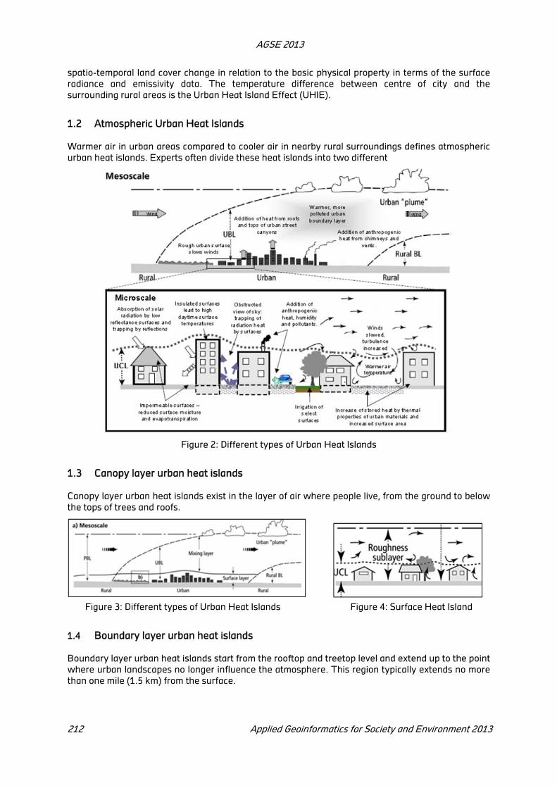
AGSE 2013


spatio-temporal land cover change in relation to the basic physical property in terms of the surface

radiance and emissivity data. The temperature difference between centre of city and the

surrounding rural areas is the Urban Heat Island Effect (UHIE).

1.2 Atmospheric Urban Heat Islands

Warmer air in urban areas compared to cooler air in nearby rural surroundings defines atmospheric

urban heat islands. Experts often divide these heat islands into two different

Figure 2: Different types of Urban Heat Islands

1.3 Canopy layer urban heat islands

Canopy layer urban heat islands exist in the layer of air where people live, from the ground to below

the tops of trees and roofs.

Figure 3: Different types of Urban Heat Islands Figure 4: Surface Heat Island

1.4 Boundary layer urban heat islands

Boundary layer urban heat islands start from the rooftop and treetop level and extend up to the point

where urban landscapes no longer influence the atmosphere. This region typically extends no more

than one mile (1.5 km) from the surface.

AGSE 2013


1.5 Surface and Air Temperatures: How Are They Related?

Surface temperatures have an indirect, influence on air temperatures, especially in the canopy layer,

which is closest to the surface. For example, parks and vegetated areas, which contribute to cooler

air temperatures? Dense, built-up areas have more air temperatures. Because air mixes within the

atmosphere, though, the relationship between surface and air temperatures is not constant, and air

temperatures typically are less than surface temperatures across an area.

Figure 5: Variations of Surface and Atmospheric Temperature

Surface and atmospheric temperatures vary over different land use areas. Surface temperatures are

more during the day, than at night but they both are fairly same at night.

Urban heat island has a significant impact on human environment such as,

Increase in demand for energy,

Increase in precipitation,

Human health problem,

Altering of local wind pattern,

Development of cloud and fog, humidity, thunderstorm activity, Weak tornadoes.

2 How to studt the effect of Urban Heat Island

The earlier studies used the in-situ measurement using the data procured by the meteorological

data which ground-based observations taken from are fixed thermometer networks with the

limitation that it cannot give the continuous information of the surface for the regional study. With

the advent of thermal remote sensing technology, remote observation of UHIs became possible using

satellite and aircraft platforms that have provided new avenues for the observation of UHIs and the

study of their causation through the combination of thermal remote sensing and urban

micrometeorology. (Voogt and Oke, 2003b)

AGSE 2013


Figure 6: Measurement Techniques of Urban Heat Islands

Figure 7: Platforms for Thermal Remote Sensing for Urban Areas

AGSE 2013


2.1 Urban Measurement: Assess Local scale Surroundings

Figure 8: Assessing Macro Scale Surroundings

2.2 Assess Micro scale Surroundings

Figure 9: Assessing Micro Scale Surrounding

Satellites with thermal sensor suitable for the study of Urban Heat Island Effect

Geostationary Operational Environmental Satellite (GOES) - 4 km

NOAA- Advance Very High Resolution Radiometer (AVHRR) - 1km

MODIS- Aqua and Terra platform – 1km

Terra-Advance Space borne Thermal Emission Reflection and Radiometer (ASTER) – 90m

AGSE 2013


Landsat 5 – Thematic Mapper – 120 m

Landsat 7 – Extended Thematic Mapper – 60 m

For climate change at regional level the image differencing technique is used. In order understand

the impact of land cover change on surface radiant temperature by concentration of heat with

respect to time was done. The calculation of temperature near the surface of the Earth, term called

as Land Surface Temperature (LST) for Urban Heat Island. Monitoring of urban heat island requires

various satellite sensors can be used to study or calculate the land surface temperature; the thermal

sensors are used to map the thermal attributes of the area. These thermal sensors with remote

sensing technology provide effective mapping heat islands. The thermal sensors pick up the thermal

energy from the Earth’s surface in the infrared electromagnetic spectrum. Researchers have tried a

variety of methods to obtain accurate measurements of the heat island. Thermometers for every

block of the city would be ideal and provide a detailed view of the surface, but is too expensive.

2.3 Urban Heat Island effect phenomenon using Remote Sensing and GIS techniques

Figure 10: Urban Heat Island effect phenomenon using Remote Sensing and GIS techniques

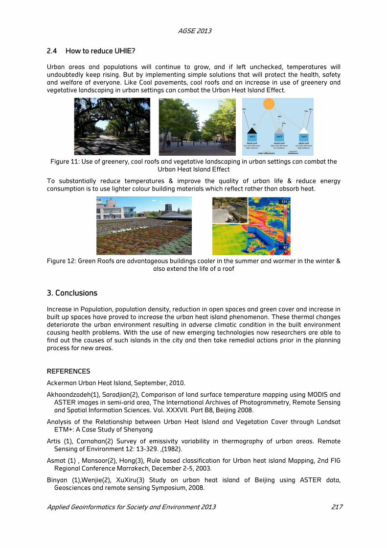
AGSE 2013


2.4 How to reduce UHIE?

Urban areas and populations will continue to grow, and if left unchecked, temperatures will

undoubtedly keep rising. But by implementing simple solutions that will protect the health, safety

and welfare of everyone. Like Cool pavements, cool roofs and an increase in use of greenery and

vegetative landscaping in urban settings can combat the Urban Heat Island Effect.

Figure 11: Use of greenery, cool roofs and vegetative landscaping in urban settings can combat the

Urban Heat Island Effect

To substantially reduce temperatures & improve the quality of urban life & reduce energy

consumption is to use lighter colour building materials which reflect rather than absorb heat.

Figure 12: Green Roofs are advantageous buildings cooler in the summer and warmer in the winter &

also extend the life of a roof

3. Conclusions

Increase in Population, population density, reduction in open spaces and green cover and increase in

built up spaces have proved to increase the urban heat island phenomenon. These thermal changes

deteriorate the urban environment resulting in adverse climatic condition in the built environment

causing health problems. With the use of new emerging technologies now researchers are able to

find out the causes of such islands in the city and then take remedial actions prior in the planning

process for new areas.

REFERENCES

Ackerman Urban Heat Island, September, 2010.

Akhoondzadeh(1), Saradjian(2), Comparison of land surface temperature mapping using MODIS and

ASTER images in semi-arid area, The International Archives of Photogrammetry, Remote Sensing

and Spatial Information Sciences. Vol. XXXVII. Part B8, Beijing 2008.

Analysis of the Relationship between Urban Heat Island and Vegetation Cover through Landsat

ETM+: A Case Study of Shenyang

Artis (1), Carnahan(2) Survey of emissivity variability in thermography of urban areas. Remote

Sensing of Environment 12: 13-329. ,(1982).

Asmat (1) , Mansoor(2), Hong(3), Rule based classification for Urban heat island Mapping, 2nd FIG

Regional Conference Marrakech, December 2-5, 2003.

Binyan (1),Wenjie(2), XuXiru(3) Study on urban heat island of Beijing using ASTER data,

Geosciences and remote sensing Symposium, 2008.

AGSE 2013


Climate and Temperature Information, http://www.climatetemp.info, April, 2011.

Coll (1), Caselles(2), Sobrino(3), and Valor(4) On the atmospheric dependence of the split window

equation for land surface temperature. International Journal of Remote Sensing, 15, 105–122,

1994.

Gillespie, Rokugawa,Hook, Matsunaga, & Kahle, A. B. A temperature and emissivity separation

algorithm for Advanced Space borne Thermal Emission and Reflection Radiometer (ASTER)

images. IEEE Transactions on Geoscience and Remote Sensing, 36, 1113 – 112, 1998.

Joshi and Bindu Bhatt Estimating temporal land surface temperature using remote sensing: a study

of Vadodara urban area, Gujarat International Journal of Geology, Earth and Environmental

Sciences.

JPL, ASTER Web, http://asterweb.jpl.nasa.gov/,September, 2010.

NASA, Landsat Program, http://landsat.gsfc.nasa.gov/, September, 2010.

NASA, MODIS Web, http://modis.gsfc.nasa.gov/, September, 2010.

Nichol, Urban Heat Islands by Day and night photogrammetric engineering & remote sensing Remote

Sensing 2005

Noorazuan bin Md. Hashim1, Asmala bin Ahmad2 and Mardina binti Abdullah3 Mapping urban heat

island phenomenon: Remote sensing approach Journal - The Institution of Engineers, Malaysia

(Vol. 68, No.3, September 2007)

Qinqin, Jianjun,Yonghang An ERDAS image processing method for retrieving LST and describing

urban heat evolution: a case study in the Pearl River Delta Region in South China, Environ Earth

Sci (2010) 59:1047–1055, Feb. 2009.

Qin, Karnieli, Berliner, A mono-algorithm for retrieving land surface temperature from Landsat TM

data and its application to the Israel–Egypt border region. International Journal of Remote Sensing

22 (18), 583–594, 2000

The Effects of Urban Heat Islands league of women voters Florida

Thermal remote sensing of urban areas: An introduction to the special issue. Remote Sensing of

Environment 104 (2006) 119–122

Trim Ball, “http://www.canadafreepress.com/index.php/article/20528”, Urban Heat Island, September

2008.

Voogta, JA, Oke TR, Thermal remote sensing of urban climates Remote Sensing of Environment 86

(2003) 370–384

Voogta, JA, Oke TR. How Researchers Measure Urban Heat Islands.

Wikipedia, http://en.wikipedia.org/wiki/Mumbai, 2011.

Wong Eva et.al., Reducing Urban Heat Islands: Compendium of Strategies Urban Heat Island Basics.

Climate Protection Partnership Division in the U.S. Environmental Protection Agency’s Office of

Atmospheric Programs.

Xu A study on information extraction of water body with the modified normalized difference water

index (MNDW I). J Remote Sens 9(5):589–595, 2005.

Zhang Zhao-Ming, HE Guo-jin, et al., Study of Urban Heat Island of Beijing City Based on RS and GIS.

Journal of Earth Sciences and Environment, 29(1), pp. 107-110, 2007.

Geo-Spatial Dimensions of Urban Sprawl of Shimla

Ashwani Luthraa, Ruchi Vasudeva

b

a Guru Ramdas School of Planning, Guru Nanak Dev University, Amritsar (Punjab, India),

[email protected]

bFreelance Urban Planner, Shimla (Himachal Pradesh, India), [email protected]

KEY WORDS: Spillover, Urban Sprawl, Sprawl Area, Suburban, Development, GIS, Land Use,

Municipal Limit

ABSTRACT

Dynamics economic activities and manpower in the cities has resulted in unprecedented migration from rural areas. Hence, cities witness expansions beyond their municipal limits, especially along their highways, countryside and surrounding green areas, commonly known as urban sprawl. Factors like congestion, high land prices, inadequate infrastructure in the municipal areas are other factors tempting spillover beyond municipal limits. Such areas grow in unplanned and haphazard manner largely and are devoid of social and physical infrastructural facilities. Mapping the volume & pattern of sprawl, land use conversion, its drivers, violations in development, etc. is extremely essential for suggesting corrective and progressive measures for controlling urban sprawl in the urban regions. A study conducted for two decades of urban sprawl of Shimla in GIS platform reflects different facets of urban sprawl and their implications on peri-urban environs and living conditions of the inhabitants. The study reflects that development of highways and other major roads has been the main driver of urban sprawl within Shimla Planning Area. The study attempts to cite other reasons for which the development has come up beyond Municipal Limits of Shimla. Based on issues of urban sprawl suggestions have been made for controlling the urban sprawl in the Planning Area of Shimla.

1 Introduction

Growth of cities is occurring faster than their spatial planning. Consequently, the added urbanites

find suburban lands most suitable to fulfill their residential requirements. Car culture has boosted the

trend of suburbanization as many of the new urbanites can afford to live in the peri-urban areas for

cheaper housing and avoiding congested city environs. Also, requirement of larger parcels of lands

for mega projects compel the developers to take up their projects in the suburban lands. Hence,

urban sprawl is witnessed as a common feature in most of the fast growing urban settlements.

Urban sprawl is a consequence of socio-economic developments under certain circumstances. It is

often associated to low residential density, scattered suburban linear patterns, and dependence on

private transport. Citing reasons to urban sprawl Siddhartha [2000] has defined it as ‘the

disconcertion of the urban activity. Urban sprawl is due to the expansion of the city beyond of its city

boundary. It is the by-product of highway and automobiles. Automobiles and highway and flyover

compel the city to grow outside from its jurisdiction boundary’. While adding urban planning

dimension to urban sprawl, Kulshrestha [2006] has defined it as ‘a process of growth of urban area

or sub urban area in an unplanned manner having no regard to social infrastructure and subsequent

needs for transport and other facilities and services’. Urban growth is a broad and vague concept

that can be subdivided into various types - sprawling or compact, dispersed (scattered) or clustered,

continuous or leapfrog, spontaneous or self-organizing, planned or organic. It may comprise physical

growth, population growth, economic growth and environmental change (decline), although there is

often a focus on the physical aspects in the domains of remote sensing and GIS [Gupta, 2011].

Popular hill cities like Shimla have also witnessed the similar patterns of urban growth and spill over.

Hence, empirical examination of nature and extent of urban sprawl reflects the causes and

consequences of urban sprawl in the Capital city of Himachal Pradesh, India.

AGSE 2013


2 Methodology

An empirical research on urban sprawl of Shimla, Himachal Pradesh, India in GIS platform has been

conducted to assess the nature and extent of urban spill over beyond Minicipal Limits of Shimla.

Study area is demarcated between Municipal Limit 1998 and proposed Planning Area of Master

Plan, Shimla (refer figure 1) and randomly selected 1621 households have been surveyed to collect

information on their socio-economic and preferential characteristics for settling on suburban lands.

Map of Shimla Planning Area, procured from Town and Country Planning Department Shimla,

Himachal Pradesh (TCPD), is scanned and geo-referenced using Survey of India topographical

sheets at 1:20,000 scale. Due to non-availability of latest spatial data, images taken from Google

Earth are used to digitize developments in the Study Area. For the same geo-referenced Study Area

boundaries are superimposed on Google Images and developments in it are digitized using ArcGIS

2010 for base map. Ground truthing is done to determine the land uses Inventory of data is created

in ArcGIS 2010 platform and volume of land use development, its distribution pattern, conversion and

other developmental characteristics are assessed and plotted on maps by generating different

thematic layers as per the scope of the study. Analysis of urban sprawl has been conducted at macro

as well as micro scale i.e. for overall study area as well as for sample pockets.

Figure 1: Study area and Google Image

2.1 Brief about Study Area

Shimla is situated on the last traverse spur of the Central Himalayas, south of the river Satluj at

31006’ North latitude and 77

005’ east to 77

013’ longitude, at an altitude of 2130 meters above mean

sea level. It is characterized by rugged topography, steep slopes, deep valleys and elongated spurs.

Endowed with high altitude, vested and varied vegetation, scenic beauty, charming climate and

everything that nature could gift, this hill station has its own identity and character. Good

connectivity by road, rail and air services make it a potential city for high growth. Being a multi-

faceted city, having administrative, educational, institutional and tourism primacy, its population has

trebled in last four decades i.e.1971-2011, registering a growth rate of 19% in 2001-11. The new

urbanites prefer to settle in its suburbs because of their socio-economic characteristics and other

preferences. Sprawl is spread over 8583 hectares of land all around the Shimla city. Like that of

Shimla city, population of Shimla Planning Area (SPA) has also grown by more than three times

during 1971-2011. Notably, population of SPA has increased very rapidly during 2001-11 i.e. from

1.75 lacs in 2001 to 2.36 lacs in 2011. About 40% of the SPA population is residing in the study area

in 2011, which has been 23% in 2001. Hence, suburbanization has been increasing in Shimla, which

reflects outward trends of growth of Shimla city.

2.2 Volume of Development

Shimla has witnessed large volume of urban spill over in the past two decades. Improved highway

network, scarcity of developable urban land, absence of Master Plan and inadequate enforcement

are some of the key players in its urban sprawl. Development in the sprawl area started with the

coming up of government offices on NH.22. Later, development of infrastructure, commercial and

AGSE 2013


public/semi-public activities, led to massive constructions in the sprawl area. Accessibility

improvements with the construction of bypass also gave boost to similar type of developments.

Figure 2: Volume of Developement

Despite all physiographic constraints, Shimla’s sprawl has consumed about 816.15 hectares of land

(refer figure 2). Urban sprawl of Shimla has occurred along major roads and eventually spread away

from these corridors in different volumes. Empirical evidences show that out of total developed area,

about 778.45 hectares is built along major roads of Shimla and remaining is sporadically developed

within the sprawl. The development along different roads has not occurred uniformly. Variations in

developed area along different roads are on account of their relative importance in the region. NH-22

is the longest road passing through the study area. Hence, majority of the development has come up

along it only. Total developed area along this highway is 497.54 hectares (63.91%), out of which

396.95 hectares (50.99%) is along NH-22 bypass. SH-13 is another important highway from the

point of view of suburban development of Shimla. About 130.79 hectares (16.80 %) land area has

developed along it. NH-205, SH-16 and link road are other major roads along which the development

has come up. The total developed area on these roads is 62.58 hectares (8.04%), 23.21 hectares

(2.98%) and 37.88 hectares (4.87%) respectively.

2.3 Existing Land Use

Shimla is an important cultural, educational and institutional centre due to which it is developing very

fast. Most of these institutes have developed within Shimla Municipal Limits. Hence, a large amount

of land is put to residential use in the sprawl area to serve the population serving in them. Heavy

traffic volume on highways bypassing Shimla has attracted commercial activities along them. Hence,

a mix of residential, commercial and public/semi-public is witnessed at important nodes to meet the

requirements of inhabiting population (refer figure 3). Of the total developed area, about 411.88

hectares (50.47%), 257.34 hectares (31.49%), 109.23 hectares (13.38%) and 38.04 hectares (4.63%)

have come up as residential, commercial, public & semi-public and transportation use respectively.

The study also reveals that commercial and public & semi-public uses have come up along major

roads/ highways. There is no area developed as park or open space in any of the residential

developments. Hence, settlements in the sprawl area are developing as satellite settlements to

Shimla city, which are dependent on it for cultural, social, educational, economic, medical, and

economic purposes. Development in sprawl area has converted the soft green picturesque into

concrete form.

AGSE 2013


Figure 3: Existing Land Use of Shimla Spral

2.4 Land Use Conversion

Lower land value, inherited land, scarcity of urban land, socio-economic and environmental factors

are some of the important factors responsible for urban spill over on barren, forest and agricultural

lands of Shimla Planning Area, leading to conversion of land use by new land uses. Empirical study

reveals that most of the development (40.14%) within the sprawl area has come up on barren land,

which can be said to be the better use of the available land (refer figure 4). But about 250.14

hectares (32.13%) of forest land has also been converted into built up area, which is a loss to green

cover. About 27.73% of the development has come up on agricultural land as well, but its percentage

share is less than that of barren and forest land, which is an economic loss to the region. Land

transformations have taken place all over the fringes of Shimla especially in South, South-West, and

North directions of Shimla. NH-22 is the longest road passing through the study area. Hence,

majority of the land use conversion has occurred along it only. About 497.54 hectares (63.91%) of

land has been converted into urban uses along NH-22, out of which 396.95 hectares (50.99%) is

along NH-22 bypass only. SH-13 has witnessed about 130.79 hectares (16.80 %) land use

conversion.

Figure 4: Land Use Conversation

2.5 Composition of Sprawl

Massive spatial growth is occurring all over the Shimla sprawl area and its character is reflected by

the nature of development, planned or unplanned. For the present study, any area approved by any

Development Authority, as designated in the Interim Development Plan of Shimla (2021) is

considered as planned area, else unplanned. The study confers that majority of the development is

unplanned and basic facilities such as water supply, sewerage, well developed road network,

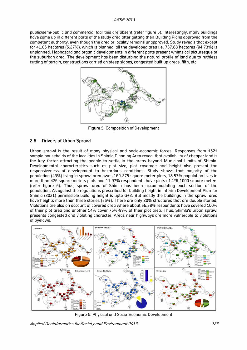
AGSE 2013


public/semi-public and commercial facilities are absent (refer figure 5). Interestingly, many buildings

have come up in different parts of the study area after getting their Building Plans approved from the

competent authority, even though the area or locality remains unapproved. Study reveals that except

for 41.06 hectares (5.27%), which is planned, all the developed area i.e. 737.88 hectares (94.73%) is

unplanned. Haphazard and organic developments in different parts present whimsical picturesque of

the suburban area. The development has been disturbing the natural profile of land due to ruthless

cutting of terrain, constructions carried on steep slopes, congested built up areas, filth, etc.

Figure 5: Composition of Development

2.6 Drivers of Urban Sprawl

Urban sprawl is the result of many physical and socio-economic forces. Responses from 1621

sample households of the localities in Shimla Planning Area reveal that availability of cheaper land is

the key factor attracting the people to settle in the areas beyond Municipal Limits of Shimla.

Developmental characteristics such as plot size, plot coverage and height also present the

responsiveness of development to hazardous conditions. Study shows that majority of the

population (43%) living in sprawl area owns 169-275 square meter plots, 18.57% population lives in

more than 426 square meters plots and 11.97% respondents have plots of 426-1000 square meters

(refer figure 6). Thus, sprawl area of Shimla has been accommodating each section of the

population. As against the regulations prescribed for building height in Interim Development Plan for

Shimla (2021) permissible building height is upto G+2. But mostly the buildings in the sprawl area

have heights more than three stories (56%). There are only 20% structures that are double storied.

Violations are also on account of covered area where about 56.38% respondents have covered 100%

of their plot area and another 14% cover 76%-99% of their plot area. Thus, Shimla’s urban sprawl

presents congested and violating character. Areas near highways are more vulnerable to violations

of byelaws.

Figure 6: Physical and Socio-Economic Development

AGSE 2013


Sprawl area of Shimla accommodates all categories of people. But mostly the residents are

educated. About 50% being from higher secondary category. Majority of the residents (48%) of the

sprawl area are in service, while 23% and 27% are in business and farming respectively. About 87%

of the residents have ownership rights of their houses in the study area.

3 Issues and Implications

Following are some of the important planning and geo-spatial issues emerging out of the

development occurring in sprawl area.

Surmounting volume of urban sprawl is a cause of worry for planners and policy makers to

accommodate fast growing population of Shimla. Since majority of the development is

residential, therefore, it makes it yet more concerned issue as unplanned development in no way

presents better quality of life to the inhabitants of these areas.

Development along the highways creates hurdles in movement for the highway traffic and at

times results into accidents. Direct openings of properties on the highways lead to unsafe traffic

and living conditions in these areas. NH-22 bypass is the most vulnerable stretch in the study

area followed by SH-13 and NH-22 as they are thickly developed roads.

Patchy commercial developments along major roads results into on street parking along them.

Vehicles parked along the highway and in no parking zones not only reduce the effective road

width and carrying capacity of the highways. This leads to traffic jams, danger to people’s lives,

loss of time & energy and environmental pollution.

Linear form of development along different roads coupled with high commercial or mixed land

use presents ribbon type of development. In the absence of any control on access to these

properties, living in these areas is very unsafe. Also, it is not possible for the authorities to

expand the roads.

Development in the sprawl area has also come up on unprotected forest lands, which has led to

environmental degradation and Shimla is reduced to a hazardous city. Depletion of green cover

due to massive constructions has vanished the wild life.

More than 80% of all the existing buildings of sprawl area do not meet the seismic code

standards as prescribed for Shimla. So, haphazard & congested development, construction on

steep slope and on sinking & sliding zone within the study area are susceptible to major natural

hazards like earthquakes etc.

Unplanned and unauthorized development in the study area presents a dismal picture of the

‘Queen of Hills’. The buildings have been developed on steep hills, which are not permitted by

the regulations prescribed in the Interim Development Plan or even practiced in Shimla. As

Shimla lies in seismic zone IV, a high intensity earthquake will result in massive causalities. The

rate of causalities shall also be higher because accesses to these areas are narrow and

development has occurred on steep hills. Nearly 40% of the total development in the study area

falls in this category.

Continuous monitoring of changing urbanism and utilization of land is urgently required to bring

about sustainable urban communities on the one hand and optimum use of suburban lands on

the other. Manual monitoring of the fast changing urban conditions is very difficult. Also, the

planning and developmental agencies are not well equipped (technologically) to perform this

responsibility. Resultantly, suburban changes are remaining unchecked, uncontrolled and

unsustainable.

Master Plan is considered as tool for controlled and planned development on the lands in the

suburbs of the cities. But the type of data required for Master Planning is not available.

Whenever a Master Plan is under preparation efforts are initiated to collect data. Time taken to

gather the required data and information is at times so long that few parcels of suburban lands

further develop, especially in fast growing cities, thus making the data obsolete for Master Plan.

Physical data is very vital for preparing the Master Plan of a city. The area covered by rapidly

growing cities is so vast that shortage of staff on the one hand and lack of trained persons on the

AGSE 2013


other hand make it almost impossible to update the existing physical conditions and

development of the cities. Updating the existing physical developments takes longer time with

indigenous technologies, which delays the Master Planning process.

Though advanced technologies like remote sensing and GIS are available currently to be used in

Master Planning process, but their application has been significantly negligible. The main

reasons for the same have been financial, administrative and technical hitches on the part of

departments and governments. These technologies are cost dearer and little technical. Hence,

lack of funds and technical manpower to operate the technology have kept the Town and

Country Planning Departments and Development Authorities far behind in planning, monitoring

and checking urbanism in general and urban sprawl in particular.

Many of the technical officials, especially the top old officials, dealing with spatial planning and

development of cities are not yet aware of the advantages and potential applications of remote

sensing and GIS. If at all they are aware then most of them are handicapped as they have never

used these technologies themselves. So, they are still working with the primitive technologies

leading to inefficiencies in planning and development mechanisms.

Even the Master Plans prepared for cities are not pragmatic in nature as they face difficulties at

the time of implementation. As these Plans are spatial by nature, so land is the resource used for

planning, which have many stakeholders or title holders. Hardly any effort is made to link the

land records and revenue records with the Master Planning process. Therefore, it becomes very

difficult to implement planning proposals due to litigations on land acquisition front. This results

in unauthorized, unplanned and unorganized developments on private lands. Suburbs are not

spared from these practices. Consequently, unplanned urban sprawl results.

The base-maps which are more essential than textual data to GIS are often lacking or outdated.

There are usually many types of base-map, each compiled by different agencies with different

accuracy and map scales. This makes them difficult to integrate into GIS environment.

4 Suggestions

Following planning and geo-spatial measures are suggested to control urban sprawl of Shimla.

The Development Plan of Shimla Planning Area should be approved immediately so that the

planning proposals can be implemented and planned development can be attained in the

suburban areas of the State Capital.

As development in different areas is not uniform and is not expected to be uniform, therefore, the

Development Plan for the city should be supported by the Zonal Development Plans, which

should provide separate zoning regulations and other Development Controls (Byelaws) for

respective zones.

As proposed in the Interim Development Plan of Shimla, 2021, construction of buildings should

not be allowed on steep slopes. Constructions in the areas having slope as high as 350 to 45

0

should be restricted as it will be dangerous for life of the inhabitants. Seismic codes as proposed

in the City Disaster Management Plan – Shimla (2012) should be followed and enforced strictly

for safety and security of the residents of these areas.

Eco-sensitive zones such as forests and water bodies should be protected from unplanned and

unauthorised developments. Separate guidelines should be framed for forests (protected and

unprotected) in the Shimla Planning Area. They should be strictly enforced to control

unauthorised development in the study area.

Ribbon development should be checked as far as possible. The same can be done by not

allowing any development to come up without prior approval of the Town & Country Planning

Department and Himachal Urban Development Authority. These agencies should be made

accountable for planned and controlled development along the highways.

Rapidity of urbanization in India creates urgency to induct advancements in the planning and

development agencies by introducing latest state of the art technologies in them. It is suggested

AGSE 2013


that Town and Country Planning Departments, Development Authorities and Urban Local Bodies

should be equipped with latest GIS and Remote Sensing technologies asking for complete

computerization of their planning and development records. Also, it is suggested for regular and

continuous update of these technologies from time to time.

If urban spatial development of the cities is to be planned and streamlined in India then paucity

of required data has to be removed. It is suggested to create data collection cells in the planning

and development agencies whose duty shall be to collect the required data for Master Planning

purposes. Trained survey staff needs to be recruited immediately to restrict the damage already

done to the minimum.

It is also suggested to create a common data framework for Master Planning purpose for the

guidance and action of different departments to collect and supply latest data to the nodal

planning agency. The required information should be made public so that transparency prevails.

5 Conclusions

Shimla is playing a multifunctional role and there is a heavy pressure on suburban land due to

urbanization forces. But unplanned, haphazard and uncontrolled development of city’s sprawl is

leading to social disaster. As city is susceptible to natural disasters like earthquakes, landslides and

cloudburst, social disaster has deteriorated the living conditions of the inhabitants of the city.

Marauding land use conversion has led to economic disorder, which not only adversely affects the

economy of the city but also affects the eco-system of the city. Due to constant physical,

environmental and aesthetic degradation of land, the city’s suburbs demonstrate it as a hazardous

city. Most serious issue concerning urban sprawl of Shimla is disturbance to natural profile of land by

cutting of terrain for constructions. Increased commercial and residential activity, unplanned physical

growth and influx of population, resulted into eyesores on the township of Shimla. Numerous

buildings are coming in a haphazard and unplanned manner. The worst part is the new

constructions that are coming up on dangerous slopes because buildings may dislocate or fail to

cope up with the gravity of geo-hazards like earthquake, landslides etc. As development in the hilly

terrain comes on different contours, so in case of demolition of structures due to earthquake (say), a

chain effect of collapse is expected to cause large scale destruction. Shimla has highly sinking zones

where any further addition of building loads could be disastrous. These include the northern slope,

especially the famous Ridge, New Shimla, etc. Thus, very serious note should be taken for

unplanned and uncontrolled sprawl of Shimla city and rigorous planning and development strategies

are needed to minimize the effect of disaster, be it liveability conditions in the localities. Planning

proposals of Development Plan of Shimla (2021) and guidelines of City Disaster Management Plan-

Shimla (2012) should be strictly followed so that the glory of magnificent hill city is retained and

pronounced for its sustainable development.

REFERENCES

Kulshrestha, S.K., 2006. Dictionary of Urban and Regional Planning, Kalpaz Publications, New Delhi,

p. 228.

Mayhew, Susan, 1999. A Dictionary of Geography, Oxford University Press, USA, p.149.

Mukherjee, S (2000), Cities Urbanization and Urban Systems, Concept Publishing Company, New

Delhi, p. 182.

Sharma, Swati, 2011. Planning Strategies for Urban Sprawl of Jaipur City, unpublished thesis, Guru

Ramdas School of Planning, Guru Nanak Dev University, Amritsar.

Sen, Sourav, 2012. Effects of Urban Sprawl on Human Habitation in Urban Fringe and Peri-Urban

Areas, ITPI Journal, Institute of Town Planner, India, New Delhi, 9(3), July – September, PP. 53-63.

Shekhar, Shashi, 2011. Urban Sprawl and Other Spatial Planning Issues in Shimla, Himachal

Pradesh, ITPI Journal, Institute of Town Planners India, New India, 8(3), July, pp. 53-66.

Vasudeva, Ruchi, 2013. Planning Strategies of Urban Sprawl of Shimla, unpublished M. Tech (Urban

Planning) thesis, Guru Ramdas School of Planning, Guru Nanak Dev University, Amritsar.

Impact of Land Use/Land Cover Pattern on Urban Heat Island in Nagpur

City Using Remote Sensing

aRajashree Kotharkar, *

bMeenal Surawar

a Department of Architecture and Planning, Visvesvaraya National Institute of Technology (VNIT),

Nagpur, E mail: [email protected]

b Department of Architecture and Planning, Visvesvaraya National Institute of Technology (VNIT),

Nagpur. E mail: [email protected]

KEY WORDS: Remote sensing, GIS, Urban Heat Island, Land use/Land cover (LU/ LC), Land surface

temperature (LST)

ABSTRACT

Urban Climate change occurs due to process of urban overheating by rapid urbanization. Urban Heat Island (UHI) effect causes increase in thermal stress for urban-dwellers and acts as a prominent urban environmental concern. UHI is found more pronounced in developing cities, so keeping in view specifically Indian cities, UHI effect in Nagpur urban area has been explored in this paper. Urban areas being the magnetic pull for population migration, further characterizes high built-up density. Moreover this population density varies as per different Land use/ Land cover types hosted by any urban areas. UHI studies have been carried for isolated stations with onsite measurements of air temperature. While the advent of remote sensing techniques has made it easier to study surface temperature UHI through remotely sensed surface reflectance data. The paper tries to understand the relationship between various LU/ LC types and their impact on UHI formation within Nagpur city. Supervised LU/ LC classification has been done as per their specific urban characteristics using ENVI-5. Change detection has been studied by carrying NDVI to understand the proportion of vegetative cover with respect to built-up ratio. ENVI-5 as a powerful image processing and analytical tool has been used to extract the land surface temperatures (LST). Temperature distribution is studied using Arc GIS to create temperature zones within LU/LC map. This Paper intends to study Land surface temperature distribution to understand different types of LU/ LC impacts contributing UHI formation in Nagpur urban areas using remote sensing.

1 Introduction

Land surface temperature (LST) changes observed for longer duration are key characteristics in

identifying urban climate change. Changes in land-surface cover can affect urban climate, and can be

identified by changes in their LST. LST distribution pattern within an urban environment and its

adjacent surroundings to demarcate UHI zones could be studied through various Land use/ Land

cover (LU/ LC) surfaces. This is due to the land once permeable is replaced with non-permeable

materials, thereby restricting evaporative cooling and water run-off on the surface (Gopalkrishnan

2003; Wong N.H. and Chen Y., 2005; Das Y., 2008 and Jusuf S.K., 2009). Impact of Land surface

temperature due to variation in LU/ LC could be measured with the help of remote sensing with GIS

modeling set up to study urban growth pattern (Weng Q., 2001; Gupta A. et al., 2009). Thermal

properties of urban building materials also determines UHI formation as building materials store

solar radiations during the day which is released at night. Urban materials reflect less and absorb

more energy thereby increases temperatures at Land surface level. (Padmanabhamurty B. et al.

1982; Sarrat C., 2006 and Kolokotroni M., 2008).Urban canyons are created by narrow streets and

tall buildings which decreases wind speed and traps heat (Oke T.R., 1972).

Gopalkrishnan, et al. (2002) used mesoscale terrain modeling to study UHI effect with respect to

vegetative cover in southern India-Chennai, Bangalore & Hyderabad. The study concludes regional

scale topographical features do not diminish the urban effects, while strongest UHI impact found in

Chennai as compared to Banglore and Hydrabad. Sarkar H. (2004), reveals that UHI varies gradually

within cities with a direct relationship to land-cover and population, mostly in tropical cities.

Badarinath, (2005), studied Hyderabad urban areas with the help of ENVISAT AATSR Data and

analyzed the urban heat island formation. It was observed that temperature variations during day

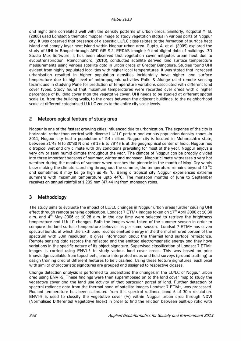
AGSE 2013


and night time correlated well with the density patterns of urban areas. Similarly, Katpatal Y. B.

(2008) used Landsat 5 thematic mapper image to study vegetation status in various parts of Nagpur

city. It was observed that presence of a specific LU/LC class relates to the formation of surface heat

island and canopy layer heat island within Nagpur urban area. Gupta, A. et al. (2009) explored the

study of UHI in Bhopal through ARC GIS 9.2, ERDAS Imagine 9 and digital data of buildings -3D

Studio Max Software. It has been observed that vegetation cover mitigates urban heat due to

evapotranspiration. Ramachandra, (2010), conducted satellite derived land surface temperature

measurements using various satellite data in urban areas of Greater Bangalore. Studies found UHI

evident from highly populated localities with higher local temperatures. It was stated that increased

urbanisation resulted in higher population densities incidentally have higher land surface

temperature due to high level of anthropogenic activities Patki & Alange used remote sensing

techniques in studying Pune for prediction of temperature variations associated with different land

cover types. Study found that maximum temperatures were recorded over areas with a higher

percentage of building cover than the vegetative cover. UHI needs to be studied at different spatial

scale i.e. from the building walls, to the areas between the adjacent buildings, to the neighborhood

scale, at different categorised LU/ LC zones to the entire city scale levels.

2 Meteorological feature of study area

Nagpur is one of the fastest growing cities influenced due to urbanization. The expanse of the city is

horizontal rather than vertical with diverse LU/ LC pattern and various population density zones. In

2011, Nagpur city had a population of 2.4 million. Nagpur city is located in Maharashtra state,

between 21°45 N to 20°30 N and 78°15 E to 79°45 E at the geographical center of India. Nagpur has

a tropical wet and dry climate with dry conditions prevailing for most of the year. Nagpur enjoys a

very dry or semi humid climate throughout the year. The climate of Nagpur can be broadly divided

into three important seasons of summer, winter and monsoon. Nagpur climate witnesses a very hot

weather during the months of summer when reaches the pinnacle in the month of May. Dry winds

blow making the climate scorching throughout the summer, the temperature remains beyond 40 0C

and sometimes it may be go high as 48 0C. Being a tropical city Nagpur experiences extreme

summers with maximum temperature upto 440C. The monsoon months of June to September

receives an annual rainfall of 1,205 mm (47.44 in) from monsoon rains.

3 Methodology

The study aims to evaluate the impact of LU/LC changes in Nagpur urban areas further causing UHI

effect through remote sensing application. Landsat 7 ETM+ images taken on 17th

April 2000 at 10:30

a.m. and 4th

May 2006 at 10:28 a.m. in the day time were selected to retrieve the brightness

temperature and LU/ LC changes. Both the images were taken of the summer season in order to

compare the land surface temperature behavior as per same season. Landsat 7 ETM+ has seven

spectral bands, of which the sixth band records emitted energy in the thermal infrared portion of the

spectrum with 30m resolution. It gives information about the thermal land surface reflectance.

Remote sensing data records the reflected and the emitted electromagnetic energy and they have

variations in the specific nature of its object signature. Supervised classification of Landsat 7 ETM+

images is carried using ENVI-5 to study various land cover areas. This was based on prior

knowledge available from toposheets, photo-interpreted maps and field surveys (ground truthing) to

assign training area of different features to be classified. Using these feature signatures, each pixel

with similar characteristic signatures are grouped and assigned to respective classes.

Change detection analysis is performed to understand the changes in the LU/LC of Nagpur urban

area using ENVI-5. These findings were then superimposed on to the land cover map to study the

vegetative cover and the land use activity of that particular parcel of land. Further detection of

spectral radiance data from the thermal band of satellite images Landsat 7 ETM+, was processed.

Radiant temperature has been calibrated from this spectral radiance band 6 of 30m resolution.

ENVI-5 is used to classify the vegetative cover (%) within Nagpur urban area through NDVI

(Normalised Differential Vegetative Index) in order to find the relation between built-up ratio with

AGSE 2013


that of vegetation. LST distribution study is carried in Arc GIS to create temperature zones within

Nagpur LU/LC maps.

4 Change detection using supervised classification

Observations of urban-rural air temperature differences i.e. UHI have been reported worldwide with

local field sites. Observed fields are extremely diverse in their physical and climatological

characteristics. They are often discussed as urban or rural while both are showing much variation in

actual land cover of the sites. To address these urban-rural features, the local climate zone (LCZ)

has framed LU/LC classification specifically catagorised on the basis of built up area, building density,

green cover ratio, open areas and water bodies. To observe UHI formation within Nagpur urban

areas, observational classification has been done under these specified classes. Vegetation and built

up ratio classification would help as observational parameters for all selected micrometeorological

survey stations to process the identification and characterization of UHI in Nagpur urban area. The

study aims to process the identification and characteristics of UHI in Nagpur city. Supervised

classification based on LU/ LC of Nagpur city is categorized to process Change detection using ENVI-

5. Diverse urban settings promote area level classification which was broadly categorised as urban

built up areas, forest/ agriculture, water bodies and open land. Further urban built up areas are

subdivided into densely built-up, high built-up, medium built-up and sparse built-up areas (Ref. Fig.

3)

17th April 2000 4th May 2006

Figure 1: Map of Nagpur Urban Land use/ Land cover through supervised classification (2000 & 2006

Classes LC class distribution LC areas in years LC changes

2000 (IN %) 2006 (IN %) 2000-2006 (IN %)

1,2,3,4 Urban Built-up Urban Densely bu-up 15.70 55.67 +39.97

Urban High bu-up

Urban Medium bu-up

Urban Low bu-up

5 Forest/ Agriculture 53.08 25.79 -27.29

6 Water bodies 1.18 1.49 +0.31

7 Open land 30.02 17.03 -12.99

Table 6: LU/ LC changes in Nagpur through supervised classification (2000-2006)

Classified images are further verified for their accuracy it was found that some open areas

resembled built up category in supervised classification. Those pixels belonging to specific areas

were identified region by region and their pixel values were changed to the actual value using spatial

pixel editor tools. This confusion in urban areas arises due to different shades of paved areas,

building roof tops, cement roads, etc. Also the building shadows and tree shadows increases the

classification confusion. Thus lots of efforts need to be taken to achieve more and more accuracy

during classification process. Each land use area is obtained for imagery using class statistics tools

available in post classification (Ref Fig.3). Change detection scenario of Land cover changes during

2000 to 2006 has been summarized in Table. 1. In 2000, LC areas of forest/ agriculture and open

land as 53.08% and 30.02% respectively, where 15.70 was found to be built-up area. In 2006, forest/

agriculture and open land were decreased to 25.79% and 17.03% respectively and built-up area was

AGSE 2013


increased to 55.67%. While the areas under water bodies slightly increased by 1.18% to 1.48%

during 2000-2006. It may have happened because of seasonal variation, but the growth of built-up

remains in the increasing rate. During this period urban built-up has been drastically increased by

39.97% of the total area, whereas forest/agricultural area have been reduced by 27.29% than

previous and open land area reduced by 12.99% during 2000 to 2006.

5 Derivation of land surface temperature (LST)

To analyse the changes in LST as per LU/ LC changes in the study region, multi temporal images

must be co-registered in the same coordinate system (i.e. UTM/ WGS84). In this study the raw

images were geo-referenced to a common UTM coordinate system based on Spectral angular

mapper algorithm with the pixel size of 30m x 30m for all bands. Multi temporal Landsat-7 ETM+

images of 2000 & 2006 were used to study UHI intensity. Urban heat island intensity is measured as

the difference between the peak temperature found inside the urban area and the background rural

temperature (Oke T.M., 1987). UHI is thus measured for the individual thermal images and then

compared between different time periods. Each ETM+ file consists of independent single-band

images which were converted into multi band image using layer stacking tool in ENVI-5. The image

subset tool is used to clip the study area. The retrieval methods of brightness temperature from the

ETM+ images consists of Normalized difference vegetative index (NDVI) which is one of the most

widely applied vegetation indices. NDVI is the ratio between the near infrared band (i.e. band 4) and

the red band (i.e. band 3) to get the vegetative information. In order to calculate NDVI equation (1)

can be used as:

(1)

Spectral emissivity can be estimated by utilizing NDVI (Griend V. D. et al., 2003; Zhang, J. et al., 2006;

Liu, L. and Zhang, Y., 2011). The emissivity values of a material ranges from 0 to 1 and it is the

relative ability of materials surface to emit energy by radiation. In general, the darker material has

close emissivity value near to 1and white reflective materials have lower emissivity value. Griend V.

D. (2003), stated the emissivity value equation (2) for the NDVI values which ranges from 0.157 to

0.727 as:

1.0094 0.0047 (2)

Zhang (2006), proposed a complete land surface emissivity estimation method using NDVI as stated

in Table.2

SR. No NDVI Land Surface emissivity(�)

1 NDVI < -0.185 0.995

2 -0.185 ≤ NDVI ≤ 0.157 0.970

3 0.157 ≤ NDVI ≤ 0.727 1.0094 0.0047

4 NDVI > 0.727 0.990

Table 2: Estimation of Emissivity using NDVI

The approaches to the retrieval of temperature has described in Landsat-7 users handbook (Ref.

Tab: 3). Firstly the DN values are converted from thermal to radiance through Band Math expression

in ENVI-5. These radiance values were further converted into degrees Kelvin to know the exact

spatial temperature distribution through Landsat calibration method. Once the DNs for the thermal

bands have been converted to radiance values, it is simply a matter of applying the inverse of the

Planck function to derive temperature values. The equation (3) to convert radiance to temperature

is:

∗ (3)

AGSE 2013


Where:

T = Effective satellite temperature in degrees Kelvin

b1 = Band 6 of Landsat7 ETM+ (the cell value as spectral radiance)

b2 =Spectral emissivity (NDVI band-calculated from equation 1)

K1 & K2=Calibration constants (Ref. Tab: 3)

Calibration constants Landsat TM Landsat ETM+

K1 607.76 666.09

K2 1260.56 1282.71

Table 3: Calibration Constant (Source-Landsat7 Users Handbook)

The ENVI formula (3) in Band Math for a Landsat7 ETM+ image as per the calibration constant is

.

. ∗ (4)

17th April 2000

4th

May 2006

Figure.2: Land surface temperature of Nagpur urban area (2000 & 2006)

AGSE 2013


Both the Landsat ETM+ images taken in day time during summer season have been compared to

retrieve Land Surface Temperature (LST). The LST in the year 2000 image ranges from 300.64 0

K

(min) to 323.14 0

K (max) with an average of 311.89 0

K. But in 2006 image the LST ranges from

320.99 0

K (min) to 343.39 0

K (max) with an average of 332.19 0

K. LST has been studied to be

increased from 2000 to 2006. The maximum LST is recorded in commercial cum residential core area

of old as well as newly developed Nagpur city in both the images. Sparsely built-up areas in south

urban fringe area are exhibiting maximum LST in 2006 than in 2000. The minimum LST is recorded

in residential area in east urban fringe of Nagpur city in 2000 than compared to 2006 (Ref. Tab.4).

Minimum LST areas are same in both the years but the expanse of minimum LST decreases as per

the time period.

6 Results and Discussions

LST distribution with respect to LU/ LC pattern has been studied based on vegetation and build-up

density classification. In both the years, LST has been observed in residential cum commercial area

which falls under urban high built-up class. Densely built-up class exhibits highest LST among

others. Sparsely vegetated areas showed higher temperatures similar to the highest recorded areas.

Classes with medium built-up areas showed less LST than densely built-up class. Those falling

under sparse built-up with dense vegetation is observed to have lowest LST. These areas with

dense vegetation exhibits less LST than densely built-up class. Areas coming under forest/

agricultural field as complete vegetation also exhibit the least LST than densely built-up class. Water

bodies and open land at certain places also shows minimum LST in both 2000 & 2006 images. It is

observed that upcoming new developments in the southern fringe area of Nagpur city which were

sub-classified under medium built-up, less vegetation & mostly open land, exhibits higher

temperature similar to densely built-up classes (Ref. Fig. 3 & 4). Study found that areas which are

having higher temperature fall under the densely built-up areas with less vegetation. It is revealed

that as the build-up area decreases with the increase in vegetation percentage throughout urban

area, LST decreases and vice- versa.

Sparsely vegetative areas having more of hard surfaces, absorbed heat during daytime and released

at night. This might be the reason why there are LST variations in different LU/ LC areas. These

areas were delineated as urban hot spots within Nagpur urban area. On the other hand sparse built-

up with dense vegetation areas and those near water bodies exhibits lowest LST. These observed

areas were delineated as urban heat sink spots within Nagpur urban area. It is observed that the

lowest LST was mostly in the green areas with less building density. While highest LST was found in

the core areas mostly in the commercial areas i.e. the CBD areas having high building density.

Higher LST might be due to congested i.e. high building density within Nagpur urban area, since it is

the old city with uneven geometry of layout. Also sparsely vegetated new urban developed areas in

the urban fringes but comparatively less building density were having higher LST distribution.

Depending upon the proximity of green areas there are temperature variations in the residential

areas. Those which are nearer to green areas are showing lower temperatures than those to the city

center. Study states that less green areas and high building density plays important role in causing

higher LST further leading to UHI formation.

7 Conclusion

Impact of LU/ LC pattern within Nagpur urban area has been studied by observing areas within

Nagpur municipal boundaries and urban fringe. Studies observed that the highest LST normally

occurs in high building density with less green areas. While the minimum LST is mostly observed in

the areas with less building density and more vegetation areas. It could be stated that higher LST

areas are causing formation of UHI in Nagpur urban areas. Among these prominent UHI hotspots, it

is also found that the most impacted are the commercial and residential land uses of Nagpur urban

areas. The commercial areas of Nagpur urban city which are highly populated, having high building

density and less vegetative cover are exhibiting UHI effect mainly due to compact building layouts.

This might be due to building density decreases sky view factor thereby traps the heat lost by

building material within the building canopy layer. Studies observed that building density plays

AGSE 2013


important role in trapping the heat and reduces the convection process in the urban environment.

These areas are less in plantations which further causes UHI formation. On the other side the

residential UHI hotspots are the southern urban-rural fringe areas which are having low building

density and are less green, have vast chunk of barren land exposed to solar radiations, thereby

experiencing UHI hotspots. UHI effect was found to be increased with increase in building density

and UHI effect decreases with increase in vegetative cover within Nagpur urban area. As a result

changes in LU/LC with respect to the activity allotted to that specific parcel of land and its vegetative

cover plays most important role in formation of UHI in Nagpur urban areas. Hence LU/ LC density

acts as the most influential determinants in the formation of UHI effect.

REFERENCES

Zhang J., W. Y. (2006). AC++ program for retrieving land surface temperature from the data of

Landsat TM/ ETM Band6. Computers & Geosciences , 1796-1805.

Thematic and Geometric Capabilities of An Object-Oriented Approach To

Derive a 3d City Model From Cartosat-1 Stereo Data And Ikonos VHR

Data

N. R. Rajpriya

Dept. of Geography, Shree H. K. Arts College, Ashram Road, Ahmedabad- 380 009, Gujarat State

(INDIA) – [email protected]

KEY WORDS: Digital Elevation Model (DEM), Stereo image, Orthoimage.

ABSTRACT

Urban design is a subject that is concerned with the shape, the surface and its physical arrangement of all kinds of urban elements. Although urban design is a practice process and needs much detailed and multi-dimensional description. 3D city models based spatial analysis gives the possibility of solving these problems. Ahmedabad is third fastest growing cities in the world with large amount of development in infrastructure and planning. The fabric of the city is changing and expanding at the same time, which creates need of 3d visualization of the city to develop a sustainable planning for the city. These areas have to be monitored and mapped on a regular basis and satellite remote sensing images provide a valuable and irreplaceable source for urban monitoring. With this, the derivation of structural urban types or the mapping of urban biotopes becomes possible. The present study focused at development of technique for 3D modeling of buildings for urban area analysis and to implement encoding standards prescribed in ‘OGC City GML’ for urban features. An attempt has been to develop a 3D city model with level of details 1 (LOD 1) for part of city of Ahmedabad in State of Gujarat, India. It shows the capability to monitor urbanization in 2D and 3D.

1. Introduction

1.1 Aim of the Study

To describe the integration of geo-informatics techniques with 3D modeling software to develop

three-dimensional GIS database which includes reconstruction of buildings and terrain using

Cartosat-1 stereo pair PAN data and multispectral high resolution data of IKONOS satellite.

To evaluate and compare different methods of generating 3D city models in a GIS environment.

To answer the questions regarding the extent of reliability, accuracy and time of geo-referenced

database.

1.2 Study Objectives

The main objective of this study is a working integration of three-dimensional model with geo-

informatics technique.

To generate Digital Elevation Model (DEM)

To generate Ortho rectified image.

To carry co-registration of IKONOS and ortho rectified image.

To extract building footprints from satellite data employing visual analysis techniques.

To generate 3D city models using building footprints and the associated heights of the building

from DEM.

AGSE 2013


2 Area of Intrest

A highly dense built-up area of Ahmedabad city is selected for this study. It covered arround11X11

Sq. Km area of the western Ahmedabad city. The study area includes some parts of the western side

of the Ahmedabad city named Bodakdev area, Vastrapur area and Satellite area. Western

Ahmedabad has grown faster than eastern Ahmedabad, especially the peripheral areas. Over the

years, rapid urbanization has led to spillover of population outside the city limits. This has resulted in

intensification of development high rise structures which have been putting tremendous pressure on

the infrastructure facilities. The skyline of Ahmedabad city rises with its horizontal expansion.

Figure 1: Area of Intrest

3 Methodology

The techniques used in the creation of a 3D GIS city model has been provided by the GIS

environment and assisted by a high resolution satellite images used digital photogrammetry and 3D

modeling software. The reliable data are prepared from digital photogrammetry and image analysis

process using high resolution satellite image, then the data extraction continues to develop GIS

database.The method processing is combined with ERDAS LPS 9.2, Arc GIS 9.3.1, Arc Globe 9.3.1,

ERDAS Imaging 9.2, iGIS 1.0, eCognition 5.0 and Microsoft Office 2007.

3.1 Data Use

The fore and after scenes of Cartosat-1 data is used to generate the Digital Elevation Model in

Leica's Photogrammetry Suite. The scenes are provided with Rational Functions Coefficients (RPC).

These coefficients are used to specify the geometric model, which defines the internal

characteristics (i.e. internal geometry of the camera or sensor while capturing the imagery) and

external parameters (i.e. original position and orientation of the camera or sensor). For visual

analysis IKONOS high resolution data is used

3.2 Data Source

Indian Space Research Organization (ISRO), GCP Library

AGSE 2013


3.3 Study Process

This study involved 4 main working processes. Photogrammetry process, Ortho-rectification process,

Creating footprint of buildings and Three-dimensional map model.

3.4 The frame work of the 3D maps model development:

Figure 2: Methodology Applied for study

3.5 Flow Chart for the proposed method:

Figure 3: Flowchart for the proposed method

4 Preprocessing of the raw imagery

Block model is binary file which contains of processed images, Ground Control Points (GCPs),

orientation parameters, image coordinates and projections. The block model is built using the

Cartosat-1 Stereo images in LPS S/W. The reference coordinate system assigned as, projection in

AGSE 2013


Geographic Lat/Lon and horizontal units are in degree. Vertical spheroid and datum are in WGS 84.

The file is generated as a block file format. To add the frame for Cartosat-1 stereo pair (Banda and

Band) images “Tif” format is used. The option “pyramid” is used for large images for faster

processing and opening in the Viewer. Point Measurement is done by applying Classic Point

Measurement tool from LPS software package. For the Point Measurement process controlled ‘z’

value assigned by GCP library using LPS S/W. With Image matching task 35 reference points

generated as Control points. Defined ground control points (GCPs) through GCP library. To update

the Z values for selected ground control points based on the vertical reference source “Automatic tie

point generation method” is used. Automatic tie point collection tools are used to measure the

corresponding image positions of tie points on overlapping images. Aerial triangulation is performed

to adjust the exterior orientation parameters and determine the XYZ coordinates of the tie points. To

add tie points one can calculate different strategy parameters. Like search size, correlation size,

least square size, feature point density, coefficient limit and initial accuracy.

4.1 Creating the Digital Elevation Model (DEM)

Automatic Terrain Extraction (ATE) is used to automatically extract digital terrain models (DTMs)

from images in a block. DEM Extraction process is done by using “DTM extrection tool” on the LPS

Project Manager toolbar. Source is taken as ‘Z’ value of the image. DTM cell size is in degree

selected for 2.5m resolution and DEM background value as default value.

4.2 Ortho rectification of cartosat-1 pan data

Criteria used to generate orthoimage are “Bilinear Interpolation method” and output cell size

selected as 2.5m and DEM is used as the source for orthoimage. DEM is a necessary input for the

generation of orthoimage, which involves terrain correction. Once a DEM has been generated over a

given area using a stereo pair, same could be used for generating Orthoimage. Resampling method is

applied to generate Orthorectified image.

Figure 4: DEM with 2.5m resolution

AGSE 2013


Figure 5: Orthoimage with 2.5m resolution

4.3 Co-registration of IKONOS and ortho rectified image of cartosat-1 data

Figure 6: Co-registration

5 3d shape file generation

For Point file generation 3D shape file is selected as the output type, and the output prefix is came in

the dem_point_shp format. Cell size is selected in meters.

5.1 Extracting building footprints from satellite data employing visual analysis

techniques:

Building footprint extraction source is IKONOS high resolution (2.5m) georeferenced image.To

digitize the footprints the database file with proper database behavior added in the software by

using data management tools in Arc CATLOG. In this study Arc Map tools are used for editing,

analyzing, and creating maps from the data for acquiring editing the geodatabase.The building

footprints are manually extracted by visualizing the image. The digitizing process of a building’s

AGSE 2013


structure to make footprint in order to create three-dimension building model would mainly examine

the edges of the building’s roof which could be seen from IKONOS image.

Figure 7: Building footprints

Figure 8: IKONOS high resolution image and building footprints

Generating 3d city models by using footprints and theassociated heights of the buildings from dem -

semi automatic method: To generate 3D model form the building footprints Arc Scene software is

used. By using ‘extrusion tool’ and assigning” mean value” of the height to the layer, 3D buildings are

generated. To correct the height of the building we have to calculate layer exaggeration of the scene

value. Applying this method one can extract 3D form of the object.

Figure 9: 3D city model applying on Arc Globe (Semi automatic method)

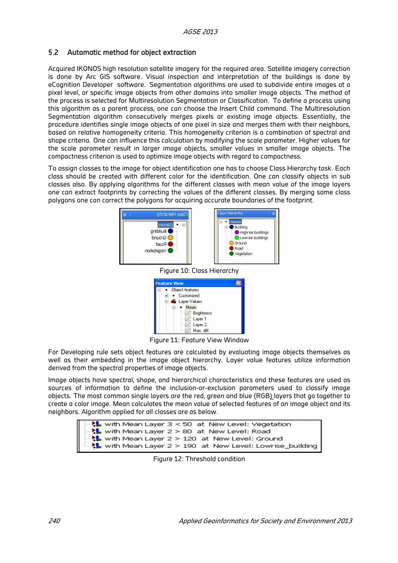
AGSE 2013


5.2 Automatic method for object extraction

Acquired IKONOS high resolution satellite imagery for the required area. Satellite imagery correction

is done by Arc GIS software. Visual inspection and interpretation of the buildings is done by

eCognition Developer software. Segmentation algorithms are used to subdivide entire images at a

pixel level, or specific image objects from other domains into smaller image objects. The method of

the process is selected for Multiresolution Segmentation or Classification. To define a process using

this algorithm as a parent process, one can choose the Insert Child command. The Multiresolution

Segmentation algorithm consecutively merges pixels or existing image objects. Essentially, the

procedure identifies single image objects of one pixel in size and merges them with their neighbors,

based on relative homogeneity criteria. This homogeneity criterion is a combination of spectral and

shape criteria. One can influence this calculation by modifying the scale parameter. Higher values for

the scale parameter result in larger image objects, smaller values in smaller image objects. The

compactness criterion is used to optimize image objects with regard to compactness.

To assign classes to the image for object identification one has to choose Class Hierarchy task. Each

class should be created with different color for the identification. One can classify objects in sub

classes also. By applying algorithms for the different classes with mean value of the image layers

one can extract footprints by correcting the values of the different classes. By merging same class

polygons one can correct the polygons for acquiring accurate boundaries of the footprint.

Figure 10: Class Hierarchy

Figure 11: Feature View Window

For Developing rule sets object features are calculated by evaluating image objects themselves as

well as their embedding in the image object hierarchy. Layer value features utilize information

derived from the spectral properties of image objects.

Image objects have spectral, shape, and hierarchical characteristics and these features are used as

sources of information to define the inclusion-or-exclusion parameters used to classify image

objects. The most common single layers are the red, green and blue (RGB) layers that go together to

create a color image. Mean calculates the mean value of selected features of an image object and its

neighbors. Algorithm applied for all classes are as below.

Figure 12: Threshold condition

AGSE 2013


Figure 13: Ground, Road, Vegetation and Building (mean value)

Figure 14: Ground, Road, Vegetation and Building

Figure 15: Footprint generation by Automatic and Semi Automatic methods

Figure 16: Comparison between Automatic and Semi Automatic footprint generation

To extract 3D form of the buildings Arc scene software is used. Point file is used as the source to

assign building heights using e-Cognition software.

AGSE 2013


5.3 Automatic method and Semi Automatic method

Figure 17: Comparison between two methods

6 Analysis

Figure 18: Analysis Table

7 Conclusion

With these methods one can extract 3D models for any city.

A working integration of three-dimensional models with geo-referenced database holds great

promise for large scale spatial study.

All though there is possibility for enhancing many techniques for different applications and one

can extract 3D model for further levels also.

Acknowledgement

I would like to earnestly thank Late Dr. S. K. Pathan, Group Director, UPDG, SAC (ISRO) for all his

guidance and help during the study and also for his valuable inputs and comments on my work. I

would like to express my deep gratitude towards my guide –Mr. Shashikant A. Sharma, Scientist-SF-

UPD/UPDG/EPSA, SAC (ISRO), Ahmedabad. and Dr. Anjana Vyas, Dean FGSA,CEPT University,

Ahmedabad for having accepted for guidance and for providing immense help throughout the entire

study. Special thanks to Mr. P. Jayprasad-Scientist ‘SE’ (ISRO) who helped me during the study.

Establishing Urbanization Trends in Mumbai Metropolitan Region By

Temporal Analysis Of Geospatial Data Sets

Priya Mendiratta*, Shirish Gedam

Centre for Studies in Resources Engineering (CSRE), Indian Institute of Technology Bombay (IITB),

Powai, Mumbai, India 400 076, [email protected], [email protected]

KEY WORDS: Multi-temporal, Landsat, Image classification, urbanization

ABSTRACT

More than half the world population (7 billion) today lives in urban areas and it is estimated that this is likely to go up to 75% by year 2025, more so in the developing world. It is also predicted that most of this spurt in urbanization is likely to be witnessed in Africa and in Asia - particularly China and India, and more particularly in Tier II cities. It therefore becomes imperative to assess infrastructure accessibility and the required quantum of its augmentation in an environmentally sustainable manner.

This study is based on the premise that evaluating the growth trends of metapolises (> 10 million population) in order to conserve peripheral land, and optimizing consumption of other natural resources in the region, would go a long way to plan for cities on their way to become a metropolis (> 1 million population) themselves.

This research paper interprets the available temporal datasets in the form of medium-resolution Landsat images of the Mumbai Metropolitan Region (MMR) over the last four decades using Object based Image classification (OBIA). It studies the spatial spread of the built-up area (BUA) in MMR through optical characteristics to identify potential growth trends. These image interpretation results are then compared to examine the regional growth trends with respect to its topographical features and recent development policies. The study also aims to examine whether alternatives to the emerging urbanization trend are feasible in order to be economical and efficient in terms of infrastructure expansion, eventually leading to sustainable development.

1 Introduction

It is in mankind's self interest to utilize natural resources in an optimal and sustainable manner.

Development, triggered by economic needs, without an appropriate base map of the natural

resources and local geography with little regard to environmental constraints, leads to irreversible

ecological damage.

Urbanization is arguably the most dramatic form of irreversible land transformation. After 2007, more

than 50% of the global population is residing in urban areas and this is expected to reach about 70%

by 2030. The United Nations projects that most of the global population growth expected in the next

30 years will be concentrated in urban areas in less developed regions (United Nations, 1999) in Asia

and Africa with only about 30-40% population currently resides in urban areas. Moreover, the total

number of very large cities in south and southeast Asia is increasing.

In India, during the last 50 years the population (today 1.2 billion) has more than doubled, but the

urban population has grown nearly five times. The number of Indian mega cities will increase from

the current three (Mumbai, Delhi and Kolkatta) to six by the year 2021 (including Bangalore, Chennai

and Hyderabad), when India will have the largest concentration of mega cities in the world

(Chakrabarti, 2001).

It is therefore necessary to have a fair assessment of a) the target population for which the planning

is undertaken, and b) the quantum of the required resources and their availability in the near vicinity

in order to work out the investments for their development and recurring expenditure for their

regular maintenance. However, the target population is only a theoretical premise as upon reaching

the target population, physically it is not possible to contain further influx.

AGSE 2013


The assessment of adjoining resources therefore gains relevance for urban development, which

under the Indian constitution, is a State subject. Prevailing legislation necessitates that urban

development be planned in the form of a 'master plan' for the next two decades for a target

population. Post economic liberalization, and especially in the context of fifty three million-plus cities

as per 2011 Census (up by 18 in the last decade) where about 13% of the total population resides,

perhaps twenty years is a relatively long time. More so, when it is taken into consideration that the

Greater Mumbai Urban Agglomeration grew by about 12% in the last decade (down from 30.5% in

the previous decade), review of existing infrastructure and planning for world class infrastructure in

the future definitely needs to be done more frequently.

This phenomenon necessitates advanced methodologies such as space technologies, to help city

planners, economists, environmentalists, ecologists and resource managers solve the problems that

accompany such growth. Urban planners need information about the rate of growth, pattern and

extent of sprawl to provide basic amenities such as water, sanitation, and electricity, etc. In this

uncontrolled situation, city planners lack tools to measure, monitor, and understand urban sprawl

processes. Remote sensing techniques have already proven useful for mapping urban areas at

various scales and obtaining data for the analysis of urban land cover change. Multi-temporal remote

sensing has become an important data-gathering tool for analyzing these changes. By using time-

series of Landsat data, we classify urban footprints since the 1970s. The Landsat and SPOT sensors

lack the spatial resolution to monitor infrastructure but they do provide the resolution and temporal

coverage to provide a 20-year record of urban land cover change. These sensors also provide the

wide area coverage necessary to image an entire city in a single instance so they can be used for

comparative analyses of urban morphology. Various studies have used Landsat satellite data for

mapping urban extent and its changes through determining impervious surfaces.

There is a general perception that urban areas in the developing world, on one hand, have higher

level of facilities and services; while on the other, urban areas are also home to the largest number of

people residing in areas without basic amenities of water supply and sanitation. This paper aims to

study the spatial spread of the built up area in MMR, with the help of data available in satellite

images of the last four decades, to trace any visible urbanization trend.

2 Study Area

Mumbai is presently the seventh largest megapolis, apart from the distinction of being a coastal city

with the highest population density after Hong Kong. The region lies between 18o33

' and 19

o31

'

north latitude, and between 72o45

' and 73

o28

' east longitude. The region in the whole is a low land

but not a plain. The average elevation of the areas above sea level is less than 100 metres but

significant local variations are brought about by a series of north-south trending hill ridges.

Apart from the land under urban area, the plain lands between the hills are mostly devoted to paddy

cultivation, except along coasts where there are marshy and salt pans. The hills are covered by

forests. The climate of Mumbai and its surrounding area is fairly equable due to the moderating

effects of the nearby sea and the fairly high amount of relative humidity in the atmosphere. The

average rainfall in the Region is over 2000 mm.

Although many definitions are used to classify urban areas, for the context of this study pertaining to

the extent of urbanisation in the Mumbai Metropolitan Region, urban land refers to the built-up area

visually discernible on a satellite image. This definition enables the measurement of the overall

spatial expansion over a defined period of time from the archived Landsat images over the last four

decades.

AGSE 2013



2.1 Data Source

Landsat images available covering the major portion of the Mumbai Metropolitan Region (MMR)

marked in black fall in path 148 and row 47 of the Landsat 4 onwards satellite's orbit. However, small

portion of the MMR on the north and west fall in the images in adjacent row/ path. Hence, the three

images are mosaic-ed to observe the Area of Interest (AOI).

Figure 2: Landsat scenes comprising Area of Interest (2002)

Fig. 2 shows an example: Landsat ETM data from the year 2002 for the metropolitan area of the

mega city of Mumbai. Clearly visible are the urbanized peninsula, the city’s large extent, the linear

axial growth and the existing satellite cities.

Seven geospatial data sets from 1972 to 2011 (MSS1972, 1977, TM1992, 1998, ETM+2002, TM2009,

2011) have been used for this study to establish a trend in the growth of urban areas in the Mumbai

Metropolitan Region (MMR). No data sets of the 1980s are available. The 4-band MSS data of the

1970s has a spatial resolution of 79ms, while the 7/8 band TM/ ETM+ datasets of the last two

decades post economic liberalization, when most of the rapid urbanization took place, have a

uniform spatial resolution of 30ms. It is pertinent to note that most datasets pertain to the period

between October and December in the corresponding year; as being coastal area, most cloud free

data is available in the post-monsoon season.

AGSE 2013


3 Methodology

The methodology adopted for identification of urban growth trends in the MMR is shown below.

Figure 3: Prposed Methodology

3.1 Image Classification

Proceeding on the lines of uniform urban classes of vegetation, impervious surfaces and soil (VIS

model) proposed for urban studies by Ridd (1995), the classification for Mumbai Metropolitan Region

being a coastal area comprises additional classes of 'water' and 'marshy'/ wetlands, which are

independent ecological systems in themselves. Further, the classes 'impervious surfaces' and 'soil'

are differently named as 'built up' and 'barren' respectively. Summarily, the satellite images for the

MMR are therefore broadly classified in to the following five categories – barren, built up, marshy,

vegetation and water.

The unique reflectance characteristics in different spectral bands by different objects on the earth's

surface form its spectral signature, and the basis of image classification. Considering that a) the AOI

is a coastal city where a cloudy sky is observed for almost eight months of the year, and b) the

periodicity of the Landsat was earlier 18 days and subsequently 16 days, significant tonal variation is

observed in images falling in the adjacent path. Hence, obtain uniform classification results,

preprocessing of images by histogram and colour matching are carried out in ENVI while mosaic-ing

the image scenes.

This study based on image classification, especially the built up class, started with pixel-based

unsupervised classification. However, the results were not so promising, considering that a) spectral

signatures alone were insufficient to distinguish between different classes (especially when the

spectral signatures of built up area in south Mumbai were classified similar to the dry marshy lands

in Dharamtar Creek), and b) the class boundaries in unsupervised classification need not necessarily

coincide with the predefined class boundaries. Hence, the need for a more intelligent classification

tool that incorporated parameters other than spectral signatures for identification of classes was

necessary.

3.2 Object based Image Analysis (OBIA)

Numerous remote-sensing techniques have been developed for analyzing the images, such as

supervised classification, texture analysis, contrast enhancement, and others that exploit the

spectral responses of various features in different multispectral bands. Significant progress has been

made in the field of artificial intelligence (AI), fuzzy logic classification, rule-based classification from

the expert systems domain, and neural nets in capturing human ways of thinking and applying them

to image analysis. Until recently, most of these techniques were applied to pixels, limiting the use of

these advanced technologies.

However, an object-oriented approach improves the image analysis and interpretation process by

taking advantage of these technologies. An object is defined as a grouping of pixels of similar

spectral and spatial properties. Thus, in OBIA, the image is analysed in object space which are then

used for classification, rather than pixels. (Navulur, 2007)

This study uses eCognition software, first launched in May 2000. The technology, referred to as

Cognition Network Technology, was realized by Nobel Laureate Prof. Dr. Gerd Binnig together with

a team of researchers at Definiens AG in Munich, Germany. To emulate the human mind's cognitive

powers, Definiens made a departure from conventional approaches. Using patented image

segmentation and classification processes, they developed a robust method of rendering knowledge

in a semantic network. The technology examines pixels not in isolation, but in context. It builds up a

Image Interpretation

of Time-series

satellite data

I

Change Detection

between images of

different dates

Trend Identification using

change detection results on GIS

platform

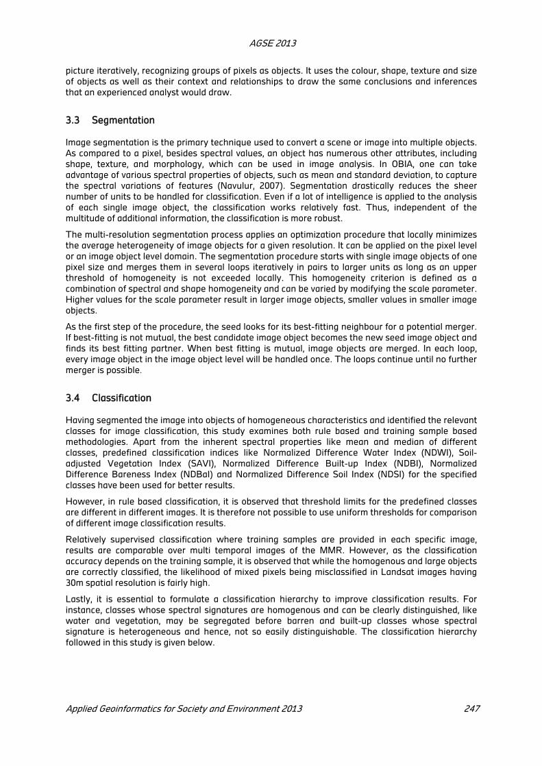
AGSE 2013


picture iteratively, recognizing groups of pixels as objects. It uses the colour, shape, texture and size

of objects as well as their context and relationships to draw the same conclusions and inferences

that an experienced analyst would draw.

3.3 Segmentation

Image segmentation is the primary technique used to convert a scene or image into multiple objects.

As compared to a pixel, besides spectral values, an object has numerous other attributes, including

shape, texture, and morphology, which can be used in image analysis. In OBIA, one can take

advantage of various spectral properties of objects, such as mean and standard deviation, to capture

the spectral variations of features (Navulur, 2007). Segmentation drastically reduces the sheer

number of units to be handled for classification. Even if a lot of intelligence is applied to the analysis

of each single image object, the classification works relatively fast. Thus, independent of the

multitude of additional information, the classification is more robust.

The multi-resolution segmentation process applies an optimization procedure that locally minimizes

the average heterogeneity of image objects for a given resolution. It can be applied on the pixel level

or an image object level domain. The segmentation procedure starts with single image objects of one

pixel size and merges them in several loops iteratively in pairs to larger units as long as an upper

threshold of homogeneity is not exceeded locally. This homogeneity criterion is defined as a

combination of spectral and shape homogeneity and can be varied by modifying the scale parameter.

Higher values for the scale parameter result in larger image objects, smaller values in smaller image

objects.

As the first step of the procedure, the seed looks for its best-fitting neighbour for a potential merger.

If best-fitting is not mutual, the best candidate image object becomes the new seed image object and

finds its best fitting partner. When best fitting is mutual, image objects are merged. In each loop,

every image object in the image object level will be handled once. The loops continue until no further

merger is possible.

3.4 Classification

Having segmented the image into objects of homogeneous characteristics and identified the relevant

classes for image classification, this study examines both rule based and training sample based

methodologies. Apart from the inherent spectral properties like mean and median of different

classes, predefined classification indices like Normalized Difference Water Index (NDWI), Soil-

adjusted Vegetation Index (SAVI), Normalized Difference Built-up Index (NDBI), Normalized

Difference Bareness Index (NDBaI) and Normalized Difference Soil Index (NDSI) for the specified

classes have been used for better results.

However, in rule based classification, it is observed that threshold limits for the predefined classes

are different in different images. It is therefore not possible to use uniform thresholds for comparison

of different image classification results.

Relatively supervised classification where training samples are provided in each specific image,

results are comparable over multi temporal images of the MMR. However, as the classification

accuracy depends on the training sample, it is observed that while the homogenous and large objects

are correctly classified, the likelihood of mixed pixels being misclassified in Landsat images having

30m spatial resolution is fairly high.

Lastly, it is essential to formulate a classification hierarchy to improve classification results. For

instance, classes whose spectral signatures are homogenous and can be clearly distinguished, like

water and vegetation, may be segregated before barren and built-up classes whose spectral

signature is heterogeneous and hence, not so easily distinguishable. The classification hierarchy

followed in this study is given below.

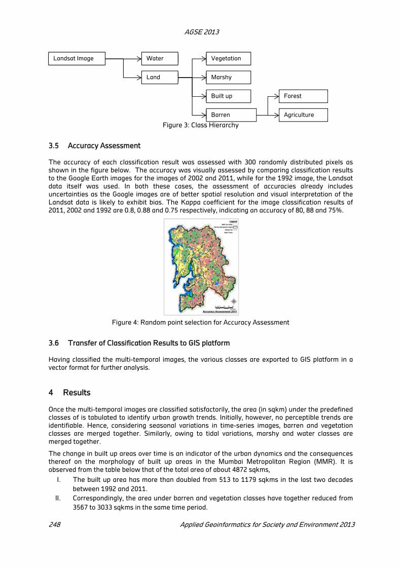
AGSE 2013


Figure 3: Class Hierarchy

3.5 Accuracy Assessment

The accuracy of each classification result was assessed with 300 randomly distributed pixels as

shown in the figure below. The accuracy was visually assessed by comparing classification results

to the Google Earth images for the images of 2002 and 2011, while for the 1992 image, the Landsat

data itself was used. In both these cases, the assessment of accuracies already includes

uncertainties as the Google images are of better spatial resolution and visual interpretation of the

Landsat data is likely to exhibit bias. The Kappa coefficient for the image classification results of

2011, 2002 and 1992 are 0.8, 0.88 and 0.75 respectively, indicating an accuracy of 80, 88 and 75%.

Figure 4: Random point selection for Accuracy Assessment

3.6 Transfer of Classification Results to GIS platform

Having classified the multi-temporal images, the various classes are exported to GIS platform in a

vector format for further analysis.

4 Results

Once the multi-temporal images are classified satisfactorily, the area (in sqkm) under the predefined

classes of is tabulated to identify urban growth trends. Initially, however, no perceptible trends are

identifiable. Hence, considering seasonal variations in time-series images, barren and vegetation

classes are merged together. Similarly, owing to tidal variations, marshy and water classes are

merged together.

The change in built up areas over time is an indicator of the urban dynamics and the consequences

thereof on the morphology of built up areas in the Mumbai Metropolitan Region (MMR). It is

observed from the table below that of the total area of about 4872 sqkms,

I. The built up area has more than doubled from 513 to 1179 sqkms in the last two decades

between 1992 and 2011.

II. Correspondingly, the area under barren and vegetation classes have together reduced from

3567 to 3033 sqkms in the same time period.

Landsat Image Water

Land

Barren

Vegetation

Marshy

Built up

Agriculture

Forest

AGSE 2013


III. The area under water and marshy together have correspondingly moved from 591 to 624

sqkms in this time period. However, the above variation in the area under marshy and water

classes may be explained due to tidal variation and the variation in unclassified class.

Class 1972 1992 2002 2011

Built up 144.41 513.40 592.35 1179.09

Barren‐Vegetation 3931.09 3567.63 3553.18 3033.93

Marshy‐Water 742.78 591.197 524.96 624.37

Total 4859.43 4872.09 4859.43 4863.74

Table 1: Area (in sqkm) under different land use in MMR 1972-2011

The findings in the above table are graphically represented below by way of a bar chart and line

diagram. It is observed that the built up area is showing consistent increase. Consequently, the

barren and vegetation classes put together are declining, notwithstanding the seasonal variations in

land cover. Besides, periodic variations in the marshy and water classes viewed together are

negligible.

Figure 5: Changes in area of different urban classes 1972-2011

The spatial distribution of the different land uses in the MMR is as pictorially represented below.

a) 1972 b) 1992 c) 2002 d) 2011

Figure 6: Spatial Distribution of different land uses in MMR 1972-2011

5 Discussion

From the sequence of classified images above, it is generally observed that especially in

Maharashtra, built up area follows a ribbon development pattern along existing transportation

corridors, road and also rail. In the Mumbai Metropolitan Region, four major growth axes are easily

identifiable. These are along the NH8 to Ahmedabad, NH3 to Nashik, NH4 to Pune and the NH17 to

Goa. Similarly, built up areas have also spread along the railway corridors - western, central and

harbour line laid down with due regard to the local topography, and the Konkan railway connecting

up to Mangalore.

0

2000

4000

6000

Built up Barren-Vegetation Marshy-Water

1972 1992 2002 2011

AGSE 2013


The municipal corporations exhibiting substantial growth in the last decade are Navi Mumbai, Mira

Bhayandar, Vasai Virar, while noticeably growing municipal councils are Kulgaon-Badlapur, all in the

Thane District and Panvel and Pen in the Raigad District. This is endorsed by the census figures

which substantiate that while the decadal growth rate of population is almost stabilised in the

Mumbai and Mumbai suburbs districts, it is falling for some of the municipal corporations in the last

decade.

In the emerging scenario, development has already engulfed the Sanjay Gandhi National Park

between the western and the central railway corridors, and the Matheran Eco-sensitive Zone

between the central and the harbour line railway corridors, while it is progressing towards the

Karnala Bird Sanctuary situated along the NH17 to Goa, it is important to ensure that these areas be

conserved.

It is observed that the region has numerically only about 25% land under built up area, but as

observed in Figure 7 above, this 25% is spatially widespread, which may partially be attributed to the

local topography. However, considering that Mumbai is among the most densely populated cities on

the earth and the adverse environmental impacts of the horizontal spread, it is essential at the same

time, to formulate policies that will promote concentration of the low density development.

6 Conclusion

6.1 Image Classification

This study uses Object Based Image Analysis (OBIA) (otherwise meant for high resolution images),

to measure the urban sprawl in the Region through archived Landsat images i.e. quantitative

measures of spatial pattern and composition that helps to describe the morphological characteristics

of urban areas and their changes through time.

Medium resolution data such as from the Landsat or SPOT programmes are useful to study urban

growth patterns over a time-span that exceeds the availability of high resolution imagery. OBIA

satisfactorily classified land use from images with a pixel size of 30 meters. Pure land use image

objects, like water and vegetation, are classified relatively better than mixed-pixel land uses like built

up and marshy lands.

It is also observed that the use of ‘nearest neighbourhood classifier’ algorithm by training samples

provide better classification results as compared to the results obtained by calibrating the rule sets.

The results obtained by the latter were not comparable as the threshold values for different urban

classes varied considerably owing to variations in the reflectance values obtained in different

seasons under various atmospheric/ luminance characteristics.

6.2 Growth Trends

Mumbai is among the most densely populated cities in the world. Urban sprawl as observed through

time-series satellite images have proved that cities grow faster spatially than demographically. As

shown by the current study, the built up area in the Mumbai Metropolitan Region (MMR) has grown

by almost 130% from about 513 to 1180 sqkms in the two decades from 1992 to 2011, while the

population in MMR during the same period has grown only about 80% from 14.5 to 26 million. The

figures indicate that the gross population density in the MMR is also declining, as observed

throughout the world.

This dilution of the urban fabric has both direct and indirect impacts on the environment and the

well-being of urban residents. For instance, uncontrolled sprawl increases energy consumption,

pollution and greenhouse gas emissions, demands more transport infrastructure, may lead to

increased flood risks and encroaches on natural landscapes. Effective urban management and

planning strategies at different levels of government are therefore essential to modulate the

environmental consequences of urban land consumption.

AGSE 2013


To develop and monitor such strategies and to assess their spatial impact, analysing and

characterising changes in urban structure is important. Data from earth observation satellites

provide regular information on urban development and could in that way contribute to mapping and

monitoring structural characteristics of expanding cities

REFERENCES

Bhagat R B (2011); Emerging Pattern of Urbanisation in India; Economic & Political Weekly, vol xlvI

no 34: 10-12

Chakrabarti, P. G. (2001). Urban crisis in India: new initiatives for sustainable cities; Development in

Practice, 11, 260-272

Kamini J., Jayanthi Satish C., and. Raghavswamy V.(2006); Spatio-Temporal Analysis of Land Use in

urban Mumbai - Using Multi-Sensor Satellite Data and GIS Techniques; Photonirvachak Journal of

the Indian Society of Remote Sensing, Vol. 34, No. 4

MMRDA, Regional Plan for Mumbai Metropolitan Region 1996-2011

Navulur, Kumar (2007); Multi-spectral Image Analysis using the Object-oriented Paradigm; CRC

Press, ISBN-13: 978-1-4200-4306-8

Ridd M K (1995); Exploring a V-I-S (vegetation-impervious surface-soil) model for urban ecosystem

analysis through remote sensing: comparative anatomy for cities, International Journal of Remote

Sensing, Vol. 16, No. 12, pp 2165-2185

Taubenböck H., Wegmann M., Roth A., Mehl H., Dech S. (2009); Urbanization in India –

Spatiotemporal analysis using remote sensing data; Computers, Environment and Urban Systems

33 (2009) 179–188

United Nations, Department of Economic and Social Affairs, Population Division (2011). World

Population Prospects: The 2010 Revision, Volume I: Comprehensive Tables. ST/ESA/SER.A/313.

Multi stage unsupervised classification for urban application

Shaily Raju Gandhi a

,Dr Anjana Vyas a

, Shashikant A. Sharma b

,Gaurav Jain b

a Department of Geomatics, Faculty of Technology, Center for Environmental Planning and

Technology University, Kasturbhai Lalbhai Campus, University Road Ahmedabad-380009, Gujarat

(India) [email protected]

b Space Applications Centre (SAC), Indian Space Research Organisation (ISRO) , Jodhpur Tekra,

Ambawadi Vistar P.O. , Ahmedabad – 380015, Gujarat (India) ,Website: www.sac.gov.in

KEY WORDS: classification, unsupervised classification, urban applications, pixels, accurate.

ABSTRACT

Grouping images into (semantically) meaningful categories using different classification techniques is challenging .There are different ways to classify an image but supervised and unsupervised classification are not application oriented. Multi stage unsupervised classification for Urban application has been derived to get accurate urban area from an image by performing unsupervised classification in multiple stages and excluding the remaining classes. This is an application oriented process in which the class which needs to be extracted is given more preference than the rest of the classes and mixing of the pixels is removed in the latter stage giving us accurate result of the required class. This method includes omissions of the unwanted classes and includes all the pixels which include bit of the mixing of the class of interest. Here all the focus is given to one class and rest of the classes are classified with less of accuracy. The accuracy of this approach is much higher as compared to the other classification methods. This method of classification can be adapted for other applications like vegetation, waste lands etc. to get accurate classification of single or more than one class.

1 Introduction

1.1 Motivation

Extracting accurate measures of urban land cover from remote sensing data is fundamentally a

challenging task due to high spectral and spatial heterogeneity of urban pixel. Urban areas are

complex landscapes of built structures and human modified land cover. Globally, urban land cover

varies in terms of construction materials, abundance of vegetation, and size of open spaces, among

other factors. Hence there is absence of globally consistent spectral signature for urban area. Even

within a single urban area , image analysis is complicated because of high spectral and spatial

variability of built up materials which results in a large number of “ mixed pixels” across a range of

spatial scale and limits the utility of traditional classification approaches. 6

1.2 Objective

To extract pure urban pixel from a raster data with minimum amount of mixing classes using

unsupervised classification.

1.3 Overview

There are different techniques for image classification. Different methods give different accuracy

results. Each pixel on a raster image contains some information. Different classification techniques

are supervised classification, unsupervised classification, hybrid classification and so on which are

useful to classify the image in different classes and helpful as input for many applications.

6 Forster, 1983

AGSE 2013


1.4 Supervised classification

The supervised classification methods are based on user-defined classes and corresponding

representative sample sets. The sample sets are specified by training raster data sets, which must

be created, prior to entering the Automatic Classification process. The Training Data button is

activated when we select a supervised classification method, which indicates that we are required to

select training, set raster. The Feature Mapping process provides the tools needed to create a

training raster, as outlined in the section entitled Creating a Training Set Raster. The training areas

are first processed to define the statistical properties of each class. In the final classification stage,

each cell in the input raster set is assigned to one of the training classes using an appropriate

decision rule.

Supervised methods produce superior results when the classification concept translates into distinct

groupings that are well represented by training areas and appropriate for the input raster’s.

Fundamental requirements for the successful use of supervised classification methods are as

follows:

We must have good knowledge of the surface in terms of types and location of features.

The set of training classes must include all significantly distinctive types of surface materials.

Each training area must be representative of its intended class

If these requirements are not met, an unsupervised method may be more suitable.

The supervised Classification methods are

Minimum Distance to Mean

Maximum Likelihood

Mahalanobis

Stepwise Linear

Suits' Maximum Relative

Back Propagation

1.5 Unsupervised classification

Thus in unsupervised classification methods are algorithms that analyze and classify a large number

of raster cells. These processes require that we set values for a few processing parameters, but the

classification process then proceeds with no user intervention. The success of the unsupervised

methods is based on the premise that the input raster dataset includes natural statistical groups of

spectral patterns that represent particular types of physical features. All of the unsupervised

classification methods, except Simple One-Pass Clustering, use an interactive process to analyze a

set of sample input cells and determine a set of class centers and associated statistical properties.

The entire input raster set is then processed, and a classification rule is used to assign each raster

cell to one of the defined classes.7

The unsupervised classification Methods are

Simple One-Pass Clustering

K Means

Fuzzy C Means

Minimum Distribution Angle

Isodata Classification

7 Anderson, J . R, Hrdy , E. E., Roach, J. T. & Witmer , R.E. , 1976

AGSE 2013


Self-Organization and

Adaptive Resonance.

ERDAS IMAGINE 8 uses the ISODATA algorithm to perform an unsupervised classification which is

adopted in the analysis and presented in this paper.

1.6 Data Used

The study has been conducted using LISS IV data acquired from RESOURCESAT- 2 satellite image

of Rajkot city. Image for November 2011 of the 150 Path and 44 Row has been downloaded for this

study.

2 Study Area

Rajkot is one of the fastest developing cities located on the western part of India. It was founded by

the ruler of Sardhar 1608 A. D. on the west bank of the river Aji as a small fortified town. Gradually, it

became a Princely State in the year 1805. In about 400 years, it has developed from a small hamlet to

a prosperous town today. Up to 1820 the growth was not too rapid, but after the British government

established its camp in 1822 the town opened new directions of growth. The industrial development

and the urban influence of the city started with the establishment of the first textile mill in the region

towards the end of 1910. About 60 industrial units came into existence between 1900 and 1920,

which induced development of the city to a great extent. Further, around the year 1940, new

industrial estates, residential areas, schools, colleges, cinema houses came into being. In the earlier

period, the establishment of cloth mills in the city led to the development of new residential areas

like Millpara, Harishchandra Plot, Gundawadi, Kevdawadi etc. A number of transport companies

established their head offices at Rajkot. The Industrial Estates known as Bhaktinagar Industrial

Estate and Aji Industrial Estate were established. Trade and Industry fast developing in the city also

attracted foreign investment during these periods. With increasing industrial, trade and commerce

activity, there has been tremendous growth in the population of the town. The city has grown up in

area from 150 hectare in 1901 to 10404 hectare in 1998. i.e. it has growth approximately 70 times of

its initial size.

8 ERDAS imagine is the software used extensively for image analysis.

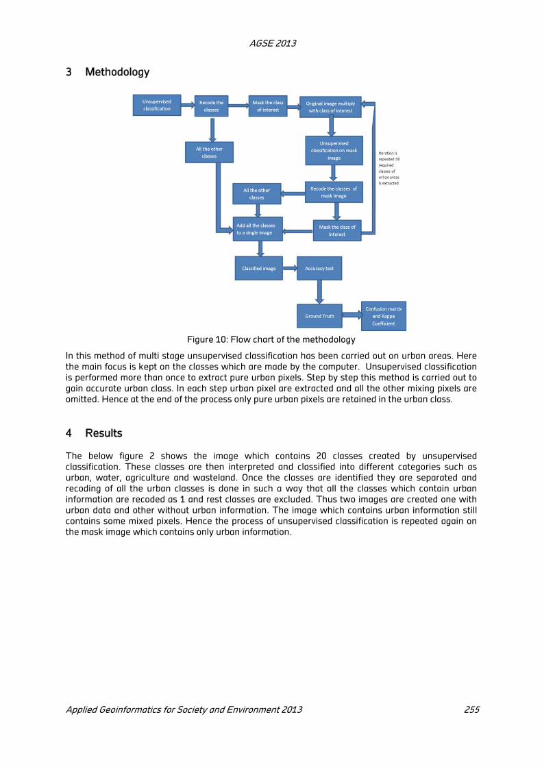
AGSE 2013


3 Methodology

Figure 10: Flow chart of the methodology

In this method of multi stage unsupervised classification has been carried out on urban areas. Here

the main focus is kept on the classes which are made by the computer. Unsupervised classification

is performed more than once to extract pure urban pixels. Step by step this method is carried out to

gain accurate urban class. In each step urban pixel are extracted and all the other mixing pixels are

omitted. Hence at the end of the process only pure urban pixels are retained in the urban class.

4 Results

The below figure 2 shows the image which contains 20 classes created by unsupervised

classification. These classes are then interpreted and classified into different categories such as

urban, water, agriculture and wasteland. Once the classes are identified they are separated and

recoding of all the urban classes is done in such a way that all the classes which contain urban

information are recoded as 1 and rest classes are excluded. Thus two images are created one with

urban data and other without urban information. The image which contains urban information still

contains some mixed pixels. Hence the process of unsupervised classification is repeated again on

the mask image which contains only urban information.

AGSE 2013


Figure 11: Unsupervised image

with 20 classes

Figure 12: Recoded

image

(contains only urban

pixels)

Figure 13: Mask image =

original image * recoded

image

Above figure 3 shows urban area extracted after the unsupervised classification and figure 4 is the

mask image which is created by multiplying the original LISS IV image and the recoded image which

contains urban area. After creating this mask image unsupervised classification is again performed

on this mask image and again the classes are divided into 20 classes from which urban classes are

extracted and other classes apart from urban are omitted from the class.

Thus above figure 5 shows second level of unsupervised classification and hence after that pure

urban pixels are obtained which is seen in figure 6 which contains pure urban information. The

process of repeating the unsupervised classification can be repeated and many number of times as

required till accurate result of the desired class is obtained. Here urban class is obtained at the end

of two iterations. Same steps can be performed more number of times. To get the classified image

as showed in figure 7 all the classes from different recoded images can be added and final output is

gained.

4.1 Accuracy assessment

Confusion Matrix is used to show the accuracy of a classification result by comparing a classification

result with ground truth information. In Error matrix diagonal cells are correctly classified pixels. The

non-diagonal column cells are omission errors and the non-diagonal row cells are commission errors.

The following table1 and table2 show the accuracy of the classification over all accuracy is 86 %

whereas Producers accuracy is 93.75% and Users accuracy for urban class is 88.24% which is

Figure 14: Unsupervised

classification of mask image Figure 15: Recode the

mask image

Figure 16: Add all the 3

recoded images

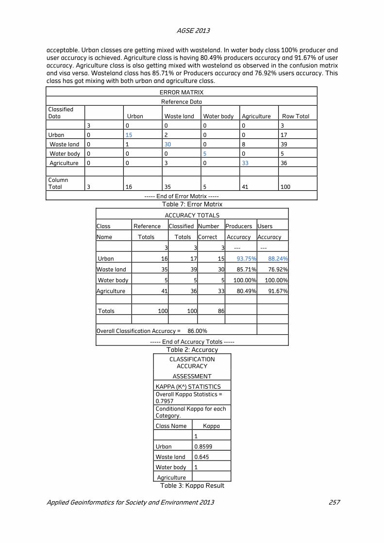
AGSE 2013


acceptable. Urban classes are getting mixed with wasteland. In water body class 100% producer and

user accuracy is achieved. Agriculture class is having 80.49% producers accuracy and 91.67% of user

accuracy. Agriculture class is also getting mixed with wasteland as observed in the confusion matrix

and visa versa. Wasteland class has 85.71% or Producers accuracy and 76.92% users accuracy. This

class has got mixing with both urban and agriculture class.

ERROR MATRIX

Reference Data

Classified

Data Urban Waste land Water body Agriculture Row Total

3 0 0 0 0 3

Urban 0 15 2 0 0 17

Waste land 0 1 30 0 8 39

Water body 0 0 0 5 0 5

Agriculture 0 0 3 0 33 36

Column

Total 3 16 35 5 41 100

----- End of Error Matrix -----

Table 7: Error Matrix

ACCURACY TOTALS

Class Reference Classified Number Producers Users

Name Totals Totals Correct Accuracy Accuracy

3 3 3 --- ---

Urban 16 17 15 93.75% 88.24%

Waste land 35 39 30 85.71% 76.92%

Water body 5 5 5 100.00% 100.00%

Agriculture 41 36 33 80.49% 91.67%

Totals 100 100 86

Overall Classification Accuracy = 86.00%

----- End of Accuracy Totals -----

Table 2: Accuracy

CLASSIFICATION

ACCURACY

ASSESSMENT

KAPPA (K^) STATISTICS

Overall Kappa Statistics =

0.7957

Conditional Kappa for each

Category.

Class Name Kappa

1

Urban 0.8599

Waste land 0.645

Water body 1

Agriculture

Table 3: Kappa Result

AGSE 2013


The kappa coefficient is another measure of the accuracy of the classification. It is calculated by

multiplying the total number of pixels in all the ground truth classes (N) by the sum of the confusion

matrix diagonals, subtracting the sum of the ground truth pixels in a class times the sum of the

classified pixels in that class summed over all classes ( ), and dividing by the total number of

pixels squared minus the sum of the ground truth pixels in that class times the sum of the classified

pixels in that class summed over all classes. From table 3 the overall Kappa co-efficient is 0.7957 and

for urban value of kappa is 0.8599 hence this method of classification is acceptable to a greater

extend and helps to get classes application oriented.

5 Conclusion

Multi stage unsupervised classification is a faster way to get application oriented classification as in

this method of classification there are more possibility to achieving more accurate results for classes

of interest. Hence same steps can be followed and results can be obtained for different applications

like agriculture, forest, wasteland etc. this method of classification is more appropriate to obtaining

pure pixels of any particular application as in this paper urban area has been extracted.

References

Anderson, J . R, Hrdy , E. E., Roach, J. T. & Witmer , R.E. , 1976 , A Land Use and Land Cover

Classification System for Use with Remote Sensor Data, Sioux Falls , SD, USA,USGS Professional

Paper 964

Benediktsson, J . A & Sveinsson , J. R , 2003 , Multisource remote sensing data classification based on

consensus and pruning. IEEE Transactions on Geoscience and Remote sensing , pp 932-936

Congalton , R.G. , 1991 , A review of assessing the accuracy of classification of remotely sensed data.

Remote Sensing of Environment, pp 35-46

Foresman, T. M., Pickett, S. T. A., & Zipperer, W. C. ,1997, Methods for spatial and temporal land use

and land cover assessment for urban ecosystems and application in the greater Baltimore-

Chesapeake region. Urban Ecosystems,pp 210–216.

Forster, B. , 1983 , Some Urban measurements from Landsat data, Photogrammetric Engineering

and remote Sensing , pp 1693-1707

Powell , R. , 2011 , Characterizing urban sub pixel composition using spectral mixture analysis ,

Urban Remote Sensing Monitoring, Synthesis and Modeling in the Urban Environment.. UK . pp.

112– 127.

Yan, X., & Zhou, L., 2011, Parameterizing neural network models to improve land classification

performance. Urban Remote Sensing Monitoring, Synthesis and Modeling in the Urban

Environment.. UK . pp. 96 – 109.

Yu, X. J., & Ng, C. N. ,2007. Spatial and temporal dynamics of urban sprawl along two urban-rural

transects: A case study of Guangzhou, China. Landscape and Urban Planning, 79, pp 96–109.

Attribute Selection Using Texture Characteristic For Object Based Image

Classification

Srivastava M.a, Arora M. K.

a, Balasubramanian R.

b

a Geomatics Engineering Section, IIT Roorkee, Roorkee 247667

b Department of Computer Science and Engineering, IIT Roorkee, Roorkee 247667, E-mail:

[email protected]

KEY WORDS: Object based image analysis, Attribute selection, Pearson’s correlation, and Texture

characteristics

ABSTRACT

Object-based image classification is an approach to classify the remote sensing image on the basis of spectral, textural and contextual attributes in contrast to spectral attributes as in pixel based classification approach. There are number of attributes of an object but only few of them are effectively important to extract an object with respect to others from the segmented image. In this paper, the redundant attributes were removed by using correlation analysis and the texture attribute characteristics. To reduce the redundancy, correlation analysis was applied to detect the magnitude of the relationship between the attributes. Based on the correlation analysis, the attribute that had a high correlation coefficient with the other attributes was removed from the attribute set. For each object, out of 35 only 20 attributes including, spectral, textures, and contextual attributes for Quickbird pan image of Chandigarh area were selected. The attribute reduction and attribute selection are applied on the segmented image. The correlation analysis combined with texture characteristics is efficient in optimizing the attribute set and these attributes are further used for image classification.

1 Introduction

The conventional pixel based classification has limitation to classify high resolution satellite image as

pixel size is very small while the it uses only spectral information (Scheiewe et al. 2001, Shackelford

and Davis 2002). The object based classification method is proposed to overcome this problem

because they can incorporate shape and texture information with spectral information. The spectral

attribute of an image object is the DN values, standard deviation of different image layers. However,

textural attributes are calculated using Gray Level Co-occurrence Matrix (GLCM), which is useful to

detect roughness of the object surface and the contextual attribute provides the image objects

spatial information such as shape, ratio etc. There are number of attributes of an object but only few

of them are effectively important to extract an object with respect to others from the segmented

image.

The object based method can be performed in three steps. In the first step of segmentation is to

partition an image into non-overlapping, meaningful and homogeneous objects. The second step is

to remove irrelevant and redundant attributes by grouping of selected attributes. In the third step

these segments are assigned to class. The attributes used for classification in the object based

procedure are the objects characteristics, differing from those in pixel-based methods (Mueller et al.

2004, Doloca 2000).

1.1 Study area and data description

The area of this study is Chandigarh (India), which is the capitol of Punjab and Haryana and lies at

30o

46’ 12” N latitude and 76o

47’ 24’’E longitude. It is well planned city. Chandigarh has a robust and

well connected road and rail network with other parts of India. A cloud free high resolution (60 cm)

panchromatic band image taken by Quick-bird sensor is used for this work.

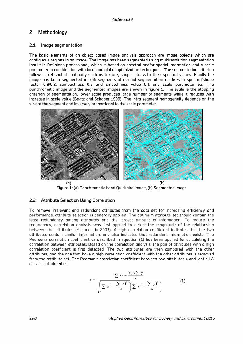
AGSE 2013


2 Methodology

2.1 Image segmentation

The basic elements of an object based image analysis approach are image objects which are

contiguous regions in an image. The image has been segmented using multiresolution segmentation

inbuilt in Definiens professional, which is based on spectral and/or spatial information and a scale

parameter in combination with local and global optimization techniques. The segmentation criterion

follows pixel spatial continuity such as texture, shape, etc. with their spectral values. Finally the

image has been segmented in 766 segments at normal segmentation mode with spectral/shape

factor 0.8/0.2, compactness 0.9 and smoothness value 0.1 and scale parameter 52. The

panchromatic image and the segmented images are shown in figure 1. The scale is the stopping

criterion of segmentation, lower scale produces large number of segments while it reduces with

increase in scale value (Baatz and Schaper 1999). The intra segment homogeneity depends on the

size of the segment and inversely proportional to the scale parameter.

(a) (b)

Figure 1: (a) Panchromatic band Quickbird image, (b) Segmented image

2.2 Attribute Selection Using Correlation

To remove irrelevant and redundant attributes from the data set for increasing efficiency and

performance, attribute selection is generally applied. The optimum attribute set should contain the

least redundancy among attributes and the largest amount of information. To reduce the

redundancy, correlation analysis was first applied to detect the magnitude of the relationship

between the attributes (Yu and Liu 2003). A high correlation coefficient indicates that the two

attributes contain similar information, and also indicates that redundant information exists. The

Pearson’s correlation coefficient as described in equation (1) has been applied for calculating the

correlation between attributes. Based on the correlation analysis, the pair of attributes with a high

correlation coefficient is first detected. The two attributes are then compared with the other

attributes, and the one that have a high correlation coefficient with the other attributes is removed

from the attribute set. The Pearson’s correlation coefficient between two attributes x and y of all N

class is calculated as;

(1)

N

yy

N

xx

N

yxxy

r2

2

2

2

AGSE 2013


2.3 Attribute Selection using Texture Characteristics

The Haralick grey-level co-occurrence matrix (GLCM) is one of the most popular second order

statistics for texture analysis in remote sensing image processing (Haralick and Shanmugam 1973).

The GLCM texture attributes are basically divided into three groups; contrast group, orderliness

group and states group. Contrast group represents the homogeneity or contrast within the land

cover types, three texture attributes, namely; contrast, homogeneity and dissimilarity are belongs to

this group. The second group provides the information regarding the uniformity of the land cover

type surface, GLCM entropy, GLCM Angular 2nd

momentum (GLCM_ASM) and gray level difference

vector (GLDV) Angular 2nd

momentum (GLDV_ASM) are belongs to this group. Third group is the

states group and provides the fundamental texture information of every land cover types. GLCM

mean, GLCM standard deviation and GLCM correlation are belongs to this group.

In the contrast group, contrast shows the homogeneity within the land cover type and varies

exponentially from 0 to 1, where 0 shows no contrast and 1represent high contrast or less

homogeneity. In similar manner dissimilarity varies linearly from 0 to 1. Entropy shows the first

order of uniformity between the land cover surfaces. High value of ASM occurs when the image

window is very orderly or uniform. The value of ASM varies from 0 for low order to 1for high order.

All three attributes, GLCM; mean, standard deviation and correlation of stats group represent

different texture characteristics. Mean reflects the brightness value, standard deviation shows the

variation in the data and the Correlation texture measures the linear dependency of grey levels on

those of neighboring pixels. The correlation values varies from -1 (no correlation) to +1 (high

correlation).

GLDV mean is similar to GLCM dissimilarity while GLDV contrast and GLCM contrast of an image are

calculated in similar manner and gives the same value hence GLDV mean and GLDV contrast have

been eliminated from the list of texture attributes.


After segmenting the image with eCognition software it is exported with its 35 attributes for further

processing. Based on the characteristics of 8 different classes (metallic road, nonmetallic road,

residential, barren land, trees, grassland, shadow and water), 20 out of 35 attributes including

spectral, texture, and shape have been selected and formed attribute set. From these 20 selected

attributes; 5 attributes are belongs to spectral, whereas 9 attributes for shape and 6 for texture

group.

3.1 Correlation Coefficient

The correlation coefficients between spectral and shape attributes with their correlation coefficients

are shown in table 1 and table 2 respectively. The attributes with high correlation coefficient 0.85

and above are not considered for further processing (Xiuying et al. 2010).

Me

an

Std

de

via

tion

Std

De

v to

ne

igh

bo

r

Me

an

diff

to

ne

igh

bo

r

Me

an

diff

to

ne

igh

bo

r

(Ab

s)

Me

an

diff

to

ne

igh

bo

r

(Da

rk)

Me

an

diff

to

ne

igh

bo

r

(Brig

ht)

Sce

ne

Ra

tio

Mean 1 0.67 0.07 0.56 0.35 0.26 0.04 1

Std deviation

1 0.14 0.62 0.67 0.43 0.46 0.67

Std Dev. to neighbor

1 0.09 0.04 0.11 0.57 0.07

Mean diff neighbor

1 0.98 0.95 0.11 0.62

Mean diff to neighbor (Abs)

1 0.97 0.96 0.14

Mean diff to neighbor (Dark)

1 0.97 0.75

Mean diff to neighbor (Bright)

1 0.2

Scene Ratio

1

Table 1: correlation coefficients between selected spectral attributes

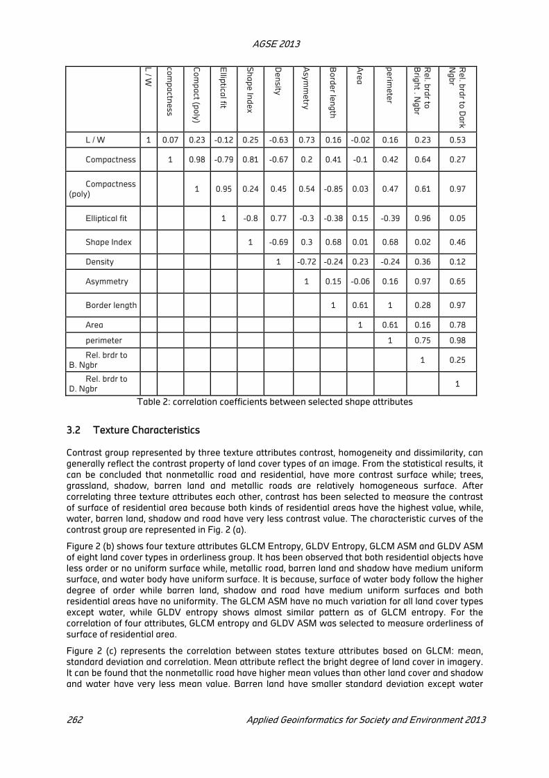
AGSE 2013


L / W

co

mp

actn

ess

Co

mp

act (p

oly

)

Ellip

tica

l fit

Sh

ap

e In

de

x

De

nsity

Asy

mm

etry

Bo

rde

r len

gth

Are

a

pe

rime

ter

Re

l. brd

r to

Brig

ht . N

gb

r

Re

l. brd

r to D

ark

Ng

br

L / W 1 0.07 0.23 -0.12 0.25 -0.63 0.73 0.16 -0.02 0.16 0.23 0.53

Compactness 1 0.98 -0.79 0.81 -0.67 0.2 0.41 -0.1 0.42 0.64 0.27

Compactness

(poly) 1 0.95 0.24 0.45 0.54 -0.85 0.03 0.47 0.61 0.97

Elliptical fit 1 -0.8 0.77 -0.3 -0.38 0.15 -0.39 0.96 0.05

Shape Index 1 -0.69 0.3 0.68 0.01 0.68 0.02 0.46

Density 1 -0.72 -0.24 0.23 -0.24 0.36 0.12

Asymmetry 1 0.15 -0.06 0.16 0.97 0.65

Border length 1 0.61 1 0.28 0.97

Area 1 0.61 0.16 0.78

perimeter 1 0.75 0.98

Rel. brdr to

B. Ngbr 1 0.25

Rel. brdr to

D. Ngbr 1

Table 2: correlation coefficients between selected shape attributes

3.2 Texture Characteristics

Contrast group represented by three texture attributes contrast, homogeneity and dissimilarity, can

generally reflect the contrast property of land cover types of an image. From the statistical results, it

can be concluded that nonmetallic road and residential, have more contrast surface while; trees,

grassland, shadow, barren land and metallic roads are relatively homogeneous surface. After

correlating three texture attributes each other, contrast has been selected to measure the contrast

of surface of residential area because both kinds of residential areas have the highest value, while,

water, barren land, shadow and road have very less contrast value. The characteristic curves of the

contrast group are represented in Fig. 2 (a).

Figure 2 (b) shows four texture attributes GLCM Entropy, GLDV Entropy, GLCM ASM and GLDV ASM

of eight land cover types in orderliness group. It has been observed that both residential objects have

less order or no uniform surface while, metallic road, barren land and shadow have medium uniform

surface, and water body have uniform surface. It is because, surface of water body follow the higher

degree of order while barren land, shadow and road have medium uniform surfaces and both

residential areas have no uniformity. The GLCM ASM have no much variation for all land cover types

except water, while GLDV entropy shows almost similar pattern as of GLCM entropy. For the

correlation of four attributes, GLCM entropy and GLDV ASM was selected to measure orderliness of

surface of residential area.

Figure 2 (c) represents the correlation between states texture attributes based on GLCM: mean,

standard deviation and correlation. Mean attribute reflect the bright degree of land cover in imagery.

It can be found that the nonmetallic road have higher mean values than other land cover and shadow

and water have very less mean value. Barren land have smaller standard deviation except water

AGSE 2013


which is zero and have larger correlation values while for water all the texture attribute of state

group have smallest value.

(a) (b) (c)

Figure 2: Texture characteristics of eight land cover types in; (a) contrast group, (b) orderliness group

and (c) states group.

Based on above statistics and analysis, the attribute sets have been decreases from 35 to 20

belonging to spectral, shape and contrast group attributes. Five spectral attributes included Mean,

Standard Deviation, Std. Dev to neighbors, ratio to scene and absolute mean difference to neighbors,

nine shape attributes included L/W, Compactness, Elliptical fit, Shape Index, Density, Asymmetry,

Border length, Area and Perimeter. With the correlation to each other in different texture groups six

texture attributes included GLCM: contrast, entropy, mean, standard deviation, correlation and GLDV

ASM are selected for image classification.

The object based image classification approach has now been applied on the segmented image. 20

selected attributes have been used for extracting the various classes during classification. The image

has been classified into eight land use classes and the classified image is shown in figure 3.

Figure 3: Classified image

4 Conclusion

The generated attributes of all segments were divided into three groups, the spectral group, the

shape group and the texture group. The Pearson’s correlation coefficient was applied to the

attributes belong to the spectral and shape group, while the texture characteristic was used for

selecting the required attributes from the texture group. It is observed that the texture characteristic

curve appears very optimistic for selecting the attributes. Total 10 attributes belonging to texture

which are divided into three groups; the contrast, orderliness and states have been used. Six

attributes that appears different characteristics were selected for classification of image.

AGSE 2013


REFERENCES

Baatz, M. and Schaper, A., 1999, Object-oriented and multi-scale image analysis in semantic

networks. In Proceedings of the 2nd International Symposium on Operationalization of Remote Sensing, 16–20 August, Enschede, The Netherlands, pp. 16–20.

Doloca, A., 2000, Feature selection for texture analysis using genetic algorithms. International Journal

of Computer Mathematics, 74, pp. 279–292.

Haralick, R.M., Shanmugam, K. and Dinstein, I., 1973, Textural features for image classification. IEEE Transactions on System, Man, and Cybernetics. SMC-3, pp. 610-621

Jon, A.B., 2003, Classification and feature extraction for remote sensing images from urban areas

based on morphological transformations. IEEE Transactions on Geoscience and Remote Sensing,

41, pp. 1940–1949

Mueller, M., Segl, K. and Kaufmann, H., 2004, Edge- and region-based segmentation technique for

the extraction of large, man-made objects in high-resolution satellite imagery. Pattern Recognition, 37, pp. 1619–1628.

Xiuying, Z., Xuezhi, F., and Hong, J., 2010, Object-oriented method for urban vegetation mapping

using IKONOS imagery. International Journal of Remote Sensing, 31, 1, pp. 177-196.

Yu, L. and Liu, H., 2003, Feature selection for high-dimensional data: a fast correlation-based filter

solution. In Proceedings of the Twentieth International Conference on Machine Learning (ICML-2003). T. Fawcett and N. Mishra (Eds.), 21–24 August 2003, Washington, DC, pp. 856–863.

Land Use land Cover Dynamics within Technopark Campus, Trivandrum,

Kerala, India

N.P. Sooraj, Rakhi. K. Raj and R. Jaishanker

Department of Ecological Informatics, Indian Institute of Information Technology and Management –

Kerala, Technopark Campus, Kariyavattom (PO), Trivandrum 695581 Kerala, India

KEY WORDS: Landuse landcover dynamics, classification, Change detection, Land management,

ABSTRACT

In 1991, Technopark, Trivandrum heralded the concept of Information Technology (IT) parks in India. It provides plug and play facility for IT entrepreneurs to establish business. The first phase of Technopark, Trivandrum was established in over 150 acres of pristine land. Technopark being a planned development activity provides a classical case to study land use land cover dynamics. The authors present the result of a study conducted to ascertain the land cover dynamics of Technopark (phase I) campus, Kerala, India over the last decade. It employed the use of satellite data acquired in 2002 and 2012 respectively by Indian Remote Sensing Satellite (IRS) using Linear Imaging Self Scanner (LISS–III) sensors. The study area extracted from both scenes were co-referenced with sub-pixel accuracy before Maximum Likelihood based supervised classification was performed. All pixels were segregated into three distinct classes viz. Vegetated, built-up and water pixel. The Kappa coefficients were pegged at 0.86 and 0.88 for 2002 and 2012 respectively. Apart from quantifying the change in vegetated vi's-à-is built up pixels within the Technopark campus, Trivandrum the present study has highlighted that in 15 years, the proportion of built up pixels equaled that of vegetated pixels within the study region. As of today the proportion of built up pixels is slightly exceeded the vegetated pixels. Some portion of the campus, which was classified as water body in 2002 too got converted into built up pixels in 2012. Vegetation cover within Technopark campus, Trivandrum decreased from 72.39% in 2002 to 52.68% in 2012.

1 Introduction

Land is a complex and dynamic combination of factors: geology, topography, hydrology, soils,

microclimates, and communities of plants and animals that are continually interacting under the

influence of climate and people's activities. It is the most important natural resource on which all

activities are based. According to Food and Agriculture Organization (FAO, 1995), information on the

rate and kind of changes in the use of land resources is essential for proper planning and

management of such resources (Phukan et al, 2013). Land cover may be defined as the biophysical

earth's surface, which includes the natural vegetation, water bodies, rock/soil, and artificial cover on

the land (Ellis & Pontius2006). When focusing on a very pure and strict sense, land-cover consists

exclusively in the description of vegetation and man-made features. However land use referred as

the use of land by human, usually with emphasis on the functional role of land in economic activities.

It is the intended employment and management underlying human exploitation of a land-cover.

There is a link between land-cover and human activities in the environment because most

contemporary land-cover is changed by human use (Allen and Barnes, 1985).

Land cover changes are of two types; Conversion and Modification. Land-cover conversion consists

of change from one cover type to another while land-cover modification involves alterations of

structure or function without a total change from one type to another which is not necessarily the

only change in land cover and it also includes the change in intensity and management (Anil et al.,

2011). Land-use change may involve either conversion from one type of use to another i.e. changes

in the pattern of land uses in an area or modification of a certain type of land use (Meyer and Turner,

1994). Land-cover/Land-use conversion takes place through many pathways such as deforestation,

desertification, agricultural intensification, etc. (Vorgelegt, 2007).Local land use and land cover

changes are fundamental agents of global climate change at all scales and are significant forces that

impact biodiversity, water and radiation budgets, and trace gas emissions. With the advent of

satellite remote sensing techniques, preparing accurate land use land cover maps and monitoring

changes at regular intervals of time is relatively simpler. Remote sensing technologies provide an

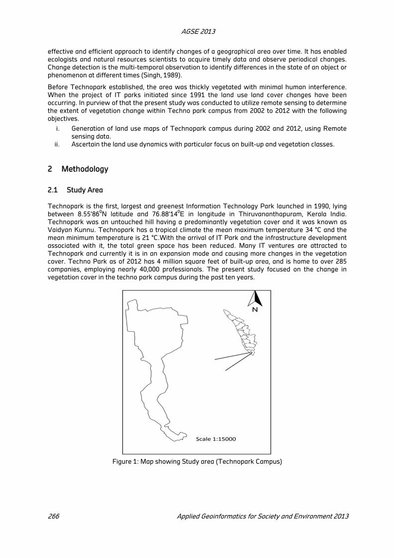
AGSE 2013


effective and efficient approach to identify changes of a geographical area over time. It has enabled

ecologists and natural resources scientists to acquire timely data and observe periodical changes.

Change detection is the multi-temporal observation to identify differences in the state of an object or

phenomenon at different times (Singh, 1989).

Before Technopark established, the area was thickly vegetated with minimal human interference.

When the project of IT parks initiated since 1991 the land use land cover changes have been

occurring. In purview of that the present study was conducted to utilize remote sensing to determine

the extent of vegetation change within Techno park campus from 2002 to 2012 with the following

objectives.

i. Generation of land use maps of Technopark campus during 2002 and 2012, using Remote

sensing data.

ii. Ascertain the land use dynamics with particular focus on built-up and vegetation classes.

2 Methodology

2.1 Study Area

Technopark is the first, largest and greenest Information Technology Park launched in 1990, lying

between 8.55’860N latitude and 76.88’14

0E in longitude in Thiruvananthapuram, Kerala India.

Technopark was an untouched hill having a predominantly vegetation cover and it was known as

Vaidyan Kunnu. Technopark has a tropical climate the mean maximum temperature 34 °C and the

mean minimum temperature is 21 °C.With the arrival of IT Park and the infrastructure development

associated with it, the total green space has been reduced. Many IT ventures are attracted to

Technopark and currently it is in an expansion mode and causing more changes in the vegetation

cover. Techno Park as of 2012 has 4 million square feet of built-up area, and is home to over 285

companies, employing nearly 40,000 professionals. The present study focused on the change in

vegetation cover in the techno park campus during the past ten years.

Figure 1: Map showing Study area (Technopark Campus)

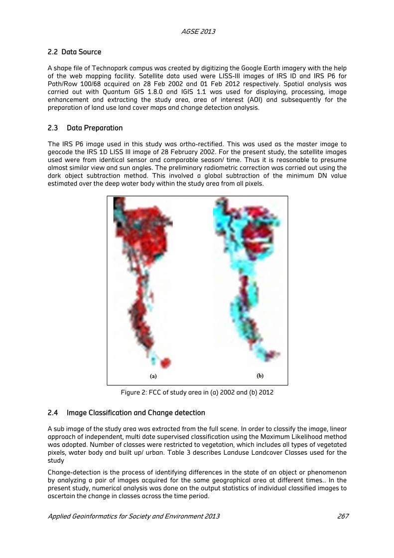
AGSE 2013


2.2 Data Source

A shape file of Technopark campus was created by digitizing the Google Earth imagery with the help

of the web mapping facility. Satellite data used were LISS-III images of IRS ID and IRS P6 for

Path/Row 100/68 acquired on 28 Feb 2002 and 01 Feb 2012 respectively. Spatial analysis was

carried out with Quantum GIS 1.8.0 and IGIS 1.1 was used for displaying, processing, image

enhancement and extracting the study area, area of interest (AOI) and subsequently for the

preparation of land use land cover maps and change detection analysis.


The IRS P6 image used in this study was ortho-rectified. This was used as the master image to

geocode the IRS 1D LISS III image of 28 February 2002. For the present study, the satellite images

used were from identical sensor and comparable season/ time. Thus it is reasonable to presume

almost similar view and sun angles. The preliminary radiometric correction was carried out using the

dark object subtraction method. This involved a global subtraction of the minimum DN value

estimated over the deep water body within the study area from all pixels.

Figure 2: FCC of study area in (a) 2002 and (b) 2012

2.4 Image Classification and Change detection

A sub image of the study area was extracted from the full scene. In order to classify the image, linear

approach of independent, multi date supervised classification using the Maximum Likelihood method

was adopted. Number of classes were restricted to vegetation, which includes all types of vegetated

pixels, water body and built up/ urban. Table 3 describes Landuse Landcover Classes used for the

study

Change-detection is the process of identifying differences in the state of an object or phenomenon

by analyzing a pair of images acquired for the same geographical area at different times.. In the

present study, numerical analysis was done on the output statistics of individual classified images to

ascertain the change in classes across the time period.

AGSE 2013


Class Name Description

1 Vegetation Dense and sparse trees, avenue trees, etc.

2 Built up

/Urban

Residential areas, Commercial and Industrial areas, transportation,

communications and utilities, mixed urban or built-up land

3 Water Lakes, streams, canals

Table 1: Description of the Land use Land Cover Change


Representative spectral profile of IRS LISS –III is depicted in Figure 4. It is evident from figure 4 that

near infrared is highly reflected by live vegetation. The very high reflectance of open land in band 4

(Short wave infrared) may be attributed to the dry sand along the coast.Landuse Land cover map of

Trivandrum Corporation were developed from satellite imageries (IRS P6 2012 and IRS 1D 2002). It

shows that there is a distribution of four land use types; built up, water body, vegetation and open

lands. Figure 5 and 6 depicts the land use land cover maps of the study areas during 2002 and 2012

respectively. Table 4 highlights the area changes in respective classes as observed in the study.

Figure 3: Spectral profile of representative classes.

Land use maps of Techno Park in the year 2002 and 2012 are shown in fig 2. Overall classification

accuracy was 0.86 and 0.88 (Kappa values) for 2002and 2012 respectively. This accuracy level

meets the recommended standards. Land use dynamics in the study region over the study period is

indicated in Table 4.

AGSE 2013


Figure 4: Land Use Land Cover Classification over Techno Park Campus in (A) 2002 and (B) 2012

Sl. No Landuse Area in Hectors

2002 2012

1 Vegetation 34.75 25.29

2 Built-up or urban area 12.91 22.40

3 Water < 1 < 1

Table.2 Table.4: Land use details of Techno Park in2002 & 2012

Figure 5: Land cover comparison from 2002 and 2012 in Technopark campus

Tables 4 show the area covered by different land use land cover classes in 2002 and 2012. Urban

area has come at the cost of vegetated pixel. During 2002 the total build up area was only 12.90 %,

while in 2012 it has increased to 9.50 %. Figure 5 depicts the inter class changes graphically. The

AGSE 2013


pressure on land by building infrastructure construction could have decreased the total area under

vegetation/ perennial trees to be replaced by built up area. Hence the findings are logical.

4 Conclusion

This information on land use / land cover is essential for the selection, planning and implementation

of land use and can be used to meet the increasing demands for basic human needs and welfare.

Change detection analysis on the multi temporal classified data revealed high amount of change in

vegetative cover in Techno Park campus. The change analysis was then focused on the dynamics of

vegetation to urban switch over. It was estimated that 9.54 % of the total vegetated land conversion

attributed for change to built up area. i.e., more than half of the total vegetation conversion was to

serve built up/ urban purposes. For a detailed understanding of the precise nature of the land use

dynamics, it is necessary to have a few more years of the date during the study period

Acknowledgement

We gratefully thank the Director of Indian Institute of Information Technology and Management-

Kerala for the support given to accomplish the work.

REFERENCE

Allen, J.C. & Barnes, D.F., 1985. The Causes of Deforestation in Developing Countries. Annals of the Association of American Geographers., vol.75,pp.163-84.

Anil, N.C., Jai Sankar, G., Jagannadha Rao,M., Prasad, I.V. R.K.V. & Sailaja, U., 2011. Land Use/Land

Cover and Change detection from parts of South West Godavari District, A.P-Using Remote

sensing And GIS technique.,J.Ind.Deophys.Union.,vol.15,issue.4, pp.187-194.

Ellis E, Pontius Jr R.G., 2006. Land-use and land-cover change—encyclopedia of earth.

http://www.eoearth.org/article/land-use_and_land-cover_change.

FAO.1995 Planning for Sustainable Use of Land Resources., FAO Land and Water Bulletin. Food and

Agriculture Organization of the United Nations, 2, Rome.

Phukan,P.,Thakuriah,G. and Saikia,R., 2013. Land use land cover change detection using Remote

sensing and GIS Techniques-A case study of Golghat district of Assam., India., Int. Res. Earth Sci.,vol.1issue.1,pp.11-15.

Singh A., 1989．Digital change detection techniques using remotely sensed data International

Journal of Remote Sensing，Vol.10(6), pp.989-1003.

Vorgelegt von., 2007.Implementation of the local land-use and land-cover change model CLUE-

sfor Central Benin by using socio-economic and remote sensing data., PhD Thesis submitted to

Reminiscent Friedrich-Wilhelm-University Bonn.,pp.12-13.

GIS Modeling to Assess Land Productivity Potential for Agriculture in

Sub-Humid (Dry) Ecosystem of Wardha District, Maharashtra

Nirmal Kumar, G. P. Obi Reddy, S. Chatterji

National Bureau of Soil Survey & Land Use Planning, Amravati Road, Nagpur – 440 033

KEY WORDS: Land Productivity Potential (LPP), NDVI, Multi-criteria Analysis

ABSTRACT

Land productivity potential (LPP) evaluation is an important step to detect the environmental limits in sustainable agriculture. These studies are generally practiced following traditional land evaluation methods using soil resource inventory datasets. In the present study, LPP assessment of culturable areas of sub-humid (dry) ecosystem of Wardha district has been carried out through close examination of the indicators of land suitability for agriculture. Based on affecting land productivity four main factors (texture, drainage, depth and erosion) readily available in soil survey reports and terrain parameters including slope and topographic wetness index have been selected for LPP assessment. The soil productivity factors, which are generally missing in the soil survey reports, are replaced with principal components (PC) of MODIS 16 day’s composite time series NDVI data for 10 years (2000-09). Multi-year time series NDVI reflects growth of vegetation for different seasons and thus indirectly reflect soil productivity. The first two PCs were found to be capturing major variations of NDVI during Kharif and Rabi seasons, respectively. The culturable areas of the district were categorized as very good, good, moderate, poor, and very poor by adopting the logical criteria. These categories were arrived at by integrating the various layers with corresponding weights in GIS using multi-criteria analysis. The study focuses on the advancement in the fields of LPP assessment and its application in crop planning. The model developed using remote sensing and GIS surpasses the evaluation methodology on soil mapping unit basis as evaluation at pixel level is carried out.

1 Introduction

The first-rank activity of land evaluation is a quantitative analysis and assessment of land

productivity potential (LPP), which is understood as the “capability of given land unit to admit, to

transform, to accumulate and to release the amounts of water, nutrients and energy necessary for

growth and production of given plants and ecosystem” (Michal D, 2003). A LPP study is a preliminary

step when assessing whether land is likely to be practical and successful for sustainable

development of an intended venture or not. These studies are generally practiced following

traditional land evaluation methods using datasets from soil resource inventory exercises. One such

soil resource inventory map is available for the study area with mapping units based polygons which

are soil series associations at 1:50,000 scale (Sharma et. al., 2008). The relatively small scale and

thus large minimum map unit size required the aggregation of spatially associated soil types into

map units that may contain up to several different components or soil series. In map units which

consist of more than one component, the proportion of the total area covered by each component is

provided, but the location within the map unit is unknown. With this type of data the variations

within the polygons cannot be detected. These maps have been used extensively in environmental

and crop suitability studies and have proven to be highly useful for land evaluation (Sharma et al.,

2005). However, the lack of locational specificity relating to the individual soil types and their

characteristics is becoming increasingly problematic in productivity and predictive modeling. With

increasing model sophistication and computing resources and the availability of high-resolution land

use and land cover data and field-specific information from ground-based Global Positioning System

(GPS) the need for more spatially precise soil data is growing. For many emerging applications such

as place-based interventions and optimized land use, we need to know the relationships amongst

soil, climate and land use with much greater precision. Furthermore, the soil survey data may not

have the soil fertility status of the units at least not the present fertility status. To overcome this soil

productivity may be surrogated by Normalized Difference Vegetation Index (NDVI) derived from

Earth Observation (EO) data integrated with other biophysical information.

AGSE 2013


The objective of this study was to integrate the soil information with terrain attributes derived from

Digital Elevation Model (DEM) and NDVI values (as a proxy for factors that affect productivity such

as climate, fertility and soil texture). Earth Observation (EO) data is increasingly being applied to the

identification of soil conditions (Zribi et al., 2011; Khaldoune et al., 2011), and soil productivity is

closely associated with vegetative reflectance and that this relationship could be used to identify the

soil units (Li et. al., 2012). In particular, the study aimed to segment polygons into finer resolution

cells using MODIS NDVI time series data in combination with ancillary data, and to create more

accurate and detailed identical soil unit maps and to generate LPP for different crops in the area at a

regional scale.

All derived data were integrated into GIS and a multi-criteria analysis method was used, to combine

factors consisting of climate, soil property, topography, vegetation and their impacts to express the

land productivity potential. The results are comprehensible map that shows crop productivity

potentials. Furthermore, the entire area was divided into six classes of extremely poor, very poor,

poor, moderate, good and very good potential for different crops.

2 Methodology

2.1 Study area:

Wardha district is located in the Vidarbha region of Maharashtra state and lies between 200 18’

North and 210 21’ North latitudes and 78

0 04’ East to 79

0 15’ east longitudes. The district covers an

area of 6309 sq. km. The climate of area is characterized by hot summers and a general dryness

throughout the year except during the south-west monsoon when the humidity is above 60 percent.

The average annual rainfall is 1090.3 mm, out of which 87 percent is received during June to

September. In general, the rainfall increases from west to east. The major land use category in the

district is agriculture. Kharif crops are widespread in the southern part. Kharif and rabi are the two

agricultural seasons. The kharif season begins in mid-June with the onset of the monsoon and

extends upto December depending on the type of crop sown. The rabi season commences in October

and extends upto February or March. The major crops grown in kharif season are cotton, soybean,

and pigeon pea as intercropping in both the crops. In the rabi season, wheat and gram are cultivated.

2.2 Land Productivity Potential modeling

The land productivity potential assessment provides information about the supply of land at various

suitability levels for different crops. For the objective, we conducted multi-criteria analysis using

ArcGIS Desktop 10 (ESRI). The variables used for classification were divided into three groups; (1)

soil productivity, represented by the first two principal components of the NDVI images, (2) terrain

parameters, represented by slope and TWI and (3) soil attributes like texture, depth, pH and

drainage – important for the crops grown in the region – taken from the soil legacy data.

All these rasters were resampled to 250 m spatial resolution to be complementary with 250 m

MODIS NDVI data. Only the culturable areas were used in the modeling process hence, agricultural

areas were masked out from all the rasters before using them in the model. These inputs are

discussed in more detail in the following sections.

2.2.1 Soil productivity (Principal Component Analysis)

Multi-year average monthly NDVI can reflect general information regarding growth of vegetation for different

seasons and thus indirectly reflect soil productivity (Li et. al., 2013). However, due to inter-annual climate

variability and different farming practices, NDVI for the same month of different years shows inconsistent

patterns. Further, NDVI is expected to saturate for high biomass values (Santin-Janin et al., 2009), especially at

the peak of the growing season. Therefore, instead of using multi-year average monthly NDVI images over the

whole growing seasons for analysis, we chose to elicit a few standardized principal components

(Eastman and Fulk, 1993) of the original NDVI images so that anomalies and images of undesirable dates

(e.g., peak NDVI images) can be effectively screened out.

Table 1 shows variance explained by each component image. Figure 1 shows PCA loadings against

different dates of NDVI images for the first two components. Component 1 indicates major variability

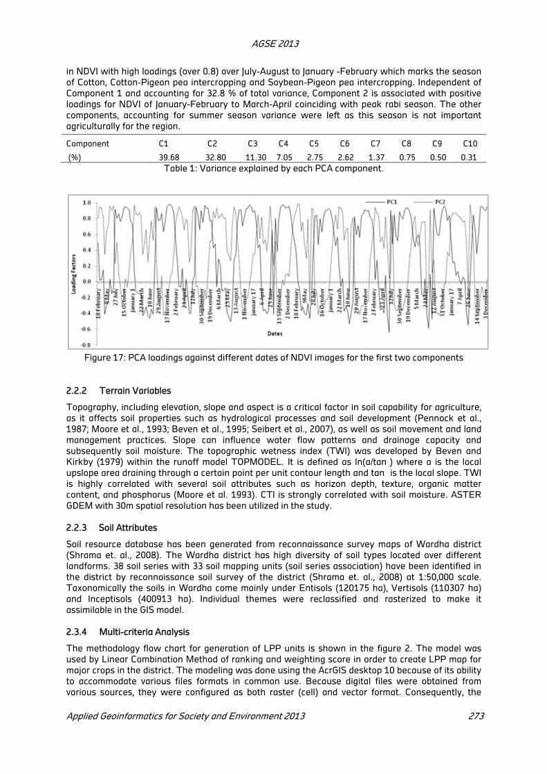
AGSE 2013


in NDVI with high loadings (over 0.8) over July-August to January -February which marks the season

of Cotton, Cotton-Pigeon pea intercropping and Soybean-Pigeon pea intercropping. Independent of

Component 1 and accounting for 32.8 % of total variance, Component 2 is associated with positive

loadings for NDVI of January-February to March-April coinciding with peak rabi season. The other

components, accounting for summer season variance were left as this season is not important

agriculturally for the region.

Component C1 C2 C3 C4 C5 C6 C7 C8 C9 C10

(%) 39.68 32.80 11.30 7.05 2.75 2.62 1.37 0.75 0.50 0.31

Table 1: Variance explained by each PCA component.

Figure 17: PCA loadings against different dates of NDVI images for the first two components

2.2.2 Terrain Variables

Topography, including elevation, slope and aspect is a critical factor in soil capability for agriculture,

as it affects soil properties such as hydrological processes and soil development (Pennock et al.,

1987; Moore et al., 1993; Beven et al., 1995; Seibert et al., 2007), as well as soil movement and land

management practices. Slope can influence water flow patterns and drainage capacity and

subsequently soil moisture. The topographic wetness index (TWI) was developed by Beven and

Kirkby (1979) within the runoff model TOPMODEL. It is defined as ln(a/tan�) where a is the local

upslope area draining through a certain point per unit contour length and tan� is the local slope. TWI

is highly correlated with several soil attributes such as horizon depth, texture, organic matter

content, and phosphorus (Moore et al. 1993). CTI is strongly correlated with soil moisture. ASTER

GDEM with 30m spatial resolution has been utilized in the study.

2.2.3 Soil Attributes

Soil resource database has been generated from reconnaissance survey maps of Wardha district

(Shrama et. al., 2008). The Wardha district has high diversity of soil types located over different

landforms. 38 soil series with 33 soil mapping units (soil series association) have been identified in

the district by reconnaissance soil survey of the district (Shrama et. al., 2008) at 1:50,000 scale.

Taxonomically the soils in Wardha come mainly under Entisols (120175 ha), Vertisols (110307 ha)

and Inceptisols (400913 ha). Individual themes were reclassified and rasterized to make it

assimilable in the GIS model.

2.3.4 Multi-criteria Analysis

The methodology flow chart for generation of LPP units is shown in the figure 2. The model was

used by Linear Combination Method of ranking and weighting score in order to create LPP map for

major crops in the district. The modeling was done using the AcrGIS desktop 10 because of its ability

to accommodate various files formats in common use. Because digital files were obtained from

various sources, they were configured as both raster (cell) and vector format. Consequently, the

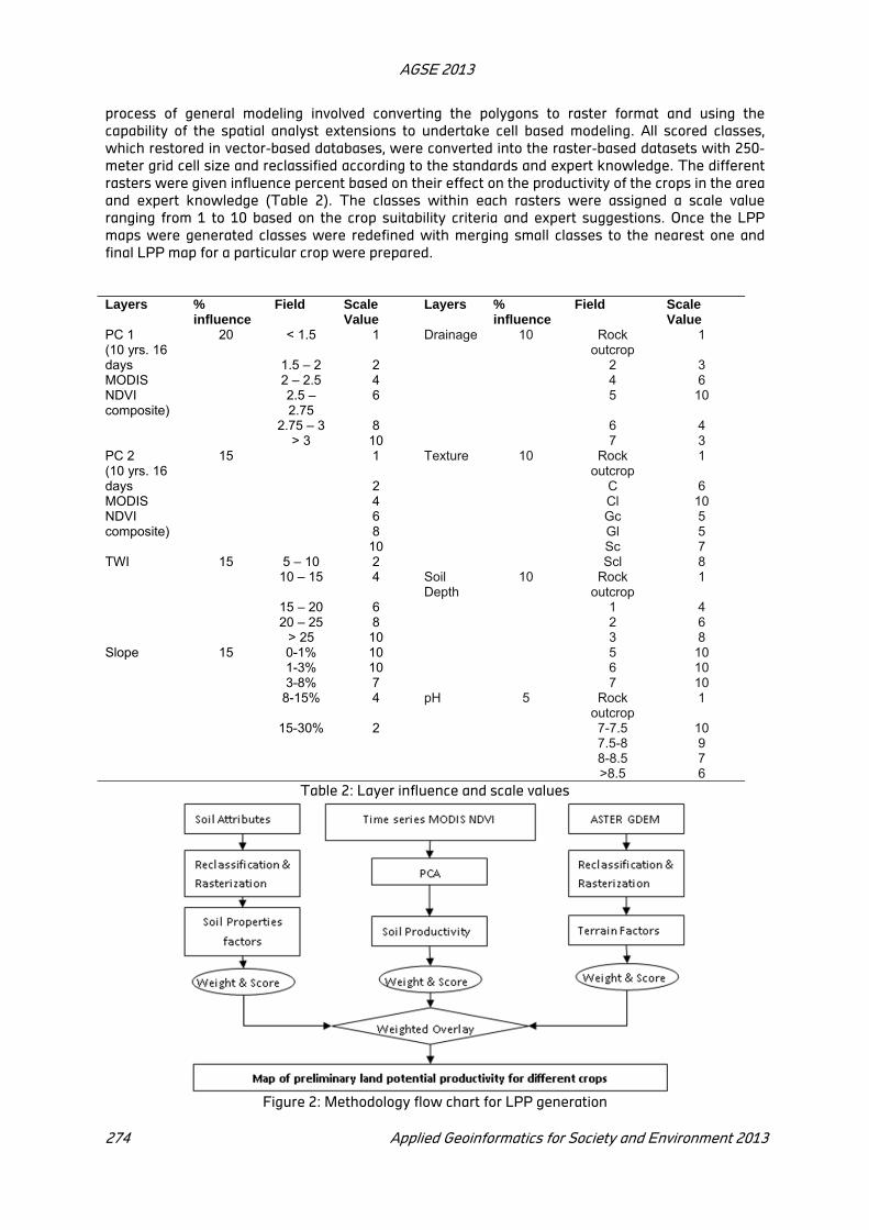
AGSE 2013


process of general modeling involved converting the polygons to raster format and using the

capability of the spatial analyst extensions to undertake cell based modeling. All scored classes,

which restored in vector-based databases, were converted into the raster-based datasets with 250-

meter grid cell size and reclassified according to the standards and expert knowledge. The different

rasters were given influence percent based on their effect on the productivity of the crops in the area

and expert knowledge (Table 2). The classes within each rasters were assigned a scale value

ranging from 1 to 10 based on the crop suitability criteria and expert suggestions. Once the LPP

maps were generated classes were redefined with merging small classes to the nearest one and

final LPP map for a particular crop were prepared.

Layers %

influence Field Scale

Value Layers %

influence Field Scale

Value PC 1 (10 yrs. 16 days MODIS NDVI composite)

20 < 1.5 1 Drainage 10 Rock outcrop

1

1.5 – 2 2 2 3 2 – 2.5 4 4 6 2.5 – 2.75

6 5 10

2.75 – 3 8 6 4 > 3 10 7 3

PC 2 (10 yrs. 16 days MODIS NDVI composite)

15 1 Texture 10 Rock outcrop

1

2 C 6 4 Cl 10 6 Gc 5 8 Gl 5 10 Sc 7

TWI 15 5 – 10 2 Scl 8 10 – 15 4 Soil

Depth 10 Rock

outcrop 1

15 – 20 6 1 4 20 – 25 8 2 6

> 25 10 3 8 Slope 15 0-1% 10 5 10

1-3% 10 6 10 3-8% 7 7 10

8-15% 4 pH 5 Rock outcrop

1

15-30% 2 7-7.5 10 7.5-8 9 8-8.5 7 >8.5 6

Table 2: Layer influence and scale values

Figure 2: Methodology flow chart for LPP generation

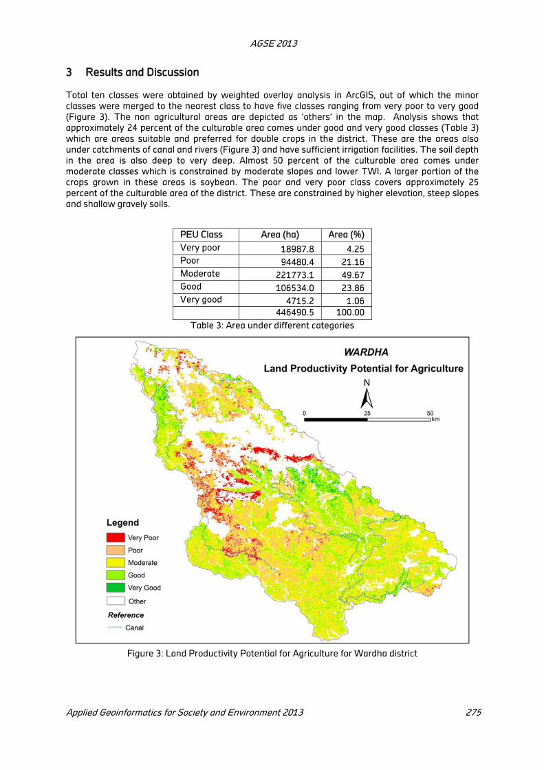
AGSE 2013



Total ten classes were obtained by weighted overlay analysis in ArcGIS, out of which the minor

classes were merged to the nearest class to have five classes ranging from very poor to very good

(Figure 3). The non agricultural areas are depicted as ‘others’ in the map. Analysis shows that

approximately 24 percent of the culturable area comes under good and very good classes (Table 3)

which are areas suitable and preferred for double crops in the district. These are the areas also

under catchments of canal and rivers (Figure 3) and have sufficient irrigation facilities. The soil depth

in the area is also deep to very deep. Almost 50 percent of the culturable area comes under

moderate classes which is constrained by moderate slopes and lower TWI. A larger portion of the

crops grown in these areas is soybean. The poor and very poor class covers approximately 25

percent of the culturable area of the district. These are constrained by higher elevation, steep slopes

and shallow gravely soils.

PEU Class Area (ha) Area (%)

Very poor 18987.8 4.25

Poor 94480.4 21.16

Moderate 221773.1 49.67

Good 106534.0 23.86

Very good 4715.2 1.06

446490.5 100.00

Table 3: Area under different categories

Figure 3: Land Productivity Potential for Agriculture for Wardha district

AGSE 2013


4 Conclusion

This study proposed a simplified approach to modeling LPP using MODIS time-series Normalized Difference

Vegetation Index (NDVI) and ancillary data, based on the hypothesis that the primary determinants of

soil productivity for agriculture may be surrogated by those data. The study has confirmed that MODIS

and ancillary data can be used to accurately identify the areal distribution of LPP classes within pre-defined

map units. These input variables can be further complemented by DEM (elevation, slope, and TWI) information

and other soil attributes available in legacy data as additional indicators of LPP for agriculture. Using a multi-

criteria GIS modeling approach base on the above data, we were able to produce LPP maps at 250 m resolution

REFERENCES

Beven, K.J., Kirkby, M.J., 1979. A physically based variable contributing area model of basin

hydrology. Hydrology Science Bulletin 24, 43–69.

Beven, K.J., Lamb, R., Quinn, P., Romanowicz, R., Freer, J., 1995. Top model. In: Singh, V.P. (Ed.),

Computer Models of Watershed Hydrology. Water Resources Publications, Colorado.

Beven, K.J., Lamb, R., Quinn, P., Romanowicz, R., Freer, J., 1995. topmodel. In: Singh, V.P. (Ed.),

Computer Models of Watershed Hydrology. Water Resources Publications, Colorado.

Eastman, J.R., Fulk, M. (1993). Long sequence time series evaluation using standardized principal

components. Photogrammetric Engineering and Remote Sensing 59 (8), 1307–1312.

Khaldoune, J., Van Bochove, E., Bernier, M., Nolin, M.C. (2011). Mapping agricultural frozen soil on

the watershed scale using remote sensing data. Applied and Environmental Soil Science, 1–16

Li Zhe, Huffman Ted,, Aining Zhang, Fuqun Zhou, Brian McConkey, 2012. Spatially locating soil

classes within complex soil polygons – Mapping soil capability for agriculture in Saskatchewan

Canada. Agriculture, Ecosystems and Environment 152 (2012) 59– 67

Moore, I.D., Gessler, P.E., Nielsen, G.A., Peterson, G.A. 1993. Soil attributes prediction using terrain

analysis. Soil Science Society of America Journal 57 (2), 443–452.

Pennock, D.J., Zebarth, B.J., De Jong, E. 1987. Landform classification and soil distribution in

hummocky terrain, Saskatchewan, Canada. Geoderma 40 (3-4), 297–315.

Robson, A., Beven, K., and Neal, C., 1992. Towards identifying sources of subsurface flow: a

comparison of components identified by a physically based runoff model and those determined by

chemical mixing techniques, Hydrological. Processes, 6, 199–214.

Santin-Janin, H., Garel, M., Chapuis, J.-L., Pontier, D., 2009. Assessing the performance of NDVI as a

proxy for plant biomass using non-linear models: a case study on the Kerguelen archipelago. Polar Biology 32 (6), 861–871.

Seibert, J., Bishop, K. H., and Nyberg, L., 1997. A test of TOPMODEL’s ability to predict spatially

distributed groundwater levels, Hydrol. Process., 11, 1131–1144,.

Sharma, J.P., Gajbhiye K.S., Mandal, C., Sinha A. K., 2005. Soil survey atlas of Wardha district,

Maharashtra. NBSS Publication 116, NBSS&LUP, Nagpur.

Sharma, J.P., Mandal, C., Raja, P., Nair, K.M., Bhaskar, B.P., and Sarkar, D., 2008. Reconnaissance

soil survey, mapping, correlation and classification of Wardha district, Maharashtra. NBSS

Publication 595, NBSS&LUP, Nagpur.

Zribi, M., Baghdadi, N., Nolin, M., 2011. Remote sensing of soil. Applied and Environmental Soil Science, 1–2.

Food Security and the Environment

Adedugbe Adebiyi

Adebol Bonifab Nigeria Limited. Area 2 Section 1 Block 16 Eleme close off Oyo Street Garki,Abuja,

[email protected]

KEY WORDS: Agriculture, Adaptation strategies, Food security, Food production, Climate change,

household needs.

ABSTRACT

Agriculture is the mainstay of most economies. In Africa it employs up to 90 per cent of the rural workforce, 60 per cent of the total (urban and rural) labour force, accounts for up to 40 per cent of export earnings and supports over 50 per cent of household needs and income while there are many studies of the impacts of change and variability on food production, few studies are devoted to a comprehensive assessment of impacts on food systems. This study is a result of food systems and household adaptation strategies in three communities in the Afram Plains, Ghana. It reveals how extreme climatic events affect rural food production, transportation, processing and storage. Adaptation strategies implemented by the three communities during past droughts serve as a foundation for planning response to future climate change. Results of the study shows food security in this region-where droughts and floods are expected to become more sever due to climate change-could be enhanced by increasing farm-based storage facilities; improving the transportation system, especially feeder roads that link food production areas and major markets; providing farmers with early warning systems; credit facility and the use of supplementary irrigation. Understanding the local context and the responses of household is very critical to the development of the effective strategies for reducing the potential adverse impacts of climatic change on food security.

1 Introduction

The agricultural sector (in the broad sense, including forestry, animal production, aquaculture, etc.)

represents the dominant part of the economy in most countries and provides the majority of

employments and livelihoods. Agriculture has- and according to most observers, will continue to have

a central role to play in the development process of the African continent. Agriculture and its

associated value chains are expected to contribute to local food security, to provide work

opportunities in rural areas, and to have a catalysis effect on the development of related economic

sectors .Agriculture faces many challenges, making it more and more difficult to achieve its primary

objective-feeding the world. As the global population continues to grow, diet changes associated

with rising incomes drive greater demand for food and other agricultural products, while global food

systems are increasingly threatened by land degradation, climate change and other stressors .Food

security and the environment is one of the fundamental concerns of the 21st

century. Ultimately,

climate change is about human acting in socio-ecological settings in which biophysical, socio-

cultural, economic, institutional, political and legal mechanism operate. It is in this complex system

that disasters emerge and that society has to cope with. Human and food security within the context

of climate change remains relatively under explored. It has now been widely established that the

pervasive societal emphasis on the modes and volume of food production in developing countries has

been detrimental to resolving problems relating to food distribution, affordability and accessibility.

The singular focus on production has consequently amplified food insecurity in many parts of the

world. Agriculture must change to meet both rising demand and become ecologically sustainable.

Agriculture has significant linkages to poverty and hunger, nutrition and health, peace and security

and preserving the world’s natural resources. Food security has been defined as the physical and

economic access to sufficient, safe and nutritious foods, which meet the individual’s dietary needs

and food preferences for an active and healthy life. Thus solving food insecurity requires a

comprehensive approach that incorporates numerous fields of planning and considers a wide range

of factors, which could be socio-economic; political or environmental in nature. Variability in climatic

conditions has been argued to be a stumbling block to food security in most developing countries and

especially in Sub-Saharan Africa. This is because, Sub-Saharan Africa already experiences high

temperatures and low (and highly variable) precipitation; second, because the economies are high

AGSE 2013


dependent on agriculture and; third, because there is low adoption of modern technology. Extreme

poverty, hunger and undernourishment can be eradicated by 2030 while protecting and even

reversing harm to natural resources, despite the challenges of climate change and weather

extremes. This paper first provides a short review of the concept of food systems and their

relationship to food security and the environment.

2 Design and Method

Africa’s vulnerability to climate change impacts have been underscored by the severe droughts

experienced recently in the Sahel in 2012 and the Horn of Africa in 2011. All these bring into focus

the serious impacts of climate change in the continent and highlighting the urgent need for

adaptation as a priority in providing sustainable solutions to reduce the vulnerability of a great

majority of Africa’s one billion citizens. Africa’s population is expected to constitute about 23% of the

global population by 2050. This places a huge dietary demand on governments and states to provide

opportunities for enough food and the new dietary demands. Both increasing and changes in dietary

preferences will further put strain on productivity in matching quantity and quality in food outputs

over the next coming years. The questions however, are the types of measures/approaches required

for the changing needs for food security. The challenges therefore are in charting new pathways to

eliminate food insecurity, adapt to the changing climate and build sustainable systems. This will

require innovative solutions that build on an internally driven process of change by individuals and

institutions coupled with adaptation to climate change. Climate change is referred to as the influence

of human activity that alters the composition of the global atmosphere, which is in addition to natural

climate variability. Agricultural production and food security in Africa are expected to be placed

under considerable additional stress by climate change. Impacts of global climatic changes could

particularly exacerbate the already poor performance in food production being experienced in most

parts of sub-Saharan Africa.

3 Study Area and Methodology

In order to explore empirical linkages between climate change and food security, Afram Plains, one

of the poorest districts in Ghana was used as a case study. The Afram Plains are located in the

transition zone between the northern Sudan savannah and the southern Guinea savannah. The

Plains comprise a mosaic of forest and savannah vegetation with a total land area of about 5,754km

of which about 2,725 km, representing 47.4% of the plains, was submerged after the construction of

the Volta Dam in the 1960s. To obtain a cross section of typical livelihoods and food systems in this

region considering geographical location, predominant economic activity and demographic

composition, three communities in the Afram Plains were selected for individual household surveys.

Twelve households were surveyed in each of the three communities: Xedzodzoekope, Mim

Kyemfere and Boakyekrom.

Xedzodzoekope is located along the shoreline of an inlet in the Afram arm of Lake Volta

approximately 8 km from the town of Fori-Fori along the main road. Fishing is the predominant

livelihood while farming, herding and charcoal production supplement income.

Mim kyemfere is located 15 km to the southeast of the district capital Donkorkrom and within 4 km

west of the main channel of Volta River. Basic crops include cashew, maize, sweet potato and citrus.

Boakyekrom is located 7 km from the Afram River along the main road which passes from Ekye

Amanfrom at the southern ferry crossing to the district capital, Donkorkrom. Yam cultivation is

remains the most prominent crop for the community.

A survey was conducted in January and February of 2008 in the three study communities. A

structural and open ended questionnaire was employed and the administration of the questionnaires

was by direct interview with the respondents. This technique was used because some of the

respondents had no formal education. The survey elicited information on household socio-

demographic characteristics, assets, income, and expenditure. It also contained questions about food

crops grown, harvested sold and consumed as well as farm inputs in the last farming season. There

were questions about observed changes and variability in climate and the impact on food production.

AGSE 2013


Finally adaptation strategies used by households during extreme climatic events and future ones

were also recorded.


The conclusion of the study is structured to take account of three critical facets of the food system

which have serious implications for food security and the subsequent adaptation strategies for

communities. The discussion of results begins with an analysis of local perceptions of climatic

changes and significant climatic events recorded through their memory. Survey respondents in all

three communities reported a delay in the onset of the major rainy season in recent years ,with little

or no rainfall occurring until the month of July and occasionally heavy rainfall in August that

saturates farmland and causes several crops to fail. Furthermore the significant climatic events

recorded through the memory of participants include the following:

(a)January-July 1976: Very hot weather conditions,

(b) 1983-1984: Drought-A year long of bush fires,

(c) October – December 1989: Very hot weather conditions,

(d) 1991: Lots of rains throughout the year,

(e) 1995: About 40 days of intensive rains,

(f) 2004: Very cold winds experienced during March- April (Easter) and November-January was

cold,

(g) 2005: Cold periods resulting in animal deaths,

(h) August 2006: 1 week of intensive rains, and

(i) 2007: Lots of rains in August and September.

In 1983/1984 farming season, Ghana experienced what could be described as the most severe

drought condition in recent memory. Irrigation was cited as a new adaptation strategy that will be

used in future extreme droughts. The adaptation strategies used during this drought along with

additional strategies that might be used in future severe droughts are shown in Table 1

Adaptation strategies to drought by

Past adaptation strategy

Xedzodz-

oekope

Mim-

Kyemfere

Boakye-

krom

Previous harvest and stored food 29 36 73

Purchase food from market - 28 18

Supported by family relations - - 9

Barter 71 18 -

Gathered from wild - 18 -

Future adaption strategy - - -

Previous harvest and stored food 30 55 75

Purchase food from market - - 17

Barter 60 9 -

Gathered from wild 9 -

Irrigation 10 - -

Start rice cultivation - - 8

Migrate - 9 -

Reduce food intake - 9 -

Table 1: Past and Future

AGSE 2013


5 Conclusion and Policy Recommendation

A survey of individual household was effective in assessing the relative status of food security and

climate adaptation strategies in three rural communities ( Boakyekrom , Xedzodzoekope and Mim

Kyemfere ) in the Afram Plains of Ghana. The majority of the households in all three communities

were of the opinion that they had enough food at the time of the survey and to a lesser extent, the

ability to acquire enough food to meet the household’s nutritional requirements in future. Extreme

climatic events however, have hampered food production and transportation networks with a

reduction in food availability in Boakyekrom as well as the other two communities.

Based on the findings presented in this paper, it is evident that addressing food security in Ghana

will require an expansion of farm-level, small-scale storage facilities. However adequate resources

must be provided to enable the new company to carry out its mandate to ensure food security and to

insulate farmers against post-harvest losses and natural disasters. It can be argued that while rural

agricultural communities may exhibit certain similar characteristics, they are not homogenous and as

such the impact of climatic changes on food security and households’ adaptation strategies of these

communities would differ. More importantly, while climatic changes are largely assumed to impact

on agriculture and other livelihood activities in Ghana, empirical research studies on the

phenomenon are limited. Understanding the local context and the responses of households is critical

to any solutions to address the challenges of food security and the environment.

REFERENCES

Amthor, Js; 2001. Effects of atmospheric CO2 concentration on wheat yield.

Brandshaw,B; Dolan, H; 2002. Farm-level adaptation to climatic variability and change.

Chambers, R; Conway, G; 1992. Sustainable rural livelihoods. Practical concepts for 21st

century

Clover, J; 2003. Food security in sub Saharan Africa

Codjoe,S; 2011. Institute for population studies, University of Ghana

Owusu, G; 2011. Institute of statistical, social and economic research, University of Ghana

Food and agricultural Organization,2001. State of food insecurity in the world. Rome

Kurukulasariya, P et al 2006. Will Africa agriculture survive climate change?

Nyanteng, VK; Dapaah, S; 1993. Agricultural development.

Nyanteng, VK(ed). Policies and options for Ghanaian economic development. Institute of Statistical,

Social and Economic Research, University of Ghana, Legon.

USAID, 1992. Policy Determination: Definition of food security, PD-19. USAID, Washington DC, p 4

Detecting spatio-temporal variation of Indian mangrove foliar phenology

using SPOT-VGT time-series data

Chellamani Prabakaran a

, Chandra Prakash Singh a

, Hitesh A Solanki b

and Jai Singh Parihar a

a Space Applications Centre, ISRO, Ambawadi Vistar P.O., Ahmedabad, Gujarat, India

b Department of Botany, Gujarat University, Ahmedabad, Gujarat, India.

KEY WORDS: Phenology, Mangrove, TIMESAT, SPOT-VGT, Climatic factors.

ABSTRACT

Mangroves are salt tolerant plant communities found in tropical and subtropical inter-tidal regions. They are regarded as the most productive forest ecosystems in the world. Phenology is the study of biological phenomena (e.g. bud burst, flowering, and leaf fall, etc.) that are controlled by environmental and climatic factors, therefore considered as a sensitive biosphere indicator of climate change. The current study is an attempt to understand the spatio-temporal variation in foliar phenology of Indian mangroves using Normalized difference vegetation index (NDVI) data. SPOT-VGT, 10 day NDVI composite products were used to predict the mangrove’s foliar phenology from 1999 to 2012. Mangrove locations were extracted from a global land cover map (GLC 2000). The NDVI data were filtered and smoothened by Savitzky-Golay fitting method using TIMESAT software. Further, the phenological variables like season start, peak, end and length were retrieved from the fitted phenological curves for every season accordingly. Average value for each variable type of the season was calculated. Average value of each variable for total season was also calculated to quantify the effect of latitude, longitude and altitude. Negative trend was observed in the season start suggesting that early greening has been setting up, leading to longer season length. At lower latitudes, the season start is late as compared to higher latitudes suggesting an early season start at northern part of India (r=-0.5). No or less significant relationships were found with other phenological variables (end and length of the season). It was observed that at lower altitude, season length was higher than that of higher altitude (r=-0.9). The change in the spatio-temporal variation of mangrove foliar phenology can be used in the future climate modeling studies.

1 Introduction

Mangroves are salt tolerant, evergreen plant communities found in the inter-tidal of tropical and

subtropical estuarine, deltaic and gulf regions. There are 114 species of true mangroves belonging to

66 genera reported over Worldwide (Tomlinson 1986). They are regarded as the most productive

forest ecosystems. Phenology is the study of recurring life – cycle events of biological phenomena

(e.g. bud burst, flowering and leaf fall, etc.) that are initiated, driven and controlled by the

environmental and the climatic factors, therefore considered as a sensitive biosphere indicator of

climate change. It is important to detect the timing of foliar (leaf) initiation, senescence, fall and

length of foliar growing season for the understanding of productivity of the plants.

The studies on the phenology of plants and flowering had started long back with many individuals

and families recording the phenological observation around them. Henry David Thoreau (1817 –

1862) compiled a vast catalog of phenological observations in the woods around Concord, MA (Miller-

Rushing et al. 2008). Phenological observations can be recorded on the ground or can be derived

from high temporal remotely sensed data. Ground-measured phenological observations provide

species-specific information with high temporal resolution, but lack a spatial component (Studer et

al. 2007). In contrast, remotely sensed data provide a large spatial and high temporal data to

estimate the phenology at a range of scale from the local to global.

Many ground based phenological studies were done in the Indian tropical forests – evergreen forest

(Bhat 1992; Kikim et al. 2001; Sundarapandian et al. 2005), deciduous forest (Singh et al. 1992; Singh

et al. 2005; Yadav et al. 2008), and mangrove forest (Upadhyay & Mishra 2010). However, these

studies were mainly focused on the flowering and leaf initiation of species-specific small area of

forest ecosystems for a limited period of 2 – 4 years. Besides, there are few studies done using

AGSE 2013


remote sensing data. Dash et al (2010) had used the MERIS Terrestrial Chlorophyll Index (MTCI) to

study the spatio-temporal variation in the phenology of four major forest types of India. Prasad et al

(2007) had used AVHRR-NDVI time series data to characterize the spatial patters in phenological

variation in eight contrasting forest types in an Indian region. Prabakaran et al (2013) studied the

forest (deciduous and evergreen) phenological patterns of Uttarkannada district using SPOT-VGT

time series data (year 1999-2007). Relatively few studies used remote sensing to extract

phenological variables over India (Jeyaseelan et al. 2007; Sarkar & Kafatos 2004).

However, there are very less studies on Indian mangrove ecosystems using remote sensing data

other than monitoring, conservation, change detection and mapping of the mangrove extent. It is

very much important to study the phenology of mangroves to understand the productivity, the effects

of climate change and health of this ecosystem. In this study, we attempt to understand the spatio-

temporal variation of Indian mangrove foliar phenology using remote sensing time-series data.

2 Materials and Methods

2.1 Study Area

All the major mangrove ecosystems found in India including Andaman and Nicobar Islands were

selected for this study. According to India state of forest report (FSI 2011), the country has about

4,661.56 km2 mangrove cover which is 0.14% of the country's total geographical area. The study

area (Figure 1) falls under tropical monsoon climate with three pronounced seasons, viz. winter

(October-January), summer (February- May) and rainy (June-September).

Figure 1: Study area. (Mangrove vegetation showed in grey colour)

2.2 Data used SPOT-VGT NDVI

Satellite Pour l' Observation de la Terre (SPOT) VEGETATION (VGT) Normalized Difference

Vegetation Index (NDVI) was used for this study. The VEGETATION Program is developed jointly by

the France space agency (CNES), the European Commission, VITO Belgium, Italy and Sweden. The

SPOT-VGT sensor, launched in 1998, possesses spectral bands specifically tailored for large-area

vegetation monitoring. The VGT-S10 products are composited (maximum-value) products of 10 days

with 1x1 km spatial resolution (Maisongrande et al. 2004).

Ancillary data

I. GLC 2000 map: The Global Land Cover Map – GLC2000 product (Bartholome & Belward, 2005) –

was used in this study to locate mangrove vegetation type. This product was created using daily

S1 data acquired by the VEGETATION sensor onboard SPOT-4, then by various classification

AGSE 2013


methods (e.g., supervised, unsupervised and hybrid methods). The landcover map for the Indian

sub-continent was downloaded from the GLC global database (http://www.gem.jrc.it/glc2000).

II. Elevation data: NASA’s Shuttle Radar Topographic Mission (SRTM) has provided the digital

elevation map (DEM) data for over 80% of the globe. 1 km re-sampled SRTM-DEM data was

downloaded from the CGIAR Consortium for Spatial Information (CGIAR-CSI) site

(http://www.csi.cgiar.org).

III. Meteorological data: Rainfall and Temperature data from 1999 – 2012 for the Indian sub-

continent was acquired from Indian Institute of Tropical meteorology (IITM), Pune, India.

3 Methodology

3.1 Phenological Curves

SPOT-VGT S10 NDVI product of 14 years (1999–2012) amounting to 504 bands (36 bands/year – 10

day composite) – were loaded in TIMESAT ver. 3.02 (Jönson & Elkundh, 2004). This program was

used to get the NDVI profile of all the study pixels. TIMESAT implements three processing methods

based on least-squares fit to the upper envelope of the NDVI data. The first method uses local

polynomial functions in the fitting, and it can classified as an adaptive Savitzky–Golay filter has been

used in this study. This method can be used to reconstruct the high quality NDVI time series data

from noisy data (Chen et al. 2004). The pre-processing to remove the spikes and outliers was carried

out by applying a median filter. Further, adaptive Savitzky–Golay filtering and curve fitting were used

to deduce the phenological parameters. This method fits a quadratic polynomial f (t) = c1 + c2t + c3t2

for each data value yi, i = 1, 2, … , N, to all 2n + 1 points in the moving window and replaces the value

Yi with the value Yi *of the polynomial at position ti in the following equation.

n

nj

jCiYiYi*

3.2 Extraction of Phenological variables

From the fourteen years data, thirteen seasons (n – 1) were extracted. The start and end of foliage

season can be set from 0 to 1. For the start of the season (SOS) and end of the season (EOS), we

used a threshold value of 0.1, i.e. 10% of the distance from the left and right minimum values from

the maximum value of the curve. Peak of the curve (100%) has been considered as maximum

greenness of that season - maximum of the season (MOS). The length of the season (LOS) is

calculated from the difference between EOS and SOS (Figure 2). From the curve fitting, the

seasonality parameters were extracted. To generate images of seasonality parameters, e.g. start of

the season, a time window containing the season was defined. For each pixel the seasonality is

established. The season falling in the time window is the desired one and the seasonality parameter

is extracted for this season and written to an image file. The extraction of images is done using

TSF_seas2img, a FORTRAN program which is an in-build algorithm provided in the TIMESAT

software. The seasonality images were created for the phenological variables – SOS, MOS, EOS and

LOS.

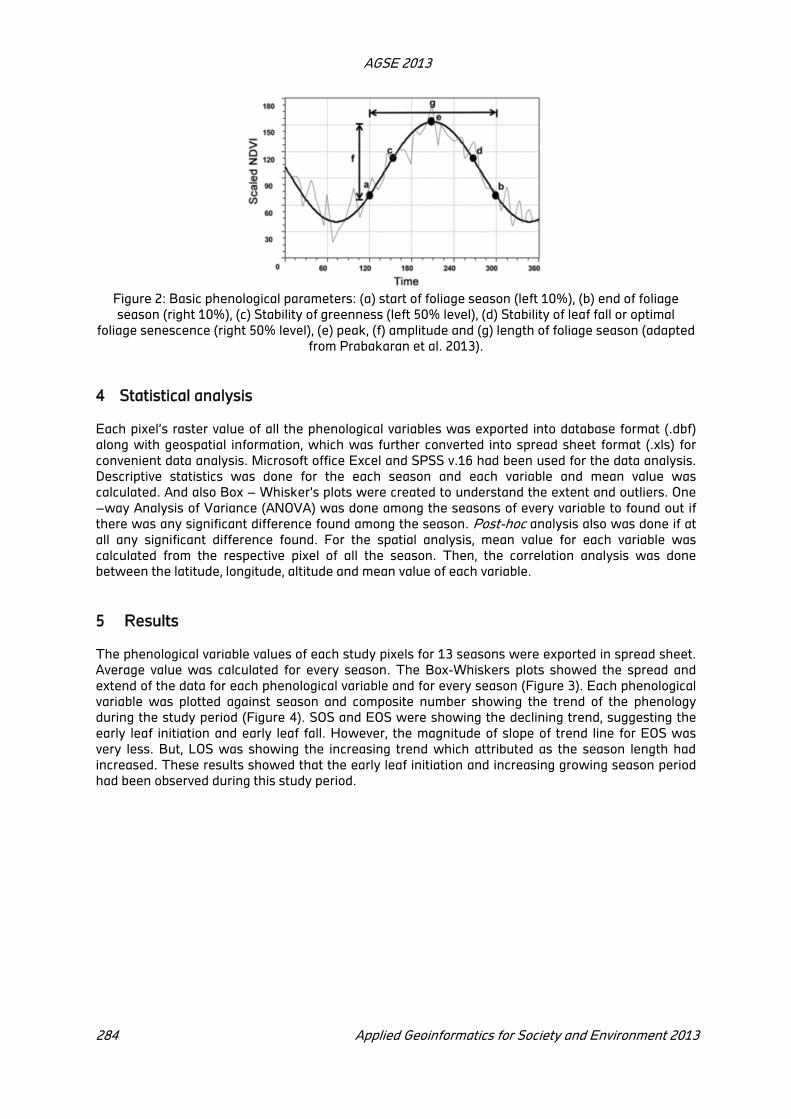
AGSE 2013


Figure 2: Basic phenological parameters: (a) start of foliage season (left 10%), (b) end of foliage

season (right 10%), (c) Stability of greenness (left 50% level), (d) Stability of leaf fall or optimal

foliage senescence (right 50% level), (e) peak, (f) amplitude and (g) length of foliage season (adapted

from Prabakaran et al. 2013).

4 Statistical analysis

Each pixel’s raster value of all the phenological variables was exported into database format (.dbf)

along with geospatial information, which was further converted into spread sheet format (.xls) for

convenient data analysis. Microsoft office Excel and SPSS v.16 had been used for the data analysis.

Descriptive statistics was done for the each season and each variable and mean value was

calculated. And also Box – Whisker’s plots were created to understand the extent and outliers. One

–way Analysis of Variance (ANOVA) was done among the seasons of every variable to found out if

there was any significant difference found among the season. Post-hoc analysis also was done if at

all any significant difference found. For the spatial analysis, mean value for each variable was

calculated from the respective pixel of all the season. Then, the correlation analysis was done

between the latitude, longitude, altitude and mean value of each variable.

5 Results

The phenological variable values of each study pixels for 13 seasons were exported in spread sheet.

Average value was calculated for every season. The Box-Whiskers plots showed the spread and

extend of the data for each phenological variable and for every season (Figure 3). Each phenological

variable was plotted against season and composite number showing the trend of the phenology

during the study period (Figure 4). SOS and EOS were showing the declining trend, suggesting the

early leaf initiation and early leaf fall. However, the magnitude of slope of trend line for EOS was

very less. But, LOS was showing the increasing trend which attributed as the season length had

increased. These results showed that the early leaf initiation and increasing growing season period

had been observed during this study period.

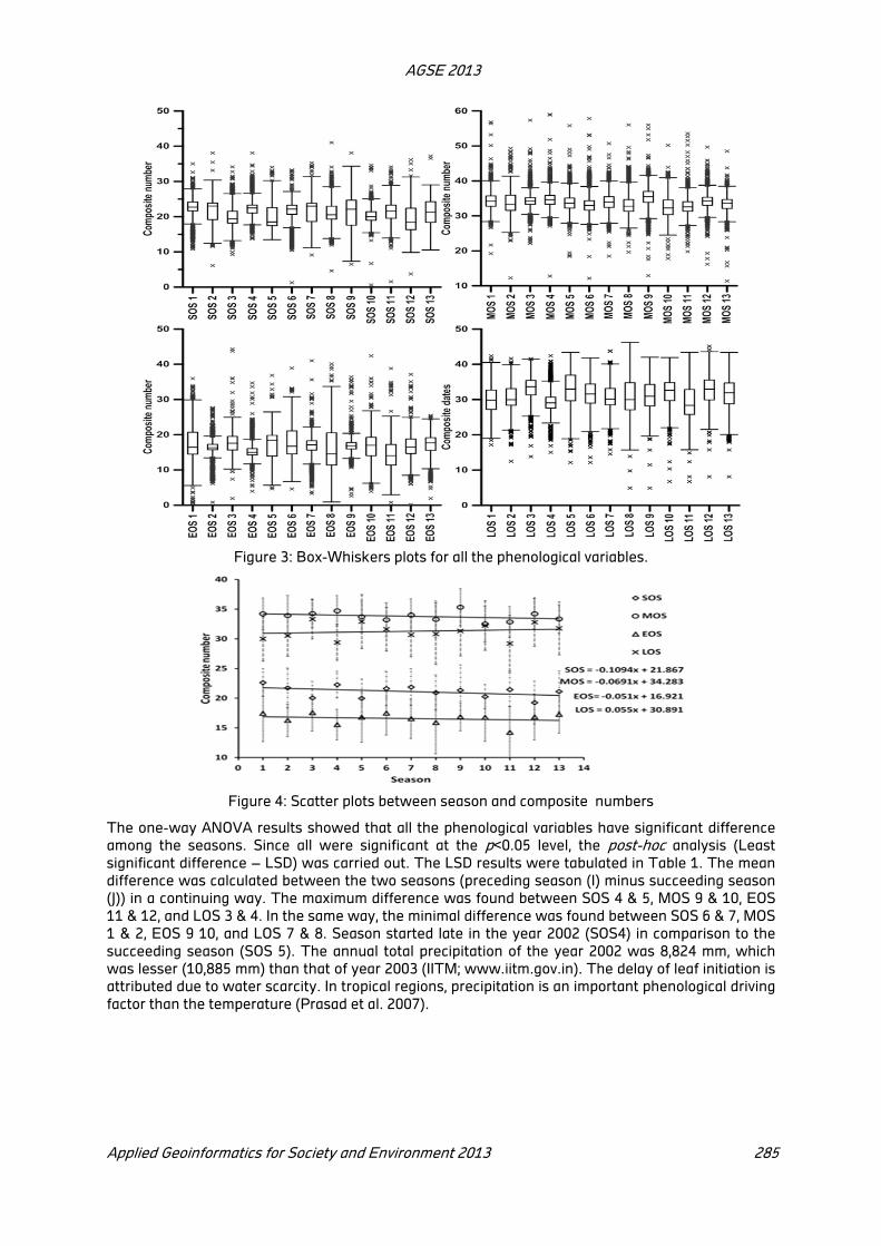
AGSE 2013


Figure 3: Box-Whiskers plots for all the phenological variables.

Figure 4: Scatter plots between season and composite numbers

The one-way ANOVA results showed that all the phenological variables have significant difference

among the seasons. Since all were significant at the p<0.05 level, the post-hoc analysis (Least

significant difference – LSD) was carried out. The LSD results were tabulated in Table 1. The mean

difference was calculated between the two seasons (preceding season (I) minus succeeding season

(J)) in a continuing way. The maximum difference was found between SOS 4 & 5, MOS 9 & 10, EOS

11 & 12, and LOS 3 & 4. In the same way, the minimal difference was found between SOS 6 & 7, MOS

1 & 2, EOS 9 10, and LOS 7 & 8. Season started late in the year 2002 (SOS4) in comparison to the

succeeding season (SOS 5). The annual total precipitation of the year 2002 was 8,824 mm, which

was lesser (10,885 mm) than that of year 2003 (IITM; www.iitm.gov.in). The delay of leaf initiation is

attributed due to water scarcity. In tropical regions, precipitation is an important phenological driving

factor than the temperature (Prasad et al. 2007).

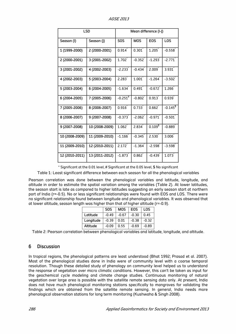
AGSE 2013


LSD Mean difference (I-J)

Season (I) Season (J) SOS MOS EOS LOS

1 (1999-2000) 2 (2000-2001) 0.914* 0.301

* 1.205

* -0.558

*

2 (2000-2001) 3 (2001-2002) 1.702* -0.352

* -1.293

* -2.771

*

3 (2001-2002) 4 (2002-2003) -2.233* -0.434

* 2.009

* 3.931

*

4 (2002-2003) 5 (2003-2004) 2.283* 1.001

* -1.264

* -3.502

*

5 (2003-2004) 6 (2004-2005) -1.634* 0.491

* -0.672

* 1.266

*

6 (2004-2005) 7 (2005-2006) -0.251# -0.802

* 0.913

* 0.939

*

7 (2005-2006) 8 (2006-2007) 0.916* 0.733

* 0.662

* -0.145

$

8 (2006-2007) 9 (2007-2008) -0.373* -2.062

* -0.971

* -0.501

*

9 (2007-2008) 10 (2008-2009) 1.062* 2.834

* 0.109

$ -0.889

*

10 (2008-2009) 11 (2009-2010) -1.166* -0.345

* 2.530

* 3.006

*

11 (2009-2010) 12 (2010-2011) 2.172* -1.364

* -2.598

* -3.598

*

12 (2010-2011) 13 (2011-2012) -1.873* 0.862

* -0.439

* 1.073

*

* Significant at the 0.01 level, # Significant at the 0.05 level, $ No significant

Table 1: Least significant difference between each season for all the phenological variables

Pearson correlation was done between the phenological variables and latitude, longitude, and

altitude in order to estimate the spatial variation among the variables (Table 2). At lower latitudes,

the season start is late as compared to higher latitudes suggesting an early season start at northern

part of India (r=-0.5). No or less significant relationships were found with EOS and LOS. There were

no significant relationship found between longitude and phenological variables. It was observed that

at lower altitude, season length was higher than that of higher altitude (r=-0.9).

SOS MOS EOS LOS

Latitude -0.49 -0.67 -0.30 0.45

Longitude -0.39 0.01 -0.38 -0.32

Altitude -0.09 0.55 -0.69 -0.89

Table 2: Pearson correlation between phenological variables and latitude, longitude, and altitude.

6 Discussion

In tropical regions, the phenological patterns are least understood (Bhat 1992; Prasad et al. 2007).

Most of the phenological studies done in India were of community level with a coarse temporal

resolution. Though these detailed study of phenology on community level helped us to understand

the response of vegetation over micro climatic conditions. However, this can’t be taken as input for

the geochemical cycle modeling and climate change studies. Continuous monitoring of natural

vegetation over large area is possible with the satellite remote sensing data only. At present, India

does not have much phenological monitoring stations specifically to mangroves for validating the

findings which are obtained from the satellite remote sensing. In general, India needs more

phenological observation stations for long term monitoring (Kushwaha & Singh 2008).

AGSE 2013


For the first time, this study attempted to establish a broad mangrove phenological pattern in India

using NDVI data for fourteen years (1999 – 2012). The spatio-temporal variation in the mangrove

phenological pattern helps us to understand the changes happened in the vegetation dynamics. The

long study period is helpful to have a broad image of changes and dynamics in the plant growth. The

phenological patterns detected from this study for key natural vegetation broadly match with ground

observations as reported in earlier studies. Mixing pixel is quite common in the mangrove region.

The boundary pixels may have the mixed spectral response from the non-mangroves such as

mudflats, creeks, and other vegetations. It is important to note that the pixel resolution used in this

study is quite coarse (1km).

Expected spatio-temporal variation of phenological patterns was observed. Mangroves are

evergreen vegetations. Throughout the season they will exchange their old leaves with new leaves.

Since, mangrove’s plant physiology is mainly controlled by water salinity, precipitation and fresh

water flow is important. Delay in the start of the greenness and early season end is mainly coincided

with the deficit rainfall condition of that season. The higher latitudes are observed with early

greenness due to the fresh water availability and south-west monsoon. Lower latitude mangroves

are receiving water mainly from north-west monsoon. And the mangroves found very near to the

coast are having longer season length than that of away from the coast.

7 Conclusion

Spatial and temporal variation of mangrove phenological pattern was observed. Negative trend was

observed in the start of the season which suggests the early season start occurred in the later

seasons of the study period. The early season start attributed to the changes in the climatic

conditions over the study area. Season length also showed an increasing trend. Growing period of

vegetation has increased over time. The temporal variation of mangrove phenology is mainly

coincided with the rainfall conditions of that season. Among all phenological variables analysed the

onset of greenness was highly related with latitude while compared with other variables. The

extracted phenological variables from this study can be used as an important input to investigation of

the impact of climate change, sea level rise on mangrove vegetation. The change in the spatio-

temporal variation of mangrove foliar phenology can be used in the future climate modeling studies

and bio-geochemical modeling. Spatial information on phenological variables is important for

planning and conservation of terrestrial ecosystems.

REFERENCES

Bartholome, E., & Belward, A. S., 2005. GLC2000: A new approach to global land cover mapping from

Earth observation data. International Journal of Remote Sensing, 26, pp. 1959−1977.

Bhat, D.M., 1992. Phenology of tree species of tropical moist forest of Uttar Kannada district,

Karnataka, India. J. Biosci., 17, pp.325 – 352.

Chen. J., Per. Jonsson, Masayuki Tamura, Zhihui Gu, Bunkei Matsushita, Lars Eklundh., 2004. A

simple method for reconstructing a high-quality NDVI time-series data set based on the Savitzky–

Golay filter. Remote Sensing of Environment, 91, pp. 332–344.

Dash, J., Jeganathan, C., Atkinson, P. M., 2010.The use of MERIS Terrestrial Chlorophyll Index to

study spatio-temporal variation in vegetation phenology over India, Remote Sensing of

Environment, 114, pp. 1388 – 1402.

Forest Survey of India (FSI), 2011. India State of Forest Report. Ministry of Environment and Forest

(MoEF), Government of India.

Jeyaseelan, A. T., Roy, P. S., & Young, S. S., 2007. Persistent changes in NDVI between 1982 and

2003 over India using AVHRR GIMMS (global inventory Modeling and mapping studies) data.

International Journal of Remote Sensing, 28, pp. 4927−4946.

Jönsson, P., & Eklundh, L., 2004. TIMESAT — A program for analyzing time-series of satellite sensor

data. Computers and Geosciences, 30, pp. 833−845.

Kikim, A., & Yadava, P., 2001. Phenology of tree species in subtropical forests of Manipur in north

eastern India, Tropical Ecology, 42, pp. 269 – 276.

AGSE 2013


Kushwaha, C. P., & Singh, K. P., 2008. India needs phenological stations network. Current Science,

95, pp. 832−834.

Maisongrande, P. B. Duchemin & G. Dedieu., 2004. VEGETATION/SPOT: an operational mission for

the earth monitoring; presentation of new standard products. International Journal of Remote

Sensing, 25, pp. 9-14.

Miller-Rushing AJ, Primack R B, Primack D, and Mukunda S., 2006. Photographs and herbarium

specimens as tools to document phenological changes in response to global warming. American

Journal of Botany, 93, pp. 1667–1674.

Prabakaran C., Singh, C.P., Panigrahy, S., and Parihar, J.S., 2013. Retrieval of forest phenological

parameters from remote sensing-based NDVI time-series data, Current Science, 105(6), pp. 795-

802.

Prasad, V. K., Badarinath, K. V. S., & Eaturu, A., 2007. Spatial patterns of vegetation phenology

metrics and related climatic controls of eight contrasting forest types in India — Analysis from

remote sensing datasets. Theoretical and Applied Climatology, 89, pp. 95−107.

Sarkar, S., & Kafatos, M., 2004. Interannual variability of vegetation over the Indian sub-continent

and its relation to the different meteorological parameters. Remote Sensing of Environment, 90,

pp. 268−280.

Singh, J.S & V.K. Singh., 1992. Phenology of seasonally dry tropical forest. Current Science, 63, pp.

684 - 688.

Singh, K.P., & Kushwaha, C. P., 2005. Paradox of leaf phenology: Shorea robusta is a semi-evergreen

species in tropical dry deciduous forests in India. Current science, 88 (11), pp. 1820 – 1824.

Studer, S., Stockli, R., Appenzeller, C., & Vidale, P. L., 2007. A comparative study of satellite and

ground-based phenology. International Journal of Biometeorology, 51, pp. 405−414.

Sundarapandian, S.M., Chandrasekaran, S. and Swamy, P.S., 2005. Phenological behavior of selected

tree species in tropical forests at Kodayar in the Western Ghats, Tamil Nadu, India, Current

Science, 88 (5), pp. 805 – 810.

Tomlinson, P. B.,1986. The Botany of Mangroves. Cambridge University Press, Cambridge, London,

New York.

Upadhyay, V.P. & Mishra, P.K., 2010. Phenology of mangroves tree species on Orissa coast, India.

Tropical Ecology 51(2), pp. 289-295.

Yadav, R.K., & A.S. Yadav., 2008. Phenology of selected woody species in a tropical dry deciduous

forest in Rajasthan, India. Tropical Ecology, 49 (1), pp. 25 – 34.

Acknowledgement

We express our sincere thanks to Mr. A S Kiran Kumar, Director, Space Applications Centre, and Dr.

R P Singh, Head, EHD for their constant support and guidance.

Spectral Distance and an Approach for Species Level Discrimination of

Mangroves

K. Arun Prasad and L. Gnanappazham

Department of Earth and Space Sciences, Indian Institute of Space Science and Technology,

Valiamala P.O, Thiruvananthapuram – 695547, Kerala, India, E-mail: [email protected],

[email protected]

KEY WORDS: Mangroves, Field spectroscopy, Spectral discrimination, Non- parametric test, J-M

distance

ABSTRACT

Monitoring and conservation of mangrove ecosystem has become one of the essential natural resource management activities in the current scenario of global warming and sea level rise. Mangroves are trees or shrubs commonly seen in mudflats of intertidal regions of tropical and subtropical coastlines and they are salt tolerant. Enhanced spectral resolution of field spectroscopy evolved in past two decades provides valuable information for hyperspectral remote sensing applications especially in forestry and environment. In this study, we examine the discrimination of field reflectance spectra of six species of Rhizophoraceae (one of the mangrove families found dominant in Indian coastlines) using non–parametric statistical methods. As the first step, the spectra collected were subjected to post-processing techniques to make the data usable for further processing. Then median spectra of six species were selected for pair-wise seperability analysis using non-parametric Mann-Whitney U test. Results depict that C. decandra is separable from B. parviflora, K. candel and R. mucronata in all wavelengths but poorly separable with B.sexangula. Spectral distance between species were also determined using Jeffries-Matusita (JM) distance measures at six wavelength locations selected on the basis of non-parametric test results. The results of J-M distance analysis also agree with that of Mann-Whitney U test.

1 Introduction

The term “Mangroves” is used to represent vegetation community usually thrives in intertidal zone of

tropical and subtropical region of the world. Increase in human population and subsequent

industrialization in past decades leads to increase in stress towards this coastal ecosystem which

consequently accelerated the clearance of mangroves (Blasco and Aizpuru, 2002). Also climate

change, sea-level rise and natural disasters like storm surges has become threats to mangrove

ecosystem for their survival (Gilman et al., 2008). Mangrove species in Rhizophoraceae family are

very important and abundant along Indian coast. Rhizophoraceae family includes four mangrove

genera namely Bruguiera, Ceriops, Kandelia and Rhizophora which has 18 mangrove species

(Tomlinson, 1994). The spectrally high dimensional data could be used to discriminate those earth

surface features having similar reflectance in broad spectral domain. Hyperspectral data has been

successfully applied in many fields including geology, forestry, agriculture and environmental

sectors. Especially in forestry, utilization of hyperspectral remote sensing data for assessing and

monitoring the spatial distribution and health has increased considerably in past decades.

Spectroradiometer provides interoperable pure reflectance value of feature of interest placed in its

field of view from its in-situ measurement. Spectral library generation for various agricultural and

wetland species has been attempted and results indicated the existence of unique spectral

signatures for particular species during unique phase of their growth (Rao et al., 2007; Zomer et al.,

2009). Spectral discrimination had been studied by utilizing field and lab reflectance data of various

vegetation types such as agricultural crops (Song et al., 2011), Mediterranean species (Manevski et

al., 2011) and also coastal vegetation including mangroves (Schmidt and Skidmore, 2003; Panigrahy

et al., 2012; Vaiphasa et al., 2005).

In this paper we investigated the spectral discrimination among six mangrove species of

Rhizophoraceae family: Bruguiera parviflora, Bruguiera sexangula, Ceriops decandra, Kandelia

AGSE 2013


candel, Rhizophora apiculata and Rhizophora mucronata using their field spectral reflectance data.

Non-parametric statistical analysis was implemented to find out wavelengths (bands) in which the

spectral separability is statistically significant. Spectral distance analysis using Jeffries-Matusita

distance method was calculated in wavelengths selected based on non-parametric test and

vegetation characteristics to know “how far” the species are in their spectral domain.

2 Materials and Methodology used

2.1 About study site

Bhitarkanika National Park is situated in northeastern part of Odisha state in Indian east coast. It is

located in the area of combined deltaic region of rivers Brahmani, Baitrani and Dhamra and has rich

alluvial deposits with gently sloping topography which supports rich flora and fauna. The total area

of Bhitarkanika wildlife sanctuary is 672 sq. km., of which core area of 145 sq. km. is covered by

mangrove forest. In the year 2002, Bhitarkanika mangrove ecosystem has been declared as ‘Ramsar’

site – A wetland of International importance by Ramsar Convention of Wetlands. The study area lies

within 20°38’19’’ N - 20°47’27’’ N latitudes and 86°49’26’’ E - 87°05’48’’ E longitudes. The area

experiences semi diurnal high and low tides twice a day and tidal amplitude ranges between 2 m –

3.5 m upstream and 3.5 m – 6 m near to river mouths (Ravishankar et al., 2004).

2.2 Field spectral data collection

Field spectral data were collected from canopies of six mangrove species, Bruguiera parviflora (BP), Bruguiera sexangula (BS), Ceriops decandra (CD), Kandelia candel (KC), Rhizophora apiculata (RA) and Rhizophora mucronata (RM) from sample plots using Analytical Spectral Device (ASD)

Fieldspec®

3 spectroradiometer in nadir position. It records reflectance in spectral range of 350 nm to

2500 nm (2151 bands) at spectral resolution of 3 nm and 10 nm with sampling interval of 1.4 nm and

2 nm in Visible-Near Infrared (350 nm – 1000 nm) and Short Wave Infrared (1000 nm – 2500 nm)

domain respectively. The spectroradiometer has three detectors for spectral data acquisition: one

512 channel silicon photodiode array which measures in Visible / Near Infrared (VNIR) region of

spectrum (350 nm – 1000 nm) and two thermo electrically cooled Indium Gallium Arsenide (InGaAs)

detectors which measures in Short Wave Infrared (SWIR) regions (SWIR1: 1000 nm to 1830 nm -

831 channels and SWIR2: 1830 nm to 2500 nm - 671 channels) (ASD, 2010). All measurements were

done between 11:00 AM and 01:00 PM in sunny days of April 2013 so that sun angle is near nadir.

More than 100 spectra per species were recorded in which each spectra itself is an average of 60

readings. The radiance recorded was converted to reflectance using Spectralon®

reference panel.

Ground truth data collection protocols were followed during field data acquisition.

2.3 Pre-processing of field spectral signature

All reflectance spectra measured were pre-processed for further analysis. The splice correction was

applied to all spectra at 1001 nm to correct the drift which occurs due to difference in thermal

sensitivity of sensors within the spectroradiometer using ASD Viewspec Pro (Beal and Eamon,

1996). Then water vapor absorption bands between 1350 nm – 1460 nm, 1790 nm – 1960 nm and

2350 nm – 2500 nm were eliminated from collected spectra which results in remaining 1718 bands

used for further analysis. After pre-processing the field spectral reflectance data collected from six

species, median spectrum for each species was calculated and plotted in Figure 1.

AGSE 2013


Figure 1: Spectral library constructed from median spectra of mangrove species of Rhizophoraceae

family

2.4 Non – parametric statistical analysis

By assuming that, spectral reflectance of six mangrove species of Rhizophoraceae do not follow

normal distribution, non- parametric analysis of variance was carried out to test the variance of

reflectance among them. The non-parametric Kruskal-Wallis test along with pair-wise Mann-

Whitney U-test was carried out by assuming the null hypothesis H0: ƞ1= ƞ2=….. = ƞ6 against the

alternative hypothesis Ha: ƞ1≠ ƞ2≠….. ≠ ƞ6 at every wavelength location considered. Here ƞ

represents the median spectral reflectance of species considered. Kruskal-Wallis test is similar to

One-way ANOVA test that can be performed on ordinal (ranked) data whereas the Mann-Whitney U

test compares median spectral reflectance of two species to find out the spectral difference between

them (Sheskin, 2004). It results whether a species is statistically separable from another species on

a particular wavelength. The number of such statistically significant species pairs was calculated at

each wavelength.

2.5 Spectral distance analysis

From the results of previous analysis, wavelengths at which maximum number of species pairs

spectrally different are evident. Based on these results and spectral characteristics of vegetation, six

wavelength locations were chosen for spectral distance analysis. Jeffries-Matusita (J-M) distance is

the method chosen to estimate the distance between each pair of mangrove species. J-M distance is

the measure of average distance between the two class density function. The J-M distance is

calculated by the formula

dabJ M ( e ) 2 1

in which,

a b

T a ba b a b

a b

C CC C

d l nC C

11

1 1 28 2 2

where, a and b are two mangrove species under comparison. μ is the mean vector, C is the

covariance matrix, T is the transposition function and |C| is the determinant of C. The value of J-M

distance ranges between 0 and √2. The increase in J-M distance value towards √2 (i.e., 1.414)

represents the increase in spectral difference between two species (Richards and Jia, 2005).

AGSE 2013



3.1 Identification of Spectrally significant bands using Non- Parametric Statistical

Analysis

The result of Kruskal-Wallis shows that the spectral discrimination among species is statistically

significant in almost all wavelengths. The test usually shows spectral similarity among species for a

wavelength only if all species pairs involved are spectrally similar in that particular wavelength. But

in our case, results show that in every wavelength at least one species pair out of total 15 species

pairs involved is statistically discriminant.

Figure 2: Number of spectrally significant species pairs obtained by Mann-Whitney U test at 99%

confidence interval in each wavelength is shaded in gray colour. The median reflectance spectrum of

R. mucronata is plotted in black line.

To find out which pair of species is statistically different at each wavelength, pair wise Mann-

Whitney U-test was performed at each wavelength for median spectra at 95% and 99% confidence

interval. The number of species pairs which are statistically significant at each wavelength is plotted

in Figure. 2. The number of statistically significant wavelengths for each species pair derived out of

Mann-Whitney U-test is given in Table 1 and their location in the spectral domain has been identified

and plotted as Figure 3.

Table 1: Number of significant wavelengths derived from Mann-Whitney U-test for each species pair

at 95% and 99% confidence level

Sl.no Species Pair No .of significant bands at 95% CL No. of significant bands at 99% CL

1 BP vs BS 1688 1686

2 BP vs CD 1718 1718

3 BP vs KC 1660 1650

4 BP vs RA 1709 1683

5 BP vs RM 1646 1630

6 BS vs CD 1402 1352

7 BS vs KC 1717 1717

8 BS vs RA 1480 1341

9 BS vs RM 1680 1671

10 CD vs KC 1718 1718

11 CD vs RA 1109 1097

12 CD vs RM 1718 1718

13 KC vs RA 1718 1718

14 KC vs RM 1645 1601

15 RA vs RM 1626 1604

AGSE 2013


Figure 3: Scatter plot showing the location of significant bands obtained from Mann-Whitney U test

for each species pair (shown in Y-axis)

The results have shown that there is significant difference between mangrove species of

Rhizophoraceae in the spectral domain considered for this study. C. decandra has higher spectral

separability with B. parviflora, K. candel and R. mucronata in almost all wavelengths under

consideration but has lesser spectral separability with B. sexangula (1352 bands). Likewise K. candel is spectrally seperable from B. sexangula and R. apiculata in all wavelengths. Almost all pairs

of species are separable in most of the bands in SWIR 1 region (1461 nm – 1789 nm) and SWIR 2

region (1961 nm - 2349 nm) but similar in VNIR bands (350 nm –1000 nm) in few pairs. Results imply

the dissimilarity in internal cell arrangement and thickness of leaves prevailing in different species.

The SWIR 2 region found to be consistent in spectral separability except the cases of B. sexangula

versus C. decandra and K. candel versus R. mucronata. The spectral reflectance of leaves is

characteristic of biochemical variables such as chlorophyll, carotenoids etc. which is noticed in

wavelength interval of 350 nm – 700 nm (Das et al., 2002). The spectral variability in near infra-red

and shortwave IR region indicates the difference in amount of scattering due to multiple refractions

and reflections at the boundary between cellular walls and mesophyll cells among species, presence

of nitrogen, protein, lignin and absorption due to water content present in leaves (Panigrahy et al.,

2012; Tomlinson, 1994).

3.2 Spectral Distance Analysis

Six sets of six wavelengths were selected for the next step, to find the spectral distance among all

combination of species pair. Selection of five set (Set 1 to Set 5) of six wavelengths was made based

on the results of the previous step and on correlation of that wavelength with the vegetation

characteristics and one set (Set 6) is made based on variance among the six species in that particular

wavelength. The spectral distance between the species is calculated by Jeffries-Matusita distance

analysis technique by giving median spectral reflectance at selected wavelengths as input and the

results are shown in Table 2.

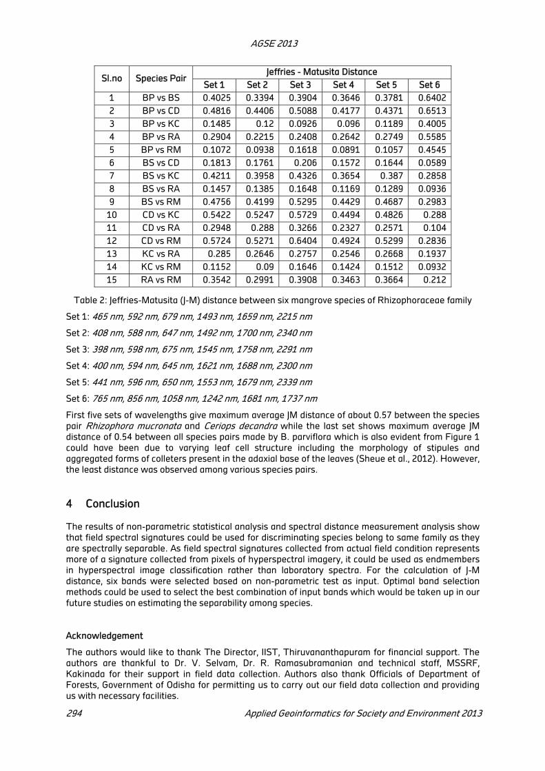
AGSE 2013


Table 2: Jeffries-Matusita (J-M) distance between six mangrove species of Rhizophoraceae family

Set 1: 465 nm, 592 nm, 679 nm, 1493 nm, 1659 nm, 2215 nm






First five sets of wavelengths give maximum average JM distance of about 0.57 between the species

pair Rhizophora mucronata and Ceriops decandra while the last set shows maximum average JM

distance of 0.54 between all species pairs made by B. parviflora which is also evident from Figure 1

could have been due to varying leaf cell structure including the morphology of stipules and

aggregated forms of colleters present in the adaxial base of the leaves (Sheue et al., 2012). However,

the least distance was observed among various species pairs.

4 Conclusion

The results of non-parametric statistical analysis and spectral distance measurement analysis show

that field spectral signatures could be used for discriminating species belong to same family as they

are spectrally separable. As field spectral signatures collected from actual field condition represents

more of a signature collected from pixels of hyperspectral imagery, it could be used as endmembers

in hyperspectral image classification rather than laboratory spectra. For the calculation of J-M

distance, six bands were selected based on non-parametric test as input. Optimal band selection

methods could be used to select the best combination of input bands which would be taken up in our

future studies on estimating the separability among species.

Acknowledgement

The authors would like to thank The Director, IIST, Thiruvananthapuram for financial support. The

authors are thankful to Dr. V. Selvam, Dr. R. Ramasubramanian and technical staff, MSSRF,

Kakinada for their support in field data collection. Authors also thank Officials of Department of

Forests, Government of Odisha for permitting us to carry out our field data collection and providing

us with necessary facilities.

Sl.no Species Pair Jeffries - Matusita Distance

Set 1 Set 2 Set 3 Set 4 Set 5 Set 6

1 BP vs BS 0.4025 0.3394 0.3904 0.3646 0.3781 0.6402

2 BP vs CD 0.4816 0.4406 0.5088 0.4177 0.4371 0.6513

3 BP vs KC 0.1485 0.12 0.0926 0.096 0.1189 0.4005

4 BP vs RA 0.2904 0.2215 0.2408 0.2642 0.2749 0.5585

5 BP vs RM 0.1072 0.0938 0.1618 0.0891 0.1057 0.4545

6 BS vs CD 0.1813 0.1761 0.206 0.1572 0.1644 0.0589

7 BS vs KC 0.4211 0.3958 0.4326 0.3654 0.387 0.2858

8 BS vs RA 0.1457 0.1385 0.1648 0.1169 0.1289 0.0936

9 BS vs RM 0.4756 0.4199 0.5295 0.4429 0.4687 0.2983

10 CD vs KC 0.5422 0.5247 0.5729 0.4494 0.4826 0.288

11 CD vs RA 0.2948 0.288 0.3266 0.2327 0.2571 0.104

12 CD vs RM 0.5724 0.5271 0.6404 0.4924 0.5299 0.2836

13 KC vs RA 0.285 0.2646 0.2757 0.2546 0.2668 0.1937

14 KC vs RM 0.1152 0.09 0.1646 0.1424 0.1512 0.0932

15 RA vs RM 0.3542 0.2991 0.3908 0.3463 0.3664 0.212

AGSE 2013


REFERENCES

ASD., 2010. Analytical Spectral Devices FieldSpec ® 3 User Manual Document 600540 Rev. J.

Beal, D., Eamon, M., 1996. Preliminary Results of Testing and a Proposal for Radiometric Error

Correction Using Dynamic , Parabolic Linear Transformations of “ Stepped ” Data. Analytical

Spectral Devices Inc, Boulder, CO, pp. 1–5.

Blasco, F., Aizpuru, M., 2002. Mangroves along the coastal stretch of the Bay of Bengal: Present

status. Indian journal of marine sciences, 31, pp. 9–20.

Das, AB., Parida, A., Basak, UC., Das, P., 2002. Studies on pigments, proteins and photosynthetic

rates in some mangroves and mangrove associates from Bhitarkanika, Orissa. Marine Biology,

141, pp. 415–422.

Gilman, EL., Ellison, J., Duke, NC., Field, C., 2008. Threats to mangroves from climate change and

adaptation options: A review. Aquatic Botany, 89, pp. 237–250.

Manevski, K., Manakos, I., Petropoulos, GP., Kalaitzidis, C., 2011. Discrimination of common

Mediterranean plant species using field spectroradiometry. International Journal of Applied Earth

Observation and Geoinformation, 13, pp. 922–933.

Panigrahy, S., Kumar, T., Manjunath, KR., 2012. Hyperspectral leaf signature as an added dimension

for species discrimination: case study of four tropical mangroves. Wetlands Ecology and

Management, 20, pp. 101–110.

Rao, NR., Garg, PK., Ghosh, SK., 2007. Development of an agricultural crops spectral library and

classification of crops at cultivator level using hyperspectral data. Precision Agriculture, 8, pp.

173–185.

Ravishankar, T., Navamuniyammal, M., Gnanappazham, L., et al., 2004. Atlas of Mangrove Wetlands

of India: Part 3 - Orissa. pp. 102.

Richards, JA., Jia, X., 2005. Remote Sensing Digital Image Analysis: An Introduction, 4th Edition.

Springer-Verlag, Berlin, pp. 273-274

Schmidt, K., Skidmore, A., 2003. Spectral discrimination of vegetation types in a coastal wetland.

Remote Sensing of Environment, 85, pp. 92–108.

Sheskin, DJ., 2004. Handbook of Parametric and Nonparametric Statistical Procedures.CRC Press,

Boka Raton, pp. 423-432.

Sheue, C., Chen, Y., Yang, Y., 2012. Stipules and colleters of the mangrove Rhizophoraceae:

morphology, structure and comparative significance. Botanical Studies, 53, pp. 243–254.

Song, S., Gong, W., Zhu, B., Huang, X., 2011. Wavelength selection and spectral discrimination for

paddy rice, with laboratory measurements of hyperspectral leaf reflectance. ISPRS Journal of

Photogrammetry and Remote Sensing, 66, pp. 672–682.

Tomlinson, PB., 1994. The Botany of Mangroves, 2nd

Edition, Cambridge University Press,

Cambridge, UK, pp. 317-360

Vaiphasa, C., Ongsomwang, S., Vaiphasa, T., Skidmore, AK., 2005. Tropical mangrove species

discrimination using hyperspectral data: A laboratory study. Estuarine, Coastal and Shelf Science,

65, pp. 371–379.

Zomer, R., Trabucco, A., Ustin, S., 2009. Building spectral libraries for wetlands land cover

classification and hyperspectral remote sensing. Journal of environmental management, 90, pp.

2170–2177.

Health Atlas of India: Study Using Night-Time Satellite Images

Koel Roychowdhurya, Simon Jones

b, *

a Institute of Sustainability and Peace (UNU – ISP), United Nations University, Tokyo, Japan,

E-mail: [email protected]

b School of Mathematical and Geospatial Sciences, RMIT University, Melbourne, Australia

E-Mail: [email protected]

KEY WORDS: Health atlas, night-time lights, DMSP – OLS, modeling, sub-national scale

ABSTRACT

India accounts for 21% of globally reported diseases. More than 6% of the GDP in India is annually lost due to premature deaths and preventable illness. India’s health problems can be better tackled by utilizing disaggregated data to support planning and policy in the health sector. The Annual Health Survey (AHS) (2010 – 13) was conducted in nine Indian states (Bihar, Jharkhand, Uttar Pradesh, Uttarakhand, Madhya Pradesh, Chhattisgarh, Orissa, Rajasthan and Assam) with the highest population growth. Due to logistical and geographic constraints it was conducted on a sample of 20.1 million population from 4.1 million households (by means of household interviews). This paper uses the night-time composite stable light data from the F18 satellite of the DMSP - OLS group of satellites of 2010 to predict health indicators across India. Models are proposed to predict infant mortality rate and natural growth rate, two of the most important health indicators. Data from 138 districts from six states was used to propose models (validated on the 38 districts of five selected states), which were then used to predict metrics for other districts. Results show that the models have an adjusted r

2 = 0.10 to 0.85 for p > 0.05 for the metrics. Maps were produced for these

metrics for the country as a whole. The proposed method has utility in estimating metrics of health at a variety of sub-national spatial levels.

1 Introduction

Since the inception of planning process, health planning has been considered an important

component of socio economic planning in India (Mishra, 2012). Recommendations from several

committees, policy documents and millennium development goals helped in formulating the health

infrastructure of the country. The UN Millennium Summit in 2000 proposed eight goals to be reached

by 2015 (United Nations Development Program, 2000) as a blueprint for better world. These are

known as the Millennium Development Goals (MDGs). These goals include Goal 1: Eradicate extreme

poverty and hunger; Goal 2: Achieve universal primary education; Goal 3: Promote Gender equality

and empower women; Goal 4: Reduce child mortality; Goal 5: Improve maternal health; Goal 6:

Combat HIV/AIDS, malaria and other diseases; Goal 7: Ensure Environmental Sustainability and Goal

8: Develop a global partnership for development (United Nations Development Program, 2000). Of

these, the goals 4 and 5 directly deal with the health sector. The Indian government has asserted its

commitment towards the attainment of these goals (Hazarika, 2012).

In India there is a sample registration system (SRS), which tracks the progress of the country

towards the MDGs. It is designed to collect data on fertility and mortality at the state and national

level (Office of the Registrar General, 2011). Although there has been commendable progress in the

health indicators of India in the last few decades (Hazarika, 2012), there are large regional variations

in these indicators within the country. The southern states have made better progress compared to

the states like Uttar Pradesh, Madhya Pradesh, Bihar, Jharkhand, Chhattisgarh, and Orissa

(Hazarika, 2012). These states share around 50% of the total population, 70% of infant deaths and

62% of maternal deaths of the country (Office of the Registrar General, 2012).

* Corresponding author.

AGSE 2013


In order to use economic development to improve the health of its population, there is a need for

disaggregated data to support planning and policy in the health sector. State level data often mask

out the districts deserving special attention for health care development. As a result, the Registrar

General of India formulated the plan for Annual Health Survey (AHS) in 2005. This was planned to be

conducted between 2010 – 13 in nine selected states of India with the highest rate of population

growth. They include Bihar, Jharkhand, Uttar Pradesh, Uttarakhand, Madhya Pradesh, Chhattisgarh,

Orissa, Rajasthan and Assam. However, this survey was mainly undertaken by means of household

interview across 284 districts by enumerators. Secondly, due to the constraints of the vastness of the

states along with the differences in the socio/economic conditions, it was conducted on a sample of

20.1 million population from 4.1 million households.

This paper uses the data published in the second round of the Annual Health Survey along with

satellite images captured at night to predict the health indicators for all the districts of India.

2 Datasets used

The current study uses satellite images captured at night by DMSP - OLS group of satellites. The

data used in this study was collected in 2010 by F18 satellite. The stable light product of the night-

time images was used in this paper.

The Operational Linescan System onboard the Defense Meteorological Satellite Programme (DMSP-

OLS) group of satellites captures the night time images of the earth. This dataset was widely applied

in different research studies. It was used to estimate the population of the countries of the world (C.

D. Elvidge, Baugh, Kihn, Kroehl, & Davis, 1997; C. D. Elvidge et al., 1997; Imhoff, Lawrence, Stutzer, &

Elvidge, 1997) the first global map of the GDP purchasing Power Parity (GDP-PPP) (Doll, Muller, &

Elvidge, 2000) and Gas flares (C. Elvidge et al., 2009). Radiance calibrated DMSP-OLS data were

used to map urban and suburban extent around cities (K. Roychowdhury, S. D. Jones, & C.

Arrowsmith, 2009; Roychowdhury, Taubenbock, & Jones, 2011). At the smaller spatial scale, DMSP-

OLS dataset was used to estimate population and other socio economic metrics for the state of

Maharashtra in India (Global Adaptation Institute, 2011; K. Roychowdhury, S. Jones, C. Arrowsmith, &

K. Reinke, 2011; K. Roychowdhury, S. Jones, & C. Arrowsmith, 2009; K. Roychowdhury, S. D. Jones, C.

Arrowsmith, & K. Reinke, 2011; Roychowdhury, Jones, Arrowsmith, & Reinke, 2010) and GDP

estimates (Bhandari & Roychowdhury, 2012).

Data from the AHS report (2011 – 12) were used along with the satellite images. The AHS report

include crude birth rate, crude death rate, natural growth rate (NGR), infant mortality rate (IMR),

neo-natal mortality rate, post neo-natal mortality rate, under five mortality rate, Gender ratio at birth,

gender ratio (0 – 4 years), maternal mortality rate and gender ratio of maternal and non-maternal

mortality rates. Out of these maternal and non-maternal mortality rates were available only for

regional subdivisions within a state and not for each district. From the remaining indicators NGR and

IMR were chosen for this study.

3 Study Area

The study was conducted in the states of Assam, Bihar, Jharkhand, Uttarakhand, Chhattisgarh and

Orissa. These states were chosen from the group of nine states on which the Annual Health Survey

(AHS) was conducted (Office of the Registrar General, 2012). These states exhibited moderate

conditions in terms of the health indicators out of the nine states in the AHS. For example Madhya

Pradesh with the highest IMR and Uttar Pradesh with the highest population were not chosen for

this study.

4 Method

Subsets of each of the six states were taken from the satellite image. The average stable light and

the standard deviation of stable lights for each district in the states were calculated from the images.

In the next step a sample of 100 districts were randomly chosen from the total of 138 districts in the

AGSE 2013


six states. The remaining 38 districts were withheld for the validation of the models. Statistical tests

were conducted on NGR and IMR of these districts. These included the plotting of histograms and

calculating skewness and kurtosis. In order to propose a method for preparing health atlas of India,

linear regression model and multiple regression models were calculated using the average and

standard deviation of stable light as independent variables or predictors.

5 Results

The AHS collects only sample data from the districts (Office of the Registrar General, 2012).

However, from the satellite images, the mean and standard deviation of the pixel values are obtained

for the total areas of the districts. In this paper the models are proposed using the sample data from

AHS with the pixel values for the whole area from the images.

The regression models were calculated with and without intercepts. The adjusted r2 of these models

are presented in table 1. The values ranged from 0.20 to 0.85 at 95% confidence interval. Models

with mean stable lights performed slightly better than the models with standard deviation of stable

lights.

Health

Indicators

Mean stable lights

(no intercept)

Standard deviation

stable lights (no

intercept)

Mean stable

lights (intercept)

Standard

deviation stable

lights

(intercept)

IMR 0.82 0.76 0.24 0.10

Natural

Growth Rate

0.78 0.71 0.087 0.10

Table 8: Adjusted r2 values of the models

The r2 values in italics were not significant at 95% confidence interval. It is interesting to note from

the adjusted r2 values that the models with no intercepts perform significantly better than those with

intercepts. However, removing the intercept does not necessarily represent a better model fit (Zar,

2010). This was also proved in the results of validation of the models. The models with intercepts

highly outperformed those without intercepts in predicting the indicators. One of the reasons for this

result was that, the models without intercept used only the pixel values multiplied by the

unstandardized coefficient � of the models. Therefore, areas with high stable lights produced higher

predicted values for IMR and NGR. But, in reality, these areas are urban and more developed parts of

India with comparatively better values for IMR and NGR. Therefore, there were more errors between

the actual and predicted values from these models. On the other hand, the models with the

intercepts used a constant along with the unstandardized coefficient �. This constant impacted the

predicted IMR and NGR from these models. These results from the models with intercepts, although

used the pixel values from the satellite image, corresponded more with the real case scenarios.

The cumulative impact of the independent variables was tested using multiple regression models.

These models were also predicted both with and without intercepts. All models were calculated at

95% confidence interval. The adjusted r2 values of the multiple regression models are shown in table

2.

Health Indicators

Mean and standard

deviation of stable lights

(no intercept)

Mean and standard

deviation of stable lights

(intercept)

IMR 0.83 0.08

Natural Growth

Rate 0.82 0.10

Table 9: Adjusted r2 values of Multiple Regression Models

AGSE 2013


The models were validated over the withheld 38 districts. The predicted values were compared with

the actual health indicators of the respective districts. Percentage residual values were calculated

for each district. The models, which predicted the health indicators with less than 20% error for the

majority of the districts, were chosen. The results of model performance are shown in table 3.

Models Percentage of districts with predicted values

within +/‐ 20% error

IMR (model with mean + no intercept) 29

IMR (model with standard deviation + no 13

IMR (model with mean + intercept) 74

IMR (model with standard deviation + 74

NGR (model with mean + no intercept) 18

NGR (model with standard deviation + no 18

NGR (model with mean + intercept) 53

NGR (model with standard deviation + 53

IMR (model with mean + standard deviation +

no intercept)

13

IMR (model with mean + standard deviation +

intercept)

71

NGR (model with mean + standard deviation +

no intercept)

32

NGR (model with mean + standard deviation +

intercept)

53

Table 10: Performance of the models in predicting health indicators

It was observed from table 3 that all the models performed equally while predicting NGR. So in order

to choose the most suitable model for NGR, the correlation coefficients (r) and the level of

significance (F) values were considered in this case. It was observed that the model with intercept

and standard deviation of stable values had the highest level of significance [f(10.9, 0.001)].

Therefore, this model was chosen for predicting the NGR for all the districts of India. In case of

predicting IMR, although the models using only mean and only standard deviation of stable lights

performed better (74%), the adjusted r2 of these models were not significant at 95% of confidence

interval (table 1). Therefore, the multiple regression model with both mean and standard deviation

was used to predict IMR for other parts of India. The proposed models for the health indicators are

shown in table 4.

Health Indicators Chosen models

IMR 60.681 – 1.915 x “mean stable lights” +

1.740 x “standard deviation stable lights”

Natural Growth Rate 18.085 – 0.318 x “Standard deviation stable

lights”

Table 11: Selected Models

5.1 Application of the model: Health Atlas for the whole of India

The models were applied to propose the health indicators for the whole of India. Indicators were

predicted for all the districts of the country. The predicted maps for IMR and NGR are shown in

figure 1 (A and B).

AGSE 2013


The maps show variation of indicators over the country as a whole. The following patterns are

highlighted in the maps:

IMR of less than 35 is found in the states of Kerala, Tamil Nadu, Pondicherry, Maharashtra, parts of

Gujarat and areas around the National Capital Region.

Most of the country has IMR ranging from 35 – 55.

Rajasthan, Madhya Pradesh, Uttar Pradesh, Bihar, Jharkhand and north eastern states have IMR

more than 55.

NGR of less than 14 are found in patches in states of Kerala, Maharashtra, Dadra and Nagar Haveli,

West Bengal and areas around the National Capital Region.

Most of the country has NGR ranging from 15 - 16.5.

Patches of high NGR are found in the north-eastern states of Arunachal Pradesh, Mizoram, Manipur,

Nagaland and Sikkim and parts of Jammu and Kashmir and Uttaranchal.

One of the major advantages of the models proposed here is that they can be used to predict health

indicators for all the districts of the country without door-to-door questionnaire survey. Although the

predicted values have an error margin of 20%, they give an overall idea and trend of the distribution

of indicators. Also, the indicators can be predicted for every year because of the annual availability of

the satellite image used. These are of immense importance as far as health planning is concerned.

The allocation of the funds for development in the health sector can also be determined using the

trend in the distribution of metrics over the country. Also because of the potential of frequent

mapping, it is possible to record the changes over time. All these will help in planning process and

the achievement of the MDGs in due course.

Another major importance of the models is that, in addition to predicting the metrics at the district

level, they also enable prediction of these indicators at administrative levels smaller than districts

such as taluks and villages. As these indicators are not yet available at such a disaggregated level,

these models can be of immense use.

Figure 18: Predicted Maps of IMR (A) and NGR (B) of India

6 Conclusion

This paper demonstrates that stable light dataset captured by DMSP - OLS satellites are useful in

predicting health indicators. This data can be used as a surrogate to prepare health atlas for sub

national levels. The method proposed in this study helps to overcome a number of problems of

(A) (B

AGSE 2013


conducting manual census as well as the errors associated with MAUP and large acquisition time. In

addition to proposing health indicators for all the districts of the country, the method is also useful to

predict the indicators for small regions such as taluks and villages. Although the results obtained in

the paper contain some error margins, overall it provides an approach for making Health Atlas at

different spatial scales for a vast country like India.

REFERENCES

Bhandari, L., & Roychowdhury, K. (2012). Night Lights and Economic Activity in India: A study using

DMSP-OLS night time images. Paper presented at the Asia Pacific Advanced Network (APAN)

Workshop, New Delhi, India.

Doll, C. N. H., Muller, J. P., & Elvidge, C. D. (2000). Night-time Imagery as a Tool for Global Mapping of

Socioeconomic Parameters and Greenhouse Gas Emissions. AMBIO: A Journal of the Human

Environment, 29(3), 157-162.

Elvidge, C. D. , Baugh, K. E. , Kihn, E. A. , Kroehl, H. W. , & Davis, E. R. . (1997). Mapping city lights

with nighttime data from the DMSP Operational Linescan System. Photogrammetric Engineering

& Remote Sensing, 63(6), 727-734.

Elvidge, C. D., Baugh, K. E., Hobson, V. R., Kihn, E. A., Kroehl, H. W., Davis, E. R., & Cocero, D. (1997).

Satellite inventory of human settlements using nocturnal radiation emissions: a contribution for

the global toolchest. Global Change Biology, 3(5), 387-395.

Elvidge, Christopher, Ziskin, Daniel, Baugh, Kimberly, Tuttle, Benjamin, Ghosh, Tilottama, Pack,

Dee, . . . Zhizhin, Mikhail. (2009). A Fifteen Year Record of Global Natural Gas Flaring Derived from

Satellite Data. Energies, 2(3), 595-622.

Global Adaptation Institute, . (2011). Global Adaptation Index (GaIn): Measuring What Matters:

Building Resilience to Cliate Change and Global Forces.

http://dl.dropboxusercontent.com/u/4234369/gain/GaIn_Paper.pdf

Hazarika, Indrajit. (2012). India at the Crossroads of Millennium Development Goals 4 and 5. Asia-

Pacific Journal of Public Health, 24(3), 450-463.

Imhoff, M. L, Lawrence, W. T., Stutzer, D. C., & Elvidge, C. D. (1997). A technique for using composite

DMSP/OLS "City Lights" satellite data to map urban area. Remote Sensing of Environment, 61(3),

361-370.

Mishra, CP. (2012). Nexus of poverty, energy balance and health. Indian journal of community

medicine: official publication of Indian Association of Preventive & Social Medicine, 37(2), 71.

Office of the Registrar General, . (2011). Maternal and Child Mortality and Total Fertility Rates:

Sample Registration System (SRS). SRS Bulletin. Retrieved 21st November, 2013, from

http://www.censusindia.gov.in/vital_statistics/SRS_Bulletins/MMR_release_070711.pdf

Office of the Registrar General, . (2012). Annual Health Survey (AHS) in 8 EAG states and Assam -

Release of district level factsheet 2010- 11: Ministry of Home Affairs, Government of India.

Roychowdhury, K., Jones, S., Arrowsmith, C, & Reinke, K. (2011). Indian census using satellite

images: Can DMSP-OLS data be used for small administrative regions? . Paper presented at the

Urban Remote Sensing Event, 2011 Joint, Munich.

Roychowdhury, K., Jones, S., & Arrowsmith, C. (2009). Assessing the utility of DMSP/OLS night-time

images for characterizing indian urbanization. Paper presented at the Urban Remote Sensing

Event, 2009 Joint.

Roychowdhury, K., Jones, S. D., Arrowsmith, C., & Reinke, K. (2011). A Comparison of High and Low

Gain DMSP/OLS Satellite Images for the Study of Socio-Economic Metrics. Selected Topics in

Applied Earth Observations and Remote Sensing, IEEE Journal of, 4(1), 35 - 42.

Roychowdhury, K., Jones, S.D., & Arrowsmith, C. (2009, 2009). Mapping Urban Areas of India from

DMSP/OLS Night-time Images. Paper presented at the Surveying & Spatial Sciences Institute

Biennial International Conference, Adelaide, Australia.

AGSE 2013


Roychowdhury, K., Jones, S.J., Arrowsmith, C, & Reinke, K. (2010). Night-time lights and levels of

development: A Study using DMSP-OLS Night-Time Images at the Sub-National Level. Paper

presented at the XXII ISPRS Congress, 25 August – 01 September 2012 Melbourne, Australia.

Roychowdhury, K., Taubenbock, H., & Jones, S. (2011). Delineating urban, suburban and rural areas

using Landsat and DMSP-OLS night-time images Paper presented at the Urban Remote Sensing

Event, 2011 Joint, Munich.

United Nations Development Program, . (2000). The Millenium Development Goals: Eight Goals for

2015. Retrieved 19th November, 2013, from

http://www.undp.org/content/undp/en/home/mdgoverview/

Zar, J. H. (2010). Biostatistical Analysis (5th ed.). Upper Saddle River, New Jersy: Pearson Education

Inc.

Integrating spatial strategy in Development planning for sustainable

resource management

Ajay Kumar Katuri a

, Prasanth C Varughese b,

,

a FoPP, CEPT University, Ahmedabad, Gujarat, India – [email protected]

b FoPP, CEPT University, Ahmedabad, Gujarat, India – [email protected]

KEY WORDS: Development Planning, Framework, Integration, Resource Management, Scales,

Spatial development strategies.

ABSTRACT

Development planning process in the country is largely disaggregated and lacks comprehensive spatial coverage and integration to envision sustainable resource management, trans-scale projects and programmes. The limitations in development planning are largely attributed to the lack of integration and coordination, resource management, envisioning of trans-scale projects, overlap and multiplicity of institutions and lack of reliable data. The strategic spatial planning with integration of relevant sectors in development planning through spatial focus is largely unexplored and primitive in the country except in master plans/ development plans. The centralized development plans/programmes enabling resource allocation and management are largely disconnected with the spatial planning proposals or rather lack the strategic spatial focus. This led to the widening spatial disparity surfacing on our spatial geography. The ideological position for this research revolves around the need for integration and pre-defined or pre-approved spatial framework as a binding regulation to inform decision making for the future development planning practice in our country. The Scholarship aims at exploring the possibilities of integrating spatial development strategies in development planning at different scales/levels for sustainable resource management. The scholarship evolves an abstract spatial framework and concludes that an intricate, manicured and integrated spatial strategy which predefines and allocates the resources holistically and sustainably would lead to a sustainable development. The scales of development planning integrated with spatial strategy could be more effective envisioning state as a fundamental unit of spatial planning and for resource.

1 Introduction

"A region is a subsystem within a larger system (for e.g.: Country, State) and if subsystems develop

greater inter connectivity and coordination; greater will be the efficiency of thesystemToday,

practices in development planning Vis a Vis spatial planning in the country is facing formidable

challenges as a resultant of changing policy frameworks and control, arisig expectations, and

widening economic, social and demographic disparities. Development planning and spatial planning

considered as two parallel processes are following divergent trajectories and the point of

convergence is still ambiguous. The need for an efficient system emphasizing greater

interconnectivity and coordination for development planning has sparked fresh waves in this

direction across the globe. Inter alia, concept of integrated and coordinated planning involving all

sectors becomes significant in all realms. Hence, the concept of strategic planning (Spatial) gained

utmost significance in present day scenario where the scale of economies and projects are seamless.

Strategic spatial planning, (Albrechts, 2004) is a “'transformative and integrative, preferably public

sector led socio-spatial process through which a vision, coherent actions and means for

implementation are produced, that shapes and frame what a place is and what it might become”.

AGSE 2013


2 Spatial geography and planned coverage

Spatial Geography in the country is poised at an interesting and alarming situation. Census 2011

covered 28 States, 7 Union Territories, 640 districts, 5,924 sub-districts, 7,935 Towns and6,40,867

Villages. In Census 2001, thecorresponding figures were 593 Districts,5,463 sub-Districts, 5,161

Towns and6,38,588 Villages. There is an increase of 47Districts, 461 Sub Districts, 2774 Towns

(242Statutory and 2532 Census Towns) and 2279Villages in Census 2011 as compared to Census

2001. From 2001, urban population (Sudhira & Gururaja, 2012) increased from 286.1 million to 377.1

million, which led to the rapid addition of towns in India, from 5161 in 2001 to 7,935 in 2011. These

figures shows the incredible rate at which the transformation happens, five a week for 10 years , an

absolute conversion of 2,774 settlements into towns, irrespective of the definition of 'urban'

(Goswami, 2011)

Albeit the no of cities are increasing, simultaneously it can be seen from the tables that the

percentage of very large villages is increasing. Large villages and medium villages on the verge of

transformation constitute about 41 % of total villages, portrays the changing spatial pattern of the

country which needs planned physical development and resource management with degrees of

integration. The spatial geography implied by the 355 million districts & increasing no of big villages

with majority of rural population (lacking planned physical and resource development) is equally

important to our 7935 urban centres. Indian urbanization during the post-independence period

exhibits dualism in the urban-regional development along with the regional and inter- state

developmental disparities (Sivaramakrishnan, Kundu, & Singh, 2007).

Figure 1: Development planning Instruments in the country

The planning instruments responsible for the planned physical, environmental and socio economic

development portrays an unfinished mosaic of spatial coverage. The planned development in the

country is mainly attributed to the only legitimate master plans for urban areas which also faces

serious implementation issues. Regional development plans rather regional plans / Environmental

plans lack comprehensive spatial coverage and legal binding owing to a host of reasons.

AGSE 2013


2.1 Scales of Planning

The scales of planning is determined mainly by the hierarchy of administrative jurisdictions namely

Country, States, Districts, Taluka, Settlements. The functional scales of planning available in the

country are Country, State, District and settlements. The spatial physical planning is confined largely

to the settlement scales and largely missing or redundant or advisory in higher scales as discussed

above. The levels of planning have got more decentralized after the 73rd & 74th CAA which

advocated more devolution of powers to three tier system of governance The transition from

centralized to decentralized form of governance is still a topic of contention.

3 Need for integration and spatial strategies

The development planning system which envisages balanced resource development in the country

by bridging regional disparities in the form of economic planning are largely aspatial and based on

centralized top-down approach. The spatial planning system which envisages responsibilities for the

physical development of the country is largely concentrated and legitimised in the urban regions of

the country (except some regional attempts like Goa Regional Plan and NCR regional Plan). Master

plans and development plans (Uttarwar, 2010) which were instrumental in spatial planning for a long

time have had a bitter experience of implementation owing to a host of factors like lack of sectoral

coordination, weak data base, financial constraints, lack of resource mobilization, lack of integration

of spatial planning proposals with economic development plan proposals.

The Structural change of Spatial planning as core 'Land-use or Physical planning' to the Integrated

Spatio-Socio-Economic plans (Integrated District Development plans prepared under the provision of

73rd CAA) understood the urgent need for spatial integration. The coverage of development planning

instruments across all scales are discussed as below.

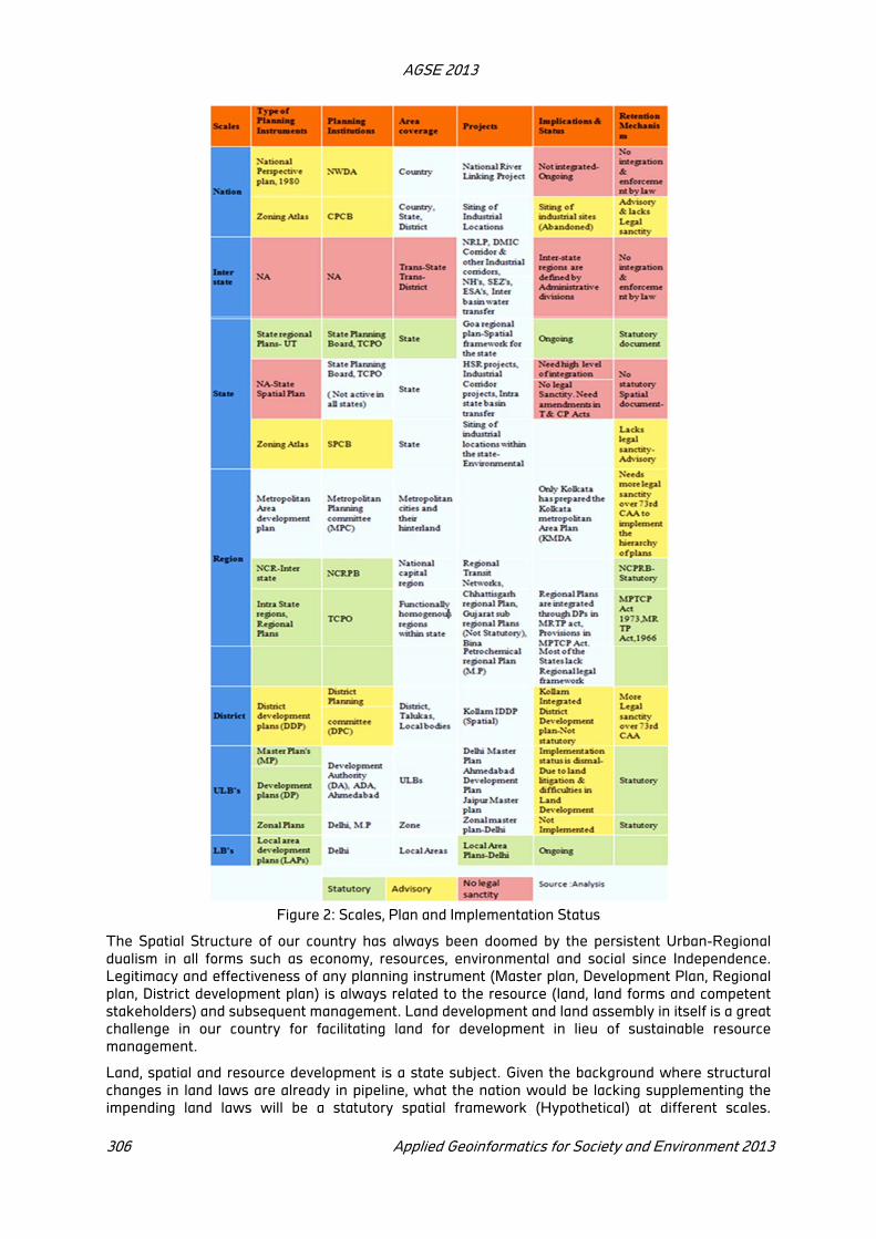
AGSE 2013


Figure 2: Scales, Plan and Implementation Status

The Spatial Structure of our country has always been doomed by the persistent Urban-Regional

dualism in all forms such as economy, resources, environmental and social since Independence.

Legitimacy and effectiveness of any planning instrument (Master plan, Development Plan, Regional

plan, District development plan) is always related to the resource (land, land forms and competent

stakeholders) and subsequent management. Land development and land assembly in itself is a great

challenge in our country for facilitating land for development in lieu of sustainable resource

management.

Land, spatial and resource development is a state subject. Given the background where structural

changes in land laws are already in pipeline, what the nation would be lacking supplementing the

impending land laws will be a statutory spatial framework (Hypothetical) at different scales.

AGSE 2013


Emphasis is added by (Steering Committee on Urban Development and Management, 2011), that

National spatial Strategic Plan and State Spatial development Plans should be made to facilitate

effective spatial planning practice and proposed research on the suitable spatial planning system in

the coming decades.

Lack of integration and guided development through spatial strategies at all scales is a persistent

vacuum in the spatial planning discourse and practice in our country. Although attempts for having

an environmental spatial framework, at an advisory level has been attempted in the case of

preparation of Zoning Atlas for siting of industries by CPCB: technical arm for MoEF, but failed to

gain the traction for enabling guided and integrated development planning with spatial focus

because of lack of integration with other important sectors and legal support.

Spatial framework or Strategies are spatial plans which inform the long term physical development

of any scale (Nation, sub-national, state, district, ULBs, PRIs) through short and medium term

projects and programmes evolved through a participatory bottom up approach. The need for spatial

framework and proper resource management is tested in cases which are beyond the planned

coverage, such as trans-scale projects/ programmes. The case which is relevant spatially and cut

across different spatial scales from the centre to the local levels irrespective of the intent and

stakeholders. The Classic example of a trans- boundary project is DMIC-Delhi Mumbai Industrial

corridor which is initiated by the central government involving 7 states and two union territories.

This mega project is unique and one of its king being initiated at the scale involving transcending

boundaries and multiple responsible authorities in the present day context. The objective of the

paper is to identify the bottlenecks and devise a spatial framework to envisage resource

management in such projects/programmes in our development planning system.

3.1 Envisioning of trans-scale projects and resource management

DMIC Corridor; classical trans-scale project, is a capital investment project of USD 90 billion with the

financial and technical aid from Japan, covering an overall length of 1483 km between the political

capital and the business capital of India i.e. Mumbai and Delhi.

Figure 3: Lack of framework Trans- jurisdictions

Although it’s an earnest attempt to connect two dominant metropolitan centres and create a corridor

of dynamic economic influence and opportunities, the mammoth project is conceived without an

informed spatial logic of resources.

DMIC is a mega infrastructure-industrial towns project envisaged ancillary to the dedicated freight

corridors proposed by the railways as western dedicated freight corridor (WDFC).It involves one sixth

of the size of India and all the scales as we have discussed earlier in the study. The spatial logic

discussed in the project is way behind in addressing host of issues in a holistic manner, including GW

exploitation, environmental compliance and implementation.

AGSE 2013


Figure 4: DMIC Region and Context (DMICDC, 2008)

There are many questions that pop up in envisioning such projects and mainly on the spatial logic of

decisions related to the multiple sectors across the boundaries.

Who will be responsible and guide decisions regarding the alignment of such projects and the

spatial logic of putting up industrial zones/ Investment corridors?

What are the processes involve in such a Trans boundary project from the conception of project

to the starting of implementation on ground?

How complex is the process of land acquisition and land management and the innumerable

departments and clearances in realising the project before implementation?

What will be the spatial development strategies for such projects of dynamic effects across

various sectors, policies and programmes and finally the scales of spatial planning?

3.2 A Mosaic of Disaggregated Sectors

The mammoth project is being planned through environmentally sensitive areas and prime

agricultural lands. This project involves regions under different jurisdictions, planning areas,

hierarchy of settlements, programme areas, water basins, and agro-climatic regions. The DMIC has

skirted the decentralization and participation agenda of the government as per 73 rd CAA and have

definitely aggravated the lack of integration and inclusive development.

For programmes/projects transcending scales which are not under planned spatial coverage, the

development planning process should be informed with spatial development strategies evolved out

from suitable parameters depicting the potential of resources in different regions. The decisions are

made with no technical spatial planning logic or framework and coordination, but arbitrary decisions

based on the existing transportation networks and structure of settlements.

The developmental disparities across the DMIC corridor among the constituent states can be

attributed to the host of reasons discussed before and the multiplicity of stakeholders and overlap of

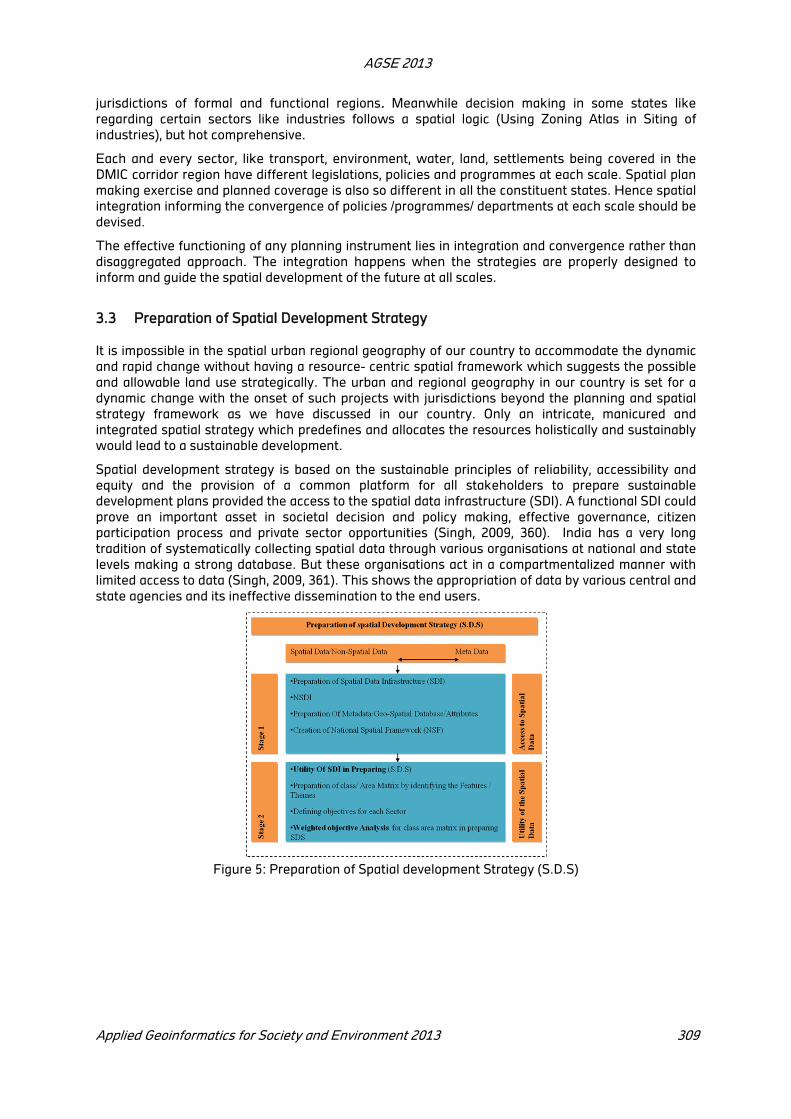
AGSE 2013


jurisdictions of formal and functional regions. Meanwhile decision making in some states like

regarding certain sectors like industries follows a spatial logic (Using Zoning Atlas in Siting of

industries), but hot comprehensive.

Each and every sector, like transport, environment, water, land, settlements being covered in the

DMIC corridor region have different legislations, policies and programmes at each scale. Spatial plan

making exercise and planned coverage is also so different in all the constituent states. Hence spatial

integration informing the convergence of policies /programmes/ departments at each scale should be

devised.

The effective functioning of any planning instrument lies in integration and convergence rather than

disaggregated approach. The integration happens when the strategies are properly designed to

inform and guide the spatial development of the future at all scales.

3.3 Preparation of Spatial Development Strategy

It is impossible in the spatial urban regional geography of our country to accommodate the dynamic

and rapid change without having a resource- centric spatial framework which suggests the possible

and allowable land use strategically. The urban and regional geography in our country is set for a

dynamic change with the onset of such projects with jurisdictions beyond the planning and spatial

strategy framework as we have discussed in our country. Only an intricate, manicured and

integrated spatial strategy which predefines and allocates the resources holistically and sustainably

would lead to a sustainable development.

Spatial development strategy is based on the sustainable principles of reliability, accessibility and

equity and the provision of a common platform for all stakeholders to prepare sustainable

development plans provided the access to the spatial data infrastructure (SDI). A functional SDI could

prove an important asset in societal decision and policy making, effective governance, citizen

participation process and private sector opportunities (Singh, 2009, 360). India has a very long

tradition of systematically collecting spatial data through various organisations at national and state

levels making a strong database. But these organisations act in a compartmentalized manner with

limited access to data (Singh, 2009, 361). This shows the appropriation of data by various central and

state agencies and its ineffective dissemination to the end users.

Figure 5: Preparation of Spatial development Strategy (S.D.S)

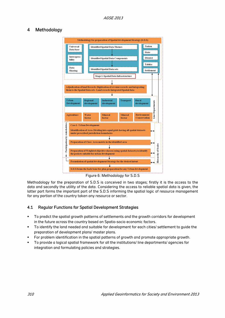
AGSE 2013


4 Methodology

Figure 6: Methodology for S.D.S

Methodology for the preparation of S.D.S is conceived in two stages; firstly it is the access to the

data and secondly the utility of the data. Considering the access to reliable spatial data is given, the

latter part forms the important part of the S.D.S informing the spatial logic of resource management

for any portion of the country taken any resource or sector.

4.1 Regular Functions for Spatial Development Strategies

To predict the spatial growth patterns of settlements and the growth corridors for development

in the future across the country based on Spatio-socio economic factors.

To identify the land needed and suitable for development for each cities/ settlement to guide the

preparation of development plans/ master plans.

For problem identification in the spatial patterns of growth and promote appropriate growth.

To provide a logical spatial framework for all the institutions/ line departments/ agencies for

integration and formulating policies and strategies.

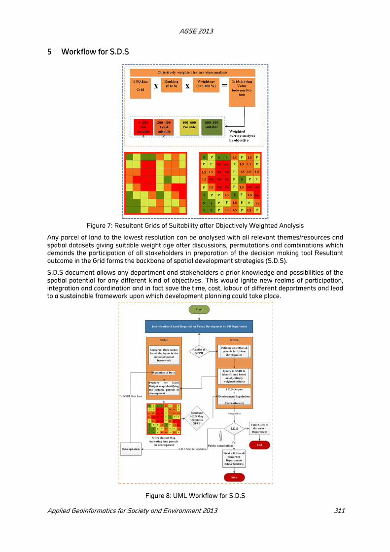
AGSE 2013


5 Workflow for S.D.S

Figure 7: Resultant Grids of Suitability after Objectively Weighted Analysis

Any parcel of land to the lowest resolution can be analysed with all relevant themes/resources and

spatial datasets giving suitable weight age after discussions, permutations and combinations which

demands the participation of all stakeholders in preparation of the decision making tool Resultant

outcome in the Grid forms the backbone of spatial development strategies (S.D.S).

S.D.S document allows any department and stakeholders a prior knowledge and possibilities of the

spatial potential for any different kind of objectives. This would ignite new realms of participation,

integration and coordination and in fact save the time, cost, labour of different departments and lead

to a sustainable framework upon which development planning could take place.

Figure 8: UML Workflow for S.D.S

AGSE 2013


The spatial integration could be achieved with the assistance of spatial development strategies as

devised. Spatial integration can be achieved through integration at all scales top to bottom and

bottom-up. The centralized decentralized system with public consultations and participations at the

stage of spatial strategy preparation give a double edged integration in which stakeholders

involvement is ensured right from the framework preparation stage.

6 Conclusion

State can become the fundamental unit of spatial planning which has the powers for spatial

planning; urban development and natural resources except a few .State can become the dividing line

for having a centralized decentralized approach in development planning with a spatial approach.

Each state should be mandated to have a state spatial planning board (either TCPO or state land use

board or state planning board can be upgraded to serve the purpose) which would prepare state

spatial development plans using the spatial development strategies for resource management as

devised

'Balanced' resource development and management can never be equal but equitable opportunities

available for growth given the availability of precious resources. Balanced development identifies the

need for strategic spatial planning though S.D.S which would inform and expedite future decision

making process where decisions are interdependent, indivisible and irreversible and knowledge of

the future is incomplete

The proposed conceptual spatial planning framework as below prepares the overall hierarchy and

the background for the S.D.S to fit in and inform the decision making process which can lead to

sustainable resource management

Figure 9: Proposed Integrated Spatial Strategy Framework in Development Planning for Sustainable

Resource Management

AGSE 2013


REFERENCES

Albrechts, L. (2004). Strategic (spatial) planning reexamined. Environment and Planning B: Planning

and Design , 31 (5), 743-758.

Department of Town and Country Planning-Local Self Government, K. (2007). Integrated District

Development Plan Local Development PLan. Trivandrum: Department of Town and Country

Planning, Government of Kerala.

DMICDC. (2008). Perspective Plan. Retrieved January 30, 2013, from http://www.dmicdc.com/:

http://www.dmicdc.com/frmDownloads.aspx?pgid=43

Goswami, R. (2011, January 30). 53 million-plus cities vs 355 million-plus districts. Retrieved January

31, 2013, from http://infochangeindia.org/: http://infochangeindia.org/population/analysis/53-

million-plus-cities-vs-355-million-plus-districts.html

Singh, P. K. (2009). Spatial Data Infrastructure in India: Status, Governance Challenges, and

Strategies for Effective Functioning. International Journal of Spatial Data infrastructures Research

, 4, 359-388.

Sivaramakrishnan, K. C., Kundu, A., & Singh, B. N. (2007). Handbook of Urbanisation of India. New

Delhi: Oxford University press.

Steering Committee on Urban Development and Management. (2011). Report of the Working Group

on Urban Strategic Planning-12th Five Year Plan. New Delhi: Ministryof Housing and Urban

Poverty Alleviation, Government of India.

Sudhira, H. S., & Gururaja, K. V. (2012). Population crunch in India: is it urban or still rural? Current

Science , 103 (1), 37-40.

Uttarwar, P. S. (2010). Procedure Based Planning: An Approach for Critical Areas. India Journal 7-12 ,

7 (2), 19-26.

Acknowledgements

This paper is an outcome of the Dual Degree programmer leading to Master of Planning in Urban and

Regional Planning and Masters of Architecture in Urban Design at CEPT University, Ahmedabad.

The author wishes to acknowledge the guidance, support and directions received from Prof Ajay K

Katuri who in his capacity as Assistant professor guided and supported this research. I am obliged to

the assistance received from C. K Koshy I.A.S, Dr N Sridharan, all officials and friends who really

accepted and rendered support during the course of the study.

Management of Land And Water Resources in Henval Watershed Using

Remote Sensing And Gis.

S. Sangita Mishra*

*Department of Civil Engineering, Saraswati College of Engineering, Mumbai University ,Kharghar,

Navi Mumbai-410210, [email protected]

KEY WORDS: Watershed management, Henval watershed, GIS, Remote sensing

ABSTRACT

The socio-economic growth of a country depends primarily on continuing preservation and effective utilization of its natural resources. In India, socio-economic conditions of most of the rural areas are below average level of development. Therefore an attempt has been made to develop and manage watersheds for this purpose applying innovative technologies like remote sensing and GIS for better interpretation. Henval watershed of Tehri-Garhwal district of Uttarakhand, covering an area of 6608 ha (66.08 km

2) and located between 78

0 15’ to 78

0 25’ E longitude and 30

0 20’ to 30

0 30’ N latitude in

India has been chosen as the present study area. The elevation varies from 1200 to 2760 m above mean sea level (MSL). The climate of this region is humid temperate but variations exist which largely depends upon the altitude and geological differences. The average temperature in this area varies from 1200 to 1400 mm of which 70 to 80 percent is received between June to September. The relative humidity at 8.30 hrs varied from 60 to 70 percent in the northern hills and 30 to 40 percent in the south-western dry areas. This study aimed at the development of action plan for land and water resources management mainly based on the land use/ land cover, geomorphology, slope and aspect of the area. From the final output of the themes generated, water harvesting ponds are recommended in the study area to increase the ground water recharge and to control soil erosion.

1 Introduction

Soil and water are the two most vital natural resources that are of crucial importance for survival of

life on biosphere. Efficient management and utilization of these resources are very important to

increase the crop production and productivity per unit area. According to Dr. H.H. Bennet, “Soil

without water is desert and water without soil is useless”. With ever increasing pressure of human

population, there is severe stress on land and water resources. India is basically an agrarian country

with a gross cropped of 177m. ha. out of the total geographical area 328.7m ha. (R.C. Tiwari et al).

Rainfed agriculture is undertaken in more than 60% of the country (National Commission on

Agriculture). After harvesting all the surface and groundwater for irrigation, the irrigated area will

only be around 52% of cropped area in the country. India receives a rainfall of 4000 billion cubic

meters annually, out of which 41% (10, 20,040 lakhs) is lost as evaporation and transpiration, 40% (9,

77,600 lakhs) lost as runoff, 10% (2, 44,400 lakhs) seeps in recharging groundwater. Out of the 40%

stream flow water, 8% is used for irrigation, 2% for domestic use, industries uses 4% and electric

generation is 12%. Hence 50% of the cropped area in the country will always depend on rain, which

is very erratic, unpredictable and distributed over a short period of 3-4 months. With such variations

in rainfall pattern, droughts and floods are recurring features of Indian agriculture.

The population of India is increasing at an annual rate of 1.7 crores and by the year 2050 may cross

150 crores. India will be requiring about 1,2010,000 lakh cubic meters of water in the year 2050 A.D

to cater to the needs of population for food, drinking water, domestic and industrial requirements

due to which there is a great need to conserve the natural resources.

* Corresponding author. Dr. S. Sangita Mishra, SCOE, Mumbai University, email:[email protected]

AGSE 2013


Keeping this in view, the concept of development of land and water resources on watershed basis

gained importance in India since 1974. The watershed approach is increasingly being deployed in

various development programs to manage the land and water resources like soil and water

conservation, dry land or rainfed farming, ravine reclamation, control of shifting cultivation etc.

Management of land and water resources in rainfed areas by integrating remote sensing and GIS is

required for optimum development of land and water resources and to meet the basic minimum

needs of the people in a sustained manner. Keeping this in view, the following objectives are

designed:

1. To study the existing cropping patterns and the available water resources in the Henval

watershed and evaluate the natural resources using Remote sensing data for the extraction of

feasibility condition for its development.

2. To map all the thematic information by interpreting the satellite imageries and SOI top sheets for

production of maps through Geomatica v.9.1.The thematic information includes Land use/Land

cover, hydro-geomorphology, drainage network, slope and aspect.

2 Description of the study area

The study area is located near Chamba-Ranichauri, on Rishikesh-Uttarkashi route, in Tehri Garhwal

district of Uttarakhand. The watershed, drains into Henval river in Tehri Garhwal district of

Uttarakhand, covering an area of 6608 ha (66.08 km2). It is located between 78

0 15’ to 78

0 25’ E

longitude and 300 20’ to 30

0 30’ N latitude. The elevation varies from 1200 to 2760 m above mean sea

level (MSL).

The climate of this region is humid temperate but variations exist which largely depends upon the

altitude and geological differences. The average temperature in this area varies from 1200 to 1400

mm of which 70 to 80 percent is received between June to September. With further increase in

elevation, rainfall tended to decrease. The relative humidity at 8.30 hrs varied from 60 to 70 percent

in the northern hills and 30 to 40 percent in the south-western dry areas.

3 Methodology

The following steps are adopted for the watershed management of Henval watershed.

Preparation of base maps using SOI toposheets. It includes contour, drainage network, village

location and watershed boundary maps.

Preparation of land use/ land cover map using maps using SOI toposheets and satellite imagery

to know the various uses which are carried out on the land.

Preparation of hydro geomorphology maps using SOI toposheets and satellite imagery which is

further used for finding the groundwater prospects and to suggest water harvesting structures

such as percolation tanks and farm ponds.

Preparation of slope and aspect maps which are vital parameters in deciding suitable land use/

land cover.

Depending on the combination of above mentioned resources themes, action plans for

catchment area are generated for the development of the watershed.


4.1 Digital Elevation Model

A DEM is a digital file of terrain elevations for ground positions. It is a raster representing the

elevations of the ground and objects. Besides providing a source of elevation, the DEM may be used

AGSE 2013


for topographic information, flow pattern, flood risk areas identification and to determine

accessibility. With the help of contour layer, digital elevation model (DEM) was prepared (figure 1).

Outlet of the watershed was located at 1200 m above msl and land elevation varied from 1200 m to

2760 m. In mid hills (1200m-1700m), crops like ragi, rainfed rice, wheat, citrus peach, plum, potato

were cultivated in south aspect and in north aspect, ragi, tomato, peach, plum, apricot, apple were

cultivated. In high hills (1700m-2500m) amaranth, ragi, French bean, peas, cabbage, potato, apple,

apricot, pea, walnut are cultivated. In very high hills (>2500m), buckwheat, peas, cabbage, potato,

apple and apricot were practiced.

4.2 Land Use/ Land Cover Map

Different land uses/land covers were digitized with G.I.S. environment by visual interpretation using

digital satellite data of 1 : 25,000 scale for the year 2002, procured from National Remote Sensing

Agency (N.R.S.A.), Hyderabad; and S.O.I. toposheet no. 53 J/7 for the year 1960 with 1 : 50,000 scale.

The satellite imagery was masked with the area of interest (watershed divide). The satellite data of

2002 and toposheet of 1960 were classified into six and three classes, respectively. During field visit,

the image elements were correlated with the ground truthing and the interpretation key was

developed. Spatial distribution of various classes for satellite data is shown in Figure. 2. Satellite

data were classified into agricultural land, chir pine forest, dense forest, dense mixed forest, and

barren land and scrub lands. Dense forest was observed mainly in northern aspects (north, north-

east, north-west) and at higher altitude whereas, major agricultural activities were taken up mainly

in southern aspects (south, south-east, south-west) at the altitude of 1400 -1800 m. Main

composition of dense forest, located in north side of study area, was pine, deodar, and oak whereas,

eastern side was surhi dominated, which was planted by forest department. Out of total area under

study, almost 24 per cent was observed under agriculture followed by dense mixed forest (21.38%),

dense forest (19.56%), chir pine (15.70%), and agro-horticulture (14.67 %). In some cases, the

cultivation had been extended even to steep slope (35-50 %). Mostly old conventional methods of

agriculture were being followed. The area under agriculture was mostly rainfed and irrigation from

perennial resources was limited to only valley areas. The cultivation was being done on well

maintained terraces especially in valleys. The cultivation was being practiced on poorly maintained

terraces on steep slopes also where erosion was the major problem. The main crops grown by the

farmers were wheat, paddy, finger millet (Eleusine coracana), millet-jhangora (Oplismenus frumentaceus). Cash crops were peas, tomato, chilli, beans, etc. The produces obtained from these

fields were not sufficient to provide the grains for the house hold use. The area under dense scrub

land faced severe to very severe erosion.

The study area delineated from the S.O.I. toposheet was also classified into three land use classes

i.e. dense forest, agricultural land and barren land. It was found that the highest percentage of area

was occupied by agriculture followed by dense forest and barren land.

4.3 Temporal Changes in Land use/Land cover

Land use dynamics was studied on the basis of classifications made by visual interpretation, using

digital satellite data for the year 2002, procured from National Remote Sensing Agency (N.R.S.A.),

Hyderabad; S.O.I. toposheet no. 53 J/7 for the year 1960 with 1 : 50,000 scale. Due to limitation with

regards to land use classification, based on toposheet, only three categories were identified

whereas, seven classes were delineated with the help of digital satellite data.

It was observed that agricultural area, over a period of 42 years, had reduced from 43.16 per cent to

23.95 per cent, i.e. it reduced up to 45 per cent. At the same time, 14.72 per cent area was occupied

by agro-horticulture in 2002, which was previously part of agricultural activity. The areal extent of

barren land, in both the cases was almost same, but location of these lands had almost changed. The

barren land had been converted into either dense forest or moderately dense forest by the year

2002. This is due to the plantation made by the forest department. In 1960, forest area was 40.93

percent, it increased up to 56.64 per cent in 2002, including both types of forest i.e. dense and mixed

dense. This scenario arrived due to the regenerative capacity of chir pine and efforts done by the

forest department as well. As far as agriculture is concerned, this scenario is not appreciable as

majority of the forest is dominated by chir pine, which makes the soil acidic and unfit for agriculture.

AGSE 2013


Figure 1: Digital Elevation Model Figure 2: Land use/cover Map

Figure 3: Drainage map Figure 4 Slope map

Figure 5: Aspect map

AGSE 2013


4.4 Drainage

Drainage pattern is characterized by irregular branching of tributaries in many directions with an

angle less than 900. The watershed was divided into six micro- watershed namely. 1. Arakot, 2.

Khuret, 3. Swari, 4. Silogi, 5. Buranskanda and 6.Nager.The drainage pattern is mainly dendritic.

Number of I, II, III, IV and V orders streams were 257, 59, 15, 4 and 1, respectively. The length of

smallest drain of I order was 135.25 m whereas, longest drain was found to be 1287.34 m. The mean

length of I, II, III, IV, V orders streams was 541.38, 574.10, 1393.82, 974.78 and 8781.09m respectively

(figure 3).

4.5 Slope and Aspect

Slope and aspect of a region are vital parameters in deciding suitable land use, as the degree and

direction of the slope decide the land use that it can support. Slope is also very important while

determining the land irrigability and land capability classification and has direct bearing on runoff.

Spatial distribution of different slope classes was prepared using SLP (algorithm for slope) algorithm

of Geomatica v 9.1 and is shown in Figure 4. Slope has been divided into nine classes as per

guidelines of IMSD (1995). Percent areal extent of different slope classes in Henval watershed is

presented in Figure 4. The dominant slope categories in the Henval watershed are moderately steep

slope (46.42 %) and followed by steep sloping (23.87 %). It was also noticed that slope of major area

of agricultural land varied from very gently sloping to moderately sloping whereas forest areas were

mainly located on higher slopes (Moderately steep slope to steep slope). Aspect map was prepared

by using ASP algorithm, which required elevation layer as input. Spatial distribution of various aspect

classes is shown in Fig. 5. It was observed that maximum area (1067.78 ha) falls under south- east

aspect (16.84%) followed by south (15.52%). Amongst all classes north-2 aspect had minimum area

(5.23%).The cumulative areas occupied by north-1, north-east, north-west and north-2 were 37.02%

whereas, south, south-east and south-west had occupied 44.424%. Rest part of the area was

occupied by east (11 %) and west (7.56 %). It was also observed that the aspect had a bearing on the

land use pattern. It was found that north; north-east and north-west aspects had thicker vegetation

than south, south-east and south-west aspects.

4.6 Development Plan for Land and Water Resources of the Study Area

Based upon the study of land use, soils, rainfall, DEM, slope/aspect and runoff, land and water

development plan has been proposed for the study area. Most of the energy needs of villages in hilly

region are met through forests, which led to the gradual depletion of forest canopies ultimately

resulting into moderate dense/degraded forests or scrub land. To care of it following major actions

have been proposed for the study area. Moderate dense forest area, 1413 ha, was dominated by chir

pine. Pine is a gregarious species and grows mainly as pure crop. It can accommodate upto 10 per

cent of associate species. Lyonia ovalifolia and Myrica esculanta may be associated in shade bearing

pockets. Afforestation should be based upon their suitability to the area as well as potential needs of

neighbouring population. Significant area was occupied by barren/rocky out crop (311.97ha). These

lands provide the opportunities for afforestation. These lands are situated aroud1200-1600 m above

mean sea level. Therefore, composition of mixed species of oak and buransh has been

recommended. Agriculture in Himalayan area is not considered economically efficient due to low

agricultural production. Therefore, there is an urgent need to think about shift from pure agriculture

to agro-forestry/agro-horticulture. Around 24 per cent (1483ha) area was occupied by agriculture.

This area provides the opportunities of bund plantation on fodder/fuel and fruit species.

In the Himalayan mountains, “naula” (1-2 m deep, approximately lined wells to get water from

seepage) and "dhara" (springs) are the main sources of water for drinking and household

consumption, because rural water supply is either irregular or unwholesome. The water yield of

natural springs is continuously declining. Springs are either drying up or becoming seasonal and

causing hydrological imbalance in the watershed. Yield of natural springs can be increased by

constructing staggered trenches. Besides this, check dam, spring storage tank and roof-top rain

water harvesting techniques can be employed in order to develop the water resources in the study

area. Preferably check dams, to tap the stream water, can be constructed on second or higher order

AGSE 2013


perennial streams with narrow valley and low bed gradient, to ensure the enough supply of water

during any seasons.To ensure proper utilization of the springs during high discharge and to detain

further discharge diminution multiple storage tanks away from the mouth of the springs are required

to construct. The rainwater which falls on the slanted roof can be harvested to storage tanks. The

collector and delivery system may be outfitted with valves and baffles to sidetrack impure water and

check sediment flow to storage tank.

5 Conclusions

Action plan for land resources development, prepared by overlaying all the thematic maps suggests

various developmental activities like gap filling, afforestation and contour bunding. Various cropping

patterns are suggested based on the soils, existing land use practices, available surface water and

ground water potential, morphology of the area, aspect and slope etc. By adopting suitable soil and

water conservation measures like contour bunding, lands with poor productivity and serious soil

erosion can be brought under fodder, silviculture and social forestry development. These

developmental activities help in reduced soil erosion, increased moisture conservation and improved

productivity of the soil. All the above conclusions aim for optimum development of land and water

resources and to meet the basic minimum needs of people thereby improving their socio-economic

conditions. The information generated from such studies can be applied by decision makers for

sustainable development of any given watershed area.

REFERENCES

Bali, J.S., 1980. Soil and water conservation of agricultural lands. In: National Symposium on Soil and Water Management in 1980’s. Indian Association of Soil and Water Conservation, Dehradun.

Bhati, T.K., Goyal, R.K. and Daulay, H.S. 1997. Development of dry land agriculture on watershed

basis in hot arid tropics of India - A case study. Annals of Arid Zone, 36(2), pp 115-121.

Biswas, J and Agarwal, S. P., 1998. Assessment of pre post treatment scenario of Baramasia micro-

watershed w.r.t. soil loss by using geographical information system. In: International Conference on “Watershed Management and Conservation”, pp 395-401.

Clarke, J.I., 1966. Morphometry from maps. Essays in Geomorphology, Elsevier Publ. Co. New York,

pp. 235-274.

Horton, R. E., 1945. Erosional development of streams and their drainage basins; Hydrological

approach to quantitative morphology. Geological Society of American Bulletin, 56: pp 275-370.

Miller, V. C., 1953. A quantitative geomorphic study of drainage basin characteristics in the clinch

mountain area, Technical report-3, Department of Geology, Columbia University.

Schumm, S. A., 1956. Evolution of drainage systems and slopes in Badlands at Perth Amboy, New

Jersey. Geological Society of America, Bulletin, 67, pp 597-646.

Strahler, A. N., 1957. Quantitative analysis of watershed geomorphology. Transaction of American Geophysical Union, 38, pp 913-920.

Vuppula. P., Asadi, S. S., Pavani S.M. and Anji Reddy M 2004. Remote Sensing Applications For the

Management of Water and Land Resources in Rainfed Area of Prakasam District, Andhra

Pradesh,India.International Society for Environmental information Sciences, 2, pp 885-892.

Benefits of Earth Observation Applicationfor Post- Conflict Nepalese

Society

Toya Nath Baral

Former Director General, Survey Department, Government of Nepal, Present Position: Geo-IT

Professional,

E-Mail: [email protected]

KEY WORDS: Geo-Information, Disaster, Environment, Earth Observation, Socio-economic,

Restructuring, Sustainable Society

ABSTRACT

Advancements in the earth observation technology have contributed to the human life considerably. Technology has proven to be exploited for making human life easier and more secure to a large extent. Space applications for managing unavoidable natural disasters, human induced disasters (during conflict) and societal problems are some of such examples. Earth Observation application, one of the major geo-information system (GIS) components has brought the possibilities of real time mapping of disasters and their in-time management. Application of GIS technology in Nepal was brought into practice during 1970’s. However, it has been realized that institutional infrastructure is yet to be strengthened to accommodate the technological advancements in this sector. Land disputes surrounding ownership and use remain a significant challenge for the country. Pervasive poverty, poor land records and land management systems, lack of awareness regarding land rights, insufficient institutional capacity, dual ownership and a lack of political commitment to resolve the problem are contributing to the issues related to landlessness. Land issues have existed for centuries and are deeply entrenched in the Nepalese society and linked to the structures of feudal land ownership and informal land tenure. Similarly, lack of automation of necessary land related data and a robust land information system, and knowledge on who has what rights to land and property in the districts, as well as the lack of institutional capacities has exacerbated the problem of land rights and access in Nepal.This paper tries to highlight on the state of the art of the Geo-information application in the country, the potential areas for exploiting maximum earth observation benefits for the society, the challenges to establish a robust Land Information System and to cope with its applications and the international co-operation required to enhance the GIS programs of the country. Lack of human resources and necessary infrastructures are the main constraints in Nepal for launching Master Development Plan for Reconstruction (MDPR) programs to uplift the Nepalese society effectively. Regional as well as international cooperation could support the country in these efforts.

1 Introduction

Nepal is a mountainous country located between latitudes 26 22’ N to 30 27’ N and longitudes 80 04’

E to 88 12’ E and lying between China and India. It has an area of 147,181 square kilometers and a

population of 30 million. Nepal has a diverse topography ranging between 58 meters to 8848 meters

above MSL and varied human culture and economic conditions. The diversity in geographical

structure results in diversity in social structures and living style. It is therefore evident that decision

makers need robust information system to understand the complexity of the country. Similarly, the

geological structure in hilly and mountainous area is hazardous. Various types of disasters like

flooding, landslides, epidemics, earthquakes equally affect the Nepalese society. It is vital to come

out of the intuition and the pressure of the interest groups alone as a basis and to bring in efficiency,

economy, effectiveness and rationality in decision-making. Hence the use of a system for the

acquisition, processing and dissemination of geographic information could not be underestimated.

GIS application when utilized to manage disasters and map societal inequities could contribute in

enhancing its effectiveness.

However, the history of modern surveying, mapping in Nepal is not too old. King Jayasthiti Malla

(1354-1395) had introduced a caste Dangol as surveyors, and hence the surveying as a profession

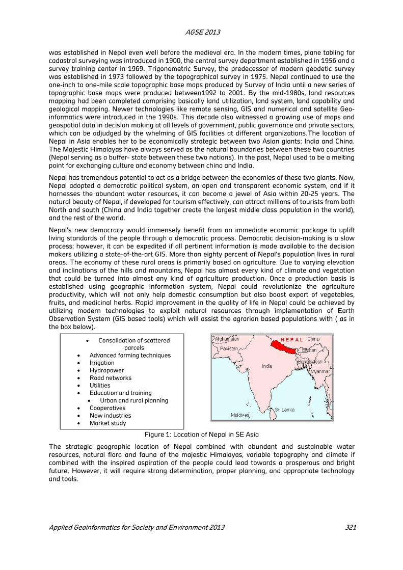
AGSE 2013


was established in Nepal even well before the medieval era. In the modern times, plane tabling for

cadastral surveying was introduced in 1900, the central survey department established in 1956 and a

survey training center in 1969. Trigonometric Survey, the predecessor of modern geodetic survey

was established in 1973 followed by the topographical survey in 1975. Nepal continued to use the

one-inch to one-mile scale topographic base maps produced by Survey of India until a new series of

topographic base maps were produced between1992 to 2001. By the mid-1980s, land resources

mapping had been completed comprising basically land utilization, land system, land capability and

geological mapping. Newer technologies like remote sensing, GIS and numerical and satellite Geo-

informatics were introduced in the 1990s. This decade also witnessed a growing use of maps and

geospatial data in decision making at all levels of government, public governance and private sectors,

which can be adjudged by the whelming of GIS facilities at different organizations.The location of

Nepal in Asia enables her to be economically strategic between two Asian giants: India and China.

The Majestic Himalayas have always served as the natural boundaries between these two countries

(Nepal serving as a buffer- state between these two nations). In the past, Nepal used to be a melting

point for exchanging culture and economy between china and India.

Nepal has tremendous potential to act as a bridge between the economies of these two giants. Now,

Nepal adopted a democratic political system, an open and transparent economic system, and if it

harnesses the abundant water resources, it can become a jewel of Asia within 20-25 years. The

natural beauty of Nepal, if developed for tourism effectively, can attract millions of tourists from both

North and south (China and India together create the largest middle class population in the world),

and the rest of the world.

Nepal’s new democracy would immensely benefit from an immediate economic package to uplift

living standards of the people through a democratic process. Democratic decision-making is a slow

process; however, it can be expedited if all pertinent information is made available to the decision

makers utilizing a state-of-the-art GIS. More than eighty percent of Nepal’s population lives in rural

areas. The economy of these rural areas is primarily based on agriculture. Due to varying elevation

and inclinations of the hills and mountains, Nepal has almost every kind of climate and vegetation

that could be turned into almost any kind of agriculture production. Once a production basis is

established using geographic information system, Nepal could revolutionize the agriculture

productivity, which will not only help domestic consumption but also boost export of vegetables,

fruits, and medicinal herbs. Rapid improvement in the quality of life in Nepal could be achieved by

utilizing modern technologies to exploit natural resources through implementation of Earth

Observation System (GIS based tools) which will assist the agrarian based populations with ( as in

the box below).

Figure 1: Location of Nepal in SE Asia

The strategic geographic location of Nepal combined with abundant and sustainable water

resources, natural flora and fauna of the majestic Himalayas, variable topography and climate if

combined with the inspired aspiration of the people could lead towards a prosperous and bright

future. However, it will require strong determination, proper planning, and appropriate technology

and tools.

Consolidation of scattered

parcels

Advanced farming techniques

Irrigation

Hydropower

Road networks

Utilities

Education and training

Urban and rural planning

Cooperatives

New industries

Market study

AGSE 2013


2 State of the Art of Geoinformation Application in Nepal

2.1 Geodetic Control Network

Geodetic control points serve as backbone for all GIS data captures. The geodetic control points are

used to transform information into a defined reference system and to check the accuracy of the GIS

products.

2.2 Status of Geodetic Network

ÊÚ

ÊÚÊÚÊÚ

ÊÚÊÚ

ÊÚ

ÊÚ

ÊÚÊÚ

ÊÚ ÊÚ

ÊÚÊÚ

ÊÚ

ÊÚ ÊÚÊÚ

ÊÚÊÚÊÚ

ÊÚ ÊÚ

ÊÚÊÚÊÚÊÚÊÚ

ÊÚ ÊÚÊÚÊÚ

ÊÚ ÊÚÊÚÊÚÊÚ

ÊÚÊÚÊÚ ÊÚÊÚ

ÊÚ

ÊÚ

ÊÚ

ÊÚ

ÊÚ

ÊÚÊÚÊÚ

ÊÚ

ÊÚ

ÊÚÊÚÊÚ

ÊÚ ÊÚ

ÊÚ

ÊÚÊÚ

ÊÚÊÚÊÚ

ÊÚ

ÊÚÊÚÊÚÊÚ

ÊÚÊÚÊÚ ÊÚ ÊÚÊÚ

ÊÚ ÊÚÊÚ

ÊÚÊÚÊÚ

ÊÚÊÚÊÚÊÚÊÚÊÚÊÚÊÚ

ÊÚÊÚÊÚÊÚÊÚ ÊÚ

ÊÚÊÚÊÚ

ÊÚÊÚÊÚ

ÊÚÊÚÊÚ

ÊÚÊÚÊÚÊÚ

ÊÚÊÚ

ÊÚ ÊÚ

ÊÚ

ÊÚÊÚ

ÊÚ

ÊÚ

ÊÚÊÚ

ÊÚ

ÊÚÊÚ

ÊÚÊÚÊÚÊÚ

ÊÚÊÚÊÚÊÚ

ÊÚÊÚ ÊÚ

ÊÚ ÊÚÊÚÊÚÊÚ

ÊÚÊÚÊÚÊÚ

ÊÚÊÚÊÚ

ÊÚÊÚÊÚ

ÊÚ

ÊÚÊÚÊÚ

ÊÚÊÚ

ÊÚ ÊÚ ÊÚ ÊÚ ÊÚ ÊÚ ÊÚÊÚÊÚÊÚ ÊÚ

ÊÚÊÚ

ÊÚÊÚÊÚÊÚ

ÊÚ

ÊÚ

ÊÚÊÚ

ÊÚ

ÊÚÊÚÊÚÊÚÊÚ

ÊÚÊÚÊÚ

ÊÚÊÚ

ÊÚÊÚÊÚ

ÊÚÊÚÊÚ

ÊÚÊÚÊÚ

ÊÚÊÚÊÚ

ÊÚÊÚÊÚ

ÊÚ

ÊÚ

Mah

akal

i Ri v

er

DOLPA

HUMLA

MUGU

DANG

KAILALI

DOTI

GORKHA

RUKUM

JUMLA

BAJHANG

ILAM

MUSTANG

KASKI

TAPLEJUNG

BANKE

BAJURA

ROLPABARDIA

SINDHULI

SURKHETMANANG

JHAPA

MYANGDI

SALYAN

SOLUKHUMBU

CHITWAN

DOLAKHA

BARA

PALPA

JAJARKOT

DARCHULA

BHAKTAPUR

PARSA

MORANG

DHADING

KALIKOT

BAITADI

ACHHAM

SANKHUWASABHA

GULMI

TANAHU

UDAYAPUR

BAGLUNG

DAILEKH

RASUWA

LAMJUNG

MAKAWANPUR

KHOTANG

SIRAHA

SAPTARI

BHOJPUR

NAWALPARASI

SARLAHI

SUNSARI

KAPILBASTU

PYUTHAN

SINDHUPALCHOWK

SYANGJA

RAMECHHAP

KANCHANPUR

NUWAKOT

RUPANDEHI

DADELDHURA

DHANUSHARAUTAHAT

PANCHTHAR

MAHOTTARI

DHANKUTA

ARGHAKHANCHI

OKHALDHUNGA

PARBAT

TEHRATHUM

LALITPUR

KATHMANDU

ÊÚ

2.3 Maps and Geo-information Prepared and Published

National Topographical Database (NTDB) of the country (1:25,000 and 1:50,000 scale)

Different types of administrative maps (District, regional, zonal, wall maps and school atlas) Large scale topographic database and digital ortho-photos (populated areas and municipalities) Land use maps and related documents of the country (selected areas),( Land utilization, Land

capability, Land system, Geological & Climate) Aerial photography, derived topographic maps and Socio economic atlas

International boundary information system

Number of sheets 563Map Scale 1:25 000

Number of sheets 119Map Scale 1:50 000

FUNDAMENTAL DIGITAL TOPOGRAPHICAL DATABASE AVAILABLE AT SURVEY DEPARTMENT

11/11/2013 Country report - Nepal : T.N.Baral, DG, DOSM 18

LEGEND

Both scales1 : 10 000 orthophoto mapping area

1 : 5 000 orthophoto mapping area

Orthophoto Map Index

National Geographic InformationInfrastructure Programme, NGIIP

NEPAL

Figure 2: National Topographic Database Figure 3: Ortho-photo Map Index

3 Cadastral Information

Nepal’s land records are captured and managed largely in the traditional manner. Whether spatial or

attribute, information is acquired, updated, collated and retrieved manually in rudimentary fashion

with a low level of precision and high risk of distortion. Consequently land records are not always

reliable, land disputes are fairly common and land registries are overwhelmed with associated

problems.

Land administrative services are costly for the government and also for the Nepalese people.

However rarely are the people satisfied with the quality of such services. Furthermore, man-to-land

Laplace points

7

Doppler points 16

First order 68

Second order 653

Cadastral Sheets :

20382

Lower order control : 47

District

Gravity :- Absolute : 9

Station

AGSE 2013


relation has changed over time and consequently, there are new demands on land administration

and management authorities from the society. Therefore, modernization on the land related services

have become imperative for the sustained existence of these authorities. Nepal already started

implementing digital cadastre as a geospatial solution to the above problem. Both the attribute and

spatial data acquisition and management are in digital mode that satisfies the present demand of the

people.

Orthophoto Over Cadastral Map

Database - Cadastral Map

Attribute information of selected parcel

(a) (b) (c)

Figure 4(a): Ortho-photo over Cadastral Layer, (b) Cadastral Database, (c) Attribute information of

selected Parcel

3.1 Land Reform and Management

District and Village level land use data acquisition is in process and final product is land use and land

use zoning database, Land capability, Geology and soil study report of each district and village level

separately. Remote sensing and GIS tools are being used to prepare land use database. Land

consolidation program is launched to solve the fragmentation of land parcels and dual ownership

causing degradation in agricultural products. The issues of bonded labors, landless people, squatters

and informal settlements will be solved phase wise under land reform and management scheme

using GI tools. National land use policy has already been published.

3.2 Major Factors Affecting the Nepalese Society

Various elements have affected the socio-economic development of Nepal. During the past decade

of conflict, development activities were stalled. Since the conflicts were rooted around the rural

areas, the situation became more unfavorable for timely affirmative change in development sector.

Education of school age children were greatly affected, the effect of which could be seen in future.

Major part of the country remained almost in isolation from the access of government during those

days. If the condition is to be considered normal, following major factors have largely affected the

socio-economic development of Nepal.

3.3 Cultural and Social Discrimination

Nepalese society is largely affected by its caste system. People from so-called upper castes have

domination over the social and cultural structure. Such groups of people are largely privileged from

the national benefits whereas certain groups covering majority of national population are

disadvantaged from the national benefits. This situation has caused dissimilarities in life standards

among the people from Nepalese societies obstructing the timely development of socio-economic

standard in equitable way.

3.4 Inequitable Distribution of Land

Land is the major asset in Nepalese economy. More than 80% of Nepalese people are engaged with

agriculture. The sector covers around 40% of national gross domestic product (G.D.P.). Majority of

the population residing in rural areas have negligible access to national infrastructure and most of

them with land. Majority of the national population living in urban areas and its outskirts also have

AGSE 2013


limited access to land. Major part of national population is engaged with agriculture but has lesser

access to land. Widespread informal settlements exist at various parts of the country without

secured tenure. Various vulnerable groups, commonly known as Mukta kamaiya (bonded labors),

Sukumbasi (landless people), Haliya (land labors used for tilling the field) are the larger community

without access to land. Further women's access to land is negligible. Experiences have shown that

these situations of inequitable access to land or unjustifiable distribution of land nourished the

conflict in a greater extent.

3.5 Difficult Geographical Terrain

Nepal has diverse and difficult geographic terrain. The elevation ranges from 58 meter to 8848 meter

from Mean Sea Level. Only about 17 % of land is plain. Rest part of the country is either hilly or

mountainous. It is difficult to develop physical infrastructures of basic civilian need to these areas.

National highway connects only a small area and Terai region. Rest part of the nation is devoid of

transport and road access. Most of the parts have neither easier access to the drinking water

sources nor supply of water for drinking purpose. Irrigation facilities are rarely available. Similar is

the case for other kinds of infrastructures. The difficult terrain structure has obstructed the

expansion of the development infrastructures that needs lots of investment and resources.

3.6 Natural Disaster

Nepalese society is largely affected by various kinds of natural disasters. Flood, landslides, out

bursting of glacial lakes, earthquakes, epidemics, etc. are the major types of natural disasters that

are affecting Nepalese society to great extent. Fragile geological formation, steep topography and

high intensity rainfall make Nepal’s ecosystem very delicate. Frequent water induced disasters occur

in Nepal especially during rainy season. Sometimes huge disasters occur and emergency resources

allocation is required. Requirement of resources in this sector is very high. Government of Nepal has

given high priority to this sector. About 75 % of annual downpour of Nepal occurs over a period of

three to four month, causing a loss of huge amounts of agricultural land and casualties. There are

about 12, 000 landslides each year, 13 % of total area of churia and mid-hilly region suffers from the

effect of landslides. At least 44 glacial lakes in the Himalayas are at risk of outburst. Each year lives

are frequently lost due to various types of epidemics. In July 1993, Nepal experienced the worst

recorded flood in its history, which came within just two days of torrential rainfall in central Nepal.

More than 1300 lives were lost and over millions of property and infrastructure destroyed. Soil

erosion is the other disaster that damages development infrastructure of the country. Similarly, the

country is largely affected by rapid deforestation. For Nepal, its forest degradation has led to

stagnant economic growth and extensive exploitation of this valuable natural resource. Population

growth and urbanization has deepened the deforestation problem.

4 Expectation of Nepalese People in Post-Conflict Nepal

After the reinstatement of the peace in the country, Nepalese people have high expectation for

everlasting peace and security to be prevailed in the country through restructuring, reconstruction

and rehabilitation in equal priority. Rapid growth in the socio-economic condition, equitable access to

national benefits, minimal losses from natural as well as human induced disasters and good

governance are some other expectations of the Nepalese people in post-conflict Nepal.

Sustainability is most challenging issue in Nepal. People by now expect sustainable development

and prosperous Nepal.

5 Role of Earth Observation Data

Earth observation refers to the collection, processing, modeling, and dissemination of data about the

Earth system. These data are collected through in situ, airborne and space-based observations,

using satellites, aircrafts, and other devices. They then can be processed into forecasts, maps, and

AGSE 2013


other decision support tools, providing valuable and often life-saving information to end users. Earth

observation data enables to make evidence-based policy decisions, to facilitate the formulation of

need based plans and to take precautionary initiatives. For the better predictions of natural

disasters, epidemics, the impact of energy choices, or variations in the climate that affect the

sustainability of infrastructures, earth observation data play significant role. In the context of

reconstruction of post-conflict Nepal, the earth observation data could be optimally used as

fundamental tool for the infrastructure and land development activity to make it sustainable.

Following are the organizations that produce GI data in larger scale in Nepal

5.1 National Survey and Mapping Agency

Survey Department, the National Mapping Organization of Nepal, has the responsibility to produce

and disseminate geodetic, cadastral, topographic data of nationwide coverage. Further, it has the

responsibility of regulating the surveying and mapping activities in the country. Global Positioning

System (GPS) is in use for establishing control points in the country these days. Various kinds of

geodetic data are ready for dissemination. In situ observations are carried out for acquiring cadastral

data. National Topographic Map series has been prepared from aerial photographs. Using satellite-

based information has commenced the update of the map series. Various kinds of Land Resources

maps, thematic maps, and administrative maps are prepared out of these data. Initiatives for

National Spatial Data Infrastructure (NSDI) are under progress since few years back.

5.1.1 Land Use Project, Ministry of Land Reform and Management

The project was established in 2001 to produce land use plans for each Village Development

Committees / Municipalities throughout the country. With limited resources, the project is working

for as per its mandate with slow pace. Topographic database, Airborne and satellite data are used

for the purpose of the project.

5.1.2. Department of Mines and Geology

Department of Mines and Geology is using airborne and satellite data for geological mapping. In situ

observations are also performed to collect geological data and data for mineral exploration.

5.1.3 Department of Forest

Department of Forest use airborne satellite data to produce maps for forest type classification, land

use / land cover classifications, change detection and forest cadastral boundary demarcation.

5.1.4 Department of Water Induced Disaster Prevention

Department of Water Induced Disaster Prevention is involved in the creation of river database and

hazard map preparation for flood affected areas and area affected by glacier lakes outburst.

5.2 Ministry of Agriculture and Cooperatives

Ministry of Agriculture and Cooperatives is mainly involved in agriculture resource management

using remote sensing technologies and Geographical Information System (GIS) applications.

5.2.1 Department of Hydrology and Meteorology

Department of Hydrology and Meteorology is responsible for weather forecast and prediction in the

country. The weather forecast and prediction is made after analyzing the satellite data downloaded

through the Internet service facility and the old database available at the department.

5.2.2 Metropolitan Cities / Municipalities for Land Resource Maps

Some of the Metropolitan cities and Municipalities have prepared land resources maps of their

territory using remote sensing images and topographic database prepared by Survey Department.

AGSE 2013


5.2.3 International Center for Integrated Mountaineering Development (ICIMOD)

ICIMOD has a mandate to establish and promote a decentralized network of partner institutions in

the Hindu Kush - Himalayan region ultimately for the sustainable mountain development. It is one of

the organizations using remote sensing image data in a larger scale.

6 Constraints in Using Gi Data

Various organizations are involved in producing earth observation data. However, it has been

experienced that the data have not been used optimally for the benefit of the society. Duplication of

resources and efforts are the mostly seen practices in the country. Some of the major drawback that

resist in making best use of GI data for the benefit of Nepalese society are as follows:

No efficient system of providing timely GI data and information for policy makers.

Imperfect mechanism for data and information sharing among stakeholders.

Lack of interoperability and compatibility of geospatial data and information.

Lack of professional education, training, and research activities.

Lack of awareness among the users, decision makers, policy makers, planners about the role of

GI data for societal benefits.

7 Earth Observation Data for Restructuring Post-Conflict Nepal

Various organizations are involved in producing earth observation data in the country. Due to various

problems as mentioned in article 7, those data are not optimally used for the development activities.

A mechanism of integrated observation through efficient data and information sharing system with

effective NSDI could be expected for optimal use of earth observation data produced from various

organizations for the sustainable development in Post-conflict Nepal. A strong networking and

awareness among the stakeholders is most essentials to work in this line.

8 Efforts for Optimizing Earth Observation Data for the Nepalese Society

National Mapping Organization of Nepal feels its leading responsibility in the field of earth

observation to amplify the awareness on the role that earth observation data can play in the

development of the country and diversify the products as per the need of the country. With its

limited resources, the department has taken various initiatives to establish an effective platform for

making optimal use of earth observation data produced from various organizations in the country.

Following are the some major initiatives of them:

NSDI initiatives have been taken through National Geographic Information Infrastructure

Program.

The overall objective of the initiatives is "To strengthen planning and resource management

through the availability of geographical information necessary for decision making"

Consultative meetings, workshop and seminars are organized time to time to enhance

awareness about the role and application of earth observation data within the professional

community.

A radio program "Hamro Jamin, Hamro Napi" is broadcasted fortnightly in Radio Nepal to

enhance awareness among general public.

Participation in the activities of international professional organizations to introduce newer

concept and technologies in the field of GI in Nepal.

Survey Department is in the position to take leading responsibility to establish a platform for

integrated earth observation and provide geo-information data needed for the reconstruction of the

country in the present context. However, some limitations such as lack of necessary infrastructure

and adequately educated human resources obstruct its endeavor. Thus the Survey Department

expects support from external agencies in its endeavors. International professional organizations

can support in capacity building of the department by providing opportunities to participate in their

AGSE 2013


activities. International academic institutions can support by providing opportunities of higher

studies and donor agencies can support in establishing necessary infrastructure in the department.

Further, the department feels its responsibility to actively support the implementation of GEOSS 10-

Year Implementation plan. Hence capacity building and infrastructure development is a must for the

department.

9 Societal Relevance

Earth observation data has very high degree of societal relevance. Efficient and transparent land

administration is one of the major components of good governance. It stimulates the land market

and contributes to reduce poverty. Efficient geo-information management is the basis of sustainable

use of natural resources.

10 Benefit of Earth Observation System

10.1 Earth Observation data support:

Effective decision making

Efficient management of natural resources in a sustainable manner

Contributes in implementing good governance

As a tool for sustainable development

Improving the quality of service delivery

Providing necessary Geo-information for successful implementation of Land Reform and

Management

Developing an infrastructure for reconstruction and rehabilitation in Post Conflict situation like

in Nepal

Better conflict management specially in land disputes

Make land market more vibrant and establish robust land information system

11 Conclusion

The agenda of the post conflict Nepal is restructuring, reconstruction and rehabilitation. Sustainable

development is one of the major expectations of Nepalese people at present. In the context of

reconstruction of post-conflict Nepal, the earth observation data could be optimally used as

fundamental tool for the development activities to make it sustainable. Various organizations are

involved in producing GI data in Nepal. Due to various problems those data are not optimally used for

the benefit of the society especially for the development activities. Integrated earth observation data

is required for sustainable development. Survey Department is making its best possible efforts to

provide an effective platform (NSDI) for providing GI data for sustainable development. Fragile

geological formation, steep topography and high intensity rainfall make Nepal’s ecosystem very

delicate. Frequent water induced disasters occur in Nepal especially during rainy season. Sometimes

huge disasters occur and emergency resources allocation is required. Requirement of resources in

this sector is very high. Prevention from disasters is very important for the improvement of living

condition of Nepali people in a sustainable manner. Most of the people affected by water induced

disasters are the poor and marginalized people. So, for poverty alleviation and sustainable

development in the country due priority should be given for mitigation of the water induced

disasters. Recognizing the importance of addressing land issues in Nepal for sustainable peace the

CPA, IOM, UNDP and UN-Habitat, as participating UN organizations (PUNOs), have come together

with their technical expertise to address the highly sensitive land issues with impartiality and

neutrality. All these organizations use earth observation data in different layers for their research

work on land issues and infrastructure development in Nepal. All GIS players of Nepal will finally

come together to establish a platform to make their GIS data interoperable.

AGSE 2013


REFERENCES

Geo-information for Sustainable Development in Nepal : Baral, T.N. Director General, Survey

Department, Government of Nepal; Presented on ‘ GEOSS-AP, Jan 2007 Japan’

Water Induced Disaster and Mitigation in Nepal : Regmi, S.B. Executive Director, Water Energy

Commission, Nepal.

Land Reform and National Development in Nepal; Professor Wen Tiejun (Beijing), Dr. Lau Kinchi

(Hongkong)

Bhattarai, S., 2005; The Role of Spatial Database in Formulating National Preparedness Plan to

address Natural Disaster in Nepal: Paper Presented on 'Seminar on Mapping the world: Today,

Tomorrow and Future for Planning as well as Decision Making Process', Nepal GIS Society, July 22,

2005, Kathmandu Nepal

Gautam, K.C., 2006: Reconstruction of Post Conflict Nepal

Bhatta, G.P., 2006: Improving Geo-information Management System for Effective Land

Administration in Post Conflict Nepal. A research proposal (unpublished)

Baral, T. N : Maximizing benefit of comprehensive GIS for Nepalese society: Paper presented on

‘AGSE 2009, Stuttgart university of Applied Sciences’, Stuttgart.

Accessed from GEO Website (GEOSS 10-Year Implementation Plan).

Oli, P.P., October 2001, Spatial Data for Land Use Planning in Nepal. The paper presented in the

International Conference on Spatial Information for Sustainable Development, in October 2001 in

Nairobi, Kenya

Prospects for Land Reform in Nepal: Comparative Studies of South Asia. Africa and the Middle East

Spring/Fall 1993 13 (1 and 2)

Global Positioning System, Remote Sensing and GIS in Survey Department of Nepal: GIS talk

Program, 2003 organized by NAAN : Baral, T.N. Deputy Director General, Survey Department,

Nepal.

Sharma, R.K., 2006, Nepal, State of the Art in the Applications of Space Technology

National Convention on Land Rights and Social Justice: Land Reform Myths or Reality Updates on

land reform in Nepal June 12, 2013 by ILC Asia

Mahara, S.P. and Pradhanang, T.B., 2006, Facts and figures of Nepal for GEOSS, Bonn, Germany 28-

29 Nov. 2006

Evaluation of Annual Soil Erosion of Panshet Watershed aSandhyarani Sahoo,

bR N Sankhua*

cM.P. Punia

aBanasthali, University, E-mail: [email protected]

bNational Water Academy, Pune, E-mail: [email protected]

c Birla Institute of Technology,JaypurE-email:[email protected]

KEY WORDS: Estimation, GIS, Loss, Soil, USLE, Watershed

ABSTRACT

The soil erosion and hydrologic response model of Khadakwasla watershed was envisaged for the study using Revised Universal Soil Loss Equation (RUSLE) erosion model. Erosion calculation requires huge amount of information and data, usually coming from different sources and available in different formats and scales. Therefore GIS was used, which helped considerably in organizing the spatial data representing the effects of each factor affecting soil erosion. The factors that most influence soil erosion are linked to topography, vegetation type, soil properties and land use/cover. Average annual soil losses were calculated by multiplying five factors: R; the erosivity factor, K; the soil erodibility factor; LS, the topographic factor; C, the crop management factor and P; the conservation support practice. The annual soil loss predictions 35 tons/ha/year for the watershed.

1 Introduction

Accelerated soil erosion is a worldwide problem because of its economic and environmental impacts.

The soil erosion of Khadakwasla watershed is envisaged for the study using Revised Universal Soil

Loss Equation (RUSLE) erosion model. Erosion calculation required huge amount of information and

data, collected from IMD and available in different formats and transformed, organized in GIS

environment representing the effects of each factor affecting soil erosion. Soil erosion is defined as

the physical degradation of the landscape over time. The process is initiated when soil particles are

detached from its original configuration by erosive forces such as rainfall. The soil particles may then

be transported by overland flow into nearby rivers. The factors that most influence soil erosion are

linked to topography, vegetation type, soil properties and land use/cover. Average annual soil losses

were calculated by multiplying five factors: R; the rain erosivity factor, K; the soil erodibility factor; LS,

the topographic factor; C, the crop management factor and P; the conservation support practice.

A method was developed in this study, which combines the (RUSLE) with the ArcGIS. The RUSLE

calculated long-term average annual soil loss by multiplying six specific factors which describe the

watershed characteristics such as rainfall, soil types, slope, and vegetation cover. The GIS is used to

store the RUSLE factors as individual digital layers and multiplied together to create a soil erosion

potential map. This combination provides a way to assess soil erosion potential of an area with

existing data sources. A digital elevation model (DEM) is used to calculate the slope steepness and

slope length factors. Landsat satellite imagery of July, 2010 is used to determine the extent of

vegetation cover and conservation practices.

1.1 Objectives

Using the rainfall, Digital Elevation Model (DEM), soil type map, and land cover map, build the soil

erosion risk map and the soil loss rates on the watershed for the following two cases

Annual average soil loss rates using RUSLE in GIS

Analyze the spatial distribution of soil erosion in the Panshet watershed.

AGSE 2013


2 The Study Area

The study area was taken as panshet watershed as depicted in the Figure 1.1. The study area is

located near Pune city, in the state of Maharashtra, India. It lies at the outskirts of Pune city towards

West direction The average rainfall is 722mm. Panshet is the source of drinking water for Pune

city.The temperature ranges from 150 C to 35

0C. The best time to visit is October-March. The Winter

Period is between Mid Nov to mid Feb characterized by Dry, cold nights, pleasantly warm days. The

spring falls in between Mid-Feb to end-March having Warm days and pleasant nights.

2.1 Location

Pune has always been known for its good climate, but in the last couple of years the city has been

receiving heavy rainfall which has given rise to yearly floods in Pune. The city is also surrounded by

dams like the Khadakwasla dam, Panshet dam, Warasgaon dam the overflowing of these dams is

the main cause of flooding in Pune. The use of gis can prove to be of immense help in the flood

management of Pune. Dam is a ubiquitously disputed subject ranging from its benefits, the effects of

dam construction towards the ecology system, the collapse of local communities and epidemic

diseases. The reason for the failure of dams is often internal piping or leakage. Another substantial

factor is the overtopping of dams in the rainy season, which gets special importance in this project. In

this project we mainly focus on the flooding problems caused by the Panshet dam, which happens to

be one of the most important dams in Pune. The study area extends from 730 25’ E to 730 52’ E and

180 21 N to 180 27’ N . Major part of the study area lies on the outskirts of Pune city towards the

West side.

2.2 River System

The study area consists of one main river namely Mutha river. The river originates in Western Ghats

and flows towards East until it confluences with the Mula river. Further it joins the river Bhima. Few

small tributaries are present in the study area, but are comparatively insignificant.

2.3 Slope

Slope plays a key roll in case of surface run off. General slope of the study area is towards East.

Western part of the study area is hilly hence has high degree of slope. Panshet subbasins have high

slope as it is situated completely in hilly region. Comparatively Eastern part that is area near Pune

city is planer.

2.4 Geology

The study area is represented by the basaltic lava flow, termed as the Deccan basalt of the major

continental Thoeiitic Province of India . These Volcanics range in age from upper cretaceous to

Miocene (Krishanan,1968). The basaltic lava flows have been found to overlie unconformably on the

sedimentary rock of the Kaladgi Supergroup .

2.5 Soil

Study area shows presence of mainly two soil groups. Group B and Group D. Soil Group B is very

shallow, somewhat excessively drained loamy, calcareous soil. It is found in the hilly area in the

watershed. Soil Group D is shallow well drained, clayey moderately calcareous soil. It is found in the

area of the and near the reservoirs and river.

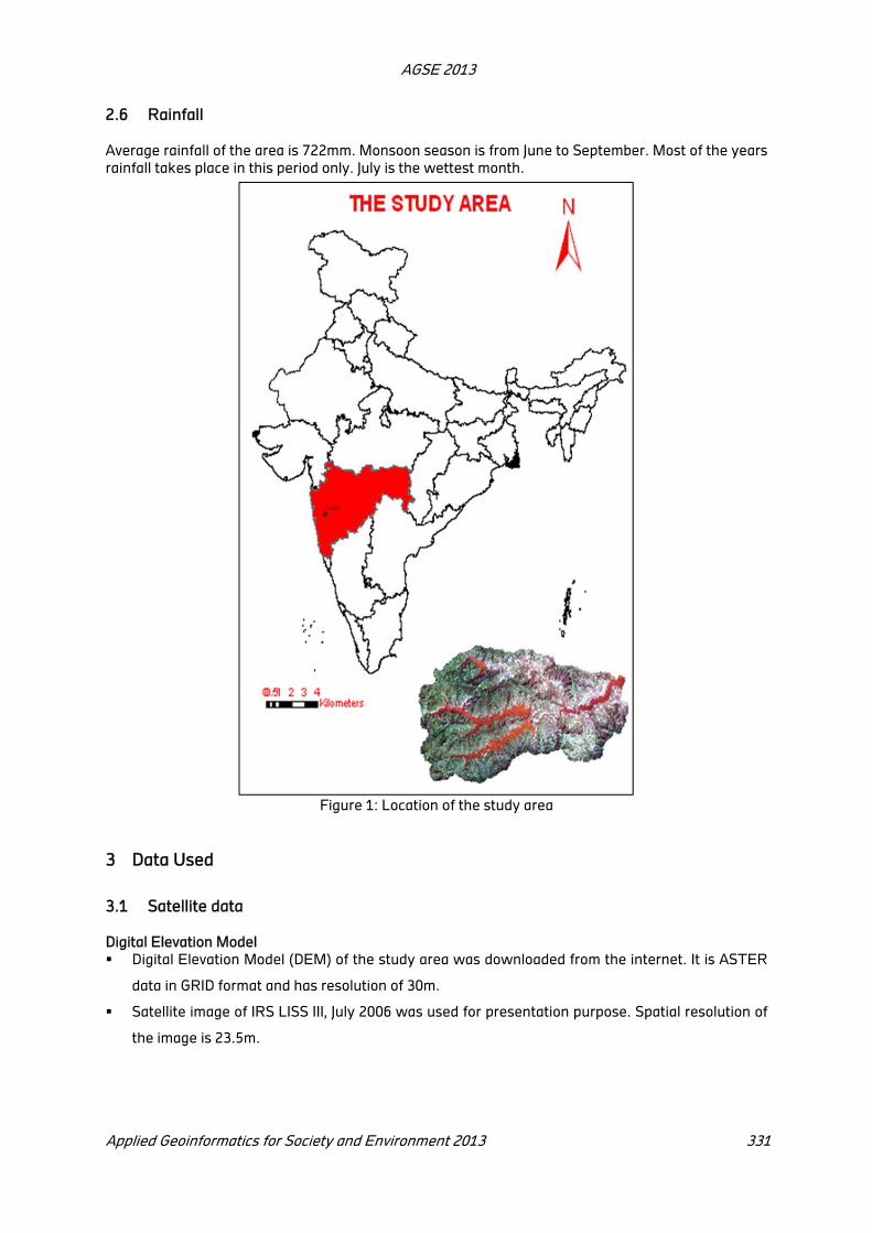
AGSE 2013


2.6 Rainfall

Average rainfall of the area is 722mm. Monsoon season is from June to September. Most of the years

rainfall takes place in this period only. July is the wettest month.

Figure 1: Location of the study area

3 Data Used

3.1 Satellite data

Digital Elevation Model

Digital Elevation Model (DEM) of the study area was downloaded from the internet. It is ASTER

data in GRID format and has resolution of 30m.

Satellite image of IRS LISS III, July 2006 was used for presentation purpose. Spatial resolution of

the image is 23.5m.

AGSE 2013


3.2 Ancillary data

Rainfall data

Rainfall data used in this study is acquired from National Water Academy, Khadakwasla toposheet

of the area.

4 Development of Rusle Soil Erosion Model

A commercial software package called ArcGIS version 9.1 is used for this paper. Two essential sub-

programs included this package are called ArcCatalog andArcMap. ArcCatalog is used for creating,

deleting, and editing the spatial data files. ArcMap is the primary application where the data is

analyzed and processed. The two spatial data types used in this project are vector and raster files.

Vector data contain features defined by a point, line, or polygon. Vector data models are useful for

storing and representing discrete features such as buildings and roads. ArcGIS implements vector

data as a shapefiles. Raster data are composed of a rectangular matrix of cells. Each cell has a width

and height and is a portion of the entire area represented by the raster. Each cell has a value which

represents the phenomenon portrayed by the raster dataset, such as a category, magnitude,

distance, or spectral value. The category could refer to a land use class, such as grassland or urban.

The cell size dimensions can be as large or as small as necessary to accurately represent the area.

All raster layers used in this project had a grid resolution of 10 square meters. The location of each

cell is defined by either its reference system or projection. The use of the same projection allows

raster layers to overlap with each other. The USLE is combined with the ArcGIS to calculate the

estimated average annual soil loss (A) that is occurring within the Panshet Watershed. Raster layers

corresponding to each of the six USLE factors are created, stored, and analyzed with the ArcGIS. This combination computes the estimated soil erosion potential for the entire watershed and areas

of high soil erosion potential are identified. The grid cells in each layer overlap and the USLE

computation can be done by multiplying all the USLE factors together (Figure 2).

Figure 2: Illustration of the USLE layers and how they overlap

AGSE 2013


The Equation (RUSLE) has been used to predict soil loss. Its output is given in predicted soil loss

(tons/acre/year). It is written as:

A=R*K*LS*C*P eqn (1)

Where, A = Mean Annual soil loss (ton.ha-1.yr-1)

R = Rainfall and Runoff Erosivity Index (MJ/ha/mm/yr)

K = Soil Erodibility Factor (ton/MJ/mm)

LS = Slope and Length of Slope Factor

C = Cropping – Management Practice Factor

P = Erosion Control Factor Practice

The image was classified in ERDAS imagine applying the Maximum Likelihood algorithm with an

accuracy of 91% and accuracy assessment done on that. Landuse classes are prepared for the

existing classes as water, forest, settlement, scrubland, vegetation. Soil theme is also prepared from

the soil texture map of the area using fields HSG (Refer to TR 55), hydraulic conductivity, Mukey,

texture, field capacity, Moisture content.

4.1 Rainfall and runoff erosivity factor (R)

The contribution of the erosive agent water (precipitation) is represented by the rainfall erosivity

factor R. This factor is may be the most important factor in the USLE compared to the other input

parameters (Jebari, 2009). The kinetic energy of the rain can be considered as the potential rainfall

energy available to be transformed into erosion. The erosivity of a single raindrop is naturally

described as the droplet kinetic energy E; the mass of the droplet multiplied by the square of the

velocity at impact divided by two; E=mV2/2 (Toy et al, 2002). The precipitation data from two

surrounding meteorological stations were used for estimating the average annual precipitation

(AAP). The estimated AAP was used for calculation of the rainfall and the runoff erosivity R-factor.

The precipitation data from two surrounding meteorological stations were used for estimating the

average annual precipitation (AAP), over the entire watershed. Reinard and Freimud (1994)

equations were used. The rainfall data are given in Table.

R = 587.8 – 1.249Pa + 0.004105Pa2 (for Pa > 850 mm) and

R <850 mm 0.04830*P1.610 (

for Pa < 850 mm)

The R-factor (Figure 4.) varied from 2534.12 to 2534.65 MJ mm/ha/year

Year / 1995 1996 1997 1998 1999 2000 2001 2002 2003 2004 2005 2006 2007

Month

January 14. Jul 0.5 02. Apr 0 0 0 06. Jun 0 0 0 10 0 0

February 0 0 0 0 0 0 0 0 03. Feb 0 0 0 0

March 0 0 0 0 0 0 0 0 0 0 0.4 04. Jan 0

April 34.5 01. Sep 20. Mai 0 0 0 02. Mai 6 01. Apr 0 36.7 0 08. Jan

May 20. Sep 04. Sep 04. Mrz 10. Mrz 36 24. Jul 04. Apr 18. Feb 0 73.3 32 64.6 03. Aug

June 58.9 193.3 287.7 95.7 165.5 147.8 78.6 201.4 163 224.2 291.7 150.2 232.5

July 187.139 206.9 165.4 244.8 156.4 94.5 118.8 31.6 90.8 59.7 309.4 404.9 293.5

August 43.8 78.9 249.5 159.2 34.8 81.5 76.3 105.4 84 330.3 232.4 378 159.9

September 191 125.6 37.1 139.3 143.6 145.4 124.2 46.9 39.5 206.8 303.9 170.7 148.9

October 71.6 191 26. Apr 92.4 195.5 41.9 114 13. Jan 72.5 05. Jun 96 50.9 0

November 01. Feb 0.9 163.3 49 0 14.

Mai 23. Feb 0.5 02. Mrz 13. Jun 0 43.5 10. Mai

December 0 0 68.9 0 0 8 0 0 0 0 0 0 0

Total R/F 623.739 803.9 1025.5 790.7 731.8 558.3 548.6 423.1 456.7 913.5 1312.5 1266.9 857.2

TABLE 1: Pune Rainfall ((Rainfall in mm)

AGSE 2013


Year / 1995 1996 1997 1998 1999 2000 2001 2002 2003 2004 2005 2006 2007

January 14. Aug 0.6 02. Mai 0 0 0 06. Jul 0.1 0.1 0.1 10. Jan 0 0

February 0 0 0 0 0 0 0 0 03. Mrz 0.1 0.1 0 0

March 0 0 0 0 0 0 0 0 0 0 0.5 04. Feb 0

April 34.6 2 20. Jun 0 0 0 02. Jun 06. Jan 01. Mai 0.1 36.8 0.1 08. Feb

May 21 5 04. Apr 10. Apr 36.1 24.

Aug 04. Mai

18.

Mrz 0.1 73.4 32.1 64.7 03. Sep

June 59 193.4 287.8 95.8 165.6 147.9 78.7 201.5 163.1 224.3 291.8 150.3 232.6

July 187.239 207 165.5 244.9 156.5 94.6 118.9 31. Jul 90.9 59.8 309.5 405 293.6

August 43.9 79 249.6 159.3 34.9 81.6 76.4 105.5 84.1 330.4 232.5 378.1 160

September 191.1 125.7 37.2 139.4 143.7 145.5 124.3 47 39.6 206.9 304 170.8 149

October 71.7 191.1 26. Mai 92.5 195.6 42 114.1 13. Feb 72.6 05. Jul 96.1 51 0.1

November 01. Mrz 1 163.4 49.1 0.1 14. Jun 23. Mrz 0.6 02. Apr 13. Jul 0.1 43.6 10. Jun

December 0 0 69.2 0 0 0 0 0 0 0 0 0 0

Total R/F 623.839 804 1025.6 790.8 731.9 558.4 548.7 423.2 456.8 913.6 1312.6 1267 857.3

Figure 3: R_FACTOR

4.2 Soil erodibility factor (K)

The soil erodibility factor (K factor) is a quantitative description of the inherent erodibility of a

particular soil type. The K factor reflects the fact that different soils erode at different rates when

the other factors that affect erosion remain the same. Soil texture is the principal cause affecting the

K-factor, but the soil structure, organic matter content, and permeability also contribute. A map for

the K-factor was produced based on the soil map and soil erodibility texture. After compiling a table

of K factor values for each soil type, the data was inputted into a newly created field on the digital

soil shapefile. The data file can be sorted according to the gridcode, which corresponds to the NRCS

ID number for each soil type. Each number class is chosen by the ‘Select by Attribute’ command

located under the Selection drop down menu. The appropriate K factor values are entered by right

AGSE 2013


clicking on the created column and selecting ‘Calculate values.’ Appropriate K factors for each soil

type are entered into the field calculator menu.

Figure 4: K-factor

4.3 Topographic factor (LS)

The basis for calculating LS factor was the Digital Elevation Model (DEM) of the study area Acording

to Raghunath (2002) it is possible to calculate directly LS factor. Higher values of LS mean higher

risk of erosion. Here, C++ executable program along with the source code files are accessible

(http://www.iamg.org). To run the program, the DEM input needs to be in text format called ASCII.

ArcMap has the function to do this located under the Conversion toolbox extension. Select the “From

Raster” extension and select the “Raster to ASCII” tool. In the menu, navigate to the DEM to be

converted and note the location of the output ASCII text file. Edit the output file into a short, easily

recognizable name fixed. The user should select “YES”. The program then begins its computation of

the DEM text file. The output consists of 16 total files with the .dat file suffix.

To convert the output files back to a raster format, the file suffix must be .txt in order for ArcMap to

recognize it. This can be done simply by right-clicking on each output file and selecting ‘rename’. By

changing only the suffix from .dat to .txt accomplishes the conversion. Open ArcMap and select the

‘ASCII to Raster’ tool under the Conversions toolbox. Individually convert the output files with the

suffixes rusle_l, rusle_s, and ruslels2 to import the LS factor as a raster layer.

AGSE 2013


Figure 5: LS-factor

4.4 Crop management factor (C)

The crop management factor was calculated mainly from literature review, since there was not local

data available regarding this factor. Based on the landuse classified image, similar ecosystems were

search on different literature sources and therefore assigned to the ones existing. The search was

orientated to those areas with similar geographical settings. C factor ranges from 1 to approximately

0, where higher values indicate no cover effect and soil loss comparable to that from a tilled bare

fallow, while lower C means a very strong cover effect resulting in no erosion. The C factor values

were entered into the new field and the shapefile was converted to a raster file format. The values

are:

Vegetation: 0.10, Settlement: 0.11, Water: 0, Scrubland: 0.25, Forest: 0.04

Figure 6: Landuse and C-factor

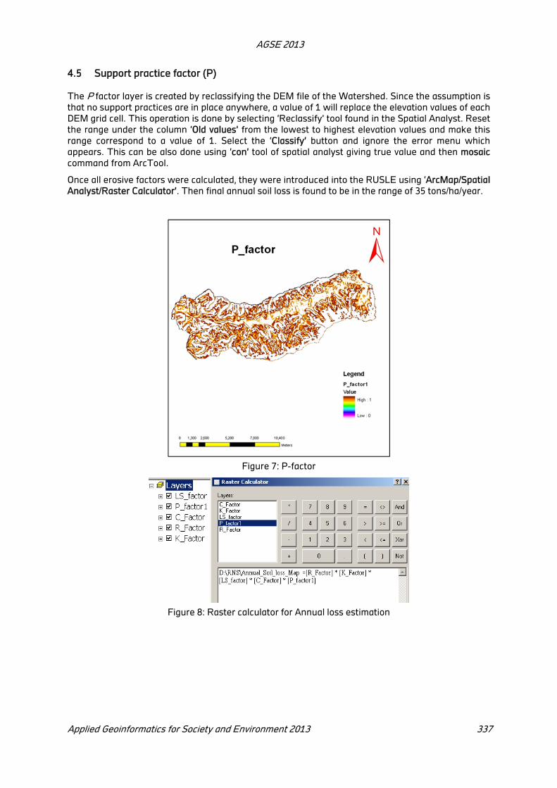
AGSE 2013


4.5 Support practice factor (P)

The P factor layer is created by reclassifying the DEM file of the Watershed. Since the assumption is

that no support practices are in place anywhere, a value of 1 will replace the elevation values of each

DEM grid cell. This operation is done by selecting ‘Reclassify’ tool found in the Spatial Analyst. Reset

the range under the column ‘Old values’ from the lowest to highest elevation values and make this

range correspond to a value of 1. Select the ‘Classify’ button and ignore the error menu which

appears. This can be also done using ‘con’ tool of spatial analyst giving true value and then mosaic

command from ArcTool.

Once all erosive factors were calculated, they were introduced into the RUSLE using ‘ArcMap/Spatial

Analyst/Raster Calculator’. Then final annual soil loss is found to be in the range of 35 tons/ha/year.

Figure 7: P-factor

Figure 8: Raster calculator for Annual loss estimation

AGSE 2013


Figure 9: Annual Soil Loss Risk Map

5 Results and discussions

Present study attempts to develop rainfall run off model using rain fall gage data, when the

simulated run is computed the program tracks all of the data in the simulation run, the selected basin

model, the selected meteorological model, and the selected control specifications.

The RUSLE model has six parameters such as rainfall runoff erosivity (R), soil erodibility (K), slope

length and steepnees (LS), cover management (C), and support practice factor (P). In the

Khadakwasla watershed, range values for those six parameters are as following.

Rainfall runoff erosivity factor (R) : 25.34~ 25.35 (100m-ton/ha/yr )

Soil erodibility factor (K) : 0 ~ 0.30 (tons/ha)

Slope length factor (LS ) : 0 ~85

Cover management factor (C) : 0 ~ 0.3

Support practice factor (P) : 0 ~ 1.0

Figure 4.58 depicts the spatial variability of gross soil erosion in the watershed. The erosion

values of 50% and 90% are about 17.5 tons/ha/year and 31.5 tons/ha/year respectively. And the

average rate of soil erosion is about 888.02 Thousand tons/year from the entire watershed.

The Khadakwasla multi-purpose dam has been operated for 50 years since it was reconstructed

in 1962 after the failure of the dam on July, 12, 1962 due to heavy run-off and failure of Panshet u/s.

However, whenever engineers of multi-purpose dam face the flood season sometimes, they are

suffering from severe turbid water into the reservoir. In order to solve this problem, the turbidity

and total suspended solids prediction system, which can analyze spatially and temporally the

gross soil erosion rate and sediment transport process in the watershed and channel, is needed for

every storm event. In addition, survey for turbidity, temperature, and TSS is necessary for the

efficient water resources and sediment management of the multi-purpose dam reservoir.

AGSE 2013


Better prediction can be complemented by accumulating more accurate input data. For example,

the accurate C value for forested area, which has been developing continuously, cannot be

predicted easily and is not able to apply without verifying the C value applied for forested area of

the other countries. Therefore, the appropriate C value for forested area of the watershed should

be found.

Even though the error of sediment deposits survey is considered, the life expectancy of dead

storage of the reservoir might be decreased compare to the design life expectancy of dead

storage. Therefore, a recent survey of the sediment deposits of the reservoir is recommended

for a better evaluation the life expectancy of reservoir.

6 Conclusions

The following conclusions emerged from the present study:

Sediment delivered from water erosion causes substantial waterway damages and water quality

degradation. Controlling sediment loading requires the knowledge of the soil erosion and

sedimentation. A number of factors such as drainage area size, basin slope, climate, land use/land

cover may affect sediment delivery processes. Accurate prediction of sediment delivery ratio is an

important and effective approach to predict sediment yield which is usually not measured. Presently

available prediction models are not generally applicable to a particular watershed. Quantitatively

analysis of several prediction models and a computationally effective suitable model with higher

accuracy has been tried in this study. GIS is used to determine the values of factors in the models.

Monitoring sediment data including those from the dam authorities gauging stations are used to

validate the models.

The method developed in this study combines the USLE with ArcGIS software. Digital maps of soil

types, vegetation, and elevation were processed according to the RUSLE conventions and the

average annual soil erosion potential for each grid cell is computed. Areas of high soil erosion

potential were identified and appropriate mitigation actions may now be considered for these areas.

The main benefit for using this approach is the rapid assessment of soil erosion potential on a

watershed scale.

The spatial variability of the Watershed was adequately accounted for by using the ArcGIS

software. The LS factor was determined by using a combination of a C++ executable program (Van

Remortel et al. 2004) and ArcGIS. This new method significantly reduced the time spent in

evaluating the LS factor for a watershed. Traditional methods computed the LS factor by making

field measurements on selected hill slopes.

The rainfall erosivity (R factor) map represents an improvement over previous estimation of the R

factor because it is derived from IMD rainfall data. The R factor map was put in ArcGIS and spline

interpolation procedure was used to assign equivalent R factors for the areas lying in between

the isoerodent lines. Although the ideal solution is to install a dense network of rain gauges to

continuously record rainfall, the costs are prohibitive and rainfall needs to be recorded for at least 10

consecutive years to be reliable enough for calculating the R factor. But only two rain gauges were

available.

The methodology developed in this research allows each layer to be independently

updated in the event a new digital map or resource is available. One area that needs to be

addressed is the assignment of proper C factor values for native vegetation. Currently, there are no

C factors defined specifically for local vegetation species. The C factor can serve as adjustment

factors in situations where soil loss needs to be lowered. Various C factors corresponding to

different types of trees or crop rotations can be inserted into the USLE calculation to see how

they would lower the projected soil loss. In order to use the USLE as a resource management tool,

additional research into the C factors for a variety of native trees and plants are needed.

The following conclusions emerged from the present study:

The annual average soil loss rate was analyzed to be 35 tons/hact/year) and gross annual average

soil erosion was about 888.2 thousand tons/year in the watershed.

AGSE 2013


In case of the spatial variability of gross soil erosion of the Khadakwasla watershed, the

relationship between probability and gross soil erosion is analyzed.

REFERENCES

Raghunath, J. (2002). “Potential erosion map for Bagmati Basin using GRASS GIS”. Proceedings of

the Open Source GIS-GRASS users conference 2002.

Reinard K.G., and J. Freimund (1994). “Using monthly precipitation data to estimate the R-factor in

the revised USLE”. Journal of Hydrology 157, pp. 287-306.

Arnold, J.G., M.D.Birket, J.R.Williams, W.F.Smith, and H.N.McGill. 1987. Modeling the effects of

urbanization on basin water yield and reservoir sedimentation. Water Resources Bulletin.

23(6):1101-1107.

Burrough, P.A., R. A. McDonnell. (1998). Principles of Geographical Information Systems. New York:

Oxford University Press.

Greiner, J. H. (1979). Erosion and Sedimentation by Water in Texas: Average Annual Rates

Estimated in 1979. Austin: Texas Department of Water Resources.

Hudak, P.F., J. Davis, J. Reinisch, D. Smith, C. Weicker, V. Woods. 2001. Soil Erosion: It’s a Slippery

Slope. Geospatial Solutions, No. 1.

Hunter, B. (1990). A Comparison of Universal Soil Loss Equation Results

Kuenstler, W. (1998). “A guidelines for the use of the Revised Universal Soil Loss Equation (RUSLE).

Chapter 5.

Metternicht G. I, and Fermont A. (1998). Estimating erosion surface features by linearmixture

modeling. Remote Sensing of Environment 64 (3): 254-265.

Mongkolsawat, C., Thirangoon, P., Sriwongsa, S. (1994). Soil erosion mapping with Universal Soil

Loss Equation and GIS. GIS development proceedings. Asian Conf. on Remote Sensing. Available

at http://www.gisdevelopment.net/aars/acrs/1994/ ts3/ts3001. shtml.

Pilesjo, P. (1992). “GIS and Remote Sensing for soil erosion studies in semi-arid environments”. PhD

thesis: Meddelanden fran Lunds Universitets Geografiska, Sweden, pp. 203.

Renard, K. G. & Freidmund, J. R. (1994). Using monthly precipitation data to estimate the R factor in

the RUSLE. Journal of Hydrology 157: 287–306.

Wainwright, J., Parsons, A. J., Michaelides, K., Powell, D. M. and Brazier, R. (Editors), (2003). Linking

short and long term soil erosion modelling. In: Long Term Hillslope and Fluvial System Modelling.

Concepts and Case Studies from the Rhine River Catchment. Springer-Verlag, Bonn, Germany.

William, J. Ripple, (1994). The GIS Applications Book Examples in Natural Resources: a

compendium, Published by: American Society for Photogrammetry and Remote Sensing.

Wischmeier W. H., and Smith DD. (1978). Predicting rainfall-erosion losses: A guide to conservation

planning. Agricultural Handbook No. 537. US Department of Agriculture.

Delineation of Groundwater Potential Zones In Parts of Bhopal District

Using AHP Technique

Himanshu Panwara, S.K.Pandey

b, AmitDaiman

c

a National Institute of Technology Warangal, AP- [email protected],

bMadhya Pradesh Council of Science and Technology, Bhopal- [email protected],

c Madhya Pradesh Council of Science and Technology, Bhopal- [email protected]

KEY WORDS: Groundwater prospect, Analytic Hierarchy Process, Remote Sensing & GIS.

ABSTRACT

Water is the most important natural resource that supports life of planetary Earth. It is the basic need of human to carry out their routine activities. In this case study, an attempt has been done to delineate groundwater potential zones in Kaliyasote Milli-Watershed in Bhopal district, Madhya Pradesh, India covering an area of 84 sq.km. The various thematic maps namely geological, geomorphological, lineament, slope, drainage and drainage density were generated using IRS (P6-resourcesat) LISS III data and referenced by Survey of India (SOI) toposheets. The information extracted from all the thematic maps were integrated in GIS environment, each map was given some weightage based on its suitability to groundwater. The method adopted to assign weightage was Analytic Hierarchy Process (AHP) which produced considerable results. On the basis of hydrology and geomorphic characteristics, six categories on groundwater prospect zones were identified i.e. excellent, very good, good, moderate, poor and very poor to NIL. The analysis reveals that the lineaments on pediplains have excellent groundwater potential followed by pediplains with very good to good potential whereas plateau remnants, lateritic uplands and cuesta have moderate to very poor potential.

1 Introduction

Rapid industrial development, urbanization and increase in agricultural production have led to

freshwater shortages in many parts of the world. Almost every species depends on water for its

survival. The increasing population is generating a huge demand of fresh and potable water supply

but the available surface water is inadequate to fulfill this requirement, as a result more stress has

been experienced to the groundwater resources which is the largest as well as the most economical

source of fresh water supply as it undergoes lower levels of contamination and wider distribution

whereas surface water needs to be treated before supply. The shortage of water is a major concern

for all living beings. About 70% of the global surface is covered with water in the form of oceans,

seas, rivers and lakes. The 97.3% of the water available on the Earth is saline and the remaining

2.7% is available as fresh water, out of which 79% lies in Polar Regions or in deep aquifers, 20%

groundwater and rest 1% in lakes. The occurrence of groundwater is not a matter of chance but a

consequence of the interaction of the climatic, geological, hydrological, physiographical and

ecological processes of nature. The exploration operation is essentially a hydrogeological and

geophysical influence-operation and depends on the correct interpretation of hydrological indicators.

The movement of groundwater is mainly controlled by porosity and permeability of the rocks. The

lithology forming different geomorphic units will have variable porosity and permeability and thereby

causing changes in groundwater potential. The surface water bodies like tanks, ponds, river, stream,

lakes, springs etc. act as the recharge zones for groundwater. The Remote Sensing techniques are

playing an important role in identifying the groundwater potential zones. These techniques have

been proven as an excellent tool for understanding the perplexing problems related to groundwater

exploration and have been well recognized in geological society. The remote sensing satellite

images, in conjunction with District Resource Maps (DRMs) provides better understanding for a

particular area and thus, helps in analyzing the various aspects like geomorphology, geology,

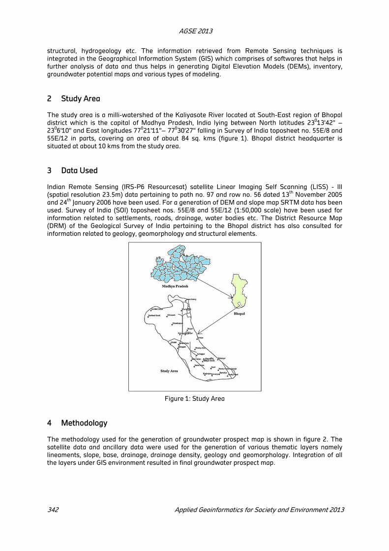
AGSE 2013


structural, hydrogeology etc. The information retrieved from Remote Sensing techniques is

integrated in the Geographical Information System (GIS) which comprises of softwares that helps in

further analysis of data and thus helps in generating Digital Elevation Models (DEMs), inventory,

groundwater potential maps and various types of modeling.

2 Study Area

The study area is a milli-watershed of the Kaliyasote River located at South-East region of Bhopal

district which is the capital of Madhya Pradesh, India lying between North latitudes 23013'42'' –

2306'10'' and East longitudes 77

021'11''– 77

030'27'' falling in Survey of India toposheet no. 55E/8 and

55E/12 in parts, covering an area of about 84 sq. kms (figure 1). Bhopal district headquarter is

situated at about 10 kms from the study area.

3 Data Used

Indian Remote Sensing (IRS-P6 Resourcesat) satellite Linear Imaging Self Scanning (LISS) - III

(spatial resolution 23.5m) data pertaining to path no. 97 and row no. 56 dated 13th

November 2005

and 24th

January 2006 have been used. For a generation of DEM and slope map SRTM data has been

used. Survey of India (SOI) toposheet nos. 55E/8 and 55E/12 (1:50,000 scale) have been used for

information related to settlements, roads, drainage, water bodies etc. The District Resource Map

(DRM) of the Geological Survey of India pertaining to the Bhopal district has also consulted for

information related to geology, geomorphology and structural elements.


4 Methodology

The methodology used for the generation of groundwater prospect map is shown in figure 2. The

satellite data and ancillary data were used for the generation of various thematic layers namely

lineaments, slope, base, drainage, drainage density, geology and geomorphology. Integration of all

the layers under GIS environment resulted in final groundwater prospect map.

AGSE 2013


Figure 2: Methodology

4.1 Thematic Layers

The satellite data that have been used had undergone image preprocessing in order to correct

distortions and to create more faithful representation. The image was georectified with geographical

coordinate system WGS 1984 and projected coordinate system Lambert Conformal Conic projection.

After preprocessing work, the image enhancement was done to improve the visual impact and to

make the image more interpretable. The other actions that were performed were mosaicking to

combine the satellite images and sub-setting to crop the study area from the satellite image.

4.2 Interpretation of Satellite Data

The False Color Composite (FCC) satellite image of the study area can be seen in figure 3. The red

tone in image represents vegetation which is basically Rabi crops as the image has taken in January.

The two water bodies can be seen in the north, as their tone is dark which indicates deep water

bodies. Light blue tone with rough texture represents settlements in the area and in between some

straight lines can be seen which are roads. The various geomorphic units having some relief can be

seen in the northern flank of the study are with greenish blue tone and smooth to slight rough

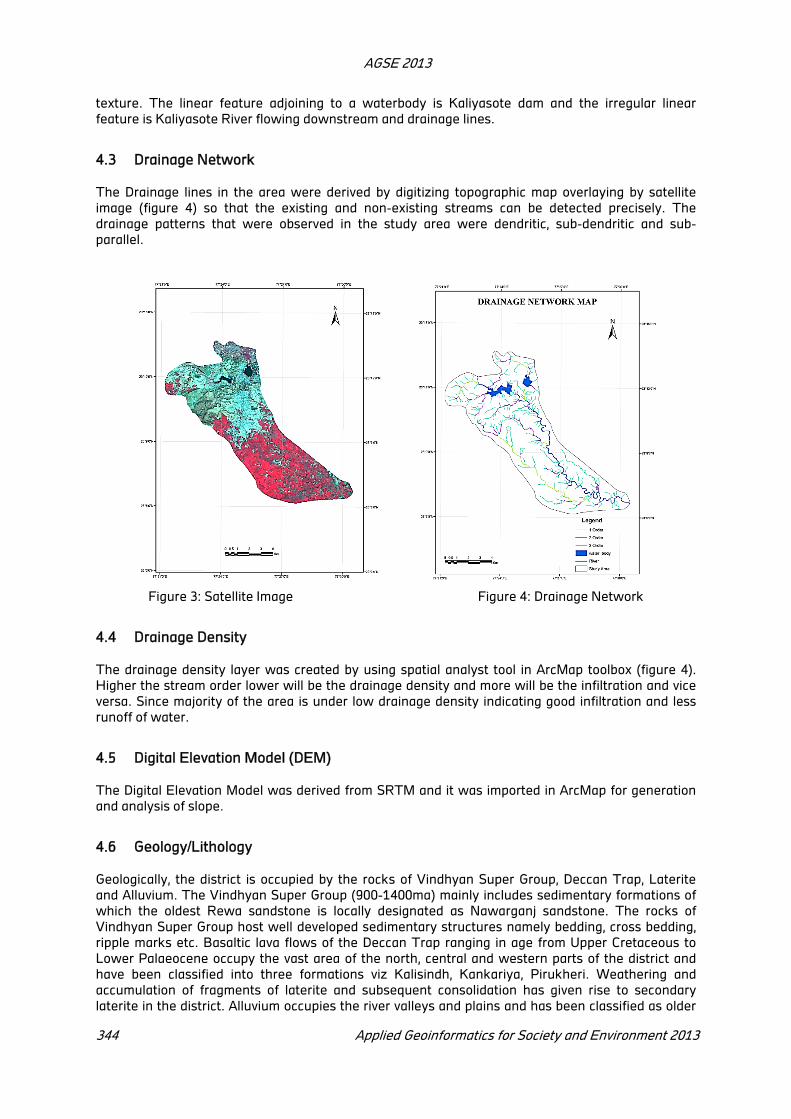
AGSE 2013


texture. The linear feature adjoining to a waterbody is Kaliyasote dam and the irregular linear

feature is Kaliyasote River flowing downstream and drainage lines.

4.3 Drainage Network

The Drainage lines in the area were derived by digitizing topographic map overlaying by satellite

image (figure 4) so that the existing and non-existing streams can be detected precisely. The

drainage patterns that were observed in the study area were dendritic, sub-dendritic and sub-

parallel.

Figure 3: Satellite Image Figure 4: Drainage Network

4.4 Drainage Density

The drainage density layer was created by using spatial analyst tool in ArcMap toolbox (figure 4).

Higher the stream order lower will be the drainage density and more will be the infiltration and vice

versa. Since majority of the area is under low drainage density indicating good infiltration and less

runoff of water.

4.5 Digital Elevation Model (DEM)

The Digital Elevation Model was derived from SRTM and it was imported in ArcMap for generation

and analysis of slope.

4.6 Geology/Lithology

Geologically, the district is occupied by the rocks of Vindhyan Super Group, Deccan Trap, Laterite

and Alluvium. The Vindhyan Super Group (900-1400ma) mainly includes sedimentary formations of

which the oldest Rewa sandstone is locally designated as Nawarganj sandstone. The rocks of

Vindhyan Super Group host well developed sedimentary structures namely bedding, cross bedding,

ripple marks etc. Basaltic lava flows of the Deccan Trap ranging in age from Upper Cretaceous to

Lower Palaeocene occupy the vast area of the north, central and western parts of the district and

have been classified into three formations viz Kalisindh, Kankariya, Pirukheri. Weathering and

accumulation of fragments of laterite and subsequent consolidation has given rise to secondary

laterite in the district. Alluvium occupies the river valleys and plains and has been classified as older

AGSE 2013


and new alluvium. Older alluvium mainly comprises yellow, grey, reddish brown clays with gravel

horizons whereas younger alluvium is confined to present day flood plains of the major rivers and

streams and consist mainly of sand, silt and subordinate amount of clay in the district.

4.7 Geomorphology

The geomorphology of the study area comprises of cuesta in the northern corner which is a hill with

gentle slope on one side and steeper slope on the other side. It is least favorable to groundwater.

Lateritic uplands which are the formation of chemically weathered subsoils rich in oxides of iron,

bauxite or both, Plateau remnant which is a flat area of great extent and elevation above the sea

level, Pediments which are gently sloping rock surface having moderate relief, Pediplains in the

southern part of the study area which is a low leveled extensive spread of rock sediments and are

most favorable to groundwater and meander scar which is a crescentic, concave mark on the face of

a bluff or valley wall, produced by the lateral plaination of a meandering stream which undercut the

bluff, and indicating the abandoned root of the stream.

Figure 5: Slope Map Figure 6: Drainage Density

AGSE 2013


Figure 7: Geological/Lithology Map Figure 8: Geomorphological Map

4.8 Structures

The lineaments in the study area were extracted by visual image interpretation. The image has

enhanced and under gone various band combinations (figure 9). They were easily identified by

drainage streams due to their linear shape at some places. All the lineaments in the study area are

micro- lineaments as their length are less than 3 km. The lineament density is more in the northern

part of the study area; their general orientation is aligned along NWSE direction. The lineaments are

the result of various faults and fractures they infer that they are the zones of increased porosity and

permeability, which in turn has greater significance in groundwater potential and its distribution.

Lineaments can be identified from remote sensing based on their linear nature, presence of

moisture, alignment of vegetation, alignment of ponds, straight stream segments etc.

5 Integrated GIS Analysis

The vector data layers derived have been finally converted into raster data sets having the same

pixel size. Each data set in a single map was assigned weightages by pair wise comparison. The

method adopted to assign weightages was Analytic Hierarchy Process (AHP) by Thomas L. Saaty

(1977) which is the most widely used decision making approach in the world today. In this method,

each class in a particular thematic map was assigned a rating by pair-wise comparison between

classes based on their relative importance. The initial ratings were adopted from continuous rating

scale developed by Saaty.

AGSE 2013


Figure 9: Structural Map

Extreme 1/9 Moderate 1/3 Strong 5

Very Strong 1/7 Equal 1 Very Strong 7

Strong 1/5 Moderate 3 Extreme 9

Table 1: Saaty’s Continuous Rating Table

5.1 Weightage Assignment

The AHP method is based on the well-defined mathematical structure of consistent matrices and

their associated right Eigen vector’s ability to generate true or approximate weights. The weightage

assignments of all the groundwater controlling factors are given below.

Distance/s (mtr) >150 100-150 50-100 0-50 Weight Weight*100

>150 1 0.143 0.111 0.091 0.036 4

100-150 7 1.000 0.778 0.636 0.250 25

50-100 9 1.286 1.000 0.818 0.321 32

0-50 11 1.571 1.222 1.000 0.393 39

Table 2: Computing of Weights for Lineaments of the study area

Drainage Order V.HIGH HIGH MODERATE LOW Weight Weight*100

1 order 1 0.333 0.200 0.143 0.063 6

2 order 3 1.000 0.600 0.429 0.188 19

3 order 5 1.667 1.000 0.714 0.313 31

No order 7 2.333 1.400 1.000 0.438 44

Table 3: Computing of Weights for Drainage lines of the study area.

AGSE 2013


Drainage Density V. HIGH HIGH MODERATE LOW V.LOW Weight Weight*100

V.HIGH 1 0.333 0.200 0.143 0.111 0.039 4

HIGH 3 1.000 0.600 0.429 0.333 0.116 12

MODERATE 5 1.667 1.000 0.714 0.556 0.193 19

LOW 7 2.333 1.400 1.000 0.778 0.270 27

V.LOW 9 3.000 3.000 1.286 1.000 0.384 38

Table 4: Computing of Weights for Drainage Density of the study area.

Slope Type

VERY

STEEP STEEP MODERATE GENTLE FLAT Weight Weight*100

VERY STEEP 1 0.334 0.2 0.143 0.112 0.057 6

STEEP 3 1 0.6 0.429 0.334 0.137 14

MODERATE 5 1.667 1 0.714 0.556 0.206 21

GENTLE 7 2.337 1.4 1 0.778 0.27 27

FLAT 9 3 1.8 1.285 1 0.33 33

Table 5: Computing of Weights for Slope of the study area..

Lithology BASALT LATERITE SANDSTONE ALLUVIUM Weight Weight*100

BASALT 1 0.333 0.200 0.111 0.056 6

LATERITE 3 1.000 0.600 0.333 0.167 17

SANDSTONE 5 1.667 1.000 0.556 0.278 28

ALLUVIUM 9 3.000 1.800 1.000 0.5 50

Table 6: Computing of Weights for Geology of the study area.

Landforms CUEST

A

LATERATI

C UPLAND

PLATEAU

REMNAN

T

PEDIMEN

T

PEDIPALI

N

MEANDE

R SCAR

Weigh

t

Weight*10

0

CUESTA 1 0.333 0.200 0.143 0.111 0.091 0.028 3

LATERATI

C UPLAND 3 1.000 0.600 0.429 0.333 0.273 0.084 8

PLATEAU

REMNANT 5 1.667 1.000 0.714 0.556 0.455 0.139 14

PEDIMENT 7 2.333 1.400 1.000 0.778 0.636 0.194 19

PEDIPALIN 9 3.000 1.800 1.286 1.000 0.818 0.250 25

MEANDER

SCAR 11 3.667 2.200 1.571 1.222 1.000 0.305 31

Table 7: Computing of Weights for Geomorphology of the study area.

5.2 Overlay Analysis

The Overlay Analysis is the final step after reclassification of raster datasets. The overlay analysis

was done in ArcMap by using Overlay tool from spatial analyst tool. The function of this tool is to

integrate all the input raster dataset. Every reclassified raster dataset added in overlay table is given

an influence factor. The influence factors were given to all reclassified raster data sets is mentioned

in Table 8.

AGSE 2013


RECLASSIFIED

MAPS

DRAINAGE

NETWORK GEOLOGY

DRAINAGE

DENSITY SLOPE

GEO-

MORPH

OLOGY

LINEAMENT Influence Influence

*100

DRAINAGE

NETWORK 1 0.333 0.200 0.143 0.111 0.091 0.027 3

GEOLOGY 3 1.000 0.600 0.429 0.333 0.273 0.084 8

DRAINAGE

DENSITY 5 1.667 1.000 0.714 0.556 0.455 0.139 14

SLOPE 7 2.333 1.400 1.000 0.778 0.636 0.194 19

GEO-

MORPHOLOGY 9 3.000 1.800 1.286 1.000 0.818 0.250 25

LINEAMENT 11 3.667 2.200 1.571 1.222 1.000 0.305 31

Table 8: Computing of Weights for all thematic maps which will be the influence factors for overlay

analysis

6 Results and Discussions

The area under study is mostly occupied by the alluvial rock formation susceptible for the occurrence

of groundwater. Based on the GIS approach, the groundwater prospective zones have been

identified, occupying central as well as southern part of the study area. Monitoring of the existing

dug wells, wells, tube wells may also enable to arrive at a judicious explanation about the

sustenance of available groundwater resource in the region. The intersecting nature of structural

elements (lineaments) has been proven to be more accurate judgement for the occurrence of

underground water resource in the region. The Analytic Hierarchy Process (AHP) has been proven

to be an efficient method to delineate groundwater potential zones by providing suitable weightages.

A deep study of AHP is required to generate more accurate results. The efficiency of the results of

AHP is based on the initial ratings which are knowledge base. More accurate these ratings, more

accurate will be the results; hence field investigation need to be done. The data related to static

water level (seasonal), water level fluctuations, recuperation, geophysical

Figure 10: Groundwater Prospect Map water Prospect Map

AGSE 2013


Investigations may better lead to achieve more precise estimation about the available groundwater

resource in the region.

REFERENCES

Biswas Arkoprovo and Jana Adarsa 2012.Delineation of Groundwater Potential Zones using Satellite

Remote Sensing and Geographic Information System Techniques: A Case study from Ganjam

district, Orissa, India, pp 1-8.

C. Travaglia and N. Dainelli 2003. Groundwater search by remote sensing: a methodological

approach (Iraq), pp. 7-24

District Census Handbook, Bhopal district, Directorate of Census Operations, Census of India 1981.

ESRI Desktop help manual, reclassification and overlay analysis.

Ernest H. Forman and Saul I. Gass. The Analytic Hierarchy Process- An Exposition, George

Washington University, Washington, pp 1-86

F.G.Bell 2007.Engineering Geology, pp 1-61, 151-172.

Gazetteer of Bhopal, District Gazetteer Department, Govt. of Madhya Pradesh.

G.S. Thakur and R.S. Raghuwanshi 2007.Perspect and Assessment of groundwater resources using

remote sensing techniques in and around Choral River Basin, Indore and Khargone District (M.P.),

pp 1-9

Geoff Coyle 2004. The Analytic Hierarchy Process (AHP), pp 1-11

J.Vijaya Kumar and M.Suresh 2009.Application of remote sensing data for delineation of

groundwater potential zones in SolipurVagu Sub-Basin of Kongal River (A.P), pp 1-5.

Jyoti Sarup and Manish K. Tiwari 2008. Delineate groundwater prospect zones and identification of

artificial recharge sites using geospatial technique, pp 1-15.

MAB Consultancy 2009. Groundwater potential zone mapping using GIS and Remote Sensing Moyal-

Teltele sub basin – Dire, Arero, Yabelo and Telteleworedas, borena zone of Oromia regional state,

pp. 1-60

Mark. J. Crawford, M.S. 1998. Physical Geology, pp 93-102.

M. H. de Freitas 2007. Engineering Geology 235-245

Saaty, T.L., 1980. “The Analytic Hierarchy Process.” McGraw-Hill, New York.

SudarsanaRaju.G 2012. Delineation of groundwater prospects zones in and around Kadiri,

Anathapur District (A.P.), pp 1-11.

SanjivKishorea and S.K. Srivastavb 2009. Ground water prospects zonation using remote sensing

and GIS - a case study of bata watershed, sirmaur district, h.p. pp 1-6.

V.K.Srivastava, DevendraNathGiri 2012. Study and Mapping of Ground Water Prospect usingRemote

Sensing, GIS and Geoelectrical resistivity techniques – a case study of Dhanbaddistrict,Jharkhand,

India, pp 1-5.

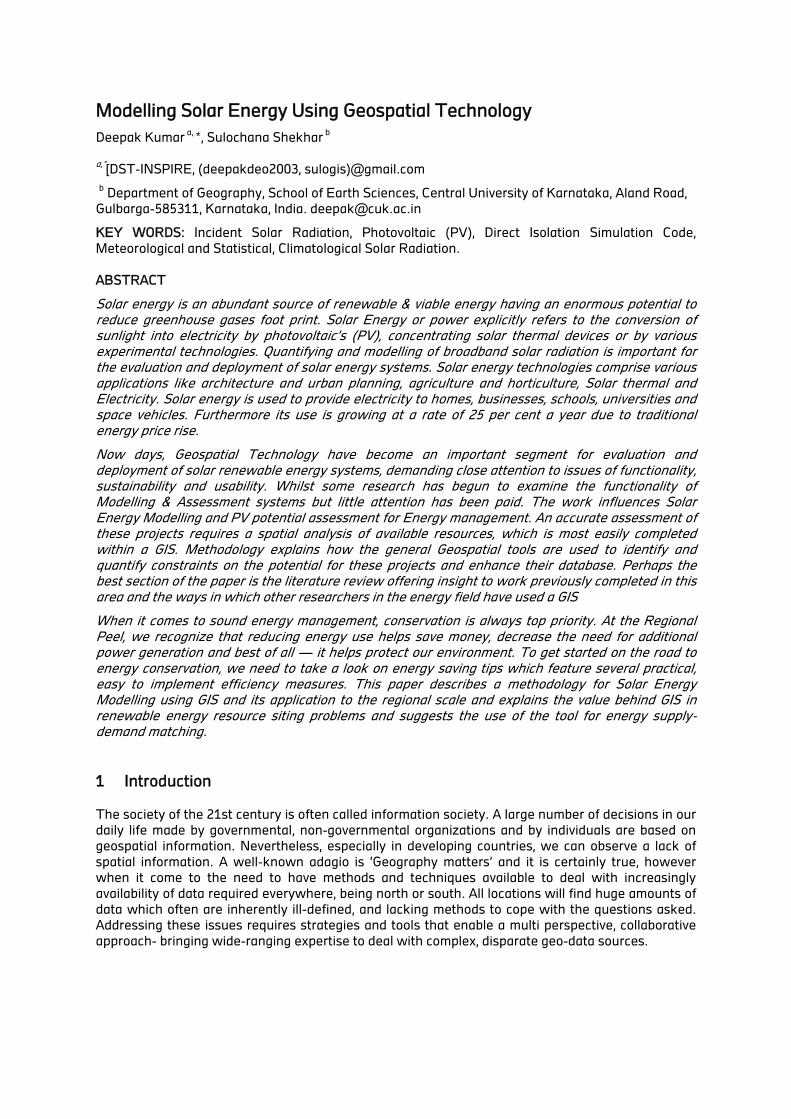
Modelling Solar Energy Using Geospatial Technology

Deepak Kumar a,

*, Sulochana Shekhar b

a,*[DST-INSPIRE, (deepakdeo2003, sulogis)@gmail.com

b Department of Geography, School of Earth Sciences, Central University of Karnataka, Aland Road,

Gulbarga-585311, Karnataka, India. [email protected]

KEY WORDS: Incident Solar Radiation, Photovoltaic (PV), Direct Isolation Simulation Code,

Meteorological and Statistical, Climatological Solar Radiation.

ABSTRACT

Solar energy is an abundant source of renewable & viable energy having an enormous potential to reduce greenhouse gases foot print. Solar Energy or power explicitly refers to the conversion of sunlight into electricity by photovoltaic’s (PV), concentrating solar thermal devices or by various experimental technologies. Quantifying and modelling of broadband solar radiation is important for the evaluation and deployment of solar energy systems. Solar energy technologies comprise various applications like architecture and urban planning, agriculture and horticulture, Solar thermal and Electricity. Solar energy is used to provide electricity to homes, businesses, schools, universities and space vehicles. Furthermore its use is growing at a rate of 25 per cent a year due to traditional energy price rise.

Now days, Geospatial Technology have become an important segment for evaluation and deployment of solar renewable energy systems, demanding close attention to issues of functionality, sustainability and usability. Whilst some research has begun to examine the functionality of Modelling & Assessment systems but little attention has been paid. The work influences Solar Energy Modelling and PV potential assessment for Energy management. An accurate assessment of these projects requires a spatial analysis of available resources, which is most easily completed within a GIS. Methodology explains how the general Geospatial tools are used to identify and quantify constraints on the potential for these projects and enhance their database. Perhaps the best section of the paper is the literature review offering insight to work previously completed in this area and the ways in which other researchers in the energy field have used a GIS

When it comes to sound energy management, conservation is always top priority. At the Regional Peel, we recognize that reducing energy use helps save money, decrease the need for additional power generation and best of all — it helps protect our environment. To get started on the road to energy conservation, we need to take a look on energy saving tips which feature several practical, easy to implement efficiency measures. This paper describes a methodology for Solar Energy Modelling using GIS and its application to the regional scale and explains the value behind GIS in renewable energy resource siting problems and suggests the use of the tool for energy supply‐demand matching.

1 Introduction

The society of the 21st century is often called information society. A large number of decisions in our

daily life made by governmental, non-governmental organizations and by individuals are based on

geospatial information. Nevertheless, especially in developing countries, we can observe a lack of

spatial information. A well-known adagio is ‘Geography matters’ and it is certainly true, however

when it come to the need to have methods and techniques available to deal with increasingly

availability of data required everywhere, being north or south. All locations will find huge amounts of

data which often are inherently ill-defined, and lacking methods to cope with the questions asked.

Addressing these issues requires strategies and tools that enable a multi perspective, collaborative

approach- bringing wide-ranging expertise to deal with complex, disparate geo-data sources.

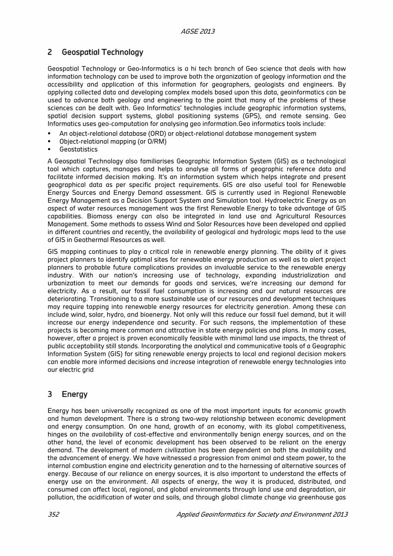
AGSE 2013


2 Geospatial Technology

Geospatial Technology or Geo-Informatics is a hi tech branch of Geo science that deals with how

information technology can be used to improve both the organization of geology information and the

accessibility and application of this information for geographers, geologists and engineers. By

applying collected data and developing complex models based upon this data, geoinformatics can be

used to advance both geology and engineering to the point that many of the problems of these

sciences can be dealt with. Geo Informatics’ technologies include geographic information systems,

spatial decision support systems, global positioning systems (GPS), and remote sensing. Geo

Informatics uses geo-computation for analysing geo information.Geo informatics tools include:

An object-relational database (ORD) or object-relational database management system

Object-relational mapping (or O/RM)

Geostatistics

A Geospatial Technology also familiarises Geographic Information System (GIS) as a technological

tool which captures, manages and helps to analyse all forms of geographic reference data and

facilitate informed decision making. It’s an information system which helps integrate and present

geographical data as per specific project requirements. GIS are also useful tool for Renewable

Energy Sources and Energy Demand assessment. GIS is currently used in Regional Renewable

Energy Management as a Decision Support System and Simulation tool. Hydroelectric Energy as an

aspect of water resources management was the first Renewable Energy to take advantage of GIS

capabilities. Biomass energy can also be integrated in land use and Agricultural Resources

Management. Some methods to assess Wind and Solar Resources have been developed and applied

in different countries and recently, the availability of geological and hydrologic maps lead to the use

of GIS in Geothermal Resources as well.

GIS mapping continues to play a critical role in renewable energy planning. The ability of it gives

project planners to identify optimal sites for renewable energy production as well as to alert project

planners to probable future complications provides an invaluable service to the renewable energy

industry. With our nation’s increasing use of technology, expanding industrialization and

urbanization to meet our demands for goods and services, we’re increasing our demand for

electricity. As a result, our fossil fuel consumption is increasing and our natural resources are

deteriorating. Transitioning to a more sustainable use of our resources and development techniques

may require tapping into renewable energy resources for electricity generation. Among these can

include wind, solar, hydro, and bioenergy. Not only will this reduce our fossil fuel demand, but it will

increase our energy independence and security. For such reasons, the implementation of these

projects is becoming more common and attractive in state energy policies and plans. In many cases,

however, after a project is proven economically feasible with minimal land use impacts, the threat of

public acceptability still stands. Incorporating the analytical and communicative tools of a Geographic

Information System (GIS) for siting renewable energy projects to local and regional decision makers

can enable more informed decisions and increase integration of renewable energy technologies into

our electric grid

3 Energy

Energy has been universally recognized as one of the most important inputs for economic growth

and human development. There is a strong two-way relationship between economic development

and energy consumption. On one hand, growth of an economy, with its global competitiveness,

hinges on the availability of cost-effective and environmentally benign energy sources, and on the

other hand, the level of economic development has been observed to be reliant on the energy

demand. The development of modern civilization has been dependent on both the availability and

the advancement of energy. We have witnessed a progression from animal and steam power, to the

internal combustion engine and electricity generation and to the harnessing of alternative sources of

energy. Because of our reliance on energy sources, it is also important to understand the effects of

energy use on the environment. All aspects of energy, the way it is produced, distributed, and

consumed can affect local, regional, and global environments through land use and degradation, air

pollution, the acidification of water and soils, and through global climate change via greenhouse gas

AGSE 2013


emissions. While fossil fuels will remain our largest source of energy for the foreseeable future, they

are ultimately finite resources. With concern over domestic supply and reliance on foreign supplies,

increasing costs and environmental impacts, there is an increasing push to utilize alternative fuel

sources. While our dependence on energy is not likely to decrease, it will be significant to foster new

innovations in energy technologies with a larger focus on energy efficiency and conservation.

The choice between different Renewable Energy Technologies to provide a given Energy Service is

based on the analysis of the best linkage between local Renewable Energy Sources, (RES) technical

aspects of each Renewable Energy Technology, and the specific characteristic of the Energy

Demand. Most variables related to distribution or those linked to space and time have geography as

their organizing principle. Many sustainability linked variables, if extrapolated, have geography as

their primary driver such as:

sources of renewable energy (solar, wind, biomass, tides, geothermal etc.), logistics (timing and pattern of resource availability and consumption), Climate change (rainfall, floods, drought, etc)

3.1 Solar Energy

It is the energy from the Sun in the form of radiated heat and light. It drives the climate and weather

and supports life on Earth. Till today solar energy technologies make controlled use of this energy

resource. Solar power is a synonym of solar energy or refers specifically to the conversion of sunlight

into

Electricity by photovoltaic’s (PV), concentrating solar thermal devices or various experimental

technologies.

3.2 Solar Radiation Basics

Incoming solar radiation (insolation) originates from the sun, is modified as it travels through the

atmosphere, is further modified by topography and surface features, and is intercepted at the

earth's surface as direct, diffuse, and reflected components.

Direct radiation is intercepted unimpeded, in a direct line from the sun.

Diffuse radiation is scattered by atmospheric constituents, such as clouds and dust.

Reflected radiation is reflected from surface features

The sum of the direct, diffuse, and reflected radiation is called total or global solar radiation

Figure 1: World Solar Energy Potential Map

Source: ArcGIS 9.3 Help

AGSE 2013


3.3 Why Solar Energy

The amount of sunlight that hits the earth’s surface in one (1) hour is enough to power the entire

world for one (1) year!!

Solar PV costs have declined dramatically due to widespread adoption, economies of scale and

technology advances.

Figure 2: World Solar Energy Potential Map

3.4 Solar Energy Breakdown

Figure 3: Solar Energy Budget

AGSE 2013


3.5 Spectral curve

Figure 4: Spectral Bandwidth of Solar Energy

2 Modelling

Modelling is a scientific activity the aim of which is to make a particular part or feature of the world

easier to understand, define, quantify, visualize, or simulate. It requires selecting and identifying

relevant aspects of a situation in the real world and then using different types of models for different

aims, such as conceptual models to better understand, operational models

to operationalize, mathematical models to quantify, and graphical models to visualize the subject.

Modelling is an essential and inseparable part of scientific activity, and many scientific disciplines

have their own ideas about specific types of modelling. There is also an increasing attention to

modelling in fields such as philosophy of science, systems theory, and knowledge visualization.

There is growing collection of methods, techniques and meta-theory about all kinds of specialized

scientific modelling.

4.1 Why Modelling

Modeling facilitates the fundamental and quantitative way to understand and analyses the complex

systems and phenomena. It is often used in place of experiments when experiments are too large,

too expensive, too dangerous, or too time consuming. These are complement to theory and

Experiments, and often integrate them. These are becoming popular in the field of Computations,

Earth and Space System Modeling.

4.2 Types of Model

There are various types of model which are being used for different purposes but generally we refer

to following types of models:

4.2.1 Deterministic/Mathematical Model

(Model in which outcomes are precisely determined through known relationships without any room for random variation and allows to make predications of y based on x. For example y=2+3x-0.4x

2 ).

4.2.2 Stochastic/Probabilistic Model

(Use ranges of values for variables in the form of probability distributions.)

AGSE 2013


4.3 Modelling Pipeline

Figure 5: Schematic for Modeling Framework

4.4 Aims & Objectives

The aim of this sequence of work is to carry out operational research to develop prototype for

ascertaining scope of solar energy modeling for managing energy associated catastrophe and eco-

friendly urbanization through spatial analysis. It is also intended to identify the prospects of

Geospatial Technology to provide expertise, advice and quality assurance in aspects of spatial

analysis for decision making to enhance aspects of analysis.

The current work will focus on the global and local energy and utilities of communities, individuals

and organizations engaged in the geospatial aspects of the planning, delivery, operations, reliability

and ongoing management of electric, gas, oil and water services throughout the world in the domain

of GIS framework. This will facilitate information exchange and collaboration between agencies and

industry by focusing on the engagement of industry within this community. The set of objectives in

order to meet these goals are:

To model and estimate the incoming solar radiation.

To demarcate the feasible zones of solar energy.

To assist decision makers for societal applications of solar energy.

5 Methodology

In the past, theoreticians have tended to deploy hierarchical models for estimation and

autocorrelation for the causal investigation of spatial processes. The underlying stochastic processes

inherent in these methods of spatial analysis deals with analysis, modeling and estimation

procedures that take account of geographical (spatial) relationships.

AGSE 2013


Figure 6: Proposed Model for Solar Energy Framework

With respect to the above-mentioned environment, a working model for the study has been designed

and shown to develop a GIS based solar energy management.

6. Spatial Pattern Analysis: Mapping Trends and Clusters

These tools can help you summarize and evaluate geographic distributions, identify statistically

significant spatial outliers and clusters (hot spots), and assess broad geographic patterns and trends

over time. These resources help to find patterns and relationships in the data, facilitating discussion,

contributing to research, and informing decision making.

6.1 Finding Cluster

Using analysis, we can feel confident in the spatial patterns we see, and in the decisions that we

make. Putting the data on a map is an important first step for finding patterns and understanding

trends. Looking at the points on a map, we can find the clusters or patterns in this point data. We

can decide where the department should allocate its resources, but just looking at points on a map is

often not enough to answer questions or make decisions using this kind of point data. That’s where

the spatial analysis tools in GIS come in.

6.2 Solar Energy Modelling With GIS

Enables to map and analyze the effect of the sun over a geographic area for specific time

periods.

It accounts for atmospheric effects, site latitude and elevation, steepness (slope) and compass

direction (aspect), daily and seasonal shifts of the sun angle, and effects of shadows cast by

surrounding topography.

AGSE 2013


The resultant outputs can be easily integrated with other geographic information system (GIS)

data and can help to model physical and biological processes as they are affected by the sun.

6.3 Solar Radiation Analysis Equations

The solar radiation analysis tools calculate insolation across a Landscape or for specific locations,

based on methods from theHemispherical view shed algorithm developed by Rich et al. (Rich

1990,Rich et al. 1994), as further developed by Fu and Rich (2000, 2002). The total amount of

radiation calculated for a particular location or area is given as global radiation. The calculation of

direct, diffuse, and global insolation are repeated for each feature location or every location on the

topographic surface producing insolation maps for an entire geographic area.

6.4 Global radiation calculation

Global radiation (Globaltot) is calculated as the sum of direct

(Dirtot) and diffuse (Diftot) radiation of all sunmap and skymap

sectors, respectively. Globaltot = Dirtot + Diftot

6.5 Datasets Used

Elevation values.

Toposheet for reference.

DEM Data from reliable sources.

High Resolution Satellite Imagery (1 to 5 m)

Ancillary data supporting ground truth(IMD Data)

6.6 Software’s Used

ArcGIS 9.x/10.x

Energy Plus 8.0

PV Studio 5.0

Solar Path Finder Assistant 5.0

Geospatial Toolkit (NREL)

AGSE 2013


6.7 Solar Radiation Modelling Framework

Figure 7: Solar Radiation Modelling Framework

6.8 Model Creation

6.8.1 Area Solar Radiation

Figure 8: Model Building for Area Solar Radiation

AGSE 2013


Point Solar Radiation

Figure 9: Model Building for Point Solar Radiation

7 Results

This section will deal with archiving and recording of the experimental results obtained through the

developed prototype or model. These results are obtained and explained to answer the questions

posed to fulfill the objectives. The prototype system architecture being developed may be used for

scientific research work for detecting and delineating precise boundaries from the input set of data

provided to it for analysis and to derive the results in graphical, pictorial or tabular format to assist or

handle energy related adversities. Finally the perceived outlines will be estimated and discussed.

Some of the sample outputs being generated will be as follows:

Area Under Solar Radiation

Feasible Solar radiation belts.

Amount of isolation being received.

Points Solar radiation.

Solar Radiation Graphics.

7.1 Area Solar Radiation Toolbox

Figure 10: Area Solar Radiation Window

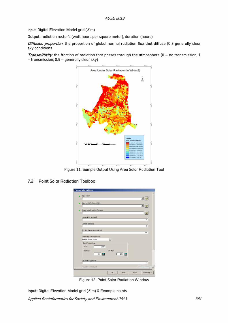
AGSE 2013


Input: Digital Elevation Model grid (X m)

Output: radiation raster's (watt hours per square meter), duration (hours)

Diffusion proportion: the proportion of global normal radiation flux that diffuse (0.3 generally clear

sky conditions

Transmittivity: the fraction of radiation that passes through the atmosphere (0 – no transmission, 1

– transmission; 0.5 – generally clear sky)

Figure 11: Sample Output Using Area Solar Radiation Tool

7.2 Point Solar Radiation Toolbox

Figure 12: Point Solar Radiation Window

Input: Digital Elevation Model grid (X m) & Example points

AGSE 2013


Output: global solar radiation on the example points

Figure 13: Sample Output Using Point Solar Radiation Tool

Attribute Table: T0 value of solar radiation at specific points in Wh/m²

8 Proposed Future Work

The growing use of mapping to support energy decision-making, among both communities and

utilities, underscores the need for web-based communication of geospatial data and for

interoperable geospatial processing queries and responses. It require the construction of a "nervous

system" that connects the diverse set of parties involved in energy decision-making to advance the

concept of an "Energy Spatial Data Infrastructure" (Energy SDI) that would inform planning and

management. The structural prototype module developed needs to be tested with feedback to be

used to design and develop a functioning system. This will also aid in presenting the overall

advantages of utilizing the concept for energy management. A pilot project needs to be developed to

respond to an assumed scenario. A software and database model need to be also developed based

on the concept in prototype model. The objectives of this pilot project will be:

Develop a practical model from conceptual model;

test the system and gain feedback for the design and development of a real functioning system;

present the overall structure, concept and advantages of developing such a system;

and present the advantages of utilizing the model in developing a support system for energy

related issues.

9 Conclusions

Solar energy is an alternative source of renewable energy that is non- polluting and can be easily

converted into electricity through the usage of photovoltaic (PV) systems. It represents an important

source of energy for the environment as it reduces the risks for climate change by helping to mitigate

AGSE 2013


fossil fuel emissions and dangerous greenhouse gases, in particular, carbon dioxide. In order to

encourage the implementation of PV systems to help alleviate the huge demands off the electrical

grid.Solar Energy is competitive, economic alternative to all form of the energy. The key to success

is long lifetimes and require minimal maintenance. Creates local jobs and promotes economic

development in rural areas. Avoids the external environmental costs associated with traditional

technologies. There are various applications of Solar Energy Technology like

Architecture and urban planning

Agriculture and horticulture

Solar lighting

Solar thermal (water heating, cooling and

ventilation, desalination and disinfection,

cooking, process heat)

Solar electricity (photovoltaics, concentrating solar

power, experimental solar power)

Acknowledgments

The author would like to acknowledge the support received from DST-INSPIRE Division, Ministry of

Science & Technology, Govt. of India for carrying out full time PhD research work at Central

University at Karnataka, Gulbarga and the faculty members of the Department of Geography, Central

University of Karnataka, in the preparation of this paper and the associated research. Special thanks

to DKD for being continuous source of inspiration to carry out the present work.

REFERENCES

Bangemann, M. 1994. Europe and the Global Information Society:Recommendations to the European Council, May, 1994. Office for official publ of the European Union.

Brand, M J D. 1995. The European geographic information infrastructure (EGII). Paper presented at

the ESIG conf, 27-29 Sept 1995, Lisbon, Portugal.

Burger, R. 1993. Information Policy: A Framework for Evaluation and Research. Ablex, Norwood, NJ.

Chorley, Lord Roger. 1987. Handling Geographic Information,Report of the Committee of Enquiry chaired by Lord Chorley.HMSO, London.

Committee on Science, Engineering, and Public Policy, "Policy Implications of Global Warming," pp.

620�628 (Washington, DC: National Academy Press, 1992).

Coopers and Lybrand. 1996. Economic Aspects of the Collection,Dissemination, and Integration of Government’s Geospatial Information. A report arising from work carried out for the Ordnance Survey, publ by Ordnance Survey, Southampton, UK.

Dutton, W H (ed). 1996. Information and CommunicationTechnologies, Visions and Realities. Oxford

Univ Pr, Oxford, UK.

Estes, J E (ed). 1994. Report of the International Symposium onCotre Data Needs for Environmental Assessment and Sustainable Development Strategies. Vols 1 and 2, 15-18 Nov 1994,

Bangkok,Thailand.

Hannes Jonsson, Friends in Conflict (London: Hurst & Co., 1982); <http://

gurukul.ucc.american.edu/ted/ICEFISH.htm>.

Kirill Ya Kondratyev, Climate Shocks: Natural and Anthropogenic (New York: Wiley, 1988).

Groot, R. 1993. Making IT work. ITC J 1993-3, pp 228-235.

Hernon, P. 1989. Discussion forum: national information policy.Gov Info Quarterly 6, 3, pp 229- 236.

Juan Carlos di Primio, "Data Quality and Compliance Control in the European Air Pollution Regime,"

in The Implementation and Effectiveness of International Environmental Commitments: Theory

and Practice, David K. Victor, Kal Raustiala, and Eugene B. Skolnikoff, eds., pp. 283, 303

(Cambridge: MIT Press, 1998).

AGSE 2013


Kenneth E. Boulding, Conflict and Defense: A General Theory (New York: Harper, 1962).

Leo Szilard and Barton J. Bernstein, The Voice of the Dolphin and Other Stories (Stanford: Stanford

University Press, 1992).

Mapping Sciences Committee. 1990. Spatial Data Needs: TheFuture of the National Mapping Programme. National Research Council, National Acad Pr, Washington DC, USA.Mapping Sciences

Committee. 1995. A Data Foundation for the National Spatial Data Infrastructure. National Research Council,National Acad Pr, Washington DC, USA.

Netherlands Commission for Geodesy. 1995. Wat is waar? Reflections on the Role of Geodesy as a Science of Spatial Information and the Desirable Developments of the Field in the Netherlands.

Sub-commission National Geodetic Plan, Publ 31,Delft, The Netherlands.Peter H. Gleick, "Water and Conflict: Fresh Water Resources and International Security," International Security 18, 1

(1993): 79, 112.

Rajabifard, A., Feeney, M., and Williamson I.P. (2002). Future Directions for the Development of Spatial Data Infrastructure, Journal of the International Institute for Aerospace Survey and Earth

Sciences, ITC, Vol. 4, No. 1, The Netherlands, PP 11-22.

Shirley Oakes Butler, "Owning Antarctica: Cooperation and Jurisdiction at the South Pole," Journal of

International Affairs 31 (1977): 35, 52.

Application of DRASTIC Model Using GIS for Evaluation Of Ground Water

Vulnerability: Study of Ahmedabad District

TUSHAR BOSEa *

, YASH MAJEETHIAb and KHUSHBOO PATEL

a

a Faculty of Technology, CEPT University

b Infrastructure Engineering and Management, Faculty of Technology, CEPT University

KEY WORDS: DRASTIC model, Ahmedabad district, ArcGIS, aquifer, vulnerability

ABSTRACT

Ahmedabad is one of the main district (zone) in state of Gujarat, India.. Groundwater is considered to be one of the most important sources of water for domestic use, agriculture and industrial use in study area.. The aim of this study is to determine the ground water vulnerability index using the DRASTIC model. The objective is to determine the susceptible ground water zone by integrating various layers using ArcGIS.. Attributes such as depth to ground water, net recharge, aquifer media, soil media, topography, impact of vadose zone and hydraulic conductivity are considered for ground water vulnerability mapping for the study area.. The ground water vulnerability index was classified into four classes viz. 100-120, 120-140, 140-160 and 160-180 corresponding to low, medium, high and very high vulnerability respectively. The vulnerability map depicts that 20.50%, 16.92%, 41.81% and 20.78% area of the Ahmedabad district falls under low, medium, high and very high vulnerability zones respectively. The present model can be used as a supplement for planning urban and industrial development in the study area.

1 Introduction to study area: Ahmedabad district

Ahmedabad district is located in the central

part of Gujarat state, India. The district is

surrounded by Gandhinagar- the state capital

and Mehsana district in north, Kheda as well

as Gulf of Khambhat in the south,

Sabarkantha district in north-east and

Bhavnagar and Surendranagar district in the

west. It lies between 22°55’ & 23°08’ north

latitude and 71°37’ & 72° 50’ east longitude.

Ahmedabad city is the largest city of Gujarat

state and the seventh largest agglomeration in

India. It is district headquarters and was also

state’s capital from May 1960 to May 1970,

before Capital was shifted to Gandhinagar 32

kilometres from Ahmedabad city. There are 11

talukas and 556 villages in Ahmedabad district. Total area of district is 7937.27 square kilometres

having population of 72,14,225 persons with 15,10,134 households.

2 Geohydrological profile

Sabarmati is the main river passing through the Ahmedabad district, originating from Aravalli ranges

of Rajasthan and meeting to sea in the Bay of Cambay. Geologically area is formed of Quaternary

alluvium deposits. The south west part of the district i.e., part of Barvada, Dhandhuka and Ranpur

talukas consist of Basalt rock, while the rest of the district consist of Alluvial formations which

consists of alternating beds of clay, gravels, cankers, sand and silt. The water is available in the form

of confined and unconfined aquifer under alluvial formations. Ahmedabad district heavily relies on

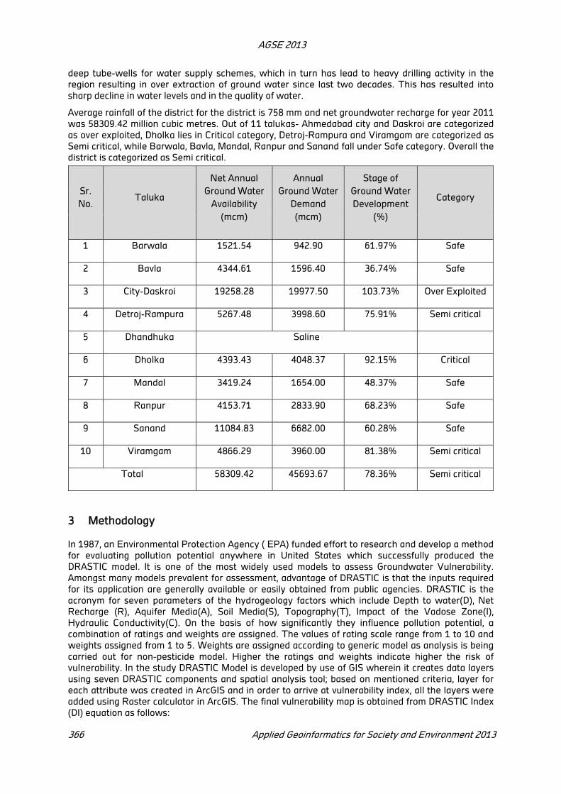
AGSE 2013


deep tube-wells for water supply schemes, which in turn has lead to heavy drilling activity in the

region resulting in over extraction of ground water since last two decades. This has resulted into

sharp decline in water levels and in the quality of water.

Average rainfall of the district for the district is 758 mm and net groundwater recharge for year 2011

was 58309.42 million cubic metres. Out of 11 talukas- Ahmedabad city and Daskroi are categorized

as over exploited, Dholka lies in Critical category, Detroj-Rampura and Viramgam are categorized as

Semi critical, while Barwala, Bavla, Mandal, Ranpur and Sanand fall under Safe category. Overall the

district is categorized as Semi critical.

Sr.

No. Taluka

Net Annual

Ground Water

Availability

(mcm)

Annual

Ground Water

Demand

(mcm)

Stage of

Ground Water

Development

(%)

Category

1 Barwala 1521.54 942.90 61.97% Safe

2 Bavla 4344.61 1596.40 36.74% Safe

3 City-Daskroi 19258.28 19977.50 103.73% Over Exploited

4 Detroj-Rampura 5267.48 3998.60 75.91% Semi critical

5 Dhandhuka Saline

6 Dholka 4393.43 4048.37 92.15% Critical

7 Mandal 3419.24 1654.00 48.37% Safe

8 Ranpur 4153.71 2833.90 68.23% Safe

9 Sanand 11084.83 6682.00 60.28% Safe

10 Viramgam 4866.29 3960.00 81.38% Semi critical

Total 58309.42 45693.67 78.36% Semi critical

3 Methodology

In 1987, an Environmental Protection Agency ( EPA) funded effort to research and develop a method

for evaluating pollution potential anywhere in United States which successfully produced the

DRASTIC model. It is one of the most widely used models to assess Groundwater Vulnerability.

Amongst many models prevalent for assessment, advantage of DRASTIC is that the inputs required

for its application are generally available or easily obtained from public agencies. DRASTIC is the

acronym for seven parameters of the hydrogeology factors which include Depth to water(D), Net

Recharge (R), Aquifer Media(A), Soil Media(S), Topography(T), Impact of the Vadose Zone(I),

Hydraulic Conductivity(C). On the basis of how significantly they influence pollution potential, a

combination of ratings and weights are assigned. The values of rating scale range from 1 to 10 and

weights assigned from 1 to 5. Weights are assigned according to generic model as analysis is being

carried out for non-pesticide model. Higher the ratings and weights indicate higher the risk of

vulnerability. In the study DRASTIC Model is developed by use of GIS wherein it creates data layers

using seven DRASTIC components and spatial analysis tool; based on mentioned criteria, layer for

each attribute was created in ArcGIS and in order to arrive at vulnerability index, all the layers were

added using Raster calculator in ArcGIS. The final vulnerability map is obtained from DRASTIC Index

(DI) equation as follows:

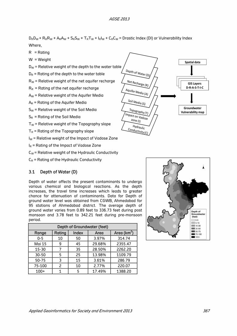
AGSE 2013


DRDW + RRRW + ARAW + SRSW + TRTW + IRIW + CRCW = Drastic Index (DI) or Vulnerability Index

Where,

R = Rating

W = Weight

DW = Relative weight of the depth to the water table

DR = Rating of the depth to the water table

RW = Relative weight of the net aquifer recharge

RR = Rating of the net aquifer recharge

AW = Relative weight of the Aquifer Media

AR = Rating of the Aquifer Media

SW = Relative weight of the Soil Media

SR = Rating of the Soil Media

TW = Relative weight of the Topography slope

TR = Rating of the Topography slope

IW = Relative weight of the Impact of Vadose Zone

IR = Rating of the Impact of Vadose Zone

CW = Relative weight of the Hydraulic Conductivity

CR = Rating of the Hydraulic Conductivity

3.1 Depth of Water (D)

Depth of water affects the present contaminants to undergo

various chemical and biological reactions. As the depth

increases, the travel time increases which leads to greater

chance for attenuation of contaminants. Data for Depth of

ground water level was obtained from CGWB, Ahmedabad for

95 stations of Ahmedabad district. The average depth of

ground water varies from 0.89 feet to 336.73 feet during post

monsoon and 3.78 feet to 342.21 feet during pre-monsoon

period.

Depth of Groundwater (feet)

Range Rating Index Area Area (km2)

0-5 10 50 3.97% 314.74

Mai 15 9 45 29.68% 2355.47

15-30 7 35 28.50% 2262.20

30-50 5 25 13.98% 1109.79

50-75 3 15 3.61% 286.79

75-100 2 10 2.77% 220.07

100+ 1 5 17.49% 1388.20

AGSE 2013


3.2 Net Recharge (R)

Recharge is the amount of water which enters the aquifer and

it is the largest pathway for contaminant transport. It will also

dilute the contaminants which enters the aquifer. Thus, more

the percolation of water in the aquifer, greater is the potential

for contaminants to increase the pollution into the aquifer.

Recharge can be calculated using climate data as:

Net Recharge = Precipitation – Evaporation – Runoff

For calculations, rainfall is considered from the data obtained

from hydrology project report, Gujarat state. Estimation of

natural ground water recharge is normally subject to errors and

no single method for recharge estimation has been yet

identified. Here, the recharge has been estimated with various

methods and average value has been considered.

Zone Chaturvedi

Method

Revised

Chaturvedi

Method

NLR technique Krishna

Rao

Method

Direct

Method

Average

R= 2.0 (P -

15)0.4

R=1.35(P -

14)0.5

R=0.63(P-

15.28)0.76

R = K (P-

X)

R=f*P

Ahmedabad

City

6.32 5.85 5.54 4.25 3.28 5.05

Barwala 6.26 5.78 5.44 4.14 3.23 4.97

Bavla 5.45 4.92 4.16 2.88 2.73 4.03

Daskroi 5.85 5.34 4.77 3.47 2.96 4.48

Detroj-

Rampura

5.88 5.37 4.82 3.52 2.98 4.52

Dhandhuka 6.26 5.78 5.43 4.14 3.23 4.97

Dholka 5.00 4.45 3.51 2.25 2.49 3.55

Mandal 5.88 5.37 4.82 3.52 2.98 4.52

Ranpur 6.76 6.33 6.30 5.06 3.60 5.61

Sanand 6.08 5.59 5.15 3.85 3.11 4.76

Viramgam 5.21 4.67 3.81 2.55 2.60 3.77

where,

R = net recharge due to precipitation during the year (inch)

P = annual precipitation (inch)

K = coefficient (0.25 for areas with P values between 23.62 to 39.37 inch)

f = infiltration factor

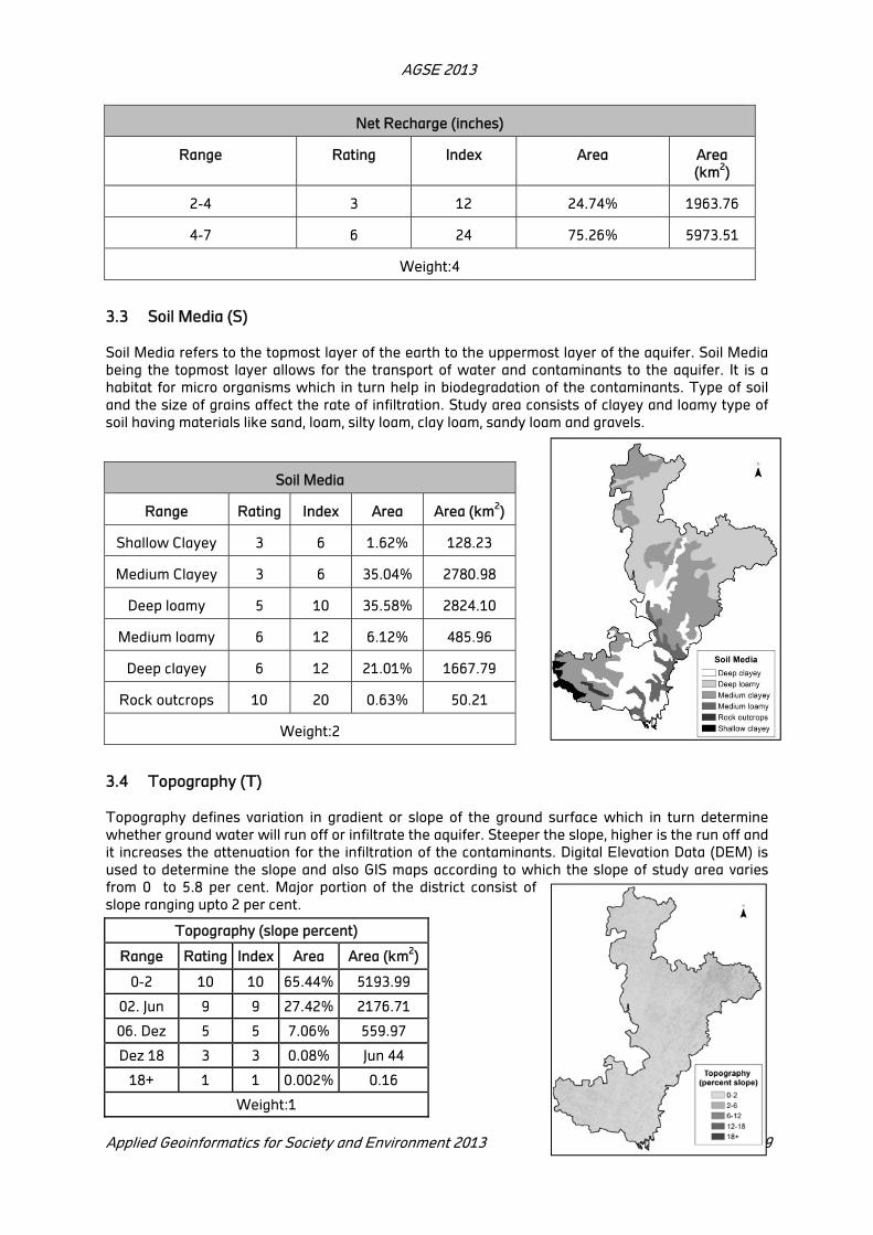
AGSE 2013


Net Recharge (inches)

Range Rating Index Area Area

(km2)

2-4 3 12 24.74% 1963.76

4-7 6 24 75.26% 5973.51

Weight:4

3.3 Soil Media (S)

Soil Media refers to the topmost layer of the earth to the uppermost layer of the aquifer. Soil Media

being the topmost layer allows for the transport of water and contaminants to the aquifer. It is a

habitat for micro organisms which in turn help in biodegradation of the contaminants. Type of soil

and the size of grains affect the rate of infiltration. Study area consists of clayey and loamy type of

soil having materials like sand, loam, silty loam, clay loam, sandy loam and gravels.

Soil Media


Shallow Clayey 3 6 1.62% 128.23

Medium Clayey 3 6 35.04% 2780.98

Deep loamy 5 10 35.58% 2824.10

Medium loamy 6 12 6.12% 485.96

Deep clayey 6 12 21.01% 1667.79

Rock outcrops 10 20 0.63% 50.21

Weight:2

3.4 Topography (T)

Topography defines variation in gradient or slope of the ground surface which in turn determine

whether ground water will run off or infiltrate the aquifer. Steeper the slope, higher is the run off and

it increases the attenuation for the infiltration of the contaminants. Digital Elevation Data (DEM) is

used to determine the slope and also GIS maps according to which the slope of study area varies

from 0 to 5.8 per cent. Major portion of the district consist of

slope ranging upto 2 per cent.

Topography (slope percent)


0-2 10 10 65.44% 5193.99

02. Jun 9 9 27.42% 2176.71

06. Dez 5 5 7.06% 559.97

Dez 18 3 3 0.08% Jun 44

18+ 1 1 0.002% 0.16

Weight:1

AGSE 2013


3.5 Impact of Vadose Zone (I)

Vadose zone is the unsaturated layer above the water table consisting of layers of bed rock as well

as surface soil without groundwater holding capacity. The

attenuation characteristic of pollution is based on permeability

of the material within the vadose zone, porosity and thickness.

The material forming the vadose zone in study area consists of

clay, sand and silt. Major portion of the district consist of Low

level alluvium followed by Coastal alluvium and High level

alluvium type of aquifer media.

Impact of Vadoze zone


High Level Alluvium 6 30 2.77% 219.54

Low Level Alluvium 7 35 56.57% 4490.40

Coastal Alluvium 8 40 40.66% 3227.33

Weight:5

3.6 Hydraulic Conductivity (C)

Hydraulic Conductivity is a rate at which material transmits

within the aquifer. It determines the rate at which contaminants

transmit from the point of contact. Hydraulic Conductivity is

affected by the gradient of the aquifer, its material and porosity.

More than one half part of the district falls in the range of 700-

1000 gpd/ft2.

Hydraulic Conductivity (gpd/ft2)


300-700 4 12 2.77% 219.54

700-1000 6 18 56.57% 4490.40

1000-2000 8 24 40.66% 3227.33

Weight:3

3.7 Ground Water Vulnerability Index

The vulnerability index computed as the sum of the products of

weights and ratings assigned to each of the input considered

above. The index ranges from 101-179. Considering Low,

Medium, High and Very high vulnerability zones entire index

range is divided into four classes 100-120, 120-140, 140-160 and

160-180, respectively. Using the mentioned classes the map was

generated which indicates following distribution pattern:

AGSE 2013


Vulnerability zone Area (km2) Area (%)

Low 1626.87 20.50

Medium 1342.61 16.92

High 3318.60 41.81

Very high 1649.20 20.78

4 Discussion

Ground water is a limited resource and already over exploited. The problem is further aggravated by

immense urban and industrial development pressure because it increases the extraction and

distribution of ground water pattern. Hence, the new development shall consider the vulnerability

index tool to determine the extent and type of development in the district.

Acknowledgement

The assistance received from Faculty of Technology, CEPT University, Ahmedabad is gratefully

acknowledged. The authors are thankful to the Central Ground Water Board, Ahmedabad for all the

data and assistance provided, which made this study possible.

REFERENCES

Abdulla M. Al-Rawabdeh, N. A.-A.-T. (2013). A GIS-Based Drastic Model for Assessing Aquifer

Vulnerability in Amman-Zerqa Groundwater Basin, Jordan. Scientific Research , 490-504.

Ahmedabad Municipal Corporation. (2014, January 07). Introduction of Amdavad. Retrieved January

07, 2014, from http://www.egovamc.com:

http://www.egovamc.com/AhmCity/introduction_Eng.aspx

C. P. Kumar, P. V. (2002). Assessment of Natural Ground Water Recharge in Upper Ganga Canal

Command Area. Journal of Applied Hydrology , 21-32.

Census of India. (2011, January 07). censusindia.gov.in. Retrieved January 07, 2014, from

http://censusindia.gov.in: http://www.censusindia.gov.in/2011-prov-results/paper2/data_files/

India2/Table_3_PR_UA_Citiees_1Lakh_and_Above.pdf

Central Ground Water Board, A. (2011). Taluka Wise Ground Water Resources, Availability,

Utilization and Stage of Ground Water Development . Ahmedabad, Gujarat, Ahmedabad.

CGWB. (2011). Ground Water Scenario in Major Cities of India.

(2009). Ground Water Resource Estimation methodology. New Delhi: Ministry of Water Resources,

Government of India. Retrieved January 09, 2014, from http://www.gwssb.org:

http://www.gwssb.org/ShowDocument.aspx?StatisticsID=4

Iuliana Gabriela Breabăn, M. P. (2012). APPLICATION OF DRASTIC MODEL AND GIS FOR

EVALUATION OF AQUIFER VULNERABILITY: STUDY CASE BARLAD CITY AREA. Water

resources and wetlands, (pp. 588-593). Tuleca - Romania.

Kommadath, A. (2000). Estimation of Natural ground water recharge. Lake 2000. Bangalore: Indian

Institute of Science.

Linda Aller, T. B. (1987). DRASTIC: A standardized system for evaluating ground water pollution

using hydogeologic settings. Oklahoma: Environmental Protection Agency.

Ronaldo Herlinger Jr, A. P. (2007). Groundwater vulnerability assessment in coastal plain of Rio

Grande do Sul State, Brazil, using drastic and adsorption capacity of soils. Environment Geology ,

819-829.

Integration of Point Cloud And Stereo Imagery For Building Footprints

Extraction

Satej Panditrao a*1

, Shefali Agrawal b1

a Centre for Environmental Planning & Technology (CEPT) University, Ahmedabad, Gujarat -380009,

India, [email protected]

b Indian Institute of Remote Sensing (IIRS), Dept. of Space, Govt. of India, Kalidas Road, Dehradun –

248001, Uttarakhand, India.

KEY WORDS: Point Cloud, feature extraction, automatic extraction, accuracy.

ABSTRACT

This study focuses on the extraction of urban terrain features including buildings and trees from two remote sensing datasets viz. OrbView-3 stereo imagery and Cartosat-1 (30 m DEM downloaded from Bhuvan). A novel and sequential multifold methodology protocol was designed for this task to analyze the feature extraction process and the outputs. Highly accurate reference point cloud data was used as ground truth, for creating DEM using OrbView-3 stereo imagery, due to its high vertical accuracy. DEM accuracy was checked by calculating difference of heights of reference point cloud and OrbView-3 DEM at few locations and followed by RMSE calculation. RMSE value obtained was 0.7648, which was very good. Bare earth height comparison of Cartosat-1 (30m) DEM and highly accurate reference point cloud was done and DEM was densified at some locations using reference point cloud. OrbView-3 and Cartosat-1 improvised DSMs were resampled successively upto 1m and then they are converted to .las file for feature extraction. Point clouds were processed and building footprints were extracted from both the datasets. Comparative assessment of building footprint as well as height extraction from these datasets was done. Heights of buildings automatically extracted from improvised DSMs and that of manually digitized using OrbView-3 stereo imagery in 3D mode were compared and effectiveness of improvised DSMs in terms of accuracy (enhancement in the level of accuracy) is checked. Completeness and Correctness values (qualitative assessment) calculated for building extraction in both the datasets gave good results. So, it can be concluded that OrbView-3 gives better results than Cartosat-1(30m DEM) and Cartosat-1 (30m DEM) can be used for automatic feature extraction where general level accuracy is required.

1 Introduction

As the world is continuously expanding, urbanization has become the topic of advanced research and

use of remote sensing and GIS in advanced urban planning has been implemented by ample number

of institutions across the globe. New and innovative techniques are being developed every day and

research community in the world is making immense efforts and so many algorithms are being

developed for their use. Photogrammetry and Point Cloud data processing are two of such

technologies, which are not so new, but new methodologies are being designed for data processing

and their applications in diverse areas like 3D modelling, feature extraction, environmental modelling

and so on. Urban feature extraction using the high resolution satellite imagery provided by numerous

satellites is a much talked about and vast research topic in which, various algorithms and ideas have

been developed so far and are still developing making this topic more and more thought provoking

and application oriented. Photogrammetry and stereo analysis are the two important techniques for feature extraction and due to 3D information extraction from these techniques; feature extraction

process has become highly efficient. As the name suggests, feature extraction deals with

identification, categorization, segmentation and delineation of various features in a particular scene

depending upon the algorithms and workflows used.

AGSE 2013


2 Study Area

In this study, Bhubaneswar city was chosen as the study area. It is the capital of Orissa state and has

urbanized set-up consisting of different types of buildings. Effectiveness of algorithms and methods

used in this study was checked using this study area.

Figure 1: Image of the study area

3 Methodology

In this study, three datasets were used. Reference Point Cloud, OrbView-3 stereo imagery and

Cartosat-1 (30m DEM). Using Photogrammetric techniques, DSM was created from OrbView-3

stereo imagery. For this task, points from reference point cloud were used as Ground control points,

due to their highly accurate elevation values. These points were taken from various landcover

classes so as to get effective and unbiased results.The resulted DSM was then resampled to 1m

using suitable resampling technique. Point Cloud was created from this DSM using LAS tools for

ArcGIS and this point clous was processed using Microstation and Terrasolid softwares, to extract

building footprints. Scene specific criteria were used for this extraction. In case of Cartosat-1 (30m)

DEM, reference point cloud was used to densify it. Using “extract values to points tool” from ArcGIS,

this densification was done and DSM raster created from highly accurate reference point cloud was

used as a base raster to extract values from it to a point shapefile. This shapefile was then converted

to raster and subsequently resampled it to 1m. Point Cloud was also created from this raster and

similar processing was carried out with this point cloud also to extract building features. For this

study, 3D point cloud extracted from very high resolution camera imagery (Aerial) was used as the

ground truth. Leica Photogrammetry Suite’s Enhanced Automatic Terrain Extraction (eATE) was

used to extract point cloud from the aerial imagery. Highly accurate DSM (~10 cm) was created from

this point cloud and building footprints were extracted. Height and area thresholds were defined for

building extraction using aerial, Orbview-3 and Cartosat-1 point clouds, depending on which

AGSE 2013


automatic extraction of building footprints was performed. Differentiating ground and non-ground

points was the most critical task and various filters have so far been used for this task.

Morphological filter, slope based filter, Interpolation based filter.

(a) (b)

Figure 2: Point cloud from (a) OrbView-3 DSM (b) Cartosat-1 DSM

(Chen et al., 2007) which uses weighted linear least squares interpolation to iteratively approximate

the terrain surface. Here, algorithm designed by LAStools for ArcGIS has been used to differentiate

ground and non-ground points. Area threshold is important while extracting buildings. Filtering of

the points is done using such threshold, which is nothing but the parameter used in Morphological

filter (Liu, 2008). Buildings can be differed from vehicles, noise etc. if the area value is smaller than

the threshold value and features like road, river can be differed from buildings whose area is

definitely bigger than the highest threshold set for the buildings. Similarly, height thresholds were

defined for trees, scrubs to discriminate then from buildings. Coplanarity and Collinearity are also

important in case of building planes, which are not prominent in case of tree or vegetation points.

Texture variance for trees and Minimum difference between returns for trees are other important

parameters used for building extraction.

4 Results

Total Image RMSE = 0.79 Pixels

Control Point RMSE Check Point RMSE

Ground X: 0.38 (13)*

Ground X: 0.54 (2) *

Ground Y: 0.46 (13) * Ground Y: 0.49 (2)

*

Ground Z: 0.46 (13) * Ground Z: 0.73 (2)

*

Image X: 0.67 (26) * Image X: 0.96 (4)

*

Image Y: 0.71 (26) * Image Y: 0.88 (4)

*

Table 1: Satellite Triangulation result.

Table 1 shows satellite triangulation result. Terrain Editor was used to remove the erroneous points

from the DSM and improve the accuracy of DSM. Accuracy of Digital Surface Model (DSM) is checked

by using following formula (Bhardwaj, A., Chatterjee, R., Jain K., (2013)).

…………….. 1)

Where, n is the number of observations or DGPS points. Here, reference point cloud points were

used instead of DGPS points at few location. 15 points from reference point cloud were used as

GCPs. So,n =15, RMSE obtained here was 0.2648 pixels. RMSE value was less than one, so the

accuracy of DSM was good.

AGSE 2013


Figure 3: Building footprints extracted from (a) OrbView-3 DSM (b) Cartosat-1 DSM

4.1 Different Types of Extracted Buidings

4.1.1 Closely spaced buildings

(a) (b) (c) (d) (e) (f)

4.1.2 Isolated Buildings

(a) (b) (c) (d) (e) (f)

4.1.3 Buildings which are complex in shape

(a) (b) (c)

AGSE 2013


4.1.4 Buildings which are definite in shape

(a) (b) (c) (d) (e) (f)

4.2 Copleteness and Correctness

Completeness and Correctness are the measures of accuracy assessment for buildings extraction.

For determining these quantities, True Positives (TP), True Negatives (TN), False Positives (FP) and

False negatives (FN) were calculated based on the rules defined in terms of threshold values of

height and area. True Positives are nothing but the buildings which are correctly extracted, False

Positives are the buildings which are falsely extracted, True Negatives are the buildings which are

correctly rejected and False Negatives are buildings which are falsely rejected. Completeness refers

to how many buildings have been extracted from the actual (total) number of buildings, whereas

Correctness refers to the chance/probability of a feature being extracted as a building.

So, Completeness = and Correctness =

OrbView-3 Cartosat-1

Completeness = 94% Completeness = 86%

Correctness = 91.26% Correctness = 75.43%

5 Conclusion

From the results obtained in this study, it is seen that, OrbView-3 stereo data has given much better

results as compared to Cartosat-1 in different types of urban set ups. Cartosat-1 data fails to

discriminate the closely spaced buildings due to low point density which is attributed to its low

spatial resolution. From the completeness and correctness values of the automatically extracted

building footprints, which are 94% and 91.26% for OrbView-3 & 86% and 75.43% for Cartosat-1

respectively, it can be concluded that, OrbView-3 dataset gives results which are very much closer

and consistent with the reference data used in this study (highly accurate point cloud) and with the

manually digitized features in 3D mode. In addition to that, there is a misclassification between

buildings and trees in Cartosat-1, where these two types of features are very closely spaced. Thus,

Cartosat-1 dataset can be used for feature extraction where general level accuracy is required. So, in

a nutshell, it can be claimed that, point cloud density, spatial resolution, availability of textural and

contextual information, filtering algorithms are the factors affecting the accuracy of the feature

extraction results. Though the results obtained from Orbview-3 are better than Cartosat-1, there are

still some problems like misclassification between buildings and trees (which is more prevalent in

Cartosat-1), errors in automatic building extraction (Cartosat-1 has more errors) etc.

Such errors could have been eliminated to a greater extent by using high resolution multispectral

imagery, which can give contextual and textural information about the features which is important in

the filtering of the point cloud data. In addition, such additional datasets would have been useful in

building up a knowledge base, so that comparison between Object Based Information Extraction and

Knowledge Based Information Extraction could be done to get more accurate results.

Dense Image Matching can be a solution in case of making DSM from photogrammetric techniques.

As the redundancy of data increases, the spatial resolution of the DSM increases, which in turn

increases the quality of building extraction.

AGSE 2013


REFERENCES

Bhardwaj, A., Chatterjee, R., Jain K., (2013). Evaluation of cartosat-1 satellite triangulation & DSMs in

varied terrain conditions. Science Research. Vol. 1, No. 2, 2013, pp. 19-24. doi:

10.11648/j.sr.20130102.12

Chen, Q., Gong, P., Baldocchi, D. and Xin, G. 2007. Filtering airborne laser scanning data with

morphological methods. Photogrammetric Engineering and Remote Sensing 73(2), 175-185.

Liu, X. (2008). Airborne Point cloud for DEM Generation: Some Critical Issues. [Electronic version].

Progress in Physical Geography, 32(1), 31-49

Quantitative Evaluation of Tree Feature Detection Capability Of Airborne

Lidar Using Very High Resolution Worldview-2 Satellite Remote Sensing

Data

Shridhar D. Jawaka*

, Satej N. Panditraob1

and Alvarinho J. Luisa

a Earth System Sciences Organization (ESSO), National Centre for Antarctic and Ocean Research,

Ministry of Earth Sciences, Govt. of India, Headland Sada, Vasco-da-Gama, Goa– 403804, India,

[email protected]; [email protected] b

Centre for Environmental Planning & Technology (CEPT) University, Ahmedabad, Gujarat -380009,

India, [email protected]

KEY WORDS: WorldView-2; LiDAR; feature extraction

ABSTRACT

We introduce a workflow for tree feature detection from airborne light detection and ranging (LiDAR) point cloud data and evaluate its accuracy using very high resolution PAN (spatial) and multispectral information of 8-band WorldView-2 imagery. LiDAR point cloud data is used to detect

tree features by classifying point elevation values. We applied a very well known method for individual tree crown delineation based on canopy height model (CHM) from the high resolution airborne LiDAR. The technique used here includes conversion of LAS file which contains LiDAR point cloud to raster/DEMs, generating the hillshade image, extracting bare earth and its editing, and finally, extraction of trees and forests. Scene dependent criteria have been used to improve the extraction results. Refining/ filtering technique used for bare earth layer were crucial, since it helped in improving the subsequent feature extraction steps. The PAN-sharpened WorldView-2 image was used to assess the accuracy of tree feature targeting using LiDAR data. The accuracy of LiDAR tree extraction amounted to 98% which is highly acceptable in remote sensing applications; so we conclude that the tree feature extraction using LiDAR is a potential application which can be used in understanding vegetation structure in various remote sensing applications.

1 Introduction

LiDAR is nowadays very effective and prolific technology as far as detailed mapping and modeling of

various types of terrain is concerned. It’s an efficient technique to map and model the vegetation

cover and trees located in the landscape. Forest resource management and its impact on various

regions is a very critical aspect and LiDAR is a very conducive tool to explore that. Individual tree

crown delineation and tree parameter extraction is a complex research topic and various methods

have been implemented for this task. LiDAR systems along with precise positioning and orientation

systems can obtain highly accurate 3D measurements of earth surface in the form of point cloud

data by using high sampling densities (NOAA, 2012).Individual trees extraction is the matter of this

study, which is highly important as far as its significant applications in ecology, environmental

sciences and forestry are concerned. Various parameters associated with the trees like tree height,

crown diameter, canopy based height, diameter at breast height (DBH), biomass, and species type

can be determined after individual extraction of trees. There are various traditional methods which

include forest inventory, aerial photography interpretation which require intensive field work and

large amount of financial support (Blaschke et al., 2006) This can be replaced by airborne LiDAR

along with very high resolution satellite imagery, which can also reduce the time consumption, labor

and enhance geographical accessibility to a significant extent (Lee et al., 2009; Rahman and Gorte,

2009; Rahman et al.2009; Rahman and Gorte, 2008).

2 Study Area

In order to determine and estimate the effectiveness of LiDAR based tree feature extraction, we

selected the part of San Francisco city, California, United States of America (37° 44" 30N', 122°

31" 30' W and 37° 41" 30'N ,122° 20" 30' W ), as a test scene. It is a highly urban area which consists

AGSE 2013


of large number of tall buildings as well as other urban features like stadiums, roads, bridge and

vegetation/trees.WorldView-2 image of the study area captured on 9th

October, 2011 is shown in

Figure 1. Necessary pre-processing methods like Data Calibration, Dark-pixel Subtraction, PAN-

sharpening etc. were employed for better visualization.

3 Methodology

LiDAR point cloud processing and feature extraction followed by its validation using hyper spatial, 8-

band WorldView-2 imagery is the crux of this study. Gram-Schmidt PAN Sharpening algorithm was

employed for PAN Sharpening of WV2 imagery and Supervised Classification using SVM classifier

was done which resulted in > 99% accuracy. Several algorithms have been employed for LiDAR point

cloud processing before by the researchers. Two important assumptions that should be taken into

consideration while point cloud processing are: 1) earth surface is smooth and continuous, 2)

neighboring point cloud data are co-related. Deterministic and Geostatistical are the two methods for

LiDAR point cloud processing. Deterministic methods assume that each input LiDAR point has a local

weight with the spatial distance (Liu, 2008), on the other hand geostatistical methods consider the

spatial distance as well as the spatial correlation for interpolating the LiDAR point data (Anderson et al., 2005).In this study, we used a method for individual tree delineation based on canopy height

model (CHM) from the high resolution airborne LiDAR point cloud data. To investigate the

algorithm’s effectiveness in extracting individual trees, we used very high resolution remote sensing

data from WorldView-2 satellite. This study aims to assess the accuracy of individual tree extraction

using LiDAR by visual interpretation of trees onto very high resolution WorldView-2 image. LiDAR

point cloud is shown in figure 2. Individual tree delineation consists of three main steps, namely 1)

extraction of digital terrain model (DTM) and normalization of point clouds, 2) individual tree crown

delineation, and 3) tree filtering. Scene specific criteria were used in this study and effectiveness of

these criteria was checked, and the results of which are shown in the Table 1 and 2


AGSE 2013


Figure 2: Representation of LIDAR point cloud

Table 1:.Criteria used for bare earth, buildings and trees extraction

Steps Criteria

Bare Earth extraction method Raster or Point Clouds

Pre-processing Auto-detect no-data

regions

Return filter All returns

Remove buildings with area less than 30 m2

Remove buildings with area more than 35000 m2

Remove buildings with height less than 2.2°

Minimum slope for building roofs 15°

Maximum slope for building roofs 40°

Texture variance for trees 80%

Minimum difference between returns for

trees

0

Smoothing tolerance 1 m

Minimum height for tall buildings 15 m

Tree extraction method Variable window search

Predominant tree/forest type Mixed

Minimum tree height 3 m

Maximum tree height 40 m

Minimum size of the forest 600 m2

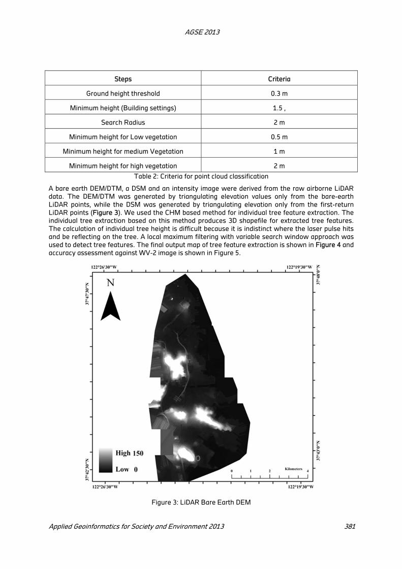
AGSE 2013


Steps Criteria

Ground height threshold 0.3 m

Minimum height (Building settings) 1.5 ,

Search Radius 2 m

Minimum height for Low vegetation 0.5 m

Minimum height for medium Vegetation 1 m

Minimum height for high vegetation 2 m

Table 2: Criteria for point cloud classification

A bare earth DEM/DTM, a DSM and an intensity image were derived from the raw airborne LiDAR

data. The DEM/DTM was generated by triangulating elevation values only from the bare-earth

LiDAR points, while the DSM was generated by triangulating elevation only from the first-return

LiDAR points (Figure 3). We used the CHM based method for individual tree feature extraction. The

individual tree extraction based on this method produces 3D shapefile for extracted tree features.

The calculation of individual tree height is difficult because it is indistinct where the laser pulse hits

and be reflecting on the tree. A local maximum filtering with variable search window approach was

used to detect tree features. The final output map of tree feature extraction is shown in Figure 4 and

accuracy assessment against WV-2 image is shown in Figure 5.

Figure 3: LiDAR Bare Earth DEM

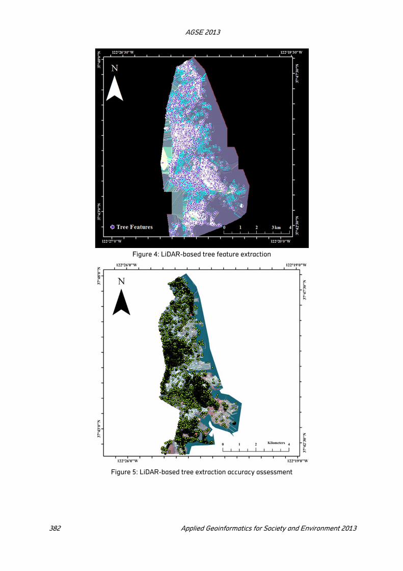
AGSE 2013


Figure 4: LiDAR-based tree feature extraction

Figure 5: LiDAR-based tree extraction accuracy assessment

AGSE 2013


4 Results

A 8-band WV-2 image was used for visual interpretation of LiDAR-classified tree features. The

image was PAN-sharpened and georeferenced which helped in proper visualization of LiDAR tree

points. In addition, the WV-2 image was orthorectified, which enhanced the accuracy of the result.

The results depicted in Table 3 show that 15143 tree features were extracted by CHM method using

LiDAR point cloud data. All the tree features extracted using LiDAR data were cross-verified using

multitemporal high resolution image, which indicates that the 14841 tree features were correctely

interepreted out of 15143 tree features. The overall accuracy of LiDAR based tree feature extraction

was found to be 98% against the high resolution satellite image as a reference. A DSM-based

shadow mask was used for reducing the potential source of error due to topography-based shadow

in high resolution image.1011 tree features under shadow were cross-verified using multitemporal

image data. LiDAR-based extraction caused over-estimation of 302 tree features, which can be

atttributed to two methodological and experimental limitations: 1) the present research was carried

out using scene dependent criteria which should be optimized with trial-and-error method, and 2)

the error might be propogated during the LiDAR filtering or classificationprocess.For optimal tree

feature extraction, we propose the rigorous optimization of criteria and synergetic usage of high

resolution data for tree feature extraction in future studies.

Attribute Value

Total tree features extracted from LiDAR by using CHM method 15143

Total tree features visually interpreted using multitemporal image

data

18841

Overall accuracy for tree feature extraction 98%

Table 3:.Statistics for LiDAR based tree feature extraction accuracy results

5 Conclusion

The high resolution airborne LiDAR data provides tremendous potential for tree feature extraction in

urban landscape and the hyperspatial WV-2 imagery supplements the accuracy assessment

procedure. The objective of this study was to evaluate CHM-based tree-feature extracting accuracy

by visual interpretation/ identification on 8-band WorldView-2 image. Our study uses the algorithm

developed by Overwatch system’s LiDAR Analyst for ArcGIS for LiDAR feature extraction and

classification with scene dependent criteria. The 8-band WorldView-2 image provides better

recognition and extraction of various land-cover features and due to the inclusion of new bands in the

imagery, the vegetation analysis becomes more effective.The present study provides following

conclusions. (1) Texture variance for trees and minimum difference between returns for trees turned

out to be the two most important factors in discriminating the tree and building features in the LiDAR

data. (2) Preprocessing of the WV-2 image improved the visualization of vegetation features. (3)

LiDAR data was found to be capable of extracting shadow-covered tree features. (4) LiDAR point

cloud data can be used in conjunction with satellite image data for supporting tree feature

extraction.The research highlights the usefulness of the commonly used methodology for the LiDAR

data processing and the effectiveness of 8-band WorldView-2 remotely sensed imagery for accuracy

assessment of LiDAR-based tree-feature extraction capability.

REFERENCES

Anderson, E. S., Thompson, J.A., &Austin,R. E. 2005.LiDAR density and linear interpolator effects on

elevation estimates, International Journal of RemoteSensing, Vol. 26, No. 18, pp. 3889-3900.

http://dx.doi.org/10.1080/01431160500181671

Blaschke, T., Lang, S., Tiede,D.,& B. Maier. 2006. 3D Forest structure analysis from optical and

LIDAR data, RevistaAmbiência, Guarapuava, v.2 Edição Especial, Vol. 1, pp. 95–110.

AGSE 2013


National Oceanic and Atmospheric Administration (NOAA) Coastal Services Center. 2012. Lidar 101:

An Introduction to Lidar Technology, Data, and Applications.Revised. Charleston, SC: NOAA

Coastal Services Center.

Lee,S.-J., Chan, Y.-C., Komatitsch, D., Huang,B.-S.,& J. Tromp.2009. Effects of realistic surface

topography on seismic ground motion in the Yangminshan region of Taiwan based upon the

spectral-element method and LiDAR DTM, Bulletin of theSeismological Society of America, Vol.

99, No. 2A, pp. 681–693. http://dx.doi.org/10.1785/0120080264

Liu, X., 2008. Airborne Point cloud for DEM Generation: Some Critical Issues,Progress in Physical Geography, Vol. 32, No.1, pp. 31-49. http://dx.doi.org/10.1177/0309133308089496

Rahman, M.Z.A., Gorte, B. G. H., & Bucksch, A.K. 2009. A new method for individual tree delineation

and undergrowth removal from high resolution airborne LiDAR, Proceedings ISPRS Workshop

Laserscanning 2009, September 1-2, France, IAPRS, Vol. XXXVIII (3/W8), p.283-288.

http://www.isprs.org/proceedings/XXXVIII/3-W8/papers/p52.pdf

Rahman, M.Z.A. and Gorte, B.G.H., 2009. Tree crown delineation from high-resolution airborne

LiDAR based on densities of high points, Proceedings ISPRS Workshop Laserscanning 2009,

September 1-2, France, IAPRS, Vol. XXXVIII (3/W8), p.123-128.

http://www.isprs.org/proceedings/XXXVIII/3-W8/papers/p51.pdf

Rahman, M.Z.A. and Gorte, B., 2008. Tree filtering for high density Airborne LiDAR data. In: R. Hill, J.

Rosette and J. Suarez (Editors), Proceedings of the Silvilaser 2008: 8th international conference on

LiDAR applications in forest assessment and inventory, 17 – 19 September, Heriot-Watt

University, Edinburgh, UK, pp. 544-553.

Acknowledgement

We are indebted to the organizers of the IEEE GRSS Data Fusion Contest (2012), who provided the

research platform and images to our research team free of cost. We also acknowledge Dr. Rajan,

Director, NCAOR, Dr. R. Ravindra, ex-Director, NCAOR, and Prof. Anjana Vyas, CEPT University for

their encouragement and motivation for this research. This is NCAOR contribution no. 21/2013

Integration of GIS, GPS and RS (3S) Tech-Stick for Visually Impaired

Alex Praveen P,

B.E., GeoInformatics Engineering (4th year), Department of Civil engineering, Regional Centre of

Anna University Chennai, Tirunelveli-7, Alex Praveen P, email: [email protected]

KEY WORDS: Tactile display; Microcontroller; Global System for Mobile communication (GSM);

Geographic Information System (GIS); Global Positioning System (GPS); Ultrasonic sensor.

ABSTRACT

Blind and visual impaired face many problems during their daily activities with navigation. Integration of GIS, GPS and RS (3S) brings new perspective to applications interrelated. This paper includes a theoretical model to provide a technological aid for visually impaired people. It inherits new technologies as, Global System for Mobile Communication (GSM) that incorporates the Global Positioning System (GPS), the Geographic Information Systems (GIS) & Remote sensing (RS), Ultrasonic sensors for obstacles detection and resulting in 3-D tactile display, a vocal communication interface to guide visually impaired users and help them travel also in unfamiliar environments independently and safely & to avoid possible obstacles. The aim of the overall system is to provide a low cost and efficient navigation aid. This theoretical model is designed to enrich the user’s real world navigation experience by augmenting their reality through vocal interfaces with related information about their prerequisite destination path. This paper describes the Tech-Stick system and emphases on easy, cheap & effective navigation design for visually impaired.

1 Introduction

With reference to the WHO June, 2012 dated report, 285 million people are visually impaired

worldwide. 39 million are blind & 246 have low vision. About 90 percent of the visually impaired live

in developing countries. 80 percent of them can be avoided or cured. India accounts 20 percent of

global blind.

Blind and visual impaired face many problems during their daily activities with navigation. Integrating

GIS, GPS & RS brings new perspective to applications interrelated. Using tactile display makes it

further more easily for the visually impaired. None of previous systems works seamlessly both

indoors & outdoors. Tech-Stick uses a precise position measurement system, a Tactile display, GSM

and a vocal communication interface to guide visually impaired users and help them travel also in

unfamiliar environments independently and safely. The user can get vocal prompts to avoid possible

obstacles. This paper describes the Tech-Stick system and emphases on easy, cheap & effective

navigation design for visually impaired.

This theoretical model is designed to enrich the user’s real world navigation experience by

augmenting their reality through vocal interfaces with related information about their prerequisite

destination path. Voice recognition, wireless communication, GIS, GPS, and ultrasonic sensor, tactile

display devices have made our goal possible.

2 Specification of Tech-Stick

The proposed system consists of a GPS, a tactile display, Ultrasonic sensor, Microcontroller, GSM &

GIS service. This system is explained separately in detail. They are as follows:

2.1 Global Positioning System (GPS)

GPS is a more common technology today & a valuable asset for society to find location & direction for

navigation easily also in unfamiliarised place. User must receive signals from minimum of 3 satellites

& 4 satellites for accuracy. Many automobiles are equipped with GPS system. A driver can get Turn-

AGSE 2013


by-turn directions to any destination nationwide. Furthermore, Individual calls 911 from GPS-enabled

cellular phones, emergency personnel can easily identified the caller’s location.

Former practically composed system for visually impaired people reviewed & evaluated by

International Braille and Technology Centre (IBTC). The three recent systems are: 1) Trekker, 2)

PAC mate GPS, 3) A Braille note GPS. These systems lags somewhat, make the visually impaired to

find it difficult to use.

2.2 Tactile Display

Tactile display is a latest technology which uses a microfluidic technology on a flat screen of smart

phones. Where, the tactile panel replaces the glass / plastic that usually sits above the touch screen

sensor & display on a touch screen device. Some channel in the panel is filled with transparent fluid

which expands upwards in the shape of the button when the pressure is increased & falls back to a

flat screen when pressure is decreased.

The keys will be hard enough to type with rest of their fingers on. Rise & fall of the keys will take

less than a second & can be controlled either by proximity sensor or an application on the device.

California based company “Tactus” developed this display in smart phones. This will be expected to

be in the market in late 2013 or early 2014.

This technology could also revolutionize game controllers, television cars & the limited nature of

smart phones & other applications for blind & visually impaired people all over the world.

2.3 Microcontroller & Ultrasonic sensors

Microcontroller (abbreviated as MCU) is a small computer on a single integrated chip containing

processor core, memory, and programmable, input/output peripherals. Typically a small amount of

RAM. MCU’s are designed for embedded applications.

They consume little power (mill watts), economical & long lasting battery makes them ideal for

applications.

Ultrasonic sensors is also known as transceiver/transducer, they both send & receive. They works on

the principle of RADAR / SONAR. They generate high frequency sound waves & evaluate the echo

received by the sensor.

Ultrasonic waves range above 18,000 hertz. This sensor turns sound waves (echo) to electrical

energy on receiving & vibrates in presence of obstacles.

2.4 Geographical Information System (GIS)

Geographical Information System (GIS) is a system designed to store, manipulate, analyze, and

manage all types of geographical data. GIS is developed for an application.

GIS application tools allow users to create interactive queries, analyze spatial information, edit data

in maps & present the result of all these operations.

2.5 Global System for Mobile communication (GSM)

Global System for Mobile communication (GSM) is a open digital cellular technology used for

transmitting mobile voice & data service.

GSM supports voice calls & data transfer speed of up to 9.6 kbps together with the transmission of

SMS.

AGSE 2013


3 Former Methodologies Used

3.1 Dishthri: An Integrated indoor /outdoor blind navigation system

This system provides the user, dynamic interactions & adaptable to work on both indoor & outdoor.

DGPS is used outdoor & ultrasonic sensor is used indoor to navigate at accuracy of 22 cm.

Flaws of the Dishthri system is user can predict orientation, distance & direction but at times,

outdoor routes subject to change will vary from the database stored in it. So, reroute is required

frequently to the database & instruments are fitted in the head of the user results in height error.

3.2 Braille Note GPS

Braille Note GPS is a speech & a braille output of PDA with an add-on GPS software & hardware

package. It’s very much expensive device nearly $5800 & much more complicated.

3.3 Trekker breeze

Trekker breeze version costs of approximately $1000 & fewer functions only available.

Trekker 3.0 is less weight, small averagely costs of $2000 but only fewer functions of GPS & PDA

(Personal Digital Assistant).

3.4 PAC mate street talk

PAC mate street talk 2.0 add-on to a pocket pc with voice & braille output. Cheaper than Braille Note

GPS. But not functional as Braille Note GPS. Its cost approximately of $4400.

3.5 Cell phone GPS

Cell phone GPS technology can be useful but have cramped interface & limited functions. Also, cell

phone GPS is not accurate as other systems. Modern technology smart phones using

GPS+GLONASS (Russian satellites) have high accuracy.

Phones such as Samsung Galaxy Note, the S3, the Google Nexus, the iPhone 5, & several others. But,

they are unaffordable by its cost.

4 Methodology of Tech-Stick Proposed

To achieve this Tech-stick System for visually impaired we device a novel system that is based on

the interplay of the RS, GIS, GPS and GSM technologies.

The GPS is a satellite-based navigation system made up of 24 satellites placed into orbit by the U.S.

Department of Defense. The location of the GPS receiver is determined using the satellite positions

as reference points. Tracking system can be utilized in identifying the position of visually impaired

person on the roads who is searching his way to a destination. With the advanced wireless

communication the information provided by a GPS & the query inquired by user as voice could be

transferred to a GIS server to answer the queries of the visually impaired and guide him to his

intended destination.

Thus, the Queries inquired by the user is send to the GIS by GSM modem. Then, the optimal path is

determined by the GIS server by using the automated algorithm. The result attained is processed &

send to the user.

Since the current visual displays are not perceivable by them we require a display that can be

perceived by the sense of touch. Best idea would be to provide a tactile based display of the plotted

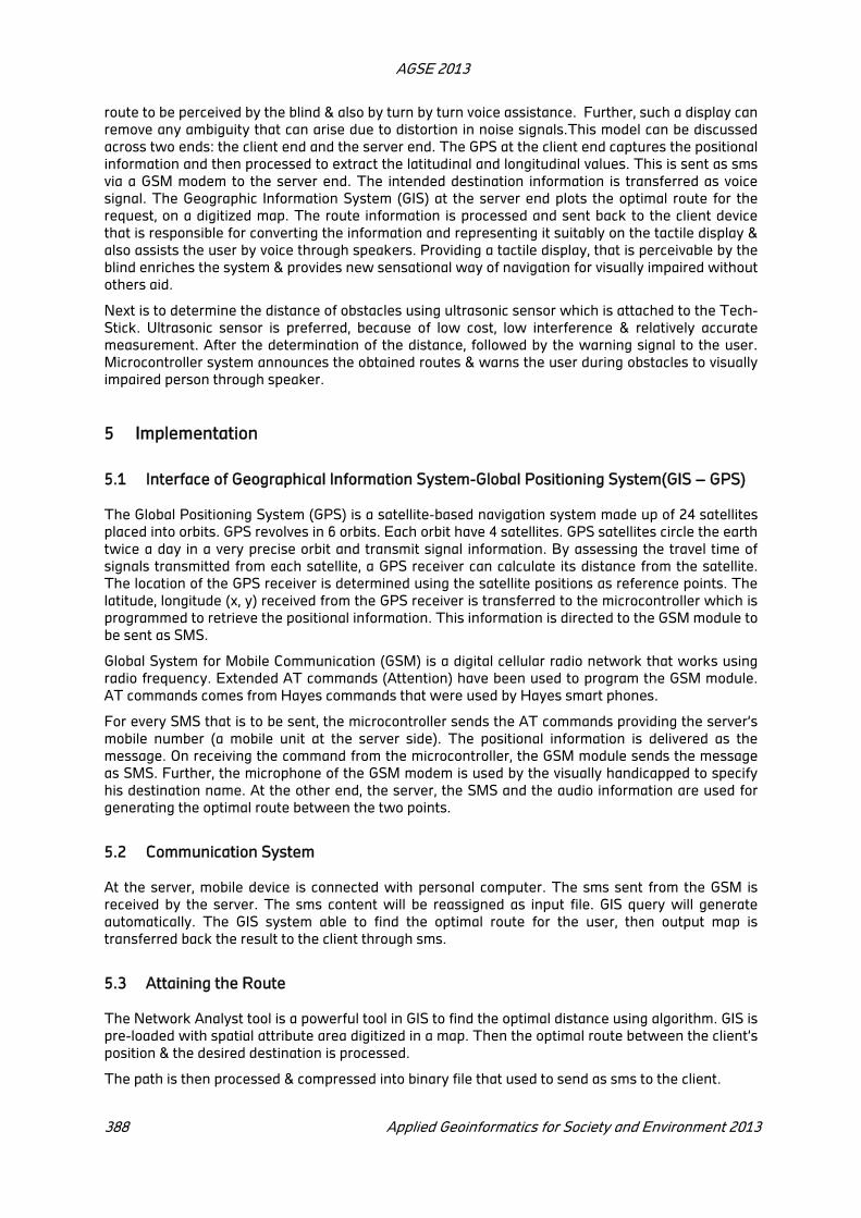
AGSE 2013


route to be perceived by the blind & also by turn by turn voice assistance. Further, such a display can

remove any ambiguity that can arise due to distortion in noise signals.This model can be discussed

across two ends: the client end and the server end. The GPS at the client end captures the positional

information and then processed to extract the latitudinal and longitudinal values. This is sent as sms

via a GSM modem to the server end. The intended destination information is transferred as voice

signal. The Geographic Information System (GIS) at the server end plots the optimal route for the

request, on a digitized map. The route information is processed and sent back to the client device

that is responsible for converting the information and representing it suitably on the tactile display &

also assists the user by voice through speakers. Providing a tactile display, that is perceivable by the

blind enriches the system & provides new sensational way of navigation for visually impaired without

others aid.

Next is to determine the distance of obstacles using ultrasonic sensor which is attached to the Tech-

Stick. Ultrasonic sensor is preferred, because of low cost, low interference & relatively accurate

measurement. After the determination of the distance, followed by the warning signal to the user.

Microcontroller system announces the obtained routes & warns the user during obstacles to visually

impaired person through speaker.

5 Implementation

5.1 Interface of Geographical Information System-Global Positioning System(GIS – GPS)

The Global Positioning System (GPS) is a satellite-based navigation system made up of 24 satellites

placed into orbits. GPS revolves in 6 orbits. Each orbit have 4 satellites. GPS satellites circle the earth

twice a day in a very precise orbit and transmit signal information. By assessing the travel time of

signals transmitted from each satellite, a GPS receiver can calculate its distance from the satellite.

The location of the GPS receiver is determined using the satellite positions as reference points. The

latitude, longitude (x, y) received from the GPS receiver is transferred to the microcontroller which is

programmed to retrieve the positional information. This information is directed to the GSM module to

be sent as SMS.

Global System for Mobile Communication (GSM) is a digital cellular radio network that works using

radio frequency. Extended AT commands (Attention) have been used to program the GSM module.

AT commands comes from Hayes commands that were used by Hayes smart phones.

For every SMS that is to be sent, the microcontroller sends the AT commands providing the server’s

mobile number (a mobile unit at the server side). The positional information is delivered as the

message. On receiving the command from the microcontroller, the GSM module sends the message

as SMS. Further, the microphone of the GSM modem is used by the visually handicapped to specify

his destination name. At the other end, the server, the SMS and the audio information are used for

generating the optimal route between the two points.

5.2 Communication System

At the server, mobile device is connected with personal computer. The sms sent from the GSM is

received by the server. The sms content will be reassigned as input file. GIS query will generate

automatically. The GIS system able to find the optimal route for the user, then output map is

transferred back the result to the client through sms.

5.3 Attaining the Route

The Network Analyst tool is a powerful tool in GIS to find the optimal distance using algorithm. GIS is

pre-loaded with spatial attribute area digitized in a map. Then the optimal route between the client’s

position & the desired destination is processed.

The path is then processed & compressed into binary file that used to send as sms to the client.

AGSE 2013


5.4 Display Module

Tactile display provides the route information to the client. The module used to convert the binary

file to observe the route information in the tactile display. The Microcontroller is programmed to

facilitate this process. This methodology is explained in the figure1 below.

Figure1: Tech-stick component Architecture

6 Observations

This paper proposed the design & architecture of innovative Tech-stick is combination of GPS, GIS,

GSM, and RS technologies in an effective & in practically possible ways. Advantages of the system

lies in the fact that it can prove to be very low cost solutions to millions of visually challenged people.

This makes the users to navigate safe & secure without human assistance.

CLIENT

GPS (X, Y)

Destination by

(X, Y) & destination

send by sms

SERVE

Obtaining (X,Y),

Structure a route-

Map prepared &

send to device Optimal route-

Map processed

Figure2: Flowchart of the system

AGSE 2013


7 Conclusion

GPS has been widely used these days mainly for tracking purposes, models like this enable many

new application for the GPS. Further, the inheritance of the GSM services with GPS, GIS technologies

provides Location Based Services (LBS) for route guidance & RS to avoid obstacles in the way for the

visually impaired. The Tactile device used for the purpose making it easier for them to understand

the route and navigate without human & dog assistance.

REFERENCES

John Roberts & Oliver Slattery, A New Refreshable Tactile Graphic Display Technology for the Blind

and Visually Impaired, National Institute of Standards and Technology.

Smartstick for Blind by S Dambhare research.ijcaonline.org/ncict/number6/ncict048.pdf

R Dan Jacobson, Postgraduate researcher, Institute of Earth Studies, University of Wales, Navigation

for the visually handicapped: Going beyond tactile Cartography.

GIS: A Visual Approach, Authors: Bruce Ellsworth Davis, Bruce Davis, Published by Delmar

Publishers ISBN: 076682764X

A Practical Guide to Geo statistical Mapping. Author: Tomislav Hengl, Publisher : University of

Amsterdam

World Health Organisation (WHO) www.who.int

http://seminarprojects.com/Thread-smart-stick-for-blind-obstacle-detection-artificial-vision-and-

real-time-assistance#ixzz2OeP0gWVs

Tactile display www.tactustechnology.com/technology

Acknowledgements

I hereby acknowledge & thankful to all who had been assisting & motivating me to promote my idea

to this level.

Customization of Normalized Difference Snow Index For Extraction Of

Snow Cover From Cryospheric Surface Using Worldview-2 Data

Shridhar D. Jawaka*

, Parag S. Khopkarb*

, Sagar P. Jadhavb and Alvarinho J. Luis

a

a Earth System Sciences Organization (ESSO), National Centre for Antarctic & Ocean Research

(NCAOR), Ministry of Earth Sciences, Govt. of India, Headland Sada, Vasco-da-Gama, India – 403804.

[email protected]; [email protected]

b Department of Geography, University of Pune, Ganeshkhind, Pune, India – 411007,

[email protected]

KEY WORDS: NDSI, Cryosphere, WorldView-2, Pan sharpening.

ABSTRACT

Using multispectral (MS) and panchromatic (PAN) images from WorldView-2 (WV-2) satellite an array of customized set of normalized difference snow index (NDSI) ratios are proposed for extraction of snow surface area in Larsemann Hills, east Antarctica, and the performance of NDSI is evaluated qualitatively as well as quantitatively. Two most widely used pansharpening algorithms: Gram-Schmidt (GS) and Wavelet based principle component analysis (W-PC), were implemented for fusing MS and PAN images. Pansharpening algorithms were compared for NDSI-based snow cover extraction to evaluate the consequent effect of fusion on spectral quality of sharpened images and possible information extraction. The present study provides an interactive method to determine the optimum combination of MSI bands that enhances discrimination of snow from the non-snow class by using the eight bands of WV-2. The error associated with NDSI customization were calculated by using bias in extracted and reference snow cover area. Our quantitative assessment of extracted snow-covered area using NDSI showed that the GS (Bias: -6126.24 m

2 & RMSE: 1637.30 m

2)

performed better than the PC (Bias: -6877.76 m2

& RMSE: 1838.16 m2) pansharpening method. The

study also revealed that band 3 (Green), 4 (Yellow), 7 (near-infrared-1) and 8 (near-infrared-2) provided a decisive tool for generating customized NDSI. Despite the availability of the limited data, the research provides new facets to spectral index ratio research which contributes to our better understanding of snow-covered regions in near future.

1 Introduction

Snow, ice, or both are key ingredients in every aspect of the cryosphere, including sea ice, glaciers,

ice shelves, icebergs, and frozen ground. Snow is precipitation made up of ice crystals (NSIDC, 2013).

Through globally interacting processes such as the inevitable transfer of heat from the warm

equatorial oceans to the cold polar latitudes, it seems reasonable to argue that all regions of Earth

are influenced by cryospheric processes and their integration into the modern climate of the planet

(Jezek, 2013). Change in spatial and temporal distribution of the cryosphere influences the water

flow in the world’s major rivers. Among the various parts of the cryosphere, glaciers play the most

important role in climate change studies since glacier recessions are indicators of global climate

change (Ambinakudige and Joshi, 2012). Airborne and space-borne remote sensing (RS) technologies

with global reach play a key role in acquiring data necessary to understand the important physical

processes and earth system interactions that govern the evolution of the Cryosphere (Jezek, 2013).

RS methods to measure Cryospheric change have always delivered to the expectations and RS

datasets have always proved to be the robust source for data mining. Satellite RS data applications

in Polar Regions started way back in 1972 at the launch of Landsat-1 (formerly ERTS-1). The

applications kept on growing since then with the use of microwave and thermal remotely sensed

datasets (Jawak et al., 2012; Jawak & Luis, 2012). Optical RS has also produced substantial results in

order to keep up with other technologies (Skvarca, 1994; Jawak & Luis, 2013). Researchers all over

the globe have capitalized on various satellite sensors for cryospheric studies. Studies have

successfully exploited Landsat (Skvarca, 1994), RADARSAT (Teleti & Luis, 2013), Satellite Pour

l’Observation de la Terre (SPOT) (Ambinakudige & Joshi, 2012), Terra Advanced Spaceborne

Thermal Emission and Reflection Radiometer (ASTER) (Ambinakudige and Joshi, 2012; Brenning et

al., 2012), Moderate Resolution Imaging Spectrometer (MODIS) (Hall et al., 2004), IRS LISS-III (Negi

AGSE 2013


et al., 2012), Advanced Land Observation Satellite (ALOS) (Thakur et al., 2013; Narama et al., 2007),

Environmental Satellite (ENVISAT) (Thakur et al., 2013), Advanced Synthetic Aperture Radar (ASAR)

(Thakur et al., 2013), IKONOS (Huggel et al., 2004), WorldView-2 (Jawak & Luis, 2011a; Jawak & Luis,

2011b; Jawak & Luis, 2013a; Jawak & Luis, 2013b) and Quickbird (Schmidt, 2009) datasets for

cryospheric studies. We have used an advanced digital image processing method named

Pansharpening. Pansharpening increases the spatial resolution while simultaneously preserves the

spectral information in the multispectral imagery (MSI) (Alparone et al., 2008). While, the feature

extraction method used in current study is semi-automatic, in which information collected by actually

visiting the field is used to understand the dimensionalities (shape, size) of a particular land-cover

area of interest. Spectral Index Ratios (SIR) or Band ratios have been used extensively in land use-

land cover (LULC) feature extraction. Bands are chosen to accentuate the identification of a

particular material. For each cell/pixel in the scene, the ratio value is computed by dividing the

brightness value in one band by that in the second band. Because the contribution of shading and

shadowing is approximately constant for all image bands, dividing the two band values effectively

cancels them out. The analyst chooses one wavelength band in which the material is highly

reflective (appearing bright), and another in which the material is strongly absorbing (appearing

dark). Usually, when the more reflective band is used in the numerator of the ratio, the occurrences

of the target material yield a higher ratio (greater than 1.0) and appear bright in the ratio image

(Jawak and Luis, 2012). WorldView-2 (WV-2) satellite, launched in Oct. 2009, offers eight channels in

a narrow contiguous bandwidth of 400-1040 nm. Out of those eight, Coastal (400-450 nm), Yellow

(585-625nm), RedEdge (705-745 nm), and Near IR-2(860-1040 nm) are the four new channels.

Coarse to medium resolution satellites such as Landsat, LISS-3, etc., can characterize LULC at larger

scales and finer details of features cannot be differentiated reliably, which in turn necessitated the

availability of high resolution datasets. High spatial resolution along with high spectral resolution (4

traditional + 4 new bands) of WV-2 may enable the analyst to achieve the 3rd level of classification

(DigitalGlobe, 2009). Current research study attempts to achieve multiple goals and does so with

high precision efficiency. Exploiting digitally processed hyperspatial WV-2 data in order to mine polar

land cover information has been the feature of this study. Snow cover extraction using SIR method

was enhanced when existing ratios were customized & new ones were developed altogether to

maximize the performance. Efficiency of these customized new ratios was quantitatively assessed

using Bias & Root Mean Square Error (RMSE). Subsequent effect of digital processing i.e.

Pansharpening on feature extraction using SIR was also examined.

2 Study Area

The Larsemann Hills (69° 20’ S to 69° 30’ S and 75° 55’ E to 76° 30’ E), named after Larsemann

Christensen, is the site where India’s 3rd Antarctic station “Bharati” has been established.

Figure 1: The promontory highlighted in the yellow envelope is the focus of this study, where India’s

third research station “Bharati” is established. The red spot on the inset picture indicates the

position of the research station on Antarctica, Source: Google Earth, grid spacing 18”×36”).

AGSE 2013


It is an ice free coastal oasis with exposed rock and low rolling hills (Fig. 1). It is the second largest

(50 sq. km) of only four major ice-free Oases found along the 5000 km coastline of East Antarctica.

3 Data Used

Radiometrically corrected WV-2 satellite imageries, i.e., PAN and MS captured on 10 Sept. 2010

have been used in current study. We used Google Earth 2012, land-cover ground survey data points

recorded in various Indian Scientific Expeditions to Antarctic (ISEA) from 2007 onwards and GIS

layers provided by Australian Antarctic Data Centre (AADC) were used as reference datasets.

WV-2 Bands Wavelength (µm) Pixel Size (m)

PAN – Panchromatic 0.450 - 0.800 0.5

Band 1 – Coastal 0.400 - 0.450 2.0

Band 2 – Blue 0.450 - 0.510 2.0

Band 3 – Green 0.510 - 0.580 2.0

Band 4 – Yellow 0.585 - 0.625 2.0

Band 5 – Red 0.630 - 0.690 2.0

Band 6 - Red Edge 0.705 – 0.745 2.0

Band 7 - NIR-1 0.770 – 0.895 2.0

Band 8 - NIR-2 0.860 – 1.040 2.0 Table 1: Spatial and Spectral Range of WV-2 Satellite

4 Methodology

The current research study has followed the methodology protocol elaborated in Fig. 2. Digital image

processing started with raw data calibration in the first step using Calibration utility tool in ENVI 4.8.

In the next step, the raw calibrated data was pansharpened or fused using ENVI 4.8 & ERDAS

IMAGINE 9.3. Pre existing Normalized difference snow indices (NDSI) were considered while

customizing & developing new NDSI ratios. We have developed 56 new band ratios for snow cover

extraction. Out of these 56 new ratios, significant ones were analyzed in this research to get desired

results. Model maker tool in ERDAS Imagine 9.3 was used to build spectral index ratio models and to

get spectral index ratio outputs. Table 2 represents the 14 NDSI models used in the present study.

Figure 2: Methodology Protocol

Snow cover area extracted through NDSI combinations was then statistically analyzed with the help

of bias & Root Mean Square Error (RMSE). Bias & RMSE were calculated in the following manner:

AGSE 2013


Bias = x - y, (1)

where, x = extracted area through NDSI ratios, y = reference area

RMSE = √ , (2)

where, n = number of band ratios considered

Sr. No. Mathematical Expression Sr. No. Mathematical Expression

F1 3 83 8

F2 8 3

8 3

F3 8 48 4

F4 3 4 8

3 4 8

F5 7 3 47 3 4

F6 8 3 4

8 3 4

F7 7 8 Band 3 Band 47 8 Band 3 Band 4

F8 5 8

5 8

F9 5 Band7 Band 85 Band7 Band 8

F10 6 8

6 8

F11 8 68 6

F12 3 6

3 6

F13 7 Band 8

7 Band 8

F14 7 Band 8

3 4 Band 5

Table 2: NDSI models used in present study


In current study, feature-extraction quality assessment approach is adopted to analyze the efficiency

and capability of SIR to mine desired geospatial information as well as image fusion techniques by

using extensive quantitative measures of extraction or classification accuracy. The bias based

comparison for all band ratios represented in Fig. 3, elaborated the trend of efficiencies of

pansharpening methods

AGSE 2013


Figure 3: BIAS based comparison of NDSI ratios

We can clearly make out that, out of 14 formulae, 10 formulae produce lesser bias with GS

pansharpening than with PC pansharpening method. Fig. 3 also depicts an important trend for 3

formulae i.e., F2, F8 and F12 where GS and PC methods perform in similar quantitative capacity.

Fig.4 comments on RMSE based comparison of pansharpening methods where it clearly indicates

that, GS (1637.30 m2) performed better than PC (1838.16 m

2). Similarly, Fig.5 depicts bias for PC

method (- 6877.76 m2) is much higher than GS (-6126.24 m

2). At last, Fig. 6 comments about the best

performing NDSI ratio by calculating average bias for both GS and PC sharpening methods and

elaborates that, F6 proves to be the best. All the observations in the current research repetitively

asserted the supremacy of GS pansharpening algorithm over PC algorithm.

Figure 4: RMSE based performance analysis of Pansharpening Methods

AGSE 2013


Figure 5: BIAS based performance analysis of Pansharpening Methods

Figure 6: Avg. bias calculated for both Pansharpening Methods

6 Conclusions

This study focuses on the customization of new NDSI ratios. SIR technique was adopted by

reviewing existing formulae then customizing & developing number of ratios with the help of spectral

signatures of snow cover feature and then by evaluating those ratios with statistical parameters like

Bias and RMSE. Out of four new bands; Yellow (Band 4), Red Edge (Band 6) and Near IR-2 (Band 8)

proved significant in extracting snow cover feature. This implies and necessarily validates the

supremacy of the Hyperspectral quality of WV-2 dataset. GS pansharpening method proved to be

better fusion algorithm than PC pansharpening. In order to achieve more significant results, more

and more number of spectral index ratios should be developed. Application of some more

pansharpening methods and more DIP algorithms to enhance the raw data quality is necessary in

order to generate more substantial results. Using more number of statistical parameters for

quantitative analysis of the results will enhance authenticity of the research.

AGSE 2013


REFERENCES

Alparone, L., Aiazzi, B., Baronti, S., Garzelli, A., Nencini, F., Selva, M. (2008). Multispectral and

Panchromatic Data Fusion Assessment Without Reference. Photogrammetric Engineering &

Remote Sensing, 74(2), pp. 193–200.

Ambinakudige, S., Joshi, K. (2012). Remote Sensing of Cryosphere, Remote Sensing - Applications,

Dr. Boris Escalante (Ed.), ISBN: 978-953-51-0651-7, InTech, DOI: 10.5772/35194. pp 369-380.

Brenning, A., Peña, M. A., Long, S., Soliman, A. (2012). Thermal remote sensing of ice-debris

landforms using ASTER: an example from the Chilean Andes. The Cryosphere, 6, pp 367–382 ,

doi:10.5194/tc-6-367-2012.

DigitalGlobe Inc. (2009). WorldView-2 White Paper- ' Benefits of the 8 spectral bands of WorldView-

2.

Hall, D.K., Key, J. R., Casey, K. A., Riggs, G. A., Cavalieri, D. J. (2004). Sea Ice Surface Temperature

Product from MODIS. IEEE Transactions on Geosciences and Remote Sensing, 42(5), pp. 1076-

1087. doi:10.1109/TGRS.2004.825587.

Huggel, C., Kääb, A., Salzmann, N. (2004). GIS‐based modeling of glacial hazards and their

interactions using Landsat‐TM and IKONOS imagery. Norwegian Journal of Geography, 58(2), pp

61-73.

Jawak, S.D., Luis, A.J. (2011a). Applications of WorldView-2 satellite data for extraction of polar

spatial information and DEM of Larsemann Hills, East Antarctica,” Proceedings of International Conference on Fuzzy Systems and Neural Computing (FSNC) 2011, HongKong, China, Vol. 3, 978-

1-4244-9216-9/11/ ©2011 IEEE, pp. 148-151.

Jawak, S. D. and Luis, A. J. (2011b). High Resolution 8-Band WorldView-2 Satellite Remote Sensing

Data for Polar Geospatial Information Mining and Thematic Elevation Mapping of Larsemann

Hills, East Antarctica, 11th International Symposium on Antarctic Earth Sciences (ISAES XI), Edinburgh, Scotland, U.K , July 2011.

Jawak, S.D., Khopkar, P.S, Jadhav, S.P. , Luis, A.J. (2012). WorldView-2 satellite remote sensing data

for polar geospatial information mining of Larsemann Hills, East Antarctica,” Proceedings of 11th

Pacific (Pan) Ocean Remote Sensing Conference (PORSEC), Id: PORSEC2012-24-00006, Kochi,

Kerala, India, 5-9 November, 2012.

Jawak, S.D., Luis, A.J. (2012). Hyperspatial WorldView-2 Satellite Remote Sensing Data for Polar

Geospatial Information Mining of Larsemann Hills, East Antarctica,” XXXII SCAR and Open Science Conference (OSC), Portland, USA, 13-25 July, 2012.

Jawak, S.D., Luis, A.J.( 2013a). A spectral index ratio-based Antarctic land cover mapping using

hyperspatial 8-band WorldView-2 imagery. Polar Science, 7(1),

http://dx.doi.org/10.1016/j.polar.2012.12.002,

http://www.sciencedirect.com/science/article/pii/S1873965212000564.

Jawak, S.D., Luis, A.J. (2013b). Improved land cover mapping using high resolution multiangle 8-band

WorldView-2 satellite remote sensing data. J. Appl. Remote Sens., Vol. 7, No. 1, Article ID: 073573.

http://dx.doi.org/10.1117/1.JRS.7.073573.

Jezek, K.C. (2013). Earth System Monitoring: Selected Entries from the Encyclopedia of

Sustainability Science and Technology, edited by J. Orcutt, DOI: 10.1007/978-1-4614-5684-1_2,

New York, pp 7-34.

Narama, C., Kääb, A., Kajiura, T., Abdrakhmatov, K. (2007). Spatial variability of recent glacier area

and volume changes in central Asia using corona, Landsat, Aster and ALOS optical satellite data.

Geophysical Research Abstracts, Vol. 9, 08178, 2007 SRef-ID: 1607-7962/gra/EGU2007-A-08178,

European Geosciences Union 2007.

Negi, H.S., Thakur, N. K., Ganju, A., and Snehmani (2012). Monitoring of Gangotri glacier using

remote sensing and ground observations. Journal of Earth System Science, 121, No. 4, pp. 855–

866.

AGSE 2013


NSIDC (2013). Education resources. http://nsidc.org/pubs/education_resources/ [accessed

10.11.2013]

Teleti, P.R., Luis, A.J. (2013). Sea Ice Observations in Polar Regions: Evolution of Technologies in

Remote Sensing. International Journal of Geosciences, 4, pp 1031-1050.

Thakur, P.K., Garg, R. D., Aggarwal, S. P., Garg, P. K., Snehmani, and Shi, J. (2013). Snow density

retrieval using SAR data: algorithm validation and applications in part of North Western Himalaya.

The Cryosphere Discuss.,7, pp 1927–1960, doi:10.5194/tcd-7-1927-2013.

Schmidt, S. (2009). Fluctuations of Raikot Glacier during the past 70 years: a case study from the

Nanga Parbat massif, northern Pakistan. Journal of Glaciology, 55(194), pp. 949-959.

Skvarca, P. (1994). Changes and surface features of the Larsen Ice Shelf, Antarctica, derived from

the Landsat and Kosmos mosaics. Annals of Glaciology, 20, pp 6-12.

Acknowledgments

We are grateful to “DigitalGlobe Inc. 8-band Research Challenge” which provided the research

platform and the necessary images free of cost. Our sincere thanks to Australian Antarctic Data

Centre for providing the supplementary GIS data layers for the study area. We acknowledge NCAOR

Director, Dr. S. Rajan and former NCAOR Director Shri. R. Ravindra, for their incessant

encouragement throughout the research. This is NCAOR contribution no. 20/2013.

Teaching Tools for Web Processing Services

Rashid Javed, Hardy Lehmkühler and Franz-Josef Behr,

Department of Geomatics, Computer Science and Mathematics, University of Applied Sciences

Stuttgart, [email protected], (hardy.lehmkuehler, franz-josef.behr)@hft-stuttgart.de

KEY WORDS: Web Processing Service, E-Learning, Interpolation

ABSTRACT:

Web Processing Services (WPS) have upgrowing concern in geoinformation research. However, teaching about them is difficult because of the generally complex circumstances of their use which limit the possibilities for hands- on- exercises on Web Processing Services.

To support understanding in teaching however a Training Tools Collection initiated at University of Applied Sciences Stuttgart (HFT). Currently it is focused on the scope of Geostatistical Interpolation of sample point data where different algorithms can be used like IDW, Nearest Neighbor etc.

The Tools Collection aims to support understanding of the scope, definition and deployment of Web Processing Services. For example it is necessary to characterize the input of Interpolation by the data set, the parameters for the algorithm and the interpolation results (here a grid of interpolated values is assumed).

This paper reports on first experiences using a pilot installation. This was intended to find suitable software interfaces for later full implementations and conclude on potential user interface characteristics. Experiences were made with Deegree software (http://www.deegree.org/), one of several Services software Suites (Collections). Being strictly programmed in Java, Deegree offers several OGC compliant service implementations, i. e., Web Map Service (WMS), Web Feature Service (WFS), Catalogue Service (CSW), Web Coverage Service (WCS), Web Processing Service (WPS) and Web Map Tile Service (WMTS), that also promise to be of benefit for the project.

The mentioned parameters for a WPS were formalized following the paradigm that any meaningful component will be defined in terms of suitable standards. E.g. the data output can be defined as a GML file. But, the choice of meaningful information pieces and user interactions is not free but partially determined by the selected WPS Processing Suite.

1. Introduction

Web Processing Services (WPSs) allow to solve single dedicated GIS analysis tasks separately and

provide their use in a network. In consequence solutions can be developed very economically and be

brought to market as well. When teaching WPSes in the context of geodata management the

problem arises to demonstrate their use without forcing users to deal with technical or programming

details. An interactive environment called “Teaching Tools for Web Processing Services” (TrTWPS)

aims to provide an interactive environment where the properties of WPSes can be experienced by

students in self-studies.

To focus on the key issue one dedicated application field is chosen. This is taken from geospatial

interpolation where different algorithms can be used and implemented as alternative Web

processing Services.

The TrTWPS are planned to offer a schematic view on such a single interpolation WPS,

manipulating its input and observing its output, the latter in numeric format or a map display.

In this paper the first attempts are reported which aimed to evaluate a Web Service provision suite

and realize a first operating interpolation WPS.

AGSE 2013


2. Background

a OGC Web Services

The development of web services had a remarkably influence on Geographical Information Systems

(GIS) over the last few decades in terms of access, sharing and processing of spatial data. This

progress moved GIS technology from centralized GIS systems to distributed GIS web services using

client/server applications (Peng & Tsou, 2003).

The Open Geospatial Consortium (OGC) is the leading organization in defining standardized

interfaces for the Spatial Data Infrastructure (SDI) to handle available geospatial data for web

services. Well-known Web services defined by OGC are Web Feature Service (WFS), Web Coverage

Service (WCS), Web Mapping Service (WMS), Catalog Service for Web (CSW) and Web Processing

Service (WPS). 9

b Web Processing Service (WPS)

Following (Schut, 2007) “WPS defines a standardized interface that facilitates the publishing of

geospatial processes, and the discovery of and binding to those processes by clients”. A process can

be simple or complex.

Figure 1: WPS (source: 52 North WPS, 2007)

WPS is generic in nature, in the sense that no specific processes, data inputs and outputs are

defined in advance. A WPS can be used to wrap up and present existing software interfaces to the

network as web services. It can also be considered as middleware.

OGC conformant Web Processing Services have been implemented for almost any GIS application

field where processing is needed. Examples are disaster management (Stollberg and Zipf, 2007),

generalization (Foerster and Stoter, 2006), hydrological models (Diaz et al., 2008), time series

analysis (Gerlach et al., 2008), forest fire analysis (Friis-Christensen et al., 2007), application profile

for 3D analysis (Lanig and Zipf, 2010) and housing marketing analysis (Stollberg and Zipf, 2008).

c Interpolation

For the setting up of a Teaching Tools Collection interpolation of a field variable was selected as

application field. This serves as one example for a processing task with specific input and output.

Interpolation serves for determining the field value for a certain location based on the values of

known surrounding data points (ISDA, 2010). Important Interpolation methods are Kriging, Spline

Interpolation and IDW (Inverse Distance Weightage).The different methods can be offered as

different Web Processing Services to fulfill the same task. While the input and output are unique as

both being sets of points with x, y and z values, some additional input parameters may differ. In the

Teaching Tools Collection, several interpolation methods should be implemented and offered as

9 A full list of the standards is available at http://www.opengeospatial.org/standards/is.

AGSE 2013


alternative options of WPSs. Their input and output should be made explicit so that the function of

any one can be observed.

For demonstration purposes a portion of a data set is taken from the textbook “Principles of

Geographical Information Systems” (Burrough and McDonnell, 1998). The input is a selection of x

and y locations with z as observed field variable. The primary output then is a set of interpolated z

values for locations on a predefined grid which can be visualized in different ways (e. g. the left and

right graph in figure 3).

3 Methodology

The worksteps of the reported developments follow the definitions of an initial custom WPS process

with Deegree web services and the WPS standards defined by OGC in 2007:

Figure 2: Adopted Workflow

3.1 Data Preparation, Processing and Properties of Processing Output

The selected data set is stored as an input file in XML format. In the process, x, y; z data is read from

this file and stored internally. Next, the formula of IDW interpolation is applied for an array of

destination grid points and finally interpolated points are saved in another XML file. Interpolation

thus gives a result of gridded x, y, z output that can be displayed in a map. The WPS also needs

specifications for any parameter that is used.

For example Figure 3 shows the results of IDW interpolation being restricted by different search

radius values. This search radius is the maximum distance between a (input) data point and an

interpolation point so that the first one will be used for the interpolation of the other one. In

consequence some interpolation points might have no data input and should be marked as – no

interpolation. So search radius is a specific parameter of interpolation and must be defined. Another

possible parameter would be the power of the inversed distance which can be (power =) 1, 2 or

higher.

AGSE 2013


Figure 3: IDW interpolation for the selected data set (black circles). Grid spacing is 50 m.

3.2 Solution Components

After the completion of process development the next step was to deploy this process as a WPS in

Deegree’s service console, a web-based administration interface for the configuration of the

installation. The adopted workflow for deployment of process is shown in figure 4.

The Process Provider is needed to integrate geospatial processes into Deegree WPS workspace. In

Degree terms it is a well-defined container for all processes written in java programming language. It

has to be defined for interpolation.

The Process Definition File is an XML resource configuration file having the thorough process

description and Process parameters for a specific process like other Deegree resource configuration

files.

Project Object Model file is a XML type file which holds detailed information about the project and its

configurations. It is necessary for building the project and compiling Processlet implementations by

using Maven. The main purpose of P.O.M file is to make geospatial API (Deegree) available to the

compiler.

3.3 Testing and Validation

Once the Web Processing Service for IDW interpolation process was deployed in the Deegree

console, a number of operations were performed on the service to test its accessibility and confirm

that the process had been configured properly. These operations include GetCapabilities function to

request metadata for the service, Describe Process function for detailed description of the process

and the Execute function.

AGSE 2013


Figure 4: Components of Interpolation Process Realization in Deegree.

4. Conclusions and Outlook

The so far developed Processing Service shows that it is not easy, but evidently meaningful to build

own services based on a Geospatial Web Service definition environment like the Deegree Suite. After

the initial implementation of the framework, other Web Processing Services can be realized similarly

with a minimal amount of effort.

To extend the educational impact more components of the Deegree environment could also be used,

i. e., the WMS for map display (e.g. of the data points for interpolation). They will help to efficiently

develop an extended prototype for the “WPS Teaching Tools Collection”, a learning environment for

Web Processing Services.

This should have the following characteristics:

A set of interpolation methods are offered as selection choices, here to be referenced as “WPS

alternatives”. They will be implemented completely conformant to the WPS definition.

Visualization of x, y, z data input and output as map displays. Examples for both can be taken

from figure 4.

Visualization of any kind of parameters (settings) that influence a “WPS alternative” besides the

x, y data points. One example is the search radius for IDW, another one could be the power of the

inverse distance value. These parameters should be automatically identified from the “WPS

alternative” definitions. Default values could ease the use of the function.

Services will be implemented strictly following the OGC standards. For example, it is planned to

use a WMS from the beginning for the mentioned data input/output maps. In later versions this

and other Web Service interfaces can be made transparent to the user like the WPS itself which

is the key issue of the application.

A User Environment will allow a schematic display with the selected “WPS alternative” as its

central element. It will show the data input (including xyz data display) and parameter settings

AGSE 2013


on one side plus xyz result data output on the other side. Input source and destination will be

read automatically from the process definition.

Easy ways to authorize the environment for users (students) in a network, e.g. of a university.

Several Geospatial Web Service environments are available as open source products (Deegree,

Geoserver, 52North), all programmed in Java. This allows to extend them with server and

visualization tools using standard technology.

The implementation will make use of a virtual server that can be extended depending on the

needs for processing speed, memory etc. As soon as the first prototype will be deployed

potential is given for the acceleration of processing speed as well as for a scaling of the system

for several simultaneous users.

REFERENCES

52 North (2007): Bringing the Web Processing Service to a new stage – new 52°North WPS

Features. http://2007.foss4g.org/presentations/viewattachment.php?attachment_id=62

Smith, J., 1987a. Close range photogrammetry for analyzing distressed trees. Photogrammetria,

42(1), pp. 47-56.

Burrough P-H., McDonnell R-A. (1998): Principles of Geographical Information Systems. Burroughs,

P.P. & McDonnel, R.A. 1998, Principles of GIS,

Díaz L., Granell C., Gould M. (2008): in press. Case Study: Geospatial processing Services for Web-

Based Hydrological Applications

Friis-Christensen A., Lutz M., Bernard L., Ostländer N. (2007): Designing Service Architectures for

Distributed Geoprocessing - Challenges and Future Directions. Transactions in GIS, 11(6): 799-818

Fitzke J., Greve K., Muller M., Poth A. (2004): Building SDIs with Free Software – The Deegree

Project, Bonn

Foerster T., Stoter J. (2006): Establishing an OGC Web Processing Service for Generalization

Processes. Workshop ICA Commission on Map Generalization and Multiple

Representation.Portland, USA

Gerlach R., Schmullius C., Nativi S. (2008): Establishing a Web Processing Service for Online Analysis

of Earth Observation Time Series Data. Geophysical Research Abstracts

ISDA (2010): Linear interpolation. WWW document, http://www.isda.org/c_and_a/pdf/linear-

interpolation7-10-06.pdf

Lanig S., Zipf A. (2010): Proposal for a Web Processing Services (WPS) Application Profile for 3D

Processing Analysis. Second International Conference on Advanced Geographic Information

Systems, Applications, and Services

Peng Z-R., Tsou M-H. (2003): Internet GIS. WWW document,

http://books.google.de/books?id=sk5UHK-

FJM8C&printsec=frontcover&hl=de&source=gbs_ge_summary_r&cad=0#v=onepage&q&f=false

Schut P. (2007): OpenGIS Web Processing Service. OpenGIS standard: OGC 05-007r7

Stollberg B., Zipf A. (2007): Development of a WPS Process Chaining Tool and Applications in a

Disaster Management Use Case For Urban Areas

Stollberg B., Zipf A. (2008): Geoprocessing Services for Spatial Decision Support in the Domain of

Housing Market Analyses - Experiences from Applying the OGC Web Processing Service Interface

in Practice

Conjunctive Use of Water Source for Establishing a Sustainable Water

Supply System for a Small Town of Bangladesh

Jobaida Hossain, Madhusudan Debnath, Md. Z. H. Siddiquee

Institute of Water Modelling, House 496, Road: 32, New DOHS, Mohakhali, Dhaka-

1206,(Bangladesh)

[email protected], [email protected], [email protected]

KEY WORDS: Population Projection, Water Demand, Water Distribution, Conjunctive Use, GIS.

ABSTRACT:

Piped water supply system is a clear indication of development. In Bangladesh, very few numbers of small towns or municipalities have piped water supply system to a little extent, so there is great need for sustainable water supply system in the municipalities. Rapid growth of population as well as climate change demands extra careful attention in order to achieve sustainable development. Proper water resources management is a must in this regard while ensuring economic and effective use of water resources is a very crucial issue. Surface water is not abundant while excessive use of groundwater causes lowering groundwater table. Conjunctive use of surface water and groundwater source can be a sustainable option. This study has made an attempt to predict population and to assess the water demand of an urban area at the end of the year 2040 with respect to availability of surface water and groundwater resources. Ghatail Municipality of Tangail district of Bangladesh has been taken as the case study area where no piped water supply system exists currently. The sources for the design network are surface water from the Bangshi River, in combination with groundwater. Flow of Bangshi River is enough to meet the water demand of the area but available for only 8 months while groundwater table of the area was found at 7 m depth. The water demand assessment has been made analyzing the demographic data in association with the land use map using ArcGIS. For the population projection, census report data has been used. Methods used in this study can be replicated for the other small towns or urban areas to ensure sustainable water supply

system. It will help to meet up the MDG target ensuring access to the safe drinking water source.

1. Introduction

Water resources management in Bangladesh faces immense challenge for resolving many

complicated problems and issues. The most critical of these are alternating flood and water scarcity

during the wet and the dry seasons. In monsoon period abundant surface water is available while in

dry season scarcity of water is experienced. Water supply in Bangladesh relies mainly on

groundwater. But huge abstraction of groundwater is causing groundwater depletion in some parts

of Bangladesh. Many shallow aquifer tube wells have become ineffective as water table is lowered.

Conjunctive use of both surface water and groundwater can be a solution for this problem. In general

terms, conjunctive use implies the planned and coordinated management of surface water and

groundwater, so as to maximize the efficient use of total water resources. Proper water resources

management is a must in this regard. The present study is an indicative evaluation of using

groundwater in combination with available surface water.

2. Study Area

Ghatail Pourashava is a municipal area of Ghatail Upazila under Tangail District. The smallest

administrative unit of a Municipality or Pourashava is ward. Ghatail Pourashava consists of 9 (nine)

wards. It has good connectivity with Dhaka, Capital of Bangladesh. Activities related to trade and

commerce are increasing day by day in Ghatail Pourashava. Though it is a very potential urban

AGSE 2013


growth center, no piped water supply system is established here. The proposed water distribution

network is designed for 30 years from the baseline year 2010.

3. Data and Software

Two types of data is required here, spatial and non-spatial data. Spatial data includes- topographic,

road network, land use information and others while non spatial includes demographic and water

quality information Data processing and analysis were performed using ESRI’s ArcGIS 9.3. In

addition the 3D analyst and Spatial Analyst tools were widely used for the accomplishment of the

study. Demographic data includes the Population data of 2011 and 2001, which have been collected

from the population census report of Bangladesh Bureau of Statistics (BBS). MS Excel was used to

find Population growth rate, Projected Population, total water demand and so on. Bentley

WaterGEMs software was used for water distribution modelling purpose.

4. Analysis


Water distribution network modeling requires input data from many sources. The data required

includes population projection, land use plan, water source assessment and topographic information.

Extensive surveys are required to collect these data from the field, however, some of the data such

as present water consumption and present population cannot be measured directly and it is rarely

known precisely.

Some maps such as, Land Use map and Digital Elevation Model (DEM) are prepared to present the

condition of the study area. Those maps are presented in Figure1 and Figure 2.

Figure 1. Land Use map of Ghatail Pourashava Figure 2. Digital Elevation Model (DEM) of Ghatail

Pourashava

4.2 Population Projection and Demand Calculation

It is seen that, the average population growth rate during the periods of 2001-2011 is 2.36 which

seems to be acceptable for base line growth rate for this Area.

AGSE 2013


Ghatail

Municipality

Predicted population growth rates (%)

2011 2015 2020 2025 2030 2035 2040

2.36 2.27 2.17 2.07 1.98 1.89 1.80

Table 1 Predicted population growth rate of the study area

Ghatail

Municipality

Predicted Population

2011 2015 2020 2025 2030 2035 2040

28,279 30,939 34,445 40,291 44,437 49,241 53,846

Table 2 predicted population growth rate of the study area

4.2.1 Domestic Water Consumption

Assessment of domestic water consumption is not possible where there is no piped water supply as

the consumers uses their daily need from both groundwater and surface water source. Quantifying

use of surface water is just a guess. Here designer judgment is predominant. Domestic water

consumption has been proposed on the basis of the published literatures on water supply and water

consumption analysis and predicted domestic water consumption shown in Table 3.

Item Description Domestic Water Consumption (lpcd)

2001 2010 2015 2020 2025 2030 2035 2040

1 Drinking 2.50 2.50 2.99 3.30 3.45 3.61 3.99 4.17

2 Washing cloths 8.50 8.51 10.17 11.23 11.74 12.28 13.56 14.18

3 Washing utensils 6.50 6.51 7.78 8.58 8.98 9.39 10.37 10.84

4 Cooking foods 4.00 4.00 4.78 5.28 5.53 5.78 6.38 6.67

5 Bathing 17.00 17.02 20.34 22.45 23.48 24.56 27.12 28.36

6 Washing house 1.50 1.50 1.79 1.98 2.07 2.17 2.39 2.50

7 Car washing 1.50 1.50 1.79 1.98 2.07 2.17 2.39 2.50

8 Gardening 3.00 3.00 3.59 3.96 4.14 4.33 4.79 5.00

9 Others 5.50 5.50 6.58 7.26 7.60 7.95 8.77 9.17

Recommended 50.00 50.05 59.81 66.04 69.07 72.23 79.75 83.41

Table 3 Domestic water consumption for urban area

4.2.2 Assessment of Water Demand

Water demand up to the end of design period 2040 has been assessed considering intended

population coverage by piped water supply system, consumers per connection for different type of

service connection, population served through each type of service connection, non-domestic

demand which also includes fire demand, water loss and etc. Projected water demand presented

graphically in Figure 3.

AGSE 2013


Figure 3. Predicted Water Demand upto the year 2040

4.3 Source Selection

4.3.1 Surface Water

Surface Water availability assessment for Ghatail Municipality was carried out from long-term

simulated discharge (comprising of 24-years model run) of validated model (North West Regional

Model) developed by Institute of Water Modeling (IWM). Flow duration curve of a stream is a plot of

discharge against the percent time the flow was equaled or exceeded.

Assessment of water availability in Bangshi River near Ghatail is shown below:

Location (From Pourashava periphery) About 9 km east (roadside)

Dependable Flow (m3/ sec) 0.284

Exploitable Flow (m3/ sec) 0.170

Availability (m3/ day) 14,688

Availability duration 8 months

It should be noted that, Dependable Flow is 80% equal or exceeded Flow and Exploitable Flow is

60% of the Dependable Flow.

4.3.2 Groundwater Source

Maximum depth to groundwater table occurs at the end of April mainly due to irrigation abstraction

and natural drainage which, however, recovers almost to its original position due to natural recharge

at the end September.

From the groundwater hydrographs and water balance for different periods the following overall

analysis can be drawn for Ghatail Municipality:

The study reveals that groundwater resources for Ghatail Municipality at the date of May 01, 2003

for 6m and 7m depths are 4.0 Mm3 and 4.80 Mm3 respectively where as the groundwater resources

at the date of November 01, 2003 have been found as 4.70 Mm3 for 6m depths and 5.50 Mm3 for 7m

depths.

By analyzing the primary groundwater quality data of 150 meter depth it is evident that this water

contains higher concentrations of iron and manganese. An iron Removal Plant needs to be installed

to bring this well water to Bangladesh standard.

4.4 Available Resources

a) Projected population and predicted Demand of Ghatail Municipality:

Projected Population at 2040: 53,846

Municipal Water Demand (m3 /d) at 2040 4,424

706 9681304

18852590

3451

4429

0

1000

2000

3000

4000

5000

2010 2015 2020 2025 2030 2035 2040

Wat

er D

eman

d (

m3/

d)

Time (year)

AGSE 2013


Municipal Water Demand (Mm3 /year) at 2040 1.61

b) Surface Water Availability:

Water Availability 14,688 m3/d

Source distance About 9 km east (roadside)

Availability duration 8 months

c) Groundwater Availability:

Water Availability 4.80 Mm3 (at 7 m depth)

Availability duration round the year

4.5 Selected Source

The Bangshi River flows about 9 km (roadside) east of the Municipality in a north-south direction.

From the analysis and findings, it appears that the quantity of water in the Bangshi River is adequate

for about only 8 (eight) months of a year and groundwater is adequate for round the year for Ghatail

Municipality.

Hence, a conjunctive use of surface water and groundwater can be promoted and a conjunctive

water allocation plan can be established. To execute the strategy, surface water will be used as a

source for six (6) months and rest of the period, groundwater will be the source of water distribution.

4.6 Water Distribution Network Design

4.6.2 Nodal Elevation

For designing water distribution network, it is compulsory to know the elevation of each junction or

node present in the network. To obtain elevation of each node, topographic information is needed.

Here the Digital Elevation Model (DEM) data is used to calculate the nodal elevation with the help of

ArcGIS.

4.6.3 Nodal Demand Assessment

For nodal demand assessment, the area under each node, population density, assessment of service

connections of each type and flow through each type of connection is needed. Linking all these

spatial and non spatial data has been done by using the analytical ability of ArcGIS toolkit. Nodal

demand calculation has been made by a program developed in MS Excel.

There are two types of data essential for assembling a water distribution model: network data,

water demand data.

Network data describes all physical components of the water distribution system and defines how

those elements are interconnected. Networks are made up of nodes and links. Nodes represent

water system features at specific locations and links define relationships between nodes. Network

data can include traditional data mainly composed of two primary types – pipe and node data.

Network geometry data are generally available in the Geographical Information System (GIS) format.

Water demand data describes two basic components of overall demand – metered or un-metered

consumption and water losses from distribution systems. Total daily water demand data is assigned

to nodes in the modeled network. Modelling demand (consumption rates) and its distribution

throughout the network is one of the key elements of a water distribution model.

4.7 Combined Water Supply Model

Pipe network model for surface water source starts from the clear water storage reservoir situated

on the ground of the surface water treatment plant. High lift pumping station will be needed to inject

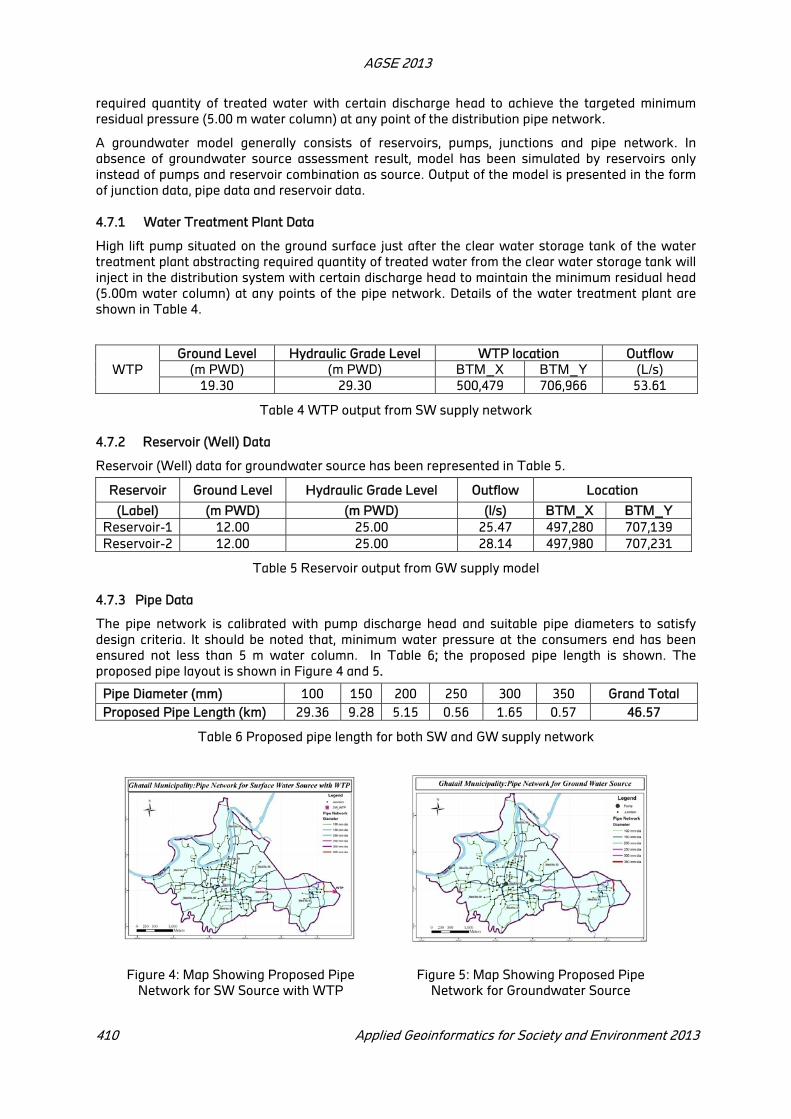
AGSE 2013


required quantity of treated water with certain discharge head to achieve the targeted minimum

residual pressure (5.00 m water column) at any point of the distribution pipe network.

A groundwater model generally consists of reservoirs, pumps, junctions and pipe network. In

absence of groundwater source assessment result, model has been simulated by reservoirs only

instead of pumps and reservoir combination as source. Output of the model is presented in the form

of junction data, pipe data and reservoir data.

4.7.1 Water Treatment Plant Data

High lift pump situated on the ground surface just after the clear water storage tank of the water

treatment plant abstracting required quantity of treated water from the clear water storage tank will

inject in the distribution system with certain discharge head to maintain the minimum residual head

(5.00m water column) at any points of the pipe network. Details of the water treatment plant are

shown in Table 4.

WTP

Ground Level Hydraulic Grade Level WTP location Outflow

(m PWD) (m PWD) BTM_X BTM_Y (L/s)

19.30 29.30 500,479 706,966 53.61

Table 4 WTP output from SW supply network

4.7.2 Reservoir (Well) Data

Reservoir (Well) data for groundwater source has been represented in Table 5.

Reservoir Ground Level Hydraulic Grade Level Outflow Location

(Label) (m PWD) (m PWD) (l/s) BTM_X BTM_Y

Reservoir-1 12.00 25.00 25.47 497,280 707,139

Reservoir-2 12.00 25.00 28.14 497,980 707,231

Table 5 Reservoir output from GW supply model

4.7.3 Pipe Data

The pipe network is calibrated with pump discharge head and suitable pipe diameters to satisfy

design criteria. It should be noted that, minimum water pressure at the consumers end has been

ensured not less than 5 m water column. In Table 6; the proposed pipe length is shown. The

proposed pipe layout is shown in Figure 4 and 5.

Pipe Diameter (mm) 100 150 200 250 300 350 Grand Total

Proposed Pipe Length (km) 29.36 9.28 5.15 0.56 1.65 0.57 46.57

Table 6 Proposed pipe length for both SW and GW supply network

Figure 4: Map Showing Proposed Pipe

Network for SW Source with WTP

Figure 5: Map Showing Proposed Pipe

Network for Groundwater Source

AGSE 2013


5. Limitations

Conjunctive use of water source is useful considering its impact on climate. But it is very costly

system to some extent. It will be expensive to construct, operate and maintain both systems

simultaneously in Pourashava level. On the other hand, for population as well as water demand

projection and growth rate analysis, population census data of 1991 and 1981 should be considered.

As the design is done for urban growth center, effect of irrigation is not considered here.

6. Conclusions

In Bangladesh water resources management is very difficult due to many diversified issued

associated. Water Managers and decision makers have to consider a large number of often

conflicting demands on the available water and operate water resources systems under numerous

constraints. Social, economic and physical constraints are equally important in water resources

development. To ensure sustainability, water resources systems need to be planned, designed and

managed in such a way that it fully meets the social and economical objectives of both present and

future. The analysis done in this study is very relevant to other urban growth centers and can be

applied for future development plan of other urban areas in Bangladesh.

REFERENCES

Ahmed, M.F. & Rahman, M.M., 2000, Water Supply & Sanitation: Rural and Low Income Urban

Communities, ITN-Bangladesh Centre for Water Supply and Waste Management, BUET.

Mustafa T. Hasan & Mahmud R. Amin (2011) “Preparing a Water Supply Master Plan for a Newly

Declared City Lacking Land-use Guidelines and Demographic Information”, USMCA, Chiangmai,

Thailand.

Population & Housing Census: Preliminary Results, 2011, Government of Bangladesh.

Population & Housing Census, 2001 Government of Bangladesh.

Bangladesh Water Utilities Data Book, 2008 Ministry of LGRD, GOB and World Bank Dhaka Office.

AGSE 2013


Effect of Ionospheric and Tropospheric delays on GNSS based

positioning

Poompavai V

Dept of Earth and Space Sciences, Indian Institute of Space Science and Technology,

Thiruvananthapuram, [email protected]

KEY WORDS: GPS, GNSS, Ionospheric delay, Tropospheric delay, Positioning Accuracy

ABSTRACT:

The GNSS is a space-based satellite navigation system that provides location and time information on the Earth. The Global positioning Satellite Navigation Signals are affected by various sources after transmission from the satellite. The effects on signal cause errors in the ranging measurement between the receiver and the satellite which contributes to the positioning error. The present work involves processing of the data files of a GPS reference station in India and subsequent analysis of those files for different time periods. This is to compare the effect of the solar cycle and the infleunce of variation in the solar activity on the electron content in the atmosphere. The ionospheric layer and the tropospheric layers cause a delay in the navigation signal. The effect of the variation in the solar activity on the positioning accuracy is studied in detail.

1. Introduction

The GNSS (Global Navigation Satellite System) is a space-based satellite navigation system that

provides location and time information in all weather conditions, anywhere on or near the Earth

where there is an unobstructed line of sight to four or more satellites. Different countries have their

own GNSS system such as GPS(Global Positioning System) of USA, GLONASS of Russia,

IRNSS(Indian Regional Navigational Satellite System) of India and Galileo of European Union.

Satellite-based navigation systems the principle of trilateration to locate the user, through

calculations involving information from a minimum 4 satellites. Each satellite transmits coded signals

at precise intervals through carrier waves at different frequencies. Using this information, any

receiver on or near the earth's surface can calculate the exact position of the transmitting satellite

and the distance (from the transmission time delay) between it and the receiver by ranging

technique. The receiver, then, converts signal information into position, velocity, and time estimates.

The GPS constellation has six orbit planes with approximately 55° inclination (tilt relative to Earth's

equator) and are separated by 60° right ascension of the ascending node with 4 or more satellites in

each orbital plane. The orbital period is one-half a sidereal day, i.e., 11 hours and 58 minutes so that

the satellites pass over the same locations.The orbits are arranged so that at least six satellites are

always within line of sight from almost everywhere on Earth's surface. There are 31 GPS satellites

currently in orbit.

2. Sources of Error

The ranging measurement or the pseuodrange is affected by many sources of error. They are:

1) Ephemeris data --Errors in the transmitted location of the satellite including SA

2) Satellite clock --Errors in the transmitted clock

3) Ionosphere --Errors in the corrections of pseudorange caused by ionospheric effects

4) Troposphere--Errors in the corrections of pseudorange caused by tropospheric effects

5) Multipath--Errors caused by reflected signals entering the receiver antenna

6) Receiver--Errors in the receiver's measurement of range caused by receiver clock error, thermal

noise, software accuracy.

AGSE 2013


3. Atmospheric based errors

With the satellites orbiting at about 20,000km above the earth, the GPS signals have to travel

through the ionosphere and the troposphere layers before reaching the receiver antenna. The

effects of atmosphere are discussed and analysed in the present study.

3.1 Ionospheric Delay

Ionosphere which extends from a height of 70 to 1000km affects the propagation of the navigation

signal through the atmosphere. The dispersive medium causes the carrier to experience a phase

advance and the code to experience a group delay The ionospheric delay is proportional to the

number of free electrons along the GPS signal path, called the total electron content (TEC). TEC

depends on the following factors:

(1) the time of day

(2) the time of year

(3) the 11-year solar cycle

(4) the geographic location

Generally, ionospheric delay is of the order of 5mto 15m, but can reach over 150m under extreme

solar activities, at midday,and near the horizon

3.2 Tropospheric Delay

The troposphere is the lowest portion of Earth's atmosphere. It contains approximately 80% of the

atmosphere's mass and 99% of its water vapour and aerosols.Tropospheric delay is a function of

refractive index and height and refractive index is dependent on temperature, pressure and humidity

along the signal path through the troposphere. Signals from satellites at low elevation angles travel a

longer path through the troposphere than those at higher elevation angles. Therefore, the

tropospheric delay is minimized at the user's zenith and maximized near the horizon.

4. Receiver independent exchange data format

RINEX (Receiver Independent Exchange Data Format) is a raw GPS static data format for data

processing and archive. It is an internationally accepted data exchange format and is in the standard

ASCII format (i.e., readable text). The RINEX format defines six different RINEX files; each contains a

header and data sections:

(1) observation data file, (2) navigation message file, (3) meteorological file, (4) GLONASS navigation

message file, (5) geostationary satellites (GPS signal payloads) data file, and (6) satellite and receiver

clock data file.The observation file contains in its header information that describes the file.s

contents such as the

station name,

antenna information,

the approximate station coordinates,

number and types of observation,

observation interval in seconds,

time of first observation record, and other information.

The observation types are defined as L1 and L2, and represent the Phase measurements on L1 and

L2 (cycles); C1 represents the pseudorange using C/A-code on L1 (meters); P1 and P2 represent the

pseudorange using P-code on L1 and L2 (meters); D1 and D2 represent the Doppler frequency on L1

and L2 (Hertz).

The GPS time frame is used for the GPS files, while the UTC time frame is used for GLONASS

files.The navigation message file contains the satellite information such as the date of file creation,

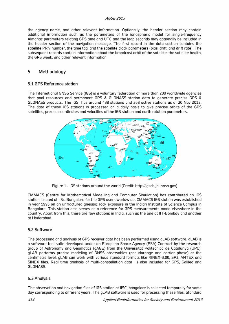
AGSE 2013


the agency name, and other relevant information. Optionally, the header section may contain

additional information such as the parameters of the ionospheric model for single-frequency

Almanac parameters relating GPS time and UTC and the leap seconds may optionally be included in

the header section of the navigation message. The first record in the data section contains the

satellite PRN number, the time tag, and the satellite clock parameters (bias, drift, and drift rate). The

subsequent records contain information about the broadcast orbit of the satellite, the satellite health,

the GPS week, and other relevant information

5 Methodology

5.1 GPS Reference station

The International GNSS Service (IGS) is a voluntary federation of more than 200 worldwide agencies

that pool resources and permanent GPS & GLONASS station data to generate precise GPS &

GLONASS products. The IGS has around 438 stations and 368 active stations as of 30 Nov 2013.

The data of these IGS stations is processed on a daily basis to give precise orbits of the GPS

satellites, precise coordinates and velocities of the IGS station and earth rotation parameters.

Figure 1 - IGS stations around the world (Credit: http://igscb.jpl.nasa.gov)

CMMACS (Centre for Mathematical Modelling and Computer Simulation) has contributed an IGS

station located at IISc, Bangalore for the GPS users worldwide. CMMACS IGS station was established

in year 1995 on an unfractured gneissic rock exposure in the Indian Institute of Science Campus in

Bangalore. This station also serves as a reference for GPS measurements made elsewhere in the

country. Apart from this, there are few stations in India, such as the one at IIT-Bombay and another

at Hyderabad.

5.2 Software

The processing and analysis of GPS receiver data has been performed using gLAB software. gLAB is

a software tool suite developed under an European Space Agency (ESA) Contract by the research

group of Astronomy and Geomatics (gAGE) from the Universitat Politecnica de Catalunya (UPC).

gLAB performs precise modeling of GNSS observables (pseudorange and carrier phase) at the

centimetre level. gLAB can work with various standard formats like RINEX-3.00, SP3, ANTEX and

SINEX files. Real time analysis of multi-constellation data is also included for GPS, Galileo and

GLONASS.

5.3 Analysis

The observation and navigation files of IGS station at IISC, bangalore is collected temporally for same

day corresponding to different years. The gLAB software is used for processing these files. Standard

AGSE 2013


Point Positioning (SPP) template is selected and the RINEX observation and navigation files are

given as input. The Modeling components of Ionosphere - Koluchar Model and Troposphere - UNB-

3 Nominal are activated for the processing. The output is then analysed to generate the NEU(North,

East, Up) Positioning error, Horizontal Positioning Error and Vertical Positioning Error plots. The

Satellite Clock offset is corrected in the processing stage. Data analysis centers located worldwide

retrieved GPS station data daily to produce IGS data products. These products, such as the daily and

weekly satellite ephemerides and the Earth rotation parameters, are in turn, submitted to the CDDIS

for availability to the global science community. The RINEX data files are downloaded from

CDDIS(Crustal Dynamics Data Information System ) website for the 14th day of years 2009 and

2012. The years 2009 and 2012 have been selected, since there was a drastic variation in the solar

activity corresponding to the solar cycle during that period. The solar cycle is the periodic change in

the sun's activity in the form of sunspots, flares, and other visible manifestations. Solar cycles have

an average duration of about 11 years. Since the Total electron content varies in the atmosphere due

to the Sun’s radiation, the present analysis was made to compare the effect of the solar cycle on the

Ionopheric and Tropospheric delay of GPS signal.

Figure 2- Solar Cycle Sun Spot Number Progression (Source: NOAA/SWPC Boulder)

The corresponding SINEX file for the station at Bangalore was uploaded in the software. SINEX -

Solution (Software/technique) INdependent EXchange Format is a data format designed to handle

information on GPS hardware (receiver,antenna), occupancy and various correspondence between

hardware, through which solution and input files can be preserved, which is essential for any serious

analysis and interpretation of GPS results. SINEX is an ASCII file with lines of 80chars or less. It

consists of a number of blocks which are mutually referenced (related) through station

codes/names, epochs and/or index counters.

6 Results and Conclusion

The plots are generated in the software for all ionosphere and troposphere corrections for the input

file. The NEU(North East Up) Positioning erros, Horizontal and Vertical positioning errros are

generated. Then, the ionopshere correction is switched off and the file is processed to find the errors

in the positioning. Similarly, tropospheric correction using a model is switched off and the effect on

positioning is found using the plots.

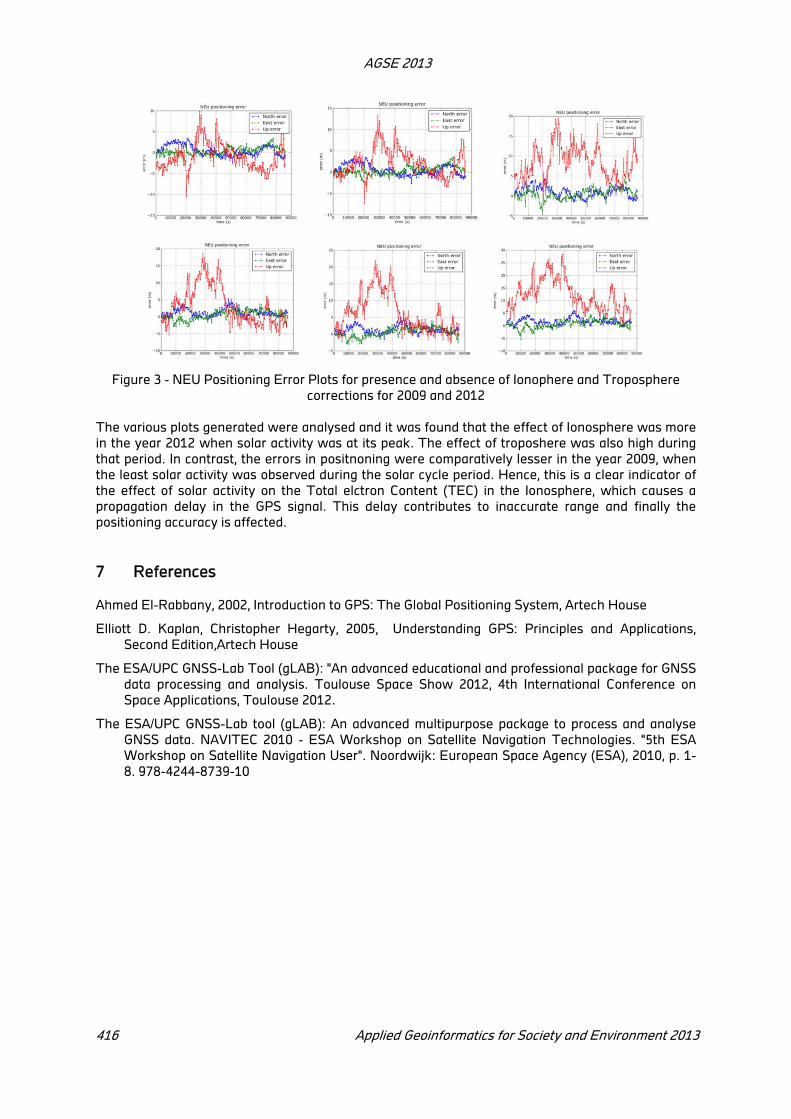
AGSE 2013


Figure 3 - NEU Positioning Error Plots for presence and absence of Ionophere and Troposphere

corrections for 2009 and 2012

The various plots generated were analysed and it was found that the effect of Ionosphere was more

in the year 2012 when solar activity was at its peak. The effect of troposhere was also high during

that period. In contrast, the errors in positnoning were comparatively lesser in the year 2009, when

the least solar activity was observed during the solar cycle period. Hence, this is a clear indicator of

the effect of solar activity on the Total elctron Content (TEC) in the Ionosphere, which causes a

propagation delay in the GPS signal. This delay contributes to inaccurate range and finally the

positioning accuracy is affected.

7 References

Ahmed El-Rabbany, 2002, Introduction to GPS: The Global Positioning System, Artech House

Elliott D. Kaplan, Christopher Hegarty, 2005, Understanding GPS: Principles and Applications,

Second Edition,Artech House

The ESA/UPC GNSS-Lab Tool (gLAB): "An advanced educational and professional package for GNSS

data processing and analysis. Toulouse Space Show 2012, 4th International Conference on

Space Applications, Toulouse 2012.

The ESA/UPC GNSS-Lab tool (gLAB): An advanced multipurpose package to process and analyse

GNSS data. NAVITEC 2010 - ESA Workshop on Satellite Navigation Technologies. "5th ESA

Workshop on Satellite Navigation User". Noordwijk: European Space Agency (ESA), 2010, p. 1-

8. 978-4244-8739-10

AGSE 2013


Hydro-Meteorological Disasters & Climate Change: Strategies, Prospects

and Challenges

Anurag Aeron1, R.D. Garg

1, D.S. Arya

1, S.P. Aggarwal

2

Department of Civil Engineering, Indian Institute of Technology, Roorkee1 ,

Department of Water Resources, Indian Institute of Remote Sensing, Dehradun2

[email protected], [email protected], [email protected], [email protected]

KEYWORDS: Hydro-meteorological disaster, Risk, Climate Change, Damage, Mitigation.

ABSTRACT:

Hydro-meteorological disasters cover about 85 to 90% of the total natural disasters in India and also account for 70 to 80% of the property and financial losses and also cause environmental damages [6]. A major hydro-meteorological disaster temporarily arrests development efforts. There are insufficient monitoring networks; poor access to historical time-series data; and a lack of analysis tools, mapping, and risk assessment. This paper presents an in-depth analysis of hydrological, meteorological and climate change disaster with respect to the pre and post disaster challenges and strategies. It is found that disaster mitigation steps are unproductive without the proper and timely financial, governance and local and global support. It also discusses disaster risk reduction and climate change adaptation, necessity to consider disaster risk reduction, effect of climate change, prospects for policy construction, challenges for disaster risk reduction and strategic plan.

1. Introduction

Government policies on Disaster Risk Reduction (DRR) and Climate Change Adaptation (CCA) are

unformed, and coordination structures are ineffective leading to a lack of budget commitment to

initiatives. The conditions for mainstreaming do not exist. Disaster response arrangements are

poorly structured and resourced leading to uncertain and delayed responses to events. There is

ineffective advocacy and support for Disaster Risk Reduction activities. Unavailability of a common

database system for storing hazard monitoring data with access to analysis tools for identifying

trends, vulnerabilities, and risks. All hazard sectors reported an inability to readily store and access

monitoring data for analytical and mapping purposes.

It is required to develop and implement the early warning systems for all hydro-meteorological

disasters. Up-gradation of communication systems for improving dissemination of warnings is

required. There is a very strong need to train the young scientists in the best Institutes or acquire

skilled manpower accessible across the world in the area of climate science. Launch of massive

public awareness programs to address people at grass-root levels to enhance coping capacity of

community (including alternative livelihoods) to decrease risk from disasters under climate change

scenarios [2]. Involvement of district and village level communities is required. The latest scientific

methods for assessment of flood should be used for reliable database and good analysis for study of

climate changes. Enhancement of observation over oceanic regions is required. As drought

frequency may increase under climate change, efforts to be devoted to introduce drought resistance

crop verities [1]. Setting up of high density observational networks suitable for detection and

monitoring of hydro-meteorological disasters are required on priority. Improve the accuracy of

weather forecasting and short-term climate prediction for high impact weather events. Train and

equip the resource center personnel to disseminate the drought-coping information, drought-

tolerant cropping material, and other resources to their local communities. Identify and evaluate

appropriate (drinking, household, and crop irrigation) and culturally acceptable water-supply

facilities for rural communities. Acquiring the political support is a must. Best practices in prevention

and mitigation should be systematically identified and disseminated.

AGSE 2013


2. Necessity To Consider Disaster Risk Reduction

Disaster risk reduction / disaster risk management is about avoiding these risks (prevention) or

limiting them (preparedness/ mitigation), by focusing on a population’s vulnerabilities and capacities

[4]. It is found according to UNDP that between 1991 and 2005:

• 3,470 million people were affected by disasters

• 960,000 people died

• Economic losses were $1,193 billion

Between 1998 and 2007:

• 76% of all disaster events were hydrological, meteorological or climatological in nature:

• They accounted for 45% of the deaths and 79% of the economic losses caused by natural

hazards

In 2011, 332 natural disasters were registered; the human and economic impacts of the disasters in

2011 were massive [5]. Natural disasters killed a total of 30 773 people and caused 244.7 million

victims worldwide. Economic damages from natural disasters were the highest ever registered, with

an estimated US$ 366.1 billion. Comparing 2011, with the previous decade data shows that the

number of victims increased compared to the annual average number of victims from 2001 to 2010 of

232.0 million. This increase is explained by the larger impact from hydrological disasters.

Hydrological disasters caused 139.8 million victims in 2011 - or 57.1% of total disaster victims in

2011 - compared to an annual average of 106.7 million hydrological disaster victims from 2001 to

2010. In 2011, 66.8% of global hydrological disaster victims were from floods and wet mass

movements in China [9]. Hydrological disasters still took by far the largest share in natural disaster

occurrence in 2011 (52.1%), followed by meteorological disasters (25.3%), climatological disasters

(11.7%) and geophysical disasters (10.8%) [5].Asia accounted in 2011 for 86.3% of global disaster

victims, followed by Africa (9.2%).In 2011, Asia also suffered the most damages (75.4% of global

disaster damages), followed by the Americas (18.4%) and Oceania (5.6%). For both Europe and

Africa, a share of 0.3% of global disaster damages was reported.

Hydrological disasters (floods and wet mass movements) still took the largest share in natural

disaster occurrence in 2011 (52.1%). Hydrological disasters caused 139.8 million victims, or 57.1% of

total disaster victims, and were responsible for 20.4% of the total reported number of people killed

and 19.3% of total damages. Meteorological disasters (storms) represented 25.3% of the total

disaster occurrence in 2011. Meteorological disasters accounted in 2011 for 10.1% of total reported

fatalities, 15.7% of total victims and 13.9% of total damages from natural disasters. Climatological

disasters (extreme temperatures, droughts and wildfires) took in 2011 an 11.7% share of total

disaster occurrence, comparable with a share of 12.9% per year on average for 2001-2010. Out of

the 39 climatological disasters, 17 were droughts, 15 extreme temperatures and 7 wildfires.

Climatological disasters took the second-largest share of total disaster victims in 2011 (64.6 million

or 26.4% of total disaster victims), as was also the case for the period 2001-2010. The reported

damages in 2011 increased by 56.3% compared to the 2001-2010 annual average damages from

these disasters. In 2011, 36 geophysical disasters (earthquakes /tsunamis, volcanoes and dry mass

movements) were registered, representing a share of 10.8% of total disaster occurrence [4].

Geophysical disasters accounted for 68.1% of total reported deaths from natural disasters in 2011,

compared to a share of 45.5% per year on average for 2001-2010. Disaster damages in Asia in 2011

were the highest ever recorded (US$ 276.0 billion) and increased by 563.4% compared to the annual

average damages from 2001 to 2010 (US$ 41.6 billion). At a global level, Asia’s share of global

damages in 2011 is 75.4%.

3. Effect of Climate Change

“More than 100 million people will die and global economic growth will be cut by 3.2 percent of gross

domestic product (GDP) by 2030 if the world fails to tackle climate change”, a report commissioned

by 20 governments said. As global average temperatures rise due to greenhouse gas emissions, the

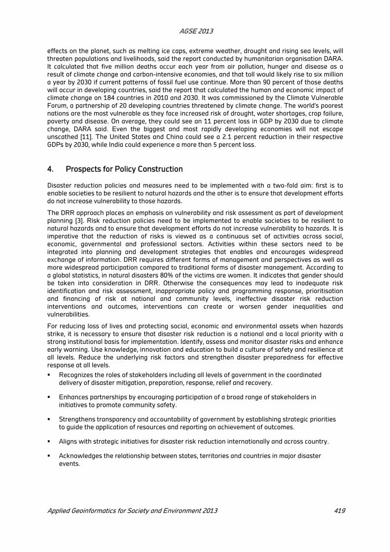
AGSE 2013


effects on the planet, such as melting ice caps, extreme weather, drought and rising sea levels, will

threaten populations and livelihoods, said the report conducted by humanitarian organisation DARA.

It calculated that five million deaths occur each year from air pollution, hunger and disease as a

result of climate change and carbon-intensive economies, and that toll would likely rise to six million

a year by 2030 if current patterns of fossil fuel use continue. More than 90 percent of those deaths

will occur in developing countries, said the report that calculated the human and economic impact of

climate change on 184 countries in 2010 and 2030. It was commissioned by the Climate Vulnerable

Forum, a partnership of 20 developing countries threatened by climate change. The world's poorest

nations are the most vulnerable as they face increased risk of drought, water shortages, crop failure,

poverty and disease. On average, they could see an 11 percent loss in GDP by 2030 due to climate

change, DARA said. Even the biggest and most rapidly developing economies will not escape

unscathed [11]. The United States and China could see a 2.1 percent reduction in their respective

GDPs by 2030, while India could experience a more than 5 percent loss.

4. Prospects for Policy Construction

Disaster reduction policies and measures need to be implemented with a two-fold aim: first is to

enable societies to be resilient to natural hazards and the other is to ensure that development efforts

do not increase vulnerability to those hazards.

The DRR approach places an emphasis on vulnerability and risk assessment as part of development

planning [3]. Risk reduction policies need to be implemented to enable societies to be resilient to

natural hazards and to ensure that development efforts do not increase vulnerability to hazards. It is

imperative that the reduction of risks is viewed as a continuous set of activities across social,

economic, governmental and professional sectors. Activities within these sectors need to be

integrated into planning and development strategies that enables and encourages widespread

exchange of information. DRR requires different forms of management and perspectives as well as

more widespread participation compared to traditional forms of disaster management. According to

a global statistics, in natural disasters 80% of the victims are women. It indicates that gender should

be taken into consideration in DRR. Otherwise the consequences may lead to inadequate risk

identification and risk assessment, inappropriate policy and programming response, prioritisation

and financing of risk at national and community levels, ineffective disaster risk reduction

interventions and outcomes, interventions can create or worsen gender inequalities and

vulnerabilities.

For reducing loss of lives and protecting social, economic and environmental assets when hazards

strike, it is necessary to ensure that disaster risk reduction is a national and a local priority with a

strong institutional basis for implementation. Identify, assess and monitor disaster risks and enhance

early warning. Use knowledge, innovation and education to build a culture of safety and resilience at

all levels. Reduce the underlying risk factors and strengthen disaster preparedness for effective

response at all levels.

Recognizes the roles of stakeholders including all levels of government in the coordinated

delivery of disaster mitigation, preparation, response, relief and recovery.

Enhances partnerships by encouraging participation of a broad range of stakeholders in

initiatives to promote community safety.

Strengthens transparency and accountability of government by establishing strategic priorities

to guide the application of resources and reporting on achievement of outcomes.

Aligns with strategic initiatives for disaster risk reduction internationally and across country.

Acknowledges the relationship between states, territories and countries in major disaster

events.

AGSE 2013


4.1 Challenges for Disaster Risk Reduction

The development of the disaster management strategy is for effective tools to enhance governance

and accountability, and to promote integrated whole-of-government solutions to complex issues. A

further influence has been the shift in national and international disaster management thinking from

focusing on reaction towards pro-active mitigation, systematic risk analysis and risk reduction, and

preparation. The lessons from recent world disaster and emergency events are clear – a

comprehensive all hazards, all agencies approach is the foundation of effective and efficient disaster

management.

Building and maintaining partnerships and collaboration across all levels of government, community

and industry, in all aspects of disaster management is a must. Protecting our natural and built

environment is the demand of time. Ensuring accountability and transparency of the disaster

management arrangements are the responsibility of all of us.

A comprehensive, all hazards, all agencies approach by achieving the right balance of prevention,

preparedness, response and recovery, regardless of the nature of the hazard through established

partnerships. Prepared communities ensuring they understand their role in disaster management

arrangements. Consultative decision-making: A transparent, systematic and consistent approach to

disaster risk assessment and management should be promoted. All levels of government apply

effective corporate governance and are committed to continuous improvement of policy, programs,

practices and service delivery to improve community safety Use collaborative and best practice

research to inform disaster management and improve the effectiveness of disaster management

principles, policy development and practices. Disaster management outcomes are achieved through

the development and implementation of sound policy and effective corporate governance. Ensure

clear and transparent decision making through collaboration, cooperation and communication.

Develop clear accountability, including defined roles and responsibilities at all levels of the disaster

management system. Legislative requirements are supported by disaster management policies.

Develop risk registers at all levels of the disaster management system that clearly identify

community vulnerability and the broader social and economic risks associated with disasters.

Strengthen regionally coordinated mitigation initiatives through whole-of-government leadership.

Share knowledge and innovative solutions to build community resilience and self-reliance. Create

aware and prepared communities. The impacts of a disaster are minimized by effective and efficient

disaster response. Ensure a coordinated approach exists across all levels of the disaster

management system through the clear definition of roles and responsibilities. Ensure a holistic

approach to community relief and recovery (immediate short and long-term) inclusive of social

(especially immediate welfare support, health and psychosocial), economic, infrastructure (including

power, water and sewerage) and environmental considerations. Ensure recovery arrangements

remain flexible and adaptable for all communities. Post-disaster assessment strengthens disaster

management capability. Specific state government agencies and organizations will be designated as

lead agencies with specific threat-based or functional responsibilities.

5. Discussion for Strategic Plan

To achieve the above mention ideas, the National Disaster Management Agency will embark on the

following:

1. Financing and Resource Mobilization Strategy: To mobilize funds for financing of the strategic

plan, two funding sources are identified, namely: one as to take advantage of available resources by

incorporating some of the activities of the plan into the regular annual budget of government and the

other is to resort to the mobilization of additional resources from development partners and the

private sector for activities that could not be incorporated in the government budget [10].

For resource mobilization, the government budget is very important for successful implementation of

the strategic plan. It will illustrate government’s strong commitment to disaster management and

risk reduction.

2. Partnership Strategy: The disaster agency will establish strategic partnerships and network with

key actor involved in disaster management and risk reduction in the country namely:

AGSE 2013


Departments of State

National Assembly

UN Agencies

National, regional and international NGOs

Traditional institutions and leaders

Private sector/business community

Researchers

Civil society organizations

Faith-based organizations

Security and Emergency Services

3. Communication Strategy: Communication strategy is instrumental not only in the implementation

of the strategic plan but also in the area of profiling and positioning the newly created National

Disaster Management office in the country and beyond. Within the framework of information and

communication technology (ICT) the National Disaster Office will:

• Establish a documentation and information centre responsible for collecting, managing and

disseminating reliable information on disaster and risk reduction in the country.

• Involve the private and public media in the activities of the National Office.

4. Monitoring and Evaluation Strategy: Monitoring and evaluation is part and parcel of any planning

process, as it is critical to the assessment of progress against benchmarks [8]. While monitoring and

evaluation are closely linked, it is important to understand the distinction between them. Whereas

monitoring is a routine on-going activity to assess program implementation in terms of resources

(inputs) invested in the program and the outputs produced, evaluation is concerned with the

assessment of the programs’ impacts on disaster and risk reduction management e.g. on the safety

and welfare of citizens.

5. National Emergency Strategy: There is an urgent need to develop a national emergency

strategy/plan since not all emergencies are classified as disaster but could be fatal and threaten

national security and stability [7].

5.1 Obstructions During Implementation

During the implementation of this strategic plan, the disaster management agency is likely to face a

number of risks that can undermine and or slow down the effective implementation of the well-

outlined strategic actions. Some of these risks are:

Lack of adequate capacity to implement the strategic plan owing to the weak agency staffing (in

quality and quantity)

Lack of enough funding is also an important risk as, without enough resources, the agency will

not be able to translate the strategy into concrete actions.

However, giving the high commitment of government and the donor community specially UNDP,

these risks could be met.

AGSE 2013


6. Conclusion and Recommendations

Vulnerable countries should be encouraged to adopt suitable disaster management systems before

disaster strikes. It is important that such systems be accepted and approved by governmental and

nongovernmental relief coordinators. Relief workers, including volunteers, should be enabled to

work together using common data sets.

Further it can be recommended to all national policy makers to commit firmly to low-carbon

prosperity and prioritize parallel measures to adapt to climate change. Unite strengths in

international partnership for support the vulnerable effectively. They should deliver fully on

commitments. Climate policy with highest co-benefits could be at highest priory. Pledge strong

national action and invest in national risk analysis. Try to adaptation policy. Boost domestic capacity

to strengthen climate governance. Promote awareness on risks as opportunities. Perform

comprehensive risk analysis for all type of hazards. Encourage diversification strategies to take

benefits of different agencies. Encourage attribution research for goal based achievements. Expand

global analysis to determine the trends. Avoid misrepresentation of risks. Focus should be on

economic development, education and environmental governance. Integrate climate strategies to

revitalize development of all sectors like industries, pollution control, forests, transportation, etc.

Brace for change and establish a thematic funding window for climate-linked emergency response.

And the most important is to evolve thinking and partnerships.

REFERENCES

[1] Iven Schad, Petra Schmitter and Camille Saint-Macary, 2012, Why do people not learn from flood

disasters? Evidence from Vietnam’s northwestern mountains, Nat Hazards, vol.62, page 221–

241.

[2] Pradeep K. Rawat, 2012, Impacts of Climate Change and Hydrological Hazards on Monsoon Crop

Patterns in the Lesser Himalaya: A Watershed Based Study, International Journal of Disaster

Risk Science, vol.3, no.2, page 98–112.

[3] Riyanti Djalante, Cameron Holley, and Frank Thomalla, 2011, Adaptive Governance and Managing

Resilience to Natural Hazards, International Journal of Disaster Risk Science, vol.2, no.4, page

1–14.

[4] A Guide for Implementing the Hyogo Framework for Action by Local Stakeholders, 2010, UNISDR.

[5] Annual Disaster Statistical Review 2011: The numbers and trends, UNISDR, Centre for Research

on the Epidemiology of Disasters, Institute of Health and Society (IRSS), Université catholique

de Louvain.

[6] Disaster Management in India - A Status Report, Government of India, Ministry of Home Affairs,

National Disaster Management Division.

[7] Emergency Management Planning Guide 2010–2011, Public Safety, Canada.

[8] Joint National Action Plan on Climate Change Adaptation and Disaster Risk Management 2010–

2015, published by Second National Communication Project, Ministry of Environment and

Climate Change, Nukualofa, Kingdom of Tonga.

[9] Natural Disaster Data Book 2011 (An Analytical Overview), Asian Disaster Reduction Center.

[10] Reducing the Risk of Disasters and Climate Variability in the Pacific Islands, Papua New Guinea

Country Assessment, Published by The World Bank, East Asia and the Pacific Region.

[11] http://daraint.org/climate-vulnerability-monitor/climate-vulnerability-initiative/

AGSE 2013


Analysing the distribution of Educational Infrastructure of Gulbarga City

through location allocation modelling.

Priya Narayanan, Mr. Krishna Udnoor

Department of Geography, Central University of Karnataka, Gulbarga, Karnataka.

Abstract

Infrastructure is the backbone for the development of any city. Every inmate of the city has equal rights to access common infrastructure, but the distribution offers prejudice and privilege to only few. What has developed and established cannot be largely modified, but what can come afresh, can surely be prioritized in a spatial context. With the power of geoinformatics, an attempt has been made to study the present distribution pattern of educational infrastructural facilities, which reveals clustered to specific locations. But a more balanced spatial distribution will be demanded for sustainable use of available infrastructure. Hence, by studying the present spatial distribution, future spatial prioritization can be developed and the same can guide the location of future educational institutions.

1. Introduction:

The invasion of quantitative revolution in geography essentially revolutionised the subject

geography, and presented a quantitative definition to the way things are distributed on the surface

of earth. This is called as “spatial analysis” by nomothetic geographers who define distributions with

empherical laws (Murayama & Thapa, 2011). This conceptualizes the search for order, regularity, of

pattern that sets the forefront of “Spatial analysis”(Berry & Marble, 1968). This quantitative

revolution paved way for sophisticated analytical methods in GIS, and has a key role to play in the

fundamentals of GIS architecture. The use of robust software for corroborative research on

population potential, location allotment, shortest routes, central place theory, population distribution

zoning, etc., has been great benefits to urban planners, regional policy makers and among

others(Nordbeck & Rystedt, 1972).Services are best utilised based on their locations. Amenities like

that of schools, hospitals, etc., influence the choice of space. Analysis of distribution pattern of

schools would provide insight towards justice for education. The absence of school in a locality and

on a contrary clustering of schools in another locality announces capitalistic benefits leaving the

service motto in question. Thus spatial distribution analysis of schools in Gulbarga city would

provide knowledge about the irregularity in the distribution of schools which can guide policy makers

as to where to place the next school in a given geographic area.

About Gulbarga: The city of Gulbarga is located in the northern part of Karnataka state, India (lat

long). The city extends for 81 sq.km and is been divided into 58 administrative wards for ease of

governance. The city plays a very important role as a prominent city in the Hyderabad-Karnataka

region which is classified as backward. This city is essentially the urban service provider for

surrounding villages. The city has a population of 5.43 lakhs. Gulbarga has an average elevation of

454 meters above mean sea level and has a gently rolling topography. Its strategic location in the

centre of Indian southern peninsular enjoys the advantage of transportation and becomes an

important landmark for the north-south connectivity. Gulbarga is politically and socially very

conducive to be smarter city as urban development has reached to its fullest scale. Hence there is

every probability that the results of this analysis may be implemented.

Educational infrastructure of Gulbarga town: No doubt that education is the driving force of

development for which the developing countries have been striving to keep education reachable to

its broadest spectrum (Lundvall & Johnson, 1994). The inequalities in access to education are

debated in social sciences (Halsey, Lauder, Brown, & Wells, 1997; Prokop, 2005; Warrington, 2005).

Inhabitants of core urbanized areas have better access to education than inhabitants of remote rural

peripheries (Kucerová & Kucera, 2012). Gulbarga city has a total of 285 schools whose

AGSE 2013


categorization is given in Table 1. As schools can be established by government, quasi-government

and private sectors, the location of the schools are profit driven. Hence there is discriminating

distribution in the schools of Gulbarga city. Analysing the pattern of distribution of schools will throw

light on the need based allocation for future.

Type of schools Counts

Pre school 24

Primary school 48

Higher primary school 48

High school 52

Primary, higher primary school 23

Pre school, primary and high school 17

Pre school, primary and high school 11

Lower primary and higher primary school 10

Nursery, pre primary, primary and high school 25

Nursery, pre primary, primary and high school 10

Primary, higher primary and high school 17

Total 285

Table 1: Number of schools in Gulbarga city

2. Methodology:

Spatial autocorrelation is a process that indicates the spatial association and spatial dependence of

geographic objects. Objects in natural system have some degree of clusters. These clusters

produce distinct spatial patterns that can be understood by the size and shape of clusters and can be

quantified according to the degree of similarity in their distribution. It measures the extent to which

the occurrence of an event in an aerial unit constrains, or makes more probable, the occurrence of

that event in neighbouring aerial unit. On the available indices of spatial autocorrelation, Moran’s I is

the oldest.

Moran’s I = ∑ ∑ , ,

∑ ∑ , , ∑

Where N is the number of cases (in this context, number of schools)

Xi is the variable value at a particular location (no. of school in a ward)

Xj is the variable value at another location

X is the mean of the variable

Wij is the weight applied to comparison between location i and location j.

In this case Moran’s I autocorrelation tool available in spatial statistics in Arc GIS software. This

evaluates weather a given pattern is clustered, dispersed or random. The z-score and p-value

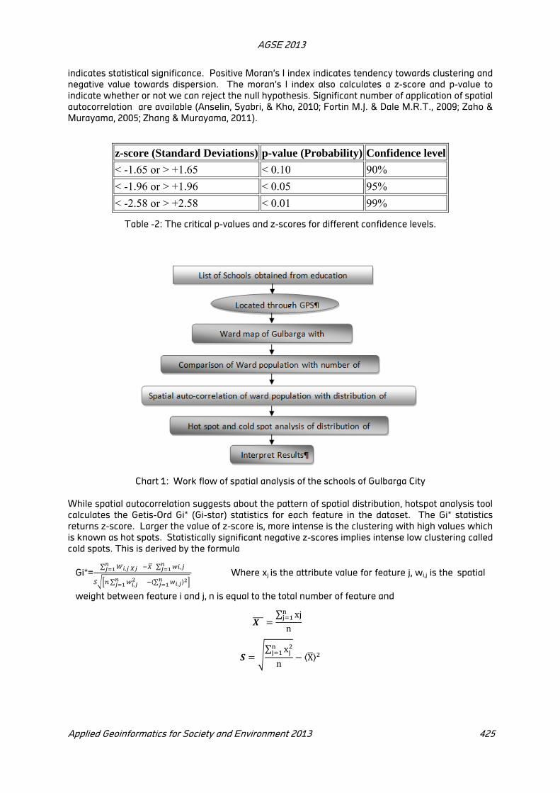
AGSE 2013


indicates statistical significance. Positive Moran’s I index indicates tendency towards clustering and

negative value towards dispersion. The moran’s I index also calculates a z-score and p-value to

indicate whether or not we can reject the null hypothesis. Significant number of application of spatial

autocorrelation are available (Anselin, Syabri, & Kho, 2010; Fortin M.J. & Dale M.R.T., 2009; Zaho &

Murayama, 2005; Zhang & Murayama, 2011).

z-score (Standard Deviations) p-value (Probability) Confidence level

< -1.65 or > +1.65 < 0.10 90%

< -1.96 or > +1.96 < 0.05 95%

< -2.58 or > +2.58 < 0.01 99%

Table -2: The critical p-values and z-scores for different confidence levels.

Chart 1: Work flow of spatial analysis of the schools of Gulbarga City

While spatial autocorrelation suggests about the pattern of spatial distribution, hotspot analysis tool

calculates the Getis-Ord Gi* (Gi-star) statistics for each feature in the dataset. The Gi* statistics

returns z-score. Larger the value of z-score is, more intense is the clustering with high values which

is known as hot spots. Statistically significant negative z-scores implies intense low clustering called

cold spots. This is derived by the formula

Gi*=∑ , ∑ ,

∑ , ⟨∑ , ⟩ Where xj is the attribute value for feature j, wi,j is the spatial

weight between feature i and j, n is equal to the total number of feature and

∑ xj

n

∑ x

n⟨X⟩

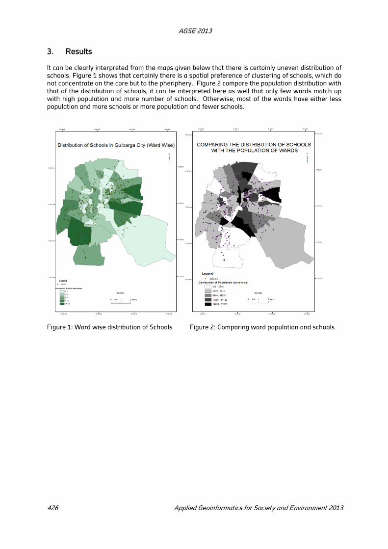
AGSE 2013


3. Results

It can be clearly interpreted from the maps given below that there is certainly uneven distribution of

schools. Figure 1 shows that certainly there is a spatial preference of clustering of schools, which do

not concentrate on the core but to the pheriphery. Figure 2 compare the population distribution with

that of the distribution of schools, it can be interpreted here as well that only few wards match up

with high population and more number of schools. Otherwise, most of the wards have either less

population and more schools or more population and fewer schools.

Figure 1: Ward wise distribution of Schools Figure 2: Comparing ward population and schools

AGSE 2013


Figure 3: Spatial Autocorrelation Report

The spatial autocorrelation report of the schools of Gulbarga city yields the Moran’s Index value as

0.032380, since this is a positive value, the tendency is towards clustering. The p value yielded is

0.008586, which is very small hence the pattern of randomness is unlikely. The z score is 2.62811

(referring to table 2), can yield 99% confidence in the results. All these strike to only one fact that

the distribution of schools is clustered.

While analysing the hotspot and cold spots of distribution of schools, Gi* score, it ranges from -

1.130971 to 3.095366. In this scale, values inclining to high negative indicate cold spots and towards

high positive indicates hot spot. Thus by calculating the Gi* score for the distribution of schools in

different wards of Gulbarga city, the results are classified into four categories and are represented in

Figure 4.

4. Discussion:

During the development process of any city, where to place a facility becomes more important for

the functional capabilities and reach of service. The hot and cold spot analysis can guide the future

allocation of schools to the cold spots regions, and avoid further allotment of schools in the hot spots.

This also can be done by providing special incentives to the schools that are ready to relocate/ incept

to the cold spots. Such analysis also scientifically brings out the reasons of location of services that

going by socio-political pressures.

AGSE 2013


Figure 4: Gi* scores of ward wise distribution of schools in Gulbarga city

Acknowledgement: This is an opportunity to express my sincere gratitude towards the funding

agency HUDCO, New Delhi which has sponsored the major research project on “Assessing and

modelling the infrastructure crunch of Gulbarga city: Holistic approach to plan a sustainable city

using Geospatial Technology”. A piece of research work of the same is being published here. I am

sincerely thankful for their unconditional support.

REFERENCES

Anselin, L., Syabri, I., & Kho, Y. (Eds.). (2010). GeoDa: An introduction to spatial data analysis. Berlin:

Springer.

Berry, B. J. L., & Marble, D. F. (1968). Spatial Anlysis: A reader in statistical geography. New Jersy:

Prentice Hall.

Fortin M.J., & Dale M.R.T. (Eds.). (2009). Spatial Autocorrelation. London: Sage.

Halsey, A. H., Lauder, H., Brown, P., & Wells, A. S. (1997). Education: Culture, Economy, and

Scociety. Oxford: Oxford University Press.

Kučerová, S., & Kučera, Z. (2012). Changes in the spatial distribution of elementary schools and their

impact on rural communities in Czechia in the second half of the 20th century. Journal of

Research in Rural Education, 27(11), 1-17.

Lundvall, B. A., & Johnson, B. (1994). The learning ecoomy. Jounal of Industry studies, 1(2), 23-42.

AGSE 2013


Murayama, Y., & Thapa, R. B. (2011). Spatial Analysis: Evolution, Methods and Applications D. Z. Sui

(Ed.) Spatila Analysis and Modelling in Geographical Transformation Process-GIS based

applications

Nordbeck, s., & Rystedt, B. (1972). Computer Cartography: The maping system NORMAP: location

models. Lund: Studentlitteratur.

Prokop, J. (2005). Škola a společnost v kritických teoriích druhé poloviny 20. století (School and

Society in critical theories of the second half of the 20th Century). . Prague: Karolinum.

Warrington, M. (2005). Mirage in the desert? Access to educational opportunities in an area of social

exculsion. Antipode, 37, 796-816.

Zaho, Y., & Murayama, Y. (Eds.). (2005). Effect characteristics of spatial resolution on the analysis of

urban land-use pattern: A case study of CBD in Tokyo using spatial autocorrelation index.

Tokyo: IGU urban commission.

Zhang, C., & Murayama, Y. (2011). Testing local spatial autocorrelation using K-orderneighbours.

London: Springer.

Band 137

2014

ISBN 978-3-940670-42-2

Documents

AGSE 2013 Proceedings (pdf)