Embed Size (px)
Citation preview

Journal of Development and
Agricultural Economics
ISSN 2006-9774
Volume 8 Number 2 February 2016

ABOUT JDAE The Journal of Development and Agricultural Economics (JDAE) (ISSN:2006-9774) is an open access journal that provides rapid publication (monthly) of articles in all areas of the subject such as The determinants of cassava productivity and price under the farmers’ collaboration with the emerging cassava processors, Economics of wetland rice production technology in the savannah region, Programming, efficiency and management of tobacco farms, review of the declining role of agriculture for economic diversity etc. The Journal welcomes the submission of manuscripts that meet the general criteria of significance and scientific excellence. Papers will be published shortly after acceptance. All articles published in JDAE are peer- reviewed.
Contact Us
Editorial Office: [email protected]
Help Desk: [email protected]
Website: http://www.academicjournals.org/journal/JDAE
Submit manuscript online http://ms.academicjournals.me/

Editors
Prof. Diego Begalli Prof. Mammo Muchie University of Verona Tshwane University of Technology, Via della Pieve, 70 - 37029 Pretoria, South Africa and San Pietro in Cariano (Verona) Aalborg University,
Italy. Denmark.
Prof. S. Mohan Dr. Morolong Bantu
Indian Institute of Technology Madras University of Botswana, Centre for Continuing Dept. of Civil Engineering, Education
IIT Madras, Chennai - 600 036, Department of Extra Mural and Public Education
India. Private Bag UB 00707 Gaborone, Botswana.
Dr. Munir Ahmad Dr. Siddhartha Sarkar
Pakistan Agricultural Research Council (HQ) Faculty, Dinhata College,
Sector G-5/1, Islamabad, 250 Pandapara Colony, Jalpaiguri 735101,West Pakistan. Bengal,
India.
Dr. Wirat Krasachat Dr. Bamire Adebayo Simeon
King Mongkut’s Institute of Technology Ladkrabang Department of Agricultural Economics, Faculty of 3 Moo 2, Chalongkrung Rd, Agriculture Ladkrabang, Bangkok 10520, Obafemi Awolowo University
Thailand. Nigeria.

Editorial Board
Dr. Edson Talamini Federal University of Grande Dourados - UFGD Rodovia Dourados-Itahum, Km 12
Cidade Universitária - Dourados, MS - Brazil.
Dr. Okoye, Benjamin Chukwuemeka National Root Crops Research Institute, Umudike. P.M.B.7006, Umuahia, Abia State. Nigeria.
Dr. Obayelu Abiodun Elijah Quo Vadis Chamber No.1 Lajorin Road, Sabo - Oke P.O. Box 4824, Ilorin Nigeria.
Dr. Murat Yercan Associate professor at the Department of Agricultural Economics, Ege University in Izmir/ Turkey.
Dr. Jesiah Selvam Indian Academy School of Management Studies(IASMS)
(Affiliated to Bangalore University and Approved By AICTE) Hennur Cross, Hennur Main Raod, Kalyan Nagar PO Bangalore-560 043
India.
Dr Ilhan Ozturk Cag University, Faculty of Economics and Admistrative Sciences, Adana - Mersin karayolu uzeri, Mersin, 33800, TURKEY.
Dr. Gbadebo Olusegun Abidemi Odularu Regional Policies and Markets Analyst, Forum for Agricultural Research in
Africa (FARA), 2 Gowa Close, Roman Ridge, PMB CT 173, Cantonments, Accra - Ghana.
Dr. Vo Quang Minh Cantho University 3/2 Street, Ninh kieu district, Cantho City, Vietnam.
Dr. Hasan A. Faruq Department of Economics Williams College of Business Xavier University Cincinnati, OH 45207 USA. Dr. T. S. Devaraja Department of Commerce and Management, Post Graduate Centre, University of Mysore, Hemagangothri Campus, Hassan-
573220, Karnataka State, India.

Table of Contents: Volume 8 Number 2 February, 2016
Journal of Development and Agricultural Economics
ARTICLES
The Development of the poultry sector in Botswana: From good intentions to legal oligopoly 14 Roman Grynberg and Masedi Motswapong Total factor productivity growth of Turkish agricultural sector from 2000 to 2014: Data envelopment malmquist analysis productivity index and growth accounting approachy 27 Abdul-Basit Tampuli ABUKARI, Burak ÖZTORNACI and Püren VEZİROĞLU Technical efficiency of smallholder wheat farmers: The case of Welmera district, Central Oromia, Ethiopia 39 Wudineh Getahun Tiruneh and Endrias Geta

Vol. 8(2), pp. 14-26, February, 2016
DOI: 10.5897/JDAE2015.0701
Article Number: 59DA71856957
ISSN 2006-9774
Copyright ©2016
Author(s) retain the copyright of this article
http://www.academicjournals.org/JDAE
Journal of Development and Agricultural Economics
Review
Development of the poultry sector in Botswana: From good intentions to legal oligopoly
Roman Grynberg1* and Masedi Motswapong2
1Economics and Management Sciences, University of Namibia, Private Bag 13301, 340 Mandume Ndemufayo Ave,
Pionierspark, Windhoek, Namibia. 2Botswana Institute for Development Policy Analysis, Private Bag BR-29, Gaborone, Botswana.
Received 13 October, 2015; Accepted 22 December, 2015
This paper examines the development of the Botswana’s poultry sector, which has become the dominant meat industry in Botswana. The poultry sector is the most successful example of import substitution in Botswana with the country having achieved national self sufficiency. The paper describes the value chain in the industry and shows how, given the small size of the market, a high degree of market concentration exists. This paper raises issues regarding the fundamental tension between competition and industrial policy in a small developing country. As the larger firms in the poultry industry move towards export readiness after 36 years of protection, the question of a new trade and industry regime is considered. Key words: Poultry industry, competition policy, trade policy.
INTRODUCTION Traditionally, Botswana has been a beef producing and consuming country but with rapid urbanization, poultry has supplanted cattle as the dominant livestock sector. The development of the industry reflects long-standing government policy dating from the 1970‟s to develop an industry which is able to meet national needs through import substitution. The early policy of import substitution, which resulted in the development of the industry,
emphasized the creation of sufficient producer surplus to encourage on-going development and investment in the industry. However, with parts of the industry now exporting, the question arises as to whether the longstanding policy of import substitution and market closure is appropriate and whether a move to a more open trading regime may not be in the benefit of the industry and the country as a whole. The purpose of this
*Corresponding author. E-mail: [email protected].
JEL Classification: Q17, Q18, D11, D21, D43.
Author(s) agree that this article remain permanently open access under the terms of the Creative Commons Attribution
License 4.0 International License

paper is to examine the development of the country‟s poultry sector, which has become the dominant meat industry in Botswana.
The second issue of relevance that will be discussed is the relationship between competition policy and development and industrial policy in a small developing country. With the completion of the Uruguay Round of negotiations, the development of the „new issues‟ such as competition policy was introduced into global trade discussions. These new issues are the product of a paradigm shift that occurred post-1995. The issue of competition policy puts into focus the related question of the development role of the state and its role in balancing consumer/producer surplus has become central to industry policy. This paper is also meant to facilitate discussion on the Botswana‟s new competition policy and act. This is especially so in light of the Economic Mapping Report commissioned by the government of Botswana, which revealed that there is market dominance in the meat industry (Ministry of Trade and Industry, 2005).
The immediate stimulus for this paper was an earlier study undertaken in 2010, where it was observed that Botswana had the Southern African Customs Union (SACU) region‟s lowest retail prices for beef using the only available common price comparator, that is, brisket and the highest price in the region for frozen chicken (BIDPA, 2010). These are two types of meat products commonly consumed by lower income groups in SACU countries. COMPETITION POLICY IN A MICRO STATE INSIDE A CUSTOMS UNION Competition policy in small and micro states The issue of competition policy has reached the global agenda largely as a result of the issue being advocated for by developed countries as part of what were then called „the new issues‟ that appeared at the Singapore Ministerial meeting of the World Trade Organisation (WTO) in 1996 (WTO,1996). In large measure, the issue has been introduced to developing countries out of the realization that market opening commitments made by them in the Uruguay Round of trade negotiations would be of no commercial value to developed countries unless there was an appropriate competition regime in WTO member states that protected the interests of exporting firms and assured contestability of markets (Sauve, 2004). Thus, developed countries and, in particular, the European Union (EU) have been pursuing an active policy of supporting rules on competition policy (Brittain, 1997). This WTO approach has also been expanded bilaterally in the EU‟s regional negotiations with the developing
Grynberg and Motswapong 15 countries of Africa, the Caribbean and the Pacific.
In all these discussions on the issue of competition policy, there has been scant consideration given to whether greater competition which is frequently associated with diminished producer surplus is beneficial for developing countries. Many developing country Non Governmental Organisations (NGOs) have pushed and supported competition policy issues in large measure out of the view that these rules can assist developing countries in strengthening their competition rules against local monopolies. In Botswana, the government has negotiated an interim Economic Partnership Agreement (EPA) with the EU, and is generally supportive of the approach which enshrines competition policy. Whether the Government of Botswana is willing, in the end, to provide legally binding commitments on competition policy in trade negotiations with developed countries, like the Caribbean has done, is to be determined in the final EPA with the EU which at the time of writing had not been concluded.
There exists a fundamental tension over the issue of competition policy and law in developing micro states such as Botswana. First, it is entirely plausible for a small state to maintain a rational competition policy that, at least for medium term, is anti-competitive, as it may be in the national interest to assist firms to accumulate sufficient capital, i.e. generate producer surplus in a particular sector, so as to assist firms to eventually become internationally competitive. Second, and it is a more pervasive issue of small and micro states, that irrespective of their development status, the existence of extended economies of scale in production and management in any given industry means that the small size of the market results in only being sufficient „market space‟ for an efficient monopolist or possibly duopolistic (Gal, 2001). This brings into question the very logic of importing policies and laws from larger developed countries that make little economic sense in developing micro-states like Botswana. The issue of whether small states are capable of conducting a competition policy based essentially on developed country competition laws, while attempting to develop import substituting sectors, is at the heart of the case of the poultry industry in Botswana. Botswana’s competition law The Competition Act passed by the Botswana parliament in late 2009 created a new Competition Commission and a new Competition Authority, which are now in full operation. The legislation provides the Commission and the Authority with the ability to undertake the usual range of activities found in most countries that have enacted

16 J. Dev. Agric. Econ. similar legislation. The authority may undertake investigations of vertical and horizontal agreements (Articles 25, 26 and 27), as well as the abuse of dominant position (Article 30). If following an investigation, it is determined that a horizontal or vertical agreement that breaches any of the prohibited behaviour specified in the Act is said to exist in a particular industry, the commission is authorized to give direction for the termination of the agreement (Article 43.1). Botswana‟s Competition Commission serves as the board for the Competition Authority, which does the investigation and recommends remedies, and makes decisions which can be fascinating to the commission. The commission acts as the tribunal to adjudicate cases brought to it by the Competition Authority or by appellants.
The act also provides for the possibility of a fine of 10% of turnover during the breach of the prohibition on such agreements up to a maximum of 3 years (Article 43.4). The remedies available to the Commission include the requirement for an enterprise to divest itself of any enterprise or assets (Article 44.3.e). These remedies are common to many Competition Laws and are similar to those that are found in South African legislation.
What is unique about the circumstance of Botswana as it pertains to Competition Act is that it is a small developing landlocked country in a customs union with a dominant partner, that is, South Africa. The issue of relevance is how significant competition policy can be under such circumstances. This is particularly important when it comes to the definition of the relevant market for the purposes of determining whether abuse of a dominant position has occurred. In the Competition Act, the relevant market is defined as „the geographical or product market used for assessing the effects of the practice, conduct or agreement on competition‟ (Article 2). In any competition law case, the most common issue of contention is the definition of the appropriate market. This can be local, national or regional and this is the subject of legal and economic disputes globally.
In the case of SACU which is a customs union where production is polarized into the largest and most developed member, South Africa, virtually for every consumer good, the relevant market is the SACU market and not Botswana, as this has been legally the case since 1910. This does not mean that the relevant market may not be national or even local, but most commonly in the case of those goods where the government has purposely closed the Botswana market for the purposes of economic development, for example, poultry, to all or most international trade, the market can be said to be the same as the legal jurisdiction covered by the Competition Act. The conundrum of competition policy in a country like Botswana, which is both small and part of a customs union, is that where the country may be the „relevant
market‟ for the purpose of the Competition Act, it is almost always so only by virtue of government policy to close the market to foreign competition, including that from other SACU members. In most cases, the relevant market is the SACU market and, therefore, the Botswana Competition Commission will only be able to operate when it works closely with its SACU counterparts (other members of the customs union). Moreover in many cases, for example, where a conspiracy occurs to raise prices or reduce or apportion output it will normally have occurred in the main market, namely South Africa, and be extended to Botswana in a pro forma manner as would be the case with the other SACU members. Botswana has no jurisdiction to investigate outside its borders and unless co-operation is close to the relevant South Africa authorities, the ability of the Botswana Competition Commission to implement its mandate will be circumscribed. Thus, the market, generally SACU, is not the same as legal jurisdiction of the legislation, that is, Botswana, and, therefore, the legislation can only have limited application as a result.
The drafters of the legislation were also well aware of the problem of statutory agencies. The legislation declares ultra vires, „enterprises acting on the basis of a statutory monopoly in Botswana‟ (Article 3.2(b)). While the poultry industry or other similar import substituting sectors cannot be seen as a statutory monopoly as is the case of infrastructure providers, such as Botswana Power Corporation; its existence is a result of government legislation providing the prohibition of imports, that is, Control of Goods (Importation of Eggs and Poultry Meat) Regulations [SI 120, 1979, 7
th December], 1979. Given
the small size of the Botswana poultry market, the closure of the market from imports, combined with the existence of significant economies of scale in the sector, meant that the Government was, in effect, creating the conditions for what is at very least a „statutory oligopoly‟, and may be a legal monopoly if one employs the 40% market share threshold as a criteria. More importantly, for the case of the poultry and other import substituting industries, the legislative drafters provided a policy based caveat for the application of remedies by the Competition Authority and Commission, which will render its work both taxing and potentially quite arbitrary in its application. In determining whether there has been an abuse of dominant position, the Competition Authority (Article 30.2) „may have regard for either the agreement or conduct in question: 1. Maintains or promotes exports from Botswana or employment in Botswana 2. Advances the strategic national interest of Botswana in relation to a particular economic activity 3. Provides social benefits which outweigh the effects on

competition 4. Occurs within the context of a citizen empowerment initiative of Government, or otherwise enhances the competitiveness of small and medium sized enterprises; or 5. In any other way enhances the effectiveness of the government‟s programmes for the development of the economy of Botswana, including the programmes of industrial development and privatization. Virtually all of these caveats, which are common to many such laws around the world, could be argued as a justification of abuse of dominant position in any of the import substituting industries in Botswana. The question of relevance is, of course, whether the cost to the consumer from the existence of a state created oligopoly is, in fact, justifiable. Nevertheless, these caveats are at the heart of the tension between development policy, which often results in the encouragement of market concentration in order to develop a new industry, and competition law, which is specifically aimed at it creating a competitive market. DEVELOPMENT OF THE POULTRY SECTOR Early developments
1
The development and commercialization of the Botswana poultry industry started in 1975 with the development of a rural project known as “Thuo ya Dikoko”. This was aimed in large measure at egg production rather than broilers. It started in several regional centres, namely Gaborone, Lobatse, Mahalapye and Maun, and poultry extension officers were sent to these centres to provide technical expertise. A religious group, the Mennonites, financed the project, which only lasted for 5 years. Under this project, the Ministry of Agriculture (MoA) was to buy day old pullets and sell them at eight weeks of age to the farmers. By selling pullets at eight weeks, the project was an attempt by the MoA to introduce poultry at relatively low risk to the small-scale farmer. It was believed that the development of small-scale poultry enterprises could greatly reduce imports and also increase the incomes of poorer families who did not own cattle.
The Government of Botswana, in an effort to encourage small producers and to create employment, established the Small Projects Programme in 1978,
1This section on the early developments of the industry draws
heavily and with permission on a paper prepared by Mr Peter
Kirby, the former Chairperson of the Botswana Poultry
Association and a pioneer in the poultry industry.
Grynberg and Motswapong 17
which provided financial support to community groups who intend to start or increase agricultural production. The upper ceiling was P25, 000, with five people constituting a group. By the end of the 1970s and in the beginning of the 1980s, the Government embarked on more far reaching policies in the poultry sector. Policy in the 1980s and 1990s By the late 1970s and early 1980s, a new more commercial approach to the development of poultry production came from the government. Three instruments of government policy have been largely responsible for the successful development of an import substituting poultry industry in Botswana since 1980. The first is the development of a government controlled marketing channel allowing Botswana access to the primary poultry market. The second policy was the Financial Assistance Policy (FAP); and the third, and arguably the most powerful and enduring instrument, has been the use of trade policy through quantitative import restrictions on the import of eggs and poultry meat into the country. In many ways, the history of the development of the poultry sector in Botswana is a microcosm of African agriculture in the post-independence era. A policy of import substitution funded with generous assistance to local producers and entrepreneurs, along with state sponsored marketing channels, was a common hallmark of early post-colonial African agriculture. As was often the case, these policies of government marketing channels and support for small scale local producers collapsed and marketing became dominated by large private sector firms with little small scale indigenous production. Poultry agricultural management association (PAMA) In the 1980s, the government assisted the poultry sector through the establishment of the Poultry Agricultural Management Association (PAMA), the function of which was to collect, buy, grade process and market poultry products for the members (Government of Botswana, 2010). Significantly, PAMA also provided feed and day old chicks (DoC) for producers, which decreased the risks faced by small scale producers. This co-operative marketing arrangement was assisted by the government and, with funding from the EU, continued until the 1960s, when it collapsed because of poor management and lack of financial expertise. With the collapse of PAMA, the direct access that had been previously available to the small scale producers and the primary poultry market decreased and eventually disappeared. Now access to the large scale supermarkets and retail chains is only

18 J. Dev. Agric. Econ. available through the out-grower programs of some of the larger producers, together with sporadic sales to individual supermarkets where purchases are not centralized. Financial assistance policy (FAP) The move to import substitution in the poultry industry was facilitated not only by the state sponsored marketing agency, but also by the now terminated Financial Assistance Policy (FAP), which began in 1982 and was ended in 2000. The FAP was created to provide assistance to firms, both local and foreign to establish or expand operations in Botswana and during the period of the program, considerable subsidies were provided. The FAP was replaced by the Citizen Entrepreneurial Development Agency (CEDA) which provides assistance to local entrepreneurs. A very substantial proportion of the larger agricultural projects in the FAP were for the development of the poultry sector; and it is one of the few lasting legacies of the policy. Few firms that were originally supported still remain in operation
2. Throughout
the entire life of the FAP, the poultry sector, both layers and broilers, were very much at the heart of assistance packages provided by the government in the agricultural sector. This was especially so for small scale projects. In the third FAP evaluation undertaken in 1995, 23% by value of the 2,800 small agricultural grants given (515) were granted to the poultry sector (MFDP, 1995)
3. Large
scale projects were also offered assistance by the FAP. According to the reviews of the sector, the government invested 24% of the FAP agricultural grants at the end of the program in 1995-1999 in the poultry sector (MFDP, 2000). The total cost of the programs in the period 1995-99 alone was P 20 million Pula. The FAP was discontinued in 2000 because of the lack of effectiveness and what was considered to be widespread abuse of the provisions. Trade policy instruments While the development of co-operative marketing
2Approximately 55% of the 134 projects in the poultry sector in
the S.E. Division in 2010, that is, in the vicinity of Gaborone,
were described as ‘collapsed’ by the Poultry Division. This
does not include all poultry firms in the industry that were
supported under the FAP, although many of the collapsed firms
date from the FAP period. 3P13 million in grants were provided to the small scale projects
in agriculture and some P4 million went to the poultry sector;
pg 47.
arrangements, such as PAMA, and the provision of subsidies and concessional loans through the FAP were important for early development of the poultry industry, these were not the most important levers of economic power used by government to facilitate the development of the poultry sector. The most powerful and enduring instrument of government policy in the poultry sector has been the protection from foreign competition through restrictions of imports which have been available since at least 1979 with the introduction of the Control of Goods (Importation of Eggs and Poultry Meat) Regulations [SI 120, 1979, 7
th December, 1979]
4. Imports are presently a
small residual of total demand and non-specialized poultry importers only have access to foreign sources of supply when domestic production is insufficient to meet local demand. Given the enduring significance of these instruments, this will be discussed at length as follows: The current size of the industry As a result of the aforementioned policies, the poultry industry is now considered one of the most important success stories of Botswana‟s policy of agricultural development and import substitution. Botswana is now largely self-sufficient in poultry meat and eggs. From its very humble beginnings, poultry meat and egg production have grown to the point where they are able to supply most of the nation‟s needs. The development of the supply of broiler meat is presented below. What is evident is that the sector only began very substantial growth from the mid-1990s. This growth and expansion of the sector can be explained in large measure from the continued restrictions imposed by the government on the trade in poultry products. This is the last remaining lever of policy that government continues to employ in the sector. Figure 1 shows the poultry population trends, both traditional and commercial in Botswana.
There is a particularly important policy consequence that stems from the history of the industry. The government‟s original objectives with regard to the development of the poultry industry were always predicated and continue even to this day to be based, at least in part, on the development of small scale local producers. The original intent of all the interventions in the sector was the establishment of an import substituting sector based on small scale producers that would assist with rural poverty alleviation. However, with the demise of PAMA and FAP, the commercial reality of the sector meant that such small scale producers would not be able
4Act to Control of Goods, Prices and Other Charges,
[CAP.43:07] Act 23, 1973.

Grynberg and Motswapong 19
Figure 1. Poultry population in Botswana. Source: Statistics Botswana, 2015.
to compete nor would they have access to the primary poultry market. The poultry policy became more reliant on restricting market access to Botswana of imports. While this policy protects both the small scale producers and large alike, it is the small scale producers who do not benefit from economies of scale; and thus, they will have the greatest difficulty finding an appropriate market niche that provides them with sufficient returns to justify their continuation in the industry. SACU AND THE BOTSWANA POULTRY IMPORT REGIME This section considers the import regime in some detail because it is the most enduring and effective instrument of government policy that has been used to support the industry. In order to fully appreciate the importance of international trade on the poultry sector one needs to appreciate that there are two levels of trade restrictions on poultry meat trade in Botswana. The first level of restriction is that imposed on SACU trade; and the second level, which is permitted for what are in effect infant industries, are national non-tariff measures.
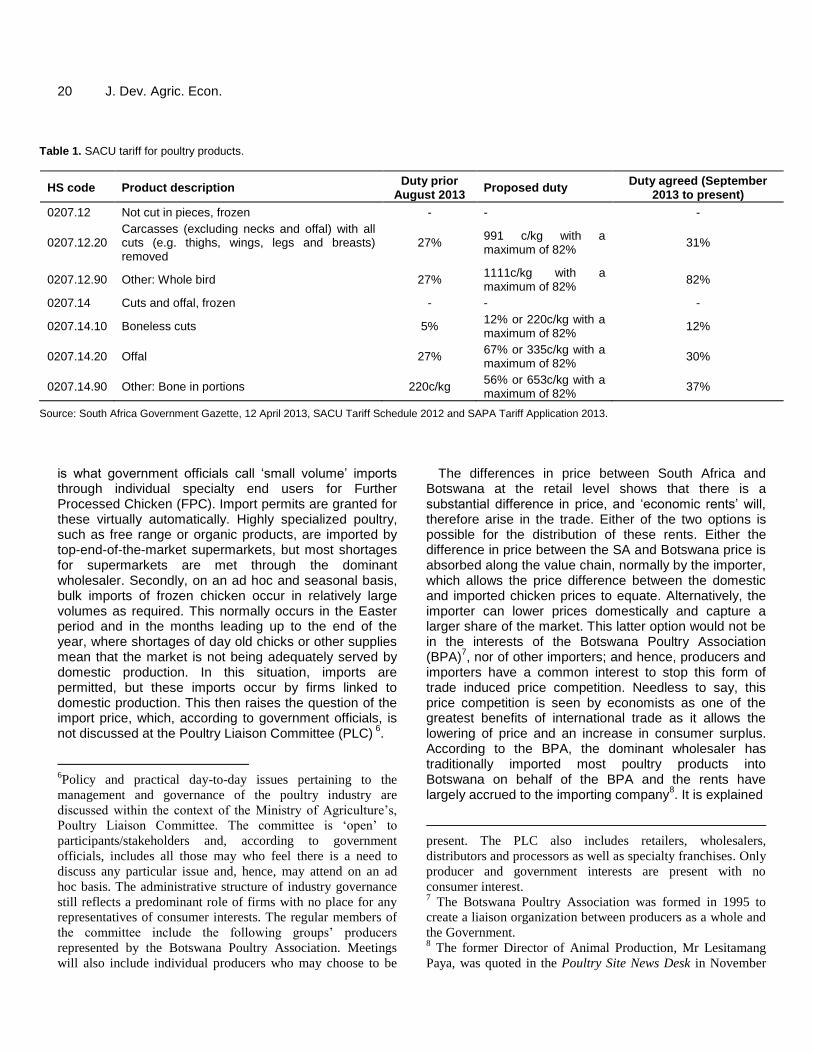
SACU trade restrictions SACU imposes a uniform common external tariff and a sample of the applied tariffs on the main poultry products is found below. The maximum tariff for poultry products were about 27%, then the South African Poultry
Association (SAPA) applied for the increase in tariffs in August 2013 through the International Trade Administration Commission (ITAC)
5. SAPA received
support from the producers in Botswana, Lesotho, Namibia and Swaziland (BLNS) and worried that their survival is threatened mainly by the large and rapid increase in the volume of imports of extremely low priced frozen chicken meat (from 97565 tonnes in 2008 to 238582 tonnes in 2012, about 40% increase).
Import duties remain high for broiler meat in most categories where competitive imports are possible (Table 1). The maximum tariff is now at 82% and used to deter export countries to 'dump' poultry in the SACU region. The industry argues that these measures are designed to support and promote the poultry producers across the entire SACU market to ensure a sustainable and competitive industry that is able to provide greater food security to the region's people. Botswana’s trade restrictions-non-tariff measures As the country is now self-sufficient, imports of poultry meat to Botswana are normally not permitted, but do occur on an ad hoc basis in either of two ways. The first
5 Under the current SACU arrangement South Africa continues
through ITAC to be responsible for the setting and amendment
of the Common External Tariff (CET) however this is due to
change once other SACU Members have established National
Bodies and the Tariff Board is set up.
20 J. Dev. Agric. Econ.
Table 1. SACU tariff for poultry products.
HS code Product description Duty prior
August 2013 Proposed duty
Duty agreed (September 2013 to present)
0207.12 Not cut in pieces, frozen - - -
0207.12.20 Carcasses (excluding necks and offal) with all cuts (e.g. thighs, wings, legs and breasts) removed
27% 991 c/kg with a maximum of 82%
31%
0207.12.90 Other: Whole bird 27% 1111c/kg with a maximum of 82%
82%
0207.14 Cuts and offal, frozen - - -
0207.14.10 Boneless cuts 5% 12% or 220c/kg with a maximum of 82%
12%
0207.14.20 Offal 27% 67% or 335c/kg with a maximum of 82%
30%
0207.14.90 Other: Bone in portions 220c/kg 56% or 653c/kg with a maximum of 82%
37%
Source: South Africa Government Gazette, 12 April 2013, SACU Tariff Schedule 2012 and SAPA Tariff Application 2013.
is what government officials call „small volume‟ imports through individual specialty end users for Further Processed Chicken (FPC). Import permits are granted for these virtually automatically. Highly specialized poultry, such as free range or organic products, are imported by top-end-of-the-market supermarkets, but most shortages for supermarkets are met through the dominant wholesaler. Secondly, on an ad hoc and seasonal basis, bulk imports of frozen chicken occur in relatively large volumes as required. This normally occurs in the Easter period and in the months leading up to the end of the year, where shortages of day old chicks or other supplies mean that the market is not being adequately served by domestic production. In this situation, imports are permitted, but these imports occur by firms linked to domestic production. This then raises the question of the import price, which, according to government officials, is not discussed at the Poultry Liaison Committee (PLC)
6.
6Policy and practical day-to-day issues pertaining to the
management and governance of the poultry industry are
discussed within the context of the Ministry of Agriculture’s,
Poultry Liaison Committee. The committee is ‘open’ to
participants/stakeholders and, according to government
officials, includes all those may who feel there is a need to
discuss any particular issue and, hence, may attend on an ad
hoc basis. The administrative structure of industry governance
still reflects a predominant role of firms with no place for any
representatives of consumer interests. The regular members of
the committee include the following groups’ producers
represented by the Botswana Poultry Association. Meetings
will also include individual producers who may choose to be
The differences in price between South Africa and Botswana at the retail level shows that there is a substantial difference in price, and „economic rents‟ will, therefore arise in the trade. Either of the two options is possible for the distribution of these rents. Either the difference in price between the SA and Botswana price is absorbed along the value chain, normally by the importer, which allows the price difference between the domestic and imported chicken prices to equate. Alternatively, the importer can lower prices domestically and capture a larger share of the market. This latter option would not be in the interests of the Botswana Poultry Association (BPA)
7, nor of other importers; and hence, producers and
importers have a common interest to stop this form of trade induced price competition. Needless to say, this price competition is seen by economists as one of the greatest benefits of international trade as it allows the lowering of price and an increase in consumer surplus. According to the BPA, the dominant wholesaler has traditionally imported most poultry products into Botswana on behalf of the BPA and the rents have largely accrued to the importing company
8. It is explained
present. The PLC also includes retailers, wholesalers,
distributors and processors as well as specialty franchises. Only
producer and government interests are present with no
consumer interest. 7 The Botswana Poultry Association was formed in 1995 to
create a liaison organization between producers as a whole and
the Government. 8 The former Director of Animal Production, Mr Lesitamang
Paya, was quoted in the Poultry Site News Desk in November

by the BPA that the choice of this company stems from the fact that it is the only company that has sufficient freezer capacity to manage the needed volume of frozen imports.
The BPA agreed that the price difference between the South African price and the domestic price will be taken up either by importers or retailers and that the retail price of imported South African chicken should not undercut the domestic producer. One of the larger supermarket chains in Botswana indicated that, when they do import chicken from South Africa through this dominant company, they have agreed on a small 5% margin; and that the difference in price is absorbed by the supermarket. Thus, the high margin available from imports is not necessarily absorbed at the producer/wholesaler end of the market. By allowing the producers to import, the economic rents created can also be absorbed by the importer-retailer. But in either case, the consumer is not the beneficiary
9. This procedure
employed by the PLC for allocating import permits stops imports from undermining domestic production and therefore limits any benefits that competition from international trade may have for consumers
10.
There has been a proliferation of imports with FPC poultry imports growing at unprecedented rate. The import data is presented in Figures 2 and 3. Total consumption of poultry meat was approximately 70,000 tonnes in 2008/09 with some 2960 tonnes of FPC chicken (MoA, 2009). Trade figures for the calendar year 2009 from the Statistics Botswana indicate that imports have fallen slightly. It is understood that a facility is under construction by one of the larger poultry producers to fill this growing segment of the market. Given the market access policy arrangements, that is, that no imports are permitted where domestic production exists, it is also understood that imports of FPC will be brought to an end with the establishment of this new processing facility.
It is also important to note that there has been evidence
2008 saying that "In an ideal situation, retailers should be the
ones to import. It is only that there is a crisis this year (FMD).
When the situation normalizes, we will call the producers and
tell them that their role is to meet the local demand. There has
been no shift away from the process of producer related
companies being permitted to import.
http://www.thepoultrysite.com/poultrynews/16510/producers-
accused-of-price-fixing 24 Nov 2008 9 In interviews some supermarkets indicated that they do lower
the price of poultry below domestic prices when they are
permitted to import. No evidence was provided of this. 10
The BPA received Pula 0.25 for every kilo of poultry meat
imported by the dominant company and these funds are used
for the maintenance of the industry association.
Grynberg and Motswapong 21
in the past of poultry meat smuggling across the border from South Africa. This indicates that the price differential between the Botswana and South African price is of a sufficient order of magnitude to justify the risks associated with these types of nefarious activities.
Not only have there been restrictions on the import of poultry meat, but there have been recent policy changes which have resulted in restrictions on the import of day old chicks, which was implemented in 2009. There are also pre-Southern African Development Community (SADC) Free Trade Area (FTA) restrictions presently in place on the import of animal feed, which must be consumed in the proportions of 70% local production to 30% imports
12.
SACU, SADC, EPA and WTO obligations What also needs to be considered in any discussion of trade in poultry products in Botswana is the nation‟s on-going commitment to the four principle trade agreements to which it is a signatory. Both the SACU Agreement (2002) and the SADC Trade Protocol, which established a free trade area between all SADC countries in 2008, as well as the WTO and the Interim EPA with the EU, are relevant to the trade in poultry products. The provisions of the SACU Agreement, to which both Botswana and South Africa are signatories, allows the BLNS members to depart from their obligations of the customs union in the case of infant industries for a period of eight years
13.
A further justification that has been offered is that the poultry restrictions can be explained under the provisions of Article 29 of SACU (2002), which provides a general exception clause for agricultural marketing
14: Member
States may impose marketing regulations for agricultural products within its borders, provided such marketing regulations shall not restrict the free trade of agricultural products between the Member States, except as defined below: (a) Emergent agriculture and elated agro-industries as
12
Statutory Instrument No.66 of 2005 states that "any person
applying for (an) import permit for maize meal, samp, maize
rice, or animal feed for poultry and livestock shall be required
to purchase at least 70 percent of the requirements locally and
the remainder can be imported”. 13
Infant industry protection is afforded under Article 26 (2) and
(3) of the SACU 2002 Agreement, which allows countries to
extend the infant industry protection for longer periods subject
to the agreement of the SACU Council. Article 26(4). 14
Pers. com, Department of Trade and Industry, 8 September
2010.

22 J. Dev. Agric. Econ.
Figure 2. Value of poultry imports into Botswana.
Figure 3. Volume of poultry meat imports into Botswana.
agreed upon by Member States; or (b) any other purpose as agreed upon between the Member States.
The Government of Botswana has notified the restriction on poultry to the SACU Council and it has been accepted
15. However, Botswana also has market
15
Pers. com, Department of Trade and Industry, 9 September
2010. It is by no means evident how Botswana could put a
legally valid case before the SACU Council that its measures in
opening commitments under SADC to remove non-tariff measures. Article 6 of the Protocol on Trade states that non-tariff barriers (NTBs) are as follows: „Except as provided for in this Protocol, Member Statesshall, in relation to intra-SADC trade:
the poultry industry do not violate the prohibition on using the
provisions of Article 25(1) of SACU 2002 for the purpose of
protection of industry.

1. Adopt policies and implement measures to eliminate all existing forms of NTBs. 2. Refrain from imposing any new NTBs. At the 6
th Special Meeting of the SADC Committee of
Ministers of Trade and Industry, held in Dar es Salaam, Tanzania, on 8 November 1999, agreement was reached on two broad areas of NTBs, namely, the core NTBs that should be eliminated immediately on commencement of the FTA implementation process, and other NTBs set aside for gradual elimination. The core NTBs identified include: 1. Cumbersome customs documentation and procedures; 2. Cumbersome import and export licensing/permits; 3. Import and export quotas (except those concerning special sensitive products as may be specified); 4. Unnecessary import ban/prohibitions. These NTBs were supposed to be eliminated for all non-sensitive products by 2008. However, despite calls by SADC members for the removal of all NTBs, there appears to be only limited appetite amongst SADC members for change in the current practices. A recent SADC review of the development of the FTA has argued (SADC, 2010):
„SADC‟s programme on the elimination of NTBs has not moved at the same pace as tariff liberalisation. In many instances, NTBs are continuously increasing and their elimination is, therefore, a critical factor in consolidating the FTA. Pursuant to this, in July 2007, SADC Ministers of Trade agreed to a mechanism for reporting, monitoring and eliminating NTBs.‟ Government of Botswana officials have also argued that
16:
Article 20 of the SADC Protocol on Trade also allows Member States to apply safeguard measures to a product only if it has been determined that such product is being imported into its territory in such increased quantities which may cause serious injury to the domestic industry. Member States shall apply safeguard measures only to the extent and for such period of time necessary to prevent or remedy serious injury and to facilitate adjustment.
There also exist WTO obligations to which Botswana is a signatory which are unlikely to be enforced because of the high cost of any potential complainant relative to the size of the market. In particular, the Uruguay Round Agreement on Agriculture strictly prohibits the type of quantitative restrictions found under the Control of Goods (Importation of Eggs and Poultry Meat) Regulations [S.I.
16
No safeguard investigation has occurred in the poultry
industry.
Grynberg and Motswapong 23 120, 1979], which imposes import licensing provisions based on volumes. These measures have been in action since 1979 and Botswana‟s commitments under the WTO, which are provided for unambiguously under the terms of Article 4(2) of the Agreement on Agriculture, which states that „Members shall not maintain, resort to or revert to any measures of the kind which have been required to be converted into ordinary customs duties‟. In other words, tariffication of all Non-Tariff Measures which was so widespread, in particular, footnote number 1 specifies that „the measures include quantitative import restrictions (GATT, 1995). This then raises the issue of how Botswana and the other small states have been able to justify and continue such quantitative restrictions. The Trade Policy Review of the WTO for Botswana (2009) states that the reasons that these import restrictions are maintained are for „food security reasons‟ (WTO, 2009). The Botswana poultry industry has indicated its intention to exports to the EU, especially for breast meat which is strongly preferred in the EU, but not in Botswana (Farmers Magazine, 2010). With the establishment of an EU standard compliant abattoir by Tswana Pride, such a development is indeed possible. Under the provisions of the Interim EPA which govern trade and commercial relations between the EU and Botswana, the sort of quantitative restrictions through import licensing used by Botswana to prohibit imports from South Africa and by extension by the EU are simply not permitted
17. While
other SACU, SADC and WTO members may turn a blind eye to the sort of quantitative restrictions imposed by Botswana in the poultry industry, it is questionable that the EU will permit exports duty free access to its market for a product which are restricted by Botswana. Moreover, the export to the EU is predicated on those import restrictions which allow Botswana producers to obtain a higher price for dark meat on the local market. While it would appear that SADC does nominally impose legal restrictions on the type of quantitative trade measures used by Botswana in the poultry industry, given the widespread use and increasing prevalence of NTBs by SADC members, it can only be concluded that these limitations on the use of these instruments are more apparent than real. The WTO also disciplines its members on precisely these forms of quantitative
17
Article 35 of the Interim EPA states:
‘All Import or Export prohibitions or restrictions in trade
between the Parties, other than customs duties and taxes and
other charges provided for under Article 22, whether made
effective through quotas, import or export licenses or other
measures, shall be eliminated upon entry into force of this
Agreement unless justified under the provisions of Article XI,

24 J. Dev. Agric. Econ. restrictions which are not permitted. It is only because the Botswana market is very small that there is no complain. But, the non-tariff barriers are in clear violation of the spirit, and, in the case of the WTO, the letter of Botswana is legal obligations. THE POULTRY VALUE CHAIN There are 9-10 relatively large producers of poultry in Botswana who are members of the BPA. However, the main supermarkets in Botswana are supplied by 5-6 companies which are closely inter-related. According to industry sources, supermarkets, which purchases 45% of poultry consumed by supermarkets, buy from „any source as long as it meets standards and price‟. The industry also suggests that in Botswana, the minimum efficient scale in the broiler industry is achieved when a facility is produced between 30,000-50,000 units per week, although much larger producers exist in South Africa. There are a large number of small and contract growers who are well below this scale level (TRANSTEC AND BIDPA, 2010)
18. Until late 2010, there were two groups in
the industry which dominated the broiler production. One of the groups is linked to other largest producers and also includes three of the biggest producers. This grouping is responsible for between 40 -60%
20 of the market share
21.
Both groups were integrated along the value chain to a greater or lesser degree with some having more backward integration into inputs and others being forward integrated into processing and supermarkets. There are also, a large number of small scale producers who supply the large firms on a contract basis, as well provide supply on government tender. In the region of Gaborone, many of these small scale producers which, in 2010, included some 18 farmers, according to the company, employed some 200 workers. These small scale producers have no direct access to supermarkets and many of their sales are to small village retail outlets and individuals. An
GATT 1994’. 20
The estimate of 60% of market share was confirmed by the
MoA as well as the Farmers Magazine Botswana,2010 which
stated that the abattoir was razed down in May 2009 and at the
time it was the largest in the country supplying 60% of chicken
consumed in the country’ 21
The Botswana National Competition Policy ( 2005, page 4 )
defined Monopolisation as:
‘The conduct and practice of a firm with a dominant position
of at least 40% or market share and significantly larger than
that of its biggest rival to maintain , enhance or exploit their
dominant power in the market place’
important market outlet for some of these relatively small producers is on tender to government institutions, such as schools and the Botswana Defence Force. The larger producers supply the out-growers with inputs. Since 2000, however, there has been a steady rise in commercial sector holdings, and by 2004, there were nominally over 300 small holdings. The majority of the holdings that were established and funded a decade or so ago under the FAP are no longer operational.
According to the government, the company which supplies some 95% of poultry feed for the industry is also owned by the dominant poultry producing group. It is important to note that the retail distributor of the production insists that, largely because of the high cost of transport, it is cheaper to procure poultry feed in Botswana rather than from South Africa. They argue that the obligation to purchase from local sources on a 70/30 basis will add pula 250-300 per tonne to the price of feed. Current levels of commercial maize production are such that this proportion of local supply of maize cannot come from domestic production of maize and, therefore, the ratio, while nominally mandatory, is aspirational in nature, rather than binding when it comes to maize farmers. The total procurement of maize of the Botswana Agricultural Marketing Board (BAMB), which is the only significant buyer, in 2009, was approximately 4,500 tonnes, almost all of which went largely to the two largest milling firms in Botswana. The domestically produced maize available through BAMB was used by these firms in the maize milling sector to produce maize meal and not in the production of animal feed. As there is very little local maize for animal feed, the 70/30 rule provides a legally assured market and that of the other very small producers, which are, in turn, largely produced from imported grains. Given current levels of maize output in Botswana, such a policy does not appear to be in the interests of the economic efficiency of the poultry industry, maize farmers or of consumers, and should, therefore, be abandoned. Therefore, the dominant firm in the industry, that is, companies owned or associated with, are vertically integrated along the value chain all the way from poultry, day old chicks, production and finally to freezer and distribution facilities. TOWARDS A SMALLHOLDER POLICY As was noted at the beginning of this paper, the original intention of Government, NGO and donor policy in the early days of the industry in the 1970s and 1980s was to use the poultry industry as a way of increasing rural incomes of smallholders and thereby alleviating poverty. However, the commercial reality of economies of scale as well as the management of PAMA and the FAP means

that now smallholders only operate in a very peripheral place in the industry, either supplying large producers as out-growers or supplying direct to small rural buyers. By and large, the smallholder, as noted above, has no direct access to the primary poultry market, that is, supermarkets. Instead, the poultry meat value chain is now dominated by one group of firms that is vertically integrated; and the original intent of the poultry policy, which was to stimulate smallholder production, has not occurred because this is counter to the commercial imperative of having large firms that benefit from economies of scale and direct marketing links to supermarkets.
Government policy towards poultry smallholders has not been sufficiently robust to fundamentally change the reality described above. Smallholder policy, given the uncompetitive current structure of the industry, can, if cast in commercial realities, be a powerful vehicle for achieving increased competition in the industry. There now appears to be every intention to return to government managed co-operatives in the poultry sector through the Livestock Management and Infrastructure Development (LIMID) II program, which will provide government assistance to the poultry sector through a 4 million Pula grant for the construction of a co-operative abattoir, which will be managed by government temporarily, „until such time as they are profitable‟. The LIMID program requires injections of capital by the members of the co-operative and, as a result, this will assure greater stakeholder intervention in management than was the case with PAMA in the 1980s. However, the LIMID II proposal, at least initially, involves a very similar dominant role for government, as was the case during PAMA. This approach failed in the past and its proponents need to demonstrate how the current LIMID proposal, whereby government will manage the proposed smallholder poultry abattoir, will lead to different outcomes from that of PAMA. Moreover, it is questionable whether such small scale abattoirs of 100,000 units per month will prove to be profitable and the government will be able to readily exit the envisaged management role in the LIMID proposal.
If the Government wishes to see the smallholder part of the industry thrive and develop, a more imaginative and well-funded proposal needs to be considered, rather than that of government management of an abattoir. Variants of the current proposal have failed in the past and there appears to be little in the LIMID proposal that draws on the PAMA experience of state control in the sector. Providing financial support to smallholders to find professional management from outside government and providing incentives to supermarkets and other consumers to invest in the development of the smallholder sector is more likely to achieve commercial
Grynberg and Motswapong 25 success in strengthening the smallholder sector than using government controlled agencies.
There is a need for the development of a comprehensive smallholder plan, which must be part of a return to a more competitive sector. What is unavoidable is the reality of economies of scale and the need to establish strong marketing links with existing supermarkets. The key to a successful smallholder plan is funding a partial liberalisation of trade with an accompanying earmarked levy on import permits that could produce sufficient revenues which could then be earmarked for a smallholder industry plan
22.
CONCLUSIONS The poultry meat industry, as it is presently functioning has succeeded in producing national self-sufficiency in poultry meat. However, based on international prices, the industry is uncompetitive and arguably it is characterized by an industry structure that is duopolistic or oligopolistic. The normal policy response of economists when such a situation arises as a result of trade restrictions is to propose substantial and immediate trade liberalisation that would permit imports from SA and elsewhere which would in turn, lower prices and increase competition. Assuming that the Government of Botswana would like to continue to see a viable and profitable domestic poultry industry, a full and complete liberalisation should be avoided at this point in the industry‟s development, as it is highly doubtful that the industry could survive such an economic shock. However, partial and progressive market opening as proposed in the policy recommendations below would increase the competitive pressures on the industry, result in lowering of prices and would also force the industry to lower its operating costs. After 36 years of trade restrictions, a modest liberalisation, as proposed below, should be considered. Policy recommendations 1. The poultry industry is Botswana‟s most successful import substituting sector and the government is quite rightly proud of the achievement of reaching national self-sufficiency in poultry products. However, that national self sufficiency has been achieved at a considerable cost to
22
A levy on imported products coming from other SACU
countries is not uncommon as these are imposed by other
BLNS countries. As it is the result of a liberalisation of intra
SACU trade, as compared to the status quo, it is more likely to
find support amongst SACU members.

26 J. Dev. Agric. Econ. the consumer as well as to the taxpayer through various investment support programs over the years. Restrictions on imports have been in place since 1979. The government needs to undertake a fundamental review of its policy for a large part of the industry does not require infant industry protection to the extent that has been the case in the past. In order to assure the long term efficiency and viability of the industry and maintain consumer support, the government needs to ease, in part, the long standing trade restrictions. However, this will need to be balanced against objective of protecting small producers who will find adjustment to a more competitive industry even more difficult. 2. The industry is vertically integrated along the value chain with two groups controlling the industry. The value chain for poultry is highly uncompetitive. As an instrument of competition policy, the government should give consideration to providing extra financial incentives to encourage new firms seeking to enter the industry to provide alternative supply of inputs, freezer facilities and poultry meat. 3. The poultry industry cannot approach international competitiveness if the government of Botswana insists on the current policy of forced domestic procurement of poultry feed, that is, 70/30 rule. Botswana‟s commercial production of grain marketed through BAMB is 4,500 tonnes and almost all is used for human consumption. Therefore, the 70/30 rule, when applied to poultry feed becomes a market support measure for local poultry feed producers and does not support local maize farmers. The poultry feed market is dominated by one firm which supplies over 90% of domestic supply. There should also be no further trade restrictions on other inputs such as DoC as this further compounds the industry‟s lack of competitiveness. 4. The government should give consideration to the development of a Smallholder Poultry Plan based in part on providing tax concessions and other benefits to larger firms and supermarkets to procure poultry from domestic smallholders. A smallholder marketing program should also be properly funded to assist smallholders to develop direct co-operative links to supermarkets though further consideration should be given to the modalities in light of the failed earlier attempts to establish PAMA. Government may wish to give consideration to imposing a levy on these poultry imports to be used to develop the small-holder poultry plan considered. Conflict of interests The authors have not declared any conflict of interests.
ACKNOWLEDGEMENTS The authors gratefully acknowledge comments of Jay Salkin and BIDPA staff on earlier versions of the paper. They are also grateful to the Statistics Botswana, Ministry of Agriculture, for providing data used in this article. REFERENCES BIDPA (2010). A study of the Impact of SACU Tariff and Trade Policy
on Food Prices in the Sub-Region. Unpublished report, BIDPA. Brittain L (1997). Competition Policy and the Trading System: Towards
International Rules in the WTO. Remarks given for the Institute for International Economics, Washington D.C., 20 November 1997.
Statistics Botswana (2015). Various trade data database. Gaborone, Botswana: Statistics Botswana.
Farmers Magazine. (2010). Tswana Pride Eyes EU Market. 7(55). Gal MS (2001). Size Does Matter: The Effect of Market Size on Optimal
Competition Policy. South Calif. Law Rev. 74:1437-1478. GATT Secretariat (1995). The Results of the Uruguay Round of
Multilateral Trade Negotiations. Government of Botswana (2010). Livestock Management and
Infrastructure Development Programme. Ministry of Agriculture, Gaborone, Botswana.
Ministry of Agriculture (2009). Department of Animal Protection. Unpublished report.
Ministry of Finance and Development Planning (1995). Third Evaluation of the Financial Assistance Policy. Report prepared by Phaleng Consultancies (Pty) Ltd.
Ministry of Finance and Development Planning. (2000). Fourth Evaluation of the Financial Assistance Policy. Report prepared by BIDPA.
Ministry of Trade and Industry. (2005). National Competition Policy for Botswana. July 2005. Gaborone, Botswana
SACU (2012). SACU Tariff Schedule 2012. Southern Africa Custom Union. Windhoek, Namibia.
SADC Secretariat (2010). Advancing Regional Economic integration in SADC through Consolidating the SADC Free Trade Area. SADC/TNF/39/2010/3.1
Sauve P (2004). Trade Rules Behind Borders., Cameron, London. South Africa Government Gazette.
The Poultry Site News Desk (2008). Producers Accused of Price Fixing. Available at: http://www.thepoultrysite.com/poultrynews/16510/producers-accused-of-price-fixing.
TRANSTEC and Botswana Institute for Development Policy Analysis (BIDPA) (2010). Botswana Agric. Sector rev. Unpublished report, BIDPA.
World Trade Organization (1996). Singapore WTO Ministerial Declaration 1996: Ministerial Declaration. WT/MIN (96)/DEC, 18 December 1996, para 20. Available at: http://www.wto.org/english/thewto_e/minist_e/min96_e/wtodec_e.htm
World Trade Organization (2009). SACU Trade Policy Review- Botswana. Geneva, Switzerland.

Vol. 8(2), pp. 27-38, February, 2016
DOI: 10.5897/JDAE2015.0700
Article Number: 6A71EE256960
ISSN 2006-9774
Copyright ©2016
Author(s) retain the copyright of this article
http://www.academicjournals.org/JDAE
Journal of Development and Agricultural Economics
Full Length Research Paper
Total factor productivity growth of Turkish agricultural sector from 2000 to 2014: Data envelopment malmquist
analysis productivity index and growth accounting approach
Abdul-Basit Tampuli ABUKARI*, Burak ÖZTORNACI and Püren VEZİROĞLU
Department of Agricultural Economics, Faculty of Agriculture, Çukurova University, Sarıçam, Adana, Turkey.
Received 5 October, 2015; Accepted 23 December, 2015
Despite the enormous diversification Turkey has made, agriculture still remains the backbone of its economy. Most of the successes Turkey’s economy has chalked came in the last 15 years; after 2000. The agricultural contribution to both gross domestic product and employment fell within this period. The answer to the state of the sector is not found in its contribution to gross domestic product or employment but the progress in its total factor productivity growth. This is defined as that part of agricultural output growth that is not explained by changes in factors of production. Like all scientific procedures, there is no one way of estimating total factor productivity growth. Considering the advantages and disadvantages methods possess over one another, it is always logical to apply more than one technique on the same data set to establish a range within which the results can be established. We settled on Data envelopment analysis malmquist productivity index and the growth accounting approach. We gathered data on agricultural output and ten inputs at the national, from 2000 to 2014. They were simultaneously applied on our data. The total factor productivity of Turkish agricultural sector grew at 28.8%, with an annual growth rate of 2%. Key words: Data envelopment analysis, growth accounting, malmquist productivity index, total factor productivity growth.
INTRODUCTION Turkey as a region has been a serious agriculturally oriented economy before and after its independence in 1923. It still remains a vital part of its economy, even though a lot of diversifications have taken place (Öztürk,
2012). With the exception of its contribution to industry, there has been a significant reduction in the contribution of Agriculture to gross domestic product (GDP), employment, foreign exchange, etc. Examining the
*Corresponding author. E-mail: [email protected]. Tel: +905073818713.
Author(s) agree that this article remain permanently open access under the terms of the Creative Commons Attribution
License 4.0 International License

28 J. Dev. Agric. Econ.
Figure 1. Turkey‟s GDP Per Capita. Source: Data from World Bank Development Indicators (WDI) (2014).
growth of Turkish GDP per capita ($) since 1960 in Figure 1. The graph exhibits a clear categorization of the growth trend as revealed by the steep slope; before 2000 and post 2000. Whiles an average annual growth in GDP per capita was $89 between 1970 and 1999, the period between 2000 and 2013 recorded $200 per annum. Within this unprecedented growth period (2000 till date), agriculture‟s contribution to GDP has been declining. However for a sector that still employs 21.1% of the country‟s labor force and contributes a lot to the industrial sector, it is important to investigate how it has performed during this period of unprecedented growth. In our opinion, this dwindling contribution of agriculture is not a cause for alarm, but the status of factor contribution to agricultural output is rather very vital. This informed our choice to access the total factor productivity growth (TFPG) of the agricultural sector within that period. TFPG indicates that part of output growth which is not resulting from the increase or decrease in factors of production (inputs) (Fadejeva and Melihovs, 2009). Existing TFPG studies also points to this same trend.
Using slow growth accounting approach (SGAA), Atiyas and Bakış (2013) found out a tremendous TFPG of 3.8% in the economy of Turkey which before then barely crossed the 1% mark. Their work is diagrammatically represented in Figure 2. From the two Figures 1 and 2, it can be seen that a lot of positive gains have occurred in post 2000 Turkey. It is therefore logical to investigate the status of agriculture within that same period.
There are so many different methods used in the estimation of TFPG. The choice of any method, among many things, depends on the researcher, the objectives of the study and the nature of the available data.
However, considering the pros and cons of each method, it is logical if possible to apply more than one method on a single data and compare the results. In the language of productivity and efficiency measurement, our data considered a single firm case (the whole of Turkey‟s agricultural sector). With this, so many TFPG methods cannot be applied on it, especially most of the frontier approaches. The two methods found to be simultaneously applicable and mathematically and theoretically related are Data envelopment analysis malmquist index (DEAMPI) and the Solow growth accounting approach (SGAA). The results from both methods give a range within which the growth of TFP of Turkish agriculture can be accessed. There have been previous researches on this topic in Turkey. These researches vary a lot from the present study. Whiles some are regional, others have targeted certain enterprises within the agricultural sector. Furthermore, the comparison with these two techniques has not been done. The main difference however, is the fact that none of them considered as many variables as ours. Literature relating to Turkey Basarir et al. (2006) found that even though annual agricultural growth rates was between 1.30 and 3.40% over 1961 to 2001 period, technical change growth rates ranged from -0.15 to 5.53%. Candemir and Deliktas (2007) also used data from 1999 to 2003 to estimate both productive efficiency and TFPG of Turkish state agricultural enterprises. While technical efficiency grew by 1.5%, there was a technical regress of 2.7%, leading

Abukari et al. 29
Figure 2. Total Factor Productivity Growth. Source: Atiyas and Bakış (2013, p.12).
to TFPG of -1.2%. In the South Marmara region of Turkey, Tipi and Rehber (2006) estimated MPI of 3.1% from 1993 to 2002. Analyzing data for the Turkish agricultural sector from 1992 to 2012, Ozden (2014) concluded there has been a TFP regress of -5.6%. Telleria and Aw-Hassan (2011) analyzed data for 12 countries within West Asia and North Africa (WANA) from 1961 to 1997. Turkey is a member of WANA. They concluded that Turkey‟s TFP of its agricultural sector grew by 12% within the period of study. Atiyas and Bakış (2013) using GAA, revealed that Agricultural TFPG grew by 6.75% from 2002 to 2006, and -1.5% from 2007 to 2011. This gave an average annual TFPG of 2.62% for 2002 to 2011 year period. Candemir et al., (2011) attempted to measure the technical efficiency as well as the TFPG of hazelnut production and sales in Turkey. They considered 2004 to 2008 time period. Using DEA, they found that the mean technical efficiency across this period varied between 0.841 and 0.938. Technical efficiency change was 1.3%, technical change was -3% and the TFPG (Malmquist Index) was 1.7%. Furthermore, Shahabinejad and Akbar (2010) set out to measure
agricultural productivity growth in the Developing Eight (D-8) of which Turkey is a member. They considered the period from 1993 to 2007. Employing DEA, they estimated the TFPG and decomposed it into technical and efficiency change (TECH and EFFCH) components. Over the period, the countries as a whole managed a little below 1% TFPG with a 1.5% growth in Technology (TECH). This was offset by a negative growth of 0.4% in technical efficiency (EFFCH). They therefore concluded that EFFCH is a constraint to TFPG while TECH fostered
the growth in TFPG. At the level of individual countries, our country of interest, Turkey, was the second highest in terms of TFPG behind Malaysia. Malaysia recorded 2.9% growth followed by 2% for Turkey. However, unlike most of the countries, Turkey recorded a positive growth in both EFFCH and TECH. Pamuk (2008) used secondary data to estimate TFPG of Turkish agriculture from 1880 to 2000. He grouped the period into two; before and post-World War Two (WW2), that is 1880 to 1950 and 1950 to 2000. He estimated 0.3% growth for 1880 to 1950 and 1.1% for 1880 to 1950.
Rungsuriyawiboon and Lissitsa (2006) measured agricultural productivity growth in the European Union and Transition Countries. Turkey was considered among countries under transition countries despite the fact that it became an associate member of EU since 1964. The period under study was 1992 to 2002. They grouped countries into three; those that joined the union before 1995, those that joined in 2004 and the transition countries. For group comparison, they further choose three countries from each group for the analysis. The order of grouping the countries were Austria, Germany and UK; Hungary, Poland and Slovenia; Russia, Turkey and Ukraine. DEA was used to estimate the Malmquist TFPG. The 9 countries‟ growth rates were; Austria (2.78%), Germany (2.82%), UK (0.30%), Hungary (1.62%), Poland (2.59%), Slovenia (7.21%), Russian (5.32%), Turkey (1.70%) and Ukraine (5.33%). Zeroing in on Turkey, they explained that Turkey‟s TFPG was attributed significantly to „frontier-shift‟ effect than „catch-up‟ effect. This was due to the fact that, of the 1.7% TFPG, EFFCH was only 0.18%, compared with 1.51%

30 J. Dev. Agric. Econ.
Figure 3. Measurement of Total Factor Productivity – Approaches. Notes: OP – Olley and Pakes approach; LP – Levinsohn and Petrin approach; ACF – Ackerberg, Caves and Frazer model. Source: Adapted from Kathuria et al. (2013, p.6) who also adapted from Mahadevan (2003).
growth in TECH.
METHODOLOGY
Efficiency and productivity measurement as well as their growth have undergone different phases in terms of methodology; from the use of index numbers, linear and quadratic programming to econometric estimation. Even though new frontiers in estimation are still being pursued, the combination of the available methods on one data set is becoming the most logical way of increasing the precision of findings. This is due to the convincing advantages and disadvantages each method possesses over the other. This study adopted the method of applying two non-parametric approaches which are popularly known in the efficiency and productivity literature as DEAMPI and SGAA, respectively. These two methods have a lot in common as far as our data is concerned. The justification for the selection of these methods is found in the explanation following Figure 3.
There are two main approaches by which TFPG can be estimated; frontier and non-frontiers approaches. Each of them has a sub classifications grouped under parametric and non-parametric approaches. The main difference between frontier and non-frontier approaches lies in the definition of the frontier. While the former establishes production frontier which corresponds to the set of maximum attainable output levels for a given combination of inputs,
the later only construct an average line using ordinary least square regression as a line of best fit (Kathuria et al., 2013). Furthermore, because the frontier approach has the best possible frontier constructed, it incorporates technical efficiency in its estimation of TFPG while the non-frontier approach assumes fully technically efficient firms (Kathuria et al., 2013; Fare et al., 1994). The sources of TFPG from the frontier approach are further divided into two; an outward shift in the defined frontier (Technical Change-TECH) and a movement towards it (Technical Efficiency Change-EFFCH). However, the non-frontier approaches only consider TECH as TFPG.
It can be seen that though, the two selected methods are under different side of the divide, they are both non-parametric methods. Because our data is a single firm case, we cannot construct a frontier for it since we need more than one firm to construct a frontier for any given year. However, under the frontier approaches it is only DEAMPI which does not require the explicit construction of a frontier, hence our choice of it from the frontier side. On the non-frontier side, there are two main approaches; PFA and GAA. The semi-parametric approach (SPA) is a combination of these two methods. Even though they all make use of the production function, GAA like the DEA approach does not have a stochastic term, making it impossible for statistical testing to be done. After settling for GAA, we further reviewed the three different indexes used under this approach. We had to choose the most appropriate one for our data. They are the Kendrick arithmetic Index (KI)

Abukari et al. 31
Figure 4. MPI, the case of many firms. Sources: Authors‟ Illustration.
(Kendrik, 1961), the Solow geometric Index (SI) (Solow, 1957) and Theil-Tornquist or Translog-Divisia Index (TLI) (Kathuria et al., 2013). The KI utilizes the income share of inputs as their weights for aggregation. This will not be possible with our data since we do not have the data on the rewards for the inputs. The SI, though with numerous assumptions fits well into our data. The data has all the requirements for its estimation. Even though Kathuria et al., (2013) considers TLI to be superior to both KI and SI, our data cannot meet its requirements for estimation. It requires current input prices for the construction of its weight. This makes it possible for the quality of inputs to be estimated.
For all GAA and PFA techniques the assumption of constant returns to scale (CRS), perfect competition and full capacity utilization are required. It is however not necessary in the case of PFA.
DEA malmquist index (DEAMPI)
Contrary to the name of the index, it was introduced by Caves et al. (1982) by using Malmquist input and output distance functions. It was however empirically applied by Fare, Grosskopf, Norris and Zhang (FGNZ) in 1994 (Kathuria et al., 2013). It is used to measure the TFPG for a group of firms or a single firm over a period of time. The difference between the two is the fact that, the former can construct a frontier for each year, while this is not possible in the single firm case. That is, more than one firm is required to construct a production frontier. In the latter case there is an implicit assumption that the firm is fully efficient for any given year, because there is no other firm for a comparison to be made.
The case of many firms Assuming one input one output case, variable return to scale (VRS) assumption with output orientation, Figure 4 shows the TPFG
of three firms, A, B and C for three consecutive years. The present year „t‟, the year before „t-1‟ and the year after „t+1‟. These three (3) firms in each year is able to construct a frontier y=f(x). Each point on the graph represents productivity (Output/Input) of the firm at the point. This makes it possible for their efficiencies to be measured. That is, those points divided by the corresponding points on the frontier. Example, under VRS assumption, the efficiencies for firm A in t-1, t and t+1 are At-1/A
1t-1, At/A1
t and At+1/A1
t+1, respectively. In order to estimate the DEAMPI for only firm A from year t-1 to t, one need to employ the concepts of distance functions as seen in equation 1. This form of presentation was referred to as Fisher ideal indexes by Caves, Christensen and Diewert (Fare et al., 1994). The index is generally defined as the geometric mean of these four indexes made up of these distance functions. For instance,
means the productivity of that firm at the current
year „t‟ compared with the previous year‟s „t-1‟ frontier or technology. That is the one in the brackets is the firm in question and what is outside the bracket is the reference technology. Mo(xt,yt, x t-1,y t-1)
=
2
1
11111
1
),(
),(*
),(
),(
ttt
o
ttt
o
ttt
o
ttt
o
yxD
yxD
yxD
yxD…… (1)
When these distance functions are rearranged according to Fare et al., (1994), it decomposes into technical efficiency change and technical change as follows: Mo(xt,yt, xt-1,yt-1) =
2
1
11
1111
111 ),(
),(*
),(
),(
),(
),(
ttt
o
ttt
o
ttt
o
ttt
o
ttt
o
ttt
o
yxD
yxD
yxD
yxD
yxD
yxD .. (2)
The ratio outside the bracket measures EFFCH while the square

32 J. Dev. Agric. Econ. root of the one inside measures the TECH (Coelli et al., 2006).
From the equation 2, it can be seen that, the EFFCH ratio is the ratio of the technical efficiency in the current year to the previous year. This ratio indicates how closer or otherwise the firm in question is to its frontier as the years pass. The rest of the equation can be seen as a ratio of efficiencies made up of references to technologies in different years. A geometric mean of these gives the TECH, which indicates the shift or change in technology between the two periods under study (Coelli et al., 2006). The product of these two indexes gives the malmquist productivity index (MPI). That is:
TFPG = EFFCH × TECH (3)
In all the indexes, EFFCH, TECH and MPI have the same interpretation. An index above one indicates a positive change or growth, below means negative and one means stagnant or no growth (Fare et al., 1994). Even though further decompositions were later developed, they are not relevant to this study. The software we used for this analysis is data envelopment analysis program (DEAP Version 2.1) by Tim Coelli. Applying this formula to Figure 4, the MPI for firm A from the year t-1 to t is algebraically represented as follows:
Mo(xt ,yt, xt-1,yt-1)=
(4)
Mathematically, it demands the solving of four different distance functions in the DEA format. Even though there are six (6) distance functions, there are actually four unique ones and the other two are repeated. Since they are output distance functions, we need to take the inverse of each of them.
St:
St:
St:
St:
Whiles ∅ represents efficiency, γ represents the weight of individual firms. Unlike normal efficiency estimation where ∅ is restricted to between 0 and 1, it may be greater than 1 in some of the linear programing since the firms are compared with the frontiers of different years (Coelli et al., 2006). These four linear programing are sufficient for only one firm. This means that if there are ten firms to be considered forty of such linear programing must be solved. The case of a single firm Let‟s us assume now that we are dealing with only one firm „A‟ with its available data for the current year „t‟, the previous year „t-1‟ and the following year „t+1‟ as represented in Figure 5. In order to construct a frontier or a production function, data on several firms are required, which is not possible in this case. The other option is to adopt an existing production function or frontier. Even though several studies have been done estimating the production function of Turkish Agriculture, none of them considers as many inputs as we have done in this study. This therefore means that there is no production function for which the firm can be compared to, other than itself. That is, unlike the case of firm A in Figure 4, there is no A1
t-1, A1
t and A1t+1. This logically means that technical efficiency will
be 1. This further implies that the first part of the MPI which measures the EFFCH will be 1, indicating no change in technical efficiency. However, the technical change component is measurable, considering the fact that the firm is using the same amount of inputs to produce more in year t and t+1. It is only in the improvement of technology that this will be possible. This value multiplied by 1 (EFFCH) will give the MPI for that firm. The solow growth accounting (SGAA) Though Robert Solow (1957) is widely considered as the originator of this approach, its origins could actually be traced back to Tinbergen (1942) (Kathuria et al., 2013). Despite the fact that GAA has a lot of differences with other known TFPG techniques, especially index numbers, it still has a strong relationship with them. MPI which has become the most widely used index for TFPG measurement has a mathematical relationship with GAA which makes it comparable to other Malmquist index results from DEA and SFA. However as explained earlier, the nature of our data (that is, the single firm case scenario, with no defined frontiers for each year), it is difficult to employ the SFA method. However, DEA does not need a functional specification (Diewert and Nakamura, 2006). In GAA, aggregate output growth is decomposed into input or factor growths as well as the growth in the residual term which represents TFPG. That is, the portion of output growth not explained by input or factor growth (Atiyas and Bakış, 2013).
According to Diewert and Nakamura (2006), the multi factor productivity measurement procedures can be classified into four: (1) The rate of growth over time of TFP, (2) The ratio of the output and the input growth rates, (3) The rate of growth in the revenue/cost ratio controlling for price change and (4) The rate of growth in the margin after controlling for price change. As can be observed, the third and fourth are in monetary terms requiring the use of rewards for inputs (wage, rent, interest etc.), the first two however do not. Considering the fact that our data is a single firm case with no price information, the first and the second procedure will be adopted.

Abukari et al. 33
Figure 5. Malmquist Index, the case of one firm. Source: Authors‟ Illustration.
Presentation With only slight modification, the presentation follows the same procedure and assumptions used by Solow himself. In his 1957 landmark paper, he modified the production function by redefining the time trend which measures TECH. That instead of Y = F (K, L, t), he represented it by Y = A (t)F (K,L). Where Y is the output and K and L represent capital and labor inputs, and the „t‟ in the function represent neutral TECH. The „A‟ measures the TFP, while its multiplicative factor, A (t) measures the cumulated effect of shifts over time that is, TFPG (Solow, 1957). Even though the use of translog production could have been possible, we are forced by the nature of our data to assume a Cobb-Douglas production function as would be explained in the data section of this paper. It has to be noted that Solow also fitted Cobb-Douglas production function on his data covering 1909 to 1949. Considering a Cobb-Douglas production function with a constant return to scale (CRS) assumption:
(5)
The parameters α and (1-α) are the fractional exponents which represent the capital and labor share of output, respectively. The sum of these parameters also defines the scale of operation. When they sum up to one it indicates CRS, below one, decreasing return to scale (DRS), and greater than one increasing return to scale (IRS). Since CRS is imposed on the formulation, their summation must be equal to one, that is α + (1-α) = 1. Basically, there are two ways of calculating the α and 1-α, that input shares; by regression analysis or extraction from the national or available data (Atiyas and Bakış, 2013). The former was used in the present analysis.
Linearizing (taking logarithm) Equation 5;
(6)
There is an implicit assumption in equation 5 that technology or TFP (A) is constant over time, after lnY is regressed on lnK and lnL. The intercept after the regression represents lnA. Differentiating with respect to time;
(7)
Mathematically, since the derivative of a logarithmic function is the
rate of change of that function, represents the rate of growth
of Y, so that , and represent the rate of growth of
Technology or TFP (A), capital (K) and labor (L), respectively. For analysis sake, let us represent the growth rates of output, TECH, capital and labor as GY, GA, GK, and GL respectively.
GY = GA + αGK + (1-α)GL (8)
Normally, from the available data GY, GK and GL are known. According to Solow, this makes it possible for the GA to be estimated as a residual, hence the name Solow residual (Atiyas and Bakış, 2013). Equation 8 allowed a non-constant technology or TFP. When GY is regressed on GK and GL, the resulting constant GA measures the TFPG for the entire years under study (Atiyas and Bakış, 2013). For annual estimation, we use the first of Diewert and Nakamura (2006)‟s classification aforementioned; the rate of growth over time of TFP becomes:
(9)

34 J. Dev. Agric. Econ. From the assumed Cobb-Douglas production function in equation 5, Yt is the aggregate agricultural output, Xt is the aggregated inputs used and At still remains the TFP.
(10)
Model presentation lnY= lnA+α1lnx1+ α2lnx2+ α3lnx3+ α4lnx4+ α5lnx5+ α6lnx6+ α7lnx7 +α8lnx8+ α9lnx9+ α10lnx10 …….. (11) α1+ α2+ α3+ α4+ α5+ α6+ α7 +α8+ α9+ α10=1 …….. (12) Differentiating with respect to time;
(13) Representing each variable growth rate by the letter „G‟ with the same input shares of output: GY = GA + α1G1+ α2G2+ α3G3+ α4G4+ α5G5+ α6G6+ α7G7 +α8G8+ α9G9+ α10G10=1 (14)
When the growth rate of agricultural output is regressed on the 10 inputs used, the intercept value GA will estimate the average percentage growth in TFP per annum, that is growth rate of TFP. When multiplied by 14, the resultant will be TFPG for the entire 15 years.
Like Cobb and Douglas, the data for the entire period under study is first used to estimate the share of each input to total agricultural output. That is from α1 to α10. This is done by running a regression on equation 11, with a CRS constraint. Since the variables are already in their logarithmic form, the growth rates (that is the G‟s in equation 14) is calculated by subtracting the previous year‟s value from the year under consideration. That is,
. The resulting from the
regression gives the TFPG per annum. Stata/MP 14.0 was used in this analysis with some calculation by Microsoft excel. Link between DEAMPI and GAA Mathematically and theoretically GAA is actually an approximation of an index number (Diewert and Nakamura, 2006). As seen earlier, DEAMPI procedure utilizes distance functions. Adopting the Cobb-Douglas production function in Equation 5;
, the distance function will be the ratio of
the point of interest to the corresponding point on the frontier.
Example for a point in year „t‟ will be .
Substituting the various distance function into equation 1, that is the original Malmquist index formulation;
= (15)
This gives an index of growth or contraction of TFP from year „t-1‟ to „t‟ used in GAA procedure. This is the same as in equation 10. According to Fare et al. (1994), this formulation in Equation 15 is equivalent to the more general formulation by Robert Solow (1957), which is the basis for the GAA to measure TFP.
According to Hulten (2000), all the productivity measurement procedures are complementary to one another. In the words of Lovell (1993): “In my judgment neither approach strictly dominates the other, although not everyone agrees with this opinion, there still remains some true believers out there”. In a commentary to this assertion, Kathuria et al. (2013) remarked that no TPFG calculation is superior to the other. The use of any technique depends on the unique situation of the researcher. According to them (Kathuria et al. (2013)), the selection can be based on factors like multiple inputs and outputs, specification of functional form, outliers, sample size, prevalence of high collinearity among inputs, noise, such as measurement error, statistical testing.
The two procedures (DEAMPI and GAA) does not consider technical efficiency, scale efficiency as well as prices. They are also both non-parametric approaches (Kathuria et al., 2013). As noted by Fare et al. (1994), when technical efficiency is not considered, especially in the single firm case, TFPG will then be synonymous to TECH. In the same vain, the TFPG in the DEA analysis is equal to TECH, because the other two components, EFFCH and SECH are all constants throughout. This clearly seen in the DEAP results in Table 2. It is for this same reason that the A(t) component in the Cobb-Douglas from which Solow proved the GAA, is simultaneously referred to as TECH and TFPG.
Data
The data used for this study are primarily secondary data from six main sources; the Statistics Division of Food and Agriculture Organization of The United Nations (FAOSTAT), International Labor Organization (ILO), The World Bank Development Indicators (WDI), International Fertilizer Association (IFA), the State Hydraulic Works of Turkey (Devlet Su İşleri-DSİ) and the most valuable Turkish Statistical Institute (TUIK). The data covered a period of 15 years spanning from 2000 to 2014. It must be noted that some of the values for some years of some variables were extrapolated, especially for 2014. This was necessary because some of the official values for those variables were not released as at the data collection period.
Variables
The study considered one output and 10 inputs at the aggregate national level. Unlike agricultural output at the farm level, we felt that aggregate agricultural output at the national level requires the inter play of many inputs. The number of input used in studies reviewed ranged from 3 to 6. We recognize the challenges faced in analyzing more variables, especially some software‟s inability to deal with more variables. Normally, the data is given the chance to determine which functional form fits it better, however because many inputs are considered, available software are not able to deal with the analysis if it takes a translog production form. Frontier 4.1c,

Stata 14 and R 3.0.1 programs could not cope up with the total number of independent variables (regressors) considered for the analysis. In the translog form, the total number of regressors or inputs generated is 77 against 15 cross sections, including the time trend variable. However, a Cobb-Douglas specification generated 11 regressors or inputs, including the time trend. This compelled us to choose the Cobb-Douglas production function to fit our data for the GAA.
Output
This is represented by the agricultural production index, which is defined as the relative level of the aggregate volume of agricultural production for each year in comparison with the base period 2004 to 2006. The weighted sum of seed and feed are deducted before this calculation is made. The unit of measurement is International dollar (Int. $). The international dollar measures the same amount of good and services which can be bought with a US dollar in America as in the country under consideration. The whole data on this variable was gotten from FAOSTAT. The only year that was extrapolated was 2014 and the variable that represents it in the study is „y‟, that is output (y).
Inputs
Land: This is defined as the total utilized agricultural land, that is cultivated land. This included land sowed (crops and vegetables), those under fallow, land occupied by ornamental plants and fruits, as well as those used as permanent meadows and pastures (TUIK). This is measured in thousand hectares (1000 Ha). Data on this was gotten from TUIK with the exception of the year 2000. This was complemented by the WDI which had the Figure for 2000. It is represented as „x1‟
Labor: Agricultural labor consists of economically active labor force of a country that is engaged in agricultural activities for living. This includes crop production, animal husbandry, hunting, forestry and fishing. The data considered 15 years of age and above as the active working population. The source of this data has been a little challenging. Turkey until 2005 was recording their labor force statistics based on the ordinary household labor force survey, but adopted the more harmonized European Union Labor Force Survey (EU LFS) from 2005. With the study period under review, this would mean that our data span the period between these two different surveys. This means that using any of them will mean the unavailability of data for a significant amount of years, which can be extrapolated. We settled for the EU LFS for two important reasons; its harmonized nature and the fact that we have to extrapolate for 5 years backwards instead of 10 years ahead if we had chosen the other one. The data was gotten from TUIK.
Agricultural machinery: A lot of items come under this category. However, monetizing these items would have been good but it is almost impossible especially for a national aggregated data like this. Unlike livestock units (LSU) for livestock and labor force survey (LFS) for labor, there is no known aggregation technique to include all type of machinery even though there is data on their respective quantities. Because of the aforementioned problem the data on machinery is limited to the two most important and highly used machines; tractors and combine-harvester. Their combined number is used.
Fertilizer: This data was extracted from the database of the International Fertilizer Association (IFA) of which Turkey is a member. The most highly used plant nutrients are considered;
Abukari et al. 35 Nitrogen (N), Potassium (K2O) and Phosphorous (P2O5). The summation of the weight of each of the nutrients is represented in the study in thousand tones nutrients. However available data fell short of two years, which was then extrapolated, that is the data did not include the years 2013 and 2014. Seed: Considering the importance of seeds as a direct input to agricultural crop production, the study considered in tones, the combined weight of all seeds in the production of all crops and plants in Turkey. These include cereals, legumes, tubers and ornamental plants. The whole data with the exception of 2014 (extrapolated) was gotten from FAOSTAT. Pesticide: Pesticide use by so far is the variable with most missing data which had to be extrapolated. Even though there are different type of chemical used in agriculture, they are basically grouped into five; insecticides, herbicides, fungicides/bactericides, rodenticides and acaricides. However, an allowance was made for other chemicals that are used but has no classification under these five. Data for this is found both in FAOSTAT and TUIK, but that of FAOSTAT has a lot of inconsistencies even though it covers the entire period of study. That of TUIK covers from 2006 to 2013. We used the information from TUIK but had to extrapolate for the missing data. They are measured in tones. Livestock: The agricultural output from livestock is directly linked to the number of animals available. They are the main source of protein, especially from their meats and eggs. However, livestock comes in different shapes, breeds and sizes. Even geographically, there is vast difference between the same kind of livestock. This makes aggregation difficult. Livestock units (LU) is an aggregation procedure used to find the total number of livestock from different categories of livestock. This technique however, varies from region to region. The designated regions are North Africa, Sub-Saharan Africa, South Africa, North America, Central America, South America, Asia, Eastern Europe, Oceania Developing, USSR and OECD. The geographical classification of Turkey as a country has been a controversy. It can be classified as Near East country, Eastern Europe and an OECD member. This poses a problem on which unit to use. We consequently settled for the OECD criterion which is less geographically defined. Regions and countries that are in the tropics use the famous Tropical Livestock Unit (TLU). In order to standardize the data, we considered Global/International Livestock Unit (ILU). In this technique, all regions are compared to that of North America, with cow as the reference (referenced as 1). The livestock considered are cattle, buffalo, sheep, goats, pigs, horses, mules, camels, asses, chickens, ducks, turkeys, geese and rabbits.
There are two major limitations to this aggregation with regards to our data. Firstly, Turkey does not have official records on the number of rabbits, but FAO has a fixed estimation of 50000. Secondly Beehives are livestock, however there is no known LSU for their measurement; hence information about it is omitted from our measurement.
(16) n = number of species/type, ILUi= ILU for species/type Water products: This input complement livestock in the provision of agricultural output especially protein related products. This input is normally not considered in most studies, however it is very important to the agricultural output of some countries. We believe

36 J. Dev. Agric. Econ.
Table 1. The variable representation of inputs and output in the study.
Land Labor Machinery Fertilizer Seed Pesticide Livestock Water products Irrigation Rainfall
x1 x2 x3 x4 x5 x6 x7 x8 x9 x10
Table 2. DEA results.
1 2 3 4 5 6 7 8
YEAR EFFCH TECH PECH SECH TFPG % CHANGE CPCH
2001 1.000 0.934 1.000 1.000 0.934 -6.6 -6.6
2002 1.000 1.068 1.000 1.000 1.068 6.8 0.2
2003 1.000 0.985 1.000 1.000 0.985 -1.5 -1.3
2004 1.000 1.033 1.000 1.000 1.033 3.3 2
2005 1.000 1.107 1.000 1.000 1.107 10.7 12.7
2006 1.000 0.954 1.000 1.000 0.954 -4.6 8.1
2007 1.000 0.904 1.000 1.000 0.904 -9.6 -1.5
2008 1.000 1.120 1.000 1.000 1.120 12 10.5
2009 1.000 0.846 1.000 1.000 0.846 -15.4 -4.9
2010 1.000 1.081 1.000 1.000 1.081 8.1 3.2
2011 1.000 1.074 1.000 1.000 1.074 7.4 10.6
2012 1.000 1.025 1.000 1.000 1.025 2.5 13.1
2013 1.000 1.149 1.000 1.000 1.149 14.9 28
2014 1.000 0.917 1.000 1.000 0.917 -8.3 19.7
Note: EFFCH stands for Technical Efficiency Change (TECH), TECHstands for Technical Change, PECH stands for Pure Efficiency Change, SECH means Scale Efficiency Change, TFPG is Total Factor Productivity Growth (TFPG) and CPCH stands for Cumulative percentage Change. Source: DEAP Version 2.1.
Turkey, which has almost half its border as coastline in addition to the numerous inland water systems, owes a significant amount of its agricultural output to its waters. The data comprises the total amount in tons of sea products, aquaculture and freshwater products. Data for 2001, 20013 and 20014 were extrapolated.
Irrigation: This input is captured as the number of dams constructed for irrigation purposes. Normally in efficiency and productivity analysis studies, this is captured as the proportion of arable land that is irrigated. However, we felt that in order to capture irrigation as an input to agricultural output, it should be the number of irrigation facilities used. If irrigated land is considered, there will be confliction with the total agricultural land which in itself is an input. These records were gotten from DSI database.
Rainfall: Rainfall is an important input in determining the aggregate agricultural output of any country. It is such an important input that its quantity, pattern and timing can have a disastrous effect on agricultural output as a whole. Even irrigation-dependent production needs rainwater to reinforce the dams for efficient operation. This data records the annual rainfall in millimeters (mm), all from DSI database.
The variable representation of inputs and output in the study is shown in Table 1.
RESULTS AND DISCUSSION
DEA results
As can be seen in Table 2, TFPG (column 6) and MPI for
that matter experienced some fluctuations over the entire 15 years. As explained earlier, all the efficiency related estimates are constant and recorded one throughout the entire period that is EFFCH, PECH and SECH. This is as a result of the absences of efficiency measurement as depicted in Figure 5, since there is no constructed frontier. A better picture of the trend is revealed in Figure 6; the number of positive growths is more and more significant than the negative growths. The diagram reveals a unique pattern of dividing the results into two; from 2000 to 2010 and from 2010 to 2014. From 2000 to 2010, all the negative cumulative growths are sandwiched between positives cumulative growths, with that of 2001 being the highest negative growth. This indicates that, there was a cyclical fluctuation in the environmental elements which heavily affect agriculture, or agricultural policy implementers were experimenting with some particular policies for each farming season. From 2010, growth has not only been positive, it has been significant and sustained for five consecutive years. The highest growth rate also occurred within this period in 2013. About 84% of the total cumulative growth occurred in that last 5 years, with only 16% for the whole of the first 10 years. The cumulative percentage change (CPCH), which is captured under column 8 of Table 2 the
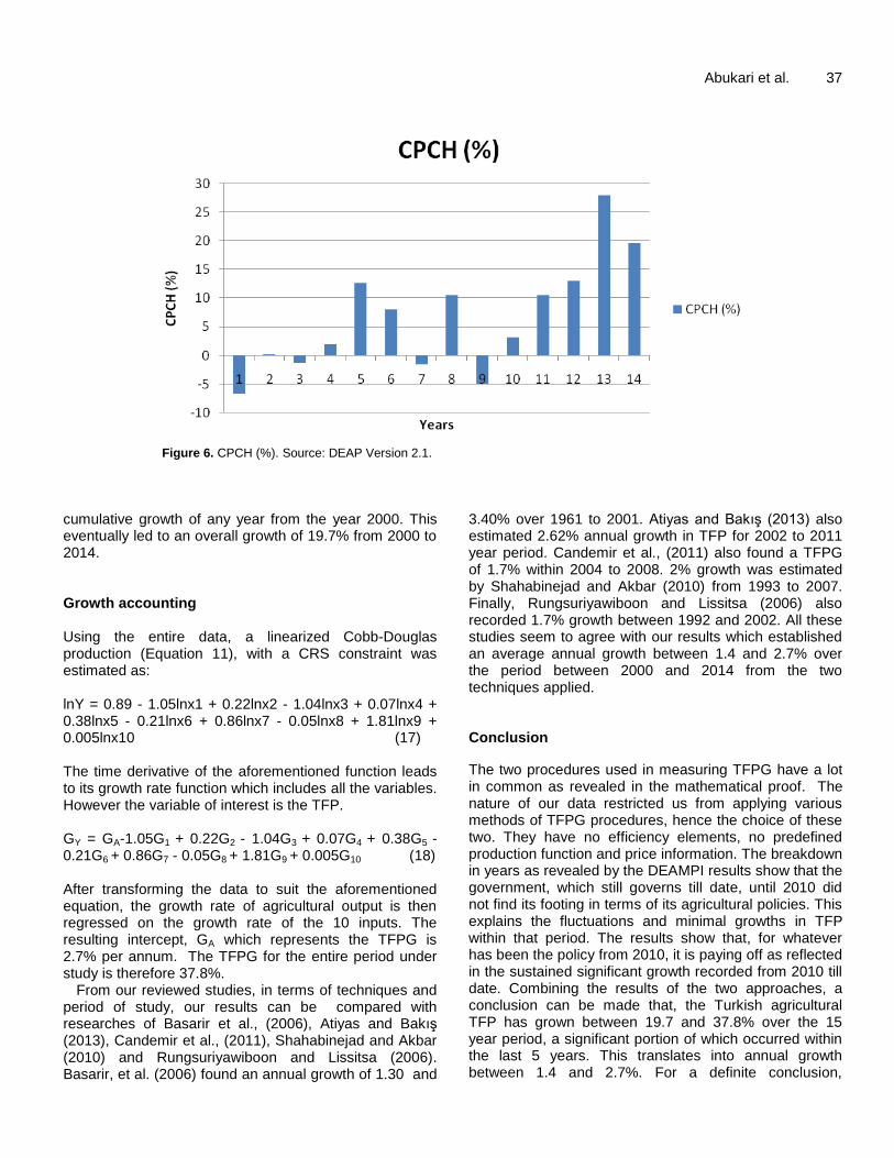
Abukari et al. 37
Figure 6. CPCH (%). Source: DEAP Version 2.1.
cumulative growth of any year from the year 2000. This eventually led to an overall growth of 19.7% from 2000 to 2014. Growth accounting Using the entire data, a linearized Cobb-Douglas production (Equation 11), with a CRS constraint was estimated as: lnY = 0.89 - 1.05lnx1 + 0.22lnx2 - 1.04lnx3 + 0.07lnx4 + 0.38lnx5 - 0.21lnx6 + 0.86lnx7 - 0.05lnx8 + 1.81lnx9 + 0.005lnx10 (17) The time derivative of the aforementioned function leads to its growth rate function which includes all the variables. However the variable of interest is the TFP. GY = GA-1.05G1 + 0.22G2 - 1.04G3 + 0.07G4 + 0.38G5 - 0.21G6 + 0.86G7 - 0.05G8 + 1.81G9 + 0.005G10 (18) After transforming the data to suit the aforementioned equation, the growth rate of agricultural output is then regressed on the growth rate of the 10 inputs. The resulting intercept, GA which represents the TFPG is 2.7% per annum. The TFPG for the entire period under study is therefore 37.8%.
From our reviewed studies, in terms of techniques and period of study, our results can be compared with researches of Basarir et al., (2006), Atiyas and Bakış (2013), Candemir et al., (2011), Shahabinejad and Akbar (2010) and Rungsuriyawiboon and Lissitsa (2006). Basarir, et al. (2006) found an annual growth of 1.30 and
3.40% over 1961 to 2001. Atiyas and Bakış (2013) also estimated 2.62% annual growth in TFP for 2002 to 2011 year period. Candemir et al., (2011) also found a TFPG of 1.7% within 2004 to 2008. 2% growth was estimated by Shahabinejad and Akbar (2010) from 1993 to 2007. Finally, Rungsuriyawiboon and Lissitsa (2006) also recorded 1.7% growth between 1992 and 2002. All these studies seem to agree with our results which established an average annual growth between 1.4 and 2.7% over the period between 2000 and 2014 from the two techniques applied. Conclusion
The two procedures used in measuring TFPG have a lot in common as revealed in the mathematical proof. The nature of our data restricted us from applying various methods of TFPG procedures, hence the choice of these two. They have no efficiency elements, no predefined production function and price information. The breakdown in years as revealed by the DEAMPI results show that the government, which still governs till date, until 2010 did not find its footing in terms of its agricultural policies. This explains the fluctuations and minimal growths in TFP within that period. The results show that, for whatever has been the policy from 2010, it is paying off as reflected in the sustained significant growth recorded from 2010 till date. Combining the results of the two approaches, a conclusion can be made that, the Turkish agricultural TFP has grown between 19.7 and 37.8% over the 15 year period, a significant portion of which occurred within the last 5 years. This translates into annual growth between 1.4 and 2.7%. For a definite conclusion,

38 J. Dev. Agric. Econ. considering an average of the two procedures, the TFP of Turkish agricultural sector grew at 28.8% with and annual growth rate of 2%.
Conflict of Interests
The authors have not declared any conflict of interests. REFERENCES Atiyas I, Bakiş O (2013). Aggregate and Sectoral TFP Growth in Turkey:
A Growth Accounting Exercise.”Sabanci University and Competitiveness Forum.http://ref.sabanciuniv.edu/sites/ref.sabanciuniv.edu/files/tfp_tur_refwp.pdf
Basarir A, Karli B, Bilgic A (2006). An evaluation of Turkish Agricultural production performance. Int. J. Agric. Biol. 8(4).
Candemir M, Deliktas E (2007). Production Efficiency and Total Factor Productivity Growth in Turkish State Agricultural Enterprises. Agric. Econ. Rev. 8(2).
Candemir M, Özcan M, Güneş M, Deliktaş E (2011). Technical efficiency and total factor productivity growth in the hazelnut agricultural sales cooperatives unions in Turkey. Math. Comput. Appl. 16(1):66-76.
Coelli TJ, Prasada RDS, O‟Donnell CJ, Battese GE (2006). An Introduction to Efficiency and Productivity Analysis, 2nd Edition, Springer, New York, 366 pp.
Diewert WE, Nakamura AO (2006). The Measurement of Aggregate Total Factor Productivity Growth. In: Heckman JJ, Leamer EE, eds., Handbook of Econometrics 6. Amsterdam: Elsevier.
Fadejeva L, Melihovs A (2009) Measuring Total Factor Productivity and Variable Factor Utilisation: Sector Approach, the Case of Latvia. Bank of Latvia. Working Paper, No. 3:40.
Fare R, Grosskopf S, Norris M, Zhang Z (1994). Productivity Growth, Technical Progress, and Efficiency Changes in Industrialized Countries", Am. Econ. Rev. 84(1):66-83.
Hulten CR (2000). Total Factor Productivity: A Short Biography, NBER Working Paper # 7471.
Kathuria V, Rajesh SNR, Kunal S (2012). Productivity Measurement in Indian Manufacturing: A comparison of alternative methods. J. Quant. Econ. 11(1-2).
Kendrick JW (1961). Productivity Trends in the United States, Princeton
University Press, Princeton. Lovell CAK (1993). Production frontiers and productive efficiency‟ in
Fried HO, Lovell CAK, Schmidt SS (eds.) The Measurement of Productivity Efficiency - Techniques and Applications, Oxford University Press, New York: pp. 3-67.
Ozden A (2014). Total factor productivity growth in Turkish agriculture: 1992-2012. Bulg. J. Agric. Sci. 20(2):469-473.
Öztürk M (2012). Agriculture, Peasantry and Poverty in Turkey in the Neo-liberal Age. Wageningen Academic Publishers.
Pamuk Ş (2008). Agriculture and Economic Development in Turkey, 1870-2000. In Agriculture and Economic Development in Europe Since 1870, eds Lains P, Pinilla V. pp. 375-396. London: Routledge.
Rungsuriyawiboon S, Lissitsa A (2006). Agricultural Productivity Growth in the European Union and Transition Countries. IAMO Discussion Paper No. 94. Leibniz Institute of Agricultural Development in Central and Eastern Europe. Halle, Germany.
Shahabinejad V, Akbari A (2010). Measuring agricultural productivity growth in Developing Eight. J. Dev. Agric. Econ. 2(9):326-332.
Solow RM (1957). Technical Change and the Aggregate Production Function. Rev. Econ. Stat. 39(3):312-320.
Telleria R, Aw-Hassan A (2011). Agricultural productivity in the WANA region. J. Comparative Asian Dev. 10(1).
Tipi T, Rehber E (2006). Measuring technical efficiency and total factor productivity in agriculture: the case of the South Marmara region of Turkey. The Royal Society of New Zealand. New Zealand J. Agric. Res. 49:137-145.
World Bank (2014). World Bank Development Indicators (WDI)- Turkey. http://data.worldbank.org/sites/default/files/wdi-2014-book.pdf

Vol. 8(2), pp. 39-51, February, 2016
DOI: 10.5897/JDAE2015.0660
Article Number: 818711256963
ISSN 2006-9774
Copyright ©2016
Author(s) retain the copyright of this article
http://www.academicjournals.org/JDAE
Journal of Development and Agricultural Economics
Full Length Research Paper
Technical efficiency of smallholder wheat farmers: The case of Welmera district, Central Oromia, Ethiopia
Wudineh Getahun Tiruneh1* and Endrias Geta2
1Department of Agricultural Economics, Extension and Gender Research (AEEGR), Ethiopian Institute of Agricultural
Research, Holetta Research Center, P. O. Box 2003, Addis Ababa, Ethiopia. 2Haramaya University, P. O. Box 2003, Addis Ababa, Ethiopia.
Received 9 May, 2015; Accepted 9 December, 2015
Increasing productivity through enhancing efficiency in cereal production in general and in wheat production in particular could be an important pace towards achieving food security. However, the strategic conceptual and empirical analysis in the context of the efficiency, which would guide policy makers and development practitioners in their efforts to revamp cereal productivity, is sparse. This study was undertaken to assess the technical efficiency and factors affecting efficiency of wheat production in Welmera district of Oromia region, Ethiopia. The primary data pertaining to farm production, input usage, and socioeconomic and institutional factors were collected during 2012/13 cropping year through a structured questionnaire from randomly selected 180 wheat farmers. The stochastic frontier and translog functional form with a one-step approach were employed to assess efficiency and factors affecting efficiency in wheat production. The maximum likelihood estimates for the inefficiency parameter depicted that most farmers in the study area were not efficient. The mean technical efficiency was found to be 57%. Factors such as sex, age and education level of the household head, livestock holding, group membership, farm size, fragmentation, tenure status and investment in inorganic fertilizers affect efficiency positively and distance to all weather roads negatively. The finding implies that there is an opportunity to improve technical efficiency among the farmers by 43% through gender-sensitive agricultural intervention, group approach extension, and attention to farmers’ education, scaling out of best farm practices. Key words: Smallholder wheat farms, translog production function, technical efficiency.
INTRODUCTION In Ethiopia, agriculture is the major option for stimulating growth, overcoming poverty, enhancing food security and improving distribution of income among the poor households. It contributes about 42% to the total gross domestic product (GDP), provides 85% of employment
opportunities, constitutes more than 80% of the nation‟s total exports, and provides most of the foreign exchange earnings to the economy (EPA, 2012). It also plays an important role in providing raw materials for domestic industries. Thus, Ethiopia‟s Growth and Transformation
*Corresponding Author. E-mail: [email protected] Tel: +251 911706033. Fax: 251112370377.
Author(s) agree that this article remain permanently open access under the terms of the Creative Commons Attribution
License 4.0 International License

40 J. Dev. Agric. Econ. Plan (GTP I) set higher growth and investment targets in agricultural sector in general and in wheat production in particular than any of earlier Ethiopia‟s national plan and will receive a special attention in the next five year plan (GTP II) (MoFED, 2010). Cereal production and marketing are the means of livelihood for millions of smallholder households and making it the single largest sub-sector in Ethiopian economy. Cereal accounts for roughly 60% of rural employment, 80% of total cultivated land, more than 40% of a typical household‟s food expenditure, and more than 60% of total caloric intake, represents about 30% of GDP (World Bank, 2007). Following maize, wheat is the second most important and productive cereal crop and its productivity shows increasing pattern (for example increased from 18.39 to 2.1 tons per hectare in 2010/2011 and 2012/2013 cropping season, respectively (CSA, 2010, 2013).
Following South Africa, Ethiopia is the second largest producer of wheat in sub-Saharan Africa. At a national level about 1.63 million ha wheat was distributed with about 4.84 million smallholder farmers (CSA, 2013). Wheat is cultivated in the highlands of Ethiopia, mainly in Oromia, Amhara, Southern Nations and Nationalities Peoples (SNNP) and Tigray regions (CSA, 2013) and it is the first most important staple crop in Welmera district. Currently, wheat is among a few crops which have received special attention from the Government of Ethiopia and NGOs operating in the country. In this regard, the government has paid attention to research and extension of wheat technologies. Moreover, Ethiopia has become a center of diversity in Eastern Africa for its wheat crop (EAAPP, 2009).
Despite the importance of wheat as a food and industrial crop and the efforts made so far to generate and disseminate improved production technologies, its productivity remains below its potential. The average wheat yield was about 2.1 tons per hectare, in 2012/2013 cropping season (CSA, 2013). Ethiopia‟s current annual wheat production of approximately 3.18 million tons is insufficient to meet domestic needs, forcing the country to import 30 to 50% of the annual wheat grain required. Therefore, these facts show that Ethiopia is the net importer of wheat to feed its growing population. Moreover, the yield gap of over 3 tons per hectare suggests that there is a potential for increasing production and productivity of smallholder wheat farmers.
Some previous studies have indicated that farm production and productivity can possibly be raised (1) by allocating more area for production, (2) by developing and adopting of new wheat technologies, and/or (3) by utilizing the available resources more efficiently (Ahmed et al., 2013; Kamruzzaman and Mohammad, 2008; Haji, 2006). Opting for the first method would mean trying to boost output at the cost of bringing marginal areas into cultivation. Some other authors also argued that with limited available suitable land especially in the highlands for cultivated area expansion, increased cereal
production and productivity will need to come from yield upgrading (Bezabeh et al., 2014; Taffesse et al., 2012). On the other hand, creation and introduction of new technologies is a long term option and requires a lot of capital for research and extension. Rather, efficient utilization of available resources is the best way of increasing production especially in the short run.
According to previous researches in Ethiopia, there also exists a wide cereal yield gap among the farmers that might be attributed to many factors such as lack of knowledge and information on how to use new crop technologies, poor management, biotic, climate factors and more others (Debebe et al., 2015; Ahmed et al., 2013; Yami et al., 2013).
Because of the scanty resources that are on ground, recently it is getting importance to use these resources at the optimum level which can be determined by efficiency searches (Gebregziabher et al., 2012; Asefa, 2012; Alene et al., 2006). Thus, increasing wheat production and productivity among smallholder producers requires a good knowledge of the current efficiency or inefficiency level inherent in the sector as well as factors responsible for this level of efficiency or inefficiency. However, previous studies in the area of wheat production efficiency are not extensive and crop specific, and are also area specific (Wassie, 2014; Yami et al., 2013; Mussa et al., 2012; Kebede and Adenew, 2011; Alene and Zeller, 2005). These studies have been at the household level ignoring the possible differences in bio-physical conditions at the plot level, and also their findings are not consistent with one another due to various reasons like agro ecological and methodological variations. Moreover, based on these literature reviews and to the best of the information we have, no studies have estimated technical efficiency of wheat farmers in Welmera district. That is, information on the levels of farm household technical efficiency and its determinant factors is lacking in the study area.
Therefore, the present study is an attempt towards assessing the technical efficiency of the farmers in the study area and aims to bridge the prevailing information gap on the contextual factors contributing to efficiency differentials in the production of wheat. The objective of the study is to measure technical efficiency of wheat production and to identify variables affecting technical efficiency of wheat producing farmers. RESEARCH METHODOLOGY
Study area
The study was conducted in Welmera district of Addis Ababa Zuria Special zone of Oromia, Regional State in Ethiopia. Welmera district is one of the eight administrative units of the Addis Ababa Zuria Special zone of Oromia Regional State. Geographically, the district is located between 8°50'-9°15'N latitude and 38°25'-38°45'E longitude and has area coverage of 66,247 ha (WORLA, 2011).
Most of its areas are high lands (Dega) and mid highlands (Weyna

Dega) with an altitude ranging from 2060 to 3380 m above sea level. Majority of the soil is reddish-brown clayey type similar to some other highland areas of Ethiopia (Asefa, 2012). The district is sub-divided in to 23 rural kebele (Kebele is the lowest administrative unit under Ethiopian condition) administrations and one town, excluding the capital town of the district. The area is characterized by mixed crop-livestock farming systems like other central highlands of Ethiopia where both crop and livestock production play a central role in the lives of the farming community. Wheat is the first major staple crop followed by barley, tef, pulses, oilseed, potato and other crops, respectively in the area. In 2011/2012 cropping season, about 33% of the crop land was covered by wheat (WOA, 2012). Sampling procedure In order to select sample farm households, a three-stage sampling technique was employed. In the first stage, study district was purposively selected based on the extent of wheat production. In the second stage, six kebeles were selected from the selected district based on the discussion with district level agricultural extension experts. Finally, from up-to-date list of sampling frame (wheat growers) obtained from extension offices at each Kebele level, 180 sample households were selected using systematic random sampling. The sample size was determined by adopting a sample size determination formula provided by Statistics Canada (2010).
Data source and collection
This study used the data collected from primary sources for 2012/2013 production season. To supplement the primary data, secondary data were collected from concerned district offices (like Agricultural Office, Holetta Agricultural Research Center (HARC) and Cooperative Offices) and from published and unpublished sources. The data is cross-sectional and quantitative in nature. Primary data contained detailed information on households‟ socioeconomic and demographic characteristics, farm charac-teristics, inputs utilization, output produced, institutional, policy related variables and production problems encountered were collected from the selected farm households using structured questionnaires filled by trained enumerators who are fluent in the local language. Close supervision and day to day check up was done by the researcher. The survey was conducted from July to August, 2013.
Data analysis
To achieve the study‟s objectives, both descriptive and inferential statistics were used. Descriptive statistics like means, standard deviations, percentages and frequency counts were used in describing socioeconomic characteristics of households, inputs, output variables, frequency distribution efficiency levels and responses on the constraints of wheat production. The stochastic frontier production function and the inefficiency model are simultaneously estimated with the maximum likelihood method using the econometric software, FRONTIER 4.1 computer programme.
Analytical framework
In this study, the stochastic frontier analysis approach was adopted to measure the technical efficiency of wheat farms. The model was independently proposed by Aigner et al. (1977) and Meeusen and
Tiruneh and Geta 41 Broeck (1977). The merits for this approach over Data Envelopment Analysis (DEA) (non-parametric) is that it accounts for a composite error term (one for statistical noise and another for technical inefficiency effects) in the specification and estimation of the frontier production function. For a number of reasons, the stochastic frontier analysis (econometric) approach has generally been preferred in the empirical application of stochastic production function model in the developing countries‟ agriculture like Ethiopia. This might be due to first the assumption that all deviations from the frontier arise from inefficiency as postulated by DEA is hard to accept, given the inherent variability of smallholder agricultural production due to external factors like pests and weather conditions. Second, most farms are very small and operated by family labor and hence farm records kept rarely. The available data on wheat production are most likely subject to measurement errors. Therefore, the stochastic frontier production required for estimating plot level efficiency is specified as:
) (1)
where Yi denotes the output for the ith sample farm, Xi represents a (1 × K) vector whose values are functions of inputs and explanatory variables for the ith farm, β is a (K × 1) vector of unknown production parameters to be estimated, Vis are assumed to be independent and identically distributed random errors which have normal
distribution with mean zero and unknown variables, , that is,
and Uis are non-negative unobservable associated
with the technical inefficiency of production such that for a given technology and levels of inputs, the observed output falls short of its potential output ( or it is a one-sided error term (U ≥ 0)
efficiency component that represents the technical inefficiency of the farm. In short, Ui estimates the shortfall in output Yi of wheat from its maximum value given by the stochastic frontier function. In other words, the basis of a frontier function can be illustrated with a farm using n inputs for wheat (X1,X2,….., Xn) to produce output Y of wheat. Efficient transformation of inputs into output is characterized by the production function f(Xi), which shows the maximum output obtainable from various input vectors. The stochastic frontier production function assumes the presence of technical inefficiency of production. Hence, the function is defined as:
=252 (2)
where is the error term that is composed of two elements,
and plot level data was collected from a total of n=252 wheat plots. The stochastic frontier analysis has been used in many studies
like by Yami et al. (2013), Beshir et al. (2012), Jaime and Salazar (2011), Tan et al. (2010), and Daniel et al. (2008) and the approach specifies technical efficiency as the ratio of the observed output to the frontier output, that means the technical efficiency of an individual farmer or farm is defined as the ratio of observed output and the corresponding frontier output, given the state of available technology, and presented as follows:
= (3)
where F (Xi;β).exp(vi-ui) is the observed output (Y) and F (Xi;β).exp(vi) is the frontier output(Y*). Pursuing Battese and Coelli (1995), the error term (vi) permits random variations in output due to factors outside the control of the farmer like weather and diseases as well as measurement error in the output variable, and is assumed to be identically, independently and normally distributed
with mean zero and constant variance ( ); that is, vi ~N(0, ).

42 J. Dev. Agric. Econ. The ui is the inefficiency component of the error term and a one-sided non-negative (u>0) random variable, is assumed to be independently distributed as truncations at µ of the normal
distribution and variance ( ), that is, ui ~N (µi, ), but if ui = 0,
the assumed distribution is half-normal. The technical inefficiency model suggested by Battese and Coelli (1995) is illustrated by: µi = Ziδi (4) where Zi is a (1 × M) vector of exogenous explanatory variables associated with the technical inefficiency effects in the ith time period, δi is an (M × 1) vector of unknown parameter to be estimated.
As mentioned earlier in the literature review, this study employed the single stage maximum likelihood estimation method used in estimating the technical efficiency levels and its determinants simultaneously. This estimation procedure guarantees that the assumption of independent distribution of the inefficiency error term is not violated. The maximum likelihood estimation of the stochastic frontier model yields the estimate for beta (β), sigma squared (σ2) and gamma (γ), and are variance parameters; γ measures the total variation of observed output from its frontier output. The study used the parameterization following Battese and Coelli (1995) and is
given as, 222
uv and )(222
uvu , where the
gamma lies between zero and one (0 ≤ γ ≤ 1). If the value is very close to zero, then the deviations are as a result of random factors and/or if the value is very close to 1, then the deviations are as a result of inefficiency factors from the frontier. Model specification Following Aigner et al. (1977), the translog production function has been used recently by many studies to estimate technical inefficiency (Geta et al., 2013; Yami et al., 2013; Beshir et al., 2012). Therefore, the translog production function stated in Equation 6 is used for the study for its flexibility for which it places no restriction unlike the Cobb-Douglas production function.
(Cobb-Douglas) (5)
(6) where i=1,2,- - - n=252, and X= vector of five input variables.
Based on the aforementioned model, a stochastic frontier model for wheat farmers is given by: ln(output)i = β0 + β1ln(Area)i + β2ln(Fert)i + β3ln(Oxndays)i + β4ln(seed)i + β5ln(lab)i + 1/2 β11ln(Area)2 + 1/2 β22ln(Fert)2 + 1/2 β33ln(Oxndays)2 + 1/2 β44ln(seed)2 + 1/2 β55ln(lab)2 + β12ln(Area) ln(Fert) + β13ln(Area) ln(Oxndays) + β14ln(Area)ln(seed) + β15ln(Area) ln(lab) + β23ln(Fert) ln(Oxndays) + β24ln(Fert) ln(seed) + β25ln(Fert) ln(lab) + β34ln(Oxndays) ln(seed) + β35ln(Oxndays) ln(lab) + β45ln(seed) ln(lab) + vi - ui (7) where output represents total yield of the ith plot in kilo gram (kg); Area represents operational area of wheat of the ith plot in hectare (ha); Fert represents the total amount of inorganic fertilizers used per plot in kg; Oxndays represents the amount of oxen days used for plowing from land preparation to planting, Seed represents the amount of seed used per plot in kg; Lab represents the total cost of
labour per day estimated at market price, and in Ethiopia farmers use herbicides instead of hand weeding, therefore, it is included that the cost of herbicide per liter estimated at market price in the total cost of labour for different farm activities, and ln represents Natural logarithm.
The specification of inefficiency model for the target commodity of individual producer is given as:
(8)
µi = δ0 + δ1Sex + δ2Age + δ3Educ + δ4Fsize +δ5Proxwroad + δ6Acredit + δ7Livestock + δ8Offrmy + δ9Gpmship + δ10Ext + δ11Train + δ12Frmsize + δ13Frgmnt + δ14Tenurstatus + δ15Costfert (9) where Sex is 1 if the household head is male, 0 otherwise; Age represents the age of the household in years; Educ stands for the education level of the household in years of formal education completed; Fsize stands for the size of the family, is converted into the same unit (Labour Force); Proxwroad is the distance from the household residence to the nearest all weather road in walking minutes; Acredit is the amount of agricultural credit received in Ethiopian Birr (ETB; Birr is the Ethiopian currency); Livestock represents the number of livestock owned in TLU; Offrmy is cash income earned from off-farm activities in ETB; Gpmemship is a dummy variable with a value =1 if the household participate in more than one farmers group, 0 otherwise; Ext stands for the number of extension contact (made with DAs and experts); Train stands for the number of trainings (on new varieties, diseases and pests, crop management) taken; Farm size stands for the total area of farm land under operation (own land + rented in + share in) in hectare; Frgmnt stands for land fragmentation, the number of wheat plots; Tenurstatus is a dummy variable, with a value of 1 if the ith farmer used his own farm plot, 0 otherwise, and Costfert stands for the proportional cost of chemical fertilizer to its variable costs incurred by the ith farmer per plot measured in ETB during 2012 cropping season.
Hypotheses testing
In spite of the magnitude and significance of the variable parameter, γ, it is also important to explain the various null hypotheses employed in this work. Three hypotheses were tested to scrutinize the adequacy of the specified model used in this study, the presence of inefficiency and exogenous variables to explain inefficiency among smallholder wheat producers. The generalized likelihood ratio statistics was used to test the hypotheses. It is specified as: LR (λ) = -2 [{lnL(H0)}- {lnL(H1)}] (10) where L(H0) and L(H1) are the values of the likelihood functions derived from restricted (null) and unrestricted (alternative) hypothesis. This has a chi-square distribution with degree of freedom equal to the difference between the numbers of estimated parameters under H1 and H0. Yet, where the test involves a γ, then the mixed chi-square distribution is used. The H0 is rejected when the estimated chi-square is greater than the critical.
RESULTS AND DISCUSSION
Descriptive statistics
The results of descriptive statistics for the entire variables

considered are presented in Table 2 for their mean, minimum, maximum and standard deviation values for continuous variables and frequencies and percents for discrete variables. The result shows that the average wheat productivity was 1.9 ton/ha and relatively lower than the national average of 2.11 ton/ha for the same cropping season (CSA, 2013). The yield was obtained by using 153.2 kg/ha of seed, 134.46 kg/ha of fertilizers (DAP + Urea), 17.25 oxen days/ha and 1282.9 ETB/ha of cost of labor incurred including the cost of herbicides (substituted for labor weed). The average size of farm allocated for wheat was 0.68 ha from a total average of 2.5 ha. This indicates that an average household allocated more than 27% of the farm land for wheat.
The average size of the household in labor force unit (LFU; is a conversion factor estimated by categorizing the age groups into nine and identifying six major farm activities (herding and domestic chores, land preparation, planting, weeding, harvesting and threshing, and transporting) with key informants through FGDs, then the key informants asked to give weight (0 to 4) to each activity for each age group, the weight was aggregated and divided by four times six = “1” is set equal to an able-bodied adult equivalent) was 3.55. The conversion factor used in estimating family members into LFU varies according to circumstances. In the developed countries, family size, labor power and dependency ratio has been estimated simply by counting the number of individuals whose age fall in defined “working-age group” or „dependent” ranges using the standard method. Sharp (2003) felt the standard method inadequate and used an innovative approach to estimating the actual labor capacity of family members based on his fieldwork (survey) in the study of measuring destitution. This study also felt the work of Sharp is inadequate to the context of the study area, because it ignores the supply of labor by elderly people who are over 60 years old and did not consider gender differential in labor supply for the different agricultural activities. Therefore, the study used a (LFU)
conversion factor obtained from own informal
qualitative survey through conducting six focal group discussions at each Kebele (Appendix).
The average livestock holding for sample households was 7.83 TLU, earned an average off-farm income of 3961.60 ETB, the average amount of credit received by households was 926.40 ETB, the average number of wheat plot was one ranging from 1 to 6, and about 34% of production expenditure was incurred for applying fertilizers compared to its variable costs. The average number of contact made by extension staffs with wheat household for crop related information was 7, and wheat growers received a one day crop specific trainings. Membership in a farmers‟ group (MFG) indexes social group. All of the households (100%) reported that they are organized in one to five farmer groups and 32% of the households reported that they belonging to more than one farmer‟s group either in crop production and/or in
Tiruneh and Geta 43 dairy cooperatives. On average the sample households spend about 20 min walk to reach the nearest all weather roads. Estimation of stochastic frontier production Before proceeding to the analyses of technical efficiency and its determinants, it was necessary to select the appropriate functional form and detect the presence of inefficiency in the production of wheat for the sample households. In a one step modeling approach, both Cobb-Douglas and translog frontier model can be used. Various restrictions were imposed on the model defined by 4 and 6. To check whether these restrictions were valid or not, the generalized likelihood ratio tests were used. The results of these tests of hypothesis for parameters of the stochastic frontier and inefficiency effects model for wheat farms in Welmera district are presented in Table 3. The first null hypothesis tested was that the coefficients of the interaction terms of input variables are zero favoring the Cobb-Douglas functional form (H0: βij = 0). The values of the logarithm of likelihood function for Cobb-Douglas and translog frontier model were -107.33 and 30.25, respectively. Therefore, the generalized likelihood ratio test is used to decide the functional form as follows: LR (λ) = -2 [{lnL(H0)}- {lnL(H1)}] = -2 [-107.33 + 30.25] = 154.16 The value of the likelihood ratio statistics was found to be 154.16 and greater than the critical χ
2 value of 18.3 with
10 degree of freedom at 5% level of significance. the null hypothesis was rejected and thus the translog functional form is preferred to Cobb-Douglas functional form for the data and more precise and consistent results. The second null hypothesis which specifies technical inefficiency effects are absent in the model (H0: γ = δ0 = δ1 = --- =δ15 =0), or all wheat farmers/farms efficient in the study area were tested against the alternative (H1: γ > 0 and δi ≠ 0 where i = 0,1, ---, 15) rejected with generalized likelihood ratio test statistic of 95 which was larger than 2.7 critical values at 5% significance level with 1 degree of freedom (Table 1) (Kodde and Palm, 1986) implying that the stochastic production function had a better fit to the data than the average production functions. In short, H0: γ = 0, all wheat producers/farms are 100% efficient and is strongly rejected. This indicates that the ex-planatory variables specified in the model make a significant contribution in explaining the inefficiency effect associated with wheat production in the study sites. The third null hypothesis, H0: δ1 = --- δ15=0, which specifies that the coefficients of the explanatory variables in the efficiency model are simultaneously zero and is strongly rejected with generalized likelihood ratio test statistics of 49.56 which was greater than 24.99 critical values

44 J. Dev. Agric. Econ.
Table 1. Selected farm households from each Kebele.
Kebele Total households Sample households
Burkusami Gebeya Robi 672 37
Telecho Gebriel 540 30
Bekekana Kore Odo 503 28
Welmera Chokie 664 36
Wajitu Harbu 452 25
Geresu Sida 446 24
Total 3277 180
Table 2. Descriptive statistical results for the variables used in the analysis (Own survey results, 2013).
Input variable Units Minimum Average Maximum Std. Deviation
Continuous variable
Yield ton/ha 1 1.9 4 0.59
Area ha 0.13 0.68 3.4 0.54
Seed Kg/ha 115 153.20 192.4 32
Fertilizer Kg/ha 26.32 148.2 400 63.5
Oxen-days Oxen-days/ha 14.08 17.25 21.74 2.16
Cost of labor ETHB/ha 646.80 1361.70 2246 400
Age of HHH years 24 43.9 78 11.3
Education years 0 3.8 12 3.74
Family size LFU 1 3.55 8.57 1.5
Distance to all WRs minute 1 20 120 22
Credit ETHB 0 926.40 10000 1704.20
Live stock TLU 1.04 7.83 27..3 4.17
Off-farm income ETHB 0 3961.80 94600 9018.50
Extension contact Number of days 0 7 42 7
Trainings Number of days 0 1 3 0.9
Farm size Ha 038 2.5 9.13 1.52
Fragmentation number 1 1.38 6 0.78
Cost of fertilizer proportion 0.08 0.34 0.8 0.1
Discrete variable
Variable Labels Frequency Percent
Sex of HHH
Female=0 19 10.6
Male=1 161 89.4
Total 180 100
Membership
1, if the household belongs to >1 FG 58 32.2
0 otherwise 122 67.8
Total 180 100
Tenure status
Own=1 198 86
Rented=0 32 14
Total 230 100
Own=1 195 77.4
Rented=0 57 22.6
Total 252 100

Tiruneh and Geta 45
Table 3. Results of hypotheses tested for the adopted model (Own survey results, 2013).
Hypothesis L(Ho) LR(λ) statistics critical 2 value df Decision
1. H0: βij = 0 -107.33 154.14 18.3 10 H0 rejected
2. H0: γ = 0 -77.7 95.00 2.7*
1 H0 rejected
3. H0: δ1 = --- = δ15=0 -54.98 49.56 24.99 15 H0 rejected
*Shows it was taken from Table 1 of Kodde and Palm (1986). with 15 degree of freedom and at 5% level of significance. This implies that there were firm-specific factors which influence upon the level of technical inefficiencies among the sampled households or farms. Similar results have been obtained by Geta et al. (2013), Yami et al. (2013) and Beshir et al. (2012). Estimates of parameters The maximum likelihood estimates of the parameters of the stochastic frontier production function (SFPF) and inefficiency model for wheat farms in Welmera district defined by Equations 4 and 6 are presented in Table 4. In the frontier model, the coefficients of wheat land and seed used were positive and significant implying that an increase to some optimum level in these inputs would increase wheat output. The coefficients of labor cost including herbicide was negative and significant in wheat cultivation implying that an increase in labor cost for wheat production would likely to reduce wheat productivity. The coefficients of interaction between wheat area and fertilizer, and area and cost of labor (the variable used to capture labor) were positive and significant implying that an increase in these inputs would increase wheat yield.
The maximum likelihood estimates for the parameter γ was nearly 1 at 1% level of significance. This indicates that 100% of the variation in output of wheat is probably due to the inefficiency effects of farmer‟s specific attributes. Thus, farm productivity differentials mainly related to the variation in wheat farms management at farmers condition. The mean technical efficiency level of wheat farms in the study site was 0.57, and ranged from 0.23 to 0.99 indicating that farmers are only producing on average 57% percent of their maximum possible output level, given the state of technology at their hand. This demonstrates there is an opportunity to improve technical efficiency among the farmers or farms and then increase wheat productivity by 43% from existing practice, input use and state of technology. Determinants of technical efficiency With regard to the sources of technical efficiency differentials among sample farmers, the estimates of
technical inefficiency effects model provide some important insights. Out of the fifteen variables used, ten variables (gender which is replaced by sex, age, education, and distance to all weather roads, livestock holding, group membership, farm size, farm fragmen-tation, tenure status and investment on fertilizers) were found to affect significantly the inefficiency of wheat farmers.
The sex of the household head is significantly negative at 1% level of significance as was expected, indicating that male headed households operating more efficiently than their female counterparts. This result is in line with the study by Daniel et al. (2008) and Kibaara and Kavoi (2012), and it is in contrast with the study by Yami et al. (2013) in selected waterlogged areas of Ethiopia.
The age coefficient in the inefficiency model is negative and statistically significant at 1% as was expected. This shows that older farmers tend to be more efficient than younger ones. Older farmers may take benefit of their experiences to use inputs more efficiently to wheat production. Hence, age of farmers is an important factor in improving the efficiency of farms. This result is in line with the study by Chiona et al. (2014), Mazumder and Gupta (2013), Dlamini et al. (2012), and Asogwa et al. (2012) and in contrast with many other studies (Yami et al., 2013; Simonyan et al., 2011; Jaime and Salazar, 2011).
The coefficient of education in years of schooling is negative in wheat cultivation as a priori expectation. The level of education is statistically significant at 1% in affecting the technical inefficiency in wheat production. Education improves the ability of the household to make informed decision about production inputs. Educated farmers more often have better access to agricultural information and higher tendency to adopt and utilize improved inputs (like fertilizers and crop varieties) more optimally and efficiently. This result is in line with the study by Geta et al. (2013), Yami et al. (2013) and Asogwa et al. (2012).
The coefficients of distance to all weather roads is negative and significant at 1% significance level which was not in the priori expectation, indicating that farmers living with distant areas from all weather roads operate more farm activities efficiently than the nearby farmers. This might be related to the availability of more off-farm activities near to all weather roads and farmers more likely spent more times outside their farm. In the study

46 J. Dev. Agric. Econ.
Table 4. Maximum likelihood estimates of inefficiency effects model (Model Result, 2013).
Variable Coefficient t-value
Constant (β0) 0.383 0.286
Ln (Area)[A] 26.09*** -27.73
Ln (Fertilizer)[F] 0.402 0.43
Ln (Oxen)[O] 1.24 1.32
Ln (Seed)[S] 2.59*** -2.75
Ln (Costlabor)[C] -5.31*** -5.647
Ln (A)2
11.88*** 16.20
Ln (F)2
-0.104 -0.14
Ln (O)2
-3.21*** -4.37
Ln (S)2
-0.627 -0.854
Ln (C)2
-1.31* -1.79
Ln(A)Ln(F) 1.48* 1.67
Ln(A)Ln(O) 0.94 1.06
Ln(A)Ln(S) -1.96** -2.207
Ln(A)Ln(C) 1.86** 2.09
Ln(F)Ln(O) 1.29 1.45
Ln(F)Ln(S) -1.31 -1.47
Ln(F)Ln(C) -1.84 -0.207
Ln(O)Ln(S) 1.07 1.20
Ln(O)Ln(C) 1.87 0.21
Ln(S)Ln(C) 6.04 0.608
Constant (δ0) -0.13 -0.37
Sex -0.94*** -3.85
Age -0.13*** -12.46
Education -0.204*** -4.33
Family size -0.62 -0.69
Distance TAWRs -0.13*** -2.71
Credit 5.90 0.86
Livestock -0.82** -2.08
Off-farm income -1.90 -0.86
Membership -0.64*** -2.79
Extension contact -0.255 -1.39
Training 0.66 0.826
Farm size -0.33** 1.98
Fragmentation -0.66*** -6.88
Tenure status -0.72*** -4.40
Cost of fertilizer -0.385*** -3.32
2.93*** 12.04
γ 1*** 384.87
*,**,***Show significant at 10, 5 and 1%, respectively. area, there are a number of flower farms and other cement factories as a reason for farmers participating in off-farm activities and operating with less efficiency for their wheat production.
The coefficient of livestock in tropical livestock unit is negative and significant at 5% significance level in wheat production. This might be because livestock provides manure as fertilizer, cash to finance input expenses and
draught power. This result is similar with the study by Beshir et al. (2012) and Mohammed et al. (2000).
The coefficient of group membership in the inefficiency effect model is negative and statistically significant at 1% significance level as it was expected, indicating that farmers involved in more than one farmers‟ group manage their wheat plots efficiently than farmers involved only in one farmers‟ group. This indicates that farmers

Tiruneh and Geta 47
Table 5. Frequency distribution of technical efficiency of wheat producers (Own Computation and Survey, 2013).
Range of technical efficiency Frequency Percent
0.11-0.2 0 0
0.21-0.3 13 5
0.31-0.4 34 13.6
0.41-0.5 59 23.4
0.51-0.6 52 20.7
0.61-0.7 35 14
0.71-0.8 26 10.3
0.81-0.9 19 7.5
0.91-0.99 14 5.5
Total 252 100
Mean 0.57 -
Min. 0.23 -
Max. 0.99 -
who belong to a more technical group are most likely to benefit from better access to information on improved inputs and practices. This result is in line with the study by Daniel et al. (2008) and Kariuki et al. (2008).
Farm size is mainly justified on the view that those farmers with large farm size can better diversify their crops and the better chance for wheat to be planted on fertile soils. In this study, there was a negative and statistically significant relationship between farm size and technical inefficiency. This result is in line with the study by Geta et al. (2013) and Beshir et al. (2012) found that farm size had a significant negative effect on farmers‟ inefficiency in maize production.
The variable land fragmentation represents the number of parcels of land on which farmers allocated for their wheat production. It was hypothesized that a farmer with more number of plots is more efficient than their counterparts who had less number of plots. The reason for this might be they are able to distribute family labor for different farm activities and there will be a chance to allocate farms with good soil fertility status for wheat cultivation. The coefficient of fragmentation in the inefficiency effect model is negative and significant at 1% level of significance, suggesting having more plots in the crops under consideration improves the level of technical efficiency of farmers. This finding is consistent with the findings by Yami et al. (2013) and Tan et al. (2010).
Tenure status or land tenancy variable is included in the model to estimate the effects of tenancy status on the level of wheat growers‟ technical inefficiencies. The estimated coefficient for tenure status (own dummy = 1, 0 otherwise) has a negative sign as it was in priori expectation. The result is statistically significant at 1% level of significance indicating that own operated farms are more efficient than tenants operated farms. The results is consistent with the findings of Kariuki et al. (2008) who found that a strong relationship between tenure security and technical efficiency.
Cost of fertilizers or investment on fertilizers is the variable mainly justified on the view that the more investment on the fertilizers by farmers can improve wheat productivity. The results of this study revealed that there was a negative and statistically significant (at 1% level of significance) relationship between investment on inorganic fertilizers and technical inefficiency. The result is in line with the study by Giannakas et al. (2001) identified a positive relationship between the level of technical efficiency and the use of inputs. Distribution of technical efficiencies The estimated mean technical efficiencies of wheat farms was found to be 0.57, indicating that farmers were only producing 57% of their maximum possible output level given the state of the technology at their disposal. This also suggests that there exist more potential for increasing wheat production by adopting best practices of best wheat producer. The frequency distribution of technical efficiency levels is presented in Table 5. The frequency distribution of technical efficiency levels was not fairly distributed. The mean predicted technical efficiency ranges from 0.23 to 0.99. Out of 100 farms, 42% of wheat farms were being operated below 51% level of technical efficiency. This implies that a large number of wheat farms in the sample faced inefficiency problems. Out of 100 farms, about 35% of the farms are being operated between the efficiency level of 51 and 70% and only about 23% of wheat farms are being operated at a higher efficiency level between 71 and 99%, respectively (Table 5). Major constraints to agriculture in the study area As shown in Table 6, about 90% of the household

48 J. Dev. Agric. Econ.
Table 6. Major problems reported by wheat farmers in the study area (Own Survey Results, 2013).
Problem Labels Frequency Percent
Disease to wheat
Most important=1, indifferent=2, and
least important=3 respectively
107, 21, 52 59, 12, 29
Lack of improved (new) varieties 86, 28, 66 47, 14, 39
Low soil fertility 162, 11, 7 90, 6, 4
High cost of fertilizers 177, 3, 0 98, 2, 0
Climate variability (rain shortage) 165, 5, 10 91.7, 2.7, 5.6
Poor quality pasture 138, 27, 15 76.7, 15, 8.3
Poor extension service 121a, 35
b, 24
c 67
a, 19
b, 13
c
a,b,c
Show most important, indifferent and least important labels, respectively. reported that soil fertility decline is the most serious problem for wheat production in the study area. This problem is aggravated by a sky rocketing fertilizer prices (98% households). About 91.7% of the households reported that climate variability (expressed in terms of shortage and untimely raining (late coming and early stop)). About 76.7% of the respondents reported that shortage of grazing land and low quality pasture for livestock are serious problems. About 47% of the households reported that there was lack of new improved varieties and quality seeds, 59% of the households reported that disease is the serious problem for wheat. These are major productivity problems that may result in higher yield gaps (Schneider and Anderson, 2010). CONCLUSION AND POLICY IMPLICATIONS The main objective dealt with in this study was to assess the technical efficiency of wheat smallholder producers and its determinant factors in Welmera district of Oromia region, highland of Ethiopia. The study used the farm-level data collected from a total of 180 households and 252 plots and estimated the stochastic frontier production function by incorporating inefficiency effects using a one-step approach.
It is found that smallholder wheat farmers are inefficient in resources used in the production of wheat in the study area. The results of efficiency analysis show that the mean technical efficiencies were 57% ranging between 23 and 99%. This suggests that farmers are not operating at the possibility production frontier and there is a considerable potential to increase the productivity of wheat with the present technologies and inputs available to smallholder wheat farmers. The distribution of farm level measures of technical efficiency shows that about 42% of wheat farms are operating below 51% level of technical efficiency, 35% of farms are found between the efficiency level of 51 and 70% technical efficiency and about 23% of farms are well operating between 71 and 99% level of technical efficiency.
The analysis of the relationships between technical efficiency and socioeconomic variables expected to have
effect on wheat farm efficiency were inspected. The identified determinants of technical efficiency were gender, age, education, and distance to all weather roads, livestock holding, group membership, farm size, fragmentation, tenure status and investment on inorganic fertilizers.
Farmers reported that soil fertility decline, climate variability, rising prices of fertilizers, lack of new improved crop varieties and quality seed, crop disease and shortage of grazing land together with low quality pasture were the most important problems to the study area which needs appropriate policy intervention to address these problems.
Therefore, the results of this study give information to policy makers on how to improve the technical efficiency and optimal use of resources in the study area. The following policy recommendations have been drawn based on the results of the study.
First, using best practices of the efficient farmers as a point of reference would help setting targets in improving efficiency levels and finding the feebleness of the present farm practices. The relatively efficient farms can also improve their efficiency more through learning the best resource allocation decision from others. This can be achieved by arranging field days, cross-visits, creating forum for experience sharing with elder households, on job trainings and demonstration on the efficient farms. Second, it is important to give due attention for farmers education through establishing and strengthening informal education and short term trainings by using the available human and infrastructural facilities like extension agents and Farmers Training Centers (FTCs). Third, initiate and support gender-sensitive agricultural intervention to improve female headed farm inefficiency. Fourth, strengthening the existing farmers groups be it formal or informal and promoting the formation of other farmers groups.
Fifth, policy initiatives that improve the livestock holding of farmers through improved livestock breeds, forage and nutrition and health services have to be put in place. Sixth, as farm size and fragmentation have a positive relationship with technical efficiency, support programs that can absorb an exploited farm labor through off-farm

activities in urban and peri-urban areas. Seventh, encourage farmers to invest on soil fertility enhancement activities by reducing the cost of production.
Finally, the study recommends further empirical work to be conducted on the effects of infrastructures like roads on technical efficiency using a large number observation. Conflict of Interests The authors have not declared any conflict of interests. ACKNOWLEDGEMENT
The authors are very grateful to East African Agriculture Productivity Project of the Ethiopian Institute of Agricultural Research for covering all the necessary study costs. REFERENCES Aigner D, Lovell CAK, Schmidt P (1977). Formulation and estimation of
stochastic production function models. J. Econom. 6(1):21-37. Ahmed B, Haji J, Geta E (2013). Analysis of Farm Households'
Technical Efficiency in Production of Smallholder Farmers: The Case of Girawa District, Ethiopia. Am.-Eur. J. Agric. Environ. Sci. 13(12): 1615-1621.
Alene DA, Manyong MV, Gockowski J (2006). The production efficiency of intercropping annual and perennial crops in Southern Ethiopia: A comparison of distance functions and production frontier. ELSVIER J. Agric. Syst. 91:57-70.
Alene DA, Zeller M (2005). Technology adoption and farmer efficiency in multiple crops production in eastern Ethiopia: A comparison of parametric and non-parametric distance functions. Agric. Econ. Rev. 6(1):5-17.
Asefa S (2012). Who is technically efficient in Crop Production in Tigray Region, Ethiopia? Stochastic Frontier Approach. Glob. Adv. Res. J. Agric. Sci. 1(7):191-200.
Asogwa BC, Umeh J, Penda ST (2012). Technical efficiency analysis of smallholder farmers in rural and periurban areas of Nigeria. J. Hum. Ecol. 37(1):57-66.
Battese GE, Coelli TJ (1995). A model for technical inefficiency effect in stochastic frontier production for panel data. Empir. Econ. 20:325-332. Retrieved from http://dx.doi.org/10.1007/bf01205442
Beshir H, Emana B, Kassa B, Haji J (2012). Economic efficiency of mixed crop-livestock production system in the North eastern highlands of Ethiopia: the stochastic frontier approach. J. Agric. Econ. Dev. 1(1):10-20.
Bezabeh E, Haregewoin T, Hailegiorgis D, Daniel F, Belay B (2014). Change And Growth Rate Analysis In Area, Yield And Production Of Wheat In Ethiopia. Int. J. Dev. Res. 4(10):1994-1995.
Chiona S, Kalinda Th, Tembo G (2014). Stochastic Frontier Analysis of the Technical Efficiency of Smallholder Maize Farmers in Central Province, Zambia. J. Agric. Sci. 6(10):108-118.
CSA (Central Statistical Agency) (2013). Area and Production of major crops: Statistical Bulletin, No. 532.
CSA (Central Statistical Agency) (2010). Area and Production of major crops: Statistical Bulletin, Vol. 1.
Daniel S, Bravo –Ureta BE, Quiroga RE (2008). Technical efficiency among peasant farmers participating in natural resource management in Central America. J. Agric. Econ. 60(1):202-219.
Debebe S, Haji J, Goshu D, Edriss KA (2015). Technical, allocative, and economic efficiency among smallholder maize farmers in Southwestern Ethiopia: Parametric approach. J. Dev. Agric. Econ. 7(8):282-291.
Tiruneh and Geta 49 Dlamini IS, Masuku BM, Rugambisa IS (2012). Technical efficiency of
maize production in Swaziland: A stochastic frontier approach. Afr. J. Agric. Res. 7(42):5628-5636.
EAAPP (East Africa Agricultural Productivity Program) (2009). A report on Integrated safeguards Datasheet Appraisal Stage. No. 47820. Retrieved from http://www.worldbank.org/projects/p112688/east-africa-agricultural-productivity ogram?lang=en
EPA (Environmental Protection Authority) (2012). National Report of Ethiopia, the United Nations conference on Sustainable Development (Rio+20). Federal Democratic Republic of Ethiopia, Addis Ababa.
Gebregziabher G, Namara RE, Holden S (2012). Technical Efficiency of Irrigated and Rain-Fed Smallholder Agriculture in Tigray, Ethiopia: A Comparative Stochastic Frontier Production Function Analysis. Quart. J. Int. Agric. 51(3):203-226.
Geta E, Bogale A, Kassa B, Elias E (2013). Productivity and efficiency analysis of smallholder maize producers in Southern Ethiopia. J. Hum. Ecol. 41(1):67-75.
Giannakas K, Sctoney R, Tzouvelkas V (2001). Technical efficiency, technological change and output growth of wheat farms in saskatchwan. Can. J. Agric. Econ. 49:135-152.
Haji J (2006). Production Efficiency of Smallholders‟ Vegetable-dominated Mixed Farming System in Eastern Ethiopia: A Non-Parametric Approach. J. Afr. Econ. 16(1):1-27.
Jaime M, Salazar A (2011). Participation in organization, technical efficiency and territorial differences, a study of small wheat farmers in Chile. J. Agric. 71(1):104-113.
Kamruzzaman M, Mohammad HI (2008). Technical efficiency of wheat growers in some selected sites of Dinajpur district of Bangladesh. Bang. J. Agric. Res. 33(3):363-373.
Kariuk DK, Ritho CN, Munei K (2008). Analysis of the effect of land on technical efficiency of smallholder crop production in Kenya. A paper presented on International Research on Food Security, Tropentag.
Kebede K, Adenew B (2011). Analysis of Technical Efficiency: Lessons and Implications for Wheat Producing Commercial Farms in Ethiopia. J. Econ. Sustain. Dev. 2(8):39-47.
Kibaara BW, Kavoi MM (2012). Application of stochastic frontier approach model to assess technical efficiency in Kenya‟s maize production. JAGST 14(1).
Kodde DA, Palm CF (1986). Wald criteria for jointly testing equality and inequality restrictions. Econometrica 54(5):1243-1248.
Mazumder R, Gupta M (2013). Technical efficiency and its determinants in backward agriculture: The case of paddy farmers of Hailakandi district of Assam. J. Reg. Dev. Plan. 2(1):35-53.
Meeusen W, Broeck JV (1977). Efficiency estimation from Cobb-Douglas production functions with composed error. Int. Econ. Rev. 18:435-444.
MoFED (Ministry of Finance and Economic Development) (2010). Growth and Transformation Plan (GTP) 2010/11-2014/15 Draft
Mohammed H, Hassan F, Mwangi W, Belay K (2000). Factors influencing technical efficiencies of barley production in Assasa district of south-eastern Ethiopia. Ethiop. J. Agric. Econ. 4(1):1-21.
Mussa CE, Obare AD, Bogale A, Simtowe PF (2012). Analysis of Resource Use Efficiency in Smallholder Mixed Crop-Livestock Agricultural Systems: Empirical Evidence from the Central Highlands of Ethiopia. Dev. Ctry. Stud. 2(9):30-40.
Schneider K, Anderson L (2010). Yield gap and productivity potential in Ethiopian Agriculture: Staple grains and pulses. EPAR Brief No. 98.
Sharp K (2003). Measuring destitution: Integrated qualitative and quantitative approaches in the analysis of survey data. IDS working paper 217.
Simonyan JB, Umoren BD, Okeye BC (2011). Gender differentials in technical efficiency among maize farmers in Essien Odimolocal government area, Nigeria. Int. J. Econ. Manage. Sci. 1(2):17-23.
Statistics Canada (2010). Survey methods and practices. 12-587-X. Retrieved from www.statcan.gc.ca.
Taffesse AS, Dorosh P, Gemessa AS (2012). Food and Agriculture in Ethiopia:Progress and Policy Challenges, University of Pennsylvania Press: Philadelphia, chap. Crop Production in Ethiopia: Regional Patterns and Trends. pp. 53-83.
Tan S, Kuyvenhove A, Qu F (2010). Impact of land fragmentation on rice producer‟s technical efficiency in South east china. NJAS-Wageningen. J. Life Sci. 57:117-123.

50 J. Dev. Agric. Econ. Wassie SB (2014). Technical efficiency of major crops in Ethiopia:
Stochastic frontier model. Acad. J. Agric. Res. 2(6):147-153. World Bank (2007). World development report: Agriculture for
development. Washington DC. WoRLA (Welmera Woreda Office of Rural Land Administration) (2011).
Land use and distribution document (unpublished). WoA (Welmera Woreda Office of agriculture) (2012). Socio-economic
profile of Welmera Woreda and crop assessment report (unpublished).
Yami M, Solomon T, Begna B, Fufa F, Alemu T, Alemu D (2013).
Sources of technical inefficiency of smallholder wheat farmers in selected water-logged areas of Ethiopia: A translog production function approach. Afr. J. Agric. Res. 8(29):3930-3940.

Tiruneh and Geta 51
Appendix. Conversion factors for individual labor capacity (Own Survey, 2013).
Age category Explanation Conversion factor
Male Female
0-5 Too young to work 0 0
6-9 Start herding calves and domestic chores under parents supervision 0.10 0.10
10-14 Herding livestock, assist fieldwork 0.40 0.30
15-24 Able to do activities that doesn‟t require more skills (like planting) 0.88 0.75
25-59 Able to do full adult workload 1.00 0.88
60-69 Elderly able to do the majority of adult workload 0.75 0.60
70-79 Elderly able to do some of adult workload 0.50 0.25
80-85 Elderly able to do very few of adult workload & female retire 0.20 0
>85 Too old to work, retired 0 0

Journal of Development
and Agricultural
Economics
Related Journals Published by Academic Journals
Journal of Plant Breeding and Crop Science
African Journal of Agricultural Research
Journal of Horticulture and Forestry
International Journal of Livestock Production
International Journal of Fisheries and Aquaculture
Journal of Cereals and Oilseeds
Journal of Soil Science and Environmental Management
Journal of Stored Products and Postharvest Research