SOUTHERN JOURNAL OF AGRICULTURAL ECONOMICS DECEMBER 1990

A Case Study of Timeliness in the Selection of Risk-EfficientMachinery ComplementsMichael E. Wetzstein, Wesley N. Musser, Ronald W. McClendon, and David M. Edwards

Abstract This paper is concerned with the intertemporal

The importance of timeliness is investigated in the stochastic impacts of timeliness issues related toselection of machinery complements for double- machinery choice. Timeliness has received consid-crop wheat and soybean production in the erable attention in the machinery selection literature.southeastern coastal plain. An intertemporal However, previous research has only focused onstochastic simulation model was developed to planting delays caused by excess soil moisture. Ongenerate probability distributions that were sandy soils with limited moisture retention capacity,evaluated with stochastic dominance analysis. This inadequate moisture for germination can also causeresearch investigated the importance of intertem- planting delays. Furthermore, spring planting delaysporal production linkages and inadequate soil mois- can influence production in the next period. Brinkture on machinery selection. Failure to include these and McCarl demonstrated that planting delaysdimensions can result in erroneous machinery postpone crop maturity and harvesting, which maychoices. preclude fall tillage operations (such as plowing) in

preparation for spring planting the following year.Key words: double-cropping, wheat, soybeans, These intertemporal effects, possibly resulting from

stochastic simulation. limited machinery capacity and weather, can bemore critical for multiple-cropping systems. Delays

Machinery selection is an important and complex in harvesting spring planted crops, such as soybeans,decision in capital intensive farming. Edwards and directly affect the timeliness of fall operations, suchBoehlje identified a number of complexities as- as planting winter wheat. Total acreage planted insociated with this decision: (1) the performance of fall then affects the crop enterprise mix and, thus,one machinery unit is influenced by the total tech- influences yield and income in the following year.nology set employed in production; (2) various costs In a risk management context, this intertemporalassociated with machinery selection, including stochastic variation in yield, acreage, and incomeeconomic depreciation, are not easily measured; (3) may be of considerable importance. Capital budget-machinery sets influence timeliness of operations ing models of machinery choice, including Reid andfor land preparation, planting, and harvesting that Bradford, have considered timeliness in an intertem-can result in lower yields; (4) the stochastic nature poral framework but not these stochastic intertem-of agricultural production systems and market prices poral effects among years. Finally, past research oncomplicates the process of isolating machinery in- the effect of timeliness on yield variation has notfluences on returns; and (5) machinery selection is always considered the interrelations of stochasticlumpy. Previous research has not attempted to prices with stochastic yields. For example, Danok etpresent a complete model of this complex machinery al. (1980) assumed fixed prices.decision process. Rather, the approach was to con- The specific purpose of this article is to present asider manageable components of machinery selec- case study on the effect timeliness in machinerytion. For example, past research has considered operations has on machinery selection for a soybeaninteraction between machinery choice and crop and wheat double-crop production system in theenterprise combinations (Danok et al. 1978, 1980) southeastern coastal plain. Because sandy soilsand income taxes and other intertemporal financial predominate in this region, the influence of bothaspects in determining the optimal life of a particular excess and inadequate soil moisture on timeliness ofmachine with capital budgeting methods (Reid and field operations is considered. As in previousBradford). machinery choice research, this case study abstracts

Michael E. Wetzstein is a Professor in the Department of Agricultural Economics at the University of Georgia. Wesley N. Musser isa Professor in the Department of Agricultural Economics at Pennsylvania State University. Ronald W. McClendon is an AssociateProfessor in the Department of Agricultural Engineering at the University of Georgia. David M. Edwards is the Director in ModelDevelopment at Dun and Bradstreet.

Copyright 1990, Southern Agricultural Economics Association.

165

from components of the interaction of machinery risk in rcjt reflects inter-temporal linkages in acreagechoice on production and financial decisions to among production seasons.facilitate the analysis. Among these components are Risk, multiple time periods, and discrete choiceincome taxes and finance, crop enterprise selection, are standard justifications for use of simulationand variable production input levels.' An additional models (Johnson and Rausser). The simulationassumption is the designation of machinery comple- model for this study has target levels of cropments as the decision variable (Danok et al., 1978; acreages, A*s, A*d, and A*w. These target levelsEdwards and Boehlje). reflect enterprise choices given land and other

resources that are exogenous to the analysis, similarCONCEPTUAL MODEL to previous studies by Edwards and Boehlje and

Russell et al. The simulation model determines en-For the research in this article, the stochastic dogenous, stochastic values of Ast < A*s, Asdt <

economic choice variable is net income before taxes A*sd, and Awt < A*w for different machinery com-associated with machinery complement j in year t, plements and weather conditions represented incjt, defined as period t and previous periods. These endogenous

variables are determined by available field days,ij = pst(Ysst Asst + YsdtAsdt) + ptYwtAwt machinery capacity, and delays in field operations

- VCmjt - FCmj - VCssAsst - VCsdAsdt, discussed in the next section.- VCwAwt,

where pst, and pwt, are per bushel soybean and wheat SIMULATION MODELprices in year t, respectively; Ysst, Ysdt, and Ywt are Probability distributions of rjt were derived withyields in bushels per acre for single- and double-crop a microanalytic simulation model, DCMOD (Chensoybeans and wheat in year t, respectively; Asst, and McClendon 1984, 1985). DCMOD simulatesAsdt, and Awt are total acreages of single- and soybean and wheat double-crop production in thedouble-crop soybeans and wheat in year t, respec- southeastern United States. DCMOD was modifiedtively;VCss, VCsd, and VCw are annual per acre to incorporate intertemporal production levels,variable costs other than machinery for single and stochastic output prices, and inadequate soil mois-double-crop soybeans and wheat, respectively; and ture for planting. A brief discussion of the uniqueVCmjt and FCmj are total annual machinery variable modifications associated with the modified model,and fixed costs for machinery complement j, respec- DCTEM, along with data sources is presentedtively. Machinery complements are assumed to be below. Wetzstein et al. present a more detailed dis-used solely for the crops. Variable machinery costs cussion.are not allocated directly to individual crops because DCTEM simulates an intertemporal dynamicthey are specific to machinery complements. As production system based on daily precipitation dataformulated, variable costs specific to crops are in- over a set of years. In accordance with Russell et al.,variant with machinery choice. Following standard past weather observations were assumed to be aprocedures, FCmj, VCss, VCsd, and VCw are as- random sample from the universe of possiblesumed to be known at the beginning of a production weather conditions. A machinery complement andseason (Dillon). However, the variables Ysst, Asst, target levels for crop acreages are parameters in theYsdt, Pst, Asdt, Ywt, Awt, Pwt, and VCmjt would usual- model. The simulator generates endogenously be stochastic. Timeliness of field operations, acreages planted to the various crops based on thewhich depend on weather events, influences planted interaction of machinery set capacity and availableacreages and yields. In turn, planted acreages deter- work days within the constraints of feasible plantingmine machinery variable costs. Acreage of wheat, and harvesting dates. Harvest summary informationAw, by definition is assumed to equal acreage of is calculated for each weather year. DCTEM thendouble-crop soybeans, Asdt. These variables are simulates the production system for the next weatherbased on the stochastic outcome of machinery com- year with acreages of fall wheat plantings in the firstplement j and stochastic variables, particularly weather year as wheat acreage to be harvested in thesingle- and double-crop soybean acreage in the pre- following spring. All wheat acreage is planted tovious production period Ass,t-l and Asd,t-l. Thus, double-cropped soybeans. If planted wheat acreage

1 Crop enterprise selection is not so limiting in this application because soybean production represents the largest production areadevoted to a single crop in Georgia, with acreage more than doubling in the past decade (Georgia Crop Reporting Service). Inaddition, recent research has also focused on variable input levels for soybeans independent of machinery choice (Boggess et al.,1983,1985).

166

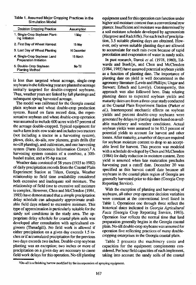
Table 1. Assumed Major Cropping Practices in the equipment used for this operation can function underSimulation Model higher soil moisture content than a conventional row

Decision Cropping Practice Assumption planter. Insufficient soil moisture was determined bya soil moisture schedule developed by agronomists

1. Single-Crop Soybean Plant- 1 May (Hargrove and Radcliffe). Foreach inch of precipita-tion, 3.5 suitable planting days are obtained. How-

2. First Day of Wheat Harvest 15 May ever, only seven suitable planting days are allowed3. Last Day of Wheat Planting 16 December to accumulate for each rain event because of rapid4. Single-Crop Soybean Land 15 March percolation and evaporation of water in sandy soils.

Preparation Initiation In past research, Danok et al. (1978, 1980), Ed-5. Double-CropSoybean No-Till wards and Boehlje, and Chen and McClendon

Planting Method (1984, 1985) have assumed potential soybean yieldsas a function of planting date. The importance ofplanting date on yield is well documented in theis less than targeted wheat acreage, single-cropliteratu(LewisandPhipsUngarandagronomy literature (Lewis and Phillips; Ungar andsoybeans in the following year are planted to acreage thisinitially targete fo doubStewart; Erbach and Lovely). Consequently, thisinitially targeted for double-cropped soybeans. a w approach was also followed here. Data relatingThus, weather years are linked by fall plantings anded el

subsequent sprin harvesplanting dates to expected soybean yields andsubsequent spring harvested acreage.eqen wsp arted arteaGeor.iacoastal . maturity dates are from a three-year study conductedThe model was calibrated for the Georgia coastalat the Coastal Plain Experiment Station (Parker et

system Based on farm record data, the reprio al.). Intertemporal stochastic effects on soybeansystem. Based on farm record data, the repre- y p yields and percent double-crop soybeans weresentative soybean and wheat double-crop operation yields and percent double-crop soybeans werewas assumed to include 600 acres with 67 perent of generated by delays in planting dates based on avail-was assumed to include 600 acres with 67 percent of able machinery and weather conditions. Actualthe acreage double-cropped. Typical equipment for b yields were assumed to be 85.5 percent ofsoybean yields were assumed to be 85.5 percent ofsuch a farm is six-row scale and includes two tractors tt t t t potential yields to account for harvest and other(not including a tractor in a harvesting system),(not including a tractor in a harvesting system), losses. After maturity, a number of days are required

plows, disks, do-alls, row planters, grain drills (for o soe m ture onen dr an accept-for soybean moisture content to drop to an accept-no-till planting), and cultivators, and one harvesting a l r r . i r w able level for harvest. This process was modeledsystem (Farm Economics Information Center).2 A A mdlsystem (Farm Economics Information Center).2 A with a schedule developed by Chen and McClendonharvesting system consists of a combine, a 300- .tingsyste c s of a c , a 3- (1984) for daily reduction in moisture content. Zerobushel trailer, and a 95-hp tractor.bushel trailer, and a 95-hp tractor. yield is assumed when late maturation precludesWeather data consisted of 58 years (1925 to 1982) harvesting past a cutoff date December 20 washarvesting past a cutoff date. December 20 wasof daily precipitation records from the Coastal Plain this harvest cutoff date because allspecified as this harvest cutoff date because allExperiment Station at Tifton, Georgia. WeatherExperiment Station at Tifton, Georgia. Weather soybeans in the coastal plain region of Georgia are

relationship to field time availability consideredrelationship to field time availability considered generally harvested prior to this date (Georgia Cropboth excessive and inadequate soil moisture. The Reporting Service)Reporting Service).relationship of field time to excessive soil moistureis complex. However, Chen and McClendon (1984, With the exception of planting and harvesting of1985) have demonstrated that a simple precipitation soybeans, all other crop operator decision variablesdelay schedule can adequately approximate avail- were constant at the conventional level listed inable field days related to excessive moisture. This Table 1. Operations one through three reflect thetype of approximation is particularly suitable for the historical dates indicated in Georgia Agriculturalsandy soil conditions in the study area. The ap- Facts (Georgia Crop Reporting Service, 1983).propriate delay schedule for coastal plain soils was Operation four reflects the normal time that landdeveloped after consultation with agricultural en- preparation generally begins in the Georgia coastalgineers (Threadgill). No field work is allowed if plain. No-till double-crop soybeans was assumed foreither precipitation on a given day exceeds 1.5 in- operation five reflecting practices of many double-ches or if accumulated precipitation for the previous cropping enterprises in the Georgia coastal plain.two days exceeds two inches. Double-crop soybean Table 2 presents the machinery costs andplanting was an exception; two inches or more of capacities for the equipment complements con-precipitation on a given day are necessary to cause sidered. Per hour field capacities of each implement,field work delays for this operation. No-till planting taking into account the sandy soils of the coastal

2Do-all is a finishing harrow modified by the incorporation of spraying equipment.

167

Table 2. Machinery Costs and Capacity, Soybean and Wheat Double - Cropping in the Georgia CoastalPlain a

Annual Fixed Cost Variable Cost Per Hour Field Capacity Per DayImplement (Dollars) (Dollars) (Acres)

Tractor

Small-95 hp 1,773.21 6.97

Medium-110 hp 2,617.20 8.41

Large-135 hp 3,462.00 10.54

Chisel Plow

4-Row 360.49 1.17 48.4

6-Row 380.00 1.24 64.5

8-Row 1,017.82 3.31 84.7

Disk4-Row 562.69 1.83 48.4

6-Row 819.86 2.67 72.6

8-row 1,390.44 4.53 96.8

Disk Plus Incorporate4-Row 587.11 1.91 32.2

6-Row 862.42 2.81 48.4

8-Row 1,448.14 4.71 64.5

Do-All4-Row 830.91 3.28 47.0

6-Row 1,003.18 3.96 70.6

8-Row 1,307.17 5.16 94.0

Row Planter4-Row 564.64 4.23 40.5

6-Row 853.01 6.31 60.8

8-Row 1,012.29 7.49 81.0

Grain Drill

4-Row 506.02 3.75 30.9

6-Row 623.18 4.61 61.7

8-Row 678.39 5.02 87.5

Cultivator4-Row 224.97 0.73 43.0

6-Row 358.85 1.41 40.3

8-Row 445.71 1.75 53.8

Cultivate Plus Post Late

4-Row 253.73 1.00 26.9

6-Row 358.85 1.41 40.3

8-Row 445.71 1.75 53.8

Combine

4-Row 6,733.25 19.32 27.1

6- and 8-Row 9,644.37 28.61 41.8

300 Bushel Trailer 250.38 0.47

a Machinery costs were calculated with the Oklahoma State Budget Generator (Kletke) with parameters appropriate forthe Georgia Coastal Plain.

168

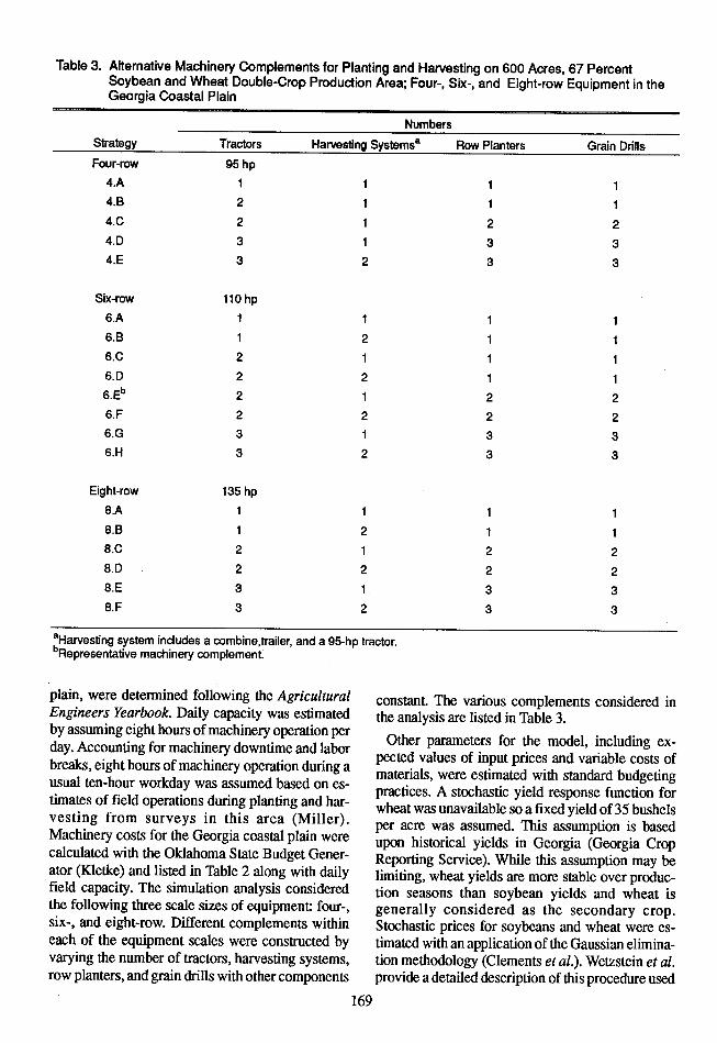
Table 3. Alternative Machinery Complements for Planting and Harvesting on 600 Acres, 67 PercentSoybean and Wheat Double-Crop Production Area; Four-, Six-, and Eight-row Equipment in theGeorgia Coastal Plain

NumbersStrategy Tractors Harvesting Systemsa Row Planters Grain DrillsFour-row 95 hp

4.A 1 1 1 14.B 2 1 1 14.C 2 1 2 24.D 3 1 3 34.E 3 2 3 3

Six-row 110 hp6.A 1 1 1 16.B 1 2 1 16.C 2 1 1 16.D 2 2 1 16.Eb 2 1 2 26.F 2 2 2 26.G 3 1 3 36.H 3 2 3 3

Eight-row 135 hp

8.A 1 1 1 18.B 1 2 1 18.C 2 1 2 28.D 2 2 2 28.E 3 1 3 38.F 3 2 3 3

aHarvesting system includes a combine,trailer, and a 95-hp tractor.bRepresentative machinery complement.

plain, were determined following the Agricultural constant. The various complements considered inEngineers Yearbook. Daily capacity was estimated the analysis are listed in Table 3.by assuming eight hours of machinery operation per day. Accounting for machinery downtime and labor Other parameters for the model, including ex-pected values of input prices and variable costs ofbreaks, eight hours of machinery operation during a materials, were estimated with standard budgetingusual ten-hour workday was assumed based on es- materials, were estimated with standard budgetingusual ten-hour workday was assumed based on es- practices. A stochastic yield response function fortimates of field operations during planting and har- wheatwasunavailableso afixed yeldof35bushelswheat was unavailable so a fixed yield of 35 bushelsvesting from surveys in this area (Miller).vesting from surveys in this area (Mller). per acre was assumed. This assumption is basedMachinery costs for the Georgia coastal plain were upon historical yields in Georgia (Georgia Cropcalculated with the Oklahoma State Budget Gener- Reporting Service). While this assumption may beator (Kletke) and listed in Table 2 along with daily limiting, wheat yields are more stable over produc-field capacity. The simulation analysis considered tion seasons than soybean yields and wheat isthe following three scale sizes of equipment: four-, generally considered as the secondary crop.six-, and eight-row. Different complements within Stochastic prices for soybeans and wheat were es-each of the equipment scales were constructed by timated with an application of the Gaussian elimina-varying the number of tractors, harvesting systems, tion methodology (Clements et al.). Wetzstein et al.row planters, and grain drills with other components provide a detailed description of this procedure used

169

in the simulation analysis. The following equation 6.E and 6.G are FSD over strategies 6.B, 6.C, 6.D,summarizes this method: 6.F, and 6.H; and 6.E is SSD over 6.A. Addition ofP= P+ AW a harvesting system to 6.E and 6.G results in ineffi-where P is a (3 xl) vector of soybean and wheat cient sets 6.F and 6.H, respectively. An additional

tractor without an associated row planter and grainprices and soybean yield; P is a (3x1) mean vector trctor without an associated 6 s not grainof P; A is a (3x3) upper-triangular, variance- drill, represented by 6.C and 6.D, is not SSD effi-

covariance matrix of P; and W is a (3x) vector of cient Results indicate that the representave farmrandom normal deviates. Mean prices of $7 ad complement, 6.E, is within the six-row efficient set

random normal deviates. Mean prices of $6.47 and $3.14 per bushel were assumed for soybeans and and that less machinery within this scale is notwheat, respectively. The variance-covariance matrix risk-efficie However, additional planting eqip-was estimated with Georgia state average price data mentasin 6.maybe efficientand Georgia coastal plain county yield data for 1973 Considering the four-row equipment scale in Tablethrough 1981 (Georgia Crop Reporting Service). 3 I 4, the largest complements within the four-rowthis simulation, wheat and soybean prices were cal- and 4.E, are SSD risk-effcien. us,

culated for each weather year of the simulation with four-row equipment may be limiting for the farmsize and percent double-cropping considered. The

simulated soybean yields in P, the above values of size and rcendouble-cppg considered. TheP~~~- and A, an ausofWfo anoFSD and SSD efficient set for eight-row equipment

P and A, and values of W from a random normal includes 8.A, 8.C, and 8.E. Similar to the six-rownumber generator. This procedure allows aggregate results, these complements employ one tractor formarket forces on prices to be influenced by ag- each set of row planters and grain drills and onegregate stochastic farm-firm events through the harvesting system. If any additional machineryvariance-covariance matrix. Reduced yields as- beyond the representative complement, 6.E, is re-sociated with planting delays caused by poor quired, it should be in the form of planting capacity.weather conditions can impact marketprices in areas TheoverallSSDset,derivedfromtheefficientsetssuch as Georgia. As Tew et al. demonstrated, a for each scale of equipment, contains 6.E and 6.Ggeneral assumption of a non-zero covariance be- (Table 4). Increasing machinery within the repre-tween price and yields is appropriate for risk sentative six-row scale may be efficient however,analysis. converting to a larger or smaller equipment scale is

First and second degree stochastic dominance SSD inefficient.criteria (FSD and SSD, respectively) were applied

The overall SSD efficient complements also cor-to the probability distributions of net returns for he oerall eicient coms ao identifying risk-efficient sets of machinery comple- resond cloey to the maximum expecte pofit

ments. Transitivity properties of stochastic choice. Machinery complement 6.E has the highest. Tr itiviy properties of stoexpected profits, followed by 4.D, 6.G, 6.A, and 8.A.

dominance were utilized in this study to reduce the expectedprofits followedbyA and number ofpair-wise comparisons. Machinery com- This similarity between expected profit and risknumber of pair-wise comparisons. Machinery com-numbef pair e 'co riss M y A aversion criteria is similar to results reported by

plements were classified into scale sets defined by aes e repord four-, six-, and eight-row equipment. Stochastic Russelleta.dominance was first applied to the distributions of The simiarity between optimal choices with ex-net returns for all complements of the same scale. pected profit and risk aversion has implications forThen the overall efficient set, considering all three the common perception that overcapitalization inscale sets, was determined with stochastic machinery is related to reducing production risk.4

dominance of the efficient sets within each Extra machinery capacity allows planting and har-machinery scale. vesting within a smaller interval about the optimal

times in situations with unfavorable weather. Fur-RESULTS thermore, it precludes underutilization of planned

acreage due to insufficient machinery capacity toBase Run of Intertemporal Model perform machinery operations during biologically

A summary of the simulation output for the dif- feasible periods. Average percent targeted acreage inferent complements is provided in Table 4. For the Table 4 allows a consideration of underutilizedrepresentative six-row equipment scale, strategies acreage. The acreage percentage for 6.E and 6.G was

3The Georgia coastal plain counties included are Appling, Atkinson, Bacon, Ben Hill, Berrian, Brooks, Bulloch, Candler,Coffie, Calquitt, Cook, Emanuel, Evans, Grady, Irwin, Jeff Davis, Lanier, Loundes, Mitchell, Montgomery, Tatnall, Thomas, Tift,Toombs, and Worth.

4This principle is implicit in most stochastic analyses of machinery choice and is widely accepted as a risk managementstrategy. Heady (p. 526) and Castle et al. (p. 174) are examples of textbook treatments of this view over the past 35 years.

170

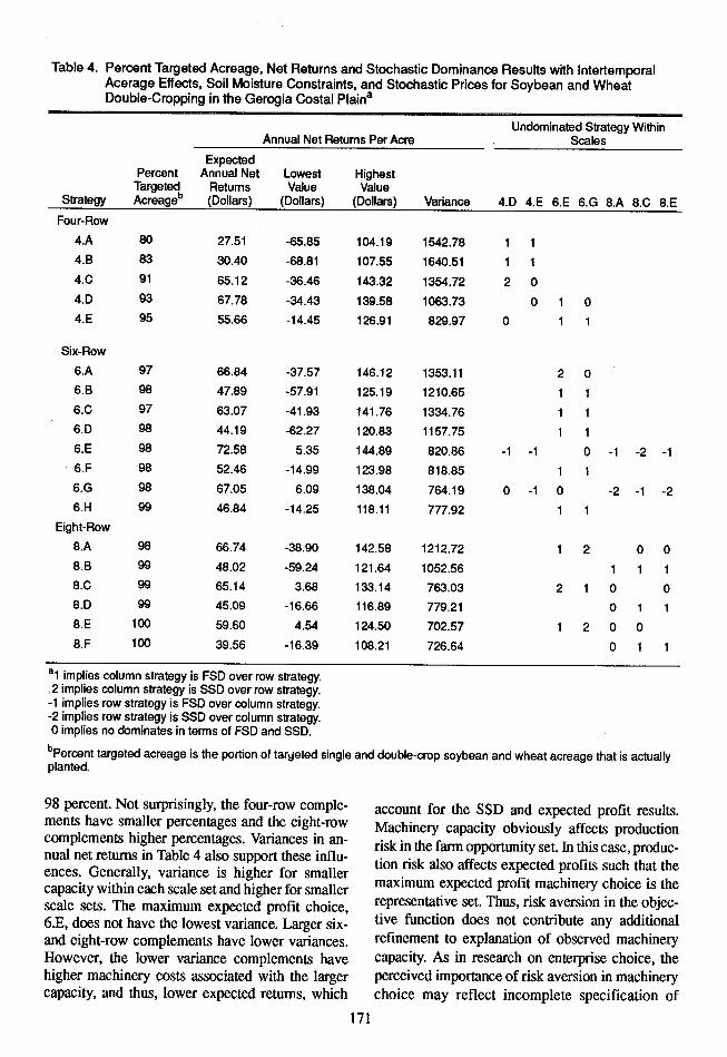
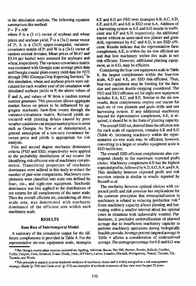
Table 4. Percent Targeted Acreage, Net Returns and Stochastic Dominance Results with IntertemporalAcerage Effects, Soil Moisture Constraints, and Stochastic Prices for Soybean and WheatDouble-Cropping in the Gerogia Costal Plaina

Undominated Strategy WithinAnnual Net Returns Per Acre Scales

ExpectedPercent Annual Net Lowest Highest

Targeted Returns Value ValueStrategy Acreageb (Dollars) (Dollars) (Dollars) Variance 4.D 4.E 6.E 6.G 8.A 8.C 8.E

Four-Row

4.A 80 27.51 -65.85 104.19 1542.78 1 14.B 83 30.40 -68.81 107.55 1640.51 1 14.C 91 65.12 -36.46 143.32 1354.72 2 04.D 93 67.78 -34.43 139.58 1063.73 0 1 04.E 95 55.66 -14.45 126.91 829.97 0 1 1

Six-Row

6.A 97 66.84 -37.57 146.12 1353.11 2 06.B 98 47.89 -57.91 125.19 1210.65 1 16.C 97 63.07 -41.93 141.76 1334.76 1 16.D 98 44.19 -62.27 120.83 1157.75 1 16.E 98 72.58 5.35 144.89 820.86 -1 -1 0 -1 -2 -16.F 98 52.46 -14.99 123.98 818.85 1 16.G 98 67.05 6.09 138.04 764.19 0 -1 0 -2 -1 -26.H 99 46.84 -14.25 118.11 777.92 1 1

Eight-Row

8.A 98 66.74 -38.90 142.58 1212.72 1 2 0 08.B 99 48.02 -59.24 121.64 1052.56 1 1 18.C 99 65.14 3.68 133.14 763.03 2 1 0 08.D 99 45.09 -16.66 116.89 779.21 0 1 18.E 100 59.60 4.54 124.50 702.57 1 2 0 08.F 100 39.56 -16.39 108.21 726.64 0 1 1

a1 implies column strategy is FSD over row strategy..2 implies column strategy is SSD over row strategy.-1 implies row strategy is FSD over column strategy.-2 implies row strategy is SSD over column strategy.0 implies no dominates in terms of FSD and SSD.

bPercent targeted acreage is the portion of targeted single and double-crop soybean and wheat acreage that is actuallyplanted.

98 percent. Not surprisingly, the four-row comple- account for the SSD and expected profit results.ments have smaller percentages and the eight-row Machinery capacity obviously affects productioncomplements higher percentages. Variances in an-complements higher percentages. Variances in an- risk in the farm opportunity set. In this case, produc-nual net returns in Table 4 also support these influ- tion risk also a s e d proits sh tt

ences. Generally, variance is htion risk also affects expected profits such that theences. Generally, variance is higher for smallercapacity within each scale set and higher for smaller maximum expected profit machinery choice is thescale sets. The maximum expected profit choice, representative set. Thus, risk aversion in the objec-6.E, does not have the lowest variance. Larger six- tive function does not contribute any additionaland eight-row complements have lower variances, refinement to explanation of observed machineryHowever, the lower variance complements have capacity. As in research on enterprise choice, thehigher machinery costs associated with the larger perceived importance of risk aversion in machinerycapacity, and thus, lower expected returns, which choice may reflect incomplete specification of

171

Table 5. Percent Targeted Acreage, Net Returns and Stochastic Dominance Results with Independence Be-tween Years, Soil Moisture Constraints, and Stochastic Prices for Soybean and Wheat Double-Cropping in the Georgia Coastal Plaina

Undominated Strategy WithinAnnual Net Returns Per Acre Scales

ExpectedPercent Annual Net Lowest HighestTargeted Returns Value Value

Strategy Acreage b (Dollars) (Dollars) (Dollars) Variance 4.C 4.D 6.A 6.E 6.G 8.A 8.C

Four-Row

4.A 100 64.18 -20.80 136.49 777.61 1 1

4.B 100 61.23 -23.75 133.54 777.62 1 1

4.C 100 72.58 -12.98 143.32 805.70 0 0 2 0

4.D 100 72.28 -3.89 139.58 762.24 0 0 1 0

4.E 100 57.13 -17.08 126.91 764.91 1 1

Six-Row

6.A 100 72.77 -17.20 146.12 828.96 0 0 0 0 0 0

6.B 100 52.48 -32.44 125.19 807.65 1 1 1

6.C 100 68.41 -21.56 141.76 828.96 1 1 0

6.D 100 48.11 -37.30 120.83 807.65 1 1 1

6.E 100 74.09 3.85 144.89 751.28 -2 -1 0 0 -1 0

6.F 100 53.96 -12.19 123.98 747.97 0 1 1

6.G 100 68.45 8.56 138.04 708.64 0 0 0 0 0 -1

6.H 100 48.24 -12.38 118.11 721.59 0 1 1

Eight-Row

8.A 100 71.16 -13.66 142.58 799.57 0 1 0 0

8.B 100 50.73 -30.16 121.65 797.24 1 1

8.C 100 66.56 6.19 133.14 706.11 0 1 0 0

8.D 100 46.51 -13.93 116.89 720.99 1 1

8.E 100 59.60 4.54 124.50 702.57 0 1

8.F 100 39.56 -16.39 108.21 726.64 1 1

1implies column strategy is FSD over row strategy.

2 implies column strategy is FSD over row strategy.2 implies column strategy is SSD over column strategy.-1 implies row strategy is FSD over column strategy.-2 implies row strategy is SSD over column strategy.0 implies no dominates in terms of FSD and SSD.

bPercent targeted acreage is the portion of total soybean and wheat acreage that was actually planted over the 58weather years.

production set relations rather than risk aversion (67 percent of the total acreage) was assumed to be

(Baker and McCarl; Musser et al.). harvested every year. Compared with endogenously

Exogenous Acreage Model determined wheat acreage (Table 4), expected an-

The intertemporal acreage influences on nual net returns are higher when the acreage planted

machinery selection were evaluated by removing is equal to the targeted acreage (Table 5). This result

from DCTEM the linkages in wheat acreage among corresponds to Brink and McCarl's findings that an

years. Instead of wheat acreage being determined assumption of independence among years consis-endogenously by the interaction of harvest time and tently resulted in estimates higher than actual in-fall weather in the previous year, 400 acres of wheat come achieved.

172

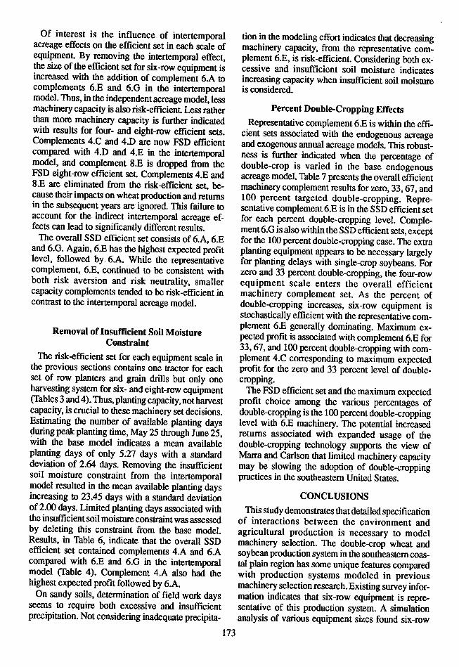
Of interest is the influence of intertemporal tion in the modeling effort indicates that decreasingacreage effects on the efficient set in each scale of machinery capacity, from the representative corn-equipment. By removing the intertemporal effect, plement 6.E, is risk-efficient. Considering both ex-the size of the efficient set for six-row equipment is cessive and insufficient soil moisture indicatesincreased with the addition of complement 6.A to increasing capacity when insufficient soil moisturecomplements 6.E and 6.G in the intertemporal is considered.model. Thus, in the independent acreage model, lessmachinery capacity is also risk-efficient. Less rather Percent Double-Cropping Effectsthan more machinery capacity is further indicated Representative complement 6.E is within the effi-with results for four- and eight-row efficient sets. cient sets associated with the endogenous acreageComplements 4.C and 4.D are now FSD efficient and exogenous annual acreage models. This robust-compared with 4.D and 4.E in the intertemporal ness is further indicated when the percentage ofmodel, and complement 8.E is dropped from the double-crop is varied in the base endogenousFSD eight-row efficient set. Complements 4.E and acreage model. Table 7 presents the overall efficient8.E are eliminated from the risk-efficient set, be- machinery complement results for zero, 33, 67, andcause their impacts on wheat production and returns 100 percent targeted double-cropping. Repre-in the subsequent years are ignored. This failure to sentative complement 6.E is in the SSD efficient setaccount for the indirect intertemporal acreage ef- for each percent double-cropping level. Comple-fects can lead to significantly different results. ment 6.G is also within the SSD efficient sets, except

The overall SSD efficient set consists of 6.A, 6.E for the 100 percent double-cropping case. The extraand 6.G. Again, 6.E has the highest expected profit planting equipment appears to be necessary largelylevel, followed by 6.A. While the representative for planting delays with single-crop soybeans. Forcomplement, 6.E, continued to be consistent with zero and 33 percent double-cropping, the four-rowboth risk aversion and risk neutrality, smaller equipment scale enters the overall efficientcapacity complements tended to be risk-efficient in machinery complement set. As the percent ofcontrast to the intertemporal acreage model. double-cropping increases, six-row equipment is

stochastically efficient with the representative com-Removal of Insufficient Soil Moise plement 6.E generally dominating. Maximum ex-Removal of InsufrficentSol Moisture pected profit is associated with complement 6.E forConstraint 33, 67, and 100 percent double-cropping with com-

The risk-efficient set for each equipment scale in plement 4.C corresponding to maximum expectedthe previous sections contains one tractor for each profit for the zero and 33 percent level of double-set of row planters and grain drills but only one cropping.harvesting system for six- and eight-row equipment The FSD efficient set and the maximum expected(Tables 3 and 4). Thus, planting capacity, not harvest profit choice among the various percentages ofcapacity, is crucial to these machinery set decisions. double-cropping is the 100 percent double-croppingEstimating the number of available planting days level with 6.E machinery. The potential increasedduring peak planting time, May 25 through June 25, returns associated with expanded usage of thewith the base model indicates a mean available double-cropping technology supports the view ofplanting days of only 5.27 days with a standard Marra and Carlson that limited machinery capacitydeviation of 2.64 days. Removing the insufficient may be slowing the adoption of double-croppingsoil moisture constraint from the intertemporal practices in the southeastern United States.model resulted in the mean available planting daysincreasing to 23.45 days with a standard deviation CONCLUSIONSof 2.00 days. Limited planting days associated with This study demonstrates that detailed specificationthe insufficient soil moisture constraint was assessed of interactions between the environment andby deleting this constraint from the base model. agricultural production is necessary to modelResults, in Table 6, indicate that the overall SSD machinery selection. The double-crop wheat andefficient set contained complements 4.A and 6.A soybean production system in the southeastern coas-compared with 6.E and 6.G in the intertemporal tal plain region has some unique features comparedmodel (Table 4). Complement 4.A also had the with production systems modeled in previoushighest expected profit followed by 6.A. machinery selection research. Existing survey infor-

On sandy soils, determination of field work days mation indicates that six-row equipment is repre-seems to require both excessive and insufficient sentative of this production system. A simulationprecipitation. Not considering inadequate precipita- analysis of various equipment sizes found six-row

173

Table 6. Net Returns and Stochastic Dominance Results for Machinery Complements in Georgia CoastalPlain With Intertemporal Years, Stochastic Prices, and No Soil Moisture Constrainta

UndominatedStrategy

Annual Net Returns Per Acre Within Scales

Expected AnnualNet Returns Lowest Value Highest Value

Strategy (Dollars) (Dollars) (Dollars) Variance 4.A 6.A 8.A

Four-Row

4.A 86.61 6.41 153.39 826.97 0

4.B 84.23 3.46 150.43 841.63 2

4.C 82.49 -1.64 148.81 852.67 1

4.D 77.79 -6.32 144.12 852.94 1

4.E 64.25 7.83 129.65 737.60 1

Six-Row

6.A 86.48 30.49 152.10 744.68 0 -1

6.B 65.93 9.51 131.29 736.59 1

6.C 82.44 26.13 147.74 736.57 1

6.D 61.57 5.15 126.93 736.59 1

6.E 80.06 23.71 145.38 737.27 1

6.F 59.17 2.71 124.41 736.34 1

6.G 73.27 16.91 138.60 737.47 1

6.H 52.38 -4.10 117.72 736.54 1

Eight-Row

8.A 80.14 24.16 145.42 737.12 1

8.B 59.63 3.19 124.99 736.96 1

8.C 71.78 15.61 136.91 734.89 1

8.D 51.11 -5.37 116.48 737.41 1

8.E 63.22 7.03 128.34 735.02 1

8.F 42.54 -13.94 107.92 737.53 1

a1 implies column strategy is FSD over row strategy.2 implies column strategy is SSD over row strategy.-1 implies row strategy is FSD over column strategy.-2 implies row strategy is SSD over column strategy.0 implies no dominates in terms of FSD and SSD.

equipment under general economic criteria to be risk ogenously, smaller machinery complements tendedefficient. However, risk aversion as a choice to be optimal. Endogenously determined wheatcriterion was not an important determinant of the acreage required larger planting equipment to avoidresults. The expected profit maximization comple- severe soybean planting and harvesting delaysment also was the representative six-row comple- w in trn, delad wha anting e ement. Production risk associated with time availables ient mo e oto plant soybeans in the choice set was crucial to both uiathe risk-aversion and risk-neutrality choices. soybean germination and emergence, which is re-

Two specific features of the production system lated to the limited moisture retention capacity of

were demonstrated to be necessary for these results. sandy soils. Again, when the inadequate moisture

First, the intertemporal acreage effects of machinery constraint was removed, smaller equipment did not

choice on wheat acreage had to be included in the cause soybean planting delays and tended to be in

model. When wheat acreage was specified ex- the efficient set. Six-row machinery would have

174

Table 7. Expected Returns and Stochastic Variation in the percentage of acreage double-Dominance Simulation for Machinery cropped supports the efficiency of six-row equip-Complements in Southeastern Georgia ment. Four-row equipment enters the risk-efficientCoastal Plain, Results With Intertem- set only for low levels of double-cropping, andporalEffects, Soil Moisture Constraints, eight-row equipment does not enter the risk-efficientand 100 Percent Double Cropping set even at 100 percent double-cropping. Repre-

a 1 Pecet Dubl Coppngsentative complement 6.E tends to dominate thesePercent Double Cropping results indicating the potential superiority of this

Economic equipment complement. As with all machinery re-Criteria 0 33 67 100 search, this conclusion may not hold if the produc-

-Efficient Machinery Complements- tion and financial choice set were expanded toSSD 4.C, 4.C, 6.E, 6.E include alternative crops and tillage methods, cus-

4.D, 4.D, 6.G tom machinery operations, and leasing machinery.6.E, 6.E, However, available survey data do not indicate use6.G 6.G of these alternatives. Inasmuch as 6.E is optimal in

Maximum 4.C 4.C, 6.E 6.E both economic results and is the representativeExpected Net 6.E aReturn choice of farmers, these alternatives likely will not

be superior to the situation considered.a The expected return for 4.C and 6.E are $34.20 and $34.33 per acre, respectively. These net returns are The domiance of the representative complementwithin 0.4 percent and, thus, are assumed to be in this research also has some interesting implica-equivalent. tions for farm management research and extension.been too large without either of these production As determined in this research, farmers in thefeatures. southeastern coastal plain have evolved to the op-

Although the solutions are specific to double-crop timum six-row size and even the specific comple-soybean and wheat in the southeastern coastal plain ment. While past farm management programs mayregion, other production regions have similar have contributed to this outcome, the results alsoproduction conditions. Other multiple crop produc- suggest caution in prescribing choices markedly dif-tion systems and systems that require fall planting ferent from current practices. As this research indi-and tillage operations could have intertemporal cates, machinery choices require complexacreage effects from machinery. Production systems consideration of many elements of production sys-on sandy soils and in semi-arid climates also could tems. If optimal decisions can be made in this case,be subject to insufficient soil moisture effects. Ex- one would expect optimality in less complexplicit attention to these issues appears warranted if management decisions. Farm managementsuch production practices are considered. programs may provide assistance in agricultural

The results of this study suggest that failure to methods and in adjusting to rapid changes in pricesconsider all relevant field time constraints may con- and technology. However, care is required in sug-tribute to the perceived machinery overcapitaliza- gesting different management strategies. As indi-tion of many farmers. This explanation of machinery cated in this research, failure to consider all relevantovercapitalization may be a relevant alternative to elements of the production system may be the sourceother explanations such as income tax management of the recommendations. Finally, this research sup-and labor availability. As with other machinery ports the classic farm management activity of main-choice literature, detailed consideration of these is- taining farm management surveys so thatsues is beyond the scope of this research. representative practices can be determined.

REFERENCESAgricultural Engineers Yearbook. American Society of Agricultural Engineers. St. Joseph, MI, 1983.Baker, T.G., and B.A. McCarl. "Representing Farm Resource Availability Over Time in Linear Programs: A

Case Study." No. Cent. J. Agr. Econ. 4(1982):59-68.Boggess, W.G., D.T. Cardelli, and C.S. Barfield. "A Bioeconomic Simulation Approach to Multi-Species

Insect Management." So. J. Agr. Econ. 17(1985):43-56.Boggess, W.G., G.D. Lynne, J.W. Jones, and D.P. Swanny. "Risk-Return Assessment of Irrigation Decisions

in Humid Regions." So. J. Agr. Econ. 15(1983):135-143.

175

Brink, L., and B.A. McCarl. "The Adequacy of a Crop Planning Model for Determining Income, IncomeChange, and Crop Mix." Canadian J. Agr. Econ. 27(1979):13-25.

Castle, E.N., M.H. Becker, and A.G. Nelson. Farm Business Management. 3rd edition. New York: Mac-Millian Publishing Company, 1987.

Chen, L.H., and R.W. McClendon. "Selection of Planting Schedule for Soybeans via Simulation." Transac-tions of the ASAE, 27(1984):29-32, 35.

Chen, L.H., and R.W. McClendon. "Soybean and Wheat Double Cropping Simulation Model." Transactionsof the ASAE, 28(1985):65-69.

Clements, A.M., H.P. Mapp, and V.R. Eidman. A Procedure for Correlating Events in Farm Firm SimulationModels. Oklahoma Agricultural Experiment Station Bulletin T-131, 1971.

Danok, A.B., B.A. McCarl, and T.K. White. "Machinery Selection and Crop Planning on a State Farm inIraq." Am. J. Agr. Econ. 60(1978):544-549.

Danok, A.B., B.A. McCarl, and T.K. White. "Machinery Selection Modeling Incorporation of WeatherVariability." Am. J. Agr. Econ. 62(1980):700-708.

Dillon, J.L. The Analysis of Response in Crop and Livestock Production. 2nd edition. Oxford: Pergamon,1977.

Edwards, W., and M. Boehlje. "Machinery Selection Considering Timeliness Losses." Transactions of the

ASAE, 23(1980):810-915, 821.Erbach, B.C. and W.G. Lovely. "Machinery Adaptation for Multiple Cropping." In Multiple Cropping. ASA

Special Publication No. 29. American Society of Agronomy, Madison, WI, (1976):339.

Farm Economics Information Center. Crop Enterprise Budgets. Department of Agricultural Economics,University of Georgia, 1977-1983.

Georgia Crop Reporting Service. Georgia Agricultural Facts. 1973-1983.

Hargrove, W.L., and D.E. Radcliffe. Personal Communication. Department of Agronomy, University ofGeorgia, Athens, GA, 1984.

Heady, E.O. Economics of Agricultural Production and Resource Use. Englewood Cliffs, NJ: Prentice-Hall,Inc., 1952.

Johnson, S.R. and G.C. Rausser. "Systems Analysis and Simulation: A Survey of Applications in Agriculturaland Resource Economics." A Survey ofAgricultural Economics Literature, Vol. 2. ed. G.G. Judge et al.Minneapolis: University of Minneapolis Press, 1977.

Kletke, D.D. Operations Manualfor the Oklahoma State University Enterprise Budget Generator. OklahomaAgricultural Experiment Station Research Report P1979, August, 1979.

Lewis, W.M., and J.A. Phillips. "Double Cropping in the Eastern United States." In Multiple Cropping. ASASpecial Publication No. 29. American Society of Agronomy, Madison, WI, (1976):41-50.

Marra, M.C., and G.A. Carlson. "Examining Double Cropping with Utility Theory." Selected paper presentedat the 1984 American Agricultural Economics Meetings in Ithaca, NY.--

Miller, B.R. "Minimum Cost Machinery Complement for Various Farm Situations." Presented paper at the

1980 American Society of Agricultural Engineers Summer Meetings, San Antonio, Texas.

Musser, W.N., B.A. McCarl, and G.S. Smith. "An Investigation of the Relationship Between ConstraintOmission and Risk Aversion Firm Risk Programming Models." So. J. Agr. Econ. 18(1986): 147-154.

Parker, M.B., W.H. Marchant, and BJ. Mullinix. "Date of Planting and Row Spacing Effects on Four SoybeanCultivars." Agronomy J. 73(1981):759-762.

Reid, D.W., and G. Bradford. "On Optimal Replacement of Farm Tractors." Am. J. Agr. Econ. 65(1983):326-331.

Russell, N.P., E.L. LaDue, and R.A. Milligan. "Choice Criteria in Farm Management Models-A Compara-tive Study of Machinery Complement Selection." No. Cent. J. Agr. Econ. 6(1984):136-141.

Tew, B.V., W.N. Musser, and G.S. Smith. "Using Non-Contemporaneous Data to Specify Risk ProgrammingModels." N.E. J. Agr. & Res. Econ. 17(1988):30-35.

Threadgill, E.D. Personal Communication. Department of Agricultural Engineering, Coastal Plain Experi-ment Station, University of Georgia, Tifton, Georgia, 1984.

176

Ungar, P.W., and B.A. Stewart. "Land Preparation and Seeding Establishment Practices in Multiple CroppingSystems." In Multiple Cropping. ASA Special Publication No. 29. American Society of Agronomy,Madison, WI, 1976.

Wetzstein, M.E., D.M. Edwards, W.N. Musser, and R.W. McClendon. An Economic Simulation of RiskEfficiency Among Alternative Double Crop Machinery Selections, University of Georgia AgriculturalExperiment Station, Research Bulletin Number 342, 1986.

177

178