Aggregate Earnings Surprises and Inflation Forecasts*

S.P. Kothari

MIT Sloan School of Management kothari@mit.edu

Lakshmanan Shivakumar

London Business School lshivakumar@london.edu

Oktay Urcan

London Business School ourcan@london.edu

April 24, 2013

Abstract

We show that aggregate earnings surprises contain information about future inflation, but macroeconomic forecasters do not fully utilize this information in generating their forecasts. Earnings news, aggregated across firms releasing earnings in a three-month period, predicts forecast errors in Producer Price Index (PPI) released in the subsequent two months. These aggregate earnings surprises do not predict forecast errors for Consumer Price Index (CPI). The results are robust to alternative specifications, and they are driven by a broad cross-section of firms rather than limited to isolated industries like the financial services industry or the retail industry. With respect to the capital markets, the bond market’s reaction to PPI news is predictable based on previously released aggregate earnings news. Collectively, the results indicate that neither macroeconomic forecasters nor bond market investors fully incorporate information in aggregate earnings surprises for future PPI.

*

We appreciate helpful comments from Bill Cready, Yaniv Konchitchki, Peter Pope and seminar

participants at Harvard Business School, Cass Business School and the 11th London Business School Accounting Symposium. Oktay Urcan acknowledges the financial support from London Business School Research and Materials Development (RAMD) Fund.

2

1. Introduction

Accurate forecasts of future inflation are crucial for almost all economic

agents. Inflation expectations affect monetary and fiscal policies of central banks and

governments, which, in turn, affect business decisions. Inflation expectations also

directly influence a variety of business decisions, including the pricing of services,

wages in labor contracts, corporate investment and financing decisions (as inflation

expectations directly affect the cost of capital) and firms’ hedging decisions. Inflation

expectations also affect banks’ lending decisions through their effect on interest rates.

Not surprisingly, a vast academic literature focuses on the forecasting of inflation and

on the evaluation of inflation forecasts. Two important unanswered questions in this

literature are whether (i) corporate earnings are useful in predicting inflation; and (ii)

macroeconomic forecasters and capital market participants efficiently incorporate

inflation information in earnings into their forecasts and thus in setting security prices.

We address these two questions in this study.

Corporations constitute a large segment of the macroeconomy. Public

companies collectively represent a substantial fraction of the macroeconomy as

employers and as producers of goods and providers of services in the economy.

Corporations also make up a large fraction of the private sector investment in an

economy. We therefore expect corporations’ activities, in aggregate, to significantly

affect the macroeconomy. Consistent with this expectation, macroeconomic variables

like the GDP, interest rates, and inflation are correlated with aggregate corporate

output (revenues) and profits (e.g., Brown and Ball, 1967; Higson, Holly and

Kattuman, 2002; Bernstein and Arnott, 2003; Shivakumar 2007). Of particular

relevance to our study is the evidence that aggregate earnings news positively

correlates with changes in interest rates and future inflation (see Kothari, Lewellen

3

and Warner, 2006; Shivakumar, 2007; Cready and Gurun, 2010). The Bureau of

Economic Analysis (BEA) releases statistics on aggregate corporate earnings every

quarter. BEA typically makes these announcements following individual firms’

preliminary earnings announcements. In fact, the BEA relies in part on the financial

information corporations file with the Securities and Exchange Commission in its

estimate of aggregate corporate earnings. But the earnings releases of individual firms

precede the BEA releases. We examine whether the resulting aggregate earnings

information anticipates inflation news in subsequent periods.

Unexpected changes in corporate profitability are likely to affect future

inflation in an economy for at least three reasons. First, current profitability, through

the persistence of earnings, is indicative of the profitability of future investments in

property, plant and equipment, research and development, and human resources.

Corporate profitability thus directly affects the perceived attractiveness of investment

opportunities, which in turn influences managers’ investment decisions. Corporate

earnings also indirectly affect firms’ capital investments in an economy. Greater

profits facilitate greater investments because financing frictions such as the cost of

raising equity capital and the costs of debt overhang are lowered with the increased

availability of internal funds (see Hennessy, Levy and Whited, 2007; Lewellen and

Lewellen, 2012). The investment decisions influence corporate demand for raw

materials and labor, which in turn raises the prices of these inputs, assuming the

supply of raw materials and labor is less than perfectly elastic.

Second, over the long run, corporate profits, dividends, and share prices all

move in sync. Increased share prices indirectly and dividend payouts directly

4

contribute to consumer spending, which induces additional demand for goods and

services in an economy.1

Finally, corporate profitability and bank lending are also positively inter-

related. Earnings growth typically results from revenue growth, which is associated

with increased working capital needs of corporations and their suppliers. Banks are

ubiquitous in providing working capital financing to businesses. Improved

profitability also lowers the credit risk (or bankruptcy risk) of a business. Thus, banks

perceive lower risk in lending as corporate profitability rises, which too contributes to

increased bank lending. The increased availability of credit that flows into corporate

investments leads to greater demand for products and services, which in turn,

increases inflation. Consistent with this effect of bank lending, Bassett et al. (2010)

document a significant increase in real GDP and inflation in the quarters immediately

following a shock that relaxes bank lending standards.

Overall, through their direct effect on aggregate demand for capital goods,

through their influence on consumer spending, and through their effect on bank

lending, we expect corporate earnings to positively affect future inflation.2

Preceding discussion outlines economic reasons why we might expect

corporate earnings to presage future inflation. However, the literature has not

examined whether macroeconomic forecasters fully exploit this link. Forecasters

might believe that listed firms’ earnings are too granular to be useful in forecasting at

1 Davis and Palumbo (2001) estimate that for each dollar of unanticipated stock price increase, consumer spending increases between 4 and 7 cents. 2 An association between corporate profits earned in a quarter and inflation in the contemporaneous quarter can be purely mechanical. A firm’s accounting earnings are calculated as the difference between revenues and expenses. Revenues are the product of current selling prices and the quantity sold. Expenses, in contrast, are historical in that the inventory sold in a period is carried on the firm’s books at historical costs, which would not fully capture the inflation affecting the selling prices of the finished goods (See Ball, Kothari and Watts, 1993). In contrast to this contemporaneous relation, the focus of this study is on evaluating whether earnings announced in a given period predicts inflation announced in subsequent periods.

5

the economy-wide level, or they might believe that corporate earnings do not contain

information incremental to scheduled, periodic releases of macroeconomic data. We

evaluate (i) whether aggregating individual firms’ earnings predicts future inflation,

and if so, (ii) whether macroeconomic forecasters and capital market participants

incorporate such information efficiently into their forecasts. Our findings suggest that

macroeconomic forecasters and capital market participants could improve their

current forecasts of inflation by incorporating the information in aggregate corporate

earnings into their forecasts.

Recent studies evaluating the role of aggregate earnings in capital markets

provide evidence consistent with aggregate earnings containing inflation news.

Kothari, Lewellen and Warner (2006) and Cready and Gurun (2010) show that

aggregate earnings surprises are negatively correlated with contemporaneous stock

market returns and bond price changes, and are positively correlated with

contemporaneous changes in T-bill rates. These findings suggest aggregate earnings

convey inflation news. Shivakumar (2007) evaluates whether aggregate corporate

earnings changes predict a variety of future macroeconomic activities, including

industrial production growth, real GDP, and inflation, and finds that aggregate

earnings are related only to future inflation.

Preceding discussion summarizes theoretical and empirical reasons to expect

aggregate earnings news to provide information about inflation. We examine whether

macro-forecasters incorporate the inflation information in aggregate earnings

surprises in their forecasts. We investigate this question empirically employing widely

used forecasts of Consumer Price Index (CPI) and Producer Price Index (PPI) from

Money Market Services International (MMS) survey.

6

We begin by documenting that the aggregate of all earnings surprises

announced publicly over a three-month window is positively correlated with future

actual PPI, but not CPI, after controlling for lagged inflation realizations. We

conjecture that these differences in the results for PPI and CPI arise because the CPI

primarily captures movements in consumption or retail prices, and includes the effects

of taxes and of imports, whereas the PPI primarily captures changes in prices of goods

and services, which are more closely linked to producers’ earnings.

We next evaluate whether aggregate earnings surprises measured in a

particular month predict future inflation forecast errors. Aggregate earnings surprises

are found to predict macroeconomists’ forecast errors in PPI released in the

subsequent two months. That is, inflation forecasters do not fully incorporate the

information about PPI contained in aggregate earnings surprises. No such evidence is

found for CPI forecast errors, which is consistent with our earlier finding that

aggregate earnings contain little information about future CPI.

The predictive ability of aggregate earnings for PPI forecast errors is robust to

alternative methodologies and to controls for other potential biases in the inflation

forecasts. We also find that this relation is driven mainly by the aggregate earnings

surprises of non-financial firms, suggesting that subsequent inflation shocks are not

just the result of greater bank lending at a time when their profits are unexpectedly

high.

Finally, we analyze capital market reaction to inflation news. Since our earlier

analysis reveals that the PPI news is predictable based on aggregate earnings

surprises, we examine whether this predictive ability carries on to the bond and equity

market reactions as well. Aggregate earnings surprises are positively related to

7

Treasury-bill yield changes at subsequent PPI announcements. We do not find similar

evidence for capital market reactions to CPI announcements, which is consistent with

our earlier results from the analysis of CPI forecast errors. We also do not find such

evidence in the equity market, consistent with equity market prices not reacting

significantly to the inflation news in aggregate earnings surprises. Equity prices seem

to react to the information in earnings surprises at the time of individual firms’

earnings announcements.

The rest of the paper is organized as follows. In the following section, we

discuss prior literature on the rationality of survey forecasts and capital market

reactions to inflation news. Section 3 explains our sample selection and empirical

methodology, and presents the descriptive data, and Section 4 presents the main

results from the analysis. Section 5 concludes.

2. Prior Literature

There is little previous research on inflation information in aggregate earnings.

However, there is evidence of an association between aggregate earnings and security

prices, and between security prices and inflation. Below we discuss these studies

briefly as a prelude to our empirical analysis. We also summarize the literature on the

macroeconomic survey data on inflation, the properties of the survey data, and the

pricing of inflation expectations as evidenced in the intra-day and longer-term

movements in stock price indices.

2.1 Stock-market returns and inflation

The literature on stock market returns and inflation can be classified into three

parts: (i) The relation between inflation, nominal interest rates, and stock prices; (ii)

The effect of news about interest rates or inflation on stock prices; (iii) Whether

8

capital market participants efficiently process information about inflation in setting

stock prices. We briefly summarize this literature as it bears on the questions

examined in our study.

Based on Irving Fisher’s proposition that nominal interest rates contain market

assessments of expected inflation, Fama and Schwert (1977) evaluate whether stock

returns are positively correlated with expected inflation and find that this is not the

case. They surprisingly find that stock returns are negatively correlated with both the

expected and unexpected components of inflation. Fama (1981) explains this puzzle

as being driven by a positive correlation between stock returns and real

macroeconomic variables and a negative relation between real activity and inflation.

French, Ruback and Schwert (1983) extend this literature to the cross-section

by testing the nominal contracting hypothesis, which states that stocks of firms with

more nominal contracts should be more sensitive to unanticipated inflation, where the

Consumer Price Index (CPI) is used to proxy for inflation. Evaluating the effect of

unanticipated inflation on debt contracts and on depreciation tax shields, they reject

the nominal contract hypothesis. Bernard (1986) extends the scope of nominal

contracts examined and documents cross-sectional variation in the relation between

inflation (CPI) shocks and stock returns.

Modigliani and Cohn (1979) represent the genesis of the literature that

evaluates whether capital market participants efficiently incorporate inflation

information in security prices and in their earnings forecasts. Modigliani and Cohn

(1979) conjecture that, when valuing stocks, investors fail to incorporate the effect of

inflation on nominal earnings, causing stock-market yields to be depressed in periods

of high inflation and to be excessive in periods of deflation. Campbell and

9

Vuolteenaho (2004) provide empirical support for this hypothesis and show that

inflation illusion explains almost 80% of the time-series variation in mispricing of the

S&P 500.

Numerous other studies also demonstrate that stock prices and market

participants do not fully incorporate information about inflation. For example,

Chordia and Shivakumar (2005) find that lagged inflation predicts stock prices, and

that this predictability varies systematically across firms, based on a firm’s earnings

exposure to inflation. Basu, Markov and Shivakumar (2010) suggest that the source

of the predictability might be because analysts do not incorporate expected inflation

information efficiently in their earnings forecasts. Konchitchki (2011) attributes the

predictability in part to financial statements not recognizing inflation gains and losses

in a timely manner. Based on stock price analysis, he concludes that investors do not

seem to fully distinguish monetary and non-monetary assets, which is fundamental to

understanding the economic effects of inflation for a firm.

In contrast to this literature, which is focused on firm-level forecasts, our study

investigates macro-level forecasting by testing whether macroeconomic forecasters

efficiently incorporate inflation information contained in lagged aggregate earnings

surprises.

2.2 Aggregate earnings and stock-market returns

Recent literature demonstrates a negative relation between aggregate earnings

growth and stock returns (see Kothari et al., 2006), which is potentially rooted in news

about inflation in aggregate earnings. The likelihood of news about inflation in

aggregate earnings serves the basis for our examination of whether macroeconomic

10

forecasters and market participants efficiently incorporate the inflation information in

aggregate earnings.

Kothari et al., (2006) conjecture that the surprising finding of a negative

relation between aggregate earnings and stock returns might be because aggregate

earnings growth contains news about changes in discount rates. Consistent with this

conjecture, they find that aggregate earnings growth is strongly correlated with

changes to several discount rate proxies, such as T-bill rates, slope of term structure

and default spread.

Research following Kothari et al. (2006) offers alternative explanations as well

as reinforces the conjecture about inflation news in aggregate earnings. Specifically,

Ball, Sadka and Sadka (2009) suggest that aggregate earnings growth is related to

expected discount rates (which include expected inflation), rather than to discount rate

news. Cready and Gurun (2010) more directly evaluate the proposition of Kothari et

al. (2006) that aggregate earnings changes captures shocks to discount rates by using

short-window market reactions to earnings announcements as a proxy for earnings

news. They show that earnings announcement returns aggregated across the stocks

announcing earnings in a day are negatively related to returns on the broader market

indices. They further show that the earnings announcement returns are associated with

contemporaneous changes in inflation expectations. Their evidence supports the view

that aggregated earnings news contains information about discount rates.

2.3 Macroeconomic survey data on inflation and stock prices

Survey data from Money Market Services (MMS) has been widely used in the

macroeconomics and finance literature to isolate the unanticipated information

component in scheduled macroeconomic announcements, and to study whether capital

11

markets react to macroeconomic announcements.3 Consistent with macroeconomic

news measured from these survey forecasts having significant capital market effects,

Urich and Wachtel (1984) document that the unanticipated component of PPI, but not

of CPI, has an immediate positive effect on short-term interest rates, and that there is

no evidence of delayed market reaction to the inflation news. Pearce and Roley (1985)

find that daily stock prices react to monetary news, but not to news about CPI, where

the news is measured relative to expectations provided by MMS survey data.

McQueen and Roley (1993) show that the relation between PPI and stock returns is

particularly strong during periods of high economic growth. Hardouvelis (1987) finds

that Treasury bond markets, but not stock markets, react to both PPI and CPI news. In

addition, a vast literature focuses on the intra-day impact of macroeconomic news

releases on capital markets. This research is mostly motivated by finance

microstructure issues such as market’s efficiency in processing new information (see

Lieberman, 2011).

Because macroeconomic survey data generate economically important capital

market reactions, research has also investigated survey forecasts for rationality and

biasedness. These studies generally yield mixed results. Pearce and Roley (1985) find

that unbiasedness of inflation forecasts from MMS surveys cannot be rejected.

Aggarwal, Mohanty and Song (1995) find that survey forecasts of several

macroeconomic series, including CPI, are consistent with the rational expectations

hypothesis, but that forecasts of a few other macroeconomic series, including PPI, are

not consistent with it. McQueen and Roley (1993) also report mixed results. They

find that the survey data, although not always unbiased or efficient, are generally

3 Studies using MMS data to compute macroeconomic news include Urich and Wachtel (1984), McQueen and Roley (1993), Elton (1999), Balduzzi, Elton and Green (2001), Flannery and Protopapadakis (2002), Andersen et al. (2003), Bernanke and Kuttner (2005), Gürkaynak, Sack and Swanson (2005) and Andersen et al. (2007).

12

superior to auto-regressive time-series models of macroeconomic data in that they

have smaller root-mean-square errors.

To summarize, inflation expectations rank among the critical variables in an

economy, and have important ramifications for resource allocation and for product

and financial markets (Thomas, 1999). Firms employ inflation forecasts in a variety of

their decisions, including pricing of products, setting wages, planning investment, and

capital budgeting. It is important to understand whether these expectations reflect all

available public information. Although prior studies focus on whether forecasts are

unbiased and efficient, they do not identify potential sources of bias. We extend the

literature by evaluating whether macroeconomic forecasters rationally incorporate

inflation information in aggregate earnings surprises.

3. Sample Selection and Data Description

3.1 Sample selection and variable definitions

Our initial sample consists of all NYSE, AMEX and NASDAQ firms in the

merged CRSP/Compustat database, with data available on earnings announcement

dates. From this sample, we include only the firms available on IBES. For each

quarterly earnings announcement, we use the most recent IBES consensus analyst

forecast prior to the announcement to calculate firm-level earnings surprises.4

Specifically, a firm-level earnings surprise is calculated as IBES-reported quarterly

earnings minus the most recent consensus analyst earnings forecast from IBES,

divided by the absolute value of the most recent consensus analyst earnings forecast.

We calculate aggregate earnings surprises by taking value-weighted and equal-

4 We do not impose any requirement on the minimum number of analysts following a firm. However, in unreported analysis, we find that our conclusions are even more strongly supported if we analyze only firms that are followed by at least 5 analysts. Our results are also robust to computing the consensus forecasts from IBES Detail History file and including only analysts’ forecasts issued in the 60 days prior to an earnings announcement.

13

weighted averages of firm-level earnings surprises over a quarter (three months). In

particular, VIBES (EIBES) is the quarterly value-weighted (equal-weighted) average

of IBES earnings surprises. In calculating aggregate earnings surprises, we exclude all

firms with share price less than $1, and earnings surprises in the top and bottom 0.5%

of the empirical distribution.

We obtain data on monthly actual inflation from the Bureau of Labor Statistics

over the period from October 1984 to December 2009. The starting date of this

sample period is governed by the availability of IBES data to construct aggregate

earnings surprises.5

Our analyses focus on both PPI and CPI measures of inflation. These have

significant differences in the way they are constructed, which could potentially cause

differences in the results for these two inflation proxies. First, whereas PPI is

constructed from the overall market output of US producers, CPI is based on goods

and services purchased by urban US households. Thus PPI excludes imports, but CPI

includes them. Second, PPI is based on the revenue received by producers, but CPI is

based on out-of-pocket expenditure by consumers. Therefore CPI includes sales and

excise taxes but PPI does not. Thus, to the extent that the US listed companies reflect

outputs by US producers rather than consumption by consumers, we would expect

aggregate earnings surprise to be more strongly related to PPI than to CPI.6

5 As we discuss in our robustness tests, we also use seasonal random-walk-based measures of earnings surprises from Compustat as an alternative measure of aggregate earnings surprises. Although this proxy does not require analyst data, for comparability we restrict the sample using this measure to the same period as those relying on IBES-based earnings surprise measures. Nonetheless, we have confirmed that our results are robust to extending the data for the random-walk-based measures to start from January 1980, which is when inflation forecast data are available from MMS surveys. 6 Aggregate earnings of US listed firms include earnings from products sold outside the US. The effect of such foreign earnings on the PPI depends on whether the product is manufactured in the US or not. Our discussions with officials at Bureau of Labor Statistics reveal that, if a product is manufactured in the US, then the prices of such products are considered for PPI, but not otherwise. In our analysis, we considered excluding foreign earnings from the definition of aggregate earnings. Given that some of the foreign earnings are relevant for PPI, a priori it is not obvious that foreign earnings should be excluded from aggregate earnings. In any case, we could not conduct our analysis on domestic

14

PPI and CPI numbers are generally announced at 8:30 a.m. EST, before stock

markets open. During our sample period, for 94% of the time, the PPI announcements

preceded the CPI announcements, with an average difference of five days.

We utilize MMS surveys to construct our proxies for market participants’

inflation expectations. The dataset includes median polled forecast values for a variety

of macroeconomic series, including PPI and CPI. The MMS surveys are conducted

every Friday morning among senior economists and bond traders with major

commercial banks, brokerage houses, and some consulting firms, mostly in the greater

New York, Chicago, and San Francisco areas. MMS surveys provide a timely source

of inflation expectation to market. For CPI and PPI surveys specifically, we find that

the median numbers of days between the surveys and the actual release of the

inflation index are five and seven, respectively.

We use the difference between actual and expected inflation as our proxy for

inflation forecast errors. For each month t, we compute the forecast errors for CPI

(ECPIt) as the percentage monthly change in actual CPI released that month minus the

median forecasted percentage change in CPI. EPPIt, which is the forecast errors for

PPI released in month t, is similarly computed. Although we use the original inflation

figures reported every month for the actuals, our results are qualitatively unaffected

when we replace the original figures by the final revised figures.

3.2 Research design and summary statistics

To investigate whether macroeconomic forecasters efficiently incorporate

inflation-related information in aggregate earnings surprises, we estimate the

following pooled regression:

earnings, as segment data on domestic earnings is available only on an annual basis in COMPUSTAT, whereas our analysis requires data at a monthly or at most quarterly frequency. Also, analysts’ forecasts for domestic earnings are unavailable to compute surprises on domestic earnings.

15

����������� �������

= �� + ��������������������� �������,���

+ ������������� ������� + ������������� �������

+ ������������� ������� + � ∆"�#�$%&���,���

+ �'∆(��%"���,��� + �)∆&�*+���,��� + �,-*."���,���

+ �/0.1���,��� + 2���(1)

where Inflation Surpriset+j is either ECPIt+j or EPPIt+j for inflation released in month

t+j (j = 0, 1 or 2) and Aggregate Earnings Surpriset-1,t-3 is either VIBESt-1,t-3 or EIBESt-

1,t-3, computed using earnings announced in months t-1 to t-3. The control variables

are defined below.7

To allay concerns that any observed relation between aggregate earnings

surprise and future inflation is confounded by omission of correlated macroeconomic

information, Equation (1) includes control variables for two macro-variables – a real

output variable and a consumption measure – and three interest rate variables.

Specifically, the following five control variables are included in the regression model:

(i) Change in default spreads, calculated as the difference in interest rates between

AAA bonds and BAA bonds from month t-4 to t-1 (∆DEFAULTt-1,t-3), (ii) Change in

yield spreads, calculated as the difference in interest rates between federal funds rate

and risk free rate from month t-4 to month t-1 (∆YIELDt-1,t-3) (iii) Change in term

spreads, calculated as the difference in interest rates between 10-year government

bonds and risk free rate from month t-4 to month t-1 (∆TERMt-1,t-3) (iv) Percentage

change in industrial production index from month t-4 to month t-1 (PRODt-1,t-3) and

7 Throughout, we use subscripts to refer to the month in which we measure the variable. For instance, ACPIt refers to CPI released in month t. If a variable is aggregated across more than one month or is computed as a change over more than a month, then the first subscript refers to the starting month of the measurement period and the second subscript refers to the ending month. Thus, VIBESt-1,t-3 refers to the aggregate value-weighted earnings surprises that are based on earnings released in months t-3 to t-1, while CONSt-1,t-3 refers to the percentage change in personal consumption expenditures that occurred in months t-3 to t-1 (which is calculated as percentage change from month t-4 to month t-1).

16

(v) Percentage change in personal consumption expenditures from month t-4 to month

t-1 (CONSt-1,t-3).8 We obtain data for macro-economic controls from Federal Reserve

Economic Data (FRED) website of St. Louis Fed.9 Additionally, to control for

potential serial correlation, lagged inflation surprises in month t-1 to t-3 are included

in the set of controls.10

We regress inflation surprise announced in month t (or, alternatively, in month

t+1 or t+2) on aggregate earnings surprise calculated from earnings announced over

months t−3 to t−1. We aggregate quarterly earnings announced over a rolling three-

month period to ensure that our aggregate measures encapsulates the earnings

information of all listed companies.11 We obtain qualitatively similar results, however,

when we replace Aggregate Earnings Surpriset−1,t−3 by the aggregate earnings surprise

measured in month t−1 alone.

The regression Equation (1) is estimated using 300 monthly observations from

January 1985 to December 2009. Table 1 reports summary statistics for the variables

used in our tests. During the sample period, the average CPI and PPI inflation rates

were 0.24% and 0.18% per month. Moreover, macroeconomic forecasts were

unbiased predictors of inflation. The median inflation forecast errors are zero for both

the CPI and PPI measures (ECPI and EPPI), and the mean forecast errors are

−0.013% for CPI and −0.033% for PPI. For both CPI and PPI, the median and mean

forecast errors are statistically indistinguishable from zero at the 5% level or better.

8 Our results are qualitatively similar when we replace the changes in financial variables with their levels at end of month t-1. 9 Additionally, including equity market returns, defined as the value-weighted CRSP index measured over months t-3 to t-1, leaves our results unchanged. The coefficient on the equity market returns is insignificant in the regressions. 10 For both CPI and PPI, aggregating forecast errors over months t−3 to t−1 rather than including each month’s inflation forecast errors separately in the regressions has little effect on our conclusions. 11 We aggregate earnings surprises over months t−3 to t−1 rather than include each month’s aggregate earnings surprise separately to avoid multicollinearity issues, as aggregate earnings surprises within a quarter are autocorrelated at the monthly frequency, with autocorrelation coefficients varying from 0.17 to 0.62 for the various aggregate earnings surprise measures.

17

We do not find any evidence that CPI and PPI forecast errors are first-order serially

correlated at conventional statistical significance levels.

The mean aggregate earnings surprise based on analysts’ earnings forecasts is

−6.7% for the value-weighted measure (VIBESt-1,t-3) and −14.4% for the equal-

weighted measure (EIBESt-1,t-3). These averages are significantly different from zero,

as are the median aggregate earnings surprises. This indicates that analysts tend to be

optimistic in their earnings expectations, and is consistent with the prior literature

(e.g., Brown, Foster and Noreen, 1985).12 Not surprisingly, aggregate earnings

surprises are highly serially correlated as overlapping firm-level earnings are used to

compute the monthly aggregate earnings.

Among the control variables, the mean and median values for ∆DEFAULTt-1,t-

3, ∆YIELDt-1,t-3, and ∆TERMt-1,t-3 are insignificantly different from zero. This suggests

that there was no trend in the interest rate variables during the sample period. The

average production index increased by 0.467%, and average personal consumption

increased by 1.372% during our sample period. These indicate that the sample period

is characterized by economic growth.

Table 2 reports Pearson correlations (above the diagonal) and Spearman

correlations (below the diagonal) among the variables of interest. The actual (as well

as forecasted) PPI and CPI measures of inflations are highly correlated with each

other. The correlation coefficients across these alternative measures of inflation

exceed 0.6, suggesting a large overlap in the price increases measured using PPI and

CPI. We find that ECPIt and EPPIt, forecast error proxies for CPI and PPI, are

significantly positively correlated with each other (Spearman correlation coefficient is

12 The extant literature on analysts’ forecasts documents a variety of biases and inefficiencies in analysts’ earnings forecasts. To the extent that biases in analysts’ forecasts induce noise in our earnings surprise measures for the aggregate market, our analyses would be conservatively biased. Nonetheless, we check the robustness of our results to time-series based measures of earnings surprises. The results from the robustness analysis are discussed in Section 4.3.

18

0.183). Both the PPI and CPI forecast errors tend to be insignificantly correlated with

aggregate earnings surprises in this univariate analysis. No clear pattern of statistical

significance is observed in the correlations between forecast errors and macro-

economic control variables. But, we find consistently positive and significant

correlations between aggregate earnings surprises and change in yield spreads as well

as industrial production index.

4. Multivariate Evidence

This section begins with a discussion of the analysis evaluating inflation

information in aggregate earnings news. We then analyze whether macro-forecasters

and capital market participants efficiently incorporate inflation information in their

forecasts.

4.1 The relation between aggregate earnings surprises and inflation realizations

We estimate a vector auto-regressive (VAR) model to examine whether

aggregate earnings surprises have information about future innovations to inflation. In

particular, we estimate the following model:

6� = �6��� + 76��� + 06��� + "6��� + 89(2)

where zt is a vector. The variables included in the vector are: (i) actual inflation

released in month t (ACPIt or APPIt), (ii) aggregate earnings surprise (VIBESt,t-2 or

EIBESt,t-2), (iii) default spread in month t (DEFAULTt), (iii) yield spread in month t

(YIELDt), (iv) term spread in month t (TERMt), (v) percentage monthly change in

industrial production index (PRODt) released in month t, and (vi) percentage monthly

change in personal consumption expenditures (CONSt) released in month t.13

13 Although this analysis is similar in spirit to that in Shivakumar (2007), who estimates OLS regression of future inflation and other macroeconomic series on lagged aggregate earnings, there are a

19

All the variables in the VAR system appear to be stationary based on the

Phillips-Perron tests for unit root.14 Our use of 4 lags in the system is identified based

on Akaike’s information criterion and on the Final Prediction Error criterion.

Consistent with prior macroeconomic literature on time-series prediction of level of

inflation (e.g., Balduzzi, 1995 and Estrella and Mishkin, 1997), the VAR analysis

includes macroeconomic variables in percentage changes and financial variables in

percentage rates.

Table 3 reports results from estimating Equation (2). Although the VAR model

includes a variety of variables and many lags of each variable, to conserve space, we

report only the coefficient estimates for the first lag of the variables from regressions

using our main variable of interest, viz. actual inflation, as the dependent variable.

The key finding is that, irrespective of the aggregate earnings surprise proxy, lagged

aggregate earnings surprises predict innovations to actual inflation only for PPI. The

coefficients on VIBESt,t-2 and EIBESt,t-2 in regression of actual PPI inflation are 1.678

and 1.761. These coefficients are statistically significant at the 5% level or better.

More importantly, these coefficients imply that a one-standard-deviation increase in

VIBESt,t-2 (EIBESt,t-2) predicts PPI to rise by 0.205% (0.301%), which is economically

large compared to the mean (median) value of APPIt of 0.181% (0.200%) in our

sample. In untabulated results, we find that the coefficient on other lags of aggregate

earnings (lags 2, 3, and 4) are generally statistically insignificant.

Focusing on the coefficients of lagged inflation, we find that the coefficients

on 1st lag of actual inflation are always positive and significant, indicating persistence

in inflation. In undocumented results, we consistently observe that the coefficients on

couple of key differences between the two studies. First, the focus in Shivakumar (2007) is on macroeconomic levels rather than on innovations to macroeconomic activity. Second, Shivakumar (2007) considers each macroeconomic series independently rather than as part of a system of equations. 14 Our findings are consistent with Halunga et al. (2009), who confirm that inflation, measured as change in CPI, is integrated of order zero since the early 1980s.

20

2nd lag of inflation are negative in CPI regressions. Coefficients on all other lags of

inflation variables are statistically insignificant.

Collectively, the results show that aggregate earnings surprises forecast future

inflation, even after taking into account potential persistence in actual inflation and

controlling for the effects of a broad set of macro-economic and financial control

variables. This finding holds only for PPI. It supports the view that unexpected

corporate profits anticipate future inflation, as conjectured earlier.

4.2 Predictive ability of aggregate earnings surprises for inflation forecast errors

If macroeconomic forecasters were to incorporate information in aggregate

earnings surprises efficiently, then such surprises should be unrelated to forecast

errors revealed at subsequent inflation announcements. This is similar in spirit to the

rationale underlying the tests of the efficiency of analysts’ earnings forecasts. We test

the above prediction by estimating regression Equation (1).

The regression results are reported in Table 4. Panel A presents the results of

regressing inflation surprises on monthly value-weighted IBES-based earnings

surprise measures. Panel B presents the results from regressions using monthly equal-

weighted IBES-based earnings surprise measures.

In all regressions of PPI-inflation forecast errors, we consistently observe a

significant coefficient on aggregate earnings surprise proxies. In both Panel A and

Panel B, coefficients on aggregate earnings surprises are significantly positive for the

one-month-ahead and two-months-ahead PPI forecast errors, indicating that

macroeconomic forecasters do not fully incorporate the information in aggregate

earnings surprises for future PPI inflation. The coefficient on VIBESt-1,t-3 (EIBESt-1,t-3)

is 0.667 (0.465) for the one-month-ahead PPI-inflation forecast error when macro-

21

economic control variables are included in the models. This coefficients decline

monotonically for subsequent months’ forecast errors. The 0.667 (0.465) coefficient

implies that a one-standard-deviation increase in VIBESt-1,t-3 (EIBESt-1,t-3) increases

forecast errors by 0.081% (0.080%), which is economically large, about 40%,

compared to the average monthly change in PPI of 0.181%.15

When we focus on regressions of CPI-inflation forecast errors, the coefficient

on aggregate earnings surprise proxies is always insignificant. This result holds across

both panels A and B, indicating that irrespective of how aggregate earnings are

measured and irrespective of whether we control for macro variables, aggregate

earnings surprises have little predictive ability for CPI-inflation forecast errors.

In addition to failing to fully incorporate PPI-inflation information in earnings,

forecasters also appear to neglect some of the information in lagged inflation itself.

This is evident from the significance of lagged inflation forecast errors included as

control variables in Equation 1. The coefficients are significantly negative in the

second lag when CPI forecast error is the dependent variable and in the third lag when

PPI forecast error is the dependent variable. The coefficients on the remaining macro

control variables are generally statistically insignificant.

Overall, the results from Table 4 suggest that macroeconomic forecasters do

not fully incorporate the inflation-related information in aggregate earnings news in

their forecasts for future PPI. We do not find any such inefficiency in the CPI

forecast. This is consistent with our results in Table 3, where we find that aggregate

15 To investigate whether the predictive ability of aggregate earnings surprise for PPI differs across macroeconomic states, in untabulated tests, we interacted VIBESt-1,t-3 (EIBESt-1,t-3) with a dummy for economic recessions defined by National Bureau of Economic Research (NBER). The coefficient on this interaction term is statistically insignificant, while that on aggregate earnings surprise is very similar to those reported here, indicating that the predictive ability of aggregate earnings on inflation forecast errors does not differ across macroeconomic expansions and contractions.

22

earnings surprises predict future innovations in PPI-inflation, but not the innovations

in CPI-inflation. The dichotomy in the results between PPI and CPI inflation is in line

with the view that listed firms’ revenues are dominated by transactions with other

businesses rather than with individuals, and so their earnings are more informative

about inflation in producers’ prices, i.e., PPI, rather than about retail price inflation

reflected in CPI. In addition, since PPI figures are released on average 5 days before

the CPI announcements, forecasters have more information available to forecast CPI.

4.3 Robustness tests

4.3.1 Time-series measures of earnings surprise

Since prior studies show that individual analyst forecasts tend to be

optimistically biased, we test the sensitivity of our analysis to an alternative time-

series-based measure of aggregate earnings surprise. This analysis also allows us to

relax the assumption that a firm needs to have analyst following in IBES before its

earnings surprises are included in aggregate earnings. This alternative measure of

earnings surprise is computed as seasonally differenced quarterly reported earnings

per share from Compustat, divided by the absolute value of the quarterly reported

earnings per share four quarters ago. Earnings are measured before extraordinary

items and discontinued operations. VCOMPt-1,t-3 (ECOMPt-1,t-3) is the quarterly value-

weighted (equal-weighted) average of earnings surprises calculated using Compustat

earnings surprises. In unreported results, we find that the mean Compustat-based

measures of earnings surprises, VCOMPt-1,t-3 and ECOMPt-1,t-3, are insignificantly

different from zero, although the median values are significantly positive.

We report results of estimating Equation (1) when we use Compustat based

aggregate earnings surprises in Table 5. Panel A (B) reports results from analyses

using value-weighted (equal-weighted) Compustat aggregate earnings surprises.

23

Consistent with Table 4, we find that Compustat-based aggregate earnings surprises

significantly predict future PPI forecast errors up to two months but not CPI forecast

errors. We obtain these results irrespective of whether we use value-weighted or

equal-weighted aggregate earnings surprises and irrespective of whether we include

macro-economic control variables.

4.3.2 Alternative definition of aggregate earnings surprise

We check the robustness of our results to the approach used to aggregate firm-

level earnings surprises by calculating aggregate earnings surprise as the ratio of two

aggregate numbers. Specifically, we first compute a firm-level unscaled earnings

surprise as the difference between reported earnings and the most recent analysts’

consensus forecasts and then for each month t, aggregate this unscaled earnings

surprise across all firms announcing earnings in months t-2 to t. We then divide the

aggregate unscaled earnings surprise by the aggregate of the absolute value of IBES

consensus earnings forecasts over the months t-2 to t to obtain our alternative measure

of aggregate earnings surprise (AGGIBESt,t-2).

Consistent with our earlier results, Panel C of Table 5 documents that the

coefficients on AGGIBESt-1,t-3 are significantly positive for up to three months when

PPI forecast error is the dependent variable. When CPI forecast error is the dependent

variable, the coefficients tend to be negative and marginally statistically significant.

These coefficients are, however, much smaller in magnitude than those in PPI forecast

error regressions and have low economic significance.

4.3.3 Quarterly analysis

The precise timing of the impact of aggregate earnings surprises on future

inflation is unknown. Although the analysis in the previous section indicates that

aggregate earnings surprises affect PPI forecasts for up to two-months ahead, we

24

aggregate inflation forecast errors over a quarter, and re-estimate Equation (1) at a

quarterly frequency to increase the power of the tests. For quarterly regressions, we

regress average inflation forecast errors announced in each calendar quarter q+1 (i.e.,

average of forecast errors for inflation figures released in months t, t+1, and t+2) on

aggregate earnings news calculated in calendar quarter q (i.e., based on earnings

released in months t−1, t−2, and t−3). The quarterly regressions also control for

lagged inflation forecast errors, measured in quarter q and include the set of macro

control variables as before. We have 100 quarterly observations for these regressions.

Results of this quarterly analysis are reported in Panel D of Table 5. The

results show that the coefficient on aggregate earnings surprise is consistently positive

and significant for regressions of PPI-inflation forecast errors, but not for CPI-

inflation forecast errors. The coefficient estimates are 0.590 and 0.403 in the PPI

forecast error regressions, with t-statistics of 2.97 and 2.76, depending on the specific

proxy employed for aggregate earnings surprise. The aggregate earnings surprise also

has reasonable explanatory power for PPI forecast errors, as seen by the adjusted R2 of

8% and 7% in the quarterly regressions. The coefficients on lagged forecast errors are

significantly negative. Finally macro-economic control variables are generally

statistically insignificant except that changes in yield spreads are weakly and

negatively associated with quarterly PPI forecast errors.16

4.4 Relationship of aggregate earnings news with PPI versus CPI forecast errors

Our finding of a relation of aggregate earnings news with PPI forecast errors,

but not with CPI forecast errors appears to contradict the evidence in prior studies that

document a positive relation between aggregate earnings news and future CPI (e.g.,

16 We obtain qualitatively similar results when we use Compustat based aggregate earnings surprises in the quarterly analysis.

25

Shivakumar, 2007). To better understand this difference, we first replicate the

evidence in Shivakumar (2007).

Every month, we regress the actual CPI-inflation in that month on aggregate

earnings changes measured over prior three months (VCOMPt-1,t-3).17 The results

from this regression are reported in Panel A of Table 6. Consistent with Shivakumar

(2007), we find a significantly positive coefficient on VCOMPt-1,t-3. However, when

lagged inflation and other control variables are included in the regression, the

coefficient on VCOMPt-1,t-3 turns insignificant. These results indicate that the CPI

information contained in lagged aggregate earnings changes documented by

Shivakumar (2007) is not incremental to information in other lagged financial and

macroeconomic variable. However, when we replace the CPI-inflation with PPI-

inflation, the coefficient on VCOMPt-1,t-3 is significantly positive, consistent with the

results from the VAR analysis reported in Table 3.

As a further robustness check for whether the lack of a relation between CPI-

inflation and aggregate earnings news is unique to the MMS forecast that we use, we

re-estimate Equation (1) after replacing ECPI with forecast errors derived from

Survey of Professional Forecasters (SPF_ECPI) maintained by the Federal Reserve of

Philadelphia.18 Unlike MMS forecasts, forecasts from the Survey of Professional

Forecasters (SPF) are available only on a quarterly basis and are available for CPI, but

not for PPI.19 So, the regressions using SPF data are estimated only on a quarterly

basis using CPI forecast errors and mirror the quarterly analysis in Section 4.3.3

17 We focus on VCOMPt-1,t-3 in these regressions to be consistent with Shivakumar (2007). However, we obtain similar conclusions when use ECOMPt-1,t-3, VIBESt-1,t-3 or EIBESt-1,t-3. 18 We use median CPI forecasts reported by Survey of Professional Forecasters and convert annualized CPI forecasts to quarterly rates. 19 The timing of the SPF surveys prior to 1990Q2 is not known with certainty. From 1990 Q2, for each quarter, the surveys are sent out at the end of the first month of that quarter and the responses are due in either the 2nd or 3rd week of the middle month. Thus, some uncertainty exists in this database about what exactly the forecasters know at the time the survey is taken.

26

The results reported in columns (i) and (ii) of Table 6, Panel B, indicate a

significantly positive coefficient on VIBESt-1,t-3 as well as EIBESt-1,t-3 indicating that

macroeconomic forecasters ignore aggregate earnings news in their forecasts of CPI.

This is surprising since we find no such evidence of CPI-forecast inefficiency in the

MMS-survey forecasts. One possible explanation is that the SPF_ECPI is correlated

with PPI shocks, causing the SPF_ECPI to be spuriously correlated with lagged

aggregate earnings news. To test this possibility, we include PPI forecast errors from

MMS survey (EPPI) for the contemporaneous quarter as an additional explanatory

variable in the regressions. The results in columns (iii) and (iv) of Table 6, Panel B

show that the coefficients on VIBES and on EIBES turn insignificant. However,

VIBES and EIBES remain significant when contemporaneous CPI forecast errors from

MMS survey are included instead of PPI forecast errors (see columns (v) and (vi) of

Table 6, Panel B). These results suggest that while SPF forecasts of CPI are

inefficient with respect to lagged aggregate earnings news, this inefficiency is due

mainly to SPF forecasters’ inefficient use of PPI information in aggregate earnings

news.20

4.5 Alternative regression specification

Although preceding results point to inefficiencies in macroeconomic

forecasters’ use of aggregate earnings surprises, it is possible that these results are

driven by biases in the research design. Prior studies show that MMS forecasts,

particularly those pertaining to PPI, are not necessarily consistent with the rational

expectations hypothesis (e.g., Aggarwal, Mohanty and Song, 1995). These studies

20 In untabulated results we also find a negative relation between SPF forecast-errors for real GDP growth and lagged aggregate earnings news. But this relation turns insignificant once we control for contemporaneous PPI forecast errors from MMS survey, indicating that aggregate earnings news mainly predicts future PPI-inflation.

27

typically estimate the following regression, and reject the null hypothesis 0δ = 0 and

1δ = 1:

���������*����6������ = ;� + ;����������#���<���� + 2�(3)

Since, in Equation (1), we implicitly impose the condition that 1δ = 1, it is

possible that the evidence of inefficient use of aggregate earnings surprises reported in

Table 4 simply reflects the invalidity of this restriction. To test this possibility, we

extend Equation (3) by including lagged aggregate earnings surprises and lagged

macro control variables as additional explanatory variables.

The results from regression of this extended Equation (3) are reported in

Table 7. To conserve space, this table and all subsequent tables report only results

from analyses of monthly inflation forecast errors using value-weighted IBES-based

aggregate earnings surprises. However, we obtain qualitatively similar results using

equal-weighted IBES-based aggregate earnings surprises or Compustat-based

aggregate earnings surprises. Where relevant, we footnote discrepancies across these

measures.

Similar to the results in Table 4, we continue to observe a significantly

positive coefficient on lagged aggregate earnings surprise measures in regressions of

PPI, but not in regressions of CPI. The coefficients on aggregate earnings surprises

are significantly positive for up to the future three months in monthly regressions of

PPI. In the regression of future PPI inflation, the coefficients on aggregate earnings

surprise vary between 0.544 and 0.732. These coefficients are statistically significant

at lower than the 1% level. In contrast, none of the aggregate earnings surprise

coefficients is significant in regressions of CPI. Finally, the lagged inflation

28

realizations tend to be significantly negative in the 1st lag for PPI forecast errors,

implying that PPI forecasts are inefficient not only with regard to the use of aggregate

earnings surprise, but also with regard to information in past inflation realizations.21

The robustness of our results to Compustat based aggregate earnings

surprises, quarterly analysis, and alternative research designs assuages concerns that

the results are induced by biases in our measures or model misspecifications.

4.6 Subsample analyses

To better understand the source of the link between aggregate earnings

surprises and inflation forecast errors, we repeat the earlier analyses for firms grouped

by industry.

4.6.1 Financial versus non-financial

Financial firms’ earnings are likely to be affected by interest rate changes, but

not immediately by the changes in the prices of commodities and raw materials that

affect the PPI. Conversely, the PPI is not likely to be directly affected by the changes

in interest rates as it responds to changes in the prices of commodities and raw

materials that are bought and sold by corporations. We therefore expect our

preceding findings to be driven by non-financial firms. To investigate this possibility,

we aggregate earnings surprises separately for firms in the financial and non-financial

sectors, and then re-estimate analyses in Tables 3 and 4 alternately using aggregate

earnings surprises from these two sectors. Panel A of Table 8 documents results from

analyses of the relation between aggregate earnings surprises and future innovations

to inflation in a vector-autoregressive framework, as done in Table 3, but now the

21 In unreported results, we confirm the robustness of these results to a quarterly analysis. In the quarterly regressions, too, we consistently find that aggregate earnings surprises have predictive power for actual PPI-inflation in the subsequent quarter.

29

regressions are estimated separately for financial and non-financial firms.

The coefficients on aggregate earnings are statistically insignificant for

financial firms irrespective of the inflation proxy we use. In contrast, the coefficient

on aggregate earnings is significantly positive for non-financial firms when PPI

inflation is the dependent variable. Further, consistent with Table 3, we don’t find a

significant relation between aggregate earnings and CPI inflation even for non-

financial firms. Overall, the results show that, as expected, the effect of aggregate

earnings news on future inflation is driven by profits of non-financial firms, which are

important in influencing future inflation.

Panel B of Table 8 reports results from estimating Equation (1) separately for

financial and non-financial firms. Similar to the results observed in Table 4, the

coefficients on lagged aggregate earnings surprises are significantly positive for non-

financial firms for up to three-month-ahead PPI forecast errors and statistically

insignificant in the CPI forecast error regressions. The coefficients on lagged

aggregate earnings surprises are insignificant for the financial firms sub-sample for

both PPI and CPI forecast error regressions. The differences in coefficients across

financial and non-financial firms are statistically significant at the 1% level for both

the month-ahead and the two-month-ahead PPI-forecast-error regressions, suggesting

that the earlier documented predictive ability of aggregate earnings surprises is driven

almost exclusively by firms in the non-financial sector.

4.6.2 Retail versus non-retail

Since our analysis thus far reveals that aggregate earnings predict only PPI-

based inflation news, we next examine whether this result arises from listed firms

dealing primarily with other businesses. We implement this by testing whether

30

aggregate earnings in the retail sector, which is the sector whose profits are most

closely tied to consumer price indices, conveys information about future CPI forecast

errors, and compare the predictive ability of earnings surprises in the retail sector with

that in the non-retail sector.

Table 9 reports results that replicate analyses in Tables 3 and 4 separately for

the retail (two-digit SIC codes between 52 and 59) and non-retail sectors. From Panel

A, which reports results from VAR analysis of future inflation on past aggregate

earnings surprises, lagged inflation, and other control variables, we find that aggregate

earnings surprises from non-retail sector are associated with future inflation

innovations only for PPI. However we don’t find any significant relationship between

aggregate earnings and innovations to future inflation, measured using either PPI or

CPI, for retail firms. This indicates that the lack of predictive ability for CPI inflation

in prior analyses is not due simply to listed firms dealing with other businesses. Even

when listed firms deal with individual consumers, as occurs in the retail sector, CPI-

inflation is not related to aggregate earnings news. We infer that the lack of a relation

between CPI-based measures of inflation and aggregate earnings news must lie in

other differences between CPI and PPI, such as the inclusion of imports and taxes in

the former but not in the latter.

The regression of inflation forecast errors, reported in Panel B of Table 9,

yields conclusions consistent with those derived from Table 4. Aggregate earnings

surprises are unrelated to future CPI-inflation forecast errors for both retail and non-

retail firms, but they are significantly related to future PPI forecast errors. While

aggregate earnings surprises of non-retail firms predict PPI forecast errors up to three-

months ahead, aggregate earnings surprises of retail firms predict at most the month-

ahead PPI forecast errors. In regressions of month-ahead PPI-inflation forecast error,

31

the coefficient on VIBESt-1,t-3 is 0.645 (t-statistic = 3.04) for non-retail firms and 0.484

(t-statistic = 2.52) for retail firms.

4.7 Effect of aggregate earnings surprises on equity/bond market reaction to inflation

news

Evidence that macroeconomic forecasters do not fully incorporate inflation

information in aggregate earnings motivates us to evaluate whether the inefficiency

carries over to the capital market’s response to scheduled inflation announcements.

Unlike macroeconomic forecasters, for whom inefficiencies in their forecasts could be

rational if the costs outweigh the benefit from incorporating all information, capital

market participants stand to gain from trading on all available information. So capital

market participants are less likely to ignore information. However, they might ignore

firm-level earnings news if they believed this information was too granular to be of

relevance in pricing government securities.

Since Hardouvelis (1987) finds inflation surprise to be significantly related to

only bond market reactions, we focus our analyses on bond-market reactions to

inflation news. However, for completeness, we also report the results from equity

market reactions.22

To test whether capital market participants efficiently utilize the inflation

information in aggregate earnings surprise, we estimate the following regression:

+��>��*��<����� = �� + ��?�7����,��� + ������������� ������� +

��-��@����_B�C_D��>��_���<����� + 2� (5)

where Market Reactiont is either the equity market or the bond market reaction to CPI

22 We confirm the evidence in Hardouvelis (1987) for our sample by regressing market reactions to inflation announcement (measured either as S&P 500 return or as change in in percentage yield on one-year Treasury bills) on contemporaneous inflation surprise (i.e., ECPIt or EPPIt). For both CPI and PPI, inflation surprises are significantly positively related to T-bill yield changes, but not to equity market returns.

32

or PPI announcement in month t, Inflation Surpriset, as before, is either ECPIt or

EPPIt and other variables are as previously defined. The model includes market

reaction on the day preceding the inflation announcement date

(Previous_day_market_reactiont) as an additional control variable to account for

potential serial correlation in market reaction. The equity market reaction is computed

as the percentage return of S&P 500 index on the scheduled CPI or PPI announcement

date..23 The bond market reaction to inflation announcement is measured as the

change in percentage yield on one-year Treasury bills on the scheduled CPI or PPI

announcement date. However, the results are qualitatively similar if we focus on the

change in yields on three-month Treasury bills instead.24

Results from estimating Equation (5) are reported in Table 10. We find a

significantly positive coefficient on lagged aggregate earnings surprises in regressions

of bond market reactions to PPI announcements. The coefficient of 0.076 on VIBESt-

1,t-3 implies that a one-standard-deviation increase in VIBESt-1,t-3 increases yield on

one-year T-bills at PPI announcement by 9.3 basis points, which is economically

meaningful, as the daily average of changes in 1-year T-bill yields is less than a basis

point. These results indicate that neither bond market participants nor macroeconomic

forecasters consider fully the information contained in aggregate earnings surprises

for future PPI. In contrast, we find that aggregate earnings surprises have insignificant

coefficient for CPI announcements in the bond market. This is consistent with our

earlier results where we find that aggregate earnings surprise has predictive power for

only future innovations to PPI and to PPI forecast errors. Lastly, consistent with

23 We get qualitatively similar results if we use equal-weighted CRSP Index of NYSE/AMEX firms or value-/equal-weighted CRSP Index of NYSE/AMEX/NASDAQ firms. 24 In untabulated analysis, we considered lagged macroeconomic and financial variables (namely, ∆TERM t-1,t-3, ∆DEFAULT t-1,t-3, ∆YIELD t-1,t-3, PRODt-1,t-3 and CONS t-1,t-3,) as additional control variables. The coefficients on all these control variables are insignificant, while the coefficient on variables of interest (namely VIBESt-1,t-3) continues to be statistically significant, although at a lower level .

33

equity markets not reacting significantly to CPI or PPI announcements, we find the

coefficient on VIBESt-1,t-3 to be statistically insignificant in regressions of equity

market reactions to these announcements.25

Overall, these results indicate that like macroeconomic forecasters, bond

market participants also do not consider fully the information contained in aggregate

earnings surprises for predicting future PPI.

5. Conclusion

The important role of the listed corporations in the macroeconomy suggests

these firms’ profits could influence future inflation in a macroeconomy, either through

the firms’ investment strategies or dividend strategies. Profitability of large

corporations also affects their ability to and demand for borrowings from the banks or

debt investors. Corporate profits also revise lenders’ assessment of the (default) risk

of the corporations and thus lenders might change the amount them might be willing

to lend. Collectively, all of these effects have the potential to affect inflation. Hence,

we investigate whether listed firms’ unexpected earnings, when aggregated, predict

future unexpected inflation, and whether macroeconomic forecasters and capital

market participants use this information in aggregate earnings efficiently.

We show that earnings news, aggregated across firms releasing earnings over

three months, predicts innovations to PPI inflation, but has little effect on innovations

to future CPI inflation. We suggest that these differences are due in part to CPI

including imported goods and sales taxes, which are unlikely to be reflected in

earnings news reported by domestic firms. We also find that macroeconomic

25 When we exclude financial firms from our computation of aggregate earnings surprise, the coefficient on VIBESt-1,t-3 is largely unchanged. Our results are also qualitatively unchanged when we replace VIBESt-1,t-3 with EIBESt-1,t-3. The coefficient on EIBESt-1,t-3 in regressions of bond market reaction to PPI announcements is 0.052 (t-statistic = 2.01), while the corresponding coefficient for CPI announcement reactions is -0.035 (t-statistic= -1.26).

34

forecasters in the MMS survey do not incorporate inflation information in aggregate

earnings news fully, as the earnings news is found to predict PPI-inflation forecast

errors in subsequent months. These results are not driven by the profitability of either

financial institutions or retail firms, suggesting that the results are driven by a broader

set of firms across industries.

We do not find that aggregate earnings news predicts future CPI-inflation

forecast errors. The lack of predictive ability for CPI forecast errors is not due to CPI

capturing retail prices rather than producers’ prices, as we find insignificant results

even when we use retail firms’ profits to compute aggregate earnings news.

Finally, we document that, although bond markets react to inflation news,

these reactions are predictable in the case of PPI inflation, based on previously

released aggregate earnings. These results indicate that, like macroeconomic

forecasters, bond market investors also do not fully incorporate information in

aggregate earnings surprises for future PPI.

35

References

Aggarwal, R., S. Mohanty, and F. Song, 1995, Are survey forecasts of macroeconomic variables rational? Journal of Business 68(1), 99–119.

Andersen, T.G., T. Bollerslev, F.X. Diebold, and C. Vega, 2003, Micro effects of macro announcements: Real-time price discovery in foreign exchange. American Economic Review 93(1), 38–62.

Andersen, T.G., T. Bollerslev, F.X. Diebold, and C. Vega, 2007, Real-time price discovery in stock, bond and foreign exchange markets. Journal of

International Economics 73, 251-277.

Anilowski, C., M. Feng and D. Skinner, 2007, Does earnings guidance affect market returns? The nature and information content of aggregate earnings guidance. Journal of Accounting and Economics 44, 36-63.

Balduzzi, P., 1995, Stock returns, inflation and the proxy hypothesis: A new look at the data, Economic Letters 48, 47-53.

Balduzzi, P., E.J. Elton, and T.C. Green, 2001, Economic news and bond prices: Evidence from the U.S. treasury market. Journal of Financial and

Quantitative Analysis 36(4), 523–543.

Ball, R., S.P. Kothari, and R.L. Watts, 1993, Economic determinants of relation between earnings changes and stock returns. The Accounting Review 68(3), 622-638.

Ball, R., G. Sadka and R. Sadka, 2009, Aggregate earnings and asset prices. Journal

of Accounting Research 47, 1097-1134.

Bassett, W.F., M.B. Chosk, J.C. Driscoll, and E. Zakrajsek, 2010, Identifying macroeconomic effects of bank lending supply shocks. Working paper, Federal Reserve Bank of Kansas City.

Basu, S., S. Markov and L. Shivakumar, 2010, Inflation, earnings forecasts and post-earnings announcement drift. Review of Accounting Studies 15(2), 403-440.

Bernanke, B.S. and K.N. Kuttner, 2005, What explains the stock market’s reaction to Federal Reserve policy? Journal of Finance 60(3), 1221–1257.

Bernard, V.L., 1986, Unanticipated inflation and the value of the firm. Journal of

Financial Economics 15, 285-321.

Bernstein, W.J. and R. D. Arnott, 2003, Earnings growth: The two percent dilution. Financial Analyst Journal 59(5), 47-55.

Brown, P., and R. Ball, 1967, Some preliminary findings on the association between the earnings of a firm, its industry and the economy. Journal of Accounting

Research 5, 55-77.

36

Brown, L., G. Foster, and E. Noreen, 1985. Security analyst multi-year earnings

forecasts and the capital market. Studies in Accounting Research, No. 23, American Accounting Association, Sarasota, FL.

Campbell, J.Y. and T. Vuolteenaho, 2004, Inflation illusion and stock prices, American Economic Review 94(2), 19-23.

Chordia, T. and L. Shivakumar, 2005, Inflation illusion and post-earnings-announcement drift. Journal of Accounting Research 43(4), 521-556.

Cready, W.M., and U.G. Gurun, 2010, Aggregate market reaction to earnings announcements. Journal of Accounting Research 48(2), 289–334.

Davis, M., and M. Palumbo, 2001, A primer on the economics and time-series econo-metrics of wealth effects. Discussion paper, Federal Reserve Board of Governors.

Elton, E.J., 1999, Expected return, realized return, and asset pricing tests. Journal of

Finance 54(4), 1199–1220.

Estrella, A. and F. Mishkin, 1997, The predictive power of the term structure of interest rates in Europe and the United States: Implications for the European Central Bank. European Economic Review 41, 1375-1401.

Fama, E.F. and G.W. Schwert, 1977, Asset returns and inflation. Journal of Financial

Economics 5, 115-146.

Fama, E.F., 1981, Stock returns, real activity, inflation and money. American

Economic Review 71(4), 545-565.

Faust, J., J.H. Rogers, S.B. Wang, and J.H. Wright, 2007, The high-frequency response of exchange rates and interest rates to macroeconomic announcements. Journal of Monetary Economics 54(4), 1051-1068.

Flannery, M. J., and A.A. Protopapadakis, 2002, Macroeconomic factors do influence aggregate stock returns. Review of Financial Studies 155(3), 751–782.

Fleming, M.J., and E.M. Remolona, 1997, What moves the bond market? Federal

Reserve Bank of New York Economic Policy Review, 31-50.

French, K., R. Ruback, G.W. Schwert, 1983, Effects of nominal contracting on stock returns. Journal of Political Economy 91, 7-97.

Gilbert, T., C. Scotti, G. Strasser and C. Vega, 2010, Why do certain macroeconomic news announcements have a big impact on asset prices? Working paper, Boston College.

Gürkaynak, R.S., B. Sack, and E. Swanson, 2005, The sensitivity of long-term interest rates to economic news: Evidence and implications for macroeconomic models. American Economic Review 95(1), 425–436.

37

Hardouvelis, G.A., 1987, Macroeconomic information and stock prices. Journal of

Economics and Business 39(2), 131–140.

Halunga, A.G., D. Osborn and M. Sensier, 2009, Changes in order of integration of US and UK inflation, Economic Letters 102(1), 30-32.

Hennessy, C.A., A. Levy and T.M. Whited, 2007, Testing Q-theory with financing frictions. Journal of Financial Economics 83(3), 691–717.

Higson, C., S. Holly and P. Kattuman, 2002, The cross-sectional dynamics of the U.S business cycle: 1950-1999. Journal of Economic Dynamics and Control 26, 1539-1555.

Jain, P.C., 1988, Response of hourly stock prices and trading volumes to economic news. Journal of Business 61(2), 219-231.

Konchitchki, Y., 2011, Inflation and nominal financial reporting: Implications for performance and stock prices, The Accounting Review 86(3), 1045-1085.

Kothari, S.P., J. Lewellen and J. Warner, 2006, Stock returns, aggregate earnings surprises, and behavioral finance. Journal of Financial Economics 79(3), 537–568.

Lewellen, J. and K. Lewellen, 2012, Investment and cashflow: New evidence. Working paper, Dartmouth University.

Liebermann, J., 2011, The impact of macroeconomic news on bond yields: (In)Stabilities over time and relative importance. Research technical paper, Central Bank of Ireland.

McQueen, G. and V.V. Roley, 1993, Stock prices, news, and business conditions. Review of Financial Studies 6(3), 683–707.

Modigliani, F. and R.A. Cohn, 1979, Inflation, rational valuation, and the market. Financial Analysts Journal, 24-44.

Pearce, D. K., and V.V. Roley, 1985, Stock prices and economic news. Journal of

Business 58(1), 49–67.

Shivakumar, L., 2007, Aggregate earnings, stock market returns and macroeconomic activity: A discussion of ‘Does earnings guidance affect market returns? The nature and information content of aggregate earnings guidance.’ Journal of

Accounting and Economics 44(1–2), 64–73.

Thomas, L.B. Jr., 1999, Survey measures of expected U.S. inflation. Journal of

Economic Perspectives 13(4), 125–144.

Urich, T., and P. Wachtel, 1984, The effects of inflation and money supply announcements on interest rates. Journal of Finance 39(4), 1177–1188.

Veredas, D., 2005, Macro surprises and short-term behaviour in bond futures. Working paper, ECARES-Université Libre de Bruxelles.

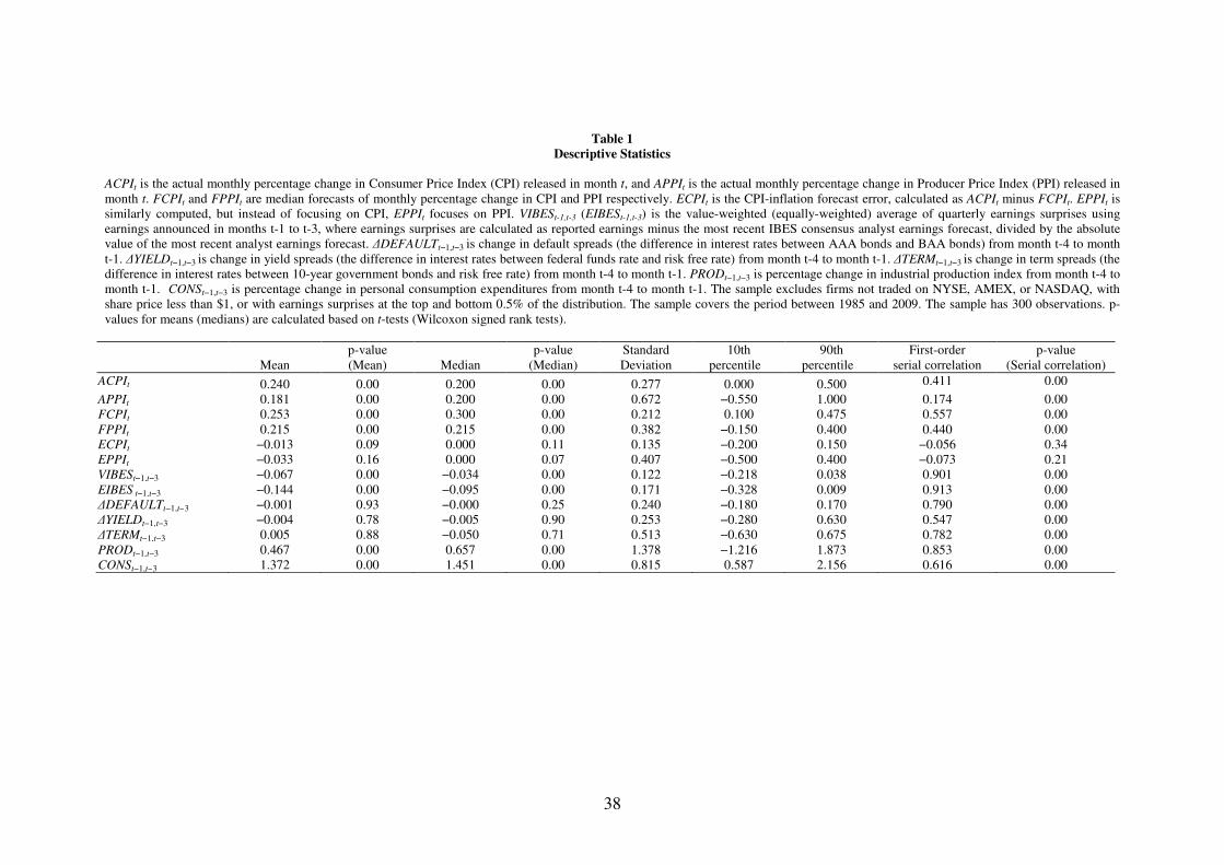
38

Table 1

Descriptive Statistics

ACPIt is the actual monthly percentage change in Consumer Price Index (CPI) released in month t, and APPIt is the actual monthly percentage change in Producer Price Index (PPI) released in month t. FCPIt and FPPIt are median forecasts of monthly percentage change in CPI and PPI respectively. ECPIt is the CPI-inflation forecast error, calculated as ACPIt minus FCPIt. EPPIt is similarly computed, but instead of focusing on CPI, EPPIt focuses on PPI. VIBESt-1,t-3 (EIBESt-1,t-3) is the value-weighted (equally-weighted) average of quarterly earnings surprises using earnings announced in months t-1 to t-3, where earnings surprises are calculated as reported earnings minus the most recent IBES consensus analyst earnings forecast, divided by the absolute value of the most recent analyst earnings forecast. ∆DEFAULTt−1,t−3 is change in default spreads (the difference in interest rates between AAA bonds and BAA bonds) from month t-4 to month t-1. ∆YIELDt−1,t−3 is change in yield spreads (the difference in interest rates between federal funds rate and risk free rate) from month t-4 to month t-1. ∆TERMt−1,t−3 is change in term spreads (the difference in interest rates between 10-year government bonds and risk free rate) from month t-4 to month t-1. PRODt−1,t−3 is percentage change in industrial production index from month t-4 to month t-1. CONSt−1,t−3 is percentage change in personal consumption expenditures from month t-4 to month t-1. The sample excludes firms not traded on NYSE, AMEX, or NASDAQ, with share price less than $1, or with earnings surprises at the top and bottom 0.5% of the distribution. The sample covers the period between 1985 and 2009. The sample has 300 observations. p-values for means (medians) are calculated based on t-tests (Wilcoxon signed rank tests).

Mean p-value (Mean) Median

p-value (Median)

Standard Deviation

10th percentile

90th percentile

First-order serial correlation

p-value (Serial correlation)

ACPIt 0.240 0.00 0.200 0.00 0.277 0.000 0.500 0.411 0.00

APPIt 0.181 0.00 0.200 0.00 0.672 −0.550 1.000 0.174 0.00 FCPIt 0.253 0.00 0.300 0.00 0.212 0.100 0.475 0.557 0.00 FPPIt 0.215 0.00 0.215 0.00 0.382 −0.150 0.400 0.440 0.00 ECPIt −0.013 0.09 0.000 0.11 0.135 −0.200 0.150 −0.056 0.34 EPPIt −0.033 0.16 0.000 0.07 0.407 −0.500 0.400 −0.073 0.21 VIBESt−1,t−3 −0.067 0.00 −0.034 0.00 0.122 −0.218 0.038 0.901 0.00 EIBES t−1,t−3 −0.144 0.00 −0.095 0.00 0.171 −0.328 0.009 0.913 0.00 ∆DEFAULTt−1,t−3 −0.001 0.93 −0.000 0.25 0.240 −0.180 0.170 0.790 0.00 ∆YIELDt−1,t−3 −0.004 0.78 −0.005 0.90 0.253 −0.280 0.630 0.547 0.00 ∆TERMt−1,t−3 0.005 0.88 −0.050 0.71 0.513 −0.630 0.675 0.782 0.00 PRODt−1,t−3 0.467 0.00 0.657 0.00 1.378 −1.216 1.873 0.853 0.00 CONSt−1,t−3 1.372 0.00 1.451 0.00 0.815 0.587 2.156 0.616 0.00

39

Table 2

Univariate Correlations

This table provides Pearson (above diagonal) and Spearman (below diagonal) correlations among variables of interest. The variables and the sample are described in Table 1. The sample has 300 observations. Correlations significant at least at 10% level are in bold.

(1) (2) (3) (4) (5) (6) (7) (8) (9) (10) (11) (12) (13)

(1) ACPIt 0.729 0.882 0.800 0.672 0.453 0.028 0.030 −0.363 0.017 −0.042 0.250 0.273 (2) APPIt 0.606 0.766 0.841 0.297 0.861 0.136 0.125 −0.258 0.041 −0.032 0.161 0.173 (3) FCPIt 0.767 0.719 0.889 0.244 0.429 0.047 0.047 −0.408 0.056 −0.044 0.309 0.310 (4) FPPIt 0.634 0.770 0.806 0.248 0.450 0.091 0.078 −0.406 0.070 −0.003 0.257 0.260

(5) ECPIt 0.697 0.186 0.156 0.157 0.258 −0.015 −0.012 −0.105 −0.054 −0.018 0.028 0.075 (6) EPPIt 0.408 0.859 0.446 0.399 0.183 0.139 0.133 −0.045 0.001 −0.050 0.024 0.041 (7) VIBESt-1,t-3 −0.098 0.086 −0.087 0.048 −0.074 0.094 0.980 −0.038 0.201 −0.055 0.422 0.203 (8) EIBESt-1,t-3 −0.106 0.073 −0.103 0.020 −0.065 0.094 0.957 0.019 0.194 −0.081 0.438 0.200

(9) ∆DEFAULTt-1,t-3 −0.147 −0.073 −0.133 −0.155 −0.078 0.025 −0.063 −0.040 −0.036 0.025 −0.204 −0.247 (10) ∆YIELDt-1,t-3 0.038 0.066 0.025 0.118 0.013 0.015 0.174 0.163 0.052 −0.098 0.171 −0.005 (11) ∆TERMt-1,t-3 −0.006 −0.054 −0.019 −0.008 0.007 −0.068 −0.154 −0.176 −0.044 −0.136 −0.246 −0.047 (12) PRODt-1,t-3 0.046 0.017 0.108 0.073 −0.063 −0.038 0.182 0.195 −0.166 0.102 −0.205 0.517

(13) CONSt-1,t-3 0.121 0.045 0.116 0.065 0.026 0.017 −0.047 −0.063 −0.067 −0.117 −0.057 0.232

40

Table 3

VAR Analysis of Inflation Realizations on Aggregate Earnings News

This table presents the results from the VAR analysis of inflation realizations on lagged aggregate earnings surprises and control variables. VAR analysis includes 4 lags but we report only the first lag’s coefficient estimate to conserve space. The z-statistics are reported in parentheses.

Dependent Variable → ACPIt ACPIt APPIt APPIt

Intercept 0.157 (2.18)

0.158 (2.22)

−0.082 (−0.42)

−0.063 (−0.32)

VIBESt−1,t−3 0.213 (0.69)

1.678 (1.96)

EIBESt−1,t−3 0.328 (1.37)

1.761 (2.65)

ACPIt−1 0.374 (6.32)

0.377 (6.38)

APPIt−1 0.098 (1.65)

0.090 (1.52)

DEFAULTt−1 −0.738 (−4.89)

−0.720 (−4.78)

−1.645 (−3.99)

−1.557 (−3.79)

YIELDt−1 0.192 (2.17)

0.184 (2.09)

0.477 (1.97)

0.486 (2.01)

TERMt−1 0.035 (0.60)

0.035 (0.60)

0.229 (1.41)

0.222 (1.37)

PRODt−1 0.006 (0.24)

0.007 (0.28)

0.000 (0.01)

0.009 (0.13)

CONSt−1 0.026 (0.87)

0.027 (0.91)

0.094 (1.16)

0.099 (1.22)

41

Table 4

Regression of Inflation Forecast Errors on Lagged Aggregate Earnings News

This table presents the results from the regressions of inflation forecast errors on lagged aggregate earnings surprises and control variables. Panel A uses value-weighted IBES earnings surprises. Panel B uses equal-weighted IBES earnings surprises. All other variables and the sample are described in Table 1. The t-statistics are reported in parentheses.

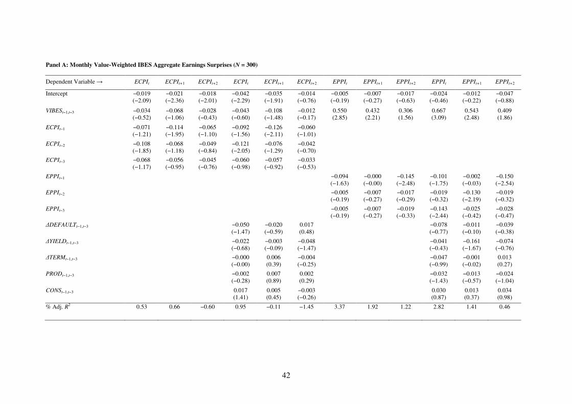
42

Panel A: Monthly Value-Weighted IBES Aggregate Earnings Surprises (N = 300)

Dependent Variable → ECPIt ECPIt+1 ECPIt+2 ECPIt ECPIt+1 ECPIt+2 EPPIt EPPIt+1 EPPIt+2 EPPIt EPPIt+1 EPPIt+2

Intercept −0.019 (−2.09)

−0.021 (−2.36)

−0.018 (−2.01)

−0.042 (−2.29)

−0.035 (−1.91)

−0.014 (−0.76)

−0.005 (−0.19)

−0.007 (−0.27)

−0.017 (−0.63)

−0.024 (−0.46)

−0.012 (−0.22)

−0.047 (−0.88)

VIBESt−1,t−3 −0.034 (−0.52)

−0.068 (−1.06)

−0.028 (−0.43)

−0.043 (−0.60)

−0.108 (−1.48)

−0.012 (−0.17)

0.550 (2.85)

0.432 (2.21)

0.306 (1.56)

0.667 (3.09)

0.543 (2.48)

0.409 (1.86)

ECPIt−1 −0.071 (−1.21)

−0.114 (−1.95)

−0.065 (−1.10)

−0.092 (−1.56)

−0.126 (−2.11)

−0.060 (−1.01)

ECPIt−2 −0.108 (−1.85)

−0.068 (−1.18)

−0.049 (−0.84)

−0.121 (−2.05)

−0.076 (−1.29)

−0.042 (−0.70)

ECPIt−3 −0.068 (−1.17)

−0.056 (−0.95)

−0.045 (−0.76)

−0.060 (−0.98)

−0.057 (−0.92)

−0.033 (−0.53)

EPPIt−1 −0.094 (−1.63)

−0.000 (−0.00)

−0.145 (−2.48)

−0.101 (−1.75)

−0.002 (−0.03)

−0.150 (−2.54)

EPPIt−2 −0.005 (−0.19)

−0.007 (−0.27)

−0.017 (−0.29)

−0.019 (−0.32)

−0.130 (−2.19)

−0.019 (−0.32)

EPPIt−3 −0.005 (−0.19)

−0.007 (−0.27)

−0.019 (−0.33)

−0.143 (−2.44)

−0.025 (−0.42)

−0.028 (−0.47)

∆DEFAULTt−1,t−3 −0.050 (−1.47)

−0.020 (−0.59)

0.017 (0.48)

−0.078 (−0.77)

−0.011 (−0.10)

−0.039 (−0.38)

∆YIELDt−1,t−3 −0.022 (−0.68)

−0.003 (−0.09)

−0.048 (−1.47)

−0.041 (−0.43)

−0.161 (−1.67)

−0.074 (−0.76)

∆TERMt−1,t−3 −0.000 (−0.00)

0.006 (0.39)

−0.004 (−0.25)

−0.047 (−0.99)

−0.001 (−0.02)

0.013 (0.27)

PRODt−1,t−3 −0.002 (−0.28)

0.007 (0.89)

0.002 (0.29)

−0.032 (−1.43)

−0.013 (−0.57)

−0.024 (−1.04)

CONSt−1,t−3 0.017 (1.41)

0.005 (0.45)

−0.003 (−0.26)

0.030 (0.87)

0.013 (0.37)

0.034 (0.98)

% Adj. R2 0.53 0.66 −0.60

0.95 −0.11

−1.45

3.37 1.92 1.22 2.82 1.41 0.46

43

Panel B: Monthly Equal-Weighted IBES Aggregate Earnings Surprises (N = 300)

Dependent Variable → ECPIt ECPIt+1 ECPIt+2 ECPIt ECPIt+1 ECPIt+2 EPPIt EPPIt+1 EPPIt+2 EPPIt EPPIt+1 EPPIt+2

Intercept −0.020 (−1.92)

−0.024 (−2.30)

−0.021 (−1.98)

−0.042 (−2.17)

−0.039 (−2.00)

−0.017 (−0.88)

0.012 (0.38)

0.001 (0.01)

−0.011 (−0.34)

−0.002 (−0.03)

−0.002 (−0.04)

−0.037 (−0.65)

EIBESt−1,t−3 −0.024 (−0.51)

−0.050 (−1.08)

−0.030 (−0.64)

−0.025 (−0.48)

−0.078 (−1.48)

−0.025 (−0.46)

0.371 (2.69)

0.253 (1.81)

0.185 (1.32)

0.465 (2.97)

0.323 (2.03)

0.262 (1.65)

ECPIt−1 −0.071 (−1.21)

−0.114 (−1.95)

−0.066 (−1.12)

−0.092 (−1.55)

−0.125 (−2.11)

−0.062 (−1.04)

ECPIt−2 −0.108 (−1.86)

−0.070 (−1.20)

−0.050 (−0.86)

−0.121 (−2.04)

−0.078 (−1.31)

−0.043 (−0.73)

ECPIt−3 −0.069 (−1.18)

−0.057 (−0.98)

−0.046 (−0.79)

−0.060 (−0.98)

−0.060 (−0.97)

−0.036 (−0.58)

EPPIt−1 −0.093 (−1.60)

0.003 (0.06)

−0.143 (−2.44)

−0.102 (−1.75)

0.001 (0.02)

−0.149 (−2.52)

EPPIt−2 −0.018 (−0.31)

−0.137 (−2.33)

−0.017 (−0.28)

−0.022 (−0.37)

−0.131 (−2.19)

−0.021 (−0.34)

EPPIt−3 −0.136 (−2.36)

−0.016 (−0.28)

−0.017 (−0.29)

−0.140 (−2.39)

−0.021 (−0.35)

−0.025 (−0.43)

∆DEFAULTt−1,t−3 −0.049 (−1.43)

−0.016 (−0.48)

0.018 (0.53)

−0.098 (−0.97)

−0.023 (−0.22)

−0.050 (−0.48)

∆YIELDt−1,t−3 −0.022 (−0.70)

−0.003 (−0.09)

−0.046 (−1.42)

−0.036 (−0.38)

−0.152 (−1.58)

−0.069 (−0.71)

∆TERMt−1,t−3 −0.000 (−0.02)

0.006 (0.37)

−0.004 (−0.23)

−0.043 (−0.91)

0.003 (0.05)

0.015 (0.32)

PRODt−1,t−3 −0.002 (−0.30)

0.007 (0.92)

0.003 (0.40)

−0.033 (−1.45)

−0.011 (−0.46)

−0.023 (−1.00)

CONSt−1,t−3 0.016 (1.41)

0.005 (0.46)

−0.003 (−0.25)

0.030 (0.87)

0.013 (0.36)

0.034 (0.98)

% Adj. R2 0.53 0.68 −0.52

0.91 −0.11

−1.38

3.09 1.38 0.99 2.60 0.74 0.21

44

Table 5

Regression of Inflation Forecast Errors on Lagged Aggregate Earnings News: Robustness

This table presents the robustness results from the regressions of inflation forecast errors on lagged aggregate earnings surprises and control variables. Panel A uses value-weighted Compustat based earnings surprises. Panel B uses equal-weighted Compustat based earnings surprises. Panel C uses AGGIBES (defined as unscaled firm-level earnings aggregated across firms releasing earnings in the three most recent months divided by aggregate of the absolute value of corresponding earnings forecasts) as an alternative proxy for aggregate earnings surprise. Panel D uses quarterly observations where dependent variable is average inflation forecast errors over the next 3 months (months t, t+1, and t+2). The t-statistics are reported in parentheses.

45

Panel A: Monthly Value-Weighted Compustat Aggregate Earnings Surprises (N = 300)

Dependent Variable → ECPIt ECPIt+1 ECPIt+2 ECPIt ECPIt+1 ECPIt+2 EPPIt EPPIt+1 EPPIt+2 EPPIt EPPIt+1 EPPIt+2

Intercept −0.017 (−2.10)

−0.017 (−2.13)

−0.017 (−2.08)

−0.038 (−2.16)

−0.025 (−1.38)

−0.010 (−0.57)

−0.047 (−1.98)

−0.041 (−1.73)

−0.040 (−1.67)

−0.041 (−0.80)

−0.016 (−0.32)

−0.055 (−1.07)

VCOMPt−1,t−3 0.001 (0.05)

0.008 (0.37)

0.005 (0.22)

−0.003 (−0.10)

0.001 (0.03)

0.015 (0.50)

0.158 (2.40)

0.155 (2.34)

0.088 (1.33)

0.244 (2.76)

0.261 (2.94)

0.163 (1.81)

ECPIt−1 −0.068 (−1.17)

−0.107 (−1.84)

−0.062 (−1.06)

−0.089 (−1.51)

−0.117 (−1.96)

−0.058 (−0.97)

ECPIt−2 −0.106 (−1.82)

−0.064 (−1.09)

−0.047 (−0.80)

−0.119 (−2.01)

−0.069 (−1.16)

−0.038 (−0.64)

ECPIt−3 −0.066 (−1.14)

−0.051 (−0.88)

−0.043 (−0.73)

−0.056 (−0.93)

−0.047 (−0.77)

−0.030 (−0.49)

EPPIt−1 −0.084 (−1.47)

0.005 (0.08)

−0.140 (−2.40)

−0.094 (−1.63)

−0.001 (−0.01)

−0.147 (−2.50)

EPPIt−2 −0.012 (−0.21)

−0.136 (−2.32)

−0.014 (−0.24)

−0.016 (−0.27)

−0.130 (−2.19)

−0.018 (−0.30)

EPPIt−3 −0.135 (−2.34)

−0.019 (−0.33)

−0.017 (−0.29)

−0.138 (−2.35)

−0.024 (−0.40)

−0.025 (−0.43)

∆DEFAULTt−1,t−3 −0.051 (−1.43)

−0.024 (−0.67)

0.011 (0.32)

−0.139 (−1.32)

−0.082 (−0.77)

−0.081 (−0.76)

∆YIELDt−1,t−3 −0.024 (−0.76)

−0.011 (−0.33)

−0.051 (−1.57)

−0.031 (−0.33)

−0.161 (−1.68)

−0.069 (−0.71)

∆TERMt−1,t−3 −0.001 (−0.07)

0.004 (0.26)

−0.003 (−0.20)

−0.018 (−0.38)

0.027 (0.57)

0.031 (0.65)

PRODt−1,t−3 −0.003 (−0.42)

0.003 (0.34)

−0.000 (−0.01)

−0.037 (−1.58)

−0.025 (−1.07)

−0.029 (−1.20)

CONSt−1,t−3 0.017 (1.37)

0.005 (0.39)

−0.005 (−0.39)

0.006 (0.16)

−0.013 (−0.36)

0.018 (0.51)

% Adj. R2 0.44 0.33 −0.64

0.83 −0.87 −1.37

2.61 2.12 1.00 2.20 2.23 0.41

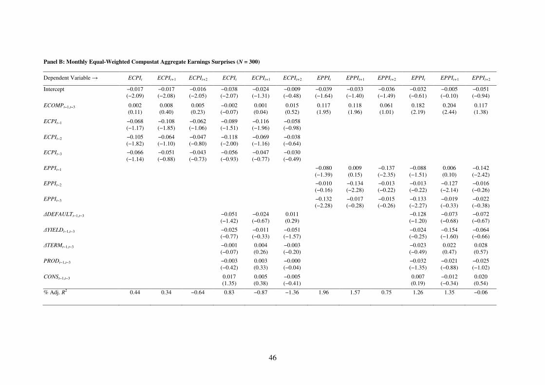
46

Panel B: Monthly Equal-Weighted Compustat Aggregate Earnings Surprises (N = 300)

Dependent Variable → ECPIt ECPIt+1 ECPIt+2 ECPIt ECPIt+1 ECPIt+2 EPPIt EPPIt+1 EPPIt+2 EPPIt EPPIt+1 EPPIt+2

Intercept −0.017 (−2.09)

−0.017 (−2.08)

−0.016 (−2.05)

−0.038 (−2.07)

−0.024 (−1.31)

−0.009 (−0.48)

−0.039 (−1.64)

−0.033 (−1.40)

−0.036 (−1.49)

−0.032 (−0.61)

−0.005 (−0.10)

−0.051 (−0.94)

ECOMPt−1,t−3 0.002 (0.11)

0.008 (0.40)

0.005 (0.23)

−0.002 (−0.07)

0.001 (0.04)

0.015 (0.52)

0.117 (1.95)

0.118 (1.96)

0.061 (1.01)

0.182 (2.19)

0.204 (2.44)

0.117 (1.38)

ECPIt−1 −0.068 (−1.17)

−0.108 (−1.85)

−0.062 (−1.06)

−0.089 (−1.51)

−0.116 (−1.96)

−0.058 (−0.98)

ECPIt−2 −0.105 (−1.82)

−0.064 (−1.10)

−0.047 (−0.80)

−0.118 (−2.00)

−0.069 (−1.16)

−0.038 (−0.64)

ECPIt−3 −0.066 (−1.14)

−0.051 (−0.88)

−0.043 (−0.73)

−0.056 (−0.93)

−0.047 (−0.77)

−0.030 (−0.49)

EPPIt−1 −0.080 (−1.39)

0.009 (0.15)

−0.137 (−2.35)

−0.088 (−1.51)

0.006 (0.10)

−0.142 (−2.42)

EPPIt−2 −0.010 (−0.16)

−0.134 (−2.28)

−0.013 (−0.22)

−0.013 (−0.22)

−0.127 (−2.14)

−0.016 (−0.26)

EPPIt−3 −0.132 (−2.28)

−0.017 (−0.28)

−0.015 (−0.26)

−0.133 (−2.27)

−0.019 (−0.33)

−0.022 (−0.38)

∆DEFAULTt−1,t−3 −0.051 (−1.42)

−0.024 (−0.67)

0.011 (0.29)

−0.128 (−1.20)

−0.073 (−0.68)

−0.072 (−0.67)

∆YIELDt−1,t−3 −0.025 (−0.77)

−0.011 (−0.33)

−0.051 (−1.57)

−0.024 (−0.25)

−0.154 (−1.60)

−0.064 (−0.66)

∆TERMt−1,t−3 −0.001 (−0.07)

0.004 (0.26)

−0.003 (−0.20)

−0.023 (−0.49)

0.022 (0.47)

0.028 (0.57)

PRODt−1,t−3 −0.003 (−0.42)

0.003 (0.33)

−0.000 (−0.04)

−0.032 (−1.35)

−0.021 (−0.88)

−0.025 (−1.02)

CONSt−1,t−3 0.017 (1.35)

0.005 (0.38)

−0.005 (−0.41)

0.007 (0.19)

−0.012 (−0.34)

0.020 (0.54)

% Adj. R2 0.44 0.34 −0.64

0.83 −0.87 −1.36

1.96 1.57 0.75 1.26 1.35 −0.06

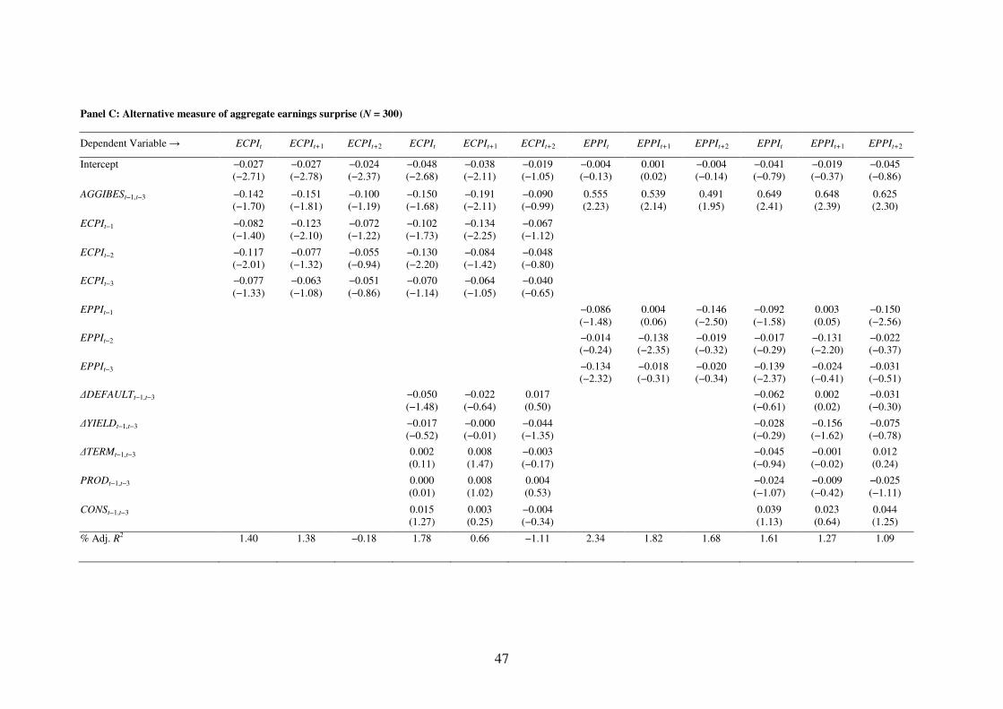
47

Panel C: Alternative measure of aggregate earnings surprise (N = 300)

Dependent Variable → ECPIt ECPIt+1 ECPIt+2 ECPIt ECPIt+1 ECPIt+2 EPPIt EPPIt+1 EPPIt+2 EPPIt EPPIt+1 EPPIt+2

Intercept −0.027 (−2.71)

−0.027 (−2.78)

−0.024 (−2.37)

−0.048 (−2.68)

−0.038 (−2.11)

−0.019 (−1.05)

−0.004 (−0.13)

0.001 (0.02)

−0.004 (−0.14)

−0.041 (−0.79)

−0.019 (−0.37)

−0.045 (−0.86)

AGGIBESt−1,t−3 −0.142 (−1.70)

−0.151 (−1.81)

−0.100 (−1.19)

−0.150 (−1.68)

−0.191 (−2.11)

−0.090 (−0.99)

0.555 (2.23)

0.539 (2.14)

0.491 (1.95)

0.649 (2.41)

0.648 (2.39)

0.625 (2.30)

ECPIt−1 −0.082 (−1.40)

−0.123 (−2.10)

−0.072 (−1.22)

−0.102 (−1.73)

−0.134 (−2.25)

−0.067 (−1.12)

ECPIt−2 −0.117 (−2.01)

−0.077 (−1.32)

−0.055 (−0.94)

−0.130 (−2.20)

−0.084 (−1.42)

−0.048 (−0.80)

ECPIt−3 −0.077 (−1.33)

−0.063 (−1.08)

−0.051 (−0.86)

−0.070 (−1.14)

−0.064 (−1.05)

−0.040 (−0.65)

EPPIt−1 −0.086 (−1.48)

0.004 (0.06)

−0.146 (−2.50)

−0.092 (−1.58)

0.003 (0.05)

−0.150 (−2.56)

EPPIt−2 −0.014 (−0.24)

−0.138 (−2.35)

−0.019 (−0.32)

−0.017 (−0.29)

−0.131 (−2.20)

−0.022 (−0.37)

EPPIt−3 −0.134 (−2.32)

−0.018 (−0.31)

−0.020 (−0.34)

−0.139 (−2.37)

−0.024 (−0.41)

−0.031 (−0.51)

∆DEFAULTt−1,t−3 −0.050 (−1.48)

−0.022 (−0.64)

0.017 (0.50)

−0.062 (−0.61)

0.002 (0.02)

−0.031 (−0.30)

∆YIELDt−1,t−3 −0.017 (−0.52)

−0.000 (−0.01)

−0.044 (−1.35)

−0.028 (−0.29)

−0.156 (−1.62)

−0.075 (−0.78)

∆TERMt−1,t−3 0.002 (0.11)

0.008 (1.47)

−0.003 (−0.17)

−0.045 (−0.94)

−0.001 (−0.02)

0.012 (0.24)

PRODt−1,t−3 0.000 (0.01)

0.008 (1.02)

0.004 (0.53)

−0.024 (−1.07)

−0.009 (−0.42)

−0.025 (−1.11)

CONSt−1,t−3 0.015 (1.27)

0.003 (0.25)

−0.004 (−0.34)

0.039 (1.13)

0.023 (0.64)

0.044 (1.25)

% Adj. R2 1.40 1.38 −0.18

1.78 0.66 −1.11

2.34 1.82 1.68 1.61 1.27 1.09

48

Panel D: Quarterly Analysis (N = 100)

Dependent Variable → ECPIt,t+2 ECPIt,t+2 EPPIt,t+2 EPPIt,t+2

Intercept −0.016 (−0.87)

−0.016 (−0.83)

0.010 (0.19)

0.030 (0.54)

VIBESt−1,t−3 0.004 (0.06)

0.590 (2.97)

EIBES t−1,t−3 0.002 (0.03)

0.403 (2.76)

ECPIt−1,t-3 −0.228 (−2.11)

−0.228 (−2.11)

EPPIt−1,t-3 −0.252 (−2.52)

−0.248 (−2.46)

∆DEFAULTt−1,t−3 0.006 (0.21)

0.007 (0.21)

−0.088 (−0.92)

−0.101 (−1.04)

∆YIELDt−1,t−3 −0.033 (−1.33)

−0.033 (−1.33)

−0.124 (−1.64)

−0.120 (−1.58)

∆TERMt−1,t−3 −0.020 (−1.40)

−0.020 (−1.40)

−0.032 (−0.73)

−0.031 (−0.69)

PRODt−1,t−3 −0.002 (−0.30)

−0.002 (−0.28)

−0.027 (−1.11)

−0.026 (−1.07)

CONSt−1,t−3 0.000 (0.00)

0.000 (0.00)

0.002 (0.05)

0.000 (0.01)

% Adj. R2 3.52 3.52

8.40 7.25

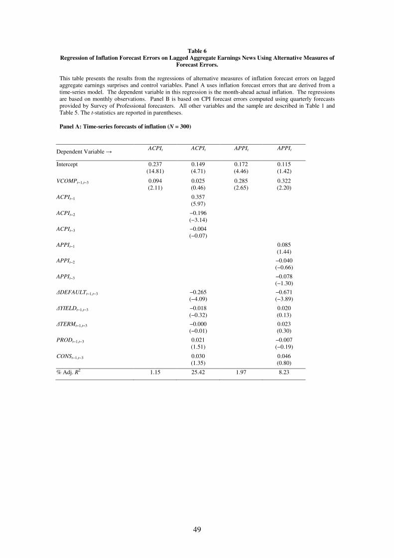
49

Table 6

Regression of Inflation Forecast Errors on Lagged Aggregate Earnings News Using Alternative Measures of

Forecast Errors.

This table presents the results from the regressions of alternative measures of inflation forecast errors on lagged aggregate earnings surprises and control variables. Panel A uses inflation forecast errors that are derived from a time-series model. The dependent variable in this regression is the month-ahead actual inflation. The regressions are based on monthly observations. Panel B is based on CPI forecast errors computed using quarterly forecasts provided by Survey of Professional forecasters. All other variables and the sample are described in Table 1 and Table 5. The t-statistics are reported in parentheses.

Panel A: Time-series forecasts of inflation (N = 300)

Dependent Variable → ACPIt

ACPIt

APPIt

APPIt

Intercept 0.237 (14.81)

0.149 (4.71)

0.172 (4.46)

0.115 (1.42)

VCOMPt−1,t−3 0.094 (2.11)

0.025 (0.46)

0.285 (2.65)

0.322 (2.20)

ACPIt−1 0.357 (5.97)

ACPIt−2 −0.196 (−3.14)

ACPIt−3 −0.004 (−0.07)

APPIt−1 0.085 (1.44)

APPIt−2 −0.040 (−0.66)

APPIt−3 −0.078 (−1.30)

∆DEFAULTt−1,t−3 −0.265 (−4.09)

−0.671 (−3.89)

∆YIELDt−1,t−3 −0.018 (−0.32)

0.020 (0.13)

∆TERMt−1,t−3 −0.000 (−0.01)

0.023 (0.30)

PRODt−1,t−3 0.021 (1.51)

−0.007 (−0.19)

CONSt−1,t−3 0.030 (1.35)

0.046 (0.80)

% Adj. R2 1.15 25.42

1.97 8.23

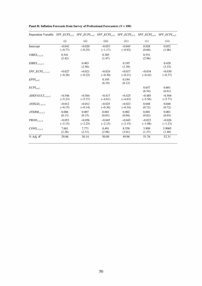
50

Panel B: Inflation Forecasts from Survey of Professional Forecasters (N = 100)

Dependent Variable SPF_ECPIt,t+2 SPF_ECPIt,t+2 SPF_ECPIt,t+2 SPF_ECPIt,t+2 SPF_ECPIt,t+2 SPF_ECPIt,t+2

(i) (ii) (iii) (iv) (v) (vi)

Intercept −0.042 (−0.77)

−0.020 (−0.35)

−0.053 (−1.17)

−0.045 (−0.92)

0.028 (0.60)

0.052 (1.06)

VIBESt−1,t−3 0.541 (2.42)

0.285 (1.47)

0.551 (2.96)

EIBES t−1,t−3 0.403 (2.50)

0.195 (1.39)

0.420 (3.15)

SPF_ECPIt−1, t−3 −0.027 (−0.28)

−0.021 (−0.22)

−0.024 (−0.30)

−0.017 (−0.21)

−0.034 (−0.42)

−0.030 (−0.37)

EPPIt,t+2 0.195 (6.19)

0.194 (6.12)

ECPIt,t+2 0.657 (6.54)

0.661 (6.61)

∆DEFAULTt−1,t−3 −0.546 (−5.23)

−0.564 (−5.37)

−0.417 (−4.61)

−0.425 (−4.63)

−0.485 (−5.56)

−0.504 (−5.77)

∆YIELDt−1,t−3 −0.012 (−0.15)

−0.012 (−0.14)

−0.025 (−0.36)

−0.023 (−0.34)

0.048 (0.72)

0.048 (0.72)

∆TERMt−1,t−3 0.006 (0.13)

0.007 (0.15)

0.001 (0.03)

0.002 (0.04)

0.001 (0.02)

0.001 (0.03)

PRODt−1,t−3 −0.053 (−2.15)

−0.056 (−2.25)

−0.045 (−2.15)

−0.045 (−2.15)

−0.023 (−1.08)

−0.026 (−1.23)

CONSt−1,t−3 7.681 (2.28)

7.771 (2.31)

8.491 (2.98)

8.558 (3.01)

3.909 (1.37)

3.9065 (1.40)

% Adj. R2 29.86 30.14

50.09 49.96 51.76 52.31

51

Table 7

Regression of Actual Inflation on Inflation Forecasts and Aggregate Earnings News

This table presents the results from regressions of actual inflation on inflation forecasts, lagged aggregate earnings surprises and control variables. All other variables and the sample are described in Table 1. The t-statistics are reported in parentheses.

Dependent Variable → ACPIt

(j = 0)

ACPIt+1 (j = 1)

ACPIt+2 (j = 2)

APPIt

(j = 0)

APPIt+1 (j = 1)

APPIt+2 (j = 2)

Intercept −0.047 (−2.53)

−0.047 (−2.43)

−0.043 (−2.25)

−0.083 (−1.82)

−0.098 (−2.08)

−0.110 (−2.31)

Inflation_Forecastt+j 1.143 (26.40)

1.156 (30.27)

1.173 (31.26)

1.611 (26.64)

1.543 (26.91)

1.512 (26.77)

VIBESt−1,t−3 0.019 (0.28)

−0.067 (−0.96)

0.025 (0.36)

0.732 (3.83)

0.665 (3.39)

0.544 (2.72)

ACPIt−1 0.042 (1.22)

−0.080 (−2.47)

−0.049 (−1.51)

ACPIt−2 −0.091 (−2.69)

−0.047 (−1.39)

0.015 (0.45)

ACPIt−3 −0.028 (−0.88)

0.012 (0.37)

0.047 (1.47)

APPIt−1 −0.094 (−2.86)

−0.027 (−0.82)

−0.043 (−1.29)

APPIt−2 −0.016 (−0.48)

−0.024 (−0.70)

−0.005 (−0.14)

APPIt−3 −0.057 (−1.79)

−0.029 (−0.88)

−0.006 (−0.18)

∆DEFAULTt−1,t−3 0.003 (0.08)

−0.022 (−0.64)

−0.002 (−0.05)

0.219 (2.32)

0.198 (2.10)

0.044 (0.47)

∆YIELDt−1,t−3 −0.019 (−0.62)

0.016 (0.51)

−0.046 (−1.47)

−0.062 (−0.74)

−0.118 (−1.39)

−0.066 (−0.76)

∆TERMt−1,t−3 −0.002 (−0.15)

0.008 (0.50)

−0.012 (−0.75)

−0.065 (−1.58)

−0.008 (−0.18)

−0.001 (−0.03)

PRODt−1,t−3 −0.006 (−0.83)

0.002 (0.21)

−0.003 (−0.42)

−0.053 (−2.72)

−0.044 (−2.17)

−0.045 (−2.19)

CONSt−1,t−3 0.015 (1.21)

0.012 (0.96)

−0.011 (−0.90)

0.016 (0.53)

0.021 (0.66)

0.026 (0.79)

% Adj. R2 78.11 77.98 77.92

73.15 72.06 71.22

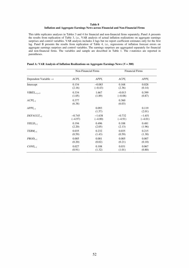
52

Table 8

Inflation and Aggregate Earnings News across Financial and Non-Financial Firms

This table replicates analyses in Tables 3 and 4 for financial and non-financial firms separately. Panel A presents the results from replication of Table 3, i.e., VAR analysis of actual inflation realizations on aggregate earnings surprises and control variables. VAR analysis includes 4 lags but we report coefficient estimates only for the first lag. Panel B presents the results from replication of Table 4, i.e., regressions of inflation forecast errors on aggregate earnings surprises and control variables. The earnings surprises are aggregated separately for financial and non-financial firms. The variables and sample are described in Table 1. The t-statistics are reported in parentheses.

Panel A: VAR Analysis of Inflation Realizations on Aggregate Earnings News (N = 300)

Non-Financial Firms Financial Firms

Dependent Variable → ACPIt APPIt ACPIt APPIt

Intercept 0.154 (2.16)

−0.083 (−0.43)

0.168 (2.36)

0.028 (0.14)

VIBESt−1,t−3 0.334 (1.05)

1.667 (1.89)

−0.013 (−0.08)

0.399 (0.87)

ACPIt−1 0.377 (6.38)

0.360 (6.03)

APPIt−1 0.093 (1.57)

0.119 (2.01)

DEFAULTt−1 −0.745 (−4.97)

−1.638 (−4.00)

−0.732 (−4.91)

−1.651 (−4.01)

YIELDt−1 0.194 (2.20)

0.496 (2.05)

0.188 (2.13)

0.481 (1.96)

TERMt−1 0.035 (0.59)

0.232 (1.43)

0.035 (0.59)

0.215 (1.30)

PRODt−1 0.005 (0.20)

0.001 (0.02)

0.005 (0.21)

0.007 (0.10)

CONSt−1 0.027 (0.91)

0.108 (1.32)

0.031 (1.01)

0.067 (0.80)

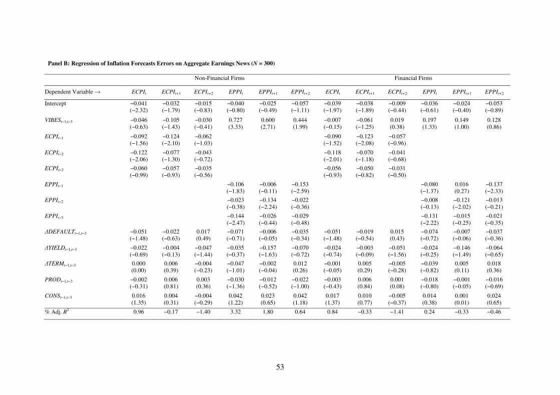
53

Panel B: Regression of Inflation Forecasts Errors on Aggregate Earnings News (N = 300)

Non-Financial Firms Financial Firms

Dependent Variable → ECPIt ECPIt+1 ECPIt+2 EPPIt EPPIt+1 EPPIt+2 ECPIt ECPIt+1 ECPIt+2 EPPIt EPPIt+1 EPPIt+2

Intercept −0.041 (−2.32)

−0.032 (−1.79)

−0.015 (−0.83)

−0.040 (−0.80)

−0.025 (−0.49)

−0.057 (−1.11)

−0.039 (−1.97)

−0.038 (−1.89)

−0.009 (−0.44)

−0.036 (−0.61)

−0.024 (−0.40)

−0.053 (−0.89)

VIBESt−1,t−3 −0.046 (−0.63)

−0.105 (−1.43)

−0.030 (−0.41)

0.727 (3.33)

0.600 (2.71)

0.444 (1.99)

−0.007 (−0.15)

−0.061 (−1.25)

0.019 (0.38)

0.197 (1.33)

0.149 (1.00)

0.128 (0.86)

ECPIt−1 −0.092 (−1.56)

−0.124 (−2.10)

−0.062 (−1.03)

−0.090 (−1.52)

−0.123 (−2.08)

−0.057 (−0.96)

ECPIt−2 −0.122 (−2.06)

−0.077 (−1.30)

−0.043 (−0.72)

−0.118 (−2.01)

−0.070 (−1.18)

−0.041 (−0.68)

ECPIt−3 −0.060 (−0.99)

−0.057 (−0.93)

−0.035 (−0.56)

−0.056 (−0.93)

−0.050 (−0.82)

−0.031 (−0.50)

EPPIt−1 −0.106 (−1.83)

−0.006 (−0.11)

−0.153 (−2.59)

−0.080 (−1.37)

0.016 (0.27)

−0.137 (−2.33)

EPPIt−2 −0.023 (−0.38)

−0.134 (−2.24)

−0.022 (−0.36)

−0.008 (−0.13)

−0.121 (−2.02)

−0.013 (−0.21)

EPPIt−3 −0.144 (−2.47)

−0.026 (−0.44)

−0.029 (−0.48)

−0.131 (−2.22)

−0.015 (−0.25)

−0.021 (−0.35)

∆DEFAULTt−1,t−3 −0.051 (−1.48)

−0.022 (−0.63)

0.017 (0.49)

−0.071 (−0.71)

−0.006 (−0.05)

−0.035 (−0.34)

−0.051 (−1.48)

−0.019 (−0.54)

0.015 (0.43)

−0.074 (−0.72)

−0.007 (−0.06)

−0.037 (−0.36)

∆YIELDt−1,t−3 −0.022 (−0.69)

−0.004 (−0.13)

−0.047 (−1.44)

−0.035 (−0.37)

−0.157 (−1.63)

−0.070 (−0.72)

−0.024 (−0.74)

−0.003 (−0.09)

−0.051 (−1.56)

−0.024 (−0.25)

−0.146 (−1.49)

−0.064 (−0.65)

∆TERMt−1,t−3 0.000 (0.00)

0.006 (0.39)

−0.004 (−0.23)

−0.047 (−1.01)

−0.002 (−0.04)

0.012 (0.26)

−0.001 (−0.05)

0.005 (0.29)

−0.005 (−0.28)

−0.039 (−0.82)

0.005 (0.11)

0.018 (0.36)

PRODt−1,t−3 −0.002 (−0.31)

0.006 (0.81)

0.003 (0.36)

−0.030 (−1.36)

−0.012 (−0.52)

−0.022 (−1.00)

−0.003 (−0.43)

0.006 (0.84)

0.001 (0.08)

−0.018 (−0.80)

−0.001 (−0.05)

−0.016 (−0.69)

CONSt−1,t−3 0.016 (1.35)

0.004 (0.31)

−0.004 (−0.29)

0.042 (1.22)

0.023 (0.65)

0.042 (1.18)

0.017 (1.37)

0.010 (0.77)

−0.005 (−0.37)

0.014 (0.38)

0.001 (0.01)

0.024 (0.65)

% Adj. R2 0.96 −0.17

−1.40

3.32 1.80 0.64

0.84 −0.33 −1.41

0.24 −0.33

−0.46

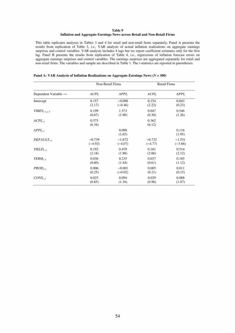
54

Table 9

Inflation and Aggregate Earnings News across Retail and Non-Retail Firms

This table replicates analyses in Tables 3 and 4 for retail and non-retail firms separately. Panel A presents the results from replication of Table 3, i.e., VAR analysis of actual inflation realizations on aggregate earnings surprises and control variables. VAR analysis includes 4 lags but we report coefficient estimates only for the first lag. Panel B presents the results from replication of Table 4, i.e., regressions of inflation forecast errors on aggregate earnings surprises and control variables. The earnings surprises are aggregated separately for retail and non-retail firms. The variables and sample are described in Table 1. The t-statistics are reported in parentheses.

Panel A: VAR Analysis of Inflation Realizations on Aggregate Earnings News (N = 300)

Non-Retail Firms Retail Firms

Dependent Variable → ACPIt APPIt ACPIt APPIt

Intercept 0.157 (2.17)

−0.090 (−0.46)

0.154 (2.22)

0.043 (0.23)

VIBESt−1,t−3 0.199 (0.67)

1.573 (1.90)

0.047 (0.30)

0.546 (1.26)

ACPIt−1 0.375 (6.34)

0.362 (6.12)

APPIt−1 0.098 (1.65)

0.116 (1.95)

DEFAULTt−1 −0.739 (−4.92)

−1.672 (−4.07)

−0.732 (−4.77)

−1.551 (−3.66)

YIELDt−1 0.192 (2.18)

0.479 (1.98)

0.181 (2.06)

0.514 (2.12)

TERMt−1 0.036 (0.60)

0.235 (1.44)

0.037 (0.61)

0.185 (1.12)

PRODt−1 0.006 (0.25)

−0.001 (−0.02)

0.005 (0.21)

0.011 (0.15)

CONSt−1 0.025 (0.85)

0.094 (1.16)

0.029 (0.96)

0.088 (1.07)

55

Panel B: Regression of Inflation Forecasts Errors on Aggregate Earnings News (N = 300)

Non-Retail Firms Retail Firms

Dependent Variable → ECPIt ECPIt+1 ECPIt+2 EPPIt EPPIt+1 EPPIt+2 ECPIt ECPIt+1 ECPIt+2 EPPIt EPPIt+1 EPPIt+2

Intercept −0.042 (−2.28)

−0.036 (−1.94)

−0.014 (−0.75)

−0.023 (−0.45)

−0.010 (−0.19)

−0.046 (−0.86)

−0.039 (−2.29)

−0.025 (−1.45)

−0.013 (−0.75)

−0.064 (−1.29)

−0.049 (−0.97)

−0.074 (−1.47)

VIBESt−1,t−3 −0.040 (−0.56)

−0.110 (−1.55)

−0.011 (−0.15)

0.645 (3.04)

0.537 (2.51)

0.402 (1.87)

−0.037 (−0.57)

−0.005 (−0.08)

−0.004 (−0.06)

0.484 (2.52)

0.198 (1.02)

0.176 (0.90)

ECPIt−1 −0.092 (−1.56)

−0.126 (−2.12)

−0.060 (−1.01)

−0.093 (−1.57)

−0.117 (−1.96)

−0.060 (−1.00)

ECPIt−2 −0.121 (−2.04)

−0.076 (−1.28)

−0.041 (−0.69)

−0.122 (−2.06)

−0.070 (−1.17)

−0.041 (−0.69)

ECPIt−3 −0.060 (−0.98)

−0.057 (−0.92)

−0.033 (−0.53)

−0.060 (−0.98)

−0.048 (−0.77)

−0.032 (−0.52)

EPPIt−1 −0.101 (−1.74)

−0.002 (−0.04)

−0.151 (−2.55)

−0.087 (−1.50)

0.014 (0.24)

−0.139 (−2.36)

EPPIt−2 −0.020 (−0.33)

−0.131 (−2.20)

−0.020 (−0.33)

−0.002 (−0.03)

−0.119 (−1.98)

−0.010 (−0.17)

EPPIt−3 −0.144 (−2.46)

−0.026 (−0.44)

−0.029 (−0.48)

−0.119 (−2.03)

−0.008 (−0.13)

−0.015 (−0.25)

∆DEFAULTt−1,t−3 −0.050 (−1.46)

−0.019 (−0.56)

0.017 (0.48)

−0.083 (−0.82)

−0.015 (−0.15)

−0.042 (−0.41)

−0.055 (−1.59)

−0.024 (−0.69)

0.016 (0.45)

−0.007 (−0.07)

0.026 (0.25)

−0.009 (−0.08)

∆YIELDt−1,t−3 −0.022 (−0.68)

−0.002 (−0.07)

−0.048 (−1.47)

−0.041 (−0.43)

−0.162 (−1.68)

−0.074 (−0.76)

−0.024 (−0.75)

−0.010 (−0.32)

−0.048 (−1.51)

−0.011 (−0.12)

−0.132 (−1.37)

−0.052 (−0.54)

∆TERMt−1,t−3 −0.000 (−0.01)

0.006 (0.37)

−0.004 (−0.25)

−0.045 (−0.95)

0.001 (0.01)

0.014 (0.29)

0.001 (0.08)

0.004 (0.27)

−0.004 (−0.24)

−0.065 (−1.35)

−0.005 (−0.10)

0.008 (0.17)

PRODt−1,t−3 −0.002 (−0.29)

0.007 (0.91)

0.002 (0.28)

−0.031 (−1.40)

−0.013 (−0.58)

−0.024 (−1.04)

−0.003 (−0.36)

0.003 (0.41)

0.002 (0.25)

−0.021 (−0.96)

0.002 (0.08)

−0.013 (−0.61)

CONSt−1,t−3 0.017 (1.41)

0.006 (0.47)

−0.003 (−0.26)

0.029 (0.84)

0.012 (0.35)

0.034 (0.97)

0.016 (1.34)

0.005 (0.40)

−0.003 (−0.27)

0.039 (1.11)

0.016 (0.44)

0.037 (1.05)

% Adj. R2 0.94 −0.04

−1.45

2.74 1.46 0.48

0.94 −0.87 −1.46

1.79 −0.32

−0.44

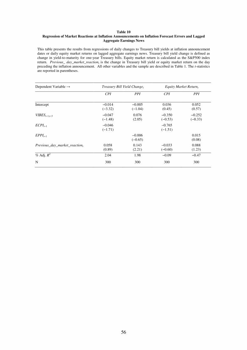
56

Table 10

Regression of Market Reactions at Inflation Announcements on Inflation Forecast Errors and Lagged

Aggregate Earnings News

This table presents the results from regressions of daily changes to Treasury bill yields at inflation announcement dates or daily equity market returns on lagged aggregate earnings news. Treasury bill yield change is defined as change in yield-to-maturity for one-year Treasury bills. Equity market return is calculated as the S&P500 index return. Previous_ day_market_reactiont is the change in Treasury bill yield or equity market return on the day preceding the inflation announcement. All other variables and the sample are described in Table 1. The t-statistics are reported in parentheses.

Dependent Variable → Treasury Bill Yield Changet Equity Market Returnt

CPI PPI CPI PPI

Intercept −0.014 (−3.32)

−0.005 (−1.04)

0.036 (0.45)

0.052 (0.57)

VIBESt−1,t−3 −0.047 (−1.48)

0.076 (2.05)

−0.350 (−0.53)

−0.252 (−0.33)

ECPIt−1 −0.046 (−1.71)

−0.765 (−1.51)

EPPIt−1 −0.006 (−0.65)

0.015 (0.08)

Previous_day_market_reactiont 0.058 (0.89)

0.143 (2.21)

−0.033 (−0.60)

0.088 (1.23)

% Adj. R2 2.04

1.98 −0.09

−0.47

N 300 300 300 300