Embed Size (px)
Citation preview

Montréal Janvier 2003
© 2003 Athanasios Orphanides, Simon van Norden. Tous droits réservés. All rights reserved. Reproduction partielle permise avec citation du document source, incluant la notice ©. Short sections may be quoted without explicit permission, if full credit, including © notice, is given to the source.
Série Scientifique Scientific Series
2003s-01
The Reliability of Inflation Forecasts Based on Output Gap Estimates in Real Time
Athanasios Orphanides, Simon van Norden

CIRANO
Le CIRANO est un organisme sans but lucratif constitué en vertu de la Loi des compagnies du Québec. Le financement de son infrastructure et de ses activités de recherche provient des cotisations de ses organisations-membres, d’une subvention d’infrastructure du ministère de la Recherche, de la Science et de la Technologie, de même que des subventions et mandats obtenus par ses équipes de recherche.
CIRANO is a private non-profit organization incorporated under the Québec Companies Act. Its infrastructure and research activities are funded through fees paid by member organizations, an infrastructure grant from the Ministère de la Recherche, de la Science et de la Technologie, and grants and research mandates obtained by its research teams.
Les organisations-partenaires / The Partner Organizations
•École des Hautes Études Commerciales •École Polytechnique de Montréal •Université Concordia •Université de Montréal •Université du Québec à Montréal •Université Laval •Université McGill •Ministère des Finances du Québec •MRST •Alcan inc. •AXA Canada •Banque du Canada •Banque Laurentienne du Canada •Banque Nationale du Canada •Banque Royale du Canada •Bell Canada •Bombardier •Bourse de Montréal •Développement des ressources humaines Canada (DRHC) •Fédération des caisses Desjardins du Québec •Hydro-Québec •Industrie Canada •Pratt & Whitney Canada Inc. •Raymond Chabot Grant Thornton •Ville de Montréal
ISSN 1198-8177
Les cahiers de la série scientifique (CS) visent à rendre accessibles des résultats de recherche effectuée au CIRANO afin de susciter échanges et commentaires. Ces cahiers sont écrits dans le style des publications scientifiques. Les idées et les opinions émises sont sous l’unique responsabilité des auteurs et ne représentent pas nécessairement les positions du CIRANO ou de ses partenaires. This paper presents research carried out at CIRANO and aims at encouraging discussion and comment. The observations and viewpoints expressed are the sole responsibility of the authors. They do not necessarily represent positions of CIRANO or its partners.
The Reliability of Inflation Forecasts Based on Output Gap Estimates in Real Time*
Athanasios Orphanides†, Simon van Norden‡
Résumé / Abstract
Dans ce papier, on jauge l’utilité de plusieurs estimations (univariées autant que multivariées) de l’écart de production pour prévoir le taux d’inflation. Une analyse ex post suggère que plusieurs de ces estimations aident à prédire l’inflation. Néanmoins, les erreurs de prédictions hors de l’enchantillon qui se sont construites avec les écarts de production estimés en temps réel indiquent que cette amélioration de prédiction est illusoire. On trouve que l’utilité des écarts de production pour prédire l’inflation a été exagérée et que les prédictions faites avec l’écart de production sont souvent moins précises que celles qui ignorent le concept d’un écart de production.
A stable predictive relationship between inflation and the output gap, often referred to as a Phillips curve, provides the basis for empirical formulations of countercyclical monetary policy in many models. In this paper, we provide an empirical evaluation of the usefulness of alternative univariate and multivariate estimates of the output gap for predicting inflation. In-sample analysis based on ex post output gap measures suggests that many of the alternative estimates we examine appear to be quite useful for predicting inflation. However, examination of out-of-sample forecasts using real-time estimates of the same measures suggests that this predictive ability is mostly illusory. We find that the usefulness of output gaps as predictors of inflation has been severely overstated and that real-time forecasts using the output gap are often less accurate than forecasts that abstract from the output gap concept altogether.
Mots clés : la courbe de Phillips, l’écart de production, des prévisions d’inflation, des données en temps réel.
Keywords: Phillips curve, output gap, inflation forecasts, real-time data.
Codes JEL : E37, C53 * We benefited from presentations of earlier drafts at the European Central Bank, CIRANO, the Federal Reserve Bank of Philadelphia Conference on Real Time Data Analysis, the Centre for Growth and Business Cycle Research, as well as at the annual meetings of the American Economics Association, the European Economics Association and the Canadian Economics Association. We would also like to thank Sharon Kozicki, Tim Cogley, Jeremy Piger and Todd Clark, for useful comments and discussions and David Baird for providing his GAUSS routines for computation of Kolmogorov-Smirnov statistics. Athanasios Orphanides wishes to thank the Sveriges Riksbank and European Central Bank for their hospitality during September 2001 when part of this work was completed. Simon van Norden wishes to thank the SSHRC and the HEC Montréal for their financial support. The opinions expressed are those of the authors and do not necessarily reflect views of the Board of Governors of the Federal Reserve System. † Correspondence: Division of Monetary Affairs, Board of Governors of the Federal Reserve System, Washington, D.C. 20551, USA. Tel.: (202) 452-2654, e-mail: [email protected]. ‡ HEC Montréal, CIRANO and CIREQ, 3000 Chemin de la Côte Sainte Catherine, Montréal, Québec, Canada, H3T 2A7. Tel.: (514) 340-6781, e-mail: [email protected].

1 Introduction
A stable predictive relationship between inflation and a measure of deviations of aggregate
demand from the economy’s potential supply—the “output gap”—provides the basis for
many formulations of activist countercyclical stabilization policy. Such a relationship, re-
ferred to as a Phillips curve, is often seen as a helpful guide for policymakers aiming to
maintain low inflation and stable economic growth.1 According to this paradigm, when ag-
gregate demand exceeds potential output, the economy is subject to inflationary pressures
and inflation should be expected to rise. Under these circumstances, policymakers might
wish to adopt policies restricting aggregate demand aiming to contain the acceleration in
prices. Similarly, when aggregate demand falls short of potential supply, inflation should
be expected to fall, prompting policymakers to consider adoption of expansionary policies
to restore stability.
Regardless of the analytical usefulness or the theoretical validity of a presumed predictive
relationship between a concept of the output gap and inflation, however, the practical
usefulness of such a relationship is largely an empirical matter. Even under the presumption
that a stable predictive relationship is present in the data, a number of issues may complicate
its use in practice. The appropriate empirical definition of “potential output”—and the
accompanying “output gap”—that might be useful in practice is far from clear. For any
given empirical definition of the gap, the exact form of its empirical relationship with
inflation cannot be known a priori and would need to be determined from the data. Further,
even if we were to assume that the proper concept and empirical relationship are identified,
the operational usefulness of this predictive relationship would be subject to the availability
of reliable estimates of the relevant gap concept in real time, when the desired inflation
forecasts are required. But as is well known, real-time estimates of the output gap are
generally subject to significant revisions. The subsequent evolution of the economy provides1The appeal of this paradigm is evidenced by the fact that many estimated models employed for monetary
policy analysis, including at numerous central banks, feature estimated “Phillips curves”of various forms.See Bryant, Hooper and Mann (1993) and Taylor (1999) for collections of monetary policy evaluation studiesthat feature such estimated models.
1

useful information for determining which part of the business cycle the economy was in at
a particular point in time—information which leads to improved estimates of the gap. As
a result, considerable uncertainty regarding the value of the gap remains even long after
it would be needed for forecasting inflation, which renders real-time estimates unreliable.2
This, in turn, raises questions regarding the empirical usefulness of the output gap for
forecasting inflation in real time.
In this paper we assess the usefulness of alternative univariate and multivariate methods
for estimation of the output gap for predicting inflation, paying particular attention to
the distinction between suggested usefulness—based on in-sample historical analysis— and
operational usefulness—based on simulated real-time out-of-sample analysis. First, using in-
sample analysis based on ex post estimates of the output gap, we confirm that some appear
to be useful for predicting inflation. This is as would be expected since the implicit Phillips
curve relationships recovered in this manner are similar to the relationships commonly
found in empirical macroeconometric models. However, the ability to explain inflation ex
post does not imply an operational ability to forecast inflation. To assess the latter, we
generate out-of-sample forecasts based on real-time output gap measures; those constructed
using only data (and parameter estimates) available at the time forecasts are generated.
For this exercise, we rely on the real-time dataset for macroeconomists which was created
and is maintained by the Federal Reserve Bank of Philadelphia.3
Our findings based on this real-time analysis suggest that the predictive ability of output
gap measures is mostly illusory. Ex post estimates of the relationship between inflation and
the output gap severely overstate the gap’s usefulness for predicting inflation. Further, real-
time forecasts using the output gap are often less accurate than forecasts that abstract from
the output gap concept altogether. These pessimistic findings mirror earlier investigations
regarding the predictive power for forecasting inflation of “unemployment gaps,” that is the
difference between the rate of unemployment and estimates of the NAIRU. As demonstrated2Orphanides and van Norden (2002) document the extent of this unreliability.3See Croushore and Stark (2001) for background information regarding this database.
2

by Staiger, Stock and Watson (1997a,b) and Stock and Watson (1999), estimates of the
NAIRU are inherently unreliable, and using information about unemployment does not lead
to a robust improvement in inflation forecasts. There are at least two possible explanations
for these results. One is simply that the existing underlying theoretical framework of the
“Phillips curve” relationships that motivate the use of output and unemployment gaps
for forecasting inflation may be seriously incomplete. Another, suggested by the findings
of pervasive instability in macroeconomic relationships documented by Stock and Watson
(1996), is that such relationships are simply not sufficiently stable over time to be useful in
practice. Regardless, of the explanation, the questionable practical usefulness of output gaps
for forecasting inflation brings into question their reliability for real-time policy analysis.
2 Trends and Cycles Ex Post and in Real Time
One way to define the output gap is as the difference between actual output and an underly-
ing unobserved trend towards which output would tend to revert in the absence of business
cycle fluctuations. Let qt denote the (natural logarithm of) actual output during quarter t,
and µt its trend. Then, the output gap, yt can be defined as the cycle component resulting
from the decomposition of output into a trend and cycle component:
qt = µt + yt
Since the underlying trend is unobserved, its measurement, and the resulting measurement
of the output gap, very much depends on the choice of estimation method, underlying
assumptions and available data that are brought to bear on the measurement problem. For
any given method, simple changes in historical data and the availability of additional data
can change, sometimes drastically, the resulting estimates of the cycle for a given quarter.
As a result, examination and interpretation of statistical relationships between the “output
gap” and other variables, such as inflation, requires additional specificity regarding the
temporal perspective from which the relationship is examined.
To illustrate this issue figures 1 and 2 provide some comparisons of output gap measures
3

obtained using the Hodrick-Prescott (HP) filter using alternative information sets.4 The
solid line in the top panel of figure 1 denotes the output gap obtained with our “final” dataset
with data ending in 1999Q4 as published in 2000Q1. The dotted line, instead, shows real-
time estimates of the gap, as could be estimated with the historical data available at the
time data first became available for that quarter. Thus, the real-time estimate for 1969Q1
was obtained by applying the Hodrick-Prescott filter to the data available in 1969Q2, when
output figures for 1969Q1 were first released. Similarly, the real-time estimate for 1995Q4
was obtained by applying the Hodrick-Prescott filter to the data available in 1996Q1. The
bottom panel provides a similar comparison of the four-quarter moving average of the output
gap, as estimated over history and in real-time. Comparison of the series in either panel
indicates that the resulting real-time and final series for the output gap exhibit significant
differences. The series roughly agree on the timing of periods when output was significantly
above or below its trend—as defined by the filter. But, as is also apparent from the figure,
the real-time and final series frequently do not even agree on whether the output gap is
positive or negative.
Figure 2 illustrates this difficulty in greater detail for two specific episodes. The top panel
compares the historical estimates of the output gap as could be constructed in 1969Q1 with
the final estimates. As can be seen, the real-time estimates as could have been constructed
at the beginning of 1969 based on this method would have suggested that the economy
was operating below its trend for the previous two years. But based on the ex post es-
timates, the output gap during the previous year was positive. The implications of this
difference for a forecasting exercise are quite clear. Presuming the presence of a positive
predictive relationship between the output gap and inflation, the ex post estimates would
have suggested inflationary pressures. But the real-time estimates would have suggested
the opposite, instead. The bottom panel provides a similar comparison where the oppo-4We selected the HP filter (Hodrick and Prescott, 1997) for this illustration because of its popularity and
simplicity which have made it a focus of extensive analysis and a benchmark for comparisons with alternativedetrending techniques, both univariate and multivariate. See, for example, Harvey and Jaeger (1993), Kingand Rebelo (1993), Cogley and Nason (1995), Kozicki (1999), and Christiano and Fitzgerald (1999).
4

site conflict is apparent. Historical estimates of the output gap as could be constructed in
1996Q1 would have indicated an overheated economy during the previous year, whereas the
final estimates suggest output was below its trend, instead. Although these examples are
merely illustrative, the suggested errors and their likely influence on the policy process are
not merely hypothetical. Indeed, the historical evidence presented in Orphanides (2003a,b)
suggests that incorrect estimates of the output gap and associated incorrect inflation fore-
casts, were important factors in the monetary policy mistakes that led to the Great Inflation
in the United States.
Further evidence of the difference between historical and real-time estimates of output
gaps has been presented by Orphanides and van Norden (1999, 2002). In Table 1, we present
some of the summary reliability indicators they examine for twelve alternative measures of
the output gap, which we employ in our analysis. (These are described in greater detail
below.) These results show that revisions in real-time estimates are often of the same
magnitude as the historical estimates themselves and confirm that historical and real-time
estimates frequently have opposite signs for many of the alternative methods.
As these examples illustrate, the presence of a predictive relationship between the output
gap and inflation based on ex post estimated output gap measures might not be sufficient
to assess whether the output gap could provide useful information for forecasting inflation
in real time. Importantly, this is a difficulty that would apply even if such a predictive
relationship were precisely estimated and known to be quite useful in-sample. Of course,
if this relationship were not known exactly, its estimation—which would also need to be
performed in real time—would present additional some difficulties. Econometric estimates
would obviously also change with the evolving renditions of historical output gaps, even for
a relationship estimated over a fixed sample.
3 A Forecasting Experiment
The results above suggest that ex post estimates of output gaps at a point in time may
differ substantially from estimates which could be made without the benefit of hindsight.
5

This in turn could affect their ability to forecast inflation. The remainder of this section
discusses the methodology used to investigate this question. We begin by describing the
data sources used, and we then discuss the measurement of the output gap in more detail.
Thereafter, we detail how the forecasting power of these output gap estimates is gauged.
3.1 Data Sources and Vintages
We use the term vintage to describe the values for data series as published at a partic-
ular point in time. Most of our data is taken from the real-time data set compiled by
Croushore and Stark (2001); we use the quarterly vintages from 1965Q1 to 1999Q4 for real
output. Construction of the output series and its revision over time is further described in
Orphanides and van Norden (1999, 2002). We use 2000Q1 data as “final data” recognizing,
of course, that “final” is very much an ephemeral concept in the measurement of output.
To measure inflation, we use the quarterly rate of inflation in the consumer price index
(CPI). We use this both for our forecasting experiments and also to estimate measures of the
output gap based on multivariate models that include inflation. For all of our analysis, we
rely on the consumer price index (CPI) as available in 2000Q1. CPI data do not generally
undergo a similar revision process as the output data. The major source of revision is
changes in seasonal factors most noticeable at a monthly frequency. We therefore use the
2000Q1 vintage of CPI data for all the analysis which allows us to focus our attention on
the effects of revisions in the output data and the estimation of the output gap in our
analysis. One of our models (Structural VAR) also uses data on interest rates which are
never revised.
3.2 Measuring Output Gaps
We construct ensembles of output gaps estimates of varying vintages. Each output gap
vintage uses precisely one vintage of the output data. An estimated output gap is called a
final estimate if it uses the final data vintage.
These ensembles of varying vintages of output gap estimates were constructed for each
of a number of different output gap estimation techniques The alternative methods are
6

detailed in the Appendix. Some, such as the linear or the quadratic trend, are based on
purely deterministic detrending methods. Some, such as the Hodrick-Prescott filter, do
not directly rely on statistical model-fitting. Five are estimated unobserved components,
of which three (Watson, Harvey-Clark and Harvey-Jaeger) are univariate models and two
(Kuttner and Gerlach-Smets) are bivariate models, using data on both output and prices.
The remaining models are all univariate with the exception of the Structural VAR method,
which uses a trivariate VAR with long-run restrictions as proposed by Blanchard and Quah
(1989).
Note that all the output gap estimation techniques (aside from the Hodrick-Prescott
filter) require that one or more parameters be estimated to fit the data. Such estimation
was repeated for every combination of technique and vintage. This means, for example,
that in constructing output gap vintages from an unobserved components model spanning
the thirty year period 1969Q1-1998Q4 (120 quarters), we reestimate the model’s parameters
120 times, and then store 120 series of filtered estimates.
3.3 Forecasting Specification
We restrict attention to linear specifications. Let πht = (400/h)(log(Pt)− log(Pt−h)) denote
inflation over h quarters ending in quarter t, at an annual rate. (The quarterly rate of
inflation is simply πt ≡ π1t = (400)(log(Pt)− log(Pt−1)).) We examine forecasts of inflation
at various horizons but are mainly interested in forecasts over a one year horizon and use that
horizon as our baseline. Thus, given data for quarter t and earlier periods, our objective
is to forecast π4t+4 = (πt+4 + πt+3 + πt+2 + πt+1)/4. We note that because of reporting
lags, information for quarter t is not available before quarter t + 1. Thus, a four-quarter
ahead forecast is a forecast five quarters ahead of the last quarter for which actual data are
available. The forecasting relationship we examine is thus:
π4t+4 = α +
n∑
i=0
βiπt−i +m∑
i=0
γiyt−i + et+4 (1)
where n and m denote the number of lags of inflation and the output gap in the equation.
7

Given a concept of the output gap, two issues complicate the interpretation of how we
could obtain inflation forecasts using equation (1). First, since the most suitable number of
lags of inflation and the output gap n and m, and the parameters of the equation are not
known a priori, these need to be estimated with available data. As our sample increases and
additional data become available we would expect, of course, that these estimates would
change.5 Second, the estimates of the historical output gap available up to some specific
period are revised and also change over time. This in turn, has two possible effects. First,
this alone can influence the determination of the most suitable number of lags and the
estimated parameters of equation (1)—for any fixed estimation sample. Second, given some
fixed values of the parameters of the equation, the implied forecasts corresponding to the
revised estimates of the output gap would be different as well.
In examining the usefulness of the output gap for predicting inflation using equation
(1), we thus perform two different experiments for every output gap estimation technique
we examine. First, we examine the in-sample fit of the the data, using final estimates of
the output gap to both estimate (1) and compute its fitted values. Second, we simulate
a real-time out-of-sample forecasting exercise. In this case, in each quarter, t we use the
tth vintage of the output gap series to estimate (1) over the full sample (which includes
determining its lag lengths m and n) and to generate its implied forecast.
To provide a benchmark for comparison, we estimate a univariate forecasting model of
inflation based on equation (1) but omitting the output gaps. Again, we do this twice, first
in-sample and second in simulated real-time, re-estimating the model with each additional
observation. Figure 3 shows the resulting in-sample and out-of-sample forecasts, and corre-
sponding forecast errors generated from our univariate and, for comparison, Figure 4 shows
the corresponding forecasts using output gaps generated with the Hodrick-Prescott filter.
This experiment is designed to mimic in a simple way the problem facing a policymaker
who wishes to forecast inflation in real time. Of course, the forecasting problem faced5The baseline results we report in subsequent sections use the Ng-Perron approach of determining lag
length within a general-to-specific testing framework and using t-ratio tests to determine the last significantlag. We also report results using the AIC and BIC model selection criteria.
8

by policymakers in practice is more complex than the one we consider. One obvious and
important difference is that the information set available to policymakers is much richer.
It is therefore possible that output gaps might improve on simple univariate forecasts of
inflation but not on forecasts using a broader range of inputs. For this reason, we feel
that the experiment we perform may actually overstate the utility of empirical output gap
models.
In addition, we examine two sets of forecasts obtained using equation (1) but replacing
the output gaps with either real or nominal output growth not subjected to any prior filtering
and/or smoothing. As van Norden (1995) explains, using output growth in this way can
be interpreted as implicitly defining an estimated output gap as a one-sided filter of output
growth with weights based on the estimated coefficients of equation (1).6 On the other hand,
this approach does not rely nor require prior estimation of an output gap measure per se and
is therefore simpler. The resulting forecasts should give the best linear unbiased predictors
of future inflation. Since our output gap measures use the same information set (past prices
and the current vintage of output) as these unrestricted forecasting equations, comparing
their forecast performance aids in isolating the usefulness of the economic structure (or
other restrictions) embedded in our output gap measures.
4 Baseline Results
4.1 In sample
To examine the in-sample performance of alternative measures of the gap, we estimated
equation (1) using observations from 1955:1 to 1998:3. To allow for direct comparison
with the simulated real-time forecasts, we examine its fit only over the period starting
in 1969:1—the first quarter for which we calculate a simulated real-time forecast. Table
2 presents the root-mean-square errors (RMSE) of the resulting in-sample forecasts (i.e.
the fitted values) of inflation. The first 12 rows in the table reflect alternative detrending
methods, and the last three show statistics for the autoregressive forecast benchmark and6van Norden refers to these estimates as TOFU (Trivial Optimal Filter - Unrestricted).
9

the forecasts based on real or nominal income growth instead of a pre-defined output gap
measure. For each method, the first column shows the resulting forecast RMSE for the whole
evaluation period, 1969-1998 and the remaining two columns show the same statistic for two
subsamples, 1969-1983 and 1984-1998. The break follows the one examined by Stock and
Watson (1999) in their study of inflation forecasts and splits the evaluation sample in two
parts with roughly equal observations. The two subsamples also correspond, respectively,
to a period of relatively high and relatively low variability in inflation. As can be seen, the
autoregressive forecast (AR) has a RMSE of about 1.9 percent for the whole period but
much higher (2.3 percent) during the first part of the sample and much lower (1.3 percent)
during the second half. A quick comparison of the RMSE of alternative methods with the
AR in column 1 indicates that (of course) all 12 of the alternative detrending techniques
have lower RMS errors for the complete sample and 10 of the 12 also suggest improvements
for both subsamples. Use of real or nominal growth also appears to improve the inflation
forecasts relative to the autoregression in both subsamples.
To assess whether these improvements are statistically significant, we computed a mod-
ified Diebold-Mariano statistic for the alternative forecasts. Table 3 shows the ratio of the
RMSEs shown in Table 2 to the RMSE of the AR forecasts, and notes when the modified
Diebold-Mariano statistic rejected the null hypothesis of no improvement in RMSE at the
5% percent level. As can be seen, over the whoel sample only the Harvey-Jaeger technique
failed to reject the null. An interesting aspect of the evaluation for the two sub-samples,
however, indicates that most of the improvement appears to be concentrated in the first
half of the sample, when inflation was more volatile. As judged by the modified Diebold-
Mariano statistic, the improvement in forecasts is statistically significant at the 5% level in
both subsamples for only three of the twelve methods.
10

4.2 Real Time
Next, we ran the simulated out-of-sample forecasting experiment. In each quarter t starting
with 1969:1, we re-estimated equation (1) with data vintage t starting from 1955:1.7 We
then used equation (1) to obtain the inflation forecast corresponding to that method for
that quarter. We repeated the procedure for each quarter up to 1998:3 and for each method.
The results are presented in Tables 4 and 5. These are directly comparable to tables 2
and 3, respectively. Comparison of the entries in Table 4 with respective entries in Table
2 indicates that the forecast performance of all methods appears markedly worse in real-
time than in-sample. For the AR forecast benchmark, for example, the RMSE in real-time
for the 1969-1998 evaluation sample is 2.3 percent, compared to the in-sample value of
1.9 percent. The forecast deterioration when we compare in-sample and real-time results,
however, appears more severe for output gap based forecasts. Looking at the ratios of the
RMSE relative to the AR forecast shown in Table 5 for the 1969-1998 period, we note that
six of the twelve output gap methods indicate that the output-gap-based forecasts are worse,
on average, than the autoregressive forecasts. Of the six that indicate some improvement,
none indicates that this improvement is statistically significant at the 5% level, based on
the modified Diebold-Marianno statistic. Interestingly, forecasts based on real and nominal
output growth appear to deteriorate somewhat less than those based on output gaps and
only forecasts based on nominal output growth appear to significantly improve on the
autoregressive forecasts for the full sample. However, examining subsamples, we note that
this improvement is only evident in the first half of the sample and is not apparent in the
second.
The results in Table 5 give grounds for doubting the usefulness of output gaps, at the
margin, for improving real-time forecasts of inflation. None are consistently significantly
useful. None appear to improve the forecasts very much. This despite the fact that the
benchmark (AR) forecast is trivially simple and uses unrealistically little information.
It is also interesting to compare the forecasting performance of the output gaps to that7Below, we consider sensitivity to the choice of starting date.
11

of real or nominal output growth rates, as shown in Table 6. The first column is replicated
from the first column of table 5, using the AR forecast as a benchmark. The second and third
column use, instead, the real and nominal growth based forecasts as benchmarks. As can be
seen, using the real or nominal growth-based forecasts as benchmarks suggests even more
disappointing results regarding the usefulness of output gaps for predicting inflation. Only
one of the twelve output gap measures suggests any overall improvement in the forecasts
over those based on real growth and none suggests any improvement over forecasts based
on nominal growth.
5 Sensitivity to Forecasting Experimental Design
In designing our forecasting experiment, we have tried to mimic the way in which profes-
sional forecasters may use the output gap to forecast inflation. However, several features of
the experimental design require judgement; the horizon over which forecasts are evaluated,
the period over which the forecasting equation is estimated, the specification of the fore-
casting equation, etc. To determine the robustness of our baseline results, in this section
we examine the sensitivity of these results to several variations in the precise specification
of the forecasting experiment and as well as the techniques used for forecast evaluation. We
begin by considering whether the results differ if we are interested in inflation forecasts over
different horizons, if we vary our estimation sample, or if we estimate and employ restricted
versions of our forecasting equation for generating forecasts.
5.1 Forecasting Horizon
Our base case results (Table 5) use an effective forecast horizon of 5 quarters (i.e. forecasting
4 periods into the future plus a 1 quarter reporting lag.) Table 7 shows how these results
vary as we vary the forcast horizon from 3 to 5, 7, and 9 quarters. On the one hand, we
might expect the relationship between inflation and the output gap to become clearer as we
increase the forecast horizon and thereby reduce the effects of other transitory shocks on
inflation. On the other hand, we would expect the effects of monetary policy to become more
12

apparent and weaken the empirical relationship as the horizon increases. In the extreme
case, where the central bank strictly and successfully targets inflation at an intermediate
horizon, the effect of policy should be to eliminate any role for output gaps in forecasting
inflation at that horizon (Goodhart’s Law). Because the Federal Reserve has been more
concerned with inflation control over the medium rather than the short term, we would
expect this effect to become more pronounced as we increase the forecast horizon.
Table 7 shows that there is a tendency for output gaps to become more informative in
forecasting inflation as we increase the forecast horizon. For example, over the full sample
the number of models which improve forecast accuracy relative to the AR rises from 9 of 14
at the 3 quarter horizon to 12 of 14 at the 9 quarter horizon. Similar improvements may be
found in the high and low inflation subsamples. However, on the whole these improvements
remain insignificant. We see from the table that evidence of a significant improvement
in forecast performance is never stronger than at the 5 quarter horizon, regardless of the
sample we examine. The only model to improve inflation forecasts significantly over the
full sample at any horizon is the nominal income growth model. In addition, none of the
models show a significant improvement in forecast performance at any horizon in the most
recent subsample. This confirms that our baseline results, presented in Table 5, are robust
to reasonable variations in the choice of forecast horizon.
5.2 Estimation Period
Another feature of our forecasting experiment which might reasonably be varied is the
sample period over which the forecasting equation is estimated. Since the end of period
is determined by data availability, this is question of when to start the estimation. The
results in Table 5 start the estimation in 1955Q1. Table 8 shows how the results change as
we consider three other possible starting dates; 1947Q1, 1960Q1 and 1965Q1.8
As can be seen, the 1955Q1 start date used in Table 5 provides the largest number of8Although the real-time output series start in 1947Q1, some of the estimated output gaps (such as the
structural VAR) require several lags of output and so their estimated gap series start somewhat later. Whenusing the 1947Q1 start date, we simply used the first available estimate of the output gap in such cases.
13

cases in which the output gap significantly improves inflation forecasts. No other start date
produces a significant improvement over the full sample. In only one other case, the Gerlach-
Smets model over the high-inflation subsample with the 1947 start, does there appear to
be a significant improvement over the univariate model. Improvements never appear to be
significant for the 1960 or 1965 start dates. With the 1965 date, forecasting in our first sub-
sample is difficult, of course, as models are estimated with few observations. But evaluation
over the second subsample, where models are estimated with a much larger number of
observations, does not indicate that starting the estimation later results in significantly
improved forecasts.
We also note that the Beveridge-Nelson, Gerlach-Smets and Kuttner models give quite
a bit (but not significantly) better RMSEs with the 1947 start; this is apparently due to
their improved performance in the high inflation subsample; the earlier start makes all three
do quite a bit worse than than before in the post-1983 period.
We conclude that our baseline results appear to be robust to a substantial range of
starting dates.
5.3 Restricting the Forecasting Model
In our forcasting equation, the level of inflation is regressed on its own lags as well as those
of the output gap. An important special case is one in which the output gap affects the
change rather than the level of inflation, that is the specification that imposes the so called
“accelerationist restriction” on the data. Our general specification nests this special case
as one in which the sum of the coefficients on lagged inflation sum to one. However, if the
special restricted case reflects the true relationship between inflation and the output gap
more accurately, we may be able to improve the accuracy of our forecasts by imposing this
restriction.
Table 9 compares the base case results from Table 5 to those produced by imposing
the accelerationist restriction (∆pi). Imposing the accelerationist restriction (∆pi columns
in the table) does not appear to change the baseline results; the number of models which
14
forecast significantly better than the AR falls by one in the full sample, rises to two in
the second subsample and is unchanged in the first subsample. No single model improves
significantly on the AR model over any two of these three samples. However, both the
Watson and the Kuttner models give significant improvements in the most recent period
and improve the RMSE by 10 to 15% in all three periods.
Table 9 also considers whether using lags of changes in the gap (∆y) rather than its
level produces better forecasts of inflation. Again, while this possibility is nested within
the specification we consider as our Base Case, imposing a valid restriction should improve
the accuracy of our forecasts. Table 9 shows that this restriction produces mixed results.
Overall forecast performance is worse, with none of the models now forecasting significantly
better than the AR model over the full sample, and every model forecasting worse than the
AR in the most recent subsample. However, performance over the first subsample improves
noticeably, with 13 of 14 models resulting in lower RMSEs and six of those forecasting
significantly better than the AR.
5.4 Final versus Real-Time Gaps
It is of interest to explore whether the weak forecasting performance we find for real-time
gaps is primarily due to the subsequent revision of these gaps (documented in Orphanides
and van Norden, 2002) or the inherent difficulty in forecasting US inflation over this period
(documented in Stock and Watson, 1999), To isolate these effects, we compared the perfor-
mance of the real-time and final output gaps in explaining inflation, both in-sample and in
simulated out-of-sample experiments.
First we compare the performance of the real-time and final output gaps in explaining
inflation in-sample in a manner analogous to that of Table 2. The results are shown in
Table 10. We see that over the full sample, use of real-time output gaps provide a better
fit for inflation (in terms of lower RMSE in-sample) than do final gaps in the majority of
cases (although the improvement over the AR model is more frequently significant for the
final gaps). In the pre-1984 sample, the real-time gaps fit better than the corresponding
15

final gap estimates in all but two cases and are always nominally significant, while in the
post-1983 sample real-time gaps provide a worse fit in all but one case and neither ever
appears to offer a significant improvement over the AR model. These results provide no
evidence to suggest that the relative inaccurracy of the real-time gaps is responsible for
their poor forecasting performance. Instead, the marked deterioration of the in-sample fit
in the latter portion of the sample period suggests quantitatively important instability in
the relationship between output gaps (however measured) and inflation.
In Table 11, we present a similar comparison of real-time and final output gaps, but
now for out-of-sample forecast performance. Over the full sample, real-time gap estimates
provide lower RMSEs slightly more often than final estimates, and provide the only instance
of a significant forecast improvement. During the high-inflation sub-sample, real-time es-
timates again provide the only nominally significant evidence of forecast improvement (in
two of the fourteen models tested); during the low-inflation subperiod no models forecast
significantly better than the AR model. In both subsamples, real-time output gap estimates
forecast better than the final estimates for 8 of the 14 models examined. This reinforces
the results from the comparison of in-sample fits; it appears that instability in the inflation-
output gap relationship, rather than the relative imprecision of real-time estimates is the
primary cause of the poor forecasting performance of the real-time gaps.
6 Sensitivity to the Econometric Methodology
The design of our forecast experiment has also required some choices regarding econometric
techniques. For example, we must select the lag structure used in the forecasting equation,
choose a way in which to evaluate the significance of a particular change in RMSE, etc.
As check of robustness against alternative choice, in this section we consider the impact of
several of these choices on the interpretation of our baseline results.
16

6.1 Lag Selection
To determine the number of lags used in our forecasting equation, we used a simple general-
to-specific testing procedure. We began with large number of lags (12) of both output
and inflation, then discarded the highest lag if its t-statistic indicated its coefficient was
insignficantly different from zero.9 Of course, if this method does a poor job of identifying
the correct lag structure, then we may expect our forecasting models to perform poorly
(although this by itself should not cause our bivariate models to perform poorly relative
to our univariate model.) Therefore, to check the robustness of our results, we repeated
the forecasting experiment using an information criterion (AIC or BIC) to determine the
number of lags of each variable used in the forecasting equation. Results are shown in Table
12.
Using BIC seems to produce some modest improvements in relative forecast accuracy
overall while using AIC gives results roughly comparable to those in Table 5. In all three
cases we find exactly one model which improves significantly on the AR model in the full
sample; the biggest change perhaps being the improvement of the forecast accuracy of the
Band-Pass model with BIC-determined lags, coming up to roughly the level of the real
and nominal output growth models. We continue to find that none of the models forecasts
significantly better than the AR model in the post-1983 period. However, the use of BIC
improves relative forecast performance in the high-inflation period, with 3 of 12 models
now forecasting significantly better than the AR model. However, two of these (Hodrick-
Prescott and Harvey-Jaeger) become the worst-performing models in the post-1983 period.
We conclude that apparent reliablity of the forecasts documented in Table 5 is not very
sensitive to the choice of lag selection technique.
6.2 Alternative use of Data Vintages
In a recent paper examining the problem of forecasting with data subject to revision, Koenig
et al. (2000) argue that we may be able to improve the accuracy of our forecasts by9We experimented briefly with the use of heteroscedasticity and autocorrelation consistent standard errors
in this test but found they made little or no difference.
17

combining different vintages of data in our estimated forecasting equation. Specifically,
they begin by considering relationships of the form
Y (t) = X(t)t · a + w(t) (2)
where Y (t) and X(t) are the “true” values of Y and X in period t. They consider the use
of alternative vintages for estimation when the official estimates of Y (t) and X(t) available
in period s, Y (t)s and X(t)s, may differ from the “true” values. When lags of X(t) enter
the above relationship, forecasters generally estimate:
Y (t)T =p∑
j=0
X(t − j)T · aj + w(t) for t = {1, ..., T} (3)
Koenig et al. point out that since this uses extensively revised estimates of X (i.e. t− j <<
T ) for most of the sample, whereas forecasts are generated using the last vintage available,
X(T )T , and neighbouring observations which are little revised, better forecast performance
may be produced by estimating:
Y (t)T =p∑
j=0
X(t − j)t · aj + w(t) for t = {1, ..., T} (4)
Here, X and its lags are no longer taken from the same vintage of data for each observation;
rather, X(t)T is replaced by unrevised estimates X(t)t, the first lag X(t − 1)T is replaced
by the first revision X(t − 1)t and so on. (Again, it is not clear that this by itself should
cause our bivariate models to perform poorly relative to our univariate model.)
On the other hand, van Norden (2002b) argues that Koenig et al.’s procedure does not
always result in improved forecasts. In particular, he suggests that when Y is not subject
to revisions, so Y (t)t = Y (t), and the underlying relationship is of the form
Y (t) = X(t) · a + w(t) (5)
rather than (2), then (3) should forecast better than (4). However, since neither (2) nor (5)
can be directly observed, only a direct comparison of forecasts from (3) and (4) can discern
the best method.
18

To investigate the possibility that respecification of the use of vintages in our our fore-
casting equation might result in better forecasts, we performed a comparison using the
combination of different data vintages suggested by Koenig et al. (2000). Because the first
data vintage in our sample was published in 1965Q2, the period over which we could es-
timate our forecasting models is considerably restricted. We therefore considered only the
forecast performance in the 1984-98 period using forecasting models estimated starting in
1965Q1 for this comparison. For computational reasons we also restricted attention to two
of our three lag-selection criteria, the AIC and BIC and did not implement the Ng-Perron
selection criterion in this case.
Table 13 presents the results results using the conventional data structure (3), with
those using the Koenig et al. structure (4), (labelled KDP in the Table.) The table does
not suggest that the alternative use of revised data changes the conclusions. The new lag
structure improves the relative RMSE in only 7 of the 28 cases examined (3 using AIC,
4 using BIC). Furthermore, although the improvements are often small, the changed lag
structue also frequently causes sharp deteriorations in forecast performance. In no case did
any of these models appear to improve significantly on those of the simple AR model, and
all but 8 of the 56 appeared to have larger RMSEs.
6.3 Bootstrap Inference and Test Power
As a last check on our results, we examine the reliability of our use of RMSE as a measure of
forecast accuracy as well as on the use of modified Diebold-Mariano tests for the significance
of measured differences in RMSE.
If a forecaster or policy-maker simply wishes to minimize expected RMSE, and can trust
historic rankings of the alternative methods to be unbiased indicators of future relative
performance, the he/she should select the model which reports the lowest such errors,
regardless of how small or large its edge over competing models. The significance of the
differences in measured performance arises only if we ask how certain they can be about
this choice of model.
19

This question in turn forces us to consider both the power and size of our statistical
tests. If our tests lack power, we might fail to detect a model with superior forecasting
ability. There are reasonable grounds to worry about the power of Diebold-Mariano and
related tests. Kilian and Inoue (2002) argue that tests of forecasting ability will tend to
be less powerful in detecting structural changes than in-sample break tests, while Clark
and McCracken (2002) argue that forecast encompassing tests offer more power against the
null of equivalent forecast performance. Despite this, we think the inferences we draw from
modified Diebold-Mariano tests are interesting for a number of reasons.
First, our baseline results clearly show that the tests we use have the power to detect
at least some interesting differences in forecast performance; in particular they suggest
that differences in RMSE of more than 15-20% will typically be statistically significant.
Therefore, while our tests may well fail to detect some significant differences in forecast
performance, such differences are likely to be limited in size and economic importance.
Second, while in-sample tests may be a more powerful way of detecting structural breaks,
the hypothesis of no structural breaks seems to us to be of less interest than that of no im-
provement in forecast accuracy. For example, it is possible that a test may detect significant
evidence of a structural break, but that the shift is small enough to be of little economic
importance.
Third, although we experimented with the use of forecast encompassing tests (along
the lines of Harvey, Leybourne and Newbold (1998) and Clark and McCracken (2002)), we
decided against their use. To be sure, they permit a direct test of an interesting hypothesis;
that a model’s forecasts cannot be improved by incorporating estimates of the output gap.
However, they allow for the weights on the output gap to be determined ex post, whereas
our testing procedure requires such weights be determined ex ante. We feel that the latter
better reflects the operational needs of forecasters. Furthermore, our bootstrap experiments
(discussed below) indicated that nominal critical values for the encompassing tests were
much less accurate than those for tests of forecast accuracy. Encompassing tests seemed to
suffer from much more severe size distortion in our setting, greatly increasing the frequency
20

of spurious findings of potential improvements in forecast performance.
The size of the tests we use is also a legitimate cause for concern. Most recently, Clark
and McCracken (2002) show that in the case of multi-step forecasts from models with esti-
mated parameters, Diebold-Mariano statistics are not pivotal even asymptotically, implying
that appropriate critical values must be determined by bootstrap or other simulation meth-
ods on a case-by-case basis. We therefore checked the accuracy of our tests using such a
bootstrap experiment.
Specifically, we estimated bivariate VAR systems of inflation and the output gap under
the restriction that the output gap does not Granger-cause inflation. Residuals from the
VAR were then used to bootstrap 2000 simulated data sets. The Granger-causal restriction
implies that the output gap should not aid in forecasting inflation in the simulated data.
The simulated data was then used to repeat our standard forecasting experiment, with
recursive lag length determination, estimation and forecasting. The resulting distribution
of our forecast test statistics under the null hypothesis was then analysed and tabulated.
This was then repeated for each of the 14 different output gap measures examined in our
study.10
Figure 5 presents a summary of the simulation results in the form of Davidson-MacKinnon
p-value plots. These graphs compare the empirical cummulative distribution function (cdf)
of the simulated Diebold-Mariano statistics to the standard normal cdf proposed by Diebold-
Mariano (1995). The difference between the two is simply the degree of observed size distor-
tion. The top-left panel in the figure is simply a scatterplot of the two cdfs; in the absence
of any size distortion we should therefore find a straight line from the origin with a slope
of 1 (shown by the green solid line.) The bottom-left panel shows the difference between10Complete details on the simulation experiment are available from the authors. Note that only final data
were used to estimate the VAR system; any effects of data revision are therefore ignored. The experimentswere computationally demanding, requiring approximately 2 weeks of CPU time on an UltraSPARC 10workstation. This was in large measure due to the need to select two optimal lag lengths for the forecastingequation at every period in every simulation for every model. Some experimentation showed that minormodifications to the determination of lag length produced only limited gains in speed but changed thedistribution of test statistics. We therefore limited our analysis to that of the ”base case” results presentedin Table 5.
21

the cdfs on the vertical axis; in the absence of any size distortion we should therefore find
a horizontal line at zero (shown by the green solid line.) The shaded region around the
x-axis in this panel shows an approximate confidence interval for the difference between the
theoretical and empirical cdf based on the 95% critical values for the Kolmogorov-Smirnov
statistic. Although the two left panels show the entire cdfs over the interval [0, 1], for
hypothesis testing we are most interested in the region close to 0, which represents small
p-values. This is more easily seen in the right panels which simply present a detail of the
left tail of the distributions from the left panels, over the [0, 0.1] interval.
The figure summarizes the distribution of the test statistics across all 14 output gap
models, for a total of 28,000 simulated data sets.11 Furthermore, it shows the distribution
of both the full-sample and the two sub-sample (1st and 2nd half) forecast test statistics.
Concentrating on the bottom-right panel, we see that all three statistics plot well above the
horizontal axis, implying the presence of significant size distortion which varies considerably
across the three statistics. For example, consider the case of the 5% nominal critical value
typically used to test the null hypothesis of no improvement in forecast accuracy; this
corresponds to the 0.05 theoretical p-value on the horizontal axis. The figure shows that
the empirical p-value is higher than this by an amount which varies considerably with the
sample considered; it is higher by about 3% for the 1st-half of the sample, 5% for the overall
sample, or 13% for the 2nd-half of the sample. Using the standard 5% critical values, we
should therefore expect to find spurious evidence of improvements in forecast performance
with a probability of between 8% and 18%, depending on the sample period we consider.
This implies that our baseline results overstate the degree to which output gaps signifi-
cantly improve the forecasts of inflation. Furthermore, this exaggeration is most severe in
the most recent half of our sample. To correct for this, we redid the analysis presented in
Table 5 with bootstrapped critical values specific to both the sample period and the model
of the output gap. We also expanded the range of test statistics we consider to include11These distributions varied somewhat across models. A complete set of p-value plots broken down by
model is available from the authors by request. We take account of this variation when we tabulate model-specific critical values, below.
22

all four considered by Clark and McCracken (2002); the original Diebold-Mariano statistic
(DM), a modified version proposed by Clark and McCracken (2002) which should be more
powerful (MSE-F), the test for forecast encompassing (FE) and its similarly modified coun-
terpart (MFE). Test statistics and their bootstrapped 95% critical values are presented in
Table 14.
The conclusions from the two tests of forecast accuracy presented in Table 14 are similar
to and somewhat more pessimistic than those in Table 5. None of the models are able
to significantly improve on the univariate forecast over the full sample or over the more
recent low-inflation period. In the high-inflation period, only the Harvey-Jaeger univariate
estimate of the gap significantly improves forecast performance relative to the AR model of
inflation. (Recall, however, that even this model does not forecast as well over this period
as the nominal output growth model.)
These results change somewhat if we test for forecast encompassing rather than forecast
accuracy. According to the MFE statistic, over the full sample, only the Harvey-Jaeger
and nominal output growth models can significantly improve the accuracy of the univariate
forecast, but no model does so over either subsample. According to the FE statistic, how-
ever, three models potentially allow us to improve on the univariate AR model in the most
recent sub sample; the linear trend, Watson and Kuttner models.
We note that aside from the nominal output growth model, all these models share the
assumption of a constant trend growth rate for potential output. This tends to cause large
revisions; Table 1 shows that three of these have the worst noise-signal ratios. Furthermore,
all three have forecast accuracy statistics which are far from significant; the best is the
Watson model with a statistic roughly half of its critical and the worst is the linear trend
which worsened forecast performance relative to the univariate model. For these reasons, we
are sceptical that forecasters would have been able to exploit the potential benefits which
the encompassing test here identifies ex post.
Overall, these results provide even less reason to expect a reliable improvement in fore-
casting performance by adding information from output gap in univariate inflation forecasts
23
than our baseline findings.
7 Conclusion
Forecasting inflation is a difficult but essential task for the successful implementation of
monetary policy. The hypothesis that a stable predictive relationship between inflation
and the output gap—a Phillips curve—is present in the data, suggests that output gap
measures could be useful for forecasting inflation. This has served as the basis for empirical
formulations of countercyclical monetary policy. We find that many alternative measures
of the output gap appear to be quite useful for forecasting inflation, on the basis of in-
sample analysis. That is, a historical Phillips curve is suggested by the data, and ex post
estimates of the output gap are useful for understanding historical movements in inflation.
However, this suggested usefulness does not imply a similar operational usefulness. Our
simulated real-time forecasting experiment suggests, instead, that this predictive ability is
mostly illusory. These disappointing results bring into question the practical usefulness of
output-gap-based Phillips curves for forecasting inflation and the monetary policy process.
24

References
Baxter, Marianne; King, Robert G., “Measuring Business Cycles: Approximate Band-PassFilters for Economic Time Series” National Bureau of Economic Research WorkingPaper: 5022, 1995.
Beveridge, S and C. R. Nelson, “A New Approach to Decomposition of Economic TimeSeries into Permanent and Transitory Components with Particular Attention to Mea-surement of the ‘Business Cycle’,” Journal of Monetary Economics, 7, 151-174, 1981.
Blanchard. Olivier and Danny Quah, “The Dynamic Effects of Aggregate Demand andSupply Disturbances,” American Economic Review, 79(4), 655-673, September, 1989.
Bryant, Ralph C., Peter Hooper and Catherine Mann eds. Evaluating Policy Regimes: NewResearch in Empirical Macroeconomics, Brookings: Washington DC, 1993.
Cayen, Jean-Philippe and Simon van Norden, “La fiabilite des estimations de l’ecart deproduction au Canada,” Bank of Canada working paper 2002-10, 2002.
Christiano, Lawrence J., and Terry J. Fitzgerald, “The Band Pass Filter,” NBER WorkingPaper, No. 7257, July 1999.
Clark, Peter K., “The Cyclical Component of U.S. Economic Activity,” Quarterly Journalof Economics 102(4), 1987, 797-814.
Clark, Todd E. and Michael W. McCracken, “Evaluating Long-Horizon Forecasts,” FederalReserve Bank of Kansas City, mimeo, 2002.
Cogley, T. and J. Nason, “Effects of the Hodrick-Prescott Filter on Trend and DifferenceStationary Time Series: Implications for Business Cycle Research.” Journal of EconomicDynamics and Control, 19(1-2), 1995, 253-78.
Croushore, Dean and Tom Stark, “A Real-Time Data Set for Macroeconomists,” Journalof Econometrics, 105, 111-130, November, 2001.
Diebold, Francis X. and Roberto S. Mariano, “Comparing Predictive Accuracy,” Journalof Business and Economic Statistics, 13, 1995, 253-265.
Gerlach, Stefan and Frank Smets, “Output Gaps and Inflation: Unobserable-ComponentsEstimates for the G-7 Countries.” Bank for International Settlements mimeo, Basel1997.
Harvey, Andrew C., “Trends and Cycles in Macroeconomic Time Series,” Journal of Busi-ness and Economic Statistics, 3 (1985). 216-227.
Harvey, Andrew C. and A. Jaeger, “Detrending, Stylized Facts, and the Business Cycle,”Journal of Applied Econometrics, 8 (1993), 231-247.
Harvey, David I., Stephen J. Leybourne, and Paul Newbold, “Tests for Forecast Encom-passing,” Journal of Business and Economic Statistics, 16(2), 254-59, April 1998.
25

Hodrick, R, and E. Prescott, “Post-war Business Cycles: An Empirical Investigation,”Journal of Money, Credit, and Banking, 29, 1997, 1-16.
Kilian, Lutz and Atsushi Inoue, “In-Sample or Out-of-Sample Tests of Predictability: WhichOne Should We Use?” ECB mimeo, 2002.
King, Robert G. and Sergio Rebelo, “Low Frequency Filtering and Real Business Cycles.”Journal of Economic Dynamics and Control, 17(1-2), 1993, 207-31.
Koenig, Evan F., Sheila Dolmas and Jeremy Piger, “The Use and Abuse of ‘Real-Time’Data in Economic Forecasting,” Federal Reserve Bank of Dallas, mimeo, 2000.
Kozicki, Sharon, “Multivariate Detrending Under Common Trend Restrictions: Implica-tions for Business Cycle Research, Journal of Economic Dynamics and Control, 23(7)June 1999, 997-1028.
Kuttner, Kenneth N., “Estimating Potential Output as a Latent Variable,” Journal ofBusiness and Economic Statistics, 12(3), 1994, 361-68.
Leitemo, Kai, and Ingum Lonning (2002), “Monetary Policymaking without the OutputGap,” Norges Bank, March.
Levin, Andrew, Volker Wieland and John Williams, “The Performance of Forecast-BasedPolicy Rules under Model Uncertainty,” American Economic Review, forthcoming, 2003.
McCallum, Bennett, “Should Monetary Policy Respond Strongly to Output Gaps?” Amer-ican Economic Review, 91(2), 258-262, May 2001.
Orphanides, Athanasios, “The Quest for Prosperity Without Inflation” Journal of MonetaryEconomics, forthcoming, 2003a.
Orphanides, Athanasios, “Monetary Policy Rules, Macroeconomic Stability and Inflation:A View from the Trenches,” Journal of Money, Credit and Banking, forthcoming, 2003b.
Orphanides, Athanasios and Simon van Norden, “The Reliability of Output Gap Estimatesin Real Time,” Finance and Economics Discussion Series 1999-38, August 1999.
Orphanides, Athanasios and Simon van Norden, “The Unreliability of Output Gap Esti-mates in Real Time,” Review of Economics and Statistics, forthcoming, 2002.
Runstler, Gerhard, “Are Real-Time Estimates of the Output Gap Reliable? An Applicationto the Euro Area,” European Central Bank mimeo, 2001.
St-Amant, Pierre and Simon van Norden, “Measurement of the Output Gap: A discussionof recent research at the Bank of Canada,” Bank of Canada Technical Report No. 79,1998.
Staiger, Douglas, James H. Stock, and Mark W. Watson, “How Precise are Estimates of theNatural Rate of Unemployment?” in Romer, Christina and David Romer, eds. ReducingInflation: Motivation and Strategy, Chicago: University of Chicago Press, 1997a.
Staiger, Douglas, James H. Stock, and Mark W. Watson, “The NAIRU, Unemploymentand Monetary Policy,” Journal of Economic Perspectives 11(1), Winter 1997b, 33-49.
26

Stock, James H. and Mark W. Watson, “Evidence on Structural Instability in Macroe-conomic Time Series Relations,” Journal of Business and Economic Statistics, 14(1),11-30, January, 1996.
Stock, James H. and Mark W. Watson, “Forecasting Inflation,” Journal of Monetary Eco-nomics, 44, 293-335, 1999.
Taylor, John B., Monetary Policy Rules, Chicago: University of Chicago, 1999.
van Norden, Simon, “Why is it so hard to measure the current output gap?” Bank of Canadamimeo, 1995.
van Norden, Simon, “Filtering for Current Analysis” Bank of Canada Working Paper, 2002.
van Norden, Simon, private correspondence with Jeremy Piger, May 2002.
Watson, Mark W., “Univariate Detrending Methods with Stochastic Trends,” Journal ofMonetary Economics, 18, 1986, 49-75.
27

Appendix: Alternative Detrending Methods
A detrending method decomposes the log of real output, qt, into a trend component, µt,and a cycle component, zt.
qt = µt + zt (A.1)
Some methods use the data to estimate the trend, µt, and define the cyclical component asthe residual. Others specify a dynamic structure for both the trend and cycle componentsand estimate them jointly. We examine detrending methods that fall into both categories.
A.1 Deterministic Trends
The first set of detrending methods we consider assume that the trend in (the logarithm of)output is well approximated as a simple deterministic function of time. The linear trend isthe oldest and simplest of these models. The quadratic trend is a popular alternative.
Because of the noticeable downturn in GDP growth after 1973, another simple deter-ministic technique is a breaking linear trend that allows for the slowdown in that year. Ourimplementation of the breaking trend method incorporates the assumption that the locationof the break is fixed and known. Specifically we assume that a break in the trend at theend of 1973 would have been incorporated in real time from 1977 on. As discussed in Or-phanides and van Norden (1999) this conforms with the debate regarding the productivityslowdown during the 1970s.
A.2 Unobserved Component Models and the Hodrick–Prescott Filter
Unobserved component (UC) models offer a general framework for decomposing outputinto an unobserved trend and a cycle, allowing for an assumed dynamic structure for thesecomponents.
This framework can also nest smoothing splines, such the popular filter proposed byHodrick and Prescott (1997) (the HP filter). We implement the HP filter, following Harveyand Jaeger (1993) and King and Rebelo (1993), by writing it in its unobserved componentsform. Assuming that the trend in (1) follows:
(1 − L)2µt = ηt (A.2)
the HP filter is obtained from (A.1) and (A.2) under the assumption that zt and ηt aremutually uncorrelated white noise processes with a fixed relative variance q. We set q tocorrespond to the standard application of the HP filter with a smoothing parameter of 1600.
UC models also permit more complex dynamics to be estimated, and we examine twosuch alternatives, by Watson (1986) and by Harvey (1985) and Clark (1987). The Wat-son model modifies the linear level model to allow for greater business cycle persistence.Specifically, it models the trend as a random walk with drift and the cycle as an AR(2)process:
µt = δ + µt−1 + ηt (A.3)
zt = ρ1 · zt−1 + ρ2 · zt−2 + εt (A.4)
28

Here εt and ηt are assumed to be i.i.d mean-zero Gaussian and mutually uncorrelated and δ,ρ1 and ρ2, and the variances of the two shocks are parameters to be estimated (5 in total).
The Harvey-Clark model similarly modifies the local linear trend model:
µt = gt−1 + µt−1 + ηt (A.5)
gt = gt−1 + νt (A.6)
zt = ρ1 · zt−1 + ρ2 · zt−2 + εt (A.7)
Here ηt, νt, and εt are assumed to be i.i.d mean-zero Gaussian and mutually uncorrelatedprocesses and ρ1 and ρ2 and the variances of the three shocks are parameters to be estimated(5 in total).
A.3 Unobserved Component Models with a Phillips Curve
Multivariate formulations of UC models attempt to refine estimates of the output gap byincorporating information from other variables linked to the gap. We consider two modelswhich add a Phillips curve to the univariate formulations described above; those of Kuttner(1994) and Gerlach and Smets (1997).
Let πt be the quarterly rate of inflation. The Kuttner model adds the following Phillipscurve equation to the Watson model:
∆πt = ξ1 + ξ2 · ∆qt + ξ3 · zt−1 + et + ξ4 · et−1 + ξ5 · et−2 + ξ6 · et−3 (A.8)
The Gerlach-Smets model modifies the Harvey-Clark model by adding the similar Phillipscurve:
∆πt = φ1 + φ2 · zt + et + φ3 · et−1 + φ4 · et−2 + φ5 · et−3 (A.9)
In each case the shock et is assumed i.i.d. mean zero and Gaussian. In the Gerlach-Smetsmodel, et is also assumed uncorrelated with shocks driving the dynamics of the trend andcycle components of output in the model. Thus, by adding the Phillips curve, the Gerlach-Smets model introduces an additional six parameters that require estimation ({φ1, ..., φ5}and the variance of et). The Kuttner model also allows for a non-zero correlation between et
and the shock to the cycle, ηt. Thus, it introduces eight additional parameters that requireestimation ({ξ1, ..., ξ6}, the variance of et and its covariance with ηt.)
A.4 The Band-Pass Filter
Another approach to cycle-trend decomposition is via the use of band-pass filters in thefrequency domain. The clearest exponent of this approach is Baxter and King (1999), whosuggest the use of truncated versions of the ideal (and therefore infinitely long) filter witha band passing fluctuations with durations between 6 and 32 quarters in length. Stockand Watson (1998) adapt this for use at the end of data samples by padding the availableobservations with forecasts from a low-order AR model fit to the data series. Following Stockand Watson, we use a filter 25 observations in length and pad using an AR(4) forecast.
29

A.5 The Beveridge-Nelson Decomposition
Beveridge and Nelson (1981) consider the case of an ARIMA(p,1,q) series, y, which is to bedecomposed into a trend and a cyclical component. For simplicity, we can assume that alldeterministic components belong to the trend component and have already been removedfrom the series. Since the first-difference of the series is stationary, it has an infinite-orderMA representation of the form
∆yt = εt + β1 · εt−1 + β2 · εt−2 + · · · = et (A.10)
where ε is assumed to be an innovations sequence. The change in the series over the nexts periods is simply
yt+s − yt =s∑
j=1
∆yt+j =s∑
j=1
et+j (A.11)
The trend is defined to be
lims→∞Et(yt+s) = yt + lim
s→∞Et(s∑
j=1
et+j) (A.12)
From equation 6, we can see that
Et(et+j) = Et(εt+j + β1 · εt+j−1 + β2 · εt+j−2 + · · ·) =∞∑
i=0
βj+i · εt−i (A.13)
Since changes in the trend are therefore unforecastable, this has the effect of decomposingthe series into a random walk and a cyclical component, so that
yt = τt + ct (A.14)
where the trend isτt = τt−1 + et
and et is white noise.To use the Beveridge-Nelson decomposition we must therefore: (1) Identify p and q
in our ARIMA(p,1,q) model. (2) Identify the {βj} in equation 6. (3) Choose some largeenough but finite value of s to approximate the limit in equation 8. (4) For all t andfor j = 1, · · · , s, calculate Et(et+j) from equation 9. (5) Calculate the trend at time t asyt + Et(
∑sj=1 et+j) and the cycle as yt minus the trend.
Based on results for the full sample, we use an ARIMA(1,1,2), with parameters re-estimated by maximum likelihood methods before each recalculation of the trend.
A.6 The Structural VAR Approach
The Structural VAR measure of the output gap is based on a VAR identified via restrictionson the long-run effects of the structural shocks, as proposed by Blanchard and Quah (1989).Our implementation is identical to that of Cayen and van Norden (2002), who use a trivariatesystem including output, CPI and yields on 3-month treasury bills. Lag lengths for the VARare selected using corrected LR tests and a general-to-specific approach.
30

Table 1
Reliability of Alternative Output Gap Measures
Method COR AR NS NSR OPSIGNLinear Trend 0.87 0.93 0.50 1.36 0.53
Quadratic Trend 0.61 0.95 0.95 0.98 0.31
Breaking Trend 0.78 0.85 0.80 0.81 0.21
Hodrick-Prescott 0.50 0.92 1.10 1.10 0.38
Band Pass 0.69 0.78 0.73 0.81 0.32
Beveridge-Nelson 0.82 0.02 0.60 0.62 0.22
Stuctural VAR 0.67 0.87 1.04 1.06 0.21
Watson 0.90 0.88 0.54 1.25 0.24
Harvey-Clark 0.88 0.88 0.61 0.64 0.13
Harvey-Jaeger 0.94 0.90 0.49 0.49 0.07
Kuttner 0.87 0.92 0.51 1.19 0.53
Gerlach-Smets 0.75 0.83 0.78 1.11 0.36
Notes: The table present summary measures of the reliability of real-time estimates of theoutput gap for 12 alternative methods of estimating the output gap. All statistics are forthe 1969:1–1998:4 period. COR, denotes the correlation of the real-time and final estimatesof the output gap. AR the first order serial correlation of the revision (the differencebetween the final and real-time series). NS indicates the ratio of the standard deviationof the revision and the standard deviation of the final estimate of the gap. NSR indicatesthe ratio of the root mean square of the revision and the standard deviation of the finalestimate of the gap. OPSIGN indicates the frequency with which the real-time and finalgap estimates have opposite signs.
31

Table 2
RMSE of Forecasts—In Sample
Method 1969-1998 1969-1983 1984-1998Linear Trend 1.601 1.953 1.137
Quadratic Trend 1.629 1.971 1.183
Breaking Trend 1.741 2.127 1.230
Hodrick-Prescott 1.662 1.885 1.399
Band Pass 1.765 2.135 1.284
Beveridge-Nelson 1.746 2.085 1.315
Stuctural VAR 1.742 2.067 1.334
Watson 1.623 1.972 1.165
Harvey-Clark 1.728 2.077 1.279
Harvey-Jaeger 1.798 2.048 1.503
Kuttner 1.550 1.902 1.079
Gerlach-Smets 1.470 1.747 1.119
AR 1.912 2.340 1.344
Real Growth 1.750 2.078 1.337
Nominal Growth 1.550 1.737 1.332
Notes: The entries show the RMSE of the inflation forecast from equation (1). The firsttwelve rows show results using alternative output gaps. The AR forecast is univariate, andthe last two rows show the forecasts based on real and nominal growth instead of the gaps.
32

Table 3
RMSE Relative to AR—In Sample
Method 1969-1998 1969-1983 1984-1998Linear Trend 0.838∗ 0.835∗ 0.846∗
Quadratic Trend 0.852∗ 0.843∗ 0.880
Breaking Trend 0.910∗ 0.909∗ 0.915∗
Hodrick-Prescott 0.869∗ 0.805∗ 1.041
Band Pass 0.923∗ 0.913∗ 0.956
Beveridge-Nelson 0.913∗ 0.891∗ 0.978
Stuctural VAR 0.911∗ 0.883∗ 0.992
Watson 0.849∗ 0.843∗ 0.867
Harvey-Clark 0.904∗ 0.888∗ 0.952
Harvey-Jaeger 0.941 0.875∗ 1.119
Kuttner 0.810∗ 0.813∗ 0.803∗
Gerlach-Smets 0.769∗ 0.747∗ 0.833
Real Growth 0.915∗ 0.888∗ 0.995
Nominal Growth 0.811∗ 0.743∗ 0.991
Notes: The entries show the ratio of the RMSE of the inflation forecast based on the methodshown and the RMSE of the AR forecast. ∗ indicates that the improvement in forecastsrelative to the AR forecast, as measured by the modified Diebold-Marianno test statistic,is statistically significant at 5 percent level.
33

Table 4
RMSE of Forecasts—Real Time
Method 1969-1998 1969-1983 1984-1998Linear Trend 2.341 2.821 1.719
Quadratic Trend 2.390 2.878 1.761
Breaking Trend 2.377 2.936 1.622
Hodrick-Prescott 2.333 2.622 1.998
Band Pass 2.244 2.634 1.763
Beveridge-Nelson 2.185 2.681 1.522
Stuctural VAR 2.483 3.007 1.798
Watson 2.214 2.764 1.453
Harvey-Clark 2.592 3.263 1.648
Harvey-Jaeger 2.111 2.316 1.880
Kuttner 2.254 2.807 1.495
Gerlach-Smets 2.242 2.810 1.451
AR 2.308 2.869 1.540
Real Growth 2.153 2.587 1.596
Nominal Growth 1.946 2.252 1.576
Notes: See notes to Tables 2 and 3.
34

Table 5
RMSE Relative to AR—Real Time
Method 1969-1998 1969-1983 1984-1998Linear Trend 1.014 0.983 1.116
Quadratic Trend 1.036 1.003 1.144
Breaking Trend 1.030 1.023 1.053
Hodrick-Prescott 1.011 0.914 1.297
Band Pass 0.973 0.918 1.144
Beveridge-Nelson 0.947 0.935 0.988
Stuctural VAR 1.076 1.048 1.168
Watson 0.959 0.964 0.944
Harvey-Clark 1.123 1.138 1.070
Harvey-Jaeger 0.915 0.807∗ 1.221
Kuttner 0.977 0.979 0.971
Gerlach-Smets 0.971 0.980 0.942
Real Growth 0.933 0.902∗ 1.036
Nominal Growth 0.843∗ 0.785∗ 1.023
Notes: See notes to Tables 2 and 3.
35
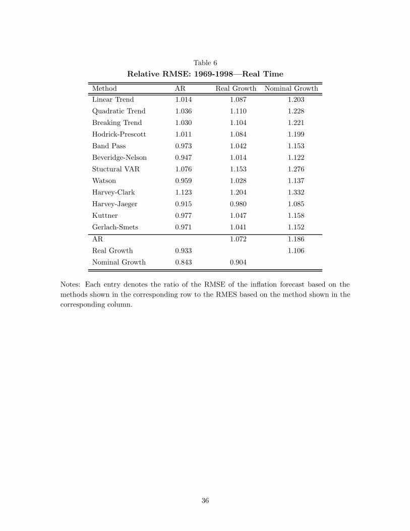
Table 6
Relative RMSE: 1969-1998—Real Time
Method AR Real Growth Nominal GrowthLinear Trend 1.014 1.087 1.203
Quadratic Trend 1.036 1.110 1.228
Breaking Trend 1.030 1.104 1.221
Hodrick-Prescott 1.011 1.084 1.199
Band Pass 0.973 1.042 1.153
Beveridge-Nelson 0.947 1.014 1.122
Stuctural VAR 1.076 1.153 1.276
Watson 0.959 1.028 1.137
Harvey-Clark 1.123 1.204 1.332
Harvey-Jaeger 0.915 0.980 1.085
Kuttner 0.977 1.047 1.158
Gerlach-Smets 0.971 1.041 1.152
AR 1.072 1.186
Real Growth 0.933 1.106
Nominal Growth 0.843 0.904
Notes: Each entry denotes the ratio of the RMSE of the inflation forecast based on themethods shown in the corresponding row to the RMES based on the method shown in thecorresponding column.
36

Table 7
RMSE Relative to AR for Alternative Horizon Forecasts
1969-1998 1969-1983 1984-1998Horizon (quarters) 3 5 7 9 3 5 7 9 3 5 7 9
Linear Trend 1.006 1.014 0.924 0.921 0.974 0.983 0.862 0.871 1.088 1.116 1.224 1.142
Quadratic Trend 0.988 1.035 0.957 0.943 0.948 1.003 0.900 0.915 1.086 1.143 1.241 1.077
Breaking Trend 1.019 1.030 1.004 0.978 0.976 1.023 0.962 0.959 1.127 1.053 1.219 1.069
Hodrick-Prescott 0.965 1.011 0.964 0.903 0.875 0.913 0.905 0.888 1.173 1.297 1.259 0.978
Band Pass 0.942 0.972 0.935 1.002 0.914 0.918 0.880 0.974 1.015 1.144 1.212 1.134
Beveridge-Nelson 0.960 0.946 0.985 0.967 0.949 0.934 0.962 0.961 0.989 0.988 1.105 0.996
Structural VAR 1.052 1.075 0.989 0.942 1.013 1.048 0.924∗ 0.899 1.151 1.167 1.311 1.135
Watson 1.000 0.959 0.891 0.908 0.972 0.963 0.879 0.896 1.071 0.943 0.962 0.970
Harvey-Clark 1.036 1.123 1.085 1.042 1.022 1.137 1.069 1.058 1.072 1.070 1.176 0.956
Harvey-Jaeger 0.939 0.914 0.876 0.935 0.814∗ 0.807∗ 0.807 0.920 1.210 1.220 1.204 1.008
Kuttner 0.970 0.976 0.902 0.871 0.953 0.978 0.875 0.868 1.016 0.970 1.044 0.887
Gerlach-Smets 0.953 0.971 0.920 0.900 0.941 0.979 0.910 0.915 0.983 0.942 0.978 0.822
Real Growth 0.954 0.933 0.941 0.992 0.913 0.901 0.899 0.985 1.054 1.036 1.160 1.027
Nominal Growth 0.916 0.843∗ 0.857∗ 0.899 0.873 0.785∗ 0.803 0.885 1.022 1.023 1.121 0.968
AR 0.014 0.023 0.032 0.040 0.017 0.029 0.041 0.050 0.010 0.015 0.018 0.023
Notes: The horizons, j ∈ {3, 5, 7, 9} indicate forecasts of the rate of inflation from quarter t − 1 to quarter t + j − 1. The last rowshows the RMSE of the AR based forecast errors for the evaluation period shown. Entries in all other rows show the ratio of theRMSE of the forecasts using the output gap in that row relative to that of the corresponding AR forecast, for the same evaluationperiod.
37

Table 8
Relative RMSE with Alternative Start of Estimation Period
1969-1998 1969-1983 1984-1998Est. Start 1947 Base 1960 1965 1947 Base 1960 1965 1947 Base 1960 1965
Linear Trend 1.126 1.014 1.105 2.705 1.046 0.983 1.103 2.962 1.579 1.116 1.113 1.121
Quadratic Trend 0.996 1.035 1.123 2.706 0.992 1.003 1.106 2.965 1.029 1.143 1.198 1.110
Breaking Trend 1.000 1.030 1.119 2.717 0.996 1.023 1.117 2.961 1.030 1.053 1.128 1.262
Hodrick-Prescott 1.059 1.011 1.302 10.617 1.026 0.913 1.304 11.804 1.270 1.297 1.292 1.424
Band Pass 1.016 0.972 1.088 6.908 0.993 0.918 1.074 7.667 1.160 1.144 1.149 1.302
Beveridge-Nelson 0.879 0.946 1.041 6.410 0.818 0.934 1.052 7.119 1.225 0.988 0.991 1.073
Structural VAR 0.999 1.075 1.033 13.493 0.918 1.048 1.003 15.015 1.447 1.167 1.159 1.175
Watson 0.993 0.959 1.115 2.798 0.989 0.963 1.136 3.065 1.018 0.943 1.013 1.148
Harvey-Clark 1.070 1.123 1.157 3.452 1.062 1.137 1.172 3.777 1.126 1.070 1.089 1.455
Harvey-Jaeger 1.025 0.914 1.102 1.363 0.977 0.807∗ 1.062 1.362 1.316 1.220 1.267 1.366
Kuttner 0.882 0.976 1.091 2.707 0.820 0.978 1.094 2.967 1.235 0.970 1.078 1.091
Gerlach-Smets 0.850 0.971 1.077 2.703 0.785∗ 0.979 1.090 2.961 1.212 0.942 1.018 1.105
Real Growth 0.940 0.933 1.033 6.312 0.932 0.901 1.036 7.008 0.992 1.036 1.017 1.107
Nominal Growth 0.971 0.843∗ 0.953 10.016 0.953 0.785∗ 0.925 11.144 1.091 1.023 1.072 1.022
AR 0.025 0.023 0.029 0.028 0.033 0.029 0.037 0.035 0.012 0.015 0.017 0.017
Notes: The table compares evaluation results when the start of the estimation models used for forecastig varies from the baseline,1955Q1, as shown. The last row shows the RMSE of the AR based forecast errors. Entries in all other rows show the ratio of theRMSE of the forecasts using the output gap in that row relative to that of the corresponding AR forecast.
38
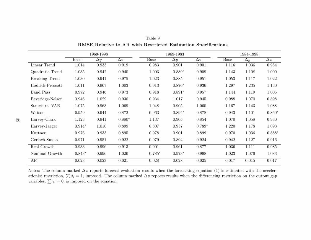
Table 9
RMSE Relative to AR with Restricted Estimation Specifications
1969-1998 1969-1983 1984-1998Base ∆y ∆π Base ∆y ∆π Base ∆y ∆π
Linear Trend 1.014 0.933 0.919 0.983 0.901 0.901 1.116 1.036 0.954
Quadratic Trend 1.035 0.942 0.940 1.003 0.889∗ 0.909 1.143 1.108 1.000
Breaking Trend 1.030 0.941 0.975 1.023 0.885 0.951 1.053 1.117 1.022
Hodrick-Prescott 1.011 0.967 1.003 0.913 0.876∗ 0.936 1.297 1.235 1.130
Band Pass 0.972 0.946 0.973 0.918 0.891∗ 0.957 1.144 1.119 1.005
Beveridge-Nelson 0.946 1.029 0.930 0.934 1.017 0.945 0.988 1.070 0.898
Structural VAR 1.075 0.963 1.069 1.048 0.905 1.060 1.167 1.143 1.088
Watson 0.959 0.944 0.872 0.963 0.894∗ 0.878 0.943 1.101 0.860∗
Harvey-Clark 1.123 0.941 0.880∗ 1.137 0.905 0.854 1.070 1.058 0.930
Harvey-Jaeger 0.914∗ 1.010 0.899 0.807 0.957 0.789∗ 1.220 1.178 1.093
Kuttner 0.976 0.933 0.895 0.978 0.901 0.899 0.970 1.036 0.888∗
Gerlach-Smets 0.971 0.951 0.922 0.979 0.894 0.924 0.942 1.127 0.916
Real Growth 0.933 0.996 0.913 0.901 0.961 0.877 1.036 1.111 0.985
Nominal Growth 0.843∗ 0.996 1.026 0.785∗ 0.973∗ 0.998 1.023 1.076 1.083
AR 0.023 0.023 0.021 0.028 0.028 0.025 0.017 0.015 0.017
Notes: The column marked ∆π reports forecast evaluation results when the forecasting equation (1) is estimated with the acceler-ationist restriction,
∑βi = 1, imposed. The column marked ∆y reports results when the differencing restriction on the output gap
variables,∑
γi = 0, is imposed on the equation.
39

Table 10
In-Sample Use of Final Versus Real-Time Output Gaps
1965-1998 1965-1983 1984-1998Final Real-Time Final Real-Time Final Real-Time
Linear Trend 0.826 0.791∗ 0.779 0.732∗ 0.982 1.015
Quadratic Trend 0.870∗ 0.865 0.850∗ 0.790∗ 0.942 1.139
Breaking Trend 0.917∗ 0.846 0.909∗ 0.786∗ 0.946 1.085
Hodrick-Prescott 0.883 0.841 0.837∗ 0.713∗ 1.038 1.220
Band Pass 0.899 0.856 0.861∗ 0.755∗ 1.029 1.159
Beveridge-Nelson 0.873 0.840 0.808∗ 0.728∗ 1.081 1.184
Structural VAR 0.911 0.950 0.853∗ 0.884∗ 1.100 1.165
Watson 0.892∗ 0.827 0.870∗ 0.794∗ 0.972 0.958
Harvey-Clark 0.934∗ 0.894 0.924∗ 0.827∗ 0.969 1.122
Harvey-Jaeger 0.937 0.897 0.873 0.762∗ 1.147 1.281
Kuttner 0.778∗ 0.782∗ 0.728∗ 0.727∗ 0.941 0.995
Gerlach-Smets 0.795∗ 0.921 0.717∗ 0.872∗ 1.036 1.090
Real Growth 0.903∗ 0.765 0.877∗ 0.652∗ 0.996 1.100
Nominal Growth 0.836∗ 0.752 0.783∗ 0.622∗ 1.008 1.117
AR 0.019 0.019 0.024 0.024 0.012 0.012
Notes: The entries show the RMSE of the inflation forecast for the AR model, and theRMSE relative to that of the AR for all other models. See also notes to Table 2.
40

Table 11Out-of-Sample Use of Final Versus Real-Time Output Gaps
1965-1998 1965-1983 1984-1998Final Real-Time Final Real-Time Final Real-Time
Quadratic Trend 0.965 1.035 0.946 1.003 1.027 1.143
Breaking Trend 1.052 1.030 1.041 1.023 1.090 1.053
Hodrick-Prescott 1.045 1.011 0.980 0.913 1.247 1.297
Band Pass 1.052 0.972 1.011 0.918 1.183 1.144
Beveridge-Nelson 1.019 0.946 0.983 0.934 1.136 0.988
Structural VAR 1.005 1.075 0.909 1.048 1.287 1.167
Watson 1.035 0.959 1.039 0.963 1.021 0.943
Harvey-Clark 1.102 1.123 1.096 1.137 1.123 1.070
Harvey-Jaeger 1.028 0.914 0.941 0.807∗ 1.286 1.220
Kuttner 0.935 0.976 0.933 0.978 0.941 0.970
Gerlach-Smets 0.906 0.971 0.876 0.979 1.007 0.942
Real Growth 0.946 0.933 0.925 0.901 1.020 1.036
Nominal Growth 0.900 0.843∗ 0.858 0.785∗ 1.038 1.023
AR 0.023 0.023 0.028 0.028 0.015 0.015
Notes: The entries show the RMSE of the inflation forecast for the AR model, and theRMSE relative to that of the AR for all other models. See also notes to Table 2.
41

Table 12RMSE Relative to AR with Alternative Lag Selection Criteria
1969-1998 1969-1983 1984-1998Base AIC BIC Base AIC BIC Base AIC BIC
Linear Trend 1.014 0.989 1.005 0.983 0.954 0.990 1.116 1.114 1.080
Quadratic Trend 1.035 0.981 0.993 1.003 0.932 0.965 1.143 1.147 1.121
Breaking Trend 1.030 1.006 0.929 1.023 0.968 0.897 1.053 1.140 1.071
Hodrick-Prescott 1.011 1.052 0.936 0.913 0.984 0.811∗ 1.297 1.276 1.404
Band Pass 0.972 1.016 0.875∗ 0.918 0.987 0.863∗ 1.144 1.120 0.936
Beveridge-Nelson 0.946 0.971 0.913 0.934 0.947 0.885 0.988 1.057 1.043
Structural VAR 1.075 1.104 1.120 1.048 1.108 1.13 1.167 1.088 1.072
Watson 0.959 0.991 0.956 0.963 1.001 0.971 0.943 0.950 0.881
Harvey-Clark 1.123 1.070 0.984 1.137 1.067 0.975 1.070 1.082 1.028
Harvey-Jaeger 0.914 0.901 0.926 0.807∗ 0.800∗ 0.786∗ 1.220 1.212 1.436
Kuttner 0.976 0.933 0.949 0.978 0.934 0.953 0.970 0.932 0.930
Gerlach-Smets 0.971 0.923 0.927 0.979 0.924 0.938 0.942 0.920 0.873
Real Growth 0.933 0.965 0.898 0.901 0.936 0.865∗ 1.036 1.069 1.050
Nominal Growth 0.843∗ 0.836∗ 0.882 0.785 0.785∗ 0.812∗ 1.023 1.009 1.171
AR 0.023 0.023 0.022 0.028 0.029 0.029 0.015 0.015 0.013
Notes: Base (Ng-Perron), AIC and BIC denote the alternative criteria for lag selection in the forecasting models. The last row showsthe RMSE of the AR based forecast errors. Entries in all other rows show the ratio of the RMSE of the forecasts using the outputgap concept in that row relative to that of the corresponding AR forecast.
42

Table 13RMSE Relative to AR with Alternative Use of Data Vintages
Conventional KDP Conventional KDPAIC AIC BIC BIC
Linear Trend 1.114 1.643 0.981 1.646
Quadratic Trend 1.147 1.637 1.154 1.314
Breaking Trend 1.140 1.296 1.255 1.206
Hodrick-Prescott 1.276 1.456 1.239 1.427
Band Pass 1.120 1.107 0.989 0.962
Beveridge-Nelson 1.057 1.030 1.063 1.094
Structural VAR 1.088 1.163 1.118 1.183
Watson 0.950 1.571 1.193 1.299
Harvey-Clark 1.082 1.543 1.511 1.517
Harvey-Jaeger 1.212 1.638 1.544 1.509
Kuttner 0.932 1.762 1.016 1.482
Gerlach-Smets 0.920 1.257 1.101 1.250
Real Growth 1.069 0.966 1.044 0.996
Nominal Growth 1.009 1.056 0.953 1.046
AR 0.019 0.017 0.016 0.016
Notes: KDP indicates the Koenig-Dolmas-Piger usage of data vintages for model estimation.The forecast evaluation period is 1984—1998. AIC and BIC denote the lag selection criteria.The last row shows the RMSE of the AR based forecast errors. Entries in all other rowsshow the RMSE using the output gap concept in that row relative to the AR RMSE.
43
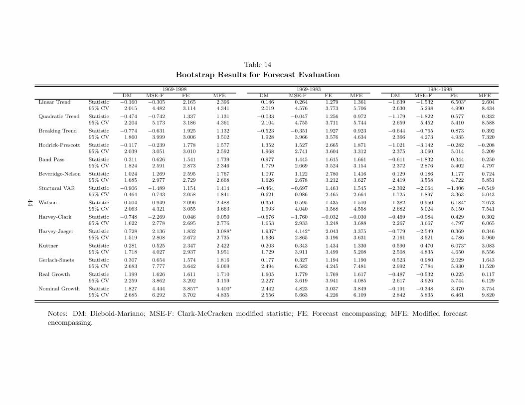
Table 14Bootstrap Results for Forecast Evaluation
1969-1998 1969-1983 1984-1998DM MSE-F FE MFE DM MSE-F FE MFE DM MSE-F FE MFE
Linear Trend Statistic −0.160 −0.305 2.165 2.396 0.146 0.264 1.279 1.361 −1.639 −1.532 6.503∗ 2.60495% CV 2.015 4.482 3.114 4.341 2.019 4.576 3.773 5.706 2.630 5.298 4.990 8.434
Quadratic Trend Statistic −0.474 −0.742 1.337 1.131 −0.033 −0.047 1.256 0.972 −1.179 −1.822 0.577 0.33295% CV 2.204 5.173 3.186 4.361 2.104 4.755 3.711 5.744 2.659 5.452 5.410 8.588
Breaking Trend Statistic −0.774 −0.631 1.925 1.132 −0.523 −0.351 1.927 0.923 −0.644 −0.765 0.873 0.39295% CV 1.860 3.999 3.006 3.502 1.928 3.966 3.576 4.634 2.366 4.273 4.935 7.320
Hodrick-Prescott Statistic −0.117 −0.239 1.778 1.577 1.352 1.527 2.665 1.871 −1.021 −3.142 −0.282 −0.20895% CV 2.039 3.051 3.010 2.592 1.968 2.741 3.604 3.312 2.375 3.060 5.014 5.209
Band Pass Statistic 0.311 0.626 1.541 1.739 0.977 1.445 1.615 1.661 −0.611 −1.832 0.344 0.25095% CV 1.824 2.591 2.873 2.346 1.779 2.669 3.524 3.154 2.372 2.876 5.402 4.797
Beveridge-Nelson Statistic 1.024 1.269 2.595 1.767 1.097 1.122 2.780 1.416 0.129 0.186 1.177 0.72495% CV 1.685 2.977 2.729 2.668 1.626 2.678 3.212 3.627 2.419 3.558 4.722 5.851
Stuctural VAR Statistic −0.906 −1.489 1.154 1.414 −0.464 −0.697 1.463 1.545 −2.302 −2.064 −1.406 −0.54995% CV 0.464 0.743 2.058 1.841 0.621 0.986 2.465 2.664 1.725 1.897 3.363 5.043
Watson Statistic 0.504 0.949 2.096 2.488 0.351 0.595 1.435 1.510 1.382 0.950 6.184∗ 2.67395% CV 2.063 4.321 3.055 3.663 1.993 4.040 3.588 4.558 2.682 5.024 5.150 7.541
Harvey-Clark Statistic −0.748 −2.269 0.046 0.050 −0.676 −1.760 −0.032 −0.030 −0.469 −0.984 0.429 0.30295% CV 1.622 2.778 2.695 2.776 1.653 2.933 3.248 3.688 2.267 3.667 4.797 6.065
Harvey-Jaeger Statistic 0.728 2.136 1.832 3.088∗ 1.937∗ 4.142∗ 2.043 3.375 −0.779 −2.549 0.369 0.34695% CV 1.519 2.808 2.672 2.735 1.636 2.865 3.196 3.631 2.161 3.521 4.786 5.960
Kuttner Statistic 0.281 0.525 2.347 2.422 0.203 0.343 1.434 1.330 0.590 0.470 6.073∗ 3.08395% CV 1.718 4.027 2.937 3.951 1.729 3.911 3.499 5.208 2.508 4.835 4.650 8.556
Gerlach-Smets Statistic 0.307 0.654 1.574 1.816 0.177 0.327 1.194 1.190 0.523 0.980 2.029 1.64395% CV 2.683 7.777 3.642 6.069 2.494 6.582 4.245 7.481 2.992 7.784 5.930 11.520
Real Growth Statistic 1.199 1.626 1.611 1.710 1.605 1.779 1.769 1.617 −0.487 −0.532 0.225 0.11795% CV 2.259 3.862 3.292 3.159 2.227 3.619 3.941 4.085 2.617 3.926 5.744 6.129
Nominal Growth Statistic 1.827 4.444 3.857∗ 5.400∗ 2.442 4.823 3.037 3.849 −0.191 −0.348 3.470 3.75495% CV 2.685 6.292 3.702 4.835 2.556 5.663 4.226 6.109 2.842 5.835 6.461 9.820
Notes: DM: Diebold-Mariano; MSE-F: Clark-McCracken modified statistic; FE: Forecast encompassing; MFE: Modified forecastencompassing.
44

Figure 1Real-Time and Final Hodrick-Prescott Output Gap
One Quarter
69 73 77 81 85 89 93 97
-0.08
-0.06
-0.04
-0.02
0.00
0.02
0.04Real Time
Final
Four-Quarter Moving Average
69 73 77 81 85 89 93 97
-0.04
-0.03
-0.02
-0.01
0.00
0.01
0.02
0.03
0.04Real Time
Final
45

Figure 2Historical Vintages and Final Hodrick-Prescott Output Gap
1969Q1 Vintage
64 65 66 67 68
-0.015
-0.010
-0.005
0.000
0.005
0.010
0.015
0.020
0.025
0.0301969:1 Vintage
Final Vintage
1996Q1 Vintage
91 92 93 94 95
-0.020
-0.015
-0.010
-0.005
0.000
0.005
0.010
0.0151996:1 Vintage
Final Vintage
46

Figure 3Univariate Inflation Forecasts
Forecasts and Realized Inflation
69 73 77 81 85 89 93 97
0.00
0.02
0.04
0.06
0.08
0.10
0.12
0.14Actual
Real Time
In Sample
Forecast Errors
69 73 77 81 85 89 93 97
-0.050
-0.025
0.000
0.025
0.050Real Time
In Sample
47

Figure 4Inflation Forecasts and Errors with the Hodrick-Prescott Output Gap
Forecasts and Realized Inflation
69 73 77 81 85 89 93 97
0.00
0.02
0.04
0.06
0.08
0.10
0.12
0.14Actual
Real Time
In Sample
Forecasts Errors
69 73 77 81 85 89 93 97
-0.06
-0.04
-0.02
0.00
0.02
0.04
0.06Real Time
In Sample
48

Figure 5Boostrap p-values
Entire Distribution Detail of Left Tail
49