Aerodynamic Shape Optimization with the Adjoint Method

Francisco Xavier Moreira Huhn

Thesis to obtain the Master of Science Degree in

Aerospace Engineering

Supervisor: Prof. Luís Rego da Cunha de Eça

Examination Committee

Chairperson: Prof. Fernando José Parracho LauSupervisor: Prof. Luís Rego da Cunha de Eça

Member of the Committee: Prof. José Firmino Aguilar Madeira

November 2015

ii

Acknowledgments

Firstly, I would like to thank my supervisor at Airbus, Joel Brezillon, without whom this work would not

have been possible.

I would like to thank Prof. Joao Pimentel Nunes, the best teacher I’ve ever had. I feel incredibly

fortunate to have been his student.

I would like to thank all my friends, who are too many to be listed here. I thank you for all your support

and memories, which I will cherish for the rest of my life.

Finally, I would like to thank Garazi Gomez de Segura for always supporting and being there for me.

iii

iv

Resumo

A maior parte dos custos de uma companhia aerea provem do consumo de combustıvel. Desta forma,

e do interesse das companhias aereas e portanto, dos fabricantes de aeronaves, que este seja mini-

mizado, por exemplo, atraves de reducao de arrasto, isto e, optimizacao aerodinamica.

Actualmente, este trabalho e feito por engenheiros com anos de experiencia, usando o seu extenso

conhecimento em aerodinamica de aeronaves. No entanto, este trabalho e feito manualmente e por

tentativa e erro, que se torna particularmente desafiante para geometrias complexas e aerodinamica

complexa.

A disciplina de optimizacao aerodinamica automatica responde a este problema. E uma disciplina

relativamente recente e promete bons resultados onde o conhecimento humano falha. Nomeadamente,

optimizacao aerodinamica de forma com o metodo adjunto oferece bastantes vantagens em relacao a

outras tecnicas. Esta tecnica, em conjuncao com outras sera estudada e aplicada a optimizacao de um

perfil aerodinamico transsonico e de um winglet de um aviao longo curso da Airbus.

Palavras-chave: optimizacao aerodinamica, metodo adjunto, forma de perfil aerodinamico,

winglet

v

vi

Abstract

The biggest cost for airlines is due to fuel consumption. Therefore, it is of the interest of airlines that fuel

consumption be minimized. This task is done by aircraft manufacturers, including Airbus, for example,

by reducing drag.

Currently, this work is done by experienced engineers with years of experience, making use of their

extensive knowledge in aircraft aerodynamics. Nevertheless, this work is done manually and by trial and

error, which becomes particularly challenging for complex shapes and complex aerodynamics.

The subject of automatic aerodynamic optimization responds to this problem. It is a recent subject

and promises good results where human insight fails. Namely, aerodynamic shape optimization with the

adjoint method offers many advantages with respect to other techniques. This technique, in conjunction

with others will be studied and applied to the optimization of a transonic airfoil and of a winglet for a long

range airplane of Airbus.

Keywords: aerodynamic optimization, adjoint method, airfoil shape, winglet

vii

viii

Contents

Acknowledgments . . . . . . . . . . . . . . . . . . . . . . . . . . . . . . . . . . . . . . . . . . . iii

Resumo . . . . . . . . . . . . . . . . . . . . . . . . . . . . . . . . . . . . . . . . . . . . . . . . . v

Abstract . . . . . . . . . . . . . . . . . . . . . . . . . . . . . . . . . . . . . . . . . . . . . . . . . vii

List of Tables . . . . . . . . . . . . . . . . . . . . . . . . . . . . . . . . . . . . . . . . . . . . . . xiii

List of Figures . . . . . . . . . . . . . . . . . . . . . . . . . . . . . . . . . . . . . . . . . . . . . xv

Nomenclature . . . . . . . . . . . . . . . . . . . . . . . . . . . . . . . . . . . . . . . . . . . . . . xvii

Glossary . . . . . . . . . . . . . . . . . . . . . . . . . . . . . . . . . . . . . . . . . . . . . . . . xix

1 Introduction 1

1.1 Motivation . . . . . . . . . . . . . . . . . . . . . . . . . . . . . . . . . . . . . . . . . . . . . 1

1.2 Topic Overview . . . . . . . . . . . . . . . . . . . . . . . . . . . . . . . . . . . . . . . . . . 1

1.3 Objectives . . . . . . . . . . . . . . . . . . . . . . . . . . . . . . . . . . . . . . . . . . . . . 2

1.4 Outline . . . . . . . . . . . . . . . . . . . . . . . . . . . . . . . . . . . . . . . . . . . . . . . 2

2 Aerodynamic Shape Optimization 3

2.1 Aerodynamics . . . . . . . . . . . . . . . . . . . . . . . . . . . . . . . . . . . . . . . . . . 3

2.1.1 Navier-Stokes Equations . . . . . . . . . . . . . . . . . . . . . . . . . . . . . . . . 3

2.1.2 Reynolds Averaged Navier-Stokes Equations (RANS) . . . . . . . . . . . . . . . . 4

2.1.3 Compressible Reynolds Averaged Navier-Stokes Equations . . . . . . . . . . . . . 5

2.1.4 Spalart-Allmaras Turbulence Model . . . . . . . . . . . . . . . . . . . . . . . . . . . 6

2.1.5 Aerodynamic Dimensionless Coefficients . . . . . . . . . . . . . . . . . . . . . . . 6

2.1.5.1 Pressure Coefficient . . . . . . . . . . . . . . . . . . . . . . . . . . . . . . 6

2.1.5.2 Friction Coefficient . . . . . . . . . . . . . . . . . . . . . . . . . . . . . . . 6

2.1.5.3 Drag Coefficient . . . . . . . . . . . . . . . . . . . . . . . . . . . . . . . . 6

2.1.5.4 Lift Coefficient . . . . . . . . . . . . . . . . . . . . . . . . . . . . . . . . . 8

2.1.5.5 Pitching Moment Coefficient . . . . . . . . . . . . . . . . . . . . . . . . . 8

2.2 Shape . . . . . . . . . . . . . . . . . . . . . . . . . . . . . . . . . . . . . . . . . . . . . . . 9

2.3 Optimization . . . . . . . . . . . . . . . . . . . . . . . . . . . . . . . . . . . . . . . . . . . 9

2.3.1 Problem Definition . . . . . . . . . . . . . . . . . . . . . . . . . . . . . . . . . . . . 9

2.3.2 Gradient-based optimization . . . . . . . . . . . . . . . . . . . . . . . . . . . . . . 10

2.3.2.1 Gradient computation by finite differences . . . . . . . . . . . . . . . . . . 10

ix

2.3.2.2 Gradient computation by the adjoint method . . . . . . . . . . . . . . . . 11

2.3.2.3 Karush–Kuhn–Tucker (KKT) conditions . . . . . . . . . . . . . . . . . . . 12

2.3.2.4 Sequential Least Squares Programming (SLSQP) . . . . . . . . . . . . . 12

2.3.3 Design of Experiments (DOE) . . . . . . . . . . . . . . . . . . . . . . . . . . . . . . 13

3 Analysis and Optimization Tools 15

3.1 Computational Fluid Dynamics . . . . . . . . . . . . . . . . . . . . . . . . . . . . . . . . . 15

3.1.1 Mesh . . . . . . . . . . . . . . . . . . . . . . . . . . . . . . . . . . . . . . . . . . . 15

3.1.2 Solver . . . . . . . . . . . . . . . . . . . . . . . . . . . . . . . . . . . . . . . . . . . 15

3.2 WORMS Optimization Chain . . . . . . . . . . . . . . . . . . . . . . . . . . . . . . . . . . 16

3.2.1 Padge . . . . . . . . . . . . . . . . . . . . . . . . . . . . . . . . . . . . . . . . . . . 16

3.2.1.1 Shape Matching . . . . . . . . . . . . . . . . . . . . . . . . . . . . . . . . 16

3.2.1.2 CAD to Mesh Link . . . . . . . . . . . . . . . . . . . . . . . . . . . . . . . 17

3.2.2 VolDef . . . . . . . . . . . . . . . . . . . . . . . . . . . . . . . . . . . . . . . . . . . 17

3.2.3 elsA . . . . . . . . . . . . . . . . . . . . . . . . . . . . . . . . . . . . . . . . . . . . 17

3.2.3.1 Target Lift . . . . . . . . . . . . . . . . . . . . . . . . . . . . . . . . . . . . 17

3.2.4 ZAPP/ZAPP-rev . . . . . . . . . . . . . . . . . . . . . . . . . . . . . . . . . . . . . 18

3.2.5 elsA-reverse . . . . . . . . . . . . . . . . . . . . . . . . . . . . . . . . . . . . . . . 18

3.2.6 VolDef-reverse . . . . . . . . . . . . . . . . . . . . . . . . . . . . . . . . . . . . . . 18

3.2.7 Padge-reverse . . . . . . . . . . . . . . . . . . . . . . . . . . . . . . . . . . . . . . 19

3.2.8 Optimizer . . . . . . . . . . . . . . . . . . . . . . . . . . . . . . . . . . . . . . . . . 19

3.3 Post-processing . . . . . . . . . . . . . . . . . . . . . . . . . . . . . . . . . . . . . . . . . 19

3.3.1 KKT Optimization Analysis . . . . . . . . . . . . . . . . . . . . . . . . . . . . . . . 19

3.3.2 Flow visualization . . . . . . . . . . . . . . . . . . . . . . . . . . . . . . . . . . . . 19

3.3.3 FFD Aerodynamic Analysis . . . . . . . . . . . . . . . . . . . . . . . . . . . . . . . 19

4 RAE2822 Airfoil Optimization 21

4.1 Test Case Definition . . . . . . . . . . . . . . . . . . . . . . . . . . . . . . . . . . . . . . . 21

4.1.1 Mesh . . . . . . . . . . . . . . . . . . . . . . . . . . . . . . . . . . . . . . . . . . . 21

4.1.2 Baseline Design . . . . . . . . . . . . . . . . . . . . . . . . . . . . . . . . . . . . . 22

4.2 Problem Description . . . . . . . . . . . . . . . . . . . . . . . . . . . . . . . . . . . . . . . 23

4.2.1 CT-Parameterization . . . . . . . . . . . . . . . . . . . . . . . . . . . . . . . . . . . 23

4.2.2 Design Space . . . . . . . . . . . . . . . . . . . . . . . . . . . . . . . . . . . . . . . 25

4.2.2.1 Normalization . . . . . . . . . . . . . . . . . . . . . . . . . . . . . . . . . 25

4.2.3 Optimization Problem . . . . . . . . . . . . . . . . . . . . . . . . . . . . . . . . . . 27

4.3 Unconstrained Optimization . . . . . . . . . . . . . . . . . . . . . . . . . . . . . . . . . . . 28

4.3.1 Optimization Analysis . . . . . . . . . . . . . . . . . . . . . . . . . . . . . . . . . . 28

4.3.2 Aerodynamic and Geometry Analysis . . . . . . . . . . . . . . . . . . . . . . . . . 29

4.3.3 Global Behavior . . . . . . . . . . . . . . . . . . . . . . . . . . . . . . . . . . . . . 31

4.4 Constrained Optimization . . . . . . . . . . . . . . . . . . . . . . . . . . . . . . . . . . . . 31

x

4.4.1 Constrained Optimization Problem . . . . . . . . . . . . . . . . . . . . . . . . . . . 31

4.4.2 Influence of ∆Clp and Optimization Analysis . . . . . . . . . . . . . . . . . . . . . 32

4.4.3 Aerodynamic and Geometry Analysis . . . . . . . . . . . . . . . . . . . . . . . . . 33

4.5 Changing Adaptation Clp . . . . . . . . . . . . . . . . . . . . . . . . . . . . . . . . . . . . 35

4.5.1 Optimization Problem . . . . . . . . . . . . . . . . . . . . . . . . . . . . . . . . . . 35

4.5.2 Optimization Analysis . . . . . . . . . . . . . . . . . . . . . . . . . . . . . . . . . . 36

4.5.3 Aerodynamic and Geometry Analysis . . . . . . . . . . . . . . . . . . . . . . . . . 36

4.6 Conclusion . . . . . . . . . . . . . . . . . . . . . . . . . . . . . . . . . . . . . . . . . . . . 39

5 Winglet Optimization 41

5.1 Test Case Definition . . . . . . . . . . . . . . . . . . . . . . . . . . . . . . . . . . . . . . . 41

5.1.1 Mesh . . . . . . . . . . . . . . . . . . . . . . . . . . . . . . . . . . . . . . . . . . . 41

5.1.2 Parameterization . . . . . . . . . . . . . . . . . . . . . . . . . . . . . . . . . . . . . 41

5.1.3 Optimization Problem . . . . . . . . . . . . . . . . . . . . . . . . . . . . . . . . . . 43

5.2 Design of Experiments . . . . . . . . . . . . . . . . . . . . . . . . . . . . . . . . . . . . . . 43

5.2.1 Identification of problematic combinations of design variables values . . . . . . . . 44

5.2.2 Relation between the objective function and constraint . . . . . . . . . . . . . . . . 44

5.2.3 Design variable influence analysis . . . . . . . . . . . . . . . . . . . . . . . . . . . 44

5.2.3.1 Checker . . . . . . . . . . . . . . . . . . . . . . . . . . . . . . . . . . . . 46

5.2.3.2 Ranker . . . . . . . . . . . . . . . . . . . . . . . . . . . . . . . . . . . . . 47

5.2.3.3 Selector . . . . . . . . . . . . . . . . . . . . . . . . . . . . . . . . . . . . . 48

5.2.3.4 Sub-design space Error . . . . . . . . . . . . . . . . . . . . . . . . . . . . 48

5.3 Baseline Solution . . . . . . . . . . . . . . . . . . . . . . . . . . . . . . . . . . . . . . . . . 50

5.4 Adjoint Optimization . . . . . . . . . . . . . . . . . . . . . . . . . . . . . . . . . . . . . . . 51

5.4.1 Starting from Baseline . . . . . . . . . . . . . . . . . . . . . . . . . . . . . . . . . . 51

5.4.1.1 Optimization Analysis . . . . . . . . . . . . . . . . . . . . . . . . . . . . . 51

5.4.1.2 Aerodynamic Analysis . . . . . . . . . . . . . . . . . . . . . . . . . . . . . 51

5.4.2 Starting from DOE Designs . . . . . . . . . . . . . . . . . . . . . . . . . . . . . . . 52

5.4.2.1 Optimization Analysis . . . . . . . . . . . . . . . . . . . . . . . . . . . . . 53

5.4.2.2 Aerodynamic Analysis . . . . . . . . . . . . . . . . . . . . . . . . . . . . . 53

5.5 Optimized Database . . . . . . . . . . . . . . . . . . . . . . . . . . . . . . . . . . . . . . . 53

5.5.1 Planform DOE . . . . . . . . . . . . . . . . . . . . . . . . . . . . . . . . . . . . . . 55

5.5.2 Optimized Solutions . . . . . . . . . . . . . . . . . . . . . . . . . . . . . . . . . . . 55

5.6 Conclusion . . . . . . . . . . . . . . . . . . . . . . . . . . . . . . . . . . . . . . . . . . . . 56

6 Conclusion 59

6.1 Future Work . . . . . . . . . . . . . . . . . . . . . . . . . . . . . . . . . . . . . . . . . . . . 60

Bibliography 61

xi

xii

List of Tables

3.1 Common elsA settings . . . . . . . . . . . . . . . . . . . . . . . . . . . . . . . . . . . . . . 16

3.2 Padge input/output summary . . . . . . . . . . . . . . . . . . . . . . . . . . . . . . . . . . 16

3.3 VolDef input/output summary . . . . . . . . . . . . . . . . . . . . . . . . . . . . . . . . . . 17

3.4 elsA input/output summary . . . . . . . . . . . . . . . . . . . . . . . . . . . . . . . . . . . 17

3.5 ZAPP input/output summary . . . . . . . . . . . . . . . . . . . . . . . . . . . . . . . . . . . 18

3.6 elsA-reverse input/output summary . . . . . . . . . . . . . . . . . . . . . . . . . . . . . . . 18

3.7 VolDef-reverse input/output summary . . . . . . . . . . . . . . . . . . . . . . . . . . . . . 19

3.8 Padge-reverse input/output summary . . . . . . . . . . . . . . . . . . . . . . . . . . . . . . 19

4.1 RAE2822 mesh summary . . . . . . . . . . . . . . . . . . . . . . . . . . . . . . . . . . . . 21

4.2 Baseline RAE2822 - Clp = 0.630± 0.001 . . . . . . . . . . . . . . . . . . . . . . . . . . . . 22

4.3 Parameterization of RAE2822 . . . . . . . . . . . . . . . . . . . . . . . . . . . . . . . . . . 24

4.4 Camber design value ranges . . . . . . . . . . . . . . . . . . . . . . . . . . . . . . . . . . 25

4.5 Normalized camber variables . . . . . . . . . . . . . . . . . . . . . . . . . . . . . . . . . . 28

4.6 Computation time . . . . . . . . . . . . . . . . . . . . . . . . . . . . . . . . . . . . . . . . . 29

4.7 Optimized RAE2822 - Far-field drag decomposition - Clp = 0.630± 0.001 . . . . . . . . . . 29

4.8 Constrained Optimized RAE2822 - Far-field drag decomposition - Clp = 0.630± 0.001 . . 35

4.9 Optimized RAE2822 at Clp = {0.54, 0.60, 0.63} ± 0.001 . . . . . . . . . . . . . . . . . . . . 37

5.1 Flight Conditions . . . . . . . . . . . . . . . . . . . . . . . . . . . . . . . . . . . . . . . . . 41

5.2 Bounds of modification to baseline design . . . . . . . . . . . . . . . . . . . . . . . . . . . 42

5.3 Inputs not correlated with any of the outputs . . . . . . . . . . . . . . . . . . . . . . . . . . 47

5.4 SDA Ranker - Input Ranking . . . . . . . . . . . . . . . . . . . . . . . . . . . . . . . . . . 47

5.5 SDA Selector - Results (All-output error calculation) . . . . . . . . . . . . . . . . . . . . . 49

5.6 SDA Selector - Results (CDp error calculation) . . . . . . . . . . . . . . . . . . . . . . . . 49

5.7 Baseline Winglet at CLp = 0.55 . . . . . . . . . . . . . . . . . . . . . . . . . . . . . . . . . 50

5.8 Optimized Winglet (starting from baseline) at CLp = 0.550± 0.001 - Variation with respect

to the baseline . . . . . . . . . . . . . . . . . . . . . . . . . . . . . . . . . . . . . . . . . . 52

5.9 Optimum design variables . . . . . . . . . . . . . . . . . . . . . . . . . . . . . . . . . . . . 53

5.10 Optimized Winglets at CLp = 0.550± 0.001 - Variation with respect to the baseline . . . . 54

xiii

xiv

List of Figures

2.1 Gradient computation error vs Gradient step size ∆D . . . . . . . . . . . . . . . . . . . . 11

2.2 Square grid examples . . . . . . . . . . . . . . . . . . . . . . . . . . . . . . . . . . . . . . 13

3.1 WORMS reverse-mode optimization workflow . . . . . . . . . . . . . . . . . . . . . . . . . 20

4.1 Mesh views . . . . . . . . . . . . . . . . . . . . . . . . . . . . . . . . . . . . . . . . . . . . 22

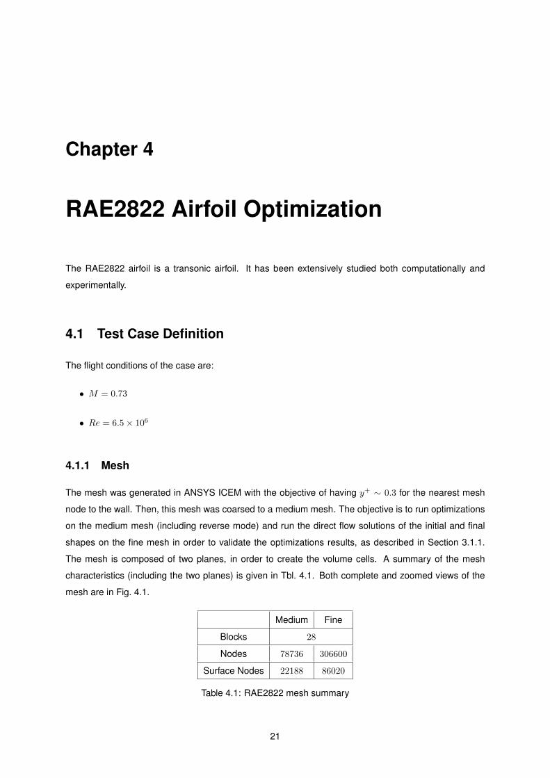
4.2 Baseline RAE2822 - ClpCd vs Clp - Fine mesh . . . . . . . . . . . . . . . . . . . . . . . . . . 23

4.3 Convergence of flow solution for Clp = 0.630± 0.001 - Fine mesh . . . . . . . . . . . . . . 23

4.4 Baseline RAE2822 - Mach field - Fine mesh . . . . . . . . . . . . . . . . . . . . . . . . . . 24

4.5 Airfoil CT-Parameterization . . . . . . . . . . . . . . . . . . . . . . . . . . . . . . . . . . . 24

4.6 Normalization effect on gradient . . . . . . . . . . . . . . . . . . . . . . . . . . . . . . . . . 27

4.7 Unconstrained optimization history . . . . . . . . . . . . . . . . . . . . . . . . . . . . . . . 29

4.8 Unconstrained Optimized RAE2822 - Cp and Cf diagrams - Fine mesh . . . . . . . . . . . 30

4.9 Optimized RAE2822 - Mach number field - Fine mesh . . . . . . . . . . . . . . . . . . . . 30

4.10 Unconstrained Optimized RAE2822 - Geometry . . . . . . . . . . . . . . . . . . . . . . . . 31

4.11 Baseline and Unconstrained Optimized RAE2822 - ClpCd polar - Fine mesh . . . . . . . . . 32

4.12 Constrained optimization history . . . . . . . . . . . . . . . . . . . . . . . . . . . . . . . . 33

4.13 Baseline, unconstrained and constrained optimized RAE2822 - ClpCd polar - Fine mesh . . 34

4.14 Constrained Optimized RAE2822 - Cp and Cf diagrams . . . . . . . . . . . . . . . . . . . 34

4.15 Constrained Optimized RAE2822 - Geometry . . . . . . . . . . . . . . . . . . . . . . . . . 35

4.16 Changing adaptation - Optimization history . . . . . . . . . . . . . . . . . . . . . . . . . . 36

4.17 Optimized designs - ClpCd polar . . . . . . . . . . . . . . . . . . . . . . . . . . . . . . . . . . 37

4.18 Changing Adaptation Optimized RAE2822 - Cp diagram . . . . . . . . . . . . . . . . . . . 38

4.19 Changing Adaptation Optimized RAE2822 - Geometry . . . . . . . . . . . . . . . . . . . . 38

5.1 Body surface mesh - Coarse mesh . . . . . . . . . . . . . . . . . . . . . . . . . . . . . . . 42

5.2 Winglet parameterization . . . . . . . . . . . . . . . . . . . . . . . . . . . . . . . . . . . . 42

5.3 Failed designs in Span vs Sweep Angle . . . . . . . . . . . . . . . . . . . . . . . . . . . . . 45

5.4 CDp vs (CLp)winglet . . . . . . . . . . . . . . . . . . . . . . . . . . . . . . . . . . . . . . . . 45

5.5 SDA Checker - Results . . . . . . . . . . . . . . . . . . . . . . . . . . . . . . . . . . . . . . 46

5.6 SDA Ranker - Results . . . . . . . . . . . . . . . . . . . . . . . . . . . . . . . . . . . . . . 47

5.7 CDp vs Height for |Span| ≤ 0.05 . . . . . . . . . . . . . . . . . . . . . . . . . . . . . . . . . 48

xv

5.8 CDp vs first four variables by Ranker . . . . . . . . . . . . . . . . . . . . . . . . . . . . . . 49

5.9 Sub-design space model error . . . . . . . . . . . . . . . . . . . . . . . . . . . . . . . . . 50

5.10 Optimization History - Initial Design: Baseline . . . . . . . . . . . . . . . . . . . . . . . . . 51

5.11 Baseline, Optimized - Position in CDp vs (CLp)winglet . . . . . . . . . . . . . . . . . . . . . 52

5.12 Optimization History - Initial Design: Baseline, DOE1, DOE2, DOE3 . . . . . . . . . . . . 54

5.13 Cp distribution on winglet . . . . . . . . . . . . . . . . . . . . . . . . . . . . . . . . . . . . 55

5.14 Planform DOE - 50 samples . . . . . . . . . . . . . . . . . . . . . . . . . . . . . . . . . . . 56

5.15 Planform vs Planform+Twist+Camber - CDp, ∆CDp, Constraint . . . . . . . . . . . . . . . 57

xvi

Nomenclature

Greek symbols

α Angle of attack.

δij Kronecker’s delta.

γ Specific heat ratio.

λ Thermal conductivity coefficient.

µ Molecular viscosity coefficient.

ρ Density.

τ Shear stress.

Roman symbols

Cd, CD Coefficient of drag.

Cf Coefficient of friction.

Cl, CL Coefficient of lift.

Cm, CM Coefficient of pitching moment.

Cp Coefficient of pressure.

cp Enthalpy specific heat.

cv Pressure specific heat.

D Design variables vector.

E Total energy.

e Internal energy.

M Mach number.

p Pressure.

Pr Prandtl number.

xvii

Q Flowfield vector.

R Discretized Navier-Stokes equations.

~q Heat flux.

R Perfect gas constant.

Re Reynolds number.

S Trace-less viscous strain-rate.

T Temperature.

~u Velocity vector.

X Computational mesh.

Subscripts

∞ Free-stream condition.

~n Normal component.

ref Reference condition.

t Time variable.

x, y, z Cartesian components.

Superscripts

* Adjoint.

T Transpose.

xviii

Glossary

CFD Computational Fluid Dynamics is a branch of

fluid mechanics that uses numerical methods

and algorithms to solve problems that involve

fluid flows.

DOE Design of Experiments is a method for design

space exploration.

FFD Far-Field Drag is a drag decomposition analy-

sis obtained with a conservation law applied at

the far-field.

HPC High Performance Computing is a computer

with a high-level computational capacity com-

pared to a general-purpose computer.

KKT Karush-Kuhn-Tucker conditions are first order

necessary conditions for a solution in nonlinear

programming to be optimal.

SDA Sensibility and dependency analysis is a

technique for finding correlations between a

database of inputs and corresponding outputs.

SLSQP Sequential Least-Squares Quadratic Program-

ming is a gradient-based algorithm for solving

non-linearly constrained optimization problems.

WORMS WORkflow Management System is a flexible

automated optimization chain developed and

used by Airbus.

xix

xx

Chapter 1

Introduction

1.1 Motivation

In 2014, the airline industry was estimated to spend 212 billion (US) dollars in jet fuel, corresponding to

29.7% of the total operating costs [1]. In order to better respond to the highly competitive air transport

industry, airlines look for the best fuel efficient aircraft. Furthermore, as fuel consumption is reduced,

carbon emissions are also reduced, which is essential to comply with new environmental regulations.

Fuel consumption reduction can be achieved by drag reduction. As an example, a reduction of 1%

in total drag corresponds to about 900kg of fuel savings for a 11000km flight.

To reduce drag, aircraft components such as: lifting surfaces, pylon, nacelles, fuselage, etc. are

aerodynamically optimized. Currently, this work is done by experienced engineers who make use of

their extensive knowledge in aircraft aerodynamics. However, this optimization is done by trial and error,

a method that becomes challenging for complex shapes.

Because of its reduced need of human insight, a solution to this problematic is the use of a fully

automatic aerodynamic optimization chain.

1.2 Topic Overview

Automatic aerodynamic optimization means that the user doesn’t interact with the optimization process.

He is responsible for setting up the design space and optimization and CFD parameters, but the whole

optimization is carried out automatically.

The optimizer evaluates many designs, attempting to minimize a given objective function. The way

these designs are generated highly depends on the chosen algorithm(s) and even the same algorithm

may produce different results, depending on how aerodynamic and optimization information, such as lift,

drag or their gradients, are computed. Since these metrics are obtained with a CFD solver, which has a

high computational cost, the selection of the optimization optimization strategy is of crucial importance

to keep a low turnaround time.

A class of algorithms that are commonly used when dealing with many parameters are gradient-

1

based algorithms. These determine the successive designs based on the gradient of the objective

function with respect to the design variables. Yet, conventional methods of gradient computation such

as finite differences are usually computationally expensive, since they require many CFD evaluations.

Moreover, they present issues such as the value step size. The adjoint method presents itself as an an-

swer to this problem, having several advantages over such conventional gradient computation methods.

An optimization of a transonic airfoil and of a long range aircraft winglet with a gradient-based algo-

rithm, aided by the adjoint method for gradient computation will be studied.

1.3 Objectives

The objectives of this internship are to:

• Understand the adjoint optimization process

• Understand the procedure of industrial aerodynamic studies

• Optimize aerodynamic shapes in two and three dimensions

• Assess the performance of the adjoint optimization in aerodynamic optimization

• Verify if the adjoint optimization is well-suited for aerodynamic optimization

• Understand how the optimizer improves aerodynamic shapes

• Understand the aerodynamic influence of each parameter

1.4 Outline

This work is divided into four parts:

• Aerodynamic Shape Optimization Theory

• Analysis and Optimization Tools at Airbus

• Two-dimensional optimization: RAE2822 transonic airfoil

• Three-dimensional optimization: long range aircraft winglet redesign

In the first part, a detailed analysis on the theory of aerodynamic shape optimization is given. The

second part presents and explains each individual tool of the optimization toolchain. The third part

deals with a two-dimensional optimization problem, which also serves as a first example of a complete

optimization process. Finally, the fourth part is dedicated to a three-dimensional real case of the winglet

of a long range aircraft designed by Airbus.

2

Chapter 2

Aerodynamic Shape Optimization

This chapter serves as an introduction to the theory of aerodynamic shape optimization.

2.1 Aerodynamics

In this section, the aerodynamics equations and models are presented. It starts with the appropriate form

of the Navier-Stokes equations, from which the Reynolds Averaged Navier-Stokes (RANS) equations are

derived. The Spalart-Allmaras turbulence model, required in order to close the system of equations, is

then described. Finally, the aerodynamic coefficients utilized to assess the aerodynamic performance

are defined and explained.

2.1.1 Navier-Stokes Equations

The fundamental equations of aerodynamics are the Navier-Stokes equations. These correspond to

balance equations, which arise from applying Newton’s second law to fluid motion, together with the

assumption that the stress in the fluid is the sum of a diffusing viscous term (proportional to the gradient

of velocity) and a pressure term. The unsteady compressible Navier-Stokes equations written in con-

servative form are presented in Eq. (2.1), where ρ is the density, ~u is the velocity, δij is the Kroenocker’s

delta, p is the pressure, τij is the shear stress, ~q is the heat flux, E ≡ e+ ukuk2 is called the total energy

and the indices i, j range from 1 to the number of spatial dimensions.

∂ρ

∂t+

∂

∂xj(ρuj) = 0 (2.1a)

∂

∂t(ρui) +

∂

∂xj(ρuiuj + pδij − τji) = 0 (2.1b)

∂

∂t(ρE) +

∂

∂xj(ρujE + ujp+ qj − uiτij) = 0 (2.1c)

For a Newtonian fluid and assuming Stokes Law for mono-atomic gases, both valid for air, the viscous

stress is given by Eq. (2.2), where µ is the fluid’s molecular viscosity coefficient and S∗ij is the trace-less

3

viscous strain-rate defined in Eq. (2.3).

τij = 2µS∗ij (2.2)

S∗ij ≡1

2

(∂ui∂xj

+∂uj∂xi

)− 1

3

∂uk∂xk

δij (2.3)

The heat flux qj is given by Fourier’s law Eq. (2.4), with T the temperature, cp the enthalpy specific

heat. The definition of Prandtl number - Eq. (2.5) - is used, where λ is the thermal conductivity coefficient.

qj = −λ ∂T∂xj≡ −cp

µ

Pr

∂T

∂xj(2.4)

Pr ≡ cpµ

λ(2.5)

Finally, this system of equations must be closed by an equation of state. Assuming a calorically

perfect gas, the relations in Eq. (2.6) are valid. cv is the pressure specific heat, R is the perfect gas

constant

γ ≡ cpcv

p = ρRT e = cvT cp − cv = R (2.6)

Equations (2.1)-(2.6), supplemented with gas data for γ, Pr, µ,R form a closed set of partial differen-

tial equations and need only be complemented with boundary conditions.

2.1.2 Reynolds Averaged Navier-Stokes Equations (RANS)

We will transform Eq. (2.1b) into dimensionless form. We start by defining reference variable values:

Uref reference speed, Lref reference length, τref =LrefUref

reference time interval, ρref reference density

and µref reference kinematic viscosity, from which we derive the normalized relations (2.7).

t = τref t ⇒ ∂

∂t=LrefUref

∂

∂t

xi = Lrefxi ⇒∂

∂xi=

1

Lref

∂

∂xi

ui = Urefui

ρ = ρrefρ

µ = µrefµ

(2.7)

We introduce Eq. (2.7) into Eq. (2.1b) and we obtain Eq. (2.8), where Re is called the Reynolds

number defined in Eq. (2.9).

4

∂

∂t(ρui) +

∂

∂xj

ρuiuj +1

2

pρrefU2

ref

2

δij

=µref

ρrefUrefLref

∂

∂xj

{µ

[(∂ui∂xj

+∂uj∂xi

)− 2

3

∂uk∂xk

δij

]}

=1

Re

∂

∂xj

{µ

[(∂ui∂xj

+∂uj∂xi

)− 2

3

∂uk∂xk

δij

]} (2.8)

Re ≡ ρrefLrefUrefµref

(2.9)

ρref , Uref and µref are usually taken at infinity (unperturbed field) and Lref is often the airfoil/wing

(possibly mean aerodynamic) chord. The Reynolds number represents a ratio between inertial forces

and viscous forces. When this number is low, viscous forces dominate. Conversely, when this number

is high, inertial forces dominate. At low Reynolds number, the non-linear (convective) terms are small

compared to the viscous terms, yielding a laminar flow. However, in the aviation industry Re ∼ 106,

meaning the non-linearities become important with respect to the viscous forces, rendering the flow

chaotic. These phenomena take place at different time and length scales. If all scales are solved, the

technique is called Direct Numerical Simulation. If only the largest scales are solved and the smallest

are modeled, the technique is called Large Eddy Simulation. However, both of these techniques are

computationally expensive. Finally, if all scales are modeled, the Reynolds Averaged Navier-Stokes

equations are solved. These are derived by introducing the Reynolds decomposition (2.10) into the

Navier-Stokes equations (2.1).

φ(t, ~x)︸ ︷︷ ︸instantaneous

= φ(~x)︸︷︷︸average

+ φ′(t, ~x)︸ ︷︷ ︸fluctuation

, φ(~x) =1

t

∫ τ+t

τ

φ(ξ, ~x)dξ (2.10)

2.1.3 Compressible Reynolds Averaged Navier-Stokes Equations

The Reynolds decomposition is usually used for averaging the Navier-Stokes equations in incompress-

ible flow. For compressible flow, another decomposition called the Favre decomposition (2.11) is used.

φ(t)︸︷︷︸instantaneous

= φ︸︷︷︸average w.r.t. time

+ φ′′(t)︸ ︷︷ ︸fluctuation

, φ =ρφ

ρ(2.11)

Introducing Eq. (2.11) into the Navier-Stokes equations (2.1) and with certain hypothesis and mod-

eling, we obtain Eq. (2.12), where µt, k, Prt are calculated with a turbulence model and µ, γ, Pr are

obtained from gas data. These are a closed set of partial differential equations, which can be solved

numerically.

∂ρ

∂t+

∂

∂xj(ρuj) = 0 (2.12a)

∂

∂t(ρui) +

∂

∂xj

(ρuiuj + pδij − τ totji

)= 0 (2.12b)

5

∂

∂t

(ρE)

+∂

∂xj

(ρujE + ujp+ qtotj − uiτ totij

)= 0 (2.12c)

τ totij ≡ τ lamij + τ turbij

τ lamij ≡ τij = µ

(∂ui∂xj

+∂uj∂xi− 2

3

∂uk∂xk

δij

)

τ turbij ≡ −ρu′′i u′′j ≈ µt(∂ui∂xj

+∂uj∂xi− 2

3

∂uk∂xk

δij

)− 2

3ρkδij

qtotj = qlamj + qturbj

qlamj ≡ qj ≈ −cpµ

Pr

∂T

∂xj= − γ

γ − 1

µ

Pr

∂

∂xj

(p

ρ

)

qturbj ≡ cpρu′′j T ≈ −cpµtPrt

∂T

∂xj= − γ

γ − 1

µtPrt

∂

∂xj

(p

ρ

)

p = (γ − 1) ρ

(E − ukuk

2− k)

2.1.4 Spalart-Allmaras Turbulence Model

The Spalart-Allmaras turbulence model is a one-equation model, which solves a transport equation for

a viscosity variable ν, usually referred to as the Spalart-Allmaras variable, from which the turbulent eddy

viscosity µt used in Eq. (2.12) is calculated. The complete description of the model is given in [19] and

its compressible form in [20].

2.1.5 Aerodynamic Dimensionless Coefficients

2.1.5.1 Pressure Coefficient

The pressure coefficient (2.13) is the difference between local static pressure p and freestream static

pressure p∞, nondimensionalized by the freestream dynamic pressure 12ρ∞U

2∞.

Cp ≡p− p∞12ρ∞U

2∞

(2.13)

2.1.5.2 Friction Coefficient

The friction coefficient (2.14) is the local wall shear stress τw, nondimensionalized by the freestream

dynamic pressure.

Cf ≡τw

12ρ∞U

2∞

(2.14)

2.1.5.3 Drag Coefficient

Drag D is defined as the force parallel to the freestream velocity ~U∞, which nondimensionalized by the

freestream dynamic pressure times a reference surface area Sref yields the drag coefficient Eq. (2.15).

6

CD ≡D

12ρ∞U

2∞Sref

(2.15)

The importance of the CD can be justified by analyzing Breguet’s range formula (2.16) for a jet

aircraft. In Eq. (2.16), SFC is the specific fuel consumption, ρ is the air density, S is the reference surface

and Winitial and Wfinal are the mission’s initial and final weights, respectively. Therefore, if optimizing

for range, it is logical that the drag be used as/or in the objective function in an aerodynamic shape

optimization problem.

Range =2

SFC

√2

ρS

CLC2D

(√Winitial −

√Wfinal

)(2.16)

There are two methods for calculating drag: near-field approach and far-field approach.

Near-Field Drag

The near-field approach consists in integrating the surface forces acting on the body and taking the

component parallel to the freestream velocity of the resulting force. In Eq. (2.17), the integral repre-

sents the sum of all forces: pressure and friction. The dot product gives the component parallel to the

freestream velocity ~U∞, since the x axis is aligned with the freestream flow.

D =

{∫SB

[(p− p∞)~n+ ~τw] dS

}· ~ex

=

∫SB

(p− p∞)~n · ~exdS +

∫SB

~τw · ~exdS

=

∫SB

(p− p∞)nxdS +

∫SB

(~τw)x dS

= Dp +Df

(2.17)

Far-Field Drag

There exist multiple formulations for the far-field drag analysis. Nevertheless, all of them are based

on the law of conservation of momentum. We present a summary of the approach by Destarac and

van der Vooren [22], which corresponds to the one implemented in the tool utilized later.

The theory is based on the assumption that the production of viscous drag and wave drag is confined

to finite non-overlapping control volumes VV (boundary and viscous shear layers) and VW (shock layers)

and that outside these volumes the flow can be considered to be inviscid. Eq. (2.18) expresses the total

drag D as the sum of viscous drag Dv (= Dvp +Df ), wave drag Dw and induced drag Di.

D = Dp +Df︸ ︷︷ ︸near-field drag

= Dv +Dw +Di︸ ︷︷ ︸far-field drag

(2.18)

However, because spurious viscous or wave drag can be generated in Vsp ≡ V \ (VV + VW ) by the

numerical scheme used to solve the equations, outside the volumes VV and VW where viscous or wave

drag production is physically justified, the near-field/far-field balance becomes Eq. (2.19), where ~fvw is

7

given by Eq. (2.20a) and ~fi by Eq. (2.20b).

D = Dp +Df = Dv +Dw +Dsp +Di

=

∫VV

∇ · ~fvwdV︸ ︷︷ ︸Dv

+

∫VW

∇ · ~fvwdV︸ ︷︷ ︸Dw

+

∫Vsp

∇ · ~fvwdV︸ ︷︷ ︸Dsp

+

∫V

∇ · ~fidV +Df +Dp︸ ︷︷ ︸Di

(2.19)

~fvw = −ρ ∆u ~U + ~τx (2.20a)

~fi = −ρ(u− u∞ −∆u)~U − (p− p∞)~ex (2.20b)

∆u = u∞

√1 + 2

∆H

u2∞− 2

(γ − 1)M2∞

[(eδsR

) γ−1γ − 1

]− u∞ (2.20c)

2.1.5.4 Lift Coefficient

Lift L is defined as the force perpendicular to the freestream velocity ~U∞, which nondimensionalized by

the freestream dynamic pressure times a reference surface area Sref yields the lift coefficient Eq. (2.21).

CL ≡L

12ρ∞U

2∞Sref

(2.21)

Similarly to the drag coefficient, the lift coefficient can be calculated by integrating the surface forces

acting on the body and taking the component perpendicular to the freestream velocity of the resulting

force. However, in contrast with the drag, the viscous lift component is negligible.

L =

{∫SB

[(p− p∞)~n+ ~τw] dS

}· ~ez

=

∫SB

(p− p∞)~n · ~ezdS +

∫SB

~τw · ~ezdS

=

∫SB

(p− p∞)nzdS +

∫SB

τwzdS

= Lp + Lf

≈ Lp

(2.22)

2.1.5.5 Pitching Moment Coefficient

The component of the resulting moment with respect to some point, parallel to ~ey is called the pitching

moment M . In a similar way to the previous aerodynamic coefficients, the pitching moment coefficient is

defined in Eq. (2.23), where Lref is a reference length, usually the (possibly mean aerodynamic) chord.

The pitching moment is considered positive when it acts to pitch the airfoil/wing nose-up. It is usually of

8

importance, either because an increase must be compensated by the elevator/canard, which might be

penalizing in terms of aerodynamics; or because of structural aspects such as twisting moment.

Cm ≡M

12ρ∞U

2∞SrefLref

(2.23)

2.2 Shape

In aerodynamic shape optimization, only design variables which modify the shape of the body are con-

sidered. This means that variables such as Mach number, Reynolds number, etc. are fixed during

optimization.

The set of design variables D describes the surface of the body. The original mesh is then deformed

at the surface from the original shape to the new shape. This deformation is then propagated to the rest

of mesh volume. We define Xs as the set of mesh surface nodes, from which Xs = Xs(D). Furthermore,

we define X as the set of all mesh nodes, including surface nodes Xs ⊂ X.

2.3 Optimization

2.3.1 Problem Definition

Consider the vector of design variables D, computational mesh X, flowfield variables Q and a cost

function f = f(Q,X). Furthermore consider a set of equality constraints G = 0 and a set of inequality

constraints H ≤ 0. Then, the aerodynamic optimization problem is defined by Eq. (2.24).

minimizeD

f(Q,X)

subject to G(Q,X) ≤ 0

H(Q,X) = 0

(2.24)

Optimization algorithms for solving problems such as Eq. (2.24) are divided into gradient-based and

non gradient-based algorithms. Genetic algorithms are found in the latter. In such an algorithm, a pop-

ulation of candidate designs is evolved toward better solutions, through an iterative process, with the

population in each iteration called a generation. The algorithm terminates when either a maximum num-

ber of generations has been produced, or a satisfactory fitness (cost function) level has been reached

for the population. However, genetic algorithms do not scale well: as the number of elements subject

to mutation increases, the size of the corresponding design space increases exponentially. Thus, for

aerodynamic optimization, where the number of design variables ranges from tens to hundreds, these

methods are not well suited.

9

2.3.2 Gradient-based optimization

The fundamental information in all gradient-based algorithms is the sensitivity or gradient of the cost

function f with respect to the design variables D.

∇f =df

dD=

[∂f

∂Di

], i = 1, . . . , |D| (2.25)

Based on this gradient, the optimizer (optimization algorithm) decides where to go to in the design

space. As an example, a generic gradient-descending method computes the next design variables

values Dk+1 at iteration k in the following way, where γ is algorithm-dependent, possibly constant:

Dk+1 = Dk − γ df

dD

∣∣∣∣D=Dk

Moreover, in an unconstrained optimization, a necessary condition for a minima is the nullity of Eq. (2.25).

The more general KKT condition, used in constrained optimization problems such as Eq. (2.24) and

presented in Section 2.3.2.3, also makes use of this gradient. Therefore, precision and speed of com-

putation of this gradient are of paramount importance for the whole optimization process.

2.3.2.1 Gradient computation by finite differences

The gradient (2.25) can be computed by forward Eq. (2.26a) or backward Eq. (2.26b) finite differences,

which are first-order methods.

df

dD=f(D + ∆D)− f(D)

∆D+O(∆D) (2.26a)

df

dD=f(D)− f(D−∆D)

∆D+O(∆D) (2.26b)

Summing Eq. (2.26a) and Eq. (2.26b), we obtain the centered finite difference Eq. (2.27), which is a

second-order method.

df

dD=f(D + ∆D)− f(D−∆D)

2∆D+O(∆D2) (2.27)

Therefore, the computation of the gradient Eq. (2.25) requires |D|+1 flow solutions (CFD evaluation)

for the first-order methods - one f(D + ∆D) for each ∆D in the direction of each design variable plus

f(D). Similarly 2 |D| flow solutions are required for the second-order method.

In both cases, the cost of gradient computation is directly proportional to the number of design

variables |D|. For aerodynamic optimization, this number ranges from tens to hundreds, rendering

these methods prohibitively expensive. Furthermore, knowing which value of finite differences step ∆D

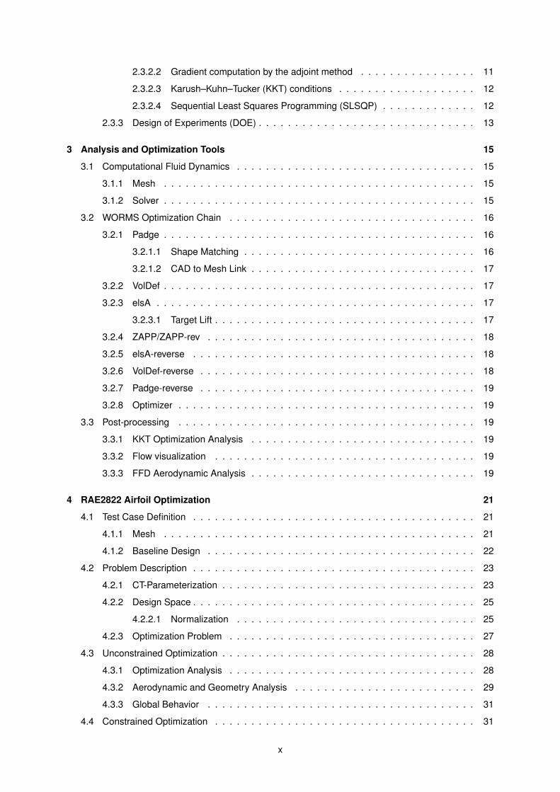
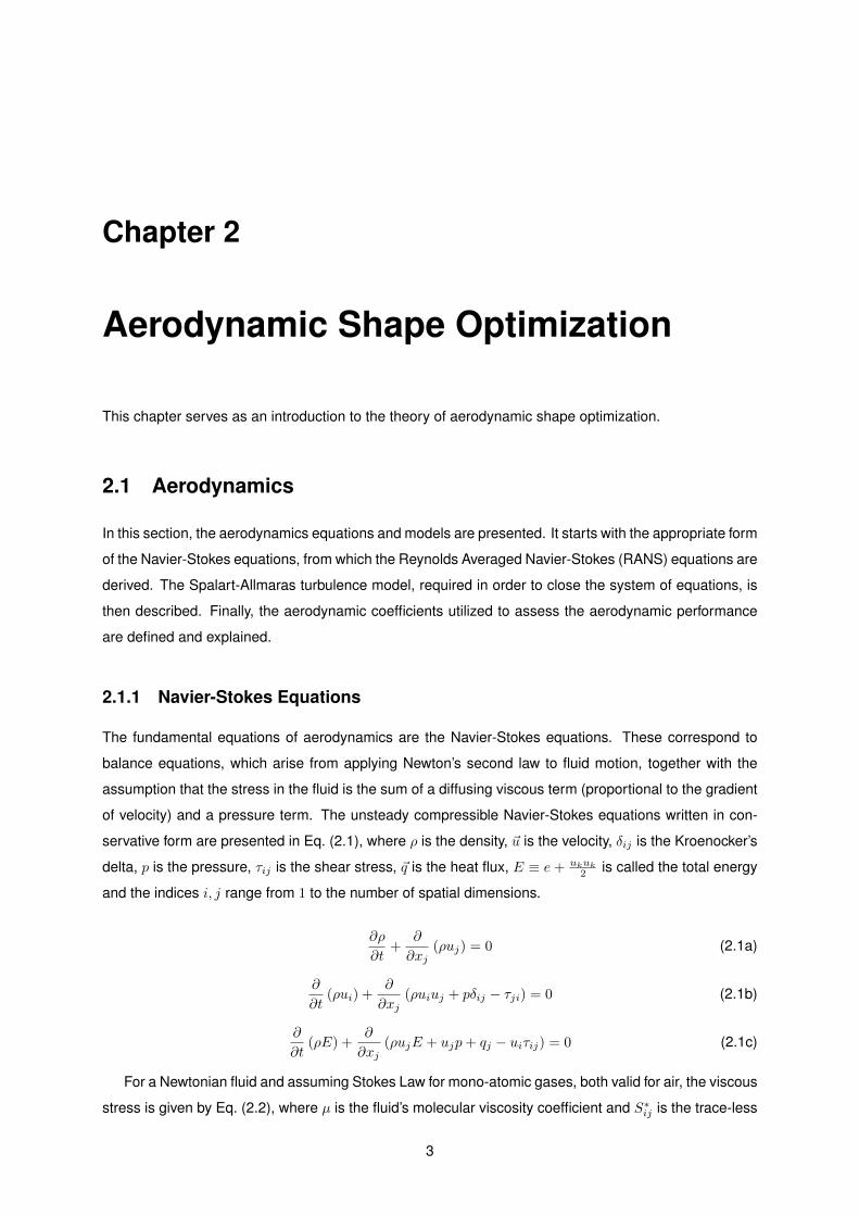
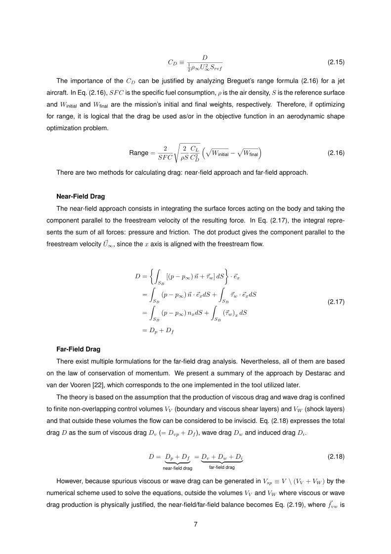
to use is not trivial. The error of gradient computation by finite differences as a function of the step ∆D

is shown in Fig. 2.1. For small ∆D, numerical errors are dominant due to the numeric subtraction in the

dividend. In fact, as ∆D grows smaller, the difference between f(D + ∆D) and f(D −∆D) becomes

smaller, canceling out the most significant and least erroneous digits and making the most erroneous

digits more important. Beyond a certain ∆D, as its value grows, the error O(∆D2) also grows.

10

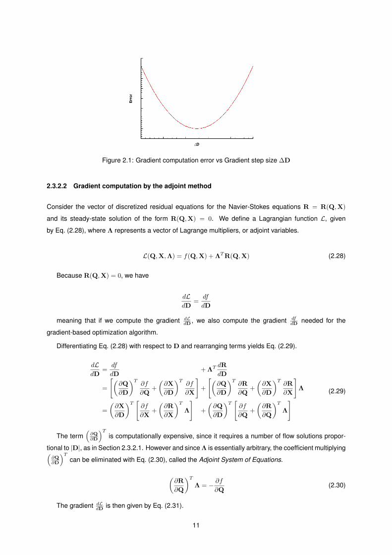
Figure 2.1: Gradient computation error vs Gradient step size ∆D

2.3.2.2 Gradient computation by the adjoint method

Consider the vector of discretized residual equations for the Navier-Stokes equations R = R(Q,X)

and its steady-state solution of the form R(Q,X) = 0. We define a Lagrangian function L, given

by Eq. (2.28), where Λ represents a vector of Lagrange multipliers, or adjoint variables.

L(Q,X,Λ) = f(Q,X) + ΛTR(Q,X) (2.28)

Because R(Q,X) = 0, we have

dLdD

=df

dD

meaning that if we compute the gradient dLdD , we also compute the gradient df

dD needed for the

gradient-based optimization algorithm.

Differentiating Eq. (2.28) with respect to D and rearranging terms yields Eq. (2.29).

dLdD

=df

dD+ ΛT dR

dD

=

[(∂Q

∂D

)T∂f

∂Q+

(∂X

∂D

)T∂f

∂X

]+

[(∂Q

∂D

)T∂R

∂Q+

(∂X

∂D

)T∂R

∂X

]Λ

=

(∂X

∂D

)T [∂f

∂X+

(∂R

∂X

)TΛ

]+

(∂Q

∂D

)T [∂f

∂Q+

(∂R

∂Q

)TΛ

] (2.29)

The term(∂Q∂D

)Tis computationally expensive, since it requires a number of flow solutions propor-

tional to |D|, as in Section 2.3.2.1. However and since Λ is essentially arbitrary, the coefficient multiplying(∂Q∂D

)Tcan be eliminated with Eq. (2.30), called the Adjoint System of Equations.

(∂R

∂Q

)TΛ = − ∂f

∂Q(2.30)

The gradient dLdD is then given by Eq. (2.31).

11

dLdD

=

(∂X

∂D

)T [∂f

∂X+

(∂R

∂X

)TΛ

](2.31)

The ∂X∂D term represents the mesh sensitivity and is developed in Eq. (2.32). Because Xs is analyti-

cally defined by D, finite differences are not required.

∂X

∂D=

∂X

∂Xs

∂Xs

∂D(2.32)

Finally, inserting Eq. (2.32) into Eq. (2.31), we obtain Eq. (2.33), where Λ is obtained by solv-

ing Eq. (2.30).

dLdD

=

(∂Xs

∂D

)T (∂X

∂Xs

)T [∂f

∂X+

(∂R

∂X

)TΛ

](2.33)

2.3.2.3 Karush–Kuhn–Tucker (KKT) conditions

The KKT conditions are first order necessary conditions for a solution in nonlinear programming to be

optimal, provided that some regularity conditions are satisfied. They are a generalization of the method

of Lagrange multipliers, which allows only equality constraints. Consider the optimization problem (2.34).

minimizex

f(x)

subject to G(x) ≤ 0

H(x) = 0

(2.34)

If xm is a local minimum, then the KKT conditions (2.35) must be verified.

−∇f(xm) =

|G|∑i=1

µi∇Gi(xm) +

|H|∑j=1

λj∇Hj(xm) (2.35a)

Gi(xm) ≤ 0, i = 1, . . . , |G|

Hj(xm) = 0, j = 1, . . . , |H|(2.35b)

µi ≥ 0, i = 1, . . . , |G| (2.35c)

µiGi(xm) = 0, i = 1, . . . , |G| (2.35d)

Notice that the inequality contribution µi∇Gi(xm) in Eq. (2.35a) only needs to be considered when

Gi(xm) = 0, since if Gi(xm) < 0 and µi ≥ 0 (from Eq. (2.35c)), then µi = 0 is necessary to satisfy

Eq. (2.35d), rendering µi∇Gi(xm) = 0. This applies for example to design space boundary constraints

xi ∈ [li, ui]⇔ xi − ui ≤ 0 ∧ li − xi ≤ 0.

2.3.2.4 Sequential Least Squares Programming (SLSQP)

SLSQP stands for Sequential Least-Squares Quadratic Programming. It is a gradient-based algorithm

for non-linearly constrained optimization problems, which supports both equality and inequality con-

12

straints. Consider the generic optimization problem (2.34).

The Lagrangian of the problem is given by Eq. (2.36), where µ and λ are the Lagrange multipliers.

L(x, µ, λ) = f(x) + µTG(x) + λTH(x) (2.36)

At iteration k, the algorithm defines an appropriate search direction dk as a solution to the quadratic

problem (2.37). The Hessian matrix ∇2xxL is computed with a BFGS update. [18]

minimized

f(xk) +∇f(xk)T d+ 12dT∇2

xxL(xk, µk, λk)d

subject to G(xk) +∇G(xk)T d ≤ 0

H(xk) +∇H(xk)T d = 0

(2.37)

2.3.3 Design of Experiments (DOE)

Design of Experiments is a method for design space exploration. The way in which the space design is

explored depends on the chosen sampling algorithm, of which there are many, such as:

• Random sampling

• Halton sampling

• Latin hypercube sampling

• Etc.

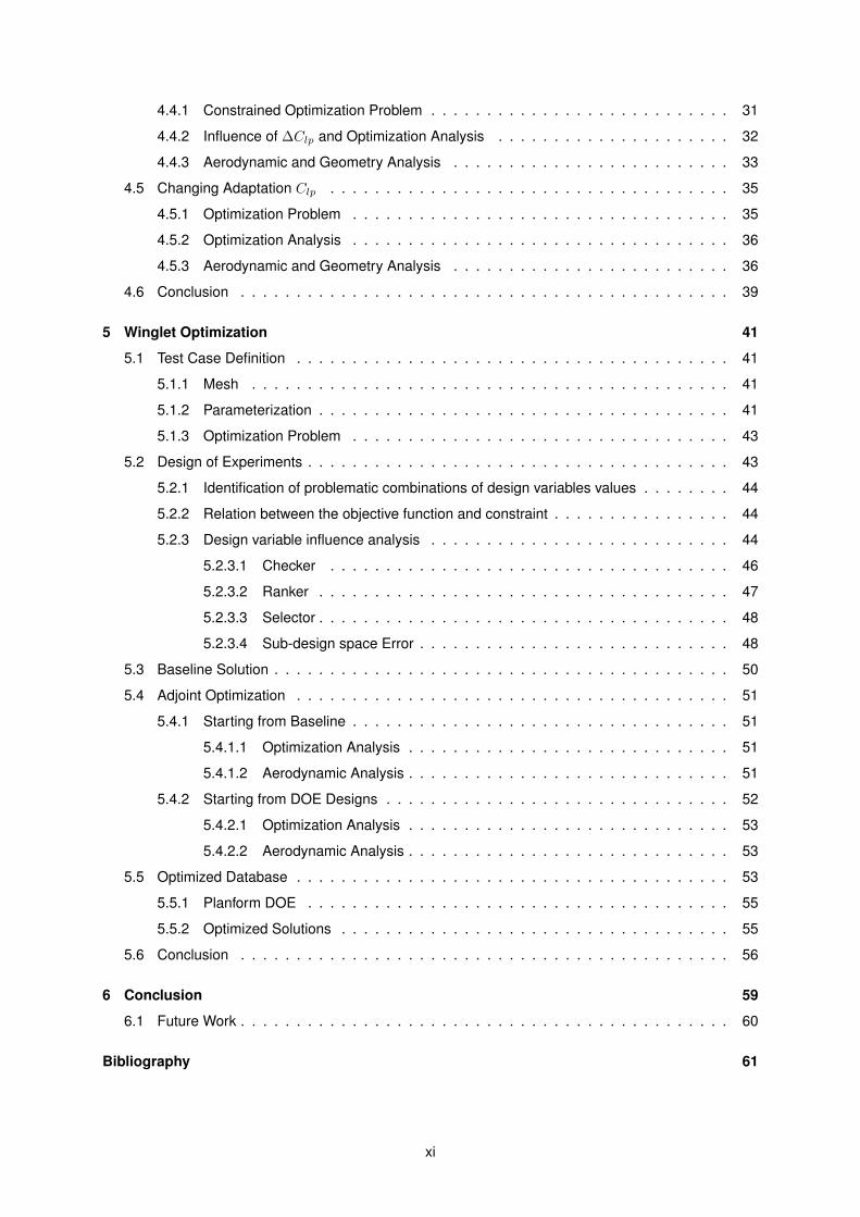
The chosen algorithm for this work is the Latin hypercube sampling, since the probability that the

samples are clustered is low.

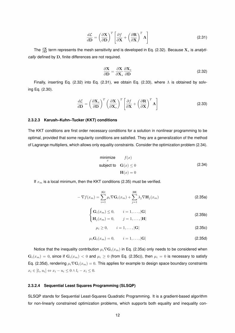
A square grid containing sample positions is a Latin square if and only if there is only one sample in

each row and each column. Fig. 2.2a and Fig. 2.2b are examples of Latin squares, while Fig. 2.2c isn’t.

The generalization of a Latin square to an arbitrary number of dimensions is called a Latin hypercube.

Consider a design space of N dimensions and a sampling of M samples. Then, the range of each

variable is divided into M equiprobable intervals. M sample points are then placed to satisfy the Latin

hypercube requirements.

(a) Latin square (b) Latin square (c) Not Latin square

Figure 2.2: Square grid examples

13

14

Chapter 3

Analysis and Optimization Tools

In this chapter, the tools utilized for either analysis or optimization are presented. Furthermore, an

explanation of how they work is given.

3.1 Computational Fluid Dynamics

3.1.1 Mesh

At Airbus, elsA only supports structured multi-block meshes. The meshes are generated using ANSYS

ICEM software. The objective is to have high-quality meshes, which satisfy some mesh quality and

boundary layer criteria (e.g. maximum skewness and y+first cell ∼ 1, respectively).

Because the generated mesh is fine, CFD simulations take a long time to run. In order to speed up

the process, the mesh is coarsed once or twice, corresponding to a reduction to one half or one quarter

of the original points, respectively. These meshes are called ”medium” and ”coarse”, respectively, and

they are used during the optimization process. After the optimization process finishes, the optimized

solution is then validated using the original fine mesh.

3.1.2 Solver

The CFD solver used in this work is elsA. It is a finite-volume CFD solver developed by ONERA (and

co-developed by many others) and it is one of the two de facto CFD solvers used in Airbus. elsA is

capable of both external and internal complex flow simulations in aerodynamics and handles structured

multi-block meshes. Its settings are divided into five groups: flight conditions, turbulence model, spatial

integration, time integration, geometry parameters. Common settings to all CFD computations for this

work are presented in Tbl. 3.1.

15

Simulation Type Compressible RANS

Turbulence Model Spalart-Allmaras

Spatial Int. Scheme 2nd order ROE

Limiter Valbada

Table 3.1: Common elsA settings

3.2 WORMS Optimization Chain

WORMS stands for WORkflow Management System. It is a flexible automated optimization chain, which

links all different components necessary to the optimization process. At each step the output of each

component is validated and the input of a component is sourced from the output of one or multiple

previous components.

WORMS allows both direct-mode (gradient by finite differences) and reverse-mode (gradient by solv-

ing the adjoint state) optimizations. The last four components described below and their chaining belong

only to the reverse-mode optimization workflow.

3.2.1 Padge

Padge is responsible for the parameterization of the body surface. That is, for a given design variables

vector D, it is responsible for calculating the surface points:

(x, y, z)s =

F (D, u) u ∈ [0, 1] if 2D geometry

F (D, u, v) u, v ∈ [0, 1] if 3D geometry

Given the new design vector variables vector D, Padge computes the new surface mesh Xs. Com-

paring this with the original surface mesh X0s, the displacement of each surface mesh node is computed

δXs = Xs −X0s.

Input Output

Computational mesh X0 ⊃ X0s

Surface mesh displacement δXsDesign variables vector D

Parameterization F(D, u, v)

Table 3.2: Padge input/output summary

3.2.1.1 Shape Matching

Given a parameterization of the body surface, a set of design variable values D = Doriginal must be found

in order to match the original shape. The process of finding D is called shape matching. It is an iterative

process and it converges when the mean distance between the initial shape and the parameterized

shape is less than a defined error value, usually 1mm for a 1m chord.

16

3.2.1.2 CAD to Mesh Link

In order to be able to compute the displacement δXs = Xs −X0s, the location of each point

(X0s

)i

of the

original surface mesh on the new surface mesh (Xs)i must be known. This is done by finding a tuple

(u, v)i = F−1((X0s)i) for each mesh point of the original surface mesh and supplying it to new surface

mapping F (u, v) = F (D, u, v).

3.2.2 VolDef

VolDef stands for Volume Deformation and it’s responsible for mesh deformation. Given the surface

mesh displacement δXs calculated by Padge, the complete mesh X is deformed. This deformation is

done by layers inside a cone emanating from the surface, with an exponential damping factor.

Input Output

Computational mesh X0 ⊃ X0s New mesh X

Surface mesh displacement δXs

Table 3.3: VolDef input/output summary

3.2.3 elsA

elsA is the CFD solver utilized both for direct CFD simulations (e.g.: airfoil polar) and for optimizations.

A description of its characteristics and capabilities is given in Section 3.1.2.

Input Output

New mesh XFlow field Q

Residuals R

Table 3.4: elsA input/output summary

3.2.3.1 Target Lift

For this work, all optimizations are run for a fixed target lift coefficient. This doesn’t mean that optimiza-

tion of a range of lift coefficients can not be done. It means that performances are always evaluated at

the same fixed target lifts.

The target lift method works by changing the angle of attack until finding an angle of attack for which

the lift coefficient is equal to the target lift coefficient. The changes in angle of attack follow an iterative

algorithm Eq. (3.1), where ω is a damping parameter, usually 0.6 and dCLdα is supplied by the user, usually

within the range [0.10, 0.14].

αn+1 = αn + ω

(dCLdα

)−1 ((CL)target − CL(αn)

)(3.1)

17

The simulation starts at a predefined α0 for Step Number time steps. Then, the iterative algorithm

begins and the flow is computed at each αn for NStepLoop time steps. When |(CL)target − CL(αn)| ≤ ε,

where ε is a pre-defined tolerance, the iterative algorithm stops and the CFD simulation is run for a final

NStepEnds time steps.

3.2.4 ZAPP/ZAPP-rev

ZAPP is a post-processing tool, responsible for computing the desired performance metrics fi (e.g.: CD,

CL, etc.) and its reverse mode computes their partial derivatives with respect to the mesh nodes ∂fi∂X

and with respect to the flow vector variables ∂fi∂Q .

Input Output

New mesh X′ Performance metrics fi

Flow field QPartial derivatives

∂fi∂X ,

∂fi∂Q

Table 3.5: ZAPP input/output summary

3.2.5 elsA-reverse

elsA-reverse is responsible for solving the adjoint-state Λ as described in Section 2.3.2.2. The adjoint-

state is then used to compute the full derivative of the function fi with respect to the mesh nodes

positions (3.2).

dfidX

=∂fi∂X

+

(∂R

∂X

)TΛ (3.2)

Input Output

New mesh XAdjoint state Λ

Flow field Q

Residues R

Full derivative dfidXPartial derivatives

∂fi∂X ,

∂fi∂Q

Table 3.6: elsA-reverse input/output summary

3.2.6 VolDef-reverse

VolDef-reverse computes the derivative of the functions fi with respect to the surface mesh nodes. It

computes the partial derivative ∂Xs

∂X and multiplies by the full derivative (3.2) computed by elsA-reverse,

resulting in Eq. (3.3).

18

dfidXs

=

(∂X

∂Xs

)T [∂fi∂Xs

+

(∂R

∂X

)TΛ

](3.3)

Input Output

New mesh XFull derivative dfi

dXsFull derivative dfidX

Table 3.7: VolDef-reverse input/output summary

3.2.7 Padge-reverse

Padge-reverse is responsible for the final step, which is transforming the derivative with respect to the

surface mesh nodes, that is, the ”shape”, into a derivative with respect to the design variables. This is

done by computing ∂Xs

∂D and multiplying by (3.3).

Input Output

Parameterization F(D, u, v)Full derivative dfi

dDFull derivative dfi

dXs

Table 3.8: Padge-reverse input/output summary

3.2.8 Optimizer

The optimizer receives the gradient of the objective and constraint functions and decides the next set of

design variable values D. The complete workflow is described in Fig. 3.1.

3.3 Post-processing

3.3.1 KKT Optimization Analysis

As described in Section 2.3.2.3, the KKT conditions are necessary conditions for a local optimum. An

analysis of the KKT conditions are done by an in-house software.

3.3.2 Flow visualization

In order to visualize the flow field and relevant aerodynamic data, an in-house software called QuickView

was used. It supports 3D visualization and multiple types of plot and is highly customizable.

3.3.3 FFD Aerodynamic Analysis

As described in Section 2.1.5.3, drag can be decomposed with a far-field analysis. This is done with an

in-house software called FFD72.

19

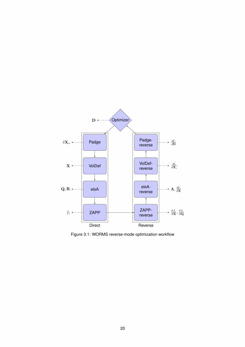
Optimizer

Padge

VolDef

elsA

ZAPP

Direct

Padge-reverse

VolDef-reverse

elsA-reverse

ZAPP-reverse

Reverse

δXs

X

Q,R

fi∂fi∂X ,

∂fi∂Q

Λ, dfidX

dfidXs

dfidD

D

Figure 3.1: WORMS reverse-mode optimization workflow

20

Chapter 4

RAE2822 Airfoil Optimization

The RAE2822 airfoil is a transonic airfoil. It has been extensively studied both computationally and

experimentally.

4.1 Test Case Definition

The flight conditions of the case are:

• M = 0.73

• Re = 6.5× 106

4.1.1 Mesh

The mesh was generated in ANSYS ICEM with the objective of having y+ ∼ 0.3 for the nearest mesh

node to the wall. Then, this mesh was coarsed to a medium mesh. The objective is to run optimizations

on the medium mesh (including reverse mode) and run the direct flow solutions of the initial and final

shapes on the fine mesh in order to validate the optimizations results, as described in Section 3.1.1.

The mesh is composed of two planes, in order to create the volume cells. A summary of the mesh

characteristics (including the two planes) is given in Tbl. 4.1. Both complete and zoomed views of the

mesh are in Fig. 4.1.

Medium Fine

Blocks 28

Nodes 78736 306600

Surface Nodes 22188 86020

Table 4.1: RAE2822 mesh summary

21

(a) Medium mesh - complete (b) Fine mesh - complete

(c) Medium mesh - zoomed (d) Fine mesh - zoomed

Figure 4.1: Mesh views

4.1.2 Baseline Design

Fig. 4.2 plots the ratio ClpCd

versus Clp for the above flight conditions. Hereinafter, an airfoil is said to

be adapted if it is operating at a Clp value Clp = Cadaptationlp for which Clp

Cdis maximum. This point is of

special interest because an aircraft usually cruises at maximum ClpCd

. It is therefore logical to increase

the performances at this point. This means that the objective is to vertically translate the point:

(Clp,

ClpCd

)Clp=Cadaptation

lp

The maximum of ClpCd

for the RAE2822 airfoil is at Clp = 0.63, at which the values of Tbl. 4.2 are

obtained. The residuals and history of both Cl and Cd of the corresponding flow solution are plotted in

Fig. 4.3.

Clp Cl AoA Cnfd Cdf Cdp Cffd Cdw Cdv −Cm Clp

Cnfd

0.63117 0.63119 1.848o 103.2 59.61 43.55 100.0 4.56 95.47 0.0882 61.18

Table 4.2: Baseline RAE2822 - Clp = 0.630± 0.001

A first result extracted from Tbl. 4.2 is that the lift viscous component Clv ≡ Cl − Clp is very small,

22

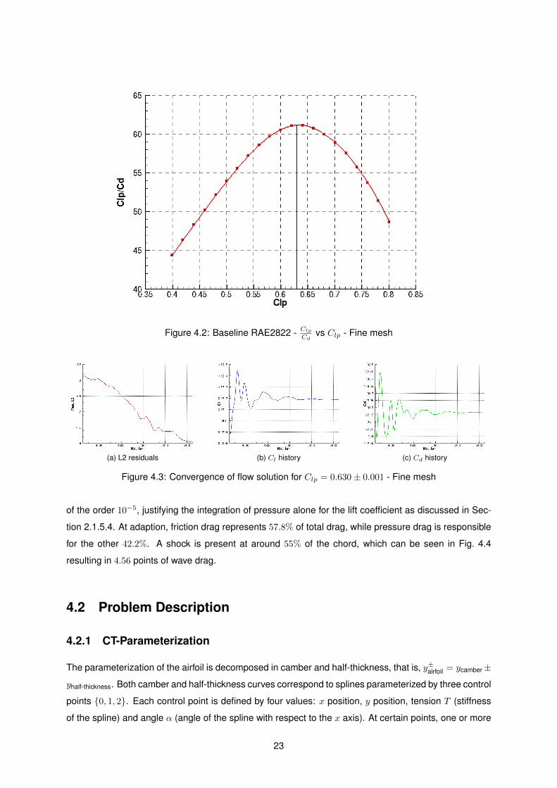
Figure 4.2: Baseline RAE2822 - ClpCd vs Clp - Fine mesh

(a) L2 residuals (b) Cl history (c) Cd history

Figure 4.3: Convergence of flow solution for Clp = 0.630± 0.001 - Fine mesh

of the order 10−5, justifying the integration of pressure alone for the lift coefficient as discussed in Sec-

tion 2.1.5.4. At adaption, friction drag represents 57.8% of total drag, while pressure drag is responsible

for the other 42.2%. A shock is present at around 55% of the chord, which can be seen in Fig. 4.4

resulting in 4.56 points of wave drag.

4.2 Problem Description

4.2.1 CT-Parameterization

The parameterization of the airfoil is decomposed in camber and half-thickness, that is, y±airfoil = ycamber±

yhalf-thickness. Both camber and half-thickness curves correspond to splines parameterized by three control

points {0, 1, 2}. Each control point is defined by four values: x position, y position, tension T (stiffness

of the spline) and angle α (angle of the spline with respect to the x axis). At certain points, one or more

23

Figure 4.4: Baseline RAE2822 - Mach field - Fine mesh

of these values might be fixed (e.g. x position of point 0 is always 0). Tbl. 4.3 and Fig. 4.5 describe the

parameterization of the airfoil.

P0 P1 P2

x y α T x y α T x y α T

Camber 0 0 1000 0

Thickness 0 0 90o 0o 1000 0

Table 4.3: Parameterization of RAE2822

C0.AngleC0.Tension

C1.AngleC1.Tension

C1.X

C1.Y

C2.AngleC2.Tension

(a) Camber parameterization

T0.Tension

T1.Tension

T1.X

T1.Y

T2.AngleT2.Tension

(b) Thickness parameterization

Figure 4.5: Airfoil CT-Parameterization

T0.Angle and T1.Angle are both fixed because they represent the leading edge circle and maximum

thickness point, respectively. From this reasoning, T0.Tension and T1.Y can be thought of as controlling

the leading edge radius and the maximum half-thickness, respectively.

24

4.2.2 Design Space

Usually, when redesigning an airfoil, one is restricted to recambering because thickness is issued from

structural/loading constraints. For this reason, the design space will match the parameterization of

the camber line, that is: C1.X, C1.Y, C0.Tension, C1.Tension, C2.Tension, C0.Angle, C1.Angle and

C2.Angle. The value range for each one is given in Tbl. 4.4.

Design Variable Lower Bound Baseline Upper Bound Unit

C1.X 100 394.8 900mm

C1.Y −20 1.915 +20

C0.Tension

40

86.52

400C1.Tension 110.4

C2.Tension 225.6

C0.Angle−15

−0.8047+15

◦C1.Angle 1.546

C2.Angle −30 −7.653 0

Table 4.4: Camber design value ranges

4.2.2.1 Normalization

One aspect of an optimization problem is the design space conditioning, which must be carefully studied.

For example, in Tbl. 4.4, there are design variables whose value range is of the order 102 and others

of the order 103. This is a possible issue from an optimizer point-of-view - since in Aerodynamics the

design space is usually multimodal, that is, presents many local minima, the optimizer might fall into one

local minima without exploring the design space.

Design space normalization comes as natural answer to this problematic behavior. There are two

usual options for normalization: either normalize each variable value range to [0, 1] or to [−1,+1]. The

former is preferred to the latter when there is no ”starting design”, because the bounds are used as a

reference. When the optimization is run from a ”baseline design”, the latter is preferred, since 0 is used

as the reference for the baseline. This way, if the normalized design variable (e.g.: thickness) is negative,

its non-normalized value has decreased, whereas a positive value corresponds to an increase.

Consider the design variable x, with lower bound l, upper bound u and baseline value b. The corre-

sponding normalized variable is x and the basis of the design space normalization is the linear transfor-

mation (4.1).

x = T (x) = αx+ β (4.1)

Ideally, all relations (4.2) would be valid. However, because the transformation is linear, unless the

[l, u] is centered around b (in this case l+u2 = b) only two of them can be respected at a time.

25

T (−1) = l T (0) = b T (+1) = u (4.2)

As the primary objective of [−1,+1] normalization is to have 0 as a baseline reference, T (0) = b must

always be respected. Furthermore, because we want to be able to generate all values in [l, u], the other

condition is chosen following Eq. (4.3).

T (−1) = l if b− l ≥ u− b

T (+1) = u otherwise(4.3)

For example, consider the first case, where T (−1) = l is to be respected. Coupled with T (0) = b:

T (−1) = l

T (0) = b⇒

α = b− l

β = b⇒ T (x) = (b− l)x+ b⇒

T (−1) = −(b− l) + b = l

T (0) = b

T (+1) = (b− l) + b ≥ (u− b) + b = u

The last step shows that u ∈ [T (−1), T (+1)] = [l, 2b − l]. The value range for x is then restricted

from [−1,+1] to [−1, T−1(u)], where T−1(u) ≤ +1, such that the normalized design space corresponds

exactly to the non-normalized one. Generally, the transformation is given by Eq. (4.4) and the normalized

design space is given in Tbl. 4.5.

x = T (x) = max(b− l, u− b)x+ b (4.4a)

x ∈

[−1, T−1(u)

]if b− l ≥ u− b[

T−1(l),+1]

otherwise(4.4b)

The effect of normalization is now calculated for a descending gradient method. Consider a descend-

ing gradient method on a normalized variable x, then (γ is the step size):

xn+1 = xn − γdf

dx

∣∣∣∣x=xn

Substituting by non-normalized variables:

α−1xn+1 + α−1β = α−1xn + α−1β − γα df

dx

∣∣∣∣x=xn

⇒ xn+1 = xn − γ

(α2 df

dx

∣∣∣∣x=xn

)

Frequently, in Aerodynamics, the design space is multimodal, that is, presents many local minima.

This might be a risk, as the optimizer might fall into one local minima without exploring the design

space. Fig. 4.6 illustrates this phenomenon and the normalization effect, where D = (x, y)T and D0 =

(0, 0)T . Normalization is done to [−1,+1] yielding αx = 2 and αy = 1. The true gradient on the non-

normalized design space points in the direction of the local minimum. However, because the optimization

and gradient are computed in the normalized design space, the x component of the gradient on the

non-normalized design space is multiplied by α2x = 4 and the y component doesn’t change because

26

α2y = 1. The step will then be taken in the direction of the modified gradient which doesn’t point in the

direction of the local minimum, possibly resulting in a better design space exploration. Obviously, this is

a particular case - in fact the opposite case may happen, when the global minimum is switched with the

local minimum and convergence speed takes a hit. However, as the main objective is not to fall directly

into a local minimum without searching elsewhere, normalization is done.

Although SLSQP was chosen instead of a descending gradient algorithm, the first step of SLSQP

is in fact equivalent to a descending gradient, since the Hessian matrix is the identity matrix at the

beginning of the optimization.

x ∈ [0, 4]

y ∈ [0, 2]

Localminimum

Globalminimum

Real gradient

Normalized gradient

Figure 4.6: Normalization effect on gradient

Summarizing the many consequences:

• A descending gradient method on a normalized design space is not equivalent to the same de-

scending gradient method on a non-normalized design space

• Each component of the gradient is multiplied by the corresponding variable scale factor α (not the

same for all variables)

• It is more unlikely to fall in a local minimum without exploring the design space

This is a common technique in the domain of optimization, namely aerodynamic optimization and it

will be used on both two and three-dimensional cases.

The resulting normalized space is given in Tbl. 4.5. It was however adapted, to always ensure a

feasible geometry. Unfeasible geometries are the result of bad combinations of design variables values

(e.g.: very low x and very high y values of C1) which are not feasible at VolDef level.

4.2.3 Optimization Problem

An optimization problem requires: an objective function, constraints (if there are any) and a design

space. The design space was defined in Section 4.2.2, leaving the objective function and constraints to

be defined. As discussed in Section 4.1.2, the baseline airfoil is adapted for Clp = 0.63 and because

aircraft usually flight at this point in cruise, it is logical to optimize at that condition. Furthermore, the

adaptation Clp = Cadaptationlp is to be kept constant at Clp = 0.63.

The choice of objective function relies on one of the following Cdp, Cdf , Cd. Cdp is chosen. Although

it might seem inconsistent, since the objective is to minimize Cd, it is not. It is a way of stating that the

objective is to minimize Cd by minimizing Cdp. Such a choice is due to the fact that the viscous adjoint

27

Design Variable Lower Bound Upper Bound Adapted Lower Bound Adapted Upper Bound

Norm.C1.X −0.58349 +1.0 −0.2 +0.65

Norm.C1.Y −1.0 +0.82524 −0.05

Norm.C0.Tension −0.14841 +1.0

Norm.C1.Tension −0.24320 +1.0 +0.25

Norm.C2.Tension −1.0 +0.93971

Norm.C0.Angle −0.89817 +1.0

Norm.C1.Angle −1.0 +0.81307

Norm.C2.Angle −1.0 +0.34244

Table 4.5: Normalized camber variables

terms in the current version of elsA-reverse are not very accurate, which is a known limitation. Further-

more, instead of computing two adjoint systems (Cdp, Cdf ), only one is computed, reducing computation

time considerably.

Regarding the constraints, we will not impose any to begin with, since a priori there is no need to. The

optimization problem is then defined in Eq. (4.5), for which the KKT conditions simplify to∇Cdp = 0 (if the

considered design is not at the boundary of the design space), because the problem is unconstrained.

minimizeD≡camber,Target Lift

Cdp|Clp=0.63 (4.5)

4.3 Unconstrained Optimization

Optimizations for solving Eq. (4.5) were run in the normalized design space.

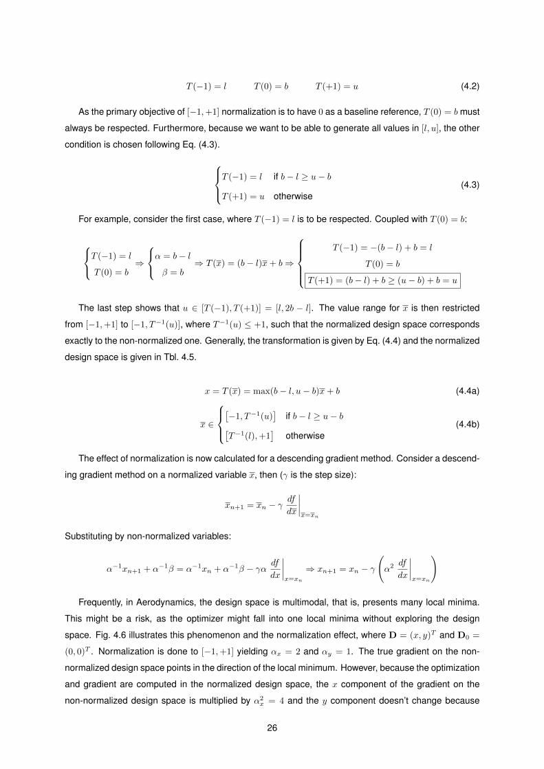
4.3.1 Optimization Analysis

The history of both objective function and gradient norm (normalized by the baseline gradient) are shown

in Fig. 4.7. The optimization takes 29 iterations to converge and 20 iterations to arrive to within 1% of

the best value on the last iteration, for which the norm of the gradient is 5% of the baseline’s. This is

certainly close to the optimality condition ∇Cdp = 0. The ”jumps” of the objective function occur at the

same time as those of the gradient norm - the optimizer tries a certain search direction, which worsens

the objective function that in turn appears on the gradient norm. Here, the gradient norm history serves

the purpose of ”optimality monitor”.

The objective function starts at 47.36 and finishes at 41.12, translating into an objective function gain

of 13.17%. These results are then validated on the fine mesh for a more precise aerodynamic analysis

as discussed in Section 4.1.1.

The optimization took slightly more than 4 hours and 16 minutes running on 24 cores in a HPC

cluster. The average computational time and average percentage of total computation time for each

component of the toolchain are given in Tbl. 4.6.

28

(a) Objective Function History (b) Gradient Norm History

Figure 4.7: Unconstrained optimization history

Padge VolDef elsA ZAPP/ZAPP-rev elsA-rev VolDef-rev Padge-rev

Time 12m23s 7m10s 2h12m06s 3m49s 1h31m56s 7m45s 1m29s

% 4.8 2.8 51.5 1.5 43.5 3.0 0.6

Table 4.6: Computation time

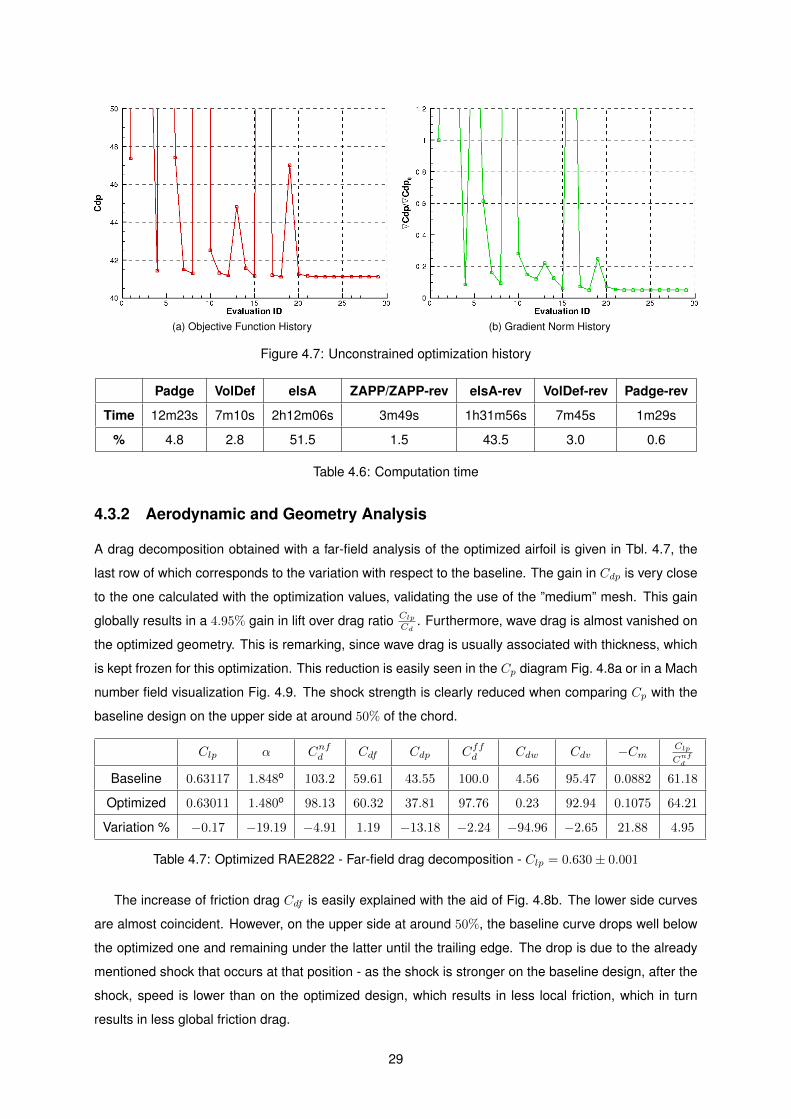
4.3.2 Aerodynamic and Geometry Analysis

A drag decomposition obtained with a far-field analysis of the optimized airfoil is given in Tbl. 4.7, the

last row of which corresponds to the variation with respect to the baseline. The gain in Cdp is very close

to the one calculated with the optimization values, validating the use of the ”medium” mesh. This gain

globally results in a 4.95% gain in lift over drag ratio ClpCd

. Furthermore, wave drag is almost vanished on

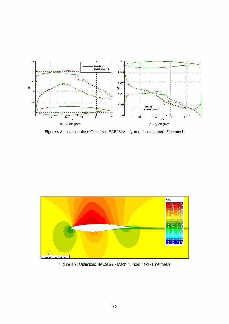
the optimized geometry. This is remarking, since wave drag is usually associated with thickness, which

is kept frozen for this optimization. This reduction is easily seen in the Cp diagram Fig. 4.8a or in a Mach

number field visualization Fig. 4.9. The shock strength is clearly reduced when comparing Cp with the

baseline design on the upper side at around 50% of the chord.

Clp α Cnfd Cdf Cdp Cffd Cdw Cdv −Cm Clp

Cnfd

Baseline 0.63117 1.848o 103.2 59.61 43.55 100.0 4.56 95.47 0.0882 61.18

Optimized 0.63011 1.480o 98.13 60.32 37.81 97.76 0.23 92.94 0.1075 64.21

Variation % −0.17 −19.19 −4.91 1.19 −13.18 −2.24 −94.96 −2.65 21.88 4.95

Table 4.7: Optimized RAE2822 - Far-field drag decomposition - Clp = 0.630± 0.001

The increase of friction drag Cdf is easily explained with the aid of Fig. 4.8b. The lower side curves

are almost coincident. However, on the upper side at around 50%, the baseline curve drops well below

the optimized one and remaining under the latter until the trailing edge. The drop is due to the already

mentioned shock that occurs at that position - as the shock is stronger on the baseline design, after the

shock, speed is lower than on the optimized design, which results in less local friction, which in turn

results in less global friction drag.

29

(a) Cp diagram (b) Cf diagram

Figure 4.8: Unconstrained Optimized RAE2822 - Cp and Cf diagrams - Fine mesh

Figure 4.9: Optimized RAE2822 - Mach number field - Fine mesh

30

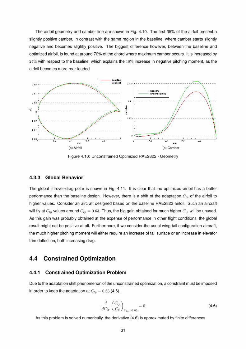
The airfoil geometry and camber line are shown in Fig. 4.10. The first 35% of the airfoil present a

slightly positive camber, in contrast with the same region in the baseline, where camber starts slightly

negative and becomes slightly positive. The biggest difference however, between the baseline and

optimized airfoil, is found at around 76% of the chord where maximum camber occurs. It is increased by

24% with respect to the baseline, which explains the 18% increase in negative pitching moment, as the

airfoil becomes more rear-loaded

(a) Airfoil (b) Camber

Figure 4.10: Unconstrained Optimized RAE2822 - Geometry

4.3.3 Global Behavior

The global lift-over-drag polar is shown in Fig. 4.11. It is clear that the optimized airfoil has a better

performance than the baseline design. However, there is a shift of the adaptation Clp of the airfoil to

higher values. Consider an aircraft designed based on the baseline RAE2822 airfoil. Such an aircraft

will fly at Clp values around Clp = 0.63. Thus, the big gain obtained for much higher Clp will be unused.

As this gain was probably obtained at the expense of performance in other flight conditions, the global

result might not be positive at all. Furthermore, if we consider the usual wing-tail configuration aircraft,

the much higher pitching moment will either require an increase of tail surface or an increase in elevator

trim deflection, both increasing drag.

4.4 Constrained Optimization

4.4.1 Constrained Optimization Problem

Due to the adaptation shift phenomenon of the unconstrained optimization, a constraint must be imposed

in order to keep the adaptation at Clp = 0.63 (4.6).

d

dClp

(ClpCd

)Clp=0.63

= 0 (4.6)

As this problem is solved numerically, the derivative (4.6) is approximated by finite differences

31

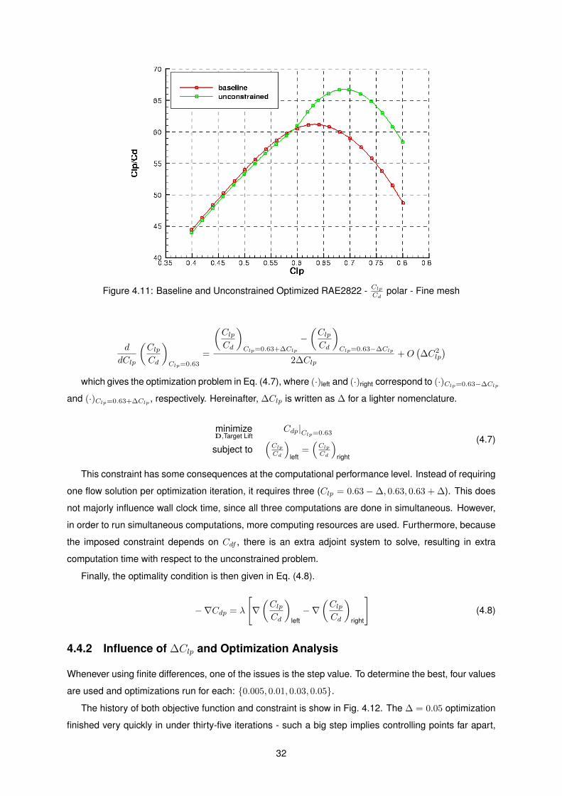
Figure 4.11: Baseline and Unconstrained Optimized RAE2822 - ClpCd polar - Fine mesh

d

dClp

(ClpCd

)Clp=0.63

=

(ClpCd

)Clp=0.63+∆Clp

−(ClpCd

)Clp=0.63−∆Clp

2∆Clp+O

(∆C2

lp

)which gives the optimization problem in Eq. (4.7), where (·)left and (·)right correspond to (·)Clp=0.63−∆Clp

and (·)Clp=0.63+∆Clp , respectively. Hereinafter, ∆Clp is written as ∆ for a lighter nomenclature.

minimizeD,Target Lift

Cdp|Clp=0.63

subject to(ClpCd

)left

=(ClpCd

)right

(4.7)

This constraint has some consequences at the computational performance level. Instead of requiring

one flow solution per optimization iteration, it requires three (Clp = 0.63 −∆, 0.63, 0.63 + ∆). This does

not majorly influence wall clock time, since all three computations are done in simultaneous. However,

in order to run simultaneous computations, more computing resources are used. Furthermore, because

the imposed constraint depends on Cdf , there is an extra adjoint system to solve, resulting in extra

computation time with respect to the unconstrained problem.

Finally, the optimality condition is then given in Eq. (4.8).

−∇Cdp = λ

[∇(ClpCd

)left−∇

(ClpCd

)right

](4.8)

4.4.2 Influence of ∆Clp and Optimization Analysis

Whenever using finite differences, one of the issues is the step value. To determine the best, four values

are used and optimizations run for each: {0.005, 0.01, 0.03, 0.05}.

The history of both objective function and constraint is show in Fig. 4.12. The ∆ = 0.05 optimization

finished very quickly in under thirty-five iterations - such a big step implies controlling points far apart,

32

which might be difficult. For ∆ = 0.03, although it takes eighty iterations to end the optimization, the

optimum value was already achieved at iteration thirty-six. The best optimization is that with ∆ = 0.01,

beating the previous by almost one drag point. To confirm that this corresponds to the optimum step

size, a final optimization with ∆ = 0.005 was run, finishing with an objective function final value even

higher the ∆ = 0.03 optimization one.

(a) Objective Function History (b) Constraint History

Figure 4.12: Constrained optimization history

Hereinafter, the optimized airfoil obtained with ∆ = 0.01 will be called constrained optimization airfoil.

4.4.3 Aerodynamic and Geometry Analysis

The global lift-over-drag polar is shown in Fig. 4.13. As intended, the constrained optimization yields

an airfoil whose adaptation is kept at the baseline’s adaptation Clp = 0.63. This results however in a

small loss of 0.8 in ClpCd

with respect to the unconstrained optimization. The gain in the region around

Clp = 0.63 is obtained in detriment of the outermost regions, where performance is lower than with the

baseline.

A drag decomposition obtained with a far-field analysis of the optimized airfoil is given in Tbl. 4.8.

The difference in performance between the unconstrained and constrained optimized airfoils is mainly

in wave drag: whereas for the former Cdw = 0.23, for the latter Cdw = 1.96. This phenomenon is clearly

seen in the Cp diagram Fig. 4.14a: the shock at around 45% of the chord is weaker than the baseline’s,

but much stronger than the unconstrained optimized airfoil’s.

The increase in friction drag with respect to the baseline design, as well as the slight difference of the

Cf diagram with respect to the unconstrained optimization follow the same reasoning as in Section 4.3.2.

Finally, the pitching moment Cm in the constrained optimization is not as strong as in the unconstrained

optimization.

The airfoil shape and its camber are shown in Fig. 4.15. Similarly to the unconstrained optimization,

the constrained optimization produces an airfoil with higher aft-camber, although by a smaller amount.

On both baseline and unconstrained optimized airfoils, camber is very small on the first 30% of the airfoil.

On the contrary, the constrained optimized airfoil presents positive camber in this region.

33

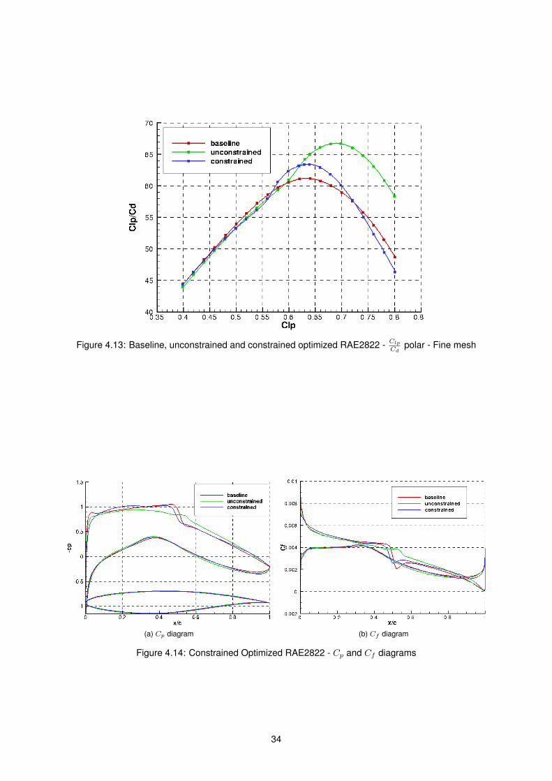
Figure 4.13: Baseline, unconstrained and constrained optimized RAE2822 - ClpCd polar - Fine mesh

(a) Cp diagram (b) Cf diagram

Figure 4.14: Constrained Optimized RAE2822 - Cp and Cf diagrams

34

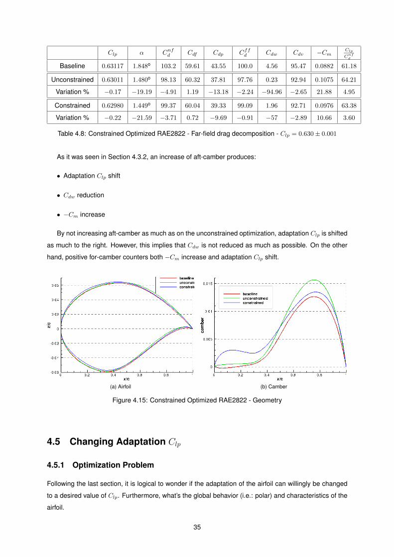
Clp α Cnfd Cdf Cdp Cffd Cdw Cdv −Cm Clp

Cnfd

Baseline 0.63117 1.848o 103.2 59.61 43.55 100.0 4.56 95.47 0.0882 61.18

Unconstrained 0.63011 1.480o 98.13 60.32 37.81 97.76 0.23 92.94 0.1075 64.21

Variation % −0.17 −19.19 −4.91 1.19 −13.18 −2.24 −94.96 −2.65 21.88 4.95

Constrained 0.62980 1.449o 99.37 60.04 39.33 99.09 1.96 92.71 0.0976 63.38

Variation % −0.22 −21.59 −3.71 0.72 −9.69 −0.91 −57 −2.89 10.66 3.60

Table 4.8: Constrained Optimized RAE2822 - Far-field drag decomposition - Clp = 0.630± 0.001

As it was seen in Section 4.3.2, an increase of aft-camber produces:

• Adaptation Clp shift

• Cdw reduction

• −Cm increase

By not increasing aft-camber as much as on the unconstrained optimization, adaptation Clp is shifted

as much to the right. However, this implies that Cdw is not reduced as much as possible. On the other

hand, positive for-camber counters both −Cm increase and adaptation Clp shift.

(a) Airfoil (b) Camber

Figure 4.15: Constrained Optimized RAE2822 - Geometry

4.5 Changing Adaptation Clp

4.5.1 Optimization Problem

Following the last section, it is logical to wonder if the adaptation of the airfoil can willingly be changed

to a desired value of Clp. Furthermore, what’s the global behavior (i.e.: polar) and characteristics of the

airfoil.

35

As such, a modification to (4.7) must be made: the constraint is applied at Clp = C∗lp instead of

Clp = 0.63. Moreover, ∆ = 0.01 is used, as discussed in Section 4.4.2. Finally, the resulting problem is

given in Eq. (4.9).

minimizeD,Target Lift

Cdp|Clp=C∗lp

subject to(ClpCdp

)Clp=C∗

lp−0.01=(ClpCdp

)Clp=C∗

lp+0.01

(4.9)

Since the unconstrained optimization shifts the adaptation to higher Clp values, C∗lp is chosen smaller

than Clp = 0.63. Two values were chosen: C∗lp = 0.60 close to the baseline adaptation and another

C∗lp = 0.54 far from the baseline adaptation.

4.5.2 Optimization Analysis

The history of the objective function and constraint are shown in Fig. 4.16. The best gain of the objective

function is obtained for C∗lp = 0.63, which was discussed in Section 4.4. The C∗lp = 0.60 results in a small

reduction of Cdp of 1.98%, corresponding to iteration 79. This gain is small due to the very high initial

constraint value. For C∗lp = 0.54, the objective function is worsened in order to satisfy the constraint,

which starts with the biggest value of all optimizations, resulting in a 7.95% increase of Cdp.

(a) Objective Function (b) Constraint

Figure 4.16: Changing adaptation - Optimization history

4.5.3 Aerodynamic and Geometry Analysis

The global lift-over-drag polar is shown in Fig. 4.17. It is clear that each polar is centered around the

intended value of Clp. Commentaries on the C∗lp = 0.63 have been made in previous sections. The

C∗lp = 0.60 slightly improves performance in Clp ∈ [0.55, 0.61] in detriment of a slight loss of performance

below Clp = 0.55 and a major loss of performance above Clp = 0.61. In the case of C∗lp = 0.54, there is

a global loss of Clp/Cd.

The far-field drag decomposition analysis for all three optimized airfoils and the corresponding base-

line values are given in Tbl. 4.9. Regarding C∗lp = 0.54, there is an increase in Cd of 1.5%, resulting

36

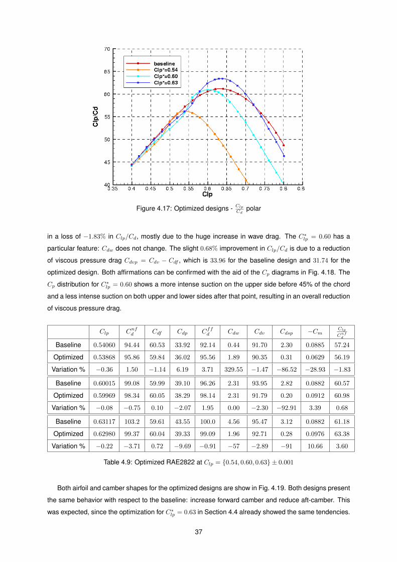
Figure 4.17: Optimized designs - ClpCd polar

in a loss of −1.83% in Clp/Cd, mostly due to the huge increase in wave drag. The C∗lp = 0.60 has a

particular feature: Cdw does not change. The slight 0.68% improvement in Clp/Cd is due to a reduction

of viscous pressure drag Cdvp = Cdv − Cdf , which is 33.96 for the baseline design and 31.74 for the

optimized design. Both affirmations can be confirmed with the aid of the Cp diagrams in Fig. 4.18. The

Cp distribution for C∗lp = 0.60 shows a more intense suction on the upper side before 45% of the chord

and a less intense suction on both upper and lower sides after that point, resulting in an overall reduction

of viscous pressure drag.

Clp Cnfd Cdf Cdp Cffd Cdw Cdv Cdsp −Cm Clp

Cnfd

Baseline 0.54060 94.44 60.53 33.92 92.14 0.44 91.70 2.30 0.0885 57.24

Optimized 0.53868 95.86 59.84 36.02 95.56 1.89 90.35 0.31 0.0629 56.19

Variation % −0.36 1.50 −1.14 6.19 3.71 329.55 −1.47 −86.52 −28.93 −1.83

Baseline 0.60015 99.08 59.99 39.10 96.26 2.31 93.95 2.82 0.0882 60.57

Optimized 0.59969 98.34 60.05 38.29 98.14 2.31 91.79 0.20 0.0912 60.98

Variation % −0.08 −0.75 0.10 −2.07 1.95 0.00 −2.30 −92.91 3.39 0.68

Baseline 0.63117 103.2 59.61 43.55 100.0 4.56 95.47 3.12 0.0882 61.18

Optimized 0.62980 99.37 60.04 39.33 99.09 1.96 92.71 0.28 0.0976 63.38

Variation % −0.22 −3.71 0.72 −9.69 −0.91 −57 −2.89 −91 10.66 3.60

Table 4.9: Optimized RAE2822 at Clp = {0.54, 0.60, 0.63} ± 0.001

Both airfoil and camber shapes for the optimized designs are show in Fig. 4.19. Both designs present

the same behavior with respect to the baseline: increase forward camber and reduce aft-camber. This

was expected, since the optimization for C∗lp = 0.63 in Section 4.4 already showed the same tendencies.

37

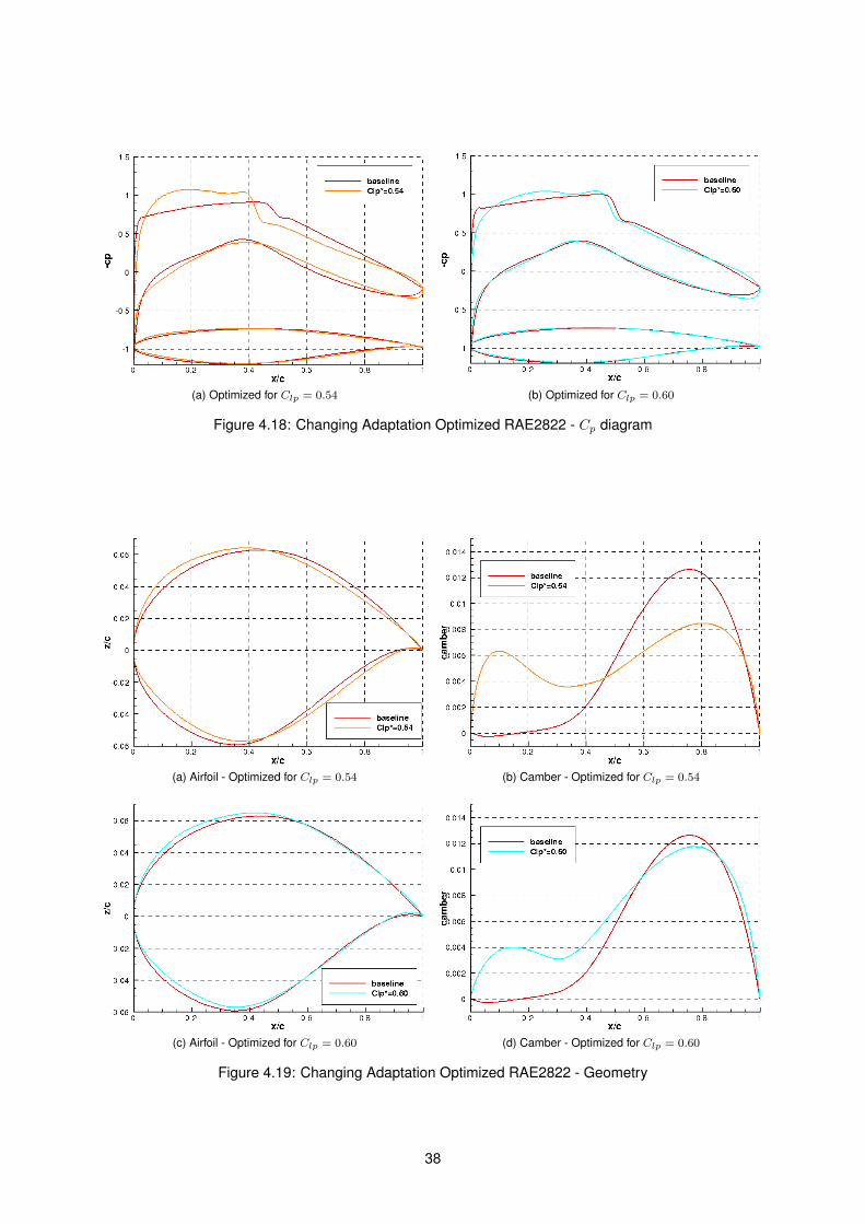
(a) Optimized for Clp = 0.54 (b) Optimized for Clp = 0.60

Figure 4.18: Changing Adaptation Optimized RAE2822 - Cp diagram

(a) Airfoil - Optimized for Clp = 0.54 (b) Camber - Optimized for Clp = 0.54

(c) Airfoil - Optimized for Clp = 0.60 (d) Camber - Optimized for Clp = 0.60

Figure 4.19: Changing Adaptation Optimized RAE2822 - Geometry

38

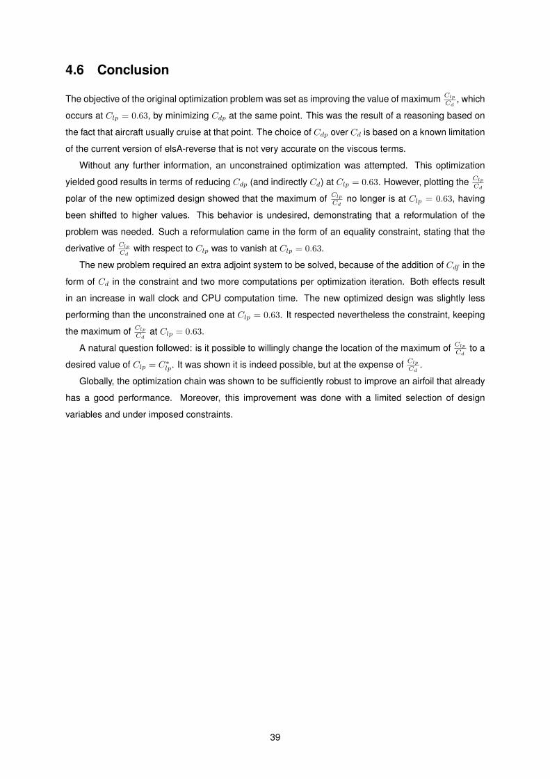
4.6 Conclusion

The objective of the original optimization problem was set as improving the value of maximum ClpCd

, which

occurs at Clp = 0.63, by minimizing Cdp at the same point. This was the result of a reasoning based on

the fact that aircraft usually cruise at that point. The choice of Cdp over Cd is based on a known limitation

of the current version of elsA-reverse that is not very accurate on the viscous terms.

Without any further information, an unconstrained optimization was attempted. This optimization

yielded good results in terms of reducing Cdp (and indirectly Cd) at Clp = 0.63. However, plotting the ClpCd

polar of the new optimized design showed that the maximum of ClpCd no longer is at Clp = 0.63, having

been shifted to higher values. This behavior is undesired, demonstrating that a reformulation of the

problem was needed. Such a reformulation came in the form of an equality constraint, stating that the

derivative of ClpCd with respect to Clp was to vanish at Clp = 0.63.

The new problem required an extra adjoint system to be solved, because of the addition of Cdf in the

form of Cd in the constraint and two more computations per optimization iteration. Both effects result

in an increase in wall clock and CPU computation time. The new optimized design was slightly less

performing than the unconstrained one at Clp = 0.63. It respected nevertheless the constraint, keeping

the maximum of ClpCd at Clp = 0.63.

A natural question followed: is it possible to willingly change the location of the maximum of ClpCd to a

desired value of Clp = C∗lp. It was shown it is indeed possible, but at the expense of ClpCd .

Globally, the optimization chain was shown to be sufficiently robust to improve an airfoil that already

has a good performance. Moreover, this improvement was done with a limited selection of design

variables and under imposed constraints.

39

40

Chapter 5

Winglet Optimization

This section deals with a long range wide-body twin-engine jet airliner designed by Airbus. The objective

is to reshape its winglet by retwist, recamber and planform redefinition.

5.1 Test Case Definition

The flight conditions are given in Tbl. 5.1.

Parameter Value

Re 5.652× 106

M 0.82

CLp 0.55

Table 5.1: Flight Conditions

5.1.1 Mesh

The mesh was generated in ANSYS ICEM and was coarsed to medium and coarse meshes. They are

composed of 1734 blocks and comprise 18187074 and 4195548 nodes, respectively. It does not include

an Horizontal Tail Plane. Optimizations will be run on the coarse mesh, in order to save on computation

time. The body surface mesh in the coarse mesh is shown in Fig. 5.1.

5.1.2 Parameterization

The winglet is defined by eight sections, called AFx, where x is the number of the section, as can be seen

in Fig. 5.2a. The first three sections are not changed, in order to assure a smooth continuity between

the wing and the winglet. The airfoils of each of the last five sections is controlled by three control points,

as can be seen in Fig. 5.2b, to which a twist angle is applied.

41

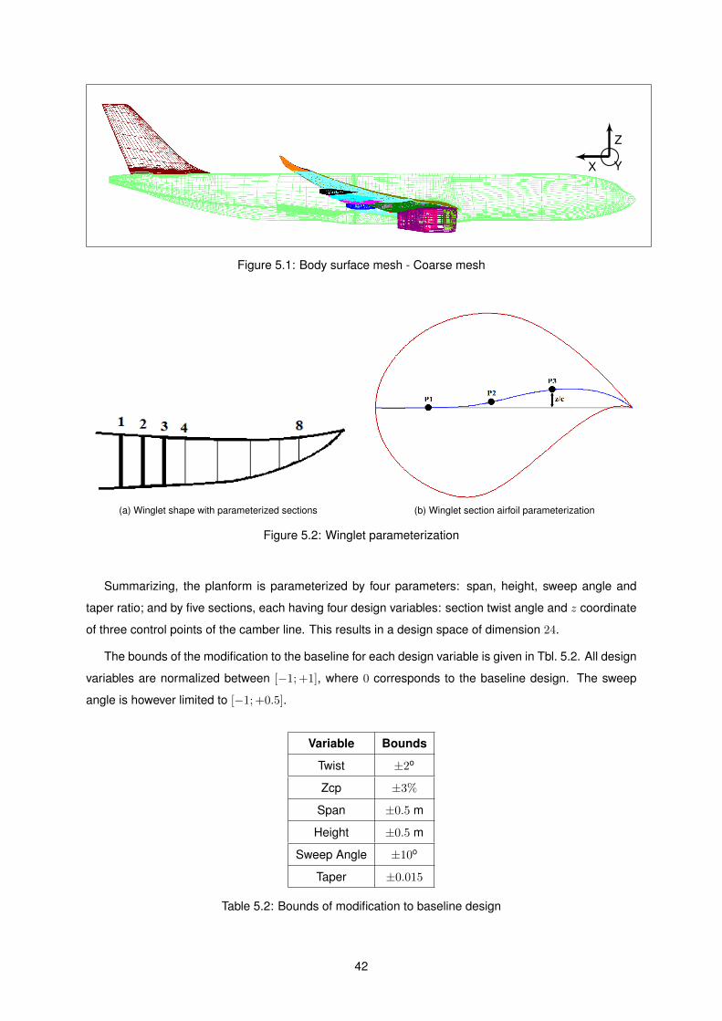
X

Z

Y

Figure 5.1: Body surface mesh - Coarse mesh

(a) Winglet shape with parameterized sections (b) Winglet section airfoil parameterization

Figure 5.2: Winglet parameterization

Summarizing, the planform is parameterized by four parameters: span, height, sweep angle and

taper ratio; and by five sections, each having four design variables: section twist angle and z coordinate

of three control points of the camber line. This results in a design space of dimension 24.

The bounds of the modification to the baseline for each design variable is given in Tbl. 5.2. All design

variables are normalized between [−1; +1], where 0 corresponds to the baseline design. The sweep

angle is however limited to [−1; +0.5].

Variable Bounds

Twist ±2o

Zcp ±3%

Span ±0.5 m

Height ±0.5 m

Sweep Angle ±10o

Taper ±0.015

Table 5.2: Bounds of modification to baseline design

42

5.1.3 Optimization Problem

The objective function of this optimization problem is the pressure drag CDp. Furthermore, a maximum

load constraint on the winglet is imposed. The problem is mathematically stated in Eq. (5.1).

minimizeD,Target Lift

CDp|CLp=0.55

subject to (CLp)winglet ≤ (CLp)maxwinglet

(5.1)

The KKT conditions for this problem are given in Eq. (5.2). Eq. (5.2b) separates in two conditions:

µ = 0 or (CLp)winglet = (CLp)maxwinglet. In the first case, Eq. (5.2a) becomes ∇CDp = 0, the optimality

condition in unconstrained problems. In the second case, the gradient of CDp must be on the opposite

direction of the gradient of (CLp)winglet at the boundary of the domain. Eq. (5.2a) is usually evaluated by

the KKT angle, that is, the angle between both gradients θ[∇CDp,∇ (CLp)winglet

].

−∇CDp = µ∇ (CLp)winglet (5.2a)

µ[(CLp)winglet − (CLp)

maxwinglet

]= 0 (5.2b)

5.2 Design of Experiments

With such complex geometry and aerodynamics, aggravated by the high number of design space di-

mensions, it is difficult to grasp a sense of the design space. Exploring the design space seems the

necessary step to begin such a complex study. The DOE comes as a natural design space exploration

method. It is a powerful tool and can be used with multiple objectives:

• Exploration of the design space

• Identification of unfeasible designs (bad combination of design variables values)

• Identifying the relation between the objective function and the constraint

• Design variable influence analysis

• Rough sense of the best design

• Seed - take a good design (arbitrary criteria) with which to start an adjoint optimization

Yet, it presents some drawbacks:

• Because the DOE doesn’t take constraints into account, if the objective is to optimize with con-

straints, many of the generated solutions might not respect the constraints

• As the number of dimensions of the design space grows larger, the required number of points to

have a significant sample grows exponentially

43

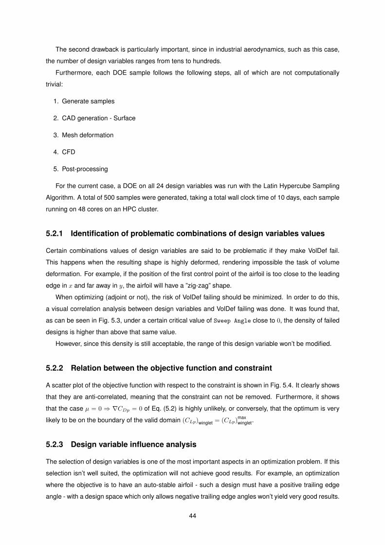
The second drawback is particularly important, since in industrial aerodynamics, such as this case,

the number of design variables ranges from tens to hundreds.

Furthermore, each DOE sample follows the following steps, all of which are not computationally

trivial:

1. Generate samples

2. CAD generation - Surface

3. Mesh deformation

4. CFD

5. Post-processing

For the current case, a DOE on all 24 design variables was run with the Latin Hypercube Sampling

Algorithm. A total of 500 samples were generated, taking a total wall clock time of 10 days, each sample

running on 48 cores on an HPC cluster.

5.2.1 Identification of problematic combinations of design variables values

Certain combinations values of design variables are said to be problematic if they make VolDef fail.

This happens when the resulting shape is highly deformed, rendering impossible the task of volume

deformation. For example, if the position of the first control point of the airfoil is too close to the leading

edge in x and far away in y, the airfoil will have a ”zig-zag” shape.

When optimizing (adjoint or not), the risk of VolDef failing should be minimized. In order to do this,

a visual correlation analysis between design variables and VolDef failing was done. It was found that,

as can be seen in Fig. 5.3, under a certain critical value of Sweep Angle close to 0, the density of failed

designs is higher than above that same value.

However, since this density is still acceptable, the range of this design variable won’t be modified.

5.2.2 Relation between the objective function and constraint

A scatter plot of the objective function with respect to the constraint is shown in Fig. 5.4. It clearly shows

that they are anti-correlated, meaning that the constraint can not be removed. Furthermore, it shows

that the case µ = 0 ⇒ ∇CDp = 0 of Eq. (5.2) is highly unlikely, or conversely, that the optimum is very

likely to be on the boundary of the valid domain (CLp)winglet = (CLp)maxwinglet.

5.2.3 Design variable influence analysis

The selection of design variables is one of the most important aspects in an optimization problem. If this

selection isn’t well suited, the optimization will not achieve good results. For example, an optimization

where the objective is to have an auto-stable airfoil - such a design must have a positive trailing edge

angle - with a design space which only allows negative trailing edge angles won’t yield very good results.

44

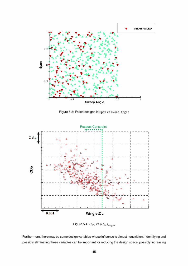
Figure 5.3: Failed designs in Span vs Sweep Angle

Respect Constraint

Figure 5.4: CDp vs (CLp)winglet

Furthermore, there may be some design variables whose influence is almost nonexistent. Identifying and

possibly eliminating these variables can be important for reducing the design space, possibly increasing

45

the convergence speed.

From the 500 samples, 377 were successfully analyzed with CFD and post-processed with a far-

field analysis. This yields the following outputs: CDp ≡ DragP, (CLp)winglet ≡ WingletCL, α ≡ AoA,

CnfD ≡ CD NF, CffD ≡ CD FF, CDw, CDi, CDvp, CDf , CDsp and CM ≡ CPitch; on which the influence

analysis is done, using the Sensitivity and Dependency Analysis tool of MACROS [24]. This tool is

composed of three sequential components:

• Checker: checks if there is a dependency between an input X and output Y (for all pairs (X,Y ))

and if it is statistically significant

• Ranker: ranks all inputs according to each input’s importance

• Selector: selects the most suitable input subset to construct an approximate model

5.2.3.1 Checker

The checker computes a correlation score and a p-value. The correlation score is a number in [−1; +1],

where 0 means that Y does not depend on X and ±1 means that Y is a deterministic function of X

(+1 if Y increases with X and −1 otherwise). p-value is the probability that a correlation was found on

the given sample while Y does not depend on X in reality. In other words, it’s the probability that the

true correlation score is (near) 0 and that the observed correlation score 6= 0 appeared by chance. The

common threshold for p-value is 5%, which is considered small enough to be sure that the correlation is

significant.

Two analysis were made, with two different correlation score functions: Pearson’s correlation score,

which can find linear dependencies; distance correlation score, which is a state-of-the-art metric and can

find any type of dependence. Fig. 5.5 shows the results of the checker analysis. There are nine inputs

marked with black rectangles, corresponding to inputs which are not correlated with any of the outputs

Tbl. 5.3. Furthermore, both linear and general correlation functions give exactly the same results, which

might indicate that for the current design space, the dependencies might be linear. The inputs in Tbl. 5.3

are eliminated and are not fed to the Ranker.

Figure 5.5: SDA Checker - Results

46

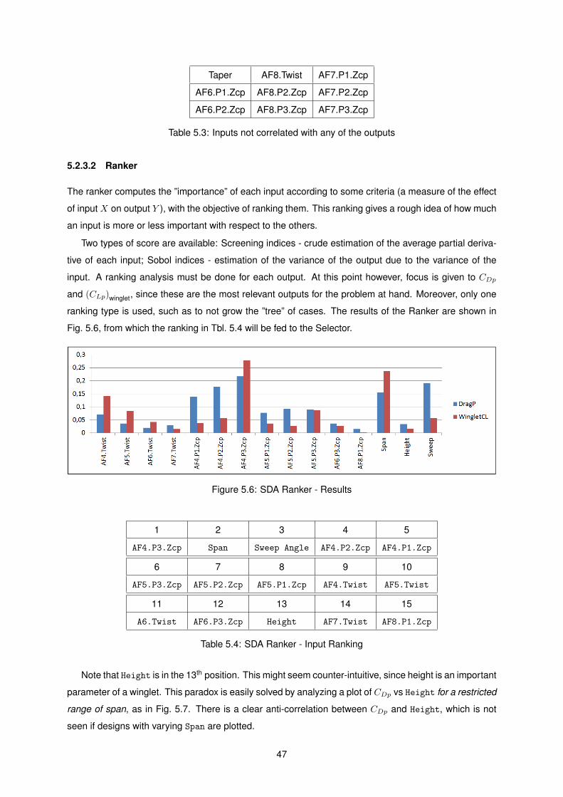
Taper AF8.Twist AF7.P1.Zcp

AF6.P1.Zcp AF8.P2.Zcp AF7.P2.Zcp

AF6.P2.Zcp AF8.P3.Zcp AF7.P3.Zcp

Table 5.3: Inputs not correlated with any of the outputs

5.2.3.2 Ranker

The ranker computes the ”importance” of each input according to some criteria (a measure of the effect

of input X on output Y ), with the objective of ranking them. This ranking gives a rough idea of how much

an input is more or less important with respect to the others.

Two types of score are available: Screening indices - crude estimation of the average partial deriva-

tive of each input; Sobol indices - estimation of the variance of the output due to the variance of the

input. A ranking analysis must be done for each output. At this point however, focus is given to CDp

and (CLp)winglet, since these are the most relevant outputs for the problem at hand. Moreover, only one

ranking type is used, such as to not grow the ”tree” of cases. The results of the Ranker are shown in

Fig. 5.6, from which the ranking in Tbl. 5.4 will be fed to the Selector.

Figure 5.6: SDA Ranker - Results

1 2 3 4 5

AF4.P3.Zcp Span Sweep Angle AF4.P2.Zcp AF4.P1.Zcp

6 7 8 9 10

AF5.P3.Zcp AF5.P2.Zcp AF5.P1.Zcp AF4.Twist AF5.Twist

11 12 13 14 15

A6.Twist AF6.P3.Zcp Height AF7.Twist AF8.P1.Zcp

Table 5.4: SDA Ranker - Input Ranking

Note that Height is in the 13th position. This might seem counter-intuitive, since height is an important

parameter of a winglet. This paradox is easily solved by analyzing a plot of CDp vs Height for a restricted

range of span, as in Fig. 5.7. There is a clear anti-correlation between CDp and Height, which is not

seen if designs with varying Span are plotted.

47

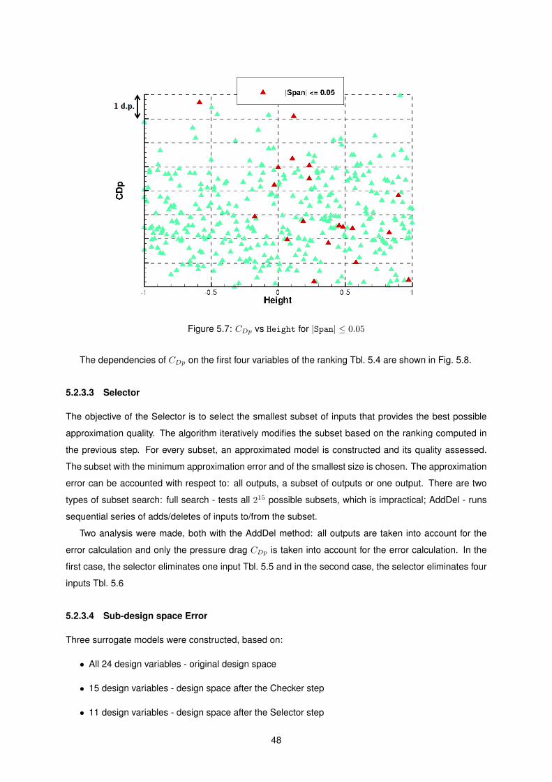
Figure 5.7: CDp vs Height for |Span| ≤ 0.05

The dependencies of CDp on the first four variables of the ranking Tbl. 5.4 are shown in Fig. 5.8.

5.2.3.3 Selector

The objective of the Selector is to select the smallest subset of inputs that provides the best possible

approximation quality. The algorithm iteratively modifies the subset based on the ranking computed in

the previous step. For every subset, an approximated model is constructed and its quality assessed.

The subset with the minimum approximation error and of the smallest size is chosen. The approximation

error can be accounted with respect to: all outputs, a subset of outputs or one output. There are two

types of subset search: full search - tests all 215 possible subsets, which is impractical; AddDel - runs

sequential series of adds/deletes of inputs to/from the subset.

Two analysis were made, both with the AddDel method: all outputs are taken into account for the

error calculation and only the pressure drag CDp is taken into account for the error calculation. In the

first case, the selector eliminates one input Tbl. 5.5 and in the second case, the selector eliminates four

inputs Tbl. 5.6

5.2.3.4 Sub-design space Error

Three surrogate models were constructed, based on:

• All 24 design variables - original design space

• 15 design variables - design space after the Checker step

• 11 design variables - design space after the Selector step

48

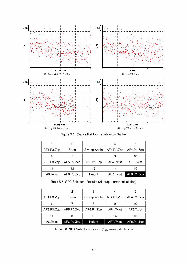
(a) CDp vs AF4.P3.Zcp (b) CDp vs Span

(c) CDp vs Sweep Angle (d) CDp vs AF4.P2.Zcp

Figure 5.8: CDp vs first four variables by Ranker

1 2 3 4 5

AF4.P3.Zcp Span Sweep Angle AF4.P2.Zcp AF4.P1.Zcp

6 7 8 9 10

AF5.P3.Zcp AF5.P2.Zcp AF5.P1.Zcp AF4.Twist AF5.Twist

11 12 13 14 15

A6.Twist AF6.P3.Zcp Height AF7.Twist AF8.P1.Zcp

Table 5.5: SDA Selector - Results (All-output error calculation)

1 2 3 4 5

AF4.P3.Zcp Span Sweep Angle AF4.P2.Zcp AF4.P1.Zcp

6 7 8 9 10

AF5.P3.Zcp AF5.P2.Zcp AF5.P1.Zcp AF4.Twist AF5.Twist

11 12 13 14 15

A6.Twist AF6.P3.Zcp Height AF7.Twist AF8.P1.Zcp

Table 5.6: SDA Selector - Results (CDp error calculation)

49

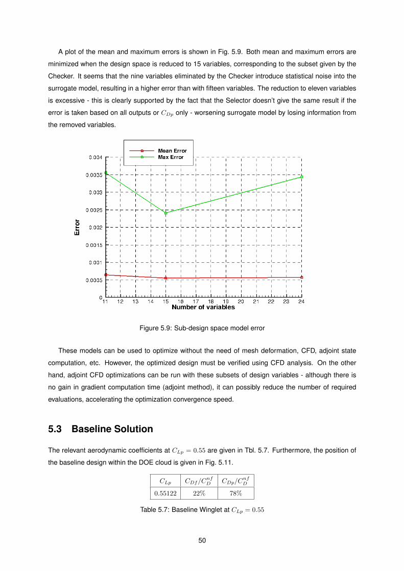
A plot of the mean and maximum errors is shown in Fig. 5.9. Both mean and maximum errors are

minimized when the design space is reduced to 15 variables, corresponding to the subset given by the

Checker. It seems that the nine variables eliminated by the Checker introduce statistical noise into the

surrogate model, resulting in a higher error than with fifteen variables. The reduction to eleven variables

is excessive - this is clearly supported by the fact that the Selector doesn’t give the same result if the

error is taken based on all outputs or CDp only - worsening surrogate model by losing information from

the removed variables.

Figure 5.9: Sub-design space model error

These models can be used to optimize without the need of mesh deformation, CFD, adjoint state

computation, etc. However, the optimized design must be verified using CFD analysis. On the other

hand, adjoint CFD optimizations can be run with these subsets of design variables - although there is

no gain in gradient computation time (adjoint method), it can possibly reduce the number of required

evaluations, accelerating the optimization convergence speed.

5.3 Baseline Solution

The relevant aerodynamic coefficients at CLp = 0.55 are given in Tbl. 5.7. Furthermore, the position of

the baseline design within the DOE cloud is given in Fig. 5.11.

CLp CDf/CnfD CDp/C

nfD

0.55122 22% 78%

Table 5.7: Baseline Winglet at CLp = 0.55

50

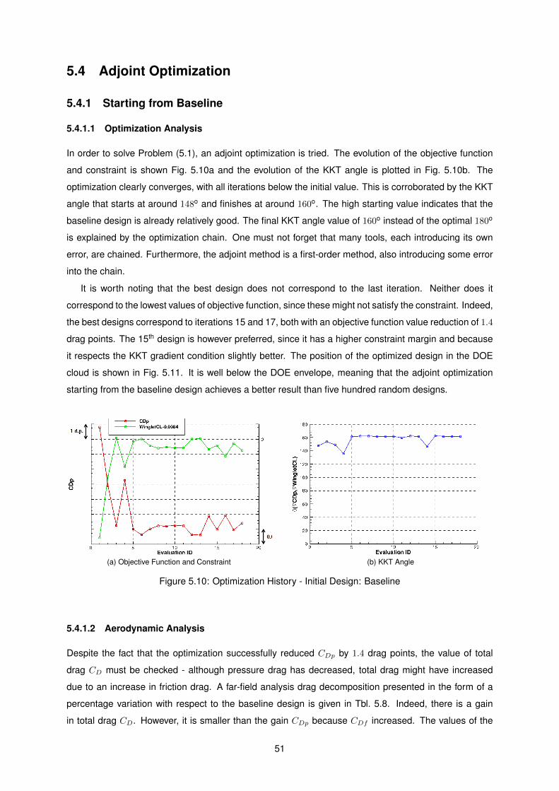
5.4 Adjoint Optimization

5.4.1 Starting from Baseline

5.4.1.1 Optimization Analysis

In order to solve Problem (5.1), an adjoint optimization is tried. The evolution of the objective function

and constraint is shown Fig. 5.10a and the evolution of the KKT angle is plotted in Fig. 5.10b. The

optimization clearly converges, with all iterations below the initial value. This is corroborated by the KKT

angle that starts at around 148o and finishes at around 160o. The high starting value indicates that the

baseline design is already relatively good. The final KKT angle value of 160o instead of the optimal 180o

is explained by the optimization chain. One must not forget that many tools, each introducing its own

error, are chained. Furthermore, the adjoint method is a first-order method, also introducing some error

into the chain.

It is worth noting that the best design does not correspond to the last iteration. Neither does it

correspond to the lowest values of objective function, since these might not satisfy the constraint. Indeed,

the best designs correspond to iterations 15 and 17, both with an objective function value reduction of 1.4

drag points. The 15th design is however preferred, since it has a higher constraint margin and because

it respects the KKT gradient condition slightly better. The position of the optimized design in the DOE

cloud is shown in Fig. 5.11. It is well below the DOE envelope, meaning that the adjoint optimization

starting from the baseline design achieves a better result than five hundred random designs.

(a) Objective Function and Constraint (b) KKT Angle

Figure 5.10: Optimization History - Initial Design: Baseline

5.4.1.2 Aerodynamic Analysis

Despite the fact that the optimization successfully reduced CDp by 1.4 drag points, the value of total

drag CD must be checked - although pressure drag has decreased, total drag might have increased

due to an increase in friction drag. A far-field analysis drag decomposition presented in the form of a

percentage variation with respect to the baseline design is given in Tbl. 5.8. Indeed, there is a gain

in total drag CD. However, it is smaller than the gain CDp because CDf increased. The values of the

51

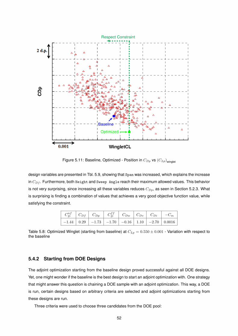
Respect Constraint

Baseline

Optimized

Figure 5.11: Baseline, Optimized - Position in CDp vs (CLp)winglet

design variables are presented in Tbl. 5.9, showing that Span was increased, which explains the increase

in CDf . Furthermore, both Height and Sweep Angle reach their maximum allowed values. This behavior

is not very surprising, since increasing all these variables reduces CDp, as seen in Section 5.2.3. What

is surprising is finding a combination of values that achieves a very good objective function value, while

satisfying the constraint.

CnfD CDf CDp CffD CDw CDv CDi −Cm−1.44 0.29 −1.73 −1.70 −0.16 1.10 −2.70 0.0016

Table 5.8: Optimized Winglet (starting from baseline) at CLp = 0.550 ± 0.001 - Variation with respect tothe baseline

5.4.2 Starting from DOE Designs

The adjoint optimization starting from the baseline design proved successful against all DOE designs.

Yet, one might wonder if the baseline is the best design to start an adjoint optimization with. One strategy

that might answer this question is chaining a DOE sample with an adjoint optimization. This way, a DOE

is run, certain designs based on arbitrary criteria are selected and adjoint optimizations starting from

these designs are run.

Three criteria were used to choose three candidates from the DOE pool:

52

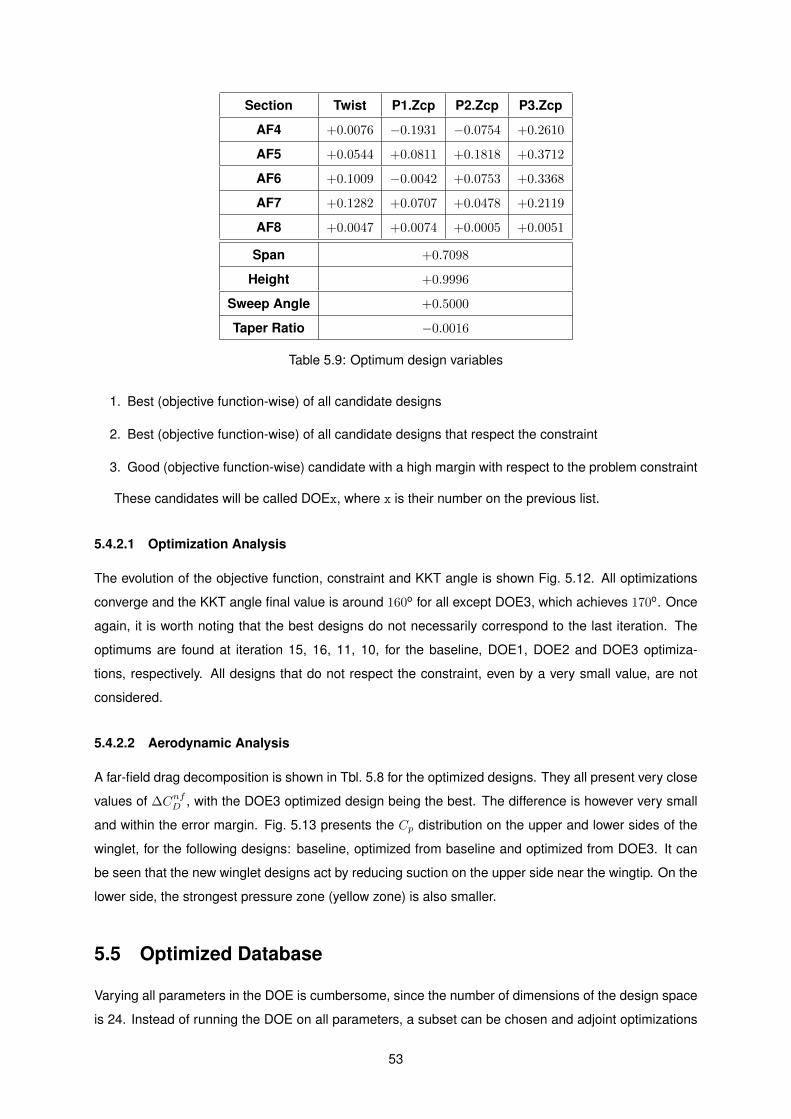
Section Twist P1.Zcp P2.Zcp P3.Zcp

AF4 +0.0076 −0.1931 −0.0754 +0.2610

AF5 +0.0544 +0.0811 +0.1818 +0.3712

AF6 +0.1009 −0.0042 +0.0753 +0.3368

AF7 +0.1282 +0.0707 +0.0478 +0.2119

AF8 +0.0047 +0.0074 +0.0005 +0.0051

Span +0.7098

Height +0.9996

Sweep Angle +0.5000

Taper Ratio −0.0016

Table 5.9: Optimum design variables

1. Best (objective function-wise) of all candidate designs

2. Best (objective function-wise) of all candidate designs that respect the constraint

3. Good (objective function-wise) candidate with a high margin with respect to the problem constraint

These candidates will be called DOEx, where x is their number on the previous list.

5.4.2.1 Optimization Analysis

The evolution of the objective function, constraint and KKT angle is shown Fig. 5.12. All optimizations

converge and the KKT angle final value is around 160o for all except DOE3, which achieves 170o. Once

again, it is worth noting that the best designs do not necessarily correspond to the last iteration. The

optimums are found at iteration 15, 16, 11, 10, for the baseline, DOE1, DOE2 and DOE3 optimiza-

tions, respectively. All designs that do not respect the constraint, even by a very small value, are not

considered.

5.4.2.2 Aerodynamic Analysis

A far-field drag decomposition is shown in Tbl. 5.8 for the optimized designs. They all present very close

values of ∆CnfD , with the DOE3 optimized design being the best. The difference is however very small

and within the error margin. Fig. 5.13 presents the Cp distribution on the upper and lower sides of the

winglet, for the following designs: baseline, optimized from baseline and optimized from DOE3. It can

be seen that the new winglet designs act by reducing suction on the upper side near the wingtip. On the

lower side, the strongest pressure zone (yellow zone) is also smaller.

5.5 Optimized Database

Varying all parameters in the DOE is cumbersome, since the number of dimensions of the design space

is 24. Instead of running the DOE on all parameters, a subset can be chosen and adjoint optimizations

53

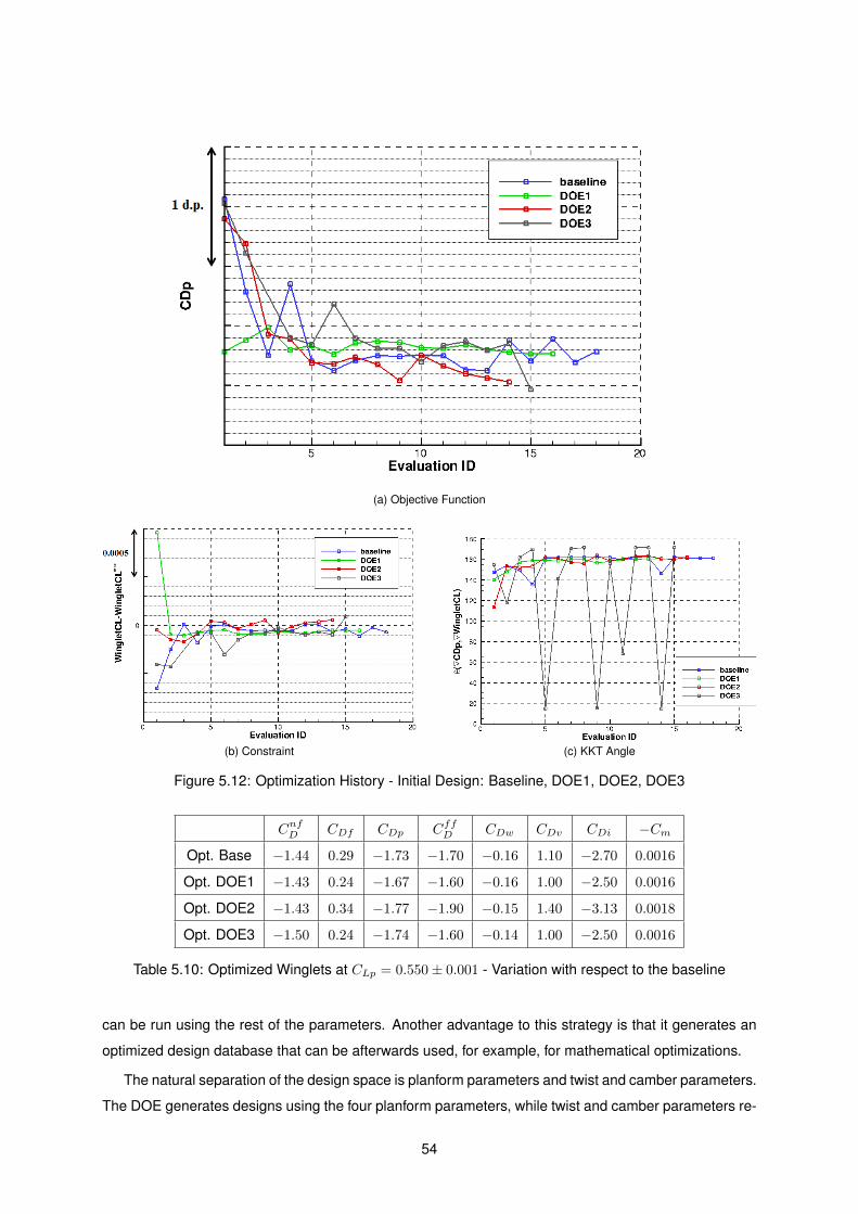
(a) Objective Function

(b) Constraint (c) KKT Angle

Figure 5.12: Optimization History - Initial Design: Baseline, DOE1, DOE2, DOE3

CnfD CDf CDp CffD CDw CDv CDi −CmOpt. Base −1.44 0.29 −1.73 −1.70 −0.16 1.10 −2.70 0.0016

Opt. DOE1 −1.43 0.24 −1.67 −1.60 −0.16 1.00 −2.50 0.0016

Opt. DOE2 −1.43 0.34 −1.77 −1.90 −0.15 1.40 −3.13 0.0018

Opt. DOE3 −1.50 0.24 −1.74 −1.60 −0.14 1.00 −2.50 0.0016

Table 5.10: Optimized Winglets at CLp = 0.550± 0.001 - Variation with respect to the baseline

can be run using the rest of the parameters. Another advantage to this strategy is that it generates an

optimized design database that can be afterwards used, for example, for mathematical optimizations.

The natural separation of the design space is planform parameters and twist and camber parameters.

The DOE generates designs using the four planform parameters, while twist and camber parameters re-

54

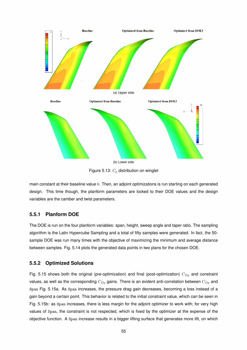
(a) Upper side

(b) Lower side

Figure 5.13: Cp distribution on winglet

main constant at their baseline value 0. Then, an adjoint optimizations is run starting on each generated

design. This time though, the planform parameters are locked to their DOE values and the design

variables are the camber and twist parameters.

5.5.1 Planform DOE

The DOE is run on the four planform variables: span, height, sweep angle and taper ratio. The sampling

algorithm is the Latin Hypercube Sampling and a total of fifty samples were generated. In fact, the 50-

sample DOE was run many times with the objective of maximizing the minimum and average distance

between samples. Fig. 5.14 plots the generated data points in two plans for the chosen DOE.

5.5.2 Optimized Solutions

Fig. 5.15 shows both the original (pre-optimization) and final (post-optimization) CDp and constraint

values, as well as the corresponding CDp gains. There is an evident anti-correlation between CDp and

Span Fig. 5.15a. As Span increases, the pressure drag gain decreases, becoming a loss instead of a

gain beyond a certain point. This behavior is related to the initial constraint value, which can be seen in

Fig. 5.15b: as Span increases, there is less margin for the adjoint optimizer to work with; for very high

values of Span, the constraint is not respected, which is fixed by the optimizer at the expense of the

objective function. A Span increase results in a bigger lifting surface that generates more lift, on which

55

(a) Height vs Span (b) Taper Ratio vs Sweep Angle

Figure 5.14: Planform DOE - 50 samples

the constraint imposes a limit. CDp is also anti-correlated with Height. However, this anti-correlation is

much weaker than in the previous case. Furthermore, the pressure drag gain is uniformly distributed, as

well as the initial constraint value. Sweep Angle presents the stronger anti-correlation with CDp of all four

planform variables. However and contrarily to Span, the gain obtained by retwisting and recambering is

not dependent on Sweep Angle, which is a direct consequence of the fact that Sweep Angle does not

influence the constraint. Taper is the least interesting of these parameters. There is no variable with a

particular dependence on it, confirming the sensitivity analysis in Section 5.2.3.

Finally, three designs are seen to be close to a 1.4 gain of CDp. However, their CDp values are slightly

higher than the previous optimized designs’.

5.6 Conclusion

This problem involved the redesign of the winglet of long range airliner designed by Airbus. This redesign

was limited to changes in planform, retwist and recamber, while the objective was to minimize drag

pressure, under a maximum load constraint.

Since the winglet is a complex shape, which forcibly results in complex aerodynamics, the behavior

of the design space is not trivial. To understand it and to assess the importance of each design vari-

able, a DOE was run on all parameters. The results of which were then analyzed, drawing important

conclusions, such as the link between objective function and constraint, explicitly demonstrating that the

maximum load constraint could not be removed. Furthermore, a sensitivity and dependency analysis

was executed based on the designs generated by the DOE. This analysis allowed the determination

of design variables that don’t have correlation with any of the outputs and supplied a ranking of the

remaining variables according to their individual importance.

An adjoint optimization was run starting from the baseline design, resulting in a considerable reduc-

tion of 1.4 drag points. The optimized design validated the previous analysis on the importance of each

design variable - the most relevant variables were at (or near) their extreme values.

Although starting an adjoint optimization from the baseline design resulted in a good Cdp reduction,

56

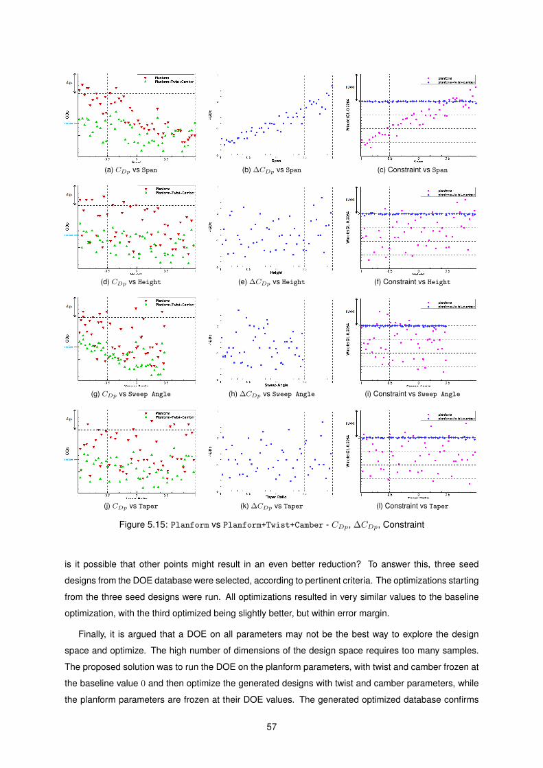
(a) CDp vs Span (b) ∆CDp vs Span (c) Constraint vs Span

(d) CDp vs Height (e) ∆CDp vs Height (f) Constraint vs Height

(g) CDp vs Sweep Angle (h) ∆CDp vs Sweep Angle (i) Constraint vs Sweep Angle

(j) CDp vs Taper (k) ∆CDp vs Taper (l) Constraint vs Taper

Figure 5.15: Planform vs Planform+Twist+Camber - CDp, ∆CDp, Constraint

is it possible that other points might result in an even better reduction? To answer this, three seed

designs from the DOE database were selected, according to pertinent criteria. The optimizations starting

from the three seed designs were run. All optimizations resulted in very similar values to the baseline

optimization, with the third optimized being slightly better, but within error margin.

Finally, it is argued that a DOE on all parameters may not be the best way to explore the design

space and optimize. The high number of dimensions of the design space requires too many samples.

The proposed solution was to run the DOE on the planform parameters, with twist and camber frozen at

the baseline value 0 and then optimize the generated designs with twist and camber parameters, while

the planform parameters are frozen at their DOE values. The generated optimized database confirms

57

the results from the sensitivity and dependency analysis and from the previous optimizations. This

strategy didn’t produce the best design, though it did generate designs whose performances are close

to that of the previous optimized designs.

Globally, the robustness of the adjoint optimization method for the current case was demonstrated.

In cases where the starting design does not respect the constraint, the optimizer successfully produces

a design that respects the constraint at the expense of the objective function. In cases where the

starting design did respect the constraint, the design was successively driven towards the boundary of

the constraint, which is in agreement with the optimality conditions. Furthermore, the adjoint optimization

alone starting from the baseline design produced a solution of the same or better quality than most of

the optimized designs obtained by chaining a DOE with an adjoint optimization.

58

Chapter 6

Conclusion

The developed work was centered around the subject of aerodynamic optimization in an industrial con-

text. More specifically, multiple strategies based on the adjoint method for gradient computation were

employed in two test cases: two-dimensional transonic airfoil and winglet of a long range Airbus aircraft.

The merits and robustness of the gradient-based optimization with gradient computed by the adjoint

method were demonstrated:

• The optimizations converged to better designs (in terms of objective function) that satisfy (to some

error margin) the problem’s optimality conditions.

• The optimization process handled well both equality and inequality constraints

Regarding the two-dimensional case, the optimization problem was defined and an unconstrained

optimization was run to solve it. The resulting design improved the objective function. However, it didn’t

have the desired global behavior, since it shifted the maximum of ClpCd to a higher value of Clp . This was

fixed by adding a constraint to the optimization problem. This constrained optimization also achieved an

improvement of the objective function of 3.60%, though smaller than the unconstrained optimization one.

Nevertheless, it showed the desired global behavior of maintaining the maximum of ClpCd at the baseline’s

maximum location of Clp = 0.63. Finally, it was shown that the location of the maximum of ClpCd

could

willingly be changed to a desired value of Clp = C∗lp < 0.63 at the expense ClpCd

.

Based on the knowledge acquired from the two-dimensional case, focus was shifted to the three-

dimensional case of the long range airliner winglet. Here, there is an increase of complexity in shape

and aerodynamics, especially highlighted by the difficulty of predicting the performance behavior with

respect to the design variables, apart from particular cases. In order to address this problem, the DOE

technique was introduced and executed. It rendered possible an analysis of sensitivity and dependency.

This analysis allowed the determination of design variables that don’t have correlation with any of the

outputs and supplied a ranking of the remaining variables according to their individual importance. Mul-

tiple strategies were employed: pure adjoint optimization starting from the baseline design and adjoint

optimization starting from three DOE designs. All four optimizations converged, resulting in very close

values, demonstrating the effectiveness of the adjoint optimization alone as a sufficient optimization pro-

cess. The hybrid strategy of chaining a DOE with adjoints optimizations was reformulated. This time,

59

the DOE only changed the planform, while the adjoint optimization only worked with twist and cam-

ber parameters. This strategy didn’t produce the best design, though it did generate designs whose

performances are close to that of the previous optimized designs.

Aerodynamic optimization methods, within an industrial framework such as Airbus, were employed

with success to the optimization of real-life cases. Moreover, results which are not trivial were found and

important conclusions drawn upon. Aerodynamic optimization is a relatively young subject and Airbus

demonstrates its presence in the front edge of this discipline.

6.1 Future Work

The two-dimensional study could be redone with another parameterization, for example, by adding an-

other point of control to the camber line. Furthermore, instead of an equality constraint, an inequality

constraint, such as |fleft − fright| ≤ ε allowing a tolerance ε could be introduced. This could potentially

ease the task of the optimizer since the constraint is not as strict as before, while still achieving the

desired result.

The three-dimensional study produced some interesting possibilities that were not studied due to

the extensiveness of the work, such as: mathematical optimization on surrogate models with CFD val-

idation and adjoint optimization on the reduced subset of variables. It would be extremely important if

it were verified, for example, that the surrogate models perform as well as (or better than) the adjoint

optimizations.

60

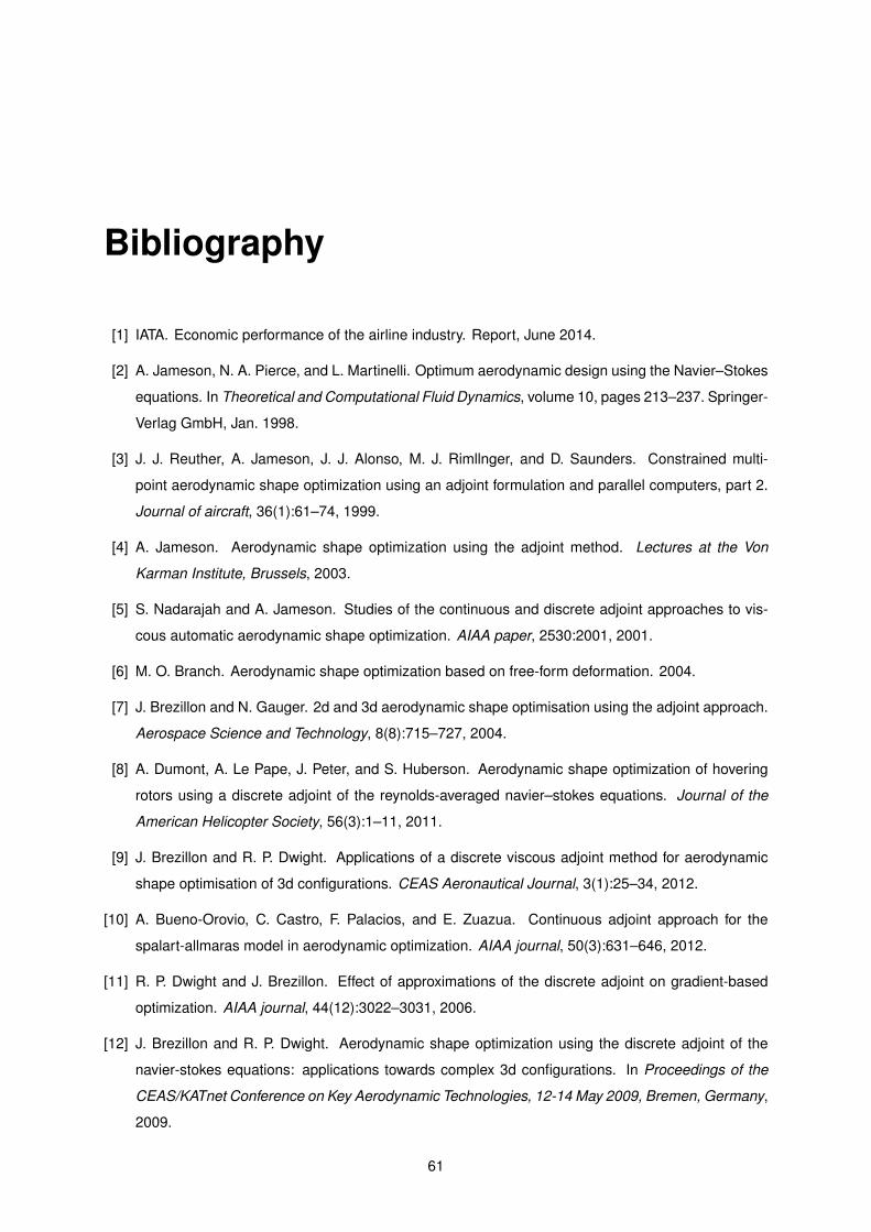
Bibliography

[1] IATA. Economic performance of the airline industry. Report, June 2014.

[2] A. Jameson, N. A. Pierce, and L. Martinelli. Optimum aerodynamic design using the Navier–Stokes

equations. In Theoretical and Computational Fluid Dynamics, volume 10, pages 213–237. Springer-

Verlag GmbH, Jan. 1998.

[3] J. J. Reuther, A. Jameson, J. J. Alonso, M. J. Rimllnger, and D. Saunders. Constrained multi-

point aerodynamic shape optimization using an adjoint formulation and parallel computers, part 2.

Journal of aircraft, 36(1):61–74, 1999.

[4] A. Jameson. Aerodynamic shape optimization using the adjoint method. Lectures at the Von

Karman Institute, Brussels, 2003.

[5] S. Nadarajah and A. Jameson. Studies of the continuous and discrete adjoint approaches to vis-

cous automatic aerodynamic shape optimization. AIAA paper, 2530:2001, 2001.

[6] M. O. Branch. Aerodynamic shape optimization based on free-form deformation. 2004.

[7] J. Brezillon and N. Gauger. 2d and 3d aerodynamic shape optimisation using the adjoint approach.

Aerospace Science and Technology, 8(8):715–727, 2004.

[8] A. Dumont, A. Le Pape, J. Peter, and S. Huberson. Aerodynamic shape optimization of hovering

rotors using a discrete adjoint of the reynolds-averaged navier–stokes equations. Journal of the

American Helicopter Society, 56(3):1–11, 2011.

[9] J. Brezillon and R. P. Dwight. Applications of a discrete viscous adjoint method for aerodynamic

shape optimisation of 3d configurations. CEAS Aeronautical Journal, 3(1):25–34, 2012.

[10] A. Bueno-Orovio, C. Castro, F. Palacios, and E. Zuazua. Continuous adjoint approach for the

spalart-allmaras model in aerodynamic optimization. AIAA journal, 50(3):631–646, 2012.

[11] R. P. Dwight and J. Brezillon. Effect of approximations of the discrete adjoint on gradient-based

optimization. AIAA journal, 44(12):3022–3031, 2006.

[12] J. Brezillon and R. P. Dwight. Aerodynamic shape optimization using the discrete adjoint of the

navier-stokes equations: applications towards complex 3d configurations. In Proceedings of the

CEAS/KATnet Conference on Key Aerodynamic Technologies, 12-14 May 2009, Bremen, Germany,

2009.

61

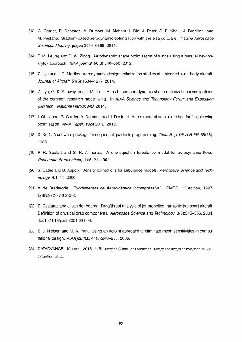
[13] G. Carrier, D. Destarac, A. Dumont, M. Meheut, I. Din, J. Peter, S. B. Khelil, J. Brezillon, and

M. Pestana. Gradient-based aerodynamic optimization with the elsa software. In 52nd Aerospace

Sciences Meeting, pages 2014–0568, 2014.

[14] T. M. Leung and D. W. Zingg. Aerodynamic shape optimization of wings using a parallel newton-

krylov approach. AIAA journal, 50(3):540–550, 2012.

[15] Z. Lyu and J. R. Martins. Aerodynamic design optimization studies of a blended-wing-body aircraft.

Journal of Aircraft, 51(5):1604–1617, 2014.

[16] Z. Lyu, G. K. Kenway, and J. Martins. Rans-based aerodynamic shape optimization investigations

of the common research model wing. In AIAA Science and Technology Forum and Exposition

(SciTech), National Harbor, MD, 2014.

[17] I. Ghazlane, G. Carrier, A. Dumont, and J. Desideri. Aerostructural adjoint method for flexible wing

optimization. AIAA Paper, 1924:2012, 2012.

[18] D. Kraft. A software package for sequential quadratic programming. Tech. Rep. DFVLR-FB, 88(28),

1985.

[19] P. R. Spalart and S. R. Allmaras. A one-equation turbulence model for aerodynamic flows.

Recherche Aerospatiale, (1):5–21, 1994.

[20] S. Catris and B. Aupoix. Density corrections for turbulence models. Aerospace Science and Tech-

nology, 4:1–11, 2000.

[21] V. de Brederode. Fundamentos de Aerodinamica Incompressıvel. IDMEC, 1st edition, 1997.

ISBN:972-97402-0-8.

[22] D. Destarac and J. van der Vooren. Drag/thrust analysis of jet-propelled transonic transport aircraft:

Definition of physical drag components. Aerospace Science and Technology, 8(6):545–556, 2004.

doi:10.1016/j.ast.2004.03.004.

[23] E. J. Nielsen and M. A. Park. Using an adjoint approach to eliminate mesh sensitivities in compu-

tational design. AIAA journal, 44(5):948–953, 2006.

[24] DATADVANCE. Macros, 2015. URL https://www.datadvance.net/product/macros/manual/5.

2/index.html.

62