Applications of Adjoint Methods for Applications of Adjoint Methods for Aerodynamic Shape OptimizationAerodynamic Shape Optimization

Arron Melvin

Adviser: Luigi Martinelli

Princeton University

FAA/NASA Joint University Program for Air Transportation

Quarterly Review

MIT

October 23, 2003

OutlineOutline

Progress Report / Review 3D Design Code for Unstructured Grids

Application of Adjoint Method to Rotating Geometry Penn State ARL (James Dreyer) - Princeton

University collaboration Hydrodynamic Propulsors

Summary

Adjoint Based Shape Optimization Adjoint Based Shape Optimization for Unstructured Gridsfor Unstructured Grids

Control Theory Approach as used on structured grids

Challenge in computation of the gradient for unstructured grids Reduced gradient formulation Gradient is derived solely from the adjoint solution and

the surface displacement, independent of the mesh modification

Methods to impose thickness constraints Cutting planes at span-wise locations & transformations

MotivationMotivation

Historical Propulsor Design Methodology – “cut & try”

Parametric

DesignDrafting

Model Design / Assembly

WT / TT Test

Interpretation

Detailed Design O(1y)

MotivationMotivation

Current Propulsor Design Methodology – “virtual cut & try”

Parametric

DesignCAD

Simulation

(AXI / 3D RANS)

Interpretation

Detailed Design O(1-2m)

Model Design / Assembly

WT / TT Test

Interpretation

Verification

BackgroundBackground

Focus of gradient-based approaches has been on the efficient determination of the cost function gradient b TI

Finite Difference

(work ~ ND )

Sensitivity Analysis( introduce R(w,F)=0 )

Continuous

DirectDifferentiation

(work ~ ND )

AdjointVariable

(work ~ Nh+1)

Discrete

DirectDifferentiation

AdjointVariable

(work ~ Nh+1 )

ii b

FwIFFwwI

b

I

),(),(

ii bb

Rw

w

R ˆˆ

ˆ

ˆ

wψ

w

Rˆ

ˆˆ

ˆ

IT

TTTTT Jt

J Dψ

Cψ

Bψ

Aψ

P

ComplexVariables

AutomaticDifferentiation

ApproachApproach

Shape Optimization of Propulsors

Shape Optimization

for

Detailed Design

High-fidelity

flow models

Large ND

Gradient-based

Adjoint Variable

discrete continuous

Flow & Adjoint SolversFlow & Adjoint Solvers

Cell-centered finite volume on hexahedra Central difference + scalar, 0(3) artificial dissipation Jameson-type Hybrid Multistage Scheme (5-3) Local time-stepping, multigrid (W) Domain decomposition / MPI Baldwin-Lomax algebraic eddy viscosity

SAME algorithm applied to Adjoint equations

Surface mesh point movement in the direction of the local quasi-normal vector, i.e.,

Design VariablesDesign Variables

tbxs

Shape OptimizationShape Optimization

Gradient-based approaches:

Steepest Descent: Relatively tolerant of errors in the gradient Partially-converged flow & adjoint solutions NO univariate searches

Conjugate Gradient & Quasi-Newton Very accurate gradient

Fully-converged flow & adjoint solutions One-dimensional minimization

O(4) fully-converged flow solutions

kkk db

kk Gd

Shape OptimizationShape OptimizationFlow ChartFlow Chart

Single-point design:

Flow Field SolutionFlow Field Solution

Adjoint B.C.sAdjoint B.C.s

Adjoint Field SolutionAdjoint Field Solution

Gradient CalculationGradient Calculation

Blade Shape ChangeBlade Shape Change

Domain Re-meshingDomain Re-meshing Final DesignFinal Design

NDES

ApplicationApplication

Marine propulsor / pumpblade shape optimization

Cost Function: Inverse Design

,2

2

1 dSppIbB d

pressuretargetpd HIREPHIREP

Bi

P

B1e

B2e

W

Bc

Bh

Bb

P

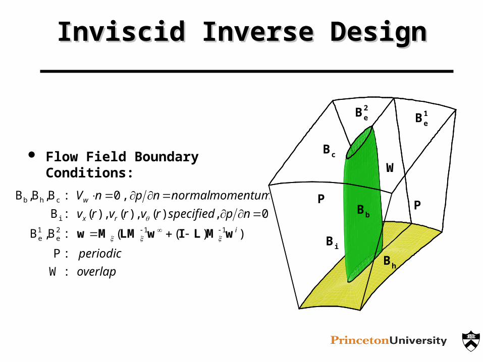
Inviscid Inverse DesignInviscid Inverse Design

Flow Field Boundary Conditions:

overlap

periodic

npspecifiedrvrvrv

momentumnormalnpnV

i

rx

w

:

:

))((:

0,)(,)(,)(:

,0:

11

W

P

B,B

B

B,B,B

2e

1e

i

chb

wMLIwLMΜw

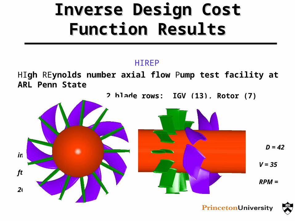
HIREPHIgh REynolds number axial flow Pump test facility at ARL Penn State

2 blade rows: IGV (13), Rotor (7)

D = 42 in.

V = 35 ft/sec

RPM = 260

Inverse Design Cost Function Inverse Design Cost Function ResultsResults

Inviscid ResultsInviscid Results

Inlet Guide Vane (IGV) & Rotor

Governing equations:3D incompressible Euler

Initial blade:NACA 0012 sections

Geometric constraint:Fixed chord line

Target pressure distributions:Separate simulations ofHIREP IGV & rotor

x / RH

Cp

-0.25 0 0.25-1.0

-0.5

0.0

0.5

1.0

ROOT

x / RH

Cp

-0.25 0 0.25

-1.0

-0.5

0.0

0.5

1.0

MID-SPAN

x / RH

Cp

-0.25 0 0.25

-0.5

0.0

0.5

1.0

targetinitialdesignTIP

Inviscid Results - IGVInviscid Results - IGV

ND-CYC

I

I rm

s

0 50 100 150 200 250 30010-6

10-5

10-4

10-3

10-2

10-1

100

10-6

10-5

10-4

10-3

10-2

10-1

100

IIrms

IGV

IGV Inverse Design(no rotation)

ND = 6321

x / RH

y/R

H

-0.6 -0.5 -0.4 -0.3 -0.2 -0.1 0.0

0.0

0.1

0.2

ROOT

x / RH

y/R

H

-0.6 -0.5 -0.4 -0.3 -0.2 -0.1 0.0

-0.1

0.0

0.1TIP

x / RH

y/R

H

-0.6 -0.5 -0.4 -0.3 -0.2 -0.1 0.0

0.0

0.1

0.2

targetinitialdesignMID-SPAN

Inviscid Results - IGVInviscid Results - IGV

DESIGN

INITIAL MID-SPAN

0.4

0.2

0.0

-0.2

-0.4

-0.6

TARGET

Cp

Inviscid Results - RotorInviscid Results - Rotor

Rotor Inverse Design(260 RPM)

ND = 6321

ND-CYC

I

I rm

s

0 50 100 150 200 250 30010-6

10-5

10-4

10-3

10-2

10-1

100

10-6

10-5

10-4

10-3

10-2

10-1

100

IIrms

ROTOR x / RH

Cp

-0.25 0 0.25

-2.0

-1.5

-1.0

-0.5

0.0

0.5

1.0

1.5

ROOT

x / RH

Cp

-0.25 0 0.25-4.5-4.0-3.5-3.0-2.5-2.0-1.5-1.0-0.50.00.51.01.52.0

targetinitialdesignTIP

x / RH

Cp

-0.25 0 0.25-2.5

-2.0

-1.5

-1.0

-0.5

0.0

0.5

1.0

1.5

MID-SPAN

Inviscid Results – Rotor DetailInviscid Results – Rotor Detail

x / RH

y/R

H

-0.8 -0.6 -0.4 -0.2 0.0

0.0

0.1

0.2

0.3

0.4

0.5

0.6

ROOT

x / RH

y/R

H

-0.8 -0.6 -0.4 -0.2 0.0

0.0

0.1

0.2

0.3

0.4

0.5

0.6

0.7

MID-SPAN

x / RH

y/R

H

-0.4 -0.2 0.0

-0.1

0.0

0.1

0.2

0.3

0.4

0.5

0.6

0.7

0.8

targetinitialdesign

TIP

Fixed LElocation

Mid-Span Leading Edge Detail

Inviscid Results – Rotor Inviscid Results – Rotor Trailing Edge DetailTrailing Edge Detail

DESIGN

INITIAL

X

YZ

DESIGN

0.8

0.4

0.0

-0.4

-0.8

-1.2

-1.6

-2.0

TARGET

Mid-span Cp

Inviscid Results – RotorInviscid Results – RotorInverse Design ConvergenceInverse Design Convergence

x / RH

Cp

-0.25 0.00 0.25

-2.5

-2.0

-1.5

-1.0

-0.5

0.0

0.5

1.0

targetinitialdesign cycle 001design cycle 005design cycle 025design cycle 100design cycle 250

ROTOR MID-SPAN

section Cl

r/R

H

-1.2 -1.1 -1.0 -0.9 -0.8 -0.7 -0.6 -0.5 -0.4 -0.3 -0.2

1.0

1.1

1.2

1.3

1.4

1.5

1.6

1.7

1.8

1.9

2.0

targetinitialdesign cycle 001design cycle 005design cycle 025design cycle 100design cycle 250

ROTOR

Inviscid Results - SummaryInviscid Results - Summary

COARSE MESH

41,225 mesh points

1,625 design variables

Wall Clock

8 CPUs (PIII)

seconds

% of Total

Flow Solution 5.39 48

Adjoint Solution 5.21 46

Gradient / Re-meshing 0.63 6

Total 11.23 100

FINE MESH

312,081 mesh points

6,321 design variables

Wall Clock

16 CPUs (PIII)

seconds

% of Total

Flow Solution 22.21 46

Adjoint Solution 21.20 44

Gradient / Re-meshing 4.97 10

Total 48.38 100

Design Cycle Timings

RANS ResultsRANS Results

Inlet Guide Vane (IGV) & Rotor

Governing equations:3D incompressible RANS

Initial blade:Perturbed HIREP

sections

Geometric constraint:Fixed chord line

Target pressure distributions:Separate simulations ofHIREP IGV (Rec =

1.8x106) & Rotor (Rec = 4.7x106)

-0.1 0.1 0.3 0.5 0.7 0.9 1.1 1.3ux

0.30.20.10.0

-0.1-0.2-0.3-0.4

Cp

Time Step

Lo

g[R

(p) m

ax

],

Lo

g[R

(p) rm

s]

CL

,C

D

0 250 500 750 1000 1250 1500

-14

-12

-10

-8

-6

-4

-2

0

2

4

0.00

0.10

0.20

0.30

0.40

0.50

MAXRMSCL

CD

IGV RANS

12 min. (24 PIII CPU)

RANS Results – IGVRANS Results – IGVConvergenceConvergence

RANS Results - IGVRANS Results - IGV

IGV Inverse Design(no rotation)

ND = 11025

ND-CYC

I

I rm

s

0 50 100 15010-6

10-5

10-4

10-3

10-2

10-6

10-5

10-4

10-3

10-2

IIrms

IGV RANSviscous* gradient

x / RH

Cp

-0.25 0 0.25

-0.5

0.0

0.5

1.0 targetinitialdesign

TIP

x / RHC

p

-0.25 0 0.25

-0.5

0.0

0.5

1.0

MID-SPAN

x / RH

Cp

-0.25 0 0.25

-0.5

0.0

0.5

1.0

ROOT

RANS Results - IGVRANS Results - IGV

x / RH

y/R

H

-0.6 -0.5 -0.4 -0.3 -0.2 -0.1 0.00.00

0.05

0.10

ROOT

x / RHy

/RH

-0.6 -0.5 -0.4 -0.3 -0.2 -0.1 0.00.00

0.05

0.10

targetinitialdesign

MID-SPAN

x / RH

y/R

H

-0.6 -0.5 -0.4 -0.3 -0.2 -0.1 0.0

0.00

0.05

TIP

0.50.40.30.20.10.0

-0.1-0.2-0.3-0.4

Cp

INITIAL

DESIGN

TARGET

RANS Results - RotorRANS Results - Rotor

Rotor Inverse Design(260 RPM)

ND = 11025

ND-CYC

I

I rm

s

0 50 100 15010-6

10-5

10-4

10-3

10-2

10-1

10-6

10-5

10-4

10-3

10-2

10-1

IIrms

ROTOR

x / RH

Cp

-0.25 0 0.25

-2.0

-1.5

-1.0

-0.5

0.0

0.5

1.0

1.5

TIP

x / RHC

p

-0.25 0 0.25

-2.0

-1.5

-1.0

-0.5

0.0

0.5

1.0

MID-SPAN

x / RH

Cp

-0.25 0 0.25

-2.0

-1.5

-1.0

-0.5

0.0

0.5

1.0 targetinitialdesign

ROOT

RANS Results - RotorRANS Results - Rotor

TARGET INITIAL

RANS Results - RotorRANS Results - Rotor

TARGET DESIGN

RANS Results - RotorRANS Results - Rotor

x / RH

y/R

H

-0.8 -0.6 -0.4 -0.2 0.0

0.0

0.1

0.2

0.3

0.4

0.5

0.6

targetinitialdesign

ROOT

x / RH

y/R

H

-0.8 -0.6 -0.4 -0.2 0.0

0.0

0.1

0.2

0.3

0.4

0.5

0.6targetinitialdesign

MID-SPAN

x / RH

y/R

H-0.4 -0.2 0.0

0.0

0.1

0.2

0.3

0.4

0.5

0.6

0.7

targetinitialdesign

TIP

Rotor Blade Section Shape Comparison: ROOT, MID-SPAN, & TIP

RANS Results - SummaryRANS Results - Summary

Sublayer-Resolved MESH

770,721 mesh points

11,025 design variables

Wall Clock

24 CPUs (PIII)

seconds

% of Total

Flow Solution 123.73 48

Adjoint Solution 116.20 46

Gradient / Re-meshing 14.55 6

Total 254.48 (4m 15.5s) 100

Design Cycle Timing

ConclusionConclusion

Established the viability of the continuous adjoint approach for the shape optimization of propulsors

Demonstrated the minimization the inverse design cost function for an incompressible axial flow pump

Demonstrated using high-fidelity flow modeling: 3D Euler, 312K mesh 3D RANS, 770K mesh

Demonstrated using large design space ND = 6,321 – 11,025

Demonstrated the cost effectiveness: 3D RANS, 11K d.v. <4.5 min./cycle on 24 PIII

CPUs