This is a preprint of the following article, which is available from http://mdolab.engin.umich.edu

Z. Lyu and J. R. R. A. Martins. Aerodynamic shape optimization of an adaptive morphing trailing edge wing.

Journal of Aircraft, 52(6):1951–1970, November 2015. doi:10.2514/1.C033116

The published article may differ from this preprint, and is available by following the DOI above.

Aerodynamic Shape Optimization of anAdaptive Morphing Trailing Edge Wing

Zhoujie Lyu1

Joaquim R. R. A. Martins2

Department of Aerospace Engineering, University of Michigan, Ann Arbor, MI

Abstract Adaptive morphing trailing edge wings have the potential to reduce the fuel burn of transportaircraft. However, to take full advantage of this technology and to quantify its benefits, design studies arerequired. To address this need, we quantify the aerodynamic performance benefits of a morphing trailing edgewing using aerodynamic design optimization. The aerodynamic model solves the Reynolds-averaged Navier–Stokes equations with a Spalart–Allmaras turbulence model. A gradient-based optimization algorithm isused in conjunction with an adjoint method that computes the required derivatives. The baseline geometryis optimized using a multipoint formulation and 192 shape design variables. The average drag coefficient isminimized subject to lift, pitching moment, geometric constraints, and a 2.5 g maneuver bending momentconstraint. The trailing edge of the wing is optimized based on the multipoint optimized wing. The trailingedge morphing is parameterized using 90 design variables that are optimized independently for each flightcondition. A total of 407 trailing edge optimizations are performed at different flight conditions to spanthe entire flight envelope. We observed 1% drag reduction at on-design conditions, and 5% drag reductionnear off-design conditions. The effectiveness of the trailing edge morphing is demonstrated by comparing itwith the optimized results of a hypothetical fully morphing wing. In addition, we compute the fuel-burnreductions for a number of flights using the optimization results. A 1% cruise fuel-burn reduction is achievedusing an adaptive morphing trailing edge for a typical long-haul twin-aisle mission.

1 IntroductionGiven the rise in environmental concerns and the volatility in fuel prices, airlines and aircraft manufacturersalike are seeking more efficient aircraft. Research in aircraft design is therefore placing an increasing emphasison fuel-burn reduction. One of the fuel-burn reduction strategies that is currently used on modern jetliners,such as the Boeing 787, is the use of cruise flaps, where a small amount of trailing edge (TE) flap and ailerondroop is used to optimize the aerodynamic performance at different cruise conditions. While cruise flaps doreduce the drag, they have a limited number of degrees of freedom. Morphing TE devices, such as FlexSysFlexFoil, could address this issue by changing the camber and flap angles at each spanwise location usinga smooth morphing surface with no gaps [1, 2]. The morphing TE has a high level of technology readinessand has the potential to be retrofitted onto existing aircraft to reduce the drag as much as possible for eachflight condition.

Previous studies on the morphing TE have focused on the design of the morphing mechanism, theactuators, and the structure [1, 2, 3]. In previous aerodynamic studies of the morphing TE, low-fidelitymethods were used [4, 5]. However, small geometry changes, such as the cruise-flap extension, require high-fidelity simulations to fully quantify the tradeoff between the induced drag and other sources of drag. In thispaper, we use a high-fidelity aerodynamic model based on the Reynolds-averaged Navier–Stokes (RANS)equations to examine this tradeoff. The boundary layer is well resolved and a Spalart–Allmaras turbulencemodel is used.

We performed a multipoint aerodynamic shape optimization of the wing to provide an optimized baselineto evaluate the TE optimization. The determination of the optimal TE shape at each spanwise locationfor each flight condition is a challenging design task. We use a gradient-based numerical optimization

1

algorithm together with an efficient adjoint implementation [6] to optimize the morphing for the differentflight conditions. A database of optimal morphing shapes at different flight conditions is generated usinga total of 407 aerodynamic shape optimizations. Once the database has been generated, we can computethe required optimal morphing shapes and related fuel-burn reductions for each mission. For comparisonpurposes, we also perform the design optimization of a fully morphing wing to quantify the theoreticalminimal drag for each condition.

This paper is organized as follows. Section 2 discusses the computational tools used in this study, andSection 3 gives the baseline geometry and optimization problem formulations. We perform a multipointoptimization of the wing in Section 4 and present the morphing TE optimization results in Section 5. Wethen discuss the fully morphing wing optimization and compare it to the morphing TE results in Sections 6and 7. We simulate a number of flight missions and quantify the fuel-burn reduction with the adaptivemorphing TE in Section 8.

2 Computational ToolsThis section describes the numerical tools and methods that are used for the shape optimization studies.These tools are components of the framework for the multidisciplinary design optimization (MDO) of air-craft configurations with high fidelity (MACH) [7]. MACH can perform the simultaneous optimization ofaerodynamic shape and structural sizing variables considering aeroelastic deflections [8]. However, in thispaper we use only the components of MACH that are relevant for aerodynamic shape optimization: thegeometric parametrization, mesh perturbation, CFD solver, and optimization algorithm. This setup hasbeen successfully used to study aerodynamic design optimization problems [9, 10, 11, 12].

2.1 Geometric ParametrizationWe use a free-form deformation (FFD) approach to parametrize the geometry [13]. The FFD volumeparametrizes the geometry changes rather than the geometry itself, resulting in a more efficient and compactset of geometry design variables, and thus making it easier to handle complex geometric manipulations. Wemay embed any geometry inside the volume by performing a Newton search to map the parameter spaceto physical space. All the geometric changes are performed on the outer boundary of the FFD volume.Any modification of this outer boundary indirectly modifies the embedded objects. The key assumption ofthe FFD approach is that the geometry has constant topology throughout the optimization process, whichis usually the case for wing design. In addition, since FFD volumes are trivariate B-spline volumes, thesensitivity information of any point inside the volume can easily be computed. Figure 1 shows the FFDvolume and geometric control points for the aerodynamic shape optimization.

Figure 1: The wing shape design variables are the z-displacement of 192 FFD control points (red and bluespheres). The TE morphing design variables are the blue control points.

To simulate the TE morphing, the last five chordwise top-bottom pairs of control points (shown in bluein Fig. 1) can move independently in the z direction. This results in a smooth morphing of the rear 45%of the chord that can tailor the airfoil camber in the spanwise direction for each flight condition. Thissimulates a morphing TE similar to that of the FlexSys morphing wing [2]. Because of the constant topologyassumption of the FFD approach, and due to limitations in the mesh perturbation, the surface has to becontinuous around the control surfaces, eliminating the control surface gap. Therefore, when the controlsurfaces deflect, there is a transition region between the control surface and the centerbody, similar to thatstudied in a continuous morphing wing [2].

2

2.2 Mesh PerturbationSince FFD volumes modify the geometry during the optimization, we must perturb the mesh for the CFDanalysis to solve for the modified geometry. The mesh perturbation scheme used in this work is a hy-bridization of algebraic and linear elasticity methods [13]. The idea behind the hybrid warping scheme is toapply a linear-elasticity-based warping scheme to a coarse approximation of the mesh to account for largelow-frequency perturbations, and to use the algebraic warping approach to attenuate small high-frequencyperturbations. The goal is to compute a high-quality perturbed mesh similar to that obtained using a linearelasticity scheme, but at a much lower computational cost.

2.3 CFD SolverWe use the SUmb flow solver [14]. SUmb is a finite-volume, cell-centered multiblock solver for the compress-ible Euler, laminar Navier–Stokes, and RANS equations (steady, unsteady, and time-periodic). It providesoptions for a variety of turbulence models with one, two, or four equations and options for adaptive wallfunctions. The Jameson–Schmidt–Turkel (JST) scheme [15] augmented with artificial dissipation is used forthe spatial discretization. The main flow is solved using an explicit multi-stage Runge–Kutta method alongwith a geometric multi-grid scheme. A segregated Spalart–Allmaras (SA) turbulence equation is iteratedwith the diagonally dominant alternating direction implicit (DDADI) method. An automatic differentiationadjoint for the Euler and RANS equations has been developed to compute the gradients [6, 16]. The adjointimplementation supports both the full-turbulence and frozen-turbulence modes, but in the present workwe use the full-turbulence adjoint exclusively. The adjoint equations are solved with the preconditionedgeneralized minimal residual method (GMRES) [17] using the Portable, Extensible Toolkit for ScientificComputation (PETSc) [18, 19, 20].

2.4 Optimization AlgorithmBecause of the high computational cost of CFD solutions, it is critical to choose an optimization algorithmthat requires a reasonably low number of function evaluations. Given the large numbers of variables requiredfor aerodynamic shape optimization, our only feasible option is to use a gradient-based optimizer. Whilethis type of optimizer converges to a single local minimum, we have previously established that for this typeof problem, there are are no significant multiple local minima. Most of the design space seems to be convex,with a single region that has closely spaced multiple local minima, for which the differences in the dragcoefficients are less than 0.05% [10]. For these reasons, we use a gradient-based optimizer combined withadjoint gradient evaluations to solve the problem efficiently.

The optimization algorithm used for all results presented herein is SNOPT (sparse nonlinear opti-mizer) [21] through the Python interface pyOpt [22]. SNOPT is a gradient-based optimizer that implementsa sequential quadratic programming method; it is capable of solving large-scale nonlinear optimization prob-lems with thousands of constraints and design variables. SNOPT uses a smooth augmented Lagrangianmerit function, and the Hessian of the Lagrangian is approximated using a limited-memory quasi-Newtonmethod.

3 Optimization Problem FormulationAll the optimizations perform lift-constrained drag minimization of the wing using the RANS equations.In this section, we provide a complete description of the problems. This type of optimization problemformulation has been previously used by the authors [10].

3.1 Common Research Model WingThe initial geometry is a wing with a blunt TE extracted from the NASA Common Research Model (CRM)wing-body geometry, which is representative of a contemporary transonic commercial transport [23, 24], witha size similar to that of a Boeing 777. Several design features, such as an aggressive pressure recovery inthe outboard wing, were introduced into the design to make it more interesting for research purposes and toprotect intellectual property. This initial geometry provides a reasonable starting point for the optimization,while leaving room for further performance improvements. In addition, the CRM was designed togetherwith the fuselage of the complete CRM configuration, so its performance is degraded when only the wing isconsidered.

3

Figure 2: CRM wing geometry scaled by its mean aerodynamic chord.

4

The geometry and specifications for this wing are given by the Aerodynamic Design Optimization Dis-cussion Group (ADODG)1 and were used as the basis for a benchmark single-point aerodynamic shapeoptimization problem defined by the group [10]. The CRM wing geometry is shown in Fig. 2. All thecoordinates are scaled by the mean aerodynamic chord (275.8 in). The resulting reference chord is 1.0, andthe half span is 3.758151. The pitching moment reference point is at x = 1.2077 and z = 0.007669, and thereference area is 3.407014 [10].

3.2 Volume GridWe generate the mesh for the CRM wing using an in-house hyperbolic mesh generator. The mesh is marchedout from the surface mesh using an O-grid topology to a farfield located at a distance of 25 times the span(about 185 mean chords). The nominal cruise flow condition is Mach 0.85, with a Reynolds number of 5million based on the mean aerodynamic chord. This Reynolds number is that specified by the CRM case andcorresponds to the wind tunnel test. We used this value so that the results are comparable to the existingbenchmarks. The mesh size and the flow solution values at the nominal operating condition are listed inTable 1. They are the same as those used by the authors to solve the ADODG CRM single-point benchmarkproblem, for which the meshes and geometries are publicly available [10].

Mesh level Mesh size CD CL CM α

h = 0 ∞ 0.01990L00 230, 686, 720 0.01992 0.5000 −0.1776 2.2199◦

L0 28, 835, 840 0.01997 0.5000 −0.1790 2.2100◦

L1 3, 604, 480 0.02017 0.5000 −0.1810 2.1837◦

L2 450, 560 0.02111 0.5000 −0.1822 2.1944◦

Table 1: Mesh convergence study for the CRM wing [10].

We perform a mesh convergence study to determine the resolution accuracy of this mesh. Table 1 liststhe drag and pitching moment coefficients for the initial meshes. We also compute the zero-grid spacing dragusing Richardson’s extrapolation, which estimates the drag value as the grid spacing approaches zero [25].The zero-grid spacing drag coefficient is 199.0 counts for the CRM wing. Since we need to perform hundredsof optimizations to optimize the TE for each flight condition, we use the L2 mesh to achieve a reasonablecomputational cost with sufficient accuracy. For simplicity, we use only the L2 mesh for the studies in thispaper. However, a multilevel approach could be used to optimize a larger grid size [11].

3.3 Objective FunctionThe baseline multipoint aerodynamic shape optimization seeks to minimize the average drag coefficients(computed by RANS solutions) of five flight conditions by varying the shape design variables subject toconstraints on the lift, pitching moment, and maneuver bending moment. Table 2 lists the lift coefficientsand Mach numbers for the five aerodynamic performance flight conditions considered (1–5). The bendingmoment constraint is enforced at flight condition 6 (also computed with RANS), which corresponds to a2.5 g pull-up maneuver. A similar multipoint approach has previously been presented by the authors [10].The morphing optimizations use exactly the same objective and constraints, but the difference is that theTE can be optimized for each flight condition independently.

3.4 Design VariablesBefore studying the TE morphing, we performed a multipoint aerodynamic shape optimization of the wingto obtain an optimized aerodynamic performance of the wing itself. The first set of design variables consistsof control points distributed on the FFD volume. A total of 192 shape variables are distributed on thelower and upper surfaces of the FFD volume, as shown in Fig. 1. The large number of shape variablesprovides more degrees of freedom for the optimizer to explore, and this allows us to fine-tune the sectionalairfoil shapes and the thickness-to-chord ratios at each spanwise location. Because of the efficient adjointimplementation, the cost of computing the shape gradients is nearly independent of the number of shapevariables [7]. The fully morphing wing optimization uses the same set of shape design variables.

5

Flight condition CL Mach number

1 0.50 0.852 0.55 0.853 0.45 0.854 0.50 0.845 0.50 0.866 2.5 g 0.86

Table 2: The multiple flight conditions represent a five-point stencil in Mach-CL space and a 2.5 g maneuvercase.

For the morphing TE optimization, we use a subset of the shape control points near the TE as the designvariables, as shown in blue in Figure 1. Each point on the top surface is paired with a corresponding pointon the bottom surface, and the z distance between each pair is constrained to be constant, i.e., the localthickness of the airfoil cannot be changed by the morphing mechanism. Only the shape over the last 45% ofthe chord is allowed to change. The shape of the forward wing remains constant.

3.5 ConstraintsSince optimizers tend to exploit any weaknesses in numerical models and problem formulations, an optimiza-tion problem needs to be carefully constrained in order to yield a physically feasible design. We performed amultipoint optimization with 6 flight conditions: 5 cruise conditions and a 2.5 g maneuver condition. Boththe lift and the pitching moment are constrained at the nominal flight condition (Mach 0.85, CL = 0.5). Thelift coefficient and pitching moment constraints are as defined in the ADODG case. The pitching momentcoefficient would be trimmed to zero by the horizontal tail in a complete configuration. In addition, the wingroot bending moment at the 2.5 g maneuver condition is constrained to be less than or equal to the nominalvalue, which is the bending moment of the baseline wing for the same maneuver condition. We also enforceseveral geometric constraints. First, we impose constant-thickness constraints distributed in a regular 25×30grid: 25 points chordwise from the 1% to the 99% chord, at 30 spanwise stations from the root to the tipof the wing, resulting in a total of 750 thickness constraints. The lower bounds of these constraints are thebaseline thicknesses at the corresponding locations, with no upper bound. These constraints ensure that thewing is practical from the structural point of view and that it can accommodate the high-lift system. Thetotal volume of the wing is also constrained to meet a fuel-volume requirement. The complete optimizationproblem is described in Table 3.

Function/variable Description Quantityminimize CD Drag coefficient

with respect to α Angle of attack 1z FFD control point z-coordinates 192

Total design variables 193

subject to CL = CLtargetLift coefficient constraint 6

CMy≥ −0.17 Pitching moment coefficient constraint 1

Cbend ≤ CbendbaseBending moment coefficient constraint 1

t ≥ tbase Minimum thickness constraints 750V ≥ Vbase Minimum volume constraint 1

Total constraints 759

Table 3: Baseline aerodynamic shape optimization problem statement

6

4 Baseline Multipoint-Optimized WingBefore we perform any morphing wing optimizations, we first optimize a fixed wing using a multipointformulation to achieve a fair baseline for comparison that represents a wing that performs well at differentflight conditions. Another reason for creating this baseline wing is that we are considering the wing alone,while the CRM wing was designed to perform well in the presence of the fuselage. In this section, we presentour aerodynamic design optimization results for the baseline wing (described in Table 3), which considersfive performance flight conditions and a 2.5 g maneuver condition. We use the L2 grid (450 k cells) for thisoptimization. Transport aircraft operate at multiple cruise conditions because of variability in the flightmissions and air traffic control restrictions. Single-point optimization at the nominal cruise condition couldoverstate the benefit of the optimization, since the optimization improves the on-design performance to thedetriment of the off-design performance. The single-point optimization benchmark problem developed bythe ADODG resulted in an optimal wing with an unrealistically sharp leading edge in the outboard sectionof the wing [10]. This was caused by a combination of the low value for the thickness constraints (25% ofthe baseline) and the single-point formulation. Therefore, in this study, we use a multipoint formulation and100% thickness constraints, which we have found to result in more realistic wings [10].

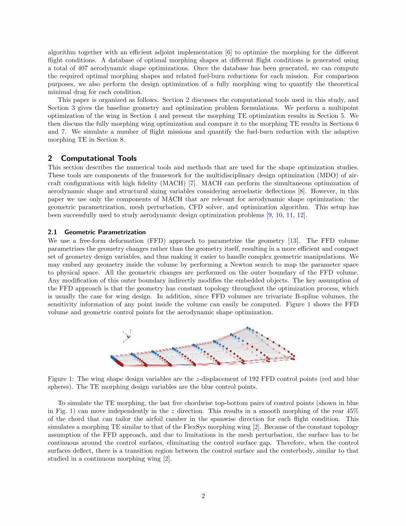
We choose five equally weighted flight conditions with different combinations of lift coefficient and Machnumber, as previously done by the authors [26, 10]. The flight conditions are the nominal cruise, ±10%of cruise CL, and ±0.01 of cruise Mach, as shown in Table 2. More sophisticated ways of choosing themultipoint flight conditions and their associated weights could be used, such as the automated proceduredeveloped by Liem et al. [27] that minimizes fleet-level fuel burn. The objective function is the average dragcoefficient for the five flight conditions, and the pitching moment constraint is enforced only for the nominalflight condition. The bending moment constraint is enforced at the 2.5 g maneuver condition at 15,000 ftand Mach 0.86.

Figure 3: The multipoint optimized wing has 5.7% lower drag.

A comparison of the initial wing—the CRM wing—and the multipoint optimized design is shown inFig. 3. The baseline results are shown in red (left wing), and the multipoint results are shown in blue (rightwing); the lift, drag, and pitching moment coefficients are also listed. The Cp for the multipoint optimizedresult corresponds to the nominal condition (Mach 0.85, CL = 0.5). We compute the shock surface from

7

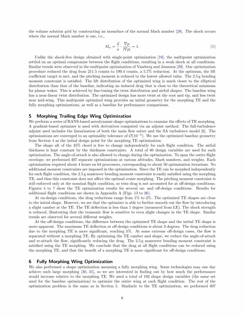
the volume solution grid by constructing an isosurface of the normal Mach number [28]. The shock occurswhere the normal Mach number is one, i.e.,

Mn =~u

a· ∇p|∇p|

= 1. (1)

Unlike the shock-free design obtained with single-point optimization [10], the multipoint optimizationsettled on an optimal compromise between the flight conditions, resulting in a weak shock at all conditions.Similar trends were observed in the multipoint optimization of Vassberg and Jameson [29]. Our optimizationprocedure reduced the drag from 211.5 counts to 199.4 counts, a 5.7% reduction. At the optimum, the liftcoefficient target is met, and the pitching moment is reduced to the lowest allowed value. The 2.5 g bendingmoment constraint is satisfied. The lift distribution of the optimized wing is much closer to the ellipticaldistribution than that of the baseline, indicating an induced drag that is close to the theoretical minimumfor planar wakes. This is achieved by fine-tuning the twist distribution and airfoil shapes. The baseline winghas a near-linear twist distribution. The optimized design has more twist at the root and tip, and less twistnear mid-wing. This multipoint optimized wing provides an initial geometry for the morphing TE and thefully morphing optimizations, as well as a baseline for performance comparisons.

5 Morphing Trailing Edge Wing OptimizationWe perform a series of RANS-based aerodynamic shape optimizations to examine the effects of TE morphing.A gradient-based optimizer is used with derivatives computed via an adjoint method. The full-turbulenceadjoint used includes the linearization of both the main flow solver and the SA turbulence model [6]. Theoptimizations are converged to an optimality tolerance of O(10−5). We use the optimized baseline geometryfrom Section 4 as the initial design point for the morphing TE optimization.

The shape aft of the 45% chord is free to change independently for each flight condition. The airfoilthickness is kept constant by the thickness constraints. A total of 80 design variables are used for eachoptimization. The angle-of-attack is also allowed to change during the optimization. To span the entire flightenvelope, we performed 407 separate optimizations at various altitudes, Mach numbers, and weights. Eachoptimization required about 4 hours on 64 processors, corresponding to about 50 optimization iterations. Noadditional moment constraints are imposed in the optimization. Since the TE can be morphed independentlyfor each flight condition, the 2.5 g maneuver bending moment constraint is easily satisfied using the morphingTE, and thus this constraint does not affect the optimal cruise morphing. The pitching moment constraint isstill enforced only at the nominal flight condition, so trim drag is not accounted for at off-design conditions.Figures 4 to 7 show the TE optimization results for several on- and off-design conditions. Results foradditional flight conditions are shown in Appendix A (Figs. 13 to 26).

At on-design conditions, the drag reductions range from 1% to 2%. The optimized TE shapes are closeto the initial shape. However, we see that the optimizer is able to further smooth out the flow by introducinga slight camber at the TE. The TE deflection is less than 1 degree (measured from LE). The shock strengthis reduced, illustrating that the transonic flow is sensitive to even slight changes in the TE shape. Similartrends are observed for several different weights.

At the off-design conditions, the difference between the optimized TE shape and the initial TE shape ismore apparent. The maximum TE deflection at off-design conditions is about 3 degrees. The drag reductiondue to the morphing TE is more significant, reaching 5%. At some extreme off-design cases, the flow isseparated without a morphing TE. By optimizing the TE camber and shape, we reduce the angle-of-attackand re-attach the flow, significantly reducing the drag. The 2.5 g maneuver bending moment constraint issatisfied using the TE morphing. We conclude that the drag at all flight conditions can be reduced usingthe morphing TE, and that the benefit of a morphing TE is more significant for off-design conditions.

6 Fully Morphing Wing OptimizationWe also performed a shape optimization assuming a fully morphing wing. Some technologies may one dayachieve such large morphing [30, 31], so we are interested in finding out by how much the performancewould increase relative to the morphing TE. We used a total of 192 shape design variables (the same setused for the baseline optimization) to optimize the entire wing at each flight condition. The rest of theoptimization problem is the same as in Section 5. Similarly to the TE optimization, we performed 407

8

Figure 4: Morphing TE optimization at MTOW on-design condition.

separate optimizations for different altitudes, Mach numbers, and weights, to span the entire flight envelope.Because of the increased design-space dimensionality, the computational cost of the optimization is higher: 6hours on 64 processors instead of 4 hours in the morphing TE case. Figures 8 and 9 show the fully morphingwing optimization results for an on-design and an off-design condition.

At on-design conditions, the fully morphing wing is only marginally better than the morphing TE wing.Specifically, the drag coefficient is decreased by about 1 count, as we can see by comparing the CD valuesof the morphing TE wing in Fig. 4 and the fully morphing wing in Fig. 8. The baseline wing is alreadyoptimized near the cruise conditions; an additional drag reduction is difficult to achieve even with a fullymorphing wing. The optimized wing shapes are very close to the baseline shape. The pressure distributionsare also quite similar to those of the optimized morphing TE designs. Therefore, we see that it suffices tochange the TE shape for drag reduction at on-design conditions.

At the off-design conditions, and similarly to the morphing TE, the fully morphing wing achieved anadditional drag reduction of more than 5%. The maximum TE deflection at off-design conditions is about3 degrees. In the flight condition shown in Fig. 9, the flow on the baseline wing is separated. The fullymorphing wing still maintains a shock-free solution and near-elliptical lift distribution even at high CL. Weobserve that the benefit of morphing wings can be magnified at off-design conditions.

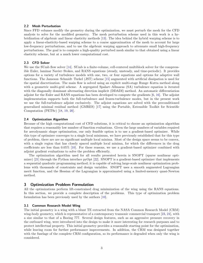
7 Comparison Between Morphing Trailing Edge and Fully Morphing WingsTo further compare the benefits of the morphing TE and the morphing wing, we plotted the percentagedrag reduction contours of each approach for the entire flight envelope for MTOW (347,500 kg), as shown inFigure 10. The drag reduction contours for other weights are shown in Appendix B (Figs. 27 and 28). Theweight and altitude range is based on the Boeing 777-200LR operation manual for long-range cruise (LRC).

The trends of the two drag reduction contours are similar. The lowest drag reductions are near the on-design conditions where the wing has been previously optimized with a multipoint formulation. These dragreductions are due to the additional degrees of freedom that allow the TE shape to change separately at eachflight condition, and they are also a result of making the 2.5 g maneuver condition constraint independentthrough load alleviation with the morphing TE. At the lower Mach number range, the drag reductionincreases with the altitude and Mach number. The highest drag reduction occurs at the flight condition with

9

Figure 5: Morphing TE optimization at half-weight on-design condition.

Figure 6: Morphing TE optimization at low-Mach low-altitude off-design condition.

10

Figure 7: Morphing TE optimization at low-Mach high-altitude off-design condition.

high altitude and low Mach, where the lift coefficient is the highest. For high Mach numbers above 0.85, thetrend reverses because of the drag divergence.

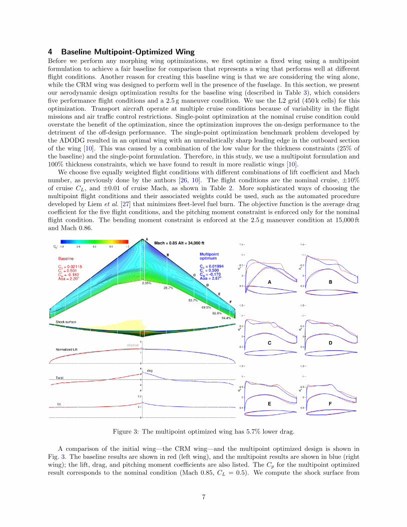
In Fig. 11 we plot the ML/D contours of the multipoint baseline, morphing TE, and fully morphingwing designs with respect to altitude and Mach number. The ML/D contours for the other weights areshown in Appendix C (Figs. 29 and 30). ML/D provides a metric for quantifying the aircraft range basedon the Breguet range equation with constant thrust-specific fuel consumption. While the thrust-specific fuelconsumption is actually not constant, assuming it to be constant is acceptable when comparing performancein a limited Mach number range [32]. We add 100 drag counts to the computed drag to account for thedrag due to the fuselage, tail, and nacelles; this gives more realistic ML/D values. In aircraft design, the99% value of the maximum ML/D contour, shown in black, is often used to examine the robustness of thedesign [23]. The point with the highest Mach number on that contour line corresponds to the LRC point,which is the point at which the aircraft can fly at a higher speed by incurring a 1% increase in fuel burn [33].

The multipoint baseline maximum ML/D occurs at the nominal flight condition (Mach 0.85; 31,000 ftaltitude). Both the morphing TE and the morphing wing increase the maximum ML/D. The maximumML/D points for the morphing TE and morphing wing are at a higher altitude and higher Mach number.Since the TE shape can be adapted for each flight condition, the drag divergence is pushed to a higherMach number. The 99% value of the maximum ML/D contour of the morphing designs is also significantlyenlarged, indicating a more robust design. We see that the morphing TE enables the aircraft to fly higherand faster without a fuel-burn penalty. To more accurately capture the tradeoffs, we would need to performa multidisciplinary study including low-speed aerodynamics, propulsion, and structure.

8 Morphing Trailing Edge Mission Fuel-Burn ReductionSince we have morphing TE optimizations spanning the entire flight envelope, we can create a surrogatemodel of optimal TE shapes for different flight conditions. This database allows us to compute the fuelburn for a series of missions without performing any additional optimizations. Since we have a relatively finediscretization of the flight region, we use a linear interpolation to evaluate the performance and optimal shapebetween the optimized points. A thrust-specific fuel consumption (TSFC) of 0.53 lb/(lbf · h) is assumed.We also add 100 drag counts to the computed drag to account for the drag due to the fuselage, tail, andnacelles. The fuel burn is then integrated backwards for a given flight profile. Figure 12 shows a typical

11

Figure 8: Fully morphing wing optimization at MTOW on-design condition.

Figure 9: Fully morphing wing optimization at low-Mach high-altitude off-design condition.

12

0.6

%

0.8%

0.8%

1%

1%

1%

2%

2%

3%

3%

3%4%

4%

5%

8%

10%

15%

20%

Mach

Alt

itu

de

(ft

)

0.76 0.8 0.84

26000

28000

30000

32000

% drag reduction with morphing TE

W = 347,500 kg

(a) Morphing TE

1%

2%

3%

3%

4%

4%

5%

5%

5%

8%

10%

15%

20%

25%

Mach

Alt

itu

de

(ft

)

0.76 0.8 0.84

26000

28000

30000

32000

% drag reduction with morphing wing

W = 347,500 kg

(b) Fully morphing wing

Figure 10: The trends of the drag reduction contours are similar, with a drag reduction of about 1% nearon-design conditions.

11

11.8

12.2

12.2

12.6

12.6

13

13

13.4

13.4

13.8

13

.814.2

14.2

Mach

Alt

itu

de

(ft

)

0.76 0.8 0.84

26000

28000

30000

32000

Multipoint optimum ML/D

max = 14.44

ML/D99%max

W = 347,500 kg

(a) Multipoint optimized baseline

13.4

13.4

13.4

13.8

13.8

14.2

Mach

Alt

itu

de

(ft

)

0.76 0.8 0.84

26000

28000

30000

32000

Morphing TE optimumML/D

max = 14.71

ML/D99%max

W = 347,500 kg

(b) Morphing TE wing

13.4

13.4

13.8

13.8

14.2

Mach

Alt

itu

de

(ft

)

0.76 0.8 0.84

26000

28000

30000

32000

Morphing wing optimumML/D

max = 14.78

W = 347,500 kg

ML/D99%max

(c) Fully morphing wing

Figure 11: The maximum ML/D occurs at a higher altitude and Mach number with morphing

flight profile for a long-range flight (this flight from Dallas Fort Worth to Sydney, Australia is currently thelongest nonstop commercial flight).

13

Figure 12: Fuel burn is reduced by 0.7% using morphing TE for DFW–SYD flight.

Since the flight is operated in the on-design condition with step climb, the TE deflection is within 1 degree.The wing tip exhibits the highest amount of deflection, from -1 degree at the initial cruise to 1 degree nearthe end of the cruise. We see a 0.7% fuel-burn reduction using morphing TE on this flight. As pointed outin Section 5, the morphing TE has higher drag reduction at off-design conditions. Table 4 shows the dragreduction for a number of hypothetical flight trajectories.

Route Distance (mi) Mach numbers Cruise altitudes (ft) Fuel-burn reduction

DFW–SYD 8578 0.85, 0.85, 0.85 31,000, 34,000, 39,000 −0.702%DTW–PVG 7120 0.85, 0.85, 0.85 33,000, 36,000, 41,000 −1.023%LAX–NRT 5440 0.80, 0.85, 0.80 33,000, 33,000, 33,000 −1.049%JFK–SFO 2580 0.84, 0.84, 0.84 32,000, 34,000, 36,000 −1.207%ATL–ORD 606 0.78, 0.80, 0.78 31,000, 31,000, 31,000 −1.074%– 2000 0.75, 0.75, 0.75 29,000, 31,000, 34,000 −1.680%

Table 4: The fuel-burn reduction is about 1% using morphing TE for various flight trajectories.

We see that the morphing TE provides about 1% fuel-burn reduction at cruise condition for the simulatedflights in Table 4. All of the simulated flights have a TE deflection within 2 degrees. Additional benefitscould be realized during the climb and descent, which are neglected in this analysis. To evaluate the climband descent, additional optimizations at lower speeds and lower altitudes would be needed to span the flightenvelope for climb and descent.

9 ConclusionsWe performed the aerodynamic shape optimization of a wide-body long-range aircraft wing (based on theNASA CRM model) with an adaptive morphing TE. For comparison, we started with a multipoint optimizedbaseline wing with no morphing, which served as the starting point for the morphing designs. We performeda total of 407 TE optimizations with different Mach numbers, altitudes, and weights to span the entire cruiseflight envelope. We also optimized a morphing wing that assumed complete freedom in shape. The results

14

Wing configuration Mach Altitude (ft) CL CD ∆CD (%)

CRM 0.85 34, 000 0.50 0.02115 +6.1%

Baseline 0.85 34, 000 0.50 0.01994 0.0%0.85 31, 000 0.43 0.01718 0.0%0.75 25, 000 0.54 0.02191 0.0%

Morphing TE 0.85 31, 000 0.43 0.01693 −1.5%0.75 25, 000 0.54 0.02084 −4.9%

Fully morphing 0.85 31, 000 0.43 0.01679 −2.3%0.75 25, 000 0.54 0.02056 −6.2%

Table 5: Summary of performance for the original CRM wing, the multipoint optimized baseline, the opti-mized morphing TE, and the optimized fully morphing wings.

are summarized in Table 5.For the morphing TE wing, a drag reduction of the order of 1% was achieved for on-design conditions,

and reductions up to 5% were achieved for off-design conditions. We further evaluated the performance of themorphing TE by comparing its benefits with those from a fully morphing wing. We did this by plotting thedrag reduction contour and the ML/D contour. The fully morphing wing yielded only marginally lower dragand a similar ML/D contour. Therefore, morphing only the TE can achieve an aerodynamic performancesimilar to that of a fully morphing wing without the drastic increase in wing morphing mechanism andweight.

Finally, we created a surrogate model of optimal TE shapes to compute the cruise fuel burn for differentflight missions. We observed about 1% fuel-burn reduction using the morphing TE. More significant fuel-burnreduction could be achieved in the climb and descent segments.

From an aerodynamic perspective, an adaptive morphing TE can easily offer additional drag reductionwithout a complete redesign of the wing. Since this technology has been demonstrated by FlexSys, and couldbe installed on conventional control surfaces, we could consider retrofitting existing aircraft. To thoroughlyevaluate the benefits, it will be necessary to perform a multidisciplinary study to examine the tradeoffsbetween aerodynamics, structures, and controls. This study should include planform design variables, sincethe load alleviation due to morphing will allow for larger spans with little or no weight penalty. We havealready performed a preliminary aerostructural optimization study [34].

10 AcknowledgmentsThe computations were performed on the Flux HPC cluster at the University of Michigan Center of AdvancedComputing, and on the Gordon cluster of the Extreme Science and Engineering Discovery Environment(XSEDE), which is supported by National Science Foundation grant number ACI-1053575. This research ispartially funded by FlexSys, Inc. The authors would like to thank Yin Yu for his assistance in generatingsome of the figures, and we are grateful to our MDOlab colleagues for their suggestions.

References[1] Kota, S., Hetrick, J., Osborn, R., Paul, D., Pendleton, E., Flick, P., and Tilmann, C., “Design and

Application of Compliant Mechanisms for Morphing Aircraft Structures,” Proceedings of the SPIESmart Structures and Materials Conference, San Diego, CA, March 2003.

[2] Kota, S., Osborn, R., Ervin, G., Maric, D., Flick, P., and Paul, D., “Mission Adaptive Compliant Wing–Design, Fabrication and Flight Test,” RTO Applied Vehicle Technology Panel (AVT) Symposium, 2009.

[3] Sofla, A. Y. N., Meguid, S. A., Tan, K. T., and Yeo, W. K., “Shape Morphing of AircraftWing: Status and Challenges,” Materials & Design, Vol. 31, No. 3, 3 2010, pp. 1284–1292.doi:10.1016/j.matdes.2009.09.011.

15

[4] Molinari, G., Quack, M., Dmitriev, V., Morari, M., Jenny, P., and Ermanni, P., “Aero-StructuralOptimization of Morphing Airfoils for Adaptive Wings,” Journal of Intelligent Material Systems andStructures, Vol. 22, No. 10, 2011, pp. 1075–1089. doi:10.1177/1045389X11414089.

[5] Lee, D., Gonzalez, L. F., Periaux, J., and Onate, E., “Robust Aerodynamic Design Optimisation ofMorphing Aerofoil/Wing using Distributed MOGA,” Proceedings of the 28th Congress of the Interna-tional Council of the Aeronautical Sciences, Optimage Ltd., on behalf of the International Council ofthe Aeronautical Sciences (ICAS), 2012.

[6] Lyu, Z., Kenway, G. K., Paige, C., and Martins, J. R. R. A., “Automatic Differentiation Adjoint ofthe Reynolds-Averaged Navier–Stokes Equations with a Turbulence Model,” 21st AIAA ComputationalFluid Dynamics Conference, San Diego, CA, Jul. 2013. doi:10.2514/6.2013-2581.

[7] Kenway, G. K. W., Kennedy, G. J., and Martins, J. R. R. A., “Scalable Parallel Approach for High-Fidelity Steady-State Aeroelastic Analysis and Derivative Computations,” AIAA Journal , Vol. 52, No. 5,May 2014, pp. 935–951. doi:10.2514/1.J052255.

[8] Kenway, G. K. W. and Martins, J. R. R. A., “Multipoint High-Fidelity Aerostructural Optimization ofa Transport Aircraft Configuration,” Journal of Aircraft , Vol. 51, No. 1, January 2014, pp. 144–160.doi:10.2514/1.C032150.

[9] Lyu, Z. and Martins, J. R. R. A., “Aerodynamic Design Optimization Studies of a Blended-Wing-BodyAircraft,” Journal of Aircraft , Vol. 51, No. 5, September 2014, pp. 1604–1617. doi:10.2514/1.C032491.

[10] Lyu, Z., Kenway, G. K., and Martins, J. R. R. A., “Aerodynamic Shape Optimization Studies on theCommon Research Model Wing Benchmark,” AIAA Journal , Vol. 53, No. 4, April 2015, pp. 968–985.doi:10.2514/1.J053318.

[11] Lyu, Z. and Martins, J. R. R. A., “Strategies for Solving High-Fidelity Aerodynamic Shape OptimizationProblems,” 15th AIAA/ISSMO Multidisciplinary Analysis and Optimization Conference, Atlanta, GA,June 2014. doi:10.2514/6.2014-2594, AIAA 2014-2594.

[12] Lyu, Z., Xu, Z., and Martins, J. R. R. A., “Benchmarking Optimization Algorithms for Wing Aerody-namic Design Optimization,” Proceedings of the 8th International Conference on Computational FluidDynamics, Chengdu, Sichuan, China, July 2014, ICCFD8-2014-0203.

[13] Kenway, G. K., Kennedy, G. J., and Martins, J. R. R. A., “A CAD-Free Approach to High-FidelityAerostructural Optimization,” Proceedings of the 13th AIAA/ISSMO Multidisciplinary Analysis Opti-mization Conference, Fort Worth, TX, Sept. 2010, AIAA 2010-9231.

[14] van der Weide, E., Kalitzin, G., Schluter, J., and Alonso, J. J., “Unsteady Turbomachinery Computa-tions Using Massively Parallel Platforms,” Proceedings of the 44th AIAA Aerospace Sciences Meetingand Exhibit , Reno, NV, 2006, AIAA 2006-0421.

[15] Jameson, A., Schmidt, W., and Turkel, E., “Numerical Solution of the Euler Equations by Finite VolumeMethods Using Runge-Kutta Time Stepping Schemes,” AIAA Paper 81-1259, 1981.

[16] Mader, C. A., Martins, J. R. R. A., Alonso, J. J., and van der Weide, E., “ADjoint: An Approachfor the Rapid Development of Discrete Adjoint Solvers,” AIAA Journal , Vol. 46, No. 4, April 2008,pp. 863–873. doi:10.2514/1.29123.

[17] Saad, Y. and Schultz, M. H., “GMRES: A Generalized Minimal Residual Algorithm for Solving Non-symmetric Linear Systems,” SIAM Journal on Scientific and Statistical Computing , Vol. 7, No. 3, 1986,pp. 856–869. doi:10.1137/0907058.

[18] Balay, S., Gropp, W. D., McInnes, L. C., and Smith, B. F., Efficient Management of Parallelism inObject Oriented Numerical Software Libraries, Birkhauser Press, 1997, pp. 163–202.

16

[19] Balay, S., Brown, J., Buschelman, K., Eijkhout, V., Gropp, W. D., Kaushik, D., Knepley, M. G.,McInnes, L. C., Smith, B. F., and Zhang, H., “PETSc Users Manual,” Tech. Rep. ANL-95/11 - Revision3.4, Argonne National Laboratory, 2013.

[20] Balay, S., Brown, J., Buschelman, K., Gropp, W. D., Kaushik, D., Knepley, M. G., McInnes, L. C.,Smith, B. F., and Zhang, H., “PETSc Web page,” 2013, http://www.mcs.anl.gov/petsc.

[21] Gill, P. E., Murray, W., and Saunders, M. A., “SNOPT: An SQP algorithm for large-scaleconstrained optimization,” SIAM Journal of Optimization, Vol. 12, No. 4, 2002, pp. 979–1006.doi:10.1137/S1052623499350013.

[22] Perez, R. E., Jansen, P. W., and Martins, J. R. R. A., “pyOpt: A Python-Based Object-OrientedFramework for Nonlinear Constrained Optimization,” Structural and Multidisciplinary Optimization,Vol. 45, No. 1, January 2012, pp. 101–118. doi:10.1007/s00158-011-0666-3.

[23] Vassberg, J. C., DeHaan, M. A., Rivers, S. M., and Wahls, R. A., “Development of a Common ResearchModel for Applied CFD Validation Studies,” 2008, AIAA 2008-6919.

[24] Vassberg, J., “A Unified Baseline Grid about the Common Research Model Wing/Body for the FifthAIAA CFD Drag Prediction Workshop (Invited),” 29th AIAA Applied Aerodynamics Conference, Jul2011. doi:10.2514/6.2011-3508.

[25] Roache, P. J., “Verification of Codes and Calculations,” AIAA Journal , Vol. 36, No. 5, 1998, pp. 696–702. doi:10.2514/2.457.

[26] Kenway, G. K. W. and Martins, J. R. R. A., “Multipoint Aerodynamic Shape Optimization Inves-tigations of the Common Research Model Wing,” AIAA Journal , 2015. doi:10.2514/1.J054154, (Inpress).

[27] Liem, R., Kenway, G. K. W., and Martins, J. R. R. A., “Multimission Aircraft Fuel Burn Minimizationvia Multipoint Aerostructural Optimization,” AIAA Journal , Vol. 53, No. 1, January 2015, pp. 104–122.doi:10.2514/1.J052940.

[28] Haimes, R., “Automated Feature Extraction from Transient CFD Simulations,” Proceeding of the 7thAnnual Conference of the CFD Society of Canada, Halifax, NS , May 1999.

[29] Vassberg, J. and Jameson, A., “Influence of Shape Parameterization on Aerodynamic Shape Optimiza-tion,” Tech. rep., Von Karman Institute, Brussels, Belgium, April 2014.

[30] Joo, J. J., Marks, C. R., Zientarski, L., and Culler, A. J., “Variable Camber Compliant Wing - Design,”23nd AIAA/AHS Adaptive Structures Conference, American Institute of Aeronautics and Astronautics(AIAA), jan 2015. doi:10.2514/6.2015-1050.

[31] Marks, C. R., Zientarski, L., Culler, A. J., Hagen, B., Smyers, B. M., and Joo, J. J., “Variable CamberCompliant Wing - Wind Tunnel Testing,” 23nd AIAA/AHS Adaptive Structures Conference, AmericanInstitute of Aeronautics and Astronautics (AIAA), jan 2015. doi:10.2514/6.2015-1051.

[32] Torenbeek, E., Advanced Aircraft Design: Conceptual Design, Analysis and Optimization of SubsonicCivil Airplanes, Wiley, West Sussex, UK, 2013.

[33] Roberson, W., Root, R., and Adams, D., “Fuel Conservation Stragtergies: Cruise Flight,” Tech. rep.,Boeing AERO Magazine, 2007.

[34] Burdette, D., Kenway, G. K. W., Lyu, Z., and Martins, J. R. R. A., “Aerostructural Design Optimizationof an Adaptive Morphing Trailing Edge Wing,” Proceedings of the AIAA Science and Technology Forumand Exposition (SciTech), Kissimmee, FL, January 2015, AIAA 2015-1129.

17

Appendix A: Morphing TE Optimization Results for Additional Flight Conditions

18

Figure 13: Morphing TE optimization at M = 0.85, Alt = 28,000 ft, and W = 347,500 kg.

Figure 14: Morphing TE optimization at M = 0.86, Alt = 25,000 ft, and W = 347,500 kg.

19

Figure 15: Morphing TE optimization at M = 0.86, Alt = 33,000 ft, and W = 347,500 kg.

Figure 16: Morphing TE optimization at M = 0.85, Alt = 34,000 ft, and W = 273,200 kg.

20

Figure 17: Morphing TE optimization at M = 0.85, Alt = 28,000 ft, and W = 273,200 kg.

Figure 18: Morphing TE optimization at M = 0.75, Alt = 25,000 ft, and W = 273,200 kg.

21

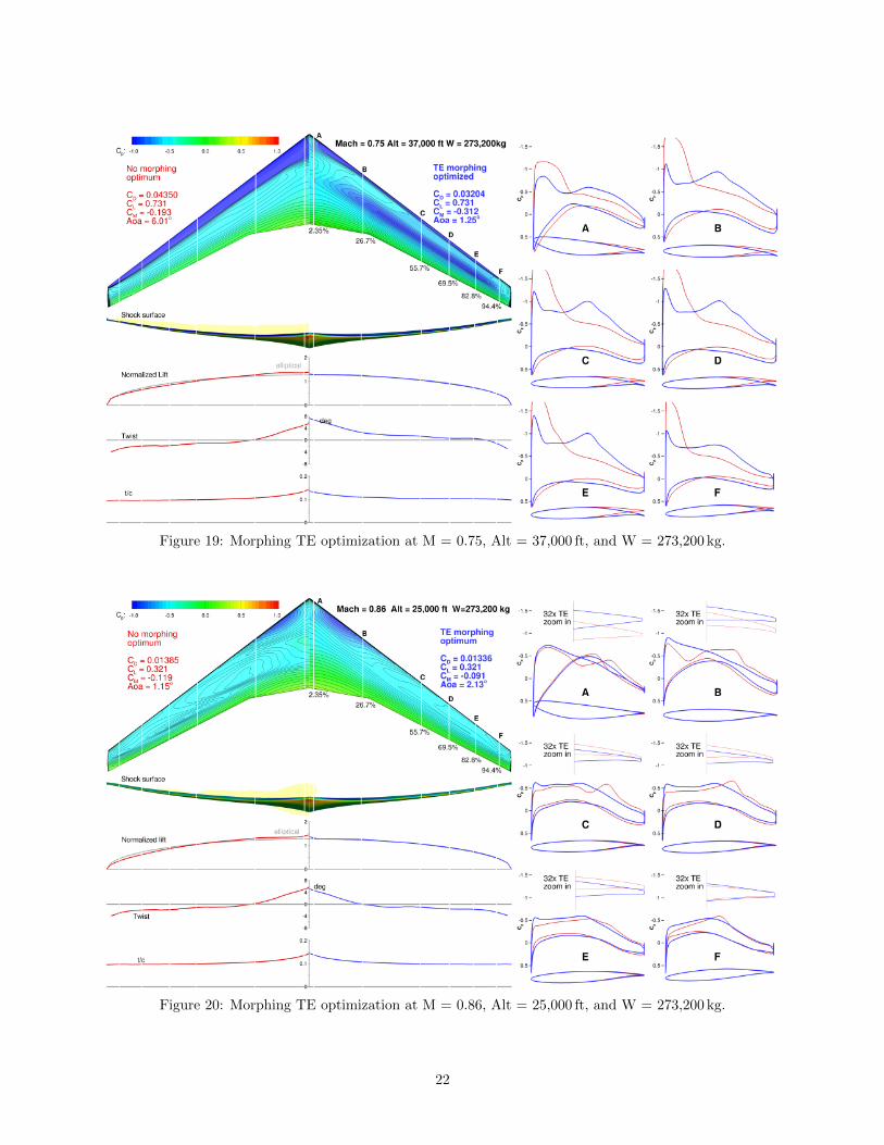
Figure 19: Morphing TE optimization at M = 0.75, Alt = 37,000 ft, and W = 273,200 kg.

Figure 20: Morphing TE optimization at M = 0.86, Alt = 25,000 ft, and W = 273,200 kg.

22

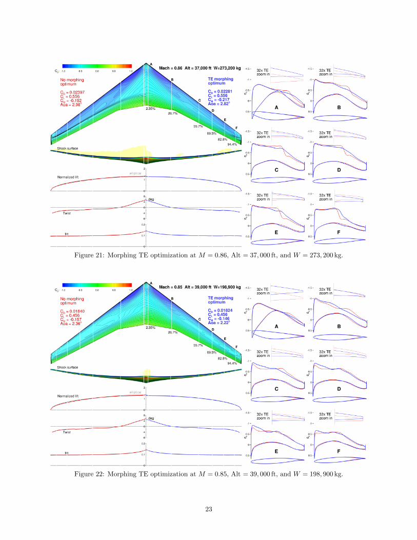
Figure 21: Morphing TE optimization at M = 0.86, Alt = 37, 000 ft, and W = 273, 200 kg.

Figure 22: Morphing TE optimization at M = 0.85, Alt = 39, 000 ft, and W = 198, 900 kg.

23

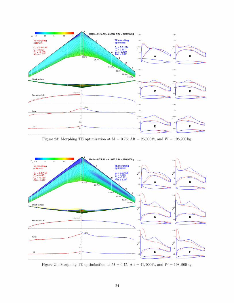
Figure 23: Morphing TE optimization at M = 0.75, Alt = 25,000 ft, and W = 198,900 kg.

Figure 24: Morphing TE optimization at M = 0.75, Alt = 41, 000 ft, and W = 198, 900 kg.

24

Figure 25: Morphing TE optimization at M = 0.86, Alt = 25, 000 ft, and W = 198, 900 kg.

Figure 26: Morphing TE optimization at M = 0.86, Alt = 41, 000 ft, and W = 198,900 kg.

25

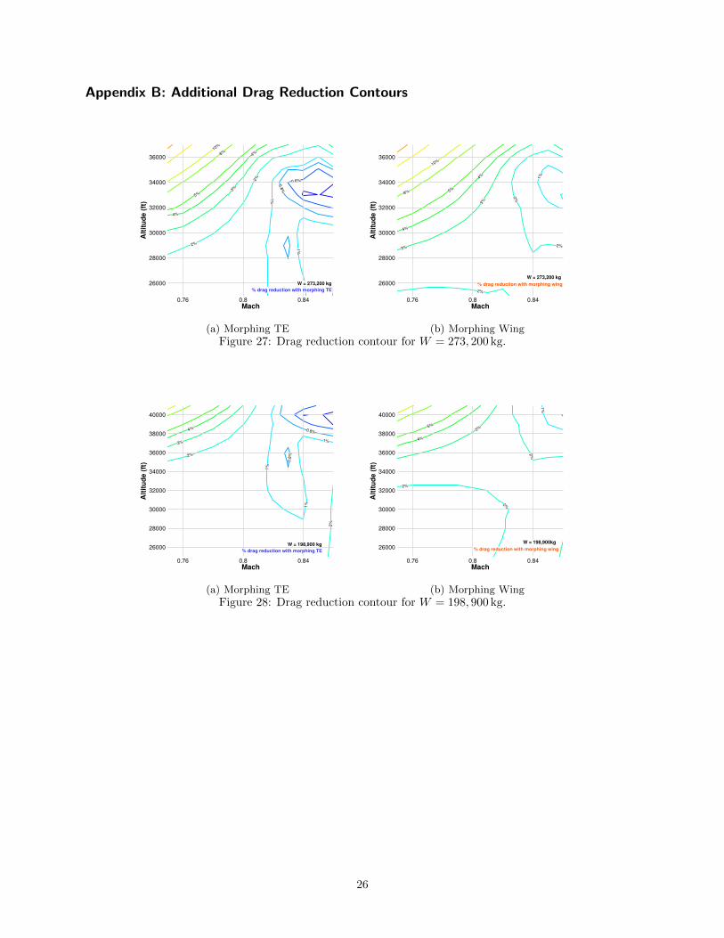
Appendix B: Additional Drag Reduction Contours

0.6%

0.8

%

1%

1%

1%

2%

2%

2%

3%

4%

4%

5%

8%10%

Mach

Alt

itu

de

(ft

)

0.76 0.8 0.84

26000

28000

30000

32000

34000

36000

% drag reduction with morphing TE

W = 273,200 kg

(a) Morphing TE

1%

2%

2%

2%

3%

3%

4%

4%

5%8%

10%

Mach

Alt

itu

de

(ft

)

0.76 0.8 0.84

26000

28000

30000

32000

34000

36000

% drag reduction with morphing wing

W = 273,200 kg

(b) Morphing WingFigure 27: Drag reduction contour for W = 273, 200 kg.

0.8%

0.8

%

1%

1%

1%

2%

2%

3%

4%

Mach

Alt

itu

de

(ft

)

0.76 0.8 0.84

26000

28000

30000

32000

34000

36000

38000

40000

% drag reduction with morphing TE

W = 198,900 kg

(a) Morphing TE

1%

2%

2%

2%

3%

4%

5%

Mach

Alt

itu

de

(ft

)

0.76 0.8 0.84

26000

28000

30000

32000

34000

36000

38000

40000

% drag reduction with morphing wing

W = 198,900kg

(b) Morphing WingFigure 28: Drag reduction contour for W = 198, 900 kg.

26

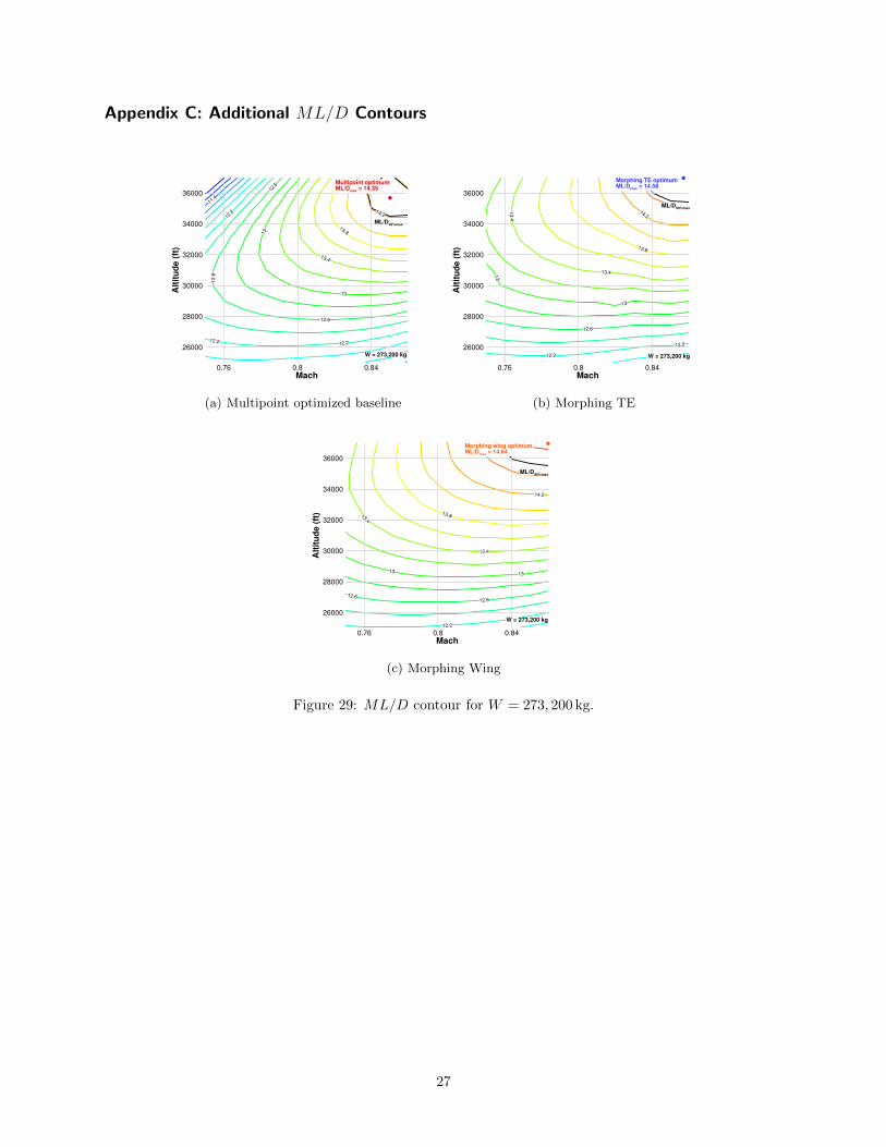
Appendix C: Additional ML/D Contours

11.4

11.8

12.212.2

12.2

12.6

12

.6

12.6

13

13

13.4

13.8

14.2

Mach

Alt

itu

de

(ft

)

0.76 0.8 0.84

26000

28000

30000

32000

34000

36000

Multipoint optimum ML/D

max = 14.35

ML/D99%max

W = 273,200 kg

(a) Multipoint optimized baseline

12.2

12.2

12.6

13

13

13.4

13

.4

13.8

14.2

Mach

Alt

itu

de

(ft

)

0.76 0.8 0.84

26000

28000

30000

32000

34000

36000

Morphing TE optimumML/D

max = 14.58

ML/D99%max

W = 273,200 kg

(b) Morphing TE

12.2

12.6

12.6

1313

13.4

13.4

13.8

14.2

Mach

Alt

itu

de

(ft

)

0.76 0.8 0.84

26000

28000

30000

32000

34000

36000

Morphing wing optimumML/D

max = 14.64

W = 273,200 kg

ML/D99%max

(c) Morphing Wing

Figure 29: ML/D contour for W = 273, 200 kg.

27

11

11

11.4

11.8

12.2

12.2

12.6

12.6

13

13

13.4

13.8

Mach

Alt

itu

de

(ft

)

0.76 0.8 0.84

30000

32000

34000

36000

38000

40000

Multipoint optimum ML/D

max = 14.04

ML/D99%max

W = 198,900 kg

(a) Multipoint optimized baseline

11

11.4

11.4

11.8

12.2

12.6

13

13.4

13.8

Mach

Alt

itu

de

(ft

)

0.76 0.8 0.84

30000

32000

34000

36000

38000

40000

Morphing TE optimumML/D

max = 14.12

ML/D99%max

W = 198,900 kg

(b) Morphing TE

11

11.4

11.4

11.8

11.8

12.212.2

12.6

1313

13.4

13.4

13.8

Mach

Alt

itu

de

(ft

)

0.76 0.8 0.84

26000

28000

30000

32000

34000

36000

38000

40000

Morphing wing optimumML/D

max = 14.17

W = 198,900 kg

ML/D99%max

(c) Morphing Wing

Figure 30: ML/D contour for W = 198, 900 kg.

28