Embed Size (px)
Citation preview

PhD. Dissertation
ADVANCED SIGNAL PROCESSING TECHNIQUES
FOR GLOBAL NAVIGATION SATELLITE SYSTEMS
RECEIVERS
Author: Carles Fernandez Prades
Thesis advisor: Prof. Juan A. Fernandez Rubio
Department of Signal Theory and CommunicationsUniversitat Politecnica de Catalunya
email: carlos, [email protected]
Barcelona, December 2005


A la iaia.

Abstract
This dissertation addresses the synchronization problem using an array of antennas in the gen-eral framework of Global Navigation Satellite Systems (GNSS) receivers. Positioning systemsare based on time delay and frequency–shift estimation of the incoming signals in the receiverside, in order to compute the user’s location. Sources of accuracy degradation in satellite–basednavigation systems are well–known, and their mitigation has deserved the attention of a numberof researchers in latter times. While atmospheric–dependant sources (delays that depend on theionosphere and troposphere conditions) can be greatly mitigated by differential systems externalto the receiver’s operation, the multipath effect is location–dependant and remains as the mostimportant cause of accuracy degradation in time delay estimation, and consequently in positionestimation, becoming a signal processing challenge.
Traditional approaches to time delay estimation are often embodied in a communicationsystems framework. Indeed, in DS–CDMA systems many techniques are driven to minimize theprobability of error in the symbol detection by taking advantage of several incoming replicasin order to increase the signal–to–noise ratio (SNR) in the detection stage. This is not the caseof GNSS, where the parameter of interest is the time delay of the line–of–sight signal (LOSS),and the rest of replicas are nuisance signals that jeopardize the LOSS time estimation accuracy.Although a number of multipath mitigation techniques have been proposed in the recent years,most of them are based in single–antenna receivers, an approach that has inherent drawbacks.In this dissertation, we propose the use of the spatial diversity provided by an antenna arrayas a possible solution for the mitigation of reflections that are correlated with the direct signal,denoted as coherent multipath along this dissertation.
After an analysis of the state–of–the–art in GNSS receiver design and providing some detailsabout the signal structure of the GPS and Galileo systems, we propose a signal model for thereception of several scaled, time-delayed and Doppler-shifted signals by an antenna array. Ina first instance, the front-end is assumed perfectly calibrated, and thus the model includes aspatial signature, unique for each direction of arrival. Due to the technologic challenge thatperfect calibration demands, an unstructured version of the signal model where the array israndomly calibrated is also provided. The particularity of both versions are a noise term whichis considered statistically white in the time dimension but colored in the space dimension. Thisapproach tries to characterize in a very simple manner the statistical behavior of multipath andinterferences exploiting the spatial diversity provided by antenna arrays. In order to establish atheoretical limit of accuracy in parameter estimation, we provide the derivation of the Cramer-Rao bounds for the estimation of directions of arrival, complex amplitudes, time delays andDoppler shifts of a set of signals. The computation of the theoretical lower bound of variancefor unbiased estimators is completed with the proof of uncoupling between the direction ofarrival and the synchronization parameters.
iv

The Dissertation follows with the application of the Maximum Likelihood (ML) approachto the proposed array signal model. The result is a new cost function whose minimization leadsto the ML joint estimation of time delays and Doppler shifts. This cost function is independentof the directions of arrival and allows its implementation in an unstructured array. Although theformulation of the problem is rather general and allows its use in a number of different appli-cations, the peculiarities of navigation signals leads to some adaptations of the algorithms tobetter suite the problem at hand and reduce their computational cost. Some iterative algorithmsbased on the obtained cost function are derived and tested in computer simulations.
Then, the problem of synchronization with antenna arrays is attacked from a completely dif-ferent point of view. If the ML procedure was based on statistical assumptions about multipathand interferences, now we take the beamforming approach, free from statistical assumptions,exploiting the electronic manipulation of the radiation pattern that allows an antenna array. Wepropose the combination of temporal and spatial references to avoid the multipath effect, the so-called space-time hybrid beamforming. The result is a beamforming algorithm which requiresa reasonable computation cost and is surprisingly linked to the ML approach. Different point-ing strategies are proposed, including the derivation of a robust version which copes with arraymiscalibration resorting to convex optimization theory.
As another original contribution of this Dissertation, the theory of beamforming has been ap-plied for first time to the satellite-based Search And Rescue system named COSPAS–SARSAT.Nowadays, the system works with four satellites that are unable to ensure global coverage,among other serious drawbacks. The European Space Agency (ESA) is evaluating the possibil-ity to equip the forthcoming Galileo satellite constellation with Search And Rescue transpon-ders. The tight power budget constraints and the accuracy requirements for emergency beaconpositioning greatly complicates the receiver design, withdrawing the use of a single-antennasystem. In this dissertation, we provide the analysis of the current emergency beacon and an-other signal structure proposed by the Centre National d’Etudes Spatiales (CNES) for a newgeneration of emergency beacons. Then, we propose the use of an antenna array in the receiverdesign and provide suitable, specially designed algorithms and extensive simulation results.
Last part of this dissertation describes the design and implementation of an antenna arraydevoted to the civil signal provided by GPS on the L1 link. We have decided to implement anantenna array in order to apply the theory explained in the previous chapters of this dissertationand provide a testbed for evaluation of the developed algorithms in conditions of real data. Weprovide details about the hardware architecture, the requirements and measurements of eachblock and some results working with real GPS data, drawing a link between signal processingtheory and its actual hardware and Software–Defined Radio (SDR) implementation.
v

Resum
Aquesta dissertacio tracta el problema de la sincronitzacio utilitzant un array d’antenes en elmarc general dels Sistemes de Navegacio Global per Satel·lit (Global Navigation Satellite Sys-tems, GNSS). Els sistemes de posicionament estan basats en l’estimacio, per part del receptor,del retard temporal i el desplacament frequencial dels senyals d’arribada, per tal de calcular laposicio de l’usuari. Les fonts de degradacio de la precisio en els sistemes de navegacio basats ensatel·lits son prou conegudes, i la seva mitigacio ha merescut l’atencio de no pocs investigadorsen els ultims temps. Les fonts de degradacio que depenen de l’atmosfera (retards lligats a lescondicions de la ionosfera i la troposfera) poden ser mitigades mitjancant sistemes diferencialsexterns a l’operacio del receptor, pero l’efecte multicamı depen de la situacio del receptor i esmante com la causa principal de la degradacio en la precisio de l’estimacio del retard temporal,i en consequencia del posicionament, esdevenint un repte per al processament de senyal.
Els plantejaments tradicionals de l’estimacio temporal estan normalment embullits en elmarc dels sistemes de comunicacions. De fet, en sistemes DS–CDMA moltes tecniques estanorientades a minimitzar la probabilitat d’error en la deteccio de sımbol aprofitant l’arribada dediferents repliques per a millorar la relacio senyal–soroll (SNR) a l’etapa de deteccio. Aquestno es el cas dels GNSS, on el parametre d’interes es el retard temporal del senyal amb vistadirecta, i la resta de repliques son senyals molestos que perjudiquen la precisio de l’estimaciodel retard del senyal directe. Encara que recentment s’han proposat molts metodes de mitigaciode l’efecte multicamı, la majoria es basen en receptors d’una sola antena, un plantejament quepateix de limitacions inherents. En aquesta dissertacio proposem l’utilitzacio de la diversitattemporal que ens proporcionen els arrays d’antenes com a una possible solucio a la mitigaciode reflexions correlades amb el senyal directe, efecte anomenat multicamı coherent al llarg dela dissertacio.
Despres d’una analisi de l’estat de l’art en el disseny de receptors per GNSS, i de propor-cionar alguns detalls sobre l’estructura de senyal dels sistemes GPS i Galileo, proposem unmodel de senyal per a la recepcio de diferents senyals escalats, retardats i amb un desplacamentDoppler mitjancant un array d’antenes. En un primer moment, considerem que el frontal deradiofrequencia es troba perfectament calibrat, de manera que el model inclou les signaturesd’espai, uniques per a cada direccio d’arribada. Degut al repte tecnologic que suposa la cal-ibracio perfecte, tambe proposem una versio desestructurada del model de senyal on l’arrayesta calibrat de manera aleatoria. La particularitat d’ambdues versions es troba al terme desoroll, considerat estadısticament blanc en el domini temporal pero colorejat a la dimensio del’espai. Aquest plantejament tracta de caracteritzar d’una manera molt simple el comportamentestadıstic del multicamı i les interferencies aprofitant la diversitat en espai que ofereixen els ar-rays d’antenes. A l’efecte d’establir un lımit teoric de la precisio en l’estimacio dels parametres,derivem els lımits de Cramer–Rao per a l’estimacio de les direccions d’arribada, amplituds com-plexes, retards temporals i desplacaments Doppler d’un conjunt de senyals. El calcul del lımit
vi

inferior teoric de la variancia per a estimadors no esbiaixats es completa amb la demostracio deldesacoblament entre els parametres de direccio d’arribada i els de sincronitzacio.
La dissertacio continua amb l’aplicacio del principi de Maxima Versemblanca (MaximumLikelihood, ML) al model de senyal de l’array. El resultat es una nova funcio de cost, la minim-itzacio de la qual porta a l’estimacio ML conjunta de retards i desplacaments Doppler. Aquestafuncio de cost es independent de les direccions d’arribada, i permet la seva implementacio enun array desestructurat. Encara que la formulacio del problema es bastant general i permetel seu us en un gran numero d’aplicacions, les peculiaritats dels senyals de navegacio sug-gereixen una adaptacio per ajustar–se millor al problema tractat i per reduır el cost computa-cional. S’han derivat alguns algorismes iteratius basats en la funcio de cost obtinguda, i s’hanprovat mitjancant simulacions numeriques.
Seguidament, el problema de la sincronitzacio amb arrays d’antenes s’aborda des d’un puntde vista completament diferent. Si el procediment ML estava basat en suposicions estadıstiquessobre el multicamı i les interferencies, ara prenem l’aproximacio de la conformacio de feix,lliure de suposicions estadıstiques, tot aprofitant la manipulacio electronica del diagrama deradiacio que permeten els arrays. Proposem la conformacio de feix hıbrida espai–temporal,consistent en la combinacio de referencies d’espai i de temps per a evitar l’efecte multicamı. Elresultat es un algorisme de conformacio de feix amb un cost computacional raonable i, sorpre-nentment, lligat al plantejament ML. Es proposen diferents estrategies d’apuntament, incloent-hi la derivacio d’una versio robusta que tracta el problema del mal calibratge fent us de la teoriade l’optimitzacio convexa.
Una altra aportacio original d’aquesta dissertacio, la teoria de la conformacio de feix s’haaplicat per primer cop al sistema de Recerca i Rescat basat en satel·lits anomenat COSPAS–SARSAT. Avui dia el sistema treballa amb quatre satel·lits, insuficients per assegurar cober-tura global, a mes d’altres limitacions importants. L’Agencia Espaial Europea (European SpaceAgency, ESA) esta avaluant la possibilitat d’equipar la proxima constel·lacio de satel·lits Galileoamb transponedors de Recerca i Rescat. El disseny del receptor es complica de manera impor-tant per les dures restriccions en el balanc de potencies i els requeriments de precisio en laposicio, fent desaconsellable l’us d’un sistema amb una sola antena. En aquesta dissertaciomostrem l’analisi del senyal de la balisa d’emergencia i d’una altra estructura de senyal pro-posada pel Centre National d’Etudes Spatiales (CNES) per a una nova generacio de balises.Tot seguit, proposem l’us d’un array d’antenes en el disseny del receptor i aportem algorismesespecialment adaptats i un bon nombre de resultats de simulacions.
L’ultima part de la dissertacio descriu el disseny i implementacio d’un array d’antenes ded-icat al senyal civil que proveeix el sistema GPS a l’enllac L1. Hem decidit implementar l’arrayper tal d’aplicar la teoria desenvolupada al llarg d’aquesta tesi, i oferir un banc de proves per al’avaluacio dels algorismes desenvolupats en condicions de dades reals. Aportem la descripciode l’arquitectura del maquinari, les especificacions i mesures de cada bloc i alguns resultats tre-
vii

ballant amb dades GPS reals, tot establint un enllac entre la teoria del processament de senyal ila seva implementacio practica en el maquinari i la part radio definida pel programari (Software–Defined Radio, SDR).
viii
Acknowledgements
Undoubtedly, the most remarkable fact I have encountered during the long journey towards myPh.D. has been the human quality of the people I met. I feel greatly privileged and honoured tohave had the opportunity to met such outstanding people. This acknowledgements are intendedto be a humble tribute to their generosity.
First of all, I want to thank my advisor Prof Juan A. Fernandez Rubio for his guidance,support and friendship over these years. His overwhelming technical insight and humanisticwisdom have been of great help, not only in the PhD. work.
The world–class experience of the Professors I met, jointly with their enthusiasm, havebeen excellent references for my day–to–day attitude about work. I want to thank specially theinsightful discussions with Gonzalo Seco (whose work has guided this dissertation) GregoriVazquez, M. A. Lagunas (who inoculated me his passion about array signal processing), SergioRuiz, Jaume Riba, Josep Sala, Olga Munoz, Ana Perez, Margarita Cabrera, Meritxell Lamarca,Ferran Marques, Toni Gasull and Josep Vidal. In the implementation of the antenna array, Iwant to thank the work in the RF chain of Pablo Honoria and his team in AD Telecom, and theknow–how of Alfredo Cano in the mechanization and isolation of the array components.
My colleagues in the PhD. period have been of exceptional help, both in technical and hu-man aspects. I want to express my infinite gratefulness to such distinguished people as DiegoBartolome, Joan Bas, Monica Caballero, Eduard Calvo, Toni Castro, Camilo Chang, Pau Closas(and his inexhaustible work in the SAR project, albeit computer crashes and other weapons ofmass destruction), Pedro Correa, Hugo Durney, Helenca Duxans, Luis Garcıa, Jose A. LopezSalcedo, Maribel Madueno, Enric Muntaner, Ali Nassar, Dani P. Palomar, Toni Pascual, Chris-tian Pomar, Alejandro Ramırez (my navigation partner, in more than one sense), Francesc Rey,Joel Sole, Fernando Ulloa, Andreu Urruela, Veronica Vilaplana and Xavi Villares.
The elaboration of a PhD. Thesis is not always a roses path. Sharing my beers and pains,I have enjoyed the invaluable support of Xenia Artigas, Carlos Aviles, Javi Ciruelos, SalvaCiruelos, Vanessa Esteban, Anna Fernandez, Montse Morell, Josep Ramon Moreso, Jordi Otero,Ignacio Paniego, Claudia Quevedo, Lenni Quevedo, Marcos Rodrigo, Monica Roig, Ivan Roura,Leo Torres, Cea Uvea and Sergio Valencia. Let me say to them a word in my mother tongue:Gracies.
At last but not the least, I want to thank my family for all the unconditional support alongthese years. Probably, nothing of this work could have been carried out without their help.
ix

x

Contents
Abstract iv
Resum vi
Acknowledgements ix
Notation xxiii
Acronyms xxv
1 Introduction 1
1.1 Global Navigation Satellite Systems . . . . . . . . . . . . . . . . . . . . . . . 3
1.2 Approach followed in this Dissertation . . . . . . . . . . . . . . . . . . . . . . 4
1.3 Organization of this Dissertation . . . . . . . . . . . . . . . . . . . . . . . . . 5
1.4 Research contributions . . . . . . . . . . . . . . . . . . . . . . . . . . . . . . 7
1.4.1 Journal papers . . . . . . . . . . . . . . . . . . . . . . . . . . . . . . 7
1.4.2 Technical reports . . . . . . . . . . . . . . . . . . . . . . . . . . . . . 7
1.4.3 International conferences . . . . . . . . . . . . . . . . . . . . . . . . . 8
1.4.4 National conferences . . . . . . . . . . . . . . . . . . . . . . . . . . . 9
1.4.5 Master Theses directed . . . . . . . . . . . . . . . . . . . . . . . . . . 10
xi

2 Fundamentals of GNSS synchronization 11
2.1 Signals coming from space . . . . . . . . . . . . . . . . . . . . . . . . . . . . 12
2.2 Technical background: a GPS receiver architecture . . . . . . . . . . . . . . . 14
2.3 Focusing the problem: the defocusing of multipath . . . . . . . . . . . . . . . 24
2.4 State-of-the-art synchronization in GNSS receivers . . . . . . . . . . . . . . . 28
2.4.1 Single-antenna techniques . . . . . . . . . . . . . . . . . . . . . . . . 28
2.4.2 Antenna array techniques . . . . . . . . . . . . . . . . . . . . . . . . . 35
2.5 GPS signal structure . . . . . . . . . . . . . . . . . . . . . . . . . . . . . . . 39
2.5.1 GPS spreading codes . . . . . . . . . . . . . . . . . . . . . . . . . . . 39
2.5.2 Navigation data messages . . . . . . . . . . . . . . . . . . . . . . . . 42
2.5.3 L5, L2 and L1 links . . . . . . . . . . . . . . . . . . . . . . . . . . . . 43
2.6 Galileo signal structure . . . . . . . . . . . . . . . . . . . . . . . . . . . . . . 44
2.6.1 Introduction to the BOC modulation . . . . . . . . . . . . . . . . . . . 45
2.6.2 Galileo spreading codes . . . . . . . . . . . . . . . . . . . . . . . . . 48
2.6.3 Navigation data messages . . . . . . . . . . . . . . . . . . . . . . . . 48
2.6.4 E5, E6 and L1 links . . . . . . . . . . . . . . . . . . . . . . . . . . . . 49
2.7 Summary . . . . . . . . . . . . . . . . . . . . . . . . . . . . . . . . . . . . . 50
3 Maximum Likelihood synchronization with antenna arrays 53
3.1 Signal model . . . . . . . . . . . . . . . . . . . . . . . . . . . . . . . . . . . 54
3.1.1 Structured array model . . . . . . . . . . . . . . . . . . . . . . . . . . 54
3.1.2 Unstructured array model . . . . . . . . . . . . . . . . . . . . . . . . 59
3.2 Cramer-Rao bounds . . . . . . . . . . . . . . . . . . . . . . . . . . . . . . . . 59
3.3 Maximum Likelihood estimation of time delays and Doppler shifts . . . . . . . 68
3.3.1 Consistency . . . . . . . . . . . . . . . . . . . . . . . . . . . . . . . . 73
3.4 Suboptimal estimators of time delays and Doppler shifts applied to GNSS . . . 75
3.4.1 Steepest descent . . . . . . . . . . . . . . . . . . . . . . . . . . . . . 77
xii

3.4.2 Newton-Raphson algorithm . . . . . . . . . . . . . . . . . . . . . . . 79
3.4.3 Line Of Sight Signal delay and carrier-phase estimation . . . . . . . . 82
3.5 Simulation studies . . . . . . . . . . . . . . . . . . . . . . . . . . . . . . . . . 84
3.5.1 Description of algorithms . . . . . . . . . . . . . . . . . . . . . . . . 85
3.5.2 Proposed scenarios . . . . . . . . . . . . . . . . . . . . . . . . . . . . 87
3.5.3 Cramer-Rao Bounds applied to GNSS signals . . . . . . . . . . . . . . 87
3.5.4 Study of multipath and interferences rejection . . . . . . . . . . . . . . 89
3.5.5 Effect of the number of samples . . . . . . . . . . . . . . . . . . . . . 92
3.5.6 Robustness against frequency errors . . . . . . . . . . . . . . . . . . . 93
3.6 Summary . . . . . . . . . . . . . . . . . . . . . . . . . . . . . . . . . . . . . 94
Appendix 3.A Projection matrix first derivative . . . . . . . . . . . . . . . . . . . . 96
Appendix 3.B Projection matrix second derivative . . . . . . . . . . . . . . . . . . 98
4 Array beamforming algorithms applied to GNSS 99
4.1 Classical multiple beamformings . . . . . . . . . . . . . . . . . . . . . . . . . 100
4.1.1 Minimum Variance multiple Beamformer (MVB) . . . . . . . . . . . . 100
4.1.2 Temporal reference multiple beamformer (TE) . . . . . . . . . . . . . 101
4.2 Hybrid Space-Time Multiple Beamforming . . . . . . . . . . . . . . . . . . . 102
4.2.1 Multiple Beamforming strategy . . . . . . . . . . . . . . . . . . . . . 102
4.2.2 Selection of satellites strategy . . . . . . . . . . . . . . . . . . . . . . 104
4.2.3 Equivalence between hybrid beamforming and ML estimation . . . . . 107
4.3 Robust Multiple Hybrid Space-Time Beamforming . . . . . . . . . . . . . . . 109
4.3.1 Convex optimization and second–order cone programs . . . . . . . . . 110
4.3.2 Application to the Hybrid Beamforming . . . . . . . . . . . . . . . . . 112
4.4 Beamforming shapes . . . . . . . . . . . . . . . . . . . . . . . . . . . . . . . 115
4.5 Summary . . . . . . . . . . . . . . . . . . . . . . . . . . . . . . . . . . . . . 117
xiii

5 Application to satellite-based Search & Rescue systems 119
5.1 Brief introduction to the SARSAT system . . . . . . . . . . . . . . . . . . . . 120
5.1.1 Satellite Constellation . . . . . . . . . . . . . . . . . . . . . . . . . . 122
5.1.2 Ground Receiving Stations . . . . . . . . . . . . . . . . . . . . . . . . 125
5.1.3 Mission Control Centers . . . . . . . . . . . . . . . . . . . . . . . . . 125
5.2 Signal model . . . . . . . . . . . . . . . . . . . . . . . . . . . . . . . . . . . 125
5.2.1 2G COSPAS/SARSAT 406 MHz Distress Beacon . . . . . . . . . . . 126
5.2.2 3G COSPAS/SARSAT 406 MHz Distress Beacon . . . . . . . . . . . . 133
5.3 Link budget . . . . . . . . . . . . . . . . . . . . . . . . . . . . . . . . . . . . 140
5.4 Single antenna techniques for Frequency and Time Difference Of Arrival esti-mation . . . . . . . . . . . . . . . . . . . . . . . . . . . . . . . . . . . . . . . 143
5.4.1 Frequency Difference Of Arrival estimation . . . . . . . . . . . . . . . 143
5.4.2 Time Difference Of Arrival estimation . . . . . . . . . . . . . . . . . . 144
5.5 Antenna array approach . . . . . . . . . . . . . . . . . . . . . . . . . . . . . . 145
5.6 Multiple beamforming architecture . . . . . . . . . . . . . . . . . . . . . . . . 149
5.7 Simulation studies . . . . . . . . . . . . . . . . . . . . . . . . . . . . . . . . . 150
5.7.1 Frequency and time difference of arrival with single antenna techniques 151
5.7.2 Single antenna vs. antenna array . . . . . . . . . . . . . . . . . . . . . 151
5.7.3 Multipath rejection . . . . . . . . . . . . . . . . . . . . . . . . . . . . 155
5.7.4 Space Resolution . . . . . . . . . . . . . . . . . . . . . . . . . . . . . 156
5.8 Summary . . . . . . . . . . . . . . . . . . . . . . . . . . . . . . . . . . . . . 158
6 Implementation of a GPS antenna array receiver 161
6.1 System architecture . . . . . . . . . . . . . . . . . . . . . . . . . . . . . . . . 162
6.2 RF front-end . . . . . . . . . . . . . . . . . . . . . . . . . . . . . . . . . . . . 162
6.2.1 Antennas . . . . . . . . . . . . . . . . . . . . . . . . . . . . . . . . . 164
6.2.2 Low Noise Amplifiers . . . . . . . . . . . . . . . . . . . . . . . . . . 164
xiv

6.2.3 Down-conversion to Intermediate Frequency . . . . . . . . . . . . . . 167
6.2.4 AD conversion: IF sampling and the incommensurability concept . . . 169
6.3 Calibration subsystem . . . . . . . . . . . . . . . . . . . . . . . . . . . . . . . 175
6.3.1 Baseband GPS-like signal generator . . . . . . . . . . . . . . . . . . . 177
6.3.2 I&Q Modulator . . . . . . . . . . . . . . . . . . . . . . . . . . . . . . 177
6.3.3 RF splitter . . . . . . . . . . . . . . . . . . . . . . . . . . . . . . . . 177
6.4 Signal storage subsystem . . . . . . . . . . . . . . . . . . . . . . . . . . . . . 180
6.5 Satellite signal acquisition . . . . . . . . . . . . . . . . . . . . . . . . . . . . 183
6.5.1 Acquisition methodology . . . . . . . . . . . . . . . . . . . . . . . . . 183
6.5.2 Software receiver approach: circular correlation method . . . . . . . . 187
6.6 Experimental results . . . . . . . . . . . . . . . . . . . . . . . . . . . . . . . 189
6.6.1 Testing the coarse and fine estimation algorithms . . . . . . . . . . . . 189
6.6.2 Testing the digital IF outputs . . . . . . . . . . . . . . . . . . . . . . . 190
6.6.3 Experiments with stored data . . . . . . . . . . . . . . . . . . . . . . . 191
6.7 From time estimation to positioning . . . . . . . . . . . . . . . . . . . . . . . 194
6.7.1 Bit synchronization . . . . . . . . . . . . . . . . . . . . . . . . . . . . 194
6.7.2 Subframe synchronization . . . . . . . . . . . . . . . . . . . . . . . . 195
6.7.3 Navigation solution . . . . . . . . . . . . . . . . . . . . . . . . . . . . 195
6.8 Summary . . . . . . . . . . . . . . . . . . . . . . . . . . . . . . . . . . . . . 199
7 Conclusions 201
Bibliography 205
Index 222
xv

xvi

List of Figures
1.1 John Harrison’s maritime chronometers. c©National Maritime Museum, London 3
2.1 CN0 evolution for several tracked satellites measured with a NovAtel OEM4receiver. . . . . . . . . . . . . . . . . . . . . . . . . . . . . . . . . . . . . . . 16
2.2 Generic GPS receiver block diagram . . . . . . . . . . . . . . . . . . . . . . . 17
2.3 Generic digital receiver channel . . . . . . . . . . . . . . . . . . . . . . . . . 21
2.4 Discriminator functions for different DLL implementations . . . . . . . . . . . 23
2.5 Multipath with the direct path (Line-Of-Sight Signal) and one single echo. . . . 25
2.6 Autocorrelation of the Line-Of-Sight signal, a delayed and attenuated replicaand the contribution of both. The simulated signal is a BPSK(1) modulationfiltered at 20 MHz. . . . . . . . . . . . . . . . . . . . . . . . . . . . . . . . . 26
2.7 S-curve for the Early minus Late power DLL with LOSS and a secondary pathreplica, producing a bias in time estimation. . . . . . . . . . . . . . . . . . . . 27
2.8 Multipath envelope for conventional DLL (δ = 1) and Narrow Correlator(δ = 0.1) 29
2.9 Multipath Elimination Technology (MET) concept . . . . . . . . . . . . . . . 30
2.10 Analysis of the Pulse Aperture Correlator (PAC) bias caused by a single reflec-tion for BPSK and BOC signals, all filtered at 20 MHz . . . . . . . . . . . . . 33
2.11 Power spectral density comparison of some modulation signals . . . . . . . . . 46
2.12 Normalized autocorrelation functions of navigation signals . . . . . . . . . . . 47
3.1 Array geometry . . . . . . . . . . . . . . . . . . . . . . . . . . . . . . . . . . 57
3.2 Intuitive interpretation of a colored noise and its effects in the covariance matrix 58
xvii

3.3 Plots of ΛML for BPSK and BOC signals . . . . . . . . . . . . . . . . . . . . . 72
3.4 Effect of multipath on ΛML . . . . . . . . . . . . . . . . . . . . . . . . . . . . 73
3.5 Cramer-Rao Bounds for time delay estimation applied to BPSK(1), BOC(1,1),BOC(10,5) and BOC(15,2.5) . . . . . . . . . . . . . . . . . . . . . . . . . . . 88
3.6 Cramer-Rao Bounds for time delay estimation applied to BPSK(1), BOC(1,1),BOC(10,5) and BOC(15,2.5) . . . . . . . . . . . . . . . . . . . . . . . . . . . 89
3.7 Time delay estimation bias produced by a specular reflection . . . . . . . . . . 90
3.8 Time delay estimation bias produced by short multipath, plotted in a logarithmicordinate axis . . . . . . . . . . . . . . . . . . . . . . . . . . . . . . . . . . . . 91
3.9 Mean Square error of time delay estimation as a function of the delay of areflection with respect to the direct signal. . . . . . . . . . . . . . . . . . . . . 92
3.10 MSE of time delay estimation when a secondary path is present, expressed as afunction of the number of pulses used n the computation . . . . . . . . . . . . 93
4.1 Proposed block diagram of the hybrid structure hSOS . . . . . . . . . . . . . . 104
4.2 Output SINR versus number of snapshots for the hybrid beamforming and itsrobust version considering a mismatch between the actual and the assumedDOA of 5o. . . . . . . . . . . . . . . . . . . . . . . . . . . . . . . . . . . . . 115
4.3 Radiation pattern generated by the hybrid space-time beamforming in a simplescenario . . . . . . . . . . . . . . . . . . . . . . . . . . . . . . . . . . . . . . 116
4.4 Radiation pattern generated by the hybrid space-time beamforming in a multi-path scenario . . . . . . . . . . . . . . . . . . . . . . . . . . . . . . . . . . . 117
5.1 Overview of COSPAS–SARSAT operation. . . . . . . . . . . . . . . . . . . . 123
5.2 Frame structure of the current beacon . . . . . . . . . . . . . . . . . . . . . . 127
5.3 Data fields of the short message format. . . . . . . . . . . . . . . . . . . . . . 128
5.4 Data fields of the long message format. . . . . . . . . . . . . . . . . . . . . . . 128
5.5 Spurious emission mask. . . . . . . . . . . . . . . . . . . . . . . . . . . . . . 129
5.6 Spurious emission mask used in simulations. . . . . . . . . . . . . . . . . . . . 129
5.7 Signal space of the current beacon modulation. . . . . . . . . . . . . . . . . . 132
5.8 Frame structure of the 3G beacon. . . . . . . . . . . . . . . . . . . . . . . . . 135
xviii

5.9 Convolutional encoder . . . . . . . . . . . . . . . . . . . . . . . . . . . . . . 135
5.10 Scrambler architecture . . . . . . . . . . . . . . . . . . . . . . . . . . . . . . 136
5.11 Signal space of the 3G beacon modulation. . . . . . . . . . . . . . . . . . . . . 138
5.12 Simulated I&Q components of the 3G beacon . . . . . . . . . . . . . . . . . . 139
5.13 Adapted–filter bank concept . . . . . . . . . . . . . . . . . . . . . . . . . . . 145
5.14 Two possible analog beamforming architectures . . . . . . . . . . . . . . . . . 147
5.15 Typical digital beamforming architecture diagram . . . . . . . . . . . . . . . . 147
5.16 Proposed block diagram of the hybrid beamforming with Selection Of Satellitesstrategy . . . . . . . . . . . . . . . . . . . . . . . . . . . . . . . . . . . . . . 150
5.17 MSE for FDOA estimation: single antenna techniques . . . . . . . . . . . . . . 152
5.18 MSE for TDOA estimation: single antenna techniques . . . . . . . . . . . . . . 152
5.19 Comparison between FFT-based frequency estimation error for a single antennareceiver and for an 8-element antenna array receiver with the following beam-forming algorithms: Temporal Reference (TRB), Minimum Variance (MVB)and hybrid with Selection Of Satellites (hSOS). . . . . . . . . . . . . . . . . . 153
5.20 Mean square error of time delay estimation for a single antenna receiver and foran 8-element antenna array with Temporal Reference (TRB), Minimum Vari-ance (MVB) and hybrid with Selection Of Satellites (hSOS) beamformers usingonly the tone and the preamble to generate the adapted–filter bank. . . . . . . . 154
5.21 Mean square error of time delay estimation for a single antenna receiver and foran 8-element antenna array with Temporal Reference (TRB), Minimum Vari-ance (MVB) and hybrid with Selection Of Satellites (hSOS) beamformers usingthe whole message to generate the adapted–filter bank. . . . . . . . . . . . . . 154
5.22 Comparison between 2G and 3G beacons Doppler estimation error with FFT-based frequency estimation method for an 8-element antenna array receiver withthe TRB, MVB and hSOS beamforming algorithms. The scenario is composedof three desired signals plus a secondary path replica . . . . . . . . . . . . . . 156
5.23 MSE for time delay estimation with an 8-element antenna array and the TRB,MVB and hSOS beamforming algorithms. The scenario is composed of threedesired signals plus a secondary path replica. Only tone and preamble has beenused. . . . . . . . . . . . . . . . . . . . . . . . . . . . . . . . . . . . . . . . . 157
xix

5.25 Minimum angle separation ensuring a gain of 10 · log10(N) plotted against thenumber of elements in the antenna array. Two existing distress signals withCN0 = 15 dB, same time delay and 3 kHz of Doppler separation have beenconsidered . . . . . . . . . . . . . . . . . . . . . . . . . . . . . . . . . . . . . 157
5.24 MSE for time delay estimation with an 8-element antenna array and the TRB,MVB and hSOS beamforming algorithms. The scenario is composed of threedesired signals plus a secondary path replica. The whole signal (tone, preambleand data) has been used in the estimation. . . . . . . . . . . . . . . . . . . . . 158
6.1 Receiver block diagram . . . . . . . . . . . . . . . . . . . . . . . . . . . . . . 163
6.2 Eight antennas arranged in a circular shape . . . . . . . . . . . . . . . . . . . 164
6.3 (a) Attenuation and return loss pecified for the Murata DFCB21G57LDJABfilter and (b) its physical appearance . . . . . . . . . . . . . . . . . . . . . . . 165
6.4 Low Noise Amplifier . . . . . . . . . . . . . . . . . . . . . . . . . . . . . . . 166
6.5 Block diagram of the front–end receiver . . . . . . . . . . . . . . . . . . . . . 168
6.6 Block diagram of the 1.4 GHz Phase–Locked Loop . . . . . . . . . . . . . . . 168
6.7 (a) Frequency characteristics of the Murata SAFJA35M4WC0Z00R03 filter and(b) its physical appearance . . . . . . . . . . . . . . . . . . . . . . . . . . . . 169
6.8 GPS signal receiver mechanization . . . . . . . . . . . . . . . . . . . . . . . . 170
6.9 Rack containing the eight RF down–shifting stages based on the GP2015 chip,the A/D converters, the local oscillator and its splitter, the power source and theinterface to the PC. . . . . . . . . . . . . . . . . . . . . . . . . . . . . . . . . 171
6.10 Rack frontal view . . . . . . . . . . . . . . . . . . . . . . . . . . . . . . . . . 172
6.11 10 MHz signal reference splitter mechanization . . . . . . . . . . . . . . . . . 172
6.12 Sampling frequency and band aliasing . . . . . . . . . . . . . . . . . . . . . . 174
6.13 Sampling signal captured by an Agilent 54622D oscilloscope . . . . . . . . . . 175
6.14 GP2015 ADC output captured by an Agilent 54622D oscilloscope . . . . . . . 176
6.15 Baseband GPS-like signal generator developed for the calibration subsystem . . 178
6.16 I&Q modulator mechanization . . . . . . . . . . . . . . . . . . . . . . . . . . 179
6.17 Implementation of the RF splitter . . . . . . . . . . . . . . . . . . . . . . . . . 179
xx

6.18 Signal acquisition concept for the designed antenna array receiver . . . . . . . 182
6.19 Doppler shifts measured with a NovAtel OEM4 stationary receiver. . . . . . . 185
6.20 Tong search detector algorithm . . . . . . . . . . . . . . . . . . . . . . . . . . 187
6.21 Testing the digital IF outputs . . . . . . . . . . . . . . . . . . . . . . . . . . . 191
6.22 Acquisition results with real data . . . . . . . . . . . . . . . . . . . . . . . . . 193
xxi

xxii
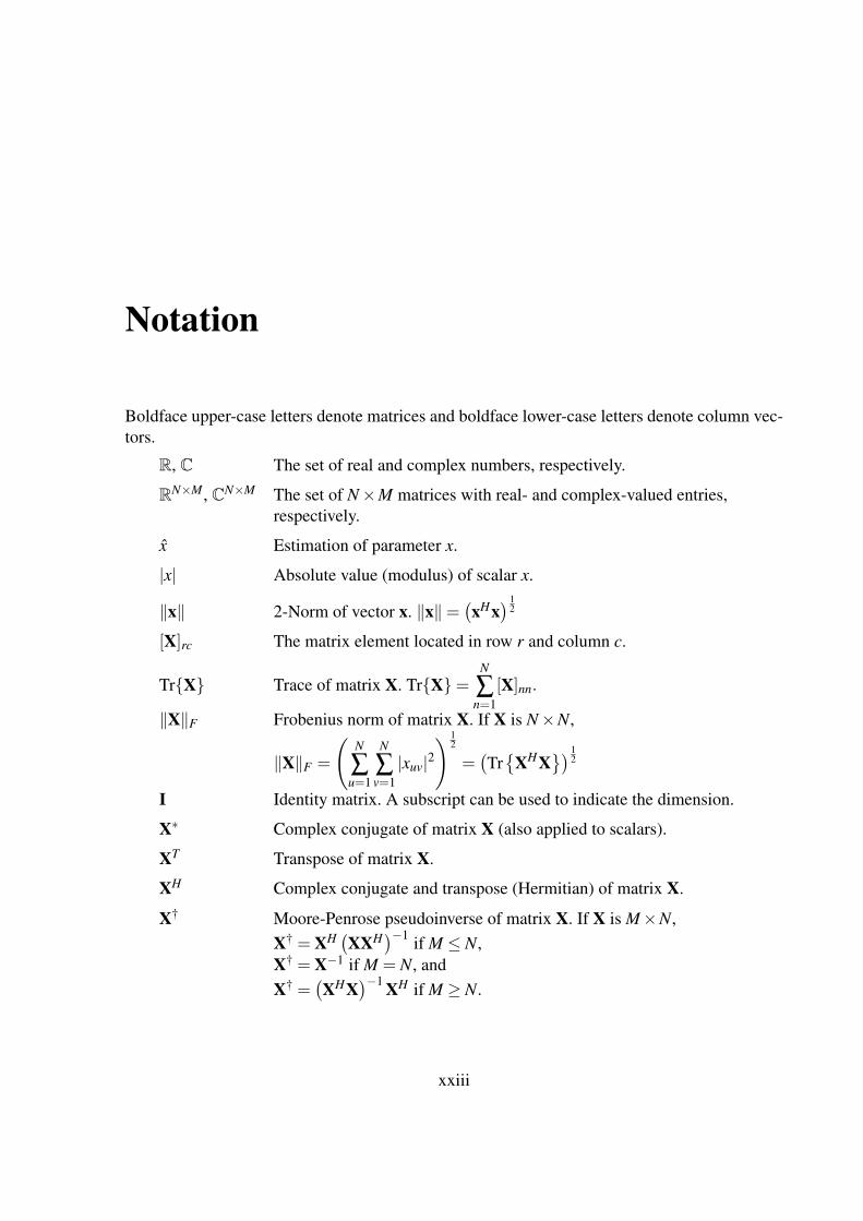
Notation
Boldface upper-case letters denote matrices and boldface lower-case letters denote column vec-tors.
R, C The set of real and complex numbers, respectively.
RN×M, CN×M The set of N×M matrices with real- and complex-valued entries,respectively.
x Estimation of parameter x.
|x| Absolute value (modulus) of scalar x.
‖x‖ 2-Norm of vector x. ‖x‖=(xHx
) 12
[X]rc The matrix element located in row r and column c.
TrX Trace of matrix X. TrX=N
∑n=1
[X]nn.
‖X‖F Frobenius norm of matrix X. If X is N×N,
‖X‖F =
(N
∑u=1
N
∑v=1|xuv|2
) 12
=(Tr
XHX) 1
2
I Identity matrix. A subscript can be used to indicate the dimension.
X∗ Complex conjugate of matrix X (also applied to scalars).
XT Transpose of matrix X.
XH Complex conjugate and transpose (Hermitian) of matrix X.
X† Moore-Penrose pseudoinverse of matrix X. If X is M×N,X† = XH (XXH)−1 if M ≤ N,X† = X−1 if M = N, andX† =
(XHX
)−1 XH if M ≥ N.
xxiii

Schur-Hadamard (elementwise) product of matrices.If A and B are two N×M matrices:
AB =
a11b11 a12b12 · · · a1Mb1M
a21b21 a22b22. . . a2Mb2M
...... . . .
...aN1bN1 aN2bN2 · · · aNMbNM
⊗ The Kronecker or tensor product. If A is m×n, then
A⊗B =
[A]11B · · · [A]1mB...
...[A]n1B · · · [A]nmB
PX Orthogonal projector onto the subspace spanned by the columns of X.
PX = X(XHX
)−1 XH .
P⊥X I−PX, orthogonal projector onto the orthogonal complementto the columns of X.
E · Statistical expectation.
ln(·) Natural logarithm (base e).
det(X) Determinant of matrix X.
ℜ·, ℑ· Real and imaginary parts, respectively
op( fN) A sequence of random variables XN is XN = op( fN), for fN > 0 ∀N,when XN
fNconverges to zero in probability, i.e.,
limN→∞
Prob∣∣∣∣XN
fN
∣∣∣∣> δ
= 0 ∀δ > 0
f (t)∗g(t) Convolution between f (t) and g(t).
argminx
f (x) Value of x that minimizes f (x).∂ f (x)
∂xiPartial derivative of function f (x) with respect to the variable xi.
∇x f (x) Gradient of function f (x) with respect to vector x.
Hx f (x) Hessian matrix of function f (x) with respect to vector x.
xxiv

Acronyms
ADC Analog-to-Digital Converter.
AGC Automatic Gain Control.
AS Anti Spoofing.
ASIC Application-Specific Integrated Circuit.
AWGN Additive White Gaussian Noise.
BNC Bayonet Neill-Concelman.
BPSK Binary Phase Shift Keying.
BOC Binary Offset Carrier.
CASM Coherent Adaptive Subcarrier Modulation.
CDMA Code Division Multiple Access.
CN0 Carrier to noise density ratio.
COTS Commercial Off-The-Shelf.
CPLD Complex Programmable Logic Device.
CRB Cramer Rao Bound.
CRC Cyclic Redundancy Check.
CS Commercial Services.
DLL Delay Locked Loop.
DOA Direction Of Arrival.
DS-SS Direct-Sequence Spread-Spectrum.
DSP Digital Signal Processor.
xxv

EIRP Effective Isotropic Radiated Power.
ELS Early/Late Slope algorithm.
EGNOS European Geostationary Navigation Overlay System.
EM Expectation Maximization algorithm.
EML Early Minus Late algorithm.
ELT Emergency Locator Transmitter.
EPIRB Emergency Position Indicating Radio Beacon.
ESPRIT Estimation of Signal Parameters via Rotational Invariance Techniques.
FDOA Frequency Difference Of Arrival.
FEC Forward Error Correction.
FFT Fast Fourier Transform.
FIM Fisher Information Matrix.
FLL Frequency Locked Loop.
FPGA Field Programmable Gate Array.
GAGAN GPS And Geo Augmentation Navigation.
GLONASS GLObalnaya Navigasionnay Sputnikovaya Sistema.
GNSS Global Navigation Satellite System.
GPS Global Positioning System.
GRAS Ground Regional Augmentation System.
GSM Global System for Mobile communications.
HRC High Resolution Correlator.
HOW Hand Over Word.
IF Intermediate Frequency.
IMU Inertial Measurement Unit.
INS Inertial Navigation System.
IQML Iterative Quadratic Maximum Likelihood algorithm.
LFSR Linear Feedback Shift Register.
xxvi

LNA Low Noise Amplifier.
LO Local Oscillator.
LS Least Squares.
LUT Local User Terminal.
LOSS Line Of Sight Signal.
MCRW Modified Correlator Reference Waveform.
MEDLL Multipath Estimating Delay Lock Loop.
MEMS Micro Electro Mechanical System.
MET Multipath Elimination Technology.
MHB Multiple Hybrid Beamforming.
MIMO Multiple Input Multiple Output.
ML Maximum Likelihood.
MSAS Multifunctional transport Satellite Augmentation System.
MSE Mean Square Error.
MUSIC MUltiple SIgnal Classification algorithm.
NCO Numerical Controlled Oscillator.
NDA Non Data Aided.
NSF Noise Subspace Fitting.
MVB Minimum Variance Beamforming.
OS Open Service.
PAC Pulse Amplitude Correlator.
PCI Peripheral Component Interconnect.
PDF Probability Density Function.
PLB Personal Locator Beacon.
PLL Phase Locked Loop.
PRN Pseudo Random Noise.
PRS Public Regulated Service.
xxvii

QPSK Quadrature Phase Shift Keying.
RF Radio Frequency.
RHCP Right Hand Circularly Polarized.
RLS Return Link Service.
RLSP Return Link Service Provider.
RMSE Root Mean Squared Error.
SAGE Space-Alternating Generalized Expectation-maximization algorithm.
SAR Search And Rescue.
SAW Surface Acoustic Wave.
SDR Software Defined Radio.
SISA Signal In Space Accuracy.
SINR Signal to Interference plus Noise Ratio.
SNR Signal to Noise Ratio.
SOCP Second Order Cone Program.
SSF Signal Subspace Fitting.
SV Space Vehicle.
TDOA Time Difference Of Arrival.
TK Teager-Kaiser algorithm.
TLM TeLeMetry word.
TTFF Time To First Fix.
TTL Transistor-Transistor Logic.
UTC Universal Time Coordinated.
VHDL Very high speed integrated circuit Hardware Description Language.
VI Virtual Instrument.
WAAS Wide Area Augmentation System.
WLS Weighted Least Squares.
WSSUS Wide Sense Stationary with Uncorrelated Scattering.
xxviii

Chapter 1
Introduction
The most exciting phrase to hear inscience, the one that heralds newdiscoveries, is not ”Eureka!” (Ifound it!) but ”That’s funny ...”
Isaac Asimov
THE art of finding the way from one place to another is called navigation. Until the 20thcentury, the term referred mainly to guiding ships across the seas. Indeed, the word “nav-
igate” comes from the Latin navis (meaning “ship”) and agere (meaning “to move or direct”).Today, the word also encompasses the guidance of travel on land, in the air, and in inner andouter space.
This encyclopedic definition talks about art, but navigation has been (and today also is)a major scientific problem. Navigation seems to start very early in time: according to Chinesestorytelling, the compass was discovered and used in wars during foggy weather before recordedhistory. Since enumerating major navigation breakthroughs along the whole history in a coupleof pages would be necessarily incomplete and unfair, we have decided to depict the huge effortdevoted to such issues dedicating a few lines to John Harrison’s life [Sob95].
In the 16 and 17th Century, thousands of sailors were dying at sea because simply they couldnot find their position, and tones of goods were lost in maritime accidents. The problem wasnot the latitude, easy to calculate from the Sun’s position, but the longitude. The longitude of alocation is directly related to the difference between the local time and the Greenwich referencetime. The local time can conveniently be fixed by a noon sighting of the Sun, but the time at anyother location requires a reliable clock, or some other way of distant time synchronization. Thus,there was necessary to build precise clocks, so it was a technological problem: pendulum or sandclocks just did not work properly in a ship, and astronomical observations were impracticable
1

Chapter 1. Introduction 2
due to water movement. In 1598, king Philip III of Spain offered a price of 6000 ducats to theone who could solve this problem. In 1707 over 2000 men died when four ships run aground onthe Scilly Isles. With this accident, the whole British society, including the scientific community,got concerned about navigation. The British Government set up a committee, named the Boardof Longitude and heard by Isaac Newton, to try and find the answer to the Longitude problem:a solution that can provide longitude to within a half of degree. This Board of Longitude wasestablished in 1714, and offered the following prices:
• 10,000 Great Britain Pounds for a method that could determine longitude within 60 nau-tical miles,
• 15,000 GBP for a method that could determine longitude within 40 nautical miles, and
• 20,000 GBP for a method that could determine longitude within 30 nautical miles.
A number of methods were proposed: the observation of Jupiter’s satellites by Galileo, thelunar tables by Tobias Mayer or the Newtonian reflecting telescope by John Hardley. None ofthem accomplished the requirements about precision and usability at sea, although they wereclearly superior to previously existing methods and were used to reform maps, with the accord-ing displeasure of the French King Louis XV, who saw the greatest reduction of land extension– at least on maps – that any France enemy could achieve in the whole history. The man whofinally won the price was a humble carpenter called John Harrison.
John Harrison (1693–1776) heard about the reward offered by the Board Of Longitude. Hespend five years to develop H1, his first mechanical clock. It was independent of the directionof gravity thanks to a new counterbalanced mechanism. H1 performed brilliantly in the cor-responding test, but Harrison asked for more money to build his next clock, H2. Three yearsmore of hard work did not satisfied him because he detected some errors in its design. Thenext work, H3, took him 19 years. H3 incorporated two new inventions of his own: a bimetallicstrip, to compensate the balance string for the effects of changes in the temperature, and thecage roller bearing, the ultimate version of his anti-friction devices. Incredibly, H3 convincedHarrison that the solution of the Longitude problem was in a completely different design: H4.This clock finally won the price, after several tests and the demonstration that it was industriallyrepeatable.
Before Harrison’s invention, only coast’s phares were reasonable reference points in navi-gation.

Chapter 1. Introduction 3
(a) H1 (1730-1735) (b) H2 (1737-1740) (c) H3 (1740-1759) (d) H4 (1755-1759)
Figure 1.1: John Harrison’s maritime chronometers. c©National Maritime Museum, London
1.1 Global Navigation Satellite Systems
Nowadays, technology has allowed us to put radiophares in the sky. Satellite–based navigationstarted in the early 1970s. Before the GPS program, three satellite systems were launched:the U.S. Navy Navigation Satellite System (also referred as Transit), which used a continuouswave signal and performed the positioning by measuring the Doppler shifts; the U.S. Navy’sTimation (TIMe navigATION) , which used an atomic clock that improves the prediction ofsatellite orbits and reduces the ground control update rate; and the U.S. Air Force project 621B.Its major novelty was the use of pseudorandom noise signal to modulate the carrier frequency.
The GPS program was approved in December 1973. The first satellite was launched in1978. In August 1993, GPS had 24 satellites in orbit and in December of the same year theinitial operational capability was established. In February 1994, the Federal Aviation Agency(FAA) declared GPS ready for aviation use. Now, there are modernization plans of GPS, whichdetails can be found in [Eis02]. Mainly, GPS Block IIR-M and IIF satellites will transmit anunencrypted L2 civil signal (L2CS) on the second carrier frequency, making the tracking of thissignal much easier and more reliable. An additional open signal called L5, centered at 1176.45MHz will become available on GPS IIF and GPS III satellites. Both new signals are expected toimprove the carrier phase tracking by means of aiding in the carrier phase ambiguity resolution.
The Russian satellite–based navigation system is called GLObal’naya Navigasionnay Sput-nikovaya Sistema, GLONASS. The first GLONASS type spacecraft (COSMOS 1413) waslaunched on October 12, 1982. GLONASS system was officially put into operation on Septem-ber 24, 1993 under the decree of the President of the Russian Federation. Nowadays this systemis not fully operational, but can be exploited jointly with GPS to improve accuracy and avail-ability.

Chapter 1. Introduction 4
On March 26, 2002, the European Council reached an unanimous agreement on the launchof the European Civil Satellite Navigation Programme: Galileo. However, at this time (Autumn2005) the frequency plan and the signal design are not completely determined. Most of thealgorithms developed in this thesis are going to be applied to the Galileo signals, in order toimprove the multipath mitigation and to cope with interferences.
1.2 Approach followed in this Dissertation
The possibility of electronically giving desired directional characteristics to an arrangement ofspaced antennas could be explained, in more mathematical terms, as the addition of an extra di-mension –space– to the estimation and detection problems, where the traditional features whichtrigger different trends amenable to statistical analysis are frequency, time and code. From aninformation theory point of view, this spatial ability provides another source of diversity whichcan be employed to separate the desired signal from noise. Here, noise must be understoodas any unwanted signal. Spatial diversity has been widely used in engineering, from the cou-ple of speakers occupied in a stereo sound system to advanced Multiple Input Multiple Output(MIMO) wireless communication systems. Actually, nature is plenty of spatial diversity exam-ples. The basic concept relies on obtaining the signal via several independent diversity branchesto get independent signal replicas.
Spatial diversity applied to the design of satellite–based navigation systems’ receivers is anew trend in digital synchronization, favored by the rapid evolution of signal processing tech-nology and the increasing interest in positioning systems, reflected in the modernization of theexisting GPS, the advent of the Galileo system or the growing effort in the hybridization withwireless communication systems.
Multipath and interferences are considered the more disturbing effects in GNSS synchro-nization, degrading the positioning final accuracy in an amount that can exceed a hundred metersin troubling scenarios. This Dissertation addresses the problem of multipath and interferencemitigation in a GNSS receiver by means of the exploitation of the spatial diversity providedby antenna arrays and its combination with the statistically-based methodology of MaximumLikelihood and the more traditional approach of digital beamforming. While ML establishesa procedure for finding estimators with desirable properties, such as functional invariance andasymptotic behavior, the beamforming approach is more intuitive and requires a lighter compu-tational cost, allowing its implementation in a practical system.
The obtained theoretical results has been applied in two different systems: the Search andRescue satellite-based system named COSPAS-SARSAT, showing an improved performancewith respect to traditional single-antenna receivers, and the GPS L1 civil signal thanks to aspecially-developed antenna array receiver. Along the Dissertation, the focus will move from
Chapter 1. Introduction 5
a theoretical approach to a practical point of view, using the navigation systems for their mainfunction: the guidance of a trip starting in estimation theory and finishing in coper wires.
1.3 Organization of this Dissertation
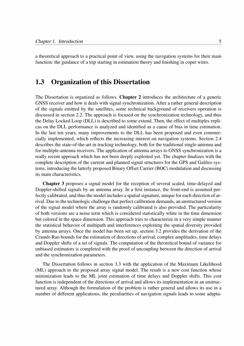
The Dissertation is organized as follows. Chapter 2 introduces the architecture of a genericGNSS receiver and how it deals with signal synchronization. After a rather general descriptionof the signals emitted by the satellites, some technical background of receivers operation isdiscussed in section 2.2. The approach is focused on the synchronization technology, and thusthe Delay Locked Loop (DLL) is described to some extend. Then, the effect of multiples repli-cas on the DLL performance is analyzed and identified as a cause of bias in time estimation.In the last ten years, many improvements to the DLL has been proposed and even commer-cially implemented, which reflects the increasing interest on navigation systems. Section 2.4describes the state-of-the-art in tracking technology, both for the traditional single-antenna andfor multiple-antenna receivers. The application of antenna arrays to GNSS synchronization is areally recent approach which has not been deeply exploited yet. The chapter finalizes with thecomplete description of the current and planned signal structures for the GPS and Galileo sys-tems, introducing the latterly proposed Binary Offset Carrier (BOC) modulation and discussingits main characteristics.
Chapter 3 proposes a signal model for the reception of several scaled, time-delayed andDoppler-shifted signals by an antenna array. In a first instance, the front-end is assumed per-fectly calibrated, and thus the model includes a spatial signature, unique for each direction of ar-rival. Due to the technologic challenge that perfect calibration demands, an unstructured versionof the signal model where the array is randomly calibrated is also provided. The particularityof both versions are a noise term which is considered statistically white in the time dimensionbut colored in the space dimension. This approach tries to characterize in a very simple mannerthe statistical behavior of multipath and interferences exploiting the spatial diversity providedby antenna arrays. Once the model has been set up, section 3.2 provides the derivation of theCramer-Rao bounds for the estimation of directions of arrival, complex amplitudes, time delaysand Doppler shifts of a set of signals. The computation of the theoretical bound of variance forunbiased estimators is completed with the proof of uncoupling between the direction of arrivaland the synchronization parameters.
The Dissertation follows in section 3.3 with the application of the Maximum Likelihood(ML) approach to the proposed array signal model. The result is a new cost function whoseminimization leads to the ML joint estimation of time delays and Doppler shifts. This costfunction is independent of the directions of arrival and allows its implementation in an unstruc-tured array. Although the formulation of the problem is rather general and allows its use in anumber of different applications, the peculiarities of navigation signals leads to some adapta-

Chapter 1. Introduction 6
tions of the algorithms to better suite the problem at hand and reduce their computational cost.Some iterative algorithms based on the obtained cost function are derived and intensively testedin computer simulations, which results are showed in section 3.5.
Chapter 4 attacks the problem of synchronization with antenna arrays from a completelydifferent point of view. If the previous chapter was based on statistical assumptions about multi-path and interferences, this one takes the beamforming approach, taking advantage of the elec-tronic manipulation of the radiation pattern that allows an antenna array. Section 4.2 proposesthe combination of temporal and spatial references to avoid the multipath effect, the so-calledspace-time hybrid beamforming. The result is a beamforming algorithm which requires a rea-sonable computation cost and is surprisingly linked to the ML approach, as showed in section4.2.3. Different pointing strategies are proposed, including the derivation of a robust versionwhich copes with array miscalibration resorting to convex optimization theory.
As another original contribution of this Dissertation, the theory of beamforming has beenapplied for first time to a satellite-based Search And Rescue system named COSPAS–SARSATin Chapter 5. Nowadays, the system works with four satellites that are unable to ensure globalcoverage, among other serious drawbacks. The European Space Agency (ESA) is evaluatingthe possibility to equip the forthcoming Galileo satellite constellation with Search And Rescuetransponders. The tight power budget constraints and the accuracy requirements for emergencybeacon positioning greatly complicates the ground receiver design, making inviable the use ofa single-antenna system. This chapter begins with the analysis of the current emergency beaconand another signal structure proposed by the Centre National d’Etudes Spatiales (CNES) fora new generation of emergency beacons. Then, we propose the use of an antenna array in thereceiver design and provide suitable, specially designed algorithms and extensive simulationresults.
Chapter 6 describes the design and implementation of an antenna array devoted to the civilsignal provided by GPS on the L1 link. We have decided to implement an antenna array inorder to apply the theory explained in the previous chapters of this dissertation and providea testbed for evaluation of the developed algorithms in conditions of real data. The chaptercontains details about the hardware architecture, the requirements and measurements of eachblock and some results working with real GPS data, drawing a link between signal processingtheory and its actual hardware implementation.
Finally, conclusions and some guidelines and suggestions for further research can be foundin Chapter 7.

Chapter 1. Introduction 7
1.4 Research contributions
The research contributions of this Dissertation are pointed out in the summary available at theend of each chapter. During the PhD. period, we has published some work not directly relatedto the main topic of this Dissertation, including collaborations in Inertial Navigation Systemsand machine-based learning and the direction of Master Theses. The full list of publications isprovided hereafter.
1.4.1 Journal papers
• [Fer05d] C. Fernandez Prades, Pau Closas Gomez, Juan A. Fernandez-Rubio and Gon-zalo Seco, “Parameter estimation techniques in Local User Terminals for Search & Res-cue systems based on Galileo and GPS satellites”, submitted to IEEE Transactions onAerospace and Electronic Systems, 2005.
• [Sec05] Gonzalo Seco, Juan A. Fernandez-Rubio, and C. Fernandez Prades, “ML esti-mator and Hybrid Beamformer for multipath and interference mitigation in GNSS re-ceivers”, IEEE Transactions on Signal Processing, vol. 53, no. 3, pp. 1194–1208, March2005, ISSN: 1053-587X.
1.4.2 Technical reports
• [Fer05e] C. Fernandez Prades, Pau Closas Gomez, and Juan A. Fernandez Rubio, “Ad-vanced Signal Processing techniques in Local User Terminals for Search & Rescue sys-tems Based on MEO satellites”, Tech. Rep. ESTEC/Contract no. 17713/03/NL/LvH/jd,Dept. of Signal Theory and Communications, Universitat Politecnica de Catalunya(UPC), Barcelona, February 2005.
• [Fer04d] C. Fernandez Prades, J. A. Fernandez Rubio, Christian Pomar Berry, and Mar-garita Cabrera Bean, “COMalaWEB. plataforma basada en noves tecnologies aplicadesa la docencia. memoria del projecte per la millora de la qualitat docent (expedient22mqd2002)”, Tech. rep., Universitat Politecnica de Catalunya (UPC), Barcelona, Spain,December 2004, in Catalan.
• [JF02] J. A. Fernandez Rubio, O. Munoz, and C. Fernandez Prades, “Analysis of TDOA,Doppler frequency and BER Estimation at the MEOLUT”, Tech. Rep. elaborated by theDept. of Signal Theory and Communications of UPC for Indra Espacio, 2002.

Chapter 1. Introduction 8
1.4.3 International conferences
• [Fer05a] C. Fernandez Prades, P. Closas Gomez, and J.A. Fernandez-Rubio, “Advancedsignal processing techniques in Local User Terminals for Search & Rescue systems basedon MEO satellites”, Proceedings of the ION GNSS, Institute Of Navigation, Long Beach,CA, September 2005. ION 2005.
• [Fer05c] C. Fernandez Prades, P. Closas Gomez, and J.A. Fernandez-Rubio, “Time-frequency estimation in the COSPAS/SARSAT system using antenna arrays: variancebounds and algorithms”, Proceedings of the 13th European Signal Processing Confer-ence, EUSIPCO, Antalya, Turkey, September 2005.
• [Fer05b] C. Fernandez Prades, P. Closas Gomez, and J.A. Fernandez-Rubio, “New trendsin global navigation systems: implementation of a GPS antenna array receiver”, Proceed-ings of the Eight International Symposium on Signal Processing and Its Applications,ISSPA, Sydney, Australia, August 2005.
• [Clo04] P. Closas Gomez, C. Fernandez Prades, J.A. Fernandez Rubio, Gonzalo Seco,and Igor Stojkovic, “Design of Local User Terminals for Search and Rescue systemswith MEO satellites”, Proceedings of the 2nd ESA Workshop on Satellite NavigationUser Equipment Technologies (NAVITEC), ESA/ESTEC, Noordwijk, The Netherlands,December 2004.
• [Fer04c] C. Fernandez Prades, and J. A. Fernandez Rubio, “Robust space-time beam-forming in GNSS by means of second-order cone programming”, Proceedings of theInternational Conference on Acoustics, Speech and Signal Processing, ICASSP, vol. 2,pp. 181184, Montreal, Quebec, Canada, May 2004.
• [Fer04a] C. Fernandez Prades, and J.A. Fernandez-Rubio, “Multi-frequency GPS/Galileoreceiver design using direct RF sampling and antenna arrays.”, Third IEEE Sensor Arrayand Multichannel Signal Processing Workshop, SAM, Sitges, Barcelona, Spain, 1821 July2004.
• [Fer04b] C. Fernandez Prades, A. Ramırez Gonzalez, Pau Closas Gomez, and Juan A.Fernandez Rubio, “Antenna array receiver for GNSS”, Proceedings of the Eight EuropeanSymposium on Global Navigation Satellite System, Rotterdam, The Netherlands, 2004.
• [Fer03a] C. Fernandez Prades, J.A. Fernandez-Rubio, and Gonzalo Seco, “A MaximumLikelihood approach to GNSS synchronization using antenna arrays”, Proceedings of theION GPS/GNSS, Institute Of Navigation, Portland, OR, September 2003.
• [Ram03] A. Ramırez Gonzalez, C. Fernandez Prades, and Juan A. Fernandez Rubio,“Some experiments using EGNOS and GPS/INS in terrestrial navigation”, Proceedings of

Chapter 1. Introduction 9
the Seventh European Symposium on Global Navigation Satellite System, Graz, Austria,2003.
• [Fer03b] C. Fernandez Prades, J.A. Fernandez-Rubio, and Gonzalo Seco, “On the equiv-alence of the joint Maximum Likelihood approach and the multiple Hybrid Beamformingin GNSS synchronization.”, Proceedings of the Sixth Baiona Workshop on Signal Pro-cessing in Communications, Baiona, Spain, September 2003.
• [Fer03d] C. Fernandez Prades, J. A. Fernandez Rubio, and Gonzalo Seco, “Joint maxi-mum likelihood of time delays and doppler shifts”, Proceedings of the Seventh Interna-tional Symposium on Signal Processing and its Applications, ISSPA 2003, IEEE, Paris,France, July 14 2003, ISBN 0780379470.
1.4.4 National conferences
• [Fer03c] C. Fernandez Prades, A. Ramırez Gonzalez, and J.A. Fernandez-Rubio, “Rec-hazo de interferencias mediante conformacion de haz hıbrida multiple en GNSS”, XVIIISimposium Nacional de la Union Cientıfica Internacional de Radio (URSI), A Coruna,Spain, September 2003, in Spanish.
• [Clo03b] P. Closas Gomez, C. Fernandez Prades, and J.A. Fernandez-Rubio, “Estimacionde parametros en sistemas search and rescue basados en satelites”, XVIII Simposium Na-cional de la Union Cientıfica Internacional de Radio (URSI), A Coruna, Spain, September2003, in Spanish.
• [Fer02] C. Fernandez Prades, O. Munoz Medina, J.A. Fernandez-Rubio, and A.Ramırez Gonzalez, “Estimacion de Maxima Verosimilitud de Retardos y Desplazamien-tos Doppler”, XVII Simposium Nacional de la Union Cientıfica Internacional de Radio(URSI), pp. 237238, Alcala de Henares, Madrid, Spain, Sep. 2002, in Spanish.
• [Ram02] A. Ramırez Gonzalez, C. Fernandez Prades, and J.A. Fernandez-Rubio, “In-tegracion GPS/INS para Navegacion Vehicular Terrestre en entornos de alta dinamica”,XVII Simposium Nacional de la Union Cientıfica Internacional de Radio (URSI), pp. 431432, Alcala de Henares, Madrid, Spain, Sep. 2002, in Spanish.
• [Fer01] C. Fernandez Prades, A. Ramırez, and J.A. Fernandez-Rubio, “Implementacionde Correccion de Pseudodistancias y del Algoritmo de Bancroft en MATLAB para elPosicionamiento Preliminar en GPS”, XVI Simposium Nacional de la Union CientıficaInternacional de Radio (URSI), pp. 287288, Madrid, Spain, Sep. 2001, in Spanish.

Chapter 1. Introduction 10
1.4.5 Master Theses directed
• [Gon03] F. J. Gonzalez Arranz, and V. Montoya Barrera, Implementacion Softwareen MATLAB y Simulink de un correlador GPS de 12 canales, Master Thesis, EscolaTecnica Superior d’Enginyeria de Telecomunicacio de Barcelona (ETSETB), UniversitatPolitecnica de Catalunya (UPC), Barcelona, Spain, October 2003, in Spanish.
• [Clo03a] P. Closas Gomez, Parameter Estimation in Search & Rescue Satellite-BasedSystems, Master Thesis, Escola Tecnica Superior d’Enginyeria de Telecomunicacio deBarcelona (ETSETB), Universitat Politecnica de Catalunya (UPC), Barcelona, Spain,November 2003.
• [Jar04] M. A. Jara Burgos, Plataforma basada en nuevas tecnologıas aplicadas a la do-cencia, Master Thesis, Escola Tecnica Superior d’Enginyeria de Telecomunicacio deBarcelona (ETSETB), Universitat Politecnica de Catalunya (UPC), Barcelona, Spain,2004, in Spanish.
• [Fon04] A. Font Valverde, and J. Tena Lucia, Programacion de Applets en comunica-ciones y procesado de senal dentro de una plataforma docente, Master Thesis, EscolaTecnica Superior d’Enginyeria de Telecomunicacio de Barcelona (ETSETB), UniversitatPolitecnica de Catalunya (UPC), Barcelona, Spain, October 2004, in Spanish.

Chapter 2
Fundamentals of GNSS synchronization
If I have seen farther than others, itis because I stood on the shouldersof giants.
Sir Isaac Newton
SYNCHRONIZATION is a critical aspect in positioning system receivers. This chapter willpresent the theoretical background of the receiver’s operation, beginning with a generic
description of the signals emitted by the satellites and the vicissitudes that they suffer beforereaching the receiver antenna. Physical explanation about the ionosphere, troposphere and othersources of distortion of the propagation velocity will be omitted, since they can be compensatedby means of data processing and differential systems (see the remarkable work of Hernandez-Pajares et al., [HP98, HP02, HP03]); here the focus will be pointed to the signal processing taskperformed by the receiver, namely estimation of time delay, carrier phase and Doppler shift ofthe received signals. After providing an overview of the classical hardware architecture and howis affected by the multipath phenomenon, which is receiver-location dependent and cannot becompensated by the aforementioned differential systems, we shall review the state-of-the-art inGNSS synchronization, highlighting how new techniques deal with multipath mitigation. Themainstream in GNSS receiver design is the single antenna approach, which has objectionablefeatures that will be pointed out. On the contrary, the use of antenna arrays represent a newtrend in the field that overcomes single antenna drawbacks, and its possibilities will be alsooutlined. The chapter finishes with a description of the current and planned GPS and Galileosignal structure.
11

Chapter 2. Fundamentals of GNSS synchronization 12
2.1 Signals coming from space
GPS and the forthcoming Galileo system are based on the transmission of a Direct–SequenceSpread–Spectrum (DS-SS) signal, which general baseband model can be expressed as
sT (t) =√
PT
(γ
∞
∑m=−∞
dI(m)pI(t−mTbI)+ j√
1− γ2∞
∑n=−∞
dQ(n)pQ(t−nTbQ)
)(2.1)
where
pI(t) =NcI−1
∑u=0
qI(t−uTPRNI) (2.2)
and
qI(t) =LcI−1
∑k=0
cI(k)gT,I(t− kTcI), (2.3)
being PT the transmitting power, γ a parameter controlling the power balance, dI(m) ∈ −1,1the data symbols, TbI the bit period, NcI the number of repetitions of a full codeword that spansa bit period, TPRNI =
TbINcI
the codeword period, cI(k) ∈ −1,1 a chip of a spreading code-word of length LcI chips, gT,I(t) the transmitting chip pulse shape, which is considered energy-normalized for notation clarity, and TcI =
TbINcI LcI
is the chip period. Subindex I refers to the In-phase component, and all parameters are equivalently defined for the Quadrature component,referred to with the subindex Q.
In case of γ = 1, expression (2.1) reduces to the BPSK DS-SS modulation. For the sakeof notation simplicity in the following analysis, we can consider normalized power PT = 1,TbI = TbQ , NcI = NcQ , LcI = LcQ and γ = 1√
2, thus reducing equation (2.1) to
sT (t) =1√2
∞
∑m=−∞
d(m)Nc−1
∑u=0
Lc−1
∑k=0
c(k)gT (t− kTc−uTPRN−mTb) =1√2
∞
∑m=−∞
d(m)p(t−mTb)
(2.4)
where d(m) = dI(m)+ jdQ(m), c(k) = cI(k)+ jcQ(k), gT (t) = gT,I(t)+ jgT,Q(t) and pI(t) =pQ(t) are complex-valued. Although the following derivation could be straightforwardly ex-tended to the general expression (2.1), model (2.4) has been used because it retains the behaviorwhich is wanted to be highlighted.
The signal emitted by the satellite travels through a radio-propagation channel. The directpath between the satellite and the receiver could not be the only way to reach the antenna. In fact,

Chapter 2. Fundamentals of GNSS synchronization 13
the ground and other objects easily reflect GNSS signals, and one or more replicas can reachthe antenna having traveled through longer paths than the direct one. Therefore, this secondary-path signals with longer propagation times are superimposed on the direct-path signal at theantenna, distorting the signal waveform’s amplitude and phase and, as will be shown in section2.3, degrading time and phase estimations. Such radio-propagation channel is modeled usinga linear time-varying channel impulse response and supposing a finite number of M paths, inaddition to the line of sight [Rap96]:
h(t;ξ) =M−1
∑m=0
am(t)e jθm(t)δ(ξ− τm(t)), (2.5)
where am(t), θm(t) and τm(t) are the amplitude, phase and delay of the m-th path, ξ is themultipath delay axis and the index m = 0 stands for the line–of–sight signal. These chan-nel parameters can be seen as realizations of random processes with underlying probabilitydensity functions fap(a), fθp(θ) and fτp(τ), respectively. The statistical behavior of the chan-nel random parameters are well studied in the literature: by instance, the time-varying enve-lope a(t) is commonly considered Rician-distributed [Rap96, Pro01], while the phase θ(t) ismostly modeled with a uniform distribution [Jak74, Rap96] and the delay τ(t) is usually as-sumed constant [Nee94, Foc01] in observation times of orders of tens of milliseconds in theL-band (which is the industry standard designation to the frequency range from 1000 MHzto 2000 MHz). In other words, the delay is considered piecewise constant: small variationsare allowed in a long time scale (on the order of few seconds), but it is assumed constant inthe observation window. In many physical channels, the statistics of the channel parameterscan be assumed approximatively stationary for sufficiently long time intervals. Therefore, it iscommon to assume a wide sense stationary channel [Jak74], where the channel impulse re-sponse has its mean and variance invariant under a translation in time: Eh(t,ξ) = µh(ξ) andEh(t1,ξ1)h∗(t2,ξ2)= Rh(t1− t2,ξ1,ξ2). The Fourier transform of the time-delay channel au-tocorrelation function, Sh( f ,ξ) = FRh(t,ξ), represents the delay-Doppler power spectrum ofthe channel, which has a frequency-dispersive nature. The spectral broadening due to the timerate of change of the channel parameters is called Doppler spread. The maximum of the Dopplerspread, fd , depends on the radial velocity νr between the transmitter and the receiver and thecarrier frequency:
fd =νr
cfc (2.6)
being c the speed of light. In case of reflections, the resulting Doppler is the sum of the Dopplershift due to the radial velocity between the satellite and the scatterer and between the scattererand the receiver [Fon98]. Different paths are assumed to be independent, completing a channelmodel which is usually referred as wide sense stationary with uncorrelated scattering (WSSUS)[Bel63]. Along the rest of the dissertation, the carrier phase evolution will be considered linearin time, and therefore θm(t) = 2π fdmt +θm.

Chapter 2. Fundamentals of GNSS synchronization 14
Considering the multipath-free situation, i.e., when only the line of sight signal is presentand thus M = 1 in equation (2.5), and taking into account the aforementioned assumptions aboutthe radio-propagation channel, the signal entering the receiver can be modeled as:
r(t) =Z
∞
−∞
sT (t−ξ)h(t;ξ)dξ = a0(t)e j(2π fd0 t+θ0)∞
∑m=−∞
d(m)p(t− τ0−mTb) (2.7)
Positioning algorithms are based on the estimations of the synchronization parameters τ0,θ0 and fd0 . Better performance in estimation directly impacts in a better performance in po-sitioning, and thus a major objective of this Dissertation is to contribute to the improvementof synchronization parameters estimation. Next section is intended to be a brief overview of ageneric GNSS receiver and how it deals with the signal in order to perform such estimation.
2.2 Technical background: a GPS receiver architecture
The trend in modern GPS receiver design is to increase the digital component integration. Thus,a high-level block diagram will be useful to describe a generic GPS receiver architecture. Inthe sequel, some of their characteristics will be outlined. For a complete description of a GPSreceiver architecture and implementation details, the reader is referred to chapter 6 or GPS-devoted textbooks such as [Par96a, Kap96].
The first element in the RF chain is a RHCP antenna, usually with nearly hemispherical gaincoverage, with the mission to receive the radionavigation signals of all the satellites in view or,using navigation nomenclature, the Line-Of-Sight Signals (LOSS). The most common antennais a low-profile type consisting of a microstrip patch element; other types include helixes ordesigns which null low-elevation angles in order to reduce multipath, as the “choke-ring”, wherethe antenna is located in the middle of a set of concentric electrically-conducting rings. The useof an antenna array, and the way to exploit its spatial diversity, is a major topic in this Thesis.
The RF signals collected by the antenna are immediately amplified by a Low Noise Am-plifier (LNA), a key element which is the most contributing block to the noise figure of thereceiver. The LNA also acts as a filter, minimizing out-of-band RF interferences and setting thesharpness of the received code: while commercial low-end receivers use to be equipped witha 2 MHz filter bandwidth for the C/A L1 code (first-null bandwidth, taking the whole mainlobe of the code spectrum), satellites are reported to have a 20 MHz filtering at the transmis-sion stage. This wider bandwidth is exploited by high-performance receivers, because a sharperpulse shaping allows better synchronization. On the contrary, a wider bandwidth implies morenoise power passing through the LNA: the noise power can be approximated by
PN = kTEB (2.8)

Chapter 2. Fundamentals of GNSS synchronization 15
where k = 1.3806×10⁻²³ JK−1 is the Boltzmann’s constant, TE is the effective noise temper-ature in kelvin (with a typical value of TE = 513 K in a GPS receiver [Bra99]) and B is thebandwidth in Hertz. Therefore, the LNA bandwidth is a design key parameter in navigationreceivers. Typical values for the LNA gain are on the order of 20−40 dB, and the noise figurefor the amplifier and associated losses (preselection filtering, burnout protection, an so on) areon the order of 3−4 dB.
The signal-to-noise ratio (SNR) can be computed at this point. Considering the L1 C/A code,satellites are reported to transmit at 478.63 W of effective isotropic radiated power (EIRP). Thepropagation losses can be approximated by
free-space loss factor =(
λ
4πr
)2
(2.9)
where λ = cfL1
= 0.19 m is the carrier wavelength and r = 2×10⁷ m is the average transmitter-to-receiver distance. This results on −182.4 dB, plus −2 dB more of atmospheric attenuation.Assuming a 2 MHz bandwidth receiver, the C/A-code SNR is
SNR = Signal power in dB−Noise power in dB (2.10)= Transmitted Signal Power+Free-space Loss+Atmospheric attenuation−PN
= 26.8+(−182.4)+(−2)− (−138.5) =−19.1 dB.
and therefore can be concluded that GPS signals are completely buried in thermal noise. TheSNR of spread-spectrum signals is a function of the point in the receiver chain under consid-eration. As showed, precorrelation SNR is negative whereas postcorrelation SNR (signal afterthe matched filter) is positive due to the despreading gain. In order to work with a bandwidth-independent metric, the SNR is normalized to a 1-Hz bandwidth, getting a carrier-to-noise den-sity ratio which is a typical metric of signal quality in navigation systems:
CN0 = 10log10 (SNR×B) [dB-Hz]. (2.11)
Following with the L1 C/A example, an SNR of −19.1 dB is equivalent to a CN0 of 43.9dB-Hz. In figure 2.1 it is showed the evolution of the CN0 for different satellites measured witha NovAtel OEM4 receiver.
After the LNA, the amplified and filtered RF signals are then downconverted to an interme-diate frequency (IF) using signal mixing frequencies from local oscillators (LOs). These LOsare derived from a receiver reference oscillator, often an oven-stabilized clock with typical ac-curacies of 10−8. There is a need for one LO per downconversion stage. Two or three downcon-version stages are commonly devoted to reject mirror frequencies or large out of band jammingsignals, in particular the 900 MHz used by the GSM mobile communication system. However,depending on the subsequent Analog-to-Digital Converter (ADC) characteristics, a one-stage

Chapter 2. Fundamentals of GNSS synchronization 16
Figure 2.1: CN0 of GPS L1 signal of several satellites measured with a NovAtel OEM4 receiver.The observation period is 12 hours, with measurements taken each second (blue points) andsmoothed with a 2-minutes rectangular window (red solid lines).
donwconversion or even a direct L-band sampling is also possible [Ako99]. The lower sidebandgenerated by the mixer process is selected, while the upper sideband is filtered by a postmixerbandpass filter. It is important to point out that signal Dopplers and PRN codes are preservedafter the mixing stage, only the carrier frequency is lowered.
The analog-to-digital conversion and the Automatic Gain Control (AGC) processes takeplace at IF, where all the signals from GPS satellites in view are buried in thermal noise, aspreviously shown. This is the reason why there is no need of high resolution ADCs; in fact,2-bit quantization is typical in GPS receivers, even 1-bit in narrow (i.e., 2 MHz) bandwidthmodels. The degradation suffered by the signal due to a finite-bit quantization depends on thenumber of quantization levels, the IF bandwidth and the ratio of the maximum ADC threshold tothe root mean square noise level. It should be noted that the 1.96-dB degradation factor usuallyapplied by quantization bit is only valid for an infinite bandwidth. Multibit adaptive-thresholdADCs has been used to mitigate narrowband interference effects [Zar02].

Chapter 2. Fundamentals of GNSS synchronization 17
RF Low Noise Amplifier
Down converter
A/D converter Digital receiver
channel 1
2 N
RHCP Antenna
Receiver processing
Navigation processing
User interface
Analog FI
Digital FI
Reference oscillator
Phase Locked Loop
Synthesiser
Automatic Gain Control
Power control
Figure 2.2: Generic GPS receiver block diagram
Once IF signal is digitized, it is ready to feed each of the N digital receiver channels. Everyreceiver channel is intended to acquire and track the signal of a single GPS satellite; typicalreceivers are equipped with N = 12 channels. This digital receiver channels are usually imple-mented in one or more Application Specific Integrated Circuits (ASICs), and their design is akey aspect in the final performance of the receiver. A generic digital receiver channel imple-ments a carrier (plus carrier Doppler) stripping with the information provided by the receiverprocessor, multiplying the digital IF signal by a local replica carrier synthesized by discreteversions of a cosine and a sine driven by means of a carrier Numerical Controlled Oscillator(NCO). The NCO produces a staircase function whose period is the desired carrier period plusthe Doppler period. The discrete cosine and sine functions map each discrete amplitude of thisstaircase function to the corresponding discrete amplitude of the cosine and sine functions. Themultiplication of the IF digitized signal by a local replica of its carrier frequency allows to pro-duce the In-phase (I) and Quadrature-phase (Q) components of the digitized signal. In closedloop operation, the carrier NCO is controlled by the carrier tracking loop in the receiver proces-sor, and the local replica phase is maintained equal, or reasonably close, to the incoming carrierphase. Some strategies for the carrier tracking loop, which controls the carrier NCO, are ana-lyzed in [Kap96]. Herein, the Phase Locked Loop (PLL), the Costas Loop and the FrequencyLocked Loop (FLL) are compared, and the recommendations are lined-up with a receiver witha Costas loop, switching to a PLL when the bit synchronization and message demodulation isachieved, and switching to an FLL during high-dynamic stress periods. Studies applied to theL5 band can be found in [Heg99, Rie01].
In many high-performance receivers, an FLL is used to compute the velocity estimate be-cause of the relationship νr = λc fd , where vr is the radial velocity and λc is the transmitted

Chapter 2. Fundamentals of GNSS synchronization 18
wavelength, and the result is referred to as the delta-range measurement. If an accumulation ofthe carrier NCO is performed, velocity is integrated and the result can be interpreted as a dis-placement relative to the start of integration. At the end of a given integration interval, a wholenumber of Doppler cycles has been counted, and usually a fraction of a cycle remains. If thisfractional phase is also measured and included in the accumulated delta-range measurement,the resulting observable is referred to as integrated Doppler or carrier phase measurement.
In the following, signal is assumed to be synchronized in frequency, and consequently thecarrier frequency and the Doppler shift of the received signal r(t), expressed in equation (2.7),have been removed by means of an analog or digital method. Considering a generic data se-quence d, chip code c, chip-shaping pulse gT (t), chip period Tc, Nc full codes in a whole bit anddata period Tb, the baseband signal can be put in the form
z0(t) = α0
∞
∑m=−∞
d(m)Nc−1
∑u=0
Lc−1
∑k=0
c(k)gT (t− τ0− kTc−uTPRN−mTb)+w(t)
= α0
∞
∑m=−∞
d(m)p(t− τ0)+w(t), (2.12)
where gT (t) is the transmitted pulse filtered by a precorrelation filter (the LNA in figure 2.2) andthe term w(t) stands for thermal noise. The objective of a synchronization method is to estimatethe time delay τ0 and the carrier phase information θ0 embedded into the phase of the complexamplitude α0 = a0e jθ0 .
Assuming w(t) as Additive White Gaussian Noise (AWGN), at least in the band of interest,it is well known that the optimum receiver is the code matched filter, expressed as
hMF(t) =Lc−1
∑k=0
c∗(k)g∗R(−t− kTc +LcTc) = q∗R(−t +LcTc). (2.13)
Theoretically gR(t) = gT (t), but actual implementations make use of approximated versions:while gT (t) is a rectangular pulse filtered at the satellite, gR(t) is digitally generated at thereceiver and therefore not filtered. In addition, gT (t) is usually filtered again by a precorrelationfilter before the matched filter, as expressed in (2.12) with gT (t). The code matched filter outputcan be written in the form
y(t) = z0(t)∗hMF(t)
= α0
∞
∑m=−∞
d(m)p(t− τ0)∗q∗R(−t +LcTc)+n(t)
= α0
∞
∑m=−∞
d(m)R pq(t− τ0−LcTc)+n(t), (2.14)

Chapter 2. Fundamentals of GNSS synchronization 19
Rpq(τ) =1
TPRN
Z TPRN+τ
τ
p(t)q(t− τ)dt
=1
TPRN
Z TPRN+τ
τ∑u
q(t−uTPRN)q(t− τ)dt
=1
TcLc
Z TPRN
τ
q(t)q(t− τ)dt +1
TcLc
Z TPRN+τ
TPRN
q(t−TPRN)q(t− τ)dt (2.15)
for τ > 0 and
Rpq(τ) =1
TPRN
Z 0
τ
q(t +TPRN)q(t− τ)dt +1
TPRN
Z TPRN+τ
0q(t)q(t− τ)dt (2.16)
for τ < 0.
The term q(t), defined in equation (2.3), is a Pulse Amplitude Modulation (PAM) containingthe spreading sequence c(k) with a pulse shaping g(t). The tilde (·) indicates that the signal haspassed through the LNA. Particularities of sequences c(k) and pulse shapes g(t) actually usedin current and planned GNSS will be outlined in sections 2.5 and 2.6.
In DS-SS terminology, the matched filter is often referred as correlator, while the processingit performs is called despreading. The correlator architecture design is closely related to thesynchronization process. Briefly speaking, synchronization algorithms can be classified in twomain categories:
• Non-Data-Aided (NDA) algorithms, also known as blind channel estimators, perform de-lay and carrier phase estimations considering data symbols unknown, just the case whenthe GNSS receiver has not reached bit synchronization and is unable to predict data bittransitions. The data modulation is removed using a nonlinear operator, such as squaringor envelope detection. The ML principle applied to model (2.12) considering a matched-filter based receiver, Nyquist pulses, AWGN and removing data dependence leads to thetime delay estimator [Mey98]
τ0NDA = argmaxτ0
ΛNDA(τ0) = argmaxτ0
N
∑n=0|y(nTs + τ0)|2 (2.17)
where y(nTs + τ0) are samples of the output of the code matched filter taken at instantsnTs + τ0, and
• Data-Aided or Decision Directed (DA/DD) algorithms exploit the a priori knowledge of atraining data sequence (DA) or the decision about the received symbols (DD). This is the

Chapter 2. Fundamentals of GNSS synchronization 20
situation when the receiver has attained bit synchronization and complete data messagedemodulation. Under the same assumptions as in NDA excepting the knowledge of thedata bit and an estimation of the carrier phase θ0, the time delay estimator is
τ0DD/DA = argmaxτ0
ΛDD/DA(τ0) = argmaxτ0
ℜ
N
∑n=0
d∗(n)y(nTs + τ0)e− jθ0
(2.18)
In both cases, the estimation implies a maximization of y(τ0) (removing the nTs dependencefor clarity) or equivalently, as shown in equation (2.14), a maximization of the correlation func-tion Rgg(τ0) over the trial value τ0.
After an acquisition period which involves a search over all possible shifts of the locallygenerated code relative to the received code (acquisition will be further discussed in chapter 6,section 6.5) until the difference between the local and the received code is lower than 1 chip, thetracking process is in charge to perform a fine adjustment of time delay and follow the possiblevariations of the parameter, expected to be slow varying. The tracking process determines theperformance of the receiver in terms of accuracy, speed or robustness to multipath; GNSS re-ceiver developers have spent a lot of effort in the design of correlator technology. The traditionalmethod, known as Delay Locked Loop (DLL), will be described hereafter while the ultimatemodifications specially devoted to GNSS receivers will be discussed in section 2.4.
The objective is to perform a practical implementation of the estimators (2.17) or (2.18).The summations of these equations are computed in a block generally referred to as Integration& Dump or predetection integration, which provides the I and Q sample streams. The accumu-lation interval is typically set to the duration of a code period (1 ms in GPS L1 C/A) prior tobit synchronization, and extended to the duration of a whole navigation data bit (20 ms in thesame example) when this synchronization is achieved. Cost functions ΛNDA(τ0) or ΛDD/DA(τ0)
are driven to the maximum using feedback loops that employ the derivative dy(τ0)dτ0
zero-crossingas timing error detector. In order to simplify the receiver implementation, the derivative is ap-proximated with finite differences, generating an advanced and delayed replica, named Earlyand Late, respect to the actual estimated timing, which sample is called Prompt. For a givenintegration period n, and for the I arm, samples for a given trial value τ are defined as
IE = y(τ+δ
2Tc), IP = y(τ), IL = y(τ− δ
2Tc) (2.19)
where δ is usually referred to as early-late spacing of the DLL, 0 < δ < 1, and Tc is the chipperiod. The terms QE , QP and QL are defined equally for the Q arm.
Depending on the combination of the early, prompt and late samples used to form the feed-back loop or, in other words, how the error signal (called discriminator in this context) is com-puted, we speak of different kinds of DLL:

Chapter 2. Fundamentals of GNSS synchronization 21
Integration & Dump
Integration & Dump
Integration & Dump
Integration & Dump
Integration & Dump
Integration & Dump
Shift register
COS map
SIN map
Carrier NCO
Code generator Code NCO
Receiver baseband processor
Carrier cycle counter
Code phase counter
Digital IF
I E
I P
I L
Q E
Q P
Q L
E P L
Figure 2.3: Generic digital receiver channel
• Early minus late power
Deml−p(τ) =(I2E +Q2
E)−(I2L +Q2
L)
(2.20)
When the discriminator Deml−p(τ) is positive, the code NCO is advanced a given fractionof chip, and when the discriminator is negative, the code NCO is consequently delayedin order to align the prompt local replica with the received one. This is a non-coherentDLL, indicating that the DLL can operate independently of the residual carrier phase andthe data demodulation. Analysis about its performance in terms of thermal noise trackingerror variance can be found in [Die92], and a refined version for low SNR conditions isformulated in [Nee95].

Chapter 2. Fundamentals of GNSS synchronization 22
• Early minus late envelope
Deml−e(τ) =√(
I2E +Q2
E)−√(
I2L +Q2
L)
(2.21)
This discriminator, or a normalized version divided by√(
I2E +Q2
E)+√(
I2L +Q2
L)
inorder to remove its amplitude sensitivity, has been widely implemented in commercialGPS receivers.
• Dot product powerDdot(τ) = (IE − IL) IP +(QE −QL)QP (2.22)
This structure makes use of all the six correlators, and this results in a lower computationalload and better performance than previous early-late discriminators at low CN0 [Bra99]and in presence of multipath [Fel97]. Some designs of GPS correlators synthesize theearly minus late replicas, IE − IL and QE −QL, to ease the computation of Ddot .
• CoherentDc(τ) =
[(IE − IL)cos(θ)+(QE −QL)sin(θ)
]sign(IP) (2.23)
The coherent architecture makes use of a data removing, expressed in the term sign(IP),and a phase alignment to achieve better performance than the non-coherent versions. Inother words, actual carrier phase θ and data symbol d(n) are removed using their estimatesθ and d(n). Although this is a more complex structure because of the needing of phaseand bit information, it is a widespread technology easily found in the market.
The expected value of the discriminator output η = ED(τ) in terms of the trial valueτ is called S-curve. The position of its zero-crossing is the mean of the time delay estimate[Sim85], and therefore it gives the desired value to compute the pseudorange and to performthe navigation solution. All of the aforementioned DLL structures provide unbiased estimatesin absence of multipath [Nee93], but when one or multiple reflections appear, the zero-crossingof the S-curve is shifted away from the true time delay of the LOSS, and consequently theestimates obtained by the DLL become biased. Next section will illustrate this effect.
If only the thermal noise is considered, the Cramer-Rao bound is the theoretical limit thatany unbiased estimator can achieve. In case of the time delay estimation, its minimum varianceis defined by [Wei03]:
σ2error ≥
1
2(
EN0
)(2π)2 R ∞
−∞f 2Sz( f )d f
(2.24)
where EN0
is the received signal energy to noise power spectral density ratio, f is the frequencyin Hertz and Sz( f ) is the normalized power spectral density of the code modulation. Therefore,

Chapter 2. Fundamentals of GNSS synchronization 23
−2 −1.5 −1 −0.5 0 0.5 1 1.5 2
−1
−0.8
−0.6
−0.4
−0.2
0
0.2
0.4
0.6
0.8
1
S−curve for different DLL implementations (BPSK signal)
Tracking error [chips]
Dis
crim
inat
or o
utpu
t
EML powerDot productCoherentEML normalized envelope
−2 −1.5 −1 −0.5 0 0.5 1 1.5 2
−1
−0.8
−0.6
−0.4
−0.2
0
0.2
0.4
0.6
0.8
1
S−curve for different DLL implementations (BOC(1,1) signal)
Tracking error [chips]D
iscr
imin
ator
out
put
EML powerDot productCoherentEML normalized envelope
Figure 2.4: Discriminator functions for different DLL implementations applied to BPSK(1) andBOC(1,1) modulation signals filtered at 20 MHz
the integral represents the second moment of Sz( f ). The square root of this second moment iscommonly referred as RMS or Gabor bandwidth [Gab46], and it is a fundamental parameter incode modulation design in order to theoretically achieve a smaller time delay error:
BG =√Z
∞
−∞
f 2Sz( f )d f (2.25)
Inspecting equation (2.25), it is observed that we can increase the Gabor bandwidth usingmodulations whose power spectrum concentrates a greater percentage of their power fartherfrom the signal center frequency, because of the weighting term f 2. This approach has been fol-lowed in the definition of the modernized GPS and the new Galileo signals with the introductionof the BOC modulation, as will be shown at the end of this chapter.
Recently, all this theory and practice has been revisited in the light of the particularities ofthe BOC modulation, described in section 2.6. This new modulation has a narrower peak in theautocorrelation function than BPSK does (see figure 2.12 for a comparison), paying a price inthe form of several secondary peaks which can confuse the tracking algorithm thus producingan estimation error. This effect can be observed in the right side of figure 2.4, where somezero crossings are near the correct one. The inspection of the S-curves suggest that the earlyminus late envelope is preferred for BOC tracking over the early minus late power or dot DLLbecause is the structure whose zero crossings are farthest from the central one. Some strategiesto overcome this ambiguity are based in comparing additional very-early and very-late outputs

Chapter 2. Fundamentals of GNSS synchronization 24
with the prompt output, determining if the prompt sample is tracking the largest peak; if not, theprompt correlator jumps to the largest of the other two gates and the process is repeated again.This is the case of the bump-jump approach [Fin99] or its variants [Fan03].
Finally, and before dwelling in the multipath effect, it is worthwhile to notice the impor-tance of the front-end bandwidth, named BRx . Although the code-tracking accuracy for biphasesignals is well studied in the literature (see [Die92] for an analysis in the context of GPS), theapproaches often resort to infinite-bandwidth signals. In [Bet00] there is an analysis that avoidsthe infinite bandwidth assumption, providing more accurate analytical expressions. This workidentifies three regions, depending on the relation between the front-end bandwidth multipliedby the chip period and the early-late discriminator two-sided space δ normalized by the chipperiod. Hence, receivers with π≤ BRxδ are referred to as space limited, provided that the errordepends primarily on the early-late space and not the front-end bandwidth. If the product ofthese two parameters decreases, and 1 < BRxδ < π, there is a transition region. If 1 > BRxδ, thereceiver is bandwidth limited because the error depends primarily on the front-end bandwidthand not on the early-late space. The relevance of this trade-off will be shown in the followingsections.
2.3 Focusing the problem: the defocusing of multipath
Removing the data bit dependence for clarity of notation, model in equation (2.12) can beextended to M replicas, each one with a different time delay and carrier phase. Assuming aperfect synchronization of fd0 and θ0 performed by the carrier tracking loop, the input of thecorrelator is
zM(t) =M−1
∑m=0
αme j2π( fdm− fd0)tLc−1
∑k=0
c(k)gT (t− τm− kTc)+w(t), (2.26)
where the index m = 0 stands for the direct path and m ≥ 1 represents all the secondary pathsreaching the antenna. Each of these replicas has its own time delay τm and differential carrierphase embedded in αm.
In general, S-curves satisfies the unbiased estimation only when M = 1 [Gau99, Sec00], i.e.,when the one-path model proposed in (2.12) is accomplished. This is not generally true when themultipath model (2.26) is applied to any of the exposed DLL architectures. The environmentswhere the multipath mitigation techniques are most needed, such as urban canyon or harshscenarios with low signal strength like indoor positioning, are precisely where these methodsare the less efficient. An illustration of this effect will be provided hereafter.

Chapter 2. Fundamentals of GNSS synchronization 25
Receiver
Line Of Sight Signal
Secondarypath
Figure 2.5: Multipath with the direct path (Line-Of-Sight Signal) and one single echo.
A very common way to introduce the multipath problem in the literature is using the partic-ularization of M = 2, a model depicted in 2.3. As can be seen, two signals impinge the receiverantenna: the desired line–of–sight signal (LOSS), which comes directly from the emitter andwhose synchronization parameters are needed for positioning, and a second signal that is a de-layed and attenuated replica of the LOSS, caused by a specular reflection. The relative timedelay between the LOSS and its echo is obviously due to the fact that the reflected replica hastraveled a longer propagation path than the direct signal. In the same way, the difference inradial velocity may be caused by the geometry, a moving receiver or a moving scatterer. Thesignal received by the antenna (figure 2.3) is an addition of these two replicas:
z1(t) = α0
Lc−1
∑k=0
c(k)gT (t− τ0− kTc)+α1e j2π( fd1− fd0)tLc−1
∑k=0
c(k)gT (t− τ1− kTc)+w(t) (2.27)
again assuming a perfect estimation of fd0 for sake of simplicity. Figure 2.3 depicts the effectof one single replica in the S-curve. The zero–crossing is shifted to the right, and it means thatthere will be a bias in the delay estimate. This result can be extended to the dot–product and thecoherent structures [Nee93]. As can be seen, if the received signal contains not only the line–of–sight signals (LOSS) but multipath echoes, the DLL code phase estimation suffers from abias term in addition to jitter. Hence, the objective is to design DLL structures that mitigatesthe multipath impact as much as possible. This bias term is commonly characterized by the so–called multipath envelope, which gives the multipath–induced error as a function of the echodelay, amplitude and carrier phase. For illustration purposes, in figures 2.8 and 2.10 there arerepresented multipath envelopes for different kinds of navigation signals and correlators.

Chapter 2. Fundamentals of GNSS synchronization 26
-1 -0.5 0 0.5 1-0.2
0
0.2
0.4
0.6
0.8
1
1.2
1.4LOSS signal
Delayed and attenuated replica
LOSS+Delayed and attenuated replica
No
rmal
ized
corr
elat
or
ou
tpu
t
Delay error / Tc
-0.01 0 0.01 0.02 0.03 0.04
1.42
1.425
1.43
1.435
1.44
1.445
1.45
1.455
Figure 2.6: Autocorrelation of the Line-Of-Sight signal, a delayed and attenuated replica andthe contribution of both. The simulated signal is a BPSK(1) modulation filtered at 20 MHz.
Actually, the signal model presented in (2.27) is the simplest manifestation of multipath,that is, only one specular reflection. Real-life environments are expected to be richer in sec-ondary echoes, as expressed in (2.26) when M > 2. In addition, irregular surfaces might causediffuse multipath, which could be modeled setting M = ∞. We speak of coherent multipath whenthose echoes are highly correlated with the direct signal. This implies that their time delay andDoppler difference respect to the LOSS are smaller than the inverse of the signal bandwidth andthe inverse of the observation time, respectively. In communications systems, coherent multi-path is modeled as a multiplicative distortion, i.e., non–frequency selective fading. On the otherhand, non–coherent multipath provides a source of diversity that is exploited to improve theperformance of the system, in the sense of bit error rate.
In GNSS terms, multipath causes a different impact in system performance than in commu-nications systems. Coherent multipath degrades the parameters of interest (namely time delayτ0, Doppler shift fd0 and carrier phase θ0) because conventional synchronization systems lockto a combination of the LOSS with the coherent reflections [Nee93, Nee95]. However, non–coherent multipath does not represent an important degradation in the LOSS parameters, and

Chapter 2. Fundamentals of GNSS synchronization 27
the bit error rate is not a problem because of the low data rate compared with the chip rate. Thus,it is not appropriate to employ the models and techniques usually adopted in a communicationsframework, and new approaches adapted to GNSS characteristics have to be developed, whichis the aim of this Thesis.
-1.5 -1 -0.5 0 0.5 1 1.5-1
-0.8
-0.6
-0.4
-0.2
0
0.2
0.4
0.6
0.8
1
=0.1
=0.5
-0.25 -0.2 -0.15 -0.1 -0.05 0 0.05 0.1 0.15 0.2 0.25-0.25
-0.2
-0.15
-0.1
-0.05
0
0.05
0.1
0.15
0.2
0.25
Bias
Dif
fere
nce
bet
wee
nla
tean
dea
rly
rep
lica
s
S-curve for non-coherent DLL (with multipath)
Delay error / Tc
Figure 2.7: S-curve for the Early minus Late power DLL with LOSS and a secondary pathreplica, producing a bias in time estimation.
The Cramer-Rao bound is not applicable to biased estimators, and consequently equation(2.24) is not valid in a multipath situation. Notwithstanding, the Gabor bandwidth remains as agood indicator of the signal robustness against multipath; generally, the larger Gabor bandwidth,the narrower autocorrelation function, and therefore signal is less affected by multipath becauseits autocorrelation peak is sharper.
Differential techniques based on operations with the pseudorange and carrier phase observ-ables in various bands and externally-provided information significantly reduce ionospheric,
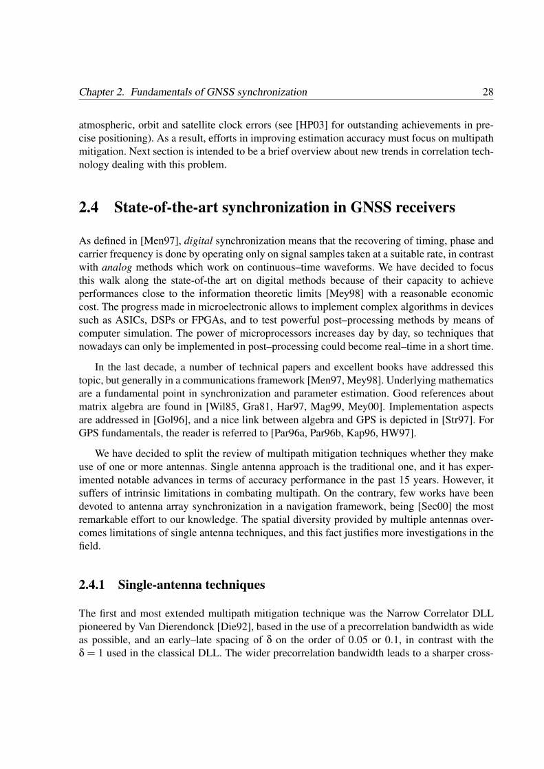
Chapter 2. Fundamentals of GNSS synchronization 28
atmospheric, orbit and satellite clock errors (see [HP03] for outstanding achievements in pre-cise positioning). As a result, efforts in improving estimation accuracy must focus on multipathmitigation. Next section is intended to be a brief overview about new trends in correlation tech-nology dealing with this problem.
2.4 State-of-the-art synchronization in GNSS receivers
As defined in [Men97], digital synchronization means that the recovering of timing, phase andcarrier frequency is done by operating only on signal samples taken at a suitable rate, in contrastwith analog methods which work on continuous–time waveforms. We have decided to focusthis walk along the state-of-the art on digital methods because of their capacity to achieveperformances close to the information theoretic limits [Mey98] with a reasonable economiccost. The progress made in microelectronic allows to implement complex algorithms in devicessuch as ASICs, DSPs or FPGAs, and to test powerful post–processing methods by means ofcomputer simulation. The power of microprocessors increases day by day, so techniques thatnowadays can only be implemented in post–processing could become real–time in a short time.
In the last decade, a number of technical papers and excellent books have addressed thistopic, but generally in a communications framework [Men97, Mey98]. Underlying mathematicsare a fundamental point in synchronization and parameter estimation. Good references aboutmatrix algebra are found in [Wil85, Gra81, Har97, Mag99, Mey00]. Implementation aspectsare addressed in [Gol96], and a nice link between algebra and GPS is depicted in [Str97]. ForGPS fundamentals, the reader is referred to [Par96a, Par96b, Kap96, HW97].
We have decided to split the review of multipath mitigation techniques whether they makeuse of one or more antennas. Single antenna approach is the traditional one, and it has exper-imented notable advances in terms of accuracy performance in the past 15 years. However, itsuffers of intrinsic limitations in combating multipath. On the contrary, few works have beendevoted to antenna array synchronization in a navigation framework, being [Sec00] the mostremarkable effort to our knowledge. The spatial diversity provided by multiple antennas over-comes limitations of single antenna techniques, and this fact justifies more investigations in thefield.
2.4.1 Single-antenna techniques
The first and most extended multipath mitigation technique was the Narrow Correlator DLLpioneered by Van Dierendonck [Die92], based in the use of a precorrelation bandwidth as wideas possible, and an early–late spacing of δ on the order of 0.05 or 0.1, in contrast with theδ = 1 used in the classical DLL. The wider precorrelation bandwidth leads to a sharper cross-

Chapter 2. Fundamentals of GNSS synchronization 29
correlation curve, and this makes the time–delay measurement easier to determine from thecorrelation output. The small value of δ provides a better approximation of the derivative sam-ples of the correlator output by the difference of the early and late samples. The correlation ofthe noise in these samples increases, so this reduces the variance of the DLL. As showed in[Wei94], the Narrow Correlator closely approaches the theoretically optimum processing if theone-path model (2.12) is considered. When a secondary path is included, it outperforms clearlythe standard one-chip spacing DLL, as observed in figure 2.8. A wider precorrelation bandwidthimplies more noise power passing through the filter, and this is a trade-off between multipathand noise mitigation found in all the single-antenna techniques described hereafter.
0 0.2 0.4 0.6 0.8 1 1.2 1.4 1.6 1.8 2−0.25
−0.2
−0.15
−0.1
−0.05
0
0.05
0.1
0.15
0.2
0.25
Reflection Delay [chips]
Tim
e D
elay
Bia
s [c
hips
]
Conventional and Narrow DLL bias produced by a single reflection for BPSK(1)
Conventional DLL, δ=1 Narrow Correlator, δ=0.1
0 0.2 0.4 0.6 0.8 1 1.2 1.4 1.6 1.8 2−0.25
−0.2
−0.15
−0.1
−0.05
0
0.05
0.1
0.15
0.2
0.25
Reflection Delay [chips]
Tim
e D
elay
Bia
s [c
hips
]
Conventional and Narrow DLL bias produced by a single reflection for BOC(1,1)
Conventional DLL, δ=1 Narrow Correlator, δ=0.1
Figure 2.8: Multipath envelope for conventional DLL (δ = 1) and Narrow Correlator (δ = 0.1)applied to BPSK(1) and BOC(1,1) modulation signals filtered at 20 MHz.
The natural extension of this effort in multipath mitigation is using a more accurate approx-imation of the derivative by means of more complex finite differences, pointing to the use ofmore correlator pairs instead of only one. For instance, the Multipath Elimination Technology(MET) [Tow94], implemented by NovAtel in the OEM2 GPSCard, is based on the symmetricshape of the theoretical correlation function in absence of multipath. This approach, also re-ferred to as Early/Late Slope technique (ELS), relies on the estimation of the slopes of bothsides of the autocorrelation function’s central peak, and compute a time delay correction thatis intended to remove the peak shift provoked by multipath. The intersection of the estimatedraising and falling slopes of the correlation function gives the tracking correction that has to beapplied to remove the multipath distortion:
∆TMET =(E1−E2)+ δ
2(a1 +a2)a1−a2
(2.28)

Chapter 2. Fundamentals of GNSS synchronization 30
where a1 = E1−E2δ
2is the raising and a2 = L1−L2
δ
2is the falling slope, as showed in figure 2.9.
When multipath is not present, the correlation function is symmetric, a1 =−a2 and the correc-tion term is ∆TMET = 0. This formula is used by software to feedback corrections to hardwarecorrelators.
Figure 2.9: Multipath Elimination Technology (MET) concept
A robust statistical approach to the multipath problem is the Multipath Estimating DelayLock Loop (MEDLL) developed by Van Nee [Nee94], where the Maximum Likelihood prin-ciple is applied to model (2.26) considering the number of reflections M− 1 known. The keyidea is to perform the estimation of the whole set of parameters of the incoming signals; whentheir amplitudes, time delays and carrier phases are estimated, the effect of the reflections in thecorrelation can be removed. Applying standard assumptions, the maximization of the likelihoodfunction yields:
τi = argmaxτ
ℜ
Ry(τ)−
M−1
∑m=0m6=i
amR(τ− τm)e− jθm
e− jθi
i = 1, ...,M−1 (2.29)
ai = ℜ
Ry(τi)−
M−1
∑m=0m6=i
amR(τi− τm)e− jθm
e− jθi
(2.30)

Chapter 2. Fundamentals of GNSS synchronization 31
θi = ∠
Ry(τi)−M−1
∑m=0m6=i
amR(τi− τm)e− jθm
(2.31)
where Ry(τ) is the I/Q downconverted correlation function and R(τ) is the reference correlationfunction. A possible implementation of the MEDLL uses 2M loops which are similar to a con-ventional DLL structure, with three correlators per loop needed to perform estimations (2.29),(2.30) and (2.31). Although the high MEDLL requirements in terms of a large number of cor-relators and computational load, it has been successfully implemented in NovAtel receiversbecause of its excellent performance in multipath mitigation. A comparison between theoreticalexpected results and experiments with real GPS L1 signals is provided in [Tow95].
The Early1/Early2 (E1/E2) tracking technique [Die97] is based on the a priori knowledgeof the theoretical leading slope of the correlation function, which is less affected by multipathbecause the reflections are always delayed respect to the direct signal. Two early correlators,named E1 and E2, whose amplitudes A1 and A2 have an ideal ratio R = A2/A1, give an actualoutput A1 and A2. The resulting ranging error can be computed as
∆R = A1−RA2 (2.32)
From equation (2.32) it is easy to see that, if the correlation function is not distorted betweenE1 and E2, then ∆R = 0. This situation is produced when the secondary signal is delayed aminimum of 1+E2 with respect to the desired signal. From this point of view it seems desirableto set E1 and E2 as early as possible, but the earlier is the gate, the noisier is the output. Again,we find a trade-off between multipath and noise mitigation.
The Double Delta (∆∆) correlator concept is based on designing discriminators with linearcombinations of two early and two late correlators. Defining as δ1 the spacing between E1 andL1 and δ2 the spacing between E2 and L2, the High Resolution Correlator (HRC) forms its codediscriminator as [McG99]:
DHRC(τ) = (E1−L1)−δ1
δ2(E2−L2). (2.33)
This structure is basically a Narrow Correlator but it introduces the information of a sec-ondary wider DLL in a weighted manner. Actually, it can be straightforwardly expressed asthe combination of two Narrow Correlators, one with a wider early-late spacing than the otherone. The same idea is already found in the Strobe Correlator [Gar96], patented by Ashtech Inc.,which discriminant is just DST ROBE = 2DHRC and therefore has the same multipath envelope.The Strobe correlator is robust to relative long-delay reflections; the price is a noise amplifica-tion greater than 10 dB [Die97].

Chapter 2. Fundamentals of GNSS synchronization 32
A generalization of this concept is a family of discriminators defined by
D(τ) =2N
∑n=1
β(n)∣∣∣∣Ry
((n−N− 1
2
)δ+ τ
)∣∣∣∣p (2.34)
where the design goal is to find the coefficients β(n) following some given criteria. This ideaspawned a number of similar approaches which use a modified receiver correlator referencewaveform with the objective to narrow the correlation function and therefore be more multipath-resistant. Examples of implementations are the Second/Forth Derivative Correlators (whichuse a digital easily-to-generate second/forth derivative of the optimal receiver showing bettermultipath resistance than the Strobe [Wei97]), the Gated Correlator [McG99] or the NovAtel-patented Pulse Aperture Correlator (PAC). As shown in [Jon04], the PAC technology is just ahardware implementation of MET, resulting in a discriminator
DPAC(τ) = 2∗ (E1−L1)− (E2−L2) (2.35)
which is proportional to DHRC and therefore with the same multipath envelope. A PAC imple-mentation is found in the NovAtel’s OEM4 GPSCard, and its better performance comparingto the MET technology is due to the 20 MHz precorrelation bandwidth, wider than the 8 MHzfilter used in former implementations [Jon04]. The generic denomination for such methods isthe Modified Correlator Reference Waveform (MCRW), which constitutes the current state ofthe art in GPS receivers [Wei03].
We can summarize the drawbacks of Double-Delta Correlators in:
• Poor receiver clock dynamic performance due to very narrow non-zero input domain.
• Degraded CN0 tracking level.
• Multipath effect at 0.1 and 1 chip in case of BPSK modulation. Worse performance incase of BOC modulation.
Recently, the nonlinear quadratic Teager-Kaiser algorithm (TK), originally introduced formeasuring the energy of a signal [Kai90], has been applied to subchip (coherent) multipathdelay estimation [Ham03] in the context of channel estimation for wireless communicationsystems, outperforming MEDLL in probability of correct acquisition regardless of its muchsimpler implementation.
Another very recent approach is the Vision Correlator introduced by NovAtel [Fen05],which is an implementation of a multipath mitigation method known as the Multipath Miti-gation Technique (MMT algorithm), developed by Weill [Wei02]. MMT is an optimized max-imum likelihood process which takes into account the direct signal and one or more multipath

Chapter 2. Fundamentals of GNSS synchronization 33
0 0.2 0.4 0.6 0.8 1 1.2 1.4 1.6 1.8 2−0.025
−0.02
−0.015
−0.01
−0.005
0
0.005
0.01
0.015
0.02
0.025
Reflection Delay [chips]
Tim
e D
elay
Bia
s [c
hips
]
(a) BPSK(1)
0 0.2 0.4 0.6 0.8 1 1.2 1.4 1.6 1.8 2−0.025
−0.02
−0.015
−0.01
−0.005
0
0.005
0.01
0.015
0.02
0.025
Reflection Delay [chips]
Tim
e D
elay
Bia
s [c
hips
]
(b) BOC(1,1)
0 0.2 0.4 0.6 0.8 1 1.2 1.4 1.6 1.8 2−0.025
−0.02
−0.015
−0.01
−0.005
0
0.005
0.01
0.015
0.02
0.025
Reflection Delay [chips]
Tim
e D
elay
Bia
s [c
hips
]
(c) BOC(10,5)
0 0.2 0.4 0.6 0.8 1 1.2 1.4 1.6 1.8 2−0.025
−0.02
−0.015
−0.01
−0.005
0
0.005
0.01
0.015
0.02
0.025
Reflection Delay [chips]
Tim
e D
elay
Bia
s [c
hips
]
(d) BOC(15,2.5)
Figure 2.10: Analysis of the Pulse Aperture Correlator (PAC) bias caused by a single reflectionfor BPSK and BOC signals, all filtered at 20 MHz

Chapter 2. Fundamentals of GNSS synchronization 34
replicas, solving the computational effort by means of a nonlinear transformation of the multi-path parameters. Each signal is represented by three parameters: the time offset τ, the amplitudeA and the carrier phase φ. For example, taking into account the LOSS and one single replica,the received signal can be expressed as
x(t) = A1e jφ1s(t− τ1)+A2e jφ2s(t− τ2)+n(t) (2.36)
This last complex baseband signal can be separated into its real and imaginary component:
i(t) = ℜx(t)= A1 cos(φ1)s(t− τ1)+A2 cos(φ2)s(t− τ2)+ni(t) (2.37)q(t) = ℑx(t)= A1 sin(φ1)s(t− τ1)+A2 sin(φ2)s(t− τ2)+nq(t) (2.38)
in which ni(t) and nq(t) are independent, real-valued and zero-mean AWGN. The functionto be minimized in order to estimate the six unknown parameters, following the ML criterion,is:
Γ =Z T
0[i(t)−A1 cos(φ1)s(t− τ1)−A2 cos(φ2)s(t− τ2)]
2 dt
+Z T
0[q(t)−A1 sin(φ1)s(t− τ1)−A2 sin(φ2)s(t− τ2)]
2 dt (2.39)
This is a highly coupled, nonlinear minimization problem on the six-dimensional spacespanned by the parameters A1, τ1, φ1, A2, τ2 and φ2, and is very difficult to solve in an efficientmanner. However, it can be simplified using the nonlinear, invertible transformation
a = A1 cos(φ1) c = A1 sin(φ1)b = A2 cos(φ2) d = A2 sin(φ2)
(2.40)
Inserting (2.40) into (2.39), the problem becomes a set of linear equations which can besolved using the Least Squares direct solution. For each pair of values τ1 and τ2, this linearsystem can be explicitly solved for the minimizing values of a, b, c and d. Thus the space tobe searched for a minimum is now 2-dimensional instead of 6-dimensional. The minimizationprocedure is as follows:
• Search the (τ1,τ2) domain. At each point (τ1,τ2) compute the values of the correlationfunctions in the linear system and then solve the system to find the values of a, b, c, andd which minimize Γ at that point.

Chapter 2. Fundamentals of GNSS synchronization 35
• Identify the point (τ1,τ2)ML where the smallest of all such minima is obtained, as well asthe associated minimizing values of a, b, c, and d.
• Transform these values of a, b, c, and d back to the estimates by using the inverse of theparameter transformation
A1 =√
a2 + c2 A2 =√
b2 +d2
φ1 = atan2(a,c) φ2 = atan2(b,d)(2.41)
Results presented in [Fen05] shows that the performance of the Vision Correlator RMS erroroutperforms PAC in the multipath sweep test. A drawback of this method is the needing of aprevious estimation of the number of replicas impinging the antenna.
In general, all these correlation techniques were designed for GPS C/A signals, whichpresent a triangular autocorrelation function corresponding to its BPSK modulation. This isnot the case of the BOC modulations, whose multi-peaked autocorrelation functions make con-ventional multipath mitigation techniques suboptimal. BOC tracking is a brand new challengein GNSS synchronization and has deserved a lot of attention in recent times [Fin99, Rie02,Hei04, Rod04a, Nun04].
In conclusion, in single antenna techniques there is generally a trade–off between multipathand noise mitigation. A major drawback of these methods is due to the fact that their abilityto discriminate the LOSS from the reflections is limited by the time resolution that the signalbandwidth imposes. An important result given in [Wei95] says that any unbiased time delayestimator based in a single antenna have a variance that approach to infinity when the relativedelay between the LOSS and its replica approach to zero, according to the Cramer-Rao bound[Tre68]. Relatively short delays are just the case of real-life multipath, where the scatterers useto be close to the receiver and the extra path covered by the wave is shorter than one chip period(about 300 m for a chip rate of 1.023 Mcps), situation referred as coherent multipath in theliterature. For all this reasons, effective multipath mitigation algorithms must resort to antennaarrays techniques.
2.4.2 Antenna array techniques
Out of the GNSS framework, there are several synchronization techniques that exploit the spa-tial diversity provided by an antenna array for improving performance in environments wheremultipath, co-channel interference or jamming are present. Some methods assume that the chan-nel matrix has been previously estimated, and perform Direction Of Arrival (DOA) and time de-lay estimation by fitting the signal model to the estimated channel. In [Vee98], the assumptionof a uniform linear array leads to closed-form estimates using a two-dimensional version of theESPRIT algorithm [Roy89], and the idea is extended to uniform rectangular arrays to estimate

Chapter 2. Fundamentals of GNSS synchronization 36
azimuth and elevation angles along with the time delays using a three-dimensional ESPRIT in[Haa98]. This particular array configuration allows the closed-form estimation of delays andDOA, and therefore these techniques cannot be applied to an arbitrary–geometry array.
Other researchers have followed the ML approach. In [Ced96], the assumption that the fad-ing channel parameters vary rapidly, while the DOAs and the delays are constant or slow varyingleads to a parameterized estimate of the channel, considering specular multipaths and gatheringnoise and interferences in a temporally white Gaussian process. A similar work, also assum-ing spatial whiteness, is reported in [Wax97]. A significant drawback of these methods is theneeding of multidimensional search procedures which involve a high computational cost. Asequential way of finding the ML estimator is the SAGE algorithm [Fes94], an extension ofthe EM algorithm [Fed98] with faster convergence. A comparison between ESPRIT and theSAGE algorithm is found in [Tsc99], where SAGE shows slight better performance in termsof accuracy at the price of a higher convergence time. Recently, the SAGE algorithm has de-served some attention of researchers, achieving a reduced computational cost [Tan03] and beingdirectly applied to GNSS synchronization [Ant04, Ant05].
In brief, these methods require an optimization of a multidimensional function and a cal-ibrated array. The aforementioned ESPRIT, which exploits the Vandermonde structure of amatrix that arises in the transformation into the frequency domain of the temporal samples,and the IQML algorithm [Bre86, Sec01] which relies in a polynomial decomposition of thecost function, are examples about how the computational efficiency can be addressed. A ma-jor step to overcome performance degradation when errors in array calibration are present isto consider an unstructured parameterization of the spatial response. Specially interesting arethe results obtained by Swindlehurst [Swi98b, Swi98a], where the assumptions of unstructuredspatial signatures and noise spatial whiteness leads to simpler estimators. In [Jak98], time delay,Doppler shift and spatial signature estimation are addressed assuming that an N-element arrayasynchronously receives M echoes of a known baseband signal s(t). Then, the baseband arrayoutput at time t is modeled as
x(t) =M
∑i=1
gis(t− τi)e j2π fdi t +n(t) (2.42)
where n(t) is additive noise (a zero mean temporally and spatially white Gaussian process withcovariance σ2I), τi is the unknown delay of the ith replica, fdi is its Doppler shift and gi is itsspatial signature. If a total of K samples are taken from the array, equation (2.42) may be writtenin a matrix form
X = G(θ)D(τ , fd)+N (2.43)

Chapter 2. Fundamentals of GNSS synchronization 37
where X =[
x(t1) . . . x(tK)]T , the ith column of D(τ , fd) is s =[
s(t1− τi)e j2π fdi t1 . . . s(tK− τi)e j2π fdi tK]T
, θ is a vector containing the DOAs of thesignals and N is defined like X. If G is taken to be an unstructured deterministic matrix, theML approach yields the following estimators:
τ , fd,G = arg minτ ,fd,G
‖X−D(τ , fd)G‖2F (2.44)
which are simplified to
τ , fd = argmaxτ ,fd
Tr
XHPDH X
(2.45)
and
G = D†(τ , fd)X (2.46)
where (·)† stands for the pseudoinverse, PDH is the projection matrix of DH and Tr· is thetrace operator.
These estimators requires a multidimensional optimization over a 2M–dimensional param-eter space, which may be computationally burdensome. This can be avoided by means of thesubspace–based estimation methods like Noise Subspace Fitting (NSF) [Sto90], Signal Sub-space Fitting (SSF) [Vib91], MUSIC, ESPRIT and IQML. Subspace methods rely on a first–order approximation of a frequency signal model. If equation (2.42) is expressed in the fre-quency domain, with some notational abuse:
x( f ) =M
∑i=1
gis( f − fdi)exp− j2πτi f+n( f ) (2.47)
where x( f ), s( f ) and n( f ) are the Fourier transforms of x(t), s(t) and n(t) respectively, and theconstant term e j2π fdiτi is lumped together with gi. Under the assumption that the Doppler shiftsare “small”, it is possible to simplify the dependence of (2.47) on the Doppler frequencies byneglecting the higher order terms in the Taylor series expansion of s( f − fdi):
s( f1− fdi)...
s( fK− fdi)
≈ s( f1)
...s( fK)
− fdi
∂s( f1)
∂ f1...
∂s( fK)∂ fK
(2.48)

Chapter 2. Fundamentals of GNSS synchronization 38
Collecting data at frequencies f1, ..., fK , the frequency model can be expressed in matrixform:
X = Q(τ , fd)G+N (2.49)
which is exactly the same model which is used in DOA estimation, interchanging the roles ofthe samples in time and space.
This approximation allows to reduce the computational burden. Due to the structure of thesignal manifold in the frequency domain, NFS and SSF reduces to a M–dimensional search forthe delay parameters. Then, Doppler parameters can be easily derived. Both methods requireinitial estimates, which can be provided by the MUSIC estimator (requires M one–dimensionalsearches) or ESPRIT (does not require any search, but ignores the Doppler shifts and has geo-metric constraints on the array manifold). The IQML algorithm is an iterative procedure whichis computationally efficient.
To our knowledge, the most outstanding work in GNSS synchronization is due to Seco,whose main results can be found in [Sec00, Sec05] and references herein. Two crucial ideascan be distilled from his results. First of all, the inclusion of multipath and interferences in aGaussian temporally–white but spatially–colored term with an arbitrary and unknown spatialcovariance matrix, although being a drastic simplification of the signal model, captures thestatistical behavior of such unwanted signals, and thus reduces the computational cost becauseno effort is devoted in estimating parameters which are not of interest in a GNSS receiver,such as DOAs or the delays of the reflections, and achieves better performance and robustnessthan other algorithms based in more complex signal models, where the reflections are takeninto account explicitly. Another advantage of this approach is the intrinsic capability to copewith diffuse multipath, since there is no need of estimating the number of specular reflectionsimpinging the array. Details about these issues will be discussed in chapter 3, extending theproblem to the joint estimation of time delays and Doppler shifts of a set of incoming signals.
The second remarkable idea in Seco’s work is the equivalence between the ML estimator anda kind of beamforming which exploits temporal and spatial reference. Thanks to a particularityof GNSS –the a priori knowledge of DOAs, a linear combination of the temporal reference andthe Minimum Variance (MV) beamforming obtains the same estimations than the ML approachdoes, reducing drastically the computational load and solving the problem in a much moreintuitively way. We will dwell in this amazing relationship in chapter 4.
The minimization of the computational burden and hardware complexity required by multi-path mitigation techniques is addressed in [Sel04]. The combination of compression techniques(using the Principal Components and Canonical Components methods) and Newton–flavoredalgorithms for the computation of ML estimators leads to efficient algorithms, demanding asmaller number of iterations than IQML or similar methods do.

Chapter 2. Fundamentals of GNSS synchronization 39
In conclusion, GNSS synchronization with antenna arrays is a promising new trend whichcopes with multipath mitigation, a source of performance degradation in positioning systemsthat cannot be mitigated with differential techniques and jeopardizes the overall accuracyachieved by the receiver. In the following chapters, we will develop new techniques and ap-proaches dealing with this topic.
Next two sections are intended to be brief descriptions of the signal structure of the currentlyexisting GPS, its modernization plans, and the state-of-the art for the planned Galileo system.Due to the novelty of these decisions (in fact, the Galileo signal structure is not closed in severalaspects at the time to write this dissertation, Autumn 2005), and the exciting perspectives thatthe scenario is going to offer to receiver designers, we have decided to include this informationfor the sake of completeness.
2.5 GPS signal structure
The interface between the GPS Space Segment and the GPS navigation User Segment consistsin two right-hand circularly polarized (RHCP) radio frequency links, named L1 and L2, and athird link L5 is envisaged. The availability of a third frequency for the general–purpose user al-lows for higher precision and faster acquisition for kinematic applications than single or doubleband receivers allow.
The L-band links are modulated by one or more bit trains, each one formed by the Modulo-2addition of a pseudo-random noise (PRN) ranging code and the downlink system data, usuallyreferred to as navigation or NAV data.
A complete description of the navigation user interfaces in NAVSTAR GPS can be found inthe interface control document [Cor03].
2.5.1 GPS spreading codes
The pseudo-random noise (PRN) codes selected for GPS, referred to as Gold codes and firstlyintroduced in [Gol67], were chosen by their desirable properties of cross-correlation and easi-ness of implementation. As explained in this chapter and detailed in chapter 6, a GPS receivermust perform a correlation operation in order to extract the signal timing and recover the dataof a set of satellites. Thus, if the receiver has M satellites in view, it must separate each satellitesignal from others and perform timing and data recovering. This separation is performed by aset of parallel correlators, each one devoted to a single satellite; for one of these correlators, asignal belonging to a certain satellite is the desired signal and all the other M− 1 signals areseen as interferers.

Chapter 2. Fundamentals of GNSS synchronization 40
This needing of system’s self-interference rejection demands spreading codes with low (andupper-bounded) cross-correlation. The Gold codes are linear combinations of two m-sequences(also called maximal length sequences) with different offset in a Galois field. All pairs of m-sequences do not yield Gold codes, and those which yield Gold codes are called preferredpairs. Gold codes have three-valued autocorrelation and cross-correlation function with values−1,−t(m), t(m)−2, where
t(m) =
2
m+12 +1 for odd m
2m+2
2 +1 for even m(2.50)
The generation of Gold codes is very simple: they consist of the modulo-2 sum of two linearfeedback shift registers (LFSR) outputs, each one defined by a feedback polynomial.
The current and planned GPS spreading codes are:
• C/A code. The PRN C/A code for the Space Vehicle (SV) number i is a Gold code,CC/A,i(t), of 1 millisecond in length at a chipping rate of 1023 Kbps. These sequences arelinear patterns generated by the modulo-2 addition of two subsequences, G1 and G2i, eachof which being 1023 chip long linear patterns. The G2i sequence is formed by effectivelydelaying the G2 sequence by an integer number of chips ranging from 5 to 950. The G1and G2 sequences are generated by 10-stage LFSRs having the following polynomials asreferred to in the shift register input:
G1 : 1+ x3 + x10, and (2.51)G2 : 1+ x2 + x3 + x6 + x8 + x9 + x10 (2.52)
• P code. The PRN P code for the SV number i is a sequence CP,i(t) of 7 days in lengthat a chipping rate of 10.23 Mbps. Again, sequences are composed by the modulo-2 sum(also denoted as “exclusive-or” or ⊕ operation) of two subsequences referred to as X1and X2i, with length 15,345,000 chips and 15,345,037 chips respectively. X1 itself isgenerated by the modulo-2 sum of the output of two 12-stage registers (X1A and X1B)short cycled to 4092 and 4093 chips respectively. When the X1A short cycles are countedto 3750, the X1 epoch is generated, occurring every 1.5 seconds. The X2i sequence is anX2 sequence (also generated by two shift registers, X2A and X2B) selectively delayed by1 to 37 chips, thereby producing a set of 37 mutually exclusive sequences of 7 days inlength. The polynomials for X1A and X1B codes, as referenced to the shift register input,are
X1A : 1+ x6 + x8 + x11 + x12, and (2.53)X1B : 1+ x+ x2 + x5 + x8 + x9 + x10 + x11 + x12 (2.54)

Chapter 2. Fundamentals of GNSS synchronization 41
while the corresponding for the X2A and X2B codes are
X2A : 1+ x+ x3 + x4 + x5 + x7 + x8 + x9 + x10 + x11 + x12, and (2.55)X2B : 1+ x2 + x3 + x4 + x8 + x9 + x12. (2.56)
• Y code. Code P, although its length, is publicly available, and this includes potential jam-mers or spoofers. A spoofer generates a signal that mimics the GPS signal and attemptsto cause the receiver to track a wrong signal. For this reason, GPS has the possibility toencrypt the public P code by a secure Y code, available only to authorized U.S. govern-ment users. Its main purpose is to assure that an eventual opponent cannot spoof the Ycode signal generating a Y code replica.
• L2 CM code. The PRN L2 civil moderate (CM) code for SV number i is a ranging codeCCM,i(t) which is 20 milliseconds in length at a chipping rate of 511.5 Kbps. It constitutesa linear pattern which is short cycled every count of 10,230 chips by resetting with aspecified initial state. This sequences will be used from the deployment of IIR-M, IIF andsubsequent blocks of SVs.
• L2 CL code. The PRN L2 civil long (CL) code for SV number i is a ranging code CCL,i(t)which is 1.5 seconds in length at a chipping rate of 511.5 Kbps. The CCL,i(t) sequenceis a linear pattern which is generated using the same code generator polynomial as theone used for CM,i(t), but short cycled every count of 767,250 chips by resetting with aspecified initial state.
• L5 codes. The PRN in-phase code (denoted as the I5-code) and the quadrature-phasecode (denoted as the Q5-code) for SV number i are ranging codes CI5,i(t) and CQ5,i(t) of1 millisecond in length at a chipping rate of 10.23 Mbps. Each code is a modulo-2 sum oftwo subsequences XA and XBIi or XBQi, which lengths are 8,190 and 8,191 respectively,that restart to generate the 10,230 chip code. The XBi is selectively delayed allowingthe generation of 74 different code sequences (37 I5 and 37 Q5). Of these, 32 pairs aredesignated for use by SVs while the remaining 5 pairs are reserved. The polynomials forXA and XBIi or XBQi codes, as referenced to the shift register input, are
XA : 1+ x9 + x10 + x12 + x13, and (2.57)XBIi or XBQi : 1+ x+ x3 + x4 + x6 + x7 + x8 + x12 + x13. (2.58)
• Non-standard codes. The so-called NSC, NSCM, NSCL, NSI5, NSQ5 and NSY codesare intentionally “incorrect” versions of the codes intended to protect the users from re-ceiving and utilizing anomalous NAV signals as a result of malfunction in the SV’s refer-ence frequency generation system.

Chapter 2. Fundamentals of GNSS synchronization 42
• M code. The M (military) code signal is designed to provide better jamming resistancethan the Y code signal, enabling transmission at much higher power without interferencewith C/A code or Y code receivers [Bar00], and it is intended to progressively replacethe military Y code providing better security in terms of exclusivity, authentication andconfidentiality, besides more robust acquisition. It consists in a binary offset carrier signalwith subcarrier frequency 10.23 MHz and spreading code rate of 5.115 Mbps, denoted asBOC(10.23,5.115) modulation, or BOC(10,5) for short. The spreading code transitionsare aligned with transitions of the square wave subcarrier. The BOC modulation will beanalyzed in section 2.6. Although the M-code signal will be implemented on some BlockIIF satellites, that are planned for launch between 2005 and 2010, a fully operationalconstellation of 18 M-code satellites will not come into operation until 2016.
2.5.2 Navigation data messages
As said above, these PRN are modulated by a BPSK signal which contains data in a muchsmaller rate than the codes. The navigation data provide the receiver with the informationneeded to perform the positioning computation. Usually referred to as NAV data or D(t), themessage is structured in a 1500 bit long frame composed of five 300 bit long subframes. Sub-frames 4 and 5 are subcommutated 25 times each, giving the total of 25 full frames to transmitthe complete data message, which is 375,000 bits long. The message is transmitted at 50 bps,and thus the subframes 1, 2 and 3 are repeated each 30 seconds, while the whole content ofsubframes 4 and 5 takes 12.5 minutes to be downloaded.
The first subframe contains, in addition to other system parameters, the information neededto perform clock correction: a third degree polynomial allows the determination of the SV PRNcode phase offset referenced to the phase center of the antennas with respect to the GPS systemtime at data transmission. Other parameters of interest in this subframe are the group delaybetween L1 P(Y) and L2 P(Y) and ionospheric corrections.
Subframes 2 and 3 contains a set of parameters (referred as ephemeris) describing the orbitof the transmitting satellite. Among them, the Keplerian orbital elements, readily
√a the square
root of the ellipse’s semimajor axis; e its eccentricity, which is defined as e =√
a2−b2
a2 , being bthe semiminor axis; i0 the inclination angle at reference time; Ω0 the longitude of the ascendingnode of orbit plane at weekly epoch; ω the argument of perigee and M0 the mean anomalyat reference time. Other parameters are intended to correct the eventual orbital perturbations:∆n the mean motion difference from computed value; Ω the rate of right ascension; and sixmore parameters indicating the sine and cosine harmonic correction terms to the argument oflatitude, orbit radius and angle of inclination. The reference time ephemeris, toe is also provided.User algorithms for the computation of satellite position and clock correction can be found in[Cor03].

Chapter 2. Fundamentals of GNSS synchronization 43
Both subframe 4 and 5 are subcommutated 25 times each; the 25 versions of these subframesare referred to as pages 1 through 25 of each subframe. The information contained herein isknown as almanac, and consists in the ephemeris of other satellites, their clock correction factor,ionospheric and Universal Time Coordinated (UTC) data, flags about the health of the SVs,indication of the Anti-Spoofing (AS) status and other system information.
Recently, some modifications of the data message has been proposed. In Block IIR-M SVs,the NAV bit train D(t) can be rate 1
2 encoded with an encoding constraint length of 7, givinga 25 bps rate resulting in 50 sps. When this encoding is activated, the message is denoted asD′(t). Moreover, starting from Block IIF SVs (overview in [Fis99]), another message formathas been defined: the GPS L2 CNAV data structure denoted as Dc(t). This data stream includesthe same data as the NAV data D(t) but in an entirely different format: it utilizes 300 bit longmessages, each one containing a Cyclic Redundancy Check (CRC) parity block of 24 bits.In addition to this protection, the bit train is Forward Error Correction (FEC) encoded by arate 1
2 convolutional code, thus offering a rate of 25 bps and 50 sps. The ultimate navigationdata modulation is envisaged for its use in the L5 band: D5(t). While the message structure isbasically the same as CNAV, in D5(t) the bit train is rate 1
2 convolutional encoded with a FECcode with constraint length 7, at a symbol rate of 100 sps.
2.5.3 L5, L2 and L1 links
The L5 link will be only available on Block IIF SVs, and the planned future Block III. Definedin [Cor02], it is a 24 MHz band centered at fL5 = 115× 10.23 = 1176.45 MHz consisting oftwo carrier components in phase quadrature. Neglecting multiplicative constants, the basebandequivalent referred to fL5 is splitted into the Inphase and Quadrature components:
sL5(t) = CI5(t)⊕D5(t)⊕nh10(t)+ jCQ5(t)⊕nh20(t). (2.59)
As can be observed, the I5 component contains a synchronization sequence nh10 = 0000110101,a 10 bit Neuman-Hoffman code that modules each 100 symbols of D5(t), and the Q5 componenthas another synchronization sequence nh20 = 00000100110101001110 at 20 kbps. A descrip-tion of the characteristics and potentialities of the L5 signal can be found in [Die00].
The L2 link is centered at fL2 = 1227.6 MHz, frequency which is coherently derived froma common frequency source to L1 within the SV: notice that fL1 = 154× 10.23 MHz andfL2 = 120× 10.23 MHz. The Control Segment is able to select different signal configurationswhich are summarized in table 2.1
The preferred situation for the civil component, known as L2 Civil Signal or L2CS,is CCM(t)⊕D′(t) chip-by-chip time multiplexed with CCL(t) in case of Block IIR-M andCCM(t)⊕Dc(t) time multiplexed with CCL(t) in case of Block IIF [Fon01]. This is because

Chapter 2. Fundamentals of GNSS synchronization 44
SV Blocks L2 In-Phase L2 Quadrature-Phase (L2CS)CP(Y )(t)⊕D(t),
Block II/IIA/IIR CP(Y )(t), or Not ApplicableCC/A(t)⊕D(t)
CCM(t)⊕D(t) time multiplexed with CCL(t),Block IIR-M CP(Y )(t)⊕D(t), or CCM(t)⊕D′(t) time multiplexed with CCL(t),
CP(Y )(t) CC/A(t)⊕D(t), orCC/A(t)
CCM(t)⊕Dc(t) time multiplexed with CCL(t),Block IIF CP(Y )(t)⊕D(t), or CC/A(t)⊕D(t), or
CP(Y )(t) CC/A(t)
Table 2.1: L2 signal configuration
biphase data modulation forces the receiver to use a Costas (squaring) loop to create a secondharmonic of the carrier, which can be tracked; the possibility to track CCL(t) without data mod-ulation allows the use of a simple Phase Locked Loop (PLL), thus improving 6 dB the trackingthreshold with respect to the Costas loop. In addition, PLL makes whole-cycle phase measure-ments rather than having to use message content to resolve the π radians phase ambiguity of theCostas loop.
The L1 link, centered at fL1 = 1575.42 MHz, consists of two components in quadraturephase, and its baseband equivalent, referred to fL1 and neglecting multiplicative constants, canbe expressed as
sL1(t) = CP(Y )(t)⊕D(t)+ jCC/A(t)⊕D(t). (2.60)
This is the link used by the commercial receivers, in particular the quadrature componentwith the C/A code. Chapter 6 will provide more details about the receiver implementation.
2.6 Galileo signal structure
Galileo will provide 10 navigation signals in RHCP in the frequency ranges 1164−1215 MHz,named E5, 1215− 1300 MHz, named E6, and 1559− 1610 MHz, referred as E2-L1-E1 orjust L1 for convenience. As a novelty, and jointly with the GPS M-code, the Binary OffsetCarrier modulation (BOC) is used as a modulation scheme. Since the BOC modulation has beenrecently introduced in the navigation’s signal playground, we will dedicate a few paragraphs tothe definition of such kind of signals.

Chapter 2. Fundamentals of GNSS synchronization 45
2.6.1 Introduction to the BOC modulation
A BOC signal is generated in baseband by the product of two signal components: a non-filteredPRN code with a chip rate rc and values ±1 and a non-filtered square signal with frequencyfs (equal or higher than rc) acting as a carrier. In general:
xBOC(t) = x(t)sign(sin(2π fst)) (2.61)
The effect of this square carrier is to split the main lobe of the PRN spectrum into two lobescentered at± fs from the central frequency. In the literature, the modulation parameters are oftenreferred explicitly as BOC( fs,rc) while in the Galileo nomenclature the used term is BOC(n,m)where n and m stands for the normalization of the carrier frequency and the code rate by thereference frequency 1.023 MHz. The expansion ratio n
m indicates the frequency distance be-tween the two main side lobes: the bigger is the ratio, the greater is the distance. On the otherhand, a higher ratio also indicates more powerful secondary lobes around these main side lobes;therefore, the ratio gives information about the selectivity of the signal. A particular case of thissignal, when n and m are integers and n = m, is the well-known Manchester code.
In case of Galileo, a slight modification is introduced to the general expression (2.61): thesine phasing modulation is changed by a cosine phasing. The main driver of this change is tochoose a signal with less interference on the existing and future GPS signals on L1, specially theM code mentioned in the previous section, which imposes important restrictions on the Galileosignal structure in order to maintain compatibility. The sine BOC modulation concentrates morepower on the inner side of the spectrum, while the cosine BOC modulation has lobes with morepower on the outer side, which reduces interferences with the GPS signal. According to [Hei04],the BOCcos(15,2.5) signal improves the spectral separation with respect to the M code in about3.8 dB with respect to its sine counterpart.
The power spectral density of a generic BOCcos( fs,rc) can be expressed as
SBOCcos( fs,rc)( f ) = rc
2sin2(
π f4 fs
)sin(
π frc
)π f cos
(π f2 fs
)2
, (2.62)
and the shape of various combinations of m and n proposed for Galileo are shown in figure 2.11.
The Alternative BOC (AltBOC) is a slight modification to the BOC modulation intendedto allow different channels in the lower and upper main split lobes. Intuitively, the idea is toperform the same process than in the BOC modulation but multiplying the baseband signalfor a complex square signal v(t) = sign(cos(2π fst))+ jsign(sin(2π fst)). Having two basebandsignals x1(t) and x2(t), the modulation can be expressed as
xAltBOC(t) = x1(t)v(t)+ x2(t)v∗(t) (2.63)

Chapter 2. Fundamentals of GNSS synchronization 46
−10 −8 −6 −4 −2 0 2 4 6 8 10−50
−45
−40
−35
−30
−25
−20
−15
−10
−5
0
Frequency [MHz]
Nor
mal
ized
spe
ctru
m [d
B]
(a) BPSK(1)
−10 −8 −6 −4 −2 0 2 4 6 8 10−50
−45
−40
−35
−30
−25
−20
−15
−10
−5
0
Frequency [MHz]
Nor
mal
ized
spe
ctru
m [d
B]
(b) BOC(1,1)
−10 −8 −6 −4 −2 0 2 4 6 8 10−50
−45
−40
−35
−30
−25
−20
−15
−10
−5
0
Frequency [MHz]
Nor
mal
ized
spe
ctru
m [d
B]
(c) BOC(10,5)
−10 −8 −6 −4 −2 0 2 4 6 8 10−50
−45
−40
−35
−30
−25
−20
−15
−10
−5
0
Frequency [MHz]
Nor
mal
ized
spe
ctru
m [d
B]
(d) BOC(15,2.5)
Figure 2.11: Power spectral density comparison of some modulation signals, filtered at 20 MHzand normalized to BPSK

Chapter 2. Fundamentals of GNSS synchronization 47
−2 −1.5 −1 −0.5 0 0.5 1 1.5 2−0.8
−0.6
−0.4
−0.2
0
0.2
0.4
0.6
0.8
1
Delay in code chips
Nor
mal
ized
aut
ocor
rela
tion
func
tion
(a) BPSK(1)
−2 −1.5 −1 −0.5 0 0.5 1 1.5 2−0.8
−0.6
−0.4
−0.2
0
0.2
0.4
0.6
0.8
1
Delay in code chips
Nor
mal
ized
aut
ocor
rela
tion
func
tion
(b) BOC(1,1)
−2 −1.5 −1 −0.5 0 0.5 1 1.5 2−0.8
−0.6
−0.4
−0.2
0
0.2
0.4
0.6
0.8
1
Delay in code chips
Nor
mal
ized
aut
ocor
rela
tion
func
tion
(c) BOC(10,5)
−2 −1.5 −1 −0.5 0 0.5 1 1.5 2−0.8
−0.6
−0.4
−0.2
0
0.2
0.4
0.6
0.8
1
Delay in code chips
Nor
mal
ized
aut
ocor
rela
tion
func
tion
(d) BOC(15,2.5)
Figure 2.12: Normalized autocorrelation functions of BPSK(1), BOC(n,n), BOC(2n,n) andBOC(6n,n), all of them filtered at 20 MHz. The maximum is not equal to one due to the bandlimiting effects

Chapter 2. Fundamentals of GNSS synchronization 48
If we recall the concept of Gabor bandwidth defined in equation (2.25) and we observethe shapes of figure 2.11, it arises that the BOC modulation has a greater Gabor bandwidththan the BPSK does because its greater concentration of power far from the center frequency.The weighting term f 2 makes a greater value of the integral in (2.25) and therefore the BOCmodulation has a theoretical minimum variance of time delay estimation lower than the BPSKmodulation. This is consequent with the results obtained in figures 2.4 and 2.8, where the ro-bustness of the BOC(1,1) modulation against multipath is evidenced compared to the BPSK.
2.6.2 Galileo spreading codes
The PRN code sequences determine system’s behavior. The design goal is offering a goodcompromise between cold start acquisition time and robustness against narrow band signals andother Radio Navigation Satellite System signals. The Galileo spreading codes, not yet defined,could consist on a short duration primary Gold code sequence of plus an minus ones, of lengthNp, modulated by a long duration secondary code predefined sequence, of length Ns, also ofplus or minus ones. Both sequences are synchronized one with the other, and in case of datachannels they are also synchronized with the data symbols. The resulting code sequence, oflength Np ·Ns, is the primary code sequence repeated a number of times equal the length ofthe secondary code, and each time multiplied by the corresponding value of the secondarysequence. The duration is the same of the long duration secondary code, and covers both of thedesigning parameters: while primary codes, with shorter duration, allow a shorter acquisitiontime, the longer secondary codes provide protection against interferences. Further alternativecodes are presently investigated [Pra02] and flexibility in the on-board implementation is beingconsidered to foresee the generation of other types of codes.
2.6.3 Navigation data messages
The data message is protected by three levels of error encoding in order to improve the Bit andFrame Error Rate. First of all, a Cyclic Redundancy Check (CRC) consisting of the addition ofredundant checksum bits at the end of each frame will allow to detect error transmissions of thereceived data. Then, a one-half Forward Error Correction (FEC) encoding using a convolutionalcode constraint length 7 inserts one additional bit per data message bit, resulting in a symbolrate twice the initial bit rate. Finally, the last step is an interleaving block that avoids burst errors,spreading the errors along the whole frame and facilitating the work of the FEC decoding.
Galileo offers four types of data, which are carried by the different radionavigation signals:
• Open Services (OS) data in the DE5A(t), DE5B(t) and DL1B(t) signals, being accessible toall users and containing navigation data and Search And Rescue (SAR) data.
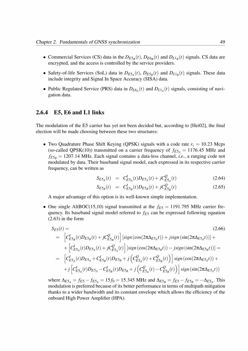
Chapter 2. Fundamentals of GNSS synchronization 49
• Commercial Services (CS) data in the DE5B(t), DE6B(t) and DL1B(t) signals. CS data areencrypted, and the access is controlled by the service providers.
• Safety-of-life Services (SoL) data in DE5A(t), DE5B(t) and DL1B(t) signals. These datainclude integrity and Signal In Space Accuracy (SISA) data.
• Public Regulated Service (PRS) data in DL6A(t) and DL1A(t) signals, consisting of navi-gation data.
2.6.4 E5, E6 and L1 links
The modulation of the E5 carrier has yet not been decided but, according to [Hei02], the finalelection will be made choosing between these two structures:
• Two Quadrature Phase Shift Keying (QPSK) signals with a code rate rc = 10.23 Mcps(so-called QPSK(10)) transmitted on a carrier frequency of fE5A = 1176.45 MHz andfE5B = 1207.14 MHz. Each signal contains a data-less channel, i.e., a ranging code notmodulated by data. Their baseband signal model, each expressed in its respective carrierfrequency, can be written as
SE5A(t) = CIE5A
(t)DE5A(t)+ jCQE5A
(t) (2.64)
SE5B(t) = CIE5B
(t)DE5B(t)+ jCQE5B
(t) (2.65)
A major advantage of this option is its well-known simple implementation.
• One single AltBOC(15,10) signal transmitted at the fE5 = 1191.795 MHz carrier fre-quency. Its baseband signal model referred to fE5 can be expressed following equation(2.63) in the form
SE5(t) = (2.66)
=[CI
E5B(t)DE5B(t)+ jCQ
E5B(t)][sign(cos(2π∆E5At))+ jsign(sin(2π∆E5At))]+
+[CI
E5A(t)DE5A(t)+ jCQ
E5A(t)][sign(cos(2π∆E5Bt))− jsign(sin(2π∆E5Bt))] =
=[CI
E5A(t)DE5A +CI
E5B(t)DE5B + j
(CQ
E5A(t)+CQ
E5B(t))]
sign(cos(2π∆E5At))+
+ j[CI
E5A(t)DE5A−CI
E5B(t)DE5B + j
(CQ
E5A(t)−CQ
E5B(t))]
sign(sin(2π∆E5At))
where ∆E5A = fE5− fE5A = 15 f0 = 15.345 MHz and ∆E5B = fE5− fE5B = −∆E5A . Thismodulation is preferred because of its better performance in terms of multipath mitigationthanks to a wider bandwidth and its constant envelope which allows the efficiency of theonboard High Power Amplifier (HPA).

Chapter 2. Fundamentals of GNSS synchronization 50
The availability of pilot (dataless) channels provides two main advantages: an improved carrier-phase tracking using a pure PLL and the possibility of longer coherent integrations without dataloss, resulting in an improved acquisition and tracking performance.
The E6 band will contain three channels, denoted by letters A, B and C, transmitted overthe same carrier at fE6 = 1278.750 MHz. Although the final decision about the multiplexingscheme is not already taken, preliminary studies point to the modified Hexaphase modulation(also referred as Interplex modulation [Rie02] or Coherent Adaptive Subcarrier Modulation,CASM [Daf99]) consisting of a QPSK signal modulated by a third channel. Its baseband signalmodel can be expressed as
SE6(t) = [CE6A(t)DE6A(t)ScE6(t)cos(m)−CE6C(t)sin(m)]+ (2.67)+ j [CE6B(t)DE6B(t)cos(m)+CE6A(t)DE6A(t)ScE6(t)CE6B(t)DE6B(t)CE6C(t)sin(m)]
where ScE6(t) is the sub-carrier for generating the BOC(10,5). The modulation index, chosen tobe m = 0.6155, is used to set the relative power between the three channels.
The L1 band will contain another three channels structured in the same way than E6 andcentered in fL1 = 1575.42 MHz:
SL1(t) =[CL1A(t)DL1A(t)ScL1A
(t)cos(m)−CL1C(t)sin(m)]+ (2.68)
+ j[CL1B(t)DL1B(t)ScL1B
(t)cos(m)
+CL1A(t)DL1A(t)ScL1C(t)CL1B(t)DL1B(t)CL1C(t)sin(m)
]where ScL1B,C
(t) generates a BOC(1,1) which will be used for Open Service (OS), Safety-of-Life Service (SoL) and Commercial Service (CS), and ScL1A
(t) generates a cosine phasedBOC(15,2.5) for the governmental Public Regulated Service (PRS). Time Division Multiplexis also being investigated to substitute the modified Hexaphase in E6 and L1, showing betterperformance in terms of correlation losses [Rie02].
The Galileo signal structure will be definitively stated in the Galileo Interface Control Doc-ument, expected to appear in 2006.
2.7 Summary
Positioning system receivers compute their position from the estimation of synchronizationparameters of several received signals. This chapter has described the architecture of a genericGNSS receiver, showing that the presence of the multipath effect biases timing estimation meth-ods based on the traditional synchronization method known as Delay Locked Loop (DLL). The

Chapter 2. Fundamentals of GNSS synchronization 51
mitigation of the multipath impact in the synchronization accuracy is the fundamental objectiveof this Thesis.
After presenting the technical background of a GNSS receiver and how its performance isaffected by multipath, the state-of-the-art of synchronization methods has been described. Ithas been argued that single antenna receivers have some intrinsic drawbacks in the mitigationof coherent multipath, and that antenna array receivers could overcome such difficulties.
Finally, the chapter provides a description of the current and planned signal structures forGPS and Galileo, the maximum exponents of the present and near future of GNSS. In caseof GPS, the current signal structure is well documented but the modernization plans are quitespread in a number of papers. In case of Galileo, any official documentation has been publishedto this date, but many results have appeared in technical conferences. The descriptions providedin sections 2.5 and 2.6 are intended to be a digest of such (often contradictory) information,organized into a systematic arrangement. The discussion includes the description of the BinaryOffset Carrier (BOC) modulation, a novelty in satellite-based positioning systems, and the Ga-bor bandwidth has been used in arguing the convenience of the BOC structure. Particularitiesof BOC tracking have also been outlined.

Chapter 2. Fundamentals of GNSS synchronization 52

Chapter 3
Maximum Likelihood synchronizationwith antenna arrays
Nothing in life is to be feared. It isonly to be understood.
Marie Curie
THE method of Maximum Likelihood (ML), pioneered by the geneticist and statistician SirRonald A. Fisher, is an estimation method which defines as an estimate of a parameter
vector ξ = (ξ1, · · · ,ξm) the member of the parameter space Ξ that maximizes the conditionalProbability Density Function (PDF) fχ(x|Ξ = ξ), given a fixed data set x = (x1, · · · ,xk). Theequivalent class of functions Λ(ξ|x) = α fχ(x|Ξ = ξ) for any positive constant α is known aslikelihood function. Therefore, the likelihood function retains the form of the PDF but with asubtle change of scope: whereas the density function is a function of the observation x whileholding the parameters ξ constants, the likelihood function is a function of the parameters ξ
while holding x constant. The Maximum Likelihood Estimator (MLE) of ξ is directly the pa-rameter vector ξML such that Λ(ξML|x)≥ Λ(ξ|x) for all ξ ∈ Ξ.
The numerical value of the likelihood function is immaterial. Since many of the densityfunctions are exponential in nature, it is very common to take the logarithm of this function forconvenience, giving place to the log-likelihood function. When the gradient of log-likelihoodfunction (usually referred to as score function) exist and the variance of the score function(marked by the inverse of the Fisher information matrix, J(ξ)) evaluated at the true value of theunknown vector parameter is positive semidefinite, the MLE has nice and desirable properties:it is asymptotically efficient (tends to be unbiased for large data records) and asymptotically op-timal (attains the Cramer-Rao Bound, the minimum achievable variance also for large data col-lections) [Kay93]. In other words, ξML is asymptotically distributed according to N (ξ,J−1(ξ)).
53

Chapter 3. Maximum Likelihood synchronization with antenna arrays 54
The invariance is another interesting property: the MLE of the vector parameter ϑ = f (ξ) isgiven by ϑML = f (ξML).
This chapter presents the application of the ML principle applied to the synchronizationof several signals by means of an antenna array. After proposing a signal model both for thestructured and unstructured array architectures, which include a novel approach to multipath andinterference modeling, we shall analyze the theoretical accuracy limits that the array approachcould provide. The next step will be the derivation of the ML estimator for a set of time delaysand Doppler shifts, which implies the minimization of a multidimensional highly nonlinearfunction. Finally, a set of suboptimal but more computationally efficient methods based oniterative procedures will be presented. A set of simulation studies will close this analysis.
3.1 Signal model
The problem under study concerns the extraction of information from measurements using anarray of antennas. The measurements are considered to be a superposition of plane waves cor-rupted by noise and, possibly, interferences and multipath. Given the measurements, the ob-jective is to estimate a set of parameters associated with the wavefronts. Hereafter, two signalmodels are proposed: the structured and the unstructured. This classification is related to theability of the array in maintaining a phase reference in the hardware part of the RF front-end.
3.1.1 Structured array model
An N–element antenna array receives M scaled, time–delayed and Doppler–shifted complexbaseband signals with known structure, si(t), i = 1, · · · ,M. The receiving baseband signal canbe modeled as
x(t) =M
∑i=1
aisi(t− τi)exp j2π fit+w(t) (3.1)
where ai is the complex amplitude of each signal, τi is the delay, fi is the Doppler shift, andw(t) is additive white Gaussian noise.
Each antenna receives a different replica of this signal, with a different phase depending onthe array geometry and the direction of arrival. This can be expressed by a vector signal model,where each row corresponds to one antenna:
x = GAd+n (3.2)
where

Chapter 3. Maximum Likelihood synchronization with antenna arrays 55
• x(t) ∈ CN×1 is the observed signal vector,
• G ∈ CN×M is the spatial signature matrix related to array geometry and Directions OfArrival (DOAs),
• A = diag(a) ∈ CM×M is a diagonal matrix with the elements of the amplitude vector aalong its diagonal,
• d = [s1(t − τ1)exp j2π f1t . . .sM(t − τM)exp j2π fMt]T , d ∈ CM×1 the delayed andDoppler–shifted narrowband signals envelopes, and
• n(t) ∈ CN×1 represents additive noise and all other disturbing terms.
In this model, the narrowband array assumption has been made. This assumption considersthat the time required for the signal to propagate along the array is much smaller than inverseof its bandwidth. So, a phase shift can be used to describe the propagation from one antenna toanother. As described in chapter 2, current navigation signals are reported to be emitted witha 20-MHz bandwidth, which inverse is 50 ns or 15 m in spatial terms. The array is expectedto be much smaller, since the carrier wavelength is on the order of 10 cm, so the assumptionseems reasonable. However, it must be pointed out that this signal model becomes invalid forlarge arrays. In the same way, we have assumed that the Doppler effect can be modeled by afrequency shift, which is commonly referred to as the narrowband signal assumption [Sto96].
In addition to these assumptions, we shall consider the baseband functions s(t) as band–limited finite–average–power signals in order to show the consistency of the ML estimator.This assumption implies that the analog autocorrelation
rss(τ) = limT→∞
1T
ZT
s(t + τ)s∗(t)dt (3.3)
is a continuous with continuous derivatives function. In the digital domain, assuming also asampling period Ts satisfying the Nyquist criterion, equation (3.3) turns in
limK→∞
1K ∑
Ks(kTs− τn)s∗(kTs− τm) = rss(τm− τn). (3.4)
Extending the concept in order to include Doppler shifts leads to
Cdd(Υ(1),Υ(2),
)= lim
K→∞
1K ∑
Kd(tk,Υ(1))dH(tk,Υ(2)) (3.5)
which will be useful in the proof of consistency provided in subsection 3.3.1.

Chapter 3. Maximum Likelihood synchronization with antenna arrays 56
The matrix G depends on the geometry of the array and on the position of the sources orconsidered scatterers. G can be regarded as a spatial signature, since it is uniquely defined fora set of sources emitting from different directions. Considering a local coordinate system (forexample east–north–up or [e,n,u] system with origin in a reference point, usually the phasecenter of the whole array), we can express the delay between array elements ∆tmn, where mrefers to a given source and n refers to a given antenna, as the dot product of the wave vectorkm (with modulus 2π
λ0and direction pointing to the signal source, defined by its azimuth φm and
elevation θm) and the position of the antenna center of phase, rn:
∆tmn = kmrn =2π
λ0(cosφm cosθm,sinφm cosφm,sinθm)
rernru
(3.6)
Generalizing this example for M sources and N antennas with arbitrary geometry, the timedelay of each source caused in each antenna can be computed and expressed in a matrix form
G = exp jπKR (3.7)
where K ∈ RM×3 is the wavenumber matrix, defined as
K =
cos(φ1)cos(θ1) sin(φ1)cos(φ1) sin(θ1)...
......
cos(φM)cos(θM) sin(φM)cos(φM) sin(θM)
(3.8)
having its rows pointing toward the corresponding emitter, being φi the angle of the source idefined anticlockwise from the e axis on the en plane and θi the angle with respect to the enplane, see figure 3.1. On the other hand,
R =
re1 . . . reN
rn1 . . . rnN
ru1 . . . ruN
∈ R3×N (3.9)
is the matrix of sensor element positions normalized to units of half wavelengths with respectto the e, n and u axes. The structure of K says that the DOAs are contained in its rows, whileR indicates that antenna locations appears in columns. Provided that the spatial signature isreferred to as a column vector in array processing literature, the transpose of G will be used inthe signal model presented in this section:
G = GT , G ∈ CN×M (3.10)
Suppose that K snapshots of the impinging signal are taken with a sampling interval Tssatisfying the Nyquist criterion. Then the sampled data can be expressed as
X = GAD+N (3.11)

Chapter 3. Maximum Likelihood synchronization with antenna arrays 57
Figure 3.1: Array geometry
using the following definitions:
• X =(
x(t0) · · · x(tK−1))∈ CN×K , referred to as the spatiotemporal data matrix
[Dog00].
• D =
s1(t0− τ1)e j2π f1t0 · · · s1(tK−1− τ1)e j2π f1tK−1
......
sM(t0− τM)e j2π fMt0 · · · sM(tK−1− τM)e j2π fMtK−1
∈CM×K , known as the ba-
sis functions matrix, and
• N =(
n(t0) · · · n(tK−1))∈ CN×K .
The term n(t) includes the contribution of several phenomena, such thermal noise, interfer-ences or multipath of each signal. We assume a complex, circularly symmetric Gaussian vectorprocess with a zero–mean, temporally white and arbitrary unknown spatial correlation matrixQ:
E n[n]= 0 (3.12)
E
n[n]nT [m]
= 0 (3.13)
E
n[n]nH [m]
= Qδn,m (3.14)
Matrix Q is not parameterized by the direction of arrival of the signals, so it is referred to asunstructured. This characteristic helps to overcome difficulties due to errors in the array calibra-tion or jamming [Sec00]. In case the noise is temporally colored, prewhitening techniques canbe applied [Sec98, Jak98, Swi98b]. This unknown spatially correlated noise allows the mitiga-tion of both interferences and multipath components. Indeed, it is specifically the fact that thecorrelation matrix is unknown and has to be estimated what will make the ML estimator capableof mitigating such components. An intuitive justification of choosing an arbitrary structure of
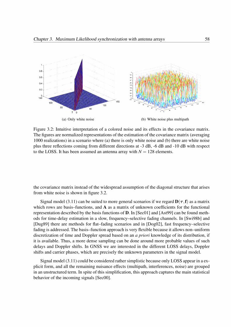
Chapter 3. Maximum Likelihood synchronization with antenna arrays 58
(a) Only white noise (b) White noise plus multipath
Figure 3.2: Intuitive interpretation of a colored noise and its effects in the covariance matrix.The figures are normalized representations of the estimation of the covariance matrix (averaging1000 realizations) in a scenario where (a) there is only white noise and (b) there are white noiseplus three reflections coming from different directions at -3 dB, -6 dB and -10 dB with respectto the LOSS. It has been assumed an antenna array with N = 128 elements.
the covariance matrix instead of the widespread assumption of the diagonal structure that arisesfrom white noise is shown in figure 3.2.
Signal model (3.11) can be suited to more general scenarios if we regard D(τ , f) as a matrixwhich rows are basis–functions, and A as a matrix of unknown coefficients for the functionalrepresentation described by the basis functions of D. In [Sec01] and [Ast99] can be found meth-ods for time-delay estimation in a slow, frequency–selective fading channels. In [Swi98b] and[Dug89] there are methods for flat–fading scenarios and in [Dog02], fast frequency–selectivefading is addressed. The basis–function approach is very flexible because it allows non–uniformdiscretization of time and Doppler spread based on an a priori knowledge of its distribution, ifit is available. Thus, a more dense sampling can be done around more probable values of suchdelays and Doppler shifts. In GNSS we are interested in the different LOSS delays, Dopplershifts and carrier phases, which are precisely the unknown parameters in the signal model.
Signal model (3.11) could be considered rather simplistic because only LOSS appear in a ex-plicit form, and all the remaining nuisance effects (multipath, interferences, noise) are groupedin an unstructured term. In spite of this simplification, this approach captures the main statisticalbehavior of the incoming signals [Sec00].

Chapter 3. Maximum Likelihood synchronization with antenna arrays 59
3.1.2 Unstructured array model
The signal model proposed in (3.2) is parameterized by the DOAs of the target signals andtheir amplitudes. As argued, the a priori knowledge of DOAs and the location of the antennaelements (and therefore matrix G) is a reasonable assumption in GNSS applications, but inpractice this assumption implies a considerable technical complexity. Instead, we can definea channel matrix H which assumes the role of GA but does not impose any structure, so isreferred to as unstructured. Thus, the signal model for a single snapshot reduces to
x = Hd+n (3.15)
and its version for K snapshots isX = HD+N, (3.16)
which is considerably simpler than (3.11). An additional advantage of such model is that itprovides robustness to errors in the array response, which is usually determined empirically bymeans of a process known as calibration, see section 6.3 for more details, or assuming identicalsensors. A perfect calibration is hardly satisfied in practice: errors in the measured gain andphase response of the antenna elements, mutual coupling, quantization and interpolation errorsin the calibration process, variations in temperature or humidity, fluctuations in the surroundingenvironment, changes in antenna location or drifts in the hardware behavior along the timecould modify significantly the actual array response and cause synchronization performancedegradation [Swi98b].
The arbitrary structure of H allows to see its columns as generic spatial signatures not onlyparameterized by DOAs, location of antennas and signal amplitudes, but taking into account ina not–explicit manner other unknown phenomenons. The price payed is the inability of the arrayin estimating carrier phases, which are of great importance in high accuracy positioning algo-rithms, and the performance degradation suffered by beamforming algorithms, which reducesignificantly the computational cost of the estimation.
3.2 Cramer-Rao bounds
Before dwelling into the analysis of estimation procedures based on the proposed signal model,it is worthwhile to compute the theoretical accuracy limits which we can expect to attain. Itis well known that, for any unbiased estimator, such limits are determined by the Cramer-RaoBound (CRB), a sort of uncertainty metric which constitutes the insuperable frontier of estima-tion accuracy. This section provides a detailed derivation of the CRB for the problem at hand.
We denote the covariance matrix of the estimation errors of a vector parameter ξ by
C(ξ) = E[
ξ−ξ][
ξ−ξ]T
. (3.17)

Chapter 3. Maximum Likelihood synchronization with antenna arrays 60
The multiple-parameter CRB states that, for any unbiased estimate of ξ,
C(ξ)≥ J−1, (3.18)
where J is commonly referred to as Fisher Information Matrix or FIM. The matrix inequalitymeans that C(ξ)− J−1 is a non-negative definite matrix. The FIM elements are defined as afunction of the likelihood function of the observed data, in the form
Juv =−E[
∂2Λx(ξ)∂ξu∂ξv
]. (3.19)
Therefore, this result also provides a lower bound on the variance of any unbiased estimatorof the parameter ξu:
var(
ξu−ξu
)≥[J−1]
uu . (3.20)
This bound is often called classic Cramer-Rao bound and depends on the actual value ofthe parameter, so it can be described as a local bound. There is a Bayesian version that takesinto account the a priori probability density of the parameters and provides a global bound thatdoes not depend on the value of the parameter on a specific trial. The derivation presented inthis section refers to the classic CRB.
In practice, computation of such bounds is usually considered to be a cumbersome or evenimpossible task because it involves the second derivative of the probability density function orof its logarithmical version, the log-likelihood function. The Gaussian assumption, even consid-ering an arbitrary covariance matrix, allows an analytical treatment as will be shown hereafter.The presence of nuisance parameters often makes the computation of the CRB difficult, as inthe case of non-data-aided (NDA) schemes, where the data symbols are the nuisance parame-ters when dealing with synchronization. In a communications framework, it is usual to applysome simplifications, leading to the modified CRB (MCRB) introduced in [D’A94], obtaininga bound lower than the true CRB that usually cannot be attained, but much simpler to compute.As argued in the previous chapter, the navigation data in GNSS is not absolutely unknown. Onthe contrary, once acquisition has been performed and a whole message has been demodulated,few changes are expected in the next message repetition. Therefore, and provided that a datasymbol spans several spreading code periods, the data symbols of the navigation message willbe considered known.
Another classification of the CRB in the context of array processing is whether it is con-ditional (or deterministic) or unconditional (or stochastic) [Ott93]. The former assumes thenuisance parameters to be nonrandom, while the latter assumes them to be Gaussian randomprocesses. For the aforementioned reasons, this derivation will refer to the conditional CRB.
Let us consider the structured array signal model expressed in equation (3.2). We canconstruct a vector stacking all the unknown (but deterministic) parameters in the form

Chapter 3. Maximum Likelihood synchronization with antenna arrays 61
ξ =[
ℜaT ℑaT φT θT τ T fT ]T and thus writing
x(t) = µx(t,ξ)+n(t) (3.21)
for convenience, where µx(t,ξ) = G(φ,θ)Ad(t,τ , f). The elements of ξ are real values. Theprobability density function for K snapshots, extending model (3.2) to (3.11), can be expressedas
px|ξ(x) =exp−∑
K−1k=0 (x(tk)−µx(tk,ξ))HQ−1(x(tk)−µx(tk,ξ))
det(πNQ)K (3.22)
which leads to the log-likelihood function defined as
Λx(ξ) = ln(
px|ξ(x))
=−K ln(det(π
NQ))
+
−K−1
∑k=0
(x(tk)−µx(tk,ξ))H Q−1 (x(tk)−µx(tk,ξ)) (3.23)
Once the log-likelihood function Λx(ξ) has been derived, the next step towards the compu-tation of the elements of the FIM consist in taking the second derivative of (3.23), as expressedin (3.19). Making use of the following identities, valid for non-singular matrices:
∂ ln(det(B(ξ)))∂ξu
= Tr
B−1(ξ)∂B(ξ)
∂ξu
, (3.24)
∂B−1(ξ)∂ξu
=−B−1(ξ)∂B(ξ)
∂ξuB−1(ξ) (3.25)
whose proofs are provided in [Kay93], the first derivative can be expressed as
∂Λx(ξ)∂ξv
=−K Tr
Q−1 ∂Q∂ξv
+
+K−1
∑k=0
(x(tk)−µx(tk,ξ))HQ−1 ∂Q∂ξv
Q−1(x(tk)−µx(tk,ξ))+
+2ℜ
K−1
∑k=0
∂(µx(tk,ξ))H
∂ξvQ−1(x(tk)−µx(tk,ξ))
, (3.26)
and the second derivative is

Chapter 3. Maximum Likelihood synchronization with antenna arrays 62
∂2Λx(ξ)∂ξu∂ξv
= K Tr
Q−1 ∂Q∂ξu
Q−1 ∂Q∂ξv−Q−1 ∂2Q
∂ξu∂ξv
+
+K−1
∑k=0
(x(tk)−µx(tk,ξ))H(−Q−1 ∂Q
∂ξuQ−1 ∂Q
∂ξvQ−1+
+ Q−1 ∂2Q∂ξu∂ξv
Q−1−Q−1 ∂Q∂ξv
Q−1 ∂Q∂ξu
Q−1)
(x(tk)−µx(tk,ξ))+
+2ℜ
K−1
∑k=0
(∂2(µx(tk,ξ))H
∂ξu∂ξvQ−1(x(tk)−µx(tk,ξ))+
− ∂(µx(tk,ξ))H
∂ξvQ−1 ∂Q
∂ξuQ−1(x(tk)−µx(tk,ξ))+
− ∂(µx(tk,ξ))H
∂ξvQ−1 ∂µx(tk,ξ)
∂ξu+
− ∂(µx(tk,ξ))H
∂ξuQ−1 ∂Q
∂ξvQ−1(x(tk)−µx(tk,ξ))
)(3.27)
The next step in the receipt given by equation (3.19) is taking the expectation of (3.27).Here the trace property xHAx = Tr
AxxH is useful for dealing with the first summatory of
the previous equation:
EK−1
∑k=0
(x(tk)−µx(tk,ξ))H(· · ·)(x(tk)−µx(tk,ξ))
=
= E
K−1
∑k=0
Tr(· · ·)(x(tk)−µx(tk,ξ))(x(tk)−µx(tk,ξ))H=
= K Tr(· · ·)Q (3.28)
where (· · ·) represents all the terms inside the big parentheses in the second and third row of(3.27). There are three terms inside the ℜ· operator of (3.27) that will disappear since wehave assumed a zero-mean noise term and therefore E (x(tk)−µx(tk,ξ))= 0. Hence,

Chapter 3. Maximum Likelihood synchronization with antenna arrays 63
E
∂2Λx(ξ)∂ξu∂ξv
=K Tr
Q−1 ∂Q
∂ξuQ−1 ∂Q
∂ξv−Q−1 ∂2Q
∂ξu∂ξv+
−Q−1 ∂Q∂ξu
Q−1 ∂Q∂ξv
+Q−1 ∂2Q∂ξu∂ξv
−Q−1 ∂Q∂ξv
Q−1 ∂Q∂ξu
−2ℜ
K−1
∑k=0
∂(µx(tk,ξ))H
∂ξuQ−1 ∂µx(tk,ξ)
∂ξv
. (3.29)
The first term cancels the third one, and the second term has also a reversed sign with respectto the fourth one. Therefore, a change in the sign is the last step to compute the elements of theFisher Information Matrix, a result also found in [Sto97]:
Juv =−E[
∂2ΛX(ξ)∂ξu∂ξv
]= K Tr
Q−1 ∂Q
∂ξvQ−1 ∂Q
∂ξu
+
+2ℜ
K−1
∑k=0
∂(µx(tk,ξ))H
∂ξuQ−1 ∂µx(tk,ξ)
∂ξv
(3.30)
Covariance matrix Q does not depend on the parameters contained in ξ, and thus ∂Q∂ξv
= 0.The final expression for the FIM elements is
Juv = 2ℜ
K−1
∑k=0
∂(µx(tk,ξ))H
∂ξuQ−1 ∂µx(tk,ξ)
∂ξv
(3.31)
which reduces to
Juv =2
σ2 ℜ
K−1
∑k=0
∂(µx(tk,ξ))H
∂ξu
∂µx(tk,ξ)∂ξv
(3.32)
when white spatial noise is considered, provided that Q = σ2I. But the key idea in the signalmodel is to include multipath and interferences in the noise term, coloring the white temporalnoise in the spatial dimension and considering an arbitrary covariance matrix Q. Gathering allnuisance signals in the term of noise n, the theoretical covariance can be put in the form:
Q = (GmpAmpDmp +GintAintDint)(GmpAmpDmp +GintAintDint)H +σ
2I (3.33)
where the subscript mp refers to multipath and int refers to interferences, and the matrices areequally constructed as G, A and D but using the parameters corresponding to such unwantedsignals. Finally, σ2 refers to the variance of the temporally white thermal noise.

Chapter 3. Maximum Likelihood synchronization with antenna arrays 64
The generic vector parameter ξ can be splitted into amplitudes, directions of arrival and syn-chronization parameters: α =
[ℜaT ℑaT ]T , Ψ =
[φT θT ]T and Υ =
[τ T fT ]T .
Therefore, the FIM can be expressed using 9 submatrices of size 2M×2M:
J =
Jαα JTΨα JT
ΥαJΨα JΨΨ JT
ΥΨJΥα JΥΨ JΥΥ
, J ∈ R6M×6M (3.34)
The elements of such submatrices can be computed using (3.30), with u,v = 1, ...,2M:
Jαuαv = 2ℜ
K−1
∑k=0
d(tk)H ∂AH
∂αuGHQ−1G
∂A∂αv
d(tk)
(3.35)
JΨuαv = 2ℜ
K−1
∑k=0
d(tk)HAH ∂GH
∂ΨuQ−1G
∂A∂αv
d(tk)
(3.36)
Jϒuαv = 2ℜ
K−1
∑k=0
∂d(tk)H
∂ϒuAHGHQ−1G
∂A∂αv
d(tk)
(3.37)
JΨuΨv = 2ℜ
K−1
∑k=0
d(tk)HAH ∂GH
∂ΨuQ−1 ∂G
∂ΨvAd(tk)
(3.38)
JϒuΨv = 2ℜ
K−1
∑k=0
∂d(tk)H
∂ϒuAHGHQ−1 ∂G
∂ΨvAd(tk)
(3.39)
Jϒuϒv = 2ℜ
K−1
∑k=0
∂d(tk)H
∂ϒuAHGHQ−1GA
∂d(tk)∂ϒv
(3.40)
The case 1 ≤ u ≤M stands for the derivative with respect to the elements of ℜa and thecase M < u≤ 2M stands for the derivative with respect to the elements of ℑa.
∂A∂αu
is an all-zero 2M×2M matrix except for a 1 in the u,u position in case of 1 ≤ u ≤M,and an all-zero 2M×2M matrix except for a j in the u,u position in case of M < u≤ 2M.
The same idea can be applied to the derivative of G,
∂G∂Ψu
= jπRT ∂KT
∂Ψu exp
jπRT KT (3.41)
and stands for the Hadamard product. The derivatives of the wavenumber matrix K, definedin (3.8), are:

Chapter 3. Maximum Likelihood synchronization with antenna arrays 65
∂K∂Ψu
=
0 0 0...
......
−sin(φu)cos(θu) cos2(φu)− sin2(φu) 0...
......
0 0 0
← uth row
for 1≤ u≤M (3.42)
and
∂K∂Ψu
=
0 0 0...
......
−cos(φ(u−M)
)sin(θ(u−M)
)0 cos
(θ(u−M)
)...
......
0 0 0
← (u−M)th row
for M < u≤ 2M (3.43)
where the derivative with respect to the elements of φ appear in the first case and with respectto the elements of θ in the second one. Finally,
∂d(tk)∂ϒu
=[
0 · · · −su(tk− τu)e j2π futk · · · 0]T for 1≤ u≤M (3.44)
and
∂d(tk)∂ϒu
=[
0 · · · j2πtks(u−M)(tk− τ(u−M))ej2π f(u−M)tk · · · 0
]Tfor M < u≤ 2M
(3.45)stand for the derivatives with respect to the elements of τ and f, respectively. The non-zeroterms are in the u–th and (u−M)–th columns, respectively. In equation (3.44), s(t) = ds(t)
dt isthe derivative of time of the waveform s(t).
Using equations (3.41-3.45) into (3.35-3.40), the FIM is completely defined and thereforethe CRB for all the parameters can be directly computed by inverting (3.34). Nonetheless, insome applications, we are only interested in computing the CRB for some parameters, andthe inversion of the whole matrix (3.34) increases unnecessarily the computational cost. Inthose cases, we can apply matrix partitioning to obtain the inverse block of interest for the

Chapter 3. Maximum Likelihood synchronization with antenna arrays 66
synchronization and DOA parameters as:
CRBsync/DOA =(
CRBΨΨ CRBTΥΨ
CRBΥΨ CRBΥΥ
)=
=[(
JΨΨ JTΥΨ
JΥΨ JΥΥ
)−(
JΨα
JΥα
)J−1
αα
(JTΨα JT
Υα
)]−1
(3.46)
or its counterpart for the amplitudes
CRBαα =
[Jαα−
(JTΨα JT
Υα
)( JΨΨ JTΥΨ
JΥΨ JΥΥ
)−1( JΨα
JΥα
)]−1
(3.47)
At this point, it is worthwhile to analyze the obtained results and distill their consequences.Some interesting conclusions about the decoupling of parameters can be extracted by the ob-servation of the matrix structures involved in the FIM elements computation. For example,considering a single impinging signal, M = 1, and focusing in equation (3.35), the derivativesare:
∂A∂α1
= 1,∂A∂α2
= j,∂AH
∂α1= 1,
∂AH
∂α2=− j. (3.48)
Substituting these derivatives in equation (3.35), taking into account the hermitic structure ofthe covariance matrix Q, and realizing that the three first terms are the hermitic version of thelast three ones, it can be deduced that the product is real and therefore
Jα1α2 = 2ℜ
j
K−1
∑k=0
d∗(tk)gHQ−1gd(tk)
= 0. (3.49)
The same result can be applied to Jα2α1 , and the ℜ· will disappear in Jα1α1 and Jα2α2 .Therefore, the submatrix for amplitudes can be written in the form
Jαα = 2K−1
∑k=0
d∗(tk)gHQ−1gd(tk)(
1 00 1
), (3.50)
which clearly indicates the decoupling of the real and imaginary part of the complex amplitude.Now, the focus of our attention will move to equation (3.46), since we are mostly interested incomputing the CRB for DOA, Doppler shift and time delay, and analyze how these parametersare coupled. Explicitly:
(CRBΨΨ CRBT
ΥΨCRBΥΨ CRBΥΥ
)=(
JΨΨ−JΨαJ−1ααJT
Ψα JTΥΨ−JΨαJ−1
ααJTΥα
JΥΨ−JΥαJ−1ααJT
Ψα JΥΥ−JΥαJ−1ααJT
Υα
)−1
(3.51)
Chapter 3. Maximum Likelihood synchronization with antenna arrays 67
The coupling of DOA and synchronization parameters is determined by the left-bottomcorner block, JΥΨ−JΥαJ−1
ααJTΨα. Applying the amplitude derivatives expressed in (3.48), we
can write
JΨα =
2ℜ
∑
K−1k=0 d∗(tk)a∗
∂gH
∂Ψ1Q−1gd(tk)
2ℜ
j ∑
K−1k=0 d∗(tk)a∗
∂gH
∂Ψ1Q−1gd(tk)
2ℜ
∑
K−1k=0 d∗(tk)a∗
∂gH
∂Ψ2Q−1gd(tk)
2ℜ
j ∑
K−1k=0 d∗(tk)a∗
∂gH
∂Ψ2Q−1gd(tk)
= 2ℜ
(1 j
)⊗
K−1
∑k=0
d∗(tk)a∗∂gH
∂ΨQ−1gd(tk)
(3.52)
where ⊗ stands for the Kronecker product. The same idea is applicable to JΥα:
JΥα = 2ℜ
(1 j
)⊗
K−1
∑k=0
∂d∗(tk)∂Υ
a∗gHQ−1gd(tk)
(3.53)
Then, applying the fact that
ℜ(
1 j)⊗S(
ℜ(
1 j)⊗T)T = ℜ
STH (3.54)
valid for matrices with appropriate dimensions, we can compute the off-diagonal block usingexpressions (3.50), (3.52), (3.53) and (3.54):
JΥΨ−JΥαJ−1ααJT
Ψα = JΥΨ−1
2∑K−1k=0 d∗(tk)gHQ−1gd(tk)
JΥαJTΨα
= JΥΨ−4ℜ
(∑
K−1k=0
∂d∗(tk)∂Υ a∗gHQ−1gd(tk)
)(∑
K−1k=0 d∗(tk)gHQ−1 ∂g
∂ΨT ad(tk))
2∑K−1k=0 d∗(tk)gHQ−1gd(tk)
= JΥΨ−2ℜ
∑
K−1k=0
∂d∗(tk)∂Υ a∗gHQ−1 ∂g
∂ΨT ad(tk)
∑K−1k=0 d∗(tk)d(tk)
∑K−1k=0 d∗(tk)d(tk)
= JΥΨ−2ℜ
K−1
∑k=0
∂d∗(tk)∂Υ
a∗gHQ−1 ∂g∂ΨT ad(tk)
= 0 (3.55)
Result (3.55) has important consequences. When substituted in (3.51), the resulting matrixis block-diagonal, and therefore CRBΥΨ = 0. In other words, the DOA and the synchroniza-tion parameters are decoupled, i.e., CRBΥΥ remains the same whether or not Ψ is known. This

Chapter 3. Maximum Likelihood synchronization with antenna arrays 68
means that we do not need aprioristic estimates of the DOA to asymptotically achieve the min-imum variance in the estimation of the synchronization parameters when an unbiased estimatoris considered.
Finally, the CRB for the synchronization parameters is:
CRBΥΥ =(JΥΥ−JΥαJ−1
ααJTΥα
)−1
=
JΥΥ−2ℜ
(∑
K−1k=0
∂d∗(tk)∂Υ a∗d(tk)
)(∑
K−1k=0 d∗(tk)gHQ−1ga∂d(tk)
∂ΥT
)∑
K−1k=0 d∗(tk)d(tk)
−1
=
JΥΥ−2|a|2gHQ−1gℜ
(∑
K−1k=0
∂d∗(tk)∂Υ d(tk)
)(∑
K−1k=0 d∗(tk)
∂d(tk)∂ΥT
)∑
K−1k=0 d∗(tk)d(tk)
−1
. (3.56)
3.3 Maximum Likelihood estimation of time delays andDoppler shifts
As explained in the introduction of this chapter, Maximum Likelihood is an statistical-basedprocedure which yields estimators with desirable properties, mainly asymptotical efficiency,asymptotical optimality and invariancy. In this section, the ML approach will be applied to theunstructured signal model (3.16). Two reasons drive to this election, instead of the structuredmodel expressed in (3.11). Firstly, an structured model implies a calibrated array, which sup-poses a great technical complexity: all the channels (here channel refers to an antenna and allthe RF front-end hardware before digitation) must maintain a phase reference, in the sense that,if a given signal impinges all the antennas at the same time, the phases at the digitation stagemust be the same for all channels, or with known differences. Chapter 6, section 6.3, will discusscalibration methods from a practical point of view.
The second reason is not practical but theoretical. As will be proved in the next pages, thechannel matrix H is not needed in the computation of the ML estimators of time delays andDoppler shifts. This means that, at least asymptotically, the same estimators can be achievedwith an structured or an unstructured array. The concept of asymptotical equivalence refers to
‖ Υunstructured− Υstructured ‖= op(‖ Υstructured−Υ ‖
)(3.57)
where ‖ · ‖ is any consistent vector norm and op(‖ Υstructured−Υ ‖
)denotes a random vari-
able that converges to zero in probability at a rate faster than ‖ Υstructured−Υ ‖→ 0, as defined

Chapter 3. Maximum Likelihood synchronization with antenna arrays 69
in [Swi98b]. Provided that the ML estimator converges to the actual value for large data col-lections (i.e., for large K), the estimates of time delays and Doppler shifts obtained both withthe structured and unstructured signal model will tend to be equal as the number of snapshotsincreases.
The advantages of an structured array and a priori known steering vector will be analyzedin subsection 3.4.3, where the particularization of M = 1 and f = 0 allows the ML estimatorof the carrier phase, and in chapter 4, where the knowledge of G will allow electronic beam-forming and estimation algorithms with an interesting connection to the ML approach but witha dramatic decreasing of the computational cost.
The probability density function (PDF) of a complex multivariate Gaussian vector x, as ex-pressed in (3.15), and considering a noise with arbitrary covariance matrix Q, can be expressedas:
p(x) =exp[−(x−Hd)HQ−1(x−Hd)
]πN det(Q)
(3.58)
Hence, the likelihood function of the data is proportional to (3.58). Applying the logarithmand neglecting irrelevant additive and multiplicative constants, we determine the negative log–likelihood function for K observations of x, thus extending the estimation to model (3.16):
Λ1(Q,H, f,τ ) = ln(det(Q))+TrQ−1C (3.59)
where C has been defined as
C =1K
K−1
∑k=0
(x(tk)−Hd(tk))(x(tk)−Hd(tk))H =
1K
(X−HD)(X−HD)H (3.60)
where only the dependency with instant tk has been expressed for convenience. From (3.58) to(3.59) we have used the trace property xHy = TryxH, which leads to xHAx = TrAxxH anddefinition (3.60) arises.
Using the following cross-correlation estimation matrix definitions:
RXX = 1K XXH RXD = 1
K XDH
RDX = RHXD RDD = 1
K DDH (3.61)
(3.60) can be expressed as
C = RXX− RXDHH−HRDX +HRDDHH (3.62)
The joint Maximum Likelihood (ML) estimate of f,τ and H, or in other words, the valueof these parameters for which the value of the observed X is most probable, is obtained byminimizing (3.59):
Q,H, f, τ |ML = arg minQ,H,f,τ
[ln(det(Q))+TrQ−1C
](3.63)

Chapter 3. Maximum Likelihood synchronization with antenna arrays 70
The gradient of (3.59) with respect to Q is
∇Q(ln(det(Q))+TrCQ−1
)=[Q−1−Q−1CQ−1]T (3.64)
Assuming K ≥ N + M, so that the matrix C is invertible with probability one, the ML esti-mate of the covariance matrix Q is
QML = C(H, f,τ )∣∣∣H=HML,f=fML,τ=τML
(3.65)
Replacing Q in (3.59) with (3.65) and neglecting the additive constant term we obtain
Λ2(H, f,τ ) = ln(det(RXX− RXDHH−HRH
XD +HRDDHH)) (3.66)
This expression can be conveniently rearranged in the following form:
Λ2(H, f,τ ) = ln(det(W))
+ ln(det(I+ B
))(3.67)
whereW = RXX− RXDR−1
DD RHXD (3.68)
andB = RDD
(H− RXDR−1
DD
)H W−1 (H− RXDR−1DD
)(3.69)
The value of the channel matrix H which nulls B and therefore minimizes Λ2 is the MLestimator
HML = RXDR−1DD (3.70)
also known as Wiener estimator. It is important to notice that estimator (3.70) minimizes (3.67)because the channel matrix has been defined unstructured, without forcing a special form of thematrix. If we had used the structured model (3.11), and therefore we had interchanged H by GAconsidering G known, the derivative of (3.67) with respect to matrix A leads to the estimator
AML =(GHW−1
ML G)−1 GHW−1
ML RXDR−1DD , (3.71)
but in the definition of A = diag(a) we are forcing a certain structure on the matrix, and there-fore diag(AML) 6= aML. The price of using the unstructured model is the inability to estimate thecarrier phase of the desired signals.
Continuing with the unstructured model, and substituting the ML estimation of the channelmatrix obtained in (3.70) in (3.65), we obtain

Chapter 3. Maximum Likelihood synchronization with antenna arrays 71
QML = RXX− RXDR−1DD RH
XD− RXDR−1DD RH
XD + RXDR−1DD RDDR−1
DD RHXD
= RXX− RXDR−1DD RH
XD
= W (3.72)
and thus we find that matrix W is the ML estimator of the unstructured covariance matrix Q.When this result is substituted in the cost function Λ2, we obtain a new cost function whoseminimization leads to the joint ML estimation of time delays and Doppler shifts:
ΛML(f,τ ) = ln(det(W))
(3.73)
and therefore
fML, τML = argminf,τ
ln(det(W))
(3.74)
Figure 3.3 plots the shape of the cost function defined in equation (3.73) applied to differentmodulations used in GNSS.
There is a special feature in equation (3.73), outlined in the introduction of this section, thathas to be highlighted: it does not depend on the estimation of the channel matrix.
At this point, we will develop a transformation of equation (3.73) that will be useful inthe next chapter to prove the equivalence between the ML approach and a special kind ofbeamforming. Applying the determinant properties det(AB) = det(A)det(B) and det(I+BC) =det(I+CB) for matrices with appropriate dimensions:
Λ3(f,τ ) = ln(det(RXX− RXDR−1
DD RHXD
))=
= ln(det(RXX
(I− R−1
XX RXDR−1DD RH
XD
)))=
= ln(det(RXX
))+ ln
(det(
I− R−12
XX RXDR−1DD RH
XDR−12
XX
)) (3.75)
Provided that RXX does not depend on the synchronization parameters, the expression canbe reduced to
Λ3 = ln(
det(
I− R−12
XX RXDR−1DD RH
XDR−12
XX
)). (3.76)
This expression can be rearranged applying definitions in (3.61). If PDH = DH(DDH)−1D is theprojection matrix over the subspace spanned by the columns of DH , and PXH defined equally, astraightforward manipulation of (3.76) yields
Λ3 = ln(det(I−PXH PDH )) (3.77)
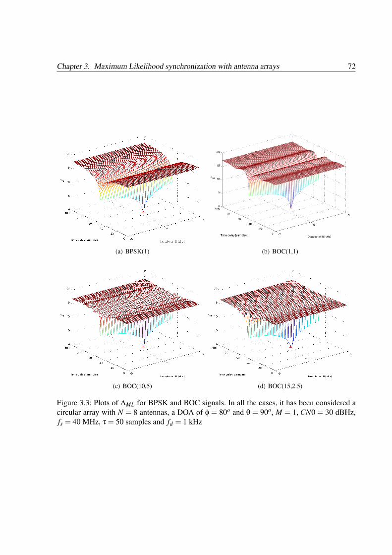
Chapter 3. Maximum Likelihood synchronization with antenna arrays 72
(a) BPSK(1) (b) BOC(1,1)
(c) BOC(10,5) (d) BOC(15,2.5)
Figure 3.3: Plots of ΛML for BPSK and BOC signals. In all the cases, it has been considered acircular array with N = 8 antennas, a DOA of φ = 80o and θ = 90o, M = 1, CN0 = 30 dBHz,fs = 40 MHz, τ = 50 samples and fd = 1 kHz

Chapter 3. Maximum Likelihood synchronization with antenna arrays 73
This expression is not useful regarding software implementation because it implies the com-putation of a determinant of a larger matrix than (3.73): while W is an N×N matrix, I−PXH PDH
is a K×K matrix, and we have assumed a number of snapshots K ≥ N + M. Equation (3.77)will be used in subsection 4.2.3 to show an interesting connection between the multiple hybridbeamforming and the joint ML estimation.
Figure 3.4: Effect of multipath on ΛML
3.3.1 Consistency
The consistency of the joint ML estimator of Doppler shifts and time delays of a set of incom-ing signals using antenna arrays presented in equation (3.73) follows from the fact that as thenumber of snapshots increases, the cost function converges with probability one to a limitingvalue which is minimized by the true values of Doppler shifts and time delays. In addition, thisconvergence will be uniform thanks to the differentiability of the autocorrelation rss(τ).

Chapter 3. Maximum Likelihood synchronization with antenna arrays 74
Resorting to the assumption of a band-limited finite-average-power signal stated in (3.3),(3.4) and (3.5), we can compute the limiting value of the cost function. When the number ofsnapshots approach to infinite, K→ ∞, the correlation terms tend to
limK→∞
RXD = limK→∞
1K
XDH = limK→∞
1K
(HD(Υtrue)+N
)DH(Υ) =
= limK→∞
1K
(HD(Υtrue)DH(Υ)+NDH(Υ)
)= HCdd(Υtrue,Υ) (3.78)
andlim
K→∞RXX = RXX. (3.79)
Using these two limiting values into ΛML = lndet(
RXX− RXDR−1DD RH
XD
), one obtains:
limK→∞
ΛML(Υ) = lndet(
RXX−HCdd(Υtrue,Υ)C−1dd (Υtrue,Υtrue)CH
dd(Υtrue,Υ)HH
)= lndet
(RXX−HCdd(Υtrue,Υtrue)HH+ (3.80)
+ H(
Cdd(Υtrue,Υtrue)−Cdd(Υtrue,Υ)C−1dd (Υ,Υ)CH
dd(Υtrue,Υ)
)HH)
Here will be useful a linear algebra result: the determinant is a nondecreasing function.Therefore, for any possible matrix B and any possible non-negative definite matrix ∆B, thedeterminant satisfies
det(B+∆B) = det(B(I+B−1∆B
))= det(B)det
(I+B−1∆B
)≥ det(B) (3.81)
since the eigenvalues of I + B−1∆B are ≥ 1, and the equality only holds when ∆B = 0. Ap-plying this result to equation (3.80), we can identify the term
∆B = H(
Cdd(Υtrue,Υtrue)−Cdd(Υtrue,Υ)C−1dd (Υ,Υ)CH
dd(Υtrue,Υ)
)HH . (3.82)
This matrix ∆B is non-negative definite because the term
Cdd(Υtrue,Υtrue)−Cdd(Υtrue,Υ)C−1dd (Υ,Υ)CH
dd(Υtrue,Υ) (3.83)
is the Schur complement of Cdd(Υ,Υ) in

Chapter 3. Maximum Likelihood synchronization with antenna arrays 75
(Cdd(Υ,Υ) CH
dd(Υtrue,Υ)
Cdd(Υtrue,Υ) Cdd(Υtrue,Υtrue)
)= lim
K→∞
1K
∞
∑K=0
(D(tk,Υ)
D(tk,Υtrue)
)(DH(tk,Υ) DH(tk,Υtrue)
)(3.84)
which is clearly non-negative definite. This result proofs that
limK→∞
ΛML(Υ)≥ lndet(RXX−HCdd(Υtrue,Υtrue)HH)= lim
K→∞ΛML(Υtrue). (3.85)
The equality in (3.85) holds if and only if the Schur complement expressed in equation(3.83) is zero, which is only possible for Υ = Υtrue if Cdd(Υ,Υ) is positive definite for anyvector Υ of length 2M whose elements are all distinct. The consistency of HML and QML followsfrom equation (3.70) and (3.72) and the consistency of ΥML.
3.4 Suboptimal estimators of time delays and Doppler shiftsapplied to GNSS
The main objective of this section is to establish procedures capable of estimating the parametervector Υ =
[τ T fT ]T basing on the optimization of the ML cost function ΛML(Υ) computed
hereinbefore.
The preceding section has presented a theoretical framework for array synchronization fol-lowing the ML approach, based on a very general signal model. The characteristics and par-ticularities of the signal structures employed in GNSS (see sections 2.5 and 2.6) have not beentaken into account. For example: the baseband signals considered in both the unstructured andstructured signal model refers to the received signal before or after the correlator? This sectionwill discuss these issues.
In order to properly select the reference waveform s(t), we could consider to choose the sig-nal before correlation. In this case, a generic waveform belonging to a GNSS can be expressedas
s(t) =∞
∑i=−∞
d(i)Nc−1
∑u=0
Lc−1
∑k=0
c(k)gT (t− kTc−uTPRN− iTb). (3.86)
Indeed, M in-view satellites can be included in the model, where the differences in eachsm(t) lie in the spreading code and maybe the pulse shaping if we are working with several

Chapter 3. Maximum Likelihood synchronization with antenna arrays 76
frequency bands. However, this approach has serious drawbacks from a practical point of view.In section 2.2 we have argued that the receiving signal is on the order of 20 dB below the noisefloor. Therefore, when computing the correlation matrix, the contribution of the reflections tothat matrix would be imperceptible compared with that of the white noise and interferences(which are generally stronger than the white noise), and it would be impossible to infer anyspatial information about the reflected replicas from that correlation matrix. In short: the co-variance matrix, when estimated before correlation, is insensitive to the reflections. Since theaim of this approach is to take advantage of the spatial dimension to mitigate both the reflec-tions and the interferences, the SNR of the desired signals must be increased: precisely, the taskthat the correlation carries out. This despreading process will increase the LOSS strength ofthe desired satellite and its coherent reflections, while the contribution of other satellites andnarrowband interferences will be kept under the noise floor. Therefore, it is desirable to applythe ML approach after the despreading process.
The increase of the SNR is not the only benefit provided by the correlation. The high chip-ping rate spreads the spectrum of the signal, requiring a much higher sampling frequency in or-der to accomplish the Nyquist sampling theorem. A higher sampling frequency implies a highernumber of samples to cover the same time span, which directly impacts on the computationalload required by the ML estimator. Even resorting to parallelization algorithms [Gol96], thegeneration of every trial W(τ , f) and its corresponding determinant could be cost-prohibitivewhen K increases.
On the contrary, working after correlation dramatically decreases the number of samples. Infact, all the information can be gathered taking a few samples of the correlator output when awhole spreading code sequence has been correlated, and the waveforms showed in figure 2.12arise from the Integration & Dump module. These waveforms appears at a code sequence rate,which is on the order of 1000 times slower than the chipping rate. In conclusion, it seems clearthat the ML estimator must be applied after the correlation process, and then
s(t) =∞
∑i=−∞
d(i)Lc
T bT c−1
∑k=0
Rg(t− kLcTc− iTb), (3.87)
probably removing the data dependence d(i) for convenience.
The time segments to be sampled are only those where the correlation function has signif-icant values: a span of two chips every code period. Therefore, the time observation span isTobs = 2Tc, which redounds in a frequency resolution of fres = 1
2Tc. If only one GPS C/A pulse
is considered, the frequency resolution is above the 500 kHz, which is clearly poor. The solutionis to integrate the samples of several pulses in order to increase frequency resolution and reducethe estimation variance.

Chapter 3. Maximum Likelihood synchronization with antenna arrays 77
This fact suggests the idea of using a suboptimal but faster acquisition method in order toobtain rough estimations of time delay and Doppler shift (some acquisition methods will bediscussed in section 6.5) and then perform a refinement in the estimations with the ML (orany other) approach. While accurate time delay estimations can be rapidly obtained with a fewpulses, the Doppler measurement might take a longer time to be computed, since the observationtime must be at least longer than one period. Accordingly, the time delay and the Doppler shiftestimation can be decoupled until the time observation span allows a reasonable frequencyresolution. However, and for the sake of completeness, the derivation of suboptimal estimatorspresented in this section will be developed for time and frequency joint estimation, although theparticularization for time delay estimation, keeping fixed the frequency, is straightforward.
The use of a PLL or a FLL, in the fashion of the traditional single-antenna receivers, beforedigitation in order to remove the Doppler shift introduces some hardware complexity becausethere is a need of maintaining a phase reference in all the RF front-ends. The different behaviorof the FLL of each RF chain provokes a mismatch between the signal model and the actualdigitized signal. Hence, there is a need of a calibration subsystem and the inclusion of its re-sults to the signal model in order to apply the derived estimators without loss of performance.The scope of this Dissertation is the estimation in the digital domain, and thus the estimationprocedures presented in the following will be based in the use of discrete samples.
3.4.1 Steepest descent
The steepest descent is an algorithm for finding a local minimum of a function in an iterativeway. It does not ensure finding the global minimum, and therefore it must be initialized withina convergence region by means of an acquisition method. Once it is initialized in a suitablesynchronization vector, Υ(0), the algorithm moves towards the direction of the local downhillgradient. Although the algorithm might suffer of slow convergence under certain conditions(drawback which is overcome by the conjugate gradient method [Arf95]), it is applied to theminimization of ΛML because the computations involved here are useful in order to obtain costfunctions with linear dependency on PDH , which is exploited by computationally efficient algo-rithms such as IQML [Bre86] or ESPRIT [Swi98a].
As stated, the estimations follow the direction of the downhill gradient in successive itera-tions:
Υ(i+1) = Υ(i)−λ(i)∇ΥΛML(Υ(i)) (3.88)
where ∇ stands for the gradient vector operator, the superindex indicates the iteration and thesubindex indicates the vector parameter on which the derivatives are performed. The weightvector λ(i) controls the size of the step in each iteration towards the direction where ΛML de-creases more quickly.

Chapter 3. Maximum Likelihood synchronization with antenna arrays 78
The elements of the gradient vector of ΛML with respect to the parameters to be estimatedcan be obtained applying equation (3.24) on the negative log–likelihood function (3.73). Hence,with respect to the u–th parameter, we get
∇ϒuΛML =∂ΛML
∂ϒu=− 1
KTr
W−1X∂PDH
∂ϒuXH
. (3.89)
In this last equation, we have made use of the derivative
∂W∂ϒu
=− 1K
X∂PDH
∂ϒuXH (3.90)
which arises directly from the definition of matrix W in equation (3.68).
The derivative ∂PDH∂ϒu
is a K×K matrix, so ∂PDH∂Υ will be a tridimensional tensor formed by
2M matrices of K×K elements, each one of them containing the partial derivatives of the PDH
elements with respect to the ϒu variables (see appendix 3.A):
∂PDH
∂ϒu= P⊥DH
∂DH
∂ϒu
(DH)†
+(
P⊥DH∂DH
∂ϒu
(DH)†
)H
(3.91)
The derivatives ∂DH
∂ fm, where m = 1, . . . ,M are easily obtained from definition of D:
∂DH
∂ fm=
0 . . . 0 − j2πt0s∗m(t0− τm)e− j2π fmt0 0 . . . 0...
......
......
0 . . . 0 − j2πtK−1s∗m(tK−1− τm)e− j2π fmtK−1 0 . . . 0
(3.92)
An equivalent procedure is applied to obtain derivatives with respect to the τm variables:
∂DH
∂τm=
0 . . . 0 −s∗m(t0− τm)e− j2π fmt0 0 . . . 0...
......
......
0 . . . 0 −s∗m(tK−1− τm)e− j2π fmtK−1 0 . . . 0
(3.93)
where sm(t) is the derivative of sm(t) with respect to t, and (·)∗ stands for the conjugate.
The weight vector λ(i) can be set heuristically or optimized by computing the gradient ofΛML(Υ(i+1)) with respect to λ(i):
∇λ(i)ΛML(Υ(i+1)) = ∇ΥΛML(Υ(i+1))∇λ(i)ΛML(Υ(i)) (3.94)

Chapter 3. Maximum Likelihood synchronization with antenna arrays 79
Setting this expression to zero, the weight vector λ(i) should be chosen so that∇ΥΛML(Υ(i+1)) and ∇λ(i)ΛML(Υ(i)) are orthogonal.
The method of Steepest Descent, among simple, is also very stable; if the minimum pointsexist, the method is guaranteed to locate them after at least an infinite number of iterations.However, the method has one very important drawback; it generally has slow convergence,specially for functions which have long, narrow valley structures. For badly scaled systems; i.e.if the eigenvalues of the Hessian matrix at the solution point are different by several orders ofmagnitude, the method could spend an infinite number of iterations before locating a minimumpoint. It starts out with a reasonable convergence, but the progress gets slower as the minimumis approached [Pre96]. Complementary features can be found in the Newton-Raphson algorithmdetailed hereafter, which starts out slowly and ends with a very rapid convergence. These twomethods can be combined, resulting in a very efficient method: the estimation procedure canstart out with the steepest descent method, and switch to the Newton-Raphson method when theprogress by the former gets slower, enjoying the quadratic convergence of the latter.
3.4.2 Newton-Raphson algorithm
If τ and f are conveniently initialized by means of an acquisition scheme, or by the SteepestDescent method as suggested, a Newton–Raphson based algorithm can be applied to find theestimations iteratively. The idea behind the Newton-Raphson method is to approximate the MLcost function (3.68) in each iteration by a quadratic function, and then move to the minimum ofthis approximation. The quadratic function for a vector Υ =
[τ T fT ]T in a suitable neigh-
borhood of the current estimated vector Υ is given by a truncated Taylor expansion:
ΛML(Υ)≈ ΛML(Υ)+(Υ− Υ)T∇ΥΛML(Υ)+
12(Υ− Υ)T HΥΛML(Υ)(Υ− Υ) (3.95)
where H stands for the Hessian matrix. The derivative of (3.95) with respect to the difference(Υ− Υ) is
∇(Υ−Υ)ΛML(Υ)≈ ∇ΥΛML(Υ)+12
HΥΛML(Υ)(Υ− Υ)+12(HΥΛML(Υ)
)T(Υ− Υ) (3.96)
Expression 12HΥΛML(Υ)(Υ − Υ) + 1
2
(HΥΛML(Υ)
)T(Υ − Υ) is equivalent to
HΥΛML(Υ)(Υ − Υ) because the signals involved in matrix D are assumed to be twicecontinuously differentiable at every point. Interchanging the order of taking partial derivatives

Chapter 3. Maximum Likelihood synchronization with antenna arrays 80
in the elements off the main diagonal does not affect the result, which will be shown, andtherefore the Hessian matrix is symmetric. Assuming that ΛML(Υ) takes its minimum value atΥ = Υ, the gradient (3.96) is zero when evaluated in this vector:
∇ΥΛML(Υ)+HΥΛML(Υ)(Υ− Υ) = 0 (3.97)
The Newton-Raphson method uses this found vector Υ as the next current estimated vector,and thus the iterativeness arises:
Υ(i+1) = Υ(i)−(
HΥΛML(Υ(i)))−1
∇ΥΛML(Υ(i)) (3.98)
The Hessian matrix can be put in the form
HΥΛML(Υ) =(
Hτ ΛML(Υ) Hτ fΛML(Υ)Hfτ ΛML(Υ) HfΛML(Υ)
)(3.99)
where each submatrix will be computed from the estimations of the last iteration:
Hτ ΛML
(τ (i), f(i)
)=
∂2ΛML
∂τ∂τ T =
∂2ΛML∂τ1∂τ1
· · · ∂2ΛML∂τ1∂τM
... . . . ...∂2ΛML∂τM∂τ1
· · · ∂2ΛML∂τM∂τM
(3.100)
HfΛML
(τ (i), f(i)
)=
∂2ΛML
∂f∂fT =
∂2ΛML∂ f1∂ f1
· · · ∂2ΛML∂ f1∂ fM
... . . . ...∂2ΛML∂ fM∂ f1
· · · ∂2ΛML∂ fM∂ fM
(3.101)
Hτ fΛML
(τ (i), f(i)
)=
∂2ΛML
∂τ∂fT =
∂2ΛML∂τ1∂ f1
· · · ∂2ΛML∂τ1∂ fM
... . . . ...∂2ΛML∂τM∂ f1
· · · ∂2ΛML∂τM∂ fM
(3.102)
Hfτ ΛML
(τ (i), f(i)
)=
∂2ΛML
∂f∂τ T =
∂2ΛML∂ f1∂τ1
· · · ∂2ΛML∂ f1∂τM
... . . . ...∂2ΛML∂ fM∂τ1
· · · ∂2ΛML∂ fM∂τM
(3.103)
The elements of the Hessian matrix of ΛML can be expressed as the derivative of the gradientvector formed by the elements defined in equation (3.89) with respect to the parameter ϒu.

Chapter 3. Maximum Likelihood synchronization with antenna arrays 81
Applying the definition of the derivative of an inverse matrix given in equation (3.25), the resultof equation (3.90), the following result
∂W−1
∂ϒu=−W−1 ∂W
∂ϒuW−1 =
1K
W−1X∂PDH
∂ϒuXHW−1, (3.104)
and the product derivative rule, each element u,v of the Hessian matrix can be computed as:
∂2ΛML
∂ϒu∂ϒv=− 1
KTr
1K
W−1X∂PDH
∂ϒuXHW−1X
∂PDH
∂ϒvXH +W−1X
∂2PDH
∂ϒu∂ϒvXH
(3.105)
In this case, ∂2PDH
∂Υ∂ΥT is a set of 2M tridimensional tensors, each one formed by 2M matricesof K×K size. Each of these matrices, identified by the subindexes u,v can be computed, asshowed in Appendix 3.B, with the expression
∂2PDH
∂ϒu∂ϒv= −∂PDH
∂ϒu
∂DH
∂ϒv
(DH)†
+P⊥DH∂DH
∂ϒu∂ϒv
(DH)†
+
+P⊥DH∂DH
∂ϒv
(DDH)−1 ∂D
∂ϒuP⊥DH +
−P⊥DH∂DH
∂ϒv
(DH)† ∂DH
∂ϒu
(DH)†
+(· · ·)H (3.106)
where (· · ·)H means that the same expression appears again conjugated and transposed.
The second derivative ∂2DH
∂ fn∂ fmis a K×M matrix with all zeros if m 6= n. In case of m = n, we
obtain:
∂2DH
∂ fm∂ fm=
0 . . . 0 −(2πt0)2 s∗m(t0− τm)e− j2π fmt0 0 . . . 0
......
......
...0 . . . 0 −(2πtK−1)
2 s∗m(tK−1− τm)e− j2π fmtK−1 0 . . . 0
(3.107)
If the derivatives are with respect to τ , the result is also a K×M matrix with all zeros if m 6= n.In case of m = n:
∂2DH
∂τm∂τm=
0 · · · 0 s∗m(t0− τm)e− j2π fmt0 0 · · · 0...
......
......
0 · · · 0 s∗m(tK−1− τm)e− j2π fmtK−1 0 · · · 0
(3.108)

Chapter 3. Maximum Likelihood synchronization with antenna arrays 82
where sm(t) is the second derivative of sm(t) with respect to t. The same structure is found inthe cross-terms: K×M matrices with all zeros if m 6= n. In case of m = n,
∂2DH
∂τm∂ fm=
0 · · · 0 j2πt0s∗m(t0− τm)e− j2π fmt0 0 · · · 0...
......
......
0 · · · 0 j2πtK−1s∗m(tK−1− τm)e− j2π fmtK−1 0 · · · 0
(3.109)
and∂2DH
∂ fm∂τm=
∂2DH
∂τm∂ fm(3.110)
A serious disadvantage of the Newton-Raphson method is that it is not necessarily globallyconvergent, meaning that it may not converge from any starting point. Even if it does con-verge, it can expend significant computational efforts in getting close enough to the solutionwhere the approximation in (3.95) becomes valid, and the convergence is fast. An improve-ment to this solution is to adjust the step size, in the same way that in the Steepest Descentalgorithm. In order to compute the step size, it is recommended to use a backtracking scheme[Pre96], where the full step λ(i) = 1 is tried first. If this step fail to satisfy the criterion for thedecrease of the function, one backtracks in a systematic way along the direction pointed by
−(
HΥΛML(Υ(i)))−1
∇ΥΛML(Υ(i)), which is often referred to as Newton direction.
3.4.3 Line Of Sight Signal delay and carrier-phase estimation
The architecture of a current GNSS receiver, as shown in chapter 2, is based on parallelization.Although a more-complex signal model taking into account all the desired signals gives moreinformation about the scenario, hardware implementation uses to devote an acquisition andtracking block per satellite, and therefore such blocks are designed using a single-signal model.This is due to the despreading process, which provides a processing gain only to the desired sig-nal and allows the estimation of its parameters. Our multi-signal approach might be well-suitedto the software radio philosophy, which will be discussed in chapter 6, or to other non-CDMAsystems such as the COSPAS-SARSAT discussed in chapter 5, but its computational require-ments are too heavy to be performed in a real-time GNSS receiver. Since the aforementionedML estimator has desirable properties in specular or diffuse multipath mitigation, it is worth-while to particularize the derivation considering the time delay and carrier phase estimation ofa single satellite signal. The original derivation of these estimators and a thoroughgoing anal-ysis of their performance is due to Gonzalo Seco and can be found in [Sec00] and [Sec05].In the context of this dissertation, these estimators appear as a natural particular case of signalmodel (3.11) considering M = 1 and a null Doppler shift, with the remarkable fact that leads toa closed-form expression for the carrier phase and a unidimensional search for the time delay.

Chapter 3. Maximum Likelihood synchronization with antenna arrays 83
Explicitly, the particularization of (3.11) for M = 1 and f = 0 is
X = agsT (τ)+N, (3.111)
being a the complex amplitude, g ∈ CN×1 the column of G corresponding to the desired signaland s(τ) ∈ CK×1 a single column of DT , that is
s(τ) =[
s(t0− τ) s(t1− τ) · · · s(tK−1− τ)]T
. (3.112)
Neglecting parameter-independent additive or multiplicative constants, the negative log-likelihood function for the collection of K snapshots is
Λ1(Q,a,τ) = ln(det(Q))+TrQ−1C (3.113)
whereC =
1K
(X−agsT (τ))(X−agsT (τ))H (3.114)
Again, the value of the covariance matrix that nulls the gradient of (3.113) with respect toQ is given by
QML = C(a,τ)∣∣∣∣ a = aML,τ = τML
(3.115)
if we assume K ≥ N + 1 in order for ensuring C to be invertible. Building on the followingdefinitions:
RXX =1K
XXH rXs(τ) =1K
Xs∗(τ) (3.116)
Ps =1K
sH(τ)s(τ) W(τ) = RXX− P−1s rXs(τ)rH
Xs(τ) (3.117)
and inserting (3.115) into (3.113), the negative log-likelihood function turns in
Λ2(a,τ) = det(RXX−agrH
Xs(τ)−a∗rXs(τ)gH + |a|2PsggH)=
= det(
W(τ)+(
ag− rXs(τ)P−1d
)Ps(ag− rXs(τ)P−1
s)H)
=
= det(W(τ)
)(1+ Ps
(ag− rXs(τ)P−1
s)H W−1(τ)
(ag− rXs(τ)P−1
d
)). (3.118)
The minimization of this last equation with respect to the amplitude yields
aML =gHW−1(τ)rXs(τ)
PsgHW−1(τ)g
∣∣∣∣τ=τML
(3.119)

Chapter 3. Maximum Likelihood synchronization with antenna arrays 84
which is the ML estimator of the line-of-sight signal complex amplitude. In addition, and due tothe invariance principle of the ML estimation, the phase of aML is directly the ML carrier phaseestimator. Substituting (3.119) in (3.118) and applying the matrix inversion lemma in W−1(τ),the new likelihood function results in
Λ3(τ) = Λ2(τ, aML) = det(RXX)
1+
∣∣∣gHR−1XX rXs(τ)
∣∣∣2(Ps− rH
Xs(τ)R−1XX rXs(τ)
)(gHR−1
XX g)−1
. (3.120)
Since the terms det(RXX) and gHR−1XX g do not depend on τ, the ML estimator of the time delay
is
τML = argmaxτ
∣∣∣gHR−1XX rXs(τ)
∣∣∣2Ps− rH
Xs(τ)R−1XX rXs(τ)
(3.121)
which involves the maximization of one-dimensional function, and thus constitutes a good can-didate for implementation in a real-time receiver.
3.5 Simulation studies
This section provides an analysis of performance of the cost functions proposed above by meansof numerical computed-based simulations. The algorithms have been tested in several scenariosin order to characterize their behavior in realistic conditions, using signal structures employed inGPS and Galileo and covering the typical ranges of expected CN0 (see figure 2.1 for real-signalmeasurements). The chosen metric has been the Mean Square Error (MSE), which combinesthe bias and variance of the estimator:
MSE(ξ) = E∣∣∣ξ− ξ
∣∣∣2= σ2(ξ)+
∣∣∣Eξ
− ξ
∣∣∣2 (3.122)
where ξ is the parameter estimation, ξ is the true value and σ stands for the standard deviation.A chip period Tc has been used as a normalization constant.
In timing estimators, when not indicated the contrary, the sampling of a single codecorrelation-output shape has been considered, truncated to the interval
[−3
2Tc,32Tc]
around theactual timing. The reader is referred to figure 2.12 to observe the shapes of the expected corre-lations. These shapes are repeated every pseudorandom code sequence, and thus the samples ofconcatenated pulses have been considered in case of needing an increased number of samples.Signal between pulses has been discarded since it does not contain useful information.

Chapter 3. Maximum Likelihood synchronization with antenna arrays 85
3.5.1 Description of algorithms
• Unstructured ML estimatorThe first tested algorithm is based on the minimization of det
(W(τ , f)
), that is, the esti-
mator provided in (3.73), considering an unstructured array and performing a grid search.Since the computation of each point of (3.73) implies the computation of an N×N de-terminant (which means the sum of N! terms, each one being a product of N terms), andthe search has to be performed in a space of 2M dimensions, it seems reasonable to ap-ply some kind of acquisition method, understood as a rough estimation algorithm witha lighter computational load, in order to reduce the search space and then apply the gridsearch over (3.73) with the purpose of refining estimation. Even when the space searchhas been reduced, the accuracy of the grid search estimation is limited by the density ofthe grid. In consequence, some interpolation method seems mandatory.
Cubic splines are frequently used in numerical analysis to fit data, specially for approx-imating complex shapes. Spline interpolation is often preferred to polynomial interpola-tion because it yields similar results even when using low degree polynomials, thus avoid-ing Runge’s phenomenon, which states that the interpolation error tends toward infinityat the ends of the interpolation interval when the degree of the polynomial increases. Inthe context of antenna array synchronization, spline interpolation will be used to computethe shape of function (3.73) avoiding the use of a very dense grid search and thus locatingthe minimum with an increased accuracy.
Considering P + 1 data points (xk,yk) such that x0 < · · · < xP, the function S(x) iscalled a cubic spline interpolation [Bar98] if there exists P cubic polynomials Sk(x) withcoefficients sk,i 0≤ i≤ 3 such that the following hold:
S(x) = Sk(x) =3
∑i=0
sk,i(x− xk)i ∀x ∈ [xk,xk+1] 0≤ k ≤ P−1 (3.123)
S(xk) = yk 0≤ k ≤ P (3.124)Sk(xk+1) = Sk+1(xk+1) 0≤ k ≤ P−2 (3.125)S′k(xk+1) = S′k+1(xk+1) 0≤ k ≤ P−2 (3.126)S′′k (xk+1) = S′′k+1(xk+1) 0≤ k ≤ P−2 (3.127)
The set of points xk, where k = 0, . . . ,P, are called the knots, and S′k and S′′k are the firstand second derivatives of the polynomial Sk. The set of cubic splines on a fixed set ofknots, forms a vector space for cubic spline addition and scalar multiplication.
Indeed, the cubic spline not only interpolates the data (xk,yk) but matches the firstand second derivatives at the knots. Constraints in the endpoints can be freely specified; acommon end point constraint is S′′(x0) = 0, S′′(xP) = 0, which is called the natural spline.Other popular choices are the clamped cubic spline, parabolically terminated spline and

Chapter 3. Maximum Likelihood synchronization with antenna arrays 86
curvature-adjusted spline [Mic98]. The cubic spline interpolation has been used in thecomputer simulations and the corresponding plots provided in this section, applied to thestructured and unstructured ML estimators.
• Structured ML estimator
The second tested algorithm is the one provided in equation (3.121). This estimator re-quires a structured array and the a priori knowledge of the line of sight signal’s directionof arrival. The search strategy has been implemented in the same way than the unstruc-tured ML estimator described above.
• Unstructured ML estimator considering white noise
In order to evaluate the gain obtained by the assumption of spatially colored noise, in-stead of the usual assumption of white noise, a white-noise based algorithm has been alsodeveloped. Its derivation has not been included in this Dissertation because it is parallelto the development of the unstructured ML estimation, but interchanging the determinantoperator by the trace operator: the ML cost function for both temporally and spatiallywhite noise can be written as
ΛwhiteML (f,τ ) = Tr
W(f,τ )
=−Tr
RXDR−1
DD RHXD
=−Tr
XPDH XH , (3.128)
which satisfies the condition of linear dependence on PDH required by iterative solutionssuch as IQML or MODE [Sto90]. Comparing criteria of white noise and temporally-colored noise, they turn out to be different metrics of the correlation matrix of the residu-als: while in the white noise case the measure corresponds to the summatory of the eigen-values of QML, in the spatially correlated noise case the metric is equal to the productoryof such eigenvalues:
det(QML
)=
N
∏i=1
λi (3.129)
Tr
QML
=N
∑i=1
λi (3.130)
where λi are the eigenvalues of QML. These measures are related to the geometric mean(spatially correlated case) and the arithmetic mean (white noise case) of λi.
The algorithm for minimizing function (3.128) has been implemented with the same gridsearch strategy explained above.

Chapter 3. Maximum Likelihood synchronization with antenna arrays 87
• Steepest DescentThe Steepest Descent algorithm with respect to the unstructured ML cost function hasbeen derived in subsection 3.4.1 and described in equation (3.88).
• Newton algorithmThe Newton-Raphson algorithm with respect to the unstructured ML cost function hasbeen derived in subsection 3.4.2 and described in equation (3.98).
3.5.2 Proposed scenarios
A set of scenarios has been designed in order to show the performance of the proposed algo-rithms in different environments. These scenarios try to be realistic representations of the elec-tromagnetic environment that surrounds an antenna array, focusing in the signal particularitiesfound in GNSS. The purpose of these scenarios is to set the conditions where the algorithms aretested, covering several situations of multipath, interferences or the reception of diverse desiredsignals.
Usually, the multipath is modeled as the LOSS and a single secondary path, in the fashionof equation (2.26) with M = 2. When a range of CN0 is scanned, the secondary path is kept 3dB below the LOSS. Both signals are aligned in phase at the first antenna, which is differentfor each direction of arrival. In GNSS, the model of one single reflection is quite representativeof the multipath effect in many situations from an statistical point of view, even in the urbancanyon environment (see [Leh04] for an experimental investigation, including a high resolutionmeasurement campaign, of the land mobile satellite navigation multipath channel). However,there are some environments where a single secondary model hardly matches the actual electro-magnetic surroundings. Examples of such situations are the multipath effect provoked by treefoliage, indoor propagation or irregular-surface scatterers. The approach followed in this chap-ter does not take into account the number of signal paths, and thus is applicable not only to theLOSS plus one replica but diffuse multipath.
3.5.3 Cramer-Rao Bounds applied to GNSS signals
Section 3.2 has provided the derivation of the CRB for a given scenario. In order to compare thepotentiality of the modulations employed in GNSS under the same conditions, all of the testedsignals – namely BPSK(1), BOC(1,1), BOC(10,5) and BOC(15,2.5), following the nomencla-ture of section 2.6– have been filtered at 20 MHz, regardless of their actual bandwidth in theplanned signal structure. The same strategy has been applied to the chip period Tc, which hasbeen set to 1 µs. The chosen sampling frequency has been set to 40 MHz. The time delay is setto τ = 0 for convenience, and the Doppler shift is fd = 0. No appreciable changes arise when

Chapter 3. Maximum Likelihood synchronization with antenna arrays 88
0 10 20 30 40 5010−11
10−10
10−9
10−8
10−7
10−6
10−5
10−4
10−3
CN0 [dB−Hz]
CR
B o
f Tim
e D
elay
est
imat
ion
/ Tc2
BPSK(1)BOC(1,1)BOC(10,5)BOC(15,2.5)
Figure 3.5: Cramer-Rao Bounds for time delay estimation applied to BPSK(1), BOC(1,1),BOC(10,5) and BOC(15,2.5)
the Doppler shift is modified. The observation period has been set to Tobs = 2Tc. A circular, 8–element array has been considered, where each antenna is half-wavelength apart from its nearestneighbors. Signals are coming from φ = 40o of azimuth and θ = 80o of elevation angle.
Figure 3.5 shows the minimum variance achievable by any unbiased time delay estimatorwhen applied to GNSS signals. As justified in previous chapter, the sharper is the autocorrelationfunction (see figure 2.12), the lower is the CRB. The figure is referred to an scenario when onlyone desired signal is present, surrounded by white noise, and the inverse of the FIM expression(3.31) is applied after the correlator.
Figure 3.6 shows the CRB in a multipath scenario, where there are the LOSS (coming fromφ = 40o and θ = 80o, with CN0 = 40 dB-Hz and filtered at 20 MHz) and a replica (coming fromφ = 60o and θ = 50o, with CN0 = 37 dB-Hz). Two signal models have been represented: onereferred to as detailed, where both signals are explicitly included in matrix D, and another onereferred to as simplified, where matrix D contains only the LOSS, and the replica is included inthe noise term. Again, an 8–element circular antenna array has been considered.
In the following experiments (mainly Monte Carlo simulations), the Cramer-Rao bound foreach given scenario will be given with the intention of providing a reference of the best possibleachievable performance.

Chapter 3. Maximum Likelihood synchronization with antenna arrays 89
0 0.2 0.4 0.6 0.8 1 1.2 1.4 1.6 1.8 210−10
10−9
10−8
10−7
10−6
CR
B o
f Tim
e D
elay
est
imat
ion
/ Tc2
Echo delay / Tc
BPSK detailed model
BPSK simplified model
BOC(1,1) detailed model
BOC(1,1) simplified model
BOC(10,5) simplified model
BOC(10,5) detailed model
BOC(15,2.5) detailed model
BOC(15,2.5) simplified model
Figure 3.6: Cramer-Rao Bounds for time delay estimation applied to BPSK(1), BOC(1,1),BOC(10,5) and BOC(15,2.5)
3.5.4 Study of multipath and interferences rejection
All the mathematical framework developed in this chapter has been based in a signal modelwhere interferences and multipath are lumped in a spatially colored term, which in turns has anarbitrary covariance matrix. This unknown structure of the covariance matrix increases notablythe complexity of the estimators, specially compared to the estimators that arise from the usualassumption of white noise and its diagonal covariance matrix.
The justification of the colored-noise assumption lies on the statistical capture of the multi-path behavior, which translates in an improved capability of the algorithm to mitigate unwantedsignals while keeping the signal model reasonably simple. Eliminating the imposition of di-agonal structure of the covariance matrix provides the algorithm with the ability of mitigatingthe multipath effect without making it explicit in the signal model. This idea has been justifiedquite intuitively in figure 3.2, and these experiments are designed to provide more quantitativeresults.

Chapter 3. Maximum Likelihood synchronization with antenna arrays 90
These set of simulations are intended to assess the robustness of the different approachesagainst multipath and interferences. The first experiment evaluates the effects provoked by thepresence of a single reflection as a function of its delay separation with respect to the LOSS,without the presence of additive white noise. It is well known that multipath propagation pro-duces a bias in the estimation of the LOSS time of arrival, but depending on the chosen approach(ML considering white noise or ML considering spatially colored noise for the structured andunstructured models), the bias can be greatly mitigated, as shown in figure 3.7.
0 0.2 0.4 0.6 0.8 1 1.2 1.4 1.6 1.8 2−0.1
−0.05
0
0.05
0.1
0.15
0.2
Delay of second path / Tc
Bia
s of
tim
e de
lay
estim
atio
n / T
c
ML unstructuredML white noiseML structured
Figure 3.7: Time delay estimation bias produced by a specular reflection
As can be observed, the ML approach considering white noise is severely biased. This be-havior is the expected one, since the algorithm is derived without considering the presence ofthe secondary path nor the DOA of the desired signal under the white noise assumption. In otherwords, the algorithm is not aware of the presence of a secondary replica nor its possibility ofexistence. The performance is much better when the spatially colored noise is considered: boththe structured and the unstructured models achieve a great multipath mitigation thanks to thedegree of freedom provided by the arbitrary covariance matrix assumption, which attempts tomodel the possible existence of multipath. The bias is only present at very short multipath. Thisrange is better plotted in figure 3.8 using a logarithmic ordinate axis. Surprisingly, the unstruc-tured approach exhibits a better performance in multipath mitigation than the structured one,even without a prior knowledge of the DOA of the desired signal.

Chapter 3. Maximum Likelihood synchronization with antenna arrays 91
0 0.05 0.1 0.15 0.2 0.25 0.3 0.35 0.4 0.45 0.510−5
10−4
10−3
10−2
10−1
100
Delay of second path / Tc
Bia
s of
tim
e de
lay
estim
atio
n / T
cML unstructuredML white noiseML structured
Figure 3.8: Time delay estimation bias produced by short multipath, plotted in a logarithmicordinate axis
The next experiment studies the Mean Square Error of the proposed estimators. The scenariois the same than above but adding white Gaussian noise. Although the biased performance ofthe estimators, the comparison with the CRB is still interesting because reflects the differencewith the best possible performance of a more complex unbiased estimator based in a signalmodel where both the LOSS and the reflection appears in a explicit manner. Indeed, we haverepresented the CRB for the signal model considering only the LOSS and gathering thermalnoise and the secondary replica in an arbitrary term, following the approach proposed in thischapter, and the CRB when both the LOSS and the replica appears explicitly on the signalmodel, which is labeled as “CRB detailed model”. The results are found in figure 3.9, obtainedafter averaging 500 independent realizations.

Chapter 3. Maximum Likelihood synchronization with antenna arrays 92
0 0.2 0.4 0.6 0.8 1 1.2 1.4 1.6 1.8 210−10
10−9
10−8
10−7
10−6
10−5
10−4
10−3
10−2
10−1
Delay of second path / Tc
MS
E o
f tim
e de
lay
estim
atio
n / T
c
CRB
CRB detailed model
ML unstructured
ML white noise
ML structured
Figure 3.9: Mean Square error of time delay estimation as a function of the delay of a reflectionwith respect to the direct signal.
3.5.5 Effect of the number of samples
The correlator output is formed by successive repetitions of the waveforms presented in figure2.12 depending on the modulation used. The duration of these waveforms is 2Tc, and the periodof code repetition is TPRN Tc. Therefore, the sampling of such signals is only performedin those 2Tc intervals where the autocorrelation is present, since no information is containedbetween pulse and pulse. Increasing the observation window involves the concatenation of agiven number of sampled pulses. The number of samples of each pulse is determined by thesampling frequency, only applied in the intervals where the expected correlation is non-zero.
The use of the concept “sampling frequency” is somewhat tricky, since it is not a uniformsampling. For example, a classical DLL employs three samples per pulse (Early-Prompt-Late,see chapter 2 for details) spaced δ
2 apart, while a PAC correlator adds two more samples (Very-Early E2, and Very-Late L2) and does not use the Prompt sample: E1-E2 and L1-L2 are spacedδ
2 apart, and E1-L1 are spaced by δ. The simulations presented in this section have been pro-grammed considering a uniform sampling during the 2Tc interval, and concatenating the sam-ples of different pulses computing its corresponding carrier phase. Notwithstanding, the ap-

Chapter 3. Maximum Likelihood synchronization with antenna arrays 93
plication of non-uniform sampling in the intervals of interest is straightforward and does notimplies modifications in the provided formulation.
0 5 10 15 20 25 30 35 40 45 5010−11
10−10
10−9
10−8
10−7
10−6
10−5
Number of pulses
MS
E o
f tim
e de
lay
estim
atio
n / T
c
CRB
ML unstructured
ML white noise
ML structured
Figure 3.10: MSE of time delay estimation when a secondary path is present, expressed as afunction of the number of pulses used in the computation. Parameters of direct signal: CN0d =30 dB-Hz, φd = 80o, θd = 80o. Parameters of the reflection: CNOm = 27 dB-Hz, φ = 70o,θ = 70o. Relative delay: Tc
4 . Relative Doppler: 1 kHz.
Figure 3.10 represents the MSE for LOSS time delay for the unstructured, structured andwhite noise ML estimators in scenario 3, where the first signal is the direct path and the secondsignal is a Tc
4 delayed, 1 kHz Doppler shifted replica of the first one. While the estimator basedin the white-noise assumption becomes biased due to the presence of multipath, the algorithmsbased in the spatially colored noise tend to the Cramer-Rao bound as the number of pulsesincrease, showing their consistency property. Surprisingly, the unstructured algorithm performsslightly better than the structured one, although the latter requires a priori information about thedirection of arrival of the desired signal.
3.5.6 Robustness against frequency errors
In all the results presented hereinbefore, the frequency offset due to the Doppler shift has beenset to zero. This decision responds to the fact that the Doppler shift cannot be estimated with anobservation window of few µs with the ML approach. The ML cost function is less sensitive tomismatches in frequency shift than in time delay, as observed in figure 3.3, and in consequence

Chapter 3. Maximum Likelihood synchronization with antenna arrays 94
the impact of frequency errors on time estimation accuracy is expected to be small. This exper-iment is intended to measure the robustness of the ML estimator against mismatches betweenthe actual Doppler and a previous frequency estimator performed by some other method.
3.6 Summary
This chapter has dealt with the Maximum Likelihood approach to antenna array synchroniza-tion and its adaptation to GNSS particularities. We have proposed two signal models, namedstructured and unstructured, based on the ability of the antenna array in keeping a phase ref-erence in all the radio-frequency chains. The key aspect in these models is the assumption ofan arbitrary and unknown covariance matrix which attempts to capture the statistical behaviorof multipath and interferences, while exploits the spatial diversity provided by antenna arrays:all the nuisance signals and noise are gathered together in a Gaussian term assumed temporallywhite but spatially colored with the intention of modeling multipath and interference nature.Then, we have derived the Cramer-Rao lower bounds of variance for unbiased estimators. Thecomputation leads to the conclusion that the synchronization and the direction of arrival pa-rameters are uncoupled and hence the same accuracy can be achieved (asymptotically) with anstructured or a more-affordable unstructured antenna array. Following the ML approach, wehave obtained a new cost function which jointly estimates time delay and Doppler shifts of anarbitrary set of waveforms. This new estimator is derived from the unstructured signal modeland does not make use of any information about the channel matrix.
This joint ML estimation implies the minimization of a determinant of a matrix with thesame size than the number of antennas, which is computationally burdensome. Two iterativealgorithms based on the well-known Steepest Descent and Newton-Raphson methods are alsoderived, providing formulae for further improvements based on the linearization of the originalcost function. The particularization of this approach to the time delay estimation of a singlewaveform allows the use of the structured model, leading to a previously derived algorithmwhich is able to estimate the carrier phase in addition to time delay, a very desirable feature forpositioning algorithms, but requires a more-complex structured array.
Publications related to this chapter are:
• [Fer05c] C. Fernandez Prades, P. Closas Gomez, and J.A. Fernandez-Rubio, “Time-frequency estimation in the COSPAS/SARSAT system using antenna arrays: variancebounds and algorithms”, Proceedings of the 13th European Signal Processing Confer-ence, EUSIPCO, Antalya, Turkey, September 2005.
• [Sec05] Gonzalo Seco, Juan A. Fernandez-Rubio, and C. Fernandez Prades, “ML esti-mator and Hybrid Beamformer for multipath and interference mitigation in GNSS re-

Chapter 3. Maximum Likelihood synchronization with antenna arrays 95
ceivers”, IEEE Transactions on Signal Processing, vol. 53, no. 3, pp. 1194–1208, March2005, ISSN: 1053-587X.
• [Fer04a] C. Fernandez Prades, and J.A. Fernandez-Rubio, “Multi-frequency GPS/Galileoreceiver design using direct RF sampling and antenna arrays.”, Third IEEE Sensor Arrayand Multichannel Signal Processing Workshop, SAM, Sitges, Barcelona, Spain, 1821 July2004.
• [Fer03a] C. Fernandez Prades, J.A. Fernandez-Rubio, and Gonzalo Seco, “A MaximumLikelihood approach to GNSS synchronization using antenna arrays”, Proceedings of theION GPS/GNSS, Institute Of Navigation, Portland, OR, September 2003.
• [Fer03b] C. Fernandez Prades, J.A. Fernandez-Rubio, and Gonzalo Seco, “On the equiv-alence of the joint Maximum Likelihood approach and the multiple Hybrid Beamformingin GNSS synchronization.”, Proceedings of the Sixth Baiona Workshop on Signal Pro-cessing in Communications, Baiona, Spain, September 2003.
• [Fer03d] C. Fernandez Prades, J. A. Fernandez Rubio, and Gonzalo Seco, “Joint maxi-mum likelihood of time delays and doppler shifts”, Proceedings of the Seventh Interna-tional Symposium on Signal Processing and its Applications, ISSPA 2003, IEEE, Paris,France, July 14 2003, ISBN 0780379470.

Chapter 3. Maximum Likelihood synchronization with antenna arrays 96
Appendix 3.A Projection matrix first derivative
When dealing with the ML cost function (3.73) in the steepest descent and the Newton-Raphsonalgorithms, there is the need of computing the partial derivatives of the projection matrix of DH
with respect to the synchronization parameters ϒi. This appendix provides the proof of equation(3.91).
Using expression PDH = DH (DH)†, where (·)† stands for the pseudoinverse, and applyingthe product differentiation rule for matrices, we obtain
∂PDH
∂ϒi=
∂DH (DH)†
∂ϒi=
∂DH
∂ϒi
(DH)†
+DH ∂(DH)†
∂Υi. (3.131)
Applying the definition of the left pseudoinverse(DH)† =
(DDH)−1 D, we can compute its
derivative
∂(DH)†
∂Υi=
∂
((DDH)−1 D
)∂ϒi
=∂
((DDH)−1
)∂ϒi
D+(DDH)−1 ∂D
∂ϒi(3.132)
The derivative of an inverse matrix takes the form
∂
((DDH)−1
)∂ϒi
=−(DDH)−1 ∂
(DDH)∂ϒi
(DDH)−1
(3.133)
Replacing (3.133) in (3.132):
∂(DH)†
∂Υi= −
(DDH)−1 ∂
(DDH)∂ϒi
(DDH)−1 D+
(DDH)−1 ∂D
∂ϒi
= −(DDH)−1 ∂
(DDH)∂ϒi
(DH)†
+(DDH)−1 ∂D
∂ϒi
=(DDH)−1
[∂D∂ϒi−
∂(DDH)∂ϒi
(DH)†
](3.134)
Expanding the term∂(DDH)
∂ϒi, we obtain
∂(DDH)∂ϒi
=∂D∂ϒi
DH +D∂DH
∂ϒi(3.135)

Chapter 3. Maximum Likelihood synchronization with antenna arrays 97
Inserting (3.135) in (3.134) and using the definition of the orthogonal projection matrix, namelyP⊥DH = I−PDH :
∂(DH)†
∂Υi=
(DDH)−1
[∂D∂ϒi− ∂D
∂ϒiDH (DH)†−D
∂DH
∂ϒi
(DH)†
]=
(DDH)−1
[∂D∂ϒi− ∂D
∂ϒiPDH −D
∂DH
∂ϒi
(DH)†
]=
(DDH)−1 ∂D
∂ϒi[I−PDH ]−
(DDH)−1 D
∂DH
∂ϒi
(DH)†
=(DDH)−1 ∂D
∂ϒiP⊥DH −
(DH)† ∂DH
∂ϒi
(DH)†
(3.136)
The pseudoinverse derivative (3.136) allows the differentiation of the projection matrix us-ing (3.131):
∂PDH
∂ϒi=
∂DH
∂ϒi
(DH)†
+DH (DDH)−1 ∂D∂ϒi
P⊥DH −DH (DH)† ∂DH
∂ϒi
(DH)†
=∂DH
∂ϒi
(DH)†
+DH (DDH)−1 ∂D∂ϒi
P⊥DH −PDH∂DH
∂ϒi
(DH)†
= (I−PDH )∂DH
∂ϒi
(DH)†
+DH (DDH)−1 ∂D∂ϒi
P⊥DH
= P⊥DH∂DH
∂ϒi
(DH)†
+(
P⊥DH∂DH
∂ϒi
(DH)†
)H
(3.137)
which is the same expression than (3.91) and that completes the proof.

Chapter 3. Maximum Likelihood synchronization with antenna arrays 98
Appendix 3.B Projection matrix second derivative
When determining the Newton direction, the Hessian matrix demands the computation of thesecond derivative of the projection matrix with respect to the synchronization parameters. Thisappendix provides the proof of equation (3.106).
The second derivative of the projection matrix can be computed starting with the resultobtained in (3.137):
∂2PDH
∂ϒk∂ϒi=
∂
∂ϒk
[P⊥DH
∂DH
∂ϒi
(DH)†
+(
P⊥DH∂DH
∂ϒi
(DH)†
)H]
=∂(I−PDH )
∂ϒk
∂DH
∂ϒi
(DH)†
+P⊥DH∂DH
∂ϒk∂ϒi
(DH)†
+
+P⊥DH∂DH
∂ϒi
(DH)†
∂ϒk+(· · ·)H (3.138)
where (· · ·)H means that the same expression appears again conjugated and transposed. Apply-ing equations (3.136) and (3.137):
∂2PDH
∂ϒk∂ϒi= −∂PDH
∂ϒk
∂DH
∂ϒi
(DH)†
+P⊥DH∂DH
∂ϒk∂ϒi
(DH)†
+
+P⊥DH∂DH
∂ϒi
[(DDH)−1 ∂D
∂ϒkP⊥DH −
(DH)† ∂DH
∂ϒk
(DH)†
]+(· · ·)H
= −P⊥DH∂DH
∂ϒk
(DH)† ∂DH
∂ϒi
(DH)†−
((DH)†
)H ∂D∂ϒk
P⊥DH∂DH
∂ϒi
(DH)†
+
+P⊥DH∂DH
∂ϒk∂ϒi
(DH)†−P⊥DH
∂DH
∂ϒi
(DDH)−1 ∂D
∂ϒkP⊥DH +
−P⊥DH∂DH
∂ϒi
(DH)† ∂DH
∂ϒk
(DH)†
+(· · ·)H (3.139)
which is the same expression than (3.106) and that completes the proof.

Chapter 4
Array beamforming algorithms applied toGNSS
Any sufficiently advancedtechnology is indistinguishablefrom magic.
Arthur C. Clarke
THE purpose of this chapter is to attack the problem of synchronization with antenna ar-rays from a spatial filtering point of view. While in chapter 3 the approach was based in
statistical properties of the incoming signals, modeling noise, multipath and interferences asa Gaussian term temporally white but colored in the space domain, this chapter will focus onthe ability of antenna arrays to filter signals in a space–time field by exploiting their spatialcharacteristics. Since the angles of arrival of line-of-sight signals in GNSS can be known whenthe navigation message and a rough positioning of the receiver are available, it makes sense tospatially filter the incoming signals such that a signal from a particular angle, or set of angles, isamplified by a constructive combination while noise and signals from other angles are rejectedby destructive interference. The spatial filter which performs such combination is commonlyreferred to as beamformer.
Beamforming with antenna arrays is a technique that consists of several antennas which out-puts are controlled in phase and gain, i.e., multiplied by complex weights, in order to achieve again pattern that can be manipulated electronically. Then, all the weighted signals are combinedto obtain a single output. Considering again an N–element array, these mentioned weights can bestacked in a complex–valued vector w ∈CN×1 =
[w0 · · · wN−1
]T , and the output signal ofthe beamformer can be computed as y = wHX. The weighting vector w, also known as beamvec-
99
Chapter 4. Array beamforming algorithms applied to GNSS 100
tor, can be designed following several criteria, usually exploiting the spatial filtering providedby antenna arrays. Classical references on this field can be found in [Mon80, Vee88, Tre02].
This chapter is organized as follows. Section 4.1 outlines two classical beamforming strate-gies, namely minimum variance and temporal reference, which exhibit different behavioragainst multipath and interference mitigation. Section 4.2 dwells on the combination of spaceand time information in designing steering strategies, leading to a hybrid beamforming whichresults in a linear combination of the aforementioned beamformings surprisingly linked to thestatistics–based Maximum Likelihood approach. Finally, the application of convex optimiza-tion to beamforming robustness will be explored and applied to the hybrid beamforming insection 4.3. Finally, some beamformer responses to given scenarios will be shown in section4.4. Some results of digital beamforming applied to synchronization parameters estimation willbe provided in chapter 5.
4.1 Classical multiple beamformings
Beamforming signal processing techniques require an structured array, which is equivalent toassume that a phase reference is kept in all the RF front-ends. This is the reason why the signalmodel used in the following sections will be the same than the proposed in equation (3.11),which is reproduced here for clarity:
X = GAD+N (4.1)
The reader is referred to the previous chapter (section 3.1) for details about the assumptionsand meanings of equation (4.1).
4.1.1 Minimum Variance multiple Beamformer (MVB)
The classical Minimum Variance Beamformer (MVB) [Cap67, App76, Wax96], also knownas Capon beamformer, consists on minimizing the total output power while forcing the beam-former to always point to the desired (narrowband) sources, centered around a known frequency.This has the effect of preserving the desired signals while minimizing contributions to the out-put due to other interfering signals, multipath and noise arriving from directions other than thedirections of interest. Considering the signal model expressed in (4.1), the MVB can be statedas
wMV B = argminw
[E∣∣wHX
∣∣2= E
wHXXHw
= wHRXXw]
(4.2)
subject to wHG = 11×M (4.3)

Chapter 4. Array beamforming algorithms applied to GNSS 101
where RXX = 1K XXH is the estimation of the data autocorrelation matrix. Applying the Lagrange
multipliers method, the MVB results in
wMV B = R−1XX G
(GHR−1
XX G)−1 1M×1 (4.4)
Equation (4.3) implies M < N linear constraints on w, and each linear constraint uses onedegree of freedom in the beamvector. Therefore, with M constraints there are N−M degrees offreedom available for minimizing variance. Other possibilities for choosing the constraint ma-trix (and the corresponding response vector) could be the derivative or the eigenvector constraintapproaches.
It is worthwhile to notice that the constraints are assumed to be linearly independent, andthus G has rank M. This implies that the directions of interest must be different between them,and a small angular separation between desired sources can produce numerical instability onthe solution.
The performance of the MVB is often analyzed in terms of the signal-to-interference-plus-noise ratio (SINR), which is affected by many parameters such as the signal-to-noise ratio(SNR), the interference-to-noise ratio (INR), the signal-to-interference ratio (SIR), the angularseparation between the desired signal and the interference, the array size and shape, the pres-ence of steering vectors errors, the correlation between the signal and the interference or thefinite sample size. An extensive analysis of performance of the MVB is provided in [Wax96],giving the idea that the algorithm tries to combine destructively the impinging undesired signalsin order to minimize their contribution to the beamformer output power.
4.1.2 Temporal reference multiple beamformer (TE)
Another classical approach to beamforming is based on the minimization of the mean squareerror, understanding error as the mismatch between the actual output signal and a referencesignal. In this case, the temporal diversity is exploited provided that the signal waveform is apriori known (see chapter 2 for a description of the expected waveforms in GNSS and chapter5 for the description of Search & Rescue applications). If spatial signatures are not taken intoaccount, the temporal reference can be expressed as aT D and this criterion can be written as
wT E = argminw
E∣∣wHX−aT D
∣∣2 (4.5)
A straightforward gradient computation leads to
wT E = R−1XX RXDa∗ (4.6)
Chapter 4. Array beamforming algorithms applied to GNSS 102
where RXX is defined as above, and RXD = 1K XDH . The amplitude vector a can be estimated
by some other method or initialized to an arbitrary value (for example, the expected receivingamplitude of the overall system). There are many schemes that use the available informationderived from the array output, array signals and so on, to make an estimate of a. This schemesare normally referred to adaptive algorithms [Hay96].
The behavior of the temporal reference beamforming tends to combine constructively all theimpinging signals in order to increase the contribution of the desired signals in the beamformeroutput.
4.2 Hybrid Space-Time Multiple Beamforming
Space reference can be combined with time reference in order to obtain an improved per-formance, exploiting both sources of diversity. This section presents a new type of multiplebeamformer based on a peculiarity of GNSS and other related systems, such as the COSPAS-SARSAT described in chapter 5: the receiver is expected to have accurate information about theDOAs of all the in-view satellites from their navigation message and a rough positioning of thereceiver. This a priori knowledge allows the proposition of a beamforming which minimizes theMean Square Error (a criterium that involves the difference between the received and a referencewaveform, and therefore is a temporal criterium) but constraining the system to always pointtowards the desired signal (being obviously a spatial criterium). This section begins with thederivation of a multiple beamforming, i.e., pointing to all the desired DOAs at the same time,and a slight modification of this strategy which lead to a more computational-affordable andeasily-implementable system. Then, the solution will be linked to the ML estimation developedin chapter 3.
4.2.1 Multiple Beamforming strategy
The derivation of the multiple hybrid beamforming (MHB) is as follows. Firstly, we define thefollowing notation based on the signal model (4.1):
RXX = 1K XXH RXD = 1
K XDH
RDX = RHXD RDD = 1
K DDH (4.7)
and
W = RXX − RXDR−1DD RH
XD (4.8)

Chapter 4. Array beamforming algorithms applied to GNSS 103
The mean square error (MSE) between the output of a beamformer with weights w and a tem-poral reference signal aT D is
J1(w,a, f,τ ) =1K
wwwHX−aT Dww2
(4.9)
In this case, the temporal reference is not completely known but parameterized by the vectorof amplitudes a, the Doppler shifts f and the time delays τ . In order to take advantage of theknowledge of the steering matrix G, a spatial constraint is imposed to force the beamformers toalways point the desired signals. The criterion of combining temporal and spatial informationcould be stated as follows:
minw,a,f,τ
J1(w,a, f,τ ) (4.10)
subject to wHG = 1 (4.11)
where 1 is a 1×M vector with all ones. The vector a that minimizes J1 for fixed w, f and τcould be computed as
aMHB =(D∗DT)−1 D∗XT w (4.12)
where matrix D is computed from previous estimations of f and τ or proper initializations.The cancelation of external interferers can be easily accommodated by adding the spatial signa-ture of the interferers to matrix G and adding zeros to the pointing vector in (4.11). Replacingequation (4.12) in (4.9) we obtain a new cost function that has to be minimized:
J2(w, f,τ ) = wHWw (4.13)
being W defined as in equation (4.8). This is a well-known M linear–constrained (4.11)quadratic–form (4.13) optimization problem. Applying Lagrange’s multipliers technique, wedefine
L = J1 +wHGλ (4.14)
and making its derivative with respect to w∗ equal to the zero vector:
∇w∗ (L(w)) = RXXw− RXDa∗+Gλ = 0 (4.15)
we obtain the beamformer which minimizes (4.10):
wMHB = R−1XX
(RXDa∗−Gλ
)(4.16)
The Lagrange’s multiplier that makes (4.16) fulfill (4.11) is
λ =−(GHR−1
XX G)−1 (1−GHR−1
XX RXDa∗)
(4.17)
Finally, inserting (4.17) in (4.16), a very interesting expression for the weight vectors is ob-tained:
wMHB = R−1XX RXDa∗+ R−1
XX G(GHR−1
XX G)−1 (1−GHR−1
XX RXDa∗)
(4.18)

Chapter 4. Array beamforming algorithms applied to GNSS 104
This beamformer is a linear combination of two previously known results. On the one hand,
wT E = R−1XX RXDa∗ (4.19)
is the result of the MSE criterion taking into account only the temporal reference, as shownin equation (4.6). On the other hand, the second term in (4.18) is a linear combination of the
columns of R−1XX G
(GHR−1
XX G)−1
, each column being a MVB pointing to the direction givenby one column of G. These two terms in (4.18) show a different behavior against multipath:while wT E tries to combine constructively the desired signal with the other replicas in orderto increase the SINR, wMV B combines destructively such signals to minimize the output signalpower. The presented hybrid beamformer combines these two behaviors in order to mitigatemultipath and interferences, as will be shown in the computer simulations of section 5.7. Figure4.1 proposes a block diagram for the hybrid approach implementation.
@@N
- LNA -N
-ADC -
@@1
- LNA -N
-ADC -
... m∼fLO
6
?
X - Beamforming Modules
G
-
a
-
wi
fd1, τ1 -
fdM , τM-
@@R
...
D
-
Figure 4.1: Proposed block diagram of the hybrid structure hSOS
4.2.2 Selection of satellites strategy
The multiple beamformer, interpreted as the pointing to all the satellites at the same time andgiving an unique output, could not be optimum in order to take advantage of existing methodsof TDOA and FDOA based on single antenna techniques, usually designed considering the re-ception of a single signal. This aspect is not very important in GNSS because the despreadingprocess isolates the desired signal from the rest on the order of 30 dB, but it can be of crucial im-portance in other non-CDMA based systems such as the COSPAS-SARSAT [Fer05e, Fer05a].
The key idea of the Selection Of Satellites (SOS) strategy is to perform parallel beamform-ings at the same time, one per tracked satellite. A simple example of such idea can be appliedto a multiple phased array beamforming:

Chapter 4. Array beamforming algorithms applied to GNSS 105
wSOS−PA,i = G(GHG
)−1
0 · · · 0 1︸︷︷︸ith component
0 · · · 0
T
(4.20)
Each beamvector wSOS−PA,i points to a certain satellite and tries to reject signals comingfrom other ones, feeding standard single–antenna based TDOA and FDOA algorithms. Sincethe incoming data (matrix X) is not used in the computation of the weighting vectors wi, asshown in equation (4.20), there is no need of digital signal processing and hence the preferredhardware architecture for this strategy uses analog amplifiers and phase shifters, which is amore–affordable technology than digital processors. The apparent movement of the satellites isslow and therefore weights will be slow-varying.
In order to achieve phase coherent measurements for each antenna element, the gain, filter-ing and downconversion must be identical (or with known differences) for each antenna chan-nel. This can be partially arranged using the same local oscillator for the downconversion anda calibration subsystem based on an externally introduced training signal. The output of eachdownconversion stage feeds a number of analog steering blocks. Each steering block points itsradiation pattern to a given satellite, while nulling the direction of arrival of other satellites.
The algorithm can be refined using the principle of the hybrid beamformer, minimizingthe MSE while imposing a spatial constraint to force the beamformers to always point thedesired signal while nulling other directions of arrival. For each beamforming module wi, withi = 1, ...,M and M being the number of tracked satellites or other known interferers, the criterioncombining both temporal and spatial information could be stated as follows:
minwi,a,f,τ
J1(wi,a, f,τ ) (4.21)
subject to wHi G = ei (4.22)
where ei is a 1×M vector with all zeros except a one in the ith component, in the fashion ofthe vector appearing in equation (4.20). The amplitudes-vector components that minimize J1for fixed wi, f and τ can be computed as
ai =(D∗DT)−1 D∗XT w∗i (4.23)
where matrix D is computed from previous estimations of f and τ or proper initializations.Constructing a =
[a1 · · · aM
]T and replacing it in (4.9) we obtain a new cost function thathas to be minimized for every beamforming module:
J2(wi) = wHi Wwi (4.24)
being W defined as in equation (4.8). This is a well-known M linear–constrained (4.22)quadratic–form (4.24) optimization problem. Applying Lagrange’s multipliers technique in the

Chapter 4. Array beamforming algorithms applied to GNSS 106
same way than in previous section, we obtain
whSOS,i = R−1XX RXDa∗+ R−1
XX G(GHR−1
XX G)−1 (ei−GHR−1
XX RXDa∗)
(4.25)
This result is a multiple beamforming which is a linear combination of the Temporal Referenceand the Minimum Variance Beamformer, as aforementioned, and benefits of the combinationof both behaviors. In addition, each beamforming module takes advantage of the estimationsperformed in other channels since, although the output of every beamforming is used to computethe corresponding fi, τi and ai with single antenna techniques applied to a cleaned signal, thecomputation of the weighting vector wi makes use of the whole estimation vectors f, τ and a,exploiting all the information available to model the scenario.
The number of satellites to be tracked is a matter of the number of implemented channelsand the number of antennas; a minimum of one antenna per tracked satellite, and a beamform-ing and subsequent application of TDOA and FDOA algorithms per channel are needed. Theoutput of this beamformer feeds the single-antenna algorithms, for example those described insections 5.4.1 and 5.4.2, leading to the estimations τi and fdi . The obtained synchronizationparameters are then used by the demodulator to decide about the received user data. Each an-tenna feeds bandpass filtering and amplifier elements, which are followed by a downconversionstage. Signals can be shifted in frequency to baseband or to a conveniently selected intermediatefrequency.
Algorithm 1 Hybrid Beamforming algorithmRequire: Matrix X, G and the structure of D(τ , f).
1: Construct RXX = 1K XXH and compute R−1
XX .2: Set spacial constraint p.3: Beamvector w(0) initialization. (Example: phased array w(0) = G
(GHG
)−1 p).4: Compute y(0) = w(0)X.5: Single–antenna time and frequency estimation from y0→ τ(0), f(0).6: Construct D(0)(τ(0), f(0)).7: for i = 1 to NUM ITER do8: Compute RXD = 1
K XDH(i−1).
9: Estimate the amplitudes vector as a =(
D∗(i−1)DT(i−1)
)−1D∗(i−1)X
T w(i−1) or by any othermethod.
10: Compute the hybrid beamforming as
w(i) = R−1XX RXD ∗a∗+ R−1
XX G(
GHR−1XX G
)−1(p−GHR−1
XX RXDa∗)
.
11: Compute y(i) = wHi X.
12: Single–antenna time and frequency estimation from yi→ τ(i), f(i).13: Construct D(i)(τ(i), f(i)).14: end for

Chapter 4. Array beamforming algorithms applied to GNSS 107
4.2.3 Equivalence between hybrid beamforming and ML estimation
In Chapter 3 we have followed the ML approach, which relies on assumptions about data statis-tics, mainly Gaussianity of nuisance signals with a non-diagonal covariance matrix. The ob-tained result is the minimization of the determinant of a parameterized matrix. Estimationsfetched with this procedure can be claimed to be optimal from an statistical point of view,that is, they are the best possible estimations if the unknown signals –noise, multipath andinterferences– distributions actually fit the premise of colored Gaussianity. However, the MLapproach does not provide an intuitive explanation about how signals are managed, and only re-sorting to matrix algebra concepts we will be able to foresee how the algorithm is manipulatinginformation.
By the other hand, hybrid beamforming yield a clear interpretation about what processesare performed on the data, namely pointing the radiation diagram of the antenna device whileminimizing the mismatch between the signal model, taken as a reference, and the actual re-ceived data. There are neither statistical nor spatial assumptions about unknown signals in thisapproach, and thus no claims about the statistical optimality of the results can be done. Indeed,hybrid beamforming implies a notably lesser computational effort than ML and seems moresuited to real–time–driven implementations. Therefore, we have presented two approaches; onecan be claimed to be statistically optimal and the other one is intuitive and computationallyefficient. This section will establish a link between these two apparently disconnected concepts.
The fundamental problem in the hybrid beamforming approach is to minimize the MSE ofthe array output regarding some spatial constraints. Hence,
w, a, f, τ |hybrid = arg minw,a,f,τ
J1(w) = arg minw,a,f,τ
1K
wwwHX−aT Dww2
(4.26)
subject to wHG = p (4.27)
being p the pointing vector depending on the chosen strategy. In previous sections, this prob-lem has been identified as an M linear–constrained (4.27) quadratic–form (4.26) optimizationproblem. Constructing the Lagrangian and equalling its derivative with respect to w to the zerovector has lead to useful expressions for the hybrid beamforming, well suited for an iterativealgorithm implementation and with an intuitive interpretation in terms of temporal referenceand minimum variance beamformers. In order to establish a relationship with the ML approach,optimization will be computed in a different order.
Since the amplitudes a are linear parameters, a straightforward derivative of J1 with respectto a and equalling to the zero vector leads to an estimation a which depends on w, f and τ .When this amplitude vector is inserted in J1, the problem can be reformulated as

Chapter 4. Array beamforming algorithms applied to GNSS 108
w, f, τ |hybrid = arg minw,f,τ
J2(w, f,τ ) = arg minw,f,τ
wHWw (4.28)
subject to wHG = p (4.29)
where W = RXX − RXDR−1DD RH
XD, as expressed in equation (4.8).
For fixed Doppler shifts f and time delays τ , the weight vector for which (4.28) is minimizedtaking into account the constrains of (4.27) is:
whybrid = W−1G(GHW−1G
)−1 pT (4.30)
When this last expression is inserted in (4.28) results in
J3(f,τ ) = p(GHW−1G
)−1 pT (4.31)
The cost function J3 contain both temporal references and spatial constraints, and its mini-mization in terms of Doppler shift and time delay drive to the desired estimations.
Matrix inversion lemma lets an insightful inversion of W:
W−1 = R−1XX + R−1
XX RXD
(RDD− RH
XDR−1XX RXD
)−1 RHXDR−1
XX (4.32)
Expression (4.32) shows that the minimization of (4.31) takes place when RDD −RH
XDR−1XX RXD is the null matrix. A direct manipulation yields that this is accomplished when
PXH PDH is the identity matrix:
RDD− RHXDR−1
XX RXD =1K
DDH− 1K
DXH (XXH)−1 XDH = 0⇒ (4.33)
⇒ DDH = DXH (XXH)−1 XDH ⇒ (4.34)
⇒ I = DPXH DH (DDH)−1⇒ (4.35)⇒ D = DPXH PDH ⇒ (4.36)
⇒(DHD
)−1 DHD =(DHD
)−1 DHDPXH PDH ⇒ (4.37)⇒ I = PXH PDH (4.38)
This is the same condition than in equation (3.77) for the minimization of the ML costfunction; when PXH PDH approaches to I, the determinant det(I−PXH PDH ) approaches to zero

Chapter 4. Array beamforming algorithms applied to GNSS 109
and hence the logarithm tends to minus infinity. Indeed, the minimization of both cost functionsis accomplished regardless the chosen hybrid beamforming strategy.
Such equivalence is particularly interesting because the beamforming approach consists ofa minimization of a cost function that has a clear interpretation, and there is no need of assump-tions about the data statistics. However, no a priori claims about the optimality of the obtainedestimates can be done. In contrast, the ML approach provides a procedure to obtain optimumestimates based on a probabilistic statement, but its interpretation in terms of how the signalsare processed is not intuitive at all.
4.3 Robust Multiple Hybrid Space-Time Beamforming
The objective of this section is to obtain a beamformer that minimizes the estimation error ex-ploiting the prior DOA information but taking into account possible uncertainties in the steeringmatrix. This will be accomplished by means of convex optimization theory [Boy04] and its ap-plication to robustness in array beamforming recently explored in [Vor03] and by the authorin [Fer04c]. After a brief outline of convex optimization and second–order cone programming,this mathematical machinery will be applied to solve the hybrid beamforming equation whenpointing errors are considered.
Pointing errors can arise from several sources. Errors in the array attitude determinationappears to have a greater impact in DOA estimation, specially when considering a mobile ar-ray and the attitude has to be constantly measured. These errors are ascribable to the InertialMeasurement Unit (IMU) used; a low–cost Micro Electro Mechanical System (MEMS) has anaccuracy of about ±5 degrees and a drift rate of 3 degrees/hour. Even with a high–accuracyIMU, pointing errors due to an array miscalibration could not be dismissable at all, providedthat array systems are known to be quite sensitive to mismatches between the presumed and theactual DOA.
Robustness in adaptive beamforming was presented in [Cox87], where a quadratic inequal-ity constraint on the array gain was used to mitigate spatially white noise. When only linearconstraints are considered, performance degradation arises because errors in the assumed steer-ing vector of the desired signal break orthogonality to the noise subspace of the array covariancematrix. A correction of the steering vector to make it orthogonal is proposed in [You94], achiev-ing interference mitigation in presence of array imperfection. Other projection methods used tomodify the steering vector are discussed in [Fel94] and [Fel96], also coping with sample co-variance error in sample matrix inversion (SMI) processing.
The application of convex optimization to robust beamforming was introduced in [Leb97].An implementation devoted to GPS based on a MVB, minimizing the array output power whileguaranteeing that the gain in the direction of the satellite is greater than unity for all values

Chapter 4. Array beamforming algorithms applied to GNSS 110
in an uncertainty ellipsoid, is described in [Lor02] and further formalized in [Lor05]. Secondorder cone programming, described hereafter, applied to the worst-case performance optimiza-tion can be found in [Vor03]. General-rank signal models are handled in [Sha03], where therobustness is achieved by means of an explicit modeling of uncertainties in the desired signalarray response and data covariance matrix as well as worst-case performance optimization, ob-taining a closed–form solution with reasonable computational complexity, since it is based onthe principal eigenvector computation of a diagonal–loaded matrix. Finally, [Ger03] providesan overview of recent trends in robust adaptive beamforming.
4.3.1 Convex optimization and second–order cone programs
The relevance of convex optimization theory is clearly expressed in a paper of Daniel P. Palo-mar: “Roughly speaking, one can say that once a problem has been expressed in convex form,it has been solved” [Pal03]. Conceived as a general framework for solving many constrainedoptimization problems on which certain conditions hold, this theory marks the way to findclosed–form solutions, and even in case of a closed–form does not exist or cannot be found,the solution can always be computed by applying efficient numerical methods. Therefore, it isinteresting to cast the robustness problem, understood as resistance to pointing errors, of thehybrid beamforming into a convex optimization problem. Before developing the robust hybridbeamforming, it is worthwhile to give some necessary definitions related to convex optimiza-tion theory. The presentation of such concepts will follow the mathematical basis provided in[Pas05]. First of all, a set A is categorized as a convex set if the line segment between any twopoints in the set lies in the set. Mathematically, it can be expressed as
κx1 +(1−κ)x2 ∈ A , ∀x1,x2 ∈ A , ∀κ ∈ [0,1] . (4.39)
A real–valued function f is a convex function if the line segment between (x1, f (x1)) and(x2, f (x2)) lies above the graph of the function f . Formally expressed, f is convex if its domaindom f is a convex set and the following inequality holds:
f (κx1 +(1−κ)x2)≥ κ f (x1)+(1−κ) f (x2), ∀x1,x2 ∈ dom f , ∀κ ∈ [0,1] . (4.40)
A convex optimization problem is defined as one of the form
minx
f0(x)
subject to fi(x)≤ 0 i = 1, . . . ,m (4.41)
aTi x = bi, i = 1, . . . , p

Chapter 4. Array beamforming algorithms applied to GNSS 111
where the cost and the inequality constraints functions f0, . . . , fm are convex and the equalityconstraint functions hi(x) = aT
i x− bi are affine, that is, with a constant slope and possibly anon-zero constant value bi. A fundamental property of such problems is that any locally optimalpoint is also globally optimal [Boy04].
The domain of the optimization problem defined in (4.41) is the set of points D for whichthe cost and all the constraint functions are defined:
D =m\
i=0
dom fi∩p\
i=1
dom hi. (4.42)
Following with definitions, the optimal value f ? of problem (4.41) is
f ? = inf f0(x : fi(x)≤ 0, i = 1, . . . ,m, hi(x) = 0, i = 1, . . . , p , (4.43)
and a point x? is an optimal solution if it solves problem (4.41), so f0(x?) = f ?, and belongs toD . The set of optimal points is the optimal set. If we assume that the optimal set is non-empty,the Lagrangian function L associated to the problem at hand is
L(x;λ,ν) = f0(x)+m
∑i=1
λi fi(x)+p
∑i=1
νihi(x), (4.44)
where λ and ν are the Lagrange multipliers vectors. The Lagrange dual function is the minimumvalue of the Lagrangian over x:
g(λ,ν) = infx∈D
L(x;λ,ν) (4.45)
Since g(λ,ν) ≤ f0(x) holds for every point x belonging to D, the dual function providesa lower bound on the optimal value of problem (4.41). The best lower bound can be found bysolving the Lagrange dual problem defined as
maxλ,ν
g(λ,ν) (4.46)
subject to λi ≥ 0, i = 1, . . . ,m (4.47)
where the optimal value d? is attained at the dual optimal variables (λ?,ν?). The relationshipd? ≤ f ? holds even if (4.41) is not convex, and it is called weak duality. In case of d? = f ?,we speak about strong duality, which holds if there exist a point x belonging to D such thatfi(x) < 0, i = 1, . . . ,m, also known as Slatter’s conditions.
The application of this theory to array beamforming relies on a subclass of convex optimiza-tion known as second-order cone program (SOCP). In a SOCP, a linear function is minimized

Chapter 4. Array beamforming algorithms applied to GNSS 112
over the intersection of an affine set and the product of second-order (quadratic) cones. Thiskind of optimization problem can be expressed as
minx
f T x (4.48)
subject to ‖Aix+bi‖ ≤ cTi x+di, i = 1, . . . ,N (4.49)
where x ∈ Rn is the optimization variable, and the problem parameters are f ∈ Rn, Ai ∈R(ni−1)×n, bi ∈ Rni−1, ci ∈ Rn and di ∈ R, and ‖ · ‖ stands for the standard Euclidean norm,‖u‖=
√uT u. Constraints expressed in (4.49) are known as second–order cone constraints of di-
mension ni because the set of points satisfying them is the inverse image of a unit second–ordercone under an affine mapping [Lob98]:
‖Aix+bi‖ ≤ cTi x+di⇐⇒
[AicT
i
]x+[
bidi
]∈ Cni (4.50)
being Cni the unit second–order cone of dimension ni:
Cni =[
ut
] ∣∣∣∣ u ∈ Rni−1, t ∈ R, ‖u‖ ≤ t
(4.51)
Therefore, the SOCP defined in (4.48-4.49) is a convex programming problem since the costfunction is convex and the constraints define a convex set.
4.3.2 Application to the Hybrid Beamforming
Let G(φ, θ) = G(φ,θ)+E, where φ,θ are the true DOAs and the error matrix E contains thedistortions in the DOA estimations. In practical applications, we assume that the error matrix Ecan be bounded in some sense; we propose the Frobenius norm
‖E‖F ≤ ε, ε > 0 (4.52)
The idea is to impose to the plane waves arriving from directions contained in the region de-fined by E an amplification gain greater than or equal to unity, following the concept explainedin [Vor03]. This leads to a reformulation of the problem:
minw
wHWw (4.53)
subject to |wHS| ≥ 11×M ∀S ∈ S(ε) (4.54)
where |·| stands for the absolute value and
S(ε) = S | S = G(φ,θ)+E,‖E‖F ≤ ε (4.55)

Chapter 4. Array beamforming algorithms applied to GNSS 113
Using (4.55) we can express the constraint (4.54) as M different constraints in the form
mine∈e | ‖e‖≤εi
|wHgi +wHei| ≥ 1, i = 1, ...,M (4.56)
where gi and ei are the column vectors of G and E, respectively, and εi is the norm bound of ei.
Note that ε =√
∑Mi=1 ε2
i .
Cauchy–Schwarz inequality states that
|wHgi +wHei| ≥ |wHgi|− |wHei| ≥ |wHgi|− εi‖wH‖, i = 1, . . . ,M (4.57)
and this expression allows an equivalent formulation of the problem:
minw
wHWw (4.58)
subject to εi‖wH‖ ≤ |wHgi|−1, i = 1, ...,M (4.59)
The M nonlinear constraints expressed in (4.59) are still nonconvex due to the absolute valueoperator. Observing the cost function (4.58), it is straightforward to notice that is invariant toan arbitrary phase rotation on the array weight vector w. Therefore, for an optimal solution ofproblem (4.58-4.59), we can always rotate it without loss of generality and make wHgi real.Therefore, we can rewrite the problem again imposing a set of constraints in order to null theimaginary part:
minw
wHWw (4.60)
subject to εi‖wH‖ ≤ wHgi−1, i = 1, ...,M (4.61)
ℑ
wHgi
= 0 i = 1, ...,M (4.62)
which is a convex problem [Vor03]. For the ease of programming, complex quantities can betransformed into real values with the following definitions:
w =[
ℜwℑw
], gi =
[ℜgiℑgi
], gi =
[ℑgi−ℜgi
], W =
[ℜW −ℑWℑw ℜW
](4.63)
which permit to express wHWw as wT Ww.
In order to cast the problem into a second–order cone program and to benefit of its simpleimplementation, the quadratic cost function wT Ww can be easily linearized. Assuming thatW is positive definite, and W = UHU is its Cholesky factorization, the cost function can beexpressed as wT Ww = ‖Uw‖2. The minimization of ‖Uw‖2 is equivalent to the minimization

Chapter 4. Array beamforming algorithms applied to GNSS 114
of ‖Uw‖. Hence, we can convert equation (4.58) into a linear cost function simply defining anonnegative scalar χ and a new (convex) constraint ‖Uw‖ ≤ χ:
minχ,w
χ (4.64)
subject to ‖Uw‖ ≤ χ (4.65)
With these considerations, the problem at hand can be rewritten as:
minχ,w
χ (4.66)
subject to ‖Uw‖ ≤ χ, (4.67)
ε1‖w‖ ≤ wT g1−1,...
εM‖w‖ ≤ wT gM−1,wT g1 = 0,
...wT gM = 0.
which is a second–order cone program. The cost function (4.66) is a convex function and theconstraints (4.67) define a convex set.
Therefore, this is a convex programming problem which can be solved efficiently in poly-nomial time via interior point algorithms [Lob98]. These methods, first introduced in [Nes94],find the optimal solution by solving a sequence of smooth unconstrained problems, usually us-ing the Newton’s method, and therefore require continuous second derivatives. Freely availablepackages implementing such methods, including the possibility to be called from MATLAB,can be found in [Lob97] and [Stu99].
In order to show the performance of this beamforming, an 8–element uniform linear ar-ray with half–wavelength antenna spacing is considered. The simulation scenario consists of aGPS–like BPSK signal 1 kHz Doppler–shifted), with CN0 = 30 dB-Hz, a bit rate of 1.023 Kbpsand taken at 4 samples per bit. It impinges the array at 45o from the broadside. An echo comingfrom −45o, CN0 = 20 dB-Hz and with a time delay of a half a bit (coherent multipath) withrespect to the LOSS and−2 kHz of Doppler shift is also present. The performance of the hybridbeamforming presented in section 4.2 and its robust robust version in the described scenario canbe viewed in figure 4.3.2, considering a mismatch of 5o in the desired DOA. Both methods arecompared with the optimal beamforming, i.e., with exact knowledge of matrix N, unavailablein practical applications. Each simulated point corresponds to the average of 100 independentrealizations. In the example, the proposed robust hybrid beamformer effectively mitigates co-herent multipath and attains a better performance than the hybrid beamforming in presence ofpointing errors. Notwithstanding, the hybrid beamforming exhibits a remarkable inherent ro-bustness against pointing errors, and the gain obtained by its robust counterpart, approximately1 dB after 500 snapshots, hardly justifies the implementation of the latter in a practical system.

Chapter 4. Array beamforming algorithms applied to GNSS 115
Figure 4.2: Output SINR versus number of snapshots for the hybrid beamforming and its robustversion considering a mismatch between the actual and the assumed DOA of 5o.
4.4 Beamforming shapes
The performance of the proposed beamforming algorithms in combination to single-antennamethods at the output of the antenna array will be provided in chapter 5, applied to Search &Rescue systems. The same algorithms can be also applied to GNSS signals, in combination withany of the existing correlation technologies for further multipath rejection. This section presentsan intuitive representation of how the beamformings work, plotting the radiation pattern gener-ated electronically.
Figure 4.3 represents in the left side a 3D plot of the radiation pattern, and the left side drawsthe level curves. In this scenario, there is a single signal present surrounded by white noise,impinging the array with an azimuth of 40o and an elevation of 80o. The azimuth is definedas expressed in figure 3.1, being φ = 0o the East and φ = 90o the North directions, and theelevation is θ = 0o at the horizon and phi = 90o at the zenith. The hybrid beamforming pointsto the direction of arrival of the desired signal, and its shape is quite similar to a conventionalphased array due to the absence of multipath or interferences.

Chapter 4. Array beamforming algorithms applied to GNSS 116
South
Azi
mut
h
North
−1 −0.8 −0.6 −0.4 −0.2 0 0.2 0.4 0.6 0.8 1−1
−0.8
−0.6
−0.4
−0.2
0
0.2
0.4
0.6
0.8
1
Figure 4.3: Radiation pattern generated by the hybrid space-time beamforming in a simple sce-nario: a single BPSK signal sampled at fs = 5 MHz, CN0 = 30 dB-Hz, azimuth φ = 40o, eleva-tion θ = 80o. A circular 12-element array has been considered.
The multipath mitigation capability of the hybrid beamforming is better represented in sce-nario 2, where among the desired signal there is also a secondary path impinging the antenna.In 4.4 we can observe how the algorithm points to the desired signal and automatically rejectsthe direction of arrival of the reflection.

Chapter 4. Array beamforming algorithms applied to GNSS 117
South
Azi
mut
h
North
−1 −0.8 −0.6 −0.4 −0.2 0 0.2 0.4 0.6 0.8 1−1
−0.8
−0.6
−0.4
−0.2
0
0.2
0.4
0.6
0.8
1
Figure 4.4: Radiation pattern generated by the hybrid space-time beamforming in a multipathscenario: the direct signal is a BPSK modulation with CN0 = 30 dB-Hz, φd = 240o and θd =80o. The reflection is 3 dB below the direct signal, Tc
4 delayed, φm = 0o and θm = 55o. A circular12-element array has been considered.
4.5 Summary
After a brief review of two classical beamforming approaches, namely the temporal referenceand the minimum variance criteria, this chapter has presented the multiple hybrid space-timebeamforming for time and frequency synchronization. This approach results in a linear combi-nation of space and time references with inherent capabilities of multipath mitigation. We haveproposed an algorithm with a reasonable computational load, suitable for being implemented ina real-time application.
The hybrid beamforming has been linked to the ML estimation proposed in the previouschapter, in a sense that both cost functions minimize under the same conditions in spite of itscompletely different approach: while ML comes from statistical assumptions, and hence can beconsidered optimum where these assumption hold, the hybrid beamforming is derived withoutany statistical inference, following an intuitive approach to the problem at hand, and any claimsabout its optimality can be done.

Chapter 4. Array beamforming algorithms applied to GNSS 118
Convex optimization has been applied to this new beamforming approach in order to obtaina version that is robust to pointing mismatches or array miscalibration. However, simulationsshow that the hybrid beamforming is inherently robust to such mismatches and the robust ver-sion achieves a small gain with respect to the non–robust one.
Some results of this research has been published in:
• [Sec05] Gonzalo Seco, Juan A. Fernandez-Rubio, and C. Fernandez Prades, “ML esti-mator and Hybrid Beamformer for multipath and interference mitigation in GNSS re-ceivers”, IEEE Transactions on Signal Processing, vol. 53, no. 3, pp. 1194-1208, March2005, ISSN: 1053-587X.
• [Fer05a] C. Fernandez Prades, P. Closas Gomez, and J.A. Fernandez-Rubio, “Advancedsignal processing techniques in Local User Terminals for Search & Rescue systems basedon MEO satellites”, Proceedings of the ION GNSS, Institute Of Navigation, Long Beach,CA, September 2005. ION 2005.
• [Fer04c] C. Fernandez Prades, and J. A. Fernandez Rubio, “Robust space-time beam-forming in GNSS by means of second-order cone programming”, Proceedings of theInternational Conference on Acoustics, Speech and Signal Processing, ICASSP, vol. 2,pp. 181184, Montreal, Quebec, Canada, May 2004.
• [Fer03b] C. Fernandez Prades, J.A. Fernandez-Rubio, and Gonzalo Seco, “On the equiv-alence of the joint Maximum Likelihood approach and the multiple Hybrid Beamformingin GNSS synchronization.”, Proceedings of the Sixth Baiona Workshop on Signal Pro-cessing in Communications, Baiona, Spain, September 2003.

Chapter 5
Application to satellite-based Search &Rescue systems
We see only what we know.
Johann Wolfgang von Goethe
COSPAS-SARSAT is a satellite-based system designed to provide distress alert and locationdata, enabling Search and Rescue (SAR) tasks in an emergency situation such as plane
collision or boat sinking. When an emergency locator beacon is activated, it emits a signalwhich is relayed by a set of satellites to a ground receiver, named Local User Terminal (LUT),in charge of processing the incoming signal replicas and determining the beacon position viaFrequency and Time Difference of Arrival (FDOA and TDOA respectively) techniques. Whenan accurate estimate of the beacon location is achieved, the information is delivered to theMission Control Center (MCC), which in turn informs the SAR team about the location of theemitting beacon.
Distress signals are emitted at 121.5 MHz or 406 MHz by the first generation (1G) or secondgeneration (2G) beacons, respectively. 1G beacons are currently obsolete because of its severallimitations, such as the lack of an unique identifier for each beacon or that while one beaconis emitting no other can use the channel. 2G beacons overcome many of these difficulties, buttheir limitations come from the satellite constellation, which has been working since the early80’s and is composed of 4 Low Earth Orbit (LEO) and 3 Geostationary Earth Orbit (GEO)satellites. Although it has demonstrated its ability to save human lives, the system is not ableto ensure neither global coverage nor low false alarm probability. Hence, it has been planed totake advantage of Medium Earth Orbit (MEO) satellites to be launched for navigation purposes,which are intended to have a SAR payload. This constellation augmentation will introduce thecapability to notify the user who, manually or automatically, activates the distress beacon that
119

Chapter 5. Application to satellite-based Search & Rescue systems 120
his position has been determined and a SAR team has been sent to rescue. This is known asthe Return Link Service (RLS) which relay Return Link Messages from the Return Link ServiceProvider (RLSP). Furthermore, improved parameter estimation will be achieved due to globalcoverage and multiple satellites in common view between the distress beacon and the LUT,eventually resulting in a more accurate position determination.
The extension of COSPAS-SARSAT to medium earth orbit satellites, as a payload in theforthcoming Galileo satellites (SAR/Galileo system) or in the modernized GPS constellation- named Distress Alerting Satellite System, (DASS) - and the tight power budget restrictionsforeseen in these systems, result in a number of challenges in estimating the signal parameterswith the required accuracy. This chapter analyzes the distress signal currently used (2G) andthe proposed one (labeled as 3G in the latter). A number of FDOA and TDOA techniques putforward for a single antenna receiver framework have been studied, and simulation results havelead to the need of using steerable antenna arrays to overcome the difficulties caused by linkbudget constraints [Clo04]. In addition, the novel kind of beamforming presented in chapter 4,which exploits time and spatial diversity, results in a well–suited solution to the problem at handand therefore is also proposed and tested.
A number of simulations have been performed to show the improvement obtained, in termsof parameter estimation error, when using antenna array techniques compared to the single an-tenna approach, as well as a tradeoff between the 2G and 3G beacons. Estimation performancehas been compared with the Cramer-Rao bound, computed with the results obtained in section3.2. Simulations show the robustness against multipath and interferences achieved thanks to thespatial filtering designed in chapter 4.
5.1 Brief introduction to the SARSAT system
In the early 1970’s a plane carrying two U.S. congressmen crashed somewhere in Alaska. Agreat effort was made to search and rescue the passengers, but to this day, no trace of the aircrafthas ever been found. After this tragedy, and many others after that, the U.S. congress mandatedthat all aircraft in the United States must carry an Emergency Locator Transmitter (ELT), whichwas designed to be automatically activated after a crash transmitting a homing signal.
The frequency selected for ELT transmissions was 121.5 MHz, the international aircraftdistress frequency. This system worked but had many limitations: the frequency was cluttered,meaning that there was no way to verify who the signal was originating from, and that whileone aircraft was using the channel no other could.
After several years a new satellite–based system was conceived, this operating on the 406MHz frequency reserved for emergency beacons. It would have a digital signal that uniquely

Chapter 5. Application to satellite-based Search & Rescue systems 121
identify each beacon, a major system’s capacity, improved location accuracy and would provideglobal coverage.
The SARSAT system was developed in a joint effort by the United States, Canada andFrance. A similar system, named COSPAS, was developed by the Soviet Union. This four na-tions: United States, Canada, France and the Soviet Union joined in 1979 to form COSPAS-SARSAT. In 1982, the first satellite was launched, and by 1984 the system was declared fullyoperational.
In the next ten years Galileo, the European Satellite Navigation System, will become areality [SG02]. In addition to its own services, Galileo will provide support to external services,COSPAS–SARSAT among them. Given that the constellation of Galileo will be equipped 30Medium Earth Orbit (MEO) satellites, the system is named MEOSAR. It will provide globalcoverage and forward communications links at 1544 MHz between COSPAS–SARSAT 406MHz distress beacons and ground receivers, so-called MEOLUTs. The major improvement tothe system provided by Galileo is the relay of feedback messages notifying the distress beaconemitter that the alarm has been received and the SAR forces are alerted. This extra feature willrequire new distress beacons with Galileo receiving capability.
Introducing Galileo constellation does not mean building new ELTs, actually all workingdistress beacons will be compatible. Thus the new system will not be noticed by existing usersbut in the performance improvement of the overall system.
To sum up, MEOSAR system advantages can be classified as follows:
• Global instantaneous coverage for 406 MHz distress beacons:
– Real–time worldwide system availability:
∗ First alert in less than 5 minutes 95 % of time, usually in less than one minute.∗ Complete polar region coverage.
– Single burst triangulation.
– Return message functionality: messages can be sent back to receiver–beacons viathe navigation signals.
• Increased accuracy for passive distress beacons positioning:
– FDOA (frequency difference of arrival) and TDOA (time difference of arrival) basedtriangulation techniques.
• Flexible data collection operation.
• Active beacon positioning capability: GalileoSat navigation system can be included in thedistress message.

Chapter 5. Application to satellite-based Search & Rescue systems 122
• Moving beacons can be continually tracked.
• Better probability of getting distress messages out from difficult terrain conditions: satel-lite visibility at high elevations angles is much improved over the LEO/GEO system.
• Potential receiver–beacon cost reductions.
• Continuous monitoring if SAR actions delayed.
• Potential insurance company interest.
The work presented in this chapter arises from the integration of COSPAS–SARSAT in theGalileo project, trying to determine suitable signal processing techniques for achieving goodaccuracy in the estimation of the distress beacon position.
The basic idea of system’s operation is shown in figure 5.1. Emergency locator beacons(named Emergency Locator Transmitter (ELT) for aircraft use, Emergency Position IndicatingRadio Beacon (EPIRB) for maritime use or Personal Locator Beacon (PLB) for personal use)are activated in emergency situations emitting a signal. The constellation of satellites relaythe beacon forward to Earth, shifting the carrier frequency to 1544 MHz. Then, this signalreaches the Local User Terminal (LUT), a ground station that is in charge of processing thesignal received and determining the original beacon position using signal processing techniques.When the position is already estimated, it is passed to the Mission Control Center (MCC) whichautomatically will send the information to the nearest Rescue Coordination Center (RCC) to theaccident that will coordinate the SAR forces to find out what had happened and rescue possiblesurvivors.
5.1.1 Satellite Constellation
At present time, COSPAS–SARSAT is composed of two satellite constellation: 4 satellites inLow Earth Orbit (LEO) and 3 satellites in Geostationary Earth Orbit (GEO). This two constel-lations constitute two complementary systems: LEOSAR and GEOSAR.
LEOSAR
The LEOSAR system consists of four satellites, two COSPAS and two SARSAT. Russia sup-plies two COSPAS satellites placed in near-polar orbits at 1000 km altitude and equipped withSAR instrumentation at 121.5 MHz and 406 MHz. The USA supplies two NOAA meteoro-logical satellites placed in sun-synchronous, near-polar orbits at about 850 km altitude, andequipped with SAR instrumentation at 121.5 MHz and 406 MHz supplied by Canada and

Chapter 5. Application to satellite-based Search & Rescue systems 123
1. A beacon emitsa distress signal
PLBELTEPIRB
2. A constellation of satellitesrelays the signal
3.A Local User Terminalreceives the replicas andcomputes the beaconposition.
4. A Mission Control Centervalidates the alert and informthe corresponding RCC
5. A Rescue Coordination Centercoordinates the rescue responseto the distress.
Figure 5.1: Overview of COSPAS–SARSAT operation.
France. Each satellite makes a complete orbit of the earth around the poles in about 100 min-utes, traveling at a velocity of 7 km per second. The satellite views a swath of the earth ofapproximately 6000 km wide as it circles the globe, giving an instantaneous “field of view”about the size of a continent. When viewed from the earth, the satellite crosses the sky in about15 minutes, depending on the maximum elevation angle of the particular pass.
COSPAS–SARSAT has demonstrated that the detection and location of 406 MHz and 121.5MHz distress beacon signals can be greatly facilitated by global monitoring based on low–altitude spacecraft in near-polar orbits. Complete, yet non continuous, coverage of the Earth isachieved using simple emergency beacons operating on 406 MHz to signal a distress. The noncontinuous aspect of the coverage occurs because the polar orbiting satellites can only view aportion of the earth at any given time. Consequently the system cannot produce distress alertsuntil the satellite is in a position where it can be seen by the distress beacon. However, since thesatellite on-board 406 MHz processor includes a memory module, the satellite is able to storedistress beacon information and rebroadcast it when the satellite comes within view of a LUT,thereby providing global coverage. With the older type of beacons operating at 121.5 MHz, thesystem coverage is neither global nor continuous because detection of the distress depends onthe availability of a ground receiving station in the satellite field of view at the same time thatthe satellite receives the beacon signal, this is one of the reasons for the COSPAS–SARSAT

Chapter 5. Application to satellite-based Search & Rescue systems 124
Council to eliminate this type of distress beacons in the next years. The LEOSAR constellationprovides a typical waiting time of less than one hour at mid-latitudes.
The LEOSAR system calculates the location of distress events using Doppler processingtechniques. By monitoring the change of the beacon frequency of the received beacon signaland knowing the exact position of the satellite, the LUT is able to calculate the location of thebeacon.
GEOSAR
The current GEOSAR constellation is composed of two satellites provided by the USA referredto as GOES East (GOES E) and GOES West (GOES W), and one satellite provided by India(INSAT). These satellites provide a continuous earth coverage.
COSPAS–SARSAT has also demonstrated that the current generation of COSPAS–SARSAT type approved beacons which operate at 406 MHz can be detected by monitoringsearch and rescue instruments on board geostationary satellites. The GEOSAR system consistsof 1544 MHz repeaters carried on board various geostationary satellites, and the associatedground facilities called GEOLUTs which process the satellite signal.
As a GEOSAR satellite remains fixed relative to the Earth, there is no Doppler effect on thereceived frequency and Doppler radio location positioning techniques cannot be used to locatedistress beacons. To provide rescuers with beacon position information, such information mustbe either:
• acquired by the beacon through an internal or an external navigation receiver and encodedin the beacon message, or
• derived, with possible delays, from the LEOSAR system.
The global system
GEOSAR and LEOSAR system capabilities are complementary. The GEOSAR system canprovide almost immediate alerting in the footprint of the GEOSAR satellite thanks to its globalcoverage during all the time, whereas the LEOSAR system provides coverage of the polar re-gions, which are beyond the coverage of geostationary satellites and computes the location ofdistress events using Doppler processing techniques. Because the satellite is continuously mov-ing with respect to the beacon, the LEOSAR system is less susceptible to obstructions whichmay block a beacon signal in a given direction.

Chapter 5. Application to satellite-based Search & Rescue systems 125
5.1.2 Ground Receiving Stations
Local User Terminals (LUTs) receive the relayed distress beacon signal from the satellites in theband of 1544 MHz. There are two types of LUTs in the COSPAS-SARSAT System, those whichare designed to operate with the LEOSAR satellite constellation are referred to as LEOLUTs,and those which operate with the GEOSAR satellite constellation are referred to as GEOLUTs.The main purpose of this chapter is to propose an architecture design and suitable estimationalgorithms for the LUTs devoted to Medium Earth Orbit satellites, the so-called MEOLUTs.
5.1.3 Mission Control Centers
MCCs have been set up in most countries operating at least one LUT. All MCCs in the systemare interconnected through appropriate networks for the distribution of system information andalert data. Their main functions are:
• collecting, storing and sorting the data from LUTs and other MCCs,
• providing data exchange within the COSPAS-SARSAT system, and
• distributing alert and location data to associated RCCs.
Most of the data fall into two general categories: alert data and system information. Alertdata is the generic term for COSPAS-SARSAT 406 MHz and 121.5 MHz data derived from dis-tress beacons. For 406 MHz beacons, alert data comprise the beacon location, if available, andinformation consisting of satellite ephemeris and time calibration data used to determine bea-con locations, the current status of the space and ground segments and coordination messagesrequired to operate the COSPAS-SARSAT system.
5.2 Signal model
In the following section, a detailed presentation of the current distress beacon specified in[Cos99] is performed in terms of signal structure, data modulation, signal space and Bit ErrorRate (BER). The specific characteristics of the signal will be used in the parameter estimationproblem later on. Similarly, an analysis is done with the 3G beacon proposed in [Sar03]. Bothbeacons have alike message structures. Firstly, a pure tone consisting of an unmodulated carrierat the transmitter frequency is used as a pilot for Doppler–shift recovery. Next, a preamble istransmitted in order to ease bit synchronization, followed by a stream of coded data, carryinginformation on the specific distress beacon -such as a reference number, type and country codes.Depending on the length of the data field, two types of messages are possible.

Chapter 5. Application to satellite-based Search & Rescue systems 126
5.2.1 2G COSPAS/SARSAT 406 MHz Distress Beacon
General information
The period between transmissions shall be 50 sec ±5 %. The repetition period shall not bestable any two transmitters appear to be synchronized closer than a few seconds over a 5–minute period, avoiding burst collision. The period shall be randomized around a mean value of50 seconds, so that time intervals between transmission are randomly distributed on the interval47.5 to 52.5 seconds.
The total transmission time shall be 440 ms ±1 percent for the short message and 520 ms±1 percent for the long message.
The carrier frequency of beacons, in accordance with the COSPAS–SARSAT 406 MHzChannel Assignment Table, shall be set at 406.025 MHz ±2 kHz. The carrier frequency shallnot vary more than ±5 kHz from 406.025 MHz in 5 years. It shall not vary more than 2 parts in109 in 100 ms.
The distress beacon shall be designed to limit any inadvertent continuous 406 MHz trans-mission to a maximum of 45 seconds.
The digital message
The key to perform a good signal processing is knowing how the signal received has beenformed, in the case of COSPAS–SARSAT there are two types of messages that a distress beaconcan send: short and long messages. Both, which modulate a 406 MHz carrier at 400 bps ±1percent, have the same format for the message with only different longitudes. The COSPAS–SARSAT message is characterized for being extremely brief, the short message duration is 440ms±1 percent and 520 ms±1 percent for the long message. There are three differentiated partsin a distress beacon message:
• Tone: the initial 160 ms ±1 percent of the transmitted signal consists of an unmodulatedcarrier at the transmitter frequency. This is not strictly digital, but indeed it is part of themessage.
• Preamble: which is formed of two known sequences of 15 and 9 bits, while the first oneis used for bit synchronization and is composed of fifteen 1s the other is used for framesynchronization being 000101111 the sequence used.
• Data: this field is where the information of the specific distress beacon is transported andis 87 and 120 bits long for the short and long message respectively. The first bit is a flag

Chapter 5. Application to satellite-based Search & Rescue systems 127
6 6 6 6Tone Preamble Data
160 ms 15 bits 9 bits88 bits – short message
120 bits – long message
Figure 5.2: Frame structure of the current beacon
that indicates whether the message is short, then the bit is set to 0, or is long, set to 1. Theinformation by itself is not important, because the processing techniques are not basedon it, but it is interesting to know how the data are organized and which error-correctingcodes are used, just to generate a realistic signal when simulating.
To clarify the way the data are organized, figure 5.2.1 shows the beacon’s frame structure:
• The first 61 data bits are referred to as the first protected data field (PDF-1). This bitsinform about the type of message send, the protocol used, the country code and otherinformation of the distress beacon.
• The following 21 data bits are a Bose–Chaudhuri–Hocquenhem or BCH(82,61) error–correcting code, which are referred to as the BCH error correcting field (BCH-1). Thiscode is a shortened form of a BCH (127,106) triple error-correcting code. This codecan detect and correct up to three bit errors in the 82 bits of (PDF-1 + BCH-1). Thecombination of PDF-1 and BCH-1 is referred to as the first protected field.
• The following group consists of data bits, the number and definition of these bits dependson the message format, as follows:
– Short message: the last 6 bits of the message in positions 107 through 112, thesedata bits are not protected. This bit group is referred to as the non-protected datafield.
– Long message: the following 26 bits of the message in positions 107 through 132.This bit group is referred to as the second protected data field (PDF-2).
• The last 12 bits of the long message, positions 133 through 144, are a BCH (38,26) error-correcting code. This bit group is referred to as the second BCH error correcting field(BCH-2). This code is a shortened form of a BCH (63,51) double error-correcting code.This code can detect and correct up to 2 bit errors in the 38 bits of (PDF-2 + BCH-2). Thecombination of PDF-2 and BCH-2 is referred to as the second protected field.

Chapter 5. Application to satellite-based Search & Rescue systems 128
The use of the Bose–Chaudhuri–Hocquenhem error–correcting code introduce a coding gain of2 dB [NAS03] in the Bit Error Rate (BER), which means that BER achieved by the modulationequation (5.11) will be improved in 2 dB.
Figure 5.3: Data fields of the short message format.
Figure 5.4: Data fields of the long message format.
The complete message, when generated, is filtered with a signal mask, whose lowpass equiv-alent is specified in figure 5.5, levels indicated are with respect the carrier power. This is doneto avoid in–band spurious emissions or, at least, reduce them to accepted levels. The carrier, andthe whole distress beacon message, have 0 dB attenuation, the mask filter is designed to passeverything in the signal bandwidth, which, as it is BPSK modulation at 400 bps, is 800 Hz.

Chapter 5. Application to satellite-based Search & Rescue systems 129
Figure 5.5: Spurious emission mask.
In figure 5.6 is depicted the equivalent lowpass of the emission mask used in simulations, thisfilter carries out with specifications in figure 5.5. This filter has been implemented with a Linear–phase FIR design using least–squares error minimization criteria with 256 coefficients.
Figure 5.6: Spurious emission mask used in simulations.

Chapter 5. Application to satellite-based Search & Rescue systems 130
Data encoding and modulation
The 2G beacon modulates a 406 MHz carrier at 400 bps ±1 percent, the duration of the toneis 160 ms ±1 %. The known preamble consists of 24 bits, and the data field is 88 or 120 bitlong depending on the type of message emitted. The message is encoded Biphase L, which isequivalent to a Manchester code. The signal space is depicted in figure 5.7; in-phase componentis constant, and the bits change the sign of the quadrature component. Note that this is equivalentto a phase modulation. Actually, as explained in the specifications [Cos99], the carrier shall bephase positively and negatively modulated by 1.1±0.1 radians. An analysis of the modulationprovided hereafter, and more details can be found in [Vrc91].
There are two basic steps when generating the modulation from a flux of bits:
• the Manchester codification of the incoming bits, and
• the addition of the ±1.1 radians phase.
Defining the rectangular window
∏
( tT
)=
1 −T2 ≤ t ≤ T
20 otherwise,
(5.1)
the Manchester pulse could be written as
pman(t) = ∏
(t− Tb
4Tb2
)−∏
(t− 3Tb
4Tb2
)Tb = 2.5 ms. (5.2)
According to [Cos99, section 2.3.5], the modulated signal can be written as
x(t) = Acos(2π fct +φ(t)) , (5.3)
where
φ(t) =Nb
∑k=1
1.1bk pman(t− kTb) (5.4)
Chapter 5. Application to satellite-based Search & Rescue systems 131
being bk =±1 the transmitted bits and Nb the number of bits, including the preamble (Nb = 112for the short message and Nb = 144 for the long one). Then,
x(t) = Acos
(2π fct +
Nb
∑k=1
1.1bk pman(t− kTb)
)
= Acos
(Nb
∑k=1
1.1bk pman(t− kTb)
)cos(2π fct)−Asin
(Nb
∑k=1
1.1bk pman(t− kTb)
)sin(2π fct)
= Acos(1.1)cos(2π fct)−Asin(1.1)Nb
∑k=1
bk pman(t− kTb)sin(2π fct) (5.5)
Until now, the signal band–pass expression has been considered. For sake of simplicity inthe mathematical analysis and the computer simulations, this band–pass function can be writtenwith its low–pass equivalent s(t) (also known as complex envelope or baseband signal):
s(t) = Acos(1.1)+ jAsin(1.1)Nb
∑k=1
bk pman(t− kTb) (5.6)
Expressing s(t) = ∑Nbk=1 sk(t− kTb), the complex envelope for a particular bit k is:
sk(t) = Acos(1.1)∏
(t− Tb
2Tb
)+ jAsin(1.1)bk pman(t) (5.7)
The energy per coded bit, Eb is
Eb =Z
∞
−∞
sk(t)s∗k(t)dt =Z
∞
−∞
(A2 cos2(1.1)∏
(t− Tb
2Tb
)+A2 sin2(1.1)∏
(t− Tb
2Tb
))dt
=Z Tb
0A2 (cos2(1.1)+ sin2(1.1)
)dt = A2Tb (5.8)
Thus signals can be represented as vector components
sk =(√
Eb cos(1.1),bk√
Eb sin(1.1))
(5.9)
whose orthonormal basis, figure 5.7, is set by
Ψ1 =1√Tb
∏
(t− Tb
2Tb
)Ψ2 =
1√Tb
pman(t) (5.10)

Chapter 5. Application to satellite-based Search & Rescue systems 132
1.1 rad
1
2
0.89 Eb
0.45 Eb
0.89 Eb
Figure 5.7: Signal space of the current beacon modulation.
The perfectly–synchronized bit-by-bit coherent–detector Bit Error Rate (BER) can be com-puted by depicting the signal space with respect the basis functions and assuming that the sig-nal is degraded by zero–mean complex Additive White Gaussian Noise (AWGN) with varianceσ2
n = N0, and both bit values with equal probability. Then, the detector threshold is a zero levelon the quadrature component. The BER is:
BER = Q(
dminσn2
)= Q
(√2Eb
N0sin(1.1)
)(5.11)
where dmin =√
Eb sin(1.1) is the minimum distance between a symbol and the threshold, andfunction Q(·) is defined as:
Q(x) =1√
2πσn
Z∞
xexp− y2
2σ2n
dy (5.12)
Notwithstanding, a BCH error–correcting code is used, and it provides a coding gain of 2dB [Cos04].
The complete message, when generated, is filtered with a frequency mask to avoid in–bandspurious emissions or, at least, reduce them to accepted levels. This frequency mask, whichbandwidth is 3 kHz, is specified in [Cos99]. In our simulations, it has been implemented with a256-coefficient linear-phase FIR filter, designed with the least-squares criterion.
The whole baseband signal can be expressed as the sum of three factors:

Chapter 5. Application to satellite-based Search & Rescue systems 133
• The pure tone sT1(t)
sT1(t) = A∏
(t− t1
2t1
)t1 = 160 ms (5.13)
• The preamble sP1(t), where ai=±1 is the sequence described in subsection 5.2.1
sP1(t) = A
(cos(1.1)+ j sin(1.1)
24
∑k=1
ak pman(t− t1− kTb)
)∏
(t− t1− t2
2t1
)(5.14)
t2 = 60 ms.
• The data sD1(t), where dk=±1 is the user data encoded as explained in figures 5.3 and5.4
sD1(t) = A
(cos(1.1)+ j sin(1.1)
L
∑k=1
dk pman(t− t1− t2− kTb)
)∏
(t− t1− t2− t3
2t3
)(5.15)
L = 88/120, t3 = 220/300 ms, (short / long message)
Resulting on the following model:
s2G(t) = sT1(t)+ sP1(t)+ sD1(t) (5.16)
5.2.2 3G COSPAS/SARSAT 406 MHz Distress Beacon
General information
At the COSPAS–SARSAT seminar held in Laval, Canada, in October 2000, France presenteda paper describing a new type of COSPAS–SARSAT 406 MHz Distress Beacon, which wouldenhance the whole system by providing a better uplink budget. They are planned to be availableafter the in flight validation on the five new Search and Rescue Processors (SARP–3) to flyon the SARSAT satellites starting in 2006. Three of these processors are already integratedon Metop 1, 2, and NOAA N’ satellites, and the remaining two should be integrated later onNPOESS satellites. In short, the deployment status is the following:
• New SARSAT Satellites. On board processing of these new beacons will be supportedby five new SARP–3 on SARSAT satellites, the first of which (EUMETSAT Metop 1) isplanned for launch in 2005. The SARP–3 will process both the current distress beaconsas well as the new type of them.

Chapter 5. Application to satellite-based Search & Rescue systems 134
• LEOSAR. From the LEOSAR perspective, the operational deployment of these improvedbeacons cannot be considered for the near–term.
• MEOSAR. A full MEOSAR constellation deployed in a short time (as GALILEO) wouldallow operational use of these new type of beacons.
• GEOSAR. Marginal benefits would be obtained on the condition that GEOLUT and LE-OLUT G–SARP processing are upgraded to accommodate new beacons.
The main characteristics of the proposed new modulation format, called Mixed QPSK(MQPSK), can be summarized in three items:
• Improvement of the uplink margin thanks to the use of a (7, 12) convolutional code, which
provides a 4.5 dB soft decoding gain. For example, using a Viterbi decoding algorithm,an Eb
N0of 5.1 dB would provide a bit error rate of 10−5. Without channel coding, an Eb
N0of
9.6 dB would be required to achieve this performance.
• Improvement of system capacity by reducing in around 20 % the duration of beaconmessages.
• Improvement of TDOA/FDOA location performance by reducing the modulation rise andfall times to 10 µs instead of the 150 µs of the standard beacons. One of the objectivesof the present work is the suitability analysis of this new type of modulation for synchro-nization purposes.
General specification of this new beacon can be found in [Sar03]. Basically, it consistsof a pure carrier preamble followed by a synchronization bit pattern and a digital messageconvolutionally encoded. It uses a non–offset modulation, QPSK, with a NRZ-L encoding forthe in-phase arm and a Biphase-L encoding for the quadrature arm. The binary rate is 800 bpsand, provided that one symbol is formed by two bits, the symbol rate is 400 sps. The beacontransmitted frequency shall be in the 80 kHz frequency band of 406.10 to 406.090 MHz.
The digital message
The initial 82 ms ±2 ms of the transmitted signal shall consist of an unmodulated carrier atthe transmitter frequency measured between the 90% power point and the beginning of themodulation. Just after the carrier wave preamble, there is a 30–bit (15 symbols) synchronizationpattern at 400 sps:
• I channel symbols : 1111 1111 1111 111
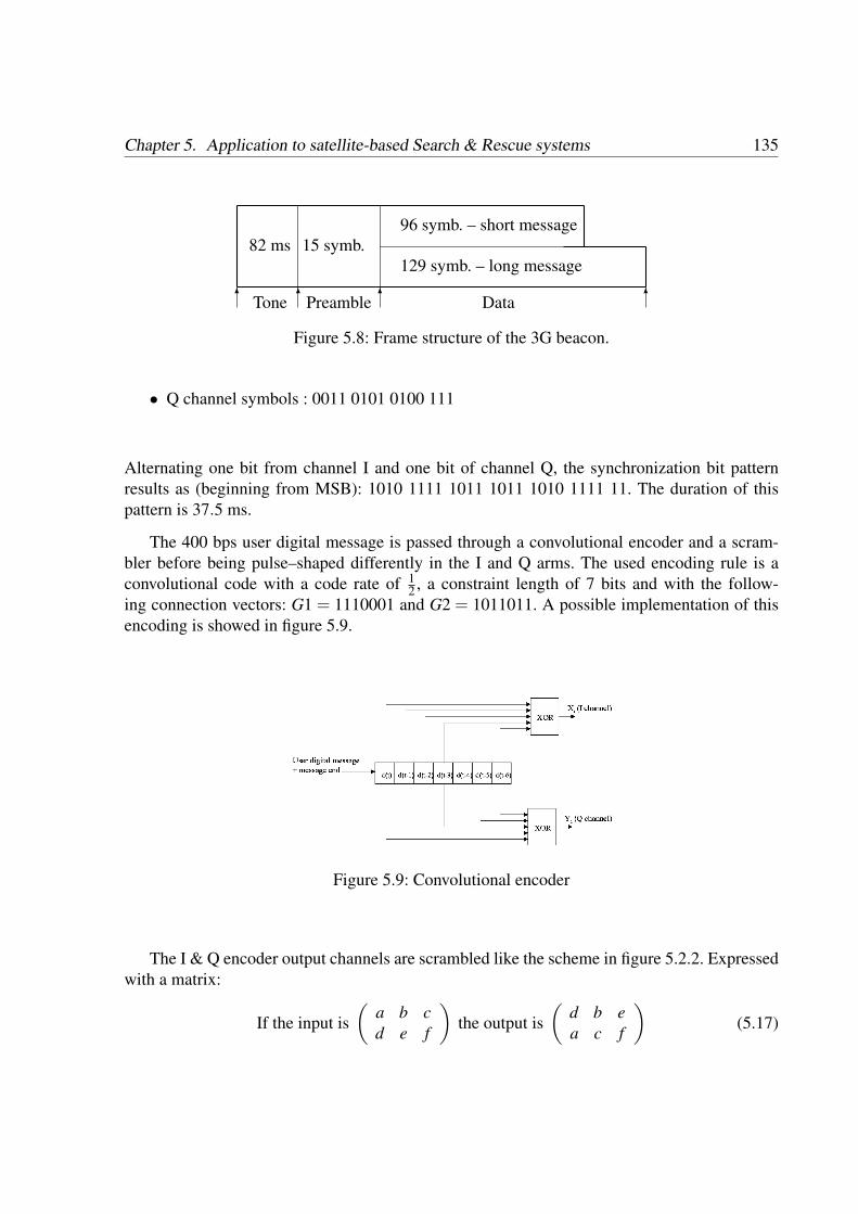
Chapter 5. Application to satellite-based Search & Rescue systems 135
6 6 6 6Tone Preamble Data
82 ms 15 symb.96 symb. – short message
129 symb. – long message
Figure 5.8: Frame structure of the 3G beacon.
• Q channel symbols : 0011 0101 0100 111
Alternating one bit from channel I and one bit of channel Q, the synchronization bit patternresults as (beginning from MSB): 1010 1111 1011 1011 1010 1111 11. The duration of thispattern is 37.5 ms.
The 400 bps user digital message is passed through a convolutional encoder and a scram-bler before being pulse–shaped differently in the I and Q arms. The used encoding rule is aconvolutional code with a code rate of 1
2 , a constraint length of 7 bits and with the follow-ing connection vectors: G1 = 1110001 and G2 = 1011011. A possible implementation of thisencoding is showed in figure 5.9.
Figure 5.9: Convolutional encoder
The I & Q encoder output channels are scrambled like the scheme in figure 5.2.2. Expressedwith a matrix:
If the input is(
a b cd e f
)the output is
(d b ea c f
)(5.17)

Chapter 5. Application to satellite-based Search & Rescue systems 136
Figure 5.10: Scrambler architecture
Depending on the user–message length, a number of ’0’ bits are appended at the end of themessage in order to clear out the convolutional encoder. If there is a short message (88 bits), themessage end consists of 8 bits. In case of long message (120 bits), 9 bits are appended.
• Short Message. The user part contains a 88–bit message, plus 8 bits more of the messageending. The first bit is ’0’ to indicate a short message. These 96 bits, at 400 bps, takes 240ms. Then:
Durationshort msg = pure carrier+ synchronization pattern+user bits= 82+37.5+240 = 359.5 ms (5.18)
• Long Message. The user part contains a 120–bit message, plus 9 bits more of the messageending. The first bit is ’1’ to indicate a short message. These 129 bits, at 400 bps, takes322.5 ms. Then:
Durationlong msg = pure carrier+ synchronization pattern+user bits= 82+37.5+322.5 = 442 ms (5.19)
Data encoding and modulation
The beacon proposed in [Sar03] modulates a 406 MHz carrier at 400 sps ±1 %, the framestructure is depicted in Figure 5.8. The tone is 82 ms ±2 ms, which is shorter than the onein existing beacon. The preamble lasts for 15 symbols, and the length of the scrambled andconvolutionally encoded data field also can contain 96 or 129 symbols. It uses a non-offsetQPSK modulation, with a NRZ-L encoding for the in-phase arm and a Biphase-L encoding forthe quadrature one.

Chapter 5. Application to satellite-based Search & Rescue systems 137
Considering the following pulse definitions,
p(t) = ∏
(t− Ts
2Ts
)Ts = 2.5 ms (5.20)
pman(t) = ∏
(t− Ts
4Ts2
)−∏
(t− 3Ts
4Ts2
)(5.21)
signal modulation can be expressed as
x(t) = ANs
∑k=1
(ck p(t− kTs)cos(2π fct)−dk pman(t− kTs)sin(2π fct)) (5.22)
where ck = ±1 and dk = ±1 are the in-phase and quadrature bits, and Ns is the number oftransmitted symbols, including the preamble (Ns = 111 for the short message and Ns = 144 forthe long one). The low–pass equivalent is
s(t) = ANs
∑k=1
(ck p(t− kTs)+ jdk pman(t− kTs)) (5.23)
Expressing s(t) = ∑Nsk=1 sk(t− kTs), the complex envelope for a particular symbol k is:
sk(t) = A(ck p(t)+ jdk pman(t)) (5.24)
The energy per bit, Eb, is
Eb =12
Z∞
−∞
sk(t)s∗k(t)dt =12
Z T s
0
(A2 +A2)dt = A2Ts = 2A2Tb (5.25)
Thus the signal can be represented, as shown in figure 5.2.2, by the vector
sk =(
ck√
Eb,dk√
Eb
)(5.26)
whose orthonormal basis is defined by
Ψ1 =1√Tb
p(t)
Ψ2 =1√Tb
pman(t) (5.27)
.

Chapter 5. Application to satellite-based Search & Rescue systems 138
(1,1)(-1,1)
(-1,-1) (1,-1)
1
2
~
~
bE
bE
bE
bE
Figure 5.11: Signal space of the 3G beacon modulation.
Assuming that the signal is degraded by zero–mean complex Additive White GaussianNoise (AWGN) with variance σ2
n = N0, and both bit values have equal probability, the perfectly-synchronized coherent-detector Symbol Error Rate (SER) is:
SER = 2Q(√
2Eb
N0
)−Q2
(√2Eb
N0
)u 2Q
(√2Eb
N0
)(5.28)
and the BER is
BER = Q(√
2Eb
N0
). (5.29)
Finally, similarly to the existing 2G beacon, the proposed 3G beacon is intended to be con-voluted with a signal mask to avoid spurious emissions. Its bandwidth is 10 kHz
As in previous chapter, we can split the whole signal in three parts:
• The pure tone sT2(t)
sT2(t) = A∏
(t− t1
2t1
)t1 = 82 ms (5.30)
• The preamble sP2(t), where ak=±1 and bk=±1 are the sequences described above:
sP2(t) = A15
∑k=1
(ak p(t− t1− kTs)+ jbk pman(t− t1− kTs))∏
(t− t1− t2
2t2
)(5.31)

Chapter 5. Application to satellite-based Search & Rescue systems 139
t2 = 37.5 ms
• The data sD2(t), where ck = ±1 and dk = ±1 are the convolutionally encoded andscrambled in-phase and quadrature user data
sD2(t) = AL
∑k=1
(ck p(t− t1− t2− kTs)+ jdk pman(t− t1− t2− kTs))∏
(t− t1− t2− t3
2t3
)(5.32)
L = 96/129, t3 = 240/322.5 ms (short / long message. In case of long message, d129 = 0)
Resulting on the following signal:
s3G(t) = sT2(t)+ sP2(t)+ sD2(t) (5.33)
Figure 5.12: Simulated I&Q components of the 3G beacon

Chapter 5. Application to satellite-based Search & Rescue systems 140
5.3 Link budget
Let M be the number of satellites concurrently seen by the user beacon and the MEOLUT. Then,the lowpass–equivalent signal received at the MEOLUT can be expressed as
bs(t) =M
∑i=1
Aie j[2π fit+φi(t)] +M
∑i=1
bins(t)+bnm(t) (5.34)
where bins(t) is a baseband AWGN (Additive White Gaussian Noise) at the i–th satellite andbnm(t) is the AWGN received at the MEOLUT. This equation allows the calculation of theSignal-to-Noise Ratio (SNR) at the i–th satellite, taking the user beacon as the transmitter andthe satellite as the receiver or, in other words, the uplink channel. In order to achieve a signal–to–noise ratio which is bandwidth–independent, the SNR is normalized to a 1 Hz bandwidth.The result is called carrier–to–noise density ratio, defined as
CN0 = 10log10(SNR×B) [dB-Hz] (5.35)
Thus, considering E|bins(t)|2
= σ2
bins= 2σ2
ins, and C = A2
2 , the SNR in the satellite is:
SNRis =A2
i
σ2bins
=A2
i
2σ2ins
=A2
i2N0sB
=(
CN0
)is
1B
(5.36)
In the downlink channel (now the emitter is the satellite and the receiver is the MEOLUT),the SNR is
SNRim =A2
i
σ2bnm
=A2
i2σ2
nm=
A2i
2N0mB=(
CN0
)im
1B
(5.37)
From equation (5.37):
A2i = σ
2bnm
(CN0
)im
1B
(5.38)
and combining (5.37) and (5.38)
σ2bins
=A2
i(CN0
)is
1B
=σ2
bnm
(CN0
)im
1B(
CN0
)is
1B
= σ2bnm
(CN0
)im(
CN0
)is
(5.39)

Chapter 5. Application to satellite-based Search & Rescue systems 141
We can define an equivalent SNR as the ratio seen from the user beacon to the MEOLUT:
SNRieq =A2
i
∑Mj=1 σ2
b jns+σ2
bnm
=A2
i
σ2bnm
[∑
Mj=1
(CN0
)jm(
CN0
)js
+1
] (5.40)
(CN0
)ieq
= B ·SNRieq =BA2
i
σ2bnm
1
∑Mj=1
(CN0
)jm(
CN0
)js
+1
=
(CN0
)im
∑Mj=1
(CN0
)jm(
CN0
)js
+1
(5.41)
In computer simulation, is usual to consider σ2nm = 1 and thus σ2
bnm= 2. With this value, we
obtain the following relationships:
σ2bins
= 2
(CN0
)im(
CN0
)is
(5.42)
A2i =
2B
(CN0
)im
(5.43)
The downlink power budget for the 406 MHz SARP channel (known as Processed DataStream or PDS channel) will be analyzed in this section, following indications given in [Cos02].The COSPAS–SARSAT PDS channel is designed to provide reliable performance if a BER of10−6 is achieved in the LEOLUT. In the following, we will assume the same requirement forthe MEOLUT receivers. Communication theory for coherent detection of a BPSK signal in aGaussian noise channel says that a theoretical value of
(EbN0
)th
= 10.6 dB is required in the PDS
channel to achieve the desired BER of 10−6.
The BER parameter is mainly governed by the energy–per–bit–to–noise–density ratio,(EbN0
), which can be calculated using the following equation:
(Eb
N0
)c= EIRP− (Lp +L f +Lo)+
(GT
)− k− r +
(PPDS
PT
)dB (5.44)
where:
• EIRP Equivalent Isotropically Radiated Power, i.e., the product of the power supplied tothe antenna and the antenna gain in a given direction relative to an isotropic antenna,

Chapter 5. Application to satellite-based Search & Rescue systems 142
• Lp Free–space path loss, which corresponds to the standard formula
Lp = 10log10
((λ
4πr
)2)
(5.45)
being λ = 19.43 cm the wavelength corresponding to 1544 MHz and r the transmitter–to–receiver distance.
• The PDS is digital data produced on-board the satellite and transmitted on the downlinksignal. This channel shares the satellite downlink carrier with other Search and Rescuechannels, such as the 121.5 MHz service. The nominal ratio of the PDS power relative tothe total transmitter power is denoted by PPDS
PTin table 5.3, but this ratio can vary due to
signal activity in other channels. This variation is included in the PDS short–term fadingloss (L f ).
• Lo are other losses, including atmospheric propagation losses, antenna polarization mis-match, antenna pointing, demodulation and bit synchronizer errors.
•(G
T
)is the antenna Gain–to–Noise Temperature ratio, including a possible radome and
cable losses.
• k is the Boltzmann constant, k = 10 · log10(1.3806 ·10−23)=−228.6 dB
Parameter COSPAS Nominal SARSAT NominalEIRP (dBW) 6.2 7.1
Lp (dB) 166.3 165.5L f (dB) 10 10Lo (dB) LUT–design, site–dependent LUT–design, site–dependent(G
T
)(dBK−1) LUT–design dependent LUT–design dependent
Slant range at 5 degrees (km) 3200 2900
Modulation loss(
PPDSPT
)(dB) −12.1 −14.1
Desired maximum BER 10−6 10−6
Calculated(
EbN0
)c
(dB)(G
T
)−Lo +12.6
(GT
)−Lo +12.3
Theoretical(
EbN0
)th
for BER = 10−6 10.6 10.6
Table 5.1: Downlink power budget parameters for PDS channels

Chapter 5. Application to satellite-based Search & Rescue systems 143
5.4 Single antenna techniques for Frequency and Time Dif-ference Of Arrival estimation
This section deals with the problem of estimating the desired parameters from a set of mea-surements recorded with a single, approximately omnidirectional antenna receiver. First, weconsider the mathematical model of such a received signal. The following subsections addressthe derivation of Frequency Difference Of Arrival and Time Difference Of Arrival estimatorswell-suited to this problem. Once the theoretical background has been discussed, results arein order to compare the different techniques and determine the minimum signal–to–noise rationeeded to achieve the required accuracy.
The measurements are considered to be a superposition of plane waves corrupted by noiseand, possibly, interferences and multipath. Given the measurements, the objective is to estimatea set of parameters associated with the wavefronts. An antenna receives M scaled, time–delayedand Doppler–shifted replicas of the distress signal relayed by the MEO satellites. The Doppler–shift of each replica is due to the relative velocity of the corresponding satellite with respect theEarth rotation and the beacon velocity; meanwhile time–delays depend on the distance betweenthe beacons and the satellites and the distance between the satellites and the LUT. The receivingcomplex baseband signal can be modeled as
x(t) =M
∑i=1
ais(t− τi)exp j2π fdit+n(t) (5.46)
where ai is the complex amplitude of each signal, s(t) is the distress signal defined in equations(5.6) and (5.23) depending on the beacon type, τi is the delay, fdi is the Doppler shift, and n(t)is AWGN.
In order to obtain beacon location, a minimum of three satellites relaying the distress mes-sage must be acquired. The location algorithm, which is not in the scope of this work, uses theestimates of both Doppler–shifts and time–delays of each received replica. The methods usedto obtain these estimates are analyzed in the following two sections.
5.4.1 Frequency Difference Of Arrival estimation
The tone is a very useful part of the distress signal for Doppler-shift estimation and tracking.The frequency power spectrums of both distress signals show a peak, centered at the carrier fre-quency, with secondary lobes containing preamble and data information. Recalling the Nyquistsampling rate theorem [Pro96] - which states that the minimum sampling rate to ensure a cor-rect reconstruction of the signal must satisfy the inequation fs ≥ 2W , where fs and W stand forthe sampling frequency and the signal bandwidth, respectively. As aforementioned, the filter

Chapter 5. Application to satellite-based Search & Rescue systems 144
mask imposes W = 3 kHz for the 2G beacons and W = 10 kHz for the 3G ones. Hence, fs mustbe dimensioned according to it.
The proposed FDOA estimation method is based on searching the peak corresponding tothe tone of the replica within an estimate of the spectrum. The difference between the nominalcarrier frequency and the actual estimated peak frequency will lead to a Doppler–shift esti-mate. To this aim, many methods proposed in the literature – Periodogram, Welch, MinimumVariance, Normalized Minimum Variance, Burg and MUSIC [Pro89, Kay98, Sch91] have beentested [Fer05e]. Results in [Clo04] show that the numbers of samples recorded at the specifiedsampling rate is high enough to achieve good results using the simpler Periodogram method,which can be implemented as a FFT-based method which in turns reduces computational costdramatically compared to the rest of studied methods.
A practical aspect to be considered when implementing such an estimation method is that,due to the finite number of samples, the estimated tone appears distorted in a way that maycause the estimation algorithm to fail. This is the so-called windowing effect which can bealleviated by applying a window to the recorded data before the estimation. Many windows havebeen tested [Fer05e], the Blackman–Harris window being the more suitable one to the problemexposed. Note that a rectangular window is equivalent to the absence of data–windowing, whichis highly undesirable.
5.4.2 Time Difference Of Arrival estimation
Estimating time–delays of each replica is mathematically equivalent to the problem of synchro-nization in a communications framework. By noticing that there are some parts of the receivedbeacon message which are a priori known, it is possible to use a bank of matched filters (figure5.13) to synchronize, i.e. estimate the delay of each incoming signal in the received burst.
The method correlates the incoming signal with a locally generated replica of the tone andthe preamble. After demodulating the data bits, the data field can be assumed to be a knownpart of the received signal and, hence, it can be used to obtain a larger sequence to improvetime–delay synchronization in a finer approach.
The delay that the emitted signal has suffered with respect to the sequence in the receiver isobtained from the position of the crosscorrelation peak. Since the M Doppler–shifts have beenestimated previously, this information can be used to make each filter be adapted to its corre-sponding received replica, which means that the locally generated sequence should be modu-lated to fc + fdoppleri . Note that computing the crosscorrelation between the received signal anda local replica is equivalent to filtering with the local replica (Figure 5.13).

Chapter 5. Application to satellite-based Search & Rescue systems 145
x(t)
- h1(t)-
fd1
- max - τ1
- h2(t)-
fd2
- max - τ2
- hM(t)-
fdM
- max - τM
......
Figure 5.13: Adapted–filter bank concept. Each branch of the bank estimates the TDOA of itscorresponding replica, τi, by maximizing the correlation between the received signal and theadapted filters. These filters are generated knowing some signal information - tone, preambleand possibly data structures - and the corresponding estimates of Doppler–shifts previouslyobtained, fdi .
5.5 Antenna array approach
There are two technical approaches to steerable antennas: mechanically moved dishes and elec-tronically steerable antenna arrays. In the case of dishes, the satellite tracking is performedby means of a mechanical engine, i.e., the antenna is physically moved to point the desiredsatellite. This solution implies high mechanical complexity and a large area (“dish farm”). Inaddition, this kind of antenna does not provide any capability of spatial processing, for instanceby nulling the reception of other unwanted signals or adaptive processing, and hence they havelimited interference rejection.
On the other hand, antenna arrays are pointed electronically: while the antenna remainsphysically immobile, the underlying signal processing steers the radiation pattern to the desireddirection. Moreover, they provide interesting capabilities of autonomous tracking and adaptivenulling. An array of sensors has the potential for improving the overall reception performanceof the relayed signals in an environment with several sources of interference, multipath propa-gation or weak signal reception.
Three approaches might be considered in the architecture of antenna array beamforming:digital, analog and a mixed strategy. Performance in terms of computational cost, estimation
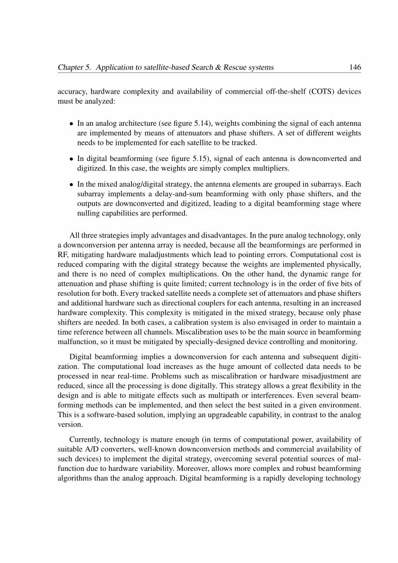
Chapter 5. Application to satellite-based Search & Rescue systems 146
accuracy, hardware complexity and availability of commercial off-the-shelf (COTS) devicesmust be analyzed:
• In an analog architecture (see figure 5.14), weights combining the signal of each antennaare implemented by means of attenuators and phase shifters. A set of different weightsneeds to be implemented for each satellite to be tracked.
• In digital beamforming (see figure 5.15), signal of each antenna is downconverted anddigitized. In this case, the weights are simply complex multipliers.
• In the mixed analog/digital strategy, the antenna elements are grouped in subarrays. Eachsubarray implements a delay-and-sum beamforming with only phase shifters, and theoutputs are downconverted and digitized, leading to a digital beamforming stage wherenulling capabilities are performed.
All three strategies imply advantages and disadvantages. In the pure analog technology, onlya downconversion per antenna array is needed, because all the beamformings are performed inRF, mitigating hardware maladjustments which lead to pointing errors. Computational cost isreduced comparing with the digital strategy because the weights are implemented physically,and there is no need of complex multiplications. On the other hand, the dynamic range forattenuation and phase shifting is quite limited; current technology is in the order of five bits ofresolution for both. Every tracked satellite needs a complete set of attenuators and phase shiftersand additional hardware such as directional couplers for each antenna, resulting in an increasedhardware complexity. This complexity is mitigated in the mixed strategy, because only phaseshifters are needed. In both cases, a calibration system is also envisaged in order to maintain atime reference between all channels. Miscalibration uses to be the main source in beamformingmalfunction, so it must be mitigated by specially-designed device controlling and monitoring.
Digital beamforming implies a downconversion for each antenna and subsequent digiti-zation. The computational load increases as the huge amount of collected data needs to beprocessed in near real-time. Problems such as miscalibration or hardware misadjustment arereduced, since all the processing is done digitally. This strategy allows a great flexibility in thedesign and is able to mitigate effects such as multipath or interferences. Even several beam-forming methods can be implemented, and then select the best suited in a given environment.This is a software-based solution, implying an upgradeable capability, in contrast to the analogversion.
Currently, technology is mature enough (in terms of computational power, availability ofsuitable A/D converters, well-known downconversion methods and commercial availability ofsuch devices) to implement the digital strategy, overcoming several potential sources of mal-function due to hardware variability. Moreover, allows more complex and robust beamformingalgorithms than the analog approach. Digital beamforming is a rapidly developing technology

Chapter 5. Application to satellite-based Search & Rescue systems 147
(a) Analog weighting (b) RF shifters
Figure 5.14: Two possible analog beamforming architectures
Figure 5.15: Typical digital beamforming architecture diagram
which is the most advanced approach to antenna array radiation pattern control. When imple-mented at the array element level, digital beamforming enables full utilization of the maximumnumber of degrees of freedom in the array. This can lead to significant improvements in beam-forming of simultaneous multiple independent beams, adaptive pattern nulling and space-timeadaptive processing, compared to traditional analog array control techniques. Because of itsflexibility, digital beamforming may find use in a wide range of phased array antenna appli-cations. Several beamforming strategies could be implemented mainly based on pointing thearray to a suitable satellite while nulling the directions of arrival of other satellites. This easesthe association of parameters and the satellite which they belong to, and mitigates a number ofproblems in the estimation stage: the mathematically equivalent multipath effect is well known

Chapter 5. Application to satellite-based Search & Rescue systems 148
as the most challenging issue in parameter estimation. Antenna array technology, and the spatialdiversity which it provides, is able to cope with this problem, as will be shown in section 5.7.
Digital array receivers include, but are not limited to, the following features: RF receiverfront-end for RF-to-IF or RF-to-baseband demodulation, analog-to-digital converters (ADC)for bandpass or baseband sampling, and digital finite impulse response (FIR) filtering for de-composition of sampled signals into in-phase and quadrature (I/Q) components. Digital beam-forming receiver technology requires all of these core digital receiving capabilities, plus manyothers which are essential for digital control and optimization of phased array antenna patterns.These include, but are not limited to the following:
• FIR digital filtering for digital beamforming receiver channel equalization to enable wide-band array-level channel-to-channel calibration,
• use of either digital sub-banding schemes such as multi-rate digital filtering or imple-mentation of fractional sample digital time delays, to enable wideband beamforming andadaptive nulling,
• a high degree of built-in programmability for implementation of advanced algorithms forbeamforming, channel filtering and sub-banding,
• module-level digital self-registration capabilities with respect to the system-level distribu-tion and temporal aligning of digital clock and synchronization signals, coherent phasingof RF local oscillator (LO) signals, and array channel calibration RF pilot tones, and
• module-level self-assessment capabilities that monitor the overall in-situ performance ofthe digital beamforming receiver array channel. In order to ensure the proper working ofthe beamforming, the amplitude and phase reference of each antenna must be kept; thisis indeed the main risk in this approach.
Accurate alignment of channels would require high precision hardware components andconsequently a high economic cost. Thus, there is a need of a calibration system. A calibrationmust be performed to match the phase and amplitude of the different hardware channels. Thecalibration must also track variations in time due to temperature, humidity or frequency, and alsoto be transparent and have no or a small noticeable effect on the normal operation of the adaptivearray antenna. Depending on the calibration method used, there will be a limited resolution inthe calibration process and the residual calibration error will degrade the performance.
In order to detect a beacon burst from three or more SARSAT-enabled satellites simulta-neously, a minimum of three tracking antennas are required. In fact, a typical ground stationwould require four to eight antennas. If a discrete ground antenna is used for each satellite, theimplementation could become cost prohibitive (also taking into account maintenance costs of
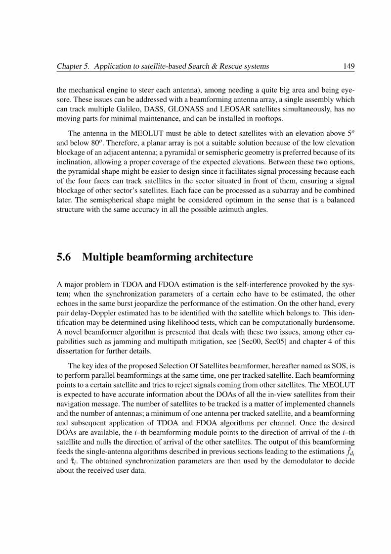
Chapter 5. Application to satellite-based Search & Rescue systems 149
the mechanical engine to steer each antenna), among needing a quite big area and being eye-sore. These issues can be addressed with a beamforming antenna array, a single assembly whichcan track multiple Galileo, DASS, GLONASS and LEOSAR satellites simultaneously, has nomoving parts for minimal maintenance, and can be installed in rooftops.
The antenna in the MEOLUT must be able to detect satellites with an elevation above 5o
and below 80o. Therefore, a planar array is not a suitable solution because of the low elevationblockage of an adjacent antenna; a pyramidal or semispheric geometry is preferred because of itsinclination, allowing a proper coverage of the expected elevations. Between these two options,the pyramidal shape might be easier to design since it facilitates signal processing because eachof the four faces can track satellites in the sector situated in front of them, ensuring a signalblockage of other sector’s satellites. Each face can be processed as a subarray and be combinedlater. The semispherical shape might be considered optimum in the sense that is a balancedstructure with the same accuracy in all the possible azimuth angles.
5.6 Multiple beamforming architecture
A major problem in TDOA and FDOA estimation is the self-interference provoked by the sys-tem; when the synchronization parameters of a certain echo have to be estimated, the otherechoes in the same burst jeopardize the performance of the estimation. On the other hand, everypair delay-Doppler estimated has to be identified with the satellite which belongs to. This iden-tification may be determined using likelihood tests, which can be computationally burdensome.A novel beamformer algorithm is presented that deals with these two issues, among other ca-pabilities such as jamming and multipath mitigation, see [Sec00, Sec05] and chapter 4 of thisdissertation for further details.
The key idea of the proposed Selection Of Satellites beamformer, hereafter named as SOS, isto perform parallel beamformings at the same time, one per tracked satellite. Each beamformingpoints to a certain satellite and tries to reject signals coming from other satellites. The MEOLUTis expected to have accurate information about the DOAs of all the in-view satellites from theirnavigation message. The number of satellites to be tracked is a matter of implemented channelsand the number of antennas; a minimum of one antenna per tracked satellite, and a beamformingand subsequent application of TDOA and FDOA algorithms per channel. Once the desiredDOAs are available, the i–th beamforming module points to the direction of arrival of the i–thsatellite and nulls the direction of arrival of the other satellites. The output of this beamformingfeeds the single-antenna algorithms described in previous sections leading to the estimations fdi
and τi. The obtained synchronization parameters are then used by the demodulator to decideabout the received user data.

Chapter 5. Application to satellite-based Search & Rescue systems 150
Actually, SOS is not a beamformer itself since it needs a beamforming algorithm to be im-plemented for every tracked satellite. Almost any beamforming technique can be used, a firstapproach can consist on a Phased Array procedure pointing the desired satellite while nullingthe others, this is indeed a good approach but it lacks of jamming and multipath rejection, hencethe SOS idea have been mixed with the Hybrid Space–Time Reference Beamforming to formthe Hybrid SOS, named hSOS. The basic idea of the beamformer is that space reference canbe combined with time reference in order to obtain an improved performance exploiting bothdiversities with a modular and parallelized structure. Given that the computation of the weight-ing vectors takes now into account temporal information and, as will be shown immediately, itneeds the incoming sampled signal stored in matrix X, a totally digital weighting architecturesuch as figure 5.16 seems a suitable structure for the implementation.
@@N
- LNA -N
-ADC -
@@1
- LNA -N
-ADC -
... m∼fLO
6
?
X - Beamforming Modules
G
-
a
-
wi
fd1, τ1 -
fdM , τM-
@@R
...
D
-
Figure 5.16: Proposed block diagram of the hybrid beamforming with Selection Of Satellitesstrategy
5.7 Simulation studies
System accuracy requirements for FDOA and TDOA estimation demand errors lower than cer-tain thresholds. These accuracy constraints (on the order of 7 µs for time delay and 1 Hz forDoppler shift estimation error) result in a minimum required signal power. The minimum CN0needed to meet the accuracy requirements will be determined for all the tested methods bycomputer simulation.

Chapter 5. Application to satellite-based Search & Rescue systems 151
5.7.1 Frequency and time difference of arrival with single antenna tech-niques
In order to compare the performance of different methods, an scenario composed of one signalimpinging on a single-antenna receiver has been simulated. The antenna has been consideredomnidirectional. For all experiments performed in this paper, the sampling frequency is 25.6kHz, which fulfills Nyquist criteria for both types of distress beacons. Results obtained havebeen plotted as a function of the CN0 of the received signal versus the Cramer–Rao Bound(CRB), which is derived in the chapter 3 of this dissertation.
Figure 5.17 shows Doppler–shift estimation error achieved with the methods studied forboth beacon structures. For practical purposes, whereas the FFT uses the whole recorded data,the rest of the methods use portions of data due to the computational cost involved in the in-version of the autocorrelation matrix. In order to improve estimates by using all available infor-mation, these methods split the received data signal in a number of smaller data packets, whichare more tractable for autocorrelation computation and matrix inversion. FFT is the methodthat will be used hereafter since it achieves the best trade-off between computational cost andestimation accuracy among other studied methods.
Notice that the CRB of both signals are slightly different, the minimum error that can beobtained with the existing beacon, when estimating Doppler–shifts, is 3 dB lower than thatachieved with the proposed beacon. This is due to a shorter tone duration in the proposed bea-con, actually half of the time which is a reduction of 3 dB in the estimation capabilities.
Time–delay estimation results have been plotted in figure 5.18 for both types of beacons.The use of the whole beacon message (tone, preamble and data, referred to as TPD) whengenerating the matched filter in a postprocessing stage, is shown to overcome the estimates oftone plus preamble (referred to as TP) based estimates. On the other hand, 3G beacons improvetime–delay estimates with respect to the actual message used by the system due to its widerfrequency mask filter, which also can be seen in the CRB.
As can be observed in figure 5.17, a dramatic improvement in estimation accuracy isachieved beyond a CN0 of 25 dB-Hz. Indeed, single antenna methods are not recommendedunder this threshold.
5.7.2 Single antenna vs. antenna array
The comparison between single antenna receiver and antenna array approach is performed ina scenario where a single signal is received. The results are encouraging since spatial diversityleads to better parameter estimation results for both types of beacon. Different types of classicbeamformers have been used to show array capabilities in Doppler–shift estimation (figure 5.19)

Chapter 5. Application to satellite-based Search & Rescue systems 152
0 5 10 15 20 25 30 35 4010−12
10−10
10−8
10−6
10−4
10−2
100
102
C/NO
[dB−Hz]
FDO
A E
stim
atio
n M
SE
[KH
z2 ]
FFTBarlettMinimum VarianceMUSICCRB
(a) 2G beacon
0 5 10 15 20 25 30 35 4010−12
10−10
10−8
10−6
10−4
10−2
100
102
C/NO
[dB−Hz]
FDO
A E
stim
atio
n M
SE
[KH
z2 ]
FFTBarlettMinimum VarianceMUSICCRB
(b) 3G beacon
Figure 5.17: MSE for FDOA estimation: single antenna techniques
0 5 10 15 20 25 30 35 4010
−10
10−8
10−6
10−4
10−2
100
102
104
C/NO
[dB−Hz]
TD
OA
Est
imat
ion
MS
E [m
s2 ]
TPTPDCRB
(a) 2G beacon
0 5 10 15 20 25 30 35 4010
−10
10−5
100
105
C/NO
[dB−Hz]
TD
OA
Est
imat
ion
MS
E [m
s2 ]
TPTPDCRB
(b) 3G beacon
Figure 5.18: MSE for TDOA estimation: single antenna techniques
and time–delay estimation using the tone and the preamble (figure 5.20) or the whole message(figure 5.21).
2G beacon structure yield better results in Doppler estimation than 3G structure because ofits longer tone field, as observed in figure 5.19. On the contrary, time delay estimation is slightly

Chapter 5. Application to satellite-based Search & Rescue systems 153
better when the 3G is considered (see figures 5.20 and 5.21) because of its wider frequency filtermask.
By using the antenna array approach, the MSE of the parameter estimations decreases dra-matically at lower CN0 of the impinging signal than the single antenna approach does, thusreducing the minimum CN0 necessary to attain a given accuracy. A general rule of thumb fordetermining the gain in CN0 obtained by an antenna array respect to the use of a single antennais 10 · log10(N) (where N is the number of antenna elements), a measure only valid when onesignal is present. This array gain can be also observed in the CRB, plotted for the case of a singleantenna and for an antenna array. In this simple scenario, all the tested beamformer algorithmsprovide a similar performance.
0 5 10 15 20 25 30 35 4010−14
10−12
10−10
10−8
10−6
10−4
10−2
100
102
C/NO
[dB−Hz]
FDO
A F
FT E
stim
atio
n M
SE
[KH
z2 ]
Single antennaCRB − single antennaTRBMVBhSOSCRB − antenna array
(a) 2G beacon
0 5 10 15 20 25 30 35 4010−12
10−10
10−8
10−6
10−4
10−2
100
102
C/NO
[dB−Hz]
FDO
A F
FT E
stim
atio
n M
SE
[KH
z2 ]
Single antennaCRB − single antennaTRBMVBhSOSCRB − antenna array
(b) 3G beacon
Figure 5.19: Comparison between FFT-based frequency estimation error for a single antenna re-ceiver and for an 8-element antenna array receiver with the following beamforming algorithms:Temporal Reference (TRB), Minimum Variance (MVB) and hybrid with Selection Of Satellites(hSOS).
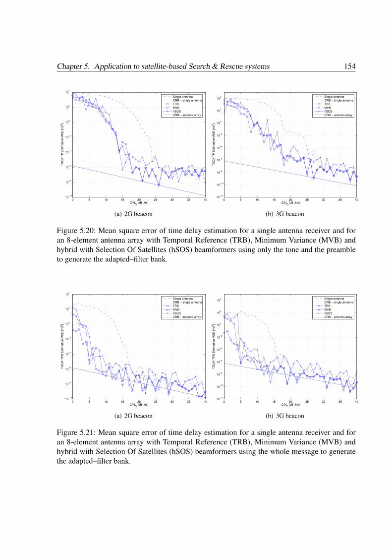
Chapter 5. Application to satellite-based Search & Rescue systems 154
0 5 10 15 20 25 30 35 4010−10
10−8
10−6
10−4
10−2
100
102
104
C/NO
[dB−Hz]
TDO
A T
P E
stim
atio
n M
SE
[ms2 ]
Single antennaCRB − single antennaTRBMVBhSOSCRB − antenna array
(a) 2G beacon
0 5 10 15 20 25 30 35 4010−12
10−10
10−8
10−6
10−4
10−2
100
102
104
C/NO
[dB−Hz]
TDO
A T
P E
stim
atio
n M
SE
[ms2 ]
Single antennaCRB − single antennaTRBMVBhSOSCRB − antenna array
(b) 3G beacon
Figure 5.20: Mean square error of time delay estimation for a single antenna receiver and foran 8-element antenna array with Temporal Reference (TRB), Minimum Variance (MVB) andhybrid with Selection Of Satellites (hSOS) beamformers using only the tone and the preambleto generate the adapted–filter bank.
0 5 10 15 20 25 30 35 4010−10
10−8
10−6
10−4
10−2
100
102
104
C/NO
[dB−Hz]
TDO
A T
PD
Est
imat
ion
MS
E [m
s2 ]
Single antennaCRB − single antennaTRBMVBhSOSCRB − antenna array
(a) 2G beacon
0 5 10 15 20 25 30 35 4010−12
10−10
10−8
10−6
10−4
10−2
100
102
104
C/NO
[dB−Hz]
TDO
A T
PD
Est
imat
ion
MS
E [m
s2 ]
Single antennaCRB − single antennaTRBMVBhSOSCRB − antenna array
(b) 3G beacon
Figure 5.21: Mean square error of time delay estimation for a single antenna receiver and foran 8-element antenna array with Temporal Reference (TRB), Minimum Variance (MVB) andhybrid with Selection Of Satellites (hSOS) beamformers using the whole message to generatethe adapted–filter bank.

Chapter 5. Application to satellite-based Search & Rescue systems 155
5.7.3 Multipath rejection
As shown in previous results, antenna array techniques improve system performance in non-aggressive scenarios. The benefits of an antenna array can be better highlighted in more com-plicated environments. A scenario consisting of two distress signals and a multipath replica issimulated. Without loss of generality, all three signals are assumed to have an angle of arrivalwith zero azimuth. The elevations with respect to the endfire are 45o and 50o for the directsignals, and 120o for the multipath component. The direct signals have Doppler–shifts equal to−2 and 0.5 kHz, and the multipath signal is affected by a Doppler–shift of 1.5 kHz. Referringthe delays to the time of arrival of the first desired signal, the delay of the multipath replica ofthis signal is 1.5 ms, and the delay of the second direct signal is 41.8 ms. Results obtained arenot compared with single antenna results since this approach fails when attempting to estimateparameters of signals corrupted by multipath or interference nuisances due to the presence of abias in time delay estimation [Nee95].
Figure 5.22 shows the MSE of the Doppler–shift estimates for both 2G and 3G beacons.Time-delay estimates can be observed in figure 5.23 for tone and preamble and in figure 5.24for the whole message.
These figures show that the hSOS algorithm avoids the undesired bias produced by the mul-tipath signal. This intrinsic capability of multipath mitigation of the hybrid beamformer is dueto the combination of temporal and spatial diversity, and constitutes a desirable characteristic totake into account in the choosing of a beamformer.
As aforementioned, Doppler estimation accuracy is higher when the 2G beacon is consid-ered because of its longer tone, as shown in figure 5.22. In this figure, the hybrid beamformerperforms better than the temporal (TRB) or spatial (MVB) reference beamformings. This be-havior highlights the ability of the hybrid beamforming in mitigating multipath without anyprior knowledge about it. In section 4.2 it was observed that the hybrid beamforming is a linearweighted combination of both temporal and spatial reference beamformers. This result can beobserved in the left side of Figure 5.22: the estimation error bound of the hybrid beamformerdecreases at lower CN0 than TRB and MVB do, but remains in a constant error floor until theCN0 is high enough to ensure the proper operation of TRB and MVB. AT that point, the hybridbeamformer error follows the behavior of the other beamformers. This figure also shows thatthe TRB fails when dealing with the 3G beacon in this scenario. Again, the reason is the shortduration of the tone field.
The formulation of the hybrid beamformer states that the estimation of time and frequencyare coupled, since both parameters are estimated jointly. Indeed, time estimation accuracy de-pends on frequency estimation accuracy. This effect is manifested in Figures 5.23 and 5.24 fortime estimation error, where the error decreases at CN0 levels close to that which frequencyestimation error does. This is the reason why the 3G beacon (with wider bandwidth and there-
Chapter 5. Application to satellite-based Search & Rescue systems 156
0 5 10 15 20 25 30 35 4010−12
10−10
10−8
10−6
10−4
10−2
100
102
C/NO
[dB−Hz]
FDO
A F
FT E
stim
atio
n M
SE
[kH
z2 ]
TRBMVBhSOSCRB − antenna array
(a) 2G beacon
0 5 10 15 20 25 30 35 4010−12
10−10
10−8
10−6
10−4
10−2
100
102
C/NO
[dB−Hz]
FDO
A F
FT E
stim
atio
n M
SE
[kH
z2 ]
TRBMVBhSOSCRB − antenna array
(b) 3G beacon
Figure 5.22: Comparison between 2G and 3G beacons Doppler estimation error with FFT-basedfrequency estimation method for an 8-element antenna array receiver with the TRB, MVB andhSOS beamforming algorithms. The scenario is composed of three desired signals plus a sec-ondary path replica
fore allowing theoretically better time estimation error than 2G) does not reach better results intime estimation than 2G, since it suffers of worse frequency estimation errors and this directlyimpacts on the final result of synchronization.
5.7.4 Space Resolution
A general rule of thumb for determining the gain obtained by an antenna array respect to theuse of a single antenna is 10 · log10(N), as showed in previous experiments. However, this ruleis not true when two sources are very close in space, when the main beam of the radiationpattern is unable to point to one source while nulling the other one. Since the wide of the beamis a function of the number of antennas, this experiment plots the minimum separation angleneeded to achieve a gain higher than the 90% of 10 · log10(N) as a function of the number ofantennas. The results are showed in figure 5.25, revealing a poor performance of the algorithmswhen two satellites have a similar angle of arrival. In this case, single antenna techniques canbe slightly modified to estimate two or more signals (for example, searching for more than onemaximum), but the masking effects avoided by the hybrid beamforming approach arises againand can seriously degrade the overall performance of the estimations.

Chapter 5. Application to satellite-based Search & Rescue systems 157
0 5 10 15 20 25 30 35 4010−10
10−5
100
105
C/NO
[dB−Hz]
TDO
A T
P E
stim
atio
n M
SE
[ms2 ]
TRBMVBhSOSCRB − antenna array
(a) 2G beacon
0 5 10 15 20 25 30 35 4010−10
10−5
100
105
C/NO
[dB−Hz]
TDO
A T
P E
stim
atio
n M
SE
[ms2 ]
TRBMVBhSOSCRB − antenna array
(b) 3G beacon
Figure 5.23: MSE for time delay estimation with an 8-element antenna array and the TRB,MVB and hSOS beamforming algorithms. The scenario is composed of three desired signalsplus a secondary path replica. Only tone and preamble has been used.
0 50 100 150 200 250 3000
5
10
15
20
25
30
Minimum signal separation ensuring a gain of 10·log10
(N)
Sig
nal s
epar
atio
n [d
egre
es]
Number of antennas
FOA
TOA (TP)
TOA (TPD)
Figure 5.25: Minimum angle separation ensuring a gain of 10 · log10(N) plotted against thenumber of elements in the antenna array. Two existing distress signals with CN0 = 15 dB, sametime delay and 3 kHz of Doppler separation have been considered

Chapter 5. Application to satellite-based Search & Rescue systems 158
0 5 10 15 20 25 30 35 4010−10
10−5
100
105
C/NO
[dB−Hz]
TDO
A T
PD
Est
imat
ion
MS
E [m
s2 ]
TRBMVBhSOSCRB − antenna array
(a) 2G beacon
0 5 10 15 20 25 30 35 4010−10
10−5
100
105
C/NO
[dB−Hz]
TDO
A T
PD
Est
imat
ion
MS
E [m
s2 ]
TRBMVBhSOSCRB − antenna array
(b) 3G beacon
Figure 5.24: MSE for time delay estimation with an 8-element antenna array and the TRB,MVB and hSOS beamforming algorithms. The scenario is composed of three desired signalsplus a secondary path replica. The whole signal (tone, preamble and data) has been used in theestimation.
5.8 Summary
This chapter has discussed about technical aspects of the COSPAS-SARSAT system, focusingon parameter estimation techniques to be implemented in future MEO Local User Terminals.Existing beacon message and a proposed one, to be used in future beacon standards, have beenanalyzed in terms of modulation aspects, signal space and Bit Error Rate. A number of FDOAand TDOA techniques have been proposed for in single antenna receivers, and obtained re-sults have shown a poor performance for the CN0 range that are commonly given with a MEOconstellation of satellites. As a novelty, this chapter has proposed an antenna array equippedreceiver to overcome low CN0 synchronization problems at MEOLUTs. A number of beam-forming techniques are studied but a specially suited one have been designed that also canmitigate the effects of interferences and multipath, obtaining estimation performances close totheoretical bounds. The Space-Time Reference Hybrid Beamforming with Selection Of Satel-lites (hSOS) algorithm has been proposed for a future implementation in real MEOLUTs.
The author has been the Technical Manager by the UPC part in a research project related toMEOLUT design, funded by the European Space Agency, which results are reported in
• [Fer05e] C. Fernandez Prades, Pau Closas Gomez, and Juan A. Fernandez Rubio, “Ad-vanced Signal Processing techniques in Local User Terminals for Search & Rescue sys-

Chapter 5. Application to satellite-based Search & Rescue systems 159
tems Based on MEO satellites”, Tech. Rep. ESTEC/Contract no. 17713/03/NL/LvH/jd,Dept. of Signal Theory and Communications, Universitat Politecnica de Catalunya(UPC), Barcelona, February 2005.
Other papers published by the author in this topic are
• [Fer05d] C. Fernandez Prades, Pau Closas Gomez, Juan A. Fernandez-Rubio and Gon-zalo Seco, “Parameter estimation techniques in Local User Terminals for Search & Res-cue systems based on Galileo & GPS satellites”, submitted to IEEE Transactions onAerospace and Electronic Systems, 2005.
• [Fer05a] C. Fernandez Prades, P. Closas Gomez, and J.A. Fernandez-Rubio, “Advancedsignal processing techniques in Local User Terminals for Search & Rescue systems basedon MEO satellites”, Proceedings of the ION GNSS, Institute Of Navigation, Long Beach,CA, September 2005. ION 2005.
• [Fer05c] C. Fernandez Prades, P. Closas Gomez, and J.A. Fernandez-Rubio, “Time-frequency estimation in the COSPAS/SARSAT system using antenna arrays: variancebounds and algorithms”, Proceedings of the 13th European Signal Processing Confer-ence, EUSIPCO, Antalya, Turkey, September 2005.
• [Clo04] P. Closas Gomez, C. Fernandez Prades, J.A. Fernandez Rubio, Gonzalo Seco,and Igor Stojkovic, “Design of Local User Terminals for Search and Rescue systemswith MEO satellites”, Proceedings of the 2nd ESA Workshop on Satellite NavigationUser Equipment Technologies (NAVITEC), ESA/ESTEC, Noordwijk, The Netherlands,December 2004.
• [Clo03a] P. Closas Gomez, Parameter Estimation in Search & Rescue Satellite-BasedSystems, Master Thesis directed by C. Fernandez Prades, Escola Tecnica Superiord’Enginyeria de Telecomunicacio de Barcelona (ETSETB), Universitat Politecnica deCatalunya (UPC), Barcelona, Spain, November 2003.

Chapter 5. Application to satellite-based Search & Rescue systems 160

Chapter 6
Implementation of a GPS antenna arrayreceiver
If you would be a real seeker aftertruth, it is necessary that at leastonce in your life you doubt, as faras possible, all things.
Rene Descartes
ARRAY signal processing theory has been deeply developed in the literature, but the imple-mentation is still cutting–edge technology, and hardly could be considered mature enough.
This chapter describes the design and implementation of an antenna array devoted to the civilsignal provided by GPS on the L1 link. We have decided to implement an antenna array in or-der to apply the theory explained in the previous chapters of this dissertation and demonstratethe concept of antenna array devoted to GNSS. The approach tries to follow the recent trendof the Software Defined Radio (SDR) paradigm: to sample as close to the antenna as possible.When a signal is sampled, powerful digital signal processing algorithms can be directly applied,taking advantage of their improved capability respect to traditional hardware-oriented methods[Mit00, Ree02, Tut02]. Software receivers applied to GNSS have deserved the interest of manyresearchers in recent times [Lin98, Tsu00, Kru01, Ako03, Kan04].
The application of SDR techniques represents an evolutionary step in the developmentof modern GNSS receivers. Software radios perform all digital signal processing via a pro-grammable microprocessor such as Field Programmable Gate Arrays (FPGA) or a Digital Sig-nal Processor (DSP) as opposed to using an Application-Specific Integrated Circuit (ASIC).This separates analog signal conditioning in hardware from digital signal processing in softwareand results in significant advantages, such as soft transition to signal modernization (particularlyimportant in the case of GNSS, which in the near future will have a number of additional signals
161

Chapter 6. Implementation of a GPS antenna array receiver 162
that can be utilized for positioning, navigation, and timing), demand for weak signal process-ing (indoor navigation) , multi-mode operation, and multi-sensor integration. Users of softwarereceivers will only need a software upgrade to allow for the inclusion of the new signal process-ing.
The main objective of this chapter is to develop a diversity receiver composed by eight RFfront-ends that provide the L1 GPS signal in an analog and digital form. The analog IF outputwill be available for further investigations, perhaps with a software receiver synchronizationmodule [Hen99, Dic00, Rev01] based on FPGA technology, but this is not in the scope of thisdissertation. Other implementations of digital beamforming are addressed in [Chi97, Miu97].The design proposed hereafter allows the digital output to be connected to a hardware correlatorto obtain pseudoranges or stored in a hard disk to apply post-processing techniques thanks to aspecially-designed storage subsystem, which will be described in section 6.4.
6.1 System architecture
The developed antenna array receiver consists of eight RF front-ends, each one comprisingthe antenna, a Low Noise Amplifier (LNA) and a frequency down-conversion performed bythe GP2015 chip of Zarlink Semiconductor [Zar02]. A local oscillator feeds all the front-ends,and a calibration subsystem keeps a phase reference in all the RF chains. In addition, a storagesubsystem which dumps the digitized output of the front-ends to a hard disk has been developedin order to test signal processing techniques with real data. This prototype allows access to boththe analog and the digitized outputs of the downconversion. The block diagram of the receiveris depicted in figure 6.1, and the rest of this section is devoted to the hardware description.
6.2 RF front-end
The system is intended to process the GPS L1 signal. As seen in section 2.5, the L1 link iscentered at fL1 = 1575.42 MHz with a baseband equivalent such as
sL1(t) = CP(Y )(t)⊕D(t)+ jCC/A(t)⊕D(t). (6.1)
This implementation will be focused in the CC/A(t) code because it has a lower chip rate thanCP(Y )(t), and thus the needed technology is more affordable. Thus, the input to the device is theGPS L1 signal, which is a spread spectrum signal centered at 1575.42 MHz, BPSK modulatedby the Coarse-Acquisition (C/A) code at 1.023 Mcps. The P (or Y) code, ten times faster, willbe filtered out by the front–end.

Chapter 6. Implementation of a GPS antenna array receiver 163
LN
A
Sig
nM
agS
amp
leC
LK
An
alo
gIF
Ou
tpu
t
40
Mh
zO
ut
10
MH
zG
P2
01
5S
AW
Fil
ter
LN
A
Sig
nM
agS
amp
leC
LK
An
alo
gIF
Ou
tpu
t
40
Mh
zO
ut
10
MH
zG
P2
01
5S
AW
Fil
ter
LN
A
Sig
nM
agS
amp
leC
LK
An
alo
gIF
Ou
tpu
t
40
Mh
zO
ut
10
MH
zG
P2
01
5S
AW
Fil
ter
Cal
ibra
tion
Sig
nal
Spli
tter
10
Mh
zR
ef
Spli
tter
Fro
nt-
end
1F
ront-
end
2F
ront-
end
8
Figu
re6.
1:R
ecei
verb
lock
diag
ram

Chapter 6. Implementation of a GPS antenna array receiver 164
6.2.1 Antennas
Figure 6.2 shows a platform where eight passive GPS antennas have been accommodated. Thedesign allows the manual movement of the antennas, allowing a circular and a rectangular ar-ray shape, each antenna being a half-wavelength apart of its nearest neighbors. The choosinghas been low–cost passive antennas manufactured by Garmin [Gar00], assuming an isotropicradiation pattern. This is obviously not true, and a three–dimensional measure of the array gain(far–field) in an anechoic chamber should be performed and multiplied by the radiation patternsynthetized by the beamforming process.
Figure 6.2: Eight antennas arranged in a circular shape
The antennas have been manipulated in order to have an SMA output, which is connected tothe amplifier described hereafter. The center of the platform is located at a latitude of 41.38943o
N (with a standard deviation of σ = 1.560 m), a longitude of 2.11239o E (σ = 1.061 m) anda height of 120.13 m (σ = 2.559 m). The attitude of the platform has also been measured. Indynamic applications, attitude measurements constitute a fundamental issue, because errors inattitude determination directly impacts in the ability of the antenna array to point its radiationdiagram to the satellites. These errors are ascribable to the Inertial Measurement Unit (IMU)used; a low–cost Micro Electro Mechanical System (MEMS) has an accuracy of about ±5o
degrees and a drift rate of 3 degrees/hour. Even with a high–accuracy IMU, pointing errors dueto an array miscalibration could not be dismissable at all, provided that array systems are knownto be quite sensitive to mismatches between the presumed and the actual DOA. Therefore, arraycalibration and attitude measurement are essential processes in the mitigation of errors causedby pointing errors. The integration of positioning and inertial navigation systems are addressedin [Far99] and [Gre01].
6.2.2 Low Noise Amplifiers
The eight Low Noise Amplifiers (LNAs) are composed by an input filter, an amplifier and anoutput filter. The main design issues of this subsystem are a low noise factor and a sufficient
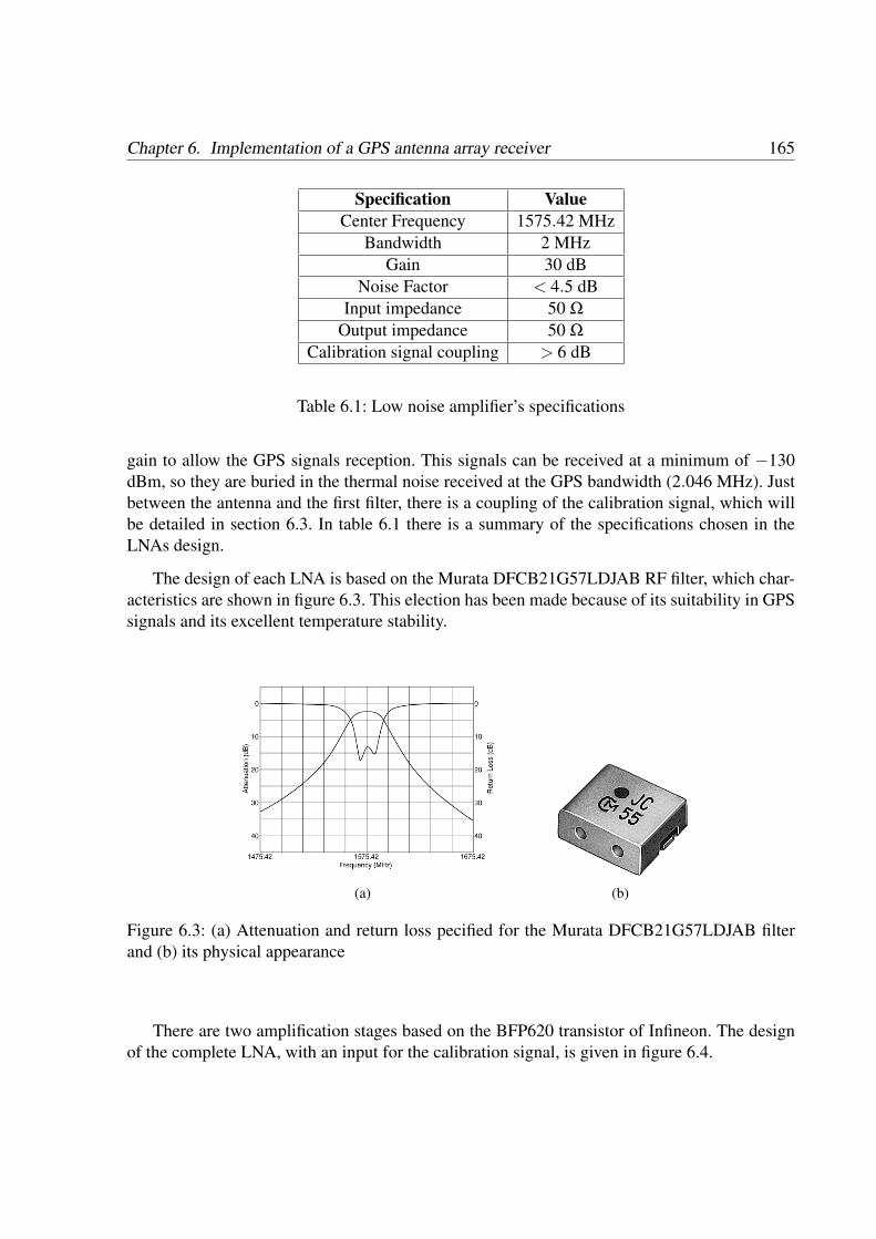
Chapter 6. Implementation of a GPS antenna array receiver 165
Specification ValueCenter Frequency 1575.42 MHz
Bandwidth 2 MHzGain 30 dB
Noise Factor < 4.5 dBInput impedance 50 Ω
Output impedance 50 Ω
Calibration signal coupling > 6 dB
Table 6.1: Low noise amplifier’s specifications
gain to allow the GPS signals reception. This signals can be received at a minimum of −130dBm, so they are buried in the thermal noise received at the GPS bandwidth (2.046 MHz). Justbetween the antenna and the first filter, there is a coupling of the calibration signal, which willbe detailed in section 6.3. In table 6.1 there is a summary of the specifications chosen in theLNAs design.
The design of each LNA is based on the Murata DFCB21G57LDJAB RF filter, which char-acteristics are shown in figure 6.3. This election has been made because of its suitability in GPSsignals and its excellent temperature stability.
(a) (b)
Figure 6.3: (a) Attenuation and return loss pecified for the Murata DFCB21G57LDJAB filterand (b) its physical appearance
There are two amplification stages based on the BFP620 transistor of Infineon. The designof the complete LNA, with an input for the calibration signal, is given in figure 6.4.
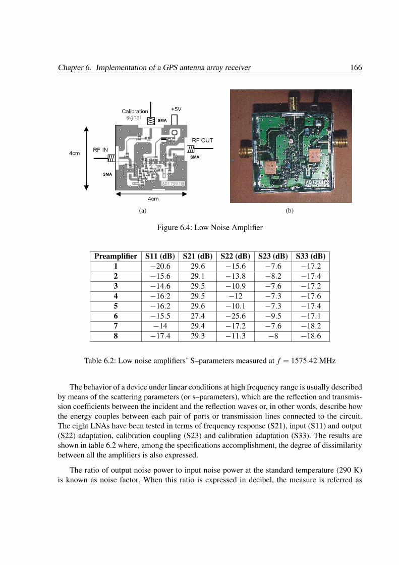
Chapter 6. Implementation of a GPS antenna array receiver 166
(a) (b)
Figure 6.4: Low Noise Amplifier
Preamplifier S11 (dB) S21 (dB) S22 (dB) S23 (dB) S33 (dB)1 −20.6 29.6 −15.6 −7.6 −17.22 −15.6 29.1 −13.8 −8.2 −17.43 −14.6 29.5 −10.9 −7.6 −17.24 −16.2 29.5 −12 −7.3 −17.65 −16.2 29.6 −10.1 −7.3 −17.46 −15.5 27.4 −25.6 −9.5 −17.17 −14 29.4 −17.2 −7.6 −18.28 −17.4 29.3 −11.3 −8 −18.6
Table 6.2: Low noise amplifiers’ S–parameters measured at f = 1575.42 MHz
The behavior of a device under linear conditions at high frequency range is usually describedby means of the scattering parameters (or s–parameters), which are the reflection and transmis-sion coefficients between the incident and the reflection waves or, in other words, describe howthe energy couples between each pair of ports or transmission lines connected to the circuit.The eight LNAs have been tested in terms of frequency response (S21), input (S11) and output(S22) adaptation, calibration coupling (S23) and calibration adaptation (S33). The results areshown in table 6.2 where, among the specifications accomplishment, the degree of dissimilaritybetween all the amplifiers is also expressed.
The ratio of output noise power to input noise power at the standard temperature (290 K)is known as noise factor. When this ratio is expressed in decibel, the measure is referred as

Chapter 6. Implementation of a GPS antenna array receiver 167
Measure Mean valueGain 29 dB
Input adaptation 18 dBOutput adaptation 18 dB
Calibration signal coupling 7.5 dBNoise Figure 5.1 dB
Table 6.3: Measures performed on the low noise amplifiers
noise figure and is a frequently used measure of an amplifier’s goodness, or its departure fromthe ideal. Thus, this is the chosen figure of merit for the amplifiers. A summary of the overallperformance of the LNAs, plus the noise figure, is shown in table 6.3. This results, comparedto the specifications table 6.1, indicate that the measured noise figure is 0.6 dB higher than thespecified parameter.
6.2.3 Down-conversion to Intermediate Frequency
The proposed design herein is based on the Zarlink Semiconductor GP2015 chip [Zar02], atriple down-conversion RF front–end, adding two more amplifiers: an RF amplifier in order toachieve a higher gain, a smaller ripple in the 2-MHz bandwidth and a smaller noise figure, andan IF amplifier which avoids a gain drop when the IF output is loaded with a 50 Ω device. TheGP2015 receives the 1575.42 MHz signals transmitted by the GPS satellites and downconvertthem to a 4.309 MHz IF, using a three stage converter with a high RF input compression point.Figure 6.5 shows the block diagram of a single front–end with its three stage mixers. Thisallows to reject large out–of–band jamming signals, particularly the 900 MHz used by the GSMsystem.
As observed in figure 6.5, the GP2015 contains three mixers at 1.4 GHz, 140 MHz and31.11 MHz. All these local oscillators are derived from a phase locked loop synthesizer with a10 MHz reference frequency. This feature allows to keep the phase reference in the eight front–ends, since the PLL of each GP2015 will tend to be phase-locked to the same 10 MHz referencesignal.
The block diagram of the Phase–Locked Loop (PLL) is shown in figure 6.6. The 10 MHzreference oscillator is an oven–stabilized crystal oscillator CO–771–B58 of Vectron [Vec]. Thisoscillator specifies a 5× 10⁻⁸ stability from 0o C to 50o C. An active splitter distributes thisclock to the eight RF front–ends and to the calibration subsystem (see figure 6.11).
The on–chip PLL generates the first local–oscillator frequency at 1400 MHz. In this firststage, the signal is down converted to 175.42 MHz and filtered with a double coupled resonator.

Chapter 6. Implementation of a GPS antenna array receiver 168
@@
LNA - Front EndMixer
-175.42 MHzFilter
- 2nd StageMixer
- 35.42 MHzFilter
AGC3rd StageMixer
4.309 MHzFilter
AmplifierIF Output
4.309 MHz
6
1.4 GHz6
140 MHz
6
31.11 MHz
Figure 6.5: Block diagram of the front–end receiver
Oscillator10 MHz
- PhaseDetector
- PLL LoopFilter
- VCO - 1.400 GHz
÷5÷7÷4
?
10 MHz
6
?
÷9
?
31.11 MHz
?
÷2
?
140 MHz
Figure 6.6: Block diagram of the 1.4 GHz Phase–Locked Loop

Chapter 6. Implementation of a GPS antenna array receiver 169
As aforementioned, this filtering allows the rejection of the image frequency and large out ofband jamming signals, such as the 900 MHz and 1800 MHz used by GSM technology.
The second stage mixer uses a 140 MHz frequency generated by the local oscillator to takethe signal down to 35.42 MHz. At this point, the selective filtering of the L1 signal is done viaa external filter with a 1 dB bandwidth of 1.90 MHz. The performance of this filter is criticalto system operation. The elected filter has been the SAFJA35M4WC0Z00R03 of Murata, basedon SAW (Surface Acoustic Wave) technology. The maximum ripple deviation specified in theband of interest is 1.6 dB, and the maximum group delay is 200 ns. Its frequency characteristicsare shown in figure 6.7.
(a) (b)
Figure 6.7: (a) Frequency characteristics of the Murata SAFJA35M4WC0Z00R03 filter and (b)its physical appearance
The output of the SAW filter then feeds the main IF amplifier and arrives to the third stagemixer. A local oscillator signal of 31.111 MHz provides a final IF at 4.309 MHz. This output isfiltered by an on–chip filter centered on 4.309 MHz. This analog signal is available with a 1 kΩ
output impedance.
6.2.4 AD conversion: IF sampling and the incommensurability concept
The block diagram of the front–end receiver depicted in figure 6.5 shows that the IF outputis centered at 4.309 MHz. In a classical superheterodyne RF front–end, the signal is usuallyshifted to baseband before digitation. Other approach recently introduced is the Direct RF sam-pling [Ako99, Psi03], consisting on sampling the RF signal of interest without a prior carrierdown–shifting to a lower intermediate frequency. The resulting sampled signal is intentionally

Chapter 6. Implementation of a GPS antenna array receiver 170
Input Frequency 1575.42 MHzBandwidth 2 MHz
Input impedance 50 Ω
Maximum input level −16 dBm at 1 dB compression.Noise factor 12 dB
Maximum gain 80 dBRipple Deviation in useful band 2 dB (max)
Group Delay in useful band 250 ns (max)Input reference clock 10 MHz
Reference clock outputFrequency 40 MHz
Level TTLOscillators phase noise −75 dBc/Hz at 10 kHz
Analog IF output 4.309 MHzDigital output 2–bits sampled IF output
Digital output level TTLExternal sampling clock
Frequency 5.714 MHzLevel TTL
Table 6.4: GPS front–end specifications
Figure 6.8: GPS signal receiver mechanization
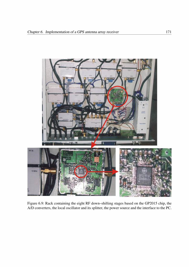
Chapter 6. Implementation of a GPS antenna array receiver 171
Figure 6.9: Rack containing the eight RF down–shifting stages based on the GP2015 chip, theA/D converters, the local oscillator and its splitter, the power source and the interface to the PC.

Chapter 6. Implementation of a GPS antenna array receiver 172
Figure 6.10: Rack frontal view, from left to right: eight analog IF outputs, reference clock(in/out), I&Q calibration signal inputs, calibration signal power controls, the acquisition cardconnector, a 40 MHz reference output and a frequency–divided output (set to 40/7 MHz) con-nected to the sampling clock input.
Figure 6.11: 10 MHz signal reference splitter mechanization
aliased to a frequency band within the Nyquist bandwidth and then processed as the output of aconventional superheterodyne front–end. This technique allows a simpler front–end design andeliminates many potential sources of channel mismatch due to the use of a single RF chain forseveral bands.
Drawbacks of this approach are related to technology: needing of high-performance analog-to-digital converters (ADC), heavy digital processing load and eventually high Q values (i. e.,filter selectivity) in bandpass filters. Direct RF sampling implies the availability of an ADCwhich can deal with huge input bandwidths, taking samples at a very high rate. In [Psi03] and[Ako03] successful implementations have been reported using a commercially available ADC[Max04], which achieves sampling rates up to 1 Gsps with 2.2 GHz of analog input bandwidth

Chapter 6. Implementation of a GPS antenna array receiver 173
working at an 8-bit resolution. Such ADC capability justifies the design of practical GNSSreceivers exploiting multiple frequency bands. If the sampling frequency is chosen properly,several signals can be aliased to nonoverlapping portions of the Nyquist bandwidth, obtainingsampled data that contains the signals from all bands of interest.
The choice of the sampling frequency for multiple frequency bands is addressed in [Ako99].Basically, it consists on an intentional aliasing of the different bandwidths of interest avoidingoverlap of the aliased bands. Firstly, the resulting intermediate frequency fIF for a given sam-pling frequency fs and carrier frequency fc can be computed as
if fix
(fcfs2
)is
even fIF = rem( fc, fs)odd fIF = fs− rem( fc, fs)
(6.2)
where f ix(·) rounds to the nearest integer towards zero and rem(a,b) is the remainder after theab division. Each entire desired band must fall within the resulting sampling bandwidth, whichcan be ensured with the following upper and lower constraints:
fIFi <fs−BWi
2(6.3)
andfIFi >
BWi
2(6.4)
Moreover, overlap of distinct signals must be avoided; this can be expressed as anotherconstraint:
| fIFi− fIFj |≤BWi +BWj
2(6.5)
The approach followed in the implementation presented in this chapter is a mixture of bothapproaches: the classical superheterodyne receiver and the aliasing techniques of the Direct RFsampling. The IF signal centered at 4.309 MHz is sampled to produce a 2–bit digital outputin an on–chip analog to digital converter, see figure 6.14. If the input frequency is fi and thesampling frequency is fs, we can found aliases in
fo = fi−nfs
2(6.6)
where n is an integer. If the input signal bandwidth is ∆ f , the minimum sampling frequency is2∆ f by the Nyquist criterion. Actually, 2.5∆ f is used because it is impractical to build so sharpfilters to limit the out–of–band signals. Thus, the required minimum sampling for the 2 MHzbandwidth of the C/A code is 5 MHz.

Chapter 6. Implementation of a GPS antenna array receiver 174
For example, if the GP2015 is used in conjunction with the GP2021 correlator [Zar01], thesampling frequency is set to 5.714 MHz. In figure 6.12 is shown how the IF spectrum is aliased.
f (MHz)
f (MHz)
2 MHz
4.309 5.714
4.309 MHz
5.7144.3091.405
−4.309
−4.309 −1.405
FrequencySampling
Figure 6.12: Sampling frequency and band aliasing
Thus, the correlator will work at 1.405 MHz to obtain the baseband signal.
The non–integer relationship between the sampling rate and the C/A code, called incommen-surability, means that the sampling will not be synchronized with the C/A code rate. Therefore,a given code (spanning 1 ms in time) and the next one will not be sampled at the same instants.Indeed, this sweeping is equivalent to interpolation when the sampling rate and the chip rateholds an integer relationship, allowing a finer time resolution.
The minimum sampling frequency that accomplishes synchronization is fs = 1.023× 5 =5.115 MHz, so the time between two samples is 195.5 ns. If the code is shifted less than 195.5

Chapter 6. Implementation of a GPS antenna array receiver 175
Figure 6.13: Sampling signal captured by an Agilent 54622D oscilloscope
ns, the sampling process will produce exactly the same output data. The corresponding distanceresolution will be 195.5×10−9×3×108 = 58.65 m, too coarse to obtain the desired accuracy.By the other hand, an incommensurable sampling frequency produces different outputs for aC/A code and the same code shifted less than fs
2 because the chips never are sampled in thesame point. Under this condition, a finer time resolution can be achieved after the correlator.
6.3 Calibration subsystem
In a practical system, one of the main difficult points in an smart antenna is to calibrate theamplitude and phase of every channel over temperature and frequency [Nut02]. Accurate align-ment of channels would require high precision hardware components and consequently a higheconomic cost. Thus, there is a need of a calibration system.
A calibration signal, consisting of two baseband unused C/A Gold code generated at TTLlevels, is upconverted by an I&Q modulator to 1.575.2 MHz, splitted out eight ways and coupled

Chapter 6. Implementation of a GPS antenna array receiver 176
Figure 6.14: GP2015 ADC output captured by an Agilent 54622D oscilloscope
between the antennas and the LNAs. The power level of this virtual satellite signal is similarto the GPS minimum level (approx. −130 dBm). Exploiting the 8051 microcontroller used toprogram the PLL, the power level of the calibration signal can be attenuated 10, 20 or 30 dBby means of a set of switches. It also can be deactivated. This system will allow a continuoustracking of the known signal and thus perform a digital calibration. The main characteristics ofthe I&Q modulator are:
• Central frequency: 1575.42 MHz
• Bandwidth: 2 MHz
• Gain: 30 dB
• Noise factor: 4.5 dB
• Input Impedance: 50 Ω
• Output Impedance: 50 Ω
• Calibration coupling: ±0.2 dB in amplitude and ±2 in phase

Chapter 6. Implementation of a GPS antenna array receiver 177
This calibration method neglects the effects of the radiating antenna elements, so a charac-terization of these elements in an anechoic chamber seems mandatory.
Another calibration method that avoids this drawback consists of emitting the signal with anantenna placed in front of the array, in the far–field at broadside, instead of taking the calibrationsignal and splitting it into each channel. This method has been discarded by practical reasons,although it could give a better performance.
6.3.1 Baseband GPS-like signal generator
The generation of the GPS-like signal (a Gold code not moduled by data) used for calibrationpurposes is implemented in a Complex Programmable Logic Device (CPLD). The Memec De-sign XC9500XV Development Kit allows Xilinx XC95144XV 2.5V CPLD to be programmedvia Very high speed integrated circuit Hardware Description Language (VHDL). It also includesa prototyping area where a bank of switches have been welded to control the generation of thecalibration signal. The designed device has two BNC outputs, where two different codes can begenerated in the In-phase and Quadrature channels and directly feed the I&Q Modulator.
6.3.2 I&Q Modulator
This device modules an In-phase and Quadrature (I&Q) baseband signals with an output fre-quency of 1575.42 MHz, accepting TTL input levels and giving a −30 dBm output, 30-dBadjustable in 2-dB steps. The local oscillator rejection is 27.7 dB, while the intermodulationproducts rejection is 27.7 dB and the local oscillator phase noise is −73.2 dBc/Hz at 10 kHz.
6.3.3 RF splitter
The calibration signal has to be delivered to the eight LNAs, where it is coupled to the inputRF signal. In order to accomplish this goal, we have designed an RF splitter which replicatesthe RF input into eight RF outputs, while electrically conditions the signals that feed the LNAs.The schema of this device is displayed in figure 6.17. It has been characterized in amplitude andphase, giving the results of table 6.7, showing the relationship in between the input port and theeight output ports.
In addition, we have characterized the eight calibration paths from the splitter input to thecoupling point in the LNAs, presenting the results in table 6.8. Differences between paths areascribable to the contribution of the RF splitter itself, but also to the insertion losses between
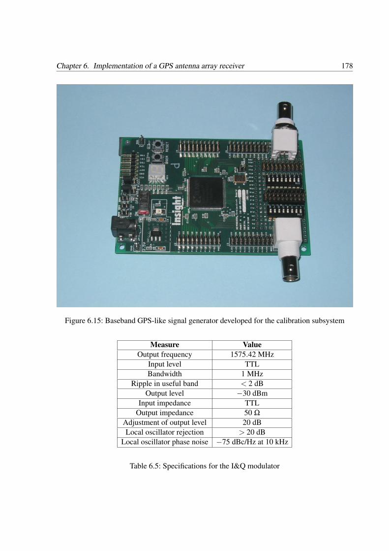
Chapter 6. Implementation of a GPS antenna array receiver 178
Figure 6.15: Baseband GPS-like signal generator developed for the calibration subsystem
Measure ValueOutput frequency 1575.42 MHz
Input level TTLBandwidth 1 MHz
Ripple in useful band < 2 dBOutput level −30 dBm
Input impedance TTLOutput impedance 50 Ω
Adjustment of output level 20 dBLocal oscillator rejection > 20 dB
Local oscillator phase noise −75 dBc/Hz at 10 kHz
Table 6.5: Specifications for the I&Q modulator

Chapter 6. Implementation of a GPS antenna array receiver 179
Measure ValueOutput frequency 1575.42 MHz
Input level 5 VppBandwidth 1 MHz
Ripple in useful band 1 dBOutput level −30.7 dBm
Input impedance > 4 kΩ
Output impedance 50 Ω
Adjustment of output level 30 dB (2-dB steps)Local oscillator rejection 27.7 dB
Intermodulation products rejection 27.7 dBLocal oscillator phase noise −73.2 dBc/Hz at 10 kHz
Table 6.6: Measures performed on the I&Q modulator
Figure 6.16: I&Q modulator mechanization
Figure 6.17: Implementation of the RF splitter

Chapter 6. Implementation of a GPS antenna array receiver 180
Insertion lossOutput port Amplitude (dB) Phase (degrees)
1 −33.7 −1582 −34.6 1653 −35.2 1734 −35.1 −1515 −35 −1576 −35.3 −1787 −35.5 1658 −35.4 −168
Table 6.7: Insertion losses in the splitter’s ports
Insertion lossPath Amplitude (dB) Phase (degrees)
1 −73.3 −3332 −73.6 183 −73.8 304 −73.5 −2815 −74.5 −3296 −73.8 −3537 −74.9 478 −75.2 7
Table 6.8: Eight path’s performance in terms of amplitude and phase
the calibration input and the RF input in the LNAs and the wires between the splitter and theLNAs.
6.4 Signal storage subsystem
The GPS receivers–computer interface proposed herein consists of a PCI bus interface betweenthe GPS receivers and a PC. The data given by each GPS front–end is sampled with 2 bits ofresolution. Due to the fact that the sampling clock is the same for the eight receivers, the twosamples of each front end can be combined in a 16 bits word. These words are buffered in aRAM memory that is connected to the PCI bus. When the PC wants to capture the receiveddata, accedes this RAM memory via the PCI bus and stores it in its own memory or hard disk.

Chapter 6. Implementation of a GPS antenna array receiver 181
To carry out this work, the acquisition card proposed is the PCI 6534 of National Instru-ments (technical specifications in [Ins01]). This device provides 32 digital data lines whichare individually configurable as input or output, grouped into four 8–bit ports. In addition, itcontains on-board memory that enables transferring data from this memory to a hard disk ata guaranteed rate. This memory feature removes the dependency on the host computer bus forapplications that require guaranteed transfer rates.
The acquisition subsystem is managed by a software developed in the LabVIEW (Lab-oratory Virtual Instrument Engineering Workbench) development environment, which allowsgraphical programming for measurement and automation. LabVIEW is based in the concept ofvirtual instrumentation, offering benefits such as flexibility, compatibility or lower cost than tra-ditional instruments. A virtual instrument consists of an industry–standard computer equippedwith powerful application software, cost-effective hardware such as plug–in boards, and driversoftware, which together perform the functions of traditional instruments. Virtual instrumentsrepresent a fundamental shift from traditional hardware–centered instrumentation systems tosoftware–centered systems that exploit the computing power, productivity, display, and connec-tivity capabilities inherent of computers.
The IF output of the RF frontend GP2015 is fed to a 2 bit quantizer which provides sign (pin15 of GP2015) and magnitude (pin 14 of GP2015) outputs. These data are latched by the risingedge of the 5.714 (=40/7) MHz sample clock. This gives a sampled IF centered on 1.405 MHz,as is shown in figure 6.12. The 6534 device mode of operation for receiving digital patternsand waveforms is called Pattern I/O. This mode allows both an external clock or an internallygenerated clock signal, given by an on-board 32–bit counter set to a user specified frequencyor by an external clock signal received from the I/O connector. The generation of an internalclock is specified in software by using two parameters, the timebase frequency and the timebasedivisor:
transfer rate (Hz) =timebase frequency
timebase divisor(6.7)
where timebase frequency can be 20 MHz, 10 MHz, 1 MHz, 100 kHz, 10 kHz, 1 kHz or 100Hz, and timebase divisor is an integer between 1 and 65,355. These values do not allow theinternal generation of the desired 5.714 MHz sample clock, thus the external reference must beused. By default, data from an external source is transferred on the rising edge of the signal.The data transfer starts, by default, upon a software command controlled in the user interface.In addition, a hardware trigger tan be used to start, stop or start–and–stop data transfer:
• Start Trigger. A start trigger is a trigger that initializes a pattern I/O upon receipt of ahardware trigger on the ACK (STARTTRIG) pin, by default in its falling edge.
• Stop Trigger. When using a stop trigger, transfer starts upon a software command. Oncea hardware trigger is received on the STOPTRIG pin, a predetermined amount of post-trigger data is saved in the buffer. Once this data is in the buffer, transfer stops.
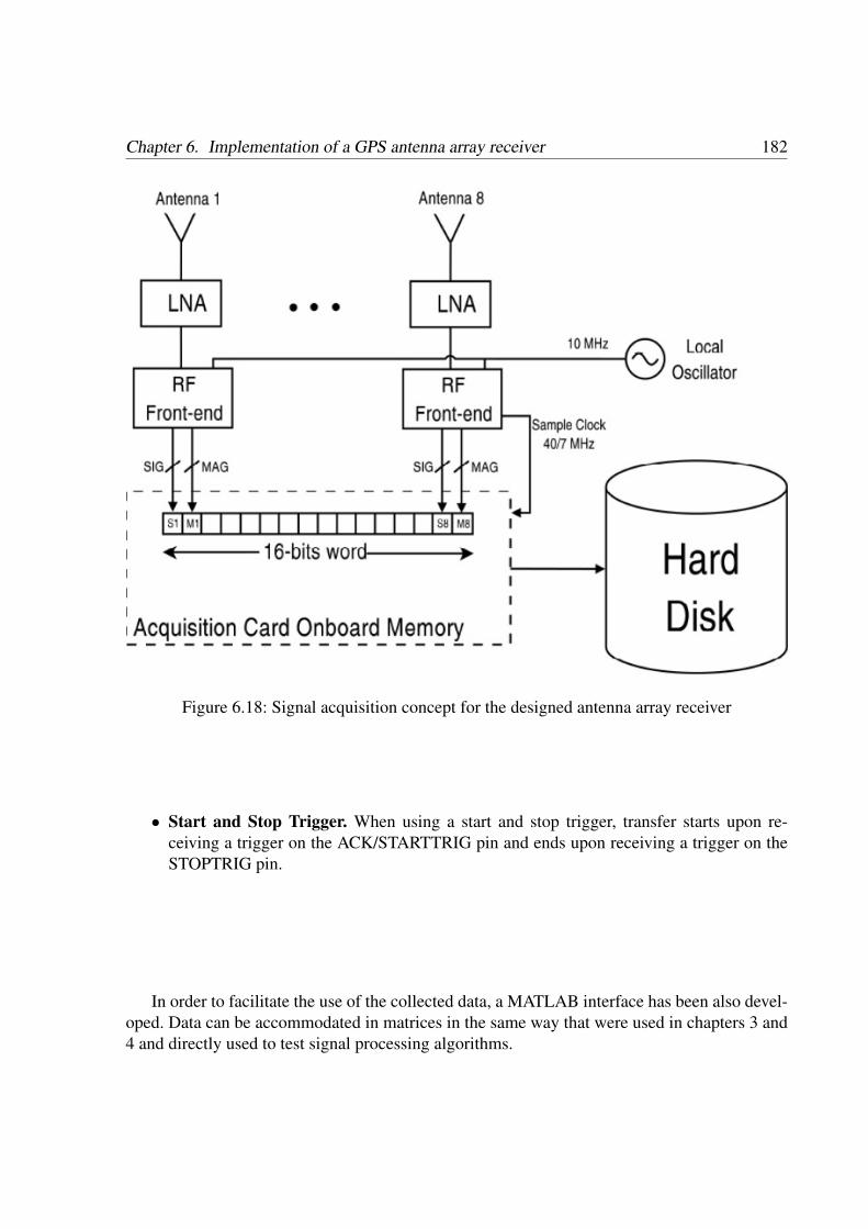
Chapter 6. Implementation of a GPS antenna array receiver 182
Figure 6.18: Signal acquisition concept for the designed antenna array receiver
• Start and Stop Trigger. When using a start and stop trigger, transfer starts upon re-ceiving a trigger on the ACK/STARTTRIG pin and ends upon receiving a trigger on theSTOPTRIG pin.
In order to facilitate the use of the collected data, a MATLAB interface has been also devel-oped. Data can be accommodated in matrices in the same way that were used in chapters 3 and4 and directly used to test signal processing algorithms.

Chapter 6. Implementation of a GPS antenna array receiver 183
6.5 Satellite signal acquisition
Signal acquisition refers to a coarse synchronization process, giving estimates of the code offsetand Doppler shift of the received signal. The key feature of an acquisition process is the speedof the method rather than the accuracy, which is achieved in the tracking stage.
6.5.1 Acquisition methodology
GPS signal acquisition is a search process over a two-dimensional grid of time (code phase) andDoppler shift. Code and frequency increments in the grid are usually referred to as bins, andthe combination of one code bin and one Doppler bin is called a cell. The acquisition process isperformed in the receiver in a parallel manner, devoting one acquisition and tracking channel persatellite. Therefore, the initial operation of a GPS receiver consists on determining the satellites(or, more precisely, the codes) to be searched. This list of theoretically in-view satellites areelaborated in function of the prior available information in the receiver. Three situations can betaken into account:
• Cold start. When the receiver has no information about its position nor the satellites al-manac, the acquisition procedure must be applied to all satellites in space. Every receiverchannel is assigned to one satellite; if the signal is not found after a given observationperiod, the channel switch to another satellite code. If the signal is found, the informationis passed to the tracking algorithm. This procedure is also known as “sky search”. Whenfour or more satellites are being tracked, and the receiver has got the ephemeris data aboutwhere the satellites are located in space, the positioning equation system can be resolved.The time elapsed between power applying and the first position computation is known asTime To First Fix (TTFF), and its average is commonly used as a figure of merit of thereceiver.
• Warm start. When a rough location and the approximate time of day are available, andthe receiver has a recently recorded almanac broadcast, an estimation of which satellitesare visible to the receiver can be performed. This reduces approximately a half of the totalnumber of satellites searched by the cold acquisition and therefore speeds the process. Thereceiver just needs the ephemeris update and time signals. Modern receivers have a smallbattery and a internal memory where the data from the last good fix is held. When poweris re-applied, this data is used as a starting point in the acquisition.
• Hot Start. When the receiver tracks a satellite and the signal line of sight is broken for ashort period of time (driving through a tunnel, in an urban canyon, under trees in a forest),but the ephemeris and almanac data is still valid, the is no need of getting ephemeris dataagain and the position can be computed after a simple signal acquisition.

Chapter 6. Implementation of a GPS antenna array receiver 184
In order to apply acquisition algorithms in an efficient manner, some parameters must beselected carefully. Achieving a better resolution implies a finer search grid and therefore morecomputational load. The first parameter to be decided is the frequency range of search. Simplegeometry and some approximations can be applied to estimate a reasonable bound for Dopplershift. Satellites takes half a sidereal day to rotate once around the earth. While the apparent daytakes 24 hours and represents the time between two successive transits of the sun across ourlocal meridian, the sidereal day is the time for the earth to turn one revolution. Defining Td asthe duration in seconds of a sidereal day (23 hours, 56 minutes and 4.09 seconds) the angularvelocity of a satellite can be computed as
dβ
dt=
2π
Td2
= 1.4584 ·10−4 rads
(6.8)
where β is the angle difference, from the satellite point of view, between the user and the Earthcenter. Considering rs = 26,560 km as the average radius of the satellite orbit, the speed of thesatellite can be approximated as vs = rs
dβ
dt = 3873.57 m/s. The Doppler shift is caused by thesatellite velocity component vd toward the user, that is
vd = vs sinγ (6.9)
where γ is the angle seen by the satellite between the center of the earth (the intersection be-tween the earth’s rotation axis and the equatorial plane) and the user’s receiver. Therefore, themaximum Doppler shift occurs when the satellite is in the horizon position, where sinγ = re
rsbeing re = 6,368 km the Earth average radius:
fdmax =fcvdmax
c=
fc
cvs
re
rs(6.10)
Taking the L1 GPS signal, fc = 1575.42 MHz, the maximum expected Doppler shift is approx-imately±5 kHz for a stationary receiver. This upper bound might be increased in high dynamicapplications, or in case of poor stability of the receiver oscillator. Figure 6.19 shows Dopplershifts measured with a NovAtel OEM4 receiver; the normalized histogram presented in the rightside has the U–shape of the well-known Jakes model [Jak74], and in this case the Doppler isbounded at ±4 kHz.
The Doppler bins must be distributed over this frequency span, usually in a uniform ar-rangement. In [Kap96], a Doppler bin is defined as bin = 2
3T , where T is the signal coherentintegration time per cell (also known as predetection or dwell time). As the C/A code period is1 ms, the maximum space between frequency bins is 667 Hz but usually the dwell time mustbe increased in order to acquire signals; the probability of detection for T = 1 ms with a singletrial is above 90% only when the signal CN0 is higher than 37 dB-Hz.
The code phase is typically searched in half-chip increments, named code bins. This pa-rameter is determined by the minimum accuracy required by the tracking loop, which is a half

Chapter 6. Implementation of a GPS antenna array receiver 185
−4000 −3000 −2000 −1000 0 1000 2000 3000 40000
0.005
0.01
0.015
0.02
0.025
Doppler [Hz]
Est
imat
ed p
roba
bilit
y de
nsity
func
tion
Figure 6.19: Doppler shifts measured with a NovAtel OEM4 stationary receiver.
a chip for the BPSK modulation but could be smaller for a BOC modulation, as observed infigure 2.12, and the computational load which can be afforded by the acquisition system.
The performance analysis for a single–dwell acquisition is usually performed by meansof the false alarm probability Pf a and the probability of detection Pd . The Pf a depends uponthe statistics of the noise at the input to the acquisition stage, and upon the chosen thresholdlevel. Assuming that the correlator is sufficiently long, the central limit theorem shows that thesamples at the input to the FFT are uncorrelated and Gaussian distributed with zero mean. Themagnitude of the FFT outputs will be Rayleigh distributed, and therefore the probability thatany one of the FFT output is greater than a threshold Vt is
Prob [FFT output > Vt |no signal] = e−V 2
t2L (6.11)
where L is the code length. All of the FFT outputs will have the same distribution, and thusthe probability of false alarm (i.e., the probability of any one of the N f f t output FFT samplesexceeding the threshold) is given by
Pf a = 1−(
1− e−V 2
t2L
)N f f t
(6.12)
If we want to maintain a constant false alarm probability throughout the whole code, thethreshold can be isolated as

Chapter 6. Implementation of a GPS antenna array receiver 186
Vt =√−2L ln(Pf a) (6.13)
The computation of the probability of detection involves the assumption of the presence ofthe desired signal among noise. In that case, and accepting the same assumptions about noisethan above, the magnitude of the FFT output samples will be Ricean distributed. If we determinethe presence of a signal if any of the output samples is greater than the threshold, the probabilityof detection can be computed as
Pd = 1−Pno detection = 1−N f f t
∏i=1
(1−Probi[output > Vt ]) (6.14)
A well-known suboptimal synchronization procedure is the Tong search detector [Kap96],which requires a reasonable computational load. The algorithm, described in figure 6.20, tries tobalance the acquisition speed with the probability of detection and false alarm. This is achievedby means of a counter variable K with a confirmation threshold A. If the result of a search overa cell during a code period Tc is above a certain threshold Vt , the variable K is incremented,and if the correlation peak is below Vt , K is decremented. In this context, every search in awhole period Tc is called a dwell. The procedure is repeated during a given number of dwells.If K reaches the value of A, the signal is declared present and the information is passed to thetracking algorithm. If K reaches 0 or the number of dwells attain the maximum allowed, thesignal is declared not present and the searching channel is devoted to another suitable satellite.The maximum acquisition speed will be achieved setting K = 1, but this parameter must beincreased to obtain a higher detection probability. A typical range for A is 8–12. The probabilityof detection and false alarm can be computed with A and the value which the counter K is resetafter a signal is declared not present [Kru01]. Usually, these probabilities are used to set upthe value of the correlation threshold in several acquisition strategies. A throughout analysis ofdetection and false alarm probabilities in GNSS signal acquisition can be found in [Rod04b].
When the Tong algorithm declares a signal as present, the acquisition can be refined witha limited search space. When the search is performed over ±2 chips and ±2 Doppler bins ata finer resolution, the algorithm is called a Vernier detector, and can be applied after the Tongprocedure to obtain a polished result to be passed to the tracking loop.
The defined structure can be categorized as a variable dwell time search detector. A fixeddwell time can be ensured with the M of N search detector. This algorithm takes N dwell timesand compares every correlation peak value with a given threshold. If M or more of them exceedthe threshold, the signal is declared present. Again, M and N parameters define a probability ofdetection and false alarm.

Chapter 6. Implementation of a GPS antenna array receiver 187
Figure 6.20: Tong search detector algorithm
Recently, some improvements to these strategies have been proposed. In [Kan04], the roughestimation of the receiver and satellites position is exploited to give a first approximation of theDoppler shift, thus reducing the frequency search space. As the objective of this chapter is todemonstrate the antenna array concept from a signal processing point of view and not to build acomputational–effective and complete GPS software receiver, the discussion about acquisitionmethodology will be left here, although remains as an open field of research, and we will focusin how a search over a single cell can be performed from a software radio approach perspective.
6.5.2 Software receiver approach: circular correlation method
The conventional approach to perform signal acquisition is through hardware in the time do-main. The state-of-the art of such hardware structures has been commented in chapter 2, andbasically they consist on performing the acquisition procedure on the input data in a continuousmanner. Once the signal is found (in most methods, when the Integration & Dump block’s out-

Chapter 6. Implementation of a GPS antenna array receiver 188
put exceeds a given threshold, see figure 2.3), the acquisition results are passed to the trackinghardware.
On the contrary, in a software receiver the acquisition is performed on a block of data,instead of a continuous process on the input data flow. Actually, the concepts of acquisition andtracking only makes sense in a real time receiver. In this case, there is a time elapse between theblock of data used in the acquisition process and the tracked data. The higher the dynamics of thetracked parameters, the shorter acquisition time is allowed because the acquisition informationcould become out of date rapidly. Therefore, low computational cost is a desirable feature in thedesign of acquisition algorithms.
If the software receiver does not operate in real time, the acquisition and tracking procedurescan be performed on the same block of data, and can be understood as rough and fine estimationmethods. Although the speed versus sensitivity trade–off is not so important for acquisitiondesign as in real time receivers, usually high precision estimation algorithms involve a very highcomputational burden (as showed in chapters 3 and 4), and thus keeping a small search space isstill desirable. The block size will be given by the parameters dynamics and the computationalpower available.
Acquisition procedures are based on correlation. The structure of GNSS signals, namely aconcatenation of repeated codes, gives to the involved sequences a circular symmetry. Thus,circular correlation is a suitable method for a software receiver approach because it operates ona block of data. The circular correlation of two finite-length sequences (we could consider theoutput of the antenna array, y = wHX and the locally generated sampled code, c) is equivalentto one period of the periodic correlation of the periodic-extended sequences y and c, and it isdefined as
z[n] =L−1
∑l=0
y[l]c[(n+ l)L] (6.15)
where the notation (·)L stands for the modulus-L operator, considering L as the number ofsamples covering one period of the satellite code. A straightforward computation of z[n] requiresa large number of operations, which can be avoided resorting to the frequency domain [Pro96]:
z[n] = F −1 Y [k]C∗[k] (6.16)
being Y [k] the Fourier transform of sequence y[l], C∗[k] the complex conjugate transform of c[l]and F −1 · the inverse Fourier transform operation. Hence, the computational efficiency ofthe FFT algorithm can be exploited in the acquisition process. The algorithm for a single-cellsearch, as mentioned above in the Tong receiver, can be stated as:

Chapter 6. Implementation of a GPS antenna array receiver 189
Algorithm 2 Acquisition/Coarse estimation algorithm1: Generate Doppler–shifted versions of the local code, ci[l].2: Perform the FFT of all Doppler–shifted versions of the local code, obtaining Ci[k].3: Perform the FFT of one code period of the input data, obtaining Y [k].4: Take the complex conjugate of the transformed input, Y ∗[k].5: Multiply Y ∗[k] by Ci[k] point by point, obtaining Zi[k].6: Perform the inverse FFT on Zi[k], obtaining zi[l].7: Take the absolute value of the previous step, |zi[l]|.8: The beginning point of the code lacq and the frequency bin facq will be given by the position
of the |zi[l]| maximum→ τacq, fdacq .
Once a coarse time an frequency estimation are performed, results can be refined with morecomplex algorithms in order to obtain more accurate results. As an example, we propose Algo-rithm 3 for a finer Doppler frequency estimation.
Algorithm 3 Tracking/Fine estimation algorithm for Doppler frequency1: Generate a local code with the result obtained in Algorithm 2, that is, τacq–delayed.2: Multiply the input data y[k] by the generated local code.3: Multiply by a complex exponential centered at fIF + fdacq .4: Decimate the obtained signal at rate R.5: Perform the FFT to the result in order to obtain a finer frequency estimation→ fd f ine .
6.6 Experimental results
6.6.1 Testing the coarse and fine estimation algorithms
The coarse estimation described in Algorithm 2, also named the acquisition process, has beenapplied to real raw data provided by the NordnavTM R–25 GPS L1 Software Receiver [Nor05],recorded on June 15th, 2004, in the European Space Research and Technology Centre (ESTEC)of the European Space Agency in Noordwijk, The Netherlands, and gently provided by Gus-tavo Lopez-Risueno. This device supplies output including navigation information (binary andNMEA), measurements, spectral analysis of the RF input, and other parameters in real-time orreplay mode. The availability of the navigation solution jointly with preprocessed raw IF signalallows the test of MATLAB–developed algorithms with real GPS data.
The receiver works with a sampling frequency of 16.3676 MHz and an intermediate fre-quency of 4.1034 MHz, and it is equipped with a front–end filter bandwidth (at −3 dB) of 2.2

Chapter 6. Implementation of a GPS antenna array receiver 190
NordnavTM R–25 Output Coarse estimation (Alg. 2) Fine estimation (Alg. 3)3.2939 3.2000 3.28482.0928 2.0000 2.0976-1.2194 -1.2000 -1.2112-2.9506 -3.0000 -2.9408-4.2575 -4.2000 -4.28801.5666 1.6000 1.6080-2.7005 -2.6000 -2.6752-2.8449 -2.8000 -2.8304
Table 6.9: Doppler coarse and fine estimation results (in kHz) of 8 in–view satellites comparedto the NordnavTM R–25 output.
MHz. In the acquisition algorithm, we have chosen a frequency span of ±4 kHz, with a totalamount of 51 frequency bins. The number of dwells has been set to 10. In the frequency track-ing (Algorithm 3), the decimation rate has been set to R = 2500 and a 210-points FFT has beenused to obtain the finer frequency estimation. The results, compared to the frequency estimationprovided by the NordnavTM R–25 Receiver, are shown in table 6.9.
6.6.2 Testing the digital IF outputs
The GP2015 chip provides 2–bit digitized signal output. In order to test this output beforethe data acquisition stage we have used a GPS Development Board equipped with the GP2040[Zar05] of Zarlink , a GPS Receiver Baseband Processor which combines the GP2021 correlator[Zar01] and a microprocessor that performs position computation.
The digital output of every array channel has been connected to the input of the correlator,bypassing the RF front–end chip of the development board and taking the signal directly fromthe array front–end. Figure 6.21 shows some details about the hardware hacking: the data cableof the acquisition card, which collects the 16 digital outputs of the array (8 channels digitizedwith 2 bits of resolution), is connected to a specially–designed, homemade device which allows,with the help of switches, to select the output of a given channel and obtain its digitized outputalong with a 40 MHz reference provided by the array front–end (see figure 6.10). This signalsare then connected to wires soldered to the input of the correlator. The result is a proper compu-tation of the antenna position in all the channels, which indicates a successful implementationof the eight GPS front–ends.

Chapter 6. Implementation of a GPS antenna array receiver 191
(a) Collecting digital data (b) GPS Development Board
(c) Accessing correlator inputs (d) More hacking details
Figure 6.21: A GPS Development Board equipped with a GP4020 Correlator chip by Zarlinkhas been used to test the digital IF output of the eight RF front–ends.
6.6.3 Experiments with stored data
The first step towards synchronization is the acquisition, which provides initialization points tomore refined estimation methods such as proposed in this dissertation. Applying the algorithmdescribed in previous section, we have been able to detect GPS satellites using the antenna arrayfront–end. The correlation search performed in every channel for a given present satellite isshown in figure 6.22, using 10 ms of stored signal. Channel ]2 has no antenna and consequentlyis unable to perform acquisition. Channels number ]7 and ]8 show to be noisier than the rest.

Chapter 6. Implementation of a GPS antenna array receiver 192
PRN CN0 Error in Doppler estimation [Hz]]1 ]2 ]3 ]4 ]5 ]6 ]7 ]8
2 41 3.8 −316.1 3.8 3.87 3.8 3.8 3.8 3.84 49 −37.5 −1157.5 −197.5 −37.5 −37.5 −197.5 −197.5 −197.57 37 −6.5 −806.5 −6.5 153.4 153.4 153.4 966.5 −6.58 38 121.2 1638.7 121.2 121.2 121.2 121.2 −5478.7 121.2
13 49 −70.1 −3270.1 −70.1 −70.1 −70.1 −70.1 −70.1 −70.120 44 −18.6 3021.3 141.3 141.3 141.3 −18.6 −18.6 141.323 48 −52.3 1867.6 −52.3 107.6 −52.3 −52.3 −532.3 −52.324 48 −13.2 −1773.2 −13.2 −13.2 −13.2 5106.7 466.7 −13.227 44 −13.9 786.1 −13.9 −13.2 −13.9 −13.9 −13.9 −13.9
Table 6.10: Doppler acquisition results. The references in error computation are the outputs ofthe NoVatel OEM4 receiver. The number of dwells has been set to 10.
The storage of data captured by the array has been complemented with the simultaneouscapture of the output given by a NovAtel OEM4 receiver. This output provides high–level infor-mation, such as the list of acquired satellites, estimated CN0, estimated Doppler, and positiondetermination. It does not give information about the time delay performed inside the device(i.e., the PAC correlators output), but the list of satellites and the estimations of Doppler canbe used as a reference to verify the results of the acquisition method performed over the datacollected by the array.
Results obtained are shown in table 6.10. The NoVatel receiver acquired nine satellites, andthe table shows their CN0 (in dB-Hz) and the difference between the Doppler estimation per-formed by the NoVatel receiver and the estimation performed on array–captured data followingthe previously described algorithm in each channel. In step 1 of the algorithm, there have beenused 51 Doppler–shifted versions of the local code spanning a range of ±4 kHz around the IF,and therefore the frequency bin in this acquisition step is 160 Hz.
In a conventional (hardware) receiver, signal tracking refers to the process in which theestimation is refined, accounting for small changes in the actual value of the tracked parameter.The DLL and its variants, described in chapter 2, are examples of tracking algorithms. In asoftware-oriented design, data is not processed as a flow of samples, i.e one by one, but as ablock of K samples. The parameter of interest is assumed to be constant in each block of data,and the concepts of acquisition/tracking can be understood as coarse/fine estimation. That is,algorithms proposed in chapter 3 and 4 can be directly applied to the data collected by thestorage subsystem of the proposed antenna array.

Chapter 6. Implementation of a GPS antenna array receiver 193
(a) Antenna 1 (b) Antenna 2
(c) Antenna 3 (d) Antenna 4
(e) Antenna 5 (f) Antenna 6
(g) Antenna 7 (h) Antenna 8
Figure 6.22: Acquisition results with real data integrating 10 dwells. Only the most significantbit (sign) of the collected samples has been used.
Chapter 6. Implementation of a GPS antenna array receiver 194
6.7 From time estimation to positioning
All the synchronization methods presented along this dissertation provide relative time andfrequency references because the clock bias of the receiver remains unknown. This section isintended to sketch the bridge between time and frequency synchronization, viewed from a signalprocessing perspective, and the main objective of a GPS receiver: position determination. Thislast step has not been performed with the data captured by the antenna array since it is out of thescope of the dissertation, although is provided hereafter for sake of completeness. Discussionsin deep about positioning algorithms can be found in [Par96a], [Kap96] and [Tsu00].
6.7.1 Bit synchronization
The output amplitude of the tracking loop, when analyzed every 1 ms, provides informationabout sign changes caused by the navigation data modulated in BPSK at 50 bps. Observingthe difference between adjacent millisecond outputs, data transitions are decided when the out-put exceeds a certain differential threshold. A number of bit synchronization techniques aredescribed in [Spi77].
The bit-synchronization histogram approach [Par96a] consist on splitting the data bit pe-riod, 20 ms, into twenty 1-ms periods, and look for a sign change. When a change is detected,the corresponding histogram bin (namely, from bin 1 to bin 20) is incremented by one. Theprocess is iterated until one bin exceeds the other 19 bins by a certain amount, usually decidedin function of the probability of an error in the sign change and the observation time.
If the software receiver is working with a block of 20 ms of data, a navigation bit will surelystart within these data but there might not be a phase transition. The receiver must wait to aphase transition to find the beginning of the first navigation bit. The validity of this transitioncan be checked in subsequent detections: bit transitions must be separated by multiples of 20 ms.If the transitions do not occur at these multiples, data contains errors and should be discarded.When the transitions are checked, tracking output data can be converted in navigation data. Ata first stage, the signs of these navigation bits can be arbitrary chosen, and adjust the polaritywith the parity check included in the message (see section 2.5).
After converting the tracking output into navigation data, the next step is to find the begin-ning of the data subframes. The minimum information needed to compute the receiver position(that is, ephemeris data and satellite clock correction) is contained in the first three subframes.Therefore, these subframes must be demodulated to compute the navigation solution.

Chapter 6. Implementation of a GPS antenna array receiver 195
6.7.2 Subframe synchronization
All the subframes begin with the telemetry (TLM) and the hand over word (HOW), being eachword a 30-bit structure. The TLM begins with the pattern 10001011, which can be exploited todetermine the beginning of the subframe. Usually, a minimum of three consecutive preamblematches are required in order to determine subframe acquisition. In the second word, HOW,bits 20− 22 are the subframe identification number, from 1 to 5, and this information can bealso used in subframe matching. The two last bits of HOW contain the polarity check, whichmust be used to correct the polarity of the word and correctly identify the pattern in TLM andthe subframe number of HOW.
First, second and third subframes contain the keplerian elements and the orbital perturba-tion parameters needed to compute the satellite’s position which will be hereafter referred toas rs, and the clock correction (algorithms in [Cor03], [Par96a] and [Tsu00]). This informationis crucial in the final computation of the receiver’s position, as will be shown in next subsec-tion. Fourth and fifth subframes contain the navigation almanac with ephemeris data and clockinformation of other satellites.
6.7.3 Navigation solution
When bit and frame synchronization have been achieved, the receiver is able to demodulate thenavigation data and perform some useful computations, such as the emitter position and thetrend of the satellite clock. But there is still a lack of an absolute time reference: along thisdissertation, time and frequency estimation have been referred to an arbitrary time start, andbit and frame synchronization are performed on the received signal, when the electromagneticwave has traveled along an unknown distance. Therefore, all time measurements until this pointare relative, related to a receiver’s clock that is not expected to be very precise, at least notso stable as the atomic clocks carried by the satellites, which furthermore are monitored andupdated by the GPS control segment [Par96a], keeping a calibration respect to the GPS timereference. The link to such stable and absolute timing is the fact that every satellite transmits atthe same time.
All the beginnings of subframe 1 from different satellites are transmitted at the same time,except for the clock correction terms of each satellite. Since beginnings of subframe 1 fromdifferent satellites are received at different times, a relative pseudorange (i.e., a relative timedifference) from the satellites to the receiver can be extracted. If we select a tracked satelliteas a reference, its relative time can be set to tr1 = 0 and then measure the time difference tothe beginning of frame 1 captured from other satellites, tr2 , tr3 , tr4 and so on. These relativetimes could be used to compute pseudoranges simply multiplying by the speed of light, leadingto positive and negative values. Usually, a constant is added to relative times in order to get

Chapter 6. Implementation of a GPS antenna array receiver 196
positive pseudoranges, hereafter named ρ. Since the time delay from the satellites to the user isin the range of 67 to 86 ms [Tsu00], a constant of 75 ms is added to the relative times computedfrom the beginning of subframe 1. The pseudorange for a given satellite can be expressed as:
ρ = c(tRx user− tT x sat) (6.17)
where c = 299,792,458 m/s is the speed of light, tRx user is the measured arrival time, includingthe user’s clock bias estimate bu and the error produced by receiver noise, multipath and othernuisance effects:
tRx user = tRx +bu +ν = tT x +Dc
+dtrop +dion +bu +ν (6.18)
In equation (6.18), tRx is the true arrival time, and it is splitted in terms of true transmission time,tT x, true distance from receiver to satellite, D, and the true delays caused by the troposphere,dtrop, and the ionosphere, dion. By the other way, the term tT x sat in equation (6.17) refers to thesatellite transmission time, which can be expressed in function of the true transmission time,tT x, and the true bias in satellite’s transmission time, bs:
tT x sat = tT x +bs. (6.19)
Since the position of the satellite, rs, can be computed from the navigation message and theposition of the user ru is the desired output (along with the user clock bias estimate), it seemsnatural to express the true distance from receiver to satellite by means of D = us [rs− ru], whereus is the true unit vector from user to satellite. Gathering this definition with equations (6.17),(6.18) and (6.19) leads to
ρ = us [rs− ru]+ c(bu−bs)+ c(dtrop +dion +ν). (6.20)
In this last equation, the satellite’s position rs is known because it has been computed from thenavigation message. Estimations of the satellite clock bias bs, the delay caused by the tropo-sphere dtrop and the delay caused by the ionosphere dion are also contained in the navigationmessage. The desired information –user’s position ru and the receiver clock bias bu– remainsunknown. Noise term ν and the misadjustments between the estimation of the commented pa-rameters from the navigation data and the true value will contribute as sources of error in thenavigation solution. If we are acquiescent in the degradation provoked by these deviations, weare only interested in four parameters: three for the user position and one for the clock bias.Indeed, four equations (i.e. four tracked satellites) will be the minimum number to work out thevalue of the unknowns. Actually, pseudorange equations are non-linear. For a given satellite i,if we make explicit reference to the three spatial unknowns, equations turns into
ρi =√
(xsi− xu)2 +(ysi− yu)2 +(zsi− zu)2 + c(bu−bs,i)+noise terms. (6.21)

Chapter 6. Implementation of a GPS antenna array receiver 197
Next step is the linearization of the problem, performed by means of taking the first orderterm of the Taylor expansion around the point of interest, r0. This point of interest could bea very rough estimation of the user’s position (for example, the country or the continent), andsubsequently be refined in latter iterations. The initialization for the satellite clock offset is setto bs,0 = 0. Namely, the truncated Taylor expansion can be written as
ρi(x,y,z,bs) w ρi(x0,y0,z0,0)+∇ ρi|(x=x0,y=y0,z=z0,bs=0) (ru− r0) (6.22)
Computing the gradient of ρi(x,y,z,bs):
∂ρi
∂x
∣∣∣∣(x=x0,y=y0,z=z0,bs=0)
, αi =x0− xsi
Di(6.23)
∂ρi
∂y
∣∣∣∣(x=x0,y=y0,z=z0,bs=0)
, βi =y0− ysi
Di(6.24)
∂ρi
∂z
∣∣∣∣(x=x0,y=y0,z=z0,bs=0)
, γi =z0− zsi
Di(6.25)
∂ρi
∂bs
∣∣∣∣(x=x0,y=y0,z=z0,bs=0)
= c (6.26)
where Di =√
(xsi− xu)2 +(ysi− yu)2 +(zsi− zu)2 is the geometric distance. Gathering the data,the model and the unknowns in a matrix notation, the equation system when N ≥ 4 satellites arebeing tracked is:
ρ1−D1 +bs,1...
ρN−DN +bs,N
=
α1 β1 γ1 1...
......
...αN βN γN 1
∆x∆y∆zcbu
(6.27)
or, more comfortably, y = Ax. Once the pseudorange equations have been linearized, a standardleast squares procedure provides an estimation of the difference between user position and clockand the linearization point:
xLS =(AT A
)−1 AT y (6.28)
The obtained position and receiver clock bias can be used as the new linearization pointand the process can be iterated to obtain a refined estimation. This solution can be improved in

Chapter 6. Implementation of a GPS antenna array receiver 198
many ways; there are a number of techniques described in GPS literature. In the following, anatural extension to the Kalman filter will be outlined, pointing out how we can include externalinformation to the navigation solution.
Intuitively, we do not expect the same quality (understood as less noisier) in all the satelliteobservations. For example, the measures obtained from a satellite with high elevation angle aremore reliable than the measures taken from a satellite near the horizon, because in the lattercase the signal has traveled a longer path through the ionosphere, a plasmatic media whichintroduces phase advance and group delay in electromagnetic propagation, and the troposphere,which introduces a delay depending on local temperature, pressure and relative humidity. Inaddition, a longer path also introduces a greater attenuation. Therefore, it seems reasonable toassign different weights to different observations dividing the observations yi by its expectedstandard deviation σi. Constructing a covariance matrix Qy with the variances along its maindiagonal, the weighted least squares estimation is:
xWLS =(AT Q−1
y A)−1 AT Q−1
y y (6.29)
Few paragraphs above we have neglected the effect of error sources, which in fact are notdismissable at all. The ionosphere is a dispersive medium located in the region of the atmo-sphere between about 70 and 1000 km above the Earth’s surface. Within this region, ultravioletrays coming from the Sun ionize gas molecules, releasing free electrons which influence elec-tromagnetic wave propagation. The delay caused by this effect can range from 3 m at night fora satellite located at zenith to more than 50 m during the day in periods with high solar activity.Ionosphere’s contribution to delay can be identified by a proper combination of measures in dif-ferent frequency bands, or obtained by external systems such as EGNOS in Europe, WAAS inthe United States, MSAS in Japan, GAGAN in India and GRAS in Australia. Information aboutthe carrier phase or integrated Doppler can also be used in precise positioning. Other sensorscan also provide information about other parameters: Inertial Measurement Units (IMUs) canfurnish the system with attitude measures, helpful in modeling the dynamics [Gre01]; a barom-eter and a thermometer can help in adjusting the troposphere delay; an electronic compass or anon-memory map reference can be used to correct the positioning... examples are almost unlim-ited. All this information can be included in the equations system as constraints, extending thevector of unknowns x to these other parameters and setting their expected values x0 and theircorresponding standard deviations arranged in a covariance matrix Qx0 . The extended problemcan be stated as:
(yx0
)=(
A1
)x (6.30)
where 1 is the identity matrix with the same range than the number of included parameters. Thesolution of this weighted least squares with aprioristic information is

Chapter 6. Implementation of a GPS antenna array receiver 199
xWLSA =(AT Q−1
y A+Q−1x0
)−1 (AT Q−1y y+Q−1
x0x0). (6.31)
Equation (6.31) can be rearranged in a more efficient computational way by means of thematrix inversion lemma, leading to the well-known structure of the Kalman filter [Kal60]:
xKalman = x0 +K(y−Ax0) (6.32)
being K the Kalman gain matrix, which weights the mismatch between the actual observationy and the predicted observation Ax0 respect to the previous estimation x0:
K = Qx0AT (Qy +AQx0AT)−1(6.33)
A number of textbooks and papers have been devoted to the Kalman filter applied to GPS,specially when dealing with GPS and Inertial Navigation Systems (INS) integration. A helpfulstarting point could be [Str97, Gre01] and references herein. These topics are out of the scopeof this dissertation, although its basic principles have been outlined in order to justify previouswork and locating time and frequency estimation in a more general framework of GNSS.
6.8 Summary
This chapter has presented the implementation of an antenna array receiver devoted to GPS,describing the overall architecture and providing practical details about requirements, measuresand vendors. The software–radio approach, in some way present in the philosophy of all thedissertation, has been used more explicitly in this chapter. Although the proposed architecturecannot be considered a genuine software–radio implementation because of the presence of afrequency down–shifting before digitation, the system characteristics that have been analyzedare extensible to technologically more advanced structures: the choosing of the sampling fre-quency for an intentional use of aliasing or the incommensurability concept can be directlyapplied to more general–purpose digital receivers. The perspectives of GNSS receivers point tothe deployment of multiple–system, multiple–band receivers which will take advantage of GPSand Galileo constellations to improve signal availability, positioning accuracy and integrity, keyfeatures in a number of applications.
In addition, calibration and data storage subsystems have been also described. These sub-systems allow the use of the receiver as a test-bed for evaluating signal processing techniquesunder realistic conditions.

Chapter 6. Implementation of a GPS antenna array receiver 200
The acquisition methodology has been stated, and results with collected data show that adigitation of only one bit of resolution is enough to obtain a correct acquisition of real satellitesignals. Finally, the computation of the receiver position has been briefly outlined.
The main results of this investigation has been published in:
• [Fer05b] C. Fernandez Prades, P. Closas Gomez, and J.A. Fernandez-Rubio, “New trendsin global navigation systems: implementation of a GPS antenna array receiver”, Proceed-ings of the Eight International Symposium on Signal Processing and Its Applications,ISSPA, Sydney, Australia, August 2005.
• [Fer04b] C. Fernandez Prades, A. Ramırez Gonzalez, Pau Closas Gomez, and Juan A.Fernandez Rubio, “Antenna array receiver for GNSS”, Proceedings of the Eight EuropeanSymposium on Global Navigation Satellite System, Rotterdam, The Netherlands, 2004.

Chapter 7
Conclusions
You have to run as fast as you canjust to stay where you are. If youwant to get anywhere, you’ll haveto run much faster.
Lewis Carroll
THE main topic of this dissertation has been the faculty of antenna arrays in multipath mit-igation. This effect is the main source in performance degradation in Global Navigation
Satellite Systems from the receiver point of view, and thus the application of synchronizationalgorithms to such systems has deserved an important portion of the whole text. We have alsointroduced a Software Defined Radio flavor to our approach because of the high quality, cost-effectiveness and versatility provided by digital signal processing algorithms when they are ex-ecuted on a general purpose processor, in contrast to traditional hardware-oriented approaches.This new trend in receiver design has been present in the philosophy of the developed algo-rithms. The obtained results are not only applicable to satellite-based positioning systems, butdirectly extensible to synchronization modules embedded in communications systems. Wirelessterrestrial applications are examples of systems in which transmitted signals are reflected andrefracted by a variety of smooth and rough terrains, and therefore the multipath propagation ispresent and it must be taken into account.
The work has begun with an overview of a generic navigation system, describing the signalprocessing tasks performed by classical receivers, both from a theoretical approach and froma hardware block-oriented description. The traditional implementation of the Maximum Like-lihood estimator for time delay synchronization, the so-called Delay Locked Loop, suffers ofbias when coherent multipath impinges the antenna and jeopardizes the whole performance ofthe receiver, that is, the positioning accuracy. This degradation, and its primordial causes, arewell-known and they have deserved the attention of many researchers in the latter years, incited
201

Chapter 7. Conclusions 202
by the amazing growth of positioning technology. A myriad of applications rely on the knowl-edge of user’s position to offer a new service or to improve an existing one, and the possibilityof hybridization with communication systems has become a reality in recent times, but it is notyet fully exploited. Chapter 2 provides an overview of the state-of-the-art in synchronizationtechnology devoted to GNSS, where the Pulse Aperture Correlator stands out among other timeestimation techniques, revealing as an excellent multipath mitigator. However, classical single-antenna receivers are inherently affected by some insuperable drawbacks, namely the fact thatdiscriminating the Line Of Sight Signal from the reflections is limited by the time resolutionimposed by the signal bandwidth, and the fact that any unbiased time delay estimator basedin a single antenna have a variance that approach to infinity when the relative delay betweenthe LOSS and its replica approach to zero, precisely the case of coherent multipath. Other ap-proaches focused in communication applications sacrifice direct signal discrimination for betterperformance in data recovering, but this is not the scope of a navigation receiver.
The use of antenna arrays in GNSS synchronization is a topic recently proposed that over-come such drawbacks. After providing a perspective of the works concerned to this issue, thelast two sections of chapter 2 describe the signal structures of the current GPS and the forthcom-ing Galileo navigation systems. In case of GPS, the description includes some modernizationplans that are dispersed in a number of technical papers, and in case of Galileo the descriptionis based in the investigation of non–official technical documents and paper proposals.
Chapter 3 constitutes the main body of the dissertation. It describes the Maximum Like-lihood approach to antenna array synchronization and its adaptation to GNSS particularities.We propose two signal models, named structured and unstructured, based on the ability of theantenna array in keeping a phase reference in all the radio-frequency chains. The key aspect inthese models is the assumption of an arbitrary and unknown covariance matrix which attemptsto capture the statistical behavior of multipath and interferences, while exploits the spatial di-versity provided by antenna arrays: all the nuisance signals and noise are gathered together ina Gaussian term assumed temporally white but spatially colored with the intention of model-ing multipath and interference nature. This approach leads to rather simple signal models, incontrast to more detailed models where the multipath and interferences appears explicitly.
Then, we derive the Cramer-Rao lower bounds of variance for unbiased estimators in or-der to obtain a reference of the goodness of the developed algorithms. The computation leadsto the conclusion that the synchronization and the direction of arrival parameters are uncou-pled and hence the same accuracy can be achieved (asymptotically) with an structured or amore-affordable unstructured antenna array. Once the theoretical limits have been identified,we follow the Maximum Likelihood approach obtaining a new cost function which jointly es-timates time delay and Doppler shifts of an arbitrary set of waveforms. This new estimator isderived from the unstructured signal model and does not make use of any information aboutthe channel matrix. The complexity of such general approach applied to the structured model isalso pointed out but not derived.

Chapter 7. Conclusions 203
This joint ML estimation implies the minimization of a determinant of a matrix with thesame size than the number of antennas, which is computationally burdensome. Two iterativealgorithms based on the well-known Steepest Descent and Newton-Raphson methods are alsoderived, providing formulae for further improvements based on the linearization of the originalcost function. The particularization of this approach to the time delay estimation of a singlewaveform allows the use of the structured model, leading to a previously derived algorithmwhich is able to estimate the carrier phase in addition to time delay, a very desirable feature forpositioning algorithms, but requires a more-complex structured array.
Simulation studies show the inherent robustness of such estimators against multipath andinterferences compared to the traditional white noise assumption. Even without any knowledgeof the channel matrix, the estimator is able to largely outperform existing procedures. The per-formance can be improved from a practical point of view if the direction of arrival of desiredsignals (a particularity of GNSS) and an structured array are available.
Prior knowledge of the directions of arrival is a natural assumption in GNSS, since the satel-lites are well-positioned and continuously broadcast information about their position, the dis-sertation dwells in the potentialities of antenna arrays from a completely different point of view.While the ML approach is based in statistical assumptions, chapter 4 attacks the synchronizationproblem from the more-intuitive digital beamforming concept. After reviewing the well-knowntime reference and minimum variance beamformers, we propose the multiple hybrid space-timebeamforming. Mainly, it consist on minimizing the square error function parameterized by thevariables of interest (time delay and Doppler shift) but forcing the radiation pattern to alwayspoint the desired signals. The result is a linear combination of the aforementioned beamformers,which exploits its complementary behavior in presence of multipath an interferences. A robustversion of the algorithm based on convex optimization and second-order cone programming,which copes with pointing errors, is also presented. In addition, the hybrid beamforming costfunction minimizes under the same condition than the ML cost function does, providing aninteresting link between two completely different approaches.
Digital beamforming dramatically reduces the computational cost compared to the ML ap-proach, and hence is more suitable to applications with long reference signals, where the man-agement of large matrices is impracticable. This is the case of the Search & Rescue satellite-based system named COSPAS-SARSAT, where time delay and Doppler shifts estimations of aset of replicas of a distress beacon relied by transponders of a constellation of satellites allow thecomputation of the beacon’s location. The European Space Agency is considering the inclusionof such transponders in the Galileo satellites, and the new generation of GPS space vehiclesare also candidates to be equipped with an onboard transponder. Chapter 5 contains a brief de-scription of the system and the analysis of the current beacon signal structure and a recentlyproposed one. Single-antenna methods for time delay and Doppler shift has been investigated,suggesting that tight power budget restrictions could severely degrade the system performance.The problem can be overcome resorting again to antenna arrays and digital beamforming. The

Chapter 7. Conclusions 204
algorithms proposed in chapter 4 are now applied to distress signals, and computer simulationsshow their excellent performance approaching the theoretical limits at very low power levels,revealing as a suitable solution for COSPAS-SARSAT receivers devoted to Medium Earth Orbitsatellites. The application of antenna arrays to the COSPAS-SARSAT system is another of thenovelties proposed in this dissertation.
Finally, and as a complement of the theoretical research, chapter 6 is devoted to the im-plementation of an antenna array designed to receive the GPS L1 link. This chapter providesa complete description of the receiver design and the specially developed interfaces to a per-sonal computer, allowing the application of the developed an other algorithms with real data.The satellite signal acquisition is discussed from a software radio perspective, since is an indis-pensable task before applying any refined tracking algorithm such as the discussed in previouschapters. However, the whole device is not so software-radio oriented as the rest of the disserta-tion due to technical and economical reasons, but technology is improving so fast that what wasalmost impossible three years ago, when the design was started, is now commercially availableand reasonably affordable. The paradigm of software radio is to digitize as close to the antennaas possible, and commercial devices tend to be able to do that. Indeed, the application of an-tenna arrays to extremely accurate synchronization becomes closer every day. We expect thatthis work will contribute with a grain of sand to the deployment of antenna arrays in positioningapplications with extremely high accuracy requirements.

Bibliography
[Ako99] Dennis M. Akos, Michael Stockmaster, James B. Y. Tsui, and Joe Caschera, “Directbandpass sampling of multiple distinct RF signals”, IEEE Transactions on Communi-cations, vol. 47, no. 7, pp. 983–988, July 1999.
[Ako03] Dennis M. Akos, Alexandru Ene, and Jonas Thor, “A prototyping platform for multi–frequency GNSS receivers”, Proceedings of the ION GPS/GNSS 2003, pp. 117–128,Portland, OR, September 2003.
[Ant04] F. Antreich, O. Esbri-Rodrıguez, J.A. Nossek, and W. Utschick, “Parameter estimationusing SAGE in a GNSS-receiver”, 2nd ESA Workshop on Satellite Navigation UserEquipment Technologies (NAVITEC), Noordwijk, The Netherlands, December 2004.
[Ant05] F. Antreich, O. Esbri-Rodrıguez, J.A. Nossek, and W. Utschick, “Estimation of syn-chronization parameters using SAGE in a GNSS-receiver”, Proceedings of the IONGPS/GNSS 2005, Long Beach, CA, September 2005.
[App76] S. P. Appelbaum, “Adaptive arrays”, IEEE Transactions on Antennas and Propaga-tion, vol. 5, pp. 585–598, 1976.
[Arf95] George B. Arfken, Hans J. Weber, and Hans-Jurgen Weber, Mathematical Methods forPhysicist, Academic Press, 4th ed., 1995.
[Ast99] David Astely, Andreas Jakobsson, and A. Lee Swindlehurst, “Burst synchronizationon unknown frequency selective channels with co-channel interference using an an-tenna array”, Vehicular Technology Conference, vol. 3, pp. 2363–2367, July 1999.
[Bar98] R. H. Bartels, J. C. Beatty, and B. A. Barsky, An Introduction to Splines for Use inComputer Graphics and Geometric Modelling, Morgan Kaufmann, San Francisco,CA, 1998.
[Bar00] Brian C. Barker, John W. Betz, John E. Clark, Jeffrey T. Correia, James T. Gillis,Steven Lazar, Lt. Kaysi A. Rehborn, and John R. Straton III, “Overview of the GPSM code signal”, Proceedings of the ION National Technical Meeting, pp. 542–549,Anaheim, CA, January 2000.
205

Bibliography 206
[Bel63] P. A. Bello, “Characterization of randomly time-variant linear channels”, IEEE Jour-nal on Selected Areas in Communications, vol. 11, pp. 360–393, December 1963.
[Bet00] J. W. Betz, and K. R. Kolodziejski, “Extended theory of Early-Late code trackingfor a bandlimited GPS receiver”, Navigation: Journal of The Institute Of Navigation,vol. 47, no. 3, pp. 211–226, Fall 2000.
[Boy04] Stephen Boyd, and Lieven Vandenberghe, Convex Optimization, Cambridge Univer-sity Press, 2004.
[Bra99] Michael S. Braasch, and A. J. Van Dierendonck, “GPS receiver architectures and mea-surements”, Proceedings of the IEEE, vol. 87, no. 1, pp. 48–64, January 1999.
[Bre86] Yoram Bresler, and Albert Macovski, “Exact Maximum Likelihood Parameter Estima-tion of Superimposed Exponential Signals in Noise”, IEEE Transactions on Acoustics,Speech and Signal Processing, vol. 34, no. 5, pp. 1081–1089, October 1986.
[Cap67] J. Capon, R. J. Greenfield, and R. J. Kolker, “Multidimensional maximum-likelihoodprocessing for a large aperture seismic array”, Proceedings IEEE, vol. 55, pp. 192–211, 1967.
[Ced96] M. Cedervall, and A. Paulraj, “Joint channel and space-time parameter estimation”,30th Asilomar Conference on Signals, Systems and Computers, vol. 1, pp. 375–379,November 1996.
[Chi97] Isamu Chiba, Ryu Miura, Toyohisa Tanaka, and Yosio Karasawa, “Digital Beam Form-ing (DBF) Antenna System for Mobile Communications”, IEEE AES Systems Maga-zine, pp. 31–41, September 1997.
[Clo03a] P. Closas Gomez, Parameter Estimation in Search & Rescue Satellite-Based Sys-tems, Master Thesis, Escola Tecnica Superior d’Enginyeria de Telecomunicacio deBarcelona (ETSETB), Universitat Politecnica de Catalunya (UPC), Barcelona, Spain,November 2003.
[Clo03b] P. Closas Gomez, C. Fernandez Prades, and J.A. Fernandez-Rubio, “Estimacion deparametros en sistemas search and rescue basados en satelites”, XVIII SimposiumNacional de la Union Cientıfica Internacional de Radio (URSI), A Coruna, Spain,September 2003, in Spanish.
[Clo04] P. Closas Gomez, C. Fernandez Prades, J.A. Fernandez Rubio, Gonzalo Seco, and IgorStojkovic, “Design of Local User Terminals for Search and Rescue systems with MEOsatellites”, Proceedings of the 2nd ESA Workshop on Satellite Navigation User Equip-ment Technologies (NAVITEC), ESA/ESTEC, Noordwijk, The Netherlands, December2004.

Bibliography 207
[Cor02] ARINC Reseach Corporation, “NAVSTAR GPS space segment/user segment L5 in-terfaces (ICD-GPS-705)”, Tech. rep., GPS NAVSTAR JPO, December 2002.
[Cor03] ARINC Reseach Corporation, “NAVSTAR GPS space segment. Navigation user in-terfaces (IDC-GPS-200C). Revision IRN-200C-005R1”, Tech. rep., GPS NAVSTARJPO, January 2003.
[Cos99] Cospas–Sarsat Council, “Specification for Cospas-Sarsat 406 MHz distress beacons”,Tech. Rep. T.001, COSPAS–SARSAT, October 1999, available at http://www.cospas-sarsat.org/download/t1oct28.pdf.
[Cos02] Cospas–Sarsat Council, “Cospas-Sarsat local user terminal performance specificationand design guidelines”, Tech. Rep. T.002, COSPAS–SARSAT, October 2002, avail-able at http://www.cospas-sarsat.org/download/t2oct02.pdf.
[Cos04] Cospas-Sarsat Council, “COSPAS–SARSAT 406 MHz MEOSAR implementationplan”, C/s r.012, issue 1, October 2004.
[Cox87] Henry Cox, Robert M. Zeskind, and Mark M. Owen, “Robust adaptive beamforming”,IEEE Transacions on Acoustics, Speech, and Signal Processing, vol. ASSP–35, no. 10,pp. 1365–1376, October 1987.
[D’A94] Aldo N. D’Andrea, Umberto Mengali, and Ruggero Reggiannini, “The modifiedCramer-Rao bound and its applications to synchronization problems”, IEEE Transac-tions on Communications, vol. COM–42, no. 2/3/4, pp. 1391–1399, February / March/ April 1994.
[Daf99] P. A. Dafesh, T. M. Nguyen, and S. Lazar, “Coherent Adaptive Subcarrier Modulation(CASM) for GPS modernization signals”, Proceedings of the ION National TechnicalMeeting, pp. 649–660, San Diego, CA, January 1999.
[Dic00] Chris Dick, Fred Harris, and Michael Rice, “Synchronization in software radios. Car-rier and timing recovery using FPGAs”, IEEE Signal Processing Magazine, vol. 17,pp. 20–35, January 2000.
[Die92] A. J. Van Dierendonck, Pat Fenton, and Tom Ford, “Theory and Performance of Nar-row Correlator Spacing in a GPS Receiver”, Navigation: Journal of The Institute ofNavigation, vol. 39, no. 3, pp. 265–283, Fall 1992.
[Die97] A. J. Van Dierendonck, and M .S. Braasch, “Evaluation of GNSS Receiver CorrelationProcessing Techniques for Multipath and Noise Mitigation”, ION National TechnicalMeeting, pp. 207–215, Santa Monica, CA, January 1997.
[Die00] A. J. Van Dierendonck, and C. Hegarty, “The new L5 civil signal”, GPS World, vol. 11,no. 9, pp. 64–70, September 2000.

Bibliography 208
[Dog00] Aleksandar Dogandzic, and Arye Nehorai, “Estimating evoked dipole responses inunknown spatially correlated noise with EGG/MEG arrays”, IEEE Transactions onSignal Processing, vol. 48, no. 1, pp. 13–25, January 2000.
[Dog02] Aleksandar Dogandzic, and Arye Nehorai, “Space–Time Fading Channel Estimationand Symbol Detection in Unknown Spatially Correlated Noise”, IEEE Transactionson Signal Processing, vol. 50, no. 3, pp. 457–474, March 2002.
[Dug89] Duncan M. Duglos, and Robert A. Scholtz, “Acquisition of spread spectrum signals byan adaptive array”, IEEE Transactions on Acoustics, Speech, and Signal Processing,vol. 37, pp. 1253–1270, August 1989.
[Eis02] Bernd Eissfeller, Christian Tiberius, Thomas Pany, and Gunter Heinrichs, “Real–TimeKinematic in the Light of GPS Modernisation and Galileo”, Galileo’s World, vol. 4,no. 2, pp. 28–33, Autumn 2002.
[Fan03] Ronald L. Fante, “Unambiguous tracker for GPS Binary-Offset-Carrier signals”, IONAnnual Meeting Proceedings, pp. 141–145, Albuquerque, NM, June 2003.
[Far99] Jay Farrell, and Matthew Barth, The Global positioning system and inertial navigation,McGraw–Hill, 1999.
[Fed98] M. Feder, and E. Weinstein, “Parameter estimation of superimposed signals usingthe EM algorithm”, IEEE Transactions on Acoustics, Speech, and Signal Processing,vol. 36, no. 4, pp. 477–489, April 1998.
[Fel94] David Feldman, and Lloyd J. Griffiths, “A projection approach for robust adaptivebeamforming”, IEEE Transactions on Signal Processing, vol. 42, no. 4, pp. 867–876,April 1994.
[Fel96] David D. Feldman, “An analysis of the projection method for robust adaptive beam-forming”, IEEE Transactions on Antennas and Propagation, vol. 44, no. 7, pp. 1023–1030, July 1996.
[Fel97] T. Felhauer, “Comparision of EML and DOT discriminator DLL multipath perfor-mance in GPS/GLONASS navigation receivers”, Electronics Letters, vol. 33, no. 3,pp. 179–181, January 1997.
[Fen05] Patrick C. Fenton, and Jason Jones, “The theory and performance of NovAtel Inc.’sVision Correlator”, Proceedings of the ION GPS/GNSS 2005, Palm Springs, CA,September 2005.
[Fer01] C. Fernandez Prades, A. Ramırez, and J.A. Fernandez-Rubio, “Implementacion deCorreccion de Pseudodistancias y del Algoritmo de Bancroft en MATLAB para el

Bibliography 209
Posicionamiento Preliminar en GPS”, XVI Simposium Nacional de la Union CientıficaInternacional de Radio (URSI), pp. 287–288, Madrid, Spain, Sep. 2001, in Spanish.
[Fer02] C. Fernandez Prades, O. Mu noz Medina, J.A. Fernandez-Rubio, and A. RamırezGonzalez, “Estimacion de Maxima Verosimilitud de Retardos y DesplazamientosDoppler”, XVII Simposium Nacional de la Union Cientıfica Internacional de Radio(URSI), pp. 237–238, Alcala de Henares, Madrid, Spain, Sep. 2002, in Spanish.
[Fer03a] C. Fernandez Prades, J.A. Fernandez-Rubio, and Gonzalo Seco, “A Maximum Like-lihood approach to GNSS synchronization using antenna arrays”, Proceedings of theION GPS/GNSS, Institute Of Navigation, Portland, OR, September 2003.
[Fer03b] C. Fernandez Prades, J.A. Fernandez-Rubio, and Gonzalo Seco, “On the equivalenceof the joint Maximum Likelihood approach and the multiple Hybrid Beamforming inGNSS synchronization.”, Proceedings of the Sixth Baiona Workshop on Signal Pro-cessing in Communications, Baiona, Spain, September 2003.
[Fer03c] C. Fernandez Prades, A. Ramırez Gonzalez, and J.A. Fernandez-Rubio, “Rechazode interferencias mediante conformacion de haz hıbrida multiple en GNSS”, XVIIISimposium Nacional de la Union Cientıfica Internacional de Radio (URSI), A Coruna,Spain, September 2003, in Spanish.
[Fer03d] C. Fernandez Prades, J. A. Fernandez Rubio, and Gonzalo Seco, “Joint maximumlikelihood of time delays and doppler shifts”, Proceedings of the Seventh Interna-tional Symposium on Signal Processing and its Applications, ISSPA 2003, IEEE, Paris,France, July 1–4 2003, ISBN 0–7803–7947–0.
[Fer04a] C. Fernandez Prades, and J.A. Fernandez-Rubio, “Multi-frequency GPS/Galileo re-ceiver design using direct RF sampling and antenna arrays.”, Third IEEE Sensor Arrayand Multichannel Signal Processing Workshop, SAM, Sitges, Barcelona, Spain, 18–21July 2004.
[Fer04b] C. Fernandez Prades, A. Ramırez Gonzalez, Pau Closas Gomez, and JuanA. Fernandez Rubio, “Antenna array receiver for GNSS”, Proceedings of the EightEuropean Symposium on Global Navigation Satellite System, Rotterdam, The Nether-lands, 2004.
[Fer04c] C. Fernandez Prades, and J. A. Fernandez Rubio, “Robust space-time beamformingin GNSS by means of second-order cone programming”, Proceedings of the Interna-tional Conference on Acoustics, Speech and Signal Processing, ICASSP, vol. 2, pp.181–184, Montreal, Quebec, Canada, May 2004.
Bibliography 210
[Fer04d] C. Fernandez Prades, J. A. Fernandez Rubio, Christian Pomar Berry, and Mar-garita Cabrera Bean, “COMalaWEB. Plataforma basada en noves tecnologies apli-cades a la docencia. Memoria del projecte per la millora de la qualitat docent(expedient 22MQD2002)”, Tech. rep., Universitat Politecnica de Catalunya (UPC),Barcelona, Spain, December 2004, in Catalan.
[Fer05a] C. Fernandez Prades, P. Closas Gomez, and J.A. Fernandez-Rubio, “Advanced signalprocessing techniques in Local User Terminals for Search & Rescue systems based onMEO satellites”, Proceedings of the ION GNSS, Institute Of Navigation, Long Beach,CA, September 2005.
[Fer05b] C. Fernandez Prades, P. Closas Gomez, and J.A. Fernandez-Rubio, “New trends inglobal navigation systems: implementation of a GPS antenna array receiver”, Proceed-ings of the Eight International Symposium on Signal Processing and Its Applications,ISSPA, Sydney, Australia, August 2005.
[Fer05c] C. Fernandez Prades, P. Closas Gomez, and J.A. Fernandez-Rubio, “Time-frequencyestimation in the COSPAS/SARSAT system using antenna arrays: variance boundsand algorithms”, Proceedings of the 13th European Signal Processing Conference,EUSIPCO, Antalya, Turkey, September 2005.
[Fer05d] C. Fernandez Prades, Pau Closas Gomez, Juan A. Fernandez-Rubio, and GonzaloSeco, “Parameter estimation techniques in Local User Terminals for Search & Rescuesystems based on Galileo & GPS satellites”, IEEE Transactions on Aerospace andElectronic Systems, 2005, submitted.
[Fer05e] C. Fernandez Prades, Pau Closas Gomez, and Juan A. Fernandez Rubio, “AdvancedSignal Processing techniques in Local User Terminals for Search & Rescue systemsBased on MEO satellites”, Tech. Rep. ESTEC/Contract no. 17713/03/NL/LvH/jd,Dept. of Signal Theory and Communications, Universitat Politecnica de Catalunya(UPC), Barcelona, February 2005.
[Fes94] J. A. Fessler, and A. O. Hero, “Space-alternating generalized expectation-maximization algorithm”, IEEE Transactions on Signal Processing, vol. 42, no. 10,pp. 2664–2677, October 1994.
[Fin99] P. Fine, and W. Wilson, “Tracking algorithm for GPS Offset Carrier Signals”, Proceed-ings of the ION National Technical Meeting, pp. 671–676, San Diego, CA, January1999.
[Fis99] Steven C. Fisher, and Kamran Ghassemi, “GPS IIF - the next generation”, Proceedingsof the IEEE, vol. 87, no. 1, pp. 24–47, January 1999.

Bibliography 211
[Foc01] Gunnar Fock, Jens Baltersee, Peter Schulz-Rittich, and Heinrich Meyr, “Channeltracking for Rake receivers in closely spaced multipath environments”, IEEE Jour-nal on Selected Areas in Communications, vol. 19, no. 12, pp. 2420–2431, December2001.
[Fon98] F. Perez Fontan, M. A. Vazquez Castro, E. Kubista, A. Paraboni, B. Arbesser-Rastburg, S. Buonomo, and J. Poiares Baptista, “A methodology for the characteri-zation of environmental effects on Global Navigation Satellite System (GNSS) propa-gation”, International Journal of Satellite Communications, , no. 16, pp. 1–22, 1998.
[Fon01] Richard D. Fontana, Wai Cheung, and Tom Stansell, “The modernized L2 civil signal”,GPS World, pp. 28–34, September 2001.
[Fon04] A. Font Valverde, and J. Tena Lucia, Programacion de Applets en comunicacionesy procesado de senal dentro de una plataforma docente, Master Thesis, EscolaTecnica Superior d’Enginyeria de Telecomunicacio de Barcelona (ETSETB), Univer-sitat Politecnica de Catalunya (UPC), Barcelona, Spain, October 2004, in Spanish.
[Gab46] D. Gabor, “Theory of communication”, Journal of the Institution of Electrical Engi-neers, vol. 93, no. 3, pp. 429–457, 1946.
[Gar96] L. Garin, F. Van Diggelen, and J. Rousseau, “Strobe & Edge correlator multipath miti-gation for code”, Proceedings of the ION GPS, pp. 657–664, Kansas City, MI, Septem-ber 1996.
[Gar00] Garmin, Olathe, Kansas, GPS 35 LP Tracpak. Technical Specification, March 2000.
[Gau99] Riccardo De Gaudenzi, “Direct-Sequence Spread-Spectrum Chip Tracking in thePresence of Unresolvable Multipath Components”, IEEE Transactions on VehicularTechnology, vol. 48, no. 5, pp. 1573–1583, September 1999.
[Ger03] Alex B. Gershman, “Robust adaptive beamforming: an overview of recent trends andadvances in the field”, Proceedings of the International Conference on Antenna Theoryand Techniques, pp. 30–35, IEEE, Sevastopol, Ukraine, September 2003.
[Gol67] R. Gold, “Optimal binary sequences for spread spectrum multiplexing”, IEEE Trans-actions on Information Theory, pp. 619–621, October 1967.
[Gol96] G. H. Golub, and C. F. van Loan, Matrix Computations, The John Hopkins UniversityPress, 3rd ed., 1996.
[Gon03] F. J. Gonzalez Arranz, and V. Montoya Barrera, Implementacion Software en MAT-LAB y Simulink de un correlador GPS de 12 canales, Master Thesis, Escola TecnicaSuperior d’Enginyeria de Telecomunicacio de Barcelona (ETSETB), UniversitatPolitecnica de Catalunya (UPC), Barcelona, Spain, October 2003, in Spanish.

Bibliography 212
[Gra81] A. Graham, Kronecker Products and Matrix Calculus with Applications, Ellis Hor-wood Limited, Chichester, England, 1981.
[Gre01] Mohinder S. Grewal, Lawrence R. Weill, Angus P. Andrews, and Angus P. Andrews,Global Positioning Systems, Inertial Navigation, and Integration, John Wiley & Sons,2001.
[Haa98] M. Haardt, C. Brunner, and J.A. Nossek, “Efficient high-resolution 3-D channelsounding”, 48th IEEE Vehicular Technology Conference, vol. 1, pp. 164–168, May1998.
[Ham03] Ridha Hamila, Elena Simona Lohan, and Markku Renfons, “Subchip multipath de-lay estimation for downlink WCDMA system based on teager-kaiser operator”, IEEEComunications Letters, vol. 7, no. 1, pp. 1–3, January 2003.
[Har97] David A. Harville, Matrix Algebra From A Statistician’s Perspective, Springer-Verlag,New York, 1997, iSBN: 0-387-94978-X.
[Hay96] Simon Haykin, Adaptive Filter Theory, Prentice Hall, 1996.
[Heg99] Christopher J. Hegarty, “Evaluation of the proposed signal structure for the new civilGPS signal at 1176.45 MHz”, Tech. rep., The MITRE Corporation, 1999.
[Hei02] Guenter W. Hein, Jeremie Godet, Jean-Luc Issler, Jean-Christophe Martin, PhilippeErhard, Rafael Lucas-Rodruez, and Tony Pratt, “Status of Galileo frequency and signaldesign”, Proceedings of the ION GPS, Portland, OR, September 2002.
[Hei04] Guenter W. Hein, Markus Irsigler, Jose Angel Avila Rodrıguez, and Thomas Pany,“Performance of Galileo L1 signal candidates”, Proceedings of the European Naviga-tion Conference GNSS 2004, Rotterdam, The Netherlands, May 16–19 2004.
[Hen99] Tim Hentschel, Matthias Henker, and Gerhard Fettweis, “The Digital Font–End ofSoftware Radio Terminals”, IEEE Personal Communications, vol. 6, no. 4, pp. 40–46,August 1999.
[HP98] M. Hernandez-Pajares, J.M. Juan, and J.G. Sole, “Global observation of the iono-spheric electronic response to solar events using ground and LEO GPS data”, Journalof Geophysical Research-Space Physics, vol. 103, no. A9, pp. 20789–20796, 1998.
[HP02] M. Hernandez-Pajares, J.M. Juan, J. Sanz, and O.L. Colombo, “Improving the real-time ionospheric determination from GPS sites at very long distances over the equa-tor”, Journal of Geophysical Research (Space Physics), vol. 107, no. A10, pp. 1–10,October 2002.

Bibliography 213
[HP03] M. Hernandez-Pajares, J.M. Juan, J. Sanz, and O.L. Colombo, “Feasibility of wide-area subdecimeter navigation with galileo and modernized gps”, IEEE Transactionson Geoscience and Remote Sensing, vol. 41, no. 9, pp. 2128–2131, September 2003.
[HW97] B. Hofmann-Wellenhof, H. Lichtenegger, and J. Collins, Global Postioning System,Theory and Practice, Springer-Verlag, New-York, 1997.
[Ins01] National Instruments, DAQ – 653X User Manual, January 2001.
[Jak74] W. C. Jakes, Microwave Mobile Communications, Wiley, New York, 1974.
[Jak98] Andreas Jakobsson, A. Lee Swindlehurst, and Petre Stoica, “Subspace–Based Estima-tion of Time Delays and Doppler Shifts”, IEEE Transactions on Signal Processing,vol. 46, no. 9, pp. 2472–2483, September 1998.
[Jar04] M. A. Jara Burgos, Plataforma basada en nuevas tecnologıas aplicadas a la do-cencia, Master Thesis, Escola Tecnica Superior d’Enginyeria de Telecomunicacio deBarcelona (ETSETB), Universitat Politecnica de Catalunya (UPC), Barcelona, Spain,2004, in Spanish.
[JF02] C. Fernandez Prades J.A. Fernandez Rubio, O. Munoz, “Analysis of TDOA, Dopplerfrequency shift and BER estimation at the MEOLUT”, Tech. rep., Elaborated by theDept. of Signal Theory and Communications of UPC for Indra Espacio, 2002.
[Jon04] Jason Jones, Pat Fenton, and Brian Smith, “Theory and perfor-mance of the Pulse Aperture Correlator”, September 2004, available athttp://www.novatel.com/Documents/Papers/PAC.pdf.
[Kai90] J. F. Kaiser, “On a simple algorithm to calculate the ‘energy’ of a signal”, Proceedingsof the International Conference on Acoustics, Speech, and Signal Processing, ICASSP,pp. 381–384, 1990.
[Kal60] R. E. Kalman, “A new approach to linear filtering and prediction problems”, Trans-actions of the ASME–Journal of Basic Engineering, vol. 82, no. Series D, pp. 35–45,1960.
[Kan04] R. Kaniuth, A. Posfay, T. Pany, J. A. Avila Rodrıguez, and B. Eissfeller, “Indoor posi-tioning with the IpexSR software receiver”, 2nd ESA Workshop on Satellite NavigationUser Equipment Technologies NAVITEC, Noordwijk, The Netherlands, December 8–10 2004.
[Kap96] E.D. Kaplan, Understanding GPS. Principles and Applications, Artech House Pub-lishers, 1996.
Bibliography 214
[Kay93] S. M. Kay, Fundamentals of Statistical Signal Processing. Estimation Theory, vol. 1,Prentice Hall, 1993.
[Kay98] S. M. Kay, Fundamentals of Statistical Signal Processing. Detection Theory, vol. 2,Prentice Hall, 1998.
[Kru01] K. Krumvieda, C. Cloman, E. Olson, J. Thomas, W. Kober, P. Madhani, and P. Axelrad,“A complete IF software GPS receiver: A tutorial about the details”, Proceedings ofthe 14th International Technical Meeting of the Satellite Division of the Institute ofNavigation, Salt Lake City, UT, September 2001.
[Leb97] Herve Lebret, and Stephen Boyd, “Antenna array pattern synthesis via convex op-timization”, IEEE Transactions on Signal Processing, vol. 45, no. 3, pp. 526–532,March 1997.
[Leh04] A. Lehner, and A. Steingass, “Measuring the navigation multipath channel - a statis-tical analysis”, 2nd ESA Workshop on Satellite Navigation User Equipment Technolo-gies (NAVITEC), Noordwijk, The Netherlands, December 2004.
[Lin98] David M. Lin, and James B. Y. Tsui, “Acquisition schemes for software GPS receiver”,Proceedings of the ION GPS/GNSS 1998, pp. 317–325, Nashville, Tennessee, Septem-ber 1998.
[Lob97] Miguel Sousa Lobo, Lieven Vanderberghe, and Stephen Boyd, SOCP Software forSecond-Order Cone Programing. User’s Guide, April 1997.
[Lob98] Miguel Sousa Lobo, Lieven Vanderberghe, Stephen Boyd, and Herve Lebret, “Ap-plications of second–order cone programming”, Linear Algebra and its Applications,vol. 284, no. 1-3, pp. 193–228, November 1998.
[Lor02] Robert G. Lorenz, and Stephen P. Boyd, “Robust beamforming in GPS arrays”, Pro-ceedings of the ION National Technical Meeting, pp. 409–427, San Diego, California,January 2002.
[Lor05] Robert G. Lorenz, and Stephen P. Boyd, “Robust minimum variance beamforming”,IEEE Transactions on Signal Processing, vol. 53, no. 5, pp. 1684–1696, May 2005.
[Mag99] Jan R. Magnus, and Heinz Neudecker, Matrix Differential Calculus with Applicationsin Statistics and Econometrics, Wiley Series in Probability and Statistics, John Wiley& Sons, Chichester, 1999.
[Max04] Dallas Semiconductor Maxim, “Maxim104 datasheet”, February 2004,http://www.maxim-ic.com/quick view2.cfm/qv pk/2026.

Bibliography 215
[McG99] G.A. McGraw, and M.S. Braash, “GNSS Multipath Mitigation Using Gated and HighResolution Correlator Concepts”, Proceedings of the ION National Technical Meeting,pp. 333–342, San Diego, CA, 1999.
[Men97] Umberto Mengali, and Aldo N. D’Andrea, Synchronization Techniques for DigitalReceivers, Plenum Press, New York, 1997.
[Mey98] Heinrich Meyr, Marc Moeneclaey, and Stefan A. Fechtel, Digital CommunicationReceivers: Synchronization, Channel Estimation, and Signal Processing, Wiley Seriesin Telecommunications and Signal Processing, John Wiley & Sons, Inc., 1998.
[Mey00] Carl D. Meyer, Matrix Analysis and Applied Linear Algebra, SIAM, Philadelphia,2000, iSBN: 0-89871-454-0.
[Mic98] Gheorghe Micula, and Sanda Micula, Handbook of Splines, Mathematics and its Ap-plications, Kluwer Academic Publishers, 1998.
[Mit00] Joseph Mitola, Software Radio Architecture: Object-Oriented Approaches to WirelessSystems Engineering, Wiley-Interscience, 2000.
[Miu97] Ryu Miura, Toyohisa Tanaka, Isamu Chiba, Akio Horie, and Yosio Karasawa, “Beam-forming experiment with a DBF multibeam antenna in a mobile satellite environment”,IEEE Transactions on Antennas and Propagation, vol. 45, no. 4, pp. 707–714, April1997.
[Mon80] Robert A. Monzingo, and Thomas W. Miller, Introduction to Adaptive Arrays, JohnWiley & Sons, 1980.
[NAS03] NASA, “GOES Interface Requirements Document: Space Segment to Search andRescue Service”, Tech. rep., National Aeronautics and Space Administration, Green-belt, Maryland, June 3 2003, dOORs DRAFT Version 1.0.
[Nee93] R. D. J. Van Nee, “Spread–spectrum code and carrier synchronization errors caused bymultipath and interference”, IEEE Transactions on Aerospace and Electronic Systems,vol. 29, no. 4, pp. 1359–1365, October 1993.
[Nee94] R. D. J. Van Nee, J. Siereveld, P. C. Fenton, and B. R. Townsend, “The multipathestimating delay lock loop: approaching theoretical accuracy limits”, IEEE PositionLocation and Navigation Symposium, pp. 246–251, Las Vegas, NE, April 1994.
[Nee95] R. D. J. Van Nee, Multipath and Multi–Transmitter Interference in Spread–SpectrumCommunication and Navigation Systems, PhD Thesis, Delft University, The Nether-lands, 1995.

Bibliography 216
[Nes94] Y. Nesterov, and A. Nemirovski, Interior point polynomial methods in convex pro-gramming, vol. 13, SIAM Studies in Applied Mathematics, 1994.
[Nor05] Nordnav Technologies, “Nordnav R–25 Software Receiver Starting Kit”, December2005, http://www.nordnav.com/products/nordnav r25/Datasheet NordNav R25 v4.0.pdf.
[Nun04] Fernando D. Nunes, Fernando M. G. Sousa, and Jose M. N. Leit ao, “Multipathmitigation technique for BOC signals using gating functions”, Proceedings of the2nd ESA Workshop on Satellite Navigation User Equipment Technologies, NAVITEC,ESA/ESTEC, Noordwijk, The Netherlands, 2004.
[Nut02] Todd W. Nuteson, James S. Clarck IV, Dewan S. Haque, and Gregory S. Mitchell,“Digital Beamforming and Calibration for Smart Antennas Using Real–Time FPGAProcessing”, Microwave Symposium Digest, vol. 1, pp. 307–310, IEEE MTT-S Inter-national, 2002.
[Ott93] B. Ottersten, M. Viberg, and P. Stoica, Radar Array Processing, Chap. 4: Exact andLarge Sample Maximum Likelihood Techniques for Parameter Estimation and Detec-tion, pp. 99–151, Springer-Verlag, Berlin, 1993.
[Pal03] Daniel P. Palomar, John M. Cioffi, and M. A. Lagunas, “Joint Tx-Rx beamforming de-sign for multicarrier MIMO channels: A unified framework for convex optimization”,IEEE Transactions on Signal Processing, vol. 51, no. 9, pp. 2381–2401, September2003.
[Par96a] B.W. Parkinson, and J.J. Spilker (eds.), Global Positioning System: Theory and Ap-plications, vol. I, vol. 163 of Progress in Astronautics and Aeronautics, AmericanInstitute of Aeronautics, Inc., Washington DC, 1996.
[Par96b] B.W. Parkinson, and J.J. Spilker (eds.), Global Positioning System: Theory and Ap-plications, vol. II, vol. 164 of Progress in Astronautics and Aeronautics, AmericanInstitute of Aeronautics, Inc., Washington DC, 1996.
[Pas05] Antonio Pascual Iserte, Channel State Information and Joint Transmitter-ReceiverDesign in Multi-Antenna Systems, PhD Thesis, Universitat Politecnica de Catalunya,Barcelona, February 2005.
[Pra02] Tony Pratt, “A new class of spreading codes exhibiting low cross-correlation proper-ties”, Proceedings of the ION GPS/GNSS, pp. 1554–1564, Portland, OR, September2002.
[Pre96] W. H. Press, S. Teukolsky, T. M. Vetterling, and B. P. Flannery, Numerical Recipes inFortran 90, Cambidge University Press, 2nd ed., 1996.

Bibliography 217
[Pro89] J.G. Proakis, and D.G. Manolakis, Introduction to Digital Signal Processing, MaxwellMacmillan, New York, 1st ed., 1989.
[Pro96] John G. Proakis, and Dimitris G. Manolakis, Digital signal processing (3rd ed.):principles, algorithms, and applications, Prentice-Hall, Inc., Upper Saddle River, NJ,USA, 1996.
[Pro01] J.G. Proakis, Digital Communciations, McGraw-Hill, New York, 4th ed., 2001.
[Psi03] Mark L. Psiaki, Steven P. Powell, Hee Jung, and Jr. Paul M. Kinter, “Design and prac-tical implementation of multi–frequency RF front ends using direct RF sampling”,Proceedings of the ION GPS/GNSS 2003, pp. 90–102, Portland, OR, September 2003.
[Ram02] A. Ramırez Gonzalez, C. Fernandez Prades, and J.A. Fernandez-Rubio, “IntegracionGPS/INS para Navegacion Vehicular Terrestre en entornos de alta dinamica”, XVIISimposium Nacional de la Union Cientıfica Internacional de Radio (URSI), pp. 431–432, Alcala de Henares, Madrid, Spain, Sep. 2002, in Spanish.
[Ram03] A. Ramırez Gonzalez, C. Fernandez Prades, and Juan A. Fernandez Rubio, “Someexperiments using EGNOS and GPS/INS in terrestrial navigation”, Proceedings of theSeventh European Symposium on Global Navigation Satellite System, Graz, Austria,2003.
[Rap96] T. S. Rappaport, Wireless communications: principles and practice, Prentice-Hall,1996.
[Ree02] Jeffrey H. Reed, Software Radio: A Modern Approach to Radio Engineering, PrenticeHall PTR, Upper Saddle River, NJ, 2002.
[Rev01] X. Reves, A. Gelonch, and F. Casadevall, “Software radio implementation of a DS-CDMA indoor subsystem based on FPGA devices”, IEEE International Symposium onPersonal, Indoor and Mobile Radio Communications, vol. 1, pp. D86–D90, September2001.
[Rie01] Lionel Ries, Joel Dantepal, and Jean-Luc Issler, “A L5 receiver test bench”, Proceed-ings of the ION GPS/GNSS 2001, pp. 683–689, Salt Lake City, UT, September 2001.
[Rie02] L. Ries, L. Lestarquit, E. Armengou-Miret, F. Legrand, and W. Vigneau, “A softwaresimulation tool for GNSS2 BOC signals analysis”, Proceedings of the ION GPS/GNSS2002, pp. 2225–2239, Portland, OR, September 2002.
[Rod04a] Jose Angel Avila Rodrıguez, Markus Irsigler, Guenter W. Hein, and Thomas Pany,“Combined Galileo/GPS frequency and signal performance analysis”, Proceedings ofthe International Technical Meeting of the Satellite Division of the Institute Of Navo-gation, ION GNSS, Long Beach, CA, September 21–24 2004.

Bibliography 218
[Rod04b] Jose Angel Avila Rodrıguez, Thomas Pany, and Bernd Eissfeller, “A theoretical anal-ysis of acquisition algorithms for indoor positioning”, 2nd ESA Workshop on SatelliteNavigation User Equipment Technologies NAVITEC, Noordwijk, The Netherlands,December 8–10 2004.
[Roy89] Richard Roy, and Thomas Kailath, “ESPRIT-Estimation of Signal Parameters Via Ro-tational Invariance Techniques”, IEEE Transactions on Acoustics, Speech, and SignalProcessing, vol. 37, no. 7, pp. 984–995, July 1989.
[Sar03] Michel Sarthou, and Claude Gal, “Sarsat-3 new generation beacon general specifica-tion”, Tech. rep., CNES, 2003.
[Sch91] Louis l. Scharf, Statistical Signal Processing. Detection, Estimation and Time seriesanalysis, Addison–Wesley, 1991.
[Sec98] G. Seco, and J.A. Fernandez-Rubio, “Maximum Likelihood Time-of-Arrival Esti-mation Using Antenna Arrays: Application to Global Navigation Satellite Systems”,Proc. IX European signal Processing Conference, EUSIPCO, pp. 213–216, Rhodes,Greece, Sep. 1998.
[Sec00] Gonzalo Seco, Antenna Arrays for Multipath and Interference Mitigation in GNSSReceivers, PhD Thesis, Universitat Politecnica de Catalunya, Barcelona, Spain, July2000, [Online]: http://www.tdx.cesca.es/TDX-0730101-124722.
[Sec01] Gonzalo Seco, A. Lee Swindlehurst, and David Astely, Signal Processing Advancesin Wireless Communications: Trends in Single- and Multi-User Systems, vol. 2, Chap.Exploiting Antenna Arrays For Synchronization, Prentice-Hall, 2001.
[Sec05] Gonzalo Seco, Juan A. Fernandez-Rubio, and Carles Fernandez-Prades, “ML esti-mator and Hybrid Beamformer for multipath and interference mitigation in GNSSreceivers”, IEEE Transactions on Signal Processing, vol. 53, no. 3, pp. 1194–1208,March 2005.
[Sel04] Jesus Selva Vera, Efficient Multipath Mitigation in Navigation Systems, PhD Thesis,Universitat Politecnica de Catalunya (UPC), Barcelona, Spain, 2004.
[SG02] F. Martinino S. Greco, and T. Sassorossi, “The Galileo Programme”, Aerotecnica Mis-sili e Spazio, vol. 81, no. 4, pp. 174–186, 2002.
[Sha03] Shahram Shahbazpanahi, Alex B. Gershman, Zhi-Quan Luo, and Kon Max Wong,“Robust adaptive beamforming for general–rank signal models”, IEEE Transactionson Signal Processing, vol. 51, no. 9, pp. 2257–2269, September 2003.
[Sim85] Marvin K. Simon, Jim K. Omura, Robert A. Scholtz, and Barry K. Levitt, SpreadSpectrum Communications, vol. III, Computer Science Press, 1985.

Bibliography 219
[Sob95] Dava Sobel, Longitude. The true story of a lone genius who solved the greatest scien-tific problem of his time, Fouth Estate, London, 1995.
[Spi77] J. J. Spilker, Digital Communications by Satellite, Prentice Hall, Englewood Cliffs,1977.
[Sto90] Petre Stoica, and Kennneth C. Sharman, “Maximum Likelihood Methods forDirection–Of–Arrival Estimation”, IEEE Transactions on Acoustics, Speech and Sig-nal Processing, vol. 38, no. 7, pp. 1132–1143, July 1990.
[Sto96] Petre Stoica, and Mats Viberg, “Maximum likelihood parameter and rank estimationin reduced–rank multivariate linear regressions”, IEEE Transactions on Signal Pro-cessing, vol. 44, no. 12, pp. 3069–3078, December 1996.
[Sto97] P. Stoica, and R. Moses, Introduction to Spectral Analysis, Prentice Hall, Upper SaddleRiver, NJ, 1997.
[Str97] Gilbert Strang, and Kai Borre, Linear Algebra, Geodesy, and GPS, Wellesley–Cambridge Press, 1997.
[Stu99] Jos F. Sturm, “Using SeDuMi 1.02, a MATLAB Toolbox for optimization over sym-metric cones”, Optimization Methods and Software, vol. 11–12, pp. 625–653, August1999.
[Swi98a] A. Lee Swindlehurst, “Time Delay and Spatial Signature Estimation Using KnownAsynchronous Signals”, IEEE Transactions on Signal Processing, vol. 46, no. 2,pp. 449–462, February 1998.
[Swi98b] A. Lee Swindlehurst, and Petre Stoica, “Maximum Likelihood Methods in Radar Ar-ray Signal Processing”, Proceedings of the IEEE, vol. 86, no. 2, pp. 419–420, February1998.
[Tan03] C. M. Tan, M. A. Beach, and A. R. Nix, “Reduced complexity channel parametersestimation with multi-dimensional Unitary-SAGE algorithm”, 5th European PersonalMobile Communications Conference, no. 492, pp. 54–59, April 2003.
[Tow94] B. Townsend, and P. Fenton, “A practical approach to the reduction of pseudorangemultipath errors in a L1 GPS receiver”, Proceedings of the ION GPS, pp. 143–148,Salt Lake City, UT, September 1994.
[Tow95] Bryan R. Townsend, Patrick C. Fenton, Keith J. Van Dierendonck, andD. J. Richard Van Nee, “L1 carrier phase multipath error reduction using MEDLLtechnology”, Proceedings of the ION GPS, Palm Springs, CA, 1995.

Bibliography 220
[Tre68] H.L. Van Trees, Detection, Estimation and Modulation Theory, Part I, Wiley, NewYork, 1968.
[Tre02] H.L. Van Trees, Optimum Array Processing. Detection, Estimation and ModulationTheory, Part IV , Wiley Interscience, 2002.
[Tsc99] M. Tschudin, C. Brunner, T. Kurpjuhn, M. Haardt, and J.A. Nossek, “Comparisonbetween unitary ESPRIT and SAGE for 3-D channel sounding”, 49th IEEE VehicularTechnology Conference, vol. 2, pp. 1324–1329, May 1999.
[Tsu00] James Bao-Yen Tsui, Fundamentals of Global Positioning System Receivers. A Soft-ware Approach, John Willey & Sons, Inc., 2000.
[Tut02] Walter H.W. Tuttlebee (ed.), Software Defined Radio: Enabling Technologies, JohnWiley & Sons, Chichester, England, 2002.
[Vec] Vectron International, Hudson, NH, CO-770 Series 4 Pin DIP Oven Controlled CrystalOscillator, http://www.vectron.com/products/ocxo/co770.htm.
[Vee88] Barry D. Van Veen, and Kevin M Buckley, “Beamforming: A versatile approach tospatial filtering”, IEEE Signal Processing Magazine, vol. 5, no. 2, pp. 4–24, April1988.
[Vee98] A. J. van der Veen, M.C. Vanderveen, and A. Paulraj, “Joint angle and delay estimationusing shift-invariance techniques”, IEEE Transactions on Signal Processing, vol. 46,no. 2, pp. 405–418, February 1998.
[Vib91] Mats Viberg, and Bjorn Ottersten, “Sensor array processing based on subspace fitting”,IEEE Transactions on Signal Processing, vol. 39, no. 5, pp. 1110–1121, May 1991.
[Vor03] Sergiy A. Vorobyov, Alex B. Gershman, and Zhi-Quan Luo, “Robust adaptive beam-forming using worst–case performance optimization: A solution to the signal mis-match problem”, IEEE Transactions on Signal Processing, vol. 51, no. 2, pp. 313–324,February 2003.
[Vrc91] G. Vrckovnik, and C. Carter, “406 MHz ELT signal spectra for SARSAT”, IEEETransactions on Aerospace and Electronic Systems, vol. 27, no. 2, pp. 388–407, March1991.
[Wax96] M. Wax, and Y. Anu, “Performance analysis of the minimum variance beamformer”,IEEE Transactions on Signal Processing, vol. 44, no. 4, pp. 928–937, April 1996.
[Wax97] M. Wax, and A. Leshem, “Joint estimation of time delays and directions of arrivalof multiple reflections of a known signal”, IEEE Transactions on Signal Processing,vol. 45, no. 10, pp. 2477–2484, October 1997.

Bibliography 221
[Wei94] Lawrence R. Weill, “C/A code pseudoranging: How good can it get?”, Proceedings ofthe ION/GPS, Salt Lake City, UT, 1994.
[Wei95] L. R. Weill, “Achieving Theoretical Accuracy Limits for Pseudoranging in Presenceof Multipath”, Proceedings of the ION GPS, Palm Springs, CA, 1995.
[Wei97] Lawrence R. Weill, “GPS multipath mitigation by means of Correlator ReferenceWaveform Design”, Proceedings of the ION National Technical Meeting, pp. 197–206, Santa Monica, CA, January 1997.
[Wei02] Lawrence R. Weill, “Multipath mitigation using modernized GPS signals: How goodcan it get?”, Proceedings of the ION GPS/GNSS, pp. 24–27, Portland, OR, September2002.
[Wei03] Lawrence L. Weill, “Multipath mitigation. How good can it get with new signals?”,GPS World, pp. 106–113, June 2003.
[Wil85] J.H. Wilkinson, The Algebraic Eigenvalue Problem, Monographs on Numerical Anal-ysis, Oxford Science Publications, 1985, iSBN: 0-19-853418-3.
[You94] Won Sik Youn, and Chong Kwan Un, “Robust adaptive beamforming based on theeigenstructure method”, IEEE Transactions on SIgnal Processing, vol. 42, no. 6,pp. 1543–1547, June 1994.
[Zar01] Zarlink Semiconductor, GP2021 GPS 12–Channel Correlator Datasheet, April 2001.
[Zar02] Zarlink Semiconductor, GP2015 GPS Receiver RF Front End Datasheet, February2002.
[Zar05] Zarlink Semiconductor, GP4020 GPS Receiver Baseband Processor Datasheet, June2005.

Index
acquisition card, 181affine function, 111almanac, 43apparent day, 184Application Specific Integrated Circuit
(ASIC), 17, 161array attitude, 164asymptotical equivalence, 68
bandwidth limited receiver, 24beamforming
definition, 99Minimum Variance, 100Temporal Reference, 101
bit synchronization, 194BOC, 44
Alternative, 45tracking, 23
Boltzmann’s constant, 15
calibration, 175carrier NCO, 17Carrier-to-noise density ratio (CN0), 15Cauchy-Schwarz inequality, 113choke-ring, 14Cholesky factorization, 113circular correlation, 188code
bin, 183code matched filter, 18codes
C/A, 40
Galileo, 48L2 CL, 41L2 CM, 41L5, 41M, 42Non-standard, 41P, 40Y, 41
Coherent Adaptive Subcarrier Modulation(CASM), 50
Control Segment, 195convex function, 110convex optimization
definition, 110domain, 111optimal set, 111optimal solution, 111optimal value, 111
convex set, 110convolutional encoder, 135correlator, 19
bump-jump, 24Double Delta (∆∆), 31E1/E2, 31ELS, 29Gated, 32High Resolution, 31MCRW, 32MEDLL, 30MET, 29Narrow, 28
222

Index 223
Pulse Aperture (PAC), 32Second Derivative, 32Strobe, 31
Costas loop, 17COTS, 146Cramer-Rao Bound, 60CRC, 48
Decision Directed/Data Aided (DD/DA), 19delta-range, 18derivative
determinant, 61inverse matrix, 61
despreading, 19detector
M of N, 186Tong, 186Vernier, 186
discriminator, 20DLL, 20–22
coherent, 22dot product, 22early minus late envelope, 22, 23early minus late power, 21
Dopplerbin, 183integrated, 18maximum, 184
Doppler spread, 13DS-SS modulation, 12dwell, 186dwell time, 184
Effective Isotropic Radiated Power (EIRP), 15Effective noise temperature, 15EGNOS, 198EM algorithm, 36Emergency Locator Transmitter (ELT), 122Emergency Position Indicating Radio Beacon
(EPIRB), 122ESPRIT algorithm, 35
Field Programmable Gate Array (FPGA), 161Fisher Information Matrix (FIM), 53, 63
definition, 60FLL, 17Forward Error Correction, 43, 48
Gabor bandwidth, 23, 27, 48GAGAN, 198GLONASS, 3Gold codes, 39GP2015, 167GP2021, 174gradient vector, 78GRAS, 198
Hadamard product, 64Hessian matrix, 79, 80Hexaphase modulation, 50HOW, 195
incommensurability, 174Inertial Measurement Unit, 109Inertial Measurement Unit (IMU), 164INS, 199Integration & Dump, 20interior point methods, 114ionosphere, 198IQML algorithm, 36
Jakes model, 184
Kalman filter, 199Keplerian elements, 42, 195knot, 85
L-band, 13Labview, 181Lagrange dual function, 111Lagrange’s multipliers, 103Lagrangian, 107Lagrangian function, 111likelihood function
definition, 53

Index 224
Line-Of-Sight Signals (LOSS), 14Linear Feedback Shift Register, (LFSR), 40LNA, 164Local User Terminal (LUT), 119Low Noise Amplifier (LNA), 14
Matrix inversion lemma, 84, 108, 199matrix partitioning, 65maximal length sequences, 40Maximum Likelihood (ML), 53Micro Electro Mechanical System, 109Micro Electro Mechanical System (MEMS),
164Mission Control Center (MCC), 119Mixed QPSK, 134Monte Carlo simulations, 88MSAS, 198multipath, 24–28
coherent, 26, 35diffuse, 26, 38, 82non-coherent, 26
narrowband array assumption, 55narrowband signal assumption, 55navigation almanac, 195navigation data
Galileo, 48GPS, 42
Neuman-Hoffman code, 43Newton direction, 82, 98Newton–Raphson algorithm, 79noise factor, 166noise figure, 14, 167Noise Subspace Fitting, 37Non-Data-Aided (NDA), 19, 60NovAtel
OEM2, 29OEM4, 15, 32
parity check, 194Personal Locator Beacon (PLB), 122PLL, 17
predetection time, 184principal eigenvector, 110projection matrix
first derivative, 78second derivative, 81
pseudorange, 196
Return Link Message, 120Return Link Service (RLS), 120Return Link Servide Provider (RLSP), 120RHCP antenna, 14RMS bandwidth, 23Runge’s phenomenon, 85
S-curve, 22s-parameters, 166SAGE algorithm, 36sample matrix inversion (SMI), 109sampling frequency, 173Schur complement, 74scrambler, 135search cell, 183sidereal day, 184signal model
frequency domain, 37Signal Subspace Fitting, 37Signal-to-noise ratio (SNR), 15sky search, 183Slatter’s conditions, 111Software Defined Radio (SDR), 161space limited receiver, 24speed of light, 196spline interpolation, 85spoofer, 41start
cold, 183hot, 183warm, 183
Steepest Descent algorithm, 77strong duality, 111subarray, 146
Index 225
Taylor expansion, 79, 197tensor, 78Time To First Fix (TTFF), 183TLM, 195troposphere, 198
unit second-order cone, 112
VDHL, 177
WAAS, 198wavenumber matrix, 56
derivative, 64weak duality, 111Wiener estimator, 70worst-case optimization, 110WSSUS, 13