Adaptive Multiple-Arm Identification∗

Jiecao Chen

Computer Science Department

Indiana University at Bloomington

jiecchen@umail.iu.edu

Xi Chen

Leonard N. Stern School of Business

New York University

xchen3@stern.nyu.edu

Qin Zhang

Computer Science Department

Indiana University at Bloomington

qzhangcs@indiana.edu

Yuan Zhou

Computer Science Department

Indiana University at Bloomington

yzhoucs@indiana.edu

June 6, 2017

Abstract

We study the problem of selecting K arms with the highest expected rewards in a stochastic n-armed

bandit game. This problem has a wide range of applications, e.g., A/B testing, crowdsourcing, simulation

optimization. Our goal is to develop a PAC algorithm, which, with probability at least 1 − δ, identifies

a set of K arms with the aggregate regret at most ε. The notion of aggregate regret for multiple-arm

identification was first introduced in Zhou et al. [2014] , which is defined as the difference of the averaged

expected rewards between the selected set of arms and the best K arms. In contrast to Zhou et al. [2014]

that only provides instance-independent sample complexity, we introduce a new hardness parameter for

characterizing the difficulty of any given instance. We further develop two algorithms and establish the

corresponding sample complexity in terms of this hardness parameter. The derived sample complexity

can be significantly smaller than state-of-the-art results for a large class of instances and matches the

instance-independent lower bound upto a log(ε−1) factor in the worst case. We also prove a lower bound

result showing that the extra log(ε−1) is necessary for instance-dependent algorithms using the introduced

hardness parameter.

1 Introduction

Given a set of alternatives with different quality, identifying high quality alternatives via a sequential

experiment is an important problem in multi-armed bandit (MAB) literature, which is also known as the

“pure-exploration” problem. This problem has a wide range of applications. For example, consider the

A/B/C testing problem with multiple website designs, where each candidate design corresponds to an

alternative. In order to select high-quality designs, an agent could display different designs to website

visitors and measure the attractiveness of an design. The question is: how should the agent adaptively

select which design to be displayed next so that the high-quality designs can be quickly and accurately

identified? For another example, in crowdsourcing, it is critical to identify high-quality workers from

∗Author names are listed in alphabetical order. Preliminary version to appear in ICML 2017.

1

a pool of a large number of noisy workers. An effective strategy is testing workers by gold questions,

i.e., questions with the known answers provided by domain experts. Since the agent has to pay a fixed

monetary reward for each answer from a worker, it is important to implement a cost-effective strategy

for to select the top workers with the minimum number of tests. Other applications include simulation

optimization, clinical trials, etc.

More formally, we assume that there are n alternative arms, where the i-th arm is associated with

an unknown reward distribution Di with mean θi. For the ease of illustration, we assume each Di is

supported on [0, 1]. In practice, it is easy to satisfy this assumption by a proper scaling. For example,

the traffic of a website or the correctness of an answer for a crowd worker (which simply takes the value

either 0 or 1), can be scaled to [0, 1]. The mean reward θi characterizes the quality of the i-th alternative.

The agent sequentially pulls an arm, and upon each pulling of the i-th arm, the i.i.d. reward from Di is

observed. The goal of “top-K arm identification” is to design an adaptive arm pulling strategy so that

the top K arms with the largest mean rewards can be identified with the minimum number of trials.

In practice, identifying the exact top-K arms usually requires a large number of arm pulls, which could

be wasteful. In many applications (e.g., crowdsourcing), it is sufficient to find an “approximate set” of

top-K arms. To measure the quality of the selected arms, we adopt the notion of aggregate regret (or

regret for short) from Zhou et al. [2014]. In particular, we assume that arms are ordered by their mean

θ1 ≥ θ2 ≥ · · · ≥ θn so that the set of the best K arms is 1, . . . ,K. For the selected arm set T with the

size |T | = K, the aggregate regret RT is defined as,

RT =1

K

(K∑i=1

θi −∑i∈T

θi

). (1)

The set of arms T with the aggregate regret less than a pre-determined tolerance level ε (i.e. RT ≤ ε)

is called ε-top-K arms. In this paper, we consider the ε-top-K-arm problem in the “fixed-confidence”

setting: given a target confidence level δ > 0, the goal is to find a set of ε-top-K arms with the probability

at least 1− δ. This is also known as the PAC (probably approximately correct) learning setting. We are

interested in achieving this goal with as few arm pulls (sample complexity) as possible.

To solve this problem, Zhou et al. [2014] proposed the OptMAI algorithm and established its sample

complexity Θ(nε2

(1 + ln δ−1

K

)), which is shown to be asymptotically optimal. However, the algorithm

and the corresponding sample complexity in Zhou et al. [2014] are non-adaptive to the underlying in-

stance. In other words, the algorithm does not utilize the information obtained in known samples to

adjust its future sampling strategy; and as a result, the sample complexity only involves the parameters

K, n, δ and ε but is independent of θini=1. Chen et al. [2014] developed the CLUCB-PAC algorithm

and established an instance-dependent sample complexity for a more general class of problems, including

the ε-top-K arm identification problem as one of the key examples. When applying the CLUCB-PAC

algorithm to identify ε-top-K arms, the sample complexity becomes O((logH(0,ε) +log δ−1)H(0,ε)) where

H(0,ε) =∑ni=1 min(∆i)

−2, ε−2, ∆i = θi− θK+1 for i ≤ K, ∆i = θK − θi for i > K. The reason why we

adopt the notation H(0,ε) will be clear from Section 1.1. However, this bound may be improved for the

following two reasons. First, intuitively, the hardness parameter H(0,ε) is the total number of necessary

pulls needed for each arm to identify whether it is among the top-K arms or the rest so that the algorithm

can decide whether to accept or reject the arm (when the arm’s mean is ε-close to the boundary between

the top-K arms and the rest arms, it can be either selected or rejected). However, in many cases, even if

an arm’s mean is ε-far from the boundary, we may still be vague about the comparison between its mean

and the boundary, i.e. either selecting or rejecting the arm satisfies the aggregate regret bound. This

may lead to fewer number of pulls and a smaller hardness parameter for the same instance. Second, the

worst-case sample complexity for CLUCB-PAC becomes O((logn + log ε−1 + log δ−1)nε−2). When δ is

a constant, this bound is logn times more than the best non-adaptive algorithm in Zhou et al. [2014].

2

In this paper, we explore towards the above two directions and introduce new instance-sensitive

algorithms for the problem of identifying ε-top-K arms. These algorithms significantly improve the

sample complexity by CLUCB-PAC for many common instances and almost match the best non-adaptive

algorithm in the worst case.

Specifically, we first introduce a new parameter H to characterize the hardness of a given instance.

This new hardness parameter H could be smaller than the hardness parameter H used in the literature,

in many natural instances. For example, we show in Lemma 1 that when θini=1 are sampled from a

continuous distribution with bounded probability density function (which is a common assumption in

Bayesian MAB and natural for many applications), for K = γn with γ ≤ 0.5, our hardness parameter

H = O(n/√ε) while H = Ω(n/ε).

Using this new hardness parameter H, we first propose an easy-to-implement algorithm– Adap-

tiveTopK and relate its sample complexity to H. In Theorem 1, we show that AdaptiveTopK uses

O((

log log(ε−1) + logn+ log δ−1)H)

to identify ε-top-K arms with probability at least 1−δ. Note that

this bound has a similar form as the one in Chen et al. [2014], but as mentioned above, we have an√ε

-factor improvement in the hardness parameter for those instances where Lemma 1 applies.

We then propose the second algorithm (ImprovedTopK) with even less sample complexity, which

removes the logn factor in the sample complexity. In Theroem 2, we show that the algorithm uses

O((

log ε−1 + log δ−1)H)

pulls to identify ε-top-K arms with probability 1 − δ. Since H is always

Ω(n/ε2) (which will be clear when the H is defined in Section 1.1), the worst-case sample complexity

of ImprovedTopK matches the best instance-independent shown in Zhou et al. [2014] up to an extra

log(ε−1) factor (for constant δ). We are also able to show that this extra log(ε−1) factor is a necessary

expense by being instance-adaptive (Theorem 3). It is also noteworthy that as a by-product of establishing

ImprovedTopK, we developed an algorithm that approximately identifies the k-th best arm, which may

be of independent interest. Please see Algorithm 2 for details.

We are now ready to introduce our new hardness parameters and summarize the main results in

technical details.

1.1 Summary of Main Results

Following the existing literature (see, e.g., Bubeck et al. [2013]), we first define the gap of the i-th arm

∆i(K) =

θi − θK+1 if i ≤ K

θK − θi if i ≥ K + 1.(2)

Note that when K = 1, ∆i(K) becomes θ1 − θi for all i ≥ 2 and ∆1(K) = θ1 − θ2. When K is clear

from the context, we simply use ∆i for ∆i(K). One commonly used hardness parameter for quantifying

the sample complexity in the existing literature (see, e.g., Bubeck et al. [2013], Karnin et al. [2013]) is

H ,∑ni=1 ∆−2

i . If there is an extremely small gap ∆i, the value of H and thus the corresponding sample

complexity can be super large. This hardness parameter is natural when the goal is to identify the exact

top-K arms, where a sufficient gap between an arm and the boundary (i.e. θK and θK+1) is necessary.

However, in many applications (e.g., finding high-quality workers in crowdsourcing), it is an overkill to

select the exact top-K arms. For example, if all the top-M arms with M > K have very close means,

then any subset of them of size K forms an ε-top-K set in terms of the aggregate regret in (1). Therefore,

to quantify the sample complexity when the metric is the aggregate regret, we need to construct a new

hardness parameter.

Given K and an error bound ε, let us define t = t(ε,K) to be the largest t ∈ 0, 1, 2, . . . ,K − 1 such

3

that

∆K−t · t ≤ Kε and ∆K+t+1 · t ≤ Kε. (3)

Note that ∆K−t · t = (θK−t − θK+1) · t upper-bounds the total gap of the t worst arms in the top K

arms and ∆K+t+1 · t = (θK − θK+t+1) · t upper-bounds the total gap of the t best arms in the non-top-K

arms. Intuitively, the definition in (3) means that we can tolerate exchanging at most t best arms in the

non-top-K arms with the t worst arms in the top-K arms.

Given t = t(ε,K), we define

Ψt = min(∆K−t,∆K+t+1), (4)

and

Ψεt = max(ε,Ψt). (5)

We now introduce the following parameter to characterize the hardness of a given instance,

H = H(t,ε) =

n∑i=1

min(∆i)−2, (Ψε

t)−2. (6)

It is worthwhile to note that in this new definition of hardness parameter, no matter how small the gap

∆i is, since Ψεt ≥ ε, we always have H(t,ε) ≤ nε−2. We also note that since Ψt is non-decreasing in t,

H(t,ε) is non-increasing in t.

Our first result is an easy-to-implement algorithm (see Algorithm 1) that identifies ε-top-K arms with

sample complexity related to H(t,ε).

Theorem 1 There is an algorithm that computes ε-top-K arms with probability at least (1 − δ), and

pulls the arms at most O((

log log ε−1 + logn+ log δ−1)H(t,ε)

)times.

We also develop a more sophisticated algorithm (see Algorithm 5) with an improved sample complex-

ity.

Theorem 2 There is an algorithm that computes ε-top-K arms with probability at least (1 − δ), and

pulls the arms at most O((

log ε−1 + log δ−1)H(t,ε)

)times.

Since Ψεt ≥ ε andH(t,ε) ≤ nε−2, the worst-case sample complexity by Theorem 2 isO

(nε2

(log ε−1 + log δ−1

)).

While the asymptotically optimal instance-independent sample complexity is Θ(nε2

(1 + ln δ−1

K

)), we

show that the log ε−1 factor in Theorem 2 is necessary for instance-dependent algorithms using H(t,ε) as

a hardness parameter. In particular, we prove the following lower-bound result.

Theorem 3 For any n,K such that n = 2K, and any ε = Ω(n−1), there exists an instance on n arms

so that H(t,ε) = Θ(n) and it requires Ω(n log ε−1) pulls to identify a set of ε-top-K arms with probability

at least 0.9.

Note that since H(t,ε) = Θ(n) in our lower bound instances, our Theorem 3 shows that the sample

complexity has to be at least Ω(H(t,ε) log ε−1) in these instances. In other words, our lower bound result

shows that for any instance-dependent algorithm, and any ε = Ω(n−1), there exists an instance where

sample complexity has to be Ω(H(t,ε) log ε−1). While Theorem 3 shows the necessity of the log ε−1 factor

in Theorem 2, it is not a lower bound for every instance of the problem.

4

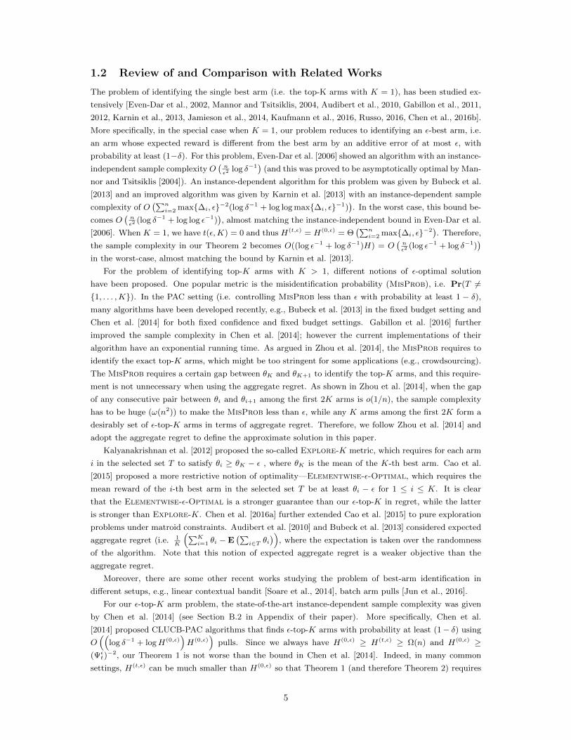
1.2 Review of and Comparison with Related Works

The problem of identifying the single best arm (i.e. the top-K arms with K = 1), has been studied ex-

tensively [Even-Dar et al., 2002, Mannor and Tsitsiklis, 2004, Audibert et al., 2010, Gabillon et al., 2011,

2012, Karnin et al., 2013, Jamieson et al., 2014, Kaufmann et al., 2016, Russo, 2016, Chen et al., 2016b].

More specifically, in the special case when K = 1, our problem reduces to identifying an ε-best arm, i.e.

an arm whose expected reward is different from the best arm by an additive error of at most ε, with

probability at least (1−δ). For this problem, Even-Dar et al. [2006] showed an algorithm with an instance-

independent sample complexity O(nε2

log δ−1)

(and this was proved to be asymptotically optimal by Man-

nor and Tsitsiklis [2004]). An instance-dependent algorithm for this problem was given by Bubeck et al.

[2013] and an improved algorithm was given by Karnin et al. [2013] with an instance-dependent sample

complexity of O(∑n

i=2 max∆i, ε−2(log δ−1 + log log max∆i, ε−1)). In the worst case, this bound be-

comes O(nε2

(log δ−1 + log log ε−1)), almost matching the instance-independent bound in Even-Dar et al.

[2006]. When K = 1, we have t(ε,K) = 0 and thus H(t,ε) = H(0,ε) = Θ(∑n

i=2 max∆i, ε−2). Therefore,

the sample complexity in our Theorem 2 becomes O((log ε−1 + log δ−1)H) = O(nε2

(log ε−1 + log δ−1))

in the worst-case, almost matching the bound by Karnin et al. [2013].

For the problem of identifying top-K arms with K > 1, different notions of ε-optimal solution

have been proposed. One popular metric is the misidentification probability (MisProb), i.e. Pr(T 6=1, . . . ,K). In the PAC setting (i.e. controlling MisProb less than ε with probability at least 1 − δ),many algorithms have been developed recently, e.g., Bubeck et al. [2013] in the fixed budget setting and

Chen et al. [2014] for both fixed confidence and fixed budget settings. Gabillon et al. [2016] further

improved the sample complexity in Chen et al. [2014]; however the current implementations of their

algorithm have an exponential running time. As argued in Zhou et al. [2014], the MisProb requires to

identify the exact top-K arms, which might be too stringent for some applications (e.g., crowdsourcing).

The MisProb requires a certain gap between θK and θK+1 to identify the top-K arms, and this require-

ment is not unnecessary when using the aggregate regret. As shown in Zhou et al. [2014], when the gap

of any consecutive pair between θi and θi+1 among the first 2K arms is o(1/n), the sample complexity

has to be huge (ω(n2)) to make the MisProb less than ε, while any K arms among the first 2K form a

desirably set of ε-top-K arms in terms of aggregate regret. Therefore, we follow Zhou et al. [2014] and

adopt the aggregate regret to define the approximate solution in this paper.

Kalyanakrishnan et al. [2012] proposed the so-called Explore-K metric, which requires for each arm

i in the selected set T to satisfy θi ≥ θK − ε , where θK is the mean of the K-th best arm. Cao et al.

[2015] proposed a more restrictive notion of optimality—Elementwise-ε-Optimal, which requires the

mean reward of the i-th best arm in the selected set T be at least θi − ε for 1 ≤ i ≤ K. It is clear

that the Elementwise-ε-Optimal is a stronger guarantee than our ε-top-K in regret, while the latter

is stronger than Explore-K. Chen et al. [2016a] further extended Cao et al. [2015] to pure exploration

problems under matroid constraints. Audibert et al. [2010] and Bubeck et al. [2013] considered expected

aggregate regret (i.e. 1K

(∑Ki=1 θi −E

(∑i∈T θi

)), where the expectation is taken over the randomness

of the algorithm. Note that this notion of expected aggregate regret is a weaker objective than the

aggregate regret.

Moreover, there are some other recent works studying the problem of best-arm identification in

different setups, e.g., linear contextual bandit [Soare et al., 2014], batch arm pulls [Jun et al., 2016].

For our ε-top-K arm problem, the state-of-the-art instance-dependent sample complexity was given

by Chen et al. [2014] (see Section B.2 in Appendix of their paper). More specifically, Chen et al.

[2014] proposed CLUCB-PAC algorithms that finds ε-top-K arms with probability at least (1− δ) using

O((

log δ−1 + logH(0,ε))H(0,ε)

)pulls. Since we always have H(0,ε) ≥ H(t,ε) ≥ Ω(n) and H(0,ε) ≥

(Ψεt)−2, our Theorem 1 is not worse than the bound in Chen et al. [2014]. Indeed, in many common

settings, H(t,ε) can be much smaller than H(0,ε) so that Theorem 1 (and therefore Theorem 2) requires

5

much less sample complexity. We explain this argument in more details as follows.

In many real-world applications, it is common to assume the arms θi are sampled from a prior distri-

bution D over [0, 1] with cumulative distribution function FD(θ). In fact, this is the most fundamental

assumption in Bayesian multi-armed bandit literature (e.g., best-arm identification in Bayesian setup

Russo [2016]). In crowdsourcing applications, Chen et al. [2015] and Abbasi-Yadkori et al. [2015] also

made this assumption for modeling workers’ accuracy, which correspond to the expected rewards. Under

this assumption, it is natural to let θi be the (1− in

) quantile of the distribution D, i.e. F−1D (1− i

n). If the

prior distribution D’s probability density function fD = dFDdθ

has bounded value (a few common examples

include uniform distribution over [0, 1], Beta distribution, or the truncated Gaussian distribution), the

arms’ mean rewards θini=1 can be characterized by the following property with c = O(1).

Definition 1 We call a set of n arms θ1 ≥ θ2 ≥ · · · ≥ θn c-spread (for some c ≥ 1) if for all i, j ∈ [n]

we have |θi − θj | ∈[|i−j|cn

, c|i−j|n

].

The following lemma upper-bounds H(t,ε) for O(1)-spread arms, and shows the improvement of our

algorithms compared to Chen et al. [2014] on O(1)-spread arms.

Lemma 1 Given a set of n c-spread arms, let K = γn ≤ n2

. When c = O(1) and γ = Ω(1), we have

H(t,ε) = O(n/√ε). In contrast, H(0,ε) = Ω(n/ε) for O(1)-spread arms and every K ∈ [n].

Proof : Given a set of n c-spread arms, we have t+1cn≤ ∆K−t ≤ c(t+1)

nand t+1

cn≤ ∆K+t+1 ≤ c(t+1)

n.

Therefore t = t(ε,K) ∈ [√Knε/c,

√cKnε − 1] = [

√γε/cn,

√cγεn − 1], and Ψt ≥ t+1

cn≥√γε/c3.

Therefore

H(t,ε) ≤ O(1)

n∑i=1

min

ci

n,Ψt

−2

≤ O

(t ·Ψ−2

t +

n∑i=t+1

(i

cn

)−2)

= O(t ·Ψ−2

t + c2n2/t)

= O(√cγεn) · c

3

γε+O

(c2n√γε/c

)= O(c3.5γ−0.5) · n√

ε.

One the other hand, we have

H(0,ε) ≥n−K∑i=1

min∆−2i+K , ε

−2 ≥n/2∑i=1

min

n2

c2i2, ε−2

=

[εn/c]∑i=1

ε−2 +

n/2∑[εn/c]+1

n2

c2i2= Ω

( ncε

).

2 An Instance Dependent Algorithm for ε-top-K Arms

In this section, we show Theorem 1 by proving the following theorem.

Theorem 4 Algorithm 1 computes ε-top-K arms with probability at least 1 − δ, and pulls the arms at

most

O

((log log(∆ε

t)−1 + logn+ log δ−1) n∑

i=1

min(∆i)−2, (∆ε

t)−2

)times, where t ∈ 0, 1, 2, . . . ,K−1 is the largest integer satisfying ∆K−t·t ≤ Kε, and ∆ε

t = max(ε,∆K−t).

Note that Theorem 4 implies Theorem 1 because of the following reasons: 1) t defined in Theorem 4

is always at least t(ε,K) defined in (3); and 2) ∆εt ≥ Ψε

t ≥ ε.Algorithm 1 is similar to the accept-reject types of algorithms in e.g. Bubeck et al. [2013]. The

algorithm goes by rounds for r = 1, 2, 3, . . . , and keeps at set of undecided arms Sr ⊆ [n] at Round r.

6

Algorithm 1: AdaptiveTopK(n, ε,K, δ)

Input: n: number of arms; K and ε: parameters in ε-top-K arms; δ: error probabilityOutput: ε-top-K arms

1 Let r denote the current round, initialized to be 0. Let Sr ⊆ [n] denote the set of candidate arms atround r. S1 is initialized to be [n]. Set A,B ← ∅

2 ∆← 2−r

3 while 2 ·∆ · (K − |A|) > εK do4 r ← r + 1

5 Pull each arm in Sr by ∆−2 ln 2nr2

δ times, and let θri be the empirical-mean

6 Define θa(Sr) and θb(Sr) be the (K − |A|+ 1)th and (K − |A|)th largest empirical-means in Sr,and define

∆i(Sr) = max(θri − θa(Sr), θb(Sr)− θri

)(7)

7 while maxi∈Sr ∆i(Sr) > 2 ·∆ do

8 x← arg maxi∈Sr ∆i(Sr)

9 if θrx > θa(Sr) then10 A← A ∪ x11 else12 B ← B ∪ x13 Sr ← Sr\x14 Sr+1 ← Sr15 ∆← 2−r

16 Set A′ as the (K − |A|) arms with the largest empirical-means in Sr+1

17 return A ∪A′

All other arms (in [n] \ Sr) are either accepted (in A) or rejected (in B). At each round, all undecided

arms are pulled by equal number of times. This number is designed in a way such that the event E ,

defined to be the empirical means of all arms within a small neighborhood of their true means, happens

with probability 1 − δ (See Definition 2 and Claim 1). Note that E is defined for all rounds and the

length of the neighborhood becomes smaller as the algorithm proceeds. We are able to prove that when

E happens, the algorithm returns the desired set of ε-top-K armsand has small query complexity.

To prove the correctness of the algorithm, we first show that when conditioning on E , the algorithm

always accepts a top-K arm in A (Lemma 3) and rejects a non-top-K arm in B (Lemma 4). The key

observation here is that our algorithm never introduces any regret due to arms in A and B. We then use

the key Lemma 5 to upper bound the regret that may be introduced due to the remaining arms. Once

this upper bound is not more than εK (i.e. the total budget for regret), we can choose the remaining

(K − |A|) arms without further samplings. Details about this analysis can be found in Section 2.1.

We analyze of the query complexity of our algorithm in Section 2.2. We establish data-dependent

bound by relating the number of pulls to each arms to both their ∆i’s and ∆K−t (Lemma 6 and Lemma 7).

2.1 Correctness of Algorithm 1

We first define an event E which we will condition on in the rest of the analysis.

Definition 2 Let E be the event that |θri − θi| < 2−r for all r ≥ 1 and i ∈ Sr.

Claim 1 Pr[E ] ≥ 1− δ.

7

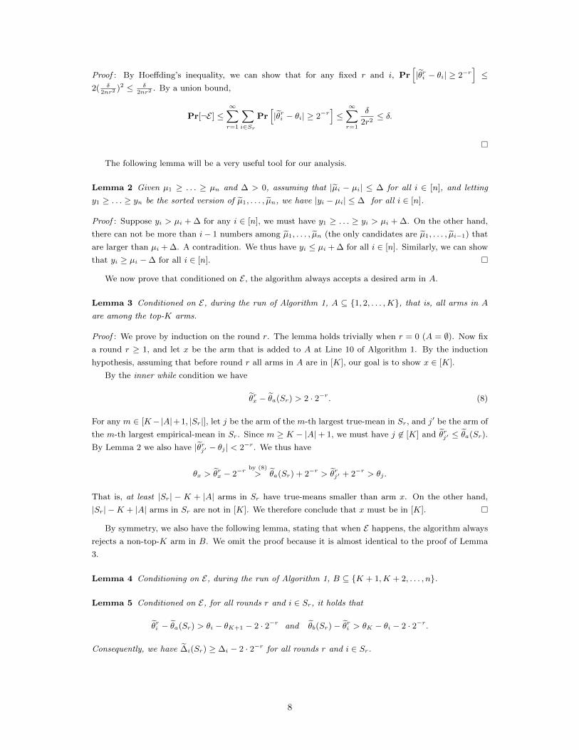
Proof : By Hoeffding’s inequality, we can show that for any fixed r and i, Pr[|θri − θi| ≥ 2−r

]≤

2( δ2nr2

)2 ≤ δ2nr2

. By a union bound,

Pr[¬E ] ≤∞∑r=1

∑i∈Sr

Pr[|θri − θi| ≥ 2−r

]≤∞∑r=1

δ

2r2≤ δ.

The following lemma will be a very useful tool for our analysis.

Lemma 2 Given µ1 ≥ . . . ≥ µn and ∆ > 0, assuming that |µi − µi| ≤ ∆ for all i ∈ [n], and letting

y1 ≥ . . . ≥ yn be the sorted version of µ1, . . . , µn, we have |yi − µi| ≤ ∆ for all i ∈ [n].

Proof : Suppose yi > µi + ∆ for any i ∈ [n], we must have y1 ≥ . . . ≥ yi > µi + ∆. On the other hand,

there can not be more than i− 1 numbers among µ1, . . . , µn (the only candidates are µ1, . . . , µi−1) that

are larger than µi + ∆. A contradition. We thus have yi ≤ µi + ∆ for all i ∈ [n]. Similarly, we can show

that yi ≥ µi −∆ for all i ∈ [n].

We now prove that conditioned on E , the algorithm always accepts a desired arm in A.

Lemma 3 Conditioned on E, during the run of Algorithm 1, A ⊆ 1, 2, . . . ,K, that is, all arms in A

are among the top-K arms.

Proof : We prove by induction on the round r. The lemma holds trivially when r = 0 (A = ∅). Now fix

a round r ≥ 1, and let x be the arm that is added to A at Line 10 of Algorithm 1. By the induction

hypothesis, assuming that before round r all arms in A are in [K], our goal is to show x ∈ [K].

By the inner while condition we have

θrx − θa(Sr) > 2 · 2−r. (8)

For any m ∈ [K−|A|+1, |Sr|], let j be the arm of the m-th largest true-mean in Sr, and j′ be the arm of

the m-th largest empirical-mean in Sr. Since m ≥ K − |A|+ 1, we must have j 6∈ [K] and θrj′ ≤ θa(Sr).

By Lemma 2 we also have |θrj′ − θj | < 2−r. We thus have

θx > θrx − 2−rby (8)> θa(Sr) + 2−r > θrj′ + 2−r > θj .

That is, at least |Sr| − K + |A| arms in Sr have true-means smaller than arm x. On the other hand,

|Sr| −K + |A| arms in Sr are not in [K]. We therefore conclude that x must be in [K].

By symmetry, we also have the following lemma, stating that when E happens, the algorithm always

rejects a non-top-K arm in B. We omit the proof because it is almost identical to the proof of Lemma

3.

Lemma 4 Conditioning on E, during the run of Algorithm 1, B ⊆ K + 1,K + 2, . . . , n.

Lemma 5 Conditioned on E, for all rounds r and i ∈ Sr, it holds that

θri − θa(Sr) > θi − θK+1 − 2 · 2−r and θb(Sr)− θri > θK − θi − 2 · 2−r.

Consequently, we have ∆i(Sr) ≥ ∆i − 2 · 2−r for all rounds r and i ∈ Sr.

8

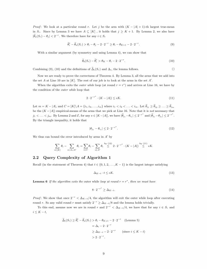
Proof : We look at a particular round r. Let j be the arm with (K − |A| + 1)-th largest true-mean

in Sr. Since by Lemma 3 we have A ⊆ [K] , it holds that j ≥ K + 1. By Lemma 2, we also have

|θa(Sr)− θj | < 2−r. We therefore have for any i ∈ Sr

θri − θa(Sr) > θi − θj − 2 · 2−r ≥ θi − θK+1 − 2 · 2−r. (9)

With a similar argument (by symmetry and using Lemma 4), we can show that

θb(Sr)− θri > θK − θi − 2 · 2−r. (10)

Combining (9), (10) and the definitions of ∆i(Sr) and ∆i, the lemma follows.

Now we are ready to prove the correctness of Theorem 4. By Lemma 3, all the arms that we add into

the set A at Line 10 are in [K]. The rest of our job is to look at the arms in the set A′.

When the algorithm exits the outer while loop (at round r = r∗) and arrives at Line 16, we have by

the condition of the outer while loop that

2 · 2−r∗· (K − |A|) ≤ εK. (11)

Let m = K − |A|, and C = [K]\A = i1, i2, . . . , im where i1 < i2 < . . . < im. Let θj1 ≥ θj2 ≥ . . . ≥ θjmbe the (K − |A|) empirical-means of the arms that we pick at Line 16. Note that it is not necessary that

j1 < . . . < jm. By Lemma 2 and E , for any s ∈ [K−|A|], we have |θjs−θis | ≤ 2−r∗

and |θjs−θjs | ≤ 2−r∗.

By the triangle inequality, it holds that

|θjs − θis | ≤ 2 · 2−r∗. (12)

We thus can bound the error introduced by arms in A′ by

∑i∈[K]

θi −∑

i∈A∪A′θi =

∑i∈C

θi −∑i∈A′

θiby (12)

≤ 2 · 2−r∗· (K − |A|)

by (11)

≤ εK.

2.2 Query Complexity of Algorithm 1

Recall (in the statement of Theorem 4) that t ∈ 0, 1, 2, . . . ,K − 1 is the largest integer satisfying

∆K−t · t ≤ εK. (13)

Lemma 6 If the algorithm exits the outer while loop at round r = r∗, then we must have

8 · 2−r∗≥ ∆K−t. (14)

Proof : We show that once 2−r < ∆K−t/4, the algorithm will exit the outer while loop after executing

round r. So any valid round r must satisfy 2−r ≥ ∆K−t/8 and the lemma holds trivially.

To this end, assume now we are in round r and 2−r < ∆K−t/4, we have that for any i ∈ Sr and

i ≤ K − t,

∆i(Sr) ≥ θri − θa(Sr) > θi − θK+1 − 2 · 2−r (Lemma 5)

= ∆i − 2 · 2−r

≥ ∆K−t − 2 · 2−r (since i ≤ K − t)

> 2 · 2−r.

9

Thus the condition of the inner while loop is satisfied, which means that all arms i with i ≤ K − t will

be added into A. Therefore we have |A| ≥ K− t when the algorithm exits the inner while loop. We then

have

2 · 2−r · (K − |A|) ≤ 2 · 2−r · t < 1

2∆K−t · t

by (13)

≤ εK/2 ≤ εK,

so the algorithm exits the outter loop.

Lemma 7 For any arm i, let ri be the round where arm i is removed from the candidate set if this ever

happens; otherwise set ri = r∗. We must have

8 · 2−ri ≥ ∆i. (15)

Proof : Suppose for contradiction that 8 · 2−ri < ∆i. By Lemma 5, we have

∆i(Sri−1) ≥ ∆i − 2 · 2−(ri−1) > 8 · 2−ri − 2 · 2−(ri−1) = 2 · 2−(ri−1).

This means that arm i would have been added either to A or B at or before round (ri − 1), which

contradicts to the fact that i ∈ Sri .

With Lemma 6 and Lemma 7, we are ready to analyze the query complexity of the algorithm in

Theorem 4. We can bound the number of pulls on each arm i by at most

ri∑j=1

22j · log(2nj2/δ) ≤ O(log(ri · nδ−1) · 22ri

). (16)

Now let us upper-bound the RHS of (16). First, if i ∈ A, then by (15) we know that ri ≤ log2 ∆−1i +O(1).

Second, by (14) we have ri ≤ r∗ ≤ log2 ∆−1K−t +O(1). Third, since 2−r

∗≥ ε/2 (otherwise the algorithm

will exit the outer while loop), we have ri ≤ r∗ ≤ log2 ε−1 + O(1). To summarize, we have ri ≤

log2 min∆−1i ,∆−1

K−t, ε−1 + O(1) = log2 min∆−1

i , (∆εt)−1 (recall that ∆ε

t = maxε,∆K−t). We thus

can upper-bound the RHS of (16) by

O((log log(∆ε

t)−1 + logn+ log δ−1) ·min(∆i)

−2, (∆εt)−2).

The total cost is a summation over all n arms.

3 An Improved Algorithm for ε-top-K Arms

In this section, we present the improved algorithm for identifying the ε-top-K arms and prove that the

algorithm succeeds with probability 1 − δ with query complexity O((log ε−1 + log δ−1)H(t,ε)) (Theo-

rem 6). This algorithm reduces the logn factor in the query complexity of Algorithm 1 to log ε−1 and is

substantially more complex than Algorithm 1.

The main procedure of the improved algorithm is described in Algorithm 5. For this algorithm, we

that assume K ≤ n/2. For the case where K > n/2, we can apply the same algorithm to identify the

ε-bottom-(n−K) arms and report the rest arms to be the ε-top-K arms. Similarly to Algorithm 1, the

improved algorithm also goes by rounds and keeps a set A of accepted arms, a set B of rejected arms,

and a set S of undecided arms. However, we can no longer guarantee that all the arms accepted in A

and rejected in B are correctly classified – otherwise, we need to apply a union bound over all arms and

this would incur an extra logn factor. To solve this problem, we have to allow a few number of mistakes.

We now illustrate the high-level idea as follows.

10

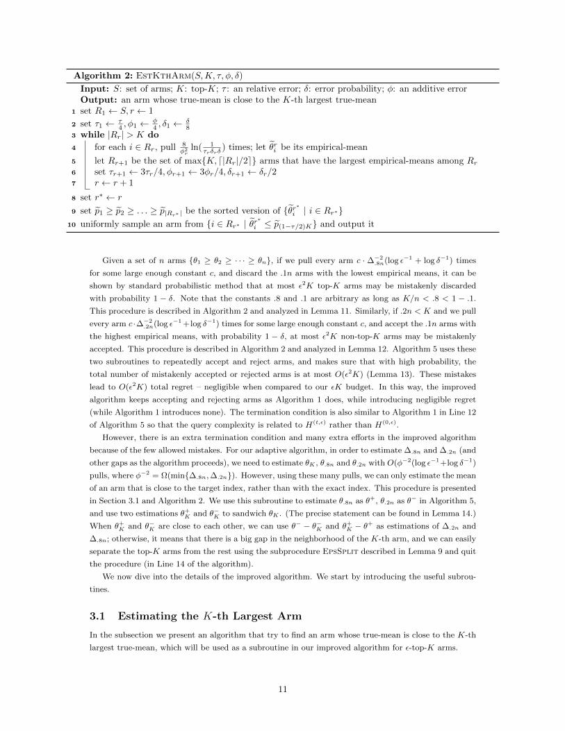
Algorithm 2: EstKthArm(S,K, τ, φ, δ)

Input: S: set of arms; K: top-K; τ : an relative error; δ: error probability; φ: an additive errorOutput: an arm whose true-mean is close to the K-th largest true-mean

1 set R1 ← S, r ← 1

2 set τ1 ← τ4 , φ1 ←

φ4 , δ1 ←

δ8

3 while |Rr| > K do

4 for each i ∈ Rr, pull 8φ2r

ln( 1τrδrδ

) times; let θri be its empirical-mean

5 let Rr+1 be the set of maxK, d|Rr|/2e arms that have the largest empirical-means among Rr6 set τr+1 ← 3τr/4, φr+1 ← 3φr/4, δr+1 ← δr/27 r ← r + 1

8 set r∗ ← r

9 set p1 ≥ p2 ≥ . . . ≥ p|Rr∗ | be the sorted version of θr∗i | i ∈ Rr∗10 uniformly sample an arm from i ∈ Rr∗ | θr

∗

i ≤ p(1−τ/2)K and output it

Given a set of n arms θ1 ≥ θ2 ≥ · · · ≥ θn, if we pull every arm c · ∆−2.8n(log ε−1 + log δ−1) times

for some large enough constant c, and discard the .1n arms with the lowest empirical means, it can be

shown by standard probabilistic method that at most ε2K top-K arms may be mistakenly discarded

with probability 1 − δ. Note that the constants .8 and .1 are arbitrary as long as K/n < .8 < 1 − .1.

This procedure is described in Algorithm 2 and analyzed in Lemma 11. Similarly, if .2n < K and we pull

every arm c ·∆−2.2n(log ε−1 +log δ−1) times for some large enough constant c, and accept the .1n arms with

the highest empirical means, with probability 1 − δ, at most ε2K non-top-K arms may be mistakenly

accepted. This procedure is described in Algorithm 2 and analyzed in Lemma 12. Algorithm 5 uses these

two subroutines to repeatedly accept and reject arms, and makes sure that with high probability, the

total number of mistakenly accepted or rejected arms is at most O(ε2K) (Lemma 13). These mistakes

lead to O(ε2K) total regret – negligible when compared to our εK budget. In this way, the improved

algorithm keeps accepting and rejecting arms as Algorithm 1 does, while introducing negligible regret

(while Algorithm 1 introduces none). The termination condition is also similar to Algorithm 1 in Line 12

of Algorithm 5 so that the query complexity is related to H(t,ε) rather than H(0,ε).

However, there is an extra termination condition and many extra efforts in the improved algorithm

because of the few allowed mistakes. For our adaptive algorithm, in order to estimate ∆.8n and ∆.2n (and

other gaps as the algorithm proceeds), we need to estimate θK , θ.8n and θ.2n with O(φ−2(log ε−1+log δ−1)

pulls, where φ−2 = Ω(min∆.8n,∆.2n). However, using these many pulls, we can only estimate the mean

of an arm that is close to the target index, rather than with the exact index. This procedure is presented

in Section 3.1 and Algorithm 2. We use this subroutine to estimate θ.8n as θ+, θ.2n as θ− in Algorithm 5,

and use two estimations θ+K and θ−K to sandwich θK . (The precise statement can be found in Lemma 14.)

When θ+K and θ−K are close to each other, we can use θ− − θ−K and θ+

K − θ+ as estimations of ∆.2n and

∆.8n; otherwise, it means that there is a big gap in the neighborhood of the K-th arm, and we can easily

separate the top-K arms from the rest using the subprocedure EpsSplit described in Lemma 9 and quit

the procedure (in Line 14 of the algorithm).

We now dive into the details of the improved algorithm. We start by introducing the useful subrou-

tines.

3.1 Estimating the K-th Largest Arm

In the subsection we present an algorithm that try to find an arm whose true-mean is close to the K-th

largest true-mean, which will be used as a subroutine in our improved algorithm for ε-top-K arms.

11

Theorem 5 For a set of arms S = θ1 ≥ . . . ≥ θ|S|, there is an algorithm, denoted by EstKthArm(S,K, τ, φ, δ),

that outputs an arm i such that θi ∈ [θK − φ, θ(1−τ)K + φ] with probability at least 1 − δ, using

O(|S|φ2 · (log τ−1 + log δ−1)

)pulls in total.

We described the algorithm in Algorithm 2. In the high level, the algorithm works in rounds, and in

each round it tries to find the top half arms in the current set, and discard the rest. We continue until

there are at most K arms left, and then we choose the output arm randomly from those with the lowest

empirical-means in the remaining arms. We are going to prove the following theorem.

3.1.1 Correctness of Algorithm 2

The following lemma is the key to the proof of correctness.

Lemma 8 With probability at least 1− δ/4, we have that

|i ∈ Rr∗ | θi < θK − φ| ≤ τδK/4.

Proof : We first define a few notations.

• Hr = i ∈ S | θi ≥ θK −∑`∈[r] φ`.

• Lr = S\Hr.

• kr = (1−∑`∈[r] τ`δ/4)K.

• For any i ∈ [n] and round r, let Xri = 1|θri − θi| ≥ φr/2 where θri is the empirical-mean of arm i

at round r (after been pulled by 8φ2r

ln( 1τrδrδ

) times at Line 4).

• R′r ⊆ Rr: the top kr−1 arms in Rr with the largest true-means.

• Ar = i ∈ R′r | Xi = 0. Ar ⊆ R′r ⊆ Rr.

• Cr = i ∈ Lr ∩Rr | Xi = 1. Cr ⊆ Rr.

We define the following event. Intuitively, it tells that most of the arms we put in Rr for the next

round processing fall into the set Hr of high true-means.

Er(r ≥ 2) : |Hr−1 ∩Rr| ≤ kr−1,

and we define E1 to be an always true event. We will prove by induction the following inequality.

Pr[Er+1 | ¬Er] ≤ δr for each r ≥ 1. (17)

We focus a particular round r ≥ 1. Define event EA : |Ar| ≤ kr, and event EC : |Cr| ≤ |Rr+1| − kr.

Claim 2 Pr[EA | ¬Er] ≤ δr/4.

Proof : By a Hoeffding’s inequality, we have for each i ∈ Rr, we have Pr[Xri = 1] ≤ τrδrδ/16. We bound

the probability the EA happens by a Markov’s inequality.

Pr[EA | ¬Er] = Pr[|Ar| ≤ kr | ¬Er] =Pr[|R′r| − |Ar| ≥ kr−1 − kr | ¬Er]

≤E[∑

i∈R′rXi | ¬Er]

]kr−1 − kr

=E[∑

i∈R′rXi]

kr−1 − kr

≤τrδrδkr−1/16

τrδK/4≤ τrδrδK/16

τrδK/4

=δr/4.

12

Claim 3 Pr[EC | ¬EA,¬Er] ≤ 3δr/4.

Proof :

Pr[EC | ¬EA,¬Er] =Pr[|Cr| ≤ |Rr+1| − kr | ¬EA,¬Er]

≤E[|Cr| | ¬EA,¬Er]|Rr+1| − kr

(Markov’s inequality) (18)

≤ (|Rr| − kr) · τrδδr/16

|Rr+1| − kr(19)

≤ (2 |Rr+1| − kr) · τrδδr/16

|Rr+1| − kr(20)

≤3δr/4, (21)

where (18) to (19) is due to the fact that conditioned on ¬Er, we have

|Cr| ≤ |Lr ∩Rr| ≤ |Lr−1 ∩Rr| = |Rr| − |Hr−1 ∩Rr|¬Er≤ |Rr| − kr−1 ≤ |Rr| − kr.

And (20) to (21) is due to the following: If |Rr+1| ≥ 2K, then since kr ≤ K we have2|Rr+1|−kr|Rr+1|−kr ≤ 3.

Otherwise if |Rr+1| < 2K, by the definition of kr, we have

|Rr+1| − kr > K − kr =∑

i∈[r−1]

τiδ/4 ≥ τrδK/3.

On the other hand, we have 2 |Rr+1| − kr ≤ 4K. We thus have (21) ≤ 3δr/4.

Claim 4 Conditioned on EC ,¬EA,¬Er, we have |Hr ∩Rr+1| ≥ kr, or, Pr[Er+1 | EC ,¬EA,¬Er] = 0.

Proof : First, conditioned on ¬Er, we have

Ar ⊆ R′r ⊆ Hr−1. (22)

We prove the claim by analyzing two cases.

1. ((Lr ∩Rr)\Cr) ∩Rr+1 = ∅. We thus have (Lr ∩Rr+1) ⊆ Cr, which implies

|Hr ∩Rr+1| ≥ |Rr+1| − |Lr ∩Rr+1| ≥ |Rr+1| − |Cr|EC≥ kr.

2. ((Lr ∩Rr)\Cr) ∩Rr+1 6= ∅. We can show that

Ar ⊆ Rr+1 (23)

Indeed, for any j ∈ Ar(⊆ Hr−1 by (22)) and any i ∈ (Lr ∩ Rr)\Cr, we have θj > θi, since

θj ≥ θK −∑`∈[r−1] φ`, while θi < θK −

∑`∈[r] φ` (by the definition of Lr). Thus conditioned on

¬EA, (22) and (23) we have

|Hr ∩Rr+1| ≥ |Hr−1 ∩Rr+1| ≥ |Ar| ≥ kr.

Now we try to prove (17).

Pr[Er+1 | ¬Er] =Pr[EA | ¬Er] + Pr[EC | ¬EA,¬Er] + Pr[Er+1 | ¬EA,¬Er]

13

≤δ/4 + 3δ/4 + 0 (Claim 2, Claim 3 and Claim 4)

=δ.

Using (17) and summing over all ` ∈ [r − 1], we have Pr[Er] ≤∑`∈[r−1] δi < δ/4 for any r ≥ 2.

In other words, with probability at least 1 − δ/4, we have for any r ≤ r∗, |Hr−1 ∩Rr| ≥ kr−1, or

|Lr−1 ∩Rr| ≤ K − kr−1 ≤ 1− (1− τδK/4) = τδK/4, which gives the lemma.

Now we are ready to prove the correctness of Theorem 5. Let

• P = i ∈ Rr∗ | θr∗i > p(1−τ/2)K.

• Q = Rr∗\P .

• L∗ = i ∈ Rr∗ | θi < θK − φ.

• For each i ∈ Rr∗ , let Yi = 1|θr∗i − θi| > φ/2.

Claim 5 Pr[θa ≥ θK − φ] ≥ 1− 3δ/4.

Proof : At Line 10 of Algorithm 2, we randomly sampled an arm a from Q. Since |Q| ≥ τK and

Pr[|L∗| < τδK/4] > 1− δ/4 (by Lemma 8), we have

Pr[a ∈ L∗] ≤ Pr[|L∗| ≥ τδK/4] + Pr[a ∈ L∗ | |L∗| < τδK/4] ≤ δ/4 +τδK/4

τK/2= 3δ/4. (24)

Claim 6 Pr[θa ≤ θ(1−τ)K + φ] ≥ 1− δ/4.

Proof : We first show that if Ya = 0 and∑i∈P Yi ≤ τK/2, then θa ≤ θ(1−τ)K +φ. Let P0 = i ∈ P | Yi =

0. By definition of P and the assumption that∑i∈P Yi ≤ τK/2, we have |P0| ≥ |P |−τK/2 ≥ (1−τ)K.

Let b be the arm in P0 that has the minimum true-mean, then we must have

θb ≤ θ|P0| ≤ θ(1−τ)K . (25)

Since a ∈ Q and b ∈ P , we have θa ≤ θb, which, together with the facts that Ya = Yb = 0 and (25), gives

θa ≤ θb + φ ≤ θ(1−τ)K + φ.

We now bound the probabilities that the two conditions hold. By a Hoeffding’s inequality, we have

Pr[Yi = 1] ≤ τδ/16 for any i ∈ Rr∗ . By a Markov’s inequality and the fact that P ⊆ Rr∗ (by definition),

we have

Pr

[∑i∈P

Yi > τK/2

]≤ Pr

∑i∈Rr∗

Yi > τK/2

≤ E[∑

i∈Rr∗Yi]

τK/2≤ τδK/16

τK/2= δ/8.

We thus have Pr[(Ya = 0) ∧ (

∑i∈P Yi ≤ τK/2)

]≥ 1− δ/16− δ/8 ≥ 1− δ/4.

The correctness of Theorem 5 immediately follows from Claim 6 and Claim 5.

3.1.2 Complexity Algorithm 2

We can bound the total number of pulls of Algorithm 2 by simply summing up the number of pulls at

each round.

14

Algorithm 3: Elim(S,K, γ, φ, δ)

Input: S: set of arms; K: top-K; γ: fraction of arms; δ: error probability; φ: an additive error

Output: Set of arms T with |T | = |S|10 such that at most γK arms in T are in the top-K arms in S

1 For each arm i in S, pull cφ2 · (log γ−1 + log δ−1) for some large enough constant c. Let θi be the

empirical-mean of the i-th arm.2 return |T | arms in S with the smallest empirical-means.

O

log |S|/K∑r=1

|Rr|φ2r

log1

τrδrδ

=O

(∞∑r=1

2−r|S|(3/4)2rφ2

·(

log1

(3/4)rτ+ log

1

(1/2)rδ+ log

1

δ

))

=O

(|S|φ2

∞∑r=1

(8

9

)r·(r + log

1

τ+ log

1

δ

))

=O

(|S|φ2·(

log1

τ+ log

1

δ

)).

The last equality follows from the fact that∑∞r=1(8/9)r · r = O(1).

Lemma 8 also implies the following lemma.

Lemma 9 For a set of arms S = θ1 ≥ . . . ≥ θ|S| such that θ(1−τ)K − θ(1+τ)K+1 ≥ φ, there is an

algorithm, denoted by EpsSplit(S,K, τ, φ, δ), that computes (2τ)-top-K correctly with probability at least

1− δ, using O(|S|φ2 · (log τ−1 + log δ−1)

)pulls in total.

Proof : To prove the lemma, we just need to replace “K” in Algorithm 2 to be “(1− τ)K”. By Lemma 8

we have with probability 1− δ that

|i ∈ Rr∗ | θi < θ(1−τ)K − φ| ≤ τδ(1− τ)K ≤ τδK.

Since θ(1−τ)K − θ(1+τ)K+1 ≥ φ we have

|i ∈ Rr∗ | θi < θ(1+τ)K+1| ≤ τδK.

Consequently,

|i ∈ Rr∗ | θi < θK| ≤ τK + τδK ≤ 2τK. (26)

Therefore we can just choose all arms in Rr∗ , together with K−|Rr∗ | arbitrary arms in the rest n−|Rr∗ |arms. By (26) the total average error is bounded by 2τK/K = 2τ .

3.2 The Improved Algorithm

In this section, we introduce an improved algorithm that removes the log(n)-factor in the sample com-

plexity.

We first introduce a few more subroutines (Lemma 10, Lemma 11, and Lemma 12) that will be useful

for our improved algorithm.

Lemma 10 [Zhou et al., 2014] For a set of arms S = θ1 ≥ . . . ≥ θ|S|, there is an algorithm, denoted

by OptMAI(S,K, ε, δ), that computes ε-top-K arms with probability 1− δ, with O(|S|ε2

log(1/δ))

pulls.

The following two lemmas show how to find a constant fraction of arms in the set of top-K arms and

a constant fraction of arms outside the set of top-K arms respectively.

15

Algorithm 4: ReverseElim(S,K, γ, φ, δ)

Input: S: set of arms; K: top-K; γ: fraction of arms; δ: error probability; φ: an additive error

Output: Set of arms T with |T | = |S|10 such that at most γK arms in T are in the top-(|S| −K) arms

in S1 For each arm i in S, pull c

φ2 · (log γ−1 + log δ−1) for some large enough constant c. Let θi be theempirical-mean of the i-th arm.

2 return |T | arms in S with the largest empirical-means.

Lemma 11 For a set of arms S = θ1 ≥ . . . ≥ θ|S| such that θK − θ |S|+K2

≥ φ, K ≤ 23|S|, there is

an algorithm, denoted by Elim(S,K, γ, φ, δ) in Algorithm 2, that computes T ⊆ S, |T | = |S|10

successfully

with probability 1− δ using O(|S|φ2 · (log γ−1 + log δ−1)

)pulls in total, such that at most γK arms in T

are in the top-K arms in S.

Proof : Let θi be the empirical-mean of arm i after being pulled by c· 1φ2 log 1

γδtimes for a sufficiently large

constant c. By a Hoeffding’s inequality, we have Pr[|θi − θi| ≥ φ/2

]≤ γδ/2. LetXi = 1|θi−θi| ≥ φ/2,

and thus E[Xi] ≤ γδ/2. Let X =∑i∈[K] Xi; we have E[X] ≤ γδK/2. By a Markov’s inequality, we have

that with probability at least 1 − δ/2, X ≤ γK. Consequently, with probability at least 1 − δ/2, there

are at most γK arms i ∈ [K] with θi ≤ θi − φ/2 ≤ θK − φ/2.

Let L = |S|+K2

+1, . . . , |S|. Since K ≤ 23|S|, we have |L| ≥ |S|

6. Using similar argument we can show

that with probability 1−δ/2, there are at least |S|10

arms i ∈ L with θi ≤ θi+φ/2 ≤ θ |S|+K2

+φ/2 ≤ θK−φ/2(since θK − θ |S|+K

2

≥ φ).

Therefore, if we choose T to be the |S|10

arms with the smallest empirical-means, then with probability

at least 1− δ, at most γK arms in T are in the top-K arms in S.

Lemma 12 For a set of arms S = θ1 ≥ . . . ≥ θ|S| such that θK2− θK ≥ φ, K ≥ |S|

3, there is

an algorithm, denoted by ReverseElim(S,K, γ, φ, δ) in Algorithm 2, that computes T ⊆ S, |T | = |S|10

successfully with probability 1− δ using O(|S|φ2 · (log γ−1 + log δ−1)

)pulls in total, such that at most γK

arms in T are in the bottom-(|S| −K) arms in S.

By symmetry, the proof to Lemma 12 is basically the same as that for Lemma 11,

Now we are ready to show our main result.

Theorem 6 Algorithm 5 computes ε-top-K arms with probability at least 1 − δ, and pulls the arms at

most

O

∑j∈[n]

min

(∆j)−2, (Ψε

t)−2(log

1

ε+ log

1

δ

) (27)

times, where t and Ψεt are defined in (3) and (5) respectively.

It is worthwhile to note that the proposed algorithm is mainly for the theoretical interest and is rather

complicated in terms of implementation. Thus, we omit the empirical study of this algorithm in the

experimental section.

In the rest of this section we prove Theorem 6 by showing the correctness of Algorithm 5 and the

analyzing its query complexity.

3.2.1 Correctness of Algorithm 5

Define E1 to be the event that all calls to the subroutine EstKthArm succeed.

16

Algorithm 5: ImprovedTopK(n,K, ε, δ)

Input: n: number of arms; K and ε: see the definition of ε-top-K arms; δ: error probability. AssumeK ≤ n/2

Output: ε-top-K arms1 set S ← [n], r ← 1, rφ ← 12 set A,B ← ∅3 set KL ← (1− ε2)K,KR ← (1 + ε2)K + 14 while S 6= ∅ do5 rφ ← rφ − 16 repeat7 rφ ← rφ + 1; φ← 2−rφ

8 θ+K ← EstKthArm(S,KR − |A| , ε2

100r2 , φ,δ

100(r+rφ)2

);

θ−K ← EstKthArm(S,KL − |A| , ε2

100r2 , φ,δ

100(r+rφ)2

)9 θ+ ← EstKthArm

(S, |S|+K−|A|2 , ε2

100r2 , φ,δ

100(r+rφ)2

);

θ− ← EstKthArm(S, K−|A|2 , ε2

100r2 , φ,δ

100(r+rφ)2

)10 until (10(K − |A|)φ < Kε) or (θ−K − θ

+K > 3φ) or

(K − |A| ≤ |S|2

)∧ (θ+K − θ+ > 3φ) or(

K − |A| > |S|2

)∧ (θ+K − θ+ > 3φ) ∧ (θ− − θ−K > 3φ)

11 if (10(K − |A|)φ < Kε) then12 return OptMAI

(S,K − |A| , φ, δ

100

)∪A

13 if (θ−K − θ+K > 3φ) then

14 return EpsSplit(S,K − |A| , KR−KLK−|A| , φ,

δ100

)∪A

15 U ← Elim(S,K − |A| , ε2

100r2 , φ,δ

100r2

)16 if (K − |A|) > |S|

2 then

17 V ← ReverseElim(S,K − |A| , ε2

100r2 , φ,δ

100r2

)18 r ← r + 1; S ← S\(U ∪ V ); A← A ∪ V ; B ← B ∪ U19 return A.

Claim 7 Pr[E1] ≥ 1− δ/10.

Proof : Note that (r + rφ) increases every time we call the four EstKthArm’s at Line 8 and Line 9.

Therefore by Theorem 5 we can bound the error probability of all calls to EstKthArm by 4·∑∞z=1

δ100z2

≤δ10.

Define E2 to be the event that all calls to the subroutines Elim and ReverseElim succeed. Since r

increases every time we call the two subroutines, by similar arguments we have:

Claim 8 Pr[E2] ≥ 1− δ/20.

Define E = E1 ∪ E2; we thus have Pr[E ] ≥ 1− δ/5.

We next show that the misclassified arms are negligible during the run of the algorithm.

Lemma 13 Conditioned on E, suppose that the conditions of Lemma 11 and Lemma 12 always hold

during the run of the Algorithm 5, then we always have

1. The number of non-top-K arms in A, denoted by ιA, is no more than ε2K40

.

17

2. The number of top-K arms in B, denoted by ιB, is no more than ε2K40

.

Proof : By Lemma 11 we have ιA ≤∑∞r=1

ε2

100r2· K ≤ ε2K

40. Similarly, by Lemma 12 we have ιB ≤∑∞

r=1ε2

100r2·K ≤ ε2K

40.

We now show that the conditions of Lemma 11 and Lemma 12 do hold. We first introducing a lemma

showing that θK is sandwiched by θ+K and θ−K during the run of Algorithm 5.

Lemma 14 Conditioned on E, at any point of the run of Algorithm 5, we have

θ−K + φ ≥ θK− ε2K

10

≥ θK ≥ θK+1 ≥ θK+1+ ε2K10

≥ θ+K − φ.

Proof : We consider a particular around r. The difference between θ+K and the fixed value θKR is generated

by calling of the subroutine EstKthArm at Line 8, which can be bounded by the the error introduced

when selecting the (KR − |A|)-th largest arm in S plus maxιA, ιB. By Theorem 5, Lemma 13 and E ,

we have θ+K ≤ θKR−τR + εR, where εR ≤ φ, and

τR ≤ τ · (KR − |A|) + maxιA, ιB ≤ε2

100r2· (1 + ε2)K +

ε2K

40≤ ε2K

20≤ KR −K −

ε2K

10.

We thus have θ+K ≤ θK+1+ ε2

10K

+ φ.

Similarly, by Theorem 5, Lemma 13 and E , we have θ−K ≥ θKL+τL − εL, where εL ≤ φ, and τL ≤maxιA, ιB ≤ ε2K

40≤ K −KL − ε2K

10. We thus have θ−K ≥ θK− ε2K

10

− φ.

We have the following immediate corollary.

Corollary 1 If θ−K − θ+K ≤ 3φ, then θK , θK+1 ∈ [θ+

K − φ, θ+K + 4φ] and θK , θK+1 ∈ [θ−K − 4φ, θ−K + φ].

In the following, for convenience, we always use S[i] to denote the true-mean of the i-th arm (sorted

decreasingly) in the current set S during the run of Algorithm 5, and use S[i..j] to denote the set of

true-means of the (i, i + 1, . . . , j)-th arms in S. Let K , K − |A|. We call S[1..K] the head of S, and

S[K + 1.. |S|] the tail of S. The following claim follows directly from Lemma 13 and Lemma 14.

Claim 9 At any point during the run of Algorithm 5, it holds that θK+ ε2K

40

≤ S[K] ≤ θK− ε2K

40

, and

consequently θ−K + φ ≥ S[K] ≥ θ+K − φ.

Lemma 15 Conditioned on E, the conditions of Lemma 11 always hold during the run of Algorithm 5,

that is, we have

S[K]− S[|S|+K

2

]≥ φ and K ≤ 2

3|S| . (28)

Proof : For the first item of (28), by Theorem 5 we have

S[|S|+K

2

]− φ ≤ θ+, (29)

which together with θ+K − θ

+ > 3φ (testing condition at Line 10) and S[K] ≥ θ+K − φ (Claim 9) give

S[K]− S[|S|+K

2

]≥ φ (by two triangle inequalities).

For the second item of (28), note that if K ≤ |S|2

, then K ≤ 23|S| holds directly. We thus consider

the case K > |S|2

. The observation is that at the beginning, before the first call to ReverseElim, we

must have called Elim a number of times; each time we remove |S|10

arms, most of which are from the

tail of S. After the first time when K > |S|2

, we call both Elim and ReverseElim, with the intention of

removing |S|10

arms from the tail and the head respectively. It may happen that after calling both Elim

and ReverseElim a few times, we again have K ≤ |S|2

, at which point we will again only call Elim until

18

the point that we are back to the case that K > |S|2

and then we will call both Elim and ReverseElim.

Basically, the two patterns ‘call Elim only’ and ‘call both Elim and ReverseElim’ interleave, and we

only need to consider one run of this interleaved sequence.

By Lemma 11 and Lemma 12 we know that at most ε2

100r2K arms in the head of S will be removed

when calling Elim, and at most ε2

100r2K arms in the tail of S will be removed when calling ReverseElim.

Therefore, the worst case for causing the imbalance between K and (|S| − K) is that each call of Elim

removes |S|10

from the tail of S, and each call of ReverseElim removes(|S|10− ε2

100r2K)

arms from the

head of S and ε2

100r2K arms from the tail of S. Note that the number of calls of Elim and ReverseElim

is bounded by O(log 1ε) since when reaching Line 15 we always have |S| ≥ Ω(φ) ≥ Ω(ε). We thus have

|S| − K|S| ≥

(1

2− 0.1

)·O(log 1/ε)∏

r=1

(1− ε2

100r2

)≥ 1

3,

which implies K ≤ 23|S|.

Lemma 16 Conditioned on E, the conditions of Lemma 12 always hold during the run of Algorithm 5,

that is, we have

S[K2

]− S[K] ≥ φ and K ≥ |S|

3. (30)

Proof : In Algorithm 5, when calling ReverseElim, we always have

θ− − θ−K > 3φ and K >|S|2. (31)

Thus K ≥ |S|3

follows directly. By Theorem 5 we have

S[K2

]+ φ ≥ θ−, (32)

which together with θ−−θ−K > 3φ (first item of (31)) and S[K] ≤ θ−K+φ (Claim 9), gives S[K2

]−S[K] ≥ φ

(by two triangle inequalities).

Lemma 15, Lemma 16 and Lemma 13 give the following corollary.

Corollary 2 Conditioned on E, during the run of Algorithm 5 we always have (1) the number of non-

top-K arms in A is no more than ιA = ε2K40

, and (2) the number of top-K arms in B is no more than

ιB = ε2K40

.

We now consider the boundary cases. At Line 11 when the condition is met, we have φ < εK10(K−|A|) ,

and thus with probability (1 − δ100

) the total error introduced by subroutine OptMAI at Line 12 is

bounded by (K − |A|)φ ≤ εK10

(Lemma 10). At Line 14, with probability (1− δ100

) the error introduced

by subroutine EpsSplit is bounded by 2 · KR−KLK−|A| · (K − |A|) ≤ 2 · 2ε2K = 4ε2K. (Lemma 9).

By E , Corollary 2, and the errors introduced by boundary cases, we have that with probability

1− δ5−2· δ

100≥ 1−δ, the total error introduced in our top-K estimation is at most ιA+ιB+ εK

10+4ε2K ≤ εK.

3.2.2 Complexity of Algorithm 5

In the whole analysis we assume that E holds. Recall that by definition ∆i = max(θi − θK+1, θK − θi),and t ∈ [K] is the largest integer such that ∆K−t · t ≤ Kε and ∆K+1+t · t ≤ Kε. Recall that Ψt =

min∆K−t,∆K+1+t, and Ψεt = max(ε,Ψt).

By Theorem 5, Lemma 11, Lemma 12, Lemma 10 and Lemma 9 we have: every call to EstKthArm

costsO(|S|φ2 log

rrφεδ

)pulls; every call to Elim and ReverseElim costsO

(|S|φ2 log r

εδ

); the call to OptMAI

19

costs O(|S|φ2 log 1

δ

); and the call to EpsSplit costs O

(|S|φ2 log K

εδK

)= O

(|S|φ2 log 1

εδ

). So our task is to

lower bound the value of φ when these subroutines are called, and the maximum values of rφ and r.

Lemma 17 Conditioned on E, at any point of the run of Algorithm 5, we have φ = Ω(Ψεt), and rφ =

O(log 1ε), r = O(log n

|S| ).

Proof : First, by the testing condition 10(K − |A|)φ < Kε at Line 10, together with the boundary cases

at Line 11-12 and the fact that φ← φ/2 at every update, it holds that

10(K − |A|) · 2φ ≥ Kε, (33)

which implies φ = Ω(ε) when we call all the subroutines.

We now show φ = Ω(Ψt). From the proof of Lemma 15 we know that during the run of the Algorithm

we always have K ≤ 2|S|3

. We focus on an arbitrary but fixed point during the run of the algorithm. By

Theorem 5 we have

S[|S|+K

2

]− φ ≤ θ+ ≤ S

[(1− ε2

100r2

)|S|+K

2

]+ φ, (34)

which, combined with the fact that K ≤ 2|S|3

, gives

S[|S|+K

2

]− φ ≤ θ+ ≤ S

[|S|+K−ε|S|

2

]+ φ. (35)

By (33) we haveε2K40≤ ε

40· 10K · 2φ ≤ εK

2. (36)

Applying Claim 9 on both sides of (34), together with (36) and K ≤ 2|S|3

we have

θK+|S|−K

2+ ε2K

40

− φ ≤ θ+ ≤ θK+|S|−K−ε|S|

2− ε2K

40

+ φ

⇒ θK+|S|−K

2+ εK

2

− φ ≤ θ+ ≤ θK+|S|−K−ε|S|

2− εK

2

+ φ

⇒ θ+ ∈ θK+η ± φ for an η ≥ |S|−K2− ε |S| ≥ 0.16 |S| . (37)

By symmetry, using a similar argument we can show that for a sufficiently small constant cη′ , we

have

θ− ∈ θK−η′ ± φ for an η′ ≥ cη′ |S| , (38)

We first consider the case where K − |A| ≤ |S|2

. We analyze the following two sub-cases.

1a) The case when η > t. We have:

φ ≥θ+K − θ

+

6(by the testing condition at Line 10 and φ← φ/2 at each update)

≥ (θK − 4φ)− (θK+η + φ)

6(by Corollary 1 and (37))

≥θK − 4φ− (θK+t+1 + φ)

6

≥Ψt − 5φ

6(by the definition of Ψt).

1b) The case when η ≤ t. We prove by contradiction. Suppose that φ ≤ Ψt/ct for a sufficiently large

constant ct, then

Ψt · t ≥ ctφ · η(37)

≥ ctφ · 0.16 |S|K≤ 2|S|

3

≥ ctφ · 0.16 · 1.5K(33)> Kε,

A contradition to the definition of t.

20

We then consider the case where K−|A| > |S|2

. Now by the testing condition at Line 10 and φ← φ/2

at each update, we know that at least one of the following inequality holds: φ ≥ θ+K−θ+

6; or φ ≥ θ−−θ−

K6

. If

the first inequality holds, the case-analysis above suffices. Otherwise, we know that the second inequality

holds, we analyze the following two sub-cases in a similar fashion.

2a) The case when η′ > t.

φ ≥θ− − θ−K

6

≥ (θK−η′ − φ)− (θK+1 + 4φ)

6(by Corollary 1 and (38))

≥ (θK−t − φ)− (θK+1 + 4φ)

6

≥Ψt − 5φ

6(by the definition of Ψt).

2b) The case when η′ ≤ t. This case is symmetric to Case 1b), and we omit here.

Since φ = 2−rφ , we immediately have rφ = O(log 1Ψεt

) = O(log 1ε). By the testing condition at Line 13,

and the fact that every time we call Elim and ReverseElim we remove a constant fraction of arms from

S, we thus have r = O(log n|S| ).

We now look at a particular call to Elim which removes 110

-fraction of arms in S, and the tail of S.

From the testing condition at Line 10 we know that

θ+K − θ

+ ≤ 3 · 2φ. (39)

From Corollary 1 we have that

θK ≤ θ+K + 4φ. (40)

From (39), (40) and the second inequality of (35), by applying two triangle inequalities we have

θK − S[|S|+K−ε|S|

2

]≤ 11φ, (41)

which implies that for all

j ∈ Q =[1.01K, |S|+K−ε|S|

2

](|Q| ≥ |S|

10since K ≤ 2|S|

3), (42)

letting m(j) ∈ [n] such that θm(j) = S[j], we have

∆m(j) = θK − S [j] ≤ 11φ. (43)

We thus can charge all the previous cost spent on the 110

-fraction of arms in S that are removed by Elim,

which is bounded by O(|S|φ2

(logdlog n

|S|e+ log 1ε

+ log 1δ

)), to

O

(∑j∈Q

1

∆2m(j)

(log

⌈log

n

m(j)−K

⌉+ log

1

ε+ log

1

δ

)), (44)

where we have used the fact that

|S| = Ω(j − K) (by (42))

≥ Ω(m(j)−K). (by (42), Corollary 2 and (36))

Note that it is possible that in multiple calls to Elim with parameters (S1, ·, ·, φ1, ·), . . . , (Sκ, ·, ·, φκ, ·)where φ1 ≥ . . . ≥ φκ, we charge the same item j ∈ Q1 ∩ . . . ∩ Qκ multiple times. However, since

21

φi+1 ≤ φi/2 for all i ∈ [κ− 1], the total charge on j is at most twice of that of the last charge (i.e., the

one with parameter φκ).

By symmetry, we can use the same arguments for ReverseElim and the head of S, and get a same

bound as (44) except that we need to replace m(j)−K with K −m(j). We thus conclude that the total

number of pulls can be bounded by

O

∑j∈[n]

1

∆2j

(log

⌈log

n∣∣j −K + 12

∣∣⌉

+ log1

ε+ log

1

δ

) . (45)

We know from Lemma 17 that we always have φ = Ω(Ψεt), we can thus “truncate” Expression (45) and

bound the total cost by

O

∑j∈[n]

1

max∆2j , (Ψ

εt)

2

(log

⌈log

n∣∣j −K + 12

∣∣⌉

+ log1

ε+ log

1

δ

) . (46)

Now we introduce the following lemma (the proof of which is deferred to the Appendix).

Lemma 18 If M > a1 ≥ . . . ≥ an ≥ 1, then∑i∈[n] ai log(n/i) ≤ O(dlogMe)

∑i∈[n] ai.

With Lemma 18 we can further simplify (46) to

O

∑j∈[n]

1

max∆2j , (Ψ

εt)

2

(log max

1

max∆2j , (Ψ

εt)

2 | j ∈ [n]

+ log

1

ε+ log

1

δ

)= O

∑j∈[n]

1

max∆2j , (Ψ

εt)

2

(log

1

ε+ log

1

δ

) .

4 A Lower Bound

In this section we prove Theorem 3. In Section 4.1, we introduce a lower-bound to a coin-tossing problem.

In Section 4.2, we reduce the proof of Theorem 3 to the coin-tossing problem.

4.1 The Coin-Tossing Problem

We say a coin is p-biased if the probability that a toss turns head is p, and we call p is the value of the

coin. Set η = 10−4.

Definition 3 (Coin-Tossing) In this problem, given a coin that may be (0.5 + η)-biased or (0.5 − η)-

biased, we want to know its exact value by tosses, and we are allowed to give up and output ‘unknown’

with probability at most 0.9.

We have the following theorem.

Theorem 7 Any algorithm that solves the coin-tossing problem correctly with probability (1 − ε) needs

Ω(log 1/ε) tosses.

Proof : Since the input is distributional we only need to focus on deterministic algorithms. Let m be the

total number of tosses of the coin, and let B = (B1, . . . , Bm) ∈ 0, 1m be the sequence of outcomes. Let

Dβ be the distribution of B where each Bi is the outcome of tossing a β-biased coin. For v ∈ 0, 1m,

let |v| be the number of 1-coordinates in v.

22

Our first observation is that for any b1,b2 ∈ 0, 1m, if |b1| = |b2|, then Pr[B = b1] = Pr[B = b2].

Therefore, the final output should only depend on the value |B| but not the ordering of the 0/1 sequence.

In other words, we can view the output of the algorithm as a function

f : 0, 1, . . . ,m → 0.5− η, 0.5 + η,⊥,

where 0, 1, . . . ,m stand for possible values of |B|, and ‘⊥’ represents ‘unknown’. Recall that the

algorithm can give up and output ‘unknown’ with probability at most 0.9. By observing that B ∼ D0.5+η

and B ∼ D0.5−η are symmetric, the best strategy must set f(x) =⊥ for x ∈ [0.5m− t, 0.5m+ t], where

t ∈ N is the maximum value such that

PrB∼D0.5−η [0.5m− t ≤ |B| ≤ 0.5m+ t] ≤ 0.9. (47)

Intuitively, [0.5m − t, 0.5m + t] is the range where conditioned on |B| ∈ [0.5m − t, 0.5m + t] the value

of the coin is the most uncertain (so that the algorithm simply outputs ‘⊥’). We set f(x) = 0.5 − η if

x ∈ [0, 0.5m− t), and f(x) = 0.5 + η if x ∈ (0.5m+ t,m]. The error probability of this strategy is

PrB∼D0.5−η [|B| > 0.5m+ t]. (48)

We now try to upper bound t. First, it is easy to see that 0.5m − t ≤ (0.5 − η)m, or t ≥ ηm, since

otherwise LHS of (47) is at most 1/2, violating the choice of t. By a Hoeffding’s inequality we have

PrB∼D0.5−η [|B| ≤ 0.5m− t] = PrB∼D0.5−η [|B| ≤ E[|B|]− (t− ηm)] ≤ e−m(t/m−η)2/2.

We thus have e−m(t/m−η)2/2 ≥ (1− 0.9)/2, and consequently

t ≤ ηm+ ct√m (49)

for some large enough constant ct.

We now lower bound the expression (48). We will need the following anti-concentration result which

is an easy consequence of Feller Feller [1943] (cf. Matousek and Vondrak. [2008]).

Fact 1 (Matousek and Vondrak. [2008]) Let Y be a sum of independent random variables, each attaining

values in [0, 1], and let σ =√

Var[Y ] ≥ 200. Then for all t ∈ [0, σ2/100], we have

Pr[Y ≥ E[Y ] + t] ≥ c · e−t2/(3σ2)

for a universal constant c > 0.

In our case, since |B| can be seen as a sum of Bernoulli variables with p = 0.5− η, Var|B| = m · (0.5−η) · (0.5 + η) ≥ 0.24m. By (49) we have ηm+ t ≤ 2ηm+ ct

√m ≤ Var|B|/100 by our choice of η. Thus

by applying Fact 1 we have

PrB∼D0.5−η [|B| > 0.5m+ t] = PrB∼D0.5−η [|B| > E[|B|] + (ηm+ t)]

≥ c · e−(ηm+t)2/(3·0.24m)

≥ e−Ω(m).

To make the best strategy succeeds with probability at least 1− ε, we have to make e−Ω(m) ≤ ε, which

means we have to set m ≥ Ω(log 1/ε).

23

4.2 The Reduction

We show a reduction from the coin-tossing problem to the ε-top-K arms problem. For technical conve-

nience we set K = n/2, and assume that εK ≥ cK for a large enough constant cK .

Lemma 19 If there is an algorithm for ε-top-K arms that succeeds with probability 0.9 using C ≤f(n,K)/poly(ε) tosses, then there is an algorithm for coin-tossing that succeeds with (1−ε) using O(C/n)

tosses. Moreover, the instances fed into the ε-top-K arms algorithm have the property that H(t,ε) =

Θ(nη−2) = Θ(n) for ε ≥ cK/K.

We prove Lemma 19 in two steps. We first perform an input reduction, and then show that we can

construct an efficient algorithm for coin-tossing using an algorithm for ε-top-K arms.

Input reduction. Given an input X for coin-tossing, we construct an input Y = (X1, . . . , Xn) for ε-top-

K arms as follows: we randomly pick a set S ⊆ [n] with |S| = K, and set Xi (i ∈ S) to be (0.5+η)-biased

coins (denoted by Xi = 0.5+η for convenience), and Xi (i 6= [n]\S) to be (0.5−η)-biased coins. We then

pick a random index I ∈ [n], and reset XI = X. Since in our input Y , the number of (0.5 + η)-biased

coins is either K − 1, K, or K + 1, while the rest are (0.5 − η)-biased coins, it can be checked that

H(t,ε) = Θ(nη−2) for ε ∈ [cK/K, η].

Claim 10 If S′ is a set of γ-top-K arms (γ ≥ 2η/K) on Y , then with probability at least 1 − 2γ/η we

can correctly determine the value of X by checking whether I ∈ S′.

Proof : If X = XI = 0.5 + η, then to compute ε-top-K arms correctly we need to output a set S′ such

that1

K·∑i∈S′

Xi ≥1

K·∑i∈S

Xi − γ ≥ (0.5 + η)− γ.

By simple calculation we must have |i ∈ S′ | Xi = 0.5 + η| ≥(

1− γ2η

)K. Since all (0.5 + η)-biased

coins are symmetric, the probability that I ∈ S′ is at least(1− γ

2η

)K + 1

≥(

1− γ

η

). (50)

Otherwise if X = XI = 0.5− η, then to compute ε-top-K arms correctly we need to output a set S′

such that1

K·∑i∈S′

Xi ≥1

K·∑i∈S

Xi − γ −2η

K≥ 0.5 + η − γ − 2η

K,

By simple calculation we must have |i ∈ S′ | Xi = 0.5 + η| ≥(

1− γη

)K, or, |i ∈ S′ | Xi = 0.5− η| ≤

γηK. Again since all (0.5− η)-biased coins are symmetric, the probability that I ∈ S′ is at most

γηK

n− (K − 1)≤ 2γ

η. (51)

By (50) and (51), we conclude that by observing whether I ∈ S′ or not we can determine whether

X = XI = 0.5 + η or 0.5− η correctly with probability at least 1− 2γ/η.

An algorithm for coin-tossing. Let ε′ = η/4 · ε. We now construct an algorithm A′ for coin-tossing

using an algorithm A for ε′-top-K arms. Given an input X for coin-tossing, we first perform the input

reduction as described above, getting an input Y . We then runA on Y . We give up and output ‘unknown’

during the run of A if the number of tosses on XI is more than 20C/n. If A finishes then let S′ be the

outputted set of top-K coins. We then perform a verification step to test whether S′ is indeed a set of

24

ε′-top-K arms, and output ‘unknown’ if the verification fails. The verification is done as follows: we first

compute ρ = 1|S′\I| ·

∑i∈S′\I Xi, and then verify whether ρ ≥ (0.5 + η)− (ε′+ 2η/K). Finally, if we have

not outputted ‘unknown’, we output X = 0.5 + η if I ∈ S′, and X = 0.5− η if I 6∈ S′.

We now try to bound the probability that A′ outputs ‘unknown’.

Claim 11 The probability that we give up during the run of A is at most 0.1.

Proof : We prove for the case X = 0.5 + η; same arguments hold for the case X = 0.5− η since we have

set K = n/2. Note that if I ∈ S, then we have K coins (including XI) in Y that has value (0.5 + η);

otherwise if I 6∈ S then we have K + 1 such coins. By symmetry, the expected tosses on XI is at most

C/K = 2C/n. By a Markov inequality the probability that XI has been tossed by at least 20C/n is at

most 0.1.

Claim 12 Suppose we do not give up when running A, the verification step fails with probability at most

0.1.

Proof : Note that A′ knows the value of all other coins except XI , simply because Xi | i ∈ [n]\I are

all constructed by A′. The 2η/K factor in the test ρ ≥ (0.5 + η) − (ε′ + 2η/K) comes from the fact

that we do not know the exact value of XI , which will affect the estimation of the 1K

∑i∈S′ Xi by at

most an additive factor 2η/K. Therefore the failure probability of the verification is at most the failure

probability of A, which is upper bounded by 0.1.

Now we are ready to prove the lemma.

Proof :(of Lemma 19) First, note that if there is an algorithm for ε-top-K arms that succeeds with

probability 0.9 using C ≤ f(n,K)·poly(ε) tosses, then there is an algorithm for ε′-top-K arms (ε′ = 4/η ·εfor a constant η) that succeeds with probability 0.9 using O(C).

We now show that Algorithm A′ constructed above for coin-tossing has the following properties,

which conclude the lemma.

1. It tosses X at most O(C/n) times.

2. It outputs ‘unknown’ with probability at most 0.9.

3. When it does not output ‘unknown’, it successfully computes X with probability at least 1− ε.

The first item holds according to the construction of A′. For the second item, the probability that A′

outputs ‘unknown’ is upper bounded by the sum of the probability that we give up when running A and

the failure probability of A, which is at most 0.1 + 0.1 < 0.9 by Claim 11 and Claim 12. For the third

item, note that any S′ that passes the verification step in A′ is a set of (ε′ + 2η/K)-top-K arms. The

item holds by applying Claim 10 (setting γ = ε′+ 2η/K). Note that 2γ/η = (2/η) · (ε′+ 2η/K) ≤ ε since

ε′ = η/4 · ε and εK ≥ cK for a sufficiently large constant cK .

By Theorem 7 and Lemma 19 we have the following theorem.

Theorem 8 Any algorithm that computes that ε-top-K arms correctly with probability 0.9 needs Ω(n log ε−1)

tosses.

Together with the bound for H(t,ε) in Lemma 19, we prove Theorem 3.

25

5 Experiments

In this section we present the experimental results. While our theorems are presented in the PAC form,

it is in general difficult to verify them directly because the parameter ε is merely an upper bound and the

actual aggregate regret may deviate from it. In our experiment, we convert our Algorithm 1 to the fixed-

budget version (that is, fix the budget of the number of pulls and calculate the aggregate regret). We

compare our Algorithm 1 (AdaptiveTopK ) with two state-of-the-art methods – OptMAI in Zhou et al.

[2014] and CLUCB-PAC in Chen et al. [2014]. The comparison between OptMAI /CLUCB-PAC and

previous methods (e.g., the methods in Bubeck et al. [2013] and Kalyanakrishnan et al. [2012]) have

already been demonstrated in Zhou et al. [2014] and Chen et al. [2014], and thus omitted here for the

clarity of the presentation. To convert our algorithm to the fixed-budget version, we remove the outer

while loop of Algorithm 1. As a replacement, we keep track of the total number of pulls, and stop pulling

the arms once the budget is exhausted.

We test our algorithm on both synthetic and real datasets as described as follows. For simulated

datasets, we set the total number of arms n = 1, 000 and vary the parameter K. We set the tolerance pa-

rameter ε = 0.01. In AdaptiveTopK and CLUCB-PAC, another parameter δ (i.e., the failure probability)

is required and we set δ = 0.01.

• TwoGroup: the mean reward for the top K arms is set to 0.7 and that for the rest of the arms is

set to 0.3.

• Uniform: we set θi = 1− in

for 1 ≤ i ≤ n.

• Synthetic-p: we set θi = (1− Kn

) + Kn· (1− i

K)p for each i ≤ K and θi = (1− K

n)− n−K

n· ( i−Kn−K )p

for each i > K. Note that Synthetic-1 is identical to Uniform. When p is larger than 1, arms

are made closer to the boundary that separates the top-K from the rest (i.e. 1 − Kn

). When p is

smaller than 1, arms are made farther to the boundary. We normalize all the arms such that the

mean values of the arms still span the whole interval [0, 1]. We consider p = .5, 1, 6.

• Rte: We generate θ from a real recognizing textual entailment (RTE) dataset Snow et al. [2008].

There are n = 164 workers and we set each θi be the true labeling accuracy of the i-th worker.

Note that the true label for each instance is provided in this dataset.

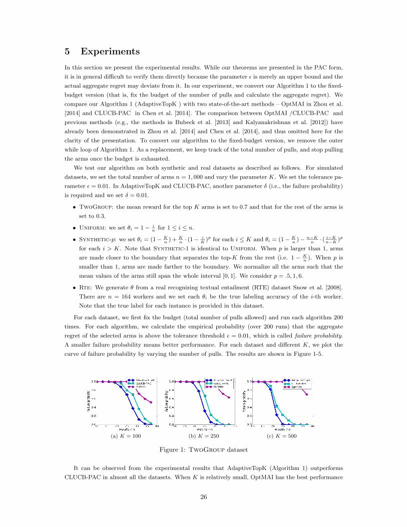
For each dataset, we first fix the budget (total number of pulls allowed) and run each algorithm 200

times. For each algorithm, we calculate the empirical probability (over 200 runs) that the aggregate

regret of the selected arms is above the tolerance threshold ε = 0.01, which is called failure probability.

A smaller failure probability means better performance. For each dataset and different K, we plot the

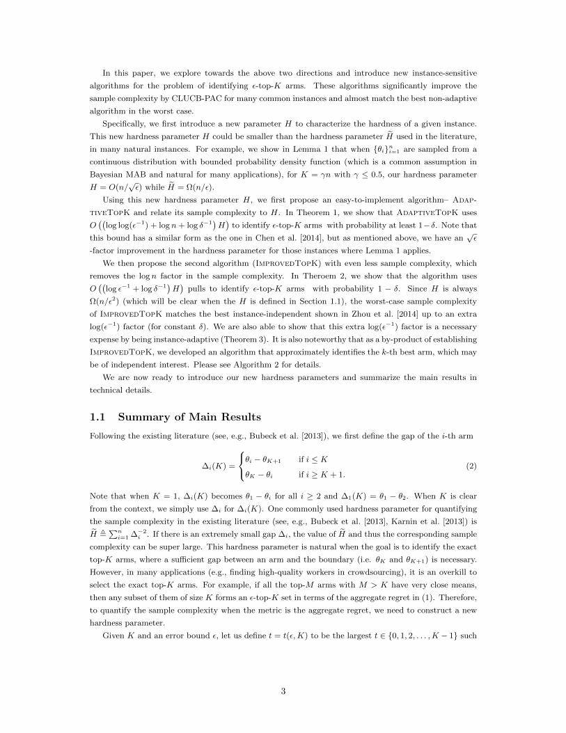
curve of failure probability by varying the number of pulls. The results are shown in Figure 1-5.

(a) K = 100 (b) K = 250 (c) K = 500

Figure 1: TwoGroup dataset

It can be observed from the experimental results that AdaptiveTopK (Algorithm 1) outperforms

CLUCB-PAC in almost all the datasets. When K is relatively small, OptMAI has the best performance

26

(a) K = 100 (b) K = 250 (c) K = 500

Figure 2: Synthetic-.5 dataset

(a) K = 100 (b) K = 250 (c) K = 500

Figure 3: Uniform dataset

(a) K = 100 (b) K = 250 (c) K = 500

Figure 4: Synthetic-6 dataset

(a) K = 30 (b) K = 50 (c) K = 80

Figure 5: Rte dataset

in most datasets. When K is large, AdaptiveTopK outperforms OptMAI . The details of the experimental

results are elaborated as follows.

• For TwoGroup dataset (see Figure 1), AdaptiveTopK outperforms other algorithms significantly

for all values ofK. The advantage comes from the adaptivity of our algorithm. In the TwoGroup dataset,

27

top-K arms are very well separated from the rest. Once our algorithm identifies this situation, it

need only a few pulls to classify the arms. In details, the inner while loop (Line 7) of Algorithm 1

make it possible to accept/reject a large number of arms in one round as long as the algorithm is

confident.

• As K increases, the advantage of AdaptiveTopK over other algorithms (OptMAI in particular)

becomes more significant. This can be explained by the definition of H(t,ε): t = t(ε,K) usually

becomes bigger as K grows, leading to a smaller hardness parameter H(t,ε).

• A comparison between Synthetic-.5, Uniform, Synthetic-6 reveals that the advantage of Adap-

tiveTopK over other algorithms (OptMAI in particular) becomes significant in both extreme scenar-

ios, i.e., when arms are very well separated (p 1) and when arms are very close to the separation

boundary (p 1).

6 Conclusion and Future Work

In this paper, we proposed two algorithms for a PAC version of the multiple-arm identification problem in

a stochastic multi-armed bandit (MAB) game. We introduced a new hardness parameter for characteriz-

ing the difficulty of an instance when using the aggregate regret as the evaluation metric, and established

the instance-dependent sample complexity based on this hardness parameter. We also established lower

bound results to show the optimality of our algorithm in the worst case. Although we only consider the

case when the reward distribution is supported on [0, 1], it is straightforward to extend our results to

sub-Gaussian reward distributions.

For future directions, it is worthwhile to consider more general problem of pure exploration of MAB

under matroid constraints, which includes the multiple-arm identification as a special case, or other

polynomial-time-computable combinatorial constraints such as matchings. It is also interesting to extend

the current work to finding top-K arms in a linear contextual bandit framework.

Appendix

Proof of Lemma 18

Proof : We partition all ai’s to groups G1, . . . , Gdlog2Me where Gj = i ∈ [n] | ai ∈ [2j−1, 2j). Let

S =∑ni=1 ai ≥ n. For each j ∈ 1, 2, . . . , dlog2 Me, let δj = 1

S

∑i∈Gj ai. Observe that we have∑

j δj = 1. We will show for each Gj that

∑i∈Gj

ai log(n/i) ≤ O(δj logM + δj log δ−1

j + 1)S. (52)

Once we establish (52), we prove the lemma as follows. We sum up the inequalities for all j and get

∑i∈[n]

ai log(n/i) ≤dlog2Me∑j=1

O(δj logM + δj log δ−1

j + 1)S

= O(dlogMe)S +O(S)

dlog2Me∑j=1

δj log δ−1j ≤ O(dlogMe)S +O(S) · logdlog2 Me ≤ O(dlogMe)S,

where the second last inequality is by Jensen’s inequality and the convexity of δ log δ over δ ∈ (0, 1).

28

Now we prove (52) for each group G = Gj and δ = δj . Let b = maxi∈Gai ≤ M . By our partition

rule we have that b ≤ 2ai for all i ∈ G. Observe that

∑i∈G

ai log(n/i) ≤ b|G|∑i=1

log(n/i) = b|G| logn− b log(|G|!) ≤ b|G| log(n/|G|) +O(b|G|). (53)

The last inequality of (53) is by Stirling’s approximation. Since b|G| ≥∑i∈G ai = δS, we have |G| ≥

δSb≥ δn

b. We finish the proof of (52) by upper-bounding the RHS of (53) by

b|G| log(bδ−1) +O(b|G|) ≤ 2δS log(bδ−1) +O(b|G|) ≤ O(δS log(Mδ−1) + S

),

where the first inequality is because b|G| ≤∑i∈G 2ai = 2δS .

References

Y. Abbasi-Yadkori, P. Bartlett, X. Chen, and A. Malek. Large-scale markov decision problems with

KL control cost and its application to crowdsourcing. In Proceedings of International Conference on

Machine Learning (ICML), 2015.

J. Audibert, S. Bubeck, and R. Munos. Best arm identification in multi-armed bandits. In Proceedings

of the Conference on Learning Theory (COLT), 2010.

S. Bubeck, T. Wang, and N. Viswanathan. Multiple identifications in multi-armed bandits. In Proceedings

of the International Conference on Machine Learning (ICML), 2013.

W. Cao, J. Li, Y. Tao, and Z. Li. On top-k selection in multi-armed bandits and hidden bipartite graphs.

In Proceedings of Advances in Neural Information Processing Systems (NIPS), 2015.

L. Chen, A. Gupta, and J. Li. Pure exploration of multi-armed bandit under matroid constraints. In

Proceedings of the Conference on Learning Theory (COLT), 2016a.

L. Chen, J. Li, and M. Qiao. Towards instance optimal bounds for best arm identification. arXiv preprint

arXiv:1608.06031, 2016b.

S. Chen, T. Lin, I. King, M. R. Lyu, and W. Chen. Combinatorial pure exploration of multi-armed

bandits. In Proceedings of Advances in Neural Information Processing Systems (NIPS), 2014.

X. Chen, Q. Lin, and D. Zhou. Statistical decision making for optimal budget allocation in crowd labeling.

Journal of Machine Learning Research, 16:1–46, 2015.

E. Even-Dar, S. Mannor, and Y. Mansour. PAC bounds for multi-armed bandit and markov decision

processes. In Proceedings of the Annual Conference on Learning Theory (COLT), 2002.

E. Even-Dar, S. Mannor, and Y. Mansour. Action elimination and stopping conditions for the multi-

armed bandit and reinforcement learning problems. Journal of machine learning research, 7:1079–1105,

2006.

W. Feller. Generalization of a probability limit theorem of cramer. Trans. Amer. Math. Soc, 54(3):

361–372, 1943.

V. Gabillon, M. Ghavamzadeh, A. Lazaric, and S. Bubeck. Multi-bandit best arm identification. In

Proceedings of Advances in Neural Information Processing Systems (NIPS), 2011.

29

V. Gabillon, M. Ghavamzadeh, and A. Lazaric. Best arm identification: A unified approach to fixed

budget and fixed confidence. In Proceedings of Advances in Neural Information Processing Systems

(NIPS), 2012.

V. Gabillon, A. Lazaric, M. Ghavamzadeh, R. Ortner, and P. Bartlett. Improved learning complexity in

combinatorial pure exploration bandits. In Proceedings of the International Conference on Artificial

Intelligence and Statistics, 2016.

K. Jamieson, M. Malloy, R. Nowak, , and S. Bubeck. UCB : An optimal exploration algorithm for

multi-armed bandits. In Proceedings of the Conference on Learning Theory (COLT), 12 2014. arXiv

preprint arXiv:1312.7308v1.

K.-S. Jun, K. Jamieson, R. Nowak, and X. Zhu. Top arm identification in multi-armed bandits with

batch arm pulls. In Proceedings of the International Conference on Artificial Intelligence and Statistics

(AISTATS), 2016.

S. Kalyanakrishnan, A. Tewari, P. Auer, and P. Stone. PAC subset selection in stochastic multi-armed

bandits. In Proceedings of International Conference on Machine Learning (ICML), 2012.

Z. Karnin, T. Koren, and O. Somekh. Almost optimal exploration in multi-armed bandits. In Proceedings

of International Conference on Machine Learning (ICML), 2013.

E. Kaufmann, O. Cappe, and A. Garivier. On the complexity of best arm identification in multi-armed

bandit models. Journal of Machine Learning Research, 17:1–42, 2016.

S. Mannor and J. N. Tsitsiklis. The sample complexity of exploration in the multi-armed bandit problem.

Journal of Machine Learning Research, 5:623–648, 2004.

J. Matousek and J. Vondrak. The probabilistic method. Lecture Notes, 2008.

D. Russo. Simple bayesian algorithms for best arm identification. In Proceedings of the Conference on

Learning Theory (COLT), 2016.

R. Snow, B. O’Connor, D. Jurafsky, and A. Y. Ng. Cheap and fast—but is it good?: Evaluating non-

expert annotations for natural language tasks. In Proceedings of the Conference on Empirical Methods

in Natural Language Processing, EMNLP ’08, pages 254–263, Stroudsburg, PA, USA, 2008. Association

for Computational Linguistics. URL http://dl.acm.org/citation.cfm?id=1613715.1613751.

M. Soare, A. Lazaric, and R. Munos. Best-arm identification in linear bandits. In Proceedings of Advances

in Neural Information Processing Systems (NIPS), 2014.

Y. Zhou, X. Chen, and J. Li. Optimal PAC multiple arm identification with applications to crowdsourcing.

In Proceedings of International Conference on Machine Learning (ICML), 2014.

30