Adaptive Kalman Filtering Methods for Low-Cost GPS/INSLocalization for Autonomous Vehicles

Adam Werries, John M. Dolan

Abstract— For autonomous vehicles, navigation systems mustbe accurate enough to provide lane-level localization. High-accuracy sensors are available but not cost-effective for pro-duction use. Although prone to significant error in poorcircumstances, even low-cost GPS systems are able to correctInertial Navigation Systems (INS) to limit the effects of deadreckoning error over short periods between sufficiently accurateGPS updates. Kalman filters (KF) are a standard approachfor GPS/INS integration, but require careful tuning in orderto achieve quality results. This creates a motivation for a KFwhich is able to adapt to different sensors and circumstanceson its own. Typically for adaptive filters, either the process (Q)or measurement (R) noise covariance matrix is adapted, andthe other is fixed to values estimated a priori. We show thatby adapting Q based on the state-correction sequence and Rbased on GPS receiver-reported standard deviation, our filterreduces GPS root-mean-squared error by 23% in comparisonto raw GPS, with 15% from only adapting R.

I. INTRODUCTION

For autonomous vehicles, navigation systems must besufficiently accurate to determine the current lane on theroad. High-accuracy sensors have been available for manydecades now, but even today they are prohibitively expensivefor automotive production. It is desirable to obtain sufficientperformance from the lowest-cost sensors available throughcareful calibration, modeling, and filtering. The Global Posi-tioning System (GPS) and Inertial Navigation Systems (INS)are used extensively in mobile robotics applications. TheINS often consists of one or more Inertial MeasurementUnits (IMU), containing a gyroscope, an accelerometer, andsometimes a magnetometer. GPS and INS are complemen-tary in terms of their respective limitations and together arecapable of providing a more accurate navigation solutionunder sensor fusion. The purpose of our research is toexplore sufficiently accurate navigation solutions such thatthe hardware cost would be consistent with use for currentproduction vehicles, and computational cost would be withinreason for modern embedded systems.

II. RELATED WORK

The conventional Kalman Filter (CKF) is widely usedfor state estimation, but is highly dependent on accuratea priori knowledge of the process and measurement noisecovariances (Q and R), which are assumed to be constant.An autonomous vehicle experiences a dynamic range of

This work was supported by the Department of Transportation UniversityTransportation Center at Carnegie Mellon University (CMU)

Adam Werries and John Dolan are with the Robotics Institute,CMU, Pittsburgh, PA 15213, USA awerries@andrew.cmu.edu;jdolan@andrew.cmu.edu

situations which will affect each sensor to a differing degree,inspiring the idea of Adaptive Kalman filtering (AKF).AKF allows for the Q (process) and/or R (measurement)noise covariance matrices to be adjusted according to theenvironment and dynamics [1].

A. Multiple-Model Adaptive Estimation (MMAE)

One adaptive method that has been used for integratinglow-cost sensors is Multiple-Model Adaptive Estimation(MMAE), which reduces the need for an accurate a prioriknowledge of Q and R, by using a bank of Kalman filters.Each filter has its own set of parameters for Q and R,along with a normalized weight for each filter in the bank.Over time, the weights are adjusted, eventually settling onthe “best” model [2]. However, running k simultaneousfilters requires k-times more computational cost [2]. Inaddition, requiring multiple approximations of Q and Rcauses performance to depend greatly on the quality of theseapproximations and their consistent applicability to differentscenarios. In order to iterate at a sufficient rate for vehiclesafety on embedded systems, the computational cost is notseen as an acceptable trade-off.

B. Innovation-based Adaptive Estimation (IAE)

In order to constantly adapt to new information, Q and Rshould reflect the noise characteristics of the current behaviorof the vehicle and sensors. Innovation-based adaptive esti-mation (IAE) uses the covariance of an N -length innovationsequence to adjust the Q and R matrices. The innovationis the difference between the expected measurement stateand the actual measurement. This has shown up to a 50%improvement over the CKF under certain conditions [3][4]. Similar to IAE, residual-based filters are shown to per-form even more accurately when computing R for low-costsensors[5], instead using the difference between the predictedstate and the corrected state. Under steady-state conditions,Q may be computed using the innovation sequence as well,but under dynamic situations it is required to use the statecorrection sequence [3].

C. Improvements

Using a CKF and INS provided with Groves’ textbook[6], we have modified the filter to improve estimates for ourvehicle. We modified the INS to process IMU measurementsin batch, averaged over the INS integration period. Wecarefully measured the lever arm from the IMU to the GPS,adding its effects to the model in order to reduce errorsresulting from the rotating reference frame. We then modified

the filter to add adaptive estimation. Typically for adaptivefilters, either R or Q is fixed, and the other is adapted [7].In this paper, we will show that accuracy can be improvedby intelligently adapting both R and Q in a stable manner.We adapted R online in a known manner by computingthe R matrix from the standard deviations (or dilution ofprecision) reported by the GPS receiver, while clampingthe result with separate minimum and maximum values forposition and velocity. This resulted in an improvement of15% in root-mean-squared (RMS) error over raw low-costGPS measurements, using as ground-truth a high-accuracyreference Applanix GPS with Real Time Kinematics (RTK)mode enabled. We then show results from adapting Qonline using the state correction sequence and scaling bythe filter time interval, resulting in an improvement of 23%in RMS error over raw GPS measurements, a further 10%improvement over the Kalman filter with only R-adaptation.Ultimately we reduced the navigation error from 2.94mRMS to 2.27m RMS, and from 6.04m max error to 4.42m.Methods for low-cost GPS/INS integrated localization thatachieve similar results require additional filter banks ortuning parameters [2] [8] [9], complex neural networks [10][11] and fuzzy logic [12][13], or violate the requirement forreal-time performance for vehicle safety by pre-filtering IMUdata with wavelet decomposition methods [10].

III. APPROACH

A. Architecture

In our system, we use a Kalman filter for a loosely-coupledintegration of GPS and INS. The INS is taken from Groves’textbook [6], along with the base Kalman filter, which washeavily modified in order to support our timing, modeling,and adaptive requirements. In loosely-coupled integration,the GPS receiver’s position and velocity solution is utilizedto apply corrections to the INS. This is opposed to themore complex tightly-coupled integration, which uses theGPS’s pseudo-range and pseudo-range-rate measurements inorder to compute a solution [6]. Shown in figure 1, the INSmaintains a running navigation solution which is used as theoutput of our navigation system. The Kalman filter statesare the position, velocity, and attitude errors of the INS,along with estimates of the accelerometer and gyroscopebiases. As each GPS solution is received, the filter iterates,using the difference between the GPS and INS solutionsas a measurement to update the filter states. A closed-loopcorrection of the INS is then applied, and the new estimatesof the biases are applied to incoming IMU measurements.The R matrix for applying GPS corrections is computedfrom the standard deviation reported by the GPS receiver.Q is then adapted online using a state-correction covariancematrix, as discussed in section III-G.

B. Kalman filtering

As shown below in algorithm 1, the standard Kalman filtermaintains a Gaussian belief state with mean x and covariancematrix P . At each iteration, the state is propagated usinga system model represented by the state transition matrix

Fig. 1. Loosely-coupled integration using a GPS to apply closed-loopcorrections to an INS

Φ and assumed-Gaussian process noise covariance matrixQ. In our case, Q describes the variation noise over a timeinterval of the INS error states, which are described in sectionIII-D. The measurement model relating the x state to itsmeasurements is described by H , with assumed-Gaussianmeasurement noise covariance matrix R. In our case, Rdescribes the noise covariance of the GPS measurementsfor position and velocity, described in section III-E. TheKalman gain K is then computed in order to optimally applythe difference between the measurement and the expectedstate after propagation by the process model. After themeasurement vector z is received, x and P are corrected.

At the end of each iteration, we have the choice of adaptingthe noise matrices or leaving them as they are.

Algorithm 1 Algorithm for Kalman Filter1: compute Φk−1 and Qk−1

2: x−k = Φk−1x+k−1

3: P−k = Φk−1P

+k−1ΦT

k−1 +Qk−1

4: compute Hk and Rk with measurement model5: Kk = P−

k HTk (HkP

−k H

Tk +Rk)−1

6: formulate zk7: x+k = x−k +Kk(zk −Hkx

−k )

8: P+k = (I −KkHk)P−

k (I −KkHk)T +KkRkKTk

9: Adapt Qk according to system performance

where:

x− = a priori state vectorx+ = a posteriori state vectorP− = a priori state error covariance matrixP+ = a posteriori state error covariance matrixz = measurement vectorΦ = process model matrix, state transitionH = measurement model matrix

Q = process noise covariance matrixR = measurement noise covariance matrixK = Kalman gain

The process model, measurement model, and adaptive algo-rithm are described in detail in the following sections.

C. INS mechanization

Following position/velocity initialization from the firstGPS fix and attitude initialization from stationary level-ing/gyrocompassing [6], the INS begins processing gyro-scope (ωb

ib) and accelerometer (f bib) measurements receivedfrom the IMU. As shown in figure 2, each measurementincrements the solution as an integral over the time interval,correcting for gravity, the rotating reference frame, and thecurrent estimate of the biases in the sensors.

Fig. 2. Earth-centered Earth-fixed frame Inertial Navigation System [6]

The INS internal state is as follows, where each state ispost-corrected by the KF,

ωbib = angular rate measurement from gyroscopef bib = specific force measurement from accelerometerCe

b = INS attitude solution, frame transformation ma-trix from body frame to Earth-centered Earth-fixed(ECEF) frame

veb = INS velocity solution of the body in the ECEFframe

peb = INS position solution of the body in the ECEFframe

D. Process model

The process model is responsible for propagation accord-ing to the expected value for each state. The state vector forour system consists of monitoring the attitude (δψ), velocity(δv), and position (δr) errors shown in figure 3, along with

Fig. 3. Diagram of vehicle showing coordinate axes and pose error variablesused in process model

the accelerometer and gyroscope biases (ba and bg),

x =

δψe

eb

δveebδreebbabg

(1)

whereδψe

eb = INS solution attitude errorδveeb = INS solution velocity errorδreeb = INS solution position errorba = Accelerometer biasbg = Gyroscope biasThus the state transition matrix is [6]

Φ =

F e11 03 03 03 Ce

b τsF e21 F e

22 F e23 Ce

b τs 0303 I3τs I3 03 0303 03 03 I3 0303 03 03 03 I3

(2)

where

F e11 = I3 − Ωe

ieτs (3a)

F e21 =

[−(Ce

b fbib

)∧]τs (3b)

F e22 = I3 − 2Ωe

ieτs (3c)

F e23 = − 2γeib

reeS(Lb)

(reeb)T

|reeb|τs (3d)

andΩe

ie = Earth rotation ratereeS = Geocentric Radius at the surface, equation as-

sumes near-surface gravitational effectsγeib = Gravity model value at current location

Lb = Current latitudeτs = Filter iteration time difference (epoch)∧ = Indicates skew-symmetric matrix of previous

vector

The process noise covariance matrix Q is first estimatedaccording to a priori testing values, and then adapted asdescribed in section III-G.

E. Measurement model

The measurement model is responsible for relating mea-surements to states. The measurement for our system consistsof the difference between the GPS and INS navigationsolutions, as in the measurement vector in (4), [6].

δze−k =

(reeaG − reeb − Ce

b lbba

veeaG − veeb − Ceb (ωb

ib ∧ lbba) + ΩeieC

eb l

bba

)(4)

To apply this measurement, we need to formulate Hk asfollows [6]

HeG,k =

[He

r1 03 −I3 03 03He

v1 −I3 03 03 Hev5

](5a)

Her1 =

[(Ce

b lbba)∧

](5b)

Hev1 =

[Ce

b (ωbib ∧ lbba)− Ωe

ieCeb l

bba∧

](5c)

Hev5 = Ce

b

[lbba∧

](5d)

where

ze−k = Measurement vector, difference between GPSand INS solutions, accounting for the lever armdifference, ECEF frame

lbba = Lever arm from IMU to GPS in body framereeaG = GPS-reported position vector, ECEF frameveeaG = GPS-reported velocity vector, ECEF frame

F. Adaptation of measurement noise matrix R

The measurement noise covariance matrix R is computedaccording to the per-axis ECEF-frame position and velocitystandard deviations reported by the GPS user-equipment.This is then scaled by the Kalman filter iteration interval.Minimum and maximum variance values were enforced inorder to ensure stability.

Rk =

σ2xk 0 00 σ2

yk 0

0 0 σ2zk

τs (6)

G. State-correction sequence adaptation of process noisematrix Q

The process noise matrix adaptation is formulated basedon the state-correction sequence [3], where N is the lengthof state-corrections sequence used in the computation.

∆xk = x+k − x−k (7a)

Qk =1

N

k∑j=k−N

∆xj∆xTj + P+

k − ΦP+k−1ΦT (7b)

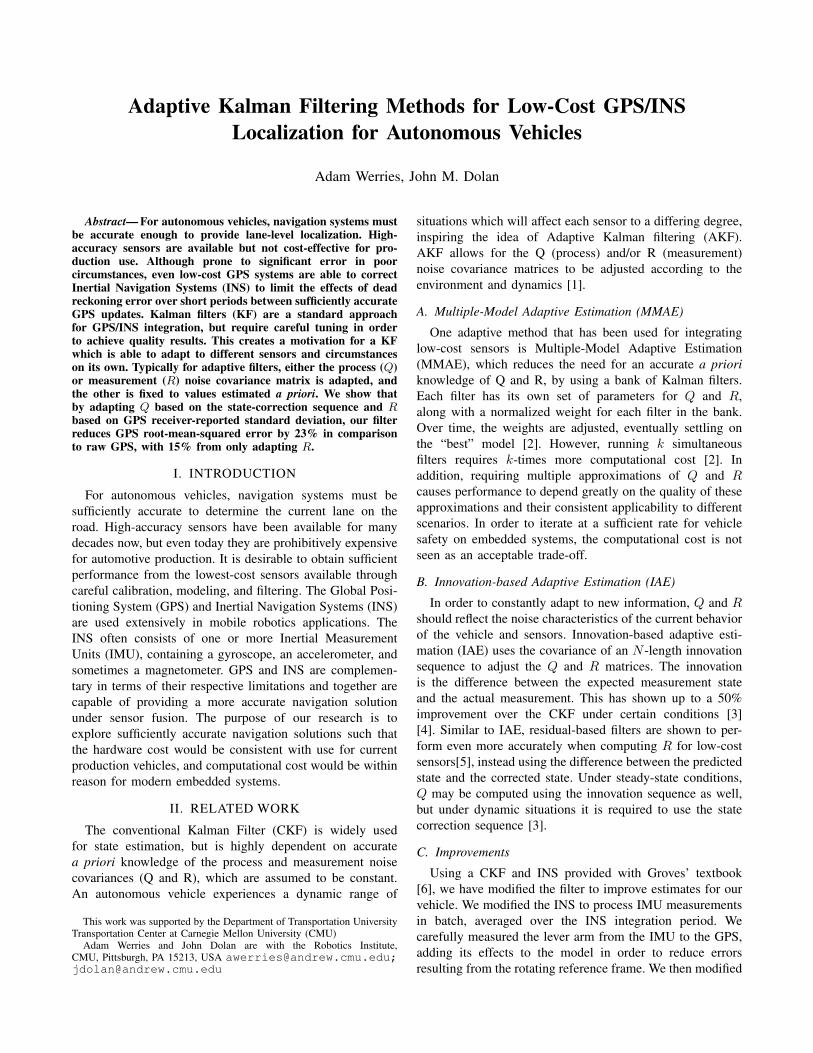
Fig. 4. Top-down view of vehicle path

IV. TESTING PROCEDURE

Testing was performed on public roads through a largepark on a hill near the Carnegie Mellon University campususing our Cadillac SRX vehicle, where the path is shown infigure 4. A high-accuracy RTK-enabled Applanix navigationmodule was used to provide an accurate-as-possible ground-truth. This specific location allows for high-quality GPSresults, and consistently provides the Applanix module withFixed or Float RTK, supplying a solution accurate to within5 (fixed) to 30 (float) centimeters. Time was synced usingthe Network Time Protocol between the vehicle’s Linuxmachines and a Raspberry Pi 2 (RPi-2) used for low-costdata collection. Time difference between the two is estimatedat less than 10ms.

A low-cost IMU (InvenSense MPU-6050) was affixed tothe RPi-2, which was then mounted in the vehicle. Thisspecific IMU is ideal because the accelerometer and gyro-scope are within the same QFN package, minimizing cross-coupling errors and relaxing the calibration requirements.This sensor was about $5 on Digikey at the time of writing.

A low-cost GPS, the Novatel Flex6, was also connectedto the same RPi-2. The GPS antenna was then mounted onthe roof of the vehicle. This GPS is ideal for our testingbecause it provides a full ECEF-frame navigation solutionwith position, velocity, and standard deviations. This GPSis available by quoted price from Novatel, but the price isconsistent with use in a production vehicle. The manufacturerclaims on the product page that with L1/L2 signals, error canreach as low as 1.2 meters, and 0.6m with SBAS [14].

Data were also collected using a Skytraq Venus 6 GPS,which was available for $50 from SparkFun at the time ofwriting, along with a $13 magnetic-mounted antenna. ThisGPS can be configured to provide ECEF coordinates forposition and velocity, although it reports dilution of precision(DOP) instead of standard deviation. This was convertedto measurement standard deviation using the manufacturer-reported standard deviation, σr = 2.5m, and the relationwith the position DOP (PDOP), σ2 = PDOP 2 × σ2

r . It is

possible to use the horizontal and vertical DOP, HDOP andV DOP , but that would require a frame change from ECEFto the local-navigation-frame (Northing, Easting) and backagain, inducing additional error based on the attitude errorof the INS.

The lever arm between the IMU and GPS mountinglocations was carefully measured, although some error isunavoidable without a full 3D model of the vehicle. It isestimated that the error is less than 5 centimeters for eachaxis, which has less than a 1% effect on the performance.

The data were then run through the filter offline inMATLAB simulation, although the intention is ultimatelyto transition to a filter in C++ running online on the RPi-2. Parameters used in the filter for initial covariance matrixestimates, adaptive window size, initial biases, etc. were cho-sen by determining a theoretically feasible range. Followingthat, scripts were used to perform a brute-force parametersearch within the feasible ranges in order to improve errorand stability. The parameter search was run over multipledatasets in order to prevent selecting minima specific to asingle dataset.

For this dataset, the IMU collects data at 1000 Hz, theNovatel at 4Hz, and the Skytraq at 1Hz. The INS system runsat 25 Hz, averaging IMU data over the interval, running theKalman filter at each iteration that a GPS solution is reported.

V. RESULTS

The U.S. Department of Transportation has a recommen-dation of at least 2.7 meters for the width of local urban roads[15]. This places a lower bound on the required performance:error and uncertainty must be no greater than half of thatwidth, 1.35m, in order to achieve lane-level localization. Theresults of testing with the IMU and GPS described in theprevious section are seen in table (I). Results are shown forboth the conventional Kalman filter, where we only adaptR based on the GPS-reported standard deviation, and ourfully adaptive Kalman filter, which uses the state-correctionsequence to estimate Q online. The window size chosen forQ for the Novatel GPS was 60, as it allowed the system toquickly respond to changing noise characteristics. Due to thepoor quality of the Skytraq GPS, smaller window sizes ofaround 5− 30 performed better, and 10 was chosen.

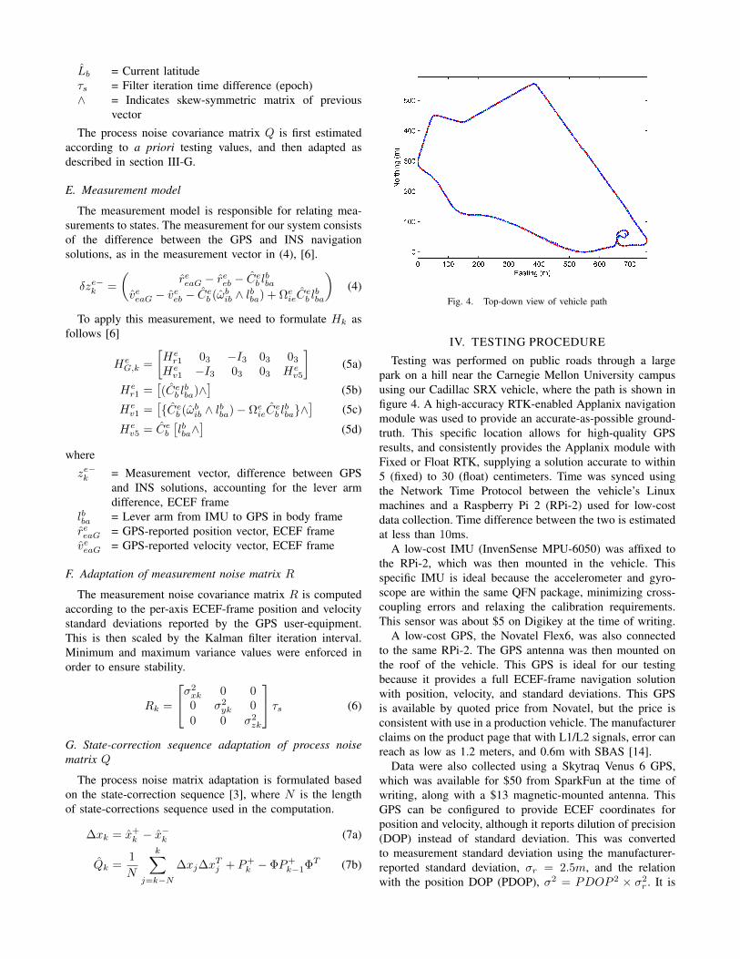
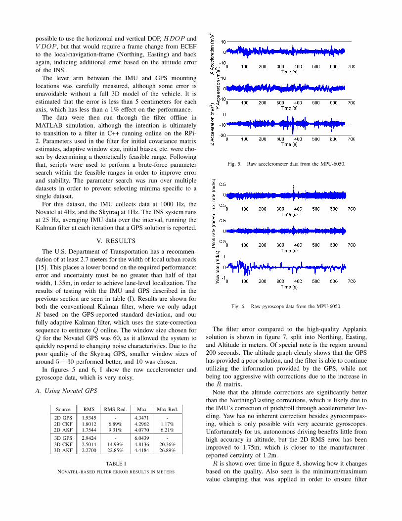
In figures 5 and 6, I show the raw accelerometer andgyroscope data, which is very noisy.

A. Using Novatel GPS

Source RMS RMS Red. Max Max Red.

2D GPS 1.9345 - 4.3471 -2D CKF 1.8012 6.89% 4.2962 1.17%2D AKF 1.7544 9.31% 4.0770 6.21%

3D GPS 2.9424 - 6.0439 -3D CKF 2.5014 14.99% 4.8136 20.36%3D AKF 2.2700 22.85% 4.4184 26.89%

TABLE INOVATEL-BASED FILTER ERROR RESULTS IN METERS

Fig. 5. Raw accelerometer data from the MPU-6050.

Fig. 6. Raw gyroscope data from the MPU-6050.

The filter error compared to the high-quality Applanixsolution is shown in figure 7, split into Northing, Easting,and Altitude in meters. Of special note is the region around200 seconds. The altitude graph clearly shows that the GPShas provided a poor solution, and the filter is able to continueutilizing the information provided by the GPS, while notbeing too aggressive with corrections due to the increase inthe R matrix.

Note that the altitude corrections are significantly betterthan the Northing/Easting corrections, which is likely due tothe IMU’s correction of pitch/roll through accelerometer lev-eling. Yaw has no inherent correction besides gyrocompass-ing, which is only possible with very accurate gyroscopes.Unfortunately for us, autonomous driving benefits little fromhigh accuracy in altitude, but the 2D RMS error has beenimproved to 1.75m, which is closer to the manufacturer-reported certainty of 1.2m.R is shown over time in figure 8, showing how it changes

based on the quality. Also seen is the minimum/maximumvalue clamping that was applied in order to ensure filter

Fig. 7. Novatel dataset. Error between ground-truth vs low-cost GPS andground-truth vs filter solution

Fig. 8. Novatel dataset. R measurement noise covariance matrix (GPS)over the course of a dataset

Fig. 9. Novatel dataset. Q process noise covariance matrix (INS error)adapting over the course of a dataset, 3D pose. Note that they are notsettling to zero, just to much smaller values.

Fig. 10. Novatel dataset. Q process noise covariance matrix adapting overthe course of a dataset, sensor biases. Note that they are not settling to zero,just to much smaller values.

Fig. 11. Novatel dataset. Standard deviation of the INS navigation solutionerror, part of covariance matrix P

Fig. 12. Novatel dataset. Standard deviation of the accelerometer and gyrobiases, part of covariance matrix P

stability. Q is shown over time in figures 9 and 10, showingextremely high noise in the beginning of the filter sequence,settling down after about 100 seconds after the accelerometerand gyroscope properties have converged. Most important,the adaptation of Q is shown to have a large effect onstabilizing the uncertainty in the INS state error and bias,as shown in figures 11 and 12.

B. Using Skytraq GPS

Fig. 13. Skytraq dataset. Error between ground-truth vs low-cost GPS andground-truth vs filter solution.

Here we show the same table and plots for the Skytraq-based filter that I included for the Novatel-based filter. TheSkytraq is considerably worse, and its navigation solutionappears to have nearly a 250ms delay. As the Skytraq doesnot provide standard deviation information, we must usethe Dilution of Precision (DOP) to estimate the changes inbelief uncertainy by the GPS solution. However, this DOPdid not appear to be very reliable, and we had to add ascale factor the manufacturer-reported standard deviation inorder to increase the uncertainty. That said, the filter is ableto reduce the error significantly, primarily for the altitudesolution.

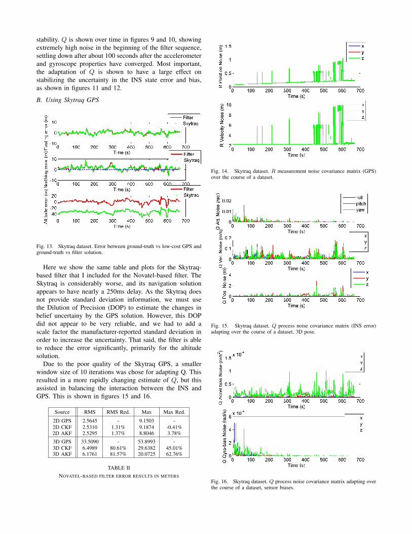
Due to the poor quality of the Skytraq GPS, a smallerwindow size of 10 iterations was chose for adapting Q. Thisresulted in a more rapidly changing estimate of Q, but thisassisted in balancing the interaction between the INS andGPS. This is shown in figures 15 and 16.

Source RMS RMS Red. Max Max Red.

2D GPS 2.5645 - 9.1503 -2D CKF 2.5310 1.31% 9.1874 -0.41%2D AKF 2.5295 1.37% 8.8046 3.78%

3D GPS 33.5090 - 53.8993 -3D CKF 6.4989 80.61% 29.6382 45.01%3D AKF 6.1761 81.57% 20.0725 62.76%

TABLE IINOVATEL-BASED FILTER ERROR RESULTS IN METERS

Fig. 14. Skytraq dataset. R measurement noise covariance matrix (GPS)over the course of a dataset.

Fig. 15. Skytraq dataset. Q process noise covariance matrix (INS error)adapting over the course of a dataset, 3D pose.

Fig. 16. Skytraq dataset. Q process noise covariance matrix adapting overthe course of a dataset, sensor biases.

Fig. 17. Skytraq dataset. Standard deviation of the INS navigation solutionerror, part of covariance matrix P

Fig. 18. Skytraq dataset. Standard deviation of the accelerometer and gyrobiases, part of covariance matrix P

C. Discussion

One possible issue shown is that the uncertainty laterin the datasets appears to reduce below the value of theerrors in the system. This shows that the filter is possiblytoo confident in its estimate, and that further tuning ofinitial parameters, minimum/maximum covariance values,and adaptation methods are required. Barring that, moreobservability through addition of more sensors may be ofassistance.

In the case of low-cost sensors, the accuracy of the gyro-scope is far too poor to achieve gyrocompassing in order toreduce the yaw error for more than initialization efforts. Thisdataset does include a dynamic initialization period, wherea vehicle induce rotations in alternating opposite directionsat sufficient speed to determine gyroscope and accelerometererrors before attempting to use the localization solution. Inthe case of large angle errors, the small-angle approximationsincluded in the model are violated, and it is likely that we will

have to account for this in future research [6]. We attemptedto use magnetometers to provide heading-angle corrections,but even after attempts at calibrating for the vehicle’s localmagnetic conditions, the data was too noisy to provide aproper correction.

The NovAtel GPS has an manufacturer-reported uncer-tainty of 1.2 meters in perfect conditions, and it is unlikelythat a loosely-coupled system consisting of INS correctedpurely by GPS will be able to reduce its RMS error belowthat. The largest improvements are made in reducing errorwhere the GPS receiver itself reports that the solution accu-racy is poor, which can be represented in R, allowing theINS to take over. It is apparent that more improvement ofthe loosely-coupled filter can allow the dead-reckoning INSto reduce maximum and RMS error to near 1.2m, whichis sufficient for lane-level localization. Wheel odometry andsteering-wheel angle integration may assist in reducing errordown to the manufacturer-reported uncertainty. Improvementbeyond that will likely require a tightly or deeply coupledfilter in order to improve the GPS solution itself, or additionalbeacon-based systems to correct drift of inertial or odometricsystems, such as visual landmark recognition.

CONCLUSION

Adapting R and Q according to the system noise charac-teristics has shown a marked improvement in localization ac-curacy for integrating low-cost GPS/INS systems. However,the quality has not improved to the point where lane-levellocalization can be achieved, and further research is requiredif we wish to use such inexpensive sensors. As always,calibration can be done more carefully, the filter can be tunedmore accurately, and vibration effects can be analyzed andreduced through mechanical and software means. Adaptivemethods such as process noise scaling [7] and reinforcementlearning for parameter estimation [16] may further improveresults.

ACKNOWLEDGMENT

Thank you to my advisors, Dr. John Dolan and Dr. RajRajkumar, for your advice and generous support throughoutmy time at CMU. Thank you to my master’s committeemembers, Dr. Michael Kaess and Daniel Maturana, foryour advice and taking time to meet with me. A specialacknowledgment to Dr. Paul D. Groves, whose clear andthorough textbook made this work possible.

REFERENCES

[1] R. Mehra, “Approaches to adaptive filtering,” vol. 17, no. 5, Oct 1972,pp. 693–698.

[2] C. Hide, T. Moore, and M. Smith, “Adaptive kalmanfiltering for low-cost ins/gps,” The Journal of Navigation,vol. 56, no. 1, pp. 143–152, 01 2003. [Online]. Available:http://search.proquest.com/docview/229556669?accountid=9902

[3] A. H. Mohamed and K. P. Schwarz, “Adaptive kalman filtering forins/gps,” Journal of Geodesy, vol. 73, no. 4, pp. 193–203, 1999.[Online]. Available: http://dx.doi.org/10.1007/s001900050236

[4] A. Fakharian, T. Gustafsson, and M. Mehrfam, “Adaptive kalmanfiltering based navigation: An imu/gps integration approach,” in Net-working, Sensing and Control (ICNSC), 2011 IEEE InternationalConference on, April 2011, pp. 181–185.

[5] C. Hide, T. Moore, and M. Smith, “Adaptive kalman filtering algo-rithms for integrating gps and low cost ins,” in Position Location andNavigation Symposium, 2004. PLANS 2004, April 2004, pp. 227–233.

[6] P. D. Groves, Principles of GNSS, Inertial, and Multisensor IntegratedNavigation Systems, 2nd ed. Artech House, Inc., 2013.

[7] W. Ding, J. Wang, C. Rizos, and D. Kinlyside, “Improvingadaptive kalman estimation in gps/ins integration,” The Journal ofNavigation, vol. 60, no. 3, pp. 517–529, 09 2007. [Online]. Available:http://search.proquest.com/docview/229564577?accountid=9902

[8] S. Y. Cho, “Im-filter for ins/gps-integrated navigation system contain-ing low-cost gyros,” IEEE Transactions on Aerospace and ElectronicSystems, vol. 50, no. 4, pp. 2619–2629, October 2014.

[9] R. Toledo-Moreo, M. A. Zamora-Izquierdo, B. Ubeda-Minarro, andA. F. Gomez-Skarmeta, “High-integrity imm-ekf-based road vehiclenavigation with low-cost gps/sbas/ins,” IEEE Transactions on Intelli-gent Transportation Systems, vol. 8, no. 3, pp. 491–511, Sept 2007.

[10] A. Noureldin, T. B. Karamat, M. D. Eberts, and A. El-Shafie, “Perfor-mance enhancement of mems-based ins/gps integration for low-costnavigation applications,” IEEE Transactions on Vehicular Technology,vol. 58, no. 3, pp. 1077–1096, March 2009.

[11] K. Saadeddin, M. F. Abdel-Hafez, M. A. Jaradat, and M. A. Jarrah,“Optimization of intelligent approach for low-cost ins/gps navigationsystem,” Journal of Intelligent & Robotic Systems, vol. 73, no. 1, pp.325–348, 2013. [Online]. Available: http://dx.doi.org/10.1007/s10846-013-9943-2

[12] X. Zhao, Y. Qian, M. Zhang, J. Niu, and Y. Kou, “An improvedadaptive kalman filtering algorithm for advanced robot navigationsystem based on gps/ins,” in Mechatronics and Automation (ICMA),2011 International Conference on, Aug 2011, pp. 1039–1044.

[13] E. Shi, “An improved real-time adaptive kalman filter for low-costintegrated gps/ins navigation,” in Measurement, Information and Con-trol (MIC), 2012 International Conference on, vol. 2, May 2012, pp.1093–1098.

[14] Flexpak6 triple-frequency + l band gnss receiver. Accessed: 2016-02-29. [Online]. Available: http://www.novatel.com/products/gnss-receivers/enclosures/flexpak6/

[15] Mitigation strategies for design exceptions: Lane width.Accessed: 2016-02-29. [Online]. Available: http://safety.fhwa.dot.gov/geometric/pubs/ mitigationstrategies/ chapter3/3 lanewidth.cfm

[16] C. Goodall, X. Niu, and N. El-Sheimy, “Intelligenttuning of a kalman filter for ins/gps navigation ap-plications,” 09 2007, pp. 2121–2128. [Online]. Available:https://www.ion.org/publications/abstract.cfm?articleID=7473