Embed Size (px)
Citation preview


AcknowledgementsThe first lecture I attended when I started studying was covering statistics and proba-
bility. However, being a freshman I entered the wrong lecture hall and ended up at a
lecture about economics in health sciences. After I recognized, quite late, that I was
sitting at the wrong lecture, I found my way to the correct lecture but had to stand for
the remaining hour. I did not know a lot about probability back then, but I did know that
the probability of having two of these major mistakes was quite rare. The beginning of
the Bachelor was mediocre, but the contrast with the ending of the Master is big.
The last few years within the specialization of Financial Engineering and Manage-
ment were unforgettable. First of all I need to thank Reinoud Joosten. Being one of the
more eccentric lecturers he was always open for an inspiring discussion within or out-
side of the college hours. Not only did he provide me this great subject for graduation,
his knowledge in the field of game theory often astonished me. At a certain moment I
even recognized that it was also in his interest to have me succeed with this subject,
behaviour of a real game theorist. Also I will cherish the discussions about language,
dialects, the university, sport and life in general.
Another important person which deserves a special acknowledgement is Berend
Roorda. During the specialization Berend was the father of the program. His passion
for risk management and finance made a lot of students, including me, enthusiastic
about these subjects within the program. During the breaks he was always there to
share his knowledge, but was also interested in the well-being of the students. Thank
you very much for your hard work and inspiration.
My family also deserves much more credit than they would ever give themselves.
Jos, Leontine and Niels, you were always there for me when I needed it the most.
Though I know that you had a rougher time with me when I drank a lot of beer and
partied too much, I could not have succeeded without your endless support.
Also my friends and loved ones, yes, what to say about you guys. All those times
we laughed about the most stupid things and had endless discussions about the most
stupid subjects, they provided me with enough distractions to keep focus on the more
serious stuff. I would also like to thank all the board members of Integrand and Nesst
for providing me an entrepreneurial challenge but also a very steep learning curve
outside of the university. And last but not least I want to thank you, the reader, for
taking the time to read this thesis.
Rogier Harmelink
iii

IV ACKNOWLEDGEMENTS

Abstract
This thesis focuses on the development of algorithms for computing the threat point
in Frequency-Dependent-games, with the Endogenous Transition Probabilities (ETP)
Endogenous Stage Payoffs (ESP) game as the most complex type of game. We limit
ourselves to two-state, two-player ergodic stochastic games with or without a FD payoff.
Also incorporated into an algorithm are so-called Endogenous Transition Probabilities,
i.e., transition probabilities that depend on the history of the play. Several algorithms
have been developed, one of them (SciPy algorithm) only works on non-FD Type I
games while the other (Relative Value Iteration algorithm) is limited to use on non-FD
Type II games. The Jointly-Convergent Pure-Strategy algorithm works on the broad
spectrum of stochastic games described in this thesis, i.e., (non)-FD Type I, Type II and
Type III games. We test the algorithms in terms of speed and accuracy and reflect on
them including a disquisition of the risks surrounding some of the algorithms. We find
that the SciPy algorithm is superior to the Jointly-Convergent Pure-Strategy algorithm
in terms of accuracy and speed when computing the threat point in non-FD Type I
games. The Relative Value Iteration algorithm works better in terms of accuracy when
compared to the Jointly-Convergent Pure-Strategy algorithm but lags in terms of speed.
The Jointly-Convergent Pure-Strategy algorithm fits all types of games while finding
reasonably accurate solutions in a reasonable time.
v

VI ABSTRACT

Contents
Acknowledgements iii
Abstract v
List of acronyms ix
1 Research Design 1
1.1 Research objective and context . . . . . . . . . . . . . . . . . . . . . . . 1
1.2 Research framework . . . . . . . . . . . . . . . . . . . . . . . . . . . . . 2
1.3 Research questions . . . . . . . . . . . . . . . . . . . . . . . . . . . . . 2
1.4 Thesis design and aim . . . . . . . . . . . . . . . . . . . . . . . . . . . . 3
2 Game Theory Literature 5
2.1 The Origin of Game Theory . . . . . . . . . . . . . . . . . . . . . . . . . 5
2.2 The Nash Equilibrium . . . . . . . . . . . . . . . . . . . . . . . . . . . . 8
2.3 Repeated Games . . . . . . . . . . . . . . . . . . . . . . . . . . . . . . . 11
2.4 Stochastic Games . . . . . . . . . . . . . . . . . . . . . . . . . . . . . . 12
2.5 Frequency-Dependent Games . . . . . . . . . . . . . . . . . . . . . . . 15
3 Building the algorithm 19
3.1 Earlier Work . . . . . . . . . . . . . . . . . . . . . . . . . . . . . . . . . . 19
3.2 From Markov Chain to Stochastic Game . . . . . . . . . . . . . . . . . . 20
3.3 Limitations game usage . . . . . . . . . . . . . . . . . . . . . . . . . . . 23
3.4 Programming Tools . . . . . . . . . . . . . . . . . . . . . . . . . . . . . . 24
3.4.1 Python . . . . . . . . . . . . . . . . . . . . . . . . . . . . . . . . . 24
3.4.2 NumPy . . . . . . . . . . . . . . . . . . . . . . . . . . . . . . . . 25
3.4.3 SciPy . . . . . . . . . . . . . . . . . . . . . . . . . . . . . . . . . 25
3.4.4 MDP Toolbox . . . . . . . . . . . . . . . . . . . . . . . . . . . . . 25
3.5 Type I games . . . . . . . . . . . . . . . . . . . . . . . . . . . . . . . . . 25
3.5.1 SciPy optimizer . . . . . . . . . . . . . . . . . . . . . . . . . . . . 27
3.5.2 Jointly-Convergent Pure-Strategy Algorithm . . . . . . . . . . . . 29
3.5.3 Visualizing the results . . . . . . . . . . . . . . . . . . . . . . . . 32
vii

VIII CONTENTS
3.5.4 Comparing the two algorithms . . . . . . . . . . . . . . . . . . . 34
3.6 Type II games . . . . . . . . . . . . . . . . . . . . . . . . . . . . . . . . . 36
3.6.1 Relative Value Iteration Algorithm . . . . . . . . . . . . . . . . . . 37
3.6.2 Jointly-Convergent Pure-Strategy Algorithm . . . . . . . . . . . . 39
3.6.3 Visualizing the results . . . . . . . . . . . . . . . . . . . . . . . . 42
3.6.4 Comparing the two algorithms . . . . . . . . . . . . . . . . . . . 43
3.7 Type III games . . . . . . . . . . . . . . . . . . . . . . . . . . . . . . . . 46
3.7.1 Visualizing the results . . . . . . . . . . . . . . . . . . . . . . . . 53
3.8 Room for further improvements . . . . . . . . . . . . . . . . . . . . . . . 55
3.9 Practical implications . . . . . . . . . . . . . . . . . . . . . . . . . . . . . 56
4 Conclusions and recommendations 57
4.1 Conclusion . . . . . . . . . . . . . . . . . . . . . . . . . . . . . . . . . . 57
4.2 Recommendations . . . . . . . . . . . . . . . . . . . . . . . . . . . . . . 58
References 59
References . . . . . . . . . . . . . . . . . . . . . . . . . . . . . . . . . . . . . 59
Appendices
A Python Code containing the Algorithms 63
A.1 How to use the Python code - A short manual on the usage . . . . . . . 63
A.1.1 Using Python . . . . . . . . . . . . . . . . . . . . . . . . . . . . . 63
A.1.2 Using the Python Code . . . . . . . . . . . . . . . . . . . . . . . 63
A.1.3 Functions . . . . . . . . . . . . . . . . . . . . . . . . . . . . . . . 64
A.1.4 An example of computations of a Type II game . . . . . . . . . . 64
A.2 Import packages . . . . . . . . . . . . . . . . . . . . . . . . . . . . . . . 66
A.3 Type I Game Code . . . . . . . . . . . . . . . . . . . . . . . . . . . . . . 66
A.4 Type I Example Games Code . . . . . . . . . . . . . . . . . . . . . . . . 68
A.5 Type II Game Code . . . . . . . . . . . . . . . . . . . . . . . . . . . . . . 69
A.6 Type II Example Games Code . . . . . . . . . . . . . . . . . . . . . . . . 91
A.7 Type III Game Code . . . . . . . . . . . . . . . . . . . . . . . . . . . . . 91
A.8 Type III Example Games Code . . . . . . . . . . . . . . . . . . . . . . . 109
List of acronyms
AIT Action Independent Transition
CAIT Current Action Independent Transition
CSP Constant Stage Payoffs
CTP Constant Transition Probabilities
ESP Endogenous Stage Payoffs
ETP Endogenous Transition Probabilities
FD Frequency-Dependent
JCPS Jointly-Convergent Pure-Strategy
MDP Markov Decision Process
NaN Not a Number
RVI Relative Value Iteration
ix

X LIST OF ACRONYMS

Chapter 1
Research Design
We start by elucidating the design of our research. We use a well-known method
by Verschuren, Doorewaard, and Mellion (2010). Beginning by stating the research
objective and the surrounding context. In the second section we derive a framework
based on the research objective and context. In order to realize this framework we
state research questions (third section) used as a guideline throughout our endeavours.
Finally, we conclude by prescribing the structure of this thesis and its aim.
1.1 Research objective and context
Modern game theory is relatively new as a subject in science. Everyone with a little
background knowledge in the subject will relate game theory to persons like John Nash
Jr. and John von Neumann. The most well-known result in game theory is the Nash
equilibrium, but science has evolved and game theory has moved on. Neymann intro-
duced a new class in game theory called stochastic games. These stochastic games
have been at interest of game theorists all around the globe, but also the subject of
new discoveries. One of these discoveries was done in 2003, when Joosten, Bren-
ner, and Witt (2003) published research in the field of Frequency-Dependent games.1
Frequency-Dependent games are stochastic games in which the stage payoffs depend
on the history of the play. The major theorem in this paper involves so-called ‘threats’.
These play an important role in game-theoretical analysis in which they determine the
set of possible equilibria. Joosten (2009) stated: “Unfortunately, there exists no general
theory on (finding) threat points in FD-games, yet." During the years, more research
has been done in the domain of FD-games, e.g. (Mahohoma, 2014), (Joosten, 2015)
and (Joosten & Samuel, 2018). Even though the first and last examples focus on com-
putations within FD-games, none of these are able to state an exact threat point.
The introduction of Endogenous Transition Probabilities by Joosten and Meijboom
(2010) added a novel dimension to the framework of FD-fishery games making analysis
1See Section 2.5 for a background on FD-games.
1

2 CHAPTER 1. RESEARCH DESIGN
of such games more complex. This clearly leaves room for research on the topic of
computations of threat points in FD-games. One should see our research as the next
step into developing a general theory in finding threat points. We focus on the algorithm
building aspect of finding these threat points. Our research objective is to calculate the
threat point in ETP-ESP games by developing an algorithm.
1.2 Research framework
In order to complete our research objective we make use of a research framework. In
this research framework we describe a few important pillars on which it will rely. The
framework can be seen as a stepwise guide being followed in order to complete the
research objective. Our research framework is built on the following five pillars.
1. Gather and summarize relevant literature in the game-theoretical domain with a
focus on FD-games.
2. Search for and prepare programming tools necessary for the development of the
algorithms with a focus on speed.
3. Develop the algorithms.
4. Test the algorithms in terms of speed, accuracy and scalability.
5. Reflect and conclude on the research performed, propose possibilities for future
research.
The intended chronological element of our research framework should be clear.
We start with a literature study, continue with a search for programming tools which are
necessary for the next step: developing the algorithms. At last we test the algorithms
and conclude the research in order to give recommendations for later research.
1.3 Research questions
The research framework constructed in the last section serves as a basis for the de-
velopment of research questions. The research questions should result in knowledge
necessary for achieving the research objective (Verschuren et al., 2010). Each core-
question can be answered with the help of so-called sub-questions. In this research
we only ask one core-question which we define as the main research question. The
main research question is also a reflection of the research objective in question form.
We state the main research question as:
How do we compute threat points efficiently in ETP-ESP games?

1.4. THESIS DESIGN AND AIM 3
We answer this main research question with help of five sub-questions. These are:
1. What has been written in the literature about game theory and Frequency-Dependent
games?
2. Which programming tools are available for game-theoretical computations?
3. Which algorithms can find a threat point and how do they work?
4. How do the algorithms perform in terms of speed and accuracy when scaled to a
larger game?
5. What can we conclude and recommend based on this research?
As one can see, these sub-questions have a direct link to the research framework.
Thus, the answering of the sub-questions should result in completing the steps de-
scribed in the research framework which in its part should result in fulfillment of the
research objective.
1.4 Thesis design and aim
This chapter describes the research design. In the second chapter we elaborate on all
relevant literature surrounding the topic, we start with basic game theory in a gradual
fashion ending up at Frequency-Dependent games. Chapter 3 focuses on developing
the algorithm, starting with an explanation of the relevant programming tools and later
in the chapter the development, testing and practical implications. We conclude and
propose recommendations for future research in the fourth chapter.
Our aim of this thesis is to offer the reader a comprehensive summary of game
theory in order to cope with a potential lack of knowledge in this domain. The more
experienced reader could skip Chapter 2 and could continue at Chapter 3. Both expe-
rienced and inexperienced readers should be able to follow the main purpose of this
thesis, developing an algorithm for calculation of threat points in ETP-ESP games.

4 CHAPTER 1. RESEARCH DESIGN

Chapter 2
Game Theory Literature
In the previous chapter we laid a foundation for our research, but in this chapter we start
with the necessary background knowledge in the domain of game theory. We start at
the origin of game theory and progressively work towards FD-games. In between we
discuss important aspects like the Nash equilibrium, repeated games and stochastic
games in general. At the end of this chapter a non-expert reader should have the
necessary background knowledge in order to follow the steps taken in the development
of the algorithm in Chapter 3.
2.1 The Origin of Game Theory
A lot of scientific literature starts with cliché introductions on the complexity of the
world we live and breath in. Although it may be a cliché, it is true to a large extent.
In order to create structure in the chaos called life, scientists have developed theories
and models based on empirical evidence to explain the complexity of life. In social
sciences the focus is on explaining behaviour of individuals in a social context. Game
theory is a mathematical discipline which forms the (descriptive) basis of analysis of
rational decision makers in a strategic environment, in which their decisions have a
direct or indirect effect on their individual payoff. According to Hyksova (2004) the first
game-theoretical analysis was done by Charles Waldegrave in 1713 as documented in
Pierre Rémond de Montmort’s “Essay d’analyse sur les jeux de hazard”, it comprises
a strategic solution to the French card game le Her (Bellhouse, 2007).
5
6 CHAPTER 2. GAME THEORY LITERATURE
We limit ourselves in the remainder to the domain of non-cooperative games, we
start with an n players non-cooperative one-shot game in which n = 2. Players play a
game consisting of states, denoted by the state space S, a nonempty and finite set. In
a one-shot game players are limited to a game with only 1 state. Player 1 can choose
an action from a nonempty and finite action set Is when in state s ∈ S. Player 2 can
choose an action from a nonempty and finite action set Js when in state s ∈ S (Flesch,
1998).
Players can choose an action with probability 1, but they can also randomize by
using a mixed action. For player 1 we denote this mixed action by xs in state s ∈ S,
which is a probability distribution on Is. Player 2 can choose a mixed action ys in state
s ∈ S, which is a probability distribution on Js. In a one-shot game with two actions
per player, x ∈ ∆1 = {x ∈ R|xi ≥ 0 for i = 1, 2 and∑2
i=1 xi = 1} and y ∈ ∆1 = {y ∈
R|yi ≥ 0 for i = 1, 2 and∑2
i=1 yi = 1}. The combination of the (mixed) actions from
both players result in payoffs r1s1(i1
s1, j1
s1) for player 1 and r2
s1(i1
s1, j1
s1) for player 2 (Flesch,
1998).
Now that we have a mathematical basis we look back at the year 1921. Émile Borel
published a few notes from 1921 until 1927 containing the first formalizations of pure
and mixed strategies, and even a first attempt at a minimax solution (Borel, 1927). But
the real breakthrough in game theory occured when Von Neumann and Morgenstern
in 1944 published their work. However this breakthrough was based on earlier work by
Von Neumann in 1928, this work already stated the minimax theorem, a revolution in
game theory:
Theorem Von Neumann (1928): “For a two-person zero-sum1 matrix game (denoted
by M ) in which player 1 chooses a mixed strategy denoted by p and player 2 a mixed
strategy denoted by q. There always exists a pair of mixed strategies (p∗, q∗) such that."
M(p∗, q∗) = maxp
minq
M(p, q) = minq
maxp
M(p, q).
1A zero-sum game is a game in which the payoff of one player is the negative payoff of the otherplayer and visa versa

2.1. THE ORIGIN OF GAME THEORY 7
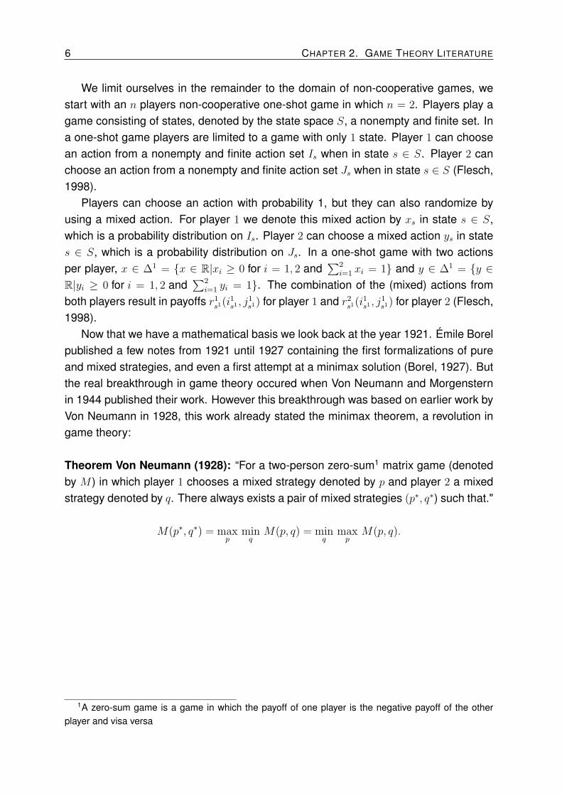
It is best to demonstrate this with an example, consider matrix game zero-sum M
which contains the payoffs for player 1 as2:[
7 3
2 2
]
Figure 2.1: Matrix Game M .
Player 1 is the row player using strategy p and player 2 is the column player using
strategy q. First we look at maxp minq M(p, q). Player 1 wants to maximize his own
payoff and therefore prefers playing the first row over the second one. Given that
Player 1 uses his first action (row), Player 2, who wants to minimize the payoff of player
1, will play the right column over the left one because 3 is smaller than 7. The result
of maxp minq M(p, q) = 3. Player 2 who wants to minimize his opponents expected
payoffs uses his second action (column) because this action weakly dominates his first
action, meaning that no matter what Player 1 does, Action 2 always has a lower payoff
to 1 than the alternative3. The result of minimax is minq maxp M(p, q) = 3.
2We only show the payoffs for player 1 as a positive payoff, the payoffs for player 2 are the negativepayoff of player 1 because it is a zero-sum game.
3In general such strategies need not be pure.

8 CHAPTER 2. GAME THEORY LITERATURE
2.2 The Nash Equilibrium
Where von Neumann can be seen as one of the founding fathers of modern game the-
ory, John Nash Jr. (from here on: Nash) can be seen as an absolute rockstar in the
world of game theory. In 1951 Nash published his PhD. thesis. A major implication of
this thesis was also published in a note called “Equilibrium Points in N-Person Games"
(Nash, 1950). Nash won a Nobel Prize in Economics together with John Harsanyi and
Reinhard Selten in 1994. He received this prize for the discovery of the solution con-
cept for non-cooperative general-sum games. This discovery was later honoured by
calling it the Nash equilibrium. Nash stated the following.
Theorem Nash: “Every finite normal form game has at least one equilibrium point
in mixed strategies (Hyksova, 2004)."
Again let’s demonstrate this theorem with the help of two examples. In the first one
we demonstrate that in a non zero-sum game there exist two Nash equilibria that are
accessible by using a pure strategy for both players. Again player 1 is the row player
with payoff matrix A and player 2 is the column player with payoff matrix B.
A =
[
9 5
9 3
]
Payoff Matrix A for Player 1.
B =
[
1 5
8 5
]
Payoff Matrix B for Player 2.
We combine these matrices to end up with the bimatrix game:[
9, 1 5, 5
9, 8 3, 5
]
Figure 2.2: Bimatrix Game [A,B], first (second) entry is the payoff to player 1(2).
In order to check whether a pure Nash equilibrium exists, we set the strategy of one
player on a fixed pure strategy and determine the best response of the other player. If
a best response of player 1 is located in the same matrix location as the best response
of player 2 then we can state that the corresponding actions for both players are a
pure Nash equilibrium. Because they are best responses for both players, no player
has the incentive to deviate from the Nash equilibrium. Applying this to bimatrix game
[A,B] gives us a new matrix in which we show the best responses of a player with a
checkmark.

2.2. THE NASH EQUILIBRIUM 9
[
9, 1 5, 5
9, 8 3, 5
]
Figure 2.3: Bimatrix Game with pure best responses [A,B].
As can be seen in Figure 2.3 the bimatrix game [A,B] has two pure Nash equilibria,
one in which player 1 plays a pure strategy of playing the bottom row and player 2 the
left column. This pure Nash equilbrium is the Pareto optimal result4 in this game. The
other equilibrium is when player 1 plays the upper row with a pure strategy and player
2 the right column with a pure strategy. This equilibrium is a Pareto inferior result in
comparison to the other pure Nash equilibrium.
A pure Nash equilibrium does not have to exist in a bimatrix game, which we show.
Again we construct a bimatrix game in which player 1 is the row player with payoffs
in matrix A and player 2 is the column player with payoffs in matrix B, resulting in the
combined bimatrix game [A,B]:
[
3, 8 7, 5
8, 1 6, 2
]
Figure 2.4: Bimatrix Game [A,B].
Again we look for the pure best responses, resulting in the following bimatrix:[
3, 8 7, 5
8, 1 6, 2
]
Figure 2.5: Bimatrix Game [A,B].
So Figure 2.5 shows that the bimatrix game [A,B] does not have a pure Nash
equilibrium. However, Nash showed that every bimatrix game in normal form has a
mixed Nash equilibrium. For example, player 1 chooses to play the upper row with
probability p and the lower row with probability (1 − p). Player 2 on the other side
chooses the left column with probability q and the right column with probability (1− q).
The solution for the mixed equilibrium is that player 1 plays strategy (14, 34) and player
2 strategy (16, 56). Player 1 receives a payoff of 61
3and his opponent 23
4.
4See for an explanation on Pareto efficiency Page 10.

10 CHAPTER 2. GAME THEORY LITERATURE
One of the greatest misconceptions surrounding the Nash equilibrium is that it is the
optimal outcome for both players in a game. The Nash equilibrium does not have to
be the highest possible payoff for an individual player nor for the two players. However,
it is the payoff for which each individual player has no rational incentive to unilaterally
deviate from. This is demonstrated by the use of the so-called prisoner’s dilemma.
In this dilemma two ‘future prisoners’ have the option to cooperate, i.e., not betraying
the other player by not telling about the crime, in order to avoid going to prison. The
other option is to defect, i.e., selling out the other player by telling. If both players
choose to defect, then both go to jail for nine years. If one player defects while the
other cooperates, then the player who cooperates is a free man while the other ends
up in jail for ten years, if both cooperate they will only serve a one year sentence. This
can be shown with the help of bimatrix game D representing the prisoner’s dilemma.
cooperate defect[ ]
cooperate −1,−1 −10, 0
defect 0,−10 − 9,−9
Figure 2.6: Prisoner’s dilemma D.
As can be seen in Figure 2.6, the Nash equilibrium is pure, and implies that both
players will defect. Therefore both end up in prison for nine year while a better outcome
would be to cooperate by both. But because each individual player has an incentive
to cheat (if the other player cooperates) and to defect (the result is not ending up in
jail if the counter party does cooperate), the result is that both players end up with
a Pareto inferior result. Pareto inferiority is linked to the concept of Pareto efficiency,
in a situation in which Pareto efficiency has been achieved, no improvement in the
allocation of the payoffs of the players can be made without sacrificing the payoff of
another player. A solution is Pareto inferior if there is a possible improvement in payoffs
for a player without reducing the payoff of another player. In the case of the prisoner’s
dilemma, the players can improve their payoff bilaterally by cooperating and obtain a
Pareto optimal result, i.e., no additional Pareto improvements can be made.

2.3. REPEATED GAMES 11
2.3 Repeated Games
In the previous section we briefly discussed so-called one-shot zero-sum games and
general-sum bimatrix games, i.e., games in which the game is only played once, re-
sulting in a single payoff. A repeated game has similarities to the one-shot game. It is
a one-shot game but now played for a finite or infinite number of times. The standard
assumption is that players are aware of all the (possible) actions and resulting payoffs
of the game until t. We call this complete information (Peters, 2015).
Repeated games have an advantage over one-shot games in the sense that they
can reach rewards5 which would normally be unattainable (Mertens, 1990). As we
stated earlier, repeated games can be played for a finite or infinite number of times.
In the first case this means that the game is played repeatedly for a finite number of
times T . The other option is to play the game forever. In game theory the infinitely
repeated type of game is studied more frequently than the finitely repeated game. A
reason for this is that it is usually unknown how long T is for a game. Also infinitely
repeated games could be more interesting because finitely repeated games can in
specific cases be rewritten as a one-shot game and lack interesting features (Vrieze,
2003b). However, both options result in cumulative payoffs, there are two common
methods for the analysis of these cumulative payoffs.
The first common method is the discounted reward criterion, with this criterion we
analyze the game by assuming that any future payoff is valued less than the same
payoff in the present. Therefore we discount future payoffs with a factor δ (0 < δ < 1).
We define the discounted criterion as follows. Player k receives a discounted reward
(γk) in a two player game in which player 1 plays strategy π and player 2 plays strategy
σ. The expected payoff of player k at time t under (π, σ) is defined by Rkt (π, σ). The
discounted reward for player k is:
γk(π, σ) =T∑
t=0
δtRkt (π, σ)
Another way to analyze repeated games is by stating that the player values the
present equally to any other period in the future. Therefore the player is indifferent with
respect to receiving a payoff now or at a future stage. In this case we are looking at an
infinite game with the limiting average reward criterion (Sorin, 2003). For player k this
is:γk(π, σ) = lim inf
T→∞
1
T
T∑
t=1
Rkt (π, σ)
In this thesis we focus on the limiting average criterion. For repeated games the
use of this limiting average reward criterion could result in the same rewards as just
analyzing a single-period (bi)matrix game.5Rewards are a result of cumulative payoffs based on a strategy pair, we introduce rewards in this
same page.

12 CHAPTER 2. GAME THEORY LITERATURE
2.4 Stochastic Games
We move on to stochastic games. Stochastic games were introducted by Shapley
(1953). Stochastic games are much more complex in comparison to repeated games.
The only thing in common is that they both are played for a(n) (in)finite number of
periods T (T ≥ 2). The difference lies within the state that game is in. In a repeated
game there is only a single state which is played for period T (T ≥ 2). In a stochastic
game the state can change, based on the transition probabilities of the state in which
the game currently is. Such transition probabilities represent the probability of moving
to the current state or going to another state. Collectively states can be seen as multiple
games that can be played but it depends on the transition probabilities whether they
are played or not. Characteristics of one-shot games, repeated games and stochastic
games are stated in Table 2.1.
Game type One-shot game Repeated game Stochastic game
T 1 ≥ 2 ≥ 2
States 1 1 ≥ 2
Table 2.1: Characteristics of different types of games.
In order to formalize the stochastic game in general we build further on the frame-
work of a non-cooperative game stated in Section 2.1. Again we have n-players
(n ≥ 2), but this time there are a multiple states denoted in the state space S. Player i
has k number of actions depending on the state being in. A strategy is stating exactly
to a player which action to play in each state at each point in time given any history of
the play. We usually denote a strategy with π for player 1 and σ for player 2. The prob-
ability of playing a state depends on the transition probabilities, denoted by matrix p. In
p the rows (r) represent the current states while the columns (c) are the possible future
states. An entry in p with row r and column c is the probability of ending up in future
state c from current state r. The rows in p should always sum up to 1 (∑n
c=0 pr,c = 1).
The combination of states S and pair of strategies (π, σ) result together with transition
probabilities p in a reward set for players denoted by R.

2.4. STOCHASTIC GAMES 13
In order to make it conceivably we show a simplified example, taken from Samuel’s
Master Thesis (2017). The example concerns a two player, two state stochastic game.
The payoffs of both players in state 1 and state 2 are given by θS1and θS2
.
θS1=
[
16, 16 14, 28
28, 14 24, 24
]
θS2=
[
4.0, 4.0 3.5, 7.0
7.0, 3.5 6.0, 6.0
]
Ending up in a certain state depends on transition probabilities p, which for both
states are given as:
pS1 =
[
0.8, 0.2 0.7, 0.3
0.7, 0.3 0.6, 0.4
]
pS2 =
[
0.5, 0.5 0.4, 0.6
0.4, 0.6 0.15, 0.85
]
This example game is a ‘commons’-type game (Hardin, 1968). In a ‘commons’
game there is a renewable common-pool resource, players share this common-pool
and use it for their individual gain which may result in depletion of the resource. A type
of game modelled as a ’commons’-type game is the fishery wars, analyzed by Levhari
and Mirman (1980) and Joosten (2007). In their fishery wars game the players catch
fish from the ocean, but overfishing can result in a depletion of the fish stock. In the
example game the depletion of the fish takes place in state S2, while state S1 represents
a higher amount of fish in the common-pool. Overfishing not only results in a higher
probability of ending up in state S2, but it also affects the transition probabilities. When
overfishing, the transition probabilities change, the transition probability of ending up in
state S2 increases while the probability of ending up in state S1 decreases.
However, the big question is now, how do we analyze these games? Shapley (1953)
proposed using the discounted criterion and proved that there is a value6 for the infinite
zero-sum game and also showed that minimax and maximin solutions exist. Gillette
(1957) introduced the limiting average criterion and showed that a value exists for infi-
nite zero-sum games with perfect information. The absolutely compelling proof came
from Mertens and Neyman (1981). They showed that a value exists for all zero-sum
stochastic games and Neyman (2003a) demonstrated that all stochastic games have
a minimax and maximin solution.
6The value of a game is the reward of the game when M(p∗, q∗) = maxp minq M(p, q) =
minq maxp M(p, q)

14 CHAPTER 2. GAME THEORY LITERATURE
Types of strategies and Folk Theorem
Finding an equilibrium, a value, a minimax or a maximin solution depends on the
type(s) of strategy being chosen by both players. In stochastic games several types
of strategies are possible, which we now describe.
Behavioral strategies are strategies in which a player takes into account the history
of play leading up to a certain state. Therefore behavioral strategies are history de-
pendent and require a player to remember the history of play in order to determine the
optimal strategy.
Markov strategies are strategies in which the player does not take the entire history
of play into account, but decides on the basis of the current state the play is in and
current period how to play.
Stationary strategies are strategies in which the decision of the player does not de-
pend on the history of play, nor on the current time, it only depends on the current state
being in. Therefore a player always plays the same (mixed) action in each state.
Behavioral strategies are the most complex strategy type described here because they
require a memory for the player. For infinite stochastic games this requires a large
memory, and therefore a lot of storage capacity. However behavioral strategies are not
always necessary. In this thesis we limit ourselves to irreducible stochastic games un-
der the limiting average criterion. Vrieze (2003a), showed that for irreducible stochastic
games stationary strategies are optimal. For reducible stochastic games, the zero-sum
game ‘Big Match’ by Blackwell and Ferguson (1968) shows that not all limiting average
stochastic games have a value that corresponds to a stationary strategy.
Another important result in literature is the Folk Theorem, stating that subgame per-
fect Nash equilibria can be reached in repeated games. When players are patient and
far-sighted (as is the case with the limiting average criterion) then, as long as the pay-
offs are feasible and strictly individually rational (Levin, 2002), any outcome satisfying
the conditions can be obtained by using a Nash equilibrium. The difference with playing
a mixed action in a one-shot game is that in practice a mixed action will be converted
to a pure action, one cannot actually randomize, but only randomize the probability that
a certain action is chosen. Therefore, the Folk Theorem and repeated games define
necessary conditions in order to actually obtain rewards. The Folk Theorem therefore
forms a basis for further analysis of equilibria in stochastic games.

2.5. FREQUENCY-DEPENDENT GAMES 15
2.5 Frequency-Dependent Games
This brings us to the class of Frequency-Dependent games, introduced in 2003 by
Brenner and Witt. Frequency-Dependent games are infinitely repeated games in which
the stage payoffs depend on the frequencies of play up until that stage and including
the current period in time. The first analysis was done by Brenner & Witt (2003), but
Joosten et al. (2003) continued by deepening on feasible results and equilibria.
This was done by introducing the concept of jointly-convergent pure-strategy pairs.
An important part of this is the relative frequency vector denoted by xt. The relative
frequency vector xt states the relative frequency of play ending up at a certain payoff
cumulatively at stage t. As an example we look at a simple 2x2 bimatrix game. The
relative frequency vector at stage t for this game looks as follows:
xt =
[
xt1 xt
2
xt3 xt
4
]
Suppose we play this bimatrix game for a period t = 100, the strategy pair (π, σ)
results in the game ending up in x1 for 75 times, in x2 20 times and x4 5 times. The
result is the relative frequency vector x100 with:
x100 =
[
0.75 0.20
0.00 0.05
]
For which:
i=4∑
i=1
xi = 1
The relative frequency vector xt therefore changes based on frequency of the his-
tory of play and as stated earlier plays a large role in the concept of jointly-convergent
pure-strategy pairs. A pure strategy is a strategy in which at any stage t in any state
a player chooses a certain action with probability 1. A strategy pair (π, σ) is jointly-
convergent for strategy of player 1 π, strategy of player 2 σ and relative frequency
vector x if and only if (Joosten et al., 2003):
lim supt→∞
Prπ,σ[|xti − xi| > ε] = 0
Jointly-convergent pure-strategy pairs are strategy pairs for which the relative fre-
quency vector converges to a vector consisting of fixed numbers with probability 1
when t goes to infinity (Billingsley, 2008). Based on this it was possible to compute
the set of feasible jointly-convergent pure-strategy rewards. The main result however
of jointly-convergent pure-strategy pairs is the following:

16 CHAPTER 2. GAME THEORY LITERATURE
Theorem: “Each pair of individually-rational jointly-convergent pure-strategy re-
wards can be supported by an equilibrium. Moreover, each pair of jointly-convergent
pure-strategy rewards giving each player strictly more than the threat-point reward, can
be supported by a subgame-perfect equilibrium. (Joosten et al., 2003)"
Key in this theorem is the so-called threat point reward. The threat point v = (v1, v2)
is defined for two players as the point in which v1 = minσ maxπ γ1(π, σ) and v2 =
minπ maxσ γ2(π, σ). So both players can threaten each other by minimizing the pay-
off of the other player while the player under threat tries to maximize its own payoff.
The threat point is the absolute minimum players can reach as a payoff equilibrium
and therefore each individual player has an individual rational payoff if he can at least
receive the threat point reward (Joosten et al., 2003). But the major result by Joosten
et al. (2003) is the following theorem:
Theorem: “Each pair of rewards in the convex hull of all individually-rational jointly-
convergent pure-strategy rewards can be supported by an equilibrium. Moreover, each
pair of rewards in the convex hull of all jointly-convergent pure strategy rewards giving
each player strictly more than the threat-point reward, can be supported by a subgame-
perfect equilibrium (Joosten et al., 2003)."
The threat point is key in finding equilibria supported by jointly-convergent pure-strategy
rewards. Threat points can be calculated analytically (e.g.,(Joosten & Meijboom, 2018))7,
but analytical methods may be too cumbersome, and as the complexity of a game in-
creases the need for a fast algorithmic solution to compute the threat point increases
equally. Joosten and Samuel (2018) have explored the domain of stochastic games
and tried to order them. Games are divided into three major categories. Type I, Type II
and Type III games. Type I games are games in which the play is repeated and transi-
tion probabilities per state are fixed, Type II games are stochastic games with constant
transition probabilities and Type III games are stochastic games in which the transition
probabilities are endogenous, which means that they depend on the history of play.
7The first working paper by Joosten and Meijboom was released in 2010, but published for the firsttime in a book in 2018.

2.5. FREQUENCY-DEPENDENT GAMES 17
Within these three categories there is also a distinction in whether the payoffs
are frequency-dependent. If they are frequency-dependent we call them Endogenous
Stage Payoffs (ESP) games. Without the frequency-dependent stage payoffs they are
called Constant Stage Payoffs (CSP) games. The same goes for the transition proba-
bilities, with frequency-dependent transition probabilities they are called Endogenous
Transition Probabilities (ETP) games and Constant Transition Probabilities (CTP) games.
Combining these in a table has been done by Joosten and Samuel (2018) and gives
the following:
CTP ETP
Type I
(p0)
Type II
(x, p0)
Type III
(x, p(x))
CSP
(θ0)AIT games Stochastic games
CAIT-games
ETP-games
ESP
(θ(x))
FD games
AIT FD gamesStochastic FD games
CAIT-ESP games
ETP-ESP games
Table 2.2: Ordering of different types of stochastic games (Joosten & Samuel, 2018).
Stochastic Frequency-Dependent (FD) games were first named this way by Mahohoma
(2014), Joosten and Samuel (2018) call this term “a tautology in the broad interpreta-
tion." Mahohoma (2014) analyzed stochastic FD games while Joosten and Meijboom
(2018) analyzed ETP-CSP games. Joosten and Samuel (2018) were the first to calcu-
late feasible rewards in ETP-ESP games. In general, the use of the term Frequency-
Dependent has been expanding over the years.
The first FD games introduced by Brenner and Witt (2003) and Joosten et al. (2003)
were additive. Later, Joosten (2007) introduced an adaptation on the Small Fish Wars
which contained FD games that are multiplicative and nonlinear. Joosten (2009) in-
troduced the first FD games which are jointly frequency dependent. In 2010, the first
FD games with Endogenous Transition Probabilities were developed by Joosten and
Meijboom. The last and most complex development in the domain of FD games was
tackled by Joosten and Samuel (2018) in the domain of ETP-ESP games.
Last but not least we clarify AIT and CAIT games. AIT stands for Action Indepen-
dent Transition (AIT) (probability) games and CAIT games are Current Action Indepen-
dent Transition (CAIT) (probability) games. AIT-games are games in which the play is
repeated and for which transition probabilities are fixed and equal in each state, i.e.,
independent from the action pair chosen. The main focus of this thesis is to develop
a threat point algorithm which is fast and suits all of these types of stochastic games.
Therefore we start at the simpler Type I games, then continue with Type II games and
finally end up with Type III games. As the complexity of the games increases, the
complexity of the computations also rises.

18 CHAPTER 2. GAME THEORY LITERATURE

Chapter 3
Building the algorithm
In this chapter we build the algorithm from the ground up, we start by introducing earlier
work which partly forms a basis for the algorithm created. Then we clarify the relation
between Markov Chains, Markov Decision Processes and Stochastic Games. We in-
troduce necessary limitations on stochastic games in order for our algorithm to work
as intended. We also introduce the programming tools used to develop the algorithm.
Once these things are clear, we start by describing the algorithm(s) for Type I games,
then continue with Type II games and end with Type III games. All code corresponding
to the algorithms can be found in Appendix A.
3.1 Earlier Work
Before we start with the building blocks of the algorithm, we look at earlier work done
in the area of computations in stochastic games. In literature, research has been con-
ducted on algorithms for stochastic games. Raghavan and Filar (1991) have conducted
a survey in which they limited to algorithms for zero-sum and non-zero-sum stochastic
games with complete information and stationary strategies. A lot of research has been
done, but mostly regarding the discounted reward criterion (Breton, Filar, Haurle, &
Schultz, 1986, e.g.). Vrieze (1981) has developed a linear programming approach to
an undiscounted stochastic game based on earlier algorithms by Filar and Raghavan
(1979). However it is unclear whether these approaches work on the broad range of
stochastic games and if they do, are they able to find the so-called threat point in every
type of game?
In 2014 Mahohoma tried to partially overcome this in his Master thesis. He analyzed
so-called stochastic FD-games (Type II, CTP-ESP). Part of his thesis is a simulation
based approach in MATLAB in order to determine equilibria, feasible rewards but also
threat points. However, one of the problems in the approach taken by Mahohoma lies
in the simulation approach and the resulting complexity of the code. As an example we
19

20 CHAPTER 3. BUILDING THE ALGORITHM
look at the determination of threat points. Mahohoma simulates the stochastic game
for a fixed period t, number of times n. Therefore a total of n simulation results is
combined and gives as an average an approximation of the threat point. Not only does
this algorithm lack the ability to give an exact result, the algorithm is also of a high
computational complexity O(n4). This does not mean that the approach of Mahohoma
is useless, it could be useful in games in which non-stationary strategies are the only
way of reaching the threat point. However, when looking at stochastic games in the
broader sense, in games in which stationary strategies always cover the threat point,
we think that this could be done in an exact and more optimized matter.
The most recent work however has been done by Joosten and Samuel (2018).
Samuel (2017) did a first analysis in her thesis. There she started the work which
is also partly used for the calculation of threat points in this thesis. Samuel defines
three algorithms in MATLAB used for computing feasible rewards in Type I, Type II and
Type III games, with or without FD payoff. The basis for the computations of the set
of feasible rewards are jointly-convergent pure-strategy rewards in which the algorithm
is limited to games with communicating states.1 This work has been formalized and
analyzed more rigorously by Joosten and Samuel (2018). The algorithm works well
and the threat point is part of the set of feasible rewards found. However, the algorithm
does not explicitly find this threat point. Another potential problem with the algorithm is
that the computational running time for a large set of rewards possibly is unnecessarily
long.
3.2 From Markov Chain to Stochastic Game
In literature there is a clear link between Markov chains on one side, and stochastic
games on the other end of the spectrum. Markov chains were introduced by and named
after the Russian mathematician Andrey Markov (1971). Markov chains are stochastic
processes in which the process is memoryless. The Markov property states that it does
not matter what the history is before the present, the only thing relevant for the future
is the present. We denote a random variable in a stochastic process at time t by Xt,
the current value of the variable is denoted by x. Mathematically, memorylessness has
the following effect on a stochastic process.
Pr(Xt+1 = x|X1 = x1, X2 = x2, . . . , Xt = xt) = Pr(Xt+1 = x|Xt = xt) (3.1)
1See next paragraph on communicating states


22 CHAPTER 3. BUILDING THE ALGORITHM
Definition Aperiodic Markov Chains: “A Markov chain is said to be aperiodic
if all its states are aperiodic. Otherwise the chain is said to be periodic (Häggström,
2002)."
Figure 3.1 is an aperiodic Markov chain. It is not the case that after a certain fixed
number of rainy days that there always will be a sunny day. Aperiodicity and irreducibil-
ity are two properties which form the basis of an interesting insight into Markov chains.
When an aperiodic and irreducible Markov chain is run for a long time, it is unclear
in which state the Markov chain is at a certain period in time. However, running the
Markov chain for an infinite period of time will result in the Markov chain settling in a
stationary distribution. This stationary distribution describes the probability of visiting
a certain state when time goes to infinity. Therefore with great precision we know the
frequency of being in a certain state when the Markov chain is run for an infinite period
of time. We therefore present an important resulting theorem which forms an important
part of this research:
Theorem: “For any irreducible and aperiodic Markov chain, there exists at least
one stationary distribution (Häggström, 2002)."
But how are Markov chains linked to stochastic games? Neymann described that
“Markov chains and Markov decision processes are special cases of stochastic games
(Neyman, 2003a)." Markov chains are necessary to model the dynamics of a system.
They state the transition probabilities of a stochastic game. In between the Markov
chain and the stochastic game is the Markov Decision Process (MDP). The MDP is a
reduction of the stochastic game in which there is only one player. Therefore the player
is able to control the play and hence the corresponding payoffs on his own. Filar and
Vrieze (1997) describe the stochastic game in terms of a competitive MDP.
In the case of one player under the limiting average criterion they describe the MDP
as follows. The player starts in initial state s while playing stationary strategy f , the
reward at time t is defined by Rt. The value of this irreducible limiting average MDP is
defined as (Filar & Vrieze, 1997):
vα(f) := limT→∞
[
( 1
T + 1
)
T∑
t=0
Esf [Rt]
]
The individual rational player always wants to maximize his own payoff. So the
problem is an optimal control problem in which the player wants to:
max vα(f)

3.3. LIMITATIONS GAME USAGE 23
This problem can also be seen as an optimal control problem in which the player
tries to control the process in such a matter that his own value is maximized (Blackwell,
1962). In literature these MDP models are not only used for stochastic games but for
a wide range of applications. They are used for decision-theoretic planning, learning
robot control and ofcourse stochastic games. MDPs are the standard for learning se-
quential decision making (Otterlo, 2009). Algorithms in order to find optimal values for
an MDP are divided into two categories. Model-free and model-based algorithms. The
first category is also known as reinforcement learning and generates approximations
while the second one is exact and uses dynamic programming as a basis (Blackwell,
1962), (Otterlo, 2009).
Because we are dealing with stochastic games in which we assume perfect infor-
mation we have all information available in order to calculate an exact result. We shall
therefore only look at model-based algorithms. These algorithms work on optimizing
value functions by either iterating over the value function (value iteration) or by chang-
ing the so-called policy (policy iteration). The policy of an MDP can be seen as a fixed
pure strategy which always is taken when in a certain state. At the heart of these algo-
rithms is the Bellman equation. The Bellman equation defines the relation between the
value function and the recursive process in order to determine the result of the value
function (Otterlo, 2009). The equation is stated as (Otterlo, 2009):
V π(s) = Eπ
{
rt + V π(st+1)|st = s}
=∑
s′
T (s, π(s), s′)(
R(s, a, s′) + V π(s′))
In which policy is represented by π, the transitions by T , current state by s, rewards
by R and current reward by r. This Bellman equation is important when we come
to an algorithm for Type II games. But for now it is most important to acknowledge
that stochastic games can be seen as competitive MDPs in which Markov chains are
responsible for the transition dynamics between the states.
3.3 Limitations game usage
In literature on stochastic games several classes of games have been distinguished.
Flesch (1998) gives an overview of the different types of stochastic games. He defines
eight types of special classes and shows important results for these games in both the
zero-sum case and general-sum case. Without going into much detail on the char-
acteristics of these special classes we only focus on important results. The zero-sum
cases of these special classes show mostly that there are optimal stationary strategies.

24 CHAPTER 3. BUILDING THE ALGORITHM
For the general-sum case there exist ε-equilibria2, but optimal stationary equilbria are
only known to exist in a select number of cases (Flesch, 1998).
We limit ourselves in the creation of the algorithm to types of games for which we
know that the algorithm works. Earlier we stated Markov chain properties which guar-
antee a stationary distribution of the chain, i.e., irreducibility and aperiodicity. There-
fore we focus on games in which the Markov chain governing the transition matrix is
ergodic.3 Games with absorbing states or more than one ergodic set are currently left
out of scope. This however, does not mean that the algorithm constructed does not
cope with any of the special classes described by Flesch (1998). We think that this
leaves room for future research. For now we focus on the above stated characteristics
and type of games displayed in Figure 2.2. We limit ourselves to two-player, two-state
games.
3.4 Programming Tools
Creating an algorithm has to be done with the help of programming languages and
tools. Earlier we stated that work has been done by Mahohoma (2014) and Samuel
(2017) in MATLAB. We choose to deviate from MATLAB and take a different approach.
First, MATLAB is a commercial programming language used mostly in the educational
domain, but because of the commercial licensing necessary to run, it limits the appli-
cability of the algorithm without a license. We are however in favor of free open-source
solutions. Secondly, because MATLAB is a commercial product we cannot always get
a grasp on what is happening under the hood of the program. In case of algorithmic
optimization this can be problematic. So a choice has been made to not continue us-
ing MATLAB but to transfer to Python. We describe Python and the other programming
tools used briefly to give the reader an impression of their possibilities.
3.4.1 Python
We first introduce the main programming language used. Python was developed in
the early 90’s by Guido van Rossum. The goal of Python is to provide easy and un-
derstandable syntax, which should result in highly readable code. Python does this by
using indentation as a major part of the programming syntax. In comparison to other
programming languages, Python has a dynamic type system, i.e., that Python does
not require the programmer to define the type of variables used. This also improves
readability a lot. On the other side, Python is an interpreted language and also a rather
slow one. In comparison to C++ or Java, Python lacks raw speed. However, Python
2ε-equilibria are equilibria that approximately satisfy the condition associated with the Nash equilib-rium. The incentive for a player to deviate from this equilibrium is ε small.
3Ergodic Markov chain are always irreducible and aperiodic

3.5. TYPE I GAMES 25
is a flexible language for which additional packages can be used to cope with this. A
lot of additional and highly optimized packages are developed for Python and can be
used.
3.4.2 NumPy
One of these packages is NumPy and was introduced in 2005 into Python. NumPy
is written in C and offers Python users multi-dimensional array and matrix tools. It is
seen as the go to solution for numerical computations with high-level4 mathematical
functions. Because NumPy has been written and compiled in C the operations are
comparable to MATLAB in terms of speed. NumPy is also open-source and develop-
ment is ongoing, so it is well-suited for the building of the algorithm in this thesis.
3.4.3 SciPy
Another comparable package is SciPy, SciPy is based on NumPy and uses a lot of at-
tributes from NumPy in order to provide scientific computing functions. SciPy contains
for example linear algebra functions and optimization functions using linear program-
ming.
3.4.4 MDP Toolbox
The last tool used is the Python MDP Toolbox. This toolbox contains multiple algorithms
(model-free and model-based) which can be used in order to solve an MDP. Most
algorithms are written with the help of NumPy and therefore speed should not be an
issue.
3.5 Type I games
We start building the algorithm by looking at Type I games. They are simple in essence
because the play in these games is repeated. This makes Type I games less hard to
analyze in comparison to Type II, let alone Type III games. But first we should state how
we enter a game into the algorithm(s). We use NumPy in order to declare matrices. In
Type I games, only two things are relevant when entering the game into an algorithm.
Most important are the reward matrices for each player, the reward matrices display the
payoffs that a player can achieve when playing pure strategies. Next is the frequency-
dependent function, the frequency-dependent function declares what the relation is
4High-level in this sense means that the programming language is of a higher abstraction in compar-ison to low-level programming languages or machine language.

26 CHAPTER 3. BUILDING THE ALGORITHM
between a potential change in payoff and the frequency of play of certain strategy
combinations. Because both can be defined in several ways, we adapt to the model
used by Samuel (2017). Samuel (2017) uses a game in which the Nash equilibrium is
also Pareto superior. However, she states that when playing this equilibrium this will
eventually have an impact on the renewable common-pool resource and will therefore
influence the payoff in the future (Samuel, 2017).
The combined payoff matrix used in order to test the algorithm is as follows:
θS1=
[
16, 16 14, 28
28, 14 24, 24
]
Samuel also created a linearly decreasing function as the frequency-dependent
function. This was specifically created for the game stated above, so we also use this
function in order to test the algorithm within this thesis.5
The frequency-dependent function for the Type I game is determined by:
FDtI = 1−
1
4(xt
2 + 2xt3)−
2xt4
3
Hence, if the payoffs are frequency-dependent, they become:
θtS1= FDt
I ·
[
16, 16 14, 28
28, 14 24, 24
]
The upper-left corner of the payoff matrix (with payoff 16 to both players) can be
seen as the responsible result of the game for which the depletion of the common-
pool resource is non-existent. The upper-right corner results in a slight depletion, while
the bottom-left corner is double the depletion compared to the upper-right corner. The
worst outcome for the common-pool resource would be the bottom-right corner, it would
result in the largest depletion effect on the renewable common-pool resource. There-
fore the players also have to take into account the long-term effect on the common-pool
resource.
But now we focus on the building of the algorithm. Because there are different ways
to skin a cat, there are also different ways to build an algorithm. We have tested two
approaches and will start with the approach which uses a SciPy optimizer. The second
approach is an adaptation of the algorithm by Joosten and Samuel (2018).
5Other games were tested by the author, but for the sake of simplicity we keep it at just one gamewithin the thesis

3.5. TYPE I GAMES 27
3.5.1 SciPy optimizer
SciPy as stated earlier is home to scientific computing packages. One of these is
the optimization package. The optimization package contains several mathematical
optimizers which are used for finding local or global optima. Mostly these optimizers
rely on methods which calculate derivatives in order to find the optimum of a function.
However a problem with these methods is that they can get stuck in local optima which
could potentially not be the global optimum (Knowles, Watson, & Corne, 2001). Using
these optimizers therefore has an inherent risk, which is that they provide possible
sub-optimal solutions.
For Type I games with no frequency-dependent function this problem is redundant.
Type I games as stated earlier are simple games which are repeated for a(n) (in)finite
number of periods. Therefore optimizing over the payoffs is like optimizing a linear
function when searching for a minimum. We start by using the optimizer for non-FD
Type I games.
Because we are looking at the threat point for two players we start by restating what
the threat point is. The threat point v is the point in which player 1 plays strategy π and
player 2 plays strategy σ for which:
v = (v1, v2) with:
v1 = minσ1
maxπ1
γ1(π1, σ1)
v2 = minπ2
maxσ2
γ2(π2, σ2)
So v1 (2) is the amount which player 1(2) can guarantee himself if player 2(1) tries to
minimize the payoff of player 1(2).
In order to find the threat point we start in Python by initializing the strategy of the
player who is threatening the other player with an empty strategy (an array containing
only zeros). Then we have to set a condition for which the stationary strategy must
hold. This condition declares that the probability assigned to all possible actions within
the strategy must sum to 1. For example, if we have a game with one-state and two
possible actions for player 2, if σ1, σ2 are the representation of player 2 choosing re-
spectively action 1, action 2 then
2∑
i=1
σi = 1
So again, the player has to choose a stationary strategy in which there is a summed
probability of 1 over all possible actions. Additionally we have to declare to the algorithm
that the bounds for assigning a probability to an action lie between 0 and 1:
28 CHAPTER 3. BUILDING THE ALGORITHM
0 ≤ σi ≤ 1
We also declare a threat function, this is the function that needs to be optimized.
In this case we first multiply the rewards with the stationary strategy chosen by the
threatening player, i.e., for v1 we multiply γ1 with σ1. Therefore function v1 has the form:
v1 = maxπ1
(γ1 · σ1)
And for v2:
v2 = maxσ2
(γ2 · π2)
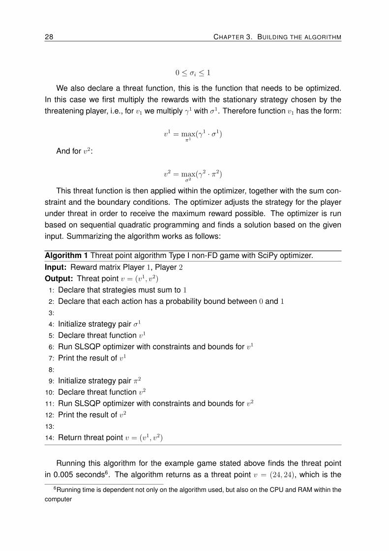
This threat function is then applied within the optimizer, together with the sum con-
straint and the boundary conditions. The optimizer adjusts the strategy for the player
under threat in order to receive the maximum reward possible. The optimizer is run
based on sequential quadratic programming and finds a solution based on the given
input. Summarizing the algorithm works as follows:
Algorithm 1 Threat point algorithm Type I non-FD game with SciPy optimizer.
Input: Reward matrix Player 1, Player 2
Output: Threat point v = (v1, v2)
1: Declare that strategies must sum to 1
2: Declare that each action has a probability bound between 0 and 1
3:
4: Initialize strategy pair σ1
5: Declare threat function v1
6: Run SLSQP optimizer with constraints and bounds for v1
7: Print the result of v1
8:
9: Initialize strategy pair π2
10: Declare threat function v2
11: Run SLSQP optimizer with constraints and bounds for v2
12: Print the result of v2
13:
14: Return threat point v = (v1, v2)
Running this algorithm for the example game stated above finds the threat point
in 0.005 seconds6. The algorithm returns as a threat point v = (24, 24), which is the
6Running time is dependent not only on the algorithm used, but also on the CPU and RAM within thecomputer
3.5. TYPE I GAMES 29
correct threat point for this game. We have confirmed this by computing the maximin
value of the game, which was 23.9. We were not able yet to incorporate the frequency-
dependent function into the SciPy algorithm. We have looked into multiple methods but
have not found an efficient and satisfactory solution.
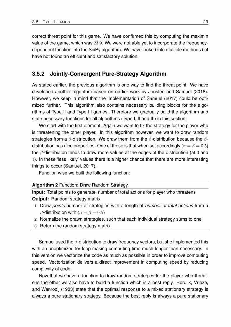
3.5.2 Jointly-Convergent Pure-Strategy Algorithm
As stated earlier, the previous algorithm is one way to find the threat point. We have
developed another algorithm based on earlier work by Joosten and Samuel (2018).
However, we keep in mind that the implementation of Samuel (2017) could be opti-
mized further. This algorithm also contains necessary building blocks for the algo-
rithms of Type II and Type III games. Therefore we gradually build the algorithm and
state necessary functions for all algorithms (Type I, II and III) in this section.
We start with the first element. Again we want to fix the strategy for the player who
is threatening the other player. In this algorithm however, we want to draw random
strategies from a β-distribution. We draw them from the β-distribution because the β-
distribution has nice properties. One of these is that when set accordingly (α = β = 0.5)
the β-distribution tends to draw more values at the edges of the distribution (at 0 and
1). In these ‘less likely’ values there is a higher chance that there are more interesting
things to occur (Samuel, 2017).
Function wise we built the following function:
Algorithm 2 Function: Draw Random Strategy.
Input: Total points to generate, number of total actions for player who threatens
Output: Random strategy matrix
1: Draw points number of strategies with a length of number of total actions from a
β-distribution with (α = β = 0.5)
2: Normalize the drawn strategies, such that each individual strategy sums to one
3: Return the random strategy matrix
Samuel used the β-distribution to draw frequency vectors, but she implemented this
with an unoptimized for-loop making computing time much longer than necessary. In
this version we vectorize the code as much as possible in order to improve computing
speed. Vectorization delivers a direct improvement in computing speed by reducing
complexity of code.
Now that we have a function to draw random strategies for the player who threat-
ens the other we also have to build a function which is a best reply. Hordijk, Vrieze,
and Wanrooij (1983) state that the optimal response to a mixed stationary strategy is
always a pure stationary strategy. Because the best reply is always a pure stationary

30 CHAPTER 3. BUILDING THE ALGORITHM
strategy, we only consider pure stationary strategies for the player who is being threat-
ened. Therefore we have to convert the strategy of the player who is threatening into a
frequency vector based on the pure stationary strategy reply of the player under threat.
Based on this we built a function which sorts strategies into frequency vectors. For
each individual player we built a separate function, but this is due to storage differences,
in essence they are comparable. The function contains:
Algorithm 3 Function: Create Frequency Vector.
Input: Total points generated, number of total actions for both players, random strategy
matrix
Output: Frequency pairs based on pure best replies from player under threat
1: Initialize frequency vector with dimensions: (total number of points · total number of
actions Player 1 , total number of actions Player 1 · total number of actions Player
2)
2: for i in range total number of actions player under threat do
3: for j in range total number of actions threatening player do
4: if v1 is searched then frequency vector[total number of points · (i − 1):total
number of points i,(number of actions player 2 · i)+j] = random strategy matrix[:,j]
5: end if
6: if v2 is searched then frequency vector[total number of points · (i − 1):total
number of points i,(number of actions player 1 · j)+i] = random strategy matrix[:,j]
7: end if
8: end for
9: end for
10: Return frequency vector
The result is a frequency vector in which only the pure stationary best replies of
the player under threat contain a non-zero frequency of play. As an example, if a
player under threat has two pure stationary strategies (as an example: left and right)
as a reply, then if there are 200 random strategies drawn for the threatening player,
the result is 400 frequency pairs in the frequency vector. The first 200 represent the
first (left) pure stationary strategy of the player under threat, the second 200 represent
the other (right) pure stationary strategy. We visualize this with an example, suppose
the player threatening plays a mixed stationary strategy in which up is played with
probability 0.8 and down with probability 0.2. Algorithm 3 then sorts this strategy in
two best replies (left and right) for the player under threat. Resulting in the following
frequency matrix, shown in Figure 3.2:

3.5. TYPE I GAMES 31
[
0.8 0
0.2 0
]
and
[
0 0.8
0 0.2
]
(3.2)
Figure 3.2: Best reply frequency matrices.
There is a trade-off taking place in this frequency vector function. By creating this
function it was inevitable to use a for-loop. Because we want to create a function which
can scale with larger games with more actions, we had to use a for-loop. However,
this for-loop was done with a NumPy for-loop, an optimized way of running a for-loop
in large matrices. Performance gains can be made if the number of actions for a game
is always fixed at the same number, in those cases a hard-coded function without for-
loops will result in a significant gain in computational performance.
At last we need to build a function which stores all the corresponding drawn random
mixed strategies with pure best responses into a logical matrix which makes extracting
the threat point easy. Therefore we built a function called payoff sort. This function
sorts the payoffs which are computed from the generated random mixed strategies
based on there relationship. So the function stores all pure best replies to a certain
drawn strategy in the same row. Function wise this has resulted in the following:
Algorithm 4 Function: Payoff sort.
Input: Total points generated, payoff matrix, total number of actions
Output: Sorted payoff matrix
Initialize empty sorted payoff matrix (number of points, number of actions)
for x in range total number of points do
for i in range total number of actions do
Sorted payoffs[x,i] = payoff matrix[points · i+ x]
end for
end for
Return sorted payoff matrix
Now we have all essential functions in order to construct the final algorithm which
calculates the threat point for a Type I (non)-FD game. We construct the algorithm in
such a way that it incorporates the frequency-dependent function for the payoffs. We
combine the above stated functions in order to construct the following algorithm:

32 CHAPTER 3. BUILDING THE ALGORITHM
Algorithm 5 (Non)-FD Type I threat point algorithm.
Input: Type I Game, total number of points, activate FD function
Output: Threat point
1:
2: If v1 is calculated, then X = 1, Y = 2,
3: If v2 is calculated, then X = 2, Y = 1
4:
5: Turn reward matrix Player X into flattened reward vector
6: Threatening strategies Player Y = Draw Random Strategies
7: Best response Player X frequency vector = Create Frequency Vector
8: if Activate FD function = True then
9: Activate and Calculate FD payoff Function result
10: end if
11: Payoffs Player X = Sum over all columns of: (Frequency Vector per row · flattened
vector Player X)
12: if FD Function is active then
13: Element wise multiplication of FD payoff function result with Payoffs Player X
14: end if
15: Sorted payoff matrix = Payoff sort
16: Pick the maximum value of each row of the sorted payoff matrix as best response
of Player X
17: Pick the minimum value over all rows as the result of vX
18:
19: Return threat point v = (v1, v2)
Filling in a total number of points generated of 100 and the FD payoff function as
not active results in a threat point of approximately (24.009, 24.0006) in roughly 0.006
seconds. When activating the FD payoff function the algorithm finds a threat point with
100 points in roughly the same amount of time with as a result (10.506, 8.0002).
3.5.3 Visualizing the results
In order to give an impression of the threat point within these games, we visualize
both the threat point and the surrounding reachable payoffs for the players. We use
the algorithm by Joosten and Samuel to calculate the set of rewards surrounding the
threat point. We use the SciPy optimizer to calculate the threat point for the Type I
non-FD game and the Jointly-Convergent Pure-Strategy (JCPS) algorithm for the Type
I FD game.


34 CHAPTER 3. BUILDING THE ALGORITHM
The effect of the depletion of the common-pool resource can clearly be seen in
Figure 3.4. In this game in which the FD payoff function is activated the players still
play the same payoff in case of the threat point, which is the bottom-right corner of
the example game resulting in the depletion of the common-pool resource. The result
of this depletion effect is that even the lowest possible pure payoff (16, 16) in the non-
FD situation is now a Pareto optimal solution. The players can threaten each other
by depleting the common-pool resource and after wards can reach several payoffs
denoted by the black lines north-east of the threat point.
3.5.4 Comparing the two algorithms
The question that still is unanswered is: which of the algorithms should we use for
Type I games? For Type I FD-games it is quite easy to choose, because the SciPy
algorithm does not incorporate FD payoff functions we cannot use this algorithm for
Type I FD-games. However, for Type I non-FD-games we have a choice between
the SciPy algorithm and the jointly-convergent pure-strategy algorithm. We test both
algorithms in terms of running time and decimal accuracy. We construct three games
to test:
1. The example game
2. A random game of size 4x4
3. A random game of size 10x10
For both algorithms these games are run, for the jointly-convergent pure-strategy
algorithm we enter multiple amounts of points in order to increase accuracy. However,
we must state that for the random games we simply do not know the exact threat
point, we could compute this by hand, but because this takes a lot of time we trust
that the algorithms should be a good approximation. We check this approximation
by calculating the maximin result, subtracting the best approximation for the maximin
result from the best approximation for the threat point should give us a reasonable
indication of the algorithm accuracy. We start by testing both algorithms on the example
game.
# points JCPS-Algorithm JCPS Algorithm Result Run-time JCPS SciPy Optimizer Result Run-time SciPy Difference JCPS - SciPy
100 (24.009, 24.0006) 0.006 seconds (24., 24.) 0.005 seconds (0.009, 0.0006)
10,000 (24.00000002, 24.00000037) 0.29 seconds (24., 24.) 0.005 seconds (2 * 10^-8, 3.7 * 10^-7)
1,000,000(24.000000000004057,
24.000000000000398)26.34 seconds (24., 24.) 0.005 seconds
(4.057 * 10^-12,
3.98 * 10^-13)
Table 3.1: Results of Example Game on algorithms.

3.5. TYPE I GAMES 35
As the results show in Table 3.1 the SciPy optimizer finds the exact threat point
within 0.005 seconds while the jointly-convergent pure-strategy algorithm can find ap-
proximations with 100 points with an accuracy of two decimals. Increasing the number
of points generated also increases accuracy a lot, to seven decimals, but also increas-
ing the run-time of the algorithm to 0.29 seconds. For 1,000,000 points, the increase
in accuracy is much lower compared to the increase time necessary to compute the
algorithm. The SciPy algorithm is clearly the winner in this comparison in case of the
example game.
The second game is a 4x4 bimatrix game randomly generated. The game is run by
both algorithms and generates the following results:
# points JCPS-Algorithm JCPS Algorithm Result Run-time JCPS SciPy Optimizer Result Run-time SciPy Difference JCPS - SciPy
100 (14.662, 12.547) 0.004 seconds (13.736842, 12.49786) 0.006 seconds (0.925158, 0.04914)
10,000 (13.759, 12.502) 0.25 seconds (13.736842, 12.49786) 0.006 seconds (0.022158, 0.00414)
1,000,000 (13.73994, 12.49384) 21.69 seconds (13.736842, 12.49786) 0.006 seconds (0.003098, -0.00402)
Table 3.2: Results of 4x4 Bimatrix Game on algorithms.
The best maximin result of this random 4x4 bimatrix game is (13.7368419, 12.49205).
The SciPy optimizer yields results which are respectively of six decimal accuracy and
two decimal accuracy. As can be seen in Table 3.2 the JCPS algorithm is not very
accurate at 100 points generated, but steadily increases the accuracy when the number
of points generated increases. For 1,000,000 points generated it comes close to the
best v1 found by the SciPy optimizer, but it even finds a more accurate threat point
for v2. The downside to all of this is the computational time necessary for the JCPS
algorithm. The SciPy optimizer is able to find an accurate result in a fraction of the
time compared to the JCPS algorithm. However, the better result for v2 at the JCPS
algorithm suggests that the SciPy optimizer might have been stuck at a local optimum.
This risk does not outweigh the benefits of the increase in computational time and
accuracy when using the SciPy algorithm in this 4x4 random bimatrix situation.
Last up is a random bimatrix game of the size 10x10. We again run the algorithms
and obtain the following results:
# points JCPS-Algorithm JCPS Algorithm Result Run-time JCPS SciPy Optimizer Result Run-time SciPy Difference JCPS - SciPy
100 (14.4978, 13.5343) 0.014 seconds (12.28409, 12.12467) 0.006 seconds (2.21371, 1.40963)
10,000 (13.3521, 12.6217) 0.75 seconds (12.28409, 12.12467) 0.006 seconds (1.06801, 0.49703)
1,000,000 (12.7718, 12.3507) 139.6 seconds (12.28409, 12.12467) 0.006 seconds (0.48771, 0.22603)
Table 3.3: Results of 10x10 Bimatrix Game on algorithms.
This last run summarized in Table 3.3 clearly shows that the JCPS algorithm fails
to generate an accurate threat point. Even when ran for a large amount of points the
algorithm is even not close to the threat point computed by the SciPy optimizer. One
could improve this within the algorithm by looking at a best approximate, and then
search locally for an improvement again. This could be repeated an infinite number

36 CHAPTER 3. BUILDING THE ALGORITHM
of times in order to find a good approximation. However, for now we deem this out of
scope in this research. We also ran the maximin algorithm with a best approximation
of (12.16356, 12.05364). The SciPy optimizer is close to the maximin approximation, but
a one decimal accuracy is still a bridge too far.
When only looking for the threat point, the SciPy optimizer is clearly the algorithm to
use. There still is a risk that the SciPy optimizer may get stuck in a local optimum. But
we have confirmed that the SciPy optimizer is able to get closer to the threat point in the
10x10 bimatrix game and the 4x4 bimatrix game, for the example game the optimizer
is able to find the exact threat point. However, this does not mean that the JCPS
algorithm is completely redundant. The JCPS algorithm has an advantage because it
also computes a part of the set of rewards of the game. If these results are required,
then one should favor the JCPS algorithm over the SciPy optimizer. The other case
in which the JCPS algorithm should be used is when the repeated game has a FD
payoff function incorporated. In all other cases, the SciPy optimizer is much faster and
provides more accurate results.
3.6 Type II games
Next up are the Type II games. Again we propose two algorithms, one relies on an
algorithm for solving a Markov Decision Process. The other one is again the JCPS
algorithm which we adapt to incorporate stochastic Type II games now. We limit our-
selves to Type II games with at maximum two states. Our algorithms can be adapted to
incorporate more states, but this makes the code more complicated than is necessary
for now.
As an example we again refer to the game used by Samuel (2017). But now we
add another state and end up with the following reward matrices:
θS1=
[
16, 16 14, 28
28, 14 24, 24
]
θS2=
[
4.0, 4.0 3.5, 7.0
7.0, 3.5 6.0, 6.0
]
And because we are now having a Type II game, we also have to deal with the
following transition probabilities:
pS1 =
[
0.8, 0.2 0.7, 0.3
0.7, 0.3 0.6, 0.4
]
pS2 =
[
0.5, 0.5 0.4, 0.6
0.4, 0.6 0.15, 0.85
]
Last but not least, we also update the FD payoff function for the ETP-ESP games.
Because we now deal with two states the FD payoff function is transformed into:
FDtII,III = 1−
1
4(xt
2 + xt3)−
xt4
3−
1
2(xt
6 + xt7)−
2xt8
3
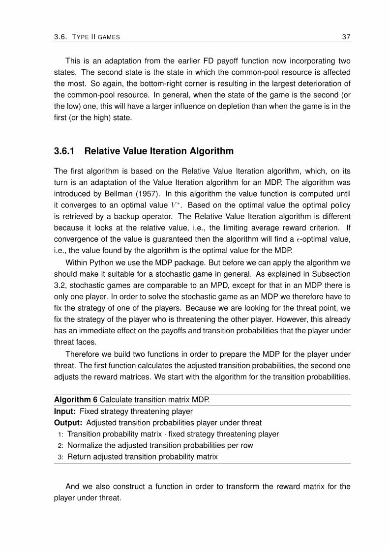
3.6. TYPE II GAMES 37
This is an adaptation from the earlier FD payoff function now incorporating two
states. The second state is the state in which the common-pool resource is affected
the most. So again, the bottom-right corner is resulting in the largest deterioration of
the common-pool resource. In general, when the state of the game is the second (or
the low) one, this will have a larger influence on depletion than when the game is in the
first (or the high) state.
3.6.1 Relative Value Iteration Algorithm
The first algorithm is based on the Relative Value Iteration algorithm, which, on its
turn is an adaptation of the Value Iteration algorithm for an MDP. The algorithm was
introduced by Bellman (1957). In this algorithm the value function is computed until
it converges to an optimal value V ∗. Based on the optimal value the optimal policy
is retrieved by a backup operator. The Relative Value Iteration algorithm is different
because it looks at the relative value, i.e., the limiting average reward criterion. If
convergence of the value is guaranteed then the algorithm will find a ε-optimal value,
i.e., the value found by the algorithm is the optimal value for the MDP.
Within Python we use the MDP package. But before we can apply the algorithm we
should make it suitable for a stochastic game in general. As explained in Subsection
3.2, stochastic games are comparable to an MPD, except for that in an MDP there is
only one player. In order to solve the stochastic game as an MDP we therefore have to
fix the strategy of one of the players. Because we are looking for the threat point, we
fix the strategy of the player who is threatening the other player. However, this already
has an immediate effect on the payoffs and transition probabilities that the player under
threat faces.
Therefore we build two functions in order to prepare the MDP for the player under
threat. The first function calculates the adjusted transition probabilities, the second one
adjusts the reward matrices. We start with the algorithm for the transition probabilities.
Algorithm 6 Calculate transition matrix MDP.
Input: Fixed strategy threatening player
Output: Adjusted transition probabilities player under threat
1: Transition probability matrix · fixed strategy threatening player
2: Normalize the adjusted transition probabilities per row
3: Return adjusted transition probability matrix
And we also construct a function in order to transform the reward matrix for the
player under threat.

38 CHAPTER 3. BUILDING THE ALGORITHM
Algorithm 7 Calculate reward matrix MDP.
Input: Fixed strategy threatening player
Output: Adjusted reward matrix player under threat
1: Reward matrix Game 1 · Fixed strategy threatening player Game 1
2: Reward matrix Game 2 · Fixed strategy threatening player Game 2
3: Append reward matrices into one matrix
4: Return adjusted reward matrix player under threat
Now that we have these two functions, we build a function which initiates the MDP
with the Relative Value Iteration algorithm for the player under threat.
Algorithm 8 Markov Decision Process solver.
Input: Fixed strategy threatening player
Output: Optimal value V ∗, optimal policy
1: Calculate adjusted transition matrix
2: Calculate adjusted reward matrix
3: Initiate Relative Value Iteration algorithm with ε accuracy
4: Run the Relative Value Iteration algorithm
5: Return optimal value V ∗ and optimal policy
The biggest setback when using the MDP algorithm is that it can only solve the
MDP for one fixed strategy of the threatening player at a time. Therefore we are forced
to generate new strategies in a for-loop. The MDP calculates the maximum value of the
player under threat, we store the result of the MDP if it is the lowest result encountered
by the threatening player. Running for an large amount of fixed strategies should result
in the threat point v. Therefore we apply the following algorithm which should find the
threat point.

3.6. TYPE II GAMES 39
Algorithm 9 Threat point MDP.
Input: Number of points to generate
Output: Threat point v = (v1, v2)
1: for i in number of points to generate do
2: Generate random fixed strategy Player 1/2
3: Normalize the fixed strategy for Player 1/2 per state
4: Run the Markov Decision Process solver
5: If the result of the solver is lower than earlier found results, then store the new
result and strategy
6: end for
7: Display the found result and prepare for local search
8: Repeat 1 to 6 while searching in local region of found result
9: Return threat point v = (v1, v2)
A remark has to be made on Algorithm 9. We apply a global search for a best
approximation in the first loop, later we apply a local search to find an even better ap-
proximation of the threat point. The local search works by altering the fixed strategy for
the threatening player by small margins, therefore we are able to find more precise re-
sults without computing unnecessary values which are very likely to give worse results.
For the example game we are able to find a threat point of v = (13.75003, 13.75002), in
around 32 seconds by generating 10, 000 points.
The MDP could theoretically find an exact threat point, but for this one has to gener-
ate a lot of points in order to increase accuracy. Therefore finding the threat point with
this algorithm should be a balance between accuracy and computational time. The
major problem is that the MDP currently does not have way to incorporate a FD payoff
function into the equation. Therefore the MDP algorithm is useful for stochastic games,
but for stochastic FD-games we need another solution.
3.6.2 Jointly-Convergent Pure-Strategy Algorithm
We adapt the jointly-convergent pure-strategy algorithm as it has been useful in Type
I games to incorporate the FD payoff function. We adjust the Type I Algorithm 5 so
that it incorporates stochastic games. Therefore we alter the Functions 2, 3 & 4. These
functions now scale with two states as an input. However, the most important challenge
is to deal with the uncertainty regarding the transition probabilities.
Joosten and Samuel (2018) cope with these difficulties by introducing the so-called
balance equation. But first we have to refer to the restrictions we have on the type
of games for which the algorithm works. We look at games in which the transition

40 CHAPTER 3. BUILDING THE ALGORITHM
probabilities in Markov chain form are irreducible and aperiodic7. If they are both, then
they are guaranteed to converge to a stationary distribution. This stationary distribution
can be found with the balance equation. If x represents the frequency vector of play
and p represents the transition probabilities, then the balance equation is given for a
two-player two state stochastic game with two actions per state is:
4∑
i=1
xi(1− pi) =8
∑
i=5
xipi (3.3)
In which must hold that:4
∑
i=1
xi(1− pi) 6= 0 (3.4)
8∑
i=5
xipi 6= 0 (3.5)
Equations 3.4 & 3.5 state that Equation 3.3 cannot end up with absorbing states.
We limit ourselves to transition probabilities which are in Markov chain form irreducible
and aperiodic, so therefore absorbing states should not occur. In order to incorporate
Equation 3.3 into the algorithm we build a function for it.
In this function we calculate the stationary distribution of the Markov chain. We
do this in a similar way as Samuel (2017), by introducing intermediate vector y and
variable Q, such that:
yS1
i =xS1
i∑4
j=1 xS1
j
(3.6)
yS2
i =xS2
i∑8
j=5 xS2
j
(3.7)
Which then are used in order to calculate Q.
Q =
∑8i=5 y
S2
i pi∑4
i=1 yS1
i (1− pi) +∑8
i=5 yS2
i pi(3.8)
The result of Equation 3.8 is Q, and in this situation Q stands for the long term
relative frequency of play taking place in State 1. (1−Q) therefore is the frequency of
play taking place in State 2.
7Also known as ergodic Markov chains.

3.6. TYPE II GAMES 41
Algorithm 10 Balance Equation Function.
Input: Frequency vector x, transition probabilities p
Output: Frequency vector x adjusted to stationary distribution
1: Initialize Q and y
2: Calculate y
3: Calculate Q with y and p
4: Calculate new frequency vector x based on Q and y
5: Return new frequency vector x adjusted to the stationary distribution
This new equation can then be used in order to calculate the threat point for (non)-
FD Type II games. We incorporate it within Algorithm 5, the result is the following
algorithm:
Algorithm 11 (Non)-FD Type II threat point algorithm.
Input: Type II Game, total number of points, activate FD payoff function
Output: Threat point
1:
2: If v1 is calculated, then X = 1, Y = 2,
3: If v2 is calculated, then X = 2, Y = 1
4:
5: Turn reward matrix Player X into flattened reward vector
6: Threatening strategies Player Y = Draw Random Strategies
7: Best response Player X frequency vector = Create Frequency Vector
8: Calculate adjusted frequency vector by computing the balance equation
9: if Activate FD payoff function = True then
10: Activate and Calculate FD Function result
11: end if
12: Payoffs Player X = Sum over all columns of: (Frequency Vector per row · flattened
vector Player X)
13: if FD Function is active then
14: Element wise multiplication of FD function result with Payoffs Player X
15: end if
16: Sorted payoff matrix = Payoff sort
17: Pick the maximum value of each row of the sorted payoff matrix as best response
of Player X
18: Pick the minimum value over all rows as the result of vX
19:
20: Return threat point v = (v1, v2)


44 CHAPTER 3. BUILDING THE ALGORITHM
generated. Therefore we look at the example game first, we know that the threat point
is v = (13.75, 13.75). We compute the threat point for an increasing number of points to
be generated and state the decimal accuracy and run-time.
# points JCPS Decimal Accuracy Run-time JCPS RVI Decimal Accuracy Run-time RVI
100 0 decimals accurate 0.004 seconds 2 decimals accurate 0.4 seconds
10,000 2 decimals accurate 0.328 seconds 4 decimals accurate 36.36 seconds
1,000,000 4 decimals accurate 22.95 seconds 6 decimals accurate 3,250.78 seconds
10,000,000 5 decimals accurate 255.3 seconds - -
Table 3.4: Accuracy versus run-time in example stochastic game with the algorithms.
Table 3.4 clearly shows that the RVI algorithm is capable of calculating a result with
a higher accuracy while needing fewer points. A remark on the side should be made
here, because the RVI algorithm uses a local search within a rough estimation. Apply-
ing a local search within a rough estimation of the JCPS algorithm could theoretically
also increase accuracy while having a low increase in run-time. However, looking at
a larger number of points generated it is clear that the JCPS algorithm is much more
efficient in computational time due to vectorization. Aiming for 4 decimal accuracy of
the threat point means that the JCPS algorithm can do the job roughly 37% quicker
than the RVI algorithm.
With this advantage for the JCPS algorithm we look at a 4x4 stochastic game in
which we generate random payoff and transition matrices. We do not know what the
exact threat point is we search for, but we check for an approximation of the lower
boundary by calculating the maximin result. The following results are obtained from
running the algorithms.
# points JCPS Algorithm Result Run-time JCPS RVI Algorithm Result Run-time RVI Difference JCPS - RVI
100 (12.1794, 10.5948) 0.006 seconds (11.5734, 10.5313) 0.391 seconds (0.606, 0.0635)
10,000 (11.1956, 10.3064) 1.342 seconds (10.7620, 10.1679) 39.48 seconds (0.4336, 0.1385)
1,000,000 (10.8054, 10.2205) 118.125 seconds (10.6523, 10.1564) 4,323.83 seconds (0.1531, 0.0641)
Table 3.5: Threat point results on random 4x4 stochastic game from the two algo-
rithms.
Again Table 3.5 shows clearly that the JCPS algorithm is much faster and there-
fore has a shorter run-time. We were able to find a best approximation of maximin of
(10.4126, 9.9896). The RVI algorithm seems to be more accurate than the JCPS algo-
rithm but still lacks to find a decimal accurate threat point. The JCPS algorithm however
gets close to the RVI algorithm when 1, 000, 000 points are generated in less computa-
tional time necessary. In order to find gather more information about the accuracy of
the algorithms we now test both algorithms for a random 10x10 bimatrix game.
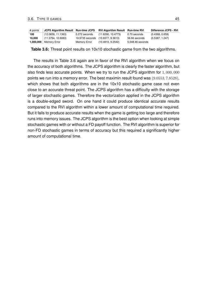
3.6. TYPE II GAMES 45
# points JCPS Algorithm Result Run-time JCPS RVI Algorithm Result Run-time RVI Difference JCPS - RVI
100 (12.0658, 11.1363) 0.272 seconds (11.6290, 10.4773) 0.70 seconds (0.4368, 0.659)
10,000 (11.3764, 10.6083) 19.9735 seconds (10.8377, 9.3613) 56.66 seconds (0.5387, 1.247)
1,000,000 Memory Error Memory Error (10.4810, 9.2542) 5,548.46 seconds
Table 3.6: Threat point results on 10x10 stochastic game from the two algorithms.
The results in Table 3.6 again are in favor of the RVI algorithm when we focus on
the accuracy of both algorithms. The JCPS algorithm is clearly the faster algorithm, but
also finds less accurate points. When we try to run the JCPS algorithm for 1, 000, 000
points we run into a memory error. The best maximin result found was (9.0553, 7.8528),
which shows that both algorithms are in the 10x10 stochastic game case not even
close to an accurate threat point. The JCPS algorithm has a difficulty with the storage
of larger stochastic games. Therefore the vectorization applied in the JCPS algorithm
is a double-edged sword. On one hand it could produce identical accurate results
compared to the RVI algorithm within a lower amount of computational time required.
But it fails to produce accurate results when the game is getting too large and therefore
runs into memory issues. The JCPS algorithm is the best option when looking at simple
stochastic games with or without a FD payoff function. The RVI algorithm is superior for
non-FD stochastic games in terms of accuracy but this required a significantly higher
amount of computational time.


3.7. TYPE III GAMES 47
The big question is, how does this adaptation influence the algorithm and more im-
portantly, what effect does this have on the stationary distribution? Joosten and Samuel
(2018) state in their paper: “determining a stationary distribution is like shooting at a
moving target". We determine the stationary distribution with the balance Equation 3.3
and with help of Equations 3.6, 3.7 & 3.8. However, determining the stationary distri-
bution results in a new frequency vector x∗ which again has an effect on the transition
probabilities. Therefore the system of Equation 3.3 cannot be seen as balanced as
long as a new frequency vector results in a new stationary distribution.
Algorithm wise this means we now have to compute y, Q and x∗ multiple times as
long as the system of balance equations has not converged into a steady state. Be-
cause we apply vectorization there is an inherent risk in computing all of these equa-
tions until all have converged. It would be much more efficient to only compute the
frequency vectors for which the system of balance has not ended up at a stationary dis-
tribution. We therefore look after each iteration which frequency vector has converged
into a stationary distribution and which not. All that have converged are removed from
the computations by removing their index values. We continue calculations for all other
vectors until we have convergence on a broad scale.
In order to incorporate this we alter the function that computes the balance equation
and gives back an adjusted frequency vector. We now incorporate the recalculation of
the balance equation based on the endogenous transition probabilities. We built the
following function:
Algorithm 12 Balance Equation ETP function.
Input: Frequency vector x, transition probabilities p, ETP matrix A
Output: Frequency vector x adjusted to stationary distribution
1: Initialize Q and y
2: Calculate y
3:
4: while Not all rows in frequency vector x have converged do
5: Calculate new p(x) with x · A
6: Calculate Q with y and p(x)
7: Calculate new frequency vector x based on Q and y
8: Check whether Q has converged based on earlier result
9:
10: if Q has converged then Remove frequency vector x from calculating a new Q
11: end if
12: end while
13: Return new frequency vector x adjusted to the stationary distribution

48 CHAPTER 3. BUILDING THE ALGORITHM
The question with Algorithm 12 is, how long does it take for all frequency vectors to
converge? We have calculated this for 65 iterations. The result shows us that roughly
99.5% has converged after 65 iterations. Joosten and Samuel (2018) have examined
the number of iterations required for general convergence, they state that after roughly
50 − 60 iterations most frequency vectors have reached a stationary state. Our own
tests confirm this in Figure 3.7. However, even 50− 60 iterations implies still quite a lot
of time when running vectorized code. Also some entries of Q refuse to converg, even
for a large number of iterations between 100− 120.
Figure 3.7: Convergence of Q.
A solution to this is the use of a so-called accelerator. Joosten and Samuel (2018)
use Aitken’s ∆2 method. An accelerator which converges a sequence to a certain
value as long as long as this sequence in it self is linearly convergent (Burden & Faires,
2010). They describe the method with the assumption that if the sequence is described
by {pn}∞
n=0, then Aitken’s ∆2 is given as:
pn = pn −(pn+1 − pn)
2
pn+2 − 2pn+1 + pn(3.10)
The problem with Equation 3.10 is that it is not always numerically stable. To im-
prove numerical stability, one should use the following adaptation of Aitken’s ∆2:
pn = pn+2 −(pn+2 − pn+1)
2
(pn+2 − pn+1)− (pn+1 + pn)(3.11)


3.7. TYPE III GAMES 51
We now incorporate the numerically stable version of Aitken’s ∆2 on the conver-
gence of Q. We adapt Algorithm 12 such that convergence of Q is sped up by using
Aitken’s ∆2 while safeguarding for possible NaN’s. The result is the following adaptation
of the algorithm.
Algorithm 13 Balance Equation ETP Aitken’s function.
Input: Frequency vector x, transition probabilities p, ETP matrix A
Output: Frequency vector x adjusted to stationary distribution
1: Initialize Q and y
2: Calculate y
3:
4: for ten iterations do
5: Calculate new p(x) with x · A
6: Calculate Q with y and p(x)
7: Calculate new frequency vector x based on Q and y
8:
9: Return Q
10: end for
11:
12: while Not all rows in frequency vector x have converged do
13: Calculate new Q with Aitken ∆2
14: Compare new Q with old Q for convergence
15: if Q has converged then Remove frequency vector x from calculating a new Q
16: end if
17: end while
18: Return new frequency vector x adjusted to the stationary distribution
We now incorporate Algorithm 13 into the Type II version of the JCPS algorithm to
create a Type III version.

52 CHAPTER 3. BUILDING THE ALGORITHM
Algorithm 14 (Non)-FD Type III threat point algorithm.
Input: Type III Game, total number of points, activate FD payoff function
Output: Threat point
1:
2: If v1 is calculated, then X = 1, Y = 2,
3: If v2 is calculated, then X = 2, Y = 1
4:
5: Turn reward matrix Player X into flattened reward vector
6: Threatening strategies Player Y = Draw Random Strategies
7: Best response Player X frequency vector = Create Frequency Vector
8: Calculate Q based on function 13 with Aitken’s ∆2
9: Calculate adjusted frequency vector with help of Q
10: if Activate FD payoff function = True then
11: Activate and Calculate FD Function result
12: end if
13: Payoffs Player X = Sum over all columns of: (Frequency Vector per row · flattened
vector Player X)
14: if FD payoff function is active then
15: Element wise multiplication of FD payoff function result with Payoffs Player X
16: end if
17: Sorted payoff matrix = Payoff sort
18: Pick the maximum value of each row of the sorted payoff matrix as best response
of Player X
19: Pick the minimum value over all rows as the result of vX
20:
21: Return threat point v = (v1, v2)
We now try Algorithm 14 by running it with the example game. Running the non-FD
version by generating 100, 000 points generates a threat point of v = (8.27508, 11.01180).
When applying the maximin algorithm and looking for the lower boundary we find a
result of (8.27501, 11.01176). Therefore we can say with certainty that our algorithm is
capable of finding a solution by generating 100, 000 points that is up to three decimals
accurate. The time necessary for finding the threat point is only roughly 39.03 seconds.
A significant improvement when looking at earlier calculations by Samuel (2017). We
also find a threat point for the FD version with 100, 000 points of v = (4.45906, 7.55750).
The maximin value found is (4.45870, 7.55619). The ETP-ESP version of the game
therefore has a two decimal accuracy and finds this within roughly 35.51 seconds.


54 CHAPTER 3. BUILDING THE ALGORITHM
In Figure 3.11 it is clearly visible what the effect is of the ETP matrix and the FD
payoff function. The threat point is almost near the lowest possible pure reward point
for both players, but now even rewards that were not obtainable without the ETP matrix
are obtainable. The threat point is close to the lowest pure reward possible. This gives
players the opportunity to reach a multitude of equilibria involving threats.
We have shown that it is possible to construct an algorithm which can cope with
calculating threat points in Type III games, especially ETP-ESP games, which can be
regarded as games with a high complexity. However, simplifying this down to games for
which the stationary distribution is guaranteed, our algorithm finds an accurate value
within reasonable time. Also the JCPS algorithm can be used on the broad spectrum
of games, not only does it apply to Type III games, but it is also useable on Type I and
Type II games.

3.8. ROOM FOR FURTHER IMPROVEMENTS 55
3.8 Room for further improvements
There are still possibilities for further improvements. Due to limited time one cannot
explore all options, but we think three paths are worth investing in.
Adapting the SciPy optimizer to work on (FD) Type II and Type III games. We
have used the SciPy optimizer in non-FD Type I games with good results. The SciPy
optimizer was able to find an ε-accurate result within a fraction of the time needed
for the JCPS algorithm. We think that it is able to deliver accurate results in Type II
and Type III games, with our without FD function, but currently we have not found a
working way to incorporate the SciPy optimizer at the basis of calculating the threat
point in these games. We have tried to use it on the MDP algorithm for determining the
minimizing strategy for the threatening player, but attempts at this were unsuccessful.
More research into the SciPy optimizer is needed in order to make it work for Type II
and Type III games.
Adjusting the MDP algorithm such that it can cope with ETP and ESP games.
We applied the Relative Value Iteration algorithm which is an algorithm for a Markov
Decision Process. Currently it is unable to handle endogenous transition probabilities
and endogenous stage payoffs. There is research on uncertainty in an MDP (Liu &
Sukhatme, 2018), (Delgado, Sanner, & de Barros, 2011). However most of these
adaptations to the MDP work with methods which are simulating a model-free MDP
and therefore have an approximation as a result. We think that it should be able to
adapt the model-based MDP algorithms such that they provide an exact solution to
ETP or ESP games.
Further optimization of the JCPS algorithm. Currently we have made a step in
the optimization of the general algorithm by introducing vectorization. In comparison
to Mahohoma (2014) and Samuel (2017) we have made a significant improvement
in terms of speed. However, during the research we also had a hard-coded version
of a 2x2 stochastic game, which was even faster than the current version. Due to
making the code scalable to larger games we had to make a concession in terms of
speed. There are possibilities to make another increase in speed by applying Aitken’s
∆2 method on convergence of the rewards. We are currently looking into possibilities
for this, but we are facing problems in retrieving the rewards in such a manner that
linear convergence is guaranteed. Once we overcome this problem, we think that we
can reduce computational time a lot while retrieving accurate results. An alternative to
this could be to apply local search as has been done with the RVI algorithm. Last but
not least, we should further investigate the option of a n-player algorithm.
56 CHAPTER 3. BUILDING THE ALGORITHM
3.9 Practical implications
During the writing of and investigations for this thesis we went from a description of
the origin of Game Theory to Frequency-Dependent Games. This chapter contains a
more technical approach into the algorithm building which has been done in this thesis.
We think that it is essential to put this algorithm into a broader practical perspective.
Currently, there is a lot of debate and maybe even hype surrounding algorithms in
general. They are seen as secret algorithms which control information and money
and because of the black box mechanism incorporated it is unclear how an algorithm
comes to a certain decision (Pasquale, 2015).
Partly this is true in our opinion due to increasingly complex deep learning algo-
rithms which seem to exihibit characteristics of black boxes. They can only be analyzed
based on their results, the inner workings of these systems are almost inscrutable, ex-
ceptions aside. We want to mention this because we think that the algorithm produced
in this thesis is not a black box. Our vision is that an algorithm is an arithmetic represen-
tation of a more complex mathematical problem. Our algorithm is a simple artihmetic
representation that follows game theoretical logic. Algorithms are necessary because
computers only can do simple calculations on the lowest level. Therefore a lot depends
on how the mathematics are defined surrounding the algorithm.
Game theory works based on the assumptions that players are rational and that
under perfect information they are able to maximize their own interests. In practice
we think that actors in everyday life are rational in general. Surely, humans are not
completely selfish, but even when they cooperate they will try to make the most out
of a situation in their own interest. A bigger problem in practice lies within the perfect
information assumption. In everyday life it seems to us that it is almost impossible to
retrieve perfect information. The complex world we live in makes it hard to retrieve
all the data necessary, and when all data is retrieved it is still hard to analyze this in
a game-theoretical sense. Analysis of game-theoretical problems which have a high
complexity is extremely time-consuming when done by hand.
Therefore we think that this algorithm has an important role. When simplifying a
complex real-life problem in such a matter that it can be analyzed as a game theoret-
ical problem, this algorithm will prove to be useful in order come to well-found conclu-
sions or interpretations. In literature a lot of practical situations have been derived in
order to fit a game theoretical context. Well-known examples are Fishery games (e.g.
(Joosten, 2007b)), economic applications (e.g. (Aumann & Hart, 1994)), advertisement
games (e.g. (Joosten, 2015)) and political games (e.g. (Finus, 2002)) . The range of
applicability is broad and should definitely not be limited to these known situations,
but as Einstein once said “Logic will take you from A to B, imagination will take you
everywhere."

Chapter 4
Conclusions and recommendations
In this section we conclude our research, refer to the progress made and do recom-
mendations for future research.
4.1 Conclusion
Our research goal was to develop an algorithm which calculates threat points in Type
I, Type II and Type III games. We have shown that there are even several algorithms to
calculate threat points in these types of games. For Type I non-FD games the SciPy op-
timizer is a faster and more accurate option than the Jointly-Convergent Pure-Strategy
algorithm. The Relative Value Algorithm can cope with ε-accurate solutions in theory,
but in practice fails to cope with larger games and cannot find exact solutions. How-
ever the algorithm still performs better in terms of accuracy in non-FD Type II games in
comparison to the Jointly-Convergent Pure-Strategy algorithm. In general, the Jointly-
Convergent Pure-Strategy algorithm has proven to be fitting in all cases while also
generating obtainable rewards. By applying vectorization and programming optimiza-
tion we have also been able to increase the speed of the algorithm. For 2x2 stochastic
games the algorithm is able to find very accurate solutions in reasonable time. Larger
games seem to be problematic for all algorithms, but even more problematic for the
Jointly-Convergent Pure-Strategy algorithm. These problems could be dealt with by
employing a local search. Additionally there are limitations on the characteristics of the
games in order to protect the guaranteed working of the algorithm. In practice, the total
structure of the game should be taken into consideration in order to retrieve an optimal
working of the algorithm.
57

58 CHAPTER 4. CONCLUSIONS AND RECOMMENDATIONS
4.2 Recommendations
As stated in this research, there are many ways to skin a cat. Therefore our research is
just a limited view on an endless sea of possibilities. First we advise for future research
to look at a way to cope with the SciPy optimizer in terms of Type II and Type III games.
In this research we were not able to find a programming logic which could cope with
the optimizer approach, but we think that there could be an enormous improvement in
speed. Secondly, we think that there should be a more theoretical approach to incorpo-
rate endogenous transition probabilities and endogenous stage payoffs. This research
could then lead to well-founded algorithms based on a Markov Decision Process for
Type II and Type III games. Last but not least, the Jointly-Convergent Pure-Strategy
algorithm can be optimized by looking for ways to guarantee linear convergence of the
payoffs and then calculating the payoff with Aitken’s ∆2 method. However, one should
keep in mind that this method is not without risks and that floating-point errors are
prone to occur. Another option would be to apply the Jointly-Convergent Pure-Strategy
algorithm with a global search and then search further locally.
For those who want to use this algorithm in finding a threat point in one of the
three types of games we advise the following. When using this algorithm for a broad
spectrum of games we should use the code as it is. If it is clear that games for a certain
reason are only applied on for example 2x2 stochastic games, then one should try to
alter the code by hard-coding the frequency vector. In this case the improvement in
speed is significant in favor of scalability.

REFERENCES 59
References
Aumann, R. J., & Hart, S. (1994). Handbook of Game Theory with Economic Applica-
tions (Vol. 2). Amsterdam: Elsevier (North-Holland).
Bellhouse, D. (2007). The Problem of Waldegrave. Electronic Journal for History
of Probability and Statistics, 3(2), 1–12. Retrieved from http://www.emis.ams
.org/journals/JEHPS/Decembre2007/Bellhouse.pdf doi: 10.1111/j.1540
-6253.1973.tb00643.x
Bellman, R. (1957). A Markovian Decision Process. Journal of Mathematics and
Mechanics, 6(5), 679–684. Retrieved from http://www.jstor.org/stable/
24900506
Billingsley, P. (2008). Probability and Measure. New York: John Wiley & Sons.
Blackwell, D. (1962). Discrete Dynamic Programming. The Annals of Mathematical
Statistics, 33, 719–726. Retrieved from https://projecteuclid.org/euclid
.aoms/1177704593 doi: 10.1214/aoms/1177704593
Blackwell, D., & Ferguson, T. S. (1968). The Big Match. The Annals of Mathematical
Statistics, 39(1), 159–163. Retrieved from https://projecteuclid.org:443/
euclid.aoms/1177698513 doi: 10.1214/aoms/1177698513
Borel, E. (1921). La théorie du jeu et les équations intégrales à novau symétrique
gauche. Comptes rendus de l’Académie des Sciences, 173(1304-1308), 58.
Borel, E. (1927). Sur les systèmes de formes linéaires à déterminant symétrique
gauche et la théorie générale du jeu. Comptes rendus de l’Académie des Sci-
ences, 184, 52–53.
Brenner, T., & Witt, U. (2003). Melioration learning in games with constant and
frequency-dependent pay-offs. Journal of Economic Behavior & Organization,
50(4), 429–448. doi: 10.1016/S0167-2681(02)00034-3
Breton, M., Filar, J. A., Haurle, A., & Schultz, T. A. (1986). On the computation of
equilibria in discounted stochastic dynamic games. In T. Basar (Ed.), Dynamic
games and applications in economics (pp. 64–87). Berlin: Springer.
Burden, R. L., & Faires, J. D. (2010). Numerical analysis (9th ed.). Boston: Cengage
Learning.
Delgado, K. V., Sanner, S., & de Barros, L. N. (2011). Efficient Solutions to Factored
MDPs with Imprecise Transition Probabilities. Artificial Intelligence, 175(9), 1498–
1527. Retrieved from http://www.sciencedirect.com/science/article/
pii/S0004370211000026 doi: 10.1016/j.artint.2011.01.001
Filar, J., & Raghavan, T. E. S. (1979). An algorithm for solving an undiscounted
stochastic game in which one player controls transitions. Research Memoran-
dum, University of Illinois, Chicago.
Filar, J., & Vrieze, K. (1997). Competitive Markov Decision Processes. New York:

60 CHAPTER 4. CONCLUSIONS AND RECOMMENDATIONS
Springer Science & Business Media. doi: 10.1007/978-1-4612-4054-9
Finus, M. (2002). Game theory and International Environmental Cooperation: Any
Practical Application? Controlling Global Warming: Perspectives from Eco-
nomics, Game Theory and Public Choice, 9–104.
Flesch, J. (1998). Stochastic Games with the Average Reward (Doctoral Dissertation).
Maastricht University.
Gillette, D. (1957). Stochastic games with zero stop probabilities. Contributions to the
Theory of Games, 3, 179–187.
Häggström, O. (2002). Finite Markov Chains and Algorithmic Applications (Vol. 52).
Cambridge: Cambridge University Press.
Hardin, G. (1968). The Tragedy of the Commons. Science, 162(3859), 1243–1248. Re-
trieved from http://science.sciencemag.org/content/162/3859/1243 doi:
10.1126/science.162.3859.1243
Hordijk, A., Vrieze, O. J., & Wanrooij, G. L. (1983). Semi-markov strategies in stochas-
tic games. International Journal of Game Theory , 12(2), 81–89. Retrieved from
https://doi.org/10.1007/BF01774298 doi: 10.1007/BF01774298
Hyksova, M. (2004). Several Milestones in the History of Game Theory. Retrieved from
http://citeseerx.ist.psu.edu/viewdoc/summary?doi=10.1.1.319.8082
Joosten, R. (2007a). Patience, Fish Wars, rarity value & Allee effects. Papers on
Economics and Evolution.
Joosten, R. (2007b). Small Fish Wars: A New Class of Dynamic Fishery-
Management Games. The IUP Journal of Managerial Economics, V (4), 17–30.
Retrieved from https://econpapers.repec.org/RePEc:icf:icfjme:v:05:y:
2007:i:4:p:17-30
Joosten, R. (2009). Strategic Advertisement with Externalities: A New Dynamic Ap-
proach. In Modeling, computation and optimization. (pp. 21–43). Singapore:
World Scientific.
Joosten, R. (2015). Long-run Strategic Advertising and Short-run Bertrand Com-
petition. International Game Theory Review , 17 (02). Retrieved from http://
www.worldscientific.com/doi/10.1142/S0219198915400149 doi: 10.1142/
S0219198915400149
Joosten, R., Brenner, T., & Witt, U. (2003). Games with frequency-dependent stage
payoffs. International Journal of Game Theory , 31(4), 609–620.
Joosten, R., & Meijboom, R. (2018). Stochastic games with endogenous transitions.
In S. Neogy, R. B. Bapat, & D. Dubey (Eds.), Mathematical programming and
game theory (pp. 205–226). Singapore: Springer. doi: https://doi.org/10.1007/
978-981-13-3059-9
Joosten, R., & Samuel, L. (2018). On finding large sets of rewards in two-player ETP-
ESP-games. Enschede.

REFERENCES 61
Knowles, J. D., Watson, R. A., & Corne, D. W. (2001). Reducing Local Optima in
Single-Objective Problems by Multi-objectivization. In International conference
on evolutionary multi-criterion optimization (pp. 269–283). Springer.
Levhari, D., & Mirman, L. (1980). The Great Fish War: An Example Using a
Dynamic Cournot-Nash Solution. Bell Journal of Economics, 11(1), 322–334.
Retrieved from https://econpapers.repec.org/RePEc:rje:bellje:v:11:y:
1980:i:spring:p:322-334 doi: 10.2307/3003416
Levin, J. (2002). Bargaining and Repeated Games (No. February). Stanford.
Liu, L., & Sukhatme, G. S. (2018). A Solution to Time-Varying Markov Decision
Processes. IEEE Robotics and Automation Letters, 3(3), 1631–1638. doi:
10.1109/LRA.2018.2801479
Mahohoma, W. (2014). Stochastic Games with Frequency Dependent Stage Payoffs
(Master Thesis). Maastricht University.
Markov, A. (1971). Extension of the Limit Theorems of Probability Theory to a Sum
of Variables Connected in a Chain. In R. Howard (Ed.), Dynamic probabilistic
systems (volume i: Markov models) (pp. 552–577). New York City: John Wiley &
Sons, Inc. Retrieved from citeulike-article-id:911035
Mertens, J. (1990). Repeated Games. In T. Ichiishi, A. Neyman, & Y. Tauman
(Eds.), Game theory and applications (pp. 77–130). San Diego: Academic
Press. Retrieved from http://www.sciencedirect.com/science/article/
pii/B978012370182450009X doi: https://doi.org/10.1016/B978-0-12-370182-4
.50009-X
Mertens, J., & Neyman, A. (1981). Stochastic Games. International Journal of Game
Theory , 10(2), 53–66.
Nash, J. (1950). Equilibrium Points in n-Person Games. Proceedings of the National
Academy of Sciences of the United States of America, 36(1), 48–49.
Nash, J. (1951). Non-Cooperative Games. Annals of Mathematics, 54(2), 286–295.
Neyman, A. (2003a). From Markov Chains to Stochastic Games. In Stochastic games
and applications (pp. 9–25). Springer.
Neyman, A. (2003b). Stochastic Games: Existence of the MinMax. doi: 10.1177/
002248716001100324
Otterlo, M. V. (2009). Markov Decision Processes: Concepts and Algo-
rithms. Retrieved from http://www.cs.vu.nl/~annette/SIKS2009/material/
SIKS-RLIntro.pdf doi: 10.1016/j.autcon.2013.05.028
Pasquale, F. (2015). The Black Box Society: The Secret Algorithms That Control
Money and Information. Cambridge: Harvard University Press.
Peters, H. (2015). Game Theory: A Multi-Leveled Approach (Second ed.). Berlin
Heidelberg: Springer-Verlag.
Raghavan, T. E. S., & Filar, J. A. (1991). Algorithms for stochastic games—a survey.

62 CHAPTER 4. CONCLUSIONS AND RECOMMENDATIONS
Zeitschrift für Operations Research, 35(6), 437–472.
Samuel, L. (2017). Computations in Stochastic Game Theory (Master Thesis).
Shapley, L. (1953). Stochastic Games. Proceedings of the National Academy of
Sciences, 39(10), 1095–1100. doi: 10.1073/pnas.39.10.1095
Sorin, S. (2003). Classification and Basic Tools. In A. Neyman & S. Sorin (Eds.),
Stochastic games and applications (pp. 27–36). New York: Springer. Retrieved
from http://www.springerlink.com/index/10.1007/978-94-010-0189-2_4
doi: 10.1007/978-94-010-0189-2
Verschuren, P., Doorewaard, H., & Mellion, M. J. (2010). Designing a Research Project
(Vol. 2). The Hague: Eleven International Publishing.
Von Neumann, J. (1928). Zur Theorie der Gesellschaftsspiele. Mathematis-
che Annalen, 100(1), 295–320. Retrieved from https://doi.org/10.1007/
BF01448847 doi: 10.1007/BF01448847
Von Neumann, J., & Morgenstern, O. (1944). Theory of Games and Economic Behav-
ior. Princeton: Princeton University Press.
Vrieze, O. J. (1981). Linear programming and undiscounted stochastic games in which
one player controls transitions. Operations-Research-Spektrum, 3, 29–35.
Vrieze, O. J. (2003a). Stochastic Games and Stationary Strategies. In A. Neyman
& S. Sorin (Eds.), Stochastic games and applications (pp. 37–50). New York:
Springer. Retrieved from http://www.springerlink.com/index/10.1007/978
-94-010-0189-2_4 doi: 10.1007/978-94-010-0189-2
Vrieze, O. J. (2003b). Stochastic Games, Practical Motivation and the Orderfield
Property for Special Classes. In A. Neyman & S. Sorin (Eds.), Stochastic
games and applications (pp. 215–225). New York: Springer. Retrieved from
http://www.springerlink.com/index/10.1007/978-94-010-0189-2_4 doi:
10.1007/978-94-010-0189-2

Appendix A
Python Code containing the
Algorithms
A.1 How to use the Python code - A short manual on
the usage
A.1.1 Using Python
Python is an interpreted language, therefore it has to run the code with help of the
Python interpreter. The Python interpreter is widely available, but for people with lim-
ited knowledge on Python we would advice to download the Anaconda package at
www.anaconda.com. Anaconda also includes a lot of the packages necessary, like
NumPy and SciPy. The MDP Toolbox, if not available in Anaconda, can be found on
https://pymdptoolbox.readthedocs.io/en/latest/api/mdptoolbox.html.
In order to read the Python code an application has to be used on Windows com-
puter. In this thesis we use Jupyter Notebook. If necessary, contact the author of this
thesis to receive the source code and Jupyter Notebook file which has been used.
A.1.2 Using the Python Code
One should first load the code described at the ‘Import packages’ section. This section
contains code which states the necessary Python packages for the computations done
in the algorithms. After this code has been loaded by the interpreter the user has
the option to choose from three types of game codes which are all accompanied by
example games. The game code per type of game contains all required coding in
order to receive visual results in this thesis. However, one could choose to only use
a subset of the functions within the code. We will describe them briefly in the next
section. All games are created by use of a class. Therefore we have programmed
63

64 APPENDIX A. PYTHON CODE CONTAINING THE ALGORITHMS
the games as a class, we will elaborate on this after the description of the different
functions with an example.
A.1.3 Functions
We introduce the functions of all the games. We state their names, describe them and
also state which input is necessary from the user.
Type of Game Function Name Description Input necessary
Type I plot_pure_reward_points Plots the pure reward points in a two dimensional figure -
Type I plot_all_reward_point Plot all possible rewards points in a Type I game FD function –>Yes = active, No = deactive
Type I plot_threat_point Plot’s the threat point (only after it has been found) -
Type I plot_threat_point_lines Plot the lines which define the limits for the NE -
Type I threat_point_algorithm Find the threat point with the SciPy algorithm -
Type I maximin_algorithm Find the maximin result with the SciPy algorithm -
Type I threat_point_optimized Find the threat point with the JCPS algorithm# of points to generate,
show strategy of player 1/player 2, print text
FD function –>Yes = active, No = deactive
Type II plot_single_period_pure_rewards Plots the pure reward points in a two dimensional figure -
Type II plot_convex_hull_pure_rewards Plot a convex hull around the pure reward points -
Type II plot_threat_point Plot’s the threat point (only after it has been found) -
Type II plot_threat_point_lines Plot the threat point lines defining the NE borders -
Type II plot_all_reward_points Plot all reward points obtainable in the game FD function –>Yes = active, No = deactive
Type II threat_point_algorithm Find the threat point with the RVI algorithmT –>Number of points to generate
sensi –>Sensitivity of the local search
Type II maximin_point Find the maximin point with the RVI algorithm T –>Number of points to generate
Type II optimized_maximin Find the maximin point with the JCPS algorithm# of points to generate,
show strategy of player 1/player 2, print text
FD function –>Yes = active, No = deactive
Type II threat_point_optimized Find the threat point with the JCPS algorithm# of points to generate,
show strategy of player 1/player 2, print text
FD function –>Yes = active, No = deactive
Type III plot_single_period_pure_rewards Plots the pure reward points in a two dimensional figure -
Type III plot_convex_hull_pure_rewards Plot a convex hull around the pure reward points -
Type III plot_all_rewards Plot all reward points obtainable in the game FD function –>Yes = active, No = deactive
Type III plot_threat_point Plot the threat point if found -
Type III plot_threat_point_lines Plot the threat point lines defining the NE borders -
Type III optimized_maximin Find the maximin point with the JCPS algorithm# of points to generate,
show strategy of player 1/player 2, print text
FD function –>Yes = active, No = deactive
Type III threat_point_optimized Find the threat point with the JCPS algorithm# of points to generate,
show strategy of player 1/player 2, print text
FD function –>Yes = active, No = deactive
A.1.4 An example of computations of a Type II game
We explain the usage of our code with a Type II non-FD game example. We need to
construct a game before we can apply functions. The Type II game is programmed
in a class called ‘StochasticGame’. The Type II game needs two types of input: The
transition probabilities and the payoffs of the game in both states. Our games are
limited to two-player, two-state games. But in general the states can contain n actions.
We define the transition probabilities and the payoffs of the game with a NumPy matrix.
See the following code:encoding=*-60
p1_1 = np.matrix(’16 14; 28 24’)
p2_1 = np.matrix(’16 28; 14 24’)

A.1. HOW TO USE THE PYTHON CODE - A SHORT MANUAL ON THE USAGE 65
p1_2 = np.matrix(’4 3.5; 7 6’)
p2_2 = np.matrix(’4 7; 3.5 6’)
trans1_1 = np.matrix(’0.8 0.7; 0.7 0.6’)
trans2_1 = np.matrix(’0.5 0.4; 0.4 0.15’)
trans1_2 = np.matrix(’0.2 0.3; 0.3 0.4’)
trans2_2 = np.matrix(’0.5 0.6; 0.6 0.85’)
Then we load these transition probabilities and payoffs by creating a new class
which we attach to the variable ‘FirstTry’.encoding=*-60
FirstTry = StochasticGame(p1_1,p2_1,p1_2,p2_2,trans1_1,trans2_1,trans1_2,trans2_2)
As a result, Python now has created a class assigned to the variable FirstTry. We
can access functions from this class by stating ‘FirstTry.functionname’. We now want
to plot all single period pure rewards, all reward points and find the maximin point and
threat point with the RVI algorithm in 10000 points with a sensitivity of 0.025. The result
is the following code:encoding=*-60
FirstTry.plot_single_period_pure_rewards()
FirstTry.plot_all_reward_points(False)
FirstTry.maximin_point(10000)
FirstTry.threat_point_algorithm(10000,0.025)
As can be seen, we set the FD function to false in the plot_all_rewards_points
function. We also fill in 10000 points to be generated in both the maximin_point and
threat_point_algorithm function. Another way to have done this was by using the
JCPS algorithm, which needs some more input. Both the maximin point and the threat
point can be found by the following code.encoding=*-60
FirstTry.threat_point_optimized(10000,False,False,True,False)
FirstTry.optimized_maximin(10000,False,False,False)
The result again is a maximin point and a threat point. But now we have to state
some more input, based on the input necessary described in the function table in the
previous section. Last but not least we are able to plot this found threat point. We
can do this with the plot_threat_point function and also plot the threat point lines, the
following code should be used in this example:encoding=*-60
FirstTry.plot_threat_point()
FirstTry.plot_threat_point_lines()
And the result should be a visualization of the Type II game without FD-payoffs.

66 APPENDIX A. PYTHON CODE CONTAINING THE ALGORITHMS
A.2 Import packages
encoding=*-60
import numpy as np #import numpy
import scipy as sp #import scipy
from scipy import optimize #import the scipy optimize part
from scipy import linalg #import the linear algebra section
from scipy.spatial import ConvexHull #import scipy convex hull package
import matplotlib.pyplot as plt #import package to plot stuff
import msmtools as msm #import package for markov chains
from msmtools.analysis import stationary_distribution #import for calculating stationary
distributions
import mdptoolbox #import toolbox for MDP’s
import time #import time package
from itertools import permutations #import package for permutations
A.3 Type I Game Code
encoding=*-60
class RepeatedGame:
"""In this type of game we model a repeated type of game. It means that we play a
repeating game
in which the payoffs are repeated for a certain (or unlimited) amount of time."""
def __init__(self,payoff_p1,payoff_p2):
"Here we initialize the game with respective playoffs for both players"
# here below we set the payoffs as an aspect of the game, for both players each
self.payoff_p1 = payoff_p1
self.payoff_p2 = payoff_p2
# we define a set of best pure strategies
self.best_pure_strategies = np.array([[1,0,1,0],[0,1,1,0],[1,0,0,1],[0,1,0,1]])
def plot_pure_reward_points(self):
"This function plots the pure reward points in a two dimensional figure"
# set the payoffs as an array
payoff_p1_array = self.payoff_p1.A1
payoff_p2_array = self.payoff_p2.A1
plt.figure() #create a figure
plt.scatter(payoff_p1_array,payoff_p2_array, label="Pure reward points", zorder=15,
color=’b’) #simple plot which plots the possible rewards
# label the x- and y-axis
plt.xlabel("Payoff Player 1")
plt.ylabel("Payoff Player 2")
def plot_all_reward_points(self,FD_yn):
"Here we plot all reward points possible in this repeated game."
# number of times the game is played (large number)
T = 100000

A.3. TYPE I GAME CODE 67
# create payoff vectors based on the number of times the game is played
Payoff1 = np.zeros(T)
Payoff2 = np.zeros(T)
x = np.zeros(4) #initialize x for frequency vector
r = np.zeros(4) #initialize r for random drawing
#loop over the number of periods and length of x
for v in range(0,T):
for i in range(0,4):
r[i] = np.random.beta(0.5,0.5) #draw r from beta distribution
norm_val = np.sum(r)
for i in range(0,4):
x[i] = r[i]/norm_val #normalize r and put it in as x
# if there is a FD type of game, then active the FD function
if FD_yn == True:
FD = 1-0.25*(x[1]+2*x[2])-(2/3)*x[3]
else:
FD = 1
# calculate the first payoffs for p1 and p2
V_p1 = x*np.transpose(self.payoff_p1.flatten())
V_p2 = x*np.transpose(self.payoff_p2.flatten())
# calculate the payoff based on the FD function
Payoff1[v] = FD*np.sum(V_p1)
Payoff2[v] = FD*np.sum(V_p2)
# store the maximal payoffs
self.maximal_payoffs = np.zeros(2)
self.maximal_payoffs[0] = np.max(Payoff1)
self.maximal_payoffs[1] = np.max(Payoff2)
all_payoffs = np.array([Payoff1,Payoff2]) #payoffs player 1 and and p2 merging
all_payoffs = np.transpose(all_payoffs) #transpose for use in convex_hull
Convex_Hull_Payoffs = ConvexHull(all_payoffs) #calculate convex_hull of the payoffs
# here below we plot the convex hull
plt.fill(all_payoffs[Convex_Hull_Payoffs.vertices,0], all_payoffs[Convex_Hull_Payoffs
.vertices,1], color=’y’, zorder=5, label="Obtainable rewards")
# plt.plot(Payoff1,Payoff2, color =’y’, zorder=2, label="Reward points") # disabled
for now
# do some nice plotting
plt.title("Reward points of Repeated game")
plt.xlabel("Payoff Player 1")
plt.ylabel("Payoff Player 2")
def plot_threat_point(self):
"Plot the threat point found (only working after the threat_point_algorithm function
has been applied)"
# here below the threat point is plotted
plt.scatter(self.threat_point[0],self.threat_point[1], color=’r’, zorder=17, label="
Threat point")
plt.legend()

68 APPENDIX A. PYTHON CODE CONTAINING THE ALGORITHMS
def plot_threat_point_lines(self):
"Plot the lines which define the limits for the NE reachable under Folk Theorem."
# plot based on the maximum payoffs and threat point
plt.plot([self.threat_point[0],self.threat_point[0]],[self.threat_point[1],self.
maximal_payoffs[1]], color=’k’, zorder=16)
plt.plot([self.threat_point[0],self.maximal_payoffs[0]],[self.threat_point[1],self.
threat_point[1]], color=’k’, zorder=16)
plt.axis(’equal’)
def threat_point_p1(self,x):
"Function in order to determinate the threat point for p1"
return np.max(np.dot(self.payoff_p1,x))
def threat_point_p2(self,x):
"Function in order to determinate the threat point for p2"
return np.max(np.dot(x,self.payoff_p2))
def maximin_p1(self,x):
"Function in order to determine the maximin strategy for p1"
return np.max(-np.dot(x,self.payoff_p1))
def maximin_p2(self,x):
"Function in order to determine the maximin strategy for p2"
return np.max(-np.dot(self.payoff_p2,x))
def threat_point_algorithm(self):
"This is the much shorter, optimized search for the threat point, not depending on
the number of actions."
start_time = time.time() # start a timer for speed measures
print("Threat point algorithm initiated")
p_initialize = np.zeros(np.size(self.payoff_p1,0)) #initialize an array for p
q_initialize = np.zeros(np.size(self.payoff_p2,1)) #initialize an array for q
A.4 Type I Example Games Code
encoding=*-60
# Here below we create a repeated game from the Llea thesis
a = RepeatedGame(np.matrix(’16 14;28 24’),np.matrix(’16 28; 14 24’))
a.threat_point_algorithm()
a.plot_pure_reward_points()
a.plot_all_reward_points(True)
a.maximin_algorithm()
a.threat_point_optimized(100000,True,True,True,True)
a.plot_threat_point()
a.plot_threat_point_lines()

A.5. TYPE II GAME CODE 69
A.5 Type II Game Code
encoding=*-60
class StochasticGame:
"""[U+FFFD]nthis class we model Stochastic Games, also known in the thesis as Type II games"""
def __init__(self,payoff_p1_game1,payoff_p2_game1,payoff_p1_game2,payoff_p2_game2,
trmatrixg1,trmatrixg2,trmatrixg3,trmatrixg4):
"Here below we initialize the game by storing payoff and transition matrices
according to the upper input."
self.payoff_p1_game1 = payoff_p1_game1 #payoff p1 in game 1
self.payoff_p2_game1 = payoff_p2_game1 #payoff p2 in game 1
self.payoff_p1_game2 = payoff_p1_game2 #payoff p1 in game 2
self.payoff_p2_game2 = payoff_p2_game2 #payoff p2 in game 2
self.transition_matrix_game1_to1 = trmatrixg1 #transition matrix from game
1 to game 1
self.transition_matrix_game2_to1 = trmatrixg2 #transition matrix from game
2 to game 1
self.transition_matrix_game1_to2 = trmatrixg3 #transition matrix from game
1 to game 2
self.transition_matrix_game2_to2 = trmatrixg4 #transition matrix from game
2 to game 2
self.printing = False #set printing to False
def plot_single_period_pure_rewards(self):
"Here we plot the pure rewards possible for a single period"
plt.figure() #create a figure
payoff_p1_g1_flat = self.payoff_p1_game1.A1 #create a flattend payoff of
p1 in game 1
payoff_p2_g1_flat = self.payoff_p2_game1.A1 #create a flattend payoff of
p2 in game 1
plt.scatter(payoff_p1_g1_flat,payoff_p2_g1_flat, label="Pure reward points Game 1",
zorder = 15) #plot payoffs game 1
payoff_p1_g2_flat = self.payoff_p1_game2.A1 #create a flattend payoff of
p1 in game 2
payoff_p2_g2_flat = self.payoff_p2_game2.A1 #and for p2 in game 2
plt.scatter(payoff_p1_g2_flat,payoff_p2_g2_flat, label="Pure reward points Game 2",
zorder = 15) #plotting this again
plt.xlabel("Payoff Player 1") #giving the x-axis the label
of payoff p1
plt.ylabel("Payoff Player 2") #and the payoff of the y-axis
is that of p2
plt.title("Reward points of Stochastic game") #and we give it a nice titel
plt.legend()
def plot_convex_hull_pure_rewards(self):
"Here we plot a convex hull around the pure reward point, therefore resulting in the
total possible reward space"
payoff_p1_g1_flat = self.payoff_p1_game1.A1 #store the flattend payoff of p1
game 1
payoff_p2_g1_flat = self.payoff_p2_game1.A1 #store the flattend payoff of p2
game 1

70 APPENDIX A. PYTHON CODE CONTAINING THE ALGORITHMS
payoff_p1_g2_flat = self.payoff_p1_game2.A1 #store the flattend payoff of p1
game 2
payoff_p2_g2_flat = self.payoff_p2_game2.A1 #store the flattend payoff of p2
game 2
payoff_p1_merged = np.concatenate((payoff_p1_g1_flat,payoff_p1_g2_flat)) #merge p1
payoffs
payoff_p2_merged = np.concatenate((payoff_p2_g1_flat,payoff_p2_g2_flat)) #merge p2
payoffs
all_payoffs = np.array([payoff_p1_merged,payoff_p2_merged]) #create one array of
payoffs
all_payoffs = np.transpose(all_payoffs) #and rotate this one
rewards_convex_hull = ConvexHull(all_payoffs) #retain the convex hull
of the payoffs
plt.fill(all_payoffs[rewards_convex_hull.vertices,0], all_payoffs[rewards_convex_hull
.vertices,1], color=’k’)
plt.title("Convex hull of payoffs")
#here above we fill the convex hull in black
def plot_threat_point(self):
"This function plots the threat point of the game"
plt.scatter(self.threat_point[0],self.threat_point[1], zorder=10, color = ’r’, label=
’Threat point’)
plt.legend()
def plot_threat_point_lines(self):
"This function plots the threat point lines defining the NE borders"
plt.plot([self.threat_point[0],self.threat_point[0]],[self.threat_point[1],self.
maximal_payoffs[1]], color=’k’, zorder=15)
plt.plot([self.threat_point[0],self.maximal_payoffs[0]],[self.threat_point[1],self.
threat_point[1]], color=’k’, zorder=15)
def plot_all_reward_points(self,FD_yn):
"Here we use the algorithm developed in the thesis of Llea with supervision of
Joosten for Type 2 games"
###Payoffs and probabilitys
payoff_p1_g1_flat = self.payoff_p1_game1.A1 #flatten payoff p1 game 1
payoff_p2_g1_flat = self.payoff_p2_game1.A1 #flatten payoff p2 game 1
payoff_p1_g2_flat = self.payoff_p1_game2.A1 #flatten payoff p1 game 2
payoff_p2_g2_flat = self.payoff_p2_game2.A1 #flatten payoff p2 game 2
A1 = np.concatenate((payoff_p1_g1_flat,payoff_p1_g2_flat)) #A1 is payoff Player 1
B1 = np.concatenate((payoff_p2_g1_flat,payoff_p2_g2_flat)) #B1 is payoff Player 2
trans_game1_1_flat = self.transition_matrix_game1_to1.A1 #flatten transition
probabilities game 1 to 1
trans_game2_1_flat = self.transition_matrix_game2_to1.A1 #flatten transition
probabilities game 2 to 1
p = np.concatenate((trans_game1_1_flat,trans_game2_1_flat)) #merge them into one
transition array
###Intialization of variables

A.5. TYPE II GAME CODE 71
T = 100000 #number of points to generate
x = np.zeros(8) #preallocate frequency array
xstar = np.zeros(8) #preallocate converged frequency array
r = np.zeros(8) #preallocate random samples from beta distribution
y = np.zeros(8) #preallocate intermediate vector
yp = np.zeros(4) #preallocate intermediate vector with transition
yp_not = np.zeros(4) #preallocate intermediate vector with transition
v_p1 = np.zeros(8) #preallocate intermediate payoffs p1
v_p2 = np.zeros(8) #preallocate intermediate payoffs p2
payoff_p1 = np.zeros(T) #preallocate definite payoffs p1
payoff_p2 = np.zeros(T) #preallocate definite payoffs p2
for t in range(0,T): #sum over the number of points to generate
for i in range(0,8):
r[i] = np.random.beta(0.5,0.5) #generate random frequency pair
for i in range(0,8):
x[i] = r[i]/np.sum(r) #normalize the frequency pair so it sums
to 1
###intermediate calculations (flow equations)
for i in range(0,4):
y[i] = x[i]/np.sum(x[0:4]) #calculate intermediate vector
for i in range(4,8):
y[i] = x[i]/np.sum(x[4:8]) #see above
for i in range(0,4):
yp_not[i] = y[i] * (1-p[i]) #prepare for Q calculations
yp[i] = y[i+4]*p[i+4]
Q = np.sum(yp)/(np.sum(yp)+np.sum(yp_not)) #calculate Q and Qnot
Q_not = 1-Q
###Solve for X
for i in range(0,4):
xstar[i] = Q*y[i] #now calculate converged frequency pairs
for i in range(4,8):
xstar[i] = Q_not*y[i] #and for second game
if FD_yn == True:
FD = 1-0.25*(xstar[1]+xstar[2])-(1/3)*xstar[3]-(1/2)*(xstar[5] + xstar[6]) -
(2/3) * xstar[7]
else:
FD = 1
for i in range(0,8):
v_p1[i] = xstar[i]*A1[i] #calculate payoffs player1
v_p2[i] = xstar[i]*B1[i] #calculate payoffs player2
### Stage payoff vectors
payoff_p1[t] = FD*np.sum(v_p1) #result is one payoff of player 1
payoff_p2[t] = FD*np.sum(v_p2) #result is one payoff of player 2
all_payoffs = np.array([payoff_p1,payoff_p2]) #payoffs player 1 and and p2 merging
all_payoffs = np.transpose(all_payoffs) #transpose for use in convex_hull
Convex_Hull_Payoffs = ConvexHull(all_payoffs) #calculate convex_hull of the payoffs

72 APPENDIX A. PYTHON CODE CONTAINING THE ALGORITHMS
self.maximal_payoffs = np.zeros(2)
self.maximal_payoffs[0] = np.max(payoff_p1)
self.maximal_payoffs[1] = np.max(payoff_p2)
#here below we fill the convex_hull of the payoffs and plot it
plt.fill(all_payoffs[Convex_Hull_Payoffs.vertices,0], all_payoffs[Convex_Hull_Payoffs
.vertices,1], color=’y’, zorder=5, label="Obtainable rewards")
def markov_decision_process_p1(self,x):
"Here we run the threat point algorithm for P1 with fixed strategy for the punisher
and the punished one maximizes this MDP"
def chance_multiplication(self,x):
"In this function we compute the new transition probabilities based on chosen
actions"
# store the actions of the players
actions_p1_game1 = self.payoff_p1_game1.shape[0]
actions_p1_game2 = self.payoff_p1_game2.shape[0]
actions_p2_game1 = self.payoff_p1_game1.shape[1]
actions_p2_game2 = self.payoff_p1_game2.shape[1]
length_of_actions = np.max([actions_p1_game1,actions_p1_game2]) # determine the
maximum length
p1_combined = np.zeros(length_of_actions, dtype=object) # prepare an object for
the probabilities
# in the loop below we calculate the new transition probabilities
for i in np.nditer(np.arange(length_of_actions)):
working_probs = np.zeros((2,2))
working_probs[0,0] = np.asscalar(np.dot(self.transition_matrix_game1_to1[i
,:],x[0:actions_p2_game1]))
working_probs[0,1] = np.asscalar(np.dot(self.transition_matrix_game1_to2[i
,:],x[0:actions_p2_game1]))
working_probs[1,0] = np.asscalar(np.dot(self.transition_matrix_game2_to1[i
,:],x[actions_p2_game1:actions_p2_game1+actions_p2_game2]))
working_probs[1,1] = np.asscalar(np.dot(self.transition_matrix_game2_to2[i
,:],x[actions_p2_game1:actions_p2_game1+actions_p2_game2]))
p1_combined[i] = working_probs/np.sum(working_probs,1)
return p1_combined
def reward_multiplication(self,x):
"This function calculates the adjusted rewards"
# initialize empty arrays
rewards_game1 = []
rewards_game2 = []
# store the actions for p2
actions_p2_game1 = self.payoff_p1_game1.shape[1]
actions_p2_game2 = self.payoff_p1_game2.shape[1]
# calculate the rewards for game 1
for i in np.nditer(np.arange(self.payoff_p1_game1.shape[0])):
rewards_game1.append(np.asscalar(np.dot(self.payoff_p1_game1[i,:],x[0:
actions_p2_game1])))

A.5. TYPE II GAME CODE 73
# calculate the rewards for game 2
for i in np.nditer(np.arange(self.payoff_p1_game2.shape[0])):
rewards_game2.append(np.asscalar(np.dot(self.payoff_p1_game2[i,:],x[
actions_p2_game1:actions_p2_game1+actions_p2_game2])))
Reward = np.array([rewards_game1,rewards_game2]) # Combine the rewards in one
array
return Reward
p1_combined = chance_multiplication(self,x) # run the transition probability function
Reward_matrix = reward_multiplication(self,x) # run the rewards function
# Run the MDP process to find the threat point for P1
mdp_threatpointp1 = mdptoolbox.mdp.RelativeValueIteration(p1_combined, Reward_matrix,
epsilon=0.00000000001)
mdp_threatpointp1.setSilent()
mdp_threatpointp1.run()
self.threatpoint_p1_policy = mdp_threatpointp1.policy # store the policy (strategy)
found
if self.printing == True:
print("Running MDP")
print("With X as",x)
print("Resulting in:")
print(mdp_treatpointp1.average_reward)
print("With policy:")
print(mdp_treatpointp1.policy)
return mdp_threatpointp1.average_reward
def markov_decision_process_p2(self,x):
"This function creates a MDP for the second player to determine the threat point"
def chance_multiplication(self,x):
"Calculates the transitions probabilities for the MDP"
# store the actions of the players
actions_p1_game1 = self.payoff_p1_game1.shape[0]
actions_p1_game2 = self.payoff_p1_game2.shape[0]
actions_p2_game1 = self.payoff_p2_game1.shape[1]
actions_p2_game2 = self.payoff_p2_game2.shape[1]
length_of_actions = np.max([actions_p2_game1,actions_p2_game2]) # determine the
maximum length of the actions
p2_combined = np.zeros(length_of_actions, dtype=object) # initialize an object
for storing the probabilities
# in this loop we calculate the probabilities and return them
for i in np.nditer(np.arange(length_of_actions)):
working_probs = np.zeros((2,2))
working_probs[0,0] = np.asscalar(np.dot(self.transition_matrix_game1_to1[:,i
],x[0:actions_p1_game1]))
working_probs[0,1] = np.asscalar(np.dot(self.transition_matrix_game1_to2[:,i
],x[0:actions_p1_game1]))
working_probs[1,0] = np.asscalar(np.dot(self.transition_matrix_game2_to1[:,i

74 APPENDIX A. PYTHON CODE CONTAINING THE ALGORITHMS
],x[actions_p1_game1:actions_p1_game1+actions_p1_game2]))
working_probs[1,1] = np.asscalar(np.dot(self.transition_matrix_game2_to2[:,i
],x[actions_p1_game1:actions_p1_game1+actions_p1_game2]))
p2_combined[i] = working_probs/np.sum(working_probs,1)
return p2_combined
def reward_multiplication(self,x):
"Calculate the rewards for the game"
# initialize and store the rewards
rewards_game1 = []
rewards_game2 = []
# store the actions of p2
actions_p1_game1 = self.payoff_p2_game1.shape[0]
actions_p1_game2 = self.payoff_p2_game2.shape[0]
# calculate the rewards of the first game
for i in np.nditer(np.arange(self.payoff_p1_game1.shape[0])):
rewards_game1.append(np.asscalar(np.dot(self.payoff_p2_game1[:,i],x[0:
actions_p1_game1])))
# calculate the rewards of the second game
for i in np.nditer(np.arange(self.payoff_p1_game2.shape[0])):
rewards_game2.append(np.asscalar(np.dot(self.payoff_p2_game2[:,i],x[
actions_p1_game1:actions_p1_game1+actions_p1_game2])))
Reward = np.array([rewards_game1,rewards_game2]) # combine the rewards of both
games
return Reward
p2_combined = chance_multiplication(self,x) # run the chance function
Reward2 = reward_multiplication(self,x) # run the rewards function
# Run the MDP for P2 and calculate his threat point
mdp_threatpointp2 = mdptoolbox.mdp.RelativeValueIteration(p2_combined, Reward2,
epsilon=0.00000000001)
mdp_threatpointp2.setSilent()
mdp_threatpointp2.run()
self.threatpoint_p2_policy = mdp_threatpointp2.policy # store the policy of p2 (best
strategy)
if self.printing == True:
print("Running MDP")
print("With X as",x)
print("Resulting in:")
print(mdp_treatpointp2.average_reward)
print("With policy:")
print(mdp_treatpointp2.policy)
return mdp_threatpointp2.average_reward
def threat_point_algorithm(self,T,sensi):
"This algorithm calculates the threat point in a two-player game with"
# set the shape of the actions for p1
x_shape_p1_g1 = self.payoff_p1_game1.shape[0]

A.5. TYPE II GAME CODE 75
x_shape_p1_g2 = self.payoff_p1_game2.shape[0]
# set the shape of the actions for p2
x_shape_p2_g1 = self.payoff_p2_game1.shape[1]
x_shape_p2_g2 = self.payoff_p2_game2.shape[1]
# combine the shapes
x_shape_p1 = x_shape_p1_g1 + x_shape_p1_g2
x_shape_p2 = x_shape_p2_g1 + x_shape_p2_g2
# initialiaze the strategies
xtry = np.zeros(4)
xtry_p1 = np.zeros(x_shape_p1)
xtry_p2 = np.zeros(x_shape_p2)
# initialize the MDP values
tried_mdp_p1 = 0
stored_value_p1 = 0
tried_mdp_p2 = 0
stored_value_p2 = 0
# initialize storage of best threat strategy
x_best_p1 = np.zeros(x_shape_p1)
x_best_p2 = np.zeros(x_shape_p2)
new_time = time.time() # start the timer!
for i in np.nditer(np.arange(T)): #loop over the number of to generate points
# generate random strategies for p1 and p2
xtry_p1 = np.random.beta(0.5,0.5,x_shape_p1)
xtry_p2 = np.random.beta(0.5,0.5,x_shape_p2)
# normalize these strategies for both p1 and p2
xtry_p1[0:x_shape_p1_g1] = xtry_p1[0:x_shape_p1_g1]/np.sum(xtry_p1[0:
x_shape_p1_g1])
xtry_p1[x_shape_p1_g1:x_shape_p1] = xtry_p1[x_shape_p1_g1:x_shape_p1]/np.sum(
xtry_p1[x_shape_p1_g1:x_shape_p1])
xtry_p2[0:x_shape_p2_g1] = xtry_p2[0:x_shape_p2_g1]/np.sum(xtry_p2[0:
x_shape_p2_g1])
xtry_p2[x_shape_p2_g1:x_shape_p2] = xtry_p2[x_shape_p2_g1:x_shape_p2]/np.sum(
xtry_p2[x_shape_p2_g1:x_shape_p2])
# run the MDP for both P1 and P2
tried_mdp_p1 = self.markov_decision_process_p1(xtry_p1)
tried_mdp_p2 = self.markov_decision_process_p2(xtry_p2)
if i == 0: # if it is the first run, just store the values
stored_value_p1 = tried_mdp_p1
stored_value_p2 = tried_mdp_p2
x_best_p1 = xtry_p1
x_best_p2 = xtry_p2
else: # if not, check if we have found lower values for both MDP’s and store them
if so
if tried_mdp_p1 < stored_value_p1:
stored_value_p1 = tried_mdp_p1
x_best_p1 = xtry_p1

76 APPENDIX A. PYTHON CODE CONTAINING THE ALGORITHMS
elif tried_mdp_p2 < stored_value_p2:
stored_value_p2 = tried_mdp_p2
x_best_p2 = xtry_p2
# print the preliminary results
print("Rough value found =",stored_value_p1)
print("With best threaten strategy:",x_best_p1)
print("For p2 =",stored_value_p2)
print("With strategy",x_best_p2)
print("Found within (seconds): ",time.time() - new_time)
print("")
print("")
print("Now let’s find a more precise point by generating more precise points in an
interval")
print("")
# again initialize the best threat strategies
updatex_p1 = np.zeros(x_shape_p1)
updatex_p2 = np.zeros(x_shape_p2)
# loop again for better results
for i in np.nditer(np.arange(T)):
# calculate updates to the found best threat strategies
updatex_p1 = x_best_p1-sensi+((x_best_p1+sensi)-x_best_p1)*np.random.beta
(0.5,0.5,x_shape_p1)
updatex_p2 = x_best_p2-sensi+((x_best_p2+sensi)-x_best_p2)*np.random.beta
(0.5,0.5,x_shape_p2)
# fail safe in case any action becomes negative
for j in np.nditer(np.arange(x_shape_p1)):
if updatex_p1[j] < 0:
updatex_p1[j] = -updatex_p1[j]
for j in np.nditer(np.arange(x_shape_p2)):
if updatex_p2[j] < 0:
updatex_p2[j] = -updatex_p2[j]
# normalize the strategies
updatex_p1[0:x_shape_p1_g1] = updatex_p1[0:x_shape_p1_g1]/np.sum(updatex_p1[0:
x_shape_p1_g1])
updatex_p1[x_shape_p1_g1:x_shape_p1] = updatex_p1[x_shape_p1_g1:x_shape_p1]/np.
sum(updatex_p1[x_shape_p1_g1:x_shape_p1])
updatex_p2[0:x_shape_p2_g1] = updatex_p2[0:x_shape_p2_g1]/np.sum(updatex_p2[0:
x_shape_p2_g1])
updatex_p2[x_shape_p2_g1:x_shape_p2] = updatex_p2[x_shape_p2_g1:x_shape_p2]/np.
sum(updatex_p2[x_shape_p2_g1:x_shape_p2])
# run the MDP for new chosen strategies
new_try_mdp_p1 = self.markov_decision_process_p1(updatex_p1)
new_try_mdp_p2 = self.markov_decision_process_p2(updatex_p2)
# if new found values are lower then store them
if new_try_mdp_p1 < stored_value_p1:
stored_value_p1 = new_try_mdp_p1
x_best_p1 = updatex_p1

A.5. TYPE II GAME CODE 77
elif new_try_mdp_p2 < stored_value_p2:
stored_value_p2 = new_try_mdp_p2
x_best_p2 = updatex_p2
# print the threat point
print("New value found =",stored_value_p1)
print("With best strategy =",x_best_p1)
print("")
print("For p2 =",stored_value_p2)
print("With strategy",x_best_p2)
print("")
print("")
print("End of algorithm")
print("")
print("")
self.threat_point = [stored_value_p1,stored_value_p2] # store the threat point
def markov_try_out_max_p1(self,x):
"Maximize the payoff by using negative values"
def chance_multiplication(self,x):
"This function calculates the transition probabilities"
# this function stores the actions of the players
actions_p1_game1 = self.payoff_p1_game1.shape[0]
actions_p1_game2 = self.payoff_p1_game2.shape[0]
actions_p2_game1 = self.payoff_p2_game1.shape[1]
actions_p2_game2 = self.payoff_p2_game2.shape[1]
length_of_actions = np.max([actions_p2_game1,actions_p2_game2]) # determine the
maximum length of the actions
p2_combined = np.zeros(length_of_actions, dtype=object) # initialize an empty
object
# calculate the transition probabilities based on chosen actions
for i in np.nditer(np.arange(length_of_actions)):
working_probs = np.zeros((2,2))
working_probs[0,0] = np.asscalar(np.dot(self.transition_matrix_game1_to1[:,i
],x[0:actions_p1_game1]))
working_probs[0,1] = np.asscalar(np.dot(self.transition_matrix_game1_to2[:,i
],x[0:actions_p1_game1]))
working_probs[1,0] = np.asscalar(np.dot(self.transition_matrix_game2_to1[:,i
],x[actions_p1_game1:actions_p1_game1+actions_p1_game2]))
working_probs[1,1] = np.asscalar(np.dot(self.transition_matrix_game2_to2[:,i
],x[actions_p1_game1:actions_p1_game1+actions_p1_game2]))
p2_combined[i] = working_probs/np.sum(working_probs,1)
return p2_combined
p2_combined_max = chance_multiplication(self,x) # run the chance multiplication
function
def reward_multiplication(self,x):
"This function computes the reward matrix based on the input strategy"

78 APPENDIX A. PYTHON CODE CONTAINING THE ALGORITHMS
# initialize the reewards for game 1 and game 2
rewards_game1 = []
rewards_game2 = []
# store the actions for p1 in game 1 and 2
actions_p1_game1 = self.payoff_p1_game1.shape[0]
actions_p1_game2 = self.payoff_p1_game2.shape[0]
# calculate the new rewards for game 1
for i in np.nditer(np.arange(self.payoff_p1_game1.shape[0])):
rewards_game1.append(np.asscalar(-np.dot(self.payoff_p1_game1[:,i],x[0:
actions_p1_game1])))
# calculate the new rewards for game 2
for i in np.nditer(np.arange(self.payoff_p1_game2.shape[0])):
rewards_game2.append(np.asscalar(-np.dot(self.payoff_p1_game2[:,i],x[
actions_p1_game1:actions_p1_game1+actions_p1_game2])))
Reward = np.array([rewards_game1,rewards_game2]) # store them in one array
return Reward
Reward2_max = reward_multiplication(self,x) # run the reward function
# run the MDP which computes the minimax for p1
mdp_threatpoint_minp1 = mdptoolbox.mdp.RelativeValueIteration(p2_combined_max,
Reward2_max, epsilon=0.00000000001)
mdp_threatpoint_minp1.setSilent()
mdp_threatpoint_minp1.run()
self.threatpoint_p1_min_policy = mdp_threatpoint_minp1.policy # store the policy
# print the result
if self.printing == True:
print("Running MDP")
print("With X as",x)
print("Resulting in:")
print(mdp_treatpoint_minp1.average_reward)
print("With policy:")
print(mdp_treatpoint_minp1.policy)
return mdp_threatpoint_minp1.average_reward
def markov_try_out_max_p2(self,x):
"The maximin version of the MDP for P2"
def chance_multiplication(self,x):
"The transition probability function"
# store the actions for both players
actions_p1_game1 = self.payoff_p1_game1.shape[0]
actions_p1_game2 = self.payoff_p1_game2.shape[0]
actions_p2_game1 = self.payoff_p1_game1.shape[1]
actions_p2_game2 = self.payoff_p1_game2.shape[1]
length_of_actions = np.max([actions_p1_game1,actions_p1_game2]) # select the
maximal length of the actions
p1_combined = np.zeros(length_of_actions, dtype=object) # initialize the p1
transition probability

A.5. TYPE II GAME CODE 79
# calculate the transition probabilities for p1
for i in np.nditer(np.arange(length_of_actions)):
working_probs = np.zeros((2,2))
working_probs[0,0] = np.asscalar(np.dot(self.transition_matrix_game1_to1[i
,:],x[0:actions_p2_game1]))
working_probs[0,1] = np.asscalar(np.dot(self.transition_matrix_game1_to2[i
,:],x[0:actions_p2_game1]))
working_probs[1,0] = np.asscalar(np.dot(self.transition_matrix_game2_to1[i
,:],x[actions_p2_game1:actions_p2_game1+actions_p2_game2]))
working_probs[1,1] = np.asscalar(np.dot(self.transition_matrix_game2_to2[i
,:],x[actions_p2_game1:actions_p2_game1+actions_p2_game2]))
p1_combined[i] = working_probs/np.sum(working_probs,1)
return p1_combined
def reward_multiplication(self,x):
"Multiply the rewards for p2’s maximin"
# initialize the array for storage
rewards_game1 = []
rewards_game2 = []
# store the actions for p2 in both games
actions_p2_game1 = self.payoff_p2_game1.shape[1]
actions_p2_game2 = self.payoff_p2_game2.shape[1]
# compute the rewards for game 1
for i in np.nditer(np.arange(self.payoff_p2_game1.shape[0])):
rewards_game1.append(-np.asscalar(np.dot(self.payoff_p2_game1[i,:],x[0:
actions_p2_game1])))
# compute the rewards for game 2
for i in np.nditer(np.arange(self.payoff_p1_game2.shape[0])):
rewards_game2.append(-np.asscalar(np.dot(self.payoff_p2_game2[i,:],x[
actions_p2_game1:actions_p2_game1+actions_p2_game2])))
Reward = np.array([rewards_game1,rewards_game2]) # combine the rewards in one
array
return Reward
p1_combined = chance_multiplication(self,x) # compute the new transition
probabilities
Reward = reward_multiplication(self,x) # compute the new rewards
# run the MDP to compute the maximin for p2
mdp_threatpointp1 = mdptoolbox.mdp.RelativeValueIteration(p1_combined, Reward,
epsilon=0.00000000001)
mdp_threatpointp1.setSilent()
mdp_threatpointp1.run()
self.threatpoint_p1_policy = mdp_threatpointp1.policy #store the policy
# print some blabla (wonder if someone ever reads this)
if self.printing == True:
print("Running MDP")
print("With X as",x)
print("Resulting in:")
print(mdp_treatpointp1.average_reward)

80 APPENDIX A. PYTHON CODE CONTAINING THE ALGORITHMS
print("With policy:")
print(mdp_treatpointp1.policy)
return mdp_threatpointp1.average_reward
def maximin_point(self,T):
"This part tries to find the maximin point for T points"
print("Trying to find the maximin values for both players")
# store the shape of the games for both players
x_shape_p1_g1 = self.payoff_p1_game1.shape[0]
x_shape_p1_g2 = self.payoff_p1_game2.shape[0]
x_shape_p2_g1 = self.payoff_p2_game1.shape[1]
x_shape_p2_g2 = self.payoff_p2_game2.shape[1]
# add up the shapes for both players
x_shape_p1 = x_shape_p1_g1 + x_shape_p1_g2
x_shape_p2 = x_shape_p2_g1 + x_shape_p2_g2
# initialize for trying strategies
x_try_p1_max = np.zeros(x_shape_p2)
x_try_p2_max = np.zeros(x_shape_p1)
# set all ’found’ values to zero
tried_mdp_p1_max = 0
stored_value_p1_max = 0
tried_mdp_p2_max = 0
stored_value_p2_max = 0
# loop over the number of points to generate
for i in range(0,T):
# draw new strategies
x_try_p1_max = np.random.beta(0.5,0.5,x_shape_p2)
x_try_p2_max = np.random.beta(0.5,0.5,x_shape_p1)
# normalize these strategies
x_try_p1_max[0:x_shape_p2_g1] = x_try_p1_max[0:x_shape_p2_g1]/np.sum(x_try_p1_max
[0:x_shape_p2_g1])
x_try_p1_max[x_shape_p2_g1:x_shape_p2] = x_try_p1_max[x_shape_p2_g1:x_shape_p2]/
np.sum(x_try_p1_max[x_shape_p2_g1:x_shape_p2])
x_try_p2_max[0:x_shape_p1_g1] = x_try_p2_max[0:x_shape_p1_g1]/np.sum(x_try_p2_max
[0:x_shape_p1_g1])
x_try_p2_max[x_shape_p1_g1:x_shape_p1] = x_try_p2_max[x_shape_p1_g1:x_shape_p1]/
np.sum(x_try_p2_max[x_shape_p1_g1:x_shape_p1])
# run the markov maximin problems
tried_mdp_p1_max = -self.markov_try_out_max_p1(x_try_p1_max)
tried_mdp_p2_max = -self.markov_try_out_max_p2(x_try_p2_max)
# if it is the first result, store it
if i == 0:
stored_value_p1_max = tried_mdp_p1_max
stored_value_p2_max = tried_mdp_p2_max
x_best_p1_max = x_try_p1_max
x_best_p2_max = x_try_p2_max

A.5. TYPE II GAME CODE 81
# if a higher value is found and it is not the first result, then store again
else:
if tried_mdp_p1_max > stored_value_p1_max:
stored_value_p1_max = tried_mdp_p1_max
x_best_p1_max = x_try_p1_max
if tried_mdp_p2_max > stored_value_p2_max:
stored_value_p2_max = tried_mdp_p2_max
x_best_p2_max = x_try_p2_max
print("Maximin value found for P1",stored_value_p1_max)
print("With best maximization strategy:",x_best_p1_max)
print("")
print("Maximin value found for P2",stored_value_p2_max)
print("With best maximization strategy:",x_best_p2_max)
print("")
print("")
def optimized_maximin(self,points,show_strat_p1,show_strat_p2,FD_yn):
"This algorithim is a more optimized way of calculating the maximin results "
print("Start of the maximin algorithm")
def random_strategy_draw(points,number_of_actions):
"This function draws random strategies from a beta distribution, based on the
number of points and actions"
# draw the strategies and normalize them
strategies_drawn = np.random.beta(0.5,0.5,(points,number_of_actions))
strategies_drawn = strategies_drawn/np.sum(strategies_drawn, axis=1).reshape([
points,1])
return strategies_drawn
def frequency_pairs_p1(points,p2_actions,p1_actions,strategies_drawn):
"This function sorts the strategies that punish based on the best replies for p1"
# store the size of the game
game_size_1 = self.payoff_p1_game1.size
game_size_2 = self.payoff_p1_game2.size
# store the actions of the game
p1_actions_game1 = self.payoff_p1_game1.shape[0]
p1_actions_game2 = self.payoff_p1_game2.shape[0]
# calculate the combination of actions and set it in a range
p1_actions_combi = p1_actions_game1*p1_actions_game2
p1_action_range = np.arange(p1_actions_combi)
# initialize a frequency pair
frequency_pairs = np.zeros((points*(p1_actions_game1*p1_actions_game2),
game_size_1+game_size_2))
# set ranges for game 1 and 2
p1_act_game1_range = np.arange(p1_actions_game1)
p1_act_game2_range = np.arange(p1_actions_game2)
# set the frequency pairs for game 1 based on best replies
for i in np.nditer(p1_action_range):
for j in np.nditer(p1_act_game1_range):
mod_remain = np.mod(i,p1_actions_game1)
frequency_pairs[i*points:(i+1)*points,p1_actions_game1*mod_remain+j] =

82 APPENDIX A. PYTHON CODE CONTAINING THE ALGORITHMS
strategies_drawn[:,j]
# set the frequency pairs for game 2 based on best replies
for i in np.nditer(p1_action_range):
for j in np.nditer(p1_act_game2_range):
floor_div = np.floor_divide(i,p1_actions_game2)
frequency_pairs[i*points:(i+1)*points,j+game_size_1+(p1_actions_game1*floor_div)] = strategies_drawn[:,p1_actions_game1+j]
return frequency_pairs
def balance_equation(self,tot_act_ut,tot_act_thr,tot_payoffs_game1,tot_payoffs,
frequency_pairs):
"Calculates the result of the balance equations in order to adjust the frequency
pairs"
# store the game size
game_size_1 = self.payoff_p1_game1.size
game_size_2 = self.payoff_p1_game2.size
# initialize yi and Q
yi = np.zeros((points*(tot_act_thr*tot_act_ut),game_size_1+game_size_2))
Q = np.zeros((1,points*(tot_act_thr*tot_act_ut)))
# calculate yi
yi[:,0:tot_payoffs_game1] = frequency_pairs[:,0:tot_payoffs_game1]/np.sum(
frequency_pairs[:,0:tot_payoffs_game1], axis=1).reshape([points*tot_payoffs_game1,1])
yi[:,tot_payoffs_game1:tot_payoffs] = frequency_pairs[:,tot_payoffs_game1:
tot_payoffs]/np.sum(frequency_pairs[:,tot_payoffs_game1:tot_payoffs], axis=1)
.reshape([points*(tot_payoffs-tot_payoffs_game1),1])
# store px
p1_px_between = np.asarray(px)
p1_px = p1_px_between[0]
# calculate Q
Q[0,:] = (np.sum(yi[:,tot_payoffs_game1:tot_payoffs]*p1_px[tot_payoffs_game1:
tot_payoffs],axis=1))/((np.dot(yi[:,0:tot_payoffs_game1],(1-p1_px[0:
tot_payoffs_game1]))+np.dot(yi[:,tot_payoffs_game1:tot_payoffs],p1_px[
tot_payoffs_game1:tot_payoffs])))
# calculate new frequency pairs based on Q
frequency_pairs[:,0:tot_payoffs_game1] = (np.multiply(Q.transpose(),yi[:,0:
tot_payoffs_game1]))
frequency_pairs[:,tot_payoffs_game1:tot_payoffs] = np.multiply((1-Q.transpose()),
yi[:,tot_payoffs_game1:tot_payoffs])
return frequency_pairs
def frequency_pairs_p2(points,p2_actions,p1_actions,strategies_drawn):
"This function sorts the punish strategies based on the best replies of p2"
# store the game size
game_size_1 = self.payoff_p2_game1.size
game_size_2 = self.payoff_p2_game2.size
# create a range of actions of both players
p1_actions_range = np.arange(p1_actions)
p2_actions_range = np.arange(p2_actions)

A.5. TYPE II GAME CODE 83
# store the shape of the both games
p2_actions_game1 = self.payoff_p2_game1.shape[1]
p2_actions_game2 = self.payoff_p2_game2.shape[1]
# calculate the range of possible actions
p2_actions_combo = p2_actions_game1*p2_actions_game2
p2_action_range = np.arange(p2_actions_combo)
# initialize the frequency pairs
frequency_pairs = np.zeros((points*(p2_actions_game1*p2_actions_game2),
game_size_1+game_size_2))
# sort the frequency pairs for the first game
for i in np.nditer(np.arange(p2_actions_game1)):
for j in np.nditer(p2_action_range):
modul = np.mod(j,p2_actions_game1)
frequency_pairs[j*points:(j+1)*points,p2_actions_game1*i+modul] =
strategies_drawn[:,i]
# sort the frequency pairs for the second game
for i in np.nditer(np.arange(p2_actions_game2)):
for j in np.nditer(p2_action_range):
divide = np.floor_divide(j,p2_actions_game2)
frequency_pairs[j*points:(j+1)*points,p2_actions_combo+divide+(i*p2_actions_game2)] = strategies_drawn[:,i+p2_actions_game1]
return frequency_pairs
def payoffs_sorted(points,payoffs,actions):
"Sort the payoffs for use on the max and min functions"
# create two ranges based on the number of points and actions
points_range = np.arange(points)
actions_range = np.arange(actions)
payoffs_sort = np.zeros((points,actions)) # initialize the payoff_sort array
# sort the payoffs
for x in np.nditer(points_range):
for i in np.nditer(actions_range):
payoffs_sort[x,i] = payoffs[points*i+x]
return payoffs_sort
## Start of p1 maximin ##
start_time = time.time() # start the time!
# flatten the transition matrices
flatten1_1 = self.transition_matrix_game1_to1.flatten()
flatten2_1 = self.transition_matrix_game2_to1.flatten()
# save and compute the total number of actions
actions_p2_game1 = self.payoff_p1_game1.shape[1]
actions_p2_game2 = self.payoff_p1_game2.shape[1]
total_actions_p2 = actions_p2_game1 + actions_p2_game2
actions_p1_game1 = self.payoff_p1_game1.shape[0]
actions_p1_game2 = self.payoff_p1_game2.shape[0]
total_actions_p1 = actions_p1_game1 + actions_p1_game2
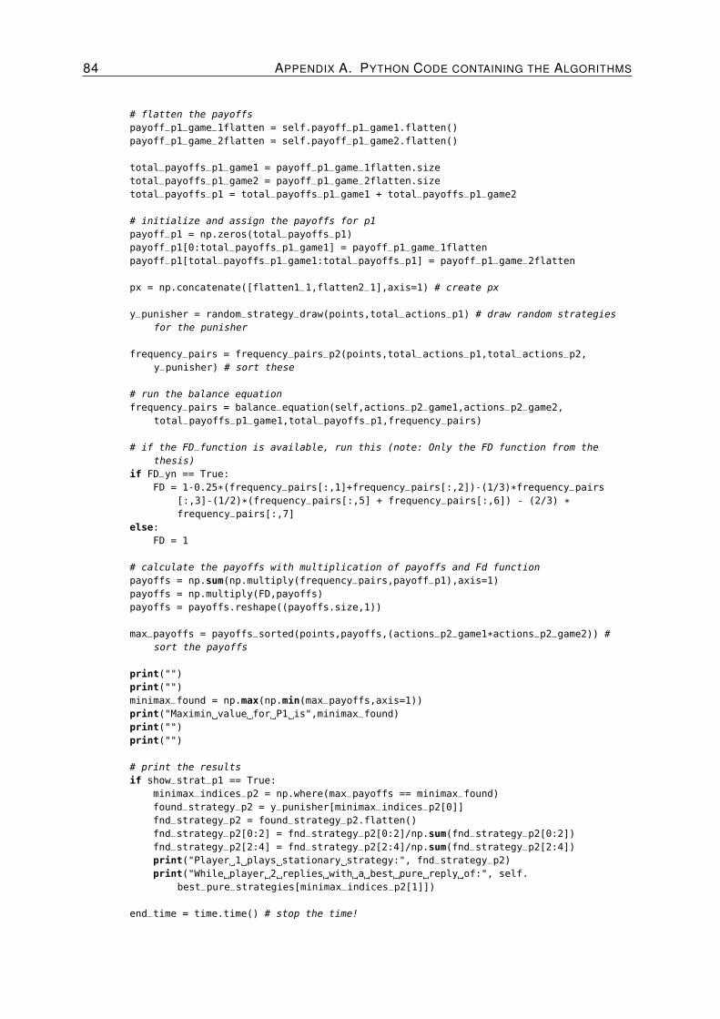
84 APPENDIX A. PYTHON CODE CONTAINING THE ALGORITHMS
# flatten the payoffs
payoff_p1_game_1flatten = self.payoff_p1_game1.flatten()
payoff_p1_game_2flatten = self.payoff_p1_game2.flatten()
total_payoffs_p1_game1 = payoff_p1_game_1flatten.size
total_payoffs_p1_game2 = payoff_p1_game_2flatten.size
total_payoffs_p1 = total_payoffs_p1_game1 + total_payoffs_p1_game2
# initialize and assign the payoffs for p1
payoff_p1 = np.zeros(total_payoffs_p1)
payoff_p1[0:total_payoffs_p1_game1] = payoff_p1_game_1flatten
payoff_p1[total_payoffs_p1_game1:total_payoffs_p1] = payoff_p1_game_2flatten
px = np.concatenate([flatten1_1,flatten2_1],axis=1) # create px
y_punisher = random_strategy_draw(points,total_actions_p1) # draw random strategies
for the punisher
frequency_pairs = frequency_pairs_p2(points,total_actions_p1,total_actions_p2,
y_punisher) # sort these
# run the balance equation
frequency_pairs = balance_equation(self,actions_p2_game1,actions_p2_game2,
total_payoffs_p1_game1,total_payoffs_p1,frequency_pairs)
# if the FD_function is available, run this (note: Only the FD function from the
thesis)
if FD_yn == True:
FD = 1-0.25*(frequency_pairs[:,1]+frequency_pairs[:,2])-(1/3)*frequency_pairs
[:,3]-(1/2)*(frequency_pairs[:,5] + frequency_pairs[:,6]) - (2/3) *frequency_pairs[:,7]
else:
FD = 1
# calculate the payoffs with multiplication of payoffs and Fd function
payoffs = np.sum(np.multiply(frequency_pairs,payoff_p1),axis=1)
payoffs = np.multiply(FD,payoffs)
payoffs = payoffs.reshape((payoffs.size,1))
max_payoffs = payoffs_sorted(points,payoffs,(actions_p2_game1*actions_p2_game2)) #
sort the payoffs
print("")
print("")
minimax_found = np.max(np.min(max_payoffs,axis=1))
print("Maximin value for P1 is",minimax_found)
print("")
print("")
# print the results
if show_strat_p1 == True:
minimax_indices_p2 = np.where(max_payoffs == minimax_found)
found_strategy_p2 = y_punisher[minimax_indices_p2[0]]
fnd_strategy_p2 = found_strategy_p2.flatten()
fnd_strategy_p2[0:2] = fnd_strategy_p2[0:2]/np.sum(fnd_strategy_p2[0:2])
fnd_strategy_p2[2:4] = fnd_strategy_p2[2:4]/np.sum(fnd_strategy_p2[2:4])
print("Player 1 plays stationary strategy:", fnd_strategy_p2)
print("While player 2 replies with a best pure reply of:", self.
best_pure_strategies[minimax_indices_p2[1]])
end_time = time.time() # stop the time!

A.5. TYPE II GAME CODE 85
print("Seconds done to generate", points, "points", end_time-start_time)
## End of P1 maximin algorithm ##
start_time_p2 = time.time() # start the time (Again!)
#flatten the payoffs
payoff_p2_game_1flatten = self.payoff_p2_game1.flatten()
payoff_p2_game_2flatten = self.payoff_p2_game2.flatten()
# store and compute the total payoffs
total_payoffs_p2_game1 = payoff_p2_game_1flatten.size
total_payoffs_p2_game2 = payoff_p2_game_2flatten.size
total_payoffs_p2 = total_payoffs_p2_game1 + total_payoffs_p2_game2
# initialize and assign the payoffs for p2
payoff_p2 = np.zeros(total_payoffs_p2)
payoff_p2[0:total_payoffs_p2_game1] = payoff_p2_game_1flatten
payoff_p2[total_payoffs_p2_game1:total_payoffs_p2] = payoff_p2_game_2flatten
px = np.concatenate([flatten1_1,flatten2_1],axis=1) # store px
x_punisher = random_strategy_draw(points,total_actions_p2) # draw punisher strategies
frequency_pairs = frequency_pairs_p1(points,total_actions_p1,total_actions_p2,
x_punisher) # best replies
# do the balance equation trick
frequency_pairs = balance_equation(self,actions_p1_game1,actions_p1_game2,
total_payoffs_p1_game1,total_payoffs_p1,frequency_pairs)
# if the FD function is on, then run it
if FD_yn == True:
FD = 1-0.25*(frequency_pairs[:,1]+frequency_pairs[:,2])-(1/3)*frequency_pairs
[:,3]-(1/2)*(frequency_pairs[:,5] + frequency_pairs[:,6]) - (2/3) *frequency_pairs[:,7]
else:
FD = 1
# compute the payoffs with the payoffs and FD function
payoffs = np.sum(np.multiply(frequency_pairs,payoff_p2),axis=1)
payoffs = np.multiply(FD,payoffs)
payoffs = payoffs.reshape((payoffs.size,1))
max_payoffs = payoffs_sorted(points,payoffs,(actions_p1_game1*actions_p1_game2))
# sort the payoffs
print("")
print("")
minimax_found_p2 = np.max(np.min(max_payoffs,axis=1)) # find the maximin value
print("Maximin value for P2 is",minimax_found_p2)
print("")
print("")
# print the strategies
if show_strat_p2 == True:
maximin_indices_p2 = np.where(max_payoffs == minimax_found_p2)
found_strategy = x_punisher[maximin_indices_p2[0]]
fnd_strategy = found_strategy.flatten()
fnd_strategy[0:2] = fnd_strategy[0:2]/np.sum(fnd_strategy[0:2])

86 APPENDIX A. PYTHON CODE CONTAINING THE ALGORITHMS
fnd_strategy[2:4] = fnd_strategy[2:4]/np.sum(fnd_strategy[2:4])
print("Player 2 plays stationairy strategy:", fnd_strategy)
print("While player 2 replies with a best pure reply of:", self.
best_pure_strategies[maximin_indices_p2[1]])
end_time_p2 = time.time() # stop the time
print("Seconds done to generate", points, "points", end_time_p2-start_time_p2)
print("")
print("")
def threat_point_optimized(self,points,show_strat_p1,show_strat_p2,print_text,FD_yn):
"The optimized, super awesome threat point algorithm!"
def random_strategy_draw(points,number_of_actions):
"This function draws random strategies from a beta distribution, based on the
number of points and actions"
# draw the strategies and normalize them
strategies_drawn = np.random.beta(0.5,0.5,(points,number_of_actions))
strategies_drawn = strategies_drawn/np.sum(strategies_drawn, axis=1).reshape([
points,1])
return strategies_drawn
def frequency_pairs_p1(points,p2_actions,p1_actions,strategies_drawn):
"This function sorts the punisher strategies based on the replies for p1"
# store the game sizes
game_size_1 = self.payoff_p1_game1.size
game_size_2 = self.payoff_p1_game2.size
# store the actions of p1 for both games
p1_actions_game1 = self.payoff_p1_game1.shape[0]
p1_actions_game2 = self.payoff_p1_game2.shape[0]
# set both actions within a certain range
p1_actions_combi = p1_actions_game1*p1_actions_game2
p1_action_range = np.arange(p1_actions_combi)
# initialize the frequency pair
frequency_pairs = np.zeros((points*(p1_actions_game1*p1_actions_game2),
game_size_1+game_size_2))
# set action ranges for both games
p1_act_game1_range = np.arange(p1_actions_game1)
p1_act_game2_range = np.arange(p1_actions_game2)
# set the best replies for the first game
for i in np.nditer(p1_action_range):
for j in np.nditer(p1_act_game1_range):
mod_remain = np.mod(i,p1_actions_game1)
frequency_pairs[i*points:(i+1)*points,p1_actions_game1*mod_remain+j] =
strategies_drawn[:,j]
# set the best replies for the second game
for i in np.nditer(p1_action_range):
for j in np.nditer(p1_act_game2_range):
floor_div = np.floor_divide(i,p1_actions_game2)
frequency_pairs[i*points:(i+1)*points,j+game_size_1+(p1_actions_game1*floor_div)] = strategies_drawn[:,p1_actions_game1+j]

A.5. TYPE II GAME CODE 87
return frequency_pairs
def balance_equation(self,tot_act_ut,tot_act_thr,tot_payoffs_game1,tot_payoffs,
frequency_pairs):
"Calculates the result of the balance equations in order to adjust the frequency
pairs"
# store size of game 1 and 2
game_size_1 = self.payoff_p1_game1.size
game_size_2 = self.payoff_p1_game2.size
# initialize yi and Q
yi = np.zeros((points*(tot_act_thr*tot_act_ut),game_size_1+game_size_2))
Q = np.zeros((1,points*(tot_act_thr*tot_act_ut)))
# compute Yi
yi[:,0:tot_payoffs_game1] = frequency_pairs[:,0:tot_payoffs_game1]/np.sum(
frequency_pairs[:,0:tot_payoffs_game1], axis=1).reshape([points*tot_payoffs_game1,1])
yi[:,tot_payoffs_game1:tot_payoffs] = frequency_pairs[:,tot_payoffs_game1:
tot_payoffs]/np.sum(frequency_pairs[:,tot_payoffs_game1:tot_payoffs], axis=1)
.reshape([points*(tot_payoffs-tot_payoffs_game1),1])
p1_px_between = np.asarray(px) # some tricks with px (ha-ha)
p1_px = p1_px_between[0]
# compute Q
Q[0,:] = (np.sum(yi[:,tot_payoffs_game1:tot_payoffs]*p1_px[tot_payoffs_game1:
tot_payoffs],axis=1))/((np.dot(yi[:,0:tot_payoffs_game1],(1-p1_px[0:
tot_payoffs_game1]))+np.dot(yi[:,tot_payoffs_game1:tot_payoffs],p1_px[
tot_payoffs_game1:tot_payoffs])))
# adjust the frequency pairs based on Q
frequency_pairs[:,0:tot_payoffs_game1] = (np.multiply(Q.transpose(),yi[:,0:
tot_payoffs_game1]))
frequency_pairs[:,tot_payoffs_game1:tot_payoffs] = np.multiply((1-Q.transpose()),
yi[:,tot_payoffs_game1:tot_payoffs])
return frequency_pairs
def frequency_pairs_p2(points,p2_actions,p1_actions,strategies_drawn):
"This function sorts the punisher strategies based on the replies for p2"
# store the sizes of both games
game_size_1 = self.payoff_p2_game1.size
game_size_2 = self.payoff_p2_game2.size
# make a nice range of the actions for both players and store them
p1_actions_range = np.arange(p1_actions)
p2_actions_range = np.arange(p2_actions)
p2_actions_game1 = self.payoff_p2_game1.shape[1]
p2_actions_game2 = self.payoff_p2_game2.shape[1]
p2_actions_combo = p2_actions_game1*p2_actions_game2
p2_action_range = np.arange(p2_actions_combo)
# initialize the frequency pairs
frequency_pairs = np.zeros((points*(p2_actions_game1*p2_actions_game2),
game_size_1+game_size_2))

88 APPENDIX A. PYTHON CODE CONTAINING THE ALGORITHMS
# loop over the first games best responses
for i in np.nditer(np.arange(p2_actions_game1)):
for j in np.nditer(p2_action_range):
modul = np.mod(j,p2_actions_game1)
frequency_pairs[j*points:(j+1)*points,p2_actions_game1*i+modul] =
strategies_drawn[:,i]
# loop over the second games best responses
for i in np.nditer(np.arange(p2_actions_game2)):
for j in np.nditer(p2_action_range):
divide = np.floor_divide(j,p2_actions_game2)
frequency_pairs[j*points:(j+1)*points,p2_actions_combo+divide+(i*p2_actions_game2)] = strategies_drawn[:,i+p2_actions_game1]
return frequency_pairs
def payoffs_sorted(points,payoffs,actions):
"This function sorts the payoffs for use on the threat point function"
# set a points and actions range
points_range = np.arange(points)
actions_range = np.arange(actions)
payoffs_sort = np.zeros((points,actions)) # initialize the payoffs sorted
# and sort them in a loop
for x in np.nditer(points_range):
for i in np.nditer(actions_range):
payoffs_sort[x,i] = payoffs[points*i+x]
return payoffs_sort
if print_text == True:
print("The start of the algorithm for finding the threat point")
print("First let’s find the threat point for Player 1")
# flatten the transition probabilities
flatten1_1 = self.transition_matrix_game1_to1.flatten()
flatten2_1 = self.transition_matrix_game2_to1.flatten()
# store the actions of both players
actions_p2_game1 = self.payoff_p1_game1.shape[1]
actions_p2_game2 = self.payoff_p1_game2.shape[1]
total_actions_p2 = actions_p2_game1 + actions_p2_game2
actions_p1_game1 = self.payoff_p1_game1.shape[0]
actions_p1_game2 = self.payoff_p1_game2.shape[0]
total_actions_p1 = actions_p1_game1 + actions_p1_game2
# Start of algorithm for player 1
start_time = time.time() # and start the time!
# flatten the payoffs of both players
payoff_p1_game_1flatten = self.payoff_p1_game1.flatten()
payoff_p1_game_2flatten = self.payoff_p1_game2.flatten()
total_payoffs_p1_game1 = payoff_p1_game_1flatten.size
total_payoffs_p1_game2 = payoff_p1_game_2flatten.size
total_payoffs_p1 = total_payoffs_p1_game1 + total_payoffs_p1_game2
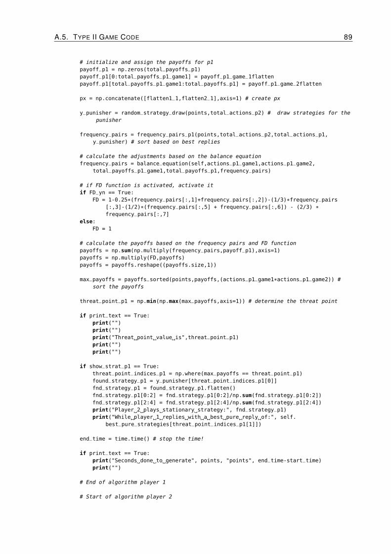
A.5. TYPE II GAME CODE 89
# initialize and assign the payoffs for p1
payoff_p1 = np.zeros(total_payoffs_p1)
payoff_p1[0:total_payoffs_p1_game1] = payoff_p1_game_1flatten
payoff_p1[total_payoffs_p1_game1:total_payoffs_p1] = payoff_p1_game_2flatten
px = np.concatenate([flatten1_1,flatten2_1],axis=1) # create px
y_punisher = random_strategy_draw(points,total_actions_p2) # draw strategies for the
punisher
frequency_pairs = frequency_pairs_p1(points,total_actions_p2,total_actions_p1,
y_punisher) # sort based on best replies
# calculate the adjustments based on the balance equation
frequency_pairs = balance_equation(self,actions_p1_game1,actions_p1_game2,
total_payoffs_p1_game1,total_payoffs_p1,frequency_pairs)
# if FD function is activated, activate it
if FD_yn == True:
FD = 1-0.25*(frequency_pairs[:,1]+frequency_pairs[:,2])-(1/3)*frequency_pairs
[:,3]-(1/2)*(frequency_pairs[:,5] + frequency_pairs[:,6]) - (2/3) *frequency_pairs[:,7]
else:
FD = 1
# calculate the payoffs based on the frequency pairs and FD function
payoffs = np.sum(np.multiply(frequency_pairs,payoff_p1),axis=1)
payoffs = np.multiply(FD,payoffs)
payoffs = payoffs.reshape((payoffs.size,1))
max_payoffs = payoffs_sorted(points,payoffs,(actions_p1_game1*actions_p1_game2)) #
sort the payoffs
threat_point_p1 = np.min(np.max(max_payoffs,axis=1)) # determine the threat point
if print_text == True:
print("")
print("")
print("Threat point value is",threat_point_p1)
print("")
print("")
if show_strat_p1 == True:
threat_point_indices_p1 = np.where(max_payoffs == threat_point_p1)
found_strategy_p1 = y_punisher[threat_point_indices_p1[0]]
fnd_strategy_p1 = found_strategy_p1.flatten()
fnd_strategy_p1[0:2] = fnd_strategy_p1[0:2]/np.sum(fnd_strategy_p1[0:2])
fnd_strategy_p1[2:4] = fnd_strategy_p1[2:4]/np.sum(fnd_strategy_p1[2:4])
print("Player 2 plays stationary strategy:", fnd_strategy_p1)
print("While player 1 replies with a best pure reply of:", self.
best_pure_strategies[threat_point_indices_p1[1]])
end_time = time.time() # stop the time!
if print_text == True:
print("Seconds done to generate", points, "points", end_time-start_time)
print("")
# End of algorithm player 1
# Start of algorithm player 2

90 APPENDIX A. PYTHON CODE CONTAINING THE ALGORITHMS
if print_text == True:
print("")
print("")
print("First start the threat point for player 2")
start_time_p2 = time.time() # new timer, new times
# flatten the payoffs for p2
payoff_p2_game_1flatten = self.payoff_p2_game1.flatten()
payoff_p2_game_2flatten = self.payoff_p2_game2.flatten()
# assign tha payoffs for p2
total_payoffs_p2_game1 = payoff_p2_game_1flatten.size
total_payoffs_p2_game2 = payoff_p2_game_2flatten.size
total_payoffs_p2 = total_payoffs_p2_game1 + total_payoffs_p2_game2
# initialize payoffs p2 and assign them
payoff_p2 = np.zeros(total_payoffs_p2)
payoff_p2[0:total_payoffs_p2_game1] = payoff_p2_game_1flatten
payoff_p2[total_payoffs_p2_game1:total_payoffs_p2] = payoff_p2_game_2flatten
px = np.concatenate([flatten1_1,flatten2_1],axis=1) # px in the mix
x_punisher = random_strategy_draw(points,total_actions_p1) # draw strategies for the
punisher
frequency_pairs = frequency_pairs_p2(points,total_actions_p2,total_actions_p1,
x_punisher) # sort based on best replies
# adjust based on the balance equation
frequency_pairs = balance_equation(self,actions_p2_game1,actions_p2_game2,
total_payoffs_p2_game1,total_payoffs_p2,frequency_pairs)
# Activate the FD function, or not
if FD_yn == True:
FD = 1-0.25*(frequency_pairs[:,1]+frequency_pairs[:,2])-(1/3)*frequency_pairs
[:,3]-(1/2)*(frequency_pairs[:,5] + frequency_pairs[:,6]) - (2/3) *frequency_pairs[:,7]
else:
FD = 1
# determine the payoffs based on the frequency pairs and FD function
payoffs = np.sum(np.multiply(frequency_pairs,payoff_p2),axis=1)
payoffs = np.multiply(FD,payoffs)
payoffs = payoffs.reshape((payoffs.size,1))
max_payoffs = payoffs_sorted(points,payoffs,(actions_p2_game1*actions_p2_game2)) #
sort the payoffs
threat_point_p2 = np.min(np.max(max_payoffs,axis=1)) # determine the threat point
if print_text == True:
print("")
print("")
print("Threat point value is",threat_point_p2)
print("")
print("")
if show_strat_p2 == True:
threat_point_indices_p2 = np.where(max_payoffs == threat_point_p2)
found_strategy = x_punisher[threat_point_indices_p2[0]]

A.6. TYPE II EXAMPLE GAMES CODE 91
fnd_strategy = found_strategy.flatten()
fnd_strategy[0:2] = fnd_strategy[0:2]/np.sum(fnd_strategy[0:2])
fnd_strategy[2:4] = fnd_strategy[2:4]/np.sum(fnd_strategy[2:4])
print("Player 1 plays stationairy strategy:", fnd_strategy)
print("While player 2 replies with a best pure reply of:", self.
best_pure_strategies[threat_point_indices_p2[1]])
end_time_p2 = time.time() # stop the time!
if print_text == True:
print("")
print("Seconds done to generate", points, "points", end_time_p2-start_time_p2)
print("")
print("")
self.threat_point = [threat_point_p1,threat_point_p2] # store the threat point
return [threat_point_p1,threat_point_p2]
A.6 Type II Example Games Code
encoding=*-60
"The first Stochastic Game is based on a Stochastic Game described in the thesis"
p1_1 = np.matrix(’16 14; 28 24’)
p2_1 = np.matrix(’16 28; 14 24’)
p1_2 = np.matrix(’4 3.5; 7 6’)
p2_2 = np.matrix(’4 7; 3.5 6’)
trans1_1 = np.matrix(’0.8 0.7; 0.7 0.6’)
trans2_1 = np.matrix(’0.5 0.4; 0.4 0.15’)
trans1_2 = np.matrix(’0.2 0.3; 0.3 0.4’)
trans2_2 = np.matrix(’0.5 0.6; 0.6 0.85’)
FirstTry = StochasticGame(p1_1,p2_1,p1_2,p2_2,trans1_1,trans2_1,trans1_2,trans2_2)
FirstTry.plot_single_period_pure_rewards()
FirstTry.plot_all_reward_points(True)
FirstTry.maximin_point(100)
timing = time.time()
FirstTry.threat_point_algorithm(10000,0.025)
now = time.time()
print(now-timing)
FirstTry.threat_point_optimized(10000,False,False,True,True)
FirstTry.plot_threat_point()
FirstTry.plot_threat_point_lines()
FirstTry.optimized_maximin(100,False,False,True)
A.7 Type III Game Code
encoding=*-60
class ETPGame:
"The ETP Game class represents the Type III games from the thesis, with or without ESP."

92 APPENDIX A. PYTHON CODE CONTAINING THE ALGORITHMS
def __init__(self,payoff_p1_game1,payoff_p2_game1,payoff_p1_game2,payoff_p2_game2,
trmatrixg1,trmatrixg2,trmatrixg3,trmatrixg4,matrixA):
"Here below we initialize the game by storing payoff and transition matrices
according to the upper input."
self.payoff_p1_game1 = payoff_p1_game1 #payoff p1 in game 1
self.payoff_p2_game1 = payoff_p2_game1 #payoff p2 in game 1
self.payoff_p1_game2 = payoff_p1_game2 #payoff p1 in game 2
self.payoff_p2_game2 = payoff_p2_game2 #payoff p2 in game 2
self.transition_matrix_game1_to1 = trmatrixg1 #transition matrix from game
1 to game 1
self.transition_matrix_game2_to1 = trmatrixg2 #transition matrix from game
2 to game 1
self.transition_matrix_game1_to2 = trmatrixg3 #transition matrix from game
1 to game 2
self.transition_matrix_game2_to2 = trmatrixg4 #transition matrix from game
2 to game 2
self.etp_matrix = matrixA
self.printing = False #set printing to False
self.best_pure_strategies = np.array([[1,0,1,0],[0,1,1,0],[1,0,0,1],[0,1,0,1]])
def plot_single_period_pure_rewards(self):
"Here we plot the pure rewards possible for a single period"
plt.figure() #create a figure
payoff_p1_g1_flat = self.payoff_p1_game1.A1 #create a flattend payoff of
p1 in game 1
payoff_p2_g1_flat = self.payoff_p2_game1.A1 #create a flattend payoff of
p2 in game 1
plt.scatter(payoff_p1_g1_flat,payoff_p2_g1_flat, label="Pure reward points Game 1",
zorder = 15) #plot payoffs game 1
payoff_p1_g2_flat = self.payoff_p1_game2.A1 #create a flattend payoff of
p1 in game 2
payoff_p2_g2_flat = self.payoff_p2_game2.A1 #and for p2 in game 2
plt.scatter(payoff_p1_g2_flat,payoff_p2_g2_flat, label="Pure reward points Game 2",
zorder = 15) #plotting this again
plt.xlabel("Payoff Player 1") #giving the x-axis the label
of payoff p1
plt.ylabel("Payoff Player 2") #and the payoff of the y-axis
is that of p2
plt.title("Reward points of ETP game") #and we give it a nice titel
plt.legend()
def plot_convex_hull_pure_rewards(self):
"Here we plot a convex hull around the pure reward point, therefore resulting in the
total possible reward space"
payoff_p1_g1_flat = self.payoff_p1_game1.A1 #store the flattend payoff of p1
game 1
payoff_p2_g1_flat = self.payoff_p2_game1.A1 #store the flattend payoff of p2
game 1
payoff_p1_g2_flat = self.payoff_p1_game2.A1 #store the flattend payoff of p1

A.7. TYPE III GAME CODE 93
game 2
payoff_p2_g2_flat = self.payoff_p2_game2.A1 #store the flattend payoff of p2
game 2
payoff_p1_merged = np.concatenate((payoff_p1_g1_flat,payoff_p1_g2_flat)) #merge p1
payoffs
payoff_p2_merged = np.concatenate((payoff_p2_g1_flat,payoff_p2_g2_flat)) #merge p2
payoffs
all_payoffs = np.array([payoff_p1_merged,payoff_p2_merged]) #create one array of
payoffs
all_payoffs = np.transpose(all_payoffs) #and rotate this one
rewards_convex_hull = ConvexHull(all_payoffs) #retain the convex hull
of the payoffs
plt.fill(all_payoffs[rewards_convex_hull.vertices,0], all_payoffs[rewards_convex_hull
.vertices,1], color=’k’)
#here above we fill the convex hull in black
def plot_all_rewards(self,FD_yn):
"This plots all rewards and is based on the algorithm by Llea Samuel"
"IMPORTANT NOTE!: GAME IS HARDCODED WITHIN THIS FUNCTION, DUE TO TIME ISSUES, ONE
SHOULD TAKE THIS INTO MIND"
np.seterr(all=’warn’,divide=’warn’) # this is to show some more information on
possible errors, can be excluded
## HERE BELOW IS HARDCODED GAME INFORMATION
A1 = np.array([16, 14, 28, 24, 4, 3.5, 7, 6])
B1 = np.array([16, 28, 14, 24, 4, 7, 3.5, 6])
p = np.array([0.8, 0.7, 0.7, 0.6, 0.5, 0.4, 0.4, 0.15])
## ABOVE IS HARDCODED GAME INFORMATION
# here below we initialize a lot of variables
x = np.zeros(8)
r = np.zeros(8)
y = np.zeros(8)
xstar = np.zeros(8)
x_a = np.zeros(8)
yp = np.zeros(4)
yp_not = np.zeros(4)
v_p1 = np.zeros(8)
v_p2 = np.zeros(8)
Q_vec = np.zeros(8)
T = 100000 # number of points to generate
payoff_p1 = np.zeros(T) # initialize payoffs for both players
payoff_p2 = np.zeros(T)
# store the matrix A
matrixA = np.matrix(’0.00 0.0 0.0 0.00 0.0 0.00 0.00 0.00; 0.35 0.3 0.3 0.25 0.2 0.15
0.15 0.05; 0.35 0.3 0.3 0.25 0.2 0.15 0.15 0.05; 0.7 0.6 0.6 0.5 0.4 0.3 0.3
0.1; 0 0 0 0 0 0 0 0; 0.35 0.3 0.3 0.25 0.2 0.15 0.15 0.05; 0.35 0.3 0.3 0.25 0.2
0.15 0.15 0.05; 0.7 0.6 0.6 0.5 0.4 0.3 0.3 0.1’)
# loop over the total number of points to generate
for t in range(0,T):
### BEGIN Q-CHECKER #####
for i in range(0,3):

94 APPENDIX A. PYTHON CODE CONTAINING THE ALGORITHMS
r[i] = np.random.beta(0.5,0.5) # generate frequencies
Norm_val = np.sum(r) # normalize them
for i in range(0,3):
x_a[i] = r[i]/Norm_val # normalize and store
# do some more fancy X calculations
x_b1 = np.array([x_a[0], x_a[2], 0 , 0])
x_b2 = np.array([x_a[1], 0, 0, 0])
x_c1 = x_b1[np.random.permutation(x_b1.size)]
x_c2 = x_b2[np.random.permutation(x_b2.size)]
for i in range(0,8):
if i < 4:
x[i] = x_c1[i]
else:
x[i] = x_c2[i-4]
# caclulate yi and yi_not
for i in range(0,4):
y[i] = x[i]/np.sum(x[0:4])
for i in range(4,8):
y[i] = x[i]/np.sum(x[4:8])
px = p - np.dot(x,matrixA) # calculate px
# start with computing Q
for w in range(0,4):
for i in range(0,4):
yp[i] = y[i+4]*px[0,i+4]
yp_not[i] = y[i]+(1-px[0,i])
Q = np.sum(yp)/(np.sum(yp_not) + np.sum(yp)) # compute Q
Q_not = 1-Q
Q_vec[w] = Q
# adjust frequency vector based on found Q
for i in range(0,4):
xstar[i] = Q*y[i]
for i in range(4,8):
xstar[i] = Q_not*y[i]
px = p - np.dot(xstar,matrixA) # adjust PX
# apply Aitken’s delta squared
Q_check_1 = Q_vec[0]-((Q_vec[1] - Q_vec[0])**2) / (Q_vec[2] - 2*Q_vec[1] + Q_vec
[0])
Q_check_2 = Q_vec[1]-((Q_vec[2]- Q_vec[1])**2) / (Q_vec[3] - 2*Q_vec[2] + Q_vec
[1])
diff = Q_check_1 - Q_check_2
# if the distribution has not settled, then infinite calculate a new Q
while diff > abs(1e-8):
Q_check_1 = Q_check_2
# new calculations of yi
for i in range(0,4):

A.7. TYPE III GAME CODE 95
yp[i] = y[i+4]*px[0,i+4]
yp_not[i] = y[i]*(1-px[0,i])
Q = (np.sum(yp)) / (np.sum(yp_not) + np.sum(yp)) # again calculate Q
Q_not = 1-Q
Q_vec[w+1] = Q
# adjust frequency vector X
for i in range(0,4):
xstar[i] = Q*y[i]
for i in range(4,8):
xstar[i] = Q_not*y[i]
px = p - np.dot(xstar,matrixA) # px calculations
# compute new Q based on aitken’s
Q_check_2 = Q_vec[w-1] - ((Q_vec[w]-Q_vec[w-1])**2)/(Q_vec[w+1] - 2*Q_vec[w]
+ Q_vec[w-1])
diff = Q_check_1 - Q_check_2
w = w+1
# apply FD function if activated
if FD_yn == True:
FD = 1-0.25*(xstar[1]+xstar[2])-(1/3)*xstar[3]-(1/2)*(xstar[5] + xstar[6]) -
(2/3) * xstar[7]
else:
FD = 1
# calculate payoffs
for i in range(0,8):
v_p1[i] = xstar[i]*A1[i]
v_p2[i] = xstar[i]*B1[i]
# calculate definitive rewards based on FD function
payoff_p1[t] = FD*np.sum(v_p1)
payoff_p2[t] = FD*np.sum(v_p2)
# store maximal payoffs
self.maximal_payoffs = np.zeros(2)
self.maximal_payoffs = [np.max(payoff_p1),np.max(payoff_p2)]
all_payoffs = np.array([payoff_p1,payoff_p2]) #payoffs player 1 and and p2 merging
all_payoffs = np.transpose(all_payoffs) #transpose for use in convex_hull
Convex_Hull_Payoffs = ConvexHull(all_payoffs) #calculate convex_hull of the payoffs
# plot a nice convex hull
plt.fill(all_payoffs[Convex_Hull_Payoffs.vertices,0], all_payoffs[Convex_Hull_Payoffs
.vertices,1], color=’y’, zorder=5, label="Obtainable rewards")
def plot_threat_point(self):
"This function plots the threat point if found"
plt.scatter(self.threat_point[0],self.threat_point[1], zorder=10, color = ’r’, label=
’Threat point’)
plt.legend()
def plot_threat_point_lines(self):
"This function plots lines around the threat point indicating the limits for the NE"
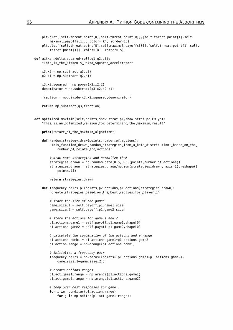
96 APPENDIX A. PYTHON CODE CONTAINING THE ALGORITHMS
plt.plot([self.threat_point[0],self.threat_point[0]],[self.threat_point[1],self.
maximal_payoffs[1]], color=’k’, zorder=15)
plt.plot([self.threat_point[0],self.maximal_payoffs[0]],[self.threat_point[1],self.
threat_point[1]], color=’k’, zorder=15)
def aitken_delta_squared(self,q1,q2,q3):
"This is the Aitken’s Delta Squared accelerator"
x3_x2 = np.subtract(q3,q2)
x2_x1 = np.subtract(q2,q1)
x3_x2_squared = np.power(x3_x2,2)
denominator = np.subtract(x3_x2,x2_x1)
fraction = np.divide(x3_x2_squared,denominator)
return np.subtract(q3,fraction)
def optimized_maximin(self,points,show_strat_p1,show_strat_p2,FD_yn):
"This is an optimized version for determining the maximin result"
print("Start of the maximin algorithm")
def random_strategy_draw(points,number_of_actions):
"This function draws random strategies from a beta distribution, based on the
number of points and actions"
# draw some strategies and normalize them
strategies_drawn = np.random.beta(0.5,0.5,(points,number_of_actions))
strategies_drawn = strategies_drawn/np.sum(strategies_drawn, axis=1).reshape([
points,1])
return strategies_drawn
def frequency_pairs_p1(points,p2_actions,p1_actions,strategies_drawn):
"Create strategies based on the best replies for player 1"
# store the size of the games
game_size_1 = self.payoff_p1_game1.size
game_size_2 = self.payoff_p1_game2.size
# store the actions for game 1 and 2
p1_actions_game1 = self.payoff_p1_game1.shape[0]
p1_actions_game2 = self.payoff_p1_game2.shape[0]
# calculate the combination of the actions and a range
p1_actions_combi = p1_actions_game1*p1_actions_game2
p1_action_range = np.arange(p1_actions_combi)
# initialize a frequency pair
frequency_pairs = np.zeros((points*(p1_actions_game1*p1_actions_game2),
game_size_1+game_size_2))
# create actions ranges
p1_act_game1_range = np.arange(p1_actions_game1)
p1_act_game2_range = np.arange(p1_actions_game2)
# loop over best responses for game 1
for i in np.nditer(p1_action_range):
for j in np.nditer(p1_act_game1_range):

A.7. TYPE III GAME CODE 97
mod_remain = np.mod(i,p1_actions_game1)
frequency_pairs[i*points:(i+1)*points,p1_actions_game1*mod_remain+j] =
strategies_drawn[:,j]
# loop over best responses for game 2
for i in np.nditer(p1_action_range):
for j in np.nditer(p1_act_game2_range):
floor_div = np.floor_divide(i,p1_actions_game2)
frequency_pairs[i*points:(i+1)*points,j+game_size_1+(p1_actions_game1*floor_div)] = strategies_drawn[:,p1_actions_game1+j]
return frequency_pairs
def balance_equation(self,tot_act_ut,tot_act_thr,tot_payoffs_game1,tot_payoffs,
frequency_pairs):
"Calculates the result of the balance equations in order to adjust the frequency
pairs"
# store the game sizes
game_size_1 = self.payoff_p1_game1.size
game_size_2 = self.payoff_p1_game2.size
# initialize yi, Q and Q_new
yi = np.zeros((points*(tot_act_thr*tot_act_ut),game_size_1+game_size_2))
Q = np.zeros((1,points*(tot_act_thr*tot_act_ut)))
Q_new = np.zeros((1,points*(tot_act_thr*tot_act_ut)))
# compute yi
yi[:,0:tot_payoffs_game1] = frequency_pairs[:,0:tot_payoffs_game1]/np.sum(
frequency_pairs[:,0:tot_payoffs_game1], axis=1).reshape([points*tot_payoffs_game1,1])
yi[:,tot_payoffs_game1:tot_payoffs] = frequency_pairs[:,tot_payoffs_game1:
tot_payoffs]/np.sum(frequency_pairs[:,tot_payoffs_game1:tot_payoffs], axis=1)
.reshape([points*(tot_payoffs-tot_payoffs_game1),1])
index_values = np.arange(points*(tot_act_thr*tot_act_ut)) # set a range
# set px range
p1_px_between = np.asarray(px)
p1_px = p1_px_between[0]
# loop for 35 iterations
for i in np.arange(35):
# in the first iteration we calculate the first Q and adjust X
if i == 0:
new_x = p1_px - np.dot(frequency_pairs,self.etp_matrix)
upper_part_Q = np.sum(np.multiply(yi[:,tot_payoffs_game1:tot_payoffs],
new_x[:,tot_payoffs_game1:tot_payoffs]),axis=1)
leftdown_part_Q = np.sum(np.multiply(yi[:,0:tot_payoffs_game1],(1-new_x
[:,0:tot_payoffs_game1])),axis=1)
rightdown_part_Q = np.sum(np.multiply(yi[:,tot_payoffs_game1:tot_payoffs
],new_x[:,tot_payoffs_game1:tot_payoffs]),axis=1)
Q_between = upper_part_Q/(leftdown_part_Q+rightdown_part_Q)
Q = Q_between
frequency_pairs[:,0:tot_payoffs_game1] = (np.multiply(Q,yi[:,0:
tot_payoffs_game1]))
frequency_pairs[:,tot_payoffs_game1:tot_payoffs] = np.multiply((1-Q),yi

98 APPENDIX A. PYTHON CODE CONTAINING THE ALGORITHMS
[:,tot_payoffs_game1:tot_payoffs])
# here we just calculate Q in order to guarantee stability
if i > 0 and i < 10:
new_x = p1_px - np.dot(frequency_pairs,self.etp_matrix)
upper_part_Q = np.sum(np.multiply(yi[:,tot_payoffs_game1:tot_payoffs],
new_x[:,tot_payoffs_game1:tot_payoffs]),axis=1)
leftdown_part_Q = np.sum(np.multiply(yi[:,0:tot_payoffs_game1],(1-new_x
[:,0:tot_payoffs_game1])),axis=1)
rightdown_part_Q = np.sum(np.multiply(yi[:,tot_payoffs_game1:tot_payoffs
],new_x[:,tot_payoffs_game1:tot_payoffs]),axis=1)
Q_between = upper_part_Q/(leftdown_part_Q+rightdown_part_Q)
Q = np.hstack((Q,Q_between))
frequency_pairs[:,0:tot_payoffs_game1] = (np.multiply(Q[:,i],yi[:,0:
tot_payoffs_game1]))
frequency_pairs[:,tot_payoffs_game1:tot_payoffs] = np.multiply((1-Q[:,i])
,yi[:,tot_payoffs_game1:tot_payoffs])
# here we calculate Q based on aitken’s delta squared
if i == 10:
Q_new = self.aitken_delta_squared(Q[:,i-3],Q[:,i-2],Q[:,i-1])
nan_org = np.where(np.isnan(Q_new)) # check where there are NaN’s
nan_indic = nan_org[0]
Q_new[nan_indic,:] = Q_between[nan_indic,:] # remove NaN’s with last
known values
Q_old = np.copy(Q_new)
Q = np.hstack((Q,Q_new))
# all remaining iterations are with Aitkens
if i > 10:
Q_new[index_values,:] = self.aitken_delta_squared(Q[index_values,i-3],Q[
index_values,i-2],Q[index_values,i-1])
Q_old2 = np.copy(Q_old)
nan_res = np.where(np.isnan(Q_new,Q_old)) # check for NaN’s
nan_indices = nan_res[0] # look where NaN’s are
# delete values which are NaN for future computations
nan_between = np.where(np.in1d(index_values,nan_indices))
nan_cands = nan_between[0]
index_values = np.delete(index_values,nan_cands)
Q_new[nan_indices,:] = Q_old2[nan_indices,:]
Q = np.hstack((Q,Q_new))
Q_old = np.copy(Q_new)
results = np.where(Q[index_values,i-1] == Q[index_values,i]) # check
where convergence has occured
remove_indices = results[0]
# remove indices which have converged
removal_between = np.where(np.in1d(index_values,remove_indices))
removal_cands = removal_between[0]
index_values = np.delete(index_values,removal_cands)

A.7. TYPE III GAME CODE 99
# compute the definitive frequency pair x
frequency_pairs[:,0:tot_payoffs_game1] = (np.multiply(Q[:,34],yi[:,0:
tot_payoffs_game1]))
frequency_pairs[:,tot_payoffs_game1:tot_payoffs] = np.multiply((1-Q[:,34]),yi[:,
tot_payoffs_game1:tot_payoffs])
return frequency_pairs
def frequency_pairs_p2(points,p2_actions,p1_actions,strategies_drawn):
"Best responses for P2 based on threaten strategies drawn"
# store the game sizes
game_size_1 = self.payoff_p2_game1.size
game_size_2 = self.payoff_p2_game2.size
# store the actions for p1 and p2 and create ranges
p1_actions_range = np.arange(p1_actions)
p2_actions_range = np.arange(p2_actions)
p2_actions_game1 = self.payoff_p2_game1.shape[1]
p2_actions_game2 = self.payoff_p2_game2.shape[1]
p2_actions_combo = p2_actions_game1*p2_actions_game2
p2_action_range = np.arange(p2_actions_combo)
# initialize the frequency pair
frequency_pairs = np.zeros((points*(p2_actions_game1*p2_actions_game2),
game_size_1+game_size_2))
# generate best responses for game 1
for i in np.nditer(np.arange(p2_actions_game1)):
for j in np.nditer(p2_action_range):
modul = np.mod(j,p2_actions_game1)
frequency_pairs[j*points:(j+1)*points,p2_actions_game1*i+modul] =
strategies_drawn[:,i]
# generate best respones for game 2
for i in np.nditer(np.arange(p2_actions_game2)):
for j in np.nditer(p2_action_range):
divide = np.floor_divide(j,p2_actions_game2)
frequency_pairs[j*points:(j+1)*points,p2_actions_combo+divide+(i*p2_actions_game2)] = strategies_drawn[:,i+p2_actions_game1]
return frequency_pairs
def payoffs_sorted(points,payoffs,actions):
"Sort the payoffs for determination of maximin"
# store the range of points and actions
points_range = np.arange(points)
actions_range = np.arange(actions)
payoffs_sort = np.zeros((points,actions)) # initialize the payoffs sort
# sort the payoffs!
for x in np.nditer(points_range):
for i in np.nditer(actions_range):
payoffs_sort[x,i] = payoffs[points*i+x]
return payoffs_sort

100 APPENDIX A. PYTHON CODE CONTAINING THE ALGORITHMS
## Start of p1 maximin ##
start_time = time.time() # START TIME
# flatten the transition matrices
flatten1_1 = self.transition_matrix_game1_to1.flatten()
flatten2_1 = self.transition_matrix_game2_to1.flatten()
# store and compute some action stuff
actions_p2_game1 = self.payoff_p1_game1.shape[1]
actions_p2_game2 = self.payoff_p1_game2.shape[1]
total_actions_p2 = actions_p2_game1 + actions_p2_game2
actions_p1_game1 = self.payoff_p1_game1.shape[0]
actions_p1_game2 = self.payoff_p1_game2.shape[0]
total_actions_p1 = actions_p1_game1 + actions_p1_game2
# flatten the payoffs
payoff_p1_game_1flatten = self.payoff_p1_game1.flatten()
payoff_p1_game_2flatten = self.payoff_p1_game2.flatten()
# compute and store some payoffs stuff
total_payoffs_p1_game1 = payoff_p1_game_1flatten.size
total_payoffs_p1_game2 = payoff_p1_game_2flatten.size
total_payoffs_p1 = total_payoffs_p1_game1 + total_payoffs_p1_game2
payoff_p2_game_1flatten = self.payoff_p2_game1.flatten()
payoff_p2_game_2flatten = self.payoff_p2_game2.flatten()
total_payoffs_p2_game1 = payoff_p2_game_1flatten.size
total_payoffs_p2_game2 = payoff_p2_game_2flatten.size
total_payoffs_p2 = total_payoffs_p2_game1 + total_payoffs_p2_game2
total_payoffs_p2_game1 = payoff_p2_game_1flatten.size
total_payoffs_p2_game2 = payoff_p2_game_2flatten.size
total_payoffs_p2 = total_payoffs_p2_game1 + total_payoffs_p2_game2
# initialize the payoff stuff for p1
payoff_p1 = np.zeros(total_payoffs_p1)
payoff_p1[0:total_payoffs_p1_game1] = payoff_p1_game_1flatten
payoff_p1[total_payoffs_p1_game1:total_payoffs_p1] = payoff_p1_game_2flatten
px = np.concatenate([flatten1_1,flatten2_1],axis=1) # px for the first time
y_punisher = random_strategy_draw(points,total_actions_p1) # draw some strategies
frequency_pairs = frequency_pairs_p2(points,total_actions_p1,total_actions_p2,
y_punisher) # sort them based on best replies
# do the balance equations with Aitken’s
frequency_pairs = balance_equation(self,actions_p2_game1,actions_p2_game2,
total_payoffs_p2_game1,total_payoffs_p2,frequency_pairs)
# activate FD function if necessary
if FD_yn == True:
FD = 1-0.25*(frequency_pairs[:,1]+frequency_pairs[:,2])-(1/3)*frequency_pairs
[:,3]-(1/2)*(frequency_pairs[:,5] + frequency_pairs[:,6]) - (2/3) *frequency_pairs[:,7]
else:
FD = 1
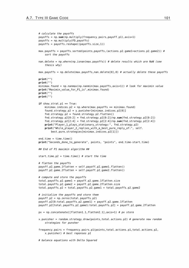
A.7. TYPE III GAME CODE 101
# calculate the payoffs
payoffs = np.sum(np.multiply(frequency_pairs,payoff_p1),axis=1)
payoffs = np.multiply(FD,payoffs)
payoffs = payoffs.reshape((payoffs.size,1))
max_payoffs = payoffs_sorted(points,payoffs,(actions_p2_game1*actions_p2_game2)) #
sort the payoffs
nan_delete = np.where(np.isnan(max_payoffs)) # delete results which are NaN (see
thesis why)
max_payoffs = np.delete(max_payoffs,nan_delete[0],0) # actually delete these payoffs
print("")
print("")
minimax_found = np.nanmax(np.nanmin(max_payoffs,axis=1)) # look for maximin value
print("Maximin value for P1 is",minimax_found)
print("")
print("")
if show_strat_p1 == True:
minimax_indices_p2 = np.where(max_payoffs == minimax_found)
found_strategy_p2 = y_punisher[minimax_indices_p2[0]]
fnd_strategy_p2 = found_strategy_p2.flatten()
fnd_strategy_p2[0:2] = fnd_strategy_p2[0:2]/np.sum(fnd_strategy_p2[0:2])
fnd_strategy_p2[2:4] = fnd_strategy_p2[2:4]/np.sum(fnd_strategy_p2[2:4])
print("Player 1 plays stationary strategy:", fnd_strategy_p2)
print("While player 2 replies with a best pure reply of:", self.
best_pure_strategies[minimax_indices_p2[1]])
end_time = time.time()
print("Seconds done to generate", points, "points", end_time-start_time)
## End of P1 maximin algorithm ##
start_time_p2 = time.time() # start the time
# flatten the payoffs
payoff_p2_game_1flatten = self.payoff_p2_game1.flatten()
payoff_p2_game_2flatten = self.payoff_p2_game2.flatten()
# compute and store the payoffs
total_payoffs_p2_game1 = payoff_p2_game_1flatten.size
total_payoffs_p2_game2 = payoff_p2_game_2flatten.size
total_payoffs_p2 = total_payoffs_p2_game1 + total_payoffs_p2_game2
# initialize the payoffs and store them
payoff_p2 = np.zeros(total_payoffs_p2)
payoff_p2[0:total_payoffs_p2_game1] = payoff_p2_game_1flatten
payoff_p2[total_payoffs_p2_game1:total_payoffs_p2] = payoff_p2_game_2flatten
px = np.concatenate([flatten1_1,flatten2_1],axis=1) # px store
x_punisher = random_strategy_draw(points,total_actions_p2) # generate new random
strategies for punsher
frequency_pairs = frequency_pairs_p1(points,total_actions_p1,total_actions_p2,
x_punisher) # best reponses p1
# balance equations with Delta Squared
102 APPENDIX A. PYTHON CODE CONTAINING THE ALGORITHMS
frequency_pairs = balance_equation(self,actions_p1_game1,actions_p1_game2,
total_payoffs_p1_game1,total_payoffs_p1,frequency_pairs)
# activate FD function if necessary
if FD_yn == True:
FD = 1-0.25*(frequency_pairs[:,1]+frequency_pairs[:,2])-(1/3)*frequency_pairs
[:,3]-(1/2)*(frequency_pairs[:,5] + frequency_pairs[:,6]) - (2/3) *frequency_pairs[:,7]
else:
FD = 1
# compute the payoffs with payoffs and FD function
payoffs = np.sum(np.multiply(frequency_pairs,payoff_p2),axis=1)
payoffs = np.multiply(FD,payoffs)
payoffs = payoffs.reshape((payoffs.size,1))
max_payoffs = payoffs_sorted(points,payoffs,(actions_p1_game1*actions_p1_game2)) #
sort the payoffs
nan_delete = np.where(np.isnan(max_payoffs)) # check where there are nan’s
max_payoffs = np.delete(max_payoffs,nan_delete[0],0) # delete these nan’s
minimax_found_p2 = np.nanmax(np.nanmin(max_payoffs,axis=1)) # find the maximin value
for p2
print("Maximin value for P2 is",minimax_found_p2)
print("")
print("")
if show_strat_p2 == True:
maximin_indices_p2 = np.where(max_payoffs == minimax_found_p2)
found_strategy = x_punisher[maximin_indices_p2[0]]
fnd_strategy = found_strategy.flatten()
fnd_strategy[0:2] = fnd_strategy[0:2]/np.sum(fnd_strategy[0:2])
fnd_strategy[2:4] = fnd_strategy[2:4]/np.sum(fnd_strategy[2:4])
print("Player 2 plays stationairy strategy:", fnd_strategy)
print("While player 2 replies with a best pure reply of:", self.
best_pure_strategies[maximin_indices_p2[1]])
end_time_p2 = time.time() # end the timer
print("Seconds done to generate", points, "points", end_time_p2-start_time_p2)
print("")
print("")
def threat_point_optimized(self,points,show_strat_p1,show_strat_p2,print_text,FD_yn):
"OPtimized threat point algorithm for ETP games"
def random_strategy_draw(points,number_of_actions):
"This function draws random strategies from a beta distribution, based on the
number of points and actions"
# draw some strategies and normalize them
strategies_drawn = np.random.beta(0.5,0.5,(points,number_of_actions))
strategies_drawn = strategies_drawn/np.sum(strategies_drawn, axis=1).reshape([
points,1])
return strategies_drawn
def frequency_pairs_p1(points,p2_actions,p1_actions,strategies_drawn):
"This function sorts the strategies based on the responses"

A.7. TYPE III GAME CODE 103
# store the game size
game_size_1 = self.payoff_p1_game1.size
game_size_2 = self.payoff_p1_game2.size
# store the actions of p1 in both game
p1_actions_game1 = self.payoff_p1_game1.shape[0]
p1_actions_game2 = self.payoff_p1_game2.shape[0]
p1_actions_combi = p1_actions_game1*p1_actions_game2
p1_action_range = np.arange(p1_actions_combi)
# initialize frequency pairs
frequency_pairs = np.zeros((points*(p1_actions_game1*p1_actions_game2),
game_size_1+game_size_2))
# set the range for both games
p1_act_game1_range = np.arange(p1_actions_game1)
p1_act_game2_range = np.arange(p1_actions_game2)
# create best response for game 1
for i in np.nditer(p1_action_range):
for j in np.nditer(p1_act_game1_range):
mod_remain = np.mod(i,p1_actions_game1)
frequency_pairs[i*points:(i+1)*points,p1_actions_game1*mod_remain+j] =
strategies_drawn[:,j]
# loop for best responses for game 2
for i in np.nditer(p1_action_range):
for j in np.nditer(p1_act_game2_range):
floor_div = np.floor_divide(i,p1_actions_game2)
frequency_pairs[i*points:(i+1)*points,j+game_size_1+(p1_actions_game1*floor_div)] = strategies_drawn[:,p1_actions_game1+j]
return frequency_pairs
def balance_equation(self,tot_act_ut,tot_act_thr,tot_payoffs_game1,tot_payoffs,
frequency_pairs):
"Calculates the result of the balance equations in order to adjust the frequency
pairs"
# store the game sizes
game_size_1 = self.payoff_p1_game1.size
game_size_2 = self.payoff_p1_game2.size
# initialize yi, Q and Q_new
yi = np.zeros((points*(tot_act_thr*tot_act_ut),game_size_1+game_size_2))
Q = np.zeros((1,points*(tot_act_thr*tot_act_ut)))
Q_new = np.zeros((1,points*(tot_act_thr*tot_act_ut)))
# compute Yi
yi[:,0:tot_payoffs_game1] = frequency_pairs[:,0:tot_payoffs_game1]/np.sum(
frequency_pairs[:,0:tot_payoffs_game1], axis=1).reshape([points*tot_payoffs_game1,1])
yi[:,tot_payoffs_game1:tot_payoffs] = frequency_pairs[:,tot_payoffs_game1:
tot_payoffs]/np.sum(frequency_pairs[:,tot_payoffs_game1:tot_payoffs], axis=1)
.reshape([points*(tot_payoffs-tot_payoffs_game1),1])
index_values = np.arange(points*(tot_act_thr*tot_act_ut)) # create a range of
index values
p1_px_between = np.asarray(px) # set px

104 APPENDIX A. PYTHON CODE CONTAINING THE ALGORITHMS
p1_px = p1_px_between[0]
# iterate for 35 iterations
for i in np.arange(35):
# first iteration, just calculate Q
if i == 0:
new_x = p1_px - np.dot(frequency_pairs,self.etp_matrix)
upper_part_Q = np.sum(np.multiply(yi[:,tot_payoffs_game1:tot_payoffs],
new_x[:,tot_payoffs_game1:tot_payoffs]),axis=1)
leftdown_part_Q = np.sum(np.multiply(yi[:,0:tot_payoffs_game1],(1-new_x
[:,0:tot_payoffs_game1])),axis=1)
rightdown_part_Q = np.sum(np.multiply(yi[:,tot_payoffs_game1:tot_payoffs
],new_x[:,tot_payoffs_game1:tot_payoffs]),axis=1)
Q_between = upper_part_Q/(leftdown_part_Q+rightdown_part_Q)
Q = Q_between
frequency_pairs[:,0:tot_payoffs_game1] = (np.multiply(Q,yi[:,0:
tot_payoffs_game1]))
frequency_pairs[:,tot_payoffs_game1:tot_payoffs] = np.multiply((1-Q),yi
[:,tot_payoffs_game1:tot_payoffs])
# for stability, calculate until iteration 9 normal Q
if i > 0 and i < 10:
new_x = p1_px - np.dot(frequency_pairs,self.etp_matrix)
upper_part_Q = np.sum(np.multiply(yi[:,tot_payoffs_game1:tot_payoffs],
new_x[:,tot_payoffs_game1:tot_payoffs]),axis=1)
leftdown_part_Q = np.sum(np.multiply(yi[:,0:tot_payoffs_game1],(1-new_x
[:,0:tot_payoffs_game1])),axis=1)
rightdown_part_Q = np.sum(np.multiply(yi[:,tot_payoffs_game1:tot_payoffs
],new_x[:,tot_payoffs_game1:tot_payoffs]),axis=1)
Q_between = upper_part_Q/(leftdown_part_Q+rightdown_part_Q)
Q = np.hstack((Q,Q_between))
frequency_pairs[:,0:tot_payoffs_game1] = (np.multiply(Q[:,i],yi[:,0:
tot_payoffs_game1]))
frequency_pairs[:,tot_payoffs_game1:tot_payoffs] = np.multiply((1-Q[:,i])
,yi[:,tot_payoffs_game1:tot_payoffs])
# apply Aitken’s
if i == 10:
Q_new = self.aitken_delta_squared(Q[:,i-3],Q[:,i-2],Q[:,i-1])
nan_org = np.where(np.isnan(Q_new)) # check whether Nan’s occur
nan_indic = nan_org[0]
Q_new[nan_indic,:] = Q_between[nan_indic,:] # replace NaN with last known
value
Q_old = np.copy(Q_new)
Q = np.hstack((Q,Q_new))
# and only Aitken’s
if i > 10:
Q_new[index_values,:] = self.aitken_delta_squared(Q[index_values,i-3],Q[

A.7. TYPE III GAME CODE 105
index_values,i-2],Q[index_values,i-1])
Q_old2 = np.copy(Q_old)
nan_res = np.where(np.isnan(Q_new,Q_old)) # check for NaN’s
nan_indices = nan_res[0]
nan_between = np.where(np.in1d(index_values,nan_indices))
nan_cands = nan_between[0]
index_values = np.delete(index_values,nan_cands) # delete NaN’s after
being returned in last known
Q_new[nan_indices,:] = Q_old2[nan_indices,:]
Q = np.hstack((Q,Q_new))
Q_old = np.copy(Q_new)
results = np.where(Q[index_values,i-1] == Q[index_values,i]) # check
whether Q converged
remove_indices = results[0]
removal_between = np.where(np.in1d(index_values,remove_indices))
removal_cands = removal_between[0]
index_values = np.delete(index_values,removal_cands)
# compute definitive x
frequency_pairs[:,0:tot_payoffs_game1] = (np.multiply(Q[:,34],yi[:,0:
tot_payoffs_game1]))
frequency_pairs[:,tot_payoffs_game1:tot_payoffs] = np.multiply((1-Q[:,34]),yi[:,
tot_payoffs_game1:tot_payoffs])
return frequency_pairs
def frequency_pairs_p2(points,p2_actions,p1_actions,strategies_drawn):
"Create frequency pairs for P2 based on best responses"
# store the size of the games
game_size_1 = self.payoff_p2_game1.size
game_size_2 = self.payoff_p2_game2.size
# store the ranges of the actions of both players
p1_actions_range = np.arange(p1_actions)
p2_actions_range = np.arange(p2_actions)
p2_actions_game1 = self.payoff_p2_game1.shape[1]
p2_actions_game2 = self.payoff_p2_game2.shape[1]
p2_actions_combo = p2_actions_game1*p2_actions_game2
p2_action_range = np.arange(p2_actions_combo)
# initialize frequency pairs
frequency_pairs = np.zeros((points*(p2_actions_game1*p2_actions_game2),
game_size_1+game_size_2))
# loop over the first game
for i in np.nditer(np.arange(p2_actions_game1)):
for j in np.nditer(p2_action_range):
modul = np.mod(j,p2_actions_game1)
frequency_pairs[j*points:(j+1)*points,p2_actions_game1*i+modul] =
strategies_drawn[:,i]
# loop over the second game
for i in np.nditer(np.arange(p2_actions_game2)):
106 APPENDIX A. PYTHON CODE CONTAINING THE ALGORITHMS
for j in np.nditer(p2_action_range):
divide = np.floor_divide(j,p2_actions_game2)
frequency_pairs[j*points:(j+1)*points,p2_actions_combo+divide+(i*p2_actions_game2)] = strategies_drawn[:,i+p2_actions_game1]
return frequency_pairs
def payoffs_sorted(points,payoffs,actions):
"This function sorts the payoffs in order to prepare the threat point"
# create ranges for points and actions
points_range = np.arange(points)
actions_range = np.arange(actions)
payoffs_sort = np.zeros((points,actions)) # nitialize the payoffs sort
# sort the payoffs!
for x in np.nditer(points_range):
for i in np.nditer(actions_range):
payoffs_sort[x,i] = payoffs[points*i+x]
return payoffs_sort
if print_text == True:
print("The start of the algorithm for finding the threat point")
print("First let’s find the threat point for Player 1")
# flatten the transition matrices
flatten1_1 = self.transition_matrix_game1_to1.flatten()
flatten2_1 = self.transition_matrix_game2_to1.flatten()
# store the actions for both players
actions_p2_game1 = self.payoff_p1_game1.shape[1]
actions_p2_game2 = self.payoff_p1_game2.shape[1]
total_actions_p2 = actions_p2_game1 + actions_p2_game2
actions_p1_game1 = self.payoff_p1_game1.shape[0]
actions_p1_game2 = self.payoff_p1_game2.shape[0]
total_actions_p1 = actions_p1_game1 + actions_p1_game2
# Start of algorithm for player 1
start_time = time.time() # timer start
# flatten payoffs game 1 and 2
payoff_p1_game_1flatten = self.payoff_p1_game1.flatten()
payoff_p1_game_2flatten = self.payoff_p1_game2.flatten()
# store size of the payoffs
total_payoffs_p1_game1 = payoff_p1_game_1flatten.size
total_payoffs_p1_game2 = payoff_p1_game_2flatten.size
total_payoffs_p1 = total_payoffs_p1_game1 + total_payoffs_p1_game2
# initialize and assign payoffs
payoff_p1 = np.zeros(total_payoffs_p1)
payoff_p1[0:total_payoffs_p1_game1] = payoff_p1_game_1flatten
payoff_p1[total_payoffs_p1_game1:total_payoffs_p1] = payoff_p1_game_2flatten
px = np.concatenate([flatten1_1,flatten2_1],axis=1) # store px
y_punisher = random_strategy_draw(points,total_actions_p2) # draw strategies for the

A.7. TYPE III GAME CODE 107
punisher
frequency_pairs = frequency_pairs_p1(points,total_actions_p2,total_actions_p1,
y_punisher) # sort based on best reply
# do the balance equations calculations
frequency_pairs = balance_equation(self,actions_p1_game1,actions_p1_game2,
total_payoffs_p1_game1,total_payoffs_p1,frequency_pairs)
# activate the FD function
if FD_yn == True:
FD = 1-0.25*(frequency_pairs[:,1]+frequency_pairs[:,2])-(1/3)*frequency_pairs
[:,3]-(1/2)*(frequency_pairs[:,5] + frequency_pairs[:,6]) - (2/3) *frequency_pairs[:,7]
else:
FD = 1
# calculate the payoffs with the frequency pairs and FD function
payoffs = np.sum(np.multiply(frequency_pairs,payoff_p1),axis=1)
payoffs = np.multiply(FD,payoffs)
payoffs = payoffs.reshape((payoffs.size,1))
max_payoffs = payoffs_sorted(points,payoffs,(actions_p1_game1*actions_p1_game2)) #
sort the payoffs
nan_delete = np.where(np.isnan(max_payoffs)) # delete payoffs which are a NaN
max_payoffs_p1 = np.delete(max_payoffs,nan_delete[0],0) # actually delete them
threat_point_p1 = np.nanmin(np.nanmax(max_payoffs_p1,axis=1)) # determine the threat
point
if print_text == True:
print("")
print("")
print("Threat point value is",threat_point_p1)
print("")
print("")
if show_strat_p1 == True:
threat_point_indices_p1 = np.where(max_payoffs_p1 == threat_point_p1)
found_strategy_p1 = y_punisher[threat_point_indices_p1[0]]
fnd_strategy_p1 = found_strategy_p1.flatten()
fnd_strategy_p1[0:2] = fnd_strategy_p1[0:2]/np.sum(fnd_strategy_p1[0:2])
fnd_strategy_p1[2:4] = fnd_strategy_p1[2:4]/np.sum(fnd_strategy_p1[2:4])
print("Player 2 plays stationary strategy:", fnd_strategy_p1)
print("While player 1 replies with a best pure reply of:", self.
best_pure_strategies[threat_point_indices_p1[1]])
end_time = time.time() # stop the time!
if print_text == True:
print("Seconds done to generate", points, "points", end_time-start_time)
print("")
# End of algorithm player 1
# Start of algorithm player 2
if print_text == True:
print("")
print("")
print("First start the threat point for player 2")

108 APPENDIX A. PYTHON CODE CONTAINING THE ALGORITHMS
start_time_p2 = time.time() # start the time (for p2)
# flatten the payoffs of the gamew
payoff_p2_game_1flatten = self.payoff_p2_game1.flatten()
payoff_p2_game_2flatten = self.payoff_p2_game2.flatten()
# check the sizes of the total payoffs
total_payoffs_p2_game1 = payoff_p2_game_1flatten.size
total_payoffs_p2_game2 = payoff_p2_game_2flatten.size
total_payoffs_p2 = total_payoffs_p2_game1 + total_payoffs_p2_game2
# initialize the payoffs for p2 and assign them
payoff_p2 = np.zeros(total_payoffs_p2)
payoff_p2[0:total_payoffs_p2_game1] = payoff_p2_game_1flatten
payoff_p2[total_payoffs_p2_game1:total_payoffs_p2] = payoff_p2_game_2flatten
px = np.concatenate([flatten1_1,flatten2_1],axis=1) # trix with px
x_punisher = random_strategy_draw(points,total_actions_p1) # draw some awesome
strategies
frequency_pairs = frequency_pairs_p2(points,total_actions_p2,total_actions_p1,
x_punisher) # sort them based on best replies
# do some balance equation accelerator magic
frequency_pairs = balance_equation(self,actions_p2_game1,actions_p2_game2,
total_payoffs_p2_game1,total_payoffs_p2,frequency_pairs)
# if the FD function must be activated, activate it
if FD_yn == True:
FD = 1-0.25*(frequency_pairs[:,1]+frequency_pairs[:,2])-(1/3)*frequency_pairs
[:,3]-(1/2)*(frequency_pairs[:,5] + frequency_pairs[:,6]) - (2/3) *frequency_pairs[:,7]
else:
FD = 1
# payoffs are calculated
payoffs = np.sum(np.multiply(frequency_pairs,payoff_p2),axis=1)
payoffs = np.multiply(FD,payoffs)
payoffs = payoffs.reshape((payoffs.size,1))
max_payoffs = payoffs_sorted(points,payoffs,(actions_p2_game1*actions_p2_game2)) #
awesome sorting process
nan_delete = np.where(np.isnan(max_payoffs)) # look for NaN’s
max_payoffs_p2 = np.delete(max_payoffs,nan_delete[0],0) # delete them where necessary
threat_point_p2 = np.nanmin(np.nanmax(max_payoffs_p2,axis=1)) # determine the threat
point
if print_text == True:
print("")
print("")
print("Threat point value is",threat_point_p2)
print("")
print("")
if show_strat_p2 == True:
threat_point_indices_p2 = np.where(max_payoffs_p2 == threat_point_p2)
found_strategy = x_punisher[threat_point_indices_p2[0]]
fnd_strategy = found_strategy.flatten()
fnd_strategy[0:2] = fnd_strategy[0:2]/np.sum(fnd_strategy[0:2])

A.8. TYPE III EXAMPLE GAMES CODE 109
fnd_strategy[2:4] = fnd_strategy[2:4]/np.sum(fnd_strategy[2:4])
print("Player 1 plays stationairy strategy:", fnd_strategy)
print("While player 2 replies with a best pure reply of:", self.
best_pure_strategies[threat_point_indices_p2[1]])
end_time_p2 = time.time() # stop the time
if print_text == True:
print("")
print("Seconds done to generate", points, "points", end_time_p2-start_time_p2)
print("")
print("")
self.threat_point = np.zeros(2)
self.threat_point = [threat_point_p1,threat_point_p2] # store the threat point!
return [threat_point_p1,threat_point_p2]
A.8 Type III Example Games Code
encoding=*-60
"ETP Example game as described in the thesis, based on a game developed by Llea Samuel"
p1_1 = np.matrix(’16 14; 28 24’)
p2_1 = np.matrix(’16 28; 14 24’)
p1_2 = np.matrix(’4 3.5; 7 6’)
p2_2 = np.matrix(’4 7; 3.5 6’)
trans1_1 = np.matrix(’0.8 0.7; 0.7 0.6’)
trans2_1 = np.matrix(’0.5 0.4; 0.4 0.15’)
trans1_2 = np.matrix(’0.2 0.3; 0.3 0.4’)
trans2_2 = np.matrix(’0.5 0.6; 0.6 0.85’)
matrixA = np.matrix(’0.00 0.0 0.0 0.00 0.0 0.00 0.00 0.00; 0.35 0.3 0.3 0.25 0.2 0.15 0.15
0.05; 0.35 0.3 0.3 0.25 0.2 0.15 0.15 0.05; 0.7 0.6 0.6 0.5 0.4 0.3 0.3 0.1; 0 0 0 0 0 0
0 0; 0.35 0.3 0.3 0.25 0.2 0.15 0.15 0.05; 0.35 0.3 0.3 0.25 0.2 0.15 0.15 0.05; 0.7 0.6
0.6 0.5 0.4 0.3 0.3 0.1’)
matrixB = np.matrix(’0.00 0.0 0.0 0.00 0.0 0.00 0.00 0.00; 0.0 0.0 0.0 0.00 0.0 0.0 0.0 0.00;
0.0 0.0 0.0 0.0 0.0 0.0 0.0 0.0; 0.0 0.0 0.0 0.0 0.0 0.0 0.0 0.0; 0 0 0 0 0 0 0 0; 0.0
0.0 0.0 0.00 0.0 0.00 0.00 0.0; 0.0 0.0 0.0 0.0 0.0 0.0 0.0 0.00; 0.0 0.0 0.0 0.0 0.0 0.0
0.0 0.0’)
FirstTryETP = ETPGame(p1_1,p2_1,p1_2,p2_2,trans1_1,trans2_1,trans1_2,trans2_2,matrixA)
FirstTryETP.optimized_maximin(1000000,False,False,True)
FirstTryETP.threat_point_optimized(1000000,True,True,True,True)
FirstTryETP.plot_single_period_pure_rewards()
FirstTryETP.plot_all_rewards(True)
FirstTryETP.plot_threat_point()
FirstTryETP.plot_threat_point_lines()