Electronic copy available at: http://ssrn.com/abstract=1480248

Accrual Reversals, Earnings and Stock Returns

ERIC ALLEN, CHAD LARSON AND RICHARD G. SLOAN*

This Version: September 2009

Correspondence: Richard Sloan Haas School of Business University of California at Berkeley Berkeley, CA 94105 Email: richard_sloan@haas.berkeley.edu

*Eric Allen is PhD Candidate at the Haas School of Business, UC Berkeley; Chad Larson is Assistant Professor at the Olin School of Business, Washington University in St. Louis; Richard Sloan is L. H. Penney Professor of Accounting at the Haas School of Business, UC Berkeley. We are grateful for the comments of workshop participants at Harvard Business School and Tsinghua University. We remain responsible for errors.

Electronic copy available at: http://ssrn.com/abstract=1480248

1

Accrual Reversals, Earnings and Stock Returns

Abstract

An inherent property of accrual accounting is that accrual estimation errors must reverse.

To the extent that extreme accruals are attributable to estimation errors, extreme accruals

should be followed by extreme accrual reversals. We show that extreme accruals are

followed by a disproportionately high frequency of extreme reversals. We also show that

the predictable earnings changes and stock returns following extreme accruals (see Sloan,

1996) are explained by extreme accrual reversals. Finally, using a hand-collected sample

of inventory write-downs, we provide direct evidence that the extreme reversals

following extreme positive inventory accruals represent the reversal of estimation errors.

2

I. Introduction

Accruals are an important feature of financial accounting. Documenting and explaining

the properties of accounting accruals is therefore a worthy goal for financial accounting

researchers. Yet research on the properties of accounting accruals is limited. Starting with

Healy (1985), a large body of research investigates whether accruals are opportunistically

manipulated by management in response to a variety of incentives. The general conclusion

emerging from this literature is that such manipulation accounts for a relatively small proportion

of the total variation in accruals.

Dechow (1994) provides evidence that the primary role of accruals is to mitigate timing

and matching problems inherent in cash-based measures of firm performance, thus making

earnings a superior summary measure of firm performance. Dechow also finds that in situations

where cash-based measures suffer most acutely from timing and matching problems, earnings

are also a less effective summary measure of firm performance. She attributes this result to the

higher degree of estimation error that is involved in making accruals under such circumstances.

Sloan (1996) demonstrates that the accrual component of earnings is less persistent than

the cash flow component of earnings. He also finds that stock prices act as if investors do not

understand the lower persistence of the accrual component of earnings. Richardson, Soliman,

Sloan and Tuna (2005) build on Sloan’s (1996) results by attributing the lower persistence of

accruals to estimation error in accruals and show that less reliable accruals (i.e., those with

greater estimation error) have lower persistence and are associated with greater mispricing.

In this study, we seek to further document and explain the properties of accruals. Previous

research has modeled accruals using simple autoregressive processes in which estimation errors

in accruals are assumed to be serially uncorrelated (e.g., Richardson et al. 2005). However, an

3

inherent property of accrual accounting is that accrual estimation errors must reverse, and so

accrual estimation errors should therefore be negatively serially correlated. For example, if

inventory is overstated in one period, then the overstatement must be reversed in a subsequent

period. If, as hypothesized by previous research, extreme accruals are frequently attributable to

accrual estimation errors, then we should observe a disproportionately high frequency of

subsequent reversals for extreme accruals. For example, firms with large positive accruals in a

given year should experience a disproportionately high frequency of large negative accruals in

subsequent years.

Consistent with the preceding discussion, we show that extreme working capital accruals

are followed by a disproportionately high frequency of extreme accrual reversals in the next

year. The probability that an extremely positive accrual in the current period will be followed by

an extremely negative accrual in the next period is significantly greater than would be expected

if accruals followed a simple autoregressive process. We also show that these accrual reversals

explain the well-documented negative relations between accruals and both future changes in

earnings and future stock returns (Sloan 1996).

Finally, we conduct a detailed examination of inventory accruals to corroborate and extend

our working capital accrual analysis. Thomas and Zhang (2002) show that inventory accruals

have a particularly strong negative association with future stock returns. Consistent with our

reversal story, we show that extremely positive inventory accruals are particularly prone to

extreme reversals and that these reversals explain their strong negative association with future

stock returns. We also conduct a detailed analysis of inventory write-downs, because inventory

write-downs represent a common way in which estimation errors in inventory accruals are

reversed. We show that extremely positive inventory accruals are more likely to be followed by

4

significant inventory write-downs, and that these write-downs are associated with significant

declines in earnings and stock returns.

Our findings make several contributions to the existing literature. First and foremost, we

provide a comprehensive analysis of extreme accrual reversals and their impact on earnings and

stock returns. The reversal of previous accrual estimation errors is an inherent feature of accrual

accounting and we show that such reversals are economically and statistically significant

components of observed accruals. An intriguing aspect of our findings concerns the predictable

nature of the accrual reversals. For example, we find that inventory write-downs are preceded by

at least two years of significantly positive inventory accruals. If accountants were to efficiently

incorporate all available information into their accrual estimates, then inventory write-downs

should not be predictable based on prior periods’ accruals. Instead, it appears that accountants

are initially reluctant to write-down inventory even in the face of significant inventory

accumulations.

Second, our results corroborate Sloan’s (1996) original explanation for the “accrual

anomaly”. A number of recent papers have questioned his explanation [e.g., Fairfield,

Whisenant and Yohn (2003); Ng (2005); Kahn (2007); Zach (2007)]. Our results demonstrate

that extreme accruals are more frequently attributable to estimation error, and hence are more

likely to be associated with subsequent accrual reversals. Investors do not appear to fully

anticipate that extreme accruals are more likely to reverse, and so react to the predictable accrual

and earnings reversals following extreme accruals as though they are unexpected.

Third, our analysis provides an explanation for the particularly strong relation between

inventory accruals and future stock returns documented in Thomas and Zhang (2002). We show

5

that extreme positive inventory accruals are particularly likely to be followed by inventory write-

downs, earnings declines and negative abnormal stock returns.

Our paper is organized as follows. Section II provides an overview of previous research

and develops our empirical predictions. Section III describes our data, section IV presents our

large sample accrual analysis and section V presents our more detailed inventory accrual

analysis. Section VI provides concluding remarks.

II. Literature Review and Hypothesis Development

Literature Review

Existing research examining extreme accrual reversals is limited. A large number of

papers show that the accrual component of earnings is, on average, positive serially correlated

and almost completely mean reverts after about 3 years. Yet almost no research has examined

accrual estimation errors or documented evidence of reversals in extreme accruals. Three

exceptions are Dechow and Dichev (2002), Chan, Jegadeesh and Lakonishok (2006) and Zach

(2007).

Dechow and Dichev (2002) measure accrual estimation errors as residuals from regressions

of accruals on past, present and future cash flows. They show that firms with extreme accrual

estimation errors tend to have extreme accruals and low earnings persistence. Thus, their

evidence is consistent with extreme accruals containing a disproportionately high frequency of

extreme accrual estimation errors and with these estimation errors causing lower earnings

persistence. They do not, however, provide direct evidence on the reversal of accrual estimation

errors or the role of accrual estimation errors in explaining the predictable earnings changes and

stock returns following extreme accruals.

6

Chan et al. (2006) look for evidence of accrual reversals by examining the behavior of

Compustat ‘special items’ in the years following extreme working capital accruals. They report

that special items are unusually large and negative for high accrual firms starting 2 years after the

high accruals. Their evidence is subject to several limitations. First, special items include both

cash and accrual related charges. Hence, their results cannot be unambiguously attributed to

accrual reversals. Second, their paper focuses on working capital accruals, whose reversals are

typically not included in special items. For example, SEC accounting rules require that

inventory write-downs be included in cost of goods sold1 and hence they are typically recorded

as such by Compustat.2 Similarly, changes in the allowance for uncollectible receivables are

typically reflected in the bad debt expense and recorded in SG&A expense by Compustat. Third,

their finding that special items do not show signs of accrual reversals until 2 years after the

accrual measurement year is puzzling, because empirical research consistently finds that the

biggest earnings and stock price reversals occur in the year immediately following extreme

accruals.

Concurrent research by Zach (2007) examines the role of accrual reversals in explaining

the accrual anomaly. Zach shows that accruals tend to be sticky, in that firm-years with extreme

accruals in one year are more likely to have extreme accruals of the same sign in a subsequent

year. We note that this result is expected given that accruals take several years to mean revert.

Zach also acknowledges some evidence of extreme accrual reversals. However, he concludes

that the evidence is mixed as to whether these accrual reversals can explain the accrual anomaly

1 See EITF 96-9 (1996). 2 We manually inspected a sample of 19 large inventory write-downs to verify their income statement classification in both the firms’ Form 10-Ks and as coded by Compustat. We found that all 19 of the firms followed EITF 96-9 in classifying their inventory write-downs as part of costs of goods sold on their income statements. However, we found that while Compustat followed this classification for 12 of the 19 cases, Compustat removed the write-downs from cost of goods sold and reclassified them as special items for the other 7 cases.

7

and that bankruptcy risk is a viable competing explanation. We provide a more comprehensive

analysis than Zach, demonstrating that accrual reversals are both economically and statistically

significant and that accrual reversals completely explain the predictable returns associated with

extreme accruals.

Hypothesis Development

The primary role of accruals is to eliminate temporary timing and matching problems with

cash flows in measuring firm performance (Dechow 1994). If accruals are successful in

performing this role, then an accrual made today should map into a cash flow generated

tomorrow. In particular, there should be no direct link between the level of an accrual made

today and the change in earnings between today and tomorrow. Note that under this story, the

relation between current accruals and future accruals is ambiguous. If the accrual corrects a

transitory mismatching problem in earnings (e.g., a temporary increase in inventory), then it will

completely reverse in a subsequent period. If the accrual represents a shift to a new steady state

(e.g., a permanent increase in inventory), then there are no implications for future accruals.

Finally, if the accrual represents a partial shift to a new steady state (e.g., a partial adjustment to

new inventory level), then the accrual will be positively related to future accruals. Consistent

with this latter explanation, prior research finds that both sales and accruals are weakly positively

serially correlated (see Nissim and Penman 2001).

Not all accruals, however, successfully correct temporary timing and matching problems

with cash flows. Some accruals represent estimation errors that do not correctly anticipate a

future cash flow (e.g., booking a receivable that is never received). Such accruals must be

reversed when it becomes clear that the corresponding cash flow will not be received. In the

case of such accrual estimation errors, we expect that there will be both an accrual reversal and

8

an earnings change corresponding to the accrual reversal. For example, an accrual estimation

error of +$1 today will cause earnings to be overstated by $1 today. Upon the discovery of this

estimation error in a subsequent period, the accrual will have to be reversed via a corresponding

accrual of -$1, causing earnings to be understated by $1 in the reversal period. The overall

impact of the estimation error is to cause earnings to be $2 lower in the reversal period relative to

the overstatement period. In summary, accrual estimation errors are associated with both

subsequent accrual reversals and subsequent earnings changes corresponding in magnitude to the

accrual reversals.

While the implications of estimation errors in accruals for future accruals and future

earnings are straightforward, the ex ante identification of accrual estimation errors is difficult.

Richardson et al. (2005) hypothesize that extreme accruals are more likely to contain extreme

estimation errors of the same sign. They model observed accruals as the sum of ‘good’ accruals

plus accrual estimation errors that are uncorrelated with good accruals. In such a setting,

extreme accruals will contain a concentration of extreme accrual estimation errors of the same

sign. However, Richardson et al. make no attempt to model accrual reversals, instead simply

assuming that the estimation errors are serially uncorrelated. In this paper, we recognize that

accrual estimation errors must reverse and consider the consequences for future accruals,

earnings and stock returns.

We begin by examining the overall rates of mean reversion in accruals and cash flows. If

accruals contain both ‘good’ components that offset transitory components in cash flows and

‘bad’ components that represent uncorrelated estimation errors, then the existence of these errors

should cause accruals to mean revert more rapidly than cash flows.

P1: Accruals mean-revert more rapidly than the cash flows.

9

Note that this prediction is subtly different from Sloan’s original prediction. Sloan’s prediction

relates to the persistence of earnings as a function of the magnitude of the accrual and cash flow

components of earnings. Our prediction relates to the persistence of accruals as a function of the

magnitude of accruals relative to the persistence of cash flows as a function of the magnitude of

cash flows.

Our next prediction focuses directly on the reversal of extreme accruals. If extreme

accruals are more likely to be attributable to estimation errors, then we should expect a

disproportionately high rate of extreme reversals for extreme accruals.

P2: Extreme accruals exhibit a disproportionately high rate of extreme subsequent reversals.

We next test whether the predictable stock returns following extreme accruals are

attributable to investors’ failure to anticipate predictable accrual reversals and the associated

predictable changes in earnings. We test this conjecture by examining the predictive ability of

accruals with respect to future earnings changes and future stock returns after controlling for

accrual reversals.

P3: After controlling for accrual reversals, accruals are no longer negatively related to future

earnings changes and future stock returns.

Our final prediction is that reversals of accrual estimation errors will tend to be preceded

by extreme accruals of the opposite sign. This prediction is a direct implication of P2. We test it

using our sample of inventory write-downs, since we know that such write-downs represent the

reversal of previous accrual estimation errors. Thus, we predict that inventory write-down firms

are preceded by extreme positive inventory accruals. This prediction serves to corroborate and

extend P2 by directly linking the extreme accrual reversals to the reversal of previous accrual

estimation errors.

10

P4: Inventory write-downs are preceded by extreme positive inventory accruals.

III. Data and Variable Measurement

We use two samples in our analysis. Our main accruals sample is obtained from the

COMPUSTAT annual file. Our second inventory write-down sample uses write-down data that

is hand collected from 10-K filings in conjunction with inventory accrual data from the

Compustat annual file. Stock return data for both samples are obtained from the CRSP monthly

returns files. Our first sample spans 1962-2006. We begin our sample in 1962 because

COMPUSTAT data prior to 1962 are generally acknowledged to suffer from serious

survivorship bias (Kothari, Shanken and Sloan 1995). As in prior research examining accruals,

we eliminate all financial services companies (SIC 6000-6999). The size of our second sample is

restricted by the cost of hand collecting inventory write-down data and is limited to the calendar

years 2001-2004.3

The financial variables of interest in this study are accruals (ACC), cash flows (CF), and

earnings (INC). The definition of earnings employed in our tests is operating income

(COMPUSTAT data item 178). We measure accruals (ACC) from the balance sheet as change

in non-cash current assets (COMPUSTAT data item 4 less COMPUSTAT data item 1) less the

change in current operating liabilities (COMPUSTAT data item 5 less COMPUSTAT data item

34 less COMPUSTAT data item 171). Note that our measure of accruals is restricted to ‘current’

or ‘working capital’ accruals and excludes ‘non-current’ or ‘investing’ accruals (see Sloan 1996;

Richardson, et al. 2005). We make this choice because our focus is on the reversal of accrual

estimation errors and because current accruals are typically expected to reverse within the next

3 We stop collecting write-downs in 2004 so as to have a subsequent period over which to analyze future performance.

11

year. By using current accruals, our empirical analysis can therefore focus on reversals

occurring in the next year without concern about a loss of power from the omission of longer-

term reversals. Cash flows (CF) are measured as the difference between income and accruals.

We require the availability of COMPUSTAT data for each of the above variables, with the

exception of COMPUSTAT data items 34 and 71 (debt in current liabilities and taxes payable),

which are set to 0 if missing. Our investigation of inventory accruals (!INV) requires data to

calculate changes in inventory (COMPUSTAT data item 3). Our large sample consists of

149,685 firm-year observations from 1962-2006 with cash flows, accruals, and income available

in both periods t and t+1 and stock return data in period t+1.

We hand collect our inventory write-down data from firms’ 10-K filings. We searched

all 10-K filings on the DirectEdgar database during the calendar years 2001-2004. We began

by conducting a keyword search for any occurrence of the word ‘write’ within 10 words of the

word ‘inventory.’ We then filtered these results using the CIK numbers of all firms that

appeared in both the CRSP and COMPUSTAT databases for the years 2001-2004 and were

traded on a major US exchange (EXCHD code equal to one, two, or, three). After filtering we

were left with 5,638 filings. We then searched and read through each 10-K for discussion or

documentation of an inventory write-down during the fiscal year. Upon finding evidence of an

inventory write-down, we collected the inventory write-down amount from the annual report4.

Our search yielded 1,886 firm-year observations reporting inventory write-downs and having the

necessary data for inclusion in our sample. Our write-down sample includes all firm-year

observations with CIK numbers and fiscal years ending in 2001-2004 from the larger 1962-2006

sample. Inventory write-down (WD) is set equal to the hand collected inventory write-down

4 Approximately 10 percent of firms acknowledge an inventory write-down in the 10-K, but fail to separately report the inventory write-down amount. We eliminate these firms from our analysis.

12

amount if an inventory write-down was identified and zero otherwise. There are 17,690 total

firm-year observations available on CRSP and COMPUSTAT with the requisite financial and

returns data for inclusion in our write-down sample.

We scale all financial variables in our sample by average total assets (COMPUSTAT data

item 6). As in previous research, we find that the distributions of our scaled financial variables

are characterized by a small number of extreme outliers. We therefore follow the standard

procedure of winsorizing observations with an absolute value greater than 1. These winsorization

procedures makes sense on a prior grounds, because situations where individual financial

variables exceed more than 100 percent of average total assets are unusual and we do not want to

give these observations excessive weight in our analysis.

We calculate twelve month buy-and-hold size-adjusted returns (SIZERET) from the

CRSP monthly and daily files. We first, using only non-financial NYSE firms, create decile

portfolios formed on market value of equity at the end of each previous calendar year. Using

breakpoints from these size decile portfolios, we place all non-financial firms listed on major

exchanges (EXCHD code equal to one, two, or, three) into their respective size deciles based on

previous end-of-year market value of equity. For each month in the calendar year, annual returns

are then calculated for each firm by compounding twelve monthly returns. If a firm is delisted

during the future return period, we calculate the return by including the firm’s delisting return

from the CRSP monthly event file. We then reinvest the proceeds in the firm’s respective decile

portfolio each month following delisting. For firms that were delisted due to poor performance

(delisting codes 500 and 520-584), we use a –35 percent delisting return for NYSE/AMEX firms

and a –55 percent delisting return for NASDAQ firms, as recommended in Shumway (1997) and

Shumway and Warther (1999). This mitigates any hindsight bias that may be caused by

13

requiring firms to survive into future periods. The buy-and-hold size adjustment for each firm’s

twelve month return is calculated by averaging all buy-and-hold twelve month returns in a firm’s

size portfolio. For our returns tests, we begin cumulating returns in the fourth month after the

fiscal year end to ensure the annual report has been made public.

IV. Large Sample Results

Descriptive Statistics

Table 1 presents descriptive statistics for our main variables of interest: working capital

accruals (ACCt), cash flows (CFt), change in inventory (!"#Vt), change in net income (!"#Ct+1),

and size-adjusted returns (SRETt+1). Consistent with prior literature, our sample mean and

median accruals are positive and slightly right skewed, while mean and median cash flows are

negative. Mean and median changes in inventory are also positive and slightly right skewed.

Mean one period ahead earnings change is slightly negative (-0.008) and one period ahead size-

adjusted returns are approximately zero (0.006). Panel B presents both Pearson and Spearman

pair-wise correlations between our variables of interest. Consistent with the accrual anomaly

documented in Sloan (1996), accruals are negatively correlated with both next period’s change in

net income and next period’s size-adjusted stock returns. We also document a negative

correlation between change in inventory and both next period’s change in net income and next

period’s size-adjusted stock returns. This is consistent with prior research demonstrating that

inventory accruals are a major contributor to the accrual anomaly (Thomas and Zhang 2002).

We provide preliminary descriptive information relating to our major predictions by

constructing transition matrices using decile portfolios of firm-years based on accruals in the

current year (t) and accruals in the subsequent year (t+1). These matrices show the relative

14

frequencies with which firms transition between accrual deciles between year t and year t+1. We

express these frequencies as a percentage of the total sample size, such that they sum to 100

percent across all 100 cells in the transition matrix. If accruals are serially uncorrelated, then we

expect 1 percent of the observations to fall within each cell in the 10 by 10 transition matrix. If

accruals are positively serially correlated, then we expect a greater proportion of observations to

fall in and around the main diagonal cells (top left through bottom right) and a lesser proportion

of the observations to fall in and around the off-diagonal cells (bottom left and top right).

We report the transition matrix for accruals in panel A of table 2. Each of the 100 cells

has four rows. The first row reports the percentage of the total sample falling into the cell. For

example, 1.97 percent of the observations fall in the (t=Bottom, t+1=Bottom) cell. The next row

reports a chi-square statistic testing the hypothesis that each cell is equal to 1 percent. Recall that

if accruals are serially uncorrelated, we expect each cell in the table to be 1 percent. The third

row reports the average change in net income deflated by average total assets between period t

and period t+1 for observations in that cell. The final row reports the average size-adjusted

return in year t+1 for observations in that cell.

Consistent with the positive serial correlation in accruals, we find that accruals tend to be

‘sticky’, in that there is a concentration of observations down the main diagonal. The

percentages down the main diagonal run from a high of 2.38 percent for the (t=Top, t+1=Top)

cell to 1.17 percent for the (t=7, t+1=7) cell. But there are also many off-diagonal percentages

that are strikingly inconsistent with this general pattern of stickiness. For example, the

percentage of firms that move from the bottom (top) decile of accruals in period t to the top

(bottom) decile of accruals in period t+1 is unusually large. We find that 1.70 percent of the

firms in the bottom decile of accruals in period t move to the top decile of accruals in period t+1.

15

We also find that 1.90 percent of the firms in the top decile of accruals in period t fall to the

bottom decile of accruals in period t+1. It is interesting to notice the U shaped pattern that

appears across the extreme accruals deciles. The number of firms in the period t bottom decile

decreases monotonically across the period t+1 deciles until decile 5, after which it increases

monotonically through decile 10. Similarly, the number of firms in the period t top decile

decreases monotonically across the period t+1 deciles until decile 5, after which it increases

monotonically through decile 10. Extreme accruals tend to either remain sticky at their current

extreme, or reverse to the opposite extreme. This is consistent with P2, whereby extreme

accruals exhibit a high incidence of extreme reversals due to the reversal of measurement error.

The changes in net income between t and t+1 closely mimic the patterns in the accrual

reversals. The biggest reduction in net income of -11.3 percent is observed at the intersection of

the top accrual decile in period t and the bottom accrual decile in period t+1. As accruals change

from being big and positive to big and negative, earnings are driven downward. This is exactly

what we predict as accrual estimation errors reverse. Similarly, the biggest increase in net

income of 9.8 percent is observed at the intersection of the bottom accrual decile in period t and

the top accrual decile in period t+1.

The year t+1 size-adjusted returns reported in the fourth row of each cell show that the

reversals in accruals and corresponding changes in net income map neatly into period t+1 stock

returns. Firms in the bottom decile of accruals in period t that remain in the bottom decile of

accruals in period t+1 experience significant negative returns in period t+1 of -7.9 percent, while

firms that experience an extreme reversal to the top accrual decile in period t+1 experience

significant positive returns of 11.4 percent. The impact of accrual reversals on returns is even

more pronounced for firms in the top decile of accruals in period t. Firms remaining in the top

16

decile of accruals in period t+1 experience significant positive returns in period t+1 of 8.7

percent, while firms that experience an extreme reversal to the bottom accrual decile in period

t+1 experience significant negative returns of -22.4 percent. The picture that emerges from these

results is that the negative relation between accruals and both future changes in net income and

future returns is driven by a disproportionately high frequency of extreme accruals that reverse to

the opposite extreme in the next period. It is as if investors do not anticipate the

disproportionately high frequency of extreme accrual reversals.

Panel B, reports the same results as panel A, but partitions on cash flow decile rankings

rather than accrual decile rankings. The first thing to notice is that cash flows tend to be much

more sticky, particularly on the low side, with 5.35 percent of firms remaining in the bottom cell

in both period t and period t+1. Secondly, evidence of the ‘U’ shape relating to extreme

reversals that we observed for accruals is much weaker for cash flows. Only 0.45 percent of the

firms in the bottom cash flow decile in period t reverse to the top decile of cash flows in period

t+1 versus 1.70 percent for accruals. Of the firms in the top decile of cash flows in period t, 0.41

percent reverse to the bottom decile of cash flows in period t+1 versus 1.90 percent for accruals.

We also observe weaker increases in stock returns as we move up the t+1 cash flow deciles. For

example, the returns for firms that move from the bottom (top) decile of cash flows in period t to

the top (bottom) decile of cash flows in period t+1 experience returns of 3.6 percent (-11.9

percent) while firms that move from the bottom (top) decile of accruals to the top (bottom) decile

of accruals experience returns of 9.8 percent (-22.4 percent).

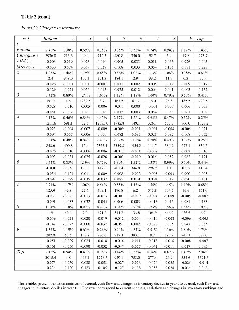
Panel C presents the same results as the first two panels for changes in inventory. The

results are similar to those for accruals. The extreme reversals are particularly striking for

changes in inventory. For example, the reversal rate from the top (bottom) decile in period t to

17

the bottom (top) decile in period t+1 is 2.16 percent (1.43 percent) for inventory changes versus

1.90 percent (1.70 percent) for accruals. We also observe the same pattern in earnings changes

and stock returns for the extreme inventory reversals, with the top (bottom) to bottom (top)

reversals exhibiting returns of -23.4 percent (22.8 percent) versus -22.4 percent (11.4 percent) for

accruals.

The evidence presented in table 2 is consistent with our second prediction that extreme

accruals exhibit a relatively high frequency of subsequent extreme reversals. The table also

demonstrates that the extreme accrual reversals are accompanied by corresponding changes in

net income and stock returns. Taken together, these results are also consistent with our third

prediction that reversals drive the predictable associations between extreme accruals and both

future changes in net income and future stock returns. We next turn to formal tests of these

predictions.

Tests of Large Sample Predictions

We test our first prediction that accruals mean-revert more rapidly than cash flows by

estimating annual cross-sectional auto-regressions for cash flows, total accruals, and inventory

changes. Table 3 reports the means and t-statistics from the 45 annual regressions coefficients

(1962-2006). Consistent with our first prediction, we find that accruals mean-revert more

rapidly than cash flows. The coefficient on cash flows is 0.551 while the coefficient on accruals

is over 90 percent smaller at 0.031. We also find that changes in inventory mean-revert more

rapidly than cash flows but less rapidly than total accruals at 0.110. The greater persistence of

inventory accruals relative to aggregate accruals likely arises because aggregate accruals net

asset and liability accruals. For example, a growing firm may have growing inventory and

growing accounts payable, but aggregate accruals net these effects and so may exhibit no

18

systematic growth. Overall, these results are consistent with our hypothesis that accruals contain

more estimation error than cash flows.

We next test our second prediction, that extreme accruals contain a disproportionately

high frequency of extreme reversals. Descriptive evidence consistent with this prediction was

already provided in table 2 and discussed earlier. Formal statistical tests are presented in table 4.

To conduct these tests, we construct a series of dummy variables that take the value of 1 for an

extreme reversal and zero otherwise. We define an extreme reversal as a move from the extreme

quintile of a variables’ distribution in year t, to the opposite extreme quintile in year t+1.5 We

examine 3 variables (ACCR, CF and !INV) and distinguish between highest-to-lowest quintile

reversals (HL) and lowest-to-highest quintile reversals (LH), thus constructing a total of 6

dummy variables (HLACCRt+1, LHACCRt+1, HLCFt+1, LHCFt+1, HL!INVt+1, LH!INVt+1). If

the variables are serially uncorrelated, we expect 4 percent of the observations to transition

between any combination of quintiles between period t and t+1. Table 3 previously illustrated

that all 3 variables are positively serially correlated ‘on average’. If the variables follow a simple

AR1 process with a positive coefficient, we would expect less than 4 percent of the observations

to fall into the extreme reversal quintiles and more than 4 percent to fall into the same quintiles

in consecutive years. But if the variables are characterized by extreme reversals, we expect the

observed percentages for the dummy variables to exceed 4 percent. We therefore report t-

statistics for the null hypothesis that the observed frequencies are 4 percent.

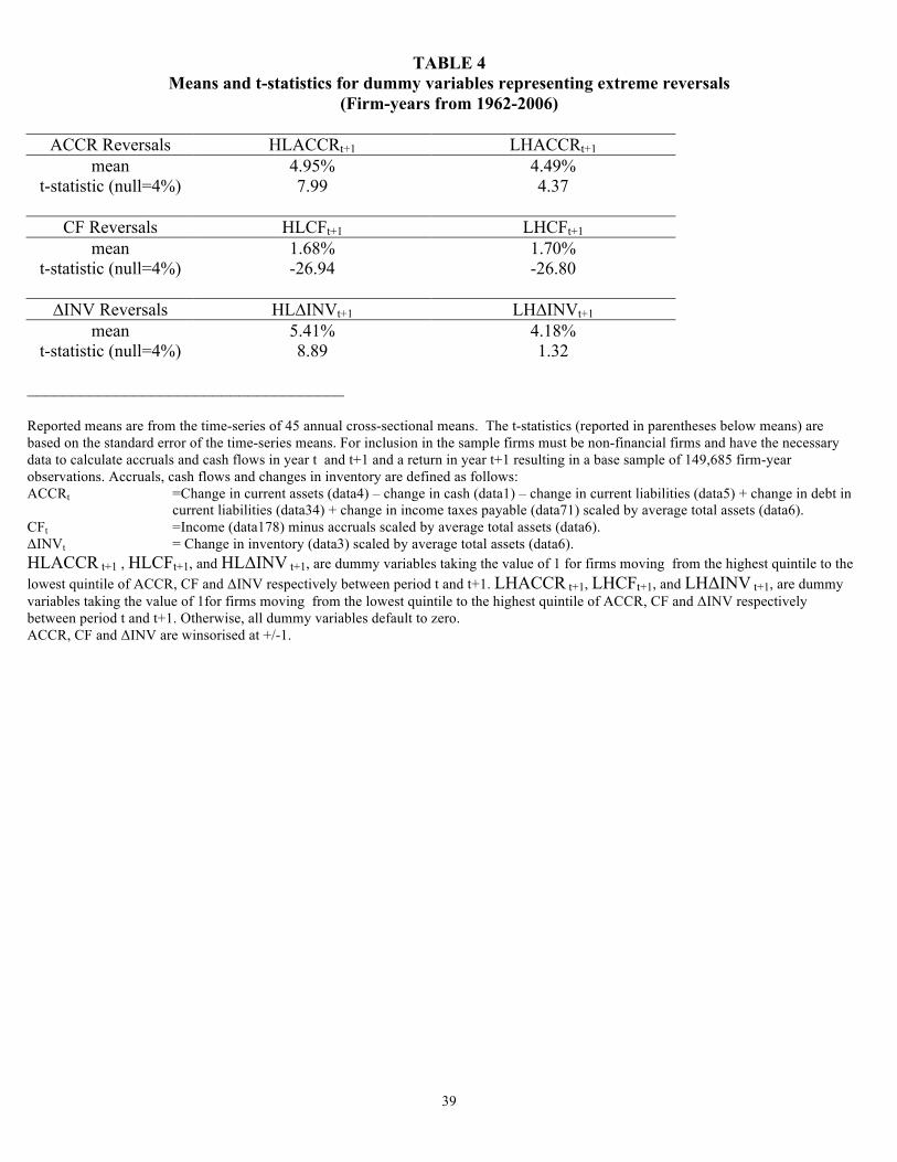
Table four reports the average percentage of firms each year experiencing extreme

reversals.6 The first set of results is for accruals and shows that extreme reversals from high to

5 We also tested this prediction using decile portfolios, with qualitatively similar results. 6 Notice that the reported means and t-statistics in table 4 are from the time-series of 45 annual cross-sectional means. Thus, the results in table 4 are not directly comparable to the descriptive results in table 2 because table 2 results are presented as a pooled sample.

19

low accrual quintiles occur 4.95 percent of the time (t=7.99) while extreme reversals from low to

high accruals occur 4.49 of the time (t=4.37). These results confirm our prediction of a

disproportionately high frequency of reversals for extreme accruals. They also indicate that

extreme reversals from high accruals to low accruals are more frequent than extreme reversals

from low accruals to high accruals. These results suggest that it is more common for positive

errors to be followed by subsequent accrual write-downs than for negative errors to be followed

by subsequent write-ups. It is often alleged that management are optimistically biased when

estimating accruals and the predominance of positive accrual estimation errors in our sample is

consistent with this allegation.

The next set of results is for cash flows. Here we see that extreme reversals from high to

low cash flow quintiles occur 1.68 percent of the time (t=-26.94) while extreme reversals from

low to high cash flows occur 1.70 percent of the time (t=-26.80). Unlike accruals, cash flows are

clearly characterized by a disproportionately low frequency of extreme accrual reversals. The

final set of results is for inventory accruals. The results here closely mirror those for accruals.

Extreme reversals from high to low !INV quintiles occur 5.41 percent of the time (t=8.89) while

extreme reversals from low to high !INV quintiles occur 4.18 percent of the time (t=1.32). We

again see the disproportionately high frequency of extreme accrual reversals and the

predominance of high-to-low reversals that is suggestive of an overall optimistic bias in accruals.

In short, the results in table 4 confirm that the lower persistence of accruals is driven, at least in

part, by a higher frequency of extreme accrual reversals.

Table 5 presents additional tests that help to quantify the impact of extreme accrual

reversals on the autoregressive properties of accruals. These regressions repeat the

autoregressions in table 3, but also include interactions with the extreme reversal dummies.

20

Since the extreme reversals dummies are constructed to capture extreme reversals, we expect the

coefficients on the interactions to be approximately -1 for all variables. To the extent that

extreme accruals play a significant role in causing the lower persistence of accruals we expect

that (i) the persistence of the main accrual effect will show a disproportionately high increase

after controlling for extreme reversals and (ii) the statistical significance of the coefficients on

the extreme reversals will be higher for accruals than for cash flows. The results are consistent

with both expectations. The autoregressive coefficient on accruals climbs from 0.031 to 0.374,

while the coefficient on cash flows only climbs from 0.551 to 0.661. The t-statistics are also

much stronger on the accrual-reversal interactions than on the cash flow reversal interactions.

The results for inventory accruals are qualitatively similar to those for aggregate accruals.

We next conduct tests of our third prediction that after controlling for accrual reversals,

accruals have no incremental explanatory power with respect to future earnings changes and

future stock returns. Table 6 presents mean regression coefficients from annual cross-sectional

regressions of both changes in future net income and future size-adjusted returns on accruals and

accrual reversals. We measure accrual reversals (ACCREVt+1) and inventory reversals

(INVREVt+1) as the difference between accruals and change in inventory in period t+1 and

period t respectively. We first estimate regressions using aggregate accruals, and we next

estimate regressions after decomposing aggregate accruals into inventory accruals (!INV) and

non-inventory accruals (ACCR-!INV).

Panel A of table 6 presents results for regressions of change in net income on accruals

and accrual reversals. In the first regression where the explanatory variable is accruals alone, we

find evidence consistent with prior literature. The coefficient on accruals is negative, -0.172, and

significant with a t-statistic of -22.58. When we also include accrual reversals in the regression,

21

the coefficient on accrual reversals is 0.199, and highly significant with a t-statistic of 12.18.

Moreover, consistent with P3, the coefficient on accruals switches signs and becomes positive,

0.023, and insignificant with a t-statistic of 1.38. After controlling for accrual reversals, accruals

are no longer negatively related to future changes in net income.

Panel B decomposes accruals into non-inventory accruals (ACCR-INV) and inventory

accruals (!INV). In the first regression, the coefficients are negative and significant on both

components of accruals, with the coefficient on inventory being the most negative. This latter

result is consistent with inventory accruals being most prone to extreme accrual reversals and

corresponding changes in net income. The second regression adds both non-inventory accrual

reversals and inventory accrual reversals to the previous regression. The results are similar to

second regression in panel A. The coefficients on both components of accrual reversals are

positive and highly significant, while the coefficients on accruals and changes in inventory are

no longer significantly negative. In summary, accrual reversals are responsible for the negative

relation between accruals and future changes in net income. After controlling for accrual

reversals, the negative relation between accruals and future changes in net income disappears.

Panels C and D replicate the results in panels A and B but use future size adjusted stock

returns (SRETt+1) as the dependent variable. Panel C presents results for regressions of SRET on

accruals and accrual reversals. In the first regression we confirm the prior finding of a

significant negative relation between accruals and future stock returns. When we include accrual

reversals in the regression, the coefficient on accrual reversals is 0.524, and highly significant

with a t-statistic of 11.46. Consistent with P3, the coefficient on accruals switches signs and

becomes positive, 0.291, and significant with a t-statistic of 3.87. After controlling for accrual

reversals, accruals are no longer negatively related to future changes in net income. In fact, the

22

sign flips and becomes positive. Panel D again decomposes accruals into non-inventory accruals

(ACCR-INV) and inventory accruals (!INV). In the first regression, both coefficients are

negative but only the coefficient on inventory is statistically significant. This confirms Thomas

and Zhang’s (2002) finding that inventory accruals have the strongest relation of all accrual

components with future stock returns. The second regression adds both non-inventory accrual

reversals and inventory accrual reversals to the previous regression. The coefficients on both

components of accrual reversals are again positive and highly significant, while the coefficients

on both inventory and non-inventory accruals flip from negative to positive. Again, the negative

relation between accruals and future stock returns disappears after controlling for accrual

reversals.

The positive coefficients on period t accruals in the regressions including the period t+1

accrual reversals have a natural interpretation. They suggest that investors at least partially

anticipate the predictable component of accrual reversals based on information available in

period t. Thus, the unpredictable component of accrual reversals implicit in period t+1 accruals

generates a stronger stock return response than the predictable component of accrual reversals

implicit in period t accruals. In other words, recall that ACCREVt+1=ACCt+1-ACCt, so the

coefficient on ACCREVt+1 measures the period t+1 unit stock return response to ACCt+1, while

the coefficient on ACCt tell us by how much lower the stock return response is to ACCt relative

to ACCt+1.

Finally, the findings in table 6 are informative for the debate over the explanation for the

negative relation between accruals and future stock returns. They corroborate the hypothesis that

accrual reversals, and their associated impact on earnings, are what drives the predictable future

stock returns. Under alternative hypotheses that accrual represent some type of risk associated

23

with firm growth or financial distress, then there is no reason to expect the subsequent accrual

reversals to explain the predictable future stock returns.

V. Inventory Write-down Sample Results

In this section, we conduct a detailed analysis of inventory accruals. We provide this

analysis to corroborate two aspects of our large sample analysis. First, Thomas and Zhang

(2002) provide evidence that inventory accruals are the single most important driver of the

returns from the “accrual anomaly”. Thus, to the extent that inventory accruals drive the accrual

anomaly, we expect a relatively high frequency of accrual reversals for inventory accruals.

Second, inventory write-downs provide a direct measure of the reversal of prior estimation error

in inventory accruals. By examining a sample of inventory write-downs, we can directly link

accrual reversals to the write-down of prior positive accrual estimation errors. Recall that our

analysis of inventory write-downs is based on a comprehensive sample of hand-collected

inventory write-downs during the 2001-2004 period. We first provide descriptive statistics on

our inventory write-down sample, and we then test predictions concerning the relation between

inventory accruals, inventory write-downs, earnings changes and stock returns.

Table 7 presents descriptive statistics for 1,886 firm-years experiencing inventory write-

downs from 2001 to 2004. Panel A provides descriptive statistics for average total assets, net

income divided by average total assets (INC), changes in inventory divided by average total

assets (!INV), inventory write-downs and inventory write-downs divided by average total assets

(WD). Note that inventory write-downs are recorded as negative amounts, consistent with their

impact on earnings. Write-down firm-years are characterized by negative mean and median

earnings and negative mean and median changes in inventory. The average write-down is left

24

skewed with a mean of -$10.44 million and a median of -$1.70 million. The write-downs

average -2.5 percent of total assets. Note that the 75th percentile of write down divided by total

assets is only -0.4 percent, indicating that there are a large number of fairly trivial write-downs in

our sample.

Panel B presents Pearson and Spearman pair-wise correlations between inventory write-

down, changes in past, current, and future inventory and changes in past, current and future

income. Write-downs are, not surprisingly, positively associated with contemporaneous changes

in inventory, as the write-downs directly cause a reduction in inventory. More interestingly, we

see that write-downs are negatively correlated with period t-1 changes in inventory. This is

consistent with write-downs representing the reversal of positive inventory accrual errors from

the prior period. We also see that inventory write-downs are positively associated with period

t+1 inventory changes, indicating that write-down firms continue to reduce inventory in the next

period. Period t inventory write-downs are positively correlated with period t change in net

income, and negatively correlated with period t+1 change in net income. The positive

contemporaneous relation demonstrates that the write-downs cause corresponding reductions in

net income. Note that the contemporaneous impact on net income is exactly what we predict for

accruals that correct prior estimation errors. Similarly, the period t+1 negative correlation arises

as period t+1 net income bounces back from its temporarily depressed level in the write-down

year.

Figure 1 provides a graphical analysis of the time-series behavior of changes in

inventory, net income, gross margin and size-adjusted returns for firms experiencing inventory

write-downs in year 0. Because our sample has a high proportion of fairly trivial write-downs,

we divide the write-down firm-years into quartiles based on the magnitude of the inventory

25

write-down scaled by average total assets. Panel A, shows that inventory write-downs follow

periods of increases in inventory that are subsequently reversed. Panel B, shows that inventory

write-down firms experience reductions in net income during the write-down year. This result

confirms that the accrual reversals represented by inventory write-downs cause sharp reductions

in the level of net income. Panel C reports the time-series behavior of gross margin surrounding

the inventory write-down. There is a sharp reduction in gross margin during the period of the

inventory write-down. The decrease in gross margin is the result of accounting for inventory

write-downs. Unlike many other asset write-downs, which are often classified as ‘special

charges’, inventory write-downs are required to be included in cost of goods sold. Thus, the

impact of write-downs on net income is driven primarily through increases in cost of goods sold

and corresponding reductions in gross margin.7 Panel D plots the mean size-adjusted returns

surrounding the inventory write-down. Write-down firms have strong positive returns in year -2

relative to the write-down year, indicating that they are ‘past winner’ firms. They then

underperform in years -1 and 0. These results indicate that the negative impact of write-downs

on net income is also reflected contemporaneously in stock returns.

Next we formally investigate the prediction that inventory write-downs in period t are

preceded by positive changes in inventory in prior periods. Table 8 reports a transition matrix

for all available COMPUSTAT firm-years in 2001-2004 using decile ranks of changes in

inventory in years t-1 and year t respectively. The first row in each cell lists the percentage of all

observations falling into that cell. If changes in inventory are serially uncorrelated, then we

would expect 1 percent of observations to fall into each cell. Consistent with the evidence in

panel C of table 2, we see that the extreme corner cells have the highest percentage of

7 Note that we obtain this result despite the fact that, as noted earlier, Compustat sometimes reclassifies inventory write-downs from cost of goods sold to special items.

26

observations. For example, 2.61 percent of the observations switch from the top decile in period

t-1 to the bottom decile in period t. This is consistent with the reversal of extreme inventory

accruals that we observed in panel C of table 2.

The second row in each cell reports the percentage of total period t inventory write-down

firms that fall into each cell. These amounts are also expected to be 1 percent if inventory write-

downs are unrelated to inventory changes in the current or prior periods. We clearly expect a

negative relation between inventory write-downs in period t and inventory changes in period t,

because write-downs directly cause a reduction in inventory. This should translate to a greater

percentage of write-downs in the first column of table 8. A more interesting prediction concerns

how write-downs in period t are related to inventory changes in period t-1. If write-downs

reflect the reversal of past extreme positive inventory accruals, we expect a concentration of

write-downs in the bottom rows of table 8. This is exactly what we see, with 7.19 percent of the

write-down’s concentrated in the bottom left cell (‘Top’ inventory change decile for period t-1,

‘Bottom’ inventory change decile for period t). If we examine the four cells in the bottom left

hand corner of table 8, we see that while these 4 cells represent just 4 percent of all cells, they

contain over 16 percent of the period t inventory write-downs.

The third row in each cell reports the average period t write-down as a percentage of total

assets. Here we see that the largest write-downs occur in the bottom left cell, confirming our

prediction that the largest write-downs are primarily driven by the reversal of extreme positive

accruals from period t-1. The results in Table 8 are consistent with the reversal of accrual

estimation error driving the poor earnings performance following periods of high accruals. In

particular, we see that inventory write-downs follow periods of extreme positive inventory

27

accruals. This is consistent with inventory write-downs reversing the effect of previous positive

estimation error in inventory accruals.

In order to formally test whether prior positive inventory accruals can explain period t

inventory write-downs, we estimate pooled cross-sectional regressions of period t inventory

write-downs on period t-1 and period t-2 changes in inventory. We also include period t-1

accruals and cash flows as controls. The regression results are presented in table 9 and they

confirm that period t inventory write-downs are strongly negatively related to both period t-1 and

period t-2 changes in inventory. For example, the coefficient on the change in inventory for

period t-1 is -0.020 (t-statistic=-7.81) and the coefficient on inventory in period t-2 is -0.016 (t-

statistic=-7.71). The coefficients on accruals and cash flows are both positive, suggesting that

firms with better underlying earnings performance (exclusive of inventory accruals) are less

likely to report write-downs.

In summary, our detailed analysis of inventory accruals corroborates the interpretation of

our large sample results. Extremely high inventory accruals result in disproportionately high

frequency of future inventory write-downs. This indicates that high inventory accruals contain a

disproportionately high concentration of positive accrual estimation errors that are reversed

through subsequent inventory write-downs.

6. Conclusions

We show that extreme accruals are associated with a disproportionately high frequency of

subsequent extreme accrual reversals. We posit that these reversals are the result of estimation

error in the extreme accruals. We also show that stock prices act as if investors do not anticipate

these predictable accrual reversals. Our results corroborate Sloan’s (1996) explanation for the

28

“accrual anomaly”. Accruals are based on accountants’ subjective estimates of future cash

flows, and so contain measurement error. Extreme accruals are more likely to be attributable to

measurement error, and hence are more likely to be associated with subsequent accrual reversals.

Investors do not appear to understand that extreme accruals are more likely to reverse, and so

react to the accrual reversals and associated earnings changes following extreme accruals as

though they are unexpected.

Our analysis of inventory accruals directly ties extreme accrual reversals to estimation

errors in the form of inventory write-downs. Future research can study other categories of

accruals and their related estimation errors. For example, overestimation in PP&E accruals is

likely to reverse through PP&E write-downs. Thus, firms with high PP&E accruals can be

expected to have a higher frequency of subsequent PP&E write-downs.

Our findings also have implications for practicing accountants and auditors. The fact that

extreme accruals are associated with predictable reversals is indicative of ‘bad’ accrual

accounting. Under ‘good’ accrual accounting, accruals would reflect unbiased estimates of the

future cash flows that they represent. The fact that extreme accruals are associated with

systematic reversals indicates that accountants and auditors are unsuccessful at identifying the

systematic errors in extreme accruals. It appears that accountants and auditors could scrutinize

extreme accruals more carefully.

We also note that extreme accrual estimation errors do not necessarily arise from the

deliberate manipulation of accruals. In the case of inventory accruals, it appears more likely that

accountants are slow to write-down inventories in response to slowing sales, rising inventory and

declining margins. Nevertheless, it appears that this sluggishness on the part of accountants

leads to temporarily inflated income and stock returns and hence inefficient allocation of

29

resources. Perhaps this inaction on the part of accountants reflects the natural reluctance on the

part of managers to publicly recognize write-downs until the evidence is overwhelming.

30

References Chan, K., L.K.C. Chan, N. Jegadeesh, J. Lakonishok. 2006. “Earnings Quality and Stock

Returns” The Journal of Business 79, no. 3. Dechow, P.M. 1994. “Accounting Earnings and Cash Flows as Measures of Firm Performance

the Role of Accounting Accruals” Journal of Accounting and Economics 18, 3-42. Dechow, P.M. and I.D. Dichev. 2002. “The Quality of Accruals and Earnings: The Role of

Accrual Estimation Errors” The Accounting Review 77, 35-59. Fairfield, P.M., S. Whisenant, T.L. Yohn. 2003. “The Differential Persistence of Accruals and

Cash Flows for Future Operating Income versus Future Profitability” Review of Accounting Studies 8, no. 2-3.

Healy, P.M. 1985. “The Effect of Bonus Schemes on Accounting Decisions” Journal of

Accounting and Economics 7, 85-107. Kahn, M., 2007. “Are Accruals Mispriced? Evidence from Tests of an Intertemporal Capital

Asset Pricing Model” Journal of Accounting and Economics 45, no. 1. Kothari, S., J. Shanken, R.G. Sloan. 1995. “Another Look at the Cross-Section of Expected

Returns” Journal of Finance 50, no. 1, 185-224. Ng, J. 2005. “Distress Risk Information in Accruals” Working Paper, University of

Pennsylvania. Nissim, D. and S. Penman, 2001. “Ratio Analysis and Equity Valuation: From Theory to

Practice” Review of Accounting Studies 6, 109-154. Richardson, S.A., R.G. Sloan, M.T. Soliman and I. Tuna. 2005. “Accrual Reliability, Earnings

Persistence and Stock Prices” Journal of Accounting and Economics 39, 437-485. Shumway, T. 1997. “The Delisting Bias in CRSP Data” Journal of Finance 52, no. 1, 327-340. Shumway. T., V.A. Warther. 1999. “The Delisitng Bias in CRSP’s Nasdaq Data and Its

Implications for the Size Effect” Journal of Finance 54, no. 6, 2361-2379. Sloan, R.G., 1996. “Do Stock Prices Fully Reflect Information in Accruals and Cash Flows

about Future Earnings?” The Accounting Review 71, no. 3, 289-315. Thomas, J.K., H. Zhang. 2002. “Inventory Changes and Future Returns” Review of Accounting

Studies 7, no. 2-3. Zach, T. 2007, “Evaluating the ‘Accrual-Fixation’ Hypothesis as an Explanation for the Accrual

Anomaly” Working Paper, Ohio State University.

31

FIGURE 1 Time-series plots of changes in inventory, income, gross margin and buy-and-hold size-adjusted returns for

firm-years experiencing inventory write-downs (N= 1,886 Firm-years from 2001-2004)

Panel A: Changes in Inventory

Panel B: Income

32

Panel C: Gross margin percentage

Panel D: Mean buy-and-hold size-adjusted returns

______________________________________ This sample consists of 1,886 firms experiencing inventory write-downs in calendar years 2001 through 2004. Firms are sorted into quartiles based on the size of the inventory write-down at time t=0. Change in inventory is measured as inventory (data3) scaled by average total assets (data6). Net income is measured as net income (data178) scaled by average total assets (data6). Gross margin percentage is measured as change in sales (data12) minus cost of goods sold (data41) divided by sales. Buy-and-hold size-adjusted returns are measured as the annual size adjusted stock return. It is measured using compounded buy-hold returns, inclusive of dividends and other distributions. The size adjustment is made by deducting the corresponding average return for all available non-financial firms in the same size-matched decile, where size is measured using market capitalization at the end of the previous year. Returns are calculated for a twelve-month period beginning four months after the end of the fiscal year. For firms that delist during our return window, we calculate the remaining return by first using the de-listing return from CRSP and then reinvesting any remaining proceeds in the firm’s size matched decile. Net income, change in inventory and gross margin percentage are winsorised at +/-1.

33

TABLE 1 Sample descriptive statistics and pair-wise correlations between accruals, cash flows, inventory changes,

future changes in income and buy-and-hold size-adjusted returns (Firm-years from 1962-2006)

Panel A: Univariate statistics

Panel B: Pair-wise correlations - Pearson (above diagonal) and Spearman (below diagonal)

______________________________________ For inclusion in the sample firms must be non-financial firms and have the necessary data to compute accruals and cash flows in year t and t+1 and a return in year t+1 resulting in a base sample of 149,685 firm-year observations. All correlations are significant at less than the .001 percent level. Accruals, cash flows and changes in inventory and income are defined as follows: ACCRt =Change in current assets (data4) – change in cash (data1) – change in current liabilities (data5) + change in debt in

current liabilities (data34) + change in income taxes payable (data71) scaled by average total assets (data6). CFt =Income (data178) minus accruals scaled by average total assets (data6). !INVt = Change in inventory (data3) scaled by average total assets (data6). !INCt = Change in net income (data178) scaled by average total assets (data6). ACCR, CF, !INV and !INC are winsorised at +/-1. SRET is the annual size adjusted stock return. It is measured using compounded buy-hold returns, inclusive of dividends and other distributions. The size adjustment is made by deducting the corresponding average return for all available non-financial firms in the same size-matched decile, where size is measured using the end of year market capitalization. Returns are calculated for a twelve-month period beginning four months after the end of the fiscal year. For firms that delist during our future return window, we calculate the remaining return by first using the de-listing return from CRSP and then reinvesting any remaining proceeds in the firm’s size matched decile.

Mean Std. Dev 25% Median 75% ACCRt 0.022 0.113 -0.020 0.013 0.060

CFt 0.027 0.207 -0.018 0.066 0.129

"INVt 0.019 0.074 -0.003 0.004 0.036

"INCt+1 -0.008 0.132 -0.038 -0.002 0.027

SRETt+1 0.006 0.799 -0.348 -0.080 0.202

ACCRt CFt "INVt "INCt+1 SRETt+1

ACCRt - -0.304 0.623 -0.153 -0.033

CFt -0.316 - -0.174 -0.161 0.037 "INVt 0.582 -0.120 - -0.101 -0.043

"INCt+1 -0.170 -0.111 -0.150 - 0.196

SRETt+1 -0.042 0.156 -0.041 0.339 -

34

TABLE 2 Distribution and returns of firm-years across accrual, cash flow and changes in inventory deciles for periods

t and t+1 (Firm years from 1962-2006)

Panel A: Total Accruals

Bottom 2 3 4 5 6 7 8 9 Top t+1

t Bottom 1.97% 1.15% 0.76% 0.62% 0.55% 0.58% 0.72% 0.85% 1.08% 1.70% Chi-square 1423.0 35.5 87.7 212.6 306.1 259.9 114.8 34.4 10.8 741.5 !INCt+1 -0.025 0.013 0.023 0.041 0.021 0.033 0.031 0.041 0.046 0.098 Sizerett+1 -0.079 0.016 0.048 0.065 0.091 0.115 0.074 0.050 0.112 0.114 2 1.06% 1.21% 1.06% 0.99% 0.87% 0.98% 1.00% 1.01% 1.00% 0.82% 5.2 63.6 4.7 0.1 25.4 0.8 0.0 0.1 0.0 45.7 -0.045 -0.003 0.001 0.006 0.005 0.009 0.009 0.013 0.017 0.033 -0.048 0.024 0.050 0.070 0.061 0.023 0.023 0.042 0.068 0.163 3 0.67% 1.07% 1.24% 1.28% 1.23% 1.14% 1.09% 0.94% 0.78% 0.57% 166.6 6.6 88.3 116.1 82.1 29.3 11.2 5.4 73.7 280.7 -0.050 -0.009 -0.002 -0.002 -0.001 0.003 0.001 0.007 0.011 0.030 -0.061 0.004 0.011 0.043 0.025 0.009 0.020 0.043 0.037 0.157 4 0.56% 0.86% 1.25% 1.46% 1.56% 1.32% 1.06% 0.84% 0.67% 0.43% 293.0 31.6 90.9 311.0 475.8 154.3 5.9 40.2 166.2 479.3 -0.063 -0.015 -0.008 -0.004 -0.003 0.000 0.001 -0.001 0.007 0.013 -0.077 0.022 -0.016 0.003 0.017 0.029 0.041 -0.003 0.032 0.127 5 0.50% 0.79% 1.13% 1.48% 1.61% 1.34% 1.08% 0.93% 0.67% 0.47% 379.7 65.0 24.0 347.2 551.5 176.0 10.5 7.1 161.3 426.1 -0.054 -0.016 -0.015 -0.006 -0.003 -0.002 -0.001 0.003 -0.002 0.016 -0.069 -0.017 -0.018 -0.003 -0.004 0.014 0.025 0.033 0.045 0.135 6 0.57% 0.90% 1.12% 1.25% 1.28% 1.32% 1.23% 1.00% 0.82% 0.52% 275.1 15.8 19.8 96.3 117.4 150.7 77.3 0.0 48.1 342.9 -0.071 -0.023 -0.011 -0.005 -0.006 -0.002 -0.002 0.002 0.002 0.016 -0.030 -0.038 -0.005 0.013 0.009 -0.008 0.029 0.058 0.082 0.140 7 0.69% 0.98% 1.09% 1.02% 1.06% 1.18% 1.17% 1.17% 0.96% 0.68% 146.0 1.0 12.1 0.5 5.6 47.7 44.6 42.4 2.1 148.4 -0.070 -0.023 -0.011 -0.009 -0.007 -0.007 -0.004 -0.002 0.002 0.008 -0.133 -0.044 -0.019 0.009 -0.001 0.031 0.000 0.010 0.056 0.098 8 0.88% 1.06% 0.97% 0.83% 0.85% 0.92% 1.07% 1.26% 1.21% 0.96% 20.9 4.7 1.7 44.6 33.8 10.4 7.8 99.8 66.7 2.3 -0.073 -0.031 -0.019 -0.015 -0.012 -0.011 -0.005 -0.008 -0.002 0.016 -0.159 -0.054 -0.031 0.015 -0.022 -0.006 0.015 -0.006 0.067 0.121 9 1.21% 1.04% 0.79% 0.62% 0.59% 0.72% 0.94% 1.16% 1.49% 1.45% 63.8 1.9 66.8 212.3 257.9 114.1 5.8 40.1 350.5 306.3 -0.086 -0.040 -0.022 -0.024 -0.015 -0.023 -0.010 -0.014 -0.004 0.002 -0.176 -0.103 -0.076 -0.025 -0.053 -0.054 -0.013 -0.046 0.041 0.111 Top 1.90% 0.96% 0.61% 0.44% 0.40% 0.50% 0.63% 0.85% 1.32% 2.38% 1212.1 1.9 228.0 461.3 537.1 376.2 204.5 32.8 149.5 2872.0 -0.113 -0.066 -0.050 -0.030 -0.035 -0.033 -0.028 -0.017 -0.026 -0.007 -0.224 -0.136 -0.098 -0.079 -0.098 -0.062 -0.070 -0.058 -0.028 0.087

35

Table 2 (cont.) Panel B: Cash Flows

Bottom 2 3 4 5 6 7 8 9 Top t+1

t Bottom 5.35% 1.65% 0.71% 0.45% 0.33% 0.27% 0.26% 0.25% 0.26% 0.45% Chi-square 28520.0 636.5 125.5 458.4 676.3 800.9 809.6 841.7 812.5 443.7 !INCt+1 -0.017 0.103 0.094 0.079 0.080 0.072 0.054 0.098 0.081 0.128 Sizerett+1 -0.126 -0.007 -0.031 0.053 -0.026 0.086 -0.008 0.059 0.057 0.036 2 1.71% 2.72% 1.66% 0.99% 0.68% 0.53% 0.43% 0.40% 0.38% 0.49% 757.9 4403.0 659.8 0.1 148.8 330.9 481.1 540.2 577.2 387.8 -0.117 -0.006 0.021 0.033 0.029 0.032 0.039 0.040 0.053 0.056 -0.137 -0.079 -0.054 -0.010 -0.003 0.054 0.139 0.086 0.244 0.226 3 0.72% 1.66% 2.02% 1.54% 1.09% 0.80% 0.63% 0.56% 0.52% 0.46% 116.4 651.9 1549.4 441.3 11.7 57.9 202.2 287.2 351.1 443.0 -0.141 -0.043 -0.009 0.008 0.009 0.018 0.019 0.022 0.029 0.057 -0.195 -0.076 -0.074 -0.017 0.011 0.015 0.045 0.057 0.137 0.283 4 0.47% 0.97% 1.57% 1.80% 1.50% 1.14% 0.86% 0.71% 0.56% 0.43% 415.2 1.0 477.9 955.9 372.7 28.8 30.6 129.0 289.9 493.0 -0.134 -0.056 -0.026 -0.004 0.005 0.012 0.015 0.014 0.031 0.042 -0.195 -0.163 -0.090 -0.042 0.009 0.058 0.078 0.139 0.167 0.301 5 0.33% 0.73% 1.13% 1.54% 1.77% 1.50% 1.12% 0.83% 0.66% 0.39% 677.6 106.3 25.5 432.8 896.7 367.0 20.6 42.4 172.0 555.3 -0.112 -0.060 -0.031 -0.013 -0.005 0.005 0.010 0.015 0.016 0.038 -0.213 -0.130 -0.105 -0.057 -0.018 0.038 0.083 0.124 0.120 0.198 6 0.27% 0.52% 0.81% 1.13% 1.50% 1.84% 1.56% 1.18% 0.76% 0.44% 786.3 351.9 55.6 23.3 375.9 1046.3 473.5 46.5 88.2 464.0 -0.121 -0.063 -0.036 -0.020 -0.011 -0.003 0.003 0.010 0.021 0.040 -0.167 -0.129 -0.068 -0.091 -0.040 0.005 0.055 0.087 0.206 0.280 7 0.25% 0.45% 0.67% 0.86% 1.13% 1.58% 1.98% 1.53% 1.05% 0.52% 851.3 452.1 164.5 28.9 23.7 493.9 1427.2 423.0 3.0 345.7 -0.100 -0.063 -0.040 -0.030 -0.016 -0.008 -0.002 0.004 0.015 0.038 -0.113 -0.105 -0.114 -0.051 -0.054 -0.003 0.023 0.078 0.162 0.321 8 0.23% 0.43% 0.56% 0.71% 0.91% 1.11% 1.57% 2.06% 1.64% 0.79% 884.3 490.9 292.5 122.0 13.5 16.4 481.3 1679.2 619.3 67.0 -0.105 -0.067 -0.050 -0.031 -0.022 -0.018 -0.009 -0.001 0.008 0.029 -0.164 -0.098 -0.102 -0.045 -0.030 -0.018 0.013 0.067 0.111 0.227 9 0.24% 0.41% 0.48% 0.56% 0.66% 0.80% 1.05% 1.66% 2.52% 1.61% 855.8 520.4 412.7 288.1 169.3 58.3 3.7 653.2 3462.3 559.6 -0.150 -0.081 -0.062 -0.039 -0.034 -0.025 -0.017 -0.011 -0.001 0.020 -0.175 -0.118 -0.104 -0.070 -0.035 -0.042 0.014 0.032 0.088 0.199 Top 0.41% 0.46% 0.40% 0.42% 0.43% 0.44% 0.54% 0.82% 1.65% 4.41% 522.1 432.8 533.1 506.8 488.0 460.7 318.4 47.5 640.6 17503.0 -0.153 -0.098 -0.094 -0.067 -0.067 -0.052 -0.054 -0.042 -0.030 -0.005 -0.119 -0.114 -0.103 -0.028 -0.060 0.004 -0.030 0.001 0.045 0.158

36

Table 2 (cont.)

Panel C: Changes in Inventory

Bottom 2 3 4 5 6 7 8 9 Top t+1 t Bottom 2.40% 1.38% 0.69% 0.38% 0.35% 0.56% 0.74% 0.94% 1.12% 1.43% Chi-square 2936.8 213.6 99.9 712.5 480.8 350.0 92.7 5.4 19.6 275.7 !INCt+1 -0.006 0.019 0.026 0.010 0.005 0.033 0.018 0.033 0.026 0.043 Sizerett+1 -0.030 0.074 0.069 0.027 0.108 0.033 0.054 0.136 0.181 0.228 2 1.03% 1.48% 1.19% 0.68% 0.56% 1.02% 1.13% 1.08% 0.98% 0.81% 2.4 348.0 102.1 251.3 184.1 2.9 33.2 11.7 0.3 52.9 -0.026 -0.001 0.001 -0.001 0.011 0.002 0.005 0.012 0.009 0.017 -0.129 -0.021 0.056 0.013 0.075 0.012 0.064 0.041 0.103 0.132 3 0.42% 0.89% 1.71% 1.07% 1.12% 1.18% 1.00% 0.79% 0.58% 0.41% 391.7 1.5 1239.5 3.9 163.5 61.3 15.0 26.3 185.5 420.5 -0.028 -0.010 -0.005 -0.006 -0.011 0.000 -0.001 0.000 0.006 0.005 -0.051 -0.036 0.026 0.016 0.012 0.003 0.054 0.056 0.061 0.102 4 0.17% 0.46% 0.84% 4.47% 2.17% 1.56% 0.62% 0.47% 0.32% 0.25% 1211.6 591.1 72.5 12085.0 1982.8 149.1 326.1 577.7 866.0 1028.2 -0.023 -0.004 -0.007 -0.009 -0.009 -0.001 -0.001 -0.008 -0.005 0.021 -0.094 0.057 -0.006 0.009 0.082 -0.035 0.028 0.032 0.108 0.072 5 0.24% 0.48% 0.84% 2.43% 2.07% 2.08% 0.70% 0.49% 0.37% 0.25% 848.0 400.8 15.4 2327.4 2359.8 1454.2 115.7 386.9 577.1 836.5 -0.026 -0.010 -0.006 -0.006 -0.013 -0.001 -0.008 0.003 0.002 0.016 -0.093 -0.031 -0.025 -0.026 -0.003 -0.019 0.015 0.052 0.082 0.171 6 0.44% 0.83% 1.19% 0.75% 1.39% 1.52% 1.38% 0.99% 0.70% 0.44% 418.0 27.6 129.6 147.8 487.4 346.8 296.9 1.1 105.7 418.4 -0.036 -0.124 -0.011 -0.009 0.008 -0.002 -0.003 -0.003 0.000 0.003 -0.092 -0.029 -0.035 -0.037 0.085 0.019 0.030 0.019 0.080 0.131 7 0.71% 1.17% 1.06% 0.56% 0.55% 1.13% 1.56% 1.45% 1.10% 0.68% 125.0 46.9 22.6 409.1 196.8 6.2 515.8 304.7 16.6 151.0 -0.033 -0.022 -0.013 -0.013 -0.007 -0.009 -0.004 -0.009 -0.005 -0.002 -0.091 -0.033 -0.032 -0.045 0.006 0.003 -0.015 0.016 0.081 0.133 8 1.04% 1.18% 0.87% 0.41% 0.34% 0.76% 1.25% 1.56% 1.54% 1.07% 1.9 49.1 9.0 671.8 514.2 133.8 104.9 466.9 435.5 6.9 -0.039 -0.021 -0.020 -0.019 -0.012 -0.004 -0.010 -0.008 -0.006 -0.005 -0.142 -0.075 -0.006 -0.037 -0.051 0.002 -0.022 0.005 0.047 0.085 9 1.37% 1.19% 0.63% 0.26% 0.24% 0.54% 0.91% 1.36% 1.80% 1.73% 202.8 53.5 158.8 986.6 717.3 393.1 9.2 193.9 945.3 783.0 -0.051 -0.029 -0.024 -0.018 -0.016 -0.011 -0.013 -0.016 -0.008 -0.007 -0.161 -0.056 -0.090 -0.032 -0.047 -0.067 -0.042 -0.011 0.017 0.085 Top 2.16% 0.94% 0.41% 0.16% 0.14% 0.33% 0.56% 0.87% 1.49% 2.94% 2015.4 4.8 446.1 1228.7 949.1 753.0 277.4 24.9 354.6 5621.6 -0.073 -0.039 -0.038 -0.053 -0.027 -0.026 -0.020 -0.025 -0.025 -0.014 -0.234 -0.120 -0.123 -0.105 -0.127 -0.108 -0.055 -0.028 -0.034 0.048

______________________________________ These tables present transition matrices of accrual, cash flow and changes in inventory deciles in year t to accrual, cash flow and changes in inventory deciles in year t+1. The rows correspond to current accruals, cash flow and changes in inventory rankings and

37

the columns correspond to future accrual, cash flow and changes in inventory rankings. Accruals and changes in inventory are ranked on an annual basis. Marginal chi-square statistics are reported below the percentages. These are based on the probability that the given cells distribution is equal to what would be expected by chance if periods t and t+1 decile assignment were independent. The third row below the chi-square statistic is the mean period t+1 change in income (data178) scaled by average total assets (data6). The fourth row is the mean period t+1 size-adjusted buy-and-hold return, SRET. SRET is measured using compounded buy-and-hold returns, inclusive of dividends and other distributions. The size adjustment is made by deducting the corresponding average return for all available non-financial firms in the same size-matched decile, where size is measured using market capitalization at the end of the previous year. Returns are calculated for a twelve-month period beginning four months after the end of the fiscal year. For firms that delist during our future return window, we calculate the remaining return by first using the de-listing return from CRSP and then reinvesting any remaining proceeds in the firm’s size matched decile. Accruals, cash flows and changes in inventory are scaled by average total assets.

38

TABLE 3 Means and t-statistics for coefficients from annual cross-sectional auto-regressions for cash flows, accruals

and change in inventory (Firm-years from 1962-2006)

Dependent Variables

Independent Variables

Intercept CFt ACCR t !INVt Adj. R2 CFt+1 0.025 0.551

(6.09) (22.93) 0.336

ACCRt+1 0.016 0.031 (6.32) (2.65) 0.007

!INVt+1 0.014 0.110 (7.77) (9.58) 0.017

____________________________________ Reported regression coefficients are mean coefficients from 45 annual regressions. The t-statistics (reported in parentheses below coefficient estimates) are based on the standard error of the coefficient estimates across the annual regressions. For inclusion in the sample firms must be non-financial firms and have the necessary data to calculate accruals and cash flows in year t and t+1 and a return in year t+1 resulting in a base sample of 149,685 firm-year observations. Accruals, cash flows and changes in inventory are defined as follows: ACCRt =Change in current assets (data4) – change in cash (data1) – change in current liabilities (data5) + change in debt in

current liabilities (data34) + change in income taxes payable (data71) scaled by average total assets (data6). CFt =Income (data178) minus accruals scaled by average total assets (data6). !INVt = Change in inventory (data3) scaled by average total assets (data6). ACCR, CF and !INV are winsorised at +/-1.

39

TABLE 4 Means and t-statistics for dummy variables representing extreme reversals

(Firm-years from 1962-2006)

____________________________________ Reported means are from the time-series of 45 annual cross-sectional means. The t-statistics (reported in parentheses below means) are based on the standard error of the time-series means. For inclusion in the sample firms must be non-financial firms and have the necessary data to calculate accruals and cash flows in year t and t+1 and a return in year t+1 resulting in a base sample of 149,685 firm-year observations. Accruals, cash flows and changes in inventory are defined as follows: ACCRt =Change in current assets (data4) – change in cash (data1) – change in current liabilities (data5) + change in debt in

current liabilities (data34) + change in income taxes payable (data71) scaled by average total assets (data6). CFt =Income (data178) minus accruals scaled by average total assets (data6). !INVt = Change in inventory (data3) scaled by average total assets (data6). HLACCR t+1 , HLCFt+1, and HL!INV t+1, are dummy variables taking the value of 1 for firms moving from the highest quintile to the lowest quintile of ACCR, CF and !INV respectively between period t and t+1. LHACCR t+1, LHCFt+1, and LH!INV t+1, are dummy variables taking the value of 1for firms moving from the lowest quintile to the highest quintile of ACCR, CF and !INV respectively between period t and t+1. Otherwise, all dummy variables default to zero. ACCR, CF and !INV are winsorised at +/-1.

ACCR Reversals HLACCRt+1 LHACCRt+1 mean 4.95% 4.49%

t-statistic (null=4%) 7.99 4.37

CF Reversals HLCFt+1 LHCFt+1 mean 1.68% 1.70%

t-statistic (null=4%) -26.94 -26.80

"INV Reversals HL"INVt+1 LH"INVt+1 mean 5.41% 4.18%

t-statistic (null=4%) 8.89 1.32

40

TABLE 5 Means and t-statistics for coefficients from annual cross-sectional auto-regressions including interactions

with dummy variables for extreme accrual reversals (Firm-years from 1962-2006)

Panel A: Accrual Regressions

Dependent Variables

Independent Variables

Intercept ACCRt ACCR*HLACCRt+1 ACCR*LHACCRt+1 Adj. R2 ACCRt+1 0.016 0.031

(6.32) (2.65) 0.007 ACCRt+1 0.011 0.374 -1.016 -1.251

(4.77) (42.42) (-48.83) (-38.97) 0.264 Panel B: Cash Flow Regressions

Dependent Variables

Independent Variables

Intercept CFt CF*HLCFt+1 CF*LHCFt+1 Adj. R2 CFt+1 0.025 0.551

(6.09) (22.93) 0.336 CFt+1 0.200 0.661 -1.314 -1.221

(5.91) (36.43) (-28.41) (-3.99) 0.478 Panel C: Change in Inventory Regressions

Dependent Variables

Independent Variables

Intercept !INVt !INV*HL!INVt+1 !INV*LH!INVt+1 Adj. R2 !INVt+1 0.014 0.110

(7.77) (9.58) 0.017 !INVt+1 0.011 0.431 -0.993 -1.292

(6.96) (38.45) (-61.12) (-32.99) 0.266 ____________________________________ Reported regression coefficients are mean coefficients from 45 annual regressions. The t-statistics (reported in parentheses below coefficient estimates) are based on the standard error of the coefficient estimates across the annual regressions. For inclusion in the sample firms must be non-financial firms and have the necessary data to calculate accruals and cash flows in year t and t+1 and a return in year t+1 resulting in a base sample of 149,685 firm-year observations. Accruals, cash flows and changes in inventory are defined as follows: ACCRt =Change in current assets (data4) – change in cash (data1) – change in current liabilities (data5) + change in debt in

current liabilities (data34) + change in income taxes payable (data71) scaled by average total assets (data6). CFt =Income (data178) minus accruals scaled by average total assets (data6). !INVt = Change in inventory (data3) scaled by average total assets (data6). HLACCR t+1 , HLCFt+1, and HL!INV t+1, are dummy variables taking the value of 1 for firms moving from the highest quintile to the lowest quintile of ACCR, CF and !INV respectively between period t and t+1. LHACCR t+1, LHCFt+1, and LH!INV t+1, are dummy variables taking the value of 1for firms moving from the lowest quintile to the highest quintile of ACCR, CF and !INV respectively between period t and t+1. Otherwise, all dummy variables default to zero. ACCR, CF and !INV are winsorised at +/-1.

41

TABLE 6 Means and t-statistics for coefficients from annual cross-sectional regressions of net income and size-

adjusted returns on accruals and accrual reversals. Regressions are estimated for both aggregate accruals and for accruals decomposed into inventory accruals (!INV) and non-inventory accruals (ACCR-INV).

(Firm-years from 1962-2006)

Panel A: Regressions of Change in Net Income on Accruals and Accrual Reversals Dependent Variables

Intercept ACCRt ACCREVt+1 Adj. R2 !INCt+1 -0.003 -0.172

(-1.81) (-22.58) 0.011

!INCt+1 -0.005 0.023 0.199 (-3.28) (1.38) (12.18) 0.035

Panel B: Regressions of Change in Net Income on Decomposed Accruals and Accrual Reversals

Dependent Variables

Independent Variables

Intercept ACCRt-INVt

ACCREV t+1 - INVREVt+1

"INVt INVREVt+1 Adj. R2

!INCt+1 -0.002 -0.146 -0.193 (-1.52) (-12.72) (-21.69) 0.036

!INCt+1 -0.004 0.071 0.200 -0.024 0.205 (-3.05) (3.34) (9.23) (-1.64) (15.85) 0.079

Panel C: Regressions of Size-Adjusted Returns on Accruals and Accrual Reversals

Dependent Variables

Intercept ACCRt ACCREVt+1 Adj. R2 SRETt+1 0.014 -0.218

(4.06) (-4.99) 0.004 SRETt+1 0.007 0.291 0.524

(1.7) (3.87) (11.46) 0.014 Panel D: Regressions of Size-adjusted Returns on Decomposed Accruals and Accrual Reversals

Dependent Variables

Independent Variables

Intercept ACCRt-INVt

ACCREV t+1 - INVREVt+1

"INVt INVREVt+1 Adj. R2

SRETt+1 0.017 -0.055 -0.447

(4.79) (-1.27) (-5.95) 0.005 SRETt+1 0.007 0.222 0.291 0.328 0.896

(1.72) (2.47) (5.12) (3.36) (14.13) 0.021 ______________________________________

Reported regression coefficients are mean coefficients from 45 annual regressions. The t-statistics (reported in parentheses below coefficient estimates) are based on the standard error of the coefficient estimates across the annual regressions. ACCREVt+1 and INVREVt+1 are the difference between accruals and changes in inventory from period t to t+1 respectively. For inclusion in the sample

42

firms must be non-financial firms and have the necessary data to calculate accruals and cash flows in year t and t+1 and a return in year t+1 resulting in a base sample of 149,685 firm-year observations. !INC is change in net income (data178) scaled by average total assets. SRET is the annual size adjusted stock return. It is measured using compounded buy-hold returns, inclusive of dividends and other distributions. The size adjustment is made by deducting the corresponding average return for all available non-financial firms in the same size-matched decile, where size is measured using market capitalization at the end of the previous year. Returns are calculated for a twelve-month period beginning four months after the end of the fiscal year. For firms that delist during our future return window, we calculate the remaining return by first using the de-listing return from CRSP and then reinvesting any remaining proceeds in the firm’s size matched decile. Accruals and changes in inventory are defined as follows:

ACCRt = Change in current assets (data4) – change in cash (data1) – change in current liabilities (data5) + change in debt in current liabilities (data34) + change in income taxes payable (data71) scaled by average total assets (data6).

!INVt = Change in inventory (data3) scaled by average total assets (data6). ACCR, !INV and !INC are winsorised at +/-1.

43

TABLE 7 Descriptive Statistics and pair-wise correlations for firms experiencing inventory write-downs

(From 2001-2004) Panel A: Descriptive Statistics

Mean 25% Median 75% Average Total Assetst (millions) 1428.94 54.4 202.7 689.2 INCt -0.056 -0.139 0.010 0.082 !INVt -0.017 -0.041 -0.005 0.017 Inventory Write-Downt (millions) -10.44 -6.50 -1.70 -0.45 WDt -0.025 -0.025 -0.010 -0.004 Panel B: Pair-wise correlations - Pearson (above diagonal) and Spearman (below diagonal)

WDt !INVt-1 !INVt !INVt+1 !INCt-1 !INCt !INCt+1 WDt - -0.095 0.368 0.280 0.005 0.247 -0.119 <0.0001 <0.0001 <0.0001 0.8135 <0.0001 0.0007 !INVt-1 -0.072 - 0.007 -0.127 0.154 -0.188 -0.043 0.0018 0.7601 <0.0001 <0.0001 <0.0001 0.0787 !INVt 0.339 0.045 - 0.147 0.106 0.214 -0.121 <0.0001 0.0496 <0.0001 <0.0001 <0.0001 <0.0001 !INVt+1 0.255 -0.079 0.169 - 0.048 0.232 0.164 <0.0001 0.0011 <0.0001 0.0487 <0.0001 <0.0001 !INCt-1 0.094 0.169 0.180 0.068 - -0.075 -0.118 <0.0001 <0.0001 <0.0001 0.0044 0.0012 <0.0001 !INCt 0.296 -0.264 0.207 0.267 -0.020 - -0.120 <0.0001 <0.0001 <0.0001 <0.0001 0.0329 <0.0001 !INCt+1 -0.125 -0.082 -0.177 0.115 -0.152 -0.030 - <0.0001 0.0007 <0.0001 <0.0001 <0.0001 0.2125

______________________________________ To create this sample we searched all 10-K filings on DirectEdgar for inventory write-downs during the calendar years 2001 through 2004. We began by taking all firms that were listed on the CRSP and COMPUSTAT databases during the period from January 1, 2000 through December 31, 2004, and eliminating all firms whose exchange code indicated they were not listed on the NASDAQ, NYSE, or AMEX stock exchanges four months after their fiscal year end. We then conduct a keyword search for any form of write within ten words of inventory and read items one through seven of each 10-K for discussion or documentation of an inventory write-down during the current fiscal year. Upon finding evidence of an inventory write-down, we collected the inventory write-down amount from the annual report. After data restrictions, our final sample consists of 1,886 firm-year observations. WD is the inventory write-down scaled by average total assets. Income and inventory changes are defined as follows: !INCt = Change in net income (data178) scaled by average total assets (data6). !INVt = Change in inventory (data3) scaled by average total assets (data6). WD, !INC and !INV are winsorised at +/-1

44

TABLE 8 Distribution of firms-years across changes in inventory deciles for period’s t-1 and t and inventory write-down statistics for period t

(Firm years from 2001-2004)

Bottom 2 3 4 5 6 7 8 9 Top t

t-1 Bottom % of the Entire Sample 2.70% 1.50% 0.85% 0.40% 0.10% 0.25% 0.46% 0.84% 1.16% 1.72% % of WD Firmst 8.27% 2.49% 1.06% 0.21% 0.16% 0.37% 0.69% 1.06% 1.80% 2.92% Avg. WDt -0.043 -0.022 -0.010 -0.010 -0.005 -0.010 -0.017 -0.011 -0.015 -0.016 2 1.31% 1.58% 1.22% 0.81% 0.24% 0.50% 0.85% 1.19% 1.26% 1.04% 3.50% 3.23% 1.22% 0.90% 0.27% 0.37% 0.80% 1.70% 1.48% 1.59% -0.048 -0.011 -0.007 -0.008 -0.004 -0.024 -0.008 -0.041 -0.010 -0.009 3 0.51% 1.13% 1.16% 1.08% 0.41% 0.69% 1.15% 1.20% 0.86% 0.67% 1.01% 1.59% 1.27% 0.32% 0.16% 0.32% 0.58% 0.85% 0.90% 0.53% -0.036 -0.010 -0.007 -0.004 -0.002 0.000 -0.005 -0.008 -0.006 -0.015 4 0.19% 0.42% 0.68% 0.91% 0.57% 6.32% 1.00% 0.77% 0.53% 0.24% 0.42% 0.53% 0.64% 0.42% 0.11% 0.11% 0.32% 0.16% 0.48% 0.21% -0.035 -0.010 -0.003 -0.003 -0.001 -0.001 -0.003 -0.003 -0.008 -0.003 5 0.03% 0.03% 0.12% 4.49% 0.05% 5.24% 0.30% 0.16% 0.16% 0.14% 0.11% 0.00% 0.11% 0.21% 0.05% 0.05% 0.05% 0.16% 0.11% 0.11% -0.029 0.000 -0.002 -0.005 -0.001 -0.028 -0.002 -0.004 -0.106 -0.009 6 0.11% 0.35% 0.60% 0.73% 5.13% 0.24% 0.78% 0.66% 0.33% 0.25% 0.16% 0.42% 0.11% 0.16% 0.16% 0.21% 0.16% 0.42% 0.37% 0.05% -0.028 -0.011 -0.033 -0.008 -0.014 -0.005 -0.009 -0.004 -0.022 -0.012 7 0.48% 0.90% 1.16% 1.09% 0.55% 0.85% 1.70% 1.46% 0.92% 0.51% 0.69% 1.43% 1.17% 0.58% 0.05% 0.21% 0.53% 0.58% 0.85% 0.42% -0.019 -0.018 -0.009 -0.004 -0.001 -0.005 -0.006 -0.009 -0.014 -0.019 ! ! ! ! ! ! ! ! ! !

45

Table 8 (cont.)

______________________________________ This table presents the distribution of firm-year changes in inventory deciles in years t-1 and t. The first row is the percentage of firm-years from the entire sample of 17,690 firm years from 2001-2004. The second row is the percentage of the 1,886 inventory write-down firm years with available data that fell in the corresponding changes in inventory deciles in years t-1 and t. The third row is the average inventory write-down in period t for inventory write-down firm years falling in each cell.

8 0.71% 1.32% 1.11% 0.77% 0.18% 0.45% 1.16% 1.70% 1.61% 0.98% 1.96% 2.17% 0.95% 0.64% 0.16% 0.37% 0.85% 1.17% 1.33% 1.22% -0.043 -0.015 -0.016 -0.008 -0.006 -0.009 -0.008 -0.011 -0.016 -0.018 9 1.35% 1.51% 1.05% 0.35% 0.06% 0.24% 0.71% 1.38% 1.73% 1.62% 4.29% 2.65% 1.43% 0.32% 0.21% 0.16% 0.85% 1.75% 2.49% 1.54% -0.046 -0.024 -0.023 -0.007 -0.005 -0.023 -0.010 -0.010 -0.016 -0.018 Top 2.61% 1.26% 0.40% 0.16% 0.06% 0.14% 0.47% 0.62% 1.44% 2.82% 7.21% 2.49% 0.58% 0.42% 0.11% 0.21% 0.37% 1.11% 2.07% 4.19% -0.063 -0.020 -0.018 -0.021 -0.006 -0.009 -0.024 -0.018 -0.046 -0.027

46

TABLE 9

Cross-sectional pooled regressions of period t+1 inventory write-down on previous period changes in inventory, cash flows and accruals

(Firm-years from 2001-2004)

Intercept !INVt-1 !INVt-2 ACCRt-1 CFt-1 Adj. R2 WDt -0.002 -0.021 0.008 0.005 0.006 (-16.79) (-6.88) (4.62) (7.72) WDt -0.002 -0.020 -0.016 0.004 0.004 0.012 (-17.89) (-7.81) (-7.71) (2.88) (8.63)

______________________________________ Reported coefficients and t-statistics in parentheses are from pooled OLS regressions. We include in the sample all non-financial firm year observations in 2001 through 2004 with the necessary data to calculate accruals and cash flows and changes in inventory in year t-1 and t and a return in year t+1 resulting in a base sample of 17,690 firm-year observations. Each individual regression is estimated with all observations with available data. The variables are defined as follows:

ACCRt =Change in current assets (data4) – change in cash (data1) – change in current liabilities (data5) + change in debt in current liabilities (data34) + change in income taxes payable (data71) scaled by average total assets (data6).

CFt =Income (data178) minus accruals scaled by average total assets (data6). !INVt = Change in inventory (data3) scaled by average total assets (data6). WDt = Hand collected inventory write-down amount scaled by average total assets (data6). !INV, WD, ACCR and CF are winsorised at +/-1.