Return Reversals, Idiosyncratic Risk and Expected Returns

Wei Huang, Qianqiu Liu∗, S.Ghon Rhee and Liang Zhang

February 26, 2007

ABSTRACT

Bali and Cakici (2006) find no relation between equally-weighted portfolio returns and idiosyncratic risk, whereas Ang et al. (2006a) report a negative relation between value-weighted portfolio returns and idiosyncratic risk. Our analyses demonstrate that both findings can be explained by short-term monthly return reversals. The abnormal positive returns from taking a long (short) position in the low (high) idiosyncratic risk portfolio are fully explained by an additional control variable, the “winners minus losers” portfolio returns, introduced to the conventional three- or four-factor time-series regression model. The cross-sectional regressions also confirm that no robust and significant relation exists between idiosyncratic risk and expected returns once we control for return reversals

All authors are at Department of Financial Economics and Institutions, Shidler College of Business, University of Hawaii at Manoa. Email: weih@hawaii.edu, qianqiu@hawaii.edu, rheesg@hawaii.edu, liangzha@hawaii.edu, respectively. * Corresponding author. Department of Financial Economics and Institutions, Shidler College of Business, University of Hawaii at Manoa, 2404 Maile Way, Honolulu, Hawaii, 96822. Tel: 808-956-8736; Email: qianqiu@hawaii.edu.

Return Reversals, Idiosyncratic Risk and Expected Returns

ABSTRACT

Bali and Cakici (2006) find no relation between equally-weighted portfolio

returns and idiosyncratic risk, whereas Ang et al. (2006a) report a negative relation between value-weighted portfolio returns and idiosyncratic risk. Our analyses demonstrate that both findings can be explained by short-term monthly return reversals. The abnormal positive returns from taking a long (short) position in the low (high) idiosyncratic risk portfolio are fully explained by an additional control variable, the “winners minus losers” portfolio returns, introduced to the conventional three- or four-factor time-series regression model. The cross-sectional regressions also confirm that no robust and significant relation exists between idiosyncratic risk and expected returns once we control for return reversals.

1

Whether idiosyncratic risk is priced in asset returns has been the subject of considerable

attention in recent years due to its critical importance in asset pricing and portfolio

allocation. This issue has gained further importance given the recent evidence that both

firm-level volatility and the number of stocks needed to achieve a specific level of

diversification have increased in the United States over time [Campbell et al. (2001)].

The empirical results reported so far are mixed. Consistent with earlier research such as

Lehmann (1990a), Lintner (1965), Tinic and West (1986), and Merton (1987), a number

of recent studies report a significant positive relation between idiosyncratic risk and

expected stock returns, either at the aggregate level [Goyal and Santa-Clara (2003), Jiang

and Lee (2005)], or at the firm or portfolio level [Malkiel and Xu (2002), Fu (2005),

Spiegel and Wang (2005), Chua et el. (2006)]. Other studies, however, do not support

this positive relation. For example, in their classic empirical asset pricing study, Fama

and MacBeth (1973) document that the statistical significance of idiosyncratic risk is

negligible. Bali et al. (2005) find that the positive relation documented by Goyal and

Santa-Clara (2003) at the aggregate level is not robust. Guo and Savickas (2006) report a

negative relation between aggregate stock market idiosyncratic volatility and the future

quarterly stock market return.

In a recent study, Ang et al. (2006a) examine the relationship between

idiosyncratic risk and the future stock return at the portfolio level. Specifically, they form

portfolios sorted by idiosyncratic risk of individual stocks defined relative to the Fama

and French (1993) three-factor model. They find that portfolios with high idiosyncratic

volatility in the current month yield low returns in the following month and the difference

between the value-weighted return on the portfolio with the highest idiosyncratic risk and

2

the return on the portfolio with the lowest idiosyncratic risk is -1.06% per month on

average. They therefore conclude that there is a negative intertemporal relation between

realized idiosyncratic risk and future stock returns. Ang et al. (2006b) also confirm this

negative relation in international markets and observe strong co-movement among stocks

with high idiosyncratic risk across countries.

In a related study, however, Bali and Cakici (2006) find that the negative relation

between idiosyncratic volatility and expected returns is not robust under different weight

scheme to calculate average portfolio returns. They find that there is no significant

difference between the equally-weighted quintile portfolio returns, when the idiosyncratic

volatility sorted quintile portfolios are constructed using the same approach as in Ang et

al. (2006a).

While raising an interesting puzzle, Ang et al. (2006a, 2006b) neither identify the

determinants of this negative relation, nor do they characterize the ex ante relation

between idiosyncratic risk and expected returns. In the presence of the seemingly

conflicting evidence compiled by Bali and Cakici (2006), the relation between the two

deserves further examination for the following three reasons. First, the negative relation

between realized idiosyncratic risk and future stock returns in Ang et al. (2006a) is non-

monotonic and driven mostly by the highest idiosyncratic volatility portfolio. For

example, while the return on the lowest idiosyncratic risk portfolio is 1.04%, it is 1.20%

for the medium idiosyncratic risk portfolio and -0.02% for the highest idiosyncratic risk

portfolio; further, while the fifth quintile portfolio with the highest idiosyncratic risk

realizes “abysmally” low average returns in the following month, the other four quintile

portfolios have positive average returns. Thus, understanding the price behavior of the

3

portfolio with the highest idiosyncratic risk seems to be the key to uncovering what

drives the negative intertemporal relation between idiosyncratic risk and stock returns.

Second, to the extent that stock prices may overreact to firm-specific information

as suggested by Jegadeesh and Titman (1995a), stocks with higher idiosyncratic risk and

hence greater firm-specific information may experience larger short-horizon return

reversals as documented in the previous literature [Jegadeesh (1990) and Lehmann

(1990b)]. As a result, the role of short-horizon return reversals warrants a careful

examination for a better understanding of the reported negative relation.

Third, while Ang et al. (2006a, 2006b) find that the cross-sectional negative

relation between idiosyncratic risk and future stock returns cannot be explained by the

common pricing factors, it remains unclear whether the negative relation between

idiosyncratic risk and stock returns holds ex ante. Asset pricing models are ex ante in

their very nature. Using past realized idiosyncratic volatility as the proxy for

idiosyncratic risk implicitly assumes that stock volatility is a martingale, which contrasts

with the evidence documented in other studies [e.g., Jiang and Lee (2005), Fu (2005)].

Hence, determining whether the ex ante relation between idiosyncratic risk and expected

returns is negative will offer a significant insight into asset pricing model specifications.

Our objectives in this study are twofold. First, we investigate why the value-

weighted (henceforth VW) portfolio of common stocks with the highest idiosyncratic risk

yields low future returns, while there is no significant return difference between the

equally-weighted (henceforth EW) quintile portfolios with different idiosyncratic

volatilities. In particular, we examine the role of short-horizon return reversals in

explaining the intertemporal relation between idiosyncratic risk and stock returns in the

4

framework of the portfolio-level analysis and time-series regressions. Second, we

investigate the role of ex ante idiosyncratic risk in asset pricing with cross-sectional

regressions at the firm level. While so doing, we construct several measures of ex ante

idiosyncratic risk to examine the robustness of the cross-sectional relation between

expected stock returns and expected idiosyncratic volatilities conditioned on firm-specific

variables.

In summary, we demonstrate why VW returns between the highest and lowest

idiosyncratic volatility quintile portfolios are significantly different, while EW returns of

the same portfolios exhibit no significant differences. Monthly return reversals of the

stocks in the highest idiosyncratic risk portfolio lead to the “abysmally” lower VW

portfolio return in the subsequent month. Because both “winners” and “losers” stocks are

highly concentrated in the portfolio with the highest idiosyncratic volatility in the

formation period and winner stocks are relatively larger than loser stocks, their return

reversals drive down the VW returns on the highest idiosyncratic risk portfolio in the

holding period. On the other hand, other portfolios with lower idiosyncratic volatility do

not experience such dramatic return reversal, given the smaller percentage of winners and

losers in those portfolios. As a result, the holding-month VW return on the highest

idiosyncratic risk portfolio is significantly lower than that on the lowest idiosyncratic risk

portfolio. In contrast, the return reversals of winner stocks and loser stocks cancel each

other in an EW portfolio and therefore the EW returns on all idiosyncratic volatility

sorted portfolios are very close.

More importantly, we further demonstrate that the negative relation between

idiosyncratic risk and subsequent VW portfolio returns are driven by return reversals

5

rather than idiosyncratic volatility. After controlling for both firm size and past returns

using a triple sorting approach, we find that the VW average return differences between

the high and the low idiosyncratic volatility portfolios disappear. However, after

controlling for firm size and idiosyncratic volatility in the same triple sorting approach,

VW return on the highest quintile portfolio sorted by formation-month return (past

winners) is significantly lower than the return on the lowest quintile portfolio (past

losers), which demonstrates that the negative relation between idiosyncratic risk and

stock returns compiled by Ang et al. (2006a, 2006b) is attributed to return reversals,

rather than idiosyncratic risk.

In addition, the time-series regression results indicate that the abnormal positive

returns that arise from taking a long (short) position in the low (high) idiosyncratic risk

portfolio can be fully explained by adding the “winners minus losers” portfolio returns as

a conditioning variable in addition to the conventional three- or four-factor model.

Finally, we examine the ex ante relation between idiosyncratic risk and expected

returns using cross-sectional regressions built on the framework of Fama-MacBeth (1973)

and Fama-French (1992). When we control for return reversals, the relation between

idiosyncratic risk and expected returns is no longer robust and significant. This finding

holds regardless of five different measures of ex ante idiosyncratic volatility measures

introduced. This result is also robust after we control for additional firm-specific

variables such as momentum, liquidity, leverage, and sample selection.

Given the evidence above, we conclude that there exists no reliable relation

between expected idiosyncratic volatility and expected return. The negative relation

documented by Ang et al. (2006a) is driven by short-term return reversals and only

6

applies to VW portfolio returns. In particular, the low future return of the high

idiosyncratic volatility portfolio is attributed to return reversals of winner stocks rather

than to high idiosyncratic volatility itself.

The remainder of our paper is organized as follows. In Section 1, using portfolio

level analysis, we examine why the VW portfolio with the highest idiosyncratic volatility

stocks has significantly lower return than the lowest idiosyncratic volatility portfolio in

the future one month holding period, while the EW portfolio of the same group of stocks

has similar return as the other quintile portfolios with different levels of idiosyncratic

volatility. In Section 2, we conduct cross-sectional regressions to explore the ex ante

relation between idiosyncratic risk and expected returns, and the role of idiosyncratic risk

in asset pricing. We offer concluding remarks in Section 3.

1. What Drives the Negative Relation between Idiosyncratic Risk and Expected VW

Portfolio Returns?

1.1 Data and Idiosyncratic Volatility Measure

Our data include NYSE, AMEX, and NASDAQ common stock daily returns and monthly

returns from July 1963 to December 2004. We obtain daily and monthly returns data

from the Center for Research in Security Prices (CRSP) and book values of individual

stocks from COMPUSTAT. We use the NYSE/AMEX/NASDAQ index return as the

market return and one-month Treasury bill rate as the proxy for the risk-free rate.

We measure idiosyncratic risk following Ang et al. (2006a) to facilitate

comparison. For each month, we run the following regression for firms that have more

than 17 daily return observations in that month:

7

,,,,,,i

dtdtiHMLdt

iSMBdt

iMKT

it

idt HMLSMBMKTr εβββα +⋅+⋅+⋅+= (1)

where, for day d in the portfolio formation period month t, idtr , is stock i’s excess return,

dtMKT , is the market excess return, dtSMB , and dtHML , represent the returns on

portfolios formed to capture the size and book-to-market effects, respectively, and idt ,ε is

the resulting residual relative to the Fama-French(1993) three-factor model.1 We use the

standard deviation of daily residuals in month t to measure the individual stock’s

idiosyncratic risk.2 3

1.2 Characteristics of Idiosyncratic Volatility-Sorted Portfolios

To conduct portfolio-level analysis, we construct quintile portfolios based on the ranking

of the idiosyncratic volatility of each individual stock and hold these portfolios for one

month. Portfolio IV1 (IV5) is the portfolio of stocks with the lowest (highest) volatility.

The portfolios are rebalanced each month. Our procedure here is the same as that of Ang

et al. (2006a) except that our sample extends from July 1963 to December 2004, whereas

their sample period stops in December 2000.

In the second column of Table 1, we report average VW returns for five portfolios

sorted by idiosyncratic volatility in the one-month holding period (month t+1)

immediately following the portfolio formation month t. Average VW returns increase

from 0.97% per month for portfolio IV1 (low volatility stocks) to 1.08% for portfolio IV2,

and further to 1.12% per month for portfolio IV3. The differences in average returns

across these three portfolios are not significant. However, as we move toward the higher

volatility stocks, average returns drop substantially: portfolio IV5, which contains stocks

with the highest idiosyncratic volatility, has an average return of only -0.03% per month.

8

The difference in monthly returns between portfolio IV5 and portfolio IV1 is -1.0% per

month with a robust t-statistic of 2.95. The pattern for the average returns of idiosyncratic

volatility-sorted portfolios is similar to that reported by Ang et al. (2006a, Table VI),

which we show in column 4 for the purpose of comparison. A negative relation emerges

between idiosyncratic volatility and expected stock returns if we focus only on the lowest

and the highest idiosyncratic volatility portfolios. If we exclude portfolio IV5 containing

the stocks with the highest idiosyncratic volatility, the return differences between the

other four portfolios are not that large, which indicates that the negative relation is mostly

driven by those stocks with extremely high idiosyncratic volatility. It can be also seen

from the last three columns of Table 1 that the stocks from the highest idiosyncratic

volatility portfolio are on average small cap and low priced. The market value of this

portfolio accounts for only about 2% of total market.

[Insert Table 1]

Since portfolio IV5 largely contains small cap and low-priced stocks, we compute

the EW average returns for each of the idiosyncratic volatility-sorted portfolios in the

same holding period. The results are reported in the third column. The monthly return

difference between portfolio IV5 and portfolio IV1 is not significant if we use EW

average returns. The EW average monthly return of portfolio IV1 is 1.21%, while that of

portfolio IV5 is 1.20%. In fact, the EW average returns of all five idiosyncratic volatility-

sorted portfolios are close. We also find that there is a huge difference between the EW

and VW returns of portfolio IV5: the former is 1.20% while the latter is only -0.03%.

However, the differences between the EW and VW returns of the other four portfolios are

not as large as that of portfolio IV5. This suggests that the VW return difference between

9

portfolios IV5 and IV1 is likely to be driven by the stocks with relatively larger market

capitalization rather than smaller-sized stocks within the highest idiosyncratic volatility

portfolio, IV5.4

To verify how portfolio returns may have changed from the formation period to

the holding period, we report each portfolio’s VW average return in the portfolio

formation month. The VW average returns during the portfolio formation month t

reported in column 5 indicate that they increase monotonically from portfolios IV1

through IV5. Since the idiosyncratic volatility portfolio is constructed based on the daily

returns in the portfolio formation month t, this result confirms that the contemporaneous

relation between stock returns and idiosyncratic volatility is actually positive [Duffee

(1995) and Fu (2005)]. The most important observation is that the VW average formation

period return of portfolio IV5, which is at 8.06% per month, is in sharp contrast to the

holding period return of -0.03%. This implies that some of the high idiosyncratic

volatility stocks are likely to be winners in the portfolio formation period, but experience

strong return reversals to become loser stocks in the holding period.

1.3 Short-Term Return Reversals

The empirical regularity that individual stock returns exhibit negative serial correlation

has been well known for a long time. For example, Jegadeesh (1990) finds that the

negative first-order correlation in monthly stock returns is highly significant; winner

stocks with higher returns in the past month (formation period) tend to have lower returns

in the current month (holding period) while loser stocks with lower returns in the past

month tend to have higher returns in the current month. He reports profits of about 2%

per month from a contrarian strategy that buys loser stocks and sells winner stocks based

10

on their prior-month returns and holds them one month. Similarly, Lehmann (1990b)

finds that the short-term contrarian strategy based on a stock’s one-week return generates

positive profits. The findings compiled by these studies are generally regarded as

evidence that stock prices tend to overreact to firm-specific information [Stiglitz (1989),

Summers and Summers (1989), Grossman and Miller (1988) and Jegadeesh and Titman

(1995b)].

If the VW return on the highest volatility portfolio is dominated by winner stocks

in the month in which the portfolio is formed, it will experience a low return in the next

one-month holding period in the presence of return reversals. Thus, the negative relation

between idiosyncratic volatility and subsequent VW portfolio returns should be caused

by return reversals of winner stocks rather than idiosyncratic volatility itself. Loser stocks

cannot have a role because loser stocks in the same highest idiosyncratic volatility

portfolio will experience return reversals and hence have high returns in the holding

month, which may partially offset this negative relation. To verify this possibility, we

examine the characteristics of ten portfolios constructed by sorting stock returns in the

same manner as Jegadeesh (1990). Specifically, we calculate the VW average returns for

ten portfolios formed based on the rankings of formation period stock returns, with P1

containing past losers and P10 containing past winners. The portfolios are then

rebalanced each month. Table 2 reports the results.

[Insert Table 2]

Consistent with Jegadeesh’s (1990) findings, the average holding period returns

exhibit a strong pattern of return reversals. P10, the past winners portfolio, becomes

losers in the following month, with returns declining from 24.95% to -0.15%, while P1,

11

the past losers portfolio, becomes winners, with returns increasing from -18.41% in the

formation period to 1.92% in the holding period. Furthermore, as shown in columns 5

and 6, the idiosyncratic volatilities in the formation period are higher in two extreme

loser/winner portfolios (P1 and P10), and lower in the middle portfolios (P5 and P6),

regardless of whether we use VW or EW scheme to calculate idiosyncratic volatility.5 For

example, the VW average idiosyncratic volatilities of P1 and P10 are both over 13%,

while the average idiosyncratic volatilities of P5 and P6 are only about 5.8% to 5.7%.

Figure 1 illustrates U-shaped curves for both EW and VW idiosyncratic volatility of the

ten portfolios sorted by the past returns. Clearly, both the “winners” and “losers” have

significantly higher idiosyncratic volatilities in the portfolio formation month. Finally,

we observe from the last two columns of Table 2 that although past winner portfolio (P10)

and loser portfolio (P1) have similar idiosyncratic volatility, the average size and price of

the past winner stocks are greater than those of loser stocks.

[Insert Figure 1]

1.4 Past Returns Distribution among Idiosyncratic Volatility-Sorted Portfolios

To highlight the role of return reversal in each of the five idiosyncratic volatility sorted

portfolios, we form two-pass independently sorted portfolios based on each stock’s

performance and idiosyncratic volatility in the formation month. We first sort all stocks

into five portfolios based on idiosyncratic volatility, with portfolio IV1 (IV5)

representing the lowest (highest) idiosyncratic volatility portfolio (these portfolios are the

same as in Table 1). We also sort stocks into ten portfolios based on returns in the one-

month formation period, with portfolio P1 (P10) representing the extreme loser (winner)

portfolio (these portfolios are the same as in Table 2). We then allocate stocks from each

12

portfolio IV1 though IV5, to one of the ten groups, P1 through P10. The breakpoints for

past stock returns sorting are independent of the idiosyncratic volatility sorting, and

therefore the sequence of these two sortings does not matter. This procedure creates 50

idiosyncratic volatility-past return portfolios with unequal number of stocks as illustrated

in Table 3.

Panel A of Table 3 presents the number of stocks within each portfolio. The total

number of common stocks assigned to the two extreme portfolios P1 and P10 amounts to

965 (= 484 + 481). Only 29 (= 13 + 16) or three percent of 965 stocks are either past

winners (P10) or past losers (P1) in the lowest idiosyncratic volatility portfolio (IV1).

However, among these 965 past winners and losers, nearly one-half (456 = 222 + 234) of

them are allocated to the highest idiosyncratic volatility portfolio (IV5).6 Furthermore,

winners and losers are also almost one-half of all the stocks within the highest

idiosyncratic volatility portfolio, IV5 (the number of all the stocks in IV5 is 960).

Interestingly, the number of winner stocks is roughly the same as that of loser stocks in

each idiosyncratic volatility-sorted portfolio. Panel A of Figure 2 shows a graphical

illustration of the symmetric distribution of past returns in each quintile portfolio.

[Insert Table 3 and Figure 2]

Panels B and C of Table 3 report the average monthly returns in the one-month

formation period and in the holding period for each of the 50 portfolios sorted

independently by idiosyncratic volatility and past return. 7 The two panels clearly

illustrate the dramatic return reversals. Loser portfolio P1 and winner portfolio P10 have

much stronger return reversals than other portfolios, especially for the highest

idiosyncratic volatility portfolios. In particular, the return of the past loser (P1) with the

13

highest idiosyncratic volatility changes from -24.29% to 4.30%, while the return of the

past winner (P10) with the same highest idiosyncratic volatility changes from 38.24% to

-0.79%. Panel B of Figure 2 illustrates the average return difference between the holding

period and the formation period of these 50 portfolios. These results are consistent with

Jegadeesh and Titman (1995a) in that higher idiosyncratic volatility stocks usually have

more firm-specific information and hence stronger short-term return reversals if stock

prices tend to overreact to firm-specific information.

Panel C also shows that the average returns on IV5 in the holding period are less

than the returns on IV1 from P3 to P10. In contrast, for the two loser portfolios, P1 and

P2, the return on IV5 is actually higher than the return on IV1. This indicates that the

holding-month return on the highest idiosyncratic risk is not always lower than that on

the lowest idiosyncratic volatility and the negative relation between idiosyncratic

volatility and future returns does not hold for all portfolios.

In Panel D, we report the average market capitalization for each of the 50

portfolios. The information gleaned from Panel D is important for our analyses to follow

given the interrelation among firm size, idiosyncratic risk, and return reversals. A strong

negative relation exists between firm size and idiosyncratic volatility within each of

return-based ten decile portfolios (P1 through P10): the highest idiosyncratic volatility

portfolio dominated by small-sized stocks and the lowest idiosyncratic volatility portfolio

associated with large-sized stocks. In addition, within each of the five idiosyncratic

volatility-sorted portfolios (IV1 through IV5), the market capitalization of past winner

stocks is much larger on average than that of loser stocks. In particular, in the highest

idiosyncratic volatility portfolio, the market capitalization of winner stocks is 70% larger

14

than that of loser stocks ($16.93 million vs. $9.98 million) although both of them are

small-cap stocks among all stocks. A graphical illustration is presented in Panel C of

Figure 2.

Combining the findings from Tables 2 and 3, we can now explain underlying

reasons for the observed differences in VW and EW returns reported in Table 1. Both

past winner and past loser stocks have high idiosyncratic volatility in the formation

month, but the winner stocks earn low returns and the loser stocks earn high returns in the

following month due to return reversals. Given that the number of winner stocks and the

number of loser stocks are roughly equal in the high idiosyncratic volatility portfolio, the

EW average return of the high idiosyncratic volatility portfolio will not be significantly

lower than that of other portfolios since the high returns of past loser stocks can

compensate for the low returns of past winner stocks in the holding month. However,

because there is a large concentration of both winner stocks and loser stocks in the

highest idiosyncratic volatility portfolio and the average size of winner stocks is

substantially larger than that of loser stocks in the portfolio formation period, winner

stocks dominate the VW high idiosyncratic volatility portfolio. The high idiosyncratic

volatility portfolio will earn higher VW returns in the formation period but significantly

lower VW returns in the holding period due to the strong return reversal pattern.

Therefore, as Table 1 shows, the VW high idiosyncratic volatility portfolios earn

significantly lower return than the low idiosyncratic volatility portfolios in the portfolio

holding period, but the EW portfolio returns do not record this difference. Similarly, this

return reversal can also be seen from the fact that the highest idiosyncratic volatility

portfolio realizes the highest return during the portfolio formation period.

15

1.5 Portfolio Returns under Different Formation and Holding Periods

We have thus far found that the negative relation between idiosyncratic volatility and

VW portfolio returns is driven by the short-term return reversals. Since the short-term

return reversals may not be persistent (see Jegadeesh (1990)), an important question is

whether this negative relation holds over the long run. To examine the performance of

idiosyncratic volatility-sorted portfolios over the long run, we form four different trading

strategies similar to Ang et al. (2006a). The trading strategies can be described by an L-

month initial formation period, an M-month waiting period, and then an N-month holding

period. At month t, we form portfolios based on the idiosyncratic volatility over a L-

month period from the end of month t - L - M to the end of month t - M, and then we hold

these portfolios from month t to month t + N for N months. To control for microstructure

noises and ensure that we only use the information available at time t to form portfolios,

we skip M (>0) months between the formation period and the holding period. For

example, for the 12/1/12 strategy, we sort stocks into quintile portfolios based on their

idiosyncratic volatility over the past 12 months; we skip 1 month and hold these EW or

VW portfolios for the next 12 months. The portfolios are rebalanced each month.8 Using

this procedure, we form four trading strategies, namely, 1/1/1, 1/1/12, 12/1/1, and 12/1/12.

We report the EW or VW average returns on these portfolios in Table 4.

Table 4 indicates that, when a one-month waiting period is imposed between the

formation period and the holding period, the return difference between portfolio IV5 and

portfolio IV1 is no longer significant under all four strategies, regardless of whether the

portfolio returns are computed using EW or VW methods.9 The only exception is the case

of VW return of 1/1/1 strategy, in which the negative difference between return on IV5

16

and return on IV1 is marginally significant at the 10% level. In fact, the negative return

differences between IV5 and IV1 decline when the holding period increases. For example,

the return difference declines from -0.61% for 1/1/1 strategy to -0.27% for 1/1/12

strategy. The EW returns of idiosyncratic volatility portfolio IV5 from 1/1/12, 12/1/1, and

12/1/12 even have the highest returns among the five IV sorted quintile portfolios,

although the differences are insignificant.

We also examine the long-run performance of the IV sorted quintile portfolios

constructed in Table 1. We compare the EW and VW returns of these five portfolios in

the following 12 months after they are formed. The difference from L/M/N strategy is

that we do not rebalance the portfolios in the holding period once they are formed, i.e.,

the components of the portfolios are unchanged over the holding period. Statistical tests

indicate that the EW return difference between IV5 and IV1 are insignificant in any of

the 12 months. For brevity, we only report VW returns of IV sorted portfolios in Table V.

We find that the return difference between IV5 and IV1 is not significant from month 2 to

month 12, and is significant only in the first month of holding period after the portfolios

are formed. For example, in month 2, the return difference between IV 5 and IV1 is -

0.51% with a t-statistic of -1.38. Returns on all five idiosyncratic volatility sorted VW

portfolios are very close in magnitude when the holding period gets longer than five

months.

Overall, our evidence again suggests the negative relation between idiosyncratic

volatility and expected returns does not hold under different formation and holding

periods that are longer than one month. The negative relation between idiosyncratic

volatility and VW portfolio returns in the subsequent month is caused by both short-term

17

return reversals and the larger firm size of the past winners in the highest idiosyncratic

volatility portfolio.

[Insert Tables 4 and 5]

1.6 Interrelation among Size, Idiosyncratic Volatility and Past Returns

If return reversals are the driving force behind the return difference in idiosyncratic

volatility-sorted VW portfolios, this negative relation between idiosyncratic volatility and

future VW portfolio returns might disappear after controlling for past stock returns.

However, Ang et al. (2006a) have shown that after controlling for past returns, the

difference in alphas of value-weighted portfolios sorted on idiosyncratic volatility is still

significantly negative. We follow their approach and conduct a dependent double sorting

based on past return and idiosyncratic volatility. We first sort stocks based on the

formation month return, then within each past return sorted portfolio, we sort stocks

based on idiosyncratic volatility. The five idiosyncratic volatility sorted portfolios (IV1

through IV5) are then averaged over each of the five past return sorted portfolios. Panel

A of Table 6 indicates that the EW return difference between IV5 and IV1 is insignificant,

while VW return difference is significantly negative after controlling for previous-month

stock returns.

To further examine return reversals, we run another dependent double sort in

which we first rank stocks based on idiosyncratic volatility, then we sort each of the

idiosyncratic volatility-sorted quintile portfolios into five portfolios based on past returns.

We compute the average of the same past return ranked portfolio across five idiosyncratic

risk portfolios. P1 (P5) stands for loser (winner) portfolio. We confirm with Panel B of

Table 6 that the reversal effect remains after controlling for idiosyncratic volatility,

18

regardless of whether they are VW or EW returns. In particular, both the EW and VW

return differences between P5 and P1 are significantly negative.

We explore the interrelation among size, idiosyncratic volatility and past returns

to evaluate the relative importance of the volatility effect and reversal effect. Since firm

size plays a critical role in determining the VW returns, different size distribution may

have an influence on the negative relation between idiosyncratic volatility and future VW

portfolio returns, even after we control for past returns and have the similar past return

distributions among all five idiosyncratic volatility sorted VW portfolios. The efficacy of

the double sorting method can be limited when a third variable is strongly correlated with

the two sorting variables. We therefore use a triple-sorting approach that simultaneously

controls for firm size and the previous one-month return to evaluate this negative relation

between idiosyncratic volatility and expected stock returns.10

Under this triple-sorting approach, we first sort stocks into five portfolios based

on each stock’s size each month. Then, within each quintile we sort stocks into five

subgroups based on the previous one-month return of stocks. This two-way sorting yields

25 portfolios. Finally, within each of these 25 portfolios, we sort stocks based on

idiosyncratic volatility. The five idiosyncratic volatility portfolios are then constructed by

averaging over each of the 25 portfolios that have the same idiosyncratic volatility

ranking. Hence, the resulting portfolios represent idiosyncratic volatility quintile

portfolios after firm size and past returns are controlled for simultaneously.

Panel A of Table 7 reports the VW average returns for idiosyncratic volatility

quintile portfolios after controlling for firm size and past returns. Although idiosyncratic

volatility increases from portfolio IV1’s 3.84% to portfolio IV5’s 13.27%, the average

19

return difference between these two extreme portfolios is very small. The VW average

one-month holding period return on portfolio IV1 is 0.88%, while the return on portfolio

IV5 is 0.71%. The return difference between portfolio IV5 and portfolio IV1 is only -

0.18%, which is insignificant. This result indicates that the negative relation between

idiosyncratic volatility and expected returns does not hold once we control for both firm

size and past returns.11 The results suggest that controlling for past returns alone cannot

control for size simultaneously, i.e., it may lead to different size distributions among

idiosyncratic volatility sorted portfolios. Although conventional two-way sorting

indicates that the volatility effect remains after controlling for past returns, it does not

reveal the real reason behind the negative relation and is insufficient in the current

scenario since it ignores the important role of size in determining the VW portfolio

returns.

[Insert Table 7]

If, indeed, it is the return reversal rather than idiosyncratic volatility that causes

the VW return difference in idiosyncratic volatility-sorted portfolios, the return difference

between the prior month’s return-sorted portfolios should remain significant even after

we control for firm size and idiosyncratic volatility. In Panel B of Table 7, we perform

another triple-sorting based on firm size, past returns, and idiosyncratic volatility. We

first control for firm size and idiosyncratic volatility, and then form VW quintile

portfolios based on the previous month’s return. The five past return-sorted portfolios are

constructed from each of the 25 size- and idiosyncratic volatility-sorted portfolios that

have the same ranking on the previous month’s return.

Panel B of Table 7 shows the VW average returns for the five previous return-

20

sorted portfolios after controlling for firm size and idiosyncratic volatility. Although firm

size and idiosyncratic volatility are roughly the same across all five portfolios, the VW

average holding month return decreases monotonically from 1.24% in portfolio P1 (the

portfolio of past loser stocks) to 0.66% in portfolio P5 (the portfolio of past winner

stocks). The difference in monthly returns between portfolio P5 and portfolio P1 is -

0.59%, which is significant. This finding again confirms that the negative relation

between idiosyncratic volatility and future VW portfolio returns are driven by return

reversals rather than idiosyncratic volatility itself.

1.7 Time-Series Regression

Studies that propose a profitable investment strategy often examine whether the

investment strategy earns abnormal returns relative to the Fama-French three-factor

model (e.g., Fama and French (1996)). In particular, one can construct return series from

an investment strategy and run the time-series regressions of the excess returns on the

investment strategy against the Fama-French three factors and the momentum factor

(Carhart (1997)) that captures the medium-term continuation of returns documented in

Jegadeesh and Titman (1993). If the intercept (Jensen’s alpha) of the regression is

significantly different from zero, which implies that risk loadings of these three or four

factors are not sufficient to explain the portfolio return, then this investment strategy can

earn abnormal profits. Ang et al. (2006b) report a significant tradable return from

portfolio that goes long in IV5 stocks and short in IV1 stocks after controlling for Fama

and French three factors. Their time series regression results thus suggest the persistence

of the negative return difference between IV5 portfolio and IV1 portfolio. To examine if

this tradable return can be related to past returns, we add an additional variable, “WML”

21

which is a “winners minus losers” returns by taking a long (and short) position in the past

winner stocks (and loser stocks) to the following time series regression:

,,1, tpt

WMLpWMLt

UMDpUMDt

HMLpHMLt

SMBpSMBt

MKTpMKTp

atp

r εβββββ +−

⋅+⋅+⋅+⋅+⋅+= (2)

where, tpr , is the excess return on VW portfolio that goes long the highest idiosyncratic

portfolio and short the lowest idiosyncratic risk portfolio (IV5-IV1), MKT is the market

excess return, SMB is the difference between the return on a portfolio of small-cap stocks

and the return on a portfolio of large-cap stocks (the size premium), HML is the

difference between the return on a portfolio comprised of high book-to-market stocks and

the return on a portfolio comprised of low book-to-market stocks (the value premium),

and UMD is the difference between the return on a portfolio comprised of stocks with

high returns from t - 12 to t - 2 and the return on a portfolio comprised of stocks with low

returns from t - 12 to t - 2 (the momentum premium). Finally, WML stands for returns on

the portfolio of “winners minus losers”. For each month, we form ten portfolios based on

the past one month returns, with P1 containing past losers and P10 containing past

winners. WML is the EW average return difference between the past winner portfolio and

the past loser portfolio during the formation period.

Table 8 reports the results of time-series regressions of monthly returns on the

“IV5-IV1” strategy against the three or four factors with (the last two rows) or without

(the first two rows) controlling for the return on the past winner minus past losers. The

estimated intercepts in the first two rows indicate that both the three- and four-factor

models leave a large negative unexplained return for the investment strategy. The

intercept on the three-factor model is -1.34%, with a t-statistic of -6.79; after we include

the momentum factor, the intercept is still as large as -1.07%, with a t-statistic of -5.40.

22

The loadings also indicate that the IV5-IV1 strategy portfolio behaves like small, growth

stocks since it loads positively and heavily on SMB but negatively on HML. Overall,

consistent with Ang et al. (2006b), the strategy based on idiosyncratic volatility can have

significant tradable return even after adjusting for the conventional four factors.

If low returns of high volatility stocks are really driven by their short-run return

reversals, the investment strategy based on idiosyncratic volatility could show strong co-

movement with the investment strategy based on stocks’ previous month returns. In

particular, the abnormal return of the IV-based investment strategy should be explained

by the difference in returns on past winner and loser stocks. To examine this hypothesis,

the WML variable is introduced as an additional explanatory variable in the three- and

four-factor models and we re-run the time-series regressions.12 The last two rows of Table

8 show that both WML coefficients are negative and statistically significant, which

indicates that the return of the idiosyncratic volatility investment strategy (IV5-IV1)

experiences reversals in the holding period. More important, none of the intercepts is

significantly different from zero with WML added to the regression. This suggests that

the VW return difference between the high idiosyncratic volatility portfolio and the low

idiosyncratic volatility portfolio can be explained by the return reversals of the prior

winner and loser stocks, while controlling for other factors. Once again, the evidence

indicates that the low return of high idiosyncratic volatility portfolio is driven by the

short-term return reversals.

[Insert Table 8]

2. Relation between Idiosyncratic Risk and Expected Return: Cross-Sectional

Evidence

23

Ang et al. (2006b) report the negative relationship between idiosyncratic volatility and

expected return in the framework of Fama-MacBeth cross-sectional regressions. In

particular, they use past idiosyncratic volatility as the predictor of future idiosyncratic

volatility and confirm that there is a negative relationship between expected idiosyncratic

volatility and expected returns. However, empirical evidence remains mixed. Some

theoretical and empirical evidence suggests a positive relation between expected

idiosyncratic volatility and future returns [Merton (1987), Barberis and Huang (2001),

Malkiel and Xu (2002), Fu (2005), Spiegel and Wang (2005), Chua et al. (2006)]. Bali

and Cakici (2006) report no robust, significant relation between idiosyncratic volatility

and expected returns in contrast to the findings of Ang et al. (2006a).

In this section, we investigate whether the predicted idiosyncratic volatility, a

proxy for expected idiosyncratic risk, is positively or negatively related to expected

returns after return reversals are accounted for. The use of cross-sectional regressions

allows us to control for multiple variables at the same time when those variables are

correlated. The coefficients in the regression indicate the effect of each explanatory

variable on the dependent variable when other variables are kept fixed. For this purpose,

we run Fama-MacBeth regressions of the cross-section of stock returns on expected

idiosyncratic volatility and other variables month-by-month and calculate time-series

averages of the coefficients. Using these regressions, we evaluate the explanatory power

of expected idiosyncratic volatility and the previous month’s return on the expected stock

return, in addition to beta, book equity to market equity ratio, and firm size as identified

by Fama and French (1992).

2.1 Constructing Expected Idiosyncratic Volatility

24

To the extent that investors make decisions based on ex ante information, it is expected

idiosyncratic risk, rather than realized idiosyncratic risk that affects equilibrium expected

returns. In this study, we use five different methods to estimate expected idiosyncratic

volatility.

2.1.1 Estimating Idiosyncratic Volatility under the Martingale Assumption

Similar to Ang et al. (2006b) approach, we use stock i’s realized idiosyncratic volatility at

month t-1, IVi,t-1, as the forecast of its idiosyncratic volatility at month t, which we denote

as EIV1i,t. This method implicitly assumes that the idiosyncratic volatility series follows a

martingale. Thus, under the martingale assumption, stock i’s expected idiosyncratic

volatility at month t is given by EIV1i,t = IVi,t-1.

2.1.2 Estimating Idiosyncratic Volatility using ARIMA

Given the time-series characteristics of the realized idiosyncratic volatility series, we

employ the best-fit autoregressive integrated moving average (ARIMA) model to

estimate expected idiosyncratic volatility over a rolling window.13 In particular, for each

month, we use the best-fit ARIMA model to predict a stock’s idiosyncratic volatility next

month based on the individual stock’s realized idiosyncratic volatility in the previous 24

months. We denote the resulting estimate as EIV2. Appendix A provides a description of

the model selection procedure for finding the best-fit ARIMA model.

2.1.3 Estimating Idiosyncratic Volatility using Portfolios

Like beta estimates for individual stocks, idiosyncratic volatility estimates for individual

stocks can suffer from the errors-in-variables problem. To mitigate this problem, we

calculate portfolio idiosyncratic volatility in the spirit of Fama and French (1992). For

each month, we form 100 portfolios based on a stock’s realized idiosyncratic volatility

25

level, where portfolio 1 (100) contains stocks with the lowest (highest) idiosyncratic

volatility. We compute a portfolio’s idiosyncratic volatility as the VW average

idiosyncratic volatility of its component stocks. We rebalance the portfolios every month

and create each portfolio’s idiosyncratic volatility time series. Next, for each month, we

use the best-fit ARIMA model to obtain the portfolio’s expected idiosyncratic volatility

based on portfolio idiosyncratic risk over the previous 36 months.14 Finally, again for

each month, we assign a portfolio expected idiosyncratic volatility to individual stocks

according to their realized idiosyncratic volatility rankings, which we use as the proxy for

the expected idiosyncratic volatility of each stock in the portfolio. We therefore obtain

the expected idiosyncratic volatility EIV3, which we use in the Fama-MacBeth cross-

sectional regressions for individual stocks.

2.1.4 Estimating Idiosyncratic Volatility using GARCH and EGARCH

In the last two decades, the autoregressive conditional heteroskedasticity (ARCH) model

of Engel (1982) has been increasingly used to capture the volatility of financial time

series. The ARCH model estimates the mean and variance jointly and captures the serial

correlation of volatility by expressing conditional variance as a distributed lag of past

squared innovations. Building upon Engel (1982), Bollerslev (1986) presents a

generalized autoregressive conditional heteroskedasticity (GARCH) model that provides

a more flexible framework to capture the persistent movements in volatility. More

recently, Nelson (1991) develops an exponential GARCH (EGARCH) model that

accommodates the asymmetric property of volatility, that is, the leverage effect, whereby

negative surprises increase volatility more than positive surprises. Following this

literature, we employ two widely used generalized ARCH models, GARCH (1, 1) and

26

EGARCH (1, 1), to capture the conditional volatility of individual stocks. The details are

provided in Appendix B. The forecasts thus obtained comprise our fourth and fifth

expected idiosyncratic volatility measure, EIV4 and EIV5, respectively.

2.2 Fama-MacBeth Cross-Sectional Regressions

Our model is very similar to Fama and MacBeth (1973) and Fama and French (1992)

except that we include the expected idiosyncratic volatility and prior month returns of

individual stocks. Specifically, we regress

,)/()( ,1,5,41,31,21,1, titittittittittittti eREIVMEBELnSizeLnBetaR ++++++= −−−− γγγγγα (3)

where tiR , is stock i’s return at month t, 1, −tiR is stock i’s return at month t-1, 1, −tiBeta is

the stock’s beta estimate at month t-1.15 tiEIV , is the predicted idiosyncratic volatility for

stock i at month t conditioning on the information available at the end of month t-1. We

use five different methods to predict the expected volatility as specified above. In

addition, 1,)( −tiSizeLn is the stock’s log market capitalization at the end of month t-1, and

1,)/( −tiMEBELn is the log of the ratio of book value to market value based at the end of

month t-1 based on last fiscal year information.16

In the above model, we use prior month returns of individual stocks to control for

return reversals. The idea is that if the stock’s previous month return is too high (low), it

will tend to reverse next month and earn a low (high) return. However, the prior month

return could be a noisy proxy for return reversals. Some small-sized stocks or value

stocks earn higher returns and these high return stocks do not necessarily tend to reverse

in the future; similarly, some large stocks and growth stocks that earn low returns in the

past do not necessarily have high returns in the next month. To distinguish whether the

high (low) returns of winner (loser) stocks are due to the overreaction to market

27

information or to their fundamental risk, we also use the previous month’s demeaned

return 1, −tiRR to proxy for the return reversal. We therefore also run the following

regression:

,)/()( ,1,5,41,31,21,1, titittittittittittti eRREIVMEBELnSizeLnBetaR ++++++= −−−− γγγγγα (4)

where ∑−

−=−− −=

1

36,1,1, 36/

t

tjjititi RRRR , is stock i’s return at month t-1 minus the mean of the

stock i’s return over the past 36 months. The intuition behind this measure is that if the

stock’s return is higher or lower than its long-term mean return, it will tend to reverse

next month. Thus, the demeaned return might be a better proxy for return reversals than

the raw return since it accounts for long-term return level.

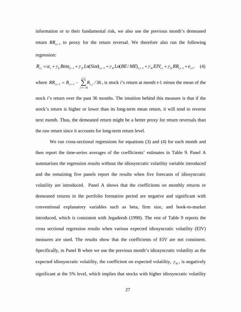
We run cross-sectional regressions for equations (3) and (4) for each month and

then report the time-series averages of the coefficients’ estimates in Table 9. Panel A

summarizes the regression results without the idiosyncratic volatility variable introduced

and the remaining five panels report the results when five forecasts of idiosyncratic

volatility are introduced. Panel A shows that the coefficients on monthly returns or

demeaned returns in the portfolio formation period are negative and significant with

conventional explanatory variables such as beta, firm size, and book-to-market

introduced, which is consistent with Jegadeesh (1990). The rest of Table 9 reports the

cross sectional regression results when various expected idiosyncratic volatility (EIV)

measures are used. The results show that the coefficients of EIV are not consistent.

Specifically, in Panel B when we use the previous month’s idiosyncratic volatility as the

expected idiosyncratic volatility, the coefficient on expected volatility, t4γ , is negatively

significant at the 5% level, which implies that stocks with higher idiosyncratic volatility

28

earn lower returns in the following month. Similar results are reported by Ang et al.

(2006b). The same result also holds in Panel D and Panel E when the expected

idiosyncratic volatility is estimated from the ARIMA model on portfolio idiosyncratic

volatility and from the GARCH (1, 1) model, respectively. However, this negative

relation is not very robust. When idiosyncratic risk is estimated by the ARIMA model

based on individual stock-level idiosyncratic volatility in Panel C, the coefficient on

expected volatility is not significant, confirming the prediction in Bali and Cakici (2006).

The coefficient on expected volatility from the EGARCH (1, 1) model in Panel F is not

significant either.17

[Insert Table 9]

However, none of the coefficients on expected idiosyncratic volatility is

significant after return reversal is controlled for. This result holds no matter which

forecast of idiosyncratic volatility is used. We also find that the magnitude of the

coefficients on expected idiosyncratic volatility become much smaller for most of the

regressions. The one-month formation period returns or demeaned returns take away all

of the explanatory power of idiosyncratic volatility. The results of Panel B where we use

the previous month’s idiosyncratic volatility as the expected idiosyncratic volatility

indicates that the volatility coefficient t4γ is -0.019, with a t-statistic of -2.44, without

controlling for the previous month’s return. However, when we add the formation period

return (formation month demeaned return) to the regressions, the coefficient t4γ is 0.001

(-0.004), with a t-statistic of 0.15 (-0.51). The evidence here once again indicates that the

negative relation between idiosyncratic volatility and expected returns is driven by return

reversals.18

29

Early theories, such as Merton (1987), argue that since investors are not able to

totally diversify idiosyncratic risk, they will demand a premium for holding stocks with

high idiosyncratic risk, and thus stocks with higher expected idiosyncratic risk should

deliver higher expected returns. We do not find reliable empirical evidence to support this

argument. No matter which method we use to forecast expected idiosyncratic volatility,

we do not find a significantly positive coefficient on expected idiosyncratic volatility.

Furthermore, after we control for return reversals, we never obtain significant coefficients

on expected idiosyncratic volatility.

From Table 2, we notice that both winner stocks and loser stocks have high

idiosyncratic risk in the formation month, but winners earn lower returns and losers earn

higher returns in the holding-period month. If we observe a negative relation between

idiosyncratic volatility and expected returns, it can only be driven by winner stocks, since

loser stocks with high idiosyncratic volatility will earn high expected returns due to their

return reversals. Therefore, we expect that this negative relation between idiosyncratic

volatility and expected returns will disappear if we exclude the winner stocks from our

sample.

To test this hypothesis, we run the same cross-sectional regressions as in Table 9,

but for every month we exclude from the sample the 50 winner stocks that have the

highest prior-month return.19 Table 10 reports the average coefficients from the cross-

sectional regressions with 50 winner stocks (about 1% of all stocks) excluded. As

predicted, the negative relation between idiosyncratic volatility and expected returns

disappears even before we control for the return reversals and none of the coefficients on

idiosyncratic risks is significant in all panels. Another interesting finding is that the

30

significance of one-month portfolio formation period returns or demeaned returns are not

affected by the exclusion of winner stocks from the sample. The evidence here therefore

suggests that the negative relation between idiosyncratic volatility and expected returns is

driven in particular by the return reversals of winner stocks.20

[Insert Table 10]

2.3 Robustness Checks

2.3.1 Estimates of Idiosyncratic Volatility

Since idiosyncratic volatilities are unobservable, we require estimates of idiosyncratic

volatility in order to perform empirical tests. Usually these estimates can be obtained

from the residuals of an asset pricing model. Because different asset pricing models call

for different approaches to measure an individual stock’s idiosyncratic risk, the relation

between idiosyncratic volatility and expected returns reported above could be driven by a

particular model used. Therefore, we use different idiosyncratic volatility estimates to

verify the robustness of our results.

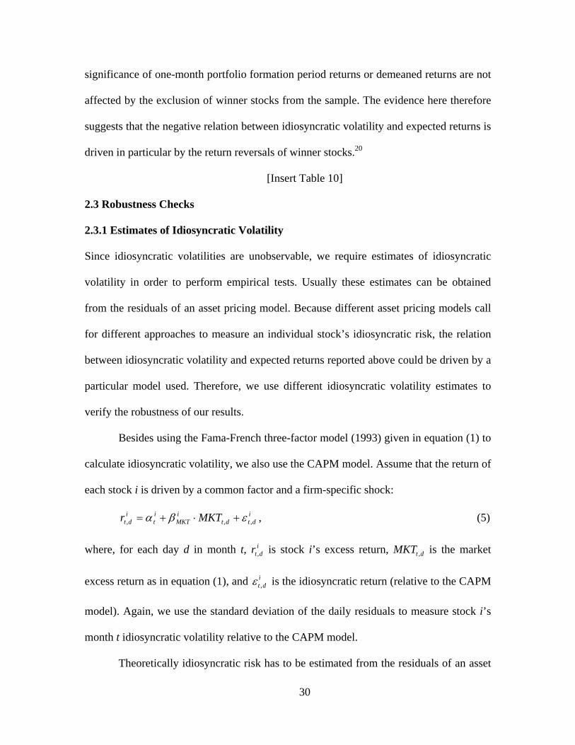
Besides using the Fama-French three-factor model (1993) given in equation (1) to

calculate idiosyncratic volatility, we also use the CAPM model. Assume that the return of

each stock i is driven by a common factor and a firm-specific shock:

idtdt

iMKT

it

idt MKTr ,,, εβα +⋅+= , (5)

where, for each day d in month t, idtr , is stock i’s excess return, dtMKT , is the market

excess return as in equation (1), and idt ,ε is the idiosyncratic return (relative to the CAPM

model). Again, we use the standard deviation of the daily residuals to measure stock i’s

month t idiosyncratic volatility relative to the CAPM model.

Theoretically idiosyncratic risk has to be estimated from the residuals of an asset

31

pricing model; empirically, however, it is very difficult to interpret the residuals

estimated from the CAPM or from a multifactor model as solely the idiosyncratic risk.

One can always argue that these residuals simply represent omitted factors and thus are

not really “idiosyncratic.” Jiang and Lee (2004) suggest that most of the return volatility

(about 85%) is idiosyncratic volatility. More importantly, since we do not know which

asset pricing model is correct; we can use total risk to proxy for idiosyncratic volatility.

This method is essentially model-free. We therefore calculate stock i’s standard deviation

of daily returns within month t and use this statistic to proxy for idiosyncratic volatility.

We use the previous month CAPM-based idiosyncratic volatility or the raw

return-based idiosyncratic volatility as the expected idiosyncratic volatility and run cross-

sectional regressions. The time-series averages of the coefficients’ estimates are reported

in Table 11. The results show that the role of idiosyncratic volatility is not significant

when we control for return reversals, and our results are not driven by any particular

approach to measure idiosyncratic volatility.

[Insert Table 11]

2.3.2 NYSE/AMEX Stocks Only

Table 11 shows that our results still hold if we only include NYSE/AMEX stocks in our

sample. The evidence confirms that our results are not driven by small-sized stocks or

illiquid stocks listed on NASDAQ. To save space, in our remaining robustness test

discussions, we use only the previous month’s idiosyncratic volatility relative to the

Fama-French model’s (1993) idiosyncratic volatility to proxy for expected idiosyncratic

volatility. Our empirical analysis indicates that all robustness test results still hold when

we use CAPM-based idiosyncratic volatility or raw return-based idiosyncratic volatility.21

32

2.3.3 Excluding Stocks with Extremely High Idiosyncratic Volatility

Idiosyncratic volatility estimates for individual stocks suffer not only from the errors-in-

variables problem, but also sampling errors. A small percentage of outliers with

exceptionally large or small returns (winners or losers) may have extremely high

idiosyncratic volatilities in a month, but never experience similar moves before and after.

Outliers can also occur because of a data error. To take this into account, we divide the

highest idiosyncratic volatility portfolio, IV5, which we have used in our portfolio level

analysis into ten sub-portfolios with the same number of stocks based on their past return

performance. The first and the last sub-portfolios include the winners and losers with

extremely high idiosyncratic volatilities. Most of them are penny stocks (with prices less

than $5). We exclude them (about %4%20%20 =× of all stocks) from our cross-

sectional regressions. Table 11 indicated that the volatility coefficient is -0.024, with an

insignificant t-statistic of -1.55. The coefficient on previous monthly returns is -0.063,

with a strongly significant t-statistic of -12.65. Therefore, our results are not driven by a

very small fraction of outliers.

2.3.4 Controlling for Leverage

Leverage is related to both past returns and volatility. Past winners have a smaller ratio of

book assets to market equity, or smaller market leverage; while an increase in leverage

produces an increase in stock volatility. We use the natural log of the ratio of the total

book value assets to book value of equity to measure book leverage in Table 11.

Consistent with Fama and French (1992), there is a negative relation between book

leverage and expected returns. Controlling for leverage does not change the effect of

idiosyncratic risk and past returns on average returns - the coefficient on past returns is

33

negatively significant, and that of idiosyncratic volatility is insignificant from zero.

2.3.5 Controlling for Momentum

Jegadeesh and Titman (1993) show that the stocks that perform the best (worst) over the

previous 3- to 12-month period tend to continue to perform well (poorly) over the

subsequent 3 to 12 months. This phenomenon is referred to as the momentum effect. If

the loser stocks during the previous month are the stocks with good historic performance

and the winner stocks are the stocks with poor historic performance, the role of return

reversals may simply proxy for the momentum effect. To examine the role of

idiosyncratic risk on expected returns after taking the momentum effect into account, we

construct the momentum variable MOM and include it in the cross-sectional regressions.

This variable is equal to the cumulative returns for six months from month t-7 to month t-

2, assuming that the current month is t.

The results in Table 11 suggest the existence of momentum since the coefficient

on MOM is positive and significant. However, controlling for momentum does not

change the effect of idiosyncratic risk on expected returns. In Table 11, the coefficient on

past returns is still significantly negative, while the coefficient on idiosyncratic volatility

is not significant.

2.3.6 Controlling for Liquidity

Liquidity measures the degree to which one can trade a large amount of stocks without

changing their prices. Many theoretical and empirical papers confirm the role of liquidity

in cross-sectional returns and document a negative relation between liquidity and

expected stock returns [Amihud and Mendelson (1986), Constantinides (1986), Brennan

and Subrahmanyam (1996), Heaton and Lucas (1996), Brennan et al. (1998), Datar et al.

34

(1998), and Huang (2002), Spiegel and Wang (2005)]. Pastor and Stambaugh (2003) also

demonstrate that stocks with high liquidity betas have high average returns. According to

them, liquidity is a systematic risk and thus assets with higher liquidity risk should have

lower prices, other things being equal, in order to compensate investors for assuming the

risk. Hence, if liquidity is indeed priced, our idiosyncratic volatility measure constructed

based on residuals from the CAPM, the Fama-French three-factor model, or total risk

could potentially capture the liquidity factor. We use two measures of liquidity to control

for liquidity risk. The first liquidity measure is the turnover ratio, which is the ratio

between share volume and shares outstanding; this metric can also be regarded as the

relative volume. Specifically, we use the previous 36 months’ average turnover rate to

proxy for liquidity in the cross-sectional regressions. Our second liquidity measure is the

historical Pastor-Stambaugh (2003) liquidity beta that measures exposure to liquidity risk.

Table 11 shows that our results are robust to liquidity risk. When idiosyncratic

volatility, past returns, and liquidity risk are included, the sign and significance of the

coefficients of past returns are unchanged, and the coefficients on idiosyncratic volatility

are very small and insignificant. The ability of liquidity to explain expected returns seems

to be limited; the coefficient on the turnover ratio is negative as the previous literature

suggests, but not significant or marginally significant at the 5% level, and the coefficient

on the liquidity beta is very close to zero and insignificant. This is consistent with Spiegel

and Wang (2005), who documents that the explanatory power of liquidity is weakened

once idiosyncratic risk is included in the regression.22

In summary, the negative relation between current-month returns and past one-

month returns is very robust to the inclusion of other explanatory variables in the cross-

35

sectional regressions, suggesting a significant short-term return reversal. On the other

hand, the negative relation between idiosyncratic volatility and cross-sectional expected

returns is not robust. In most of the regressions, no discernable relation exists between

expected idiosyncratic volatility and expected returns once we control for past returns.

Once some winner stocks are excluded from the sample, the coefficients on expected

idiosyncratic volatility are consistently insignificant whether we control for return

reversals or not. Our results are not depending on a very small fraction of outliers in the

sample.

3. Conclusion

Empirical support for the relation between idiosyncratic volatility and expected stock

returns has been mixed. Recently, Ang et al. (2006a, 2006b) document that portfolio

with high monthly idiosyncratic volatility delivers low VW average return in the next one

month, suggesting a negative intertemporal relation between idiosyncratic risk and stock

returns. Bali and Cakici (2006), however, find no robust, significant relation between

idiosyncratic volatility and expected portfolio returns. Most important, they find that the

relation is not consistent under different choices of weight schemes in computing

portfolio returns. While these results identify an interesting “puzzle,” neither the cause of

the negative relation in Ang et al. (2006a) nor the reason in Bali and Cakici (2006) is

known. Furthermore, there is no understanding of the relation between ex ante

idiosyncratic risk and expected return.

In this paper, we demonstrate that the negative intertemporal relation between

idiosyncratic risk and VW portfolio returns and no relation between idiosyncratic risk and

EW portfolio returns are driven by short-term return reversals. In particular, we observe

36

that nearly half of the stocks in the portfolio with the highest idiosyncratic volatility are

either winner stocks or loser stocks. The winner stocks tend to be relatively larger cap

stocks than the loser stocks in the portfolio formation period and they experience

significant return reversals, which drive down the VW return on the portfolio in the next

month and cause the negative relation to appear. In contrast, there is no significant

difference in the EW returns on the five portfolios sorted by idiosyncratic volatility

because return reversals experienced by winner and loser stocks offset each other. In the

absence of return reversals for longer holding periods, no negative relation is observed

between idiosyncratic volatility and stock returns, regardless of VW or EW portfolio

return. This result provides further supportive evidence that return reversals are the

driving force of the negative relation. Our evidence from idiosyncratic volatility-sorted

portfolios that control for both size and past returns also suggest that negative VW return

difference between the highest idiosyncratic volatility portfolio and the lowest

idiosyncratic volatility portfolio is driven by the short term return reversal, rather than

idiosyncratic volatility itself.

The time-series regression results indicate that the seemingly abnormal positive

return from taking a long position in the lowest idiosyncratic risk portfolio and a short

position in the highest idiosyncratic risk portfolio can be fully explained by adding the

“winners minus losers” return to the conventional three- or four-factor model.

Finally, we use five different approaches to form ex ante idiosyncratic risk and

conduct cross-sectional tests. Once again, we find that there is no robust, significant

relation between ex ante idiosyncratic volatility and expected returns. There is a

significantly negative relation between current-month returns and past one-month returns,

37

indicating a strong return reversal effect. In all of the regressions with the full sample of

all common stocks, the relation between expected idiosyncratic volatility and expected

returns is flat once we control for past returns. Our results are robust to the inclusion of

other variables such as beta, size, book-to-market, momentum, liquidity, leverage,

different measures of idiosyncratic volatility, and excluding a small percentage of

extremely high idiosyncratic volatility stocks from the sample. Overall, our results

suggest that return reversal is the underlying reason behind the negative relation between

idiosyncratic risk and subsequent stock returns. The role of idiosyncratic risk is

significantly weakened when past return is used as a conditional variable. Our study thus

contributes toward understanding of the role of idiosyncratic risk in asset pricing.

38

Appendix A: Forecasting Idiosyncratic Volatility using ARIMA

To obtain the best-fit ARIMA model, we first de-trend the data using a linear trend model,

then take the residuals and compute autocovariances for the number of lags it takes for

the autocorrelation to be not significantly different from zero. We run a regression of the

current values against the lags, using the autocovariances in a Yule-Walker framework.

We do not admit any autoregressive parameter that is not significant and find the

autoregressive parameter that is the least significant and exclude it from the model. We

continue this process until only significant autoregressive parameters remain. With this,

we generate forecasts using the estimated model.

Appendix B: Forecasting Idiosyncratic Volatility using GARCH and EGARCH

Using GARCH (1, 1), we have the following process for each stock i at month t:

,,, titiHMLt

iSMBt

iMKTiti HMLSMBMKTr εβββα +⋅+⋅+⋅+= (6)

tititi h ,,, νε ⋅= ,

where ti,ν is independently and identically distributed (i.i.d.) with standard normal

distribution and tih , can be expressed as

21,11,1, −− ++= ti

iti

iiti hh εαδω . (7)

The equation for the mean of the GARCH (1, 1) model is the Fama-French three-

factor model as given in equation (6). The conditional (on time t-1 information)

distribution of the residual ti,ε is assumed to be normal with mean zero and variance tih , .

39

We estimate the idiosyncratic risk of individual stocks as the square root of the

conditional variance tih , , which is a function of the past one month’s residual variance and

the shock as specified in equation (7). For each month and each stock, we run the

GARCH (1, 1) model using the monthly returns in the previous 30 months (if available)

and the forecasts thus obtained for the next month comprise our fourth expected

idiosyncratic volatility measure, EIV4.

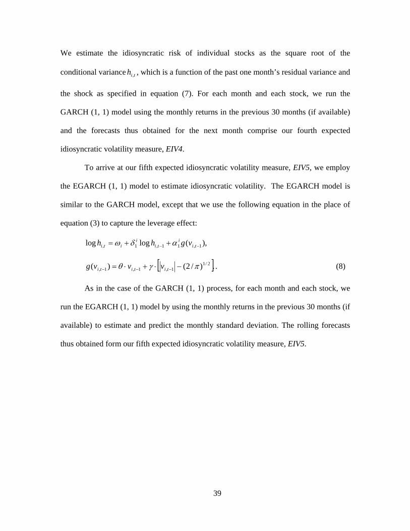
To arrive at our fifth expected idiosyncratic volatility measure, EIV5, we employ

the EGARCH (1, 1) model to estimate idiosyncratic volatility. The EGARCH model is

similar to the GARCH model, except that we use the following equation in the place of

equation (3) to capture the leverage effect:

),(loglog 1,11,1, −− ++= tii

tii

iti vghh αδω

[ ].)/2()( 2/11,1,1, πγθ −⋅+⋅= −−− tititi vvvg . (8)

As in the case of the GARCH (1, 1) process, for each month and each stock, we

run the EGARCH (1, 1) model by using the monthly returns in the previous 30 months (if

available) to estimate and predict the monthly standard deviation. The rolling forecasts

thus obtained form our fifth expected idiosyncratic volatility measure, EIV5.

40

REFERENCES

Amihud, Yakov, and Haim Mendelson, 1986, Asset pricing and the bid-ask spread,

Journal of Financial Economics 17, 223-249.

Ang, Andrew, Robert J. Hodrick, Yuhang Xing and Xiaoyan Zhang, 2006a, The cross-

section of volatility and expected returns, Journal of Finance 61, 259-299.

Ang, Andrew, Robert J. Hodrick, Yuhang Xing and Xiaoyan Zhang, 2006b, High

idiosyncratic volatility and low returns: international and further US evidence,

Working paper, Columbia University.

Bali, Turan G., Nusret Cakici, 2006, Idiosyncratic volatility and the cross-section of

expected returns, Journal of Financial and Quantitative Analysis, forthcoming.

Bali, Turan G., Nusret Cakici, Xuemin Yan and Zhe Zhang, 2005, Does idiosyncratic

volatility really matter? Journal of Finance 60, 905-929.

Barberis, N., and M. Huang, 2001, Mental accounting, loss aversion, and individual stock

returns, Journal of Finance 56, 1247-1292.

Bollerslev, Tim, 1986, Generalized autoregressive conditional heteroskedasticity, Journal

of Econometrics 31, 307-328.

Brennan, Michael J., Tarun Chordia, and Avanindhar Subrahmanyam, 1998, Alternative

factor specifications, security characteristics, and the cross-section of expected stock

returns, Journal of Financial Economics 49, 345-373.

Brennan, Michael J. and Avanindhar Subrahmanyam, 1996, Market microstructure and

asset pricing: On the compensation for illiquidity in stock returns, Journal of

Financial Economics 41, 441-464.

41

Campbell, John Y., Martin Lettau, Burton G. Malkiel, and Yexiao Xu, 2001, Have

individual stocks become more volatile? An empirical exploration of idiosyncratic

risk, Journal of Finance 56, 1-43.

Carhart, Mark M., 1997, On persistence in mutual fund performance, Journal of Finance

52, 57-82.

Chua, Choong Tze, Jeremy Goh, Zhe Zhang, 2006, Idiosyncratic volatility matters for the

cross-section of returns–in more ways than one, Working Paper, Singapore

Management University.

Constantinides, George, 1986, Capital market equilibrium with transaction costs, Journal

of Political Economy 94, 842-862.

Datar, Vinay T., Narayan Y. Naik, and Robert Radcliffe, 1998, Liquidity and asset

returns: An alternative test, Journal of Financial Markets 1, 203-219.

Diether, Karl B., Christopher J. Malloy, and Anna Scherbina, 2002, Differences of

opinion and the cross section of stock returns, Journal of Finance 57, 2113-2141.

Duffee, Gregory R., 1995, Stock returns and volatility: A firm-level analysis, Journal of

Financial Economics 37, 399-420.

Engel, Robert F., 1982, Autoregressive conditional heteroskedasticity with estimates of

the variance of United Kingdom inflation, Econometrica 50, 987-1007.

Fama, Eugene F., and James D. MacBeth, 1973, Risk, return, and equilibrium: Empirical

tests, Journal of Political Economy 81, 607-636.

Fama, Eugene F., and Kenneth R. French, 1992, The cross-section of expected stock

returns, Journal of Finance 47, 427-465.

Fama, Eugene F., and Kenneth French, 1993, Common risk factors in the returns on

42

stocks and bonds, Journal of Financial Economics 33, 3-56.

Fama, Eugene F. and French, Kenneth R., 1996, Multifactor explanations of asset pricing

anomalies, Journal of Finance 51, 55-84.

French, Kenneth R., G. William Schwert, and Robert F. Stambaugh, 1987, Expected

stock returns and volatility, Journal of Financial Economics 19, 3-29.

Fu, Fangjian, 2005, Idiosyncratic risk and the cross-section of expected stock returns,

Working paper, University of Rochester.

Goyal, Amit and Pedro Santa-Clara, 2003, Idiosyncratic volatility matters! Journal of

Finance 58, 975-1007.

Guo, Hui and Robert Savickas, 2006, Idiosyncratic volatility, stock market volatility, and

expected stock returns, Journal of Business and Economic Statistics 24, 43-56.

Heaton, John, and Deborah J. Lucas, 1996, Evaluating the effects of incomplete markets

on risk sharing and asset pricing, Journal of Political Economy 104, 443-487.

Huang, Ming, 2002, Liquidity shocks and equilibrium liquidity premia, Journal of

Economic Theory, forthcoming.

Jegadeesh, Narasimhan, 1990, Evidence of predictable behavior of security returns,

Journal of Finance 45, 881-898.

Jegadeesh, Narasimhan and Sheridan Titman, 1993, Returns to buying winners and

selling losers: Implications for stock market efficiency, Journal of Finance 48, 65-

91.

Jegadeesh, Narasimhan and Sheridan Titman, 1995a, Overreaction, delayed reaction and

contrarian profits, Review of Financial Studies 8, 973-993.

Jegadeesh, Narasimhan and Sheridan Titman, 1995b, Short-horizon return reversals, and

43

bid-ask spread, Journal of Financial Intermediation 4, 116-132.

Jegadeesh, Narasimhan and Sheridan Titman, 2001, Profitability of momentum strategies:

An evaluation of alternative explanations, Journal of Finance 56, 699-720.

Jiang, Xiaoquan and Bong-Soo Lee, 2005, On the dynamic relation between returns and

idiosyncratic volatility, Working paper, University of Houston.

Lehmann, Bruce, 1990a, Residual risk revisited, Journal of Econometrics 45, 71-97.

Lehmann, Bruce, 1990b, Fads, martingales and market efficiency, Quarterly Journal of

Economics 105, 1-28.

Lintner, John, 1965, The valuation of risky assets and the selection of risky investment in

stock portfolio and capital budgets, Review of Economics and Statistics 47, 13-37.

Malkiel, Burton G., and Yexiao Xu, 2002, Idiosyncratic risk and security returns,

Working paper, University of Texas at Dallas.

Merton, Robert C., 1973, An intertemporal capital asset pricing model, Econometrica 41,

867-887.

Merton, Robert C., 1987, Presidential address: A simple model of capital market

equilibrium with incomplete information, Journal of Finance 42, 483-510.

Grossman, Sanford and Merton H. Miller, 1988, Liquidity and market structure, Journal

of Finance 43, 617-633.

Newey, Whitney K., and Kenneth D. West, 1987, A simple positive-definite

heteroskedasticity and autocorrelation consistent covariance matrix, Econometrica

55, 703-708.

Pastor, Lubos, and Robert F. Stambaugh, 2003, Liquidity risk and expected stock returns,

Journal of Political Economy 111, 642-685.

44

Shanken, Jay A., 1992, On the estimation of beta-pricing models, Review of Financial

Studies 5, 1-33.

Spiegel, Matthew, and Xiaotong Wang, 2005, Cross-sectional variation in stock returns:

Liquidity and idiosyncratic risk, Working Paper, Yale University.

Stiglitz, Joseph E., 1989, Using tax policy to curb speculative trading, Journal of

Financial Services Research 3, 101-115.

Summers, Lawrence H., and Victoria P. Summers, 1989, When financial markets work

too well: A cautious case for a securities transactions tax, Journal of Financial

Services Research 3, 261-286.

Tinic, Seha M., and Richard R.West, 1986, Risk, return and equilibrium: A revisit,

Journal of Political Economy 94, 126-147.

45

Footnotes

1 We thank Kenneth French for making the data available on his website.

2 We also use the standard deviation of the residuals from the capital asset pricing model (CAPM) and the

returns to measure idiosyncratic volatility and obtain qualitatively similar results.

3 To measure the monthly idiosyncratic volatility of stock i, we follow French et al. (1987) and multiply

the standard deviation of daily residuals in month t ( tiSTD , ) by tin , , where tin , is the number of trading

days during month t. Therefore tititi STDnIV ,,, = is stock i’s realized idiosyncratic volatility in month t.

4 Bali and Cakici (2006) call the largest stocks in the tenth sub-quintile of the highest idiosyncratic

volatility quintile portfolio as “biggest of small stocks” and find that their returns are much lower than

those of the “smallest of small stocks” in the first sub-quintile of the same quintile portfolio.

5 This is more obvious if we use total volatility as the measure of idiosyncratic volatility. In this case,

idiosyncratic volatility is simply the standard deviation of stock returns and “high volatility” means very

positive returns or very negative returns, that is, winners or losers.

6 Jiang and Lee (2004) find that on average, idiosyncratic volatility is about 85% of total stock return

volatility. Since winner and loser stocks often have larger total volatility, it is not surprising to find the

large presence of both of them in the highest idiosyncratic volatility portfolio.

7 We report the simple (equally-weighted) average monthly returns in Panels B and C. This implies that we

treat the stocks within each of the 50 idiosyncratic volatility-past return sorted portfolios as homogeneous,

and stocks from different portfolios as heterogeneous.

8 For the 12/1/12 strategy, each quintile portfolio changes 1/12th of its composition each month, where each

1/12th part of the portfolio consists of a value-weighted portfolio or equally-weighted portfolio. The first

(fifth) quintile portfolio consists of 1/12th of the lowest (highest) idiosyncratic stocks from 1 month ago

until from 12 months ago.

9 Ang et al. (2006a) document that the negative relation between past idiosyncratic volatility and future

returns still holds for a long horizon when they compare the difference in Fama-French three-factor (FF-3)

alphas between value-weighted portfolio IV5 and portfolio IV1 of the above four strategies. Our analysis is

based on the value-weighted or equally-weighted return difference of portfolio IV5 and portfolio IV1 over

46

the long run.

10 The same approach is adopted by Diether et al. (2002). Sorting portfolios on more than two dimensions

is useful in controlling for the effects of multiple factors at the same time.

11 We also conduct a triple sort based on stock price, past returns, and idiosyncratic volatility, and find

qualitatively similar results, that is, the average return difference between portfolio 5 and portfolio 1

remains insignificant. This is not surprising given the high correlation (0.76) between stock price and firm

size. These results are not reported but available upon request.

12 Strictly speaking, WML here is not a trading strategy since we are calculating its return during the

formation period. However, we use the formation period to capture the lead-lag relation between this

portfolio and the idiosyncratic volatility-based portfolio. We also construct WML by using the EW or VW

average return difference between P10 and P1 during the holding period and the Short-Term Reversal

Factor taken from Professor Kenneth French’s website. These WMLs can be thought of as risk factors since

they are evaluated in the same period as the dependent variables, the IV portfolio spread. However, none of

these factors could explain the IV portfolio return spread because the intercepts are all significantly

negative. These results are available upon request.

13 Bali and Cakici (2006) show that the realized idiosyncratic volatility measure obtained from monthly

data is a more accurate proxy for the expected idiosyncratic volatility than that based on daily data within

the same month. Under this new measure, they find that the cross-sectional relation between the realized

idiosyncratic volatility and expected (VW or EW) portfolio returns is flat.

14 We also use a portfolio’s previous 100 months’ idiosyncratic volatility to predict expected idiosyncratic

volatility; the results are similar.

15 To reduce errors-in-variables problems, we assign individual stock betas based upon 100 portfolios,

sorted using the Fama and French (1992) methodology. In particular, each month, all stocks are sorted into

10 groups by market capitalization. Within each size group, stocks are sorted again by their betas into ten

equal-numbered groups. The beta of each stock is estimated from a market model using the previous 24 to

60 months of returns, as available. The 100 portfolios thus obtained are rebalanced every month. We use

NYSE-listed stocks to determine the cutoff value for each size group to ensure that the ranking is not

dominated by many small-cap stocks on NASDAQ. For each portfolio, we compute its return in each

47

month and then regress the return series against the market return and the one-month lagged market return.

The portfolio betas therefore equal the sum of these two beta coefficients. Finally, we assign the portfolio

betas to individual stocks according to their size-beta ranking in each month.

16 To ensure that accounting data are known before they are used to explain the cross-section of stock

returns, we use a firm’s market equity at the end of December of year t-1 to compute its year t-1 book-to-

market ratio, and then match the book-to-market ratio for calendar year t-1 with the returns from July of

year t to June of t+1.

17 Fu (2005) runs a similar cross-sectional regression and finds that the coefficient on expected

idiosyncratic volatility is significantly positive. Although he also uses an EGARCH model to estimate

expected idiosyncratic volatility, he chooses the best-fit EGARCH model among nine EGARCH (p, q)

models, with ,3p1 ≤≤ 3q1 ≤≤ , according to the Akaike Information Criterion to obtain the expected

idiosyncratic volatility for each individual stock.

18 Ang et al. (2006b) find the negative relation between idiosyncratic volatility and expected returns after

controlling for the lagged return. However, the lagged returns in their paper are a firm’s returns over the

previous six months. Therefore it takes account of both short term return reversals and the momentum

effect.

19 We also conduct analysis by excluding portfolio P10. By excluding all winner stocks from our sample,

we obtain qualitatively similar results.

20 On the contrary, if we exclude 50 loser stocks from the sample and use daily standard deviation in the

previous month to predict expected idiosyncratic volatility, we find that the coefficient on the expected

idiosyncratic risk is negatively significant, even after past returns are controlled for. The coefficient on past

returns is still highly significant and negative. Consistent with Bali and Cakici (2006), this shows that the

relation between idiosyncratic volatility and cross-section expected returns is not robust and easily affected

if we exclude only the extreme winners or losers in the sample.

21 When we exclude penny stocks (stock prices less than $5) from NYSE/AMEX universe, there is a

negative relation between idiosyncratic volatility and future returns if we use raw return-based idiosyncratic

volatility, even after past returns are controlled for. The reason is that more losers than winners are

excluded from the sample because of their relatively lower prices, which leads to the negative significance

48

of idiosyncratic volatility in some of the cross-sectional regressions. The coefficients on past returns are

still significantly negative in all regressions.

22 The difference from our result is that Spiegel and Wang (2005) find a positive relation between

idiosyncratic volatility and expected returns by using monthly data to measure idiosyncratic volatility,

following Fu (2005).

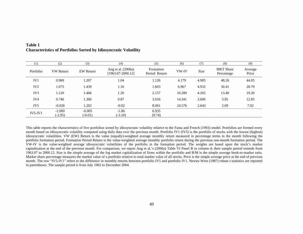
49

Table 1 Characteristics of Portfolios Sorted by Idiosyncratic Volatility

(1) (2) (3) (4) (5) (6) (7) (8) (9)

Portfolio VW Return EW Return Ang et al. (2006a) [1963.07-2000.12]

Formation Period Return VW-IV Size MKT Share

Percentage Average

Price

IV1 0.969 1.207 1.04 1.126 4.179 4.985 48.26 44.05

IV2 1.075 1.439 1.16 1.603 6.967 4.932 30.41 28.79

IV3 1.120 1.466 1.20 2.157 10.289 4.265 13.40 19.20

IV4 0.746 1.300 0.87 3.016 14.341 3.600 5.95 12.85

IV5 -0.026 1.202 -0.02 8.061 24.576 2.643 2.09 7.02

IV5-IV1 -1.000 (-2.95)

-0.005 (-0.01)

-1.06 (-3.10)

6.935 (9.74)

This table reports the characteristics of five portfolios sorted by idiosyncratic volatility relative to the Fama and French (1993) model. Portfolios are formed every month based on idiosyncratic volatility computed using daily data over the previous month. Portfolio IV1 (IV5) is the portfolio of stocks with the lowest (highest) idiosyncratic volatilities. VW (EW) Return is the value (equally)-weighted average monthly return measured in percentage terms in the month following the portfolio formation period. Formation Period Return is the value-weighted average monthly portfolio return during the previous one-month formation period. The VW-IV is the value-weighted average idiosyncratic volatilities of the portfolio in the formation period. The weights are based upon the stock’s market capitalization at the end of the previous month. For comparison, we report Ang et al.’s (2006a) Table VI Panel B in column 4; their sample period extends from 1963.07 to 2000.12. Size is the simple average of the log market capitalization of firms within the portfolio and B/M is the simple average book-to-market ratio. Market share percentage measures the market value of a portfolio relative to total market value of all stocks. Price is the simple average price at the end of previous month. The row “IV5-IV1” refers to the difference in monthly returns between portfolio IV5 and portfolio IV1. Newey-West (1987) robust t-statistics are reported in parentheses. The sample period is from July 1963 to December 2004.

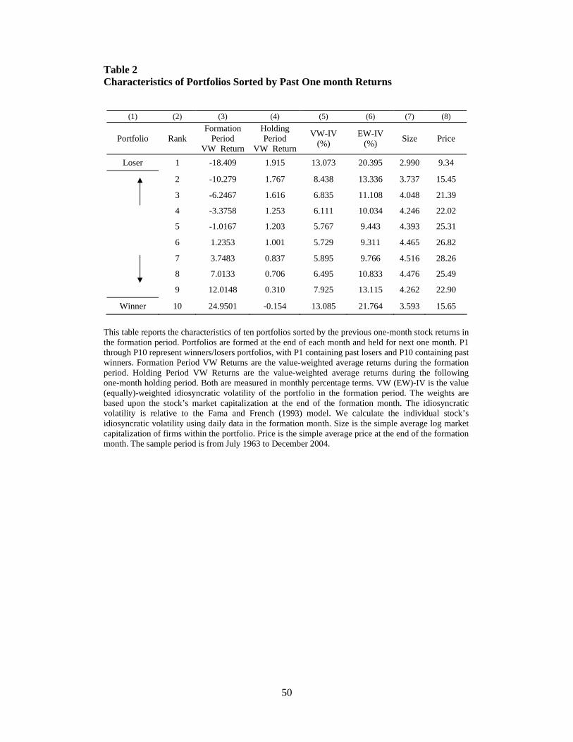
50

Table 2 Characteristics of Portfolios Sorted by Past One month Returns

(1) (2) (3) (4) (5) (6) (7) (8)

Portfolio Rank Formation

Period VW Return

Holding Period

VW Return

VW-IV (%)

EW-IV (%) Size Price

Loser 1 -18.409 1.915 13.073 20.395 2.990 9.34 2 -10.279 1.767 8.438 13.336 3.737 15.45

3 -6.2467 1.616 6.835 11.108 4.048 21.39

4 -3.3758 1.253 6.111 10.034 4.246 22.02

5 -1.0167 1.203 5.767 9.443 4.393 25.31

6 1.2353 1.001 5.729 9.311 4.465 26.82 7 3.7483 0.837 5.895 9.766 4.516 28.26

8 7.0133 0.706 6.495 10.833 4.476 25.49

9 12.0148 0.310 7.925 13.115 4.262 22.90

Winner 10 24.9501 -0.154 13.085 21.764 3.593 15.65

This table reports the characteristics of ten portfolios sorted by the previous one-month stock returns in the formation period. Portfolios are formed at the end of each month and held for next one month. P1 through P10 represent winners/losers portfolios, with P1 containing past losers and P10 containing past winners. Formation Period VW Returns are the value-weighted average returns during the formation period. Holding Period VW Returns are the value-weighted average returns during the following one-month holding period. Both are measured in monthly percentage terms. VW (EW)-IV is the value (equally)-weighted idiosyncratic volatility of the portfolio in the formation period. The weights are based upon the stock’s market capitalization at the end of the formation month. The idiosyncratic volatility is relative to the Fama and French (1993) model. We calculate the individual stock’s idiosyncratic volatility using daily data in the formation month. Size is the simple average log market capitalization of firms within the portfolio. Price is the simple average price at the end of the formation month. The sample period is from July 1963 to December 2004.

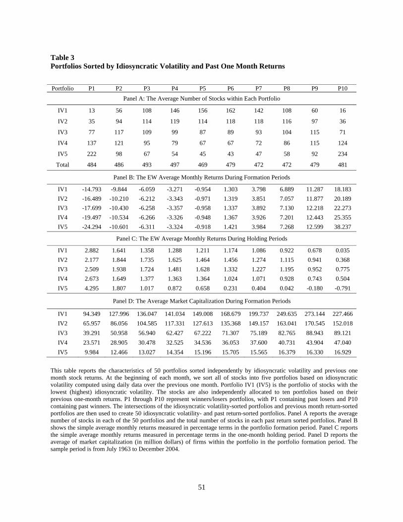
51

Table 3 Portfolios Sorted by Idiosyncratic Volatility and Past One Month Returns

Portfolio P1 P2 P3 P4 P5 P6 P7 P8 P9 P10 Panel A: The Average Number of Stocks within Each Portfolio

IV1 13 56 108 146 156 162 142 108 60 16

IV2 35 94 114 119 114 118 118 116 97 36

IV3 77 117 109 99 87 89 93 104 115 71

IV4 137 121 95 79 67 67 72 86 115 124

IV5 222 98 67 54 45 43 47 58 92 234

Total 484 486 493 497 469 479 472 472 479 481

Panel B: The EW Average Monthly Returns During Formation Periods

IV1 -14.793 -9.844 -6.059 -3.271 -0.954 1.303 3.798 6.889 11.287 18.183 IV2 -16.489 -10.210 -6.212 -3.343 -0.971 1.319 3.851 7.057 11.877 20.189 IV3 -17.699 -10.430 -6.258 -3.357 -0.958 1.337 3.892 7.130 12.218 22.273 IV4 -19.497 -10.534 -6.266 -3.326 -0.948 1.367 3.926 7.201 12.443 25.355 IV5 -24.294 -10.601 -6.311 -3.324 -0.918 1.421 3.984 7.268 12.599 38.237

Panel C: The EW Average Monthly Returns During Holding Periods

IV1 2.882 1.641 1.358 1.288 1.211 1.174 1.086 0.922 0.678 0.035 IV2 2.177 1.844 1.735 1.625 1.464 1.456 1.274 1.115 0.941 0.368 IV3 2.509 1.938 1.724 1.481 1.628 1.332 1.227 1.195 0.952 0.775 IV4 2.673 1.649 1.377 1.363 1.364 1.024 1.071 0.928 0.743 0.504 IV5 4.295 1.807 1.017 0.872 0.658 0.231 0.404 0.042 -0.180 -0.791

Panel D: The Average Market Capitalization During Formation Periods

IV1 94.349 127.996 136.047 141.034 149.008 168.679 199.737 249.635 273.144 227.466 IV2 65.957 86.056 104.585 117.331 127.613 135.368 149.157 163.041 170.545 152.018 IV3 39.291 50.958 56.940 62.427 67.222 71.307 75.189 82.765 88.943 89.121 IV4 23.571 28.905 30.478 32.525 34.536 36.053 37.600 40.731 43.904 47.040 IV5 9.984 12.466 13.027 14.354 15.196 15.705 15.565 16.379 16.330 16.929

This table reports the characteristics of 50 portfolios sorted independently by idiosyncratic volatility and previous one month stock returns. At the beginning of each month, we sort all of stocks into five portfolios based on idiosyncratic volatility computed using daily data over the previous one month. Portfolio IV1 (IV5) is the portfolio of stocks with the lowest (highest) idiosyncratic volatility. The stocks are also independently allocated to ten portfolios based on their previous one-month returns. P1 through P10 represent winners/losers portfolios, with P1 containing past losers and P10 containing past winners. The intersections of the idiosyncratic volatility-sorted portfolios and previous month return-sorted portfolios are then used to create 50 idiosyncratic volatility- and past return-sorted portfolios. Panel A reports the average number of stocks in each of the 50 portfolios and the total number of stocks in each past return sorted portfolios. Panel B shows the simple average monthly returns measured in percentage terms in the portfolio formation period. Panel C reports the simple average monthly returns measured in percentage terms in the one-month holding period. Panel D reports the average of market capitalization (in million dollars) of firms within the portfolio in the portfolio formation period. The sample period is from July 1963 to December 2004.

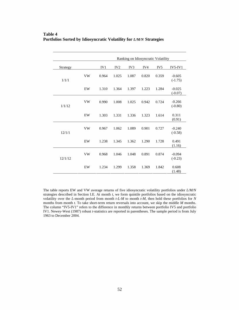
52

Table 4 Portfolios Sorted by Idiosyncratic Volatility for L/M/N Strategies

Ranking on Idiosyncratic Volatility

Strategy

IV1

IV2

IV3

IV4

IV5

IV5-IV1

VW 0.964 1.025 1.087 0.820 0.359

-0.605 (-1.75)

1/1/1

EW 1.310 1.364 1.397 1.223 1.284

-0.025 (-0.07)

VW 0.990 1.008 1.025 0.942 0.724

-0.266 (-0.80)

1/1/12

EW 1.303 1.331 1.336 1.323 1.614

0.311 (0.91)

VW 0.967 1.062 1.089 0.901 0.727

-0.240 (-0.58)

12/1/1

EW 1.238 1.345 1.362 1.290 1.728

0.491 (1.16)

VW 0.968 1.046 1.048 0.891 0.874

-0.094 (-0.23)

12/1/12

EW 1.234 1.299 1.358 1.369 1.842

0.608 (1.48)

The table reports EW and VW average returns of five idiosyncratic volatility portfolios under L/M/N strategies described in Section I.E. At month t, we form quintile portfolios based on the idiosyncratic volatility over the L-month period from month t-L-M to month t-M, then hold these portfolios for N months from month t. To take short-term return reversals into account, we skip the middle M months. The column “IV5-IV1” refers to the difference in monthly returns between portfolio IV5 and portfolio IV1. Newey-West (1987) robust t-statistics are reported in parentheses. The sample period is from July 1963 to December 2004.

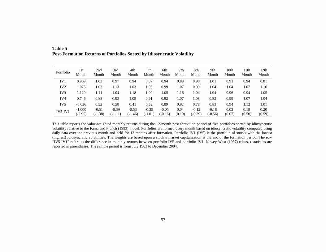
53

Table 5 Post-Formation Returns of Portfolios Sorted by Idiosyncratic Volatility

Portfolio 1st Month

2nd Month

3rd Month

4th Month

5th Month

6th Month

7th Month

8th Month

9th Month

10th Month

11th Month

12th Month

IV1 0.969 1.03 0.97 0.94 0.87 0.94 0.88 0.90 1.01 0.91 0.94 0.81 IV2 1.075 1.02 1.13 1.03 1.06 0.99 1.07 0.99 1.04 1.04 1.07 1.16 IV3 1.120 1.11 1.04 1.18 1.09 1.05 1.16 1.04 1.04 0.96 0.94 1.05 IV4 0.746 0.88 0.93 1.05 0.91 0.92 1.07 1.08 0.82 0.99 1.07 1.04 IV5 -0.026 0.52 0.58 0.41 0.52 0.89 0.92 0.78 0.83 0.94 1.12 1.01

IV5-IV1 -1.000 (-2.95)

-0.51 (-1.38)

-0.39 (-1.11)

-0.53 (-1.46)

-0.35 (-1.01)

-0.05 (-0.16)

0.04 (0.10)

-0.12 (-0.39)

-0.18 (-0.56)

0.03 (0.07)

0.18 (0.50)

0.20 (0.59)

This table reports the value-weighted monthly returns during the 12-month post formation period of five portfolios sorted by idiosyncratic volatility relative to the Fama and French (1993) model. Portfolios are formed every month based on idiosyncratic volatility computed using daily data over the previous month and held for 12 months after formation. Portfolio IV1 (IV5) is the portfolio of stocks with the lowest (highest) idiosyncratic volatilities. The weights are based upon a stock’s market capitalization at the end of the formation period. The row “IV5-IV1” refers to the difference in monthly returns between portfolio IV5 and portfolio IV1. Newey-West (1987) robust t-statistics are reported in parentheses. The sample period is from July 1963 to December 2004.

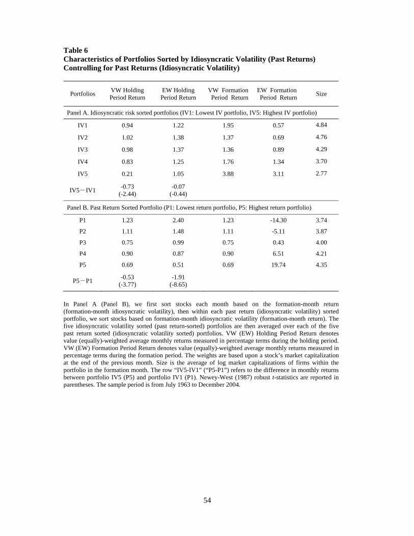
54

Table 6 Characteristics of Portfolios Sorted by Idiosyncratic Volatility (Past Returns) Controlling for Past Returns (Idiosyncratic Volatility)

Portfolios VW Holding Period Return

EW Holding Period Return

VW Formation Period Return

EW Formation Period Return Size

Panel A. Idiosyncratic risk sorted portfolios (IV1: Lowest IV portfolio, IV5: Highest IV portfolio)

IV1 0.94 1.22 1.95 0.57 4.84

IV2 1.02 1.38 1.37 0.69 4.76

IV3 0.98 1.37 1.36 0.89 4.29

IV4 0.83 1.25 1.76 1.34 3.70

IV5 0.21 1.05 3.88 3.11 2.77

IV5－IV1 -0.73 (-2.44)

-0.07 (-0.44)

Panel B. Past Return Sorted Portfolio (P1: Lowest return portfolio, P5: Highest return portfolio)

P1 1.23 2.40 1.23 -14.30 3.74

P2 1.11 1.48 1.11 -5.11 3.87

P3 0.75 0.99 0.75 0.43 4.00

P4 0.90 0.87 0.90 6.51 4.21

P5 0.69 0.51 0.69 19.74 4.35

P5－P1 -0.53 (-3.77)

-1.91 (-8.65)

In Panel A (Panel B), we first sort stocks each month based on the formation-month return (formation-month idiosyncratic volatility), then within each past return (idiosyncratic volatility) sorted portfolio, we sort stocks based on formation-month idiosyncratic volatility (formation-month return). The five idiosyncratic volatility sorted (past return-sorted) portfolios are then averaged over each of the five past return sorted (idiosyncratic volatility sorted) portfolios. VW (EW) Holding Period Return denotes value (equally)-weighted average monthly returns measured in percentage terms during the holding period. VW (EW) Formation Period Return denotes value (equally)-weighted average monthly returns measured in percentage terms during the formation period. The weights are based upon a stock’s market capitalization at the end of the previous month. Size is the average of log market capitalizations of firms within the portfolio in the formation month. The row “IV5-IV1” (“P5-P1”) refers to the difference in monthly returns between portfolio IV5 (P5) and portfolio IV1 (P1). Newey-West (1987) robust t-statistics are reported in parentheses. The sample period is from July 1963 to December 2004.

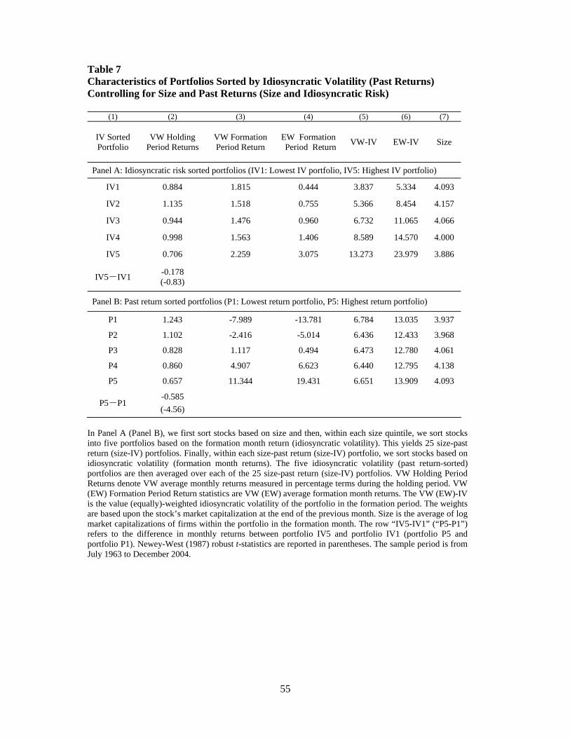
55

Table 7 Characteristics of Portfolios Sorted by Idiosyncratic Volatility (Past Returns) Controlling for Size and Past Returns (Size and Idiosyncratic Risk)

(1) (2) (3) (4) (5) (6) (7)

IV Sorted Portfolio

VW Holding Period Returns

VW Formation Period Return

EW Formation Period Return VW-IV EW-IV Size

Panel A: Idiosyncratic risk sorted portfolios (IV1: Lowest IV portfolio, IV5: Highest IV portfolio)

IV1 0.884 1.815 0.444 3.837 5.334 4.093

IV2 1.135 1.518 0.755 5.366 8.454 4.157

IV3 0.944 1.476 0.960 6.732 11.065 4.066

IV4 0.998 1.563 1.406 8.589 14.570 4.000

IV5 0.706 2.259 3.075 13.273 23.979 3.886

IV5－IV1 -0.178 (-0.83)

Panel B: Past return sorted portfolios (P1: Lowest return portfolio, P5: Highest return portfolio)

P1 1.243 -7.989 -13.781 6.784 13.035 3.937

P2 1.102 -2.416 -5.014 6.436 12.433 3.968

P3 0.828 1.117 0.494 6.473 12.780 4.061

P4 0.860 4.907 6.623 6.440 12.795 4.138

P5 0.657 11.344 19.431 6.651 13.909 4.093

P5－P1 -0.585 (-4.56)

In Panel A (Panel B), we first sort stocks based on size and then, within each size quintile, we sort stocks into five portfolios based on the formation month return (idiosyncratic volatility). This yields 25 size-past return (size-IV) portfolios. Finally, within each size-past return (size-IV) portfolio, we sort stocks based on idiosyncratic volatility (formation month returns). The five idiosyncratic volatility (past return-sorted) portfolios are then averaged over each of the 25 size-past return (size-IV) portfolios. VW Holding Period Returns denote VW average monthly returns measured in percentage terms during the holding period. VW (EW) Formation Period Return statistics are VW (EW) average formation month returns. The VW (EW)-IV is the value (equally)-weighted idiosyncratic volatility of the portfolio in the formation period. The weights are based upon the stock’s market capitalization at the end of the previous month. Size is the average of log market capitalizations of firms within the portfolio in the formation month. The row “IV5-IV1” (“P5-P1”) refers to the difference in monthly returns between portfolio IV5 and portfolio IV1 (portfolio P5 and portfolio P1). Newey-West (1987) robust t-statistics are reported in parentheses. The sample period is from July 1963 to December 2004.

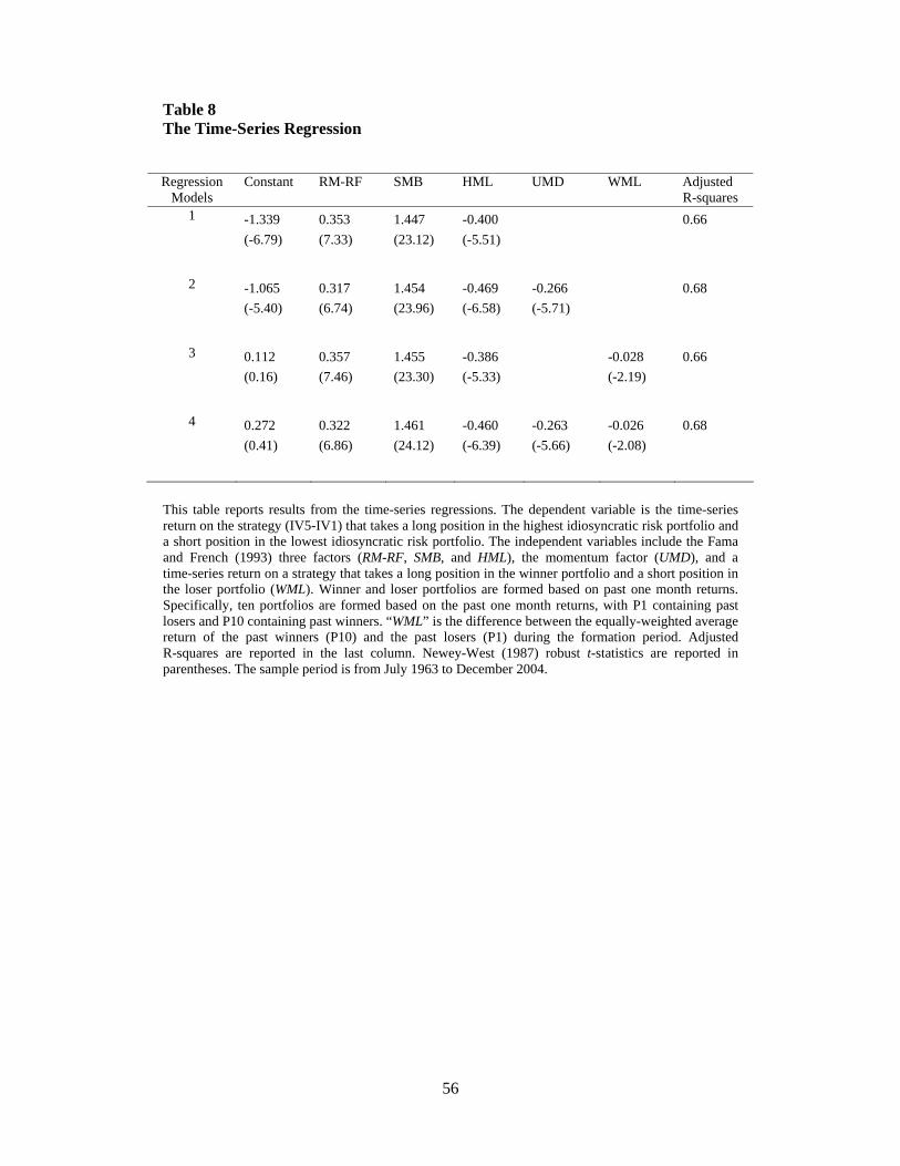
56

Table 8 The Time-Series Regression Regression

Models Constant RM-RF SMB HML UMD WML Adjusted

R-squares 1 -1.339

(-6.79) 0.353 (7.33)

1.447 (23.12)

-0.400 (-5.51)

0.66

2 -1.065 (-5.40)

0.317 (6.74)

1.454 (23.96)

-0.469 (-6.58)

-0.266 (-5.71)

0.68

3 0.112 (0.16)

0.357 (7.46)

1.455 (23.30)

-0.386 (-5.33)

-0.028 (-2.19)

0.66

4 0.272 (0.41)

0.322 (6.86)

1.461 (24.12)

-0.460 (-6.39)

-0.263 (-5.66)

-0.026 (-2.08)

0.68

This table reports results from the time-series regressions. The dependent variable is the time-series return on the strategy (IV5-IV1) that takes a long position in the highest idiosyncratic risk portfolio and a short position in the lowest idiosyncratic risk portfolio. The independent variables include the Fama and French (1993) three factors (RM-RF, SMB, and HML), the momentum factor (UMD), and a time-series return on a strategy that takes a long position in the winner portfolio and a short position in the loser portfolio (WML). Winner and loser portfolios are formed based on past one month returns. Specifically, ten portfolios are formed based on the past one month returns, with P1 containing past losers and P10 containing past winners. “WML” is the difference between the equally-weighted average return of the past winners (P10) and the past losers (P1) during the formation period. Adjusted R-squares are reported in the last column. Newey-West (1987) robust t-statistics are reported in parentheses. The sample period is from July 1963 to December 2004.

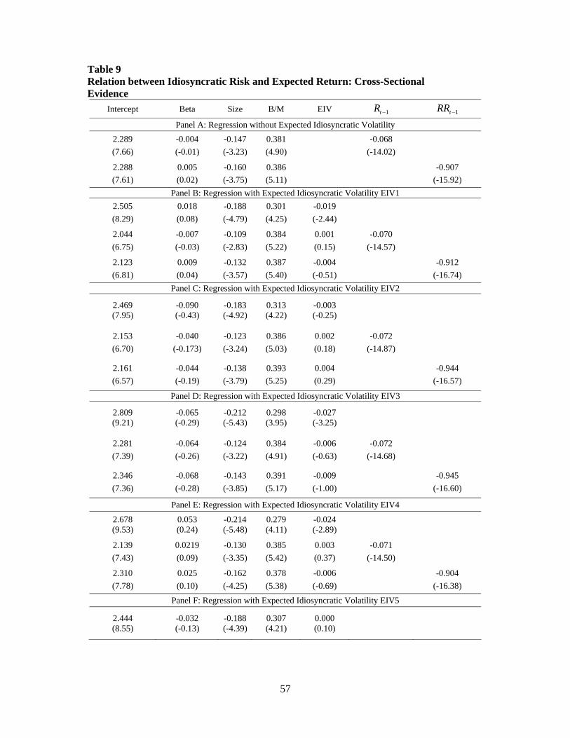
57

Table 9 Relation between Idiosyncratic Risk and Expected Return: Cross-Sectional Evidence

Intercept Beta Size B/M EIV 1−tR 1−tRR

Panel A: Regression without Expected Idiosyncratic Volatility 2.289 (7.66)

-0.004 (-0.01)

-0.147 (-3.23)

0.381 (4.90)

-0.068

(-14.02)

2.288 (7.61)

0.005 (0.02)

-0.160 (-3.75)

0.386 (5.11)

-0.907

(-15.92) Panel B: Regression with Expected Idiosyncratic Volatility EIV1

2.505 (8.29)

0.018 (0.08)

-0.188 (-4.79)

0.301 (4.25)

-0.019 (-2.44)

2.044 (6.75)

-0.007 (-0.03)

-0.109 (-2.83)

0.384 (5.22)

0.001 (0.15)

-0.070 (-14.57)

2.123 (6.81)

0.009 (0.04)

-0.132 (-3.57)

0.387 (5.40)

-0.004 (-0.51)

-0.912

(-16.74) Panel C: Regression with Expected Idiosyncratic Volatility EIV2

2.469 (7.95)

-0.090 (-0.43)

-0.183 (-4.92)

0.313 (4.22)

-0.003 (-0.25)

2.153 (6.70)

-0.040 (-0.173)

-0.123 (-3.24)

0.386 (5.03)

0.002 (0.18)

-0.072 (-14.87)

2.161 (6.57)

-0.044 (-0.19)

-0.138 (-3.79)

0.393 (5.25)

0.004 (0.29)

-0.944

(-16.57)

Panel D: Regression with Expected Idiosyncratic Volatility EIV3

2.809 (9.21)

-0.065 (-0.29)

-0.212 (-5.43)

0.298 (3.95)

-0.027 (-3.25)

2.281 (7.39)

-0.064 (-0.26)

-0.124 (-3.22)

0.384 (4.91)

-0.006 (-0.63)

-0.072 (-14.68)

2.346 (7.36)

-0.068 (-0.28)

-0.143 (-3.85)

0.391 (5.17)

-0.009 (-1.00)

-0.945

(-16.60)

Panel E: Regression with Expected Idiosyncratic Volatility EIV4

2.678 (9.53)

0.053 (0.24)

-0.214 (-5.48)

0.279 (4.11)

-0.024 (-2.89)

2.139 (7.43)

0.0219 (0.09)

-0.130 (-3.35)

0.385 (5.42)

0.003 (0.37)

-0.071 (-14.50)

2.310 (7.78)

0.025 (0.10)

-0.162 (-4.25)

0.378 (5.38)

-0.006 (-0.69)

-0.904

(-16.38)

Panel F: Regression with Expected Idiosyncratic Volatility EIV5

2.444 (8.55)

-0.032 (-0.13)

-0.188 (-4.39)

0.307 (4.21)

0.000 (0.10)

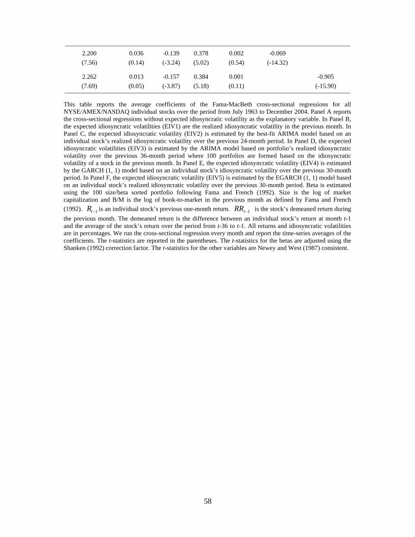
58

2.200 (7.56)

0.036 (0.14)

-0.139 (-3.24)

0.378 (5.02)

0.002 (0.54)

-0.069 (-14.32)

2.262 (7.69)

0.013 (0.05)

-0.157 (-3.87)

0.384 (5.18)

0.001 (0.11)

-0.905

(-15.90)

This table reports the average coefficients of the Fama-MacBeth cross-sectional regressions for all NYSE/AMEX/NASDAQ individual stocks over the period from July 1963 to December 2004. Panel A reports the cross-sectional regressions without expected idiosyncratic volatility as the explanatory variable. In Panel B, the expected idiosyncratic volatilities (EIV1) are the realized idiosyncratic volatility in the previous month. In Panel C, the expected idiosyncratic volatility (EIV2) is estimated by the best-fit ARIMA model based on an individual stock’s realized idiosyncratic volatility over the previous 24-month period. In Panel D, the expected idiosyncratic volatilities (EIV3) is estimated by the ARIMA model based on portfolio’s realized idiosyncratic volatility over the previous 36-month period where 100 portfolios are formed based on the idiosyncratic volatility of a stock in the previous month. In Panel E, the expected idiosyncratic volatility (EIV4) is estimated by the GARCH (1, 1) model based on an individual stock’s idiosyncratic volatility over the previous 30-month period. In Panel F, the expected idiosyncratic volatility (EIV5) is estimated by the EGARCH (1, 1) model based on an individual stock’s realized idiosyncratic volatility over the previous 30-month period. Beta is estimated using the 100 size/beta sorted portfolio following Fama and French (1992). Size is the log of market capitalization and B/M is the log of book-to-market in the previous month as defined by Fama and French (1992). 1−tR is an individual stock’s previous one-month return. 1−tRR is the stock’s demeaned return during the previous month. The demeaned return is the difference between an individual stock’s return at month t-1 and the average of the stock’s return over the period from t-36 to t-1. All returns and idiosyncratic volatilities are in percentages. We run the cross-sectional regression every month and report the time-series averages of the coefficients. The t-statistics are reported in the parentheses. The t-statistics for the betas are adjusted using the Shanken (1992) correction factor. The t-statistics for the other variables are Newey and West (1987) consistent.

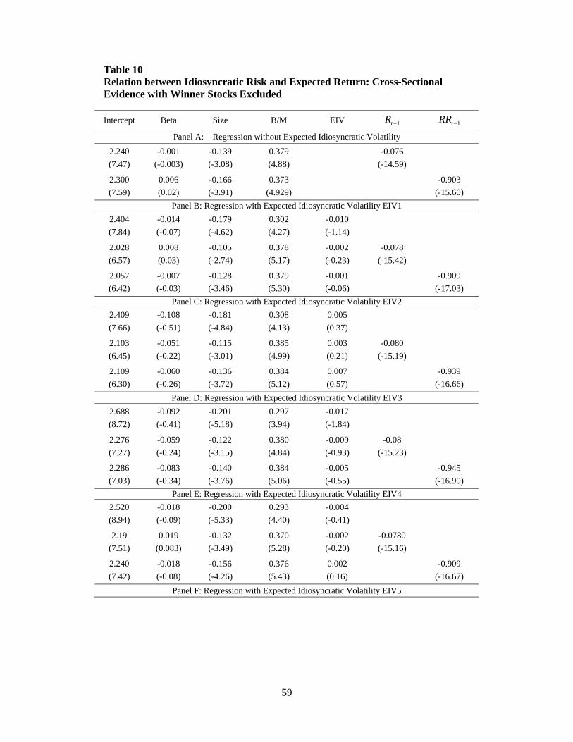
59

Table 10 Relation between Idiosyncratic Risk and Expected Return: Cross-Sectional Evidence with Winner Stocks Excluded

Intercept Beta Size B/M EIV 1−tR 1−tRR

Panel A: Regression without Expected Idiosyncratic Volatility

2.240 (7.47)

-0.001 (-0.003)

-0.139 (-3.08)

0.379 (4.88)

-0.076

(-14.59)

2.300 (7.59)

0.006 (0.02)

-0.166 (-3.91)

0.373 (4.929)

-0.903

(-15.60) Panel B: Regression with Expected Idiosyncratic Volatility EIV1

2.404 (7.84)

-0.014 (-0.07)

-0.179 (-4.62)

0.302 (4.27)

-0.010 (-1.14)

2.028 (6.57)

0.008 (0.03)

-0.105 (-2.74)

0.378 (5.17)

-0.002 (-0.23)

-0.078 (-15.42)

2.057 (6.42)

-0.007 (-0.03)

-0.128 (-3.46)

0.379 (5.30)

-0.001 (-0.06)

-0.909

(-17.03) Panel C: Regression with Expected Idiosyncratic Volatility EIV2

2.409 (7.66)

-0.108 (-0.51)

-0.181 (-4.84)

0.308 (4.13)

0.005 (0.37)

2.103 (6.45)

-0.051 (-0.22)

-0.115 (-3.01)

0.385 (4.99)

0.003 (0.21)

-0.080 (-15.19)

2.109 (6.30)

-0.060 (-0.26)

-0.136 (-3.72)

0.384 (5.12)

0.007 (0.57)

-0.939

(-16.66) Panel D: Regression with Expected Idiosyncratic Volatility EIV3

2.688 (8.72)

-0.092 (-0.41)

-0.201 (-5.18)

0.297 (3.94)

-0.017 (-1.84)

2.276 (7.27)

-0.059 (-0.24)

-0.122 (-3.15)

0.380 (4.84)

-0.009 (-0.93)

-0.08 (-15.23)

2.286 (7.03)

-0.083 (-0.34)

-0.140 (-3.76)

0.384 (5.06)

-0.005 (-0.55)

-0.945

(-16.90) Panel E: Regression with Expected Idiosyncratic Volatility EIV4

2.520 (8.94)

-0.018 (-0.09)

-0.200 (-5.33)

0.293 (4.40)

-0.004 (-0.41)

2.19 (7.51)

0.019 (0.083)

-0.132 (-3.49)

0.370 (5.28)

-0.002 (-0.20)

-0.0780 (-15.16)

2.240 (7.42)

-0.018 (-0.08)

-0.156 (-4.26)

0.376 (5.43)

0.002 (0.16)

-0.909

(-16.67) Panel F: Regression with Expected Idiosyncratic Volatility EIV5

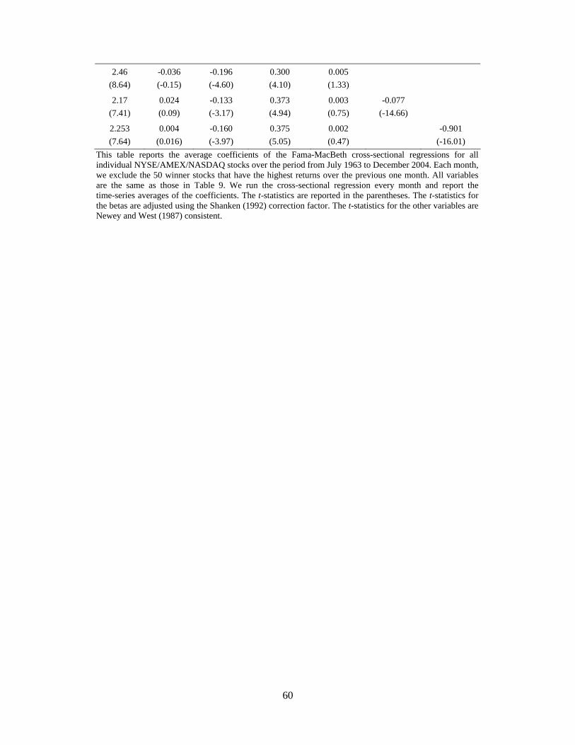
60

2.46 (8.64)

-0.036 (-0.15)

-0.196 (-4.60)

0.300 (4.10)

0.005 (1.33)

2.17 (7.41)

0.024 (0.09)

-0.133 (-3.17)

0.373 (4.94)

0.003 (0.75)

-0.077 (-14.66)

2.253 (7.64)

0.004 (0.016)

-0.160 (-3.97)

0.375 (5.05)

0.002 (0.47)

-0.901

(-16.01) This table reports the average coefficients of the Fama-MacBeth cross-sectional regressions for all individual NYSE/AMEX/NASDAQ stocks over the period from July 1963 to December 2004. Each month, we exclude the 50 winner stocks that have the highest returns over the previous one month. All variables are the same as those in Table 9. We run the cross-sectional regression every month and report the time-series averages of the coefficients. The t-statistics are reported in the parentheses. The t-statistics for the betas are adjusted using the Shanken (1992) correction factor. The t-statistics for the other variables are Newey and West (1987) consistent.

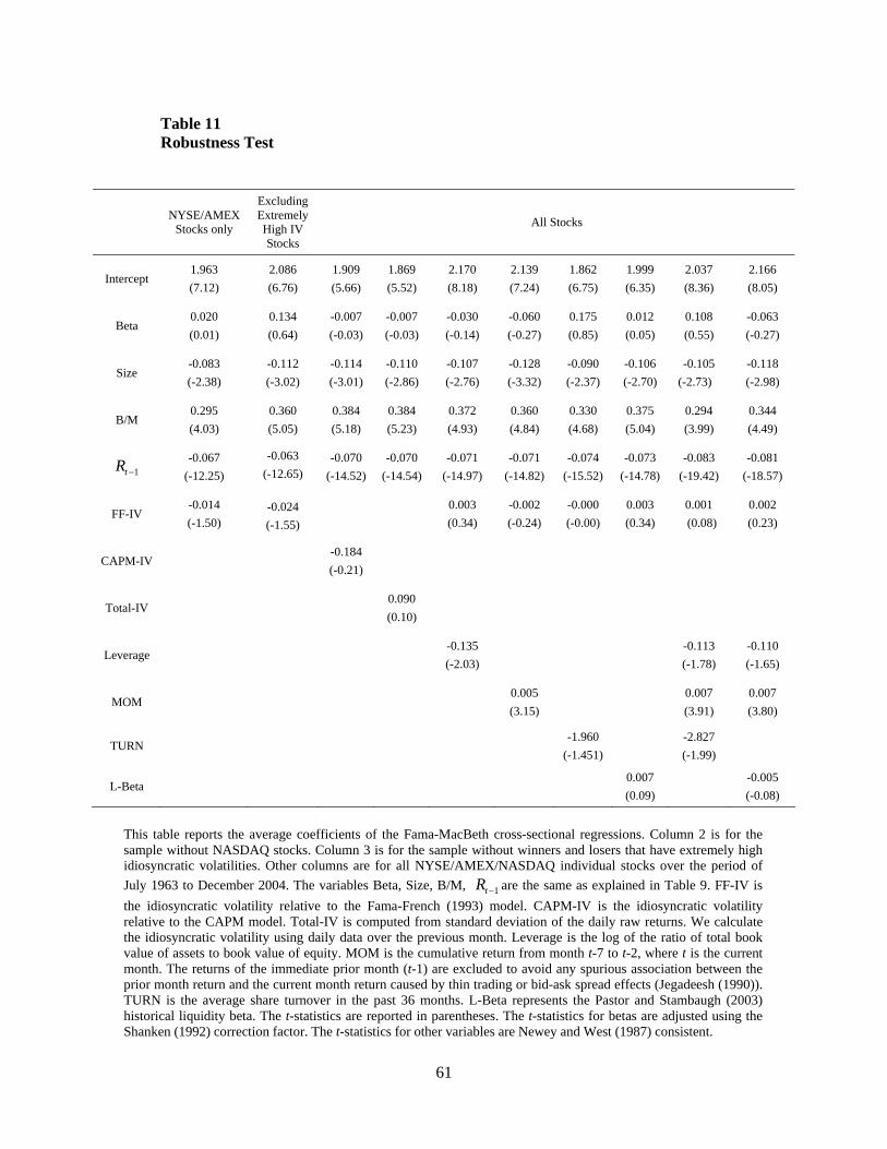
61

Table 11 Robustness Test

NYSE/AMEX Stocks only

Excluding Extremely High IV Stocks

All Stocks

Intercept 1.963 (7.12)

2.086 (6.76)

1.909 (5.66)

1.869 (5.52)

2.170 (8.18)

2.139 (7.24)

1.862 (6.75)

1.999 (6.35)

2.037 (8.36)

2.166 (8.05)

Beta 0.020 (0.01)

0.134 (0.64)

-0.007 (-0.03)

-0.007 (-0.03)

-0.030 (-0.14)

-0.060 (-0.27)

0.175 (0.85)

0.012 (0.05)

0.108 (0.55)

-0.063 (-0.27)

Size -0.083 (-2.38)

-0.112 (-3.02)

-0.114 (-3.01)

-0.110 (-2.86)

-0.107 (-2.76)

-0.128 (-3.32)

-0.090 (-2.37)

-0.106 (-2.70)

-0.105 (-2.73)

-0.118 (-2.98)

B/M 0.295 (4.03)

0.360 (5.05)

0.384 (5.18)

0.384 (5.23)

0.372 (4.93)

0.360 (4.84)

0.330 (4.68)

0.375 (5.04)

0.294 (3.99)

0.344 (4.49)

1−tR -0.067

(-12.25)

-0.063 (-12.65)

-0.070 (-14.52)

-0.070 (-14.54)

-0.071 (-14.97)

-0.071 (-14.82)

-0.074 (-15.52)

-0.073 (-14.78)

-0.083 (-19.42)

-0.081 (-18.57)

FF-IV -0.014 (-1.50)

-0.024 (-1.55)

0.003 (0.34)

-0.002 (-0.24)

-0.000 (-0.00)

0.003 (0.34)

0.001 (0.08)

0.002 (0.23)

CAPM-IV -0.184

(-0.21)

Total-IV

0.090 (0.10)

Leverage

-0.135 (-2.03)

-0.113 (-1.78)

-0.110 (-1.65)

MOM

0.005 (3.15)

0.007 (3.91)

0.007 (3.80)

TURN

-1.960

(-1.451)

-2.827 (-1.99)

L-Beta

0.007 (0.09) -0.005

(-0.08)

This table reports the average coefficients of the Fama-MacBeth cross-sectional regressions. Column 2 is for the sample without NASDAQ stocks. Column 3 is for the sample without winners and losers that have extremely high idiosyncratic volatilities. Other columns are for all NYSE/AMEX/NASDAQ individual stocks over the period of July 1963 to December 2004. The variables Beta, Size, B/M, 1−tR are the same as explained in Table 9. FF-IV is the idiosyncratic volatility relative to the Fama-French (1993) model. CAPM-IV is the idiosyncratic volatility relative to the CAPM model. Total-IV is computed from standard deviation of the daily raw returns. We calculate the idiosyncratic volatility using daily data over the previous month. Leverage is the log of the ratio of total book value of assets to book value of equity. MOM is the cumulative return from month t-7 to t-2, where t is the current month. The returns of the immediate prior month (t-1) are excluded to avoid any spurious association between the prior month return and the current month return caused by thin trading or bid-ask spread effects (Jegadeesh (1990)). TURN is the average share turnover in the past 36 months. L-Beta represents the Pastor and Stambaugh (2003) historical liquidity beta. The t-statistics are reported in parentheses. The t-statistics for betas are adjusted using the Shanken (1992) correction factor. The t-statistics for other variables are Newey and West (1987) consistent.

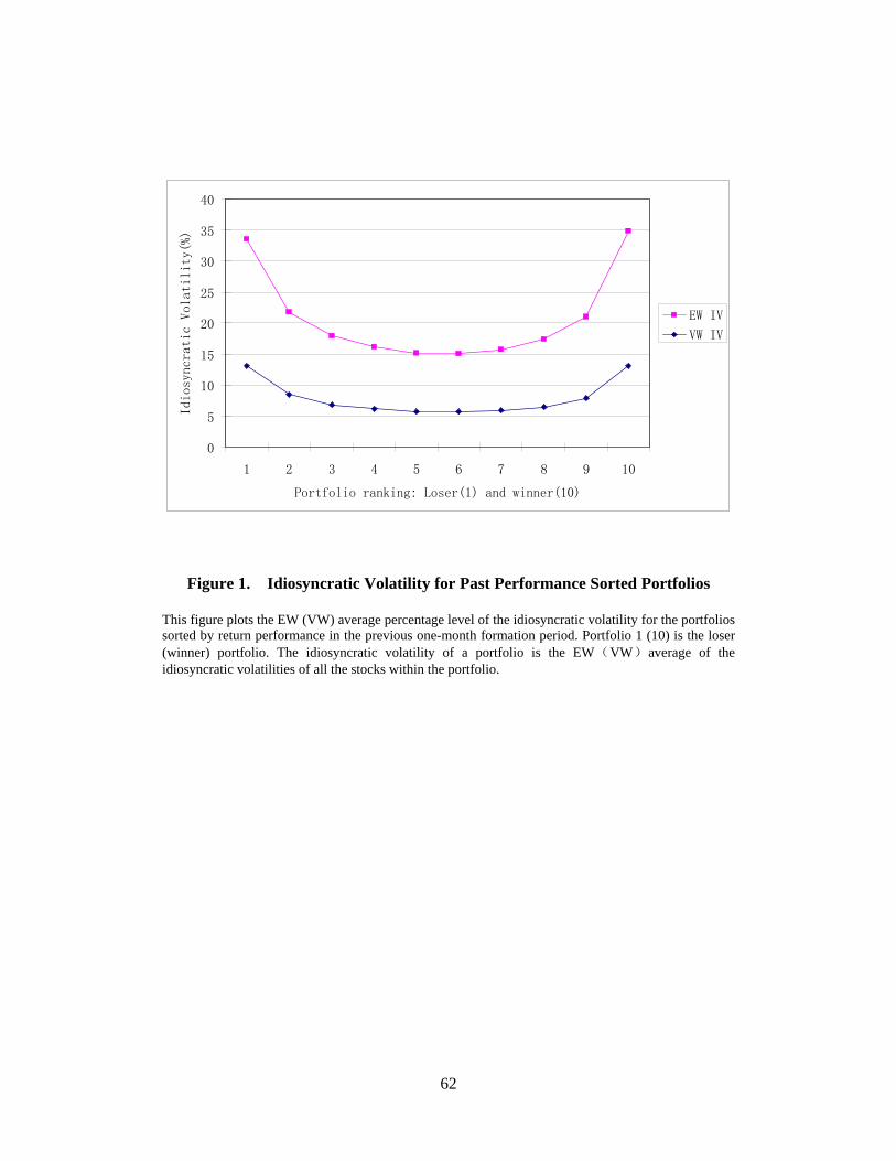
62

0

5

10

15

20

25

30

35

40

1 2 3 4 5 6 7 8 9 10

Portfolio ranking: Loser(1) and winner(10)

Idiosyncratic Volatility(%)

EW IV

VW IV

Figure 1. Idiosyncratic Volatility for Past Performance Sorted Portfolios This figure plots the EW (VW) average percentage level of the idiosyncratic volatility for the portfolios sorted by return performance in the previous one-month formation period. Portfolio 1 (10) is the loser (winner) portfolio. The idiosyncratic volatility of a portfolio is the EW（VW）average of the idiosyncratic volatilities of all the stocks within the portfolio.

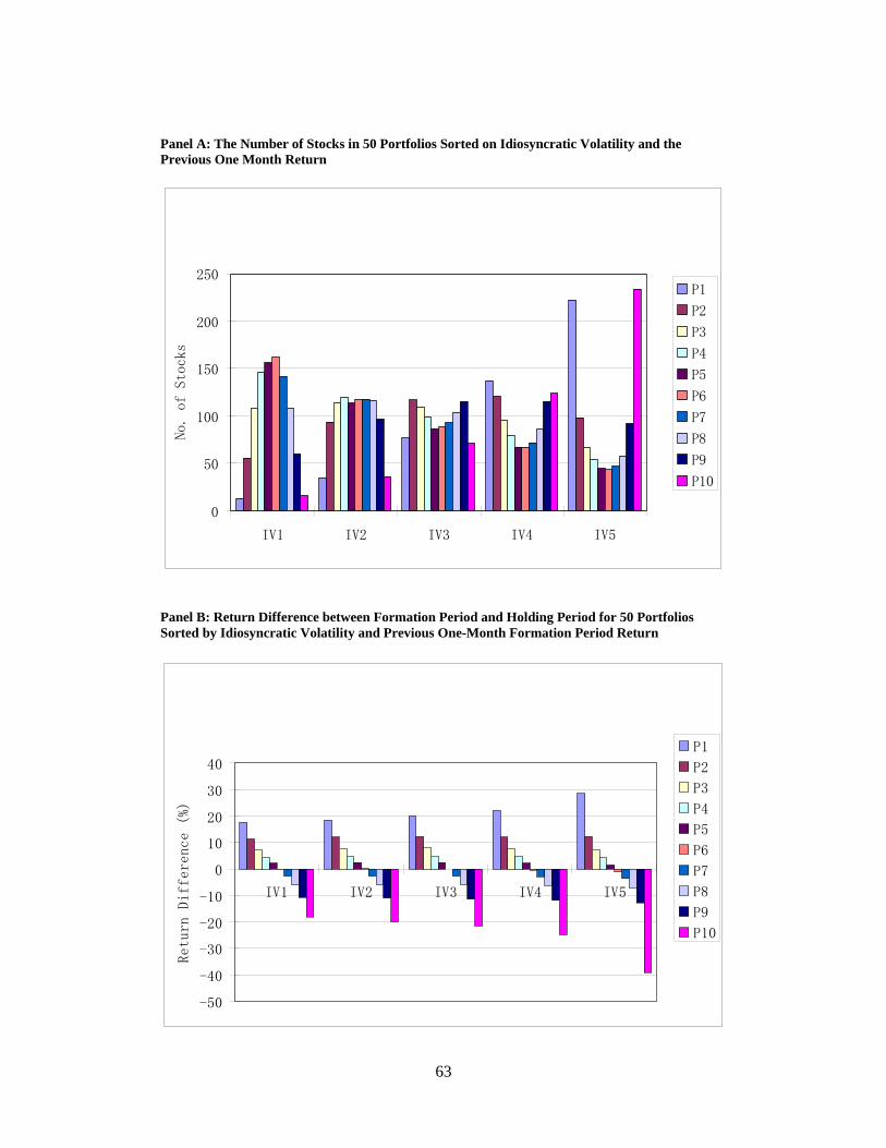
63

Panel A: The Number of Stocks in 50 Portfolios Sorted on Idiosyncratic Volatility and the Previous One Month Return

0

50

100

150

200

250

IV1 IV2 IV3 IV4 IV5

No.

of Stoc

ks

P1

P2

P3

P4

P5

P6

P7

P8

P9

P10

Panel B: Return Difference between Formation Period and Holding Period for 50 Portfolios Sorted by Idiosyncratic Volatility and Previous One-Month Formation Period Return

-50

-40

-30

-20

-10

0

10

20

30

40

IV1 IV2 IV3 IV4 IV5

Return Difference (%)

P1

P2

P3

P4

P5

P6

P7

P8

P9

P10

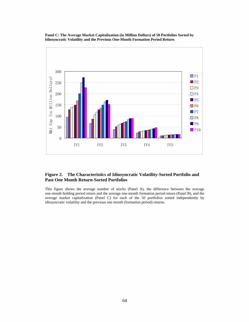
64

Panel C: The Average Market Capitalization (in Million Dollars) of 50 Portfolios Sorted by Idiosyncratic Volatility and the Previous One-Month Formation Period Return

0

50

100

150

200

250

300

IV1 IV2 IV3 IV4 IV5

Mkt Cap (in Mil

lion Dollar

s)

P1

P2

P3

P4

P5

P6

P7

P8

P9

P10

Figure 2. The Characteristics of Idiosyncratic Volatility-Sorted Portfolio and Past One Month Return-Sorted Portfolios This figure shows the average number of stocks (Panel A), the difference between the average one-month holding period return and the average one-month formation period return (Panel B), and the average market capitalization (Panel C) for each of the 50 portfolios sorted independently by idiosyncratic volatility and the previous one month (formation period) returns.