Embed Size (px)
Citation preview

Accrual reversals and cash conversion∗
Matthew J. Bloomfield1, Joseph Gerakos†1 and Andrei Kovrijnykh2
1University of Chicago Booth School of Business
2W. P. Carey School of Business, Arizona State University
June 13, 2015
Abstract
We estimate the firm-level rate at which working capital accruals convert into future cash flows.
These conversion rates determine the expected cash value of a dollar of working capital accruals
and can therefore be used to improve the comparability of accruals across firms. For firms whose
accrual innovations reverse within one year, we find that, on average, a one dollar innovation
to accruals translates into 95 cents of cash flow in the subsequent fiscal year. We find that the
relation between working capital accruals and annual returns increases with the rate at which
accrual innovations convert to cash flows. Moreover, when accrual innovations convert more
quickly and completely to cash flows, firms are less likely to receive an Accounting and Auditing
Enforcement Release (AAER) from the SEC.
JEL classifications: M41, M42.
Keywords: Accruals; earnings; cash flows; AAERs.
∗We thank Ray Ball, Phil Berger, Rob Bloomfield, Ilia Dichev (discussant), Peter Easton, Frank Ecker (discussant),Rich Frankel, Richard Leftwich, Michal Matejka, Xiumin Martin, Mike Minnis, Valeri Nikolaev, Doug Skinner, JimWahlen, Terri Yohn, Paul Zarowin, and workshop participants at Arizona State University, Indiana University, theUniversity of Chicago, and Washington University at St. Louis, and conference participants at the 2014 Conferenceon Financial Economics and Accounting and the 2015 Financial Accounting and Reporting Section Midyear Meetingfor their comments.†Corresponding author. Mailing address: University of Chicago Booth School of Business, 5807 South Wood-
lawn Avenue, Chicago, IL 60637, United States. E-mail address: [email protected]. Telephone number:+1 (773) 834-6882.

1. Introduction
When accountants include accruals in the calculation of earnings, there is an implicit notion that
a dollar of accruals converts into a dollar of cash flows. We demonstrate, in the context of working
capital accruals, that firms vary in this respect—a dollar of accruals can be worth more in some
firms than in others. In absolute terms, a dollar of accruals can be worth more or less than a dollar
of cash, depending on the firm’s accounting policies, composition of accruals, estimation errors, and
manipulation. For example, if a firm systematically over-estimates (under-estimates) the allowance
for doubtful accounts, then a dollar of accounts receivable will convert, in expectation, into more
(less) than a dollar of future cash flows. When the expected cash value of a dollar of accruals varies
across firms, the simple addition of accruals and cash flows reduces the comparability of earnings.
We propose a methodology to estimate, at the firm-level, the expected cash value of a dollar of
working capital accruals. These expected cash values can be used to adjust accruals to increase their
comparability across firms. To estimate expected cash values, we leverage a mechanical property of
accrual accounting: any accrual must eventually reverse, either by converting into cash flows or by
being written off. As an example, consider accounts receivable. When a payment for a sale shifts
from one financial reporting period to the subsequent period, this shift affects accruals in both
periods by the same amount but with opposite signs. The accrual in the first period increases by
the sale amount—an effect we term the “innovation.” In the subsequent period, after the receivable
is paid off (or written off), the accrual decreases by the amount of the sale—an effect we refer to
as the “reversal.”
From a statistical perspective, the mechanical relation between current innovations and subse-
quent reversals implies that working capital accruals follow a moving average process. If accrual
innovations fully reverse in one year, then a single moving average term with a coefficient of negative
one describes the reversal. Reversals that occur over multiple years can be described by multiple
moving average terms whose coefficients sum to negative one.
We find that 73% of the firms in our sample have an estimated MA(1) coefficient that is
indistinguishable from negative one, which corresponds to accrual innovations fully reversing within
1

one year. If we allow for multiple moving average terms (i.e., MA(2) or MA(3)), we find that the
sum of the estimated moving average coefficients converges to negative one for 95% of our sample.
These results provide support for modeling firm-level accrual reversals as a moving average process.1
The moving average regression allows us to identify the unexpected portion of a period’s accrual
innovation—the accrual “shock”—as the regression residual.2 These accrual shocks underpin our
estimation of each firm’s cash “conversion rate” (i.e., the expected cash value of a one dollar
accrual innovation). For each firm, we regress future cash flows on the estimated accrual shocks
and interpret the slope coefficient as the firm’s conversion rate. We find that the distribution of
our estimated conversion rates has significant mass close to one, indicating that, for the typical
firm, accrual innovations almost fully convert into cash flows within one year. The estimated rate
at which accrual innovations convert into cash flows is greater than one for some firms. Although
this could be simply dismissed as estimation noise, we believe that the conversion rate can truly
be greater than one for some firms. That is, a one dollar innovation to accruals converts into more
than one dollar of cash flows within one year. Such a rate can occur when the firm is systematically
unconditionally conservative in estimating future gains associated with the current assets.
We next examine whether accruals with high estimated conversion rates have stronger associa-
tions with returns than accruals with low estimated conversion rates. Consistent with our measure
capturing the expected cash value of accruals, we find that the association between accruals and
annual returns increases in the cash conversion rate. As a final step, we validate our cash con-
version measure by examining whether it is associated with the likelihood that a firm receives
an Accounting and Auditing Enforcement Release (“AAER”), which the Securities and Exchange
Commission issues after concluding an investigation of misconduct. We explore this association
under the intuition that a low conversion rate is indicative of poor financial reporting, which can
include earnings management. We find that the rate at which a firm’s accrual innovations convert
1These findings provide evidence that OLS regressions of accruals on firm fundamentals likely have negativelyautocorrelated errors, thereby requiring a standard error adjustment.
2Unlike many previous studies (e.g. Jones (1991), Dechow and Dichev (2002)), we do not interpret these resid-uals as evidence of earnings management or “discretionary” accruals. In our framework, they arise naturally fromunexpected timing differences between economic transactions and cash receipts or disbursals.
2

into cash flows is negatively associated with the likelihood that the firm receives an AAER. We
further study the link between the speed of reversals and AAER issuances. Consistent with the
possibility that slower reversals are the result of delayed write-offs, we find that AAERs are more
likely for firms with slower reversal speeds.3
We contribute to the accounting literature along multiple dimensions. First, we explicitly
model accruals as a stochastic process. Our approach allows us to distinguish between the current
innovation and the reversal of the past innovation. We demonstrate, analytically and empirically,
that accrual reversals can be captured using a moving average specification. For 95% of the firms
in our sample, we find full reversal within three years.4 Moreover, including the moving average
term in the accrual regression doubles explanatory power as measured by Adjusted R2. These
findings contrast with the results of Allen, Larson, and Sloan (2013). They find that the reversal
of accrual innovations is limited to “good” accruals, which they define as accruals predicted by the
Dechow-Dichev model. At the same time, they find no evidence of reversals in accrual estimation
errors, which represent half of the accrual volatility in their setting.
The cash conversion rate can replace traditional discretionary accrual measures in their role as
proxies for accrual quality (e.g., Jones, 1991; Dechow and Dichev, 2002). A benefit of using the
cash conversion rate as a measure of accrual quality is that it is not contaminated by operating
volatility. The inability to separate accrual quality from operating volatility has been a major
concern regarding the traditional measures (for example, McNichols, 2002; Kothari, Leone, and
Wasley, 2005; Hribar and Nichols, 2007; Wysocki, 2009; Ball, 2013).
We also extend prior research that examines the time series structure of accruals, cash flows, and
earnings. For example, Dechow, Kothari, and Watts (1998) propose a model that explains the serial
and cross-correlations of accruals, cash flows, and earnings. In their model, sales follow a random
3Note that “speed” and “rate” are not synonymous in the context of our study. We use “speed” in reference toaccrual reversals, where the reversal speed is defined by the number of years required for a complete reversal. We use“rate” in reference to cash conversion, where the conversion rate is defined as the expected cash value of a one dollaraccrual innovation. In particular, a “complete reversal” does not imply that the accrual innovation fully convertedinto cash—it could have been written off.
4In a related study, Dechow, Hutton, Kim, and Sloan (2012) examine the timing of accrual reversals around AAERevents.
3

walk, and shocks to sales are the only source of uncertainty. Similar to Jones (1991), they assume
a deterministic relationship between sales and working capital.5 This deterministic relationship,
along with a random walk in sales, allows for a simple temporal structure in the three accounting
series. We extend this approach by introducing another source of uncertainty. Specifically, we
allow for innovations to working capital that represent timing differences. Timing differences occur
when cash receipts or disbursals are temporally separated from associated economic transactions.
To the extent such events are random, they represent an additional source of uncertainty. Such
uncertainty breaks the deterministic link between sales and working capital.
In addition, we contribute to the literature on the temporal structure of accounting variables
(e.g., Dechow, 1994). The motivations for this literature include the prediction of future cash flows
and the analysis of why earnings outperform cash flows in predicting future cash flows. In the
second stage of our analysis, we revisit the prediction of future cash flows and find that we improve
the predictive ability of the model by including estimated shocks to working capital as a regressor.
Finally, it is worth relating our measure to the empirical result that accruals and cash flows are
negatively correlated. Dechow (1994) attributes this negative correlation to the “natural” smooth-
ing role of accruals. Subsequent research attributes cross-sectional variation in this correlation to
earnings management and differences in accrual quality (for example, Leuz, Nanda, and Wysocki,
2003). In our model, the negative correlation arises naturally because shocks to working capital
enter accruals and cash flows with opposite signs. Cross-sectional variation in the correlation is
determined by the relative magnitude of working capital shocks to sales shocks, thereby limiting
the ability of the correlation to capture accrual quality.
There are several caveats to our cash conversion estimates. First, we estimate the conversion
rates for accrual shocks rather than for entire accruals. Hence, we estimate the conversion rate only
for the unexpected portion of accruals. We do so because statistically reversals can be identified
only for shocks and not for entire accruals. As discussed by Allen, Larson, and Sloan (2013), when
a reversing accrual is replaced by a new accrual of the same magnitude, there is no effect on the
5For an additional example of this assumption, see Barth, Cram, and Nelson (2001).
4

level of total accruals and therefore no variation useful for the statistical estimation of reversals
or cash conversion. In principle, the expected and unexpected components of accruals can convert
into cash at different rates. One should keep this caveat in mind when interpreting our results.
Second, we estimate average conversion rates over the firm’s recorded history. Our methodology
works best if conversion rates are stationary. This may not be the case if, for example, cash
conversion rates vary through time in response to changes in firms’ strategies and macroeconomic
conditions. Our estimates do not capture such changes.
Third, our approach emphasizes the expected cash value of accruals. Under our valuation
perspective, a higher conversion rate always implies higher value regardless of whether the rate is
smaller or greater than one. However, from the perspective of comparing the cash and non-cash
components of earnings, one could argue that the ideal conversion rate is precisely one, because
when accruals are combined with cash flows to calculate earnings, the scale of both components of
earnings needs to be the same. We do not take this position and instead interpret our measure as
purely directional, with a higher conversion rate corresponding to higher expected cash value.
2. Variation in cash conversion rates
Prior research (e.g., Dechow and Dichev, 2002) typically assumes that the average conversion
rate of a dollar of accruals to cash is one. However, there are many reasons why there could be
variation in the average conversion rate. We discuss several scenarios below.
2.1. Financial reporting choices
Financial reporting choices that affect the conversion rate can be broadly described as a degree
of unconditional conservatism in managerial estimates relating to working capital. For example, the
bad debt allowance can be used to inflate or deflate accounts receivable at the manager’s discretion
(e.g., Jackson and Liu, 2010). If the manager systematically classifies 40% of accounts receivable
as bad debt whereas the actual collection rate is on average 75%, then the conversion rate for
accounts receivable will be 75/(100-40), or 1.25. If, on the other hand, the manager allows for no
5
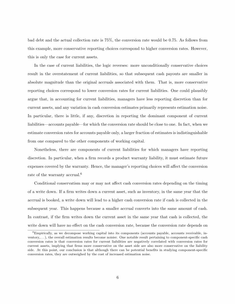
bad debt and the actual collection rate is 75%, the conversion rate would be 0.75. As follows from
this example, more conservative reporting choices correspond to higher conversion rates. However,
this is only the case for current assets.
In the case of current liabilities, the logic reverses: more unconditionally conservative choices
result in the overstatement of current liabilities, so that subsequent cash payouts are smaller in
absolute magnitude than the original accruals associated with them. That is, more conservative
reporting choices correspond to lower conversion rates for current liabilities. One could plausibly
argue that, in accounting for current liabilities, managers have less reporting discretion than for
current assets, and any variation in cash conversion estimates primarily represents estimation noise.
In particular, there is little, if any, discretion in reporting the dominant component of current
liabilities—accounts payable—for which the conversion rate should be close to one. In fact, when we
estimate conversion rates for accounts payable only, a larger fraction of estimates is indistinguishable
from one compared to the other components of working capital.
Nonetheless, there are components of current liabilities for which managers have reporting
discretion. In particular, when a firm records a product warranty liability, it must estimate future
expenses covered by the warranty. Hence, the manager’s reporting choices will affect the conversion
rate of the warranty accrual.6
Conditional conservatism may or may not affect cash conversion rates depending on the timing
of a write down. If a firm writes down a current asset, such as inventory, in the same year that the
accrual is booked, a write down will lead to a higher cash conversion rate if cash is collected in the
subsequent year. This happens because a smaller accrual converts into the same amount of cash.
In contrast, if the firm writes down the current asset in the same year that cash is collected, the
write down will have no effect on the cash conversion rate, because the conversion rate depends on
6Empirically, as we decompose working capital into its components (accounts payable, accounts receivable, in-ventory,. . . ), the overall estimation results become noisier. One notable result pertaining to component-specific cashconversion rates is that conversion rates for current liabilities are negatively correlated with conversion rates forcurrent assets, implying that firms more conservative on the asset side are also more conservative on the liabilityside. At this point, our conclusion is that although there can be potential benefits in studying component-specificconversion rates, they are outweighed by the cost of increased estimation noise.
6

the prior year’s ending accrual. Thus, firms that write down assets in a more timely fashion will,
ceteris paribus, have higher conversion rates.
2.2. Inventory
It is convenient to distinguish two types of shocks to working capital operating through the
firm’s inventory—procurement shocks and sales shocks. Consider a firm that spends $50 of cash
on January 1 of every year on inventory. It sells the inventory to a single client for $100 of cash on
December 31 of the same year. The net cash flow of the firm in steady state is $50 and it has no
accruals in the normal course of business.
In the context of this example, a procurement shock would occur if the firm purchased inventory
for year t one day earlier, on December 31 of the year t−1. The net cash flow in year t−1 would
be zero ($100 of revenue minus $50 for inventory purchased on January 1 and $50 for inventory
purchased on December 31), and in year t it would be $100 ($100 of revenue and no cash outflow
for inventory). In this case, the period t−1 inventory shock would be $50, which is the difference
between actual inventory of $50 and the steady state inventory of $0. Similarly, the period t shock
to net cash flow would also be $50, which is the difference between the period’s net cash flow of $100
and the steady state net cash flow of $50. The cash conversion rate in this case would therefore be
equal to one.
For this same firm, a sales shock would occur if the sale of inventory takes place on January 1
of year t+1 instead of December 31 of year t. In this case, there will be no sales in period t and
$50 worth of inventory at the end of year t. Hence, the net cash flow of year t would be negative
$50. At the end of year t+1, there will be no inventory and sales in year t+1 would be $200. Thus,
net cash flow for year t+1 would be $150. In this example, every dollar of the inventory shock
translates into two dollars of net cash flow in the subsequent period (i.e., the cash conversion rate
is two).
In both of the above scenarios, economic events resulted in a $50 shock to inventory. However,
7

the cash conversion rates associated with these shocks differ—a rate of one for the procurement
shock and a rate of two for the sales shock.7
2.3. Accounting estimation errors
Unlike unconditional conservatism, accounting estimation errors do not represent any particular
“bias” in accruals. Hence, one might conclude that estimation errors have no effect on the average
cash conversion rate. Nonetheless, the effect is there and is akin to the attenuation bias caused
by measurement error in a regressor—it drives the conversion rate toward zero. However, unlike
traditional measurement error in a regressor, accounting estimation errors do not lead to a biased
statistical estimate of the conversion rate. Instead, they drive the actual conversion rate toward
zero, because the accounting estimation error is a part of the reported accrual that does not convert
into cash.
An important caveat is that our approach estimates the cash conversion rate for unexpected
accruals. To the extent that estimation errors reside solely in unexpected accruals, they may lead to
a divergence between the cash conversion rates for expected and unexpected accruals. For example,
if 100% of unexpected accruals are accounting estimation errors, then the actual conversion rate
for unexpected accruals will be zero, because estimation errors are unrelated to future cash flows.
At the same time, the firm can have a perfectly predictable level of accruals for which the cash
conversion rate will be one (e.g., $100 dollars of accruals always converts into $100 of cash in the
subsequent year).
3. Accrual reversals
In this Section, we outline the mechanics of accrual reversals and our approach to identifying
accrual shocks. The central assumption in our specification is that the balances of working capital
7Neither sales shocks nor procurement shocks generate a plausible scenario where the firm continually fails torecoup inventory purchases. The lack of a justified write down can, however, lead to a conversion rate lower thanone. For example, assume that there is inventory at the end of the year that will have to be sold at a discount fromcost in the subsequent year. If the firm does not write down this inventory at the end of the year, the cash conversionrate will be less than one.
8

accounts cannot be perfectly predicted based other accounting variables, such as sales and earn-
ings. We distinguish between expected levels of working capital (e.g., accounts receivable, accounts
payable, and inventory), which represent expectations based on other observable variables, and in-
novations to the levels of working capital that represent new information and which are independent
and identically distributed across periods.
For example, the levels of the working capital accounts8 can be specified as follows:
ARt = ARt + εAR,t
INVt = INV t + εINV,t
APt = AP t + εAP,t,
in which ARt, INV t, and AP t represent expectations based on other observable accounting vari-
ables commonly used in the literature (e.g., sales). Note that these conditional expectations are not
forecasts in a predictive sense. Instead, they represent a summary of all information about working
capital account balances contained in other observable, contemporaneous accounting variables. In
particular, the conditioning variables can include earnings and sales that are contemporaneous with
accruals.9
The level of working capital can then be expressed as:
WCt = ARt + INVt −APt
= (ARt + INV t −AP t) + (εAR,t + εINV,t − εAP,t).
This equation can be simplified as:
WCt = WCt + εt, (1)
8Working capital is the difference between current assets and current liabilities. For expository purposes, weuse just accounts receivable, inventory, and accounts payable in this example. In our empirical analyses, we use acomprehensive measure of working capital accruals based on Dechow and Dichev (2002).
9Note, however, that we cannot condition on both cash flows and earnings given the identity that accruals equalearnings minus cash flows.
9

in which WCt represents period t’s expected level of working capital and the accrual shock εt =
εAR,t + εINV,t − εAP,t. In our specification, accrual shocks capture information in accruals that
is incremental to that included in observable accounting variables. The shocks can arise from
fundamental sources (such as random delays in payments) as well as actions by the manager (i.e.,
estimation errors or earnings management).
If we re-express equation (1) in changes, then:
∆WCt = WCt −WCt−1 = ∆WCt − εt−1 + εt. (2)
In what follows we refer to ∆WCt as period t’s “accrual.” Note that in this equation, period t’s
accrual includes the current period’s shock, εt, as well as the reversal of the prior period’s shock,
εt−1. This specification requires that shocks are independent across periods.
From a statistical perspective, it is convenient to think about the reversal of εt−1 in terms of a
moving average process. Complete reversal of εt−1 in year t corresponds to a moving average coef-
ficient equal to negative one. However, innovations might not necessarily reverse in the subsequent
year. For example, if a firm keeps uncollectable accounts on the books for multiple years before
writing them off, the reversal will spread over multiple years. For these firms, complete reversal
implies that the sum of multiple moving average coefficients converges to negative one.
As a simple example that focuses on just one working capital account, consider a firm with a
fixed level of annual revenue that faces uncertainty about when it collects payment for this revenue,
but all payments are collected within a year. For such a firm, the accounts receivable accrual will
be stochastic even though revenue is deterministic. As an example of a negative shock, consider
a customer that typically buys on credit but in this period pays cash. This cash purchase would
represent a negative shock to accounts receivable. A positive shock would be a customer who
typically pays cash but buys on credit in this period. At the end of the fiscal year, the level of the
accounts receivable accrual, ARt, will equal the unpaid balance for the year’s transactions. Hence,
the change in the accounts receivable accrual, ∆ARt, will equal the current year’s unpaid balance
minus last year’s unpaid balance. Thus, ∆ARt can be described by the following moving average
10

process:
∆ARi,t = αi + φXi,t + θiεi,t−1 + εi,t (3)
where αi represents firm i’s average change in accounts receivable, Xi,t represents control variables,
εi,t represents the period’s shock to accounts receivable, and εi,t−1 represents the prior period’s
shock to accounts receivable with θi determining the extent to which the prior period’s shock
reverses.
4. Empirical approach
We describe in this Section our empirical approach to estimating both accrual reversals and the
cash conversion rate. We begin our empirical analysis by estimating accrual shocks on a firm-by-firm
basis using the following moving average specification:
∆WCi,t = αi + φiXi,t + θiεi,t−1 + εi,t, (4)
where αi represents firm i’s average change in working capital, Xi,t represents control variables, εi,t
represents the period’s shock to working capital accruals, and εi,t−1 represents the prior period’s
shock to working capital accruals with θi determining the extent to which the prior period’s shock
to accruals reverses. If firm i’s working capital accruals fully reverse within one year, then θi will
be close to negative one.
Shocks to accruals eventually reverse in one of two ways—either into cash flows or as a write-off.
To estimate the propensity of these shocks to convert into cash flows rather than being written
off, we regress next year’s operating cash flows on the estimated accrual shocks. We run these
regressions at the firm-level and interpret the coefficient on the accrual shock as the firm-specific
conversion rate (i.e. the expected cash value of a dollar of accruals):
CFOi,t+1 = αi + βiεi,t + γiXi,t + ηi,t+1, (5)
11

where i indexes firms, t indexes fiscal years, CFO represents cash flows, α represents average levels
of cash flows, X and γ represent control variables and their coefficients, and η represents the error
term. Firm i’s cash conversion rate is βi, which is the coefficient on the estimated accrual shock,
εi,t. This coefficient measures the extent to which a particular firm’s accrual shocks translate into
next year’s cash flows.
This specification allows the estimated cash conversion rate to vary across firms. Given that
earnings are calculated as the sum of cash flows and accruals (which implicitly assumes a cash
conversion rate of one), one might expect that the estimated cash conversion rate (βi) would be
close to one for all firms. However, as we discuss in Section 2, financial reporting choices, inventory,
and estimation errors can drive variation in cash conversion rates.
Our working capital measure includes deferred revenue along with current assets and other
current liabilities. Relative to accruals that are followed by a cash receipt or payment, deferred
revenue is less intuitive with respect to the cash conversion rate. The logic for deferred revenue is
that a positive shock to deferred revenue constitutes a negative accrual shock, which is associated
with a negative shock to the subsequent period’s cash flow. Conditional on next period’s earnings,
overall cash flows will be lower than usual because the cash associated with the deferred revenue
shock was received in the previous period.10
If our specification for accruals reversals and cash conversion is descriptive, then we would expect
several empirical regularities. First, the distribution of estimated moving average coefficients in the
MA(1) specification will have substantial mass at negative one. Second, for the subset of firms
with estimated moving average coefficients that differ from negative one in the MA(1) specification,
moving average terms in the MA(q) specification will sum to negative one. Third, the mass of the
estimated cash conversion rates will be close to one.
Further, we propose several applications of our cash conversion measure, which can be considered
validations of our approach. First, we examine whether equity markets place higher value on
10Cash has already been received when the firm books a deferred revenue accrual. Hence, deferred revenue is unlikelyto be a driver of heterogeneity in cash conversion rates across firms. However, it could be a major determinant of thetiming of accrual reversals, which we examine in later empirical analysis.
12

accruals that have greater expected cash value. Second, we examine whether low cash conversion
rates are associated with lower financial reporting quality as proxied by receiving an AAER.
5. Data and variables
Our sample consists of non-financial firms from the Compustat Annual Fundamentals Merged
file. To construct our working capital accruals measure, we follow Hribar and Collins (2002) and
use Compustat’s Statement of Cash Flows data. We require non-missing firm-year observations for
total assets (AT), operating cash flows (CFO), revenue (REVT), costs of goods sold (COGS) income
before extraordinary items (IB), change in accounts receivable (RECCH), and change in inventory
(INVCH). Following Dechow and Dichev (2002), we drop firms with fewer than eight years of data.
Finally, we require that the moving average regression converges. Our sample selection process
leads to a sample of 74,148 firm-years from 5,206 unique firms over the period 1987–2013.
We define working capital accruals (∆WC) as the sum of changes in accounts receivable, in-
ventory, and other assets (net of liabilities) less the sum of changes in accounts payable and taxes
payable. From Compustat, this measure can be constructed as:
∆WC = −(RECCH + INV CH +APALCH + TXACH +AOLOCH). (6)
We set missing values of APALCH, AOLOCH, and TXACH equal to zero. This measure of working
capital accruals is based on the cash flow statement and is identical to that used in Dechow and
Dichev (2002). We differ, however, in that we do not scale our measure by average total assets.
Given that our estimation of firm-level conversion rates is based on firm-level time series regressions,
there is no benefit to scaling. Moreover, because we do not scale, our measure of cash conversion has
a simple economic interpretation—the extent to which a one dollar innovation to accruals converts
into future cash flows. If we were to follow prior research and deflate by total assets, we would lose
this simple economic interpretation.
To validate the cash conversion and accrual quality measures, we further employ stock return
13
data from CRSP and AAER issuance data from UC Berkeley’s Center for Financial Reporting &
Management.
6. Results
6.1. Moving average regressions
We start by estimating equation (4) on firm-by-firm basis. In the regressions, we include several
variables to control for ∆WCt: revenue (REVT); cost of goods sold (COGS); selling, general, and
administrative expenses (XSGA) to capture supply and demand shocks; and special items (SPI)
to capture write-offs and other one time events. We take these variables from Compustat and set
missing values of XSGA and SPI equal to zero. We find similar results if we exclude special items
and if we estimate the regressions with no control variables. Our empirical specification is then:
∆WCi,t = αi + φ1,iREV Ti,t + φ2,iCOGSi,t + φ3,iSGAi,t + φ4,iSPIi,t +
q∑j=1
θi,jεi,t−j + εi,t, (7)
where εi,t represents firm i’s accrual innovation in period t and q represents the number of moving
average terms. The results for these regressions are presented in Table 2.
Panel A presents descriptive statistics for the distributions of the estimated coefficients when we
allow for only one moving average term (i.e., q = 1). The median coefficient on the moving average
term is negative one and continues to be negative one up to the 73rd percentile, implying that for the
majority of firms, an accrual shock fully reverses within one year. The coefficients on revenue, cost
of goods sold, and selling, general, and administrative expenses are consistent with intuition. A one
dollar increase in revenue is, on average, associated with a 24-cent increase in accruals. Similarly,
one dollar increases in costs of goods sold and selling, general, and administrative expenses are,
on average, associated with 23- and 25-cent decreases in accruals. With respect to special items,
(which includes write-offs,) a one dollar decrease is, on average, associated with a 10-cent decrease
in accruals. In terms of explanatory power, the moving average regressions have an average adjusted
14

R2 of 0.423. If we estimate ordinary least squares regressions with the same control variables, but
exclude the moving average term, the average adjusted R2 drops by over half.
Panel B presents the convergence of the sum of moving average coefficients, θi, as we vary the
number of moving average terms (q). If we allow for one moving average term, the coefficient is
within ±0.01 of negative one for 3,656 of the 5,026 firms in our sample (73%). For the remaining
1,370 firms, if we re-estimate the regressions allowing for two moving average terms (i.e., q = 2),
the sum of the two moving average coefficients is indistinguishable from negative one for 783 firms.
Similarly, if we allow for three moving average terms for the remaining 587 firms, the sum of the
coefficients is indistinguishable from negative one for 313 firms. Overall, if we allow for up to three
moving average terms, the sum of the moving average coefficients is indistinguishable from negative
one for 95% of the sample.
There appears to be an industry effect with respect to the number of moving average terms
required for the coefficient sum to converge to negative one. For example, if we allow for only one
moving average term, the coefficient is indistinguishable from negative one for 77% of retail firms
and 57% of firms in defense and airplane manufacturing.11 We attribute these differences in part
to operating cycles. Retail firms likely have short operating cycles, thereby leading to reversals
within one year. In contrast, defense contractors and airplane manufacturers likely have longer
operating cycles that lead to longer term reversals. However, we cannot rule out the possibility
that the number of required moving average terms reflects the extent to which firms delay writing
off accruals. We examine this alternative interpretation in Section 6.4.
Next, we restrict our analysis to the subset of firms for which the moving average coefficient is
indistinguishable from negative one when we allow for only one moving average term (i.e., q = 1).
We restrict our analysis to this sample in order to reduce measurement error in the estimates
of the accrual innovations. For example, if the results in Panel B of Table 2 arise from cross-
sectional variation in operating cycle, then regressions that allow for only one moving average term
are misspecified for firms with moving average coefficients distinguishable from negative one. Our
11Industries are defined using the Fama and French 48 industry classification.
15

approach is sensitive to measurement error because our estimated accrual innovations serve as
regressors in the next set of regressions. Measurement error would cause attenuation bias in our
estimates of the cash conversion rate. We explore the effect of measurement error in section 8.3
and find evidence inconsistent with measurement error substantially attenuating our estimates of
the cash conversion rate.
For this restricted sample, Panel C presents the distributions of the coefficient estimates for the
control variables. The means and medians presented in Panel C are close to those presented in
Panel A. For example, in Panel C, the means are 0.22, −0.22, −0.23, and 0.09 for revenue, cost of
goods sold, selling, general, and administrative expenses, and special items as compared to 0.24,
−0.23, −0.25, and 0.10 in Panel A.
6.2. Conversion into cash flows and income
We next estimate our measure of the cash conversion rate—the rate at which accrual shocks
convert into future cash flows. To do so, we estimate firm-by-firm regressions based on the specifi-
cation presented in equation (5). Prior research suggests that income before extraordinary items is
an ideal forecaster of future cash flows (e.g., Dechow, Kothari, and Watts, 1998; Ball, Sadka, and
Sadka, 2009). Thus, in our cash flow regressions, we include income before extraordinary items as
a control variable. This leads to the following empirical specification:
CFOi,t+1 = αi + βiεi,t + γiIBi,t + ηi,t+1, (8)
where εi,t is firm i’s estimated accrual shock for period t taken from equation (7). Our measure of
the cash conversion rate, βi, measures the extent to which an accrual shock converts to cash flows
in the subsequent year.
Panel A of Table 3 presents the coefficient estimates from these regressions. The mean and
median estimates of cash conversion are significantly greater than zero and close to one (0.95 and
0.97), implying that for the typical firm, a one dollar shock to accruals converts to 95–97 cents in
the subsequent year. Moreover, these results suggest that estimated accrual innovations provide
16

explanatory power in the prediction of cash flows that is incremental to income before extraordinary
items. In an untabulated test, we find similar results if we use the same controls as those included
in the moving average regressions and if we exclude income before extraordinary items. The mean
and median coefficients on income are 0.43 and 0.31, implying that for the typical firm, a dollar
of income is associated with 31–43 cents of cash flow in the subsequent year. These estimates are
similar in magnitude to those presented in Dechow, Kothari, and Watts (1998, Table 4).
When an accrual innovation is written-off in the following year, the write-off reduces income.
Consistent with our predictions, Panel B of Table 3 shows that accrual innovations are negatively
associated with future earnings. In terms of economic magnitude, on average, nine cents of a one
dollar accrual innovation is written-off in the subsequent year. Furthermore, we find that the rates
at which accrual innovations convert into cash flows and earnings are highly correlated (ρ = 0.46),
suggesting that higher rates of cash conversion can be attributed, in large part, to lower rates of
accrual write-offs.
6.3. Relation with returns
We next examine whether the accruals of firms with higher cash conversion rates have higher
contemporaneous associations with returns than firms with low conversion rates. To do so, we
estimate the following regression specification:
ri,t = α+ βCashF lowi,t + φCRi + γAccrualsi,t + δAccrualsi,t × CRi + Controls+ εi,t, (9)
where ri,t is firm i’s return for year t, CashF lowi,t is firm i’s cash flows from operation deflated by
the market value of equity for year t, Accrualsi,t is firm i’s accruals deflated by the market value
of equity for year t, and CRi is a measure of the rate at which accruals convert into future cash
flows. We use two formulations of CRi, an indicator variable which takes a value of one if a firm’s
estimated conversion rate exceeds one and a continuous variable defined by the percentile rank of
the firm’s estimated conversion rate. As controls, we include in the regressions the natural logarithm
of the firm’s market value of equity and the natural logarithm of the firm’s book-to-market ratio.
17

Panel A of Table 4 presents descriptive statistics for the variables used in the regressions.
Accounting variables and returns are Winsorized at the 2.5% and 97.5% levels. We Winsorize at
this higher level compared to the previous and subsequent analyses due to the increased kurtosis
arising from deflating by the market value of equity. Panel B presents the results. The dependent
variable in the regressions is the buy-and-hold annual return starting four days after the prior
fiscal year’s earnings announcement and ending three days after the current fiscal year’s earnings
announcement. Columns (1) through (3) present baseline regressions that include cash flows and
accruals on their own and together. Cash flows are positively and significantly associated with
returns both on their own and when they are included along with accruals. In contrast, accruals
are significantly positive only when included along with cash flows.
In columns (4) and (5), we add the cash conversion rate measures along with their interactions
with accruals. For both cash conversion rate measures, the coefficients on accruals remain signif-
icant and positive but attenuate in these specifications. In addition, the main effects on the cash
conversion rate measures are negative and significant while the interactions between accruals and
the cash conversion rate measures are positive and significant. In terms of economic significance,
if a firm moves from the lowest to the highest percentile of cash conversion, then the estimated
association of accruals and returns increases by approximately 118%.
6.4. AAERs
We use AAERs to validate our measure under the intuition that a lower cash conversion rate is
likely associated with the firm having lower quality financial reporting, which can include earnings
management. During the sample period, 2.8% of firms received at least one AAER. Table 5 presents
logit regressions that evaluate the association between a firm’s cash conversion rate and likelihood
the firm receives an AAER.
We estimate the logit regressions with and without industry fixed effects (based on the 48 Fama
and French industries) to control for industry effects. We examine this link using two measures
of the cash conversion rate: the estimated rate Winsorized at 1% and 99%; the percentile rank
18
of the estimated conversion rate. In specifications (1) through (4), we analyze only those firms
for which reversals occur within one year. In specifications (5) through (8), we include the entire
sample. Consistent with the notion that a lower cash conversion rate is indicative of weaker financial
reporting, the coefficient on cash conversion is negative and statistically significant at the 0.05 or
0.01 level, across all regressions. Moreover, the coefficients on the cash conversion measure change
only slightly when we include industry fixed effects, suggesting that cross-industry differences do
not drive heterogeneity in conversion rates.12
We next explore the relation between AAERs and the number of moving average terms required
to fully capture the reversal of an accrual innovation. It could be that long (greater than one year)
operating cycles lead to the requirement for more than one moving average term. An alternative
interpretation is that some firms fail to write-off “bad” accruals in a timely fashion. Such firms
instead keep these working capital accruals on their balance sheets for extended periods of time,
despite their low probability of eventual cash conversion. If this is the case, then the likelihood
of receiving an AAER should increase in the number of required moving average terms. When
we examine this prediction in Table 6, we find that the likelihood of receiving an AAER increases
monotonically in the number of moving average terms required to fully capture the reversal of an
accrual innovation.13
7. Relation with prior research
The discretionary accrual literature seeks to explain accruals via other accounting variables
(e.g., sales and property, plant & equipment). Under this traditional approach, accrual quality is
defined as the ability of these other accounting variables to explain variation in accruals and all
residual volatility is interpreted as “low” quality accruals (see Gerakos, 2012).
Ironically, the traditional approach assumes that high quality accruals have no informational
12We find similar results if we estimate an ordinary least square regression that uses the proportion of years thatreceived an AAER as the dependent variable.
13Again, we find similar results if we estimate an ordinary least square regression that uses the proportion of yearsthat received an AAER as the dependent variable.
19

value because all information is contained in the other accounting variables. This assumption
contrasts with the Financial Accounting Standards Board’s view of accrual accounting:
Information about enterprise earnings based on accrual accounting generally provides a
better indication of an enterprise’s present and continuing ability to generate favorable
cash flows than information limited to financial effects of cash receipts and payments.
(Financial Accounting Standards Board, 1978)
Consistent with accruals having informational value, Subramanyam (1996) finds that discretionary
accruals are positively associated with annual returns. The information in accruals could relate
to timing differences between transactions and payments or to underlying economic performance.
For example, inventory can increase if the firm purchases raw materials for the next fiscal year.
Alternatively, inventory can increase (decrease) if the firm experiences a negative (positive) demand
shock. In either case, the traditional approach classifies such accruals as low quality.
Dechow and Dichev (2002) present a framework that is most closely related to our approach.
They focus on the link between accruals and cash flows and propose a measure that is aimed at
capturing the conversion of accruals into cash flows. They focus on the portion of accruals related
to future cash realizations and view it as a noisy estimate of future cash receipts or disbursals. The
main conceptual distinction between their approach and our approach is that they are interested
in how noisy the conversion process is (i.e., the residual variance), while we are interested in the
extent of conversion (i.e., what proportion of accrual innovations translates into future cash flows,
on average). From a statistical perspective, Dechow and Dichev (2002) are primarily interested
in the variance due to accounting errors. While the cash conversion rates that we estimate are
also affected by accounting errors, as we discuss in the previous section, other factors (financial
reporting choices, noise, and inventory) can also affect conversion rates.
Nikolaev (2014) extends the general framework developed by Dechow and Dichev (2002). He
specifies multiple moment conditions that allow him to identify different components of cash flow
variance. Specifically, he separates performance shocks, payment timing shocks, and accounting
error and then proceeds to construct a measure of accrual quality based on the portion of accrual
20

volatility attributable to accounting error. This extension allows him to isolate operating volatility
from other sources of uncertainty in cash flows and accruals, thereby addressing one of the important
issues with the original Dechow and Dichev measure. Nonetheless, this measure is based on the
premise that accounting noise (i.e., residual volatility) is the key determinant of accrual quality.
In contrast, we are interested in systematic biases generated by different accounting practices.
8. Additional analyses
8.1. Shock to the level of working capital
To specify the moving average structure of accruals, we assume that shocks to the level of
working capital are transitory. However, for 13% of the firms in our sample, shocks to the level of
working capital are significantly autocorrelated. In additional analysis, we therefore drop all firms
with significant autocorrelations in shocks to the level of working capital. For this restricted sample,
we find that both the proportion of firms for which the first moving average term is indistinguishable
from negative one and the average rate of cash conversion remains unchanged.
8.2. Correlation between accrual shocks and contemporaneous income
In the regressions used to estimate our cash conversion rate measure, we include income before
extraordinary items. Hence, correlations between accrual innovations and income can mechanically
affect our cash conversion estimates. In untabulated analyses, we find that the average correlation
between the accrual innovations and contemporaneous income is close to zero, suggesting that such
correlations do not affect our cash conversion estimates. To further evaluate this effect, we exclude
income before extraordinary items from the cash conversion regressions and find similar results.
8.3. Measurement error
Our cash conversion measure is based on the slope coefficient linking accrual shocks to future
cash flows. Thus, measurement error in the estimated accrual innovations could attenuate our cash
21

conversion rate estimate. Given that the distribution of estimated conversion rates has considerable
mass around one, it seems unlikely measurement error/attenuation bias plays a large role in driving
heterogeneity in our conversion rate estimates—such bias would pull the the distribution towards
zero. However, we employ one additional test to further quell this concern. We identify “extreme”
shocks, defined as shocks that are more than one standard deviation away from a firm’s average
shock. Under the intuition that extreme shocks are more likely to contain measurement error, we
test whether extreme shocks convert at a significantly lower rate than non-extreme shocks. Results
for this analysis are presented in Table 7. We find no evidence that extreme shocks convert at a
different rate than non-extreme shocks, suggesting that measurement error does not play a large
role.14
9. Conclusion
We estimate the rate at which accrual shocks convert into future cash flows. For firms whose
accrual shocks reverse within one year, we find that, on average, a one dollar innovation to accruals
translates into 95 cents of cash flow in the subsequent fiscal year. We find that accruals are more
highly correlated with contemporaneous returns for firms with higher conversion rates. We also
find that our conversion rate estimates are associated with AAER issuances, with lower conversion
rates predictive of greater AAER likelihoods.
There are several caveats to our approach. First, it is based on firm-level moving average
regressions and therefore requires lengthy time series. Second, our measure is at the firm-level, not
the firm-year-level. It is therefore of limited applicability in settings such as examining whether a
firm increased accruals to meet or beat an analyst forecast. One novel feature of our cash conversion
measure is that it is not based on the residual variance of accruals and is therefore not contaminated
by operating volatility. This has been a major disadvantage of traditional measures of earnings
14The sample size for this analysis drops from 3,656 to 3,517 because 39 firms lack sufficient variation in εi,t toidentify the coefficients on Extremei,t and the interaction between Extremei,t and εi,t.
22

management and accrual quality (e.g., Jones and Dechow-Dichev). In fact, one could consider the
cash conversion rate to be an alternative measure of accrual quality.
23

REFERENCES
Allen, E., Larson, C., Sloan, R., 2013. Accruals reversals, earnings and stock returns. Journal of
Accounting and Economics 56, 113–129.
Ball, R., 2013. Accounting informs investors and earnings management is rife: Two questionable
beliefs. Accounting Horizons 27, 847–853.
Ball, R., Sadka, G., Sadka, R., 2009. Aggregate earnings and asset prices. Journal of Accounting
Research 47, 1097–1133.
Barth, M., Cram, D., Nelson, K., 2001. Accruals and the prediction of future cash flows. The
Accounting Review 76, 27–58.
Dechow, P., 1994. Accounting earnings and cash flows as measures of firm performance: The role
of accruals. Journal of Accounting and Economics 18, 3–42.
Dechow, P., Dichev, I., 2002. The quality of accruals and earnings: The role of accual estimation
error. The Accounting Review 77, 35–59.
Dechow, P., Hutton, A., Kim, J., Sloan, R., 2012. Detecting earnings management: A new approach.
Journal of Accounting Research 50, 275–334.
Dechow, P., Kothari, S., Watts, R., 1998. The relation between earnings and cash flows. Journal of
Accounting and Economics 25, 133–168.
Financial Accounting Standards Board, 1978. Statement of Financial Accounting Concepts No. 1:
Objectives of Financial Reporting by Business Enterprises.
Gerakos, J., 2012. Discussion of detecting earnings management: A new approach. Journal of
Accounting Research 50, 335–347.
Hribar, P., Collins, D., 2002. Errors in estimating accruals: Implications for empirical research.
Journal of Accounting Research 40, 105–134.
24

Hribar, P., Nichols, C., 2007. The use of unsigned earnings quality measures in tests of earnings
management. Journal of Accounting Research 45, 1017–1053.
Jackson, S., Liu, X., 2010. The allowance for uncollectible accounts, conservatism, and earnings
management. Journal of Accounting Research 48, 565–601.
Jones, J., 1991. Earnings management during import relief investigations. Journal of Accounting
Research 29, 193–228.
Kothari, S., Leone, A., Wasley, C., 2005. Performance matched discretionary accruals. Journal of
Accounting and Economics 39, 163–197.
Leuz, C., Nanda, D., Wysocki, P., 2003. Earnings management and investor protection: an inter-
national comparison. Journal of Financial Economics 69, 505–527.
McNichols, M., 2002. Discussion of the quality of accruals and earnings: The role of accrual esti-
mation errors. The Accounting Review 77, 61–69.
Nikolaev, V., 2014. Indentifying accrual quality, Unpublished working paper, University of Chicago.
Subramanyam, K., 1996. The pricing of discretionary accruals. Journal of Accounting and Eco-
nomics 22, 249–281.
Wysocki, P., 2009. Assessing earnings quality: U.S. and international evidence, Unpublished work-
ing paper, University of Miami.
25

Table 1: Descriptive statistics
This table presents descriptive statistics for the full sample. The sample consists of non-financialfirms with at least eight years of data in the interval of 1987–2013 and that have non-missingvalues of RECCH, INVCH, REVT, COGS, IB, CFO and AT. We set missing values of APALCH,TXACH, AOLOCH, XSGA, and SPI to zero. ∆ Working capital is calculated as the sum ofchanges in accounts receivable (RECCH), inventory (INVCH) and other net assets (AOLOCH) lessthe sum of changes in accounts payable (APALCH) and taxes payable (TXACH). Operating cashflows (CFO), revenue (REVT), costs of goods sold (COGS), and income (IB) are all as availablein Compustat. Number of years is the number of annual observations by firm between 1987 and2013. Panel A presents summary statistics and Panel B presents Spearman correlations. Variablesare neither deflated nor Winsorized.
Panel A: Summary statistics
Variables N Mean SD Q1 Median Q3
∆ Working capital 74148 14.085 286.584 −2.441 0.896 9.798Operating cash flows 74148 273.828 1581.806 0.206 10.586 77.611Revenue 74148 2413.124 11961.872 42.020 194.723 933.553Cost of goods sold 74148 1626.977 8960.396 23.338 114.846 578.798SG&A 74148 418.971 1969.081 10.182 39.168 166.327Special items 74148 −29.031 468.173 −2.779 0.000 0.000Income 74148 119.646 1005.747 −1.732 4.019 36.035Number of years 5026 14.842 5.500 10.000 13.000 19.000
Panel B: Spearman correlations
Variables (1) (2) (3) (4) (5) (6) (7)
(1) ∆ Working capital 1.000(2) Operating cash flows −0.024 1.000(3) Revenue 0.185 0.774 1.000(4) Cost of goods sold 0.178 0.721 0.977 1.000(5) SG&A 0.158 0.640 0.857 0.790 1.000(6) Special items 0.028 −0.130 −0.219 −0.203 −0.246 1.000(7) Income 0.225 0.698 0.619 0.572 0.491 0.127 1.000(8) Number of years 0.025 0.143 0.140 0.147 0.097 0.082 0.167
26

Table 2: Moving average regressions
This table presents coefficient estimates from firm-specific moving average regressions for workingcapital accruals. Panel A presents descriptive statistics for the estimated moving average regressioncoefficients for the entire sample. Panel B depicts the rate at which the sum of moving averagecoefficients converge to −1 if we allow for multiple moving average terms. Panel C presents de-scriptive statistics for the control variable coefficient estimates for the subset of firms for which thecoefficient on a single moving average term is within 0.01 of −1. For all three panels, the generalizedestimating equation is:
∆WCi,t = αi + φ1,iREV Ti,t + φ2,iCOGSi,t + φ3,iSGAi,t + φ4,iSPIi,t +
q∑j=1
θi,jεi,t−j + εi,t,
where i indexes firms, t indexes years, and q denotes the number of moving average terms. InPanels A and C, q is fixed at 1. The sample is from 1987–2013. Variables are neither deflated norWinsorized. Reported coefficients are Winsorized at the 1% and 99% levels.
Panel A: MA(1) coefficient estimates
Variables N Mean SD Q1 Median Q3
Moving average term 5026 −0.614 0.682 −1.000 −1.000 −0.288Revenue 5026 0.237 0.722 −0.078 0.170 0.526Cost of goods sold 5026 −0.226 0.982 −0.628 −0.162 0.166SG&A 5026 −0.252 1.320 −0.719 −0.182 0.201Special items 5026 0.099 2.328 −0.326 0.066 0.582Adj. R2 5026 0.423 0.436 0.262 0.502 0.700
Panel B: Convergence of the moving average coefficients
Moving average terms N Σθi,j = −1 Σθi,j 6= −1 Proportion Cum. proportion
1 5026 3656 1370 0.73 0.732 1370 783 587 0.57 0.883 587 313 274 0.53 0.95
Panel C: MA(1) coefficient estimates conditional on θi,1 = −1
Variables N Mean SD Q1 Median Q3
Revenue 3656 0.224 0.744 −0.096 0.159 0.518Cost of goods sold 3656 −0.216 1.007 −0.627 −0.154 0.178SG&A 3656 −0.227 1.361 −0.712 −0.169 0.237Special items 3656 0.090 2.461 −0.350 0.062 0.620Adj. R2 3656 0.517 0.365 0.389 0.573 0.740
27

Table 3: Conversion into cash flows and income
This table presents descriptive statistics for coefficient estimates from firm-specific time series re-gressions that measure the rates at which accrual shocks convert into the next year’s cash flowsand income before extraordinary items. The sample is the subset of 3,656 firms for which, in thefirm-specific MA(1) regression, the estimated coefficient on the lagged residual (accrual shock) iswithin 0.01 of −1. The estimating equations are:
CFOi,t+1 = αi + βiεi,t + γiIBi,t + ηi,t+1,
IBi,t+1 = αi + βiεi,t + γiIBi,t + ηi,t+1,
where i indexes firms, t indexes years, and εi,t is a residual from a firm-specific MA(1) regressionbased on equation (7), representing a shock to working capital accruals. The sample is from 1987–2013. Variables are neither deflated nor Winsorized. Panel A presents the estimated coefficientsfrom the cash flow regressions and Panel B presents the estimated coefficients from the incomeregressions. Reported coefficients are Winsorized at the 1% and 99% levels.
Panel A: Cash flow regressions
Variables N Mean SD Q1 Median Q3
εt 3656 0.954 1.515 0.348 0.965 1.550Income 3656 0.428 1.114 0.019 0.310 0.772
Panel B: Income regressions
Variables N Mean SD Q1 Median Q3
εt 3656 −0.088 2.163 −0.712 −0.110 0.417Income 3656 0.431 0.854 0.089 0.402 0.710
28

Table 4: Relation with stock returns
This table presents descriptive statistics and regressions that examine the relation between annualstock returns and cash conversion rates. Panel A presents descriptive statistics for the variablesused in the regressions. We deflate accounting variables by the firm’s market value at the beginningof the fiscal year. Accounting variables and returns are Winsorized at the 2.5% and 97.5% levels.We Winsorize at this higher level compared to the previous and subsequent analyses due to theincreased kurtosis arising from deflating by the market value of equity. Panel B presents regressionsof stock returns on the firm’s cash flows, accruals, and interactions between accruals and the firm’sestimated conversion rate. In each specification, the dependent variable is the annualized buy-and-hold return. We use two measures of the cash conversion rate: an indicator for whether theconversion rate is greater than or equal to one; the firm’s percentile rank. Standard errors, presentedare parentheses, are clustered by year.
Panel A: Descriptive statistics
Variables N Mean SD Q1 Median Q3
Cash flows 42676 0.118 0.247 0.011 0.078 0.161Accruals 42676 0.010 0.124 −0.020 0.007 0.044Annual return 42676 0.143 0.618 −0.258 0.039 0.381log(Size) 42676 12.160 2.059 10.666 12.023 13.524log(BTM) 42676 −7.526 1.072 −8.111 −7.536 −6.994
Panel B: Annual return regressions
Variables (1) (2) (3) (4) (5)
Cash flows 0.397∗∗∗ 0.491∗∗∗ 0.492∗∗∗ 0.491∗∗∗(0.048) (0.058) (0.058) (0.058)
Accruals 0.189 0.472∗∗∗ 0.403∗∗∗ 0.299∗(0.116) (0.133) (0.141) (0.154)
High cash conversion −0.018∗∗∗(0.005)
High cash conversion × Accruals 0.150∗∗∗(0.044)
Cash conversion percentile −0.034∗∗∗(0.009)
Cash conversion percentile × Accruals 0.352∗∗∗(0.092)
log(Size) −0.028∗∗∗ −0.020∗∗ −0.030∗∗∗ −0.031∗∗∗ −0.031∗∗∗(0.008) (0.008) (0.008) (0.008) (0.008)
log(BTM) −0.001 0.050∗∗ −0.012 −0.012 −0.012(0.023) (0.023) (0.025) (0.025) (0.025)
Constant 0.433∗ 0.761∗∗∗ 0.363 0.373 0.382(0.218) (0.208) (0.234) (0.234) (0.234)
Observations 42676 42676 42676 42676 42676Adj. R2 0.034 0.017 0.042 0.042 0.042
*** p<0.01, ** p<0.05, * p<0.1 29

Tab
le5:
Ass
oci
atio
nw
ith
AA
ER
s
Th
ista
ble
pre
sents
esti
mate
softh
eex
tent
tow
hic
hth
eca
shco
nver
sion
and
accr
ual
qu
alit
ym
easu
res
exp
lain
AA
ER
s.W
eu
selo
git
regr
essi
ons
inw
hic
hth
ed
epen
den
tva
riab
leis
anin
dic
ator
for
wh
eth
erth
efi
rmre
ceiv
esat
leas
ton
eA
AE
Rov
erth
esa
mp
lep
erio
d.
Reg
ress
ion
sar
ees
tim
ate
dw
ith
and
wit
hou
tin
du
stry
fixed
effec
tsw
her
ein
du
stry
mea
sure
du
sin
gth
eF
ama
and
Fre
nch
48in
du
stry
clas
sifi
cati
on.
Inea
chp
anel
,th
esa
mp
lefo
rth
efi
rst
fou
rsp
ecifi
cati
ons
con
sist
sof
the
set
of3,
656
firm
sfo
rw
hic
hth
ees
tim
ated
mov
ing
aver
age
coeffi
cien
ton
the
lagg
edre
sid
ual
isn
otd
isti
ngu
ish
able
from
neg
ativ
eon
e.T
he
fin
alfo
ur
spec
ifica
tion
su
seth
efu
llsa
mp
le.
Th
esa
mp
leis
from
1987
–201
3.In
even
num
ber
edsp
ecifi
cati
on
s(t
hose
wit
hin
du
stry
fixed
effec
ts)
we
rep
ort
smal
ler
sam
ple
size
sb
ecau
seso
me
firm
sei
ther
lack
anin
du
stry
assi
gnm
ent
or
resi
de
inin
du
stri
esw
hic
hre
ceiv
eze
roA
AE
Rs
over
our
sam
ple
per
iod
,an
dar
eth
us
excl
ud
edfr
omth
ean
alysi
s.
Pro
bab
ilit
yof
at
least
on
eA
AE
R(L
ogit
)
Vari
able
s(1
)(2
)(3
)(4
)(5
)(6
)(7
)(8
)
Cash
conve
rsio
nra
te−
0.1
31∗∗
−0.1
51∗∗
−0.1
49∗∗∗−
0.1
60∗∗∗
(0.0
64)
(0.0
69)
(0.0
53)
(0.0
56)
Cash
conve
rsio
nra
tep
-til
e−
0.89
9∗∗
−0.
986∗∗∗
−1.
053∗∗∗−
1.08
0∗∗∗
(0.3
55)
(0.3
71)
(0.2
82)
(0.2
90)
Con
stan
t−
3.4
35∗∗∗
−4.1
08∗∗∗
−3.
041∗∗∗
−3.
711∗∗∗
−3.3
20∗∗∗−
3.4
71∗∗∗−
2.90
6∗∗∗−
3.01
3∗∗∗
(0.1
09)
(1.0
09)
(0.2
11)
(1.0
25)
(0.0
81)
(1.0
17)
(0.1
43)
(1.0
23)
Ind
ust
ryfi
xed
effec
tsN
oY
esN
oY
esN
oY
esN
oY
esS
am
ple
θ i=−
1θ i
=−
1θ i
=−
1θ i
=−
1F
ull
Fu
llF
ull
Fu
ll
Ob
serv
atio
ns
3656
3109
3656
3109
5026
4780
5026
4780
Pse
ud
oR
-squ
are
d0.
004
0.0
310.0
070.0
340.0
050.0
310.0
100.0
35
*p<
0.1,
**
p<
0.0
5,***
p<
0.01
30

Table 6: Time to reversal and AAERs
This table presents estimates of the relation between AAERs and the number of moving averageterms required for their sum to be indistinguishable from negative one. The dependent variable isan indicator for whether the firm receives at least one AAER over the sample period. All regressionsare estimated using logit. Regressions are estimated with and without industry fixed effects withindustry measured using the Fama and French 48 industry classification. The sample is from 1987–2013. In column (2) (with industry fixed effects) we report smaller sample sizes because somesfirm either lack an industry assignment or reside in industries which receive zero AAERs over oursample period, and are thus excluded from the analysis.
Moving average terms (1) (2)
2 Lags 0.209 0.190(0.220) (0.221)
3 Lags 0.684∗∗ 0.621∗∗(0.269) (0.272)
4+ Lags 0.825∗∗∗ 0.850∗∗∗(0.270) (0.273)
Constant −3.541∗∗∗ −3.675∗∗∗(0.100) (1.019)
Industry fixed effects No Yes
Observations 5026 4780Pseudo R-squared 0.009 0.033
* p<0.1, ** p<0.05, *** p<0.01
31

Table 7: Measurement error
This table presents descriptive statistics for coefficient estimates from firm-specific time series re-gressions that measure the rates at which accrual shocks convert into the next year’s cash flows andallow the conversion to vary with the size of the accrual shock. The sample is the subset of firmsfor which, in the firm-specific MA(1) regression, the estimated coefficient on the lagged residual(accrual shock) is within 0.01 of negative one. The estimating equation is:
CFOi,t+1 = αi + βiεi,t + φiExtremei,t + δiεi,t × Extremei,t + γiIBi,t + ηi,t+1,
where i indexes firms, t indexes years, and εi,t is a residual from a firm-specific MA(1) regressionbased on equation (7), representing a shock to working capital accruals, and Extremei,t is anindicator variable which takes a value of one if εi,t is more than one standard deviation from theaverage for firm i. The sample is from 1987–2013. Variables are neither deflated nor Winsorized.Reported coefficients are Winsorized at the 1% and 99% levels. The sample shrinks to 3,517 becausesome firms do not have enough extreme shocks to identify the coefficients.
Variables N Mean SD Q1 Median Q3
εi,t 3517 1.130 8.391 −1.125 0.795 2.702εi,t × Extremei,t 3517 −0.140 11.526 −2.322 0.168 2.614IBi,t 3517 0.409 0.782 0.003 0.324 0.800
32