1

Abaqus Implementation of Extended Finite Element Method

Using a Level Set Representation

for Three-Dimensional Fatigue Crack Growth and Life Predictions

Jianxu Shi1, David Chopp

2, Jim Lua

1, N. Sukumar

3, and Ted Belytschko

4

1Global Engineering and Materials, Inc.

One Airport Place, Princeton, NJ 08540 U.S.A. 2Northwestern University, Dept. of Engineering Sciences and Applied Mathematics

2145 Sheridan Road, Room M448, Evanston, IL 60208 U.S.A. 3University of California at Davis, Dept. of Civil & Environmental Engineering

One Shields Avenue, Davis, CA 95616 U.S.A. 4Northwestern University, Dept. of Mechanical Engineering

2145 Sheridan Road, Room A212, Evanston, IL 60208 U.S.A.

Abstract: A three-dimensional extended finite element method (X-FEM) coupled with a narrow

band fast marching method (FMM) is developed and implemented in the Abaqus finite element package

for curvilinear fatigue crack growth and life prediction analysis of metallic structures. Given the level set

representation of arbitrary crack geometry, the narrow band FMM provides an efficient way to update

the level set values of its evolving crack front. In order to capture the plasticity induced crack closure

effect, an element partition and state recovery algorithm for dynamically allocated Gauss points is

adopted for efficient integration of historical state variables in the near-tip plastic zone. An

element-based penalty approach is also developed to model crack closure and friction. The proposed

technique allows arbitrary insertion of initial cracks, independent of a base 3D model, and allows

non-self-similar crack growth pattern without conforming to the existing mesh or local remeshing.

Several validation examples are presented to demonstrate the extraction of accurate stress intensity

factors for both static and growing cracks. Fatigue life prediction of a flawed helicopter lift frame under

the ASTERIX spectrum load is presented to demonstrate the analysis procedure and capabilities of the

method.

Keywords: X-FEM, stress intensity factor, crack growth, fatigue life prediction, fracture mechanics

Nomenclature

𝛥𝑎𝑖 , 𝛥𝑎max crack growth vector at tip 𝑖, maximum crack growth vector

𝑏𝑖 jump function displacement variables at node 𝑖

2

𝐵𝑖,con /jump /tip strain-displacement matrix with respect to continuous/jump/tip displacements

𝐵𝑖𝑠 global-local matrix to compute crack surface displacement jumps

𝑐𝑗𝑖 displacement variables with respect to branch function 𝑗 at node 𝑖

𝐶 fatigue parameter in the Paris law

𝑫𝒔 tangent matrix in crack surface contact and frictional sliding

𝑫 tangent matrix in material deformation

𝐸 material Young’s modulus

𝑓 body force in a continuum body

ℎ𝑐𝑟 critical value of crack surface penetration displacement

𝐻 𝜉, 휂, 휁 jump enrichment as function of reference coordinates 𝜉, 휂, 휁

𝑭𝒔 nodal reaction force in crack surface contact and friction

𝑭𝒆𝒍𝒆𝒙𝒕 equivalent nodal external forces of the element

𝐾I, 𝐾II , 𝐾III stress intensity factor in mode I, mode II, and mode III

𝐾eqv equivalent stress intensity factor to compute crack growth vector

𝛥𝐾𝑖 , 𝛥𝐾max magnitude of 𝐾eqv within a load cycle at tip 𝑖, its maximum value

∆𝐾th threshold value of 𝛥𝐾 in fatigue crack growth

∆𝐾walker modified 𝛥𝐾 in Walker’s equation for fatigue crack growth

𝑲𝒆𝒍 stiffness matrix of the element

𝑲𝒔 penalty stiffness matrix in contact and frictional sliding

𝑚 fatigue parameter in the Paris law

𝑁𝑖 𝜉, 휂, 휁 tri-linear shape function at node 𝑖

𝛥𝑁 accumulated load cycles during an analysis increment

𝑝 order of the polynomial used in state variable fitting

𝑃1, 𝑃2, 𝑃∗ cut points, midpoint between 𝜓 = −𝑟 ∩ 𝜑 = 0 and element edges

𝑷 polynomial function used in state variable fitting

𝑅 fatigue load ratio parameter

𝑹 transformation matrix between global-local coordinates

𝑹𝒆𝒍 nodal residuals of the element

sℎ , s𝑖 , 𝑠∗ state variable at Gauss point, element node 𝑖, and arbitrary location

𝑆 crack surface area

𝑇1, 𝑇2, 𝑇∗ cut points, midpoint between 𝜓 = 0 ∩ 𝜑 = 0 and element edges

𝑇𝑖∗, 𝑇max

∗ tip point corresponding to 𝛥𝐾𝑖 and 𝛥𝐾max

𝑈𝑖 displacement variables at node 𝑖

𝑈I , 𝑈II ,𝑈III local displacement jumps in mode I, mode II, mode III components

𝑼𝒆𝒍 nodal variables of the element

Greek Symbols

𝛾 parameter in Walker’s equation for fatigue crack growth

3

휀𝑖𝑗 material strain tensor

(𝜉, 휂, 휁) element reference coordinates

휃 angular variable in branch functions

𝜅 material parameter in plain strain/plain stress calculations

𝜇 material parameter in plain strain/plain stress calculations

𝜈 material Possion’s ratio

𝜋INT virtual energy associated with crack surface interactions

𝜎𝑖𝑗 material stress tensor

𝜏 crack surface interaction force

𝜑 level set variable describing signed distance to crack surface

𝜓 level set variable describing signed distance to crack front

𝛹𝑗 𝑟,휃 𝜓 value at node 𝑗 with local polar coordinates 𝑟, 휃

𝛺, 𝜕Ω domain, boundary of domain of a continuum body

1. Introduction

Fracture and failure is particularly significant in the damage tolerance assessment of advanced

metallic joints, since manufacturing flaws and in-service damage most often manifest themselves as initial

cracks. To assess the criticality of an initial flaw and its impact on the residual strength and life, a finite

element analysis is typically performed for various crack shapes, sizes, and locations. The finite element

method poses certain limitations in such analyses since changes in the topology of the crack require

remeshing of the domain. This tends to be a severe restriction and is burdensome for crack growth

simulations in complex geometries. To alleviate the computational burden associated with the insertion of

arbitrary cracks into an finite element model, the extended finite element method (X-FEM) (Belytschko

and Black, 1999; Moes et al., 1999) has provided significant advantages over other approaches such as

boundary element methods (Cruse, 1988), remeshing methods (Carter et al., 2000; Maligno et al., 2010),

and element deletion methods (Henshell and Shaw, 1975). While the application of the boundary element

method can accurately capture the near tip singularities, its extension to elasto-plastic fracture problems is

quite awkward due to the use of a domain integration of fictitious body forces to account for the

nonlinearity. An element deletion method is easy to implement, but it suffers from a severe dependence of

the solution on the size and structure of the mesh. An automatic adaptive remeshing scheme can be

difficult to apply to geometrically nonlinear problems involved in contact and friction of a growing

crack, because of the large computational burden. The presence of multiple cracks will make the current

state-of-the-art remeshing scheme intractable. In X-FEM, the finite element space is enriched with a

discontinuous (jump) function and the near-tip asymptotic functions, which are added to the standard

finite element approximation through the framework of partition of unity (Melenk and Babusk, 1996).

Reviews on X-FEM are available in the literature (Karihaloo and Xiao, 2003; Abdelaziz, 2008;

Belytschko et al., 2009). Numerous illustrations have demonstrated the key advantage of X-FEM,

especially the ability to characterize arbitrarily shaped cracks in finite element methods without remeshing.

4

With X-FEM, it is not necessary to reconstruct the finite element mesh as the problem evolves, therefore

completely eliminating the need for remeshing.

Given the many attractive features of X-FEM in performing the damage tolerance assessment and

simulating a curvilinear crack growth path in a complicated 3D geometry, several attempts have been

promoted to integrate X-FEM with existing commercial FEM solvers. Sukumar et al. (2003)

implemented X-FEM in Dynaflow (Prevost, 1983). Nisto et al. (2005) described implementation with an

explicit dynamic code DynELA (Pantale et al., 2004); Bordas et al. (2006) integrated a 3D X-FEM

coupled with level set method into a commercial FEM package I-DEAS; and very recently, Giner et al.

(2009) implemented a 2D X-FEM within Abaqus. Indeed, another 2D X-FEM was implemented as an

add-on library kit for Abaqus (Shi et al., 2008) that works seamlessly with the commercial, off-the-shelf

(COTS) version of Abaqus/Standard and Abaqus/CAE for automated crack onset and growth. This 2D

version was applied to fatigue life prediction considering residual stresses in Lua et al. (2008) and

composite joints reliability assessment in Lua et al. (2009).

Driven by emerging needs in accurate and efficient characterization a surface crack in a complicated

3D geometry, the existing toolkit has to be extended for the 3D cases. The X-FEM capability was

recently included in Abaqus Version 6.9, but only for a static crack. For a growing crack, a ghost node

concept is employed, instead of nodal degree-of-freedom (DOF) enrichment with discontinuous

functions, and the crack growth is driven by de-cohesion laws, instead of fracture mechanics criteria.

Since the current design and certification of metallic structures conducted by major aerospace and ship

industries are still based on the theory of linear elastic fracture mechanics (LEFM), an accurate

calculation of the stress intensity factors in a growing crack is essential for performing the structural

integrity and durability assessment. To meet such technical requirements and comply with the current

damage tolerance design practices and certification guidelines, a discrete fracture mechanics approach

has to be employed for the development of the 3D X-FEM toolkit for a commercial FEM solver.

The 3D X-FEM toolkit for Abaqus (XFA3D) has been developed and validated using a suite of

benchmark problems. The main features of XFA3D include: 1) model preparation and arbitrary insertion

of initial cracks that are independent of the base model via Abaqus/CAE; 2) extraction of stress intensity

factors on static or growing crack fronts in metallic structures via the crack tip opening displacement

(CTOD) and life predictions for constant or variable fatigue load; 3) accurate extraction of Strain Energy

Release Rate (SERR) via the modified Virtual Crack Closure Technique (mVCCT) for composite

applications; and 4) post-processing of the cracked region using Abaqus/Viewer. The critical

components of XFA3D include: the level set representation and updates for a stationary and growing

crack, the penalty approach for interface interactions in crack closure and friction, the element slicing

state recovery algorithm for elasto-plastic fracture problems, and the extraction of fracture driving force

along the crack front. A summary of the novel developments in these key solution modules of XFA3D is

given below.

In XFA3D, a level set approach along with an enhanced fast marching method is integrated with

5

X-FEM to describe the initial crack geometry and track its growth. Stolarska et al. (2001) introduced the

level set method (Osher and Sethian, 1988) into 2D X-FEM to describe a crack path. The 3D X-FEM

coupled with the level set method was used to simulate non-planar crack growth in Moes et al. (2002)

and Gravouil et al. (2002). In this approach a 3D crack is defined by two almost-orthogonal level sets

that are derived from the signed distance functions. One function describes the crack surface in 3D space

and the other is used to describe the crack front. With this implicit description of the crack front, an

arbitrary evolving crack can be captured without explicit geometric representation of the crack. The 3D

X-FEM was then coupled with the Fast Marching Method (Sethian, 1999), a more efficient level set

algorithm, to solve single (Sukumar et al., 2003), multiple planar cracks (Chopp et al., 2003), or

nonplanar crack growth (Sukumar et al., 2008). In this paper we further improve the level set update

algorithm by introducing a narrow band concept for efficient update of the level sets for grid points near

the front, a C(2)

-smooth triquintic interpolation of level sets (Chopp, 2001), and a skin of the X-FEM

region to identify the active level set zone for edge crack problems (with an opened crack front curve).

These enhancements enable a more robust front tracking in the complicated 3D geometry where crack

front turning, branching or elimination is inevitable during simulations.

In order to enhance the robustness and practicability for solving real industrial problems, the

nonlinear material behavior especially in the vicinity of the near tip zone has to be considered. In plastic

fracture mechanics, Elguedj et al. (2006) utilized the Hutchinson-Rice-Rosengren (HRR) fields

containing six enrichment functions and a fixed distribution of Gauss points to obtain accurate

prediction of near-tip plastic field for 2D problems. This approach in 3D would require 21 nodal DOFs

and a large number of Gauss points per element. In this paper, a slicing scheme proposed by Sukumar et

al. (2000) is extended to 3D partially cut elements. If the crack propagates in a new direction, the

element slicing scheme needs to be updated to be coherent with the new crack surface; therefore the

locations of Guass points will change from the previous increment. In our implementation, the

superconvergent patch recovery (Zienkiewicz et al., 1992), or SPR mapping is developed to recover the

material states for the new set of Gauss points. Note that the state mapping is only needed for the new

partially cut elements and when the plastic strains are not negligible. In practice, only a confined region

(of several millimeters) around an active growing tip needs this state recovery step to account for the

effects from the plastic zone. In other regions only minimal Gauss points are deployed as long as there

are enough Gauss points to avoid weak singularity in the global stiffness matrix. For the current plastic

fracture problems under small scale yielding we still use the four branch functions as in X-FEM

formulation in LEFM. In fact, if calculation of displacement jumps in CTOD already takes into account

plastic deformations, the K estimates are still accurate for a confined plasticity zone ahead of tips. To

consider the effects of crack closure, frictional contact, or other interfacial forces, in this paper we also

develop an element-based penalty contact approach following the principle of virtual work. Alternative

approaches have been used, including the LATIN iterative scheme with 2D X-FEM as in Dolbow et al.

(2001) the penalty contact with 2D X-FEM as in Khoei et al. (2006) and the Lagrange contact as in

Khoei et al. (2009). We opt for a direct contact formulation to avoid new unknowns at the local level.

Since a Lagrange approach cannot be easily implemented as a user element algorithm in Abaqus, the

penalty approach appears to be a more rational choice for our implementation.

6

The user subroutine interface, scripting-based CAE/GUI customization, and C++ ODB API

available in the Abaqus package are utilized to create a complete toolkit for general fracture and fatigue

analyses. In particular, the user element library (UEL) is used to implement X-FEM elements; the user

external database (UEXTERNALDB) is used to control the analysis flow, to integrate an embedded

FMM solver, and to store analysis data. In the presence of residual stresses, the initial stress subroutine

(SIGINI) is used to introduce an initial stress condition. Isotropic elastic, elasto-plastic, and orthotropic

elastic material models are implemented as the Abaqus user materials (UMAT) to be linked with the

UEL. Customer material models can be linked using a very similar UMAT interface provided within the

toolkit. Although only the linear, brick element type is fully implemented, its extension to other

materials or elements can be easily achieved since the framework codes are written in C++ with

modularization. A basic GUI panel is developed to assist users to prepare X-FEM input files within

Abaqus/CAE. At the end of load increments, analysis results are saved into a separate ODB file using

the Abaqus C++ API, so that the users can use Abaqus/Viewer for post-processing needs. Parallel runs

and the 64-bit platform (in Linux) are supported to provide access for larger applications. To our best

knowledge, both the stress intensity factor prediction along a growing crack front and the fatigue life

prediction are not available in the existing package of X-FEM in Abaqus Version 6.9.

The paper is organized as follows. A 3D X-FEM element formulation using a B-bar method is given

in Section 2. Sections 3 & 4 describe an implicit representation of crack geometry, a triquintic

interpolation of level sets, and a narrow band FMM for level set updates. In Section 5, a 3D crack front

tracking and fatigue growth control algorithm is introduced. A penalty approach to characterize crack

surface interactions, in particular contact and friction, is given in Section 6. Section 7 presents a slicing

scheme to consider both completely cut and partially cut cases. In Section 8, an SPR state mapping

algorithm is described for dynamically allocated material point integration. Section 9 provides a suite of

example problems for parametric study and accuracy demonstration at sub-component level under

monotonic and cyclic loading. Finally, in Section 10, an industrial example is presented to illustrate

crack growth simulation and life prediction in a complex helicopter component under spectrum loading.

2. A Modified 3D X-FEM Element Formulation to Avoid Mesh Locking

In this section the 3D X-FEM is developed for both linear and nonlinear materials. In the standard

X-FEM formulation the displacements are approximated by

𝑢 𝜉, 휂, 휁 = 𝑁𝑖 𝜉, 휂, 휁 𝑖 𝑈𝑖 + 𝑁𝑖 𝜉, 휂, 휁 𝑖 𝐻 𝜉, 휂, 휁 𝑏𝑖 +

𝑁𝑖 𝜉, 휂, 휁 𝑖 𝛹𝑗 𝑟,휃 𝑗 𝑐𝑗𝑖 (1)

where 𝑁𝑖 𝜉, 휂, 휁 are shape functions; 𝑈𝑖 ∈ 𝐑3 are nodal displacement parameters for all nodes of the

hexahedral element: 1~8; 𝑏𝑖 ∈ 𝐑3 are jump function parameters at the jump-enriched nodes; and the

𝑐𝑗𝑖 ∈ 𝐑3 × 𝐑4 are branch function parameters at the tip-enriched nodes. The jump function 𝐻 is

7

defined as the sign of level set 𝜑:

𝐻 𝜉, 휂, 휁 =

+1: 𝜑 𝜉, 휂, 휁 > 0

−1: 𝜑 𝜉, 휂, 휁 < 0

±1: 𝜑 𝜉, 휂, 휁 = 0

(2)

Note the function 𝐻 𝜉, 휂, 휁 when 𝜑 𝜉, 휂, 휁 = 0 is not well defined; 𝐻 𝜉, 휂, 휁 = ±1 and

𝐻 𝜉, 휂, 휁 = 2 is only a convenient designation to evaluate the displacement jumps for a point sitting

on the crack surface. The branch functions, noted 𝛹𝑗 , are also defined in a usual way by:

𝑟 sin 휃

2 , 𝑟 cos

휃

2 , 𝑟 sin

휃

2 sin(휃) , 𝑟 cos

휃

2 sin(휃) (3)

where 𝑟 = 𝜑2(𝜉, 휂, 휁) + 𝜓2(𝜉, 휂, 휁) and 휃 = atan 𝜑(𝜉 ,휂 ,휁)

𝜓(𝜉 ,휂 ,휁) . The level set fields 𝜙 = {𝜑,𝜓} in the

X-FEM domain are interpolated by the shape functions:

𝜙 𝜉, 휂, 휁 = 𝑁𝑖(𝜉, 휂, 휁)𝑖 𝛷𝑖 . (4)

In our 3D X-FEM elements the B matrix is modified from the standard formulation to be fully

compatible with Abaqus solid elements. The modified B matrix is also known as the B-bar method

(Nagtegaal et al., 1974), since the actual volume changes at the Gauss points are replaced by the average

of volume change over the entire element. The modified strain-displacement relation helps to prevent

mesh locking and therefore provides an accurate solution for highly incompressible cases. Using the

modified B-matrix also ensures the derived X-FEM, if not cut by a crack, is fully compatible with the

linear, fully integrated element in Abaqus.

To derive the strain operator we recall the deformation gradient:

𝜕𝛥𝑢

𝜕𝑥=

𝜕𝑁𝑖

𝜕𝜉

𝜕𝜉

𝜕𝑥𝑖 𝛥𝑈𝑖 = 𝑁𝑖 ,𝜉𝐽−1

𝑖 𝛥𝑈𝑖 , where 𝐽−1 is the inverse of the transformation matrix 𝐽. In the

B-bar method we estimate the volumetric average of the terms in the deformation gradient operator, or

𝑁 𝑖,𝜉 ≜1

𝑉𝑒 𝑁𝑖 ,𝜉 𝑑𝑣𝑉𝑒

≈ 𝑁𝑖 ,𝜉 |𝜉=0. If one denotes:

𝑁 𝑖,𝜉 = (𝑁𝑖,𝜉 |𝜉=0 − 𝑁𝑖 ,𝜉)/3, (5)

then the modified B-matrix for the unenriched nodes takes the form:

𝐵𝑖,con = 𝐽−1

𝑁𝑖 ,𝜉 + 𝑁 𝑖 ,𝜉 𝑁 𝑖 ,휂 𝑁 𝑖,휁

𝑁 𝑖,𝜉

𝑁 𝑖,𝜉𝑁𝑖 ,휂𝑁𝑖 ,휁

0

𝑁𝑖 ,휂 + 𝑁 𝑖,휂

𝑁 𝑖 ,휂𝑁𝑖 ,𝜉

0𝑁𝑖 ,휁

𝑁 𝑖,휁

𝑁𝑖 ,휁 + 𝑁 𝑖,휁0𝑁𝑖 ,𝜉𝑁𝑖 ,휂

(6)

where the derivatives of the shape functions are readily available.

8

For the jump-enriched nodes the extra terms of the B-matrix are simply 𝐵𝑖,jump = 𝐻𝐵𝑖 ,con , because

the derivative of 𝐻 is zero. Note the jump function, 𝐻, is multiplied term by term in forming 𝐵𝑖 ,con , so

the B-matrix is:

𝐵𝐽 = [𝐵𝐽 ,con |𝐵𝐽 ,jump ] (7)

where the subscript 𝐽 indicates the nodes with jump enrichment.

For the tip enriched nodes the extra terms of the B-matrix are:

𝐵𝑖 ,𝑗 ,tip = 𝐽−1

(𝑁𝑖 ,𝜉 + 𝑁 𝑖,𝜉)𝛹𝑗 + (𝑁𝑖 + 𝑁 𝑖)𝛹𝑗 ,𝜉 𝑁 𝑖 ,휂𝛹𝑗 + 𝑁 𝑖𝛹𝑗 ,휂 𝑁 𝑖 ,휁𝛹𝑗 + 𝑁 𝑖𝛹𝑗 ,휁

𝑁 𝑖 ,𝜉𝛹𝑗 + 𝑁 𝑖𝛹𝑗 ,𝜉

𝑁 𝑖 ,𝜉𝛹𝑗 + 𝑁 𝑖𝛹𝑗 ,𝜉

𝑁𝑖 ,휂𝛹𝑗 + 𝑁𝑖𝛹𝑗 ,휂

𝑁𝑖 ,휁𝛹𝑗 + 𝑁𝑖𝛹𝑗 ,휁

0

(𝑁𝑖 ,휂 + 𝑁 𝑖 ,휂)𝛹𝑗 + (𝑁𝑖 + 𝑁 𝑖)𝛹𝑗 ,휂

𝑁 𝑖 ,휂𝛹𝑗 + 𝑁 𝑖𝛹𝑗 ,휂

𝑁𝑖 ,𝜉𝛹𝑗 + 𝑁𝑖𝛹𝑗 ,𝜉

0𝑁𝑖 ,휁𝛹𝑗 + 𝑁𝑖𝛹𝑗 ,휁

𝑁 𝑖 ,휁𝛹𝑗 + 𝑁 𝑖𝛹𝑗 ,휁

(𝑁𝑖 ,휁 + 𝑁 𝑖 ,휁)𝛹𝑗 + (𝑁𝑖 + 𝑁 𝑖)𝛹𝑗 ,휁

0𝑁𝑖 ,𝜉𝛹𝑗 + 𝑁𝑖𝛹𝑗 ,𝜉

𝑁𝑖 ,휂𝛹𝑗 + 𝑁𝑖𝛹𝑗 ,휂

(8)

where the subscript, 𝑗 = 1~4, represent the branch functions. To obtain the derivatives of the branch

functions, the chain rule is used, or 𝛹𝑗 ,𝜉 = 𝛹𝑗 ,𝑟𝑟,𝜉 + 𝛹𝑗 ,휃휃,𝜉 , with 𝑟,𝜉 = 𝑟,𝜑𝜑,𝜉 + 𝑟,𝜓𝜓,𝜉 and 휃,𝜉 =

휃,𝜑𝜑,𝜉 + 휃,𝜓𝜓,𝜉 . The derivatives of the branch functions 𝛹𝑗 ,𝑟 and 𝛹𝑗 ,휃 are listed below:

𝛹1,𝑟 =1

2 𝑟sin

휃

2 ; 𝛹1,휃 =

𝑟

2cos

휃

2

𝛹2,𝑟 =1

2 𝑟cos

휃

2 ; 𝛹2,휃 = −

𝑟

2sin

휃

2 (9)

𝛹3,𝑟 =1

2 𝑟sin

휃

2 sin 휃 ; 𝛹3,휃 =

𝑟

2cos

휃

2 sin 휃 + 𝑟 sin

휃

2 cos 휃

𝛹4,𝑟 =1

2 𝑟cos

휃

2 sin 휃 ; 𝛹4,휃 = −

𝑟

2sin

휃

2 sin 휃 + 𝑟 cos

휃

2 cos 휃

The transformation derivatives from (𝜑,𝜓) to (𝑟,휃) are:

𝑟,𝜑 =𝜑

𝑟 , 𝑟,𝜓 =

𝜓

𝑟 , 휃,𝜑 =

𝜓

𝑟2 , and 휃,𝜓 = −𝜑

𝑟2 . (10)

From Eqn (4), the level set derivatives 𝜑,𝜉 and 𝜓,𝜉 can be interpolated in terms of shape function

derivatives, namely:

𝜑,𝜉 = 𝑁𝑖 ,𝜉𝑖 𝛷𝑖 , 𝜑,휂 = 𝑁𝑖 ,휂𝑖 𝛷𝑖 , 𝜑,휁 = 𝑁𝑖 ,휁𝑖 𝛷𝑖 , and

9

𝜓,𝜉 = 𝑁𝑖 ,𝜉𝑖 𝛹𝑖 , 𝜓,휂 = 𝑁𝑖 ,휂𝑖 𝛹𝑖 , 𝜓,휁 = 𝑁𝑖 ,휁𝑖 𝛹𝑖 . (11)

Finally the B-matrix for tip-enriched nodes can be written as:

𝐵𝑇 = [𝐵𝑇,con |𝐵𝑇,1,tip |𝐵𝑇,2,tip |𝐵𝑇,3,tip |𝐵𝑇,4,tip ] (12)

where 𝑇 denotes the nodes with tip enrichment. The strain vector defined as

𝜺 ≜ {휀11 , 휀22 , 휀33 , 휀12 , 휀13 , 휀23} is evaluated by:

𝜺 = 𝐵𝑘𝑘=1,8 𝑈𝑘 (13)

where 𝑈𝑘 is the vector of all active unknowns at the node 𝑘. Note the dimensions of the B-matrix for

regular nodes is 6 × 3, for jump-enriched nodes is 6 × 6, and for tip-enriched nodes is 6 × 15. The

dimensions of the 𝑈 vector for regular nodes is 3 × 1, for jump-enriched nodes is 6 × 1, and for

tip-enriched nodes is 15 × 1. For an incremental formulation, the strain increments are expressed as:

𝜟𝜺 = 𝐵𝑘𝑘=1,8 𝛥𝑈𝑘 and the stresses for a small deformation problem can be written as: 𝜟𝝈 = 𝝈𝟎 +

𝑫𝜟𝜺, where D is the tangent material matrix.

The remaining part of the element formulation is quite straightforward. We assemble the B-matrices

for the element operator: 𝑩 = [𝐵1 𝐵2 … |𝐵8] where the dimension of the 𝑩 matrix is

6 × total active DOFs of this element. Thus the element stiffness matrix is:

𝑲𝒆𝒍 = 𝑩⊺𝑫𝑩 d𝑥 d𝑦 d𝑧 = (𝑩⊺𝑫𝑩)𝛼𝑖𝑤𝛼𝑖𝑖 𝐽𝛼𝛼 (14)

where 𝐽𝛼 is the volume of sub-element 𝛼 ; 𝑤𝛼𝑖 is the local weight at sampling point 𝑖 of the

sub-element; and (𝑩⊺𝑫𝑩)𝛼𝑖

stands for the matrix evaluated at that sampling point. The element RHS

vector is given by:

𝑹𝒆𝒍 = 𝑩⊺ 𝝈 d𝑥 d𝑦 d𝑧 = (𝑩⊺ 𝝈)𝛼𝑖𝑤𝛼𝑖𝑖 𝐽𝛼𝛼 (15)

where 𝝈 is the stress vector 𝝈 ≜ {𝜎11 ,𝜎22 ,𝜎33 ,𝜎12 ,𝜎13 ,𝜎23}. In Abaqus the Newton-Raphson iteration

is used to resolve the nodal residuals:

𝑲𝒆𝒍𝜟𝑼𝒆𝒍 = 𝑭𝒆𝒍𝒆𝒙𝒕 −𝑹𝒆𝒍 (16)

Here the vector of nodal unknowns 𝜟𝑼𝒆𝒍 = [𝑈1 𝑈2 … |𝑈8] and 𝑭𝒆𝒍𝒆𝒙𝒕 is the vector of nodal external

loads.

3. Implicit Crack Representation and Initialization of the Level Set Representation

In the level set representation, a 3D crack is defined by two orthogonal level set fields. One of them

describes the crack surface {x: (x) = 0 and (x) ≤ 0}, and the second is used to describe the crack front

{x: (x) = 0 and (x) = 0}. This implicit description of the crack surface by level sets can be illustrated

in Figure 1.

10

The values of the two functions are generated and maintained on a narrow band of grid points around the

crack surface and tip, and are used to obtain not only geometric information about the location of the

crack, but also provides a local coordinate system that is used to generate the enrichment functions used

in the X-FEM formulation. This is accomplished by also requiring that always represents the signed

distance to the extended crack surface, while gives the signed distance to the surface that intersects the

crack surface at the crack front and is also orthogonal to the crack surface.

To initialize the values for and , we start by initializing on the gridpoints of the elements that

are cut by the extended initial crack surface (see circled gridpoints in Figure 2). For a given gridpoint, x,

the value of (x) is the minimum distance between x and the crack surface elements. Assuming y is the

point on a particular element where the minimum distance is obtained, and n is the unit normal to the

element containing the point y, (x) is initialized by:

nyxx )( (17)

Once (x) is computed for each gridpoint on an element cut by the crack surface, the remainder of the

domain, up to the narrow band limit (see the square points in Figure 2), is initialized by using the Fast

Marching Method to extend the values out to a distance , the width of the narrow band around the

crack surface as illustrated in Figure 2.

In this case, the values are extended

1 (18)

in the remainder of the narrowband outside the directly-computed points. This extends , as the signed

distance function, radially outward from the crack surface.

Once is computed, the crack tip function, , can now be determined so that for the crack front

given as a sequence of points ym, (ym) = 0, and is a signed distance function such that

(ym ) (ym ) 0. Let y(s) be a parameterization of the crack tip, which interpolates the points ym ,

then (x) is computed by:

(xijk ) xijk y(s) dy

ds n dy

ds n (19)

Figure 1: Illustration of the crack surface function and the crack front

function.

Figure 2: Illustration of the narrowband, in gray, of points around the crack surface,

in cross-section, where the FMM mesh maintains signed values. The circled points

are where the initialized values are computed directly and the squared points are

where the values are computed using the FMM.

11

where n is the normal to the crack surface, the point y(s) is the point on the crack tip nearest to x, and

dy

dsn gives the normal to the isosurface (x) = 0. Note the values of and are set only within a

specified bandwidth, , from the crack surface. Thus, these values are set only for grid points x such that

(x) and |(x)| .

4. Update of the Level Set Representation

The first step in updating the level set functions and is to reconstruct the crack front as a

one-dimensional parameterized curve from the intersection of the two isosurfaces, {x : (x) = 0} {x :

(x) = 0}. To do this, we start by locating a voxel that is cut by both isosurfaces, which is easily

identified by a box that contains a change of sign in the values of both and at the gridpoint vertices.

Next, the point in the center of this voxel is used as an initial condition for an iterative projection onto

the intersection. The iteration is given by

xn1 p(xn)p(xn)q(xn )q(xn) (20)

where p(x) is the triquintic interpolant for (x), and q(x) is the triquintic interpolant for (x). If the

iteration takes xn+1

out of the voxel, then the interpolants for the new voxel are used on subsequent

iterations until it converges. Typically, only two or three iterations are required to achieve convergence,

when p(xn+1

) 0 and q(xn+1

) 0. The solution of this iteration is set to be y0, the first point on the

crack tip parameterization.

Given the point ym, we find ym+1 by first finding

x ym p(ym )q(ym )

p(ym )q(ym ) (21)

where is the preferred approximate spacing between ym and ym+1. The point y* is then projected onto

{x : (x) = 0} {x : (x) = 0} using Eqn (20) to give ym+1. This continues until we close the loop by

finding a point ym+1 such that ||ym+1 – y0|| < , or ym+1 is outside the computational domain. In the latter

case, the crack tip is treated as an edge crack, and the crack tip must be completed by starting at y0 and

then proceeding backward, i.e. using - in place of in Eqn (21) until the crack tip again exits the

domain. For our tests, we used

12min(x,y,z), where x, y, z, are the space step sizes of the

mesh in each of the coordinate directions.

Once the crack tip has been parameterized, we then update and on all grid points within a

specified bandwidth distance from the crack front by direct calculation using a similar formulation to

that used in Sukumar et al. (2008) except that only the narrow band region near the front is updated. In

this case, given a gridpoint x, we first locate the point y on the crack front nearest to x using the

12

parameterized representation. Let F(y) be the crack front velocity at the point y, then the new value for

is given by

(x)F

F x y (22)

Once is computed, is given by

(x) (F )F

(F )F x y F t (23)

Note that the above formulas do not require the previous value to be valid, hence even if the point x may

have not been in the narrow band before, it can still be easily updated. The bandwidth chosen must be

large enough so that after the crack front has advanced, there are enough grid points around the new

crack front location in order to populate all the data required for the triquintic interpolant around the

crack front. This includes any voxel cut by the crack surface as well as a 6x6x6 array of gridpoints

centered around that voxel. Thus, the bandwidth chosen will depend on the grid size, time step size, and

maximum tip speed.

5. 3D Crack-Front Tracking and Growth Control Module

In our Abaqus implementation, a key module is what used to interpolate data between the Abaqus

FEM solver and the embedded level set representation. This module tracks the crack front and estimates

the crack front velocity vectors based on the crack tip driving force and the fatigue law. The Abaqus user

subroutine, UEXTERNALDB, is used to manage nonlocal data that cannot be accessed or updated

through UEL’s functional interface. These data include the nodal level set variables, element integration

scheme, sub-element mesh for subsequent visualization, Gauss point coordinates, and strain/stress

variables at Gauss points. They cannot fit in the existing Abaqus facilities due to the following

considerations: 1) the level set variables are initialized and updated by coupling the separate level set

representation, not within the user element subroutine; 2) the element slicing scheme and integration

point locations may be changed between analysis increments, whereas in the Abaqus solver the number

of Gauss points and their locations are fixed throughout the whole analysis; and 3) the crack data,

including tip point locations, fracture mechanics properties, crack growth velocity, and other fracture

parameters, are not associated with FEM nodes or elements, therefore they cannot be stored in

element-based or node-based facilities.

The user external database (UEXTERNALDB) subroutine is also used to control the analysis

procedure. Before the start of analysis, level set variables are initialized to describe the initial crack

geometry. At the beginning of the load increment, the crack front may advance based on the growth law;

the nodal level set variables are updated using the level set representation; and subsequently the nodal

enrichment type and the element slicing scheme are updated accordingly. At the end of the load

increment, a post-processing module is called. The stress intensity factors at identified tip points are

13

calculated; the primary and derived variables are propagated onto the sub-element mesh for visualization

purposes; and the X-FEM subdomain data are saved into the Abaqus output database, or an odb file. The

specific algorithms in crack front tracking and growth control are listed below:

1. Level set initialization. A structured grid for the level set representation is constructed based on the

X-FEM domain min/max and the user-specified grid size dx, dy, dz. A 3D surface mesh describing

the initial crack surface, crack front, and surface boundary is used to initialize the level set values at

grid nodes. Another surface mesh describing the free surfaces, or the skin of the X-FEM element

region, is used to identify the active level set region by intersecting the level set grid domain. Only

the level set variables in the active region of the level set domain are initialized and subsequently

updated. The level set initialization and updates are discussed in Sections 3, 4.

2. Crack growth control. The stress intensity factors (KI, KII, and KIII) are estimated with respect to a

local coordinate system {e1, e2, e3} at a tip point, such that e1 is the normal to the tangent surface of

the crack, and e2 is on the tangent surface and normal to the crack front curve. The crack growth

direction vector, ∆𝑎, is determined as follows. The growth is assumed to be on the {e1, e2} plane and

the angle between ∆𝑎 and e2 is determined such that the stress intensity factor KI is maximum.

This is consistent with the maximum hoop direction which can be expressed as:

휃 = 2atan[1

4(𝐾I

𝐾II±

𝐾I

𝐾II

2

+ 8)]. (24)

The crack growth size, ∆𝑎, is computed from numerical integration of the Paris law

∆𝑎 = 𝐶(∆𝐾 − ∆𝐾th )𝑚 d𝑁𝛥𝑁

(25)

where 𝐶 and 𝑚 are fracture parameters, ∆𝐾th is the threshold depending on materials, and ∆𝐾

is the range of equivalent 𝐾 during a load cycle. In the presence of mean stress and nonzero load

ratio, the Walker's equation is used instead, where ∆𝐾 is replaced by

∆𝐾walker =∆𝐾

(1−𝑅)1−𝛾 , (26)

where 𝑅 is the load ratio, and 𝛾 is a material constant which can be calibrated from da-dN curves

at different R ratios. For a 3D crack, multiple sampling tip points are selected along the front and

denoted by 𝑇𝑖∗. It is necessary to adjust 𝛥𝑎𝑖 , which corresponds to tip 𝑇𝑖

∗, such that 𝛥𝑁 is

consistent for all tip points. For constant amplitude loading an explicit formula can be used to adjust

𝛥𝑎𝑖 . In this case we first identify the sampling point 𝑇max∗ that possesses the maximum ∆𝐾. 𝛥𝑁 is

then back-calculated using the Paris law based on the user-specified 𝛥𝑎max . Different from a

conventional approach where 𝛥𝑁 is used for the update, we choose 𝛥𝑎max as the controlling

parameter of the analysis procedure because of the freedom of crack growth without conformation to

the existing mesh. In addition, the accelerated crack growth behavior near the final failure stage may

result in a large crack growth step size under a predefined 𝛥𝑁. With a predefined 𝛥𝑎max , 𝛥𝑎𝑖 at all

tip points along the crack front can be estimated by:

𝛥𝑎𝑖 = 𝛥𝐾𝑖−𝛥𝐾th

𝛥𝐾max −𝛥𝐾th 𝑚

𝛥𝑎max . (27)

14

The crack tracking and update can be illustrated in Figure 3:

3. Nodal updates. The crack growth vectors, ∆𝑎, and the coordinates of the tip points where ∆𝑎 are

computed, are required by the embedded level set representation to update the level set variables in

the active region. The tip points are selected at the mid-points of the crack line segments connecting

the two intersection points of the tip element boundary and the crack front. After update of the level

set values, 𝜑 and 𝜓, they are interpolated to the FEM nodes. The shortest distance from an FEM

node to the front can then be recovered as 𝜑2 + 𝜓2. The tip enrichment is assigned to the nodes

that are closer to the front than a user-specified value. All the nodes of an element partially cut by the

crack surface are tip-enriched to ensure the partition of unity and reproduction of the asymptotic

field for those elements. For the nodes that are not within the tip enrichment zone but are connected

to an element completely cut by the crack surface, jump function enrichment is assigned to those

nodes.

4. Allocation of CTOD displacement sampling points. It is convenient to estimate displacement

jumps at a point on the crack surface using:

𝑈 𝑥,𝑦, 𝑧 = 𝑢 𝜉, 휂, 휁 =

𝑁𝑖 휁, 휂, 𝜉 𝐻 𝑥+,𝑦+, 𝑧+ − 𝐻 𝑥−,𝑦−, 𝑧− 𝑏𝑖 +𝑖

𝑁𝑖 휁, 휂, 𝜉 𝛹1 𝑥+,𝑦+, 𝑧+ − 𝛹1 𝑥

−,𝑦−, 𝑧− 𝑐1𝑖𝑖 (28)

where 𝑥,𝑦, 𝑧 and 𝜉, 휂, 휁 are global and local coordinates of the sampling point; 𝑥+,𝑦+, 𝑧+

and 𝑥−,𝑦−, 𝑧− are coinciding points associated with to the positive and negative surfaces of a

crack, respectively. By substituting the following equations into Eqn (28):

𝐻 𝑥+,𝑦+, 𝑧+ = +1, 𝐻 𝑥−,𝑦−, 𝑧− = −1,

𝛹1 𝑥+,𝑦+, 𝑧+ = r sin(

π

2) 𝛹1 𝑥

−,𝑦−, 𝑧− r sin(−π

2)

we obtain:

𝑢(𝜉, 휂, 휁) = 𝟐 𝑁𝑖 휁, 휂, 𝜉 (𝑏𝑖 +𝑖 𝑟 𝑐1𝑖) (30)

Note that for points on the crack surface behind the front the orientation angle 휃 = ±𝜋. From the

above equation it is seen to be convenient to allocate the CTOD sampling points through an element

loop because transferring from a local coordinate system to the global coordinate system is much

easier. The specific algorithm to identify the CTOD elements is the following:

1) Find the candidate elements with nodal level set 𝜓min < −𝑟 < 𝜓max , where 𝑟 is the offset

distance from the tip where displacement jumps are censored for CTOD;

2) Select elements that actually contain a segment of the 𝜓 = −𝑟surface and a segment of

𝜑 = 0;

Figure 3: Overview of crack tracking and growth control.

15

3) On the two element facets that contain the intersection points of the curve: 𝜓 = −𝑟∩𝜑 = 0,

find the local coordinates of points on 𝜓 = −𝑟 using the gradient-based search on the bilinear

surface:

𝜓 𝜉′, 휂′ = 𝑁𝑖(𝜉′,휂′)𝛹𝑖𝑖=1,4 (31)

where 𝛹𝑖 , 𝑖 = 1~4 are nodal 𝛹 values of the concerned facet and (𝜉′, 휂′) are the two varying

coordinates on the facet (with the third coordinate being constant: -1 or +1). These two intersection

points are designated by tri-variant reference coordinates as 𝑃1 𝜉1, 휂1, 휁1 and 𝑃2 𝜉2, 휂2, 휁2 Note

two of the triple 𝜉, 휂, 휁 are 𝜉′, 휂′ and the third one is ±1. Find the global coordinates of

𝑃1/2 𝑥,𝑦, 𝑧 using the following shape function interpolation:

𝑥 𝜉, 휂, 휁 = 𝑁𝑖(𝜉, 휂, 휁)𝑋𝑖𝑖 , 𝑦 𝜉, 휂, 휁 = 𝑁𝑖(𝜉, 휂, 휁)𝑌𝑖𝑖 ,

𝑧 𝜉, 휂, 휁 = 𝑁𝑖(𝜉, 휂, 휁)𝑌𝑖𝑖 (32)

Now, select the CTOD censoring point as the midpoint of the line segment: 𝑃1 -𝑃2 , or

𝑃∗(𝑥1+𝑥2

2,𝑦1+𝑦2

2,𝑧1+𝑧2

2).

4) Follow the similar approach in Step (3), except that the cylinder is now 𝜓 = 0 and the

intersection points 𝑇1 𝑥, 𝑦, 𝑧 or 𝑇2 𝑥,𝑦, 𝑧 are the tip points on curve: 𝜓 = 0 ∩ 𝜑 = 0;

5) Project 𝑃∗ onto the crack front segment: 𝑇1-𝑇2 and designate the projected point as 𝑇∗;

6) Define a coordinate system {e1, e2, e3} that is consistent to the local fracture mode

decomposition and attach it to the tip point 𝑇∗, such that e1 is a unitary vector parallel to the crack

surface normal direction, e2 is a unitary vector parallel to the tip growth direction, or 𝑃∗𝑇∗, and

e3 is also a unitary vector parallel to the tangent direction of the front curve: 𝑇1-𝑇2. The global to

local transformation matrix 𝑹 can be defined as:

𝑹 =

Xe1Xe2

Xe3

Ye1Ye2

Ye3

Ze1Ze2

Ze3

. (33)

7) Finally, it is important to adjust the actual offset distance from its nominal value of 𝑟 to the

true distance between 𝑃∗ and 𝑇∗.

5. Update of element integration scheme. For elements that are cut partially or completely by a crack

surface, a new slicing scheme is needed to reflect crack advance. The details of element slicing are

discussed in Section 7.

6. Post-processing for fracture mechanics analysis. At the element level, compute the displacement

jumps 𝑢(𝜉, 휂, 휁) , where (𝜉, 휂, 휁) are reference coordinates of the sampling point 𝑃∗. At the

system level, once the iteration is converged, transform 𝑢 into the local coordinate system

using: 𝑅 𝑢 = (𝑈I , 𝑈II ,𝑈III ). Compute the stress intensity factors:

𝐾I =𝜇 2𝜋

𝑟

𝜅+1𝑈I, 𝐾II =

𝜇 2𝜋𝑟

𝜅+1𝑈II , and 𝐾III =

𝜇 2𝜋𝑟

2𝑈III . (34)

For fatigue life prediction under multi-axial loading, the following equivalent stress intensity factor,

16

𝐾eqv , is also computed:

𝐾eqv = 𝐾I2 + 𝐾II

2+(1 − 𝜈2)𝐾III2 (35)

In Eqn (35) 𝜇 and where 𝜅 are defined by 𝜇 =𝐸

2(1+𝜈), 𝜅 = 3 − 4𝜈 for the plain-strain

assumption or 𝜅 = (3 − 𝜈)/(1 + 𝜈) for the plain-stress assumption, respectively; 𝜈 is Possion’s

ratio, 𝐸 is the Young’s modulus, and 𝑟 is the true distance from the sampling point 𝑃∗ to its

corresponding tip point 𝑇∗. To avoid direct calculation of 𝐾eqv in cyclic loading, the linear scaling

of 𝐾eqv is used such that ∆𝐾 = 𝐾eqv𝑃max −𝑃min

𝑃ref, where 𝑃max and 𝑃min are the external loads at

the turning points. To accurately capture the non-self-similar and non-planar growth pattern of a 3D

evolving crack, the crack growth driving force {∆𝐾𝑖} is computed at a set of predefined sampling

points {𝑇𝑖∗}. The computed {∆𝐾𝑖} are then used to determine the growth velocity vectors defined

in Eqn (27) of Step 2 to track its growth.

6. Penalty Approach for Contact and Friction

Residual stresses and near tip plasticity may cause crack close during the growth process. Sliding

and frictional contact are important aspects in computing the crack tip driving force for crack onset and

growth prediction. Such contact interactions can be described by the principle of virtual work in the

following equilibrium equation:

𝜎: 𝛿휀𝛺

d𝑣 + 𝜏 ∙ 𝛿 𝑢 d𝑠 = 𝑓 ∙ 𝛿𝑢d𝑣 + 𝜏 ∙ 𝛿𝑢d𝑠𝜕ΩΩ𝑆

with 𝑢 ∙ 𝑛 ≥ 0 (36)

where 𝑢 is the displacement jump defined in Eqn (30), 𝑛 is the crack surface normal direction, and

𝜏 ∙ 𝛿 𝑢 d𝑠𝑆

is the virtual work associated with the surface interaction. This surface interaction term

may be denoted by 𝛿𝜋𝐼𝑁𝑇 and is usually presented in the local coordinate system defined by the front

tangential and surface normal at the front, ie.,

𝛿𝜋INT = 𝜏 ∙ 𝛿Δd𝑠𝑆

(37)

In Eqn (37) 𝜏 is the surface traction in the local coordinate system; 𝛿𝛥 contains the opening

displacements along the normal and two sliding directions and it relates to 𝑢 by 𝛿𝛥 = 𝑅𝛿 𝑢 , where

𝑅 is defined in Eqn (33). Using Eqn (30), if we introduce 𝐵𝑖𝑠 = 𝑅𝑁𝑖[2, 2 𝑟]𝑖 , then the opening

displacements can be expressed by 𝛿𝛥 = 𝐵𝑖𝑠

𝑖 𝛿[𝑏, 𝑐1]𝑖⊺. Applying the Gauss quadrature in Eqn (37),

we get:

17

𝛿d𝜋INT = d𝜏 ∙ 𝛿Δd𝑠 = 𝑠𝑙d𝜏𝑙𝛿𝛥𝑙𝑙𝑆 (38)

where 𝑠𝑙 is surface area associated with the contact integration point, 𝑙, 𝜏𝑙 refers to the reaction force,

and 𝛥𝑙 represents to the displacement jumps at this integration point. The traction force 𝜏𝑙 contains

both the contact reaction force and the frictional force, and is related to 𝛥𝑙 as:

𝜏𝑙 = 𝐷𝑠𝛥𝑙 = −𝐾1 0 0𝜇𝐾1 𝐾2 0𝜇𝐾1 0 𝐾3

𝛥𝑙 ,1𝛥𝑙 ,2𝛥𝑙 ,3

(39)

where the penalty stiffness 𝐾1 ramps down to zero when 𝛥𝑙 ,1 ≥ −ℎ𝑐𝑟 , and ℎ𝑐𝑟 is the critical

penetration displacement across the surface; 𝐾2 or 𝐾3 also ramps down to zero when 𝛥𝑙 ,2 or 𝛥𝑙 ,3 ≥

𝛥𝑐𝑟 respectively, and 𝛥𝑐𝑟 is the critical elastic slip after which the contact surfaces start to slide; and

𝜇 is the Coulomb friction parameter. Now the surface interaction term 𝛿d𝜋𝐼𝑁𝑇 becomes:

δd𝜋INT = 𝑠𝑙 𝛿[𝑏, 𝑐1]𝑖𝐵𝑖𝑠⊺𝐷𝑠𝐵𝑖

𝑠𝑖𝑙 d[𝑏, 𝑐1]𝑖

⊺ = 𝑠𝑙𝑙 𝜹𝑼⊺(𝑩𝒔⊺𝑫𝒔𝑩𝒔)𝒍𝐝𝑼 (40)

This term contributes to the element stiffness as the penalty stiffness matrix and the penalty force vector:

𝑲𝒔 = 𝑠𝑙𝑙 (𝑩𝒔⊺𝑫𝒔𝑩𝒔)𝒍 and 𝑭𝒔 = −𝑲𝒔𝑼 (41)

The penalty contact algorithm is summarized below. For each equilibrium iteration:

1) Identify the surface segment that is in contact; calculate the global – local transformation matrix 𝑹.

2) Allocate integration points along the contact surface; obtain the coordinates of the integration points

in the local coordinate system; calculate the surface area 𝑠𝑙 .

3) Calculate the surface B-matrix 𝑩𝒔 at the integration points based on Eqn (40).

4) Calculate the total displacement jumps 𝛥 = 𝐵𝑖𝑠

𝑖 [𝑏, 𝑐1]𝑖⊺ = 𝑩𝒔𝑼;

5) If 𝛥𝑙 ,1 ≥ −ℎ𝑐𝑟 , then calculate the penalty stiffness matrix 𝑲𝒔 and nodal penalty force 𝑭𝒔 based

on Eqn (41), and then assemble the corresponding terms to the element stiffness matrix 𝑲𝒆𝒍 in Eqn

(14) and the vector of right-hand-side 𝑹𝒆𝒍 in Eqn (15).

7. Slicing Schemes for Numerical Integration of Completely or Partially Cut Elements

For an element being cut by a crack surface, its volume should be divided into sub-regions inside

which the displacements are continuous functions, so that the nodes and weights of Gauss quadrature

rules can be computed for each sub-region. Distinct from local remeshing schemes, the volumetric

integration is performed at the element level, not its sub-elements. Slicing scheme was introduced in

Sukumar et al. (2000) for an element completely cut by a bilinear crack surface.

In this section the slicing scheme is naturally extended to the partial cut cases shown in Figure 4.

The algorithm for complete cut cases as in Figure 4(a) can be summarized as follows: 1) the intersected

18

facets of an element are firstly identified by the intersection points c1 and c2; 2) the facets are then sliced

into triangles by connecting corner nodes k1, k2, k3 or k4, intersection points c1 or c2, and the area centers

of either sub-region; and 3) the tetrahedral sub-elements of the underlined brick element are obtained by

connecting the triangles and the volumetric centers of either sub-volume. For partially cut cases, the

crack surface is extended tangentially to the element facets. For the facets that are cut completely by the

extended surface, the same triangulation scheme in Figure 4(a) is adopted, while for the other facets cut

by both original and extended surfaces, a different triangulation scheme in Figure 4(b) is used. In this

scheme the area centers are skipped and all triangles connect to the crack tip.

The element slicing is performed once until the next change due to mesh interactions. Therefore

only the elements inside the tip enrichment zone are checked against re-slicing when the intersecting

crack advances, including the partially cut elements and the unpartitioned elements that connect to any

of the tip enriched nodes. Double nodes are created for the intersections points, c1 and c2 in scheme (a)

and c2 in scheme (b) and the area center in scheme (b) that are on the crack surface and behind the tips.

For these double nodes, the 𝜑 level set values are either 0+ or 0

- in order to reserve the sign that

designates the association of the nodes to the positive crack surface or negative crack surface,

respectively.

8. SPR State Mapping for Dynamically Allocated Material Point Integration

The element slicing scheme given in Sukumar et al. (2000) is adopted in our implementation

because it represents exact volume integration with O(hp+1

) polynomials with much fewer Gauss points.

The only disadvantage of such slicing is that the integration points are dynamically allocated from one

load increment to another. This is not an issue for elastic simulation if one uses a total strain-stress

formulation. In the case of crack propagation in elastic–plastic fracture mechanics, material point

behavior depends on the load history and an incremental form of material constitutive models has to be

used. The recovery of material state variables, or projection of stress and plastic flow onto new

integration points, cannot be avoided. In order to resolve this issue, (Elguedj et al., 2006) has proposed a

hybrid approach consisting of a second set of static integration points to keep track of the plastic flow.

That approach requires 256+256 integration points for a 2D quad element stiffness generation; therefore

it would be too computationally intensive for a practical 3D problem.

There are several state mapping algorithms, including: 1) element oriented interpolation using shape

functions, typically used in visualization modules; 2) classical L2 projection which was widely used in

the 70’s; and 3) the patch-oriented transfer super-convergent patch recovery, or SPR, in

Zienkiewicz-Zhu (1992) which obtains a uniform O(hp+1

) accuracy of stress. Unlike the L2 method

Figure 4: Slicing scheme on the quad facet: (a) scenarios of facets being completely

cut by a crack surface represented by the line c1-c2; and (b) scenarios of facets

partially cut by a crack surface.

19

where the accuracy degenerates near the element boundary, in both cases the SPR can recover the stress

to an order higher than the shape function uniformly in the element domain.

To enhance the numerical efficiency, a super-convergent patch recovery (SPR) mapping is

developed for dynamic allocation of Gauss points. During the construction step, the state components at

the interpolating nodes are estimated using a least square fitting from the neighboring Gauss points.

Under the recovery step, the states at the new Gauss points are obtained by shape function interpolation

in the underlined tetrahedron sub-element.

The algorithm for the construction step is described as follows. Assume that a nodal state 𝑠𝑁 can be

interpolated by a polynomial function, 𝑠𝑝(𝑥𝑘 ,𝑦𝑘 , 𝑧𝑘) where p denotes the polynomial order. We have:

𝑠𝑝 𝑥𝑘 ,𝑦𝑘 , 𝑧𝑘 = 𝑷 𝑥𝑘 ,𝑦𝑘 , 𝑧𝑘 𝒂 (42)

where:

𝑷 𝑥𝑘 ,𝑦𝑘 , 𝑧𝑘 = [1, 𝑥𝑘 ,𝑦𝑘 , 𝑧𝑘 , 𝑥𝑘2 ,𝑦𝑘

2, 𝑧𝑘2, 𝑥𝑘𝑦𝑘 , 𝑥𝑘𝑧𝑘 , 𝑦𝑘𝑧𝑘 … ], and

𝒂 = [𝑎0, 𝑎1,𝑎2,𝑎3,𝑎11 ,𝑎22 ,𝑎33 ,𝑎12 ,𝑎12 ,𝑎23 … ]⊺ (43)

The coefficients 𝒂 are found via the least square fitting from high accuracy sampling points sℎ (Gauss

points), or by solving the linear equation

𝑷 𝑥𝑘 ,𝑦𝑘 , 𝑧𝑘 ⊺

𝑘 𝑷 𝑥𝑘 ,𝑦𝑘 , 𝑧𝑘 𝒂 = 𝑷 𝑥𝑘 ,𝑦𝑘 , 𝑧𝑘 𝑘⊺

sℎ 𝑥𝑘 ,𝑦𝑘 , 𝑧𝑘 (44)

where the subscript 𝑘 indicates the Gauss points being used for this fitting. The nodal state s𝑖 is then

interpolated by

s𝑖 𝑥𝑁 ,𝑦𝑁 , 𝑧𝑁 = 𝑷 𝑥𝑁 ,𝑦𝑁 , 𝑧𝑁 𝒂 (45)

Note that the state s𝑖 is recovered for all sub-nodes, 𝑖, in X-FEM elements containing active crack tips.

For the recovery step, the state at a new Gauss point is determined by:

𝑠∗ = 𝑁𝑖 𝜉∗, 휂∗, 휁∗ 𝑠𝑖𝑖 (46)

where 𝑁𝑖 is the shape function associated with sub-node 𝑖.

The matrix inversion involved in Eqn (44) is only performed once per element regardless of the

number of nodes of an element; propagating the state to nodes and interpolation to new Gauss points are

essentially linear transformation and takes O(number of nodes per element) operations. Most FEM

nodes belong to several patches and different values of s𝐼 will be available. Each of these values is

super-convergent and a simple averaging process gives generally the best approximation. In performing

the least square fitting operation locally based coordinate origins should be used to avoid

ill-conditioning. This is particularly important for 𝑝 > 2 (in near-tip elements 𝑝 as high as 10 is used).

9. 3D X-FEM Validation Examples

In this section, the published data for standard and modified compact test specimens (miss-hole

20

configuration vs. sink-hole configuration) are utilized to evaluate the proposed method. These examples

study the accuracy of predictions of stress intensity factors, curvilinear crack paths, and fatigue life.

Mesh sensitivity study and parametric study on several X-FEM control parameters are also performed.

9.1 Validation of stress intensity factors using a standard compact specimen

The first example shown in Figure (5) features a standard compact test specimen subjected to

uniaxial tension. It is used to validate stress intensity factor prediction by comparing to the analytical

solution of Lei (2006). Specimen geometry and material properties are adopted from Lei (2006). The

width of specimen is of 38.2 mm, height 45.84 mm, thickness 15.35 mm, and the distance of tip from

the center of loading holes 21.01 mm. The material is a 316H steel. An elasto-plastic material model is

employed, with E = 160 GPa, E1 = 1,466 MPa, y = 234 MPa, and Poisson’s ratio v = 0.28. A crack of

length a = 21.01 mm is inserted. A vertical tension load of 11 kN is applied to create a pure Mode I case.

The geometry of the specimen and the mesh design is shown in Figure 5. We apply a refined mesh near

the tip region. There are six elements along the specimen width direction.

The analytical solution given by Lei (2006) for plane strain is:

𝐾 =𝑃

𝐵𝑊12

2+𝑎

𝑊

1−𝑎

𝑊

32

𝑓(𝑎

𝑊) , (47)

where 𝑓 𝑎

𝑊 = 0.886 + 4.64

𝑎

𝑊− 13.32(

𝑎

𝑊)2 + 14.72(

𝑎

𝑊)3 − 5.6(

𝑎

𝑊)4

It gives K = 1317.63 MPa mm1/2

for the geometry of our problem.

Several combinations of X-FEM parameters were used; and the K values along the crack front

direction are plotted in Figure 6. Note that since we have six elements along the width, six data points

for each combination of parameters are obtained. They are plotted in a dimensionless form relative to the

plane strain solution K = 1317.63 MPa mm1/2

. The characteristic near-tip element size is 0.35 mm. We

choose the enrichment radius as 1) 0.3 mm, that is, only the nodes shared by the partially cut elements

are enriched by branch functions, 2) 0.55 mm with two layers of elements surrounding the crack front

being tip-enriched, and 3) 0.75 mm with three layers of tip enriched elements. Because of the embedded

singular field in the branch functions, the offset distance, r, in CTOD should be less dependent on the K

estimates as indicated in Eqn (35). We select r from 0.0001 mm to 0.90 mm. These results confirm that

for all tests with enrichment radius more than twice of the element size and the CTOD offset distance

less than enrichment radius, the K predictions are within 5% error by comparing to the reference

solution. Note that in using the CTOD, the plane strain solution is used to back-calculate the stress

intensity factor.

Figure 5: K validation using a standard compact test specimen. (a) Specimen

dimensions and X-FEM mesh design; (b) von Mises stresses in deformed shape.

21

9.2 Mesh sensitivity study of a miss-hole compact test specimen problem

This second example considers a modified compact tension (CT) specimen in Miranda et al. (2003)

with an additional hole in the standard CT specimen. The CT specimen geometry is detailed in Figure 7

(unit: millimeter). The presence of the additional hole will perturb the crack path, resulting in a

curvilinear crack growth. In the first case we consider the miss-hole configuration with the hole position

of A = 8.3 mm and B = 8.1 mm. The material is a cold rolled SAE 1020 steel. The material properties

are: Young’s modulus E = 205, yield strength y = 285 MPa and the ultimate strength u = 491 MPa.

The geometry of the specimen is shown in Figure 7. For the fatigue crack growth prediction, the Paris

law is used with the parameters C = 4.5E-10, m = 2.1 as defined in Eqn (25), and the fatigue growth

threshold value ∆𝐾th = 11.6 MPa m .

We used two meshing schemes: a free mesh, or an unstructured mesh, and a structured mesh. In this

case we use one element through the depth. The mesh design, the overall crack growth path, and the von

Mises stress distribution at the final configurations are shown in Figure 8. Note that for both models the

smallest characteristic element size is about 0.3 mm. An almost identical crack path and stress profile are

obtained using both the free and structured mesh.

In Figure 9 we plot KI (Figure 9-a) and KII (Figure 9-b) as functions of the crack extension size in

mm. Results from several combinations of parameters are plotted:

1) Free mesh with crack growth size da = 0.3 mm, enrichment zone size r = 0.75 mm, COTD offset

distance l = 0.75 mm;

2) Free mesh with crack growth size da = 1.0 mm, enrichment zone size r = 0.90 mm, COTD offset

distance l = 0.75 mm;

3) Structured mesh with crack growth size da = 1.0 mm, enrichment zone size r = 0.90 mm, COTD

offset distance l = 0.75 mm;

4) Free mesh with crack growth size da = 0.5 mm, enrichment zone size r = 0.75 mm, COTD offset

Figure 6: (a) Dimensionless K values in reference to Eqn (47) using X-FEM with

a combination of parameter settings; and (b) relative errors in K prediction as a

function of the tip enrichment radius and the CTOD offset distance.

Figure 7: Geometry of the modified CT specimen. A = 8.3 mm and B = 8.1 mm for

the miss-hole configuration; and A = 8.4 mm and B = 6.9 mm for the sink-hole

configuration.

Figure 8: Mesh sensitivity study of crack growth patterns for the miss-hole CT

specimen under constant cyclic loading

22

distance l = 0.01 mm; and

5) Structured mesh with crack growth size da = 0.5 mm, enrichment zone size r = 0.75 mm, COTD

offset distance l = 0.01 mm.

Both KI and KII solutions agree reasonably well with each other, regardless the use of different X-FEM

analysis controlling parameters. Note that ideally KII should be zero because the mode I direction is

assumed as the crack growth direction shown in Eqn (24). However, since the direction is explicitly

determined, or the direction for the next time increment is determined by the KI and KII values from the

previous increment, the KII can be a rather small positive or negative value as the crack grows,

depending on the selected crack growth size. A larger numerical noise in KII indicates that a smaller

growth size may be needed.

Figure 10 plots the crack profiles (Figure 10-a) and the fatigue life prediction (Figure 10-b) under a

constant amplitude cyclic load. All the five cases shown in Figure 9, along with one additional free-mesh

case: 6) Free mesh with crack growth size da = 1.0 mm, enrichment zone size of 0.75 mm, COTD offset

distance of 0.01 mm, and an 11-Gauss-point integration scheme used for all sub-elements after the

element slicing. Note among all other cases only the partially-cut elements use 11-Gauss-point

integration for their sub-elements. For the elements sharing a tip-enriched node, the 4-Gauss-point

integration is used, and for the elements sharing a jump-enriched node, the 1-Gauss-point integration is

used. For uncut brick elements not connecting to any tip-enriched nodes, the full integration using

8-Gauss-point integration is used. As shown in Figure 10, the prediction on the crack paths and life

curve a(N) are similar with a small deviation.

9.3 Validation of fatigue life prediction using the modified CT specimens: miss-hole configuration

and sink-hole configuration

To compare with the experiment data presented in Miranda et al. (2003), the same applied load

curve is employed such that the resulting SIF range is constant: Δ𝐾 = 20 MPa m. The actual applied

load for both hole configurations is interpolated from data shown in Miranda et al. (2003) and then used

in the analyses, which ranges from about 750 kN to 225 kN (Figure 11).

Figure 9: Stress intensity factors KI (a) and KII (b) as functions of crack extension

size, using combinations of X-FEM analysis controlling parameters.

Figure 10: Crack profile (a) and fatigue life prediction (b) as functions of crack

extension size, using combinations of X-FEM analysis controlling parameters.

Figure 11: Loading history for the modified-hole CT specimen analyses.

23

The predicted KI by X-FEM is substituted back into the equation: 𝑓 𝑎

𝑤 =

𝐾𝐼𝑤𝑡

𝑃 𝜋𝑎 to calculate 𝑓

𝑎

𝑤

and compared with the prediction in Miranda et al. (2003). The calculated f(a/w) from X-FEM are

plotted with the reference solution in Figure 12. The X-FEM prediction matches the reference curves

very well. This excellent agreement further verifies the accuracy of X-FEM in predicting the KI and KII

for a growing curvilinear crack.

The a(N) curves prediction for both sink-hole and miss-hole cases are compared with the experimental

data in Figure 13. Note that the a(N) curves should be close to linear since the tests are controlled under

a constant Δ𝐾 = 20 MPa m. For the sink-hole case, the X-FEM prediction curve agrees well with the

experiment measurements. For the miss-hole case, the model slightly underestimates the fatigue life for

a given crack length a due to the intrinsic variability in fatigue testing results. Despite this, the overall

trend is still in good agreement with the test data.

Several snapshots on crack growth path at different number of cycles are shown in Figure 14 for both

miss-hole and sink-hole configuration.

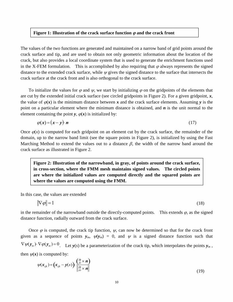
Finally, the X-FEM crack path predictions are plotted on the digital images of the actual test specimens

as shown in Figure 15. The measured crack paths for both the sink and miss case are in excellent

agreement with the corresponding XFEM prediction.

10. Demonstration Example: Crack Growth and Fatigue Life Predictions in a Complex Helicopter

Component under Spectrum Loadin

To further demonstrate the current 3D X-FEM toolkit for fatigue life prediction of a structural

component subjected to spectrum loading, a round-robin problem provided by Airbus/UK is considered

here. The problem has also been studied by Newman et al. (2006). Two solution steps are used to

Figure 12: Comparison of calculated f(a/w) for the modified-hole specimens.

Figure 13: Comparison of fatigue life prediction for the modified-hole specimens

Figure 14: Snapshots of CT specimen von Mises stress as crack grows.

Figure 15: Comparison of crack path prediction: miss-hole (CT1) on the left and sink-hole

(CT2) on the right.

24

simulate the fatigue crack growth and remaining life under spectrum loading: 1) use of the 3D X-FEM

toolkit to determine the functional relation between the crack length and its associated stress intensity

factors; and 2) perform the post fatigue life prediction using the AFGROW (Harter, 2008) originally

developed by the Air Force Research Laboratory.

The selected geometry is a flanged plate with a central lightening hole as shown in Figure 16. This is

representative of many features found in a helicopter lift frame. Crack growth would be initiated from a

corner defect, a=b=2.0 mm on the inner edge of the hole. The selected material is aluminum alloy of AA

7010 T73651. Comprehensive constant amplitude fatigue crack growth rates, covering threshold to near

failure, at four R-ratios between 0.9 and 0.1, were supplied by Airbus/UK.

The analysis procedure is summarized as follows (Figure 17):

1. In the solid domain, identify the region where crack may penetrate; then specify the region using

the X-FEM element type U1381. Use static analysis procedure in Abaqus and specify the time

increment size as the maximum crack growth size. Apply the static load using nominal P.

2. Create the initial crack geometry and discretize the geometry using a triangular shell mesh.

Assemble the crack mesh so that the intersection of the crack mesh and the solid mesh defines

the initial, ¼-circular edge crack at the corner of the raised hole.

3. Create the X-FEM specification file that associates the solid model file, the crack mesh file, and

specifies X-FEM and level set representation parameters (most important parameters including:

the enrichment zone size, the CTOD offset distance, and the level set representation grid size).

4. Execute the Abaqus analysis using the X-FEM user subroutine library.

5. The analysis results include regular solutions (displacement and stress variables) that are

viewable in CAE, the location of sampling tip points along the crack front at the end of each time

increment, and the Ks solutions at those tip points.

6. Import the tip location and K solution (K(a) curve or converted beta curve) into AFGROW, along

with the material fatigue data, for the life prediction.

The von Misses stress distribution for the component at the initial configuration is shown in Figure

18, where the maximum far-field stress at the raised hole is 130 MPa. As can be seen from Figure 18, the

stress field is intensified at the crack tip region.

Figure 16: Crack growth prediction in a complex helicopter component under spectrum

loading

Figure 17: Illustration of X-FEM model preparation.

Figure 18: X-FEM model and von Mises stress prediction at initial configuration.

25

The deformed shape and the Von Misses stress distribution at the final configuration of fatigue

analysis is shown in Figure 19.

The crack profiles using two different mesh designs are showing in Figure 20. Note that the maximum

growth size, 𝛥𝑎max as in Eqn (27) is set to be 0.5 mm.

After the determination of the functional relation between the crack size and its stress intensity

factors along the crack front, a life prediction analysis is performed next using AFGROW. The spectrum

to be used is the standard spectrum ASTERIX provided by Airbus/UK. ASTERIX has been derived from

real strain data measured on a helicopter lift frame, using the same procedures as were used for the

derivation of the rotor blade spectra HELIX and FEL. All three spectra are from the same 140 sorties

representing 190.5 hours of flight. The sequence of maneuvers in each sortie is fixed. The total number

of cycles in its complete form is 3.67 X 105 cycles. Given the fatigue test data at several applied ratios, a

general curve-fit model is developed to characterize the load ratio (R) dependent crack growth. The

accuracy of the load ratio dependent fatigue model at several distinct R values is shown in Figure 21.

The total analysis consists of 40 increments (0.5 mm max. crack growth per increment) in a single

step, and took 3410 wall o'clock seconds on a laptop PC. A relatively coarse mesh (element size

0.3~1.0mm) generates very consistent crack profiles and K estimates by comparison with a finer mesh

model. The crack travels to the threshold zone (about 5mm of the Y coordinate) at about 390,000

cycles and before the end of the main plate ( Y=17 mm) at about 480,000 cycles. The early phase of

predicted life is very different from the previous 2D predictions, which verifies the necessity of using 3D

analysis. The early development of crack profiles, from the ¼-circular initial crack to the straight

cut-through crack in the main plate, significantly affects the fatigue life prediction result.

In X-FEM, the displacement enrichment using four branch functions allows a quite accurate estimate

of the near-tip opening displacements and K’s; therefore a relatively coarse and uniform mesh can be

used in crack growth simulation. Using the narrow-band level set updates minimizes the mesh

sensitivity of crack growth prediction. The current X-FEM solver can already predict fatigue life for

constant-magnitude cyclic load case. For a variable-magnitude load case, fatigue life prediction is relied

on a step-by-step, one-way coupling to AFGROW. In each step, a simplified crack growth model is

adopted with the K(a) profile at the free edge as the input data.

Figure 19: X-FEM model and von Mises stress prediction at final configuration.

Figure 20: Crack profiles comparison using coarse and fine mesh models.

Figure 21: Load ratio dependent fatigue model at several distinct r values.

26

11. Conclusions

A three-dimensional finite element method for the analysis of fatigue crack growth has been

developed based on the extended finite element method (X-FEM). Both step function enrichments and

singular enrichments to capture the behavior near the crack front are included. The resulting formulation

can deal with small scale plasticity effectively. The crack morphology is described by level set methods

that, in conjunction with X-FEM, allow for convenient modeling of growing cracks without remeshing:

the crack geometry can be completely independent of the structure of the mesh. The method employs a

new variant of the fast marching method which enables efficient updates of the level sets, and thus the

crack geometry. In this method, triquintic interpolants are used for front reconstruction and the level set

updates that are used to model crack growth. Methods for dealing with crack closure effects have also

been described.

The methodologies have been incorporated in the Abaqus program. The user element option is

employed to implement the X-FEM elements. By means of the UXTERNALDB the analysis flow is

controlled, including the integration of the fast marching method solver and the special output features for

X-FEM. Verification and validation studies were performed using standard and modified compact tension

specimens.

For the standard CT specimen, the fracture parameters predicted from the X-FEM toolkit agree very

well with the analytical solution. A parametric study has also been performed to explore the mesh

sensitivity and the perturbation of the XFEM modeling parameters on the prediction of fracture parameter,

crack path, and fatigue life. Using the modified CT specimens for miss-hole and sink-hole configurations

given by Miranda et al. (2003), distinct fatigue crack growth behavior was simulated and showed to have

an excellent agreement with the experimental observations. The X-FEM prediction of the fatigue life also

agrees well with the reported test data.

Finally, the full capability of the tool was revealed via its application to a 3D helicopter lift frame

subjected to a real spectrum loading. Excellent agreement has been achieved by comparing the model

prediction with the test data provided by Airbus at two fatigue crack growth stages. The 3D X-FEM

analysis has also demonstrated that the use of a 2D through-the-thickness crack would be too conservative

since a significant number of cycles have been exhausted in forming the 2D crack from an initial 3D crack.

Acknowledgements

The authors gratefully acknowledge the support for X-FEM solid element and life prediction

development from ONR 331 under contract N00014-07-C-0442, N00014-08-C-0433, and

N00014-09-C-0416 with Dr. Paul Hess as the program manager. Some X-FEM framework development

was also supported by AFRL/MLBC under contract FA8650-07-C-5015 with Dr. David Mollenhauer as

27

the program manager. We also very appreciate Dr. Jianhong Lin of Airbus/UK for providing data and

valuable advices on the demonstration example problem.

References

[1] Abdelaziz Y, Hamouine A. A survey of the extended finite element. Comp Struct. 86:1141-1151.

2008.

[2] Belytschko T, Lu Y, Gu L. Element-free Galerkin methods. Int J Num Meth Eng. 37:229–56, 1994.

[3] Belytschko T, Krongauz Y, Organ D, Fleming M, Krysl P. Meshless methods: an overview and

recent developments. Comp Meth Appl Mech Eng. 139:3–47, 1996.

[4] Belytschko T, Black T. Elastic crack growth in finite elements with minimal remeshing. Int J Num

Meth Eng. 45:601–20, 1999.

[5] Belytschko T, Gracie R, Ventura G. A review of extended/generalized finite element methods for

material modeling. Model Simu Mat Sci Eng. 17(4): , 2009.

[6] Bordas S, Moran B. Enriched finite elements and level sets for damage tolerance assessment of

complex structures. Eng Fract Mech. 73:1176–201, 2006.

[7] Carter, BJ, Wawrzynek PA, Ingraffea AR. Automated 3-D crack growth simulation. Int J Numer

Meth Eng. 47:229-253, 2000.

[8] Chopp DL. Some improvements of the fast marching method. SIAM J Sci Comp. 23(1):230-244,

2001.

[9] Chopp DL, Sukumar N. Fatigue crack propagation of multiple coplanar cracks with the coupled

extended finite element/fast marching method. Int J Eng Sci. 41:845–69, 2003.

[10] Cruse T. Boundary element analysis in computational fracture mechanics. Kluwer-Dordrecht. 1988.

[11] Daux C, Moes N, Dolbow J, Sukumar N, Belytschko T. Arbitrary branched and intersecting cracks

with the extended finite element method. Int J Num Meth Eng. 48:1741–60, 2000.

[12] Dolbow J. An extended finite element method with discontinuous enrichment for applied mechanics.

PhD thesis, Northwestern University. 1999.

[13] Dolbow J, Moes N, Belytschko T. An extended finite element method for modeling crack growth

with frictional contact. Comput Meth Appl Mech Eng. 190:6825–46, 2001.

[14] Dolbow J, Devan A. Enrichment of enhanced assumed strain approximations for representing strong

discontinuities: addressing volumetric incompressibility and the discontinuous patch test. Int J Num

Meth Eng. 59:47–67, 2004.

[15] Elguedj T, Gravouil A, Combescure A. Appropriate extended functions for XFEM simulation of

plastic fracture mechanics. Comp Meth App Mech Eng. 195:501-515, 2006.

[16] Giner E, Sukumar N, Tarancon JE, Fuenmayor FJ. An Abaqus implementation of the extended

finite element method. Eng Fract Mech. 76:347-368, 2009.

[17] Gravouil A, Moes N, Belytschko T. Non-planar 3D crack growth by the extended finite element and

level sets part II: level set update. Int J Num Meth Eng. 53:2569–86, 2002.

[18] Harter J. AFGROW Users Guide and Technical Manual. AFRL-VA-WP-TR-2008-XXXX, Air

Force Research Laboratory, July 2008.

28

[19] Henshell RD, Shaw KG. Crack tip finite elements are unnecessary. Int J Numer Meth Eng.

9:495-507, 1975.

[20] Huang R, Sukumar N, Pre′vost J. Modeling quasi-static crack growth with the extended finite

element method part II: numerical applications. Int J Solids Struct 40:7539–52, 2003.

[21] Karihaloo BL, Xiao QZ. Modeling of stationary and growing cracks in FE framework without

remeshing: a state-of-the-art review. Comp Struct. 81:119–29, 2003.

[22] Khoei AR, Nikbakht M. Contact friction modeling with the extended finite element method

(X-FEM). J Mat Proces Tech, (177)1-3:58-62, 2006.

[23] Khoei AR, Biabanaki SOR, Anahid M. A Lagrangian-extended finite element method in modeling

large-plasticity deformations and contact problems, Int J Mech Sci, (51)5:384-401. 2009.

[24] Lei Y. Finite element crack closure analysis of a compact tension specimen, Int J Fat. 30: 21-31,

2008.

[25] Lua J, Shi J, Liu P, Collette M. Curvilinear crack growth and remaining life prediction of aluminum

weldment using X-FEM, 49th AIAA/ASME/ASCE/AHS/ASC Structures, Structural Dynamics, and

Materials Conference. #AIAA-2008-1839, 2008.

[26] Lua J, Englestad, S. Pi-Joint reliability assessment using X-FEM/script, 50th

AIAA/ASME/ASCE/AHS/ASC Structures, Structural Dynamics, and Materials Conference. 2009.

[27] Maligno AR, Rajaratnam S, Leen SB, Williams EJ. A three-dimensional (3D) numerical study of

fatigue crack growth using remeshing techniques. Eng Fract Mech. 77:94-111, 2010.

[28] Miranda ACO, Meggiolaro MA, Castro JTP, Matha LF, Bittencourt TN. Fatigue life and crack path

predictions in generic 2D structural components. Eng Fract Mech. 70:1259–1279, 2003.

[29] Melenk JM, Babuska I. The partition of unity finite element method: basic theory and applications.

Comp Meth Appl Mech Eng 139:289–314, 1996.

[30] Moes N, Dolbow J, Belytschko T. A finite element method for crack growth without remeshing. Int

J Num Meth Eng. 46:131–50, 1999.

[31] Moes N, Gravouil A, Belytschko T. Non-planar 3D crack growth by the extended finite element and

level sets part I: mechanical model. Int J Num Meth Eng. 53:2549–68, 2002.

[32] Nagtegaal J C, Parks DM, Rice JR. On numerically accurate finite element solutions in the fully

plastic range. Comp Meth Applied Mech Eng. (4): 153–177, 1974.

[33] Nistro I, Pantale′ O, Caperaa S. On the modeling of the dynamic crack propagation by extended

finite element method: numerical implantation in DYNELA code. In: VIII international conference

on computational plasticity, COMPLAS VIII, Barcelona; 2005.

[34] Newman JCR, Irving, PE, Lin J, Le DD. Crack growth predictions in a complex helicopter

component under spectrum loading, Fat Fract Eng Mat Struct. 29:949–958, 2006.

[35] Oden TJ, Belytschko T, Babuska, Hughes TJR, Research directions in computational mechanics.

Comp Meth Applied Mech Eng. 192: 913-922, 2003.

[36] Osher S, Sethian J. Fronts propagating with curvature dependent speed: algorithms based on

Hamilton–Jacobi formulations. J Comp Phys. 79(1):12–49, 1988.

[37] Pantale′ O, Caperaa S, Rakotomalala R. Development of an object oriented finite element program:

application to metal forming and impact simulation. J-CAM. 186(1–2):341–51, 2004.

[38] Pre′vost J. Dynaflow. Princeton University. 1983.

29

[39] Sethian J. Fast marching methods. SIAM Rev. 41(2):199–235, 1999.

[40] Shi J, Lua J, Waisman H, Belytschko T, Sukumar N. X-FEM toolkit for automated crack onset and

growth prediction, 49th AIAA/ASME/ASCE/AHS/ASC Structures, Structural Dynamics, and

Materials Conference. #AIAA-2008-1763, 2008.

[41] Stolarska M, Chopp DL, Moes N, Belyschko T. Modeling crack growth by level sets in the

extended finite element method. Int J Num Meth Eng. 51:943–60, 2001.

[42] Sukumar N, Chopp DL, Moran B. Extended finite element method and fast marching method for

three-dimensional fatigue crack propagation. Eng Fract Mech. 70:29–48, 1999.

[43] Sukumar N, Moes N, Moran B, Belytschko T. Extended finite element method for

three-dimensional crack modelling. Int J Num Meth Eng, 48:1549–70, 2000.

[44] Sukumar N, Pre′vost JH. Modeling quasi-static crack growth with the extended finite element

method part I: computer implementation. Int J Solids Struct 40:7513–37, 2003.

[45] Sukumar N, Chopp DL, Bechet E, Moes N. Three-dimensional non-planar crack growth by a

coupled extended finite element and fast marching method, Int J Num Meth Eng. 76(5):727-748,

2008.

[46] Ventura G. On elimination of quadrature subcells for discontinuous functions in the extended finite

element method. Int J Num Meth Eng 66:761–95, 2006.

[47] Xiao QZ, Karihaloo BL. Improving the accuracy of X-FEM crack tip fields using higher order

quadrature and statically admissible stress recovery. Int J Num Meth Eng 2006;66:1378–410.

[48] Zienkiewicz, O C, Zhu, J Z. The superconvergence patch recovery and a posteriori estimates. Part 1:

The recovery technique, Int J Num Meth Eng. 33: 1331—1364, 1992.

[49] Zienkiewicz, OC, Taylor, RL. The Finite Element Method, Fifth edition, Butterworth-Heinemann.

2000.

30

Figure 1: Illustration of the crack surface function and the crack front function.

Figure 2: Illustration of the narrowband, in gray, of points around the crack surface, in

cross-section, where the FMM mesh maintains signed values. The circled points are where

the initialized values are computed directly and the squared points are where the values are

computed using the FMM.

31

Figure 3: Overview of crack tracking and growth control.

(a) (b)

Figure 4: Slicing scheme on the quad facet: (a) scenarios of facets being completely cut by a

crack surface represented by the line c1-c2; and (b) scenarios of facets partially cut by a crack

surface.

(a) (b)

Figure 5: K validation using a standard compact test specimen. (a) Specimen dimensions and

X-FEM mesh design; (b) von Mises stresses in deformed shape.

32

(a)

(b)

Figure 6: (a) Dimensionless K values in reference to Eqn (47) using X-FEM with a

combination of parameter settings; and (b) relative errors in K prediction as a function of the

tip enrichment radius and the CTOD offset distance.

0.80

0.85

0.90

0.95

1.00

1.05

1.10

0.0 5.0 10.0 15.0

Dim

ensi

on

less

K

IV

alu

e (1

00%

Pla

ne

Str

ain

Ref

eren

ce

Solu

tion

= 1

317.6

3

MP

mm

1/2

)

Tip Coordinate in Through-Thickness Direction (mm)

from Boundary to Boundary

r=0.3,l=0.1r=0.3,l=0.01r=0.3,l=0.001r=0.55,l=0.1r=0.55,l=0.01r=0.55,l=0.001r=0.75,l=0.90r=0.75,l=0.5r=0.75,l=0.05r=0.75,l=0.1r=0.75,l=0.01r=0.75,l=0.001r=0.75,l=0.0001

1.E-04

1.E-03

1.E-02

1.E-01

1.E+00

0.0001 0.001 0.01 0.1 1Rel

ati

ve

erro

rs t

o t

he

solu

tion

ob

tain

ed

by r

= 0

.75 m

m a

nd

l =

0.0

001 m

m

CTOD offset distance in K calculation (mm)

r=0.30 mm (1-layer enrichment)

r=0.55 mm (2-layer enrichment)

r=0.75 mm (3-layer enrichment)

33

Figure 7: Geometry of the modified CT specimen. A = 8.3 mm and B = 8.1 mm for the

miss-hole configuration; and A = 8.4 mm and B = 6.9 mm for the sink-hole configuration.

Figure 8: Mesh sensitivity study of crack growth patterns for the miss-hole CT specimen

under constant cyclic loading

34

(a)

(b)

Figure 9: Stress intensity factors KI (a) and KII (b) as functions of crack extension size, using

combinations of X-FEM analysis controlling parameters.

0.0

500.0

1,000.0

1,500.0

2,000.0

2,500.0

0.0 5.0 10.0 15.0 20.0 25.0 30.0 35.0

K1 (

MP

am

m0.5

)

Crack Extension (mm)

Free Mesh (da=0.3)

Free Mesh (da=1.0)

Structured Mesh (da=1.0)

Free Mesh (da=0.5,r=0.75,l=0.01)

Structured Mesh (da=0.5,r=0.75,l=0.01)

-250.0

-200.0

-150.0

-100.0

-50.0

0.0

50.0

100.0

150.0

200.0

250.0

0.0 5.0 10.0 15.0 20.0 25.0 30.0 35.0

Free Mesh (da=0.3)

Free Mesh (da=1.0)

Structured Mesh (da=1.0)

35

(a)

(b)

Figure 10: Crack profile (a) and fatigue life prediction (b) as functions of crack extension size,

using combinations of X-FEM analysis controlling parameters.

200

2,000

20,000

0.2 2.0 20.0

Nu

mb

er o

f C

ycl

es

Crack Extension (mm)

Free Mesh (da=0.3,r=0.75,l=0.75)

Free Mesh (da=1.0,r=0.90,l=0.75)

Structured Mesh (da=1.0,r=0.90,l=0.75)

Free Mesh (da=0.5,r=0.75,l=0.01)

Structured Mesh (da=0.5,r=0.75,l=0.01)

Free Mesh (da=1.0,r=0.75,l=0.01) Full Int

36

Figure 11: Loading history for the modified-hole CT specimen analyses.

Figure 12: Comparison of calculated f(a/w) for the modified-hole specimens.

0

100

200

300

400

500

600

700

800

0 0.002 0.004 0.006 0.008 0.01 0.012 0.014

Load

(kN

)

Total crack growth length (m)

Miss-hole load

Sink-hole load

Poly. (Miss-hole load)

4

5

6

7

8

9

10

11

12

0.20 0.30 0.40 0.50 0.60 0.70

f(a/w

)

a/w

Miss-hole reference

Miss-hole X-FEM

Sink-hole reference

Sink-hole X-FEM

37

Figure 13: Comparison of fatigue life prediction for the modified-hole specimens

Figure 14: Snapshots of CT specimen von Mises stress as crack grows.

0.0

2.0

4.0

6.0

8.0

10.0

12.0

14.0

16.0

18.0

20.0

0.00 0.10 0.20 0.30 0.40

Tota

l cr

ack l

ength

, a (

mm

)

Fatigue cycles (in millions)

Miss-hole experiment

Miss-hole X-FEM

Sink-hole experiment

Sink-hole X-FEM

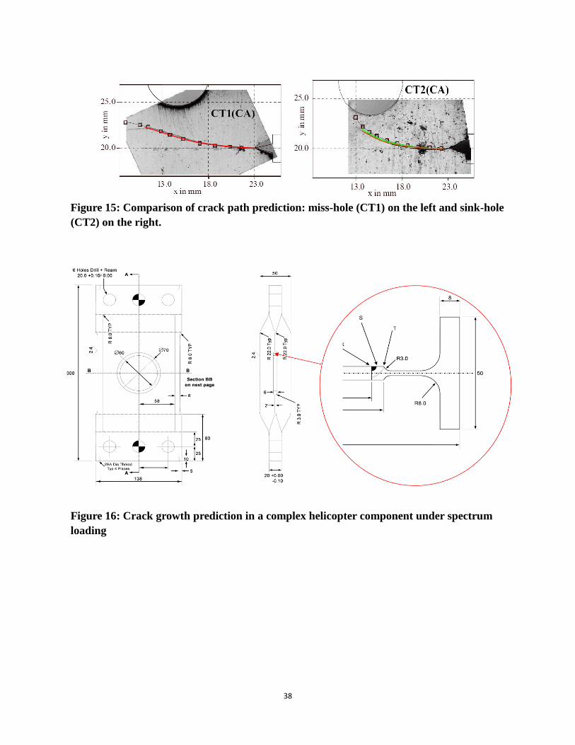
38

Figure 15: Comparison of crack path prediction: miss-hole (CT1) on the left and sink-hole

(CT2) on the right.

Figure 16: Crack growth prediction in a complex helicopter component under spectrum

loading

39

Figure 17: Illustration of X-FEM model preparation.

Figure 18: X-FEM model and von Mises stress prediction at initial configuration.

Figure 19: X-FEM model and von Mises stress prediction at final configuration.

40

Figure 20: Crack profiles comparison using coarse and fine mesh models.

Figure 21: Load ratio dependent fatigue model at several distinct r values.