Embed Size (px)
Citation preview

Aalborg Universitet
Interference-robust Air Interface for 5G Small Cells
Tavares, Fernando Menezes Leitão
Publication date:2015
Document VersionPublisher's PDF, also known as Version of record
Link to publication from Aalborg University
Citation for published version (APA):Tavares, F. M. L. (2015). Interference-robust Air Interface for 5G Small Cells: Managing inter-cell interferencewith advanced receivers and rank adaption. Department of Electronic Systems, Aalborg University.
General rightsCopyright and moral rights for the publications made accessible in the public portal are retained by the authors and/or other copyright ownersand it is a condition of accessing publications that users recognise and abide by the legal requirements associated with these rights.
? Users may download and print one copy of any publication from the public portal for the purpose of private study or research. ? You may not further distribute the material or use it for any profit-making activity or commercial gain ? You may freely distribute the URL identifying the publication in the public portal ?
Take down policyIf you believe that this document breaches copyright please contact us at [email protected] providing details, and we will remove access tothe work immediately and investigate your claim.
Downloaded from vbn.aau.dk on: juli 17, 2018

Interference-robust AirInterface for 5G Small CellsManaging inter-cell interference with advanced
receivers and rank adaptation
Ph.D. DissertationFernando Menezes Leitão Tavares
Aalborg UniversityDepartment of Electronic Systems
Fredrik Bajers Vej 7DK – 9220 Aalborg

Thesis submitted: February 17th, 2015PhD Supervisor: Assoc. Prof. Troels Bundgaard Sørensen
Aalborg UniversityAssistant PhD Supervisor: Prof. Preben Mogensen
Aalborg UniversityAssistant PhD Supervisor: Assoc. Prof. Gilberto Berardinelli
Aalborg UniversityPhD Committee: Prof. Klaus Pedersen
Aalborg UniversityProf. Mikko ValkamaTampere University of TechnologyErik Dahlman, Ph.D.Senior Expert, Ericsson, Sweden
PhD Series: Faculty of Engineering and Science, AalborgUniversity
ISBN: 978-87-7152-059-0
Published by:Aalborg University PressSkjernvej 4A, 2nd floorDK – 9220 Aalborg ØPhone: +45 [email protected]
Copyright c© 2015 by Fernando Menezes Leitão Tavares.All rights reserved.
Printed in Denmark by Uniprint, 2015

Abstract
Since the release of the first High Speed Packet Access (HSPA) networks in2005, the demand for mobile broadband services has increased continuouslyat staggering rates, fuelled by the mass adoption of smartphones. It is fore-cast that this trend will continue for at least the next decade, pushing theexisting wireless network infrastructure to the limit. Mobile network oper-ators must invest in network expansion to deal with this problem, but thepredicted network requirements show that a new Radio Access Technology(RAT) standard will be fundamental to reach the future target performance.This new 5th Generation (5G) RAT standard is expected to support data ratesgreater than 10 Gbps with very low latency, very low energy consumptionand provide the required scalability that will allow the network to transporta 1000 to 10000 times more mobile data traffic in 2020 than a similar networkwould do in 2010.
To meet these challenging network capacity expansion requirements, thedesign of the new 5G RAT standard will make use of three main strategies:more antennas, more spectrum and more cells. All these strategies will haveimportant roles in the new system, but the deployment of a massive numberof small cells, especially indoors, is expected to provide the largest improve-ment in network capacity. However, the benefits of this type of ultra-densedeployment do not come for free; strong inter-cell interference, an inherentproblem of dense networks, has the potential to limit the expected gains. Dueto the fundamental role of inter-cell interference in this type of networks, theinter-cell interference problem must be addressed since the beginning of thedesign of the new standard.
This Ph.D. thesis deals with the design of an interference-robust air in-terface for 5G small cell networks. The interference robustness is achievedby the clever design of the radio frame structure in such a way that interfer-ence suppression receivers can efficiently and effectively mitigate the effectsof inter-cell interference. A detailed receiver model is derived (including alsoreceiver imperfections, such as estimation errors and receiver front-end lim-itations) and applied in extensive system-level simulation campaigns. Thesesimulations show that, when the interference-robust air interface design is
iii

used, interference suppression receivers are indeed a valid alternative to tra-ditional Inter-cell Interference Coordination (ICIC) techniques that are com-monly applied to improve the outage performance of these networks.
Moreover, a novel inter-cell interference management concept is proposed.This concept is based on the effect that the rank adaptation decisions in onecell cause on the neighbouring cells when interference suppression receiversare used. The concept, known as victim-aware rank adaptation, may be usedto improve the outage data rates of the network. In particular, the Maxi-mum Rank Planning (MRP) technique is shown to outperform traditionalfrequency reuse planning, with the advantage of lower implementation com-plexity due to the simplified planning process.

Resumé
Mobil bredbåndskommunikation har været i en konstant og voldsom vækstsiden introduktionen af High Speed Packet Access (HSPA) i 2005, primærtnæret af den brede accept af smartphones. Det forventes at tendensen vilfortsætte minimum det kommende tiår og dermed strække den eksisterendetrådløse netværksinfrastruktur til sit yderste. For at imødegå begrænsning-erne er det nødvendigt at mobiloperatørerne investerer i udvidelser af deresnetværk. Det er dog klart fra netværkskravene at en ny teknologistandardfor radiotilgang vil være påkrævet for at kunne opfylde målkravene. En så-dan ny 5. generations (5G) radioteknologi forventes at supportere dataraterder overstiger 10 Gbps med meget lav tidsforsinkelse, meget lavt strømfor-brug, og en skalerbarhed der tillader netværket at transportere 1.000 til 10.000gange mere mobildatatrafik i 2020 end et tilsvarende netværk tillader i 2010.
For at imødekomme disse udfordrende krav til ekspansion af netværk-skapacitet vil designet af en ny 5G radioteknologi gøre brug af tre hoved-strategier: Flere antenner, udvidet frekvensspektrum, og flere radioceller.Disse strategier vil hver især have en afgørende rolle i 5G, men den massiveudrulning af små radioceller, specielt indendørs, forventes at bidrage medden største forbedring af netværkskapaciteten. Kapacitetsforbedringen kom-mer dog ikke uden omkostninger; den kraftige inter-celle interferens, derer resultat af netværksfortætningen, kan potentielt begrænse de forventedeforbedringer. I betragtning af den centrale rolle som inter-celle interferensudgør i denne type netværk, er det oplagt at adressere inter-celle interferen-sproblematikken allerede i designet af en ny 5G standard.
Denne ph.d. afhandling omhandler designet af en interferensrobust ra-diogrænseflade for et 5G netværk med små radioceller. Robustheden over-for interferens er opnået ved et intelligent design af radio rammestrukturen,således at interferensundertrykkende modtagere effektivt kan undertrykkeeffekten af inter-celle interferens. Der er udviklet en detaljeret modtager-model, inkluderende ikke-idealiteter såsom estimeringsfejl og signalbegræn-sninger i modtagerdelen, og denne model er anvendt i et omfattende sæt afsystemsimuleringer. Resultaterne fra simuleringerne viser at interferensun-dertrykkende modtagere, i samspil med den interferensrobuste radiogrænse-
v

flade, udgør et essentielt alternativ til traditionelle inter-celle interferensko-ordinations teknikker (ICIC) der typisk anvendes til at forbedre dækningenfor de mest (interferens) udsatte brugere.
Afhandlingen foreslår også et nyskabende koncept for interferenshånd-tering. Konceptet er baseret på den effekt som rank-opdateringer i een cellebevirker på naboceller når interferens-undertrykkende modtagere benyttes.Konceptet, benævnt ”victim-aware” rank-opdatering, kan benyttes til at for-bedre dækningen for interferens- udsatte brugere; det vises i afhandlingen, atspecielt teknikken med Maximum Rank Planning (MRP) giver bedre dækn-ing end traditionel frekvensplanlægning, og tilmed med fordel af en lavereimplementeringskompleksitet grundet en simplere planlægningsproces.
Translated by Associate Prof. Troels B. Sørensen, Aalborg University, Denmark.

Contents
Abstract iii
Resumé v
Thesis Details xi
Preface xiii
List of Abbreviations xv
I Extended Summary 1
1 Introduction 31.1 5G mobile networks . . . . . . . . . . . . . . . . . . . . . . . . . 4
1.1.1 General 5G mobile network requirements . . . . . . . . 41.1.2 Ultra-dense small cell deployments . . . . . . . . . . . . 61.1.3 5G small cell RAT concept . . . . . . . . . . . . . . . . . . 7
1.2 Objectives and scientific methodology . . . . . . . . . . . . . . . 81.3 Contributions and publications . . . . . . . . . . . . . . . . . . . 91.4 Thesis outline . . . . . . . . . . . . . . . . . . . . . . . . . . . . . 13
2 Inter-cell interference mitigation using interference suppression re-ceivers 152.1 Introduction . . . . . . . . . . . . . . . . . . . . . . . . . . . . . . 152.2 Understanding inter-cell interference mitigation . . . . . . . . . 162.3 Using MIMO receivers for inter-cell interference suppression . 20
2.3.1 IRC receiver . . . . . . . . . . . . . . . . . . . . . . . . . . 222.3.2 IRC-SIC receiver . . . . . . . . . . . . . . . . . . . . . . . 282.3.3 Receiver front-end imperfections . . . . . . . . . . . . . . 31
2.4 Summary . . . . . . . . . . . . . . . . . . . . . . . . . . . . . . . . 31
vii
Contents
3 Interference-robust air interface for 5G small cells 333.1 Introduction . . . . . . . . . . . . . . . . . . . . . . . . . . . . . . 333.2 General design targets and solutions . . . . . . . . . . . . . . . . 33
3.2.1 Reaching the peak data rate target . . . . . . . . . . . . . 343.2.2 Dynamic TDD . . . . . . . . . . . . . . . . . . . . . . . . . 353.2.3 Meeting the low latency target . . . . . . . . . . . . . . . 373.2.4 Waveform . . . . . . . . . . . . . . . . . . . . . . . . . . . 383.2.5 System numerology . . . . . . . . . . . . . . . . . . . . . 39
3.3 Traditional interference mitigation support . . . . . . . . . . . . 403.4 Support for interference suppression receivers . . . . . . . . . . 42
3.4.1 Support for IRC receivers . . . . . . . . . . . . . . . . . . 423.4.2 Support for IRC-SIC receivers . . . . . . . . . . . . . . . 47
3.5 Summary . . . . . . . . . . . . . . . . . . . . . . . . . . . . . . . . 48
4 Performance evaluation 494.1 Introduction . . . . . . . . . . . . . . . . . . . . . . . . . . . . . . 494.2 General simulation assumptions . . . . . . . . . . . . . . . . . . 49
4.2.1 Simulation scenario . . . . . . . . . . . . . . . . . . . . . 494.2.2 Physical layer assumptions . . . . . . . . . . . . . . . . . 514.2.3 Simulation setup . . . . . . . . . . . . . . . . . . . . . . . 51
4.3 Inter-cell interference suppression performance . . . . . . . . . 524.4 Performance considering receiver imperfections . . . . . . . . . 554.5 Interference suppression versus Frequency Reuse Planning (FRP) 614.6 Using victim-aware rank adaptation . . . . . . . . . . . . . . . . 66
4.6.1 Maximum Rank Planning (MRP) . . . . . . . . . . . . . . 684.6.2 Taxation-based Rank Adaptation (TRA) . . . . . . . . . . 70
4.7 Summary . . . . . . . . . . . . . . . . . . . . . . . . . . . . . . . . 71
5 Conclusions and future work 755.1 Conclusions and recommendations . . . . . . . . . . . . . . . . . 755.2 Future work . . . . . . . . . . . . . . . . . . . . . . . . . . . . . . 76
Bibliography 79
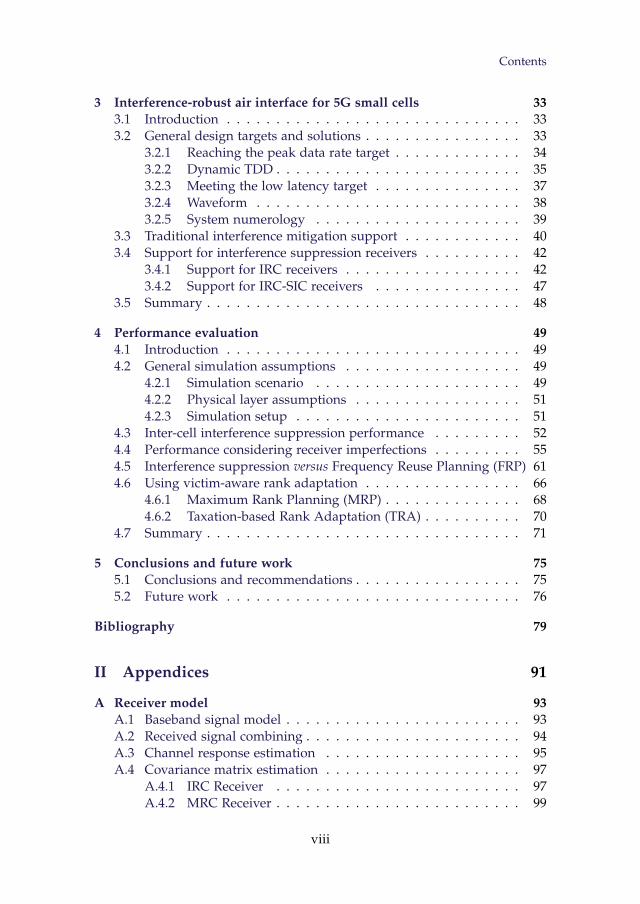
II Appendices 91
A Receiver model 93A.1 Baseband signal model . . . . . . . . . . . . . . . . . . . . . . . . 93A.2 Received signal combining . . . . . . . . . . . . . . . . . . . . . . 94A.3 Channel response estimation . . . . . . . . . . . . . . . . . . . . 95A.4 Covariance matrix estimation . . . . . . . . . . . . . . . . . . . . 97
A.4.1 IRC Receiver . . . . . . . . . . . . . . . . . . . . . . . . . 97A.4.2 MRC Receiver . . . . . . . . . . . . . . . . . . . . . . . . . 99
viii

Contents
A.5 Receive front-end imperfections model . . . . . . . . . . . . . . 100A.6 Successive interference cancellation . . . . . . . . . . . . . . . . 102A.7 Signal-to-interference-plus-noise ratio . . . . . . . . . . . . . . . 103
B Detailed simulation assumptions 105B.1 Simulation tool . . . . . . . . . . . . . . . . . . . . . . . . . . . . 105B.2 Simulation scenario . . . . . . . . . . . . . . . . . . . . . . . . . . 107B.3 Propagation model . . . . . . . . . . . . . . . . . . . . . . . . . . 108
B.3.1 Deterministic path loss . . . . . . . . . . . . . . . . . . . 108B.3.2 Log-normal shadowing . . . . . . . . . . . . . . . . . . . 109B.3.3 Frequency-selective time-varying signal fading . . . . . 109
B.4 Frequency allocation . . . . . . . . . . . . . . . . . . . . . . . . . 110B.5 Traffic model . . . . . . . . . . . . . . . . . . . . . . . . . . . . . . 111B.6 User scheduling model . . . . . . . . . . . . . . . . . . . . . . . . 112B.7 Physical layer model . . . . . . . . . . . . . . . . . . . . . . . . . 112B.8 Rank and precoding matrix adaptation model . . . . . . . . . . 113
III Papers 115
A On the Potential of Interference Rejection Combining in B4G Net-works 117I Introduction . . . . . . . . . . . . . . . . . . . . . . . . . . . . . . 119II Signal Model . . . . . . . . . . . . . . . . . . . . . . . . . . . . . . 120III Simulation Setup . . . . . . . . . . . . . . . . . . . . . . . . . . . 122
A. Physical Layer Assumptions . . . . . . . . . . . . . . . . 122B. Simulation Scenarios . . . . . . . . . . . . . . . . . . . . . 123C. Simulation Results . . . . . . . . . . . . . . . . . . . . . . 124
IV Performance Evaluation . . . . . . . . . . . . . . . . . . . . . . . 126V Conclusion . . . . . . . . . . . . . . . . . . . . . . . . . . . . . . . 129References . . . . . . . . . . . . . . . . . . . . . . . . . . . . . . . . . . 130
B On the impact of receiver imperfections on the MMSE-IRC receiverperformance in 5G networks 133I Introduction . . . . . . . . . . . . . . . . . . . . . . . . . . . . . . 135II Radio Frame Format . . . . . . . . . . . . . . . . . . . . . . . . . 136III Signal Model . . . . . . . . . . . . . . . . . . . . . . . . . . . . . . 136
A. Received Signal Combining . . . . . . . . . . . . . . . . . 137B. Covariance Matrix Estimation . . . . . . . . . . . . . . . 137C. Channel Response Estimation Error . . . . . . . . . . . . 139D. Receiver Front-End Errors . . . . . . . . . . . . . . . . . . 139
IV Simulation Setup . . . . . . . . . . . . . . . . . . . . . . . . . . . 141A. Simulation Scenario . . . . . . . . . . . . . . . . . . . . . 141
ix

Contents
B. Physical Layer Assumptions . . . . . . . . . . . . . . . . 142V Performance Evaluation . . . . . . . . . . . . . . . . . . . . . . . 143VI Conclusion . . . . . . . . . . . . . . . . . . . . . . . . . . . . . . . 146References . . . . . . . . . . . . . . . . . . . . . . . . . . . . . . . . . . 148
C Inter-cell interference management using Maximum Rank Planningin 5G small cell networks 151I Introduction . . . . . . . . . . . . . . . . . . . . . . . . . . . . . . 153II Interference Rejection Combining in 5G . . . . . . . . . . . . . . 154III Maximum Rank Planning . . . . . . . . . . . . . . . . . . . . . . 155IV Simulation Setup . . . . . . . . . . . . . . . . . . . . . . . . . . . 158V Performance Evaluation . . . . . . . . . . . . . . . . . . . . . . . 160VI Conclusion . . . . . . . . . . . . . . . . . . . . . . . . . . . . . . . 163References . . . . . . . . . . . . . . . . . . . . . . . . . . . . . . . . . . 163
D Managing inter-cell interference with advanced receivers and rankadaptation in 5G small cells 165I Introduction . . . . . . . . . . . . . . . . . . . . . . . . . . . . . . 167II System Model . . . . . . . . . . . . . . . . . . . . . . . . . . . . . 168
A. 5G Frame Format Concept . . . . . . . . . . . . . . . . . 168B. Receiver Model . . . . . . . . . . . . . . . . . . . . . . . . 170C. Rank adaptation . . . . . . . . . . . . . . . . . . . . . . . 173
III Simulation Setup . . . . . . . . . . . . . . . . . . . . . . . . . . . 174IV Performance Evaluation . . . . . . . . . . . . . . . . . . . . . . . 176
A. Scenario A - Indoor Hotspot (OSG) . . . . . . . . . . . . 177B. Scenario B - Indoor Office (OSG) . . . . . . . . . . . . . . 178C. Scenario C - Indoor Office (CSG) . . . . . . . . . . . . . . 179
V Conclusion and Future Works . . . . . . . . . . . . . . . . . . . . 182References . . . . . . . . . . . . . . . . . . . . . . . . . . . . . . . . . . 182
x

Thesis Details
Thesis Title: Interference-robust Air Interface for 5G Small Cells: Man-aging inter-cell interference with advanced receivers andrank adaptation
Ph.D. Student: Fernando Menezes Leitão TavaresSupervisors: Assoc. Prof. Troels B. Sørensen, Aalborg University
Prof. Preben Mogensen, Aalborg UniversityAssoc. Prof. Gilberto Berardinelli, Aalborg University
The main body of this thesis consist of the following papers.
[A] Fernando Menezes Leitão Tavares, Gilberto Berardinelli, Nurul HudaMahmood, Troels Bundgaard Sørensen and Preben Mogensen, "On thePotential of Interference Rejection Combining in B4G Networks", IEEE78th Vehicular Technology Conference (VTC Fall), September 2013.
[B] Fernando Menezes Leitão Tavares, Gilberto Berardinelli, Nurul HudaMahmood, Troels Bundgaard Sørensen and Preben Mogensen, "On theimpact of receiver imperfections on the MMSE-IRC receiver perfor-mance in 5G networks", IEEE 79th Vehicular Technology Conference(VTC Spring), May 2014.
[C] Fernando Menezes Leitão Tavares, Gilberto Berardinelli, Nurul HudaMahmood, Troels Bundgaard Sørensen and Preben Mogensen, "Inter-cell interference management using maximum rank planning in 5Gsmall cell networks", IEEE 11th International Symposium on WirelessCommunications Systems (ISWCS), August 2014.
[D] Fernando Menezes Leitão Tavares, Gilberto Berardinelli, Davide Ca-tania, Troels Bundgaard Sørensen and Preben Mogensen, "Managinginter-cell interference with advanced receivers and rank adaptation in5G small cells", submitted to IEEE 21st European Wireless (EW) Confer-ence, May 2015.
xi

Thesis Details
This thesis has been submitted for assessment in partial fulfilment of thePh.D. degree. The thesis is based on the submitted or published scientific pa-pers which are listed above. Parts of the papers are used directly or indirectlyin the extended summary of the thesis. As part of the assessment, co-authorstatements have been made available to the assessment committee and arealso available at the Faculty. The thesis is not in its present form acceptablefor open publication but only in limited and closed circulation as copyrightmay not be ensured.
xii

Preface
This thesis is the result of a research project carried out at the Wireless Com-munication Networks (WCN) section, Institute of Electronic Systems, Aal-borg University, Denmark. The work was carried out in parallel with themandatory courses and teaching/working obligations required to obtain thePh.D. degree.
The project was financed by the "Danish Council for Independent Re-search" (Det Frie Forskningsråd, DFF), “Technology and Production Sciences”(Forskningsrådet for Teknologi og Produktion, FTP), in connection with theresearch project "Cognitive Radio Concepts for Beyond-Femtocells". The re-search project has been completed under the supervision and guidance of As-sociate Professor Troels Bundgaard Sørensen (Aalborg University), AssociateProfessor Gilberto Berardinelli (Aalborg University) and Professor PrebenMogensen (Aalborg University and Nokia Networks, Denmark).
The thesis investigates concepts related to the design of an interference-robust air interface for 5th Generation (5G) ultra-dense small cell networks;in particular, the investigation is focused on concepts related to the use ofadvanced receivers and rank adaptation techniques as tools for managinginter-cell interference.
I would like to express my sincere gratitude to my supervisors. Theirguidance has been fundamental to accomplishing the tasks of this project;their encouragement, an invaluable source of energy for enduring the thoughtimes. I must mention that they have taught me countless lessons for bothmy professional and personal lives.
I am also sincerely thankful to my current and former colleagues fromboth the Wireless Communication Networks section and Nokia Networks,Denmark. I would like to thank them for the amazing working environmentwhere I had the pleasure to work since moving to Denmark. I will howeverrefrain from mentioning names; it would be a sin to forget any of them.
My deepest gratitude goes to my family, in particular my parents Flavioand Walkyria, my brother Bernardo and my sister Marina, for their encour-agement and support. I could not have asked for a better family.
xiii

Preface
To my beloved wife, Ana Paulla.
Words will never be enough to express how thankful I am for each and everymoment we have been together. Life at your side has been happier than Icould ever expect, especially now that we were blessed with the birth of ourbeloved son, Daniel. I will always be truly thankful for your love and dedi-cation.
Fernando Menezes Leitão TavaresFebruary 17th, 2015
xiv

List of Abbreviations
256-QAM 256-ary Quadrature Amplitude Modulation
3GPP 3rd Generation Partnership Program
4G 4th Generation
5G 5th Generation
ABS Almost Blank Subframe
ADC Analog-to-Digital Converter
AF Activity Factor
AGC Automatic Gain Control
AMC Adaptive Modulation and Coding
AP Access Point
AWGN Additive White Gaussian Noise
BLER Block Error Rate
CDF Cumulative Distribution Function
CoMP Coordinated Multi-Point
CP Cyclic Prefix
CSG Closed Subscriber Group
DCCH Downlink Control Channel
DFT-s-OFDM DFT-spread OFDM
DL Downlink
DMRS Demodulation Reference Signal
xv

List of Abbreviations
DR Deployment Ratio
DRX Discontinuous Reception
DSB Data-Symbol Based
EDGE Enhanced Data Rates for GSM Evolution
EVM Error Vector Magnitude
FBMC Filter Bank Multicarrier
FDD Frequency Division Duplex
FD-ICIC Frequency-domain ICIC
FFR Fractional Frequency Reuse
FR1 Frequency Reuse 1
FR2 Frequency Reuse 2
FR4 Frequency Reuse 4
FRP Frequency Reuse Planning
GNSS Global Navigation Satellite System
GP Guard Period
GPS Global Positioning System
GSM Global System for Mobile Communications
HSPA High Speed Packet Access
ICIC Inter-cell Interference Coordination
IMT International Mobile Telecommunications
IRC Interference Rejection Combining
ITU International Telecommunication Union
LNA Low-Noise Amplifier
LTE Long Term Evolution
LTE-A Long Term Evolution - Advanced
MA Multiple Access
MCL Minimum Coupling Loss
xvi

List of Abbreviations
MCS Modulation and Coding Scheme
MIMO Multiple-Input Multiple-Output
ML Maximum Likelihood
MMSE Minimum Mean Square Error
MRC Maximal Ratio Combining
MRP Maximum Rank Planning
MTC Machine Type Communications
OFDM Orthogonal Frequency Division Multiplexing
OOBE Out-of-Band Emission
OSG Open Subscriber Group
PAPR Peak-to-Average Power Ratio
PMI Precoding Matrix Index
PTP Precision Time Protocol
QPSK Quadrature Phase Shift Keying
RAT Radio Access Technology
RI Rank Indicator
RSB Reference-Symbol Based
SC-FDM Single-Carrier FDM
SDCH Shared Data Channel
SDR Software-Defined Radio
SIC Successive Interference Cancellation
SINR Signal-to-Interference-plus-Noise Ratio
SNR Signal-to-Noise Ratio
SRA Selfish Rank Adaptation
SU-MIMO Single-User Multiple-Input Multiple-Output
TB Transport Block
TDD Time Division Duplex
xvii

List of Abbreviations
TD-ICIC Time-domain ICIC
TRA Taxation-based Rank Adaptation
UCCH Uplink Control Channel
UE User Equipment
UFMC Universal-Filtered Multi-Carrier
UL Uplink
UMTS Universal Mobile Telecommunications System
URC Ultra Reliable Communication
WRC World Radiocommunication Conference
ZT-DFT-s-OFDM Zero-Tail DFT-s-OFDM
xviii

Part I
Extended Summary
1

Chapter 1
Introduction
Our society continues to demand more and better mobile broadband serviceswith every passing day. Since the release of the first High Speed Packet Ac-cess (HSPA) networks in 2005 [1], the demand for mobile broadband serviceshas increased continuously at staggering rates, fuelled by the mass adop-tion of smartphones. It is forecast that this trend will continue for at leastthe next decade, pushing the existing wireless network infrastructure to thelimit. Mobile network operators must keep up with this demand, preparingtheir networks for the future capacity and performance requirements. Whileoperators all around the world are busy deploying their 4th Generation (4G)networks, the mobile industry and the academia are already starting to in-vestigate the 5th Generation (5G) of mobile networks.
There is consensus in the mobile industry that 5G will not consist in asingle new Radio Access Technology (RAT) like its predecessor. It will consistin a framework in which different RATs will coexist, each of them operatingwith a different goal. Given the important role that dense small cell networksare expected to play in future heterogeneous deployments, a RAT optimizedfor this type of networks fits perfectly in the 5G framework.
This research work is part of a larger research and development projectto design a novel 5G RAT concept optimized for dense small cell networks.One of the project’s main challenges is how to cope with the severe inter-cellinterference conditions that limit the performance of this type of deployment.This Ph.D. thesis deals with this problem and proposes the use of advancedreceivers capable of suppressing interference as the main tool to mitigate andmanage the negative effect caused by inter-cell interference on the perfor-mance of small cell networks.
3
Chapter 1. Introduction
1.1 5G mobile networks
According to a study on the long-term historical progress of informationtechnologies [2], the performance of essential information technology com-ponents (data storage, communication and computation) improves between25% and 40% per year. At these rates, approximately 10 to 30 times betterperformance is expected every decade and 100 to 1000 times better every twodecades. These multiplicative factors seem to match well with the evolutionof cellular networks from the 1st to the 4th generation [3].
This historical trend is however not continuous [2]. When new technol-ogy is developed, its performance improves exponentially until it reaches itsnatural physical limits. At this point, it is surpassed by new revolutionarytechnology which is just starting its development history. Again, the evo-lution of cellular networks RAT seems to follow this trend, with a new RATstandard been specified approximately 10 years after its predecessor, creatingthe opportunity to relieve the burden of backward compatibility and to takeadvantage of the evolution of technological components, such as better dig-ital signal processing and radio frequency circuitry. This is the main reasonwhy the mobile industry believes a new generation of RAT standards shouldbe specified until 2020 (roughly 10 years after the specification of Long TermEvolution - Advanced (LTE-A), agreed to be the 4th generation of mobilecommunication technology) [3].
1.1.1 General 5G mobile network requirements
With the 2020 horizon in mind, industry and academia have started the ex-ploratory research phase that precedes the standardization process (expectedto begin around 2016). Although consensus has not been reached yet, a set ofhigh-level requirements for the 5G networks has already been defined. Usingthe technological progress growth rate, 5G is expected to outperform at least10 times 4G in all performance aspects [4, 5, 6], such as:
• 10 Gbps peak data rate (both downlink and uplink);• 100 Mbps cell edge data rate;• Less than 1 ms latency;• Wake-up time from "inactive" to "active" mode in the order of 10 ms;• 10 to 100 times more connected devices per area;
Other requirements are also under discussion as, for example, better sup-port for Machine Type Communications (MTC) by improving significantlythe energy efficiency (10 year-long battery life for sensor-like MTC devices) [7],and support for Ultra Reliable Communication (URC) links [8], that will beimportant to enable mission critical services.
4

1.1. 5G mobile networks
However, the most challenging requirement for 5G seems to be the re-quired network capacity. Demand for mobile broadband services continueto increase at staggering rates. Forecasts such as Cisco’s Global Mobile DataTraffic Forecast Update predict that global mobile data traffic will continue toincrease at a annual growth rate of 61% from 2013 to 2018. At this pace, net-work capacity should increase approximately 117 times in the next decade.
1.5 EB2.6 EB
4.4 EB
7.0 EB
10.8 EB
15.9 EB
0
9
18
2013 2014 2015 2016 2017 2018
Exabytes per Month
Fig. 1.1: Cisco forecasts 15.9 Exabytes per month of mobile data traffic by 2018
If other factors, such as the increasing number of cellular network sub-scribers, are included in the forecast, data traffic volume is expected to in-crease between approximately 160 to 500 times from 2010 to 2020 [4]. Ex-trapolating this numbers to 2030, data traffic volume will increase from ap-proximately 2300 or 14000 times as compared to 2010 [9]. Considering that5G networks will carry most of this data until they are replaced by new net-works, it is clear that providing sufficient network capacity will indeed be achallenging task.
To fulfil the challenging capacity expansion requirement, new solutionswill be required. There are three basic strategies to expand network capac-ity [10]:
• improve spectral efficiency per link;• increase the amount of used spectrum;• increase the number of cells per area;
The first option has limited impact. To increase spectral efficiency perlink, systems must rely on Multiple-Input Multiple-Output (MIMO) technol-
5

Chapter 1. Introduction
ogy and increase considerably the number of transmit and receive antennasper device to reach higher spatial multiplexing factors. However, given thecomplexity and costs of multi-antenna devices, it is unlikely that the numberof antennas used by most of the devices will increase by a factor larger thantwo or four.
The use of large portions of millimetre-wave (mm-wave) spectrum range(from 30 to 300 GHz) has been considered as an option to increase the ca-pacity of the network [11]. However, for systems operating at lower carrierfrequencies, in the so called centimetre-wave (cm-wave) range (from 3 to 30GHz), there is some consensus that the biggest contributor to capacity expan-sion will be the increase in the total number of cells [6]. For this reason, it isexpected that ultra-dense small cell deployments will become a key featureof 5G networks.
1.1.2 Ultra-dense small cell deployments
Higher network capacity may be achieved by increasing network density(deploying more infrastructure nodes to increase the reuse of spectrum re-sources). Ideally, network planners would continue to reduce the inter-sitedistance of a homogeneous hexagonal cell deployment. However, this strat-egy is not economically feasible (due to high cost of site acquisition) nortechnically efficient (due to uneven geographical traffic distribution) [10].
Instead, heterogeneous networks have become the industry trend [12].These networks are composed of tightly integrated layers of macro cells(high-power base stations) and small cells (low-power base stations). In thissetup, the macro cells ensure basic service coverage, while small cells providehigh capacity in high traffic density areas.
A recent study on LTE-A heterogeneous networks concluded that a threelayer network composed of macro cells, outdoor small cells and indoor smallcells will be necessary to guarantee high quality service as data traffic de-mand increases a thousand times [13]. Different network configurations weretested with the target of at least 10 Mbps to more than 90% of all users, andaccording to the study, the outdoor and the indoor small cell layers shouldbe roughly ten times and a hundred times denser than the macro cell layer,respectively. Moreover, the indoor small cell layer was found to be funda-mental for the network due to the high outdoor-to-indoor penetration lossesand the fact that about 70% of all traffic is generated indoors. In fact, it wasnot possible to find a network configuration without indoor small cells thatreached the target performance.
Another important conclusion of this study [13] was the need for morespectrum. Even if the three layer heterogeneous LTE-A network uses theentire existing International Mobile Telecommunications (IMT) spectrum (in-cluding 2nd and 3nd generation re-farmed spectrum), the network would not
6

1.1. 5G mobile networks
be able to reach the capacity target as the user throughput requirement in-creases from 1 to 10 Mbps. The study suggests the use of an extra 200 MHzband at 3.5 GHz carrier frequency to reach the target. The InternationalTelecommunication Union (ITU) has signalled that a new globally harmo-nized spectrum band from 3.4 to 4.9 GHz may indeed be allocated for mobilebroadband services at the World Radiocommunication Conference (WRC)that will occur in 2015. Also according to the same study [13], this newspectrum should ideally be used only by small cell layers, to avoid complexcross-layer inter-cell interference problems, with relatively aggressive trafficsteering applied to move traffic towards the small cell layers.
Using this LTE-A network expansion study as a guideline for the future,it has become clear that ultra-dense small cell layers will play a major role infuture mobile networks. However, LTE-A is only a barely adequate RAT forultra-dense small cells, especially for indoor small cells. For this reason, theresearch and development of a more adequate small cells RAT that takes intoaccount characteristics of this type of networks is so important.
1.1.3 5G small cell RAT concept
Motivated by the need for a new RAT, a new project was started with thegoal of designing a new 5G RAT concept optimized for small cells operatingon the new 3.4 to 4.9 GHz spectrum range. This project was born fromthe cooperation between Nokia Networks and the Wireless CommunicationNetworks research group at Aalborg University, Denmark.
One of the main goals of this research project is to find adequate solu-tions to reduce the impact of inter-cell interference on the performance ofultra-dense small cell networks. A small cell network operating on dedica-ted spectrum is free of cross-layer inter-cell interference problems. This isa great advantage, because this type of interference is difficult to manageand degrades considerably the performance of the network. However, smallcells still interfere with each other, and the same-layer inter-cell interferenceincreases as the cells become smaller.
In LTE-A networks, multiple different Inter-cell Interference Coordination(ICIC) solutions have been proposed for mitigating the inter-cell interferenceproblem, e.g. static and adaptive Fractional Frequency Reuse (FFR) [14].LTE-A Release 10 and 11 focused on co-channel interference coordinationsolutions for heterogeneous networks scenarios [12]. In 2013, the 3rd Genera-tion Partnership Program (3GPP) started to investigate solutions specificallydesigned for dense small cell networks operating on dedicated spectrum, butstill the emphasis was on interference coordination techniques [15, 16, 17].
A different approach for coping with severe inter-cell interference is torely on the use of interference suppression receivers. The theory behindthese receivers is already well known [18, 19, 20] and attempts to use them
7

Chapter 1. Introduction
in cellular networks have occurred in the past. In fact, interference sup-pression concepts have been used in Global System for Mobile Communica-tions (GSM) [21, 22, 23] and Universal Mobile Telecommunications System(UMTS) [24, 25, 26] cellular networks, as an attempt to deal with increasedlevels of interference. However, until recently, their practical implementationwas considered too complex and costly (especially for the user equipmentside). This situation is changing quickly. The technological evolution of elec-tronic components, especially the digital components that continue to followMoore’s law [27], enable the use of complex advanced receiver methods ateconomically feasible costs even in lower end devices.
Recently, the use of this type of receivers has been considered by 3GPP forLTE-A networks [28, 29, 30, 31, 32, 33]. The conclusions of these studies showthat, under specific conditions, interference suppression receivers can indeedreduce the negative effects of inter-cell interference in LTE-A networks. How-ever, there are also many situations, including important use cases, in whichinterference suppression receivers barely improve the performance of the net-work.
The main reason for these low performance gains is the fact that LTE-Anetworks were not designed to rely on interference suppression receivers asa tool to manage inter-cell interference and the standard cannot be updatedto include the necessary features to support the required suppression perfor-mance due to backward compatibility problems. In LTE-A networks, the roleof interference suppression receivers is limited only to an extra "best-effort"layer of protection. In the case of the new 5G RAT, the opportunity to de-sign a system in which interference suppression receivers play a major rolein mitigating inter-cell interference is still open.
1.2 Objectives and scientific methodology
The main objective of this research work is to test the hypothesis that practicalinterference suppression receivers may be used as the main tool to manageinter-cell interference in ultra-dense small cell networks. This hypothesisleads to a number of research questions to be answered:
• If ideal conditions are assumed, what are the effective inter-cell inter-ference suppression capabilities of these receivers?
• How does the system design influence the receiver’s interference sup-pression capability?
• If conditions are not ideal (e.g. receiver imperfections), do advancedreceivers still guarantee satisfactory performance?
• Is it possible to use interference rejection receivers as an alternative totraditional ICIC techniques? How?
8

1.3. Contributions and publications
Since this project is not based on an existing system, the following generalsteps were used to test the hypothesis and answer the research questions:
1. Survey and literature review about advanced multi-antenna receiver,focusing on their interference suppression capabilities;
2. Design of the necessary system features to provide support for high-performance inter-cell interference suppression;
3. Development of an interference suppression receiver model, that takesinto account the proposed RAT concept design and the effects of re-ceiver imperfections;
4. Performance evaluation comparing the proposed solution to traditionalinter-cell interference management techniques.
This project requires the development of a receiver model for the evalua-tion of the performance of the proposed solutions. Ideally, the performancewould be evaluated analytically, but considering the need to evaluate theperformance of a large network involving multiple cells and devices, an an-alytical evaluation would be unfeasible given the complexity of the system.For this reason, system-level simulations are used for assessing the networkperformance.
Typically, system-level simulation models do not capture adequately theoperational details of the physical layer, especially details regarding interfer-ence suppression capabilities (as it is, for example, the case of link-to-systeminterfaces in the form of look-up tables). Therefore, the development of anew system-level simulation receiver model that captures these details was afundamental part of this research work.
1.3 Contributions and publications
This section presents the list of publications that have been authored or co-authored during this Ph.D. project. The papers are grouped according totheir relevance to this thesis. The main content of this thesis is based on thefollowing four conference papers, which have been reprinted at the end ofthis document.
• Fernando Menezes Leitão Tavares, Gilberto Berardinelli, Nurul HudaMahmood, Troels Bundgaard Sørensen and Preben Mogensen, "On thePotential of Interference Rejection Combining in B4G Networks", IEEE78th Vehicular Technology Conference (VTC Fall), September 2013.
Contribution: This paper presents the first results regarding the po-tential benefits of interference suppression in 5G small cell networks,
9

Chapter 1. Introduction
presenting the system-level simulation receiver model and a compar-ison between the interference-aware Interference Rejection Combining(IRC) receiver and the interference-unaware Maximal Ratio Combin-ing (MRC) receiver. The performance of both receivers is compared intwo different indoor small cell scenarios with different static frequencyreuse plans.
• Fernando Menezes Leitão Tavares, Gilberto Berardinelli, Nurul HudaMahmood, Troels Bundgaard Sørensen and Preben Mogensen, "On theimpact of receiver imperfections on the MMSE-IRC receiver perfor-mance in 5G networks", IEEE 79th Vehicular Technology Conference(VTC Spring), May 2014.
Contribution: This paper extends the system-level simulation receivermodel presented in the first paper by including the effects of receiverimperfections (channel response and received signal covariance matrixestimation errors, and receiver front-end imperfections related to dy-namic range problems). The receivers are tested considering differentestimation methods and receiver front-end configurations to evaluatethe level of performance degradation and whether the gains due to theuse of interference suppression were maintained.
• Fernando Menezes Leitão Tavares, Gilberto Berardinelli, Nurul HudaMahmood, Troels Bundgaard Sørensen and Preben Mogensen, "Inter-cell interference management using Maximum Rank Planning in 5Gsmall cell networks", IEEE 11th International Symposium on WirelessCommunications Systems (ISWCS), August 2014.
Contribution: This paper presents the Maximum Rank Planning (MRP)technique, a novel method to manage inter-cell interference using thevictim-aware rank adaptation concept. This simple technique is com-pared to Frequency Reuse Planning (FRP) and it is shown that MRPis a valid alternative to traditional inter-cell interference managementtechniques. The proposed technique offers the advantage of simplernetwork management since resource allocation plans are not necessary.
• Fernando Menezes Leitão Tavares, Gilberto Berardinelli, Davide Ca-tania, Troels Bundgaard Sørensen and Preben Mogensen, "Managinginter-cell interference with advanced receivers and rank adaptation in5G small cells", submitted to IEEE 21st European Wireless (EW) Confer-ence, May 2015.
Contribution: In this paper, the possibility of using interference sup-pression receivers as an alternative to traditional inter-cell interference
10
1.3. Contributions and publications
management techniques is verified in three different indoor small cellscenarios. The paper present performance evaluation results includingthe use of victim-aware rank adaptation techniques and the extendedreceiver model that includes the use of Successive Interference Cancel-lation (SIC) receivers to further improve network performance.
A journal paper presenting a comprehensive evaluation of interferencesuppression receivers in 5G small cell networks is planned for submissionin a forthcoming special issue of the Journal of Signal Processing Systems(JSPS).
Besides the aforementioned publications, this project contributed to thefollowing two conference papers regarding the proposed 5G RAT concept.
• Preben Mogensen, Kari Pajukoski, Esa Tiirola, Eeva Lähetkangas, JaakkoVihriälä, Seppo Vesterinen, Matti Laitila, Gilberto Berardinelli, GustavoWagner Oliveira da Costa, Luis Guilherme Uzeda Garcia, FernandoMenezes Leitão Tavares and Andrea Fabio Cattoni, "5G small cell op-timized radio design", IEEE 2013 Global Communications Conference(GLOBECOM), December 2013.
• Preben Mogensen, Kari Pajukoski, Esa Tiirola, Jaakko Vihriälä, EevaLähetkangas, Gilberto Berardinelli, Fernando Menezes Leitão Tavares,Nurul Huda Mahmood, Mads Lauridsen, Davide Catania and AndreaFabio Cattoni, "Centimeter-Wave Concept for 5G Ultra-Dense SmallCells", IEEE 79th Vehicular Technology Conference (VTC Spring), May2014.
Moreover, the following conference papers regarding different conceptsthat are related to the 5G RAT concept were also co-authored.
• Eeva Lähetkangas, Kari Pajukoski, Gilberto Berardinelli, Fernando Me-nezes Leitão Tavares, Esa Tiirola, Ilkka Harjula, Preben Mogensen andBernhard Raaf, "On the Selection of Guard Period and Cyclic Prefix forBeyond 4G TDD Radio Access Network", IEEE 19th European Wireless(EW) Conference, April 2013.
• Oscar Tonelli, Gilberto Berardinelli, Fernando Menezes Leitão Tavares,Andrea Fabio Cattoni, Istvan Kovacs, Troels Bundgaard Sørensen, PetarPopovski and Preben Mogensen, "Experimental validation of a dis-tributed algorithm for dynamic spectrum access in local area networks",IEEE 77th Vehicular Technology Conference (VTC Spring), May 2013.
• Gilberto Berardinelli, Fernando Menezes Leitão Tavares, Nurul HudaMahmood, Oscar Tonelli, Andrea Fabio Cattoni, Troels Bundgaard Sø-rensen and Preben Mogensen, "Distributed synchronization for Beyond
11

Chapter 1. Introduction
4G Indoor Femtocells", IEEE 20th International Conference on Telecom-munications (ICT), May 2013.
• Gilberto Berardinelli, Fernando Menezes Leitão Tavares, Troels Bund-gaard Sørensen, Preben Mogensen and Kari Pajukoski, "Zero-tail DFT-spread-OFDM signals", IEEE 2013 Global Communications Conference(GLOBECOM) Workshop, December 2013.
• Gilberto Berardinelli, Fernando Menezes Leitão Tavares, Olav Tirkko-nen, Troels Bundgaard Sørensen and Preben Mogensen, "DistributedInitial Synchronization for 5G small cells", IEEE 79th Vehicular Technol-ogy Conference (VTC Spring), May 2014.
• Nurul Huda Mahmood, Gilberto Berardinelli, Fernando Menezes LeitãoTavares, Mads Lauridsen, Preben Mogensen and Kari Pajukoski, "AnEfficient Rank Adaptation Algorithm for Cellular MIMO Systems withIRC Receivers", IEEE 79th Vehicular Technology Conference (VTC Spring),May 2014.
• Nurul Huda Mahmood, Gilberto Berardinelli, Fernando Menezes LeitãoTavares and Preben Mogensen, "A distributed interference-aware rankadaptation algorithm for local area MIMO systems with MMSE re-ceivers", IEEE 11th International Symposium on Wireless Communica-tions Systems (ISWCS), August 2014.
• Gilberto Berardinelli, Fernando Menezes Leitão Tavares, Troels Bund-gaard Sørensen, Preben Mogensen and Kari Pajukoski, "On the poten-tial of zero-tail DFT-spread-OFDM in 5G networks", IEEE 80th VehicularTechnology Conference (VTC Fall), September 2014.
• Gilberto Berardinelli, Jakob Lindbjerg Buthler, Fernando Menezes LeitãoTavares, Oscar Tonelli, Dereje Assefa, Farhood Hakhamaneshi, TroelsBundgaard Sørensen and Preben Mogensen, "Distributed Synchroniza-tion of a testbed network with USRP N200 radio boards", AsilomarConference on Signals, Systems and Computers (ASILOMAR), Novem-ber 2014.
• Dereje Assefa Wassie, Gilberto Berardinelli, Fernando Menezes LeitãoTavares, Oscar Tonelli, Troels Bundgaard Sørensen and Preben Mo-gensen, "Experimental Evaluation of Interference Rejection Combiningfor 5G Small Cells", accepted to IEEE Wireless Communications and Net-working Conference (WCNC2015), March 2015.
• Dereje Assefa Wassie, Gilberto Berardinelli, Fernando Menezes LeitãoTavares, Troels Bundgaard Sørensen and Preben Mogensen, "Experi-mental Verification of Interference Mitigation techniques for 5G Small
12

1.4. Thesis outline
Cells", accepted to IEEE 81st Vehicular Technology Conference (VTC Spring),May 2015.
1.4 Thesis outline
This dissertation consists of 5 chapters and 2 appendices, which are orga-nized as follows:
• Chapter 2: Inter-cell interference mitigation using interference suppressionreceivers is dedicated to the analysis of the fundamental concepts be-hind the use of interference suppression receivers as a tool to manageinter-cell interference, including a brief discussion using informationtheory concepts. The chapter also presents the analysis of the aspectsrequired for supporting high-performance interference suppression us-ing advanced multi-antenna receivers, which was a key input for thedesign of the RAT concept.
• Chapter 3: Interference Robust Air Interface for 5G Small Cells describes 5GRAT concept for ultra-dense small cell networks, which was proposedin [6]. The first part of the chapter provides an overall description ofthe concept, whereas the remainder of the chapter presents the designsolutions and features used to provide the support for interference sup-pression receiver.
• Chapter 4: Performance Evaluation presents an extensive set of perfor-mance evaluation results used to test the main hypothesis of this inves-tigation.
• Chapter 5: Conclusions and Future Work concludes the thesis and presentsrecommendations for the next steps that will bring the new 5G conceptcloser to reality, including interesting and important topics for futureinvestigations.
• Appendix A: Receiver Model presents the details of the receiver modeldeveloped for the performance evaluation study.
• Appendix B: Detailed Simulation Assumptions describes in details the sim-ulation assumptions and the simulation tool developed for and used inthis project.
13

Chapter 1. Introduction
14

Chapter 2
Inter-cell interferencemitigation using interferencesuppression receivers
2.1 Introduction
The performance of modern wireless networks is often limited by the interfer-ence between multiple communication links. Interference distorts the desiredsignal and reduces the probability of successful reception. If strong enough,interference may even hinder the possibilities of communication. This is thereason why techniques for reducing the negative effect caused by interfer-ence in the performance of wireless communication links, collectively knownas interference mitigation techniques, are so important.
Interference is a problem that comes in many forms: inter-symbol inter-ference caused by multiple propagation paths, adjacent-channel interferencecaused by out-of-band emissions, inter-carrier interference caused by fre-quency offset in Orthogonal Frequency Division Multiplexing (OFDM) sym-bols, etc. As the wireless communication technology evolves, interferencemitigation techniques have become more effective, to the point that sometypes of interference do not pose much of a challenge any more. For exam-ple, the use of OFDM has reduced considerably the negative effects of inter-symbol interference and adjacent-channel interference, which are problemsthat still limit the performance of Global System for Mobile Communications(GSM)/Enhanced Data Rates for GSM Evolution (EDGE) networks [34, 35,36, 37].
Co-channel interference generated by the simultaneous use of frequencyresources by multiple cells is a complex problem that still poses significant
15

Chapter 2. Inter-cell interference mitigation using interference suppression receivers
challenges for cellular network designers. This chapter presents a discussionabout the use of interference suppression receivers as a tool to manage andmitigate the effects of inter-cell interference.
2.2 Understanding inter-cell interference mitigation
Information theory provides a good framework to study the case of neigh-bour cells that interfere with each other. Figure 2.1 shows a schematic ofthe two-user Gaussian Interference Channel [38], as it is called in informa-tion theory. In this figure, hjk, j, k = 1, 2 represent the channel gain betweentransmitter j and receiver k.
𝑇𝑥1
𝑇𝑥2
𝑅𝑥1
𝑅𝑥2
ℎ11
ℎ22
ℎ12
ℎ21
Fig. 2.1: Two-user Gaussian Interference Channel.
Although deceptively simple, the general capacity region for this channelis still unknown, i.e. tight performance bounds are only known for someparticular cases [38]. The simplest of the solutions is to treat interference asnoise, which is the best strategy when interference is low (|h11| > |h21| and|h22| > |h12|). When interference is strong (|h21| > |h11| and |h12| > |h22|),joint decoding is the solution. Other more complex solutions also exist, suchas the Han-Kobayashi Inner Bound [39, 38]. The combination of treatinginterference as noise and joint decoding is known to be capacity achieving ifboth the transmitters use Gaussian point-to-point codes (codes that maximizethe utility of the Gaussian point-to-point channel) [40].
Given the complexity of the other solutions, interference is usually treatedas noise, but this solution is only useful when interference is weak. Intu-itively, the solution for the strong interference problem comes from the splitof the interference channel into Multiple Access (MA) channels. The splitinto two MA channels allows the use of solutions that are known to maxi-mize the performance of this type of channel, such as time-division multipleaccess and successive cancellation decoding [38]. The difference in this case
16

2.2. Understanding inter-cell interference mitigation
as compared to the real MA channel is that each receiver will discard the sig-nal sent by the interfering transmitter. The complete solution is then obtainedby coordinating the allocation of resources in the different MA channels suchthat the allocations are orthogonal.
This is the basis for the use of inter-cell interference mitigation techniquesbased on resource orthogonalization. The use of these techniques startedearly in the history of cellular networks. As networks became larger andmore complex, the techniques evolved to fulfil new requirements. Intelli-gence was included to automate the process of deciding the best strategy foreach pair of interfering links (treat interference as noise or use orthogonalresource) and to decide the best resource allocation.
Another way to deal with the interference channel problem is to add com-munication links connecting the transmitters or the receivers to each other.The two options are depicted in Figure 2.2.
𝑇𝑥1
𝑇𝑥2
𝑅𝑥1
𝑅𝑥2
ℎ11
ℎ22
ℎ12
ℎ21
𝑇𝑥1
𝑇𝑥2
𝑅𝑥1
𝑅𝑥2
ℎ11
ℎ22
ℎ12
ℎ21
Fig. 2.2: MIMO Broadcast Channel (left) and MIMO Multiple Access Channel (right) formed byconnecting two transmitters and two receivers, respectively.
According to information theory, solutions for both cases are known if theextra communication links are perfect [38]. When transmitters are connected,the interference channel becomes a Multiple-Input Multiple-Output (MIMO)Broadcast Channel. When the receivers are connected, it becomes a MIMOMultiple Access Channel. Both options may be used in cellular networks, byconnecting base stations using high speed, low latency links, thus forming aMIMO Broadcast Channel in downlink and a MIMO Multiple Access Chan-nel in uplink. This is the main idea of Coordinated Multi-Point (CoMP) orNetwork MIMO techniques [41, 42]. These techniques mitigate the effects ofinter-cell interference by effectively turning multiple cells into a single one.
In scenarios in which the use of high speed, low latency communicationlinks between the base stations is not an option (due to high deploymentcosts, for example), these methods cannot be applied. However, if devicesare equipped with multiple antennas, MIMO technology offers other options
17

Chapter 2. Inter-cell interference mitigation using interference suppression receivers
for dealing with the inter-cell interference problem.The study of the MIMO interference channel is a hot topic in the in-
formation theory field, but similarly to the single antenna device case, thebounds of the capacity region are still unknown [38]. Generally, the samesolutions for the scalar Gaussian interference channel may be applied to thevector channel. Complex techniques for achieving high network capacityhave also been proposed, including for example the use of interference align-ment methods [43, 44]. The main limitation of these techniques is the need formulti-cell coordination, a feature that limits the use of interference alignmentin large networks.
An alternative solution for the MIMO interference channel with indepen-dent cells is to use the same intuitive idea of splitting the interference channelinto MA channels. Figure 2.3 exemplifies the split of an Gaussian Vector In-terference Channel in which the receivers use two antennas each into twoGaussian Vector Multiple Access Channels [38]. In this figure, hjk, j, k = 1, 2represents the channel gain vector between transmitter j and receiver k.
𝑇𝑥1
𝑇𝑥2
𝑅𝑥1
ℎ11
ℎ21
𝑇𝑥1
𝑇𝑥2 𝑅𝑥2ℎ22
ℎ12
Fig. 2.3: MIMO Interference Channel split into two MIMO MA channels.
Besides the solutions for the single antenna MA channels, the capacity ofthis MA channel may also be maximized using the spatial domain. The opti-mal solution (sum-capacity) of the Gaussian Vector Multiple Access Channelis obtained with a water-filling solution that aligns the signal direction andthe amount of power at the transmitter side based on channel conditions [45].
The water-filling solution is not suitable for the channel in Figure 2.3, be-cause transmitters are independent, and therefore the transmitted signal areindividually generated and encoded. In this case, the spatial domain may beused to deal with inter-cell interference by applying the same receiver tech-niques applied to separate multiple simultaneous MIMO spatial multiplexingsignals. This is the basis for the use of interference suppression receivers tomitigate the effects of inter-cell interference in cellular networks.
The inter-cell interference mitigation techniques that operate in the spatial
18

2.2. Understanding inter-cell interference mitigation
domain follows the same general principles of techniques operating in theother domains, e.g. time, frequency and code domains. However, the numberof degrees of freedom that are available to separate the signals is limited bythe number of receive antennas, whereas in the other domains, the systemmay be designed with arbitrarily large number of orthogonal resources. Thislimitation leads to situations in which there are more signals than receiveantennas to separate them.
In the case of a point-to-point MIMO channel, it is well accepted thatthe number of simultaneous transmitted signals should be smaller than orequal to the number of antennas of the device with the smallest number ofantennas. However, in the case of the MIMO MA channel (and by extensionthe MIMO interference channel), the number of transmitted signals may behigher than the number of receive antennas, as it is exemplified in Figure 2.4.
𝑇𝑥1
𝑇𝑥3
𝑅𝑥1
ℎ11
ℎ31
𝑇𝑥2
ℎ21
Fig. 2.4: MIMO MA channel with more transmitters than receive antennas.
Fortunately, the interference suppression receivers can deal with this sit-uation. The signal separation will not be ideal and some interference con-tribution from interference sources will still distort the useful signal, butit is expected that the use of interference suppression receivers can reducethe impact of inter-cell interference. However, the performance of interfer-ence suppression receivers in 5th Generation (5G) dense small cells is stillunknown. This information is particularly important to help decide whichinter-cell interference management mechanisms should the new 5G RadioAccess Technology (RAT) concept [6] rely on.
Another complicating factor regarding the use of interference suppressionreceivers to mitigate inter-cell interference is the use of spatial multiplexing.If devices are equipped with multiple antennas for both transmission andreception, spatial multiplexing may be used to boost the maximum rates thatthe MIMO point-to-point link can reach. This is another situation, depictedin Figure 2.5, in which the number of simultaneous signals can become largerthan the number of receive antennas.
In MIMO point-to-point links, rank adaptation algorithms are used to
19

Chapter 2. Inter-cell interference mitigation using interference suppression receivers
𝑇𝑥1
𝑇𝑥2
𝑅𝑥1
ℎ11
ℎ21
Fig. 2.5: MIMO MA channel with more transmitted signals than receive antennas.
adjust the ideal number of simultaneous signals, according to channel con-ditions. In the MIMO MA channel case, interference-aware rank adaptationalgorithms may be used to adjust the number of streams also according to theinterference conditions. In this case, the rank adaptation algorithm shouldbalance the trade-off between the spatial multiplexing and inter-cell interfer-ence suppression.
If the number of streams in all the cells is selected in a cooperative man-ner, it may be possible to adjust the network conditions to match the num-ber of signals with the number of receive antennas available. The study oftechniques that adjust the parameters of rank adaptation to optimize the per-formance of the network instead of the performance of single links indepen-dently is also a topic that deserves attention.
2.3 Using MIMO receivers for inter-cell interfer-ence suppression
To suppress interference, MIMO receivers that are able to deal with mul-tiple signals at the same time must be used. The optimal MIMO receiverin which the signal sources are individually generated and encoded is theMaximum Likelihood (ML) receiver [19]. This receiver jointly processes themultiple received signals, performing an exhaustive search over the spaceformed by the combination of all possible transmitted signals. Unfortunately,the search space increases exponentially with the number of signals, and thecomplexity of the ML receiver becomes prohibitively high. The complexityis further exacerbated in the case of coded transmissions. For this reason,the use of suboptimal low complexity receivers that closely approximate theperformance of the ML receiver is preferred.
The complexity of the joint processing receiver may be reduced by split-
20

2.3. Using MIMO receivers for inter-cell interference suppression
ting the receiver into two stages: a signal combining stage and a signal de-coding stage [19]. Multiple receiver types can be obtained by combining dif-ferent signal combining and signal decoding stages, including interferencesuppression receiver types.
The signal combining stage performs linear operations with the multi-ple signals received by the multiple antennas and generates estimates of thesignals to be decoded. The optimal combination is the use of the Mini-mum Mean Square Error (MMSE) combining rule [20]; using this rule, thecombiner stage outputs signal estimates with the highest possible Signal-to-Interference-plus-Noise Ratio (SINR). It has been proved that the MMSEcombiner preserves the mutual information of all received signals and thatthere is no performance loss (same performance of ML receiver), if the two-stage receiver uses a MMSE combiner and a joint signal decoding stage [19].Using the MMSE combiner stage, the receiver can effectively mitigate themutual interference caused by multiple received signals. Due to this capabil-ity, a receiver that uses a MMSE combiner stage to suppress interference isusually referred to as an Interference Rejection Combining (IRC) receiver ora MMSE-IRC receiver.
Unfortunately, the complexity of the joint signal decoding stage also in-creases exponentially. The simplest alternative to this problem is to de-code each signal individually, treating post-combining residual interferenceas noise. This simple alternative is currently used by the majority of MIMOreceivers.
Another suboptimal alternative is to apply the Successive InterferenceCancellation (SIC) principle [38, 18, 46], which consists in the iterative pro-cess of removing the interference contribution of each decoded signal fromthe signals that have not been decoded yet. The SIC principle can be appliedto any received signal (including inter-cell interfering signals) as far as theside information necessary to decode the signal is available at the receiver.
By combining the MMSE combining stage with the decoding stage op-tions at hand, the receiver designer obtains two MIMO receivers that maybe used to suppress interference: the IRC receiver, composed by a MMSEcombining stage and a individual decoding stage, and the IRC-SIC receiver,composed by a MMSE combining stage and a SIC decoding stage. Theseoptions are presented in Figure 2.6.
In the following subsections, each of these receivers will be described.The subsections will also include a discussion on what affects the receiver’sability to suppress interference and how the system should be designed tosupport their operation.
21

Chapter 2. Inter-cell interference mitigation using interference suppression receivers
MMSECombiner
Decoder
Decoder
Decoder
Decoder
MMSECombiner
SIC Decoder
Fig. 2.6: IRC receiver (left) and IRC-SIC receiver (right).
2.3.1 IRC receiver
The interference suppression capability of the IRC receiver lies only in theMMSE combiner stage. To better explain this capability, a receiver model isused throughout this subsection. This receiver model is explained in detailin Appendix A.
The model assumes a wireless network system based on OFDM in whichall network nodes transmit time-aligned frames. The network is composed ofmultiple devices, each of them with Ntx transmit and Nrx receive antennas.The OFDM baseband received signal vector r [Nrx× 1] at one of these devicesis given in the frequency domain by
r =NT
∑k=1
NkS
∑l=1
hk,lsk,l + n (2.1)
where NT is the number of transmitting devices, NkS is the number of data
streams transmitted by the k-th device, hk,l [Nrx× 1] is the equivalent channelresponse vector through which sk,l , the l-th data signal transmitted by the k-th transmitter, reaches the receiver. Vector n [Nrx × 1] is the additive noisevector. This equation is valid for a generic subcarrier of a generic OFDMsymbol. The subcarrier and symbol indexes are not displayed for the sake ofnotation simplicity.
Estimates of data symbols are obtained by combining the received signalsusing a weighting vector and are used by the decoding stage to obtain thetransmitted bits. The estimate of the i-th data symbol transmitted by the j-thtransmitter is given by
si,j = wHi,jr (2.2)
where (·)H is the Hermitian conjugate operator and wi,j [Nrx × 1] is the com-bining vector for the data signal si,j. Using the MMSE combining rule, the
22

2.3. Using MIMO receivers for inter-cell interference suppression
combining vector wi,j is calculated according to
wi,j = R−1r hi,j (2.3)
where Rr [Nrx×Nrx] is the covariance matrix of the received signal r, definedas
Rr = E{rrH} (2.4)
where E{·} is the expectation operator. Figure 2.7 shows the schematic forthe IRC receiver model.
𝒓
𝒏
Linear Combiner ?
+
𝑹𝒓, 𝒉𝑘,𝑙
𝑠𝑘,𝑙 𝑏𝑘,𝑙 𝑏𝑘,𝑙+
𝒉𝑘,𝑙
𝑠𝑘,𝑙
𝑘 = 1…𝑁𝑇
𝑙 = 1…𝑁𝑆𝑘 Channel &
Cov. Matrix Estimator
Demodulator/Decoder
TransmissionFormat
Information
Fig. 2.7: IRC receiver schematic.
In practical receivers, the values of hi,j and Rr must be estimated to cal-culate the combining vector wi,j, as given by
wi,j = R−1r hi,j (2.5)
where hi,j and Rr are the estimates of hi,j and Rr, respectively. The qualityof the estimation is a key element that affects the operation of the MMSEcombining stage. In modern wireless systems, the estimation process of thechannel response vectors is aided by pilot or reference signals [47, 48, 49,50]. These signals are designed in such a way that the channel coefficientsmay be estimated with sufficient accuracy, and adequate time, frequency andsampling resolution.
Conversely, contemporary systems do not provide aids for the estimationof the received signal covariance matrix. In systems in which interference isnegligible or the sum of the multiple interference signals may be modelled asa single uncorrelated signal at the different receive antennas, the lack of esti-mation aids is not critical. By treating interference as spatially uncorrelatednoise, wideband long-term estimates of the interference-plus-noise power ateach receive antenna may be used to generate an estimate of the covariancematrix. This is assumption is reasonable for scenarios in which the overallinterference statistics do not change quickly over time.
23

Chapter 2. Inter-cell interference mitigation using interference suppression receivers
Unfortunately, this is not the case of all scenarios. It is expected that inter-cell interference will have different characteristics in small cell networks dueto many factors, e.g. the number of users per cell and the proximity of trans-mitters. In this case, it is common to find a single or few interfering sourcesthat are responsible for most of the interfering power. As these interferencesources change, the overall interference statistics change abruptly, affectingconsiderably the accuracy of the received signal covariance matrix. Besides,without the averaging effect due to the sum of multiple sources, it is not rea-sonable to assume that the interference signals at the receive antennas willbe uncorrelated. Therefore, the full covariance matrix must be estimated, notonly the diagonal elements.
Therefore, to guarantee that the IRC receiver will be able to reject inter-cell interference, the system must be designed to aid the covariance matrixestimation process, providing the means for the receiver to use accurate andtimely estimates. The following list summarizes the key aspects that must beconsidered to meet this design requirement.
Inter-cell Synchronization
The first aspect that must be considered in the design of a system in whichthe IRC receiver will be used to reject inter-cell interference is inter-cell syn-chronization. The presence of signals that are not time aligned complicatesthe estimation process. In this case, the receiver must rely on long-term esti-mation to account for the uncertainties, reducing the time/frequency/spatialresolution of the estimation.
The design of contemporary cellular systems only provides the means forthe synchronization necessary for the coherent detection, i.e. the synchro-nization mechanism is designed to align the receiver with the transmitterthat sends the desired signals. Receivers may synchronize reception withmore than one transmitter, but RAT standards do not provide native mech-anisms for the synchronization of transmitters in different cells (they mustrely on other standards).
Other mechanisms may be used for synchronizing cells when necessary.Good examples are the synchronization of base stations using Global Navi-gation Satellite Systems (GNSSs) [51], such as the Global Positioning System(GPS) system, or methods to provide carrier-grade synchronization signals,such as the Synchronous Ethernet (ITU-T G.8261, G.8262 and G.8264) andthe IEEE 1588 Precision Time Protocol (PTP) standards [52, 53, 54]. Theseare viable options in many situations in which synchronization is necessary,but not all of them. For example, GPS synchronization does not work wellin indoor scenarios, where the GPS signal is often attenuated to undetectablelevels, and the PTP standard requires the installation of special transparentnetwork equipment or the use of direct dedicated links between base stations,
24

2.3. Using MIMO receivers for inter-cell interference suppression
a requirement that is not economically feasible in many scenarios.Therefore, a system that expects to use IRC receivers to effectively reject
inter-cell interference cannot rely on the existing options. The system mustprovide a novel native mechanism for the inter-cell synchronization.
Frame format design
The accuracy of the covariance matrix estimation also depends on the frameformat design. One of the key aspects of the design is interference stabi-lization. First, the period of application of the covariance matrix estimateis defined by the period in which the interference sources do not change.Whenever the interference sources change, a new estimate is necessary toaccurately represent the new interference conditions. Second, if interferencesources do not change during the estimation period, it is possible to uselonger estimation periods (with more samples) that yield higher interferenceestimation accuracy. Conversely, if interference change during this period,the estimate is affected by systemic errors; the estimate will represent a com-bination of the interference conditions, before and after the change.
Ideally, the frame should be designed to guarantee long periods in whichinterference sources do not change, providing high accuracy estimation withlow estimation overhead. However, shorter periods are necessary to supportlow latency and to provide more flexibility for radio resource management.Therefore, to balance flexibility and estimation accuracy, the frame designshould use an interference stabilization period that is just long enough toprovide sufficient estimation accuracy.
The required amount of samples, and consequently the length of the esti-mation period, depends on the covariance matrix estimation method applied.The methods may be classified in Data-Symbol Based (DSB) and Reference-Symbol Based (RSB) methods [30, 29, 55]. The former type of method usesthe received data symbols to perform a direct estimation of the covariancematrix. The estimator for the DSB method is given by
Rr =1
QDS∑
< f ,t>∈PDS
r( f , t)r( f , t)H (2.6)
where PDS is the set of indexing pairs for the subcarriers of the OFDM sym-bols in which data symbols are transmitted and QDS is the cardinality ofPDS.
The RSB methods perform indirect estimation of the covariance matrix,using channel response estimates to aid the estimation process. The use ofchannel response estimates helps to reduce the uncertainty about the receivedsignals, reducing the number of samples needed for accurate estimation. The
25

Chapter 2. Inter-cell interference mitigation using interference suppression receivers
estimator for the RSB mehod is given by
Rr =NT
∑k=1
NkS
∑l=1
hk,l hHk,l + Rn (2.7)
where Rn is the estimate of Rn, which is given by
Rn =1
QRS∑
< f ,t>∈PRS
(r( f , t)−NT
∑k=1
NkS
∑l=1
hk,l pk,l( f , t))(r( f , t)−NT
∑k=1
NkS
∑l=1
hk,l pk,l( f , t))H
(2.8)where pk,l represents the l-th reference symbols transmitted by the k-th trans-mitter, PRS is the set of indexing pairs for the subcarriers of the OFDM sym-bols in which reference symbols (used for covariance matrix estimation) aretransmitted and QRS is the cardinality of PRS.
The use of RSB methods is a clear advantage for systems that requireagility and flexibility, because the smaller number of required samples (ascompared to the DSB methods), reduces the need for long estimation periodsand therefore allows for shorter frame formats. However, the use of RSBmethods implies the frame format must be designed taking into account theneed for accurate estimation of the channel response vectors (ideally alsoincluding the estimation of vectors regarding inter-cell interferers).
The frame design should also include mechanisms to guarantee orthogo-nality between reference symbols used by transmitters in different cells. Thisrequirement is commonly disregarded when interference is treated as noise,but in strong inter-cell interference scenarios, such design choice leads tolow-accuracy channel response vectors due to interference between referencesymbols transmitted at the same frame positions (in the case of separation ofreference symbols in time and frequency domains) or using the same codesor sequences (in the code domain case).
To further facilitate the estimation process, the frame format design mustensure data symbols and reference symbols transmitted by different devices(either in the same cell or in neighbour cells) do not interfere with each other.Reference symbols and data symbols have different characteristics that maketheir estimation processes different. Therefore, it must be enforced that theseparation of data and reference symbols is consistent among all transmittedsignals (both intra-cell and inter-cell).
As an example, in Long Term Evolution (LTE) Release 8, pilot symbolswere intended only for intra-cell interference estimation [48], with orthog-onal reference sequences designed to allow the separate estimation of thechannels relative to the different sectors of the same base station [56]. In LongTerm Evolution - Advanced (LTE-A), new methods to improve the channelestimation were included, but the focus was still intra-cell estimation [57, 58].
26

2.3. Using MIMO receivers for inter-cell interference suppression
The lack of consistency in the position of reference symbols make it verydifficult for receivers to perform inter-cell channel estimation, as it is the casewith LTE Frequency Division Duplex (FDD) when different MIMO transmis-sion modes are used by devices transmitting over the same resource block.In Time Division Duplex (TDD) systems, such as LTE TDD, there is the pos-sibility of Uplink (UL) to Downlink (DL) or DL to UL interference. In thiscase, consistent reference symbol positions is required between both link di-rections [48].
For these reasons, it is fundamental that the design of the frame formatfor the new 5G RAT takes into account these guidelines if the IRC receiver isexpected to be used as an effective tool to suppress inter-cell interference.
Rank and Precoding Matrix Adaptation
Rank and precoding matrix adaptation is a key feature of MIMO systems.Precoding matrix adaptation algorithms are used to improve the robustnessof the link by choosing the precoding weights for each transmitted spatialstreams, whereas rank adaptation chooses the ideal number of transmitteddata stream, balancing the trade-off between transmit diversity and spatialmultiplexing gains.
When the IRC receiver is used to reject inter-cell interference, the rankadaptation algorithms must be modified to consider this characteristic of thereceiver, because the trade-off is not only between transmit diversity and spa-tial multiplexing any longer; inter-cell interference rejection must be includedamong the trade-off factors.
The capability to reject interference that is inherent to the IRC receiveris limited by the number of receive antennas. As a rule of thumb, the IRCreceiver can reject up to Nrx − 1 interference signals at a time, where Nrxis the number of receive antennas, as mentioned before. The receiver doesnot differentiate interference signals based on whether they come from thetransmitter that sends the desired signal (inter-stream interference) or an-other transmitter (inter-cell interference). Therefore, if there is the need toreject more inter-cell interference streams, the transmitter must use less spa-tial streams. The responsible for making this decision is the rank adaptationalgorithm.
Rank adaptation algorithms that are aware of inter-cell interference rejec-tion (hereby referred to as IRC-aware algorithms) may be selfish or victim-aware [59, 60, 61]. Since the number of interfering streams that may be re-jected by the IRC receiver is limited by the total number of receive antennas,the decision of one transmitter regarding the number of data streams to sendimpacts the performance of a receiver in another cell. A selfish rank adapta-tion algorithm ignores this effect and attempts to maximize the performanceof the link. A victim-aware algorithm considers this effect and focus on the
27

Chapter 2. Inter-cell interference mitigation using interference suppression receivers
overall network performance.Overall network performance can vary considerably based on the type
of rank adaptation algorithm used. It is therefore necessary to investigatewhich types of rank adaptation algorithms are recommended for 5G smallcell network scenarios, so that RAT design guidelines regarding their use canbe defined.
2.3.2 IRC-SIC receiver
The IRC-SIC receiver is the combination of the MMSE combiner stage with adecoding stage that uses the SIC technique. Figure 2.8 shows the schematicfor the IRC-SIC receiver model.
𝒓
𝒏
Linear Combiner
?
−
+
𝑹𝒓, 𝒉𝑘,𝑙
𝑠𝑘,𝑙
𝑏𝑘,𝑙
𝑏𝑘,𝑙
+
𝒉𝑘,𝑙
𝑠𝑘,𝑙
𝑘 = 1…𝑁𝑇
𝑙 = 1…𝑁𝑆𝑘 Channel &
Cov. Matrix Estimator
Demodulator/Decoder
𝒉𝑘,𝑙
Encoder/Modulator
TransmissionFormat
Information
𝑠𝑘,𝑙
Fig. 2.8: IRC-SIC receiver schematic.
The interference cancellation part of the IRC-SIC receiver lies in the loopthat is used to rebuild the interference signals using the decoded signals.Every signal that is successfully decoded is encoded and multiplied by thechannel response estimates and then subtracted from the total received signalvector. After this step is completed, the receiver attempts to decode anothersignal and the cycle continues either until all desired signals are decoded orno more signals can be decoded.
The following equation shows the interference cancellation step. The re-ceived signal vector r after each iteration is given by
r =NT
∑k=1
NkS
∑l=1
hk,lsk,l + n− ∑k,l∈D
hk,lsk,l (2.9)
where D is the set of signals that are already decoded.The performance of the IRC-SIC receiver depends largely on the number
of signals that it is able to decode. Ideally, the system design should maxi-mize the probability that the receiver will have all the required information
28

2.3. Using MIMO receivers for inter-cell interference suppression
for decoding as many signals as possible. The following list summarizesthe key aspects (besides the aspects already described concerning the IRCreceiver) that must be considered to reach this goal.
Decoding information signalling
The decoding stage can only decode a signal if the required side informa-tion is available. Side information describes the transmitted signal charac-teristics. For example, in the case of LTE networks, the decoding process re-quires transmission information parameters, such as Modulation and CodingScheme (MCS), Precoding Matrix Index (PMI), Rank Indicator (RI), TransportBlock (TB) size, just to mention a few [48, 62].
Receivers may attempt to blindly decode the side information requiredfor decoding, but this approach is inefficient and reduces the probability ofsuccessful data decoding. For this reason, the side information is transmittedusing control channels that are dimensioned to carry the required informa-tion to decode the desired signals with the smallest possible overhead.
Using this information, the receiver can apply the interference cancella-tion principle to the inter-stream interference. Since all signals are desired(although they assume the role of interferers when another desired signal isbeing decoded), all the required information to decode them must be avail-able at the receiver even if interference cancellation is not to be applied.
Conversely, there are no mechanisms designed to transmit the side infor-mation regarding inter-cell interference to the interfered receivers in neigh-bour cells. This condition limits the applicability of SIC to inter-cell interfer-ence. Therefore, if SIC is expected to be used for this purpose, the systemshould assist the receivers to obtain the information about inter-cell interfer-ence. One possibility is to include control channels that carry this informationto other cells. However, there must be a balance between the performancegains due to inter-cell interference cancellation and the performance lossesdue to increased control channel overhead.
Spatial stream to codeword mapping
When multiple signals are transmitted using spatial streams, these signalsmay be combined in a single codeword that aggregates the symbols from allstreams or in multiple codewords. In LTE, for example, the spatial streamto codeword mapping defines that transmissions with more than 2 spatialstreams, i.e transmissions with two, four or eight spatial streams, are mappedto two codewords only [48]. This decision was made to reduce the controlchannel overhead since transmission format information must be transmittedfor each codeword. However, it may limit the interference cancellation gains,because the maximum theoretical SIC gain can only be achieved if one spatial
29

Chapter 2. Inter-cell interference mitigation using interference suppression receivers
data stream corresponds to one codeword. Nevertheless, the ideal numberfrom the system-level point of view may be lower depending on the balancebetween control channel overhead and performance gains.
Link adaptation
Link adaptation algorithms are fundamental to match the ideal MCS to thechannel conditions. The algorithm controls the Block Error Rate (BLER) byselecting the ideal MCS, aiming at maximizing the transmission data rates,considering the required retransmissions in case a transmission fails.
When SIC receivers are used, it is important to consider the impact ofthe choice of the MCS on the BLER of all spatial streams at once. Take asan example the case of a system in which a IRC-SIC receiver is used andthe transmitter sends two spatial streams mapped onto two codewords. Forthe first codeword, the probability of successful reception is a function of theMCS selected by the link adaptation algorithm and the SINR at receptiontime. For the second codeword, the same is valid, but the SINR depends onwhether the first codeword was decoded or not. This situation complicatesthe selection of the MCS for the second codeword, because the SINR can bevery different in each case.
If the algorithm chooses to be conservative, assuming that the first code-word will probably not be decoded, the benefits of interference cancellationdisappear. If it is aggressive and assumes the first codeword will be decoded,it may lead to excessively high retransmission rates. Therefore, smart linkadaptation algorithms specifically designed for systems in which IRC-SICreceivers are used are required.
The situation gets even more complicated when the IRC-SIC receiver isexpected to cancel inter-cell interference, because even if the side informationrequired for decoding the inter-cell interference signal is available, the SINRof the interference signals may not be sufficient to decode them. The requiredSINR depends on the MCS used for transmission, but the selection of MCSdoes not take into account the fact that some receivers may benefit fromdecoding and cancelling them.
The receivers may attempt to decode the signals opportunistically, butthe benefits of this strategy are expected to be low (interference links tend tohave lower capacity than the main links) [63, 64]. The use of victim-aware linkadaptation algorithms, following the same idea of victim-aware rank adap-tation algorithms, is a possibility that still needs to be investigated. Thesealgorithms may attempt to choose the MCS to increase the probability thatthe interfered receivers will be able to decode and cancel them. However, itsfeasibility and potential benefits are still unknown.
30

2.4. Summary
2.3.3 Receiver front-end imperfections
In theory, very strong interference signals can lead to saturated signals atthe receiver input, making it impracticable to separate desired and interfer-ing signals using interference suppression techniques. The impact causedby these interference signals depends on receiver characteristics, such as thereceiver’s dynamic range.
Ideally, an Automatic Gain Control (AGC) mechanism adjusts the gain ofthe receiver’s amplifiers, such as the Low-Noise Amplifier (LNA), in such away that the dynamic range of the Analog-to-Digital Converter (ADC) mod-ule is best utilized [65, 66, 55]. However, if interference signals are muchstronger than the desired signals, the ADC’s dynamic range may not be suf-ficient for correctly converting the signals from the analog to the digital do-main, leading to signals with amplitude larger than the ADC’s full range(which causes signal clipping) or signals with too low amplitude (which leadsto poor Signal-to-Noise Ratio (SNR) due to quantization noise). This problemis further exacerbated due to AGC estimation delays.
These effects may affect the performance of the receiver directly or indi-rectly: directly, by reducing the signal’s SINR, and indirectly, by reducingthe quality of the channel response and received signal covariance matrixestimates. Moreover, since these effects occur at the receiver front-end, theinterference suppression techniques cannot be applied to alleviate the prob-lem. These techniques may only be applied after analog-to-digital conversion.Therefore, it is important to measure the impact of receiver imperfections onthe receiver’s interference suppression capabilities.
2.4 Summary
The use of advanced MIMO receivers to suppress inter-cell interference hasthe potential to largely improve the performance of wireless networks, butthis potential will only be reached if the system is carefully designed to pro-vide the support for the receiver’s operation. The system design must ad-dress multiple aspects, such as inter-cell synchronization, channel estimationsupport and side information availability. These aspects must be evaluatedalongside the multiple other aspects that define the design requirements forthe 5G RAT concept. For this reason, it is important to consider the supportfor interference suppression receivers right at the beginning of the conceptdesign process.
31

Chapter 2. Inter-cell interference mitigation using interference suppression receivers
32

Chapter 3
Interference-robust airinterface for 5G small cells
3.1 Introduction
In this chapter, the design of the proposed interference-robust air interfaceconcept for 5G small cells is presented. The design process that led to thisconcept included multiple design targets based on the system performancerequired to meet the future customers expectations. The first part of the chap-ter describes the general design targets and solutions for the 5G RAT conceptproposed in [6]. This overall description is used to explain the basic systemcharacteristics that were taken into account during the design of inter-cell in-terference mitigation solutions. In the remainder of the chapter, the supportto traditional inter-cell interference mitigation solutions is briefly described,followed by a detailed description of the solutions used to provide the re-quired support for the use of interference suppression receivers as the maintool to manage inter-cell interference in the target scenarios.
It is important to mention that the 5G RAT concept is the result of a co-operation project between Nokia Networks and the Wireless CommunicationNetworks research group at Aalborg University, Denmark. This thesis dis-cusses the contributions made to the project regarding the use of advancedreceivers to suppress and manage inter-cell interference.
3.2 General design targets and solutions
A careful design of the RAT concept must aim at fulfilling the performancerequirements using solutions that are both simple and cost-effective. Fig-ure 3.1 presents the general design targets for the RAT concept together with
33

Chapter 3. Interference-robust air interface for 5G small cells
the key technologies that may be used to reach them [4, 6, 67]. The mappingbetween the technologies and the targets they address is also shown in thefigure.
Design Targets
Less than 1ms latency
Flexible operation in unpaired bands
Self-optimized APs
Long battery life
Multi-hop, D2D & self-backhaul
10 Gpbs peak data rate
Simplicity & cost-effectiveness
Native location services support
High rank MIMO
Interference suppression
OFDM modulation
Optimized frame structure
Interference coordination
Dynamic TDD
Distributed synchronization
Scalable carrier bandwidth
Design Solutions
Fig. 3.1: 5G small cell RAT concept design targets and solutions.
As the figure shows, multiple solutions will be used to address each ofthe design requirements. In the following subsections, selected system fea-tures relevant to the design of the inter-cell interference suppression supportfeatures are discussed.
3.2.1 Reaching the peak data rate target
The 10 Gbps peak data rate target is the starting point to the definition of ba-sic characteristics of the RAT. The bandwidth and spectral efficiency requiredto reach the target data rate at the physical layer are given by:
R = BS (3.1)
where R is the data rate in bits/s, B is the bandwidth in Hz and S is thespectral efficiency in bits/s/Hz.
The peak data rate will only be reached at favourable conditions. There-fore, the maximum spectral efficiency of the system will be given by thespectral efficiency of the highest modulation and coding scheme multipliedby the maximum number of simultaneous spatial data streams used for trans-mission. Ideally, spectral efficiency much higher than that of LTE-A wouldbe desired, but a more reasonable assumptions is that this number will not
34

3.2. General design targets and solutions
increase much. It is expected that better transceivers will be able to use 256-ary Quadrature Amplitude Modulation (256-QAM) (due to the use of higherquality electronic components), whereas four transmit and receive antennaswill become the standard for devices operating in the cm-wave spectrum.Using these numbers, the required bandwidth to reach the 10 Gbps target is312.5 MHz.
However, this analysis assumes an overhead-free system. Assuming 20%overhead, which is close to the overhead in LTE, the required bandwidthbecomes 390.625 MHz. For this reason, it is assumed that 400 MHz will berequired, leaving 21.875% of margin to be used as overhead, if necessary.Note that, even in the 3.4 to 4.9 GHz spectrum region, it may be difficult toallocate contiguous 400 MHz bands. Thus, the RAT concept must supportthe use of carrier aggregation.
3.2.2 Dynamic TDD
The system is designed according to a cell-based architecture, with the Ac-cess Point (AP) clearly defined as the controller of the cell, i.e. the AP isresponsible for scheduling when each User Equipment (UE) associated to thecell should access the radio resources.
A cell-based architecture requires a duplexing scheme to separate UL andDL transmission. Considering the target deployment conditions, TDD wasconsidered a better option than FDD for multiple reasons:
• possibility to use unpaired bands;• lower device cost due to the use of duplexing switches instead of du-
plexing filters;• possibility to exploit channel reciprocity;• possibility to adjust UL/DL resource allocation depending on traffic
dynamics;
The last item of the list is a key aspect of the concept design. Macro cellsand small cells have different data traffic demand dynamics. The demandfor the traffic generated by a single user changes very quickly over time. Thesame is also valid for the ratio between DL and UL traffic. However, the totaldemand and the average UL/DL ratio change slowly in macro cells, due tothe large number of users served per cell, as it is exemplified by Figure 3.2.The split of resources allocated for DL and UL transmissions also changesslowly, without big impact in the performance of the network.
Small cells will serve a much smaller number of users at the same time.Therefore, demand and ratio are expected to change much faster. If the splitof resources is not adapted at the same rate, performance will be degraded.As an example, the ideal UL/DL resource ratio can change instantaneously,
35

Chapter 3. Interference-robust air interface for 5G small cells
in a small cell with only one connected user, when this user begins to uploadsomething to the cloud right after downloading something from a remoteserver.
User 1
User 2
User 3
User N
UL/DL
Average
Ratio
Time t0
User 1
User 2
User 3
User N
UL/DL
Average
Ratio
Time t1
User 1
User 2
User 3
User N
UL/DL
Average
Ratio
Time t2
Fig. 3.2: Example of variation of UL/DL traffic demand over time, showing the demand fordifferent users and the resulting average UL/DL traffic ratio.
A solution for this problem is the use of flexible UL/DL resource alloca-tion, also known as Dynamic TDD [68, 69]. When Dynamic TDD is used,each cell can decide the link direction (DL or UL) independently at eachframe, enabling the possibility of adjusting instantaneously to variations intraffic demand.
Ideally, it must be possible to allocate 100% of the resources for a singledirection if necessary. However, even if the traffic is completely unidirec-tional, the transmission of data still requires the use of control channel inboth directions, due to the need to exchange of important control messages,such as acknowledgements and channel quality measurements. Figure 3.3shows the schematic of the Dynamic TDD frame structure designed for the5G cm-wave RAT concept [67, 70, 71].
DCCH SDCHUCCH
Control Part Data Part
Fre
quen
cy
Time
Fig. 3.3: Proposed 5G RAT frame format [67].
36

3.2. General design targets and solutions
This frame is composed of a control part that includes both a DownlinkControl Channel (DCCH) and a Uplink Control Channel (UCCH), and a datapart that includes a Shared Data Channel (SDCH) that may be used for DLor UL transmissions. Since the control and data part are independent, thereis no limitation to the allocation of resources for any direction, i.e. everyframe may be selected for DL or UL transmissions irrespective of selection inprevious frames.
The use of the SDCH is limited to one direction at a time, i.e. in eachcell, the AP may not schedule DL and UL transmissions in the same frame.Besides, every device is expected to transmit for the whole duration of theSDCH. The reasons for these restrictions will be explained in Section 3.4.
3.2.3 Meeting the low latency target
To meet the 1 ms latency target, the full transmission procedure in both ULand DL directions must be completed in 1 ms or less. The full procedureincludes the exchange of request and grant messages before data transmis-sions, the data transmissions itself and the exchange of acknowledgementmessages after data transmission. This process requires the use of multipleframes. Figures 3.4 and 3.5 explains how the full transmission procedure canbe completed in four frames in DL and UL directions, respectively [70].
Frame N Frame N+1 Frame N+2 Frame N+3
Downlink Transmission Uplink Transmission
Receive GrantTime
Receive Scheduled Data Transmit Ack/Nack
Fig. 3.4: Downlink transmission procedure.
In DL, the AP transmits a scheduling grant message over the DCCH atframe N, followed by the transmission of data over the SDCH at frame N+1.Due to the time needed to process the data at the receiver, it is assumed thatthe acknowledgement message (Ack/Nack) is transmitted by the UE over theUCCH at frame N+3.
In UL, the UE first transmits a scheduling request message over the UCCHat frame N+1, followed by the transmission of the scheduling grant messageby the AP over the DCCH at frame N+1. The UE transmits the data overthe SDCH at frame N+2 and the procedure ends with the transmission of the
37

Chapter 3. Interference-robust air interface for 5G small cells
Frame N Frame N+1 Frame N+2 Frame N+3
Downlink Transmission Uplink Transmission
Receive GrantTime
Transmit Scheduled DataReceive
Ack/Nack
Transmit
Request
Fig. 3.5: Uplink transmission procedure.
acknowledgement message over DCCH at frame N+4.Both transmission procedures require a minimum of 4 frames to complete.
Therefore, to meet the 1 ms latency target, the frame length must be 0.25ms or less, and the format must include opportunities to transmit controlmessages in both link directions at each frame.
3.2.4 Waveform
Even though novel waveforms have been proposed for 5G networks, OFDMis still considered a reasonable solution, balancing well simplicity and capa-bility [67, 6]. OFDM has indeed many disadvantages including high Peak-to-Average Power Ratio (PAPR), high Out-of-Band Emission (OOBE) and themandatory use of Cyclic Prefixs (CPs) to cope with the time dispersion ofthe multipath channel. Nevertheless, OFDM is much simpler than otherproposed waveforms, such as Filter Bank Multicarrier (FBMC) [72, 73] andUniversal-Filtered Multi-Carrier (UFMC) [74] and provides simple supportfor MIMO techniques [75].
A variant of OFDM that is only marginally more complex and still sup-ports MIMO techniques very well are the DFT-spread OFDM (DFT-s-OFDM)waveforms. DFT-s-OFDM, also known as Single-Carrier FDM (SC-FDM), isthe waveform used in UL transmissions in LTE/LTE-A [48]. This waveformhas lower PAPR than OFDM, a feature that can reduce the transmitter’s en-ergy consumption (due to higher power amplifier efficiency). This advantagecomes at the cost of higher BLER when compared to OFDM at the same SNRlevel.
The novel Zero-Tail DFT-s-OFDM (ZT-DFT-s-OFDM) [76, 77, 75] is almostas simple as the traditional DFT-s-OFDM and has the advantage of betterOOBE than OFDM and the possibility to dynamically adjust the length of thecyclic prefix, without impacting the system numerology. The main benefit ofthis feature is to extend the range of the small cell without the need for time
38

3.2. General design targets and solutions
advance procedure, a procedure used to compensate the propagation delaysin large cells. The main disadvantage of the time advance procedure is thelonger time required to setup a new link, which increases latency and energyconsumption due to longer "wake up" periods.
The possibility of applying the ZT-DFT-s-OFDM waveform to the pro-posed 5G RAT concept is still under investigation. Therefore, OFDM wave-form is assumed in this thesis.
3.2.5 System numerology
The proposed 5G RAT concept uses 0.25 ms long frames, composed of 14OFDM symbols and three Guard Periods (GPs) for transitions from UL to DLand vice-versa [67, 6]. The guard periods are positioned such that the shareddata part may be used for UL or DL transmissions regardless of the trans-mission direction in previous frames or in the control part. The Figure 3.6presents a detailed schematic of the frame, whereas Table 3.1 summarizes theframe structure numerology. The table also shows the numerology of otherrelevant systems for comparison.
Time
Data PartControl Part
Fre
qu
ency
33
00
sub
carriers x 6
0 k
Hz =
19
8 M
Hz
DCCH UCCH
GP
SDCH (12 OFDM Symbols)
0.25 ms
Fig. 3.6: Detailed schematic of the 5G RAT frame format.
Considering the 5G numerology presented in Table 3.1, the peak data ratetarget (10 Gbps) is reached if the system (i) uses 12 of the 14 symbols for
39

Chapter 3. Interference-robust air interface for 5G small cells
Table 3.1: 5G RAT concept numerology compared to LTE, LTE-A and IEEE 802.11ac [78] (basedon similar table in [67]).
5G LTE LTE-A1 802.11ac
Carrier bandwidth [MHz] 200 20 100 20 160
Subcarrier spacing [kHz] 60 15 15 312.5 312.5
Symbol length [µs] 16.67 66.67 66.67 4 4
FFT size 4096 2048 5×2048 64 512
Effective subcarriers 3300 1200 5×1200 56 484
TTI duration [ms] 0.25 1 1 variable variable
Number of GP 3 2 2 none none
Number of symbols/frame 14 14 14 n.a. n.a.
CP duration [µs]2 1 4.7 4.7 0.4 0.4
GP duration [µs] 0.89 66.67 66.67 none none
Overhead (CP+GP) [%] 6.67 7.25 7.25 11 111 Based on a 5 Component Carrier (CC) configuration.2 Assuming the short Cyclic Prefix (CP) configuration.
data transmission (in the SDCH) and (ii) combines two 200 MHz carriers. Inthis case, the peak throughput at the physical layer is 10.1376 Gbps (20.8%overhead) [67].
3.3 Traditional interference mitigation support
The use of interference mitigation solutions is required for reaching high per-formance in small cell networks. The 5G cm-wave RAT concept was designedto support both traditional inter-cell interference coordination techniques andinterference suppression receivers as the main interference mitigation solu-tions. This section deals with the traditional techniques.
The support for interference mitigation solutions was designed basedon the assumption that it will be possible to synchronize the transmissionand reception in different cells. In OFDM-based systems, synchronization isachieved if the OFDM symbols transmitted by different devices are receivedwith a time misalignment τM that fulfils the following requirement [67]:
τM < TCP − τD − τHW − 2τP (3.2)
where TCP is the duration of the CP, τD is the delay spread of the channel,
40

3.3. Traditional interference mitigation support
τHW is the delay response of the hardware filters and τP is the propagationdelay. According to this formula, time misalignment τM must be within afraction of TCP. Assuming cells with 100 meters radius, which gives approx-imately 100 ns and 170 ns for τD and τP [79], respectively, and τHW in theorder of 50 ns, the time misalignment τM must be less than 510 ns for 1 µsCP duration [67].
Network synchronization solutions, such as the IEEE 1588 PTP, cannotprovide this synchronization accuracy level, whereas GPS-based synchro-nization is not possible due to high penetration losses in indoor scenarios.For these reasons, another solution for synchronizing the 5G small cells hasbeen investigated and proposed [80, 81]. In this solution, multiple APs ex-change over-the-air beacon messages that are used to correct the local timingreference. Using system-level simulations, this distributed synchronizationmethods has been shown to achieve residual synchronization error below 200ns. The method was also tested in a testbed network using Software-DefinedRadio (SDR) boards, confirming its feasibility [82].
The first benefit of inter-cell network synchronization is the possibilityof separating the control and data parts of the frame, creating a protectedcontrol part that is only interfered by control parts of other transmissions.This separation simplifies the management of inter-cell interference levels inthe control channels since UL-to-DL and DL-to-UL interference cannot occur.
A synchronized network also allows for the efficient use of inter-cell in-terference coordination techniques in the frequency and time domains. Theadvantage of synchronization for time-domain technique is obvious. In thefrequency domain, inter-cell synchronization help to avoid the need for guardbands between different frequency allocation units. If cells are not synchro-nized, OFDM signals sent by multiple devices cannot be fully separated inthe receiver; the interference signals in one allocation unit leak into otherunits. Therefore, guard bands would be required for minimizing this prob-lem. If cells are synchronized, separating inter-cell signals in different alloca-tion units become as simple as separating intra-cell signals and guard bandsare not necessary.
For Frequency-domain ICIC (FD-ICIC), the frame may be divided in re-source allocation units of approximately 10 MHz each. Both control and dataparts are divided in blocks with independent allocation for each part (i.e.the frequency resources in the control part are not required to match theresources in the data part). This feature supports better adjustment for thedifferent needs for interference protection in the different frame parts. FD-ICIC may be complemented by Inter-cell Interference Coordination (ICIC) inthe component carrier domain in the same way as it is done in LTE-A [83].
Time-domain ICIC (TD-ICIC) is limited to frame by frame allocation. TheICIC allocation algorithm decides which frames shall be used by which cell,and if devices of a cell shall not use a frame, they can mute completely,
41

Chapter 3. Interference-robust air interface for 5G small cells
because no control information is transmitted in the data part. This is anadvantage as compared to LTE-A because the use of Almost Blank Subframes(ABSs) is not necessary [84, 85].
The support for both FD-ICIC and TD-ICIC techniques also enables theuse of mixed strategies that split resources in both domains. These strate-gies can be used to optimize the performance according to latency and en-ergy consumption requirements. For example, FD-ICIC is generally better forlower latency requirements, whereas TD-ICIC increase the number of oppor-tunities to apply energy saving strategies such as Discontinuous Reception(DRX) [86].
Another important aspect is the support for inter-cell message exchange,a feature used by ICIC techniques with centralized control and distributedICIC techniques based on explicit coordination. The design of over-the-aircontrol channels for this purpose is a topic that is still under investigation.
3.4 Support for interference suppression receivers
In this section, the design solutions used to provide the support necessaryfor interference suppression receivers are described. The idea behind suchdesign is that the support will allow these receivers to perform as close to theideal as possible, enabling their use as the main tools to deal with inter-cellinterference in small cell networks.
3.4.1 Support for IRC receivers
As it was discussed in the previous chapter, the ideal IRC receiver can sepa-rate multiple received signals, achieving the optimal SINR for each of them.The performance of the receiver depends on the accuracy of the estimatesof the channel response vectors and the received signal covariance matrix.The system design must therefore provide the means for obtaining highlyaccurate estimates at low complexity levels.
The first requirement is to guarantee inter-cell synchronization. This re-quirement is the same as the one discussed for other forms of inter-cell inter-ference mitigation. Besides the aforementioned benefits of inter-cell synchro-nization, its use also enables the estimation of reference symbols transmittedby devices in other cells, facilitating the process of inter-cell interference esti-mation.
The main challenge for obtaining highly accurate interference signal esti-mates is the fact that long-term averages are not good enough to representthe interference conditions in small cell networks. Small cells usually servefew users at a time, causing received signal fluctuations much larger thanthose observed in macro cells. The small number of users also increases the
42
3.4. Support for interference suppression receivers
probability that a single (or few) interference signals will represent the largestpart of the total interference and noise (i.e. the ratio between the power of thedominant interferer and the sum of the power of the rest of the interferers isusually very high in these scenarios). The use of Dynamic TDD makes theproblem more complicated. Since cells are allowed to independently changethe transmission direction at every frame, the interference sources may alsochange at every frame. Therefore, a better solution than long-term estimationis necessary.
Just-in-time estimation
The chosen design solution is to support "just-in-time" estimation, i.e. createthe conditions to estimate with high accuracy all the required parametersthat describe the interference conditions during a single frame using onlyinformation contained in that frame. Using this strategy, the interferencesource changes from frame to frame do not impact the estimation process;new estimations are made for each new frame.
To enable "just-in-time" estimation, the frame design enforces (i) the useof the SDCH for a single direction at a time, and (ii) the alignment of signalsources in the frequency domain (there cannot exist partial overlap of fre-quency allocation units in different cells). This enforcement guarantees thatthe interference sources will not change during a frame and that the esti-mates will represent the whole frame and not just part of it. By stabilizinginterference sources, solutions for enabling the estimation of the parametersbecome much simpler.
Another important characteristic of the frame design is the use of iden-tical frame formats for UL and DL transmissions. Using this approach, theproblem created by UL-to-DL and DL-to-UL interference that may appearin TDD systems is eliminated; even if cells use Dynamic TDD, all receivedsignals may be processed in the same way, regardless of link direction.
As a minimum requirement, the IRC receiver needs estimates of the chan-nel response vectors regarding the desired signals and an estimate of the re-ceived signal covariance matrix. One possibility is to assume that the channelvectors will be estimated using reference symbols located at the control chan-nels, whereas the covariance matrix will be obtained using the data symbolsof the SDCH (using the DSB estimation method). This solution works, butdue to the limited number of data symbols in a single frame, the number ofsamples may be insufficient to reach the required estimation accuracy level.
Another possibility is to transmit reference symbols in the SDCH, follow-ing the same principles as the UE-specific Demodulation Reference Signal(DMRS) in LTE-A [87, 48]. If all transmitters that are sending data in a spe-cific channel also send reference symbols in the same frame, it is possible toestimate the currently active interference signals and calculate the received
43

Chapter 3. Interference-robust air interface for 5G small cells
signal covariance matrix using a RSB estimation method. This strategy re-quires that the multiple transmitters use orthogonal reference symbols toguarantee that channel vector estimates regarding different sources do notinterfere with each other. Another important requirement is the use of pre-coded reference symbols. If non-precoded reference symbols were used, thereceiver would need to know the rank and precoding matrix used by eachsignal source at each frame, a situation that would prove impracticable.
The greatest advantage of this approach is the higher estimation accu-racy that can be reached. Since the estimation is based on reference symbolsproperly designed for the task, the number of samples required to reach therequired accuracy is lower, providing a solution that better fits with "just-in-time" estimation in a very short frame.
The performance of both "just-in-time" estimation methods is investigatedusing system-level simulations and the receiver model presented in AppendixA (including the receiver front-end imperfections model). The receiver modeltakes into account the RAT concept numerology presented in Table 3.1 todefine the number of estimation samples that are available at each frame,depending on the estimation method used.
The number of samples is calculated assuming that the frequency reso-lution of covariance matrix estimation will be 900 kHz, which is equivalentto 15 OFDM subcarriers [55]. Figure 3.7 shows the details of the SDCH, de-picting the position of the DMRS. Using this configuration, the number ofsamples QDS for the estimation of the received signal covariance matrix Rrusing the DSB method is therefore 165 samples (11 OFDM symbols × 15 sub-carriers). In the case of the RSB method, the number of samples QRS used toestimate the residual covariance matrix Rn is 15 samples. The results of thisevaluation are presented in Chapter 4.
Rank adaptation for IRC receivers
The use of inter-cell synchronization and "just-in-time" estimation helps theIRC receiver to operate close to its ideal performance. Nevertheless, the datarates that can be achieved still depend on the performance of the rank andprecoding adaptation algorithm. As discussed in the previous chapter, theamount of interference that the IRC receiver is able to reject depends on thenumber of antennas and the number of received signals. Rank adaptationis therefore used for choosing the ideal number of transmitted data streams,balancing the interference rejection capability and the spatial multiplexinggains.
The implementation of IRC-aware rank adaptation algorithms becomevery simple when "just-in-time" estimation is used, because all the informa-tion necessary to estimate the expected performance for each possible rank(e.g. channel and covariance matrix estimates) is readily available. The only
44

3.4. Support for interference suppression receivers
Time
Fre
qu
ency
15
sub
carriers x 6
0 k
Hz =
90
0 k
Hz
SDCH (12 OFDM Symbols)
DMRS Data Symbols (11 OFDM Symbols)
Fig. 3.7: Detailed schematic of the Shared Data Channel (SDCH).
performance limiting factor that remains is the delay between deciding therank to be used and the actual transmission using that rank. Since the in-terference sources can change at every new frame, the rank adaptation algo-rithm should try to anticipate the changes to reach optimal performance.
Besides the individual link management role, the IRC-aware rank adap-tation algorithm may also play a role in the management of network-wideinter-cell interference levels. By using victim-aware rank adaptation algo-rithms [59, 60, 61], the probability that the IRC receivers will have enoughdegrees of freedom to reject enough inter-cell interference may be increased.In this research work, the goal has been to identify simple victim-aware rankadaptation strategies that enable effective network-wide inter-cell interfer-ence management. The ultimate goal is to verify the hypothesis that inter-cellinterference mitigation using interference suppression receivers may be easilyapplied as an alternative to mitigation in the frequency and time domains.
Maximum Rank Planning (MRP) The simplest of these victim-aware rankadaptation strategies is the Maximum Rank Planning (MRP) technique [59].This technique consists in limiting the maximum number of data streamsthat may be used by a transmitter. This approach forces a reduction in thenumber of streams transmitted, increasing the probability that the victimreceivers will be able to reject the interference.
The advantage of MRP is the improved performance in cells that are heav-ily interfered, because the small number of data streams have higher prob-
45

Chapter 3. Interference-robust air interface for 5G small cells
ability of been rejected. The ideal rank limit depends on the interferenceconditions. The limit may be applied network-wide, limiting all cells in thesame way, or some method to select the limit for each cell can be devised.
Taxation-based Rank Adaptation (TRA) Victim-aware rank adaptation al-gorithms may also be designed to apply simple weights to the each possi-ble rank, artificially making higher ranks less attractive during the selectionprocess. This weights may be constant or adjusted according to inter-cellinterference levels [60].
A simple and practical example of a dynamic victim-aware rank adapta-tion algorithm is the Taxation-based Rank Adaptation (TRA) algorithm pro-posed in [61]. The principle of this algorithm is to introduce a taxation mech-anism that discourages the selection of higher ranks when this would harmthe neighbour cells. To select the rank for transmission, the j-th transmittingnode selects the rank N j
S that is expected to maximize Πj, which is given by
Πj = CN j
S− fW(N j
S)C(I)︸ ︷︷ ︸Taxation for rank N j
S
(3.3)
where CN j
Sis the expected link capacity in case rank N j
S is selected, fW(N jS)
is a monotonically increasing weighting function, which quantifies the levelof taxation, and C(I) is a metric proportional to the inter-cell interferencegenerated by the j-th transmitting node. Conservative and aggressive victim-aware rank adaptation strategies are obtained using different weight func-tions fW(N j
S).Ideally, the C(I) metric should be calculated based on the actual instan-
taneous interference caused by the transmissions. However, obtaining suchinformation is not feasible in practice, because it would require the exchangeof impracticable amounts of information among neighbour cells. For this rea-son, the TRA algorithm proposed in [61] uses the interference received by thej-th node to calculate the C(I) metric (even though it is admittedly a subopti-mal approximation). Using this approximation, the C(I) metric is calculatedas
C(I) = log2
1 +tr(
∑NTk=1 ∑
NkS
l=1 hk,l hHk,l
)tr(Rn)
(3.4)
where tr(·) is the matrix trace operator.
46

3.4. Support for interference suppression receivers
3.4.2 Support for IRC-SIC receivers
The proposed system design provides support for the cancellation of inter-stream interference. The support for inter-cell interference cancellation wasnot included in the design due to the reasons presented below.
As it was discussed in the previous chapter, interference cancellation re-quires the successful decoding of the signals before they can be removed fromthe overall received signal. The success of the decoding operation dependson the matching between the link capacity (between the interfering transmit-ter and the receiver) and the MCS used for the transmission of the signal. Ifthe probability that this matching will occur is low, the benefits of inter-cellinterference cancellation will also be low.
The probability of matching depends on the link adaptation strategy ap-plied to adjust the MCS of the multiple transmitted signals. If the link adap-tation is independent and selfish, the inter-cell interference cancellation be-comes opportunistic and these opportunities rarely happen in small cell sce-narios [63]. The other possibility is to choose the MCS of the multiple signalsaiming at increasing the probability that they will be decodable at the victimreceivers. However, this approach would required a centralized brute-forceexhaustive search of all possible MCS combinations for the multiple links ofthe network. Considering the complexity of this approach, the use of victim-aware link adaptation was discarded and not considered in the concept de-sign.
Considering that the benefits of inter-cell interference cancellation in thetarget scenarios are probably low, the incentive for including mechanismsfor making the side information required for inter-cell interference cancel-lation available was also low. This mechanism would increase considerablythe control channel overhead if over-the-air inter-cell messages were to beexchanged or would require wired connections between the multiple accesspoints, a possibility that was ruled out due to the high costs and the increaseddeployment complexity.
Nevertheless, interference cancellation may be applied to inter-stream in-terference. This strategy surely does not deal directly with the small cellnetwork’s main problem (inter-cell interference), but it has the potential toindirectly help, by increasing the degrees-of-freedom of the MMSE combinerstage as the desired signals are decoded and removed from the total receivedsignal.
The support for the use of IRC-SIC receiver to cancel inter-stream inter-ference is much simpler than that required for inter-cell interference cancella-tion. In fact, all the side information required for decoding the desired signalsmust be transmitted even if interference cancellation is not used. There is noneed to design additional control channels for the task. By enforcing differentcodewords in each spatial stream, the gain of inter-stream interference can-
47

Chapter 3. Interference-robust air interface for 5G small cells
cellation can be maximized. The remaining requirement is the use of a linkadaptation algorithm that is aware of the interference cancellation process.Novel link adaptation algorithms that account for this new requirement arestill under investigation.
3.5 Summary
By carefully designing the features necessary to support their operation, in-terference suppression receivers can operate close to their ideal performance.This condition leads to an air interface that presents very high robustness tostrong inter-cell interference. With the additional aid of victim-aware rankadaptation algorithms to further improve network-wide interference condi-tions, this new interference-robust air interface is expected to be fundamentalfor the deployment of 5G ultra-dense small cell networks. The performanceevaluation presented in next chapter verifies whether it is indeed possibleto use of advanced receivers and victim-aware rank adaptation to manageinter-cell interference in these networks.
48

Chapter 4
Performance evaluation
4.1 Introduction
This chapter presents the performance evaluation study conducted to test themain hypothesis of this research work, i.e. whether the use of interferencesuppression receivers may be used as a valid alternative to traditional inter-cell interference coordination techniques in dense small cell networks. Beforedelving into the results, the simulator assumptions are briefly described (thedetailed description is presented in Appendix B). The simulation results andthe discussion regarding their implications are presented in the remainingsections.
4.2 General simulation assumptions
4.2.1 Simulation scenario
Three different representative dense indoor small cell scenarios are used inthe performance evaluation. These scenarios are formed by the combinationof a network topology, which may be either Indoor Hotspot or Indoor Office,and a cell access mode, which may be either Open Subscriber Group (OSG)or Closed Subscriber Group (CSG).
Figure 4.1(a) shows the schematic of the Indoor Hotspot network topol-ogy. This topology consists in a large open area, measuring 40 by 100 meters,which is similar to an airport check-in hall or a large conference hall. Thetotal area of the hall is divided in 40 cells, each of them represented by a "vir-tual" square area measuring 10 by 10 meters. There are no walls in betweenthe square areas. One AP is deployed in the middle of each area (fixed to thecelling) and one UE randomly placed per area. This network topology uses
49

Chapter 4. Performance evaluation
the Winner II Indoor Hotspot (B3) model [88] for both large and small scalepropagation effects.
10 m
10 m
(a) Indoor Hotspot
10 m
10 m
10 m
(b) Indoor Office
Fig. 4.1: Network topologies used in the performance evaluation.
The schematic of the Indoor Office network topology is presented in Fig-ure 4.1(b). This topology emulates office or apartment buildings. The topol-ogy consists in two buildings separated by a ten-meter-wide street. Eachbuilding is formed by two rows of ten offices and each office measures 10 by10 meters. One AP and one UE are deployed per office, summing up 40 cellsper floor. In this study, only one floor is considered due to simulation timerestrictions. This network topology uses the 3rd Generation Partnership Pro-gram (3GPP) Dual Stripe model [89] and the Winner II Indoor Hotspot (A1)model [88] for both large and small scale propagation effects, respectively.
When the CSG is enforced, the UEs may only connect to the AP locatedin the same office; when the OSG access mode is used instead, the UEs mayfreely connect to any cell. In the OSG case, a cell selection algorithm choosesthe AP to which each UE should be connected based on the highest receivedpower. If no UEs are connected to a certain AP, this AP is turned off duringthe simulation. If more than one UE connect to the same AP, a simple fairround-robin frequency-domain scheduling algorithm is used to assign theradio resources to each UE.
Table 4.1 describes the scenarios according to the combinations. Notethat the combination of Indoor Hotspot network topology with CSG accessmode is missing from the table. Although possible, this scenario is deemedas highly improbable and thus it is not considered in this study.
Table 4.1: Simulation scenarios used in the performance evaluation.
Scenario Network Topology Access Mode
Scenario A Indoor Hotspot OSGScenario B Indoor Office OSGScenario C Indoor Office CSG
50

4.2. General simulation assumptions
The load of the network is controlled with the Activity Factor (AF) pa-rameter. This parameter defines the probability that a cell will not be idleduring a certain time frame, i.e. the probability that either the AP or the UEwill transmit (in all simulations, UL and DL transmissions are equiprobable).The AF parameter is one of the parameters used to control the random datatraffic model, which is used to model the Dynamic TDD frame structure, andaffects the short-term interference conditions of the network.
4.2.2 Physical layer assumptions
The receiver model described in Appendix A is used to calculate the SINRof each received signal at each time frame. The SINR is adjusted using anError Vector Magnitude (EVM) model to account for transceiver imperfec-tions (EVM is 5% except when stated otherwise). The adjusted SINR is thenused to calculate the approximate instantaneous cell throughput using thewell-known Additive White Gaussian Noise (AWGN) channel capacity for-mulation. The maximum spectral efficiency efficiency is limited to 8 bps/Hzper spatial stream (which is equivalent to 256-QAM) and the minimum de-codable SINR is -6 dB (the SINR required to decode Quadrature Phase ShiftKeying (QPSK) with coding rate 1/6 [90]).
It is assumed that all devices are equipped with multi-antenna transceiverswith 4 transmit and 4 receive antennas each. Each device may transmit upto 4 simultaneous spatial data streams and the LTE Release 8 precoding ma-trix codebook [48] is used to match the number of transmitted signals to thenumber of transmit antennas. The rank adaptation model assumes that therank and precoding selection feedback from the receiver to the transmitter isideal, i.e. each transmitter-receiver pair independently selects the rank andprecoding matrix at each frame based on the current channel and interfer-ence conditions. Moreover, wideband feedback is assumed (the same matrixis used for all allocated frequency resources). The different types of rankadaptation algorithms used in the performance evaluation were the SelfishRank Adaptation (SRA), the MRP [59] and the TRA [61] algorithms.
4.2.3 Simulation setup
A quasi-static system-level simulator is used for estimating the network per-formance. Each simulation consists in 200 snapshots of 200 time frames.The frequency-selective fast fading is updated at each time frame (block fad-ing model is assumed), but the large scale propagation effects (pathloss andshadowing) are kept constant for the duration of the snapshot.
The average throughput of each cell is calculated for each snapshot as theaverage instantaneous throughput including transmissions in both directions(discarding idle frames). All average cell throughputs in all snapshots are
51

Chapter 4. Performance evaluation
collected to create an empirical Cumulative Distribution Function (CDF) persimulation. The throughput values are also used to calculate the key perfor-mance indicators used in the performance evaluation: outage (5th percentile),average and peak (95th percentile) throughputs.
4.3 Inter-cell interference suppression performance
In the first part of this performance evaluation, the network performance isestimated in the three different scenarios considering different receiver types.The goal is to provide a general view of the potential benefits of the use ofinter-cell interference suppression in each scenario.
Figures 4.2, 4.3 and 4.4 present the cumulative distribution probability ofthe average cell throughput (in the form of CDF curves) for Scenarios A, Band C, respectively. All simulation cases consider fully deployed networkswith either low (25% AF) or maximum (100% AF) network traffic load. Allcells use the same spectrum resources, i.e. Frequency Reuse 1 (FR1), and therank adaptation method used is selfish (SRA) in all cases. The key perfor-mance indicators and the performance gains over the baseline are presentedin Tables 4.2, 4.3 and 4.4 for Scenarios A, B and C, respectively.
This set of results clearly shows that interference suppression receivers(IRC and SIC) outperform the baseline receiver (MRC) in all three scenar-ios and different network traffic load conditions. Nevertheless, considerablydifferent performance gains are observed in each scenario.
In Scenario A, the performance gain reduces as the load increases. Thismay be observed comparing the gains with 25% AF and 100% AF. This isexplained by the large number of strong inter-cell signals that interfere thereceived signals (mostly due to the lack of walls separating the cells). As thenetwork load increases from 25% to 100%, the number of inter-cell interfer-ence signals that are treated as spatially uncorrelated noise increases, gettingclose to a condition similar to the MRC receiver that treats all inter-cell inter-ference as noise.
Another interesting fact about Scenario A is the behaviour of the selfishrank adaptation algorithm. When the network traffic is 100%, the rank adap-tation algorithm rarely uses more than one spatial stream (rank 1). This isconfirmed by the low peak data rates (which are bellow one fourth of themaximum data rate) and the almost identical CDFs regarding IRC and SICreceivers, suggesting that there are no inter-stream signals to be cancelled.This behaviour indicates that the interference condition in this scenario isbalanced, i.e. as network load increases, the inter-cell interference affectshomogeneously all the cells.
In Scenario B, the performance gains due to the use of interference sup-pression receivers increase as the network traffic load increases, as opposed
52

4.3. Inter-cell interference suppression performance
0 500 1000 1500 2000 2500 30000
10
20
30
40
50
60
70
80
90
100
Average Cell Throughput [Mbps]
CD
F [%
]
MRCIRCSIC
(a) Low load (25% AF)
0 500 1000 1500 2000 2500 30000
10
20
30
40
50
60
70
80
90
100
Average Cell Throughput [Mbps]
CD
F [%
]
MRCIRCSIC
(b) Maximum load (100% AF)
Fig. 4.2: Simulation results comparing the performance of different receiver types in Scenario A(Indoor Hotspot OSG) for different network traffic loads.
Table 4.2: Key performance indicators (in Mbps) for different receiver types and performancegains over the baseline receiver (MRC) in Scenario A (Indoor Hotspot OSG).
Load Receiver Outage Average Peak
25%MRC 593.8 998.7 1468.1IRC 870.3 (+46.6%) 1314.8 (+31.6%) 1845.9 (+25.7%)SIC 881.4 (+48.4%) 1375.1 (+37.7%) 1990.4 (+35.6%)
100%MRC 218.1 487.7 823.7IRC 291.4 (+33.6%) 595.8 (+22.2%) 959.9 (+16.5%)SIC 302.6 (+38.7%) 594.2 (+21.8%) 971.8 (+18.0%)
53

Chapter 4. Performance evaluation
to Scenario A. This situation is explained by the signal power attenuationcaused by the walls that separate the cells, which causes few inter-cell inter-ference signals to dominate the overall interference power.
At low load, the number of cells that are affected by overwhelming inter-cell interference levels is very low. This is observed in the low outage gainwhen the IRC receiver is used. As the load increases, the interference levelincreases, but only few signals are relevant to the overall interference leveland, by suppressing some or all of them, the SINR is significantly improved.
The performance gain due to the use of SIC also increases as the networkload increases, but it is important to note that the difference between theoutage gain when the IRC or the SIC receiver is used becomes marginal.This indicates that the rank adaptation algorithm is forced to select low rankfor the cells in high interference conditions. In this situation, the potentialbenefits of SIC are reduced, but the use of SIC is still advantageous for alarge number of cells.
0 1000 2000 3000 4000 5000 6000 70000
10
20
30
40
50
60
70
80
90
100
Average Cell Throughput [Mbps]
CD
F [%
]
MRCIRCSIC
(a) Low load (25% Deployment Ratio (DR))
0 1000 2000 3000 4000 5000 6000 70000
10
20
30
40
50
60
70
80
90
100
Average Cell Throughput [Mbps]
CD
F [%
]
MRCIRCSIC
(b) Maximum load (100% DR)
Fig. 4.3: Simulation results comparing the performance of different receiver types in Scenario B(Indoor Office OSG) for different network traffic loads.
Finally, in Scenario C, the results present the largest performance gainsdue to the use of interference suppression receivers, with up to 135% out-age throughput gain. Once more, all performance indicators are improved,clearly indicating that the use of interference suppression receivers is highlyrecommended. The interference conditions in Scenario C are very similar toScenario B. The walls cause few inter-cell interference signals to dominate theoverall interference power, but in Scenario C the interference levels are evenhigher due to the use of CSG access mode.
The results also show that the use of SIC receiver may lead to unexpectednegative effects in the network. Note that, at 100% load, the outage through-put (and the corresponding performance gain) when SIC is used is lower than
54

4.4. Performance considering receiver imperfections
Table 4.3: Key performance indicators (in Mbps) for different receiver types and performancegains over the baseline receiver (MRC) in Scenario B (Indoor Office OSG).
Load Receiver Outage Average Peak
25%MRC 2543.5 4041.7 5372.4IRC 3054.0 (+20.1%) 4374.3 (+8.2%) 5549.7 (+3.3%)SIC 3404.2 (+33.8%) 4885.2 (+20.9%) 5996.3 (+11.6%)
100%MRC 605.5 1997.6 3700.4IRC 1023.3 (+69.0%) 2439.8 (+22.1%) 4009.7 (+8.4%)SIC 1068.0 (+76.4%) 2795.7 (+40.0%) 4862.7 (+31.4%)
when IRC is used. This occurs because the use of SIC increases the proba-bility that higher ranks are used in the network, causing negative effects onthe performance of the linear combining stage and reducing the inter-cell in-terference suppression performance. This effect is observed especially in thecells that have already exhausted the degrees of freedom to reject interferenceand are therefore forced to treat the extra interference signals as noise.
0 1000 2000 3000 4000 5000 6000 70000
10
20
30
40
50
60
70
80
90
100
Average Cell Throughput [Mbps]
CD
F [%
]
MRCIRCSIC
(a) Low load (25% DR)
0 1000 2000 3000 4000 5000 6000 70000
10
20
30
40
50
60
70
80
90
100
Average Cell Throughput [Mbps]
CD
F [%
]
MRCIRCSIC
(b) Maximum load (100% DR)
Fig. 4.4: Simulation results comparing the performance of different receiver types in Scenario C(Indoor Office CSG) for different network traffic loads.
4.4 Performance considering receiver imperfections
In this section, receiver imperfections are considered in the performance eval-uation. In the first part of the section, performance obtained using the twodifferent covariance matrix estimation methods are compared to the idealperformance. The objective is to identify which method performs best and
55

Chapter 4. Performance evaluation
Table 4.4: Key performance indicators (in Mbps) for different receiver types and performancegains over the baseline receiver (MRC) in Scenario C (Indoor Office CSG).
Load Receiver Outage Average Peak
25%MRC 1823.0 3439.5 5105.1IRC 2396.7 (+31.5%) 3830.5 (+11.4%) 5242.9 (+2.7%)SIC 2660.3 (+45.9%) 4367.2 (+27.0%) 5818.1 (+14.0%)
100%MRC 277.5 1463.1 3175.3IRC 652.4 (+135.1%) 1942.7 (+32.8%) 3612.3 (+13.8%)SIC 549.0 (+97.8%) 2123.6 (+45.1%) 4265.6 (+34.3%)
whether the number of estimation samples per frame is sufficient. The rest ofthe section deals with the receiver front-end imperfections that may directlyaffect the interference suppression capability of the receivers.
In this part of the performance evaluation, only Scenario C is considered.This scenario was chosen due to the large performance gains of the advancedreceivers observed in the first stage of the evaluation. The idea is to observewhether these gains are maintained when the imperfections are considered.The scenario is also considered due to the strong interference dominancecondition observed in the network. In this condition, the combining stageis more susceptible to poor performance because small errors may lead toinefficient rejection of the relevant interferers.
The network traffic load is set to two thirds of the maximum (approxi-mately 67%), which leads to equal probabilities of idle, DL and UL frames.This setup is used to create an interference scenario in which the interferencelevel varies significantly from frame to frame. This large interference levelvariation is expected to be a problem for the receiver front-end.
In this part of the performance evaluation study, the EVM model is dis-abled, i.e. the only receiver imperfections considered are those modelled bythe receiver model presented in Appendix A. Table 4.5 presents the valuesused to adjust the receiver model to emulate the expected conditions usingthe optimized frame structure.
Figure 4.5 shows a comparison of the performance of the IRC and SICto the baseline receiver (MRC) when different received signal covariance ma-trix methods are used. In each figure, three different cases are shown foreach receiver: ideal estimation, DSB estimation and RSB estimation. Table 4.6summarizes the performance indicators and the losses due to imperfect esti-mation.
From the results, it is possible to conclude that the RSB method outper-forms the DSB method, regardless of receiver type. This result is valid con-sidering the number of estimation samples available for each method in the
56

4.4. Performance considering receiver imperfections
Table 4.5: Physical layer parameters.
Number of samples for estimation
Channel Vector QH 4 samplesCovariance Matrix (DSB) QDSB 165 samplesCovariance Matrix (RSB) QRSB 15 samples
Receiver front-end parameters
Noise Figure NF 8 dBADC Full Range Amplitude A 1 VBack-off factor ε 11.8 dBAGC delay τ 0 or 1 TTIADC resolution b 6 or 10 bits
0 1000 2000 3000 4000 5000 60000
10
20
30
40
50
60
70
80
90
100
Average Cell Throughput [Mbps]
CD
F [%
]
Ideal MRCMRC DSBMRC RSBIdeal IRCIRC DSBIRC RSB
(a) IRC vs. MRC
0 1000 2000 3000 4000 5000 60000
10
20
30
40
50
60
70
80
90
100
Average Cell Throughput [Mbps]
CD
F [%
]
Ideal MRCMRC DSBMRC RSBIdeal SICSIC DSBSIC RSB
(b) SIC vs. MRC
Fig. 4.5: Comparison between ideal, DSB and RSB covariance matrix estimation methods inScenario C.
57

Chapter 4. Performance evaluation
Table 4.6: Key performance indicators (in Mbps) for different covariance matrix estimation meth-ods and performance gain/loss over the baseline (ideal estimation) in Scenario C.
Receiver Method Outage Average Peak
MRCIdeal 406.6 1704.0 3556.4DSB 383.1 (-5.8%) 1457.3 (-14.5%) 2868.7 (-19.3%)RSB 393.2 (-3.3%) 1631.9 (-4.2%) 3486.6 (-2.0%)
IRCIdeal 802.1 2220.5 3947.6DSB 689.5 (-14.0%) 1806.0 (-18.7%) 3142.8 (-20.4%)RSB 756.4 (-5.7%) 2120.6 (-4.5%) 3830.6 (-3.0%)
SICIdeal 792.5 2624.6 4795.0DSB 803.9 (+1.4%) 2230.2 (-15.0%) 3748.6 (-21.8%)RSB 722.8 (-8.8%) 2533.0 (-3.5%) 4737.9 (-1.2%)
optimized frame structure (assuming 900 KHz frequency resolution, thereare 15 and 165 samples for RSB and DSB, respectively). The better perfor-mance with RSB is obtained despite the lower number of estimation samples;this occurs because the quality of the estimation depends on both the power(variance) of the estimated signal and the number of samples. With RSB,the covariance matrix is only calculated for the residual signal, a signal withmuch less power than the received signal used in the DSB method.
Observing the results for the SIC receiver, it is possible to notice that thereis a slight increase in the outage performance when the DSB method is used.This counter-intuitive result is explained by the same mechanism that leadsto lower outage throughput in comparison to the IRC receiver. When the DSBmethod is used, the use of higher ranks becomes less common and this im-pacts positively the performance of highly interfered receivers. Despite thisresult, the use of the RSB method provides the best overall network perfor-mance.
The impact of receiver front-end imperfections is observed in Figures 4.6and 4.7 for both IRC and SIC receivers, respectively. The figures show theimpact of ADC resolution when the AGC mechanism is assumed ideal or de-layed. In all cases, the RSB covariance matrix estimation method is assumed.Tables 4.7 and 4.8 present the performance indicators for IRC and SIC cases,respectively.
When ideal AGC is assumed, the results show that ADC circuits with 10bits resolution lead to low performance degradation (with up to 5.6% and6.9% outage performance degradation for IRC and SIC, respectively). Theresults also show that the use of lower resolution will degrade much morethe performance, as it is observed when 6 bits resolution ADC is used.
The performance degradation increases when the delayed AGC is as-
58

4.4. Performance considering receiver imperfections
0 1000 2000 3000 4000 5000 60000
10
20
30
40
50
60
70
80
90
100
Average Cell Throughput [Mbps]
CD
F [%
]
Ideal IRCIRC RSB 6 bits ADCIRC RSB 10 bits ADC
(a) Ideal AGC
0 1000 2000 3000 4000 5000 60000
10
20
30
40
50
60
70
80
90
100
Average Cell Throughput [Mbps]C
DF
[%]
Ideal IRCIRC RSB 6 bits ADCIRC RSB 10 bits ADC
(b) Delayed AGC
Fig. 4.6: Simulation results for different IRC receiver front-end parameters in Scenario C.
0 1000 2000 3000 4000 5000 60000
10
20
30
40
50
60
70
80
90
100
Average Cell Throughput [Mbps]
CD
F [%
]
Ideal SICSIC RSB 6 bits ADCSIC RSB 10 bits ADC
(a) Ideal AGC
0 1000 2000 3000 4000 5000 60000
10
20
30
40
50
60
70
80
90
100
Average Cell Throughput [Mbps]
CD
F [%
]
Ideal SICSIC RSB 6 bits ADCSIC RSB 10 bits ADC
(b) Delayed AGC
Fig. 4.7: Simulation results for different SIC receiver front-end parameters in Scenario C.
59

Chapter 4. Performance evaluation
sumed, because the receivers ability to adjust the received signal to the dy-namic range is reduced (the receiver is not able to predict changes in inter-ference levels). In this case, the outage throughput losses increase to 12.6%and 14.7% for IRC and SIC cases, respectively. This losses are considerableand indicate that the use of higher-resolution ADC circuits or faster AGCmechanisms may be necessary.
Table 4.7: Key performance indicators (in Mbps) for IRC receiver with different ADC resolutionvalues and AGC delay configurations and performance gain/loss over the baseline (ideal receiverfront-end) in Scenario C.
AGC ADC Outage Average Peak
Ideal 802.1 2220.5 3947.6
Ideal 6 bits 694.7 (-13.4%) 1970.3 (-11.3%) 3379.5 (-14.4%)10 bits 757.0 (-5.6%) 2173.5 (-2.1%) 3917.1 (-0.8%)
Delayed6 bits 614.1 (-23.4%) 1926.6 (-13.2%) 3355.1 (-15.0%)10 bits 700.8 (-12.6%) 2138.3 (-3.7%) 3889.5 (-1.5%)
Table 4.8: Key performance indicators (in Mbps) for SIC receiver with different ADC resolutionvalues and AGC delay configurations and performance gain/loss over the baseline (ideal receiverfront-end) in Scenario C.
AGC ADC Outage Average Peak
Ideal 792.5 2624.6 4795.0
Ideal 6 bits 761.9 (-3.9%) 2336.0 (-11.0%) 4186.3 (-12.7%)10 bits 738.1 (-6.9%) 2513.2 (-4.2%) 4704.2 (-1.9%)
Delayed6 bits 624.2 (-21.2%) 2303.7 (-12.2%) 4245.3 (-11.5%)10 bits 676.2 (-14.7%) 2515.0 (-4.2%) 4732.9 (-1.3%)
To conclude the evaluation regarding the impact of receiver imperfections,the performance of the different receivers is compared assuming imperfect re-ceivers, i.e. assuming channel and covariance matrix estimation errors (RSBmethod is assumed), and receiver front-end errors (10 bits ADC with delayedAGC). Figure 4.8 shows this comparison and Table 4.9 presents the perfor-mance indicators and the corresponding gains in both ideal and imperfectcases.
The results show that there is indeed degradation of the interference sup-pression capability, which is confirmed by the lower outage throughput gains.Besides, the results show that the SIC receiver suffers more with the imper-fections than the IRC receiver. Nonetheless, the performance gains obtained
60

4.5. Interference suppression versus Frequency Reuse Planning (FRP)
0 1000 2000 3000 4000 5000 60000
10
20
30
40
50
60
70
80
90
100
Average Cell Throughput [Mbps]
CD
F [%
]
Ideal MRCIdeal IRCIdeal SICImperfect MRCImperfect IRCImperfect SIC
Fig. 4.8: Simulation results for different receiver types considering receiver imperfections (RSBcovariance matrix estimation, 10 bits ADC resolution and delayed AGC) in Scenario C.
using interference suppression receivers are still high and indicate that theseimperfections do not make their advantages disappear.
Table 4.9: Key performance indicators (in Mbps) for different ideal and imperfect receiver con-figurations and performance gains over the baseline receiver (MRC) in Scenario C. The imperfectreceiver configuration assumes RSB covariance matrix estimation, 10 bits ADC resolution anddelayed AGC.
Case Receiver Outage Average Peak
IdealMRC 406.6 1704.0 3556.4IRC 802.1 (+97.2%) 2220.5 (+30.3%) 3947.6 (+11.0%)SIC 792.5 (+94.9%) 2624.6 (+54.0%) 4795.0 (+34.8%)
ImperfectMRC 385.4 1677.3 3501.5IRC 700.8 (+81.8%) 2138.3 (+27.5%) 3889.5 (+11.1%)SIC 676.2 (+75.4%) 2515.0 (+49.9%) 4732.9 (+35.2%)
4.5 Interference suppression versus Frequency ReusePlanning (FRP)
The next step in this performance evaluation is to compare the use of inter-ference suppression receivers to Frequency Reuse Planning (FRP). Althoughother techniques could also be used in the comparison, FRP was chosen forthis work as a representative inter-cell interference management technique.The reason for restricting the comparison to FRP was to reduce the complex-ity of the comparison process. If complex dynamic ICIC methods were usedas baseline, the uncertainties regarding the parameters used to control the
61

Chapter 4. Performance evaluation
methods and other practicalities would complicate the analysis of the results.By using FRP as baseline, this problems do not occur, since FRP is a wellunderstood and simple-to-apply technique.
For this comparison, the term network configuration is used to refer to thecombination of a receiver type and a frequency reuse plan. For each scenarioand network traffic load condition, the baseline configuration is the com-bination of the baseline receiver (MRC) with the frequency reuse plan thatprovides the highest outage data rate (which is used as the target require-ment in this comparison). This baseline configuration is compared with twoconfigurations each formed by one of the interference suppression receiversand FR1.
Starting with Scenario A, it is possible to verify in Figure 4.9(a) that theuse of FRP does not bring any benefit to the network. The same is confirmedby the performance indicators in Table 4.10; FR1 is the best performing con-figuration at all tested loads.
Using the combination of MRC and FR1 as baseline, Figure 4.9(b) con-firms that interference suppression receivers do perform better than FRP inScenario A. The complete comparison (for all different loads) is presentedin Table 4.11. The numbers show that the use of interference suppressionreceivers can not only match the outage data rate performance, but also in-crease this performance indicator by up to 48.4% at low load condition (25%)and 38.7% in a fully loaded network (100%). Increases in average and peakthroughputs are also observed, indicating overall network performance en-hancement. Moreover, the fact that more conservative frequency reuse plans(Frequency Reuse 2 (FR2) and Frequency Reuse 4 (FR4)) do not improve theperformance indicate that dynamic frequency reuse strategies would also nothelp in this case.
0 500 1000 1500 20000
10
20
30
40
50
60
70
80
90
100
Average Cell Throughput [Mbps]
CD
F [%
]
MRC FR1MRC FR2MRC FR4
(a) MRC performance for different FRP
0 500 1000 1500 20000
10
20
30
40
50
60
70
80
90
100
Average Cell Throughput [Mbps]
CD
F [%
]
MRC FR1IRC FR1SIC FR1
(b) IRC and SIC vs. MRC with FR1
Fig. 4.9: Simulation results comparing the best baseline configuration to interference suppressionreceivers in Scenario A (100% network traffic load).
62

4.5. Interference suppression versus Frequency Reuse Planning (FRP)
Table 4.10: Key performance indicators (in Mbps) for the MRC receiver with different frequencyreuse plans in Scenario A. The best configuration for each network traffic load is highlightedwith bold fonts.
Load FRP Outage Average Peak
25%FR1 593.8 998.7 1468.1FR2 487.0 764.7 1090.9FR4 408.1 611.4 842.1
50%FR1 355.7 682.0 1073.9FR2 306.8 516.8 774.2FR4 248.8 395.0 566.0
75%FR1 266.8 556.0 919.1FR2 226.8 423.0 656.6FR4 187.3 315.4 479.6
100%FR1 218.1 487.7 823.7FR2 175.4 365.1 586.4FR4 151.9 271.8 423.2
In Scenario B, the best performing baseline configuration changes withthe network load, as it is shown in Table 4.12. As the network load increases,the best performing configuration should go from FR1 at 25% to FR4 at 75%load and beyond. Figure 4.10(a) presents the average cell throughput CDFsfor the different frequency reuse plans at 100% network traffic load.
Once more, the configurations that use interference suppression receiversoutperform the baseline configuration, as it is shown in Table 4.12. All per-formance indicators are improved at all network traffic load conditions. Thenumbers also show that cells in good interference conditions are highly pe-nalized by the frequency reuse scheme used to protect cells that are in badinterference conditions. This penalization is considerably minimized wheninterference suppression receivers are used, which results in very high av-erage and peak data rate gains (up to 132.3% average throughput gain and224.4% peak throughput gain). These results confirm that interference sup-pression receivers may also be used as an alternative to FRP in Scenario B,with highly improved average and peak throughputs as additional benefits.
Finally, the comparison is made in Scenario C. In this scenario, the bestperforming baseline configurations are the same as in Scenario B, as it isshown in Table 4.14. However, the difference in outage throughput with thedifferent frequency reuse plans is more pronounced as it may be verified inFigure 4.11(a). When the network load is 100%, the outage throughput withFR4 is almost three times larger than the outage with FR1.
When comparing the baseline configurations to the interference suppres-sion receiver configuration using the results presented in Table 4.15, it be-
63

Chapter 4. Performance evaluation
Table 4.11: Key performance indicators (in Mbps) for different receiver types and performancegains over the baseline network configuration in Scenario A.
Load Receiver FRP Outage Average Peak
25%MRC FR1 593.8 998.7 1468.1IRC FR1 870.3 (+46.6%) 1314.8 (+31.6%) 1845.9 (+25.7%)SIC FR1 881.4 (+48.4%) 1375.1 (+37.7%) 1990.4 (+35.6%)
50%MRC FR1 355.7 682.0 1073.9IRC FR1 518.5 (+45.8%) 875.1 (+28.3%) 1306.8 (+21.7%)SIC FR1 523.9 (+47.3%) 892.0 (+30.8%) 1351.9 (+25.9%)
75%MRC FR1 266.8 556.0 919.1IRC FR1 378.6 (+41.9%) 701.3 (+26.1%) 1077.6 (+17.2%)SIC FR1 374.9 (+40.5%) 708.3 (+27.4%) 1126.7 (+22.6%)
100%MRC FR1 218.1 487.7 823.7IRC FR1 291.4 (+33.6%) 595.8 (+22.2%) 959.9 (+16.5%)SIC FR1 302.6 (+38.7%) 594.2 (+21.8%) 971.8 (+18.0%)
0 1000 2000 3000 4000 5000 60000
10
20
30
40
50
60
70
80
90
100
Average Cell Throughput [Mbps]
CD
F [%
]
MRC FR1MRC FR2MRC FR4
(a) MRC performance for different FRP
0 1000 2000 3000 4000 5000 60000
10
20
30
40
50
60
70
80
90
100
Average Cell Throughput [Mbps]
CD
F [%
]
MRC FR4IRC FR1SIC FR1
(b) IRC and SIC vs. MRC with FR4
Fig. 4.10: Simulation results comparing the best baseline configuration to interference suppres-sion receivers in Scenario B (100% network traffic load).
64

4.5. Interference suppression versus Frequency Reuse Planning (FRP)
Table 4.12: Key performance indicators (in Mbps) for the MRC receiver with different frequencyreuse plans in Scenario B. The best configuration for each network traffic load is highlightedwith bold fonts.
Load FRP Outage Average Peak
25%FR1 2543.5 4041.7 5372.4FR2 1952.0 2610.8 3104.9FR4 1320.9 1509.2 1584.0
50%FR1 1441.2 3018.3 4678.0FR2 1468.7 2276.7 2990.1FR4 1164.0 1444.0 1584.0
75%FR1 901.9 2403.6 4109.6FR2 1060.4 2004.8 2914.3FR4 1062.8 1398.2 1584.0
100%FR1 605.5 1997.6 3700.4FR2 784.0 1794.4 2839.9FR4 946.2 1357.7 1584.0
Table 4.13: Key performance indicators (in Mbps) for different receiver types and performancegains over the baseline network configuration in Scenario B.
Load Receiver FRP Outage Average Peak
25%MRC FR1 2543.5 4041.7 5372.4IRC FR1 3054.0 (+20.1%) 4374.3 (+8.2%) 5549.7 (+3.3%)SIC FR1 3404.2 (+33.8%) 4885.2 (+20.9%) 5996.3 (+11.6%)
50%MRC FR2 1468.7 2276.7 2990.1IRC FR1 1986.2 (+ 35.2%) 3411.3 (+ 49.8%) 4846.5 (+ 62.1%)SIC FR1 2175.4 (+ 48.1%) 3970.6 (+ 74.4%) 5628.6 (+ 88.2%)
75%MRC FR4 1062.8 1398.2 1584.0IRC FR1 1420.7 (+ 33.7%) 2851.9 (+ 104.0%) 4387.5 (+ 177.0%)SIC FR1 1510.9 (+ 42.2%) 3247.6 (+ 132.3%) 5138.3 (+ 224.4%)
100%MRC FR4 946.2 1357.7 1584.0IRC FR1 1023.3 (+8.1%) 2439.8 (+79.7%) 4009.7 (+153.1%)SIC FR1 1068.0 (+12.9%) 2795.7 (+105.9%) 4862.7 (+207.0%)
65

Chapter 4. Performance evaluation
comes evident that interference suppression receivers are not capable of pro-tecting the network as well as FRP when the network load is high. Theoutage throughputs are up to 32.9% lower when interference suppressionreceivers are used. This situation may also be observed in Figure 4.11(b).The other performance indicators (average and peak throughputs) are muchhigher when interference suppression receivers are used, but the main re-quirement of providing outage throughput that is greater than or equal tothe throughput obtained with the use of frequency reuse plans is not met. Itis therefore necessary to apply an inter-cell interference management mecha-nism to reach the required outage throughput target in Scenario C.
0 1000 2000 3000 4000 5000 60000
10
20
30
40
50
60
70
80
90
100
Average Cell Throughput [Mbps]
CD
F [%
]
MRC FR1MRC FR2MRC FR4
(a) MRC performance for different FRP
0 1000 2000 3000 4000 5000 60000
10
20
30
40
50
60
70
80
90
100
Average Cell Throughput [Mbps]
CD
F [%
]
MRC FR4IRC FR1SIC FR1
(b) IRC and SIC vs. MRC FR4
Fig. 4.11: Simulation results comparing the best baseline configuration to interference suppres-sion receivers in Scenario C (100% network traffic load).
4.6 Using victim-aware rank adaptation
In this section, two different victim-aware rank adaptation algorithms areevaluated as tools for improving the outage performance obtained when in-terference suppression receivers are used in Scenario C. The Maximum RankPlanning (MRP) technique is evaluated first, followed by the Taxation-basedRank Adaptation (TRA) algorithm.
In this part of this performance evaluation work, the definition of the termnetwork configuration is extended to include the rank adaptation techniqueused in combination with the other parameters. Therefore, a configuration isfrom here on the combination of a receiver type, a frequency reuse plan anda rank adaptation method. The baseline configuration used in this part ofthe evaluation is still the same: the combination of the MRC receiver with thebest performing frequency reuse plan (from the outage performance point-of-view) and the selfish rank adaptation. The interference suppression receivers
66

4.6. Using victim-aware rank adaptation
Table 4.14: Key performance indicators (in Mbps) for the MRC receiver with different frequencyreuse plans in Scenario C. The best configuration for each network traffic load is highlightedwith bold fonts.
Load FRP Outage Average Peak
25%FR1 1823.0 3439.5 5105.1FR2 1711.6 2457.5 3034.2FR4 1256.9 1482.2 1584.0
50%FR1 837.8 2314.7 4103.0FR2 1115.8 2051.5 2914.2FR4 1087.4 1417.8 1583.6
75%FR1 466.1 1848.4 3665.6FR2 770.8 1772.5 2765.8FR4 913.3 1346.6 1583.4
100%FR1 277.5 1463.1 3175.3FR2 550.8 1586.8 2667.8FR4 818.6 1294.7 1583.3
Table 4.15: Key performance indicators (in Mbps) for different receiver types and performancegains over the baseline network configuration in Scenario C.
Load Receiver FRP Outage Average Peak
25%MRC FR1 1823.0 3439.5 5105.1IRC FR1 2396.7 (+31.5%) 3830.5 (+11.4%) 5242.9 (+2.7%)SIC FR1 2660.3 (+45.9%) 4367.2 (+27.0%) 5818.1 (+14.0%)
50%MRC FR2 1115.8 2051.5 2914.2IRC FR1 1350.8 (+21.1%) 2854.3 (+39.1%) 4482.5 (+53.8%)SIC FR1 1396.2 (+25.1%) 3307.9 (+61.2%) 5270.9 (+80.9%)
75%MRC FR4 913.3 1346.6 1583.4IRC FR1 879.1 (-3.7%) 2290.8 (+70.1%) 3938.8 (+148.7%)SIC FR1 853.8 (-6.5%) 2573.7 (+91.1%) 4656.5 (+194.1%)
100%MRC FR4 818.6 1294.7 1583.3IRC FR1 652.4 (-20.3%) 1942.7 (+50.1%) 3612.3 (+128.2%)SIC FR1 549.0 (-32.9%) 2123.6 (+64.0%) 4265.6 (+169.4%)
67
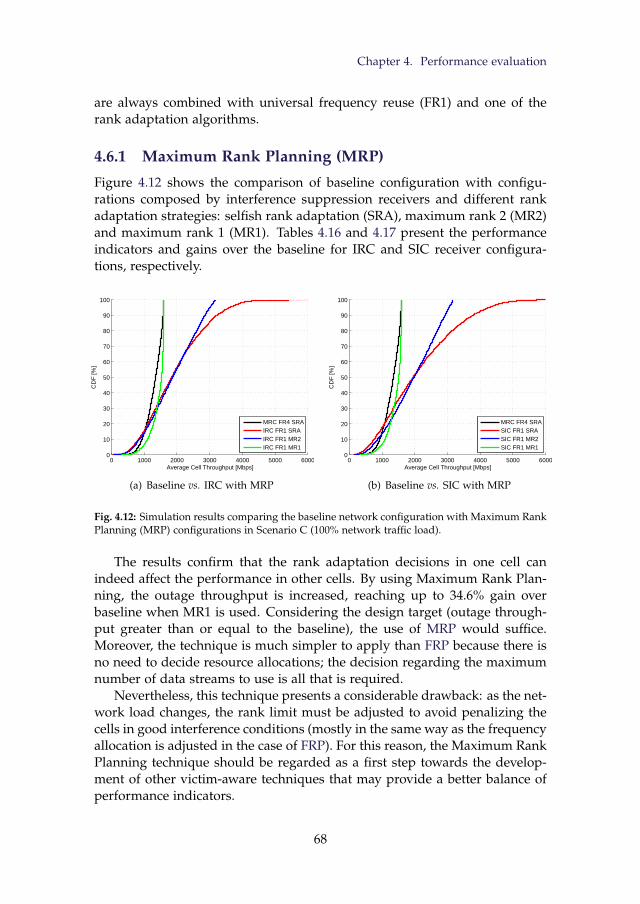
Chapter 4. Performance evaluation
are always combined with universal frequency reuse (FR1) and one of therank adaptation algorithms.
4.6.1 Maximum Rank Planning (MRP)
Figure 4.12 shows the comparison of baseline configuration with configu-rations composed by interference suppression receivers and different rankadaptation strategies: selfish rank adaptation (SRA), maximum rank 2 (MR2)and maximum rank 1 (MR1). Tables 4.16 and 4.17 present the performanceindicators and gains over the baseline for IRC and SIC receiver configura-tions, respectively.
0 1000 2000 3000 4000 5000 60000
10
20
30
40
50
60
70
80
90
100
Average Cell Throughput [Mbps]
CD
F [%
]
MRC FR4 SRAIRC FR1 SRAIRC FR1 MR2IRC FR1 MR1
(a) Baseline vs. IRC with MRP
0 1000 2000 3000 4000 5000 60000
10
20
30
40
50
60
70
80
90
100
Average Cell Throughput [Mbps]
CD
F [%
]
MRC FR4 SRASIC FR1 SRASIC FR1 MR2SIC FR1 MR1
(b) Baseline vs. SIC with MRP
Fig. 4.12: Simulation results comparing the baseline network configuration with Maximum RankPlanning (MRP) configurations in Scenario C (100% network traffic load).
The results confirm that the rank adaptation decisions in one cell canindeed affect the performance in other cells. By using Maximum Rank Plan-ning, the outage throughput is increased, reaching up to 34.6% gain overbaseline when MR1 is used. Considering the design target (outage through-put greater than or equal to the baseline), the use of MRP would suffice.Moreover, the technique is much simpler to apply than FRP because there isno need to decide resource allocations; the decision regarding the maximumnumber of data streams to use is all that is required.
Nevertheless, this technique presents a considerable drawback: as the net-work load changes, the rank limit must be adjusted to avoid penalizing thecells in good interference conditions (mostly in the same way as the frequencyallocation is adjusted in the case of FRP). For this reason, the Maximum RankPlanning technique should be regarded as a first step towards the develop-ment of other victim-aware techniques that may provide a better balance ofperformance indicators.
68

4.6. Using victim-aware rank adaptation
Table 4.16: Key performance indicators (in Mbps) for IRC receiver with different MRP plans andperformance gains over the baseline network configuration in Scenario C.
Load Configuration Outage Average Peak
75%MRC/FR4/SRA 913.3 1346.6 1583.4IRC/FR1/SRA 879.1 (-3.7%) 2290.8 (+70.1%) 3938.8 (+148.7%)IRC/FR1/MR2 962.5 (+5.4%) 2137.0 (+58.7%) 3071.2 (+94.0%)IRC/FR1/MR1 1218.7 (+33.4%) 1502.6 (+11.6%) 1584.0 (+0.0%)
100%MRC/FR4/SRA 818.6 1294.7 1583.3IRC/FR1/SRA 652.4 (-20.3%) 1942.7 (+50.1%) 3612.3 (+128.2%)IRC/FR1/MR2 674.4 (-17.6%) 1861.8 (+43.8%) 3001.2 (+89.6%)IRC/FR1/MR1 939.7 (+14.8%) 1423.0 (+9.9%) 1584.0 (+0.0%)
Table 4.17: Key performance indicators (in Mbps) for SIC receiver with different MRP plans andperformance gains over the baseline network configuration in Scenario C.
Load Configuration Outage Average Peak
75%MRC/FR4/SRA 913.3 1346.6 1583.4SIC/FR1/SRA 853.8 (-6.5%) 2573.7 (+91.1%) 4656.5 (+194.1%)SIC/FR1/MR2 1035.7 (+13.4%) 2240.4 (+66.4%) 3119.7 (+97.0%)SIC/FR1/MR1 1229.1 (+34.6%) 1507.7 (+12.0%) 1584.0 (+0.0%)
100%MRC/FR4/SRA 818.6 1294.7 1583.3SIC/FR1/SRA 652.4 (-20.3%) 1942.7 (+50.1%) 3612.3 (+128.2%)SIC/FR1/MR2 660.2 (-19.3%) 1933.8 (+49.4%) 3047.5 (+92.5%)SIC/FR1/MR1 926.2 (+13.1%) 1410.2 (+8.9%) 1584.0 (+0.0%)
69

Chapter 4. Performance evaluation
4.6.2 Taxation-based Rank Adaptation (TRA)
To test whether a simple victim-aware rank adaptation algorithm can adjustautomatically the outage performance gains without penalizing excessivelythe other performance indicators, the Taxation-based Rank Adaptation (TRA)algorithm was configured using two sets of taxation weights: a conservativeset (TRA-C) and a aggressive set (TRA-A), corresponding to high and lowtaxation settings, respectively. Table 4.18 present the weights for each config-uration. These weights were heuristically selected as examples; they are notin any way regarded as optimal weights.
Table 4.18: Taxation weights for conservative and aggressive configurations.
Configuration Label Rank 1 Rank 2 Rank 3 Rank 4
Conservative TRA-C 0 1/2 2/3 3/4Aggressive TRA-A 0 1/4 2/6 3/8
In Figure 4.13, the performance of the victim-aware rank adaptation algo-rithm is compared to the baseline. The figure shows that both configurations(TRA-C and TRA-A) outperform the baseline in all aspects. The TRA-C con-figuration performs almost identically to the MR1 configuration, whereas theTRA-A configuration provides better performance on the top of the curveand slightly worse performance on the bottom (though still better than thebaseline). Tables 4.19 and 4.20 present the performance indicators for IRCand SIC configurations, respectively.
0 1000 2000 3000 4000 5000 60000
10
20
30
40
50
60
70
80
90
100
Average Cell Throughput [Mbps]
CD
F [%
]
MRC FR4 SRAIRC FR1 SRAIRC FR1 TRA−CIRC FR1 TRA−A
(a) Baseline vs. IRC with TRA
0 1000 2000 3000 4000 5000 60000
10
20
30
40
50
60
70
80
90
100
Average Cell Throughput [Mbps]
CD
F [%
]
MRC FR4 SRASIC FR1 SRASIC FR1 TRA−CSIC FR1 TRA−A
(b) Baseline vs. SIC with TRA
Fig. 4.13: Simulation results comparing the baseline network configuration with Taxation-basedRank Adaptation (TRA) configurations in Scenario C (100% network traffic load).
The performance indicators in Tables 4.19 and 4.20 show that either weightsetting could be used to guarantee outage throughput greater than or equal
70

4.7. Summary
Table 4.19: Key performance indicators (in Mbps) for IRC receiver with different TRA configu-rations and performance gains over the baseline network configuration in Scenario C.
Load Configuration Outage Average Peak
25%MRC/FR1/SRA 1823.0 3439.5 5105.1IRC/FR1/SRA 2396.7 (+31.5%) 3830.5 (+11.4%) 5242.9 (+2.7%)IRC/FR1/TRA-C 1841.3 (+1.0%) 2644.5 (-23.1%) 3775.8 (-26.0%)IRC/FR1/TRA-A 2276.6 (+24.9%) 3563.6 (+3.6%) 4931.8 (-3.4%)
50%MRC/FR2/SRA 1115.8 2051.5 2914.2IRC/FR1/SRA 1350.8 (+21.1%) 2854.3 (+39.1%) 4482.5 (+53.8%)IRC/FR1/TRA-C 1478.8 (+32.5%) 1749.1 (-14.7%) 2243.4 (-23.0%)IRC/FR1/TRA-A 1436.5 (+28.7%) 2506.4 (+22.2%) 3945.8 (+35.4%)
75%MRC/FR4/SRA 913.3 1346.6 1583.4IRC/FR1/SRA 879.1 (-3.7%) 2290.8 (+70.1%) 3938.8 (+148.7%)IRC/FR1/TRA-C 1217.8 (+33.3%) 1522.4 (+13.1%) 1688.6 (+6.6%)IRC/FR1/TRA-A 1102.5 (+20.7%) 1904.5 (+41.4%) 3113.9 (+96.7%)
100%MRC/FR4/SRA 818.6 1294.7 1583.3IRC/FR1/SRA 652.4 (-20.3%) 1942.7 (+50.1%) 3612.3 (+128.2%)IRC/FR1/TRA-C 953.0 (+16.4%) 1422.6 (+9.9%) 1584.0 (+0.0%)IRC/FR1/TRA-A 883.1 (+7.9%) 1609.1 (+24.3%) 2818.0 (+78.0%)
to the baseline outage throughput. However, the conservative setting penal-izes excessively the average and peak throughputs at lower network trafficload conditions (with up to 22.6% degradation), as it may be verified in Fig-ure 4.14. The aggressive setting offers a more balanced situation; this config-uration outperforms the baseline configurations, improving all performanceindicators, when used with both types of interference suppression receiversin all the different network traffic load conditions (with the exception of aslight peak performance degradation with IRC receiver at 25% network load).
4.7 Summary
The results presented in this performance evaluation support the conclusionthat interference suppression receivers may indeed be used as a valid alter-native for traditional frequency reuse techniques with the additional benefitof better performance indicators in the scenarios considered in this study.This conclusion is only true if a system design that offers support for high-performance operation of interference suppression receivers, such as the op-timized frame design presented in Chapter 3, is utilized, and victim-awarerank adaptation algorithms are applied to adjust the interference conditions
71

Chapter 4. Performance evaluation
Table 4.20: Key performance indicators (in Mbps) for SIC receiver with different TRA configu-rations and performance gains over the baseline network configuration in Scenario C.
Load Configuration Outage Average Peak
25%MRC/FR1/SRA 1823.0 3439.5 5105.1SIC/FR1/SRA 2660.3 (+45.9%) 4367.2 (+27.0%) 5818.1 (+14.0%)SIC/FR1/TRA-C 1900.1 (+4.2%) 2790.2 (-18.9%) 3951.4 (-22.6%)SIC/FR1/TRA-A 2463.1 (+35.1%) 3973.4 (+15.5%) 5488.2 (+7.5%)
50%MRC/FR2/SRA 1115.8 2051.5 2914.2SIC/FR1/SRA 1396.2 (+25.1%) 3307.9 (+61.2%) 5270.9 (+80.9%)SIC/FR1/TRA-C 1469.2 (+31.7%) 1787.8 (-12.9%) 2426.5 (-16.7%)SIC/FR1/TRA-A 1445.7 (+29.6%) 2801.3 (+36.6%) 4523.2 (+55.2%)
75%MRC/FR4/SRA 913.3 1346.6 1583.4SIC/FR1/SRA 853.8 (-6.5%) 2573.7 (+91.1%) 4656.5 (+194.1%)SIC/FR1/TRA-C 1216.0 (+33.1%) 1527.9 (+13.5%) 1743.1 (+10.1%)SIC/FR1/TRA-A 1072.6 (+17.4%) 2087.4 (+55.0%) 3730.9 (+135.6%)
100%MRC/FR4/SRA 818.6 1294.7 1583.3SIC/FR1/SRA 549.0 (-32.9%) 2123.6 (+64.0%) 4265.6 (+169.4%)SIC/FR1/TRA-C 963.5 (+17.7%) 1424.2 (+10.0%) 1584.0 (+0.0%)SIC/FR1/TRA-A 866.2 (+5.8%) 1692.7 (+30.7%) 3263.3 (+106.1%)
0 1000 2000 3000 4000 5000 60000
10
20
30
40
50
60
70
80
90
100
Average Cell Throughput [Mbps]
CD
F [%
]
MRC FR1 SRAIRC FR1 SRAIRC FR1 TRA−CIRC FR1 TRA−A
(a) Baseline vs. IRC with TRA
0 1000 2000 3000 4000 5000 60000
10
20
30
40
50
60
70
80
90
100
Average Cell Throughput [Mbps]
CD
F [%
]
MRC FR1 SRASIC FR1 SRASIC FR1 TRA−CSIC FR1 TRA−A
(b) Baseline vs. SIC with TRA
Fig. 4.14: Simulation results comparing the baseline network configuration with Taxation-basedRank Adaptation (TRA) configurations in Scenario C (25% network traffic load).
72

4.7. Summary
in scenarios with unbalanced interference conditions such as Scenario C (In-door Office CSG). Moreover, the results also show that interference suppres-sion receivers improve the network performance indicators even when re-ceiver imperfections are considered in the evaluation, as long as the RSBcovariance matrix estimation method and reasonably accurate ADC modulesare used.
73

Chapter 4. Performance evaluation
74

Chapter 5
Conclusions and future work
This project focused on the design of an interference-robust air interfacefor 5G ultra-dense small cell networks, using interference suppression re-ceivers and victim-aware rank adaptation techniques as the main tools forcoping with the inter-cell interference problem. In this brief final chapter,the project’s main findings are summarized; general recommendations andsuggestions for future studies are also provided.
5.1 Conclusions and recommendations
The main conclusion of this research work is the confirmation that interfer-ence suppression receivers are indeed a valid alternative to other types ofinter-cell interference management techniques in ultra-dense small cell net-works. The results show that a considerable amount of inter-cell interferenceis suppressed, leading to improved network performance indicators in all thescenarios. The frame structure optimized for "just-in-time" estimation andthe victim-aware rank adaptation techniques are key aspects for reaching themain target.
The interference suppression receivers are shown to be robust to imper-fections. The overall performance numbers are degraded due to the esti-mation errors and receiver front-end imperfections, but the results also showthat the degradation is limited and the interference suppression receivers stillperform much better than the baseline.
Finally, it is possible to conclude that the use of victim-aware rank adap-tation algorithms is a new technique full of potential. The results show thatsimple techniques that do not require complex algorithms, large amounts ofcalculations or overly complicated protocols can provide a simple method toadjust the interference levels in the networks, providing fair overall networkperformance and high-quality services to the large majority of users.
75
Chapter 5. Conclusions and future work
The standardization process regarding 5G networks will start soon. Evenbefore this time comes, companies will start discussions about their 5G vi-sions as a first step towards consensus. Considering the results of the presentresearch work, some recommendations for the standardization process maybe formulated:
• Consider how to deal with inter-cell interference from the very be-ginning of the system design – Given the relevance of inter-cell inter-ference problem in dense small-cell networks, it is rather important tosearch for methods to deal with it soon in the design process. By start-ing early, system designers have more opportunity to design the fea-tures required to support efficient inter-cell interference managementmethods.
• Include the support for inter-cell interference suppression in the sys-tem design – Interference suppression receivers require informationabout the interfering signals to perform well and providing this in-formation may require the use of reference signals and control channelmessages. This situation may indeed lead to higher control channeloverhead, but care should be taken before deciding to minimize theoverhead. Saving a few bits in overhead now may cost a large numberof bits in the future.
• Consider the spatial domain when designing inter-cell interferencemanagement techniques – The spatial domain may be used to providethe degrees-of-freedom that are needed for interference management, ina similar way as do the other commonly used domains (frequency andtime). By carefully considering the characteristics of each domain, ad-equate inter-cell interference management techniques may be designedfor each scenario.
5.2 Future work
This section addresses some guidelines for future work concerning the use ofinterference suppression receiver in ultra-dense small cell networks.
In this thesis, it was assumed that orthogonal reference signals will beused by the different transmitters in order to allow for high-accuracy chan-nel estimation. This assumption was considered adequate for the level ofdetail of the investigation, but in reality the number of orthogonal referencesignals will be limited and this limitation may lead to reference signal in-terference (also know as the pilot contamination problem [91]). Therefore,further evaluation of the concept considering the impact of quasi-orthogonaland non-orthogonal reference signals is recommended. This investigation
76

5.2. Future work
should included the search for mechanisms for assigning the multiple refer-ence signals for the different transmitters with the goal of minimizing theirmutual interference. Ideally, such mechanism should be self-organizing to fitadequately with the rest of the concept.
Another important aspect is to study is the impact of narrow-band rankadaptation, which has the potential to improve even further the network per-formance. However, the study of narrow-band rank adaptation should con-sider the increased control channel overhead (due to the larger amount ofnecessary feedback information), trying to balance the benefits and draw-backs.
The analysis of the performance of the network should consider the ex-istence of devices with different number of receive antennas. The numberof antennas assumed in this work (four antennas) should be considered asthe minimum requirement for the typical mobile broadband device. How-ever, the existence of devices with more than four antennas should not beexcluded from the investigation. Their existence will increase the complexityof the scenario and will make the design of victim-aware rank adaptationtechniques more complex.
The careful design of link adaptation algorithms for this type of networkswill be of paramount importance. The use of interference suppression re-ceivers can provide robustness to quickly-changing interference sources, butalso makes the link very sensible to the choices made by the rank adapta-tion algorithm. The study of link adaptation algorithms that jointly considermodulation, coding rate, number of streams (rank) and precoding matrix inthe decisions is recommended.
Moreover, the comparison between interference suppression receivers withother candidate 5G techniques, such as the use of very large antenna arrays(also known as Massive MIMO) [92] and CoMP [42], is recommended. Perfor-mance evaluations comparing these techniques will be invaluable to decideif the additional costs of these more complex techniques are compensated bythe additional performance gains. In these studies, the use of interferencesuppression receivers as suggested in this thesis may be used as a baselinefor comparison.
Finally, the development of proof-of-concept experiments is highly rec-ommended. Using testbed platforms consisting of multiple SDR devices,experiments may be designed to test the concepts presented in this thesis. Inthat respect, experimental activities have already started at the Wireless Com-munication Networks section at Aalborg University, where a testbed networkconsisting of four cells with MIMO devices with two transmit/receive anten-nas has been used to verify the benefits of the use of the IRC receiver [93] andthe MRP rank adaptation technique [94]. This testbed will soon be upgradedto test larger networks and higher-order antenna configurations.
77

Chapter 5. Conclusions and future work
78

Bibliography
[1] 3GPP TS 25.308. High Speed Downlink Packet Access (HSDPA); Overalldescription; Stage 2. v12.2.0. Mar. 2015. url: http://www.3gpp.org.
[2] Heebyung Koh and Christopher L. Magee. “A functional approach forstudying technological progress: Application to information technol-ogy”. In: Technological Forecasting and Social Change 73.9 (2006), pp. 1061–1083.
[3] B. Raaf, W. Zirwas, K.-J. Friederichs, E. Tiirola, M. Laitila, P. Marsch,and R. Wichman. “Vision for Beyond 4G broadband radio systems”.In: Personal Indoor and Mobile Radio Communications (PIMRC), 2011 IEEE22nd International Symposium on. Sept. 2011, pp. 2369–2373. doi: 10.1109/PIMRC.2011.6139944.
[4] Preben Mogensen, Kari Pajukoski, Bernhard Raaf, Esa Tiirola, EevaLähetkangas, Istvan Z. Kovács, Gilberto Berardinelli, Luis G. UzedaGarcia, Liang Hu, and Andrea F. Cattoni. “B4G local area: High levelrequirements and system design”. In: Globecom Workshops (GC Wk-shps), 2012 IEEE. Dec. 2012, pp. 613–617. doi: 10.1109/GLOCOMW.2012.6477644.
[5] A. Osseiran, F. Boccardi, V. Braun, K. Kusume, P. Marsch, M. Mater-nia, O. Queseth, M. Schellmann, H. Schotten, H. Taoka, H. Tullberg,M.A. Uusitalo, B. Timus, and M. Fallgren. “Scenarios for 5G mobileand wireless communications: the vision of the METIS project”. In:Communications Magazine, IEEE 52.5 (May 2014), pp. 26–35. issn: 0163-6804. doi: 10.1109/MCOM.2014.6815890.
[6] Preben Mogensen, Kari Pajukoski, Esa Tiirola, Jaakko Vihriälä, EevaLähetkangas, Gilberto Berardinelli, Fernando Menezes Leitão Tavares,Nurul Huda Mahmood, Mads Lauridsen, Davide Catania, and An-drea Fabio Cattoni. “Centimeter-wave concept for 5G ultra-dense smallcells”. In: Vehicular Technology Conference (VTC Spring), 2014 IEEE 79th.May 2014.
79

Bibliography
[7] F Boccardi, R.W. Heath, A. Lozano, T.L. Marzetta, and P. Popovski.“Five disruptive technology directions for 5G”. In: CommunicationsMagazine, IEEE 52.2 (Feb. 2014), pp. 74–80. issn: 0163-6804. doi: 10.1109/MCOM.2014.6736746.
[8] Petar Popovski. “Ultra-Reliable Communication in 5G Wireless Sys-tems”. Accepted to the 1st International Conference on 5G for Ubiq-uitous Connectivity, November 2014.
[9] ITU 5D/TEMP/435-E. IMT traffic estimates beyond the year 2020 - Work-ing document towards a preliminary draft new report ITU-R M (IMT BE-YOND2020 TRAFFIC). June 2014. url: http://www.itu.int/.
[10] N. Bhushan, Junyi Li, D. Malladi, R. Gilmore, D. Brenner, A. Damn-janovic, R. Sukhavasi, C. Patel, and S. Geirhofer. “Network densifica-tion: the dominant theme for wireless evolution into 5G”. In: Commu-nications Magazine, IEEE 52.2 (Feb. 2014), pp. 82–89. issn: 0163-6804.doi: 10.1109/MCOM.2014.6736747.
[11] T.S. Rappaport, Shu Sun, R. Mayzus, Hang Zhao, Y. Azar, K. Wang,G.N. Wong, J.K. Schulz, M. Samimi, and F. Gutierrez. “MillimeterWave Mobile Communications for 5G Cellular: It Will Work!” In: Ac-cess, IEEE 1 (2013), pp. 335–349. issn: 2169-3536. doi: 10.1109/ACCESS.2013.2260813.
[12] A. Damnjanovic, J. Montojo, Yongbin Wei, Tingfang Ji, Tao Luo, M.Vajapeyam, Taesang Yoo, Osok Song, and D. Malladi. “A survey on3GPP heterogeneous networks”. In: Wireless Communications, IEEE 18.3(June 2011), pp. 10–21. issn: 1536-1284. doi: 10 . 1109 / MWC . 2011 .5876496.
[13] Liang Hu, L. Luque Sanchez, M. Maternia, I. Kovacs, B. Vejlgaard,P. Mogensen, and H. Taoka. “Heterogeneous LTE-Advanced NetworkExpansion for 1000x Capacity”. In: Vehicular Technology Conference (VTCSpring), 2013 IEEE 77th. June 2013, pp. 1–5. doi: 10.1109/VTCSpring.2013.6692578.
[14] G. Boudreau, J. Panicker, Ning Guo, Rui Chang, Neng Wang, and S.Vrzic. “Interference coordination and cancellation for 4G networks”.In: Communications Magazine, IEEE 47.4 (Apr. 2009), pp. 74–81. issn:0163-6804. doi: 10.1109/MCOM.2009.4907410.
[15] 3GPP TR 36.932. Scenarios and requirements for small cell enhancementsfor E-UTRA and E-UTRAN. v12.1.0. Mar. 2013. url: http://www.3gpp.org.
[16] 3GPP TR 36.872. Small cell enhancements for E-UTRA and E-UTRAN -Physical layer aspects. v12.1.0. Dec. 2013. url: http://www.3gpp.org.
80

Bibliography
[17] 3GPP TR 36.842. Study on Small Cell enhancements for E-UTRA and E-UTRAN; Higher layer aspects. v12.0.0. Jan. 2014. url: http://www.3gpp.org.
[18] Sergio Verdu. Multiuser Detection. 1st. New York, NY, USA: CambridgeUniversity Press, 1998. isbn: 0521593735.
[19] Jinho Choi. Optimal Combining and Detection: Statistical Signal Process-ing for Communications. Cambridge: Cambridge University Press, 2010.
[20] J. Winters. “Optimum Combining in Digital Mobile Radio with Cochan-nel Interference”. In: Selected Areas in Communications, IEEE Journal on2.4 (July 1984), pp. 528–539. issn: 0733-8716. doi: 10.1109/JSAC.1984.1146095.
[21] J. Karlsson and J. Heinegard. “Interference rejection combining forGSM”. In: Universal Personal Communications, 1996. Record., 1996 5thIEEE International Conference on. Vol. 1. Sept. 1996, 433–437 vol.1. doi:10.1109/ICUPC.1996.557950.
[22] M. Escartin and P.A. Ranta. “Interference rejection with a small an-tenna array at the mobile scattering environment”. In: Signal ProcessingAdvances in Wireless Communications, First IEEE Signal Processing Work-shop on. Apr. 1997, pp. 165–168. doi: 10.1109/SPAWC.1997.630223.
[23] J.D. Laster and J. Reed. “Interference rejection in digital wireless com-munications”. In: Signal Processing Magazine, IEEE 14.3 (May 1997),pp. 37–62. issn: 1053-5888. doi: 10.1109/79.587051.
[24] P. Patel and J. Holtzman. “Analysis of a simple successive interfer-ence cancellation scheme in a DS/CDMA system”. In: Selected Areasin Communications, IEEE Journal on 12.5 (June 1994), pp. 796–807. issn:0733-8716. doi: 10.1109/49.298053.
[25] J.M. Holtzman. “DS/CDMA successive interference cancellation”. In:Spread Spectrum Techniques and Applications, 1994. IEEE ISSSTA ’94.,IEEE Third International Symposium on. July 1994, 69–78 vol.1. doi:10.1109/ISSSTA.1994.379614.
[26] A.L.C. Hui and Khaled Letaief. “Successive interference cancellationfor multiuser asynchronous DS/CDMA detectors in multipath fad-ing links”. In: Communications, IEEE Transactions on 46.3 (Mar. 1998),pp. 384–391. issn: 0090-6778. doi: 10.1109/26.662644.
[27] G.E. Moore. “Cramming More Components Onto Integrated Circuits”.In: Proceedings of the IEEE 86.1 (Jan. 1998), pp. 82–85. issn: 0018-9219.doi: 10.1109/JPROC.1998.658762.
[28] 3GPP TR 36.829. Enhanced performance requirement for LTE User Equip-ment (UE). v11.1.0. Jan. 2013. url: http://www.3gpp.org.
81

Bibliography
[29] 3GPP TR 36.866. Study on Network-Assisted Interference Cancellation andSuppression (NAIC) for LTE. v12.0.1. Mar. 2014. url: http://www.3gpp.org.
[30] M. Lampinen, F. Del Carpio, T. Kuosmanen, T. Koivisto, and M. Enescu.“System-Level Modeling and Evaluation of Interference SuppressionReceivers in LTE System”. In: Vehicular Technology Conference (VTCSpring), 2012 IEEE 75th. May 2012, pp. 1–5. doi: 10.1109/VETECS.2012.6239964.
[31] K. Pietikainen, F. Del Carpio, H. Maattanen, M. Lampinen, T. Koivisto,and M. Enescu. “System-Level Performance of Interference Suppres-sion Receivers in LTE System”. In: Vehicular Technology Conference (VTCSpring), 2012 IEEE 75th. May 2012, pp. 1–5. doi: 10.1109/VETECS.2012.6239969.
[32] Y. Ohwatari, N. Miki, T. Abe, and H. Taoka. “Investigation on Ad-vanced Receiver Employing Interference Rejection Combining in Asyn-chronous Network for LTE-Advanced Downlink”. In: Vehicular Tech-nology Conference (VTC Spring), 2012 IEEE 75th. May 2012, pp. 1–6.doi: 10.1109/VETECS.2012.6240127.
[33] Y. Ohwatari, N. Miki, T. Asai, T. Abe, and H. Taoka. “Performanceof Advanced Receiver Employing Interference Rejection Combiningto Suppress Inter-Cell Interference in LTE-Advanced Downlink”. In:2011 IEEE Vehicular Technology Conference (VTC Fall). Sept. 2011, pp. 1–7. doi: 10.1109/VETECF.2011.6093196.
[34] S. Golestaneh, H.M. Hafez, and S.A. Mahmoud. “The effect of adjacentchannel interference on the capacity of FDMA cellular systems”. In:Vehicular Technology, IEEE Transactions on 43.4 (Nov. 1994), pp. 946–954. issn: 0018-9545. doi: 10.1109/25.330157.
[35] G. Bauch and V. Franz. “Iterative equalization and decoding for theGSM-system”. In: Vehicular Technology Conference, 1998. VTC 98. 48thIEEE. Vol. 3. May 1998, 2262–2266 vol.3. doi: 10.1109/VETEC.1998.686160.
[36] Timo Halonen, Javier Romero, and Juan Melero. GSM, GPRS and EDGEperformance: evolution towards 3G/UMTS. John Wiley & Sons, 2004.
[37] Mikko Saily, Guillaume Sebire, and Eddie Riddington. GSM/EDGE:Evolution and performance. John Wiley & Sons, 2011.
[38] Abbas El Gamal and Young-Han Kim. Network information theory. Cam-bridge University Press, 2011.
[39] Te Han and K. Kobayashi. “A new achievable rate region for the inter-ference channel”. In: Information Theory, IEEE Transactions on 27.1 (Jan.1981), pp. 49–60. issn: 0018-9448. doi: 10.1109/TIT.1981.1056307.
82

Bibliography
[40] F. Baccelli, A. El Gamal, and D.N.C. Tse. “Interference Networks WithPoint-to-Point Codes”. In: Information Theory, IEEE Transactions on 57.5(May 2011), pp. 2582–2596. issn: 0018-9448. doi: 10.1109/TIT.2011.2119230.
[41] S. Venkatesan, A. Lozano, and R. Valenzuela. “Network MIMO: Over-coming Intercell Interference in Indoor Wireless Systems”. In: Sig-nals, Systems and Computers, 2007. ACSSC 2007. Conference Record ofthe Forty-First Asilomar Conference on. Nov. 2007, pp. 83–87. doi: 10.1109/ACSSC.2007.4487170.
[42] R. Irmer, H. Droste, P. Marsch, M. Grieger, G. Fettweis, S. Brueck, H.P.Mayer, L. Thiele, and V. Jungnickel. “Coordinated multipoint: Con-cepts, performance, and field trial results”. In: Communications Maga-zine, IEEE 49.2 (Feb. 2011), pp. 102–111. issn: 0163-6804. doi: 10.1109/MCOM.2011.5706317.
[43] O. El Ayach, S.W. Peters, and Jr. Heath R.W. “The practical challengesof interference alignment”. In: Wireless Communications, IEEE 20.1 (Feb.2013), pp. 35–42. issn: 1536-1284. doi: 10.1109/MWC.2013.6472197.
[44] S.W. Peters and R.W. Heath. “Cooperative Algorithms for MIMO In-terference Channels”. In: Vehicular Technology, IEEE Transactions on 60.1(Jan. 2011), pp. 206–218. issn: 0018-9545. doi: 10.1109/TVT.2010.2085459.
[45] Wei Yu, Wonjong Rhee, S. Boyd, and J.M. Cioffi. “Iterative water-fillingfor Gaussian vector multiple-access channels”. In: Information Theory,IEEE Transactions on 50.1 (Jan. 2004), pp. 145–152. issn: 0018-9448. doi:10.1109/TIT.2003.821988.
[46] S. Haykin, M. Sellathurai, Y. de Jong, and T. Willink. “Turbo-MIMO forwireless communications”. In: Communications Magazine, IEEE 42.10(Oct. 2004), pp. 48–53. issn: 0163-6804. doi: 10.1109/MCOM.2004.1341260.
[47] M. Morelli and U. Mengali. “A comparison of pilot-aided channelestimation methods for OFDM systems”. In: Signal Processing, IEEETransactions on 49.12 (Dec. 2001), pp. 3065–3073. issn: 1053-587X. doi:10.1109/78.969514.
[48] 3GPP TS 36.211. Evolved Universal Terrestrial Radio Access (E-UTRA);Physical channels and modulation. v11.1.0. Dec. 2012. url: http://www.3gpp.org.
[49] 3GPP R1-062642. Uplink Reference Signal Design in EUTRA. Oct. 2006.url: http://www.3gpp.org.
[50] 3GPP R1-080506. UE specific reference signal pattern. Jan. 2008. url:http://www.3gpp.org.
83

Bibliography
[51] C.J. Hegarty and E. Chatre. “Evolution of the Global Navigation Satel-liteSystem (GNSS)”. In: Proceedings of the IEEE 96.12 (Dec. 2008), pp. 1902–1917. issn: 0018-9219. doi: 10.1109/JPROC.2008.2006090.
[52] S. Chia, M. Gasparroni, and P. Brick. “The next challenge for cellularnetworks: backhaul”. In: Microwave Magazine, IEEE 10.5 (Aug. 2009),pp. 54–66. issn: 1527-3342. doi: 10.1109/MMM.2009.932832.
[53] P. Briggs, R. Chundury, and J. Olsson. “Carrier ethernet for mobilebackhaul”. In: Communications Magazine, IEEE 48.10 (Oct. 2010), pp. 94–100. issn: 0163-6804. doi: 10.1109/MCOM.2010.5594683.
[54] “IEEE Standard for a Precision Clock Synchronization Protocol forNetworked Measurement and Control Systems”. In: IEEE Std 1588-2002 (2002), pp. i–144. doi: 10.1109/IEEESTD.2002.94144.
[55] Fernando M.L. Tavares, Gilberto Berardinelli, Nurul H. Mahmood,Troels B. Sørensen, and Preben Mogensen. “On the Impact of Re-ceiver Imperfections on the MMSE-IRC Receiver Performance in 5GNetworks”. In: Vehicular Technology Conference (VTC Spring), 2014 IEEE79th. May 2014, pp. 1–6. doi: 10.1109/VTCSpring.2014.7023014.
[56] L. Thiele, M. Schellmann, S. Schiffermuller, V. Jungnickel, and W. Zir-was. “Multi-Cell Channel Estimation using Virtual Pilots”. In: Vehic-ular Technology Conference, 2008. VTC Spring 2008. IEEE. May 2008,pp. 1211–1215. doi: 10.1109/VETECS.2008.256.
[57] A. Ghosh, R. Ratasuk, B. Mondal, N. Mangalvedhe, and T. Thomas.“LTE-advanced: next-generation wireless broadband technology [In-vited Paper]”. In: Wireless Communications, IEEE 17.3 (June 2010), pp. 10–22. issn: 1536-1284. doi: 10.1109/MWC.2010.5490974.
[58] Thien-Toan Tran, Yoan Shin, and Oh-Soon Shin. “Overview of en-abling technologies for 3GPP LTE-advanced”. In: EURASIP Journalon Wireless Communications and Networking 2012.1 (2012), p. 54. issn:1687-1499. doi: 10.1186/1687-1499-2012-54. url: http://jwcn.eurasipjournals.com/content/2012/1/54.
[59] F.M.L. Tavares, G. Berardinelli, N.H. Mahmood, T.B. Sørensen, andP. Mogensen. “Inter-cell interference management using MaximumRank Planning in 5G small cell networks”. In: Wireless Communica-tions Systems (ISWCS), 2014 11th International Symposium on. Aug. 2014,pp. 628–632. doi: 10.1109/ISWCS.2014.6933430.
[60] N.H. Mahmood, G. Berardinelli, F.M.L. Tavares, and P. Mogensen.“A distributed interference-aware rank adaptation algorithm for lo-cal area MIMO systems with MMSE receivers”. In: Wireless Commu-nications Systems (ISWCS), 2014 11th International Symposium on. Aug.2014, pp. 697–701. doi: 10.1109/ISWCS.2014.6933443.
84

Bibliography
[61] Davide Catania, Andrea Fabio Cattoni, Nurul Huda Mahmood, GilbertoBerardinelli, Frank Frederiksen, and Preben Mogensen. “A DistributedTaxation Based Rank Adaptation Scheme for 5G Small Cells”. Ac-cepted to the 2015 IEEE 81st Vehicular Technology Conference (VTCSpring), May 2015.
[62] 3GPP TS 36.211. Evolved Universal Terrestrial Radio Access (E-UTRA);Medium Access Control (MAC) protocol specification. v12.4.0. Jan. 2015.url: http://www.3gpp.org.
[63] N.H. Mahmood, L.G. Uzeda Garcia, P. Popovski, and P.E. Mogensen.“On the performance of successive interference cancellation in 5Gsmall cell networks”. In: Wireless Communications and Networking Con-ference (WCNC), 2014 IEEE. Apr. 2014, pp. 1154–1159. doi: 10.1109/WCNC.2014.6952292.
[64] P. Popovski, H. Yomo, K. Nishimori, R. Di Taranto, and R. Prasad.“Opportunistic Interference Cancellation in Cognitive Radio Systems”.In: New Frontiers in Dynamic Spectrum Access Networks, 2007. DySPAN2007. 2nd IEEE International Symposium on. Apr. 2007, pp. 472–475. doi:10.1109/DYSPAN.2007.68.
[65] D. Dardari. “Joint clip and quantization effects characterization inOFDM receivers”. In: Circuits and Systems I: Regular Papers, IEEE Trans-actions on 53.8 (2006), pp. 1741–1748. issn: 1549-8328. doi: 10.1109/TCSI.2006.875170.
[66] Chun-Tao Lin and Wen-Rong Wu. “Clipping ratio estimation for OFDMreceivers”. In: Vehicular Technology Conference (VTC Spring), 2005 IEEE61st. 2005. doi: 10.1109/VETECS.2005.1543414.
[67] P. Mogensen, K. Pajukoski, E. Tiirola, E. Lahetkangas, J. Vihriala, S.Vesterinen, M. Laitila, G. Berardinelli, G.W.O. Da Costa, L.G.U. Gar-cia, F.M.L. Tavares, and A.F. Cattoni. “5G small cell optimized radiodesign”. In: Globecom Workshops (GC Wkshps), 2013 IEEE. Dec. 2013,pp. 111–116. doi: 10.1109/GLOCOMW.2013.6824971.
[68] D. Catania, M.G. Sarret, A.F. Cattoni, F. Frederiksen, G. Berardinelli,and P. Mogensen. “The Potential of Flexible UL/DL Slot Assignmentin 5G Systems”. In: Vehicular Technology Conference (VTC Fall), 2014IEEE 80th. Sept. 2014, pp. 1–6. doi: 10.1109/VTCFall.2014.6966202.
[69] Davide Catania, Marta Gatnau, Andrea Fabio Cattoni, Frank Frederik-sen, Gilberto Berardinelli, and Preben Mogensen. “Flexible UL/DL inSmall Cell TDD Systems: A Performance Study with TCP Traffic”. Ac-cepted to the 2015 IEEE 81st Vehicular Technology Conference (VTCSpring), May 2015.
85

Bibliography
[70] E. Lahetkangas, K. Pajukoski, J. Vihriala, G. Berardinelli, M. Laurid-sen, E. Tiirola, and P. Mogensen. “Achieving low latency and en-ergy consumption by 5G TDD mode optimization”. In: Communica-tions Workshops (ICC), 2014 IEEE International Conference on. June 2014,pp. 1–6. doi: 10.1109/ICCW.2014.6881163.
[71] Eeva Lahetkangas, Kari Pajukoski, Jaakko Vihriala, and Esa Tiirola.“On the flexible 5G dense deployment air interface for mobile broad-band”. In: 5G for Ubiquitous Connectivity (5GU), 2014 1st InternationalConference on. Nov. 2014, pp. 57–61. doi: 10.4108/icst.5gu.2014.258101.
[72] B. Farhang-Boroujeny. “OFDM Versus Filter Bank Multicarrier”. In:Signal Processing Magazine, IEEE 28.3 (May 2011), pp. 92–112. issn:1053-5888. doi: 10.1109/MSP.2011.940267.
[73] F. Schaich. “Filterbank based multi carrier transmission (FBMC) - evolv-ing OFDM: FBMC in the context of WiMAX”. In: Wireless Conference(EW), 2010 European. Apr. 2010, pp. 1051–1058. doi: 10.1109/EW.2010.5483518.
[74] V. Vakilian, T. Wild, F. Schaich, S. Ten Brink, and J. F. Frigon. “Universal-filtered multi-carrier technique for wireless systems beyond LTE”. In:Globecom Workshops (GC Wkshps), 2013 IEEE. Dec. 2013, pp. 223–228.doi: 10.1109/GLOCOMW.2013.6824990.
[75] Gilberto Berardinelli, Kari Pajukoski, Eeva Lahetkangas, Risto Wich-man, Olav Tirkkonen, and Preben Mogensen. “On the Potential ofOFDM Enhancements as 5G Waveforms”. In: Vehicular Technology Con-ference (VTC Spring), 2014 IEEE 79th. May 2014, pp. 1–5. doi: 10.1109/VTCSpring.2014.7023019.
[76] G. Berardinelli, F.M.L. Tavares, T.B. Sørensen, P. Mogensen, and K.Pajukoski. “Zero-tail DFT-spread-OFDM signals”. In: Globecom Work-shops (GC Wkshps), 2013 IEEE. Dec. 2013, pp. 229–234. doi: 10.1109/GLOCOMW.2013.6824991.
[77] G. Berardinelli, F.M.L. Tavares, T.B. Sørensen, P. Mogensen, and K.Pajukoski. “On the Potential of Zero-Tail DFT-Spread-OFDM in 5GNetworks”. In: Vehicular Technology Conference (VTC Fall), 2014 IEEE80th. Sept. 2014, pp. 1–6. doi: 10.1109/VTCFall.2014.6966089.
[78] “IEEE Standard for Information technology - Telecommunications andinformation exchange between systemsLocal and metropolitan areanetworks - Specific requirements - Part 11: Wireless LAN Medium Ac-cess Control (MAC) and Physical Layer (PHY) Specifications - Amend-ment 4: Enhancements for Very High Throughput for Operation inBands below 6 GHz.” In: IEEE Std 802.11ac-2013 (Amendment to IEEE
86

Bibliography
Std 802.11-2012, as amended by IEEE Std 802.11ae-2012, IEEE Std 802.11aa-2012, and IEEE Std 802.11ad-2012) (Dec. 2013), pp. 1–425. doi: 10.1109/IEEESTD.2013.6687187.
[79] H. Hashemi. “The indoor radio propagation channel”. In: Proceedingsof the IEEE 81.7 (July 1993), pp. 943–968. issn: 0018-9219. doi: 10.1109/5.231342.
[80] G. Berardinelli, F.M.L. Tavares, N.H. Mahmood, O. Tonelli, A.F. Cat-toni, T.B. Sørensen, and P. Mogensen. “Distributed synchronization forbeyond 4G indoor femtocells”. In: Telecommunications (ICT), 2013 20thInternational Conference on. May 2013, pp. 1–5. doi: 10.1109/ICTEL.2013.6632081.
[81] Gilberto Berardinelli, Fernando M.L. Tavares, Olav Tirkkonen, TroelsB. Sørensen, and Preben Mogensen. “Distributed Initial Synchroniza-tion for 5G Small Cells”. In: Vehicular Technology Conference (VTC Spring),2014 IEEE 79th. May 2014, pp. 1–5. doi: 10.1109/VTCSpring.2014.7022884.
[82] G. Berardinelli, J.L. Buthler, F.M.L. Tavares, O. Tonelli, D. Assefa, F.Hakhamaneshi, T.B. Sørensen, and P. Mogensen. “Distributed Syn-chronization of a testbed network with USRP N200 radio boards”.In: Asilomar Conference on Signals, Systems and Computers. ConferenceRecord. Nov. 2014.
[83] L.G.U. Garcia, IZ. Kovacs, K.I Pedersen, G. W O Costa, and P.E. Mo-gensen. “Autonomous Component Carrier Selection for 4G Femtocells- A Fresh Look at an Old Problem”. In: Selected Areas in Communica-tions, IEEE Journal on 30.3 (Apr. 2012), pp. 525–537.
[84] K.I. Pedersen, Yuanye Wang, B. Soret, and F. Frederiksen. “eICIC Func-tionality and Performance for LTE HetNet Co-Channel Deployments”.In: Vehicular Technology Conference (VTC Fall), 2012 IEEE. Sept. 2012,pp. 1–5. doi: 10.1109/VTCFall.2012.6399106.
[85] K.I. Pedersen, Yuanye Wang, S. Strzyz, and F. Frederiksen. “Enhancedinter-cell interference coordination in co-channel multi-layer LTE-advancednetworks”. In: Wireless Communications, IEEE 20.3 (June 2013), pp. 120–127.
[86] Mads Lauridsen, Gilberto Berardinelli, Troels B. Sorensen, and PrebenMogensen. “Ensuring Energy Efficient 5G User Equipment by Tech-nology Evolution and Reuse”. In: Vehicular Technology Conference (VTCSpring), 2014 IEEE 79th. May 2014, pp. 1–6. doi: 10.1109/VTCSpring.2014.7022914.
87

Bibliography
[87] Young-Han Nam, Y. Akimoto, Younsun Kim, Moon-il Lee, K. Bhattad,and A. Ekpenyong. “Evolution of reference signals for LTE-advancedsystems”. In: Communications Magazine, IEEE 50.2 (Feb. 2012), pp. 132–138. issn: 0163-6804. doi: 10.1109/MCOM.2012.6146492.
[88] P. Kyösti et al. WINNER II Channel Models. D1.1.2 v1.1. IST-WINNER,Sept. 2007. url: https://www.ist-winner.org/WINNER2-Deliverables/D1.1.2v1.1.pdf.
[89] 3GPP TR 36.814. Evolved Universal Terrestrial Radio Access (E-UTRA);Further advancements for E-UTRA physical layer aspects. v9.0.0. Mar. 2010.url: http://www.3gpp.org.
[90] Harri Holma and Antii Toskala. LTE for UMTS: Evolution to LTE-Advanced.Wiley, 2011.
[91] J. Jose, A. Ashikhmin, T.L. Marzetta, and S. Vishwanath. “Pilot con-tamination problem in multi-cell TDD systems”. In: Information Theory,2009. ISIT 2009. IEEE International Symposium on. June 2009, pp. 2184–2188. doi: 10.1109/ISIT.2009.5205814.
[92] E. Larsson, O. Edfors, F. Tufvesson, and T. Marzetta. “Massive MIMOfor next generation wireless systems”. In: Communications Magazine,IEEE 52.2 (Feb. 2014), pp. 186–195. issn: 0163-6804. doi: 10.1109/MCOM.2014.6736761.
[93] Dereje Assefa Wassie, Gilberto Berardinelli, Fernando Menezes LeitãoTavares, Oscar Tonelli, Troels Bundgaard Sørensen, and Preben Mo-gensen. “Experimental Evaluation of Interference Rejection Combin-ing for 5G Small Cells”. Accepted to the 2015 IEEE Wireless Commu-nications and Networking Conference (WCNC), March 2015.
[94] Dereje Assefa Wassie, Gilberto Berardinelli, Fernando Menezes LeitãoTavares, Troels Bundgaard Sørensen, and Preben Mogensen. “Experi-mental Verification of Interference Mitigation techniques for 5G SmallCells”. Accepted to the 2015 IEEE 81st Vehicular Technology Confer-ence (VTC Spring), May 2015.
[95] R. Gold. “Optimal binary sequences for spread spectrum multiplexing(Corresp.)” In: Information Theory, IEEE Transactions on 13.4 (Oct. 1967),pp. 619–621. issn: 0018-9448. doi: 10.1109/TIT.1967.1054048.
[96] D. Chu. “Polyphase codes with good periodic correlation properties(Corresp.)” In: Information Theory, IEEE Transactions on 18.4 (July 1972),pp. 531–532. issn: 0018-9448. doi: 10.1109/TIT.1972.1054840.
[97] Antonio M Tulino and Sergio Verdú. “Random matrix theory andwireless communications”. In: Communications and Information theory1.1 (2004), pp. 1–182.
88

Bibliography
[98] WB Smith and RR Hocking. “Algorithm as 53: Wishart variate gener-ator”. In: Applied Statistics (1972), pp. 341–345.
[99] D. Morales-Jimenez, J.F. Paris, J.T. Entrambasaguas, and Kai-Kit Wong.“On the Diagonal Distribution of a Complex Wishart Matrix and itsApplication to the Analysis of MIMO Systems”. In: Communications,IEEE Transactions on 59.12 (2011), pp. 3475–3484. issn: 0090-6778. doi:10.1109/TCOMM.2011.100611.100641.
[100] B. Widrow, I. Kollar, and Ming-Chang Liu. “Statistical theory of quan-tization”. In: Instrumentation and Measurement, IEEE Transactions on45.2 (1996), pp. 353–361. issn: 0018-9456. doi: 10.1109/19.492748.
[101] F.M.L. Tavares, G. Berardinelli, N.H. Mahmood, T.B. Sørensen, andP. Mogensen. “On the Potential of Interference Rejection Combiningin B4G Networks”. In: Vehicular Technology Conference (VTC Fall), 2013IEEE 78th. Sept. 2013, pp. 1–5. doi: 10.1109/VTCFall.2013.6692318.
[102] 3GPP TR 25.951. FDD Base Station (BS) classification. v12.0.0. Oct. 2014.url: http://www.3gpp.org.
[103] Stefania Sesia, Matthew Baker, and Issam Toufik. LTE - The UMTSLong Term Evolution: from theory to practice. Chichester, West Sussex:Wiley, 2009. isbn: 9780470697.
89

Bibliography
90

Part II
Appendices
91


Appendix A
Receiver model
In this appendix, the receiver model used for system-level simulations is pre-sented. The baseband signal model is described first, followed by the descrip-tion of the general received signal combining method. Channel response andreceived signal covariance matrix estimation are then discussed, includingthe error models for both types of estimation. Finally, the model for SIC isdescribed and the equations used to calculate the SINR used in the simula-tions are presented in the last section of this appendix.
A.1 Baseband signal model
The baseband signal model assumes a network composed of multiple trans-mitting and receiving devices. Each device is equipped with Ntx transmitand Nrx receive antennas. All devices transmit time-aligned OFDM symbols.The received baseband signal vector r( f , t) with dimension [Nrx × 1] is givenin the frequency domain by
r( f , t) =NT
∑k=1
NkS
∑l=1
hk,l( f , t)sk,l( f , t) + n( f , t) (A.1)
where NT is the number of devices transmitting at the same time and NkS is
the number of data streams transmitted by the k-th device, which is limited to1 ≤ Nk
S ≤ min(Nrx, Ntx). The indexes f and t represent the OFDM subcarrierand OFDM time symbol indexes, respectively1. These indexes are omitted inthe following equations for the sake of simplicity. The scalar sk,l represents
1Note that this model is a discrete time and frequency representation of the received basebandsignal. Both indexes f and t are integers, with 0 ≤ f ≤ Nsc − 1 and −∞ ≤ t ≤ ∞, where Nsc isthe total number of OFDM subcarriers.
93

Appendix A. Receiver model
the data symbol of the l-th stream transmitted by the k-th transmitter throughthe equivalent complex channel given by the vector hk,l [Nrx × 1].
The equivalent complex channel vector hk,l is assumed to include the ef-fects of signal precoding, transmit power amplification, transmit and receiveantenna gains, and large and small scale propagation effects (path loss, shad-owing and fast fading). The vectors hk,l are assumed to be constant for theduration of the transmission interval, i.e. a block fading model is assumed.
The model assumes that transmitted signals sk,l have zero mean and unitypower, and that the signals transmitted by the multiple devices are uncorre-lated, i.e.
µsk,l = E{sk,l} = 0 (A.2)
σsk,l si,j = E{sk,ls∗i,j} =
{1 if k = i and l = j0 if k 6= i or l 6= j
(A.3)
where E{·} is the expectation operator.The vector n [Nrx × 1] represents the additive noise. The m-th element
of n, which is relative to the m-th receive antenna, has power σ2nm and all
elements of n are uncorrelated, i.e.
µnx = E{nx} = 0 (A.4)
σnxny = E{nxn∗y} ={
σ2nx if y = x
0 if y 6= x(A.5)
If the simplified receiver front-end model is used, the power σ2nm is equal
to the additive thermal noise power σ20 (which may be adjusted based on a
noise figure model). In the case of the detailed receiver front-end model, σ2nm
will depend on the characteristics of both the receiver and the input signal.Note that the formula for the received signal vector r may be split in
multiple parts depending on the intended desired signal. Assuming that thedesired signal is the symbol on the j-th stream sent by the i-th transmitter,i.e. si,j, the received signal vector may be described as follows
r = hi,jsi,j︸ ︷︷ ︸desiredsignal
+Ni
S
∑l=1l 6=j
hi,lsi,l
︸ ︷︷ ︸inter-streaminterference
+NT
∑k=1k 6=i
NkS
∑l=1
hk,lsk,l
︸ ︷︷ ︸other
interference
+n (A.6)
A.2 Received signal combining
To generate an estimate of the j-th signal sent by the i-th transmitter, theelements of the received signal r are combined using vector wi,j. The estimate
94

A.3. Channel response estimation
si,j is given bysi,j = wH
i,jr (A.7)
where (·)H is the Hermitian conjugate operator.The optimal combining vector wi,j is obtained using the MMSE estimate
[19], given bywi,j = R−1
r hi,j (A.8)
where hi,j is the equivalent complex channel vector through which the j-thsignal transmitted by the i-th transmitter was sent, and Rr [Nrx × Nrx] is thecovariance matrix of the received signal r, defined as
Rr = E{rrH} (A.9)
In reality, the receiver uses estimates of the equivalent complex channelvector hi,j and the received signal covariance matrix Rr. Therefore, the com-bining vector used in practical receivers is given by
wi,j = R−1r hi,j (A.10)
where Rr is the estimate of Rr and hi,j is the estimate of hi,j.
A.3 Channel response estimation
The channel response is estimated using reference symbols that are knownto both the transmitter and the receiver. These symbols, also known as pilots,are transmitted in predefined positions in the frame. When these pilots aretransmitted, the received signal r in the frequency domain is given by
r( f , t) =NT
∑k=1
NkS
∑l=1
hk,l( f , t)pk,l( f , t) + n( f , t) (A.11)
where NT is the number of devices transmitting reference symbols at thesame time and Nk
S is the number of reference symbols transmitted on thespatial domain by the k-th device. The scalar pk,l represents the l-th pilotsymbol transmitted by the k-th transmitter2.
Assuming pi,j p∗i,j = 1, the channel estimate hi,j obtained using the re-
ceived signal r and the pilot pi,j known at the receiver side is given by
hi,j = rp∗i,j (A.12)
2Note that in Eq. A.11 the value of pilots pk,l( f , t) is zero in most of the ( f , t) positions. Thenon-zero ( f , t) positions are defined by the pilot spacing configuration in the time and frequencydomains.
95

Appendix A. Receiver model
where (·)∗ is the conjugate operator. Ideally, the pilot symbols pk,l shouldbe designed to guarantee that the different pilots transmitted by the multipledevices (including those in other cells) do not interfere with each other. Thisrequirement is fulfilled if the pilots transmitted by each device do not over-lap, i.e. they use different different positions in the frame (different f and tindexes) or different frames. The other possibility is to use orthogonal ref-erence sequences, such as Gold codes [95] or Zadoff-Chu [96, 48] sequences.If the pilots fulfil this requirement then it is possible to obtain the channelestimate hi,j without any interference, i.e. the estimate is given by
hi,j = (NT
∑k=1
NkS
∑l=1
hk,l pk,l + n)p∗i,j (A.13)
=NT
∑k=1
NkS
∑l=1
hk,l pk,l p∗i,j + np∗i,j (A.14)
= hi,j + np∗i,j (A.15)
= hi,j + e (A.16)
where ei,j is the residual estimation error. This error is modelled using thecovariance of the vector ei,j, given by
Re = E{(np∗i,j)(np∗i,j)H} (A.17)
= E{n(p∗i,j pi,j)nH} (A.18)
= E{nnH} (A.19)
= Rn (A.20)
where Rn is the covariance of the noise vector n.The model assumes that the estimation method may use multiple samples
of the same pilot (received in different positions of the frame) to obtain thechannel estimate. The use of multiple estimates helps to improve the qualityof the estimation by reducing the power of the noise error e. This possibilityis also considered in the model. In the simulations, the vector ei,j is modelledas a circularly-symmetric Complex Normal random vector with zero meanand covariance equal to Rn/QH , where QH is the number of samples usedto estimate the channel response vector [50]. The number of samples QH de-pends on the reference symbol design as well as on the frequency correlationof the channel [49].
ei,j ∼ CN (0, Rn/QH) (A.21)
If ideal estimation is assumed, the channel estimates match exactly withthe channel coefficients, i.e. the equivalent channel vector hi,j is given by
hi,j = hi,j (A.22)
96

A.4. Covariance matrix estimation
A.4 Covariance matrix estimation
Different methods for the estimation of the received signal covariance ma-trix Rr can be used depending on the assumptions made about the receivedsignals, and by extension, about the received signal covariance matrix. Thecovariance matrix estimation model for the IRC receiver is presented first, fol-lowed by the model used for the Maximal Ratio Combining (MRC) receiver.
A.4.1 IRC Receiver
Assuming that the channel response vectors hk,l are constant, the receivedsignal covariance matrix Rr is given by
Rr = E{rrH} (A.23)
= E{(NT
∑k=1
NkS
∑l=1
hk,lsk,l + n)(NT
∑k=1
NkS
∑l=1
hk,lsk,l + n)H} (A.24)
= E{(NT
∑k=1
NkS
∑l=1
hk,lsk,l)(NT
∑k=1
NkS
∑l=1
hk,lsk,l)H}+ E{nnH} (A.25)
=NT
∑k=1
NkS
∑l=1
E{(hk,lsk,l)(hk,lsk,l)H}+ E{nnH} (A.26)
=NT
∑k=1
NkS
∑l=1
hk,lE{sk,ls∗k,l}hHk,l + E{nnH} (A.27)
=NT
∑k=1
NkS
∑l=1
hk,lhHk,l + Rn (A.28)
where Rn is the covariance matrix of the noise vector n.In practice, the receiver must use an estimate of the covariance matrix
Rr. In this model, two estimation methods are considered: DSB and RSBmethods [30].
Data-Symbol Based (DSB) Estimation The DSB method is the most directmethod of estimation. The method uses the samples of the received signalat the many different positions of the frame that contain data symbols toestimate the covariance matrix. The estimate of the covariance matrix usingthe DSB method is given by
Rr =1
QDS∑
< f ,t>∈PDS
r( f , t)r( f , t)H (A.29)
97

Appendix A. Receiver model
where PDS is the set of indexing pairs for the subcarriers of the OFDM sym-bols in which data symbols are transmitted and QDS is the cardinality ofPDS.
The covariance matrix estimate is modelled in the simulations as a ran-dom matrix sample drawn from a Wishart distribution [97, 98] with covari-ance matrix Rr (as in Eq. A.28) and QDS degrees of freedom.
Rr ∼1
QDSW(Rr, QDS) (A.30)
Reference-Symbol Based (RSB) Estimation The RSB method uses the chan-nel response estimates to improve the accuracy of the received signal covari-ance matrix estimate. If only the channel response estimates relative to thedesired signals (k = i) are known, the estimate of the covariance matrix usingthe RSB method is given by
Rr =Ni
S
∑l=1
hi,l hHi,l + Rz (A.31)
where Rz is the estimate of the covariance matrix relative to the residualinterference plus noise signal vector. This estimate is given by
Rz =1
QRS∑
< f ,t>∈PRS
(r( f , t)−Ni
S
∑l=1
hi,l pi,l( f , t))(r( f , t)−Ni
S
∑l=1
hi,l pi,l( f , t))H (A.32)
where PRS is the set of indexing pairs for the subcarriers of the OFDM sym-bols in which reference symbols (used for covariance matrix estimation) aretransmitted and QRS is the cardinality of PRS.
The covariance matrix estimate Rz is also modelled in simulations as arandom matrix sample drawn from a Wishart distribution with covariancematrix Rz and QRS degrees of freedom, i.e.
Rz ∼1
QRSW(Rz, QRS) (A.33)
where the covariance matrix Rz is calculated as
Rz =NT
∑k=1k 6=i
NkS
∑l=1
hk,lhHk,l + Rn (A.34)
If the channel response estimates are known for all signals, including theinterferers (k ∈ {1, . . . , NT}), the estimate of the covariance matrix using the
98

A.4. Covariance matrix estimation
RSB method is given by
Rr =NT
∑k=1
NkS
∑l=1
hk,l hHk,l + Rn (A.35)
where Rn is the estimate of Rn, which is calculated as
Rn =1
QRS∑
< f ,t>∈PRS
(r( f , t)−NT
∑k=1
NkS
∑l=1
hk,l pk,l( f , t))(r( f , t)−NT
∑k=1
NkS
∑l=1
hk,l pk,l( f , t))H
(A.36)The covariance matrix estimate Rn is modelled in simulations as a random
matrix sample drawn from Wishart distribution with covariance matrix Rnand QRS degrees of freedom.
Rn ∼1
QRSW(Rn, QRS) (A.37)
Since the covariance matrix Rn is diagonal (there is no correlation betweenthe elements of the additive noise vector n), each one of the diagonal elementsmay be estimated individually to reduce the complexity of the estimation. Ifthis approach is used to estimate Rn, the diagonal elements may be modelledusing random samples drawn from a Chi-squared distribution [99], wherethe index m indicates the m-th receive antenna.
σ2nm ∼
σ2nm
QRS − 1χ2(QRS − 1) (A.38)
A.4.2 MRC Receiver
The MRC receiver assumes the sum of all interference coming from othertransmitters may be modelled as additive noise, i.e. it assumes there is nocorrelation between the signals received by the different receive antennas,leading to the assumption of a diagonal covariance matrix Rz. This assump-tion simplifies the estimation process because the diagonal elements may beestimated individually.
In this case, the estimate of the m-th diagonal element of the Rz matrix isgiven by
σ2zm =
1QRS
∑< f ,t>∈PRS
(rm( f , t)−Ni
S
∑l=1
hi,l,m pi,l( f , t))(rm( f , t)−Ni
S
∑l=1
hi,l,m pi,l( f , t))H
(A.39)
99

Appendix A. Receiver model
where rm and hi,l,m are the m-th elements of the vectors r and hi,l , respectively.The estimate of the Rz matrix is then obtained as
Rz = diag(σ2z1
, σ2z1
, . . . , σ2zNrx
) (A.40)
In simulations, the diagonal elements of the Rz matrix are modelled usinga Chi-squared distribution. The m-th element is given by
σ2zm ∼
σ2zm
QRS − 1χ2(QRS − 1) (A.41)
where the variance σ2zm is calculated as
σ2zm =
NT
∑k=1k 6=i
NkS
∑l=1
hk,l,mh∗k,l,m + σ2nm (A.42)
A.5 Receive front-end imperfections model
This part of the model is used to account for the errors due to imperfec-tions in the receiver front-end. These imperfections exist due to limitations inthe AGC and ADC mechanisms. Depending on the characteristics of the re-ceiver, these limitations may increase the received signal noise floor, leadingto higher estimation errors, inaccurate receiver combining and poor interfer-ence suppression.
The model is divided in two parts: the amplification part, that includesthe effect of power estimation delay, signal amplification and correspondingSNR degradation, and the analog-to-digital conversion part, that includesthe signal quality degradation due to quantization and clipping errors. Fig-ure A.1 presents a schematic for the model, depicting the input and outputsignals of each stage.
The input baseband signal at the m-th antenna (before the receiver front-end components) is given by
r(1)m( f , t) =
NT
∑k=1
NkS
∑l=1
hk,l,m( f , t)sk,l( f , t) + vm( f , t) (A.43)
where vm is the additive thermal noise with power σ20 . The mean received
power of the t-th OFDM symbol is given by
σ2r(1)
m(t) =
1Nsc
Nsc
∑f=1
(NT
∑k=1
NkS
∑l=1|hk,l,m( f , t)|2 + σ2
0 ) (A.44)
100

A.5. Receive front-end imperfections model
𝑟𝑚1(𝑓, 𝑡)
AGC
𝑟𝑚2(𝑓, 𝑡)
ADC 𝑟𝑚3(𝑓, 𝑡)
Amplification
Stage
Analog-to-Digital
Conversion
Fig. A.1: Receiver Front-End Model
where Nsc is the number of OFDM subcarriers.In the amplification stage, AGC mechanism attempts to adjust the ampli-
fication gain to make best use of the ADC dynamic range. In practice, thereis a delay between the estimation of the received signal power and the ad-justment of the gain. The amplification gain applied to the signal received atthe m-th antenna at time t is given by [65]
gm(t) =A√
εσ2r(1)
m(t− τ)
(A.45)
where A is the ADC full range amplitude, ε is the back-off factor and τ is theAGC estimation delay. The back-off ε is use to account for the difference be-tween the peak and average values of the received signal. In ideal conditions,this value controls the probability that the input signal will be clipped by theADC. The value of ε may be calculated for a desired probability by assum-ing the OFDM signal to be a band-limited zero-mean Gaussian stationaryprocess [65].
The output signal power after the amplification stage is given by
σ2r(2)
m(t) =
1Nsc
Nsc
∑f=1
(NT
∑k=1
NkS
∑l=1
g2m(t)|hk,l,m( f , t)|2 + g2
m(t)Fσ20 ) (A.46)
where F is the the noise factor of the amplification stage.In the quantization stage, the quantization noise due to the analog-to-
digital conversion process is included. The model assumes the quantizationnoise to be independently and uniformly distributed [65, 100]. This noise isincluded as an extra additive noise term with power given by
σ2q =
A22−2b
3(A.47)
101

Appendix A. Receiver model
where b is the ADC word-length in bits. This parameter defines the resolutionof the ADC process.
The clipping stage accounts for the noise generated when the amplitudeof the input signal at the ADC input is higher than the ADC full range ampli-tude. This process causes two types of effects: signal amplitude compressionand additive noise power enhancement. The amplitude compression of theinput signal relative to the m-th antenna at time t is calculated as [66]
αm(t) = 1− e−β2m(t) +
√π
2βm(t)erfc(βm(t)) (A.48)
where erfc(·) is the complementary error function and βm(t) is the clippingratio given by
βm(t) =
√√√√ A2
σ2r(2)
m(t)
(A.49)
The power of the clipping noise is calculated as a function of the inputsignal signal power σ2
r(2)m(t) and is given by [66]
σ2cm(t) = (1− e−β2
m(t) − α2m(t))σ
2r(2)
m(t) (A.50)
The output signal power after the analog-to-digital conversion stage isgiven by
σ2r(3)
m(t) =
1Nsc
Nsc
∑f=1
(NT
∑k=1
NkS
∑l=1
α2m(t)g2
m(t)|hk,l,m( f , t)|2 + gm(t)2Fσ20 + σ2
q + σ2cm(t))
(A.51)When the receiver front-end error model is used, the received signal after
the ADC stage relative to the m-th antenna at time t is given by
r(3)m( f , t) =
NT
∑k=1
NkS
∑l=1
αm(t)gm(t)hk,l,m( f , t)sk,l( f , t) + nm( f , t) (A.52)
and the power of the additive noise term nm( f , t) is given by
σ2nm(t) = gm(t)2Fσ2
0 + σ2q + σ2
cm(t) (A.53)
A.6 Successive interference cancellation
If SIC is used, a iterative process takes place in the receiver. In each iteration,the receiver attempts to decode one of the multiple sk,l signals that composesthe received signal r using the estimated signal sk,l . If successful, this signal
102

A.7. Signal-to-interference-plus-noise ratio
is reconstructed and removed from the received signal r, eliminating its in-terfering contribution to the decoding of the other signals. Therefore, aftereach iteration, the received signal r is given by
r( f , t) =NT
∑k=1
NkS
∑l=1
hk,lsk,l + n−NT
∑k=1
NkS
∑l=1︸ ︷︷ ︸
<k,l>∈D
hk,lsk,l (A.54)
where D is the set of indexing pairs of the signals that have already beendecoded. A practical receiver that uses SIC must use estimates of the chan-nel response vectors hk,l and the transmitted symbols sk,l . Therefore, in thepractical receiver, the received signal r is given after each iteration by
r( f , t) =NT
∑k=1
NkS
∑l=1
hk,lsk,l + n−NT
∑k=1
NkS
∑l=1︸ ︷︷ ︸
<k,l>∈D
hk,l sk,l (A.55)
i.e. the effectiveness of the interference cancellation depends both on thequality of the channel estimation and on the correctness of the signal decod-ing process. In this model, it is assumed that a verification mechanism is usedto guarantee that only correctly decoded codewords are used for cancellation,i.e. set D only contains the indexes of correctly decoded symbols.
A.7 Signal-to-interference-plus-noise ratio
The SINR of the estimated signal si,j is obtained through the decompositionof the total power of the estimated signal into desired and interference plus
103

Appendix A. Receiver model
noise contributions. The total power of si,j is given by
σ2si,j
= E{(wHi,jr)(w
Hi,jr)
H} (A.56)
= wHi,jE{rrH}wi,j (A.57)
= wHi,jRrwi,j (A.58)
= wHi,j(
NT
∑k=1
NkS
∑l=1
hk,lhHk,l + Rn)wi,j (A.59)
= wHi,j(
NiS
∑l=1
hi,lhHi,l +
NT
∑k=1k 6=i
NkS
∑l=1
hk,lhHk,l + Rn)wi,j (A.60)
= wHi,j(hi,jh
Hi,j +
NiS
∑l=1l 6=j
hi,lhHi,l +
NT
∑k=1k 6=i
NkS
∑l=1
hk,lhHk,l + Rn)wi,j (A.61)
= wHi,j(hi,jh
Hi,j)wi,j + wH
i,j(Ni
S
∑l=1l 6=j
hi,lhHi,l +
NT
∑k=1k 6=i
NkS
∑l=1
hk,lhHk,l + Rn)wi,j (A.62)
This equation may be simplified to separate the desired signal part fromthe interference and noise part, as follows
σ2si,j
= wHi,j(hi,jh
Hi,j)wi,j︸ ︷︷ ︸
desired signalpower
+wHi,j(Rr − hi,jh
Hi,j)wi,j︸ ︷︷ ︸
interference and noisepower
(A.63)
Using this formulation, the SINR of the estimated signal si,j is given by
γi,j =wH
i,j(hi,jhHi,j)wi,j
wHi,j(Rr − hi,jh
Hi,j)wi,j
(A.64)
If SIC is used, the covariance matrix used in the SINR formula is updatedat every iteration to remove the contribution from the cancelled interferers.
Rr =NT
∑k=1
NkS
∑l=1
hk,lhHk,l + Rn −
NT
∑k=1
NkS
∑l=1︸ ︷︷ ︸
<k,l>∈D
hk,l hHk,l (A.65)
104

Appendix B
Detailed simulationassumptions
The simulation tool used to generate the results presented in this thesis andin the related publications was initially developed for inter-cell interferencecoordination studies. The main focus was to evaluate different distributedmechanisms for the allocation of time/frequency resources among neighbourcells. The simulator was coded in Matlab and was designed to be modularand testable.
During this research project, this simulator was modified to include thenew features necessary for the investigation on the use of interference sup-pression receivers as a tool to manage inter-cell interference, such as the re-ceiver model presented in Appendix A. A detailed description of the simu-lation tool and the models used for system-level simulations is presented inthe following sections.
B.1 Simulation tool
The high-level flowchart of the simulation tool is presented in Figure B.1(a).The simulator uses a Monte Carlo simulation approach in which many dif-ferent trials are used to achieve statistical reliability. These different trials,also known as "snapshots", generate data that is collected and post-processedto derive the statistical indicators used to analyse the network when differentsets of input parameters are used.
For each snapshot, the simulator generates a new network topology, i.e.the APs and UEs are positioned in different positions following a set of posi-tioning rules that depend on the scenario selected for simulation. During thisstep, every variable that is not time dependent is pre-calculated to save simu-
105

Appendix B. Detailed simulation assumptions
lation time. For example, the large scale propagation effects are calculated atthis point, since device mobility is not considered in these simulations due tothe short time span of each snapshot. For the same reason, the cell associationprocess is also performed only once at the beginning of each snapshot.
In each snapshot a predefined number of frames is simulated. Each frameconsists in a sequence of steps, as shown in Figure B.1(b). The final result ofeach frame is a set of variables that describe the status of the network at theend of that time frame. This set includes for example the instantaneous SINRand throughput of each link at that specific frame. After enough frames havebeen simulated, a new snapshot starts with a new topology. This process isrepeated until the end of the simulation.
Read input parameters
Start
End
Initialize modules
Generate topology
Enough snapshots?
Collect statistics
Simulate snapshot
Store snapshot results
yes
no
(a) High-level flowchart
Update channel model
Start
End
Update traffic model
User scheduling
Enough frames?
Calculate SINR
Map SINR to throughput
Rank and precoding matrix adaptation
Store frameresults
no
yes
(b) Snapshot flowchart
Fig. B.1: Simulation flowcharts
106

B.2. Simulation scenario
10 m
10 m
10 m
Fig. B.2: Indoor Office [89]
B.2 Simulation scenario
The general simulation scenario consists of a small-cell network operatingover a 200 MHz frequency band at 3.5 GHz. This frequency band is dedicatedfor the operation of the small-cell network, i.e. it is assumed that the bandis free of interference coming from other networks or layers (such as a macrocell layer, for example).
Two different indoor deployment scenarios are considered in this study.The first scenario, hereby referred to as the Indoor Office scenario, is a stan-dard 3GPP scenario that was first used for the evaluation of LTE femto-cells [89]. This scenario is also known as the dual-stripe scenario in the lit-erature. The scenario, depicted in Figure B.2, consists in two office buildingsseparated by a ten-meter-wide street. Each building is composed of two rowsof ten offices per floor. Each office measures ten meters by ten meters.
In this scenario, one AP and a configurable number of UEs are droppeduniformly at random positions in each office. Devices are not dropped out-doors. The position of the APs is random in this scenario to emulate theusers deploying their APs at any place in the offices (i.e. the network opera-tor has no control over the location of the APs in this scenario). Although thenumber of UEs per office may be configured, the simulations in this researchwork were always configured with one UE per office.
The second scenario, hereby referred to as the Indoor Hotspot scenario,is a simple modification of the first scenario [101]. This scenario mimics alarge hall in which multiple APs are deployed to cover the area of the hall.Figure B.3 depicts the scenario. The scenario consists of four rows of tenvirtual square spaces (there are no walls separating the square spaces in thisscenario). One AP is deployed in the middle of each virtual square space,creating a uniform coverage area throughout the hall. The UEs are thendropped uniformly at random positions. Again, no devices are dropped
107

Appendix B. Detailed simulation assumptions
10 m
10 m
Fig. B.3: Indoor Hotspot [101]
outdoors.Each deployment scenario may be configured to assume either CSG or
OSG access modes. In CSG mode, the UEs are only allowed to connect tothe AP located in the same office, whereas in OSG mode, the UEs may freelyconnect to any AP. In the OSG case, the UEs are connected to the AP thatwill lead to the link with the smallest total propagation loss.
The Indoor Office scenario may also be configured to emulate differentnetwork densities by changing the cell DR, i.e. the probability that an APwill exist in either each office. This probability is modelled as the outcome ofa Bernoulli trial. Therefore, the actual number of APs deployed per snapshotis given by a Binomial distribution with number of trials equal to the numberof offices or spaces and probability equal to the deployment ratio.
B.3 Propagation model
The propagation model includes both large-scale (deterministic path loss andlog-normal shadowing) and small-scale (frequency-selective time-varying sig-nal fading) effects.
B.3.1 Deterministic path loss
For the Indoor Office scenario, the deterministic path loss model for the stan-dard 3GPP dual-stripe scenario [89] is used. This model takes into accountthe attenuation loss due to the walls that may exist in between devices. Themodel provides path loss formulas for links between devices in the samebuilding and devices in different buildings. The path loss in decibels [dB] isgiven by
PL = 38.46 + 20 log10 R + 0.7d2Dindoor + qLiw + 18.3n((n+2)/(n+1)−0.46) (B.1)
108
B.3. Propagation model
and
PL = max(15.3 + 37.6 log10 R, 38.46 + 20 log10 R) (B.2)
+ 0.7d2Dindoor + qLiw + 2Low + 18.3n((n+2)/(n+1)−0.46) (B.3)
for devices in the same building and devices in different buildings, respec-tively. In these formulas, R is the linear distance between transmitter andreceiver in meters (considering the three spatial dimensions) and d2Dindoor isthe linear indoor distance in the xy-plane (excluding height) also in meters.This additional loss of 0.7 dB per meter models the loss due to furniture andother obstacles found indoors. The model also accounts for the loss due tointernal walls (Liw) and external walls (Low), where q is the total numberof internal walls traversed by the signal. Finally, n is the number of floorsseparating the transmitter from the receiver in multi-floor deployments. TheMinimum Coupling Loss (MCL) in this scenario is 45 dB [102].
The model for the Indoor Hotspot scenario is the Winner II Indoor Hotspot(B3) model [88]. In this model the formula used depends on the line-of-sightconditions. The path in decibels [dB] is given in this case by
PL = max(70, 13.9 log10 R + 64.4 + 20 log10( fc/5)) (B.4)
andPL = max(60, 37.8 log10 R + 36.5 + 23 log10( fc/5)) (B.5)
if the links are in line-of-sight and non-line-of-sight conditions, respectively.The variable fc is the carrier frequency in GHz. In this scenario, the MCL is70 dB. The probability of line-of-sight is calculated for each link based on thedistance between transmitter and receiver, according to the following rule.
P(LOS) ={
1 if R ≤ 10e−(R−10)/45 if R > 10
(B.6)
B.3.2 Log-normal shadowing
The shadowing for each link is given by a random sample drawn from log-normal distributions. In the Indoor Office scenario, the parameters of thisdistribution depend on whether the link is an interfering link or not. Thevalues are 8 dB for interfering links and 6 dB for the other [89]. In the IndoorHotspot scenario, the parameter depends on the line-of-sight-condition. Thevalues are 3 dB for line-of-sight links and 4 dB for non-line-of-sight links [88].
B.3.3 Frequency-selective time-varying signal fading
Signal fading is modelled as a frequency-selective time-varying process, us-ing the channel model developed during the Winner II project [88]. The
109

Appendix B. Detailed simulation assumptions
fading channel samples are pre-calculated and saved in a large binary file inorder to reduce simulation time. In each simulation snapshot, different partsof the file are selected randomly to emulate the signal fading for the differentlinks. Care was taken to guarantee that the samples used in different snap-shots have very low correlation and that this correlation does not affect theaccuracy of the results.
Different files were created for the different scenarios and for differentline-of-sight conditions. The Winner II scenario used for the Indoor Officeand the Indoor Hotspot scenarios were the Indoor Office (A1) and IndoorHotspot (B3), respectively [88]. It was assumed that all devices of the networkuse the same type of antenna: a simple uniform linear array with four dipoleelements, with half wave-length distance between adjacent elements.
A fading sample generator script (which is a deliverable of the WinnerII project) was used to create the fading files for the MIMO channel. Thescript was configured to generate channel samples for each possible pathbetween the four transmit antennas and the four receive antennas at everytenth time frame, which for the proposed 5G RAT concept means every 2.5ms. This time resolution was chosen to reduce file size, taking advantageof the fact that the channel varies slowly in indoor scenarios. Each channelsample is given in the time domain in the form of a power delay profile. Thecarrier frequency was set to 3.5 GHz and the device speed was assumed tobe 3 km/h, even though devices are static, to account for moving objects orpeople in the indoor spaces.
The time-domain channel samples were converted to the frequency do-main, taking the proposed 5G RAT concept as the base model for the frequency-domain signal. The conversion assumed that the FFT size of OFDM transceiveris 4096 and that each subcarrier is 60 kHz wide. The system uses 3300 sub-carriers in total, using 198 MHz of the 200 MHz frequency band allocatedfor the system. The frequency resolution of the file is equal to 900 kHz (15subcarriers).
B.4 Frequency allocation
Frequency allocation according to static frequency reuse plans was usedin the simulations to evaluate the benefits of interference suppression re-ceivers in different inter-cell interference conditions. Three basic plans wereused during the project: universal frequency reuse (or simply Reuse 1) andplanned frequency reuse with reuse factors equal to 2 and 4 (referred to asReuse 2 and Reuse 4, respectively). Figures B.4 and B.5 show the frequencyallocation plans for Reuse 2 and Reuse 4 cases in the Indoor Office and IndoorHotspot scenarios, respectively.
110

B.5. Traffic model
1 2 1 2 1 2 1 2 1 2
2 1 2 1 2 1 2 1 2 1
1 2 1 2 1 2 1 2 1 2
2 1 2 1 2 1 2 1 2 1
(a) Frequency Reuse 2
1 2 1 2 1 2 1 2 1 2
3 4 3 4 3 4 3 4 3 4
1 2 1 2 1 2 1 2 1 2
3 4 3 4 3 4 3 4 3 4
(b) Frequency Reuse 4
Fig. B.4: Frequency Allocation Plans - Indoor Office Scenario
1 2 1 2 1 2 1 2 1 2
2 1 2 1 2 1 2 1 2 1
1 2 1 2 1 2 1 2 1 2
2 1 2 1 2 1 2 1 2 1
(a) Frequency Reuse 2
1 2 1 2 1 2 1 2 1 2
3 4 3 4 3 4 3 4 3 4
1 2 1 2 1 2 1 2 1 2
3 4 3 4 3 4 3 4 3 4
(b) Frequency Reuse 4
Fig. B.5: Frequency Allocation Plans - Indoor Hotspot Scenario
B.5 Traffic model
Two different traffic models were used in the simulations: a downlink-onlyfull-buffer traffic model, that assumes all APs transmit in all time framesduring the simulation period, and a three-state random traffic model, thatassumes that the state of each cell may randomly change between DL, ULor idle at every time frame. In the three-state random traffic model, theprobability that the state of the cell will change from one state to the other ismodelled as a discrete-time Markov process. Figure B.6 shows the schematicfor the process.
The three-state random traffic model was included in the simulator tomimic the effect of Dynamic TDD on the inter-cell interference conditionsof the network. This model is also used to control the average load of thenetwork by determining the average number of times that a cell will not bein the idle state i.e. there will be either a DL or a UL transmission. Thisaverage is hereby referred to as the AF of the network.
Although the three-state random traffic model implemented in the sim-ulator may be used with any transition probability matrix, the simulationsregarding this thesis always used transition matrices with identical rows.This setup leads to a three-state Bernoulli scheme in which the probabilityof transition does not depend on the current state. Therefore, the AF can be
111

Appendix B. Detailed simulation assumptions
DL
Idle
UL
𝑃𝐷𝐿→𝐷𝐿 𝑃𝑈𝐿→𝑈𝐿
𝑃𝐼𝑑𝑙𝑒→𝐼𝑑𝑙𝑒
𝑃𝐷𝐿→𝐼𝑑𝑙𝑒 𝑃𝑈𝐿→𝐼𝑑𝑙𝑒
𝑃𝐼𝑑𝑙𝑒→𝐷𝐿 𝑃𝐼𝑑𝑙𝑒→𝑈𝐿
𝑃𝑈𝐿→𝐷𝐿
𝑃𝐷𝐿→𝑈𝐿
Fig. B.6: Three-state Traffic Model
defined in this cases simply as the probability of not choosing the idle state,i.e. choosing either the DL or the UL states.
B.6 User scheduling model
The user scheduling model implements a simple frequency-domain channel-blind fair-resource scheduler that operates independently in each cell. Thescheduler always allocates an equal share of resources for the active users.Moreover, all the resources are always used at every time frame.
B.7 Physical layer model
The physical layer model uses the concept of resource blocks to calculate theinstantaneous throughput of each link. Each resource block is defined as 15subcarriers (900 kHz) for the duration of one time frame (0.25 ms). In thisdescription of the model, the index ϕ is used to identify the multiple resourceblocks of a single time frame.
At every time frame, the SINR of all relevant received signals is calculatedusing the receiver model described in Appendix A. These SINR values arethen adjusted using the EVM model [103] to avoid unrealistically high SINRvalues.1 The EVM is a widely accepted model to emulate the expected qualityof the communication system devices. Using this model, a EVM value inpercentage is used to derive a maximum asymptotic value that the SINR mayreach. This value is given by
γmax = −20 log10(EVM/100) (B.7)
1The EVM model is only used when the receiver front-end model presented in Appendix Ais not used.
112

B.8. Rank and precoding matrix adaptation model
The EVM-adjusted SINR value for the j-th stream transmitted by the i-thtransmitter at the ϕ-th resource block is then given by
γi,jEVM(ϕ) =
γi,j(ϕ)γmax
γi,j(ϕ) + γmax(B.8)
These values are then used to calculate the spectral efficiency of the links.The spectral efficiency for the j-th stream transmitted by the i-th transmitterat the ϕ-th resource block is then given in bits/s/Hz by
ηi,j(ϕ) =
ηmax if γi,jEVM
≥ γmax
log2(1 + γi,jEVM(ϕ)) if γmin ≤ γi,jEVM
< γmax
0 if γi,jEVM< γmin
(B.9)
where γmin is the minimum required SINR for decoding any signal and γmaxis the maximum SINR given by
γmax = 2ηmax − 1 > γmin (B.10)
where ηmax is the maximum spectral efficiency that the link may reach. Thevalues γmin and ηmax are derived from the Adaptive Modulation and Coding(AMC) scheme used by the communication system.
The spectral efficiency values are used to calculate the data rate for eachindividual stream. The data rate for the j-th stream transmitted by the i-thtransmitter is calculated using the average spectral efficiency over the multi-ple allocated resource blocks and is given in bits/s/Hz by
Ri,j =BwNϕ
Nϕ
∑ϕ=1
ηi,j(ϕ) (B.11)
where Bw is the total allocated bandwidth used by the signal and Nϕ is thenumber of allocated resource blocks. Finally, the instantaneous total data ratefor the signals transmitted by the i-th transmitter is given by
Ri =Ni
S
∑l=1
Ri,j (B.12)
where NiS is the number of data streams transmitted by the i-th transmitter.
B.8 Rank and precoding matrix adaptation model
The aim of the rank and precoding matrix adaptation model is to emulatethe effect of the adaptation algorithms that are used to find the ideal rank
113

Appendix B. Detailed simulation assumptions
and precoding matrices for the transmission of signals. The model imple-mented in the simulator assumes independent adaptation for each link, i.e.each transmitter-receiver pair tries to choose a matrix to maximize the datarate of their links. In this model, the receiver chooses the best matrix andsends to the transmitter through a feedback channel the index that identi-fies this matrix in a larger set of matrices. The set of precoding matricesused by the simulator is the LTE codebook for downlink closed-loop Single-User Multiple-Input Multiple-Output (SU-MIMO) transmissions []. This setof precoding matrices is used for both DL and UL transmissions.
The following algorithm describes the rank and precoding adaptation pro-cess in the simulation.
1. InitializationAt the first time frame of the snapshot, a random matrix Ck [Ntx × Nk
S]is selected for the k-th transmitter from the set of all Rank 1 matrices.The first time frames of each snapshot are discarded from the collectionof results to avoid the transient effect due to this initial setup;
2. Update channel vectorsAll equivalent channel vectors hk,l are updated to account for the se-lected matrices. This update is performed using the non-precodedchannel matrix Hk [Nrx× Ntx] that is output by the channel model. Theprecoded channel matrix Hk [Nrx × Nk
S] is then given by
Hk = HkCk (B.13)
and the precoded equivalent channel vectors hk,l are the columns of Hk,i.e.
Hk =[hk,1 hk,2 . . . hk,Nk
S
](B.14)
3. Search best matrix for each linkThe search for the best matrix for each link is performed by testingwhich matrix would have led to the highest throughput assuming allthe rest was constant. Therefore, for the search relative to the i-th trans-mitter, all possible Ci are tested while Ck for k 6= i are constant. The Cimatrix that leads to the highest throughput is selected for transmissionat the next time frame;
4. Repeat steps 2 and 3 per each frame until the end of the snapshot
In the case that the MRP technique [59] is used, the algorithm is modifiedto limit the set of rank and precoding matrices that may be used by each link,whereas in the case of TRA [61], the algorithm is uses the taxation metric todecide which matrix to use.
114

Part III
Papers
115


Paper A
On the Potential of Interference Rejection Combiningin B4G Networks
Fernando M. L. Tavares, Gilberto Berardinelli, Nurul H.Mahmood, Troels B. Sørensen, and Preben Mogensen
The paper has been published in theProceedings of the IEEE 78th Vehicular Technology Conference (VTC Fall),
September 2013.

c© 2013 IEEEThe layout has been revised.

I. Introduction
Abstract
Beyond 4th Generation (B4G) local area networks will be characterized by the denseuncoordinated deployment of small cells. This paper shows that inter-cell interfer-ence, which is a main limiting factor in such networks, can be effectively containedusing Interference Rejection Combining (IRC) receivers. By simulation we investi-gate two significantly different interference scenarios with dense small cell deploy-ment. The results show that IRC brings considerable improvement in outage as wellas in peak and median throughputs in both scenarios, and thus has a big potential asa capacity and coverage enhancing technique for B4G. The IRC gain mechanism de-pends strongly on the interference scenario and to some extent on the use of frequencyreuse. These results are achieved with no coordination among cells and suggests thatMultiple Input Multiple Output (MIMO) rank adaptation and IRC can be performedindependently.
I. Introduction
In the last decades, several generations of Radio Access Networks (RANs)have been designed to cope with the growing demand for wireless services. Anew disruptive system has emerged approximately every 10 years to alleviatebackward compatibility problems and to take advantage of the evolution ofthe technology components. Considering that the specifications of the LongTerm Evolution - Advanced (LTE-A) radio standard were submitted in 2010,a novel Beyond 4th Generation (B4G) RAN is then expected to emerge in themarket around 2020 [1].
This new RAN should be designed to support the massive deployment ofsmall cells, since this type of deployment is foreseen as a solution for meet-ing the future capacity expansion requirements [1]. As deployments becomedenser, their uncoordinated nature will inevitably aggravate the inter-cellinterference problem, causing considerable impact on the network perfor-mance. The allocation of orthogonal spectrum resources to cells that stronglyinterfere with each other is often considered as the solution for this prob-lem [2, 3].
With the evolution of electronic hardware and Multiple-Input Multiple-Output (MIMO) techniques, inter-cell interference suppression techniques,whose application was previously limited by their large computational bur-den, may now be cost-effectively implemented in receivers. It is reasonableto believe that this kind of receivers can offer high performance gains in in-terference limited scenarios, but, to the best of our knowledge, all the systemlevel performance evaluation studies on the topic focus on macro cell andheterogeneous Long Term Evolution (LTE) and LTE-A network scenarios [4,5, 6, 7].
119

Paper A.
Different baseband processing techniques may be used to suppress theinter-cell interference. For instance, Successive Interference Cancellation (SIC)and Parallel Interference Cancellation (PIC) techniques decode both the de-sired and the interfering signal to cancel their mutual interference contri-bution [8]. Conversely, Interference Rejection Combining (IRC) is a linearcombining technique that relies on multiple receive antennas and the esti-mate of the interfering channels to project the received signals on a subspacein which the Mean Square Error (MSE) is minimized [9]. IRC is attractivegiven its simplicity and maturity, and it represents a straightforward add-onto the known Minimum Mean Square Error (MMSE) detector, which is nowconsidered the baseline detector in LTE networks [10].
In this paper, we present the first system level downlink performanceevaluation of inter-cell interference suppression for different local area smallcell B4G scenarios. Specifically, we consider scenarios with dense small celldeployment and two modes of operation: one with closed subscriber modeof relevance for office buildings (or private apartments) and one with opensubscriber mode of relevance for public hot spots. We use a signal model thatincludes spatial multiplexing precoding with multiple data layers (both forthe desired and the interfering signals) to verify their effects on the interfer-ence rejection capabilities of IRC and contrast it with the use of different fre-quency reuse schemes. Our ultimate goal is to address the effective potentialof this detector on the performance of B4G networks, providing informationthat will help guide the design of this new RAN.
The paper is organized as follows. We first describe the signal model usedin the simulations in Section II and the details related to the simulation setupin Section III; we present and analyse the simulation results in Section IV;finally, we draw our conclusions in Section V.
II. Signal Model
In this section, we present the analytical signal model of the detectors thatare used in our system evaluation.
We assume that the generic i-th network node is equipped with Ntx trans-mit antennas and Nrx receive antennas, and can transmit 1 ≤ Nstreamsi ≤min(Nrx, Ntx) data streams. The number of transmitted streams is also oftenreferred as transmission rank. For simplicity, we present the system model fora generic Orthogonal Frequency Division Multiplexing (OFDM) frequencysubcarrier.
Let us denote with si the Nstreamsi × 1 data column vector of the i-th node.The vector si is mapped over the Ntx antennas by the Ntx×Nstreamsi precodingmatrix Ci. Let us assume that the subscript D denotes the desired signalat the receiver side, and the subscript Iq the q-th interfering signal. After
120

II. Signal Model
transmission over the fading channel, the Nrx × 1 frequency domain receivedcolumn vector at a particular receiver can then be expressed as
r = HDsD + HIsI + n (A.1)
where
• n is the Nrx × 1 Additive White Gaussian Noise (AWGN) contributionvector with power σ2
0 ;
• HD and HIq are the equivalent channel matrices which include the pre-coding matrices, i.e. HD = HDCD and HIq = HIq CIq , with HD and HIq
being the Nrx × Ntx fading channel matrices;
• sI and HI represent the concatenation of the NI received interfering sig-nals and the concatenation of their equivalent NI channels, respectively,i.e.
sI = [sTI1
. . . sTIq
. . . sTINI
]T (A.2)
HI = [HI1 . . . HIq . . . HINI] (A.3)
where (·)T denotes the transpose operator.
Let us also define the generic MMSE combining matrix [11]:
W = (HDHHD + Rn)
−1HD (A.4)
where (·)H is the hermitian operator and HD represents the estimated equiv-alent channel matrix of the desired signal.
The desired sD is then estimated by using the combining matrix W:
sD = WHr (A.5)
The following detectors can be specified according to the nature of thematrix Rn:
• MMSE - Interference Rejection Combining (MMSE-IRC):
Rn = E{
HIHHI}+ σ2
0 INrx (A.6)
where INrx denotes the Nrx × Nrx identity matrix.
• MMSE - Maximal Ratio Combining (MMSE-MRC):
Rn = diag([m1 · · ·mNrx ]) (A.7)
121

Paper A.
where
mz = E{ NI
∑q=1
Nstreamsq
∑k=1
∣∣∣HIq(z,k)
∣∣∣2}+ σ20 (A.8)
with HIq(z,k)corresponding to the element in the z-th row and the k-th
column of HIq .
While in the MMSE-MRC detector the matrix Rn can be computed byestimating the total interference plus noise power at each receive antenna, Rnin the MMSE-IRC detector corresponds to the estimated covariance matrixof the interfering signals. Therefore, MMSE-IRC assumes knowledge of eachinterfering channel at each antenna which may impose strict requirements onthe system design since each node would need to discriminate the referencesequences sent by multiple interferers. We assume here that such a systemdesign is possible, and consider it to be a topic for future work.
III. Simulation Setup
As mentioned in the introduction, the usage of IRC detectors is foreseen asparticularly beneficial in scenarios characterized by a dense uncoordinateddeployment of small cells. This paper aims at addressing such potential withan extensive system level evaluation. In this section, we describe in detailsthe physical layer assumptions, scenarios and simulation setup used in oursimulation campaign.
A. Physical Layer Assumptions
We assume ideal channel estimation of both desired and interfering signalsbased on the aforementioned reference sequences. Rank and precoding adap-tation feedback with no errors and one frame delay is assumed. The precod-ing matrices used are those defined in [12] for downlink closed-loop single-user MIMO in LTE, and are applied per Physical Resource Block (PRB) infrequency domain for the assumed OFDM based system [1].
We calculate the Signal-to-Interference-plus-Noise Ratio (SINR) for the j-th stream as follows [11]:
SINRj =WH
(j)HD(j)HH
D(j)W(j)
WH(j)(HD(j)
HHD(j)
+ HIHHI + σ2
0 INrx)W(j)(A.9)
where A(j) denotes the j-th column of matrix A and A(j) is the matrix ob-tained by removing the j-th column from matrix A.
122

III. Simulation Setup
The SINR values are then adjusted using the following Error Vector Mag-nitude (EVM) model to account for transceiver implementation imperfec-tions.
SINRevm,j =SINRj · SINRmax
SINRj + SINRmax(A.10)
Based on the resulting SINR we calculate the corresponding data rate us-ing the Shannon formula, with maximum spectral efficiency limited to 6bits/s/Hz (uncoded 64QAM modulation). All streams are added, resultingin the total data rate per User Equipment (UE). Table A.1 summarizes thesephysical layer details.
Table A.1: Physical Layer Assumptions
Physical Layer Model [1]
Spectrum Allocation 200 MHz at 3.5 GHz
Frame Duration 0.25 ms
Access Scheme
Downlink OFDMA
3000 subcarrriers 60 kHz each
15 subcarriers per PRB
Transmission Power 20 dBm
Receiver Noise Figure 9 dB
MIMO SchemeClosed-loop SU-MIMO with
dynamic rank and precoder adaptation
Spectral Efficiency Model
Maximum Spectral Efficiency 6 bits/s/Hz 64 QAM (1/1)
Error Vector Magnitude 5% SINRmax ≈ 26dB
B. Simulation Scenarios
Two simulation scenarios were selected for this study. Scenario A is an indooroffice scenario used for the study of femtocells [13]. This scenario is depictedin Figure A.1(a). It consists of two office buildings, each located at one side ofa 10 meter wide street. Each building is modelled as two rows of 10 squareoffices. For simplicity, only one floor was simulated with one UE and oneAccess Point (AP) randomly placed in each office. Each office may have one
123

Paper A.
active cell under Closed Subscriber Group (CSG) access mode, i.e. the UE canonly connect to the AP in the same office and not to any of the neighbour’sAPs. Large scale propagation effects (pathloss and shadowing) are calculatedusing the 3GPP Dual Stripe model [13].
10 m
10 m
10 m
(a) Scenario A - Indoor Office
10 m
10 m
(b) Scenario B - Indoor Hotspot
Fig. A.1: Simulation Scenarios
Figure A.1(b) depicts Scenario B. This scenario simulates an indoor hotspotscenario, similar to an airport check-in hall or a large conference hall, for ex-ample. The total area of the hall is divided in square areas and one AP isinstalled in the center of each of them, summing up 40 APs. In this scenario,the user may connect to any of the available APs, i.e. the network operatesin Open Subscriber Group (OSG) access mode. One UE is randomly placedin each square area and each UE selects which AP to connect to based on thehighest received power. In case an AP does not serve any UE, it is switchedoff. In this scenario, pathloss and shadowing are calculated according to theWINNER II Indoor Hotspot (B3) channel model [14].
Small scale fading samples used in the simulation were computed usingthe WINNER II channel model (Indoor Office (A1) for Scenario A and theIndoor Hotspot (B3) for Scenario B) [14]. We assume uniform linear antennaarrays with four elements separated by λ/2 in both APs and UEs. In bothscenarios, we assume 3 Km/h mobility that may be due to device mobilityor other objects moving in the same area causing the channel to change.Table A.2 presents further details on the simulation scenarios.
C. Simulation Results
The network downlink performance was evaluated using a quasi-static sys-tem level simulator. The statistical reliability of the simulations is ensuredby collecting results from 500 snapshots. Each snapshot evaluates a timespan of 50 frames in which the fast fading channel values are updated everyframe, but pathloss and shadowing remain constant. An Empirical Cumu-lative Distribution Function (ECDF) is then calculated using the throughputof all cells in all snapshots. Three key performance indicators (KPIs) were
124

III. Simulation Setup
Table A.2: Simulation Setup
Scenario A - Indoor Office
Access Mode Closed Subscriber Group (CSG)
Data Generation Full Buffer Traffic
Path Loss3GPP Dual Stripe Model
45 dB Minimum Coupling Loss
Wall LossInternal Walls 5 dB attenuation
External Walls 10 dB attenuation
Shadowing Std. DeviationServing Cell 6 dB
Other Cells 8 dB
Fast FadingWINNER II CDL Model
Indoor Office (A1) - 3 Km/h
Antenna ConfigurationUniform Linear Array (ULA)
4 antenna elements (0.5λ spacing)
Scenario B - Indoor Hotspot
Access Mode Open Subscriber Group (OSG)
Data Generation Full Buffer Traffic
Path LossWINNER II Indoor Hotspot (B3) Model
70 dB Minimum Coupling Loss
Shadowing Std. Deviation Line of Sight 3 dB
Non Line of Sight 4 dB
Fast FadingWINNER II CDL Model
Indoor Hotspot (B3) - 3 Km/h
Antenna ConfigurationUniform Linear Array (ULA)
4 antenna elements (0.5λ spacing)
125

Paper A.
extracted from the ECDFs, namely peak (95%-tile), median (50%-tile) andoutage (5%-tile) data rates.
In both network scenarios, we simulate different frequency reuse schemesby splitting the total bandwidth and assigning only part of the Physical Re-source Blocks (PRBs) to each cell. We simulate the scenarios with Reuse1 (R1), Reuse 2 (R2) and Reuse 4 (R4). In the case of R1, all PRBs are usedby all cells, but in the case of R2 and R4, each cell will use only a half and aquarter of all PRBs, respectively. In these two cases, the frequency allocationfollows a geometrical pattern that maximizes the distance between two cellsusing the same set of PRBs.
IV. Performance Evaluation
In this section, we present the numerical simulation results using differentcombinations of receiver type and planned frequency reuse schemes. First,we discuss the results for Scenario A. Figure A.2(a) displays the networkthroughput performance assuming MMSE-MRC and MMSE-IRC detectors,for different frequency reuse patterns, while Table A.3 presents the KPIs andthe relative gains of MMSE-IRC over MMSE-MRC for all Scenario A simu-lation cases. The MMSE-IRC detector shows considerable gain in terms ofoutage data rate with respect to MMSE-MRC when R1 is adopted. Suchimprovement diminishes with higher reuse factors, due to the lower totalinterference to be rejected. However, the relative data rate gains that MMSE-IRC provides over MMSE-MRC are very large, with improvements of 267.5%,82.2% and 28.3% in R1, R2 and R4 cases, respectively.
The large data rate gain of MMSE-IRC in scenario A is due to its capabilityof rejecting the strongest interfering signals. The particular setup with mul-tiple walls and CSG access mode (i.e., the signal from the serving AP may beweaker than the interferer signals) reduces the overall interference power atthe UE and let the most significant interference components be suppressed.
The results also suggest that the negative effects due to multi-stream inter-cell interference on the performance of MMSE-IRC are limited. IRC providessignificant outage data rate improvement despite the fact that many cells con-sistently use spatial multiplexing to transmit multiple data stream to reachhigher data rates in this scenario.
Figure A.2(b) shows the performance results of both detectors for Sce-nario B, which represents a different interference situation. As the resultsin Table A.4 show, the use of MMSE-IRC improves the outage data rates by25.0%, 33.5% and 51.0% for the R1, R2 and R4 cases, respectively. Notice thatthe outage data rate gains actually improve as higher reuse factors are used.In this scenario, the OSG access mode reduces the probability of very stronginterference, but on the other hand there are no walls to attenuate the inter-
126

IV. Performance Evaluation
0 500 1000 1500 2000 2500 3000 3500 40000
10
20
30
40
50
60
70
80
90
100
Data Transmission Rate [Mbps]
EC
DF
[%]
MRC R1IRC R1MRC R2IRC R2MRC R4IRC R4
(a) Scenario A - Indoor Office
0 500 1000 1500 20000
10
20
30
40
50
60
70
80
90
100
Data Transmission Rate [Mbps]
EC
DF
[%]
MRC R1IRC R1MRC R2IRC R2MRC R4IRC R4
(b) Scenario B - Indoor Hotspot
Fig. A.2: ECDFs showing the data transmission rates in Mbps for both detector types (MMSE-MRC and MMSE-IRC) and different frequency reuse schemes.
127

Paper A.
Table A.3: Data Rates - Scenario A [Mbps]
Outage MMSE-MRC MMSE-IRC Gains
R1 91.8 337.4 (+267.5%)
R2 314.7 573.6 (+82.2%)
R4 543.4 697.1 (+28.3%)
Median MMSE-MRC MMSE-IRC Gains
R1 837.5 1261.2 (+50.6%)
R2 1178.4 1402.4 (+19.0%)
R4 1026.0 1029.6 (+0.3%)
Peak MMSE-MRC MMSE-IRC Gains
R1 2576.7 2804.2 (+8.8%)
R2 2058.3 2065.1 (+0.3%)
R4 1080.0 1080.0 -
ference generated by the multiple cells that transmit in the same hall. Theseconditions lead to a situation in which the interference is actually spatiallywhiter than in Scenario A. As the reuse factor increases, the number of in-terferers is reduced and the interference becomes less white, i.e. the receivedsignal is dominated by a few strong interferers, and this is the situation inwhich interference rejection works better.
Furthermore, all cells experience considerable throughput gains, as op-posed to Scenario A where the cells in the worst conditions (i.e., lower partof the ECDF) benefit much more than the others. The median data rates areimproved by 23.5%, 25.6% and 36.6% and the peak data rates are improvedby 23.3%, 23.6% and 29.8% for R1, R2 and R4 cases, respectively. In this sce-nario, the cells in the top half of the ECDF also experience high interferencelevels, limiting the throughput to about half of the maximum link capacity.MMSE-IRC rejects more interference in this situation than in the case of thecells in the top half of the ECDFs in Scenario A. However, the median andpeak data rate gains are actually reduced as higher reuse factor schemes areused and the overall interference level is reduced.
The results also show that, if higher reuse factors are used in an attemptto reduce the interference levels in Scenario B, the throughputs are actuallyreduced, because the improvement in SINR is not sufficient to compensatefor the reduction in the available bandwidth per cell. Thus, a technique that
128

V. Conclusion
Table A.4: Data Rates - Scenario B [Mbps]
Outage MMSE-MRC MMSE-IRC Gains
R1 113.7 142.1 (+25.0%)
R2 104.7 139.8 (+33.5%)
R4 87.4 131.9 (+51.0%)
Median MMSE-MRC MMSE-IRC Gains
R1 233.1 287.9 (+23.5%)
R2 201.7 253.3 (+25.6%)
R4 162.8 222.4 (+36.6%)
Peak MMSE-MRC MMSE-IRC Gains
R1 435.4 536.6 (+23.3%)
R2 346.3 428.0 (+23.6%)
R4 272.3 353.3 (+29.8%)
is capable of reducing the interference levels without limiting the bandwidthis particularly interesting in this scenario.
V. Conclusion
In this paper, we discussed the potential benefits of IRC as a baseline detectorfor Beyond 4G small cell networks, where inter-cell interference is identifiedas the main limiting factor for the throughput performance. Performanceresults in indoor office and indoor hotspot scenarios have shown the effec-tiveness of the MMSE-IRC receiver in improving the network throughputwith respect to baseline MMSE-MRC detector. The gains are observed evenwhen frequency reuse is used to combat the high interference levels, sug-gesting that both techniques may be used together to improve the networkperformance. Also, MIMO rank coordination among neighbour cells doesnot seem to be required to reach very good results, although it may provideadditional gains over those presented in this paper.
The results confirm that the benefits of IRC are large enough to substan-tiate further studies that will evaluate its performance in situations that arecloser to reality, including the effects of channel and interference covariancematrix estimation errors and limitations. Further studies will also addressthe design of a B4G frame structure that provides the support for IRC to per-
129

Paper A.
form consistently, including the adequate design of reference symbols andthe necessary means to stabilize the interference during the transmission ofa frame.
References
[1] Preben Mogensen, Kari Pajukoski, Bernhard Raaf, Esa Tiirola, EevaLähetkangas, Istvan Z. Kovács, Gilberto Berardinelli, Luis G. UzedaGarcia, Liang Hu, and Andrea F. Cattoni. “B4G local area: High levelrequirements and system design”. In: Globecom Workshops (GC Wk-shps), 2012 IEEE. Dec. 2012, pp. 613–617. doi: 10.1109/GLOCOMW.2012.6477644.
[2] G. Boudreau, J. Panicker, Ning Guo, Rui Chang, Neng Wang, and S.Vrzic. “Interference coordination and cancellation for 4G networks”.In: Communications Magazine, IEEE 47.4 (Apr. 2009), pp. 74–81. issn:0163-6804. doi: 10.1109/MCOM.2009.4907410.
[3] V. Chandrasekhar, J. Andrews, and A. Gatherer. “Femtocell networks:a survey”. In: Communications Magazine, IEEE 46.9 (Sept. 2008), pp. 59–67. issn: 0163-6804. doi: 10.1109/MCOM.2008.4623708.
[4] M. Lampinen, F. Del Carpio, T. Kuosmanen, T. Koivisto, and M. Enescu.“System-Level Modeling and Evaluation of Interference SuppressionReceivers in LTE System”. In: Vehicular Technology Conference (VTCSpring), 2012 IEEE 75th. May 2012, pp. 1–5. doi: 10.1109/VETECS.2012.6239964.
[5] K. Pietikainen, F. Del Carpio, H. Maattanen, M. Lampinen, T. Koivisto,and M. Enescu. “System-Level Performance of Interference Suppres-sion Receivers in LTE System”. In: Vehicular Technology Conference (VTCSpring), 2012 IEEE 75th. May 2012, pp. 1–5. doi: 10.1109/VETECS.2012.6239969.
[6] Y. Ohwatari, N. Miki, T. Abe, and H. Taoka. “Investigation on Ad-vanced Receiver Employing Interference Rejection Combining in Asyn-chronous Network for LTE-Advanced Downlink”. In: Vehicular Tech-nology Conference (VTC Spring), 2012 IEEE 75th. May 2012, pp. 1–6.doi: 10.1109/VETECS.2012.6240127.
[7] Yousuke Sano, Yusuke Ohwatari, Nobuhiko Miki, Akihito Morimoto,and Yukihiko Okumura. “Investigation on link performance modelingof advanced receiver employing interference rejection combining insystem level evaluation for LTE-Advanced downlink”. In: 2012 Inter-national Symposium on Wireless Communication Systems (ISWCS). Aug.2012, pp. 919–923. doi: 10.1109/ISWCS.2012.6328502.
130

References
[8] S. Haykin, M. Sellathurai, Y. de Jong, and T. Willink. “Turbo-MIMO forwireless communications”. In: Communications Magazine, IEEE 42.10(Oct. 2004), pp. 48–53. issn: 0163-6804. doi: 10.1109/MCOM.2004.1341260.
[9] J. Winters. “Optimum Combining in Digital Mobile Radio with Cochan-nel Interference”. In: Selected Areas in Communications, IEEE Journal on2.4 (July 1984), pp. 528–539. issn: 0733-8716. doi: 10.1109/JSAC.1984.1146095.
[10] 3GPP TR 36.829. Enhanced performance requirement for LTE User Equip-ment (UE). v11.1.0. Jan. 2013. url: http://www.3gpp.org.
[11] Jinho Choi. Optimal Combining and Detection: Statistical Signal Process-ing for Communications. Cambridge: Cambridge University Press, 2010.
[12] 3GPP TS 36.211. Evolved Universal Terrestrial Radio Access (E-UTRA);Physical channels and modulation. v11.1.0. Dec. 2012. url: http://www.3gpp.org.
[13] 3GPP TR 36.814. Evolved Universal Terrestrial Radio Access (E-UTRA);Further advancements for E-UTRA physical layer aspects. v9.0.0. Mar. 2010.url: http://www.3gpp.org.
[14] P. Kyösti et al. WINNER II Channel Models. D1.1.2 v1.1. IST-WINNER,Sept. 2007. url: https://www.ist-winner.org/WINNER2-Deliverables/D1.1.2v1.1.pdf.
131

Paper A.
132

Paper B
On the impact of receiver imperfections on theMMSE-IRC receiver performance in 5G networks
Fernando M. L. Tavares, Gilberto Berardinelli, Nurul H.Mahmood, Troels B. Sørensen, and Preben Mogensen
The paper has been published in theProceedings of the IEEE 79th Vehicular Technology Conference (VTC Spring),
May 2014.

c© 2014 IEEEThe layout has been revised.

I. Introduction
Abstract
The usage of Minimum Mean Square Error – Interference Rejection Combining(MMSE-IRC) receivers is expected to be a significant performance booster in theultra-dense deployment of small cells envisioned by an upcoming 5th generation(5G) Radio Access Technology (RAT). However, hardware limitations of the radio-frequency front-end and poor covariance matrix estimation may severely compromiseits ideal gains. In this paper, we evaluate the network performance of MMSE-IRCreceivers by including the effects of the receiver imperfections as well as realistic co-variance matrix estimates. System level simulation results confirm that a realisticMMSE-IRC receiver can achieve throughput gains close to ideal, provided a rea-sonably high resolution Analog-to-Digital Converter (ADC) as well as a supportiveradio frame format design are used.
I. Introduction
The growing demand for wireless communications services is the main driverfor the design of a novel 5th Generation (5G) Radio Access Technology (RAT).This novel system is expected to operate in ultra-dense small cell networkscenarios, providing Gbps data rates with very low latency [1].
5G networks will employ different techniques for mitigating the inter-cell interference, which is considered the main performance limiting factorin such dense scenarios. One very promising technique is the use of ad-vanced receivers capable of suppressing interference, such as the MinimumMean Square Error – Interference Rejection Combining (MMSE-IRC) receiver.This receiver has the potential to significantly improve the 5G network per-formance, as was demonstrated in [2], but its performance depends on theaccuracy of the channel response and the received signal covariance matrixestimates, as shown in [3, 4, 5] for Long Term Evolution (LTE) networks. Theestimation accuracy is affected by the quality of the receiver components, aswell as on the radio frame format used by the network.
In this paper, we study the performance of the MMSE-IRC receiver in5G local area networks using system level simulations that model in detailthe effects of receiver imperfections and the effects of channel response andcovariance matrix estimation errors. Our aim is to address the potential ofthe MMSE-IRC receiver in realistic conditions in order to justify its naturalinclusion in the 5G design.
This paper is organized as follows. Section II describes how the radioframe format may affect the performance of the MMSE-IRC receiver. Wepresent the receiver model used in the simulations in Section III and wedescribe the simulation setup in Section IV. In Section V, we present anddiscuss the simulation results. Section VI closes the paper with conclusions
135

Paper B.
and future work.
II. Radio Frame Format
The design for a new 5G radio frame format was proposed in [6]. This newdesign was driven by two main requirements. The frame format must pro-vide the means for accurate channel response and covariance matrix estima-tion, enabling the possibility of achieving high IRC gains. Further, very lowlatency is required, suggesting the design of a radio frame format with veryshort Transmit Time Interval (TTI) and flexible Uplink (UL) and Downlink(DL) resource allocation. Using this flexibility, each AP may decide the trans-mission direction at each TTI, reducing the Round Trip Time (RTT). However,such increased flexibility leads to network scenarios with rapidly varying in-terference sources, which may impact the accuracy of the covariance matrixestimation.
In design proposed in [6], a very short TTI duration (0.25 ms) is usedto meet the latency requirement. To meet the other requirement, the sameframe format is used for UL and DL, and the transmission direction is setto be constant within the TTI. Thus, provided all the transmitting devices(both APs and UEs) are synchronized, the interference is stabilized for theduration of a TTI. By assuming that all APs and UEs which are transmittingsimultaneously use orthogonal reference sequences, an accurate covariancematrix estimation method can be applied.
Even though this frame format provides inbuilt support for the MMSE-IRC receiver, the short TTI size limits the number of samples that may be usedin practical covariance matrix estimation methods, resulting in estimationerrors. Also, the potentially very different power levels observed in each TTIdue to varying interference sources may degrade the radio frequency (RF)front-end performance due to dynamic range limitations. Therefore, our aimis to evaluate the performance degradation caused by these imperfections,using a signal model that includes the effects of estimation errors and RFfront-end imperfections. We present this model in the next section.
III. Signal Model
Let us consider a network composed by devices with Ntx transmit and Nrxreceive antennas each. All devices are time aligned and transmit MIMOOFDM signals. The received baseband signal column vector r with dimen-sion [Nrx × 1] at a generic device is then given by
r =NT
∑k=1
NkS
∑l=1
hk,lsk,l + n (B.1)
136

III. Signal Model
where NT is the number of transmitters and NkS is the number of data streams
transmitted by the k-th device (also denoted as its rank), which is limited bymin(Nrx, Ntx). The scalar sk,l represents the l-th symbol transmitted by thek-th transmitter through the equivalent complex channel represented by thevector hk,l [Nrx × 1]. The vector n [Nrx × 1] represents the additive noise.Note that this equation holds for a generic subcarrier in a generic OFDMsymbol, whose indexes are omitted for the sake of simplicity.
We assume that the transmitted symbols sk,l have unit power, which holdsfor typical symbol constellations, and that there is no correlation betweenthe multiple symbols sent by all the transmitters. We also assume that thechannel response is constant for the duration of a TTI and that the equivalentchannel vectors include the effect of the transmit power amplification, largescale and small scale propagation effects, and the [Ntx×Nk
S] precoding matrixat the transmitter.
A. Received Signal Combining
An estimate of the j-th signal sent by the i-th transmitter can be obtained byapplying the combining vector wi,j [Nrx × 1].
si,j = wHi,jr (B.2)
Using the MMSE criterion to maximize the SINR [7], the combining vectorwi,j is given by
wi,j = R−1r hi,j (B.3)
where hi,j is the equivalent channel vector relative to the j-th symbol trans-mitted by the i-th transmitter and Rr [Nrx × Nrx] is the covariance matrix ofthe received signal vector r, defined as
Rr = E{rrH} (B.4)
where E{·} denotes the expectation operator.
B. Covariance Matrix Estimation
Ideally, if an infinite number of samples were available, the received signalcovariance matrix would be given by
Rr =NT
∑k=1
NkS
∑l=1
hk,lhHk,l + Rn (B.5)
where Rn is the covariance of the additive noise vector n. However, in prac-tice the estimation process is prone to errors due to the limited number of
137

Paper B.
data symbols. In this paper, we consider two covariance matrix estimationapproaches for the MMSE-IRC receiver: Data Symbol Based (DSB) and Ref-erence Symbol Based (RSB) [3].
The DSB method is a direct estimation of the covariance matrix usinga finite number of data symbols sk,l as samples. As suggested in [3], wemodel the DSB covariance matrix with estimation errors as a random matrixsample drawn from the Wishart distribution W with covariance matrix Rrand QDSB degrees of freedom. The number of degrees of freedom is given bythe number of resource elements (OFDM subcarriers) per frame designatedfor data transmission in the frame format.
Rr ∼1
QDSBW(Rr, QDSB
)(B.6)
The RSB method estimates the covariance matrix using only the referencesymbols. This method uses an estimate of the equivalent channel hi,j, ob-tained from such reference symbols, to indirectly calculate the contributionof the desired signal to the covariance matrix. Thus, the RSB covariance ma-trix estimate is
Rr =Ni
S
∑l=1
hi,l hHi,l + Rz+n (B.7)
where hi,l are the estimates of hi,l and Rz+n the estimate of the matrix Rz+n,which represents the contribution of the interference and the noise to thetotal covariance matrix. The matrix Rz+n can be expressed as
Rz+n =NT
∑k=1k 6=i
NkS
∑l=1
hk,lhHk,l + Rn (B.8)
where the first term is the covariance of the inter-cell interference and thelast is the covariance of the additive noise. Since in practice the number ofsamples for the estimation of Rz+n is also limited, we also model Rz+n as arandom matrix drawn from a Wishart distribution. In this case, the distribu-tion has covariance Rz+n and QRSB degrees of freedom, which corresponds tothe number of resource elements per frame designated for reference symboltransmission.
Rz+n ∼1
QRSBW(Rz+n, QRSB
)(B.9)
We also use the Minimum Mean Square Error – Maximum Ratio Com-bining (MMSE-MRC) receiver as a baseline receiver in our simulations. TheMMSE-MRC receiver assumes no correlation between the signals received ondifferent antennas, leading to the assumption of a diagonal covariance ma-trix. In this case, the m-th diagonal elements (for the m-th receive antenna)
138

III. Signal Model
are given by
σ2m =
NT
∑k=1
NkS
∑l=1
hk,l,mh∗k,l,m + σ2nm (B.10)
where hk,l,m is the m-th antenna equivalent channel component from vectorhk,l and σ2
nm is the additive noise power at the m-th antenna. Models for bothDSB and RSB methods may be derived using the same rationale used forthe MMSE-IRC receiver but using in this case a Chi-squared distribution tomodel the covariance matrix estimation errors [8].
C. Channel Response Estimation Error
Assuming that perfectly orthogonal sequences are used as reference signals,the equivalent channel response estimation error depends only on the noisereceived on each antenna. The scalar hi,j,m is the estimate of the equivalentchannel coefficient hi,j,m, which is the m-th element of the vector hi,j corre-sponding to the m-th receive antenna. This estimate is given by
hi,j,m = hi,j,m + ei,j,m (B.11)
where ei,j,m is the estimation error. We model this error as a Complex Normalrandom variable with zero mean and σ2
nm /QH variance [9], where σ2nm is the
additive noise power at the m-th antenna and QH is the number of samplesused for the channel response estimation. The number of samples QH de-pends on the reference symbol design as well as on the frequency correlationof the channel [10].
ei,j,m ∼ CN(0,
σ2nm
QH
)(B.12)
D. Receiver Front-End Errors
In the 5G system, with the assumption of flexible UL/DL resource allocation,the received signal power may vary significantly due to multiple sources ofinterference turning on and off at every TTI. This process may affect some keyreceiver front-end components. Ideally, the Automatic Gain Control (AGC)mechanism estimates the total received signal power and chooses the ampli-fier gain that minimizes the errors caused by the Analog-to-Digital Converter(ADC) quantization and clipping effects [11]. If the AGC mechanism can-not track the variation of the total received signal power, these errors maybecome larger and impact the receiver performance. It also affects the esti-mation processes, leading to inaccurate received signal combining and poorinterference rejection. We now update our received signal model by addingthe effects of these imperfections.
139
Paper B.
Let us define σ2rm [t] as the total power of the input signal rm[t] at the m-th
antenna and time t as
rm[t] =NT
∑k=1
NkS
∑l=1
hk,l,m[t]sk,l [t] + υm[t] (B.13)
where υm[t] represents the additive noise term with power σ20 observed at the
m-th antenna (before the receiver front-end components).We divide our front-end model in three stages: amplification, quantiza-
tion and clipping. At the amplification stage, we first model the noise figureof the amplifier by multiplying the additive noise power σ2
0 by the averagenoise factor F. Then, we calculate the amplification gain based on the totalreceived signal power per antenna. The gain is then given by
g[t] =A√
εσ2r [t− τ]
(B.14)
where A is the ADC full range amplitude, ε is the back-off factor and τ is thedelay of the estimation of the total received power σ2
r used by the AGC. Notethat we drop the antenna index for the sake of simplicity. The back-off factorε must be used to account for the ratio between the peak and the averagevalues of the input signal. This value controls the probability of clipping inthe case of ideal operation of the AGC and may be calculated for a desiredprobability by assuming the OFDM signal to be a band-limited Gaussian zeromean stationary process [11].
The quantization stage adds the ADC quantization noise. The quantiza-tion noise power σ2
q does not depend on the input signal power, but only onthe ADC full range value A and the ADC word-length in bits b. By assumingthe noise to be independently and uniformly distributed, the quantizationnoise is given by [12, 11]
σ2q =
A22−2b
3(B.15)
The clipping stage adds the noise generated when the amplitude of thesignal at the ADC input is higher than the ADC full range amplitude A. Theclipping error power σ2
c [t] is calculated as a function of the received signalpower at the input of the ADC and is given by [13]
σ2c [t] = (1− e−β2[t] − α2[t])σ2
r [t] (B.16)
where β[t] is the clipping ratio, defined as
β[t] =
√A2
σ2r [t]
(B.17)
140

IV. Simulation Setup
and α[t] is the amplitude compression value, defined as
α[t] = 1− e−β2[t] +
√π
2β[t] erfc(β[t]) (B.18)
where erfc(·) denotes the complementary error function.The output signal after the front-end can then be expressed as
r[t] =NT
∑k=1
NkS
∑l=1
g[t]α[t]hk,l [t]sk,l [t] + n[t] (B.19)
where n[t] is the additive noise term composed by the amplified input noise,the quantization noise and the clipping noise. This noise term is modeledas an independent complex normal random variable with zero mean andvariance given by
σ2n [t] = (g2[t]F)σ2
0 + σ2q + σ2
c [t] (B.20)
IV. Simulation Setup
In this section, we present the details about the simulation scenario used tostudy the impact of receiver imperfections on the performance of a multi-cell network with MMSE-IRC receivers. We also present the physical layerassumptions used in the simulations.
A. Simulation Scenario
The local area network scenario [14] used in the simulations consists of 40indoor small cells. Figure C.2 presents the schematic of the scenario. Eachcell is located in one of the offices of two buildings that are separated by aten-meter wide street. Each building is composed by two rows of 10 squareoffices, each of them measuring 10 by 10 meters. In each cell, one AP and oneUE are randomly positioned. Each UE connects to the AP in the same office,i.e. a CSG access mode is enforced.
10 m
10 m
10 m
Fig. B.1: 3GPP Dual Stripe Simulation Scenario [14].
141

Paper B.
Table B.1: Simulation Scenario
Data GenerationInfinite Buffer UL/DL
Flexible UL and DL resource allocation
Access Mode Closed Subscriber Group (CSG)
Path Loss3GPP Dual Stripe Model
45 dB Minimum Coupling Loss
Wall LossInternal Walls 5 dBExternal Walls 10 dB
Shadowing Std. DeviationServing Cell 6 dBOther Cells 8 dB
Fast FadingWINNER Phase II Model
Indoor Office (A1) - 3 Km/h
Antenna ConfigurationUniform Linear Array (ULA)
4 antenna elements (0.5λ spacing)
System Bandwidth 198 MHz
The data generation is modeled as an infinite buffer in both uplink anddownlink. We model the flexible UL and DL resource allocation as a MarkovProcess with identical transition matrix and three possible outcomes: ULtransmission, DL transmission or idle. The transmit direction decisions ineach cell are independent and uncorrelated.
The large scale propagation effects (path loss and shadowing) are mod-eled using the 3GPP Dual Stripe model [14] whereas the small scale effects(fast fading and antenna characteristics) are modeled using the WINNERPhase II Indoor Office (A1) [15]. We assume that both APs and UEs areequipped with uniform linear array antennas with 4 elements each. The el-ements are placed at λ/2 distance of each other. Table C.1 presents furtherdetails regarding the scenario.
B. Physical Layer Assumptions
Ideal rank adaptation with no feedback or errors is assumed, i.e. the numberof transmit data streams for each AP/UE is dynamically selected at each TTIdepending on the instantaneous interference conditions. The LTE precodingmatrix codebook for downlink closed-loop single user MIMO is used anda single rank is selected across the entire bandwidth [16]. We also assumeideal link adaptation with one codeword per spatial stream. The SINR of the
142

V. Performance Evaluation
Table B.2: Physical Layer Parameters
Frame FormatQH 4 samples
QDSB 165 samplesQRSB 15 samples
Receiver Front-End
F 8 dBA 1 Vε 11.8 dBτ 0 or 1 TTI1
b 6 or 10 bits
estimated symbol si,j is given by
γi,j =wH
i,j(hi,jhHi,j)wi,j
wHi,j
( NiS
∑l=1l 6=j
hi,lhHi,l +
NT
∑k=1k 6=i
NkS
∑l=1
hk,lhHk,l + Rn
)wi,j
We limit the minimum decodable SINR to -10 dB. Using the SINR andShannon’s AWGN channel capacity formulation, we calculate the spectralefficiency per spatial stream. The maximum spectral efficiency is limited to8 bits/s/Hz, which is equivalent to uncoded 256-QAM modulation. We sumthe spectral efficiency of all streams and multiply the result by the systembandwidth to obtain the total data rate.
Table B.2 presents the physical layer parameters related to the model. Thenumber of samples used by channel response and covariance matrix estima-tion methods were calculated based on the frame format presented in [6].The back-off parameter ε was calculated based on a Peak-to-Average PowerRatio (PAPR) equal to 11.8 dB, which results in a probability of clipping equalto 10−4.
V. Performance Evaluation
A quasi-static system-level simulator was used to evaluate the performance ofa network in which the described receivers with imperfections are used. Eachsimulation consists of 200 snapshots of 200 radio frames each. In each snap-shot, the devices are randomly placed in the cells. The fast fading samplesare updated at each TTI while the large scale parameters (path loss and shad-owing) remain constant. We evaluate the performance using ECDFs of the
1There is no need to consider further delay values since there is no correlation between trans-mit decisions at consecutive TTIs.
143
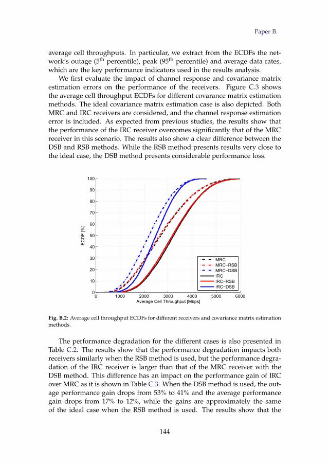
Paper B.
average cell throughputs. In particular, we extract from the ECDFs the net-work’s outage (5th percentile), peak (95th percentile) and average data rates,which are the key performance indicators used in the results analysis.
We first evaluate the impact of channel response and covariance matrixestimation errors on the performance of the receivers. Figure C.3 showsthe average cell throughput ECDFs for different covarance matrix estimationmethods. The ideal covariance matrix estimation case is also depicted. BothMRC and IRC receivers are considered, and the channel response estimationerror is included. As expected from previous studies, the results show thatthe performance of the IRC receiver overcomes significantly that of the MRCreceiver in this scenario. The results also show a clear difference between theDSB and RSB methods. While the RSB method presents results very close tothe ideal case, the DSB method presents considerable performance loss.
0 1000 2000 3000 4000 5000 60000
10
20
30
40
50
60
70
80
90
100
AverageDCellDThroughputD[Mbps]
EC
DF
D[B]
MRCMRC−RSBMRC−DSBIRCIRC−RSBIRC−DSB
Fig. B.2: Average cell throughput ECDFs for different receivers and covariance matrix estimationmethods.
The performance degradation for the different cases is also presented inTable C.2. The results show that the performance degradation impacts bothreceivers similarly when the RSB method is used, but the performance degra-dation of the IRC receiver is larger than that of the MRC receiver with theDSB method. This difference has an impact on the performance gain of IRCover MRC as it is shown in Table C.3. When the DSB method is used, the out-age performance gain drops from 53% to 41% and the average performancegain drops from 17% to 12%, while the gains are approximately the sameof the ideal case when the RSB method is used. The results show that the
144

V. Performance Evaluation
Table B.3: Performance degradation due to covariance matrix estimation errors
Case Receiver Outage Peak Average
DSBMRC -14% -24% -20%IRC -21% -25% -23%
RSBMRC -3% -1% -1%IRC -3% 0% -1%
Table B.4: Performance gain of IRC over MRC with different covariance matrix estimation meth-ods
Case Outage Peak Average
Ideal 53% 4% 17%DSB 41% 2% 12%RSB 52% 4% 17%
RSB method significantly outperforms the DSB method, even when channelresponse estimation errors and limited number of samples are considered.This is because the RSB method exploits the more accurate channel responseestimate and the possibility of discriminating the contribution of the desiredsignals to the covariance matrix from the interference and noise contribu-tions, leading to a better estimate of the covariance matrix. Note that this isenabled by the radio frame format discussed in Section II.
We now evaluate the impact of the receiver front-end imperfections on theoverall network performance. Figure C.4 shows the average cell throughputECDFs for the ideal front-end case and for the imperfect front-end cases forboth MRC and IRC receivers. RSB covariance matrix estimation method isassumed, and channel response estimation error is included. Only the lowerpart of the ECDF is displayed in the figure in order to highlight the outagedata rate. The results show that the performance of the receivers stronglydepends on the AGC delay and the ADC resolution.
The performance degradation due to receiver front-end errors is also pre-sented in Table B.5. Significant degradation is experienced in case of lowADC resolution (6 bits). The performance of both receivers is considerablyworse than the ideal performance, reaching up to 21% average cell through-put reduction. This performance reduction is due to the impact that thequantization noise causes on the estimation accuracy, leading to poor re-ceived signal combining and poor interference rejection in the case of IRC.The results also show that, if we use a reasonably high resolution ADC (10bits), the performance degradation is limited, reducing the key performanceindicator by at most 6% in the worst case. Note that ADCs with 10 bits
145

Paper B.
200 400 600 800 1000 1200 1400 1600 1800 20000
1
2
3
4
5
6
7
8
9
10
AverageDCellDThroughputD[Mbps]
EC
DF
D[n]
IdealDFrontDEndIdealDAGCD/D6DbitsDADCIdealDAGCD/D10DbitsDADCDelayedDAGCD/D6DbitsDADCDelayedDAGCD/D10DbitsDADC
MRC
IRC
Fig. B.3: Average cell throughput ECDFs for different receivers and receiver front-end configu-rations.
resolution (or more) are commonly used in commercial LTE devices.Analyzing the difference between the performance degradation with the
ideal AGC (τ = 0) and the delayed AGC (τ = 1), we conclude that the rapidlyvarying interference sources impact the receiver performance significantly.Results show that the outage throughput degradation is higher when wecompare the ideal AGC model to the delayed one. However, the use of higherresolution ADC (10 bits) reduces the overall impact of the AGC’s inability toperfectly track the received signal power levels.
Table B.6 confirms that it is possible to obtain a realistic IRC receiver withperformance very close to the ideal, even in a scenario with rapidly varyinginterference sources. An IRC receiver with delayed AGC and low resolutionADC (6 bits) would have much lower performance gain, especially in termsof outage throughput. However, using a higher resolution ADC (10 bits),the performance difference is almost negligible. Thus, we can conclude thatit is possible to obtain the very high data rate gains of IRC by exploitingthe mentioned radio frame format [6], as long as the RSB covariance matrixestimation method and a reasonably high resolution ADC (10 bits) are used.
VI. Conclusion
In this paper, we evaluated the impact of receiver imperfections on the per-formance of the MMSE-IRC receiver using system-level simulations. We pre-
146

VI. Conclusion
Table B.5: Performance degradation due to receiver front-end errors
AGC ADC Receiver Outage Peak Average
Ideal6 bits
MRC -10% -16% -14%IRC -12% -17% -15%
10 bitsMRC -3% +1% -1%IRC -2% 0% -1%
Delayed6 bits
MRC -15% -15% -15%IRC -21% -17% -17%
10 bitsMRC -5% +1% -1%IRC -6% 0% -2%
Table B.6: Performance gain of IRC over MRC with different receiver front-end configurations
AGC ADC Outage Peak Average
Ideal Ideal 52% 4% 17%
Ideal6 bits 48% 3% 16%
10 bits 54% 3% 17%
Delayed6 bits 41% 3% 15%
10 bits 50% 3% 17%
147

Paper B.
sented a model that captures the effects of channel response and covariancematrix estimation errors as well as receiver front-end imperfections.
Performance results show that using a radio frame format designed tosupport the MMSE-IRC receiver, the adequate covariance matrix estimationmethod and a reasonably high resolution ADC, the MMSE-IRC receiver isable to reach performance levels close to the ideal. This realistic MMSE-IRC receiver presents low throughput degradation and keeps considerableperformance gains over a realistic MMSE-MRC receiver.
Our future work will focus on radio resource management for 5G net-works, such as rank and precoding matrix adaptation algorithms. Our aimis to investigate algorithms aimed at optimizing the operation of MMSE-IRCreceivers with rapidly varying interference sources.
References
[1] Preben Mogensen, Kari Pajukoski, Bernhard Raaf, Esa Tiirola, EevaLähetkangas, Istvan Z. Kovács, Gilberto Berardinelli, Luis G. UzedaGarcia, Liang Hu, and Andrea F. Cattoni. “B4G local area: High levelrequirements and system design”. In: Globecom Workshops (GC Wk-shps), 2012 IEEE. Dec. 2012, pp. 613–617. doi: 10.1109/GLOCOMW.2012.6477644.
[2] F.M.L. Tavares, G. Berardinelli, N.H. Mahmood, T.B. Sørensen, andP. Mogensen. “On the Potential of Interference Rejection Combiningin B4G Networks”. In: Vehicular Technology Conference (VTC Fall), 2013IEEE 78th. Sept. 2013, pp. 1–5. doi: 10.1109/VTCFall.2013.6692318.
[3] M. Lampinen, F. Del Carpio, T. Kuosmanen, T. Koivisto, and M. Enescu.“System-Level Modeling and Evaluation of Interference SuppressionReceivers in LTE System”. In: Vehicular Technology Conference (VTCSpring), 2012 IEEE 75th. May 2012, pp. 1–5. doi: 10.1109/VETECS.2012.6239964.
[4] K. Pietikainen, F. Del Carpio, H. Maattanen, M. Lampinen, T. Koivisto,and M. Enescu. “System-Level Performance of Interference Suppres-sion Receivers in LTE System”. In: Vehicular Technology Conference (VTCSpring), 2012 IEEE 75th. May 2012, pp. 1–5. doi: 10.1109/VETECS.2012.6239969.
[5] Y. Ohwatari, N. Miki, T. Asai, T. Abe, and H. Taoka. “Performanceof Advanced Receiver Employing Interference Rejection Combiningto Suppress Inter-Cell Interference in LTE-Advanced Downlink”. In:2011 IEEE Vehicular Technology Conference (VTC Fall). Sept. 2011, pp. 1–7. doi: 10.1109/VETECF.2011.6093196.
148

References
[6] P. Mogensen, K. Pajukoski, E. Tiirola, E. Lahetkangas, J. Vihriala, S.Vesterinen, M. Laitila, G. Berardinelli, G.W.O. Da Costa, L.G.U. Gar-cia, F.M.L. Tavares, and A.F. Cattoni. “5G small cell optimized radiodesign”. In: Globecom Workshops (GC Wkshps), 2013 IEEE. Dec. 2013,pp. 111–116. doi: 10.1109/GLOCOMW.2013.6824971.
[7] Jinho Choi. Optimal Combining and Detection: Statistical Signal Process-ing for Communications. Cambridge: Cambridge University Press, 2010.
[8] D. Morales-Jimenez, J.F. Paris, J.T. Entrambasaguas, and Kai-Kit Wong.“On the Diagonal Distribution of a Complex Wishart Matrix and itsApplication to the Analysis of MIMO Systems”. In: Communications,IEEE Transactions on 59.12 (2011), pp. 3475–3484. issn: 0090-6778. doi:10.1109/TCOMM.2011.100611.100641.
[9] 3GPP R1-080506. UE specific reference signal pattern. Jan. 2008. url:http://www.3gpp.org.
[10] 3GPP R1-062642. Uplink Reference Signal Design in EUTRA. Oct. 2006.url: http://www.3gpp.org.
[11] D. Dardari. “Joint clip and quantization effects characterization inOFDM receivers”. In: Circuits and Systems I: Regular Papers, IEEE Trans-actions on 53.8 (2006), pp. 1741–1748. issn: 1549-8328. doi: 10.1109/TCSI.2006.875170.
[12] B. Widrow, I. Kollar, and Ming-Chang Liu. “Statistical theory of quan-tization”. In: Instrumentation and Measurement, IEEE Transactions on45.2 (1996), pp. 353–361. issn: 0018-9456. doi: 10.1109/19.492748.
[13] Chun-Tao Lin and Wen-Rong Wu. “Clipping ratio estimation for OFDMreceivers”. In: Vehicular Technology Conference (VTC Spring), 2005 IEEE61st. 2005. doi: 10.1109/VETECS.2005.1543414.
[14] 3GPP TR 36.814. Evolved Universal Terrestrial Radio Access (E-UTRA);Further advancements for E-UTRA physical layer aspects. v9.0.0. Mar. 2010.url: http://www.3gpp.org.
[15] P. Kyösti et al. WINNER II Channel Models. D1.1.2 v1.1. IST-WINNER,Sept. 2007. url: https://www.ist-winner.org/WINNER2-Deliverables/D1.1.2v1.1.pdf.
[16] 3GPP TS 36.211. Evolved Universal Terrestrial Radio Access (E-UTRA);Physical channels and modulation. v11.1.0. Dec. 2012. url: http://www.3gpp.org.
149

Paper B.
150

Paper C
Inter-cell interference management using MaximumRank Planning in 5G small cell networks
Fernando M. L. Tavares, Gilberto Berardinelli, Nurul H.Mahmood, Troels B. Sørensen, and Preben Mogensen
The paper has been published in theProceedings of the 2014 11th International Symposium on Wireless
Communications Systems (ISWCS),August 2014.

c© 2014 IEEEThe layout has been revised.

I. Introduction
Abstract
In this paper, we propose Maximum Rank Planning (MRP) as a novel inter-cellinterference management technique for the ultra-dense uncoordinated deployment ofsmall cells targeted by 5th Generation (5G) networks. Rather than operating in thefrequency domain as the conventional Frequency Reuse Planning (FRP) technique,MRP acts by reducing the number of Multiple Input Multiple Output (MIMO)spatial multiplexing streams. This reduction leads to an increased probability thatthe Interference Rejection Combining (IRC) receiver will have sufficient degrees-of-freedom to reject the strongest interferers. System-level simulation results show thatMRP outperforms FRP in both low and high traffic load conditions, with 44% and49% outage throughput gains in each case, respectively.
I. Introduction
The ultra-dense uncoordinated deployment of local area small cells is envi-sioned as the main solution to reach the ambitious capacity requirements offuture 5G networks [1]. However, this type of deployment can only providethe expected network capacity boost in case efficient inter-cell interferencemitigation techniques are applied.
The conventional approach to deal with inter-cell interference is to useFrequency Reuse Planning (FRP) (static or dynamic) [2, 3, 4], i.e. allocat-ing orthogonal frequency chunks to neighbor cells that experience significantmutual interference. Frequency reuse techniques can be used to improve theoutage and average data rates, with the obvious drawback of limiting thepeak network throughput since each cell is operating over only a portion ofthe available spectrum. FRP is particularly advantageous for mobile networkoperators that aim at guaranteeing minimum quality of service requirementsfor their subscribers.
The usage of advanced receivers is also a promising solution to deal withthe inter-cell interference. In particular, IRC receivers exploit the degrees offreedom of multiple antenna transceivers for projecting the interfering signalsonto an orthogonal subspace with respect to the desired ones [5]. Thoughadvanced receivers such as IRC have been shown to significantly improvethe network performance, they are typically able to suppress only a limitednumber of significant interferers; FRP may then still be needed to improveaverage and outage data rates. Nonetheless, conventional FRP is unaware ofthe interference suppression capabilities of the receivers, leading to inefficientradio resource management decisions.
In this paper, we present a novel Maximum Rank Planning (MRP) tech-nique which is conceived as an alternative to FRP for networks equippedwith IRC receivers. The principle of the novel technique is to act on the
153

Paper C.
spatial resources of the multiple antenna transceiver rather than on the spec-trum resources. We present system-level simulation results that compare theperformance of MRP and FRP in the context of the 5G small cell networkconcept envisioned in [1], though a generalization to other air interfaces isstraightforward.
The paper is structured as follows. Section II recalls the usage of IRC re-ceivers in 5G networks. We present the novel MRP technique in Section IIIand we describe the simulation setup in Section IV. In Section V, we presentand discuss the simulation results. Section VI closes the paper with conclu-sions and future work.
II. Interference Rejection Combining in 5G
In [1] we have proposed a clean slate approach for a 5G concept optimizedfor ultra-dense deployment of small cells. Time Division Duplex (TDD)mode is recognized as the preferred operational mode given its flexibilityand the possibility of exploiting unpaired bands. Fundamental technicalfeatures are MIMO antenna techniques, optimized frame structure, flexibleuplink/downlink resource allocation and the aforementioned IRC receivers.It is well known that the degrees of freedom of MIMO transmission can beused to send multiple data streams or to increase the reliability of a numberof streams lower than the antenna cardinality. Further, when IRC receiversare adopted, some of the degrees of freedom can be used for suppressingstreams that compose the interfering signals, with penalty in terms of spatialmultiplexing gain since the number of desired streams which can be trans-mitted has to be lowered.
The IRC receiver uses received samples or channel estimates to createan Interference-plus-noise Covariance Matrix (ICM) that is used to calculatethe optimal combining matrix. To work efficiently, the IRC receiver requiresaccurate ICM estimation that can only be obtained if the interfering sourcesremain the same for the duration of the estimation period [6]. The framestructure proposed in [1] is particularly suited for an efficient usage of IRC.It assumes the transmission direction (UL or DL) to remain constant withina frame. By assuming neighbor cells to be time synchronized, such designallows the interference pattern to be constant within the frame. Further, theframe features a time symbol dedicated to the reference sequences used forchannel estimation purposes. By assuming the use of orthogonal referencesequences, each AP or UE is able to estimate the channel of both desiredand interfering nodes regardless of the transmission direction. This enablesjust-in-time estimation of the ICM and fast tuning of the IRC filter. Usingthis radio frame format, we have shown in previous studies that IRC caneffectively reduce the inter-cell interference perceived by the receiver [7], even
154

III. Maximum Rank Planning
when receiver imperfections and estimation errors are considered [8].A rank adaptation algorithm is used to find for each cell the rank (number
of spatial streams) that provides the best trade-off between spatial multiplex-ing gain and interference rejection capabilities according to the estimatedinterference scenario and channel fading conditions. Since the performanceof the IRC receiver depends on the number of spatial streams that composeeach interfering signal, the outcome of the rank adaptation algorithm mayimpact the performance in neighbor cells in case the decisions are taken ateach cell independently. Each degree-of-freedom can be used to reject onlyone interfering spatial stream. Thus, depending on the decision of the rankadaptation algorithm of the interfering cell, the IRC receiver may be able toreject either completely or partially the interfering signal.
Generally, this dependency leads to low outage throughput performancewhenever neighbor cells experience unbalanced reciprocal interference dueto the specific topology. For instance, if cell A experiences significant inter-ference from cell B, while cell B is not affected by the transmissions occurringin cell A, the rank adaptation in cell B may opt for the maximum number oftransmission streams, but this would generate disruptive interference levelsin cell A, which would react by drastically reducing its transmission rank. Insome cases, the number of degrees-of-freedom may not be sufficient to rejectthe interfering signal completely, leading to very low throughput. The over-all network throughput may then be penalized by such selfish behavior. Theusage of a centralized entity that chooses the best rank for each cell or a de-centralized victim-aware solution in which the transmission rank at each cellis chosen in a cooperative manner, such as [9], can avoid situations such asthe above, but they require message exchange mechanisms between differentcells which may not be feasible in real networks.
III. Maximum Rank Planning
Maximum Rank Planning (MRP) is an inter-cell interference managementtechnique that consists in limiting the maximum rank that the rank adap-tation algorithm at each transmitter may use. By reducing the rank of thestrong interferers, MRP increases the probability that the interfered receiverswill have enough degrees-of-freedom to reject them. Note that this techniqueis only recommended for networks in which all devices use receivers capableof rejecting interference and interference-aware rank adaptation algorithmsare used to decide between spatial multiplexing and interference rejection.
The maximum rank limit may be configured individually for each trans-mitter and the configuration depends mostly on the expected inter-cell inter-ference they generate to the neighbor cells. The limit can be static or dynamic(similar to dynamic FRP). In this paper, we show only the static case in which
155

Paper C.
UE1 AP1 AP2 UE2b.
f f
UE1 AP1 AP2 UE2c.
f f
UE1 AP1 AP2 UE2d.
f f
UE1 AP1 AP2 UE2e.
f f
UE1 AP1 AP2 UE2a.
f f
Fig. C.1: Example of Maximum Rank Planning (MRP) working principle.
all transmitters have the same maximum rank limit. Methods to select thelimit individually for each transmitter and to adapt the selection accordingto the traffic dynamics are topics we plan to investigate in the future.
The schematic in Figure C.1 provides an example to demonstrate theworking principle of MRP. The schematic shows in five different cases howtwo neighbor cells interact with each other. In this example, we assume thatall devices use IRC receivers and all of them feature four transmit/receiveantennas. We also assume that, given the position of the devices, the APs cangenerate strong mutual inter-cell interference, which impedes any receptionin case there are not sufficient degrees of freedom to reject it, whereas UEsare not affected by inter-cell interference. The following notation is used inthe example: Ts represents the maximum throughput per spatial stream overthe entire system spectrum, and T1 and T2 represent the maximum overallthroughput that Cell 1 (AP1 and UE1) and Cell 2 (AP2 and UE2) can reach inthe different cases, respectively.
Figure C.1a) shows the case in which UE1 transmits to AP1 and the linkbetween AP2 and UE2 is idle. We suppose in this case that the rank adap-tation algorithm decided to use only 3 simultaneous spatial streams (rank3) to transmit data to AP1 due to the current conditions of the channel, i.e.T1 = 3Ts.
In Figure C.1b), AP2 starts to transmit to UE2 using 4 spatial streams(rank 4). Since both cells use the same portion of the spectrum, AP1 receivesthe inter-cell interference from AP2. The IRC receiver in AP1 has only one
156

III. Maximum Rank Planning
free degree-of-freedom, so it is able to reject only one of the spatial streamscoming from AP2 (the other spatial streams still cause interference). In thissituation, the throughput in the link between UE1 and AP1 is severely re-duced (T1 = 0 and T2 = 4Ts).
In Figure C.1c), the rank adaptation algorithm reduces the number ofstreams in the link between UE1 and AP1 to one (rank 1). Now the IRCreceiver can reject 3 of the 4 spatial streams that transmitted by AP2. This newsituation reduces the effect of the inter-cell interference, but the throughputis still very low (T1 = 0 and T2 = 4Ts). Since mobile network operators aimat guaranteeing a minimum quality of service requirement, a solution thatimproves the throughput in Cell 1 is required.
The typical solution for this problem is to use FRP. In Figure C.1d), thespectrum is divided in two orthogonal channels and a different channel isallocated for each cell. Now, the transmission in each cell does not interferewith the other, but the data rates are hard limited to half of what they couldbe if each cell were using the whole spectrum alone, i.e. T1 = 1.5Ts andT2 = 2Ts.
Figure C.1e) depicts the case in which MRP is used. The network is con-figured such that both cells use the whole spectrum and their maximum ranklimit is set to 2 spatial streams, forcing the rank adaptation algorithm to re-duce the rank from 3 to 2 spatial streams in Cell 1 and from 4 to 2 spatialstreams in Cell 2. Now the IRC receiver in AP1 can completely reject the inter-cell interference from AP2. The advantage of MRP when compared to FRPin this example is the higher throughput in Cell 1 (T1 = 2Ts and T2 = 2Ts).With MRP, the throughput in Cell 1 is only reduced by one third (from 3 to2 spatial streams), when compared to the situation in Figure C.1a), whereasit is reduced by half in the FRP case.
This example shows one possible situation in which the MRP techniqueoutperforms FRP. Generally, MRP outperforms the FRP whenever rejectingsmall number of the strongest interfering streams improves significantly theSINR. In this case, MRP provides the advantage of quickly adjusting to theinstantaneous interference conditions, rejecting the strongest interferers. Thisis particularly advantageous in the case of ultra-dense uncoordinated deploy-ments (as targeted by our 5G concept) in which it is difficult to determinethe strongest interferers beforehand. Conversely, FRP performs better thanMRP when many interferers with relatively low power accumulate to causedisruptive interference. In this case, the IRC receiver will not have enoughdegrees of freedom to reject enough of interferers and significantly improvethe performance.
It is difficult to determine analytically which of the two techniques willprovide the best overall performance in each scenario. Their performance de-pends on the specific scenario topology, that varies due to the unpredictableposition of each node and their probability of transmission. Thus, our pro-
157

Paper C.
posed technique will be evaluated with system level simulations.
IV. Simulation Setup
In this section, we present the simulation setup used to compare the perfor-mance of MRP and FRP. Figure C.2 shows a schematic that represents theindoor local area network scenario. The scenario is composed of 40 indoorsmall cells. Each cell is located in one of the offices of two buildings whichare separated by a 10 meter wide street. Each building has 2 rows of 10 officesand each office measures 10 by 10 meters. One UE and one AP are located ineach cell and their position inside the cell is randomly selected to emulate anuncoordinated deployment. Each UE can only connect to the AP in the sameoffice i.e. the cell selection is limited by CSG.
10 m
10 m
10 m
Fig. C.2: 3GPP Dual Stripe Simulation Scenario [10].
The large scale propagation effects (pathloss and shadowing) are modeledaccording to the 3GPP Dual Stripe Model [10]. The small scale effects (fastfading and antenna characteristics) follow the WINNER Phase II Indoor Of-fice (A1) model [11]. In the simulations, all devices use Uniform Linear Array(ULA) antennas with 4 elements, which are spaced by λ/2 from each other.The same antenna array is used for both transmission and reception. We as-sume the system uses a 200 MHz band, which is the baseline assumption inour envisioned 5G concept [1].
We assume the cells to be time aligned; further each cell can freely decideat each Transmission Time Interval (TTI) the transmission direction (UL, DLor idle). This decision is modeled using a Markov Process. The transitionprobabilities are selected such that the probability of selecting the idle modeis controllable, but the probabilities of selecting either UL or DL modes areidentical. The random processes in each cell are independent and uncorre-lated.
A rank adaptation algorithm at the receiver side is used to select the num-ber of spatial streams. The decision is based only on instantaneous channeland interference conditions. The decision is informed to the transmitter that
158

IV. Simulation Setup
Table C.1: Simulation Scenario
Spectrum Allocation 200 MHz at 3.5 GHz
Transmit Time Interval 0.25 ms
Data GenerationInfinite Buffer UL/DL
Flexible UL and DL resource allocation
Access Mode Closed Subscriber Group (CSG)
Path Loss3GPP Dual Stripe Model
45 dB Minimum Coupling Loss
Wall LossInternal Walls 5 dBExternal Walls 10 dB
Shadowing Std. DeviationServing Cell 6 dBOther Cells 8 dB
Fast FadingWINNER Phase II Model
Indoor Office (A1) - 3 Km/h
Antenna ConfigurationUniform Linear Array (ULA)
4 antenna elements (0.5λ spacing)
Transmission Power 20 dBm
Receiver Noise Figure 9 dB
Error Vector Magnitude 5% SINRmax ≈ 26dB
159

Paper C.
Table C.2: Outage throughput performance comparison - Low network load (50%)
Case Setup MRC IRC
Baseline FR1/MR4 1218.0 1466.0FRP FR2/MR4 1226.0 (+1%) 1400.0 (-5%)MRP FR1/MR2 1044.0 (-14%) 1762.0 (+20%)
uses the selected number of streams in the next TTI. A precoding matrix isused to map the streams to the four transmit antennas (the LTE downlinkclosed-loop single user MIMO codebook [12] is adopted).
The instantaneous SINR is calculated at each TTI using an IRC receiversystem-level simulation model [7]. The usage of IRC is also compared to theMaximum Ratio Combining (MRC) receiver, which represents the baselineinter-cell interference unaware receiver in this study. The models output oneSINR value for each spatial stream. These values are adjusted using a EVMmodel to account for the receiver imperfections and limitations [13].
We assume ideal link adaptation with one codeword per spatial stream.We calculate the spectral efficiency for each stream using Shannon’s capacityformula, considering that the minimum decodable SINR is -10 dB and thatthe maximum spectral efficiency per spatial stream is 8 bits/s/Hz (uncoded256-QAM). The total throughput is obtained by multiplying the sum of thespectral efficiency of all spatial streams by the signal bandwidth.
V. Performance Evaluation
We evaluate the performance of MRP using a quasi-static system level simu-lator. Each simulation consists of 200 snapshots of 200 frames each. In eachsnapshot, the devices (AP and UE) are randomly placed in the cells. The fastfading samples are updated at each frame, but the large scale values (pathlossand shadowing) remain constant. We evaluate the performance using ECDFsof the average cell throughput. In particular, we consider the outage (5th per-centile) throughput as the main key performance indicator (as mentioned inthe introduction, we assume that mobile network operators aim at improvingminimum quality of service requirements).
Two different network load situations are considered: a low load case(50% activity factor) and a high load case (100% activity factor), where theactivity factor is the probability that a cell is not in idle mode. In each case,we provide ECDFs for both MRC and IRC receivers. We refer to the case withFrequency Reuse x and Maximum Rank y as FRx/MRy.
Figure C.3 shows the ECDF of the average cell throughput in the low net-work load case for different MRP and FRP combinations. The baseline case
160

V. Performance Evaluation
0 1000 2000 3000 4000 5000 60000
10
20
30
40
50
60
70
80
90
100
AverageDCellDThroughputD[Mbps]
EC
DF
D[I]
MRCDFR1/MR4MRCDFR2/MR4MRCDFR1/MR2IRCDFR1/MR4IRCDFR2/MR4IRCDFR1/MR2
Fig. C.3: Average cell throughput ECDFs for different FRP/MPR combinations and low networkload (50%).
in which all the cells use the entire spectrum and the maximum number ofstreams (FR1/MR4) is also included, along with the FRP/MRP combinationsthat are used in this case to improve the outage throughput in the network.We select the FRP/MRP combinations that reduce the peak throughput byhalf (by dividing the bandwidth in one case and limiting the number ofstreams in the other) as a reasonable trade-off. These combinations are theFR2/MR4 (FRP) and the FR1/MR2 (MRP).
We can notice in the figure that IRC clearly outperforms MRC in all thecases. FR2/MR4 case provides a slightly better outage throughput thanFR1/MR4 in the case of MRC, whereas the overall performance with theFR1/MR2 setup is worse than FR1/MR4, because the MRC receiver is not ca-pable of rejecting any interference. However, when the IRC receiver is used,the FR2/MR4 case does not provide any benefit whereas the FR1/MR2 caseprovides significant outage gains over the baseline FR1/MR4. The resultsclearly show that MRP outperforms FRP when IRC receiver are used in thisscenario. This is due to the uncoordinated characteristic of the deploymentthat favors a technique that can adapt to the unpredictable position of thestrongest interferers.
Table C.2 presents the outage throughput values for the low network loadcase. The table shows the outage throughput gains for different FRP/MRPcombinations over the baseline FR1/MR4. The numbers clearly show that thebest strategy for the MRC receiver is the FRP (FR2/MR4) with 1% gain over
161

Paper C.
0 1000 2000 3000 4000 5000 60000
10
20
30
40
50
60
70
80
90
100
AverageDCellDThroughputD[Mbps]
EC
DF
D[I]
MRCDFR1/MR4MRCDFR4/MR4MRCDFR1/MR1IRCDFR1/MR4IRCDFR4/MR4IRCDFR1/MR1
Fig. C.4: Average cell throughput ECDFs for different FRP/MPR combinations and high networkload (100%).
Table C.3: Outage throughput performance comparison - High network load (100%)
Case MRC IRC
FR1/MR4 487.0 907.0FR4/MR4 798.0 (+64%) 967.0 (+7%)FR1/MR1 448.0 (-9%) 1191.0 (+31%)
the MRC baseline whereas the best strategy for IRC is the MRP (FR1/MR2)with 20% gain over the IRC baseline. Further significant insights can beobtained by comparing the performance of the MRC and the IRC receiverswhen the corresponding best strategy for each receiver is used. When theIRC is used with FRP, the outage gain over the MRC with FRP is only 14% inthis scenario. In case the IRC is used in combination with the MRP strategy,the gain is increased to 44%.
A similar situation occurs in the high network load case. The ECDF curvesin Figure C.4 show that the inter-cell interference problem is more severe inthis case. Thus, it is necessary to use the FR/MR combinations that reducethe peak throughput to one fourth of its maximum value to significantly im-prove the outage performance. Once more, we observe that the IRC receiveroutperforms the MRC receiver. It is also clear that the strategy that providesthe best outage performance is the FRP in the MRC receiver case and theMRP in the IRC receiver case.
162

VI. Conclusion
The outage performance gains for the high network load case are pre-sented in Table C.3. Again, the outage performance in the MRC receiver caseis only improved when the FRP is used. FRP provides 64% gain whereas theMRP reduces the gain by 9%. Conversely, the outage performance in the IRCreceiver case is improved when the MRP is used, with 31% over the baseline,whereas the FRP only improves the outage performance by 7%. We can alsocompare the benefit of using the MRP by comparing the gain of the IRC re-ceiver over the MRC receiver. The outage performance in the IRC receiverwith FRP case is 21% better than the MRC with FRP case while it is 49%better in case the MMSE-IRC with MRP is used instead.
VI. Conclusion
In this paper, we presented the Maximum Rank Planning technique as a novelinter-cell interference management technique for 5G local area networks. Thistechnique operates on the MIMO spatial domain by relying on the capabil-ity of the advanced receiver to reject inter-cell interference. By limiting themaximum rank used by each transmitter, it increases the probability that thereceivers will be able to effectively reject the inter-cell interference, thus im-proving the outage data rates. We evaluated the performance of MRP byusing system-level simulations and compared it to the performance of con-ventional FRP in the same network. Performance results show that MRP out-performs FRP when IRC receivers are used, providing 44% and 49% outagethroughput gains in low and high traffic load conditions, respectively.
Our future work will focus on methods to dynamically configure the max-imum rank that may be used by each transmitter in the network. Our aim isto investigate algorithms that can adjust the maximum rank according to thenetwork topology as well as take into account long-term traffic variations.
References
[1] Preben Mogensen, Kari Pajukoski, Esa Tiirola, Jaakko Vihriälä, EevaLähetkangas, Gilberto Berardinelli, Fernando Menezes Leitão Tavares,Nurul Huda Mahmood, Mads Lauridsen, Davide Catania, and An-drea Fabio Cattoni. “Centimeter-wave concept for 5G ultra-dense smallcells”. In: Vehicular Technology Conference (VTC Spring), 2014 IEEE 79th.May 2014.
[2] I. Katzela and M. Naghshineh. “Channel assignment schemes for cel-lular mobile telecommunication systems: a comprehensive survey”.In: Communications Surveys Tutorials, IEEE 3.2 (2000), pp. 10–31.
163

Paper C.
[3] Yuanye Wang et al. “Fixed Frequency Reuse for LTE-Advanced Sys-tems in Local Area Scenarios”. In: Vehicular Technology Conference, 2009.VTC Spring 2009. IEEE 69th. Apr. 2009, pp. 1–5.
[4] J. Ellenbeck, C. Hartmann, and L. Berlemann. “Decentralized inter-cellinterference coordination by autonomous spectral reuse decisions”. In:Wireless Conference, 2008. EW 2008. 14th European. June 2008, pp. 1–7.
[5] Jinho Choi. Optimal Combining and Detection: Statistical Signal Process-ing for Communications. Cambridge: Cambridge University Press, 2010.
[6] P. Mogensen, K. Pajukoski, E. Tiirola, E. Lahetkangas, J. Vihriala, S.Vesterinen, M. Laitila, G. Berardinelli, G.W.O. Da Costa, L.G.U. Gar-cia, F.M.L. Tavares, and A.F. Cattoni. “5G small cell optimized radiodesign”. In: Globecom Workshops (GC Wkshps), 2013 IEEE. Dec. 2013,pp. 111–116. doi: 10.1109/GLOCOMW.2013.6824971.
[7] F.M.L. Tavares, G. Berardinelli, N.H. Mahmood, T.B. Sørensen, andP. Mogensen. “On the Potential of Interference Rejection Combiningin B4G Networks”. In: Vehicular Technology Conference (VTC Fall), 2013IEEE 78th. Sept. 2013, pp. 1–5. doi: 10.1109/VTCFall.2013.6692318.
[8] Fernando M.L. Tavares, Gilberto Berardinelli, Nurul H. Mahmood,Troels B. Sørensen, and Preben Mogensen. “On the Impact of Re-ceiver Imperfections on the MMSE-IRC Receiver Performance in 5GNetworks”. In: Vehicular Technology Conference (VTC Spring), 2014 IEEE79th. May 2014, pp. 1–6. doi: 10.1109/VTCSpring.2014.7023014.
[9] B. Clerckx et al. “A Practical Cooperative Multicell MIMO-OFDMANetwork Based on Rank Coordination”. In: Wireless Communications,IEEE Transactions on 12.4 (Apr. 2013), pp. 1481–1491.
[10] 3GPP TR 36.814. Evolved Universal Terrestrial Radio Access (E-UTRA);Further advancements for E-UTRA physical layer aspects. v9.0.0. Mar. 2010.url: http://www.3gpp.org.
[11] P. Kyösti et al. WINNER II Channel Models. D1.1.2 v1.1. IST-WINNER,Sept. 2007. url: https://www.ist-winner.org/WINNER2-Deliverables/D1.1.2v1.1.pdf.
[12] 3GPP TS 36.211. Evolved Universal Terrestrial Radio Access (E-UTRA);Physical channels and modulation. v11.1.0. Dec. 2012. url: http://www.3gpp.org.
[13] Harri Holma and Antii Toskala. LTE for UMTS: Evolution to LTE-Advanced.Wiley, 2011.
164

Paper D
Managing inter-cell interference with advancedreceivers and rank adaptation in 5G small cells
Fernando M. L. Tavares, Gilberto Berardinelli, Davide Catania,Troels B. Sørensen, and Preben Mogensen
The paper has been submitted to theIEEE 21th European Wireless (EW) Conference,
May 2015.

c© 2015 IEEEThe layout has been revised.

I. Introduction
Abstract
The use of receivers with interference suppression capabilities is expected to be a sig-nificant performance booster in 5th Generation (5G) ultra-dense small cell networks.In this respect, they could represent an alternative to traditional frequency reuse tech-niques, facilitating the inter-cell interference management. In this paper, we evaluatewhether it is possible to rely on such advanced receivers as the main tool to deal withthe inter-cell interference problem. We present a system-level performance evalua-tion in three different dense indoor small cell scenarios using a receiver model thatincludes both interference rejection combining (IRC) and successive interference can-cellation (SIC) principles, as well as different rank adaptation strategies. Our resultsconfirm that interference suppression receivers with a supportive system design canindeed represent a valid alternative to frequency reuse. They achieve similar outagedata rate performance in comparison to reuse strategies (resource orthogonalization),but higher average and peak throughput.
I. Introduction
The deployment of ultra-dense small cell networks is foreseen as a cost-effective solution for coping with wireless network congestion caused by theever increasing demand for mobile broadband services, but the existing RATstandards are not well suited for this type of deployment. For this reason, anovel 5G RAT concept optimized for small cell networks operating at carrierfrequencies bellow 6 GHz has been proposed in [1].
The main performance limiting factor in such ultra-dense deployments isthe presence of strong inter-cell interference. While traditional approachesfor dealing with inter-cell interference are based on the usage of static ordynamic frequency reuse techniques, advanced receivers with interferencesuppression capabilities also have the potential to boost the performance ofdense small cells and could be used as an alternative to the traditional ap-proaches. Such an alternative is important for this type of networks, becausestatic frequency reuse planning may be inherently impracticable in the caseof uncoordinated deployments and dynamic frequency reuse has significantsystem costs in terms of signalling overhead. Besides, the dynamic tech-niques may not be able to promptly adapt to the quickly varying interferencepatterns which are expected in dense small cell networks [1].
In a previous work [2], we have identified that the linear IRC receiverconsistently outperforms its inter-cell interference unaware counterpart, theMaximum Ratio Combining (MRC) receiver, when the supportive system de-sign proposed in [1] is used. The frame design that is part of this conceptprovides the mechanisms to guarantee high-performance inter-cell interfer-ence suppression, even when estimation errors and receiver front-end imper-
167

Paper D.
fections are considered in the evaluation [3].Nevertheless, the use of interference suppression receivers as an alterna-
tive to frequency reuse techniques has not been evaluated yet. In this paper,we evaluate with system-level simulations whether replacing traditional fre-quency reuse techniques is actually possible by comparing them with thenetwork performance of interference suppression receivers in three represen-tative dense indoor small cell scenarios. This evaluation is performed usingan updated receiver model that includes the use of a Successive InterferenceCancellation (SIC) decoding stage [4] to reduce the negative effects of inter-stream interference and considering the latest results regarding the use ofsmart victim-aware rank adaptation algorithms [5, 6] as additional protectionmechanism to manage the inter-cell interference levels in dense small cellnetworks.
The paper is structured as follows. Section II presents the system modelused in the simulations. The details related to the simulation setup are de-scribed in Section III. We present and analyse the simulation results in Sec-tion IV and we close the paper with conclusions and future work in Sec-tion V.
II. System Model
In this section, we present the model used in our system-level simulations.We will first review some important details about the 5G RAT concept pro-posed in [1], and then present the mathematical model used to evaluate theperformance of the receivers. Finally, we will present the principles of therank adaptation algorithms used in the evaluation.
A. 5G Frame Format Concept
The goal of this subsection is to present the relevant assumptions which easethe usage of advanced receivers in our proposed 5G concept [1]. In partic-ular, the aim in [1] was to integrate in a single concept the support for thetechnical features that are expected to have fundamental roles in dense smallcell networks. Some of these features include: (i) TDD, given its flexibilityand the possibility of exploiting unpaired bands, (ii) very short frame length,to fulfil the latency requirement, (iii) flexible UL/DL resource allocation (alsoknown as Dynamic TDD), to provide flexibility to adjust to the instantaneoustraffic demands, and (iv) Single User MIMO (SU-MIMO) and IRC receiver, asmentioned before. The need to consider all these features in a single conceptled us to design the frame format depicted in Figure D.1.
We assume a system based on OFDM in which all network nodes transmittime-aligned frames. The proposed frame is 0.25 ms long (short enough to
168
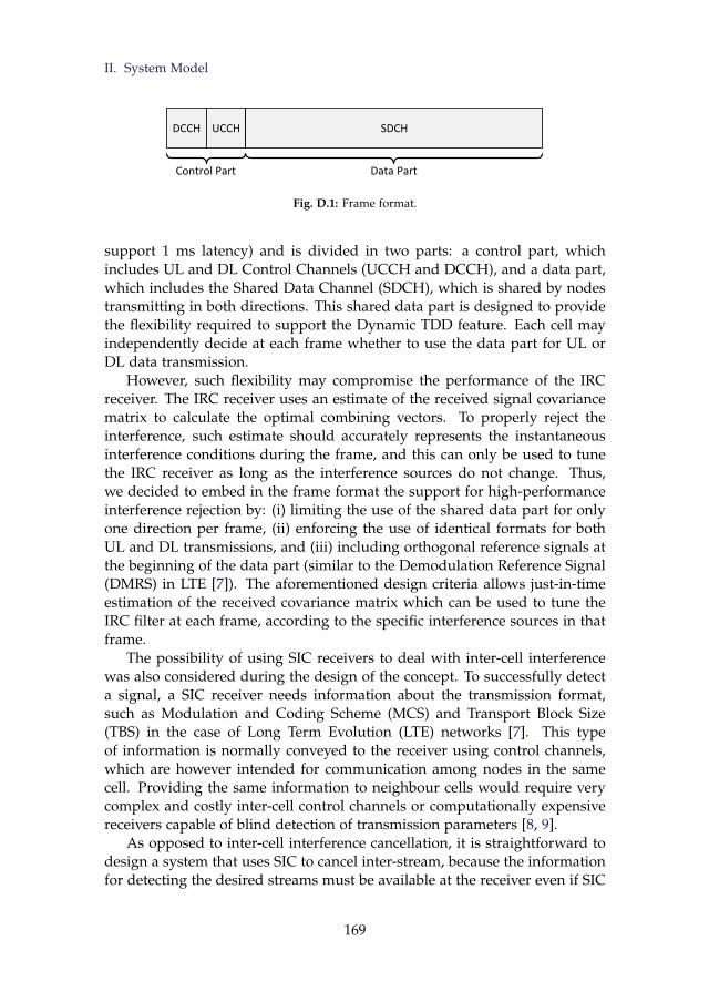
II. System Model
DCCH UCCH SDCH
Control Part Data Part
Fig. D.1: Frame format.
support 1 ms latency) and is divided in two parts: a control part, whichincludes UL and DL Control Channels (UCCH and DCCH), and a data part,which includes the Shared Data Channel (SDCH), which is shared by nodestransmitting in both directions. This shared data part is designed to providethe flexibility required to support the Dynamic TDD feature. Each cell mayindependently decide at each frame whether to use the data part for UL orDL data transmission.
However, such flexibility may compromise the performance of the IRCreceiver. The IRC receiver uses an estimate of the received signal covariancematrix to calculate the optimal combining vectors. To properly reject theinterference, such estimate should accurately represents the instantaneousinterference conditions during the frame, and this can only be used to tunethe IRC receiver as long as the interference sources do not change. Thus,we decided to embed in the frame format the support for high-performanceinterference rejection by: (i) limiting the use of the shared data part for onlyone direction per frame, (ii) enforcing the use of identical formats for bothUL and DL transmissions, and (iii) including orthogonal reference signals atthe beginning of the data part (similar to the Demodulation Reference Signal(DMRS) in LTE [7]). The aforementioned design criteria allows just-in-timeestimation of the received covariance matrix which can be used to tune theIRC filter at each frame, according to the specific interference sources in thatframe.
The possibility of using SIC receivers to deal with inter-cell interferencewas also considered during the design of the concept. To successfully detecta signal, a SIC receiver needs information about the transmission format,such as Modulation and Coding Scheme (MCS) and Transport Block Size(TBS) in the case of Long Term Evolution (LTE) networks [7]. This typeof information is normally conveyed to the receiver using control channels,which are however intended for communication among nodes in the samecell. Providing the same information to neighbour cells would require verycomplex and costly inter-cell control channels or computationally expensivereceivers capable of blind detection of transmission parameters [8, 9].
As opposed to inter-cell interference cancellation, it is straightforward todesign a system that uses SIC to cancel inter-stream, because the informationfor detecting the desired streams must be available at the receiver even if SIC
169

Paper D.
is not used. Although it does not deal directly with the inter-cell interferenceproblem, the use of inter-stream interference cancellation can potentially im-prove the network performance by improving the efficiency of SU-MIMO,increasing the peak and average cell throughputs.
This frame format concept is the base on top of which we derive ourreceiver model described in the next section.
B. Receiver Model
In this subsection, we present the receiver model used in our system-levelsimulations. The schematic of the receiver on which the model is based isdepicted in Figure D.2. The schematic includes both the linear and the non-linear receivers. The non-linear receiver includes also the dashed part, whichrepresents the blocks used for interference cancellation.
Fig. D.2: Receiver Schematic: (i) linear receiver (full lines); (ii) non-linear receiver (full anddashed lines).
We assume a network composed of nodes with Ntx transmitting and Nrxreceiving antennas. At each frame, NT nodes transmit. Each transmittingnode k transmits Nk
S ≤ min(Nrx, Ntx) streams. The received signal r [Nrx × 1]is given by
r =NT
∑k=1
NkS
∑l=1
hk,lsk,l + n (D.1)
where the scalar sk,l represents the symbol transmitted in the l-th layer bythe k-th transmiter, hk,l [Nrx × 1] is the vector of the equivalent channel coef-ficients that models the path of the symbol stream of the l-th layer from thek-th transmitter to the receiver and the vector n [Nrx× 1] represents the addi-tive noise. Note that this equation holds for a generic subcarrier in a genericOFDM symbol, whose indexes are omitted for the sake of simplicity.
170

II. System Model
We assume that the transmitted symbols sk,l have zero mean and unitpower, and that there is no correlation between the multiple symbols sent byall the transmitters. We also assume that the channel response is constantfor the duration of a frame (block fading), and that the equivalent channelvectors hk,l include the effect of the transmit power amplification, large scaleand small scale propagation effects, and the [Ntx × Nk
S] precoding matrix atthe transmitter.
Let us assume that k = 1 always refers to the transmitter that transmitsthe desired signal. The first step is to linearly combine r to obtain an estimateof the N1
S desired signals s1,l (l = 1 . . . N1S). The estimates can be obtained as
followss1,l = wH
1,lr (D.2)
where w1,l are the linear combining vectors, which according to the MMSEcriterion are given by
w1,l = R−1r h1,l (D.3)
where Rr is the estimate of the covariance matrix Rr of the received signal r,and h1,l is the estimate of h1,l .
We assume that the covariance matrix Rr is estimated using the orthog-onal reference symbols transmitted at the beginning of the data part. Thus, inthe case of the IRC receiver, i.e. the receiver that uses the inter-cell interference-aware MMSE linear combiner (MMSE-IRC), the estimate Rr can be calculatedas
Rr =NT
∑k=1
NkS
∑l=1
hk,l hHk,l + Rn (D.4)
where Rn is the estimate of the additive noise covariance matrix Rn. TheRn matrix is diagonal and each one of the diagonal terms σ2
m represents thepower of the additive noise at the m-th antenna. In this case, σ2
m = σ2n , where
σ2n is the noise power.
For comparison, we also model the Maximal Ratio Combining (MRC) re-ceiver, i.e. the receiver that uses the inter-cell interference-unaware MMSElinear combiner (MMSE-MRC). This receiver treats inter-cell interference asnoise, i.e. it assumes that there is no correlation between the inter-cell inter-ference signals received by the different antennas. In this case, the estimateRr is given by
Rr =N1
S
∑l=1
h1,l hH1,l + Rn (D.5)
and the diagonal elements of Rn are given by
σ2m =
NT
∑k=2
NkS
∑l=1|hk,l,m|2 + σ2
nm (D.6)
171
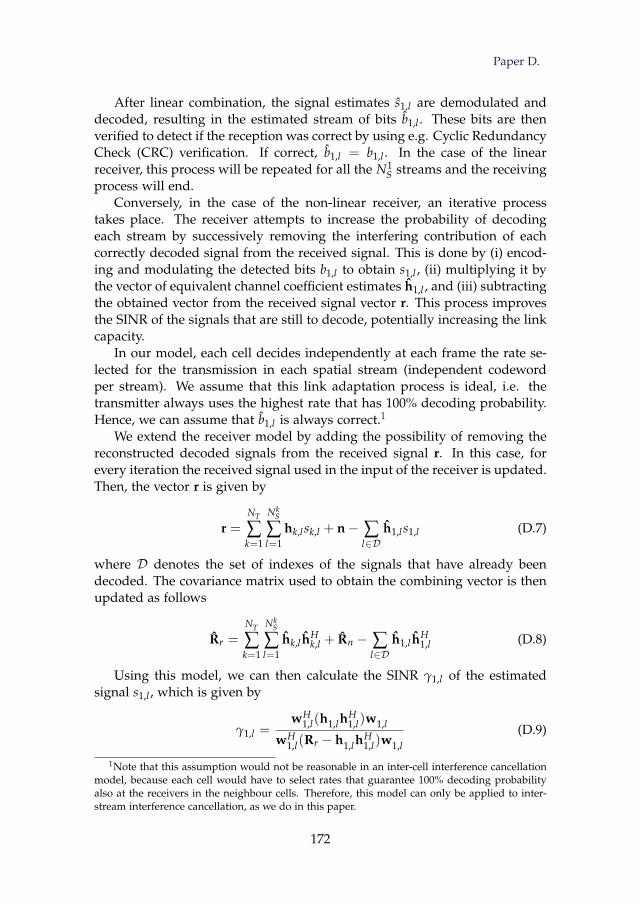
Paper D.
After linear combination, the signal estimates s1,l are demodulated anddecoded, resulting in the estimated stream of bits b1,l . These bits are thenverified to detect if the reception was correct by using e.g. Cyclic RedundancyCheck (CRC) verification. If correct, b1,l = b1,l . In the case of the linearreceiver, this process will be repeated for all the N1
S streams and the receivingprocess will end.
Conversely, in the case of the non-linear receiver, an iterative processtakes place. The receiver attempts to increase the probability of decodingeach stream by successively removing the interfering contribution of eachcorrectly decoded signal from the received signal. This is done by (i) encod-ing and modulating the detected bits b1,l to obtain s1,l , (ii) multiplying it bythe vector of equivalent channel coefficient estimates h1,l , and (iii) subtractingthe obtained vector from the received signal vector r. This process improvesthe SINR of the signals that are still to decode, potentially increasing the linkcapacity.
In our model, each cell decides independently at each frame the rate se-lected for the transmission in each spatial stream (independent codewordper stream). We assume that this link adaptation process is ideal, i.e. thetransmitter always uses the highest rate that has 100% decoding probability.Hence, we can assume that b1,l is always correct.1
We extend the receiver model by adding the possibility of removing thereconstructed decoded signals from the received signal r. In this case, forevery iteration the received signal used in the input of the receiver is updated.Then, the vector r is given by
r =NT
∑k=1
NkS
∑l=1
hk,lsk,l + n− ∑l∈D
h1,ls1,l (D.7)
where D denotes the set of indexes of the signals that have already beendecoded. The covariance matrix used to obtain the combining vector is thenupdated as follows
Rr =NT
∑k=1
NkS
∑l=1
hk,l hHk,l + Rn − ∑
l∈Dh1,l h
H1,l (D.8)
Using this model, we can then calculate the SINR γ1,l of the estimatedsignal s1,l , which is given by
γ1,l =wH
1,l(h1,lhH1,l)w1,l
wH1,l(Rr − h1,lh
H1,l)w1,l
(D.9)
1Note that this assumption would not be reasonable in an inter-cell interference cancellationmodel, because each cell would have to select rates that guarantee 100% decoding probabilityalso at the receivers in the neighbour cells. Therefore, this model can only be applied to inter-stream interference cancellation, as we do in this paper.
172

II. System Model
The total throughput will be the sum of the individual stream through-puts. As a performance bound, we calculate the throughputs as the achiev-able rates (Shannon capacity) at the SINRs in (D.9).
Although the model considers the possibility of imperfect channel andreceived signal covariance matrix estimation, in this paper, we assume perfectestimation, i.e. hk,l = hk,l and Rr = Rr.
C. Rank adaptation
The rank adaptation mechanism is responsible for balancing in each linkthe trade-off between spatial multiplexing gain and interference suppressioncapabilities by properly selecting the number of streams to be transmitted.Since the total number of received interfering streams impacts the perfor-mance of the IRC receiver (as a rule of thumb, the IRC receiver is capableof rejecting up to Nrx − 1 streams), the rank adaptation decision in one cellalso affects the performance of neighbour cells. Therefore, the use of victim-aware rank adaptation algorithms, i.e. algorithms that consider this potentialnegative effect, may help improve the performance of the network. In this pa-per, the following rank adaptation approaches are used in the performanceevaluation:
Selfish Rank Adaptation (SRA)
If selfish rank adaptation is used, each node k selects the transmission rank(Nk
S) as the one which is expected to maximize its Shannon capacity CNkS
given its estimated SINR conditions. By using a selfish rank adaptation, eachnode aims then at boosting its throughput regardless to the impact it maygenerate to neighbour cells.
Victim-aware Rank Adaptation (VRA)
If victim-aware rank adaptation is used, each node selects the transmissionrank with some regard to the interference it may generate to the neighbourcells. In this work, we refer to the rank adaptation technique proposed in [6],which has been shown to guarantee a good outage performance, while pro-viding the benefit of higher average throughputs in both low and high inter-cell interference conditions. The principle of this algorithm is to introducea taxation mechanism which discourages the selection of higher ranks incase of high generated interference. Node k selects the transmission rank Nk
Swhich is expected to maximize the following metric Πk:
Πk = CNkS− fW(Nk
S)C(I)︸ ︷︷ ︸Taxation for rank Nk
S
(D.10)
173

Paper D.
where C(I) is the capacity of the interfering channels, and fW is a monoton-ically increasing weighting function of rank Nk
S which quantifies the level ofdiscouragement. Further details are in [6]. Ideally, the term C(I) should becomputed according to the outgoing interference, i.e. the interference whichis generated to the neighbour cells. However, obtaining such informationis not feasible in practice since it would require impracticable amounts ofcontrol information exchange among neighbour cells. As done in [6], C(I)is then sub-optimally computed as a function of the incoming interferencerather than outgoing interference, since such information can be easily re-trieved given our described frame structure.
III. Simulation Setup
Three different scenarios are used in the performance evaluation. Figure D.3(a)depicts the network topology for Scenario A. This topology simulates an In-door Hotspot network, similar to an airport check-in hall or a large confer-ence hall, for example. The total area of the hall is divided in "virtual" squareareas (there are no internal walls) and one AP is installed in the centre of eachof them, summing up 40 APs. In this scenario, the user may connect to any ofthe available APs, i.e. the network operates in Open Subscriber Group (OSG)access mode. One UE is randomly placed in each square area and each UE se-lects which AP to connect based on the highest received power. In case an APdoes not serve any UE, it is switched off for the rest of the simulation drop;if an AP serves more than one UE, a fair round-robin frequency-frequencydomain scheduling is assumed.
Scenarios B and C use the same Indoor Office network topology [10], butdifferent access modes. Figure D.3(b) depicts the network topology, whichconsists of 40 cells deployed in 2 office buildings (one cell per office). Eachbuilding is divided in 2 rows of 10 offices. Each office measures ten-by-tenmeters. The two buildings are separated by a ten-meter wide street. In eachcell, there is one AP and one UE. In Scenario B, the OSG access mode isassume (the same as Scenario A), but in Scenario C, a CSG access mode isenforced and an UEs can only connect to the AP in the same office.
In all scenarios, both APs and UEs are equipped with uniform linearantenna arrays, composed of 4 elements equally spaced by half wavelength.The system operates at 3.5 GHz carrier frequency and occupies 200 MHz ofspectrum. Table D.1 presents further details on the simulation scenarios.
We model the effect of flexible UL/DL resource allocation on the interfer-ence pattern using a three-state model. In this model, each cell independentlyselects either to transmit in UL, in DL or not to transmit at all (mute). A three-state Markov process is used to control the state transition probabilities. Theprocesses regarding different cells are uncorrelated. In this study, we use the
174

III. Simulation Setup
10 m
10 m
(a) Indoor Hotspot
10 m
10 m
10 m
(b) Indoor Office [10]
Fig. D.3: Network topologies
Table D.1: Simulation Scenario Details
Indoor Hotspot (Scenario A)
Path LossWINNER II Indoor Hotspot (B3) Model [11]
70 dB Minimum Coupling Loss
Shadowing Std. Deviation Line of Sight 3 dBNon Line of Sight 4 dB
Fast FadingWINNER II CDL Model [11]
Indoor Hotspot (B3) - 3 Km/h
Indoor Office (Scenario B and C)
Path Loss3GPP Dual Stripe Model [10]
45 dB Minimum Coupling Loss
Wall LossInternal Walls 5 dBExternal Walls 10 dB
Shadowing Std. DeviationServing Cell 6 dBOther Cells 8 dB
Fast FadingWINNER Phase II Model [11]Indoor Office (A1) - 3 Km/h
175

Paper D.
term activity factor to refer to the probability that the cell is not idle. Whennot idle, the probability of transmitting in each direction is always identical(50% UL and 50% DL). This parameter is used to control the network loadand will be used in the performance evaluation.
The physical layer model assumes one codeword per spatial layer (whichimplies one Modulation and Coding Scheme (MCS) per layer) and the SINRis calculated per layer using (D.9). The values are then adjusted using anEVM model (EVM = 5%). The link adaptation model used is ideal: the rateof each codeword perfectly matches with the instantaneous capacity of thechannel at reception time. However, the rate is upper limited by a maximumspectral efficiency constraint of 8 bps/Hz, which is equivalent to uncoded256-QAM modulation, and lower bounded by a minimum decodable SINRof -6 dB, below which codewords are discarded.
The model also assumes ideal rank adaptation, i.e. each cell indepen-dently selects the number of streams at each frame based on instantaneousinterference conditions, according to the selfish or victim-aware strategies de-fined above. The LTE Release 8 precoding matrix codebook for closed-loopSU-MIMO [7] is used for mapping the number of streams to the number oftransmit antennas.
The network performance is evaluated using a quasi-static system-levelsimulator. Each simulation consists of 200 snapshots of 200 frames each. Ineach snapshot, one AP and one UE are randomly positioned in each cell. Thefast fading is updated at each frame (block fading model), but the pathlossand the shadowing remain constant for the duration of the snapshot.
IV. Performance Evaluation
In order to test the hypothesis that interference suppression receivers canbe used to manage inter-cell interference as an alternative to frequency reuseplanning, both strategies are compared in the three scenarios presented above.The network performance are quantified by calculating the average cell through-put for each cell2, collecting these results to create empirical Cumulative Dis-tribution Functions (CDFs) and calculating the key performance indicatorsthat are used in our performance analysis: outage (5th percentile), averageand peak (95th percentile) network throughputs.
The use of interference suppression receivers is considered a valid alter-native to traditional frequency reuse techniques (confirming the hypothesis)if the outage throughput observed using the former is equal or larger thanthe baseline outage throughput with traditional frequency reuse. In that re-
2Since each cell may randomly select the link direction at each frame, the average cell through-put is calculated as the average of the instantaneous throughput per frame, including both ULand DL frames and excluding idle frames.
176

IV. Performance Evaluation
spect, we define for comparison a baseline configuration, which includes theinterference-unaware MRC receiver, a selfish rank adaptation (SRA), and thefrequency reuse scheme that guarantees the best outage throughput observedamong the reuse 1 (FR1), reuse 2 (FR2) and reuse 4 (FR4) options.
All the configurations using interference suppression receivers (IRC andIRC-SIC) adopt instead universal frequency reuse (FR1), and their rank adap-tation method may be either selfish (SRA) or victim-aware (VRA).
A. Scenario A - Indoor Hotspot (OSG)
In Scenario A, the baseline configuration assumes FR1, since it can be shownto provide better outage performance than FR2 and FR4 when the networkis fully loaded (100%); the benefits of higher SINR obtained using frequencyreuse planning do not compensate the smaller bandwidth used per cell inthis large indoor hall.
The hypothesis is tested in this scenario by comparing the baseline tothe performance of configurations that use IRC and SIC receivers, frequencyreuse 1 (FR1) and selfish rank adaptation (SRA). This comparison is depictedin Figure D.4, where the average cell throughput CDFs for the different re-ceiver types are shown. It is clear from the curves that IRC and SIC configu-rations outperform the baseline configuration; as presented in Table D.2, allnetwork performance indicators are improved, indicating that the use of in-terference suppression receivers in Scenario A is not only an alternative, butalso a bonus for the network.
Table D.2: Scenario A - Key performance indicators [in Mbps] and performance gains over thebaseline configuration (100% network load)
Configuration Outage Average Peak
MRC/FR1/SRA 218.1 487.7 823.7IRC/FR1/SRA 291.4 (+33.6%) 595.8 (+22.2%) 959.9 (+16.5%)SIC/FR1/SRA 302.6 (+38.7%) 594.2 (+21.8%) 971.8 (+18.0%)
The results also show that there is almost no difference between the per-formance of IRC and SIC. This situation occurs because the very high inter-cell interference levels observed in this scenario force the rank adaptationalgorithm to select rank 1 almost all the time. In such situation, the bene-fit of SIC disappears because there are no inter-stream interfering signals tobe cancelled. It also indicates that the use of victim-aware rank adaptationwould not improve the performance of the network, since all transmitters arealready using the lowest rank.
177

Paper D.
0 500 1000 15000
10
20
30
40
50
60
70
80
90
100
Average Cell Throughput [Mbps]
CD
F [
%]
MRC/FR1/SRA
IRC/FR1/SRA
SIC/FR1/SRA
Fig. D.4: Average cell throughput CDFs - Scenario A (100% network load)
B. Scenario B - Indoor Office (OSG)
In Scenario B, the walls provide some protection against inter-cell interfer-ence. Nevertheless, the uncoordinated deployment of cells still creates situ-ations in which receivers are interfered by strong inter-cell signals. The useof OSG access mode alleviates the problem, but it is still useful to apply aconservative frequency reuse plan when the network is fully loaded. In thiscase, for the baseline configuration the frequency reuse plan that providesthe highest outage throughput can be shown to be FR4.
Figure D.5 shows the average cell throughput CDFs for the different con-figurations, still assuming a fully loaded network. Again, the configurationswith IRC and SIC and selfish rank adaptation are shown to outperform thebaseline (victim-aware rank adaptation is also not need in this scenario). Thisis also observed in the numbers presented in Table D.3.
Table D.3: Scenario B - Key performance indicators [in Mbps] and performance gains over thebaseline configuration (100% network load)
Configuration Outage Average Peak
MRC/FR4/SRA 964.2 1357.7 1584.0IRC/FR1/SRA 1023.3 (+8.1%) 2439.8 (+79.7%) 4009.7 (+153.1%)SIC/FR1/SRA 1068.0 (+12.9%) 2795.7 (+105.9%) 4862.7 (+207.0%)
178

IV. Performance Evaluation
0 1000 2000 3000 4000 5000 60000
10
20
30
40
50
60
70
80
90
100
Average Cell Throughput [Mbps]
CD
F [
%]
MRC/FR4/SRA
IRC/FR1/SRA
SIC/FR1/SRA
Fig. D.5: Average cell throughput CDFs - Scenario B (100% network load)
The outage throughput is very similar in the three cases (with only smallthroughput gain), but the average and peak throughputs are considerably im-proved; the average and peak throughputs are up to 106% and 207% higherwhen the interference suppression receivers are used. It is therefore possibleto claim that the use of interference suppression receivers is also a valid in-terference mitigation strategy in scenario B, with a large improvement overaverage and peak throughputs as additional benefits.
C. Scenario C - Indoor Office (CSG)
The inter-cell interference levels in Scenario C are higher than in Scenario Bdue to the CSG access mode. The use of frequency reuse planning providesthe required protection to guarantee reasonable outage levels: FR4 is thenselected here for the baseline configuration.
As opposed to the other scenarios, the use of interference suppressionreceivers is here not enough to reach the same outage throughput of thebaseline configuration if the network is fully loaded. Figure D.6 and Table D.4show a worse outage performance of both IRC and SIC configurations, eventhough their average and peak throughputs are much higher. In this scenario,interference suppression receivers can provide outage throughputs higher orequal to MRC with FR4 only if the network load is 50% or less.
The outage throughputs for the configurations with advanced receiversmay be improved using the victim-aware rank adaptation algorithm. Two
179

Paper D.
0 1000 2000 3000 4000 5000 60000
10
20
30
40
50
60
70
80
90
100
Average Cell Throughput [Mbps]
CD
F [
%]
MRC/FR4/SRA
IRC/FR1/SRA
SIC/FR1/SRA
SIC/FR1/VRA−C
SIC/FR1/VRA−A
Fig. D.6: Average cell throughput CDFs - Scenario C (100% network load)
Table D.4: Scenario C - Key performance indicators [in Mbps] and performance gains over thebaseline configuration (100% network load)
Configuration Outage Average Peak
MRC/FR4/SRA 818.6 1294.7 1583.3IRC/FR1/SRA 652.4 (-20.3%) 1942.7 (+50.1%) 3612.3 (+128.2%)SIC/FR1/SRA 549.0 (-32.9%) 2123.6 (+64.0%) 4265.6 (+169.4%)SIC/FR1/VRA-C 973.9 (+19.0%) 1434.4 (+10.8%) 1584.0 (+0.0%)SIC/FR1/VRA-A 874.3 (+6.8%) 1743.7 (+34.7%) 3397.1 (+114.6%)
180

IV. Performance Evaluation
options are used for the victim-aware rank adaptation, namely conservative(VRA-C) and aggressive (VRA-A), corresponding to high and low taxation forhigher ranks, respectively, with reference to Equation D.10. It is clear fromresults in Figure D.6 that both configurations can provide outage through-puts comparable with the baseline configuration.3 The difference lies in theaverage and peak throughputs, as it is shown in Table D.4. The conservativeconfiguration limits such indicators to similar values of the baseline configu-ration, whereas they perform better in the case of aggressive rank adaptation.
The difference between the two strategies is more evident when the net-work is operating at low load (25% network load). Here, the conservativeconfiguration shows poor performance, because it imposes a large limitationwhen the load is low, as it is shown in Figure D.7 and Table D.5. Conversely,the aggressive configuration provides a good trade-off between protection inhigh load conditions (reasonable outage performance) and performance inlow load conditions.
0 1000 2000 3000 4000 5000 60000
10
20
30
40
50
60
70
80
90
100
Average Cell Throughput [Mbps]
CD
F [
%]
MRC/FR1/SRA
IRC/FR1/SRA
SIC/FR1/SRA
SIC/FR1/VRA−C
SIC/FR1/VRA−A
Fig. D.7: Average cell throughput CDFs - Scenario C (25% network load)
Therefore, it is possible to confirm that interference suppression receiversare also a valid alternative for Scenario C, where the use of a victim-awarealgorithm is required to reach the required outage throughput.
3Note that a configuration combining victim-aware rank adaptation and the MRC receiver isnot recommended since the number of interfering streams does not impact the MRC receiverperformance. Therefore, this possibility is not included in this performance evaluation.
181

Paper D.
Table D.5: Scenario C - Key performance indicators [in Mbps] and performance gains over thebaseline configuration (25% network load)
Configuration Outage Average Peak
MRC/FR1/SRA 1823.0 3439.5 5105.1IRC/FR1/SRA 2396.7 (+31.5%) 3830.5 (+11.4%) 5249.7 (+2.7%)SIC/FR1/SRA 2660.3 (+45.9%) 4367.2 (+27.0%) 5818.1 (+14.0%)SIC/FR1/VRA-C 1990.1 (+4.2%) 2790.2 (-18.9%) 3951.4 (-22.6%)SIC/FR1/VRA-A 2463.1 (+35.1%) 3973.4 (+15.5%) 5488.2 (+7.5%)
V. Conclusion and Future Works
In this paper, we tested the usage of computationally feasible advanced re-ceivers, namely IRC and IRC-SIC, as an alternative solution to traditionalfrequency reuse techniques for managing inter-cell interference in an ultra-dense small cell scenario. We discussed how the proposed 5G RAT conceptprovides the support required for high performance interference suppressionand how victim-aware rank adaptation strategies may be used to reach thedesired outage throughput performance.
The results obtained in an indoor hall and an indoor office scenario (OSGaccess mode) show that it is possible to obtain the same or higher outagethroughput performance than frequency reuse using the interference sup-pression receivers and a selfish rank adaptation, with the extra advantage ofhigher average and peak throughput. In the indoor office scenario operatingin CSG access mode, similar performance results are obtained with the us-age of a victim-aware rank adaptation, confirming that the use interferencesuppression receivers is indeed an valid alternative.
Our future work will focus on the extended evaluation of interferencesuppression receivers in 5G dense small cell networks considering the effectsof estimation errors and receiver front-end imperfections and the evaluationof different victim-aware rank adaptation strategies.
References
[1] Preben Mogensen, Kari Pajukoski, Esa Tiirola, Jaakko Vihriälä, EevaLähetkangas, Gilberto Berardinelli, Fernando Menezes Leitão Tavares,Nurul Huda Mahmood, Mads Lauridsen, Davide Catania, and An-drea Fabio Cattoni. “Centimeter-wave concept for 5G ultra-dense smallcells”. In: Vehicular Technology Conference (VTC Spring), 2014 IEEE 79th.May 2014.
182

References
[2] F.M.L. Tavares, G. Berardinelli, N.H. Mahmood, T.B. Sørensen, andP. Mogensen. “On the Potential of Interference Rejection Combiningin B4G Networks”. In: Vehicular Technology Conference (VTC Fall), 2013IEEE 78th. Sept. 2013, pp. 1–5. doi: 10.1109/VTCFall.2013.6692318.
[3] Fernando M.L. Tavares, Gilberto Berardinelli, Nurul H. Mahmood,Troels B. Sørensen, and Preben Mogensen. “On the Impact of Re-ceiver Imperfections on the MMSE-IRC Receiver Performance in 5GNetworks”. In: Vehicular Technology Conference (VTC Spring), 2014 IEEE79th. May 2014, pp. 1–6. doi: 10.1109/VTCSpring.2014.7023014.
[4] Sergio Verdu. Multiuser Detection. 1st. New York, NY, USA: CambridgeUniversity Press, 1998. isbn: 0521593735.
[5] N.H. Mahmood, G. Berardinelli, F.M.L. Tavares, and P. Mogensen.“A distributed interference-aware rank adaptation algorithm for lo-cal area MIMO systems with MMSE receivers”. In: Wireless Commu-nications Systems (ISWCS), 2014 11th International Symposium on. Aug.2014, pp. 697–701. doi: 10.1109/ISWCS.2014.6933443.
[6] Davide Catania, Andrea Fabio Cattoni, Nurul Huda Mahmood, GilbertoBerardinelli, Frank Frederiksen, and Preben Mogensen. “A DistributedTaxation Based Rank Adaptation Scheme for 5G Small Cells”. Ac-cepted to the 2015 IEEE 81st Vehicular Technology Conference (VTCSpring), May 2015.
[7] 3GPP TS 36.211. Evolved Universal Terrestrial Radio Access (E-UTRA);Physical channels and modulation. v11.1.0. Dec. 2012. url: http://www.3gpp.org.
[8] 3GPP TR 36.866. Study on Network-Assisted Interference Cancellation andSuppression (NAIC) for LTE. v12.0.1. Mar. 2014. url: http://www.3gpp.org.
[9] W. Nam, D. Bai, J. Lee, and I Kang. “Advanced interference manage-ment for 5G cellular networks”. In: Communications Magazine, IEEE52.5 (May 2014), pp. 52–60.
[10] 3GPP TR 36.814. Evolved Universal Terrestrial Radio Access (E-UTRA);Further advancements for E-UTRA physical layer aspects. v9.0.0. Mar. 2010.url: http://www.3gpp.org.
[11] P. Kyösti et al. WINNER II Channel Models. D1.1.2 v1.1. IST-WINNER,Sept. 2007. url: https://www.ist-winner.org/WINNER2-Deliverables/D1.1.2v1.1.pdf.
183


![Robust Frequency-Hopping System for Channels with ...community.wvu.edu/~mcvalenti/documents/51presentation.pdf · with Interference and Frequency-Selective Fading ... [h(x|y)] where](https://img.dokumen.tips/doc/110x75/5ac125b97f8b9ad73f8c979b/robust-frequency-hopping-system-for-channels-with-mcvalentidocuments51presentationpdfwith.jpg)