Minnesota State University, Mankato Minnesota State University, Mankato

Cornerstone: A Collection of Scholarly Cornerstone: A Collection of Scholarly

and Creative Works for Minnesota and Creative Works for Minnesota

State University, Mankato State University, Mankato

All Graduate Theses, Dissertations, and Other Capstone Projects

Graduate Theses, Dissertations, and Other Capstone Projects

2018

Robust Power Interface for Smart Grid with Renewable Energy Robust Power Interface for Smart Grid with Renewable Energy

Source-to-Grid Functionality Source-to-Grid Functionality

BoHyun Ahn Minnesota State University, Mankato

Follow this and additional works at: https://cornerstone.lib.mnsu.edu/etds

Part of the Controls and Control Theory Commons, and the Power and Energy Commons

Recommended Citation Recommended Citation Ahn, B. (2018). Robust Power Interface for Smart Grid with Renewable Energy Source-to-Grid Functionality [Master’s thesis, Minnesota State University, Mankato]. Cornerstone: A Collection of Scholarly and Creative Works for Minnesota State University, Mankato. https://cornerstone.lib.mnsu.edu/etds/840/

This Thesis is brought to you for free and open access by the Graduate Theses, Dissertations, and Other Capstone Projects at Cornerstone: A Collection of Scholarly and Creative Works for Minnesota State University, Mankato. It has been accepted for inclusion in All Graduate Theses, Dissertations, and Other Capstone Projects by an authorized administrator of Cornerstone: A Collection of Scholarly and Creative Works for Minnesota State University, Mankato.

Robust Power Interface for Smart Grid with

Renewable Energy Source-to-Grid Functionality

A THESIS

SUBMITTED TO THE GRADUATE SCHOOL OF

MINNESOTA STATE UNIVERSITY, MANKATO

BY

BoHyun Ahn

IN PARTIAL FULFILLMENT OF THE REQUIREMENTS

FOR THE DEGREE OF

Master of Science in Electrical Engineering

Advisor: Dr. Vincent Winstead, Ph.D., P.E.

December, 2018

ⓒ BoHyun Ahn 2018

ALL RIGHTS RESERVED

Robust Power Interface for Smart Grid with

Renewable Energy Source-to-Grid Functionality

A THESIS PRESENTED

BY

BoHyun Ahn

Approved as to style and content by:

Vincent Winstead, Ph.D., P.E.

Advisor, Professor of Electrical and Computer Engineering and Technology

Han-Way Huang, Ph.D.

Professor of Electrical and Computer Engineering and Technology

Xuanhui Wu, Ph.D.

Associate Professor of Electrical and Computer Engineering and Technology

I

Acknowledgements

It is my honor and distinct pleasure to thank the many people who have guided me through my

graduate schooling. I sincerely do not have the words to thank you to my advisor, Professor Vincent

Winstead, for guiding me from undergraduate to master’s program, giving me the opportunity to

join his renewable energy research team. I feel honored to be a student of Professor Winstead’s.

I would like to thank my committee members, Professor Han-Way Huang and Professor Xuanhui

Wu.

Special thanks to Professor Jianwu Zeng for advice about power electronics and software problems.

I would like to thank my parents and my fiancé who have believed in me from the start and

provided unfailing love and support.

II

Dedication

This thesis is dedicated to God, my parents Sang-Ho Ahn and Gyeong-Sook Baek, my sister So-

Young Ahn, my godparents Dean Bowyer and Cheri Bowyer, my fiancé Hara Goo, and the rest of

my friends. I would have never accomplished what I have without the huge support system of

family. I am blessed to have them and for that I am eternally grateful.

III

Abstract

Many renewable energy companies design wind turbine generators, solar panels, or electrical car

batteries with different specifications according to their management philosophy. And typical

commercial power converters are not universally designed for all different types of renewable

energy systems. Because of this lack of flexibility and interoperability, a universal and scalable

smart grid power converter design is desirable. Designing a robust controlled bi-directional power

converter is the motivation for this thesis as the first step to develop a more universal converter

topology connecting renewable energy sources and the electrical smart-grid of the future.

Renewable energy such as wind or solar power are promising alternatives with many advantages

to traditional energy sources but they cannot provide a constant power flow due to the inherent

variability of weather. For example, wind speed fluctuates depending on its elevation and solar

irradiance fluctuates when moving clouds cover the sun. These example scenarios can be

considered as uncertainty and one can assume that uncertainty is time varying as well. For these

reasons, it is clear that wind turbine generators and solar panels cannot generate constant power

levels and it may result in malfunctions in the converter and instability in the grid.

IV

Traditional and modern control theories, such as PID controllers, are not always tolerant to changes

in the environment. Thus, the application of a robust control theory, such as a H∞ control technique,

is proposed. The objective of this thesis is to compare an H∞ robust controller to a PI controller.

To apply the controllers, a plant consisting of a bi-directional AC/DC Dual-Active-Bridge (DAB)

converter topology is studied and presented. This topology was recently proposed by N. D. Weise

et al [1] and [4]. Also, to design the controllers, a small signal approach based on the converter

topology to provide a transfer function generated from a model averaging process is obtained.

The presented converter has continuous-time behavior with discrete switching events. Thus, this

converter can be described by the properties of switched systems which are subordinate to hybrid

systems. To verify the stability of the switched converter system, a continuous Lyapunov function

is constructed.

Results from the model are compared against the simulation results and theory. Different control

strategies are presented and compared.

V

Contents

Acknowledgements ........................................................................................................................ i

Dedication ...................................................................................................................................... ii

Abstract .......................................................................................................................................... iii

List of Tables ................................................................................................................................ vii

List of Figures ............................................................................................................................. viii

1 Introduction ................................................................................................................................ 1

2 AC/DC Dual-Active-Bridge Analysis........................................................................................ 3

2.1 Analysis ................................................................................................................................. 3

2.2 Simulation........................................................................................................................... 12

2.3 Conclusion .......................................................................................................................... 18

3 Small-signal System Model Analysis ...................................................................................... 19

3.1 Analysis ............................................................................................................................... 19

3.2 Simulation........................................................................................................................... 23

VI

3.3 Conclusion .......................................................................................................................... 27

4 Robust Control Analysis .......................................................................................................... 28

4.1 Analysis ............................................................................................................................... 28

4.2 Simulation........................................................................................................................... 35

4.3 Conclusion .......................................................................................................................... 41

5 Hybrid System Model Analysis ............................................................................................... 42

5.1 Analysis ............................................................................................................................... 42

5.2 Simulation........................................................................................................................... 46

5.3 Conclusion .......................................................................................................................... 51

Conclusion ................................................................................................................................... 52

References .................................................................................................................................... 53

Appendix A. Leakage Inductance .............................................................................................. 58

VII

List of Tables

Table 2.1: Simulation Parameters. ............................................................................................................................... 12

Table 5.1: Simulation Parameters. ............................................................................................................................... 46

VIII

List of Figures

Fig. 2.1: Topology of the proposed converter. ............................................................................................................... 3

Fig. 2.2: Switching sequence within period 𝑇𝑆 for the AC-side H-bridge components. .............................................. 5

Fig. 2.3: Switching sequence within period 𝑇𝑆 for the DC-side H-bridge components. .............................................. 6

Fig. 2.4: Modulation cycle of one switching period when the AC source voltage swings positive (𝑣𝑖(𝑡) > 0)............ 8

Fig. 2.5: Sinusoidal Pulse Width Modulation. ............................................................................................................. 10

Fig. 2.6: Simulation results when phase shift ratio is positive (+0.3). ......................................................................... 15

Fig. 3.1: Plot of X(t) over a single input waveform cycle. .......................................................................................... 24 Fig. 3.2: Plot of X(t) over a single switching period.................................................................................................... 25

Fig. 3.3: Plot of 𝑋 + 𝑥(𝑡) over a single input waveform cycle.................................................................................. 26

Fig. 4.1: Simple closed-loop control system. ............................................................................................................... 29 Fig. 4.2: H∞ controller design for the converter. .......................................................................................................... 33 Fig. 4.3: Block Diagram of augw function in MATLAB. ............................................................................................ 36 Fig. 4.4: Step Response of G(s). .................................................................................................................................. 37

Fig. 5.1: A Simple Mechanism of a Hybrid System. ................................................................................................... 42 Fig. 5.2: Two and Half Cycles. .................................................................................................................................... 46

1

Chapter 1

Introduction

Renewable energy such as wind power, solar power, and the use of biofuels are promising alternatives to

traditional energy sources derived from oil and gas, and promises to positively impact global climate change

reducing the effects due to the combustion of fossil fuels mostly in cars, factories and power plants.

Electrical power converters allow for the transfer of power and improve power quality between renewable

energy sources and the electrical grid. For high efficiency and power density with bi-directional power flow,

Dual-Active-Bridge (DAB) single-stage AC/DC converters have been proposed in [1], [2], [3], [4], and [5].

The analysis of the AC/DC DAB converter in [1], [2], and [3] was implemented under open-loop conditions.

A Proportional Integral (PI) controller for control to the converter was introduced in [4]. And, a DQ

controller was applied to the converter in [5] and [6]. In wind turbine systems, uncertainty arises at all

points in the process, from measuring the wind speed to the uncertainty in a power curve due to wind speed

fluctuations and weather conditions [7]. The previously mentioned control algorithms are not always

tolerant to changes in the environment [8]. H∞ robust control theory seeks to impose a bound on the

uncertainty in the form of minimizing a system norm derived through uncertainty modeling [10], [19], [20],

[21], [22], [23], [24], [25] and [26]. However, control methodologies such as those based on H∞ can be

2

computationally expensive. For designing the closed-loop H∞ control system, a dynamic plant model of the

converter should be obtained first. The plant modeling component is approached through the derivation of

a small-signal plant model using a state-space averaging technique introduced in [9], [13], [14], [15], [16],

[17] and [18]. The goal of this thesis is to compare multiple control architectures including H∞ robust

controller and PI controller to the designed plant modeling. Then the stability of the plant will be verified

by the construction of Lyapunov function [27], [28], [29], and [30].

3

Chapter 2

AC/DC Dual-Active-Bridge Analysis

2.1 Analysis

Fig. 2.1: Topology of the proposed converter.

Fig. 2.1 shows the topology of the proposed converter. This is the single-stage DAB bi-directional

AC/DC converter. The proposed converter is similar to that found previously in the literature [1]

4

and [4], however, we incorporate a lumped resistance on the transformer secondary side to provide

enhanced model accuracy. In Fig. 2.1, the primary side H-bridge is connected to an input AC

source with voltage 𝑣𝑖(𝑡) at an input frequency 𝑓𝑖 with a peak magnitude of input voltage 𝑉𝑖,

i.e. 𝑣𝑖(𝑡) = 𝑉𝑖 ∙ 𝑠𝑖 𝑛(𝜔𝑡) = 𝑉𝑖 ∙ 𝑠𝑖 𝑛(2𝜋𝑓𝑖𝑡).

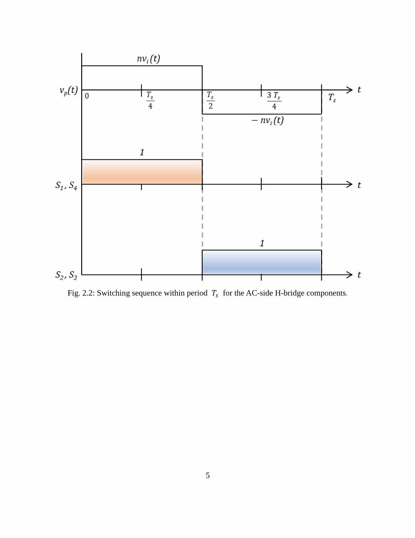
The switches 𝑆1, 𝑆2, 𝑆3, and 𝑆4 on the primary side H-bridge (the AC side) are four-quadrant

switches and are realized with emitter tied IGBTs. It must be four-quadrant because the AC source

voltage swings both positive and negative. The switches are operated by digital pulses at a

switching frequency 𝑓𝑠. During the first half switching period 𝑇𝑠

2=

1

𝑓𝑠

2=

1

2∙𝑓𝑠, 𝑆1 and 𝑆4 are on

and 𝑆2 and 𝑆3 are off. In this period, positive 𝑣𝑖(𝑡) is applied to 𝑣𝑝(𝑡) at the primary side of

the transformer then positive 𝑛𝑣𝑖(𝑡) is applied to 𝑛𝑣𝑝(𝑡) where the secondary side of the

transformer. During the second half switching period, 𝑆1 and 𝑆4 are off and 𝑆2 and 𝑆3 are on.

In this period, negative 𝑣𝑖(𝑡) is applied to 𝑣𝑝(𝑡) at the primary side of the transformer. Then

negative 𝑛𝑣𝑝(𝑡) is observed on the secondary side. In other words, the states are on and off for

50% of one switching period 𝑇𝑠 =1

𝑓𝑠. The waveform of the two switching states at 𝑣𝑝(𝑡) is

depicted in Fig. 2.2.

5

Fig. 2.2: Switching sequence within period 𝑇𝑠 for the AC-side H-bridge components.

6

Fig. 2.3: Switching sequence within period 𝑇𝑠 for the DC-side H-bridge components.

7

The switches 𝑆5, 𝑆6, 𝑆7, and 𝑆8 on the secondary side H-bridge (the DC-side) are two-quadrant

switches and components are assumed to be ideal. In Fig. 2.3, when the switches 𝑆5 and 𝑆8 are

on and the switches 𝑆6 and 𝑆7 are off simultaneously, positive 𝑉𝑂 is applied to 𝑣𝑠(𝑡). When the

switches 𝑆5 and 𝑆8 are off and the switches 𝑆6 and 𝑆7 are on simultaneously, negative 𝑉𝑂 is

applied to 𝑣𝑠(𝑡). In the rest of the switching cases, zero voltage is applied to 𝑣𝑠(𝑡).

The pulse width of 𝑣𝑠(𝑡) is defined by time-varying duty ratio, 𝐷(𝑡). Within period Ts, the

voltage waveform, 𝑣𝑠(𝑡), must be phase shifted, by 𝛥𝑡 (see Fig 2.3), in order to control power

transfer. The first and second plots of Fig. 2.4 show the comparison between the waveform at

𝑣𝑝(𝑡) and the phase shifted waveform at 𝑣𝑠(𝑡). Here, the waveform at 𝑣𝑠(𝑡) must stay inside of

the waveform at 𝑣𝑝(𝑡). When 𝛥𝑡 is assigned as positive, power flows from AC source to DC

source. When 𝛥𝑡 is assigned as negative, power flows from DC source to AC source.

In this analysis, the turns ratio of the transformer is assumed to be one and the magnetizing

inductance, and cores losses of the transformer are all neglected. Thus, this transformer can be

considered as an ideal transformer. The proposed modulation scheme utilizes the leakage

inductance of the transformer to transfer power in the topology shown in Fig. 1. The transformer

has a turns ratio of 1 : 𝑛 and the primary and secondary leakage inductance, 𝐿, is connected to

the secondary side as 𝐿 = 𝐿𝑃𝑛2 + 𝐿𝑠 , for analysis. The concept of the leakage inductance is

described in detail in Appendix A and [32]. The small-valued resistor representing the lumped

resistance, 𝑅, is added to enhance the accuracy of the model and facilitates a state-space average

modeling for analysis and designing a small-signal transfer function. The secondary side H-bridge

is connected to a DC source with voltage 𝑉𝑜.

8

Fig. 2.4: Modulation cycle of one switching period when the AC source voltage swings positive

(𝑣𝑖(𝑡) > 0).

The input AC voltage source, 𝑣𝑖(𝑡), on the AC-side H-bridge is defined in equation (2.1).

𝑣𝑖(t) = 𝑉𝑖𝑠𝑖𝑛(2𝜋𝑓𝑖𝑡). (2.1)

On the primary side of the transformer, the primary voltage pulse, 𝑣𝑝(𝑡), is applied by the AC-

9

side H-bridge with 50% pulse width of the switching period. The parameter 𝑣𝑝(𝑡) is defined in

equation (2.2).

𝑛𝑣𝑝(𝑡) = {𝑛𝑣𝑖(𝑡); 0 < 𝑡 <

𝑇𝑠

2

−𝑛𝑣𝑖(𝑡); 𝑇𝑠

2< 𝑡 < 𝑇𝑠

. (2.2)

On the secondary side of the transformer, the secondary voltage pulse, 𝑣𝑠(𝑡), is applied by the

DC-side H-bridge with a phase shifted time-varying duty ratio. The time-varying duty ratio, 𝐷(𝑡)

is defined in equation (2.3).

𝐷(𝑡) =𝑛|𝑣𝑖(𝑡)|

𝑉𝑜=

𝑛∙(𝑠𝑖𝑔𝑛[𝑣𝑖(𝑡)]∙𝑣𝑖(𝑡))

𝑉𝑜 , (2.3)

where

𝑠𝑔𝑛(𝑣𝑖(𝑡)) = {

+1; 𝑣𝑖(𝑡) > 0

0; 𝑣𝑖(𝑡) = 0

−1; 𝑣𝑖(𝑡) < 0

The peak duty ratio is defined as �̂�(𝑡) =𝑛𝑉𝑖

𝑉𝑜. Here, given 𝑛 and 𝑣𝑖(𝑡), 𝑉𝑖 and 𝑉𝑜 are selected

to keep 𝐷(𝑡) < 1. For modulation regarding the time-varying duty ratio, the sinusoidal pulse

width modulation (SPWM) technique is applied [11], [12].

10

Fig. 2.5: Sinusoidal Pulse Width Modulation.

A sinusoidal wave is compared with a reference triangular wave. Here, the frequency of the

triangular wave is higher than the sinusoidal wave. Comparing two waves using a comparator,

when the magnitude of sinusoidal wave is higher than the triangular wave, the digital value of the

comparator output is 1. Otherwise, it is zero. From this process, a PWM wave, which has variable

pulse width, is generated.

Furthermore, the phase shift, ∆𝑡, is defined in equation (2.4), where 𝛿 is a phase shift ratio and

satisfies |𝛿| ≤ (1 − 𝐷(𝑡)).

𝛥𝑡 = 𝛿∙𝑇𝑠

4 . (2.4)

Thus, 𝑣𝑠(𝑡) can be defined over a single complete switching period, 𝑇𝑠.

11

𝑣𝑠(𝑡) =

{

0; 0 ≤ 𝑡 <

𝑇𝑠

4(1 + 𝛿 − 𝐷(𝑡))

𝑠𝑔𝑛(𝑣𝑖(𝑡)) ∙ 𝑉𝑜; 𝑇𝑠

4(1 + 𝛿 − 𝐷(𝑡)) ≤ 𝑡 <

𝑇𝑠

4(1 + 𝛿 + 𝐷(𝑡))

0; 𝑇𝑠

4(1 + 𝛿 + 𝐷(𝑡)) ≤ 𝑡 <

3𝑇𝑠

4+𝑇𝑠

4(𝛿 − 𝐷(𝑡))

−𝑠𝑔𝑛(𝑣𝑖(𝑡)) ∙ 𝑉𝑜; 3𝑇𝑠

4+𝑇𝑠

4(𝛿 − 𝐷(𝑡)) ≤ 𝑡 <

3𝑇𝑠

2+𝑇𝑠

4(𝛿 + 𝐷(𝑡))

0; 3𝑇𝑠

4+𝑇𝑠

4(𝛿 + 𝐷(𝑡)) ≤ 𝑡 < 𝑇𝑠.

(2.5)

Applying Kirchoff’s Voltage Law (KVL), around the transformer in Fig. 2.1, yields the following:

𝑣𝐿(𝑡) = 𝑛𝑣𝑝(𝑡) − 𝑣𝑠(𝑡) − 𝑖𝐿(𝑡)𝑅. (2.6)

The inductor voltage, 𝑣𝐿(𝑡), can be defined as follows assuming that the inductor current is

initially zero and 𝑣𝑖(𝑡) is positive. After applying equations (2.2) and (2.5) for each time interval

of 𝑇𝑠, Equation (7) can be derived verifying the third plot in Fig. 2.4.

𝑣𝐿(𝑡) = 𝐿𝑑𝑖𝐿(𝑡)

𝑑𝑡

=

{

𝑛𝑣𝑖(𝑡) − (0) − 𝑖𝐿(𝑡)𝑅, 0 ≤ 𝑡 <

𝑇𝑠4(1 + 𝛿 − 𝐷)

𝑛𝑣𝑖(𝑡) − (+𝑉𝑜) − 𝑖𝐿(𝑡)𝑅,𝑇𝑠4(1 + 𝛿 − 𝐷) ≤ 𝑡 <

𝑇𝑠4(1 + 𝛿 + 𝐷)

𝑛𝑣𝑖(𝑡) − (0) − 𝑖𝐿(𝑡)𝑅,𝑇𝑠4(1 + 𝛿 + 𝐷) ≤ 𝑡 <

𝑇𝑠2

−𝑛𝑣𝑖(𝑡) − (0) − 𝑖𝐿(𝑡)𝑅,𝑇𝑠2≤ 𝑡 <

𝑇𝑠2+𝑇𝑠4(1 + 𝛿 − 𝐷)

−𝑛𝑣𝑖(𝑡) − (−𝑉𝑜) − 𝑖𝐿(𝑡)𝑅,𝑇𝑠2+𝑇𝑠4(1 + 𝛿 − 𝐷) ≤ 𝑡 <

𝑇𝑠2+𝑇𝑠4(1 + 𝛿 + 𝐷)

−𝑛𝑣𝑖(𝑡) − (0) − 𝑖𝐿(𝑡)𝑅,𝑇𝑠2+𝑇𝑠4(1 + 𝛿 + 𝐷) ≤ 𝑡 < 𝑇𝑠

12

=

{

𝑛𝑣𝑖(𝑡) − 𝑖𝐿(𝑡)𝑅, 0 ≤ 𝑡 <

𝑇𝑠

4(1 + 𝛿 − 𝐷)

𝑛𝑣𝑖(𝑡) − 𝑉𝑜 − 𝑖𝐿(𝑡)𝑅,𝑇𝑠

4(1 + 𝛿 − 𝐷) ≤ 𝑡 <

𝑇𝑠

4(1 + 𝛿 + 𝐷)

𝑛𝑣𝑖(𝑡) − 𝑖𝐿(𝑡)𝑅,𝑇𝑠

4(1 + 𝛿 + 𝐷) ≤ 𝑡 <

𝑇𝑠

2

−𝑛𝑣𝑖(𝑡) − 𝑖𝐿(𝑡)𝑅,𝑇𝑠

2≤ 𝑡 <

𝑇𝑠

2+𝑇𝑠

4(1 + 𝛿 − 𝐷)

−𝑛𝑣𝑖(𝑡) + 𝑉𝑜 − 𝑖𝐿(𝑡)𝑅,𝑇𝑠

2+𝑇𝑠

4(1 + 𝛿 − 𝐷) ≤ 𝑡 <

𝑇𝑠

2+𝑇𝑠

4(1 + 𝛿 + 𝐷)

−𝑛𝑣𝑖(𝑡) − 𝑖𝐿(𝑡)𝑅,𝑇𝑠

2+𝑇𝑠

4(1 + 𝛿 + 𝐷) ≤ 𝑡 < 𝑇𝑠.

(2.7)

According to Equation (2.7) and the third plot of Fig. 2.4, when the inductor, L, has positive voltage

(charging), the current through the inductor (orange line), 𝑖𝐿(𝑡) increases linearly. Again, the

resistor, R, is a small value. However, when the inductor has negative voltage (discharging), the

inductor current decreases.

2.2 Simulation

Parameter Value Unit

n 1

L 50 uH

R 0.1 Ohm

Vi 100 Volt

Vo 250 Volt

Ts 0.0001 s

δ 0.3

fi 60 Hz

Table 2.1: Simulation Parameters.

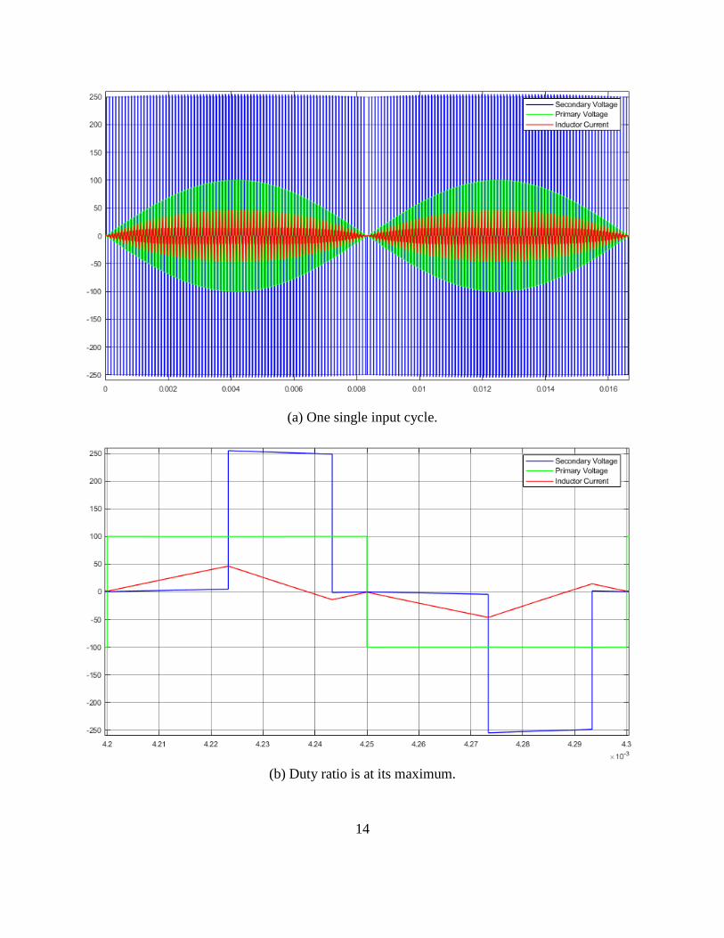
The simulation results are implemented by MATLAB and Simulink. The simulation results of the

proposed converter in Fig. 2.1, with the SPWM technique and the simulation parameters given in

Table 2.1, applied is shown in Fig. 2.6, and 2.7. In the Table 2.1, the phase shift ratio is defined as

13

δ. The peak value of the input AC source (Vi) is given 100 V and the output DC source (Vo) is set

to 250 V. Because the input AC source frequency (fi) is set to 60 Hz, one input cycle is 1/60 Hz =

0.0167 s. Fig 2.6 (a) shows the simulation result regarding one single input cycle when the phase

shift ratio δ is positive (+0.3). And Fig. 2.7 (a) shows the simulation result when δ is negative (-

0.3).

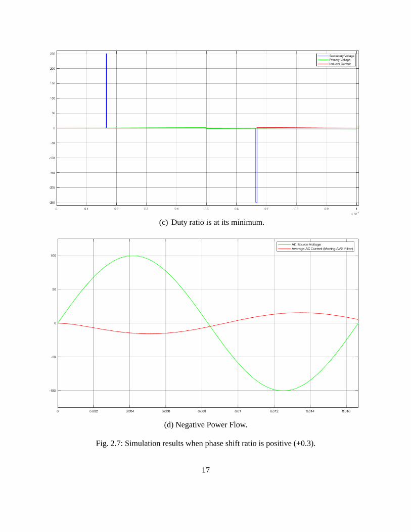
Regardless of the different sign of phase shift ratio, both simulation results show the DC output as

250 V (Blue), the AC input as 100 V peak (Green), and the Inductor current (Red). From 0 to

0.0083 sec, the green input sine wave swings positive, and, from 0.0083 sec to 0.0167 sec, the sine

wave swings negative. Fig 2.6 (b)-(c) and Fig 2.7 (b)-(c) are zoom in from Fig 2.6 (a) and Fig 2.7

(b) separately. From equation (2.3) or looking at Fig 2.6 (a) and 2.7 (a), when the input AC source

has a peak value, it shows the maximum duty ratio in Fig. 2.6 (b) and Fig. 2.7 (b) near 0.00425 sec

on the plot, separately. Otherwise, it shows the minimum duty ratio in each Fig. 2.6 (c) and Fig 2.7

(c) near 0 sec on the plot.

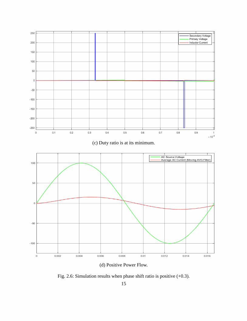
Considering the direction of phase shift ratio, when δ is set to positive, the waveforms of the input

AC voltage and the inductor current are in phase (Fig 2.6 (d)). This means the power flows from

the AC source to the DC source. However, when δ is negative, the waveforms are 180 degree out

of phase. In other words, the power is flowing from the DC source to the AC source and

demonstrates the capability for bi-directional power transfer.

14

(a) One single input cycle.

(b) Duty ratio is at its maximum.

15

(c) Duty ratio is at its minimum.

(d) Positive Power Flow.

Fig. 2.6: Simulation results when phase shift ratio is positive (+0.3).

16

(a) One single input cycle.

(b) Duty ratio is at its maximum.

17

(c) Duty ratio is at its minimum.

(d) Negative Power Flow.

Fig. 2.7: Simulation results when phase shift ratio is positive (+0.3).

18

2.3 Conclusion

The proposed single-stage DAB bi-directional AC/DC converter was analyzed in detail and

simulated. The simulation results confirm the theoretical analysis. Finally, the capability of bi-

directional power flow was demonstrated.

19

Chapter 3

Small-signal System Model Analysis

3.1 Analysis

In this chapter, a state-space averaging technique and small-signal modeling is introduced and

applied to the proposed converter shown in Fig. 2.1. In the past, for modeling the switching

converters in general, there were two main techniques: state-space modeling technique and

averaging technique. R.D. Middlebrook and Slobodan Cuk in the literature [15] first introduced a

state-space averaging method bridging the gap between the two techniques, since then this method

has been generally used in power electronics. The proposed converter is controlled via the time-

varying duty ratio of the gate signals and changes to phase shift ratio δ. Thus, the converter is

highly non-linear having both analogue and digital features. As a result, the state-space averaging

technique can be applied to linearize this system and obtain the dynamic model of the converter.

See [9], [13], [14], [15], [16], [17], and [18]. The total number of storage elements in the converter

determines the order of the system. In the proposed converter, one inductor is connected to the

20

secondary side of the transformer. Thus, this is a 1st order system. Equation (2.7) defines the

inductor voltage, 𝑣𝐿(𝑡) , for each time interval of one complete switching period, 𝑇𝑠 . The

waveform of inductor current (orange line) in Fig. 2.4 shows that the waveform during the first

half switching period, whose time interval is zero to 𝑇𝑠

2 is asymmetric to the waveform during the

second half switching period, whose time interval is time from 𝑇𝑠

2 to 𝑇𝑠 because of the switching

states described in Fig. 2.2 and 2.3. In other words, the total sum of the inductor current during

every single complete switching period results in zero.

Thus, in using the small signal modeling process combined with the state-space averaging

technique, only one variable half switching period is considered, when the switches 𝑆1 and 𝑆4

are on and 𝑆2 and 𝑆3 are off and with time varying duty ratio, D, and with 𝑣𝑖(𝑡) > 0.

𝐿𝑑𝑖𝐿(𝑡)

𝑑𝑡=

{

𝑛𝑣𝑖(𝑡) − 𝑖𝐿𝑅; 0 ≤ 𝑡 <

𝑇𝑠

4(1 + 𝛿 − 𝐷(𝑡))

𝑛𝑣𝑖(𝑡) − 𝑉𝑜 − 𝑖𝐿𝑅; 𝑇𝑠

4(1 + 𝛿 − 𝐷(𝑡)) ≤ 𝑡 <

𝑇𝑠

4(1 + 𝛿 + 𝐷(𝑡))

𝑛𝑣𝑖(𝑡) − 𝑖𝐿𝑅; 𝑇𝑠

4(1 + 𝛿 + 𝐷(𝑡)) ≤ 𝑡 <

𝑇𝑠

2

. (3.1)

Equation (3.1) is rewritten from Equation (2.7) only considering the first half switching period.

�̇�(𝑡) =

{

−

𝑅

𝐿𝑋(𝑡) +

1

𝐿𝑈(𝑡); 0 ≤ 𝑡 <

𝑇𝑠

4(1 + 𝛿 − 𝐷(𝑡))

−𝑅

𝐿𝑋(𝑡) + (

1

𝐿−

1

𝐿∙𝐷(𝑡))𝑈(𝑡);

𝑇𝑠

4(1 + 𝛿 − 𝐷(𝑡)) ≤ 𝑡 <

𝑇𝑠

4(1 + 𝛿 + 𝐷(𝑡))

−𝑅

𝐿𝑋(𝑡) +

1

𝐿𝑈(𝑡);

𝑇𝑠

4(1 + 𝛿 + 𝐷(𝑡)) ≤ 𝑡 <

𝑇𝑠

2

. (3.2)

Here, {𝐴𝑖 = −𝑅

𝐿; 𝑖 = 1, 2, 3} and B = [B1 B2 B3] = [

1

𝐿 (1

𝐿−

1

𝐿∙𝐷) 1

𝐿]. The state-space averaged

equation provided through the conduction ratio is written as

21

�̇�(𝑡) = [𝐴1 ((1 + 𝛿 − 𝐷(𝑡))

2) + 𝐴2(𝐷(𝑡)) + 𝐴3 (

(1 − 𝛿 − 𝐷(𝑡))

2)] 𝑋(𝑡)

+[𝐵1 ((1+𝛿−𝐷(𝑡))

2) + 𝐵2(𝐷(𝑡)) + 𝐵3 (

(1−𝛿−𝐷(𝑡))

2)]𝑈(𝑡), (3.3)

where 𝐷(𝑡) = �̅� + 𝑑(𝑡), 𝑋(𝑡) = �̅� + 𝑥(𝑡), and 𝑈(𝑡) = �̅� + 𝑢(𝑡). The variable d(t) is a small

signal variation of D(t), and x(t) is a small signal variation of X(t). The mean of D, or �̅�, can be

computed as

�̅� =𝑛∙𝑉𝑖

𝑉𝑜∙𝜋∙ ∫ sin(𝑡) 𝑑𝑡 =

𝜋

0

2∙𝑛∙𝑉𝑖

𝑉𝑜∙𝜋.

The nominal X, or �̅�, can be computed by averaging 𝑖𝐿(𝑡) over a complete cycle 0≤ 𝑡 ≤ 𝑇𝑠. To

derive the average source current, 𝑖�̅�(𝑡), from [1], the equation is

𝑖�̅�(𝑡) =2𝑛

𝑇𝑠∙ ∫ 𝑖𝐿(𝜏) 𝑑𝜏 =

𝑇𝑠20

𝛾1(𝐷(𝑡))+𝛾2

where 𝛾1 is a negative approximately linear function of D under typical converter parameters

with 0 < D(t) < 1.

The dynamics can be rewritten as

�̇� + �̇�(𝑡) = [𝐴1 ((1+𝛿−(�̅�+𝑑(𝑡)))

2) + 𝐴2(�̅� + 𝑑(𝑡)) + 𝐴3 (

(1−𝛿−(�̅�+𝑑(𝑡)))

2)] (�̅� + 𝑥(𝑡)) +

+ [𝐵1 ((1+𝛿−(�̅�+𝑑(𝑡)))

2) + 𝐵2(�̅� + 𝑑(𝑡)) + 𝐵3 (

(1−𝛿−(�̅�+𝑑(𝑡)))

2)] (�̅� + 𝑢(𝑡)).

After expanding and dividing the equation then neglecting the high order small signal variation, it

22

yields

�̇�(𝑡) = [𝐴1 (−𝑑(𝑡)

2) + 𝐴2(𝑑(𝑡)) + 𝐴3 (

−𝑑(𝑡)

2)] �̅�

+ [𝐴1 ((1 + 𝛿 − �̅�)

2) + 𝐴2(�̅�) + 𝐴3 (

(1 − 𝛿 − �̅�)

2)] 𝑥(𝑡)

+ [𝐵1 ((1 + 𝛿 − �̅�)

2) + 𝐵2(�̅�) + 𝐵3 (

(1 − 𝛿 − �̅�)

2)] 𝑢(𝑡)

+ [𝐵1 (−𝑑(𝑡)

2) + 𝐵2(𝑑(𝑡)) + 𝐵3 (

−𝑑(𝑡)

2)] �̅�

�̇�(𝑡) = [𝐴1 ((1 + 𝛿 − �̅�)

2) + 𝐴2(�̅�) + 𝐴3 (

(1 − 𝛿 − �̅�)

2)] 𝑥(𝑡)

+ [𝐵1 ((1 + 𝛿 − �̅�)

2) + 𝐵2(�̅�) + 𝐵3 (

(1 − 𝛿 − �̅�)

2)] 𝑢(𝑡)

+ [[−𝐴12+ 𝐴2 −

𝐴32] �̅� + [−

𝐵12+ 𝐵2 −

𝐵32] �̅�] 𝑑(𝑡)

≡ 𝐸𝑥(𝑡) + 𝐻𝑢(𝑡) + 𝐹𝑑(𝑡), 𝑎𝑎𝑎𝑎𝑎𝑎𝑎𝑎𝑎𝑎𝑎𝑎𝑎𝑎𝑎𝑎𝑎𝑎𝑎𝑎𝑎𝑎𝑎𝑎𝑎𝑎𝑎𝑎𝑎

where

𝐸 = [𝐴1 ((1 + 𝛿 − �̅�)

2) + 𝐴2(�̅�) + 𝐴3 (

(1 − 𝛿 − �̅�)

2)],

𝐻 = [𝐵1 ((1 + 𝛿 − �̅�)

2) + 𝐵2(�̅�) + 𝐵3 (

(1 − 𝛿 − �̅�)

2)],

𝐹 = [−𝐴12+ 𝐴2 −

𝐴32] �̅� + [−

𝐵12+ 𝐵2 −

𝐵32] �̅�. aaaaaaa

23

In short, E is the average of Ai, H is the average of Bi, and F is the difference of Ai. Therefore, the

control-to-output small-signal transfer function provided through Laplace transform is

𝑥(𝑡)

𝑑(𝑡)= [𝑠𝐼 − 𝐸]−1𝐹 =

𝑎𝑑𝑗[𝑠𝐼−𝐸]

𝑑𝑒𝑡 [𝑠𝐼−𝐸]∙ 𝐹. (3.4)

3.2 Simulation

In section 3.1, only first half switching period has considered for analysis. The half switching

period results will be used for designing controllers in chapter 4. In this simulation part, however,

first one full switching period will be considered and simulated.

Equation (3.2) is rewritten as the first full switching period:

�̇� =

{

−

𝑅

𝐿𝑋 +

1

𝐿𝑈, 0 < 𝑡 <

𝑇𝑠

4(1 + 𝛿 − 𝐷)

−𝑅

𝐿𝑋 + (

1

𝐿−

1

𝐿∙𝐷)𝑈,

𝑇𝑠

4(1 + 𝛿 − 𝐷) < 𝑡 <

𝑇𝑠

4(1 + 𝛿 + 𝐷)

−𝑅

𝐿𝑋 +

1

𝐿𝑈,

𝑇𝑠

4(1 + 𝛿 + 𝐷) < 𝑡 <

𝑇𝑠

2𝑅

𝐿𝑋 −

1

𝐿𝑈,

𝑇𝑠

2< 𝑡 <

𝑇𝑠

2+𝑇𝑠

4(1 + 𝛿 − 𝐷)

𝑅

𝐿𝑋 + (−

1

𝐿+

1

𝐿∙𝐷)𝑈,

𝑇𝑠

2+𝑇𝑠

4(1 + 𝛿 − 𝐷) < 𝑡 <

𝑇𝑠

2+𝑇𝑠

4(1 + 𝛿 + 𝐷)

𝑅

𝐿𝑋 −

1

𝐿𝑈,

𝑇𝑠

2+𝑇𝑠

4(1 + 𝛿 + 𝐷) < 𝑡 < 𝑇𝑠.

(3.5)

Using the parameters given in Table 2.1, the simplified plant is simulated with 𝑣𝑖(𝑡) applied over

multiple cycles. The resulting plot of inductor current is shown below for the original (𝑋(𝑡)), and

simplified model (�̅� + 𝑥(𝑡)). Fig. 3.1 contains the simulation results based on the theoretical

analysis regarding equation 3.5. This simulation time is from zero to one input period, i.e. Ti =

1/60 Hz = 0.0167 seconds. Thus, time-varying duty ratio, D(t) is used instead of the fixed peak

24

duty radio, D, at this time. To solve six differential and sequential equations, the last solution value

of each equation is used as the initial condition of the next time period equation. Here, the initial

condition of the first equation of the first simulation is set to zero. The trajectory results are

combined into a single plot.

Fig. 3.1: Plot of X(t) over a single input waveform cycle.

During the first half of the input waveform cycle in Fig. 3.1, when the time axis is restricted to the

interval [4.2e-3, 4.3e-3], i.e. the 43rd switching period, X(t) shows the peak amplitude of

approximately 45. At this period, the time-varying duty ratio, D(t) is also at its maximum. Thus,

the plot in Fig. 3.2 follows the plot of inductor current (orange line) in Fig. 4. Both Fig. 3.1 and

3.2 show that the inductor current has both positive and negative values.

25

When the only positive primary voltage, +vp(t), is applied to the inductor though the two four-

quadrant switches S1 and S4, the inductor current increases. Here, the initial inductor current is

zero. When the only negative primary voltage, -vp(t), is applied to the inductor though switches S2

and S3, the inductor current decreases. When both the positive primary and secondary voltages

apply to the inductor, the inductor current decreases. Also, when both the negative primary and

secondary voltages apply to the inductor, the inductor current increases.

Fig. 3.2: Plot of X(t) over a single switching period.

26

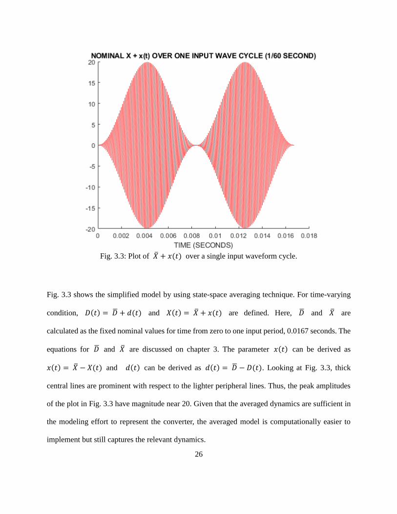
Fig. 3.3: Plot of �̅� + 𝑥(𝑡) over a single input waveform cycle.

Fig. 3.3 shows the simplified model by using state-space averaging technique. For time-varying

condition, 𝐷(𝑡) = �̅� + 𝑑(𝑡) and 𝑋(𝑡) = �̅� + 𝑥(𝑡) are defined. Here, �̅� and �̅� are

calculated as the fixed nominal values for time from zero to one input period, 0.0167 seconds. The

equations for �̅� and �̅� are discussed on chapter 3. The parameter 𝑥(𝑡) can be derived as

𝑥(𝑡) = �̅� − 𝑋(𝑡) and 𝑑(𝑡) can be derived as 𝑑(𝑡) = �̅� − 𝐷(𝑡). Looking at Fig. 3.3, thick

central lines are prominent with respect to the lighter peripheral lines. Thus, the peak amplitudes

of the plot in Fig. 3.3 have magnitude near 20. Given that the averaged dynamics are sufficient in

the modeling effort to represent the converter, the averaged model is computationally easier to

implement but still captures the relevant dynamics.

27

3.3 Conclusion

A small signal model averaging method has been proposed to simplify the modeling dynamics of

an AC/DC bi-directional DAB converter intended for grid connect applications. The proposed

converter topology incorporates inductor and resistor lumped components for enhanced model

accuracy and the system model was simulated (using MATLAB/Simulink) under the original

exponential dynamics as well as the averaged dynamics. These simulation results were compared

and demonstrate a model complexity as well as simulation computational complexity advantage

for the model derived through the small signal averaged methodology.

28

Chapter 4

Robust Control Analysis

4.1 Analysis

There are many reference papers which cover techniques for robust control theory, especially for

the H∞ control method. These techniques are frequently implemented in high-level mathematics.

It may cause some difficulties to understand even basic mechanisms of this theory. To provide

appropriate context, basic control theory is briefly reviewed to justify why robust control theory is

needed and to introduce the definition of robust control.

According to the reference paper in [8], historically, control theory can be broken down into two

main fields: conventional control and modern control. Conventional control theory has allowed

people to control the systems for centuries and became interesting with the development of

feedback theory. Feedback loops can be applied to the open-loop systems, also called plants, for

the purpose of stabilizing the entire system. This applied feedback system is also referred to as the

29

closed-loop systems.

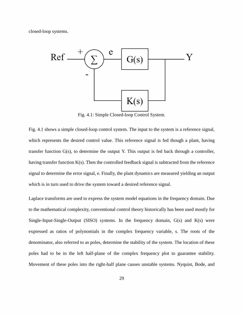
Fig. 4.1: Simple Closed-loop Control System.

Fig. 4.1 shows a simple closed-loop control system. The input to the system is a reference signal,

which represents the desired control value. This reference signal is fed though a plant, having

transfer function G(s), to determine the output Y. This output is fed back through a controller,

having transfer function K(s). Then the controlled feedback signal is subtracted from the reference

signal to determine the error signal, e. Finally, the plant dynamics are measured yielding an output

which is in turn used to drive the system toward a desired reference signal.

Laplace transforms are used to express the system model equations in the frequency domain. Due

to the mathematical complexity, conventional control theory historically has been used mostly for

Single-Input-Single-Output (SISO) systems. In the frequency domain, G(s) and K(s) were

expressed as ratios of polynomials in the complex frequency variable, s. The roots of the

denominator, also referred to as poles, determine the stability of the system. The location of these

poles had to be in the left half-plane of the complex frequency plot to guarantee stability.

Movement of these poles into the right-half plane causes unstable systems. Nyquist, Bode, and

30

Root locus methods were developed to show graphically the movements of poles in the frequency

domain.

Modern control theory was developed along with fast growing computer technology. The system

model equations were calculated efficiently and quickly on computers. It allows for

computationally feasible Multiple-Input-Multiple-Output (MIMO) systems. It was shown that any

n-th order differential equations describing a system model could be reduced to multiple 1st order

equations grouped in the form of a matrix. The state space matrix equations are shown:

�̇� = 𝐴𝒙 + 𝐵𝒖

𝐲 = 𝐶𝒙 + 𝐷𝒖,

where 𝒙 is a vector representing states, 𝒖 is a vector representing inputs, and A, B, C, D are

constant matrices for linear time-invariant systems. The key issue driving the need for modern

control theory is optimization. Thus, many methods to optimize the constant state matrices were

developed.

However, the conventional and modern control theory incorporating optimization were not always

tolerant to changes inside or outside of the system [8]. Thus, robust control theory was developed

because this theory can accommodate uncertainties which arise at every point of the system. In

other words, the key issue with robust control systems is uncertainty and how the control system

can deal with this problem. To handle uncertainties, having an appropriate model of uncertainty

models is the first step. One traditional method to define an uncertainty is modeled as probability

distributions via stochastic control theory. But this method has not been widely used in engineering.

Robust control theory seeks to bound the uncertainty rather than express it in a direct distribution

31

form. Given a bound on the uncertainty, the controller can deliver results that meet the system

requirements in all cases. Therefore, robust control theory can be stated as a worst-case analysis

method.

Due to the inconsistent nature of wind and solar by time-varying climate condition, the PV panels

and wind turbines may generate unpredictable power. Also, the system of renewable energy

sources itself may not operate properly if subsystem components are worn-out or broken. All

assumptions above can be considered as uncertainties. According to [21] and [22], among the

robust control techniques that are being gradually investigated in power electronics, the H∞

approach is a good candidate in many applications due in part to its linear characteristics, and the

derived controller which can also be used in large signal applications such as wind turbine

generators. The main antecedent in the use of H∞ control in DC-DC boost converters can be found

in the paper of Naim et al. [20]. According to this literature, the conventional closed-loop control

approach to DC-DC switch-mode converter shows a major problem when the transfer function

from the control input to the output voltage has a right-half-plane-zero (RHPZ). In conventional

design, designing low-output impedance (minimized weighting function) is not an objective.

Rather, it is obtained indirectly by increasing the loop gain and this increase is generally in conflict

with the phase-margin requirement. Thus, the presence of an RHPZ severely restricts the closed-

loop bandwidth. However, the goal H∞ control strategy is to design the minimized output

impedance as much as possible over a given frequency range and this can be overcome the

difficulties of the conventional approach.

Regarding the application of H∞ robust control techniques to the power electronic converters

application, most of papers were published for DC-DC buck, boost or buck-boost converter in [10],

32

[19], [20], [21], [22], [23], [24], [25], and [26]. However, in this thesis, H∞ robust controller for

AC-DC bi-directional DAB converter is investigated.

In the H∞ approach, the infinity norm, denoted as ||∙||∞ , of each input/output signal has upper bound

of unity.

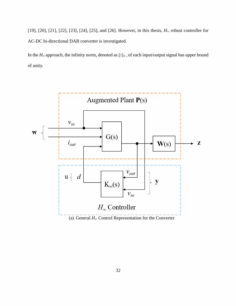
(a) General H∞ Control Representation for the Converter

33

(a) Compact H∞ Control Representation.

Fig. 4.2: H∞ Controller Design for the Converter.

General H∞ control representation for the converter in Fig. 4.2 (a) from [20] and [31] shows the

converter model (G(s)), the H∞ controller (K∞(s)), and the stable vector weighting function (W(s)).

The vector w contains the perturbations (vin and iout), the output vector z is the weighted error

signal, the vector y contains the measurement outputs of the converter (vout and vin), and the control

input u is the duty cycle (d).

The simplified H∞ control representation is showed in Fig. 4.2 (b) from [21] and [26], where P(s)

is the augmented plant.

Assuming that x is the state vector of the plant, w is the input of the plant, y is the input of the H∞

controller, and u is the output of the H∞ controller, the state space system equations for general

plant (but not related to the converter application) is described as follows:

�̇� = A𝐱 + B1𝐰+ B2𝐮

𝐳 = C1𝐱 + D11𝐰+ D12𝐮

𝐲 = C2𝐱 + D21𝐰+ D22𝐮

34

𝐮 = K∞(s) ∙ 𝐲.

P(s) is the general plant which can be described in matrix form as

𝐏(s) = [𝐀P 𝐁P𝐂P 𝐃P

].

Linear fractional transformation (LFT) is described in K. Zhou et al. [27] and it used to get a

transfer function using above equations.

According to the reference paper [21], the closed-loop transfer function matrix, Tzw, can be

obtained using LFT as below:

𝐓𝐳𝐰 =𝐳

𝐰= [𝐀P + 𝐁P ∙ K∞(s) ∙ (𝐈 − 𝐃P ∙ K∞(s))

−1 ∙ 𝐂P],

where,

𝐀p = A, 𝐁p = [B1 B2], 𝐂p = [C1C2], 𝐃p = [

D11 D12D21 D22

],

and I is the identity matrix of appropriate dimension.

The goal of H∞ control is to find a controller K∞(s) that stabilizes the plant P(s) minimizing the ∞-

norm of Tzw.

And the transfer function matrix, Tzw , can be describes as below:

||𝐓𝐳𝐰||∞ = 𝑠𝑢𝑝 𝜎(𝑤) < γ, 0 < γ ≤ 1

where ||𝐓𝐳𝐰||∞ is the maximal gain of the transfer function matrix Tzw, here, ||∙||∞ denotes the

matrix which is the supremum (sup) of the Tzw over all frequencies, and 𝜎(𝑤) is a maximum

singular value. For more mathematical descriptions, see [20], [21], [26].

35

In practice, an H∞ controller with ||𝐓𝐳𝐰||∞ as close to γ𝑜𝑝𝑡𝑖𝑚𝑎𝑙 can be obtained by the Robust

Control Toolbox of MATLAB, called hinfsyn function. This function needs only the state-space

description of the plant (the state-space averaged converter model from chapter 4) and stable

weighting functions for uncertainty.

4.2 Simulation

Applying the transfer function of the proposed converter by the state-spacing averaged technique,

equation (3.4), and selecting the weighting functions for uncertainty models, optimal H∞ controller

can be designed using hinfsyn function in MATLAB.

The linearized converter’s transfer function G can be rewritten as below by using equation (3.4)

and Table 2.1:

G(s) = 𝑥

𝑑(s) =

�̂�𝐿

𝑑(s) =

−50000

𝑠+2000U (4.1)

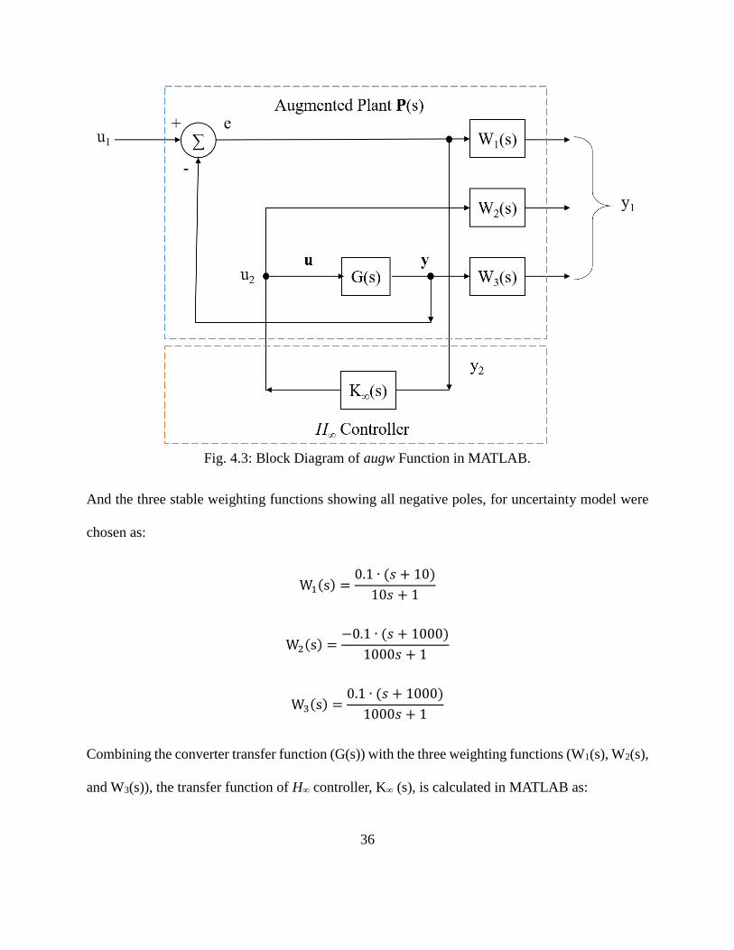
A MATLAB function, augw, can build a state-space model of an augmented LTI plant P(s) with

three weighting functions W1(s), W2(s), and W3(s) indicating uncertainty to the error signal,

control signal, and output signal respectively. Fig. 4.3 shows the block diagram of augw function.

36

Fig. 4.3: Block Diagram of augw Function in MATLAB.

And the three stable weighting functions showing all negative poles, for uncertainty model were

chosen as:

W1(s) =0.1 ∙ (𝑠 + 10)

10𝑠 + 1

W2(s) =−0.1 ∙ (𝑠 + 1000)

1000𝑠 + 1

W3(s) =0.1 ∙ (𝑠 + 1000)

1000𝑠 + 1

Combining the converter transfer function (G(s)) with the three weighting functions (W1(s), W2(s),

and W3(s)), the transfer function of H∞ controller, K∞ (s), is calculated in MATLAB as:

37

K∞(s) =−73.17s3 − 1.463 ∙ 105s2 − 292.7s − 0.1463

s4 + 5.001 ∙ 106s3 + 6.756 ∙ 106s2 + 6.773 ∙ 106s + 6706

Here, the widely used PI controller and proposed H∞ controller are applied to the converter system

separately and compared.

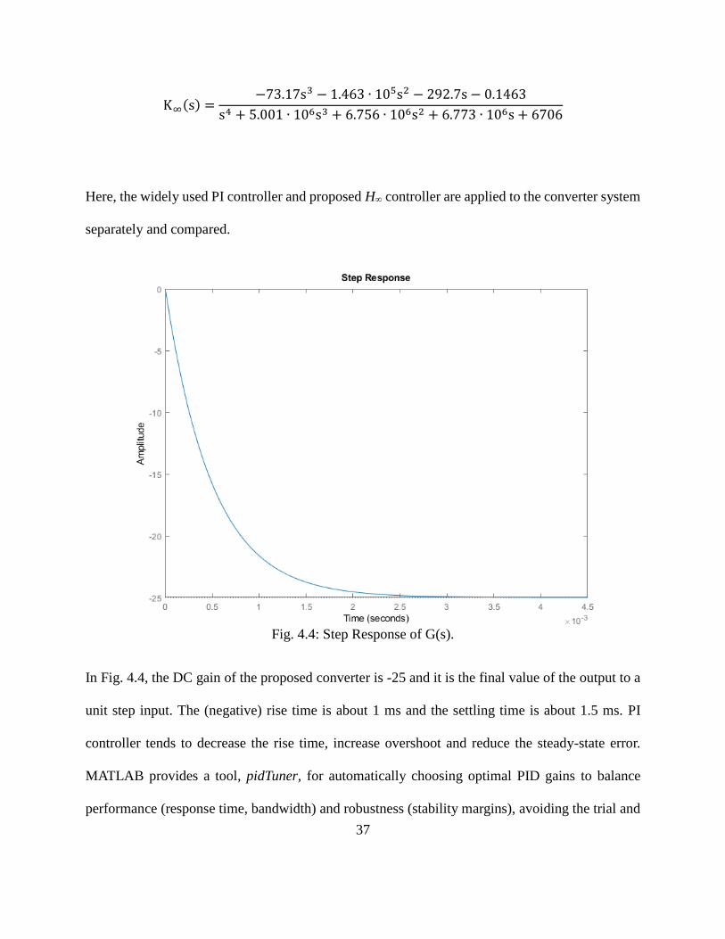
Fig. 4.4: Step Response of G(s).

In Fig. 4.4, the DC gain of the proposed converter is -25 and it is the final value of the output to a

unit step input. The (negative) rise time is about 1 ms and the settling time is about 1.5 ms. PI

controller tends to decrease the rise time, increase overshoot and reduce the steady-state error.

MATLAB provides a tool, pidTuner, for automatically choosing optimal PID gains to balance

performance (response time, bandwidth) and robustness (stability margins), avoiding the trial and

38

error process of traditional PID tuning method.

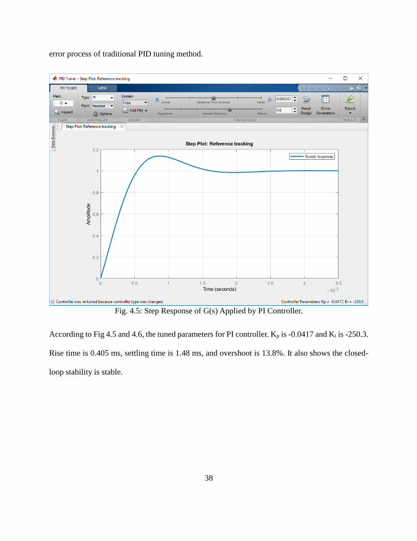
Fig. 4.5: Step Response of G(s) Applied by PI Controller.

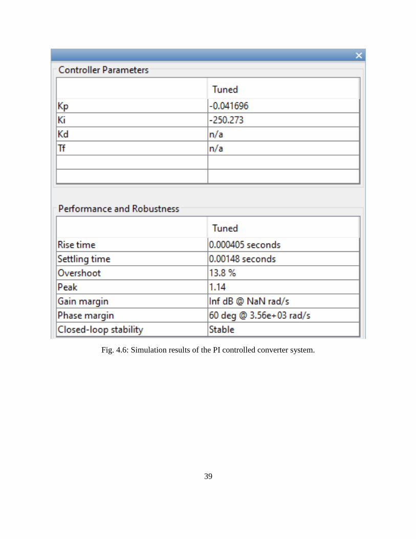
According to Fig 4.5 and 4.6, the tuned parameters for PI controller. Kp is -0.0417 and Ki is -250.3.

Rise time is 0.405 ms, settling time is 1.48 ms, and overshoot is 13.8%. It also shows the closed-

loop stability is stable.

39

Fig. 4.6: Simulation results of the PI controlled converter system.

40

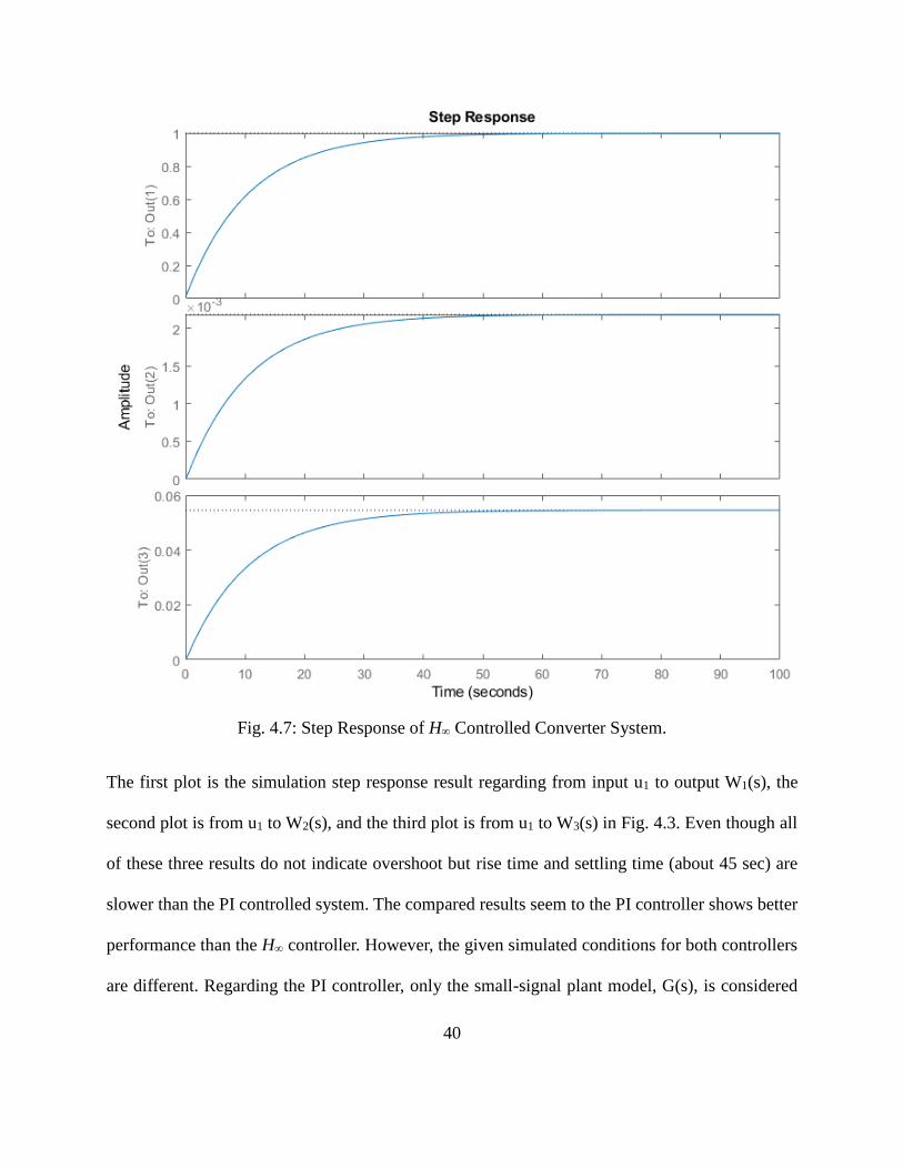
Fig. 4.7: Step Response of H∞ Controlled Converter System.

The first plot is the simulation step response result regarding from input u1 to output W1(s), the

second plot is from u1 to W2(s), and the third plot is from u1 to W3(s) in Fig. 4.3. Even though all

of these three results do not indicate overshoot but rise time and settling time (about 45 sec) are

slower than the PI controlled system. The compared results seem to the PI controller shows better

performance than the H∞ controller. However, the given simulated conditions for both controllers

are different. Regarding the PI controller, only the small-signal plant model, G(s), is considered

41

without weighting functions (noises or perturbations) because PID control theory and the

MATLAB function, pidtuner, can be applied to only a SISO (Single-Input-Single-Output) system.

However, the H∞ control theory and the MATLAB function, augw and hinfsyn, must be considered

the plant model with weighting functions. In other words, both controllers are not compared under

the same condition due to the theoretical issue. Thus, at this moment, we cannot determine which

control technique is better. And finding an optimal method to compare two control techniques

under the same condition will be the future work.

4.3 Conclusion

Robust H∞ control theory was introduced and the simulations were implemented comparing the

result of H∞ controller with PI controller to the proposed converter. According to the simulation

results, even though the PI controller applied to the proposed converter looks more effective than

an H∞ controller, we could not conclude which is better controller due to different simulated

conditions by different approached PID and H∞ theories. Thus finding a method to compare two

controllers will be the future work.

42

Chapter 5

Hybrid System Model Analysis

5.1 Analysis

Hybrid systems describe the behavior of dynamical systems that interact between continuous and

discrete dynamics [16], [17]. Continuous dynamics can be typically represented by several

different differential equations, or a continuous-time control system, such as a linear system �̇� =

Ax + Bu, where x is state and u is control input. Meanwhile, discrete dynamics such as finite-state

machine with state q that describe the digital or logical behavior.

Continuous Dynamics Interaction Discrete Dynamics

Fig. 5.1: A Simple Mechanism of a Hybrid System.

43

Fig. 5.1 shows a brief hybrid system mechanism. A hybrid system arises when the input v

determined by the continuous state x triggers the discrete dynamics or the input u determined by

the discrete dynamics state q yields continuous dynamics.

Switched systems are subordinate to hybrid systems. Based on the concept of hybrid systems,

greater emphasis on properties of the continuous dynamics neglecting the details of discrete

dynamics but considering all possible switching patterns can be referred to as switched systems.

The proposed converter has continuous-time behavior with discrete switching events. Thus, this

converter can be described by the properties of switched systems. Using the stored energy in the

inductor, especially inductor current, as a Lyapunov function, a switching rule is applied to the

converter. Then, stability analysis and control synthesis for this switched converter system will be

derived by construction of piecewise continuous Lyapunov functions.

A stable switching method by a Lyapunov function exists as long as there exists a stable convex

combination of the system matrices. The switching signal may depend on time, state, or generated

by more complex techniques. In this thesis, the switching signal is defined by the state (inductor

current).

In this section, a pair of two unstable affine systems, A1 and A2, is considered. The control objective

is to switch between the two systems to asymptotically stabilize the state trajectory of

�̇�(𝑡) = 𝐴𝛼𝑥(𝑡) + 𝑏𝛼 (5.1)

by proper choice of a switching rule defined by 𝑎 ∶ ℝ𝑛 × ℝ → {1, 2} which is piecewise constant,

called switching signal, over finite intervals. The subsystem ∑i is active when 𝛼 = i, where i = 1,

2.

44

To construct Lyapunov functions for switched systems, finding a stable convex combination is the

first step. To find the stable convex combination, the approach proposed by Wicks et al. [27]

introduces three different methods: time average control, sliding mode control, and finite-time

switched control. In this paper, only time average switching strategy will be used to define a stable

convex combination.

The averaged system, also referred to as a convex combination of the subsystems, can be defined:

∑eq : �̇� = 𝐴𝑒𝑞𝑥 + 𝑏𝑒𝑞, (5.2)

where 𝐴𝑒𝑞 = 𝛼𝐴1 + (1 − 𝛼)𝐴2 𝑎𝑛𝑑 𝑏𝑒𝑞 = 𝛼𝑏1 + (1 − 𝛼)𝑏2 with 0 < 𝛼 < 1. Therefore 𝛼 +

(1 − 𝛼) = 1.

The time average control implements 𝐴𝑒𝑞 by rapid time switching between 𝐴1 and 𝐴2. Here,

𝐴1 has a duty cycle proportional to 𝛼 and 𝐴2 has a duty cycle proportional to (1 − 𝛼).

Asymptotic stability requires that 𝐴𝑒𝑞 be a stability matrix and 𝑏𝑒𝑞 is zero, i.e.

𝐴𝑒𝑞 = 𝛼𝐴1 + (1 − 𝛼)𝐴2 𝑖𝑠 𝐻𝑢𝑟𝑤𝑖𝑡𝑧 (5.3)

𝑏𝑒𝑞 = 𝛼𝑏1 + (1 − 𝛼)𝑏2 = 0 (5.4)

See [27] for a theorem and its proof regarding (5.3) and (5.4).

This is an algorithm for finding an 𝛼 for which 𝐴𝑒𝑞 is stable according to [27]:

(i) Compute the set

{𝛽𝑖 > 0|∃𝜔𝑖 ∋ 𝑑𝑒𝑡[𝐴1 + 𝛽𝑖𝐴2 + 𝑗𝜔𝑖𝐼] = 0}

and order this set so that 𝛽1 ≤ 𝛽2 ≤ ⋯ ≤ 𝛽𝑚 where 𝑚 is the cardinality of the set.

45

(ii) Define the set of interval endpoints

𝐵 = {0, 𝛽1,⋯ , 𝛽𝑚, ∞}

(iii) Define the set of test points

Γ = {𝛾0 =𝛽1

2, 𝛾1 =

𝛽1+𝛽2

2, ⋯ , 𝛾𝑖 =

𝛽𝑖+𝛽𝑖+1

2, ⋯ , 𝛾𝑚−1 =

𝛽𝑚−1+𝛽𝑚

2 , 𝛾𝑚 = 2𝛽𝑚 + 1}.

(iv) Determine if Λ[𝐴1 + 𝛾𝑖𝐴2] ⊂ ℂ− for some 𝑖. If so then 𝛼 =

1

𝛾𝑖+1 satisfies

λ[𝐴𝑒𝑞(𝛼)] ⊂ ℂ−. Otherwise no such 𝛼 exists.

Then, the 𝛼 can be applied to the Lyapunov equation to find its solution, 𝑃𝑒𝑞:

𝐴𝑒𝑞𝑇 𝑃𝑒𝑞 + 𝑃𝑒𝑞𝐴𝑒𝑞 = −𝑄𝑒𝑞 , (5.5)

where 𝑄𝑒𝑞 is any positive definite real symmetric 2x2 matrix, such as the identity matrix.

Using the solution of the Lyapunov function, 𝑄1 and 𝑄2 are calculated by the equation below:

𝑄𝑖 = −(𝐴𝑖𝑇𝑃𝑒𝑞 + 𝑃𝑒𝑞𝐴𝑖), (5.6)

where i = 1, 2.

[1] and [2] describe the switching rule based on the above results.

𝑠1(𝑥) = 𝑥𝑇(𝑄1 − 𝜖𝑄2)𝑥

𝑠2(𝑥) = 𝑥𝑇(𝑄2 − 𝜖𝑄1)𝑥

Where 𝜖 is any number chosen to satisfy 0 < 𝜖 < 1.

𝑑𝑒𝑡[𝐴1 + 𝛽𝑖𝐴2 + 𝑗𝜔𝑖𝐼] = 0

46

5.2 Simulation

Parameter Value Unit

𝛼 0.6

L 50 uH

R 0.1 Ohm

𝜖 0.05

Table 5.1: Simulation Parameters.

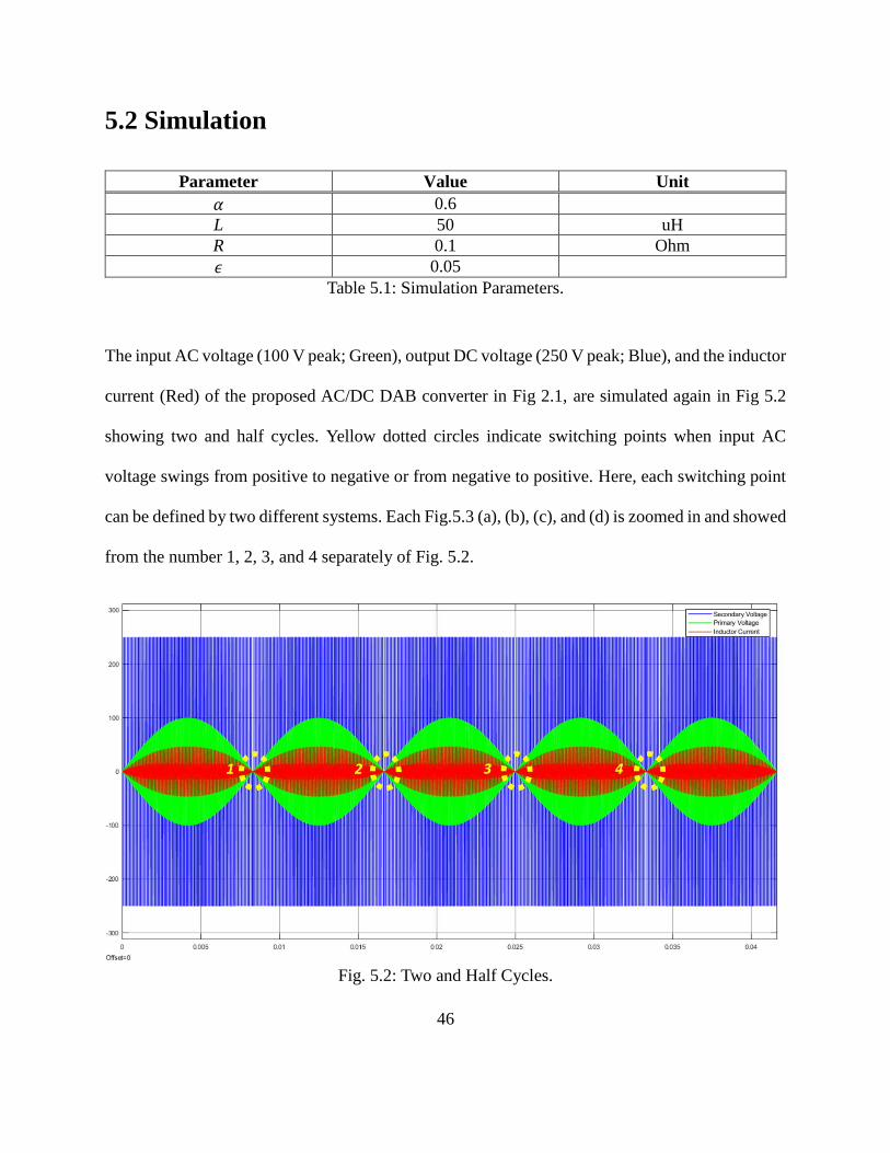
The input AC voltage (100 V peak; Green), output DC voltage (250 V peak; Blue), and the inductor

current (Red) of the proposed AC/DC DAB converter in Fig 2.1, are simulated again in Fig 5.2

showing two and half cycles. Yellow dotted circles indicate switching points when input AC

voltage swings from positive to negative or from negative to positive. Here, each switching point

can be defined by two different systems. Each Fig.5.3 (a), (b), (c), and (d) is zoomed in and showed

from the number 1, 2, 3, and 4 separately of Fig. 5.2.

Fig. 5.2: Two and Half Cycles.

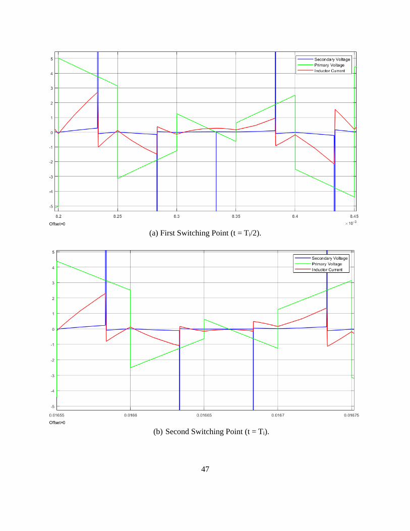
47

(a) First Switching Point (t = Ti/2).

(b) Second Switching Point (t = Ti).

48

(c) Third Switching Point (t = 3*Ti/2).

(d) Fourth Switching Point (t = 2*Ti).

Fig. 5.3: Comparison between Different Switching Points.

49

According to Fig. 5.3 (a)-(d), the inductor current (Red) in every different switching point was

jumped showing non-linear current flow between two systems. These four different non-linear

currents are complicated to compute. Defining an exact non-linear equation in this problem may

be complicated. Thus, applying a random noise to the stable linear function is one way to achieve

non-linear function approximately. To solve this problem, a random noise was generated and

applied to two systems, 𝑋1̇ and 𝑋2̇. Then, by using concatenated two modeling method, two of

2-by-2 unstable matrix was derived to implement the switched system theory.

Fig. 5.4: Concatenating Method.

Here,

𝒚1 = [

−𝑅

𝐿0

normrnd(0,1) normrnd(0,1)

] 𝑿 + [1

𝐿0

]𝑼 = 𝑨𝟏𝑿 + 𝑩𝟏𝑼

and

50

𝒚2 = [𝑅

𝐿0

-normrnd(0,1) -normrnd(0,1)] 𝑿 + [

−1

𝐿

0]𝑼 = 𝑩𝟐𝑿 +𝑩𝟐𝑼.

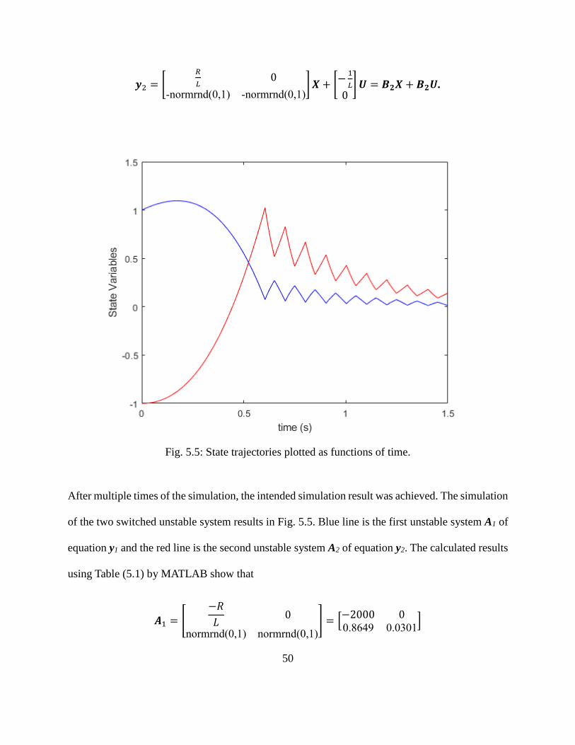
Fig. 5.5: State trajectories plotted as functions of time.

After multiple times of the simulation, the intended simulation result was achieved. The simulation

of the two switched unstable system results in Fig. 5.5. Blue line is the first unstable system A1 of

equation y1 and the red line is the second unstable system A2 of equation y2. The calculated results

using Table (5.1) by MATLAB show that

𝑨1 = [

−𝑅

𝐿0

normrnd(0,1) normrnd(0,1)

] = [−2000 00.8649 0.0301

]

51

𝑨2 = [

𝑅

𝐿0

-normrnd(0,1) -normrnd(0,1)

] = [2000 0

-0.1649 −0.6277]

and

𝑷𝑒𝑞 = [0.0013 −1.4146𝑒 − 06

-1.4146e-06 1.8580], where Peq is the solution of Lyapunov function.

The simulation result shows that, as time goes on, two switched unstable systems asymptotically

approach a steady state value of approximately 0.2.

5.3 Conclusion

In this chapter, the stability of the proposed converter as an application of switched systems is

demonstrated by construction of Lyapunov function. To find a stable convex combination, random

noise was generated for modeling non-linear functions. Finally, two unstable systems were

simulated under the theoretical understanding and the simulation result showed that two unstable

systems by switching eventually stabilized.

52

Chapter 6

Conclusion

For designing a universal and scalable grid power converter, a bi-directional dual-active bridge

AC/DC power converter using H∞ controller is developed and simulated. To design the H∞

controller, the system transfer function should be obtained first. State-space averaging technique

was used to obtain small-signal plant model for its transfer function. Then H∞ controller was

calculated by MATLAB and compared with the performance of PI controller. According to the

simulation results, even though the PI controller applied to the proposed converter looks more

effective than an H∞ controller, we could not conclude which is better controller due to different

simulated conditions by different approached PID and H∞ theories. Thus finding a method to

compare two controllers will be the future work. In addition to, the stability was verified using

switched system theory by the construction of the Lyapunov function.

53

References

[1] N. D. Weise, G. Castelino, K. Basu, and N. Mohan, A single-stage dual-active-bridge-based

soft switched ac/dc converter with open-loop power factor correction and other advanced

features, IEEE Transactions on Power Electronics, vol. 29, no. 8, pp. 40074016, Aug

2014.

[2] G. Castelino, K. Basu, N. Weise and N. Mohan, A bi-directional, isolated, single-stage, DAB-

based AC-DC converter with open-loop power factor correct- ion and other advanced

features, 2012 IEEE International Conference on Industrial Technology, Athens, 2012,

pp. 938-943.

[3] R. Baranwal, G. F. Castelino, K. Iyer, K. Basu and N.Mohan, A Dual-Active-Bridge-Based

Single-Phase AC to DC Power Electronic Transformer With Advanced Features, IEEE

Transactions on Power Electronics, vol. 33, no. 1, pp. 313-331, Jan. 2018.

[4] Weise, Nathan David. (2011). Universal utility interface for plug-in hybrid electric vehicles

with vehicle-to-grid functionality.., Retrieved from the University of Minnesota Digital

Conservancy, http://hdl.handle.net/11299/116540.

[5] Y. P. Chan, K. H. Loo and Y. M. Lai, Single-Stage Resonant AC-DC Dual Active Bridge

54

Converter with Flexible Active and Reactive Power Control, 2016 IEEE Vehicle Power

and Propulsion Conference (VPPC), Hangzhou, 2016, pp. 1-6.

[6] N. Weise, DQ current control of a bidirectional, isolated, single-stage AC-DC converter for

vehicle-to-grid applications, 2013 IEEE Power & Energy Society General Meeting,

Vancouver, BC, 2013, pp. 1-5.

[7] Matthew Lackner, Anthony Rogers, and James Manwell. Uncertainty Analysis in Wind

Resource Assessment and Wind Energy Production Estimation, 45th AIAA Aerospace

Sciences Meeting and Exhibit, Aerospace Sciences Meetings,

https://doi.org/10.2514/6.2007-1222

[8] Leo Rollins, “Robust Control Theory.” Internet:

https://users.ece.cmu.edu/˜koopman/des_s99/control_theory/, Spring 1999 [Nov. 01,

2017].

[9] Benny Yeung. Chapter 7 Dynamic Modelling and Control of DC/DC Converters, Internet:

ftp://ftp.ee.polyu.edu.hk/echeng/EE529_PowerElect_Utility/07.%20Dynamic%20Modell

ing%20and%20Control%20of%20DC-DC%20Converters%20(Benny%20Yeung).pdf

[Feb. 01, 2017].

[10] Mirzaei, M., Poulsen, N. K., & Niemann, H. H. (2012). Wind Turbine Control: Robust

Model Based Approach. Kgs. Lyngby: Technical University of Denmark. (IMM-PHD-

2012; No. 281).

[11] Tennessee Tech University, Chapter 2 Single Phase Pulse Width Modulated Inverters,

Internet: https://www.tntech.edu/files/cesr/StudThesis/asuri/Chapter2.pdf [Oct. 01, 2017].

[12] A.M. Gole, Sinusoidal Pulse width modulation, 24.437 Power electronics, 2000, Internet:

55

http://encon.fke.utm.my/nikd/SEM4413/spwm.pdf [Oct. 01, 2017]

[13] Georgios D. Demetriades, On Small-Signal Analysis and Control of The Single- and The

Dual-Active Bridge Topologies, KTH, Stockholm, 2005. Internet: http://kth.diva-

portal.org/smash/get/diva2:7434/FULLTEXT01.pdf.

[14] BoHyun Ahn and Vincent Winstead, Small Signal Model Averaging of Bi-Directional

Converter, EIT Conference 2018, Rochester, Michigan, May 5, 2018, no. 227.

[15] R. D. Middlebrook and Slobodan Cuk, A General Unified Approach to Modelling

Switching-Converter Power Stages, IEEE Power Electronics Specialists Conference,

Cleveland, Ohio, June 8-10, 1976, pp. 73-86.

[16] W.P.M.H. Heemels, D. Lehmann, J. Lunze, and B. De Schutter, Introduction to hybrid

systems, Chapter 1 in Handbook of Hybrid Systems Control – Theory, Tools,

Applications (J. Lunze and F. Lamnabhi-Lagarrigue, eds.), Cambridge, UK: Cambridge

University Press, ISBN 978-0-521-76505-3, pp. 3–30, 2009.

[17] Daniel Liberzon, Switched Systems: Stability Analysis and Control Synthesis: Lecture Notes

for HYCON-EECI Graduate School on Control, Coordinated Science Laboratory,

University of Illinois at Urbana-Champaign, U.S.A. Internet:

http://liberzon.csl.illinois.edu/teaching/Liberzon-LectureNotes.pdf.

[18] D. Hernandez-Torres, O. Sename, D. Riu, and F. Druart, On the Robust Control of DC-DC

Converters: Application to a Hybrid Power Generation System, 4th IFAC Symposium on

System, Structure and Control (SSSC 2010), Sep 2010, Ancona, Italy.

56

[19] G. Weiss, Q.C. Zhong, and T.C. Green, H∞ Repetitive Control of DC-AC Converters in

Microgrids, IEEE Transactions on Power Electronics, Vol. 19, No 1, January 2004. Pp.

219-230.

[20] R. Naim, G. Weiss, and S. Ben-Yaakov, H∞ Control Applied to Boost Power Converters,

IEEE Transactions on Power Electronics, vol. 12, no. 4, July 1997.

[21] E. Vidal-Idiarte, L. Martinez-Salamero, H. Valderrama-Blavi, F. Guinjoan, and J. Maixe,

Analysis and Design of H∞ Control of Nonminimum Phase-Switching Converters, IEEE

Transactions on Circuit and Systems-I: Fundamental Theory and Applications, vol. 50,

no. 10, October 2003.

[22] E. Vidal-Idiarte, L. Martinez-Salamero, H. Valderrama-Blavi, and F. Guinjoan, H∞ Control

of DC-to-DC Switching Converters, in Proc. IEEE Int. Symp. Citcuits and Systems,

ISCAS’99, vol. 5, 1999, pp. 238-241.

[23] Yan-hua Xian and Jiu-chao Feng, Output Feedback H-infinity Control for Buck Converter

with Unvertainty Parameters, 2011 IEEE 13th International Conference on

Communication Technology, Jinan, 2011, pp. 887-891.

[24] Andreas Kugi and Kurt Schlacher, Nonlinear H∞ -Controller Design for a DC-to-DC Power

Converter, IEEE Transactions on Control Systems Technology, vol. 7, no. 2, March

1999.

[25] D. Hernandez-Torres, O. Sename, D. Riu, and F. Druart, On the Robust Control of DC-DC

Converters: Application to a Hybrid Power Generation System, 4th IFAC Symposium on

System, Structure and Control (SSSC 2010), Sep 2010, Ancona, Italy.

[26] K. Zhou and J. C. Doyle, Essentials of Robust Control, Prentice-Hall, 1998

57

[27] Mark A. Wicks et al, Construction of Piecewise Lyapunov Functions for Stabilizing

Switched Systems, Proceedings of the 33rd IEEE Conference on Decision and Control,

Lake Buena Vista, Florida, December 1994, pp. 3492-3497.

[28] Mark A. Wicks et al, Structured Rank-Reducing Matrix Perturbations: Theory and

Computation, American Control Conference, 1992, pp. 649-653.

[29] Yimin Lu et al, Hybrid Feedback Switching Control in a Buck Converter, 2008 IEEE

International Conference on Automation and Logistics, Qingdao, China, September,

2008, pp. 207-210.

[30] Paolo Bolzern et al, Quadratic stabilization of a switched affine system about a

nonequilibrium point, proceeding of the 2004 American Control Conference, Boston,

Massachusetts, June 30-July 2, 2004, pp 3890 – 3895.

[31] MathWorks, “augw.” Internet: https://www.mathworks.com/help/robust/ref/augw.html [Oct.

20, 2018].

[32] Voltech, “Measuring Leakage Inductance”, Internet: http://www.voltech.com/Articles/104-

105/1_What_is_Leakage_Inductance [Jun. 18, 2018].

58

Appendix A

Leakage Inductance

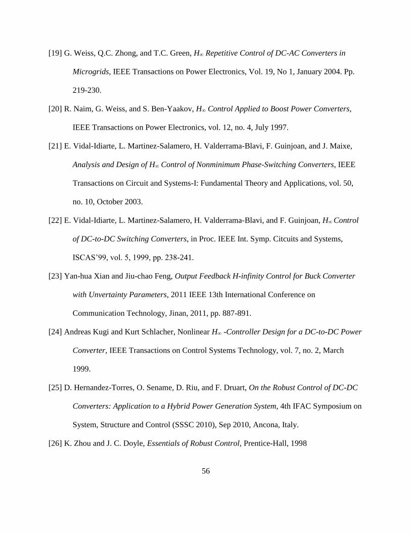
The concept of the leakage inductance is studied in [32]. An ideal transformer is lossless and

perfectly coupled. In other words, all of magnetic flux in the ideal transformer flows between the

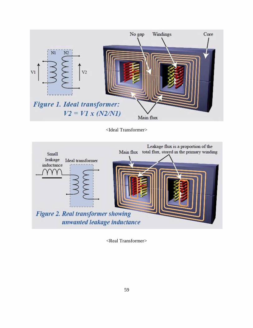
primary winding and the secondary winding completely. However, a real transformer losses some

of the magnetic flux between the primary winding and the secondary winding. The lost flux,

“leakage flux”, in the real transformer should be compensated for an additional inductor, “leakage

inductance” that is in series with the primary or secondary winding to operate the transformer

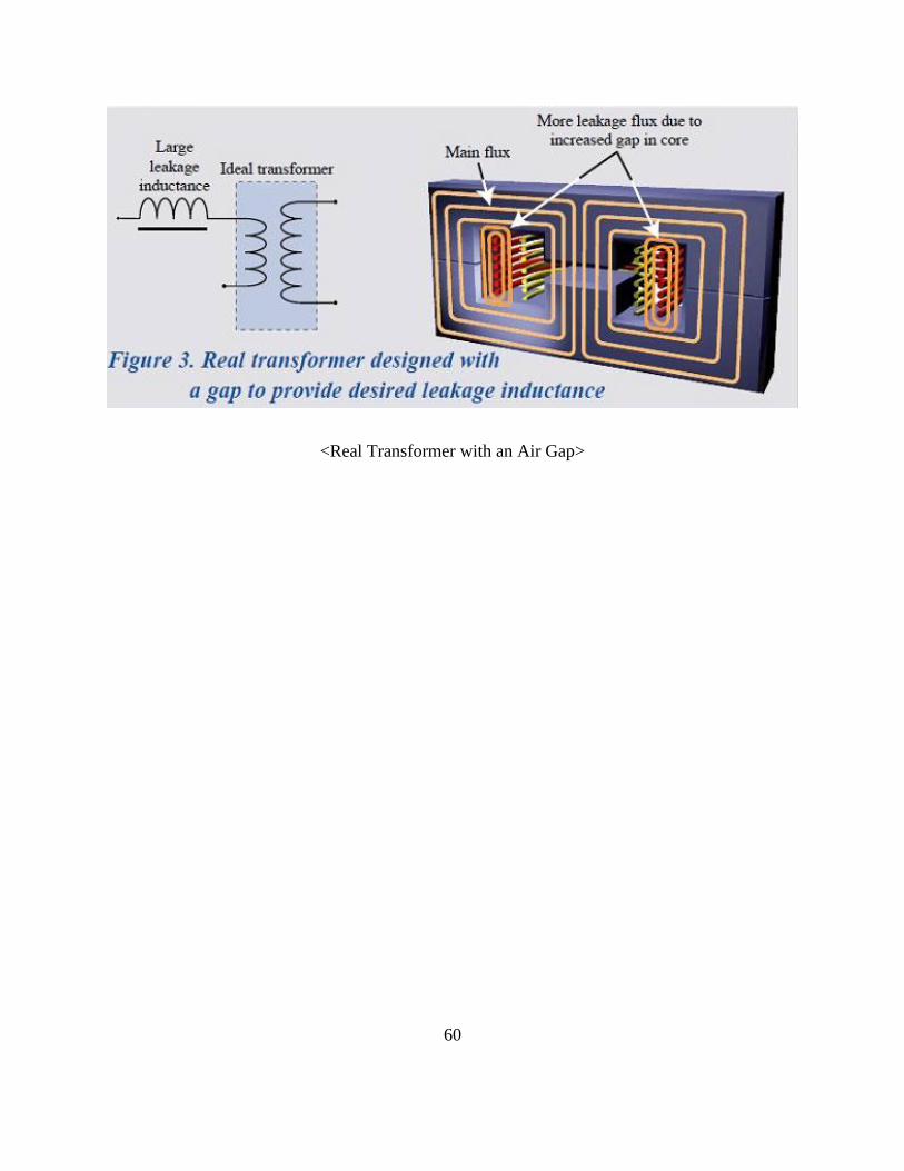
accurately. If there exists an air gap in the core of real transformer, larger leakage inductance is

required.

59

<Ideal Transformer>

<Real Transformer>

60

<Real Transformer with an Air Gap>