Embed Size (px)
Citation preview
A THESIS SUBMITTED IN PARTIAL FULFILLMENT OF THE REQUIREMENTS FOR THE DEGREE OF BACHELOR
OF TECHNOLOGY IN MECHANICAL ENGINEERING
Submitted By: Under the Guidance Of: Manish Kumar (110ME0297) Prof. R.K. Sahoo Dept. Of Mechanical Engg. Dept. Of Mechanical Engg. National Institute of Technology, Rourkela National Institute of Technology, Rourkela
This is to certify that the thesis entitled ‘Phasor Analysis of GM – type Double
Inlet Pulse Tube Refrigerator’ submitted by Manish Kumar bearing roll number
110ME0297 in the partial fulfillment of the requirement for the degree of
Bachelor of Technology in Mechanical Engineering, National Institute of
Technology, Rourkela, is being carried out under my supervision.
To the best of my knowledge, the matter embodied in the thesis has not been
submitted to any other university/institute for the award of any degree or
diploma.
Date: 6th May 2014 Prof. R.K. Sahoo
Dept. Of Mechanical Engineering
National Institute of Technology, Rourkela-769008

Title Page Number
Acknowledgement (i)
Abstract (ii)
List of Figure/Graph (iii) – (iv)
List of Table/Flow Chart (v)
Nomenclature (vi) – (vii)
Chapter 1: Introduction 1 – 9
Chapter 2: Literature Survey 10 – 12
Chapter 3: Aim of the Present Work 13 – 14
Chapter 4: Thermodynamic Study of DIPTR 15 – 20
Chapter 5: Algorithm for the Program and Output 21 – 28
Chapter 6: Phasor Analysis 29 – 31
Chapter 7: Design of the Pulse Tube 32 – 40
Chapter 8: Conclusion 41 – 42
References 43 – 44

i
I would like to express my deepest gratitude to my supervisor Prof. R.K. Sahoo for
his immense support and guidance throughout this project. It was his constant
moral boost and thorough discussion on the subject that has led to the completion
of this project.
I would also like to take this opportunity to thank Mr. Sachindra Rout, Phd and Mr.
Pankaj Kumar, Phd for their guidance and help without which this project would
not have been completed.
Last but not the least I would like to thank my family and friends for their support
and blessings.
Date: 6th May 2014 Manish Kumar
Roll Number – 110ME0297
Dept. Of Mechanical Engineering
National Institute of Technology, Rourkela - 769008
ii
The simplicity and varied application of a pulse tube refrigerator has always gained the attention
of many scientist and researchers towards itself. It is because of this very reason that various
different types of pulse tube refrigerator has come up with time.
A GM type double inlet pulse tube refrigerator (DIPTR) is one of the many configuration of the
pulse tube that has come up with time. Although the configuration of a DIPTR seems to be quite
simple but its working principle is a bit complicated.
The aim of the present work is to study the working principle behind a DIPTR and develop a
MATLAB code for the same and use it further to draw a phasor for the governing equation, so as
to validate the output of the code developed.
The MATLAB code and the phasor developed in this work is then used to develop a simplified
design method for determining the dimension of the pulse tube of a DIPTR.
iii
Figure/Graph
Number
Description Page Number
Fig 1.1 Schematic diagram for Stirling Type Orifice Pulse Tube
Refrigerator
7
Fig 1.2 Schematic diagram for GM Type Orifice Pulse Tube
Refrigerator
7
Fig 4.1 Schematic diagram of a Double Inlet Pulse Tube
Refrigerator (DIPTR)
17
Fig 5.1 Graph representing the pressure oscillation within the
pulse tube (Pt) and the compressor (Pcp)
25
Fig 5.2 Graph representing the mass flow rates through the
regeneratorregM
, double inlet valve
DIM
and the
compressor cM
25
Fig 5.3 Graph representing the mass flow rates through hot-end
heat exchanger hhxM
, the orifice
0M
and the
phase phM
26
Fig 5.4 Graph representing mass flow rates through the
compressor ptM
and the pressure oscillation within the
pulse tube (Pt)
26

iv
Fig 5.5 Graph representing mass flow rate through cold-end heat
exchanger chxM
and the pulse tube
ptM
27
Fig 6.1 Phasor Representation for a Double Inlet Pulse Tube
Refrigerator (DIPTR)
31
Fig 7.1 Graph representing the pressure oscillation within the
pulse tube (Pt) and the compressor (Pcp)
37
Fig 7.2 Graph representing the mass flow rates through the
regeneratorregM
, double inlet valve
DIM
and the
compressor cM
37
Fig 7.3 Graph representing the mass flow rates through hot-end
heat exchanger hhxM
, the orifice
0M
and the
phase phM
38
Fig 7.4 Graph representing mass flow rates through the
compressor ptM
and the pressure oscillation within the
pulse tube (Pt)
38
Fig 7.5 Graph representing mass flow rate through cold-end heat
exchanger chxM
and the pulse tube
ptM
39
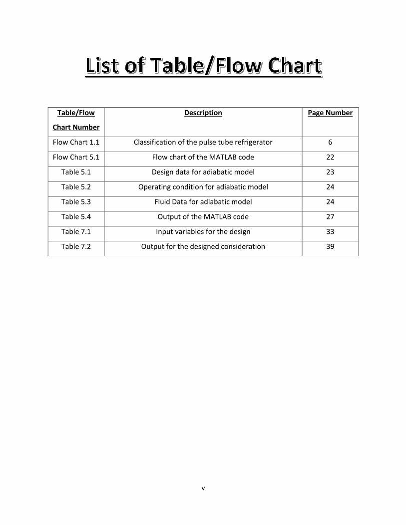
v
Table/Flow
Chart Number
Description Page Number
Flow Chart 1.1 Classification of the pulse tube refrigerator 6
Flow Chart 5.1 Flow chart of the MATLAB code 22
Table 5.1 Design data for adiabatic model 23
Table 5.2 Operating condition for adiabatic model 24
Table 5.3 Fluid Data for adiabatic model 24
Table 5.4 Output of the MATLAB code 27
Table 7.1 Input variables for the design 33
Table 7.2 Output for the designed consideration 39
vi
Symbol Description
ev Porosity of regenerator ( void volume /
total volume)
f Frequency (Hz)
m
/ M
Mass flow rate (kg/s)
P Pressure (MPa)
Qc Cooling capacity
R Gas constant (J/kg K)
T Temperature (K)
t Time (s)
V Volume (m3)
Z Orifice impedance (Pa s/kg)
Teff
ln
h c
h
c
T T
TT
Veq pt
chx hhx
VV V
rv v eq pt
eff c
e V V
T T
h Enthalpy
U Internal energy
cp Specific heat at constant pressure
cv Specific heat at constant volume
Creg Conductance of regenerator

vii
Volumetric fractional pulse tube compliance
flow through DI valve
Fractional orifice flow though DI valve
Angular frequency
Specific heat ratio ( p vc c
Stokes Boundary layer thickness
Density
Kinematic viscosity
A Area of cross section
W Work
Subscripts Description
reg Regenerator
pt Pulse tube
cp Compressor
ph Phase
chx Cold end heat exchanger
hhx Hot end heat exchanger
o Orifice
DI Double inlet
c Cold end
h Hot end
1 Oscillating pressure (MPa)
0 Buffer
amp Amplitude
< > Average

Page | 1
Page | 2
Cryogenics comes from the combination of two different Greek words, namely “kryos”, which
means very cold or freezing and “genes” means to produce. Cryogenics is thus defined as the
branch of physics and engineering which deals with the study of very low temperature (below
123K), their production and the materials behavior at such low temperature.
1.1. Cryocooler
Cryocoolers are refrigeration machines/equipment having very low achievable
refrigeration temperature (below 123K) and low refrigeration power (in the order of 5-
500 Watts).
1.2. Classification of Cryocooler
Walker in 1983 classified cryocoolers on the basis of type of heat exchanger used into two
types [1]:
1.2.1. Recuperative Cryocooler
The flow of the working fluid in this type of cryocooler is unique and hence they
are analogous to direct current electrical systems. The compressor and expander
have separate inlet and outlet valves for maintaining the flow direction. In rotary
motion of components there’s a maximum chance for back flow because of which
valves are necessary when the system has any rotary or turbine component [2].
The efficiency of the cryocooler depends a lot on the working fluid because it
forms an important part of the cycle. The main advantage of recuperative
cryocooler is that, that they can be scaled to any size for specific output. Joule
Thomson cryocooler and Brayton cryocooler are few of the examples of
recuperative type cryocooler.
1.2.2. Regenerative Cryocooler
The flow of working fluid in this type of cryocooler is oscillatory and hence have
an analogy to alternative current electrical system. The working fluid inside this
type of cryocooler oscillates in cycles and while passing through the regenerator
exchanges heat with the wire mesh present within the regenerator. The
Page | 3
regenerator takes up the heat from the working fluid in one half on the cycle and
returns the same in the other half. The wire mesh used in regenerator are very
efficient because of their very high heat capacity and low heat transfer losses, but
these cryocoolers cannot be scaled up to large sizes. The phase relation between
mass flow and pressure variation is responsible for the cooling effect produced.
The oscillating pressure can be produced with or without the help of valves as in
Stirling and Pulse type type cryocooler, and Gifford McMahon type cryocooler
respectively.
1.3. Application of Cryocooler
The major applications of cryocoolers are summarized below [3].
1.3.1. Military
(i) Infrared sensors for night vision & missile guidance
(ii) Infrared sensors for satellite based surveillance
(iii) Gamma-ray sensors for monitoring nuclear activity
(iv) Superconducting magnets used in mine sweeping
1.3.2. Environmental
(i) Infrared sensors used in satellites for atmospheric studies
(ii) Pollution monitoring infrared sensors
1.3.3. Commercial
(i) Cryopumps for semiconductor fabrication
(ii) Cellular-phone base stations using superconductors
(iii) Superconductors used in voltage standards
(iv) Superconductors used in high-speed communications
Page | 4
(v) Semiconductors used in high-speed computers
(vi) Infrared sensors employed in NDE and process monitoring
(vii) Industrial gas liquefaction
1.3.4. Medical
(i) Cooling of superconducting magnets used in MRI
(ii) SQUID magnetometers for heart and brain studies
(iii) Liquefaction of oxygen
(iv) Cryogenic cryosurgery and catheters
1.3.5. Transportation
(i) LNG for fleet vehicles
(ii) Superconducting magnets used in maglev trains
(iii) Infrared sensors used in aircraft’s night vision
1.3.6. Energy
(i) LNG for peak shaving
(ii) Superconducting power applications like motors, transformers etc.
(iii) Thermal loss measurement’s infrared sensors
1.3.7. Police and Security
(i) Infrared sensors used in night-security and rescue
1.3.8. Agriculture
(i) Storage of biological cells and specimens
Because of the various special application of the cryocooler as mentioned above, the
demands for high performance reliability, low vibration, efficiency, long life time, small
Page | 5
size and weight have become an important aspect for the improvement of the
cryocoolers. The regenerative cryocoolers have higher efficiency than that of recuperative
cryocoolers due to smaller heat transfer loss, both Stirling cryocoolers and Gifford-
McMahon (G-M) cryocoolers have an expansion devices (i.e., moving parts) at their cold
ends. The moving parts in the cold end are needed in order to adjust the phase angle and
to recover the energy flow, which result in the decrease in reliability of the system and
shorten the life times of the cryocoolers. The absence of such moving parts in the pulse
tube refrigerator/cryocooler at their cold end and thus have an advantages over other
cryocoolers due to its simplicity and is hence more reliable in operation.
1.4. Pulse Tube Refrigerator/Cryocooler
Cooling effect at one end of a hollow tube with a pulsating pressure at the other end was
first observed by Gifford and Longsworth [4] in the early 1960’s and marked the inception
of one of the most promising cryogenics refrigerators called BPTR i.e. Basic Pulse Tube
Refrigerator. The absence of moving parts at the cold end is what that differentiate it from
other cryocooler. The associated advantage of simplicity and enhanced reliability has
seeked the attention of many research workers and had made it one of the most
important topics of modern cryogenics.
1.4.1. Working of Pulse Tube Regrigerator/Cryocooler
Pulse Tube Refrigerator (PTR) are capable of cooling to a temperature below 123K.
The Pulse Tube Refrigerator implements the theory of oscillatory compression and
expansion of the gases within a closed volume which is far different from the one
used in ordinary refrigeration cycles where the entire refrigeration cycle is based
on vapour compression cycles. A PTR is requires a time dependent solution
because of the oscillatory movement of the working fluid within it and its because
of the same reason that the system at any point in a cycle will reach the same state
in the next subsequent cycle.

Page | 6
It is a closed system wherein the oscillating gas which flows throughout the
system is generated at one end, which is usually produced by an oscillating piston.
The oscillating gas flow can carry away heat from a low temperature point to the
hot end heat exchanger if power factor for the phasor quantities are favorable.
The size of the pulse tube and the power input determines the maximum amount
of heat they can remove.
1.4.2. Classification of Pulse Tube Refrigerator
The following flow chart describes the various types of Pulse Tube Refrigerator
with the diagram of the Basic Pulse Tube Refrigerator shown below the same.
Pulse Tube Refrigerator
Stirling Type Gifford McMahon Type
Based on Geometry Based on Phase Shift
Inline Basic
U-Type Orifice
Co-Axial Inertence Tube
Annular Double Inlet Valve
Based on Frequency
Low Frequency High Frequency Very High Frequency
Flow Chart 1.1 Classification of Pulse Tube Refrigerator

Page | 7
Compressor Reservoir
Hot-Heat
After-cooler Exchanger
Regenerator Pulse Tube
Cold Heat
Exchanger
Fig.1.1 Schematic diagram for Stirling Type Orifice Pulse Tube Refrigerator
Compressor Reservoir
Valve Mechanism
Hot Heat
Exchanger
Pulse Tube
Regenerator
Cold Heat
Exchanger
Fig.1.2 Schematic diagram for GM Type Orifice Pulse Tube Refrigerator

Page | 8
1.4.3. Common components of Pulse Tube Refrigerator
1.4.3.1. Compressor
Compressor converts the applied electrical energy into required
mechanical input required for compressing the working gas and
producing its required oscillation desired in the Pulse Tube Refrigerator.
1.4.3.2. After-Cooler
After-cooler is used to extract the heat from the working gas that it gains
due to its compression and thus also helps in reducing the working load
of the regenerator.
1.4.3.3. Regenerator
The regenerator is considered to be one of the most important part of
the cryocooler, because it’s the part of the refrigerator which is
responsible for repeatedly removing and giving back heat to the working
gas during its oscillation.
1.4.3.4. Cold End Heat Exchanger
It can be viewed as the analogous of the evaporator used in the vapor
compression refrigeration cycle. This is where the refrigeration load is
absorbed by the system.
1.4.3.5. Pulse Tube
It appears as a hollow tube but is the most critical component of the
pulse tube refrigeration system as it’s the one which is responsible for
transferring heat from the cold heat exchanger to the hot heat
exchanger by the enthalpy flow.
Page | 9
1.4.3.6. Hot End Heat Exchanger
Heat of compression in every periodic cycle is rejected through this
heat exchanger.
1.5. Double Inlet Pulse Tube Refrigerator (DIPTR)
This configuration of the pulse tube refrigerator incorporates an orifice and a DI (double
inlet) valve in the basic pulse tube refrigerator model. The need for employing an orifice
and a DI valve was to improve the phase relation between the mass flow rate and the
pressure oscillation. The following diagram shows a schematic view of a DIPTR.

Page | 10

Page | 11
In 1963 Gifford and Longsworth [4] discovered the Basic Pulse Tube Refrigeration technique
where a very simple effect i.e. oscillation of working gas (pressurization and depressurization)
makes it possible to construct very low temperature refrigerators without the use of low
temperature moving parts or the Joule-Thomson effect. The design was put forward using a
hollow tube with one end closed and the other open with the closed end responsible for heat
exchange at ambient temperature and the open end serving as the cold end. A thermodynamic
model of BPTR was put forward by de Boer [5] with various improvements by taking into account
the gas motion during the cooling and heating steps that result in more accurate temperature
profiles.
The first improvisation to the basic pulse tube refrigerator was made in 1984 by Mikulin et al. [6]
where they installed an orifice and reservoir at the top of the pulse tube to allow some gas to
pass into and out of a large reservoir volume. This configuration of the pulse tube refrigerator
was given the name as the Orifice Pulse Tube Refrigerator. An analytical model for OPTR was put
forward by Starch and Radebaugh [7] who made a simple expression for the gross refrigeration
power, which agrees with experiments.
The next improvisation to the pulse tube was made by Zhu etal. [8], where they introduced a
double inlet valve in the orifice pulse tube model and thus named their configuration of the pulse
tube as Double Inlet Pulse Tube Refrigerator (DIPTR). The reason for introducing a double inlet
valve along with the orifice was to optimize the phase relation between the mass flow rate and
the pressure oscillation. An improved numerical model for simulating the oscillating fluid flow
and detail dynamic performance of the OPTR and DIPTR was put forward by Ju et al.[9]
Because of the simplicity of the mechanism employed in here and the lower attainable
temperature, pulse tube refrigerator has caught eyes of many research workers. A lot of work
are being done to understand its working principle and a number of theories have been put
forward to explain the same.
Prakash in [10] came out with the theoretical analysis of the thermodynamics equations
governing the mechanism behind the double inlet pulse tube refrigerator. He plotted the various
mass flow rate graphs and the pressure oscillation graph using software. The results obtained
Page | 12
from his work resembles a lot to the experimental data but there were still fluctuation in the
results obtained by his work.
In the later works, the mass flow rates were made analogous to AC current flow. This concept led
to phasor representation of the mass flow rates and the pressure wave. L.Mohanta and M.D.
Atrey in 2011 [11] came forward with one such phasor diagram representing the various mass
flow rates. This phasor representation of the mass flow rate became a prominent way of
analyzing the phase difference between the mass flow rates and the pressure variation.
Hoffman and Pan [12] studied the phase shifting in Pulse Tube Refrigerator and worked on the
phasor representation of the mass flow rates and pressure oscillation. They studied the phase
relation for different configuration of the pulse tube refrigerators and experimentally concluded
the optimum phase relation for the same.
These phasors represented each mass flow rates as a vector quantity and just plotted the
governing equations. There were no concrete relation as to how the exact phase difference can
be obtained. They merely served as a method to cross verify the experimental/analytical works.

Page | 13
Page | 14
After going through the various literature, we decided to work on the following topics related to
Double Inlet Pulse Refrigerator (DIPTR):
3.1. To study the thermodynamic phenomenon occurring within the DIPTR and derive the
equations for various mass flow rates and the pressure variation.
3.2. To develop a MATLAB code from the governing thermodynamic equations, so as to get
the exact variation of mass flow rates and the pressure oscillation within the DIPTR.
3.3. To plot the mass flow rates and pressure oscillation on a phasor, so as to visualize the
dependence of one quantity on the other and study the phase relationship.
3.4. To design the dimension of a pulse tube based on the COP and the refrigeration effect
required.
Page | 15

Page | 16
The study of the working process of the pulse tube refrigerator becomes very complex due to the
oscillating flow and due to the presence of the regenerator, orifice-reservoir and the double inlet
valve. Compression and expansion of the gas column inside the pulse tube is the reason behind
the cooling effect observed at the cold end of the pulse tube. The compression and expansion
process of the working gas within the pulse tube lies between adiabatic and isothermal
processes.
Liang et al [13] was the first to attempt solving the working mechanism of pulse tube refrigerator
by analyzing the thermodynamic behavior of the gas element as adiabatic process.
The following assumptions are made in conjunction with the adiabatic behavior of the working
gas:
Hot-end heat exchanger, cold-end heat exchanger and the regenerator have been
assumed to be perfect, which means that there will be a constant temperature gradient
between its hot end and its cold end and the heat exchangers will work at constant
temperature at steady state.
Working fluid has been assumed to be an ideal gas.
Viscous effect of the gas has been neglected.
The variation of mass flow rates, pressure and temperature has been assumed to be
sinusoidal.
There is no phase difference between the pressure and the temperature throughout the
working space of the pulse tube refrigerator.
There is no length wise mixing or heat conduction.
The following figure represents a GM type Double Inlet Pulse Tube Refrigerator (DIPTR) with the
working fluid assumed to be Helium gas.

Page | 17
DI Valve DIm
cpm
orifice
regm
chxm
ptm
hhxm
phm
om
Regenerator chx Pulse Tube hhx Reservoir Compressor
Fig. 4.1 Schematic Diagram of a Double Inlet Pulse Tube Refrigerator (DIPTR)
The pressure variation within the pulse tube has been assumed to be sinusoidal, so the pressure variation
at any instant within the pulse tube is computed with the help of the following equation, i.e.
Ppt = P0 + P1 sin (ωt) …(1)
where;
ω = 2 π f ...(2)
Now in order to calculate mass flow rate, pressure and temperature as a function of time and position in
the system, the governing equations are applied to all of the discrete volumes. These equations include
the ideal gas law, the mass conservation equation and the energy conservation equations.
Substituting the ideal gas law into the mass conservation equations for the regenerator gives [14]:
reg regreg chx
reg eff eff
PV VdM d dPm m
dt dx RT RT dt
…(3)
where;
Teff = ln( / )
h c
h c
T T
T T
…(4)
Page | 18
As the temperature profile within the regenerator has been assumed to vary linearly along its
length, so instead of average temperature we have to take the logarithmic mean temperature of
the same.
Since the temperature at the hot-end heat exchanger and the cold-end heat exchanger has been
assumed to be constant so similarly proceeding we can get the mass flow rates at the hot-end
heat exchanger and the cold-end heat exchanger as:
chx chxchx pt
chx c c
PV VdM d dPm m
dt dx RT RT dt
…(5)
and
hhx hhxhhx ph
hhx h h
PV VdM d dPm m
dt dx RT RT dt
…(6)
For determining the mass flow rate within the pulse tube we assume energy conservation
equation instead of mass conservation as the temperature is known to vary along with the
pressure which is sinusoidal in nature. Hence applying the energy conservation equation in the
pulse tube we get,
pt hhxc h
pt
dUm h m h
dt
…(7)
From equation number (7) and the ideal gas law, we get
v ptpt hhxp c h
c V dPc m T m T
R dt
…(8)
or,
pt hpt hhx
c c
V TdPm m
RT dt T
…(9)
Combining equation (5), (6) and (9) we get another way of expressing the mass flow rate through
the cold-end heat exchanger, i.e.
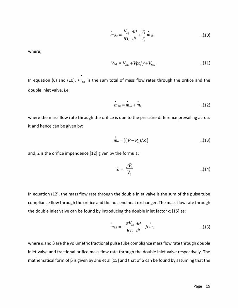
Page | 19
eq hchx ph
c c
V TdPm m
RT dt T
…(10)
where;
Veq = chx hhxV Vpt V …(11)
In equation (6) and (10), phm
is the sum total of mass flow rates through the orifice and the
double inlet valve, i.e.
ph DI om m m
…(12)
where the mass flow rate through the orifice is due to the pressure difference prevailing across
it and hence can be given by:
o om P P Z
…(13)
and, Z is the orifice impendence [12] given by the formula:
Z = 0
0
P
V
…(14)
In equation (12), the mass flow rate through the double inlet valve is the sum of the pulse tube
compliance flow through the orifice and the hot-end heat exchanger. The mass flow rate through
the double inlet valve can be found by introducing the double inlet factor α [15] as:
eqDI o
h
V dPm m
RT dt
…(15)
where α and β are the volumetric fractional pulse tube compliance mass flow rate through double
inlet valve and fractional orifice mass flow rate through the double inlet valve respectively. The
mathematical form of β is given by Zhu et al [15] and that of α can be found by assuming that the
Page | 20
ratio of the mass flow rate through the regenerator and the double inlet valve to be in a constant
ratio [16], i.e.
β =
2
2 2
1 11 1
1 1ln
2 2
h h
c c
reghh h h
c ptc c c
T T
T T
VT T T TT V T T T
k
0
0
P
V
…(16)
and
α = β (1 + reg c
v
eq eff
V Te
V T) …(17)
The pressure variation within the pulse tube is already know but the pressure variation of the
compressor is still not known, which can be found by assuming that the mass flow rate within
the regenerator is directly proportional to the pressure difference between the compressor and
the pulse tube i.e.
( )reg cpr tg Cm P P
…(18)
where, Crg is calculated using Ergun’s law for laminar flow [17] and is mathematically given by the
following formula:
2 2 3
24 150 (1 )
reg h v
reg v
reg
D D e
L eC
…(19)
As shown in the schematic diagram, it is clear that the total mass flow rate through the
compressor will be the sum of the mass flow rates through the regenerator and the double inlet
valve, thus we have;
cp reg DIm m m
…(20)

Page | 21

Page | 22
The algorithm for the above set of equations was made and the concerned program was written
in MATLAB so as to get the exact mass flow rates, the pressure variation and the different phase
relations required for plotting the phasor. The following flow chart shows the methodology
adopted for writing the code.
Feed the input data
(such as the dimension
of the various component and
the properties of the working fluid)
Declare the array variables for storing
the instantaneous flow rates, time
and pressure oscillation
Set the step size
for time
Assign the time values to
the time array
Calculate the various required
parameters/values
Page | 23
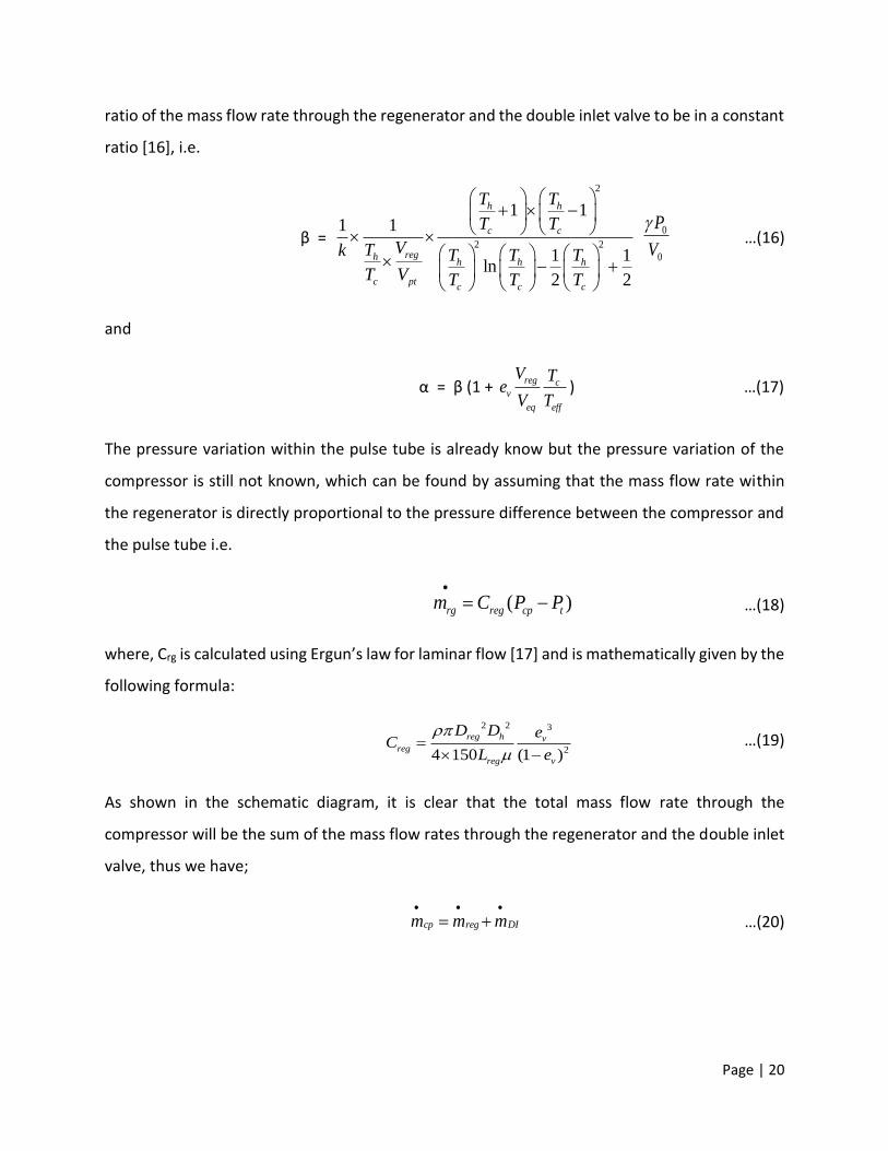
Start a loop from t = 0 till t = set time
and calculate the required values
Compute the amplitude for
each quantity
Plot the graphs for the required items
Flow Chart 5.1 Flow Chart for the MATLAB program
The above algorithm was compiled in MATLAB program and was executed for the following
configuration of the DIPTR taken from [10]:
a) Design Data
Table 5.1 Design Data for Adiabatic Model
Components Parameters
Regenerator Length (Lreg) = 0.3 m
Diameter (Dreg) = 0.032 m
Porosity (ev) = 0.7
Hydraulic Diameter (Dh) = 0.04 mm
Pulse Tube Length (Lpt) = 0.8 m
Diameter (Dpt) = 0.02 m
Volume (Vpt) = 0.00025 m3
Cold-end Heat Exchanger Dead Volume (Vchx) = 0.00002 m3
Hot-end Heat Exchanger Dead Volume (Vhhx) = 0.00002 m3
Orifice Diameter (D0) = 1 mm
DI Valve Diameter (D0) = 1 mm
Reservoir Volume (Vr) = 0.007 m3
Page | 24
b) Operating Condition
Table 5.2 Operating Condition for Adiabatic Model
Operating Parameters Values
Average Pressure 10.5 bar
Oscillating Pressure 2 bar
Frequency 2 Hz
Cold- End Heat Exchanger 100 K
Hot-End Heat Exchanger 300 K
c) Fluid Data for Helium
Table 5.3 Fluid Data for Adiabatic Model
Physical Condition Physical Properties
Temperature (200K)
Pressure (10 bar)
Dynamic Viscosity (µ) = 15.21x10⁻⁶ Ns/m2
Density ( ) = 2.389 Kg/m3
Specific Heat Capacity at Constant
Pressure (Cp) = 5193.0 J/Kg K
Gas Constant (R) = 2074.6 J/Kg K
Adiabatic Constant ( ) = 1.67
The following results were obtained from the execution of the MATLAB code which were in
accordance to the results obtained by Prakash [10] with the graphs being more smoother than
what obtained by his analysis:
A. Graph representing the pressure variation within the pulse tube (Pt), the compressor (Pc)
and the reservoir (Pr).
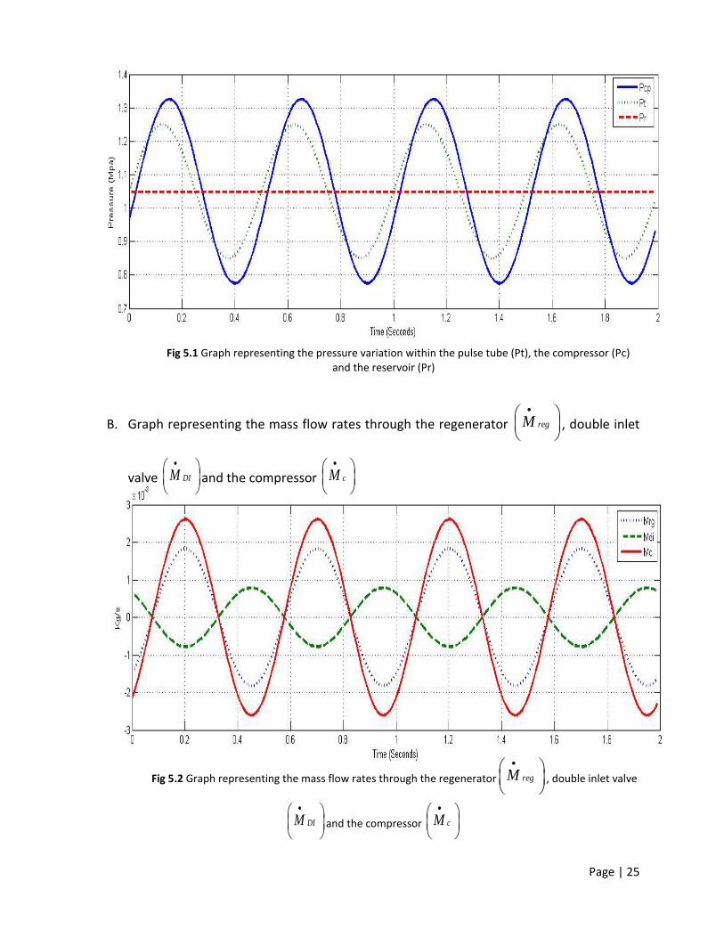
Page | 25
Fig 5.1 Graph representing the pressure variation within the pulse tube (Pt), the compressor (Pc) and the reservoir (Pr)
B. Graph representing the mass flow rates through the regenerator regM
, double inlet
valve DIM
and the compressor cM
Fig 5.2 Graph representing the mass flow rates through the regenerator regM
, double inlet valve
DIM
and the compressor cM
Page | 26
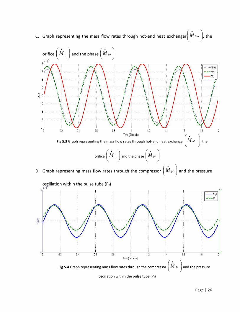
C. Graph representing the mass flow rates through hot-end heat exchanger hhxM
, the
orifice 0M
and the phase phM
Fig 5.3 Graph representing the mass flow rates through hot-end heat exchanger hhxM
, the
orifice 0M
and the phase phM
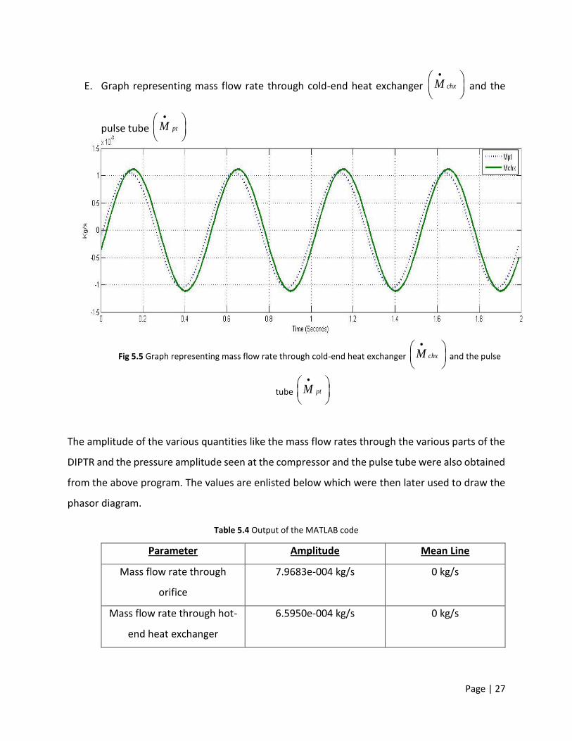
D. Graph representing mass flow rates through the compressor ptM
and the pressure
oscillation within the pulse tube (Pt)
Fig 5.4 Graph representing mass flow rates through the compressor ptM
and the pressure
oscillation within the pulse tube (Pt)
Page | 27
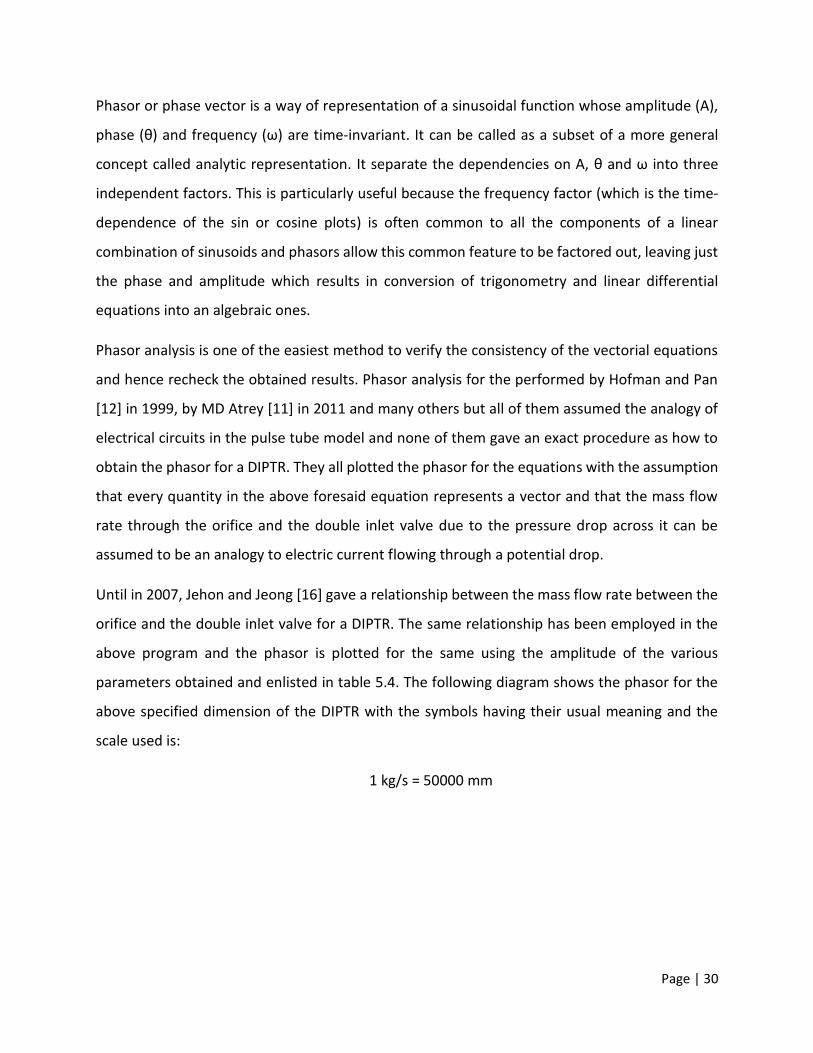
E. Graph representing mass flow rate through cold-end heat exchanger chxM
and the
pulse tube ptM
Fig 5.5 Graph representing mass flow rate through cold-end heat exchanger chxM
and the pulse
tube ptM
The amplitude of the various quantities like the mass flow rates through the various parts of the
DIPTR and the pressure amplitude seen at the compressor and the pulse tube were also obtained
from the above program. The values are enlisted below which were then later used to draw the
phasor diagram.
Table 5.4 Output of the MATLAB code
Parameter Amplitude Mean Line
Mass flow rate through
orifice
7.9683e-004 kg/s 0 kg/s
Mass flow rate through hot-
end heat exchanger
6.5950e-004 kg/s 0 kg/s

Page | 28
Mass flow rate through cold-
end heat exchanger
0.0011 kg/s 0 kg/s
Mass flow rate through the
pulse tube
0.0011 kg/s 0 kg/s
Mass flow rate through the
regenerator
0.0018 kg/s 0 kg/s
Mass flow rate through the
double inlet valve
7.8245e-004 kg/s 0 kg/s
Mass flow rate through the
compressor
0.0026 kg/s 0 kg/s
Mass flow rate through the
phase
7.3027e-004 kg/s 0 kg/s
Pressure amplitude in the
pulse tube
0.2 MPa 1.05 MPa
Pressure amplitude in the
compressor
0.27555 MPa 1.05 MPa

Page | 29
Page | 30
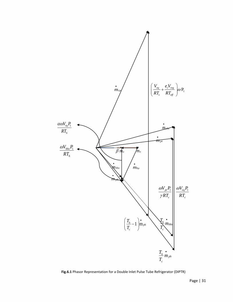
Phasor or phase vector is a way of representation of a sinusoidal function whose amplitude (A),
phase (θ) and frequency (ω) are time-invariant. It can be called as a subset of a more general
concept called analytic representation. It separate the dependencies on A, θ and ω into three
independent factors. This is particularly useful because the frequency factor (which is the time-
dependence of the sin or cosine plots) is often common to all the components of a linear
combination of sinusoids and phasors allow this common feature to be factored out, leaving just
the phase and amplitude which results in conversion of trigonometry and linear differential
equations into an algebraic ones.
Phasor analysis is one of the easiest method to verify the consistency of the vectorial equations
and hence recheck the obtained results. Phasor analysis for the performed by Hofman and Pan
[12] in 1999, by MD Atrey [11] in 2011 and many others but all of them assumed the analogy of
electrical circuits in the pulse tube model and none of them gave an exact procedure as how to
obtain the phasor for a DIPTR. They all plotted the phasor for the equations with the assumption
that every quantity in the above foresaid equation represents a vector and that the mass flow
rate through the orifice and the double inlet valve due to the pressure drop across it can be
assumed to be an analogy to electric current flowing through a potential drop.
Until in 2007, Jehon and Jeong [16] gave a relationship between the mass flow rate between the
orifice and the double inlet valve for a DIPTR. The same relationship has been employed in the
above program and the phasor is plotted for the same using the amplitude of the various
parameters obtained and enlisted in table 5.4. The following diagram shows the phasor for the
above specified dimension of the DIPTR with the symbols having their usual meaning and the
scale used is:
1 kg/s = 50000 mm
Page | 31
cpm
1P
eq v reg
c eff
V e V
RT RT
1eq
h
V P
RT
chxm
ptm
1hhx
h
V P
RT
om
om
hhxm
bym
phm
1pt
c
V P
RT
1eq
c
V P
RT
1 mhph
c
T
T
hhhx
c
Tm
T
h
ph
c
Tm
T
Fig.6.1 Phasor Representation for a Double Inlet Pulse Tube Refrigerator (DIPTR)

Page | 32

Page | 33
There are various ways in which the design for a pulse can be done. Some used the entropy
method [16] where as some used the software like REGEN [18] for finding out the desired
dimension of the pulse tube for a set working condition.
In this present work we came up with a new and simplified methodology for finding out the
required dimensions of a pulse tube working at a specified condition. The steps for the same is
discussed below, which is later verified using the output of the MATLAB code:
7.1. Steps for Designing
7.1.1. Set the working parameters
We first set the desired working parameters for a DIPTR such as the mean pressure
(P0), the oscillating pressure (P1), the refrigeration power required (Qc), working
frequency (f), an orifice with known max mass flow rate through it ( om
) and the
operating temperatures (Th and Tc)
In the present work we have decided to design a pulse tube for a DIPTR whose
working parameters are:
Table 7.1 Input variables for the design
Parameter Symbol Data
Mean Pressure P0 20 MPa
Oscillating Pressure P1 2 MPa
Refrigeration Power
Required
Qc 50 Watts
Working Frequency f 2 Hz
Cold end temperature Tc 60 K
Hot end temperature Th 300 K
Mass flow through
orifice om
4.18x10⁻⁴ kg/s
Page | 34
7.1.2. COP of the Double Inlet Pulse Tube Refrigerator (DIPTR)
The COP (co-efficient of performance) for a standard Carnot refrigerator is given by
the following formula:
( ) ccarnot
h c
TCOP
T T
...(21)
Since the COP of a GM type pulse tube refrigerator is about 15%-20% of the standard
Carnot refrigerator [19]. So we have:
_ _( ) 0.15( )GM pulse tube carnotCOP COP …(22)
The COP of a refrigerator is actually the ratio of the cooling effect produced by the
system to the work input, hence we can define COP in another way as:
c
cp
QCOP
W …(23)
So for the set model we get the value of Wcp to be as 534Watts
7.1.3. Mass flow rate through the compressor
The average mass flow rate through the compressor can be found by using the
relation [16 ]:
0
( )1
hcomp p H L
cp
TW m C P P
P
…(24)
Where cp
m
is the average mass flow rate through the compressor which is related
to its amplitude by:
2( )cp ampcp
mm
…(25)

Page | 35
Hence we get the value of the amplitude of the mass flow rate through the
compressor to be as 6.72x10⁻³ kg/s
7.1.4. Volume ratio between the regenerator and the pulse tube
The phasor diagram is then used to find a relation between the mass flow rates
through the orifice and the compressor. The obtained relationship is:
11 1v reg eq eqh h h
cp o
amp ampeff c c h c c
e V V VT T Tm P m
RT RT T RT T T
…(26)
where o
amp
m
can be found by using equation (13).
The volume of the regenerator and that of the pulse tube can be assumed to have
a particular ratio or else we can have the volume of the regenerator using REGEN
software [18]. For the present work we have assumed the volume of regenerator
and that of the pulse tube to be same, which is true in most of the practical cases.
Hence we have:
Vrg = Vpt = 8.034x10⁻⁵ m-3
7.1.5. Mass flow rate through the pulse tube
The phasor is again used to find out the amplitude of the mass flow rate through
the pulse tube which is given by the formula:
01 1pt eqhhx h
pt
amp ampc c c c
V VV Tm P m
RT RT RT T
…(27)
The obtained value for our design is 5.72x10⁻³ Kg/s
7.1.6. Thermal boundary layer thickness
Since we have assumed no heat dissipation across the wall of the pulse tube the
diameter of the pulse tube should be large enough to neglect the effect of any

Page | 36
boundary layer formation. The boundary layer thickness can be found out by using
the Stokes formula given as:
…(28)
The value obtained for our design requirement is 3.337x10⁻⁴ m.
7.1.7. Minimum area of cross section of the pulse tube
We have assumed a laminar flow of the oscillating flow within the pulse tube, hence
the Reynolds Number for the same should be within certain limits which is 280 in
this case [20]. The fixing up of the Reynolds number makes it easier to calculate the
minimum area of cross-section as given by the formula [20]:
minRe
ptmA
…(29)
The minimum area thus obtained from the above relation is 2.12x10⁻⁴ m.
7.1.8. Dimension of the pulse tube
With the minimum area of cross section known we can find out the minimum
diameter for the pulse tube and then take assume a diameter of about 1.2-1.5 times
the obtained diameter. The diameter obtained would then be used to calculate the
length of the pulse tube as the volume being calculated earlier.
The obtained diameter for the above case is about 1.5 times the calculated diameter
and is 2.46 cm and hence the length is 16.3 cm.
7.1.9. Volume of the reservoir
Since we have assumed mass flow through the orifice as given under orifice
specification, the volume of the reservoir can be found using the relation given in
equation (14), which comes out to be 0.007 m3
2
Page | 37
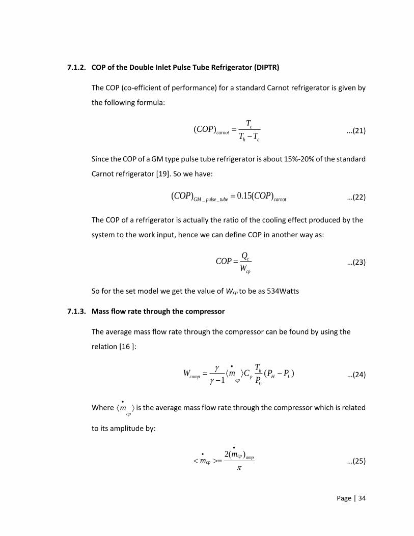
7.2. MATLAB Output
7.2.1. Graphs
A. Graph representing the pressure oscillation within the pulse tube (Pt), the
compressor (Pcp) and the reservoir (Pr)
Fig 7.1 Graph representing the pressure oscillation within the pulse tube (Pt), the compressor (Pcp) and the reservoir (Pr)
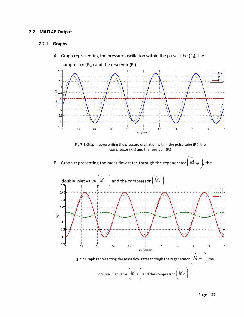
B. Graph representing the mass flow rates through the regenerator regM
, the
double inlet valve DIM
and the compressor cM
Fig 7.2 Graph representing the mass flow rates through the regenerator regM
, the
double inlet valve DIM
and the compressor cM
Page | 38
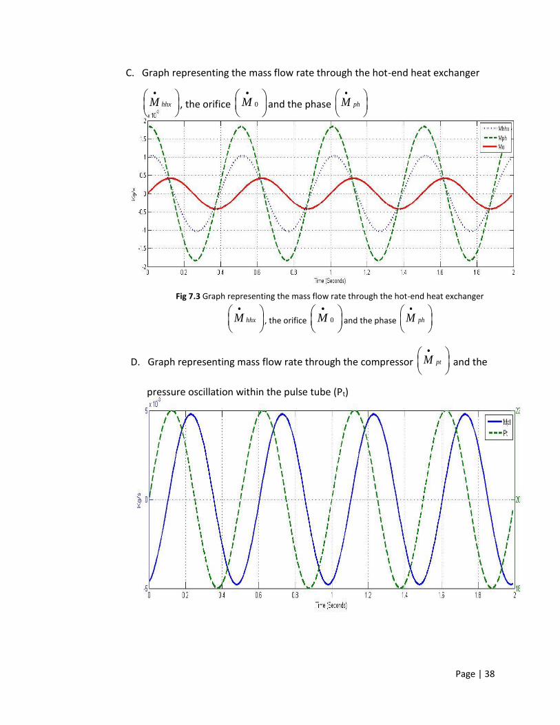
C. Graph representing the mass flow rate through the hot-end heat exchanger
hhxM
, the orifice 0M
and the phase phM
Fig 7.3 Graph representing the mass flow rate through the hot-end heat exchanger
hhxM
, the orifice 0M
and the phase phM
D. Graph representing mass flow rate through the compressor ptM
and the
pressure oscillation within the pulse tube (Pt)

Page | 39
Fig 7.4 Graph representing mass flow rate through the compressor ptM
and
the pressure oscillation within the pulse tube (Pt)
E. Graph representing the mass flow rate through the cold-end heat exchanger
chxM
and the pulse tube ptM
Fig 7.5 Graph representing the mass flow rate through the cold-end heat exchanger
chxM
and the pulse tube ptM
7.2.2. Data
Table 7.1 Output for the designed consideration
Parameter Amplitude Mean Line
Mass flow through orifice 4.1833e-004 kg/s 0 kg/s
Mass flow through hot-end
heat exchanger
0.0010 kg/s 0 kg/s
Mass flow through cold-
end heat exchanger
0.0088 kg/s 0 kg/s
Mass flow through the
pulse tube
0.0048 kg/s 0 kg/s
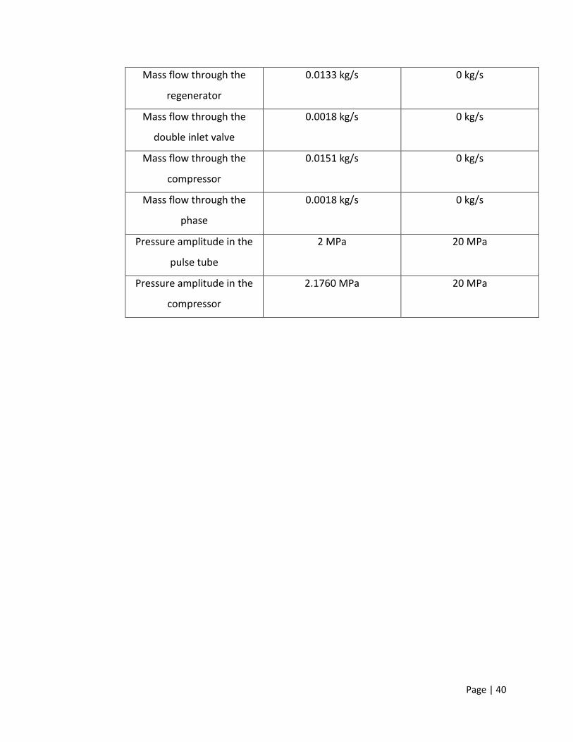
Page | 40
Mass flow through the
regenerator
0.0133 kg/s 0 kg/s
Mass flow through the
double inlet valve
0.0018 kg/s 0 kg/s
Mass flow through the
compressor
0.0151 kg/s 0 kg/s
Mass flow through the
phase
0.0018 kg/s 0 kg/s
Pressure amplitude in the
pulse tube
2 MPa 20 MPa
Pressure amplitude in the
compressor
2.1760 MPa 20 MPa

Page | 41
Page | 42
A thorough study of the mass flow rate through the various parts of a GM type Double Inlet Pulse
Tube Refrigerator (DIPTR) was made. This study helped in developing a MATLAB code which
produces the time variation graph for the mass flow rate and pressure oscillation at different
parts of the GM type Double Inlet Pulse Tube Refrigerator (DIPTR) when the initial working
condition and the dimension for the various component of the DIPTR is provided.
The output of the MATLAB program was further utilized to construct a phasor diagram for the
mass flow rates at various sections of the GM type DIPTR, which is a convenient way to observe
the phase relationship and hence make necessary adjustment to optimize the output.
At the end of the present work a simplified (approximate) methodology has been put forward for
finding out the dimension of the pulse tube of a GM type DIPTR using the phasor diagram whose
results were then verified with the outcomes of the MATLAB program.
The output shown by the MATLAB code were within 10% - 15% range of the predicted results
which shows that the methodology adopted for designing the pulse tube is considerable to a
great extent.

Page | 43
Page | 44
1. Walker, Graham. "NOMENCLATURE AND CLASSIFICATION OF
CRYOCOOLERS." Proceedings of the Symposium on Low Temperature Electronics and
High Temperature Superconductors. Vol. 88. No. 9. Electrochemical Society, 1988.
2. Ray Radebaugh 2000, ―Pulse Tube Cryocoolers for Cooling Infrared Sensors‖,
Proceedings of SPIE, the International Society for Optical Engineering, Infrared
Technology and Applications XXVI, Vol. 4130, pp. 363-379.
3. Radebaugh, Ray. Development of the pulse tube refrigerator as an efficient and reliable
cryocooler, Proc. Institution of Refrigeration (London) 1999-2000.
4. Gifford, W.E. and Longsworth, R.C. Pulse tube refrigeration, Trans ASME B J Eng
Industry 86(1964), pp.264-267.
5. de Boer, P. C. T., Thermodynamic analysis of the basic pulse-tube refrigerator,
Cryogenics34(1994) ,pp. 699-711 .
6. Mikulin, E.I., Tarasow, A.A. and Shkrebyonock, M.P. Low temperature expansion pulse
tube, Advances in cryogenic engineering 29(1984), pp.629-637.
7. Storch, P.J. and Radebaugh, R Development and experimental test of an analytical model
of the orifice pulse tube refrigerator, Advances in cryogenic engineering 33(1988),
pp.851-859.
8. Zhu Shaowei, Wu Peiyi and Chen Zhongqi, Double inlet pulse tube refrigerators: an
important improvement, Cryogenics30 (1990), pp. 514-520.
9. Ju Y. L., Wang C. and Zhou Y. ,Numerical simulation and experimental verification of
the oscillating flow in pulse tube refrigerator, Cryogenics, 38(1998), pp.169-176.
10. Prakash
11. L.Mohanta and M.D. Atrey, Phasor Analysis of Pulse Tube Refrigerator, Cryocoolers 16
(2011), 299-308
12. A. Hofmann and H. Pan, Phase Shifting in Pulse Tube Refrigerator, Cryogenics (1999)
13. Prakash,45
14. Jong Hoon Baik, Design Methods in Active Valve Pulse Tube Refrigerator, Cryogenics
(2003)
15. Zhu S, Kawano S, Nogawa M and Inoue T, Work Loss in Double Inlet Pulse Tube
Refrigerators, Cryogenics 38 (1998), 803-6
Page | 45
16. Jeheon Jung and Sangkwon Jeong, Optimal Pulse Tube Volume Design in GM type Pulse
Tube Refrigerator, Cryogenics 47 (2007),510-516
17. Prakash Crg
18. Zhi-hua Gan, Guo-jun LIU, Ying-zhe WU, Qiang CAO, Li-min QIU, Guo-bang CHEN
and J.M. PFOTENHAUER , Study on a 5.0 W/ 80 K Single Stage Stirling type Pulse
Tube Cryocooler, Cryocooler (2008) 9 (9):1277-1282
19. Lecture on Cryocooler [2.2], University of Wisconsin Madison
20. R. Akhavan, R.D. Kamm, and A.H. Shapiro, "An Investigation of Transition to
Turbulence in Bounded Oscillatory Stokes Flows - Part 1. Experiments," J. Fluid Mech.,
vol. 225, (1991), pp. 395-422