A Theory of Dividend Smoothing1

Ilan GuttmanGraduate School of Business

Stanford Universityiguttman@stanford.edu

Ohad KadanJohn M. Olin School of BusinessWashington University in St. Louis

kadan@wustl.edu

Eugene KandelSchool of Business Administrationand Department of Economics

Hebrew Universitymskandel@mscc.huji.ac.il

This version: September 2008

1We would like to thank three anonymous referees, E¢ Benmelech, Sugato Bhattacharyya,Martin Cripps, Peter DeMarzo, Zsuzsanna Fluck, Paolo Fulghieri (the Editor), ArmandoGomes, Milt Harris, Kose John, Avner Kalay, Praveen Kumar, Jeremy Stein, Jaime Zender,Je¤ Zwiebel; seminar participants at Hebrew University, University of Houston, RutgersUniversity, Stanford University, Tel Aviv University, and Washington University in St. Louis;and participants of the UtahWinter Finance 2007, Gerzensee 2007, FIRS 2008, andWFA 2008conferences for helpful comments and suggestions. Mike Borns and Janice Fisher providedexcellent editorial assistance. Kandel expresses gratitude for �nancial assistance from theKruger Center for Finance at Hebrew University.

Abstract

Dividend smoothing remains a puzzle for �nancial economists. We present a model inwhich smoothing of dividends arises as an equilibrium outcome. A manager who caresabout the intrinsic value of the �rm as well as its current stock price has to decidehow to allocate earnings between investments and dividends. Since the stock price isdetermined by uninformed investors, the manager has an incentive to in�ate dividendsand lower investment relative to the �rst best. We show that there is a continuum ofequilibria in which the dividend is constant for a range of realized earnings. Comparedto the standard separating equilibrium, this partial pooling induces higher �rm value,lower average dividends, and lower deviation from the �rst-best investment. We arguethat the previous year�s dividend can serve as a �focal point,�allowing managers andinvestors to coordinate on just one in a continuum of equilibria. We conclude thatdividend smoothing provides a partial remedy to underinvestment resulting frominformation asymmetries. We also o¤er several new testable predictions relatingdividend smoothing to investors�mix, managerial incentives, and investment.

1 Introduction

Dividends have long puzzled �nancial economists (see Allen and Michaely (2003) for

an extensive survey). In this paper we focus on one aspect of this puzzle: dividend

smoothing. Lintner (1956) interviewed managers from 28 companies and found that

rather than setting dividends each year independently based on that year�s earnings,

they �rst decide whether to change dividends from the previous year�s level. Man-

agers claimed to reduce dividends only when they had no other choice, and increase

dividends only if they were con�dent that future cash �ows could sustain the new

dividend level. Two beliefs were expressed strongly: that investors put a premium

on companies with stable dividends, and that markets penalize �rms that cut divi-

dends. Furthermore, Lintner found that managers were setting the dividend policy

�rst, while adjusting other cash-related decisions to the chosen dividend level. Al-

most �fty years later, in a survey of 384 �nancial executives, Brav, Graham, Harvey,

and Michaely (2005) found that similar considerations still play a dominant role in

determining dividends in publicly traded �rms. By contrast, Michaely and Roberts

(2007) found that dividend smoothing is signi�cantly less likely in private �rms.

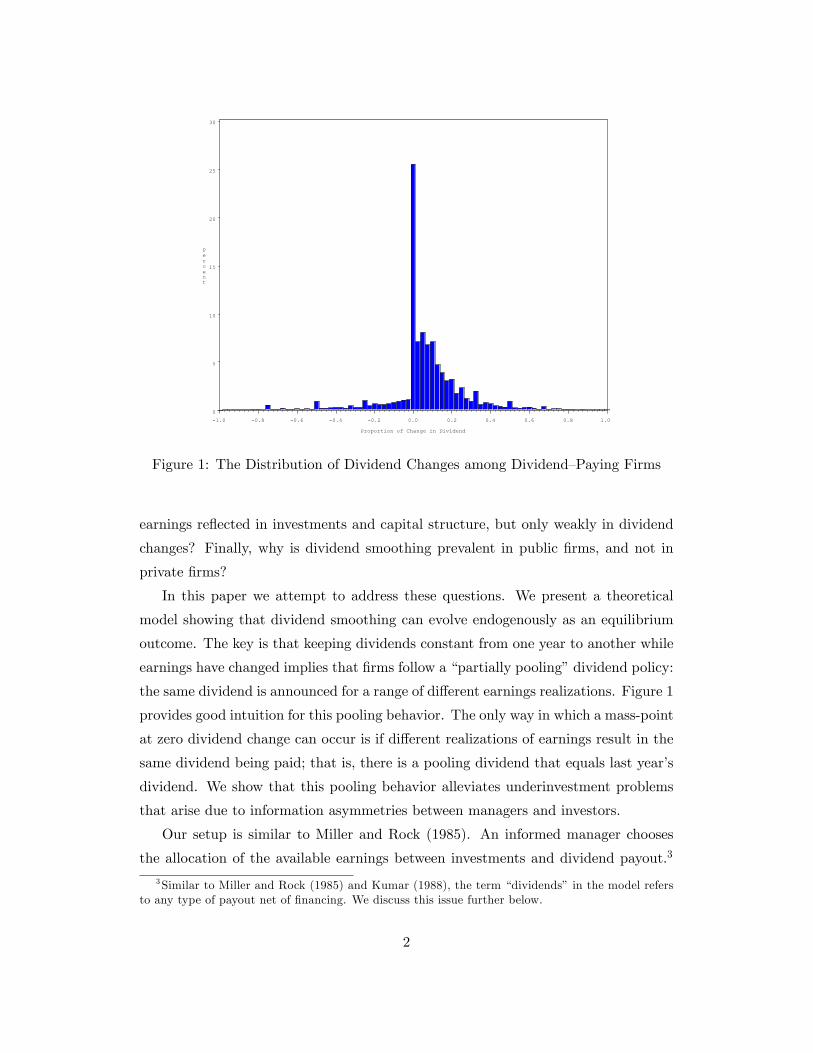
For the purposes of this paper, we de�ne dividend-smoothing as keeping the

dividends per-share constant over two or more consecutive years. This de�nition

is stronger than the one implied by Lintner�s paper, which requires only that the

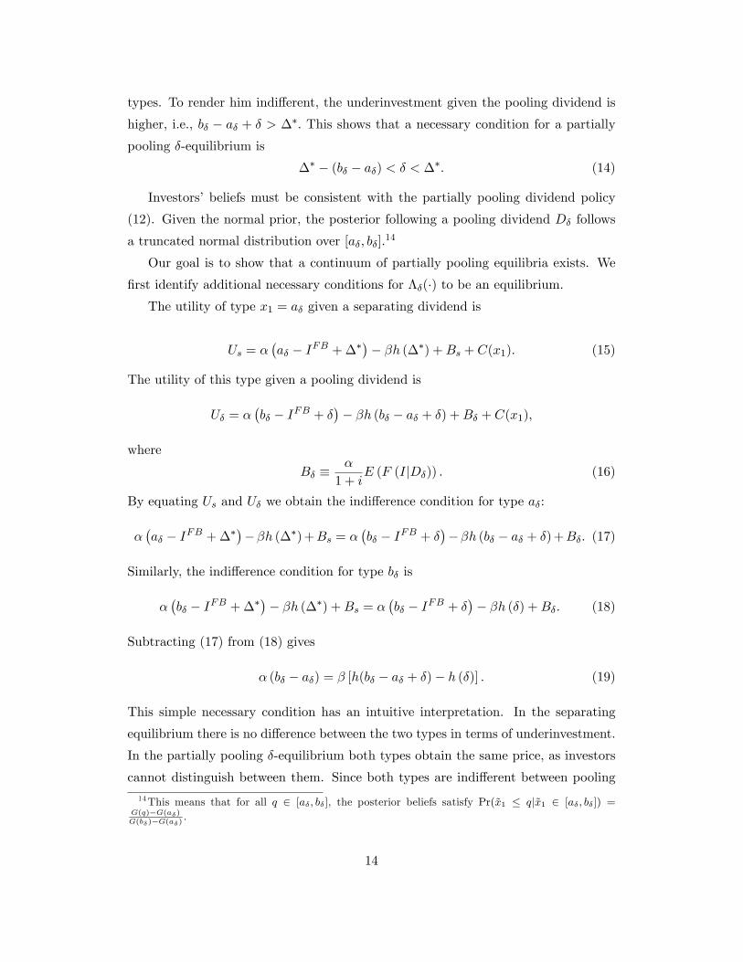
variation in dividends is lower than the variation in earnings. Figure 1 illustrates

the dividend-smoothing phenomenon based on our de�nition. The �gure shows the

distribution of the proportions of annual dividend changes over the 40-year period

1966-2005 for all Compustat �rms that paid dividends over two consecutive years.1

The �gure shows an over 25% mass-point at zero change.2

While dividend smoothing is an empirical regularity, it is quite perplexing theo-

retically. Why would well-diversi�ed investors value a smoothed stream of dividends?

After all, any idiosyncratic risk of dividend changes can be diversi�ed away. Why do

investors view dividend cuts as bad news in excess of what they have learned from the

reported cash �ows and earnings? Why don�t managers adjust dividends frequently

to better re�ect the level of current earnings? Why are changes in cash �ows and

1Note that over this time period the proportion of dividend-paying �rms out of the total numberof listed �rms has signi�cantly declined. See Fama and French (2001).

2 In the �gure, dividend per share (adjusted for splits and other changes in the number of shares)is calculated as the ratio between Compustat items 26 and 27.

1

Percent

0

5

10

15

20

25

30

Proportion of Change in Dividend

­1.0 ­0.8 ­0.6 ­0.4 ­0.2 0.0 0.2 0.4 0.6 0.8 1.0

Figure 1: The Distribution of Dividend Changes among Dividend�Paying Firms

earnings re�ected in investments and capital structure, but only weakly in dividend

changes? Finally, why is dividend smoothing prevalent in public �rms, and not in

private �rms?

In this paper we attempt to address these questions. We present a theoretical

model showing that dividend smoothing can evolve endogenously as an equilibrium

outcome. The key is that keeping dividends constant from one year to another while

earnings have changed implies that �rms follow a �partially pooling�dividend policy:

the same dividend is announced for a range of di¤erent earnings realizations. Figure 1

provides good intuition for this pooling behavior. The only way in which a mass-point

at zero dividend change can occur is if di¤erent realizations of earnings result in the

same dividend being paid; that is, there is a pooling dividend that equals last year�s

dividend. We show that this pooling behavior alleviates underinvestment problems

that arise due to information asymmetries between managers and investors.

Our setup is similar to Miller and Rock (1985). An informed manager chooses

the allocation of the available earnings between investments and dividend payout.3

3Similar to Miller and Rock (1985) and Kumar (1988), the term �dividends� in the model refersto any type of payout net of �nancing. We discuss this issue further below.

2

The total earnings and the investment are private information and cannot be credibly

conveyed to investors; thus the observed dividend payment serves as a signal. The

manager cares about the short-term stock price in addition to its long-term (intrin-

sic) value. Such objective functions appear to be well documented in reality. While

we assume this objective function as given exogenously, we also propose several sce-

narios under which it can evolve in an endogenous manner. Linking the manager�s

compensation to short-term stock price induces her to raise the dividends in order to

signal higher earnings, resulting in underinvestment relative to the �rst-best level.

In the equilibria studied in Miller and Rock (1985), the dividend reveals all the

private information of the manager to investors. These perfectly separating equilibria

are ine¢ cient: the manager overpays dividends and underinvests, and yet receives no

informational rents. In our setting, while a unique separating equilibrium exists, it

is just one of a multitude of equilibria. Our focus is on more e¢ cient equilibria that

are consistent with dividend smoothing over time.

The equilibria we consider are partially pooling: they have full revelation of earn-

ings for very low and very high outcomes, but for all �intermediate outcomes� the

same dividend is announced. Thus, for a wide range of earnings realizations the

manager chooses exactly the same dividend. We show the existence of a continuum

of such partially pooling equilibria.4 All these equilibria Pareto-dominate the fully

separating equilibrium. Both the manager and the investors bene�t from dividend

pooling. The manager prefers any of the partially pooling equilibria to the standard

fully revealing equilibrium, since the investment in the former is closer to �rst-best.

Investors are assumed to be fully diversi�ed, and thus e¤ectively risk-neutral. As a

result, the stock price re�ects, on average, the increased �rm value resulting from the

more e¢ cient investment level in the partially pooling equilibrium.5

Next we discuss how the multiplicity of partially pooling equilibria in a static

model is translated into dividend smoothing over time. The challenge for the man-

ager and the investors is to coordinate on just one equilibrium out of a continuum.

We �rst show that our static results can be generalized to a dynamic setting with

myopic managers and investors. We then argue that the previous year�s dividend is a4These equilibria are somewhat similar to those studied in Harrington (1987) in the context of

limit pricing; in Bernheim (1994) in the context of conformity, customs, and fads; and in particularin Guttman, Kadan and Kandel (2006) in the context of accounting earnings management.

5 If investors are risk averse then the Pareto-dominance result becomes more subtle. In that case,partial revelation of information exposes investors to more risk, which has to be weighed against thelower underinvestment.

3

natural candidate for a �focal point�that enables investors and managers to coordi-

nate on just one equilibrium. All players coordinate on the partially pooling dividend

strategy that yields a pooling dividend equal to the dividend paid in the previous

year. Deviations from the last-year dividend are observed only if the earnings are

either too low or too high, so that the last-year dividend can no longer be supported.

This is consistent with Lintner�s �ndings. Thus a partially pooling dividend policy

may yield smoothing of dividends over time. We use a detailed example to illustrate

this process.

To summarize: our argument has three steps. First, we note that keeping divi-

dends constant when earnings have changed implies some pooling behavior. We thus

show that in a Miller-Rock-type model there exists a continuum of partially pooling

equilibria. Second, we show that these equilibria Pareto-dominate the separating

one, and therefore are more likely to prevail. Finally, we argue that managers and

investors choose the last-year dividend to coordinate on one of these equilibria. This

combination predicts that dividends, once announced, persist over time, until the

earnings change to the extent that they no longer support the smoothed dividend.

Then the dividend is cut or increased, and the process starts over again.

Our model o¤ers several testable implications. First, we show that adverse selec-

tion and stock-based compensation are important determinants of dividend smooth-

ing. Hence, dividend smoothing is more likely in public �rms, as shown by Michaely

and Roberts (2007). Furthermore, our model shows that dividend smoothing is as-

sociated with measures of managerial myopia such as short-term incentives. The

model also suggests that better investment opportunities result in more dividend

smoothing. Moreover, periods of smoothing are associated with higher investment

and are followed by periods of higher pro�tability. We also study an extension that

admits retained earnings and o¤ers insights on the correlations between dividends,

investments, and retained earnings in the presence of dividend smoothing.

A shortcoming of the Miller-Rock setup is that it does not enable us to formally

distinguish between di¤erent types of payout. Our intention, however, is to focus

on dividends and not consider stock repurchases, which are an alternative form of

payout (e.g., Grullon and Michaely (2002)). The empirical literature does distinguish

between the two. For example, Jagannathan, Stephens, and Weisbach (2000) show

that stock repurchases are primarily used to pay out transitory, non-operating cash

�ows (although this pattern may be changing), whereas dividends are paid out of

4

operating cash �ows, which are the focus of the model. Additionally, dividends are

typically announced and paid on a regular basis, and a dividend announcement repre-

sents a binding commitment. In contrast, stock repurchase programs are announced

occasionally, and o¤er just an option to repurchase: they do not commit the �rm.

Thus, while repurchases and dividends are often viewed as close substitutes, for the

purposes of our study they are not, as they are associated with di¤erent kinds of cash

�ows, and their information content is di¤erent.

The rest of the paper is organized as follows. Section 2 discusses related literature.

Section 3 develops the basic setup and presents the separating equilibrium in which no

smoothing occurs. In Section 4 we develop and discuss our newly suggested partially

pooling equilibria. Section 5 discusses dividend smoothing over time, and how it

evolves from the partially pooling equilibria. Section 6 presents extensions to the

model. The empirical predictions are discussed in Section 7. Section 8 concludes.

Proofs are in the appendices.

2 Related Literature

Our model adds to the theoretical literature on costly dividend signaling.6 Important

early contributions to this literature are Bhattacharya (1979), John and Williams

(1985), Miller and Rock (1985), Ofer and Thakor (1987), Ambarish, John, and

Williams (1987), Bernheim (1991), and Hausch and Seward (1993). These papers

use perfectly separating equilibria, and do not consider dividend smoothing.7

John and Nachman (1987) and Kumar and Spatt (1987) present dynamic models

with smoothing of dividends. John and Nachman study an inter-temporal signaling

model in which dividends have an adverse tax treatment. In their model, optimal

�nancing and dividend strategies are determined by an endogenous structure of sig-

naling costs, which is related to a permanent component of earnings. They show

that many aspects of dividend smoothing emerge endogenously. Kumar and Spatt

6The empirical evidence on dividend signaling is mixed. This literature includes: Penman (1983),Smith and Watts (1992), Bernheim and Wantz (1995), Yoon and Starks (1995), DeAngelo, DeAngelo,and Skinner (1996), Amihud and Murgia (1997), Benartzi, Michaely, and Thaler (1997), Nissimand Ziv (2001), Grullon et al. (2005), Johnson, Lin, and Song (2006), and Chang, Kumar, andSivaramakrishnan (2006). See Allen and Michaely (2003) for an extensive survey.

7A well-known criticism of the dividend signaling literature is Dybvig and Zender (1991), whoargue that the ine¢ ciencies associated with asymmetric information can be avoided by optimalcontracting. See Persons (1994) and Baranchuk, Dybvig, and Yang (2007) for the on-going discussionof this criticism.

5

(1987) analyze a dynamic model with risk-averse investors and �rms whose invest-

ments are subject to serially correlated shocks. Firms in the model have private

information on their prospects and idiosyncratic risk. The authors show that un-

der certain conditions, �rms will have incentives to smooth dividends and create a

reputation for having low systematic risk. Our paper o¤ers a di¤erent rationale for

dividend smoothing, which relies on the e¢ ciency of partially pooling equilibria.

Kumar (1988) is the �rst to point out the connection between dividend smooth-

ing and partition pooling. He presents a signaling model in which managers and

investors di¤er in their level of risk aversion. In his model, dividends serve as a co-

ordination device between managers and investors, as in the �cheap talk� literature

originated by Crawford and Sobel (1982). Therefore, in his model there is no sepa-

rating equilibrium; the only equilibria are either completely pooling (�babbling�) or

�step-function� equilibria.8 Our approach is di¤erent: we adhere to the costly sig-

naling approach, starting from a standard model as in Miller and Rock (1985). We

show that the separating equilibria, the focus of prior studies, form just a subset of

all possible equilibria. Moreover, separating equilibria turn out to be ine¢ cient com-

pared to equilibria with pooling. This insight enables us to provide a new rationale

for dividend smoothing.

Finally, Allen, Bernardo, and Welch (2000) suggest an explanation for dividend

smoothing relying on the di¤erences in taxation between individuals and institutions.

In their model, taxable dividends attract informed institutions. Dividend reduction

indicates a desire to reduce institutional ownership. Firms that bene�t from institu-

tional ownership avoid cutting their dividends.

3 Model

3.1 Basic Setup

We develop a two-period model in the spirit of Miller and Rock (1985). The earnings

of a �rm in period t = 1; 2, which are denoted by xt, are determined by the previous

period investment and a random shock:

xt = F (It�1) + "t;

8Kumar and Lee (2001) o¤er a dynamic generalization of Kumar�s (1988) model.

6

where It�1 is the investment in period t� 1; F (�) is a production function, and "t isa random shock. The initial investment I0 is given exogenously, as is the dividend

from the previous period D0.

For simplicity, investments are assumed to be non-negative in each period (It �0):9 The production function is assumed to be twice continuously di¤erentiable, in-

creasing, and concave: F 0 > 0 and F 00 < 0. We further assume limIt!0

F 0 (It) =1 and

limIt!1

F 0 (It) = 0. The random shocks "t are drawn from normal distributions with

means 0 and variances �2t : Hence ~xt is normal with mean F (It�1) and variance �2t

(t = 1; 2):We denote the densities of ~xt by gt and the cumulative distributions by Gt:

For simplicity, the random shocks are assumed to be uncorrelated: Cov ("1; "2) = 0:10

At the beginning of period 1, the manager privately observes the realized earnings

of the �rm, x1. At times, we refer to x1 as the manager�s �type.�Given his type, the

manager decides how to allocate x1 between dividend payments (D1) and investment

(I1). Since most of the �action� in the model is in period 1, we typically suppress

the subscripts and use I and D instead of I1 and D1. Thus,

x1 = I +D: (1)

Investors are risk-neutral. They observe neither x1 nor "1; and use the dividend

as a signal: All the parameters of the model are common knowledge. The �rm is

liquidated in period 2, and shareholders receive a liquidating dividend equal to x2:

Given a period 1 dividend payment of D and investment of I; the present value

of the expected cash �ows to the investors, which we refer to as the intrinsic �rm

value, is

V I(x1; D) = D +1

1 + i[F (I) + E (~"2j"1)] = D +

1

1 + iF (x1 �D) ; (2)

where i � 0 is an appropriate risk-adjusted discount rate.The �rst-best dividend/investment decision is obtained if the manager seeks to

maximize the intrinsic value. We denote the �rst-best investment level by IFB. It

equates the marginal return on investments with the inter-temporal opportunity cost:

F 0(IFB) = 1 + i or IFB = F 0�1(1 + i): (3)

9 It is easy to incorporate negative investment (asset sales) into the model.10 Introducing positive correlation or even slightly negative correlation between the random shocks

does not change the results.

7

Investors use the information contained in the dividend to price the stock. The

market value of the �rm at the end of period 1 is

VM (D) = D +1

1 + iE (F (~x1 �D) jD) : (4)

We assume that the manager is compensated based on both the stock price in

period 1 and the liquidating value in period 2. The fact that some of this compen-

sation vests in period 1 gives rise to a certain degree of managerial myopia (as in

Stein (1989)). Thus, instead of maximizing the intrinsic value, the manager chooses

dividend/investment to maximize a weighted average of the intrinsic value and the

short-term market value:

U(x1; D) � �VM (D) + �V I(x1; D); (5)

where �; � > 0; and VM and V I are given by (4) and (2) respectively. The assumption

that � > 0 requires some justi�cation, as it clearly diverts the manager away from

the �rst-best investment level. For the ease of exposition we defer this discussion to

Section 6, where we discuss ways to motivate and endogenize this objective function.

The manager has two con�icting interests: on the one hand he would like to boost

the stock price by announcing a high dividend, resulting in lower than the �rst-best

investment. On the other hand, he does not want to underinvest too much, because

the marginal cost of underinvestment is increasing due to the concavity of F (�).To gain better intuition we will rewrite the manager�s objective function in a way

that emphasizes the trade-o¤s he faces. First, note that (5) can be written as follows:

U = �

�D +

1

1 + iE (F (I) jD)

�+ �

�D +

F (I)

1 + i

�: (6)

In what follows it is useful to de�ne a separate variable that captures the extent

of underinvestment � � IFB � I: It is also useful to de�ne a function h : R ! Rcapturing the real cost of underinvestment measured as the di¤erence between the

net present value under the �rst-best investment and the NPV under the actual

investment,

h (�) � F�IFB

�1 + i

� IFB!��F (I)

1 + i� I�: (7)

The properties of F (�) imply that h (�) satis�es standard properties of loss functions:h (0) = 0, h0 (0) = 0; h0 (�) > (<)0 i¤ � > (<)0; h00 (�) > 0; lim�!IFB h

0 (�) =1.

8

That is, the �rst-best investment implies zero loss, while any deviation from �rst-best

implies increasing marginal losses.

We can now rewrite the manager�s payo¤ function (6) as

U = �D � �h(�) +B(D) + C(x1); (8)

where

B(D) � �

1 + iE (F (IjD)) and C(x1) � �

�x1 � IFB +

1

1 + iF�IFB

��:

The �rst component, �D; captures the manager�s direct bene�t from the dividend,

ignoring any informational e¤ects. The second component, ��h(�); is the real costto the manager resulting from suboptimal investment, again ignoring informational

e¤ects. The third component, B(D), depends on investors�beliefs about the invest-

ment given the dividend. The last component, C(x1), depends neither on investors�

beliefs nor on the manager�s investment decision, but only on the realized earnings

x1.

A useful feature of the manager�s objective function is the Milgrom and Shannon

(1995) single-crossing property.

De�nition 1 A utility function U : R2 ! R satis�es the Milgrom�Shannon Single-Crossing Property (SCP) in (x;D) if, for all xH > xL and DH > DL; if U(xL; DH) �U(xL; DL); then U(xH ; DH) > U(xH ; DL):

That is, SCP is satis�ed if, whenever a low type manager weakly prefers a high

dividend to a low dividend, then a high type manager strictly prefers a high dividend

to a low dividend. The following lemma is an immediate consequence of the convexity

of h (�) :

Lemma 1 For any given investors� beliefs, the manager�s utility U(x1; D) satis�es

the Milgrom�Shannon SCP in (x1; D):

Equilibrium De�nition. A dividend policy is a mapping � : R ! R assigning adividend D = �(x1) to any realization of period 1 earnings. Given any dividend D;

investors�beliefs are a probability distribution over ~x1.

A Perfect Bayesian Equilibrium is a combination of a dividend policy and in-

vestors�beliefs such that:

9

1. For all x1; �(x1) 2 argmaxD U(x1; D), where the expectations conditional ondividend D are calculated using the investors�beliefs.

2. Investors�beliefs are consistent with � (�) using Bayes rule, whenever applicable.

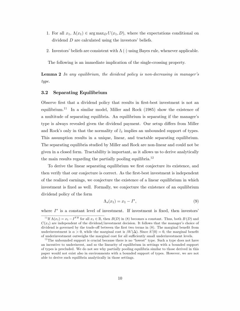
The following is an immediate implication of the single-crossing property.

Lemma 2 In any equilibrium, the dividend policy is non-decreasing in manager�s

type.

3.2 Separating Equilibrium

Observe �rst that a dividend policy that results in �rst-best investment is not an

equilibrium.11 In a similar model, Miller and Rock (1985) show the existence of

a multitude of separating equilibria. An equilibrium is separating if the manager�s

type is always revealed given the dividend payment. Our setup di¤ers from Miller

and Rock�s only in that the normality of ~"t implies an unbounded support of types.

This assumption results in a unique, linear, and tractable separating equilibrium.

The separating equilibria studied by Miller and Rock are non-linear and could not be

given in a closed form. Tractability is important, as it allows us to derive analytically

the main results regarding the partially pooling equilibria.12

To derive the linear separating equilibrium we �rst conjecture its existence, and

then verify that our conjecture is correct. As the �rst-best investment is independent

of the realized earnings, we conjecture the existence of a linear equilibrium in which

investment is �xed as well. Formally, we conjecture the existence of an equilibrium

dividend policy of the form

�s(x1) = x1 � I�; (9)

where I� is a constant level of investment. If investment is �xed, then investors�

11 If �(x1) = x1� IFB for all x1 2 R, then B(D) in (8) becomes a constant. Thus, both B (D) andC(x1) are independent of the dividend/investment decision. It follows that the manager�s choice ofdividend is governed by the trade-o¤ between the �rst two terms in (8). The marginal bene�t fromunderinvestment is � > 0, while the marginal cost is �h0(�): Since h0(0) = 0; the marginal bene�tof underinvestment outweighs the marginal cost for all su¢ ciently small underinvestment levels.12The unbounded support is crucial because there is no �lowest�type. Such a type does not have

an incentive to underinvest, and so the linearity of equilibrium in settings with a bounded supportof types is precluded. We do not see why partially pooling equilibria similar to those derived in thispaper would not exist also in environments with a bounded support of types. However, we are notable to derive such equilibria analytically in those settings.

10

beliefs about investment must re�ect this, and B (D) becomes a constant denoted by

Bs ��

1 + iF (I�) : (10)

Since C(x1) also does not depend on D; the manager trades o¤ only the �rst two

terms in (8). The �rst�order condition then gives

h0 (��) =�

�; (11)

where �� = IFB � I� > 0 is the optimal level of underinvestment.13 This completesthe existence argument. We �rst conjectured the existence of a separating equilibrium

in which dividend policy is linear and investment is constant. We then showed that

under investors�beliefs that derive from such a policy it is optimal for the manager to

distribute a dividend that keeps investment (and underinvestment) constant. Showing

that this linear equilibrium is the unique separating equilibrium in this model is a

bit more subtle. The proof is in Appendix A. The next proposition summarizes these

results.

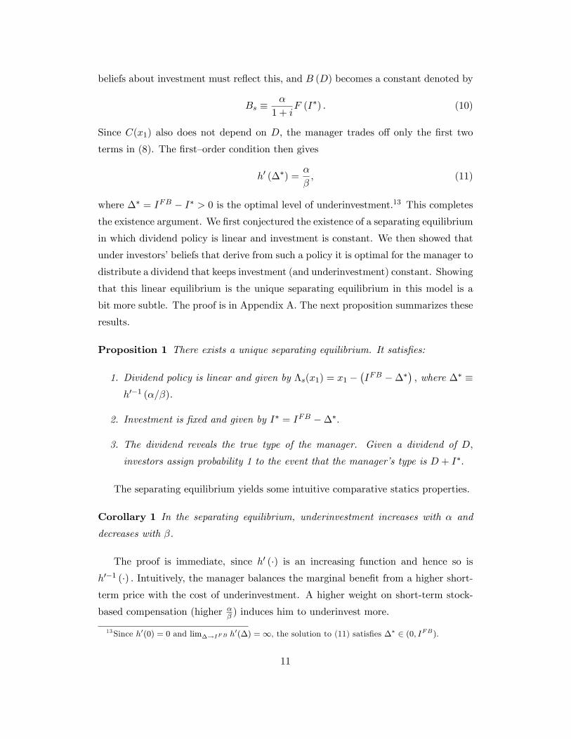
Proposition 1 There exists a unique separating equilibrium. It satis�es:

1. Dividend policy is linear and given by �s(x1) = x1 ��IFB ���

�; where �� �

h0�1 (�=�).

2. Investment is �xed and given by I� = IFB ���:

3. The dividend reveals the true type of the manager. Given a dividend of D;

investors assign probability 1 to the event that the manager�s type is D + I�:

The separating equilibrium yields some intuitive comparative statics properties.

Corollary 1 In the separating equilibrium, underinvestment increases with � and

decreases with �.

The proof is immediate, since h0 (�) is an increasing function and hence so ish0�1 (�) : Intuitively, the manager balances the marginal bene�t from a higher short-

term price with the cost of underinvestment. A higher weight on short-term stock-

based compensation (higher �� ) induces him to underinvest more.

13Since h0(0) = 0 and lim�!IFB h0(�) =1, the solution to (11) satis�es �� 2 (0; IFB).

11

4 Partially Pooling Equilibria

The separating equilibrium serves as a benchmark for our analysis. An important

feature of this equilibrium is that di¤erent types always pay di¤erent dividends.

We will seek a smoothed-out version of the separating equilibrium: unless earnings

are very low or very high, all manager types pay the same dividend. Such partial

pooling of dividends is necessary to generate smoothing over time: if the type space is

continuous and the last-year dividend is announced with a positive probability, then

there must exist a pooling interval of types.

We obtain such partial pooling by constructing an equilibrium in which there is

an interval [a; b] such that all manager types x1 in this interval announce the same

dividend (the �pooling dividend�). Outside of this interval, managers follow a sepa-

rating strategy. Investors�beliefs must be consistent with this strategy: conditional

on observing the pooling dividend they update their beliefs using Bayes rule given

the information that the manager�s type falls in the interval [a; b]: Thus, while the

pooling dividend provides information to investors by narrowing the set of potential

manager�s types, this information is not perfect.

To establish such an equilibrium we modify the linear separating equilibrium

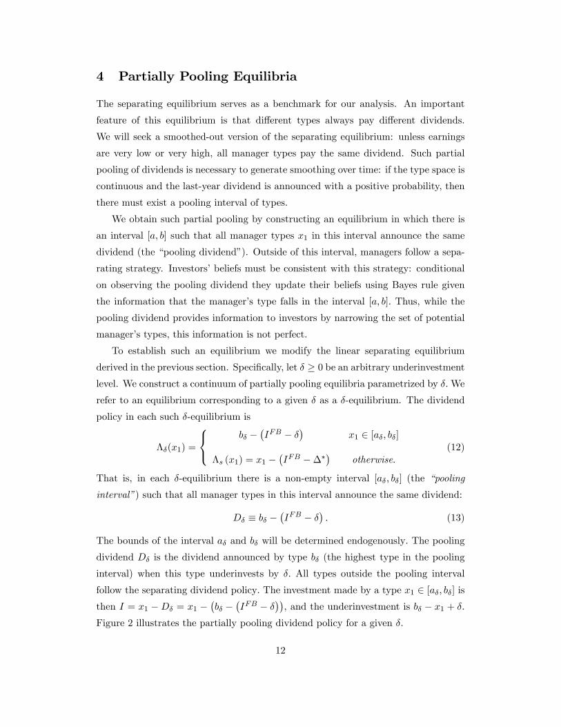
derived in the previous section. Speci�cally, let � � 0 be an arbitrary underinvestmentlevel. We construct a continuum of partially pooling equilibria parametrized by �:We

refer to an equilibrium corresponding to a given � as a �-equilibrium. The dividend

policy in each such �-equilibrium is

��(x1) =

8<:b� �

�IFB � �

�x1 2 [a�; b�]

�s (x1) = x1 ��IFB ���

�otherwise.

(12)

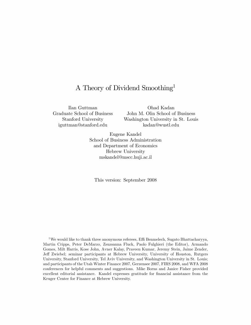
That is, in each �-equilibrium there is a non-empty interval [a�; b�] (the �pooling

interval�) such that all manager types in this interval announce the same dividend:

D� � b� ��IFB � �

�: (13)

The bounds of the interval a� and b� will be determined endogenously: The pooling

dividend D� is the dividend announced by type b� (the highest type in the pooling

interval) when this type underinvests by �: All types outside the pooling interval

follow the separating dividend policy: The investment made by a type x1 2 [a�; b�] isthen I = x1 �D� = x1 �

�b� �

�IFB � �

��, and the underinvestment is b� � x1 + �:

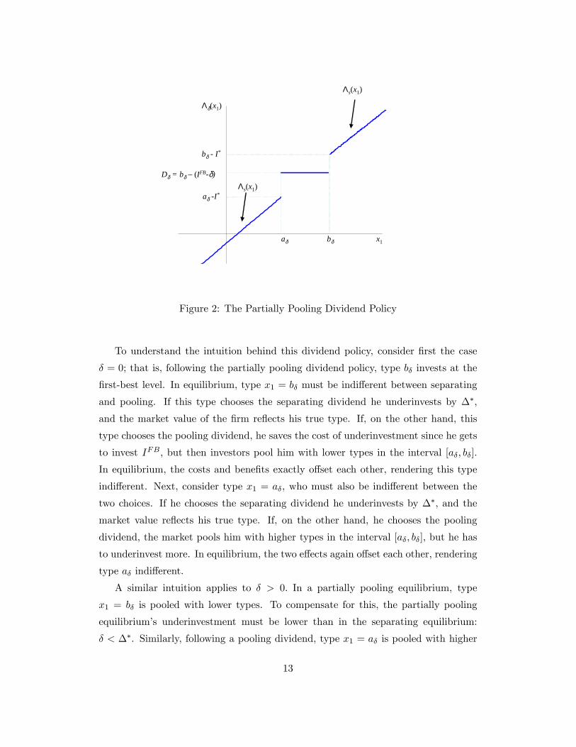
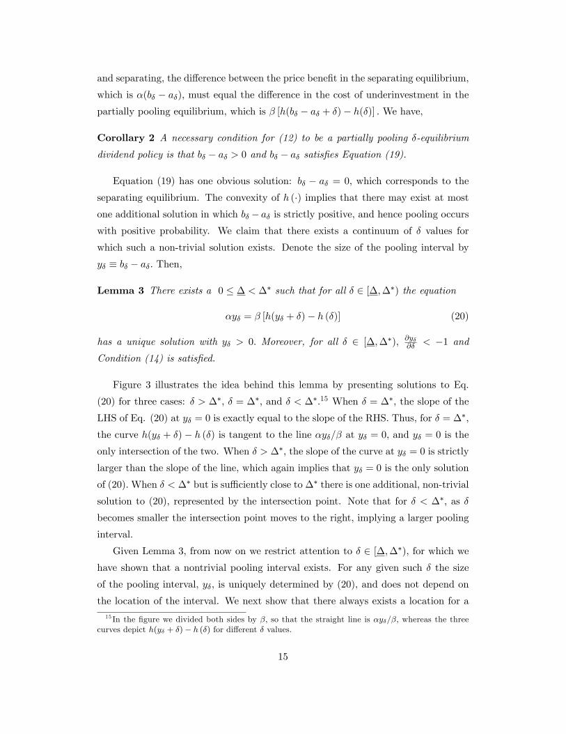
Figure 2 illustrates the partially pooling dividend policy for a given �.

12

aδ bδ x1

Λδ(x1)

Dδ = bδ –(IFB­δ)

bδ ­ I*

aδ ­I*

Λs(x1)

Λs(x1)

Figure 2: The Partially Pooling Dividend Policy

To understand the intuition behind this dividend policy, consider �rst the case

� = 0; that is, following the partially pooling dividend policy, type b� invests at the

�rst-best level. In equilibrium, type x1 = b� must be indi¤erent between separating

and pooling. If this type chooses the separating dividend he underinvests by ��;

and the market value of the �rm re�ects his true type. If, on the other hand, this

type chooses the pooling dividend, he saves the cost of underinvestment since he gets

to invest IFB; but then investors pool him with lower types in the interval [a�; b�]:

In equilibrium, the costs and bene�ts exactly o¤set each other, rendering this type

indi¤erent. Next, consider type x1 = a�, who must also be indi¤erent between the

two choices. If he chooses the separating dividend he underinvests by ��; and the

market value re�ects his true type. If, on the other hand, he chooses the pooling

dividend, the market pools him with higher types in the interval [a�; b�]; but he has

to underinvest more. In equilibrium, the two e¤ects again o¤set each other, rendering

type a� indi¤erent.

A similar intuition applies to � > 0: In a partially pooling equilibrium, type

x1 = b� is pooled with lower types. To compensate for this, the partially pooling

equilibrium�s underinvestment must be lower than in the separating equilibrium:

� < ��. Similarly, following a pooling dividend, type x1 = a� is pooled with higher

13

types. To render him indi¤erent, the underinvestment given the pooling dividend is

higher, i.e., b� � a� + � > ��: This shows that a necessary condition for a partiallypooling �-equilibrium is

�� � (b� � a�) < � < ��: (14)

Investors�beliefs must be consistent with the partially pooling dividend policy

(12). Given the normal prior, the posterior following a pooling dividend D� follows

a truncated normal distribution over [a�; b�]:14

Our goal is to show that a continuum of partially pooling equilibria exists. We

�rst identify additional necessary conditions for ��(�) to be an equilibrium.The utility of type x1 = a� given a separating dividend is

Us = ��a� � IFB +��

�� �h (��) +Bs + C(x1): (15)

The utility of this type given a pooling dividend is

U� = ��b� � IFB + �

�� �h (b� � a� + �) +B� + C(x1);

where

B� ��

1 + iE (F (IjD�)) : (16)

By equating Us and U� we obtain the indi¤erence condition for type a�:

��a� � IFB +��

���h (��)+Bs = �

�b� � IFB + �

���h (b� � a� + �)+B�: (17)

Similarly, the indi¤erence condition for type b� is

��b� � IFB +��

�� �h (��) +Bs = �

�b� � IFB + �

�� �h (�) +B�: (18)

Subtracting (17) from (18) gives

� (b� � a�) = � [h(b� � a� + �)� h (�)] : (19)

This simple necessary condition has an intuitive interpretation. In the separating

equilibrium there is no di¤erence between the two types in terms of underinvestment.

In the partially pooling �-equilibrium both types obtain the same price, as investors

cannot distinguish between them. Since both types are indi¤erent between pooling

14This means that for all q 2 [a�; b�], the posterior beliefs satisfy Pr(~x1 � qj~x1 2 [a�; b�]) =G(q)�G(a�)G(b�)�G(a�)

.

14

and separating, the di¤erence between the price bene�t in the separating equilibrium,

which is �(b� � a�); must equal the di¤erence in the cost of underinvestment in thepartially pooling equilibrium, which is � [h(b� � a� + �)� h(�)] : We have,

Corollary 2 A necessary condition for (12) to be a partially pooling �-equilibrium

dividend policy is that b� � a� > 0 and b� � a� satis�es Equation (19).

Equation (19) has one obvious solution: b� � a� = 0; which corresponds to the

separating equilibrium. The convexity of h (�) implies that there may exist at mostone additional solution in which b� � a� is strictly positive, and hence pooling occurswith positive probability. We claim that there exists a continuum of � values for

which such a non-trivial solution exists. Denote the size of the pooling interval by

y� � b� � a�: Then,

Lemma 3 There exists a 0 � � < �� such that for all � 2 [�;��) the equation

�y� = � [h(y� + �)� h (�)] (20)

has a unique solution with y� > 0: Moreover, for all � 2 [�;��); @y�@� < �1 andCondition (14) is satis�ed.

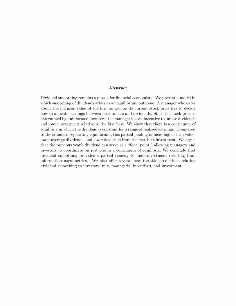
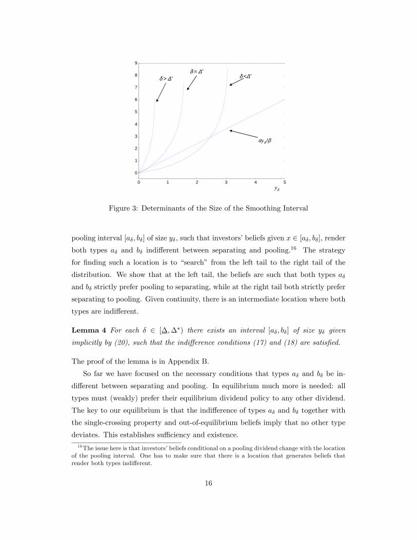
Figure 3 illustrates the idea behind this lemma by presenting solutions to Eq.

(20) for three cases: � > ��; � = ��; and � < ��:15 When � = ��; the slope of the

LHS of Eq. (20) at y� = 0 is exactly equal to the slope of the RHS. Thus, for � = ��;

the curve h(y� + �) � h (�) is tangent to the line �y�=� at y� = 0; and y� = 0 is theonly intersection of the two. When � > ��; the slope of the curve at y� = 0 is strictly

larger than the slope of the line, which again implies that y� = 0 is the only solution

of (20):When � < �� but is su¢ ciently close to �� there is one additional, non-trivial

solution to (20), represented by the intersection point. Note that for � < ��; as �

becomes smaller the intersection point moves to the right, implying a larger pooling

interval.

Given Lemma 3, from now on we restrict attention to � 2 [�;��), for which wehave shown that a nontrivial pooling interval exists. For any given such � the size

of the pooling interval, y�; is uniquely determined by (20), and does not depend on

the location of the interval. We next show that there always exists a location for a15 In the �gure we divided both sides by �; so that the straight line is �y�=�; whereas the three

curves depict h(y� + �)� h (�) for di¤erent � values.

15

0 1 2 3 4 5

0

1

2

3

4

5

6

7

8

9

δ > ∆∗δ = ∆∗

δ <∆∗

yδ

αρyδ /βαyδ /β

Figure 3: Determinants of the Size of the Smoothing Interval

pooling interval [a�; b�] of size y�, such that investors�beliefs given x 2 [a�; b�]; renderboth types a� and b� indi¤erent between separating and pooling.16 The strategy

for �nding such a location is to �search� from the left tail to the right tail of the

distribution. We show that at the left tail, the beliefs are such that both types a�

and b� strictly prefer pooling to separating, while at the right tail both strictly prefer

separating to pooling. Given continuity, there is an intermediate location where both

types are indi¤erent.

Lemma 4 For each � 2 [�;��) there exists an interval [a�; b�] of size y� given

implicitly by (20), such that the indi¤erence conditions (17) and (18) are satis�ed.

The proof of the lemma is in Appendix B.

So far we have focused on the necessary conditions that types a� and b� be in-

di¤erent between separating and pooling. In equilibrium much more is needed: all

types must (weakly) prefer their equilibrium dividend policy to any other dividend.

The key to our equilibrium is that the indi¤erence of types a� and b� together with

the single-crossing property and out-of-equilibrium beliefs imply that no other type

deviates. This establishes su¢ ciency and existence.16The issue here is that investors�beliefs conditional on a pooling dividend change with the location

of the pooling interval. One has to make sure that there is a location that generates beliefs thatrender both types indi¤erent.

16

Note that given a partially pooling dividend policy �� (�) ; the dividend pay-ment never lies in the range

�a� � I�; b� � IFB + �

�[�b� � IFB + �; b� � I�

�: To

completely specify the equilibrium, we must de�ne the out-of-equilibrium beliefs as-

sociated with these zero-probability dividends. For simplicity, we assume �rst that in

observing such a dividend, investors believe that the manager is �mistakenly�playing

the separating dividend policy.17 See Appendix C for a generalization.18 We are now

ready to state our main existence result.

Proposition 2 For any � 2 [�;��) there exists an interval [a�; b�] such that �� (�)as given in (12) is an equilibrium. Furthermore,

1. The size of the pooling interval is given implicitly by (19).

2. Given a dividend of D� = b���IFB � �

�(the pooling dividend), investors�beliefs

follow a truncated normal distribution over [a�; b�]: For any other dividend D,

investors assign probability 1 to the event that the manager�s type is D + I�:

The proof is in Appendix A. This completes the �rst step of our argument: a

continuum of partially pooling equilibria exists in our model.

4.1 Example

To illustrate the partially pooling equilibria assume the production function takes

the form: F (I) = 2pI: Set parameter values to � = 0:7; � = 1; i = 0; I0 = 0:5;

and �1 = 0:2: It is easy to verify that the �rst-best investment is IFB = 1:0: The

investment in the separating equilibrium is I� = 0:346; and the underinvestment

is �� = 0:654: Table 1 presents the results for the partially pooling �-equilibria

for several � < �� values. For each � we �rst calculated the size of the pooling

interval, y�; by numerically solving the implicit equation in (20). Then, using a grid

search we found a� and b� such that b� � a� = y�; and the indi¤erence conditions aresatis�ed. The pooling dividend, D�; is then given by (13). Using the parameters of the

distribution function we also calculated the probability of pooling: Pr fx1 2 [a�; b�]g :17That is, given an out-of-equilibrium dividend D, investors assign probability 1 to the event that

the manager�s type is D + I�:18 In Appendix C we characterize the set of out-of equilibrium beliefs supporting the �-equilibria.

We also show the existence of monotonic out-of-equilibrium beliefs that support the �-equilibria, anddiscuss the robustness of these beliefs vis-à-vis standard re�nement concepts.

17

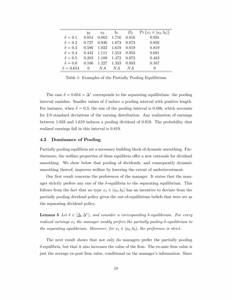
y� a� b� D� Pr fx1 2 [a�; b�]g� = 0:1 0:854 0:862 1:716 0:816 0:931� = 0:2 0:727 0:946 1:673 0:873 0:892� = 0:3 0:586 1:033 1:619 0:919 0:819� = 0:4 0:442 1:111 1:553 0:953 0:691� = 0:5 0:283 1:189 1:472 0:972 0:483� = 0:6 0:106 1:227 1:333 0:933 0:167� = 0:654 0 NA NA NA 0

Table 1: Examples of the Partially Pooling Equilibrium

The case � = 0:654 = �� corresponds to the separating equilibrium: the pooling

interval vanishes. Smaller values of � induce a pooling interval with positive length.

For instance, when � = 0:3; the size of the pooling interval is 0.586, which accounts

for 2.9 standard deviations of the earning distribution. Any realization of earnings

between 1.033 and 1.619 induces a pooling dividend of 0.919. The probability that

realized earnings fall in this interval is 0.819.

4.2 Dominance of Pooling

Partially pooling equilibria are a necessary building block of dynamic smoothing. Fur-

thermore, the welfare properties of these equilibria o¤er a new rationale for dividend

smoothing. We show below that pooling of dividends, and consequently dynamic

smoothing thereof, improves welfare by lowering the extent of underinvestment.

Our �rst result concerns the preferences of the manager. It states that the man-

ager strictly prefers any one of the �-equilibria to the separating equilibrium. This

follows from the fact that no type x1 2 (a�; b�) has an incentive to deviate from the

partially pooling dividend policy given the out-of-equilibrium beliefs that were set as

the separating dividend policy.

Lemma 5 Let � 2 [�;��); and consider a corresponding �-equilibrium. For everyrealized earnings x1 the manager weakly prefers the partially pooling �-equilibrium to

the separating equilibrium. Moreover, for x1 2 (a�; b�); the preference is strict.

The next result shows that not only do managers prefer the partially pooling

�-equilibria, but that it also increases the value of the �rm. The ex-ante �rm value is

just the average ex-post �rm value, conditional on the manager�s information. Since

18

the manager is strictly better o¤ in the partially pooling equilibrium, it must be that

the ex-ante �rm value is higher. But this in turn is possible only if investment moved

closer to the �rst-best level. Thus, both the manager and the investors ex-ante prefer

pooling to perfect separation. Formally,

Proposition 3 Set � 2 [�;��); and consider a corresponding �-equilibrium. Then,

1. The expected intrinsic value is higher under the partially pooling �-equilibrium

than under the separating equilibrium.

2. The expected underinvestment and expected dividends are lower under the par-

tially pooling �-equilibrium than under the separating equilibrium.

3. The �-equilibrium generates higher expected investment and higher expected re-

turn on investment than the separating equilibrium.

4. Investors ex-ante prefer the �-equilibrium to the separating equilibrium.

5. The �-equilibrium Pareto-dominates the separating equilibrium.

Proof: In Appendix A.

Pooling enables the manager to retain some information rents. Compared to the

separating equilibrium, the additional uncertainty introduced by the noisy pooling

dividend does not pose a problem to fully diversi�ed (risk-neutral) investors, since

the �rm is still correctly priced on average. Furthermore, in the �-equilibrium the

investment is, on average, closer to its �rst-best level, increasing the �rm value to

the investors. Thus, both the manager and the investors bene�t from the pooling.

As any one of the partially pooling equilibria dominates the separating equilibrium,

the latter does not survive the equilibrium selection criterion of Maskin and Tirole

(1992).

This completes the second step of our argument. Any one of the partially pooling

equilibria Pareto-dominates the fully revealing one, which provides motivation for

why a partially pooling equilibrium may be played. Next we discuss how a partially

pooling equilibrium in a single period translates into dividend smoothing over time.

5 Dynamic Dividend Smoothing

As discussed in the introduction, dividend smoothing manifests itself as the practice

of keeping dividends constant over two or more consecutive periods. This is a stronger

19

notion of smoothing than the one advocated in Lintner (1956), which requires that

the variation in dividends is lower than the variation in earnings. An immediate

implication is that some pooling must be present. In this section we outline a sim-

ple dynamic version of the model and demonstrate how coordination on one of the

partially pooling equilibria can result in dividend smoothing over time.

5.1 Simpli�ed Dynamic Setting

Assume a �nite number of periods t = 1; :::; T: Earnings in each period are xt =

F (It�1) + "t; where It is the investment at time t and "t is normally distributed

with mean 0.19 At each time period the manager has to choose how to allocate the

earnings xt between a dividend payment Dt and investment It: The initial investment

and dividend I0 and D0 are given exogenously.

Solving the dynamic model presents two technical challenges:

1. Once earnings fall in the pooling interval in period t � 1, the distribution ofxt = F (It�1) + "t from the investors�point of view is the sum of two random

variables: one has a �nite support and the other is normal. This sum is not

normally distributed. This raises technical di¢ culties, as our existence proof

makes use of the tail properties of the normal distribution.

2. Allowing the manager and the investors to take into account the e¤ect of the

dividend choice in period t on future earnings in all upcoming periods under-

mines the linearity of the separating equilibrium, making the related partially

pooling equilibria intractable.

The �rst problem has a manageable solution. We show that while the distribution

of earnings in periods 2; :::; T may not be normal, it has the same tail properties as

the normal distribution. This enables us to use similar techniques to those used in

the static setting to prove existence of equilibria in a dynamic setup. To overcome

the second problem, we assume (similar to Stein (1989)) that both the manager and

the investors are myopic: every period t they care only about the trade-o¤ between

the dividend paid in period t and the expected earnings in period t+1:20 That is, the

objective of the manager is to maximize a linear combination of the stock price at

19The production function is assumed identical for all periods 1; :::; T ; however, it is easy to gen-eralize the model to a time-varying production function.20Given this assumption, the model can also accommodate an in�nite number of periods.

20

time t and the intrinsic value, under the assumption that the �rm will be liquidated

at time t+ 1. Formally, the manager maximizes in period t

Ut(xt; Dt) � ��Dt +

1

1 + iE (F (xt �Dt) jD1; D2; :::; Dt)

�+�

�Dt +

1

1 + iF (xt �Dt)

�:

(21)

This assumption enables us to restore the tractability of the partially pooling equi-

libria.21

It is important to note that this myopia does not transform the dynamic game

into a sequence of separate �one shot�games. The reason is that investment is carried

from one period to the next. If a pooling strategy is played in period t; investors are

uncertain about the amount of investment, and this a¤ects their beliefs and pricing

in period t + 1; t + 2; etc. This is re�ected in (21), as investors condition their

expectations in period t on the entire history of dividends up to this point in time.

One obvious equilibrium in this myopic, dynamic setting is to play the separating

equilibrium outlined in Proposition 1 in each period. Next, we show the existence of

a continuum of equilibria with partial pooling in this setting.

Proposition 4 Assume that the manager and the investors are myopic (as explained

above). There exist � < ��; a continuum of vectors (�1; :::; �T ) 2 [�;��)T ; and

corresponding intervals [a�1;b�1 ] ; :::; [a�T ;b�T ] such that the dynamic dividend policy

��t(xt) =

8<:b�t �

�IFB � �t

�xt 2 [a�t ; b�t ]

�s (xt) = xt ��IFB ���

�otherwise

for t = 1; :::; T

with appropriate investors�beliefs constitute an equilibrium in the dynamic game. Any

of these equilibria Pareto-dominates the equilibrium in which the separating dividend

policy is played for all t = 1; ::; T:

Proof: In Appendix D.

5.2 Coordination and Smoothing

Though our dynamic setting shows the existence of a continuum of partially pooling

equilibria, it is mute on how investors and the manager coordinate on just one out

21We emphasize that this assumption is made for tractability reasons only. While we are not ableto solve analytically for a partially pooling equilibrium in the full-�edged dynamic model, we do notsee why the dynamic smoothing identi�ed below would not work in such a setting.

21

of these equilibria. In fact, the game theoretic literature has very little to say about

equilibrium selection. The dominance of any partially pooling equilibrium over the

separating one, suggests that managers and investors will try to coordinate on one

of the partially pooling equilibria. However, we cannot rank the partially pooling

equilibria in terms of their e¢ ciency.22

One way to generate coordination is to use the last-year dividend as a �focal

point.�That is, in each year t = 1; :::; T; the manager and the investors coordinate

on playing a partially pooling �t-equilibrium in which the pooling dividend in year t

equals the dividend paid in year t� 1: Then, there is an interval of earnings [a�t;b�t ]such that for all earnings therein, the manager announces a dividend that equals the

last-year dividend. This gives rise to dividend smoothing over time. Only if earnings

are outside this interval is the dividend di¤erent from the last-year dividend, in which

case it fully reveals the earnings.

We illustrate this by an example using the myopic-dynamic setting developed

above. Assume the game is played for T = 3 years. The production function is

F (It�1) = 2pIt�1 with parameter values as in Table 1. The initial investment is

I0 = 0:5; and the initial dividend is D0 = 0:82. Table 2 presents the results of a path

of realizations of xt and equilibrium play using coordination in dividends.

In year 1, F (I0) = 2p0:5 = 1:41: Hence, earnings in year 1 are distributed

normally with mean 1.41 and S.D. 0.2. We use these parameters to �nd a �1 value,

such that the pooling dividend D�1 is equal to the dividend in the previous period,

namely, 0:82. The result is �1 = 0:11: We then assume that the manager and the

investors coordinate on playing the partially pooling equilibrium that corresponds

to �1 = 0:11: We numerically �nd the pooling interval in this case, which turns

out to be [0:87; 1:71]: Thus, the size of the pooling interval is y�1 = 0:84; and the

probability of dividend smoothing is 0:93: The earnings realization in this case is

1:45; which falls inside the pooling interval. As a result, the dividend announced is

D1 = ��1(1:45) = 0:82, which is equal to D0.23

The investment in year 1 is I1 = x1 �D1 = 1:55� 0:82 = 0:73; and the expectedreturn on investment is F (I1) = 1:7: Consequently, the earnings in year 2, are nor-

mally distributed with mean 1:7 and S.D. 0.2. The investors do not know at this

22We have shown (Lemma 3) that the size of the pooling interval decreases in �: The location ofthe interval also varies with �; but in a non-monotone manner that we cannot track analytically.23Had the separating equilibrium been played, the dividend would have been increased to

�s (1:55) = 1:21:

22

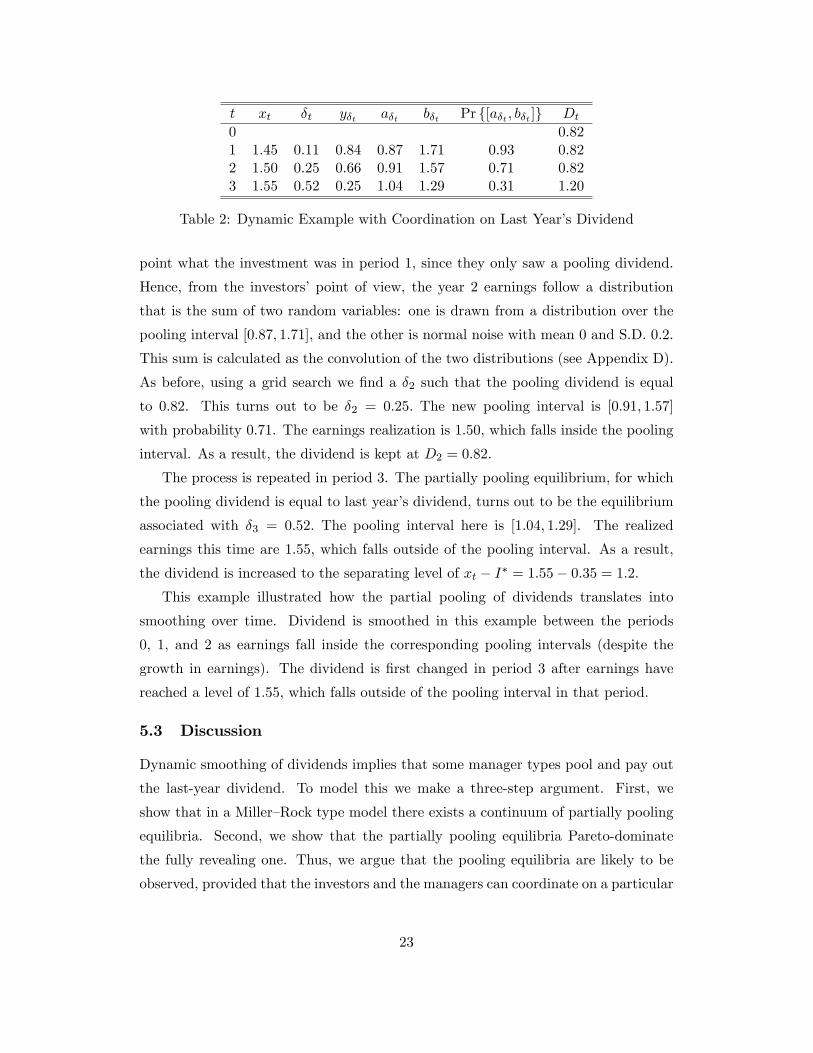
t xt �t y�t a�t b�t Pr f[a�t ; b�t ]g Dt0 0:821 1:45 0:11 0:84 0:87 1:71 0:93 0:822 1:50 0:25 0:66 0:91 1:57 0:71 0:823 1:55 0:52 0:25 1:04 1:29 0:31 1:20

Table 2: Dynamic Example with Coordination on Last Year�s Dividend

point what the investment was in period 1, since they only saw a pooling dividend.

Hence, from the investors�point of view, the year 2 earnings follow a distribution

that is the sum of two random variables: one is drawn from a distribution over the

pooling interval [0:87; 1:71]; and the other is normal noise with mean 0 and S.D. 0.2.

This sum is calculated as the convolution of the two distributions (see Appendix D).

As before, using a grid search we �nd a �2 such that the pooling dividend is equal

to 0.82. This turns out to be �2 = 0:25: The new pooling interval is [0:91; 1:57]

with probability 0.71. The earnings realization is 1.50, which falls inside the pooling

interval. As a result, the dividend is kept at D2 = 0:82.

The process is repeated in period 3. The partially pooling equilibrium, for which

the pooling dividend is equal to last year�s dividend, turns out to be the equilibrium

associated with �3 = 0:52: The pooling interval here is [1:04; 1:29]. The realized

earnings this time are 1.55, which falls outside of the pooling interval. As a result,

the dividend is increased to the separating level of xt � I� = 1:55� 0:35 = 1:2:This example illustrated how the partial pooling of dividends translates into

smoothing over time. Dividend is smoothed in this example between the periods

0, 1, and 2 as earnings fall inside the corresponding pooling intervals (despite the

growth in earnings). The dividend is �rst changed in period 3 after earnings have

reached a level of 1.55, which falls outside of the pooling interval in that period.

5.3 Discussion

Dynamic smoothing of dividends implies that some manager types pool and pay out

the last-year dividend. To model this we make a three-step argument. First, we

show that in a Miller�Rock type model there exists a continuum of partially pooling

equilibria. Second, we show that the partially pooling equilibria Pareto-dominate

the fully revealing one. Thus, we argue that the pooling equilibria are likely to be

observed, provided that the investors and the managers can coordinate on a particular

23

one. Finally, we argue that managers and investors can use the last-year dividend to

coordinate on one of these equilibria. This coordination device is simple and, once

established, does not require year-to-year adjustments. This combination predicts

that dividends, once announced, persist over time, until the earnings change to the

extent that they fall outside of the equilibrium pooling region. Then the dividend is

cut or increased, and the process starts again.

Ultimately, the claim that dividend smoothing is a result of coordination should

be empirically tested. While a serious empirical study of this question is beyond the

scope of this paper, we present below some illustrative evidence that seems consistent

with the notion of coordination. In Figure 1 we have shown that the unconditional

probability of a �rm not changing its dividend from one year to the next during

1966-2005 is over 25%. Are all �rms equally likely to engage in this practice, or are

some �rms more prone to do so persistently, as would be expected from a coordination

story? We calculated that 38% of all �rms that ever paid dividends two years in a row

between 1966 and 2005 never smoothed dividends even once in those 40 years. This

already suggests that not all �rms are playing the smoothing game. Furthermore,

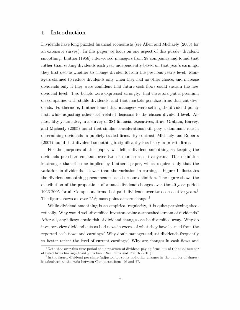
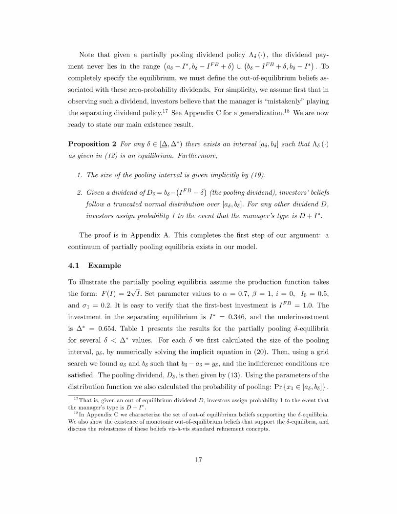
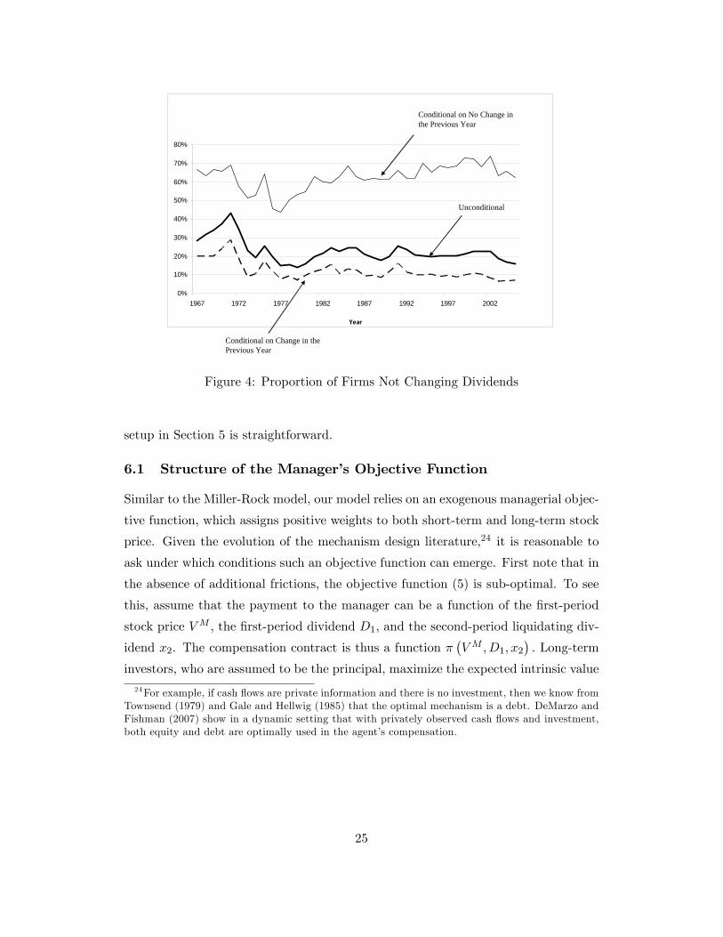
Figure 4 presents the probability of not changing the dividend per share from year t

to year t+1; unconditionally, as well as conditional on dividend change (or no change)

from year t� 1 to year t. Conditional on not changing their dividend in the previousyear (thin line), around 60% of �rms do not change their dividend the following year

either. Conditional on changing the dividend in the previous year (dashed line),

only slightly more than 10% keep the dividend constant in the following year. These

simple statistics suggest that there exists a sub-sample of dividend-paying �rms that

consistently engage in dividend smoothing, while other �rms do not. To us, this

suggests that the former �rms had adopted the last-year dividend as a coordination

device.

6 Extensions

In this section we explore two extensions to the base model. First we study the

structure of the manager�s objective function, and identify scenarios under which

such an objective function can evolve endogenously. Then we explore how allowing

the �rm to retain some of the earnings a¤ects our results. Throughout this section

we use the static version of the model. Adapting the results to the dynamic-myopic

24

0%

10%

20%

30%

40%

50%

60%

70%

80%

1967 1972 1977 1982 1987 1992 1997 2002

Year

Conditional on No Change inthe Previous Year

Unconditional

Conditional on Change in thePrevious Year

Figure 4: Proportion of Firms Not Changing Dividends

setup in Section 5 is straightforward.

6.1 Structure of the Manager�s Objective Function

Similar to the Miller-Rock model, our model relies on an exogenous managerial objec-

tive function, which assigns positive weights to both short-term and long-term stock

price. Given the evolution of the mechanism design literature,24 it is reasonable to

ask under which conditions such an objective function can emerge. First note that in

the absence of additional frictions, the objective function (5) is sub-optimal. To see

this, assume that the payment to the manager can be a function of the �rst-period

stock price VM ; the �rst-period dividend D1; and the second-period liquidating div-

idend x2. The compensation contract is thus a function ��VM ; D1; x2

�: Long-term

investors, who are assumed to be the principal, maximize the expected intrinsic value

24For example, if cash �ows are private information and there is no investment, then we know fromTownsend (1979) and Gale and Hellwig (1985) that the optimal mechanism is a debt. DeMarzo andFishman (2007) show in a dynamic setting that with privately observed cash �ows and investment,both equity and debt are optimally used in the agent�s compensation.

25

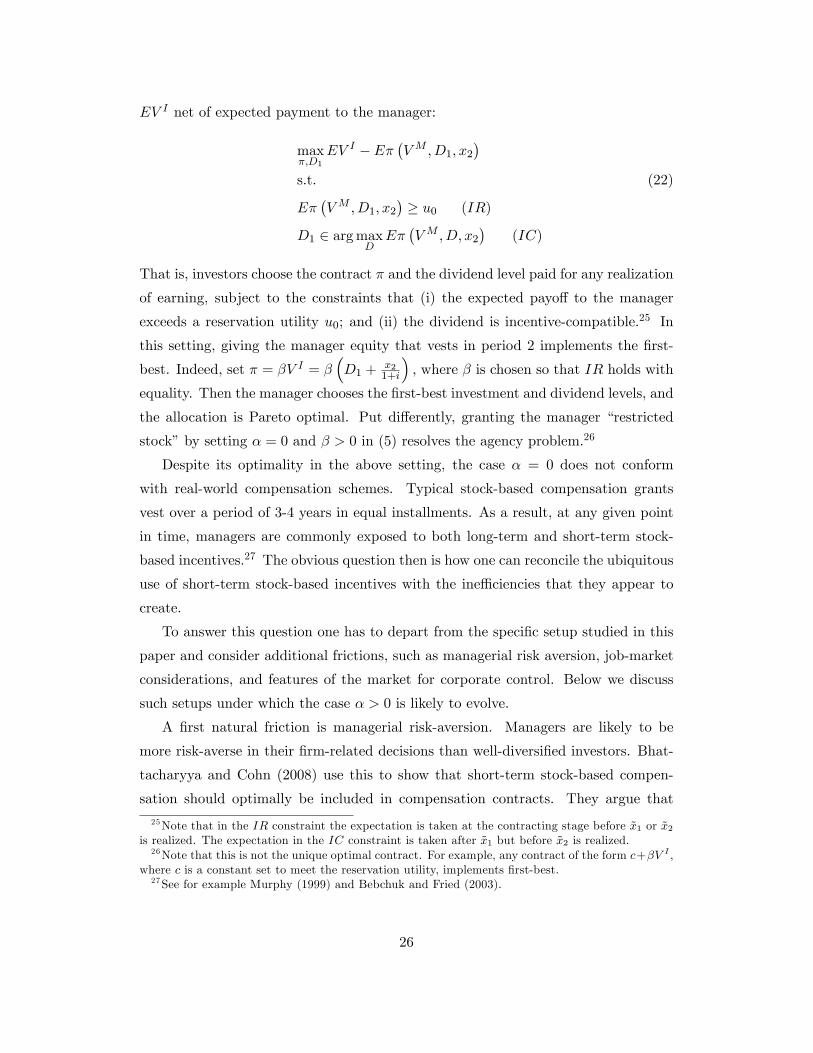
EV I net of expected payment to the manager:

max�;D1

EV I � E��VM ; D1; x2

�s.t. (22)

E��VM ; D1; x2

�� u0 (IR)

D1 2 argmaxDE��VM ; D; x2

�(IC)

That is, investors choose the contract � and the dividend level paid for any realization

of earning, subject to the constraints that (i) the expected payo¤ to the manager

exceeds a reservation utility u0; and (ii) the dividend is incentive-compatible.25 In

this setting, giving the manager equity that vests in period 2 implements the �rst-

best. Indeed, set � = �V I = ��D1 +

x21+i

�; where � is chosen so that IR holds with

equality. Then the manager chooses the �rst-best investment and dividend levels, and

the allocation is Pareto optimal. Put di¤erently, granting the manager �restricted

stock�by setting � = 0 and � > 0 in (5) resolves the agency problem.26

Despite its optimality in the above setting, the case � = 0 does not conform

with real-world compensation schemes. Typical stock-based compensation grants

vest over a period of 3-4 years in equal installments. As a result, at any given point

in time, managers are commonly exposed to both long-term and short-term stock-

based incentives.27 The obvious question then is how one can reconcile the ubiquitous

use of short-term stock-based incentives with the ine¢ ciencies that they appear to

create.

To answer this question one has to depart from the speci�c setup studied in this

paper and consider additional frictions, such as managerial risk aversion, job-market

considerations, and features of the market for corporate control. Below we discuss

such setups under which the case � > 0 is likely to evolve.

A �rst natural friction is managerial risk-aversion. Managers are likely to be

more risk-averse in their �rm-related decisions than well-diversi�ed investors. Bhat-

tacharyya and Cohn (2008) use this to show that short-term stock-based compen-

sation should optimally be included in compensation contracts. They argue that

25Note that in the IR constraint the expectation is taken at the contracting stage before ~x1 or ~x2is realized. The expectation in the IC constraint is taken after ~x1 but before ~x2 is realized.26Note that this is not the unique optimal contract. For example, any contract of the form c+�V I ,

where c is a constant set to meet the reservation utility, implements �rst-best.27See for example Murphy (1999) and Bebchuk and Fried (2003).

26

short-term stock-based compensation mitigates the reluctance of risk-averse man-

agers to pursue risky and pro�table projects. Linking manager�s pay to short-term

realizations provides managers with insurance against bad outcomes in the long run.

This induces managers to take risky and pro�table bets. Bhattacharyya and Cohn

conclude that optimal compensation contracts include both short-term and long-term

stock-based compensation.

Stein (1989) provides a di¤erent explanation. He argues that the �rm may face

early takeover or early funding requirements. As a result, even if the explicit manage-

rial contract relies solely on long-term stock price, the manager�s objective function

de facto depends on the short-term price as well.

Career concerns can also play a role. Consider for example a setting in which man-

agers di¤er in terms of their ability, where higher ability is associated with higher

expected earnings. Then the stock price is informative about both investments and

managerial ability. Thus, career-minded managers assign positive weights to both

short- and long-term incentives. Additionally, outside options for the manager are

likely to be correlated with the short-term stock price. Therefore, linking the man-

ager�s pay to short-term price realizations may help retain the manager.

Based on the above arguments, we feel that � > 0 is a reasonable assumption and

a fair description of reality.

6.2 Retained Earnings

It is tempting to interpret (1) as implying that in the Miller-Rock model, dividends

and investments are perfectly negatively correlated. Such a conclusion would contrast

empirical regularities suggesting no such relation (e.g. Fama 1974). Note, however,

that the model does not have any de�ned implications for the correlation between div-

idends and investments, since (1) does not imply that higher earnings are associated

with lower investments.28 As an example, in the separating equilibrium investments

are constant and thereby uncorrelated with dividends. In the partially pooling equi-

libria, outside of the pooling interval investment is constant and dividends increase

in earnings. Inside the pooling interval, investment increases in earnings while the

dividend is constant. As a result, the correlation between investments and dividends

28Lemma 2 shows that dividends (weakly) increase in earnings. Investments, however, may in-crease, decrease, or stay constant when earnings increase. This prevents a simple signing of thecorrelation between dividends and investments.

27

in these equilibria is quite low, in accordance with the evidence.

A natural question is whether the correlation structure between investments and

dividends in the partially pooling equilibria is an artifact of the inability of managers

in the model to retain earnings. To explore this issue we outline below a simple

extension that allows for retained earnings.

Assume that the earnings in period 1 are allocated between dividends D; invest-

ments I; and retained cash/earnings R: That is, replace (1) with

x1 = I +D +R: (23)

Assume that retained earnings are used by the �rm for operating activities, working

capital, and short-term investments. It is reasonable that the bene�t from retained

earnings B (R) is a concave function with similar properties to those of the production

function F (�) : This implies that the �rst-best level of retained earnings RFB is givenimplicitly by

B0�RFB

�= 1 + i: (24)

If retained earnings were observable by investors, then the manager would always

set them at the �rst-best level, and the results stay qualitatively the same as in the

base model. A more interesting case is when retained earnings, similar to investments,

are not perfectly observable by investors. Here, the dividend serves as a signal for

both investments and retained earnings. Given this structure, for any earnings level,

the manager has to choose the dividend, investment, and retained earnings. Since

the manager has complete leeway in optimizing between investments and retained

earnings, in equilibrium, the marginal productivity of investments equals the marginal

bene�t from retained earnings:

F 0 (I) = B0 (R) : (25)

This de�nes an implicit relation between investments and retained earnings. From

(25) and the concavity of F (�) and B (�) ; it is immediate that investments and re-tained earnings are positively correlated. Furthermore, (25), (24), and (3) imply that

underinvestment must be accompanied by a retained earnings level below �rst-best,

while overinvestment implies retained earnings higher than �rst-best.

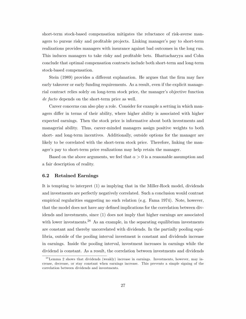
Using these observations, one can rewrite the objective function of the manager

(8) as

U = �D � �h(�T ) +B(D) + C(x1);

28

where �T ��IFB � I

�+�RFB �R

�is the sum of the underinvestment and deviation

from the �rst-best retained earnings, and h (�) is the real cost of this deviation.Moreover, (25) implies that h (�) has the same loss-function properties as h (�) : Fromhere, the derivation of the separating equilibrium and partially pooling equilibria is

similar to the base case of the model.

This simple extension has several implications. First, similar to the base-case

model, in the separating equilibrium the sum of investments and retained earnings

must be constant, and hence by (25), both are constant and uncorrelated with div-

idends. In the partially pooling equilibria, investments and retained earnings are

�xed outside the pooling interval. Inside the pooling interval, both investments and

retained earnings are positively correlated with earnings. Overall, in this model both

investments and retained earnings exhibit a weak correlation with dividends.

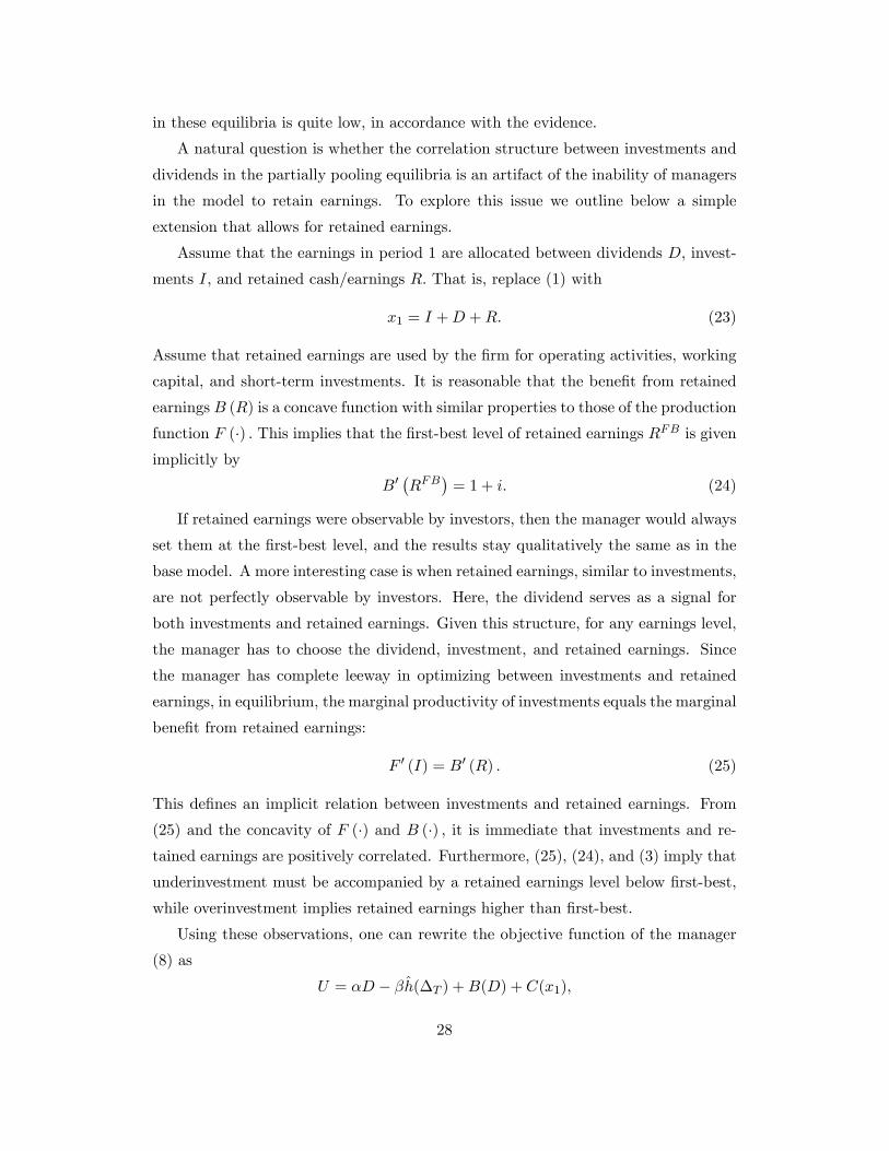
7 Empirical Predictions

The main novel implication of our model is that dividend smoothing can arise endoge-

nously in a world where earnings, return on investment, and managerial compensation

are all continuous and smooth. In addition, our model has several empirical predic-

tions on the relations between dividend smoothing, investments, �rm pro�tability,

ownership mix, and managerial incentives.29

A �rst set of empirical implications comes from analyzing the determinants of the

size of the pooling interval given implicitly in (20).

Lemma 6 For any given � 2 [�;��) : @y�@� > 0; and@y�@� < 0:

The proof is immediate, since increasing � and decreasing � raises the slope of the

straight line in Figure 3, moving the intersection point to the right. Note, however,

that an increase in the size of the interval does not automatically imply a higher

probability of pooling, since the location of the interval changes as well. We have

checked numerically (using Cobb�Douglass production functions) that the movement

of the interval is of second order relative to the increase in size. Thus, an increase in�� is likely to be associated with an increase in the probability of dividend smoothing.

29The speci�c choice of model (Miller and Rock) does not seem to be crucial for the smoothingargument. While we have not done the analysis, similar partially pooling equilibria are also likelyto emerge in other static models of dividend signaling. The empirical predictions below rely on oursetting only.

29

The ratio �� is a measure of managerial myopia. It can be given two interpreta-

tions. First, �� is a measure of the extent of short-term stock-based compensation.

Thus, we predict that a higher extent of short-term stock-based compensation is

associated with more dividend smoothing.30 Additionally, Stein (1989) argues that

managers are prone to short-term incentives in �rms that are likely to be acquired

and �rms that need to raise capital in the short term. Our model suggest that such

�rms are likely to exhibit a larger extent of dividend smoothing. A second inter-

pretation of �� is based on the premise that the manager represents the interests of

both short-term and long-term investors.31 Using this interpretation, �rms with more

short-term investors (or �rms in which short-term investors have more in�uence) tend

to smooth dividends more. In particular, this suggests that dividend smoothing is

less likely in private �rms.

Next, note that a second way to move the intersection point in Figure 3 to the right

is to �atten the convex curve. This curve determines the real cost of underinvestment,

and is analogous to the investment opportunity curve. A �atter curve means that the

marginal cost of underinvestment increases at a slower rate. Thus, better investment

opportunities (a �atter curve) are associated with more dividend smoothing.

Finally, Proposition 3 suggests that both investments and the return on invest-

ments are higher on average when �rms smooth dividends. This has both cross-

sectional and time-series implications: �rms that smooth dividends are expected to

invest more and to show higher pro�tability in following years. Similarly, periods of

dividend smoothing should be associated with higher investments, and followed by

high pro�tability.

8 Conclusion

Dividend smoothing manifests itself as the practice of �rms keeping their dividends

constant over several years, until earnings change signi�cantly. An implication is

that �rms follow a partially pooling dividend policy in which the same dividend is

paid over an interval of earnings realizations. This behavior is not re�ected in the

perfectly separating equilibria studied in the classic dividend signaling models.

30Note that in a setting that allows for an endogenous managerial objective function (see Sec-tion 6.1), both managerial incentives and dividend smoothing/investment decisions are determinedendogenously. Thus, testing this prediction is not easy and requires �nding a good instrument forcompensation.31This is the original interpretation of Miller and Rock (1985).

30

We show that while such a unique separating equilibrium exists in our setting,

the model has a multitude of partially pooling equilibria. These equilibria have full

revelation of earnings for low and high outcomes, but for all �intermediate outcomes�

the same dividend is announced. Thus, for all earnings that fall within a designated

interval the manager chooses exactly the same dividend. Investors anticipate this be-

havior and price the �rm correctly given this dividend policy. We show the existence

of a continuum of such partially pooling equilibria.

Both the manager and the investors prefer any one of the partially pooling equi-

libria to the standard separating equilibrium. This suggests that they coordinate on

playing one of these equilibria. We argue that the last-year dividend can serve as

a simple and robust coordination mechanism allowing them to focus on just one of

the partially pooling equilibria. Thus, they play a partially pooling equilibrium in

which this year�s pooling dividend is equal to last year�s dividend. As a result, unless

earnings fall outside of the pooling interval, the dividend is not changed. This gives

rise to dividend smoothing over time.

References

[1] Allen F., A. Bernardo, and I. Welch, 2000, A Theory of Dividends Based on Tax

Clienteles, Journal of Finance 55, 2499-2536.

[2] Allen, F., and R. Michaely, 2003, Payout Policy, in Handbook of Economics, ed.

G. Constantinides, M. Harris, and R. Stulz, Elsevier/North-Holland.

[3] Ambarish, R., K. John, and J. Williams, 1987, E¢ cient Signaling with Dividends

and Investments, Journal of Finance 42, 321-343.

[4] Amihud, Y., and M. Murgia, 1997, Dividends, Taxes, and Signaling: Evidence

from Germany, Journal of Finance 52, 397-408.

[5] Banks, J. S., and J. Sobel, 1987, Equilibrium Selection in Signaling Games,

Econometrica 55, 647-661.

[6] Baranchuk, N., P. H. Dybvig, and J. Yang, 2007, Renegotiation-Proof Contract-

ing, Disclosure, and Incentives for E¢ cient Investment, working paper, Wash-

ington University in St. Louis.

31

[7] Bebchuk, L. A., and J. M. Fried, 2003, Executive Compensation as an Agency

Problem, Journal of Economic Perspectives 17, 71-92.

[8] Benartzi, S., R. Michaely, and R. H. Thaler, 1997, Do Changes in Dividends

Signal the Future or the Past? Journal of Finance 52, 1007-34.

[9] Bernheim, D., 1991, Tax Policy and the Dividend Puzzle, The RAND Journal

of Economics 22, 455-476.

[10] Bernheim, D., 1994, A Theory of Conformity, Journal of Political Economy 102,

841-877.

[11] Bernheim, D., and A. Wantz, 1995, A Tax-Based Test of the Dividend Signaling

Hypothesis, The American Economic Review 85, 532-551.

[12] Bhattacharya, S., 1979, Imperfect Information, Dividend Policy, and �The Bird

in the Hand�Fallacy, The Bell Journal of Economics 10, 259-270.

[13] Bhattacharyya, S., and J. Cohn, 2008, The Temporal Structure of Equity

Compensation, working paper, University of Michigan, available at SSRN:

http://ssrn.com/abstract=1108765.

[14] Brav, A., J. R. Graham, C. R. Harvey, and R. Michaely, 2005, Payout Policy in

the 21st Century, Journal of Financial Economics 77, 483-527.

[15] Chang, A., P. Kumar, and S. Sivaramakrishnan, 2006, Dividend Changes and

Signaling of Future Cash Flows, working paper, University of Houston.

[16] Cho, I., and D. M. Kreps, 1987, Signaling Games and Stable Equilibria, Quar-

terly Journal of Economics 102, 179-221.

[17] Cho, I., and J. Sobel, 1990, Strategic Stability and Uniqueness in Signaling

Games, Journal of Economic Theory, 50, 381-413.

[18] Crawford, V., and J. Sobel, 1982, Strategic Information Transmission, Econo-

metrica 50, 1431-1451.

[19] DeAngelo, H., L. DeAngelo, and D. J. Skinner, 1996, Reversal of Fortune: Div-

idend Signaling and the Disappearance of Sustained Earnings Growth, Journal

of Financial Economics 40, 341-371.

32

[20] DeMarzo, P. M. M. J. Fishman, 2007, Optimal Long-Term Financial Contract-

ing, Review of Financial Studies 20, 2079-2128.

[21] Dybvig, P. H. and J. F. Zender, 1991, Capital Structure and Dividend Irrelevance

with Asymmetric Information, Review of Financial Studies 4, 201-219.

[22] Fama, E., 1974, The Empirical Relationships Between the Dividend and Invest-

ment Decisions of Firms,American Economic Review, 64, 304-318 .

[23] Fama E. F., and K. R. French, 2001, Disappearing Dividends: Changing Firm

Characteristics or Lower Propensity to Pay? Journal of Financial Economics 60,

3-43.

[24] Gale D. and M. Hellwig, 1985, Incentive-Compatible Debt Contracts: The One-

Period Problem, The Review of Economic Studies 52, 647-663.

[25] Guttman I., O. Kadan, and E. Kandel, 2006, A Rational Expectations Theory

of Kinks in Financial Reporting, Accounting Review 81, 811-848.

[26] Grullon, G., and R. Michaely, 2002, Dividends, Share Repurchases, and the

Substitution Hypothesis, Journal of Finance 57, 1649-1684.

[27] Grullon, G., R. Michaely, S. Benartzi, and R. H. Thaler, 2005, Dividend Changes

Do Not Signal Changes in Future Pro�tability, The Journal of Business 78, 1659-

1682.

[28] Harrington, E. J., 1987, Oligopolistic Entry Deterrence under Incomplete Infor-

mation, The RAND Journal of Economics 18, 211-231.

[29] Hausch, D. B., and J. K. Seward, 1993, Signaling with Dividends and Share

Repurchases: A Choice between Deterministic and Stochastic Cash Distribution,

The Review of Financial Studies 6, 121-154.

[30] Jagannathan, M., C. P. Stephens, and M. S. Weisbach, 2000, Financial Flex-

ibility and the Choice between Dividends and Stock Repurchases, Journal of

Financial Economics 57, 355-384.

[31] John, K., and D. C. Nachman, 1988, On the Optimality of Intertemporal

Smoothing of Dividends, working paper, NYU and Georgia Institute of Tech-

nology.

33

[32] John, K., and J. Williams, 1985, Dividends, Dilution, and Taxes: A Signaling

Equilibrium, The Journal of Finance 40, 1053-1070.

[33] Johnson S. A., J. Lin, and K. Roy Song, 2006, Dividend Policy, Signaling, and

Discounts on Closed-End Funds, Journal of Financial Economics 81, 539-562.

[34] Kohlberg, E., and J. F. Mertens, 1986, On the Strategic Stability of Equilibria,

Econometrica 54, 1003-1038.

[35] Kumar, P., 1988, Shareholder�Manager Con�ict and the Information Content of

Dividends, The Review of Financial Studies 1, 111-136.

[36] Kumar, P., and B. Lee, 2001, Discrete Dividend Policy with Permanent Earnings,

Financial Management 30, 55-76.

[37] Kumar, P., and C. Spatt, 1987, Asymmetric Information and the Smoothing of

Dividends, Working Paper, Carnegie Mellon University.

[38] Lintner, J., 1956, Distribution of Incomes of Corporations among Dividends,

Retained Earnings, and Taxes, American Economic Review 46, 97-113.

[39] Maskin E., and J. Tirole, 1992, The Principal-Agent Relationship with an In-

formed Principal, 2: Common Values, Econometrica 60, 1-42.

[40] Michaely, R., and M. Roberts, 2007, Dividend Smoothing, Agency Costs, and

Information Asymmetry: Lessons from the Dividend Policies of Private Firms,

working paper.

[41] Milgrom, P., and C. Shannon, 1994, Monotone Comparative Statics, Economet-

rica 62, 157-180.

[42] Miller, H. M., and K. Rock, 1985, Dividend Policy under Asymmetric Informa-

tion, The Journal of Finance 40, 1031-1051.

[43] Murphy, K. J., 1999, Executive Compensation, in Orley Ashenfelter and David

Card (eds.), Handbook of Labor Economics, Vol. 3b, Elsevier Science North

Holland, Chapter 38: 2485-2563.

[44] Nissim, D., and A. Ziv, 2001, Dividend Changes and Future Pro�tability, Journal

of Finance 56, 2111-33.

34

[45] Ofer, A. R., and A. V. Thakor, 1987, A Theory of Stock Price Responses to Al-

ternative Corporate Cash Disbursement Methods: Stock Repurchases and Divi-

dends, Journal of Finance 42, 365-394.

[46] Penman, S. H., 1983, The Predictive Content of Earnings Forecasts and Divi-

dends, Journal of Finance 38, 1181-99.

[47] Persons, J. C., 1994, Renegotiation and the Impossibility of Optimal Investment,

Review of Financial Studies 7, 419-449.

[48] Smith, C. W., and R. L. Watts, 1992, The Investment Opportunity Set and

Corporate Financing, Dividend, and Compensation Policies, Journal of Financial

Economics 32, 263-292.

[49] Stein, J. C., 1989, E¢ cient Capital Markets, Ine¢ cient Firms: A Model of

Myopic Corporate Behavior, Quarterly Journal of Economics 104, 655-669.

[50] Townsend, R., 1979, Optimal Contracts with Competitive Markets and Costly

State Veri�cation, Journal of Economic Theory 21, Pages 265-293.

[51] Yoon, P. S., and L. T. Starks, 1995, Signaling, Investment Opportunities, and

Dividend Announcements, Review of Financial Studies 8, 995-1018.

Appendix A - Proofs

Proof of Lemma 1: Fix investors�beliefs and let DH > DL: From (8), and recalling

that � = IFB � (x1 �D); we have

U�x1; D

H�� U

�x1; D

L�= �

�DH �DL

�� �

�h(IFB � x1 +DH)� h(IFB � x1 +DL)

�+B(DH)�B(DL):

Di¤erentiating by x1 gives

@

@x1

�U�x1; D

H�� U

�x1; D

L��= �

�h0(IFB � x1 +DH)� h0(IFB � x1 +DL)

�;

which is positive by the convexity of h (�) ; as required:

Proof of Proposition 1: In the text we have shown existence and derived the

properties of the linear separating equilibrium. Below we show uniqueness. We �rst

establish two properties of any separating equilibrium.

35

Claim 1: In any separating equilibrium, dividend policy is di¤erentiable everywhere.

Proof of Claim 1: Consider any separating equilibrium. Suppose that given this

equilibrium a type x1 optimally pays a dividend ofD�: LetD > D�: By the optimality

of D� and using (8):

�D� � �h�IFB � (x1 �D�)

�+B (D�) � � (D)� �h

�IFB � (x1 �D)

�+B (D) :

Rearranging yields

� (D �D�)� ��h�IFB � (x1 �D)

�� h

�IFB � (x1 �D�)

��� B (D�)�B (D) :

By the di¤erentiability of h we have

h�IFB � (x1 �D)

�� h

�IFB � (x1 �D�)

�= h0 (�D) (D �D�) ;

where IFB� (x1 �D�) < �D < IFB� (x1 �D) ; and limD!D� �D = IFB� (x1 �D) :

It follows that

� (D �D�)� �h0 (�D) (D �D�) � B (D�)�B (D) ;

or equivalently

�h0 (�D)� � �B (D)�B (D�)

D �D� : (26)

Consider now D < D�: As before, we can write

� (D �D�)� �h0 (�D) (D �D�) � B (D�)�B (D) ;

where IFB�(x1 �D) < �D < IFB�(x1 �D�) ; and limD!D� �D = IFB�(x1 �D) :

Equivalently,

�h0 (�D)� � �B (D)�B (D�)

D �D� : (27)

Combining (26) and (27) yields

�h0 (�D)� � �B (D)�B (D�)

D �D� � �h0 (�D)� �:

By the continuity of h0 (�) ; both the RHS and LHS converge to the same limit,implying that B (D) is di¤erentiable at D�: As this argument applies to any D�; it

follows that B (D) is di¤erentiable everywhere. But, in a separating equilibrium with

dividend policy � (�), B (D) = �1+iF

���1 (D)

�. Thus, the di¤erentiability of B (�)

implies that dividend policy is also di¤erentiable.

36

Claim 2: In any separating equilibrium, investment is bounded between 0 and IFB:

That is, there can never be overinvestment in a separating equilibrium.

Proof of Claim 2: Consider a separating equilibrium with dividend policy � (�) :Denote ' = ��1: Assume on the contrary that for some x1; � (x1) = D�; and

IFB < x1�D�: By (6); the equilibrium payo¤ to a manager paying a dividend D� is

(using ' (D�) = x1)

U (D�) = �

�D� +

F (' (D�)�D�)1 + i

�+ �

�D +

F (x1 �D�)1 + i

�:

By Claim 1 we can di¤erentiate to obtain

U 0 (D�) = �

�1 +

F 0 (' (D�)�D�) ('0 (D�)� 1)1 + i

�| {z }

A

+ �

�1� F

0 (x1 �D�)1 + i

�| {z }

B

:

By the concavity of F (�) and using x1 �D� > IFB and (3) we obtain that Term B

is strictly positive. Also, by Lemma 2, '0 (D�)� 1 � �1; and hence again by (3) andthe concavity of F (�) ; Term A is positive. It follows that U 0 (D�) is strictly positive,

contradicting that D� is optimal.

We now turn to the uniqueness proof. By Claim 1 and using (8), we can write

the �rst order condition of the manager:

�� �h0�IFB � x1 +D

�+B0 (D) = 0:

In a separating equilibrium, B (D) = �1+iF (x1 �D) : Hence:

�� �h0�IFB � F�1

�1 + i

�B (D)

��+B0 (D) = 0:

This di¤erential equation describes B (D) in equilibrium. By the di¤erentiability of

h0 (�) and F (�) we have that B (�) is twice di¤erentiable. Implicitly di¤erentiating byD yields:

B00 (D) = ��h00�IFB � F�1

�1 + i

�B (D)

�� 1+i� B

0 (D)

F 0�F�1

�1+i� B (D)

�� : (28)

As h00 > 0 and F 0 > 0; B (D) is either (i) decreasing and convex everywhere; or (ii)

increasing and concave everywhere. From Claim 2, investment is bounded between 0

and IFB; hence, the range of � (�) is the entire real line. It follows that B (D) has theentire real line as its domain but is bounded between 0 and �

1+iF�IFB

�: However, a

37

monotone bounded function with the entire real line as its domain must either be a

constant or change somewhere from being convex to concave (or concave to convex).

We conclude that B (D) must be constant everywhere. It follows that investment

is constant, and the separating equilibrium is linear. Thus, the linear equilibrium

established in the text is the unique separating equilibrium.

Proof of Lemma 3: We will show that the straight line '1(y) =�y� and the curve

'2(y) = h(y+ �)� h (�) must cross at y > 0 for some � values in a left neighborhoodof ��:

The slope of '2 (�) is �=� while the slope of '2 (�) is '02(y) = h0(y+�): Consider thecase � = ��: In this case '02(y) = h

0(y +��); and in particular, '02(0) = h0(��) = �

�

(by 11). Since '1 (0) = '2 (0) this means that for � = ��; '2 (�) is tangential to '1 (�)

at 0. Moreover, since h (�) is convex, y = 0 is the only intersection point of the twocurves. Hence, in this case '2 (�) lies everywhere above '1 (�) :

Consider now the case � = �� � "; where " > 0 can be arbitrarily small. Then,

'02 (0) = h0(�� � ") < h0 (��) ;

due to the convexity of h (�) : Since '1 (�) and '2 (�) still coincide at y = 0; there is

a right neighborhood of y = 0 for which '2(y) < '1 (y) : Also, because for � = ��,

'2 (�) lies everywhere above '1 (�) and strictly so for y > 0; and since " > 0 can bearbitrarily small, there must by a y > 0 for which '2(y) > '1 (y) : Consequently, by

continuity of both '1 (�) and '2 (�), the two curves must meet for some y > 0: The

crossing point is unique since h (�) is strictly convex.By the implicit function theorem,

@y�@�

=� (h0 (y� + �)� h0 (�))�� �h0 (y� + �)

= � h0 (y� + �)� h0 (�)h0 (y� + �)� h0 (��)

< �h0 (y� + �)� h0 (��)h0 (y� + �)� h0 (��)

= �1;

where the �rst equality follows from implicitly di¤erentiating (20), the second equality

from (11), and the inequality from the convexity of h (�).Since y� = b� � a�; it remains to show that for � < ��; �y� + �� < �: De�ne

R(�) � � + y� ���: Since y� vanishes for � = �� we have R(��) = 0. Moreover,

@R(�)

@�= 1 +

@y�@�

< 0;

showing that R(�) is strictly positive for � < ��; as required.

38

Proof of Proposition 2: Let � 2 [�;��): From Lemma 4 there exists a non-empty

interval [a�; b�] such that the indi¤erence conditions (17) and (18) are satis�ed. We

�rst show that following any earnings x1 2 (a�; b�) ; the manager strictly prefers toannounce the pooling dividend, D� = b� � IFB + �, to any other out-of-equilibriumdividend, D 2

�a� � IFB +��; b� � IFB + �

�[�b� � IFB + �; b� � IFB +��

�.

Consider D0 2�a� � IFB +��; b� � IFB + �

�: Following earnings a�, the man-

ager strictly prefers the pooling dividend to D0. By the single-crossing property,

following earnings x01 > a� the manager strictly prefers the pooling dividend to D0,

as required.

Consider now D00 2�b� IFB + �; b� IFB +��

�. We assume (by contradiction)

that there exists realized earnings x001 2 (a�; b�) for which the manager strictly prefersthe dividend D00 to D�. According to the single-crossing property, it must be that

also following earnings b� (which are higher than x001) the manager strictly prefers the

dividend D00 to D�. This contradicts the fact that following earnings b� the manager

prefers D� to any other dividend.

The claim that given earnings x1 =2 (a�; b�), type x1 prefers the separating divi-dend to the pooling dividend follows from a similar application of the SCP.

Proof of Lemma 5: For x1 < a� and x1 > b� the partially-pooling and separating

dividend policies are identical. For x1 = a� and x1 = b� the manager is indi¤erent

between the two alternatives. Thus, consider x1 2 (a�; b�): The partially-pooling

dividend policy is to pay a dividend of D� = ��(x1) = b���IFB � �

�: The separating

dividend policy is to pay a dividend equal to Ds = �s(x1) = x1 ��IFB ���

�:

Consider the following two cases:

Case 1: D� � Ds: We know that type a� prefers paying D� to �s(x1):32 By the SCP,and since D� > Ds; it follows that type x1 (which is higher than a�) strictly prefers

the pooling dividend over the separating dividend policy.

Case 2: D� < Ds: Again, we know that type b� prefers paying D� to �s(x1): By

the SCP, and since D� > Ds it follows that type x1 (which is lower than b�) strictly

prefers the pooling dividend to the separating dividend policy.

Proof of Proposition 3. Set � 2 [�;��); and consider the corresponding �-

32This is because paying D� gives him the same utility as his own separating dividend (by (17)),and his separating dividend is preferred by him to type x1�s separating dividend, since the separatingdividend policy is an equilibrium.

39

equilibrium.

Claim 1. From Lemma 5 we know that the manager prefers the �-equilibrium to

the separating equilibrium for every x1; and strictly so on a positive length interval.

It follows that the manager also strictly prefers the �-equilibrium to the separating

equilibrium in expectation (ex-ante). That is,

E�U = E���VM

�+ E�

��V I

�> EsU = Es

��VM

�+ Es

��V I

�; (29)

where E� and Es stand for expectation under the partially pooling and separating

equilibria, respectively. The ex-ante expected market value equals the intrinsic value

of the �rm. That is, E��VM

�= E�

�V I�and Es

�VM

�= Es

�V I�: Hence, (29) can

be written as

(�+ �)E�(VI) > (�+ �)Es(V

I);

which implies that E�(V I) > Es(VI): Namely, the expected intrinsic value of the

�rm is higher in the partially pooling equilibrium.

Claims 2 and 3. Rearranging terms in (17) gives

� (�� � �)� � (h (��)� h (�)) = B� �Bs:

By Lemma 10 (Appendix B), the LHS is strictly positive. It follows that B��Bs > 0:From the de�nitions of Bs and B� (Eq. (10) and (16)) we have

0 < B� �Bs =�

1 + iE (F (IjD�))� F (I�) :

This implies that E (F (IjD�)) > F (I�) : Now, the monotonicity and concavity of

F (�) imply that also E (IjD�) > I�:33 Thus, expected investment and expected returnon investment are higher in the �-equilibrium, while expected underinvestment and

expected dividends are lower.

Claim 4. Since the expected value of the �rm is higher under the partially pooling

equilibrium, and the investors price the stock correctly on average, they ex-ante prefer

the �-equilibrium.

Claim 5. Since both the manager and the investors ex-ante prefer the �-equilibrium,

it Pareto-dominates the separating equilibrium.

33To see this, assume on the contrary that E (I1jD�) � I�: Then, by the monotonicity of F (�) ;we have F (E (IjD�)) � F (I�) : By Jensen�s inequality using the concavity of F (�) ; E (F (IjD�)) �F (I�) �a contradiction.

40

Appendix B - Proof of Lemma 4

We �rst prove preliminary results in Lemmas 7, 8, 9, and 10 below.

Lemma 7 For all y > 0 the following hold:

lima!1

E (x1 � ajx1 2 [a; a+ y]) = 0

lima!�1

E (x1 � (a+ y) jx1 2 [a; a+ y]) = 0:

Proof of Lemma 7: The proof follows from standard properties of the normal

distribution. See Lemma 16 (in Appendix D) for a more general proof that establishes

this result for a wide class of distributions that includes the normal.

Lemma 8 Let � 2 [�;��); and let y� > 0 be the uniquely determined size of the pool-ing interval. Also, let D� = a+ y� �

�IFB � �

�be the pooling dividend corresponding

to a and �: De�ne

L1 (a) � E (F (x1 �D�)� F (a�D�)jx1 2 [a; a+ y�])

L2 (a) � E (F (x1 �D�)� F (a+ y� �Da)jx1 2 [a; a+ y�]) :

Then, lima!1 L1 (a) = 0 and lima!�1 L2 (a) = 0:

Proof of Lemma 8: Using the mean value theorem, we can write

L1(a) = E�F 0 (�a) (x1 � a) jx1 2 [a; a+ y�]

�;

where

IFB � � � y� < �a < x1 � a� y� + IFB � �:

Since x1 � a < y� we haveIFB � y� < �a < IFB:

That is, regardless of a; �a is bounded in the interval [IFB � y�; IFB]: Since F 0 (�) is

continuous it follows that F 0 (�a) is uniformly bounded. So, there are m;m > 0 such

that m � F 0 (�a) � m for all a 2 R: It follows that

mE(x1�a)jx1 2 [a; a+y�] � E�F 0 (�a) (x1 � a)jx1 2 [a; a+ y�]

�� mE(x1�a)jx1 2 [a; a+y�]:

But, from Lemma 7, both the LHS and the RHS of this inequality tend to 0 as

a!1: This shows that lima!1 L1(a) = 0: The second limit is proved similarly.

41

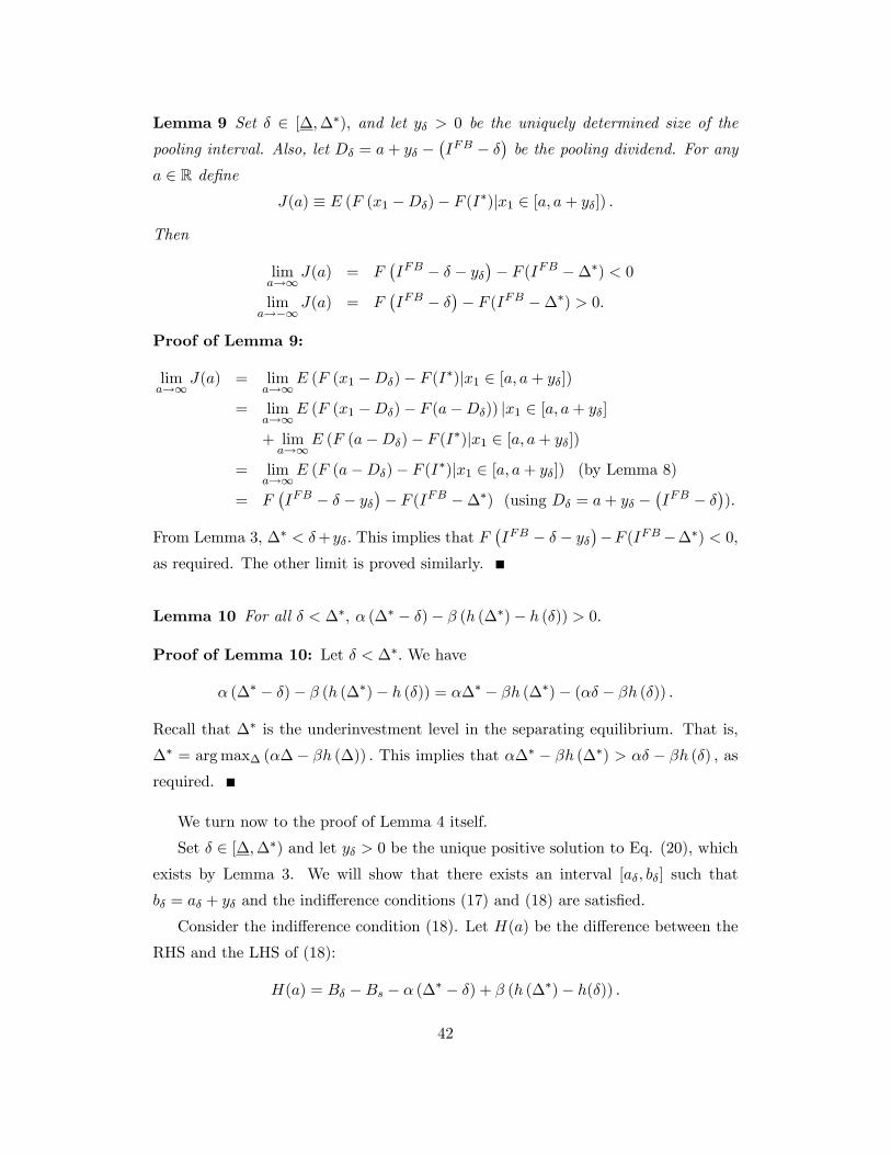
Lemma 9 Set � 2 [�;��); and let y� > 0 be the uniquely determined size of the

pooling interval. Also, let D� = a+ y� ��IFB � �

�be the pooling dividend. For any

a 2 R de�neJ(a) � E (F (x1 �D�)� F (I�)jx1 2 [a; a+ y�]) :

Then

lima!1

J(a) = F�IFB � � � y�

�� F (IFB ���) < 0

lima!�1

J(a) = F�IFB � �

�� F (IFB ���) > 0:

Proof of Lemma 9:

lima!1

J(a) = lima!1

E (F (x1 �D�)� F (I�)jx1 2 [a; a+ y�])

= lima!1

E (F (x1 �D�)� F (a�D�)) jx1 2 [a; a+ y�]

+ lima!1

E (F (a�D�)� F (I�)jx1 2 [a; a+ y�])

= lima!1

E (F (a�D�)� F (I�)jx1 2 [a; a+ y�]) (by Lemma 8)

= F�IFB � � � y�

�� F (IFB ���) (using D� = a+ y� �

�IFB � �

�):

From Lemma 3, �� < �+y�: This implies that F�IFB � � � y�

��F (IFB���) < 0,

as required. The other limit is proved similarly.

Lemma 10 For all � < ��; � (�� � �)� � (h (��)� h (�)) > 0:

Proof of Lemma 10: Let � < ��: We have

� (�� � �)� � (h (��)� h (�)) = ��� � �h (��)� (�� � �h (�)) :

Recall that �� is the underinvestment level in the separating equilibrium. That is,

�� = argmax� (��� �h (�)) : This implies that ��� � �h (��) > �� � �h (�) ; asrequired.

We turn now to the proof of Lemma 4 itself.

Set � 2 [�;��) and let y� > 0 be the unique positive solution to Eq. (20), whichexists by Lemma 3. We will show that there exists an interval [a�; b�] such that

b� = a� + y� and the indi¤erence conditions (17) and (18) are satis�ed.

Consider the indi¤erence condition (18). Let H(a) be the di¤erence between the

RHS and the LHS of (18):

H(a) = B� �Bs � � (�� � �) + � (h (��)� h(�)) :

42

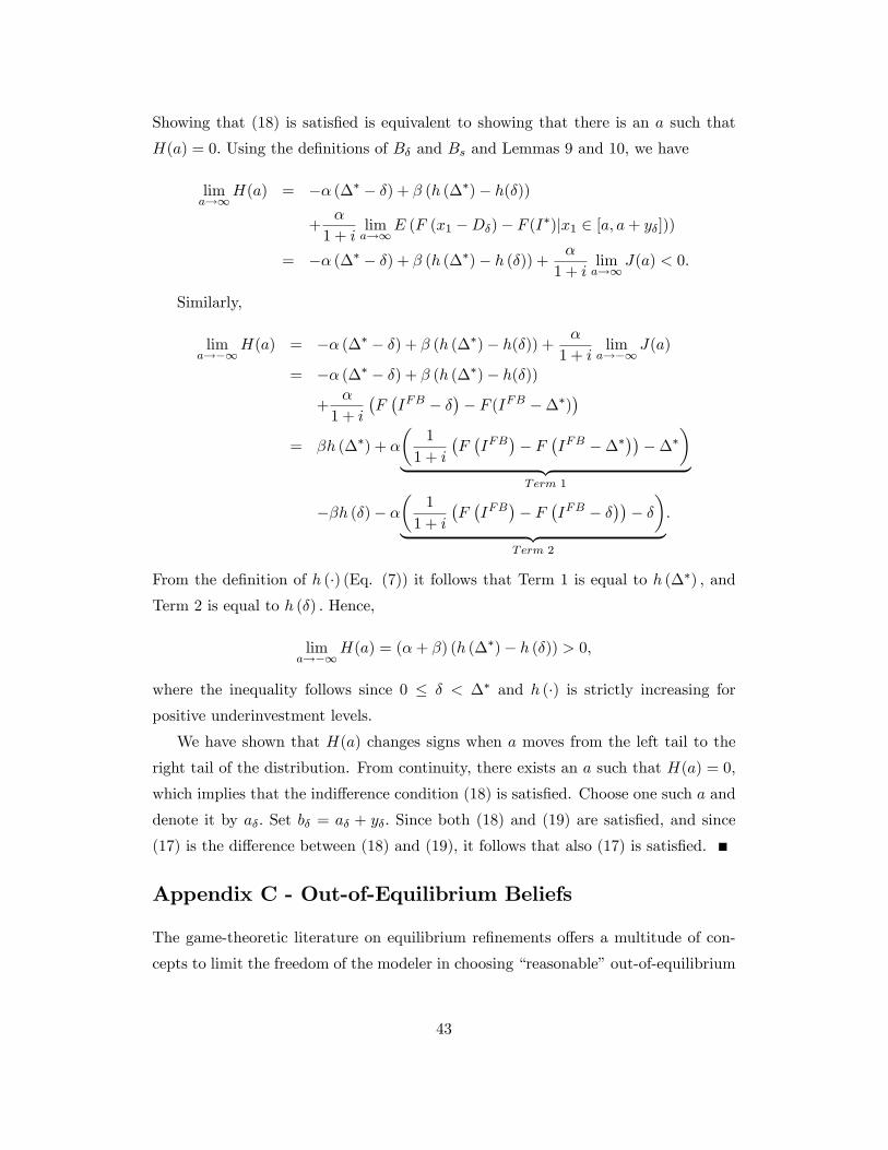
Showing that (18) is satis�ed is equivalent to showing that there is an a such that

H(a) = 0: Using the de�nitions of B� and Bs and Lemmas 9 and 10, we have

lima!1

H(a) = �� (�� � �) + � (h (��)� h(�))

+�

1 + ilima!1

E (F (x1 �D�)� F (I�)jx1 2 [a; a+ y�]))

= �� (�� � �) + � (h (��)� h (�)) + �

1 + ilima!1

J(a) < 0:

Similarly,

lima!�1

H(a) = �� (�� � �) + � (h (��)� h(�)) + �

1 + ilim

a!�1J(a)

= �� (�� � �) + � (h (��)� h(�))

+�

1 + i

�F�IFB � �

�� F (IFB ���)

�= �h (��) + �

�1

1 + i

�F�IFB

�� F

�IFB ���

�����

�| {z }

Term 1

��h (�)� ��

1

1 + i

�F�IFB

�� F

�IFB � �

��� ��

| {z }Term 2

:

From the de�nition of h (�) (Eq. (7)) it follows that Term 1 is equal to h (��) ; and

Term 2 is equal to h (�) : Hence,

lima!�1

H(a) = (�+ �) (h (��)� h (�)) > 0;

where the inequality follows since 0 � � < �� and h (�) is strictly increasing forpositive underinvestment levels.

We have shown that H(a) changes signs when a moves from the left tail to the

right tail of the distribution. From continuity, there exists an a such that H(a) = 0;

which implies that the indi¤erence condition (18) is satis�ed. Choose one such a and

denote it by a�: Set b� = a� + y�: Since both (18) and (19) are satis�ed, and since

(17) is the di¤erence between (18) and (19), it follows that also (17) is satis�ed.

Appendix C - Out-of-Equilibrium Beliefs

The game-theoretic literature on equilibrium re�nements o¤ers a multitude of con-

cepts to limit the freedom of the modeler in choosing �reasonable�out-of-equilibrium

43

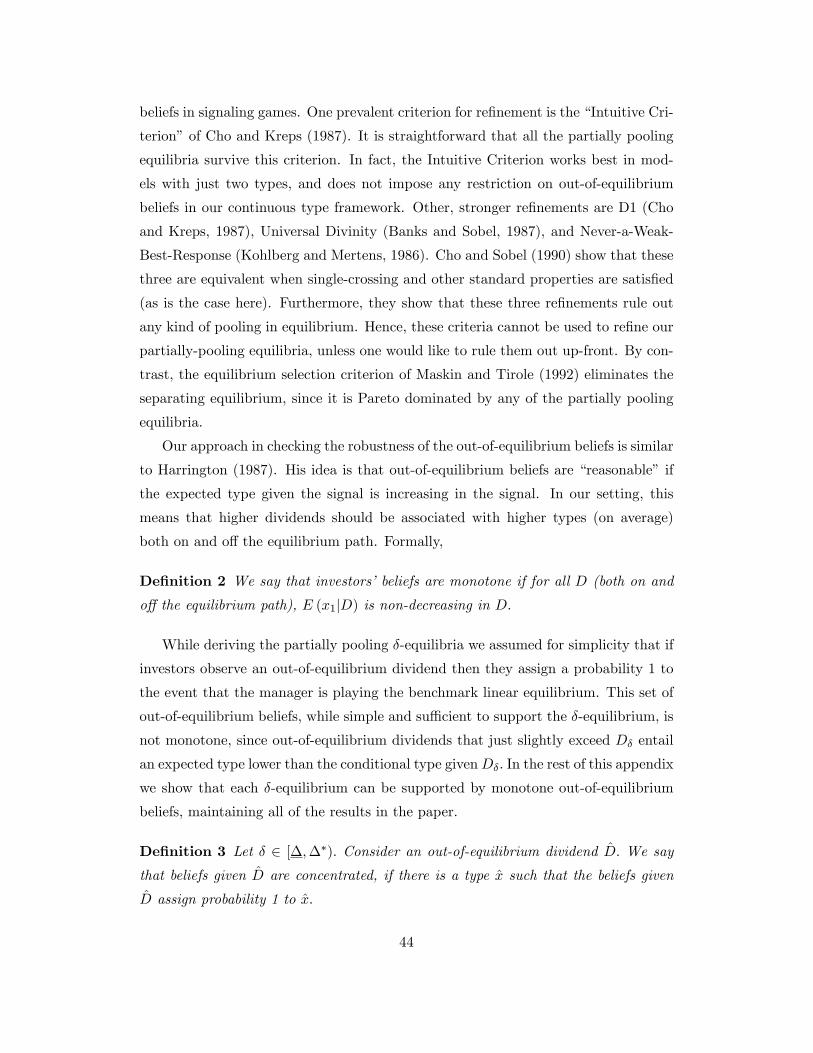
beliefs in signaling games. One prevalent criterion for re�nement is the �Intuitive Cri-

terion�of Cho and Kreps (1987). It is straightforward that all the partially pooling

equilibria survive this criterion. In fact, the Intuitive Criterion works best in mod-

els with just two types, and does not impose any restriction on out-of-equilibrium

beliefs in our continuous type framework. Other, stronger re�nements are D1 (Cho

and Kreps, 1987), Universal Divinity (Banks and Sobel, 1987), and Never-a-Weak-

Best-Response (Kohlberg and Mertens, 1986). Cho and Sobel (1990) show that these

three are equivalent when single-crossing and other standard properties are satis�ed

(as is the case here). Furthermore, they show that these three re�nements rule out

any kind of pooling in equilibrium. Hence, these criteria cannot be used to re�ne our

partially-pooling equilibria, unless one would like to rule them out up-front. By con-

trast, the equilibrium selection criterion of Maskin and Tirole (1992) eliminates the

separating equilibrium, since it is Pareto dominated by any of the partially pooling

equilibria.

Our approach in checking the robustness of the out-of-equilibrium beliefs is similar

to Harrington (1987). His idea is that out-of-equilibrium beliefs are �reasonable� if

the expected type given the signal is increasing in the signal. In our setting, this

means that higher dividends should be associated with higher types (on average)

both on and o¤ the equilibrium path. Formally,

De�nition 2 We say that investors�beliefs are monotone if for all D (both on and

o¤ the equilibrium path), E (x1jD) is non-decreasing in D:

While deriving the partially pooling �-equilibria we assumed for simplicity that if

investors observe an out-of-equilibrium dividend then they assign a probability 1 to

the event that the manager is playing the benchmark linear equilibrium. This set of

out-of-equilibrium beliefs, while simple and su¢ cient to support the �-equilibrium, is

not monotone, since out-of-equilibrium dividends that just slightly exceed D� entail

an expected type lower than the conditional type givenD�: In the rest of this appendix

we show that each �-equilibrium can be supported by monotone out-of-equilibrium

beliefs, maintaining all of the results in the paper.

De�nition 3 Let � 2 [�;��): Consider an out-of-equilibrium dividend D: We say

that beliefs given D are concentrated, if there is a type x such that the beliefs given

D assign probability 1 to x:

44

We will show that there is a concentrated set of out-of-equilibrium beliefs that is

also monotone.

Recall that all out of equilibrium dividends satisfy D 2�a� � I�; b� � IFB + �

�[�

b� � IFB + �; b� � I��: The single-crossing property suggests that if a� is indi¤erent

between its pooling dividend D� = b� � IFB + � and an out-of-equilibrium dividend

D 2�a� � I�; b� � IFB + �

�; then all types in the pooling interval (a�; b�) will strictly

prefer the pooling dividend. Similarly, if b� is indi¤erent between the pooling dividend

and an out-of-equilibrium dividend D 2�b� � IFB + �; b� � I�

�then all types in the

pooling interval strictly prefer the pooling dividend. Thus, a natural candidate for

a monotone and concentrated set of out-of-equilibrium beliefs is those beliefs that

render types a� and b� indi¤erent between the pooling divided and the appropriate

out-of-equilibrium dividend.

Let c� be implicitly de�ned by

F (c� �D�) = E (F (x�D�) jD�) : (30)

That is, if investors assign a probability 1 to the event that the manager�s type is

c�; then given a dividend of D� the market price would be the same as the market

price in the pooling dividend case. Clearly, c� 2 (a�; b�) : The uniqueness of c� is asimple application of the implicit function theorem. Consider an out-of-equilibrium

dividend D and a concentrated belief x 2 (a�; b�) : The market price given these twois

VM�x; D

�= D +

1

1 + iF�x� D

�:

Consider now an out-of-equilibrium dividend D 2�a� � I�; b� � IFB + �

�: Compare

the utility of a type a� manager who issues a dividend D to the utility of such a

manager if he issues the separating dividend. The former naturally depends on the

out-of-equilibrium beliefs. If beliefs are such that the market price is identical to the

separating price, then the manager obviously prefers the separating dividend to D

because the market price is identical, while the intrinsic value is lower given D: If, on

the other hand, beliefs are such that the market price is equal to VM (D�), then the

type a� manager strictly prefers D to the separating dividend. This follows since the

market price is identical now to the pooling dividend price, while the intrinsic value is

higher, and we know that a type a� is indi¤erent between separation and pooling. By

continuity, there is a market price P between the separating price of a� and VM (D�)

45

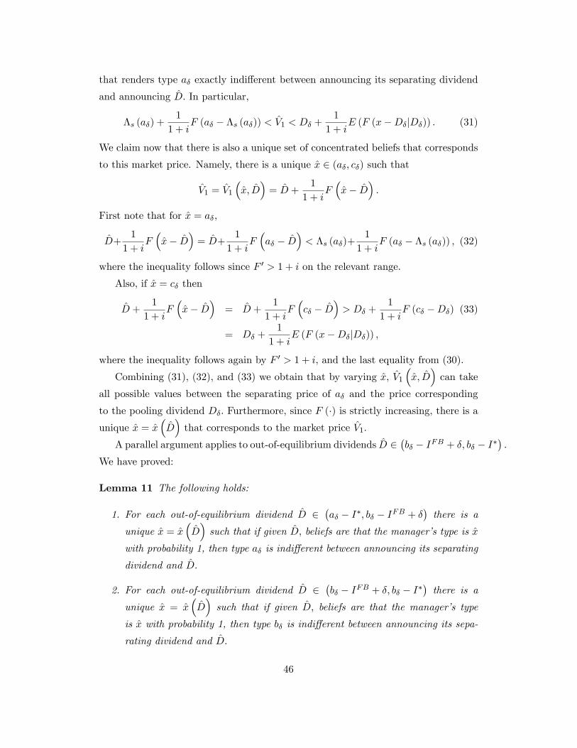
that renders type a� exactly indi¤erent between announcing its separating dividend

and announcing D: In particular,

�s (a�) +1

1 + iF (a� � �s (a�)) < V1 < D� +

1

1 + iE (F (x�D�jD�)) : (31)

We claim now that there is also a unique set of concentrated beliefs that corresponds

to this market price. Namely, there is a unique x 2 (a�; c�) such that

V1 = V1

�x; D

�= D +

1

1 + iF�x� D

�:

First note that for x = a�,

D+1

1 + iF�x� D

�= D+

1

1 + iF�a� � D

�< �s (a�)+

1

1 + iF (a� � �s (a�)) ; (32)

where the inequality follows since F 0 > 1 + i on the relevant range.

Also, if x = c� then

D +1

1 + iF�x� D

�= D +

1

1 + iF�c� � D

�> D� +

1

1 + iF (c� �D�) (33)

= D� +1

1 + iE (F (x�D�jD�)) ;

where the inequality follows again by F 0 > 1 + i, and the last equality from (30).

Combining (31), (32), and (33) we obtain that by varying x; V1�x; D

�can take

all possible values between the separating price of a� and the price corresponding

to the pooling dividend D�: Furthermore, since F (�) is strictly increasing, there is aunique x = x

�D�that corresponds to the market price V1:

A parallel argument applies to out-of-equilibrium dividends D 2�b� � IFB + �; b� � I�

�:

We have proved:

Lemma 11 The following holds:

1. For each out-of-equilibrium dividend D 2�a� � I�; b� � IFB + �

�there is a

unique x = x�D�such that if given D; beliefs are that the manager�s type is x

with probability 1, then type a� is indi¤erent between announcing its separating

dividend and D:

2. For each out-of-equilibrium dividend D 2�b� � IFB + �; b� � I�

�there is a

unique x = x�D�such that if given D; beliefs are that the manager�s type

is x with probability 1, then type b� is indi¤erent between announcing its sepa-

rating dividend and D:

46

From the derivation above, it is easy to see that x�D�is continuous at D� =

b� � IFB + � and strictly increasing everywhere:We have proved the following result:

Proposition 5 Let � 2 [�;��): There is a unique set of concentrated out-of-equilibriumbeliefs supporting the �-equilibrium, such that:

1. For each out-of-equilibrium dividend D 2�a� � I�; b� � IFB + �

�; type a� is in-

di¤erent between announcing D and announcing its separating dividend �s (a�) :

2. For each out-of-equilibrium dividend D 2�b� � IFB + �; a� � I�

�, type b� is in-

di¤erent between announcing D and announcing its separating dividend �s (b�) :

Furthermore, this set of beliefs is continuous and monotone increasing.

We can now replace the out-of-equilibrium beliefs used in Section 4 with the

monotone out-of-equilibrium beliefs derived in Proposition 5. The existence result is

then intact as are all of the other results in the paper.

Appendix D - Derivations for the Dynamic Setup

Preliminary Results

We start by developing results that enable us to calculate the conditional expectations

in (21). In the one period model, the prior distribution was normal, and the posterior

conditional on pooling was truncated normal. This is no longer the case in the

dynamic model. Instead, if a partially pooling equilibrium was played in period

t � 1 and a pooling dividend was announced; then earnings in period t (from the

point of view of the uninformed investors) follow a sum of a random variable with

a continuous distribution over a bounded support and a normal noise term. The

following results study the tail properties of such distributions, which are essential

for proving existence of equilibrium in the dynamic setup.

Let y > 0: Let ~w be a random variable with support in the form of a compact

interval [a; a+ y] and a continuous density �(w) for w 2 [a; a+ y]: Let ~" be normallydistributed random noise. For brevity, assume that ~" is standard normal, with density

� (�) : We are interested in the distribution of ~z � ~w + ~": Clearly ~z has continuous

density and its support is the entire real line; however, ~z is not normally distributed.

47

The density of ~z; h (z) ; is given by the convolution

h(z) =

Z a+y

a� (w)� (z � w)) dw: (34)

We �rst argue that while h (�) is not normal, it approaches the normal density inboth the left and the right tails. Formally,

Lemma 12 The following hold:

1. limz!1 jh (z)� � (z)j = 0:

2. limz!�1 jh (z)� � (z)j = 0:

Proof of Lemma 12: Note that for all z; � (z) =R a+ya � (w)� (z) dw: Hence;

h(z)� � (z) =Z a+y

a� (w) (� (z � w)� � (z))) dw:

Denote � zw � min fz � w; zg and �� zw � max (z � w; z) : By the mean value theorem,� (z � w)� � (z)) = �w�0 (�w) for some �w 2 (� zw; �� zw) : By the triangle inequalityfor integrals,

jh(z)� � (z)j =����Z a+y

a� (w)w�0 (�w) dw

���� � Z a+y

a� (w) jwj

���0 (�w)�� dw.Now, recall that the normal density satis�es �0 (z) < 0 and �00 (z) > 0 for all z

su¢ ciently large, and �0 (z) > 0 and �00 (z) < 0 for all z su¢ ciently small. For all

z su¢ ciently large �00 (z) > 0, hence���0 (�w)�� < ���0 (�� zw)�� : Consequently, for all z

su¢ ciently large

jh(z)� � (z)j <Z a+y

a� (w) jwj

���0 (�� zw)�� dw:Note that limz!1 �0 (�� zw) = 0: Hence, by Lebesgue�s dominated convergence the-

orem, limz!1 jh(z)� � (z)j = 0: In a similar manner, limz!�1 jh(z)� � (z)j = 0:

The following lemma shows a standard property of the normal density.

Lemma 13 For all t > 0; limc!1�(c+t)�(c) = 0 and limc!�1

�(c+t)�(c) =1:

48

The proof is immediate from the functional form of the normal density. Next we

show that the same property holds for h (�) : First, for each two real numbers c; wdenote

�c (w) ��(w)� (c� w)R a+y

a �(u)� (c� u) du:

Note that �c(w) is a probability measure over [a; a+ y]:

Lemma 14 For all t > 0; limc!1h(c+t)h(c) = 0 and limc!�1

h(c+t)h(c) =1:

Proof of Lemma 14: Using (34),

h(c+ t)

h (c)=

R a+ya �(w)� (c+ t� w) dwR a+ya �(w)� (c� w) dw

=

R a+ya �(w)� (c� w) �(c+t�w)�(c�w) dwR a+y

a �(w)� (c� w) dw

=

Z a+y

a�c (w)

� (c+ t� w)� (c� w) dw:

Note that �(c+t�w)�(c�w) is increasing in w; implying thatmaxa�w�a+y�(c+t�w)�(c�w) = �(c+t�a�y)

�(c�a�y) :

Consequently,

h(c+ t)

h (c)�Z a+y

a�c (w)

� (c+ t� a� y)� (c� a� y) dw =

� (c+ t� a� y)� (c� a� y) :

It follows that

0 � limc!1

h(c+ t)

h (c)� limc!1

� (c+ t� a� y)� (c� a� y) = 0;

where the last equality follows from Lemma 13. Thus, limc!1h(c+t)h(c) = 0: In a similar

way it can be shown that limc!�1h(c+t)h(c) =1:

The next lemma establishes an additional useful property of the normal density.

Lemma 15 Let t > 0: limc!1R c+tc

�(z)�(c)dz = 0 and limc!�1

R c+tc

�(z)�(c)dz =1:

Proof of Proposition 15: For any " 2 (0; t) and c su¢ ciently large we haveZ c+t

c

� (z)

� (c)dz =

Z c+"

c

� (z)

� (c)dz +

Z c+t

c+"

� (z)

� (c)dz

� "+� (c+ ")

� (c)(t� ") ( since

� (z)

� (c)� 1 on [c; c+ "] ).

Hence,

0 � limc!1

Z c+t

c

� (z)

� (c)dz � "+ lim

c!1� (c+ ")

� (c)(t� ") = " (by Lemma 13).

49

But, this is true for all " > 0 and hence limc!1R c+tc

�(z)�(c)dz = 0. A similar argument

applies to the other limit.

We can now establish the next lemma.

Lemma 16 Assume that h (z) is given by (34) : For all t > 0; limc!1E (z � cjz 2 [c; c+ t]) =0 and limc!�1E (z � c� tjz 2 [c; c+ t]) = 0:

Proof of Lemma 16:

limc!1

E (z � cjz 2 [c; c+ t]) = limc!1

R c+tc (z � c)h (z) dzR c+t

c h (z) dz:

By Lemma (12) both the numerator and the denominator tend to 0. By L�Hopital�s

rule:

limc!1

E (z � cjz 2 [c; c+ t]) = limc!1

t � h (c+ t)�R c+tc h (z) dz

h (c+ t)� h (c)

= t limc!1

1

1� h(c)h(c+t)

� limc!1

R c+tc

h(z)h(c)dz

h(c+t)h(c) � 1

The �rst limit is 0 by Lemma 14. Consider the second limit. The denominator tends

to �1 by Lemma 14. We claim that the numerator tends to zero. Indeed,Z c+t

c

h (z)

h (c)dz =

Z c+t

c

R a+ya �(w)� (z � w) dwR a+ya �(w)� (c� w) dw

dz =

Z c+t

c

Z a+y

a

� (c� w)�(w)R a+ya �(u)� (c� w) du

� (z � w)� (c� w)dwdz

�Z c+t

c

Z a+y

a

� (c� w)�(w)R a+ya �(u)� (c� w) du

� (z � a� y)� (c� a� y)dwdz =

Z c+t

c

� (z � a� y)� (c� a� y)dz:

However, by Lemma 15, limc!1R c+tc

�(z�a�y)�(c�a�y)dz = 0; implying that limc!1

R c+tc

h(z)h(c)dz =

0: It follows that limc!1E (z � cjz 2 [c; c+ t]) = 0 as required. The other limit is

proved in a similar manner.

Proof of Proposition 4

At each period t = 1; :::; T the manager maximizes (21). Hence, the objective function

of a manager in period t is identical to that of the static model, except that he takes

into account that investors condition the market price on all prior dividends. We will

show existence of equilibrium by induction. The case t = 1 coincides with the static

case. Using Proposition 2, choose some �1 < �� and consider the corresponding

�1-partially pooling equilibrium with a pooling interval [a�1 ; b�1 ].

50

Consider now the case t = 2: If a pooling dividend was paid in period 1, then

earnings in period 2 follow a distribution that is the sum of a random variable with

support [a�1;b�1 ] and "1. The density of this sum can be written using the convolution

in (34) : Lemma 16 then shows that the statement of Lemma 7 applies to this distri-

bution. It follows that the results of Lemma 4 hold for this distribution and hence so

do the results of Proposition 2. That is, there exists a �2 < �� and a corresponding

�2-equilibrium with a pooling interval [a�2 ; b�2 ] for the second period.

We now continue this process for all t = 3; ::; T: In each period we get a distri-

bution of earnings that is a sum of a random variable with a bounded support and

a normal noise, and the same procedure applies. This process generates a sequence

�1; �2; :::; �T and corresponding pooling intervals. The myopia of the manager and

investors guarantees that the sequence of short-term equilibria established in each

period is an equilibrium in the dynamic game.

51