A Theoretical Analysis of Contrastive Unsupervised ...A Theoretical Analysis of Contrastive Unsupervised Representation Learning Sanjeev Arora1 2 Hrishikesh Khandeparkar1 Mikhail Khodak3

A Theoretical Analysis of Contrastive Unsupervised Representation Learning

Sanjeev Arora 1 2 Hrishikesh Khandeparkar 1 Mikhail Khodak 3 Orestis Plevrakis 1 Nikunj Saunshi 1

arora,hrk,orestisp,[email protected] [email protected]

Abstract

Recent empirical works have successfully usedunlabeled data to learn feature representationsthat are broadly useful in downstream classifica-tion tasks. Several of these methods are remi-niscent of the well-known word2vec embeddingalgorithm: leveraging availability of pairs of se-mantically “similar” data points and “negativesamples,” the learner forces the inner product ofrepresentations of similar pairs with each other tobe higher on average than with negative samples.The current paper uses the term contrastive learn-ing for such algorithms and presents a theoreticalframework for analyzing them by introducing la-tent classes and hypothesizing that semanticallysimilar points are sampled from the same latentclass. This framework allows us to show provableguarantees on the performance of the learned rep-resentations on the average classification task thatis comprised of a subset of the same set of latentclasses. Our generalization bound also shows thatlearned representations can reduce (labeled) sam-ple complexity on downstream tasks. We conductcontrolled experiments in both the text and imagedomains to support the theory.

1. IntroductionThis paper concerns unsupervised representation learning:using unlabeled data to learn a representation function fsuch that replacing data point x by feature vector f(x) innew classification tasks reduces the requirement for labeleddata. This is distinct from semi-supervised learning, wherelearning can leverage unlabeled as well as labeled data.(Section 7 surveys other prior ideas and models).

For images, a proof of existence for broadly useful represen-tations is the output of the penultimate layer (the one before

1Princeton University, Princeton, New Jersey, USA. 2Institute forAdvanced Study, Princeton, New Jersey, USA. 3Carnegie MellonUniversity, Pittsburgh, Pennsylvania, USA.

Copyright 2019 by the authors.

the softmax) of a powerful deep net trained on ImageNet.In natural language processing (NLP), low-dimensional rep-resentations of text – called text embeddings – have beencomputed with unlabeled data (Peters et al., 2018; Devlinet al., 2018). Often the embedding function is trained byusing the embedding of a piece of text to predict the sur-rounding text (Kiros et al., 2015; Logeswaran & Lee, 2018;Pagliardini et al., 2018). Similar methods that leverage simi-larity in nearby frames in a video clip have had some successfor images as well (Wang & Gupta, 2015).

Many of these algorithms are related: they assume access topairs or tuples (in the form of co-occurrences) of text/imagesthat are more semantically similar than randomly sampledtext/images, and their objective forces representations torespect this similarity on average. For instance, in order tolearn a representation function f for sentences, a simplifiedversion of what Logeswaran & Lee (2018) minimize is thefollowing loss function

Ex,x+,x−

[− log

(ef(x)T f(x+)

ef(x)T f(x+) + ef(x)T f(x−)

)]

where (x, x+) are a similar pair and x− is presumably dis-similar to x (often chosen to be a random point) and typi-cally referred to as a negative sample. Though reminiscentof past ideas – e.g. kernel learning, metric learning, co-training (Cortes et al., 2010; Bellet et al., 2013; Blum &Mitchell, 1998) – these algorithms lack a theoretical frame-work quantifying when and why they work. While it seemsintuitive that minimizing such loss functions should leadto representations that capture ‘similarity,’ formally it isunclear why the learned representations should do well ondownstream linear classification tasks – their somewhatmysterious success is often treated as an obvious conse-quence. To analyze this success, a framework must connect‘similarity’ in unlabeled data with the semantic informationthat is implicitly present in downstream tasks.

We propose the term Contrastive Learning for such methodsand provide a new conceptual framework with minimalassumptions1. Our main contributions are the following:

1The alternative would be to make assumptions about genera-tive models of data. This is difficult for images and text.

arX

iv:1

902.

0922

9v1

[cs

.LG

] 2

5 Fe

b 20

19

Contrastive Unsupervised Representation Learning

1. We formalize the notion of semantic similarity by in-troducing latent classes. Similar pairs are assumed tobe drawn from the same latent class. A downstreamtask is comprised of a subset of these latent classes.

2. Under this formalization, we prove that a representa-tion function f learned from a function class F by con-trastive learning has low average linear classificationloss if F contains a function with low unsupervisedloss. Additionally, we show a generalization bound forcontrastive learning that depends on the Rademachercomplexity of F . After highlighting inherent limita-tions of negative sampling, we show sufficient proper-ties of F which allow us to overcome these limitations.

3. Using insights from the above framework, we providea novel extension of the algorithm that can leveragelarger blocks of similar points than pairs, has bettertheoretical guarantees, and performs better in practice.

Ideally, one would like to show that contrastive learning al-ways gives representations that compete with those learnedfrom the same function class with plentiful labeled data.Our formal framework allows a rigorous study of such ques-tions: we show a simple counterexample that prevents sucha blanket statement without further assumptions. However,if the representations are well-concentrated and the meanclassifier (Definition 2.1) has good performance, we canshow a weaker version of the ideal result (Corollary 5.1.1).Sections 2 and 3 give an overview of the framework and theresults, and subsequent sections deal with the analysis. Re-lated work is discussed in Section 7 and Section 8 describesexperimental verification and support for our framework.

2. Framework for Contrastive LearningWe first set up notation and describe the framework forunlabeled data and classification tasks that will be essentialfor our analysis. Let X denote the set of all possible datapoints. Contrastive learning assumes access to similar datain the form of pairs (x, x+) that come from a distributionDsim as well as k i.i.d. negative samples x−1 , x

−2 , . . . , x

−k

from a distribution Dneg that are presumably unrelated to x.Learning is done over F , a class of representation functionsf : X → Rd, such that ‖f(·)‖ ≤ R for some R > 0.

Latent Classes

To formalize the notion of semantically similar pairs(x, x+), we introduce the concept of latent classes.

Let C denote the set of all latent classes. Associated witheach class c ∈ C is a probability distribution Dc over X .

Roughly, Dc(x) captures how relevant x is to class c. Forexample, X could be natural images and c the class “dog”whose associated Dc assigns high probability to images

containing dogs and low/zero probabilities to other images.Classes can overlap arbitrarily.2 Finally, we assume a distri-bution ρ over the classes that characterizes how these classesnaturally occur in the unlabeled data. Note that we make noassumption about the functional form of Dc or ρ.

Semantic Similarity

To formalize similarity, we assume similar data points x, x+

are i.i.d. draws from the same class distributionDc for someclass c picked randomly according to measure ρ. Negativesamples are drawn from the marginal of Dsim:

Dsim(x, x+) = Ec∼ρDc(x)Dc(x+) (1)

Dneg(x−) = Ec∼ρDc(x−) (2)

Since classes are allowed to overlap and/or be fine-grained,this is a plausible formalization of “similarity.” As the iden-tity of the class in not revealed, we call it unlabeled data.Currently empirical works heuristically identify such similarpairs from co-occurring image or text data.

Supervised Tasks

We now characterize the tasks that a representation functionf will be tested on. A (k + 1)-way3 supervised task Tconsists of distinct classes c1, . . . , ck+1 ⊆ C. The labeleddataset for the task T consists of m i.i.d. draws from thefollowing process:

A label c ∈ c1, ..., ck+1 is picked according to a distribu-tion DT . Then, a sample x is drawn from Dc. Together theyform a labeled pair (x, c) with distribution

DT (x, c) = Dc(x)DT (c) (3)

A key subtlety in this formulation is that the classes indownstream tasks and their associated data distributions Dcare the same as in the unlabeled data. This provides a path toformalizing how capturing similarity in unlabeled data canlead to quantitative guarantees on downstream tasks. DT isassumed to be uniform4 for theorems in the main paper.

Evaluation Metric for Representations

The quality of the representation function f is evaluatedby its performance on a multi-class classification task Tusing linear classification. For this subsection, we fix atask T = c1, ..., ck+1. A multi-class classifier for T isa function g : X → Rk+1 whose output coordinates areindexed by the classes c in task T .

The loss incurred by g on point (x, y) ∈ X × T is defined

2An image of a dog by a tree can appear in bothDdog &Dtree.3We use k as the number of negative samples later.4We state and prove the general case in the Appendix.


as `(g(x)y − g(x)y′y′ 6=y), which is a function of a k-dimensional vector of differences in the coordinates. Thetwo losses we will consider in this work are the standardhinge loss `(v) = max0, 1+maxi−vi and the logisticloss `(v) = log2 (1 +

∑i exp(−vi)) for v ∈ Rk. Then the

supervised loss of the classifier g is

Lsup(T , g) := E(x,c)∼DT

[`(g(x)c − g(x)c′c′ 6=c

)]To use a representation function f with a linear classifier,a matrix W ∈ R(k+1)×d is trained and g(x) = Wf(x) isused to evaluate classification loss on tasks. Since the bestW can be found by fixing f and training a linear classifier,we abuse notation and define the supervised loss of f on Tto be the loss when the best W is chosen for f :

Lsup(T , f) = infW∈R(k+1)×d

Lsup(T ,Wf) (4)

Crucial to our results and experiments will be a specific Wwhere the rows are the means of the representations of eachclass which we define below.Definition 2.1 (Mean Classifier). For a function f and taskT = (c1, . . . , ck+1), the mean classifier is Wµ whose cth

row is the mean µc of representations of inputs with label c:µc := E

x∼Dc[f(x)]. We use Lµsup(T , f) := Lsup(T ,Wµf)

as shorthand for its loss.

Since contrastive learning has access to data with latentclass distribution ρ, it is natural to have better guaranteesfor tasks involving classes that have higher probability in ρ.Definition 2.2 (Average Supervised Loss). Average loss fora function f on (k + 1)-way tasks is defined as

Lsup(f) := Ecik+1

i=1∼ρk+1

[Lsup(cik+1

i=1 , f) | ci 6= cj]

The average supervised loss of its mean classifier is

Lµsup(f) := Ecik+1

i=1∼ρk+1

[Lµsup(cik+1

i=1 , f) | ci 6= cj]

Contrastive Learning Algorithm

We describe the training objective for contrastive learning:the choice of loss function is dictated by the ` used inthe supervised evaluation, and k denotes number of neg-ative samples used for training. Let (x, x+) ∼ Dsim,(x−1 , .., x

−k ) ∼ Dkneg as defined in Equations (1) and (2).

Definition 2.3 (Unsupervised Loss). The population loss is

Lun(f) := E[`(f(x)T

(f(x+)− f(x−i )

)ki=1

) ](5)

and its empirical counterpart with M samples(xj , x

+j , x

−j1, ..., x

−jk)Mj=1 from Dsim ×Dkneg is

Lun(f) =1

M

M∑j=1

`(f(xj)

T(f(x+

j )− f(x−ji))ki=1

)(6)

Note that, by the assumptions of the framework describedabove, we can now express the unsupervised loss as

Lun(f)

= Ec+,c−i∼ρk+1

Ex,x+∼D2

c+

x−i ∼Dc−i

[`(f(x)T

(f(x+)− f(x−i )

))]

The algorithm to learn a representation function from F isto find a function f ∈ arg minf∈F Lun(f) that minimizesthe empirical unsupervised loss. This function f can besubsequently used for supervised linear classification tasks.In the following section we proceed to give an overview ofour results that stem from this framework.

3. Overview of Analysis and Results

What can one provably say about the performance of f?As a first step we show that Lun is like a “surrogate” forLsup by showing that Lsup(f) ≤ αLun(f),∀f ∈ F , sug-gesting that minimizing Lun makes sense. This lets usshow a bound on the supervised performance Lsup(f) ofthe representation learned by the algorithm. For instance,when training with one negative sample, the performance onaverage binary classification has the following guarantee:

Theorem 4.1 (Informal binary version).

Lsup(f) ≤ αLun(f) + η GenM + δ ∀f ∈ F

where α, η, δ are constants depending on the distributionρ and GenM → 0 as M → ∞. When ρ is uniform and|C| → ∞, we have that α, η → 1, δ → 0.

At first glance, this bound seems to offer a somewhat com-plete picture: When the number of classes is large, if theunsupervised loss can be made small by F , then the super-vised loss of f , learned using finite samples, is small.

While encouraging, this result still leaves open the question:Can Lun(f) indeed be made small on reasonable datasetsusing function classes F of interest, even though the similarpair and negative sample can come from the same latentclass? We shed light on this by upper-bounding Lun(f) bytwo components: (a) the loss L6=un(f) for the case where thepositive and negative samples are from different classes; (b)a notion of deviation s(f), within each class.

Theorem 4.5 (Informal binary version).

Lsup(f) ≤ L6=un(f) + βs(f) + η GenM ∀f ∈ F

for constants β, η that depend on the distribution ρ. Again,when ρ is uniform and |C| → ∞ we have β → 0, η → 1.

This bound lets us infer the following: if the class F is richenough to contain a function f for which L6=un(f)+βs(f) is


low, then f has high supervised performance. Both L6=un(f)and s(f) can potentially be made small for rich enough F .

Ideally, however, one would want to show that f can com-pete on classification tasks with every f ∈ F

(Ideal Result): Lsup(f) ≤ αLsup(f) + η GenM (7)

Unfortunately, we show in Section 5.1 that the algorithmcan pick something far from the optimal f . However, weextend Theorem 4.5 to a bound similar to (7) (where theclassification is done using the mean classifier) under as-sumptions about the intraclass concentration of f and aboutits mean classifier having high margin.

Sections 6.1 and 6.2 extend our results to the more compli-cated setting where the algorithm uses k negative samples(5) and note an interesting behavior: increasing the num-ber of negative samples beyond a threshold can hurt theperformance. In Section 6.3 we show a novel extension ofthe algorithm that utilizes larger blocks of similar points.Finally, we perform controlled experiments in Section 8 tovalidate components of our framework and corroborate oursuspicion that the mean classifier of representations learnedusing labeled data has good classification performance.

4. Guaranteed Average Binary ClassificationTo provide the main insights, we prove the algorithm’s guar-antee when we use only 1 negative sample (k = 1). Forthis section, let Lsup(f) and Lµsup(f) be as in Definition2.2 for binary tasks. We will refer to the two classes in thesupervised task as well as the unsupervised loss as c+, c−.Let S = xj , x+

j , x−j Mj=1 be our training set sampled from

the distributionDsim×Dneg and f ∈ arg minf∈F Lun(f).

4.1. Upper Bound using Unsupervised Loss

Let f|S =(ft(xj), ft(x

+j ), ft(x

−j ))j∈[M ],t∈[d]

∈ R3dM bethe restriction on S for any f ∈ F . Then, the statisticalcomplexity measure relevant to the estimation of the repre-sentations is the following Rademacher average

RS(F) = Eσ∼±13dM

[supf∈F〈σ, f|S〉

]Let τ = E

c,c′∼ρ21c = c′ be the probability that two classes

sampled independently from ρ are the same.Theorem 4.1. With probability at least 1− δ, for all f ∈ F

Lµsup(f) ≤ 1

(1− τ)(Lun(f)− τ) +

1

(1− τ)GenM

where

GenM = O

RRS(F)

M+R2

√log 1

δ

M

Remark. The complexity measureRS(F) is tightly relatedto the labeled sample complexity of the classification tasks.For the function class G = wT f(·)|f ∈ F , ‖w‖ ≤ 1that one would use to solve a binary task from scratch usinglabeled data, it can be shown that RS(F) ≤ dRS(G),whereRS(G) is the usual Rademacher complexity of G onS (Definition 3.1 from (Mohri et al., 2018)).

We state two key lemmas needed to prove the theorem.

Lemma 4.2. With probability at least 1−δ over the trainingset S, for all f ∈ F

Lun(f) ≤ Lun(f) +GenM

We prove Lemma 4.2 in Appendix A.3.

Lemma 4.3. For all f ∈ F

Lµsup(f) ≤ 1

(1− τ)(Lun(f)− τ)

Proof. The key idea in the proof is the use of Jensen’s in-equality. Unlike the unsupervised loss which uses a randompoint from a class as a classifier, using the mean of theclass as the classifier should only make the loss lower. Letµc = E

x∼Dcf(x) be the mean of the class c.

Lun(f) = E(x,x+)∼Dsimx−∼Dneg

[`(f(x)T (f(x+)− f(x−)))

]=(a) E

c+,c−∼ρ2x∼Dc+

Ex+∼Dc+x−∼Dc−

[`(f(x)T (f(x+)− f(x−)))

]≥(b) E

c+,c−∼ρ2E

x∼Dc+

[`(f(x)T (µc+ − µc−))

]=(c) (1− τ) E

c+,c−∼ρ2[Lµsup(c+, c−, f)|c+ 6= c−] + τ

=(d) (1− τ)Lµsup(f) + τ

where (a) follows from the definitions in (1) and (2), (b)follows from the convexity of ` and Jensen’s inequality bytaking the expectation over x+, x− inside the function, (c)follows by splitting the expectation into the cases c+ = c−

and c+ 6= c−, from symmetry in c+ and c− in samplingand since classes in tasks are uniformly distributed (generaldistributions are handled in Appendix B.1). Rearrangingterms completes the proof.

Proof of Theorem 4.1. The result follows directly by apply-ing Lemma 4.3 for f and finishing up with Lemma 4.2.

One could argue that if F is rich enough such that Lun canbe made small, then Theorem 4.1 suffices. However, in thenext section we explain that unless τ 1, this may notalways be possible and we show one way to alleviate this.


4.2. Price of Negative Sampling: Class Collision

Note first that the unsupervised loss can be decomposed as

Lun(f) = τL=un(f) + (1− τ)L6=un(f) (8)

where L 6=un(f) is the loss suffered when the similar pair andthe negative sample come from different classes.

L6=un(f)

= Ec+,c−∼ρ2x,x+∼D2

c+

x−∼Dc−

[`(f(x)T (f(x+)− f(x−)))|c+ 6= c−

]

and L=un(f) is when they come from the same class. Let ν

be a distribution over C with ν(c) ∝ ρ2(c), then

L=un(f) = E

c∼νx,x+,x−∼D3

c

[`(f(x)T (f(x+)− f(x−)))

]≥ Ec∼ν,x∼Dc

[`(f(x)T (µc − µc))

]= 1

by Jensen’s inequality again, which implies Lun(f) ≥ τ . Ingeneral, without any further assumptions on f , Lun(f) canbe far from τ , rendering the bound in Theorem 4.1 useless.However, as we will show, the magnitude of L=

un(f) canbe controlled by the intraclass deviation of f . Let Σ(f, c)the covariance matrix of f(x) when x ∼ Dc. We define anotion of intraclass deviation as follows:

s(f) := Ec∼ν

[√‖Σ(f, c)‖2 E

x∼Dc‖f(x)‖

](9)

Lemma 4.4. For all f ∈ F ,

L=un(f)− 1 ≤ c′s(f)

where c′ is a positive constant.

We prove Lemma 4.4 in Appendix A.1. Theorem 4.1 com-bined with Equation (8) and Lemma 4.4 gives the followingresult.

Theorem 4.5. With probability at least 1− δ, ∀f ∈ F

Lsup(f) ≤ Lµsup(f) ≤ L6=un(f) + β s(f) + η GenM

where β = c′ τ1−τ , η = 1

1−τ and c′ is a constant.

The above bound highlights two sufficient properties of thefunction class for unsupervised learning to work: when thefunction class F is rich enough to contain some f with lowβs(f) as well as low L6=un(f) then f , the empirical mini-mizer of the unsupervised loss – learned using sufficientlylarge number of samples – will have good performance onsupervised tasks (low Lsup(f)).

5. Towards Competitive GuaranteesWe provide intuition and counter-examples for why con-trastive learning does not always pick the best supervisedrepresentation f ∈ F and show how our bound capturesthese. Under additional assumptions, we show a competitivebound where classification is done using the mean classifier.

5.1. Limitations of contrastive learning

The bound provided in Theorem 4.5 might not appear as themost natural guarantee for the algorithm. Ideally one wouldlike to show a bound like the following: for all f ∈ F ,

(Ideal 1): Lsup(f) ≤ αLsup(f) + η GenM (10)

for constants α, η and generalization error GenM . Thisguarantees that f is competitive against the best f on theaverage binary classification task. However, the bound weprove has the following form: for all f ∈ F ,

Lµsup(f) ≤ αL6=un(f) + βs(f) + η GenM

To show that this discrepancy is not an artifact of our anal-ysis but rather stems from limitations of the algorithm, wepresent two examples in Figure 1. Our bound appropriatelycaptures these two issues individually owing to the largevalues of L6=(f) or s(f) in each case, for the optimal f .

In Figure 1a, we see that there is a direction on which f1

can be projected to perfectly separate the classes. Since thealgorithm takes inner products between the representations,it inevitably considers the spurious components along theorthogonal directions. This issue manifests in our bound asthe term L6=un(f1) being high even when s(f1) = 0. Hence,contrastive learning will not always work when the onlyguarantee we have is that F can make Lsup small.

This should not be too surprising, since we show a relativelystrong guarantee – a bound on Lµsup for the mean classifierof f . This suggests a natural stronger assumption that Fcan make Lµsup small (which is observed experimentallyin Section 8 for function classes of interest) and raises thequestion of showing a bound that looks like the following:for all f ∈ F ,

(Ideal 2): Lµsup(f) ≤ αLµsup(f) + ηGenM (11)

without accounting for any intraclass deviation – recall thats(f) captures a notion of this deviation in our bound. How-ever this is not true: high intraclass deviation may not implyhigh Lµsup(f), but can make L=

un(f) (and thus Lun(f))high, resulting in the failure of the algorithm. Consequently,the term s(f) also increases while L6=un does not necessarilyhave to. This issue, apparent in Figure 1b, shows that a guar-antee like (11) cannot be shown without further assumptions.


(a) Mean is bad (b) High intraclass variance

Figure 1. In both examples we have uniform distribution overclasses C = c1, c2, blue and red points are in c1 and c2 re-spectively and Dci is uniform over the points of ci. In the firstfigure we have one point per class, while in the second we havetwo points per class. Let F = f0, f1 where f0 maps all pointsto (0, 0) and f1 is defined in the figure. In both cases, using thehinge loss, Lsup(f1) = 0, Lsup(f0) = 1 and in the second caseLµsup(f1) = 0. However, in both examples the algorithm will pickf0 since Lun(f0) = 1 but Lun(f1) = Ω(r2).

5.2. Competitive Bound via Intraclass Concentration

We saw that Lµsup(f) being small does not imply lowLµsup(f), if f is not concentrated within the classes. Inthis section we show that when there is an f that has intra-class concentration in a strong sense (sub-Gaussianity) andcan separate classes with high margin (on average) with themean classifier, then Lµsup(f) will be low.

Let `γ(x) = (1− xγ )+ be the hinge loss with margin γ and

Lµγ,sup(f) be Lµsup(f) with the loss function `γ .

Lemma 5.1. For f ∈ F , if the random variable f(X),where X ∼ Dc, is σ2-sub-Gaussian in every direction forevery class c and has maximum normR = maxx∈X ‖f(x)‖,then for all ε > 0,

L 6=un(f) ≤ γLµγ,sup(f) + ε

where γ = 1 + c′Rσ√

log Rε and c′ is some constant.

The proof of Lemma 5.1 is provided in the Appendix A.2.Using Lemma 5.1 and Theorem 4.5, we get the following:

Corollary 5.1.1. For all ε > 0, with probability at least1− δ, for all f ∈ F ,

Lµsup(f) ≤ γ(f)Lµγ(f),sup(f) + βs(f) + ηGenM + ε

where γ(f) is as defined in Lemma 5.1, β = c′ τ1−τ ,

η = τ1−τ and c′ is a constant.

6. Multiple Negative Samples and BlockSimilarity

In this section we explore two extensions to our analysis.First, in Section 6.1, inspired by empirical works like Lo-

geswaran & Lee (2018) that often use more than one nega-tive sample for every similar pair, we show provable guar-antees for this case by careful handling of class collision.Additionally, in Section 6.2 we show simple examples whereincreasing negative samples beyond a certain threshold canhurt contrastive learning. Second, in Section 6.3, we ex-plore a modified algorithm that leverages access to blocksof similar data, rather than just pairs and show that it hasstronger guarantees as well as performs better in practice.

6.1. Guarantees for k Negative Samples

Here the algorithm utilizes k negative samples x−1 , ..., x−k

drawn i.i.d. from Dneg for every positive sample pair x, x+

drawn from Dsim and minimizes (6). As in Section 4, weprove a bound for f of the following form:

Theorem 6.1. (Informal version) For all f ∈ F

Lsup(f) ≤ Lµsup(f) ≤ αL6=un(f) + βs(f) + η GenM

where L6=un(f) and GenM are extensions of the correspond-ing terms from Section 4 and s(f) remains unchanged. Theformal statement of the theorem and its proof appears inAppendix B.1. The key differences from Theorem 4.5 are βand the distribution of tasks in Lsup that we describe below.The coefficient β of s(f) increases with k, e.g. when ρ isuniform and k |C|, β ≈ k

|C| .

The average supervised loss that we bound is

Lsup(f) := ET ∼D

[Lsup(T , f)

]where D is a distribution over tasks, defined as follows:sample k + 1 classes c+, c−1 , . . . , c

−k ∼ ρk+1, conditioned

on the event that c+ does not also appear as a negativesample. Then, set T to be the set of distinct classes inc+, c−1 , . . . , c

−k . Lµsup(f) is defined by using Lµsup(T , f).

Remark. Bounding Lsup(f) directly gives a bound foraverage (k + 1)-wise classification loss Lsup(f) from Def-inition 2.2, since Lsup(f) ≤ Lsup(f)/p, where p is theprobability that the k + 1 sampled classes are distinct. Fork |C| and ρ ≈ uniform, these metrics are almost equal.

We also extend our competitive bound from Section 5.2 forthe above f in Appendix B.2.

6.2. Effect of Excessive Negative Sampling

The standard belief is that increasing the number of negativesamples always helps, at the cost of increased computationalcosts. In fact for Noise Contrastive Estimation (NCE) (Gut-mann & Hyvarinen, 2010), which is invoked to explain thesuccess of negative sampling, increasing negative sampleshas shown to provably improve the asymptotic variance of


the learned parameters. However, we find that such a phe-nomenon does not always hold for contrastive learning –larger k can hurt performance for the same inherent reasonshighlighted in Section 5.1, as we illustrate next.

When ρ is close to uniform and the number of negativesamples is k = Ω(|C|), frequent class collisions can preventthe unsupervised algorithm from learning the representationf ∈ F that is optimal for the supervised problem. In thiscase, owing to the contribution of s(f) being high, a largenumber of negative samples could hurt. This problem, infact, can arise even when the number of negative samplesis much smaller than the number of classes. For instance,if the best representation function f ∈ F groups classesinto t “clusters”,5 such that f cannot contrast well betweenclasses from the same cluster, then L6=un will contribute tothe unsupervised loss being high even when k = Ω(t). Weillustrate, by examples, how these issues can lead to pickingsuboptimal f in Appendix C. Experimental results in Fig-ures 2a and 2b also suggest that larger negative samples hurtperformance beyond a threshold, confirming our suspicions.

6.3. Blocks of Similar Points

Often a dataset consists of blocks of similar data insteadof just pairs: a block consists of x0, x1, . . . xb that are i.i.d.draws from a class distribution Dc for a class c ∼ ρ. Intext, for instance, paragraphs can be thought of as a blockof sentences sampled from the same latent class. How canan algorithm leverage this additional structure?

We propose an algorithm that uses two blocks: one forpositive samples x, x+

1 , . . . , x+b that are i.i.d. samples from

c+ ∼ ρ and another one of negative samples x−1 , . . . x−b that

are i.i.d. samples from c− ∼ ρ. Our proposed algorithmthen minimizes the following loss:

Lblockun (f) :=

E[`

(f(x)T

(∑i f(x+

i )

b−∑i f(x−i )

b

))] (12)

To understand why this loss function make sense, recall thatthe connection between Lµsup and Lun was made in Lemma4.3 by applying Jensen’s inequality. Thus, the algorithmthat uses the average of the positive and negative samplesin blocks as a proxy for the classifier instead of just onepoint each should have a strictly better bound owing tothe Jensen’s inequality getting tighter. We formalize thisintuition below. Let τ be as defined in Section 4.Proposition 6.2. ∀f ∈ F

Lsup(f) ≤ 1

1− τ(Lblockun (f)− τ

)≤ 1

1− τ(Lun(f)− τ)

This bound tells us that Lblockun is a better surrogate for Lsup,

5This can happen when F is not rich enough.

making it a more attractive choice than Lun when largerblocks are available.6. The algorithm can be extended, anal-ogously to Equation (5), to handle more than one negativeblock. Experimentally we find that minimizing Lblockun in-stead of Lun can lead to better performance and our resultsare summarized in Section 8.2. We defer the proof of Propo-sition 6.2 to Appendix A.4.

7. Related WorkThe contrastive learning framework is inspired by severalempirical works, some of which were mentioned in theintroduction. The use of co-occurring words as semanti-cally similar points and negative sampling for learning wordembeddings was introduced in Mikolov et al. (2013). Subse-quently, similar ideas have been used by Logeswaran & Lee(2018) and Pagliardini et al. (2018) for sentences representa-tions and by Wang & Gupta (2015) for images. Notably thesentence representations learned by the quick thoughts (QT)method in Logeswaran & Lee (2018) that we analyze hasstate-of-the-art results on many text classification tasks. Pre-vious attempts have been made to explain negative sampling(Dyer, 2014) using the idea of Noise Contrastive Estima-tion (NCE) (Gutmann & Hyvarinen, 2010) which relies onthe assumption that the data distribution belongs to someknown parametric family. This assumption enables them toconsider a broader class of distributions for negative sam-pling. The mean classifier that appears in our guarantees isof significance in meta-learning and is a core component ofProtoNets (Snell et al., 2017).

Our data model for similarity is reminiscent of the one inco-training (Blum & Mitchell, 1998). They assume accessto pairs of “views” with the same label that are conditionallyindependent given the label. Our unlabeled data model canbe seen as a special case of theirs, where the two views havethe same conditional distributions. However, they addition-ally assume access to some labeled data (semi-supervised),while we learn representations using only unlabeled data,which can be subsequently used for classification when la-beled data is presented. Two-stage kernel learning (Corteset al., 2010; Kumar et al., 2012) is similar in this sense: inthe first stage, a positive linear combination of some basekernels is learned and is then used for classification in thesecond stage; they assume access to labels in both stages.Similarity/metric learning (Bellet et al., 2012; 2013) learnsa linear feature map that gives low distance to similar pointsand high to dissimilar. While they identify dissimilar pairsusing labels, due to lack of labels we resort to negative sam-pling and pay the price of class collision. While these worksanalyze linear function classes, we can handle arbitrarilypowerful representations. Learning of representations that

6Rigorous comparison of the generalization errors is left forfuture work.


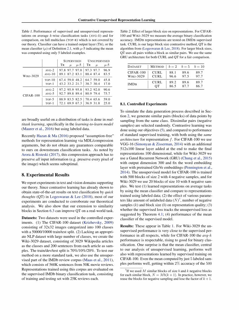
Table 1. Performance of supervised and unsupervised represen-tations on average k-wise classification tasks (AVG-k) and forcomparison, on full multiclass (TOP-R) which is not covered byour theory. Classifier can have a trained output layer (TR), or themean classifier (µ) of Definition 2.1, with µ-5 indicating the meanwas computed using only 5 labeled examples.

SUPERVISED UNSUPERVISEDTR µ µ-5 TR µ µ-5

WIKI-3029

AVG-2 97.8 97.7 97.0 97.3 97.7 96.9AVG-10 89.1 87.2 83.1 88.4 87.4 83.5

TOP-10 67.4 59.0 48.2 64.7 59.0 45.8TOP-1 43.2 33.2 21.7 38.7 30.4 17.0

CIFAR-100

AVG-2 97.2 95.9 95.8 93.2 92.0 90.6AVG-5 92.7 89.8 89.4 80.9 79.4 75.7

TOP-5 88.9 83.5 82.5 70.4 65.6 59.0TOP-1 72.1 69.9 67.3 36.9 31.8 25.0

are broadly useful on a distribution of tasks is done in mul-titask learning, specifically in the learning-to-learn model(Maurer et al., 2016) but using labeled data.

Recently Hazan & Ma (2016) proposed “assumption-free”methods for representation learning via MDL/compressionarguments, but do not obtain any guarantees comparableto ours on downstream classification tasks. As noted byArora & Risteski (2017), this compression approach has topreserve all input information (e.g. preserve every pixel ofthe image) which seems suboptimal.

8. Experimental ResultsWe report experiments in text and vision domains supportingour theory. Since contrastive learning has already shown toobtain state-of-the-art results on text classification by quickthoughts (QT) in Logeswaran & Lee (2018), most of ourexperiments are conducted to corroborate our theoreticalanalysis. We also show that our extension to similarityblocks in Section 6.3 can improve QT on a real-world task.

Datasets: Two datasets were used in the controlled exper-iments. (1) The CIFAR-100 dataset (Krizhevsky, 2009)consisting of 32x32 images categorized into 100 classeswith a 50000/10000 train/test split. (2) Lacking an appropri-ate NLP dataset with large number of classes, we create theWiki-3029 dataset, consisting of 3029 Wikipedia articlesas the classes and 200 sentences from each article as sam-ples. The train/dev/test split is 70%/10%/20%. To test ourmethod on a more standard task, we also use the unsuper-vised part of the IMDb review corpus (Maas et al., 2011),which consists of 560K sentences from 50K movie reviews.Representations trained using this corpus are evaluated onthe supervised IMDb binary classification task, consistingof training and testing set with 25K reviews each.

Table 2. Effect of larger block size on representations. For CIFAR-100 and WIKI-3029 we measure the average binary classificationaccuracy. IMDB representations are tested on IMDB supervisedtask. CURL is our large block size contrastive method, QT is thealgorithm from (Logeswaran & Lee, 2018). For larger block sizes,QT uses all pairs within a block as similar pairs. We use the sameGRU architecture for both CURL and QT for a fair comparison.

DATASET METHOD b = 2 b = 5 b = 10

CIFAR-100 CURL 88.1 89.6 89.7WIKI-3029 CURL 96.6 97.5 97.7

IMDBCURL 89.2 89.6 89.7

QT 86.5 87.7 86.7

8.1. Controlled Experiments

To simulate the data generation process described in Sec-tion 2, we generate similar pairs (blocks) of data points bysampling from the same class. Dissimilar pairs (negativesamples) are selected randomly. Contrastive learning wasdone using our objectives (5), and compared to performanceof standard supervised training, with both using the samearchitecture for representation f . For CIFAR-100 we useVGG-16 (Simonyan & Zisserman, 2014) with an additional512x100 linear layer added at the end to make the finalrepresentations 100 dimensional, while for Wiki-3029 weuse a Gated Recurrent Network (GRU) (Chung et al., 2015)with output dimension 300 and fix the word embeddinglayer with pretrained GloVe embeddings (Pennington et al.,2014). The unsupervised model for CIFAR-100 is trainedwith 500 blocks of size 2 with 4 negative samples, and forWiki-3029 we use 20 blocks of size 10 with 8 negative sam-ples. We test (1) learned representations on average tasksby using the mean classifier and compare to representationstrained using labeled data; (2) the effect of various parame-ters like amount of unlabeled data (N )7, number of negativesamples (k) and block size (b) on representation quality; (3)whether the supervised loss tracks the unsupervised loss assuggested by Theorem 4.1; (4) performance of the meanclassifier of the supervised model.

Results: These appear in Table 1. For Wiki-3029 the un-supervised performance is very close to the supervised per-formance in all respects, while for CIFAR-100 the avg-kperformance is respectable, rising to good for binary clas-sification. One surprise is that the mean classifier, centralto our analysis of unsupervised learning, performs wellalso with representations learned by supervised training onCIFAR-100. Even the mean computed by just 5 labeled sam-ples performs well, getting within 2% accuracy of the 500

7If we used M similar blocks of size b and k negative blocksfor each similar block, N = Mb(k+ 1). In practice, however, wereuse the blocks for negative sampling and lose the factor of k+ 1.


200 400 600 800 1000Unlabeled data

72.5

75.0

77.5

80.0

82.5

85.0

87.5

90.0

92.5

Accu

racy

k=1k=2k=4k=10

(a) CIFAR-100

50 100 150 200 250 300 350 400Unlabeled data

8

10

12

14

16

18

20

22

24

Accu

racy

k=1k=4k=8k=50

(b) Wiki-3029

0 10 20 30 40 50Epoch

0.2

0.4

0.6

0.8

1.0

Loss

Unsup train lossUnsup test lossSup loss

(c) Wiki-3029

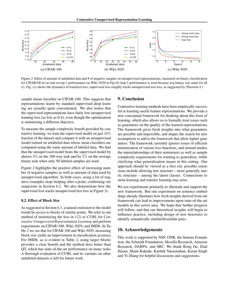
Figure 2. Effect of amount of unlabeled data and # of negative samples on unsupervised representations, measured on binary classificationfor CIFAR100 in (a) and on top-1 performance on Wiki-3029 in Fig (b) (top-1 performance is used because avg binary was same for allk). Fig. (c) shows the dynamics of train/test loss; supervised loss roughly tracks unsupervised test loss, as suggested by Theorem 4.1

sample mean classifier on CIFAR-100. This suggests thatrepresentations learnt by standard supervised deep learn-ing are actually quite concentrated. We also notice thatthe supervised representations have fairly low unsupervisedtraining loss (as low as 0.4), even though the optimizationis minimizing a different objective.

To measure the sample complexity benefit provided by con-trastive learning, we train the supervised model on just 10%fraction of the dataset and compare it with an unsupervisedmodel trained on unlabeled data whose mean classifiers arecomputed using the same amount of labeled data. We findthat the unsupervised model beats the supervised model byalmost 4% on the 100-way task and by 5% on the averagebinary task when only 50 labeled samples are used.

Figure 2 highlights the positive effect of increasing num-ber of negative samples as well as amount of data used byunsupervised algorithm. In both cases, using a lot of neg-ative examples stops helping after a point, confirming oursuspicions in Section 6.2. We also demonstrate how thesupervised loss tracks unsupervised test loss in Figure 2c.

8.2. Effect of Block Size

As suggested in Section 6.3, a natural extension to the modelwould be access to blocks of similar points. We refer to ourmethod of minimizing the loss in (12) as CURL for Con-trastive Unsupervised Representation Learning and performexperiments on CIFAR-100, Wiki-3029, and IMDb. In Ta-ble 2 we see that for CIFAR-100 and Wiki-3029, increasingblock size yields an improvement in classification accuracy.For IMDb, as is evident in Table 2, using larger blocksprovides a clear benefit and the method does better thanQT, which has state-of-the-art performance on many tasks.A thorough evaluation of CURL and its variants on otherunlabeled datasets is left for future work.

9. ConclusionContrastive learning methods have been empirically success-ful at learning useful feature representations. We provide anew conceptual framework for thinking about this form oflearning, which also allows us to formally treat issues suchas guarantees on the quality of the learned representations.The framework gives fresh insights into what guaranteesare possible and impossible, and shapes the search for newassumptions to add to the framework that allow tighter guar-antees. The framework currently ignores issues of efficientminimization of various loss functions, and instead studiesthe interrelationships of their minimizers as well as samplecomplexity requirements for training to generalize, whileclarifying what generalization means in this setting. Ourapproach should be viewed as a first cut; possible exten-sions include allowing tree structure – more generally met-ric structure – among the latent classes. Connections tometa-learning and transfer learning may arise.

We use experiments primarily to illustrate and support thenew framework. But one experiment on sentence embed-dings already illustrates how fresh insights derived from ourframework can lead to improvements upon state-of-the-artmodels in this active area. We hope that further progresswill follow, and that our theoretical insights will begin toinfluence practice, including design of new heuristics toidentify semantically similar/dissimilar pairs.

10. AcknowledgementsThis work is supported by NSF, ONR, the Simons Founda-tion, the Schmidt Foundation, Mozilla Research, AmazonResearch, DARPA, and SRC. We thank Rong Ge, EladHazan, Sham Kakade, Karthik Narasimhan, Karan Singhand Yi Zhang for helpful discussions and suggestions.


ReferencesArora, S. and Risteski, A. Provable benefits of representa-

tion learning. arXiv, 2017.

Bellet, A., Habrard, A., and Sebban, M. Similarity learningfor provably accurate sparse linear classification. arXivpreprint arXiv:1206.6476, 2012.

Bellet, A., Habrard, A., and Sebban, M. A survey on metriclearning for feature vectors and structured data. CoRR,abs/1306.6709, 2013.

Blum, A. and Mitchell, T. Combining labeled and unlabeleddata with co-training. In Proceedings of the EleventhAnnual Conference on Computational Learning Theory,COLT’ 98, 1998.

Chung, J., Gulcehre, C., Cho, K., and Bengio, Y. Gatedfeedback recurrent neural networks. In Proceedings ofthe 32Nd International Conference on International Con-ference on Machine Learning - Volume 37, ICML’15.JMLR.org, 2015.

Cortes, C., Mohri, M., and Rostamizadeh, A. Two-stagelearning kernel algorithms. 2010.

Devlin, J., Chang, M.-W., Lee, K., and Toutanova, K. BERT:Pre-training of deep bidirectional transformers for lan-guage understanding. arXiv preprint arXiv:1810.04805,10 2018.

Dyer, C. Notes on noise contrastive estimation and negativesampling. CoRR, abs/1410.8251, 2014. URL http://arxiv.org/abs/1410.8251.

Gutmann, M. and Hyvarinen, A. Noise-contrastive esti-mation: A new estimation principle for unnormalizedstatistical models. In Proceedings of the Thirteenth Inter-national Conference on Artificial Intelligence and Statis-tics, pp. 297–304, 2010.

Hazan, E. and Ma, T. A non-generative framework andconvex relaxations for unsupervised learning. In NeuralInformation Processing Systems, 2016.

Kiros, R., Zhu, Y., Salakhutdinov, R., Zemel, R. S., Torralba,A., Urtasun, R., and Fidler, S. Skip-thought vectors. InNeural Information Processing Systems, 2015.

Krizhevsky, A. Learning multiple layers of features fromtiny images. Technical report, 2009.

Kumar, A., Niculescu-Mizil, A., Kavukcoglu, K., andDaume, H. A binary classification framework for two-stage multiple kernel learning. In Proceedings of the 29thInternational Coference on International Conference onMachine Learning, ICML’12, 2012.

Logeswaran, L. and Lee, H. An efficient framework forlearning sentence representations. In Proceedings of theInternational Conference on Learning Representations,2018.

Maas, A. L., Daly, R. E., Pham, P. T., Huang, D., Ng, A. Y.,and Potts, C. Learning word vectors for sentiment anal-ysis. In Proceedings of the 49th Annual Meeting of theACL: Human Language Technologies, 2011.

Maurer, A. A vector-contraction inequality for rademachercomplexities. In International Conference on AlgorithmicLearning Theory, pp. 3–17. Springer, 2016.

Maurer, A., Pontil, M., and Romera-Paredes, B. The benefitof multitask representation learning. J. Mach. Learn. Res.,2016.

Mikolov, T., Sutskever, I., Chen, K., Corrado, G. S., andDean, J. Distributed representations of words and phrasesand their compositionality. In Neural Information Pro-cessing Systems, 2013.

Mohri, M., Rostamizadeh, A., and Talwalkar, A. Founda-tions of machine learning. MIT press, 2018.

Pagliardini, M., Gupta, P., and Jaggi, M. Unsupervisedlearning of sentence embeddings using compositionaln-gram features. Proceedings of the North AmericanChapter of the ACL: Human Language Technologies,2018.

Pennington, J., Socher, R., and Manning, C. D. GloVe:Global vectors for word representation. In Proceedingsof the Conference on Empirical Methods in Natural Lan-guage Processing, 2014.

Peters, M. E., Neumann, M., Iyyer, M., Gardner, M., Clark,C., Lee, K., and Zettlemoyer, L. Deep contextualizedword representations. In Proceedings of NAACL-HLT,2018.

Simonyan, K. and Zisserman, A. Very deep convolu-tional networks for large-scale image recognition. arXivpreprint arXiv:1409.1556, 2014.

Snell, J., Swersky, K., and Zemel, R. Prototypical networksfor few-shot learning. In Advances in Neural InformationProcessing Systems 30. 2017.

Wang, X. and Gupta, A. Unsupervised learning of visualrepresentations using videos. In Proc. of IEEE Interna-tional Conference on Computer Vision, 2015.

http://arxiv.org/abs/1410.8251

http://arxiv.org/abs/1410.8251


A. Deferred ProofsA.1. Class Collision Lemma

We prove a general Lemma, from which Lemma 4.4 can be derived directly.

Lemma A.1. Let c ∈ C and ` : Rt → R be either the t-way hinge loss or t-way logistic loss, as defined in Section 2. Letx, x+, x−1 , ..., x

−t be iid draws from Dc. For all f ∈ F , let

L=un,c(f) = E

x,x+,x−i

[`(f(x)T

(f(x+)− f(x−i )

)ti=1

)]Then

L=un,c(f)− `(~0) ≤ c′t

√‖Σ(f, c)‖2 E

x∼Dc[‖f(x)‖] (13)

where c′ is a positive constant.

Lemma 4.4 is a direct consequence of the above Lemma, by setting t = 1 (which makes `(0) = 1), taking an expectationover c ∼ ν in Equation (13) and noting that Ec∼ν [L=

un,c(f)] = L=un(f).

Proof of Lemma A.1. Fix an f ∈ F and let zi = f(x)T(f(x−i )− f(x+)

)and z = maxi∈[t] zi. First, we show that

L=un,c(f)− `(~0) ≤ c′E[|z|], for some constant c′. Note that E[|z|] = P[z ≥ 0]E[z|z ≥ 0] + P[z ≤ 0]E[−z|z ≤ 0] ≥ P[z ≥

0]E[z|z ≥ 0].

t-way hinge loss: By definition `(v) = max0, 1+maxi∈[t]−vi. Here, L=un,c(f) = E[(1+z)+] ≤ E[max1+z, 1] =

1 + P[z ≥ 0]E[z|z ≥ 0] ≤ 1 + E[|z|].

t-way logistic loss: By definition `(v) = log2(1 +∑ti=1 e

−vi), we have L=un,c(f) = E[log2(1 +

∑i ezi)] ≤ E[log2(1 +

tez)] ≤ max zlog 2 + log2(1 + t), log2(1 + t) = P[z≥0]E[z|z≥0]

log 2 + log2(1 + t) ≤ E[|z|]log 2 + log2(1 + t).

Finally, E[|z|] ≤ E[maxi∈[t] |zi|] ≤ tE[|z1|]. But,

E[|z1|] = Ex,x+,x−1

[ ∣∣f(x)T(f(x−1 )− f(x+)

)∣∣ ]≤ Ex

‖f(x)‖

√√√√Ex+,x−1

[ (f(x)T

‖f(x)‖(f(x−1 )− f(x+)

))2] ≤ √2

√‖Σ(f, c)‖2 E

x∼Dc[‖f(x)‖]

A.2. Proof of Lemma 5.1

Fix an f ∈ F and suppose that within each class c, f is σ2-subgaussian in every direction. 8 Let µc = Ex∼Dc

[f(x)]. This

means that for all c ∈ C and unit vectors v, for x ∼ Dc, we have that vT (f(x) − µc) is σ2-subgaussian. Let ε > 0 andγ = 1 + 2Rσ

√2 logR+ log 3/ε. 9 Consider fixed c+, c−, x and let f(x)T (f(x−)− f(x+)) = µ+ z, where

µ = f(x)T (µc− − µc+) and z = f(x)T(f(x−)− µc−

)− f(x)T

(f(x+)− µc+

)For x+ ∼ D+

c , x− ∼ D−c independently, z is the sum of two independent R2σ2-subgaussians (x is fixed), so z is 2R2σ2-

subgaussian and thus p = Pr[z ≥ γ − 1] ≤ e−4R2σ2(2 logR+log 3/ε)

4R2σ2 = ε3R2 . So, Ez[(1 + µ + z)+] ≤ (1 − p)(γ + µ)+ +

p(2R2 + 1) ≤ γ(1 + µγ )+ + ε (where we used that µ+ z ≤ 2R2). By taking expectation over c+, c− ∼ ρ2, x ∼ Dc+ we

8A random variable X is called σ2-subgaussian if E[eλ(X−E[X])] ≤ eλ2σ2/2, ∀λ ∈ R. A random vector V ∈ Rd is σ2-subgaussian in

every direction, if ∀u ∈ Rd, ||u|| = 1, the random variable 〈u, V 〉 is σ2-subgaussian.9We implicitly assume here that R ≥ 1, but for R < 1, we just set γ = 1 + 2Rσ

√log 3/ε and the same argument holds.


have

L6=un(f) ≤ Ec+,c−∼ρ2x∼Dc+

[γ

(1 +

f(x)T (µc− − µc+)

γ

)+

∣∣∣∣c+ 6= c−

]+ ε

= γ Ec+,c−∼ρ2

[1

2E

x∼Dc+

[(1 +

f(x)T (µc− − µc+)

γ

)+

]+

1

2E

x∼Dc−

[(1 +

f(x)T (µc+ − µc−)

γ

)+

] ∣∣∣∣c+ 6= c−

]+ ε

= γ Ec+,c−∼ρ2

[Lµγ,sup(c+, c−, f)

∣∣c+ 6= c−]

+ ε

(14)

where Lµγ,sup(c+, c−, f) is Lµsup(c+, c−, f) when `γ(x) = (1 − x/γ)+ is the loss function. Observe that in 14 weused that DT are uniform for binary T , which is an assumption we work with in section 4, but we remove it in section 5.The proof finishes by observing that the last line in 14 is equal to γLµγ,sup(f) + ε.

A.3. Generalization Bound

We first state the following general Lemma in order to bound the generalization error of the function class F on theunsupervised loss function Lun(·). Lemma 4.2 can be directly derived from it.

Lemma A.2. Let ` : Rk → R be η-Lipschitz and bounded by B. Then with probability at least 1− δ over the training setS = (xj , x+

j , x−j1, . . . , x

−jk)Mj=1, for all f ∈ F

Lun(f) ≤ Lun(f) +O

ηR√kRS(F)

M+B

√log 1

δ

M

(15)

where

RS(F) = Eσ∼±1(k+2)dM

[supf∈F〈σ, f|S〉

](16)

and f|S =(ft(xj), ft(x

+j ), ft(x

−j1), . . . , , ft(x

−jk))j∈[M ]t∈[d]

Note that for k + 1-way classification, for hinge loss we have η = 1 and B = O(R2), while for logistic loss η = 1 andB = O(R2 + log k). Setting k = 1, we get Lemma 4.2. We now prove Lemma A.2.

Proof of Lemma A.2. First, we use the classical bound for the generalization error in terms of the Rademacher complexityof the function class (see (Mohri et al., 2018) Theorem 3.1). For a real function class G whose functions map from a set Zto [0, 1] and for any δ > 0, if S is a training set composed by M iid samples zjMj=1, then with probability at least 1− δ

2 ,for all g ∈ G

E[g(z)] ≤ 1

M

M∑j=1

g(zi) +2RS(G)

M+ 3

√log 4

δ

2M(17)

whereRS(G) is the usual Rademacher complexity. We apply this bound to our case by setting Z = X k+2, S is our trainingset and the function class is

G =

gf (x, x+, x−1 , ..., x

−k ) =

1

B`(f(x)T

(f(x+)− f(x−i )

)ki=1

) ∣∣∣f ∈ F (18)

We will show that for some universal constant c,RS(G) ≤ cηR√k

B RS(F) or equivalently

Eσ∼±1M

[supf∈F

⟨σ, (gf )|S

⟩]≤ cηR

√k

BE

σ∼±1d(k+2)M

[supf∈F

⟨σ, f|S

⟩](19)


where (gf )|S = gf (xj , x+j , x

−j1, ..., x

−jk)Mj=1. To do that we will use the following vector-contraction inequality.

Theorem A.3. [Corollary 4 in (Maurer, 2016)] Let Z be any set, and S = zjMj=1 ∈ ZM . Let F be a class of functionsf : Z → Rn and h : Rn → R be L-Lipschitz. For all f ∈ F , let gf = h f . Then

Eσ∼±1M

[supf∈F

⟨σ, (gf )|S

⟩]≤√

2L Eσ∼±1nM

[supf∈F

⟨σ, f|S

⟩]

where f|S =(ft(zj)

)t∈[n],j∈[M ]

.

We apply Theorem A.3 to our case by setting Z = X k+2, n = d(k + 2) and

F =f(x, x+, x−j1, ..., x

−jk) = (f(x), f(x+), f(x−j1), ..., f(x−jk))|f ∈ F

We also use gf = gf where f is derived from f as in the definition of F . Observe that now A.3 is exactly in the form of 19 and

we need to show that L ≤ c√2

ηR√k

B for some constant c. But, for z = (x, x+, x−1 , ..., x−k ), we have gf (z) = 1

B `(φ(f(z)))

where φ : R(k+2)d → Rk and φ((vt, v

+t , v

−t1, ..., v

−tk)t∈[d]

)=(∑

t vt(v+t − v−ti )

)i∈[k]

. Thus, we may use h = 1B ` φ to

apply Theorem A.3.

Now, we see that φ is√

6kR-Lipschitz when∑t v

2t ,∑t(v

+t )2,

∑t(v−tj)

2 ≤ R2 by computing its Jacobian. Indeed, for alli, j ∈ [k] and t ∈ [d], we have ∂φi

∂vt= v+

t − v−ti ,∂φi∂v+t

= vt and ∂φi∂v−tj

= −vt1i = j. From triangle inequaltiy, the Frobenius

norm of the Jacobian J of φ is

||J ||F =

√∑i,t

(v+t − v−ti )2 + 2k

∑t

v2t ≤

√4kR2 + 2kR2 =

√6kR

Now, taking into account that ||J ||2 ≤ ||J ||F , we have that φ is√

6kR-Lipschitz on its domain and since ` is η-Lipschitz,we have L ≤

√6ηR

√k

B .

Now, we have that with probability at least 1− δ2

Lun(f) ≤ Lun(f) +O

ηR√kRS(F)

M+B

√log 1

δ

M

(20)

Let f∗ ∈ arg minf∈F Lun(f). With probability at least 1− δ2 , we have that Lun(f∗) ≤ Lun(f∗)+3B

√log 2

δ

2M (Hoeffding’s

inequality). Combining this with Equation (20), the fact that Lun(f) ≤ Lun(f∗) and applying a union bound, finishes theproof.

A.4. Proof of Proposition 6.2

By convexity of `,

`

(f(x)T

(∑i f(x+

i )

b−∑i f(x−i )

b

))= `

(1

b

∑i

f(x)T(f(x+

i )− f(x−i )))≤ 1

b

∑i

`(f(x)T

(f(x+

i )− f(x−i )))

Thus,

Lblockun (f) = Ex,x+

i

x−i

[`

(f(x)T

(∑i f(x+

i )

b−∑i f(x−i )

b

))]≤ Ex,x+

i

x−i

[1

b

∑i

`(f(x)T

(f(x+

i )− f(x−i )))]

= Lun(f)


The proof of the lower bound is analogous to that of Lemma 4.3.

B. Results for k Negative SamplesB.1. Formal theorem statement and proof

We now present Theorem B.1 as the formal statement of Theorem 6.1 and prove it. First we define some necessary quantities.

Let (c+, c−1 , . . . , c−k ) be k + 1 not necessarily distinct classes. We define Q(c+, c−1 , . . . , c

−k ) to be the set of distinct classes

in this tuple. We also define I+(c−1 , ..., c−k ) = i ∈ [k] | c−i = c+ to be the set of indices where c+ reappears in the

negative samples. We will abuse notation and just write Q, I+ when the tuple is clear from the context.

To define L6=un(f) consider the following tweak in the way the latent classes are sampled: sample c+, c−1 , . . . , c−k ∼ ρk+1

conditioning on |I+| < k and then remove all c−i , i ∈ I+. The datapoints are then sampled as usual: x, x+ ∼ D2c+ and

x−i ∼ Dc−i , i ∈ [k], independently.

L6=un(f) := Ec+,c−ix,x+,x−i

[`(f(x)T

(f(x+)− f(x−i )

)i/∈I+

) ∣∣∣|I+| < k]

which always contrasts points from different classes, since it only considers the negative samples that are not from c+.

The generalization error is 10

GenM = O

R√kRS(F)

M+ (R2 + log k)

√log 1

δ

M

were RS(F) is the extension of the definition in Section 4: RS(F) = E

σ∼±1(k+2)dM

[supf∈F 〈σ, f|S〉

], where f|S =(

ft(xj), ft(x+j ), ft(x

−j1), . . . , , ft(x

−jk))j∈[M ],t∈[d]

.

For c+, c−1 , ..., c−k ∼ ρk+1, let τk = P[I+ 6= ∅] and τ ′ = P[c+ = c−i ,∀i]. Observe that τ1, as defined in Section 4, is

P[c+ = c−1 ]. Let pmax(T ) = maxcDT (c) and

ρ+min(T ) = min

c∈TPc+,c−i ∼ρk+1

(c+ = c|Q = T , I+ = ∅

)In Theorem B.1 we will upper bound the following quantity: E

T ∼D

[ρ+min(T )

pmax(T ) Lµsup(T , f)

](D was defined in Section 6.1).

Theorem B.1. Let f ∈ arg minf∈F Lun(f). With probability at least 1− δ, for all f ∈ F

ET ∼D

[ρ+min(T )

pmax(T )Lµsup(T , f)

]≤ 1− τ ′

1− τkL6=un(f) + c′k

τ11− τk

s(f) +1

1− τkGenM

where c′ is a constant.

Note that the definition of s(f) used here is defined in Section 4

Proof. First, we note that both hinge and logistic loss satisfy the following property: ∀I1, I2 such that I1 ∪ I2 = [t] we havethat

`(vii∈I1) ≤ `(vii∈[t]) ≤ `(vii∈I1) + `(vii∈I2) (21)

We now prove the Theorem in 3 steps. First, we leverage the convexity of ` to upper bound a supervised-type loss with theunsupervised loss Lun(f) of any f ∈ F . We call it supervised-type loss because it also includes degenerate tasks: |T | = 1.

10The log k term can be made O(1) for the hinge loss.


Then, we decompose the supervised-type loss into an average loss over a distribution of supervised tasks, as defined in theTheorem, plus a degenerate/constant term. Finally, we upper bound the unsupervised loss Lun(f) with two terms: L6=un(f)that measures how well f contrasts points from different classes and an intraclass deviation penalty, corresponding to s(f).

Step 1 (convexity): When the class c is clear from context, we write µc = Ex∼c

[f(x)]. Recall that the sampling procedure for

unsupervised data is as follows: sample c+, c−1 , ..., c−k ∼ ρk+1 and then x, x+ ∼ D2

c+ and x−i ∼ Dc−i , i ∈ [k]. So, we have

Lun(f) = Ec+,c−i ∼ρ

k+1

x,x+∼D2c+

x−i ∼Dc−i

[`

(f(x)T

(f(x+)− f(x−i )

)ki=1

)]

= Ec+,c−i ∼ρ

k+1

x∼Dc+

Ex+∼Cc+x−i ∼Dc−

i

[`

(f(x)T

(f(x+)− f(x−i )

)ki=1

)]≥ Ec+,c−i ∼ρ

k+1

x∼Dc+

[`

(f(x)T

(µc+ − µc−i

)ki=1

)]

(22)

where the last inequality follows by applying the usual Jensen’s inequality and the convexity of `. Note that in the upperbounded quantity, the c+, c−1 , ..., c

−k don’t have to be distinct and so the tuple does not necessarily form a task.

Step 2 (decomposing into supervised tasks) We now decompose the above quantity to handle repeated classes.

Ec+,c−i ∼ρ

k+1

x∼Dc+

[`

(f(x)T

(µc+ − µc−i

)ki=1

)]

≥ (1− τk) Ec+,c−i ∼ρ

k+1

x∼Dc+

[`

(f(x)T

(µc+ − µc−i

)ki=1

) ∣∣∣∣∣I+ = ∅

]+ τk E

c+,c−i ∼ρk+1

[`( 0, ..., 0︸︷︷︸|I+| times

)|I+ 6= ∅]

≥ (1− τk) Ec+,c−i ∼ρ

k+1

x∼Dc+

[`

(f(x)T (µc+ − µc)

c∈Qc 6=c+

)∣∣∣∣∣I+ = ∅

]+ τk E

c+,c−i ∼ρk+1

[`|I+|(~0)

∣∣∣ I+ 6= ∅](23)

where `t(~0) = `(0, . . . , 0) (t times). Both inequalities follow from the LHS of Equation (21). Now we are closer to ourgoal of lower bounding an average supervised loss, since the first expectation in the RHS has a loss which is over a set ofdistinct classes. However, notice that this loss is for separating c+ from Q(c+, c−1 , ..., c

−k ) \ c+. We now proceed to a

symmetrization of this term to alleviate this issue.

Recall that in the main paper, sampling T from D is defined as sampling the (k+1)-tuple from ρk+1 conditioned on I+ = ∅and setting T = Q. Based on this definition, by the tower property of expectation, we have

Ec+,c−i ∼ρ

k+1

x∼Dc+

[`

(f(x)T (µc+ − µc)

c∈Qc 6=c+

)∣∣∣∣∣I+ = ∅

]

= ET ∼D

Ec+,c−i ∼ρ

k+1

x∼Dc+

[`(f(x)T

(µc+ − µc

)c∈Qc6=c+

)∣∣∣Q = T , I+ = ∅]

= ET ∼D

Ec+∼ρ+(T )x∼Dc+

[`(f(x)T

(µc+ − µc

)c∈Tc6=c+

)](24)

where ρ+(T ) is the distribution of c+ when (c+, c−1 , ..., c−k ) are sampled from ρk+1 conditioned on Q = T and I+ = ∅.

Recall that ρ+min(T ) from the theorem’s statement is exactly the minimum out of these |T | probabilities. Now, to lower

bound the last quantity with the LHS in the theorem statement, we just need to observe that for all tasks T


Ec+∼ρ+(T )x∼Dc+

[`(f(x)T

(µc+ − µc

)c∈Tc6=c+

)]

≥ ρ+min(T )

pmax(T )E

c+∼DTx∼Dc+

[`(f(x)T

(µc+ − µc

)c∈Tc6=c+

)]

=ρ+min(T )

pmax(T )Lsup(T , f)

(25)

By combining this with Equations (22), (23), (25) we get

(1− τk) ET ∼D

[ρ+min(T )

pmax(T )Lsup(T , f)

]≤ Lun(f)− τk E

c+,c−i ∼ρk+1

[`|I+|(~0)

∣∣∣ I+ 6= ∅]

(26)

Now, by applying Lemma A.2, we bound the generalization error: with probability at least 1− δ, ∀f ∈ F

Lun(f) ≤ Lun(f) +GenM (27)

However, Lun(f) cannot be made arbitrarily small. One can see that for all f ∈ F , Lun(f) is lower bounded by the secondterm in Equation (22), which cannot be made arbitrarily small as τk > 0.

Lun(f) ≥ Ec+,c−i ∼ρ

k+1

x,x+∼Dc+x−i ∼Dc−

i

[`(f(x)T

(f(x+)− f(x−i )

)i∈I+

)]≥ τ E

c+,c−i ∼ρk+1

[`|I+|(~0)

∣∣∣ I+ 6= ∅]

(28)

where we applied Jensen’s inequality. Since τk is not 0, the above quantity can never be arbitrarily close to 0 (no matter howrich F is).

Step 3 (Lun decomposition) Now, we decompose Lun(f) by applying the RHS of Equation (21)

Lun(f) ≤ Ec+,c−i ∼ρ

k+1

x,x+∼D2c+

x−i ∼Dc−i

[`(f(x)T

(f(x+)− f(x−i )

)i/∈I+

)+ `(f(x)T

(f(x+)− f(x−i )

)i∈I+

)](29)

= Ec+,c−i ∼ρ

k+1

x,x+∼D2c+

x−i ∼Dc−i, i/∈I+

[`(f(x)T

(f(x+)− f(x−i )

)i/∈I+

)]+ E

c+,c−i ∼ρk+1

x,x+∼D2c+

x−i ∼Dc−i, i∈I+

[`(f(x)T

(f(x+)− f(x−i )

)i∈I+

)](30)

= (1− τ ′) Ec+,c−i ∼ρ

k+1

x,x+∼D2c+

x−i ∼Dc−i,i /∈I+

[`(f(x)T

(f(x+)− f(x−i )

)i/∈I+

)∣∣∣|I+| < k]

+τk Ec+,c−i ∼ρ

k+1

x,x+∼D2c+


[`(f(x)T

(f(x+)− f(x−i )

)i∈I+

) ∣∣∣∣∣I+ 6= ∅

] (31)

Observe that the first term is exactly (1− τ ′)L6=un(f). Thus, combining (26), (27) and (31) we get


(1− τk) ET ∼D

[ρ+min(T )

pmax(T )Lsup(T , f)

]≤ (1− τ ′)L6=un(f) +GenM

+ τk Ec+,c−i ∼ρk+1

[E

x,x+∼D2c+


[`(f(x)T

(f(x+)− f(x−i )

)i∈I+

)]− `|I+|(~0)

∣∣∣∣∣I+ 6= ∅

]

︸︷︷︸∆(f)

(32)

From the definition of I+, c−i = c+, ∀i ∈ I+. Thus, from Lemma A.1, we get that

∆(f) ≤ c′ Ec+,c−i ∼ρk+1

[|I+|

√‖Σ(f, c)‖2 E

x∼Dc[‖f(x)‖]

∣∣∣ I+ 6= ∅]

(33)

for some constant c′.

Let u be a distribution over classes with u(c) = Pc+,c−i ∼ρk+1 [c+ = c|I+ 6= ∅] and it is easy to see that u(c) ∝ ρ(c)(1−

(1− ρ(c))k)

By applying the tower property to Equation (33) we have

∆(f) ≤ c′ Ec∼u

[E

c+,c−i ∼ρk+1

[|I+|

∣∣c+ = c, I+ 6= ∅] √‖Σ(f, c)‖2 E

x∼Dc[‖f(x)‖]

](34)

But,

Ec+,c−i ∼ρk+1

[|I+|

∣∣c+ = c, I+ 6= ∅]

=

k∑i=1

Pc+,c−i ∼ρk+1

(c−i = c+

∣∣c+ = c, I+ 6= ∅)

= kPc+,c−i ∼ρk+1

(c−1 = c+

∣∣c+ = c, I+ 6= ∅)

= kPc+,c−i ∼ρk+1

(c−1 = c+ = c

)Pc+,c−i ∼ρk+1

(c+ = c, I+ 6= ∅

)= k

ρ2(c)

ρ(c)(1− (1− ρ(c))k

) = kρ(c)

1− (1− ρ(c))k

(35)

Now, using the fact that τk = 1−∑c′ ρ(c′)(1− ρ(c′))k =

∑c′ ρ(c′)

(1− (1− ρ(c′))k

)and τ1 =

∑c ρ

2(c),

τk1− τk

∆(f) ≤ τk1− τk

c′ Ec∼u

[k

ρ(c)

1− (1− ρ(c))k

√‖Σ(f, c)‖2 E

x∼Dc[‖f(x)‖]

]= c′k

τk1− τk

∑c

ρ2(c)∑c′ ρ(c′) (1− (1− ρ(c′))k)

√‖Σ(f, c)‖2 E

x∼Dc[‖f(x)‖]

= c′kτ1

1− τkEc∼ν

[√‖Σ(f, c)‖2 E

x∼Dc[‖f(x)‖]

]= c′k

τ11− τk

s(f)

(36)

and we are done.

B.2. Competitive Bound

As in Section 5.2, we prove a competitive type of bound, under similar assumptions. Let `γ(v) = max0, 1 +maxi−vi/γ, v ∈ Rk, be the multiclass hinge loss with margin γ and for any T let Lµγ,sup(T , f) be Lµsup(T , f)

when `γ is used as loss function. For all tasks T , let ρ′+(T ) is the distribution of c+ when (c+, c−1 , ..., c−k ) are sampled

from ρk+1 conditioned on Q = T and |I+| < k. Also, let ρ′+max(T ) be the maximum of these |T | probabilities andpmin(T ) = minc∈T DT (c).


We will show a competitive bound against the following quantity, for all f ∈ F : ET ∼D′

[ρ′+max(T )pmin(T ) L

µγ,sup(T , f)

], where

D′ is defined as follows: sample c+, c−1 , ..., c−k ∼ ρk+1, conditioned on |I+| < k. Then, set T = Q. Observe that when

I+ = ∅ with high probability, we have D′ ≈ D.

Lemma B.2. For all f ∈ F suppose the random variable f(X), where X ∼ Dc, is σ2(f)-subgaussian in every directionfor every class c and has maximum norm R(f) = maxx∈X ‖f(x)‖. Let f ∈ arg minf∈F Lun(f). Then for all ε > 0, withprobability at least 1− δ, for all f ∈ F

ET ∼D

[ρ+min(T )

pmax(T )Lµsup(T , f)

]≤ αγ(f) E

T ∼D′

[ρ′

+max(T )

pmin(T )Lµγ,sup(T , f)

]+ βs(f) + ηGenM + ε

where γ(f) = 1 + c′R(f)σ(f)(√

log k +√

log R(f)ε ), c′ is some constant, α = 1−τ ′

1−τk , β = k τ11−τk and η = 1

1−τk .

Proof. We will show that ∀f ∈ F

L 6=un(f) ≤ γ(f) ET ∼D′

[ρ′

+max(T )


](37)

and the Lemma follows from Theorem 6.1. Now, we fix an ε > 0, an f ∈ F and we drop most of the arguments f in the restof the proof. Also, fix c+, c−1 . . . c

−k , x and let t = k − |I+|. We assume without loss of generality, that c+ 6= c−i , ∀i ∈ [t].

Now,maxi∈[t]

f(x)T (f(x−i )− f(x+)) ≤ µ+ maxiz−i − z

+ (38)

where µ = maxi∈[t] f(x)T (µc−i− µc+), z−i = f(x)T (f(x−i ) − µc−i

) and z+ = f(x)T (f(x+) − µc+). zi are cen-

tered σ2R2-subgaussian, so from standard properties of subgaussian random variables P[maxi z−i ≥

√2σR√

log t +√2c1σR

√logR/ε] ≤ (ε/R)c1 (again we consider here the case where R ≥ 1 and for R < 1, the same arguments hold

but with removing R from the log). z+ is also centered σ2R2-subgaussian, so P[z+ ≥√

2c1σR√

logR/ε] ≤ (ε/R)c1 .Let γ = 1 + c′σR(

√log t +

√logR/ε) for appropriate constant c′. By union bound, we have p = P[maxi z

−i − z+ ≥

γ − 1] ≤ 2(ε/R)c1 . Thus, Ez+,z−i [(1 + µ+ maxi z−i − z+)+] ≤ (1− p)(µ+ γ)+ + p(2R2 + 1) ≤ γ(1 + µ/γ)+ + ε (for

appropriate constant c1). By taking expectation over c+, c−i ∼ ρk+1, conditioned on |I+| < k , and over x ∼ Dc+ we get

L6=un(f) ≤ γ Ec+,c−i ∼ρ

k+1

x∼Dc+

[(1 +

maxc∈Q,c 6=c+ f(x)T (µc − µc+)

γ

)+

∣∣∣∣|I+| < k

]

= γ ET ∼D′

Ec+,c−i ∼ρ

k+1

x∼Dc+

[(1 +

maxc∈Q,c 6=c+ f(x)T (µc − µc+)

γ

)+

∣∣∣∣Q = T , |I+| < k

]

= γ ET ∼D′

Ec+∼ρ′+(T )x∼Dc+

[(1 +

maxc∈T,c 6=c+ f(x)T (µc − µc+)

γ

)+

]≤ γ E

T ∼D′

[ρ′

+max(T )


](39)

C. Examples for Section 6.2

Here, we illustrate via examples two ways in which the increase of k can lead to suboptimal f . We will consider the hingeloss as the loss function, while the examples carry over trivially for logistic loss.

1. The first example is the case where even though there exist representations in F that can separate every class, thesuboptimal representation is picked by the algorithm when k = Ω(|C|). Let C = cii∈[n] where for each class, Dci is


uniform over two points x1i , x

2i . Let ei be the indicator vectors in Rn and let the class F consists of f0, f1 with

f0, f1 : X 7→ Rn where f1(x1i ) = 3/2rei and f1(x2

i ) = 1/2rei for all i, for some r > 0, and f0 = ~0. Finally, ρ isuniform over C. Now, when the number of negative samples is Ω(n), the probability that ∃j ∈ [k] such that c+ = c−j isconstant, and therefore Lun(f) = Ω(r2) > 1 = Lun(f0) when r is large. This means that despite Lsup(C, f1) = 0,the algorithm will pick f0 which is a suboptimal representation.

2. We can extend the first example to the case where, even when k = o(|C|), the algorithm picks suboptimal representations.To do so, we simply ‘replicate’ the first example to create clusters of classes. Formally, let C = ciji,j∈[n] where foreach class, Dcij is uniform over two points x1

ij , x2ij. Finally, same as above, let F consist of two functions f0, f1.

The function f1 maps f1(x1ij) = 3/2rei and f1(x2

ij) = 1/2rei for all i, j and f0 = ~0. ρ is uniform over C. Now, notethat f1 ‘clutsters’ the n2 classes and their points into n clusters, each along an ei. Thus, it is only useful for contrastingclasses from different clusters. However, note that the probability of intra-cluster collision with k negative samplesis 1 − (1 − 1/n)k. When k = o(n), we have that Lun(f1) = o(1) < 1 = Lun(f0) so the algorithm will pick f1.However, when k = Ω(n), Lun(f) = Ω(r2) > 1 = Lun(f0) and the algorithm will pick the suboptimal representationf0. Thus, despite |C| = n2, having more than n negative samples can hurt performance, since even tough f1 cannotsolve all the tasks, the average supervised loss over t-way tasks, t = o(n), is Lsup(f) ≤ O(1− (1− 1/n)t−1) = o(1).

D. ExperimentsD.1. Wiki-3029 construction

We use the Wikipedia dump and select articles that have entries in the WordNet, have at least 8 sections and at least 12sentences of length at least 4 per section. At the end of this filtering we are left with 3029 articles with at least 200 sentencesper article. We then sample 200 sentences from each article and do a 70%/10%/20% train/dev/test split.

D.2. GRU model

We use a bi-directional GRU with output dimension of 300 trained using dropout 0.3. The input word embeddings areinitialized to pretrained CC GloVe vectors and fixed throughout training.

Documents

A Theoretical Analysis of Contrastive Unsupervised ...A Theoretical Analysis of Contrastive Unsupervised Representation Learning Sanjeev Arora1 2 Hrishikesh Khandeparkar1 Mikhail Khodak3