Embed Size (px)
Citation preview

A STUDY ON MIMO BEAMFORMING FOR
WIRELESS COMMUNICATION SYSTEMS IN
FREQUENCY-SELECTIVE FADING
CHANNELS
HUY HOANG PHAM
THE UNIVERSITY OF ELECTRO-COMMUNICATIONS
MARCH 2006

c© Copyright 2006 by Huy Hoang Pham
All Rights Reserved

A STUDY ON MIMO BEAMFORMING FOR
WIRELESS COMMUNICATION SYSTEMS IN
FREQUENCY-SELECTIVE FADING
CHANNELS
APPROVED BY SUPERVISORY COMMITEE
Chairperson: Professor Yoshio Karasawa
Member: Professor Takeshi Hashimoto
Member: Professor Masashi Hayakawa
Member: Professor Tadashi Fujino
Member: Professor Nobuo Nakajima

A Study on MIMO Beamforming for Wireless
Communication Systems in Frequency-Selective FadingChannels
Huy Hoang Pham
ABSTRACT
In recent years, multiple-input multiple-output (MIMO) antennas systems have
quickly become an inevitable wireless technology not only for WLANs but also for
mobile networks. Based on the benefits of using multiple transmit antennas and
multiple receive antennas, MIMO systems can provide high quality and high speed
services. However, for high speed transmission, frequency-selective fading (FSF) is
a factor that will degrade the system performance and may cause significant link
failure in a broadband wireless communications environment. Two architectures
have been investigated for MIMO system to mitigate the effect of FSF. The first
architecture is transmission of multiple data streams through spatial multiplexing
such as MIMO OFDM (Orthogonal Frequency Division Multiplexing), MIMO SDM
(Spatial Division Multiplexing). The second architecture is transmission of a single
data stream such as MIMO system based on the transmit diversity technique or
using Tapped Delay Line (TDL) structure. Unfortunately, those proposed schemes
for both single and multiple data streams in FSF are still a lot of complexities
concerning the configuration. In principle, they are not yet to show how many
delayed channels should be cancelled by a MIMO system. This dissertation gives
insight into the weights determination scheme for a simple MIMO beamforming
configuration with assumption of perfect channel state information at both the
transmitter and receiver. Based on our proposed iterative update algorithm, the
optimal transmit and receive weight vectors are determined to apply to MIMO

frequency-selective fading channels that will maximize the output SINR (Signal
to Interference and Noise Ratio) and show maximum number of delayed channels
cancellation.
Firstly, the dissertation presents an issue problem of a single data stream trans-
mission using MIMO beamforming scheme. An iterative update algorithm for the
transmit and receive weight vectors is determinated in a single user case. Using
this method, the degree of freedom (DOF) of both the transmit and the receive
antennas are joined together to suppress the delayed channels and maximize the
output SINR. The maximum number of delayed channels cancellation is analyzed
based on the DOF and confirmed by the computer simulation results.
Next, an iterative update algorithm for transmit and receive weight vectors
for multiuser system has been studied to apply to MIMO frequency-selective fad-
ing channels. Based on the proposed iterative algorithm, improvement of output
SINR and maximum number of delayed channels cancellation are ascertained by
our analysis and results of computer simulation.
Finally, based on assumption of the delayed channels are known as well as the
desired channel, a spatial-temporal adaptive MIMO beamforming scheme has pro-
posed to improve the system performance by utilizing multiple delayed versions of
the transmitted signal. Numerical results demonstrate in comparison with simula-
tion results to validate the analysis.
v
ACKNOWLEDGEMENTS
First of all, I would like to express my deepest gratitude to my dissertation
advisor Prof. Yoshio Karasawa for his guidance and research support throughout
the duration of this work. He is brilliant, knowledgeable, insightful, and most
importantly, always available. He inspired me to think critically and build physical
intuition on research. I feel very lucky to have an adviser as glorious as him. I hope
and look forward to continue collaboration with him in the future.
I am also grateful to my second advisor Prof. Takeshi Hashimoto for his guid-
ance and valuable comments on this work.
I also would like further to thank the members of my thesis committee, Prof.
Tadashi Fujino, Prof. Masashi Hayakawa, Prof. Nobuo Nakajima, Prof. Takeshi
Hashimoto, Prof. Yoshio Karasawa for their feedbacks and advices that helped to
improve the overall quality of dissertation.
I also would like to thank Dr. Tetsuki Taniguchi for many valuable discussions
on this research. Working with him on math problems was always fun! I enjoyed
several long discussions. Thanks also go to members of Karasawa Laboratory for
useful discussion, support and fun that I spent my time as graduate student at The
University of Electro-Communications.
Further I would like to thank Ministry of Education, Culture, Sport, Science
and Technology (MEXT), Japan for providing me an opportunity to study in Japan
and for giving the Monbukagakusho scholarship during the time of this research.
Finally, I would very much like to thank to my dearest parents, brother and
sister for their love and support. Thanks to my father who always encourages and
gives me the strength to arrive at this important milestone. Thanks to my mother
for her love and countless sacrifices for providing me with the best educational
opportunities. I am thankful to my wife Duong Hoang Huong for giving me love
and encouragement during the most important time of this work.

CONTENTS
CONTENTS i
LIST OF TABLES v
LIST OF FIGURES vi
1 Introduction 1
1.1 Context of Work . . . . . . . . . . . . . . . . . . . . . . . . . . . . 1
1.2 Original Contributions . . . . . . . . . . . . . . . . . . . . . . . . . 3
1.3 Structure of the Thesis . . . . . . . . . . . . . . . . . . . . . . . . . 4
2 Fundamentals of Adaptive Arrays 6
2.1 Basic Concepts of Adaptive Signal Processing . . . . . . . . . . . . 6
2.2 Uniformly Linear Array . . . . . . . . . . . . . . . . . . . . . . . . 8
2.3 Beamforming and Spatial Filtering . . . . . . . . . . . . . . . . . . 10
2.4 Adaptive Criteria . . . . . . . . . . . . . . . . . . . . . . . . . . . . 14
2.4.1 Minimum Mean Square Error (MMSE) . . . . . . . . . . . . 14
2.4.2 Maximum-Signal-to-Noise and Interference Ratio (MSINR) . 16
2.4.3 Minimum Variance (MV) . . . . . . . . . . . . . . . . . . . . 17
2.4.4 Maximum Likelihood (ML) . . . . . . . . . . . . . . . . . . 17
2.5 Adaptive Algorithms . . . . . . . . . . . . . . . . . . . . . . . . . . 18
i

CONTENTS
2.5.1 Least Mean Square (LMS) . . . . . . . . . . . . . . . . . . . 19
2.5.2 Sample Matrix Inversion (SMI) . . . . . . . . . . . . . . . . 20
2.5.3 Recursive Least Square (RLS) . . . . . . . . . . . . . . . . . 21
2.6 Benefits of Using Adaptive Arrays in Wireless Communication Systems 23
2.6.1 Signal Quality Improvement . . . . . . . . . . . . . . . . . . 23
2.6.2 Range Extension . . . . . . . . . . . . . . . . . . . . . . . . 24
2.6.3 Increase in Capacity . . . . . . . . . . . . . . . . . . . . . . 25
2.6.4 Reduction in Transmit Power . . . . . . . . . . . . . . . . . 25
2.7 Summary . . . . . . . . . . . . . . . . . . . . . . . . . . . . . . . . 25
3 MIMO System for Wireless Communications 27
3.1 Basic Concepts . . . . . . . . . . . . . . . . . . . . . . . . . . . . . 27
3.2 Narrowband MIMO Channel . . . . . . . . . . . . . . . . . . . . . . 28
3.2.1 Single Data Stream Transmission . . . . . . . . . . . . . . . 28
3.2.2 Multiple Data Streams Transmission . . . . . . . . . . . . . 29
3.3 Wideband MIMO Channel . . . . . . . . . . . . . . . . . . . . . . . 31
3.3.1 Single Data Stream Transmission . . . . . . . . . . . . . . . 31
3.3.2 Multiple Data Streams Transmission . . . . . . . . . . . . . 33
3.4 Motivations . . . . . . . . . . . . . . . . . . . . . . . . . . . . . . . 35
3.5 Summary . . . . . . . . . . . . . . . . . . . . . . . . . . . . . . . . 36
4 MIMO Beamforming for Single Data Stream Transmission in FSF
Channels 37
4.1 Propagation Model . . . . . . . . . . . . . . . . . . . . . . . . . . . 37
4.2 Transmit and Receive Weight Vectors Determination . . . . . . . . 39
4.2.1 Receive Weight Vector Determination . . . . . . . . . . . . . 39
4.2.2 Transmit Weight Vector Determination . . . . . . . . . . . . 40
ii
CONTENTS
4.2.3 Iterative Weight Vector Update Algorithm . . . . . . . . . . 42
4.3 Interference Cancellation Ability Analysis . . . . . . . . . . . . . . 43
4.4 Output SINR . . . . . . . . . . . . . . . . . . . . . . . . . . . . . . 44
4.5 Simulation Results . . . . . . . . . . . . . . . . . . . . . . . . . . . 44
4.5.1 Simulation Conditions . . . . . . . . . . . . . . . . . . . . . 44
4.5.2 Results . . . . . . . . . . . . . . . . . . . . . . . . . . . . . . 46
4.6 Summary . . . . . . . . . . . . . . . . . . . . . . . . . . . . . . . . 48
5 Multiuser MIMO Beamforming for Single Data Stream Transmis-
sion in FSF Channels 54
5.1 Propagation Model . . . . . . . . . . . . . . . . . . . . . . . . . . . 54
5.2 Transmit and Receive Weight Vectors Determination . . . . . . . . 57
5.2.1 Receive weight vector determination . . . . . . . . . . . . . 57
5.2.2 Transmit weight vector determination . . . . . . . . . . . . . 57
5.2.3 Iterative Weight Update Algorithms . . . . . . . . . . . . . 58
5.3 Interference Cancellation Ability Analysis . . . . . . . . . . . . . . 60
5.4 Output SINR . . . . . . . . . . . . . . . . . . . . . . . . . . . . . . 63
5.5 Simulation Results . . . . . . . . . . . . . . . . . . . . . . . . . . . 63
5.5.1 Simulation Conditions . . . . . . . . . . . . . . . . . . . . . 63
5.5.2 Results . . . . . . . . . . . . . . . . . . . . . . . . . . . . . . 64
5.6 Summary . . . . . . . . . . . . . . . . . . . . . . . . . . . . . . . . 67
6 Spatial-Temporal MIMO Beamforming for Single Data Stream Trans-
mission in FSF Channels 73
6.1 Propagation Model . . . . . . . . . . . . . . . . . . . . . . . . . . . 73
6.1.1 Spatial-domain Signal Processing . . . . . . . . . . . . . . . 74
6.1.2 Spatial-Temporal Signal Processing . . . . . . . . . . . . . . 76
iii

CONTENTS
6.2 Weights Determination of the Proposed Spatial-Temporal Adaptive
MIMO Beamforming . . . . . . . . . . . . . . . . . . . . . . . . . . 78
6.3 Output SINR . . . . . . . . . . . . . . . . . . . . . . . . . . . . . . 80
6.4 Simulation Results . . . . . . . . . . . . . . . . . . . . . . . . . . . 81
6.4.1 Simulation Conditions . . . . . . . . . . . . . . . . . . . . . 81
6.4.2 Results . . . . . . . . . . . . . . . . . . . . . . . . . . . . . . 82
6.5 Summary . . . . . . . . . . . . . . . . . . . . . . . . . . . . . . . . 84
7 Conclusion and Future Work 90
7.1 Conclusions . . . . . . . . . . . . . . . . . . . . . . . . . . . . . . . 90
7.2 Future Work . . . . . . . . . . . . . . . . . . . . . . . . . . . . . . . 92
A Determination of Transmit Weight Vector w(opt)t,i for the ith User 93
REFERENCE 95
iv
LIST OF TABLES
4.1 Simulation model for MIMO beamforming . . . . . . . . . . . . . . 45
5.1 Simulation model for multiuser MIMO beamforming . . . . . . . . . 64
5.2 Interference channels cancellation ability of i.i.d channels of user 1
and user 2, respectively . . . . . . . . . . . . . . . . . . . . . . . . . 71
6.1 Simulation model for MIMO beamforming . . . . . . . . . . . . . . 82
v

LIST OF FIGURES
2.1 Different geometry configurations of antenna arrays. . . . . . . . . . 7
2.2 Adaptive Array Configuration. . . . . . . . . . . . . . . . . . . . . . 7
2.3 Singal model for ULA. . . . . . . . . . . . . . . . . . . . . . . . . . 8
2.4 Configuration of an adaptive narrowband beamformer. . . . . . . . 11
2.5 Configuration of an adaptive wideband beamformer. . . . . . . . . . 12
2.6 Frequency domain beamformer using FFT. . . . . . . . . . . . . . . 13
2.7 MMSE criterion Adaptive Array. . . . . . . . . . . . . . . . . . . . 14
2.8 An example of the LMS learning curve using linear array elements
with d = λ/2, N = 4, µ = 0.005, SNRin = 10dB . . . . . . . . . . . . 20
2.9 An example of the RLS learning curve using linear array elements
with d = λ/2, N = 4, γ = 1, SNRin = 10dB . . . . . . . . . . . . . . 22
2.10 Output SNR versus number of array elements. . . . . . . . . . . . . 24
3.1 Narrowband MIMO channel configuration with beamforming. . . . 28
3.2 Narrowband MIMO channel configuration for multiple data stream
transmission. . . . . . . . . . . . . . . . . . . . . . . . . . . . . . . 30
3.3 Broadband MIMO channel and beamforming configuration. . . . . . 32
3.4 Broadband MIMO channel and beamforming for multiple data streams
configuration. . . . . . . . . . . . . . . . . . . . . . . . . . . . . . . 34
4.1 Broadband MIMO channel and beamforming configuration. . . . . . 37
vi

LIST OF FIGURES
4.2 Assumption of power delay profiles: a. A discrete-time uniform power
delay profile; b. A discrete-time exponential power delay profile. . . 49
4.3 SINR in flat and frequency-selective fading channels when using wt
and wr calculated from A(0). . . . . . . . . . . . . . . . . . . . . . . 50
4.4 Convergence characteristics for different delays. . . . . . . . . . . . 50
4.5 CDF of SINR for the 4x4 MIMO at the receiver. . . . . . . . . . . . 51
4.6 SINR performance of the proposed 4x4 MIMO system in case of
L = 6 and L = 7. . . . . . . . . . . . . . . . . . . . . . . . . . . . . 51
4.7 Median value of SINR vs. the number of delayed channels. . . . . . 52
4.8 Average SINR of MxN MIMO as a function of the delay spread στ .
(model 2) . . . . . . . . . . . . . . . . . . . . . . . . . . . . . . . . 52
4.9 The maximum delay spread realizing acceptable communication qual-
ity as a function of the number of array elements. (model 2) . . . . 53
5.1 Broadband MIMO channel and beamforming configuration for a multi-
user system. . . . . . . . . . . . . . . . . . . . . . . . . . . . . . . . 55
5.2 Block diagram of the maximizing SINR by means of receiver-side
weight vector optimization. (Q = 2) [Algorithm A] . . . . . . . . . 58
5.3 Block diagram of the maximizing SINR based on iterative update of
weight vectors at BS. (Q = 2) [Algorithm B] . . . . . . . . . . . . . 59
5.4 Examples of the channel impulse response. . . . . . . . . . . . . . . 61
5.5 Convergence characteristics of 4×4 MIMO system for two users using
model 1.(upper: for user 1, lower: for user 2) . . . . . . . . . . . . . 68
5.6 Distribution function of SINR for two users 4 × 4 MIMO system: a.
CDF for User 1 (upper); b. CDF for user 2 (lower). . . . . . . . . . 69
5.7 Distribution function of SINR for two users 6 × 4 MIMO system. . . 70
5.8 Median value of SINR as a function of L1 in case of L1 = L2. . . . . 72
5.9 Average SINR of MIMO system as a function of the delay spread στ . 72
vii

LIST OF FIGURES
6.1 Spatial Adaptive MIMO Beamforming configuration for FSF Channels. 74
6.2 Spatial-Temporal MIMO Beamforming configuration for FSF Channels. 77
6.3 Distribution function of SINR for a 4 × 4 MIMO system: (a) CDF
for s(0)(t); (b) CDF for s(1)(t); (c) CDF for s(2)(t); (d) CDF for s(3)(t) 86
6.4 Median value of SINR vs. the number of interferences for a 4 × 4
MIMO system: (a) SNRin = 40dB; (b) SNRin = 20dB . . . . . . . . 87
6.5 Median value of SINR vs. the number of interferences for a 4 × 8
MIMO system: (a) SNRin = 40dB; (b) SNRin = 20dB . . . . . . . . 88
6.6 Average SINR of MIMO system as a function of the delay spread στ . 89
viii

Chapter 1
Introduction
1.1 Context of Work
Wireless communications networks are growing from 3G toward a new generation,
which provide high quality and high speed services. For the demands in broadband
wireless access technologies such as mobile internet, multi-media, however, one of
the main problems addressed in wireless communications is signal distortion. It
can be classified as Inter-Symbol Interference (ISI) due to the signal delay of going
through the multipath fading and Co-Channel Interference (CCI) due to the multi-
ple accesses that will degrade the performance of system and may cause significant
link failure in a wireless communications environment [1]-[8].
Adaptive array is one of the most expected ways that enables to improve the
performance of wireless communication system. In particular, an important feature
is its capability to cancel CCI independent of the angle of arrival. The more an-
tenna elements in an array, the more degrees of freedom (DOF) of array possess
to combat the interference and mulitpath fading. For instance, an N -element an-
tenna array has (N −1) DOF and thus can cancel (N −1) CCIs independent of the
multipath environment. For ISI, however, since the conventional adaptive arrays
using narrowband beamformer processes the received signal only in spatial domain,
it cannot treat the delayed versions of the transmitted signal as separated signals.
The solution to the problem is to keep the arrays from having to use its spatial
processing in combination with temporal filter using tapped delayed line (TDL)
structure [9, 10]. It is also referred to as wideband beamformer adaptive arrays.
Therefore, spatial and temporal equalizer based on an antenna array will become
1

1.1 Context of Work
a breakthrough technique, which has capability to suppress effectively both CCI
and ISI. Much research on spatial and temporal signal processing using an antenna
array at base station (BS) has been proposed. Several adaptive algorithms for de-
riving the optimal weight vector in the time domain such as Least Mean Squares
(LMS), Recursive Least Squares (RLS), and Constant Modulus Algorithm (CMA),
which have been illustrated in chapter 2, are view points of extending techniques of
spatial and temporal digital equalizer. However, resolving simultaneously both the
CCI and the ISI is a difficult task for spatial and temporal adaptive array (STAA)
since it requires recursive computation slow convergence in searching for optimum
weight vector.
Multiple antenna structure divided into two groups has been of special inter-
est, particularly in the last two decades. They are including: use of antenna array
only at receiver, known as single-input multiple-outputs (SIMO) systems; and use
of antenna only at transmitter, known as multiple-inputs single-output (MISO)
systems. However, in order to satisfy the needs of the high performance and capac-
ity of wireless communications system, use of antenna arrays at both transmitter
and receiver, known as multiple-input multiple-output (MIMO) systems have been
proposed in recent years. If multipath scattering is sufficiently rich and properly ex-
ploited, MIMO systems show high performance and capacity compared with SIMO
and MISO systems. While most researches have considered the theoretical capac-
ity and output maximum Signal-to-Noise and Interference Ratio (SINR) of MIMO
systems in flat fading environment [26]-[38], the implementation issues in wideband
MIMO systems for frequency-selective fading environment are still a challenging
topic which needs to be resolved.
For solving the MIMO frequency-selective fading channels, spatial multiplex-
ing OFDM has been proposed to transmit multiple independent streams simul-
taneously, where the number of independent streams is limited by the minimum
number of antenna elements at both ends thus frequency-selective MIMO channels
are transformed into several frequency-flat MIMO channels. And besides, the de-
cision feedback equalization technique, where MIMO antennas systems equipped
with tapped delayed line (TDL) structure, have been proposed for mitigating the
frequency-selective fading. However, they so far still suffer from computational
complexity, compact and low-cost hardware. Although there are many techniques
2

1.2 Original Contributions
proposed for MIMO frequency-selective fading environment with or without prior
knowledge of Channel State Information (CSI) at the transmitter and/or receiver,
they do not yet point out how many delayed channels can be effectively cancelled
by using adaptive beamforming by adjusting both the transmit and receive weight
vectors in the MIMO system. Therefore, the solution to the problem is to determi-
nate the optimal transmit and receive weight vectors for MIMO frequency-selective
fading without using the TDL equipment.
With M and N antenna elements equipped at the transmitter and receiver, re-
spectively, the weight vectors determination scheme for the transmitter and receiver
of a MIMO beamforming is performed by utilizing spatial filter to mitigate CCI and
ISI and maximize the output SINR. On the other hand, our proposed scheme has a
capability to reduce computational complexity and achieve faster convergence rate
compared with MIMO systems having TDL structure in the transmitter and/or
receiver.
The original contributions of our work are presented in the next section.
1.2 Original Contributions
Several contributions on the weight vectors determination for the transmitter and
receiver of the MIMO beamforming configuration and its performance has been
made in this work. Parts of these contributions have been published or submitted
for publication. The following list summarizes our main contributions within the
scope of this work.
• Firstly, a detailed weight vectors for transmitter and receiver of a MIMO
beamforming scheme in frequency-selective fading environment is presented
in Chapter 4. The result of analysis was published in the IEICE Transaction
on Communications, vol.E87-B, no.8, August, 2004.
• Second is the detailed weight vectors for multiuser system of a MIMO beam-
forming in frequency-selective fading channels performed in Chapter 5. The
result of the analysis was published in the IEICE Transaction on Funda-
mentals, Special Section on Adaptive Signal Processing and Its Applications,
vol.E88-A, no.3, March, 2005.
3

1.3 Structure of the Thesis
• Third is an extensible configuration of MIMO beamforming that improves the
performance of system by utilizing multiple delayed versions of the transmitted
signal instead of suppressing them. The result of the analysis is submitted to
IEICE Transaction on Communications (Under 1st Review)
1.3 Structure of the Thesis
The organization of this thesis is as follows.
We begin by describing fundamentals of adaptive arrays in Chapter 2. The
basic concepts and classification of adaptive arrays are presented. Then the array
signal model in multipath fading environments is developed. Criteria to optimize
performance of adaptive arrays and adaptive algorithms to obtain optimal weight
vector are also summarized.
In Chapter 3, such a single data stream and multiple data streams transmissions
using a single carrier are presented providing a fundamental understanding of the
MIMO beamforming with the perfect CSI at both sides in wireless communications.
A SIMO system with a single antenna element at the transmitter and N antenna
elements at the receiver has (N − 1) DOF that mitigates effectively (N − 1) inter-
ferences. Similarly to a MISO system with M antenna elements at the transmitter
and a single antenna element at the receiver has a capability to cancel (M − 1) in-
terferences. As a result, the DOF or maximum cancellation number of interferences
for the MIMO system with M antenna elements at the transmitter and N antenna
elements at the receiver should be a certain, which is whether larger than that of
both SIMO and MISO systems or not, is described here.
In Chapter 4, we propose the weight vectors determination for the transmit-
ter and receiver for MIMO beamforming for a single data stream transmission in
frequency-selective fading channels. Through studying the optimal transmit and
receive weight vectors determination for MIMO frequency-selective fading, I have
successfully proposed the cancellation of (M + N − 2) delayed channels for the
MIMO beamforming scheme, where M and N are antenna elements at base sta-
tion (BS) and mobile station (MS), respectively. Based on the proposed MIMO
beamforming scheme without using TDL can effectively mitigate multipath fading
in frequency-selective channels while having reduced computational complexity.
4
1.3 Structure of the Thesis
The detailed weight vectors determination for multiuser system of a MIMO
beamforming for a single data stream transmission in frequency-selective fading
channels is presented in Chapter 5. Based on the method proposed in Chapter 4,
we analyze a maximum number of interference channels, which could be eliminated
in multiuser system, in two cases of the receive weight vectors optimization only and
iterative update of both end weight vectors. For the first case, which is character-
ized by simple scheme, shown good performance for propagation channel when the
preceding channel of the desired user has few its own interference channels, while
the second case shown better performance but more sophisticated scheme.
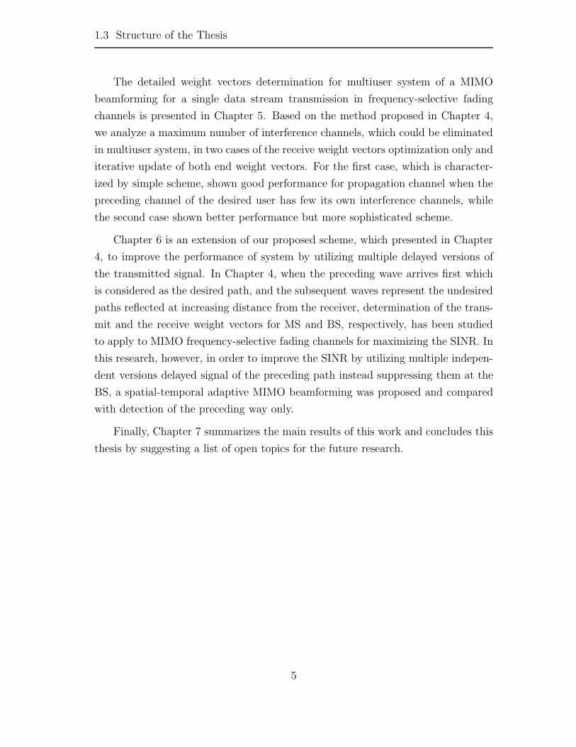
Chapter 6 is an extension of our proposed scheme, which presented in Chapter
4, to improve the performance of system by utilizing multiple delayed versions of
the transmitted signal. In Chapter 4, when the preceding wave arrives first which
is considered as the desired path, and the subsequent waves represent the undesired
paths reflected at increasing distance from the receiver, determination of the trans-
mit and the receive weight vectors for MS and BS, respectively, has been studied
to apply to MIMO frequency-selective fading channels for maximizing the SINR. In
this research, however, in order to improve the SINR by utilizing multiple indepen-
dent versions delayed signal of the preceding path instead suppressing them at the
BS, a spatial-temporal adaptive MIMO beamforming was proposed and compared
with detection of the preceding way only.
Finally, Chapter 7 summarizes the main results of this work and concludes this
thesis by suggesting a list of open topics for the future research.
5

Chapter 2
Fundamentals of Adaptive Arrays
This Chapter presents principal concepts of antenna arrays. Array signal model
and different types of adaptive beamforming for narrow and wide band signals
are illustrated. In particular, criteria for performance optimization and adaptive
algorithms are analyzed in searching the optimal weight vector for antenna array.
Finally, the benefits of using adaptive arrays in wireless communication system are
also discussed.
2.1 Basic Concepts of Adaptive Signal Processing
An antenna array consists of two or more antenna elements that are spatially ar-
ranged by a real-time adaptive processor which produce a directional radiation
pattern. Some time antenna array is also referred to as adaptive antennas or smart
antennas. Antenna array can be arranged in various geometry configurations of
which the most popular are linear, circular and planar shown in Figure 2.1.
A linear antenna array consists of antenna elements separated on a straight line
by a given distance. If adjacent elements are equally spaced the array is referred to
as a uniformly linear array (ULA). If, in addition, the phase αn of the feeding current
to the nth antenna element is increased by αn = nα, where α is a constant, then the
array is referred to as a progressive phase-shift array. If the feeding amplitudes are
constant, then the array is called a uniform array. Similarly, if the array elements
are arranged in a circular manner as depicted in Figure 2.1(b), then the array
is referred to as an uniform circular array (UCA). The circular array produces
beams of a wider width than the corresponding linear array when they are the same
6

2.1 Basic Concepts of Adaptive Signal Processing
(a)
(b) (c)
Figure 2.1: Different geometry configurations of antenna arrays.
Figure 2.2: Adaptive Array Configuration.
number of elements and the same spacing between them. While both linear and
circular arrays can only perform one-dimensional beamforming (horizontal plane),
the planar antenna array can be used for two-dimensional (2-D) beamforming (both
in vertical and horizontal planes). An example realization of a planar array is
depicted in Figure 2.1(c).
The principle of antenna arrays is the same although theirs geometry config-
urations are different. However, since the analysis and synthesis are simple, the
uniformly linear arrays are often used in both study and experiment compared to
that of the rest. The detailed mathematics of geometries can be described in [11].
Throughout this work, the uniformly linear array is restricted to our study. Figure
7

2.2 Uniformly Linear Array
2.2 shows the most basic structure of the linear adaptive array, which is discussed
in these section as follows.
2.2 Uniformly Linear Array
Consider an N -element ULA which is illustrated in Figure 2.3.
1( )n t2 ( )n t( )nn t( )Nn t
12nN
dsin�
�
d
Plane Wave Front Incident Plane Wave
ReferenceElement
Figure 2.3: Singal model for ULA.
In Figure 2.3, the array elements are equally spaced by a distance d, and a plan
wave arrives at the array from a direction θ off the array broad side. The angle θ is
measured from the principle axis of the array and is called the direction-of-arrival
(DOA) or angle-of-arrival (AOA) of the received signal. The plane wave front at
the first element should propagate through a distance d sin θ to arrive at the second
element. If we take the first element as the reference element and the signal at the
reference element is s(t), then the phase delay of the signal at element n relative
to element 1 is (n − 1)kd sin θ, where k = 2π/λ is a number waves and λ is the
wavelength of the carrier. Therefore, the received signal at the nth element is given
by
xn(t) = s(t)e−j 2πλ
(n−1)d sin θ (2.1)
where j =√−1 is the imaginary.
8
2.2 Uniformly Linear Array
Let us arrange xn(t) in a vector form as
x(t) = [x1(t) x2(t) ... xN(t)]T (2.2)
and let
a(θ) = [1 e−j 2πλ
d sin θ ... e−j 2πλ
(N−1)d sin θ]T (2.3)
where (.)T denotes the transpose operation. Then equation 2.2 may be expressed
in vector form as
x(t) = a(θ)s(t) + n(t) (2.4)
where the noise vector has been defined as
n(t) = [n1(t) n2(t) ... nN(t)]T (2.5)
The vector x(t) is often referred to as the array input data vector and a(θ) is
called the steering vector. In ULA, the steering vector is only a function of the
angle-of-arrival. However, in general, the steering vector is also a function of the
individual element response, the array geometry and signal frequency over which
the collection of steering vectors for all angles and frequencies is referred to as the
array manifold.
It should be note that if the bandwidth of the impinging signal expressed in
(2.1) is much smaller than the reciprocal of the propagation time across the array,
the signal is referred to as narrowband signal; otherwise it is referred to as wideband
signal.
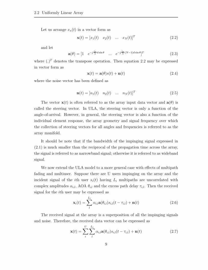
We now extend the ULA model to a more general case with effects of multipath
fading and multiuser. Suppose there are U users impinging on the array and the
incident signal of the ith user si(t) having Li multipaths are uncorrelated with
complex amplitudes αi,l, AOA θi,l and the excess path delay τi,l. Then the received
signal for the ith user may be expressed as
xi(t) =
Li∑l
αi,la(θi,l)si,l(t − τi,l) + n(t) (2.6)
The received signal at the array is a superposition of all the impinging signals
and noise. Therefore, the received data vector can be expressed as
x(t) =
U∑i
Li∑l
αi,la(θi,l)si,l(t − τi,l) + n(t) (2.7)
9

2.3 Beamforming and Spatial Filtering
In matrix notation, (2.7) becomes
x(t) = A(Θ)s(t) + n(t) (2.8)
where A(Θ) is N × U matrix of the steering vectors
A(Θ) = [a(Θ1) a(Θ2) ... a(ΘU )] (2.9)
and
s(t) = [s1(t) s2(t) ... sU(t)]T (2.10)
2.3 Beamforming and Spatial Filtering
Beamforming techniques exist that can yield multiple, simultaneously available
beams. The beams can be made to have high gain and low side-lobes, or con-
trolled beam width. Adaptive beamforming techniques dynamically adjust the ar-
ray pattern to optimize some characteristic of the received signal. The desired and
interfering signals usually originate from different spatial locations, antenna arrays
can exploit the spatial characteristic to reject interfering signals having a DOA dif-
ferent from that of a desired signal sources. Multi-polarized array can also reject
interfering signals having different polarization states from the desired signal, even if
the signals have the same DOA. This process of maximizing the signal-to-noise and
interference (SINR) based on their spatial characteristic is called spatial filtering
and is used in the reverse or uplink (from mobile to base station). Similarly, based
on the information estimated from uplink, beamforming is utilized in the forward
or downlink (from base station to mobile) to maximize the transmit power of base
station to a desired user while suppressing the others. On one hand, antenna arrays
using adaptive beamforming are to maximize the SINR, they are called adaptive
beamforming. On the other hand, they are designed to steer toward the beams and
away from the specific interference locations, it is called null-beamforming.
The antenna elements in an adaptive array collect spatial samples of propagating
wave fields, which are processed by the beamformer [12]. Currently, there are two
types of beamformer, namely, narrowband beamformer and wideband beamformer.
A typical narrowband and wideband beamformers are shown in Figure 2.4 and
Figure 2.5.
10

2.3 Beamforming and Spatial Filtering
N
d
1w
2w
nw
Nw
( )y t
1
2
n
( )Nx t
( )nx t
2 ( )x t
1( )x t
Figure 2.4: Configuration of an adaptive narrowband beamformer.
In Figure 2.4, the output of array multiplied by a weight vector of the received
signal at time t is given by
y(t) =N∑
n=1
w∗nxn(t) (2.11)
where wn is called the complex weight and xn(t) is the received signal at sensor nth.
Equation (2.11) may also be rewritten in vector form as
y(t) = wHx(t) (2.12)
where (.)H denotes the complex conjugate (Hermitian) transpose and w is called
the complex weight vector and is defined as
w = [w1 w2 ... wN ]T (2.13)
In Figure 2.5, the received signal vector is fed into both spatial and tempo-
ral domains and employed to process when signals of significant frequency extent
(broadband) are of interest. This beamformer process is called spatial-temporal
equalizer. The output may be expressed as
y(t) =
N∑n=1
K−1∑k=0
w∗n,kxn(t − k) (2.14)
11

2.3 Beamforming and Spatial Filtering
N
d
( )y t
1
2
n
1z -
1z -
1z -
1z -
1z - 1z -
1z - 1z -
1z - 1z -
1z - 1z -
11w12w 1( 1)Kw - 1Kw
2Kw2( 1)Kw -22w21w
1nw2nw ( 1)n Kw - nKw
NKw( 1)N Kw -2Nw1Nw
1( )x t
2 ( )x t
( )nx t
( )Nx t
Figure 2.5: Configuration of an adaptive wideband beamformer.
where K − 1 is the number of delays in each of the N sensor elements. Let
w = [w1,0 w1,1 ... w1,K−1 ... wN,0 wN,1 ... wN,K−1]T (2.15)
and
x(t) = [x1(t) ... x1(t − K + 1) ... xN (t) ... xN(t − K + 1)]T (2.16)
The output of the broadband beamformer can be now rewritten as
y(t) = wHx(t) (2.17)
The TDL is not only useful for providing the desired adjustment of gain and
phase for wideband signals but also for other purpose such as mitigation of mul-
tipath under frequency-selective fading and compesation for effects of interchannel
mismatch [10, 13]. However, the broadband beamformer using TDL structure is
practical difficulties associated with the equalization at several megabits per second
with high speed, compact, and low-cost hardware. Beside the broadband beam-
former using TDL considered so far is a classical time domain processor, Fast Fourier
12

2.3 Beamforming and Spatial Filtering
transform (FFT) has been used to replace TDL structure in the beamformer con-
figuration resulting in an equivalent frequency domain broadband beamformer as
shown in Figure 2.6 [8],[10].
N
d
( )y t
1
2
n
( )Nx t
( )nx t
2 ( )x t
1( )x t S
P/
S
P/
S
P/
S
P/
1kw
2kw
nkw
Nkw
1
1
1
1
k
k
k
k
K
K
K
K
( )ky f
1( )y f
( )Ky f
IFFT
P
S/
S/P: serial-to-parallel conversionP/S: parallel-to-serial conversion
Figure 2.6: Frequency domain beamformer using FFT.
In Figure 2.6, broadband signals from each element are transformed into fre-
quency domain using the FFT and each frequency bin is processed by a narrow-band
processor structure. In other words, each signal xn(t) is decomposed into K subband
signals and converted into the frequency domain using the FFT filter bank. After
being multiplied by the optimum weights, which estimated from adaptive algorithm
such as the Least Mean Square (LMS) algorithm, the weight samples are combined
corresponding to each subband. The combined samples are then converted back
into time domain using the IFFT filter bank. Finally, the array output signal y(t)
is achieved after the parallel-to-serial conversion. The advantage of the frequency
domain approach is reduction of computational load and increases the convergence
rate. Since the weight vector for each subband is estimated independently, the pro-
cess of selecting the weight vectors can be performed in parallel, leading to fast
weight update [8].
13
2.4 Adaptive Criteria
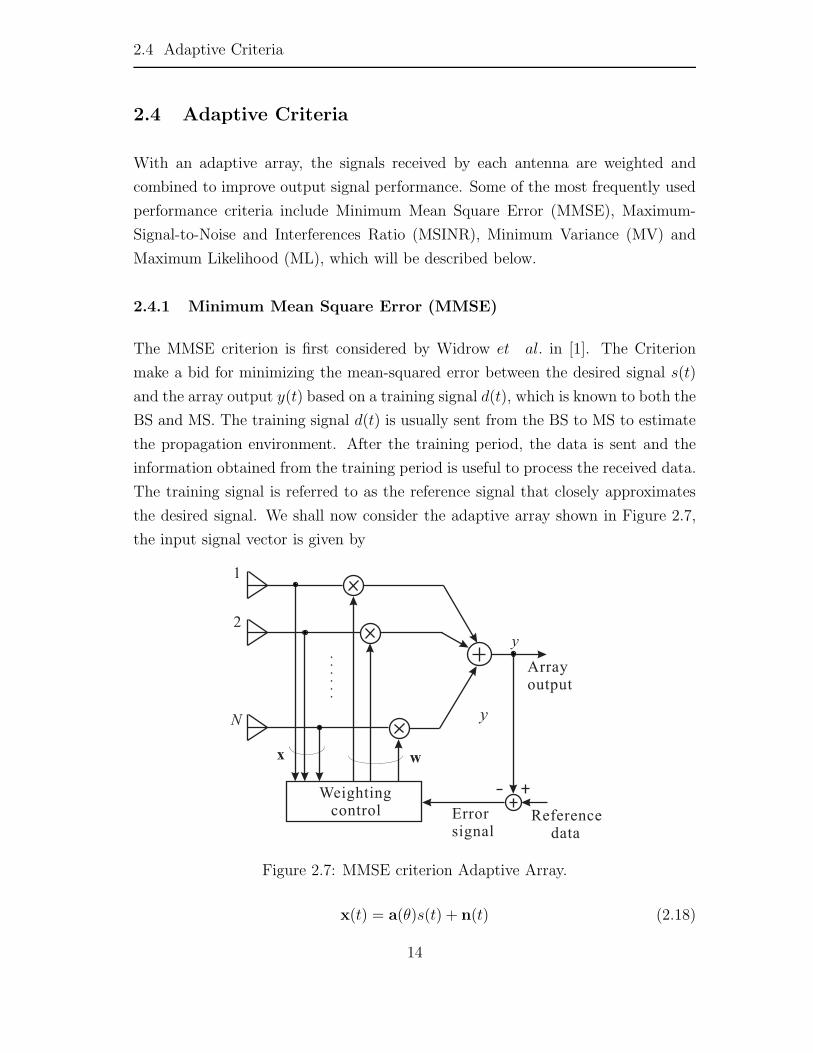
2.4 Adaptive Criteria
With an adaptive array, the signals received by each antenna are weighted and
combined to improve output signal performance. Some of the most frequently used
performance criteria include Minimum Mean Square Error (MMSE), Maximum-
Signal-to-Noise and Interferences Ratio (MSINR), Minimum Variance (MV) and
Maximum Likelihood (ML), which will be described below.
2.4.1 Minimum Mean Square Error (MMSE)
The MMSE criterion is first considered by Widrow et al. in [1]. The Criterion
make a bid for minimizing the mean-squared error between the desired signal s(t)
and the array output y(t) based on a training signal d(t), which is known to both the
BS and MS. The training signal d(t) is usually sent from the BS to MS to estimate
the propagation environment. After the training period, the data is sent and the
information obtained from the training period is useful to process the received data.
The training signal is referred to as the reference signal that closely approximates
the desired signal. We shall now consider the adaptive array shown in Figure 2.7,
the input signal vector is given by
Figure 2.7: MMSE criterion Adaptive Array.
x(t) = a(θ)s(t) + n(t) (2.18)
14

2.4 Adaptive Criteria
where n(t) is the i.i.d additive noise vector, which is assumed to be complex Gaus-
sian process with zero-mean and variance N0, θ is the AOA, and a is the array
propagation vector for the desired signal (steering vector)
a(θ) = [1 ejπ sin θ ... ej(N−1)π sin θ]T (2.19)
The beamformer in the receiver uses the information of the training signal to
compute the optimal weight vector w(opt). If the channel environment and the
interference characteristics remain constant from one training period until the next,
the weight vector w(opt) will use to give the output y(t)
y(t) = wHx(t) (2.20)
Then the error signal is given by
e(t) = d(t) − y(t)
= d(t) − wHx(t) (2.21)
and the mean-squared error is defined by
E{|e(t)|2} = E{|d(t) − wHx(t)|2} (2.22)
where E{.} denotes the ensemble expectation operator. Expanding (2.22) we have
E{|e(t)|2} = E{|d(t)|2} −wT E{w∗(t)d(t)} − wHE{x(t)d∗(t)} + wHE{x(t)xH(t)}w= E{|d(t)|2} −wTp∗
xr −wHpxr + wHRxxw (2.23)
where pxr = E{x(t)d∗(t)} is the N×1 cross-correlation vector and Rxx = E{x(t)xH(t)}is the M × M correlation matrix. Here (.)∗ denotes the complex conjugate. The
optimum weight vector can be found by setting the gradient of (2.23) with respect
to w equal to zero
∇wE{|e(t)|2} = −2pxr + 2Rxxw = 0 (2.24)
Rearranging
Rxxw = pxr (2.25)
Assuming Rxx is non-singular, the optimum solution is found as
wopt = R−1prx (2.26)
15
2.4 Adaptive Criteria
Equation (2.26) is called the Wiener-Hopf equation [14]. By substituting (2.26)
into (2.23), we have the minimum of mean-squared error
E{|e(t)|2} = E{|d(t)|2} − pHxrR
−1xxpxr (2.27)
2.4.2 Maximum-Signal-to-Noise and Interference Ratio (MSINR)
This criterion is used to maximize the output SINR at BS. Starting from (2.18),
the output of the array can be expressed as
y(t) = wHx(t) = wHs(t) + wHn(t)
= ys(t) + yn(t) (2.28)
The average output SINR is given by
SINR = E{ |ys(t)|2|yn(t)|2} = E{ wHs(t)sH(t)w
wHn(t)nH(t)w} =
wHRssw
wHRnnw(2.29)
where Rss = s(t)sH(t) and Rnn = n(t)nH(t). Taking the gradient of (2.29) with
respect to w is
∇wSINR =∇w(wHRssw)(wHRuuw) − (wHRssw)∇w(wHRnnw)
(wHRnnw)2
=2Rssw(wHRuuw) − 2Rnnw(wHRssw)
(wHRnnw)2(2.30)
The optimum weight vector wopt can be found by setting ∇wSINR = 0, which
leads to
Rss =wHRssw
wHRnnwRnnw (2.31)
Noting that Rss = E{s(t)sH(t)} = E{|s(t)|2a(θ)aH(θ)} and aH(θ)wE{|s(t)|2}is a scalar, we have
a(θ) =wHa(θ)
wHRnnwRnnw (2.32)
Define
1
ζ=
wHa(θ)
wHRnnw(2.33)
Then the optimum weight vector can be expressed in a similar form of the
Wiener-Hopf equation as
wopt = ζR−1nna(θ) (2.34)
16

2.4 Adaptive Criteria
2.4.3 Minimum Variance (MV)
If the desired signal and its direction are both known, one way of ensuring a good
signal reception is to minimize the output noise variance. Minimum variance is also
known as linear constrained minimum variance (LCMV). Recall the beamformer
output from (2.12)
y(t) = wHx(t) = wHa(θ)s(t) + wHn(t) (2.35)
In order to ensure that the desired signal is passed with a specific gain and
phase, a constraint may be used to so that response of the beamformer to the
desired signal is
wHa(θ) = g (2.36)
Minimization of contributions of the output due to interference is accomplished
by choosing the weight vector to minimize the variance of the output power
Var{y(t)} = wHRssw + wHRnnw (2.37)
subject to the constraint defined in (2.36). Using the method of Lagrange, we have
∇w(1
2wHRnnw + β[1 − wHa(θ)]) = Rnnw − βa(θ) (2.38)
where
β =g
aH(θ)R−1nna(θ)
(2.39)
then the optimum weight vector using MV criterion can be expressed as
wopt = βR−1nna(θ) (2.40)
when g = 1, the MV beamformer is often referred to as the Capon beamformer [14].
2.4.4 Maximum Likelihood (ML)
The Maximum-Likelihood criterion is known to be a powerful approach and fre-
quently used in signal processing. Recall the input signal vector from (2.12)
x(t) = a(θ)s(t) + n(t) = s(t) + n(t) (2.41)
17

2.5 Adaptive Algorithms
Letting px(t)|s(t)(x(t)) denotes the probability density function for s(t) given x(t).
Since the natural logarithm is a monotone function, we define the Likelihood func-
tion as
�(x(t)) = − ln(px(t)|s(t)(x(t))) (2.42)
Assume that the u(t) is a stationary zero-mean Gaussian vector having a co-
variance matrix Ruu. The Likelihood function can be expressed as
�(x(t)) = C(x(t) − a(θ)s(t))HR−1uu (x(t) − a(θ)s(t)) (2.43)
where C is a constant with respect to x(t) and s(t).
The Maximum Likelihood estimate s(t) of the s(t) is given by the location of
the maximum of the Likelihood function. Using derivatives, the calculation of the
Maximum Likelihood estimate becomes
∂�(x(t))
s(t)= −2aH(θ)R−1
uux(t) + 2s(t)aH(θ)R−1uua(θ) = 0 (2.44)
Since aH(θ)R−1uua(θ) is a scalar, (2.44) is expressed as
s(t) =aH(θ)R−1
uu
aH(θ)R−1uua(θ)
x (2.45)
Comparing (2.45) with (2.12), the optimal weight vector using ML criterion is given
by
w(opt)ML =
R−1uua(θ)
aH(θ)R−1uua(θ)
(2.46)
Define
η =1
aH(θ)R−1uua(θ)
(2.47)
then the optimal weight vector using ML criterion can be expressed
w(opt)ML = ηR−1
uua(θ) (2.48)
The ML beamformer is also referred to as the Capon beamformer.
2.5 Adaptive Algorithms
In the preceding section, we have shown that the optimum criteria are closely related
to each other. Therefore, the choice of a particular criterion is not critically impor-
tant in terms of performance. On the other hand, the choice of adaptive algorithms
18

2.5 Adaptive Algorithms
for deriving the adaptive weight vector is highly important in that it determines
both the speed of convergence and hardware complexity required to implement the
algorithm. In this section, we will discuss a number of common adaptive techniques.
2.5.1 Least Mean Square (LMS)
The Least Mean Square is the most popular adaptive algorithm for continuous
adaptation. It has been well studied and is well understood [15]. It is based on the
steepest-descent method, which is proceeded as follows
1. Begin with an initial value w(0) for the weight vector, which is chosen arbi-
trarily. Typically, w(0) is set equal to a column vector of an M ×M identity
matrix.
2. Using this initial or present guess, compute the gradient vector ∇(J(t)) at
time t (i.e., the tth iteration).
3. Compute the next guess at the weight vector by making a change in the initial
or present guess in a direction opposite to that of the gradient vector.
4. Go back to step 2 repeat the process.
It is intuitively reasonable that successive corrections to the weight vector in
the direction of the negative of the gradient vector eventually lead to the MSE, at
which point the weight vector assumes its optimum value. According to the method
of steepest decent, the updated value of the weight vector at time t+1 is computed
by using the simple recursive relation.
Now, we can describe the LMS algorithm by the following three equations
y(t) = wH(t)x(t) (2.49)
e(t) = d(t) − y(t) (2.50)
w(t + 1) = w(t) − µ
2∇E{e2(t)} (2.51)
where µ is the step size which controls the convergence characteristics of w(t)
0 < µ <1
λmax(2.52)
19
2.5 Adaptive Algorithms
Here λmax is the largest eigenvalue of the covariance matrix Rxx, we have
∇E{e2(t)} = −2pxr + 2Rxxw(t) (2.53)
Replacing (2.53) into (2.41), we have
w(t + 1) = w(t) + µ[pxr − Rxxw(t)]
= w(t) + µx(t)e∗(t) (2.54)
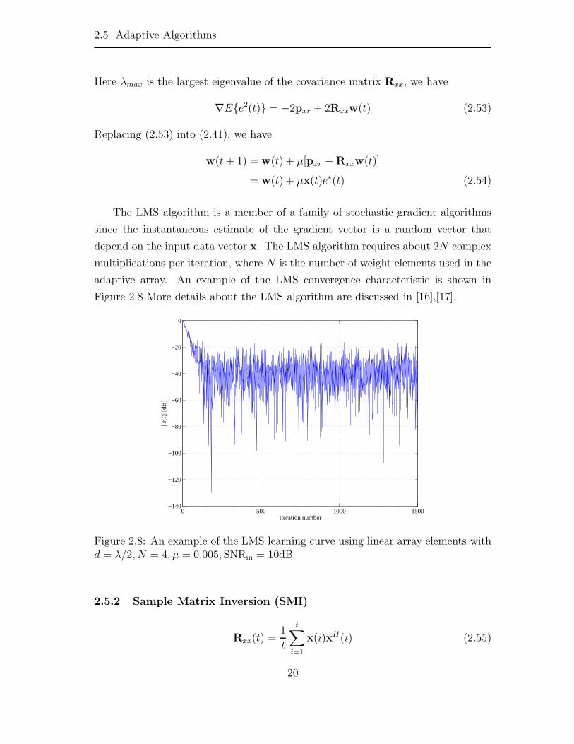
The LMS algorithm is a member of a family of stochastic gradient algorithms
since the instantaneous estimate of the gradient vector is a random vector that
depend on the input data vector x. The LMS algorithm requires about 2N complex
multiplications per iteration, where N is the number of weight elements used in the
adaptive array. An example of the LMS convergence characteristic is shown in
Figure 2.8 More details about the LMS algorithm are discussed in [16],[17].
0 500 1000 1500−140
−120
−100
−80
−60
−40
−20
0
Iteration number
| e(t
)| [d
B]
Figure 2.8: An example of the LMS learning curve using linear array elements withd = λ/2, N = 4, µ = 0.005, SNRin = 10dB
2.5.2 Sample Matrix Inversion (SMI)
Rxx(t) =1
t
t∑i=1
x(i)xH(i) (2.55)
20
2.5 Adaptive Algorithms
rxr(t) =1
t
t∑i=1
x(i)p∗(i) (2.56)
It follows that the estimated weight vector using the SMI algorithm is given by
w(t) = R−1xx (t)pxr(t) (2.57)
Note that the SMI is a block-adaptive algorithm and has been shown to be the
fastest algorithm for estimating the optimum weight vector [18]. However, it suffers
the problems of increased computational complexity and numerical instability due
to inversion of a large matrix.
2.5.3 Recursive Least Square (RLS)
Unlike the LMS algorithm which uses the method of steepest-descent to update
the weight vector, the Recursive Least Square (RLS) algorithm uses the method of
least-squares to adjust the weight vector. In the method of least squares, we choose
the weight vector w(t), so as to minimize a cost function that consists of the sum of
error squares over a time window. In the method of steepest-descent, on the other
hand, we choose the weight vector to minimize the ensemble average of the error
squares.
In the exponentially weighted RLS algorithm, at time t, the weight vector is
chosen to minimize the cost function.
Q(t) =t∑
i=1
γt−i|e(i)|2 (2.58)
where γ is a positive constant close to one, which determines how quickly the
previous data are de-emphasized. In a stationary environment, however, γ should
be equal to 1, since all data past and present should have equal weight. The RLS
algorithm can be described by the following equations
q(t) =γ−1P(t − 1)x(t)
1 + γ−1xH(t)P(t − 1)x(t)(2.59)
α(t) = d(t) − wH(t − 1)x(t) (2.60)
w(t) = w(t − 1) + q(t)α∗(t) (2.61)
21
2.5 Adaptive Algorithms
P(t) = γ−1P(t − 1) − γ−1q(t)wH(t)P(t − 1) (2.62)
The initial value of P(t) can be set to
P(0) = δ−1I (2.63)
where I is the N × N identity matrix, and δ is a small positive constant.
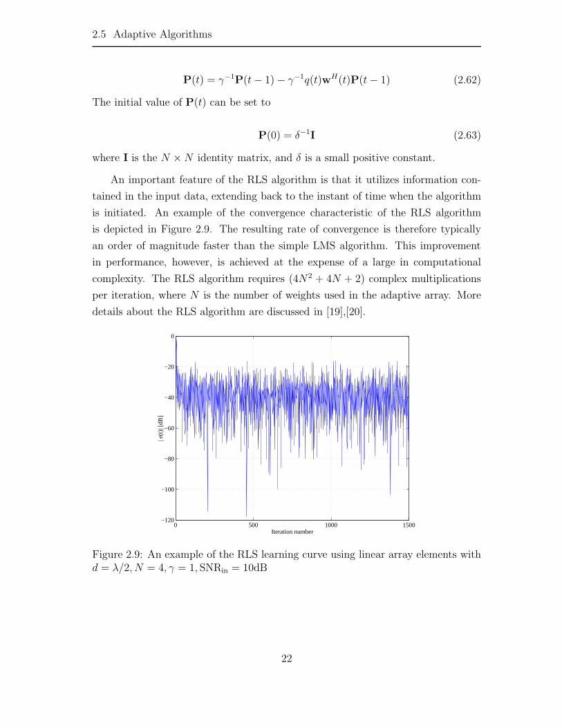
An important feature of the RLS algorithm is that it utilizes information con-
tained in the input data, extending back to the instant of time when the algorithm
is initiated. An example of the convergence characteristic of the RLS algorithm
is depicted in Figure 2.9. The resulting rate of convergence is therefore typically
an order of magnitude faster than the simple LMS algorithm. This improvement
in performance, however, is achieved at the expense of a large in computational
complexity. The RLS algorithm requires (4N2 + 4N + 2) complex multiplications
per iteration, where N is the number of weights used in the adaptive array. More
details about the RLS algorithm are discussed in [19],[20].
0 500 1000 1500−120
−100
−80
−60
−40
−20
0
Iteration number
| e(t
)| [d
B]
Figure 2.9: An example of the RLS learning curve using linear array elements withd = λ/2, N = 4, γ = 1, SNRin = 10dB
22

2.6 Benefits of Using Adaptive Arrays in Wireless Communication Systems
2.6 Benefits of Using Adaptive Arrays in Wireless Commu-
nication Systems
If a base station in a cellular system uses an adaptive, several benefits are produced
[21, 22]:
2.6.1 Signal Quality Improvement
The antenna gain is the increased average output SINR with these multiple anten-
nas. Define the input SNR as SNRin than if the N antennas are employed, the
combined signals are added in phase, while the noise is added incoherently, produc-
ing (N − 1) degree of freedom to suppress (N − 1) interferences. In a propagation
environment without multipath fading, the output SINR can be found as
SINRout = N × SNRinput (2.64)
or
SINRout[dB] = log10 N + SNRinput[dB] (2.65)
From (2.65), it is clear that the array gain achieved by an adaptive array is
G = log10 N (2.66)
In the multipath fading environment, if L delayed versions of the transmitted
signal are exploited effectively, the output SINR is given by
SINRout[dB] = G + 10 log10(L) + SNRin[dB] (2.67)
Let us taking a simple case of spatially uncorrelated 2-paths model as an exam-
ple, the output SINR is estimated as
SINRout[dB] = G + 10 log10(2) + SNRin[dB] (2.68)
Figure 2.10 shows the SNR versus the number of employed array elements. This
means that the richer the multipath fading environment is, the more diversity gain
can be achieved.
23

2.6 Benefits of Using Adaptive Arrays in Wireless Communication Systems
1 2 3 4 5 6 7 8 9 100
10
20
30
40
50
60
70
Number of array elements
Out
put S
INR
[dB
]
SNRin
= 0dB (1−path)SNR
in = 0dB (2−path)
SNRin
= 10dB (1−path)SNR
in = 10dB (2−path)
SNRin
= 20dB (1−path)SNR
in = 20dB (2−path)
Figure 2.10: Output SNR versus number of array elements.
2.6.2 Range Extension
An important benefit of smart antennas is range extension. Range extension allows
the mobile to operate farther from the base station without increasing the uplink
power transmitted by the mobile unit or the downlink power required from the base
station transmitter.
For a constant path loss exponent of l ≥ 2, the range of a cell using adaptive
array Ra is greater than the range using conventional antenna Rc. The range
extension factor (REF) is given by [23]
REF =Ra
Rc
= M1/l (2.69)
Then the extended area coverage factor (ECF), which is the ratio of the area of
a cell covered with adaptive array Aa to the area of a cell covered using conventional
antenna Ac, is given by
ECF =Aa
Ac
=
(Ra
Rc
)2
= M2/l (2.70)
24

2.7 Summary
2.6.3 Increase in Capacity
Capacity is related to the spectral efficiency of a system. The spectral efficiency E
measured in channels/km2/MHz is expressed as
E =Bt/Bch
BtNcAc=
1
BchNcAc(2.71)
where Bt is the total bandwidth of the system available for voice channels in MHz,
Bch is the bandwidth per voice channel in MHz, Nc is the number of cells per cluster.
The capacity of a system is measured in channels/km2 and is given by [24],[25]
C = EBt =Bt
BchNcAc=
Nch
NcAc(2.72)
where Nch = Bt/Bch is the total number of available voice channels in the system.
Example 1
A system with Nch = 280 channels and with conventional base station antennas
uses a seven-cell frequency reuse pattern (Nc = 7). Each cell covers an area of
Ac = 50km2. From (2.72), the capacity is Cc = 2807×50
= 0.8 channels/km2. By using
an adaptive array at the base station, ICI is reduced and Nc can be reduced to 4.
The capacity is Ca = 2804×50
= 1.4 channels/km2.
It is clear that use of adaptive array can improve system capacity compared to
the conventional system at the same range.
2.6.4 Reduction in Transmit Power
Based on the array gain achieved by an adaptive array, the reduction in the required
transmit power of the base station is available. Consequently, on the one hand, the
reduction in the transmit power is beneficial to user’s health. On the other hand,
the battery life can be extended.
2.7 Summary
We have provided an overview of adaptive arrays for wireless communications. The
array signal models of the narrowband and broadband beamforming for multipath
25

2.7 Summary
fading environments were described. Then the essential features of four criteria,
namely, MMSE, MSINR, MV, ML, and adaptive algorithms, namely, LMS, SMI,
RSL for finding optimal weight vector of adaptive arrays were illustrated. Finally,
we have shown that using adaptive arrays at base station can bring several efficient
benefits for wireless communication systems.
26

Chapter 3
Multiple-Input Multiple-Output (MIMO) System
for Wireless Communications
3.1 Basic Concepts
The application of adaptive antennas to mobile systems has significant advantages
in terms of coverage, channel capacity and signal quality. Several adaptive antenna
systems have been proposed and presented at the base station (BS) of the wireless
communication systems. However, demands for broadband wireless access technolo-
gies such as mobile internet, multi-media services given by wireless communication
systems are rapidly growing during the latest few years. In the effort to deliver high-
bit-rates in broadband wireless systems, the transmission techniques are required to
be able to cope with multipath fading channels. One of the most expected solutions
is using adaptive antennas at both transmitter and receiver [26]-[39]. It is referred
to as a multiple-input multiple-output (MIMO) antennas system. MIMO systems
are classified into two groups: (1) research on a high-quality transmission of a single
data stream such as space-time codes, a transmit/receive diversity, and transceiver
beamforming [30]-[37] or (2) research on a high-data-rate transmission of multiple
independent data streams such as VBLAST, MIMO-OFDM [38]-[42].
Although a single data stream or multiple data streams is propagated and mixed
in the air, they can be recover at the receiver by using spatial filter and correspond-
ing signal processing. This Chapter presents the principle of a single data and
multiple data streams transmissions of a MIMO system under flat and frequency-
selective fading channels with the perfect Channel State Information (CSI) at both
sides. Finally, motivation to use of a MIMO beamforming method in multipath
27

3.2 Narrowband MIMO Channel
fading environment is discussed.
3.2 Narrowband MIMO Channel
3.2.1 Single Data Stream Transmission
A narrowband communication system of M transmit and N receive antennas is
shown in Figure 3.1.
N
( )y t
1
2
n
( )Nx t
( )nx t
2 ( )x t
1( )x t
,1tw
,2tw
,t mw
,t Mw
,1rw
,2rw
,r nw
,r Nw
( )s t
1
2
m
M
11a
nma
NMa
Figure 3.1: Narrowband MIMO channel configuration with beamforming.
Under the assumption of flat fading, the propagation characteristic between
those arrays is expressed by transmission matrix A, where an,m represents the chan-
nel gain response between the mth antenna element in the transmitter and the nth
antenna element in the receiver. The transmit signal s(t) is distributed to antenna
array and multiplied by complex weight wt,m for mth element. Adding white Gaus-
sian noise and multiplying complex weight wr,n for nth element, the output signal
y(t) of the system is given by
y(t) =
N−1∑n=0
M−1∑m=0
w∗r,nan,mwt,ms(t) +
N−1∑n=0
w∗r,nnn(t) (3.1)
The equation (3.1) can be expressed in a vector form as
y(t) = wHr Awts(t) + wH
r n(t) (3.2)
28
3.2 Narrowband MIMO Channel
where
wr = [wr,0, wr,1, ..., wr,N−1]T (3.3)
and
wt = [wt,0, wt,1, ..., wt,M−1]T (3.4)
Here (.)H , (.)∗ and (.)T represent the Hermitian transpose, conjugate and transpose
of vector (or matrices).
Based on the maximal ratio combining (MRC) method, with the transmit and
receive weight vectors wt and wr in terms of the constraint of ‖ wt ‖=‖ wr ‖= 1,
the maximum of output signal-to-noise ratio is given by
SNRout =wH
r AwtwHt AHwr
||wr||Ps
PN
(3.5)
where Ps and PN are power of the transmitted signal and the noise. Thus, Ps/PN
is referred to the input SNR.
If the channel matrix A is known well at both sides, the received SNR is op-
timized by choosing the weight vectors wr and wt as the principal left and right
singular vectors of the channel matrix A. The corresponding received SNR is given
by
SNRout = λmaxSNRin (3.6)
where λmax is the largest eigenvalue of the Wishart matrix AAH.
The resulting capacity can be given by [38],[43]
C = log2(1 + λmaxSNRin) b/s/Hz (3.7)
3.2.2 Multiple Data Streams Transmission
A narrowband communication system of M transmit and N receive antennas for
multiple data streams transmission is shown in Figure 3.2.
From the singular value decomposition (SVD) theory, we have
A = wrΣwt =
P∑p=1
√λpwr,pw
Ht,p (3.8)
29

3.2 Narrowband MIMO Channel
N
1
2
n
1
2
m
M
�1
2�
p�
P�
rWtW
Figure 3.2: Narrowband MIMO channel configuration for multiple data streamtransmission.
where wr and wt are unitary matrices of left and right singular vector
wr = [wr,1,wr,2, ...,wr,P ] (3.9)
wt = [wt,1,wt,2, ...,wt,P ] (3.10)
and Σ is a diagonal matrix of singular values
Σ = diag(λ1/21 , λ
1/22 , ..., λ
1/2P ) (3.11)
where
λ1 > λ2 > ... > λP > 0 (3.12)
and P is the rank of the channel matrix
P = rank(A) = min(M, N) (3.13)
The SVD transforms the MIMO channel into P parallel independent channels
and the performance on each of the channels will be depend on its gain λp.
The resulting capacity can be expression as [38],[43]
C =
P∑p=1
log2(1 + λpSNRin) b/s/Hz (3.14)
30

3.3 Wideband MIMO Channel
3.3 Wideband MIMO Channel
In case of flat fading, the beamforming or SVD with power allocation scheme by
water filling is known to be an effective approach under the assumption of perfect
CSI in both the transmitter and the receiver. And besides, various space-time cod-
ing techniques are used when the transmitter or the receiver is uniformed [38],[44].
However, under frequency-selective multipath fading channels, those methods could
not be simply applied due to the inter symbol interference (ISI) caused by signals
arriving through delay paths. Recently, two architectures have been investigated for
MIMO systems to mitigate the effect of frequency-selective fading channels. The
first architecture is transmission of multiple data streams through spatial multi-
plexing or space-time codes combined with the orthogonal frequency division mul-
tiplexing. However, the multicarrier MIMO system is considered a most attractive
candidate since the frequency-selective MIMO channels are transformed into several
frequency flat MIMO sub-channel by using OFDM system [45]-[47]. Besides mul-
ticarrier MIMO system using either the spatial multiplexing OFDM or space-time
code OFDM, the second architecture is a single carrier MIMO system using beam-
forming, which has been studied extensively [48]-[51]. Throughout this work, we
shall restrict our study to the single carrier MIMO system under frequency-selective
multipath fading environment with prior knowledge of CSI at both the transmitter
and the receiver.
3.3.1 Single Data Stream Transmission
A general MIMO beamforming for the single data stream transmission under frequency-
selective fading channels is shown in Figure 3.3. The number of transmit and receive
antennas is M and N , respectively.
For wireless broadband systems, the MIMO propagation channel can be modeled
as
H(τ) =
L∑l=0
A(l)δ(τ − l�τ) (3.15)
31

3.3 Wideband MIMO Channel
( )s t
twrw
( )y t
1
2
M
1
2
N
(0)A
(1)A
( )LA
Figure 3.3: Broadband MIMO channel and beamforming configuration.
A(l) =
⎛⎜⎜⎜⎝
a(l)11 a
(l)12 · · · a
(l)1M
a(l)21 a
(l)22 · · · a
(l)2M
· · · · · · · · · · · ·a
(l)N1 a
(l)N2 · · · a
(l)NM
⎞⎟⎟⎟⎠ (3.16)
A(0) (l=0) is considered the channel information of the preceding wave and regarded
as the desired channel. A(l) (l = 1, ..., L) is the lth delayed channel information
which is considered interference channels. The notation a(l)nm means the lth delayed
path gain response between the mth transmit antenna and the nth receive antenna.
�τ is the unit delay time, which corresponds to symbol period Ts, of the modulated
signal.
The output of array elements is combined with a weight vector to recover the
transmitted data. Thus the output signal at the receiver is expressed as
y(t) =L∑
l=0
wHr A(l)wts(t − l∆τ) + wH
r n(t) (3.17)
where s(t) is the source signal, and n = [n1, n2, ..., nN ]T is the additive white gaus-
sian noise (AWGN) vector. The beamforming transmit and receive weight vectors
wt,wr are defined as
wt = [wt1, wt2, · · · , wtM ]T (3.18)
wr = [wr1, wr2, · · · , wrN ]T (3.19)
32
3.3 Wideband MIMO Channel
Assume that each delayed signal is uncorrelated and zero-mean, thereby
〈s∗(t − i∆τ)s(t − j∆τ)〉 = 0 for i = j (3.20)
Let us define Ps, PN and 1/γ, which are the signal power, noise power and
power ratio of the signal to noise.
〈|s|2〉 = Ps (3.21)
〈|n1|2〉 = 〈|n2|2〉 · · · = 〈|nN |2〉 = PN (3.22)
1/γ ≡ Ps/PN (3.23)
Therefore, the SINR at the receiver is given by
Γ(wt,wr) =|wH
r A(0)wt|2Ps
|∑Ll=1 wH
r A(l)wt|2Ps + ||wr||2PN
=wH
r A(o)wtwHt (A(o))Hwr∑L
l=1 wHr A(l)wtwH
t (A(l))Hwr + γwHr wr
(3.24)
3.3.2 Multiple Data Streams Transmission
A general MIMO beamforming for multiple data stream transmission under frequency-
selective fading channels is shown in Figure 3.4. The number of transmit and receive
antennas is M and N , respectively. The received signal at receiver can be expressed
as
r(t) =
Q∑i=1
L∑l=0
A(l)w(i)t s(i)(t − l∆τ) + n(t) (3.25)
where s(i) is the ith transmit data, n(t) is the i.i.d additive noise, which is assumed to
be complex Gaussian process with zero-mean and variance N0/2. The beamforming
transmit weight vector w(i)t is estimated for finding the largest eigenvalue for λmax
of the correlation matrix (A(i))HA(i) when A(i)(i ≤ L) is considered as the desired
channel.
Assume that the source signals are mutually uncorrelated with zero-mean and
unit variance, thereby
< (s(i)(t − l∆τ))∗s(i)(t − k∆τ) > for l = k (3.26)
33

3.3 Wideband MIMO Channel
Figure 3.4: Broadband MIMO channel and beamforming for multiple data streamsconfiguration.
< (s(i)(t))∗s(j)(t) >= 0 for i = j (3.27)
Multiplying complex weight vector w(k)r for detecting the transmitted data
stream s(k)(t), the output signal y(k)(t) is given by
y(k)(t) =
Q∑i=1
L∑l=0
w(k)r A(l)w
(i)t s(i)(t − (l + k − 1)∆τ) + w(k)
r n(t) (3.28)
The output SINR at the BS for finding the transmitted data stream s(k)(t) is
given by
Γ(w(k)t ,w(k)
r ) =(w(k))HA(k)w
(k)t (w
(k)t )H(A(k))Hw
(k)r
R(k)inf + γ(k)(w
(k)r )Hw
(k)r
(3.29)
where R(k)inf is the sum of interferences of the desired signal for the transmitted data
stream s(k)(t) and interferences caused by other transmitted data streams.
R(k)inf =
L∑l=0,l �=k
(w(k)r )HA(l)w
(k)t (w
(k)t )H(A(l))Hw(k)
r
+
Q∑i=1,i�=k
L∑l=0
(w(i)r )HA(l)w
(i)t (w
(i)t )H(A(l))Hw(i)
r (3.30)
34

3.4 Motivations
3.4 Motivations
As we have mentioned earlier, CCI and ISI are two factors which degrade the per-
formance of wireless communication systems. Adaptive array utilizing a spatial
filter has capability to mitigate CCI. For instance, an N element antenna array
has (N − 1) DOF and thus can suppress (N − 1) CCIs independent of the mul-
tipath environment [18],[22]. However, adaptive array exploited a spatial domain
is unavailable to treat the delayed versions of the transmitted signal as separated
signals. One of solutions is combination with temporal filter using TDL structure.
For demands in wireless access technologies such as mobile quality and high speed
service, the needs of the high performance and capacity of wireless communica-
tions system are required. The MIMO antenna systems using TDL structure for
suppressing the ISI have been absolutely considered. However, the SIMO or MISO
systems using TDL structure have been known to be practical difficulties associated
with the equalization at several megabits per second with high speed, compact and
low cost hardware. Therefore, although MIMO systems using TDL structure have
capability to suppress both CCI and ISI [50]-[53], but they are more difficult from
computational complexity and low convergence in searching for optimal weights.
On the other hand, Although MIMO systems using TDL structure adapt to
mitigate the CCI and ISI in wireless communications, they do not yet point out
clearly how many delayed channels can be effectively cancelled by using adaptive
beamforming by adjusting both the transmitter and the receiver weight vectors.
Since antenna array is used in both the transmitter and the receiver of MIMO sys-
tems, the DOF or maximum cancellation number of delayed channels is considered
to be larger than that of both SIMO and MISO systems. Through straightfor-
ward thinking, we expect that DOF of MIMO systems with M antenna elements at
the transmitter antennas and N antenna elements at the receiver (M × N MIMO
systems) is given by
DOF = M + N − 2 (3.31)
Assume that the input SNR is the threshold for communicating. In order to
achieve the equation (3.31), the output SINR obtained from the equation (3.24)
must be larger or equal to that of the input SNR in all cases of number of delayed
channels increasing from 1 to (M + N − 2). Since both the transmit and receive
35

3.5 Summary
weight vectors, however, are contained in the numerator and denominator, the
equation (3.24) becomes a multivariable nonlinear equation. It seems difficult to
find optimal transmit and receive weight vectors analytically. Meanwhile, in order
to resolve the problem, we propose a solution to find the optimal transmit and
receive weight vector based on an iterative weight update algorithm for maximizing
the output SINR under the effects of frequency-selective fading channels.
3.5 Summary
Basic overviews of the single and multiple data streams transmission models for both
narrow and wide bands MIMO beamforming with the perfect CSI at both sides
under multipath fading were presented. It was shown that the optimal transmit
and receive weight vectors become one of main factors to suppress CCI and ISI in
wireless communications system.
The motivations of our proposed scheme for MIMO beamforming method in
wireless communications system were also discussed. It was expected that our
propose scheme can effectively mitigate both CCI and ISI while maximizing the
output SINR at the receiver. On the other hand, based on our proposed method,
the convergence rate in searching the optimal weights and computational complexity
are reduced considerably.
36

Chapter 4
MIMO Beamforming for Single Data Stream
Transmission in FSF Channels
4.1 Propagation Model
Consider a MIMO wireless communication system shown in Figure 4.1, where M and
N is the number of antenna elements of the transmitter and receiver, respectively.
The idea is to transmit a single data stream simultaneously on the different antennas
of the transmitter, but at the same carrier frequency.
( )s t
twrw
( )y t
1
2
M
1
2
N
(0)A
(1)A
( )LA
Figure 4.1: Broadband MIMO channel and beamforming configuration.
For wireless broadband systems, the MIMO propagation channel can be modeled
37

4.1 Propagation Model
as
H(τ) =L∑
l=0
A(l)δ(τ − l�τ) (4.1)
A(l) =
⎛⎜⎜⎜⎝
a(l)11 a
(l)12 · · · a
(l)1M
a(l)21 a
(l)22 · · · a
(l)2M
· · · · · · · · · · · ·a
(l)N1 a
(l)N2 · · · a
(l)NM
⎞⎟⎟⎟⎠ (4.2)
where A(0)(l = 0) is the channel information of the preceding wave which we regard
as the desired channel. A(l)(l = 1, ..., L) is the lth delayed channel information
which we consider as interference channel. The notation a(l)nm means the lth delayed
path gain response between the mth transmit antenna and the nth receive antenna.
�τ is the unit delay time, which corresponds to symbol period Ts, of the modulated
signal.
Since the received signal is assumed stationary, the output of antenna array is
combined with complex weight vector to recover the transmitted signal. Thus the
received signal at the receiver is expressed as
y(t) =
L∑l=0
wHr A(l)wts(t − l∆τ) + wH
r n(t) (4.3)
where s(t) is the transmitted signal, and n = [n1, n2, ..., nN ]T is the additive white
Gaussian noise (AWGN) vector. The beamforming transmit and receive weight
vectors wt,wr are defined as
wt = [wt1, wt2, · · · , wtM ]T (4.4)
wr = [wr1, wr2, · · · , wrN ]T (4.5)
Assume that each delayed signal is uncorrelated and zero-mean, thereby
〈s∗(t − i∆τ)s(t − j∆τ)〉 = 0 for i = j (4.6)
The power of the received signal is given by
y2(t) = |wHr A(0)wts(t) +
L∑l=1
wHr [A(l)wts(t − l∆τ)] + wH
r n(t)|2
= |wHr A(0)wts(t)|2 + |
L∑l=1
wHr [A(l)wts(t − l∆τ)]|2 + |wH
r n(t)|2 (4.7)
38

4.2 Transmit and Receive Weight Vectors Determination
Let us define Ps, PI , PN and 1/γ the signal power, interference power, noise
power and power ratio of the signal to noise. The power of the received signal is
rewritten by
y2(t) = |wHr A(0)wt|2Ps +
L∑l=1
|wHr A(l)wt|2P(l)
I + |wHr wr|2PN (4.8)
Therefore, the output SINR at the receiver is given by
Γ(wt,wr) =wH
r A(o)wtwHt (A(o))Hwr∑L
l=1 wHr A(l)wtwH
t (A(l))Hwr + γwHr wr
=wH
r R0wr
wHr Rnrwr
(4.9)
where
R0 = A(o)wtwHt (A(o))H (4.10)
and
Rnr =L∑
l=1
wHr A(l)wtw
Ht (A(l))Hwr + γwH
r wr (4.11)
The equation (4.9) is a multivariable nonlinear equation. Since both the trans-
mit and receive weight vectors are contained in numerator and denominator, it seems
difficult to find optimal transmit and receive weight vectors analytically. Meanwhile,
in order to resolve this, we propose a solution to determine the optimal transmit
and receive weight vectors based on an iterative weight update algorithm for maxi-
mizing the output SINR under the effects of frequency-selective fading channels as
follows.
4.2 Transmit and Receive Weight Vectors Determination
4.2.1 Receive Weight Vector Determination
Assume that the transmit weight vector is given with a mandatory condition of
wHt wt = 1 and an optional condition of wH
r wr = 1, the steering vector of the
desired signal is A(0)wt, thereby, the receive weight vector which are resolved by
Maximum-Signal-to-Noise (MSN) method [16], can be expressed as follows.
39
4.2 Transmit and Receive Weight Vectors Determination
Taking the gradient of equation (4.9) with respect to wr give
∇Γwr(wt,wr) =∇(wH
r R0wr)(wHr Rnrwr) − (wH
r R0wr)∇(wHr Rnrwr)
(wHr Rnrwr)2
=2R0wr(w
Hr Rnrwr) − 2Rnrwr(w
Hr R0wr)
(wHr Rnrwr)2
(4.12)
The optimal receive weight vector w(opt) can be found by setting ∇Γwr(wt,wr) =
0, which leads to
R0wr =wH
r R0wr
wHr Rnrwr
Rnrwr (4.13)
Substituting (4.10) into (4.13), we have
A(o)wtwHt (A(o))Hwr =
wHr A(o)wtw
Ht (A(o))Hwr
wHr Rnrwr
Rnrwr (4.14)
Since wHt (A(o))Hwr is a scalar, (4.14) is rewritten as
A(o)wt =wH
r A(o)wt
wHr Rnrwr
Rnrwr (4.15)
Let us define 1ζ≡ wH
r A(0)wt
wHr Rnrwr
, then the receive weight vector is given by
wr = ζR−1nr A
(0)wt (4.16)
In equation (4.11), Rnr, is an Hermitian matrix, and the coefficient ζ is a
complex scalar that does not affect the received SINR itself in (4.16). Thus the
optimal receive weight vector can be normalized and given by
w(opt)r =
R−1nr A
(0)wt
‖R−1nr A
(0)wt‖ (4.17)
Accordingly, the optimal receive weight vector can be determined if the transmit
weight vector is given.
4.2.2 Transmit Weight Vector Determination
Assume that the receive weight vector is given that is allowed to determine the
optimal transmit weight vector satisfying the condition wHt wt = 1. To find the
40

4.2 Transmit and Receive Weight Vectors Determination
optimal transmit weight vector which maximizes output SINR at the receiver, we
use the Lagrange multiplier method [54] as follows.
φ = Γ(wt,wr) + λ(1 − wHt wt) (4.18)
From equation (4.9), we rewrite Γ(wt,wr) expression as
Γ(wt,wr) =wH
r A(o)wtwHt (A(o))Hwr∑L
l=1 wHr A(l)wtw
Ht (A(l))Hwr + γwH
r wr
=wH
t (A(o))HwrwHr A(o)wt∑L
l=1 wHt (A(l))HwrwH
r A(l)wt + γwHr wr
=wH
t R0wt
wHt Rltwt + γwH
r wr
(4.19)
where
R0 ≡ (A(o))HwrwHr A(o) (4.20)
and
Rlt ≡L∑
l=1
(A(l))HwrwHr A(l) (4.21)
Taking the derivative of equation (4.18) with respect to wt and setting it to
zero.∂φ
∂wt=
∂Γ
∂wt+
∂λ(1 − wHt wt)
∂wt= 0 (4.22)
then,
R0wt(wHt Rltwt + γ‖wr‖2) − Rltwt(w
Ht R0wt)
(wHt Rltwt + γ‖wr‖2)2
− λwt = 0 (4.23)
By multiplying the left and right sides of (4.23) by weight vector wHt , we have
wHt
R0wt(wHt Rltwt + γ‖wr‖2) − Rltwt(w
Ht R0wt)
(wHt Rltwt + γ‖wr‖2)2
− λwHt wt = 0 (4.24)
Applying the condition of wHt wt = 1, (4.24) is rewritten as
(wHt R0wt)w
Ht Rltwt + wH
t R0wtγ‖wr‖2 − wHt Rltwt(w
Ht R0wt)
(wHt Rltwt + γ‖wr‖2)2
− λ = 0 (4.25)
Therefore, the parameter λ is given by
λ =wH
t R0wtγ‖wr‖2
(wHt Rltwt + γ‖wr‖2)2
(4.26)
41

4.2 Transmit and Receive Weight Vectors Determination
Substituting (4.26) and (4.20) into (4.23). We have
R0wt(wHt Rltwt + γ‖wr‖2) = wH
t R0wt(Rlt + γ‖wr‖2)wt
(A(o))HwrwHr A(o)wt(w
Ht Rltwt + γ‖wr‖2) = wH
t (A(o))HwrwHr A(o)wt(Rlt + γ‖wr‖2)wt
(4.27)
Since wHr A(o)wt is a scalar, (4.27) is rewritten as
(A(o))Hwr =wH
t (A(o))Hwr
wHt Rltwt + γ‖wr‖2
(Rlt + γ‖wr‖2)wt (4.28)
Let us define 1ξ≡ wH
t (A(o))Hwr
wHt Rltwt+γ‖wr‖2 , then the equation (4.28) can be expressed as
wt = ξR−1nt (A(o))Hwr (4.29)
where
Rnt = Rlt + γ‖wr‖2 (4.30)
Without detailed calculation of ξ, the optimal transmit weight vector can be
given by
w(opt)t =
R−1nt (A(o))Hwr
‖R−1nt (A(o))Hwr‖
(4.31)
We conclude that the determination of transmit and receive weight vectors by
pointing out that the receive weight vector is estimated by (4.17) with the given
transmit weight vector. Similarly for the transmit weight vector, it is estimated
by (4.31) with the given receive weight vector. However, because the simultane-
ous equations become a nonlinear formula, it seems not easy to solve analytically.
Therefore, an iterative algorithm, which estimates the receive and transmit weight
vectors alternately is a simple way to reach solution for maximizing SINR. The
iterative operation (u > 1) is described in the next section.
4.2.3 Iterative Weight Vector Update Algorithm
For the updated receive weight vector
The updated receive weight vector at time u is given by
wr(u) = R−1nr (u − 1)A(o)wt(u − 1) (4.32)
42

4.3 Interference Cancellation Ability Analysis
where
Rnr(u) ≡L∑
l=1
A(l)wt(u)wHt (u)(A(l))H + γI (4.33)
and
wr(u) =wr(u)
‖wr(u)‖ (4.34)
Rnr(u − 1) is updated based on the previous transmitted weights wt(u) for
finding the optimal receive weights wr(u).
For the updated transmit weight vector
The update transmit weight vector at time u is given by
wt(u) = R−1nt (u)(A(o))Hwr(u) (4.35)
where
Rnt(u) ≡L∑
l=1
(A(l))Hwr(u)wHr (u)A(l) + γI (4.36)
and
wt(u) =wt(u)
‖wt(u)‖ (4.37)
Similarly, Rnt(u) is also updated based on the previous received weights wr(u),
for finding the optimal transmit weights wt(u).
In this work, the initial transmit weight vector wt(0) for u = 0 is determined
from MIMO system in flat fading channel environment as follows.
w(opt)t {= wt(0)} = et,max (4.38)
The vector et,max is the eigenvector corresponding to the largest eigenvalue λmax,
for the correlation matrix (A(o))HA(o) [43],[56].
4.3 Interference Cancellation Ability Analysis
Since the transmit and receive weight vectors are alternately updated based on the
proposed iterative update weight algorithm, the DOFs of both the transmitter and
receiver antennas are combined together to suppress the delayed versions of the
preceding signal. Thus, for a MIMO system with M and N antennas equipped at
43

4.4 Output SINR
both the transmitter and the receiver, respectively, the maximum number of delayed
channels cancellation when jointing DOF of both sides is expected as
L = (M − 1) + (N − 1) = M + N − 2 (4.39)
The maximum number of delayed channels cancellation is clearly confirmed by
computer simulation.
4.4 Output SINR
Based on the proposed method, the optimal transmit and receive weight vectors
are used in the transmitter and receiver, respectively for the single data stream
transmission. The output signal at the receiver side is given by
y(t) =L∑
l=0
(woptr )HA(l)(wt)
opts(t − l∆τ) + (woptr )Hn(t) (4.40)
The output SINR of the proposed scheme is calculated via the cross-correlation
coefficient and given by
ρ =E[y(t)s∗(t)]√
E[|y(t)|2]E[|s(t)|2] (4.41)
The output SINR is finally computed via the correlation coefficient as
SINRout =|ρ|2
1 − |ρ|2 (4.42)
4.5 Simulation Results
4.5.1 Simulation Conditions
In this section, we offer the simulation conditions to demonstrate our analysis.
We assumed that the components of the channel state matrix are independent
identically distributed (i.i.d) with the uniform power delay profile (model 1) and
the exponential power delay profile (model 2) [55], respectively, given by
p(τ) =
L∑l=0
δ(τ − lTs) (model 1) (4.43)
44

4.5 Simulation Results
p(τ) =PR
στ
L∑l=0
e−τ
στ δ(τ − lTs) (model 2) (4.44)
where Ts is the symbol period of the transmitted signal, PR denotes the average
power of multipath signals, and στ represents the delay spread.
For model 1, each impulse a(l)nm is generated by the i.i.d. process while keeping
< |a(l)nm|2 >= 1 for n = 1 ∼ N, m = 1 ∼ M and l = 0 ∼ L. Figure 4.2(a) shows the
assumed channel model considered in uniform power delay profile. Since the main
purpose of this paper is to establish the weights determination scheme and identify
the limit of delayed channels cancellation by means of our proposed scheme, we
adopted an unrealistic propagation channel and a high SNR. In order to clarify the
limit of the delayed channels cancellation ability, we set a sufficiently high Ps/PN ,
such that Ps/PN = 40dB.
Although the uniform power delay profile is effective for examination of the
working mechanism of the proposed scheme, it is not realistic in indoor and outdoor
wireless propagation environments. Therefore, model 2 will be used in order to
evaluate the quantitative characteristics. Figure 4.2(b) shows the assumed channel
model considered in the exponential power delay profile.
For both profiles, the amplitude of each impulse follows independent complex
Gaussian distribution where the average follows (4.43) or (4.44). The simulation
conditions are summarized in Table 4.1.
Table 4.1: Simulation model for MIMO beamforming
Parameters ValueType of array linear(M, N) antennas (2,2), (3,3), (4,4), (8,8)Type of modulation BPSKSignal length 104 symbolsSampling type 1 sample/symbolInput SNR 20dB, 40dB
45
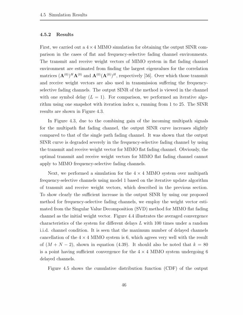
4.5 Simulation Results
4.5.2 Results
First, we carried out a 4×4 MIMO simulation for obtaining the output SINR com-
parison in the cases of flat and frequency-selective fading channel environments.
The transmit and receive weight vectors of MIMO system in flat fading channel
environment are estimated from finding the largest eigenvalues for the correlation
matrices (A(0))HA(0) and A(0)(A(0))H , respectively [56]. Over which those transmit
and receive weight vectors are also used in transmission suffering the frequency-
selective fading channels. The output SINR of the method is viewed in the channel
with one symbol delay (L = 1). For comparison, we performed an iterative algo-
rithm using one snapshot with iteration index u, running from 1 to 25. The SINR
results are shown in Figure 4.3.
In Figure 4.3, due to the combining gain of the incoming multipath signals
for the multipath flat fading channel, the output SINR curve increases slightly
compared to that of the single path fading channel. It was shown that the output
SINR curve is degraded severely in the frequency-selective fading channel by using
the transmit and receive weight vector for MIMO flat fading channel. Obviously, the
optimal transmit and receive weight vectors for MIMO flat fading channel cannot
apply to MIMO frequency-selective fading channels.
Next, we performed a simulation for the 4 × 4 MIMO system over multipath
frequency-selective channels using model 1 based on the iterative update algorithm
of transmit and receive weight vectors, which described in the previous section.
To show clearly the sufficient increase in the output SINR by using our proposed
method for frequency-selective fading channels, we employ the weight vector esti-
mated from the Singular Value Decomposition (SVD) method for MIMO flat fading
channel as the initial weight vector. Figure 4.4 illustrates the averaged convergence
characteristics of the system for different delays L with 100 times under a random
i.i.d. channel condition. It is seen that the maximum number of delayed channels
cancellation of the 4 × 4 MIMO system is 6, which agrees very well with the result
of (M + N − 2), shown in equation (4.39). It should also be noted that k = 80
is a point having sufficient convergence for the 4 × 4 MIMO system undergoing 6
delayed channels.
Figure 4.5 shows the cumulative distribution function (CDF) of the output
46
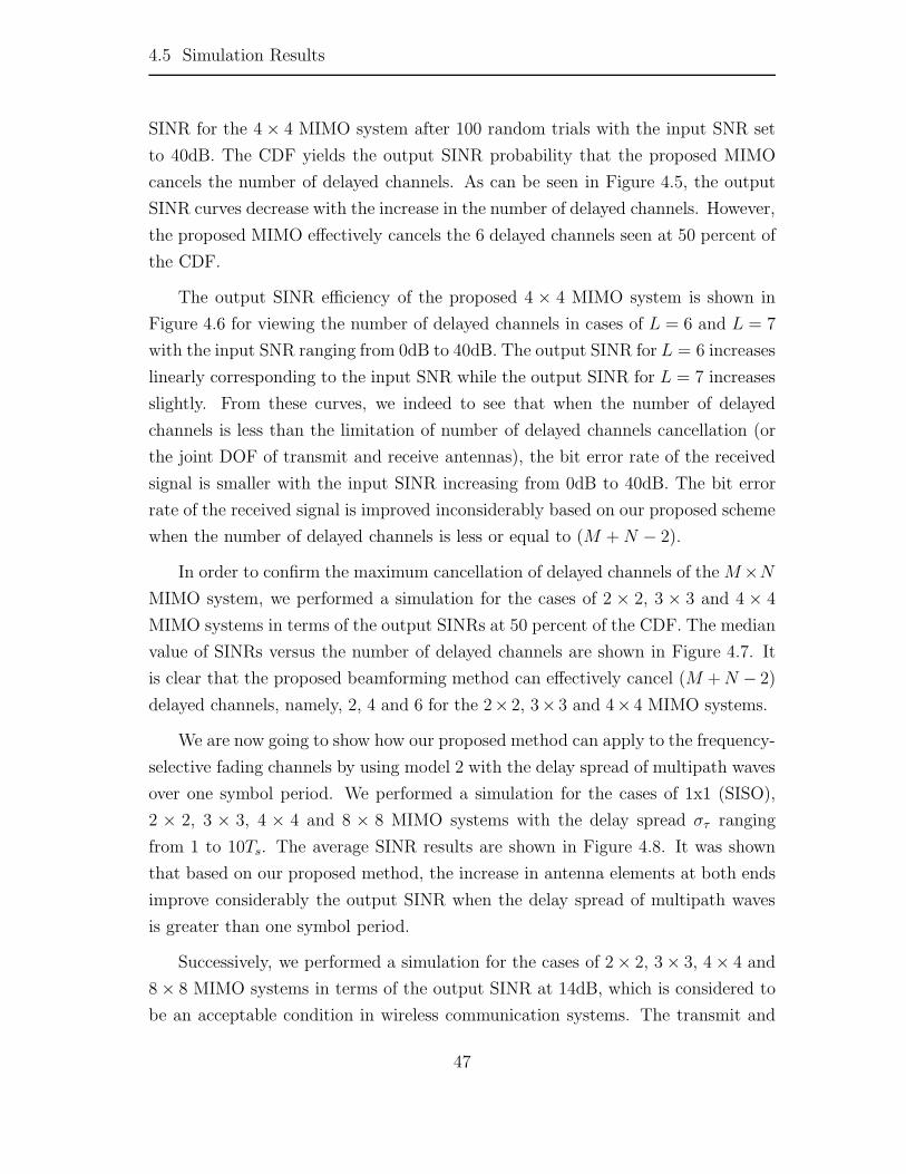
4.5 Simulation Results
SINR for the 4 × 4 MIMO system after 100 random trials with the input SNR set
to 40dB. The CDF yields the output SINR probability that the proposed MIMO
cancels the number of delayed channels. As can be seen in Figure 4.5, the output
SINR curves decrease with the increase in the number of delayed channels. However,
the proposed MIMO effectively cancels the 6 delayed channels seen at 50 percent of
the CDF.
The output SINR efficiency of the proposed 4 × 4 MIMO system is shown in
Figure 4.6 for viewing the number of delayed channels in cases of L = 6 and L = 7
with the input SNR ranging from 0dB to 40dB. The output SINR for L = 6 increases
linearly corresponding to the input SNR while the output SINR for L = 7 increases
slightly. From these curves, we indeed to see that when the number of delayed
channels is less than the limitation of number of delayed channels cancellation (or
the joint DOF of transmit and receive antennas), the bit error rate of the received
signal is smaller with the input SINR increasing from 0dB to 40dB. The bit error
rate of the received signal is improved inconsiderably based on our proposed scheme
when the number of delayed channels is less or equal to (M + N − 2).
In order to confirm the maximum cancellation of delayed channels of the M×N
MIMO system, we performed a simulation for the cases of 2 × 2, 3 × 3 and 4 × 4
MIMO systems in terms of the output SINRs at 50 percent of the CDF. The median
value of SINRs versus the number of delayed channels are shown in Figure 4.7. It
is clear that the proposed beamforming method can effectively cancel (M + N − 2)
delayed channels, namely, 2, 4 and 6 for the 2× 2, 3× 3 and 4× 4 MIMO systems.
We are now going to show how our proposed method can apply to the frequency-
selective fading channels by using model 2 with the delay spread of multipath waves
over one symbol period. We performed a simulation for the cases of 1x1 (SISO),
2 × 2, 3 × 3, 4 × 4 and 8 × 8 MIMO systems with the delay spread στ ranging
from 1 to 10Ts. The average SINR results are shown in Figure 4.8. It was shown
that based on our proposed method, the increase in antenna elements at both ends
improve considerably the output SINR when the delay spread of multipath waves
is greater than one symbol period.
Successively, we performed a simulation for the cases of 2 × 2, 3 × 3, 4 × 4 and
8 × 8 MIMO systems in terms of the output SINR at 14dB, which is considered to
be an acceptable condition in wireless communication systems. The transmit and
47

4.6 Summary
receive antennas of the M ×N MIMO beamforming systems with (M = N) versus
the delay spread στ is shown in Figure 4.9. It was shown that στ = (N − 1)Ts
for (M = N) is a maximum delay spread where a reliable communication can be
achieved by the proposed beamforming method.
4.6 Summary
In this paper, we proposed the weights determination scheme for MIMO beamform-
ing in frequency-selective fading channels. This scheme yields the output SINR
improvement based on the iterative update algorithm of the transmit and receive
weight vectors and enables the cancellation of (M + N − 2) delayed channels. The
simulation result shows that the convergence speed of our proposed method is fast
with knowledge of the CSI at both the transmitter and receiver.
48

4.6 Summary
0 2 4 6 8 10 12−50
−40
−30
−20
−10
0
10
Access delay
Rel
ativ
e av
erag
e po
wer
(dB
)
(a) A discrete−time uniform power delay profile (in case of Li=7)
0 5 10 15 20 25 30−50
−40
−30
−20
−10
0
10
Access delay
Rel
ativ
e av
erag
e po
wer
(dB
)
(b) A discrete−time exponential power delay profile (in case of στ= 5)
Figure 4.2: Assumption of power delay profiles: a. A discrete-time uniform powerdelay profile; b. A discrete-time exponential power delay profile.
49

4.6 Summary
5 10 15 20 250
10
20
30
40
50
60
70
80
Interation index
SINR [dB]
SINR estimation at the receiver
Single path flat fading channel (L=0)Multipath flat fading channel (L=0)Frequency-selective fading channels (L=1)
Figure 4.3: SINR in flat and frequency-selective fading channels when using wt andwr calculated from A(0).
20 40 60 80 1000
10
20
30
40
50
60
Iteration index: k
Average SINR [dB]
SINR estimation at the receiver
L = 0 L = 1 L = 2 L = 3 L = 4 L = 5
L = 6
L = 7
Figure 4.4: Convergence characteristics for different delays.
50

4.6 Summary
0 10 20 30 40 500
0.1
0.2
0.3
0.4
0.5
0.6
0.7
0.8
0.9
1
SINR [dB]
Cumulative probability Median
value
L = 0123456
7
Figure 4.5: CDF of SINR for the 4x4 MIMO at the receiver.
0 5 10 15 20 25 30 35 400
5
10
15
20
25
30
35
40
45
50
SINRin
SIN
Rou
t
4x4 MIMO Beamforming
For L = 6For L = 7
Figure 4.6: SINR performance of the proposed 4x4 MIMO system in case of L = 6and L = 7.
51

4.6 Summary
0 1 2 3 4 5 6 70
5
10
15
20
25
30
35
40
45
50
55
Number of delayed channels: L
SINR [dB]
(M=N=4) (M=N=3)
(M=N=2)
Figure 4.7: Median value of SINR vs. the number of delayed channels.
0 1 2 3 4 5 6 7 8 9 10−5
0
5
10
15
20
25
30
35
40
delay spread στ
Ave
rage
SIN
R [
dB]
SINR estimation at the receiver
SISO2x2 MIMO3x3 MIMO4x4 MIMO8x8 MIMO
Figure 4.8: Average SINR of MxN MIMO as a function of the delay spread στ .(model 2)
52

4.6 Summary
0 1 2 3 4 5 6 7 80
1
2
3
4
5
6
7
8
9
10
N (M = N)
Del
ay s
prea
d σ
τ [T
s]
SINR ≅ 14dB
Figure 4.9: The maximum delay spread realizing acceptable communication qualityas a function of the number of array elements. (model 2)
53

Chapter 5
Multiuser MIMO Beamforming for Single Data
Stream Transmission in FSF Channels
In this chapter, we propose a MIMO beamforming scheme using a single data stream
transmission for multiuser systems in frequency-selective multipath channels. As-
sume that the channel state information (CSI) is perfectly known at both transmit-
ter and receiver. The transmit weight vector for each user and the receive weight
vector at base station (BS) corresponding to each user are calculated using two
proposed algorithms, which maximize the output SINR for all receivers and every
single link at the same time. Deriving MIMO beamforming for the single user sys-
tem from Chapter 4, we analyze a maximum number of interference channels which
could be eliminated in multiuser system.
5.1 Propagation Model
Suppose there are Q users communicating with a BS. The ith user has a linear array
antenna with Mi elements, where i = 1, ..., Q. BS has an adaptive antenna with N
elements. A general MIMO beamforming for a single data stream transmission for
multiuser system under frequency-selective fading channels environment is shown
in Figure 5.1.
For wireless broadband systems, the MIMO propagation channel can be modeled
as
Hi(τ) =
Li−1∑l=0
A(l)i δ(τ − l�τ) (5.1)
54

5.1 Propagation Model
,1rw
1
2
N
1( )y t
( )Qy t
1
2
1M
1
2
,t Qw
,1tw
1( )s t
( )Qs t
QM
,r Qw
(0)
1A
(1)
1A
1( 1)
1
L -A
( 1)QL
Q
-A
(1)
QA
(0)
QA
1user
user Q
1user
user Q
Base Station
Figure 5.1: Broadband MIMO channel and beamforming configuration for a multi-user system.
A(l)i =
⎛⎜⎜⎜⎝
a(l)11,i a
(l)12,i · · · a
(l)1M,i
a(l)21,i a
(l)22,i · · · a
(l)2M,i
· · · · · · · · · · · ·a
(l)N1,i a
(l)N2,i · · · a
(l)NM,i
⎞⎟⎟⎟⎠ (5.2)
where A(0)i is the channel information of the preceding wave of the ith user, which
we regard as the desired channel in this work, while A(l)i (l = 1, ..., Li − 1), is the
lth delayed channel information of the preceding channel of the ith user, which we
consider as interference channels. The notation a(l)nm,i means the lth interference
path response between the mth transmit antenna of the ith user and nth receive
antenna of the BS. �τ is the unit delay time, which corresponds to symbol period
Ts, of the modulated signal.
Since the received signal is assumed stationary. the output of array elements
55

5.1 Propagation Model
is combined with complex weight vector to extract the desired signal. Thus the
received signal for the ith user at the BS is expressed as
yi(t) =
Q∑j=1
Lj−1∑l=0
wHr,iA
(l)j wt,jsj(t − l∆τ) + wH
r,in(t) (5.3)
where sj(t) is the transmit data of the jth user, and n = [n1, n2, ..., nN ]T is the
additive white Gaussian noise (AWGN) vector. The beamforming transmit and
receive weight vectors wt,i and wr,i for the ith user are defined as
wt,i = [wt1,i, wt2,i, · · · , wtM,i]T (5.4)
wr,i = [wr1,i, wr2,i, · · · , wrN,i]T (5.5)
Assume that the source signals are mutually uncorrelated with zero-mean and
unit variance, thereby
〈s∗i (t − l∆τ)si(t − k∆τ)〉 = 0 for l = k (5.6)
〈s∗i (t)sj(t)〉 = 0 for i = j (5.7)
Let us define Ps,i, PN and 1/γi, representing the signal power, noise power and
power ratio of the signal to noise for the ith user:
〈|si|2〉 = Ps,i (5.8)
〈|n1|2〉 = 〈|n2|2〉 · · · = 〈|nN |2〉 = PN (5.9)
1/γi ≡ Ps,i/PN (5.10)
The output SINR at the BS for the ith user is given by
Γ(wt,i,wr,i) =wH
r,iA(o)i wt,iw
Ht,i(A
(o)i )Hwr,i
Rinf + γiwHr,iwr,i
(5.11)
where Rinf is the sum of interference channels of the preceding channels of the ith
user and interference channels caused by other users.
Rinf =
Li−1∑l=1
wHr,iA
(l)i wt,iw
Ht,i(A
(l)i )Hwr,i
+
Q∑j=1,j �=i
Lj−1∑l=0
wHr,iA
(l)j wt,jw
Ht,j(A
(l)j )Hwr,i (5.12)
56

5.2 Transmit and Receive Weight Vectors Determination
Similarly to Chapter 4, since the transmit and receive weight vectors for detec-
tion of the ith user are contained in numerator and denominator, (5.11) is a mul-
tivariable nonlinear equation. It seems to be difficult to find the optimal transmit
and receive weight vectors analytically. Determination of the transmit and receive
weight vectors for detection of the ith user under the effects of frequency-selective
fading channels and multiuser is described in the next section.
5.2 Transmit and Receive Weight Vectors Determination
We employ the MSINR method to determine the optimal transmit and receive
weight vectors, for which single user case is described in detail in [57]. By extending
the method to multiuser case, the receive and transmit weight vectors determination
for the ith user is summarized in the following.
5.2.1 Receive weight vector determination
Assume that all the transmit weight vectors (wt,j, j = 1, ..., Q) are given, and an
optional condition of wHr,iwr,i = 1 to keep the total noise power constant. The
steering vector of the desired signal is A(0)i wt,i and based on the MSINR method,
the receive weight vector at BS for the ith user is given by
w(opt)r,i = R−1
nr,iA(0)i wt,i/‖R−1
nr,iA(0)i wt,i‖ (5.13)
where Rnr,i is a covariance matrix, which includes total information of interference
channels of the ith user and interference channels caused by other users, given by
Rnr,i ≡Li−1∑l=1
A(l)i wt,iw
Ht,i(A
(l)i )H
+
Q∑j=1,j �=i
Lj−1∑l=0
A(l)j wt,jw
Ht,j(A
(l)j )H
+ γiI (5.14)
5.2.2 Transmit weight vector determination
Assume that the receive weight vector wr,i and all the transmit weight vectors
excluding wt,i are given, we determine the optimal transmit weight vector satisfying
57

5.2 Transmit and Receive Weight Vectors Determination
the condition wHt,iwt,i=1. Based on the method of Lagrange multiplier, the optimal
transmit weight vector for the ith user is given by
w(opt)t,i = R−1
nt,i(A(o)i )Hwr,i/‖R−1
nt,i(A(o)i )Hwr,i‖ (5.15)
where Rnt,i is a covariance matrix, which includes total information of interference
channels of the ith user and interference channels caused by other users, given by
Rnt,i ≡Li−1∑l=1
(A(l)i )Hwr,iw
Hr,iA
(l)i
+
Q∑j=1,j �=i
Lj−1∑l=0
wHt,j(A
(l)j )Hwr,iw
Hr,iA
(l)j wt,jI
+ γiI (5.16)
The detailed transmit weight vector determination is seen in the Appendix A.
We conclude that by giving the transmit weight vector of the ith user and fixing
all the transmit weight vectors of the rest of users, the optimal receive weight vector
at BS for the ith user is calculated by Eq.(5.13). Similarly, the optimal transmit
weight vector for the ith user is calculated through Eq.(5.15) by giving the receive
weight vector at the BS for the ith user and all the transmit weight vectors excluding
wt,i.
5.2.3 Iterative Weight Update Algorithms
In this section, we propose two algorithms along the lines of optimization principles.
Block diagram of algorithm A and algorithm B are shown in Figure 5.2 and 5.3,
respectively
OptimizedGiven For what
1 1SINR of fory s
2 2SINR of fory s,2 (0)tw
,1(0)tw,1(1)rw
,2 (1)rw
Figure 5.2: Block diagram of the maximizing SINR by means of receiver-side weightvector optimization. (Q = 2) [Algorithm A]
58
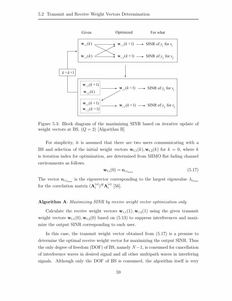
5.2 Transmit and Receive Weight Vectors Determination
OptimizedGiven For what
,1( )t kw
,2 ( )t kw
1 1SINR of fory s
2 2SINR of fory s
,1( 1)r k +w
,2 ( 1)r k +w
,2 ( 1)r k +w
,1( 1)r k +w
,1( 1)t k +w
,2 ( 1)t k +w
1 1SINR of fory s
2 2SINR of fory s
1k k= +
,2 ( )t kw
,1( 1)t k +w
Figure 5.3: Block diagram of the maximizing SINR based on iterative update ofweight vectors at BS. (Q = 2) [Algorithm B]
For simplicity, it is assumed that there are two users communicating with a
BS and selection of the initial weight vectors wt,1(k),wt,2(k) for k = 0, where k
is iteration index for optimization, are determined from MIMO flat fading channel
environments as follows.
wt,i(0) = et,imax(5.17)
The vector et,imaxis the eigenvector corresponding to the largest eigenvalue λimax
for the correlation matrix (A(o)i )HA
(o)i [56].
Algorithm A: Maximizing SINR by receive weight vector optimization only
Calculate the receive weight vectors wr,1(1),wr,2(1) using the given transmit
weight vectors wt,1(0),wt,2(0) based on (5.13) to suppress interferences and maxi-
mize the output SINR corresponding to each user.
In this case, the transmit weight vector obtained from (5.17) is a premise to
determine the optimal receive weight vector for maximizing the output SINR. Thus
the only degree of freedom (DOF) of BS, namely N−1, is consumed for cancellation
of interference waves in desired signal and all other multipath waves in interfering
signals. Although only the DOF of BS is consumed, the algorithm itself is very
59

5.3 Interference Cancellation Ability Analysis
simple and seems practical.
Algorithm B: Maximizing SINR based on iterative update of both ends weight
vectors
1. Calculate the receive weight vectors wr,1(k + 1),wr,2(k + 1) with the given
transmit weight vectors wt,1(k),wt,2(k) based on (5.13) for maximizing SINR
corresponding to each user.
2. Calculate the transmit weight vectors wt,1(k + 1),wt,2(k + 1) by the updated
receive weight and previous transmitted weight vectors wr,1(k + 1),wt,2(k)
and wr,2(k+1),wt,1(k+1), respectively, based on (5.15) for maximizing SINR
corresponding to each user.
3. Go to step 1 and repeat the iteration until a certain condition for termination
is satisfied.
4. Send the optimal transmit weight vector obtained at BS to mobile stations.
Using this transmit weight vector at each user side, the SINR of each user is
maximized at the BS.
The maximum SINR is given in (5.11) where wt,i and wr,i are replaced by w(opt)t,i
and w(opt)r,i , respectively. Although both the algorithm A and B maximize SINR, the
algorithm A is a scheme which optimizes the weight vector of receiver side only
while the algorithm B is an algorithm which optimizes the weight vector of both
transmitter and receiver at BS. Thus, condition is different even if it is the same
propagation environment, the performance (namely, obtained maximum SINR) of
the algorithm B is better. The detailed analysis of this algorithm is carried out in
the next section from the view point of DOF.
5.3 Interference Cancellation Ability Analysis
In this section, we investigate the interference channels cancellation ability of the
proposed MIMO beamforming method in the single data stream transmission for
multiuser system. In general, an M element array, where the optimal beamformer
60
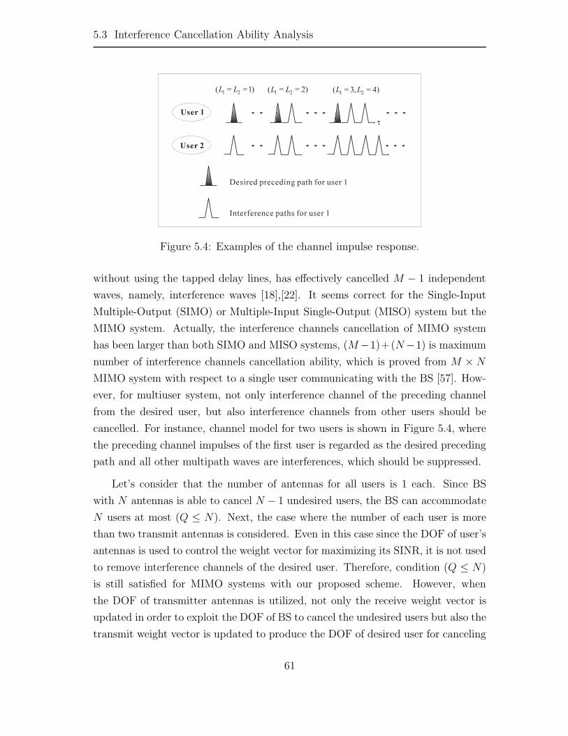
5.3 Interference Cancellation Ability Analysis
User 1
User 2
Desired preceding path for user 1
Interference paths for user 1
1 2( 1)L L= = 1 2( 2)L L= = 1 2( 3, 4)L L= =
�
Figure 5.4: Examples of the channel impulse response.
without using the tapped delay lines, has effectively cancelled M − 1 independent
waves, namely, interference waves [18],[22]. It seems correct for the Single-Input
Multiple-Output (SIMO) or Multiple-Input Single-Output (MISO) system but the
MIMO system. Actually, the interference channels cancellation of MIMO system
has been larger than both SIMO and MISO systems, (M−1)+(N −1) is maximum
number of interference channels cancellation ability, which is proved from M × N
MIMO system with respect to a single user communicating with the BS [57]. How-
ever, for multiuser system, not only interference channel of the preceding channel
from the desired user, but also interference channels from other users should be
cancelled. For instance, channel model for two users is shown in Figure 5.4, where
the preceding channel impulses of the first user is regarded as the desired preceding
path and all other multipath waves are interferences, which should be suppressed.
Let’s consider that the number of antennas for all users is 1 each. Since BS
with N antennas is able to cancel N − 1 undesired users, the BS can accommodate
N users at most (Q ≤ N). Next, the case where the number of each user is more
than two transmit antennas is considered. Even in this case since the DOF of user’s
antennas is used to control the weight vector for maximizing its SINR, it is not used
to remove interference channels of the desired user. Therefore, condition (Q ≤ N)
is still satisfied for MIMO systems with our proposed scheme. However, when
the DOF of transmitter antennas is utilized, not only the receive weight vector is
updated in order to exploit the DOF of BS to cancel the undesired users but also the
transmit weight vector is updated to produce the DOF of desired user for canceling
61

5.3 Interference Cancellation Ability Analysis
its own interference channels. They are alternately updated to eliminate much more
interference channels. We summarize now the conditions to find a total number of
interference channels cancellation as follows.
• A maximum number of users Q is less than or equal to BS array antenna N
(Q ≤ N).
• The DOF of BS, N − 1, could be used to cancel interference channels of any
users.
• If the DOF of BS is larger than a total interference channels of all the undesired
users, the DOF remainder of BS might be useful for the desired user to cancel
more interference channels themselves.
• The DOF of the desired ith user, Mi − 1, could be used to cancel its own
interference channels {A(l)i ; l = 1, ..., Li − 1}.
• The DOF remainder of each user cannot cancel interference channels of other
users. In other words, BS can only utilize its own DOF remainder to cancel
interference channels of users.
For the algorithm A, the condition for interferences cancellation for the ith user
in multiuser system is found through an inequality, which set up based on the above
conditions and is given by
N − 1 ≥ LU + (Li − 1) for algorithm A (5.18)
where LU is a total number of interference channels of all the undesired users, and
is given by
LU =
Q∑j=1,j �=i
Lj (5.19)
Based on the update of transmit and receive weight vectors, the BS exploits
its DOF to cancel interference channels of all the undesired users and the DOF of
desired user is used to cancel interference channels themselves. Therefore, a total
number of interference channels cancellation for the ith user in multiuser system
using the algorithm B is found through an inequality in the following.
N − 1 ≥ LU + LD for algorithm B (5.20)
62

5.4 Output SINR
where LD is the remainder of interference channels of the desired user after using
its DOF to cancel interference channels themselves, and is given by.
LD = max{(Li − 1) − (Mi − 1), 0} (5.21)
In the following, the effectiveness of above inequalities (5.18) and (5.20) are
clearly confirmed by the computer simulation.
5.4 Output SINR
Based on the proposed method for multiuser system, the optimal transmit and
receive weight vectors are used in the transmitters and receiver, respectively for
single data stream transmission. The output signal of the ith user at the BS is
given by
yi(t) =
Q∑j=1
Lj−1∑l=0
(woptr,i )HA
(l)j wopt
t,j sj(t − l∆τ) + (woptr,i )Hn(t) (5.22)
where woptt,j and wopt
r,i are the optimal transmit and receive weight vectors, respec-
tively, obtained from either the algorithm A or the algorithm B.
Then the output SINR of the ith user is calculated via the cross-correlation
coefficient ρi at the BS and given by
ρi =E[yi(t)s
∗i (t)]√
E[|yi(t)|2]E[|si(t)|2](5.23)
The output SINR calculation via the correlation coefficient for the ith user at the
BS is finally given by
SINRout,i =|ρi|2
1 − |ρi|2 (5.24)
5.5 Simulation Results
5.5.1 Simulation Conditions
In this section, to demonstrate the performance of the proposed algorithms, com-
puter simulations are carried out for two users communicating with a BS case. We
63
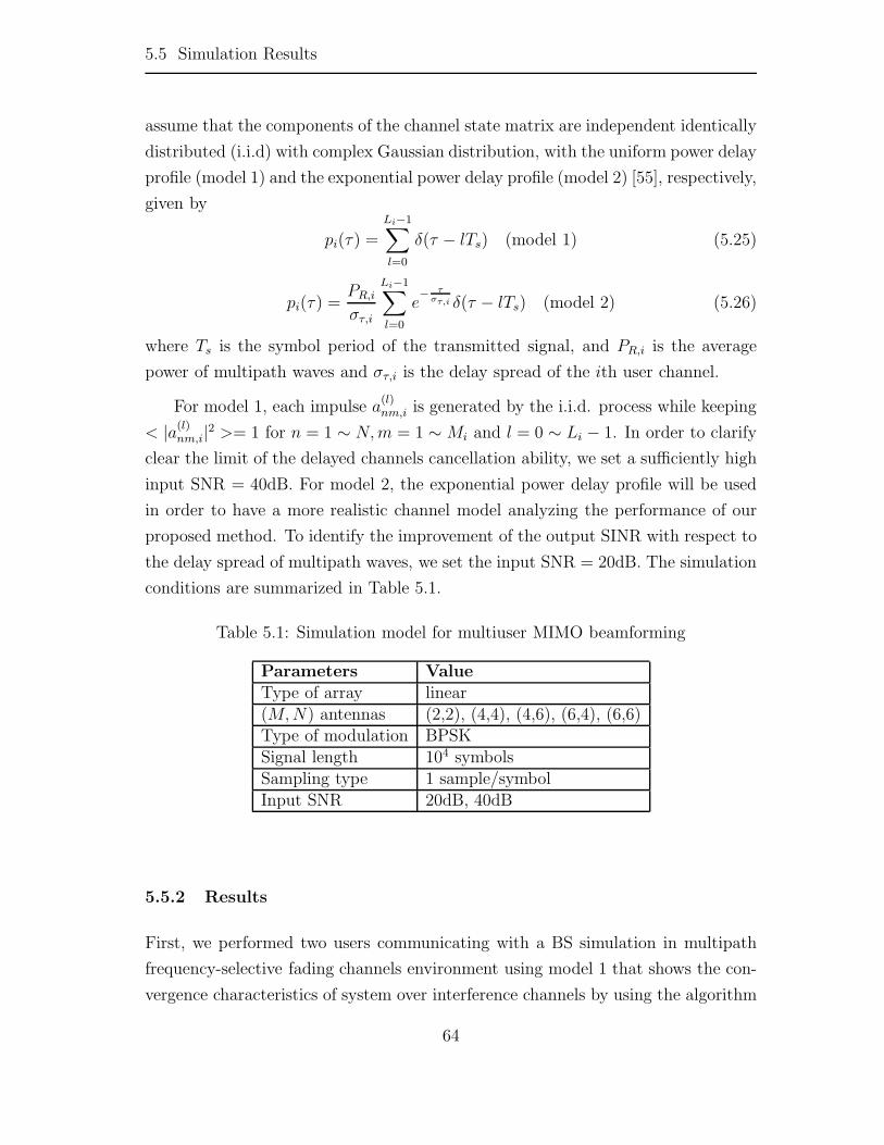
5.5 Simulation Results
assume that the components of the channel state matrix are independent identically
distributed (i.i.d) with complex Gaussian distribution, with the uniform power delay
profile (model 1) and the exponential power delay profile (model 2) [55], respectively,
given by
pi(τ) =
Li−1∑l=0
δ(τ − lTs) (model 1) (5.25)
pi(τ) =PR,i
στ,i
Li−1∑l=0
e− τ
στ,i δ(τ − lTs) (model 2) (5.26)
where Ts is the symbol period of the transmitted signal, and PR,i is the average
power of multipath waves and στ,i is the delay spread of the ith user channel.
For model 1, each impulse a(l)nm,i is generated by the i.i.d. process while keeping
< |a(l)nm,i|2 >= 1 for n = 1 ∼ N, m = 1 ∼ Mi and l = 0 ∼ Li − 1. In order to clarify
clear the limit of the delayed channels cancellation ability, we set a sufficiently high
input SNR = 40dB. For model 2, the exponential power delay profile will be used
in order to have a more realistic channel model analyzing the performance of our
proposed method. To identify the improvement of the output SINR with respect to
the delay spread of multipath waves, we set the input SNR = 20dB. The simulation
conditions are summarized in Table 5.1.
Table 5.1: Simulation model for multiuser MIMO beamforming
Parameters ValueType of array linear(M, N) antennas (2,2), (4,4), (4,6), (6,4), (6,6)Type of modulation BPSKSignal length 104 symbolsSampling type 1 sample/symbolInput SNR 20dB, 40dB
5.5.2 Results
First, we performed two users communicating with a BS simulation in multipath
frequency-selective fading channels environment using model 1 that shows the con-
vergence characteristics of system over interference channels by using the algorithm
64
5.5 Simulation Results
B. The number of antenna elements of BS and each user are equal to 4. In order
to make clear interference channels cancellation limit, the input SNR is set to be of
40dB. The reference source signal of each user is used in BS to detect the desired
signal. The simulation result is shown in Figure 5.5.
Although the propagation environment of user 1 and 2 has the same statisti-
cal characteristic, instantaneous environment given by complex random number is
different. Then the transmit weight vector of user 1 and 2 is optimized at BS with
respect to its received signal. Thus, since the statistical characteristic of propaga-
tion environment and antennas number of two users are the same, two convergence
characteristics are similar. After 100 times trials by changing the propagation con-
ditions keeping the given statistical property constant, it can be identified that the
system cancels a total number of 5 interference channels (namely, L1 = L2 = 3)
for both user 1 and user 2. Since the increase in interferences leads to the matrix
be full rank so that the increase in interference channels lead to longer convergence
time. It is seen that k = 80 is a point having sufficient convergence characteristic
of system corresponding to 5 interference channels.
Next, for comparison of two proposed algorithms, we carried out a two-user
4×4 MIMO system simulation using model 1 that yields the cumulative distribution
function (CDF) of SINR. The simulation of CDF shows that the proposed multiuser
MIMO beamforming system cancels a number of interference channels effectively.
The simulation result is shown in Figure 5.6.
As can be seen from the CDF for user 1 in Figure 5.6(a), user 1 and user 2 are
considered to be the desired and undesired users, respectively. Let’s consider the
case of (L1 = L2 = 2) with the transmit and receive antennas (M1 = M2 = N = 4),
for instance. By substituting those values into inequalities (18) and (20), we have
(3 ≥ LU +1) for the algorithm A and (3 ≥ LU +0) for the algorithm B. As a result,
LU = 2, 3 for the algorithm A and B, respectively, which verified by the result of
simulation. Moreover, the LU obtained from inequalities (18) and (20) also imply
that the algorithm A cannot remove for (L1 = 2, L2 ≥ 3) while the algorithm B
cancels effectively for (L1 = 4, L2 = 3). The performance characteristics obtained
by using the algorithm B is better than algorithm A since DOF of the desired user
is effectively utilized to cancel many copies of its preceding channel.
Similarly, Figure 5.7 compares two proposed algorithms for a two-user MIMO
65

5.5 Simulation Results
system using model 1 where the number of antenna elements of each user is equal
to 6 while the number of antenna elements of BS is 4.
As can be seen in Figure 5.7, when user 1 and user 2 are considered as the
desired and undesired users, respectively, the system has an ability to cancel less
than or equal 5 waves of 7 total interference channels using the algorithm B. On
the contrary, when user 2 and user 1 are considered as the desired and undesired
users, respectively, the system has an ability to cancel effectively the total interfer-
ence channels. Similarly to system using the algorithm A, the simulation resusts
obtained from the algorithm A and B agree very well with the relation given by
inequalities (5.18) and (5.20). The algorithm B eliminates considerably the number
of interference channels compared to the algorithm A.
Successively, we performed several two-user MIMO system simulations using
model 1 to verify the relation of inequalities (5.18) and (5.20), which given in Table
5.2. Herein, M1, L1 and M2, L2 are the number of antennas and i.i.d. channels of
user 1 and user 2. N is the number of antennas of BS. O and X denote the possibility
of interference channels cancellation satisfied and unsatisfied with inequalities (5.18)
and (5.20), by judging whether the median value of SINR is larger than 30dB (O)
or not (X). The computer simulations for the algorithm A and algorithm B are
in good agreement with the results estimated from relation of inequalities (5.18)
and (5.20), respectively. It is also observed that the algorithm B improves the
performance of system when the preceding channel of the desired user has a lot of
its own interference channels.
Figure 5.8 shows the SINRs viewing at 50 percent of the CDF versus the total
number of interference and delayed channels of the 4 × 4, 4 × 6, and 6 × 4 MIMO
systems. As can be seen in Figure 5.8, the total number of interference channels
cancelled by exploiting the DOF of both the BS and users of the algorithm B is
larger than that of the algorithm A. Since the DOF of the transmit antennas for each
user is used to cancel its own interference channels, it is not available to eliminate
interference channels of any other users. However, the DOF of the receive antennas
for BS has capable to cancel interference channels for all users if the number of
interference channels are within the DOF. Therefore, the increasing the number
of antennas of BS is better than that of mobile stations to suppress interference
channels.
66

5.6 Summary
We are now going to show how our proposed schemes apply to multiuser MIMO
system in frequency-selective fading channels using model 2 for the delay spread of
multipath waves over one symbol period. We performed a simulation for two-user
in the cases of 4 × 4, 4 × 6, and 6 × 4 MIMO systems with the input SNR = 20dB
and delay spread στ ranging from 0 to 5Ts. The simulation result is shown in Figure
5.9. It is shown that the performance of system obtained by using the algorithm
B is better than the algorithm A and the increase in number of antennas at BS
improves the SINR compared to the increase in number of antennas at the desired
user.
5.6 Summary
We have proposed multiuser MIMO beamforming system for the single data stream
transmission. The proposed algorithms are applied to multi-user systems in frequency-
selective fading channels without using the tapped delay line structure. The algo-
rithm A, which is characterized by simple scheme, showed good performance for
propagation channel when the preceding channel of the desired user has few its own
interference channels, while the algorithm B, which is more sophisticated scheme,
shown better performance for canceling not only interference channels caused by
other users but also more its own interference channels as shown in Figure 5.9. The
improvement of SINR by the proposed algorithms allows that either the more in-
terference channels can be suppressed or more users can be supported in multiuser
MIMO systems where a maximum cancellation number of interference channels
must satisfy with (5.18) and (5.20).
67

5.6 Summary
10 20 30 40 50 60 70 80 90 1000
10
20
30
40
50
60SINR estimation at the Base Station for user 1
Ave
rage
SIN
R [
dB]
Iteration index k
(L1=1, L
2=0) (L
1=L
2=1) (L
1=L
2=2)
(L1=L
2= 3)
(L1=L
2= 4)
10 20 30 40 50 60 70 80 90 1000
10
20
30
40
50
60SINR estimation at the Base Station for user 1
Ave
rage
SIN
R [
dB]
Iteration index k
(L1=0, L
2=1) (L
1=L
2=1) (L
1=L
2=2)
(L1=L
2= 3)
(L1=L
2= 4)
Figure 5.5: Convergence characteristics of 4 × 4 MIMO system for two users usingmodel 1.(upper: for user 1, lower: for user 2)
68

5.6 Summary
0 10 20 30 40 50 600
0.1
0.2
0.3
0.4
0.5
0.6
0.7
0.8
0.9
1
SINR [dB]
Cum
mul
ativ
e pr
obab
ility
CDF for user 1
Algorithm AAlgorithm B
(L1=1, L
2=0)
(L1=L
2=1)
(L1=L
2=2)
(L1=L
2= 3)
0 10 20 30 40 50 600
0.1
0.2
0.3
0.4
0.5
0.6
0.7
0.8
0.9
1
SINR [dB]
Cum
mul
ativ
e pr
obab
ility
CDF for user 2
Algorithm AAlgorithm B
(L1=0, L
2=1)
(L1=L
2=1)
(L1=L
2=2)
(L1=L
2= 3)
Figure 5.6: Distribution function of SINR for two users 4 × 4 MIMO system: a.CDF for User 1 (upper); b. CDF for user 2 (lower).
69

5.6 Summary
0 10 20 30 40 50 600
0.1
0.2
0.3
0.4
0.5
0.6
0.7
0.8
0.9
1
SINR [dB]
Cum
mul
ativ
e pr
obab
ility
CDF for User 1
Algorithm AAlgorithm B
(L1=1, L
2=0)
(L1=L
2=1)
(L1=L
2=2)
(L1=L
2= 3)
(L1= 3, L
2= 4)
(L1= 3, L
2= 5)
0 10 20 30 40 50 600
0.1
0.2
0.3
0.4
0.5
0.6
0.7
0.8
0.9
1
SINR [dB]
Cum
mul
ativ
e pr
obab
ility
CDF for User 2
Algorithm AAlgorithm B
(L1=0, L
2=1)
(L1=L
2=1)
(L1=L
2=2)
(L1=L
2= 3)
(L1= 3, L
2= 4)
(L1= 3, L
2= 5)
Figure 5.7: Distribution function of SINR for two users 6 × 4 MIMO system.
70

5.6 Summary
Table 5.2: Interference channels cancellation ability of i.i.d channels of user 1 anduser 2, respectively
71

5.6 Summary
1 2 3 4 5 6 70
10
20
30
40
50
60
The number of interference channels: L1( =L
2 )
SIN
R [
dB]
4x4 MIMO (Algorithm A)4x4 MIMO (Algorithm B)6x4 MIMO (Algorithm A)6x4 MIMO (Algorithm B)4x6 MIMO (Algorithm A)4x6 MIMO (Algorithm B)
( L1 = L
2 )
Figure 5.8: Median value of SINR as a function of L1 in case of L1 = L2.
0 0.5 1 1.5 2 2.5 3 3.5 4 4.5 50
5
10
15
20
25
30
35
Delay spread στ ( T
s )
SIN
R [
dB]
4x4 MIMO (Algorithm A)4x4 MIMO (Algorithm B)6x4 MIMO (Algorithm A)6x4 MIMO (Algorithm B)4x6 MIMO (Algorithm A)4x6 MIMO (Algorithm B)
Figure 5.9: Average SINR of MIMO system as a function of the delay spread στ .
72

Chapter 6
Spatial-Temporal MIMO Beamforming for Single
Data Stream Transmission in FSF Channels
This chapter presents spatial-temporal MIMO beamforming for single carrier trans-
mission in frequency-selective fading (FSF) channels with an assumption of perfect
channel state information (CSI) at both sides. The transmit and receive weight vec-
tors for detection of the preceding signal and the receive weight vectors for detection
of the delayed versions of the preceding signal incoming BS at different time are
estimated by using an iterative update algorithm. Based on minimum mean square
error (MMSE) method, multiple delayed waves are exploited to maximize the out-
put SINR instead of suppressing them at the receiver side. This improvement of
output SINR is useful for MIMO beamforming systems to complement the high-
quality in broadband wireless communications when the distance of transmission is
made sufficiently large.
6.1 Propagation Model
Similarly to MIMO beamforming for single data stream transmission in frequency-
selective fading channels, which has been proposed in Chapter 4, the MIMO prop-
agation channel, where the number of transmitter and receiver antennas is M and
N , respectively, can be modeled as
H(τ) =L∑
l=0
A(l)δ(τ − l�τ) (6.1)
73

6.1 Propagation Model
A(l) =
⎛⎜⎜⎜⎝
a(l)11 a
(l)12 · · · a
(l)1M
a(l)21 a
(l)22 · · · a
(l)2M
· · · · · · · · · · · ·a
(l)N1 a
(l)N2 · · · a
(l)NM
⎞⎟⎟⎟⎠ (6.2)
where A(0)(l = 0) is the channel information of the preceding wave which we regard
as the desired channel in this work. A(l)(l = 1, ..., L) is the lth delayed channel
information. The notation a(l)nm means the lth delayed path gain response between
the mth transmit antenna and nth receive antenna. �τ is the unit delay time,
which corresponds to symbol period Ts, of the modulated signal.
6.1.1 Spatial-domain Signal Processing
A spatial-domain MIMO beamforming for a single data stream transmission, which
has proposed in [57], under FSF channels is shown in Figure 6.1.
( )s t
twrw
( )y t
1
2
M
1
2
N
(0)A
(1)A
( )LA
Figure 6.1: Spatial Adaptive MIMO Beamforming configuration for FSF Channels.
The output of array elements is linearly combined with weight vector to give
the received signal. The output signal at the receiver can be expressed as
y(t) =
L∑l=0
wHr A(l)wts(t − l∆τ) + wH
r n(t) (6.3)
where s(t) is the transmitted signal, and n = [n1, n2, ..., nN ]T is i.i.d. additive noise
vector, which is assumed to be complex Gaussian processes with zero-mean and
74

6.1 Propagation Model
variance N0/2. The beamforming transmit and receive weight vectors wt,wr are
defined as
wt = [wt1, wt2, · · · , wtM ]T (6.4)
wr = [wr1, wr2, · · · , wrN ]T (6.5)
Assume that each delayed signal is uncorrelated and zero-mean, thereby
〈s∗(t − i∆τ)s(t − j∆τ)〉 = 0 for i = j (6.6)
Let us define Ps, PN and 1/γ representing the signal power, noise power and power
ratio of the signal to noise.
〈|s|2〉 = Ps (6.7)
〈|n1|2〉 = 〈|n2|2〉 · · · = 〈|nN |2〉 = PN (6.8)
1/γ ≡ Ps/PN (6.9)
If CSI of the preceding channel A(0) is known well at both sides, the output
SINR at the receiver is given by
Γ(wt,wr) =wH
r A(o)wtwHt (A(o))Hwr∑L
l=1 wHr A(l)wtw
Ht (A(l))Hwr + γwH
r wr
(6.10)
Since both the transmit and receive weight vectors are contained in the nu-
merator and denominator, (6.10) is considered a multivariable nonlinear equation.
It seems to be difficult to find the optimal weight vectors for the transmitter and
receiver analytically for maximizing the output SINR at the receiver. The solution
to find the optimal receiver and transmitter weight vectors for MIMO system in
FSF channels for detecting only the preceding signal is based on an iterative weight
update algorithm, which has been proposed in the Chapter 4. In the proposed
algorithm, the receiver and transmitter weight vectors are calculated and updated
alternately by using MMSE criterion and Lagrange method, respectively. Briefly,
the iterative operation (u > 1) is described as follows.
For the receiver weight vector
wr(u) = wr(u)/‖wr(u)‖ (6.11)
75

6.1 Propagation Model
where
wr(u) = R−1nr (u − 1)A(o)wt(u − 1) (6.12)
and
Rnr(u) ≡L∑
l=1
A(l)wt(u)wHt (u)(A(l))H + γI (6.13)
Rnr(u − 1) is updated based on the previous transmitted weight vector wt(u)
for finding the optimal receive weight vector wr(u).
For the transmitter weight vector
wt(u) = wt(u)/‖wt(u)‖ (6.14)
where
wt(u) = R−1nt (u)(A(o))Hwr(u) (6.15)
and
Rnt(u) ≡L∑
l=1
(A(l))Hwr(u)wHr (u)A(l) + γI (6.16)
Similarly, Rnt(u) is also updated based on the previous received weight vector
wr(u) for finding the optimal transmit weight vector wt(u).
Based on the proposed scheme, the degree of freedom (DOF) of both the trans-
mitter and receiver are joined together to suppress the delayed versions of the pre-
ceding signal while maximizing the output SINR at the receiver. The maximum
number of the delayed channels cancellation ability for M × N MIMO system is
confirmed by the computer simulation and given by
L = M + N − 2 (6.17)
Deriving from (6.17), the transmitter and receiver contributed their maximum
DOF through out the proposed method to mitigate effectively the delayed versions
of the preceding signal without using the tapped delayed line structure.
6.1.2 Spatial-Temporal Signal Processing
Although the spatial-domain adaptive MIMO beamforming had proposed to sup-
press ISI, since the preceding signal is considered as the desired signal and the
76

6.1 Propagation Model
subsequent signals are referred to as interferences reflected at increasing distance
of transmission, the more delayed signals increase the more output SINR at re-
ceiver is degraded. In this paper, we propose spatial-temporal MIMO beamforming
that improve the output SINR at receiver by utilizing multiple delayed versions
of the preceding signal instead of suppressing them. The spatial-temporal MIMO
beamforming configuration is shown in Figure 6.2.
Spatial - Domain Adaptive MIMOBeamforming [9]
Spatial - Temporal Adaptive MIMO Beamforming [proposed in this paper]
1
2
N
1
2
M
( )s t
(0)
tw
(0)
rw
(1)
rw
( )K
rw
sKT
( 1) sK T-
( )y t
1( )n t
2 ( )n t
( )Nn t
(0)A
(1)A
( )LA
opt
cw
(0)ˆ ( )s t
(1)ˆ ( )s t
( )ˆ ( )Ks t
Figure 6.2: Spatial-Temporal MIMO Beamforming configuration for FSF Channels.
Assume that the delayed channels A(k) for k = 1, .., K < L are known as well
as the preceding channel A(0), the delayed versions of the transmitted signal are
uncorrelated and might be also detected simultaneously at the receiver.
By multiplying the receive weight vector w(k)r , the output signal arrived at time
k at the receiver can be expressed as
s(k)(t) = w(k)r A(k)w
(0)t s(t − k∆τ)
+L∑
l=0,l �=k
w(k)r A(l)w
(0)t s(t − l∆τ) + w(k)
r n(t) (6.18)
Since the path lengths of the preceding and delayed signals are different, the
received signal s(k)(t) has the same data as the preceding signal s(0)(t) but it is
77

6.2 Weights Determination of the Proposed Spatial-Temporal Adaptive MIMO
Beamforming
shifted by amount of k symbols delay time. In order to utilize the detected signals
s(0)(t) to s(K)(t) for maximizing the output SINR at the receiver, they are led into
a temporal-domain system, where the received signal s(k)(t) is retarded by (K − k)
symbols time to form all the received signals having the same amount of delay time.
Then, the output array elements are combined with the optimal weight vector to
recover the data with highest output SINR. The output signal after spatial-temporal
signal processing can be given by
y(t) =
K∑k=0
(w(k)c )∗s(k)(t) = wH
c s(t) (6.19)
If the optimal transmit and receive weight vectors are given, the overall SINR
at the receiver based on the spatial-temporal adaptive signal processing is expected
by
SINRout = SINR0 +
K∑k=1
SINRk (6.20)
where SINR0 and SINRk is the output SINR obtained from the preceding signal
s(0)(t) and the delayed signal s(k)(t), respectively.
6.2 Weights Determination of the Proposed Spatial-Temporal
Adaptive MIMO Beamforming
The optimal transmit and receive weight vectors of the spatial-temporal signal pro-
cessing, which combines the delayed signals with the preceding signal for maximizing
the output SINR at the receiver, are illustrated as follows.
• Calculate the optimal receive and transmit weight vectors w(0)r (u), w
(0)t (u) at
the uth iteration for detection of the preceding signal, which has been pro-
posed in [57], and given by
w(0)r (u) =
R−1r0 (u − 1)A(0)w
(0)t (u)
||R−1r0 (u − 1)A(0)w
(0)t (u)||
(6.21)
w(0)t (u) =
R−1t0 (u)(A(0))Hw
(0)r (u)
||R−1t0 (u)(A(0))Hw
(0)r (u)||
(6.22)
78

6.2 Weights Determination of the Proposed Spatial-Temporal Adaptive MIMO
Beamforming
where
Rr0(u) =L∑
l=1
A(l)w(0)t (u)(w
(0)t )H(u)(A(l))H + γI (6.23)
and
Rt0(u) =
L∑l=1
(A(l))Hw(0)r (u)(w(0)
r )H(u)A(l) + γI (6.24)
• Go to the (u + 1)th iteration until a certain condition for termination is sat-
isfied.
w(0)r → w(0),opt
r (6.25)
w(0)t → w
(0),optt (6.26)
• Calculate the optimal receive weight vector w(k)r for detection of the kth de-
layed signal based on the optimal transmit weight vector w(0),optt , which up-
dated from the iterative algorithm.
w(k)r =
R−1rk A(k)w
(0),optt
||R−1rk A(k)w
(0),optt ||
(6.27)
where
Rrk =
L∑l=0,l �=k
A(l)w(0),optt (w
(0),optt )H(A(l))H + γI (6.28)
• Calculate the weight vector woptc to maximize the output SINR at the receiver
based on MMSE criterion.
woptc = arg min
wc
E{|s(t) −wHc s(t)|2} (6.29)
where E{.} represents the expected operation, and s(t) = [s(0)(t) ... s(K)(t)].
Taking the derivative of the argument of (6.29) with respective to weight vec-
tor wc then equating it to zero yields
woptc = R−1
ss pss (6.30)
where
Rss = E{s(t)sH(t)} (6.31)
is the covariance matrix of the received signals and
pss = E{s(t)s∗(t)} (6.32)
is the correlation vector of the received signal s(t) with reference data s(t).
79

6.3 Output SINR
Since the preceding channel A(0) is considered as the desired channel, the opti-
mal transmit and receive weight vectors w(0),optt and w
(0),optr are estimated based on
the iterative update algorithm, which has been proposed in [57]. On the other hand,
assume that the delayed channels A(1), ...,A(K)(K ≤ L) are also known as well as
the desired channel, the delayed versions of the preceding signal can be detected at
the receiver side. Since the weight vector of the transmitter is updated to join the
DOF of both the transmitter and receiver to suppress (M + N − 2) interferences
while maximizing the output SINR of the preceding signal, it does not provide its
DOF for detection of the delayed signals. In other word, only DOF of the receiver
is available to suppress (N − 1) interferences for detection of the delayed signals.
6.3 Output SINR
Based on the proposed spatial-domain signal processing, the optimal transmit and
receive weight vectors are used in the transmitter and receiver, respectively for
single data stream transmission. The output signal of the kth received signal (k =
0, 1, ..., K) at the receiver side is given by
s(k)(t) = w(k),optr A(k)w
(0),optt s(t − k∆τ)
+
L∑l=0,l �=k
w(k),optr A(l)w
(0),optt s(t − l∆τ) + w(k),opt
r n(t) (6.33)
The output SINR of the kth received signal is calculated via the cross-correlation
coefficient ρk at BS and given by
ρk =E[s(k)(t)s∗(t − k + 1)]√
E[|s(k)(t)|2]E[|s(t − k + 1)|2] (6.34)
The output SINR calculation via the correlation coefficient for the kth received
signal at the BS is finally given by
SINRk =|ρk|2
1 − |ρk|2 (6.35)
Based on temporal-domain signal processing, the output signal that combined
the preceding signal and the delayed signals by multiplied the optimal weight vector
80

6.4 Simulation Results
is given by
y(t) =
K∑k=0
(w(k),opt
c
)∗s(k)(t) (6.36)
The output SINR of spatial-temporal adaptive signal processing is calculated
via the cross-correlation coefficient ρ at BS and given by
ρk =E[y(t)s∗(t)]√
E[|y(t)|2]E[|s(t)|2] (6.37)
Finally, the output SINR calculation via the correlation coefficient is given by
SINRout =|ρ|2
1 − |ρ|2 (6.38)
6.4 Simulation Results
6.4.1 Simulation Conditions
In this section, we carry out the performance analysis of the proposed spatial-
temporal MIMO beamforming in frequency-selective fading channels using simula-
tion results by computer programs. The computer simulations are performed for
single data stream transmission in a single user case, where the MS is equipped with
M = 4 antenna elements while the BS has N = {4, 8} antenna elements, which re-
spectively results in 4×4 and 4×8 MIMO systems. We assume that the components
of the channel state matrix are independent identically distributed (i.i.d) with com-
plex Gaussian distribution, with the uniform power delay profile (model 1) and the
exponential power delay profile (model 2) [55], respectively, given by
p(τ) =L∑
l=0
δ(τ − lTs) (model 1) (6.39)
p(τ) =PR
στ
L∑l=0
e−τ
στ δ(τ − lTs) (model 2) (6.40)
where Ts is the symbol period of the transmitted signal, and PR is the average power
of multipath waves and στ is the delay spread.
For model 1, each impulse a(l)nm is generated by the i.i.d. process while keeping
< |a(l)nm|2 >= 1 for n = 1, 2, ..., N, m = 1, 2, ..., M and l = 0, 1, ..., L.
81
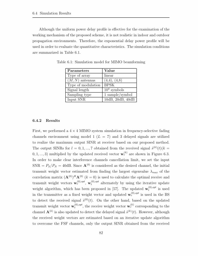
6.4 Simulation Results
Although the uniform power delay profile is effective for the examination of the
working mechanism of the proposed scheme, it is not realistic in indoor and outdoor
propagation environments. Therefore, the exponential delay power profile will be
used in order to evaluate the quantitative characteristics. The simulation conditions
are summarized in Table 6.1.
Table 6.1: Simulation model for MIMO beamforming
Parameters ValueType of array linear(M, N) antennas (4,4), (4,8)Type of modulation BPSKSignal length 104 symbolsSampling type 1 sample/symbolInput SNR 10dB, 20dB, 40dB
6.4.2 Results
First, we performed a 4 × 4 MIMO system simulation in frequency-selective fading
channels environment using model 1 (L = 7) and 3 delayed signals are utilized
to realize the maximum output SINR at receiver based on our proposed method.
The output SINRs for l = 0, 1, ..., 7 obtained from the received signal s(k)(t)(k =
0, 1, ..., 3) multiplied by the updated received vector w(k)r are shown in Figure 6.3.
In order to make clear interference channels cancellation limit, we set the input
SNR = PS/PN = 40dB. Since A(0) is considered as the desired channel, the initial
transmit weight vector estimated from finding the largest eigenvalue λmax of the
correlation matrix (A(0))HA(0) (k = 0) is used to calculate the optimal receive and
transmit weight vectors w(0),optr , w
(0),optt alternately by using the iterative update
weight algorithm, which has been proposed in [57]. The updated w(0),optt is used
in the transmitter as a fixed weight vector and updated w(0),optr is used in the BS
to detect the received signal s(0)(t). On the other hand, based on the updated
transmit weight vector w(0),optt , the receive weight vector w
(k)r corresponding to the
channel A(k) is also updated to detect the delayed signal s(k)(t). However, although
the received weight vectors are estimated based on an iterative update algorithm
to overcome the FSF channels, only the output SINR obtained from the received
82

6.4 Simulation Results
signal s(0)(t) is better than all the rest. It is clear that the degree of freedom
(DOF) at both the MS (M − 1) and the BS (N − 1) sides are exploited to suppress
(M + N − 2 = 6) interferences for the received signal s(0)(t) while only the DOF of
the BS side is exploited to cancel (N − 1 = 3) interferences for the received signal
s(k)(t).
Figure 6.4 shows the output SINRs viewing at median value of the CDF of the
detected signals based on our proposed scheme for a 4 × 4 MIMO system in terms
of the input SNR of 40dB and 20dB. Since each the signal s(k)(t) detected is useful
to improve efficiently the output SINR, the result of our proposed scheme is better
than that of detection of the preceding signal only. The simulation result is shown
that the improved output SINR based on our proposed method agreed very well
with (6.20). However, the output SINR improvement depends on the number of BS
antennas because only the DOF of the BS is used to suppress the interferences of
the delayed signal s(k)(t)(k = 0).
In order to verify the considerably improvement of output SINR based on our
proposed scheme when increasing the number of BS antennas, a 4×8 MIMO system
simulation in case of the input SNR of 40dB and 20dB are shown in Figure 6.5. It is
shown that the transmit data is detected not only by using the preceding wave but
also by exploiting its copies incoming the BS. On the other hand, the performance
of 4 × 4 and 4 × 8 MIMO systems for (L ≥ 4) and (L ≥ 8), respectively, might be
also improved slightly based on the proposed scheme when the input SNR is less
than 40dB.
We are now going to show how our proposed schemes apply to MIMO system
in FSF channels using model 2 for the delay spread of multipath waves over one
symbol period. We performed a simulation for a single user case in the case of 4×4,
and 4×8 MIMO systems with the input SNR = 10 dB and delay spread στ ranging
from 0 to 5Ts. For comparison, 4 × 4 and 4 × 8 MIMO systems using the transmit
and receive weight vectors obtained from finding the largest eigenvalues for the
correlation matrices (A(0))HA(0) and A(0)(A(0))H , respectively, are also performed
(It is called MIMO SVD). The simulation result is shown in Figure 6.6.
In Figure 6.6, both the output SINRs obtained from detection of the preceding
signal and the proposed method are better than that of the MIMO SVD. Even if
increasing the number of antennas at the receiver, the output SINR obtained from
83
6.5 Summary
4 × 8 MIMO SVD is less than that of 4 × 4 MIMO system for detections of s(0)(t)
and the proposed scheme. The more delay spread στ is larger, the more output
SINR of our proposed scheme improve considerably compared to that of detection
of the preceding signal s(0)(t) only. Moreover, the proposed 4 × 4 MIMO system
might be considered to be equivalent to 4 × 8 MIMO system for detection of the
preceding signal s(0)(t) only.
6.5 Summary
We have proposed spatial-temporal MIMO beamforming system for single data
stream transmission. The proposed scheme is applied for a single user for frequency-
selective fading channels without using the tapped delay line. The transmit and
receive weight vectors of the preceding signal and the receive weight vector of each
delayed signal estimated by using an iterative update algorithm are used to detect
the transmitted signal incoming the base station at different time. Over which
multiple detected signals are useful to maximize the output SINR compared to de-
tection of the preceding signal only. The improvement of SINR by the proposed
scheme allows that MIMO system can be suffered from interferences when the dis-
tance of transmission is made sufficiently large and the delay spread is larger than
one symbol period. The providing high-bit-rate with high performance by using
our proposed scheme without using the tapped delay lines is possible in MIMO
frequency-selective fading channels.
84

6.5 Summary
−10 0 10 20 30 40 50 600
0.1
0.2
0.3
0.4
0.5
0.6
0.7
0.8
0.9
1
SINR [dB]
Cum
mul
ativ
e pr
oabi
lity
L = 01
2345
67
(a)
−10 0 10 20 30 40 50 600
0.1
0.2
0.3
0.4
0.5
0.6
0.7
0.8
0.9
1
SINR [dB]
Cum
mul
ativ
e pr
oabi
lity
L = 123
456
7
(b)
85

6.5 Summary
−10 0 10 20 30 40 50 600
0.1
0.2
0.3
0.4
0.5
0.6
0.7
0.8
0.9
1
SINR [dB]
Cum
mul
ativ
e pr
oabi
lity
L = 23
5 4 67
(c)
−10 0 10 20 30 40 50 600
0.1
0.2
0.3
0.4
0.5
0.6
0.7
0.8
0.9
1
SINR [dB]
Cum
mul
ativ
e pr
oabi
lity
L = 34567
(d)
Figure 6.3: Distribution function of SINR for a 4 × 4 MIMO system: (a) CDF fors(0)(t); (b) CDF for s(1)(t); (c) CDF for s(2)(t); (d) CDF for s(3)(t)
86

6.5 Summary
(a)
(b)
Figure 6.4: Median value of SINR vs. the number of interferences for a 4×4 MIMOsystem: (a) SNRin = 40dB; (b) SNRin = 20dB
87

6.5 Summary
(a)
(b)
Figure 6.5: Median value of SINR vs. the number of interferences for a 4×8 MIMOsystem: (a) SNRin = 40dB; (b) SNRin = 20dB
88

6.5 Summary
Figure 6.6: Average SINR of MIMO system as a function of the delay spread στ .
89
Chapter 7
Conclusion and Future Work
This chapter summarizes the results of this work and presents open topics for the
future research. Finally, conclusion of is included.
7.1 Conclusions
In recent years, MIMO antennas systems are used in fading environments to exploit
an enormous capacity advantage. It is regarded as one of the most promising tech-
nologies to improve performance and coverage of system. Several techniques have
been studied successfully for flat fading environment but frequency-selective fading
channels. In order to solve the MIMO frequency-selective fading channels, spatial
multiplexing OFDM has been proposed to transmit multiple independent streams
simultaneously. However, the performance of system is degraded by increasing the
distance of transmission. And besides, the decision feedback equalization technique,
where MIMO antennas systems equipped with TDL structure, will be one of the
topics research for mitigating the frequency-selective fading channels and maximize
the performance of system. However, they so far still suffer from computational
complexity, compact and low-cost hardware. Meanwhile, the determination of op-
timal transmit and receive weight vectors for MIMO beamforming system using
a single data stream transmission is one of the simple and sufficient solutions for
frequency-selective fading channels and maximize the output SINR at the BS. Ac-
cording to the numerical and simulation results shown in this work, the following
concluding remarks are obtained.
• The optimal transmit and receive weights determination scheme for MIMO
90

7.1 Conclusions
beamforming for single data stream transmission in frequency-selective fading
channels has been analyzed and developed. Through studying the iterative
weight update algorithm for the transmitter and receiver in the MIMO beam-
forming, we have successfully proposed the cancellation of (M+N−2) delayed
channels for MIMO system with M and N antenna elements at mobile and
base stations, respectively. Using this method, MIMO beamforming system
can effectively mitigate multipath fading in frequency-selective fading chan-
nels with low computational complexity compared to MIMO system using
TDL structure.
• Deriving from the weights determination scheme, MIMO beamforming us-
ing single data stream transmission for multiuser system has been proposed.
Thereon, a maximum number of interference channels, which could be elimi-
nated in multiuser system, is analyzed in two cases of the receive weight vec-
tors optimization only and iterative update of both transmitter and receiver
weight vectors optimization. For the first case, which is characterized by sim-
ple scheme, shown good performance for propagation channel with the pre-
ceding channel of the desired user has few its own interference channels, while
the second case shown better performance but more sophisticated scheme.
• Since the preceding signal is considered as the desired signal and the subse-
quent signals are referred to as interferences reflected at increasing the distance
of transmission, which described in Chapter 6. However, the more delayed sig-
nals increase the more performance of system is degraded. In order to improve
the output SINR at the BS, the spatial-temporal MIMO beamforming for sin-
gle data stream transmission has been analyzed and developed. Using this
method, not only the preceding signal but also several delayed versions of the
preceding signal are detected at the receiver. Over which, multiple detected
signals are useful to maximize the performance of system compared to that
of detection of the preceding only. This improvement of performance is use-
ful for MIMO systems to complement the high-quality in broadband wireless
communication when the distance of transmission is made sufficiently large.
91

7.2 Future Work
7.2 Future Work
Referring to the above conclusions, there are several areas of this work which could
be extended for future research.
• MIMO beamforming for multiple data streams transmission in frequency-
selective fading channels is a challenging topic that increases the capacity
compared to the MIMO beamforming for single data stream transmission
while maximizing the SINR. It is expected to realize extremely high capacity
communication system.
• MIMO beamforming for multi-carrier transmission is expected to improve
both capacity and performance of system compared with MIMO beamforming
for single carrier transmission in frequency-selective fading environment.
• MIMO propagation channel measurement and characterization at 5GHz with
the expected results based on the proposed researches will be of great benefits
for implementing wideband MIMO frequency-selective fading channels.
• Novel MIMO data transmission scheme in fast fading environment for vehicu-
lar communications is the next research that contributes to the new-generation
wireless access system such as MIMO cellular system, intelligent transporta-
tion system (ITS), and ad hoc networks.
92

Appendix A
Determination of Transmit Weight Vector w(opt)t,i
for the ith User
In the appendix, we will explain the transmit weight vector determination.
Starting from Eq.(5.11), we rewrite the output SINR for the ith user expression
as
Γ(wt,i;wr,j(j = 1, ..., Q, j = i)) =wH
t,iA(o)i wr,iw
Hr,i(A
(o)i )Hwt,i
Rinf + γiwHr,iwr,i
(A.1)
where
Rinf =
Li−1∑l=1
wHt,iA
(l)i wr,iw
Hr,i(A
(l)i )Hwt,i
+
Q∑j=1,j �=i
Lj−1∑l=0
wHt,iA
(l)j wr,jw
Hr,j(A
(l)j )Hwt,i (A.2)
We use the Lagrange multiplier method under condition of wHt,iwt,i = 1. Specif-
ically
φi = Γ(wt,i;wr,j, (j = 1, ..., Q, j = i)) + λi(1 −wHt,iwt,i) (A.3)
where λi represents the Lagrange multiplier.
Taking the derivative of (A.3) with respect to wt,i and setting it to zero.
∂φi
∂wt,i=
∂Γ(wt,i;wr,j, (j = 1, ..., Q, j = i))
∂wt,i+
λi(1 − wHt,iwt,i)
∂wt,i= 0 (A.4)
93
And as a consequence, we have
[(A(0)i )Hwr,iw
Hr,iA
(0)i wt,i][Rinf + γiw
Hr,iwr,i]
(Rinf + γiwHr,iwr,i)2
−∑Li
l=1(A(l)i )Hwr,iw
Hr,iA
(l)i wt,i
(Rinf + γiwHr,iwr,i)2
(wHt,i(A
(0)i )Hwr,iw
Hr,iA
(0)i wt,i)
− λiwt,i = 0 (A.5)
In order to calculate the value of λi, (A.5) is multiplied by weight vector wHt,i
with the condition ‖wt,i‖ = 1, then we have
λi =wH
t,i(A(0)i )Hwr,iw
Hr,iA
(0)i wt,i
(Rinf + γiwHr,iwr,i)2
Q∑j=1,j �=i
Lj∑l=0
wHt,j(A
(l)j )Hwr,iw
Hr,iA
(l)j wt,j
+ γiwHr,iwr,i (A.6)
Substituting (A.6) into (A.5), and since wHr,iA
(0)i wt,i is a scalar, we have
wt,i =Rinf + γiw
Hr,iwr,i
wHt,i(A
(0)i )Hwr,i
R−1nt,i(A
(0)i )Hwr,i (A.7)
where Rnt,i is defined in the the Chapter 5, and is given by
Rnt,i ≡Li−1∑l=1
(A(l)i )Hwr,iw
Hr,iA
(l)i +
Q∑j=1,j �=i
Lj−1∑l=0
wHt,j(A
(l)j )Hwr,iw
Hr,iA
(l)j wt,jI
+ γiI (A.8)
Let us define
ξ =Rinf + γiw
Hr,iwr,i
wHt,iA
(0)i wr,i
(A.9)
Equation (A.7) can be written as
wt,i = ξR−1nt,i(A
(0)i )Hwr,i (A.10)
Without detailed calculation of ξ, the optimal transmit weight vector for the
ith user can be normalized and given by
w(opt)t,i =
R−1nt,i(A
(o)i )Hwr,i
‖R−1nt,i(A
(o)i )Hwr,i‖
(A.11)
94

REFERENCE
[1] B. Widrow, P. E. Mantey, L. J. Griffiths, and B. B. Goode, “Adaptive AntennaSystems,” Proc. IEEE, vol. 55, no. 12, pp. 2143-2159, December 1967.
[2] S. Heykin (ed.), “Array Signal Processing”, Englewood Cliffs, New Jersey, Prentice-Hall, 1985.
[3] J. H. Winters, “Optimum combining in digital mobile radio with cochannel interfer-ence,” IEEE JSAC, vol. SAC-2, no. 4, pp. 528-539, November 1984.
[4] Y. Ogawa, M. Ohmiya, and K. Itoh, “An adaptive array system for high-speed mobilecommunications,” IEICE Trans. Commun., vol. E75-B, no. 5, pp. 413-421, May 1992.
[5] Y. Ogawa, M. Ohmiya, and K. Itoh, “An LMS adaptive array for multipath fading re-duction,” IEEE Trans. Aerosp. Electron. Syst., vol. AES-23, no. 1, pp. 17-23, January1987.
[6] K. Takao and N. Kikuma, “An adaptive array utilizing an adaptive spatial averagingtechnique for multipath environment,” IEEE Trans. Antennas Propag., vol. AP-35,no. 12, pp. 1389-1396, December 1987.
[7] L. C. Godara, “Application of antenna arrays to mobile communications, part I:Performance improvement, feasibility, and system considerations,” Proc. IEEE, vol.85, no. 7, pp. 1031-1060, July 1997.
[8] L. C. Godara, “Application of antenna arrays to mobile communications, part II:Beam-forming and direction-of-arrival considerations,” Proc. IEEE, vol. 85, no. 8, pp.1195-1245, August 1997.
[9] R. Kohno, “Spatial and temporal communication theory using adaptive antennaarray,” IEEE Personel Communications, vol. 5, pp. 28-35, February 1998.
[10] A. J. Paulraj and C. Papadias, “Space-time processing for wireless communications,”IEEE Signal Processing Mag., vol. 14, no. 4, pp. 49-83, Nov. 1997.
[11] P. H. Lehne and M. Pettersen, “An overview of smart antenna technology for mobilecommunications systems,” IEEE Communication Survey, vol. 2, no. 4, pp. 2-13,Fourth Quarter 1999.
95

REFERENCE
[12] B. D. Van Veen and K. M. Buckley, “Beamforming: A versatile approach to spatialfiltering,” IEEE Signal Processing Mag., pp. 4-24, April 1988.
[13] R. A. Monzigo and T. W. Miller, “Introduction to Adaptive Array,” John Wiley &Sons, 1980.
[14] J. Litva and T. L. Y. Lo, “Digital Beamforming in Wireless Communications,”Artech House, 1996.
[15] B. Widrow and S. D. Stearns, “Adaptive Signal Processing,” Prentice House, 1985.
[16] N. Kikuma, “Adaptive Signal Processing with Array Antenna,” Science and Tech-nology Publishing Co., Ltd., Japan, 1999.
[17] L. C. Godara, “Impoved LMS algorithm for adaptive beamforming,” IEEE Trans.Antenna Propagat., vol. 38, no. 10, pp. 1631-1635, October 1990.
[18] J. E. Hudson, “Adaptive Array Principle,” Peter Peregrinus Ltd., 1981.
[19] E. Eleftheriou and D. D. Falconer “Tracking properties and steady state performanceof RLS adaptive filter algorithms,” IEEE Trans. on Acoust., Speech, Signal Processing,vol. ASSP-34, no. 5, pp. 1097-1110, October 1986.
[20] F. Asano, Y. Suzuki and T. Sone, “Convergence characteristics of the adaptive arrayusing RLS algorithm,” IEICE Trans. on Fundamentals, vol. E80-A, no. 1, pp. 148-158,1997.
[21] G. V. Tsoulos, “Smart Antennas for Mobile Communication Systems,” Electronicsand Communication Engineering Journal, vol. 12, no. 2, pp. 84-94, April 1999.
[22] J. H. Winters, “Smart Antennas for Wireless Systems,” IEEE Personal Communi-cations, vol. 5, no. 1, pp. 23-27, February 1988.
[23] J. C. Liberti and T. S. Rappaport, “Smart Antennas for Wireless Communications,”New Jersey, Prentice Hall, 1999.
[24] S. C. Swales, M. A. Beach, and D. J. Edwards “Multi-beam adaptive base stationantennas for cellular land mobile radio systems,” 39th IEEE Vehicular TechnologyConference, vol. 1, pp. 341-348, 1989.
[25] S. C. Swales, M. A. Beach, D. J. Edwards, and J. P. McGeehan, “The performanceenhancement of multibeam adaptive base-station antennas for cellular land mobileradio systems,” IEEE Trans. Vehicular Technology, vol. 29, no. 1, pp. 56-67, February1990.
[26] E. Telatar, “Capacity of multi-antenna Gaussian channels,” AT&T Bell Labs Tech.Memo.,March 1995.
[27] K. J. R. Liu, F. R. Farrokhi, and L. Tassiulas, “Transmit and receive diversityand equalization in wireless networks with fading channels,” Proc. IEEE Globecom,Phoenix, AZ, pp. 1193-1198, November 1997.
96

REFERENCE
[28] G. J. Foschini and M. J. Gans, “On limits of wireless communications in a fadingenvironment when using multiple antennas,” Wireless Personal Commun., vol. 6, no.3, pp. 311-335, March 1998.
[29] G. J. Foschini, G. D. Golden, R. A. Valenzuela, and P. W. Wolniansky, “Simpli-fied processing for high spectral efficiency wireless communication employing multi-element arrays,” IEEE J. Select. Areas Commun., vol. 17, pp. 1841-1852, November1999.
[30] V. Tarokh, N. Seshadri, and A. R. Calderbank, “Space-time codes for high data ratewireless communication: Performance criterion and code construction,” IEEE Trans.Inf. Theory, vol. 44, no. 2, pp. 744-765, March 1998.
[31] S. M. Alamouti, “A simple transmi diversity technique for wireless communications,”IEEE J. Select. Areas Commun., vol. 16, no. 8, pp. 1451-1458, October 1998.
[32] G. G. Raleigh and J. M. Cioffi, “Spatio-temporal coding for wireless communication,”IEEE Trans. Commun., vol. 46, no. 3, pp. 357-366, 1998.
[33] A. F. Naguib, N. Seshadri, and A. R. Calderbank, “Increase data rate over wirelesschannels,” IEEE Signal Process. Mag., vol. 17, no. 3, pp. 76-92, May 2000.
[34] J. Fu, T. Taniguchi, and Y. Karasawa, “Simplified estimation method for MRC trans-mission characteristics in Rayleigh i.i.d MIMO channel,” IEICE Trans. Commun., vol.J86-B, no. 9, pp. 1963-1970, September 2003.
[35] S. Catreux, L. J. Greenstein, and V. Erceg, “Some results and insights on theperformance gains of MIMO systems,” IEEE J. Select. Areas Commun., vol. 21, no.5, pp. 839-847, June 2003.
[36] J. Yang and S. Roy, “On joint transmitter and receiver optimization for multiple-input multiple-output (MIMO) transmission systems,” IEEE Trans. Commun., vol.42, no. 12, pp. 3221-3231, 1994.
[37] K. K. Wong, R. D. Murch, and K. B. Letaief, “Optimizing time and space SIMOantenna system for frequency-selective fading channels,” IEEE J. Select. Areas Com-mun., vol. 19, no. 7, pp. 1395-1407, July 2001.
[38] J. Bach Andersen, “Array gain and capacity for known random channels with mul-tiple element arrays at both ends,” IEEE J. Select. Areas Commun., vol. 18, no. 11,pp. 2172-2178, November 2000.
[39] G. J. Foschini, “Layered space-time architecture for wireless communication in afading environment when using multi-element antennas,” Bell Labs Technical Journal,vol. 1, no. 2, pp. 41-49, August 1996.
[40] H. Sampath, P. Stoica, and A. Paulraj, “Generalized linear precoder and decoderdesign for MIMO channels using the weighted MMSE criterion,” IEEE Trans. onCommun., vol. 49, no. 12, pp. 2198-2206, December. 2001.
97
REFERENCE
[41] K. Miyashita, T. Nishimura, T. Ohgane, Y. Takatori, and K. Cho, “High-data-rate transmission with eigenbeam-space division multiplexing (E-SDM) in a MIMOchannel,” Proc. IEEE VTC 2002-Fall, vol. 3, pp. 1302-1306, September 2002.
[42] T. Ohgane, T. Nishimura, and Y. Ogawa, “Applications of space division multiplex-ing and those performance in a MIMO channel,” IEICE Trans. Commun., vol. E88-B,no. 5, pp. 1843-1851, May 2005.
[43] Y. Karasawa, “MIMO propagation channel modeling,” IEICE Trans. Commun., vol.E88-B, no. 5, pp. 1829-1842, May 2005.
[44] T. Taniguchi, R. Takemoto, X. N. Tran, and Y. Karasawa, “A design method ofMIMO communication system with robustness to eigenvector mismatch problem,”Technical Report of IEICE A.P2003-9 SAT2003-9, pp. 51-55, April 2003.
[45] R. Van Nee and R. Prasad, “OFDM for wireless multimedia communications,” Nor-wood, Artech House, 2000.
[46] D. Tujkovic and E. Sottani, “Orthogonalized spatial multiplexing for MIMOWCDMA downlink over frequency-selective Rayleigh fading channels,” Asilomar2002, Pac. Grove, Cal, USA, 2002.
[47] A. Benjebbour, Y. Seki, and Yoshida, “Simplified channel tracking for MIMO-OFDMsystems,” IEICE Trans. Commun., vol. E86-B, no. 10, pp. 3013-3022, October 2005.
[48] A. M. Tehrani, B. Hassibi, and J. M. Cioffi, “Adaptive equalization of multiple-input multiple-output (MIMO) frequency selective channels,” Proc. 33rd AsilomarConnference on Signal, Systems and Computers, Pacific Grove, CA, pp. 547-551,November 1999.
[49] C. Tidestav, A. Ahlen, and M. Sternad, “Realizable MIMO Decision Feedback,”IEEE International Conference on Acoustics, Speech and Signal Processing, AR, pp.2591-2594, March 1999.
[50] J. F. Frigon, and B. Daneshrad, “A multiple input-multiple output (MIMO) adaptivedecision feedback equalizer (DFE) with cancellation for wideband space-time commu-nications,” International Journal of Wireless Information Networks, vol. 9, no. 1, pp.13-23, January. 2002.
[51] J. H. Chang, L. Tassiulas, and F. Rashid-Farrokhi, “Joint transmitter receiver di-versity for efficient space division multiaccess,” IEEE Trans. Wireless Commun., vol.1, no. 1, pp. 16-27, January. 2002.
[52] T. Taniguchi, H. H. Pham, X. N. Tran, and Y. Karasawa, “Maximum SINR designmethod of MIMO communication systems using tapped delay line structure in receiverside,” 59th IEEE Semiannual Vehicular Technology Conference, Milan, Italy, May2004.
98

REFERENCE
[53] T. Taniguchi, H. H. Pham, X. N. Tran, and Y. Karasawa, “Maximum SINR de-sign and performance Analysis of MIMO communication systems with tapped delayline structure,” 15th IEEE International Personal, Indoor and Mobile Commun.,Barcelona, Spain, September 2004.
[54] S. Haykin, “Adaptive Filter Theory,” 3rd ed., Prential-Hall, Engle-wood Cliff, NJ,1996.
[55] T. S. Rappaport, “Wireless Communications: Principles and practice,” PrenticeHall, New Jersy, 1996.
[56] Y. Karasawa, “Radiowave Propagation Fundametals of Digital Mobile Communica-tions,” Corona Publishing Co., Tokyo 2003.
[57] H. H. Pham, T. Taniguchi, and Y. Karasawa, “The weights determination scheme forMIMO beamforming in frequency-selective fading channels,” IEICE Trans. Commun.,vol. E87-B, no. 8, August 2004.
99

List of Original Publication Related to the
Dissertation
Journal Paper
1. Huy Hoang Pham, Tetsuki Taniguchi, and Yoshio Karasawa,“The Weights Deter-mination Scheme for MIMO Beamforming in Frequency-Selective Fading Channels,”IEICE Transactions on Communications, Vol.E87-B, No.8, pp.2243-2249, August2004.(Related to the content of Chapter 4)
2. Huy Hoang Pham, Tetsuki Taniguchi, and Yoshio Karasawa, “Multiuser MIMOBeamforming for Single Data Stream Transmission in Frequency-Selective FadingChannels,” IEICE Transactions on Fundamentals, Special Section on Adaptive Sig-nal Processing and Its Applications, Vol. E88-A, No. 3, pp.651-659, March 2005.(Related to the content of Chapter 5)
3. Huy Hoang Pham, Tetsuki Taniguchi, and Yoshio Karasawa, “Spatial-TemporalAdaptive MIMO Beamforming for Frequency-Selective Fading Channels,” IEICETransactions on Communications. (Under 1st Review)(Related to the content of Chapter 6)
International Conference and Presentations
1. Huy Hoang Pham, Tetsuki Taniguchi, and Yoshio Karasawa, “MIMO Beamformingfor High-Bit-Rate Transmission over Frequency -Selective Fading Channels,” TheIEEE International Symposium on Spread Spectrum Techniques and Applications(ISSSTA’04), Sydney, Australia, September 2004.(Related to the content of Chapter 4)
2. Tetsuki Taniguchi, Huy Hoang Pham, and Yoshio Karasawa, “Maximum SINR De-sign Method of MIMO Communication Systems Using Tapped Delay Line Structurein Receiver Side,” 59th IEEE Semiannual Vehicular Technology Conference, Milan,Italy, May 2004.(Related to the content of Chapter 4)
100

REFERENCE
3. Tetsuki Taniguchi, Huy Hoang Pham, and Yoshio Karasawa, “Maximum SINR De-sign and Performance Analysis of MIMO Communication Systems with TappedDelay Line Structure,” 15th IEEE International Personal, Indoor and Mobile Ra-dio Communications, Barcelona, Spain, September 2004.(Related to the content of Chapter 4)
4. Tetsuki Taniguchi, Huy Hoang Pham, and Yoshio Karasawa, “Multimode Trans-mission Scheme for MIMO System Under Frequency -Selective Fading,” JINA2004,C4.6, Nice, France, Nov.2004.(Related to the content of Chapter 3)
5. Huy Hoang Pham, Tetsuki Taniguchi, and Yoshio Karasawa, “Spatial-TemporalAdaptive MIMO Beamforming for High-Quality Transmission over Frequency-SelectiveFading Channels,” The IEEE Advanved International Conference on Telecommu-nications (AICT’06), Guadeloupe, French Caribbean 2006. (Submitted)(Related to the content of Chapter 6)
Other Conference Papers and Presentations
1. Huy Hoang Pham, Tetsuki Taniguchi, and Yoshio Karasawa, “How Many DelayedChannels Can Be Cancelled by MxN MIMO Beamfoming?,” Technical Report ofIEICE, AP2003-130, pp. 83-87, Aug. 2003.
2. Tetsuki Taniguchi, Huy Hoang Pham, and Yoshio Karasawa, “Maximum SINR De-sign of MIMO Communication Systems with Tapped Delay Line Structure in Re-ceiver Side,”Technical Report of IEICE, AP2003-144, pp. 67-71, Sep. 2003.
3. Huy Hoang Pham, Tetsuki Taniguchi, and Yoshio Karasawa, “MIMO Beamformingfor Frequency-Selective Fading Channels,” IEICE General Conference, B-1-240,September. 2003.
4. Tetsuki Taniguchi, Huy Hoang Pham, and Yoshio Karasawa, “Maximum SINR De-sign of MIMO Communication Systems with Tapped Delay Line Structure,” IEICEGeneral Conference, B-1-241, September 2003.
5. Tetsuki Taniguchi, Huy Hoang Pham, and Yoshio Karasawa, “Design and Perfor-mance of MIMO Communication Systems with Tapped Delay Line Structure inTransmitter and Receiver Sides,” Technical Report of IEICE, AP2003-213, Nov.2003.
6. Huy Hoang Pham, Tetsuki Taniguchi, and Yoshio Karasawa, “MIMO Beamformingfor Multi-User System in Frequency-Selective Fading Channels,” Technical Reportof IEICE, AP2004-15, SAT2004-4, pp. 19-24, May 2004.
101

REFERENCE
7. Tetsuki Taniguchi, Huy Hoang Pham, and Yoshio Karasawa, “Multistream Trans-mission under Frequency-Selective Fading Using MIMO System Equipped withTapped Delay Line,” Technical Report of IEICE, AP2004-68, SAT2004-66, pp.13-17, July 2004.
8. Huy Hoang Pham, Tetsuki Taniguchi, and Yoshio Karasawa, “Spatial-TemporalAdaptive MIMO Beamforming for Frequency-Selective Fading Channels,” IEICEGeneral Conference, B-1-241, September 2005.
9. Tetsuki Taniguchi, Huy Hoang Pham, and Yoshio Karasawa, “MIMO Communica-tion Systems for STBC Transmission under Frequency -Selective Fading Environ-ment,” IEICE General Conference, B-5-10, September 2005.
10. Hari Setiawan, Huy Hoang Pham, Tetsuki Taniguchi, and Yoshio Karasawa, “Broad-band MIMO Measurement using the Delayed Channel Cancellation System,” IEICEGeneral Conference, B-1-234, September 2005.
102

Author Biography
Huy Hoang Pham was born in Thai Binh, Vietnam on 16th February 1976. Here-ceived B.E degree from Ho Chi Minh University of Technology, Vietnam in 1999 andM.S degree from the University of Electro-Communications, Tokyo, Japan in 2003. Heis currently a Ph.D. student in Department of Electronic Engineering, The University ofElectro-Communications, Tokyo, Japan. His research interests are in the areas of adap-tive array antenna, space-time adaptive beamforming, DS-CDMA for FDD system, flatand frequency selective fading channels, multiple-input multiple-output and multiusersystems.
103