A Stabilized Finite Element Method for theDarcy Problem on Surfaces ∗

Peter Hansbo† Mats G. Larson ‡

January 11, 2018

Abstract

We consider a stabilized finite element method for the Darcy problem on a surfacebased on the Masud-Hughes formulation. A special feature of the method is that thetangential condition of the velocity field is weakly enforced through the bilinear formand that standard parametric continuous polynomial spaces on triangulations can beused. We prove optimal order a priori estimates that take the approximation of thegeometry and the solution into account.

1 Introduction

In this note we develop a stabilized finite element method for Darcy flow on triangulationsof a smooth surface. Starting from the Masud-Hughes formulation [12] we obtain a veryconvenient method based on a coercive bilinear form that can handle different approxi-mation spaces. More precisely, we consider parametric continuous piecewise polynomialelements, with possibly different orders in the mapping as well as the spaces for the velocityand pressure. A special feature of our approach is that we avoid using vector elements anddiscretize the tangent velocity vector componentwise in R3 together with a weak enforce-ment of the tangent condition. Our approach is in contrast with the recent report [7] wherea method for Darcy flow based on Raviart-Thomas spaces was presented.

We derive error estimates that takes the approximation of the geometry and the solutioninto account and separates the dependency of the different orders of approximations. Theerror in the velocity is defined using standard componentwise liftings based on the closest

∗This research was supported in part by the Swedish Foundation for Strategic Research Grant No.AM13-0029, the Swedish Research Council Grants No. 2011-4992 and No. 2013-4708, and Swedish strategicresearch programme eSSENCE.†Department of Mechanical Engineering, Jonkoping University, SE–551 11 Jonkoping, Sweden, Pe-

ter.Hansbo@jth.hj.se‡Department of Mathematics and Mathematical Statistics, Umea University, SE–901 87 Umea, Sweden,

mats.larson@math.umu.se

1

arX

iv:1

511.

0374

7v1

[m

ath.

NA

] 1

2 N

ov 2

015

point mapping and we show an energy estimate, an L2 estimate for the pressure, and anL2 estimate for the tangential part of the velocity which is slightly sharper with respect tothe geometry approximation compared to the bound for the full velocity vector providedby the energy norm estimate. We also provide numerical results confirming our theoreticalinvestigations.

Recently there has been an increasing activity in research on finite elements on surfaces,in particular, we mention the following references that are relevant to this work: finiteelement methods for membrane shell problem based on tangential calculus [9] (linear) and[10] (nonlinear), higher order methods for the Laplace-Beltrami operator [4], continuous-discontinuous Galerkin methods for the biharmonic problem [11], and the seminal paper [5]where finite elements for the Laplace-Beltrami was first developed. For general backgroundon finite elements for PDEs on surfaces we refer to the recent review article [6] and thereferences therein.

The outline of the reminder of the paper is as follows: In Section 2 we precent the Darcyproblem on a surface and the necessary background on tangential calculus. In Section 3we define the triangulations and their approximation properties, the finite element spaces,the interpolation theory, and finally the finite element method. In Section 4 we collectnecessary results on lifting and extension of functions between the exact and discretesurfaces. In Section 5 we derive a priori error estimates starting with a Strang lemmaand then estimates of the quadrature errors in the forms resulting approximation of thegeometry, which together with the interpolation results yields the final estimate. Estimatesfor the presssure and tangential part of the velocity are derived using duality techniques.Finally, in Section 6 we present numerical examples.

2 The Darcy Problem on a Surface

2.1 The Surface

Let Γ be a closed smooth surface embedded in R3 with signed distance function ρ, exteriorunit normal n = ∇ρ, and closest point mapping p : R3 → Γ. Then there is a δ0 > such thatpmaps each point in Uδ0(Γ) to precisely one point on Γ, where Uδ(Γ) = {x ∈ R3 : ρ(x) < δ}is an open tubular neighborhood of Γ.

2.2 Tangential Calculus

For each function u defined on Γ we let the extension ue to the neighborhood Uδ0(Γ) bedefined by the pull back ue = u◦p. For a function u : Γ→ R we then define the tangentialgradient

∇Γu = P Γ∇ue (2.1)

where P Γ = I − n ⊗ n is the projection onto the tangent plane Tx(Γ). The surfacedivergence of a vector field u : Γ→ R3 is defined by

divΓ(u) = tr(u⊗∇Γ) = div(u)− n · (u⊗∇) · n (2.2)

2

Decomposing u into a tangent and normal component

u = ut + unn (2.3)

we have the identitydivΓu = divΓut + unH (2.4)

whereH = tr(κΓ) (2.5)

is twice the mean curvature of the surface and κΓ = κ|Γ, with κ = ∇⊗∇ρ, is the curvaturetensor of Γ. Using Green’s formula we have

(divΓvt, q)Γ = −(vt,∇Γq)Γ (2.6)

for tangential vector fields vt.

2.3 The Surface Darcy Problem

Tangential Vector Field Formulation. The Darcy problem takes the form: find atangential vector field ut : Γ → T (Γ) representing velocity and the pressure p : Γ → Rsuch that

divΓut = f on Γ (2.7)

ut +∇Γp = g on Γ (2.8)

where f : Γ→ R is a given function such that∫

Γf = 0 and g : Γ→ R3 is a given tangential

vector field. The corresponding weak form reads: find (ut, p) ∈ V t ×Q such that

at((ut, p), (vt, q)) = l(q) ∀(vt, q) ∈ V t ×Q (2.9)

where

at((ut, p), (vt, q)) = (ut,vt)Γ + (∇Γp,vt)Γ − (ut,∇Γq)Γ (2.10)

l(q) = (f, q)Γ + (g,v)Γ (2.11)

with V t = {v : Γ→ R3 : v ∈ [L2(Γ)]3,n · v = 0} and Q = {q ∈ H1(Γ) : ∫Γ q = 0}.Since Γ is smooth and p ∈ Q is the solution to the elliptic problem divΓ(∇Γp) =

divΓut − divΓg = f − divΓg, we have the elliptic regularity estimate

‖p‖Hs+2(Γ) . ‖f − divΓg‖Hs(Γ) . ‖f‖Hs(Γ) + ‖g‖Hs+1(Γ) (2.12)

which combined with ‖ut‖Hs+1(Γ) = ‖g −∇Γp‖Hs+1(Γ) ≤ ‖g‖Hs+1(Γ) + ‖p‖Hs+2(Γ) gives

‖ut‖Hs+1(Γ) + ‖p‖Hs+2(Γ) . ‖f‖Hs(Γ) + ‖g‖Hs+1(Γ) (2.13)

3

General Vector Field Formulation. Letting u be a vector field with a nonzero normalcomponent and recalling the split u = ut + unn, see equation (2.3), we get the problem:find (u, p) ∈ V ×Q such that

a((u, p), (v, q)) = l(q) ∀(v, q) ∈ V ×Q (2.14)

where

a((u, p), (v, q)) = (ut,vt)Γ + (un, vn)Γ + (∇Γp,vt)Γ − (ut,∇Γq)Γ (2.15)

= (u,v)Γ − (p, divΓvt)Γ + (divΓut, q)Γ (2.16)

= (u,v)Γ − (p, divΓv)Γ + (p,Hvn)Γ + (divΓu, q)Γ − (unH, q)Γ (2.17)

and V = {v : Γ→ R3 : v ∈ [L2(Γ)]3} is the space of general L2(Γ) vector fields.We note that (∇Γp,v)Γ = (∇Γp,vt)Γ , since ∇Γp is tangential, and therefore we get a

weak enforcement of the tangential condition un = u ·n = 0 by setting q = 0 and v = vnn.Testing instead with a tangential vector field vt ∈ V t ⊂ V and q ∈ Q we recover theDarcy problem (2.9).

Remark 2.1 We note that we have the identity

a((u, p), (v, q)) = (u,v)Γ + (∇Γp,vt)Γ − (ut,∇Γq)Γ (2.18)

= (u,v)Γ − (p, divΓvt)Γ + (divΓut, q)Γ (2.19)

= (u,v)Γ − (p, divΓv)Γ + (p,Hvn)Γ + (divΓu, q)Γ − (unH, q)Γ (2.20)

where we used the identity (2.4) for the surface divergence of a general vector field in the laststep. We note that the third form (2.20) involves quantities that are directly computablewhile the second form (2.19) involves the surface divergence of the tangent componentdivΓvt, which is more complicated to compute. When constructing a numerical methodbased on the divergence form (2.20) the term (vn, Hq)Γ either has to be included, whichinvolves computation of H, or alternatively a stronger penalty on the normal componentvn must be added in order to control the inconsistency resulting from neglecting the term.Neither alternative is attractive.

2.4 Masud-Hughes Stabilized Weak Formulation

The Masud-Hughes weak formulation, originally proposed in [12] for planar domains, forthe surface Darcy problem with a general vector field velocity takes the form: find (u, p) ∈V ×Q such that

A((u, p), (v, q)) = L((v, q)) ∀(v, q) ∈ V ×Q (2.21)

4

where

A((u, p), (v, q)) = (u,v)Γ (2.22)

+ (∇Γp,v)Γ − (u,∇Γq)Γ

+1

2(u+∇Γp,−v +∇Γq)Γ

L((v, q)) = (f e, q)Γ + (ge,v)Γ +1

2(ge,−v +∇Γq)Γ (2.23)

Expanding the forms we obtain

A((u, p), (v, q)) =1

2(u,v)Γ +

1

2(∇Γp,∇Γq)Γ +

1

2(∇Γp,v)Γ −

1

2(u,∇Γq)Γ (2.24)

L((v, q)) = (f e, q)Γ +1

2(ge,v +∇Γq)Γ (2.25)

and thus A has consists of a symmetric and a skew symmetric part.

3 The Finite Element Method

3.1 Triangulation of the Surface

Parametric Triangulated Surfaces. Let K ⊂ R2 be a reference triangle and let Pkg(K)

be the space of polynomials of order less or equal to kg defined on K. Let Γh,kg be atriangulated surface with quasi uniform triangulation Kh,kg and mesh parameter h ∈ (0, h0]

such that each triangle K = FK,kg(K) where FK,kg ∈ [Pkg(K)]3. Let nh be the elementwisedefined normal to Γh. We let Eh,kg denote the set of edges in the triangulation. Forsimplicity we use the notation Kh = Kh,kg , Eh = Eh,kg , and Γh = Γh,kg when appropriate.

Geometry Approximation Property. We assume that the family {Γh,kg , h ∈ (0, h0]}approximates Γ in the following way

• Γh,kg ⊂ Uδ0(Γ) and p : Γh,kg → Γ is a bijection.

• The following estimates hold

‖p‖L∞(Γh,kg ) . hkg+1, ‖n ◦ p− nh‖L∞(Γh,kg ) . hkg (3.1)

These properties are valid, e.g., if FK,kg is constructed using Lagrange interpolation of thesurface.

5

3.2 Parametric Finite Element Spaces

LetVh,k,kg = {v : v|K ◦ FK,kg ∈ Pk(K), ∀K ∈ Kh,kg ; v ∈ [C0(Γh)]

3} (3.2)

be the space of parametric continuous piecewise polynomials of order k mapped with amapping of order kg. We let

V h = [Vh,ku,kg ]3, Qh = {q ∈ Vh,kp,kg : ∫

Γh,kg

q = 0} (3.3)

be the finite element spaces for velocity and pressure, consisting of continuous piecewisepolynomials of order ku and kp, respectively, with parametric map of order kg (which isthe same for both spaces).

3.3 Interpolation

Letπh,1 : L2(Kh,1) 3 v 7→ πh,1v ∈ Vh,k,1 (3.4)

be a Scott-Zhang type interpolant. Then, for each element K ∈ Kh,1 we have the followingelementwise estimate

‖ve−πh,1ve‖Hm(K) . hs−m‖ve‖Hs(N(K)) . ‖v‖Hs(N l(K)), m ≤ s ≤ k+1, m = 0, 1 (3.5)

where N(K) is the union of the neighboring elements to element K and N l(K) = (N(K))l.In (3.5) the first inequality follows from interpolation theory, see [2], and the second fromthe chain rule in combination with L∞ boundedness of derivatives of the closest point mapp in the tubular neighborhood Uδ0(Γ) which follows from smoothness of Γ.

Next we define the interpolant πh,kg : L2(Kh)→ Vh,1,kg as follows

πh,kgve|K = (πh,1v

e) ◦GK,kg ,1 (3.6)

where GK,kg ,1 = FK,1 ◦ F−1K,kg

: Kkg → K1 is a bijection from the curved triangle Kkg tothe corresponding flat triangle K1. Using uniform L∞ bounds on GK,kg ,1 and its first orderderivative we have the estimates

‖ve − πh,kgve‖Hm(Kkg ) . ‖ve − πh,1ve‖Hm(K1) (3.7)

. hs−m‖ve‖Hs(N(K1)) . hs−m‖v‖Hs(N l(K1)) (3.8)

and thus we conclude that we have the estimate

‖ve − πh,kgve‖Hm(Kkg ) . hs−m‖v‖Hs(N l(K1)), m ≤ s ≤ k + 1, m = 0, 1 (3.9)

for all K ∈ Kh,kg . We also have the stability estimate

‖πh,kgve‖Hm(Kkg ) . ‖v‖Hm(N l(K1)), m = 0, 1 (3.10)

6

When appropriate we simplify the notation and write πh = πh,kg .Finally, we have the super–approximation result

‖(I − πh)(χev)‖Γh . h‖χ‖Wkg+1∞ (Γ)

‖v‖Γh (3.11)

for χ ∈ W kg+1∞ (Γ) and v ∈ Vh,kg .

3.4 Masud-Hughes Stabilized Finite Element Method

The finite element method based on the Masud-Hughes weak formulation (2.21) for thesurface Darcy problem takes the form: find (uh, ph) ∈ V h ×Qh such that

Ah((uh, ph), (v, q)) = Lh((v, q)) ∀(v, q) ∈ V h ×Qh (3.12)

where

Ah((u, p), (v, q)) = (u,v)Γh (3.13)

+ (∇Γhp,v)Γh − (u,∇Γhq)Γh

+1

2(u+∇Γhp,−v +∇Γhq)Γh

=1

2(u,v)Γh +

1

2(∇Γhp,∇Γhq)Γh +

1

2(∇Γhp,v)Γh −

1

2(u,∇Γhq)Γh (3.14)

Lh((v, q)) = (f e, q)Γh + (ge,v)Γh +1

2(ge,−v +∇Γhq)Γh (3.15)

= (f e, q)Γh +1

2(ge,v +∇Γhq)Γh (3.16)

Remark 3.1 We could add the term cN(nh · u,nh · v)Γh, where cN ≥ 0 is a parameter,to enforce the normal constraint more strongly. We will, however, see that we can takecN = 0, and no significant advantages of taking cN > 0 has been observed in our numericalexperiments.

4 Preliminary Results

4.1 Extension and Lifting of Functions

In this section we summarize basic results concerning extension and liftings of functions.We refer to [3] and [4] for further details.

Extension. Recalling the definition ve = v ◦ p of the extension and using the chain rulewe obtain the identity

∇Γhve = BT

t ∇Γv (4.1)

7

whereBt = P Γ(I − ρκ)P Γh : Tx(K)→ Tp(x)(Γ) (4.2)

and we recall that κ = ∇⊗∇ρ which may be expressed in the form

κ(x) =2∑i=1

κei1 + ρ(x)κei

aei ⊗ aei (4.3)

where κi are the principal curvatures with corresponding orthonormal principal curvaturevectors ai, see [8] Lemma 14.7. We note that there is δ > 0 such that the uniform bound

‖κ‖L∞(Uδ(Γ)) . 1 (4.4)

holds. Furthermore, we have the inverse mapping

B−1t = P Γh(I − ρκ)−1P Γ : Tp(x)(Γ)→ Tx(K) (4.5)

We extend Bt to Tx(K)⊕Nx(K), where Nx(K) is the vector space of vector fields thatare normal to K at x ∈ K, by defining

B = (P ΓBtP Γh + n⊗ nh) (4.6)

with inverseB−1 = (P ΓhB

−1t P Γ + nh ⊗ n) (4.7)

We note that B and B−1 preserves the tangent and normal spaces as follows

BTx(K) = Tp(x)(Γ), BNx(K) = Np(x)(Γ) (4.8)

andB−1Tp(x)(Γ) = Tx(K), B−1Np(x)(Γ) = Nx(K) (4.9)

For clarity, we will employ the notation B(p(x)) = B(x) for each x ∈ K, K ∈ Kh, sothat we do not have to indicate lift or extensions of the operator B.

Lifting. The lifting wl of a function w defined on Γh to Γ is defined as the push forward

(wl)e = wl ◦ p = w on Γh (4.10)

and we have the identity∇Γw

l = B−T (∇Γhw)l (4.11)

8

4.2 Estimates Related to B

Using the uniform bound (4.4) it follows that

‖B‖L∞(Γh) . 1, ‖B−1‖L∞(Γ) . 1 (4.12)

Furthermore, we have the estimates

‖B − I‖L∞(Γh) . hkg ‖I −BTB‖L∞(Γh) . hkg+1 (4.13)

To prove the first estimate in (4.13) we note, using the definition (4.2) of B and the bound(3.1) on ρ that

B = P ΓP Γh + n⊗ nh +O(hkg+1) (4.14)

Next writing I = P Γ + n⊗ n = P 2Γ + n⊗ n, where we used that P Γ is a projection, we

obtainB − I = P Γ(P Γh − P Γ) + n⊗ (nh − n) +O(hkg+1) (4.15)

and thus the estimate follows using (3.1) since ‖P Γ−P Γh‖L∞(Γh) . ‖n−nh‖L∞(Γh) . hkg .For the second estimate in (4.13) we use the identities I = P Γh + nh ⊗ nh and (4.14)

to conclude that

BTB−I = P ΓhP ΓP Γh +nh⊗nh−I+O(hkg+1) = P ΓhP ΓP Γh−P Γh +O(hkg+1) (4.16)

Now

P ΓhP ΓP Γh−P Γh = (P Γhn)⊗(P Γhn) = (P Γh(n−nh))⊗(P Γh(n−nh)) ∼ O(h2kg) (4.17)

where we used the bound for the error in the discrete normal (3.1). Thus the second boundin (4.13) follows.

Further, the surface measure dΓ = |B|dΓh, where |B| = |det(B)| is the absolute valueof the determinant of B and we have the following estimates

‖1− |B|‖L∞(Γh) . hkg+1, ‖|B|‖L∞(Γh) . 1, ‖|B|−1‖L∞(Γh) . 1 (4.18)

4.3 Norm Equivalences

In view of the bounds in Section 4.2 and the identities (4.1) and (4.11) we obtain thefollowing equivalences

‖vl‖L2(Γ) ∼ ‖v‖L2(Γh), ‖v‖L2(Γ) ∼ ‖ve‖L2(Γh) (4.19)

and‖∇Γv

l‖L2(Γ) ∼ ‖∇Γhv‖L2(Γh), ‖∇Γv‖L2(Γ) ∼ ‖∇Γhve‖L2(Γh) (4.20)

9

4.4 Poincare Inequality

We have the following Poincare inequality

‖v‖Γh . ‖∇Γhv‖Γh ∀v ∈ Qh (4.21)

To prove (4.21) we let

λS(v) = |S|−1

∫S

v, S ∈ {Γ,Γh} (4.22)

be the average over S. Using the fact that α = λΓh(v) is the constant that minimizes‖v − α‖Γh , norm equivalence (4.19) to pass from Γh to Γ, the standard Poincare estimateon Γ, and at last norm equivalence (4.20) to pass back to Γh, we obtain

‖v − λΓh(v)‖Γh ≤ ‖v − λΓ(vl)‖Γh . ‖vl − λΓ(vl)‖Γ . ‖∇Γvl‖Γ . ‖∇Γhv‖Γh (4.23)

which proves (4.21).

5 Error Estimates

5.1 Norms

Let|||(v, q)|||2 = ‖v‖2

Γ + ‖∇Γq‖2Γ, |||(v, q)|||2h = ‖v‖2

Γh+ ‖∇Γhq‖2

Γh(5.1)

Using (4.19) and (4.20) we have the following equivalences

|||(vl, ql)||| ∼ |||(v, q)|||h, |||(v, q)||| ∼ |||(ve, qe)|||h (5.2)

5.2 Coercivity and Continuity

Lemma 5.1 The following statements hold:

• The form Ah is coercive and continuous

|||(v, q)|||2h . Ah((v, q), (v, q)) ∀(v, q) ∈ V h ×Qh (5.3)

Ah((v, q), (w, r)) . |||(v, q)|||h|||(w, r)|||h ∀(v, q), (w, r) ∈ V h ×Qh (5.4)

for all h ∈ (0, h0].

• The form Lh is continuous

Lh((v, q)) . (‖f‖Γ + ‖g‖Γ)|||(v, q)|||h ∀(v, q) ∈ V h ×Qh (5.5)

for all h ∈ (0, h0].

• There exists a unique solution to (3.12).

10

Proof. Coercivity of Ah follows directly from the definition (3.13) of the stabilized bilinearform. Continuity of Ah follows from the Cauchy-Schwarz inequality. Continuity of Lh fol-lows directly from the Cauchy-Schwarz inequality and the Poincare inequality. Existenceand uniqueness of a solution to (3.12) follows from the Lax-Milgram lemma.

Remark 5.1 Clearly the analogous results holds for the continuous forms A and L onV ×Q, defined in (2.22) and (2.23), and the variational problem (2.21).

5.3 Discrete Stability Estimate

Lemma 5.2 The solution (uh, ph) to (3.12), satisfies the stability estimate

|||(uh, ph)|||h + h−1‖n · uh‖Γh . ‖f‖Γ + ‖g‖Γ (5.6)

Proof. First Test Function. With (v, q) = (uh, ph) in (3.12) we obtain

|||(uh, ph)|||2h . Ah((uh, ph), (uh, ph)) = Lh((uh, ph)) . (‖f‖Γ + ‖g‖Γ)|||(uh, ph)|||h (5.7)

where we used (5.3) and (5.4) together with the continuity

Lh((v, q)) . (‖f‖Γ + ‖g‖Γ)|||(v, q)|||h,∀(v, q) ∈ V h ×Qh (5.8)

of Lh, which follows from Cauchy-Schwarz and the Poincare inequality (4.21). Thus weconclude that

|||(uh, ph)|||h . ‖f‖Γ + ‖g‖Γ (5.9)

Second Test Function. Setting q = 0 in (3.12) we note that the following equationholds

(uh,v)Γh + (∇Γhph,v)Γh = (ge,v)Γh , ∀v ∈ V h (5.10)

Choosing the test function v = πh(nπh(n · uh)) we get the identity

(uh, πh(nπh(n · uh)))Γh︸ ︷︷ ︸I

+ (∇Γhph, πh(nπh(n · uh)))Γh︸ ︷︷ ︸II

= (ge, πh(nπh(n · uh)))Γh︸ ︷︷ ︸III

(5.11)

Term I. We have

(uh, πh(nπh(n · uh)))Γh

= (n · uh,n · uh)Γh + (πh(nπh(n · uh))− n(n · uh),n · uh)Γh (5.12)

≥ ‖n · uh‖2Γh− ‖πh(nπh(n · uh))− n(n · uh)‖Γh‖n · uh‖2

Γh(5.13)

≥ (1− δ)‖n · uh‖2Γh− δ−1 ‖πh(nπh(n · uh))− n(n · uh)‖2

Γh︸ ︷︷ ︸F

(5.14)

11

where we used the Cauchy-Schwarz inequality and finally ab ≤ δa2 + δ−1b2, δ > 0. Esti-mating the second term on the right hand side by adding and subtracting suitable termswe obtain

F . ‖(πh − I)(nπh(n · uh))‖2Γh

+ ‖n(πh − I)(n · uh)‖2Γh

(5.15)

. h2‖πh(n · uh)‖2Γh

+ h2‖uh‖2Γh

(5.16)

. h2‖uh‖2Γh

(5.17)

where we used the super–approximation (3.11) and in the last step the L2 stability (3.10)of the interpolant πh. We thus arrive at

I & (1− δ)‖n · uh‖2Γh− Ch2‖uh‖2

Γh(5.18)

Term II. We have

II . ‖∇Γhph‖Γh‖P Γhπh(nπh(n · uh))‖Γh (5.19)

. h‖∇Γhph‖Γh‖n · uh‖Γh (5.20)

≤ δ−1Ch2‖∇Γhph‖2Γh

+ δ‖n · uh‖2Γh

(5.21)

Here we used the estimate

‖P Γhπh(nπh(n · uh))‖Γh

. ‖P Γh(πh − I)(nπh(n · uh))‖Γh + ‖(P Γhn)πh(n · uh)‖Γh (5.22)

. h‖πh(n · uh)‖Γh + ‖P Γhn‖L∞(Γh)‖πh(n · uh)‖Γh (5.23)

. h‖n · uh‖Γh + hkg‖n · uh‖Γh (5.24)

. h‖n · uh‖Γh (5.25)

where we added and subtracted nπh(n · uh), used the triangle inequality followed by thesuper–approximation (3.11) and the L2 stability (3.10) of the interpolant, and finally usedthe fact that kg ≥ 1 and h ∈ (0, h0].

Term III. We have

|III| = |(ge, πh(nπh(n · uh)))Γh | (5.26)

= |(ge, (πh − I)(nπh(n · uh)))Γh| (5.27)

. ‖ge‖Γh‖(πh − I)(nπh(n · uh))‖Γh (5.28)

. h‖ge‖Γh‖πh(n · uh)‖Γh (5.29)

. h‖ge‖Γh‖n · uh‖Γh (5.30)

≤ δ−1Ch2‖ge‖2Γh

+ δ‖n · uh‖2Γh

(5.31)

where we used the fact that (ge,n)Γ = 0 to subtract nπh(n · uh), used the Cauchy-Schwarz inequality, used the super–approximation (3.11), and the L2 stability (3.10) of theinterpolant.

12

Conclusion. Collecting the bounds (5.18), (5.21), and (5.31), for I, II, and III, respec-tively, we arrive at

(1− 3δ) ‖n · uh‖2Γh

. δ−1h2‖ge‖Γh + δ−1h2‖uh‖2Γh

+ δ−1h2‖∇Γhph‖2Γh

(5.32)

. δ−1h2(‖ge‖Γh + |||(uh, ph)|||2h

)(5.33)

. δ−1h2 (‖f‖Γ + ‖g‖Γ) (5.34)

where we used (5.9) in the last step. Choosing δ small enough completes the proof.

5.4 Interpolation Error Estimates

Using the interpolation error estimate (3.9) we directly obtain the following interpolationestimates in the energy norm

|||(v, q)− (πhve, πhq

e)l||| ∼ |||(v, q)− (πhve, πhq

e)|||h (5.35)

. hku+1‖v‖Hku+1(Γ) + hkp‖q‖Hkp+1(Γ) (5.36)

for (v, q) ∈ Hku+1(Γ)×Hkp+1(Γ). If v is tangential, n · v = 0, we also have the estimate

‖n · πhv‖Γh = ‖n · (πhv − v)‖Γh . h‖v‖H1(Γ) (5.37)

5.5 Strang’s Lemma

Lemma 5.3 Let (u, p) be the solution to (2.9) and (uh, ph) the solution to (3.12), thenthe following estimate holds

|||(u, p)− (uh, ph)l||| . |||(ue − πhue, pe − πhpe)|||h (5.38)

+A((πhu

e, πhpe)l, (v, q)l)− Ah(πhue, πhpe), (v, q)))

|||(v, q)|||h

+L(v, q)l)− Lh((v, q))

|||(v, q)|||h

for all h ∈ (0, h0].

Proof. Adding and subtracting an interpolant and using the triangle inequality we obtain

|||(u, p)− (ulh, plh)||| ∼ |||(ue, pe)− (uh, ph)|||h (5.39)

. |||(ue, pe)− (πhue, πhp

e)|||h + |||(πhue, πhpe)− (uh, ph)|||h (5.40)

To estimate the second term use (5.3) to conclude that

|||(πhue, πhpe)− (uh, ph)|||h . sup(v,q)∈V h×Qh

Ah((πhue, πhp

e)− (uh, ph), (v, q))

|||(v, q)|||h(5.41)

13

Using Galerkin orthogonality (3.12) to eliminate (uh, ph), and then adding the weak formof the exact problem, the numerator may be written in the following form

Ah((πhue, πhp

e)− (uh, uh), (v, q))

= Ah((πhue, πhp

e), (v, q))− Lh((v, q)) (5.42)

= Ah((πhue, πhp

e), (v, q))−A((u, p), (v, q)l) + L((v, q)l)︸ ︷︷ ︸=0

−Lh((v, q)) (5.43)

= Ah((πhue, πhp

e), (v, q))− A((πhue, πhp

e)l, (v, q)l) (5.44)

+ L((v, q)l)− Lh((v, q))+ A(((πhu

e)l − u, (πhpe)l − p), (v, q)l)

where at last we added and subtracted an interpolant. Estimating the right hand side andusing (5.41) the lemma follows immediately.

5.6 Quadrature Error Estimates

Lemma 5.4 The following estimates hold

|(vl,wl)Klh − (v,w)Kh| . hkg+1‖v‖Kh‖w‖Kh (5.45)

|(vl,∇Γql)Klh − (v,∇Γhq)Kh| . hkg+1

(‖v‖Kh + h−1‖n · v‖Kh

)‖∇Γhq‖Kh (5.46)

|(∇Γql,∇Γr

l)Klh − (∇Γhq,∇Γhr)Kh| . hkg+1‖∇Γhq‖Klh‖∇Γhr‖Kh (5.47)

|L((vL, ql))− Lh((v, q))| . hkg+1(‖f‖Γ + ‖g‖Γ)|||(v, q)|||h (5.48)

for all (v, q), (w, r) ∈ V h ×Qh and h ∈ (0, h0].

Proof. (5.45): Changing domain of integration from Klh to Kh in the first term and usingthe bound (4.18) for |B| we obtain

|(vl,wl)Klh − (v,w)Kh| = |((|B| − 1)v,w)Kh| (5.49)

. ‖|B| − 1‖L∞(Kh)‖v‖Kh‖w‖Kh (5.50)

. hkg+1‖v‖Kh‖w‖Kh (5.51)

(5.46): Changing domain of integration from Klh to Kh in the first term we obtain

|(vl,∇Γql)Klh − (v,∇Γhq)Kh|

= |(vl,B−T (∇Γhq)l)Klh − (v,∇Γhq)Kh| (5.52)

= |((P Γh(|B|B−1 − I)v,∇Γhq)Kh| (5.53)

14

Here we have the identity

P Γh(|B|B−1 − I)v = P Γh(|B| − 1)B−1 + P Γh(B−1 − I) (5.54)

where we note that the first term i O(hkg+1) using (4.18) and the second takes the form

P Γh(B−1 − I) = P Γh(P ΓhP Γ + nh ⊗ n+O(hkg+1)− I) (5.55)

= P ΓhQΓ +O(hkg+1) (5.56)

Thus we conclude that

|(vl,∇Γql)Klh − (v,∇Γhq)Kh| = |((P Γh(|B|B−1 − I)v,∇Γhq)Kh|

. hkg+1‖v‖Kh‖∇Γhq‖Kh + |((P Γhn)(n · v),∇Γhq)Kh| (5.57)

. hkg+1‖v‖Kh‖∇Γhq‖Kh + hkg‖n · v‖Kh‖∇Γhq‖Kh (5.58)

(5.47): Using (4.11), changing domain of integration from Klh to Kh in the first term weobtain

|(∇Γql,∇Γr

l)Klh − (∇Γhq,∇Γhr)Kh|= |(B−T (∇Γhq)

l,B−T (∇Γhr)l)Klh − (∇Γhq,∇Γhr)Kh| (5.59)

= |((|B|B−1B−T − I)∇Γhq,∇Γhr)Kh| (5.60)

. ‖(|B|B−1B−T − I)‖L∞(Kh)‖∇Γhq‖Kh‖∇Γhr‖Kh (5.61)

. hkg+1‖∇Γhq‖Kh‖∇Γhr‖Kh (5.62)

Here we used the estimate

‖(|B|B−1B−T − I)‖L∞(Kh) . ‖|B| − 1‖L∞(Kh)‖B−1‖L∞(Kh)‖B−T‖L∞(Kh) (5.63)

+ ‖B−1‖L∞(Kh)‖I −BBT‖L∞(Kh)‖B−T‖L∞(Kh) . hkg+1 (5.64)

where we employed (4.12), (4.13), and (4.18).(5.48): Changing domain of integration from Klh to Kh and using (4.18) we obtain

|(f, ql)Klh − (f e, q)Kh|+ |(g,vl)Kh − (ge,v)Kh| (5.65)

= |((|B| − 1)f e, q)Kh|+ |((|B| − 1)ge,v)Kh | (5.66)

. ‖|B| − 1‖L∞(Γh)(‖f e‖Kh‖q‖Kh + ‖ge‖Kh‖v‖Kh) (5.67)

. ‖|B| − 1‖L∞(Γh)(‖f e‖2Kh + ‖ge‖2

Kh)1/2(‖∇Γhq‖2Kh + ‖v‖2

Kh)1/2 (5.68)

. hkg+1(‖f‖Γ + ‖g‖Γ)|||(v, q)|||h (5.69)

where we used the Poincare inequality (4.21).

We collect our results in a convenient form for the developments below in the followingcorollary.

15

Corollary 5.1 The following estimates hold

|A((v, q)l, (w, r)l)− Ah((v, q), (w, r))|

. hkg+1(|||(v, q)|||h + h−1‖n · v‖2

Γh

)(|||(w, r)|||h + h−1‖n ·w‖2

Γh

)(5.70)

and|L((v, q)l)− Lh((v, q))| . hkg+1

(‖f‖Γ + ‖g‖Γ

)|||(v, q)|||h (5.71)

for all (v, q) and (w, r) ∈ V h ×Qh and h ∈ (0, h0].

5.7 Error Estimates

Theorem 5.1 Let (u, p) be the solution to (2.9) and (uh, ph) the solution to (3.12) andassume that the geometry approximation property holds, then for the following estimateholds

|||(u− ulh, p− plh)||| . hku+1‖u‖Hku+1(Γ) + hkp‖p‖Hkp+1(Γ) + hkg(‖f‖Γ + ‖g‖Γ) (5.72)

for all h ∈ (0, h0].

Proof. Starting from Strang’s lemma we need to estimate the three terms on the righthand side in (5.38). For the first term using the interpolation estimate gives

|||u− πhue, p− πhpe||| . hku+1‖u‖Hku+1(Γ) + hkp‖p‖Hkp+1(Γ) (5.73)

For the second term using the quadrature estimate (5.70) we obtain∣∣∣A((πhue, πhp

e)l, (v, q)l)− Ah(πhue, πhpe), (v, q)))∣∣∣

. hkg+1(|||(πhue, πhpe)|||h + h−1‖n · πhue‖Γh

)︸ ︷︷ ︸

.|||(u,p)|||+‖u‖H1(Γ)

(|||(v, q)|||h + h−1‖n · v‖Γh

)︸ ︷︷ ︸

.h−1|||(v,q)|||h

(5.74)

. hkg(‖u‖H1(Γ) + ‖p‖H1(Γ))|||(v, q)|||h (5.75)

where we used the interpolation estimate (5.37) for the first term. For the third term,applying (5.71), directly gives∣∣∣L((v, q)l)− Lh(v, q)

∣∣∣ . hkg+1(‖f‖Γ + ‖g‖Γ

)|||(v, q)|||h (5.76)

Combining the three estimates with the Strang lemma we directly obtain the desired esti-mate.

16

Theorem 5.2 Under the same assumptions as in Theorem 5.1 the following estimate holds

‖p− plh‖Γ . hku+2‖u‖Hku+1(Γ) + hkp+1‖p‖Hkp+1(Γ) + hkg+1(‖f‖Γ + ‖g‖Γ)

for all h ∈ (0, h0].

Proof. Recall that λS(v) = |S|−1∫Sv is the average of a function in L2(S), S ∈ {Γ,Γh},

see (4.22). Then we have

‖p− plh‖Γ ≤ ‖p− (plh − λΓ(plh))‖Γ︸ ︷︷ ︸I

+ |λΓ(plh)− λΓh(ph)|︸ ︷︷ ︸II

(5.77)

where we added and subtracted λΓ(plh) and used the fact that λΓh(ph) = 0.

Term I. Let (φ, χ) ∈ V t ×Q be the solution to the continuous dual problem

−divΓφ = ψ on Γ (5.78)

−φt +∇Γχ = 0 on Γ (5.79)

for ψ ∈ L2(Γ) with∫

Γψ = 0. We then have the elliptic regularity bound

‖φ‖H1(Γ) + ‖χ‖H2(Γ) . ‖ψ‖Γ (5.80)

Furthermore, we have the weak form

A((v, q), (φ, χ)) = (q, ψ) ∀(v, q) ∈ V ×Q (5.81)

and setting (v, q) = (u− ulh, p− plh) we obtain the error representation formula

(p− plh, ψ) = A((u− ulh, p− plh), (φ, χ)) (5.82)

= A((u− ulh, p− plh), (φ, χ)− (πhφ, πhχ)) (5.83)

+ A((u− ulh, p− plh), (πhφ, πhχ))

= A((u− ulh, p− plh), (φ, χ)− (πhφ, πhχ)) (5.84)

+ L((πhφ, πhχ))− Lh((πhφ, πhχ))

+ Ah((uh, ph), (πhφ, πhχ))− A((uh, ph)l, (πhφ, πhχ)l)

= I1 + I2 + I3 (5.85)

Term I1. Using the continuity of A, the energy error estimate (5.72), and the interpola-tion error estimate (5.36) we obtain

|I| . |||(u− ulh, p− plh)||| |||(φ, χ)− (πhφ, πhχ)l||| (5.86)

.(hku+1‖u‖Hku+1(Γ) + hkp‖p‖Hkp+1(Γ)

)(h‖φ‖H1(Γ) + h‖χ‖H2(Γ)

)(5.87)

.(hku+2‖u‖Hku+1(Γ) + hkp+1‖p‖Hkp+1(Γ)

)‖ψ‖Γ (5.88)

17

Term I2. Using the quadrature estimate (5.71) we directly obtain

|II| . hkg+1(‖f‖Γ + ‖g‖Γ

)|||(πhφ, πhχ)|||h . hkg+1

(‖f‖Γ + ‖g‖Γ

)‖ψ‖Γ (5.89)

where we used stability (3.10) of the interpolant and stability (5.80) of the solution to thedual problem.

Term I3. Using the quadrature estimate (5.70) we obtain

|III| . hkg+1(|||(uh, ph)|||h + h−1‖n · uh‖Γh

)(|||(πhφ, πhχ)|||h + h−1‖n · πhφ‖Γh

)(5.90)

. hkg+1(‖f‖Γ + ‖g‖Γ)(|||(φ, χ)|||+ ‖φ‖H1(Γ)) (5.91)

. hkg+1(‖f‖Γ + ‖g‖Γ)‖ψ‖Γ (5.92)

where we used, the stability (3.10) of the interpolant, the estimate (5.37) for the normalcomponent of the interpolant, and the stability (5.80) of the dual problem.

Conclusion Term I. Finally, setting ψ = p− (plh − λΓ(plh))/‖p− (plh − λΓ(plh))‖Γ, andcollecting the estimates of terms I1, I2, and I3, we obtain

I . hku+2‖u‖Hku+1(Γ) + hkp+1‖p‖Hkp+1(Γ) + hkg+1(‖f‖Γ + ‖g‖Γ) (5.93)

Term II. Changing the domain of integration from Γ to Γh, we obtain the identity

λΓ(plh)− λΓh(ph) = |Γ|−1

∫Γ

plh − |Γh|−1

∫Γh

ph (5.94)

=

∫Γh

(|Γ|−1|B| − |Γh|−1)ph (5.95)

Using the estimates |B| = 1 + O(hkg+1) and |Γh| = |Γ| + O(hkg+1), and some obviousmanipulations we obtain

|λΓ(plh)− λΓh(ph)| . ‖|Γ|−1|B| − |Γh|−1‖L∞(Γh)‖ph‖Γh (5.96)

. hkg+1‖∇Γhph‖Γh . hkg+1(‖f‖Γ + ‖g‖Γ) (5.97)

where at last we used the Poincare estimate (4.21). Thus we conclude that

II . hkg+1(‖f‖Γ + ‖g‖Γ) (5.98)

Conclusion. Together the estimates (5.93) and (5.98) of Terms I and II proves the de-sired estimate.

18

Theorem 5.3 Under the same assumptions as in Theorem 5.1 the following estimate holds

‖P Γ(u− ulh)‖Γ . hku+1‖u‖Hku+1(Γ) + hkp‖p‖Hkp+1(Γ) + hkg+1(‖f‖Γ + ‖g‖Γ)

for all h ∈ (0, h0].

Proof. Let (φh, χh) be the solution to the discrete dual problem

Ah((v, q), (φh, χh)) = (ψe,v)Γh (5.99)

where ψ : Γ → R3 is a given tangential vector field. We note that there is a uniquesolution to (5.99) , and using the technique in the proof of Lemma 5.2, we conclude thatthe following stability estimate holds

|||(φh, χh)|||h + h−1‖n · φh‖Γh . ‖ψ‖Γ (5.100)

Setting (v, q) = (πhu−uh, πhp−ph) in (5.99) we obtain the error representation formula

(πhu− uh,ψe)Γh = Ah((πhu− uh, πhp− ph), (φh, χh)) (5.101)

= Ah((πhu, πhp), (φh, χh))− Lh((φh, χh)) (5.102)

= Ah((πhu, πhp), (φh, χh)) (5.103)

−A((u, p), (φh, χh)l) + L((φh, χh)

l)︸ ︷︷ ︸=0

−Lh((φh, χh))

= A((πhu, πhp)l − (u, p), (φh, χh)

l) (5.104)

+ Ah((πhu, πhp), (φh, χh))− A((πhu, πhp)l, (φh, χh)

l)

+ L((φh, χh)l)− Lh((φh, χh)) (5.105)

= I + II + III (5.106)

The terms may be estimated as follows.

Term I. We have

|I| . |||(u− (πhu)l, p− (πhp)l)||| |||(φh, χh)|||h (5.107)

.(hku+1‖u‖Hku+1(Γ) + hkp‖p‖Hkp+1(Γ)

)‖ψ‖Γ (5.108)

where we used continuity of Ah, the interpolation estimate (3.9), and the stability estimate(5.100).

Term II. We have

|II| . hkg+1(|||(πhu, πhp)|||h + h−1‖n · πhu‖Γh

)(|||(φh, χh)|||h + h−1‖n · φh‖Γh

)(5.109)

. hkg+1(‖u‖H1(Γ) + ‖p‖H1(Γ)‖ψ‖Γ (5.110)

where we used the quadrature estimate (5.70), the stability of the interpolation operator,and the stability estimate (5.100).

19

Term III. We have

|III| . hkg+1(‖f‖Γ + ‖g‖Γ)|||(φh, χh)‖h (5.111)

. hkg+1(‖f‖Γ + ‖g‖Γ)‖ψ‖Γ (5.112)

where we used the quadrature estimate (5.71) and the stability estimate (5.100).

Conclusion. Finally, setting ψ = P Γeh,u/‖P Γeh,u‖Γ we have

(eh,u,ψ)Γh = ‖P Γeh,u‖Γh ∼ ‖P Γ(u− ulh)‖Γh (5.113)

where we used equivalence of norms (4.19). Thus the proof is complete.

6 Numerical Example: Flow on a Torus

Let Γ be the torus, given implicitly by the solution to

(R−√x2 + y2)2 + z2 − r2 = 0

were R = 1 is the major and r = 1/2 is the minor radius and let the right-hand side gcorrespond to the solution

ut =(

2xz,−2yz, 2(x2 − y2)(R−√x2 + y2)/

√x2 + y2

), un = 0, p = z.

Note that divΓu = 0, so f = 0. The errors are computed on the discrete geometry bydefining ep := ‖pe − ph‖Γh and eu := ‖ue − uh‖Γh . For the evaluation of the integral(gh,v)Γh , we use gh = ge. We have used cN = 0, see Remark 3.1. We emphasize thatcN > 0 does not affect the asymptotic convergence rate; however, for large cN a lockingeffect can occur. Moderate sizes of cN have a negligible effect on the error.

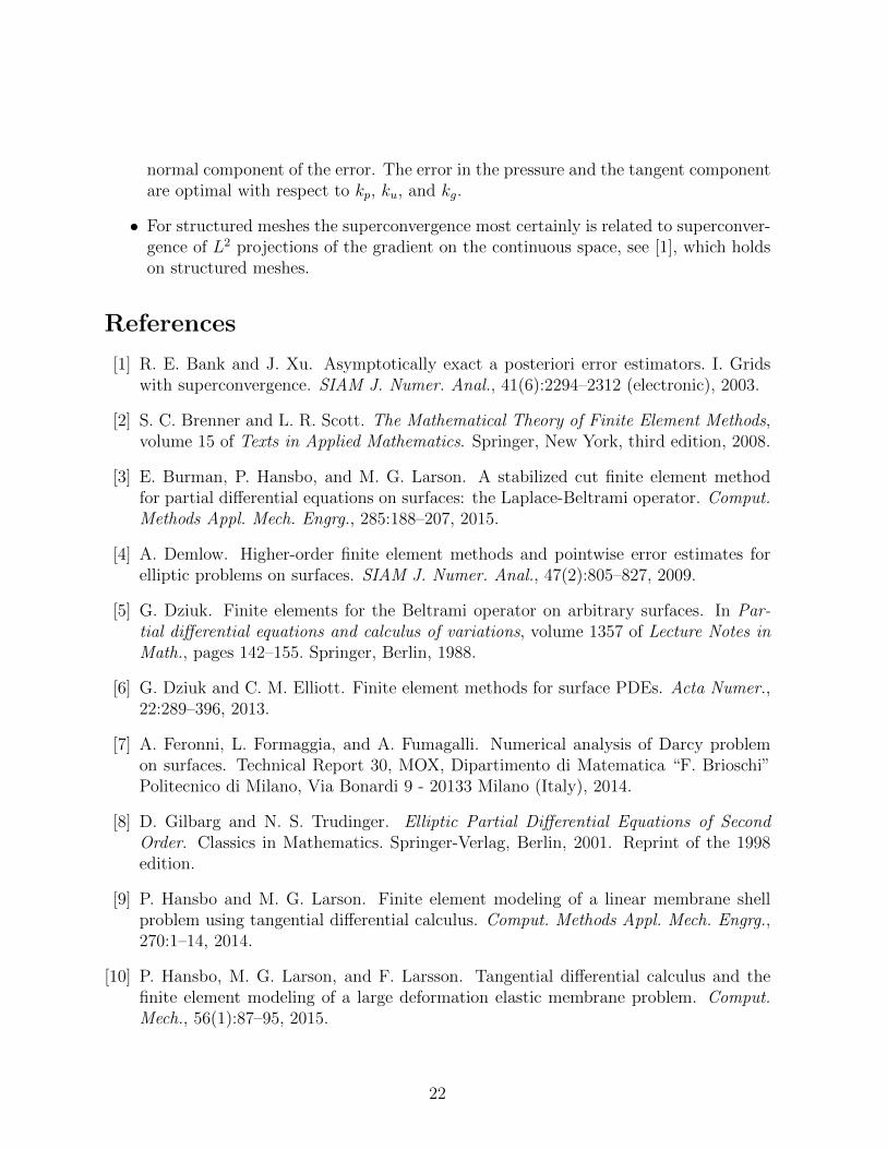
In Fig. 1 we show the computed velocity field on a particular mesh, with computedpressure isolevels on the same mesh in Fig. 2.

In order to make a comparison between structured and unstructured meshes, we createa sequence of unstructured meshes by randomly moving the nodes on each mesh in asequence of structured meshes. A typical example is shown in Fig. 3. We then make eightcomparisons:

We note the following: for Case 1 (Fig. 4), the geometry error does not affect thesolution and we get optimal O(h2)-convergence in pressure and superconvergence O(h2)–convergence of velocities, related to the structuredness of the meshes. In Case 2 (Fig.4), the increase in polynomial degree for the pressure does not help because of the poorgeometry approximation and we keep O(h2)–convergence.

For Case 3 (Fig. 5) we lose the superconvergence in velocity, which becomes O(h); forCase 4 (Fig. 5) we regain optimal convergence for the velocity of O(h2) but, as for Case 2,

20

Case ku kp kg Mesh Order eu Order ep

1 1 1 1 Structured 2 22 1 2 1 Structured 2 23 1 1 1 Unstructured 1 24 1 2 1 Unstructured 2 25 1 1 2 Structured 2 26 1 2 2 Structured 2 37 1 1 2 Unstructured 1 28 1 2 2 Unstructured 2 3

Table 1: The eight cases considered in the numerical examples together with the observedorders of convergence.

the geometry approximation precludes optimal convergence of the pressure which remainsO(h2).

For Case 5 (Fig. 6) we have optimal convergence in pressure of O(h2) and supercon-vergence of velocity of O(h2). Improving the pressure approximation as in Case 6 (Fig. 6)now leads to the expected convergence of O(h2) for velocity and O(h3) for pressure.

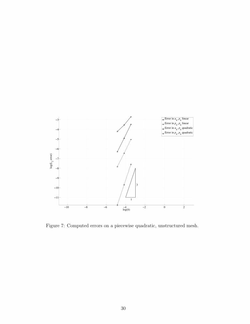
On unstructured meshes, Case 7 (Fig. 7) we lose the superconvergence of velocities andobtain only O(h) in velocity error with linear pressures, while Case 8 (Fig. 7) again givesthe expected error of O(h2) for velocity and O(h3) for pressure.

We conclude that:

• Piecewise linear approximations for uh and ph have superconvergence of velocity onstructured meshes, both for piecewise linear and piecewise quadratic geometry.

• Increasing the polynomial degree of the pressure to P 2 increases the convergenceof a piecewise linear velocity from O(h) to O(h2) on unstructured meshes, both forpiecewise linear and piecewise quadratic geometry.

• Increasing the convergence rate of the pressure, from O(h2) to O(h3), when goingfrom P 1 to P 2 approximations requires that the same increase is being made in thegeometry approximation.

Comments:

• For unstructured meshes these results are in accordance with the theoretical inves-tigations in Section 5. We note, however, that in the numerical results the normalcomponent of the error in the velocity also converges optimally, i.e. of order kg + 1,with respect to the order of approximation of the geometry while in Theorem 5.1 weachieve order kg. In Theorem 5.3 we, however, show that the tangent componentof the error is indeed optimal with respect to the order of the approximation of thegeometry. Thus our theoretical results are in line with the numerical results butslightly weaker with respect to the order of approximation of the geometry for the

21

normal component of the error. The error in the pressure and the tangent componentare optimal with respect to kp, ku, and kg.

• For structured meshes the superconvergence most certainly is related to superconver-gence of L2 projections of the gradient on the continuous space, see [1], which holdson structured meshes.

References

[1] R. E. Bank and J. Xu. Asymptotically exact a posteriori error estimators. I. Gridswith superconvergence. SIAM J. Numer. Anal., 41(6):2294–2312 (electronic), 2003.

[2] S. C. Brenner and L. R. Scott. The Mathematical Theory of Finite Element Methods,volume 15 of Texts in Applied Mathematics. Springer, New York, third edition, 2008.

[3] E. Burman, P. Hansbo, and M. G. Larson. A stabilized cut finite element methodfor partial differential equations on surfaces: the Laplace-Beltrami operator. Comput.Methods Appl. Mech. Engrg., 285:188–207, 2015.

[4] A. Demlow. Higher-order finite element methods and pointwise error estimates forelliptic problems on surfaces. SIAM J. Numer. Anal., 47(2):805–827, 2009.

[5] G. Dziuk. Finite elements for the Beltrami operator on arbitrary surfaces. In Par-tial differential equations and calculus of variations, volume 1357 of Lecture Notes inMath., pages 142–155. Springer, Berlin, 1988.

[6] G. Dziuk and C. M. Elliott. Finite element methods for surface PDEs. Acta Numer.,22:289–396, 2013.

[7] A. Feronni, L. Formaggia, and A. Fumagalli. Numerical analysis of Darcy problemon surfaces. Technical Report 30, MOX, Dipartimento di Matematica “F. Brioschi”Politecnico di Milano, Via Bonardi 9 - 20133 Milano (Italy), 2014.

[8] D. Gilbarg and N. S. Trudinger. Elliptic Partial Differential Equations of SecondOrder. Classics in Mathematics. Springer-Verlag, Berlin, 2001. Reprint of the 1998edition.

[9] P. Hansbo and M. G. Larson. Finite element modeling of a linear membrane shellproblem using tangential differential calculus. Comput. Methods Appl. Mech. Engrg.,270:1–14, 2014.

[10] P. Hansbo, M. G. Larson, and F. Larsson. Tangential differential calculus and thefinite element modeling of a large deformation elastic membrane problem. Comput.Mech., 56(1):87–95, 2015.

22

[11] K. Larsson and M. G. Larson. A continuous/discontinuous Galerkin method anda priori error estimates for the biharmonic problem on surfaces. Technical re-port, Umea University, Department of Mathematics, SE-90187, Umea, Sweden, 2015.arXiv:1305.2740v2.

[12] A. Masud and T. J. R. Hughes. A stabilized mixed finite element method for Darcyflow. Comput. Methods Appl. Mech. Engrg., 191(39-40):4341–4370, 2002.

23

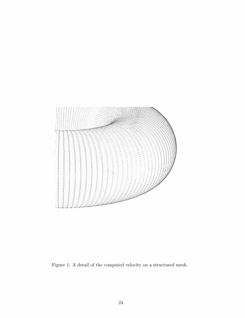
Figure 1: A detail of the computed velocity on a structured mesh.

24

Figure 2: Computed pressure on a structured mesh.

25

Figure 3: Unstructured mesh acquired by jiggling the nodes of a structured mesh.

26

ï7 ï6 ï5 ï4 ï3 ï2 ï1

ï7

ï6.5

ï6

ï5.5

ï5

ï4.5

ï4

ï3.5

1

2

log(h)

log(

L 2 err

or)

Error in uh, ph linear

Error in ph, ph linear

Error in uh, ph quadratic

Error in ph, ph quadratic

Figure 4: Computed errors on a piecewise linear, structured mesh.

27

ï7 ï6 ï5 ï4 ï3 ï2 ï1

ï7.5

ï7

ï6.5

ï6

ï5.5

ï5

ï4.5

ï4

ï3.5

ï3

1

2

log(h)

log(

L 2 err

or)

Error in uh, ph linearError in ph, ph linearError in uh, ph quadraticError in ph, ph quadratic

Figure 5: Computed errors on a piecewise linear, unstructured mesh.

28

ï10 ï8 ï6 ï4 ï2 0 2ï12

ï11

ï10

ï9

ï8

ï7

ï6

ï5

ï4

1

3

log(h)

log(

L 2 err

or)

Error in uh, ph linearError in ph, ph linearError in uh, ph quadraticError in ph, ph quadratic

Figure 6: Computed errors on a piecewise quadratic, structured mesh.

29

ï10 ï8 ï6 ï4 ï2 0 2

ï11

ï10

ï9

ï8

ï7

ï6

ï5

ï4

ï3

1

3

log(h)

log(

L 2 err

or)

Error in uh, ph linearError in ph, ph linearError in uh, ph quadraticError in ph, ph quadratic

Figure 7: Computed errors on a piecewise quadratic, unstructured mesh.

30