Embed Size (px)
Citation preview

A Search for the Rare Decay D0 --+ µ+ µ-
by
Hugo R. Hemaindez Mora
Thesis submitted in panial fulfillment of the requirements for the degree of
MASTER OF SCIENCE
in
Physics
UNIVERSITY OF PUERTO RICO
MAYAGUEZ CAMPUS
Approved by:
Doria! Castellanos, Ph.D. Member, Graduate Committee
~~~ Wolf gang A. Ro Ike, Ph.D. Representative of Gra uat Studies
~~-Au'. Doria! Castellanos, Ph.D.
2001
I I Date
1//)-/rJ/ Date
Date
7-/23/ 0 (
Date
Date Chairpe f the Department
kui u~f ~ ,d.cDO f L. Antonio Esteve , h.D. Director of Graduate
\
(
Date

Abstract
This thesis presents a search for the rare decay D0 ~ µ+ µ- based on data collected
by the Fennilab fixed target photoproduction experiment called FOCUS (FNAL-E83 I).
This decay is an example of a flavor-changing neutral current process which, according
to the Standard Model, should occur at a very low branching ratio of at most 10- 15•
A rate higher than this would be an indication of new physics. Using a blind analysis
method which consists of the observation of events outside a defined signal area, the
optimum selection criteria for candidate events was determined. This method minimizes
bias by basing the choice on the background observed outside the signal region and not
on maximizing the signal under study. The ratio of background outside to background
inside the signal region was determined using an independent real data sample. The result
for the branching ratio of the D0 ~ µ+ µ- decay at 90% Confidence Level upper limit is
2.1x10⁻⁵ which reduces the published value by 50%. No evidence was found for this rare
decay.
ii

Resumen
Este trabajo de tesis presenta la busqueda del decaimiento raro D0 ~ µ+ µ- basado
en datos colectados por el ex.perimento de fotoproducci6n de blanco fijo de Fennilab
llamado FOCUS (FNAL-E83 I). Este decaimiento es un ejemplo de un proceso de
cambio de sabor a traves de corrientes neutrales (FCNC) el cual, de acuerdo con el
Modelo Estandar, deberia ocurrir a una muy baja probabilidad a un orden de 10- 15• Una
probabilidad mayor a esta podria ser una indicaci6n de nueva fisica. Usando un metodo
de amilisis a ciegas que consiste en la observaci6n de eventos fuera de una region definida
como area de seiial, se detennin6 un criterio 6ptimo de selecci6n en la bllsqueda de eventos
candidatos. El uso de este metodo de analisis penniti6 minimizar el prejuicio presente en
la elecci6n de nuestro criterio cual estaba basado en observar eventos de ruido fuera del
area de seiial con la idea de no max.imizar la seiial bajo estudio. La raz6n de ruido fuera del
area de seiial al ruido dentro de esta se detennin6 usando una muestra real independiente.
El resultado para la raz6n de porcentaje para el decaimiento D0 ~ µ+ µ- mostr6 un llmite
superior (con un nivel de confianza de 90%) de 2.1 x 10⁻⁶ , el cual reduce en un 50% el
valor publicado hasta ahora. No se encontr6 evidencia alguna para este decaimiento raro.
iii

To God,
for my country: ~BIA,
to my beautiful city 8'¥NQUILLA,
to my wife Diane,
to my parents Fanny and Anthony and,
to my brothers Madelaine and Jorge Luis.
I Los quiero muchisimo!!! I
To the thousands of countrymen who have fallen while
I have been in the "Isla del Encanto" because of the absurd
conflict that lives within the boundaries of my harmed
country, specially to a person who was an example to me and
my professional guide, Professor Lisandro Vargas Zapata,
cowardly murdered by gunmen on february 23, 200 I at his
doorstep in Barranquilla.
iv

Acknowledgments
There are so many people that in one way or another have contributed in my
development as a human being and as a professional. To mention them all would be
impossible. It is very difficult to even mention some before others. The most important
thing is that all of those who believed in me, will always hold a key to my heart.
First of all. I thank God, that entity who has given us life and with that, a great number
of questions that we try to answer day by day. I thank Him for giving me the opportunity of
being born in ~IA. a country that even now, when it is going through a crisis, has
a face unknown to many. The face of a country that always fought for progress, of a hard
working country that is proud of its roots, that cries for those who have fallen and misses
those who are missing. A country that screams for freedom, but above all, there is a cry of
hope that the armed conflict that harms us will end. We want a free country for all!
I don't want to leave behind my city, 8'¥NQUILLA, my "Curramba la Bella".
The city that watched me grow up. On her streets I learned to live life to the extreme. It
was there where my life is centered and the crib of my professional future. I have great
expectations for my professional development and I wish to offer those to my loved city.
v

I thank Fanny Mora. my mother, for making me into what I am today. Without her
unconditional help I wouldn't heve gotten to this point. To her above all, I dedicate this
triumph. To my brothers, Madelaine and Jorge Luis, for believing in me and for taking care
of my mother while I was absent. To my father Anthony Valle, for always being there in
the g(lod times as well as in the bad times.
~TO RICO is a country that I will always have with me. A master's degree, a
marriage and a family. All this I take from you "Isla del Encanto". I thank my wife Diana
for her unconditional help. Thank you for sharing my good times and my sorrow.
An immensurable thanks to the friendship, professional and economic support that
Dr. Angel M. L6pez gave me. Thank you for everything you did during the time I worked
for you, and for always believing in me and trusting me. To professors Will E. Johns and
Hector Mendez for helping me out without asking and also to Dr. WeiJun Xiong. Thanks
to Dr. Wolfgang Rolke for your cooperation in the statistical analysis for this work. Your
contribution was of great importance for me. Overall, to all of those who work with me at
the HEP lab at Mayagilez. Those from the past: Alejandro Mirles, Carlos Rivera. Mauricio
Suarez, Salvador Carrillo, Fabiola Vazquez and Kennie Cruz; and those from the present:
Jose A. Quinones, Eduardo Luiggi, Alexis Paris, Luis A. Ninco and Carlos R. Perez. Thank
you guys!!!
To the Physics Department at Mayaguez Campus and its director when I became a
part of the University, Dr. Dorial Castellanos (January, 1998), who gave me chance to make
it happen. I that all of those at the FOCUS Collabontion for giving me the opportunity
vi

to work on their experiment. To all those people who work at EPSCoR but most of all to
Sandra Troche who was always there for me.
To the great friendships I made in PR. To Juan Carlos Hernandez, Carlos Jose and
specially to their parents Jose "Machito" Hernandez and Juanita Gonzalez. You were the
family I needed throughtout these three years.
Thanks to Mr. Joe Ortiz for helping me in my college studies, thank you for helping
me pursue the grounds of PR. I also thank Mr. Felix Rivera, and the Romero Valle family
as well as Valle Miranda family. Thanks for everything. I thank Mr. Rafael Sanjuan and
his family for being there when I needed it. A special thanks to Mrs. Martha Castano, may
God bless your noble soul.
I thank my professors at the Universidad del Atlantico - Barranquilla: Arnaldo
Cohen and Oswaldo Dede, for making me look at science. To my colleagues and friends
Arnulfo Barrios, Oscar Montesinos, Harkccynn Torregroza, Ericka Navarro and Rafael
Manga. I also thank my High School teachers from the Bienestar Social de la Policfa
- Barranquilla: Blas T6rres, Carlos Bray and Orlando Ortiz, specially Mr. Armando
Consuegra (Barrabas).
To all of these whom I have mentioned as well as those whom I have not, otherwise
I would never be able to finish ...
Mil y mil gracias! ! !
vii

Agradecimientos
Son muchas las personas que de una u otra forma ban contribuido en mi desarrollo
como ser humano y como profesional. Enumerarlas a todas resultaria imposible. Inclusive
mencionar algunas primero que a otras resulta diffcil para mi. Lo mas importante que
quiero manifestar es que a todas estas personas que creyeron en mi por siempre las llevare
en mi coraz6n.
Inicialmente quisiera darle las gracias a Dios, a ese ser que nos ha otorgado la vida
y con ella un sinnumero de interrogantes que dia a dia tratamos de contestarnos. A El le
agradezco el haberme dado la oportunidad de nacer donde naci, mi patria c:f.oMBIA, un
pals que aun cuando en estos momentos atraviesa por momentos de crisis posee una cara
que muchos de nosotros desconocemos. La cara de un pueblo que por siempre ha luchado
por salir adelante, de un pueblo trabajador y orgulloso de sus raices, que llora a sus hijos
caidos y extraiia a sus hijos ausentes. Un pueblo que lanza a todo pulm6n un grito de
libertad, pero sabre todo un grito de esperanza por la culminaci6n de este conflicto armado
que nos acongoja. Queremos un pals Libre para todos!
No quiero dejar de lado a mi B'RaANQUILLA del alma, a mi Curramba la Bella.
La ciudad que me vi6 crecer. En sus calles aprendi a vivir la vida en cada uno de los
viii

extremos que esta nos presenta. Y es alli donde se centra mi vida y mi futuro profesional.
Resultan inmensas las expectativas de poder desarrollarme como profesional y ofrecer mis
servicios a la ciudad de mis amores.
Le agradezco a mi madre, Fanny Mora, por hacer de mi lo que hoy en dia soy. Sin el
apoyo incondicional de parte de ella no hubiese sido posible la consecusi6n de cada uno de
mis exitos. A ella mas que a nadie dedico este triunfo que hoy dia estoy consiguiendo. A
mis hermanos, Madelaine y Jorge Luis, por creer en mi y por cuidar de mi madre durante
mi ausencia. A mi padre, Anthony Valle, por estar alli siempre, tanto en las buenas como
en las malas.
fi.JFRTO RICO es una tierra que llevare conmigo por siempre. Una maestria, muchos
amigos, un matrimonio y una familia. Todo esto me llevo de tus suelos "Isla del Encanto".
Agradezco enormemente la ayuda incondicional recibida de parte de Diana, mi esposa.
Gracias por compartir a mi lado mis alegrias y soportar ademas las tristezas y los malos
ratos.
Un agradecimiento mas que enorme a la amistad, el apoyo profesional y econ6mico
que me brind6 el Dr. Angel M. L6pez. Gracias por todo lo que hizo por mi durante el
periodo en el que estuve trabajando a su lado, por creer siempre en mi y por brindarme su
confianza A los profesores Will E. Johns y Hector Mendez por la ayuda que me brindaron
sin nunca recibir una negativa de su parte. Al Dr. WeiJun Xiong por su colaboraci6n y su
apoyo a mi trabajo. Gracias por la ayuda brindada por parte del Dr. Wolfgang Rolke. Su
colaboraci6n en el analisis estadistico para este trabajo de tesis fue de gran importancia.
En general a todos los compaiieros del laboratorio de HEP en Mayagilez. Los del pasado:
ix

Alejandro Mirles, Carlos Rivera, Mauricio Suarez, Salvador Carrillo, Fabiola Vazquez y
Kennie Cruz; los del presente: Jose A. Quinones, Eduardo Luiggi, Alexis Paris, Luis A.
Ninco y Carlos R. Perez. Muchachos, gracias!!!
Al Departamento de Fisica del RUM y su director en el periodo (Enero de 1998)
en que inicie estudios graduados en UPR. A ellos Jes agradezco el habenne brindado la
oportunidad para que esto fuese una realidad. Agradecimientos muy especiales a toda
la gente de FOCUS Collaboration por darme la oportunidad de trabajar en este gran
experimento. A todas las personas que trabajan en EPSCoR en especial a Sandra Troche
por su incondicional ayuda y por su constante colaboraci6n.
A las grandes amistades construidas durante mi pennanencia en PR. A Juan Carlos
Hernandez, Carlos Jose y en especial a sus padres Jose "Machito" Hernandez y Juanita
Gonzalez. Ustedes fueron el soporte familiar que tanta ayuda me hizo en estos ultimos tres
afios tiempo que dur6 mi maestria.
Gracias especiales a Joe Ortiz por apoyarme incondicionalmente en mis estudios
universitarios, gracias por tu patrocinio en mi empresa hacia PR. lgualmente le agradezco
a Felix Rivera, a la Familia Romero Valle al igual que a la Familia Valle Miranda. Gracias
por su patrocinio. Agradezco a Rafael Sanjuan y familia por siempre estar cuando los
necesitabamos. Gracias. A Martha Castano, un mi116n de bendiciones para usted mi bella
dam a.
Agradezco a mis profesores de la Universidad del Atltintico - Ba"anquilla: Arnaldo
Cohen y Oswaldo Dede, por inculcarme los deseos de hacer ciencia. A mis colegas y
x

amigos de universidad, Arnulfo Barrios, Oscar Montesinos, Harkccynn Torregroza, Ericka
Navarro y Rafael Manga. lgualmente agradezco a todos mis profesores de Bachillerato en
el Bienestar Social de la Policfa • Barranquilla: Blas T6rres, Carlos Bray y Orlando Ortiz,
especialmente a Armando Consuegra (Barrabas).
A todas las personas que he mencionado al igual que a las muchas que deje de
mencionar pues nunca terminaria este documento ...
Mil y mil gracias!!!
xi

Contents
List of Tables
List of Figures
List of Abbreviations
1 Introduction
I . I The Standard Model
I. I.I Fundamental Particles . . . . . . . . . . .
xviii
xix
xxi
1
2
3
Bosons . . . . . . . . . . . . . . . . . . . . . . . . . . . . . . . . 4
Fermions ................. .
l. l .2 Interactions . . . . . . . . . . . . . . . . .
Long and Short Distance Effects . . . . . .
4
6
9
Feynman Diagrams . . . . . . . . . . . . . . . . . . . . . . . . . . I 0
1.2 Conservation Laws . . . . . . . . . . . . . . . . . . . . . . . . . . . . . . I 0
xii

1.2. l Conservation of Angular Momentum and Helicity Suppression . . . 11
1.2.2 Conservation of the electrical charge . . . . . . . . . . . . . . . . . 12
1.2.3 Lepton Number Conservation . . . . . . . . . . . . . . . . . . . . 13
1.2.4 Baryon Number Conservation . . . . . . . . . . . . . . . . . . . . 14
1.2.5 Flavor Conservation . . . . . . . . . . . . . . . . . . . . . . . . . 15
1.3 Cabibbo Theory . . . . . . . . . . . . . . . . . . . . . . . . . . . . . . . . 16
a) Cabibbo-Favored . . . . . . . . . . . . . . . . . . . . . . . . . . . . . . 19
b) Cabibbo-Suppressed . . . . . . . . . . . . . . . . . . . . . . . . . . . . 20
c) Doubly-Cabibbo-Suppressed . . . . . . . . . . . . . . . . . . . . . . . . 21
1.4 GIM Mechanism . . . . . . . . . . . . . . . . . . . . . . . . . . . . . . . 22
1.5 Rare and Forbidden Decays . . . . . . . . . . . . . . . . . . . . . . . . . . 24
a) Lepton Family Number Violation . . . . . . . . . . . . . . . . . . . . . 24
b) Lepton Number Violating . . . . . . . . . . . . . . . . . . . . . . . . . 24
c) Flavour-Changing Neutral-Currents . . . . . . . . . . . . . . . . . . . . 24
1.6 Special Relativity . . . . . . . . . . . . . . . . . . . . . . . . . . . . . . . 25
I. 7 Confidence Intervals and Confidence Levels . . . . . . . . . . . . . . . . . 29
2 Previous Works 30
2.1 FCNC Decay Theory . . . . . . . . . . . . . . . . . . . . . . . . . . . . . 30
xiii

2.2 Previous Searches for Rare Charm Decays . . . . . . . . . . . . . . . . . . 32
2.2. I The Hadroproduction WA92 Experiment . . . . . . . . . . . . . . 33
2.2.2 The Hadroproduction E79 I Experiment . . . . . . . . . . . . . . . 34
2.2.3 The Photoproduction E687 Experiment . . . . . . . . . . . . . . . 36
2.3 FOCUS . . . . . . . . . . . . . . . . . . . . . . . . . . . . . . . . . . . . 38
2.3. I Introduction . . . . . . . . . . . . . . . . . . . . . . . . . . . . . . 38
2.3.2 The FOCUS Photon Beam . . . . . . . . . . . . . . . . . . . . . . 39
2.3.3 Inside the FOCUS Experiment . . . . . . . . . . . . . . . . . . . . 40
3 Objectives 44
4 Procedure 46
4.1 Data Format . . . . . . . . . . . . . . . . . . . . . . . . . . . . . . . . 47
4.2 Reconstruction Process . . . . . . . . . . . . . . . . . . . . . . . . . . . . 48
4.3 Data Selection . . . . . . . . . . . . . . . . . . . . . . . . . . . . . . . . . 50
4.3. l Selection Variables . . . . . . . . . . . . . . . . . . . . . . . . . . 50
a) Vertexing . . . . . . . . . . . . . . . . . . . . . . . . . . . 50
I. L/a . . . . . . . . . . . . . . . . . . . . . . . . . . . . 52
2. Primary Vertex Multiplicity . . . . . . . . . . . . . . . . . . . 52
3. Vertex Confidence Levels . . . . . . . . . . . . . . . . . . . . 52
xiv

4. Vertex z Positions . . . . . . . . . . . . . . . . . . . . . . . . 52
5. Vertex Isolations . . . . . . . . . . . . . . . . . . . . . . . . 53
b) Particle Identification . . . . . . . . . . . . . . . . . . . . . . . 53
I. Muon Identification . . . . . . . . . . . . . . . . . . . . . . . 53
i. Kaon Consistency for Muons . . . . . . . . . . . . . . . . . 54
ii. Inner Muons . . . . . . . . . . . . .......... 55
A) Number of Missed Muon Planes . . . . . . . . . . . . . 56
8) Inner Muon Confidence Level . . . . . . . . . . . . . . 56
iii. Outer Muons . . . . . . . . . . . . . . . . . . . . . . . . . 56
A) Outer Muon Confidence Level . . . . . . . . . . . . . . 56
2. Hadron Identification . . . . . . . . . . . . . . . . . . . . . . 56
i. Kaonicity . . . . . . . . . . . . . . . . . . . . . . . . . . . 57
ii. Pion Consistency . . . . . . . . . . . . . . . . . . . . . . . 57
3. Momentum . . . . . . . . . . . . . . . . . . . . . . . . . . . 58
4. Dimuonic Invariant Mass . . . . . . . . . . . . . . . . . . . . 58
4.3.2 FOCUS Data Selection Stages . . . . . . . . . . . . . . . . . . . . 59
a) Passi . . . . . . . . . . . . . . . . . . . . . . . . . . . . . . . . 59
b) Skiml . . . . . . . . . . . . . . . . . . . . . . . . . . . . . . . 59
c) Skim2 .................... 59
xv

d) Skim3 ............................... 61
4.4 Nonnalizing Mode . . . . . . . . . . . . . . . . . . . . . . . . . . . . . . 63
4.5 Monte Carlo Simulation . . . . . . . . . . . . . . . . . . . . . . . . . . . 65
a) D0 ~ µ+ µ- Events . . . . . . . . . . . . . . . . . . . . . . . . 66
b) D0 ~ K-7r+ Events. . . . . . . . . . . . . . . . . . . . . . . . 66
c) D0 ~ rr+7r- and D0 ~ K+ K- Events . . . . . . . . . . . . . . 67
4.6 Analysis Methodology . . . . . . . . . . . . . . . . . . . . . . . . . . . . 67
4.6.I Blind Analysis ...................... 67
4.6.2 Rolke and Lopez Limits . . . . . . . . . . . . . . . . . . . . . . . 67
4.6.3 Detennination of Sensitivity and Confidence Limits . . . . . . . . . 69
4.6.4 Sidebands Background and Signal Area . . . . . . . . . . . . . . . 71
4. 7 Background Study . . . . . . . . . . . . . . . . . . . . . . . . . . . . . . 72
4. 7 .1 Introduction . . . . . . . . . . . . . . . . . . . . . . . . . . . . . . 72
4. 7 .2 MislD Study . . . . . . . . . . . . . . . . . . . . . . . . . . . . . 73
4.7.3 Background Ratio Study . . . . . . . . . . . . . . . . . . . . . . . 74
4.8 Optimization of the Selection Criteria . . . . . . . . . . . . . . . . . . . . 78
4.8. I Fixed Cuts and Variable Cut Ranges . . . . . . . . . . . . . . . . . 79
4.8.2 Optimization Based on Sensitivity . . . . . . . . . . . . . . . . . . 80
xvi

S Results and Conclusions 81
5.1 MisID ..................................... 81
5.2 Background Ratio . . . . . . . . . . . . . . . . . . . . . . . . . . . . . . . 82
5.3 Skimming Results . . . . . . . . . . . . . . . . . . . . . . . . . . . . . . . 83
5.4 Cut Optimization Results . . . . . . . . . . . . . . . . . . . . . . . . . . . 86
5.5 Confidence Limits . . . . . . . . . . . . . . . . . . . . . . ....... 89
5.6 Conclusions . . . . . . . . . . . . . . . . . . . . . . . . . . . . . . . . . . 91
Bibliography 92
xvii

List of Tables
2.1 Chronological branching ratios for the ~C = 1 weak neutral-current decay D0 ~ µ+µ- . ................................. 32
4.1 Description of Superstreams . . . . . . . . . . . . . . . . . . . . . . . . . 61
4.2 Description of Superstream I ............... 62
4.3 Sensitivity number as per Rolke and Lopez . . .......... 69
4.4 An example of Rolke and L6pez 90% Confidence Limits 70
4.5 Dimuonic Invariant Mass Cuts for Sidebands and Signal Regions . . 79
4.6 Cut values for each variable considered in the optimization process . 80
5.1 Best Cut Combination. . . . . . . . . . . . . . . . . . . . . . . . . . . . . 86
5.2 Results of Cut Optimization . . . . . . . . . . . . . . . . . . . . . . . . . 88
xviii

List of Figures
I . I The Standard Model for Elementary Particles . . . . .
1.2 Transformations permmited by the Standard Model . .
5
8
1.3 Feynman diagram a weak process mediated by a vinual boson exchange. . . I 0
1.4 A charged current interaction . . . . . . . . . . . . . . . . . . . . . . . . . 12
1.5 Feynman diagram for a weak transition . . . . . . . . . . . . . . . . . . . 17
1.6 Representation for the CKM matrix elements . . . . . . . . . . . . . . . . 20
1.7 Feynman diagram for a Cabibbo-Favored process . . . . . . . . . . . . . . 20
1.8 Feynman diagram for a Cabibbo-Suppressed process . 21
1.9 Feynman diagram for a Doubly-Cabibbo-Suppressed process . . . . . . . . 21
I . I 0 Weak interactions in neutral-current processes . . . . . . . . . . . . . . . . 22
2.1 Feynman diagrams for the decay D0 ~ µ+ µ- . . . . . . . . . . . . . 31
2.2 Proton synchrotron and beamlines at Fermilab . . . . . . . . . . . . . . . . 38
2.3 The E83 l Photon Beam . . . . . . . . . . . . . . . . . . . . . . . . . . . . 39
xix

2.4 The FOCUS Spectrometer . . . . . . . . . . . . . . . . . . . . . . . . . . 41
4.1 Trajectories through the FOCUS spectrometer . . . . . . . . . . . . . . . . 49
4.2 Production and decay vertices for the D0 --+ µ+ µ- process . . . . . . . . . 51
4.3 Analysis overview of FOCUS . . . . . . . . . . . . . . . . . . . . . . . . 60
4.4 Monte Carlo generated process schematization for the decay D0 ~ µ+ µ- 66
4 5 Do + - I . M d' 'b . 71 . ~ µ µ nvanant ass 1stn ut1ons . . . . . . . . . . . . . . . . . .
4.6 Dimuonic Invariant Mass comparison of Monte Carlo data from D0 ~ 7r+ 7r-and D0 ~ µ+µ- ............................... 75
4.7 Dimuonic invariant mass of D0 ~ K-7r+ generated by Monte Carlo . 76
4.8 Background comparison between real and Monte Carlo data . . . . . . . . 77
5.1 MisID as a function of momentum . . . . . . . . . . . . . . . . . . . . . . 82
5.2 Typical Invariant Mass Distribution Used in Calculating the Background Ratio. . . . . . . . . . . . . . . . . . . . . . . . . . . . . . . . . . . . . . 83
5.3 Invariant Mass Distributions for Skim3 Cuts . . . . . . . . . . . . . . . 84
5.4 Invariant Mass Distributions for Skim4 Cuts . . . . . . . . . . . . . . . . . 85
5.5 Mass distributions for the best cut combination. . . . . . . . . . . . . . . . 87
5.6 Invari~nt. Mass Distribution for Background Ratio using the best cut combmatton . . . . . . . . . . . . . . . . . . . . . . . . . . . . . . . . . . 89
5.7 Event candidates for the D0 --+ µ+µ-process . . . . . . . . . . . . . . . . 90
xx

BR:
CERN:
CITADL:
CKMMatrix:
CP Violation:
CL:
CLP:
CLS:
E687:
E831:
E791:
Fermilab:
FNAL-E831:
FCNC:
FOCUS:
GIM Mechanism:
GeV:
IMU:
IMUCL:
ISOP:
ISOS:
Klµ:
LFNV:
LNV:
Ua:
MeV:
MisID:
MISS PL:
Ml:
List of Abbreviations
Beryllium Oxide. Branching Ratio. Organisation Europeenne pour la Recherche Nucleaire. Cerenkov Identification Through A Digital Likelihood. Cabibbo-Kobayashi-Maskawa Quark-Mixing Matrix. Charge-Parity Violation. Confidence Level. Primary Vertex CL. Secondary Vertex CL. Fermilab Experiment 687. Fermilab Experiment 831.
Fermilab Experiment 791.
Fermi National Accelerator Laboratory. Fermilab Experiment 831.
Flavor-Changing Neutral-Current. Fotoproduction Of Charm with an Upgraded Spectrometer. Glashow-Hiopoulos-Maiani Mechanism. Giga Electron Volt. Inner Muon System. Inner Muon CL. Primary Vertex Isolation. Secondary Vertex Isolation. Kaon Consistency to separate kaons from muons. Lepton Family Number Violation. Lepton Number Violation. Separation between the production and decay vertices divided by the error, <J, on that measurement. Mega Electron Volt. Percent of events misidentified within any specific analysis. Number of Missed Muon Planes. Magnet Number l.
xxi

M,,,,: OMU:
OMUCL:
PAW:
Passi: PWC:
Skiml:
Skim2:
Skim3:
Skim4:
SSD: ZVPRIM: ZVSEC:
Magnet Number 2.
Lorentz Dimuonic Invariant Mass.
Outer Muon System.
Outer Muon CL. Physics Analysis Workstation.
Basic event reconstruction stage.
Proportional Wire Chambers.
First data reconstruction selection stage. Second data reconstruction selection stage.
Third data reconstruction selection stage.
Fourth data reconstruction selection stage.
Silicon Microvertex Detectors. Primary Vertex z Position.
Secondary Vertex z position. ~ W(1r K): Kaonicity.
11'con: Pion Consisitency. tr zi: Difference between the Primary Vertex z position and the z target
edge divided by the uncertainty.
tr z2 : Difference between the Secondary Vertex z position and the z target edge divided by the uncertainty.
xx ii

Chapter 1
Introduction
This thesis is a research work in a topic of high energy physics. It is also a formative
work and could be used as a source of reference for students and people interested in
knowing more about the physics related with the microscopic world around us.
The Standard Model of electroweak interactions is used to understand the decays
of heavy quarks which are known to us. A significant observation of charm Flavor
Changing Neutral-Current decays, predicted to occur rarely (in the Standard Model the
neutral-current interactions do not change flavor), would imply new physics beyond the
Standard Model.
Rare decay modes are probes of particle states or mass scales which cannot be
accessed directly. One of the most interesting processes to study is the D0 -t µ+ µ
decay (all references to this decay also implies the corresponding charge-conjugate state
D0 -t µ-µ+). The main goal of the work reported in this thesis was the measurement of

§ I. I The Standard Model 2
the branching ratio for this decay and a comparison to the actual 90% Confidence Level
upper limit 4.1 x 10⁻⁶•
This chapter will display some basic and interesting concepts used for this study.
First, an introduction to the Standard Model of elementary particles is done, next some of
the conservation laws are discussed. The Cabibbo Theory and the GIM Mechanism will
also be discussed in this chapter. Basic information about Rare and Forbidden decays will
be shown defining three important related processes: Lepton Family Number Violation,
Lepton Number Violation and Flavor-Changing Neutral-Currents. A short representation
of Special Relativity will be discussed and finally some useful concepts about Confidence
Intervals will be defined.
1.1 The Standard Model
At the beginning of the 20th century, physicists thought that all matter was composed
of atoms as the fundamental building block. As the century entered adolescence, it was
discovered that atoms are constructed from electrons and a small positive charged nucleus.
This nucleus was subsequently found to be composed of protons which have a positive
charge, and neutrons (except the Hydrogen nucleus), which are uncharged. However,
during the latter half of the century, physicists determined that neither protons nor neutrons
are fundamental. A better description about the matter in the universe was obtained and
now we know that all matter is made from one or more of sixteen elementary particles.
To explain the nature of these elementary particles and the forces between them, a

§ I. I The Standard Model 3
theory has been developed called the Standard Model [1-3). The model describes all matter
and forces in the universe (except gravity) and it is a package of two theories: the Unified
Electroweak [4, p.95] and Quantum Chromodynamics [4, p.85).
1.1.1 Fundamental Particles
The Standard Model divides the elementary particles into two groups called bosons
and fermions which are differentiated according to the behavior of multiparticle systems.
Bosons obey the Bose-Einstein statistics and fermions obey the Fermi-Dirac statistics. The
Bose-Einstein statistics means that any number of identical bosons can exist in the same
quantum state. This is very essential in shaping the statistical behavior of a large number
of bosons. On the other hand, in the Fermi-Dirac statistics two fermions cannot coexist in
the same quantum state. Whichever statistics a particle follows will determine the w wave
function's symmetry under interchange of particles. If these two particles have identical
I '111 2 (wave-function squared), the probability of particle I being in one spot and particle 2
at another, must be equal to the probability that the first particle is in the second spot and
particle 2 is in the first. Therefore, under interchange the wave-function '11(-x) = ±w(x)
where x is the relative position.
For identical bosons the Bose-Einstein symmetry principle states that the wave
function under interchange must go to plus itself
w(-x) = w(x) (I. I)
and, for identical fermions the Pauli principle states that the wave-function under

§ I. I The Standard Model 4
interchange must go to minus itself
'11(-i) = -'11(i) (1.2)
For non relativistic speeds, the total wave-function of the pair can be expressed as a
product of functions depending on spatial coordinates and spin orientation:
l'11(i)) = o(space}/3(spin) (1.3)
where the spatial part, o, will describe the orbital motion of one particle about the other. It
can happen that a is symmetric or antisymmetric under interchange and the spin function /3
may be symmetric (spins parallel) or antisymmetric (spins antiparallel) under interchange.
Bosons. They are: photon, gluon, w± and z0• These particles have an integral spin
(0, I, 2, ... ) and are known as the intermediary particles because they are responsible for
carrying the force interactions. The photon is massless with spin I and is the intermediary
of the electromagnetic interaction. There is one kind of photon and two photons do not
directly interact with one another. The gluon is massless with spin I and is the intermediary
of the strong interaction. There are eight types of gluons, each different from one another
only by a quantum number called color. The gluons interact with one another. The w±
( m :::::: 80.4 Ge V) and z0 ( m :::::: 91.2 Ge V), all of spin l, are the intermediaries of the weak
interaction. The w± and z0 do not interact with one another.
Fermions. They have a half-integral spin(~. ~ •... ) and constitute the fundamental
families of matter. These are divided into quarks with fractional electric charges (+ilel
and -klel> and leptons with integer charge (-lie!> or no charge (neutrinos). At the same

§ I. I The Standard Model 5
time, quarks are subdivided into six different particles: up (m :::::: I to 5 MeV), charm
(m:::::: 1.15 to 1.35 GeV) and top (m:::::: 169 to 179 GeV) with electric charges of +~lel and
down (m:::::: 3 to 9 MeV), strange (m:::::: 75 to 170 MeV) and bottom (m:::::: 4.0 to 4.4 GeV)
with -~le!. The six types of quarks are sometimes called flavors. Leptons are subdivided
into three different electrically charged particles, the electron, e (m :::::: 0.511 MeV), the
muon,µ (m:::::: 105.7 MeV), and the tau, r (m:::::: 1.777 GeV), with their respective neutral
neutrinos, lie (m < 3 eV), 11µ (m < 0.19 MeV) and vT (m < 18.2 MeV). Each particle,
quark or lepton, has its respective antiparticle with the same mass but with opposite electric
charge. Figure 1.1 shows the fundamental particles of matter arranged into families by the
Standard Model.
Figure I. I: The Standard Model for Elementary Panicles.

§ I. I The Standard Model 6
Each of the three columns corresponds to a ''family". The relationships among the
particles in a family are the same as those in the other two families. In a way we have three
copies of the same structure. In each of the families there is a lepton and a quark doublet.
The charge of the members of the doublets differ by one e unit. The main difference
between families are the masses of their members. The first family members are low mass
while the masses of the third family are much higher. This large difference in mass is one
of the principal open mysteries in elementary particle physics.
1.1.2 Interactions
Of the known four forces, two, gravity and electromagnetism, have a long range and
are common in every day life. The remaining two forces, the strong and weak nuclear
forces, have such a small range that it is frequently compared to the size of an atomic
nucleus. Due to its low strength, gravity is still not a complete part of the Standard
Model. Another interaction that has an infinite range is the electromagnetic interaction
whose effects have been measured throughout immense scales. The strong interaction
holds together the nucleus working against the electrostatic repulsion that occurs between
protons. Lastly, the weak interaction is known to be responsible for a large variety of
radioactive decays. Also, it is responsible for the interactions that occur between neutrinos
and matter.
Besides electric charge, quarks and gluons have another type of charge. It is called
the color charge. The effects of the strong nuclear force or color force are only felt by
quarks. It is a very strong force that binds quarks together forming particles. There are
§ I. I The Standard Model 7
three "colors" for quarks which are usually called "red", "blue" and "yellow". If you put
together a red quark with an antired antiquark, the product is colorless. If you put together
a red, a blue and a yellow quark, the product is also colorless.
Due to the nature of the color interaction, combinations with a net color charge are
highly unstable. If one starts with a system with no net color charge, it will never separate
into color charged pieces. The reason for this is believed to be that, due to the fact that
gluons have a color charge, there is an "anti-screening" effect whereby the effective force
between two quarks increases with distance. This increased potential energy is converted
to quark-antiquark pairs in such a way that the separated pieces are each colorless. This
is believed to be the reason no system with a net color charge has ever been directly
observed, including both quarks or gluons. However, through the use of deep inelastic
scattering experiments, the interactions of gluons or quarks with incoming projectiles has
been inferred.
Only groups of two quarks (mesons formed of a quark and an antiquark) or three
quarks (baryons formed of three quarks or three anti-quarks), have been seen. Collectively,
these groups are called hadrons. On the other hand, leptons can exist without the
companionship of other particles since they have no color charge. The net force between
color neutral systems (the strong force) actually decreases with distance.
The weak interaction is felt by both quarks and leptons. There is a deep relationship
between the weak interaction and the family structure of quarks and leptons. In the case
of the leptons, it is only possible to change leptons within the same family into each other.
Thus, the electron can be turned into Ve but not into a muon. The weak interaction can act
within the lepton families, but not between them. There are complications when it comes

§ I. I The Standard Model 8
to the quarks. Here also the weak interaction can tum one flavor into another. However,
it is not true to say that the weak force cannot act across families. It can, but with a much
reduced effect.
Quarks 0 © CD
IX I XI @-©-®
(a)
©
I @
Leptons 0 0
I I <;) (9 (b)
Figure 1.2: Transfonnations pennmited by the Standard Model. (a) The effect of the weak force on the quarks. Transfonnations such as b ~ u are also possible. (b) The effect of the weak force on the leptons. Transfonnations within families are represented by vertical arrows and across families are represented by horizontal and diagonal arrows.
For quarks, the electric charge changing transformations within families and across
families are dominant (the vertical transformations are more probable and the diagonal
transformations are less probable) as seen in Figure 1.2. This does not mean that
transformations due to neutral currents cannot occur. Quark transitions such as c -+ u,
in which the charge is the same, could occur through a neutral current zo. What happens
is that transitions such as this one have a small probability of occurrence compared to the
electric charge changing transitions. In Section 1.3, this will be explained in more detail.
As mentioned before, the weak interactions of quarks as well as leptons are mediated
by the w+, w- and Zo. In the Standard Model leptons cannot have cross transformations
directly. Nevertheless, the Standard Model permits processes such as e+ e- -+ µ+ µ- where
the e+ e- first converts to a z0 which then turns into µ+ µ-. It is important to note that all

§ I. I The Standard Model 9
particles that have an electric charge including the W feel the electromagnetic force but the
gravity force does not have an observable effect in particle physics.
Short and Long Distance Effects. Quantum mechanically interactions are due
to the exchange of virtual bosons. The fundamental color interaction between quarks
is mediated by virtual gluons. Effects due to such fundamental processes involving a
finite number of quark-gluon vertices are called short distance effects. The effective
strength of this fundamental interaction is relatively small and Feynman diagrams (See
next section.) and perturbation theory can be used to calculate them. However, the gluons
(unlike the photon and the intermediaries of the weak interaction) carry color charge. The
consequences of this color charge are profound. Gluon-gluon interactions are possible.
These leads to an "antiscreening" effect where the effective color interaction between
quarks actually increases with distance instead of decreasing as in the electromagnetic and
weak interactions. The result is that strong interactions between hadrons decrease with
energy since at higher energy the component quarks interact at shorter distances. At lower
energies and longer distances the effective interaction is larger and it is not possible to
calculate such "long distance effects" using perturbation theory.
In hadron decay the fundamental decay mechanism may well be a weak interaction
between the constituent quarks but as the decay products separate long distance effects
due to the color interaction will play an important role. Some characteristics of the
decay will be determined by its fundamental weak nature but other characteristics will
be strongly affected by the long distance effects. For example, parity violation in a
decay is an indication of its fundamental weak nature. However, the precise values of
lifetimes and branching ratios can not be calculated with pure perturbation theory. Our

§ 1.2 Conservation Laws 10
current best understanding of such decays uses our knowledge of the weak interaction
in perturbation theory calculations together with phenomenological models for the long
distance effects of the color interaction. In the future it is hoped that lattice gauge theory
numerical calculations of the color interaction will achieve sufficient accuracy as to make
phenomenological models unnecessary. These do not use perturbation theory to calculate
color interaction effects.
Feynman Diagrams. A Feynman diagram is a representation of the way particles
interact with one another by the exchange of bosons. They are extremely useful in making
perturbation theory calculations because each representation is associated with fonnal rules
for assigning vertex couplings, propagator tenns, etc.
e e
e e
Figure 1.3: Feynman diagram for a weak process mediated by a virtual boson exchange.
1.2 Conservation Laws
Among the most significant aids to understanding what takes place in the universe are
the conservation laws, given that they identify those types of interactions that cannot occur.

§ 1.2 Conservation Laws 11
It is a trustworthy rule of thumb in physics that whatever thing is not definitely prohibited
will occur.
In classical mechanics, the invariants are the conservation of the electric charge,
the conservation of linear momentum, the conservation of energy and mass, and the
conservation of the angular momentum. In the quantum world, there are other invariants
as well that are preserved in some types of interactions but not others. For example, the
isotopic spin is preserved in the strong interactions but not in interactions concerning the
electroweak force.
1.2.1 Conservation of Angular Momentum and Helicity Suppression
The helicity of a particle is defined as its spin projection along its direction of motion.
A particle with spin vector tr and momentum p has helicity
H = tr.p ltrllPI
(1.4)
For spin ~there are only two possible helicity states, ±1. If the helicity of a particle
is positive, it is called right-handed, and left-handed if the helicity is negative. The
corresponding states are denoted as ¢Rand lfJL respectively.
Due to the nature of the weak interaction, lepton states from weak decays are
predominantly left-handed. This helicity predominance is stronger the lower the mass
of the lepton. In the case of the neutrino, it is total. Only left-handed v have been
observed. For other leptons, the term helicity suppression is used. This means that right-

§ 1.2 Conservation Laws 12
handed leptons and left-handed antileptons are produced with much lower probability. The
D0 has spin zero so the two muons in D0 -+ µ+ µ- must have opposite spin to conserve
angular momentum. But they also have opposite momentum so they have the same helicity.
However one is an antilepton. Thus, the weak decay D0 -+ µ+ µ- is helicity suppressed.
1.2.2 Conservation of the electrical charge
Whichever reaction, the entire charge of all the particles before the reaction has got
to be identical to the whole charge of all the particles following the reaction. For instance,
in a beta decay, a neutron decays to form a proton and an electron plus an antineutrino.
This begins with a zero charge and finishes one part negative and one part positive charge.
Figure 1.4 shows the contribution of charge for each fermion involved in the reaction.
n -+ p + e + 'iie
with charges: 0 +Ilel -llel 0
p e
n
Figure 1.4: A charged current interaction. The neutron has a quark content of udd and its charge is +2/3lel - l/3lel - l/3lel = Olel. The proton quark content is uud and its charge is +2/3lel + 2/3lel - l/3lel = llel. The electron has -llel as charge and the Ve has Olel as charge.
(1.5)

§ 1.2 Conservation Laws 13
Conservation of electrical charge prevents the color force from materializing quarks
such as u and Ci from energy (the total charge is not zero). However, a uc materialization
would conserve charge. Yet, such materialization is not seen in color force reactions. The
properties of the color force dictate that the quark and antiquarks involved must be of the
same flavor. It is not possible to materialize a u and a c by the color force but you can
materialize au and a ii.
Flavor-changing processes can not occur via the color force or the electromagnetic
force, only via the weak force. Since the color and electromagnetic forces satisfy more
conservation laws than the weak force, many particles can only decay weakly. This fact
allows us to study the weak force by studying those decays.
1.2.3 Lepton Number Conservation
A lepton number is a tag used to indicate which particles are leptons and which ones
are not. Every lepton has a lepton number of l, which is split into three different "values":
Le, Lµ and L.ro On the other hand, every antilepton has a lepton number of -1. Other
particles will have a lepton number of 0. Le, Lµ and LT are called lepton family numbers.
Both lepton number and lepton family number are always conserved according to the
Standard Model. To understand the difference between them, consider the process
(1.6)
where the lepton numbers and lepton family numbers are:

§ 1.2 Conservation Laws 14
L: 0 -t -I I Le: 0 -t 0 I Lµ: 0 -t -I 0
For this reaction we can see that the lepton number is conserved but not the lepton
family number. It is due to the fact that for this process in the initial state we do not
have any lepton but in the final state we have two leptons of different families. The decay
D0 -t µ±e":f is a Lepton Family Number Violation process which is not permitted to occur
within the Standard Model.
A process permitted by the Standard Model is
where the lepton numbers are
Vµ + e -t µ + Ve
0 -t
I -t 0 0 -t
I 0
( 1.7)
For the process above the lepton family number as well as the lepton number are
conserved.
1.2.4 Baryon Number Conservation
Analogous to leptons, the baryon number is a tag used to indicate which particles are
baryons and which ones are not. All baryons have a baryon number of 1. Each antibaryon

§ 1.2 Conservarion Laws 15
has a baryon number of -1. Every quark has a baryon number of 1/3. Antiquarks have
a baryon number of -1/3 and, therefore, each meson has a baryon number of 0. Every
lepton has a baryon number of 0. In all reactions, the total baryon number of the particles
prior to the reaction is the same as the total baryon number following the reaction. For
example,
n ~ p + e + Ile ( 1.8)
where the baryon numbers are
B: 1 ~ 1 0 0
Lepton and baryon number conservation are ad hoc assumptions in the Standard
Model in contrast to other conservation laws such as charge conservation which are related
to the nature of the interactions. This brings up the possibility that lepton and baryon
number conservation may be violated in some (as yet unobserved) processes.
1.2.5 Flavor Conservation
In particle physics another frequently used term is flavor. Quarks have different
flavors such as: up, down, strange, etc. There are six flavors of quarks. The flavor number
for each quark in the order of its mass is the following: U = 1, D = -1, C = 1,
S = -1, T = 1 and B = -1.
The strong and electromagnetic interactions conserve the quark flavor numbers while
the weak interaction does not. Flavor change occurs mostly through the charged weak
§ 1.3 Cabibbo Theory 16
interactions since the flavor-changing neutral-current weak interaction is suppressed by the
GIM mechanism. This is explained in detail in Section 1.4.
1.3 Cabibbo Theory
Transitions between quarks of different flavors occur only due to the weak
interaction. For the electromagnetic and color interactions all families behave the same.
The only differences between them are their masses. When we talk about quarks of
different flavors, we are referring to mass eigenstates. However, these states are not
eigenstates of the total Hamiltonian (which includes the weak interaction) because, if they
were, flavor would be conserved in weak decays.
The weak decay process can be described as follows. At t = 0, a quark is created
in a mass (flavor) eigenstate via an electromagnetic or color interaction. This state can
be written as a linear superposition of weak eigenstates each of which has a well-defined
and different lifetime. It is said that the quark is in a "mixed" state. As time evolves, the
weak eigenstate mix changes because of the different lifetime evolutions. At a later time t,
the state has acquired components of other mass eigenstates (other flavors) thus explaining
flavor transitions.
Only quarks with the same charge can mix. Due to the explicit form of the weak
interaction, it is only necessary to consider mixing of the -1/3 quarks (this induces
transitions involving the +2/3 quarks also). The mixing is treated mathematically via the
unitary Cabibbo-Kobayashi-Maskawa (CKM) (5, 6] matrix whose elements are

§ 1.3 Cabibbo Theory 17
d' d
s (1.9)
b' b
In the lenguage of Feynman diagrams the charged weak transition occurs at a vertex
such as that shown in Figure 1.5 where q is a +2/3 quark and q' is a -1/3 quark.
q ~q' Figure 1.5: Feynman diagram for a weak transition.
Mixing is treated mathematically by taking the coupling at that vertex to be
proportional to g\i~q' where g is the universal weak-coupling strength which is the same
for all three families. Notice the reason for the names of the CKM matrix elements Vqq'
since they are associated with the coupling between +2/3 and -1/3 quarks. For example,
amplitudes for the processes b -+ c and b -+ u are proportional to Vcb and Vub• respectively.
The CKM matrix is in general complex but, due to the unitarity condition, it can be
shown that the most general form contains only four real parcUTleters which can be chosen
to be three angles (912 , 923 ,(J13) and one phase <513 [7-10]. The angles 9ii are related to
the mixing between the families i and j. Defining Ci; = cos 9i; and Si; = sin 9i; this
parametrization gives:

§ 1.3 Cabibbo Theory 18
(l.10)
Those matrix elements with a simple form can be directly measured in a decay
process and are found in the first row and third column. C13 is known to deviate from
unity only in the sixth decimal place. Therefore, Vud = C12 1 Vus = S12, Vcb = S23 and
Vtb = C2a to an excellent approximation. The phase <51a lies in the range 0 ~ d13 < 27r,
with non-zero values breaking CP invariance for the weak interactions.
An alternative approximate parametrization is given by Wolfenstein [ 11] using the
fact that S 12 » S 23 » S 13 are all small. The size of the Cabibbo angle1 is set as,\ = S12
and then the other elements are expressed in terms of leading powers of .;\ up to the third
order:
V= (I. II)
having A, p and T/ as real numbers that are of order unity.
Transitions between quarks for the two family case are described by the
transformation 1 A = sin 812 = sin 9c ::::: 0.22 where 9c is the Cabibbo angle (9c ::::: 0.23 rad).

§ 1.3 Cabibbo Theory 19
( d' ) ( cos Oc sin Oc ) ( d )
s' = -sin Oc cos Oc s (1.12)
In this approximation, the transition c -+ s and u -+ d are proportional to cos2 Oc
while the transitions c -+ d and s -+ u are proportional to sin2 Oc. This is a good
approximation since S12 =sin Oc » S23 » S13.
A relation between the two smallest elements of the CKM matrix \!~b and Vid is
obtained by applying the ortogonality condition to the first and third columns:
( 1.13)
where each term in the sum is of the order ,\3• In the parametrization given above, Vcb, Vcd
and Vib are real, and by using Vud ~ Vib ~ 1 and Val < 0 we obtain
(1.14)
This equation is represented geometrically by an "unitarity" triangle [7] in the
complex plane. The lengths of the two upper sides are proportional to the magnitudes of
the least well known elements of the CKM matrix, Vub and Vid as shown in the Figure 1.6
The Standard Model of CP violation can be tested by measuring the sides and angles
of the unitarity triangle to test whether they really form a triangle.
a) Cabibbo-Favored. The diagonal elements of the CKM matrix are much larger

§ 1.3 Cabibbo Theory
A
c B
Figure 1.6: Representation for the CKM Matrix elements. An unitary triangle in the complex plane is formed by the CKM matrix elements v;b. Vid. and s12 Vci,·
20
than the off-diagonal elements. Thus transformations within families are much more likely.
Transitions proportional to cos2 Oc are known as Cabibbo-Favored.
u Jr+ wt:=:
c .. Do K-
u u
Figure 1.7: Feynman diagram for a Cabibbo-Favored process. A charm quark is transformed into a strange quark. The other transformation of a w+ into u and d quarks in the second vertex is also Cabibbo-Favored.
If we consider the process in which a D0 is decaying into K-7r+ shown in Figure I. 7,
a charm quark of the D0 particle is transformed into a strange quark. This is Cabibbo
Favored. In the second vertex the w+ is decaying into a ud. This is also a Cabibbo-Favored
process because u and dare quarks of the same family.

§ I .J Cabibbo Theory 21
b) Cabibbo-Suppressed. Transitions proportional to sin2 Be are known as
Cabibbo-Suppressed. These are transformations between the first and second families.
u 7r+ wC: c • Do 7r -
ii ii
Figure 1.8: Feynman diagram for a Cabibbo-Suppressed process. In this process a chann quark is changed to a down quark. The w+ decay venex is Cabibbo-Favored just as in D0 ~ K-11'+ (figure 1. 7).
In Figure 1.8 a charm quark turns into a down quark in a D0 process decaying into a
1T'+1T'-. The second quark-W vertex is a Cabibbo-Favored process.
c) Doubly-Cabibbo-Suppressed. Processes in which two quark-W vertices
are of the Cabibbo-Suppresed type are known as Doubly-Cabibbo-Suppressed. The decay
mode D0 ~ K+ 11'- is shown as an example of these processes (Figure 1.9).
u K+ wC: c • Do 7r -
ii ii
Figure 1.9: Feynman diagram for a Doubly-Cabibbo-Suppressed process. For this process both venices, the W-quark and the quark-W, are Cabibbo-Suppressed processes.

§ 1.4 GIM Mechanism 22
1.4 GIM Mechanism
The process D0 -t µ+ µ- is a flavor changing neutral current process which is
suppressed in the Standard Model due to the GIM mechanism, proposed in a famous
paper [12) by Glashow-Iliopoulus-Maiani in which they explain the suppression of flavor
changing neutral-currents. They suggested that, instead of a triplet of quarks (u, d, s), there
were two doublets of quarks (u, d) and (c, s). This suggestion required a new quark respect
to the Cabibbo model, the charm quark. This prediction was made before the experimental
discovery of this quark.
(a)
(b)
Figure 1.10: Weak interactions in neutral-current processes. (a) Feynman diagrams for a neutral current in the three-quark model. (b) Including the charm quark, extra terms are added.
If we have a z0 as carrier of a weak interaction as shown in Figure I . I 0 we have that
§ 1.4 GIM Mechanism 23
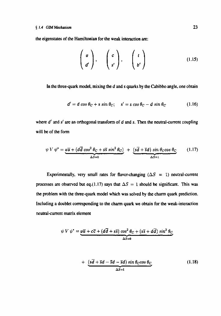
the eigenstates of the Hamiltonian for the weak interaction are:
( ;. ) ' ( ; ) ' (:. ) ( 1.15)
In the three-quark model, mixing the d ands quarks by the Cabibbo angle, one obtain
d' = d cos Oc + s sin Oc; s' = s cos Oc - d sin Oc (1.16)
where d' ands' are an orthogonal transform of d ands. Then the neutral-current coupling
will be of the form
1/J V ¢• = uu + (dd cos2 Oc + ss sin2 Oc) + (sd + sd) sin Occos Oc (1.17)
AS=l
Experimentally, very small rates for flavor-changing (~S = 1) neutral-current
processes are observed but eq.( 1.17) says that ~S = 1 should be significant. This was
the problem with the three-quark model which was solved by the charm quark prediction.
Including a doublet corresponding to the charm quark we obtain for the weak-interaction
neutral-current matrix element
1/J V 1/J' = uu +cc+ (dd + ss) cos2 Oc + (ss + dd) sin2 Oc
AS=O
+ (sd + sd - sd - sd) sin Occos Oc (1.18)
AS=l

§ 1.5 Rare and Forbidden Decays 24
where the strangeness-changing part vanishes due to the effect of the charm quark. To first
order, there are no strangeness-changing neutral-currents and similarly no charm-changing
neutral-currents. This cancellation of flavor-changing neutral-current processes occurs only
in the first order Feynman diagrams (tree level). Flavor-changing neutral-currents can occur
in the Standard Model through higher order terms (loop diagrams) which are suppressed
due to the smallness of the weak interaction coupling.
1.5 Rare and Forbidden Decays
Rare and forbidden decays are divided into three different groups: Lepton Family
Number Violating (LFNV), Lepton Number Violating (LNV) and Flavor Changing Neutral
Current (FCNC).
a) Lepton Family Number Violation. Processes of this type are forbidden
because they do not conserve the lepton family number. For instance, processes such as
D0 -t µ±e=f and v+ -t h+µ±e=f and v+ -t h-µ+e+ where h is 7r or K and (d,s) (d,s) '
the leptons belong to different families, are examples of this mode. These decays would
suggest the existence of heavy neutral leptons with non-negligible couplings to e and µ.
b) Lepton Number Violating. Since there is no explanation in the Standard Model
for the lepton number conservation, we can expect a violation at some presently unknown
energy range. Processes such as D~,s l -t h- f.+ t.+ in which leptons come from the same
family and are of same charge are examples of LNV modes.
c) Flavor-Changing Neutral-Current In the Standard Model the neutral-current

§ 1.6 Special Relativity 25
interactions change of the flavor is at a very low level. Lower limits for charm-changing
neutral-current are expected. Such decays are expected only in second-order in the
electroweak coupling in the Standard Model. Processes in the D system refer to the decays
D0 ~ z+1- and D~,s) ~ h+e+e-, etc. Test for charm FCNC are limited to hadron decays
into lepton pairs.
1.6 Special Relativity
We will go through a brief review of special relativity to establish notation and
whatever points are necessary for this work. If we have a particle that is moving anywhere
close to light speed, the relations of its energy and momentum will be different from those
at a lower speed:
p="'rmv, (1.19)
and
E = "'rmc2, (1.20)
where
1 v "'f = .jl - 132 and /3 = ~' ( 1.21)

§ 1.6 Special Relativity 26
c is the velocity of light in vacuum, m is the mass of the particle at the rest. From eq's.
(I. t 9), ( 1.20) and ( 1.21 ):
E -y=
mc2 ( 1.22)
Note that if v = 0, E = me?. Special units are used in particle physics such that
c = 1 and Ii= 1. Energy, momentum and mass are then all in units of GeV, and time and
length will be in units of GeV - 1•
Let us consider the displacement, a four-vector which is generalized by special
relativity as the difference between two "events", where both the spatial displacement and
time of occurrence are considered.
(1.23)
The invariant dot product concept is generalized as well
This an invariant under Lorentz transformations for any pair of vectors .4 and B
which transform like "event" vectors. Energy and three-momentum form such a vector.
This four-momentum vector is
( 1.25)
Consider the situation where a primed system moves with the constant velocity v

§ 1.6 Special Relativity 27
with respect to the unprimed system. v is in the direction of +x and we will use f3 for
the fractional velocity of the coordinate system. Consider a system with momentum p and
energy E. The Lorentz transformation equations are:
I I Py = Py, P:: = P:; (1.26)
p~ = /{px - {3E); (1.27)
E' = 1(E - f3Px) ( 1.28)
Under a Lorentz transformation, the scalar product of two four-vectors is invariant.
Momentum and energy form a four-vector just like position and time. The lifetime (T)
of an unstable moving particle is calculated to be equal to "'fTo where To is the particle's
lifetime as measured in its rest frame.
The Lorentz invariant mass of any system is its energy in a frame where it is at rest.
In our analysis we are trying to identify decay processes of a short-lived particle into two
opposite charged particles. The decaying particle travels a negligible distance making it
impossible to determine the identity of the particle based on its trajectory. Therefore, an
important quantity in our work is the Lorentz invariant mass which is used to determine if
two particles (whose momenta, p1 and P2 are known) are the daughters from the decay of a
particle of mass M into products of mass m1 and m2.
Conservation of energy and momentum is used in order to reconstruct M2 from the

§ 1.6 Special Relativity
candidate decay products:
We can define the Lorentz invariant quantity
28
(1.29)
Notice that j\1/12 can be calculated from the assumed masses mi. m2 and the measured
momenta Pi. iJ2 in any frame. M12 is called the invariant (mt.m2) mass of the two-particle
system. If these two particles did indeed have the masses m1 and m2 and if they did indeed
come from the decay of a particle M, then M12 will be equal to M within experimental
errors. The calculation of invariant mass is a major tool in identifying decays.
If we consider the D0 -t µ+ µ- process, m1 = m2 = mµ ~ 105.66 MeV (4, p.23]
and P1 = fjµl' P2 = fjµ 2 , thus
( 1.31)
and the Lorentz invariant mass for the D0 will be given by
where Pµ 1 , Pµ 2 and Oµµ are measured quantities.

§ I. 7 Contidence Intervals and Contidence Levels 29
1. 7 Confidence Intervals and Confidence Levels
Several concepts in statistics will be useful in our work. Confidence limits [13) refer
to those values that define an interval range of confidence (lower and upper boundaries)
for an unknown parameter. If independent samples are taken repeatedly from the same
population and a confidence interval calculated for each sample, then a certain percentage
of the intervals will include the real value of the parameter.
A different concept is that of Confidence Level. This statistic is used in hypothesis
testing where one calculates a x2 from the deviations of the observed data from the
hypothesis. If the hypothesis is correct, high values of x2 are unlikely. The confidence
level is defined as
( 1.33)
where F N ( z) is the x2 probability density which depends on the number of observations, N.
The confidence level (CL) is a random variable. If the hypothesis is correct, it has a uniform
probability density and all values of CL are equally likely. This may seem to make it not
very useful. However, if the hypothesis is not correct, high values of x2 (corresponding
to low values of CL) will be likely. One can statistically differentiate the cases where the
hypothesis is fulfilled by requiring a minimum CL value.

Chapter 2
Previous Works
2.1 FCNC Decay Theory
The fundamental work concerning FCNC decays is the famous paper by Glashow,
Iliopoulos & Maiani in which they propose the existence of the charm quark and discuss
how it can explain the suppression of FCNC decays [ 12] through what is now called the
GIM mechanism. This has been discussed in Section 1.4.
With respect to D0 -+ µ+ µ- which is a charm FCNC decay, the GIM mechanism
leads to suppression of the tree-level diagrams such as Figure 2.1.a. In a 1997 paper [14],
Pakvasa presented the latest calculation for this process. He found that the short distance
effects are dominated by internal s-quark loop diagrams which are suppressed by the
smallness of the s quark mass and by helicity considerations (Section 1.2. I).
30

§ 2.1 FCNC Decay Theory
c c
w (a) Suppressed Diagram of First Order (b) Penguin Diagram
c
(c) Box Diagram
Figure 2.1: Feynman diagrams for the decay o0 ~ µ + µ-. (b) and ( c) are second order diagrams with quark masses d, s, and b within the loops that give a rate proportional tom~. being m5 the mass of the strange quark. (a) represents a suppressed diagram of first order.
31
Pakvasa calculated the short distance effects to be of the order of 10-19• However,
the long distance effects are large bringing Pakvasa's calculation of the Standard Model
branching ratio to 10-15 for o0 --1' µ+µ-.
The long distance effects are due to intermediate states such as 7!'0 , K 0 , K 0, TJ, TJ' or
7l'7r and K K 0 [14].

§ 2.2 Previous Searches for Rare Charm Decays 32
2.2 Previous Searches for Rare Charm Decays
Many experiments have reported limits for the branching ratio of the rare decay
D0 --+ µ+ µ- as is shown in Table 2.1 published by Particle Data Group in 2000 (4. p.566].
Table 2.1: Chronological branching ratios for the ~C = 1 weak neutral-current decay D0 --+ µ+µ-.
Value Experiment Comment Year (at CL 90%) Name < 5.2 x 10-ti E791 7r- 500GeV 2000 < 1.6 x 10⁻⁵ E789 p nucleus 800 Ge V 2000 < 4.1 x 10⁻⁶ Beatrice 7r- Cu, W 350 GeV 1997 < 4.2 x 10⁻⁶ E771 p Si, 800 GeV 1996 < 3.4 x 10⁻⁵ CLEO e+e- ~ -y(4S) 1996 < 7.6 x 10⁻⁶ Beatrice 7r- Cu, W 350 GeV 1995 < 4.4 x 10⁻⁵ E653 'Tr- emulsion 600 GeV 1995 < 3.1 x 10⁻⁵ E789 -4.1 ± 4.8 events 1994 < 7.0 x 10⁻⁵ ARGUS e+e- 10 GeV 1988 < 1.1x10⁻⁵ SPEC p;,- W 225 GeV 1986 < 3.4 x 10⁻⁴ EMC Deep inelastic µ- N 1985
In this section we will discuss the most recent experiments. We will also discuss
the FOCUS predecessor experiment, E687, which searched for other FCNC charm decays
but not D0 --+ µ+ µ-. The first experiment is the one that has obtained the lowest limit,
the CERN1 WA92 BEATRICE experiment. Then we present Fermilab's2 E791 and finally
E687. 1CERN -Organisation Europeenne pour la Recherche Nucleaire 2Fennilab -Fenni National Accelerator Laboratory

§ 2.2 Previous Searches for Rare Chann Decays 33
2.2.1 The Hadroproduction WA92 Experiment
During the 1992-93 data-taking period of the BEATRICE Collaboration, the
hadroproduction WA92 experiment [15) at CERN Super Proton Synchrotron was carried
out. In the interactions of 350 GeV 7r+ particles in a W target during 1992 (W92 runs),
charmed particles were produced as well as in the Cu target of 1992 and 1993 (Cu92 and
Cu93 runs respectively). The apparatus was made up of a 2 mm thick target followed by
a beam hodoscope and by an in-target counter (IT), a high-resolution silicon-microstrip
detector (SMD), a large magnetic spectrometer and a muon hodoscope.
Candidate events D0 ~ µ+ µ- were required to be in a mass range between
1.80 - 1.92 GeV. Dimuonic events were required and were selected by a dimuon trigger.
Events that came from target interactions as well as those in IT counters were accepted.
Dimuonic events associated to a simple secondary vertex were differentiated from events
where both muons came from different secondary vertices. The D0 ~ K-7r+ decay
process was the normalizing mode which was detected in runs of Cu(W) applying the same
selection criteria for the dimuonic events except the ones for lepton identification.
Monte Carlo simulation generators used Phytia 5.4 and Jetset 7.3 [lfrl9] to
understand the hard processes and quark fragmentation. Fluka [20, 21] was used to
determine the characteristics of all other interaction products. Monte Carlo simulations
generated events that contained a pair of charmed particles. Dimuonic events coming
from the Monte Carlo simulated D0 ~ µ+µ- decays were treated in the same way as
the experimental data permitting the determination of the efficiencies and the acceptance
ratios.

§ 2.2 Previous Searches for Rare Charm Decays 34
No D0 ~µ+µ-candidate was found [15). This result led to an upper limit on the
branching fraction B(D0 ~ µ+ µ-) of 4.1 x 10⁻⁶ at 90% confidence level. Systematic
errors on the whole analysis procedure did not significantly alter this value.
2.2.2 The Hadroproduction E791 Experiment
Events collected in the E791 experiment [22] were produced by a 500 GeV 11"+ beam
in five target foils. This was a hadroproduction experiment in which track and vertex
reconstruction were provided by 23 silicon microstrip planes and 45 wire chamber planes,
plus two magnets. Muon identification was obtained from two planes of scintillation
counters. The experiment also included electromagnetic and hadronic calorimeters and
two multi-cell Cerenkov counters that provided 7r / K separation in the momentum range
6-60 GeV.
In the analysis stage, to separate "good" events from background noise, a separation
of the production vertex from the decay vertex was required by more than 12 ai. where
a L is the calculated longitudinal resolution. Also the secondary vertex was required to be
separated from the closest material in the target foils by more than 5 a~, where a~ is the
separation uncertainty.
E79 I used as a Monte Carlo simulation generator Pythia/Jetset [23, 24] and modeled
the effects of resolution, geometry, magnetic fields, multiple scattering, interactions in the
detector material, detector efficiencies and the analysis cuts. As normalizing mode in the
study of the rare decays D0 ~ µ+µ-, D0 ~ e+e- and D0 ~ µ±e"f-, the Cabbibo-Favored
mode D0 ~ K- 11"+ was used.

§ 2.2 Previous Searches for Rare Charm Decays 35
Before the branching fractions were caJculated for each of the channels studied,
E79 I used a blind analysis technique. All the events within a AMs range around the
D0 mass were "masked" in order to avoid bias in the cut selection due to the presence or
absence of a possible signaJ. The cut selection was based on the study of events generated
by Monte Carlo for signal events and real data for background events. Background
events were chosen and studied in mass windows Akls before and after the signal area.
The signaJ area was chosen as 1.83 < M(D0 ) < 1.90. The 90% upper limit was
calculated using the method of Feldman & Cousins [25] to account for background,
and then corrected for systematic errors by the method of Cousins & Highland [26].
The upper limit was determined from the number of candidate events and the expected
number of background events within the signal region. Only after the cuts were optimized
was the signal area unmasked and then the number of events within the window was
N obs = N Sig+ NM isl o+ N Cmb• where N Sig corresponds to the number of "good" candidates
of D0 ~ µ+µ-, NMis!D corresponds to hadronic decays with pions misidentified as
muons, and Ncmb corresponds to combinatoric background arising primarily from false
vertices and partially reconstructed charm decays.
No evidence for the rare decay D0 ~ µ+ µ- was found [22]. The 90% confidence
level branching fraction limit was 5.2 x 10⁻⁶• Systematic errors in this analysis included
statistical errors from the fit in the normalization sample; statistical errors on the number of
Monte Carlo events for both the normaJizing mode and the process studied; uncertainties
in the calculation of MisID background; and uncertainties in the relative efficiency for each
mode.

§ 2.2 Previous Searches for Rare Charm Decays 36
2.2.3 The Photoproduction E687 Experiment
Production and decays of charm particles from high energy collisions with a
high intensity photon beam and a beryllium target were studied by the Fennilab E687
experiment (27) using a multiparticle spectrometer for particle identification and vertexing
of charged hadrons and leptons. From the Tevatron beam, a photon beam from
bremsstrahlung of secondary electrons ((E) = 350 GeV) hit a beryllium target. Charged
particles were traced by four silicon microstrip detector stations. Those detectors were
very efficient for separating primary and secondary vertices. Charged particle momentum
was detennined from deflections in two analysis magnets of opposite polarity with five
stations of multiwire proportional chambers. In order to identify electrons, pions, kaons
and protons, three multicell threshold Cerenkov counters were used. There were two
electromagnetic calorimeters. Particles which passed the apertures of both magnets were
detected by the inner calorimeter which covered the forward solid angle. Those particles
that only passed the first magnet were detected by the outer calorimeter covering the outer
annular region. Two sections of thick steel muon filters divided four proportional tube
planes which were used to identify muons in the forward solid angle [28).
The selection of candidates for o+ --+ h±fft+ and o+ --+ K-7r+7r- started by
making three-track combinations of an event with the right particle identification. The
combination of the resulting three tracks were fit to a common secondary vertex.
In order to detect muons with a momentum higher than 4 Ge V, planes of scintillator
material in addition to four stations of proportional tubes, altogether known as the Muon

§ 2.2 Previous Searches for Rare Charm Decays 37
System, were used by the E687 Collaboration. A muon Confidence Level was calculated
when classifying candidate muon trajectories. At least I% was required for the CL.
In order to identify electrons, information of tracks associated with electromagnetic
showers in either of the two electromagnetic calorimeters was used if they were consistent
with the electron hypothesis in the Cerenkov counters.
The sensitivity to the measured branching ratios was optimized for each decay mode
studied in E687. This sensitivity depended on the efficiency relative to the nonnalizing
mode. This was calculated using a Pythia [29) Monte Carlo simulation generator along with
a detailed spectrometer simulation, the amount of normalizing mode events (determined
from a fit to the invariant mass plot), and the amount of background in the signal region
(detennined using sidebands before and after the defined signal region).
Monte Carlo signal shapes and background shapes derived from data were used to
calculate the 90% CL upper limit on the number of signal events in the corresponding mass
plot. Misidentification of hadrons was the primary background in the E687 analysis. Three
track combinations with no lepton identification were used to determine the shape of the
background. The probability of misidentifying a hadron as a lepton was introduced as a
weight on each lepton candidate.
No evidence for the fourteen exclusive modes of rare and forbidden decays was
observed in this experiment [27]. However, 90% CL upper limits on their absolute
branching fractions in the (9 - 20) x 10-5 range were detennined.

§ 2.3 FOCUS 38
2.3 FOCUS
2.3.1 Introduction
Since hadrons with quarks from the 2nd and 3rd family exist only rarely in nature,
we need a way to produce them copiously to study them effectively. The method of
photoproduction in the experiment E83 I [30) that took place in the Fermi National
Accelerator Laboratory (Fennilab) near Chicago, Illinois was used to create particles
with the charm quark. The E83 l experiment, or FOCUS ( "Fotoproduction Of Charm
with an Upgraded Spectrometer"), was an upgrade version of the E687 experiment
(Section 2.2.3) and was a heavy-flavor (produces particles with 2nd family, or higher,
quarks) photoproduction experiment located at the Wide Band Photon Area.
800-kV CockcroftWolton AcctlefatOr
Mnon Alea
Neutrino Area
Figure 2.2: Proton synchrotron and beamlines at Fennilab. The FOCUS experiment is located at the Wide Band Photon Area in the East Proton Area.

§ 2.3 FOCUS 39
2.3.2 The FOCUS Photon Beam
To photoproduce panicles which contain the chann quark it is necessary to generate
photons with a high energy (about 300 GeV). At Fennilab the initial beam is a 800 GeV
Tevatron proton beam [31, p. I 0).
Double Band Photon Beam
Moaentaa Selecttn& Dipoles
-
Production Target
e+
~~=i:. Radlal=t ~s,.... SWeepiq
Dipoles - Recoil e+ • Recoil Polltronmmmlllll llmllllll Sectron Detector Bxpertaent Taraet Detector
Figure 2.3: The E83 l Photon Beam (FOCUS Collaboration Figure).
As shown in Figure 2.3, a photon beam was produced after three different stages.
A neutral beam produced from 800 GeV protons incident on a liquid deuterium target
included a variety of neutral particles along with high energy photons from 71'"0 decays.
Charged secondaries and uninteracted protons were taken out of the beam and absorbed
by the beryllium target dump (not shown). All the neutral secondary trajectories produced

§ 2.3 FOCUS 40
were transmited within an aperture of 1.0 mr horizontally an 0. 7 mr vertically with respect
to the incident proton beam trajectories. To absorb a smaller portion of these secondary
photons a Deuterium target material was used.
The photons that were left produced a e+e- pair due to electromagnetic interactions
in passing through a 60% radiation length lead convertor. The pairs were separated from
the neutrals using momentum selecting dipoles and then put together focusing them onto
another target This momentum selection was necessary to purify thee- and e+ beams by
reducing their charged hadronic background considerably. A neutral dump was used to
remove hadronic neutral particles.
Finally, photons that came from bremsstrahlung were produced from the focused
e+e- beam which was passed through a 20% radiation length lead radiator. Recoiled
electrons were taken out of the photon beam and absorbed by an electron dump.
2.3.3 Inside the FOCUS Experiment
FOCUS utilized a forward large aperture fixed-target multi-particle spectrometer,
to be explained in Figure 2.4, to measure the interactions of high energy photons on
a segmented BeO target. This spectrometer had excellent particle identification and
vertexing for charged hadrons and leptons.
The experiment collected data during the 1996 - 97 fixed target run and is
investigating several topics in charm physics including high precision studies of charm
semileptonic decays, Quantum Chromodynamics studies using double charm events,

§ 2.3 FOCUS 41
a measurement of the absolute branching fraction for the D0 meson, a systematic
investigation of charm baryons and their lifetimes, and searches for D0 mixing, CP
violation, rare and forbidden decays, and fully leptonic decays of the D+.
T•rae• ReP,•
Tubes
Beam Direction
Outer Electromagnetic
P.W.C.'s Calorimeter
Cerenkov
l Outer Muon R.P.C.'s
t
Counters Magnet
Spectrometer
Inner
Beam
Calorimeter Muon Filter
Figure 2.4: The FOCUS Spectrometer (FOCUS Collaboration Figure).
In the FOCUS spectrometer a BeO target was used to produce primary and secondary
particles coming from interactions between the Tevatron photon beam and protons within
the target(/+ p ~ X + p). The target was segmented in four separate parts in order to
maximize the percentage of charm decays which occured outside the target material.
Two trigger counters and two silicon tracking systems were in the target region as
shown in the Figure 2.4. Charged particles which emerged from the target were tracked
by two systems of silicon microvertex detectors (SSD). The first system was mingled with

§ 2.3 FOCUS 42
the experimental target while the second was just downstream of the target and consisted
of twelve planes of microstrips arranged in three views. Altogether these two detectors
allowed to differentiate primary and secondary vertices with high resolution. Two magnets
(Ml and M2) of opposite polarity with five stations of multi wire proportional chambers
(PWC's) were used to measure the momentum of charged particles using the deflection of
the particles when passing through the magnets. There were three PWCs before Ml and
two between Ml and M2.
Three threshold multicell Cerenkov counters were used to identify electrons, pions,
kaons and protons [31, p.16). Two types of calorimeter were used to detennine the particle
energy. The first calorimeters were two electromagetic calorimeters. The inner calorimeter,
a lead glass block array, covered the central solid angle and detected particles which passed
through the apertures of both magnets. The outer calorimeter covered the outer angular
annulus described by particles that pass through the first magnet but not the second. The
second calorimeter type was a hadronic calorimeter consisting of iron and scintillating tiles
which was used primarily in the experiment trigger but was also used to reconstruct neutral
hadrons.
To identify muons, FOCUS had a detailed detecting system. Muons were identified
in either a fine grained scintilator hodoscope with an iron filter (covering the inner region)
or in an outer system that used resistive plate chambers and the iron yoke of the second
magnet as a filter. The muon system was constituted by two sub-systems: the Inner Muon
System which was composed of 9 planes of scintillator material, in which three were used
as triggers of data acquisition, and three iron filters [32, 33), and the Outer Muon System

§ 2.3 FOCUS 43
composed of resistive plate chambers which detected muons with an angle greater than 125
milliradians.
In order to analyze the interactions in the spectrometer, the analog signals from each
of the detectors had to be digitalized and recorded. This was the task of the data acquisition
system. The FOCUS data acquisition system had to deal with input data in a number of
different data formats, merge all this data into one stream, and put the output on 8 mm
magnetic tapes. Information from the different detectors was read out and then these data
were put on a data acquisition system bus.
Data for each event was taken off the data adquisition system bus and placed
into a temporary memory system; data could be written to and read from this system
simultaneously. Later on, the data was buffered on disk and written to tape. During the
run, FOCUS collected more than 108 events and reconstructed more than 106•
The FOCUS Collaboration has published four papers studying different topics in
charm physics (34-39).

Chapter3
Objectives
As a departure point for this thesis, the following objectives were considered:
1. The detennination of the probability of misidentifying a meson as a muon (MislD)
in FOCUS as a function of momentum.
2. The development of software for the search for the rare decay D0 ~ µ+ µ- using
blind analysis methods.
3. The preselection (from the large FOCUS data set) of a small and flexible set of event
candidates for D0 ~ µ+ µ- as well as for the D0 ~ K-rr+ nonnalizing mode.
4. The detennination of the relative efficiency for the detection of D0 ~ µ+ µ- and
D0 ~ K- tr+ in FOCUS using Monte Carlo simulation to generate and analyze
appropriate samples of the decays.
44

§ 3 Objectives 45
5. The determination of the background level in the D0 ~ µ+ µ- analysis by using an
independent data set and the misid measurements.
6. The determination of the 90% confidence region for the branching ratio of the decay
D0 ~ µ+ µ-. In using the high statistics FOCUS data set and in optimizing the
analysis cuts, the objective is to improve existing measurements and obtain tighter
(more precise) confidence limits.

Chapter4
Procedure
This chapter will describe how the search for the rare decay D0 -7 µ+ µ- was carried
out. Initially, will be discussed the FOCUS data fonnat and the reconstruction process.
Then will be defined each one of the variables used in this study. Next, the various stages
of data reduction will be discussed. The use of a nonnalization mode will be explained.
Basically the method used in this work is known as blind analysis which consists in the
optimization of the selection criteria by minimizing the background in the data sidebands.
The use of Monte Carlo simulation to detennine detection efficiencies as well as to study
backgrounds will be discussed. The methodology leads to the detennination of confidence
intervals for the value of the D0 -7 µ+ µ- branching ratio.
46

§ 4.1 Data Format 47
4.1 Data Format
We will begin by discussing the form of the data produced in the experiment. For this,
it is advisable to be familiar with the concept of an "event". This refers to one instance of a
photon interacting in the target producing various particles which travel through some or all
of the detectors. Some of the particles produced decay in or near the target into secondary
decay products which are the ones actually detected. The experimental ideal is to use the
information from the detectors in order to measure the characteristics of the decay. To this
end, it would be easier if the set of detector signals came anly from the decay of interest and
its associated production partners. In practice, this is never perfectly achieved. The "raw"
data consists of sets of signals which approach the ideal of coming from one and only
one physical event. Each of these sets is called a "raw data event". Typically it contains
information about the physical event but also detector noise and information about particle
trajectories unrelated to the physical event. Given the experimental difficulty, many raw
data events contain no interesting physical events.
Each raw data event is an independent unit of data which is "reconstructed"
separately. Reconstruction is the process whereby the physical characteristics of the
underlying particle trajectories are extracted from the raw detector data. The raw data event
is either discarded if it is not at all interesting or convened to a "reconstructed data event"
which contains the values of the physical variables such as the number of trajectories that
were registered by the PWC chambers, the momentum of the particles, etc. In FOCUS, the
reconstruction process is called Pass I (see Section 4.3.2). All data (raw and reconstructed)
is stored on magnetic tape.

§ 4.2 Reconstruction Process 48
Reconstructed output tapes from Pass I contain all kinds of physical events, instances
of a myriad of interesting processes all in the same tape. There are thousands of tapes.
The next step is to group events of the same kind with the goal of having all the
events of the process under study being contained in a small data file. The most efficient
way to do this is to do it in steps called "skims". At each skim level, stricter event selection
criteria are applied and the data is separated into a larger number of groups each of which
contains a smaller amount of data.
4.2 Reconstruction Process
To have a more precise idea of how the data selection process is done in FOCUS,
it is necessary to be familiar with the trajectory reconstruction process. A great deal of
the information deposited in the FOCUS detectors are presented as hits which we have
to interrelate to be able to detemine which hits in different detectors correspond to one
particular trajectory.
Between the target and the first magnet (MI) we find the Silicon Microstrip Detector
(SSD) which has four stations. After MI the tracking is done by five multi wire proportional
chambers (PWCs). Each one of these, called PO, Pl, P2, P3 and P4, has four planes.
Outside of the magnets the trajectories will be straight line segments which will be
reconstructed in the SSDs and PWCs. The trajectories will bend in the magnetic fields so
that the straight line segments will be different in the three regions: (I) before MI, (2)

§ 4.2 Reconstruction Process 49
between Ml and M2 and (3) after M2. These will be reconstructed by (I) SSD, (2) PO, Pl,
P2 and, (3) P3 and P4.
The process of SSD track reconstruction consists of finding trajectories with the SSD
detector. The steps are grouping hit strips into clusters of hits, finding each one of the three
measurement directions to project the clusters, and then, combining these into trajectories.
Then PWC trajectories are found. There must be hits in at least three chambers. Those with
hits in all five PWCs are referred to as "tracks". The ones with hits in only the first three
chambers are referred to as "stubs". The SSD and the PWC trajectories must be associated
with one another to be able to get the necessary information for the reconstruction of the
charm decay. To identify a "link" the SSD and the PWC trajectories must be extrapolated
to the center of MI and must have consistent slopes and intercepts.
Muon llod.,,..,opc
Muon Fiiters
I • P.W.C.s
·-. ·.
Figure 4.1: Trajectories through the FOCUS spectrometer. A view of some trajectories within the FOCUS spectrometer. The first and second trajectories are detected by the Outer Muon System. Trayectories two, three and four are detected using the Inner Muon System.

§ 4.3 Data Selection 50
Figure 4.1 shows some trajectories passing through the spectrometer. Trajectory I
corresponds to a three-chamber track while the third and fourth trajectories (3 and 4 in the
figure) correspond to five-chamber tracks. The second trajectory (2) has hits in all the PWC
chambers except in P3. This trajectory can still be reconstructed in the region after M2 by
combining the information from PO, Pl, P2 and P4.
4.3 Data Selection
4.3.1 Selection Variables
In this section we will discuss the different variables used for this work. They will be
divided into two types: vertexing and particle identification.
a) Vertexing. Using the FOCUS microstrip detectors we can take advantage of the
fact that charmed particles travel short distances within the spectrometer before they decay
while non-charmed particles tend to either decay immediately at the production point or to
pass through the whole spectrometer without decaying. This means that for charmed decays
we can reconstruct two distinct vertices in the event: the primary or production vertex and
the secondary or decay vertex. A diagram of a D0 4- µ+µ-decay and its vertices is shown
in Figure 4.2. By reconstructing the two vertices, we obtain several quantities on which
we can do "cuts" to reduce non-charmed backgrounds. A cul refers to an event selection
criteria which is implemented by requiring a certain range of values for a particular variable.
A vertexing algorithm (40] is used to reconstruct a D0 4- µ+ µ- decay candidate. It

§ 4.3 Data Selection
µ
µ+
I:+
Figure 4.2: Production and decay venices for the o0 --t µ+ µ- process. Figure shows the schematization of the production and decay venices for the o0 --t µ + µ - process.
51
starts with two distinct trajectories that meet the requirements to be called a µ+ µ- pair.
The venexing algorithm calculates a confidence level (CLS) for the hypothesis that these
trajectories come from a common point and finds that point for the cases which have a
CLS > 1%.
Let us say that a useful vertex is found. The putative D0 trajectory can be calculated
by adding the muon momentum vectors. Then the algorithm tries to find the primary vertex
using other trajectories in the event in combination with the o0 candidate. The algorithm
begins by taking all of the two-trajectory combinations (one of which must be the D0 and
the other must not be a daughter muon) and fits them to a vertex hypothesis again requiring
a minimum CL of I% [41). If the trajectories are accepted, the algorithm tries to put more
and more trajectories in that vertex until the confidence level falls below I%. The resulting
primary has a maximum number of daughters with a CL (CLP) greater than I% [41 ].

§ 4.3 Data Selection 52
Using information coming from the vertexing algorithm we can define the following
variables to be used in the analysis for the rare decay D0 ~ µ+ µ-:
1. Ua. Short lived hadronic background is removed by requiring a minimum
separation between the primary and secondary vertices. The detachment cut will require a
minimum L/a where Lis the distance between the two vertices and a is the error on that
measurement. Figure 4.2 illustrates this situation in which the errors on vertex positions
are shown as ellipses.
2. Multiplicity of the Primary Vertex. This refers to the number of trajectories
produced in the interaction that occurs within the target. Higher multiplicity primary
vertices have less background.
3. Vertex Confidence Levels. Each vertex is formed by a reconstruction algorithm
that has an associated confidence level. Due to measurement errors the trajectories will
not all intersect at the same point. However we can define error ellipses for each pair
of trajectories (Figure 4.2). We then calculate the probability that, within their errors, all
candidate tracks are consistent with intersecting. Confidence levels above I% are required
for minimal cuts on these values. Sometimes a larger cut is used to reject backgrounds.
CLP stands for the primary vertex confidence level and CLS for the secondary.
4. Primary and Secondary Vertex z Position. The FOCUS targets are thin Hat
wafers in the xy plane. Thus the primary vertex z position (ZVPRIM) becomes the critical
variable in identifying good events where the primary vertex occurs within the target and
background when it occurs outside the target. For certain long lived charmed particles, a
large percentage of the decays (secondary vertex) will occur outside the target segments

§ 4.3 Data Selection 53
where there will be less background due to interactions of secondary particles with the
target material. The secondary vertex z position (ZVSEC) can be used to maximize the
signal to noise ratio.
Due to experimental resolution, these variables are not used directly but instead are
used in a ratio with the experimental uncertainty. For this purpose we will define the
variable a: which is the difference between the z vertex position and the z target edge
divided by the uncertainty. Due to the four-part target segmentation we need to check if the
vertex is occurring between the segments or within these. For a: < 0 the vertex is inside
the target material and for a: > 0 the vertex is outside. For the primary vertex we use a:1
and for the secondary a :2 •
S. Vertex Isolation. The primary vertex isolation, /SOP, gives a large confidence
level when one of the trajectories in the seconda.ry vertex is also consistent with being in
the primary. Therefore, the lower the ISOP value, there will be an unlikely chance that
any charm candidate trajectories will be in fact associated with the primary vertex. The
secondary vertex isolation, /SOS, is the confidence level for a trajectory that is not in the
primary vertex to be in the secondary vertex together with the presumed decay daughters.
This variable comes in handy for rejecting background from higher multiplicity decays by
requiring low values of ISOS.
b) Particle Identification. This analysis concentrates on identifying two types of
particles: muons and hadrons.
1. Muon Identification. Muon identification is possible because muons are the
only charged particles which can penetrate large amounts of material. The method used
§ 4.3 Data Selection 54
to detect muons is to place charged particle detectors behind a large amount of shielding
material (typically steel). There are a pair of different kinds of detection systems for muons
in FOCUS. These are: the Inner Muon detector and the Outer Muon detector. The first one
uses common scintillator detector elements and the second uses resistive plate chambers tc
detect passing muons.
For the inner region the system for muon detection uses three muon scintillating
hodoscope stations: MHI, MH2 and MH3. The first two stations register hits in x and y
whereas the third station registers hits in a uv plane which is oriented ± 30° with respect to
the xy plane.
The algorithm of muon identification [33] was developed at the University of Puerto
Rico, Mayagiiez Campus, with the purpose of calculating for each trajectory a confidence
level to decide the degree of reliability in the classification of that trajectory as a real muon.
The algorithm is based on the following considerations: the multiple Coulomb scattering
and the geometry of the scintillators that make up each one of the planes of the muon
identification system. It is described in detail by Ramirez [33] and Wiss [42,43).
There are two ways a muon identification algorithm can fail. One is to fail to identify
a muon as a muon. This characteristic is measured as the algorithm's efficiency. The other
is to identify a non-muon as a muon. That is measured by the misidentification. These two
characteristics are correlated. A good algorithm achieves a balance between them.
In the muon identification we are considering the following variables:
i. Kaon Consistency for Muons. We can use the kaon consistency variable (see

§ 4.3 Data Selection 55
hadron identification) to separate kaons from muons aJso, since pions and muons behave
almost identically in the Cerenkov system. The name given for this variable is K / µ.
ii. Inner Muons. For the Inner Muon System (IMU) the algorithm begins by
verifying if the candidate trajectories to be muons leave signal in the five PWC chambers.
The trajectories are projected into the IMU planes and associated hits are identified by
looking within a circle around the projection .
In the IMU system there are six MH planes. There must be four hits in these
planes. We can proceed to calculate x2 which gives us the trajectory compatibility with
the MH hits. There are two other things that are taken into consideration when we do this
calculation. These are the multiple Coulomb scattering that occurs inside the steel filters
and the granularity of the scintillator paddles.
Lastly, an isolation variable is calculated which corresponds to the largest CL for any
other trajectory to have caused the same MH hits.
Because there are steel filters in the IMU that can stop muons with low momentum,
the number of required planes is reduced to two from the original number of four for
candidates with a momentum less than 10 GeV. This will increase the efficiency at low
momentum.
The efficiency for the muon identification algorithm is over 98% for momentum
above 10 GeV while misidentification is of the order of 0.5%. In-flight Tr -+ µ11µ decays
candidate to the misidentification rate. For this decay the pion and muon direction of flight
are very closely matched.

§ 4.3 Data Selection 56
Information obtained from the IMU is contained in the following variables:
A) Number of Mi~ Muon Planes. The number of missed muon planes
corresponds to the number of MH planes without signal. In this analysis this variable
is called MISSPL.
8) Inner Muon Confidence Level. The muon identification algorithm calculates
a x2 value for each trajectory that passes a minimal requirement in the number of MH
planes with signals. Trajectories that do not correspond to muons tend to have higher x2
because they have different behavior compared with muons [32, p.11 ]. The inner muon CL
(/MUCL) is calculated from the x2•
iii. Outer Muons. Muons are identified in the Outer Muon System ( OMU) almost the
same way as in the IMU. There is an internal magnetic field in the iron shield (M2) which
can cause some problems when it comes to OMU identification because it deflects muons.
Muons must be traced through the magnetic field in the M2 steel. Multiple Coulomb
scattering smearing must be applied to the traced position.
The OMU reconstruction algorithm is efficient for muons down to E::: 4 GeV, the
range of muons in the M2.
A) Outer Muon Confidence Level. In the same way as is calculated the IMUCL, the
OMUCL is determined coming from the measurement of the x2 value for each trajectory
that passed a minimal requirement within the OMU.
2. Hadron Identification. To identify hadrons such as rr±, K±, p /p, FOCUS
developed an algorithm called C/TADL (Cerenkov Identification Through A Digital

§ 4.3 Data Selection 57
Likelihood) [44) which calculates the probabilities for several hypothesis about the identity
of a trajectory. The identities considered are electrons, pions, kaons and protons (and
their antiparticles). The µ± hypothesis is not considered separately from the 11'± since
the momentum range over which the two hypotheses can be separated is limited. In the
Cerenkov system the behavior of these two particles, muons and pions, is similar due to
their close mass values. For each of the four hypothesis, CITADL calculates the cone due
to the Cerenkov effect and the average number of photons emitted. Poisson statistics are
used to calculate the probability that the observed size of the signals in the Cerenkov cells
is consistent with the identity hypothesis.
From the probability 'P, the algorithm calculates the negative log-likelihood
Wabs(i) = -2 ln 'Pi for each particle hypothesis i.
Variables used in hadron identification are:
i. Kaonicity. It is defined as the difference between the lt'o11s for the kaon and pion
hypothesis.
(4.1)
Statistically, kaonicity is larger for real kaons that for real pions.
ii. Pion Consistency. A variable called pion consistency or 1l'con is used to identify
pions. This variable is related to the probability that the pion hypothesis is better in

§ 4.3 Data Selection 58
comparison to other kinds of hypothesis. 1rcon is defined as
1rcon = W0bs(best hypothesis) - Wobs(7r) (4.2)
where the ivobs(best hypothesis) corresponds to the minimal value of the likelihood for
all the hypothesis considered. Typically we use a cut of 1rcon > 0 for pion identification.
Other variables used in the analysis are:
3. Momentum. To measure the momentum of a particle, FOCUS determined the
deflection angles in each one of the magnetic fields produced by MI and M2. For three
chamber trajectories the momentum is measured by M 1 and for five-chamber trajectories
the momentum is measured by M2.
The momentum resolution for trajectories measured in M 1 is approximately
<Jp = 0.034 x P 1 + (17 GeV)2 p lOOGeV p
(4.3)
and the resolution for trajectories measured in M2 is
<Jp = 0.014 x P 1 + (23 GeV)2 p lOOGeV p
(4.4)
At high momentum, the resolution is limited by the position resolution of the PWC
system; at low momentum it is dominated by multiple Coulomb scattering.
4. Dimuonic Invariant Mass. The mass of primary particles is calculated from the

§ 4.3 Data Selection 59
infonnation obtained from the particles into which these decay (Section 1.6). In our case
this is the two muon trajectories into which the D0 decays.
4.3.2 FOCUS Data Selection Stages
There are 6.5 billion photon interaction events on about 6000 8 mm magnetic tapes
which constitute the raw data set of FOCUS. Obviously, this is way too much data for
an individual researcher to handle. Therefore, the analysis was divided into three steps.
Figure 4.3 shows a summary of the FOCUS analysis process. The reason for doing the
selection in stages is to avoid having to handle the totality of the data again in the case that
some problem is later found in the selection process. In a multistage procedure, one only
need begin at the stage previous to the problem.
a) Pass1. This is the basic event reconstruction stage including track reconstruction
and particle identification. It lasted from January, 1998 to October, 1998. The output
consisted of "reconstructed events" made up of the values for the physical variables of the
event. It was put onto another set of 6000 8 mm magnetic tapes.
b) Skim1. Here, the reconstructed data was divided into six "Superstreams". This
was done in order to make the size of the data easier to handle. Approximately one half
of the events from Pass I met the requirements for Skim 1 and depending on the physical
topics that were considered they were put into different Superstreams (see Table 4.1 ).
Each Superstream consisted of 200-500 8 mm magnetic tapes. Skim I was carried out at
the Universities of Colorado and Vanderbilt from October, 1998 to February, 1999.

§ 4.3 Data Selection
~'J1 ~S Reconstruction Overview
__ , I
' Mass S1oragc
J<;f lbw O.ia
, I ,
J<:f Ri:con D•ti 15'l-o(l1wm
IOd.lysolSkiml j
• I \ , ',,
--.,~ Mainline Tape Pa1h
- - _.,.. E!lprcsslinc Nc1work Palh
... --' ' Express
Analysis Shill Monitor J'k Ri:con Ch.1nn Yidd
Monitor
\ I I I
~·:•---, '
_ .. ~----
,
' \
Figure 4.3: Analysis overview of FOCUS. The solid lines show the path of the data written to 8 mm magnetic tapes. The dotted lines illustrate the distribution of large amounts of data via the Internet, which was used to help collaborators get data quickly for studies and preliminary analyses (E. Vaandering's Thesis Figure).
60
c) Skim2. The six Skim l Superstreams were divided into many other Substreams.
Those events that did not pass the more specific cuts were not included but not all of the
skims had additional cuts.

§ 4.3 Data Selection
Table 4.1: Descriptions of Superstreams. There are about 30 different data subsets grouped into six Superstreams based on physics topics and the types of information present.
Super Physics Skim2 Stream Topics Institution
I Semileptonic Puerto Rico 2 Topological vertexing and K~ Illinois 3 Calibration CBPF, Brazil 4 Baryons Fermilab 5 Diffractive (light quark states) California, Davis 6 Hadronic meson decays California, Davis
61
Table 4.1 shows the five institutions involved in Skim2. There were 5-12 Substreams
written from each of the Superstreams. Calibration data samples and many topics in physics
were brought together by these Substreams. Similar computing models between the Skim l
and the Skim2 were used but they varied by institutions. Skim2 began in January, 1999 and
finished by June, 1999.
Table 4.2 refers to the output of the Superstream l reconstructed and analyzed by the
HEP Group of the University of Puerto Rico at Mayagiiez Campus during January to June
of 1999. More than 500 tapes of semileptonic events were skimmed and divided into five
differents subsamples.
d) Skim3. It is in this stage where we really apply strong selection criteria which
lead us to obtain a reduced output yet still leaves us with a certain amount of flexibility
in the detailed analysis and optimization. It is very difficult to have to work with dozens
of tapes in the detailed analysis. Skim3 reduced this number to one tape. Just the same
as in earlier stages, the idea with Skim3 was to obtain a more compact sample that would
contain the great majority of a certain kind of event.

§ 4.3 Data Selection
Table 4.2: Descriptions of Superstream l. This Superstream was developed by the University of Puerto Rico at Mayagilez Campus. There are five different skims grouped according to physics topics.
Sub Physics Output Stream Topics Tapes
l Semimuonic 26 2 Dileptonic/PPbar 45 3 Semielectronic with mesons 37 4 Semielectronic with baryons 27 5 Normalization 58
62
The data in Substream 2 of Superstream l was used as the starting point in Skim3
because it provided the highest efficiency for the detection of D0 ~ µ+ µ-. The main
idea of Skim3 was to require the existence of two linked muon candidate trajectories
with opposite charge coming from a parent that was identified with a cut in the dimuonic
invariant mass around the mass of the D0 (between l. 7 and 2.1 Ge V). In addition to
this, certain vertex identification conditions were required consisting of CLP > 1 % and
C LS > 1 %. Furthermore, the production vertex was required to be separated from the
decay vertex by at least three times the separation error (L/a > 3). With this we achieved
a reduction in the data size from 45 tapes of 4.5 Gbytes each to one 3 Gbyte tape. The 3
Gbytes were easily kept on disk for greater convenience.
At the end of Skim3, we continued to reduce the data by a process which we call
Skim4. The selection criteria required for Skim4 were the following:
These cuts were based on the experience acquired in previous FOCUS data analysis;
these were known to have high efficiency.
The output from Skim4 was a matrix of m x n as an event file where m is the number

§ 4.4 Normalizing Mode 63
-+ Vertex isolation cuts < I% -+ Vertices z position, -10 < z < 2
-+ Daughter momentum > 7 Ge V -+ We required a MISSPL ~ 3
-+ IMUCL > 1% -+ OMUCL > 1%
of variables with information to be stored and n is the number of pair trajectories accepted
as muon candidates. The total data size did not exceed 500 Mbytes. This matrix is called
an ntuple, which is analysed using software developed by CERN called PAW (Physics
Analysis Workstation) [45] which lets us easily manipulate the information stored. It uses
histograms, vectors and other familiar objects to provide the statistical or mathematical
analysis interactively. An ntuple allows us to try different analysis criteria in a short time
interval.
4.4 Normalizing Mode
The object of this study is to determine at what frequency do D0 -+ µ+ µ- occur in
nature. This means that we will indirectly measure how many times this process occurs
with respect to a large sample that contains many different processes.
The branching ratio (BR) is defined as the fraction of decays to a particular channel.
Mathematically
B h. R . Number of D0 -+ µ+µ-produced
ranc mg atw = (4.5) Total number of D0 produced

§ 4.4 Normalizing Mode 64
If we consider a well known process where the frequency at which it occurs is known
with some certainty then we can use that process to measure the total number of D0 's
produced.
0 Number of D0 ~X's produced Total number of D produced= BR(DO ~ X) (4.6)
The process D0 ~Xis called the normalizing mode. In FOCUS a process coming
from D0 as primary particle is D0 ~ K-1T'+. It is known as a Golden Mode due to its
large BR value. In the analysis for the search of the process D0 ~ µ+ µ- we can consider
D0 ~ K-1T'+ as the normalizing mode. Then the BR of the decay D0 ~ µ+ Jl- can be
calculated as:
(4.7)
The number of produced particles is calculated as the number of observed particles
divided by the efficiency (f) of detection calculated by Monte Carlo simulations. Then eq.
( 4. 7) turns into
where the ratio fK'lr/£1111 corresponds to the relative efficiency to be calculated making
parallel Monte Carlo simulations for the two processes, D0 ~µ+µ-and D0 ~ K-1T'+.
BR(D0 ~ K-7T'+) has been previously measured by other experiments as 3.83±0.09x10⁻²
[4, p.36].
The data events for the normalizing mode were selected using the same selection

§ 4.5 Monte Carlo Simulation 65
criteria (except for particle identification) used to select the dimuonic data events. The
nonnalizing mode data was obtained from Substream 5 of the Superstream 1. This
Substream contained hadronic decays selected with the same basic conditions as the other
Superstream I events with the specific purpose of serving as a normalization sample.
4.S Monte Carlo Simulation
Because of the complexity of High Energy Physics experiments and the impossibility
of calculating every effect analytically, simulation methods are commonly used. Computers
have pseudo-random number generators which are used to simulate approximations of
expected results coming from the theoretical predictions. We call this simulation method
Monte Carlo. In FOCUS, generated Monte Carlo events were used as a measurement tool
for the efficiencies and also as an infonnative tool about the fonn of the background within
our dimuonic sample.
Two mathematicians, the American J. Neyman and the Hungarian S. Ulam gave
birth to this method in Monaco in 1949 as an alternative solution to probabilistic as
well as detenninistic problems. Using a computer, the Monte Carlo method performs
statistical sampling experiments by simulating random quantities, thereby providing us
with approximate calculations in High Energy Physics problems [46].
FOCUS used the Pythia 6.127 [47] generator as a Monte Carlo simulator to model
chann production by photon interactions with the target material. Pythia generated a cc
pair where it was possible to specify the type of charm (D0, v+, Ed". etc.) generated and

§ 4.5 Monte Carlo Simulation 66
a specific decay path. Typically this was done for one of the chann quarks while the other
was left free to hadronize and decay according to the known cross sections and branching
ratios. To simulate all the processes within the FOCUS spectrometer, an algorithm called
ROGUE was developed [48].
r:f--+. µ+µ- Events. To calculate dimuonic efficiencies it was necessary to
generate Monte Carlo data which were required to pass through the same selection
criteria that were applied to real data, in other words, the requirements set by Pass l,
Skim I, Skim2, Skim3 and Skim4. 800,000 events were generated for the process
r + p ~ (D0 ~ µ+ µ-) + c represented in Figure 4.4.
y
Do µ+
~.~µ .. .. ·····
c Figure 4.4: Monte Carlo generated process schematization for the decay o0 -t µ+ µ-.
The number of events provided us with enough sampling statistics to make accurate
determinations of the detection efficiencies.
r:f --+. K-7r+ Events. 800,000 D0 ~ K- 7r+ events were generated. The same
selection criteria were applied as with the normalizing data.
The decay channel D0 ~ K- 7r+ is very imponant in this work because this is the

§ 4.6 Analysis Methodology 67
normalizing mode used in the BR(D0 ~ µ+ µ-) measurement. In addition to that, the
same decay channel is present as possible background in our dimuonic sample.
cl' --+ w+w- and cl' --+ K+ K- Events. The processes D0 ~ 7r+7r- and
D0 ~ K+ K- were also considered in the background study. For the first process, 1.5
million events were simulated and 4.3 million events for the second.
4.6 Analysis Methodology
4.6.1 Blind Analysis
Our Blind analysis excludes all the events within a defined symmetric area around
the value of the D0 mass in the process of cut selection. This area is called the signal area.
In other words, cut optimization is based on reducing background and not on maximizing
the signal under study. The point of this is not to introduce bias due to the possible apparent
absence or presence of a potential signal after having applied a specific group of selection
cuts. Once the optimization stage ended we opened the "hidden" area of the signal and
calculated the confidence interval.
4.6.2 Rolke and Lopez Limits
The statistical method proposed by Rolke and Lopez [49] was used to calculate the
sensitivities and the confidence intervals. They suggest a technique to place limits on
§ 4.6 Analysis Methodology 68
signals that are small when background noise is present. This technique is based on a
combination of a two dimensional confidence region and a large sample approximation to
the likelihood-ratio test statistic. Automatically it quotes upper limits for small signals and
also two-sided confidence intervals for large samples.
The technique of Feldman and Cousins [25] does not consider the amount of
uncertainty in the background. The new Rolke and L6pez technique deals with the
background uncertainty as a statistical error. The technique performs very well. It has
good power and has correct coverage. This method can be used for two situations: when
sidebands data give an estimated background rate and when it comes from Monte Carlo. It
can also be used if there is a second background source in the signal region.
To understand the results of this technique we will need the following notation: x will
represent the observed events in our signal region, y will be the events in the background
region and / will be the ratio of the sidebands background to the signal background. The
expected background rate is b = y/1 and the Sensitivity Number, N8(D0 ~ µ+µ-), is
defined as the average 90% upper limit for an ensemble of experiments having an average
of y events in the sidebands and no true signal. Table 4.3 gives the sensitivity numbers for
different values of the confidence level, / and y. During the various stages of this analysis
computer routines provided by Rolke and L6pez were used to calculate sensitivity numbers
and confidence limits. The value of / for each set of cuts was determined as explained in
Section 4.7. The sensitivity numbers were used to select the optimum set of cuts. Then the
confidence limits were computed from the values of x, y and / for that set of cuts. Examples
of confidence limits are given in Table 4.4

§ 4.6 Analysis Methodology
Table 4.3: Sensitivity number as per Raike and L6pez. The number of background events in the sidebands is y. The estimated background rate is b = y/r.
90%C.L. 99%C.L. y r=l r=2 r=l r=2 0 2.21 2.21 4.52 4.52 l 3.31 2.82 6.22 5.35 2 3.97 3.17 7.12 6.14 3 4.62 3.49 8.17 6.45 4 5.29 4.03 8.99 7.12 5 5.90 4.23 9.77 7.43 6 6.37 4.60 10.52 8.00 7 6.86 4.79 11.21 8.30 8 7.23 5.14 11.85 8.86 9 7.64 5.32 12.51 9.02 10 8.01 5.62 13.04 9.52 11 8.40 5.78 13.55 9.76 12 8.71 6.08 14.15 10.14 13 9.09 6.19 14.63 10.37 14 9.39 6.45 15.14 10.76 15 9.71 6.59 15.64 10.96
4.6.3 Determination of Sensitivity and Confidence Limits
69
We define the experimental sensitivity as the average upper limit for the branching
ratio that would be obtained by an ensemble of experiments with the expected background
and no true signal. Therefore, the experimental sensitivity is calculated in the same way as
the branching ratio except that the sensitivity number is used for the number of observed
signal events. For each particular set of cuts, r is determined as explained in Section 4. 7 .3.
y/r is the predicted level of background, b. Having this in mind, we can determine the

§ 4.6 Analysis Methodology
Table 4.4: An example of Rolke and L6pez 90% Confidence Limits. y is the number of events observed in the background region and and x is the number of events observed in the signal region. A value of r = 2 has been assumed.
y x 0 I 2 3 4 0 0,2.21 0,2.27 0,1.58 0,1.28 0,0.9 I 0,3.65 0,3.22 0,3.44 0,3.06 0,2.87 2 0.42,5.3 0,4.87 0,4.43 0,4 0,4.41 3 0.97,6.81 0.08,6.37 0,5.93 0,5.49 0,5.05 4 1.54,8.25 0.74,7.8 0.03,7.36 0,6.91 0,6.47 5 2.16,9.63 1.42,9.18 0.74,8.73 0.07,8.28 0,7.83 6 2.82,10.98 2.12, 10.53 1.45,10.08 0.8,9.62 0.17,9.17 7 3.5, 12.3 2.83, 11.84 2.18,11.39 1.54, 10.94 0.91,10.48 8 4.2,13.59 3.55,13.14 2.91,12.68 2.29,12.23 1.67,11.77 9 4.92,14.87 4.29,14.42 3.66,13.96 3.04,13.5 2.43,13.05 IO 5.66, 16.14 5.03,15.68 4.42,15.22 3.81,14.77 3.21,14.31
experimental sensitivity as
70
where, N8 (D0 -t µ+µ-) is the sensitivity number (Section 4.6.2) which is determined
using the Rolke and L6pez routines from the number of events observed in the sidebands,
y, and the background ratio, T.
In simple terms, the sensitivity is mainly dependent on the ratio of NB/ fµµ. We wish
to minimize this ratio which means having low background with high efficiency.
Once the optimum set of cuts had been determined, we proceeded to open the hidden
signal region and determined the corresponding confidence limits for the D0 -t µ+ µ-

§ 4.6 Analysis Methodology 71
branching ratio by using eq. (4.9) and substituting the appropiate Rolke and L6pez limits
in place of Ns.
4.6.4 Sidebands Background and Signal Area
In this analysis, the signal area as well as the sidebands were defined from the
invariant mass distribution of Monte Carlo generated data (Figure 4.5a). The ability of the
FOCUS Monte Carlo to predict signal width has been verified with other copious charm
signals.
Yonle Ca,10 s·rrulohtd Dote f"CCUS Prociucec ;oto
'""" jJJ10 I 7'><l0
l/r-at l9t • / 91 Pl 2.306.
O• llllltlCi..:V
0 Pl I e64 PJ 0.1'86[-01 I P4 IJ2~.
p~ 1.l90 7000 P6 361.1
P7 -200.~
1500
I~ !CO
1000 " f J \
500 ~ I \ :1 J J, '~ . I
L/~ • 8 US:> 19 I g, 1 I,, • 8 I 8, I g 1.g~ ] (c:.¥1
(ol t•I (Ce¥)
Figure 4.5: D0 ~ µ+ µ- Invariant Mass distributions. (a) distribution for generated Monte Carlo data with a gaussian fit. The gaussian width is equal to 0.016 Ge V. (b) Representation of the sidebands and the signal area for the FOCUS produced data showing the signal and sideband areas. Skim3 cuts have been applied and the signal area has been masked.
The width of the invariant mass distribution for D0 ~ µ+ µ- events is approximately
equal to <J = 0.016 GeV. The signal area was taken as ±2a around a D0 mass of 1.865

§ 4. 7 Background Study 72
GeV (4, p.36]. Each one of the sidebands had a width equal to the signal area width but
the sidebands were not located immediately after the signal area. Between each sideband
and the signal area, a buffer area was left with a width also equal to 2u. In this way the left
sideband was defined as 1.737 < Mµµ < 1.801 and right sideband 1.929 < Mµµ < 1.993
as shown in Figure 4.5b.
4. 7 Background Study
4. 7 .1 Introduction
The most important aspect of the analysis is the choice of a set of selection criteria
which optimize the probability of observing the signal if it is present. Generally this
choice will not be one which eliminates all background because such cuts usually reduce
the efficiency of detection of the signal to unacceptably small values. It is therefore
important to be able to predict the background level accurately in order to measure the
significance of the candidate events. Due to the uncertainties in simulating the background,
our analysis methodology relies mainly on the real data (in the sidebands) to predict the
background in the signal. However, this methodology requires a determination of the ratio
of sideband to signal background, r. This, in tum, requires a determination of the shape of
the background. As is explained in this section, this shape is also obtained from real data.
Fortunately, since they are not strong-interacting, muons are not produced copiously
and it is even rarer that a pair of muons is produced in either a production or decay vertex.
In addition, events where the pair of muons come from a non-D0 two-body decay are

§ 4. 7 Background Study 73
eliminated by the invariant mass cut while those where the muon pair is formed at the
production vertex (e.g. those from the Bethe-Heitler process) are eliminated by the L/u
cut. In fact, the main source of background in our final sample are events where one or two
mesons have been misidentified as muons. Therefore the understanding of the background
started with a study of this misidentification using real data. These results were used to
validate the capability of the Monte Carlo to simulate this effect. The Monte Carlo was then
used to study some known decay processes which could contribute to the background if the
decay products were misidentified as muons. Finally, the background ratio was determined
from an independent real data sample of events with no muons in the final state by assuming
that the background consisted of such events except that both decay products had been
misidenti tied.
4. 7 .2 MisID Study
The goal of this study was to determine the misidentification probability as a function
of momentum. Samples of real and simulated K~ ~ 1r+7r- decays were used for this
purpose.
The real data was obtained from 140 raw data tapes. K~ decays were identified with
the following requirements: vertex conditions for a pair of opposite charged particles, the
two pion trajectories must have left a signal in the five PWC chambers, and the dipionic
mass in a range around the K~ mass (0.477 < A'1rrrr < 0.517), being the K~ mass equal to
0.498 GeV (4, p.32]. Furthermore, decay candidates had to have linked trajectories between
the silicon detectors and the PWCs. Events which pass these requirements are called

§ 4. 7 Background Study 74
Type-9 K~ [32, p.27]. By detennining how many of these trajectories were identified as
muons one could detennine the misidentification probability as a function of momentum.
A sample of simulated Type-9 K~ ~ 7r+7r- decays was generated with Monte Carlo
by artificially lowering the K~ lifetime thus forcing the K~ to decay near the target and
obtaining a large sample of pions coming from the target. This sample was analyzed in the
same way as the real Type-9 K~ data obtaining consistent results between the two samples
(See Section 5. I).
4. 7 .3 Background Ratio Study
In order to have a rough idea of the nature of the background, Monte Carlo was used
to generate two-body mesonic D0 decays which were expected to contribute significantly
to the background. The first decay simulated was D0 ~ 7r+7r-. Figure 4.6 shows the
comparison of the dimuonic invariant mass distributions for D0 ~µ+µ-and D0 ~ 7r+7r-.
The D0 ~ 7r+7r- peak is slightly shifted from the D0 mass due to the difference between
the pion and muon mass. Since that difference is small, the shift in the peak is small
and the invariant mass cut will not help us to eliminate this background. Fortunately, the
D0 ~ 7r+7r- decay is Cabibbo-Suppressed and the FOCUS muon system is very good at
rejecting pions (low misidentification probabilities).
The other background decay generated was D0 ~ K-rr+. Figure 4.7 shows the
dimuonic invariant mass distribution for D0 ~ K- 11"+ events. Due to the large mass
difference between the kaon and the muon, the peak is much more shifted but it does
fall within the left sideband. D0 ~ K- 11"+ is a Cabibbo-Favored decay. Fortunately, it lies

§ 4. 7 Background Study
5000
4000
3000
1m background located in our signal area
1.85 1.9 1.95
!'!-'No MulO
2 (CeV)
Figure 4.6: Dimuonic Invariant Mass comparison of Monte Carlo data from D0 ~11'+11'- and o0 ~ µ+µ-.
75
outside our signal area and can be almost entirely eliminated by the invariant mass cut.
This distribution also shows an additional continuous background inside the signal region.
This background is from the other charm particle in the event. (Charm is always produced
in pairs). It is made up of semimuonic events where the neutrino is not observed or from
partially-reconstructed hadronic decays. It is very difficult to simulate all such background
components and to know their relative abundance. This is why we do not rely on simulation
to obtain the background sideband to signal ratio.
As an alternative to simulation data, a sample of real data from Superstream 2 (also

§ 4. 7 Background Study 76
1800
1600
1400
1200
1000
800 ~ /
600 f .ao~ 200 r
0 ~ ................................................ '-'--'-' .................................... ....._.__._._. ____ .....__.__._._._......._~~_......._~ 1.6 1.65 1.7 1.75 1.8 1.85 1.9 t.95 2 2.05 2.1
(CeV) µ.µ.No MulD
Figure 4.7: Dimuonic invariant mass of o 0 ~ K-'Tr+ generated by Monte Carlo.
called Global Vertex) was used to detennine the background ratio. This superstream was
selected with a minimum of requirements and contains all backgrounds to our signal. In
particular, no particle identification was used in making SS2. Our procedure consisted in
submitting this sample to the same skimming process as the real data except that no muon
requirement was used. It was only necessary to work with ,..., I 0% of the total SS2 data in
order to obtain sufficient statistical power for our purposes.
As an example of the dimuonic invariant mass distributions obtained with this
procedure, Figure 4.8 shows the results when one applies tight cuts to the SS2 sample.

§ 4. 7 Background Study 77
The D0 --+ K-7r+ is the dominant feature in the distribution but a D0 --+ 7r+7r- peak is
also evident as well as other background. The D0 --+ 7r+7r- peak is much smaller than the
D0 --+ K-Tr+ peak because it is Cabibbo-Suppressed. The peak from D0 --+ K+K- lies
completely outside any region of interest. As the cuts are varied, the ratio of the background
in the sidebands to that in the signal (T) varies but the number of events in the histograms is
sufficient to allow a precise determination of this ratio which is calculated using weighted
histograms as explained below.
Global Vertex Data ( 107. 552 Tapes). Dimuonic Background Study
2250
2000
§ c' -> .-· ,,.
ii\ii 0° -) K - r;'
~ Do -;. -<. -< .
1750 fl)rIJ 1500 r 1250
1000
750
500
250
0 '-'-''-'-'...J......C
s:g~c· area /
/ /
)/
s·cebar'.CS
1 .2 1.3 1.4 1.5 1.6 1.7 1.8 1.9 2 2. 1 2.2 (GeV)
µµ. moss - No MulD
Figure 4.8: Background comparison between real and Monte Carlo data Distribution from SS2 data with tight cuts but no muon identification. These events constitute the main source of background when the decay products are misidentified as muons. There are evident peaks from the processes o0 -+ K-11'+, o0 -+ 11'+11'- and o0 -+ K+ Kalong with other background.

§ 4.8 Optimization of the Selection Criteria 78
In order to take into consideration the probability of the decay products being
misidentified as muons, the background ratio was determined from weighted histograms.
Each entry in the dimuonic invariant mass histograms of the SS2 data (such as Figure 4.8)
was weighted with the product of the momentum-dependent MisID probabilities for each
of the two decay products. Events with two muons were eliminated from the sample but
events with one muon were allowed in order to include semimuonic background. The
weight was calculated as follows:
w = /1 * h (4.10)
where f = 1.0 for muons, and f = M isl D for non-muons. Then, we have that
• w =Mis[ Dl *Mis! D2 if neither decay product is identified as a muon.
• w = i\Jisl D if one of the two decay products is identified as a muon.
Results from this procedure are presented in Chapter 5. A value for the background
ratio ( T) was obtained for each of the sets of cuts considered.
4.8 Optimization of the Selection Criteria
The optimization procedure of our selection criteria was the longest and most
tiresome phase of this effort. It established the final criteria for the selection of muon
candidate events. The aspect that was constantly kept in mind was to eliminate a large
number of background events maintaining high efficiency values.

§ 4.8 Optimization of the Selection Criteria 79
For this procedure we started with the application of fixed (constant) cuts which
correspond to the cuts applied in the selection process including Skim4. Due to
correlations, the optimization of the cuts required a procedure which considered a large
number of cut sets. This implied a selection of the appropiate cut ranges for each one of
these variables. Once each cut range had been determined we proceeded to optimize our
selection criteria with the idea of obtaining the best set of cuts to be applied in our search
of dimuonic events.
4.8.1 Fixed Cuts and Variable Cut Ranges
In addition to the cuts applied in the earlier stages, in this analysis the Skim4 cuts
were used as fixed or constant requirements. Table 4.5 presents the fixed cuts applied to the
invariant mass variable which define the sideband and signal regions.
Table 4.5: Dimuonic Invariant Mass Cuts for Sidebands and Signal Regions.
Variable Cut Name Applied
Sidebands 1. 737 < M"" < 1.801 (left) 1.929 < M"" < 1.993 (right)
Signal Area 1.833 < M"" < 1.897
The range of the variable cuts including the variables used for hadron identification
were chosen on the basis of the experience with previous FOCUS analysis. These are
presented in Table 4.6.

§ 4.8 Optimization of the Selection Criteria 80
Table 4.6: Cut values for each variable considered in the optimization process.
Variable Name Cut Applied -+Vertex ID L/a > 5,7,9 CLS > 0.01, 0.05, 0.1 ISOP < 10-4,10-3,10-2
ISOS < 10-4 ,10-3,10-2
t1:1 ~ 0,2 -+Muon ID Klµ < 5,8 MISS PL < 1,2,3 IMUCL > 0.01, 0.03, 0.05 -+Meson ID aW(7rK) ~ 1, 4, 7 11"con ~ -1, -3, -5
4.8.2 Optimization Based on Sensitivity
All possible cut sets that could be fonned from the cut values in Table 4.6 were
considered. The total number of cut sets was 26244. The sensitivity was calculated for
each cut set as presented in eq.(4.9). The optimum cut set was defined as the one with the
lowest sensitivity.

Chapter 5
Results and Conclusions
5.1 MisID
The measurement of the percentage of pions that were misidentified as muons
was carried out using a large sample of K~ ~ 7r+7r- decays using Type-9 K~ data
events. Results from this study are presented in Figure 5.1 for which the following muon
identification cuts were applied:
• Inner Muon CL > 1 %.
• MISSPL < 2.
We can see that for low momentum the probability of pion misidentification is greater
than for high momentum for real data as well as for Monte Carlo simulated data. This is
81

§ 5.2 Background Ratio
g 2
0 iii ~ 1.8
1.6 r
1.4
1.2
0.8
0.6
0.4
0.2
o ~ I I
10
I
'
I I I
20
Pion Mis!D Vs Momentum
I I I
30 40
-* - K, Octa
- • - K, Mor:e Carlo
50
I ,___._I !--~
I
i I I I I I
60 70 Momentum (GeV)
Figure 5.1: Mis ID as a function of momentum.
82
due to the fact that several effects that contribute to pion MisID, such as pion decays and
multiple Coulomb scattering, become larger at low momentum. The results from data and
Monte Carlo are consistent within errors.
5.2 Background Ratio
Figure 5.2 shows a typical weighted invariant mass distribution for background ratio
of a specific set of cuts selection using Global Vertex sample. The background ratio r was

§ 5.3 Skimming Results 83
calculated by integrating this histogram numerically in the sidebands as well as the signal
region.
> "' ::i; 0.06
<O ui ........ "' c "' ~ 0.05
0.04
0.0.3
~ 002 ~ 0.01
Global Vertex Doto ( 107. Super Stream 2 tapes)
side:Jorc
Q'-'-.1.l.-..._.__._..__.__....Da<=i....1-.J,......_..........__._.....-c;a~~-'-.J..-'.-"-""'-'~
1.75 1.8 1.85 1.9 1.95 2 (GeV)
µµmoss
Figure 5.2: Typical Weighted Invariant Mass Distribution Used in Calculating the Background Ratio.
5.3 Skimming Results
Invariant mass distributions with Skim3 selection criteria are shown in Figure 5.3 for
dimuonic as well as normalizing samples.

§ 5.3 Skimming Results
180
160
140
120
100
80
60
40
20
0
40000
35000
30000
25000
20000
15000
10000
5000
0 1.8
1.8 1.9
Dimuon moss - Doto
2 (Cel/)
Entnn 2Jl17~
1.85 1.9
KIT moss - Data
1.95 (CeV)
2500
2000
1500
1000
500
0
2500
2000
1500
1000
500
0
1.8 1.9 2 (CeV)
Dimuon moss - Monte Corio
Cntrin
(a)
1.8 1.85 1.9
KIT mess - Mante Corio
1.95 (CeV)
Figure 5.3: Invariant Mass Distributions for Skim3 Cuts. (a) Dimuon real data sample. (b) D0 -+ µ+µ- Monte Carlo sample. (c) Normalization real data sample. (d) Normalization Monte Carlo sample. The signal region has been masked for the di muon real data. The real data samples have large background levels with these loose cuts.
84
Following the blind analysis methodology, only sideband events are presented for the
dimuon real data. For the real data distributions we can see a higher level of background
(Figure 5.3.a and Figure 5.3.c). Figure 5.4 shows the same distributions displayed in

§ 5.3 Skimming Results 85
Figure 5.3 with the difference that these distributions correspond to events selected using
Skim4 criteria
3
2.5
2
1.5
0.5
0
iOOOO
8000
6000
4000
2000
0
1.8 1.9
Dimuon moss - Dote
(,,t, ...
(c)
1.8 1.9
Kn moss - Doto
2 (GeV)
IJOeOI
2 (CeV)
2500
2000
1500
1000
500
0
1000
800
600
400
200
0
1.8 1.9
Dimuon mess - Monte Carlo
(d)
1.8 1.9
Krr moss - Monte Corio
2 (GeV)
l1l21
2 (CeV)
Figure 5.4: Invariant Mass Distributions for Skim4 Cuts. A considerable reduction in the level of background is achieved with the application of these stronger cuts.
Although the background in the dimuon real data (Figure 5.4.a) has been reduced
considerably with the Skim4 cuts, it is necessary to reduce it even further to obtain the

§ 5.4 Cut Optimization Results 86
best measurement. The determination of the optimum cut set to achieve this reduction is
discussed in the next Section.
5.4 Cut Optimization Results
Using the cut ranges shown in Table 4.6, the values of r that had been previously
determined and the Rolke and L6pez routines, the sensitivity was determined for each
of the 26244 different combinations of cuts. The lowest sensitivity was obtained for the
following cut set.
Table 5.1: Best Cut Combination.
L/tr > 7.0 II ISOP < 1% ISOS < 1% CLS > 1%
lTz1 < 1 MISS PL < 3 IMUCL > 1% OMUCL > 1% K/µ < 8.0
I aW(7rK) > 1.0 II
II 1rcon > -5.o II

§ 5.4 Cut Optimi7.ation Results
0.8
0.6
0.4
0.2
0
12000
10000
8000
6000
4000
2000
0
1.8 1.9
Dimuon moss - Doto
Yie·c = 1.35432.
1.8 1.9
Krr moss - Data
cai I
(c)
2 (GeV)
2 (CeV)
2000
1750
1500
1250
1000
750
500
250
0
1400
1200
1000
800
600
400
200
0
1.8 1.9
Di muon moss - Monte Corio
~ .. = .3.97.
(d)
1.8 1.9
Krr mess - Monte Corio
Figure 5.5: Mass distributions for the best cut combination.
87
2 (CeV)
2 (CoV)
For these cuts the dimuon mass distributions for the sidebands data and the
D0 ~ µ+ µ- Monte Carlo are presented in Figure 5.5.a and Figure 5.5.b. There are five
events in the sidebands. The efficiency for detecting D0 ~ µ+ µ- is 2.8%.
The distributions for the normalizing mode are Figure 5.5.c and Figure 5.5.d. For
the real data the yield correspo.1ds to the number of events in the Gaussian curve. For the
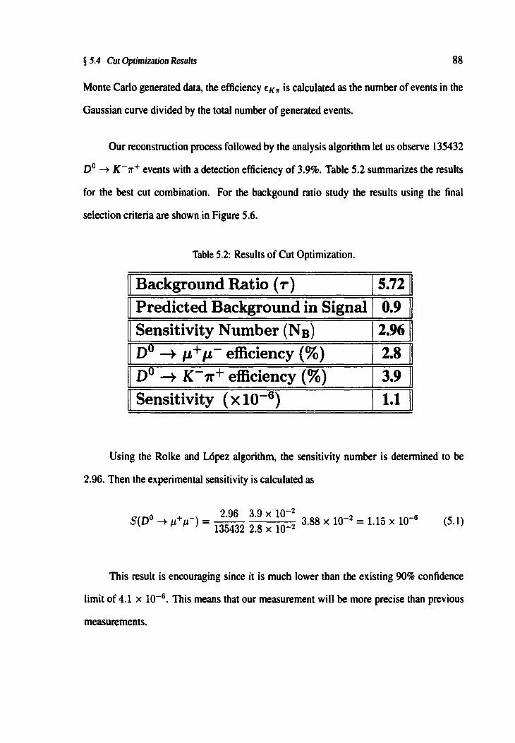
§ 5.4 Cut Optimiz.ation Results 88
Monte Carlo generated data, the efficiency f.Krr is calculated as the number of events in the
Gaussian curve divided by the total number of generated events.
Our reconstruction process followed by the analysis algorithm let us observe 135432
D0 ~ K- 7r+ events with a detection efficiency of 3.9%. Table 5.2 summarizes the results
for the best cut combination. For the backgound ratio study the results using the final
selection criteria are shown in Figure 5.6.
Table 5.2: Results of Cut Optimization.
II Background Ratio ( T) 5.72 II Predicted Background in Signal 0.9
Sensitivity Number (Na) 2.96 I D0 --t µ+µ-efficiency (3) 2.8 D0 --t K-7r+ efficiency (3) 3.9 Sensitivity ( x 10-6) 1.1 1
Using the Rolke and L6pez algorithm, the sensitivity number is determined to be
2.96. Then the experimental sensitivity is calculated as
( 0 + -) 2.96 3.9 x 10⁻²
-2 -6 SD ~ µ µ = 135432 2.8 x 10⁻² 3.88 x 10 = 1.15 x 10 (5.1)
This result is encouraging since it is much lower than the existing 90% confidence
limit of 4.1 x 10⁻⁶• This means that our measurement will be more precise than previous
measurements.

§ 5.5 Confidence Limits
Global Vertex Dote ( 103 Super Stream 2 tapes)
> ., ::::i;
~ 0.06
' "' c ., >
L;J
0.05
0.04
0.03
0.02
0.01
sidebarc
1.75 1.8
signc 1
orec
1.85
µµ.moss
1.9
es 19 41
sidebcnd
1.95 2 (GeV)
Figure 5.6: Invariant Mass Distribution for Background Ratio using the best cut combination.
5.5 Confidence Limits
89
Once our selection criteria were optimized, we proceeded to open the masked area.
Applying the best cut combination to dimuonic events within our signal area we have two
events in that region. Thus, we have five events in sidebands area (y = 5) and two events
in the signal area (x = 2).
Using the Rolke and L6pez routines, for r = 5.72, the background rate (b = y/r) is
0.9 and, the 90% confidence level lower limit is 0 and the 90% confidence level upper limit

§ 5.5 Confidence Limits
sideband
0.8
0.6
0.4
0.2
0 1.75 1.8
s:gnal area
1.85 1.9
Oimuon mass - Octa
sideband
1.95 2 (GeV)
Figure 5. 7: Event candidates for the D0 -+ µ+ µ- process. Figure display the only two events within the signal area which survives the optimum selection criteria in the study of the rare decay D0 -+ µ+µ-.
is 5.34. The 90% upper confidence limit for the branching ratio is calculated as
90
0 + - - 5.34 3.9 x 10⁻² 2 6
BR(D --+ µ µ ) -135432 2
.8
x 10
_2
3.88 x 10- = 2.1 x 10- (5.2)
§ 5.6 Conclusions 91
No definitive evidence of the rare decay D0 --+ µ+ µ- was found in this analysis.
However, our work allows us to set a lower 90% confidence level upper limit for this decay.
5.6 Conclusions
Monte Carlo simulation of the level of meson misidentification in FOCUS
was confirmed by experimental measurements using real data. The misidentification
measurements were used as the basis of a method to determine the ratio of background
in the invariant mass sidebands versus background in the signal region. This method used
real data and avoided systematic uncertainties in the use of simulation.
It was possible to reduce the background in this analysis significantly using well
known selection variables based on the characteristics of the signal being sought. The
blind analysis methodology provided an excellent way of optimizing the event selection
criteria with a minimum of bias.
The main conclusion obtained from this work was the reduction of the upper limit in
the branching ratio at a half of the value previously published by PDG. No evidence for the
rare decay D0 ~ µ+ µ- was found. The 90% CL branching ratio limit was 2.1 x 10⁻⁵.


![Visual FoxPro · µ¦µ ° x \ z x µ »£µ¡ o°¥ ´ ¦r £µ Á¦¸¥ ¸ É z z ] ^ y æ Á¦¸¥ »Ã ´¥ª· ¥µ ¤ µ¦µ ° x \ y ] µ £¦ ¸ ´ ªµ¨ £µ Á¦¸¥](https://img.dokumen.tips/doc/110x75/5e9a8f84e4b3f621a5474f89/visual-x-z-x-o-r-z-z-.jpg)


![1. Excel. µ file- µ « . µ µ µ µ µ µ µ µ ; µµ ; µµ µ Excel Word; µ µ µµ ;[ ] µ , µ µ µ](https://img.dokumen.tips/doc/110x75/5e1c0fbb3625a8105f7711f5/1-excel-excel-word-.jpg)