Embed Size (px)
Citation preview
A Review of Measuring Upper Ocean Responses to HurricanesSynclaire Truesdale ~ Texas A&M University ~ [email protected]
1. Introduction 4. Remote Sensing3. In Situ Instrumentation
❖ The upper ocean and hurricanes have a complex relationship:
Cool Deeper Water
Warm Surface Water
Fuel for Hurricane
---1000m--- Vertical Mixing
Friction Evaporation
Figure 1: The left shows how the upper ocean affects hurricane intensity and developmentby supplying energy through frictional heat of the winds and latent heat of evaporation.The right shows how a hurricane affects the upper ocean through driving vertical mixingby upwelling of cold water to the surface and downwelling warm water from the surface.
Figure 2: From Chen et al. (2013). Observed airborne Doppler radar wind field compared with acoupled atmosphere-ocean model and coupled atmosphere-ocean-wave model.
Data Assimilation and Numerical Model Forecasting
No
rth
Dis
tan
ce f
rom
Cen
ter
(km
) Winds (m/s)100
50
0
-50
-100
100
50
0
-50
-100
100
50
0
-50
-100-100 -50 0 50 100 -100 -50 0 50 100 -100 -50 0 50 100
East Distance from Storm Center (km)
Observed Wind Field Atmo-Ocean Model Atmo-Ocean-Wave Model
❖ The development of in situ instruments greatly improved the temporal and spatial coverage of upper ocean data during and after hurricanes.
3a Gliders
3b. Floats & Drifters
3c. Moored Systems 5km windsAir tempWater temp
0 10 20 30 40 50
Hours since 2 PM 10/2/15 at Buoy 42058
Figure 12: From Hsu (2017). 5-km wind speed, air temperature and water temp. during the time of Hurricane Matthew (2016).
5 km
win
d (m
/s),
Tem
p (d
eg C
)
Figure 6: Teledyne Marine Slocum glider .
Figure 11: Buoy from National Data Buoy Center
❖ Gliders take profiles of different data along a programmed track, giving scientists control of where measurements can be taken. Figure 7: From Dong et al. (2017), pre-storm conditions in North
Atlantic in Oct. 2014, before Hurricane Gonzalo.
3915 Floatsworldwide
❖ Argo floats have greatly increased the spatial coverage of ocean data and the chance to measure near hurricane events.
❖ Moored systems combine multiple sensors to provide many detailed data of both the atmosphere and the ocean.
❖ These systems reveal the limitation of in situ instruments― they can only measure data at one location at a time.
❖ Remote sensing by geostationary (GOES) and polar orbiting satellites gives a bigger, detailed picture of changes occurring in the upper ocean following hurricanes.
BEFORE
Figure 9: From the Argo official website showing the number of deployed floats as of 3/10/19.
AFTER
6 10 14 18 22 26 30Temperature (deg C)
Figure 13: Modified from Son et al. (2007), Composite satellite images of sea surface temp before and after the passage of Hurricane Fabian (2004). Black arrows are storm track.
Dashed lines are 350 km from storm center. Circles show regions of SST cooling after the storm passed.
BEFORE AFTER
0.01 0,10 1.00 10.0Chlorophyll-a (mg/m3)
Figure 14: Modified from Son et al. (2007), Composite satellite images of chlorophyll-aconcentration before and after Hurricane Fabian (2004). Lines are the same as Figure 13.
Circles show location of a large phytoplankton bloom.
❖ New innovations in remote sensing for ocean color have led to leaps in understanding the biological response to hurricanes.
60
50
40
30
20
❖ Increased upper ocean data can make data assimilation more powerful in numerical models used for hurricane forecasting.
Before Hurricane Hilda (1964) passed
❖ In the 1960’s-70’s an invaluable data source came from observations aboard shipping vessels, including sea surface temperature and atmospheric conditions
2. Early Methods
Bathythermograph
❖ BT’s verified SST cooling following the passage of a hurricane that was first observed by merchant vessels at sea.
Figure 3: By Karsten Petersen. The Danish cargo liner “Boribana”.
Figure 4 : By Tin Can Sailors. A bathythermograph (BT) used in the 1960’s.
Figure 5 : From Leipper (1967), Temperature vs Depth from a BT.
0
100
200
300
0
100
200
300
Temperature Cross Section
Salinity Cross Section
Dep
th (m
eter
s)
Latitude Salinity
2005 2010 2015
240220200180160140
Oxygen (µM)D
epth
(m)
0
100
200
300
400
Figure 10: Modified from the Argo official website. Data is demonstrating new innovative biogeochemical sensors that have been added to some floats.
Figure 8: By NOAA Research News. An Argo float being
deployed from a boat.
5. Outstanding Research
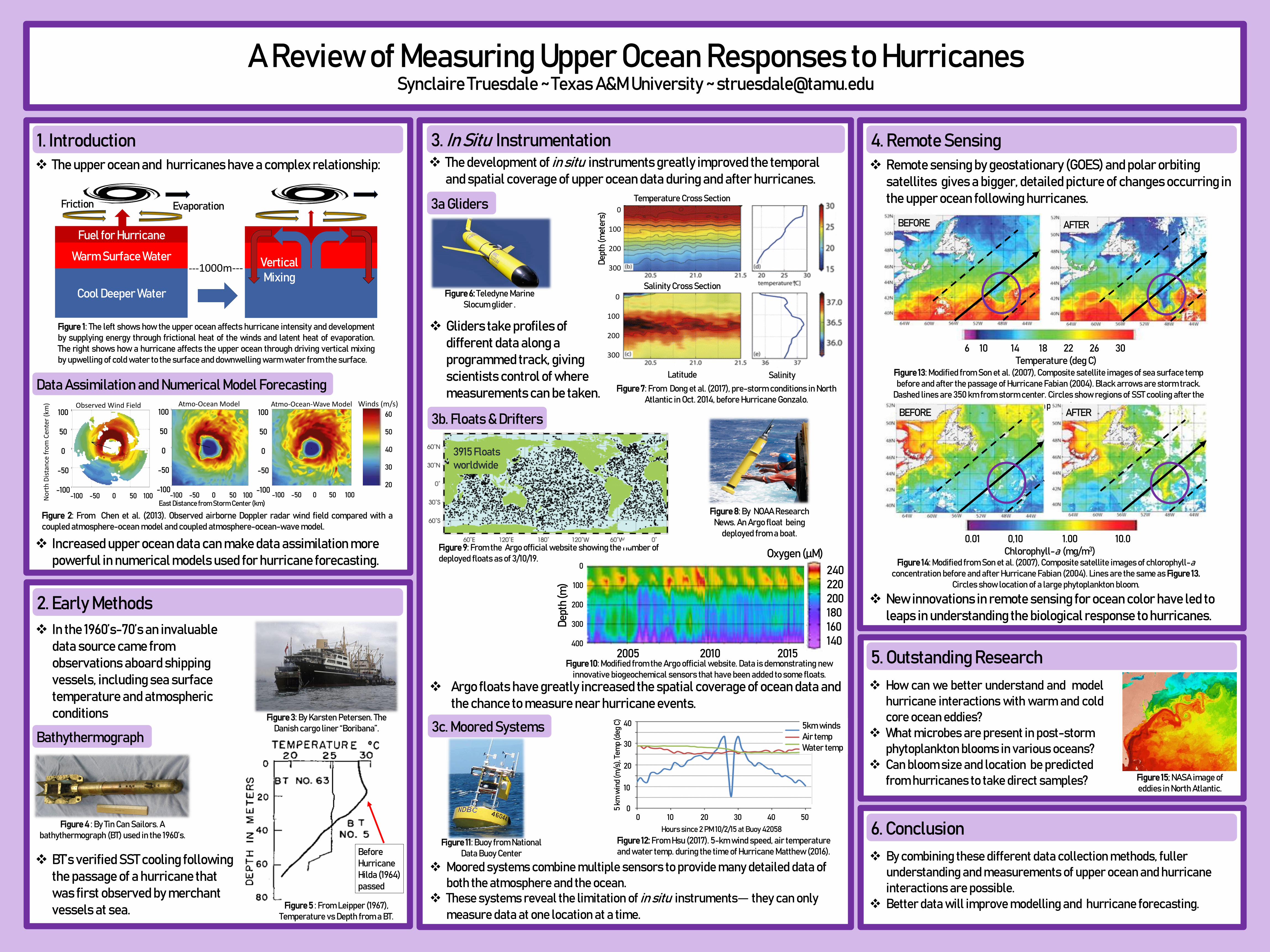
Figure 15; NASA image of eddies in North Atlantic.
❖ How can we better understand and modelhurricane interactions with warm and coldcore ocean eddies?
❖ What microbes are present in post-storm phytoplankton blooms in various oceans?
❖ Can bloom size and location be predicted from hurricanes to take direct samples?
6. Conclusion
❖ By combining these different data collection methods, fuller understanding and measurements of upper ocean and hurricane interactions are possible.
❖ Better data will improve modelling and hurricane forecasting.
40
30
20
10
0