A Review of“Customized Dynamic Load Balancing for a

Network of Workstations”

Taken from work done by:

Mohammed Javeed Zaki, Wei Li, Srinivasan Parthasarathy

Computer Science Department, University of Rochester (June 1997)

Presenter: Jacqueline Ewell

Introduction

With the rapid advances in computational power, speed, cost, memory, and high-speed

network technologies, a “Network of Workstations” provides an attractive scalable

alternative compared to custom parallel machines. Scalable distributed shared-memory

architectures rely on the ability for each processor to maintain a load balance. Load

balancing involves assigning each processor a proportional amount of work bases on its

performance, thereby minimizing total execution time of the program. There are two

types of load balancing, static and dynamic. Static load balancing allows the programmer

to delegate responsibility to each processor before run time. The simplest approach is the

static block-scheduling scheme, which assigns equal blocks of iterations to each of the

processors. Another scheme of static load balancing is the static interleaved scheme,

which assigns iteration in a cyclic fashion. This makes programming much easier and can

solve many problems inherit in load balancing caused by processor heterogeneity and

non-uniform loops. Static scheduling avoids run time scheduling overheads.

However, due to transient external loads applied by multiple-users on a network of

workstations, heterogeneity with processors (different speeds), memory (varying amounts

of available memory), networks (varying cost of communication among pairs of

processors), and software (programs may have varying amount of work in each iteration),

a dynamic approach to load balancing is necessary. Dynamic load balancing allows,

during run-time, the ability to delegate work based on run-time performance of the

networked set of workstations, keeping in mind the trade-off of task-switching and load-

imbalance costs. The idea of Dynamic vs. Static load balance is not new. However,

there have been many load-balancing schemes developed, each with specific applications

in mind under varying programs and system parameters. Therefore, wouldn’t it be nice

to customize dynamic load balancing dependant on applications to yield the best

performance possible? The paper entitled “Customized Dynamic Load Balancing for a

Network of Workstations”, identifies this problematic situation and presents a hybrid

compile-time and runtime modeling and decision process, which selects the best scheme,

based on run-time feedback from the processors and its performance.

Dynamic Load Balancing (DLB) Strategies

When the execution time of loop iterations is not predictable at compile time, runtime

dynamic scheduling should be used with the additional runtime cost of managing task

allocation. There have been a number of models developed for dynamic loop scheduling.

The task queue model has been targeted towards shared memory machines, while the

diffusion model has been used for distributed memory machines [4,5,6]. The task queue

model assumes a central task queue where if a processor finishes its assigned work, more

work can be obtained from the queue. This approach can be self-guided or a master may

remove the work and allocate it the processor. In the diffusion model, all work is

delegated to each processor and when an imbalance is detected between a processor and

its neighbor, work movement occurs.

A third scheduling strategy may be used and is the bases of the paper in discussion. The

approach uses past performance information to predict the future performance. Among

these approaches have been the Global Distributed scheme, the Global Central scheme,

the Local Distributed scheme, the Global Centralized scheme using automatic generation

of parallel programs, the Local Distributed receiver-initiated scheme, and the Local

Centralized scheme. In all cases, the load balancing involves periodic exchange of

performance information. The method discussed in the paper implements, instead of

periodic exchange, an interrupt-base receiver. Its goal is to select among the given

schemes, the best load balancing scheme at run-time.

These strategies lie on the extremes points on the two axes, global vs. local and central

vs. distributed. There are more schemes that lie within the extreme points, and they will

be explored in future works.

Global Strategy:

In the global scheme, all load-balancing decisions are made on a global scale. That is, all

processors get an interrupt once one processor has completed its work. Then all the

processors send their performance profile to the load balancer. In the Centralized

scheme, the load balancer is located in a centralized area, often on the master processor.

After calculating the new distribution, the load balancer sends instructions to all the

processors who have to send work to the others. The receiving processors just wait until

they have received all the data necessary to proceed. In a Distributed scheme, the load

balancer is replicated on all the processors. The profile information is broadcast to all the

processors and the receiving processors wait for the work while the sending processors

ship the data. This method eliminates the need for instructions from the master

processor.

Local Strategy:

In the local scheme, the processors are divided into groups of size K. The load balancing

decisions are only done within a group (K block static partitioning; other approaches such

Distribute

d

Local Global

Centralize

as K-nearest neighbor and dynamic partitioning may also be used). Profile information is

only exchanged with a group. The Centralized scheme still only has one load balancer,

instead of one per group. The load balancer, besides learning the profile performance of

each processor, must also keep track of which group each processor is in. As for the

Distributed scheme, each processor still maintains its own load balancer and profiles are

sent amongst all the processors in the group.

Tradeoffs:

Global vs. Local: For the Global scheme, since global information is available at

synchronization time, the work distribution is nearly optimal, and convergence is faster

than Local scheme. However, communication and synchronization cost is much higher

in the Global scheme. For the Local scheme, even though initially, the groups may be

partitioned statically, all groups are assumed to be divided up evenly by performance and

speed, performance of each processor may change over time. Thus, one group of

processors with poor performance will be overloaded while another group of processors

may be idle for a period of time.

Centralized vs. Distributed: In the Centralized scheme, having one load balancer could

limit the scalability of the network. For the Distributed scheme, synchronization involves

an “all-to-all” broadcasting of profiles. This may cause a high rate of bus contention. On

the other hand, in the Centralized scheme, and “all-to-one” profile send must be

completed as well as a “one-to-all” instruction send. This reduces much of the

transmission along the bus but requires a two step process. Calculations on the

distribution of work will also effect the cost since the Centralized scheme must in effect

do the calculations sequentially while the Distributed scheme may do the calculation in

parallel.

Basic Steps to DLB:

• Initial: assignment of work will be divided equally amongst the processors.

• Synchronization: In the approach discussed in the paper, synchronization is

triggered when the fastest processor finishes its portion of the work. The processor

sends an interrupt to all the other processors. Once the interrupts have been seen by

each processor, the processors in turn, send their performance profiles to the load

balancer. In the local scheme, synchronization occurs within a group.

• Performance Metric: The whole past history of the processor or a portion of the

history can be used to calculate the load function. The metric that was used in the

paper was the number of iterations done per second since the last synchronization

point.

• Work and Data Movement : If the amount of work/data to be moved is below a

threshold, then the work/data is not moved. This may signify that there is little work

left to be done and that the system was pretty much balanced.

• Profitability Analysis: If there is sufficient work/data that needs to be moved, a

profitability analysis function is applied. This invokes the re-distribution of

work/data as long as the potential benefit results in at least a 10% improvement in

execution time.

DLB Modeling and Decision Process

Modeling Parameters

• Processor Parameters: information about each processor available for computation

1. Number of Processors (P) – assume fixed number of processors

2. Normalized Processor Speed (Si) – ratio of processor’s performance with respect

to a base processor

3. Number of Neighbors (K) – number of processors in the group for the Local

Scheme

• Program Parameters: information about the application

1. Data Size (N) – could be different size arrays

2. Number of loop iterations (I) – this is usually some function of data size

3. Work per iteration (W) – amount of work measured in terms of the number of

basic operations per iteration; function of data size

4. Data Communication (D) – number of bytes that need to be communicated per

iteration

5. Time to execute an iteration (T) – seconds to process an iteration on the base

processor

• Network Parameters: properties of the interconnection network

1. Network Latency (L) – time it takes to send a single byte message between

processors

2. Network Bandwidth (B) – number of bytes that can be transferred per second over

the network

3. Network Topology – this influences the latency and bandwidth; it also has an

impact on the number of neighbors for local strategies

• External Load Modeling: one of the main reasons to selecting customized dynamic

loading was the fear of transient external loads entering the system. For the DLB

model to be as accurate as possible, this transient external load needs to be model.

The following variables are implemented in the model:

1. Maximum Load (m)– specifies the maximum amount of load the a single

processor may experience

2. Duration of Persistence (d) – indicated the amount of time this load is applied to

the processor. A discrete random load function with maximum amplitude of m

lasts for d seconds in duration.

Total Cost

The total cost function is given by:

Total Cost = Cost of Synchronization +

Cost of calculating the new distribution +

Cost of Sending the Instructions (for centralized schemes)+

Cost of Data Movement

Synchronization Cost

• GCDLB: one-to-all (P) + all-to-one (P)

• GDDLB: one-to-all (P) + all-to-all (P2)

• LCDLB: one-to-all (K) + all-to-one (K)

• LDDLB: one-to-all (K) + all-to-all (K2)

Cost of Calculating New Distribution

Cost is usually very small.

Cost of Sending Instructions

The cost is the number of messages being sent times the latency.

Cost of Data Movement

Basically, the cost of data movement is given by:

=> Number of Messages being sent * Latency +

Number of iterations moved *

(Number of Bytes that need to be communicated per iteration /

Bandwidth)

The derivation to this formula is laid out in the paper [1].

Decision Process

Work is initially partitioned evenly among all the processors. The fastest processor in the

entire system for the centralized model vs. the fastest processor in each group will initiate

the interrupt for synchronization once it has finished all the work delegated to it. At this

point, more than 1/P work has been done. The load functions and average effective speed

for each processor is calculated by the performance information sent by each processor to

the load balancer. The load function is combined with the other parameters in the model

and quantitative information on the behavior of the different schemes is calculated. The

result will allow the model to select the best strategy after this stage.

Runtime System

The runtime system consists of the DLB libraries for all the strategies, the actual decision

process for choosing among the schemes and data movement routines to handle

redistribution. The source code to source code translation of a sequential program to a

paralyzed one using PVM for message passing and the DLB library calls was developed.

Experiments

Matrix Multiplication:

Matrix Multiplication is given as Z = X • Y (where X is an n ∗ r, and Y is an r ∗ m

matrix). The experiment was run with m=400 and different values of r and n. Figure 1

shows the result of this experiment using 4 processors. The bars represent the execution

time if one of the schemes were chosen for the given problem. Each bar is normalized

with respect to the case where no dynamic load balancing exists. The data size is set to

n=400, r=400; n=400, r=800; n=800, r=400; and n=800, r=800; respectively.

Figure 1. Matrix Multiplication (P = 4)

Figure 2 shows the result of this experiment when you increase the number of processors

to 16. The data size is set to n=400, r=400; n=400, r=800; n=800, r=400; and n=800,

r=800; respectively.

Figure 2. Matrix Multiplication (P=16)

Matrix Multiplication Results

From an analysis of the figures, it can be observed that if the computational cost versus

the communication cost ratio is large, global strategies are favored. As the ratio

decreases, local strategies are more adapted to be favored. The factors that influence this

ratio are the work per iteration, number of iterations, and the number of processors. Such

as in the second figure, the processors increase the synchronization cost, and the

difference between global and local schemes are less obvious. The Centralized scheme

incurs a sufficient amount of overhead such as sequential redistribution and instruction

sends, that the Distributed scheme is favored.

TRFD

The TRFD, from the Perfect Benchmark suite, contains two main computational loops,

which are load balanced separately. There is only one major array of size

[n(n+1)/2]x[n(n+1)/2]. Experiments were run where n=30,40, and 50 with 4 processors

and 16 processors. Results from modeling each scheme is shown in figure 3 and 4.

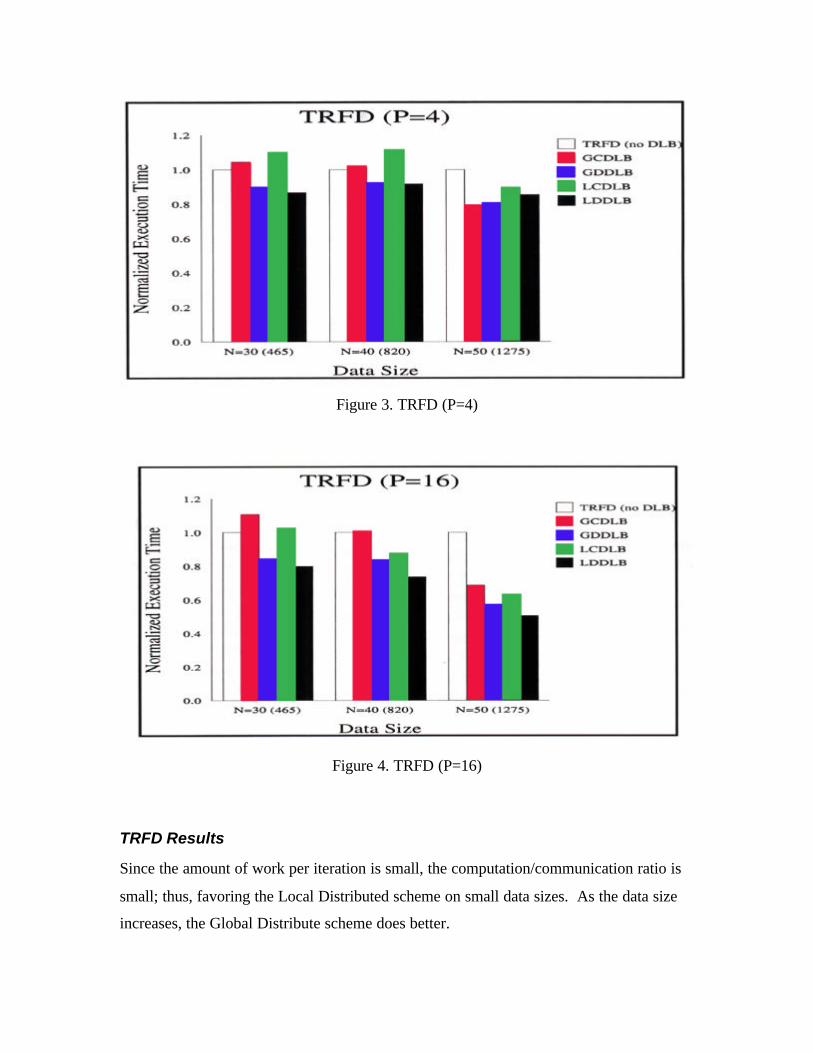
Figure 3. TRFD (P=4)

Figure 4. TRFD (P=16)

TRFD Results

Since the amount of work per iteration is small, the computation/communication ratio is

small; thus, favoring the Local Distributed scheme on small data sizes. As the data size

increases, the Global Distribute scheme does better.

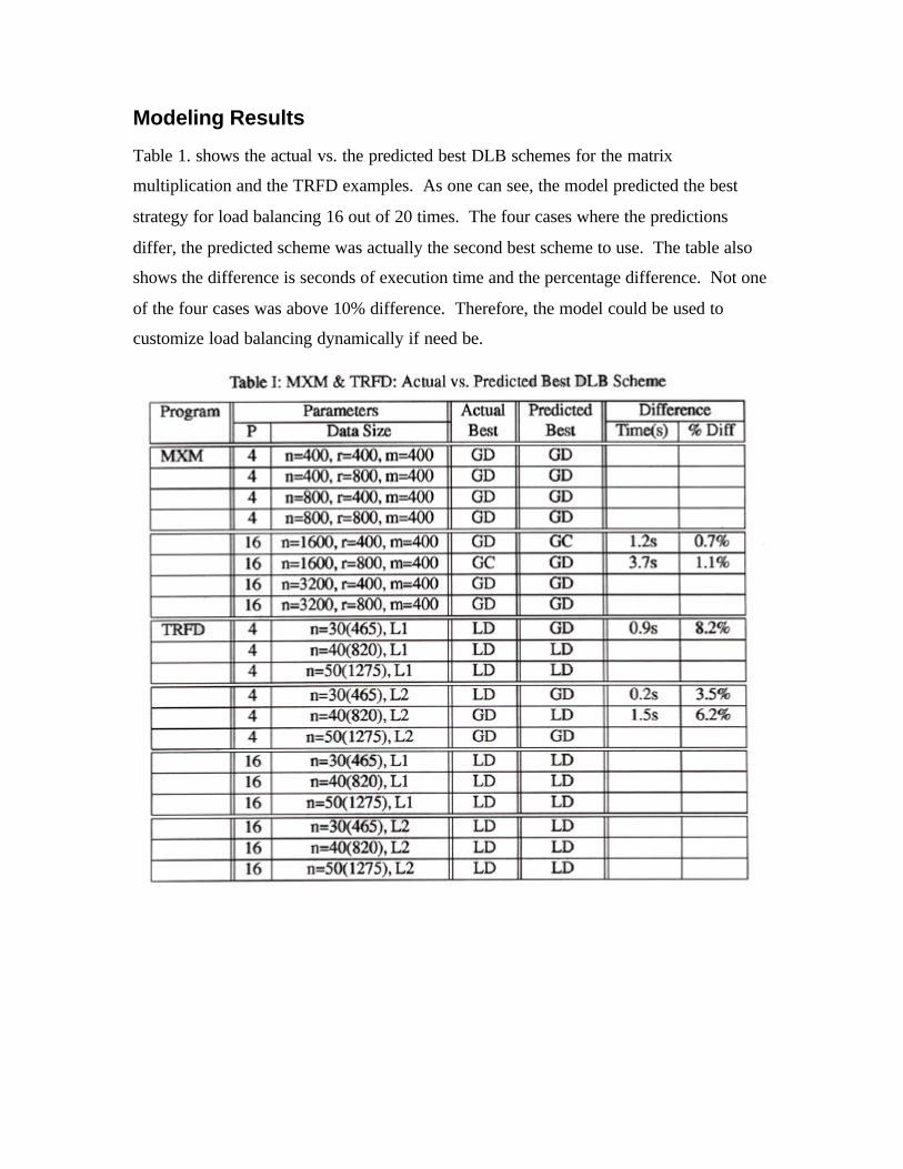
Modeling Results

Table 1. shows the actual vs. the predicted best DLB schemes for the matrix

multiplication and the TRFD examples. As one can see, the model predicted the best

strategy for load balancing 16 out of 20 times. The four cases where the predictions

differ, the predicted scheme was actually the second best scheme to use. The table also

shows the difference is seconds of execution time and the percentage difference. Not one

of the four cases was above 10% difference. Therefore, the model could be used to

customize load balancing dynamically if need be.

Conclusions

From the experiments, one can see clearly that different schemes are best for different

applications on different systems. Furthermore, transient external loads can inhibit

performance on any one of the workstations that are networked together. Therefore,

customized dynamic load balancing is essential if the optimal load balancing scheme(s)

are to be use, resulting in optimal execution time. Given the existing model, it is very

possible to select a good scheduling scheme during runtime. Future work must be need

since the only schemes tested were at the extremes of schemes where performance

profiles are shared among processors. Other scheme to be tested should include a

derivative of the Local Distributed scheme where instead of replicating the load balancer

on every processor, each group of processors may have its own load balancer. Another

derivation that should be looked at is similar to Local schemes. However, instead of

restricting the groups to only sharing work amongst the other processor in the group, the

group is allowed to steal work from other groups when it has reached below a threshold.

Dynamic Group membership is another derivation that may lead to better load balancing.

Hierarchical schemes may also be looked at as an alternative.

References

[1] Zaki, Mohammed Javeed, Li, Wei, Parthasarathy, Srinivasan, "Customized Dynamic

Load Balancing for a Network of Workstations" , JPDC, Special Issue on Workstation

Clusters and Network-Based Computing 43 (2), June 1997, 156--162.

http://www.cs.rochester.edu/trs/systems-trs.html

[2] Zaki, Mohammed Javeed, Li, Wei, Parthasarathy, Srinivasan, "Customized Dynamic

Load Balancing for a Network of Workstations" , 5th IEEE Int'l. Symp. on High-

Performance Distributed Computing (HPDC-5), Syracuse, NY, August 1996.

http://www.cs.rochester.edu/trs/systems-trs.html

[3] Cierniak, Michal, Zaki, Mohammed Javeed, Li, Wei, "Compile-time Scheduling

Algorithms for Heterogeneous Network of Workstations" , The Computer Journal; Special

Issue on Automatic Loop Parallelization 40 (6), December 1997, 356--372.

http://www.cs.rochester.edu/trs/systems-trs.html

[4] R.D. Blumofe and D.S. Park, “Scheduling Large-Scale Parallel Computations on

Network of Workstations”, 3rd IEEE Intl. Symp. High-Performance Distributed

Computing, Aug. 1994

http://www.cs.utexas.edu/users/rdb/papers.html